1

Global Biodiversity Indicators: scenario modelling for fisheries policy

Kathryn Sullivan

September 2010

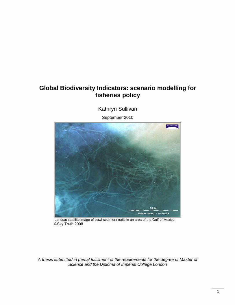
Landsat satellite image of trawl sediment trails in an area of the Gulf of Mexico.

©Sky Truth 2008

A thesis submitted in partial fulfillment of the requirements for the degree of Master of Science and the Diploma of Imperial College London

2

Abstract

The Convention on Biological Diversity set a target to reduce the rate of biodiversity loss

by 2010. This target has not been met, and in the wake of this, scientists are looking at

the suite of global biodiversity indicators developed to measure progress towards this

target, to see how they can be improved and refined for use in the future. Adapting these

indicators raises an opportunity to predict impacts of new environmental policies, and to

assess the success of past management decisions. However, in order to do this the

connection between different policy options and indicators needs to be fully understood.

In this study, I look at potential of Marine ocean systems indicators to investigate this

policy-indicator interface. Marine systems are an area of concern for conservation

practitioners and policy makers alike, and so make an ideal test case. I use an

ecosystem model, Ecopath, to model the outcomes of two marine fisheries policies on

two well developed biodiversity indicators, the Red List Index and the Living Planet

Index. I found that the indicators are able to detect policy change, but the more fine

scale impacts of policy change are not well reflected in the indicators. A number of

weaknesses in both the modelling process and the indicators were identified. The

indicators need to be used in conjunction as their primary weakness is species

composition. Without being fully representative of all species it is unlikely that one single

indicator will provide a complete picture of biodiversity

3

Acknowledgements Firstly, I would like to thank my supervisors, Dr. Ben Collen (Institute of Zoology) and Dr.

Emily Nicholson (Imperial College), for their advice, suggestions and endless support

over the past six months. I would also like to thank Imperial College for providing

financial support for this project.

I would also like to express my gratitude to Alberto Barausse, for his exceptional work on

the modelling component of this study. My thanks go to Louise McRae (Institute of

Zoology), Julia Blanchard (Imperial College), Julia Jones (Bangor Unversity) and Hugh

Possingham (Queensland University) for their advice and suggestions from the very

beginning.

Thanks to everyone at the Institute of Zoology for their help and humour during the long

write up. Thanks to my family and friends for their support and patience over the course

of the last year.

A special thanks to Brendan for listening to every single problem I encountered, no

matter what time of the day or night, and for sharing this experience with me.

4

Contents

Contents ..................................................................................................................................... 4

1 Introduction ........................................................................................................................ 7

1.1 Aims ............................................................................................................................ 9

1.2 Objectives .................................................................................................................... 9

1.3 Thesis Structure ......................................................................................................... 10

2 Background ....................................................................................................................... 11

2.1 CBD Indicators ........................................................................................................... 11

2.2 Living Planet Index Background .................................................................................. 12

2.3 The Red List Index ...................................................................................................... 14

2.4 Current and potential future uses of global biodiversity indicators ............................. 17

2.5 Fisheries in Crisis ........................................................................................................ 18

2.6 Ecopath Modelling ..................................................................................................... 21

3 Method ............................................................................................................................. 23

3.1 Choosing Suitable Scenarios ....................................................................................... 23

3.2 Indicator selection ..................................................................................................... 24

3.3 Ecopath Modelling ..................................................................................................... 24

3.4 Indicator Analysis - Living Planet Index ....................................................................... 28

3.4.1 Allocating models to ocean systems ................................................................... 29

3.4.2 Allocating Species to functional groups .............................................................. 29

3.4.3 Calculating the LPI .............................................................................................. 30

3.4.4 Aggregating the LPI ............................................................................................ 30

3.5 Indicator Analysis – Red List Index .............................................................................. 31

3.5.1 Allocating species to a model ............................................................................. 31

3.5.2 Allocating species to a functional group ............................................................. 31

3.5.3 Determining projected Red List Status ................................................................ 31

3.5.4 Allocating models to ocean systems ................................................................... 32

3.5.5 Aggregating Regional Red Lists ........................................................................... 33

4 Results ............................................................................................................................... 34

4.1 Aggregated LPI and RLI for the Six Study Regions ....................................................... 34

4.2 Regional LPI Results ................................................................................................... 34

4.3 Regional RLI Results ................................................................................................... 36

4.4 Case Study 1: The North Sea and Baltic Sea ................................................................ 37

to recover from both policies. This is likely to be a result of its longer generation length. ...... 41

5

4.5 Case Study 2: The South Pacific Ocean ....................................................................... 41

5 Discussion ......................................................................................................................... 44

5.1 Policy Results ............................................................................................................. 44

5.2 The different roles of the indicators ........................................................................... 45

5.3 Taxonomic Bias of the Indicators ................................................................................ 46

5.4 Species community interactions ................................................................................. 49

5.5 Limitations of Ecopath Modelling ............................................................................... 50

5.6 Sensitivity analysis ..................................................................................................... 51

5.7 Concluding remarks ................................................................................................... 52

References ................................................................................................................................ 53

6 Appendix ........................................................................................................................... 60

6

List of Figures

Figure 2.1: ............................................................................................................................... 20 Figure 3.1: ............................................................................................................................... 23 Figure 3.2: ............................................................................................................................... 25 Figure 4.1: .............................................................................................................................. 35 Figure 4.2: .............................................................................................................................. 39 Figure 4.3: ............................................................................................................................... 40 Figure 4.4: ............................................................................................................................... 42 Figure 4.5: .............................................................................................................................. 43

List of Tables Table 2.1: ................................................................................................................................ 15 Table 3.1: .............................................................................................................................. 27 Table 3.2: ............................................................................................................................... 29

Abbreviations CBD: Convention on Biological Diversity

LPI: The Living Planet Index

RLI: The Red List Index

MTI: Marine Trophic Index

BAU: Business-as-Usual

CR: Critically Endangered

EN: Endangered

VU: Vulnerable

NT: Near Threatened

LC: Least Concern

DD: Data Deficient

Word count: 14,971

7

1 Introduction

The Convention on Biological Diversity target to “significantly reduce the rate of

biodiversity loss by 2010” has not been met (Butchart et al. 2010). As a result, we are left

with a selection of indicators in need of development, to allow continued, improved

monitoring of the state of the world‟s biodiversity (Jones et al. In review). Biological

diversity is defined by the CBD as, “the variability among living organisms from all

sources including . . .terrestrial, marine and other aquatic ecosystems and the ecological

complexes of which they are part: this includes diversity within species, between species

and of ecosystems” (Millennium Ecosystem Assessment, 2005). To assess the progress

towards this target, a suite of indicators was developed, of which, only 9 of the 29

headline indicators are fully developed (Walpole et al. 2009). However, many of these

indicators, were selected not for their relevance or rigour, but because the data are

available (Mace et al. 2010). As we have reached 2010, the focus has now shifted to

these indicators, and the conservation community is asking how these indicators can be

used to assess global biodiversity. As a result, Jones et al. (In review) considered what

the full role of these indicators is, and how best they can be utilised and improved.

No single indicator will be able to give a complete picture of biodiversity; however by

using a number in conjunction, they may provide us with a representation of what is

occurring. One important role of indicators highlighted by Jones et al. (In review) is

improved understanding of how indicators will respond to policy change. This means

using the indicators as a tool for predicting change as a result of new policy, and

potentially auditing past conservation decisions, to assess their success. However, to do

this successfully the gaps in our knowledge need to be filled. Even within a field as well

studied as agriculture, which is vital for global food production, there are gaps and

inconsistencies in the data and the way it is collected (Millennium Ecosystem

Assessment, 2005). What is needed is a common protocol, enabling data collection for a

suite of metrics (Sachs et al. 2010). As we develop similar metrics for biodiversity it is

vital that they are statistically robust, and provide some insight into the mechanisms

driving any changes (Dobson, 2005).

It is important for indicators to fulfil the roles outlined above. Firstly, knowing past

successes and failures provides important information for the improvement of decision

making (Sutherland et al. 2004). In addition, policy makers will work harder to meet

8

commitments and targets if, in the future, there is the possibility that failure to do so will

be detected (Jones et al. In review). If indicators can be used to audit policy decisions, it

is logical for them to also be used proactively, to decide between competing policy

options. However, the connection between policy decisions and global biodiversity

indicators is still to be explored for most indicators (Jones et al. In review).

One system where the impact of policy upon indicators could be investigated is the

marine ocean system. Marine systems are subject to much disturbance as a result of

commercial fishing (Thrush and Dayton, 2002), while recent crashes in fish stocks mean

that policies affecting them are up for revision (Caddy and Seijo, 2005). The extent and

intensity of human disturbance to marine ecosystems is a significant threat to both

structural and functional biodiversity, and in many cases it has virtually eliminated natural

systems that might serve as baselines to evaluate fishing impacts (Thrush and Drayton,

2002). Of all fishing practises, bottom trawling is arguably the most destructive (Kaiser et

al. 2006). Trawl gear affects the environment in both direct and indirect ways. Direct

effects include scraping and ploughing of the substrate, sediment resuspension,

destruction of benthos, and dumping of processing waste. Indirect effects include post-

fishing mortality and long-term trawling induced changes to the benthos (Jones, 1992). It

is understood that the greater the frequency of gear impacts on an area, the greater the

likelihood of permanent change. In deeper waters (<1000m), where the fauna is less

adapted to changes in sediment regimes, and disturbance from storm events the effects

of fishing gear take longer to disappear, here recovery is probably measured in decades

(Jones, 1992).

9

1.1 Aims This project was developed from points raised in a recent study by Jones et al. (In

review), that stressed the importance of understanding and developing Global

Biodiversity Indicators, particularly in the wake of the failure to meet the CBD 2010

targets (Butchart et al 2010). Specifically, Jones et al. (In review) suggest that in order to

maximise the utility of the current biodiversity indicator set, we must improve our

understanding of how indicators will respond to changes in environmental policy. Given

that the capability of the current set of CBD indicators to detect changes in policy is

unknown, it is appropriate that they are evaluated against a range of policy scenarios.

This involves a number of stages, from policy and indicator selection through to

modelling and indicator analysis.

I model two policy scenarios to investigate their impact on two indicators. The policy

scenarios being addressed in this project are:

Scenario 1: A 50% reduction in bottom trawling effort within the selected study

regions.

Scenario 2: A 100% reduction (i.e. a total ban) in bottom trawling within the

selected study regions.

The affects of these two policy scenarios were then tested to see how they impacted the

two selected indicators; the Red List Index (RLI) and the Living Planet Index (LPI).

1.2 Objectives To model both the direct and indirect effects of the two scenarios using Ecopath

with Ecosim software (Ecopath).

To test the capabilities of two global biodiversity indicators (Living Planet Index

and the Red List Index), to detect the effects of the chosen policy scenarios

To assess the differences in the response of the indicators to the policies

To compare the responses of the indicators between different regions

To critically appraise the biodiversity indicators, and make recommendations for

their improvement

10

1.3 Thesis Structure

Chapter 2 provides a background to the Global Biodiversity Indicators, and specifically

the ones being assessed in this study. It also provides some context to the policies being

investigated and why they are important. Finally, it describes the development and

background of the models used to assess the impacts of the policies.

Chapter 3 describes the methods used in the study, starting with the selection of the

scenarios and indicators to investigate. It then goes on to describe the modelling

process in greater detail, and states the regions analysed. This is followed by the

process used to project the results of the models with the two chosen indicators.

The results of the study are outlined in Chapter 4, starting with the aggregated results of

the Indicator projections, and progressing to two regional case studies.

The final Chapter (5) suggests reasons and causes for the observed results, and then

places them in the broader context of previous research. It then examines the limitations

of both the indicators and the Ecopath modelling process, and identifies any gaps in the

current knowledge or understanding.

11

2 Background

In the following sections, I discuss why indicators should be studied and tested, and

outline the theory and background behind the project and the choices made. I start with

a review of global indicators, in particular the indicators of interest: the Red list Index

(RLI) and the Living Planet Index (LPI). I then describe the policy area of interest: bottom

trawling, giving a brief background to commercial fishing and the problems inherent with

bottom trawling. I then go on to briefly outline the models that will be used to complete

this study.

2.1 CBD Indicators In 2002 and 2003, at the World Summit on Sustainable development in Johannesburg,

some significant political commitments towards the conservation of biodiversity were

made (Mace and Baillie, 2007). 188 countries pledged to reduce the rate of biodiversity

loss by 2010 (Walpole et al., 2009), and more recently, this target has been included in

the Millennium Development Goals (Millennium Development Goal Indicators, 2008). As

we have entered 2010, it is clear that the target has not been met, and that in fact, there

are problems with the target itself being vague and hard to quantify (Mace et al. 2010).

In order to track progress towards this target, a headline set of indicators have been

developed to gauge a range of measures of status of biodiversity, pressures causing

biodiversity change and human responses to these changes (Jones et al. In review).

The purpose of the CBD 2010 Biodiversity Indicators is to measure changes in

biodiversity at a number of levels, from genes to ecosystems (Butchart et al., 2010).

Once fully established, they should be able to quantify how habitats and populations

react to changes in threat ranging from invasive species (McGeoch et al. 2010) to

changes in freshwater ecosystems (Revenga et al. 2005). There is also potential for

them to monitor the effectiveness of reactive measures, such as changes in legislation

that are aimed at protecting biodiversity (Dobson, 2005). In order for indicators to

achieve their potential, it is important that the manner in which they will respond to

changes in biodiversity, and as a result of specific legislation, is fully understood (Jones

et al. In review). However, only nine of the indicators within the CBD framework of 22

(headline) indicators are now considered to be completely developed, and have founded

methods (Walpole et al. 2009), four of which are the indicators of biodiversity trends:

RLI, LPI, protected area coverage and forest cover.

12

In order to refine and improve the indicators, it is vital that their aims and purposes are

clear and understood. Jones et al. (In review) outline the main objectives of the current

global indicator set, highlight the areas where improvement is needed and recommend

how this can be achieved. The study also categorises the purposes of the indicators into

two main groups: knowledge focused and action focused. This basically translates to

collecting information without a direct link to management or policy action, and collecting

information where it feeds directly in to management or policy action (Jones et al. In

review). The CBD indicators were intended to promote more cohesion amongst

disciplines, to encourage the use of a globally accessible format for environmental

monitoring by conservation biologists and ecologists etc. (Dobson, 2005). However, so

far this does not appear to have succeeded. Unfortunately the current set of indicators

continues to suffer from gaps in coverage, both regionally and taxonomically. More effort

is required to ensure those groups that underpin ecosystem function, although less

charismatic, are included, e.g. fungi, nematodes and arthropods etc. (Dobson, 2005).

In other disciplines, better linked indicators have been established (Shin et al. 2010). For

example, within fisheries science, ecosystem indicators have been developed that

include and synthesise a range of information that underlies ecosystem status and how it

responds to fishing pressure. These indicators are intended to serve as signals that

something is happening, other than what is actually being measured. However, more

emphasis of these is placed on assessing trends within ecosystems, rather than

assessing the systems current ecological status (Shin et al. 2010). Within fisheries

science, and indeed elsewhere, it is thought that for indicators to be of any use, they

must be capable of summarising an array of complex processes in a single number,

where otherwise the processes would be difficult to understand. Indicators must also be

useful for communication and, where possible, policy and management (Pauly and

Watson, 2005). For example, the Marine Trophic Index, has been adopted as the

headline marine indicator by the CBD and describes complex interactions between

ecosystems and fisheries, and communicates the effects of fisheries on species

replacement (Pauly and Watson, 2005).

2.2 Living Planet Index Background The LPI was started in 1997 as a WWF project to establish a measure of the changing

condition of global biodiversity over time. The first index was published in 1998, in the

13

Living Planet Report (Loh et al. 1998) and has since been updated biennially. The aim of

the LPI is to measure average population trends of vertebrates from across the globe

since 1970.

Currently the index is based on nearly 11,500 time series of populations for more than

2,500 species (Collen et al. 2009; Global Biodiversity Outlook 3, 2010). The index is

restricted to vertebrate species abundance trends from the year 1970 onwards due to

data availability. Invertebrates are excluded from the index as there are very few time

series available for them, and those that do exist are from geographically restricted

locations (Loh et al., 2005).

In order for a series to be included it must meet the following criteria (Collen et al. 2009):

(1) Estimates available for at least two years from 1970 onwards.

(2) Estimates of population size, population density, biomass or number of nests.

Numbers of densities of animals taken through harvest either by hunting or

fisheries, although sometimes taken as indicative of population size or density,

are not used.

(3) Survey methods and area covered are comparable throughout each survey of the

series (as far as can be ascertained).

(4) Time series with little or no indication of how, where or when the data were

collected are not used.

(5) The data source is referenced and traceable

Before any calculations are carried out, the data are divided up into biome depending on

the species primary habitat. Within each biome, species are divided into either

biogeographic realm, or to the ocean they inhabit. Each time-series is given a quality

rating by combining several features of the study: source type, method type, and

whether or not a measure of variation was calculated. Time series with scores four or

below are considered to be poor quality, and those with a score of five or above are

considered high quality (Collen et al. 2009). Multiple time-series for a single species

within a realm or ocean, are treated as a single time-series, so that each species carries

equal weight within each realm or ocean (Loh et al. 2005; Collen et al. 2009).

When the LPI was first established the annual change in abundance by species was

aggregated using a chain method (Loh et al. 1998), which was later complimented with a

14

linear modelling method (Loh et al 2005). In 2009, Collen et al. reassessed these

methods, and introduced a generalized additive modelling technique (GAM: Fewster et

al. 2000, Buckland et al. 2005). A GAM framework is thought to be advantageous in

long-term trend analysis, as it allows the change in mean abundance to follow a smooth

curve, and not just a linear form. It also provides greater flexibility for drawing out the

long-term trends (non-linear) that are generally not revealed by the chain method (Collen

et al. 2009; methods for calculation covered in detail in the method, section 3.4.3).

2.3 The Red List Index The IUCN Red List of Endangered species has a long history dating back to the 1950s

when IUCN began creating lists of species at risk of extinction. During the 1960s these

became known as the international red data books for birds and mammals. Species

coverage in the Red Data books increased in the 1970s as IUCN attempted to include all

higher vertebrates and representative groups of plants, fishes, and invertebrates (Mace

et al., 2008). The initial categories developed were; endangered, vulnerable, rare and

indeterminate, insufficiently known, and out of danger. The categories were developed to

separate extinction risk, and expressed the degree of threat and levels of uncertainty. In

the 1980s, the assessment criteria and categories for classifying species began to be

questioned (Mace et al., 2008). In 1984 a need for a more widely applicable system that

was more robust and objective was called for (Fitter and Fitter, 1987). This led to the

development of the IUCN Species Survival Commission (SSC) Steering Committee,

which reviewed, revised and tested a new set of quantitative criteria and threat

categories. New criteria were developed between 1991-1995, and in 1994 version 2.3

was accepted and published, with Mace and Lande‟s (1991) proposal providing the

basis. During 1996-1999 these again went under a review process to produce the new

criteria, version 3.01, which were formally adopted by IUCN‟s council in 2000, and first

applied to species in 2002 (Mace et al. 2008).

The purpose of the Red Lists was to direct conservation action through raising

awareness of the plight of declining species (IUCN 2010). The IUCN Red List is

designed for application at the global level to taxonomic levels of the species and below.

The goals of the IUCN Red List are to (IUCN 2010):

Identify and document those species most in need of conservation attention if

global extinction rates are to be reduced; and

15

Provide a global index of the state of change of biodiversity.

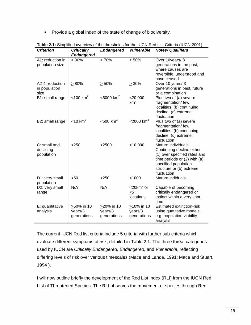
Table 2.1: Simplified overview of the thresholds for the IUCN Red List Criteria (IUCN 2001)

Criterion Critically Endangered

Endangered Vulnerable Notes/ Qualifiers

A1: reduction in population size

> 90% > 70% > 50% Over 10years/ 3 generations in the past, where causes are reversible, understood and have ceased.

A2-4: reduction in population size

> 80% > 50% > 30% Over 10 years/ 3 generations in past, future or a combination

B1: small range <100 km2

<5000 km2 <20 000

km2

Plus two of (a) severe fragmentation/ few localities, (b) continuing decline, (c) extreme fluctuation

B2: small range <10 km2 <500 km

2 <2000 km

2 Plus two of (a) severe

fragmentation/ few localities, (b) continuing decline, (c) extreme fluctuation

C: small and declining population

<250 <2500 <10 000 Mature individuals. Continuing decline either (1) over specified rates and time periods or (2) with (a) specified population structure or (b) extreme fluctuation

D1: very small population

<50 <250 <1000 Mature indiduals

D2: very small range

N/A N/A <20km2 or

<5 locations

Capable of becoming critically endangered or extinct within a very short time

E: quantitative analysis

>50% in 10 years/3 generations

>20% in 10 years/3 generations

>10% in 10 years/3 generations

Estimated extinction-risk using quatitative models, e.g. population viability analysis

The current IUCN Red list criteria include 5 criteria with further sub-criteria which

evaluate different symptoms of risk, detailed in Table 2.1. The three threat categories

used by IUCN are Critically Endangered, Endangered, and Vulnerable, reflecting

differing levels of risk over various timescales (Mace and Lande, 1991; Mace and Stuart,

1994 ).

I will now outline briefly the development of the Red List Index (RLI) from the IUCN Red

List of Threatened Species. The RLI observes the movement of species through Red

16

List categories over time. The categories can be used to calculate the rate at which

species under threat move to extinction (Butchart et al. 2004, 2007). The RLI is based

on the number of species in each Red List category. Categories were each weighted, to

make the index sensitive to not only the total number of threatened species, but also to

the changes in category given to each species (Butchart et al., 2004). The RLI is not just

capable of tracking global trends. It can be disaggregated to show trends for species in

different ecosystems, habitats, taxonomic groups etc., and for species relevant to

different international law (Butchart et al., 2007).

RLI has changed and improved since it was initially developed and tested in 2004 using

bird data from 1988-2004. Three shortcomings in the original design were identified

(Butchart et al. 2007) leading to the revision of the original formula. The first was that

newly evaluated species may have introduced bias to the index. If a species was

previously assessed as Data Deficient or was newly recognised taxonomically, they may

introduce a “false” change to the index trend once their assessment is included (Butchart

et al., 2007). The second is that RLI values were affected by the frequency of

assessments. Using the original formulation the RLI value is dependent on the number

of assessments that precede it since the baseline year. The third shortcoming was that

the RLI performs inappropriately when it reaches in zero. The 1988-2004 bird dataset

used to develop the formula showed an important, but relatively small proportional

decline in status over time. This did not prepare the formula for the problems that may

arise when a group of species undergo a large proportional decline in status. If the RLI

calculated declines to zero (by 100%) it subsequently cannot change, even if the species

continued to decline (Butchart et al., 2007). To address these outlined shortcomings, the

original formula was revised, and subsequently became easier to interpret (Butchart et

al., 2007). For details of the formula please see Methods section 3.5.3.

Instead of measuring the state of biodiversity, the RLI measures the rate of biodiversity

loss. The RLI is calculated from changes between the Red List categories, hence an RLI

value is an index of the proportion of species expected to avoid extinction in the near

future, without any conservation action (Butchart et al. 2007). If the rate of biodiversity

loss is increasing it is shown by a downward trend in the RLI, whereas a decrease in the

rate of biodiversity loss is shown by an upward trend. A horizontal line means the

expected rate of species extinctions is remaining the same (Butchart et al. 2007).

17

The RLI has some shortcomings, which are currently being addressed by further

research. These include taxonomic bias, documentation of reasons for change, and time

lags and the resolution of changes (Butchart et al. 2005). The validity of the IUCN Red

List Index as an indicator could be compromised by taxonomic bias. This problem is in

part being addressed by expanding taxonomic coverage through the sampled approach

to Red Listing (a random sample of 1,500 species from new taxonomic groups being

assessed; (Baillie et al 2008; Collen et al. 2009). As the species are tracked over time

and move between categories, it is important to have a good auditing system to allow

documentation outlining the reasons for re-classification (IUCN 2001). These are

currently classified as being “genuine” (e.g. due to change in species abundance) and

“non-genuine” (e.g. due to change in knowledge). Due to the nature of the Red List

categories, RLIs have a moderately course level of resolution of status changes.

However, the disadvantages of this are potentially outweighed by the advantage of

having a repeatable method to assess all the species within a taxonomic group, and not

just a subset for which detailed information is available (Butchart et al. 2004). The index

may also be insensitive to status changes as a result of time lags between changes in a

species and changes in the RLI value. Work is being done to mitigate this latter problem,

and a study completed addressing changing statuses of birds, found that the true index

value may lie somewhere between 0.21%-0.37% of what had previously been estimated

(Butchart et al., 2004).

2.4 Current and potential future uses of global biodiversity indicators Currently the indicators developed by the CBD are not being used to their full potential

i.e. to drive policy change and audit management decisions (Jones et al. In review). It is

known that the world has not met the CBD 2010 target, and so has failed to reduce

biodiversity loss (Mace et al. 2010). The LPI has fallen by about 30% since 1970 (The

Living Planet Report, 2008). It is described as a “measure of global biodiversity only as

far as trends in vertebrate species populations are representative of wider trends in all

species, genes and ecosystems” (Loh et al. 2005). However, it is not known if trends in

vertebrates would convey true trends of other taxonomic groups, and this needs to be

investigated if the LPI is to be used successfully to assess the full impact of new

environmental policy and to audit past management decisions. Currently, the Red List

can be used to prioritize species for conservation action, and the RLI can be used to

18

analyze trends in the few groups where species have been reassessed (Butchart et al.

2005; Butchart et al. 2007). However, it is yet to be used to assess the impact of specific

policy (assuming that it is capable of detecting such trends). This is considered to be the

future use of indicators in the wake of the CBD (Jones et al. In review).

The Marine Trophic Index is another of the headline CBD indicators. In the past it was

used to identify what is now a widely known phenomenon called „fishing down marine

food webs‟ (Pauly et al. 1998). It has been developed to clearly describe and

communicate the complex interactions between fisheries and marine ecosystems (Pauly

and Watson, 2005). In the future, specific Marine Trophic Index values could be used as

targets for management interventions, and so could be used to monitor the response of

systems to policy interventions. However, our present knowledge of systems does not

allow for critical trophic level threshold values to be indentified (Watson and Pauly,

2005).

2.5 Fisheries in Crisis In recent years there has been a lot of focus on sustainable fisheries and fisheries

management. Current global marine fisheries landing trends provide little evidence of

sustainability of marine resources and suggest a number of them are in fact in decline

(Caddy and Seijo, 2005). Sustainable target levels for managed fisheries in the past

have focused on reaching the maximum sustainable yield (MSY), however recent

experience suggests that MSY is risky target for fisheries management (Caddy and

Seijo, 2005). Not enough is known about stock status and fluctuations in productivity to

accurately predict the MSY for a fishery (Larkin, 1977). Progress towards reducing

overfishing is hampered by a reluctance to tolerate the inevitable short-term economic

and social costs of doing so (Worm et al. 2009). In addition to this, government subsidies

often encourage overfishing, and need to be urgently readdressed (Sumaila et al. 2007).

Radical policies are needed to allow fisheries to recover, however the management of

fisheries is a complex process and requires multidisciplinary integration between

ecology, resource biology, economics and politics (Caddy and Seijo, 2005). The affect

of these policies on biodiversity needs to be known, in order to monitor their success

once enforced.

Briefly outlined next is the history of commercial sea fishing, which dates back centuries.

At the end of the first millennium Europe was changing and developing. As the European

19

economy emerged, many workers began specialising in trades such as metalwork,

leather tanning and fishing (Roberts, 2007). Bottom trawling was first mentioned in 1376,

in a complaint made to King Edward III. It was a request that he ban the use of this new

and destructive fishing gear (Roberts, 2007). The complaints made in the late 14th

century included the decrease in captured fish size, the capture of non-target species,

and the notion that fish were deteriorating (Jones, 1992). Bottom trawling remains the

primary method of catching bottom-dwelling fish (Thurstan et al. 2010). Bottom trawlers

were sail powered and fished close to the shore until the end of the nineteenth century.

However, the development of steam trawlers in the 1880s resulted in the quick growth in

fishing effort that continued throughout the twentieth century (Knauss, 2005). Steam

trawlers were controversial in the United Kingdom, through their competition with line

fishers for fish. This resulted in a government enquiry in 1885, examining claims that

trawls were causing damage to habitats, and reducing fish stocks (Roberts, 2007). Due

to the absence of any fishery data or statistics the enquiry could not reach any

conclusions, and instead recommended that catch data should be collected. All major

ports in England and Wales, as of 1889, began gathering fishery statistics. The data this

provides about fleet composition and fish landings, allows the reconstruction of the

changes in the commercial fishing industry over the last century (Roberts, 2007). Since

the nineteenth century industrialisation of fishing, landings per unit of fishing power

(LPUP) has reduced by 94% - 17 fold (Thurstan et al. 2010). This suggests a remarkable

change in seabed ecosystems, and a decrease in the availability of bottom-living fish

(Thurstan et al. 2010). This could be partly due to the setting of quotas by politicians 20-

25% higher than advised by scientists since 1984, under the Common Fisheries Policy.

This has kept landings constant, despite falls in spawning stocks (Thurstan et al. 2010).

In modern fisheries, towed bottom trawls are believed to be one of the biggest sources of

global anthropogenic disturbance to the seabed and the species that inhabit it (Kaiser et

al., 2006) (See Fig.1.1). Globally trawlers cover an area of 15 million km2 of seabed per

year. That equates to an area 150 times larger than that which is deforested annually

(Malakoff, 1998). The design of trawl nets, is to catch species that are economically

valuable, however, as they are a “mobile non-selective fishing gear” they collect every

species they encounter (Kumar and Deepthi, 2006). This results in the catch of non-

target species, known as „by-catch‟. This by-catch, combined with the amount of

„discarded catch‟ (portion of catch returned to the sea), is a major concern associated

20

with the practise of trawling (Kumar and Deepthi, 2006). The major reasons for

discarding by-catch are (Kumar and Deepthi, 2006):

(1) Minimal commercial value,

(2) the costs of landing, and

(3) storage capacity of the vessel

There are also concerns about the effects of dumping substantial amounts of discards

and waste, such as fish heads and frames, on the seabed (Jones, 1992). Commercial

bottom trawling contributes approximately 27 million tonnes of discard per year. This is

more than half of all fish captured from marine fisheries directly for human consumption

annually (Kumar and Deepthi, 2006).

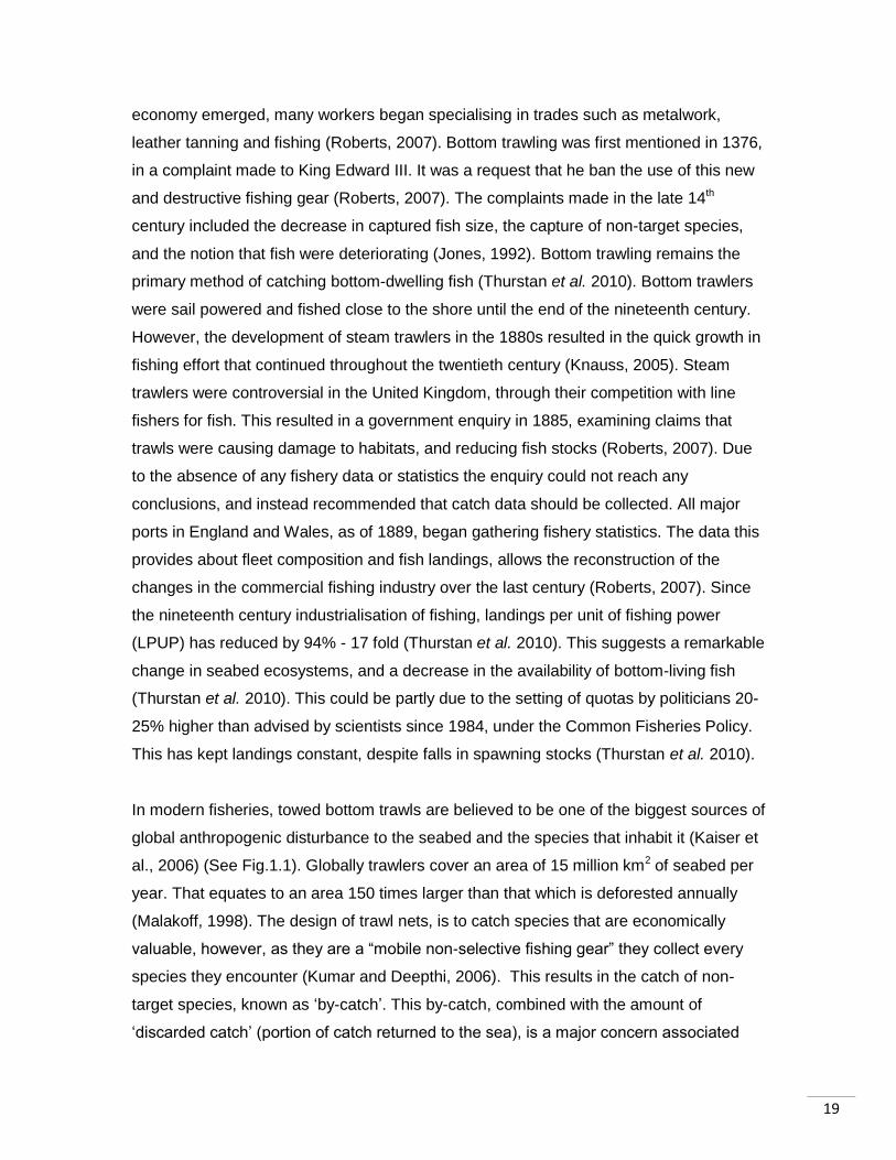
Figure 2.1: (a) Hexactinellid sponges are found only on deep-water reefs off the western coast of Canada, (b) The same area of sea floor after the trawl has gone. © Manfred Krauter 2007

In the North Sea alone, over the last decade trawlers have used heavier gears, and

more than 90% of the seabed has been trawled at least once, and in a number of cases

six times a year (Olsgard et al. 2008). Usually, the seabed is affected more when in

contact with heavier gear. The damage varies with the amount of gear used, together

with the structure and depth of the seabed and the strength of the currents (Jones,

1992). There are a number of direct and indirect effects from trawling. The direct effects

include things such as sediment resuspension, ploughing and scraping of the substrate,

and the dumping of discards and processing waste. Indirect effects are things such as

long-term changes to the habitat as a result of trawling, and post-fishing mortality (Jones,

1992).

(a) (b)

21

The indiscriminate nature of bottom trawls is one of the primary reasons for concern with

regards to high by-catch levels, and unsustainable fishing, but there are a whole host of

other effects, both direct, and indirect, that they can have on marine environments.

Bobbins and chains attached to the gear can leave distinctive tracks in the seafloor, and

potentially skim off the sediment on the surface. Otter boards leave imprints on the

seabed, and can plough a groove, which can be between a few centimetres and 0.3m

deep (Jones, 1992). The persistence of trawl tracks varies depending on the substrate

and water movement. However, where seamounts are trawled, and deep-sea corals are

damaged, the substrate could potentially take decades or even hundreds of years to

recover (Althous et al. 2009). As trawls flatten the seafloor the habitat becomes more

homogenous. This can be a significant factor in survival and recruitment for a variety of

marine organisms, including some species of commercial importance (Kumar and

Deepthi, 2006). Another effect of trawling is the resuspension of sediment. As the trawl

gear passes over the seafloor it causes a disturbance in the surface sediment. It can

result in damage and/ or removal of much of the resident biota. In addition, it can impact

a number of ecosystem functions such as the remineralisation of organic matter and

fluxes in nutrients (Olsgard et al., 2008). These changes and alterations to ecosystems

functioning are just some of the indirect results that bottom trawling can have on our

global marine environments.

2.6 Ecopath Modelling In fisheries science, a range of models are available to look at trends in fish populations

due to changes in communities, ecosystems, and exploitation rates. Single-species

models are commonly used to calculate the exploitation rate that provides the MSY for a

specific stock (Worm et al. 2009). Multispecies models range from simpler community

models to very complex ecosystem models. They can be used to predict the effects of

exploitation on species composition, biomass, size structure and other ecosystem

properties (Fulton et al. 2003). There has been a move towards the ecosystem approach

to fisheries globally over the last decade. In order to do this, single-species models need

to be integrated with ecosystem level assessments (Shin & Shannon, 2009).

Ecopath is one model that has been used often to assess the impact of protected areas

(Pauly et al., 2000). It was developed in the early 1980‟s by Polovina (1984), and since

then has been continuously developed. Ecopath is a static, mass-balanced snapshot of

22

the system. Ecosim, a development of Ecopath, emerged in 1995, adding dynamic

modelling capability. In 1998 Ecospace was developed and resulted in an integrated

software package „Ecopath with Ecosim‟ (Ecopath) (Christensen and Walters, 2004). It is

based on a two master equations. The first describes the production term, and the

second is the energy balance for each group of species (functional group) within the

model (Christensen and Walters, 2004).

Although Ecopath has been used for over 20 years there are still some potential

drawbacks to consider. Ecopath provides an „instantaneous estimate of biomasses,

mortaility rates and trophic flows, for some reference period (usually a year). As biomass

is generally at equilibrium the models assume no trends under constant fishing. To alter

this, a rate of biomass „accumulation‟ or „depletion‟ can be entered into the model,

however this can be difficult to paramaterise and can lead to misleading results

(Christensen and Walters, 2004). Due to their complexity it is hard to quantify the

uncertainty that is inherent in the models. It is important to recognise this when

comparing policy comparisons within Ecopath (Christensen and Walters, 2004).

23

3 Method

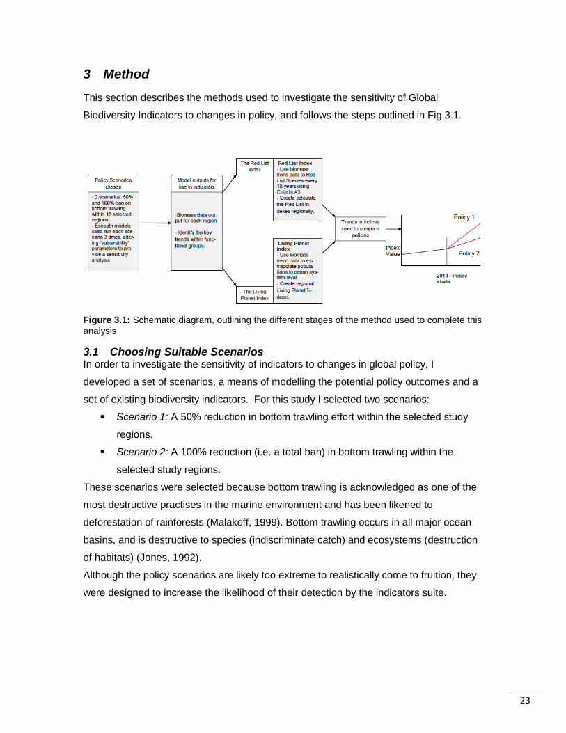
This section describes the methods used to investigate the sensitivity of Global

Biodiversity Indicators to changes in policy, and follows the steps outlined in Fig 3.1.

Figure 3.1: Schematic diagram, outlining the different stages of the method used to complete this

analysis

3.1 Choosing Suitable Scenarios In order to investigate the sensitivity of indicators to changes in global policy, I

developed a set of scenarios, a means of modelling the potential policy outcomes and a

set of existing biodiversity indicators. For this study I selected two scenarios:

Scenario 1: A 50% reduction in bottom trawling effort within the selected study

regions.

Scenario 2: A 100% reduction (i.e. a total ban) in bottom trawling within the

selected study regions.

These scenarios were selected because bottom trawling is acknowledged as one of the

most destructive practises in the marine environment and has been likened to

deforestation of rainforests (Malakoff, 1999). Bottom trawling occurs in all major ocean

basins, and is destructive to species (indiscriminate catch) and ecosystems (destruction

of habitats) (Jones, 1992).

Although the policy scenarios are likely too extreme to realistically come to fruition, they

were designed to increase the likelihood of their detection by the indicators suite.

24

3.2 Indicator selection Out of the 29 indicator measures outlined by the CBD, nine are now considered to be

well-developed, and have well founded, peer reviewed methods (Walpole et al., 2009).

For this study, it was important to investigate how well these fully developed indicators

perform, and whether they can actually fill their potential role, helping to inform policy

decisions. I also considered how relevant the indicators were to the policy decision.

Following a ban or reduction in bottom trawling, increases in abundance of commercial

species and prominent by-catch species were expected. As a result of this, the extinction

risk for many species was anticipated to decline. The indicators selected needed to be

able to detect these changes, and any indirect changes as result of this, within the

system in order to detect the policy. As the policies being studied were based in marine

systems, and were based on fishing catch reduction some indicators would be more

informative than others. For example, it is harder to study “Connectivity/ fragmentation of

ecosystems” in marine systems than in many terrestrial systems.

I selected two indicators from the CBD set to study the effects of the policy scenarios:

the Living Planet Index (Collen et al. 2009), and the Red List Index (Butchart et al.

2004), as they are capable of detecting changes in abundance and extinction risk, and

so are relevant to the changes expected following enforcement of the policy scenarios.

In addition, they are applicable to terrestrial, freshwater and marine systems, and so

could be used in the future for a wider range of policy decisions. The Marine Trophic

Index (Pauly and Watson, 2005) was another obvious choice to test the impact of policy

change in the marine environment, however, data are not widely available so it was

beyond the scope of this project.

3.3 Ecopath Modelling In order to investigate whether Global Biodiversity Indicators are capable of detecting

changes as a result of the policy scenarios, the first step was to model the effects of the

policy change in different regions. To do this, Ecopath models were chosen. They were

selected as they provide ecosystem level information in the form of biomass changes

among species or groups of species (functional groups). In addition, due to the inclusion

of non-catch species, they allow the investigation of the indirect effects of the bottom

trawl reduction policy, such as changes in food-chain structure. Alternative models were

25

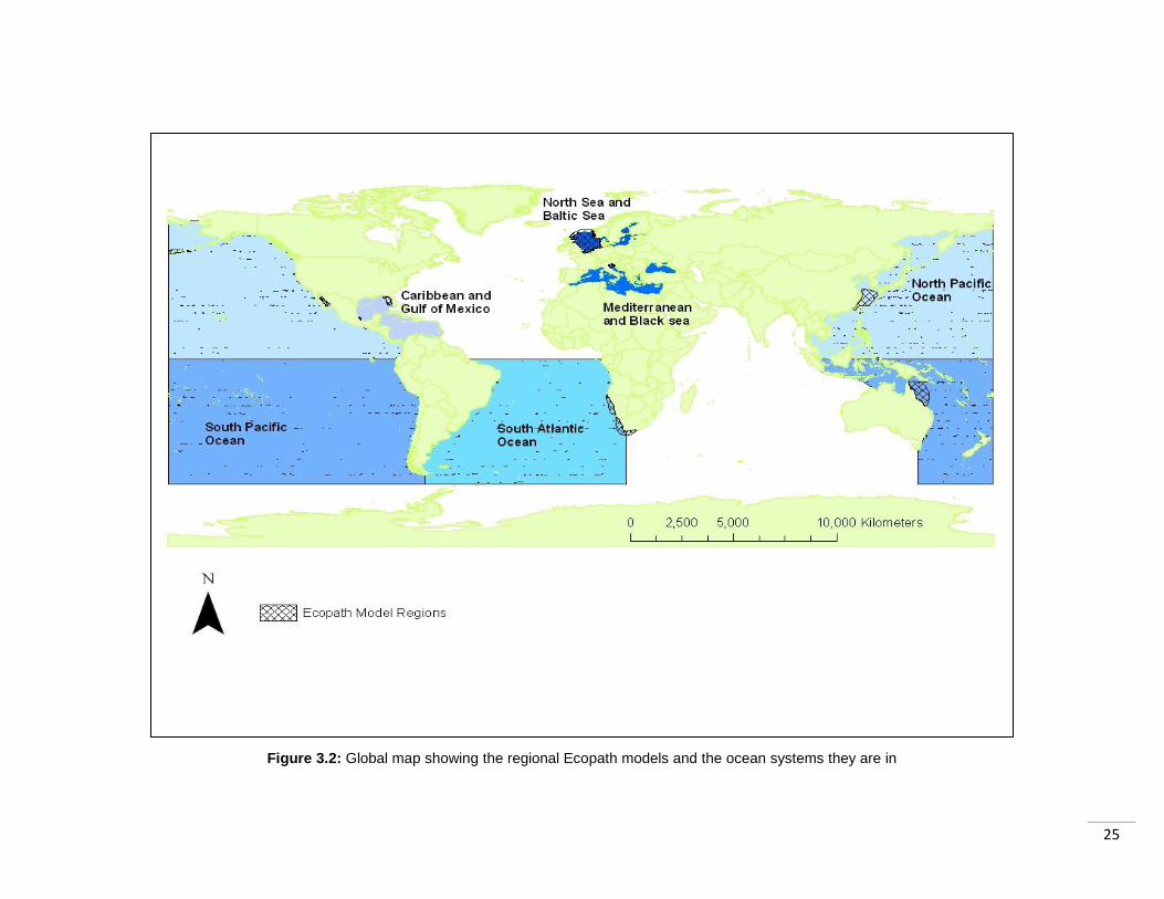
Figure 3.2: Global map showing the regional Ecopath models and the ocean systems they are in

26

considered, such as single-species models (Versteeg et al. 1999, Kinzey and Punt,

2009) and the multispecies models used by Worm et al. (2003) and Van Kirk et al.

(2010). However, as they lacked inclusion of non-commercial species, such as non-

target fish species, marine mammals etc. their capacity to detect indirect impacts of the

removal of bottom trawling were limited.

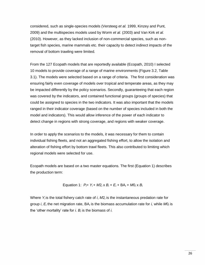
From the 127 Ecopath models that are reportedly available (Ecopath, 2010) I selected

10 models to provide coverage of a range of marine environments (Figure 3.2, Table

3.1). The models were selected based on a range of criteria. The first consideration was

ensuring fairly even coverage of models over tropical and temperate areas, as they may

be impacted differently by the policy scenarios. Secondly, guaranteeing that each region

was covered by the indicators, and contained functional groups (groups of species) that

could be assigned to species in the two indicators. It was also important that the models

ranged in their indicator coverage (based on the number of species included in both the

model and indicators). This would allow inference of the power of each indicator to

detect change in regions with strong coverage, and regions with weaker coverage.

In order to apply the scenarios to the models, it was necessary for them to contain

individual fishing fleets, and not an aggregated fishing effort, to allow the isolation and

alteration of fishing effort by bottom trawl fleets. This also contributed to limiting which

regional models were selected for use.

Ecopath models are based on a two master equations. The first (Equation 1) describes

the production term:

Equation 1: Pi= Yi + M2i x Bi + Ei + BAi + M0i x Bi

Where Yi is the total fishery catch rate of i, M2i is the instantaneous predation rate for

group i, Ei the net migration rate, BAi is the biomass accumulation rate for i, while M0i is

the „other mortality‟ rate for i. Bi is the biomass of i.

27

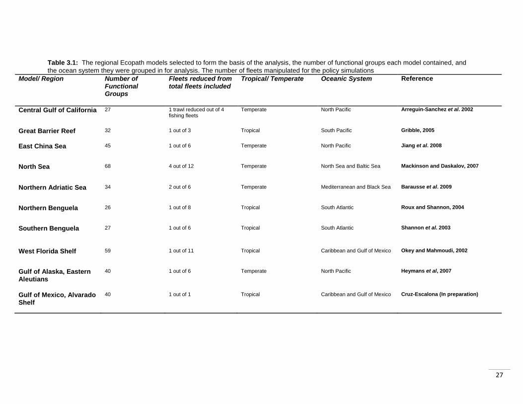
Table 3.1: The regional Ecopath models selected to form the basis of the analysis, the number of functional groups each model contained, and

the ocean system they were grouped in for analysis. The number of fleets manipulated for the policy simulations

Model/ Region Number of Functional Groups

Fleets reduced from total fleets included

Tropical/ Temperate Oceanic System Reference

Central Gulf of California

27 1 trawl reduced out of 4 fishing fleets

Temperate North Pacific Arreguin-Sanchez et al. 2002

Great Barrier Reef

32 1 out of 3 Tropical South Pacific Gribble, 2005

East China Sea

45 1 out of 6 Temperate North Pacific Jiang et al. 2008

North Sea

68 4 out of 12 Temperate North Sea and Baltic Sea Mackinson and Daskalov, 2007

Northern Adriatic Sea

34 2 out of 6 Temperate Mediterranean and Black Sea Barausse et al. 2009

Northern Benguela

26

1 out of 8 Tropical South Atlantic Roux and Shannon, 2004

Southern Benguela

27 1 out of 6 Tropical South Atlantic Shannon et al. 2003

West Florida Shelf

59 1 out of 11

Tropical Caribbean and Gulf of Mexico Okey and Mahmoudi, 2002

Gulf of Alaska, Eastern Aleutians

40 1 out of 6 Temperate North Pacific Heymans et al, 2007

Gulf of Mexico, Alvarado Shelf

40

1 out of 1 Tropical Caribbean and Gulf of Mexico Cruz-Escalona (In preparation)

28

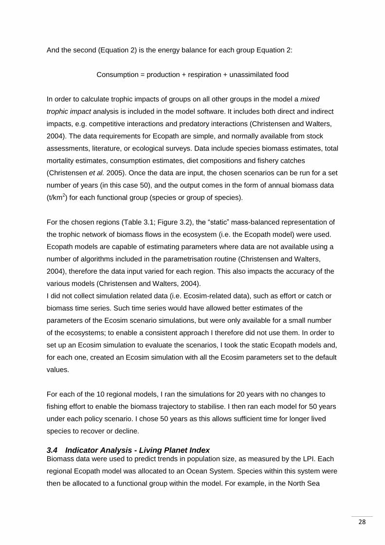
And the second (Equation 2) is the energy balance for each group Equation 2:

Consumption = production + respiration + unassimilated food

In order to calculate trophic impacts of groups on all other groups in the model a mixed

trophic impact analysis is included in the model software. It includes both direct and indirect

impacts, e.g. competitive interactions and predatory interactions (Christensen and Walters,

2004). The data requirements for Ecopath are simple, and normally available from stock

assessments, literature, or ecological surveys. Data include species biomass estimates, total

mortality estimates, consumption estimates, diet compositions and fishery catches

(Christensen et al. 2005). Once the data are input, the chosen scenarios can be run for a set

number of years (in this case 50), and the output comes in the form of annual biomass data

(t/km2) for each functional group (species or group of species).

For the chosen regions (Table 3.1; Figure 3.2), the “static” mass-balanced representation of

the trophic network of biomass flows in the ecosystem (i.e. the Ecopath model) were used.

Ecopath models are capable of estimating parameters where data are not available using a

number of algorithms included in the parametrisation routine (Christensen and Walters,

2004), therefore the data input varied for each region. This also impacts the accuracy of the

various models (Christensen and Walters, 2004).

I did not collect simulation related data (i.e. Ecosim-related data), such as effort or catch or

biomass time series. Such time series would have allowed better estimates of the

parameters of the Ecosim scenario simulations, but were only available for a small number

of the ecosystems; to enable a consistent approach I therefore did not use them. In order to

set up an Ecosim simulation to evaluate the scenarios, I took the static Ecopath models and,

for each one, created an Ecosim simulation with all the Ecosim parameters set to the default

values.

For each of the 10 regional models, I ran the simulations for 20 years with no changes to

fishing effort to enable the biomass trajectory to stabilise. I then ran each model for 50 years

under each policy scenario. I chose 50 years as this allows sufficient time for longer lived

species to recover or decline.

3.4 Indicator Analysis - Living Planet Index Biomass data were used to predict trends in population size, as measured by the LPI. Each

regional Ecopath model was allocated to an Ocean System. Species within this system were

then be allocated to a functional group within the model. For example, in the North Sea

29

model species Clupea harengus was allocated to the functional group „Herring‟ and

Megaptera novaeangliae to the group „Baleen whale‟ (for further examples of functional

groups see table 3.2). Each model within an ocean system was extrapolated to the level of

ocean system, by not just allocating species from the model location to a functional group,

but allocating all species within the system as a whole to a functional group. This assumes

that a reduction in bottom-trawling would have the same effect across the entire system, and

that fishing pressure was the same across the entire system.

3.4.1 Allocating models to ocean systems Within the LPI there are a number of ocean systems used to classify the location of

populations. Models were allocated to whichever of these systems they were found in

(Figure 3.2; Table 3.1)

3.4.2 Allocating Species to functional groups Species for each ocean system were allocated to a functional group within the model, unless

there was no applicable group. Original authors of each of the regional Ecopath models set

up functional groups. These ranged between models from groups of species such as

“Marine Mammals” to single species groups such as “Atlantic Cod”. There were differences

between the level of detail and number of functional groups per model. Some models used

functional groups based on families and species (e.g. East China Sea; Jiang et al. 2008),

where as others were more habitat focussed (e.g. West Florida Shelf model; Okey and

Mamoudi, 2002). Species were allocated at a population level, as many regions contain

numerous populations of the same species. Where there was more than one model for an

ocean system (e.g. the North Pacific, which contains the „Aleutian Island‟ (Heymans et al.

2007), „Central Gulf of California‟ (Arreguin-Sanchez et al. 2002) and the „East China Sea‟

(Jiang et al. 2008) models), species were allocated to a functional group within the model

that best matched their actual distribution. For example, in the North Pacific Fratercula

cirrhata was allocated to the functional group “seabirds” within the

Aleutian Islands model over the Central Gulf of

California, or the East China Sea, as this overlaps

with more of their range than either of the other

models.

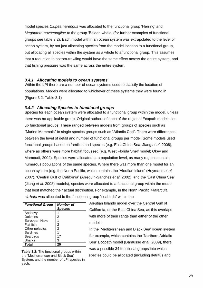
In the ‟Mediterranean and Black Sea‟ ocean system

for example, which contains the „Northern Adriatic

Sea‟ Ecopath model (Barausse et al. 2009), there

was a possible 34 functional groups into which

species could be allocated (including detritus and

Functional Group Number of Species

Anchovy 1 Dolphins 2 European Hake 1 Flat fish 2 Other pelagics 2 Sardines 1 Sea birds 17 Sharks 3

Total 29

Table 3.2: The functional groups within

the „Mediterranean and Black Sea‟ System, and the number of LPI species in each.

30

zooplankton). However, only eight were applicable to the species present on the LPI (Table

3.2).

3.4.3 Calculating the LPI Once all possible species were allocated a functional group, the raw population data was

then extrapolated to 2010 from the end point of their time series using a linear projection of

the average annual rate change in abundance over the course of each time series. Once all

populations that were to be included in the models (all those within a functional group) had

been extended to 2010, they were then extended for 30 years, using the annual rates of

change calculated from the biomass results of the regional Ecopath models. This created an

annual time series running from the start year of the population, up to 2040. These

calculations assumed a 1:1 relationship between change in biomass and abundance.

Following Collen et al (2009) I calculated an aggregated trend in population abundance

using a generalized additive modeling (GAM) framework. I implemented a GAM, specified

with the mgcv package framework in R (Wood 2006). For each time series, I followed the

method outlined by Collen et al. (2009). The Index value (I) was calculated in year t as:

Where dt is the mean value of species with multiple time series.

A GAM was fitted on observed values with log10 (Nt) as the dependent variable (where N is

the population variable) and year (t) as the independent. Fitted GAM values were used to

calculate predicted values for all years (including those with no real count data) and

averaged and aggregated d values from the imputed counts. A bootstrap resampling

technique was used to provide confidence limits around the index values. In order to

calculate the bootstrap replicate, for each interval, t-1 to t (where t is year), a sample of nt,

species specific values of dt was selected at random with replacement from the nt observed

values (Collen et al. 2009).

3.4.4 Aggregating the LPI An aggregated regional LPI was created by combining the six ocean system LPI‟s. The

systems are: „Caribbean and Gulf of Mexico‟, „Mediterranean and Black Sea‟, „North Pacific

Ocean‟, „North Sea and Baltic Sea‟, „South Atlantic Ocean‟ and „South Pacific Ocean‟. As

species are recorded in the LPI by population there were no concerns about duplication in

the results.

31

3.5 Indicator Analysis – Red List Index I extracted annual biomass data for every species or functional group from the regional

Ecopath models. I investigated the effect of this data on the Red List Index (RLI) by

matching Red Listed species to species within the model, or assigning them to functional

groups where no match was available (not all species in the models have Red List

assessments). For example, in the North Sea model species Clupea harengus was allocated

to the functional group „Herring‟ and Megaptera novaeangliae to the group „Baleen whale‟

(Table 3.2). The Red Lists data were obtained from www.iucnredlist.org, or from unpublished

assessments which are currently being added to the red list (Collen, In preperation). This

data consisted of species assessments, the Red List criteria used for the assessments,

distribution information and life history information such as generation length. Where life

history data were unavailable from the Red List, it was gathered from FishBase (2010).

3.5.1 Allocating species to a model For a species from the Red List to be allocated to a model, it was assumed that any species

present in the same FAO Major Fishing Area (FAO, 2010) as the model had the potential to

be included unless it was in a Red List threat category based on a range restriction (criterion

D). For example, any species found in the Mediterranean and Black Sea FAO Major Fishing

area was allocated to a functional or species group within the Northern Adriatic Sea Ecopath

model, unless they were in a threat category using criterion D that stated it was exclusively

found elsewhere, not included in the area of this model.

3.5.2 Allocating species to a functional group Species on the Red List were allocated to functional groups in the models as outlined in

section 3.4.2.

3.5.3 Determining projected Red List Status Species were assigned a new projected Red List Status every 10 years for the 50 years of

each regional Ecopath model run under the 2 scenarios, based on how trends in biomass

triggered category listing under criterion A4 (IUCN, 2001), based on the trends in biomass

for the functional group they were in (as produced by the regional Ecopath Models). This

criterion specifies an “observed, estimated, inferred, projected or suspected population

decline” (IUCN, 2001). If a species‟ decline is greater than 80% it is classed as Critically

Endangered (CR), if it is between 80% and 50% it is Endangered (EN), and if it is between

30% and 50% it is Vulnerable (VU). Anything less than that, or a population increase, than it

was classed as Least Concern (LC). The Near Threatened (NT) status could not be

allocated, as that is ordinarily allocated to species where potential threats can be inferred, or

the species has undergone declines that are close to reaching a threat category threshold

32

and the threats facing it are likely to continue in the future. Data Deficient (DD) species were

not allocated new Red List status as little information is known about them.

In order to calculate the Red List Status the average annual change in proportion of biomass

over the 10 year period was calculated and projected forward over the longer of 3

generations or 10 years (IUCN 2001) for each species to give a trend in abundance over the

period, using the equation:

Nt /N0 = (1+y)t

Where t is the number of years (either 3 generations or 10 years), y is the annual rate of

change, Nt is the population size in year t, and N0 is the current population size. Where

generation length was not known for a species, the default value of ten years, given by

IUCN, was used to assess their status. This was the case only for species of fishes. The

estimated change in abundance over the assessment period for that species was then used

to allocate a Red List status. During the analysis, a 1:1 relationship was assumed between

biomass and abundance. I excluded species assessed as Data Deficient and species with

restricted range, classified under Criterion D, as they are unlikely to benefit from the

reduction in trawling, and could not be included in the model.

The RLI was calculated as follows, using the IUCN weighting system used outlined by

Butchart et al., (2004) and revised by Butchart et al. (2007):

RLIt=(M-Tt)/M

Where each threat category is weighted and assigned a threat score, M is the “maximum

threat score”, i.e. the number of species multiplied by the maximum category weight, T is the

“current threat score” and t is the year. The RLI for each region was then calculated for each

year of assessments (2020, 2030, 2040 and 2050 - assuming the policy was implemented in

2010, first year of results 2011). The temporal trend generated was used to see if the effects

of the ban could be detected in the RLI.

3.5.4 Allocating models to ocean systems Models were allocated to the same ocean systems as for the LPI (Section 3.4.1; Table 3.1).

This was to allow easy comparison of the results. They were allocated to ocean systems

after the individual Red List statuses had been calculated however. This was because the

models included in an ocean system could contain the same species, where this occurred,

33

the population trends for those species were aggregated and the Red List status

recalculated based on the aggregated trend data (IUCN 2001).

3.5.5 Aggregating Regional Red Lists An aggregated RLI was compiled using the Red Lists created for the six ocean systems.

Again, where there were duplicate species with potentially, differing Red List statuses, Red

List status was calculated using the combined regional trends. The RLI was then calculated

as previously outlined in section 3.5.3.

34

4 Results

4.1 Aggregated LPI and RLI for the Six Study Regions The aggregated LPI of the six ocean systems („Caribbean and Gulf of Mexico‟,

„Mediterranean and Black Sea‟, „North Pacific‟, „North Sea and Baltic Sea‟, „South Atlantic‟

and „South Pacific‟) shows populations stabilizing but showing no signs of recovery (Fig 4.1,

(a)). Following a 100% reduction in bottom trawling it stabilizes after a 16% decline from the

start of the LPI in 1970, and 1% decline from the start of the policy in 2010. As a result of a

50% reduction, abundance trends are only 1% lower. The difference between the impacts of

the two policies is much smaller than anticipated.

The Red List Index (Fig 4.1, (b)) shows after 10years a 1.3% decline in response to a 100%

reduction in fishing effort and an increase of 3.4% in response to a 50% reduction. This

means a complete halt to bottom trawling results in a short-term increase in the number of

species in IUCN threat categories. However this decline is followed by a swift recovery and

the index then stabilizes at 98%, which means 98% of species included in the index are in

„non-threat‟ categories. Following either a 100% or a 50% reduction in bottom trawling, the

RLI shows all previously threatened species (except those categorized using criterion D) are

downgraded to non-threat categories after 20 years of the policy being introduced.

Overall, initial observations appear to show that the two indicators being studied can detect

the policy of halting bottom trawling: the LPI shows stabilization, although not a recovery in

abundance, while the RLI shows species extinction risk decline, resulting in them being

downgraded. The impacts of a 50% reduction policy are very similar, populations within the

LPI stabilize, and extinction risk also declines. Analyzing the underlying regional patterns will

give a better understanding of the aggregated results and what they mean, which we do

below.

4.2 Regional LPI Results One of the most notable things from the analysis is the small difference detected by the

indicators between the two policies. The differences range from population trends being 0.3

% higher following a 100% reduction in bottom trawling over a 50% reduction („South Atlantic

Ocean‟), to 14% lower following a 100% reduction („North Sea and Baltic Sea‟). It was

anticipated that the two policies would have more differing effects for the indicators to detect.

Within the regional results, the key trend within the LPI was rapid stabilization.

35

Figure 4.1: Aggregated across all six study regions, the LPI (a) and RLI (b) compare a 50% reduction in bottom trawling and 100% reduction. The dashed lines on (a) show the boot strapped confidence

intervals, and the vertical line indicates the start of the policy in the 2010, with the first results of the policy in 2011.

0

0.2

0.4

0.6

0.8

1

1.2

1.4

1970 1975 1980 1985 1990 1995 2000 2005 2010 2015 2020 2025 2030 2035 2040

Ind

ex

Va

lue

Year

50% Reduction Policy 100% Reduction Policy

(a)

0.92

0.93

0.94

0.95

0.96

0.97

0.98

0.99

2010 2020 2030 2040 2050 2060

Ind

ex

Va

lue

Year

50% Reduction Policy 100% Reduction Policy

(b)

36

All the regions in the LPI, under both policies showed population trends stabilizing within 10-

15 years of the policy being enforced (Appendix 1.1). The LPI values for the two scenarios in

each region were very similar, in most cases with the 100% reduction having a slightly

higher LPI (i.e. relatively greater abundance).

The temperate regions appeared to be impacted differently to the tropical regions. In two

cases, the LPI was higher for 50% reduction than 100% reduction after stabilisation: the

„North Sea‟ and the „Mediterranean and Black Sea‟, though in the latter the initial impact of

100% was greater. Both showed increasing abundance trends prior to the policies. The

„North Pacific Ocean‟ system differs from the other two temperate systems as it is declining

prior to the policy. It then stabilizes as the other two do, but abundance is 3% higher

following the complete ban in bottom trawling than following the 50% reduction.

The tropical regions showed differing trends to those outlined for the temperate regions. The

„Caribbean and Gulf of Mexico‟ index was in decline prior to the policies. It stabilized as a

result of the policies, with both policies showing very similar trends in abundance, with the

difference between them being 1% in 2040 (100% reduction index higher than 50% index).

The „South Atlantic Ocean‟ was also declining before the policies were enforced and again

showed very similar responses to both. The index is 0.3% higher in 2040 following the 100%

reduction as opposed to the 50% reduction in bottom trawling. The „South Pacific Ocean‟

index shows a bigger difference in its response to the two policy scenarios. The LPI is 4.3%

higher in 2040 if bottom trawling is completely stopped, than if there is a 50% reduction.

Before the policies are enforced the index trend was increasing.

It is initially unclear as to why there appear to be differences in the response of tropical and

temperate systems. It could be a result of the data available for these regions, or as a result

of true differences in the way these systems react to the policy. In two out of the three

temperate systems („North Sea and Baltic Sea‟ and the „Mediterranean and Black Sea‟

systems) the 100% reduction in bottom trawling resulted in lower abundance than the 50%

reduction. However, this was not the case in any of the tropical systems.

4.3 Regional RLI Results When the RLI was looked at regionally, it could be seen that most regions showed almost no

difference between the two policies. In three cases no differences were detected by the RLI

(„Mediterranean and Black Sea‟, „Caribbean and Gulf of Mexico‟ and „South Pacific Ocean‟).

37

Those regions that did react differently to the two policies settled into the same values after

20 years (Appendix 1.2).

Similarly to the LPI, there was a difference between the way tropical and temperate systems

performed. The „Mediterranean and Black Sea‟ index shows no difference in the response to

the two different policies. Both policies result in an increase in the index, which then remains

stable. The two other temperate systems however both show declines in the index, after 10

years of the policy being enforced, following the 100% reduction in bottom trawling.

The tropical systems show a different response to the temperate ones. Both the „Caribbean

and Gulf of Mexico‟ and the „South Pacific Ocean‟ indexes show the same response

following both policies. They increase after 10 years of the policy, and then remain stable at

that level. They show all species (except those classified using criterion D) move into „non-

threat‟ categories. The species showing this quick change between categories are generally

short-lived fish species. If it were marine mammals, or other longer lived species, the

changes between categories would be expected to take longer. The „South Atlantic Ocean‟

index however takes longer to recover following the 100% reduction policy. After 10 years of

the policy, the index increases by 4%, as species extinction risk declines, it then increases

by 1% in the following 10 years, and then remains constant. They delay in stabilization is a

result of all the species in the index becoming „non-threatened‟ except for the „mesopelagic‟

functional group species (and those threatened under criterion D), which declines (moves

from „Least Concern‟ to „Vulnerable‟) in the ten years after the policy enforcement and then

recovers to „Least Concern‟ in the following ten years.

Due to the differences in the response of tropical and temperate systems seen in both the

indicators, two regions were selected as case studies to investigate these effects in more

detail: the temperate system of the „North Sea and Baltic Sea‟, and the tropical „South Pacific

Ocean‟.

4.4 Case Study 1: The North Sea and Baltic Sea Following a 50% reduction in bottom trawling both the LPI and RLI show a rapid stabilization

(Fig 4.2). In the LPI there appears to be no recovery of populations, which one would expect

to appear as an increasing trend in abundance. The index remains at a constant level over

the 30 year period after the policy is enacted. The RLI shows species being downgraded to

non-threat categories 10 years after the policy is enforced, and then remaining in those

categories over the following 40 years. All species are down listed except those that are

(a)

38

threatened and listed using criterion D. This downgrade occurs very quickly after the policy is

enforced, and could be due to the short generation length of the species.

Both indices show a larger decline in index value following a complete reduction in bottom

trawling than following a 50% reduction (Fig 4.2). This is an unexpected result, as it would be

anticipated that the complete removal of a fishing pressure (especially one as destructive as

bottom trawling) would cause greater increases in species abundance than a 50% reduction

in fishing pressure. The LPI shows lower population abundance after the complete reduction

policy, than after the 50% reduction policy, and the RLI shows some species become more

threatened (and then recover) as a result, whereas after a 50% reduction they recover

without a decline.

To investigate why the LPI may react to the policies in this way, I disaggregated the regional

index into functional groups; the relative abundance of each group is shown in Figure 4.3. In

total, 24 functional groups (two of which were predatory) from the Ecopath model were

included. Of these, the single largest group contributing to the index was the „seabirds‟ group

which made up 47% of the species in the LPI for the region. The four next biggest

contributors were „small demersal fish‟ (10% of species in the regional LPI), „large demersal

fish‟ (8%), and „miscellaneous pelagic filter feeders‟ and „small sharks‟ (both 4%). All the

other functional groups had only one or two species represented in the LPI. As Ecopath

models are based on predator prey relations, the original biomass results of these top five

contributing functional groups were compared to the biomass results of the predatory

functional groups of the highest trophic levels (top of the food-chain) (Fig 4.3).

It is evident that the regional LPI response is driven by the relative increase in biomass of

„top‟ predators and with a corresponding decrease in prey groups and seabirds. These

biomass trends are greater following the 100% reduction in bottom trawl fishing effort; hence

the greater decline in the LPI, which is dominated by prey groups and seabirds (Fig 4.3, note

differences in axis scale). Although one functional group included in the LPI did significantly

increase in biomass („large demersal fish‟) it appears that this increase was not large enough

to outweigh the decrease in „seabird‟ biomass, as seabirds accounted for 47% of the species

included in the LPI in the region. These shifts in biomass may also account for the decline

seen in the RLI after 10 years of the 100% reduction policy. The decline in the RLI is seen as

„sandeels‟ move from „Least Concern‟ to „Vulnerable‟. This could be the result of biomass

declining in this functional group and increasing in a predatory functional group that predates

sandeels (e.g. „Atlantic cod‟). The one marine mammal group included is seen to take longer

39

Figure 4.2: The „North Sea and Baltic Sea‟ System LPI (a) and the RLI (b) compare a 50% reduction and 100% reduction in bottom trawling. The dashed lines on (a) show the boot strapped confidence

intervals, and the vertical line indicates the start of the policy in the 2010, with the first results of the policy in 2011.

0

0.5

1

1.5

2

2.5

3

3.5

4

Ind

ex

Va

lue

Year

50% Reduction Policy 100% Reduction Policy

(a)

0.97

0.975

0.98

0.985

0.99

2010 2020 2030 2040 2050 2060

Ind

ex

Va

lue

Year

50% Reduction Policy 100% Reduction Policy

(b)

40

Figure 4.3: Comparison between the biomass, following a 50% reduction in bottom trawling (a) and a 100% reduction (b) results, of the five functional group contributing the majority of species to the LPI

analysis, and the five predatory functional groups of the highest trophic level in the „North Sea and Baltic Sea‟ ocean system

0

0.5

1

1.5

2

2.5

2010 2015 2020 2025 2030 2035 2040 2045 2050 2055 2060

Re

lati

ve

Pro

po

rtio

na

l C

ha

ng

e in

Bio

ma

ss

Year

Seabirds SealsSmall demersal fish Large piscivorous sharksLarge demersal fish Toothed whalesMiscellaneous filterfeeding pelagic fish SpurdogSmall sharks Starry ray + others

Included Functional Groups Predator y Functional Groups

(a)

0

0.5

1

1.5

2

2.5

3

3.5

4

2010 2015 2020 2025 2030 2035 2040 2045 2050 2055 2060

Re

lati

ve

Pro

po

rtio

na

l C

ha

ng

e in

Bio

ma

ss

Year

Seabirds SealsSmall demersal fish Large piscivorous sharksLarge demersal fish Toothed whalesMiscellaneous filterfeeding pelagic fish SpurdogSmall sharks Starry ray + others

Included Functional Groups Predator y Functional Groups

(b)

41

to recover from both policies. This is likely to be a result of its longer generation length.

4.5 Case Study 2: The South Pacific Ocean In the „South Pacific Ocean‟ system, both indicators display a more intuitive result. Regional

abundance increases to around 50% more than the index value in 1970, following a

complete regional ban in bottom trawling (Fig 4.4, a). The regional change in LPI in response

to a 50% ban is qualitatively very similar though slightly less. This is different to what is seen

in the majority of temperate systems studied (Appendix 1.1; 1.2). The RLI shows a reduction

in extinction risk (number of species in threatened categories) as a result of both policies

(Fig 4.4, b). Both policies result in a stabilised index very quickly after the enforcement. This

is a trend seen throughout all the regions.

Typically the LPI stabilizes after only 10 years, whereas the RLI may take up to twenty years

(Appendix 1.2). It can be seen in this example that not only does the LPI stabilise very

quickly following the enforcement but that the difference between the index values for each

policy are very small (4%) (Fig 4.4, a). To investigate why it stabilises so quickly, five

functional groups were disaggregated from the index, and their individual LPI‟s were

analysed (Fig 4.5). The groups were: „small schooling fish‟, „inshore finfish‟, „large fish

carnivores‟, „seabirds‟ and „sea turtles‟. From this it can be seen that all the functional groups

stabilize after 5 years, apart from „sea turtles‟, which stabilize after about 15 years. The delay

seen in the „sea turtles‟ functional group could be the result of their longer generation

lengths. This also shows that the low index values of three of the groups („small schooling

fish‟, „large fish carnivores‟ and „inshore finfish‟) do not greatly impact the overall index of the

region (Fig 4.4). This is likely due to the „seabirds‟ group containing 15 of the regions 42 LPI

species, and so driving the trend of the index; as the other functional groups contain fewer

species in this regional LPI.

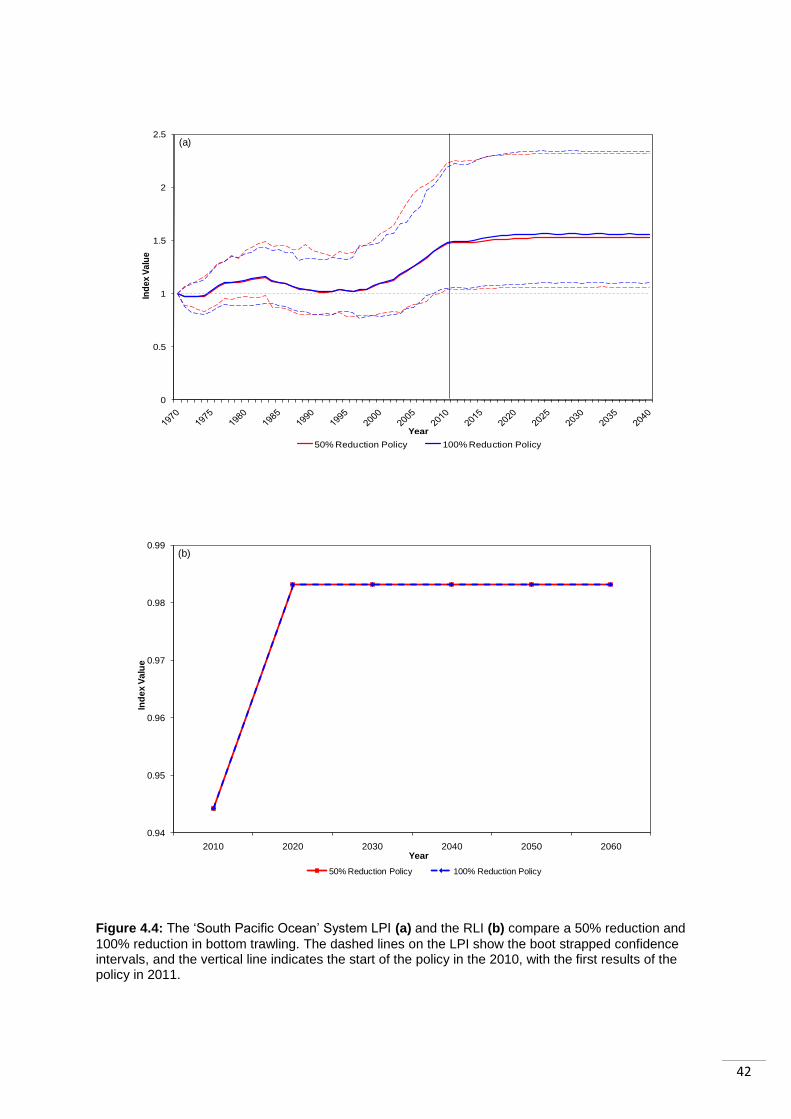
42

0

0.5

1

1.5

2

2.5In

de

x V

alu

e

Year

50% Reduction Policy 100% Reduction Policy

(a)

0.94

0.95

0.96

0.97

0.98

0.99

2010 2020 2030 2040 2050 2060

Ind

ex

Va

lue

Year

50% Reduction Policy 100% Reduction Policy

(b)

Figure 4.4: The „South Pacific Ocean‟ System LPI (a) and the RLI (b) compare a 50% reduction and

100% reduction in bottom trawling. The dashed lines on the LPI show the boot strapped confidence intervals, and the vertical line indicates the start of the policy in the 2010, with the first results of the policy in 2011.

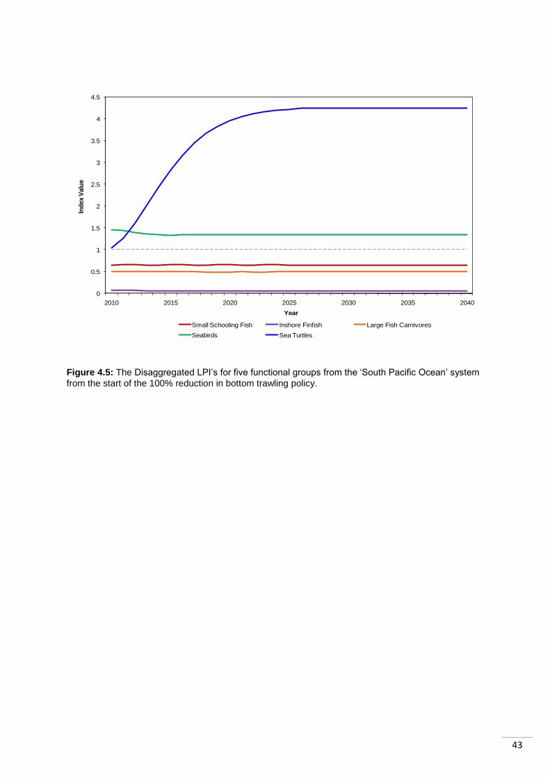
43

Figure 4.5: The Disaggregated LPI‟s for five functional groups from the „South Pacific Ocean‟ system

from the start of the 100% reduction in bottom trawling policy.

0

0.5

1

1.5

2

2.5

3

3.5

4

4.5

2010 2015 2020 2025 2030 2035 2040

Ind

ex V

alu

e

Year

Small Schooling Fish Inshore Finfish Large Fish Carnivores

Seabirds Sea Turtles

44

5 Discussion

5.1 Policy Results The aggregated index produced for both the LPI and RLI suggests that the two indicators

tested are capable of detecting changes in the status and trends of biodiversity, produced by

the alternative fishing policies modelled in this study. However, the difference in response to

the two policies is extremely small, a trend seen at the regional level too. Both indicators

show populations and species stabilising after the policy and in the case of the RLI a

reduction in extinction risk. In addition, the indicators behave differently to one another,

which reflects the different aspects of biodiversity trends they represent: abundance and

extinction risk.

The LPI shows populations stabilising after the policies in all regions, but does not increase,

so species abundance does not increase after the policy. The aggregated index shows little

or no recovery after the policies. If recovery continued at the slow rate suggested by the

modelling, it would take over 100 years for populations to return to the levels they were in

1970. Similar patterns of slow recovery have been observed in marine systems off the East

Coast of Canada. 15 years after the moratorium on fishing, and despite considerable

conservation efforts, few demersal fish species showed any signs of recovery (Caddy and

Seijo, 2005). In contrast to this, the invertebrates in the region showed huge increases in

productivity, close to historical highs (Caddy and Seijo, 2005); such species are not included

in either the LPI or RLI.

The aggregated RLI for all six ocean systems presents a different result to the LPI, and

shows, a somewhat unexpected response to change in both fisheries policies. In the 10

years immediately after a 100% reduction in bottom trawling, many species appear to face a

higher extinction risk than following a 50% reduction, which results in an index that declines

after 10 years of policy enforcement and recovers in the proceeding 10 years. On further

investigation this global acceleration in extinction risk is driven by species in temperate

regions, which appear to be impacted differently to tropical regions. Within temperate

regions some species moved into threat categories in the 10 years immediately after the

policy, as a result of predator release following the alleviation of fishing pressure (e.g. the

„North Sea and Baltic Sea‟ system). The species in the tropics may have been less

vulnerable to this affect due to naturally higher productivity in tropical regions (Bellwood and

Hughes, 2001) allowing mid-trophic level prey species to recover. As criterion A was used to

Red List the species, the decline in index value indicates that there was an increase in the

number of species in the threatened categories („Critically Endangered‟, „Endangered‟,

45

„Vulnerable‟) as a result of population decline. By virtue of this, similar trends to those seen

in the LPI would be anticipated.

There are three reasons why the indicators could be presenting different results. Firstly, the

indicators detect different aspects of biodiversity change. The second is that different

species contribute to the indicators, and indicators are bias towards temperate vertebrate

species (Pereira & Cooper 2006); and the third is that the effects are due to community

interactions between species that are being detected by the indicators. It is likely that all

these reasons contribute to the results seen here, and being able to discern between them

would improve our understanding of the indicators.

5.2 The different roles of the indicators The RLI is regarded as a course resolution indicator, due to the broad nature of the Red List

categories (Butchart et al. 2005). This means that populations have to undergo substantial

changes in range, distribution or size before crossing the criteria threshold to qualify for

either higher or lower Red List status (Butchart et al. 2005). This is unavoidable when using

the Red List categories rather than more precise parameters such as population size

estimates. This makes the RLI complimentary to the LPI, a population based index (Butchart

et al. 2005). This was seen in the current project, when investigating the „South Pacific

Ocean‟ case study. The RLI presented both policies as being equally beneficial to the

system, where as the LPI was capable of detecting the finer scale differences in the

population abundance. A time-lag between changes in species populations or range, and

the change being detected has been previously reported for the RLI (Butchart et al. 2005).

This was not seen in the current study however, as there were no large declines of the

monitored species, however, had the species coverage been more extensive, and more of

the dynamics of the systems been detected, it is likely that this may have been an issue.

The response of the Red List to both policies was the same in the South Pacific Ocean

system: an increase in index value, whereby all species that could be listed as Least

Concern by 2040 were. On first appraisal this suggests that both policies deliver equal

benefit to species, which is true, if you consider only extinction risk. Both policies do reduce

extinction risk to species equally in that species are downgraded, however, they may do this

to varying degrees which cannot be captured by the RLI as it has no way of distinguishing

between levels of „non-threat‟ category. This means that one species could be showing

increasing trends in abundance and be listed in the same „non-threat‟ category as a species

that‟s abundance is remaining constant over time, and is just outside a „threat‟ category

46

threshold. Although these species will both be classed as non-threatened, they are reacting

very differently to the policies, and the latter is certainly more vulnerable to future potential

threats than the other. The LPI detects a difference between the two policies (albeit small),

because in population abundance data, it uses a more fine scale measure of biodiversity

change (Loh et al. 2005; Collen et al. 2009). The RLI shows no difference between the two

policies as once the more coarse measure of biodiversity change, extinction risk, is below a

certain threshold (declines less than 30% over the longer of 10 years or 3 generations

(IUCN, 2001)), no category change can take place (Butchart et al. 2004; Butchart et al.

2007). However, as the LPI gives all species equal weighting within the index (Collen et al.

2009), it is easily dominated by one „functional group‟ of species, as seen in the North Sea

and Baltic Sea system where seabirds appear to have dominate the index. One way to

compensate for this would be to give different groups of species different weighting within

the index to compensate for any taxonomic bias.

From a policy perspective, the value of modelling is the ability to identify differences between

a range of alternatives (Mackinson et al. 2009); however the RLI is unable to do this after

extinction risk is decreased past a critical threshold. This could be important in a system

where a number of populations are close to the threshold and vulnerable to future threats.

For example, if a species appears to have recovered as it is no longer classed as

threatened, but in reality is close to the „Vulnerable‟ criteria threshold of a 30% decline

(IUCN, 2001). If fishing effort is increased, this could result in a population collapse and the

species being up-listed back into a threat category.

5.3 Taxonomic Bias of the Indicators As mentioned in previous studies (Butchart et al. 2005; Loh et al. 2005; Collen et al. 2009)

the primary drawback of the indicators was the taxonomic coverage and representativeness

of the population data. This was most striking in the LPI. The LPI contains time series for

over 11,500 populations of 2,500 species (Collen et al. 2009), but it is not necessarily the

lack of taxonomic diversity that is the problem, rather the uneven coverage of species across

the world. Ideally, the perfect dataset would make significant steps to correct the current

taxonomic bias, and would contain a higher proportion of diversity (Dobson, 2005) from

every system on the planet.

Some regions in this analysis were dominated by seabird data (e.g. Northern Benguela

regional model), whereas others were predominantly fish species (e.g. Great Barrier Reef).

The effects of these species biases were evident in the way the indicators reacted to the

47

policy change. The species coverage did not reflect the regions they were representing. To

truly represent the regions the indicators need to contain a wider sample of species. It is

unfeasible for them to contain all species, but they should aim to be a representative sample

of what is present (Butchart et al. 2005). Typically, tropical regions are more species rich

(Bergmann, 1847; Gaston, 2000), however the tropical regions only contained 152 species,

in the LPI, where as the temperate regions contained 252. In addition, upwelling regions

such as the Northern Benguela, should be areas of high fish productivity (Bianchi et al.

2000), and yet was dominated by species of seabird. It was only when combined with the

Southern Benguela region that the coverage of species became more even.

Different functional groups of species were used in the two indicators, based on the different

species they included. Neither indicator has complete coverage of all the species in a

system, as the LPI does not contain any invertebrate species, and the RLI is limited the

groups that have previously been assessed. This means that neither of them is likely to be a

perfect tool for monitoring change. However, the knowledge of where there coverage varies

allows for better interpretation of their results. Where the same functional group was used in

both indicators, the number of species it was applied to differed within regions (Appendix

1.3, 1.4). This would impact the way the indicators responded to the policy. For example, if

there was one functional group that was drastically reduced as a result of the policy, and that

species was only included in one indicator, it would influence the response of that indicator

and show a decline, whereas the other indicator would show an increase in abundance due

to the exclusion of that species and the inclusion of others. This was shown to an extent in

the RLI for the „North Sea and Baltic Sea‟ region, which noticeably decreased as result of

declines in functional group „sandeels‟. However, this effect was not detected by the LPI,

which did not contain the „sandeels‟ functional group. The effects of the policy on the

indicators need to be discerned from the effects of their species composition.

In the North Sea and Baltic Sea system the majority of species in the LPI analysis were

„seabirds‟ and low- to mid-trophic species (that are typically preyed upon by other high-

trophic species). The only predatory group included was „small sharks‟. Research by Petire

et al. (2009) suggests that predator-prey interactions can be very important in temperate

systems, and shows that a reduction in the fishing pressure on predator species does not

necessarily result in a recovery of that species in the following decade. With a reduction in

fishing effort modelled in this study, there appears to be a predatory release, with increases

in the biomass of the predatory functional groups (Seals, Piscivorous Sharks, Toothed

Whales, Spurdog and Starry Ray + Others). These seem to dominate the system resulting in

reduced biomass in prey functional groups. This shows that the results are a product of the

48

functional groups included in the analysis, and had the region contained alternative species

the LPI trend observed would be different.

The quick recovery times observed in the RLI may be the result of short-lived species on the

index, as it is short-lived fish species changing threat category. Had longer lived species

contributed more than the recovery could have been prolonged. The reduction in the Red

List Index in the North Sea and Baltic Sea system is due to declines in the prey-species

functional group „Sandeels‟. The release of predatory species is much greater following a

complete ban on bottom trawling, hence the lower abundance trends seen which lead to a

decline in the RLI. However, this observed RLI decline may have been larger or more

prolonged had other functional groups been included. This is also the case for the LPI. Out

of the 63 functional groups in the Ecopath model, 24 were present in the species contained

in the LPI. As „Seabirds‟ was the applied to 39 species out of a possible 83 (Appendix 1.3) it

is likely that they are heavily driving the decline.

In the South Pacific Ocean system the breadth of predator and prey species included is

greater than in the North Sea and Baltic Sea. This means that more complex food-web

interactions are included in the index, as opposed to just model responses from one group.

Despite the inclusion of more functional groups from different trophic levels, it is unlikely that

the wide reaching impacts of the policies throughout the ecosystem will be detected. This is

because the species coverage of the indicators does not accurately reflect the species

actually present (Pereira and Cooper. 2006), especially in the tropics, where biodiversity is

greatest (Bergmann, 1947; Gaston 2000). Despite, the models featuring a wider variety of

species in the indicators, the indicators themselves are limited by what species they contain.

Although the RLI shows comprehensive coverage within certain taxonomic groups, relatively

few groups have been completely assessed. This is constantly improving, but the RLI is not

representative of biodiversity as a whole (Butchart et al. 2005), and so is limited in what it

can detect. The Sampled Red List Index (SRLI) is designed to address this problem. It aims

to measure the changing relative extinction-risk of all species, major taxonomic groups,

realms, and three primary ecosystems (Butchart et al. 2005; Baillie et al. 2008). However,

this will be limited by the availability of data and resources. This sampling approach will

include the assessment of invertebrate groups, and will begin to cover the taxonomic gaps

inherent in the RLI.

49

5.4 Species community interactions As the LPI only includes vertebrate species, it is likely that complex ecosystem dynamics are

being missed. Practises like bottom trawling, change the structure of fish communities

through not only direct mortality from fishing, but from the related destruction of large

epibenthic organisms (Bianchi et al. 2000) and habitat alteration (Jones, 1992). If these are

not monitored for recovery then vital information pertaining to the recovery of other species

will be lacking. The „patchy‟ coverage even of vertebrate species impacts on the results

seen, as demonstrated in the North Sea and Baltic Sea case study. The North Sea is

considered to be dominated by bottom-up control (Fredericksen et al. 2006), which implies

the system is controlled by food abundance and the availability of prey. This has far reaching

effects on the dynamics of marine top predators and seabirds. There have been documented

cases, where crashes in prey species have resulted in the breeding failure of seabirds (e.g.

Anker-Nilssen et al. 1997). It is possible that this is the cause of the biomass decrease in the

„Seabirds‟ functional group, and resulted in the severe decline seen in the LPI. By having

data available predominantly for prey species, the increases in predator abundance were not

seen. This is important when indicators are being considered for use as tools to audit

management decisions and to predict the responses of specific policy changes. If they are

not able to detect dynamics within ecosystems, they will never detect the full effects of the

policy. This predatory release is similar to what has been seen in some Marine Protected

Areas (Lamb and Johnson, 2010). Although fishing mortality rates are directly reduced by

the ban in fishing, apex predators recover quickly and may have strong indirect effects on

non-target species. Lamb and Johnson (2010) also found that the largest species in the

systems increased in biomass, as seen in this study by the increase in predatory group

biomass, intermediate-size species decreased in biomass, and small-size species showed

variable responses. This suggests that significant reductions in fishing effort can

substantially alter the composition and structure of fish communities.

It appears from the interaction between the 50% reduction and 100% reduction, that the

ecological predator-prey relationships have remained intact (Petrie et al. 2009) within the

South Pacific Ocean, and there has not been a sudden predatory release, resulting in

depletion of a number of prey functional groups. As this is a tropical region, it is likely to be

more species-rich than the temperate regions (Bergmann, 1847; Gaston, 2000). Species rich

systems are more stable and resilient to changes in environmental factors such as reduction

in fishing effort due to the stabilising role of alternate predators (Petrie et al. 2009). This too

could account for the trends observed in the LPI. The response of the South Pacific Ocean

LPI is more typical of what might be expected following the two policy scenarios, whereby a

50

greater increase in overall population trend follows a complete ban in bottom trawling

compared to that following a 50% reduction. This suggests the ecosystem improves more

following a complete fishing ban, than from a reduction in fishing effort.

There are other dynamics at play in the marine system especially with regard to fish that it is

possible our indicators may not be able detect. Fishing not only affects demersal fish through

direct removal, but it also through habitat modification, and changes in species composition

and size-structure (Bianchi et al. 2000). Bianchi et al. (2000) found that regional differences

in size spectra of commercial fish are a result of different histories of fishing intensity, and so

their interpretation of the spectra was not straightforward. The regional differences in

exploitation history could also affect species recovery as a result of alleviating fishing

pressure. Wide ranging changes in the demersal fish community in the Gulf of Thailand were

linked to the rapid expansion of the trawl fishery after 1961 (Pauly, 1988). Size spectra differ

between ecosystems and are affected by the histories of fishing intensity (Bianchi et al.

2000). During periods of heavy exploitation, there is a smaller range of sizes, whereas

during periods of less exploitation the size range increases (Bianchi et al. 2000). These

kinds of system specific dynamics will not be detected by global biodiversity indicators.

5.5 Limitations of Ecopath Modelling One of the drawbacks of using Ecopath models is that they are mass-balanced models,

which focus on the flow of biomass among trophic groups. The assumptions that all energy

is cycled within the system, and that each species has an inflexible diet, are not always

supported (Heithaus et al. 2007). In terms of the models used for this analysis, the mass-

balance has the effect that biomass very quickly (generally within 10-15 years) stabilised as

the models returned to equilibrium. This rapid stabilisation may be an accurate reflection of

species recovery; however, it did appear to happen quicker than anticipated based on

previous studies (Althous et al. 2009). This could also be an artefact of the species included

in the indicators. It could be that the indicators, especially the LPI, did not include enough of

the longer-lived species such as sea mammals, for the effects of their recovery to make a

difference to the stabilisation period of the models. Long-Lived species require recovery

periods of several decades (MacArthur and Wilson, 1967; Purvis et al. 2000; Purvis et al.

2005). It will be difficult to convey the interactions between the recovery times of the short-

and long-lived species in one indicator such as the LPI. As a bias in species composition in

favour of bigger, longer-lived, commercially important species, would result in slower

recovery times.

51

Although ecosystem models have been used in the past to investigate the effects of fishing

and trophic interactions between species, the results should always be treated cautiously, as

other unknown or untested factors may be responsible for the resultant model trends

(Mackinson et al 2009). The results demonstrated in this study could be the result of a whole

host of changes in the ecosystem resulting from the policy change simulations. Trends

predicted by food-web models are complex and often have poor data sources, as there are

few fisheries independent data sets, making them open to questioning (Caddy and Seijo,

2005).

One major limitation of using these ecosystem models, is that due to the mass-balance

assumptions of the models a „business-as-usual‟ (BAU) scenario would give a flat line as the

model is assumed to be in equilibrium. This is a problem, as the LPI data shows this is not

the case, with populations changing abundance over time. This means no BAU scenario

could be used for comparison with the indicator results.

5.6 Sensitivity analysis In complex ecosystem models, with numerous parameters, such as Ecopath, it can be

difficult to quantify uncertainty. Ecopath software has a resampling routine, Ecoranger, which

can be included in the models. It calculates input probability distributions for the estimated

parameters (Christensen and Walters, 2004). However, it was beyond the scope of this

project to investigate the sensitivity of every parameter within the Ecopath models, due to

the number of models used, and the number of parameters in each model.

Without any formal sensitivity analysis, it is important to consider which areas of the process

could be affected by uncertainty. It is likely that the models are open to inaccuracy in the way

they represent the biological systems being analysed, which will impact the validity of any

results produced (Regan et al. 2002). In this study there is uncertainty in the representation

of the systems by the models, as Ecopath models assume static mass-balance over the

course of a year (Christensen et al. 2005), implying that they are modelling a closed

systems, which they are not. Other areas of uncertainty could also impact the modelling

process such as: systematic error, for example a bias in the measuring or sampling of

species. This is likely to be having an effect on the modelling process as the majority of the

model data came from fisheries estimates, but without sensitivity analysis it is difficult to

quantify the size of this impact. Natural variation in systems is another area of uncertainty

not accounted for in the Ecopath models, as they are deterministic. However, by ignoring

stochasticity, temporal and spatial components of the system such as disease spread

52

through communities and weather fluctuations are missed, and their impacts unknown

(Regan et al. 2002). Additional issues of uncertainty lie with subjective judgement, and a

host of linguistic uncertainties (Regan et al. 2002). These issues, could not only affect the

Ecopath models, but are also applicable to the assemblage of the indicators themselves.

5.7 Concluding remarks The modelling presented here suggests that it is too late for many marine species to rebuild

stocks to previous levels. The models imply that bottom trawling has an impact on the

environment, but these effects vary in duration and extent depending on locality. It would be

an important next step to investigate the underlying socioeconomic and ecological variables

that would enable some regions to conserve, restore and rebuild marine resources (Worm et

al, 2009). In order to effectively reduce overfishing and to set sustainable goals policy

makers and management authorities need to face the short-term economic and social costs

of reducing fishing (Worm et al. 2009). Until this is done, there will be no enforceable

effective fisheries policies that will reduce anthropogenic impact on marine environments.

We have to link the conservation and sustainable use of biodiversity and the indicators to the

development issues that policy-makers and the majority of the general public care about. It is

important to develop agreed national or international indicators for biodiversity aspects of

sustainable development that are also compatible with, and appropriate for, national

sustainable development objectives (Watson, 2005).

Ultimately, what this study has shown is that although the two indicators explored here, the

LPI and the RLI, are capable of detecting changes in policy, they cannot detect all the effects

of the policy given their current taxonomic and global coverage. Until the gaps in coverage

are filled, they are unlikely to be useful in decision making at a policy level. They will need

further rigorous testing and refining to ensure key impacts of policy are detected, and that

differences in policy results can be seen. It has also been demonstrated in this study that

indicators are potentially strongest when used in conjunction and, the use of another system

specific indicator such as the Marine Trophic Indicator may help in detecting changes

missed by the LPI and RLI. Work still needs to be done, to ensure there is a strong

understanding of how global biodiversity indicators and policy interact and can be used in

the wake of 2010.

53

References

Althaus, F., A. Williams, T. A. Schlacher, R. J. Kloser, M. A. Green, B. A. Barker, N. J. Bax,

P. Brodie, and M. A. Schlacher-Hoenlinger. 2009. Impacts of bottom trawling on deep-coral ecosystems of seamounts are long-lasting. Marine Ecology-Progress Series 397:279-294.

Anker-Nilssen, T., R. T. Barrett, and J. V. Krasnov. 1997. Long- and short-term responses of

seabirds in the Norwegian and Barents Seas to changes in stocks of prey fish. Pages 683-698. Forage Fishes in Marine Ecosystems.

Arreguin-Sanchez, F., E. Arcos, and E. A. Chavez. 2002. Flows of biomass and structure in

an exploited benthic ecosystem in the gulf of California, Mexico. Ecological Modelling 156:167-183.

Baillie, J. E. M., B. Collen, R. Amin, H. R. Akcakaya, S. H. M. Butchart, N. Brummitt, T. R.

Meagher, M. Ram, C. Hilton-Taylor, and G. M. Mace. 2008. Toward monitoring global biodiversity. Conservation Letters 1:18-26.

Barausse, A., A. Duci, C. Mazzoldi, Y. Artioli, and L. Palmeri. 2009. Trophic network model

of the northern Adriatic Sea: analysis of an exploited and eutrophic ecosystem. Estuarine Coastal and Shelf Science 83:577-590.

Bellwood, D. R., and T. P. Hughes. 2001. Regional-Scale Assembly Rules and Biodiversity

of Coral Reefs. Science 292:1532-1535. Bergmann, C. 1847. Über die Verhältnisse der Wärmeökonomie der Thiere zu ihrer Grösse.

Gottinger Studien 3:595-708. Bianchi, G., H. Gislason, K. Graham, L. Hill, X. Jin, K. Koranteng, S. Manickchand-Heileman,

I. Paya, K. Sainsbury, F. Sanchez, and K. Zwanenburg. 2000. Impact of fishing on size composition and diversity of demersal fish communities. Ices Journal of Marine Science 57:558-571.

Buckland, S. T., A. E. Magurran, R. E. Green, and R. M. Fewster. 2005. Monitoring change

in biodiversity through composite indices. Philosophical Transactions of the Royal Society B-Biological Sciences 360:243-254.

Butchart, S. H. M., H. Resit Akçakaya, J. Chanson, J. E. M. Baillie, B. Collen, S. Quader,

W. R. Turner, R. Amin, S. N. Stuart, and C. Hilton-Taylor. 2007. Improvements to the Red List Index. PLoS ONE 2:e140.

Butchart, S. H. M., A. J. Stattersfield, J. Baillie, L. A. Bennun, S. N. Stuart, H. R. Akcakaya, C. Hilton-Taylor, and G. M. Mace. 2005. Using Red List Indices to measure progress towards the 2010 target and beyond. Philosophical Transactions of the Royal Society B-Biological Sciences 360:255-268.

Butchart, S. H. M., A. J. Stattersfield, L. A. Bennun, S. M. Shutes, H. R. Akçakaya, J. E. M.

Baillie, S. N. Stuart, C. Hilton-Taylor, and G. M. Mace. 2004. Measuring Global Trends in the Status of Biodiversity: Red List Indices for Birds. PLoS Biol 2:e383.

54

Butchart, S. H. M., M. Walpole, B. Collen, A. van Strien, J. P. W. Scharlemann, R. E. A. Almond, J. E. M. Baillie, B. Bomhard, C. Brown, J. Bruno, K. E. Carpenter, G. M. Carr, J. Chanson, A. M. Chenery, J. Csirke, N. C. Davidson, F. Dentener, M. Foster, A. Galli, J. N. Galloway, P. Genovesi, R. D. Gregory, M. Hockings, V. Kapos, J.-F. Lamarque, F. Leverington, J. Loh, M. A. McGeoch, L. McRae, A. Minasyan, M. H. Morcillo, T. E. E. Oldfield, D. Pauly, S. Quader, C. Revenga, J. R. Sauer, B. Skolnik, D. Spear, D. Stanwell-Smith, S. N. Stuart, A. Symes, M. Tierney, T. D. Tyrrell, J.-C. Vie, and R. Watson. 2010. Global Biodiversity: Indicators of Recent Declines. Pages 1164-1168.

Caddy, J. F., and J. C. Seij. 2005. This is more difficult than we thought! The responsibility of

scientists, managers and stakeholders to mitigate the unsustainability of marine fisheries. Philosophical Transactions of the Royal Society B-Biological Sciences 360:59-75.

Christensen, V., and C. J. Walters. 2004. Ecopath with Ecosim: methods, capabilities and

limitations. Ecological Modelling 172:109-139. Christensen, V., C. J. Walters, and D. Pauly. 2005. Ecopath with Ecosim: a User's Guide.

Page 154. Fisheries Centre, Univeristy of British Columbia, Vancouver. Collen, B., N. Dewhurst, and M. Bohm. In Preparation. Global Status of Marine Fish.

Assessments submitted to IUCN Red List v2010.4. www.iucnredlist.org. Collen, B., J. Loh, S. Whitmee, L. McRae, R. Amin, and J. E. M. Baillie. 2009. Monitoring

Change in Vertebrate Abundance: the Living Planet Index. Conservation Biology 23:317-327.

Cruz-Escalana, V. H. In Preparation. Structure and function of the continental shelf ecosystem of

the Northwest Gulf of Mexico Dobson, A. 2005. Monitoring global rates of biodiversity change: challenges that arise in

meeting the Convention on Biological Diversity (CBD) 2010 goals. Royal Society Philosophical Transactions Biological Sciences 360:229-241.

Ecopath. 2010. http://ecopath.org/models. Ecopath with Ecosim. FAO. 2010. FAO (Fisheries and Aquaculture Department) Major Fishing Areas;

http://www.fao.org/fishery/area/search/en. Fewster, R. M., S. T. Buckland, G. M. Siriwardena, S. R. Baillie, and J. D. Wilson. 2000.

Analysis of population trends for farmland birds using generalized additive models. Ecology 81:1970-1984.

Fitter, R., and M. Fitter. 1987. The road to extinction in R. Fitter, and M. Fitter, editors. IUCN,

Gland, Switzerland. Frederiksen, M., M. Edwards, A. J. Richardson, N. C. Halliday, and S. Wanless. 2006. From

plankton to top predators: bottom-up control of a marine food web across four trophic levels. Journal of Animal Ecology 75:1259-1268.

Froese, R., and D. Pauly. 2010. Fishbase, www.fishbase.org, version (05/2010). Fulton, E. A., A. D. M. Smith, and C. R. Johnson. 2003. Effect of complexity on marine

ecosystem models. Marine Ecology-Progress Series 253:1-16.

55

Gaston, K. J. 2000. Global patterns in biodiversity. Nature 405:220-227. Gribble, N. A. 2001. A Model of the Ecosystem, and Associated Penaeid Prawn Community,

in the Far Northern Great Barrier Reef. Pages 189-207 in E. Wolankski, editor. Oceanographic processes of coral reefs: physical and biological links in the Great Barrier Reef. CRC Press, Townsville.

Heithaus, M. R., A. Frid, A. J. Wirsing, and B. Worm. 2008. Predicting ecological

consequences of marine top predator declines. Trends in Ecology & Evolution 23:202-210.

Heymans, S. J. J. 2005. Ecosystem model of the eastern Aleutians and central Gulf of

Alaska in 1963. University of British Columbia Fisheries Centre Research Reports 13:83-105.

IUCN. 2001. IUCN Red List categories and criteria: version 3.1. IUCN, Gland, Switzerland,

and Cambridge, United Kingdom. IUCN. 2010. IUCN Red List of Threatened Species. Version 2010.2.

http://www.iucnredlist.org. Jiang, H., H.-Q. Cheng, H.-G. Xu, F. Arreguín-Sánchez, M. J. Zetina-Rejón, P. Del Monte

Luna, and W. J. F. Le Quesne. 2008. Trophic controls of jellyfish blooms and links with fisheries in the East China Sea. Ecological Modelling 212:492-503.

Jones, J., B. Collen, P. W. J. Baxter, P. Bubb, J. B. Illian, T. E. Katzner, A. Keane, J. Loh, E. McDonald-Madden, E. Nicholson, H. M. Pereira, H. P. Possingham, A. S. Pullin, A. S. L. Rodrigues, V. Ruiz-Gutierrez, M. Sommerville, and E. J. Milner-Gulland. In Review. The „why‟, „what‟ and „how‟ of global biodiversity indicators beyond 2010.

Jones, J. B. 1992. Environmental impact of trawling on the seabed: a review. New Zealand

Journal of Marine and Freshwater Research 26:59-67. Jones, J. B., J. Bielby, M. Cardillo, S. A. Fritz, J. O'Dell, C. D. L. Orme, K. Safi, W. Sechrest,

E. H. Boakes, C. Carbone, C. Connolly, M. J. Cutts, J. K. Foster, R. Grenyer, M. Habib, C. A. Plaster, S. A. Price, E. A. Rigby, J.Rist, A.Teacher, O. R. P. B. Emonds, J. L. Gittleman, G. M. Mace, and A. Purvis. 2009. PanTHERIA: A species-level database of life-history, ecology and geography of extant and recently extinct mammals. Ecology 90: 2648.

Kaiser, M. J., K. R. Clarke, H. Hinz, M. C. V. Austen, P. J. Somerfield, and I. Karakassis.

2006. Global analysis of response and recovery of benthic biota to fishing. Marine Ecology Progress Series 311:1-14.

Kinzey, D., and A. E. Punt. 2009. Multispecies and Single-Species Models of Fish

Population Dynamics: Comparing Parameter Estimates. Natural Resource Modeling 22:67-104.

Knauss, J. M. 2005. The Growth of British Fisheries during the Industrial Revolution. Pages

1 - 11. Taylor & Francis. Kumar, A. B., and G. R. Deepthi. 2006. Trawling and by-catch: Implications on marine

ecosystem. Current Science 90:922-931. Lamb, R. W., and D. W. Johnson. 2010. Trophic restructuring of coral reef fish communities

in a large marine reserve. Marine Ecology-Progress Series 408:169-180.

56

Larkin, P. A. 1977. Epitaph for Concept of Maximum Sustained Yield. Transactions of the American Fisheries Society 106:1-11.

Loh, J., R. E. Green, T. Ricketts, J. Lamoreux, M. Jenkins, V. Kapos, and J. Randers. 2005.

The Living Planet Index: using species population time series to track trends in biodiversity. Philosophical Transactions of the Royal Society B-Biological Sciences 360:289-295.

Loh, J., J. Randers, A. MacGillivray, V. Kapos, M. jenkins, B. Groombridge, N. Cox, and B.

Warren. 1998. Living Planet Report. WWF, Gland, Switzerland. MacArthur, R. H., and E. O. Wilson 1967. The equilibrium theory of island biogeography.

Princeton University Press. Mace, G. M., and J. E. M. Baillie. 2007. The 2010 Biodiversity Indicators: Challenges for

Science and Policy. Pages 1406-1413. Mace, G. M., N. J. Collar, K. J. Gaston, C. Hilton-Taylor, H. R. Akcakaya, N. Leader-

Williams, E. J. Milner-Gulland, and S. N. Stuart. 2008. Quantification of Extinction Risk: IUCN's System for Classifying Threatened Species. Conservation Biology 22:1424-1442.

Mace, G. M., W. Cramer, S. Díaz, D. P. Faith, A. Larigauderie, P. Le Prestre, M. Palmer, C.

Perrings, R. J. Scholes, M. Walpole, B. A. Walther, J. E. M. Watson, and H. A. Mooney. 2010. Biodiversity targets after 2010. Current Opinion in Environmental Sustainability 2:3-8.

Mace, G. M., and R. Lande. 1991. Assessing Extinction Threats - toward a Reevaluation of

Iucn Threatened Species Categories. Conservation Biology 5:148-157. Mace, G. M., and S. N. Stuart. 1994. Draft IUCN Red List Categories, Version 2.2. Species

21-22: 13-24. Mackinson, S., and G. Daskalov. 2007. An ecosystem model of the North Sea to support an

ecosystem approach to fisheries management: description and parameterisation. Page 196. Science Series Technical Report. Cefas, Lowestoft.

Mackinson, S., G. Daskalov, J. J. Heymans, S. Neira, H. Arancibia, M. Zetina-Rejón, H.

Jiang, H. Q. Cheng, M. Coll, F. Arreguin-Sanchez, K. Keeble, and L. Shannon. 2009. Which forcing factors fit? Using ecosystem models to investigate the relative influence of fishing and changes in primary productivity on the dynamics of marine ecosystems. Ecological Modelling 220:2972-2987.

Malakoff, D. 1998. FISHERIES SCIENCE:Papers Posit Grave Impact of Trawling. Pages

2168b-. McGeoch, M. A., S. H. M. Butchart, D. Spear, E. Marais, E. J. Kleynhans, A. Symes, J.

Chanson, and M. Hoffmann. 2010. Global indicators of biological invasion: species numbers, biodiversity impact and policy responses. Diversity and Distributions 16:95-108.

Millennium Ecosystem Assessment. 2005. Ecosystems and Human Well being. Millenium

Ecosystem Assessment World Resources Institute, Synthesis Washington DC.

57

Okey, T. A., G. A. Vargo, S. Mackinson, M. Vasconcellos, B. Mahmoudi, and C. A. Meyer. 2004. Simulating community effects of sea floor shading by plankton blooms over the West Florida Shelf. Ecological Modelling 172:339-359.

Olsgard, F., M. T. Schaanning, S. Widdicombe, M. A. Kendall, and M. C. Austen. 2008.

Effects of bottom trawling on ecosystem functioning. Journal of Experimental Marine Biology and Ecology 366:123-133.

Pauly, D., V. Christensen, J. Dalsgaard, R. Froese, and F. Torres, Jr. 1998. Fishing down

marine food webs. Science (Washington D C) 279:860-863. Pauly, D., V. Christensen, and C. Walters. 2000. Ecopath, Ecosim, and Ecospace as tools

for evaluating ecosystem impact of fisheries. ICES Journal of Marine Science 57:697-706.

Pauly, D., and R. Watson. 2005. Background and interpretation of the 'Marine Trophic Index'

as a measure of biodiversity. Royal Society Philosophical Transactions Biological Sciences 360:415-423.

Pereira, H. M., and H. D. Cooper. 2006. Towards the global monitoring of biodiversity

change. Trends in Ecology & Evolution 21:123-129. Petrie, B., K. T. Frank, N. L. Shackell, and W. C. Leggett. 2009. Structure and stability in

exploited marine fish communities: quantifying critical transitions. Fisheries Oceanography 18:83-101.

Polovina, J. J. 1984. Model of a Coral-Reef Ecosystem .1. the Ecopath Model and Its

Application to French Frigate Shoals. Coral Reefs 3:1-11. Purvis, A., M. Cardillo, and R. Grenyer. 2005. Correlates of extinction risk: phylogeny,

biology, threat and scale. Symposium of the Zoological Society of London. Phylogeny and Conservation, Conservation Biology Series, London.

Purvis, A., J. L. Gittleman, and G. M. Mace. 2000. Predicting extinction risk in declining

species. Proceedings of the Royal Society B - Biological Sciences 267:1947-1952. Regan, H. M., M. Colyvan, and M. A. Burgman. 2002. A taxonomy and treatment of

uncertainty for ecology and conservation biology. Ecological Applications 12:618-628.

Revenga, C., I. Campbell, R. Abell, P. de Villiers, and M. Bryer. 2005. Prospects for

monitoring freshwater ecosystems towards the 2010 targets. Philosophical Transactions of the Royal Society B-Biological Sciences 360:397-413.

Roberts, C. 2007. The Unnatural History of the Sea. Island Press, Washington DC. Roux, J. P., and L. J. Shannon. 2004. Ecosystem approach to fisheries management in the

northern Benguela: The Namibian experience. African Journal of Marine Science 26:79-93.

Sachs, J., R. Remans, S. Smukler, L. Winowiecki, S. J. Andelman, K. G. Cassman, D.

Castle, R. DeFries, G. Denning, J. Fanzo, L. E. Jackson, R. Leemans, J. Lehmann, J. C. Milder, S. Naeem, G. Nziguheba, C. A. Palm, P. L. Pingali, J. P. Reganold, D. D. Richter, S. J. Scherr, J. Sircely, C. Sullivan, T. P. Tomich, and P. A. Sanchez. 2010. Monitoring the world's agriculture. Nature 466:558-560.

58

Shannon, L. J., C. L. Moloney, A. Jarre, and J. G. Field. 2003. Trophic flows in the southern Benguela during the 1980s and 1990s. Journal of Marine Systems 39:83-116.

Shin, Y.-J., A. Bundy, L. J. Shannon, M. Simier, M. Coll, E. A. Fulton, J. S. Link, D. Jouffre,

H. Ojaveer, S. Mackinson, J. J. Heymans, and T. Raid. 2010. Can simple be useful and reliable? Using ecological indicators to represent and compare the states of marine ecosystems. Pages 717-731.

Shin, Y.-J., and L. J. Shannon. 2009. Using indicators for evaluating, comparing, and

communicating the ecological status of exploited marine ecosystems. 1. The IndiSeas project. Pages 686-691.

Sumaila, U. R., A. Khan, R. Watson, G. Munro, D. Zeller, N. Baron, and D. Pauly. 2007. The

World Trade Organization and global fisheries sustainability. Fisheries Research 88:1-4.

Sutherland, W. J., A. S. Pullin, P. M. Dolman, and T. M. Knight. 2004. The need for

evidence-based conservation. Trends in Ecology & Evolution 19:305-308. Thrush, S. F., and P. K. Dayton. 2002. Disturbance to marine benthic habitats by trawling

and dredging: Implications for marine biodiversity. Annual Review of Ecology and Systematics 33:449-473.

Thurstan, R. H., S. Brockington, and C. M. Roberts. 2010. The effects of 118 years of

industrial fishing on UK bottom trawl fisheries. Nat Commun 1:1-6. Van Kirk, K. F., T. J. Quinn, and J. S. Collie. 2010. A multispecies age-structured

assessment model for the Gulf of Alaska. Canadian Journal of Fisheries and Aquatic Sciences 67:1135-1148.

Versteeg, D. J., S. E. Belanger, and G. J. Carr. 1999. Understanding single-species and

model ecosystem sensitivity: Data-based comparison. Environmental Toxicology and Chemistry 18:1329-1346.

Walpole, M., R. E. A. Almond, C. Besancon, S. H. M. Butchart, D. Campbell-Lendrum, G. M.

Carr, B. Collen, L. Collette, N. C. Davidson, E. Dulloo, A. M. Fazel, J. N. Galloway, M. Gill, T. Goverse, M. Hockings, D. J. Leaman, D. H. W. Morgan, C. Revenga, C. J. Rickwood, F. Schutyser, S. Simons, A. J. Stattersfield, T. D. Tyrrell, J.-C. Vie, and M. Zimsky. 2009. Tracking Progress Toward the 2010 Biodiversity Target and Beyond. Pages 1503-1504.

Watson, R. T. 2005. Turning science into policy: challenges and experiences from the

science-policy interface. Royal Society Philosophical Transactions Biological Sciences 360:471-477.

Wood, S. N. 2006. Generalized additive models: an introduction with R. Chapman & Hall/

CRC, Boca Raton, Florida. Worm, B., R. Hilborn, J. K. Baum, T. A. Branch, J. S. Collie, C. Costello, M. J. Fogarty, E. A.

Fulton, J. A. Hutchings, S. Jennings, O. P. Jensen, H. K. Lotze, P. M. Mace, T. R. McClanahan, C. Minto, S. R. Palumbi, A. M. Parma, D. Ricard, A. A. Rosenberg, R. Watson, and D. Zeller. 2009. Rebuilding global fisheries. Science (Washington D C) 325:578-585.

2008. The Living Planet Report in C. Hails, editor. WWF, Gland, Switzerland.

59

2010. Global Biodiversity Outlook 3. Page 94. Secretariat of the Convention on Biological Diversity, Montreal.

60

6 Appendix

Appendix 1. 1: Comparisons of the LPI for both bottom trawl reduction policies, in all the ocean systems analysed: (a) Caribbean and Gulf of Mexico, (b) Mediterranean and Black Sea, (c) North Pacific Ocean, (d) North Sea and Baltic Sea, (e) South Atlantic Ocean, (f) South Pacific Ocean. The

dashed lines indicate the boot strapped confidence intervals, and the vertical line indicates the start of the policy in the 2010, with the first results of the policy in 2011.

(a)

0

0.2

0.4

0.6

0.8

1

1.2

1.4

Ind

ex

Va

lue

Year

50% Reduction Policy 100% Reduction Policy

61

0

1

2

3

4

5

6

7

8

9

Ind

ex

Va

lue

Year

50% Reduction Policy 100% Reduction Policy

(b)

0

0.2

0.4

0.6

0.8

1

1.2

1.4

Ind

ex

Va

lue

Year

50% Reduction Policy 100% Reduction Policy

(c)

62

0

0.5

1

1.5

2

2.5

3

3.5

4

Ind

ex

Va

lue

Year

50% Reduction Policy 100% Reduction Policy

(d)

0

0.2

0.4

0.6

0.8

1

1.2

1.4

Ind

ex

Va

lue

Year

50% Reduction Policy 100% Reduction Policy

(e)

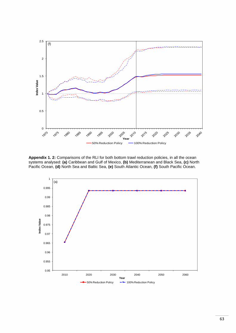
63

Appendix 1. 2: Comparisons of the RLI for both bottom trawl reduction policies, in all the ocean systems analysed: (a) Caribbean and Gulf of Mexico, (b) Mediterranean and Black Sea, (c) North Pacific Ocean, (d) North Sea and Baltic Sea, (e) South Atlantic Ocean, (f) South Pacific Ocean.

0

0.5

1

1.5

2

2.5

Ind

ex

Va

lue

Year

50% Reduction Policy 100% Reduction Policy

(f)

0.95

0.955

0.96

0.965

0.97

0.975

0.98

0.985

0.99

0.995

1

2010 2020 2030 2040 2050 2060

Ind

ex

Va

lue

Year

50% Reduction Policy 100% Reduction Policy

(a)

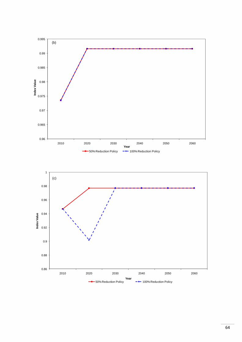
64

0.86

0.88

0.9

0.92

0.94

0.96

0.98

1

2010 2020 2030 2040 2050 2060

Ind

ex

Va

lue

Year50% Reduction Policy 100% Reduction Policy

(c)

0.96

0.965

0.97

0.975

0.98

0.985

0.99

0.995

2010 2020 2030 2040 2050 2060

Ind

ex

Va

lue

Year

50% Reduction Policy 100% Reduction Policy

(b)

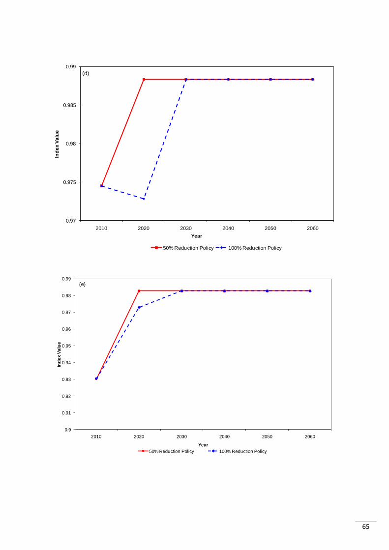
65

(d)

0.97

0.975

0.98

0.985

0.99

2010 2020 2030 2040 2050 2060

Ind

ex

Va

lue

Year

50% Reduction Policy 100% Reduction Policy

0.9

0.91

0.92

0.93

0.94

0.95

0.96

0.97

0.98

0.99

2010 2020 2030 2040 2050 2060

Ind

ex

Va

lue

Year

50% Reduction Policy 100% Reduction Policy

(e)

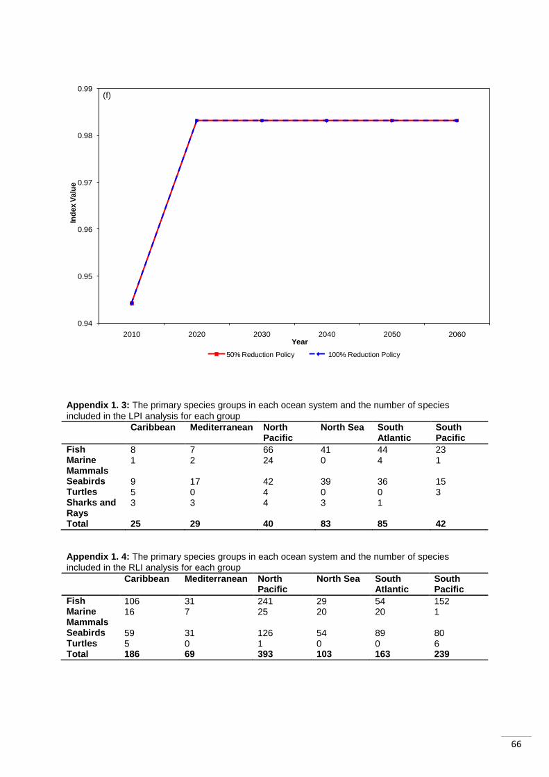
66

0.94

0.95

0.96

0.97

0.98

0.99

2010 2020 2030 2040 2050 2060

Ind

ex

Va

lue

Year

50% Reduction Policy 100% Reduction Policy

(f)

Appendix 1. 3: The primary species groups in each ocean system and the number of species

included in the LPI analysis for each group

Caribbean Mediterranean North Pacific

North Sea South Atlantic

South Pacific

Fish 8 7 66 41 44 23 Marine Mammals

1 2 24 0 4 1

Seabirds 9 17 42 39 36 15 Turtles 5 0 4 0 0 3 Sharks and Rays

3 3 4 3 1

Total 25 29 40 83 85 42

Appendix 1. 4: The primary species groups in each ocean system and the number of species

included in the RLI analysis for each group

Caribbean Mediterranean North Pacific

North Sea South Atlantic

South Pacific

Fish 106 31 241 29 54 152 Marine Mammals

16 7 25 20 20 1

Seabirds 59 31 126 54 89 80 Turtles 5 0 1 0 0 6 Total 186 69 393 103 163 239