getting started with ti-nspire™ high school science
TRANSCRIPT
Getting Started with
TI-Nspire™ High School Science
© 2011 Texas Instruments Incorporated Materials for Institute Participant*
*This material is for the personal use of T3 instructors in delivering a T3 institute. T3 instructors are further granted limited
permission to copy the participant packet in seminar quantities solely for use in delivering seminars for which the T3 Office
certifies the Instructor to present. T3 Institute organizers are granted permission to copy the participant packet for
distribution to those who attend the T3 institute. Request for permission to further duplicate or distribute this material must
be submitted in writing to the T3 Office.
*This material is for the personal use of participants during the institute. Participants are granted limited permission to copy
handouts in regular classroom quantities for use with students in participants’ regular classes and in presentations and/or
conferences conducted by participant inside his/her own district institutions. Request for permission to further duplicate or
distribute this material must be submitted in writing to the T3 Office.
Texas Instruments makes no warranty, either expressed or implied, including but not limited to any implied warranties of merchantability and fitness for a particular purpose, regarding any programs or book materials and makes such materials available solely on an “as-is” basis. In no event shall Texas Instruments be liable to anyone for special, collateral, incidental, or consequential damages in connection with or arising out of the purchase or use of these materials, and the sole and exclusive liability of Texas Instruments, regardless of the form of action, shall not exceed the purchase price of this calculator. Moreover, Texas Instruments shall not be liable for any claim of any kind whatsoever against the use of these materials by any other party. Mac is a registered trademark of Apple Computer, Inc. Windows is a registered trademark of Microsoft Corporation. T3·Teachers Teaching with Technology, TI-Nspire, TI-Nspire Navigator, Calculator-Based Laboratory, CBL 2, Calculator-Based Ranger, CBR, Connect to Class, TI Connect, TI Navigator, TI SmartView Emulator, TI-Presenter, and ViewScreen are trademarks of Texas Instruments Incorporated.

High School Science
©2011 Texas Instruments Incorporated 1 education.ti.com
Day One Page # 1. Overview, Logistics, and Introductions (includes TI-Nspire™ CX CAS Scavenger
Hunt) Reflective Questions: What is one thing that excites you most about the handheld?
Do you have any burning questions yet? (refer to parking lot for others) How did the login to NavigatorTM go? Was it intrusive? What do you like about TI-NspireTM so far? What would you like to see?
7
2. Introductory Activity – Using the Temperature Probe Reflective Questions: How does it feel to be like your students? Would you do things differently? What activities are currently in your curriculum that could be adapted to using this probe? What is the pedagogical importance of making your predictions and writing them down?
17
3. Fahrenheit to Celsius (Science Nspired) Reflective Questions: What questions do you have about the use of the TI-NspireTM Lab Cradle? How do student understand an algebraic equation (in x and y) as compared to using a “scientific formula” with meaningful variable symbols? How does the science context help in understanding the concept of a function?
27
4. Nailing Density Reflective Questions: How are Lists & Spreadsheet pages different from Data & Statistics pages? Where would this activity fit into your curriculum? Do you teach slope? Delta notation? What were some classroom strategies in using the technology that were modeled and useful?
35
5. Science Handheld Skills Reflective Questions: What are the benefits of using the TI-Nspire™ CAS to solve problems? What connection does this have to mathematics? How can defining variables and deriving equations be used effectively in your classroom? When would isolating variables be useful in the science classroom? Which method of isolating variables do you prefer? What other uses of the functions of a TI-NspireTM CAS can you devise? Is dimensional analysis something you teach?
45
6. River of Life Reflective Questions: What did you like about this activity? Where would this activity fit into your curriculum?
49
High School Science
©2011 Texas Instruments Incorporated 2 education.ti.com
7. Terminal Velocity Reflective Questions: How does the TI-Nspire™ technology change teaching the concept of terminal velocity? How does using the Strike Out feature reinforce the nature of science? How did our use of Lists & Spreadsheet and Data & Statistics in DataQuestTM differ from their use in the Density activity?
59
8. Reflections & Homework for Day 1 Reflective Questions:
Reflect on your learning today: What have you accomplished? What issues do you have? How can the use of technology engage students and help them better understand
science concepts? How do feel about the length of the TI-Nspire™ documents? How many pages of instructions do you feel is optimal for student use?
How does a teacher’s role change in an inquiry classroom? What questions do you have about DataQuestTM or the TI-NspireTM CX? Homework: Temperature Up and Down. Create a three-page TI-Nspire™ document
containing a notes page, DataQuest™ application, and either a Lists & Spreadsheet or Data & Statistics page. Generate data using the temperature sensor in at least two different temperature environments in this document.
67
Day Two Page #
1. Overview Day 2 Reflective Questions: What issues did you encounter when using the TI-Nspire™ independently?
2. Heat of Fusion Reflective Questions: What are the math/science connections? (Creating graphs and labeling portions of them) What are some potential extensions, questions, and assessment ideas that would go well with this type of activity? How might you encourage students to explore further? How can this activity/investigation assist students to better understand the mathematics at a higher cognitive level?
69
3. Sweating Alcohol Reflective Questions: What did you like about this activity? What did you not like that you would want to improve? Where would this activity fit into your curriculum?
79
4. MnM Decay Reflective Questions: How does the technology in this activity scaffold math skills so students can still explore concepts? Would this be better with a pre-made TI-Nspire™ document? Why or why not? Do students need to understand natural logarithms to do the calculations? Is this good or bad?
How does the use of the NavigatorTM enhance this activity?
89
High School Science
©2011 Texas Instruments Incorporated 3 education.ti.com
5. Thirst Quenchers Inquiry Reflective Questions: How does the color capability of the TI-NspireTM enhance this activity? What activities in your curriculum would be enhanced by adding pictures? What are some learning opportunities for students to be involved with the logistics of setup and cleanup? Advantages, disadvantages, and ideas? How could this activity be modified to be more inquiry-based?
95
6. Boyles Law Reflective Questions: What did you like about this activity? What did you not like that you would want to improve? Where would this activity fit into your curriculum?
105
7. Graph Matching Reflective Questions: What math connections can you address with this activity?
What issues do you predict in implementing TI-NspireTM use with your students?
115
8. Reflections and Exit Card for Day 2 Reflective Questions: Which parts of the day’s activities made you consider new approaches to teaching any of the science content areas that were explored?
How does a teacher’s role change in an inquiry classroom? What questions do you have about DataQuest™ or the TI-NspireTM CX? Share your thoughts about an activity that you especially enjoyed working on today.
127
Day Three Page #
1. Overview Day 3 Reflective Questions: What issues did you have with the homework?
What handheld skills need more work?
2. Computer Lab: Teacher Software Reflective Questions: What is the value of the software?
129
3. Computer Lab: Exploring Science Nspired Reflective Questions: Was the website easy to navigate?
How did you like the lesson format? Which activities are you considering for use in your classroom?
145
High School Science
©2011 Texas Instruments Incorporated 4 education.ti.com
4. Carousel (Choice of activities) Beers Law- (Colorimeter) Waves & Spectrum- (TI-Nspire™ document only) Static & Kinetic Friction-Physics (Dual-Force sensor and CBR2) Cellular Respiration- (CO2 sensor) Enzyme Action- (Gas Pressure sensor) Sound Waves and Beats (Microphone) Sound and Waves (TI-Nspire™ document only) Breath of Fresh Air (Current sensor) NASA Website Exploration TI Science Nspired Website Exploration
Reflective Questions: Why did you choose this activity? “This activity would be good for me to use in_____ because ____.” Or “This activity was not what I thought for me to use in ____, but it could be used or adapted for ____.” Discuss issues around the effective use or adaptation of this activity for student learning.
What are some pedagogical implications of the activity and its technology use? What is the content relevance? How might it engage and motivate your students? How does it add new TI-Nspire™ skills to your repertoire?
147
5. Project or Carousel Presentations Reflective Questions: What skills have you developed using Nspire and which ones do you feel are at the mastery level?
What changes will you make when you do this in your classroom? What skills have you acquired in using the handheld with sensors?
6. Reflections & Wrap-up for Institute Reflective Questions: What resources are available to support your implementation of TI-Nspire™ technology in your classroom?
What will you need to do between this workshop and the first day of school to be ready to use this technology in your classroom?
219
Welcome to TEACHER NOTES
GETTING STARTED WITH TI-NSPIRE™ IN HIGH SCHOOL SCIENCE
©2011 Texas Instruments Incorporated 1 education.ti.com
Welcome to High School Science
This three-day workshop is intended for beginning users of the TI-Nspire™ technology. During our time together, you will have many opportunities to work through activities with your peers. And, of course, you have the help and guidance of an experienced TI-Nspire user—your T3 Instructor.
In the course of these few days together, you will learn many of the features of the TI-Nspire™ handheld and software in the context of classroom-ready activities and other explorations. The Instructor will lead you through several activities, demonstrating suitable pedagogical techniques with the technology, and will facilitate discussions about classroom and educational issues as well as address any concerns you might have. You will also be given time to explore some activities of your choice and share your thoughts and challenges with the whole group.
The foci of this workshop are for you to:
Observe, learn, and practice sound pedagogy for using technology in the classroom.
Learn about and practice with the TI-Nspire™ document model and its features.
Experience the use of TI-Nspire™ handhelds by setting up experiments and collecting data.
Explore a variety of data collection sensors.
The materials include three types of documents:
Teacher Notes (in this format)
Student Activity (activity/instruction sheets)
TI-Nspire documents
You will be asked to take on several different roles during the workshop:
You might take on the role of a student as you learn specific science and mathematics content.
You will think like the classroom teacher considering the impacts on classroom management.
You will think like an educator using sound pedagogy to enhance student learning.
You will rely on one another as content specialists, helping to apply or adapt activities to particular lessons and to make the connections among the science disciplines.
You are a full learning partner here and will be immersed in this technology experience. Practice is the best way to become comfortable with the technology, including setting up activities, cleaning up, contributing to discussions, and asking questions. Your sincere contributions to your roles in the team will make this workshop successful.
7
Welcome to TEACHER NOTES
GETTING STARTED WITH TI-NSPIRE™ IN HIGH SCHOOL SCIENCE
©2011 Texas Instruments Incorporated 2 education.ti.com
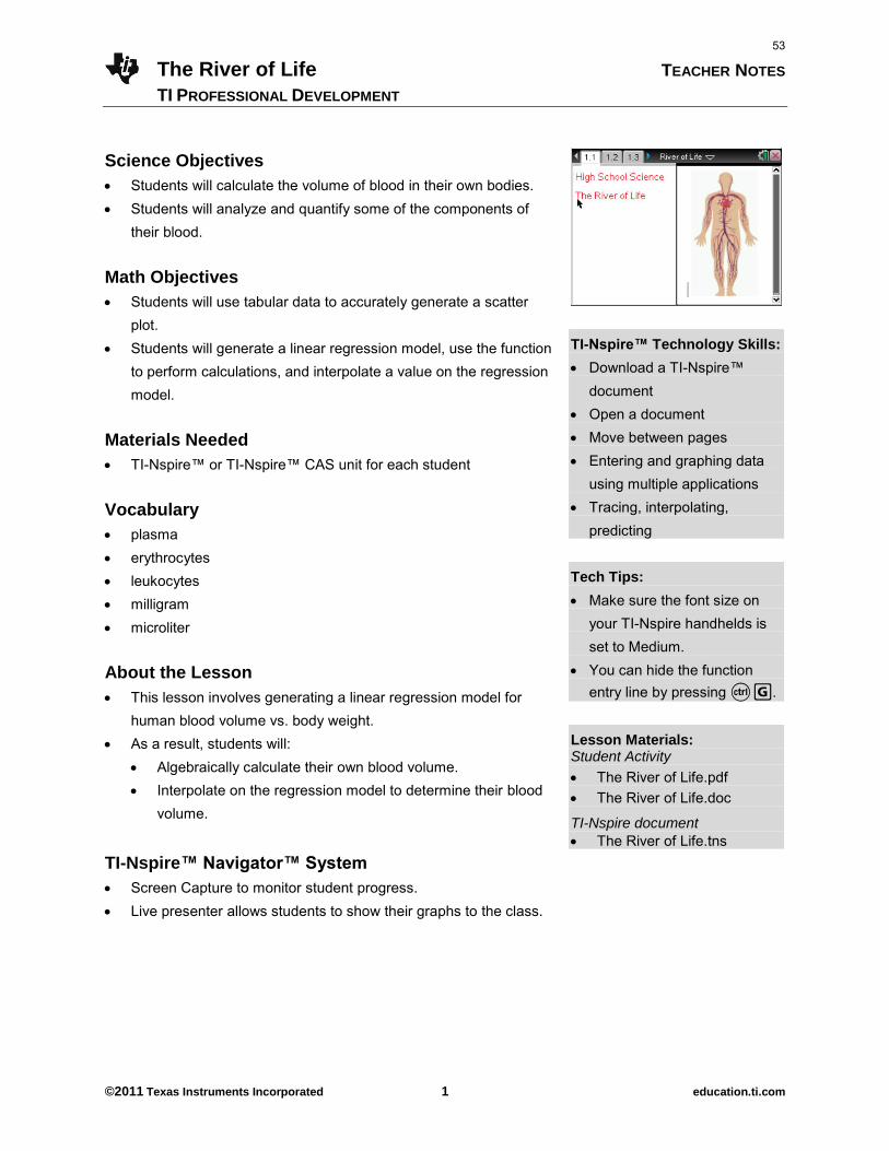
Science Objectives
Student activities will include science content or skill objectives that can be expected to be achieved by completion of the activity. They will be written as: Students will . . ..
Vocabulary
Possible lesson vocabulary list.
About the Lesson
A short overview of the lesson will be given here.
TI-Nspire™ NavigatorTM System TI-Nspire Navigator will be available throughout the workshop,
and used by the instructor to facilitate your learning (and as a demonstration of how it can benefit classroom teaching). Many of the activities will have Navigator suggestions, but the activities can still be done without Navigator in your classroom.
For those with TI-Navigator access in the classroom, TI-Navigator suggestions are given at appropriate points in the activities.
Activity Materials
A list of materials and equipment, along with any advance preparation needed, will be listed where needed.
TI-Nspire™ Technology Skills: New or significant skills for
each activity will be listed here. This is a good chance for you to review them for your students, or for yourself.
Tech Tips:
Some common technical issue resolutions or shortcuts are given here and throughout the notes.
Lesson Materials:
Print or electronic files are listed here.
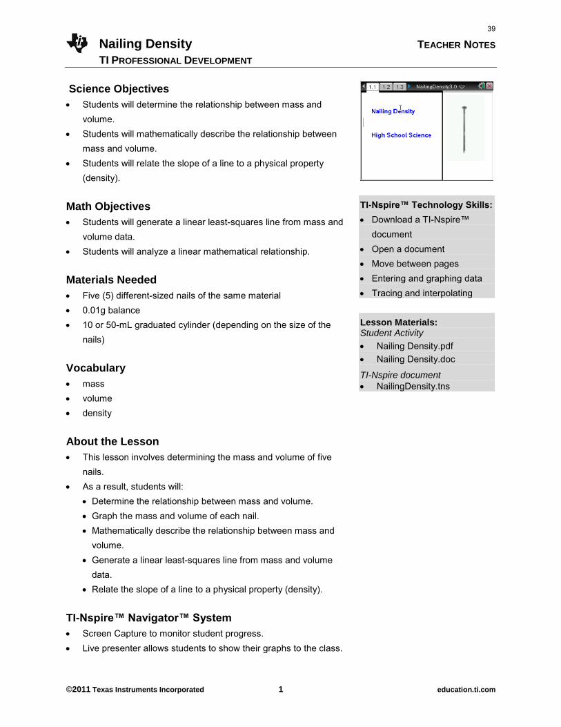
A Screen Shot of page 1.1 for the TI-Nspire document that accompanies the activity.
8
Welcome to TEACHER NOTES
GETTING STARTED WITH TI-NSPIRE™ IN HIGH SCHOOL SCIENCE
©2011 Texas Instruments Incorporated 3 education.ti.com
Discussion Points and Possible Answers Suggestions for introducing the activity are given. Throughout the activity, specific suggestions or answers to questions from the Student activity are provided for each step. This parallels, but does not repeat, the Student Activity. You will need to read through (and work through) the Student Activity and TI-Nspire document.
Wrap Up
A short summary of the expected outcomes of the activity along with some suggestions for discussion, connections, or extensions are provided. Assessment Ideas on how and where assessment can be linked to the activity are provided. The assessment may be formative and informal, or summative and much more formal, including actual testing on the TI-Nspire. TI-Nspire Navigator Note 1
Specific notes for Navigator use are provided where suitable.
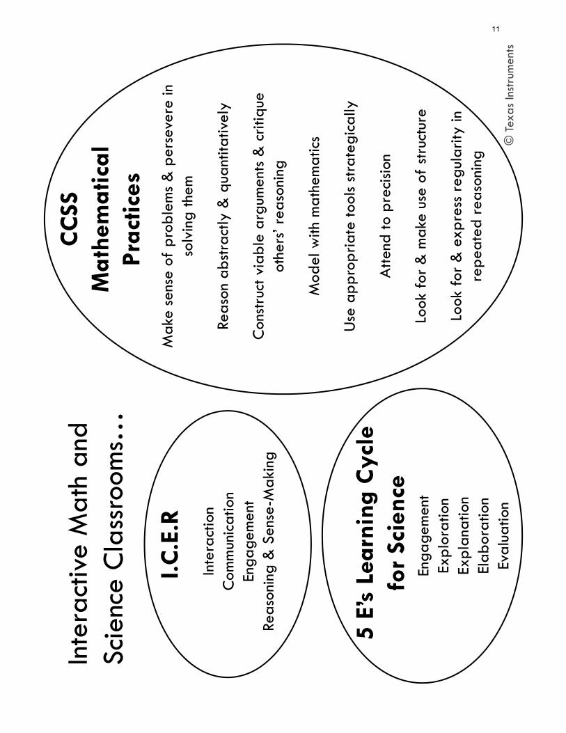
References will be made where appropriate to point out how activities address: Common Core State Standards Mathematical Practices
Constructivist 5-E’s Processes
9

This page intentionally left blank
10
Mak
e se
nse
of p
robl
ems
& p
erse
vere
in
solv
ing
them
Reas
on a
bstra
ctly
& q
uant
itativ
ely
Con
stru
ct v
iabl
e ar
gum
ents
& c
ritiq
ue
othe
rs’ r
easo
ning
Mod
el w
ith m
athe
mat
ics
Use
app
ropr
iate
tool
s st
rate
gica
lly
Atte
nd to
pre
cisio
n
Look
for
& m
ake
use
of s
truc
ture
Look
for
& e
xpre
ss r
egul
arity
in
repe
ated
rea
soni
ng
Enga
gem
ent
Expl
orat
ion
Expl
anat
ion
Elab
orat
ion
Eval
uatio
n
Inte
ract
ion
Com
mun
icat
ion
Enga
gem
ent
Reas
onin
g &
Sen
se-M
akin
g
I.C.E
.R
5 E’
s Le
arni
ng C
ycle
fo
r Sc
ienc
e
CC
SS
Mat
hem
atic
al
Prac
tices
Inte
ract
ive
Mat
h an
d Sc
ienc
e C
lass
room
s…
© T
exas
Inst
rum
ents
11

This page intentionally left blank
12
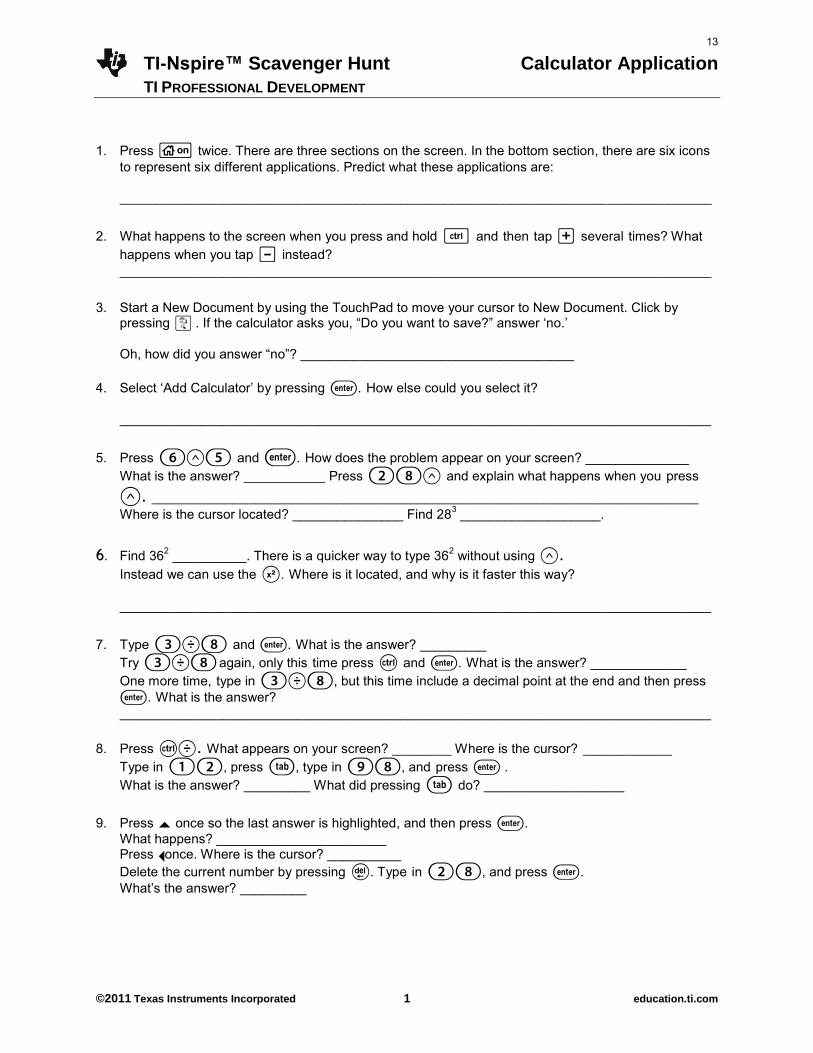
TI-Nspire™ Scavenger Hunt Calculator Application
TI PROFESSIONAL DEVELOPMENT
©2011 Texas Instruments Incorporated 1 education.ti.com
1. Press c twice. There are three sections on the screen. In the bottom section, there are six icons
to represent six different applications. Predict what these applications are: ________________________________________________________________________________
2. What happens to the screen when you press and hold / and then tap + several times? What
happens when you tap - instead? ________________________________________________________________________________
3. Start a New Document by using the TouchPad to move your cursor to New Document. Click by
pressing x . If the calculator asks you, “Do you want to save?” answer „no.‟ Oh, how did you answer “no”? _____________________________________
4. Select „Add Calculator‟ by pressing ·. How else could you select it?
________________________________________________________________________________
5. Press 6l5 and ·. How does the problem appear on your screen? ______________
What is the answer? ___________ Press 28l and explain what happens when you press l. __________________________________________________________________________ Where is the cursor located? _______________ Find 283 ___________________.
6. Find 362 __________. There is a quicker way to type 362 without using l.
Instead we can use the q. Where is it located, and why is it faster this way? ________________________________________________________________________________
7. Type 3p8 and ·. What is the answer? _________
Try 3p8 again, only this time press / and ·. What is the answer? _____________ One more time, type in 3p8, but this time include a decimal point at the end and then press ·. What is the answer? ________________________________________________________________________________
8. Press /p. What appears on your screen? ________ Where is the cursor? ____________
Type in 12, press e, type in 98, and press · . What is the answer? _________ What did pressing e do? ___________________
9. Press £ once so the last answer is highlighted, and then press ·.
What happens? _______________________ Press ¡once. Where is the cursor? __________ Delete the current number by pressing .. Type in 28, and press ·. What‟s the answer? _________
13
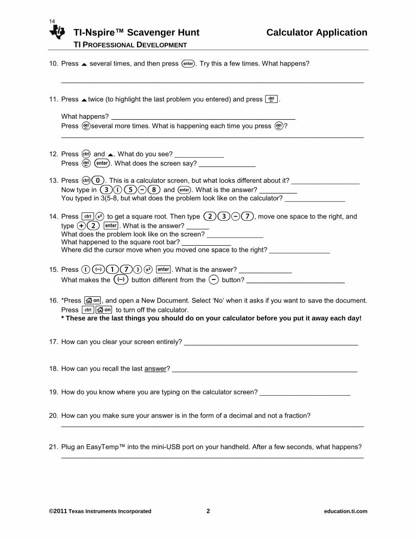
TI-Nspire™ Scavenger Hunt Calculator Application
TI PROFESSIONAL DEVELOPMENT
©2011 Texas Instruments Incorporated 2 education.ti.com
10. Press £ several times, and then press ·. Try this a few times. What happens? ________________________________________________________________________________
11. Press £ twice (to highlight the last problem you entered) and press ..
What happens? ___________________________________________ Press .several more times. What is happening each time you press .? ________________________________________________________________________________
12. Press / and £. What do you see? _____________
Press . ·. What does the screen say? _______________ 13. Press /0. This is a calculator screen, but what looks different about it? __________________
Now type in 3(5-8 and ·. What is the answer? __________ You typed in 3(5-8, but what does the problem look like on the calculator? ________________
14. Press /q to get a square root. Then type 23-7, move one space to the right, and
type +2 ·. What is the answer? ______ What does the problem look like on the screen? _______________ What happened to the square root bar? _____________ Where did the cursor move when you moved one space to the right? ________________
15. Press (v17)q ·. What is the answer? ______________
What makes the v button different from the - button? _______________________
16. *Press c, and open a New Document. Select „No‟ when it asks if you want to save the document.
Press /c to turn off the calculator. * These are the last things you should do on your calculator before you put it away each day!
17. How can you clear your screen entirely? ______________________________________________ 18. How can you recall the last answer? _________________________________________________ 19. How do you know where you are typing on the calculator screen? ________________________ 20. How can you make sure your answer is in the form of a decimal and not a fraction?
________________________________________________________________________________ 21. Plug an EasyTemp™ into the mini-USB port on your handheld. After a few seconds, what happens? ________________________________________________________________________________
14
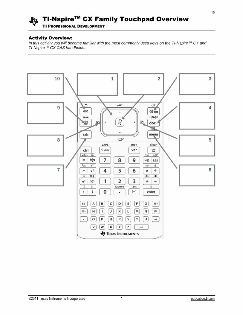
TI-Nspire
TM
CX Family Touchpad Overview
TI PROFESSIONAL DEVELOPMENT
©2011 Texas Instruments Incorporated 1 education.ti.com
Activity Overview:
In this activity you will become familiar with the most commonly used keys on the TI-Nspire™ CX and TI-Nspire™ CX CAS handhelds.
10
9
1 2 3
4
5 8
6 7
15

This page intentionally left blank
16
Introductory Data Collection Activity Name Student Activity Class
©2011 Texas Instruments Incorporated 1 education.ti.com
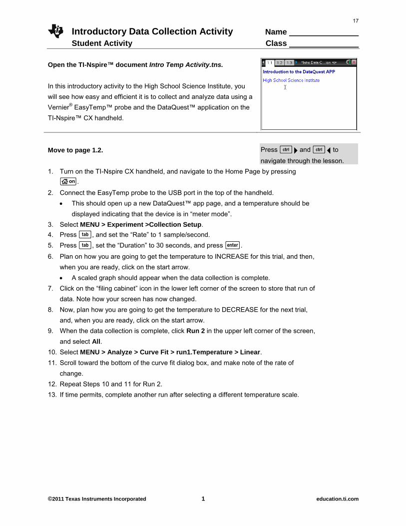
Open the TI-Nspire™ document Intro Temp Activity.tns.
In this introductory activity to the High School Science Institute, you will see how easy and efficient it is to collect and analyze data using a Vernier® EasyTemp™ probe and the DataQuest™ application on the TI-Nspire™ CX handheld.
Move to page 1.2.
Press / ¢ and / ¡ to
navigate through the lesson. 1. Turn on the TI-Nspire CX handheld, and navigate to the Home Page by pressing
c.
2. Connect the EasyTemp probe to the USB port in the top of the handheld. This should open up a new DataQuest™ app page, and a temperature should be
displayed indicating that the device is in “meter mode”. 3. Select MENU > Experiment >Collection Setup. 4. Press e, and set the “Rate” to 1 sample/second. 5. Press e, set the “Duration” to 30 seconds, and press ·.
6. Plan on how you are going to get the temperature to INCREASE for this trial, and then, when you are ready, click on the start arrow. A scaled graph should appear when the data collection is complete.
7. Click on the “filing cabinet” icon in the lower left corner of the screen to store that run of data. Note how your screen has now changed.
8. Now, plan how you are going to get the temperature to DECREASE for the next trial, and, when you are ready, click on the start arrow.
9. When the data collection is complete, click Run 2 in the upper left corner of the screen, and select All.
10. Select MENU > Analyze > Curve Fit > run1.Temperature > Linear. 11. Scroll toward the bottom of the curve fit dialog box, and make note of the rate of
change. 12. Repeat Steps 10 and 11 for Run 2. 13. If time permits, complete another run after selecting a different temperature scale.
17
Introductory Data Collection Activity Name Student Activity Class
©2011 Texas Instruments Incorporated 2 education.ti.com
1. In this activity, what was the significance of a positive rate of change? 2. Describe the appearance of the graph from Trial 1. 3. What was the significance of a negative rate of change? 4. Describe the appearance of the graph from Trial 2. 5. At approximately what time during the data collection were the temperatures of both
trials the same? 6. At approximately what temperature are the graphs of the two trials the same?
18
Using the Temperature Sensor Name Student Activity Class
©2011 Texas Instruments Incorporated 1 education.ti.com
Open a new TI-Nspire document. In this activity, you will learn how to collect data with the temperature sensor and the TI-Nspire™ by setting up a 25-second experiment. You will be given a challenge to interpret and explain the data.
Turn on your TI-Nspire handheld.
Press / ¢ and / ¡ to
navigate through the lesson. 1. Open a new document by pressing c and selecting New Doc.
A Save message box might appear.
Press · to save, or press e and · to not save; ask your teacher what you should do.
2. Obtain a temperature sensor from your teacher. DO NOT TOUCH the metal part of the sensor as it will ruin this experiment.
3. Connect the temperature sensor cable to your TI-Nspire handheld. Make sure the cable is pushed in securely.
4. What happens to your handheld?
5. Select MENU > Experiment > Collection Setup.
6. Press e to move through the field cells. Set the Rate (samples/second) to 2 and the Duration
(seconds) to 25 s and press ·.
7. How many temperature readings will the system collect?
8. Listen to your teacher carefully. You will be assigned to one of two groups, each with different instructions. Once you are clear on your instructions, take a moment to sketch what you think your graph of temperature vs time will look like in the space below. Label some key points.
19
Using the Temperature Sensor Name Student Activity Class
©2011 Texas Instruments Incorporated 2 education.ti.com
9. When instructed to do so, click a on the Start button and move your fingers on the sensor as
assigned. Watch the graph develop as you go. The experiment will end automatically.
10. Does your graph look like your predicted sketch? Consider some of your labeled key points.
11. Share your graph with someone of the same group and develop an explanation for the shape of the graph.
12. Knowing what the other group’s procedure was, and having an explanation for your data, predict what you think the graphs from the other group will look like. Sketch your prediction here.
13. Share your data graph with students from the other group. Develop a hypothesis on the operation of the temperature sensor that explains the results.
14. Can you suggest some experiments that would be interesting to run with this temperature sensor?
20
Using the Temperature Sensor TEACHER NOTES
TI PROFESSIONAL DEVELOPMENT
©2011 Texas Instruments Incorporated 1 education.ti.com
Science Objectives
Students will set up a data collection experiment. Students will make predictions based on given instructions. Students will collect and interpret data. Students will consider applications of the temperature sensor.
Vocabulary
temperature heat prediction hypothesis
About the Lesson
This activity involves collecting data with a temperature sensor and setting up the experimental parameters to fit the situation.
As a result, students will: Predict what they expect to see, compare results, and try to
explain the results. Acquire the skills to set up and use the temperature sensor in
other experiments.
TI-NspireTM NavigatorTM System Use Screen Capture to show results from different groups. Pick
representative or exemplary results to use in discussing the conclusions.
Activity Materials
Vernier Easy-Temp™ or the Easy-Link™ and the Stainless Steel
Temperature sensor.
TI-Nspire™ Technology Skills: Open a new document Set up a data collection
experiment Collect data with a sensor
Tech Tips:
Data collection occurs in the Vernier® DataQuestTM
application, which can be viewed as a meter, as a graph, or as a data table.
Lesson Files: Student Activity
Using_the_Temperature_ Sensor.doc
Using_the_Temperature_ Sensor.pdf
21
Using the Temperature Sensor TEACHER NOTES
TI PROFESSIONAL DEVELOPMENT
©2011 Texas Instruments Incorporated 2 education.ti.com
Discussion Points and Possible Answers
Tech Tip: Ensure that students (and you) do not touch the metal part of the temperature sensor at all before beginning the experiment as their fingers will heat up the sensor and the metal will conduct that heat as well. It takes several minutes for the sensor to return to room temperature.
Tech Tip: When opening a new document, the system might give a warning message about saving the previous document. Decide ahead of time what might have been open on the handheld, and whether it should be saved or discarded..
1. Open a new document by pressing c and selecting New Doc.
A Save message box might appear.
Press · to save, or press e and · to not save; ask your teacher what you should do.
2. Obtain a temperature sensor from your teacher. DO NOT TOUCH the metal part of the sensor as it will ruin this experiment.
3. Connect the temperature sensor cable to your TI-Nspire handheld. Make sure the cable is pushed in securely.
TI-Nspire™ Navigator™ Opportunity: Screen Capture
See Note 1 at the end of this lesson. 4. What happens to your handheld?
Answer: The handheld automatically detects the temperature sensor and opens the Vernier DataQuest application.
Tech Tip: If a student does not automatically see the DataQuest
application, make sure the temperature sensor is completely plugged into the handheld and that a New Document was created.
The temperature sensor runs off the TI-NspireTM handheld’s battery.
Ensure that the handhelds are charged sufficiently to run the sensor.
5. Select MENU > Experiment > Collection Setup.
22
Using the Temperature Sensor TEACHER NOTES
TI PROFESSIONAL DEVELOPMENT
©2011 Texas Instruments Incorporated 3 education.ti.com
6. Press e to move through the field cells. Set the Rate (samples/second) to 2 and the Duration
(seconds) to 25 s and press ·.
7. How many temperature readings will the system collect?
Answer: The system will collect an initial reading (time = 0) and two temperatures per second for 25 seconds = 51 temperature readings.
Teacher Tip: Divide the room in half. Call one side group A, and the other side group B. Explain the procedure to everyone. Group A Group A will start to collect data, then immediately rub their fingers on the base of the metal part of the sensor. Rub hard to create friction, and move fingers toward the tip for a time of about 10 s. Stay at the tip for about 2 s, then, still rubbing, move the fingers back toward the base for about 10 s. Group B
Group B will start to collect data, then immediately rub their fingers on the tip of the metal part of the sensor. Rub hard to create friction, and move the fingers toward the base for a time of about 10 s. Stay at the base for about 2 s, then, still rubbing, move the fingers back toward the tip for about 10 s. Answer any questions, and then have the students predict what they think the data plot will look like. Key points to consider are the start temperature and the maximum temperature, but let them decide.
8. Once you are clear on your instructions, take a moment to sketch what you think your graph of temperature vs time will look like in the space below. Label some key points.
Sample Answers: Student prediction graphs will vary.
9. When instructed to do so, click a on the Start button and move your fingers on the sensor as
assigned. Watch the graph develop as you go. The experiment will end automatically.
10. Does your graph look like your predicted sketch? Consider some of your labeled key points.
Sample Answers: Student answers will vary.
23
Using the Temperature Sensor TEACHER NOTES
TI PROFESSIONAL DEVELOPMENT
©2011 Texas Instruments Incorporated 4 education.ti.com
Teacher Tip: Consider key points in the actual data and encourage discussion about what the initial temperature should have been, and why the maximum temperature did not reach body temperature.
11. Share your graph with someone of the same group and develop an explanation for the shape of the graph.
Teacher Tip: The students should share only within their group at this time. Their task is to try to explain the shape of their data plot.
12. Knowing what the other group’s procedure was, and having an explanation for your
data, predict what you think the graphs from the other group will look like. Sketch your prediction.
Sample Answers: Student answers will vary.
Teacher Tip: Encourage discussion so they can make individual or group predictions about the other group’s data.
TI-Nspire™ Navigator™ Opportunity: Screen Captures
See Note 2 at the end of this lesson.
13. Share your data graph with students from the other group. Develop a hypothesis on the operation of the temperature sensor that explains the results.
Sample Answers: There might be several explanations. The reason for the difference between the groups is that the thermistor (the actual sensor) is embedded inside the metal rod near the tip. The tip is therefore more sensitive than the base. The metal rod does conduct heat, so the temperature starts to rise when near the tip. The metal rod also takes time to cool down, so once the tip is heated, the temperature does not drop right away. The sensor takes some time to react to temperature changes.
Tech Tip: The temperature sensor has an operational range of –40°C to 135°C. Its response rate depends on the environment. For a 90% change in reading, it takes about 10 s in water while stirring and 400 s in still air. This can make an interesting discussion for students studying heat and heat transfer.
24
Using the Temperature Sensor TEACHER NOTES
TI PROFESSIONAL DEVELOPMENT
©2011 Texas Instruments Incorporated 5 education.ti.com
14. Can you suggest some experiments that would be interesting to run with this temperature sensor?
Sample Answers: Students can be very creative in suggesting uses for the temperature sensor. This can be a motivational moment to foreshadow future activities you may have planned for the students.
Wrap Up
Upon completion of the lesson, the teacher should ensure that students are able to understand: Experimental design issues. Basic concepts about heat and how the temperature sensor works.
This experiment can be a short, fun activity to lead to more detailed activities about interpreting data plots, or it can be about understanding the technology and heat concepts a little better. Assessment An opportunity to assess students’ understanding of experimental set-up and the use of the temperature sensor is a short challenge. Ask them how hot they could get the temperature sensor using only their hands. Have them change the experiment set-up to something appropriate and be ready to start in a designated amount of time (2–4 minutes). With TI-Nspire Navigator, you can tell students you will display their work as they go. TI-Nspire Navigator Note 1
Question 1, Screen Captures: These can be a useful tool to monitor student progress and detect difficulties early. Do not display screen shots unless you want the class to look at and talk about them; they can be distracting. Note 2
Question 7, Screen Captures: Here is an ideal place to display screen captures to focus student attention and discussion. Screen captures can be displayed with or without student names. Decide whether you want to praise someone’s work or just display some representative work anonymously.
25

This page intentionally left blank
26
Fahrenheit vs. Celsius Name Student Activity Class
©2011 Texas Instruments Incorporated 1 education.ti.com
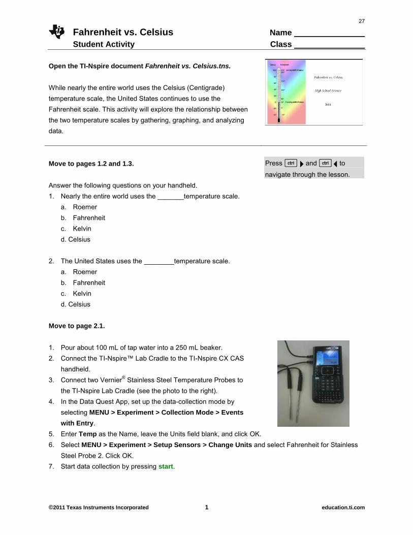
Open the TI-Nspire document Fahrenheit vs. Celsius.tns. While nearly the entire world uses the Celsius (Centigrade) temperature scale, the United States continues to use the Fahrenheit scale. This activity will explore the relationship between the two temperature scales by gathering, graphing, and analyzing data.
Move to pages 1.2 and 1.3.
Press / ¢ and / ¡ to
navigate through the lesson. Answer the following questions on your handheld. 1. Nearly the entire world uses the _______temperature scale.
a. Roemer b. Fahrenheit c. Kelvin
d. Celsius 2. The United States uses the ________temperature scale.
a. Roemer b. Fahrenheit c. Kelvin
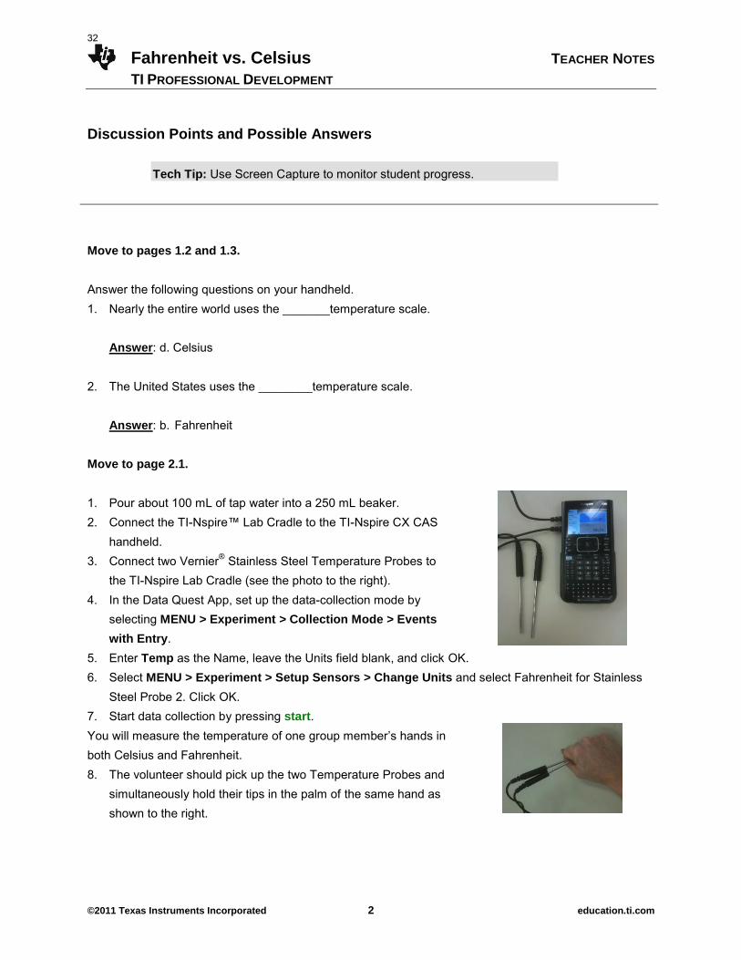
d. Celsius Move to page 2.1. 1. Pour about 100 mL of tap water into a 250 mL beaker. 2. Connect the TI-Nspire™ Lab Cradle to the TI-Nspire CX CAS
handheld. 3. Connect two Vernier® Stainless Steel Temperature Probes to
the TI-Nspire Lab Cradle (see the photo to the right). 4. In the Data Quest App, set up the data-collection mode by
selecting MENU > Experiment > Collection Mode > Events
with Entry.
5. Enter Temp as the Name, leave the Units field blank, and click OK. 6. Select MENU > Experiment > Setup Sensors > Change Units and select Fahrenheit for Stainless
Steel Probe 2. Click OK. 7. Start data collection by pressing start.
27
Fahrenheit vs. Celsius Name Student Activity Class
©2011 Texas Instruments Incorporated 2 education.ti.com
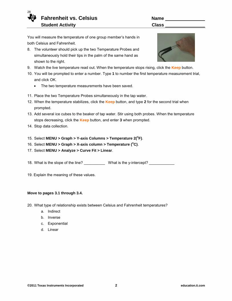
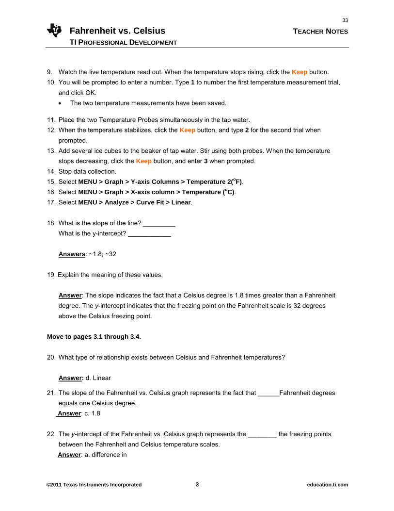
You will measure the temperature of one group member’s hands in both Celsius and Fahrenheit. 8. The volunteer should pick up the two Temperature Probes and
simultaneously hold their tips in the palm of the same hand as shown to the right.
9. Watch the live temperature read out. When the temperature stops rising, click the Keep button. 10. You will be prompted to enter a number. Type 1 to number the first temperature measurement trial,
and click OK. The two temperature measurements have been saved.
11. Place the two Temperature Probes simultaneously in the tap water. 12. When the temperature stabilizes, click the Keep button, and type 2 for the second trial when
prompted. 13. Add several ice cubes to the beaker of tap water. Stir using both probes. When the temperature
stops decreasing, click the Keep button, and enter 3 when prompted. 14. Stop data collection. 15. Select MENU > Graph > Y-axis Columns > Temperature 2(
oF).
16. Select MENU > Graph > X-axis column > Temperature (oC).
17. Select MENU > Analyze > Curve Fit > Linear. 18. What is the slope of the line? __________ What is the y-intercept? ____________ 19. Explain the meaning of these values. Move to pages 3.1 through 3.4. 20. What type of relationship exists between Celsius and Fahrenheit temperatures?
a. Indirect b. Inverse c. Exponential d. Linear
28

Fahrenheit vs. Celsius Name Student Activity Class
©2011 Texas Instruments Incorporated 3 education.ti.com
21. The slope of the Fahrenheit vs. Celsius graph represents the fact that ______Fahrenheit degrees equals one Celsius degree.
a. 32 b. 5/9 c. 1.8 d. -32
22. The y-intercept of the Fahrenheit vs. Celsius graph represents the ________ the freezing points
between the Fahrenheit and Celsius temperature scales. a. difference in b. magnitude of c. ratio of d. product of
Extension 1. Select MENU > Graph >Y-axis Columns > Temperature(oC). 2. Select MENU > Graph > X-axis Column > Temperature 2(oF). 3. Repeat steps 15-17. 4. What is the slope of the line? __________ What is the y-intercept? ____________ 5. Explain the meaning of these values. 6. Disconnect the Temperature Probes. 7. Properly dispose of the water in the beaker. 23. The slope of the Celsius vs. Fahrenheit graph in the Extension is the ___________of the slope from
the Fahrenheit vs. Celsius graph. a. product b. equivalent c. reciprocal d. natural log
29

This page intentionally left blank
30
Fahrenheit vs. Celsius TEACHER NOTES
TI PROFESSIONAL DEVELOPMENT
©2011 Texas Instruments Incorporated 1 education.ti.com
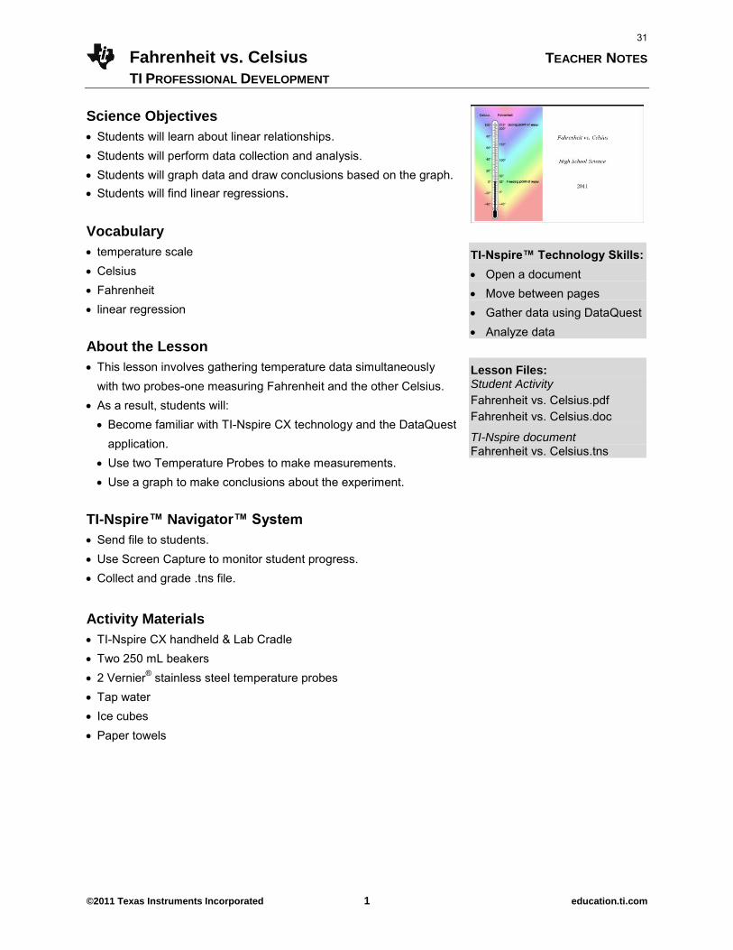
Science Objectives
Students will learn about linear relationships. Students will perform data collection and analysis. Students will graph data and draw conclusions based on the graph. Students will find linear regressions.
Vocabulary
temperature scale Celsius Fahrenheit linear regression About the Lesson
This lesson involves gathering temperature data simultaneously with two probes-one measuring Fahrenheit and the other Celsius.
As a result, students will: Become familiar with TI-Nspire CX technology and the DataQuest
application. Use two Temperature Probes to make measurements. Use a graph to make conclusions about the experiment.
TI-Nspire™ Navigator™ System
Send file to students. Use Screen Capture to monitor student progress. Collect and grade .tns file.
Activity Materials
TI-Nspire CX handheld & Lab Cradle Two 250 mL beakers 2 Vernier® stainless steel temperature probes Tap water Ice cubes Paper towels
TI-Nspire™ Technology Skills: Open a document Move between pages Gather data using DataQuest Analyze data
Lesson Files: Student Activity
Fahrenheit vs. Celsius.pdf Fahrenheit vs. Celsius.doc
TI-Nspire document Fahrenheit vs. Celsius.tns
31
Fahrenheit vs. Celsius TEACHER NOTES
TI PROFESSIONAL DEVELOPMENT
©2011 Texas Instruments Incorporated 2 education.ti.com
Discussion Points and Possible Answers
Tech Tip: Use Screen Capture to monitor student progress.
Move to pages 1.2 and 1.3.
Answer the following questions on your handheld. 1. Nearly the entire world uses the _______temperature scale. Answer: d. Celsius 2. The United States uses the ________temperature scale.
Answer: b. Fahrenheit Move to page 2.1. 1. Pour about 100 mL of tap water into a 250 mL beaker. 2. Connect the TI-Nspire™ Lab Cradle to the TI-Nspire CX CAS
handheld. 3. Connect two Vernier® Stainless Steel Temperature Probes to
the TI-Nspire Lab Cradle (see the photo to the right). 4. In the Data Quest App, set up the data-collection mode by
selecting MENU > Experiment > Collection Mode > Events
with Entry.
5. Enter Temp as the Name, leave the Units field blank, and click OK. 6. Select MENU > Experiment > Setup Sensors > Change Units and select Fahrenheit for Stainless
Steel Probe 2. Click OK. 7. Start data collection by pressing start. You will measure the temperature of one group member’s hands in both Celsius and Fahrenheit. 8. The volunteer should pick up the two Temperature Probes and
simultaneously hold their tips in the palm of the same hand as shown to the right.
32
Fahrenheit vs. Celsius TEACHER NOTES
TI PROFESSIONAL DEVELOPMENT
©2011 Texas Instruments Incorporated 3 education.ti.com
9. Watch the live temperature read out. When the temperature stops rising, click the Keep button. 10. You will be prompted to enter a number. Type 1 to number the first temperature measurement trial,
and click OK. The two temperature measurements have been saved.
11. Place the two Temperature Probes simultaneously in the tap water. 12. When the temperature stabilizes, click the Keep button, and type 2 for the second trial when
prompted. 13. Add several ice cubes to the beaker of tap water. Stir using both probes. When the temperature
stops decreasing, click the Keep button, and enter 3 when prompted. 14. Stop data collection. 15. Select MENU > Graph > Y-axis Columns > Temperature 2(
oF).
16. Select MENU > Graph > X-axis column > Temperature (oC).
17. Select MENU > Analyze > Curve Fit > Linear. 18. What is the slope of the line? _________
What is the y-intercept? ____________ Answers: ~1.8; ~32 19. Explain the meaning of these values. Answer: The slope indicates the fact that a Celsius degree is 1.8 times greater than a Fahrenheit
degree. The y-intercept indicates that the freezing point on the Fahrenheit scale is 32 degrees above the Celsius freezing point.
Move to pages 3.1 through 3.4.
20. What type of relationship exists between Celsius and Fahrenheit temperatures?
Answer: d. Linear
21. The slope of the Fahrenheit vs. Celsius graph represents the fact that ______Fahrenheit degrees equals one Celsius degree.
Answer: c. 1.8
22. The y-intercept of the Fahrenheit vs. Celsius graph represents the ________ the freezing points between the Fahrenheit and Celsius temperature scales.
Answer: a. difference in
33
Fahrenheit vs. Celsius TEACHER NOTES
TI PROFESSIONAL DEVELOPMENT
©2011 Texas Instruments Incorporated 4 education.ti.com
Extension
1. Select MENU > Graph >Y-axis Columns > Temperature(oC). 2. Select MENU > Graph > X-axis Column > Temperature 2(oF). 3. Repeat steps 15-17. 4. What is the slope of the line? __________ What is the y-intercept? ____________ 5. Explain the meaning of these values. 6. Disconnect the Temperature Probes. 7. Properly dispose of the water in the beaker. 23. The slope of the Celsius vs. Fahrenheit graph in the Extension is the ___________of the slope
from the Fahrenheit vs. Celsius graph.
Answer: c. reciprocal
Wrap Up
Upon completion of the discussion, the teacher should ensure that students are able to understand: How to connect to Lab Cradle to the CX. How to connect probes to Lab Cradle. How to gather and analyze data. The relationship between the Fahrenheit and Celsius temperature scales.
Assessment Students will complete the embedded multiple choice questions in the Fahrenheit vs. Celsius .tns file. In addition, students will answer questions on the student activity sheet. TI-Nspire Navigator
Note 1: Portfolio and Slide Show
Use the TI-Nspire Navigator to draw back, grade, and save the .tns file to the Portfolio. Use Slide Show to view student responses.
34
Nailing Density Name Student Activity Class
©2011 Texas Instruments Incorporated 1 education.ti.com
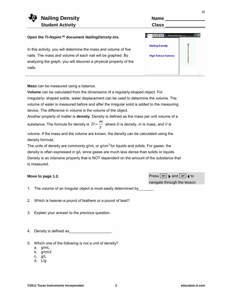
Open the TI-Nspire™ document NailingDensity.tns. In this activity, you will determine the mass and volume of five nails. The mass and volume of each nail will be graphed. By analyzing the graph, you will discover a physical property of the nails.
Mass can be measured using a balance. Volume can be calculated from the dimensions of a regularly-shaped object. For irregularly- shaped solids, water displacement can be used to determine the volume. The volume of water is measured before and after the irregular solid is added to the measuring device. The difference in volume is the volume of the object. Another property of matter is density. Density is defined as the mass per unit volume of a
substance. The formula for density is
D m
V where D is density, m is mass, and V is
volume. If the mass and the volume are known, the density can be calculated using the density formula. The units of density are commonly g/mL or g/cm3 for liquids and solids. For gases, the density is often expressed in g/L since gases are much less dense than solids or liquids. Density is an intensive property that is NOT dependent on the amount of the substance that is measured. Move to page 1.2.
Press / ¢ and / ¡ to
navigate through the lesson. 1. The volume of an irregular object is most easily determined by_______. 2. Which is heavier-a pound of feathers or a pound of lead? 3. Explain your answer to the previous question. 4. Density is defined as____________________. 5. Which one of the following is not a unit of density?
a. g/mL b. g/cm3 c. g/L d. L/g
35
Nailing Density Name Student Activity Class
©2011 Texas Instruments Incorporated 2 education.ti.com
Move to page 2.1. Nails will be provided by your teacher. 6. Add enough water to the graduated cylinder to cover the tallest nail (do NOT add the
nails to the water yet). 7. Read the initial volume to the nearest 0.1 mL, and record it in the spreadsheet on Page
2.1 under volw for 0 nails. 8. Measure the mass of the first nail to 0.01 g, and record it under massn for 1 nail. 9. Gently let one nail slide head first into the tilted cylinder, and measure the new volume
under volw for 1 nail. 10. Repeat this procedure for the four remaining nails, accumulating all of the nails in the
graduated cylinder. 11. Calculate the total mass of nails in the spreadsheet by adding each to the previous
total using cell notation (in cell C2 enter =C1+B2). Repeat for the four remaining nails. 12. Calculate the volume of each nail by subtracting the previous water volume from the
current (in cell E2 enter =D2-D1). Repeat for the remaining four nails. 13. Calculate the density of the nails by dividing the mass of the nail by its volume (enter =
massn/voln in the formula bar under dens). Move to page 2.3. 14. On the Data & Statistics page (Page 2.3), explore some graphs by clicking an axis and
choosing the variable you want to plot. 15. Plot massn vs. voln, and determine the best fit line for the nails’ volume and mass
relationship by selecting MENU > Analyze > Regression > Show Linear(mx + b). 17. Plot masst vs. volw and again find the best line.
Cycle between the last two graphs to see the similarities and differences.
Move to page 3.1. 18. a. What is the regression equation for your graph?
b. What is the slope of the line? c. What would the units of the slope be?
36
Nailing Density Name Student Activity Class
©2011 Texas Instruments Incorporated 3 education.ti.com
19. The formula for Density is:
D m
V, where D is density, m is mass, and V is volume.
Rearrange the formula for density by isolating mass instead of density.
20. Rewrite the regression equation from the Data & Statistics page, replacing the “x”
variable with V for volume and the “y” variable with m for mass.
21. How does the rearranged
D m
V equation from question 19 compare with the
equation that you wrote for question 20? Explain. 22. a. What does the slope of the graph on the Data & Statistics page represent?
b. What unit(s) would be assigned to the slope of this graph?
23. Why are the densities calculated for each nail not exactly the same and not exactly equal to the slope of the line?
24. Use the Internet to visit http://www.engineeringtoolbox.com/metal-alloys-densities-
d_50.html. Use this page to identify the element or metal alloy whose properties would match the density that you calculated for the nail. Remember that 1 kg/m3 = 0.001 g/cm3 and that 1 cm3 = 1mL.
25. Refer to the data that was collected. What effect does increasing the mass of the nail
have on the volume of the nail?
26. Refer to the data that was collected. What effect does increasing the mass of the nail have on the density of the nail?
37
Nailing Density Name Student Activity Class
©2011 Texas Instruments Incorporated 4 education.ti.com
27. Which of the following is NOT true of the density of a substance?
a. intensive property b. extensive property c. characteristic or identifying property d. temperature dependent
28. Summarize what you have learned about density from this experiment.
38
Nailing Density TEACHER NOTES
TI PROFESSIONAL DEVELOPMENT
©2011 Texas Instruments Incorporated 1 education.ti.com
Science Objectives
Students will determine the relationship between mass and volume.
Students will mathematically describe the relationship between mass and volume.
Students will relate the slope of a line to a physical property (density).
Math Objectives
Students will generate a linear least-squares line from mass and volume data.
Students will analyze a linear mathematical relationship. Materials Needed
Five (5) different-sized nails of the same material 0.01g balance 10 or 50-mL graduated cylinder (depending on the size of the
nails)
Vocabulary
mass volume density About the Lesson
This lesson involves determining the mass and volume of five nails.
As a result, students will: Determine the relationship between mass and volume. Graph the mass and volume of each nail. Mathematically describe the relationship between mass and
volume. Generate a linear least-squares line from mass and volume
data. Relate the slope of a line to a physical property (density).
TI-Nspire™ Navigator™ System
Screen Capture to monitor student progress. Live presenter allows students to show their graphs to the class.
TI-Nspire™ Technology Skills: Download a TI-Nspire™
document Open a document Move between pages Entering and graphing data Tracing and interpolating
Lesson Materials: Student Activity
Nailing Density.pdf Nailing Density.doc
TI-Nspire document
NailingDensity.tns
39
Nailing Density TEACHER NOTES
TI PROFESSIONAL DEVELOPMENT
©2011 Texas Instruments Incorporated 2 education.ti.com
Discussion Points and Possible Answers
Mass can be measured using a balance. Volume can be calculated from the dimensions of a regularly-shaped object. For irregularly- shaped solids, water displacement can be used to determine the volume. The volume of water is measured before and after the irregular solid is added to the measuring device. The difference in volume is the volume of the object. Another property of matter is density. Density is defined as the mass per unit volume of a
substance. The formula for density is
D m
V where D is density, m is mass, and V is
volume. If the mass and the volume are known, the density can be calculated using the density formula. The units of density are commonly g/mL or g/cm3 for liquids and solids. For gases, the density is often expressed in g/L since gases are much less dense than solids or liquids. Density is an intensive property that is NOT dependent on the amount of the substance that is measured. Move to page 1.2.
1. The volume of an irregular object is most easily determined by_______.
Answer: Water displacement.
2. Which is heavier-a pound of feathers or a pound of lead?
Answer: Neither.
3. Explain your answer to the previous question.
Answer: Neither a pound of feathers nor a pound of lead is heavier—their mass is both equal to one pound. However, the lead has a much greater density since the volume of one pound of lead would be much less than the volume of pound of feathers.
4. Density is defined as____________________.
Answer: mass per unit volume
40
Nailing Density TEACHER NOTES
TI PROFESSIONAL DEVELOPMENT
©2011 Texas Instruments Incorporated 3 education.ti.com
5. Which one of the following is not a unit of density?
a. g/mL b. g/cm3 c. g/L d. L/g
Answer: d. L/g
Move to page 2.1. Nails will be provided by your teacher. 6. Add enough water to the graduated cylinder to cover the tallest nail (do NOT add the
nails to the water yet). 7. Read the initial volume to the nearest 0.1 mL, and record it in the spreadsheet on Page
2.1 under volw for 0 nails. 8. Measure the mass of the first nail to 0.01 g, and record it under massn for 1 nail. 9. Gently let one nail slide head first into the tilted cylinder, and measure the new volume
under volw for 1 nail. 10. Repeat this procedure for the four remaining nails, accumulating all of the nails in the
graduated cylinder. 11. Calculate the total mass of nails in the spreadsheet by adding each to the previous
total using cell notation (in cell C2 enter =C1+B2). Repeat for the four remaining nails. 12. Calculate the volume of each nail by subtracting the previous water volume from the
current (in cell E2 enter =D2-D1). Repeat for the remaining four nails. 13. Calculate the density of the nails by dividing the mass of the nail by its volume (enter =
massn/voln in the formula bar under dens). Move to page 2.3. 14. On the Data & Statistics page (Page 2.3), explore some graphs by clicking an axis and
choosing the variable you want to plot. 15. Plot massn vs. voln, and determine the best fit line for the nails’ volume and mass
relationship by selecting MENU > Analyze > Regression > Show Linear(mx + b). 17. Plot masst vs. volw and again find the best line.
Cycle between the last two graphs to see the similarities and differences.
41
Nailing Density TEACHER NOTES
TI PROFESSIONAL DEVELOPMENT
©2011 Texas Instruments Incorporated 4 education.ti.com
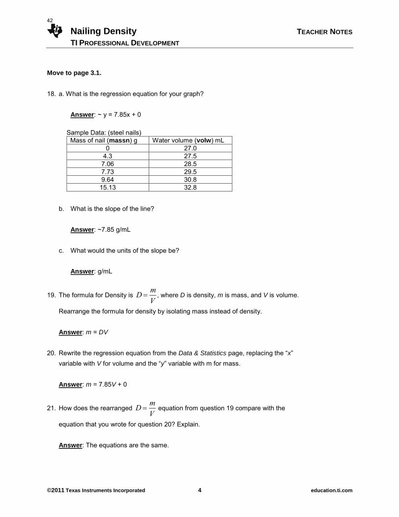
Move to page 3.1. 18. a. What is the regression equation for your graph?
Answer: ~ y = 7.85x + 0
Sample Data: (steel nails) Mass of nail (massn) g Water volume (volw) mL
0 27.0 4.3 27.5 7.06 28.5 7.73 29.5 9.64 30.8 15.13 32.8
b. What is the slope of the line?
Answer: ~7.85 g/mL
c. What would the units of the slope be?
Answer: g/mL
19. The formula for Density is
D m
V, where D is density, m is mass, and V is volume.
Rearrange the formula for density by isolating mass instead of density. Answer: m = DV
20. Rewrite the regression equation from the Data & Statistics page, replacing the “x”
variable with V for volume and the “y” variable with m for mass.
Answer: m = 7.85V + 0
21. How does the rearranged
D m
V equation from question 19 compare with the
equation that you wrote for question 20? Explain.
Answer: The equations are the same.
42
Nailing Density TEACHER NOTES
TI PROFESSIONAL DEVELOPMENT
©2011 Texas Instruments Incorporated 5 education.ti.com
22. a. What does the slope of the graph on the Data & Statistics page represent?
Answer: The density.
b. What unit(s) would be assigned to the slope of this graph?
Answer: g/mL
23. Why are the densities calculated for each nail not exactly the same and not exactly equal to the slope of the line?
Sample Answers: Because of experimental errors.
24. Use the Internet to visit http://www.engineeringtoolbox.com/metal-alloys-densities-
d_50.html. Use this page to identify the element or metal alloy whose properties would match the density that you calculated for the nail. Remember that 1 kg/m3 = 0.001 g/cm3 and that 1 cm3 = 1mL.
Answer: Iron and steel.
25. Refer to the data that was collected. What effect does increasing the mass of the nail
have on the volume of the nail? Answer: The volume increases.
26. Refer to the data that was collected. What effect does increasing the mass of the nail
have on the density of the nail?
Answer: The density is unchanged.
26. Which of the following is NOT true of the density of a substance? a. intensive property b. extensive property c. characteristic or identifying property d. temperature dependent
Answer: b. Extensive property.
43
Nailing Density TEACHER NOTES
TI PROFESSIONAL DEVELOPMENT
©2011 Texas Instruments Incorporated 6 education.ti.com
27. Summarize what you have learned about density from this experiment.
Sample Answers: Answers will vary. The density of a substance is a constant, independent of mass and volume and only changes with temperature. Density is an intensive property that is characteristic of a substance. Density can be used to identify a substance.
TI-Nspire Navigator Opportunity: Screen Capture
See Note 1 at the end of this lesson.
Wrap Up
Upon completion of this discussion, the teacher should ensure that students understand: The relationship between mass and volume. The relationship between the slope of a line and density. Assessment Formative and summative assessment questions are embedded in the TI-Nspire™
document. The questions will be graded when the TI-Nspire™ documents are retrieved. The Slide Show can be utilized to give students immediate feedback on their assessment.
TI-Nspire Navigator Notes
Note 1: Screen Capture
Screen Capture can be used to monitor student progress.
44
Science Handheld Skills TEACHER NOTES
TI PROFESSIONAL DEVELOPMENT
©2011 Texas Instruments Incorporated 1 education.ti.com
Science Objectives
Students will learn to convert units using conversion factors. Students will learn to define variables and derive equations. Students will learn to isolate variables from equations.
Math Objectives
Students will learn to convert units using conversion factors. Students will learn to define variables and derive equations. Students will learn to isolate variables from equations. Students will learn to use the Solve function.
Vocabulary
conversion factor variable define solve derive About the Lesson
This lesson explores the functionality of the TI-Nspire™ CAS
handheld in the context of the science classroom. As a result, students will:
Convert units using conversion factors.
Define variables and derive equations.
Isolate variables in a scientific equation.
TI-Nspire™ Navigator™ System
Use Screen Capture to monitor student progress. Use TI-NspireTM CAS Teacher Software to illustrate solutions. Make a student Live Presenter for practice problems.
TI-Nspire™ Technology
Skills: Use of / p to generate
a fraction template Define variables Derive an equation Use the Solve command to
isolate a variable from an equation
Tech Tips:
Make sure students multiply between each fraction term when converting units.
When writing equations, be certain that students place a multiplication symbol between each variable.
Lesson Materials:
TI-NspireTM CAS Handheld
TI-NspireTM Navigator
TI-NspireTM CAS Teacher Software
45
Science Handheld Skills TEACHER NOTES
TI PROFESSIONAL DEVELOPMENT
©2011 Texas Instruments Incorporated 2 education.ti.com
Part 1 – Converting Units with Conversion Factors
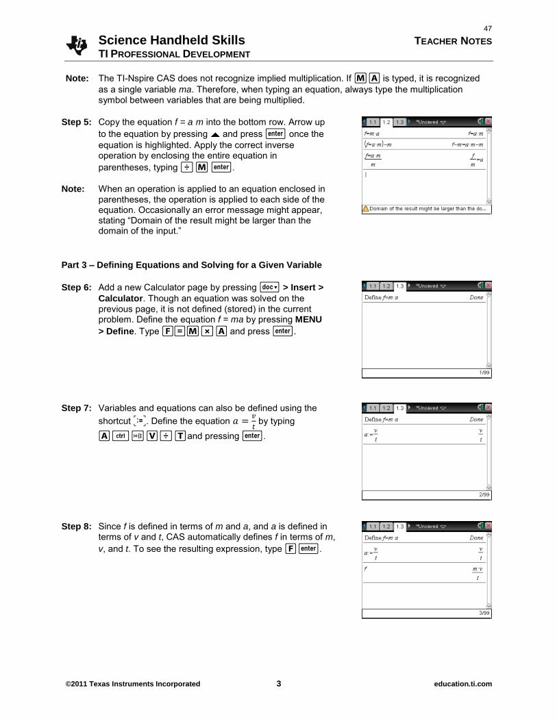
Step 1: Create a New Document with a Calculator application by pressing c > New Document > Add Calculator. If
you are asked whether you want to save the current document, select “No” by pressing e and ·.
Step 2: Convert 55 mm to km using conversion factors. Type 55rMM, then type r, and access the fraction template by pressing /p. To use the conversion factor 1 cm = 10 mm, type 1rCM in the numerator and move the cursor to the denominator by pressing ¤. Type 10rMM and exit the fraction template by pressing ¢. Repeat this process with the conversion
factors 1 m = 100 cm and 1 km = 1000 m. Use the screen on the right as guidance. Once the conversion factor 1 km = 1000 m has been typed, press ·.
Note: When typing a numerical value with units, a multiplication
symbol must always be typed between the numerical value and the abbreviation for units.
Step 3: Whenever possible, the TI-Nspire returns a non-integral value as a rational number. To receive a decimal approximation, press /=.
Note: A warning message appears at the bottom of the screen,
which states, “Domain of the result might be larger than the domain of the input.”
Part 2 – Solving an Equation for a Given Variable
Step 4: Add a new Calculator page by pressing ~ > Insert > Calculator. Solve the equation f = ma for a by typing F = M r A and pressing ·. The handheld returns the equation with the variables on the right in alphabetical order.
Solve the equation erroneously by subtracting m from each side of the equation. Press –M · and CAS automatically subtracts m from each side of the equation.
46
Science Handheld Skills TEACHER NOTES
TI PROFESSIONAL DEVELOPMENT
©2011 Texas Instruments Incorporated 3 education.ti.com
Note: The TI-Nspire CAS does not recognize implied multiplication. If M A is typed, it is recognized as a single variable ma. Therefore, when typing an equation, always type the multiplication symbol between variables that are being multiplied.
Step 5: Copy the equation f = a·m into the bottom row. Arrow up to the equation by pressing £ and press · once the equation is highlighted. Apply the correct inverse operation by enclosing the entire equation in parentheses, typing p M ·.
Note: When an operation is applied to an equation enclosed in
parentheses, the operation is applied to each side of the equation. Occasionally an error message might appear, stating “Domain of the result might be larger than the domain of the input.”
Part 3 – Defining Equations and Solving for a Given Variable
Step 6: Add a new Calculator page by pressing ~ > Insert > Calculator. Though an equation was solved on the previous page, it is not defined (stored) in the current problem. Define the equation f = ma by pressing MENU
> Define. Type F=M r A and press ·.
Step 7: Variables and equations can also be defined using the shortcut Ï. Define the equation
by typing
A / t V p T and pressing ·.
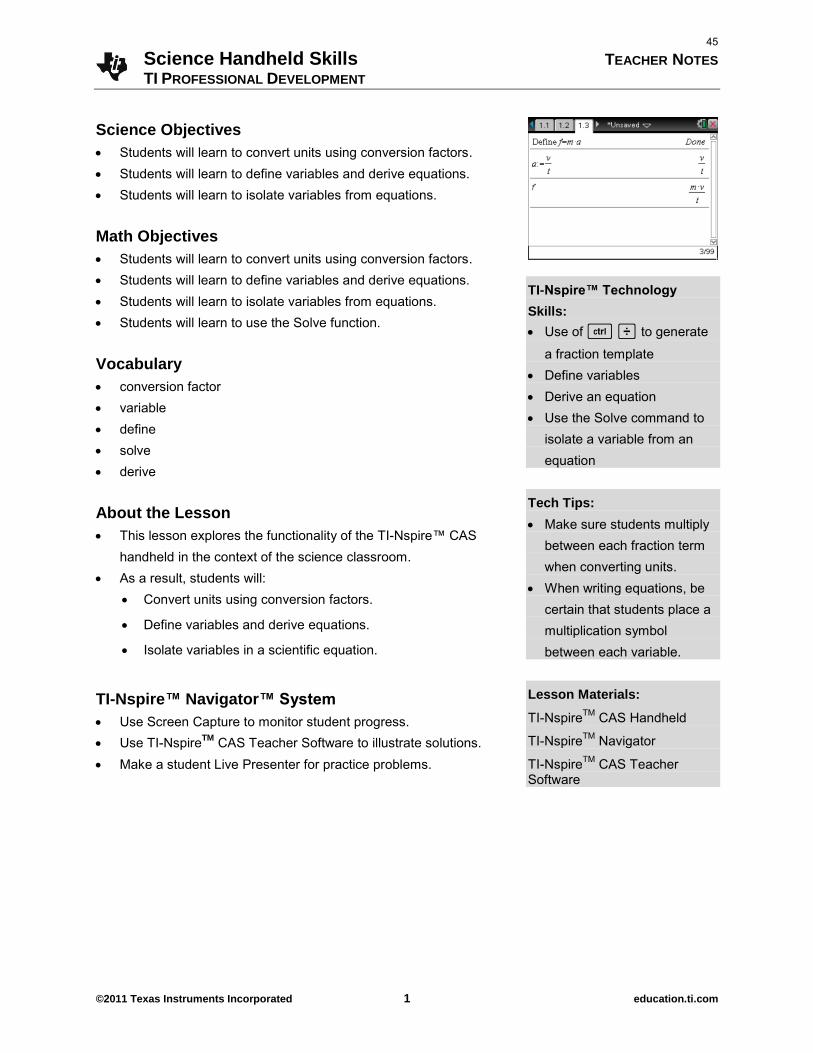
Step 8: Since f is defined in terms of m and a, and a is defined in terms of v and t, CAS automatically defines f in terms of m, v, and t. To see the resulting expression, type F ·.
47
Science Handheld Skills TEACHER NOTES
TI PROFESSIONAL DEVELOPMENT
©2011 Texas Instruments Incorporated 4 education.ti.com
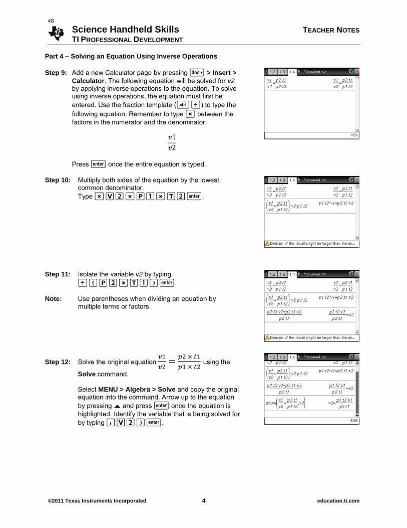
Part 4 – Solving an Equation Using Inverse Operations
Step 9: Add a new Calculator page by pressing ~ > Insert > Calculator. The following equation will be solved for v2 by applying inverse operations to the equation. To solve using inverse operations, the equation must first be entered. Use the fraction template (/ p) to type the following equation. Remember to type r between the factors in the numerator and the denominator.
Press · once the entire equation is typed.
Step 10: Multiply both sides of the equation by the lowest common denominator. Type r V 2 r P 1 r T 2 ·.
Step 11: Isolate the variable v2 by typing p ( P 2 r T 1 ) ·.
Note: Use parentheses when dividing an equation by
multiple terms or factors.
Step 12: Solve the original equation
using the
Solve command.
Select MENU > Algebra > Solve and copy the original equation into the command. Arrow up to the equation by pressing £ and press · once the equation is highlighted. Identify the variable that is being solved for by typing , V 2 ) ·.
48
The River of Life Name Student Activity Class
©2011 Texas Instruments Incorporated 1 education.ti.com
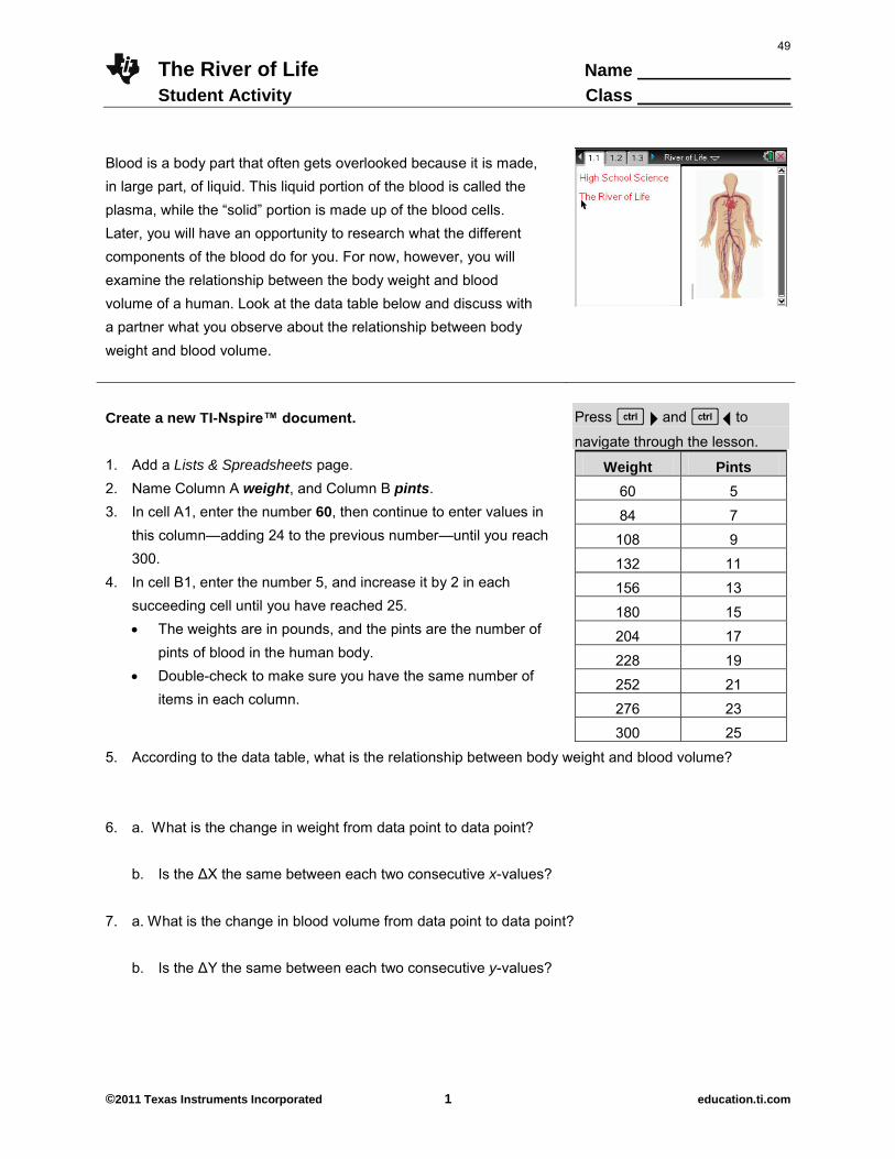
Blood is a body part that often gets overlooked because it is made, in large part, of liquid. This liquid portion of the blood is called the plasma, while the “solid” portion is made up of the blood cells.
Later, you will have an opportunity to research what the different components of the blood do for you. For now, however, you will examine the relationship between the body weight and blood volume of a human. Look at the data table below and discuss with a partner what you observe about the relationship between body weight and blood volume.
Create a new TI-Nspire™ document.
Press / ¢ and / ¡ to
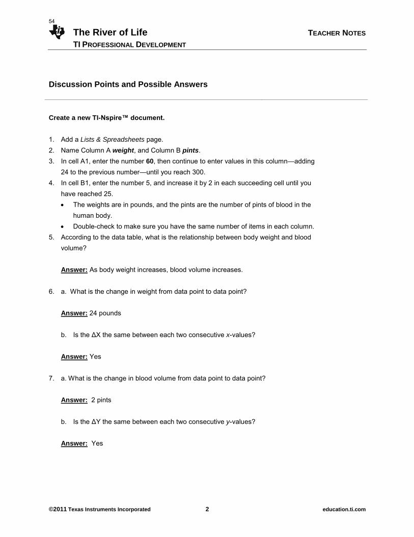
navigate through the lesson. 1. Add a Lists & Spreadsheets page. 2. Name Column A weight, and Column B pints. 3. In cell A1, enter the number 60, then continue to enter values in
this column—adding 24 to the previous number—until you reach 300.
4. In cell B1, enter the number 5, and increase it by 2 in each succeeding cell until you have reached 25. The weights are in pounds, and the pints are the number of
pints of blood in the human body. Double-check to make sure you have the same number of
items in each column.
Weight Pints
60 5 84 7 108 9 132 11 156 13 180 15 204 17 228 19 252 21 276 23 300 25
5. According to the data table, what is the relationship between body weight and blood volume? 6. a. What is the change in weight from data point to data point?
b. Is the ΔX the same between each two consecutive x-values?
7. a. What is the change in blood volume from data point to data point? b. Is the ΔY the same between each two consecutive y-values?
49
The River of Life Name Student Activity Class
©2011 Texas Instruments Incorporated 2 education.ti.com
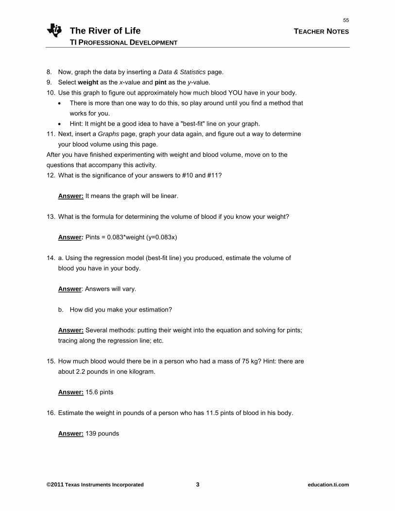
8. Now, graph the data by inserting a Data & Statistics page. 9. Select weight as the x-value and pint as the y-value. 10. Use this graph to figure out approximately how much blood YOU have in your body.
There is more than one way to do this, so play around until you find a method that works for you.
Hint: It might be a good idea to have a "best-fit" line on your graph. 11. Next, insert a Graphs page, graph your data again, and figure out a way to
determine your blood volume using this page. After you have finished experimenting with weight and blood volume, move on to
the questions that accompany this activity. 12. What is the significance of your answers to #10 and #11?
13. What is the formula for determining the volume of blood if you know your weight? 14. a. Using the regression model (best-fit line) you produced, estimate the volume of
blood you have in your body.
b. How did you make your estimation? 15. How much blood would there be in a person who had a mass of 75 kg? Hint: there are
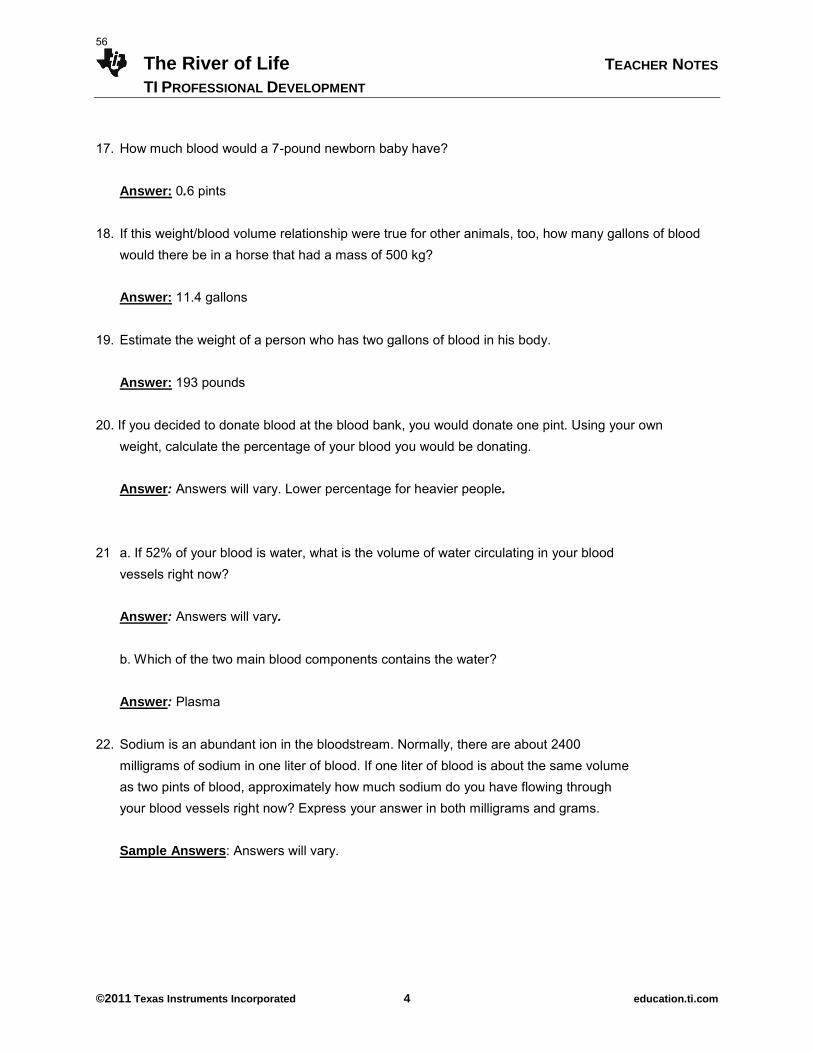
about 2.2 pounds in one kilogram. 16. Estimate the weight in pounds of a person who has 11.5 pints of blood in his body. 17. How much blood would a 7-pound newborn baby have? 18. If this weight/blood volume relationship were true for other animals, too, how many
gallons of blood would there be in a horse that had a mass of 500 kg? 19. Estimate the weight of a person who has two gallons of blood in his body.
50
The River of Life Name Student Activity Class
©2011 Texas Instruments Incorporated 3 education.ti.com
20. If you decided to donate blood at the blood bank, you would donate one pint. Using your own weight, calculate the percentage of your blood you would be donating.
21 a. If 52% of your blood is water, what is the volume of water circulating in your blood
vessels right now? b. Which of the two main blood components contains the water? 22. Sodium is an abundant ion in the bloodstream. Normally, there are about 2400
milligrams of sodium in one liter of blood. If one liter of blood is about the same volume as two pints of blood, approximately how much sodium do you have flowing through your blood vessels right now? Express your answer in both milligrams and grams.
23. One of the most important functions of the blood is to transport oxygen to all of your
cells, and the cells that take care of this for you are called erythrocytes, or red blood cells. Red blood cells are by far the most numerous cells in the blood, averaging about 4.5 x 10⁶ cells per microliter (1000 microliter = 1ml; 1000ml = 1L). How many microliters are there in one liter? Using this information, calculate the approximate number of red blood cells you have in your body right now.
24. Leukocytes, or white blood cells, are another type of blood cell in your body. Human
blood contains about 7.0 x 10³ WBC's per microliter. Calculate the approximate number of leukocytes you have in your body right now.
25. White blood cells function mainly in defending you against infections. Explain why the
number of white blood cells in a person’s body may tend to fluctuate a lot more than the
number of red blood cells does.
51

This page intentionally left blank
52
The River of Life TEACHER NOTES
TI PROFESSIONAL DEVELOPMENT
©2011 Texas Instruments Incorporated 1 education.ti.com
Science Objectives
Students will calculate the volume of blood in their own bodies. Students will analyze and quantify some of the components of
their blood.
Math Objectives
Students will use tabular data to accurately generate a scatter plot.
Students will generate a linear regression model, use the function to perform calculations, and interpolate a value on the regression model.
Materials Needed
TI-Nspire™ or TI-Nspire™ CAS unit for each student
Vocabulary
plasma erythrocytes leukocytes milligram microliter About the Lesson
This lesson involves generating a linear regression model for human blood volume vs. body weight.
As a result, students will: Algebraically calculate their own blood volume. Interpolate on the regression model to determine their blood
volume.
TI-Nspire™ Navigator™ System
Screen Capture to monitor student progress. Live presenter allows students to show their graphs to the class.
TI-Nspire™ Technology Skills: Download a TI-Nspire™
document Open a document Move between pages Entering and graphing data
using multiple applications Tracing, interpolating,
predicting
Tech Tips:
Make sure the font size on your TI-Nspire handhelds is set to Medium.
You can hide the function entry line by pressing / G.
Lesson Materials: Student Activity
The River of Life.pdf The River of Life.doc
TI-Nspire document
The River of Life.tns
53
The River of Life TEACHER NOTES
TI PROFESSIONAL DEVELOPMENT
©2011 Texas Instruments Incorporated 2 education.ti.com
Discussion Points and Possible Answers
Create a new TI-Nspire™ document. 1. Add a Lists & Spreadsheets page. 2. Name Column A weight, and Column B pints. 3. In cell A1, enter the number 60, then continue to enter values in this column—adding
24 to the previous number—until you reach 300. 4. In cell B1, enter the number 5, and increase it by 2 in each succeeding cell until you
have reached 25. The weights are in pounds, and the pints are the number of pints of blood in the
human body. Double-check to make sure you have the same number of items in each column.
5. According to the data table, what is the relationship between body weight and blood volume?
Answer: As body weight increases, blood volume increases.
6. a. What is the change in weight from data point to data point?
Answer: 24 pounds b. Is the ΔX the same between each two consecutive x-values?
Answer: Yes
7. a. What is the change in blood volume from data point to data point?
Answer: 2 pints
b. Is the ΔY the same between each two consecutive y-values?
Answer: Yes
54
The River of Life TEACHER NOTES
TI PROFESSIONAL DEVELOPMENT
©2011 Texas Instruments Incorporated 3 education.ti.com
8. Now, graph the data by inserting a Data & Statistics page. 9. Select weight as the x-value and pint as the y-value. 10. Use this graph to figure out approximately how much blood YOU have in your body.
There is more than one way to do this, so play around until you find a method that works for you.
Hint: It might be a good idea to have a "best-fit" line on your graph. 11. Next, insert a Graphs page, graph your data again, and figure out a way to determine
your blood volume using this page. After you have finished experimenting with weight and blood volume, move on to the questions that accompany this activity. 12. What is the significance of your answers to #10 and #11?
Answer: It means the graph will be linear.
13. What is the formula for determining the volume of blood if you know your weight?
Answer: Pints = 0.083*weight (y=0.083x)
14. a. Using the regression model (best-fit line) you produced, estimate the volume of blood you have in your body.
Answer: Answers will vary. b. How did you make your estimation? Answer: Several methods: putting their weight into the equation and solving for pints; tracing along the regression line; etc.
15. How much blood would there be in a person who had a mass of 75 kg? Hint: there are
about 2.2 pounds in one kilogram.
Answer: 15.6 pints
16. Estimate the weight in pounds of a person who has 11.5 pints of blood in his body.
Answer: 139 pounds
55
The River of Life TEACHER NOTES
TI PROFESSIONAL DEVELOPMENT
©2011 Texas Instruments Incorporated 4 education.ti.com
17. How much blood would a 7-pound newborn baby have?
Answer: 0.6 pints
18. If this weight/blood volume relationship were true for other animals, too, how many gallons of blood would there be in a horse that had a mass of 500 kg?
Answer: 11.4 gallons 19. Estimate the weight of a person who has two gallons of blood in his body.
Answer: 193 pounds
20. If you decided to donate blood at the blood bank, you would donate one pint. Using your own weight, calculate the percentage of your blood you would be donating.
Answer: Answers will vary. Lower percentage for heavier people.
21 a. If 52% of your blood is water, what is the volume of water circulating in your blood
vessels right now? Answer: Answers will vary.
b. Which of the two main blood components contains the water?
Answer: Plasma 22. Sodium is an abundant ion in the bloodstream. Normally, there are about 2400
milligrams of sodium in one liter of blood. If one liter of blood is about the same volume as two pints of blood, approximately how much sodium do you have flowing through your blood vessels right now? Express your answer in both milligrams and grams.
Sample Answers: Answers will vary.
56
The River of Life TEACHER NOTES
TI PROFESSIONAL DEVELOPMENT
©2011 Texas Instruments Incorporated 5 education.ti.com
23. One of the most important functions of the blood is to transport oxygen to all of your cells, and the cells that take care of this for you are called erythrocytes, or red blood cells. Red blood cells are by far the most numerous cells in the blood, averaging about 4.5 x 10⁶ cells per microliter (1000 microliter = 1ml; 1000ml = 1L). How many microliters are there in one liter? Using this information, calculate the approximate number of red blood cells you have in your body right now.
Sample Answers: Answers will vary
24. Leukocytes, or white blood cells, are another type of blood cell in your body. Human blood contains about 7.0 x 10³ WBC's per microliter. Calculate the approximate number of leukocytes you have in your body right now.
Sample Answers: Answers will vary.
25. White blood cells function mainly in defending you against infections. Explain why the number of white blood cells in a person’s body may tend to fluctuate a lot more than the
number of red blood cells does.
Answer: WBC numbers tend to increase when a person is sick or injured.
TI-Nspire Navigator Opportunity: Screen Capture
See Note 1 at the end of the lesson.
Wrap Up
Assessment Formative assessment will consist of questions embedded in the TI-Nspire document. The questions will be graded when the document is retrieved. The Slide Show can be utilized to give students immediate feedback on their assessment. TI-Nspire™ Navigator™ Notes
Note 1: Screen Capture
Screen Capture can be used to monitor student progress.
57

This page intentionally left blank
58
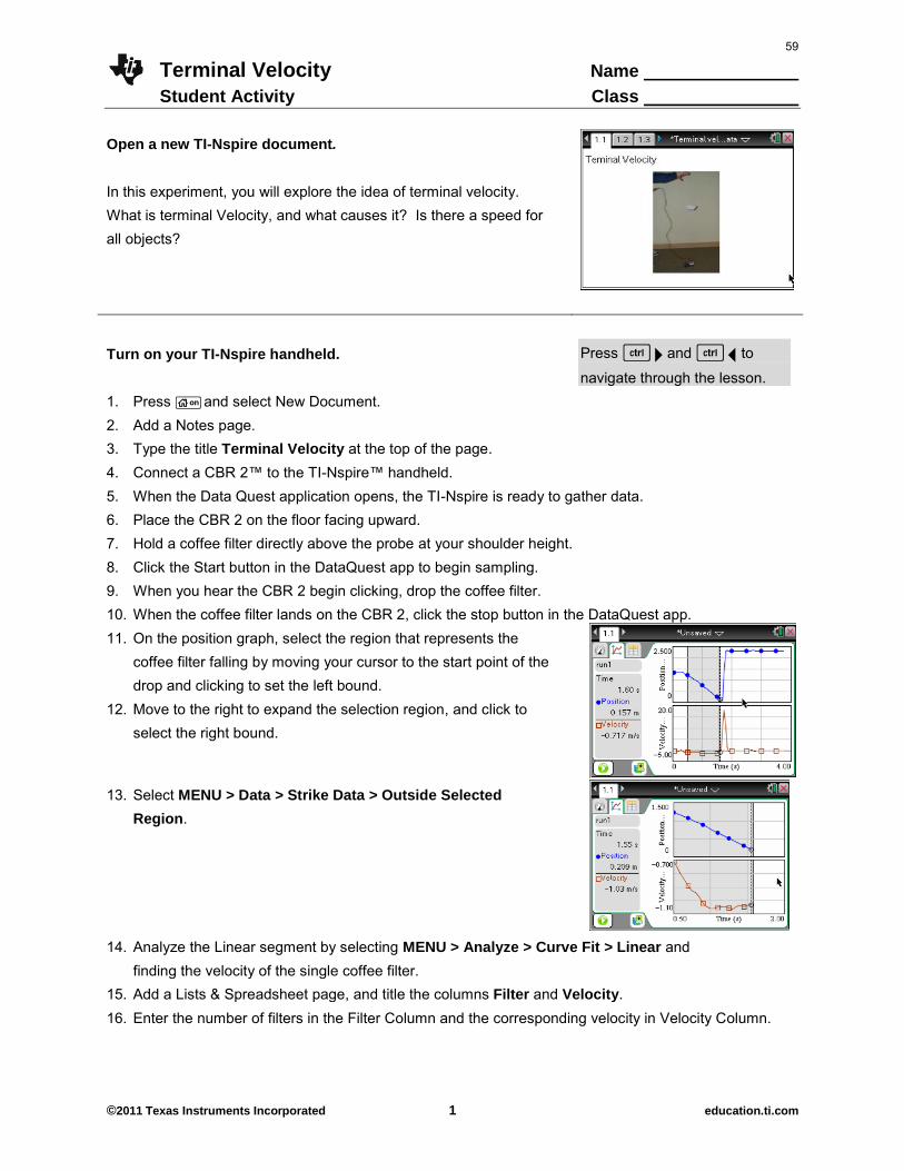
Terminal Velocity Name Student Activity Class
©2011 Texas Instruments Incorporated 1 education.ti.com
Open a new TI-Nspire document. In this experiment, you will explore the idea of terminal velocity. What is terminal Velocity, and what causes it? Is there a speed for all objects?
Turn on your TI-Nspire handheld.
Press / ¢ and / ¡ to
navigate through the lesson. 1. Press c and select New Document. 2. Add a Notes page. 3. Type the title Terminal Velocity at the top of the page. 4. Connect a CBR 2™ to the TI-Nspire™ handheld. 5. When the Data Quest application opens, the TI-Nspire is ready to gather data. 6. Place the CBR 2 on the floor facing upward. 7. Hold a coffee filter directly above the probe at your shoulder height. 8. Click the Start button in the DataQuest app to begin sampling. 9. When you hear the CBR 2 begin clicking, drop the coffee filter. 10. When the coffee filter lands on the CBR 2, click the stop button in the DataQuest app. 11. On the position graph, select the region that represents the
coffee filter falling by moving your cursor to the start point of the drop and clicking to set the left bound.
12. Move to the right to expand the selection region, and click to select the right bound.
13. Select MENU > Data > Strike Data > Outside Selected
Region.
14. Analyze the Linear segment by selecting MENU > Analyze > Curve Fit > Linear and
finding the velocity of the single coffee filter. 15. Add a Lists & Spreadsheet page, and title the columns Filter and Velocity. 16. Enter the number of filters in the Filter Column and the corresponding velocity in Velocity Column.
59
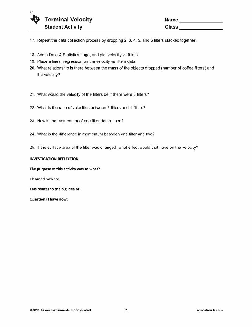
Terminal Velocity Name Student Activity Class
©2011 Texas Instruments Incorporated 2 education.ti.com
17. Repeat the data collection process by dropping 2, 3, 4, 5, and 6 filters stacked together.
18. Add a Data & Statistics page, and plot velocity vs filters. 19. Place a linear regression on the velocity vs filters data. 20. What relationship is there between the mass of the objects dropped (number of coffee filters) and
the velocity? 21. What would the velocity of the filters be if there were 8 filters? 22. What is the ratio of velocities between 2 filters and 4 filters? 23. How is the momentum of one filter determined? 24. What is the difference in momentum between one filter and two? 25. If the surface area of the filter was changed, what effect would that have on the velocity? INVESTIGATION REFLECTION The purpose of this activity was to what? I learned how to: This relates to the big idea of: Questions I have now:
60
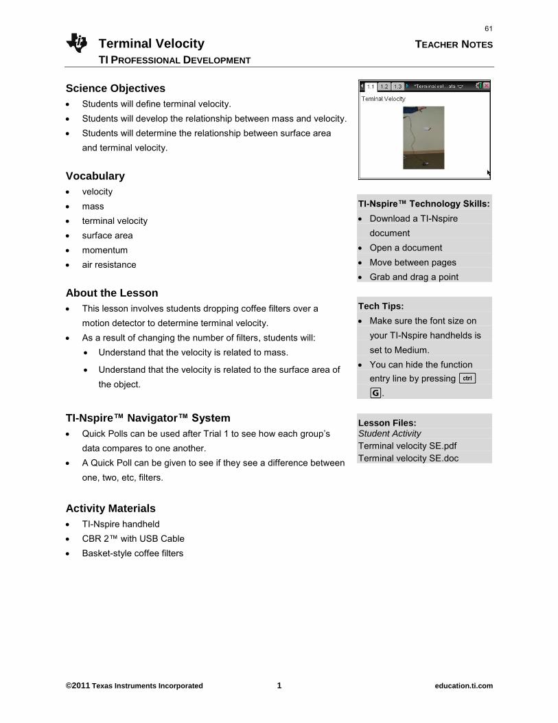
Terminal Velocity TEACHER NOTES
TI PROFESSIONAL DEVELOPMENT
©2011 Texas Instruments Incorporated 1 education.ti.com
Science Objectives
Students will define terminal velocity. Students will develop the relationship between mass and velocity. Students will determine the relationship between surface area
and terminal velocity. Vocabulary
velocity mass terminal velocity surface area momentum air resistance About the Lesson
This lesson involves students dropping coffee filters over a motion detector to determine terminal velocity.
As a result of changing the number of filters, students will: Understand that the velocity is related to mass.
Understand that the velocity is related to the surface area of the object.
TI-Nspire™ Navigator™ System
Quick Polls can be used after Trial 1 to see how each group’s data compares to one another.
A Quick Poll can be given to see if they see a difference between one, two, etc, filters.
Activity Materials
TI-Nspire handheld CBR 2™ with USB Cable Basket-style coffee filters
TI-Nspire™ Technology Skills: Download a TI-Nspire
document Open a document Move between pages Grab and drag a point
Tech Tips:
Make sure the font size on your TI-Nspire handhelds is set to Medium.
You can hide the function entry line by pressing / G.
Lesson Files: Student Activity
Terminal velocity SE.pdf Terminal velocity SE.doc
61
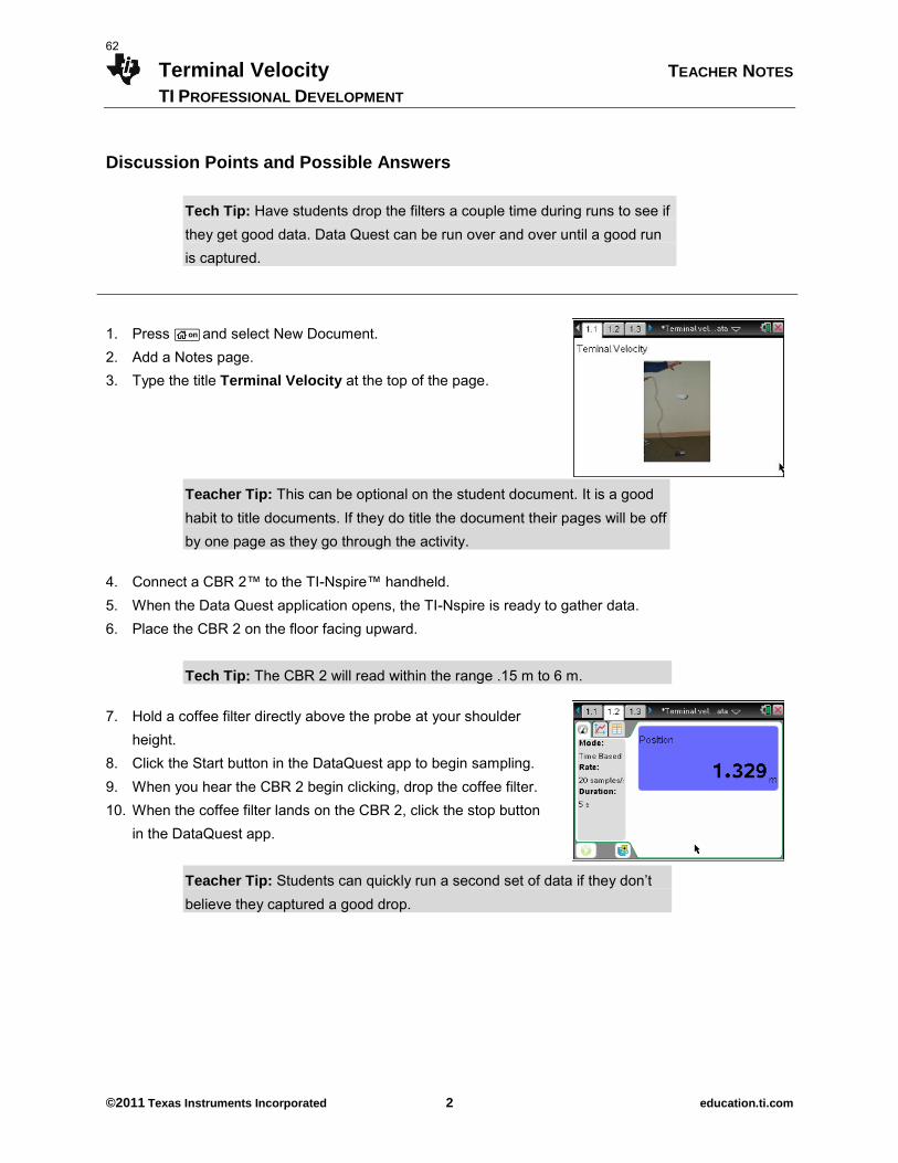
Terminal Velocity TEACHER NOTES
TI PROFESSIONAL DEVELOPMENT
©2011 Texas Instruments Incorporated 2 education.ti.com
Discussion Points and Possible Answers
Tech Tip: Have students drop the filters a couple time during runs to see if they get good data. Data Quest can be run over and over until a good run is captured.
1. Press c and select New Document. 2. Add a Notes page. 3. Type the title Terminal Velocity at the top of the page.
Teacher Tip: This can be optional on the student document. It is a good habit to title documents. If they do title the document their pages will be off by one page as they go through the activity.
4. Connect a CBR 2™ to the TI-Nspire™ handheld. 5. When the Data Quest application opens, the TI-Nspire is ready to gather data. 6. Place the CBR 2 on the floor facing upward.
Tech Tip: The CBR 2 will read within the range .15 m to 6 m.
7. Hold a coffee filter directly above the probe at your shoulder height.
8. Click the Start button in the DataQuest app to begin sampling. 9. When you hear the CBR 2 begin clicking, drop the coffee filter. 10. When the coffee filter lands on the CBR 2, click the stop button
in the DataQuest app.
Teacher Tip: Students can quickly run a second set of data if they don’t
believe they captured a good drop.
62
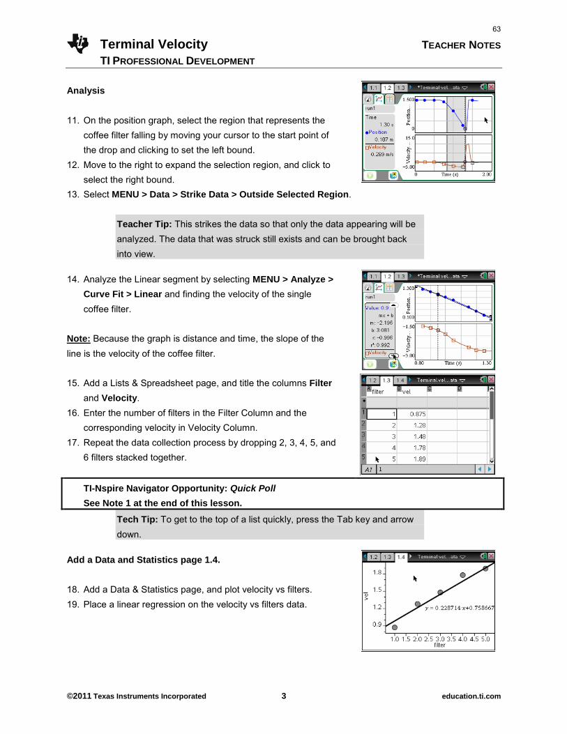
Terminal Velocity TEACHER NOTES
TI PROFESSIONAL DEVELOPMENT
©2011 Texas Instruments Incorporated 3 education.ti.com
Analysis 11. On the position graph, select the region that represents the
coffee filter falling by moving your cursor to the start point of the drop and clicking to set the left bound.
12. Move to the right to expand the selection region, and click to select the right bound.
13. Select MENU > Data > Strike Data > Outside Selected Region.
Teacher Tip: This strikes the data so that only the data appearing will be analyzed. The data that was struck still exists and can be brought back into view.
14. Analyze the Linear segment by selecting MENU > Analyze >
Curve Fit > Linear and finding the velocity of the single coffee filter.
Note: Because the graph is distance and time, the slope of the line is the velocity of the coffee filter.
15. Add a Lists & Spreadsheet page, and title the columns Filter
and Velocity. 16. Enter the number of filters in the Filter Column and the
corresponding velocity in Velocity Column. 17. Repeat the data collection process by dropping 2, 3, 4, 5, and
6 filters stacked together.
TI-Nspire Navigator Opportunity: Quick Poll
See Note 1 at the end of this lesson.
Tech Tip: To get to the top of a list quickly, press the Tab key and arrow down.
Add a Data and Statistics page 1.4. 18. Add a Data & Statistics page, and plot velocity vs filters. 19. Place a linear regression on the velocity vs filters data.
63
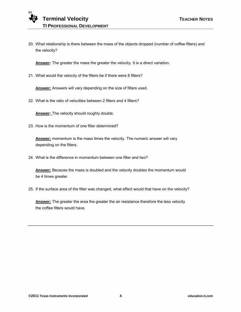
Terminal Velocity TEACHER NOTES
TI PROFESSIONAL DEVELOPMENT
©2011 Texas Instruments Incorporated 4 education.ti.com
20. What relationship is there between the mass of the objects dropped (number of coffee filters) and the velocity?
Answer: The greater the mass the greater the velocity. It is a direct variation.
21. What would the velocity of the filters be if there were 8 filters?
Answer: Answers will vary depending on the size of filters used. 22. What is the ratio of velocities between 2 filters and 4 filters?
Answer: The velocity should roughly double. 23. How is the momentum of one filter determined?
Answer: momentum is the mass times the velocity. The numeric answer will vary depending on the filters.
24. What is the difference in momentum between one filter and two?
Answer: Because the mass is doubled and the velocity doubles the momentum would be 4 times greater.
25. If the surface area of the filter was changed, what effect would that have on the velocity?
Answer: The greater the area the greater the air resistance therefore the less velocity the coffee filters would have.
64
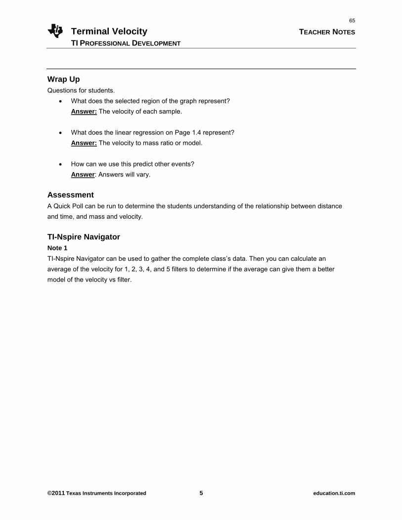
Terminal Velocity TEACHER NOTES
TI PROFESSIONAL DEVELOPMENT
©2011 Texas Instruments Incorporated 5 education.ti.com
Wrap Up
Questions for students. What does the selected region of the graph represent?
Answer: The velocity of each sample.
What does the linear regression on Page 1.4 represent? Answer: The velocity to mass ratio or model.
How can we use this predict other events? Answer: Answers will vary.
Assessment A Quick Poll can be run to determine the students understanding of the relationship between distance and time, and mass and velocity. TI-Nspire Navigator Note 1
TI-Nspire Navigator can be used to gather the complete class’s data. Then you can calculate an average of the velocity for 1, 2, 3, 4, and 5 filters to determine if the average can give them a better model of the velocity vs filter.
65

This page intentionally left blank
66
Day 1 Reflections and Homework TEACHER NOTES
HIGH SCHOOL SCIENCE
©2011 Texas Instruments Incorporated 1 education.ti.com
Reflections:
Take a few minutes to reflect on your learning - what you have accomplished? What issues do you have?
Reflect on the day’s activities, and consider how the use of technology can engage students and help them better understand science concepts.
Questions to Discuss:
Which parts of the day’s activities made you consider new
approaches to teaching any of the science content areas that were explored?
How does a teacher’s role change in an inquiry classroom? How do feel about the length of the TI-Nspire documents? How many pages of instructions do you feel is optimal for student
use? What questions do you have about DataQuestTM or the
TI-NspireTM CX? Homework
Temperature Up and Down. Create a three-page TI-Nspire™ document containing a Notes page, a DataQuest
TM App, and either a Lists & Spreadsheet or Data & Statistics page. Generate data using the temperature sensor in at least two different temperature environments in this document.
Ticket Outta Here:
Complete and hand in the first “Ticket Outta Here”.
Today’s Activities:
Using the Temperature Sensor
Fahrenheit to Celsius Nailing Density Science Handheld Skills River of Life
Terminal Velocity
TI Equipment used today:
TI-NspireTM CX CAS TI-NspireTM Lab CradleTM TI-Nspire NavigatorTM
Vernier Sensors used today:
EasyTempTM Stainless Steel temperature CBR 2TM Visit http://education.ti.com/calculators/tisciencenspired/ for lesson updates and tech tip videos.
67
Day 1 Reflections and Homework TEACHER NOTES
HIGH SCHOOL SCIENCE
©2011 Texas Instruments Incorporated 2 education.ti.com
Ticket Outta Here DAY 1 Exit Card
1. Reflect on your learning - what you have accomplished? 2. What issues do you have? 3. How can the use of technology engage students and help them better understand science concepts? Anything else?
68
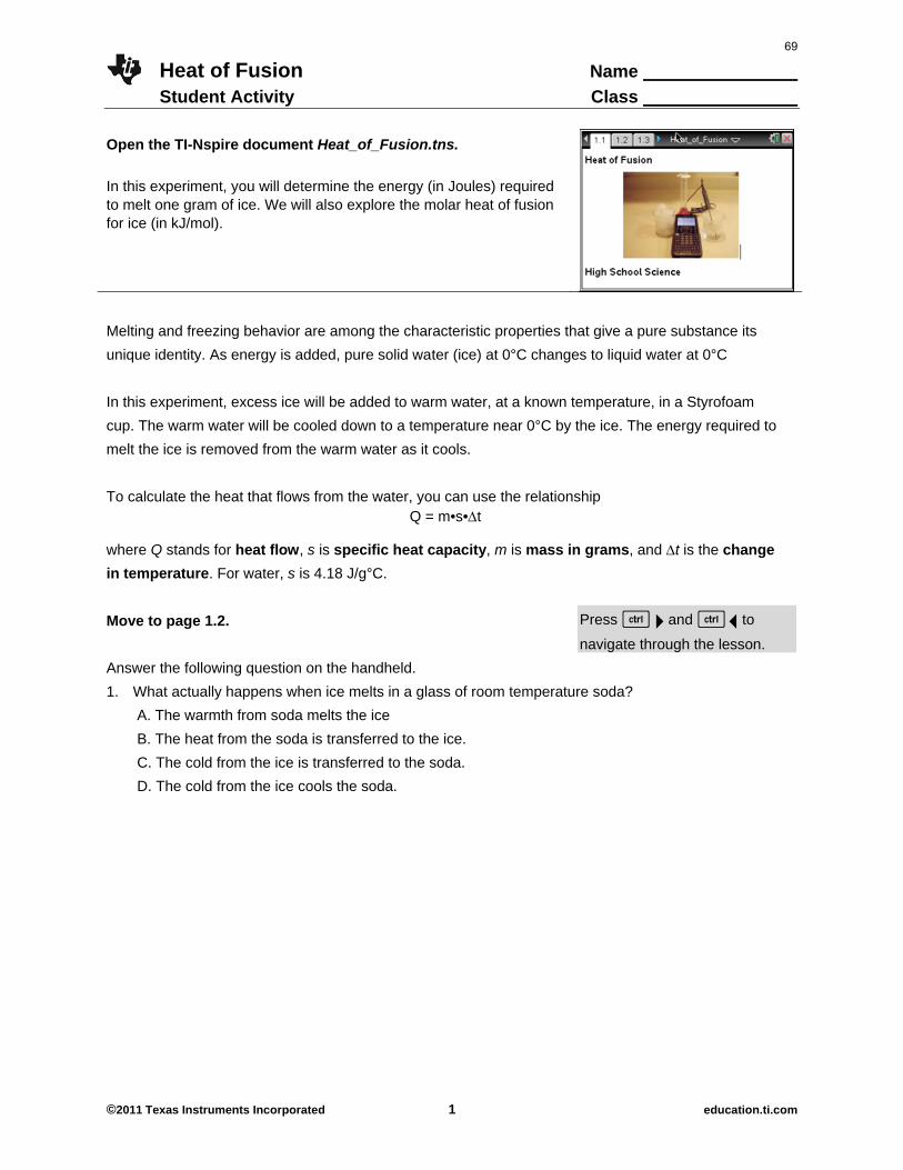
Heat of Fusion Name Student Activity Class
©2011 Texas Instruments Incorporated 1 education.ti.com
Open the TI-Nspire document Heat_of_Fusion.tns.
In this experiment, you will determine the energy (in Joules) required to melt one gram of ice. We will also explore the molar heat of fusion for ice (in kJ/mol).
Melting and freezing behavior are among the characteristic properties that give a pure substance its
unique identity. As energy is added, pure solid water (ice) at 0°C changes to liquid water at 0°C
In this experiment, excess ice will be added to warm water, at a known temperature, in a Styrofoam
cup. The warm water will be cooled down to a temperature near 0°C by the ice. The energy required to
melt the ice is removed from the warm water as it cools.
To calculate the heat that flows from the water, you can use the relationship Q = m•s•t
where Q stands for heat flow, s is specific heat capacity, m is mass in grams, and t is the change
in temperature. For water, s is 4.18 J/g°C.
Move to page 1.2.
Press / ¢ and / ¡ to
navigate through the lesson.
Answer the following question on the handheld.
1. What actually happens when ice melts in a glass of room temperature soda?
A. The warmth from soda melts the ice
B. The heat from the soda is transferred to the ice.
C. The cold from the ice is transferred to the soda.
D. The cold from the ice cools the soda.
69
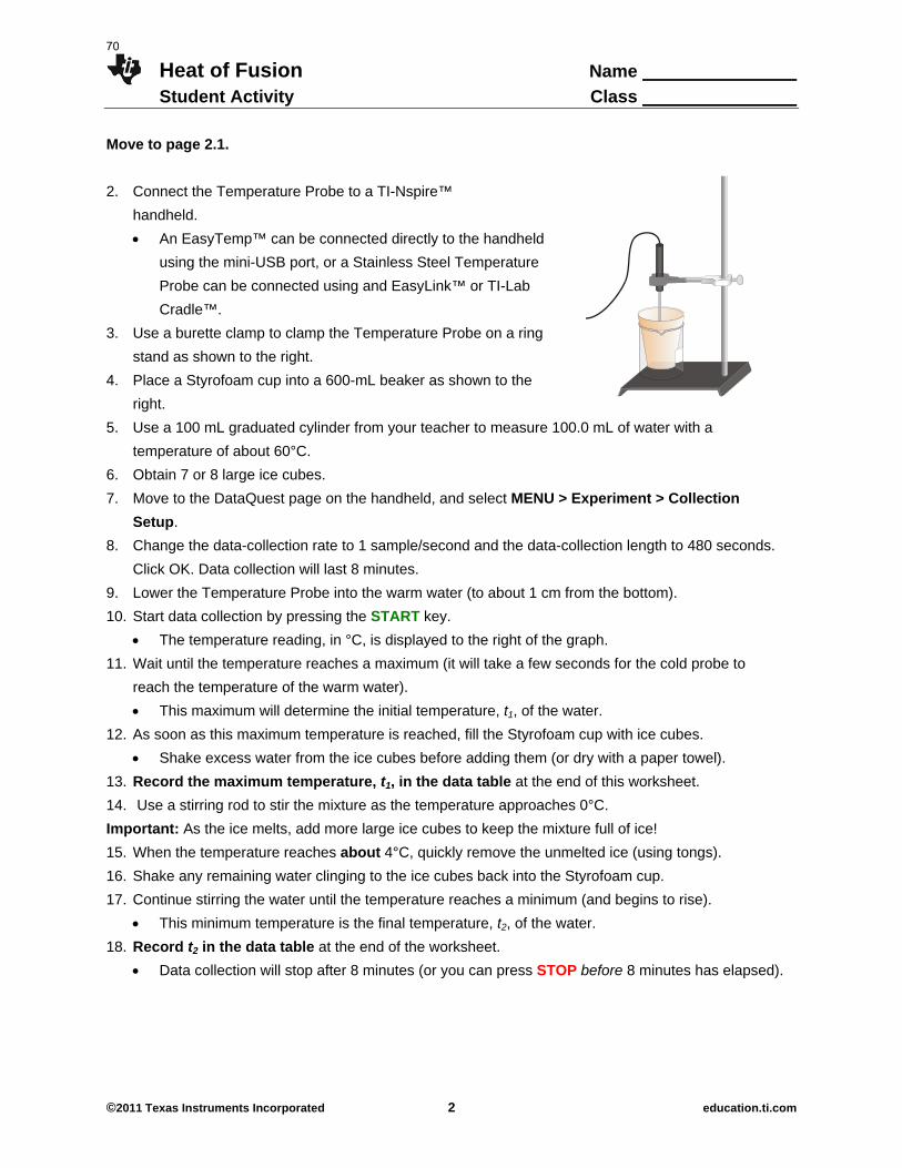
Heat of Fusion Name Student Activity Class
©2011 Texas Instruments Incorporated 2 education.ti.com
Move to page 2.1.
2. Connect the Temperature Probe to a TI-Nspire™
handheld.
An EasyTemp™ can be connected directly to the handheld
using the mini-USB port, or a Stainless Steel Temperature
Probe can be connected using and EasyLink™ or TI-Lab
Cradle™.
3. Use a burette clamp to clamp the Temperature Probe on a ring
stand as shown to the right.
4. Place a Styrofoam cup into a 600-mL beaker as shown to the
right.
5. Use a 100 mL graduated cylinder from your teacher to measure 100.0 mL of water with a
temperature of about 60°C.
6. Obtain 7 or 8 large ice cubes.
7. Move to the DataQuest page on the handheld, and select MENU > Experiment > Collection
Setup.
8. Change the data-collection rate to 1 sample/second and the data-collection length to 480 seconds.
Click OK. Data collection will last 8 minutes.
9. Lower the Temperature Probe into the warm water (to about 1 cm from the bottom).
10. Start data collection by pressing the START key.
The temperature reading, in °C, is displayed to the right of the graph. 11. Wait until the temperature reaches a maximum (it will take a few seconds for the cold probe to
reach the temperature of the warm water).
This maximum will determine the initial temperature, t1, of the water.
12. As soon as this maximum temperature is reached, fill the Styrofoam cup with ice cubes.
Shake excess water from the ice cubes before adding them (or dry with a paper towel). 13. Record the maximum temperature, t1, in the data table at the end of this worksheet. 14. Use a stirring rod to stir the mixture as the temperature approaches 0°C.
Important: As the ice melts, add more large ice cubes to keep the mixture full of ice!
15. When the temperature reaches about 4°C, quickly remove the unmelted ice (using tongs).
16. Shake any remaining water clinging to the ice cubes back into the Styrofoam cup.
17. Continue stirring the water until the temperature reaches a minimum (and begins to rise).
This minimum temperature is the final temperature, t2, of the water.
18. Record t2 in the data table at the end of the worksheet.
Data collection will stop after 8 minutes (or you can press STOP before 8 minutes has elapsed).
70
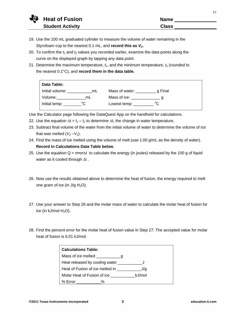
Heat of Fusion Name Student Activity Class
©2011 Texas Instruments Incorporated 3 education.ti.com
19. Use the 100 mL graduated cylinder to measure the volume of water remaining in the
Styrofoam cup to the nearest 0.1 mL, and record this as V2.
20. To confirm the t1 and t2 values you recorded earlier, examine the data points along the
curve on the displayed graph by tapping any data point.
21. Determine the maximum temperature, t1, and the minimum temperature, t2 (rounded to
the nearest 0.1°C), and record them in the data table.
Data Table:
Initial volume: ___________mL Mass of water: _________ g Final
Volume:_____________mL Mass of ice: _____________ g
Initial temp: ________oC Lowest temp: _________ oC
Use the Calculator page following the DataQuest App on the handheld for calculations.
22. Use the equation t = t1 – t2 to determine t, the change in water temperature.
23. Subtract final volume of the water from the initial volume of water to determine the volume of ice
that was melted (V2 –V1).
24. Find the mass of ice melted using the volume of melt (use 1.00 g/mL as the density of water).
Record in Calculations Data Table below.
25. Use the equation Q = m•s•t to calculate the energy (in joules) released by the 100 g of liquid
water as it cooled through t .
26. Now use the results obtained above to determine the heat of fusion, the energy required to melt
one gram of ice (in J/g H2O).
27. Use your answer to Step 26 and the molar mass of water to calculate the molar heat of fusion for
ice (in kJ/mol H2O).
28. Find the percent error for the molar heat of fusion value in Step 27. The accepted value for molar
heat of fusion is 6.01 kJ/mol.
Calculations Table:
Mass of ice melted ___________g
Heat released by cooling water ___________J
Heat of Fusion of ice melted in ___________J/g
Molar Heat of Fusion of ice ___________kJ/mol
% Error ___________%
71
Heat of Fusion Name Student Activity Class
©2011 Texas Instruments Incorporated 4 education.ti.com
29. Using your previous knowledge of the boiling point of water and melting point of ice, explain your
results in the space below.
30. Explain your percent error value. Give possible sources of error.
72
Heat of Fusion TEACHER NOTES
HIGH SCHOOL SCIENCE
©2011 Texas Instruments Incorporated 1 education.ti.com
Science Objectives Students will collect, analyze, and interpret data to develop a
mathematical model that explains their experimental results.
Students will determine the heat of fusion for ice and their percent
error.
Vocabulary heat energy
specific heat
molar mass
heat of fusion
About the Lesson This lesson involves observing the effect of adding ice to warm
water.
As a result, students will:
Analyze data to determine a mathematical model to explain
their experimental results.
Calculate heat of fusion for ice and percent error.
Speculate on possible sources of error.
TI-Nspire™ Navigator™ System Send and collect the Heat_of_Fusion.tns file.
Screen Capture to monitor student progress.
Live Presenter allows students to show their heat calculations to
the class
Discuss results using Slideshow.
Activity Materials TI-NspireTM CX CAS handheld
600-mL Beakers
100 mL Graduated Cylinder
Styrofoam cups
Ice
warm water
Tongs
Paper Towels
TI-Nspire™ Technology Skills:
Download a TI-NspireTM
document
Move between pages
Use DataQuestTM App
Use math boxes
Tech Tips:
Make sure the font size on
your TI-NspireTM handhelds is
set to Medium.
Lesson Files: Student Activity Heat_of_Fusion_Student.pdf Heat_of_Fusion_Student.doc
TI-Nspire document Heat_of_Fusion.tns Vernier® Equipment: Vernier EasyTemp™ OR EasyLink™ and the
Stainless Steel Temperature sensor OR
TI-Nspire™ Lab Cradle™ and the Stainless Steel Temperature sensor
73
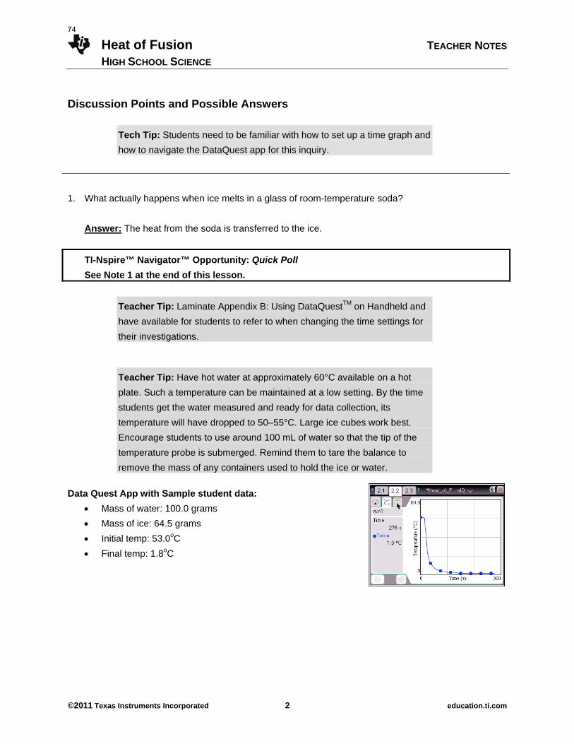
Heat of Fusion TEACHER NOTES
HIGH SCHOOL SCIENCE
©2011 Texas Instruments Incorporated 2 education.ti.com
Discussion Points and Possible Answers
Tech Tip: Students need to be familiar with how to set up a time graph and
how to navigate the DataQuest app for this inquiry.
1. What actually happens when ice melts in a glass of room-temperature soda?
Answer: The heat from the soda is transferred to the ice.
TI-Nspire™ Navigator™ Opportunity: Quick Poll
See Note 1 at the end of this lesson.
Teacher Tip: Laminate Appendix B: Using DataQuestTM on Handheld and
have available for students to refer to when changing the time settings for
their investigations.
Teacher Tip: Have hot water at approximately 60°C available on a hot
plate. Such a temperature can be maintained at a low setting. By the time
students get the water measured and ready for data collection, its
temperature will have dropped to 50–55°C. Large ice cubes work best.
Encourage students to use around 100 mL of water so that the tip of the
temperature probe is submerged. Remind them to tare the balance to
remove the mass of any containers used to hold the ice or water.
Data Quest App with Sample student data:
Mass of water: 100.0 grams
Mass of ice: 64.5 grams
Initial temp: 53.0oC
Final temp: 1.8oC
74
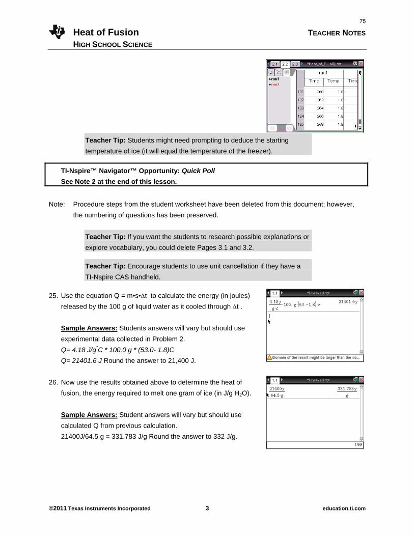
Heat of Fusion TEACHER NOTES
HIGH SCHOOL SCIENCE
©2011 Texas Instruments Incorporated 3 education.ti.com
Teacher Tip: Students might need prompting to deduce the starting
temperature of ice (it will equal the temperature of the freezer).
TI-Nspire™ Navigator™ Opportunity: Quick Poll
See Note 2 at the end of this lesson.
Note: Procedure steps from the student worksheet have been deleted from this document; however,
the numbering of questions has been preserved.
Teacher Tip: If you want the students to research possible explanations or
explore vocabulary, you could delete Pages 3.1 and 3.2.
Teacher Tip: Encourage students to use unit cancellation if they have a
TI-Nspire CAS handheld.
25. Use the equation Q = m•s•t to calculate the energy (in joules)
released by the 100 g of liquid water as it cooled through t .
Sample Answers: Students answers will vary but should use
experimental data collected in Problem 2.
Q= 4.18 J/g*C * 100.0 g * (53.0- 1.8)C
Q= 21401.6 J Round the answer to 21,400 J.
26. Now use the results obtained above to determine the heat of
fusion, the energy required to melt one gram of ice (in J/g H2O).
Sample Answers: Student answers will vary but should use
calculated Q from previous calculation.
21400J/64.5 g = 331.783 J/g Round the answer to 332 J/g.
75
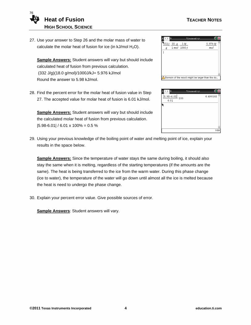
Heat of Fusion TEACHER NOTES
HIGH SCHOOL SCIENCE
©2011 Texas Instruments Incorporated 4 education.ti.com
27. Use your answer to Step 26 and the molar mass of water to
calculate the molar heat of fusion for ice (in kJ/mol H2O).
Sample Answers: Student answers will vary but should include
calculated heat of fusion from previous calculation.
(332 J/g)(18.0 g/mol)/1000J/kJ= 5.976 kJ/mol
Round the answer to 5.98 kJ/mol.
28. Find the percent error for the molar heat of fusion value in Step
27. The accepted value for molar heat of fusion is 6.01 kJ/mol.
Sample Answers: Student answers will vary but should include
the calculated molar heat of fusion from previous calculation.
|5.98-6.01| / 6.01 x 100% = 0.5 %
29. Using your previous knowledge of the boiling point of water and melting point of ice, explain your
results in the space below.
Sample Answers: Since the temperature of water stays the same during boiling, it should also
stay the same when it is melting, regardless of the starting temperatures (if the amounts are the
same). The heat is being transferred to the ice from the warm water. During this phase change
(ice to water), the temperature of the water will go down until almost all the ice is melted because
the heat is need to undergo the phase change.
30. Explain your percent error value. Give possible sources of error.
Sample Answers: Student answers will vary.
76
Heat of Fusion TEACHER NOTES
HIGH SCHOOL SCIENCE
©2011 Texas Instruments Incorporated 5 education.ti.com
Wrap Up Discuss with students possible sources of error in the experiment.
Assessment Formative assessment will consist of questions embedded in the .tns file.
TI-Nspire Navigator Note 1
Question 2, Feature: Quick Poll
Use TI-Nspire Navigator to send a Quick Poll with Question number 2. Engage students in discussion
around why different answers might make sense. Don’t mark correct answer at this point if using the
Slide Show to review responses with class.
Note 2
Feature: Quick Poll
Use TI-Nspire Navigator to send a quick poll with Question number 4. Engage students in discussion
around whether or not the differences between their predicted and actual results are significant.
Encourage them to share why they think the data supports or refutes their claims.
77

This page intentionally left blank
78
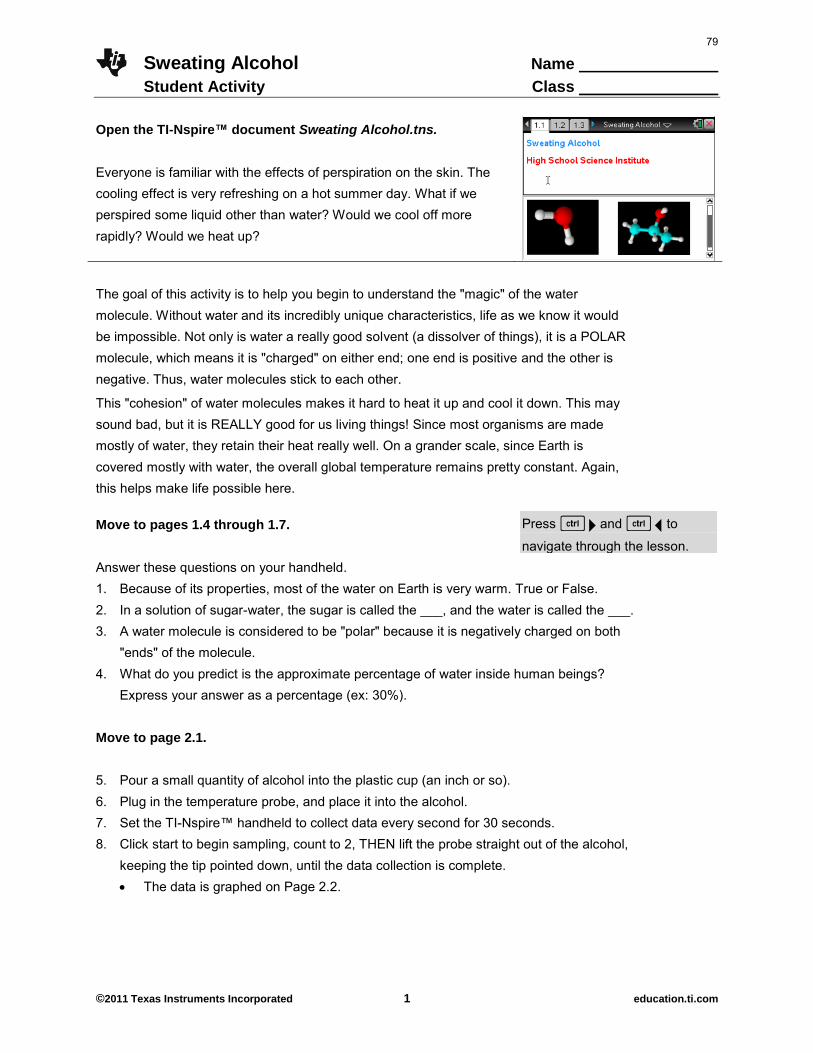
Sweating Alcohol Name Student Activity Class
©2011 Texas Instruments Incorporated 1 education.ti.com
Open the TI-Nspire™ document Sweating Alcohol.tns. Everyone is familiar with the effects of perspiration on the skin. The cooling effect is very refreshing on a hot summer day. What if we perspired some liquid other than water? Would we cool off more rapidly? Would we heat up?
The goal of this activity is to help you begin to understand the "magic" of the water molecule. Without water and its incredibly unique characteristics, life as we know it would be impossible. Not only is water a really good solvent (a dissolver of things), it is a POLAR molecule, which means it is "charged" on either end; one end is positive and the other is negative. Thus, water molecules stick to each other.
This "cohesion" of water molecules makes it hard to heat it up and cool it down. This may sound bad, but it is REALLY good for us living things! Since most organisms are made mostly of water, they retain their heat really well. On a grander scale, since Earth is covered mostly with water, the overall global temperature remains pretty constant. Again, this helps make life possible here.
Move to pages 1.4 through 1.7. Press / ¢ and / ¡ to
navigate through the lesson. Answer these questions on your handheld. 1. Because of its properties, most of the water on Earth is very warm. True or False. 2. In a solution of sugar-water, the sugar is called the ___, and the water is called the ___. 3. A water molecule is considered to be "polar" because it is negatively charged on both
"ends" of the molecule. 4. What do you predict is the approximate percentage of water inside human beings?
Express your answer as a percentage (ex: 30%).
Move to page 2.1.
5. Pour a small quantity of alcohol into the plastic cup (an inch or so). 6. Plug in the temperature probe, and place it into the alcohol. 7. Set the TI-Nspire™ handheld to collect data every second for 30 seconds. 8. Click start to begin sampling, count to 2, THEN lift the probe straight out of the alcohol,
keeping the tip pointed down, until the data collection is complete. The data is graphed on Page 2.2.
79
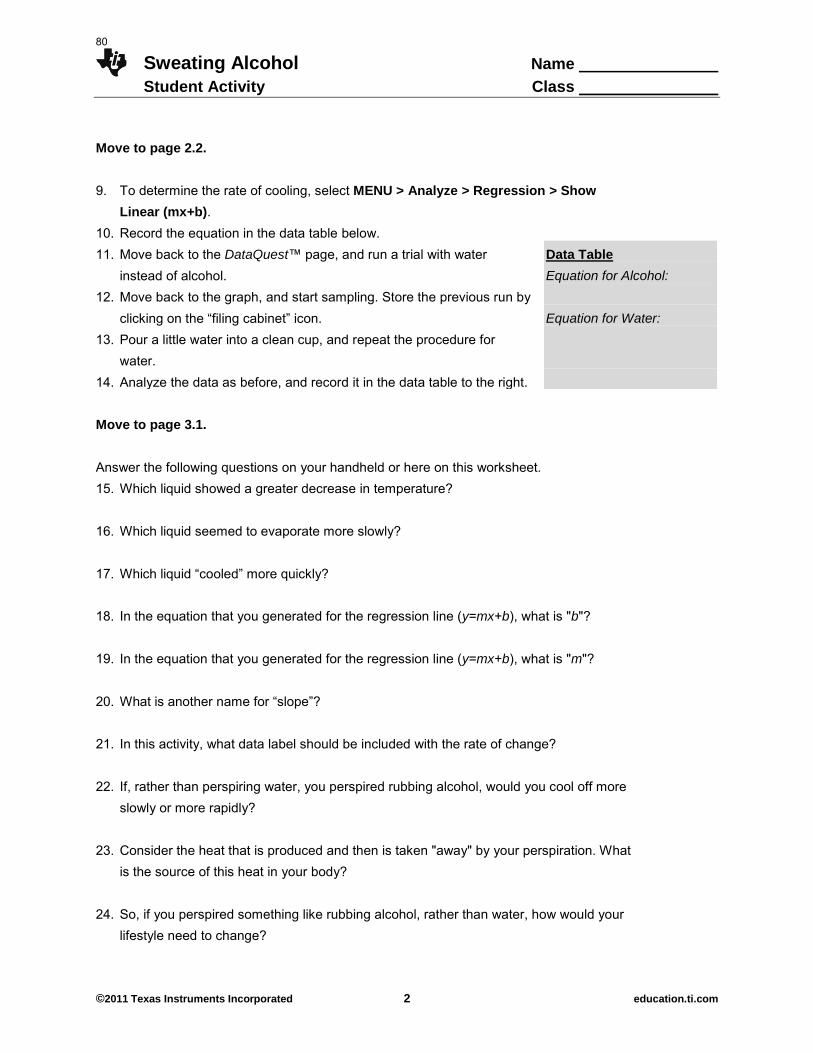
Sweating Alcohol Name Student Activity Class
©2011 Texas Instruments Incorporated 2 education.ti.com
Move to page 2.2.
9. To determine the rate of cooling, select MENU > Analyze > Regression > Show
Linear (mx+b). 10. Record the equation in the data table below. 11. Move back to the DataQuest™ page, and run a trial with water
instead of alcohol. 12. Move back to the graph, and start sampling. Store the previous run by
clicking on the “filing cabinet” icon. 13. Pour a little water into a clean cup, and repeat the procedure for
water. 14. Analyze the data as before, and record it in the data table to the right.
Data Table
Equation for Alcohol:
Equation for Water:
Move to page 3.1.
Answer the following questions on your handheld or here on this worksheet. 15. Which liquid showed a greater decrease in temperature? 16. Which liquid seemed to evaporate more slowly? 17. Which liquid “cooled” more quickly? 18. In the equation that you generated for the regression line (y=mx+b), what is "b"? 19. In the equation that you generated for the regression line (y=mx+b), what is "m"? 20. What is another name for “slope”? 21. In this activity, what data label should be included with the rate of change? 22. If, rather than perspiring water, you perspired rubbing alcohol, would you cool off more
slowly or more rapidly? 23. Consider the heat that is produced and then is taken "away" by your perspiration. What
is the source of this heat in your body? 24. So, if you perspired something like rubbing alcohol, rather than water, how would your
lifestyle need to change?
80

Sweating Alcohol Name Student Activity Class
©2011 Texas Instruments Incorporated 3 education.ti.com
25. Is water a polar or a nonpolar molecule? 26. Predict whether alcohol is a polar or a nonpolar molecule.
81

This page intentionally left blank
82
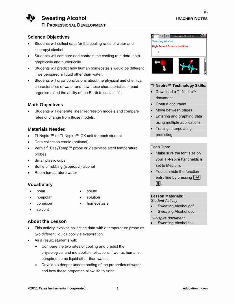
Sweating Alcohol TEACHER NOTES
TI PROFESSIONAL DEVELOPMENT
©2011 Texas Instruments Incorporated 1 education.ti.com
Science Objectives
Students will collect data for the cooling rates of water and isopropyl alcohol.
Students will compare and contrast the cooling rate data, both graphically and numerically.
Students will predict how human homeostasis would be different if we perspired a liquid other than water.
Students will draw conclusions about the physical and chemical characteristics of water and how those characteristics impact organisms and the ability of the Earth to sustain life.
Math Objectives
Students will generate linear regression models and compare rates of change from those models.
Materials Needed
TI-Nspire™ or TI-Nspire™ CX unit for each student Data collection cradle (optional) Vernier® EasyTemp™ probe or 2 stainless steel temperature
probes Small plastic cups Bottle of rubbing (isopropyl) alcohol Room temperature water
Vocabulary
polar solute nonpolar solution cohesion homeostasis solvent
About the Lesson
This activity involves collecting data with a temperature probe as two different liquids cool via evaporation.
As a result, students will: Compare the two rates of cooling and predict the
physiological and metabolic implications if we, as humans, perspired some liquid other than water.
Develop a deeper understanding of the properties of water and how those properties allow life to exist.
TI-Nspire™ Technology Skills: Download a TI-Nspire™
document Open a document Move between pages Entering and graphing data
using multiple applications Tracing, interpolating,
predicting
Tech Tips:
Make sure the font size on your TI-Nspire handhelds is set to Medium.
You can hide the function entry line by pressing / G.
Lesson Materials: Student Activity
Sweating Alcohol.pdf Sweating Alcohol.doc
TI-Nspire document
Sweating Alcohol.tns
83
Sweating Alcohol TEACHER NOTES
TI PROFESSIONAL DEVELOPMENT
©2011 Texas Instruments Incorporated 2 education.ti.com
TI-Nspire™ Navigator™ System
Screen Capture to monitor student progress. Live Presenter allows students to show their graphs to the class.
Discussion Points and Possible Answers
The goal of this activity is to help you begin to understand the "magic" of the water molecule. Without water and its incredibly unique characteristics, life as we know it would be impossible. Not only is water a really good solvent (a dissolver of things), it is a POLAR molecule, which means it is "charged" on either end; one end is positive and the other is negative. Thus, water molecules stick to each other.
This "cohesion" of water molecules makes it hard to heat it up and cool it down. This may sound bad, but it is REALLY good for us living things! Since most organisms are made mostly of water, they retain their heat really well. On a grander scale, since Earth is covered mostly with water, the overall global temperature remains pretty constant. Again, this helps make life possible here.
Move to pages 1.4 through 1.7.
Answer these questions on your handheld. 1. Because of its properties, most of the water on Earth is very warm. True or False.
Answer: False.
2. In a solution of sugar-water, the sugar is called the ___, and the water is called the ___.
Answer: B. solute; solvent
3. A water molecule is considered to be "polar" because it is negatively charged on both "ends" of the molecule.
Answer: Wrong.
4. What do you predict is the approximate percentage of water inside human beings?
Express your answer as a percentage (ex: 30%).
Answer: 60-65%.
84
Sweating Alcohol TEACHER NOTES
TI PROFESSIONAL DEVELOPMENT
©2011 Texas Instruments Incorporated 3 education.ti.com
Move to page 2.1.
5. Pour a small quantity of alcohol into the plastic cup (an inch or so). 6. Plug in the temperature probe, and place it into the alcohol. 7. Set the TI-Nspire handheld to collect data every second for 30 seconds. 8. Click start to begin sampling, count to 2, THEN lift the probe straight out of the alcohol,
keeping the tip pointed down, until the data collection is complete. The data is graphed on Page 2.2.
Move to page 2.2.
9. To determine the rate of cooling, select MENU > Analyze > Regression > Show
Linear (mx+b). 10. Record the equation in the data table below. 11. Move back to the DataQuest™ page, and run a trial with water
instead of alcohol. 12. Move back to the graph, and start sampling. Store the previous run by
clicking on the “filing cabinet” icon. 13. Pour a little water into a clean cup, and repeat the procedure for
water. 14. Analyze the data as before, and record it in the data table to the right.
Data Table
Equation for Alcohol:
Answer: Answers may vary Equation for Water:
Answer: Answers may vary
Move to page 3.1.
Answer the following questions on your handheld or here on this worksheet. 15. Which liquid showed a greater decrease in temperature?
Answer: Alcohol 16. Which liquid seemed to evaporate more slowly?
Answer: Water 17. Which liquid “cooled” more quickly?
Answer: Alcohol
85
Sweating Alcohol TEACHER NOTES
TI PROFESSIONAL DEVELOPMENT
©2011 Texas Instruments Incorporated 4 education.ti.com
18. In the equation that you generated for the regression line (y=mx+b), what is "b"?
Answer: The “y-intercept”, which is the temperature when the data collection started. 19. In the equation that you generated for the regression line (y=mx+b), what is "m"?
Answer: The rate of change (slope) in temperature in degrees per second. 20. What is another name for “slope”?
Answer: Rate of change. 21. In this activity, what data label should be included with the rate of change?
Answer: Degrees/second.
22. If, rather than perspiring water, you perspired rubbing alcohol, would you cool off more slowly or more rapidly?
Answer: More rapidly.
23. Consider the heat that is produced and then is taken "away" by your perspiration. What
is the source of this heat in your body?
Answer: Cell respiration. 24. So, if you perspired something like rubbing alcohol, rather than water, how would your
lifestyle need to change?
Answer: You’d need to eat more. 25. Is water a polar or a nonpolar molecule?
Answer: Polar.
86
Sweating Alcohol TEACHER NOTES
TI PROFESSIONAL DEVELOPMENT
©2011 Texas Instruments Incorporated 5 education.ti.com
26. Predict whether alcohol is a polar or a nonpolar molecule.
Answer: Nonpolar.
TI-Nspire Navigator Opportunity: Screen Capture
See Note 1 at the end of this lesson.
Assessment Formative assessment will consist of questions embedded in the TI-Nspire document. The questions will be graded when the document is retrieved. The Slide Show can be utilized to give students immediate feedback on their assessment. TI-Nspire Navigator
Note 1 Screen Capture
Screen Capture can be used to monitor student progress.
87

This page intentionally left blank
88
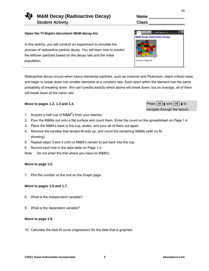
M&M Decay (Radioactive Decay) Name Student Activity Class
©2011 Texas Instruments Incorporated 1 education.ti.com
Open the TI-Nspire document MnM decay.tns In this activity, you will conduct an experiment to simulate the process of radioactive particle decay. You will learn how to predict the leftover particles based on the decay rate and the initial population.
Radioactive decay occurs when heavy elemental particles, such as Uranium and Plutonium, reach critical mass and begin to break down into smaller elements at a constant rate. Each atom within the element has the same probability of breaking down. We can’t predict exactly which atoms will break down, but on average, all of them will break down at the same rate. Move to pages 1.2, 1.3 and 1.4.
Press / ¢ and / ¡ to
navigate through the lesson. 1. Acquire a half cup of M&M®s from your teacher. 2. Pour the M&Ms out onto a flat surface and count them. Enter the count on the spreadsheet on Page 1.4. 3. Place the M&M’s back in the cup, shake, and pour all of them out again. 4. Remove the candies that landed M-side up, and count the remaining M&Ms (with no M
showing). 5. Repeat steps 3 and 4 until no M&M’s remain to put back into the cup. 6. Record each trial in the data table on Page 1.4. Note: Do not enter the trial where you have no M&M’s. Move to page 1.5.
7. Plot the number vs the trial on the Graph page. Move to pages 1.6 and 1.7.
8. What is the independent variable? 9. What is the dependent variable? Move to page 1.9.
10. Calculate the best fit curve (regression) for the data that is graphed.
89
M&M Decay (Radioactive Decay) Name Student Activity Class
©2011 Texas Instruments Incorporated 2 education.ti.com
Move to pages 1.10 through 1.14.
11. What equation did you get for your M&M decay? 12. In the general equation y=abx, a represents what?
13. In the general equation y=abx, x represents what?
14. In the general equation y=abx, y represents what?
15. In the general equation y=abx, b represents what?
90
M&M Decay (Radioactive Decay) TEACHER NOTES
TI PROFESSIONAL DEVELOPMENT
©2011 Texas Instruments Incorporated 1 education.ti.com
Science Objectives
Students will count the number of decaying particles (M&M’s). Students will graph the particles (M&M’s) vs the trials. Students will determine a decay curve and the variables that
affect the curve. Vocabulary
decay exponential population growth rate growth factor About the Lesson
This lesson involves the idea of exponential decay. As a result, students will:
Observe particles decaying ( in the form of M&M’s). Calculate a relationship between the time and the number of
M&M’s. Determine the exponential decay curve for their sample. Determine what each variable in the decay curve represents.
TI-Nspire™ Navigator™ System
Use the Quick Poll to send a list out to the students and gather the data from their trials.
Use Teacher Edition Computer Software to review student documents.
TI-Nspire™ Technology Skills: Download a TI-Nspire
document Open a document Move between pages Grab and drag a point
Tech Tips:
Make sure the font size on your TI-Nspire handhelds is set to Medium.
Lesson Files: Student Activity
MnM decay.pdf MnM decay.doc
TI-Nspire document
MnM decay.tns
91
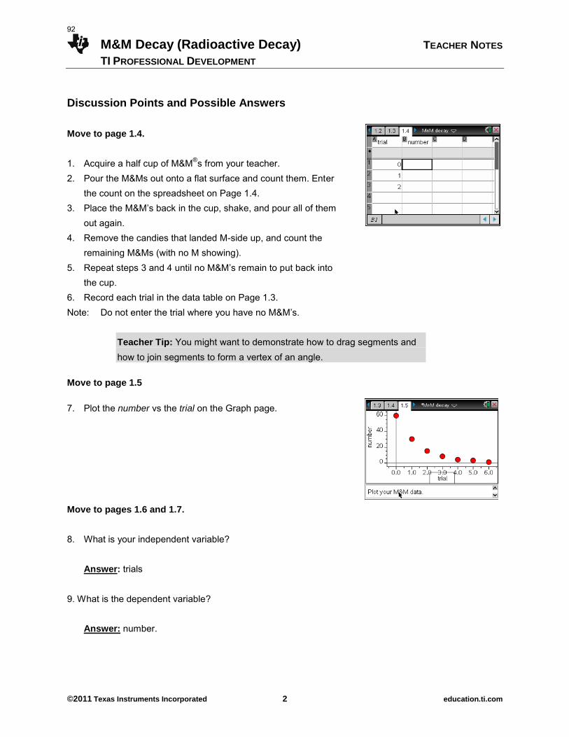
M&M Decay (Radioactive Decay) TEACHER NOTES
TI PROFESSIONAL DEVELOPMENT
©2011 Texas Instruments Incorporated 2 education.ti.com
Discussion Points and Possible Answers
Move to page 1.4.
1. Acquire a half cup of M&M®s from your teacher. 2. Pour the M&Ms out onto a flat surface and count them. Enter
the count on the spreadsheet on Page 1.4. 3. Place the M&M’s back in the cup, shake, and pour all of them
out again. 4. Remove the candies that landed M-side up, and count the
remaining M&Ms (with no M showing). 5. Repeat steps 3 and 4 until no M&M’s remain to put back into
the cup. 6. Record each trial in the data table on Page 1.3. Note: Do not enter the trial where you have no M&M’s.
Teacher Tip: You might want to demonstrate how to drag segments and how to join segments to form a vertex of an angle.
Move to page 1.5 7. Plot the number vs the trial on the Graph page.
Move to pages 1.6 and 1.7.
8. What is your independent variable?
Answer: trials
9. What is the dependent variable?
Answer: number.
92
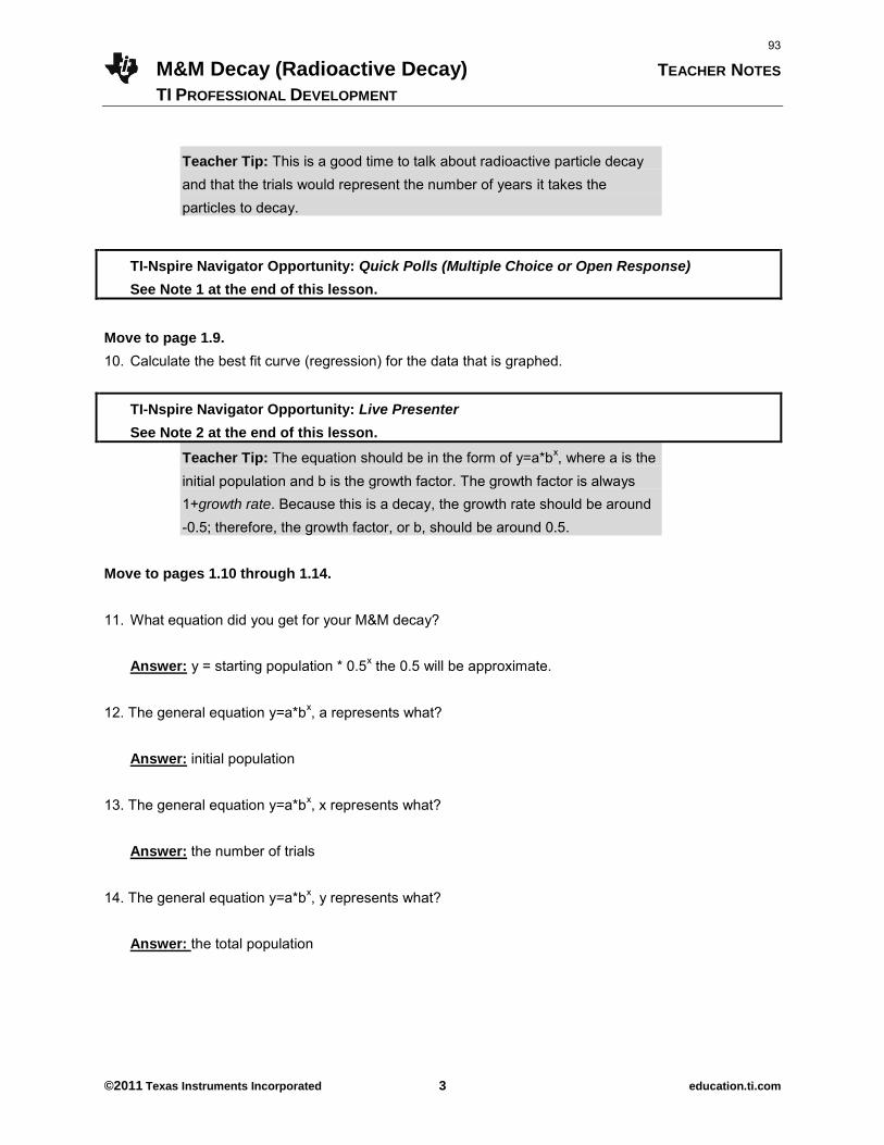
M&M Decay (Radioactive Decay) TEACHER NOTES
TI PROFESSIONAL DEVELOPMENT
©2011 Texas Instruments Incorporated 3 education.ti.com
Teacher Tip: This is a good time to talk about radioactive particle decay and that the trials would represent the number of years it takes the particles to decay.
TI-Nspire Navigator Opportunity: Quick Polls (Multiple Choice or Open Response)
See Note 1 at the end of this lesson.
Move to page 1.9.
10. Calculate the best fit curve (regression) for the data that is graphed.
TI-Nspire Navigator Opportunity: Live Presenter
See Note 2 at the end of this lesson. Teacher Tip: The equation should be in the form of y=a*bx, where a is the initial population and b is the growth factor. The growth factor is always 1+growth rate. Because this is a decay, the growth rate should be around -0.5; therefore, the growth factor, or b, should be around 0.5.
Move to pages 1.10 through 1.14.
11. What equation did you get for your M&M decay?
Answer: y = starting population * 0.5x the 0.5 will be approximate.
12. The general equation y=a*bx, a represents what?
Answer: initial population
13. The general equation y=a*bx, x represents what?
Answer: the number of trials
14. The general equation y=a*bx, y represents what?
Answer: the total population
93
M&M Decay (Radioactive Decay) TEACHER NOTES
TI PROFESSIONAL DEVELOPMENT
©2011 Texas Instruments Incorporated 4 education.ti.com
15. The general equation y=a*bx, b represents what?
Answer: the growth factor
Teacher Tip: Now that the students have established an understanding of a growth or decay curve, you can discuss the idea of initial moles or grams of radioactive materials and the decay of these materials over time.
Extension
Gather data on different radioactive isotopes and have students determine a rate curve for the decay of the radioactive particles based on the half-lives.
Wrap Up
Upon completion of the discussion, the teacher should ensure that students are able to understand: The equation for population decay in simplest form is y=abx.
They should understand that y represents the population at any time x, a is the initial population and b is the growth factor or 1+ the growth rate.
TI-Nspire Navigator Note 1
Question 9, Quick Polls (Multiple Choice or Open Response)
Draw a sketch of 4 different decay curves with different steepness of curve and the initial point crossing the y-axis marked. Ask the students:
1. What is the initial population for the first curve?
2. Which curve has the smallest growth factor?
3. Which graph decays the quickest?
4. Which graph has the greatest decay rate? Note 2
Question 10, Live Presenter Once students have generated a graph, it would be a good time to make one of the students Live Presenter to discuss with the class the meaning of the curve generated.
94
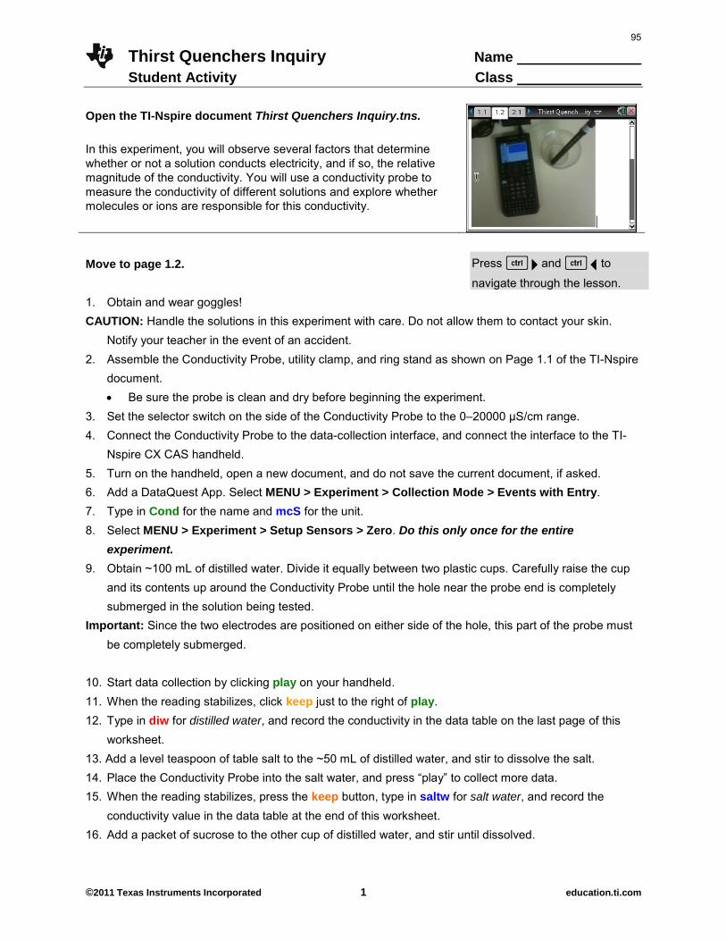
Thirst Quenchers Inquiry Name Student Activity Class
©2011 Texas Instruments Incorporated 1 education.ti.com
Open the TI-Nspire document Thirst Quenchers Inquiry.tns. In this experiment, you will observe several factors that determine whether or not a solution conducts electricity, and if so, the relative magnitude of the conductivity. You will use a conductivity probe to measure the conductivity of different solutions and explore whether molecules or ions are responsible for this conductivity.
Move to page 1.2. Press / ¢ and / ¡ to
navigate through the lesson. 1. Obtain and wear goggles! CAUTION: Handle the solutions in this experiment with care. Do not allow them to contact your skin.
Notify your teacher in the event of an accident. 2. Assemble the Conductivity Probe, utility clamp, and ring stand as shown on Page 1.1 of the TI-Nspire
document. Be sure the probe is clean and dry before beginning the experiment.
3. Set the selector switch on the side of the Conductivity Probe to the 0–20000 µS/cm range. 4. Connect the Conductivity Probe to the data-collection interface, and connect the interface to the TI-
Nspire CX CAS handheld. 5. Turn on the handheld, open a new document, and do not save the current document, if asked. 6. Add a DataQuest App. Select MENU > Experiment > Collection Mode > Events with Entry. 7. Type in Cond for the name and mcS for the unit. 8. Select MENU > Experiment > Setup Sensors > Zero. Do this only once for the entire
experiment.
9. Obtain ~100 mL of distilled water. Divide it equally between two plastic cups. Carefully raise the cup and its contents up around the Conductivity Probe until the hole near the probe end is completely submerged in the solution being tested.
Important: Since the two electrodes are positioned on either side of the hole, this part of the probe must be completely submerged.
10. Start data collection by clicking play on your handheld. 11. When the reading stabilizes, click keep just to the right of play. 12. Type in diw for distilled water, and record the conductivity in the data table on the last page of this
worksheet. 13. Add a level teaspoon of table salt to the ~50 mL of distilled water, and stir to dissolve the salt. 14. Place the Conductivity Probe into the salt water, and press ―play‖ to collect more data. 15. When the reading stabilizes, press the keep button, type in saltw for salt water, and record the
conductivity value in the data table at the end of this worksheet. 16. Add a packet of sucrose to the other cup of distilled water, and stir until dissolved.
95
Thirst Quenchers Inquiry Name Student Activity Class
©2011 Texas Instruments Incorporated 2 education.ti.com
17. Measure the conductivity as above for the salt water, type in sugw for sugar water, and record the conductivity value in the data table.
18. Repeat the data collection using ~50 mL of tap water, and type in tapw for tap water. 19. Stop data collection by clicking stop. 20. Click on the Table View tab ( ) to view a table of the conductivity values you collected. Record
these values in your data table. 21. Press / ~ to insert a Data & Statistics page. 22. Move the cursor to the x-axis, press / b, and select Add X Variable with Summary Variable.
23. Tab to OK from the Summary Chart Dialog Box. 24. Move the cursor to the first bar for distilled water. Press /, and select MENU > Color > Fill Color,
and choose a color for the distilled water bar. 25. Repeat for the salt water solution and the sucrose solution, choosing a different color for each one. 26. Compare and contrast the conductivity values for each. It is now time to think about a researchable question to investigate. You have various substances to test. Read the discussion below before moving to procedure 15. Discussion: So far in this activity, you have learned some properties of strong electrolytes, weak electrolytes, and non-electrolytes by observing the behavior of these substances in aqueous solutions using a Conductivity Probe. When the probe was placed in a solution that contains ions, and thus has the ability to conduct electricity, an electrical circuit is completed across the electrodes that are located on either side of the hole near the bottom of the probe body. This results in a conductivity value that can be read by a data-collection interface. The unit of conductivity used in this experiment is the microsiemens per centimeter, or µS/cm. The size of the conductivity value depends on the ability of the aqueous solution to conduct electricity. Strong electrolytes produce large numbers of ions, which results in high conductivity values. Weak electrolytes result in low conductivity, and non-electrolytes should result in no conductivity.
96
Thirst Quenchers Inquiry Name Student Activity Class
©2011 Texas Instruments Incorporated 3 education.ti.com
In each part of the experiment, you are observing a different property of electrolytes. Keep in mind that you will be encountering three types of compounds and aqueous solutions:
1—Ionic Compounds
These are usually strong electrolytes and can be expected to 100% dissociate in aqueous solution. Example: NaCl(s) Na
+(aq) + Cl
–(aq)
2—Molecular Compounds
These are usually non-electrolytes. They do not dissociate to form ions. Resulting solutions do not conduct electricity. Example: C12H22O11(l) C12H22O11(aq)
3—Molecular Acids
These are molecules that can partially or wholly dissociate, depending on their strength. Example: Strong electrolyte H2SO4 H
+(aq) + HSO4
–(aq) (100% dissociation)
Example: Weak electrolyte H3PO4 H+(aq) + H2PO4
–(aq) (<100% dissociation)
27. Now that you have read about electrolytes and nonelectrolytes, discuss with your partner an area that you would like to investigate regarding common soft drinks. Read the labels of the substances (both solutions and solids) provided to gather more
information for your researchable question. Write up a hypothesis, and be prepared to share it with the group. Also, determine what materials and procedures that you plan to follow. Do not begin your experiment until after the group discussion of researchable questions!
28. Once the researchable question has been approved by the group, you will be given time to do complete your research, graph your data, and prepare a report to the group. Your report will include:
a) your original hypothesis
b) pertinent data (Data table in DataQuest)
c) a graph (Data and Statistics page)
d) the conclusion to be drawn from your research—was your hypothesis borne out?
e) suggestion(s) for further research
97
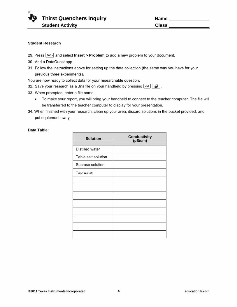
Thirst Quenchers Inquiry Name Student Activity Class
©2011 Texas Instruments Incorporated 4 education.ti.com
Student Research
29. Press ~ and select Insert > Problem to add a new problem to your document.
30. Add a DataQuest app. 31. Follow the instructions above for setting up the data collection (the same way you have for your
previous three experiments). You are now ready to collect data for your researchable question. 32. Save your research as a .tns file on your handheld by pressing / ».
33. When prompted, enter a file name. To make your report, you will bring your handheld to connect to the teacher computer. The file will
be transferred to the teacher computer to display for your presentation. 34. When finished with your research, clean up your area, discard solutions in the bucket provided, and
put equipment away. Data Table:
Solution Conductivity
(µS/cm)
Distilled water
Table salt solution
Sucrose solution
Tap water
98
Thirst Quenchers Inquiry TEACHER NOTES
TI PROFESSIONAL DEVELOPMENT
©2011 Texas Instruments Incorporated 1 education.ti.com
Science Objectives:
Students will write equations for the dissociation of compounds in water.
Students will use a Conductivity Probe to measure the conductivity of solutions.
Students will determine which molecules or ions are responsible for conductivity of solutions.
Students will investigate the conductivity of common drinks resulting from substituent compounds that dissociate to produce different numbers of ions.
Vocabulary
conductivity electrolyte nonelectrolyte molecular acid molecular compound ionic compound molecule ion About the Lesson
This lesson involves testing the conductivity of common solutions. As a result, students will:
Perform the preliminary activity, and then generate a researchable question of their own.
Plan their research, carry out the research plan, organize and graph the data, draw a conclusion, and communicate the results.
TI-Nspire™ Navigator™ System
Observe student progress by using Screen Captures during student experimentation.
Make students the Live Presenter when they are ready to make their research reports.
TI-Nspire™ Technology Skills: Download a TI-Nspire
document Open a document Move between pages Collect data using Vernier
Data Quest Open a Data and Statistics
Page
Create a colored bar graph of data
Tech Tips:
Make sure the font size on your TI-Nspire handhelds is set to Medium.
Lesson Files: Student Activity
Thirst Quenchers Inquiry.pdf Thirst Quenchers.doc
99
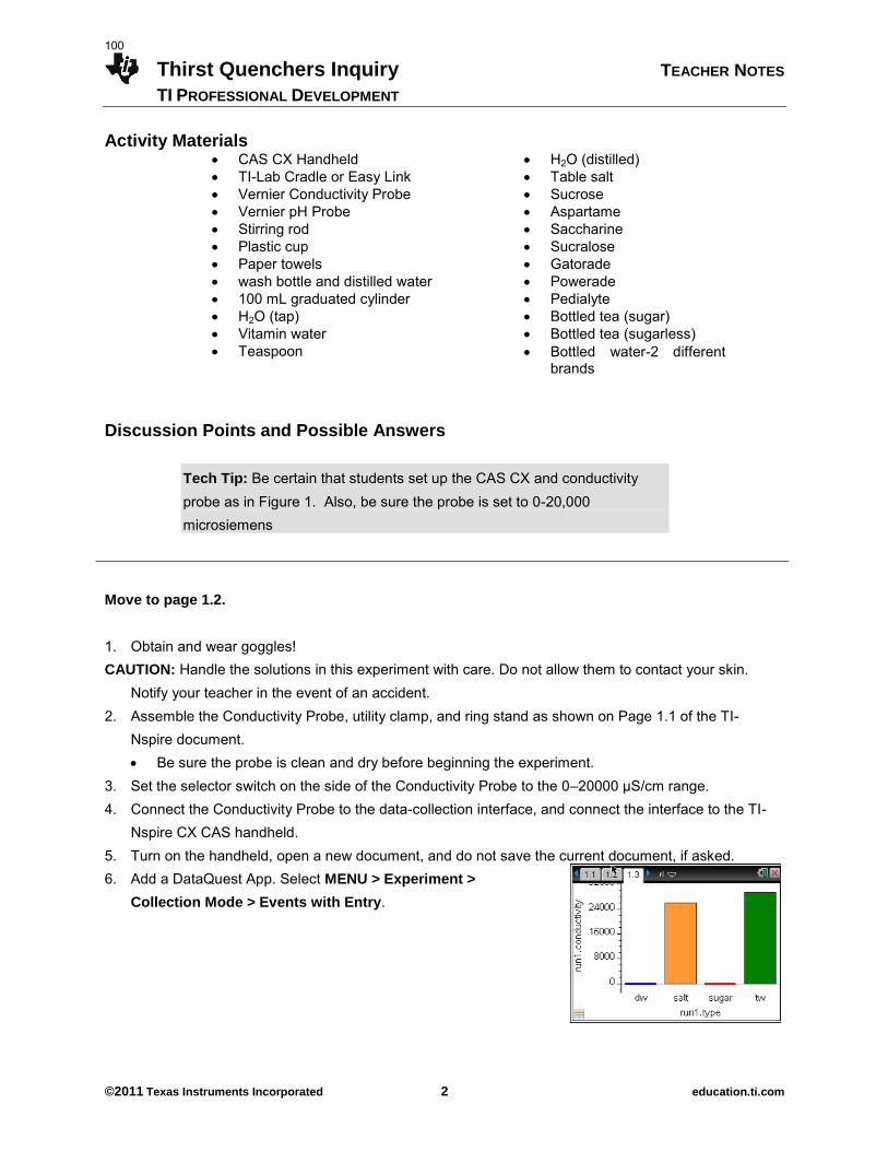
Thirst Quenchers Inquiry TEACHER NOTES
TI PROFESSIONAL DEVELOPMENT
©2011 Texas Instruments Incorporated 2 education.ti.com
Discussion Points and Possible Answers
Tech Tip: Be certain that students set up the CAS CX and conductivity probe as in Figure 1. Also, be sure the probe is set to 0-20,000 microsiemens
Move to page 1.2. 1. Obtain and wear goggles! CAUTION: Handle the solutions in this experiment with care. Do not allow them to contact your skin.
Notify your teacher in the event of an accident. 2. Assemble the Conductivity Probe, utility clamp, and ring stand as shown on Page 1.1 of the TI-
Nspire document. Be sure the probe is clean and dry before beginning the experiment.
3. Set the selector switch on the side of the Conductivity Probe to the 0–20000 µS/cm range. 4. Connect the Conductivity Probe to the data-collection interface, and connect the interface to the TI-
Nspire CX CAS handheld. 5. Turn on the handheld, open a new document, and do not save the current document, if asked. 6. Add a DataQuest App. Select MENU > Experiment >
Collection Mode > Events with Entry.
Activity Materials CAS CX Handheld H2O (distilled) TI-Lab Cradle or Easy Link Table salt Vernier Conductivity Probe Sucrose Vernier pH Probe Aspartame Stirring rod Saccharine Plastic cup Sucralose Paper towels Gatorade wash bottle and distilled water Powerade 100 mL graduated cylinder Pedialyte H2O (tap) Bottled tea (sugar) Vitamin water Bottled tea (sugarless) Teaspoon Bottled water-2 different
brands
100
Thirst Quenchers Inquiry TEACHER NOTES
TI PROFESSIONAL DEVELOPMENT
©2011 Texas Instruments Incorporated 3 education.ti.com
7. Type in Cond for the name and mcS for the unit. 8. Select MENU > Experiment > Setup Sensors > Zero. Do this only once for the entire
experiment.
9. Obtain ~100 mL of distilled water. Divide it equally between two plastic cups. Carefully raise the cup and its contents up around the Conductivity Probe until the hole near the probe end is completely submerged in the solution being tested.
Important: Since the two electrodes are positioned on either side of the hole, this part of the probe must be completely submerged.
10. Start data collection by clicking play on your handheld. 11. When the reading stabilizes, click keep just to the right of play. 12. Type in diw for distilled water, and record the conductivity in the data table on the last page of this
worksheet. 13. Add a level teaspoon of table salt to the ~50 mL of distilled water, and stir to dissolve the salt. 14. Place the Conductivity Probe into the salt water, and press ―play‖ to collect more data. 15. When the reading stabilizes, press the keep button, type in saltw for salt water, and record the
conductivity value in the data table at the end of this worksheet. 16. Add a packet of sucrose to the other cup of distilled water, and stir until dissolved.
TI-Nspire Navigator Opportunity: Screen Capture
See Note 1 at the end of this lesson.
17. Measure the conductivity as above for the salt water, type in sugw for sugar water, and record the
conductivity value in the data table. 18. Repeat the data collection using ~50 mL of tap water, and type in tapw for tap water. 19. Stop data collection by clicking stop. 20. Click on the Table View tab ( ) to view a table of the conductivity values you collected. Record
these values in your data table. 21. Press / ~ to insert a Data & Statistics page. 22. Move the cursor to the x-axis, press / b, and select Add X Variable with Summary
Variable. 23. Tab to OK from the Summary Chart Dialog Box. 24. Move the cursor to the first bar for distilled water. Press /, and select MENU > Color > Fill
Color, and choose a color for the distilled water bar. 25. Repeat for the salt water solution and the sucrose solution, choosing a different color for each one. 26. Compare and contrast the conductivity values for each. It is now time to think about a researchable question to investigate. You have various substances to test. Read the discussion below before moving to procedure 15.
101
Thirst Quenchers Inquiry TEACHER NOTES
TI PROFESSIONAL DEVELOPMENT
©2011 Texas Instruments Incorporated 4 education.ti.com
27. Now that you have read about electrolytes and nonelectrolytes, discuss with your partner an area that you would like to investigate regarding common soft drinks. Read the labels of the substances (both solutions and solids) provided to gather more
information for your researchable question. Write up a hypothesis, and be prepared to share it with the group. Also, determine what materials and procedures that you plan to follow. Do not begin your experiment until after the group discussion of researchable questions!
Teacher Tip: You will need to record the researchable question for each group and decide whether the researchable question is appropriate and safe.
28. Once the researchable question has been approved by the group, you will be given time to do complete your research, graph your data, and prepare a report to the group. Your report will include:
a) your original hypothesis
b) pertinent data (Data table in DataQuest)
c) a graph (Data and Statistics page)
d) the conclusion to be drawn from your research—was your hypothesis borne out?
e) suggestion(s) for further research
Student Research
29. Press ~ and select Insert > Problem to add a new problem to your document.
30. Add a DataQuest app. 31. Follow the instructions above for setting up the data collection (the same way you have for your
previous three experiments). You are now ready to collect data for your researchable question. 32. Save your research as a .tns file on your handheld by pressing / ».
33. When prompted, enter a file name. To make your report, you will bring your handheld to connect to the teacher computer. The file
will be transferred to the teacher computer to display for your presentation. 34. When finished with your research, clean up your area, discard solutions in the bucket provided, and
put equipment away.
102
Thirst Quenchers Inquiry TEACHER NOTES
TI PROFESSIONAL DEVELOPMENT
©2011 Texas Instruments Incorporated 5 education.ti.com
Wrap Up
Upon completion of the discussion, the teacher should ensure that students are able to understand: How to connect the Lab Cradle™ to the TI-Nspire CX CAS handheld. How to connect a probe to the to Lab Cradle. How to gather and analyze data. How to make a colored bar graph.
Assessment The teacher will assess the students from their report to the class on their research. The student will save the TNS file and the teacher will collect it at the end of the activity for further assessment. TI-Nspire Navigator
Note 1 Screen Capture
Observe student progress throughout the activity by using Screen Capture.
103

This page intentionally left blank
104
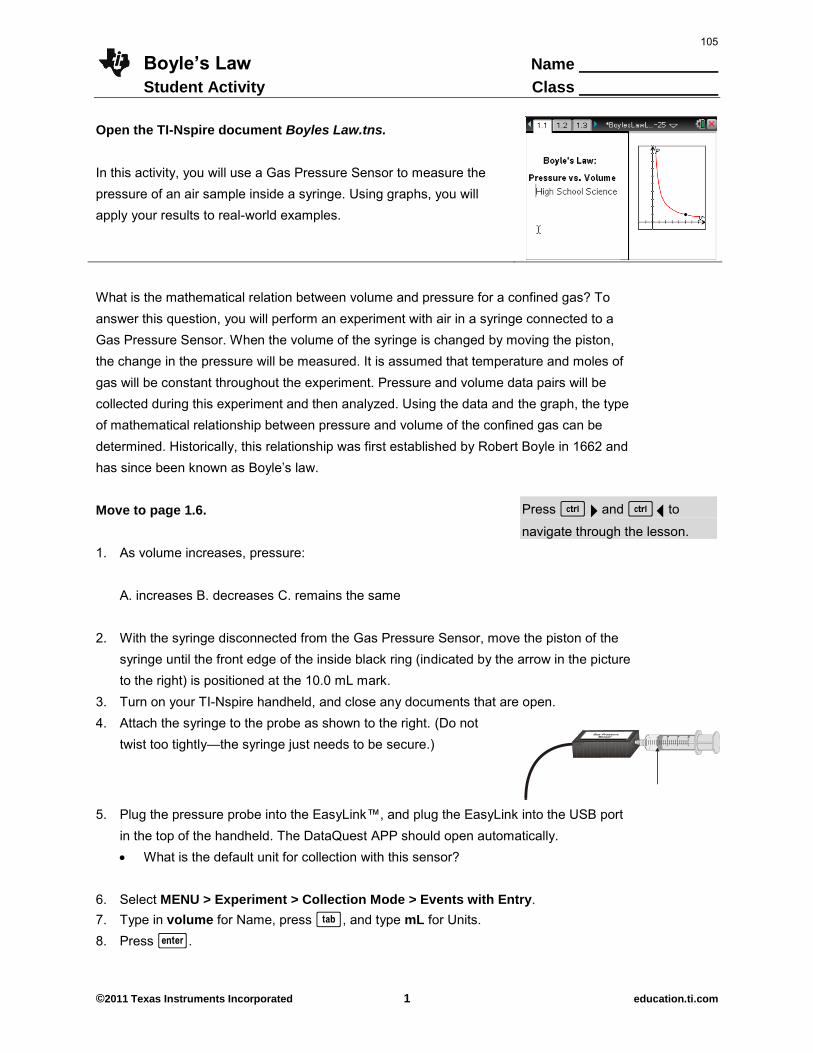
Boyle’s Law Name Student Activity Class
©2011 Texas Instruments Incorporated 1 education.ti.com
Open the TI-Nspire document Boyles Law.tns. In this activity, you will use a Gas Pressure Sensor to measure the pressure of an air sample inside a syringe. Using graphs, you will apply your results to real-world examples.
What is the mathematical relation between volume and pressure for a confined gas? To answer this question, you will perform an experiment with air in a syringe connected to a Gas Pressure Sensor. When the volume of the syringe is changed by moving the piston, the change in the pressure will be measured. It is assumed that temperature and moles of gas will be constant throughout the experiment. Pressure and volume data pairs will be collected during this experiment and then analyzed. Using the data and the graph, the type of mathematical relationship between pressure and volume of the confined gas can be determined. Historically, this relationship was first established by Robert Boyle in 1662 and has since been known as Boyle’s law. Move to page 1.6.
Press / ¢ and / ¡ to
navigate through the lesson. 1. As volume increases, pressure: A. increases B. decreases C. remains the same 2. With the syringe disconnected from the Gas Pressure Sensor, move the piston of the
syringe until the front edge of the inside black ring (indicated by the arrow in the picture to the right) is positioned at the 10.0 mL mark.
3. Turn on your TI-Nspire handheld, and close any documents that are open. 4. Attach the syringe to the probe as shown to the right. (Do not
twist too tightly—the syringe just needs to be secure.)
5. Plug the pressure probe into the EasyLink™, and plug the EasyLink into the USB port
in the top of the handheld. The DataQuest APP should open automatically. What is the default unit for collection with this sensor?
6. Select MENU > Experiment > Collection Mode > Events with Entry. 7. Type in volume for Name, press e, and type mL for Units. 8. Press ·.
105
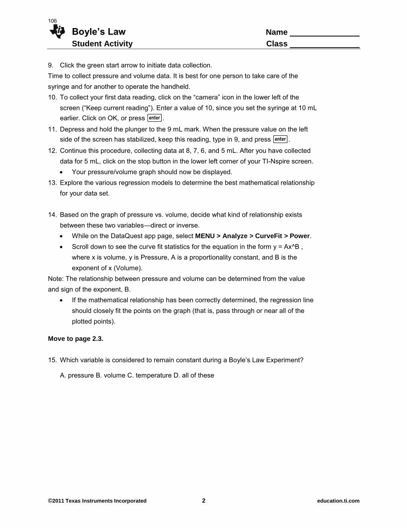
Boyle’s Law Name Student Activity Class
©2011 Texas Instruments Incorporated 2 education.ti.com
9. Click the green start arrow to initiate data collection. Time to collect pressure and volume data. It is best for one person to take care of the syringe and for another to operate the handheld. 10. To collect your first data reading, click on the “camera” icon in the lower left of the
screen (“Keep current reading”). Enter a value of 10, since you set the syringe at 10 mL
earlier. Click on OK, or press ·.
11. Depress and hold the plunger to the 9 mL mark. When the pressure value on the left side of the screen has stabilized, keep this reading, type in 9, and press ·.
12. Continue this procedure, collecting data at 8, 7, 6, and 5 mL. After you have collected data for 5 mL, click on the stop button in the lower left corner of your TI-Nspire screen. Your pressure/volume graph should now be displayed.
13. Explore the various regression models to determine the best mathematical relationship for your data set.
14. Based on the graph of pressure vs. volume, decide what kind of relationship exists
between these two variables—direct or inverse. While on the DataQuest app page, select MENU > Analyze > CurveFit > Power. Scroll down to see the curve fit statistics for the equation in the form y = Ax^B ,
where x is volume, y is Pressure, A is a proportionality constant, and B is the exponent of x (Volume).
Note: The relationship between pressure and volume can be determined from the value and sign of the exponent, B.
If the mathematical relationship has been correctly determined, the regression line should closely fit the points on the graph (that is, pass through or near all of the plotted points).
Move to page 2.3. 15. Which variable is considered to remain constant during a Boyle’s Law Experiment? A. pressure B. volume C. temperature D. all of these
106
Boyle’s Law Name Student Activity Class
©2011 Texas Instruments Incorporated 3 education.ti.com
16. To linearize the data and confirm that an inverse relationship exists between pressure and volume, plot a graph of pressure vs. reciprocal of volume (1/Volume) in DataQuest: Select MENU > Data > New Calculated Column. Type InverseV for Name. Short Name: 1/V Units: 1/mL Expression: 1/Volume Click OK, or press ·.
Select MENU > Graph > Select X-axis > InverseV.
17. Calculate the regression line y = mx + b where x is 1/volume, y is pressure, m is a proportionality constant, and b is the y-intercept. On the DataQuest page, select MENU
> Analyze > Curve Fit > Linear. Move to page 3.2. 18. If the volume is doubled from 5 to 10 mL, what does the data show happens to the
pressure? A. increases B. decreases C. doubles D. cut in half 19. If the volume is halved from 20 to 10 mL, what does the data show happens to the
pressure? A. increases B. decreases C. doubles D. cut in half 20. Based on the data, what would be expected to happen to the pressure if the volume in
the syringe were increased from 10 to 40 mL? A. increase B. decrease C. quadruple D. cut to 1/4th 21. From the answers to the above three questions and from the shape of the curve of the
plot, of pressure vs. volume, what is the relationship between the pressure and volume of a confined gas?
A. inverse B. direct C. quadratic D. impossible to determine
107
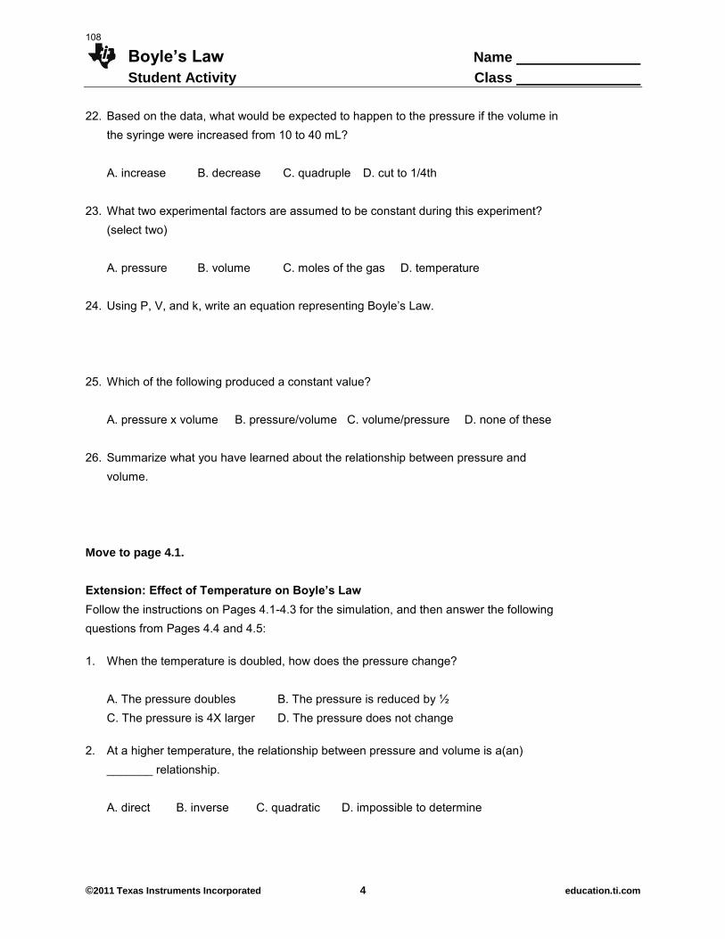
Boyle’s Law Name Student Activity Class
©2011 Texas Instruments Incorporated 4 education.ti.com
22. Based on the data, what would be expected to happen to the pressure if the volume in the syringe were increased from 10 to 40 mL?
A. increase B. decrease C. quadruple D. cut to 1/4th 23. What two experimental factors are assumed to be constant during this experiment?
(select two) A. pressure B. volume C. moles of the gas D. temperature 24. Using P, V, and k, write an equation representing Boyle’s Law. 25. Which of the following produced a constant value? A. pressure x volume B. pressure/volume C. volume/pressure D. none of these 26. Summarize what you have learned about the relationship between pressure and
volume. Move to page 4.1. Extension: Effect of Temperature on Boyle’s Law
Follow the instructions on Pages 4.1-4.3 for the simulation, and then answer the following questions from Pages 4.4 and 4.5: 1. When the temperature is doubled, how does the pressure change? A. The pressure doubles B. The pressure is reduced by ½
C. The pressure is 4X larger D. The pressure does not change 2. At a higher temperature, the relationship between pressure and volume is a(an)
_______ relationship. A. direct B. inverse C. quadratic D. impossible to determine
108
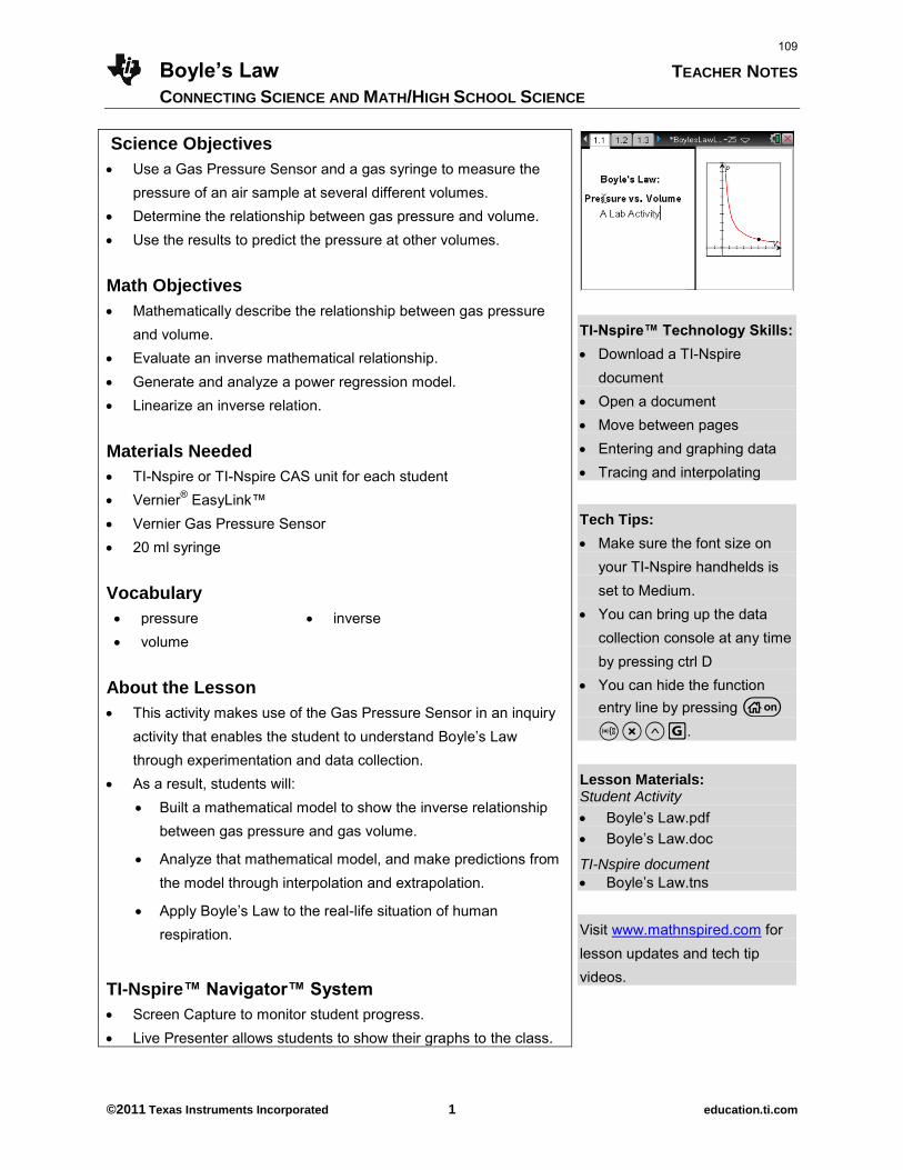
Boyle’s Law TEACHER NOTES
CONNECTING SCIENCE AND MATH/HIGH SCHOOL SCIENCE
©2011 Texas Instruments Incorporated 1 education.ti.com
Science Objectives
Use a Gas Pressure Sensor and a gas syringe to measure the pressure of an air sample at several different volumes.
Determine the relationship between gas pressure and volume. Use the results to predict the pressure at other volumes.
Math Objectives
Mathematically describe the relationship between gas pressure and volume.
Evaluate an inverse mathematical relationship. Generate and analyze a power regression model. Linearize an inverse relation. Materials Needed
TI-Nspire or TI-Nspire CAS unit for each student Vernier® EasyLink™ Vernier Gas Pressure Sensor 20 ml syringe
Vocabulary
pressure inverse volume
About the Lesson
This activity makes use of the Gas Pressure Sensor in an inquiry activity that enables the student to understand Boyle’s Law
through experimentation and data collection. As a result, students will:
Built a mathematical model to show the inverse relationship between gas pressure and gas volume.
Analyze that mathematical model, and make predictions from the model through interpolation and extrapolation.
Apply Boyle’s Law to the real-life situation of human respiration.
TI-Nspire™ Navigator™ System
Screen Capture to monitor student progress. Live Presenter allows students to show their graphs to the class.
TI-Nspire™ Technology Skills: Download a TI-Nspire
document Open a document Move between pages Entering and graphing data Tracing and interpolating
Tech Tips:
Make sure the font size on your TI-Nspire handhelds is set to Medium.
You can bring up the data collection console at any time by pressing ctrl D
You can hide the function entry line by pressing c t r l G.
Lesson Materials: Student Activity
Boyle’s Law.pdf
Boyle’s Law.doc
TI-Nspire document
Boyle’s Law.tns
Visit www.mathnspired.com for lesson updates and tech tip videos.
109
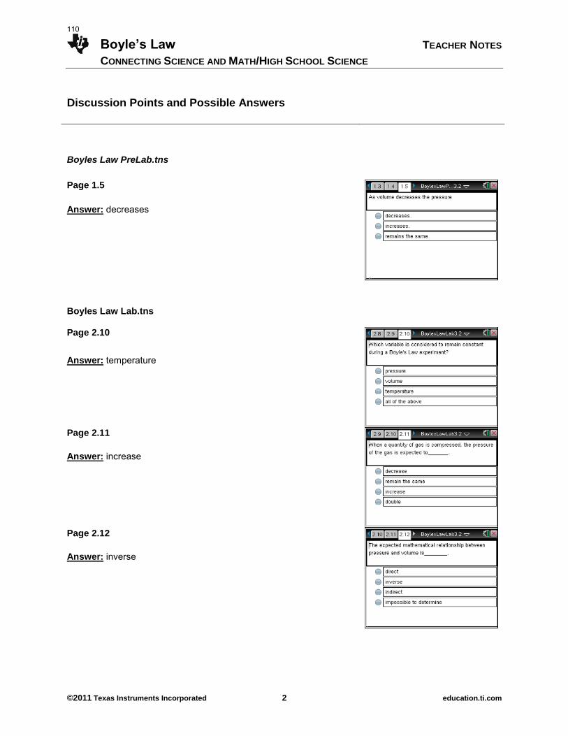
Boyle’s Law TEACHER NOTES
CONNECTING SCIENCE AND MATH/HIGH SCHOOL SCIENCE
©2011 Texas Instruments Incorporated 2 education.ti.com
Discussion Points and Possible Answers
Boyles Law PreLab.tns
Page 1.5
Answer: decreases
Boyles Law Lab.tns
Page 2.10
Answer: temperature
Page 2.11
Answer: increase
Page 2.12
Answer: inverse
110
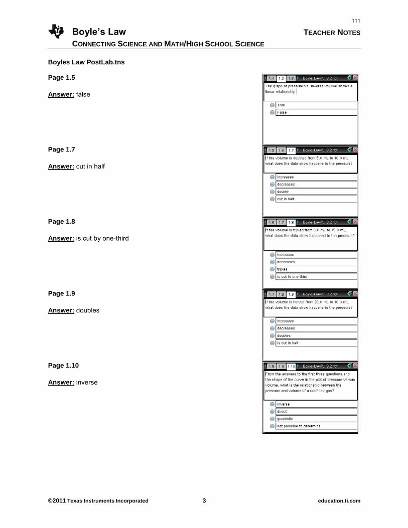
Boyle’s Law TEACHER NOTES
CONNECTING SCIENCE AND MATH/HIGH SCHOOL SCIENCE
©2011 Texas Instruments Incorporated 3 education.ti.com
Boyles Law PostLab.tns
Page 1.5
Answer: false
Page 1.7
Answer: cut in half
Page 1.8
Answer: is cut by one-third
Page 1.9
Answer: doubles
Page 1.10
Answer: inverse
111
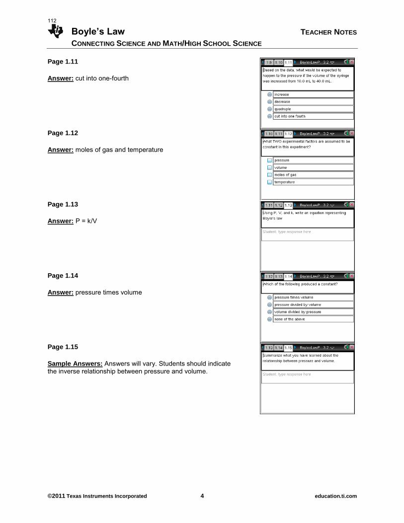
Boyle’s Law TEACHER NOTES
CONNECTING SCIENCE AND MATH/HIGH SCHOOL SCIENCE
©2011 Texas Instruments Incorporated 4 education.ti.com
Page 1.11
Answer: cut into one-fourth
Page 1.12
Answer: moles of gas and temperature
Page 1.13
Answer: P = k/V
Page 1.14
Answer: pressure times volume
Page 1.15
Sample Answers: Answers will vary. Students should indicate the inverse relationship between pressure and volume.
112
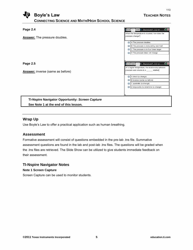
Boyle’s Law TEACHER NOTES
CONNECTING SCIENCE AND MATH/HIGH SCHOOL SCIENCE
©2011 Texas Instruments Incorporated 5 education.ti.com
Page 2.4
Answer: The pressure doubles.
Page 2.5
Answer: inverse (same as before)
TI-Nspire Navigator Opportunity: Screen Capture
See Note 1 at the end of this lesson.
Wrap Up
Use Boyle’s Law to offer a practical application such as human breathing. Assessment Formative assessment will consist of questions embedded in the pre-lab .tns file. Summative assessment questions are found in the lab and post-lab .tns files. The questions will be graded when the .tns files are retrieved. The Slide Show can be utilized to give students immediate feedback on their assessment.
TI-Nspire Navigator Notes Note 1 Screen Capture
Screen Capture can be used to monitor students.
113

This page intentionally left blank
114
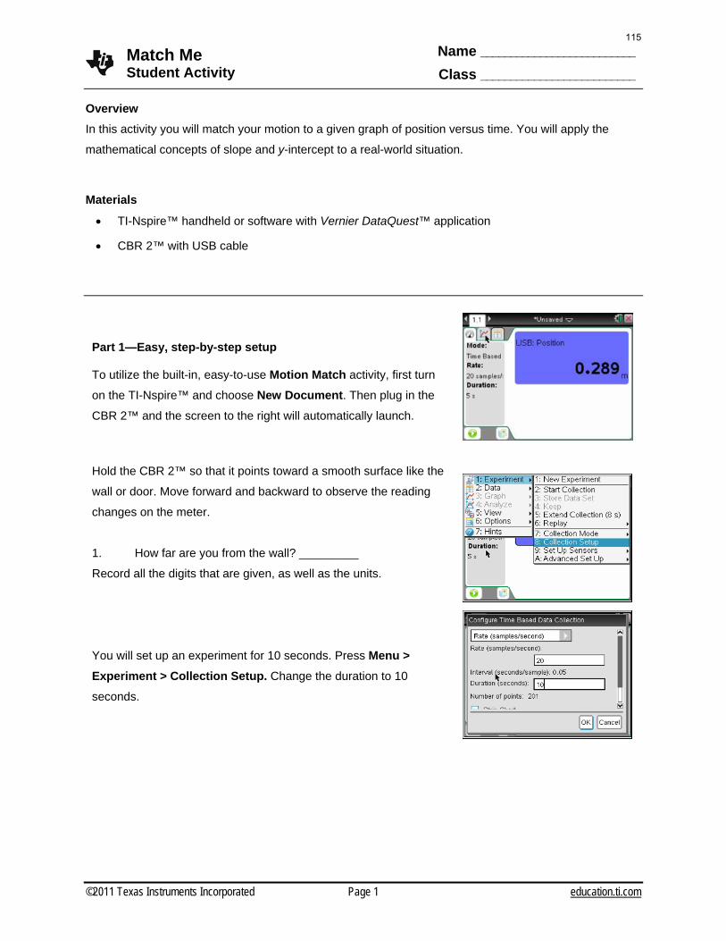
Match Me Student Activity
Name __________________________
Class __________________________
©2011 Texas Instruments Incorporated Page 1 education.ti.com
Overview
In this activity you will match your motion to a given graph of position versus time. You will apply the
mathematical concepts of slope and y-intercept to a real-world situation.
Materials
TI-Nspire™ handheld or software with Vernier DataQuest™ application
CBR 2™ with USB cable
Part 1—Easy, step-by-step setup
To utilize the built-in, easy-to-use Motion Match activity, first turn
on the TI-Nspire™ and choose New Document. Then plug in the
CBR 2™ and the screen to the right will automatically launch.
Hold the CBR 2™ so that it points toward a smooth surface like the
wall or door. Move forward and backward to observe the reading
changes on the meter.
1. How far are you from the wall? _________
Record all the digits that are given, as well as the units.
You will set up an experiment for 10 seconds. Press Menu >
Experiment > Collection Setup. Change the duration to 10
seconds.
115
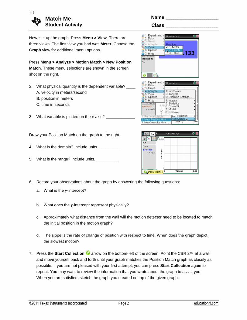
Match Me Student Activity
Name __________________________
Class __________________________
©2011 Texas Instruments Incorporated Page 2 education.ti.com
Now, set up the graph. Press Menu > View. There are
three views. The first view you had was Meter. Choose the
Graph view for additional menu options.
Press Menu > Analyze > Motion Match > New Position
Match. These menu selections are shown in the screen
shot on the right.
2. What physical quantity is the dependent variable? ____
A. velocity in meters/second
B. position in meters
C. time in seconds
3. What variable is plotted on the x-axis? _____________
Draw your Position Match on the graph to the right.
4. What is the domain? Include units. _________
5. What is the range? Include units. __________
6. Record your observations about the graph by answering the following questions:
a. What is the y-intercept?
b. What does the y-intercept represent physically?
c. Approximately what distance from the wall will the motion detector need to be located to match
the initial position in the motion graph?
d. The slope is the rate of change of position with respect to time. When does the graph depict
the slowest motion?
7. Press the Start Collection arrow on the bottom-left of the screen. Point the CBR 2™ at a wall
and move yourself back and forth until your graph matches the Position Match graph as closely as
possible. If you are not pleased with your first attempt, you can press Start Collection again to
repeat. You may want to review the information that you wrote about the graph to assist you.
When you are satisfied, sketch the graph you created on top of the given graph.
116
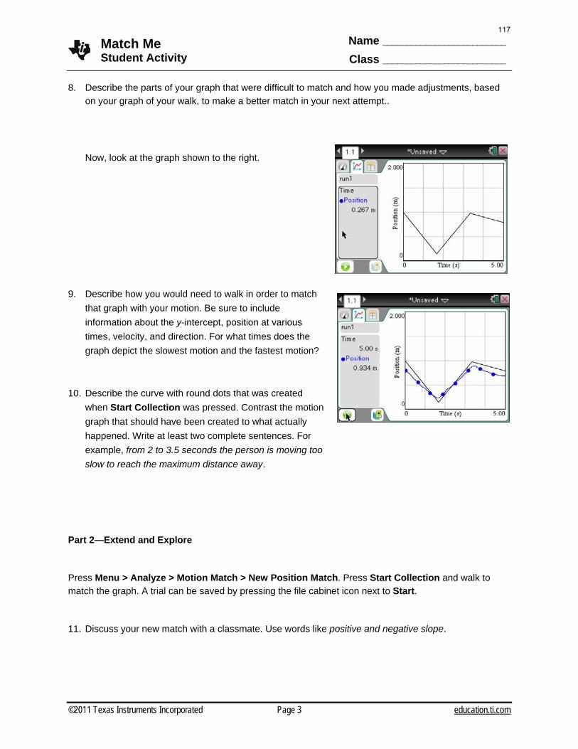
Match Me Student Activity
Name __________________________
Class __________________________
©2011 Texas Instruments Incorporated Page 3 education.ti.com
8. Describe the parts of your graph that were difficult to match and how you made adjustments, based
on your graph of your walk, to make a better match in your next attempt..
Now, look at the graph shown to the right.
9. Describe how you would need to walk in order to match
that graph with your motion. Be sure to include
information about the y-intercept, position at various
times, velocity, and direction. For what times does the
graph depict the slowest motion and the fastest motion?
10. Describe the curve with round dots that was created
when Start Collection was pressed. Contrast the motion
graph that should have been created to what actually
happened. Write at least two complete sentences. For
example, from 2 to 3.5 seconds the person is moving too
slow to reach the maximum distance away.
Part 2—Extend and Explore
Press Menu > Analyze > Motion Match > New Position Match. Press Start Collection and walk to match the graph. A trial can be saved by pressing the file cabinet icon next to Start.
11. Discuss your new match with a classmate. Use words like positive and negative slope.
117

This page intentionally left blank
118
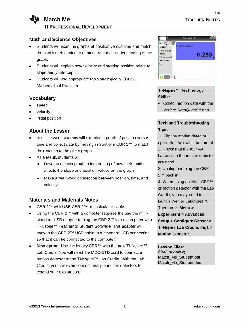
Match Me TEACHER NOTES
TI PROFESSIONAL DEVELOPMENT
©2011 Texas Instruments Incorporated 1 education.ti.com
Math and Science Objectives Students will examine graphs of position versus time and match
them with their motion to demonstrate their understanding of the
graph.
Students will explain how velocity and starting position relate to
slope and y-intercept.
Students will use appropriate tools strategically. (CCSS
Mathematical Practice)
Vocabulary speed
velocity
initial position
About the Lesson In this lesson, students will examine a graph of position versus
time and collect data by moving in front of a CBR 2™ to match
their motion to the given graph.
As a result, students will:
Develop a conceptual understanding of how their motion
affects the slope and position values on the graph
Make a real-world connection between position, time, and
velocity
Materials and Materials Notes CBR 2™ with USB CBR 2™–to–calculator cable.
Using the CBR 2™ with a computer requires the use the mini-
standard USB adaptor to plug the CBR 2™ into a computer with
TI-Nspire™ Teacher or Student Software. This adapter will
convert the CBR 2™ USB cable to a standard USB connection
so that it can be connected to the computer.
New option: Use the legacy CBR™ with the new TI-Nspire™
Lab Cradle. You will need the MDC-BTD cord to connect a
motion detector to the TI-Nspire™ Lab Cradle. With the Lab
Cradle, you can even connect multiple motion detectors to
extend your exploration.
TI-Nspire™ Technology
Skills:
Collect motion data with the
Veriner DataQuest™ app.
Tech and Troubleshooting
Tips:
1. Flip the motion detector
open. Set the switch to normal.
2. Check that the four AA
batteries in the motion detector
are good.
3. Unplug and plug the CBR
2™ back in.
4. When using an older CBR™
or motion detector with the Lab
Cradle, you may need to
launch Vernier LabQuest™.
Then press Menu >
Experiment > Advanced
Setup > Configure Sensor >
TI-Nspire Lab Cradle: dig1 >
Motion Detector.
Lesson Files: Student Activity Match_Me_Student.pdf Match_Me_Student.doc
119
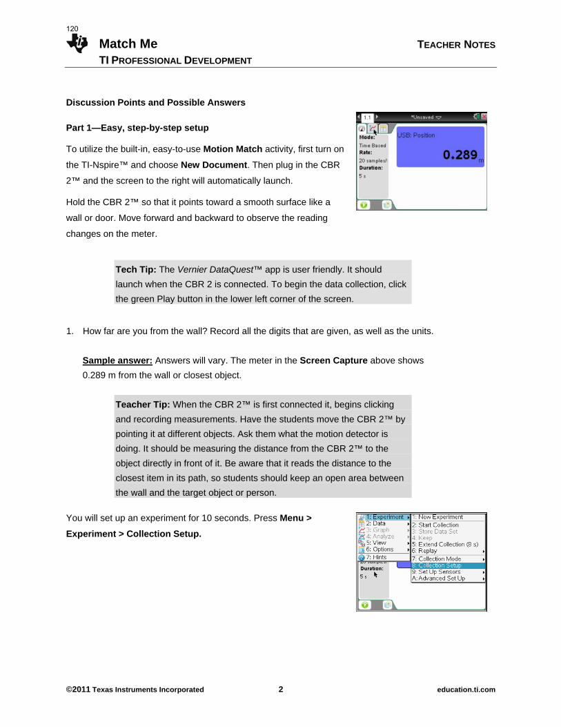
Match Me TEACHER NOTES
TI PROFESSIONAL DEVELOPMENT
©2011 Texas Instruments Incorporated 2 education.ti.com
Discussion Points and Possible Answers
Part 1—Easy, step-by-step setup
To utilize the built-in, easy-to-use Motion Match activity, first turn on
the TI-Nspire™ and choose New Document. Then plug in the CBR
2™ and the screen to the right will automatically launch.
Hold the CBR 2™ so that it points toward a smooth surface like a
wall or door. Move forward and backward to observe the reading
changes on the meter.
Tech Tip: The Vernier DataQuest™ app is user friendly. It should
launch when the CBR 2 is connected. To begin the data collection, click
the green Play button in the lower left corner of the screen.
1. How far are you from the wall? Record all the digits that are given, as well as the units.
Sample answer: Answers will vary. The meter in the Screen Capture above shows
0.289 m from the wall or closest object.
Teacher Tip: When the CBR 2™ is first connected it, begins clicking
and recording measurements. Have the students move the CBR 2™ by
pointing it at different objects. Ask them what the motion detector is
doing. It should be measuring the distance from the CBR 2™ to the
object directly in front of it. Be aware that it reads the distance to the
closest item in its path, so students should keep an open area between
the wall and the target object or person.
You will set up an experiment for 10 seconds. Press Menu >
Experiment > Collection Setup.
120
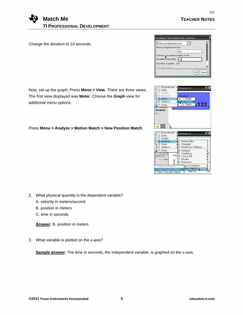
Match Me TEACHER NOTES
TI PROFESSIONAL DEVELOPMENT
©2011 Texas Instruments Incorporated 3 education.ti.com
Change the duration to 10 seconds.
Now, set up the graph. Press Menu > View. There are three views.
The first view displayed was Meter. Choose the Graph view for
additional menu options.
Press Menu > Analyze > Motion Match > New Position Match.
2. What physical quantity is the dependent variable?
A. velocity in meters/second
B. position in meters
C. time in seconds
Answer: B. position in meters 3. What variable is plotted on the x-axis?
Sample answer: The time in seconds, the independent variable, is graphed on the x-axis.
121
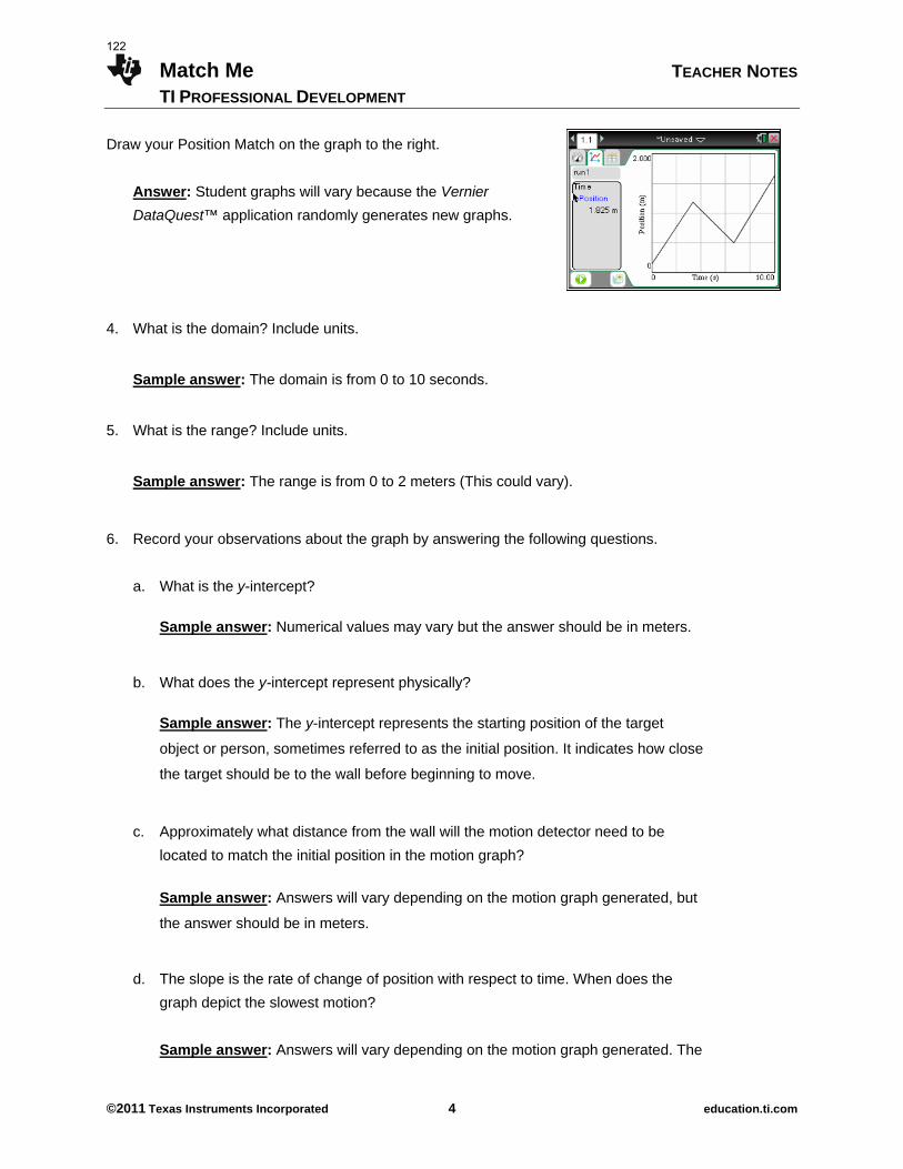
Match Me TEACHER NOTES
TI PROFESSIONAL DEVELOPMENT
©2011 Texas Instruments Incorporated 4 education.ti.com
Draw your Position Match on the graph to the right.
Answer: Student graphs will vary because the Vernier
DataQuest™ application randomly generates new graphs.
4. What is the domain? Include units.
Sample answer: The domain is from 0 to 10 seconds.
5. What is the range? Include units.
Sample answer: The range is from 0 to 2 meters (This could vary).
6. Record your observations about the graph by answering the following questions.
a. What is the y-intercept?
Sample answer: Numerical values may vary but the answer should be in meters.
b. What does the y-intercept represent physically?
Sample answer: The y-intercept represents the starting position of the target
object or person, sometimes referred to as the initial position. It indicates how close
the target should be to the wall before beginning to move.
c. Approximately what distance from the wall will the motion detector need to be
located to match the initial position in the motion graph?
Sample answer: Answers will vary depending on the motion graph generated, but
the answer should be in meters.
d. The slope is the rate of change of position with respect to time. When does the
graph depict the slowest motion?
Sample answer: Answers will vary depending on the motion graph generated. The
122
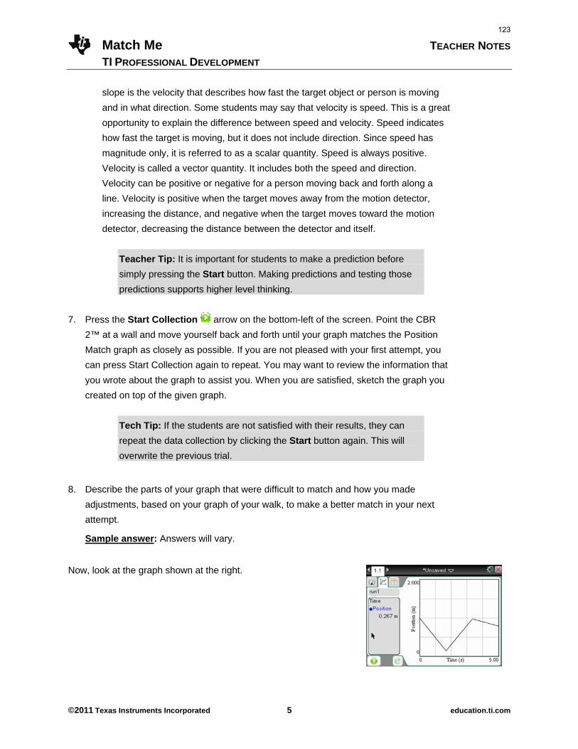
Match Me TEACHER NOTES
TI PROFESSIONAL DEVELOPMENT
©2011 Texas Instruments Incorporated 5 education.ti.com
slope is the velocity that describes how fast the target object or person is moving
and in what direction. Some students may say that velocity is speed. This is a great
opportunity to explain the difference between speed and velocity. Speed indicates
how fast the target is moving, but it does not include direction. Since speed has
magnitude only, it is referred to as a scalar quantity. Speed is always positive.
Velocity is called a vector quantity. It includes both the speed and direction.
Velocity can be positive or negative for a person moving back and forth along a
line. Velocity is positive when the target moves away from the motion detector,
increasing the distance, and negative when the target moves toward the motion
detector, decreasing the distance between the detector and itself.
Teacher Tip: It is important for students to make a prediction before
simply pressing the Start button. Making predictions and testing those
predictions supports higher level thinking.
7. Press the Start Collection arrow on the bottom-left of the screen. Point the CBR
2™ at a wall and move yourself back and forth until your graph matches the Position
Match graph as closely as possible. If you are not pleased with your first attempt, you
can press Start Collection again to repeat. You may want to review the information that
you wrote about the graph to assist you. When you are satisfied, sketch the graph you
created on top of the given graph.
Tech Tip: If the students are not satisfied with their results, they can
repeat the data collection by clicking the Start button again. This will
overwrite the previous trial.
8. Describe the parts of your graph that were difficult to match and how you made
adjustments, based on your graph of your walk, to make a better match in your next
attempt.
Sample answer: Answers will vary.
Now, look at the graph shown at the right.
123
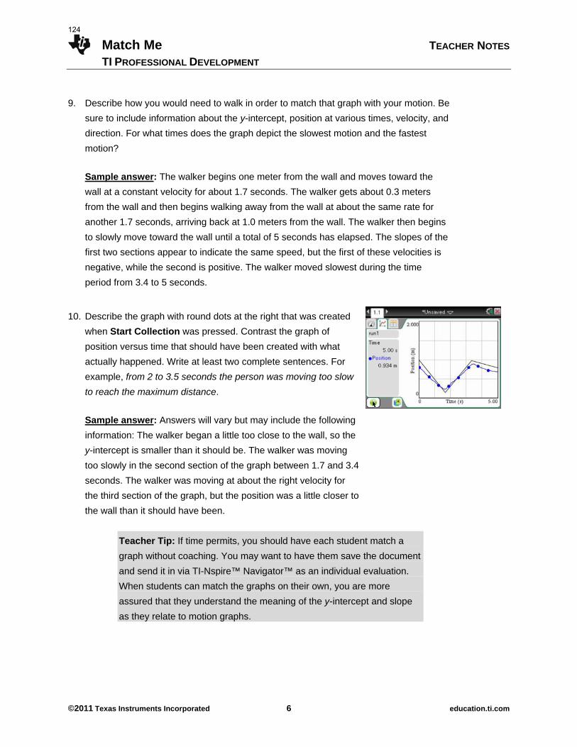
Match Me TEACHER NOTES
TI PROFESSIONAL DEVELOPMENT
©2011 Texas Instruments Incorporated 6 education.ti.com
9. Describe how you would need to walk in order to match that graph with your motion. Be
sure to include information about the y-intercept, position at various times, velocity, and
direction. For what times does the graph depict the slowest motion and the fastest
motion?
Sample answer: The walker begins one meter from the wall and moves toward the
wall at a constant velocity for about 1.7 seconds. The walker gets about 0.3 meters
from the wall and then begins walking away from the wall at about the same rate for
another 1.7 seconds, arriving back at 1.0 meters from the wall. The walker then begins
to slowly move toward the wall until a total of 5 seconds has elapsed. The slopes of the
first two sections appear to indicate the same speed, but the first of these velocities is
negative, while the second is positive. The walker moved slowest during the time
period from 3.4 to 5 seconds.
10. Describe the graph with round dots at the right that was created
when Start Collection was pressed. Contrast the graph of
position versus time that should have been created with what
actually happened. Write at least two complete sentences. For
example, from 2 to 3.5 seconds the person was moving too slow
to reach the maximum distance.
Sample answer: Answers will vary but may include the following
information: The walker began a little too close to the wall, so the
y-intercept is smaller than it should be. The walker was moving
too slowly in the second section of the graph between 1.7 and 3.4
seconds. The walker was moving at about the right velocity for
the third section of the graph, but the position was a little closer to
the wall than it should have been.
Teacher Tip: If time permits, you should have each student match a
graph without coaching. You may want to have them save the document
and send it in via TI-Nspire™ Navigator™ as an individual evaluation.
When students can match the graphs on their own, you are more
assured that they understand the meaning of the y-intercept and slope
as they relate to motion graphs.
124
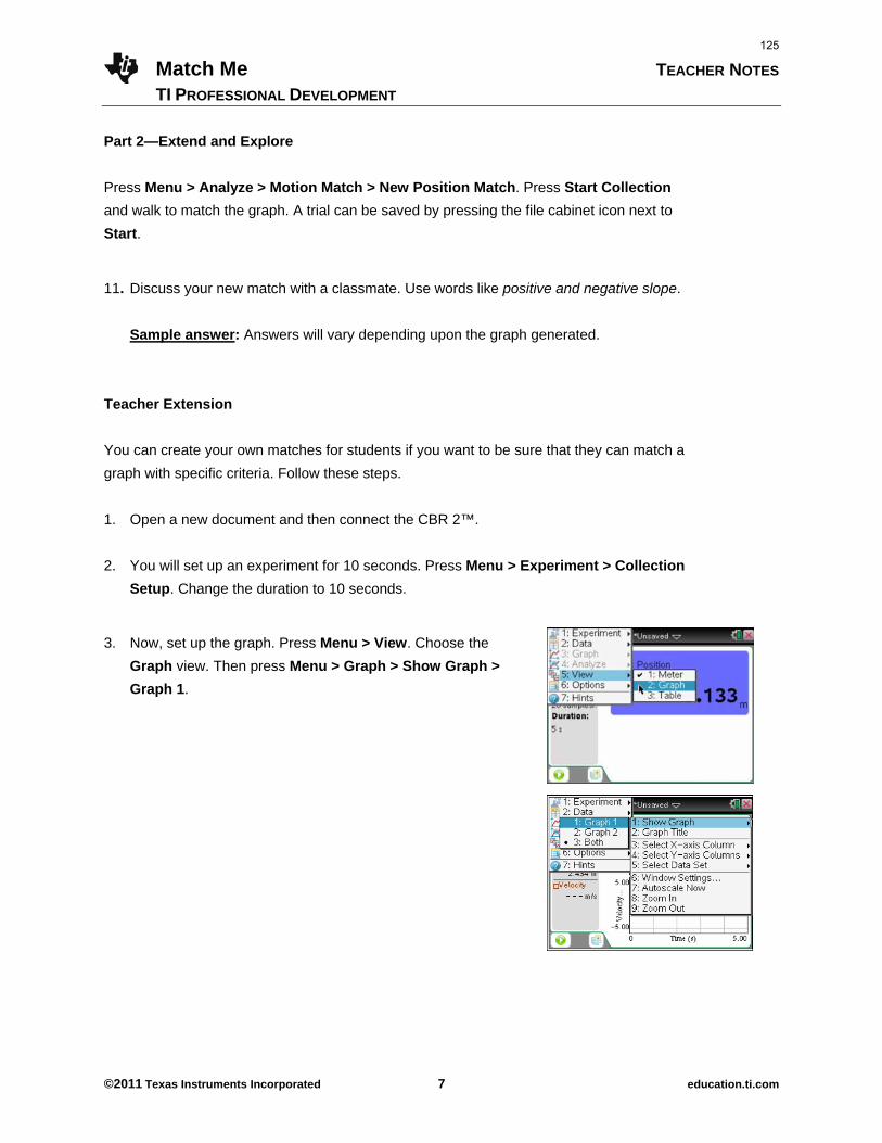
Match Me TEACHER NOTES
TI PROFESSIONAL DEVELOPMENT
©2011 Texas Instruments Incorporated 7 education.ti.com
Part 2—Extend and Explore
Press Menu > Analyze > Motion Match > New Position Match. Press Start Collection
and walk to match the graph. A trial can be saved by pressing the file cabinet icon next to
Start.
11. Discuss your new match with a classmate. Use words like positive and negative slope.
Sample answer: Answers will vary depending upon the graph generated.
Teacher Extension
You can create your own matches for students if you want to be sure that they can match a
graph with specific criteria. Follow these steps.
1. Open a new document and then connect the CBR 2™.
2. You will set up an experiment for 10 seconds. Press Menu > Experiment > Collection
Setup. Change the duration to 10 seconds.
3. Now, set up the graph. Press Menu > View. Choose the
Graph view. Then press Menu > Graph > Show Graph >
Graph 1.
125
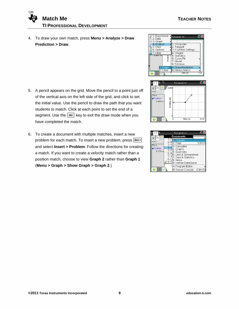
Match Me TEACHER NOTES
TI PROFESSIONAL DEVELOPMENT
©2011 Texas Instruments Incorporated 8 education.ti.com
4. To draw your own match, press Menu > Analyze > Draw
Prediction > Draw.
5. A pencil appears on the grid. Move the pencil to a point just off
of the vertical axis on the left side of the grid, and click to set
the initial value. Use the pencil to draw the path that you want
students to match. Click at each point to set the end of a
segment. Use the d key to exit the draw mode when you
have completed the match.
6. To create a document with multiple matches, insert a new
problem for each match. To insert a new problem, press ~
and select Insert > Problem. Follow the directions for creating
a match. If you want to create a velocity match rather than a
position match, choose to view Graph 2 rather than Graph 1
(Menu > Graph > Show Graph > Graph 2.)
126
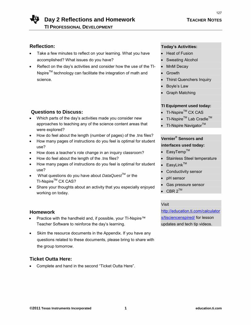
Day 2 Reflections and Homework TEACHER NOTES
TI PROFESSIONAL DEVELOPMENT
©2011 Texas Instruments Incorporated 1 education.ti.com
Reflection:
Take a few minutes to reflect on your learning. What you have accomplished? What issues do you have?
Reflect on the day’s activities and consider how the use of the TI-NspireTM technology can facilitate the integration of math and science.
Questions to Discuss:
Which parts of the day’s activities made you consider new
approaches to teaching any of the science content areas that were explored?
How do feel about the length (number of pages) of the .tns files? How many pages of instructions do you feel is optimal for student
use? How does a teacher’s role change in an inquiry classroom? How do feel about the length of the .tns files? How many pages of instructions do you feel is optimal for student
use? What questions do you have about DataQuest
TM or the TI-NspireTM CX CAS?
Share your thoughts about an activity that you especially enjoyed working on today.
Homework
Practice with the handheld and, if possible, your TI-Nspire™
Teacher Software to reinforce the day’s learning.
Skim the resource documents in the Appendix. If you have any questions related to these documents, please bring to share with the group tomorrow.
Ticket Outta Here:
Complete and hand in the second “Ticket Outta Here”.
Today’s Activities:
Heat of Fusion Sweating Alcohol MnM Decay Growth Thirst Quenchers Inquiry Boyle’s Law Graph Matching
TI Equipment used today:
TI-NspireTM CX CAS TI-NspireTM Lab CradleTM TI-Nspire NavigatorTM
Vernier® Sensors and
interfaces used today:
EasyTempTM Stainless Steel temperature EasyLinkTM Conductivity sensor pH sensor Gas pressure sensor CBR 2TM Visit http://education.ti.com/calculators/tisciencenspired/ for lesson updates and tech tip videos.
127
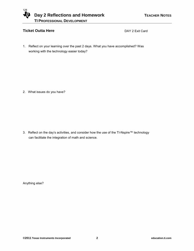
Day 2 Reflections and Homework TEACHER NOTES
TI PROFESSIONAL DEVELOPMENT
©2011 Texas Instruments Incorporated 2 education.ti.com
Ticket Outta Here DAY 2 Exit Card
1. Reflect on your learning over the past 2 days. What you have accomplished? Was
working with the technology easier today? 2. What issues do you have? 3. Reflect on the day’s activities, and consider how the use of the TI-Nspire™ technology
can facilitate the integration of math and science. Anything else?
128
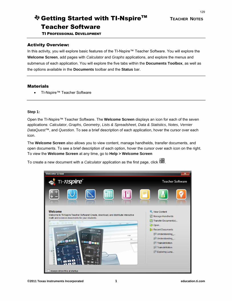
Getting Started with TI-NspireTM
TEACHER NOTES
Teacher Software
TI PROFESSIONAL DEVELOPMENT
©2011 Texas Instruments Incorporated 1 education.ti.com
Activity Overview:
In this activity, you will explore basic features of the TI-Nspire™ Teacher Software. You will explore the Welcome Screen, add pages with Calculator and Graphs applications, and explore the menus and submenus of each application. You will explore the five tabs within the Documents Toolbox, as well as the options available in the Documents toolbar and the Status bar.
Materials
TI-Nspire™ Teacher Software
Step 1:
Open the TI-Nspire™ Teacher Software. The Welcome Screen displays an icon for each of the seven applications: Calculator, Graphs, Geometry, Lists & Spreadsheet, Data & Statistics, Notes, Vernier
DataQuest™, and Question. To see a brief description of each application, hover the cursor over each icon.
The Welcome Screen also allows you to view content, manage handhelds, transfer documents, and open documents. To see a brief description of each option, hover the cursor over each icon on the right. To view the Welcome Screen at any time, go to Help > Welcome Screen
To create a new document with a Calculator application as the first page, click .
129
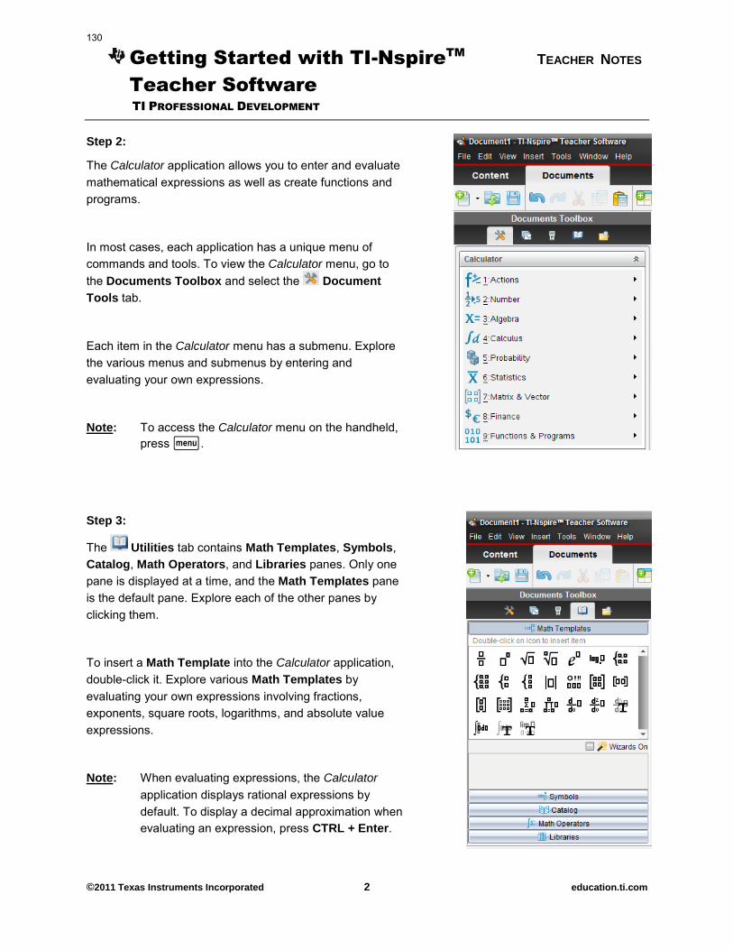
Getting Started with TI-NspireTM
TEACHER NOTES
Teacher Software
TI PROFESSIONAL DEVELOPMENT
©2011 Texas Instruments Incorporated 2 education.ti.com
Step 2:
The Calculator application allows you to enter and evaluate mathematical expressions as well as create functions and programs.
In most cases, each application has a unique menu of commands and tools. To view the Calculator menu, go to the Documents Toolbox and select the Document
Tools tab.
Each item in the Calculator menu has a submenu. Explore the various menus and submenus by entering and evaluating your own expressions.
Note: To access the Calculator menu on the handheld, press b.
Step 3:
The Utilities tab contains Math Templates, Symbols, Catalog, Math Operators, and Libraries panes. Only one pane is displayed at a time, and the Math Templates pane is the default pane. Explore each of the other panes by clicking them.
To insert a Math Template into the Calculator application, double-click it. Explore various Math Templates by evaluating your own expressions involving fractions, exponents, square roots, logarithms, and absolute value expressions.
Note: When evaluating expressions, the Calculator application displays rational expressions by default. To display a decimal approximation when evaluating an expression, press CTRL + Enter.
130
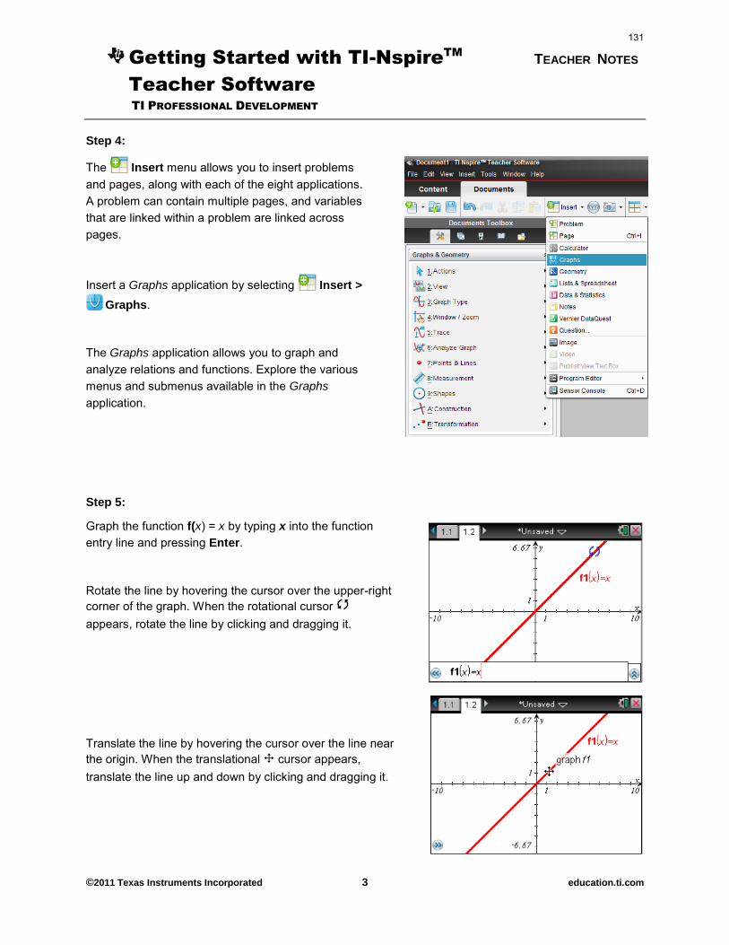
Getting Started with TI-NspireTM
TEACHER NOTES
Teacher Software
TI PROFESSIONAL DEVELOPMENT
©2011 Texas Instruments Incorporated 3 education.ti.com
Step 4:
The Insert menu allows you to insert problems and pages, along with each of the eight applications. A problem can contain multiple pages, and variables that are linked within a problem are linked across pages.
Insert a Graphs application by selecting Insert >
Graphs.
The Graphs application allows you to graph and analyze relations and functions. Explore the various menus and submenus available in the Graphs application.
Step 5:
Graph the function f(x) = x by typing x into the function entry line and pressing Enter.
Rotate the line by hovering the cursor over the upper-right corner of the graph. When the rotational cursor é appears, rotate the line by clicking and dragging it.
Translate the line by hovering the cursor over the line near the origin. When the translational ö cursor appears, translate the line up and down by clicking and dragging it.
131
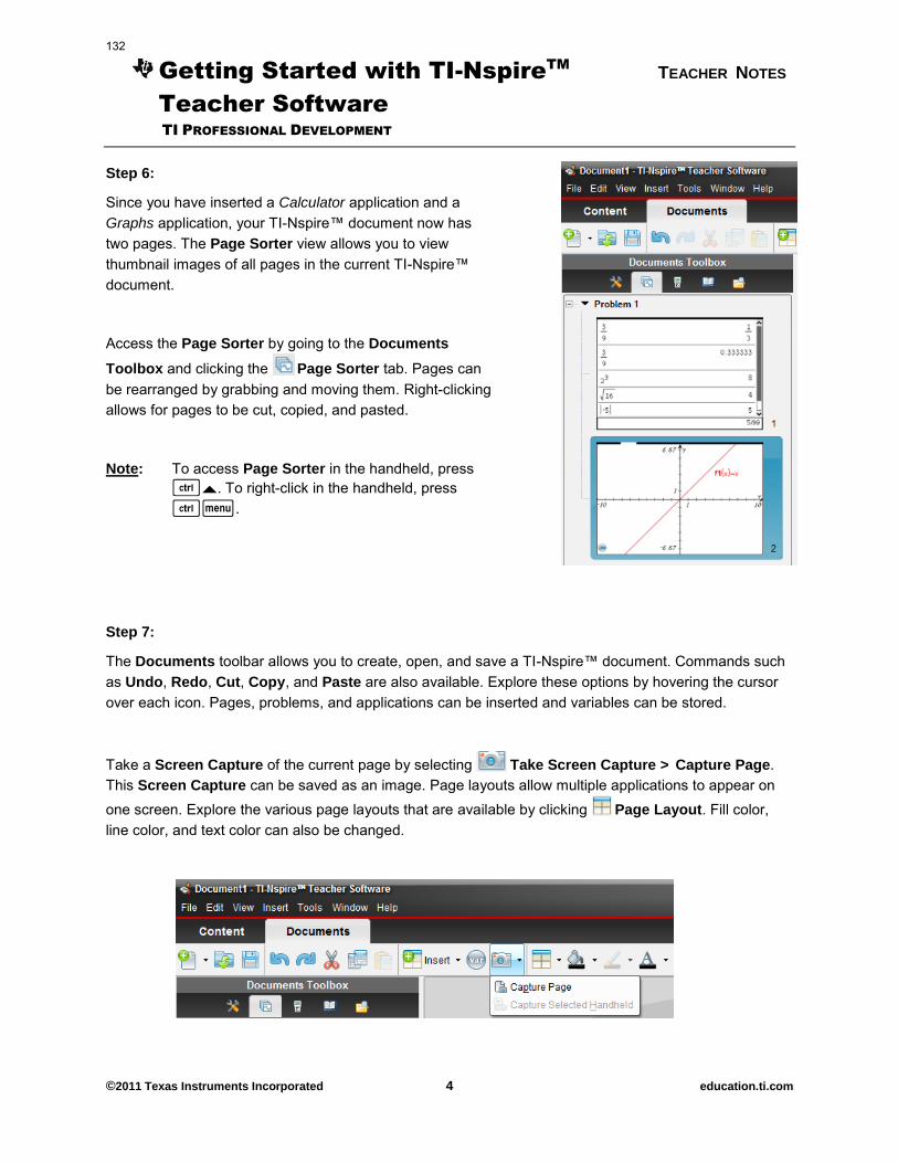
Getting Started with TI-NspireTM
TEACHER NOTES
Teacher Software
TI PROFESSIONAL DEVELOPMENT
©2011 Texas Instruments Incorporated 4 education.ti.com
Step 6:
Since you have inserted a Calculator application and a Graphs application, your TI-Nspire™ document now has two pages. The Page Sorter view allows you to view thumbnail images of all pages in the current TI-Nspire™ document.
Access the Page Sorter by going to the Documents
Toolbox and clicking the Page Sorter tab. Pages can be rearranged by grabbing and moving them. Right-clicking allows for pages to be cut, copied, and pasted.
Note: To access Page Sorter in the handheld, press /£. To right-click in the handheld, press /b.
Step 7:
The Documents toolbar allows you to create, open, and save a TI-Nspire™ document. Commands such as Undo, Redo, Cut, Copy, and Paste are also available. Explore these options by hovering the cursor over each icon. Pages, problems, and applications can be inserted and variables can be stored.
Take a Screen Capture of the current page by selecting Take Screen Capture > Capture Page. This Screen Capture can be saved as an image. Page layouts allow multiple applications to appear on one screen. Explore the various page layouts that are available by clicking Page Layout. Fill color, line color, and text color can also be changed.
132
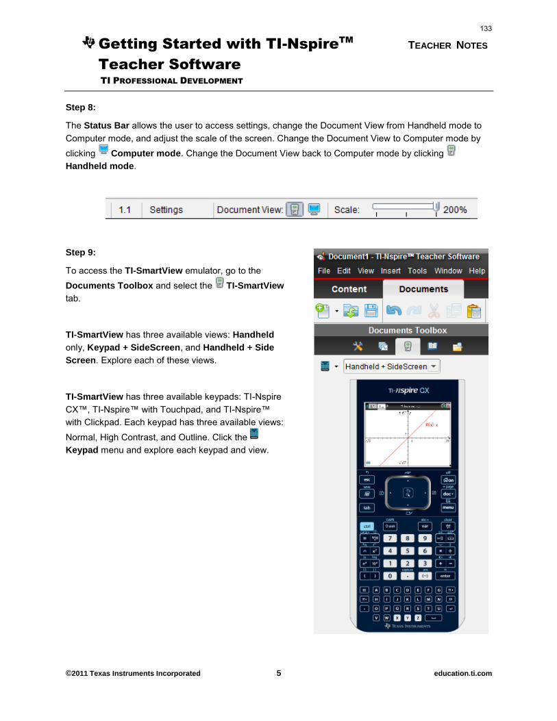
Getting Started with TI-NspireTM
TEACHER NOTES
Teacher Software
TI PROFESSIONAL DEVELOPMENT
©2011 Texas Instruments Incorporated 5 education.ti.com
Step 8:
The Status Bar allows the user to access settings, change the Document View from Handheld mode to Computer mode, and adjust the scale of the screen. Change the Document View to Computer mode by clicking Computer mode. Change the Document View back to Computer mode by clicking Handheld mode.
Step 9:
To access the TI-SmartView emulator, go to the Documents Toolbox and select the TI-SmartView
tab.
TI-SmartView has three available views: Handheld only, Keypad + SideScreen, and Handheld + Side
Screen. Explore each of these views.
TI-SmartView has three available keypads: TI-Nspire CX™, TI-Nspire™ with Touchpad, and TI-Nspire™ with Clickpad. Each keypad has three available views: Normal, High Contrast, and Outline. Click the Keypad menu and explore each keypad and view.
133
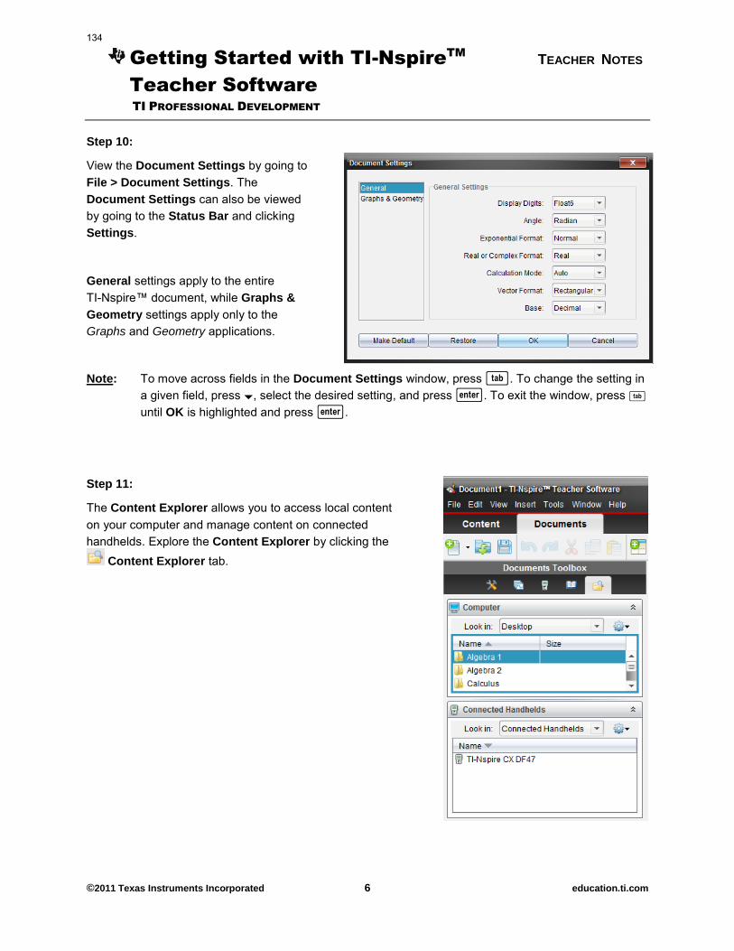
Getting Started with TI-NspireTM
TEACHER NOTES
Teacher Software
TI PROFESSIONAL DEVELOPMENT
©2011 Texas Instruments Incorporated 6 education.ti.com
Step 10:
View the Document Settings by going to File > Document Settings. The Document Settings can also be viewed by going to the Status Bar and clicking Settings.
General settings apply to the entire TI-Nspire™ document, while Graphs &
Geometry settings apply only to the Graphs and Geometry applications.
Note: To move across fields in the Document Settings window, press e. To change the setting in a given field, press ¤, select the desired setting, and press ·. To exit the window, press e until OK is highlighted and press ·.
Step 11:
The Content Explorer allows you to access local content on your computer and manage content on connected handhelds. Explore the Content Explorer by clicking the
Content Explorer tab.
134
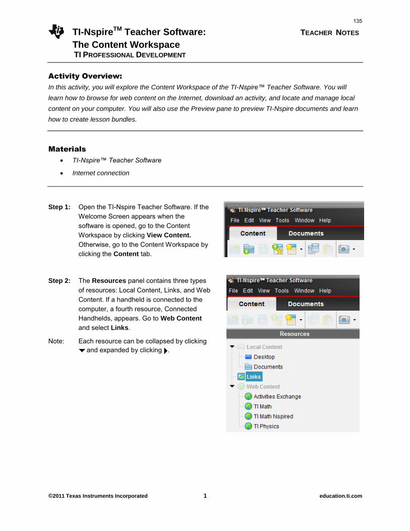
TI-NspireTM Teacher Software: TEACHER NOTES
The Content Workspace TI PROFESSIONAL DEVELOPMENT
©2011 Texas Instruments Incorporated 1 education.ti.com
Activity Overview:
In this activity, you will explore the Content Workspace of the TI-Nspire™ Teacher Software. You will
learn how to browse for web content on the Internet, download an activity, and locate and manage local
content on your computer. You will also use the Preview pane to preview TI-Nspire documents and learn
how to create lesson bundles.
Materials
TI-Nspire™ Teacher Software
Internet connection
Step 1: Open the TI-Nspire Teacher Software. If the Welcome Screen appears when the software is opened, go to the Content Workspace by clicking View Content.
Otherwise, go to the Content Workspace by clicking the Content tab.
Step 2: The Resources panel contains three types of resources: Local Content, Links, and Web Content. If a handheld is connected to the computer, a fourth resource, Connected Handhelds, appears. Go to Web Content
and select Links.
Note: Each resource can be collapsed by clicking ¤ and expanded by clicking ¢.
135
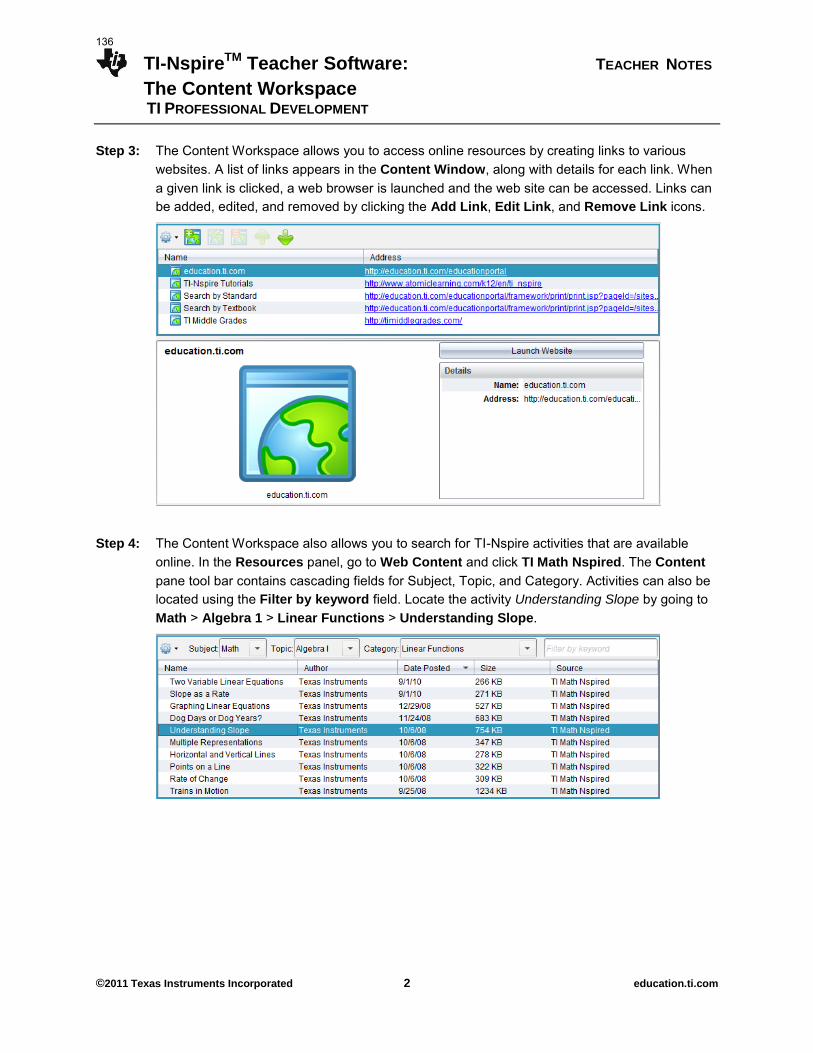
TI-NspireTM Teacher Software: TEACHER NOTES
The Content Workspace TI PROFESSIONAL DEVELOPMENT
©2011 Texas Instruments Incorporated 2 education.ti.com
Step 3: The Content Workspace allows you to access online resources by creating links to various websites. A list of links appears in the Content Window, along with details for each link. When a given link is clicked, a web browser is launched and the web site can be accessed. Links can be added, edited, and removed by clicking the Add Link, Edit Link, and Remove Link icons.
Step 4: The Content Workspace also allows you to search for TI-Nspire activities that are available online. In the Resources panel, go to Web Content and click TI Math Nspired. The Content pane tool bar contains cascading fields for Subject, Topic, and Category. Activities can also be located using the Filter by keyword field. Locate the activity Understanding Slope by going to Math > Algebra 1 > Linear Functions > Understanding Slope.
136
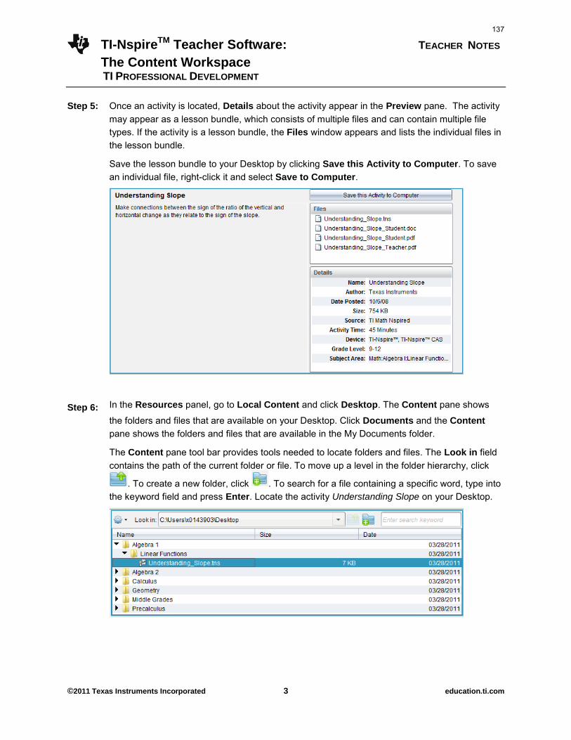
TI-NspireTM Teacher Software: TEACHER NOTES
The Content Workspace TI PROFESSIONAL DEVELOPMENT
©2011 Texas Instruments Incorporated 3 education.ti.com
Step 5: Once an activity is located, Details about the activity appear in the Preview pane. The activity may appear as a lesson bundle, which consists of multiple files and can contain multiple file types. If the activity is a lesson bundle, the Files window appears and lists the individual files in the lesson bundle.
Save the lesson bundle to your Desktop by clicking Save this Activity to Computer. To save an individual file, right-click it and select Save to Computer.
Step 6: In the Resources panel, go to Local Content and click Desktop. The Content pane shows
the folders and files that are available on your Desktop. Click Documents and the Content pane shows the folders and files that are available in the My Documents folder.
The Content pane tool bar provides tools needed to locate folders and files. The Look in field contains the path of the current folder or file. To move up a level in the folder hierarchy, click
. To create a new folder, click . To search for a file containing a specific word, type into the keyword field and press Enter. Locate the activity Understanding Slope on your Desktop.
137
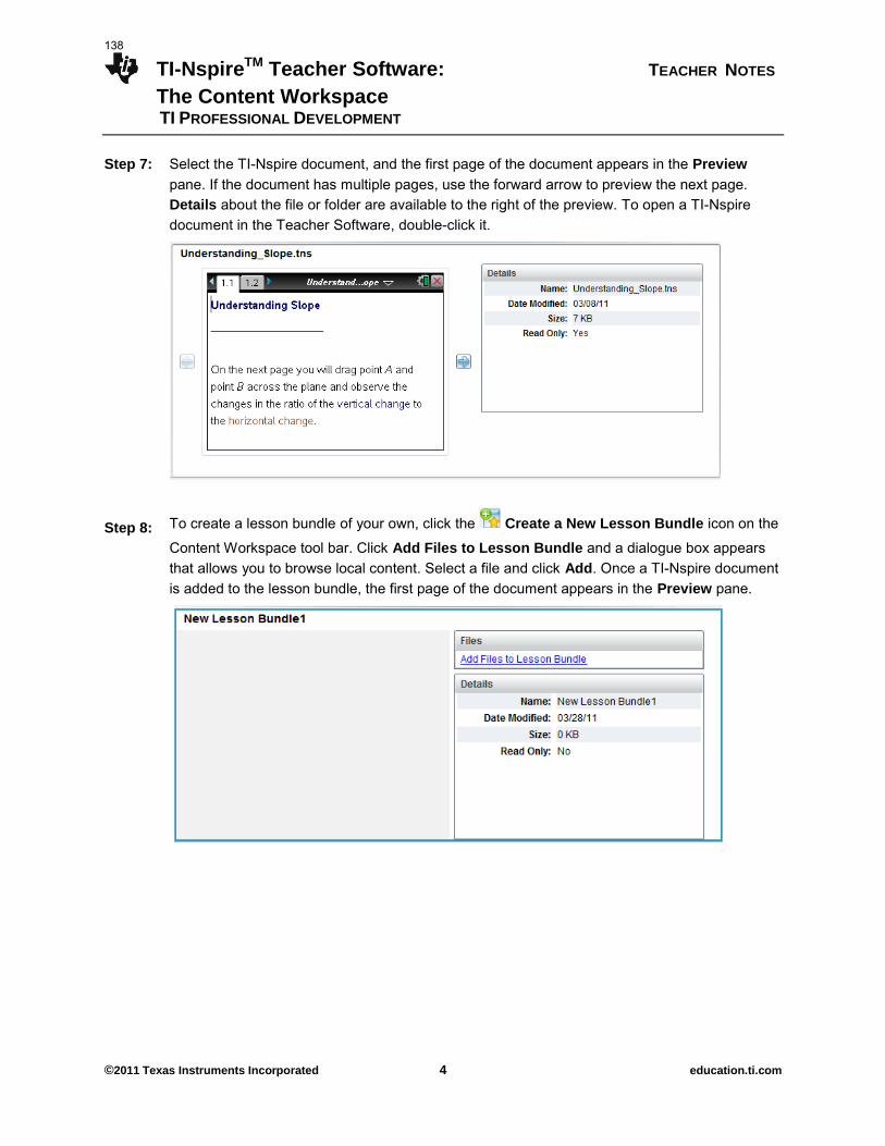
TI-NspireTM Teacher Software: TEACHER NOTES
The Content Workspace TI PROFESSIONAL DEVELOPMENT
©2011 Texas Instruments Incorporated 4 education.ti.com
Step 7: Select the TI-Nspire document, and the first page of the document appears in the Preview pane. If the document has multiple pages, use the forward arrow to preview the next page. Details about the file or folder are available to the right of the preview. To open a TI-Nspire document in the Teacher Software, double-click it.
Step 8: To create a lesson bundle of your own, click the Create a New Lesson Bundle icon on the
Content Workspace tool bar. Click Add Files to Lesson Bundle and a dialogue box appears that allows you to browse local content. Select a file and click Add. Once a TI-Nspire document is added to the lesson bundle, the first page of the document appears in the Preview pane.
138
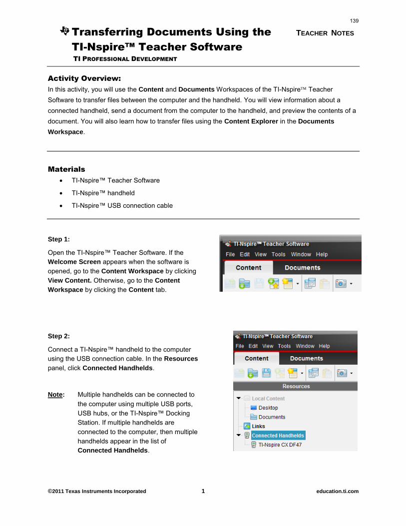
Transferring Documents Using the TEACHER NOTES
TI-Nspire™ Teacher Software TI PROFESSIONAL DEVELOPMENT
©2011 Texas Instruments Incorporated 1 education.ti.com
Activity Overview:
In this activity, you will use the Content and Documents Workspaces of the TI-Nspire Teacher Software to transfer files between the computer and the handheld. You will view information about a connected handheld, send a document from the computer to the handheld, and preview the contents of a document. You will also learn how to transfer files using the Content Explorer in the Documents
Workspace.
Materials
TI-Nspire™ Teacher Software
TI-Nspire™ handheld
TI-Nspire™ USB connection cable
Step 1:
Open the TI-Nspire™ Teacher Software. If the Welcome Screen appears when the software is opened, go to the Content Workspace by clicking View Content. Otherwise, go to the Content
Workspace by clicking the Content tab.
Step 2:
Connect a TI-Nspire™ handheld to the computer using the USB connection cable. In the Resources
panel, click Connected Handhelds.
Note: Multiple handhelds can be connected to the computer using multiple USB ports, USB hubs, or the TI-Nspire™ Docking Station. If multiple handhelds are connected to the computer, then multiple handhelds appear in the list of Connected Handhelds.
139
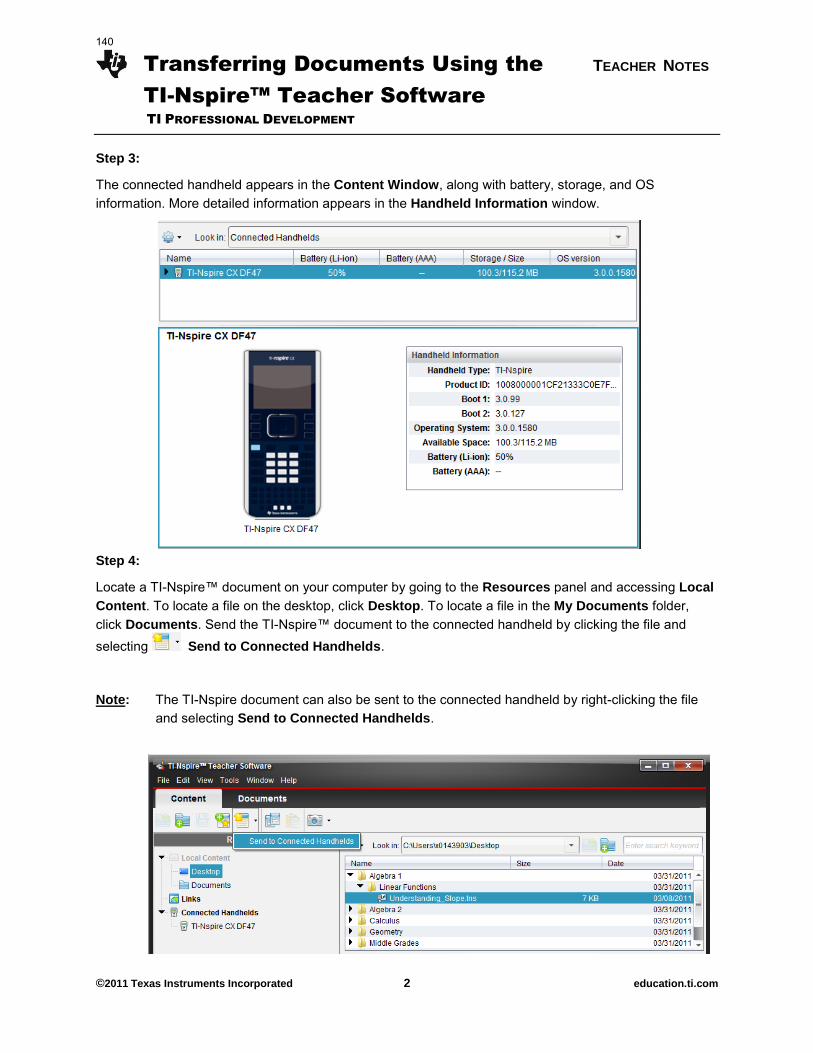
Transferring Documents Using the TEACHER NOTES
TI-Nspire™ Teacher Software
TI PROFESSIONAL DEVELOPMENT
©2011 Texas Instruments Incorporated 2 education.ti.com
Step 3:
The connected handheld appears in the Content Window, along with battery, storage, and OS information. More detailed information appears in the Handheld Information window.
Step 4:
Locate a TI-Nspire™ document on your computer by going to the Resources panel and accessing Local
Content. To locate a file on the desktop, click Desktop. To locate a file in the My Documents folder, click Documents. Send the TI-Nspire™ document to the connected handheld by clicking the file and selecting Send to Connected Handhelds.
Note: The TI-Nspire document can also be sent to the connected handheld by right-clicking the file and selecting Send to Connected Handhelds.
140
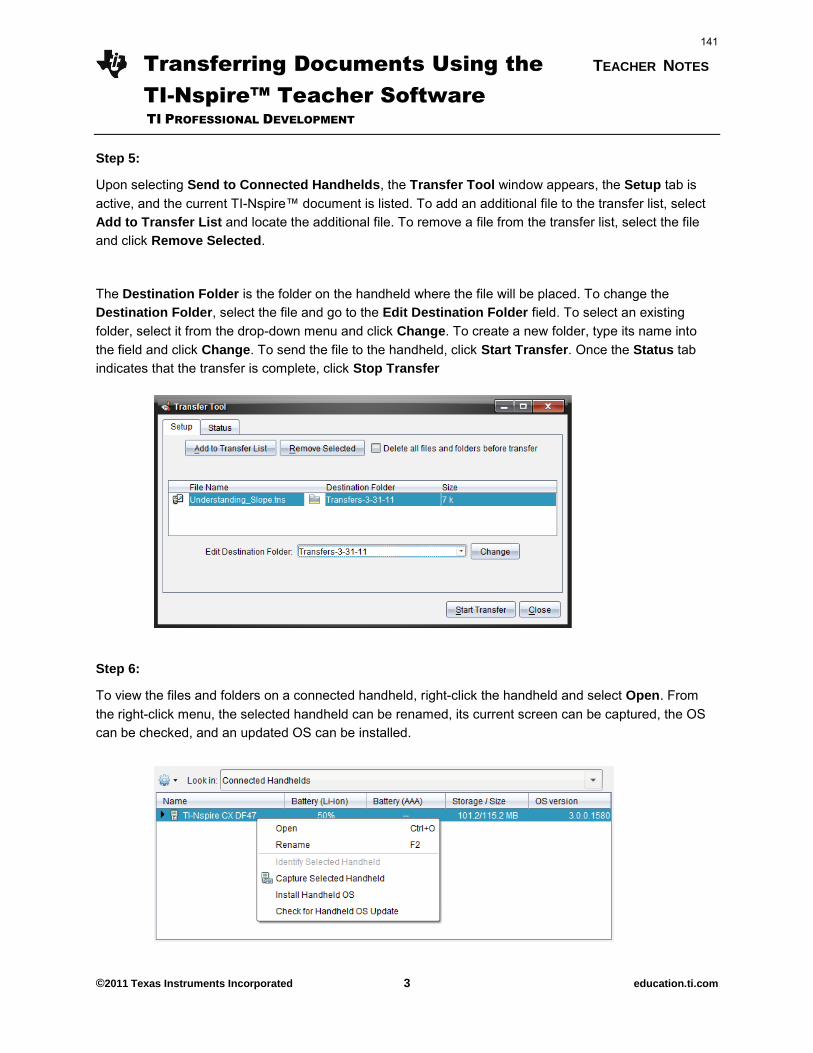
Transferring Documents Using the TEACHER NOTES
TI-Nspire™ Teacher Software
TI PROFESSIONAL DEVELOPMENT
©2011 Texas Instruments Incorporated 3 education.ti.com
Step 5:
Upon selecting Send to Connected Handhelds, the Transfer Tool window appears, the Setup tab is active, and the current TI-Nspire™ document is listed. To add an additional file to the transfer list, select Add to Transfer List and locate the additional file. To remove a file from the transfer list, select the file and click Remove Selected.
The Destination Folder is the folder on the handheld where the file will be placed. To change the Destination Folder, select the file and go to the Edit Destination Folder field. To select an existing folder, select it from the drop-down menu and click Change. To create a new folder, type its name into the field and click Change. To send the file to the handheld, click Start Transfer. Once the Status tab indicates that the transfer is complete, click Stop Transfer
Step 6:
To view the files and folders on a connected handheld, right-click the handheld and select Open. From the right-click menu, the selected handheld can be renamed, its current screen can be captured, the OS can be checked, and an updated OS can be installed.
141
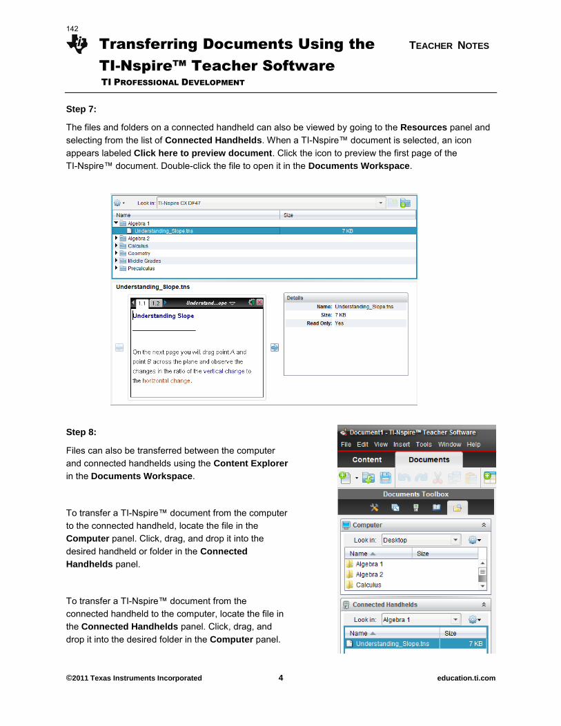
Transferring Documents Using the TEACHER NOTES
TI-Nspire™ Teacher Software
TI PROFESSIONAL DEVELOPMENT
©2011 Texas Instruments Incorporated 4 education.ti.com
Step 7:
The files and folders on a connected handheld can also be viewed by going to the Resources panel and selecting from the list of Connected Handhelds. When a TI-Nspire™ document is selected, an icon appears labeled Click here to preview document. Click the icon to preview the first page of the TI-Nspire™ document. Double-click the file to open it in the Documents Workspace.
Step 8:
Files can also be transferred between the computer and connected handhelds using the Content Explorer
in the Documents Workspace.
To transfer a TI-Nspire™ document from the computer to the connected handheld, locate the file in the Computer panel. Click, drag, and drop it into the desired handheld or folder in the Connected
Handhelds panel.
To transfer a TI-Nspire™ document from the connected handheld to the computer, locate the file in the Connected Handhelds panel. Click, drag, and drop it into the desired folder in the Computer panel.
142
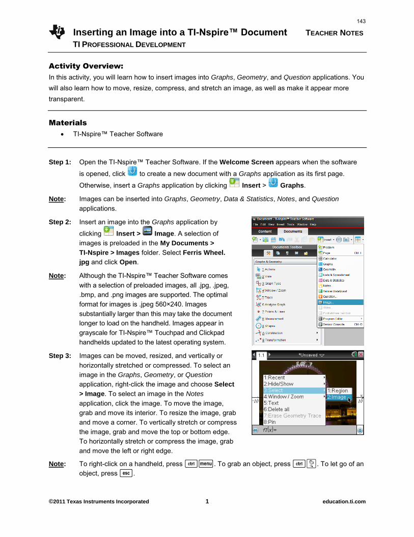
Inserting an Image into a TI-Nspire™ Document TEACHER NOTES
TI PROFESSIONAL DEVELOPMENT
©2011 Texas Instruments Incorporated 1 education.ti.com
Activity Overview:
In this activity, you will learn how to insert images into Graphs, Geometry, and Question applications. You will also learn how to move, resize, compress, and stretch an image, as well as make it appear more transparent.
Materials
TI-Nspire™ Teacher Software
Step 1: Open the TI-Nspire™ Teacher Software. If the Welcome Screen appears when the software
is opened, click to create a new document with a Graphs application as its first page.
Otherwise, insert a Graphs application by clicking Insert > Graphs.
Note: Images can be inserted into Graphs, Geometry, Data & Statistics, Notes, and Question applications.
Step 2: Insert an image into the Graphs application by
clicking Insert > Image. A selection of images is preloaded in the My Documents >
TI-Nspire > Images folder. Select Ferris Wheel.
jpg and click Open.
Note: Although the TI-Nspire™ Teacher Software comes with a selection of preloaded images, all .jpg, .jpeg, .bmp, and .png images are supported. The optimal format for images is .jpeg 560×240. Images substantially larger than this may take the document longer to load on the handheld. Images appear in grayscale for TI-Nspire™ Touchpad and Clickpad handhelds updated to the latest operating system.
Step 3: Images can be moved, resized, and vertically or horizontally stretched or compressed. To select an image in the Graphs, Geometry, or Question application, right-click the image and choose Select
> Image. To select an image in the Notes application, click the image. To move the image, grab and move its interior. To resize the image, grab and move a corner. To vertically stretch or compress the image, grab and move the top or bottom edge. To horizontally stretch or compress the image, grab and move the left or right edge.
Note: To right-click on a handheld, press /b. To grab an object, press /x. To let go of an object, press d.
143
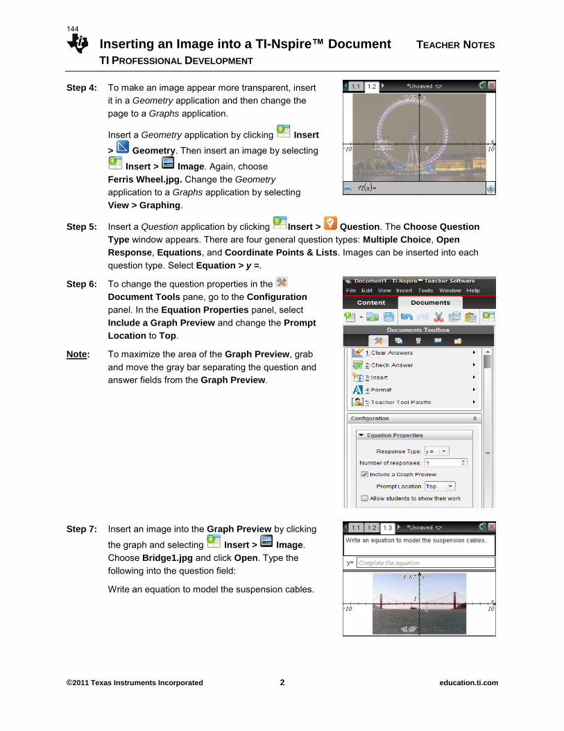
Inserting an Image into a TI-Nspire™ Document TEACHER NOTES
TI PROFESSIONAL DEVELOPMENT
©2011 Texas Instruments Incorporated 2 education.ti.com
Step 4: To make an image appear more transparent, insert it in a Geometry application and then change the page to a Graphs application.
Insert a Geometry application by clicking Insert
> Geometry. Then insert an image by selecting
Insert > Image. Again, choose Ferris Wheel.jpg. Change the Geometry application to a Graphs application by selecting View > Graphing.
Step 5: Insert a Question application by clicking Insert > Question. The Choose Question
Type window appears. There are four general question types: Multiple Choice, Open
Response, Equations, and Coordinate Points & Lists. Images can be inserted into each question type. Select Equation > y =.
Step 6: To change the question properties in the Document Tools pane, go to the Configuration
panel. In the Equation Properties panel, select Include a Graph Preview and change the Prompt
Location to Top.
Note: To maximize the area of the Graph Preview, grab and move the gray bar separating the question and answer fields from the Graph Preview.
Step 7: Insert an image into the Graph Preview by clicking
the graph and selecting Insert > Image. Choose Bridge1.jpg and click Open. Type the following into the question field:
Write an equation to model the suspension cables.
144
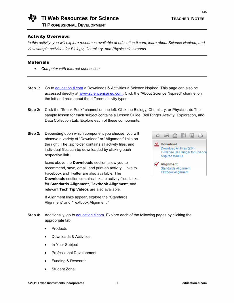
TI Web Resources for Science TEACHER NOTES
TI PROFESSIONAL DEVELOPMENT
©2011 Texas Instruments Incorporated 1 education.ti.com
Activity Overview:
In this activity, you will explore resources available at education.ti.com, learn about Science Nspired, and
view sample activities for Biology, Chemistry, and Physics classrooms.
Materials
Computer with Internet connection
Step 1: Go to education.ti.com > Downloads & Activities > Science Nspired. This page can also be accessed directly at www.sciencenspired.com. Click the “About Science Nspired” channel on
the left and read about the different activity types.
Step 2: Click the “Sneak Peek” channel on the left. Click the Biology, Chemistry, or Physics tab. The
sample lesson for each subject contains a Lesson Guide, Bell Ringer Activity, Exploration, and Data Collection Lab. Explore each of these components.
Step 3: Depending upon which component you choose, you will observe a variety of “Download” or “Alignment” links on
the right. The .zip folder contains all activity files, and individual files can be downloaded by clicking each respective link.
Icons above the Downloads section allow you to recommend, save, email, and print an activity. Links to Facebook and Twitter are also available. The Downloads section contains links to activity files. Links for Standards Alignment, Textbook Alignment, and relevant Tech Tip Videos are also available.
If Alignment links appear, explore the “Standards
Alignment” and “Textbook Alignment.”
Step 4: Additionally, go to education.ti.com. Explore each of the following pages by clicking the appropriate tab:
Products
Downloads & Activities
In Your Subject
Professional Development
Funding & Research
Student Zone
145

This page intentionally left blank
146
The Carousel – Exploring TI-NspireTM Activities TEACHER NOTES
TI PROFESSIONAL DEVELOPMENT
©2011 Texas Instruments Incorporated 1 education.ti.com
About the Activity
You have seen a number of sources for activities. To allow you to make the most relevant use of the remainder of this workshop, you will have time to explore activities that are of particular interest to you for your classroom use.
Some activities are contained in your workshop binder, some are available online through the Teacher Software, or you might have found something on your own that you would like to explore. You will share your findings with the whole group.
TI-NspireTM NavigatorTM System If you want, you can use the workshop TI-NspireTM NavigatorTM
set to practice or to enhance your activity presentation, engage your fellow participants, and share any .tns files you found useful. The T3 Instructor will be happy to help you with that.
Sources for Activity Materials: High School Science
workshop binder TI-NspireTM Teacher Software
Content links NASA website Science Nspired website
Activities
Work together with a partner to explore one or two of the following activities. Prepare a short presentation for the whole group to share what you discovered!
1. Beer's Law (Science Nspired): In this activity, you will be using the VernierTM Colorimeter to determine the concentration of an unknown, simulated nickel (II) sulfate solution. Teacher Notes and Student Activity sheet can be found in your binder. Download the Beer’s LawHSS.tns file
from your instructor. 2. Waves and Spectrum (Science Nspired): In this activity, you will use the TI-NspireTM CX CAS
handheld to investigate the relationship between waves and electron energy jumps within the atom. Teacher Notes and Student Activity sheet can be found in your binder. Download the Waves and Spectrum.tns file from your instructor.
3. Static and Kinetic Friction (from Science with TI-Nspire © 2011, Vernier Software &
Technology): In this activity, you will use a Vernier® Force Sensor to study static and kinetic friction on a wooden block. A CBR 2TM or motion detector will also be used to analyze the kinetic friction acting on a sliding block. The coefficient of friction will be determined. Teacher Notes and Student Activity sheet can be found in your binder. No provided .tns file for this activity.
4. Cellular Respiration( from Science with TI-Nspire © 2011, Vernier Software & Technology): In this activity, you will use a Vernier® CO2 Gas Sensor to measure the concentrations of CO2 of germinating and non-germinating peas during cell respiration. Teacher Notes and Student Activity sheet can be found in your binder. Download the Cellular Respiration.tns file from your instructor.
147
The Carousel – Exploring TI-NspireTM Activities TEACHER NOTES
TI PROFESSIONAL DEVELOPMENT
©2011 Texas Instruments Incorporated 2 education.ti.com
5. Enzyme Action (from Science with TI-Nspire © 2011, Vernier Software & Technology): In this activity, you will measure the rate of enzyme activity under various conditions, such as different enzyme concentrations, pH values, and temperatures using the Vernier Gas Pressure Sensor. Teacher Notes and Student Activity sheet can be found in binder. Download the Enzyme Activity.tns file from your instructor.
6. Sound Waves and Beats (from Science with TI-Nspire © 2011, Vernier Software & Technology)
In this activity, you will use the Vernier Microphone to measure the frequency, amplitude, and period of sound waves from tuning forks or an electronic keyboard. Teacher Notes and Student Activity sheet can be found in your binder. No provided .tns file for this activity.
7. Sound and Waves (Science Nspired): In this activity you will use the TI-NspireTM CX CAS handheld to change characteristics of a sine wave to discover the frequency, amplitude, and phase shift. Then you will use these properties to see the affect of adding two waves together where you will discover dampening and beats.
8. Breath of Fresh Air (NASA): In this AP Level Chemistry activity, a Vernier Current probe will be utilized to solve a real problem for the International Space Station (ISS). You will use an electrolysis apparatus to generate oxygen and hydrogen gas and then use the data to create an understanding of current and moles of electrons. Teacher Notes and Student Activity sheet can be found in your binder. Download the Breath_Fresh_Air.tns file from your instructor.
9. NASA Website Exploration: Visit the NASA website to view or download files to your computer: http://www.nasa.gov/audience/foreducators/mathandscience/subject/index.htm
10. TI Science Nspired Website Exploration: Visit http://education.ti.com/calculators/tisciencenspired/ to explore or select TI-NspireTM activities for your classroom.
Discussion Points
Please work through an activity or two in the time provided. While completing the activity, consider: How does it add new TI-Nspire skills to your repertoire? What are some pedagogical implications of the activity and its technology use? What is the content relevance? How might it engage and motivate your students? You are encouraged to work in small groups and discuss as you go. Each group will give a short presentation on an activity and the results of the discussions surrounding
it.
Tech Tip: Try using any .tns files on both the TI-Nspire Teacher Software and the TI-Nspire handheld. Transfer any documents from one to the other and back again.
148

The Carousel – Exploring TI-NspireTM Activities TEACHER NOTES
TI PROFESSIONAL DEVELOPMENT
©2011 Texas Instruments Incorporated 3 education.ti.com
Tech Tip: Try using any .tns files on both the TI-Nspire™ Teacher Software and the TI-Nspire™ handheld. Transfer any documents from one to the other and back again.
149

This page intentionally left blank
150
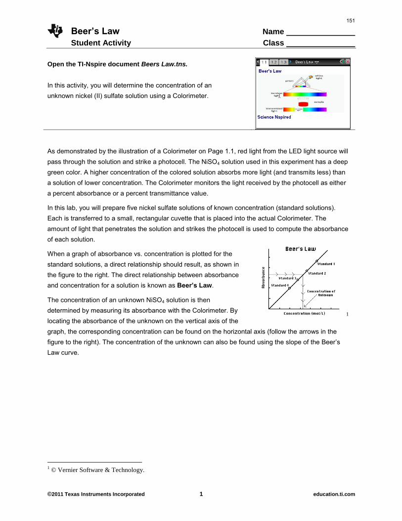
Beer’s Law Name Student Activity Class
©2011 Texas Instruments Incorporated 1 education.ti.com
Open the TI-Nspire document Beers Law.tns. In this activity, you will determine the concentration of an unknown nickel (II) sulfate solution using a Colorimeter.
As demonstrated by the illustration of a Colorimeter on Page 1.1, red light from the LED light source will pass through the solution and strike a photocell. The NiSO4 solution used in this experiment has a deep green color. A higher concentration of the colored solution absorbs more light (and transmits less) than a solution of lower concentration. The Colorimeter monitors the light received by the photocell as either a percent absorbance or a percent transmittance value.
In this lab, you will prepare five nickel sulfate solutions of known concentration (standard solutions). Each is transferred to a small, rectangular cuvette that is placed into the actual Colorimeter. The amount of light that penetrates the solution and strikes the photocell is used to compute the absorbance of each solution.
When a graph of absorbance vs. concentration is plotted for the standard solutions, a direct relationship should result, as shown in the figure to the right. The direct relationship between absorbance and concentration for a solution is known as Beer’s Law.
The concentration of an unknown NiSO4 solution is then determined by measuring its absorbance with the Colorimeter. By locating the absorbance of the unknown on the vertical axis of the
1
graph, the corresponding concentration can be found on the horizontal axis (follow the arrows in the figure to the right). The concentration of the unknown can also be found using the slope of the Beer’s
Law curve.
1 © Vernier Software & Technology.
151
Beer’s Law Name Student Activity Class
©2011 Texas Instruments Incorporated 2 education.ti.com
Move to pages 1.4 through 1.7. Press / ¢ and / ¡ to
navigate through the lesson. Answer the following questions on your handheld. 1. The wavelength of light used by the colorimeter should be ______________ by the colored solution. 2. The NiSO4 solution used in the experiment has a deep ______________ color. 3. For this experiment, the LED of the colorimeter needs to be set to ____________________. 4. A higher concentration of solution absorbs ________________ light. 5. The relationship between absorbance and concentration is _________________________. 6. The linear relationship between absorbance and concentration is called _________________ Law. 7. The concentration of the unknown can be determined by using the ____________ of the regression
line on the graph. Lab Set-Up and Procedures 8. Obtain and wear goggles.
CAUTION: Be careful not to ingest any nickel(II) sulfate solution or spill any on your skin. 9. Label five clean, dry test tubes with the numbers 1–5. 10. From a burette, deliver 2, 4, 6, 8, & 10 mL of 0.40 M nickel(II) sulfate solution into Test Tubes 1–5,
respectively. 11. From the second burette, deliver 8, 6, 4, 2, and 0 mL of distilled water into Test Tubes 1–5,
respectively. 12. Thoroughly mix each solution with a stirring rod. 13. Clean and dry the stirring rod between stirrings. Concentrations for the trials are: 0.08 M, 0.16M,
0.24M, 0.32M, and 0.40M, respectively. 14. Prepare a blank by filling an empty cuvette 3/4 full with distilled water.
Note: To correctly use a cuvette, remember: All cuvettes should be wiped clean and dried on the outside with a tissue. Handle cuvettes only by the top edge of the ribbed sides. All solutions should be free of bubbles. Always position the cuvette so the light passes through the clear sides.
152
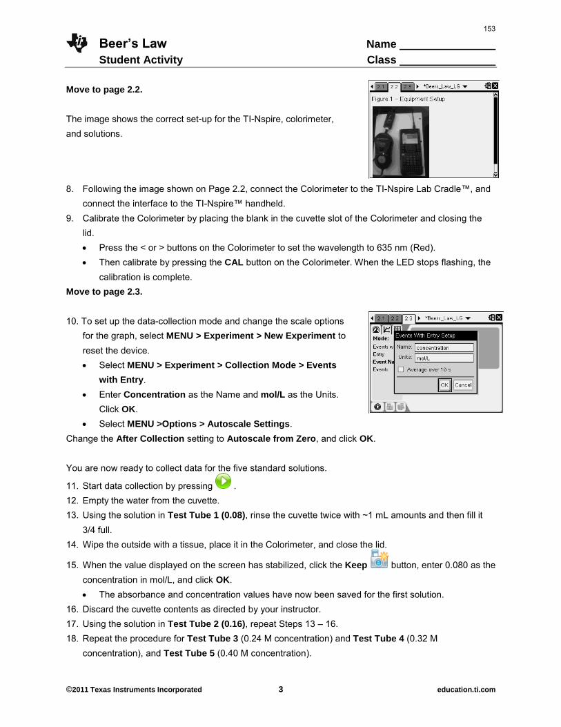
Beer’s Law Name Student Activity Class
©2011 Texas Instruments Incorporated 3 education.ti.com
Move to page 2.2.
The image shows the correct set-up for the TI-Nspire, colorimeter, and solutions.
8. Following the image shown on Page 2.2, connect the Colorimeter to the TI-Nspire Lab Cradle™, and
connect the interface to the TI-Nspire™ handheld. 9. Calibrate the Colorimeter by placing the blank in the cuvette slot of the Colorimeter and closing the
lid. Press the < or > buttons on the Colorimeter to set the wavelength to 635 nm (Red). Then calibrate by pressing the CAL button on the Colorimeter. When the LED stops flashing, the
calibration is complete. Move to page 2.3.
10. To set up the data-collection mode and change the scale options
for the graph, select MENU > Experiment > New Experiment to reset the device. Select MENU > Experiment > Collection Mode > Events
with Entry. Enter Concentration as the Name and mol/L as the Units.
Click OK.
Select MENU >Options > Autoscale Settings. Change the After Collection setting to Autoscale from Zero, and click OK. You are now ready to collect data for the five standard solutions.
11. Start data collection by pressing . 12. Empty the water from the cuvette. 13. Using the solution in Test Tube 1 (0.08), rinse the cuvette twice with ~1 mL amounts and then fill it
3/4 full. 14. Wipe the outside with a tissue, place it in the Colorimeter, and close the lid.
15. When the value displayed on the screen has stabilized, click the Keep button, enter 0.080 as the concentration in mol/L, and click OK. The absorbance and concentration values have now been saved for the first solution.
16. Discard the cuvette contents as directed by your instructor. 17. Using the solution in Test Tube 2 (0.16), repeat Steps 13 – 16. 18. Repeat the procedure for Test Tube 3 (0.24 M concentration) and Test Tube 4 (0.32 M
concentration), and Test Tube 5 (0.40 M concentration).
153
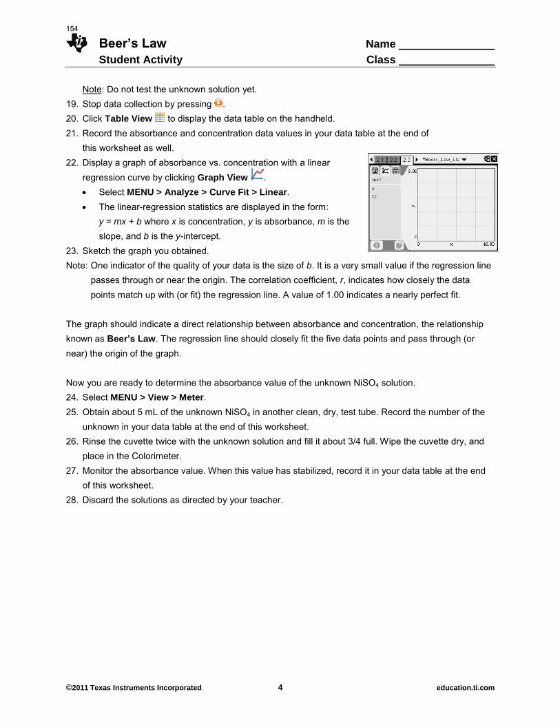
Beer’s Law Name Student Activity Class
©2011 Texas Instruments Incorporated 4 education.ti.com
Note: Do not test the unknown solution yet. 19. Stop data collection by pressing . 20. Click Table View to display the data table on the handheld. 21. Record the absorbance and concentration data values in your data table at the end of
this worksheet as well. 22. Display a graph of absorbance vs. concentration with a linear
regression curve by clicking Graph View . Select MENU > Analyze > Curve Fit > Linear. The linear-regression statistics are displayed in the form:
y = mx + b where x is concentration, y is absorbance, m is the slope, and b is the y-intercept.
23. Sketch the graph you obtained.
Note: One indicator of the quality of your data is the size of b. It is a very small value if the regression line passes through or near the origin. The correlation coefficient, r, indicates how closely the data points match up with (or fit) the regression line. A value of 1.00 indicates a nearly perfect fit.
The graph should indicate a direct relationship between absorbance and concentration, the relationship known as Beer’s Law. The regression line should closely fit the five data points and pass through (or near) the origin of the graph.
Now you are ready to determine the absorbance value of the unknown NiSO4 solution. 24. Select MENU > View > Meter. 25. Obtain about 5 mL of the unknown NiSO4 in another clean, dry, test tube. Record the number of the
unknown in your data table at the end of this worksheet. 26. Rinse the cuvette twice with the unknown solution and fill it about 3/4 full. Wipe the cuvette dry, and
place in the Colorimeter. 27. Monitor the absorbance value. When this value has stabilized, record it in your data table at the end
of this worksheet. 28. Discard the solutions as directed by your teacher.
154
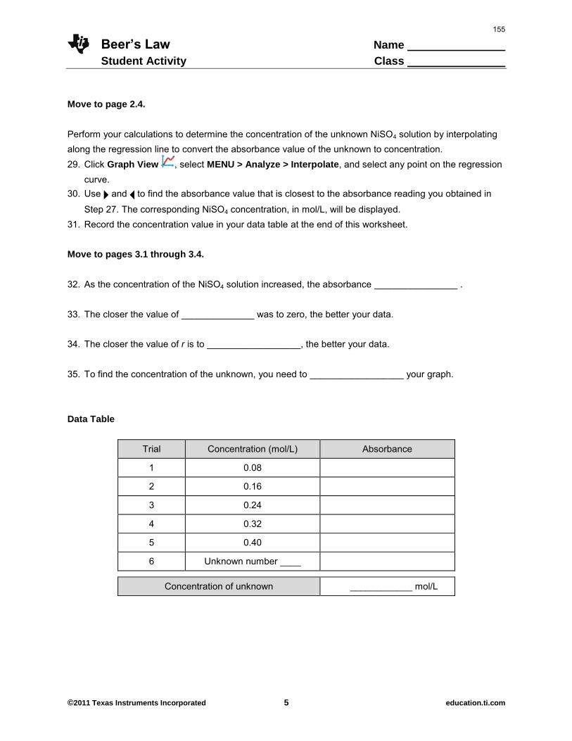
Beer’s Law Name Student Activity Class
©2011 Texas Instruments Incorporated 5 education.ti.com
Move to page 2.4. Perform your calculations to determine the concentration of the unknown NiSO4 solution by interpolating along the regression line to convert the absorbance value of the unknown to concentration. 29. Click Graph View , select MENU > Analyze > Interpolate, and select any point on the regression
curve. 30. Use ¢ and ¡ to find the absorbance value that is closest to the absorbance reading you obtained in
Step 27. The corresponding NiSO4 concentration, in mol/L, will be displayed. 31. Record the concentration value in your data table at the end of this worksheet. Move to pages 3.1 through 3.4. 32. As the concentration of the NiSO4 solution increased, the absorbance ________________ . 33. The closer the value of ______________ was to zero, the better your data. 34. The closer the value of r is to __________________, the better your data. 35. To find the concentration of the unknown, you need to __________________ your graph.
Data Table
Trial Concentration (mol/L) Absorbance
1 0.08 2 0.16
3 0.24
4 0.32 5 0.40
6 Unknown number ____
Concentration of unknown ____________ mol/L
155

This page intentionally left blank
156
Beer’s Law TEACHER NOTES
SCIENCE NSPIRED
©2011 Texas Instruments Incorporated 1 education.ti.com
Science Objectives
Students will make a serial dilution of a NiSO4 standard solution. Students will use a Colorimeter to measure the absorbance value
of each standard solution. Students will find the relationship between absorbance and
concentration of a solution. Students will use the results of this experiment to determine the
unknown concentration of another NiSO4 solution. Vocabulary
absorbance Colorimeter correlation coefficient slope transmittance y-intercept About the Lesson
This lesson involves absorbance data for solutions of various concentration.
As a result, students will: Prepare five (5) NiSO4 standard solutions.
Use a Colorimeter to measure the absorbance value of each standard solution.
Find the relationship between absorbance and concentration of a solution.
Use the results of this experiment to determine the unknown concentration of another NiSO4 solution.
TI-Nspire™ Navigator™ System
Send Beers_Law.tns file to students. Use Screen Capture to monitor student progress. Collect and grade Beers_Law.tns file.
TI-Nspire™ Technology Skills: Download a TI-Nspire™
document Open a document Move between pages Use DataQuest App
Tech Tips:
Make sure the font size on your TI-Nspire handhelds is set to Medium.
You start and stop data
collection by pressing
and .
Lesson Files: Student Activity
Beers_Law_Student.pdf Beers_Law_Student.doc
TI-Nspire document Beers_Law.tns
Visit www.sciencenspired.com for lesson updates and tech tip videos.
157
Beer’s Law TEACHER NOTES
SCIENCE NSPIRED
©2011 Texas Instruments Incorporated 2 education.ti.com
Activity Materials
TI-Nspire™ Technology TI Lab Cradle™ or EasyLink™ Vernier® Colorimeter Two burettes Double burette clamp Ring stand Wash bottle & distilled water One cuvette Test tube rack & five (5) 20X150 mm test tubes Stirring rod KimWipes or tissues (preferably lint-free) 5 mL of “NiSO4” unknown solution (for example-55 mL of “stock” solution and 45
mL of water-0.22 M) 8-9 drops of green food coloring per liter of water to mimic 0.40 M NiSO4. (Nickel is
a carcinogen, so the green food coloring is an excellent substitute.) Check the absorbance of this stock solution to be certain it falls in the range of 0.40 to 0.80.
Activity Overview
Please print the student worksheet and make it available to students before beginning the lab. Lab background information as well as lab procedures are included only in the student worksheet. Always remember to review any safety precautions thoroughly with your students prior to starting the lab.
Students can answer the questions posed in the .tns file and submit for grading with TI-Nspire Navigator (optional) or students can answer directly on the student worksheet
Ensure that students collect data on the 5 known substances and look at the graph before they actually measure the absorbance of the unknown solution. This will allow them to make predictions based on the graph of the data.
158
Beer’s Law TEACHER NOTES
SCIENCE NSPIRED
©2011 Texas Instruments Incorporated 3 education.ti.com
Discussion Points and Possible Answers
TI-Nspire Navigator Opportunity
Use the TI-Nspire™ Navigator™ System to monitor student progress using Screen Capture.
Have students answer the pre-lab questions directly on their student worksheets or on Pages 1.4 – 1.7 prior to starting the lab procedure. Students will need to have read the background information presented in the Student Worksheet. 1. The wavelength of light used by the colorimeter should be _______ by the colored solution. Answer: absorbed 2. The NiSO4 solution used in the experiment has a deep _______ color.
Answer: green 3. For this experiment, the LED of the colorimeter needs to be set to _________.
Answer : red 4. A higher concentration of solution absorbs ________ light.
Answer: more
5. The relationship between absorbance and concentration is __________. Answer: direct 6. The linear relationship between absorbance and concentration is called ________ Law.
Answer: Beer’s 7. The concentration of the unknown can be determined by using the ______ of the regression line on
the graph.
Answer: slope
159
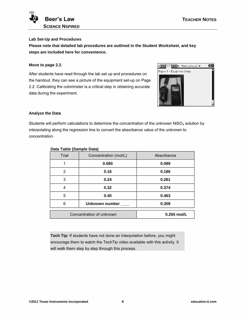
Beer’s Law TEACHER NOTES
SCIENCE NSPIRED
©2011 Texas Instruments Incorporated 4 education.ti.com
Lab Set-Up and Procedures Please note that detailed lab procedures are outlined in the Student Worksheet, and key
steps are included here for convenience.
Move to page 2.2.
After students have read through the lab set up and procedures on the handout, they can see a picture of the equipment set-up on Page 2.2. Calibrating the colorimeter is a critical step in obtaining accurate data during the experiment.
Analyze the Data
Students will perform calculations to determine the concentration of the unknown NiSO4 solution by interpolating along the regression line to convert the absorbance value of the unknown to concentration.
Data Table (Sample Data)
Trial Concentration (mol/L) Absorbance
1 0.080 0.089
2 0.16 0.186
3 0.24 0.281
4 0.32 0.374
5 0.40 0.463
6 Unknown number ____ 0.308
Concentration of unknown 0.265 mol/L
Tech Tip: If students have not done an Interpolation before, you might encourage them to watch the TechTip video available with this activity. It will walk them step by step through this process.
160
Beer’s Law TEACHER NOTES
SCIENCE NSPIRED
©2011 Texas Instruments Incorporated 5 education.ti.com
Post-lab Assessment Have students respond to the questions (below) directly on their student worksheets (or on Pages 3.1 through 3.4) once they have completed the lab. 8. As the concentration of the nickel(II) sulfate solution increased, the absorbance _______. Answer: increased 9. The closer the value of ______ was to zero, the better your data. Answer: b 10. The closer the value of r is to ______, the better your data. Answer: 1 11. To find the concentration of the unknown, you need to _______ your graph.
Answer: interpolate
TI-Nspire Navigator Opportunity
Use the TI-Nspire™ Navigator™ System to collect, grade, and save the .tns file to the Portfolio. Use Slide Show to view student responses.
Wrap Up
Upon completion of the lab and discussion, the teacher should ensure that students are able to understand: The importance of accurately preparing solutions for the lab. How to gather and analyze data. The relationship between the absorbance and concentration of a solution.
Assessment Students can complete the embedded multiple choice questions in the Beers_Law.tns file. In addition, students can answer questions on the student activity sheet.
161

This page intentionally left blank
162
Cellular Respiration Name Student Activity Class
©2011 Texas Instruments Incorporated 1 education.ti.com
Open the TI-Nspire document Cellular Respiration.tns.
In this activity, you will be measuring the rate of cellular respiration
in germinating peas. Do you think that pea plants only do
photosynthesis and that cellular respiration is reserved for
animals? Think again!
Of all the major biochemical processes in the living world, none is as universal as aerobic
cellular respiration. The vast majority of organisms on our planet break down glucose
(C6H12O6) in the presence of oxygen (O2) using cell mitochondria. This process is called
cellular respiration. The waste by-products of this process are carbon dioxide (CO2) and
water (H2O).
Cellular Respiration plays a major role in the overall metabolism of an organism.
"Metabolism" can be subdivided into processes that BUILD bigger molecules from smaller
ones (anabolism), and those that BREAK bigger molecules into smaller ones (catabolism).
This activity will give you the opportunity to measure the rate of one of these processes—
cellular respiration. During the activity, be thinking about examples of various types of
metabolic processes.
Move to pages 1.5 through 1.12.
Press / ¢ and / ¡ to
navigate through the lesson.
Answer the following questions on your handheld.
1. Which of the following is NOT a reasonable way to measure the rate of cell respiration in a high
school science lab setting?
A. Measure how fast glucose is made
B. Measure how fast oxygen gets used up
C. Measure how fast carbon dioxide is produced
2. In which cellular organelle is glucose MADE?
A. Mitochondria B. Ribosome C. Chloroplast D. Nucleus
3. Whereas animal cells can do only cell respiration, plant cells can only do photosynthesis.
A. True B. False
4. Eukaryotic cells have nuclei.
A. True B. False
163
Cellular Respiration Name Student Activity Class
©2011 Texas Instruments Incorporated 2 education.ti.com
5. Eukaryotic cells have mitochondria.
A. True B. False
6. Prokaryotic cells contain:
A. Nuclei, but no mitochondria B. No nuclei, but mitochondria
C. Nuclei and mitochondria D. Neither nuclei nor mitochondria
7. Which of the following is NOT a eukaryotic cell?
A. A plant leaf epidermis cell B. A lactobacillus bacterium
C. A mushroom cell D. An iguana muscle cell
8. C6H12O6 + O2 CO2 + H2O
When this equation is correctly balanced, the coefficients for oxygen and CO2 should be:
A. 1, 1 B. 3, 3 C. 6, 6 D. 12, 12
Move to page 2.2.
9. Connect the EasyLink™ to your TI-Nspire handheld, and then connect the CO2 sensor to the
EasyLink.
10. Allow time for the probe to "warm up", and for the display to stabilize (1-2 min.).
11. Set up the data collection to collect every 10 seconds for a total of 10 minutes.
12. Put 10 non-germinating peas in the small cup.
13. Answer the following questions BEFORE collecting data.
Move to pages 2.3 and 2.4.
14. During this portion of the experiment, what do you predict will happen with the carbon dioxide level
in the reaction bottle? I predict it will:
A. Increase B. Decrease C. Neither increase nor decrease
15. In performing a scientific experiment, a prediction of expected results is called the:
A. control B. variable C. conclusion D. theory
164
Cellular Respiration Name Student Activity Class
©2011 Texas Instruments Incorporated 3 education.ti.com
Move to page 2.5.
16. When you are ready, pour the non-germinating peas into the reaction bottle, start the data
collection, and place the probe into the bottle.
17. During the experiment, move to the next page, and watch the data being graphed as it is collected.
Move to page 2.7.
18. Determine the rate of CO2 production by selecting MENU > Analyze > Regression > Show Linear
(mx+b).
19. Record the rate (“m”) in the data table.
20. Return the dry peas to the container from which you got them.
Move to page 2.8.
21. Use the spreadsheet on Page 2.8 to record the cell respiration rates for your first trial.
Move to page 2.9.
22. Were you correct in the prediction you made earlier?
A. Yes B. No
Move to page 2.10.
23. What should the "data label" be for the rate of change in this experiment?
24. Between trials, fill the bottle with water, then pour the water out. This removes any residual carbon
dioxide left from the previous trial.
25. Repeat the procedure using: 10 germinating peas (Trial 2) 5 germinating and 5 dry peas (Trial 3) 10 germinating peas in an ice water bath (Trial 4) 10 germinating peas in a warm water bath (Trial 5)
26. Record your analyses in the data table.
27. Write up a descriptive analysis of the results of your experiments.
165
Cellular Respiration Name Student Activity Class
©2011 Texas Instruments Incorporated 4 education.ti.com
Move to pages 3.1 through 3.13.
Answer the following questions on your handheld.
28. Why did you perform one trial using peas that were not yet germinating?
29. Non-germinating peas are in a state of dormancy. What would you expect the CO2 production to
be?
30. What difference in CO2 production would you expect if using 5 germinating peas instead of 10?
31. If you got some CO2 production from the non-germinating peas, how should you mathematically
adjust the CO2 production from the germinating peas?
a. I should add the CO2 production from the non-germinating to the germinating data.
b. I should subtract the CO2 production from the non-germinating to the germinating data.
32. Which would you predict would have a great CO2 production rate: 10 peas at room temperature or
10 peas in warm water? Explain.
33. If you used an oxygen gas sensor instead of a CO2 sensor, predict what results.
34. Were your germinating peas performing photosynthesis? Explain by citing evidence from the
experiment.
35. Which biochemical process(es) can be performed by plants?
A. Photosynthesis B. Cellular Respiration
C. Both photosynthesis and cellular respiration
D. Neither photosynthesis nor cellular respiration
36. What cellular organelles would you expect to find in plant cells?
A. Mitochondria B. Chloroplasts
C. Both mitochondria and chloroplasts
D. Neither mitochondria nor chloroplasts
37. Which cellular organelles would you expect to find in animal cells?
A. Mitochondria B. Chloroplasts
C. Both mitochondria and chloroplasts
D. Neither mitochondria nor chloroplasts
166
Cellular Respiration Name Student Activity Class
©2011 Texas Instruments Incorporated 5 education.ti.com
38. OVERALL, the process of photosynthesis is:
A. Anabolic B. Catabolic
C. Both anabolic and catabolic
D. Neither anabolic nor catabolic
39. OVERALL, the process of cellular respiration is:
A. Anabolic B. Catabolic
C. Both anabolic and catabolic
D. Neither anabolic nor catabolic
167

This page intentionally left blank
168
Cellular Respiration TEACHER NOTES
TI PROFESSIONAL DEVELOPMENT
©2011 Texas Instruments Incorporated 1 education.ti.com
Science Objectives Students will collect data for carbon dioxide amounts when
testing germinating and non-germinating peas.
Students will do several trials using several different variables.
Math Objectives Students will generate, compare, and analyze the rates of change
(slopes) of several linear mathematical models.
Materials Needed TI-Nspire™ or TI-Nspire™ CAS handheld
Easy Link™
Vernier® CO2 Gas Sensor
Reaction bottle
Dry, non-germinating peas
Germinating peas
Ice
Warm water
Vocabulary cellular respiration germinating
photosynthesis non-germinating
glucose mitochondria
variable enzymes
control
About the Lesson This lesson involves collecting data for the carbon dioxide output
of germinating peas in an enclosed container.
As a result, students will:
Compare the rates of change when different variables are
tested.
TI-Nspire™ Navigator™ System Use Screen Capture to monitor student progress.
Live Presenter allows students to show their graphs to the class.
TI-Nspire™ Technology Skills:
Download a TI-Nspire
document
Open a document
Move between pages
Entering and graphing data
using multiple applications
Tracing, interpolating,
predicting
Tech Tips:
Make sure the font size on
your TI-Nspire handhelds is
set to Medium.
You can hide the function
entry line by pressing / G.
Lesson Materials: Student Activity
Cellular Respiration.pdf
Cellular Respiration.doc
TI-Nspire document Cellular Respiration.tns
169
Cellular Respiration TEACHER NOTES
TI PROFESSIONAL DEVELOPMENT
©2011 Texas Instruments Incorporated 2 education.ti.com
Discussion Points and Possible Answers
Move to pages 1.5 through 1.12.
Answer the following questions on your handheld.
1. Which of the following is NOT a reasonable way to measure the rate of cell respiration in a high
school science lab setting?
Answer: A. Measure how fast glucose is made
2. In which cellular organelle is glucose MADE?
Answer: C. Chloroplast
3. Whereas animal cells can do only cell respiration, plant cells can only do photosynthesis.
Answer: B. False
4. Eukaryotic cells have nuclei.
Answer: A. True
5. Eukaryotic cells have mitochondria.
Answer: A. True
6. Prokaryotic cells contain:
Answer: D. Neither nuclei nor mitochondria
7. Which of the following is NOT a eukaryotic cell?
Answer: B. A lactobacillus bacterium
170
Cellular Respiration TEACHER NOTES
TI PROFESSIONAL DEVELOPMENT
©2011 Texas Instruments Incorporated 3 education.ti.com
8. C6H12O6 + O2 CO2 + H2O
When this equation is correctly balanced, the coefficients for oxygen and CO2 should be:
Answer: C. 6, 6
Move to page 2.2.
9. Connect the EasyLink™ to your TI-Nspire handheld, and then connect the CO2 sensor to the
EasyLink.
10. Allow time for the probe to "warm up", and for the display to stabilize (1-2 min.).
11. Set up the data collection to collect every 10 seconds for a total of 10 minutes.
12. Put 10 non-germinating peas in the small cup.
13. Answer the following questions BEFORE collecting data.
Move to pages 2.3 and 2.4.
14. During this portion of the experiment, what do you predict will happen with the carbon dioxide level
in the reaction bottle? I predict it will:
Sample Answers: Student answers will vary.
15. In performing a scientific experiment, a prediction of expected results is called the:
Answer: A. control
Move to page 2.5.
16. When you are ready, pour the non-germinating peas into the reaction bottle, start the data
collection, and place the probe into the bottle.
17. During the experiment, move to the next page, and watch the data being graphed as it is collected.
Move to page 2.7.
18. Determine the rate of CO2 production by selecting MENU > Analyze > Regression > Show Linear
(mx+b).
19. Record the rate (“m”) in the data table.
20. Return the dry peas to the container from which you got them.
171
Cellular Respiration TEACHER NOTES
TI PROFESSIONAL DEVELOPMENT
©2011 Texas Instruments Incorporated 4 education.ti.com
Move to page 2.8.
21. Use the spreadsheet on Page 2.8 to record the cell respiration rates for your first trial.
Move to page 2.9.
22. Were you correct in the prediction you made earlier?
Sample Answers: Student answers will vary.
Move to page 2.10.
23. What should the "data label" be for the rate of change in this experiment?
Answer: Parts per thousand CO2/second.
24. Between trials, fill the bottle with water, then pour the water out. This removes any residual carbon
dioxide left from the previous trial.
25. Repeat the procedure using: 10 germinating peas (Trial 2)
5 germinating and 5 dry peas (Trial 3)
10 germinating peas in an ice water bath (Trial 4)
10 germinating peas in a warm water bath (Trial 5)
26. Record your analyses in the data table.
27. Write up a descriptive analysis of the results of your experiments.
Sample Answers: Answers will vary.
Move to page 3.1.
28. Why did you perform one trial using peas that were not yet germinating?
Answer: As a control.
172
Cellular Respiration TEACHER NOTES
TI PROFESSIONAL DEVELOPMENT
©2011 Texas Instruments Incorporated 5 education.ti.com
Move to page 3.2.
29. Non-germinating peas are in a state of dormancy. What would you expect the CO2 production to
be?
Answer: Zero. Move to page 3.3.
30. What difference in CO2 production would you expect if using 5 germinating peas instead of 10?
Answer: Approximately half the production of CO2.
Move to page 3.4.
31. If you got some CO2 production from the non-germinating peas, how should you mathematically
adjust the CO2 production from the germinating peas? Answer: b. I should subtract the CO2 production from the non-germinating to the germinating data.
Move to page 3.5.
32. Which would you predict would have a great CO2 production rate: 10 peas at room temperature or
10 peas in warm water? Explain.
Answer: Warm water. Heat speeds up the activity rate of enzymes (cellular respiration). Move to page 3.6.
33. If you had used an oxygen gas sensor instead of a CO2 sensor, predict what results would you
have expected.
Answer: Oxygen levels would have decreased because it is used for cellular respiration.
173
Cellular Respiration TEACHER NOTES
TI PROFESSIONAL DEVELOPMENT
©2011 Texas Instruments Incorporated 6 education.ti.com
Move to page 3.7.
34. Were your germinating peas doing photosynthesis? Explain by citing evidence from the
experiment.
Answer: No. Carbon Dioxide levels increased in the chamber. There were no leaves on the plant yet.
Move to page 3.8.
35. Which biochemical process(es) can be performed by plants?
Answer: B. Both photosynthesis and cellular respiration
Move to page 3.9.
36. What cellular organelles would you expect to find in plant cells? Answer: C. Both mitochondria and chloroplasts
Move to page 3.10.
37. Which cellular organelles would you expect to find in animal cells?
Answer: A. Mitochondria
Move to page 3.11.
38. OVERALL, the process of photosynthesis is: Answer: A. Anabolic
Move to page 3.12.
39. OVERALL, the process of cellular respiration is:
Answer: B. Catabolic
TI-Nspire Navigator Opportunity: Screen Capture
See Note 1 at the end of the lesson.
174
Cellular Respiration TEACHER NOTES
TI PROFESSIONAL DEVELOPMENT
©2011 Texas Instruments Incorporated 7 education.ti.com
Assessment Formative assessment will consist of questions embedded in the .tns file. The questions will be graded
when the .tns file is retrieved. The Slide Show can be utilized to give students immediate feedback on
their assessment.
TI-Nspire Navigator
Note 1
Screen Capture can be used to monitor student progress.
175

This page intentionally left blank
176
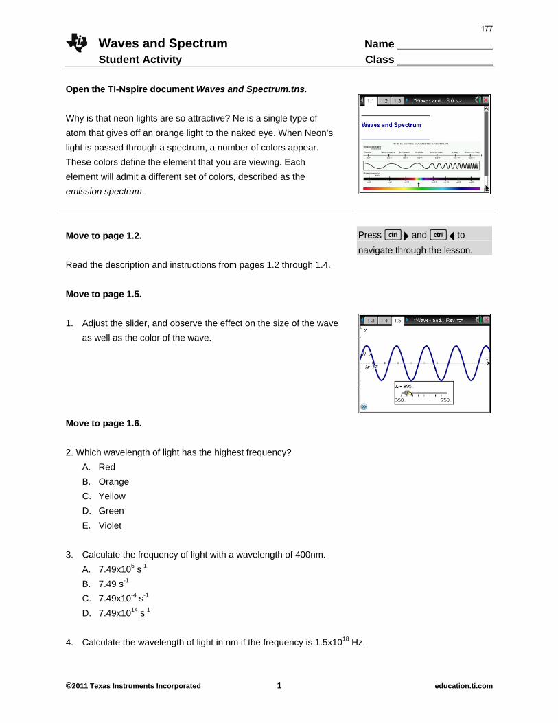
Waves and Spectrum Name Student Activity Class
©2011 Texas Instruments Incorporated 1 education.ti.com
Open the TI-Nspire document Waves and Spectrum.tns.
Why is that neon lights are so attractive? Ne is a single type of
atom that gives off an orange light to the naked eye. When Neon’s
light is passed through a spectrum, a number of colors appear.
These colors define the element that you are viewing. Each
element will admit a different set of colors, described as the
emission spectrum.
Move to page 1.2.
Press / ¢ and / ¡ to
navigate through the lesson.
Read the description and instructions from pages 1.2 through 1.4.
Move to page 1.5.
1. Adjust the slider, and observe the effect on the size of the wave
as well as the color of the wave.
Move to page 1.6.
2. Which wavelength of light has the highest frequency?
A. Red
B. Orange
C. Yellow
D. Green
E. Violet
3. Calculate the frequency of light with a wavelength of 400nm.
A. 7.49x10⁵ s-1
B. 7.49 s-1
C. 7.49x10⁻⁴ s-1
D. 7.49x10¹⁴ s-1
4. Calculate the wavelength of light in nm if the frequency is 1.5x10¹⁸ Hz.
177
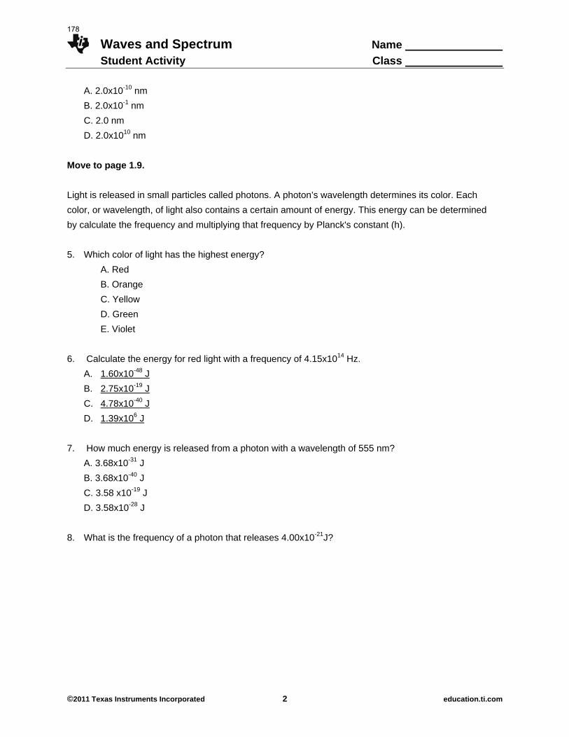
Waves and Spectrum Name Student Activity Class
©2011 Texas Instruments Incorporated 2 education.ti.com
A. 2.0x10⁻¹⁰ nm
B. 2.0x10⁻¹ nm
C. 2.0 nm
D. 2.0x10¹⁰ nm
Move to page 1.9.
Light is released in small particles called photons. A photon’s wavelength determines its color. Each
color, or wavelength, of light also contains a certain amount of energy. This energy can be determined
by calculate the frequency and multiplying that frequency by Planck's constant (h).
5. Which color of light has the highest energy?
A. Red
B. Orange
C. Yellow
D. Green
E. Violet
6. Calculate the energy for red light with a frequency of 4.15x10¹⁴ Hz.
A. 1.60x10-48 J
B. 2.75x10⁻¹⁹ J
C. 4.78x10-40 J
D. 1.39x10⁶ J
7. How much energy is released from a photon with a wavelength of 555 nm?
A. 3.68x10⁻³¹ J
B. 3.68x10-40 J
C. 3.58 x10⁻¹⁹ J
D. 3.58x10⁻²⁸ J
8. What is the frequency of a photon that releases 4.00x10⁻²¹J?
178
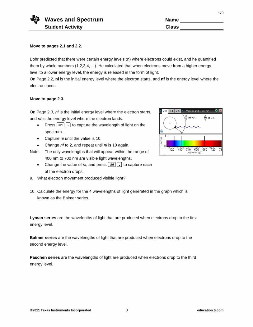
Waves and Spectrum Name Student Activity Class
©2011 Texas Instruments Incorporated 3 education.ti.com
Move to pages 2.1 and 2.2.
Bohr predicted that there were certain energy levels (n) where electrons could exist, and he quantified
them by whole numbers (1,2,3,4, ...). He calculated that when electrons move from a higher energy
level to a lower energy level, the energy is released in the form of light.
On Page 2.2, ni is the initial energy level where the electron starts, and nf is the energy level where the
electron lands.
Move to page 2.3.
On Page 2.3, ni is the initial energy level where the electron starts,
and nf is the energy level where the electron lands.
Press / ^ to capture the wavelength of light on the
spectrum.
Capture ni until the value is 10.
Change nf to 2, and repeat until ni is 10 again.
Note: The only wavelengths that will appear within the range of
400 nm to 700 nm are visible light wavelengths.
Change the value of ni, and press / ^ to capture each
of the electron drops.
9. What electron movement produced visible light?
10. Calculate the energy for the 4 wavelengths of light generated in the graph which is
known as the Balmer series.
Lyman series are the wavelenths of light that are produced when electrons drop to the first
energy level.
Balmer series are the wavelengths of light that are produced when electrons drop to the
second energy level.
Paschen series are the wavelengths of light are produced when electrons drop to the third
energy level.
179
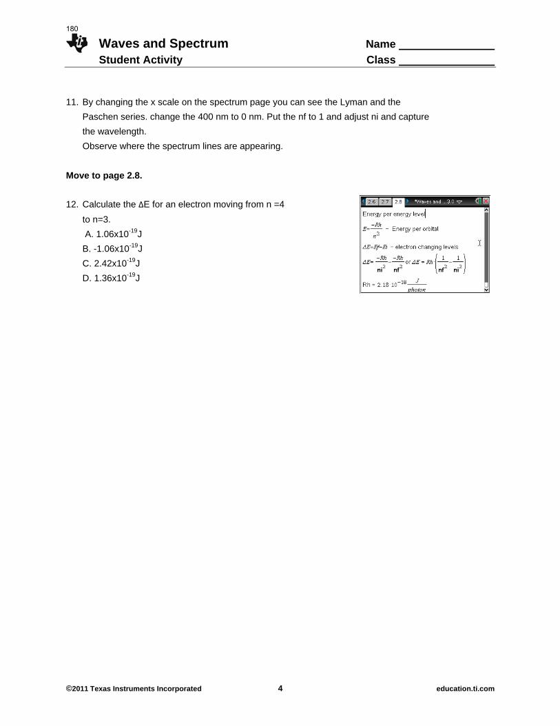
Waves and Spectrum Name Student Activity Class
©2011 Texas Instruments Incorporated 4 education.ti.com
11. By changing the x scale on the spectrum page you can see the Lyman and the
Paschen series. change the 400 nm to 0 nm. Put the nf to 1 and adjust ni and capture
the wavelength.
Observe where the spectrum lines are appearing.
Move to page 2.8.
12. Calculate the ∆E for an electron moving from n =4
to n=3.
A. 1.06x10⁻¹⁹J
B. -1.06x10⁻¹⁹J
C. 2.42x10⁻¹⁹J
D. 1.36x10⁻¹⁹J
180
Waves and Spectrum TEACHER NOTES
TI PROFESSIONAL DEVELOPMENT
©2011 Texas Instruments Incorporated 1 education.ti.com
Science Objectives Students will study the relationship between wavelength,
frequency, and color.
Students will calculate wavelengths and frequencies.
Students will calculate the energy of electromagnetic radiation
using Planck’s Constant.
Students will study the energy changes as electrons change
energy levels in an atom.
Students will learn about the Balmer, Paschen, and Lyman
Series.
Students will calculate the energy change that an electron
undergoes when changing energy levels using the Rhydberg
Constant.
Vocabulary speed of light photons
wavelength Planck’s Constant
frequency Balmer Series
electromagnetic Paschen Series
radiation Lyman Series
visible spectrum Rhydberg Constant
About the Lesson This lesson involves the relationship between waves and electron
energy jumps within the atom.
As a result, students will:
Study the relationship between wavelength, frequency ,and
color.
Calculate wavelengths and frequencies.
Calculate the energy of electromagnetic radiation using
Planck’s Constant.
Study the energy changes as electrons change energy levels
in an atom.
Learn about the Balmer, Paschen, and Lyman Series.
Calculate the energy change that an electron undergoes
when changing energy levels using the Rhydberg Constant.
TI-Nspire™ Technology Skills:
Download a TI-Nspire
document
Open a document
Move between pages
Capture a data point using
/ ^
Tech Tips:
Make sure that participants
understand how to capture a
data point using / ^
Lesson Materials:
TI-Nspire document Waves and Spectrum.tns
181
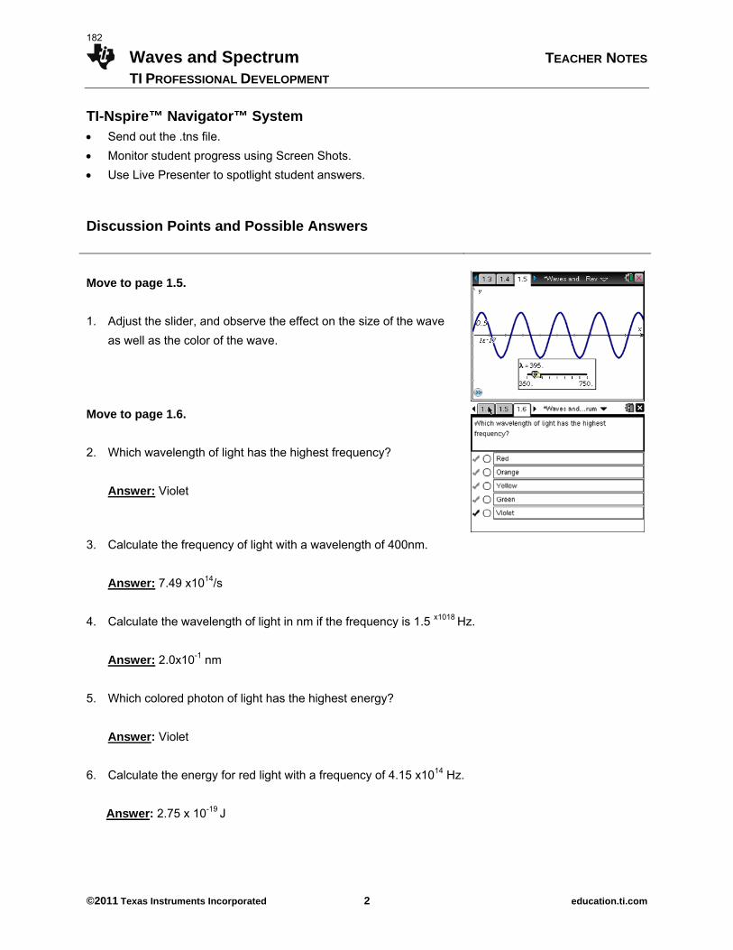
Waves and Spectrum TEACHER NOTES
TI PROFESSIONAL DEVELOPMENT
©2011 Texas Instruments Incorporated 2 education.ti.com
TI-Nspire™ Navigator™ System Send out the .tns file.
Monitor student progress using Screen Shots.
Use Live Presenter to spotlight student answers. Discussion Points and Possible Answers
Move to page 1.5.
1. Adjust the slider, and observe the effect on the size of the wave
as well as the color of the wave.
Move to page 1.6.
2. Which wavelength of light has the highest frequency?
Answer: Violet
3. Calculate the frequency of light with a wavelength of 400nm.
Answer: 7.49 x10¹⁴/s
4. Calculate the wavelength of light in nm if the frequency is 1.5 x10¹⁸ Hz.
Answer: 2.0x10⁻¹ nm
5. Which colored photon of light has the highest energy?
Answer: Violet
6. Calculate the energy for red light with a frequency of 4.15 x10¹⁴ Hz.
Answer: 2.75 x 10⁻¹⁹ J
182
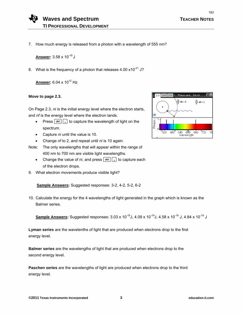
Waves and Spectrum TEACHER NOTES
TI PROFESSIONAL DEVELOPMENT
©2011 Texas Instruments Incorporated 3 education.ti.com
7. How much energy is released from a photon with a wavelength of 555 nm?
Answer: 3.58 x 10⁻¹⁹ J
8. What is the frequency of a photon that releases 4.00 x10⁻²¹ J?
Answer: 6.04 x 10¹² Hz
Move to page 2.3.
On Page 2.3, ni is the initial energy level where the electron starts,
and nf is the energy level where the electron lands.
Press / ^ to capture the wavelength of light on the
spectrum.
Capture ni until the value is 10.
Change nf to 2, and repeat until ni is 10 again.
Note: The only wavelengths that will appear within the range of
400 nm to 700 nm are visible light wavelengths.
Change the value of ni, and press / ^ to capture each
of the electron drops.
9. What electron movements produce visible light?
Sample Answers: Suggested responses: 3-2, 4-2, 5-2, 6-2
10. Calculate the energy for the 4 wavelengths of light generated in the graph which is known as the
Balmer series.
Sample Answers: Suggested responses: 3.03 x 10⁻¹⁹J, 4.09 x 10⁻¹⁹J, 4.58 x 10⁻¹⁹ J, 4.84 x 10⁻¹⁹ J
Lyman series are the wavelenths of light that are produced when electrons drop to the first
energy level.
Balmer series are the wavelengths of light that are produced when electrons drop to the
second energy level.
Paschen series are the wavelengths of light are produced when electrons drop to the third
energy level.
183
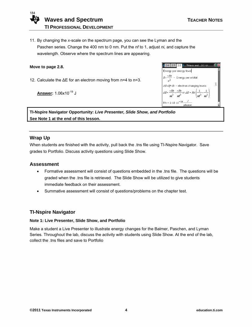
Waves and Spectrum TEACHER NOTES
TI PROFESSIONAL DEVELOPMENT
©2011 Texas Instruments Incorporated 4 education.ti.com
11. By changing the x-scale on the spectrum page, you can see the Lyman and the
Paschen series. Change the 400 nm to 0 nm. Put the nf to 1, adjust ni, and capture the
wavelength. Observe where the spectrum lines are appearing.
Move to page 2.8.
12. Calculate the ∆E for an electron moving from n=4 to n=3.
Answer: 1.06x10⁻¹⁹ J
TI-Nspire Navigator Opportunity: Live Presenter, Slide Show, and Portfolio
See Note 1 at the end of this lesson.
Wrap Up When students are finished with the activity, pull back the .tns file using TI-Nspire Navigator. Save
grades to Portfolio. Discuss activity questions using Slide Show.
Assessment Formative assessment will consist of questions embedded in the .tns file. The questions will be
graded when the .tns file is retrieved. The Slide Show will be utilized to give students
immediate feedback on their assessment.
Summative assessment will consist of questions/problems on the chapter test.
TI-Nspire Navigator
Note 1: Live Presenter, Slide Show, and Portfolio
Make a student a Live Presenter to illustrate energy changes for the Balmer, Paschen, and Lyman Series. Throughout the lab, discuss the activity with students using Slide Show. At the end of the lab, collect the .tns files and save to Portfolio
184
Sound and Waves Name Student Activity Class
©2011 Texas Instruments Incorporated 1 education.ti.com
Open the TI-Nspire document Sound and Waves.tns.
Sound is created by movement of air particles. These particles
move in specific patterns to create noise or notes. Specific notes
such as a C note is created by a very specific pattern. These
patterns can be modeled by waves. In this activity you will explore
these wave patterns and relate them to the sound.
Move to page 1.2. Press / ¢ and / ¡ to
navigate through the lesson.
1. Explore the wave that is generated on Page 1.2 by changing the amp (amplitude) slider
and observing the results. Change the freq (frequency) slider, and observe the changes
that occur.
Move to pages 1.3 to 1.7.
2. What happens to the wave when amplitude (amp) is changed?
3. What parts of the wave do not change when you adjust the amplitude?
4. If the amplitude is set to 5, how is the 5 represented on the graph?
5. What changes when frequency (freq) is changed?
6. If the frequency is 2, how is this number represented on the graph?
Amplitude is the height of the wave from the line of symmetry or the middle of the wave.
Frequency is the number of waves per time interval.
Sound travels in waves with different frequencies and amplitudes.
185
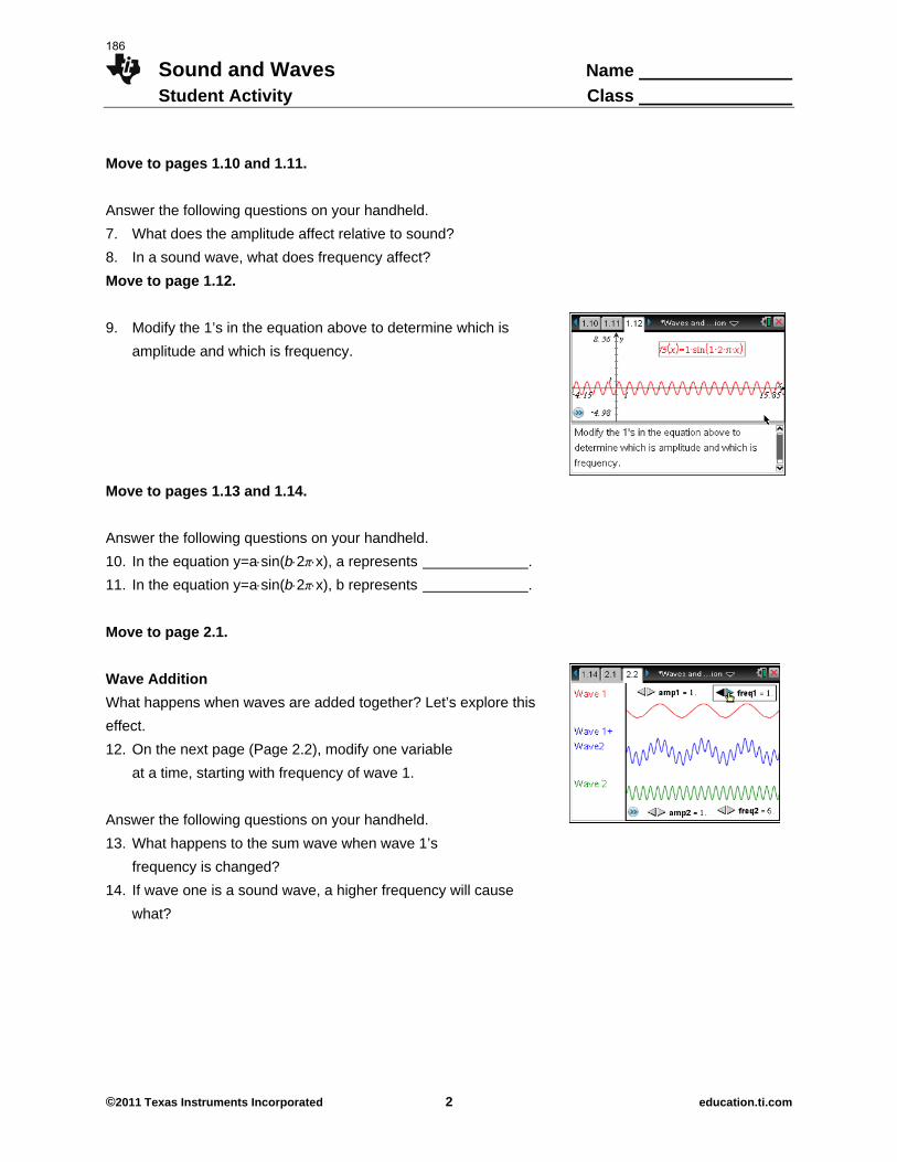
Sound and Waves Name Student Activity Class
©2011 Texas Instruments Incorporated 2 education.ti.com
Move to pages 1.10 and 1.11.
Answer the following questions on your handheld.
7. What does the amplitude affect relative to sound?
8. In a sound wave, what does frequency affect?
Move to page 1.12.
9. Modify the 1’s in the equation above to determine which is
amplitude and which is frequency.
Move to pages 1.13 and 1.14.
Answer the following questions on your handheld.
10. In the equation y=asin(b2πx), a represents .
11. In the equation y=asin(b2πx), b represents .
Move to page 2.1.
Wave Addition
What happens when waves are added together? Let’s explore this
effect.
12. On the next page (Page 2.2), modify one variable
at a time, starting with frequency of wave 1.
Answer the following questions on your handheld.
13. What happens to the sum wave when wave 1’s
frequency is changed?
14. If wave one is a sound wave, a higher frequency will cause
what?
186
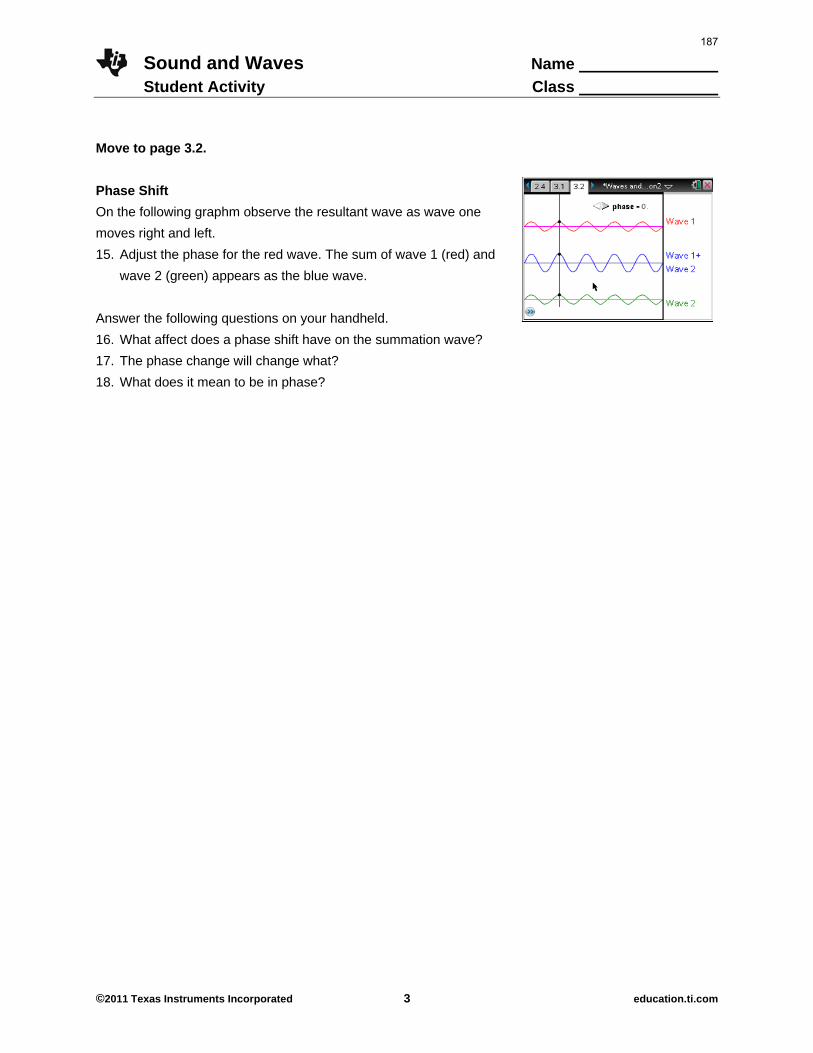
Sound and Waves Name Student Activity Class
©2011 Texas Instruments Incorporated 3 education.ti.com
Move to page 3.2.
Phase Shift
On the following graphm observe the resultant wave as wave one
moves right and left.
15. Adjust the phase for the red wave. The sum of wave 1 (red) and
wave 2 (green) appears as the blue wave.
Answer the following questions on your handheld.
16. What affect does a phase shift have on the summation wave?
17. The phase change will change what?
18. What does it mean to be in phase?
187

This page intentionally left blank
188
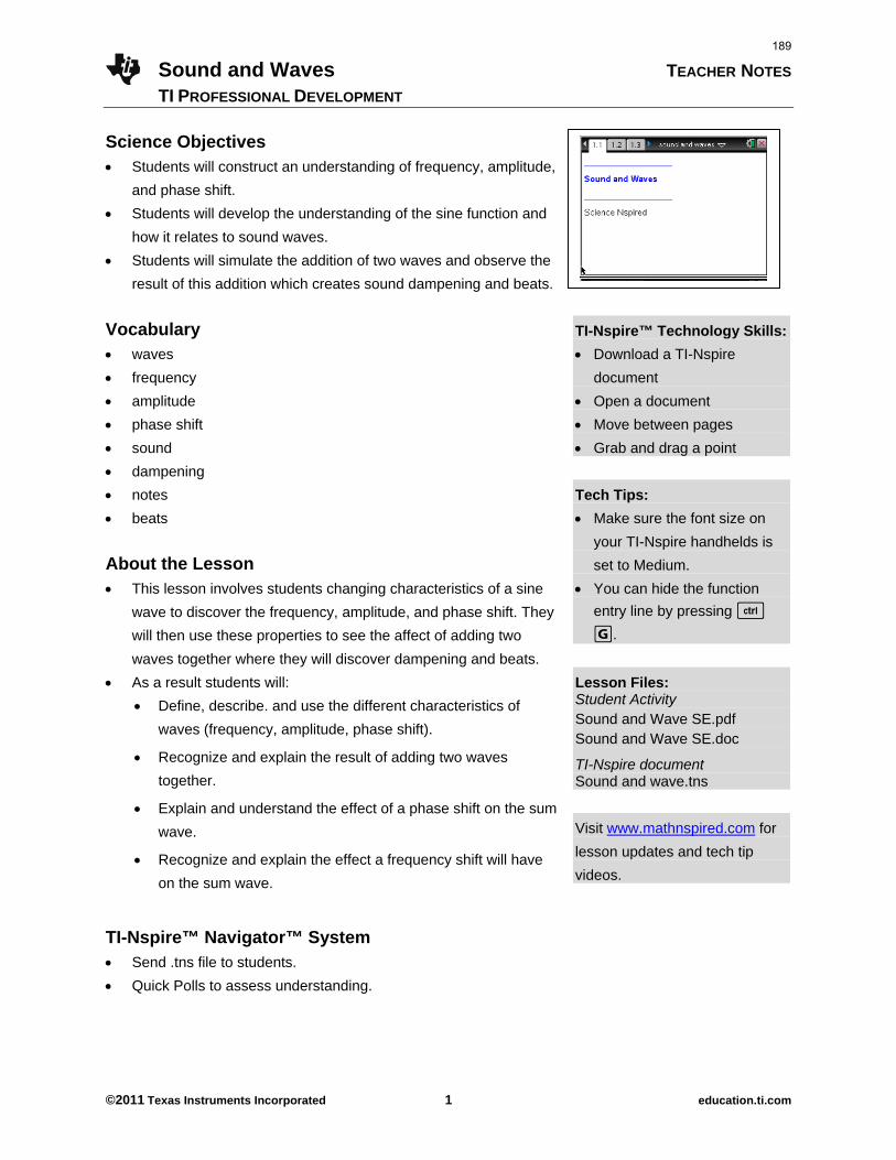
Sound and Waves TEACHER NOTES
TI PROFESSIONAL DEVELOPMENT
©2011 Texas Instruments Incorporated 1 education.ti.com
Science Objectives Students will construct an understanding of frequency, amplitude,
and phase shift.
Students will develop the understanding of the sine function and
how it relates to sound waves.
Students will simulate the addition of two waves and observe the
result of this addition which creates sound dampening and beats.
Vocabulary waves
frequency
amplitude
phase shift
sound
dampening
notes
beats
About the Lesson This lesson involves students changing characteristics of a sine
wave to discover the frequency, amplitude, and phase shift. They
will then use these properties to see the affect of adding two
waves together where they will discover dampening and beats.
As a result students will:
Define, describe. and use the different characteristics of
waves (frequency, amplitude, phase shift).
Recognize and explain the result of adding two waves
together.
Explain and understand the effect of a phase shift on the sum
wave.
Recognize and explain the effect a frequency shift will have
on the sum wave.
TI-Nspire™ Navigator™ System Send .tns file to students.
Quick Polls to assess understanding.
TI-Nspire™ Technology Skills:
Download a TI-Nspire
document
Open a document
Move between pages
Grab and drag a point
Tech Tips:
Make sure the font size on
your TI-Nspire handhelds is
set to Medium.
You can hide the function
entry line by pressing / G.
Lesson Files: Student Activity Sound and Wave SE.pdf Sound and Wave SE.doc
TI-Nspire document Sound and wave.tns
Visit www.mathnspired.com for
lesson updates and tech tip
videos.
189
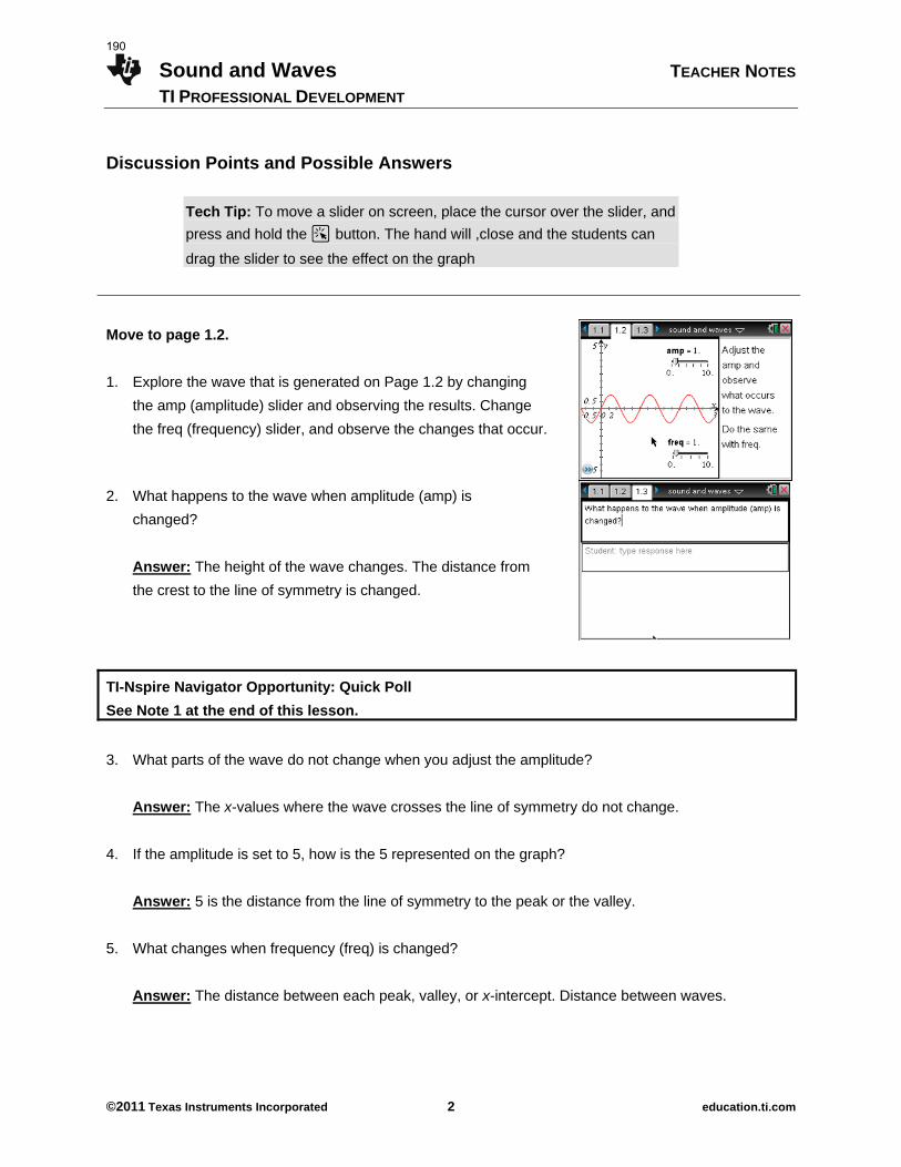
Sound and Waves TEACHER NOTES
TI PROFESSIONAL DEVELOPMENT
©2011 Texas Instruments Incorporated 2 education.ti.com
Discussion Points and Possible Answers
Tech Tip: To move a slider on screen, place the cursor over the slider, and
press and hold the a button. The hand will ,close and the students can
drag the slider to see the effect on the graph
Move to page 1.2.
1. Explore the wave that is generated on Page 1.2 by changing
the amp (amplitude) slider and observing the results. Change
the freq (frequency) slider, and observe the changes that occur.
2. What happens to the wave when amplitude (amp) is
changed?
Answer: The height of the wave changes. The distance from
the crest to the line of symmetry is changed.
TI-Nspire Navigator Opportunity: Quick Poll
See Note 1 at the end of this lesson.
3. What parts of the wave do not change when you adjust the amplitude?
Answer: The x-values where the wave crosses the line of symmetry do not change.
4. If the amplitude is set to 5, how is the 5 represented on the graph?
Answer: 5 is the distance from the line of symmetry to the peak or the valley.
5. What changes when frequency (freq) is changed?
Answer: The distance between each peak, valley, or x-intercept. Distance between waves.
190
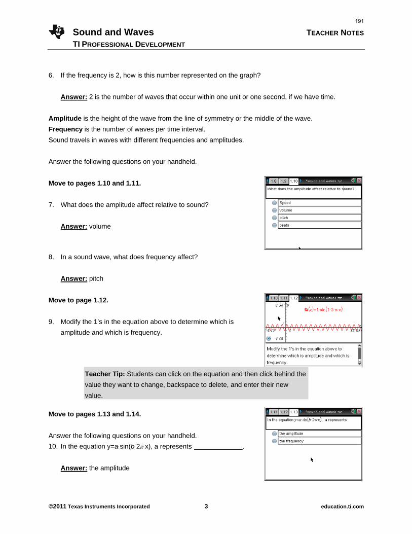
Sound and Waves TEACHER NOTES
TI PROFESSIONAL DEVELOPMENT
©2011 Texas Instruments Incorporated 3 education.ti.com
6. If the frequency is 2, how is this number represented on the graph?
Answer: 2 is the number of waves that occur within one unit or one second, if we have time.
Amplitude is the height of the wave from the line of symmetry or the middle of the wave.
Frequency is the number of waves per time interval.
Sound travels in waves with different frequencies and amplitudes.
Answer the following questions on your handheld.
Move to pages 1.10 and 1.11.
7. What does the amplitude affect relative to sound?
Answer: volume
8. In a sound wave, what does frequency affect?
Answer: pitch
Move to page 1.12.
9. Modify the 1’s in the equation above to determine which is
amplitude and which is frequency.
Teacher Tip: Students can click on the equation and then click behind the
value they want to change, backspace to delete, and enter their new
value.
Move to pages 1.13 and 1.14.
Answer the following questions on your handheld.
10. In the equation y=asin(b2πx), a represents .
Answer: the amplitude
191
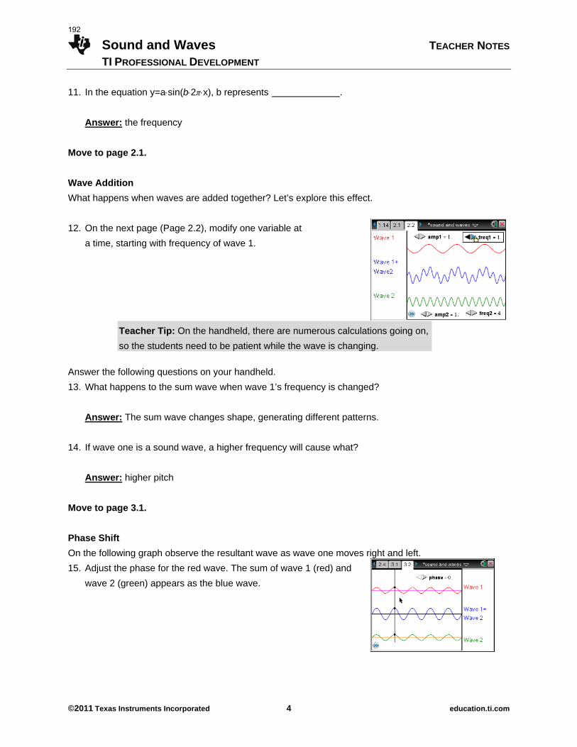
Sound and Waves TEACHER NOTES
TI PROFESSIONAL DEVELOPMENT
©2011 Texas Instruments Incorporated 4 education.ti.com
11. In the equation y=asin(b2πx), b represents .
Answer: the frequency
Move to page 2.1.
Wave Addition
What happens when waves are added together? Let’s explore this effect.
12. On the next page (Page 2.2), modify one variable at
a time, starting with frequency of wave 1.
Teacher Tip: On the handheld, there are numerous calculations going on,
so the students need to be patient while the wave is changing.
Answer the following questions on your handheld.
13. What happens to the sum wave when wave 1’s frequency is changed?
Answer: The sum wave changes shape, generating different patterns.
14. If wave one is a sound wave, a higher frequency will cause what?
Answer: higher pitch
Move to page 3.1.
Phase Shift
On the following graph observe the resultant wave as wave one moves right and left.
15. Adjust the phase for the red wave. The sum of wave 1 (red) and
wave 2 (green) appears as the blue wave.
192
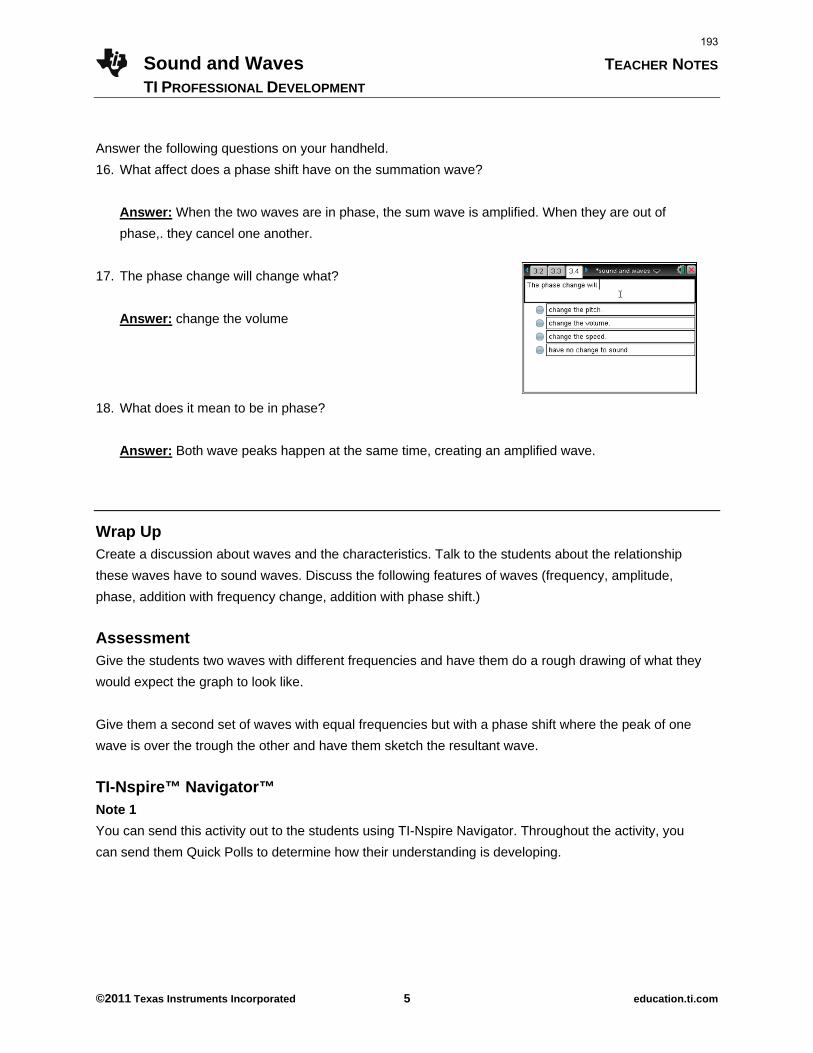
Sound and Waves TEACHER NOTES
TI PROFESSIONAL DEVELOPMENT
©2011 Texas Instruments Incorporated 5 education.ti.com
Answer the following questions on your handheld.
16. What affect does a phase shift have on the summation wave?
Answer: When the two waves are in phase, the sum wave is amplified. When they are out of
phase,. they cancel one another.
17. The phase change will change what?
Answer: change the volume
18. What does it mean to be in phase?
Answer: Both wave peaks happen at the same time, creating an amplified wave.
Wrap Up Create a discussion about waves and the characteristics. Talk to the students about the relationship
these waves have to sound waves. Discuss the following features of waves (frequency, amplitude,
phase, addition with frequency change, addition with phase shift.)
Assessment Give the students two waves with different frequencies and have them do a rough drawing of what they
would expect the graph to look like.
Give them a second set of waves with equal frequencies but with a phase shift where the peak of one
wave is over the trough the other and have them sketch the resultant wave.
TI-Nspire™ Navigator™ Note 1
You can send this activity out to the students using TI-Nspire Navigator. Throughout the activity, you
can send them Quick Polls to determine how their understanding is developing.
193

This page intentionally left blank
194

www.nasa.gov A Breath of Fresh Air: TI-Nspire Lab Activity 1/4
*AP is a trademark owned by the College Board, which was not involved in the production of, and does not endorse, this product.
A BREATH OF FRESH AIR
TI-Nspire™ Lab Activity
Background
The International Space Station (ISS) is a research laboratory being assembled in low Earth orbit by five international partners. Construction of the ISS began in 1998 and is scheduled for completion in 2011. Crews aboard the ISS conduct experiments in biology, chemistry, physics, medicine and physiology, as well as astronomical and meteorological observations. The microgravity environment of space makes the ISS a unique laboratory for the testing of spacecraft systems that will be required for future exploration missions beyond low Earth orbit.
The ISS travels in orbit around the Earth at an average speed of 27,743.8 km/h (17,239.2 mph) completing 15.7 orbits per day. The ISS is operated jointly among five participating space agencies: the United States’ National Aeronautics and Space Administration (NASA), the European Space Agency (ESA), the Russian Federal Space Agency (RKA), the Japan Aerospace Exploration Agency (JAXA) and the Canadian Space Agency (CSA).
An international crew, of typically six members, resides on the ISS for approximately 6 months. Since the first crew aboard the ISS in 1998, humans have maintained a permanent presence in space. In addition to the crew aboard the ISS, personnel on the ground located in mission control centers operated by the five participating space agencies, control the operations of the ISS. The ISS requires a constant supply of oxygen to keep the astronauts safe and in top condition. Because oxygen is a consumable on the ISS, there needs to be a continuous source of new oxygen. On Earth, new oxygen is produced from plants through the process of photosynthesis. On the ISS, there is not enough space to carry the amount of plant material that would be required to produce the oxygen needed. Instead, oxygen is supplied by a variety of sources.
Figure 1: The ISS orbiting the Earth as observed by Space Shuttle Discovery on March 26, 2009
195
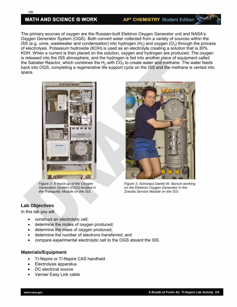
www.nasa.gov A Breath of Fresh Air: TI-Nspire Lab Activity 2/4
The primary sources of oxygen are the Russian-built Elektron Oxygen Generator unit and NASA’s Oxygen Generator System (OGS). Both convert water collected from a variety of sources within the ISS (e.g. urine, wastewater and condensation) into hydrogen (H2) and oxygen (O2) through the process of electrolysis. Potassium hydroxide (KOH) is used as an electrolyte creating a solution that is 30% KOH. When a current is then placed on the solution, oxygen and hydrogen are produced. The oxygen is released into the ISS atmosphere, and the hydrogen is fed into another piece of equipment called the Sabatier Reactor, which combines the H2 with CO2 to create water and methane. The water feeds back into OGS, completing a regenerative life support cycle on the ISS and the methane is vented into space.
Figure 2: A mock-up of the Oxygen Generation System (OGS) located in the Tranquility Module on the ISS
Figure 3: Astronaut Daniel W. Bursch working on the Elektron Oxygen Generator in the Zvezda Service Module on the ISS
Lab Objectives
In this lab you will
construct an electrolytic cell; determine the moles of oxygen produced; determine the mass of oxygen produced; determine the number of electrons transferred; and compare experimental electrolytic cell to the OGS aboard the ISS.
Materials/Equipment
TI-Nspire or TI-Nspire CAS handheld Electrolysis apparatus DC electrical source Vernier Easy Link cable
196
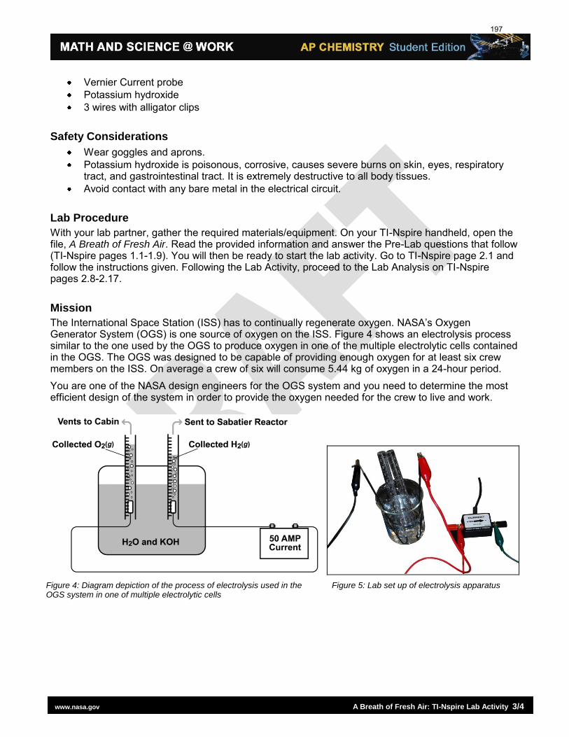
www.nasa.gov A Breath of Fresh Air: TI-Nspire Lab Activity 3/4
Vernier Current probe Potassium hydroxide 3 wires with alligator clips
Safety Considerations
Wear goggles and aprons. Potassium hydroxide is poisonous, corrosive, causes severe burns on skin, eyes, respiratory
tract, and gastrointestinal tract. It is extremely destructive to all body tissues. Avoid contact with any bare metal in the electrical circuit.
Lab Procedure
With your lab partner, gather the required materials/equipment. On your TI-Nspire handheld, open the file, A Breath of Fresh Air. Read the provided information and answer the Pre-Lab questions that follow (TI-Nspire pages 1.1-1.9). You will then be ready to start the lab activity. Go to TI-Nspire page 2.1 and follow the instructions given. Following the Lab Activity, proceed to the Lab Analysis on TI-Nspire pages 2.8-2.17.
Mission
The International Space Station (ISS) has to continually regenerate oxygen. NASA’s Oxygen Generator System (OGS) is one source of oxygen on the ISS. Figure 4 shows an electrolysis process similar to the one used by the OGS to produce oxygen in one of the multiple electrolytic cells contained in the OGS. The OGS was designed to be capable of providing enough oxygen for at least six crew members on the ISS. On average a crew of six will consume 5.44 kg of oxygen in a 24-hour period. You are one of the NASA design engineers for the OGS system and you need to determine the most efficient design of the system in order to provide the oxygen needed for the crew to live and work.
Figure 4: Diagram depiction of the process of electrolysis used in the OGS system in one of multiple electrolytic cells
Figure 5: Lab set up of electrolysis apparatus
197
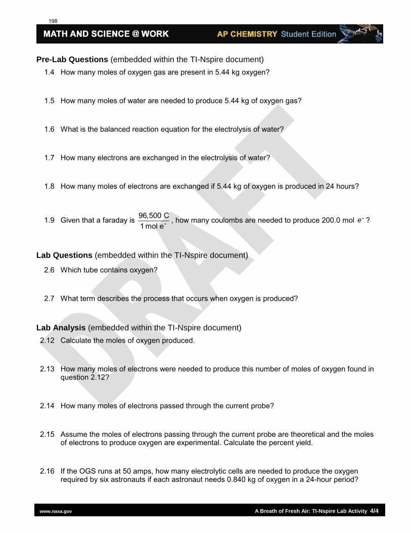
www.nasa.gov A Breath of Fresh Air: TI-Nspire Lab Activity 4/4
Pre-Lab Questions (embedded within the TI-Nspire document)
1.4 How many moles of oxygen gas are present in 5.44 kg oxygen?
1.5 How many moles of water are needed to produce 5.44 kg of oxygen gas?
1.6 What is the balanced reaction equation for the electrolysis of water?
1.7 How many electrons are exchanged in the electrolysis of water?
1.8 How many moles of electrons are exchanged if 5.44 kg of oxygen is produced in 24 hours?
1.9 Given that a faraday is 96,500 C1 mol e
, how many coulombs are needed to produce 200.0 mol e ?
Lab Questions (embedded within the TI-Nspire document)
2.6 Which tube contains oxygen?
2.7 What term describes the process that occurs when oxygen is produced?
Lab Analysis (embedded within the TI-Nspire document) 2.12 Calculate the moles of oxygen produced.
2.13 How many moles of electrons were needed to produce this number of moles of oxygen found in question 2.12?
2.14 How many moles of electrons passed through the current probe?
2.15 Assume the moles of electrons passing through the current probe are theoretical and the moles of electrons to produce oxygen are experimental. Calculate the percent yield.
2.16 If the OGS runs at 50 amps, how many electrolytic cells are needed to produce the oxygen required by six astronauts if each astronaut needs 0.840 kg of oxygen in a 24-hour period?
198
DataQuest
29
Science with TI-Nspire Technology © Vernier Software & Technology 29 - 1
Static and Kinetic Friction
If you try to slide a heavy box resting on the floor, you may find it difficult to get the box moving. Static friction is the force that is acting against the box. If you apply a light horizontal push that does not move the box, the static friction force is also small and directly opposite to your push. If you push harder, the friction force increases to match the magnitude of your push. There is a limit to the magnitude of static friction, so eventually you may be able to apply a force larger than the maximum static force, and the box will move. The maximum static friction force is sometimes referred to as starting friction. We model static friction, Fstatic, with the inequality Fstatic s N where s is the coefficient of static friction and N the normal force exerted by a surface on the object. The normal force is defined as the perpendicular component of the force exerted by the surface. In this case, the normal force is equal to the weight of the object.
Once the box starts to slide, you must continue to exert a force to keep the object moving, or friction will slow it to a stop. The friction acting on the box while it is moving is called kinetic friction. In order to slide the box with a constant velocity, a force equivalent in magnitude to the force of kinetic friction must be applied. Kinetic friction is sometimes referred to as sliding friction. Both static and kinetic friction depend on the surfaces of the box and the floor, and on how hard the box and floor are pressed together. We model kinetic friction with Fkinetic = k N, where k is the coefficient of kinetic friction.
In this experiment, you will use a Force Sensor to study static friction and kinetic friction on a wooden block. A Motion Detector will also be used to analyze the kinetic friction acting on a sliding block.
OBJECTIVES
Use a Force Sensor to measure the force of static and kinetic friction.
Determine the relationship between force of static friction and the weight of an object.
Measure the coefficients of static and kinetic friction for a particular block and track.
Use a Motion Detector to independently measure the coefficient of kinetic friction and compare it to the previously measured value.
Determine if the coefficient of kinetic friction depends on weight.
MATERIALS
TI-Nspire handheld or string computer and TI-Nspire software block of wood with hook data-collection interface balance or scale Vernier Force Sensor mass set Motion Detector or CBR 2 or graph paper (optional) Go!Motion
199
DataQuest 29
29 - 2 Science with TI-Nspire Technology
PRE-LAB QUESTIONS
1. In pushing a heavy box across the floor, is the force you need to apply to start the box moving greater than, less than, or the same as the force needed to keep the box moving? On what1 are you basing your choice?
2. How is the force of friction related to the weight of the box? Explain.
PROCEDURE
Part I Investigating Friction
1. Measure the mass of the block and record it in the data table.
2. Set the range switch on the Force Sensor to 10 N. Connect the Force Sensor to the data-collection interface. Connect the interface to the TI-Nspire handheld or computer.
3. Choose New Experiment from the Experiment menu. Choose Collection Setup from the
Experiment menu. Enter 5 for the duration. The number of points collected should be 251. Select OK.
4. Zero the Force Sensor.
a. Hold the Force Sensor so the working axis is horizontal.
b. With the Force Sensor axis held horizontally and no force applied, choose Set Up Sensors ► Zero from the Experiment menu. When the process is complete, the readings for the sensors should be close to zero.
5. Tie one end of a string to the hook on the Force Sensor and the other end to the hook on the
wooden block. Place a total of 1 kg mass on top of the block, fastened so the masses cannot shift. Practice pulling the block and masses with the Force Sensor using a straight-line motion. Slowly and gently pull horizontally with a small force. Very gradually, taking one full second, increase the force until the block starts to slide, and then keep the block moving at a constant speed for another second.
6. Sketch a graph of force vs. time for the force you felt on your hand. Label the portion of the graph corresponding to the block at rest, the time when the block just started to move, and the time when the block was moving at constant speed.
7. Hold the Force Sensor in position, ready to pull the block, but with no tension in the string.
8. Start data collection ( ). Wait a moment, then pull the block as before, taking care to increase the force gradually.
9. Inspect your graph. Repeat Step 8 as needed until you have a graph that reflects the desired motion, including pulling the block at constant speed once it begins moving. Print or sketch the graph for later reference.
200
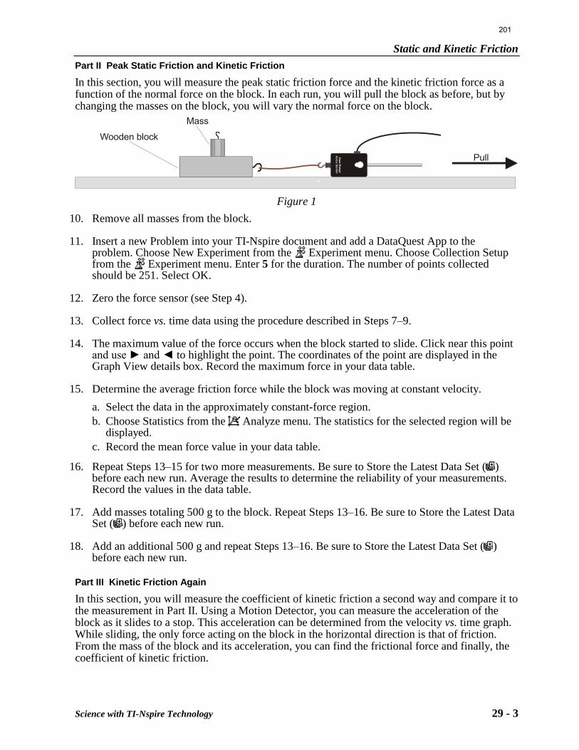
Static and Kinetic Friction
Science with TI-Nspire Technology 29 - 3
Part II Peak Static Friction and Kinetic Friction
In this section, you will measure the peak static friction force and the kinetic friction force as a function of the normal force on the block. In each run, you will pull the block as before, but by changing the masses on the block, you will vary the normal force on the block.
Wooden block
Pull
Mass
Du
al -R
an
ge
Fo
rce S
en
so
r
Figure 1
10. Remove all masses from the block.
11. Insert a new Problem into your TI-Nspire document and add a DataQuest App to the problem. Choose New Experiment from the Experiment menu. Choose Collection Setup from the Experiment menu. Enter 5 for the duration. The number of points collected should be 251. Select OK.
12. Zero the force sensor (see Step 4).
13. Collect force vs. time data using the procedure described in Steps 7–9.
14. The maximum value of the force occurs when the block started to slide. Click near this point and use ► and ◄ to highlight the point. The coordinates of the point are displayed in the Graph View details box. Record the maximum force in your data table.
15. Determine the average friction force while the block was moving at constant velocity.
a. Select the data in the approximately constant-force region.
b. Choose Statistics from the Analyze menu. The statistics for the selected region will be displayed.
c. Record the mean force value in your data table.
16. Repeat Steps 13–15 for two more measurements. Be sure to Store the Latest Data Set ( ) before each new run. Average the results to determine the reliability of your measurements. Record the values in the data table.
17. Add masses totaling 500 g to the block. Repeat Steps 13–16. Be sure to Store the Latest Data Set ( ) before each new run.
18. Add an additional 500 g and repeat Steps 13–16. Be sure to Store the Latest Data Set ( ) before each new run.
Part III Kinetic Friction Again
In this section, you will measure the coefficient of kinetic friction a second way and compare it to the measurement in Part II. Using a Motion Detector, you can measure the acceleration of the block as it slides to a stop. This acceleration can be determined from the velocity vs. time graph. While sliding, the only force acting on the block in the horizontal direction is that of friction. From the mass of the block and its acceleration, you can find the frictional force and finally, the coefficient of kinetic friction.
201
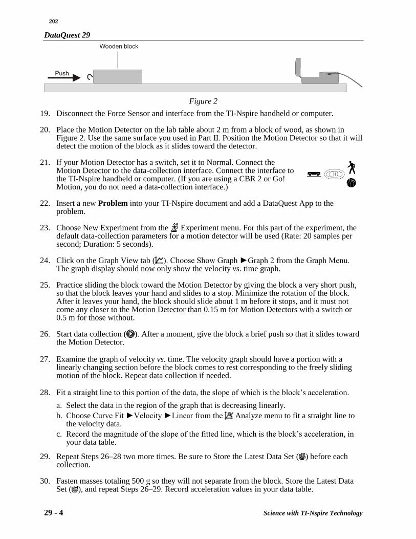
DataQuest 29
29 - 4 Science with TI-Nspire Technology
Wooden block
Push
Figure 2
19. Disconnect the Force Sensor and interface from the TI-Nspire handheld or computer.
20. Place the Motion Detector on the lab table about 2 m from a block of wood, as shown in Figure 2. Use the same surface you used in Part II. Position the Motion Detector so that it will detect the motion of the block as it slides toward the detector.
21. If your Motion Detector has a switch, set it to Normal. Connect the Motion Detector to the data-collection interface. Connect the interface to the TI-Nspire handheld or computer. (If you are using a CBR 2 or Go!
Motion, you do not need a data-collection interface.)
22. Insert a new Problem into your TI-Nspire document and add a DataQuest App to the problem.
23. Choose New Experiment from the Experiment menu. For this part of the experiment, the default data-collection parameters for a motion detector will be used (Rate: 20 samples per second; Duration: 5 seconds).
24. Click on the Graph View tab ( ). Choose Show Graph ►Graph 2 from the Graph Menu. The graph display should now only show the velocity vs. time graph.
25. Practice sliding the block toward the Motion Detector by giving the block a very short push, so that the block leaves your hand and slides to a stop. Minimize the rotation of the block. After it leaves your hand, the block should slide about 1 m before it stops, and it must not come any closer to the Motion Detector than 0.15 m for Motion Detectors with a switch or 0.5 m for those without.
26. Start data collection ( ). After a moment, give the block a brief push so that it slides toward the Motion Detector.
27. Examine the graph of velocity vs. time. The velocity graph should have a portion with a
linearly changing section before the block comes to rest corresponding to the freely sliding motion of the block. Repeat data collection if needed.
28. Fit a straight line to this portion of the data, the slope of which is the block’s acceleration.
a. Select the data in the region of the graph that is decreasing linearly.
b. Choose Curve Fit ►Velocity ►Linear from the Analyze menu to fit a straight line to the velocity data.
c. Record the magnitude of the slope of the fitted line, which is the block’s acceleration, in your data table.
29. Repeat Steps 26–28 two more times. Be sure to Store the Latest Data Set ( ) before each
collection.
30. Fasten masses totaling 500 g so they will not separate from the block. Store the Latest Data Set ( ), and repeat Steps 26–29. Record acceleration values in your data table.
202
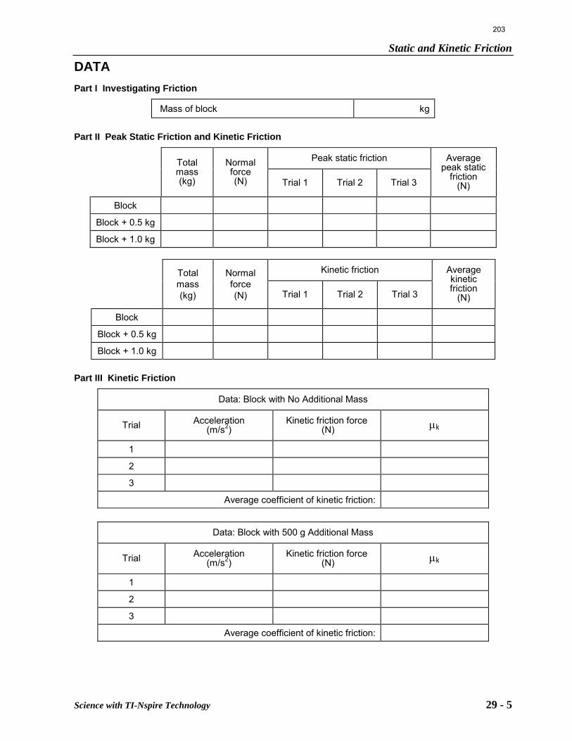
Static and Kinetic Friction
Science with TI-Nspire Technology 29 - 5
DATA
Part I Investigating Friction
Mass of block kg Part II Peak Static Friction and Kinetic Friction
Total mass (kg)
Normal force (N)
Peak static friction Average peak static
friction (N) Trial 1 Trial 2 Trial 3
Block
Block + 0.5 kg
Block + 1.0 kg
Total mass (kg)
Normal force (N)
Kinetic friction Average kinetic friction
(N) Trial 1 Trial 2 Trial 3
Block
Block + 0.5 kg
Block + 1.0 kg Part III Kinetic Friction
Data: Block with No Additional Mass
Trial Acceleration (m/s2)
Kinetic friction force (N) k
1
2
3
Average coefficient of kinetic friction:
Data: Block with 500 g Additional Mass
Trial Acceleration (m/s2)
Kinetic friction force (N) k
1
2
3
Average coefficient of kinetic friction:
203
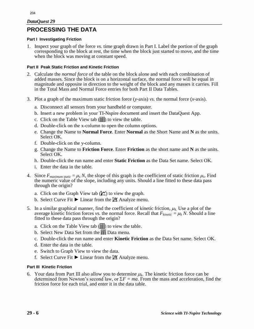
DataQuest 29
29 - 6 Science with TI-Nspire Technology
PROCESSING THE DATA
Part I Investigating Friction
1. Inspect your graph of the force vs. time graph drawn in Part I. Label the portion of the graph corresponding to the block at rest, the time when the block just started to move, and the time when the block was moving at constant speed.
Part II Peak Static Friction and Kinetic Friction
2. Calculate the normal force of the table on the block alone and with each combination of added masses. Since the block is on a horizontal surface, the normal force will be equal in magnitude and opposite in direction to the weight of the block and any masses it carries. Fill in the Total Mass and Normal Force entries for both Part II Data Tables.
3. Plot a graph of the maximum static friction force (y-axis) vs. the normal force (x-axis).
a. Disconnect all sensors from your handheld or computer.
b. Insert a new problem in your TI-Nspire document and insert the DataQuest App.
c. Click on the Table View tab ( ) to view the table.
d. Double-click on the x-column to open the column options.
e. Change the Name to Normal Force. Enter Normal as the Short Name and N as the units. Select OK.
f. Double-click on the y-column.
g. Change the Name to Friction Force. Enter Friction as the short name and N as the units. Select OK.
h. Double-click the run name and enter Static Friction as the Data Set name. Select OK.
i. Enter the data in the table. 4. Since Fmaximum static = s N, the slope of this graph is the coefficient of static friction s. Find
the numeric value of the slope, including any units. Should a line fitted to these data pass through the origin?
a. Click on the Graph View tab ( ) to view the graph.
b. Select Curve Fit ► Linear from the Analyze menu. 5. In a similar graphical manner, find the coefficient of kinetic friction, k. Use a plot of the
average kinetic friction forces vs. the normal force. Recall that Fkinetic = k N. Should a line fitted to these data pass through the origin?
a. Click on the Table View tab ( ) to view the table.
b. Select New Data Set from the Data menu.
c. Double-click the run name and enter Kinetic Friction as the Data Set name. Select OK.
d. Enter the data in the table.
e. Switch to Graph View to view the data.
f. Select Curve Fit ► Linear from the Analyze menu. Part III Kinetic Friction
6. Your data from Part III also allow you to determine k. The kinetic friction force can be determined from Newton’s second law, or F = ma. From the mass and acceleration, find the friction force for each trial, and enter it in the data table.
204
Static and Kinetic Friction
Science with TI-Nspire Technology 29 - 7
7. From the friction force, determine the coefficient of kinetic friction for each trial and enter the values in the data table. Also, calculate an average value for the coefficient of kinetic friction for the block and for the block with added mass.
QUESTIONS
Part I Starting Friction
1. Consider the force vs. time graph you created in Part I. Compare the force necessary to keep the block sliding compared to the force necessary to start the slide. How does your answer compare to your answer to question 1 in the Pre-Lab Questions section?
2. The coefficient of friction is a constant that relates the normal force between two objects (blocks and table) and the force of friction. Based on your graph from Part I, would you expect the coefficient of static friction to be greater than, less than, or the same as the coefficient of kinetic friction?
Part II Peak Static Friction and Kinetic Friction
3. Should the graph of the maximum static friction force vs. the normal force (see Processing the Data Step 3) pass through the origin? Explain.
4. Should the graph of the average kinetic friction force vs. the normal force (see Processing the Data Step 5) pass through the origin? Explain.
Part III Kinetic Friction
5. Draw a free-body diagram for the sliding block.
6. Does the coefficient of kinetic friction depend on speed? Explain, using your experimental data.
7. Does the force of kinetic friction depend on the weight of the block? Explain.
8. Does the coefficient of kinetic friction depend on the weight of the block?
9. Compare your coefficients of kinetic friction determined in Part III to that determined in Part II. Discuss the values. Do you expect them to be the same or different?
EXTENSIONS
1. How does the surface area of the block affect the force of friction or the coefficient of friction? Devise an experiment that can test your hypothesis.
2. Examine the force of static friction for an object on an incline. Find the angle that causes a wooden block to start to slide. Calculate the coefficient of friction and compare it to the value you obtain when the angle of the incline is 0°.
3. Try changing the coefficient of friction by using wax or furniture polish on the table. How much does it change?
205
Experiment
TEACHER INFORMATION 29
Science with TI-Nspire Technology © Vernier Software & Technology 29 - 1 T
Static and Kinetic Friction
1. Editable Microsoft Word versions of the student pages and pre-configured TI-Nspire files can be found on the CD that accompanies this book. See Appendix A for more information.
2. For consistent results in this experiment, be sure that the wooden block and table surfaces are clean and free of grease. A missing peak in the static friction force or a variable force during the constant-speed portion of the motion are both indications that the surfaces of the block or table need cleaning. One way to prepare a new, clean surface is to wrap the block in a sheet of paper.
3. You may choose to use the 50 N range instead of the 10 N range if friction forces are large.
4. Dynamics carts with friction pads can be used as an alternative to the wooden block.
5. Coach students to increase the applied force very slowly and evenly. The tendency is to increase the applied force too rapidly.
6. You may want to prepare special wooden blocks for this experiment with drilled holes for your particular mass sets. It is then very easy for students to change the total mass of the block system, and the holes prevent the masses from shifting.
7. Blocks can be stacked to increase mass, but take care that the system moves as a rigid unit.
8. In using the Motion Detector, it is important to realize that the ultrasound is emitted in a cone about 30º wide. Anything within the cone of ultrasound can cause a reflection and possibly an accidental measurement. A common problem in using Motion Detectors is getting unintentional reflections from a desk, chair, or computer in the room.
9. Motion detectors without a mode switch do not properly detect objects closer than 0.5 m. As a result, such motion detectors must be farther away from the experiment than described in the student notes. In contrast, Motion detectors with a mode switch will detect objects as close as 0.15 m. Ideally, an experiment will be set up so that the target is nearly this close at the point of closest approach, giving the best possible data.
10. Sometimes a target may not supply a strong reflection of the ultrasound. Attaching a piece of rigid card stock to the block can improve the reflection but it will also increase the error as air resistance will also act to stop the block.
11. A natural break point is between Parts II and III. If the lab needs to be shortened, Part III could be omitted. Many physics teachers feel, however, that the best part of the lab is Part III because it connects Newton’s second law directly to the friction equation in the solution of the problem. It also addresses the most confusing concepts to the student – the forces on a freely moving object.
12. Note on Extension 2: An alternative way of measuring friction coefficients is to tilt an inclined plane up until the block just starts sliding. At that point, the normal force is mg cos and the force down the ramp is mg sin , so you can find the coefficient of static friction from s = Fstatic/FN = tan . If you tip it up but bump the block until it slides with a constant
206
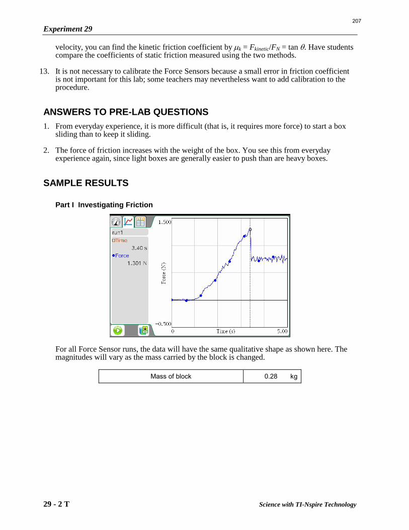
Experiment 29
29 - 2 T Science with TI-Nspire Technology
velocity, you can find the kinetic friction coefficient by k = Fkinetic/FN = tan . Have students compare the coefficients of static friction measured using the two methods.
13. It is not necessary to calibrate the Force Sensors because a small error in friction coefficient is not important for this lab; some teachers may nevertheless want to add calibration to the procedure.
ANSWERS TO PRE-LAB QUESTIONS
1. From everyday experience, it is more difficult (that is, it requires more force) to start a box sliding than to keep it sliding.
2. The force of friction increases with the weight of the box. You see this from everyday experience again, since light boxes are generally easier to push than are heavy boxes.
SAMPLE RESULTS
Part I Investigating Friction
For all Force Sensor runs, the data will have the same qualitative shape as shown here. The magnitudes will vary as the mass carried by the block is changed.
Mass of block 0.28 kg
207
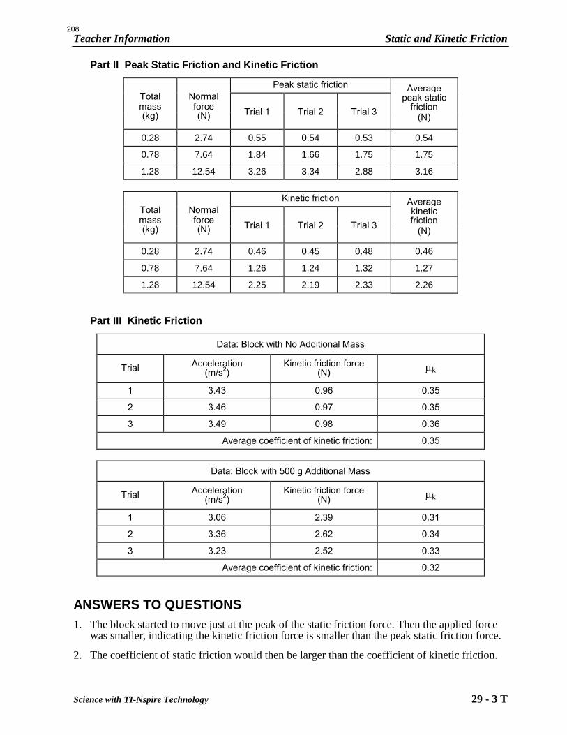
Teacher Information Static and Kinetic Friction
Science with TI-Nspire Technology 29 - 3 T
Part II Peak Static Friction and Kinetic Friction
Total mass (kg)
Normal force (N)
Peak static friction
Average
Trial 1 Trial 2 Trial 3 peak static
friction
(N)
0.28
2.74 0.55 0.54 0.53 0.54
0.78 7.64 1.84 1.66 1.75 1.75
1.28 12.54 3.26 3.34 2.88 3.16
Total mass (kg)
Normal force (N)
Kinetic friction
Average
Trial 1 Trial 2 Trial 3 kinetic friction
(N)
0.28 2.74 0.46 0.45 0.48 0.46
0.78 7.64 1.26 1.24 1.32 1.27
1.28 12.54 2.25 2.19 2.33 2.26
Part III Kinetic Friction
Data: Block with No Additional Mass
Trial Acceleration (m/s2)
Kinetic friction force (N) k
1 3.43 0.96 0.35
2 3.46 0.97 0.35
3 3.49 0.98 0.36
Average coefficient of kinetic friction: 0.35
Data: Block with 500 g Additional Mass
Trial Acceleration (m/s2)
Kinetic friction force (N) k
1 3.06 2.39 0.31
2 3.36 2.62 0.34
3 3.23 2.52 0.33
Average coefficient of kinetic friction: 0.32
ANSWERS TO QUESTIONS
1. The block started to move just at the peak of the static friction force. Then the applied force was smaller, indicating the kinetic friction force is smaller than the peak static friction force.
2. The coefficient of static friction would then be larger than the coefficient of kinetic friction.
208
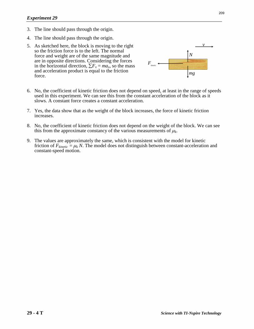
Experiment 29
29 - 4 T Science with TI-Nspire Technology
3. The line should pass through the origin.
4. The line should pass through the origin.
5. As sketched here, the block is moving to the right so the friction force is to the left. The normal force and weight are of the same magnitude and are in opposite directions. Considering the forces in the horizontal direction, Fx = max, so the mass and acceleration product is equal to the friction force.
Fkinetic
mg
v
N
6. No, the coefficient of kinetic friction does not depend on speed, at least in the range of speeds used in this experiment. We can see this from the constant acceleration of the block as it slows. A constant force creates a constant acceleration.
7. Yes, the data show that as the weight of the block increases, the force of kinetic friction increases.
8. No, the coefficient of kinetic friction does not depend on the weight of the block. We can see this from the approximate constancy of the various measurements of k.
9. The values are approximately the same, which is consistent with the model for kinetic friction of Fkinetic = k N. The model does not distinguish between constant-acceleration and constant-speed motion.
209

This page intentionally left blank
210
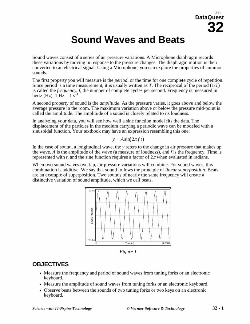
DataQuest
32
Science with TI-Nspire Technology © Vernier Software & Technology 32 - 1
Sound Waves and Beats
Sound waves consist of a series of air pressure variations. A Microphone diaphragm records these variations by moving in response to the pressure changes. The diaphragm motion is then converted to an electrical signal. Using a Microphone, you can explore the properties of common sounds.
The first property you will measure is the period, or the time for one complete cycle of repetition. Since period is a time measurement, it is usually written as T. The reciprocal of the period (1/T) is called the frequency, f, the number of complete cycles per second. Frequency is measured in hertz (Hz). 1 Hz = 1 s–1.
A second property of sound is the amplitude. As the pressure varies, it goes above and below the average pressure in the room. The maximum variation above or below the pressure mid-point is called the amplitude. The amplitude of a sound is closely related to its loudness.
In analyzing your data, you will see how well a sine function model fits the data. The displacement of the particles in the medium carrying a periodic wave can be modeled with a sinusoidal function. Your textbook may have an expression resembling this one:
y A f t sin 2
In the case of sound, a longitudinal wave, the y refers to the change in air pressure that makes up the wave. A is the amplitude of the wave (a measure of loudness), and f is the frequency. Time is represented with t, and the sine function requires a factor of 2 when evaluated in radians.
When two sound waves overlap, air pressure variations will combine. For sound waves, this combination is additive. We say that sound follows the principle of linear superposition. Beats are an example of superposition. Two sounds of nearly the same frequency will create a distinctive variation of sound amplitude, which we call beats.
Figure 1
OBJECTIVES
Measure the frequency and period of sound waves from tuning forks or an electronic keyboard.
Measure the amplitude of sound waves from tuning forks or an electronic keyboard.
Observe beats between the sounds of two tuning forks or two keys on an electronic keyboard.
211
DataQuest 32
32 - 2 Science with TI-Nspire Technology
MATERIALS
TI-Nspire handheld or Vernier Microphone computer and TI-Nspire software 2 tuning forks or an electronic keyboard data-collection interface
PRELIMINARY QUESTIONS
1. Why are instruments tuned before being played as a group? In which ways do musicians tune their instruments?
2. Given that sound waves consist of a series of air pressure increases and decreases, what would happen if an air pressure increase from one sound wave was located at the same place and time as a pressure decrease from another of the same amplitude?
PROCEDURE
1. Connect the Microphone to the data-collection interface. Connect the interface to the TI-Nspire handheld or computer.
2. Be sure your handheld or computer software is set to perform angle calculations in Radians.
3. Choose New Experiment from the Experiment menu. For Part I of the experiment, the default data-collection parameters for a microphone will be used (Rate: 10,000 samples per second; Duration: 0.03 seconds).
4. To center the waveform on zero, it is necessary to zero the Microphone channel. With the room quiet, choose Set Up Sensor ► Zero from the Experiment menu. When the process is complete, the reading for the sensor should be close to zero.
Part I Simple Waveforms
5. Produce a sound with a tuning fork or keyboard, and hold it close to the Microphone. Start data collection ( ). When data collection is complete, a graph will be displayed.
6. The data should be sinusoidal in form, similar to the graph in Figure 1. If you are using a tuning fork, strike it against a soft object such as a rubber mallet or the rubber sole of a shoe. Striking it against a hard object can damage it. If you strike it too hard or too softly, the waveform may be rough; collect data again.
7. Print or make a sketch of your graph. Record the note you played in Tables 1, 2 and 3.
8. To examine the data pairs on the displayed graph, click any data point. Use ► and ◄ to record the times for the first and last peaks of the waveform. Count the number of complete cycles that occur between your first measured time and the last. Divide the difference, t, by the number of cycles to determine the period of the tuning fork. Record these values in Table 1.
9. Calculate the frequency of the tuning fork based on the period you calculated in Step 8. Record this value in Table 1.
10. Examine the graph again to find the maximum and minimum sound values for an adjacent peak and trough. Calculate the amplitude of the wave by taking half of the difference between the maximum and minimum y values. Record the values in Table 2.
212
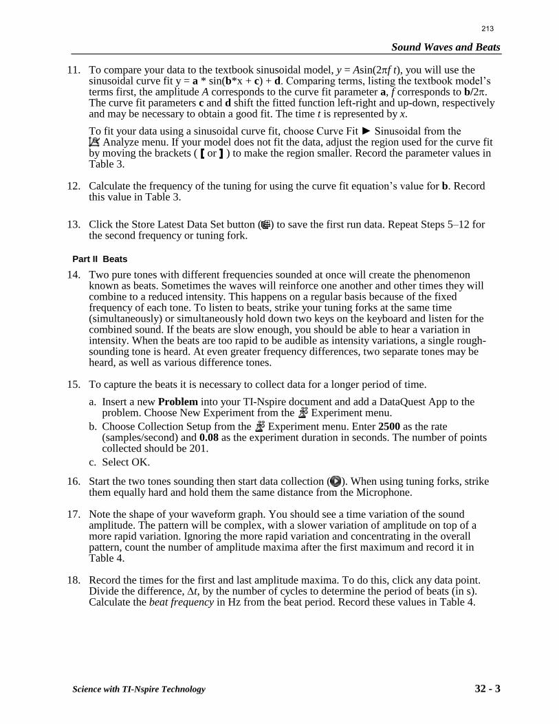
Sound Waves and Beats
Science with TI-Nspire Technology 32 - 3
11. To compare your data to the textbook sinusoidal model, y = Asin(2f t), you will use the
sinusoidal curve fit y = a * sin(b*x + c) + d. Comparing terms, listing the textbook model’s terms first, the amplitude A corresponds to the curve fit parameter a, f corresponds to b/2. The curve fit parameters c and d shift the fitted function left-right and up-down, respectively and may be necessary to obtain a good fit. The time t is represented by x.
To fit your data using a sinusoidal curve fit, choose Curve Fit ► Sinusoidal from the
Analyze menu. If your model does not fit the data, adjust the region used for the curve fit by moving the brackets ( [ or ] ) to make the region smaller. Record the parameter values in Table 3.
12. Calculate the frequency of the tuning for using the curve fit equation’s value for b. Record this value in Table 3.
13. Click the Store Latest Data Set button ( ) to save the first run data. Repeat Steps 5–12 for
the second frequency or tuning fork.
Part II Beats
14. Two pure tones with different frequencies sounded at once will create the phenomenon known as beats. Sometimes the waves will reinforce one another and other times they will combine to a reduced intensity. This happens on a regular basis because of the fixed frequency of each tone. To listen to beats, strike your tuning forks at the same time (simultaneously) or simultaneously hold down two keys on the keyboard and listen for the combined sound. If the beats are slow enough, you should be able to hear a variation in intensity. When the beats are too rapid to be audible as intensity variations, a single rough-sounding tone is heard. At even greater frequency differences, two separate tones may be heard, as well as various difference tones.
15. To capture the beats it is necessary to collect data for a longer period of time.
a. Insert a new Problem into your TI-Nspire document and add a DataQuest App to the problem. Choose New Experiment from the Experiment menu.
b. Choose Collection Setup from the Experiment menu. Enter 2500 as the rate (samples/second) and 0.08 as the experiment duration in seconds. The number of points collected should be 201.
c. Select OK.
16. Start the two tones sounding then start data collection ( ). When using tuning forks, strike them equally hard and hold them the same distance from the Microphone.
17. Note the shape of your waveform graph. You should see a time variation of the sound amplitude. The pattern will be complex, with a slower variation of amplitude on top of a more rapid variation. Ignoring the more rapid variation and concentrating in the overall pattern, count the number of amplitude maxima after the first maximum and record it in Table 4.
18. Record the times for the first and last amplitude maxima. To do this, click any data point. Divide the difference, t, by the number of cycles to determine the period of beats (in s). Calculate the beat frequency in Hz from the beat period. Record these values in Table 4.
213
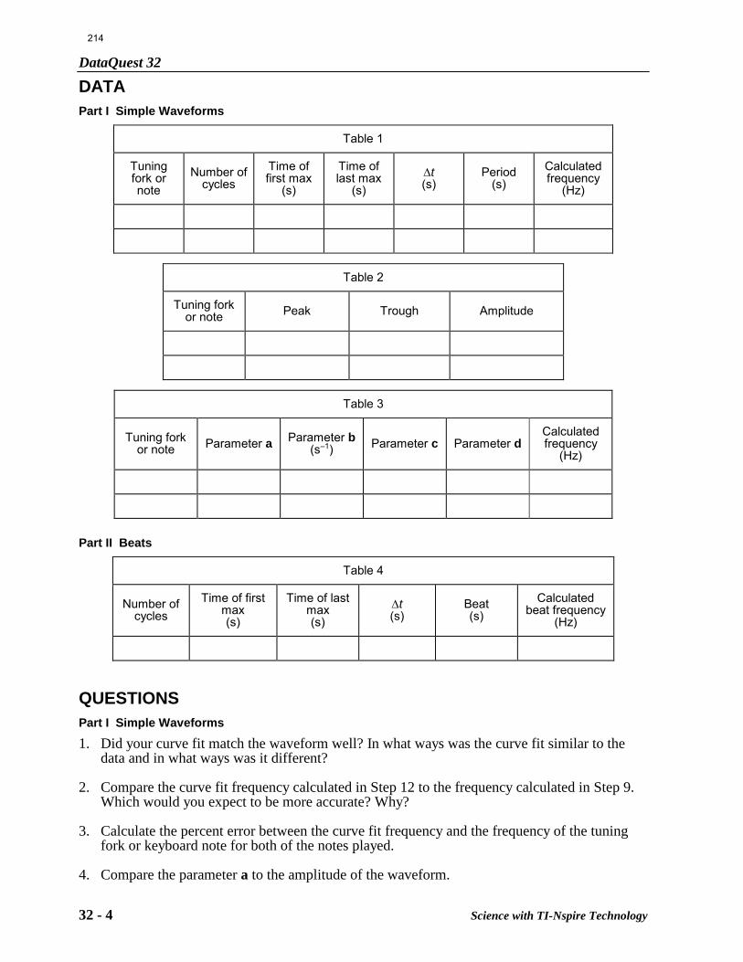
DataQuest 32
32 - 4 Science with TI-Nspire Technology
DATA
Part I Simple Waveforms
Table 1
Tuning fork or note
Number of cycles
Time of first max
(s)
Time of last max
(s) t (s)
Period (s)
Calculated frequency
(Hz)
Table 2
Tuning fork or note Peak Trough Amplitude
Table 3
Tuning fork or note Parameter a Parameter b
(s–1) Parameter c Parameter d Calculated frequency
(Hz)
Part II Beats
Table 4
Number of cycles
Time of first max (s)
Time of last max (s)
t (s)
Beat (s)
Calculated beat frequency
(Hz)
QUESTIONS
Part I Simple Waveforms
1. Did your curve fit match the waveform well? In what ways was the curve fit similar to the data and in what ways was it different?
2. Compare the curve fit frequency calculated in Step 12 to the frequency calculated in Step 9. Which would you expect to be more accurate? Why?
3. Calculate the percent error between the curve fit frequency and the frequency of the tuning fork or keyboard note for both of the notes played.
4. Compare the parameter a to the amplitude of the waveform.
214
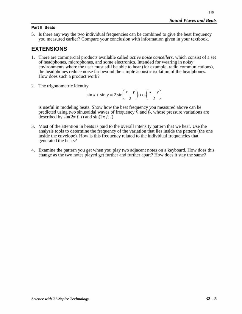
Sound Waves and Beats
Science with TI-Nspire Technology 32 - 5
Part II Beats
5. Is there any way the two individual frequencies can be combined to give the beat frequency you measured earlier? Compare your conclusion with information given in your textbook.
EXTENSIONS
1. There are commercial products available called active noise cancellers, which consist of a set of headphones, microphones, and some electronics. Intended for wearing in noisy environments where the user must still be able to hear (for example, radio communications), the headphones reduce noise far beyond the simple acoustic isolation of the headphones. How does such a product work?
2. The trigonometric identity
sin sin sin cosx yx y x y
2
2 2
is useful in modeling beats. Show how the beat frequency you measured above can be predicted using two sinusoidal waves of frequency f1 and f2, whose pressure variations are described by sin(2 f1 t) and sin(2 f2 t).
3. Most of the attention in beats is paid to the overall intensity pattern that we hear. Use the analysis tools to determine the frequency of the variation that lies inside the pattern (the one inside the envelope). How is this frequency related to the individual frequencies that generated the beats?
4. Examine the pattern you get when you play two adjacent notes on a keyboard. How does this change as the two notes played get further and further apart? How does it stay the same?
215
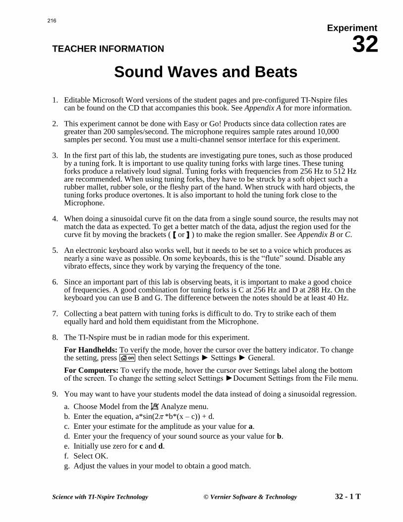
Experiment
TEACHER INFORMATION 32
Science with TI-Nspire Technology © Vernier Software & Technology 32 - 1 T
Sound Waves and Beats
1. Editable Microsoft Word versions of the student pages and pre-configured TI-Nspire files can be found on the CD that accompanies this book. See Appendix A for more information.
2. This experiment cannot be done with Easy or Go! Products since data collection rates are greater than 200 samples/second. The microphone requires sample rates around 10,000 samples per second. You must use a multi-channel sensor interface for this experiment.
3. In the first part of this lab, the students are investigating pure tones, such as those produced by a tuning fork. It is important to use quality tuning forks with large tines. These tuning forks produce a relatively loud signal. Tuning forks with frequencies from 256 Hz to 512 Hz are recommended. When using tuning forks, they have to be struck by a soft object such a rubber mallet, rubber sole, or the fleshy part of the hand. When struck with hard objects, the tuning forks produce overtones. It is also important to hold the tuning fork close to the Microphone.
4. When doing a sinusoidal curve fit on the data from a single sound source, the results may not match the data as expected. To get a better match of the data, adjust the region used for the curve fit by moving the brackets ( [ or ] ) to make the region smaller. See Appendix B or C.
5. An electronic keyboard also works well, but it needs to be set to a voice which produces as nearly a sine wave as possible. On some keyboards, this is the “flute” sound. Disable any vibrato effects, since they work by varying the frequency of the tone.
6. Since an important part of this lab is observing beats, it is important to make a good choice of frequencies. A good combination for tuning forks is C at 256 Hz and D at 288 Hz. On the keyboard you can use B and G. The difference between the notes should be at least 40 Hz.
7. Collecting a beat pattern with tuning forks is difficult to do. Try to strike each of them equally hard and hold them equidistant from the Microphone.
8. The TI-Nspire must be in radian mode for this experiment.
For Handhelds: To verify the mode, hover the cursor over the battery indicator. To change the setting, press c then select Settings ► Settings ► General.
For Computers: To verify the mode, hover the cursor over Settings label along the bottom of the screen. To change the setting select Settings ►Document Settings from the File menu.
9. You may want to have your students model the data instead of doing a sinusoidal regression.
a. Choose Model from the Analyze menu.
b. Enter the equation, a*sin(2 *b*(x – c)) + d.
c. Enter your estimate for the amplitude as your value for a.
d. Enter your the frequency of your sound source as your value for b.
e. Initially use zero for c and d.
f. Select OK.
g. Adjust the values in your model to obtain a good match.
216
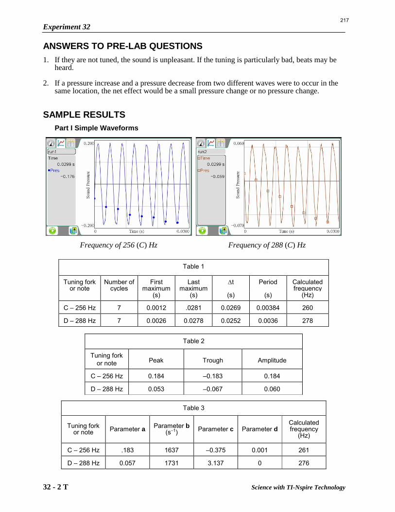
Experiment 32
32 - 2 T Science with TI-Nspire Technology
ANSWERS TO PRE-LAB QUESTIONS
1. If they are not tuned, the sound is unpleasant. If the tuning is particularly bad, beats may be heard.
2. If a pressure increase and a pressure decrease from two different waves were to occur in the same location, the net effect would be a small pressure change or no pressure change.
SAMPLE RESULTS
Part I Simple Waveforms
Frequency of 256 (C) Hz Frequency of 288 (C) Hz
Table 3
Tuning fork or note Parameter a Parameter b
(s–1) Parameter c Parameter d Calculated frequency
(Hz)
C – 256 Hz .183 1637 –0.375 0.001 261
D – 288 Hz 0.057 1731 3.137 0 276
Table 1
Tuning fork or note
Number of cycles
First maximum
Last maximum
t
Period
Calculated frequency
(s) (s) (s) (s) (Hz)
C – 256 Hz 7 0.0012 .0281 0.0269 0.00384 260
D – 288 Hz 7 0.0026 0.0278 0.0252 0.0036 278
Table 2
Tuning fork or note Peak Trough Amplitude
C – 256 Hz 0.184 –0.183 0.184
D – 288 Hz 0.053 –0.067 0.060
217
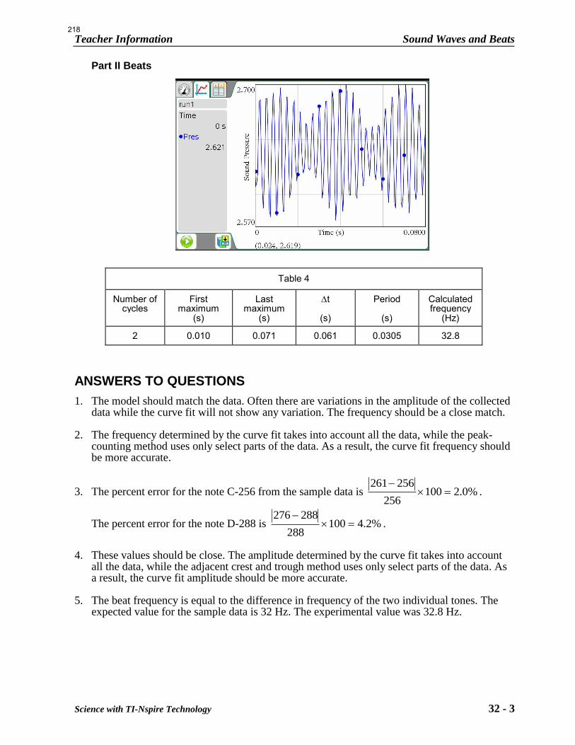
Teacher Information Sound Waves and Beats
Science with TI-Nspire Technology 32 - 3
Part II Beats
Table 4
Number of cycles
First maximum
Last maximum
t
Period
Calculated frequency
(s) (s) (s) (s) (Hz)
2 0.010 0.071 0.061 0.0305 32.8
ANSWERS TO QUESTIONS
1. The model should match the data. Often there are variations in the amplitude of the collected data while the curve fit will not show any variation. The frequency should be a close match.
2. The frequency determined by the curve fit takes into account all the data, while the peak-counting method uses only select parts of the data. As a result, the curve fit frequency should be more accurate.
3. The percent error for the note C-256 from the sample data is %0.2100256
256261
.
The percent error for the note D-288 is %2.4100288
288276
.
4. These values should be close. The amplitude determined by the curve fit takes into account all the data, while the adjacent crest and trough method uses only select parts of the data. As a result, the curve fit amplitude should be more accurate.
5. The beat frequency is equal to the difference in frequency of the two individual tones. The expected value for the sample data is 32 Hz. The experimental value was 32.8 Hz.
218
Day 3 Reflections and Wrap-up TEACHER NOTES
TI PROFESSIONAL DEVELOPMENT
©2011 Texas Instruments Incorporated 1 education.ti.com
Reflection: Take a few minutes to reflect on your learning. What you have
accomplished over these past 3 days?
What will you need to do between this workshop and the first day
of school to be ready to use this technology in your classroom?
What resources are available to support your implementation of
TI-NspireTM technology in your classroom?
Questions to Discuss: Which parts of today’s activities made you consider new
approaches to teaching any of the science content areas that were explored?
Share your thoughts about an activity that you especially enjoyed
working on today.
Ticket Outta Here: Complete and hand in the final “Ticket Outta Here”.
Today’s Activities:
Exploring Teacher Software
Exploring tnsp files
Exploring Science Nspired
Carousel
Presentations
TI Equipment used today:
TI-NspireTM CX CAS
TI-NspireTM CX CAS Teacher
Software
TI-NspireTM Lab CradleTM
TI-Nspire™ NavigatorTM
Vernier® Sensors and
interfaces used today:
Colormeter
Dual Force sensor
CO2 sensor
EasyLinkTM
Microphone
Current sensor
Gas pressure sensor
CBR 2TM
Visit
http://education.ti.com/calculator
s/tisciencenspired/ for lesson
updates and tech tip videos.
219
Day 3 Reflections and Wrap-up TEACHER NOTES
TI PROFESSIONAL DEVELOPMENT
©2011 Texas Instruments Incorporated 2 education.ti.com
Ticket Outta Here DAY 3 Exit Card
1. Reflect on your learning over the past 3 days. What you have accomplished?
2. What will you need to do between this workshop and the first day of school to be ready to use this technology in your classroom?
3. What resources are available to support your implementation of TI-NspireTM technology into your
classroom?
4. Anything else?
220
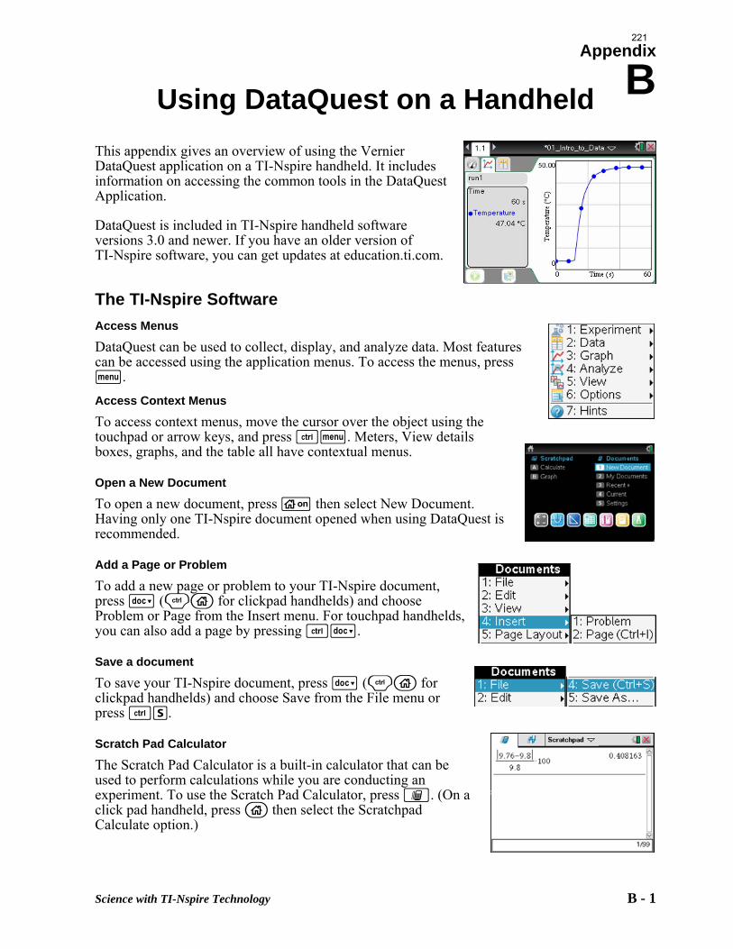
Appendix
B
Science with TI-Nspire Technology B - 1
Using DataQuest on a Handheld
This appendix gives an overview of using the Vernier DataQuest application on a TI-Nspire handheld. It includes information on accessing the common tools in the DataQuest Application.
DataQuest is included in TI-Nspire handheld software versions 3.0 and newer. If you have an older version of TI-Nspire software, you can get updates at education.ti.com.
The TI-Nspire Software
Access Menus
DataQuest can be used to collect, display, and analyze data. Most features can be accessed using the application menus. To access the menus, press b.
Access Context Menus
To access context menus, move the cursor over the object using the touchpad or arrow keys, and press /b. Meters, View details boxes, graphs, and the table all have contextual menus.
Open a New Document
To open a new document, press c then select New Document. Having only one TI-Nspire document opened when using DataQuest is recommended.
Add a Page or Problem
To add a new page or problem to your TI-Nspire document, press ~ (/c for clickpad handhelds) and choose Problem or Page from the Insert menu. For touchpad handhelds, you can also add a page by pressing /~.
Save a document
To save your TI-Nspire document, press ~ (/c for clickpad handhelds) and choose Save from the File menu or press /S.
Scratch Pad Calculator
The Scratch Pad Calculator is a built-in calculator that can be used to perform calculations while you are conducting an experiment. To use the Scratch Pad Calculator, press ». (On a click pad handheld, press c then select the Scratchpad Calculate option.)
221

Appendix B
B - 2 Science with TI-Nspire Technology
222
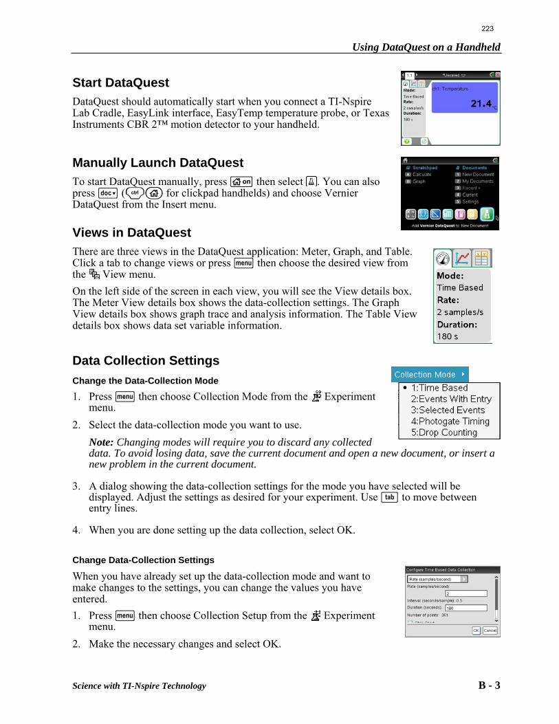
Using DataQuest on a Handheld
Science with TI-Nspire Technology B - 3
Start DataQuest
DataQuest should automatically start when you connect a TI-Nspire Lab Cradle, EasyLink interface, EasyTemp temperature probe, or Texas Instruments CBR 2™ motion detector to your handheld.
Manually Launch DataQuest
To start DataQuest manually, press c then select . You can also press ~ (/c for clickpad handhelds) and choose Vernier DataQuest from the Insert menu.
Views in DataQuest
There are three views in the DataQuest application: Meter, Graph, and Table. Click a tab to change views or press b then choose the desired view from the View menu.
On the left side of the screen in each view, you will see the View details box. The Meter View details box shows the data-collection settings. The Graph View details box shows graph trace and analysis information. The Table View details box shows data set variable information.
Data Collection Settings
Change the Data-Collection Mode
1. Press b then choose Collection Mode from the Experiment menu.
2. Select the data-collection mode you want to use.
Note: Changing modes will require you to discard any collected data. To avoid losing data, save the current document and open a new document, or insert a new problem in the current document.
3. A dialog showing the data-collection settings for the mode you have selected will be displayed. Adjust the settings as desired for your experiment. Use e to move between entry lines.
4. When you are done setting up the data collection, select OK.
Change Data-Collection Settings
When you have already set up the data-collection mode and want to make changes to the settings, you can change the values you have entered.
1. Press b then choose Collection Setup from the Experiment menu.
2. Make the necessary changes and select OK.
223
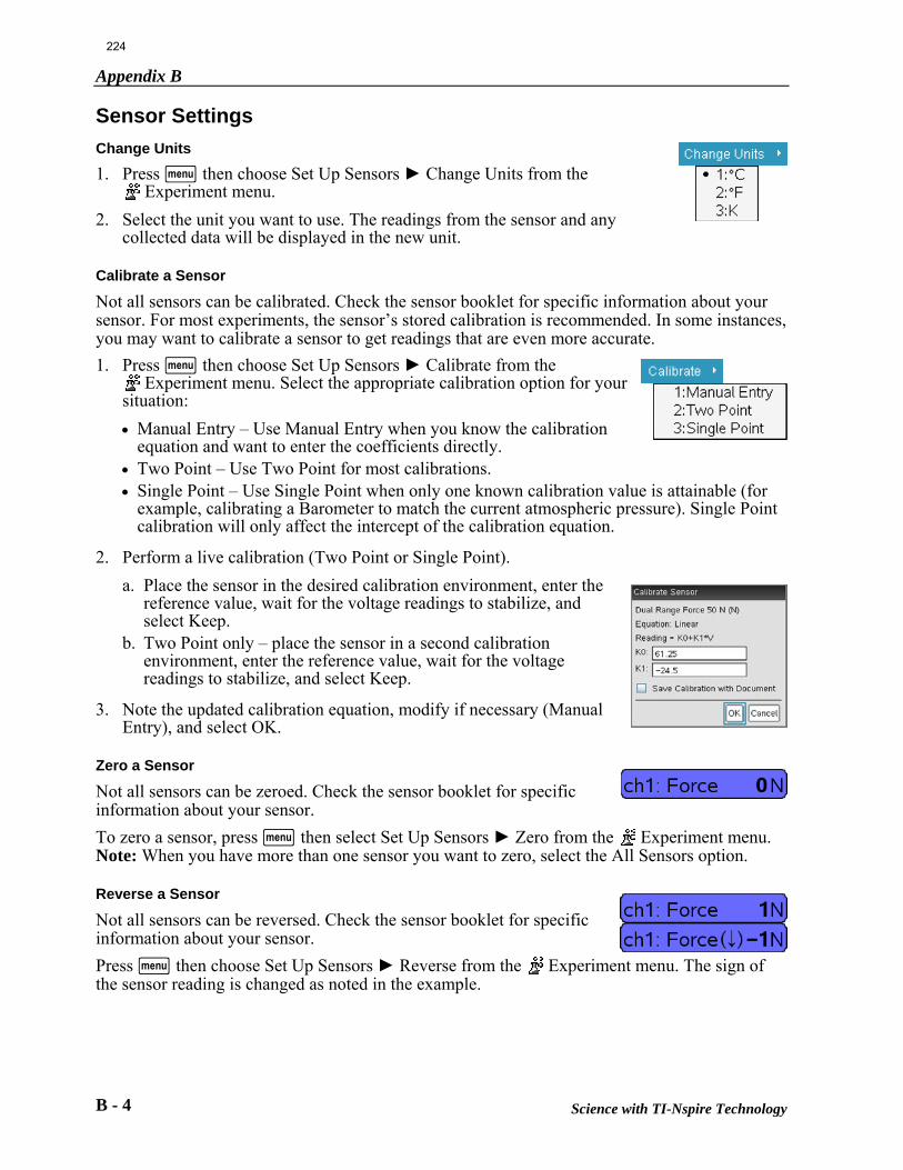
Appendix B
B - 4 Science with TI-Nspire Technology
Sensor Settings
Change Units
1. Press b then choose Set Up Sensors ► Change Units from the Experiment menu.
2. Select the unit you want to use. The readings from the sensor and any collected data will be displayed in the new unit.
Calibrate a Sensor
Not all sensors can be calibrated. Check the sensor booklet for specific information about your sensor. For most experiments, the sensor’s stored calibration is recommended. In some instances, you may want to calibrate a sensor to get readings that are even more accurate.
1. Press b then choose Set Up Sensors ► Calibrate from the Experiment menu. Select the appropriate calibration option for your
situation:
Manual Entry – Use Manual Entry when you know the calibration equation and want to enter the coefficients directly.
Two Point – Use Two Point for most calibrations. Single Point – Use Single Point when only one known calibration value is attainable (for
example, calibrating a Barometer to match the current atmospheric pressure). Single Point calibration will only affect the intercept of the calibration equation.
2. Perform a live calibration (Two Point or Single Point).
a. Place the sensor in the desired calibration environment, enter the reference value, wait for the voltage readings to stabilize, and select Keep.
b. Two Point only – place the sensor in a second calibration environment, enter the reference value, wait for the voltage readings to stabilize, and select Keep.
3. Note the updated calibration equation, modify if necessary (Manual
Entry), and select OK.
Zero a Sensor
Not all sensors can be zeroed. Check the sensor booklet for specific information about your sensor.
To zero a sensor, press b then select Set Up Sensors ► Zero from the Experiment menu. Note: When you have more than one sensor you want to zero, select the All Sensors option.
Reverse a Sensor
Not all sensors can be reversed. Check the sensor booklet for specific information about your sensor.
Press b then choose Set Up Sensors ► Reverse from the Experiment menu. The sign of the sensor reading is changed as noted in the example.
224
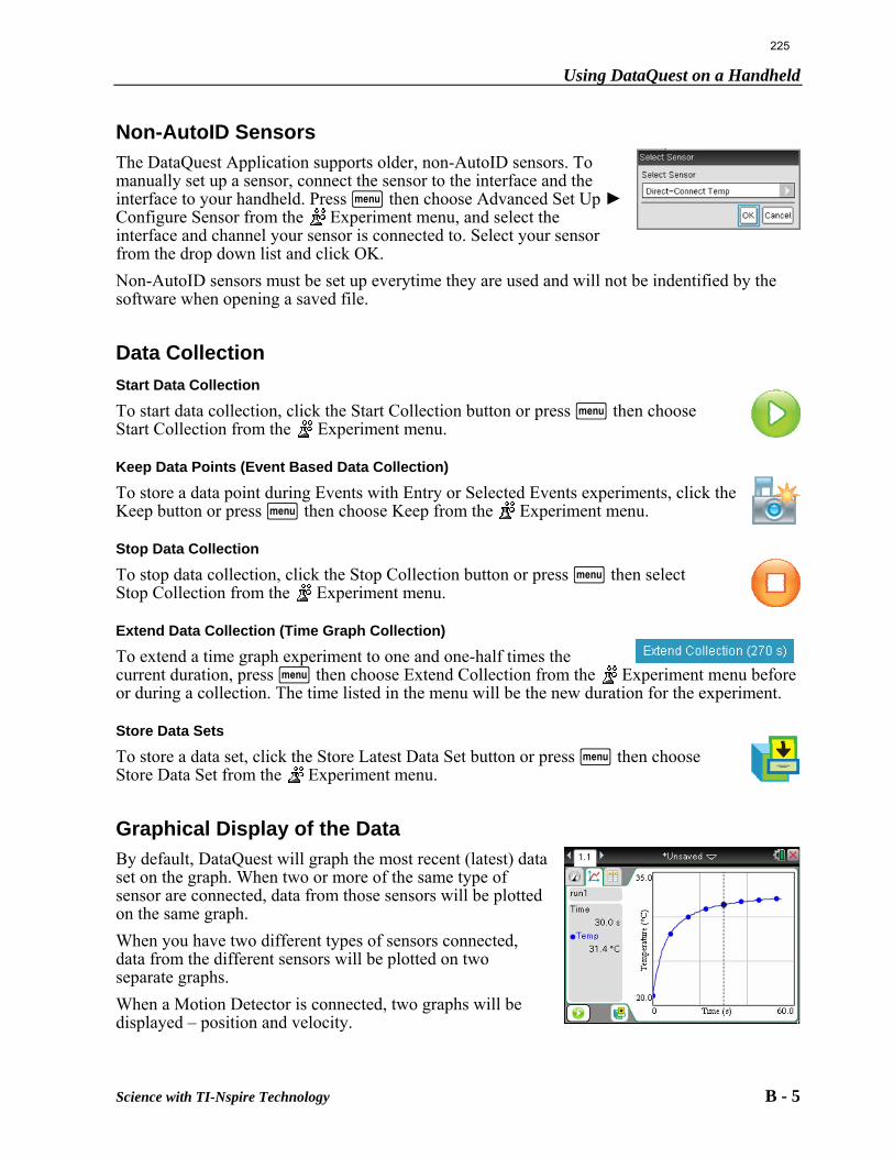
Using DataQuest on a Handheld
Science with TI-Nspire Technology B - 5
Non-AutoID Sensors
The DataQuest Application supports older, non-AutoID sensors. To manually set up a sensor, connect the sensor to the interface and the interface to your handheld. Press b then choose Advanced Set Up ► Configure Sensor from the Experiment menu, and select the interface and channel your sensor is connected to. Select your sensor from the drop down list and click OK.
Non-AutoID sensors must be set up everytime they are used and will not be indentified by the software when opening a saved file.
Data Collection
Start Data Collection
To start data collection, click the Start Collection button or press b then choose Start Collection from the Experiment menu.
Keep Data Points (Event Based Data Collection)
To store a data point during Events with Entry or Selected Events experiments, click the Keep button or press b then choose Keep from the Experiment menu.
Stop Data Collection
To stop data collection, click the Stop Collection button or press b then select Stop Collection from the Experiment menu.
Extend Data Collection (Time Graph Collection)
To extend a time graph experiment to one and one-half times the current duration, press b then choose Extend Collection from the Experiment menu before or during a collection. The time listed in the menu will be the new duration for the experiment.
Store Data Sets
To store a data set, click the Store Latest Data Set button or press b then choose Store Data Set from the Experiment menu.
Graphical Display of the Data
By default, DataQuest will graph the most recent (latest) data set on the graph. When two or more of the same type of sensor are connected, data from those sensors will be plotted on the same graph.
When you have two different types of sensors connected, data from the different sensors will be plotted on two separate graphs.
When a Motion Detector is connected, two graphs will be displayed – position and velocity.
225
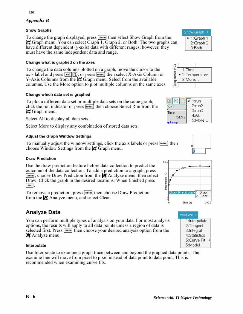
Appendix B
B - 6 Science with TI-Nspire Technology
Show Graphs
To change the graph displayed, press b then select Show Graph from the Graph menu. You can select Graph 1, Graph 2, or Both. The two graphs can
have different dependent (y-axis) data with different ranges; however, they must have the same independent data and range.
Change what is graphed on the axes
To change the data columns plotted on a graph, move the cursor to the axis label and press /a, or press b then select X-Axis Column or Y-Axis Columns from the Graph menu. Select from the available columns. Use the More option to plot multiple columns on the same axes. Change which data set is graphed
To plot a different data set or multiple data sets on the same graph, click the run indicator or press b then choose Select Run from the
Graph menu.
Select All to display all data sets.
Select More to display any combination of stored data sets. Adjust the Graph Window Settings
To manually adjust the window settings, click the axis labels or press b then choose Window Settings from the Graph menu. Draw Prediction
Use the draw prediction feature before data collection to predict the outcome of the data collection. To add a prediction to a graph, press b, choose Draw Prediction from the Analyze menu, then select Draw. Click the graph in the desired locations. When finished press d.
To remove a prediction, press b then choose Draw Prediction from the Analyze menu, and select Clear.
Analyze Data
You can perform multiple types of analysis on your data. For most analysis options, the results will apply to all data points unless a region of data is selected first. Press b then choose your desired analysis option from the
Analyze menu. Interpolate
Use Interpolate to examine a graph trace between and beyond the graphed data points. The examine line will move from pixel to pixel instead of data point to data point. This is recommended when examining curve fits.
226
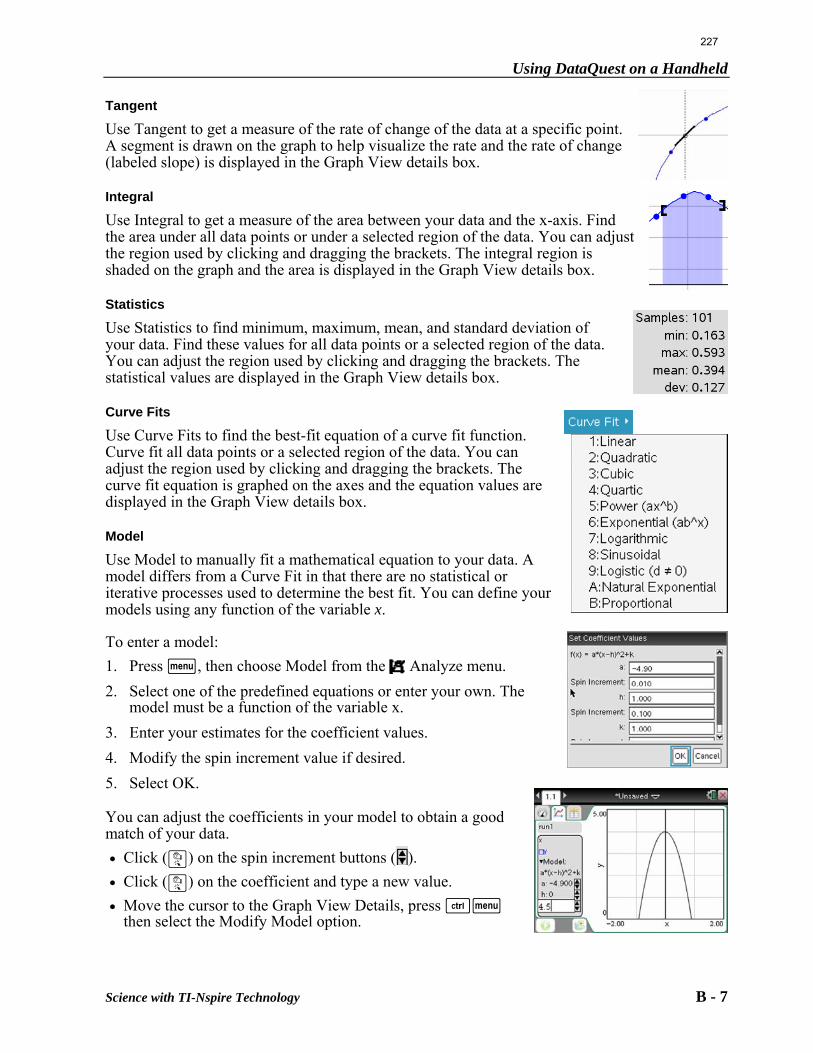
Using DataQuest on a Handheld
Science with TI-Nspire Technology B - 7
Tangent
Use Tangent to get a measure of the rate of change of the data at a specific point. A segment is drawn on the graph to help visualize the rate and the rate of change (labeled slope) is displayed in the Graph View details box.
Integral
Use Integral to get a measure of the area between your data and the x-axis. Find the area under all data points or under a selected region of the data. You can adjust the region used by clicking and dragging the brackets. The integral region is shaded on the graph and the area is displayed in the Graph View details box.
Statistics
Use Statistics to find minimum, maximum, mean, and standard deviation of your data. Find these values for all data points or a selected region of the data. You can adjust the region used by clicking and dragging the brackets. The statistical values are displayed in the Graph View details box.
Curve Fits
Use Curve Fits to find the best-fit equation of a curve fit function. Curve fit all data points or a selected region of the data. You can adjust the region used by clicking and dragging the brackets. The curve fit equation is graphed on the axes and the equation values are displayed in the Graph View details box.
Model
Use Model to manually fit a mathematical equation to your data. A model differs from a Curve Fit in that there are no statistical or iterative processes used to determine the best fit. You can define your models using any function of the variable x.
To enter a model:
1. Press b, then choose Model from the Analyze menu.
2. Select one of the predefined equations or enter your own. The model must be a function of the variable x.
3. Enter your estimates for the coefficient values.
4. Modify the spin increment value if desired.
5. Select OK. You can adjust the coefficients in your model to obtain a good match of your data.
Click (x) on the spin increment buttons ( ).
Click (x) on the coefficient and type a new value.
Move the cursor to the Graph View Details, press /b then select the Modify Model option.
227
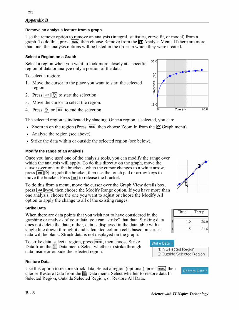
Appendix B
B - 8 Science with TI-Nspire Technology
Remove an analysis feature from a graph
Use the remove option to remove an analysis (integral, statistics, curve fit, or model) from a graph. To do this, press b then choose Remove from the Analyse Menu. If there are more than one, the analysis options will be listed in the order in which they were created.
Select a Region on a Graph
Select a region when you want to look more closely at a specific region of data or analyze only a portion of the data.
To select a region:
1. Move the cursor to the place you want to start the selected region.
2. Press /x to start the selection.
3. Move the cursor to select the region.
4. Press x or d to end the selection. The selected region is indicated by shading. Once a region is selected, you can:
Zoom in on the region (Press b then choose Zoom In from the Graph menu).
Analyze the region (see above).
Strike the data within or outside the selected region (see below). Modify the range of an analysis
Once you have used one of the analysis tools, you can modify the range over which the analysis will apply. To do this directly on the graph, move the cursor over one of the brackets, when the cursor changes to a white arrow, press /x to grab the bracket, then use the touch pad or arrow keys to move the bracket. Press d to release the bracket.
To do this from a menu, move the cursor over the Graph View details box, press /b, then choose the Modify Range option. If you have more than one analysis, choose the one you want to adjust or choose the Modify All option to apply the change to all of the existing ranges.
Strike Data
When there are data points that you wish not to have considered in the graphing or analysis of your data, you can “strike” that data. Striking data does not delete the data; rather, data is displayed in the data table with a single line drawn through it and calculated column cells based on struck data will be blank. Struck data is not displayed on the graph.
To strike data, select a region, press b, then choose Strike Data from the Data menu. Select whether to strike through data inside or outside the selected region.
Restore Data
Use this option to restore struck data. Select a region (optional), press b then choose Restore Data from the Data menu. Select whether to restore data In Selected Region, Outside Selected Region, or Restore All Data.
228
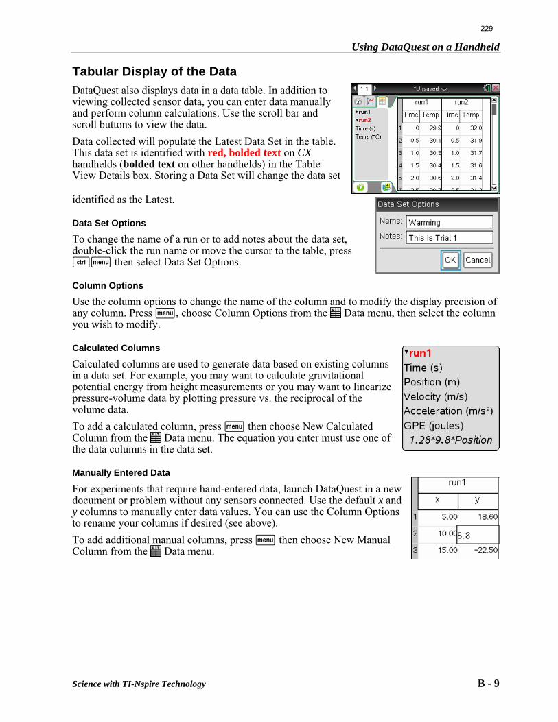
Using DataQuest on a Handheld
Science with TI-Nspire Technology B - 9
Tabular Display of the Data
DataQuest also displays data in a data table. In addition to viewing collected sensor data, you can enter data manually and perform column calculations. Use the scroll bar and scroll buttons to view the data.
Data collected will populate the Latest Data Set in the table. This data set is identified with red, bolded text on CX handhelds (bolded text on other handhelds) in the Table View Details box. Storing a Data Set will change the data set
identified as the Latest.
Data Set Options
To change the name of a run or to add notes about the data set, double-click the run name or move the cursor to the table, press /b then select Data Set Options.
Column Options
Use the column options to change the name of the column and to modify the display precision of any column. Press b, choose Column Options from the Data menu, then select the column you wish to modify.
Calculated Columns
Calculated columns are used to generate data based on existing columns in a data set. For example, you may want to calculate gravitational potential energy from height measurements or you may want to linearize pressure-volume data by plotting pressure vs. the reciprocal of the volume data.
To add a calculated column, press b then choose New Calculated Column from the Data menu. The equation you enter must use one of the data columns in the data set.
Manually Entered Data
For experiments that require hand-entered data, launch DataQuest in a new document or problem without any sensors connected. Use the default x and y columns to manually enter data values. You can use the Column Options to rename your columns if desired (see above).
To add additional manual columns, press b then choose New Manual Column from the Data menu.
229
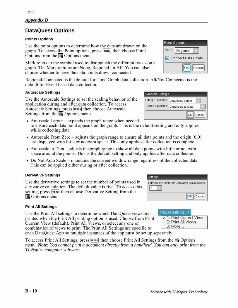
Appendix B
B - 10 Science with TI-Nspire Technology
DataQuest Options
Points Options
Use the point options to determine how the data are drawn on the graph. To access the Point options, press b then choose Point Options from the Options menu.
Mark refers to the symbol used to distinguish the different traces on a graph. The Mark options are None, Regional, or All. You can also choose whether to have the data points drawn connected.
Regional/Connected is the default for Time Graph data collection. All/Not Connected is the default for Event based data collection.
Autoscale Settings
Use the Autoscale Settings to set the scaling behavior of the application during and after data collection. To access Autoscale Settings, press b then choose Autoscale Settings from the Options menu.
Autoscale Larger – expands the graph range when needed to ensure each data point appears on the graph. This is the default setting and only applies while collecting data.
Autoscale From Zero – adjusts the graph range to ensure all data points and the origin (0,0) are displayed with little or no extra space. This only applies after collection is complete.
Autoscale to Data – adjusts the graph range to show all data points with little or no extra space around the points. This is the default setting and only applies after data collection.
Do Not Auto Scale – maintains the current window range regardless of the collected data. This can be applied either during or after collection.
Derivative Settings
Use the derivative settings to set the number of points used in derivative calculation. The default value is five. To access this setting, press b then choose Derivative Setting from the
Options menu.
Print All Settings
Use the Print All settings to determine which DataQuest views are printed when the Print All printing option is used. Choose from Print Current View (default), Print All Views, or select any one or combination of views to print. The Print All Settings are specific to each DataQuest App so multiple instances of the app must be set up separately.
To access Print All Settings, press b then choose Print All Settings from the Options menu. Note: You cannot print a document directly from a handheld. You can only print from the TI-Nspire computer software.
230
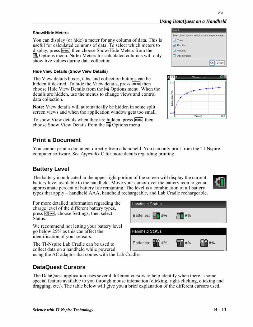
Using DataQuest on a Handheld
Science with TI-Nspire Technology B - 11
Show/Hide Meters
You can display (or hide) a meter for any column of data. This is useful for calculated columns of data. To select which meters to display, press b then choose Show/Hide Meters from the
Options menu. Note: Meters for calculated columns will only show live values during data collection.
Hide View Details (Show View Details)
The View details boxes, tabs, and collection buttons can be hidden if desired. To hide the View details, press b then choose Hide View Details from the Options menu. When the details are hidden, use the menus to change views and control data collection.
Note: View details will automatically be hidden in some split screen views and when the application window gets too small.
To show View details when they are hidden, press b then choose Show View Details from the Options menu.
Print a Document
You cannot print a document directly from a handheld. You can only print from the TI-Nspire computer software. See Appendix C for more details regarding printing.
Battery Level
The battery icon located in the upper right portion of the screen will display the current battery level available to the handheld. Move your cursor over the battery icon to get an approximate percent of battery life remaining. The level is a combination of all battery types that apply – handheld AAA, handheld rechargeable, and Lab Cradle rechargeable.
For more detailed information regarding the charge level of the different battery types, press c, choose Settings, then select Status.
We recommend not letting your battery level go below 25% as this can affect the identification of your sensors.
The TI-Nspire Lab Cradle can be used to collect data on a handheld while powered using the AC adaptor that comes with the Lab Cradle.
DataQuest Cursors
The DataQuest application uses several different cursors to help identify when there is some special feature available to you through mouse interaction (clicking, right-clicking, clicking and dragging, etc.). The table below will give you a brief explanation of the different cursors used.
231
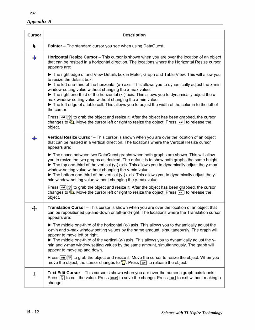
Appendix B
B - 12 Science with TI-Nspire Technology
Cursor
Description
Pointer – The standard cursor you see when using DataQuest.
Horizontal Resize Cursor – This cursor is shown when you are over the location of an object that can be resized in a horizontal direction. The locations where the Horizontal Resize cursor appears are:
► The right edge of and View Details box in Meter, Graph and Table View. This will allow you to resize the details box. ► The left one-third of the horizontal (x-) axis. This allows you to dynamically adjust the x-min window-setting value without changing the x-max value. ► The right one-third of the horizontal (x-) axis. This allows you to dynamically adjust the x-max window-setting value without changing the x-min value. ► The left edge of a table cell. This allows you to adjust the width of the column to the left of the cursor.
Press /x to grab the object and resize it. After the object has been grabbed, the cursor changes to . Move the cursor left or right to resize the object. Press d to release the object.
Vertical Resize Cursor – This cursor is shown when you are over the location of an object that can be resized in a vertical direction. The locations where the Vertical Resize cursor appears are:
► The space between two DataQuest graphs when both graphs are shown. This will allow you to resize the two graphs as desired. The default is to show both graphs the same height. ► The top one-third of the vertical (y-) axis. This allows you to dynamically adjust the y-max window-setting value without changing the y-min value. ► The bottom one-third of the vertical (y-) axis. This allows you to dynamically adjust the y-min window-setting value without changing the y-max value.
Press /x to grab the object and resize it. After the object has been grabbed, the cursor changes to . Move the cursor left or right to resize the object. Press d to release the object.
Translation Cursor – This cursor is shown when you are over the location of an object that can be repositioned up-and-down or left-and-right. The locations where the Translation cursor appears are:
► The middle one-third of the horizontal (x-) axis. This allows you to dynamically adjust the x-min and x-max window setting values by the same amount, simultaneously. The graph will appear to move left or right. ► The middle one-third of the vertical (y-) axis. This allows you to dynamically adjust the y-min and y-max window setting values by the same amount, simultaneously. The graph will appear to move up and down.
Press /x to grab the object and resize it. Move the cursor to resize the object. When you move the object, the cursor changes to . Press d to release the object.
Text Edit Cursor – This cursor is shown when you are over the numeric graph-axis labels. Press x to edit the value. Press · to save the change. Press d to exit without making a change.
232
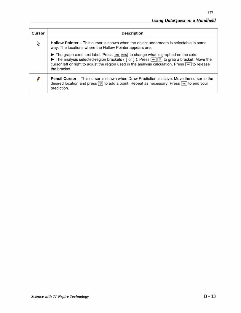
Using DataQuest on a Handheld
Science with TI-Nspire Technology B - 13
Cursor
Description
Hollow Pointer – This cursor is shown when the object underneath is selectable in some way. The locations where the Hollow Pointer appears are:
► The graph-axes text label. Press /b to change what is graphed on the axis. ► The analysis selected-region brackets ( [ or ] ). Press /x to grab a bracket. Move the cursor left or right to adjust the region used in the analysis calculation. Press d to release the bracket.
Pencil Cursor – This cursor is shown when Draw Prediction is active. Move the cursor to the desired location and press x to add a point. Repeat as necessary. Press d to end your prediction.
233

This page intentionally left blank
234
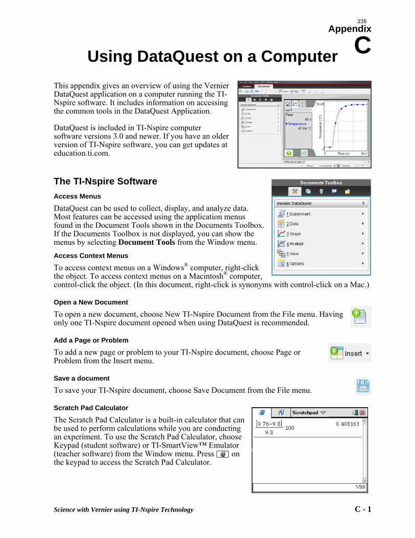
Appendix
C
Science with Vernier using TI-Nspire Technology C - 1
Using DataQuest on a Computer
This appendix gives an overview of using the Vernier DataQuest application on a computer running the TI-Nspire software. It includes information on accessing the common tools in the DataQuest Application.
DataQuest is included in TI-Nspire computer software versions 3.0 and newer. If you have an older version of TI-Nspire software, you can get updates at education.ti.com.
The TI-Nspire Software
Access Menus
DataQuest can be used to collect, display, and analyze data. Most features can be accessed using the application menus found in the Document Tools shown in the Documents Toolbox. If the Documents Toolbox is not displayed, you can show the menus by selecting Document Tools from the Window menu.
Access Context Menus
To access context menus on a Windows® computer, right-click the object. To access context menus on a Macintosh® computer, control-click the object. (In this document, right-click is synonyms with control-click on a Mac.)
Open a New Document
To open a new document, choose New TI-Nspire Document from the File menu. Having only one TI-Nspire document opened when using DataQuest is recommended.
Add a Page or Problem
To add a new page or problem to your TI-Nspire document, choose Page or Problem from the Insert menu.
Save a document
To save your TI-Nspire document, choose Save Document from the File menu.
Scratch Pad Calculator
The Scratch Pad Calculator is a built-in calculator that can be used to perform calculations while you are conducting an experiment. To use the Scratch Pad Calculator, choose Keypad (student software) or TI-SmartView™ Emulator (teacher software) from the Window menu. Press » on the keypad to access the Scratch Pad Calculator.
235
Appendix C
C - 2 Science with Vernier using TI-Nspire Technology
Start DataQuest
DataQuest should automatically start when TI-Nspire software is running on your computer and you connect a TI-Nspire Lab Cradle, Go! Link interface, Go!Temp temperature probe, or Go!Motion motion detector.
Manually Launch DataQuest
To start DataQuest manually, choose Vernier DataQuest from the Insert menu.
Views in DataQuest
There are three views in the DataQuest application: Meter, Graph, and Table. Click a tab to change views or choose the desired view from the View menu.
On the left side of the screen in each view, you will see the View details box. The Meter View details box shows the data-collection settings. The Graph View details box shows graph trace and analysis information. The Table View details box shows data set variable information.
Data Collection Settings
Change the Data-Collection Mode
1. Choose Collection Mode from the Experiment menu or right click the Meter Details and select Collection Mode.
2. Select the data-collection mode you want to use.
Note: Changing modes will require you to discard any collected data. To avoid losing data, save the current document and open a new document, or insert a new problem in the current document.
3. A dialog showing the data collection settings for the mode you have selected will be displayed. Adjust the settings as desired for your experiment.
4. When you are done setting up the data collection, select OK.
Change Data-Collection Settings
When you have already set up the data-collection mode and want to make changes to the settings, you can change the values you have entered.
1. Choose Collection Setup from the Experiment menu or right-click the Meter View details box and select Collection Setup.
2. Make the necessary changes and select OK.
236
Using DataQuest on a Computer
Science with Vernier using TI-Nspire Technology C - 3
Sensor Settings
Change Units
1. Choose Set Up Sensors ► Change Units from the Experiment menu or right-click the sensor’s meter and select Change Units.
2. Select the unit you want to use. The readings from the sensor and any collected data will be displayed in the new unit.
Calibrate a Sensor
Not all sensors can be calibrated. Check the sensor booklet for specific information about your sensor. For most experiments, the sensor’s stored calibration is recommended. In some instances, you may want to calibrate a sensor to get readings that are even more accurate.
1. Choose Set Up Sensors ► Calibrate from the Experiment menu or right-click the sensor’s meter and select Calibrate. Select the appropriate calibration option for your situation:
Manual Entry – Use Manual Entry when you know the calibration equation and want to enter the coefficients directly.
Two Point – Use Two Point for most calibrations. Single Point – Use Single Point when only one known calibration value is attainable (for
example, calibrating a Barometer to match the current atmospheric pressure). Single Point calibration will only affect the intercept of the calibration equation.
2. Perform a live calibration (Two Point or Single Point).
a. Place the sensor in the desired calibration environment, enter the reference value, wait for the voltage readings to stabilize, and select Keep.
b. Two Point only – place the sensor in a second calibration environment, enter the reference value, wait for the voltage readings to stabilize, and select Keep.
3. Note the updated calibration equation, modify if necessary
(Manual Entry), and select OK.
Zero a Sensor
Not all sensors can be zeroed. Check the sensor booklet for specific information about your sensor.
To zero a sensor, select Set Up Sensors ► Zero from the Experiment menu or right-click the sensor’s meter and select Zero. Note: When you have more than one sensor you want to zero at the same time, select Set Up Sensors ► Zero ► All Sensors from the Experiment menu.
Reverse a Sensor
Not all sensors can be reversed. Check the sensor booklet for specific information about your sensor.
Choose Set Up Sensors ► Reverse from the Experiment menu or right-click the sensor’s meter and select Reverse. The sign of the sensor reading is changed as noted in the example.
237
Appendix C
C - 4 Science with Vernier using TI-Nspire Technology
Non-AutoID Sensors
The DataQuest Application supports older, non-AutoID sensors. To manually set up a sensor, connect the sensor to the interface and the interface to your computer. Choose Advanced Set Up ► Configure Sensor from the
Experiment menu, and select the interface and channel your sensor is connected to . Select your sensor from the drop down list and click OK.
Non-AutoID sensors must be set up everytime they are used and will not be indentified by the software when opening a saved file.
Data Collection
Start Data Collection
To start data collection, click the Start Collection button or choose Start Collection from the Experiment menu.
Keep Data Points (Event Based Data Collection)
To store a data point during Events with Entry or Selected Events experiments, click the Keep button or choose Keep from the Experiment menu.
Stop Data Collection
To stop data collection, click the Stop Collection button or select Stop Collection from the Experiment menu.
Extend Data Collection (Time Graph Collection)
To extend a time graph experiment duration to one and one-half times the current duration, choose Extend Collection from the Experiment menu before or during a collection. The time listed in the menu will be the new duration for the experiment.
Store Data Sets
To store a data set, click the Store Current Data Set button or choose Store Data Set from the Experiment menu.
Graphical Display of the Data
By default, DataQuest will graph the most recent (latest) data set on the graph. When two or more of the same type of sensor are connected, data from those sensors will be plotted on the same graph.
When you have two different types of sensors connected, data from the different sensors will be plotted on two separate graphs.
When a Motion Detector is connected, two graphs will be displayed – position and velocity.
238
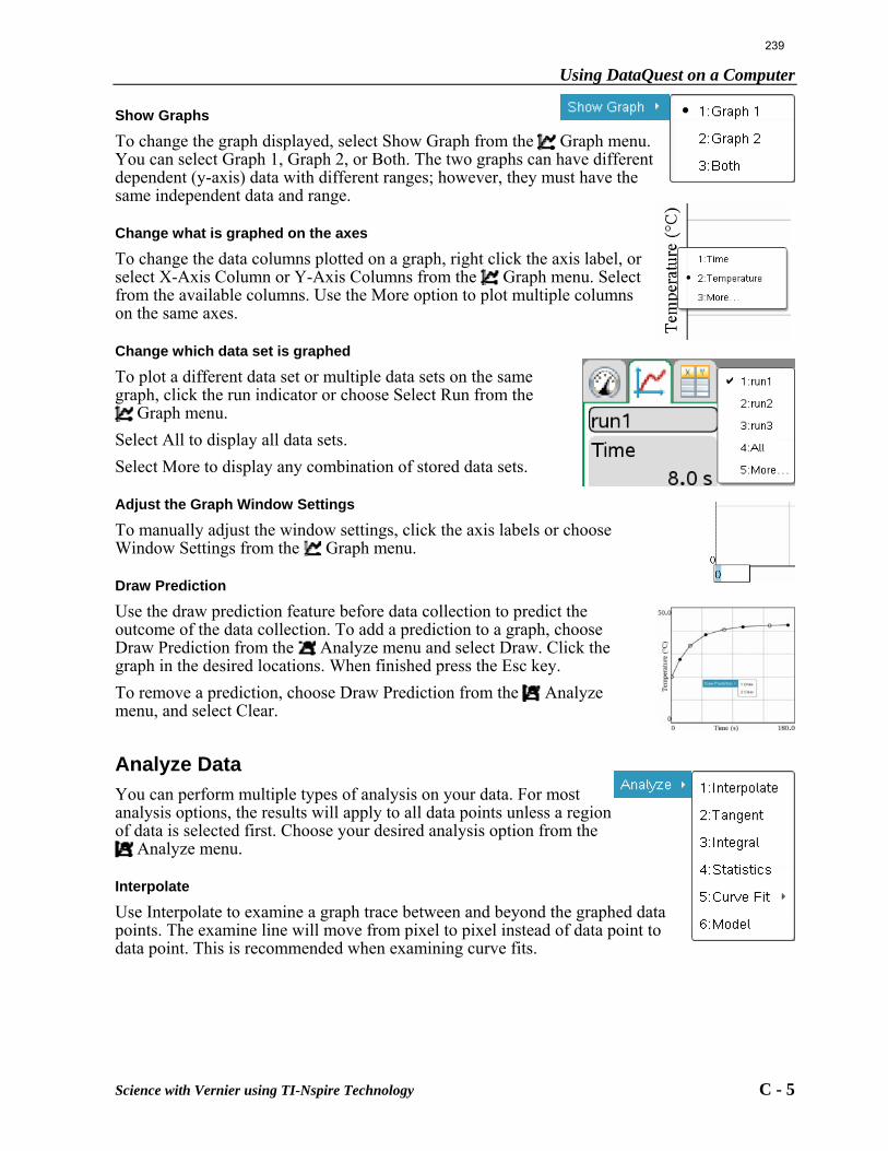
Using DataQuest on a Computer
Science with Vernier using TI-Nspire Technology C - 5
Show Graphs
To change the graph displayed, select Show Graph from the Graph menu. You can select Graph 1, Graph 2, or Both. The two graphs can have different dependent (y-axis) data with different ranges; however, they must have the same independent data and range.
Change what is graphed on the axes
To change the data columns plotted on a graph, right click the axis label, or select X-Axis Column or Y-Axis Columns from the Graph menu. Select from the available columns. Use the More option to plot multiple columns on the same axes. Change which data set is graphed
To plot a different data set or multiple data sets on the same graph, click the run indicator or choose Select Run from the
Graph menu.
Select All to display all data sets.
Select More to display any combination of stored data sets. Adjust the Graph Window Settings
To manually adjust the window settings, click the axis labels or choose Window Settings from the Graph menu. Draw Prediction
Use the draw prediction feature before data collection to predict the outcome of the data collection. To add a prediction to a graph, choose Draw Prediction from the Analyze menu and select Draw. Click the graph in the desired locations. When finished press the Esc key.
To remove a prediction, choose Draw Prediction from the Analyze menu, and select Clear.
Analyze Data
You can perform multiple types of analysis on your data. For most analysis options, the results will apply to all data points unless a region of data is selected first. Choose your desired analysis option from the
Analyze menu. Interpolate
Use Interpolate to examine a graph trace between and beyond the graphed data points. The examine line will move from pixel to pixel instead of data point to data point. This is recommended when examining curve fits.
239
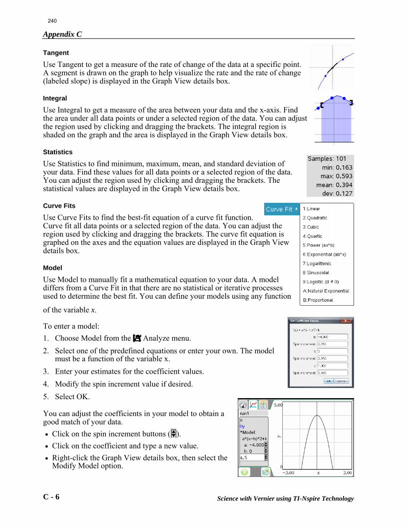
Appendix C
C - 6 Science with Vernier using TI-Nspire Technology
Tangent
Use Tangent to get a measure of the rate of change of the data at a specific point. A segment is drawn on the graph to help visualize the rate and the rate of change (labeled slope) is displayed in the Graph View details box.
Integral
Use Integral to get a measure of the area between your data and the x-axis. Find the area under all data points or under a selected region of the data. You can adjust the region used by clicking and dragging the brackets. The integral region is shaded on the graph and the area is displayed in the Graph View details box.
Statistics
Use Statistics to find minimum, maximum, mean, and standard deviation of your data. Find these values for all data points or a selected region of the data. You can adjust the region used by clicking and dragging the brackets. The statistical values are displayed in the Graph View details box.
Curve Fits
Use Curve Fits to find the best-fit equation of a curve fit function. Curve fit all data points or a selected region of the data. You can adjust the region used by clicking and dragging the brackets. The curve fit equation is graphed on the axes and the equation values are displayed in the Graph View details box.
Model
Use Model to manually fit a mathematical equation to your data. A model differs from a Curve Fit in that there are no statistical or iterative processes used to determine the best fit. You can define your models using any function
of the variable x.
To enter a model:
1. Choose Model from the Analyze menu.
2. Select one of the predefined equations or enter your own. The model must be a function of the variable x.
3. Enter your estimates for the coefficient values.
4. Modify the spin increment value if desired.
5. Select OK. You can adjust the coefficients in your model to obtain a good match of your data.
Click on the spin increment buttons ( ).
Click on the coefficient and type a new value.
Right-click the Graph View details box, then select the Modify Model option.
240
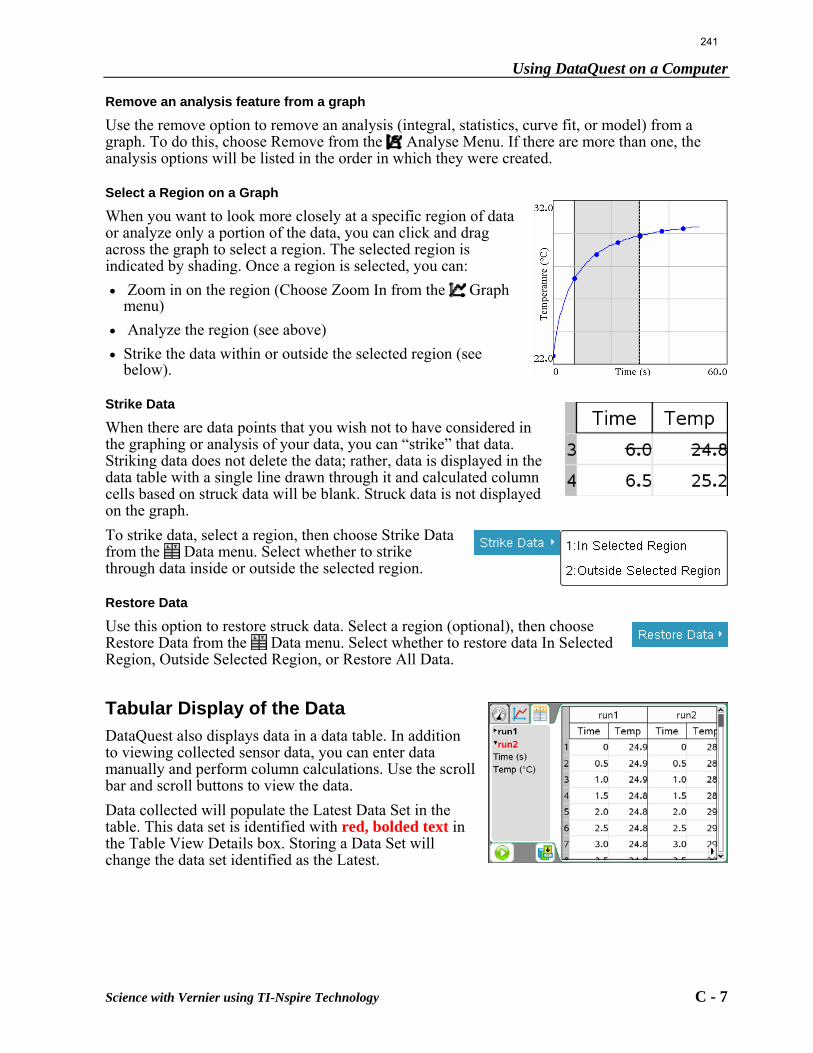
Using DataQuest on a Computer
Science with Vernier using TI-Nspire Technology C - 7
Remove an analysis feature from a graph
Use the remove option to remove an analysis (integral, statistics, curve fit, or model) from a graph. To do this, choose Remove from the Analyse Menu. If there are more than one, the analysis options will be listed in the order in which they were created.
Select a Region on a Graph
When you want to look more closely at a specific region of data or analyze only a portion of the data, you can click and drag across the graph to select a region. The selected region is indicated by shading. Once a region is selected, you can:
Zoom in on the region (Choose Zoom In from the Graph menu)
Analyze the region (see above)
Strike the data within or outside the selected region (see below).
Strike Data
When there are data points that you wish not to have considered in the graphing or analysis of your data, you can “strike” that data. Striking data does not delete the data; rather, data is displayed in the data table with a single line drawn through it and calculated column cells based on struck data will be blank. Struck data is not displayed on the graph.
To strike data, select a region, then choose Strike Data from the Data menu. Select whether to strike through data inside or outside the selected region.
Restore Data
Use this option to restore struck data. Select a region (optional), then choose Restore Data from the Data menu. Select whether to restore data In Selected Region, Outside Selected Region, or Restore All Data.
Tabular Display of the Data
DataQuest also displays data in a data table. In addition to viewing collected sensor data, you can enter data manually and perform column calculations. Use the scroll bar and scroll buttons to view the data.
Data collected will populate the Latest Data Set in the table. This data set is identified with red, bolded text in the Table View Details box. Storing a Data Set will change the data set identified as the Latest.
241
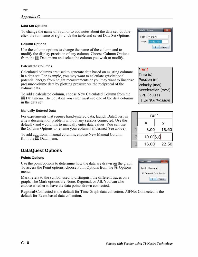
Appendix C
C - 8 Science with Vernier using TI-Nspire Technology
Data Set Options
To change the name of a run or to add notes about the data set, double-click the run name or right-click the table and select Data Set Options.
Column Options
Use the column options to change the name of the column and to modify the display precision of any column. Choose Column Options from the Data menu and select the column you wish to modify.
Calculated Columns
Calculated columns are used to generate data based on existing columns in a data set. For example, you may want to calculate gravitational potential energy from height measurements or you may want to linearize pressure-volume data by plotting pressure vs. the reciprocal of the volume data.
To add a calculated column, choose New Calculated Column from the Data menu. The equation you enter must use one of the data columns
in the data set.
Manually Entered Data
For experiments that require hand-entered data, launch DataQuest in a new document or problem without any sensors connected. Use the default x and y columns to manually enter data values. You can use the Column Options to rename your columns if desired (see above).
To add additional manual columns, choose New Manual Column from the Data menu.
DataQuest Options
Points Options
Use the point options to determine how the data are drawn on the graph. To access the Point options, choose Point Options from the Options menu.
Mark refers to the symbol used to distinguish the different traces on a graph. The Mark options are None, Regional, or All. You can also choose whether to have the data points drawn connected.
Regional/Connected is the default for Time Graph data collection. All/Not Connected is the default for Event based data collection.
242
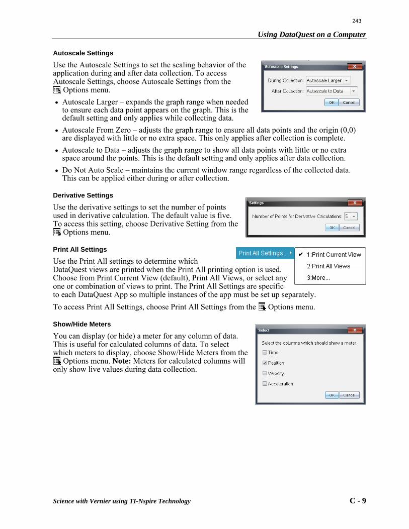
Using DataQuest on a Computer
Science with Vernier using TI-Nspire Technology C - 9
Autoscale Settings
Use the Autoscale Settings to set the scaling behavior of the application during and after data collection. To access Autoscale Settings, choose Autoscale Settings from the
Options menu.
Autoscale Larger – expands the graph range when needed to ensure each data point appears on the graph. This is the default setting and only applies while collecting data.
Autoscale From Zero – adjusts the graph range to ensure all data points and the origin (0,0) are displayed with little or no extra space. This only applies after collection is complete.
Autoscale to Data – adjusts the graph range to show all data points with little or no extra space around the points. This is the default setting and only applies after data collection.
Do Not Auto Scale – maintains the current window range regardless of the collected data. This can be applied either during or after collection.
Derivative Settings
Use the derivative settings to set the number of points used in derivative calculation. The default value is five. To access this setting, choose Derivative Setting from the
Options menu.
Print All Settings
Use the Print All settings to determine which DataQuest views are printed when the Print All printing option is used. Choose from Print Current View (default), Print All Views, or select any one or combination of views to print. The Print All Settings are specific to each DataQuest App so multiple instances of the app must be set up separately.
To access Print All Settings, choose Print All Settings from the Options menu.
Show/Hide Meters
You can display (or hide) a meter for any column of data. This is useful for calculated columns of data. To select which meters to display, choose Show/Hide Meters from the
Options menu. Note: Meters for calculated columns will only show live values during data collection.
243
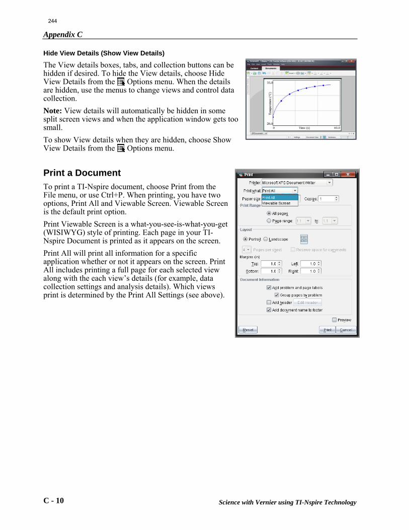
Appendix C
C - 10 Science with Vernier using TI-Nspire Technology
Hide View Details (Show View Details)
The View details boxes, tabs, and collection buttons can be hidden if desired. To hide the View details, choose Hide View Details from the Options menu. When the details are hidden, use the menus to change views and control data collection.
Note: View details will automatically be hidden in some split screen views and when the application window gets too small.
To show View details when they are hidden, choose Show View Details from the Options menu.
Print a Document
To print a TI-Nspire document, choose Print from the File menu, or use Ctrl+P. When printing, you have two options, Print All and Viewable Screen. Viewable Screen is the default print option.
Print Viewable Screen is a what-you-see-is-what-you-get (WISIWYG) style of printing. Each page in your TI-Nspire Document is printed as it appears on the screen.
Print All will print all information for a specific application whether or not it appears on the screen. Print All includes printing a full page for each selected view along with the each view’s details (for example, data collection settings and analysis details). Which views print is determined by the Print All Settings (see above).
244
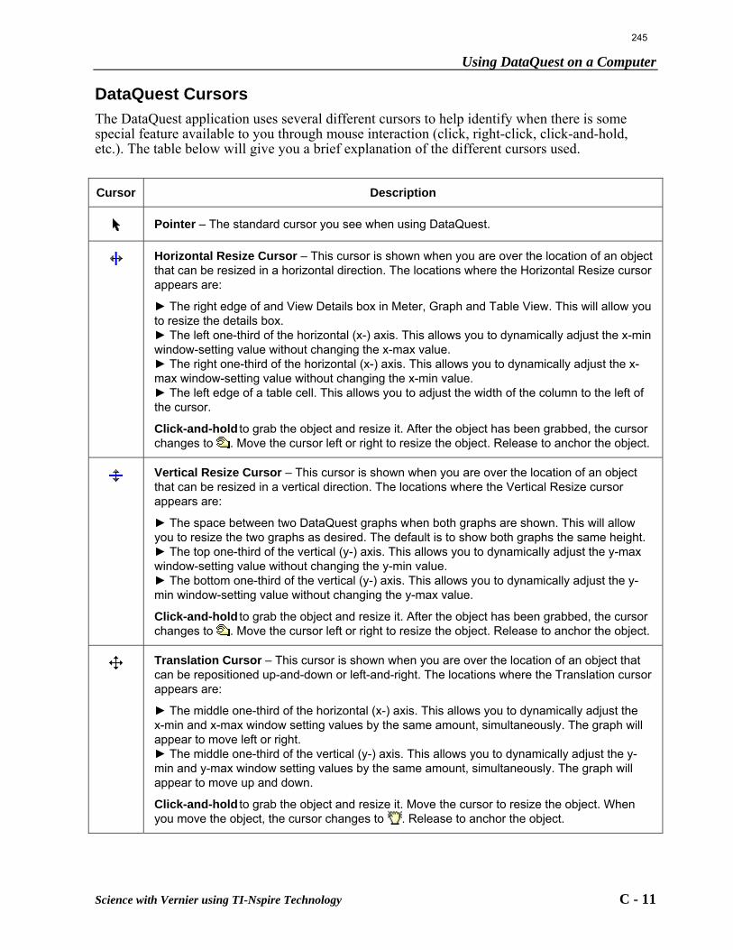
Using DataQuest on a Computer
Science with Vernier using TI-Nspire Technology C - 11
DataQuest Cursors
The DataQuest application uses several different cursors to help identify when there is some special feature available to you through mouse interaction (click, right-click, click-and-hold, etc.). The table below will give you a brief explanation of the different cursors used.
Cursor
Description
Pointer – The standard cursor you see when using DataQuest.
Horizontal Resize Cursor – This cursor is shown when you are over the location of an object that can be resized in a horizontal direction. The locations where the Horizontal Resize cursor appears are:
► The right edge of and View Details box in Meter, Graph and Table View. This will allow you to resize the details box. ► The left one-third of the horizontal (x-) axis. This allows you to dynamically adjust the x-min window-setting value without changing the x-max value. ► The right one-third of the horizontal (x-) axis. This allows you to dynamically adjust the x-max window-setting value without changing the x-min value. ► The left edge of a table cell. This allows you to adjust the width of the column to the left of the cursor.
Click-and-hold to grab the object and resize it. After the object has been grabbed, the cursor changes to . Move the cursor left or right to resize the object. Release to anchor the object.
Vertical Resize Cursor – This cursor is shown when you are over the location of an object that can be resized in a vertical direction. The locations where the Vertical Resize cursor appears are:
► The space between two DataQuest graphs when both graphs are shown. This will allow you to resize the two graphs as desired. The default is to show both graphs the same height. ► The top one-third of the vertical (y-) axis. This allows you to dynamically adjust the y-max window-setting value without changing the y-min value. ► The bottom one-third of the vertical (y-) axis. This allows you to dynamically adjust the y-min window-setting value without changing the y-max value.
Click-and-hold to grab the object and resize it. After the object has been grabbed, the cursor changes to . Move the cursor left or right to resize the object. Release to anchor the object.
Translation Cursor – This cursor is shown when you are over the location of an object that can be repositioned up-and-down or left-and-right. The locations where the Translation cursor appears are:
► The middle one-third of the horizontal (x-) axis. This allows you to dynamically adjust the x-min and x-max window setting values by the same amount, simultaneously. The graph will appear to move left or right. ► The middle one-third of the vertical (y-) axis. This allows you to dynamically adjust the y-min and y-max window setting values by the same amount, simultaneously. The graph will appear to move up and down.
Click-and-hold to grab the object and resize it. Move the cursor to resize the object. When you move the object, the cursor changes to . Release to anchor the object.
245
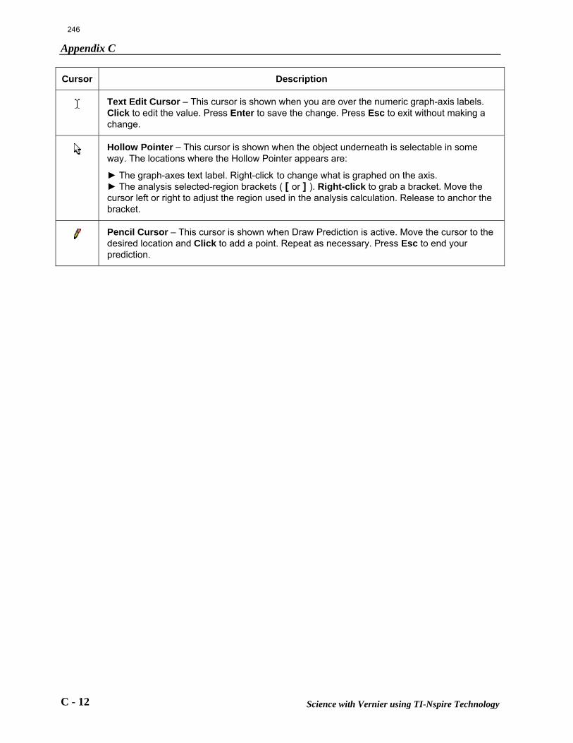
Appendix C
C - 12 Science with Vernier using TI-Nspire Technology
Cursor
Description
Text Edit Cursor – This cursor is shown when you are over the numeric graph-axis labels. Click to edit the value. Press Enter to save the change. Press Esc to exit without making a change.
Hollow Pointer – This cursor is shown when the object underneath is selectable in some way. The locations where the Hollow Pointer appears are:
► The graph-axes text label. Right-click to change what is graphed on the axis. ► The analysis selected-region brackets ( [ or ] ). Right-click to grab a bracket. Move the cursor left or right to adjust the region used in the analysis calculation. Release to anchor the bracket.
Pencil Cursor – This cursor is shown when Draw Prediction is active. Move the cursor to the desired location and Click to add a point. Repeat as necessary. Press Esc to end your prediction.
246
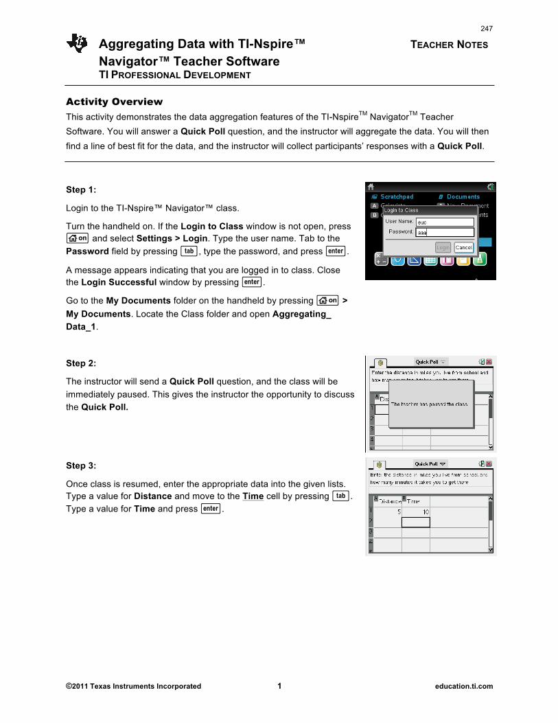
Aggregating Data with TI-Nspire™ TEACHER NOTES Navigator™ Teacher Software
TI PROFESSIONAL DEVELOPMENT
©2011 Texas Instruments Incorporated 1 education.ti.com
Activity Overview
This activity demonstrates the data aggregation features of the TI-NspireTM NavigatorTM Teacher
Software. You will answer a Quick Poll question, and the instructor will aggregate the data. You will then
find a line of best fit for the data, and the instructor will collect participants’ responses with a Quick Poll.
Step 1:
Login to the TI-Nspire™ Navigator™ class.
Turn the handheld on. If the Login to Class window is not open, press c and select Settings > Login. Type the user name. Tab to the
Password field by pressing e, type the password, and press ·.
A message appears indicating that you are logged in to class. Close the Login Successful window by pressing ·.
Go to the My Documents folder on the handheld by pressing c >
My Documents. Locate the Class folder and open Aggregating_
Data_1.
Step 2:
The instructor will send a Quick Poll question, and the class will be
immediately paused. This gives the instructor the opportunity to discuss
the Quick Poll.
Step 3:
Once class is resumed, enter the appropriate data into the given lists. Type a value for Distance and move to the Time cell by pressing e.
Type a value for Time and press ·.
247
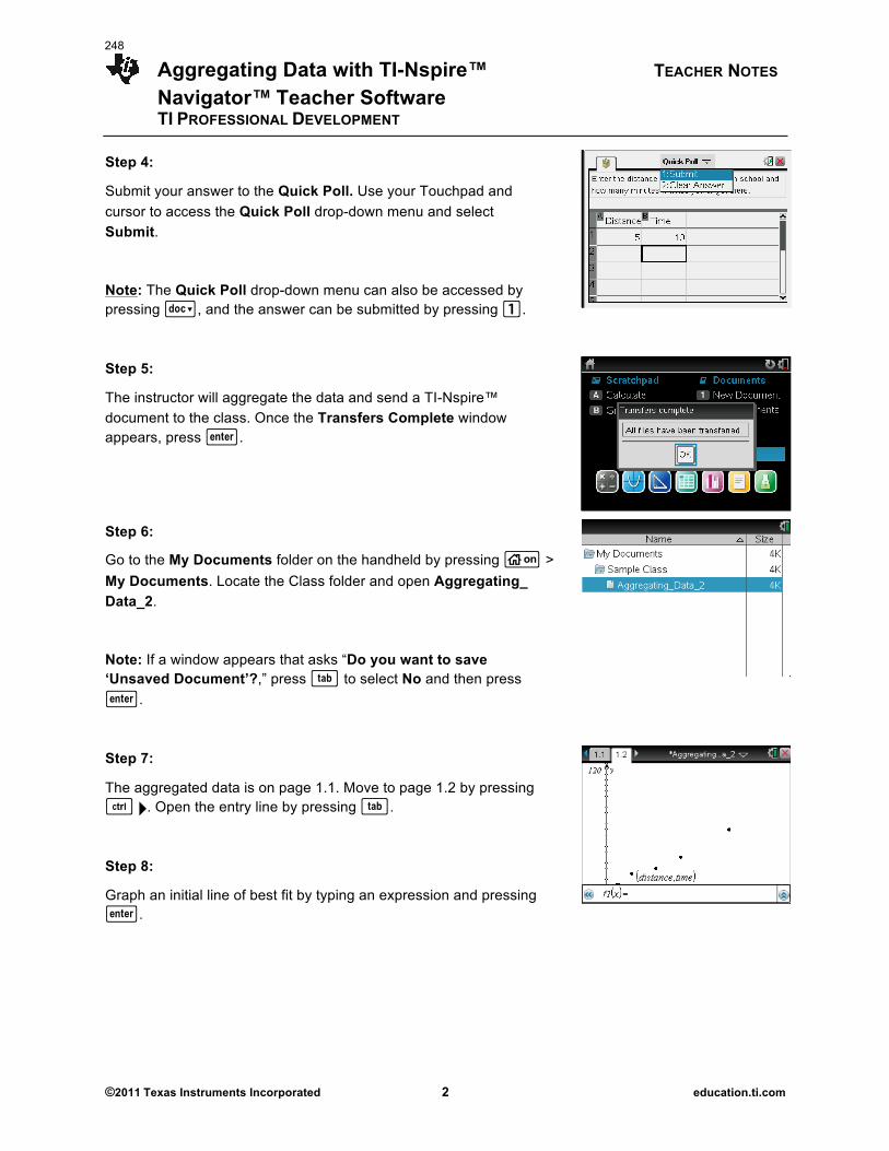
Aggregating Data with TI-Nspire™ TEACHER NOTES Navigator™ Teacher Software
TI PROFESSIONAL DEVELOPMENT
©2011 Texas Instruments Incorporated 2 education.ti.com
Step 4:
Submit your answer to the Quick Poll. Use your Touchpad and
cursor to access the Quick Poll drop-down menu and select
Submit.
Note: The Quick Poll drop-down menu can also be accessed by pressing ~, and the answer can be submitted by pressing 1.
Step 5:
The instructor will aggregate the data and send a TI-Nspire™
document to the class. Once the Transfers Complete window appears, press ·.
Step 6:
Go to the My Documents folder on the handheld by pressing c >
My Documents. Locate the Class folder and open Aggregating_
Data_2.
Note: If a window appears that asks “Do you want to save ‘Unsaved Document’?,” press e to select No and then press
·.
Step 7:
The aggregated data is on page 1.1. Move to page 1.2 by pressing / ¢. Open the entry line by pressing e.
Step 8:
Graph an initial line of best fit by typing an expression and pressing ·.
248
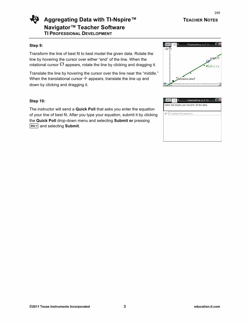
Aggregating Data with TI-Nspire™ TEACHER NOTES Navigator™ Teacher Software
TI PROFESSIONAL DEVELOPMENT
©2011 Texas Instruments Incorporated 3 education.ti.com
Step 9:
Transform the line of best fit to best model the given data. Rotate the
line by hovering the cursor over either “end” of the line. When the rotational cursor é appears, rotate the line by clicking and dragging it.
Translate the line by hovering the cursor over the line near the “middle.” When the translational cursor ö appears, translate the line up and
down by clicking and dragging it.
Step 10:
The instructor will send a Quick Poll that asks you enter the equation
of your line of best fit. After you type your equation, submit it by clicking
the Quick Poll drop-down menu and selecting Submit or pressing ~ and selecting Submit.
249

This page intentionally left blank
250
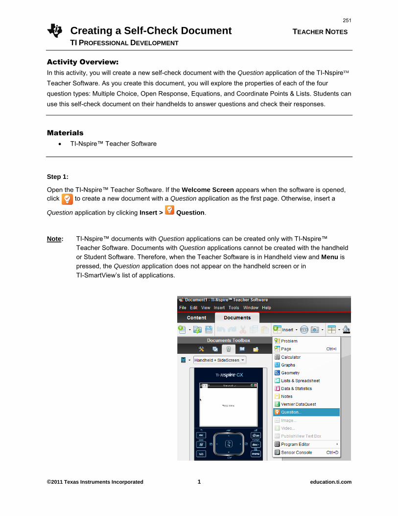
Creating a Self-Check Document TEACHER NOTES
TI PROFESSIONAL DEVELOPMENT
©2011 Texas Instruments Incorporated 1 education.ti.com
Activity Overview:
In this activity, you will create a new self-check document with the Question application of the TI-Nspire Teacher Software. As you create this document, you will explore the properties of each of the four question types: Multiple Choice, Open Response, Equations, and Coordinate Points & Lists. Students can use this self-check document on their handhelds to answer questions and check their responses.
Materials
TI-Nspire™ Teacher Software
Step 1:
Open the TI-Nspire™ Teacher Software. If the Welcome Screen appears when the software is opened, click to create a new document with a Question application as the first page. Otherwise, insert a
Question application by clicking Insert > Question.
Note: TI-Nspire™ documents with Question applications can be created only with TI-Nspire™ Teacher Software. Documents with Question applications cannot be created with the handheld or Student Software. Therefore, when the Teacher Software is in Handheld view and Menu is pressed, the Question application does not appear on the handheld screen or in TI-SmartView’s list of applications.
251
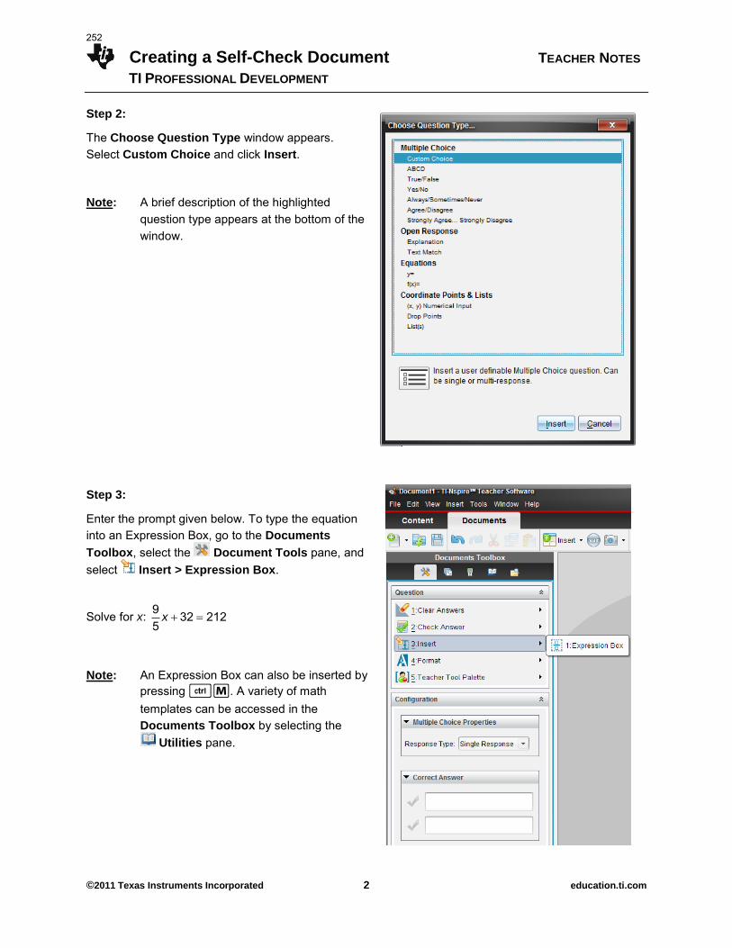
Creating a Self-Check Document TEACHER NOTES
TI PROFESSIONAL DEVELOPMENT
©2011 Texas Instruments Incorporated 2 education.ti.com
Step 2:
The Choose Question Type window appears. Select Custom Choice and click Insert.
Note: A brief description of the highlighted question type appears at the bottom of the window.
Step 3:
Enter the prompt given below. To type the equation into an Expression Box, go to the Documents
Toolbox, select the Document Tools pane, and select Insert > Expression Box.
Solve for x: 9 32 2125
x
Note: An Expression Box can also be inserted by pressing /M. A variety of math templates can be accessed in the Documents Toolbox by selecting the
Utilities pane.
252
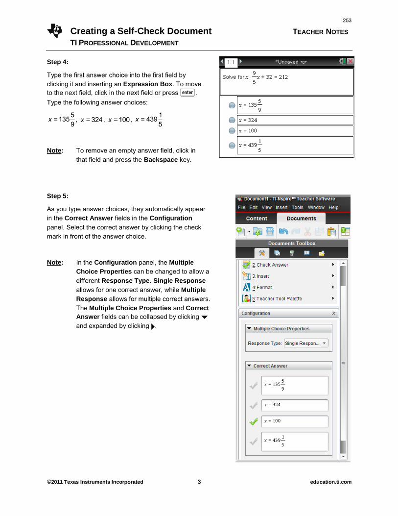
Creating a Self-Check Document TEACHER NOTES
TI PROFESSIONAL DEVELOPMENT
©2011 Texas Instruments Incorporated 3 education.ti.com
Step 4:
Type the first answer choice into the first field by clicking it and inserting an Expression Box. To move to the next field, click in the next field or press ·. Type the following answer choices:
x = 135 59
, x = 324 , x = 100, x = 439 15
Note: To remove an empty answer field, click in that field and press the Backspace key.
Step 5:
As you type answer choices, they automatically appear in the Correct Answer fields in the Configuration
panel. Select the correct answer by clicking the check mark in front of the answer choice.
Note: In the Configuration panel, the Multiple
Choice Properties can be changed to allow a different Response Type. Single Response allows for one correct answer, while Multiple
Response allows for multiple correct answers. The Multiple Choice Properties and Correct
Answer fields can be collapsed by clicking ¤ and expanded by clicking ¢.
253
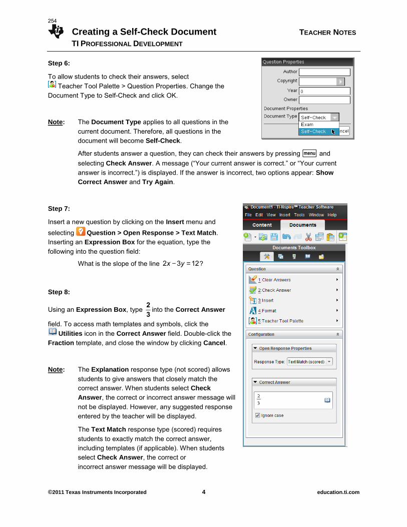
Creating a Self-Check Document TEACHER NOTES
TI PROFESSIONAL DEVELOPMENT
©2011 Texas Instruments Incorporated 4 education.ti.com
Step 6:
To allow students to check their answers, select Teacher Tool Palette > Question Properties. Change the
Document Type to Self-Check and click OK.
Note: The Document Type applies to all questions in the current document. Therefore, all questions in the document will become Self-Check.
After students answer a question, they can check their answers by pressing b and selecting Check Answer. A message (“Your current answer is correct.” or “Your current
answer is incorrect.”) is displayed. If the answer is incorrect, two options appear: Show
Correct Answer and Try Again.
Step 7:
Insert a new question by clicking on the Insert menu and selecting Question > Open Response > Text Match. Inserting an Expression Box for the equation, type the following into the question field:
What is the slope of the line 2x - 3y = 12?
Step 8:
Using an Expression Box, type 2
3into the Correct Answer
field. To access math templates and symbols, click the Utilities icon in the Correct Answer field. Double-click the
Fraction template, and close the window by clicking Cancel.
Note: The Explanation response type (not scored) allows students to give answers that closely match the correct answer. When students select Check
Answer, the correct or incorrect answer message will not be displayed. However, any suggested response entered by the teacher will be displayed.
The Text Match response type (scored) requires students to exactly match the correct answer, including templates (if applicable). When students select Check Answer, the correct or incorrect answer message will be displayed.
254
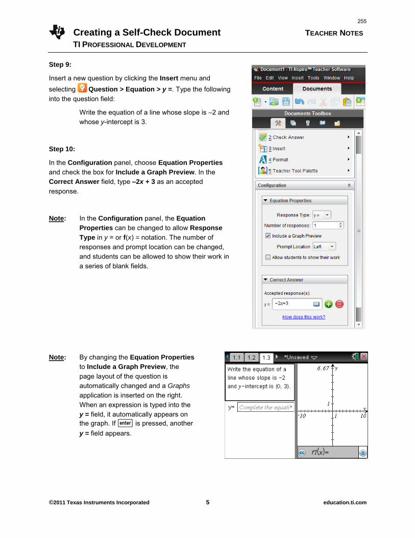
Creating a Self-Check Document TEACHER NOTES
TI PROFESSIONAL DEVELOPMENT
©2011 Texas Instruments Incorporated 5 education.ti.com
Step 9:
Insert a new question by clicking the Insert menu and selecting Question > Equation > y =. Type the following into the question field:
Write the equation of a line whose slope is –2 and whose y-intercept is 3.
Step 10:
In the Configuration panel, choose Equation Properties
and check the box for Include a Graph Preview. In the Correct Answer field, type –2x + 3 as an accepted response.
Note: In the Configuration panel, the Equation
Properties can be changed to allow Response
Type in y = or f(x) = notation. The number of responses and prompt location can be changed, and students can be allowed to show their work in a series of blank fields.
Note: By changing the Equation Properties
to Include a Graph Preview, the page layout of the question is automatically changed and a Graphs application is inserted on the right. When an expression is typed into the y = field, it automatically appears on the graph. If · is pressed, another y = field appears.
255
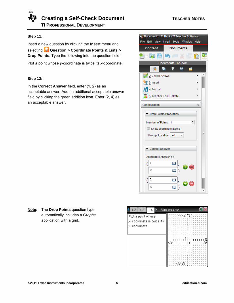
Creating a Self-Check Document TEACHER NOTES
TI PROFESSIONAL DEVELOPMENT
©2011 Texas Instruments Incorporated 6 education.ti.com
Step 11:
Insert a new question by clicking the Insert menu and selecting Question > Coordinate Points & Lists >
Drop Points. Type the following into the question field:
Plot a point whose y-coordinate is twice its x-coordinate.
Step 12:
In the Correct Answer field, enter (1, 2) as an acceptable answer. Add an additional acceptable answer field by clicking the green addition icon. Enter (2, 4) as an acceptable answer.
Note: The Drop Points question type automatically includes a Graphs application with a grid.
256
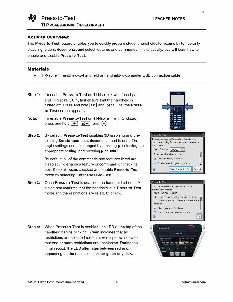
Press-to-Test TEACHER NOTES
TI PROFESSIONAL DEVELOPMENT
©2011 Texas Instruments Incorporated 1 education.ti.com
Activity Overview:
The Press-to-Test feature enables you to quickly prepare student handhelds for exams by temporarily disabling folders, documents, and select features and commands. In this activity, you will learn how to enable and disable Press-to-Test.
Materials
TI-Nspire™ handheld-to-handheld or handheld-to-computer USB connection cable
Step 1: To enable Press-to-Test on TI-Nspire™ with Touchpad and TI-Nspire CX™, first ensure that the handheld is turned off. Press and hold d and c until the Press-
to-Test screen appears.
Note: To enable Press-to-Test on TI-Nspire™ with Clickpad, press and hold d, c, and w.
Step 2: By default, Press-to-Test disables 3D graphing and pre-existing Scratchpad data, documents, and folders. The angle settings can be changed by pressing ¢, selecting the appropriate setting, and pressing ¢ or ·.
By default, all of the commands and features listed are disabled. To enable a feature or command, uncheck its box. Keep all boxes checked and enable Press-to-Test mode by selecting Enter Press-to-Test.
Step 3: Once Press-to-Test is enabled, the handheld reboots. A dialog box confirms that the handheld is in Press-to-Test mode and the restrictions are listed. Click OK.
Step 4: When Press-to-Test is enabled, the LED at the top of the handheld begins blinking. Green indicates that all restrictions are selected (default), while yellow indicates that one or more restrictions are unselected. During the initial reboot, the LED alternates between red and, depending on the restrictions, either green or yellow.
257
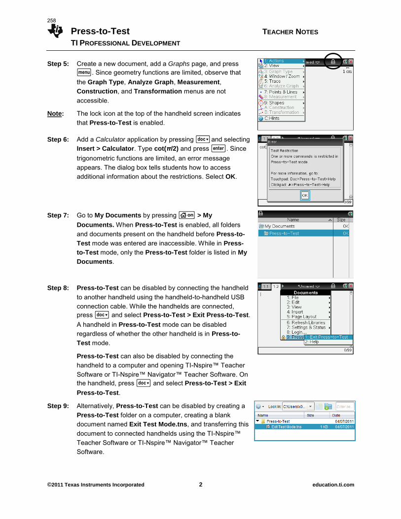
Press-to-Test TEACHER NOTES
TI PROFESSIONAL DEVELOPMENT
©2011 Texas Instruments Incorporated 2 education.ti.com
Step 5: Create a new document, add a Graphs page, and press b. Since geometry functions are limited, observe that the Graph Type, Analyze Graph, Measurement, Construction, and Transformation menus are not accessible.
Note: The lock icon at the top of the handheld screen indicates that Press-to-Test is enabled.
Step 6: Add a Calculator application by pressing ~ and selecting Insert > Calculator. Type cot(π/2) and press ·. Since trigonometric functions are limited, an error message appears. The dialog box tells students how to access additional information about the restrictions. Select OK.
Step 7: Go to My Documents by pressing c > My
Documents. When Press-to-Test is enabled, all folders and documents present on the handheld before Press-to-
Test mode was entered are inaccessible. While in Press-
to-Test mode, only the Press-to-Test folder is listed in My
Documents.
Step 8: Press-to-Test can be disabled by connecting the handheld to another handheld using the handheld-to-handheld USB connection cable. While the handhelds are connected, press ~ and select Press-to-Test > Exit Press-to-Test. A handheld in Press-to-Test mode can be disabled regardless of whether the other handheld is in Press-to-
Test mode.
Press-to-Test can also be disabled by connecting the handheld to a computer and opening TI-Nspire™ Teacher Software or TI-Nspire™ Navigator™ Teacher Software. On the handheld, press ~ and select Press-to-Test > Exit
Press-to-Test.
Step 9: Alternatively, Press-to-Test can be disabled by creating a Press-to-Test folder on a computer, creating a blank document named Exit Test Mode.tns, and transferring this document to connected handhelds using the TI-Nspire™
Teacher Software or TI-Nspire™ Navigator™ Teacher Software.
258
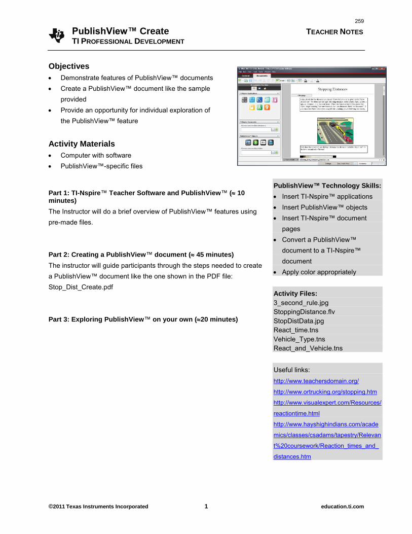
PublishView™ Create TEACHER NOTES TI PROFESSIONAL DEVELOPMENT
©2011 Texas Instruments Incorporated 1 education.ti.com
Objectives
Demonstrate features of PublishView™ documents Create a PublishView™ document like the sample
provided Provide an opportunity for individual exploration of
the PublishView™ feature
Activity Materials
Computer with software PublishView™-specific files Part 1: TI-Nspire™ Teacher Software and PublishView™ ( 10 minutes)
The Instructor will do a brief overview of PublishView™ features using pre-made files.
Part 2: Creating a PublishView™ document ( 45 minutes)
The instructor will guide participants through the steps needed to create a PublishView™ document like the one shown in the PDF file: Stop_Dist_Create.pdf
Part 3: Exploring PublishView™ on your own (20 minutes)
PublishView™ Technology Skills: Insert TI-Nspire™ applications Insert PublishView™ objects Insert TI-Nspire™ document
pages Convert a PublishView™
document to a TI-Nspire™ document
Apply color appropriately
Activity Files:
3_second_rule.jpg StoppingDistance.flv StopDistData.jpg React_time.tns Vehicle_Type.tns React_and_Vehicle.tns Useful links: http://www.teachersdomain.org/
http://www.ortrucking.org/stopping.htm
http://www.visualexpert.com/Resources/
reactiontime.html
http://www.hayshighindians.com/acade
mics/classes/csadams/tapestry/Relevan
t%20coursework/Reaction_times_and_
distances.htm
259
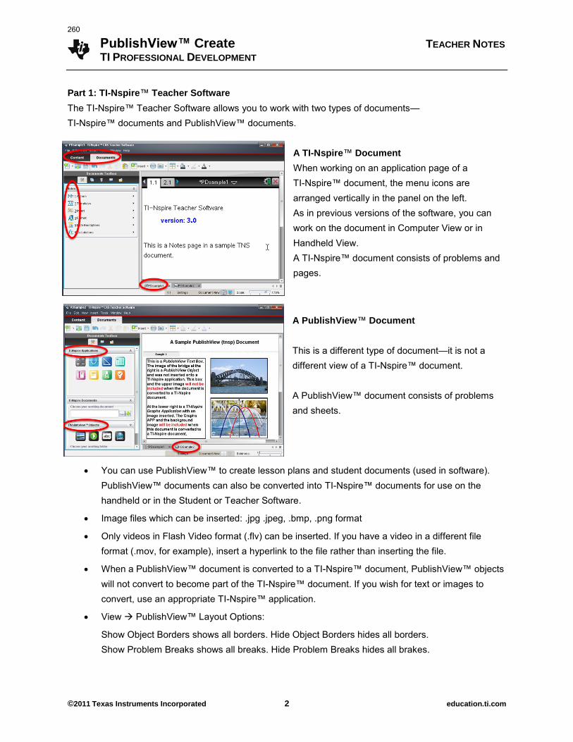
PublishView™ Create TEACHER NOTES TI PROFESSIONAL DEVELOPMENT
©2011 Texas Instruments Incorporated 2 education.ti.com
Part 1: TI-Nspire™ Teacher Software
The TI-Nspire™ Teacher Software allows you to work with two types of documents— TI-Nspire™ documents and PublishView™ documents.
A TI-Nspire™ Document
When working on an application page of a TI-Nspire™ document, the menu icons are arranged vertically in the panel on the left. As in previous versions of the software, you can work on the document in Computer View or in Handheld View. A TI-Nspire™ document consists of problems and pages.
A PublishView™ Document
This is a different type of document—it is not a different view of a TI-Nspire™ document. A PublishView™ document consists of problems and sheets.
You can use PublishView™ to create lesson plans and student documents (used in software). PublishView™ documents can also be converted into TI-Nspire™ documents for use on the handheld or in the Student or Teacher Software.
Image files which can be inserted: .jpg .jpeg, .bmp, .png format
Only videos in Flash Video format (.flv) can be inserted. If you have a video in a different file format (.mov, for example), insert a hyperlink to the file rather than inserting the file.
When a PublishView™ document is converted to a TI-Nspire™ document, PublishView™ objects will not convert to become part of the TI-Nspire™ document. If you wish for text or images to convert, use an appropriate TI-Nspire™ application.
View PublishView™ Layout Options:
Show Object Borders shows all borders. Hide Object Borders hides all borders. Show Problem Breaks shows all breaks. Hide Problem Breaks hides all brakes.
260
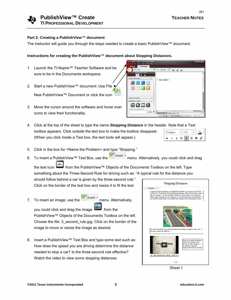
PublishView™ Create TEACHER NOTES TI PROFESSIONAL DEVELOPMENT
©2011 Texas Instruments Incorporated 3 education.ti.com
Part 2: Creating a PublishView™ document
The instructor will guide you through the steps needed to create a basic PublishView™ document. Instructions for creating the PublishView™ document about Stopping Distances. 1. Launch the TI-Nspire™ Teacher Software and be
sure to be in the Documents workspace. 2. Start a new PublishView™ document: Use File
New PublishView™ Document or click the icon .
3. Move the cursor around the software and hover over icons to view their functionality.
4. Click at the top of the sheet to type the name Stopping Distance in the header. Note that a Text
toolbox appears. Click outside the text box to make the toolbox disappear. (When you click inside a Text box, the text tools will appear.)
5. Click in the box for <Name the Problem> and type ―Stopping.‖
6. To insert a PublishView™ Text Box, use the menu. Alternatively, you could click and drag
the text icon from the PublishView™ Objects of the Documents Toolbox on the left. Type
something about the Three-Second Rule for driving such as: ―A typical rule for the distance you should follow behind a car is given by the three-second rule.‖ Click on the border of the text box and resize it to fit the text.
7. To insert an image, use the menu. Alternatively,
you could click and drag the image from the PublishView™ Objects of the Documents Toolbox on the left.
Choose the file: 3_second_rule.jpg. Click on the border of the image to move or resize the image as desired.
8. Insert a PublishView™ Text Box and type some text such as: How does the speed you are driving determine the distance needed to stop a car? Is the three-second rule effective? Watch the video to view some stopping distances.
Sheet 1
261
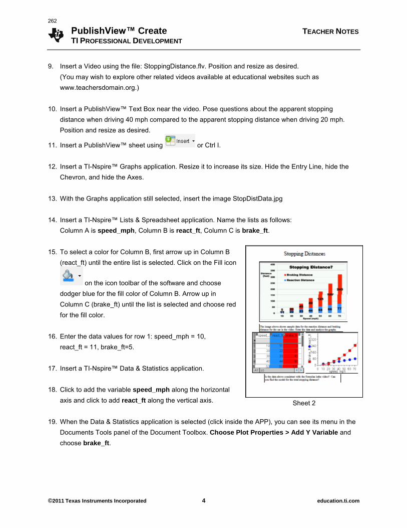
PublishView™ Create TEACHER NOTES TI PROFESSIONAL DEVELOPMENT
©2011 Texas Instruments Incorporated 4 education.ti.com
9. Insert a Video using the file: StoppingDistance.flv. Position and resize as desired. (You may wish to explore other related videos available at educational websites such as www.teachersdomain.org.)
10. Insert a PublishView™ Text Box near the video. Pose questions about the apparent stopping distance when driving 40 mph compared to the apparent stopping distance when driving 20 mph. Position and resize as desired.
11. Insert a PublishView™ sheet using or Ctrl I.
12. Insert a TI-Nspire™ Graphs application. Resize it to increase its size. Hide the Entry Line, hide the Chevron, and hide the Axes.
13. With the Graphs application still selected, insert the image StopDistData.jpg
14. Insert a TI-Nspire™ Lists & Spreadsheet application. Name the lists as follows: Column A is speed_mph, Column B is react_ft, Column C is brake_ft.
15. To select a color for Column B, first arrow up in Column B (react_ft) until the entire list is selected. Click on the Fill icon
on the icon toolbar of the software and choose dodger blue for the fill color of Column B. Arrow up in Column C (brake_ft) until the list is selected and choose red for the fill color.
16. Enter the data values for row 1: speed_mph = 10, react_ft = 11, brake_ft=5.
17. Insert a TI-Nspire™ Data & Statistics application.
18. Click to add the variable speed_mph along the horizontal axis and click to add react_ft along the vertical axis.
19. When the Data & Statistics application is selected (click inside the APP), you can see its menu in the Documents Tools panel of the Document Toolbox. Choose Plot Properties > Add Y Variable and choose brake_ft.
Sheet 2
262
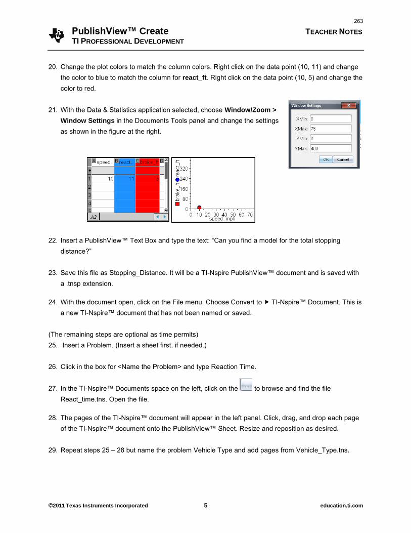
PublishView™ Create TEACHER NOTES TI PROFESSIONAL DEVELOPMENT
©2011 Texas Instruments Incorporated 5 education.ti.com
20. Change the plot colors to match the column colors. Right click on the data point (10, 11) and change the color to blue to match the column for react_ft. Right click on the data point (10, 5) and change the color to red.
21. With the Data & Statistics application selected, choose Window/Zoom >
Window Settings in the Documents Tools panel and change the settings as shown in the figure at the right.
22. Insert a PublishView™ Text Box and type the text: ―Can you find a model for the total stopping
distance?‖
23. Save this file as Stopping_Distance. It will be a TI-Nspire PublishView™ document and is saved with a .tnsp extension.
24. With the document open, click on the File menu. Choose Convert to TI-Nspire™ Document. This is
a new TI-Nspire™ document that has not been named or saved.
(The remaining steps are optional as time permits) 25. Insert a Problem. (Insert a sheet first, if needed.)
26. Click in the box for <Name the Problem> and type Reaction Time.
27. In the TI-Nspire™ Documents space on the left, click on the to browse and find the file React_time.tns. Open the file.
28. The pages of the TI-Nspire™ document will appear in the left panel. Click, drag, and drop each page
of the TI-Nspire™ document onto the PublishView™ Sheet. Resize and reposition as desired. 29. Repeat steps 25 – 28 but name the problem Vehicle Type and add pages from Vehicle_Type.tns.
263

PublishView™ Create TEACHER NOTES TI PROFESSIONAL DEVELOPMENT
©2011 Texas Instruments Incorporated 6 education.ti.com
30. Repeat steps 25 – 28 but name the problem Reaction and Vehicle Type and add pages from React_and_Vehicle.tns.
264
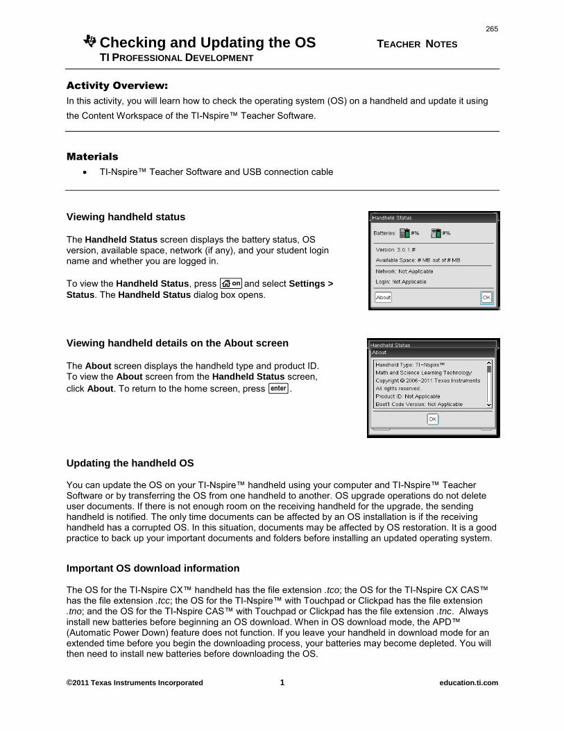
Checking and Updating the OS
TEACHER NOTES
TI PROFESSIONAL DEVELOPMENT
©2011 Texas Instruments Incorporated 1 education.ti.com
Activity Overview:
In this activity, you will learn how to check the operating system (OS) on a handheld and update it using the Content Workspace of the TI-Nspire™ Teacher Software.
Materials
TI-Nspire™ Teacher Software and USB connection cable
Viewing handheld status The Handheld Status screen displays the battery status, OS version, available space, network (if any), and your student login name and whether you are logged in. To view the Handheld Status, press c and select Settings >
Status. The Handheld Status dialog box opens.
Viewing handheld details on the About screen The About screen displays the handheld type and product ID. To view the About screen from the Handheld Status screen, click About. To return to the home screen, press ·.
Updating the handheld OS
You can update the OS on your TI-Nspire™ handheld using your computer and TI-Nspire™ Teacher Software or by transferring the OS from one handheld to another. OS upgrade operations do not delete user documents. If there is not enough room on the receiving handheld for the upgrade, the sending handheld is notified. The only time documents can be affected by an OS installation is if the receiving handheld has a corrupted OS. In this situation, documents may be affected by OS restoration. It is a good practice to back up your important documents and folders before installing an updated operating system.
Important OS download information The OS for the TI-Nspire CX™ handheld has the file extension .tco; the OS for the TI-Nspire CX CAS™ has the file extension .tcc; the OS for the TI-Nspire™ with Touchpad or Clickpad has the file extension .tno; and the OS for the TI-Nspire CAS™ with Touchpad or Clickpad has the file extension .tnc. Always install new batteries before beginning an OS download. When in OS download mode, the APD™ (Automatic Power Down) feature does not function. If you leave your handheld in download mode for an extended time before you begin the downloading process, your batteries may become depleted. You will then need to install new batteries before downloading the OS.
265
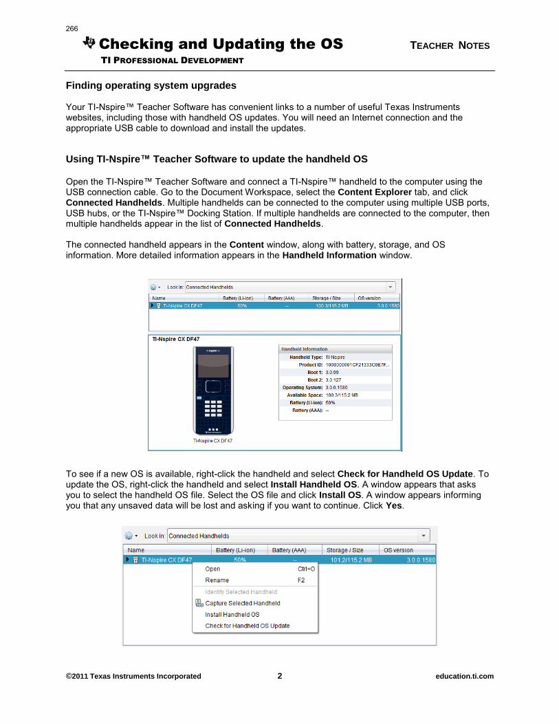
Checking and Updating the OS
TEACHER NOTES
TI PROFESSIONAL DEVELOPMENT
©2011 Texas Instruments Incorporated 2 education.ti.com
Finding operating system upgrades
Your TI-Nspire™ Teacher Software has convenient links to a number of useful Texas Instruments websites, including those with handheld OS updates. You will need an Internet connection and the appropriate USB cable to download and install the updates.
Using TI-Nspire™ Teacher Software to update the handheld OS Open the TI-Nspire™ Teacher Software and connect a TI-Nspire™ handheld to the computer using the USB connection cable. Go to the Document Workspace, select the Content Explorer tab, and click Connected Handhelds. Multiple handhelds can be connected to the computer using multiple USB ports, USB hubs, or the TI-Nspire™ Docking Station. If multiple handhelds are connected to the computer, then multiple handhelds appear in the list of Connected Handhelds. The connected handheld appears in the Content window, along with battery, storage, and OS information. More detailed information appears in the Handheld Information window. To see if a new OS is available, right-click the handheld and select Check for Handheld OS Update. To update the OS, right-click the handheld and select Install Handheld OS. A window appears that asks you to select the handheld OS file. Select the OS file and click Install OS. A window appears informing you that any unsaved data will be lost and asking if you want to continue. Click Yes.
266
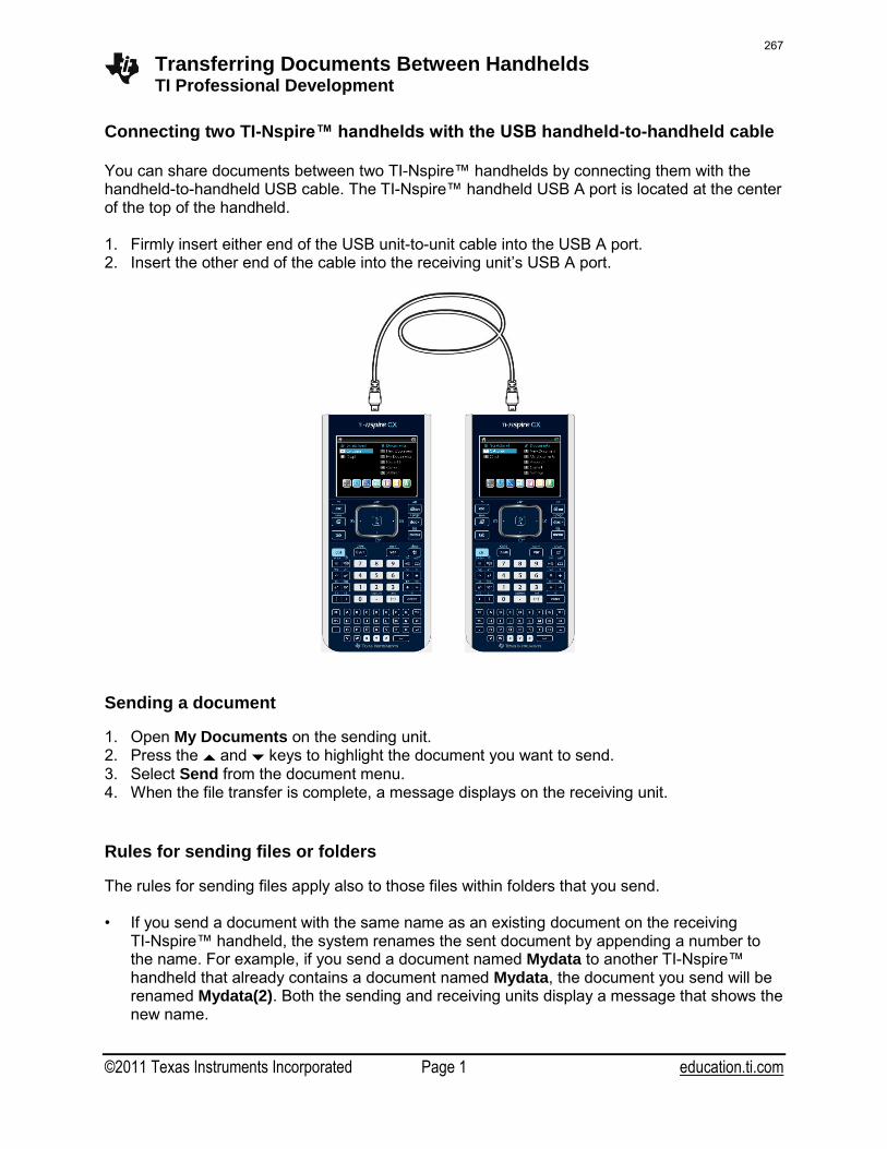
Transferring Documents Between Handhelds TI Professional Development
©2011 Texas Instruments Incorporated Page 1 education.ti.com
Connecting two TI-Nspire™ handhelds with the USB handheld-to-handheld cable You can share documents between two TI-Nspire™ handhelds by connecting them with the handheld-to-handheld USB cable. The TI-Nspire™ handheld USB A port is located at the center of the top of the handheld. 1. Firmly insert either end of the USB unit-to-unit cable into the USB A port. 2. Insert the other end of the cable into the receiving unit’s USB A port.
Sending a document
1. Open My Documents on the sending unit. 2. Press the £ and ¤ keys to highlight the document you want to send. 3. Select Send from the document menu. 4. When the file transfer is complete, a message displays on the receiving unit. Rules for sending files or folders
The rules for sending files apply also to those files within folders that you send. • If you send a document with the same name as an existing document on the receiving
TI-Nspire™ handheld, the system renames the sent document by appending a number to the name. For example, if you send a document named Mydata to another TI-Nspire™ handheld that already contains a document named Mydata, the document you send will be renamed Mydata(2). Both the sending and receiving units display a message that shows the new name.
267
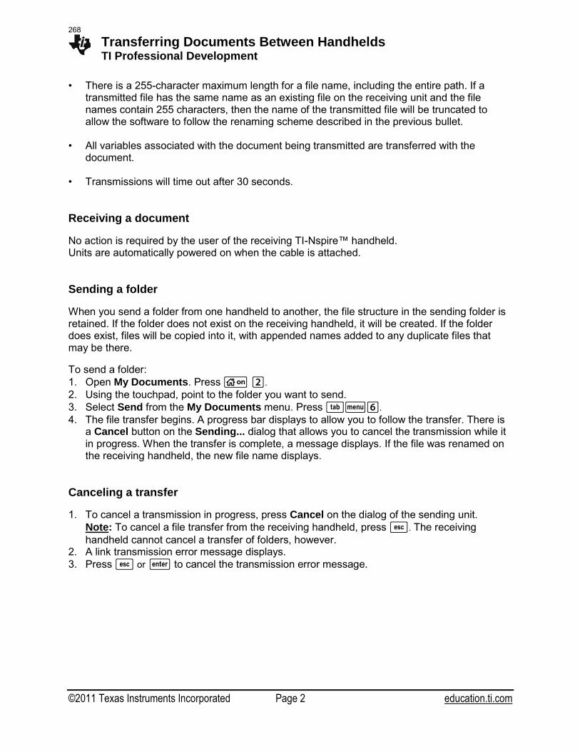
Transferring Documents Between Handhelds TI Professional Development
©2011 Texas Instruments Incorporated Page 2 education.ti.com
• There is a 255-character maximum length for a file name, including the entire path. If a transmitted file has the same name as an existing file on the receiving unit and the file names contain 255 characters, then the name of the transmitted file will be truncated to allow the software to follow the renaming scheme described in the previous bullet.
• All variables associated with the document being transmitted are transferred with the
document. • Transmissions will time out after 30 seconds.
Receiving a document
No action is required by the user of the receiving TI-Nspire™ handheld. Units are automatically powered on when the cable is attached.
Sending a folder
When you send a folder from one handheld to another, the file structure in the sending folder is retained. If the folder does not exist on the receiving handheld, it will be created. If the folder does exist, files will be copied into it, with appended names added to any duplicate files that may be there.
To send a folder: 1. Open My Documents. Press c 2.
2. Using the touchpad, point to the folder you want to send. 3. Select Send from the My Documents menu. Press eb6.
4. The file transfer begins. A progress bar displays to allow you to follow the transfer. There is a Cancel button on the Sending... dialog that allows you to cancel the transmission while it in progress. When the transfer is complete, a message displays. If the file was renamed on the receiving handheld, the new file name displays.
Canceling a transfer
1. To cancel a transmission in progress, press Cancel on the dialog of the sending unit. Note: To cancel a file transfer from the receiving handheld, press d. The receiving handheld cannot cancel a transfer of folders, however.
2. A link transmission error message displays. 3. Press d or · to cancel the transmission error message.
268