geostrophic currents in the presence of an internal waves field in bahÍa de banderas, mexico...
TRANSCRIPT
Available in: http://www.redalyc.org/articulo.oa?id=73000418
Red de Revistas Científicas de América Latina, el Caribe, España y Portugal
Sistema de Información Científica
Luis Plata, Anatoliy Filonov, Irina Tereshchenko, Liza Nelly, César Monzón, David Avalos, Carlos Vargas
Geostrophic currents in the presence of an internal waves field in Bahía de Banderas, México
e-Gnosis, núm. 4, 2006, p. 0,
Universidad de Guadalajara
México
How to cite Complete issue More information about this article Journal's homepage
e-Gnosis,
ISSN (Electronic Version): 1665-5745
Universidad de Guadalajara
México
www.redalyc.orgNon-Profit Academic Project, developed under the Open Acces Initiative
© 2006, e-Gnosis [online] Vol. 4, Art. 18 Geostrophic currents in the presense…Plata L. et al.
ISSN: 1665-5745 -1 / 43- www.e-gnosis.udg.mx/vol4/art18
GEOSTROPHIC CURRENTS IN THE PRESENCE OFAN INTERNAL WAVES FIELD IN BAHÍA DE BANDERAS, MEXICO
CORRIENTES GEOSTRÓFICAS EN PRESENCIA DE UN CAMPO DE ONDAS INTERNASEN LABAHÍA DE BANDERAS, MÉXICO
Luis Plata 1, Anatoliy Filonov 2, Irina Tereshchenko 2,Liza Nelly 3, César Monzón 2, David Avalos 4 and Carlos Vargas 2
[email protected] / [email protected] / [email protected] /[email protected] / [email protected] / [email protected] / [email protected]
Recibido: marzo 28, 2006 / Aceptado: diciembre 12, 2006 / Publicado: diciembre 20, 2006
ABSTRACT. The characteristics of internal waves in Bahía de Banderas were determined by means of oscillating CTD casts froma fast oceanographic survey done on April 24 and 25, 2001. Previous studies have shown that the continental shelf of the MexicanPacific, including Bahía de Banderas, possesses favorable conditions for the generation on internal waves. Fluctuations of thehydrophysical characteristics of the continental shelf caused by the presence and propagation of internal waves are smoothedusing a filter whose parameters are determined by the shape of the spatial correlation function of the field pulses relative to theanalyzed characteristic. Once internal waves are filtered, temperature, salinity and geostrophic velocity fields are shown fordifferent depths and the general pattern of the geostrophic circulation in the bay is discussed. The strongest currents were presentsouth of Islas Marietas and at the east zone of the bay. It can be stated that the geostrophic circulation in the bay in spring has animportant role in the water masses exchange between the zone close to the east coast, inside the bay, and the open ocean.
KEYWORDS. Geostrophic currents, internal waves, temperature and salinity fields, Bahía de Banderas.
RESUMEN. Las características de las ondas internas en la Bahía de Banderas fueron determinadas por medio de lances con unCTD ondulante a partir de un muestreo oceanográfico rápido realizado los días 24 y 25 de abril de 2001. Estudios previos hanmostrado que la plataforma continental del Pacífico mexicano, incluyendo la Bahía de Banderas, presenta condiciones favorablespara la generación de ondas internas. Las fluctuaciones de las características hidrofísicas en el área de estudio fueron suavizadasmediante un filtro cuyos parámetros están determinados por la forma de la función de correlación espacial de los pulsos delcampo de la característica analizada. Una vez filtrado el efecto de las ondas internas, se muestran los campos de temperatura,salinidad y velocidad geostrófica para diferentes profundidades y se discute el comportamiento de la circulación geostrófica en labahía. Las corrientes más intensas se presentaron en la parte sur de las Islas Marietas y en la zona este de la bahía. Puedeestablecerse que la circulación geostrófica en primavera en el área de estudio tiene un papel importante en el intercambio demasas entre la zona próxima a la costa este, dentro de la bahía, y el océano abierto.
PALABRAS CLAVE. Corrientes geostróficas, ondas internas, campos de temperatura y salinidad, Bahía de Banderas.
1 Posgrado en Oceanografía Costera, Universidad Autónoma de Baja California, Álvaro Obregón y Julián Carrillo s/n ColoniaNueva, Mexicali, B. C., 21100, México – iio.ens.uabc.mx/
2 Departamento de Física del Centro Universitario de Ciencias Exactas e Ingenierías de la Universidad de Guadalajara. Blvd.Marcelino García Barragán No. 1451, Guadalajara, Jalisco, 44430, México - www.cucei.udg.mx/
3 Posgrado en Desarrollo Sustentable y Turismo, Centro Universitario de La Costa, Universidad de Guadalajara. Av. Universidadde Guadalajara No. 203, Delegación Ixtapa. Puerto Vallarta, Jalisco, 48280, México - www.cuc.udg.mx
4 Posgrado en Ciencias del Mar y Limnologia, Universidad Nacional Autónoma de México. Instituto de Ciencias del Mar yLimnología, Circuito exterior, C. U., Coyoacán, México, 04510 D. F. – www.mar.icmyl.unam.mx
© 2006, e-Gnosis [online] Vol. 4, Art. 18 Geostrophic currents in the presense…Plata L. et al.
ISSN: 1665-5745 -2 / 43- www.e-gnosis.udg.mx/vol4/art18
1. Introduction
The dynamics of water masses on the continental shelf of the Mexican Pacific coast is affected bybarotropic and baroclinic tide. Internal tides are known to cause significant vertical variations in allhydrophysical parameters on the continental shelf. The spatial slopes of the dynamic heights on thecontinental shelf can be up to one order of magnitude greater than the normal values of the open ocean.Seiwell [1] and later Defant [2] were the first to show that internal tides may cause the temperature andsalinity measurements on the continental shelf to provide different results with respect to the geostrophiccurrents, depending on the tidal phase in which they were taken. Since the publication of Defant’s work [2]on the reality and illusion in oceanographic measurements in regions with intense internal waves,researchers became aware of this intimidating problem and ceased to calculate geostrophic currents even inareas on the continental shelf where geostrophic balance can be maintained.
Filonov et al. [3] proposed a method to conduct a fast oceanographic survey with an oscillating CTD in agrid of numerous and successive stations that would allow them to filter these data and to remove theinfluence of internal waves. The filtering method proposed by Filonov [4] is based on a smoothing of thefields of temperature and salinity with a filter, whose parameters are determined by the shape of the spatialcorrelation function of the field’s pulses. The filtering method was successfully tested using data from a fastoceanographic survey near Barra de Navidad, Mexico [4].
Internal waves have important scientific relevance because they play a fundamental role in the vertical andhorizontal mixing. The generation of internal wave vary considerably from one place to another as regardsthe function of the bottom slope ( dxdz=� ) and the stratification of the water column (N2). The latterdetermines the inclination of the upward internal tide energy flux’s path, i.e., the slope of the characteristicray: � = arc tan [(N 2 � �
2)/ (�2�f 2)]-0.5, where � is the barotropic tide wave’s frequency. Energytransmission from barotropic to baroclinic tide is more effective when 1��� , which is considered a critical
value. If 1<�� (>1), the energy is transmitted to the coast (out from the coast) [5]. Based on this criterion,previous studies have shown that the continental shelf of the Mexican Pacific, from Manzanillo (Colima) toBahía de Banderas (Jalisco and Nayarit), possesses favorable conditions for the generation of internal wavesof large amplitude [11].
Previous investigations [11-17] have shown that the main characteristics of the internal tides in thecontinental shelf of the Mexican Pacific coast are very discernible. The internal tide includes a dominantsemidiurnal tide, which is represented by a strong signal and a high peak in the spectrum of temperatureoscillations. The barotropic tide in the survey area has a mixed character with a dominant semidiurnalcomponent. Coastal areas experienced distorted semidiurnal internal waves traveling coastward. Studiesbased on the Baines’ model [5] showed that here the energy flow of the barotropic tide to the internal tidecan vary significantly at different sections of the slope, depending on the arrival angle of the barotropicwave relative to that of the slope. With a perpendicular arrival, the energy flux has a maximum with thevalue 763 W/m2, and the extent of the initial internal disturbance is of 4.9 m [11].
Nonlinear disintegration of waves and instability of their sinusoidal shape, as they propagate to the coast,sometimes give rise to the generation of bores or solitons [7, 18, 19]. As a result, the energy from theupward internal tide is completely dispersed on the continental shelf, giving rise to the formation ofsuccessively shorter internal waves and, at the same time, provoking changes in the stratification and mixingof the water column.
© 2006, e-Gnosis [online] Vol. 4, Art. 18 Geostrophic currents in the presense…Plata L. et al.
ISSN: 1665-5745 -3 / 43- www.e-gnosis.udg.mx/vol4/art18
Study area
Location
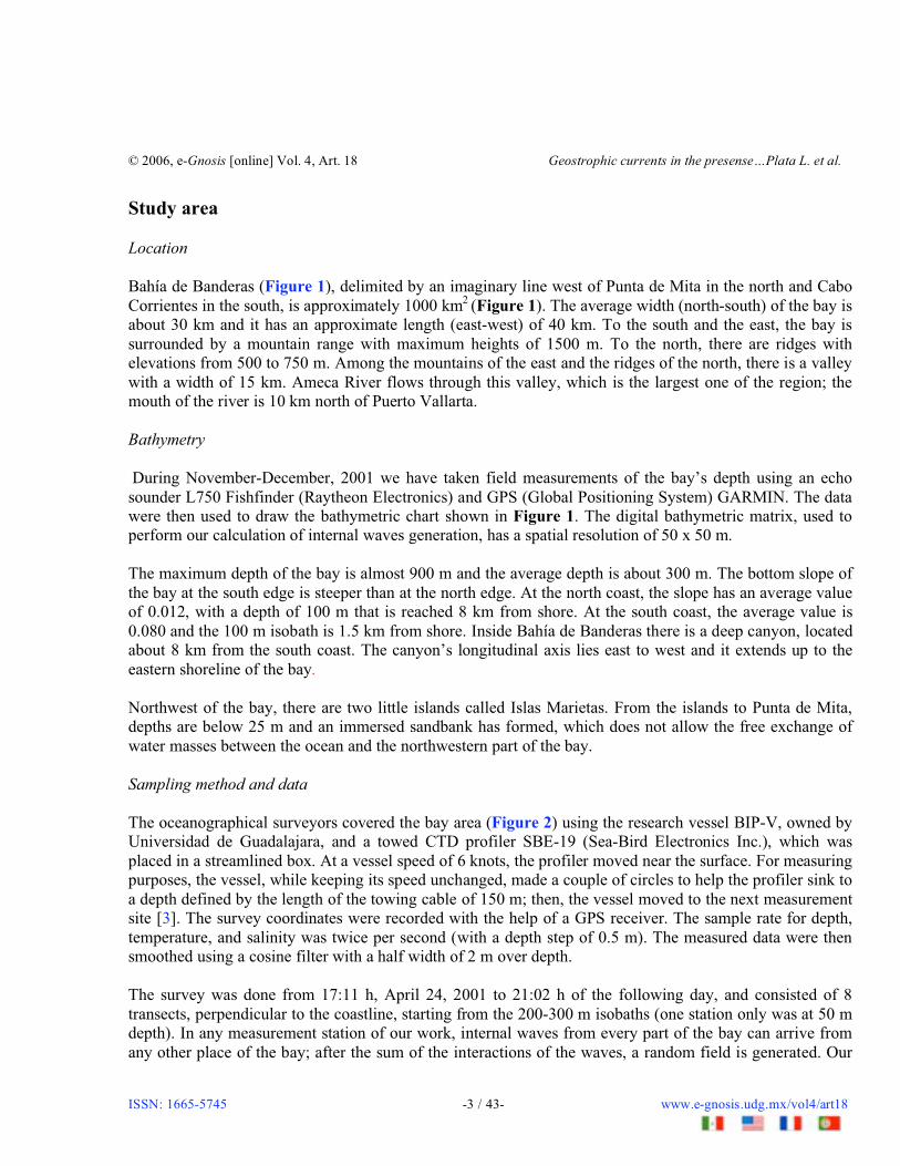
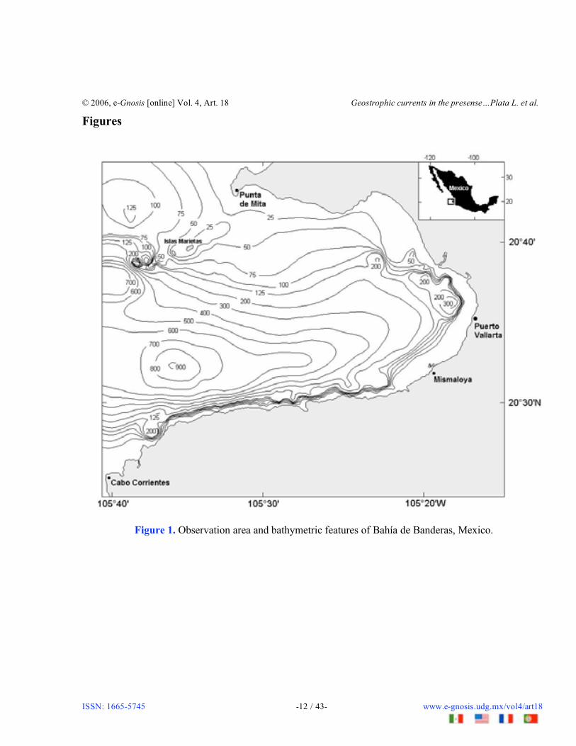
Bahía de Banderas (Figure 1), delimited by an imaginary line west of Punta de Mita in the north and CaboCorrientes in the south, is approximately 1000 km2 (Figure 1). The average width (north-south) of the bay isabout 30 km and it has an approximate length (east-west) of 40 km. To the south and the east, the bay issurrounded by a mountain range with maximum heights of 1500 m. To the north, there are ridges withelevations from 500 to 750 m. Among the mountains of the east and the ridges of the north, there is a valleywith a width of 15 km. Ameca River flows through this valley, which is the largest one of the region; themouth of the river is 10 km north of Puerto Vallarta.
Bathymetry
During November-December, 2001 we have taken field measurements of the bay’s depth using an echosounder L750 Fishfinder (Raytheon Electronics) and GPS (Global Positioning System) GARMIN. The datawere then used to draw the bathymetric chart shown in Figure 1. The digital bathymetric matrix, used toperform our calculation of internal waves generation, has a spatial resolution of 50 x 50 m.
The maximum depth of the bay is almost 900 m and the average depth is about 300 m. The bottom slope ofthe bay at the south edge is steeper than at the north edge. At the north coast, the slope has an average valueof 0.012, with a depth of 100 m that is reached 8 km from shore. At the south coast, the average value is0.080 and the 100 m isobath is 1.5 km from shore. Inside Bahía de Banderas there is a deep canyon, locatedabout 8 km from the south coast. The canyon’s longitudinal axis lies east to west and it extends up to theeastern shoreline of the bay.
Northwest of the bay, there are two little islands called Islas Marietas. From the islands to Punta de Mita,depths are below 25 m and an immersed sandbank has formed, which does not allow the free exchange ofwater masses between the ocean and the northwestern part of the bay.
Sampling method and data
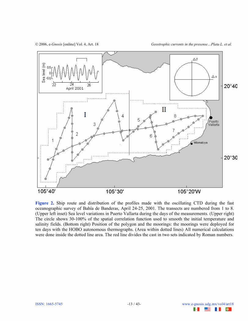
The oceanographical surveyors covered the bay area (Figure 2) using the research vessel BIP-V, owned byUniversidad de Guadalajara, and a towed CTD profiler SBE-19 (Sea-Bird Electronics Inc.), which wasplaced in a streamlined box. At a vessel speed of 6 knots, the profiler moved near the surface. For measuringpurposes, the vessel, while keeping its speed unchanged, made a couple of circles to help the profiler sink toa depth defined by the length of the towing cable of 150 m; then, the vessel moved to the next measurementsite [3]. The survey coordinates were recorded with the help of a GPS receiver. The sample rate for depth,temperature, and salinity was twice per second (with a depth step of 0.5 m). The measured data were thensmoothed using a cosine filter with a half width of 2 m over depth.
The survey was done from 17:11 h, April 24, 2001 to 21:02 h of the following day, and consisted of 8transects, perpendicular to the coastline, starting from the 200-300 m isobaths (one station only was at 50 mdepth). In any measurement station of our work, internal waves from every part of the bay can arrive fromany other place of the bay; after the sum of the interactions of the waves, a random field is generated. Our
© 2006, e-Gnosis [online] Vol. 4, Art. 18 Geostrophic currents in the presense…Plata L. et al.
ISSN: 1665-5745 -4 / 43- www.e-gnosis.udg.mx/vol4/art18
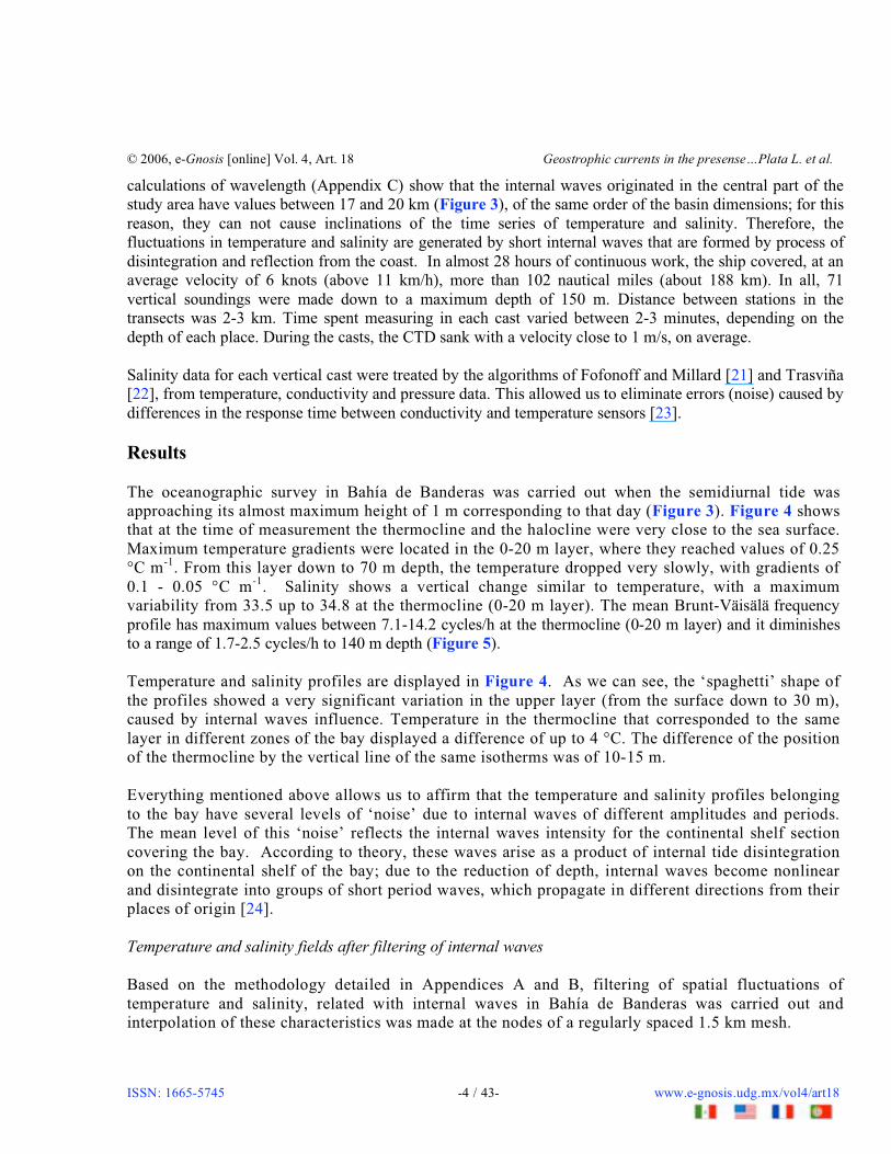
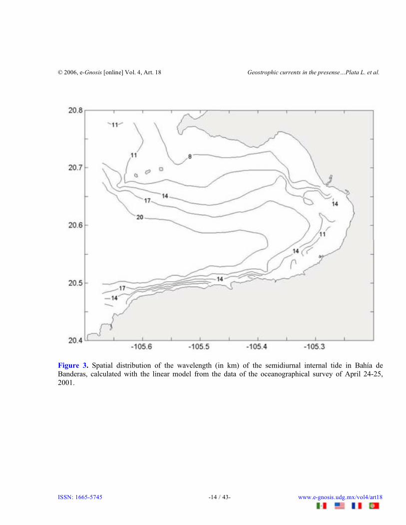
calculations of wavelength (Appendix C) show that the internal waves originated in the central part of thestudy area have values between 17 and 20 km (Figure 3), of the same order of the basin dimensions; for thisreason, they can not cause inclinations of the time series of temperature and salinity. Therefore, thefluctuations in temperature and salinity are generated by short internal waves that are formed by process ofdisintegration and reflection from the coast. In almost 28 hours of continuous work, the ship covered, at anaverage velocity of 6 knots (above 11 km/h), more than 102 nautical miles (about 188 km). In all, 71vertical soundings were made down to a maximum depth of 150 m. Distance between stations in thetransects was 2-3 km. Time spent measuring in each cast varied between 2-3 minutes, depending on thedepth of each place. During the casts, the CTD sank with a velocity close to 1 m/s, on average.
Salinity data for each vertical cast were treated by the algorithms of Fofonoff and Millard [21] and Trasviña[22], from temperature, conductivity and pressure data. This allowed us to eliminate errors (noise) caused bydifferences in the response time between conductivity and temperature sensors [23].
Results
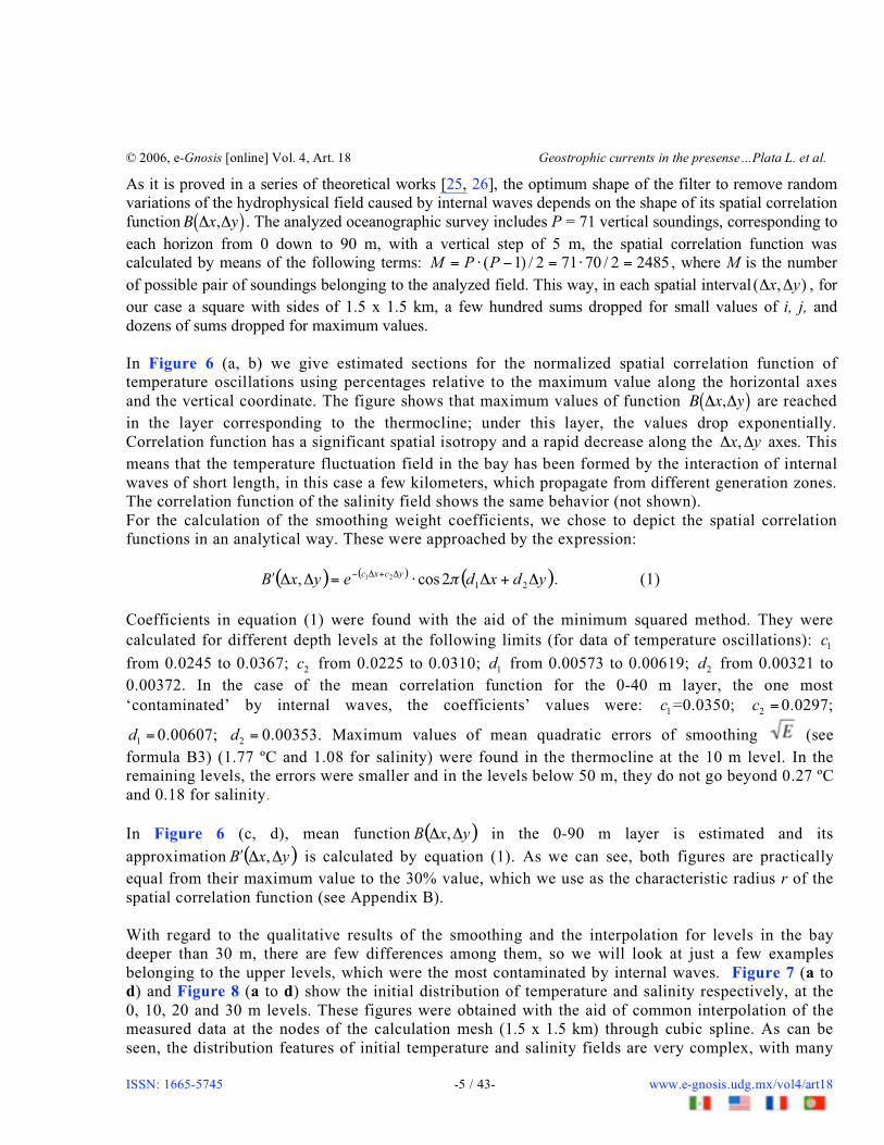
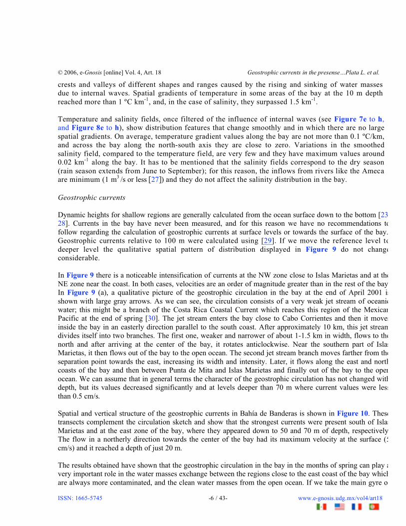
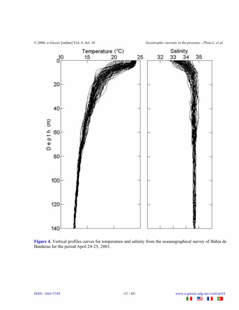
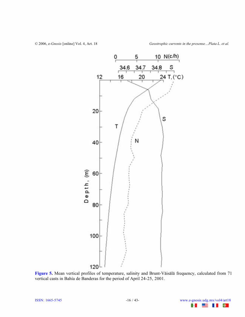
The oceanographic survey in Bahía de Banderas was carried out when the semidiurnal tide wasapproaching its almost maximum height of 1 m corresponding to that day (Figure 3). Figure 4 showsthat at the time of measurement the thermocline and the halocline were very close to the sea surface.Maximum temperature gradients were located in the 0-20 m layer, where they reached values of 0.25°C m-1. From this layer down to 70 m depth, the temperature dropped very slowly, with gradients of0.1 - 0.05 °C m-1. Salinity shows a vertical change similar to temperature, with a maximumvariability from 33.5 up to 34.8 at the thermocline (0-20 m layer). The mean Brunt-Väisälä frequencyprofile has maximum values between 7.1-14.2 cycles/h at the thermocline (0-20 m layer) and it diminishesto a range of 1.7-2.5 cycles/h to 140 m depth (Figure 5).
Temperature and salinity profiles are displayed in Figure 4. As we can see, the ‘spaghetti’ shape ofthe profiles showed a very significant variation in the upper layer (from the surface down to 30 m),caused by internal waves influence. Temperature in the thermocline that corresponded to the samelayer in different zones of the bay displayed a difference of up to 4 °C. The difference of the positionof the thermocline by the vertical line of the same isotherms was of 10-15 m.
Everything mentioned above allows us to affirm that the temperature and salinity profiles belongingto the bay have several levels of ‘noise’ due to internal waves of different amplitudes and periods.The mean level of this ‘noise’ reflects the internal waves intensity for the continental shelf sectioncovering the bay. According to theory, these waves arise as a product of internal tide disintegrationon the continental shelf of the bay; due to the reduction of depth, internal waves become nonlinearand disintegrate into groups of short period waves, which propagate in different directions from theirplaces of origin [24].
Temperature and salinity fields after filtering of internal waves
Based on the methodology detailed in Appendices A and B, filtering of spatial fluctuations oftemperature and salinity, related with internal waves in Bahía de Banderas was carried out andinterpolation of these characteristics was made at the nodes of a regularly spaced 1.5 km mesh.
© 2006, e-Gnosis [online] Vol. 4, Art. 18 Geostrophic currents in the presense…Plata L. et al.
ISSN: 1665-5745 -5 / 43- www.e-gnosis.udg.mx/vol4/art18
As it is proved in a series of theoretical works [25, 26], the optimum shape of the filter to remove randomvariations of the hydrophysical field caused by internal waves depends on the shape of its spatial correlationfunctionB �x,�y( ) . The analyzed oceanographic survey includes P = 71 vertical soundings, corresponding toeach horizon from 0 down to 90 m, with a vertical step of 5 m, the spatial correlation function wascalculated by means of the following terms: 24852/70712/)1( =�=��= PPM , where � is the numberof possible pair of soundings belonging to the analyzed field. This way, in each spatial interval ( , )x y� � , forour case a square with sides of 1.5 � 1.5 km, a few hundred sums dropped for small values of i, j, anddozens of sums dropped for maximum values.
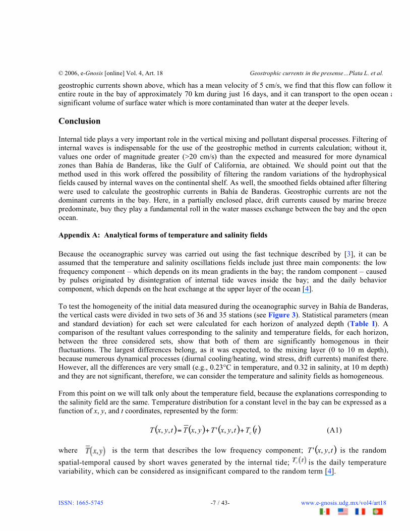
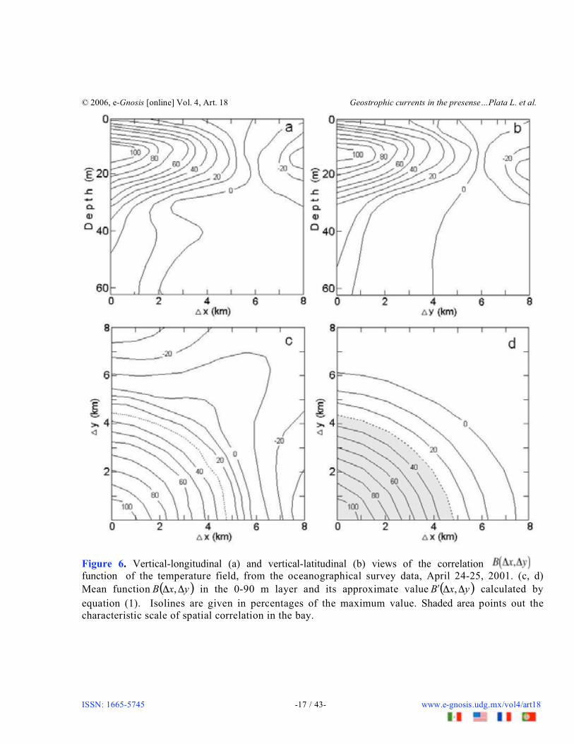
In Figure 6 (a, b) we give estimated sections for the normalized spatial correlation function oftemperature oscillations using percentages relative to the maximum value along the horizontal axesand the vertical coordinate. The figure shows that maximum values of function B �x,�y( ) are reachedin the layer corresponding to the thermocline; under this layer, the values drop exponentially.Correlation function has a significant spatial isotropy and a rapid decrease along the yx �� , axes. Thismeans that the temperature fluctuation field in the bay has been formed by the interaction of internalwaves of short length, in this case a few kilometers, which propagate from different generation zones.The correlation function of the salinity field shows the same behavior (not shown).For the calculation of the smoothing weight coefficients, we chose to depict the spatial correlationfunctions in an analytical way. These were approached by the expression:
( ) ( ) ( )ydxdeyxBycxc
�+��=����+��
212cos, 21 � . (1)
Coefficients in equation (1) were found with the aid of the minimum squared method. They werecalculated for different depth levels at the following limits (for data of temperature oscillations): 1c
from 0.0245 to 0.0367; 2c from 0.0225 to 0.0310; 1d from 0.00573 to 0.00619; 2d from 0.00321 to0.00372. In the case of the mean correlation function for the 0-40 m layer, the one most‘contaminated’ by internal waves, the coefficients’ values were: 1c =0.0350; =2c 0.0297;
=1d 0.00607; =2d 0.00353. Maximum values of mean quadratic errors of smoothing (seeformula B3) (1.77 ºC and 1.08 for salinity) were found in the thermocline at the 10 m level. In theremaining levels, the errors were smaller and in the levels below 50 m, they do not go beyond 0.27 ºCand 0.18 for salinity.
In Figure 6 (c, d), mean function ( )yxB �� , in the 0-90 m layer is estimated and its
approximation ( )yxB ��� , is calculated by equation (1). As we can see, both figures are practicallyequal from their maximum value to the 30% value, which we use as the characteristic radius r of thespatial correlation function (see Appendix B).
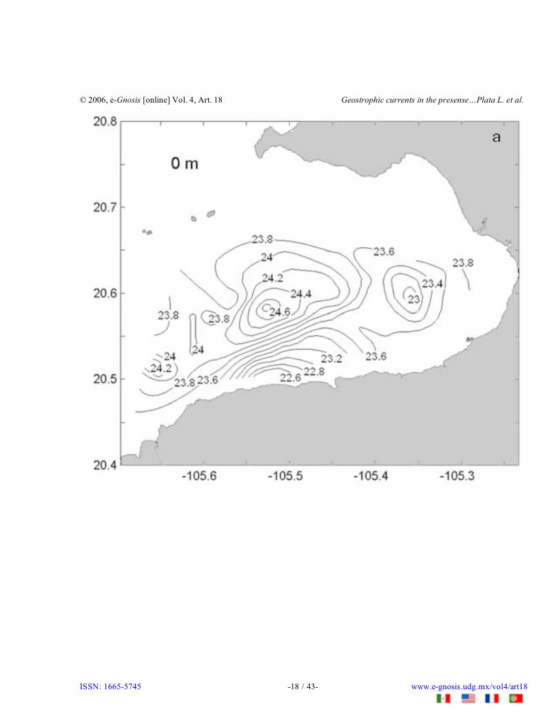
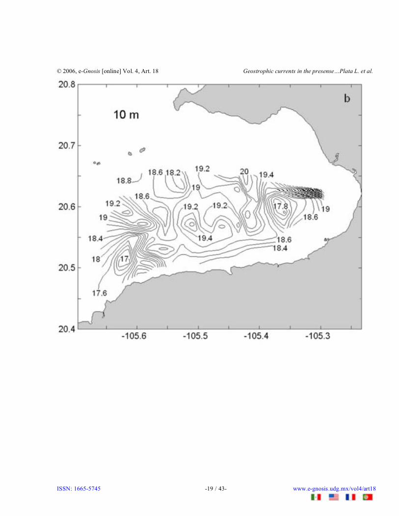
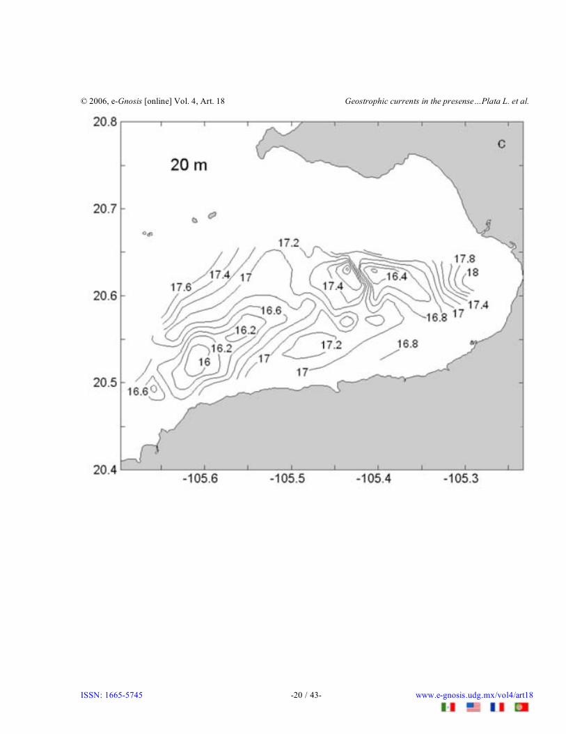
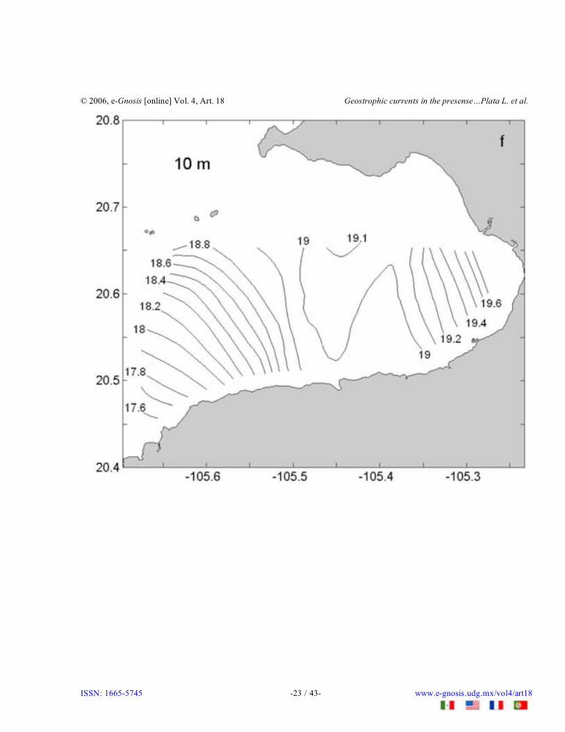
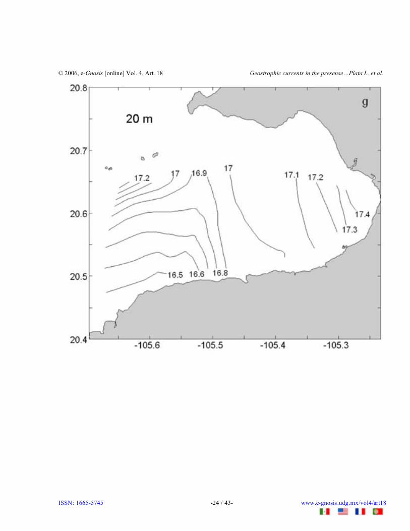
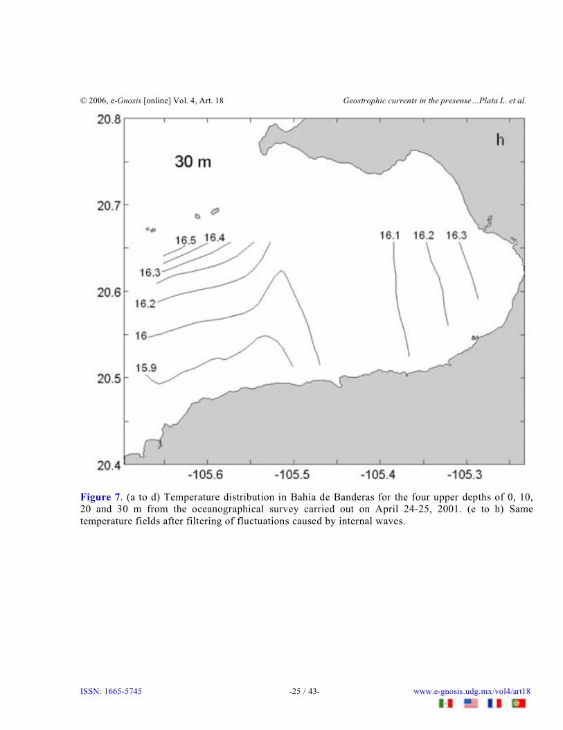
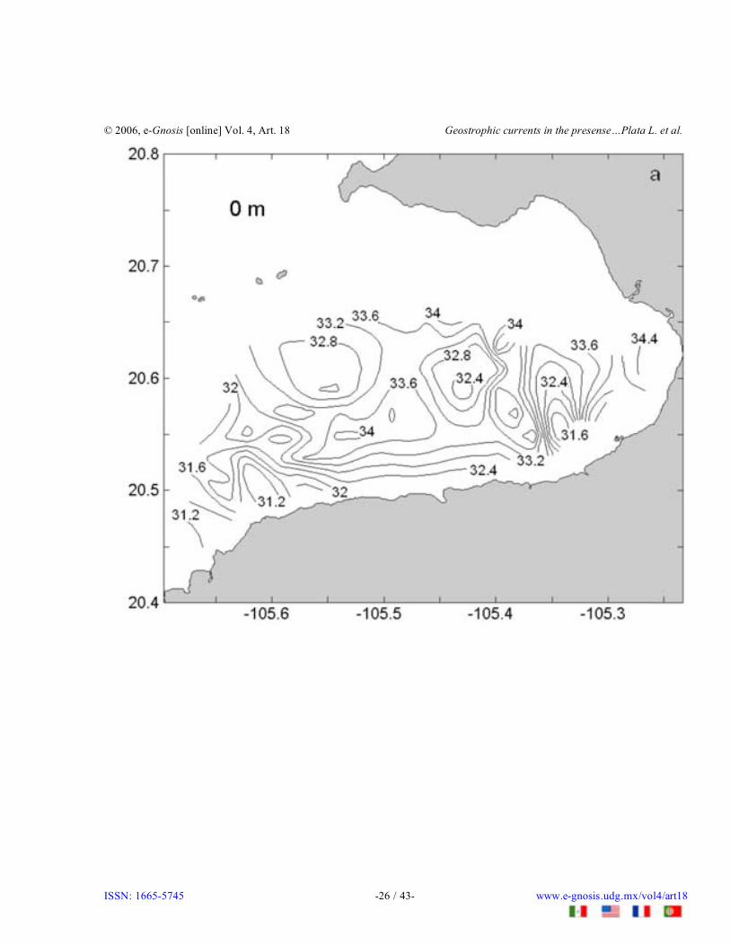
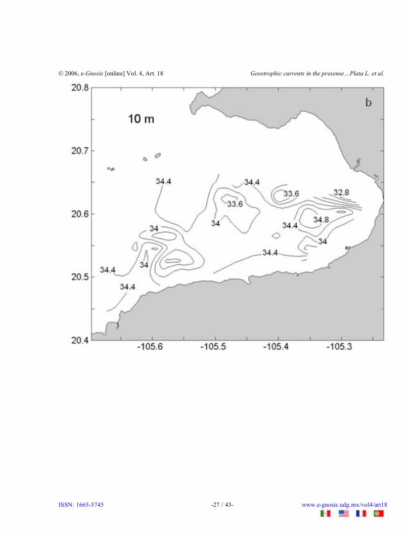
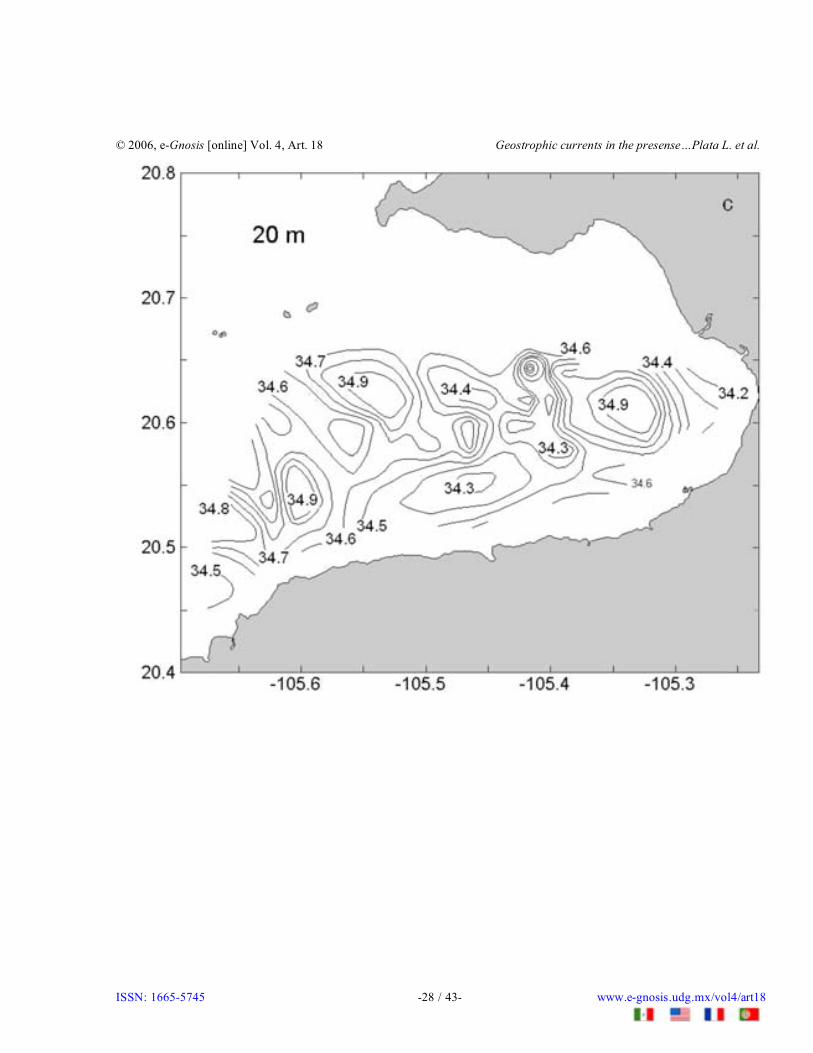
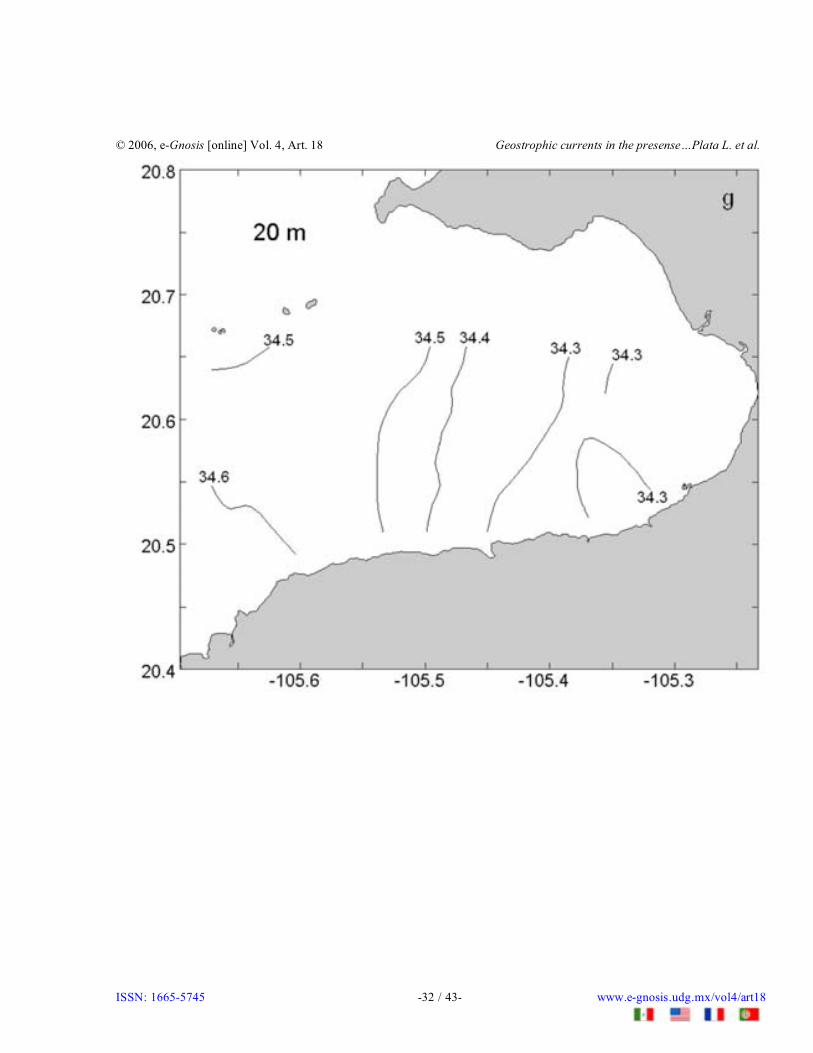
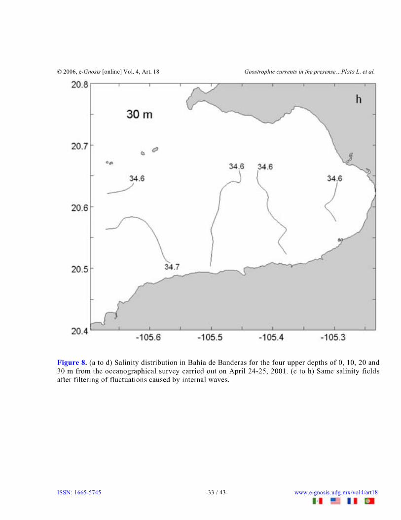
With regard to the qualitative results of the smoothing and the interpolation for levels in the baydeeper than 30 m, there are few differences among them, so we will look at just a few examplesbelonging to the upper levels, which were the most contaminated by internal waves. Figure 7 (a tod) and Figure 8 (a to d) show the initial distribution of temperature and salinity respectively, at the0, 10, 20 and 30 m levels. These figures were obtained with the aid of common interpolation of themeasured data at the nodes of the calculation mesh (1.5 � 1.5 km) through cubic spline. As can beseen, the distribution features of initial temperature and salinity fields are very complex, with many
© 2006, e-Gnosis [online] Vol. 4, Art. 18 Geostrophic currents in the presense…Plata L. et al.
ISSN: 1665-5745 -6 / 43- www.e-gnosis.udg.mx/vol4/art18
crests and valleys of different shapes and ranges caused by the rising and sinking of water massesdue to internal waves. Spatial gradients of temperature in some areas of the bay at the 10 m depthreached more than 1 ºC km-1, and, in the case of salinity, they surpassed 1.5 km-1.
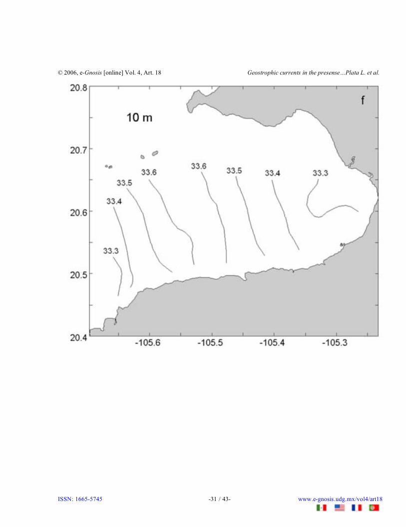
Temperature and salinity fields, once filtered of the influence of internal waves (see Figure 7e to h,and Figure 8e to h), show distribution features that change smoothly and in which there are no largespatial gradients. On average, temperature gradient values along the bay are not more than 0.1 ºC/km,and across the bay along the north-south axis they are close to zero. Variations in the smoothedsalinity field, compared to the temperature field, are very few and they have maximum values around0.02 km-1 along the bay. It has to be mentioned that the salinity fields correspond to the dry season(rain season extends from June to September); for this reason, the inflows from rivers like the Amecaare minimum (1 m3 /s or less [27]) and they do not affect the salinity distribution in the bay.
Geostrophic currents
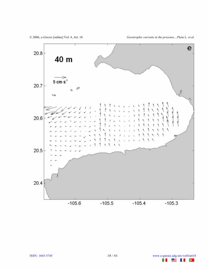
Dynamic heights for shallow regions are generally calculated from the ocean surface down to the bottom [2328]. Currents in the bay have never been measured, and for this reason we have no recommendations tofollow regarding the calculation of geostrophic currents at surface levels or towards the surface of the bay.Geostrophic currents relative to 100 m were calculated using [29]. If we move the reference level todeeper level the qualitative spatial pattern of distribution displayed in Figure 9 do not changeconsiderable.
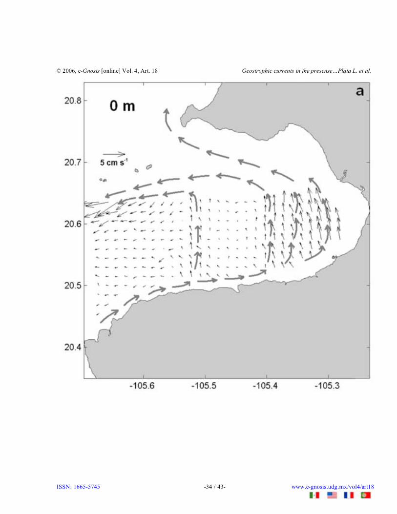
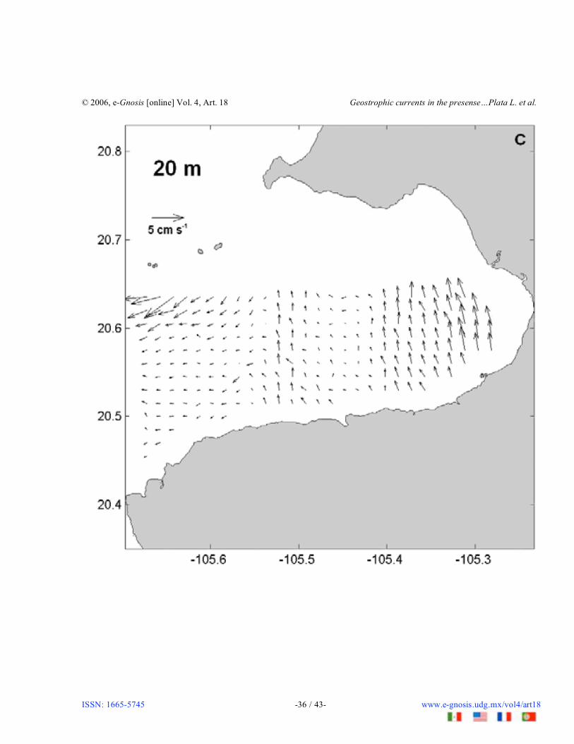
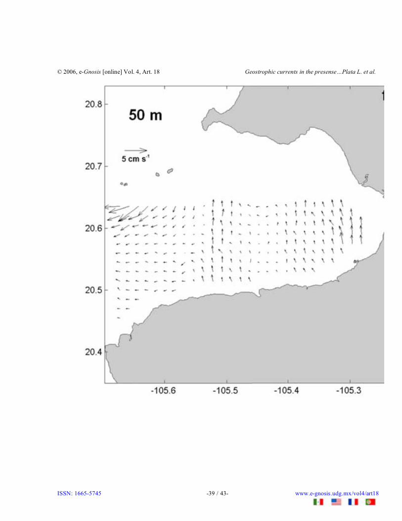
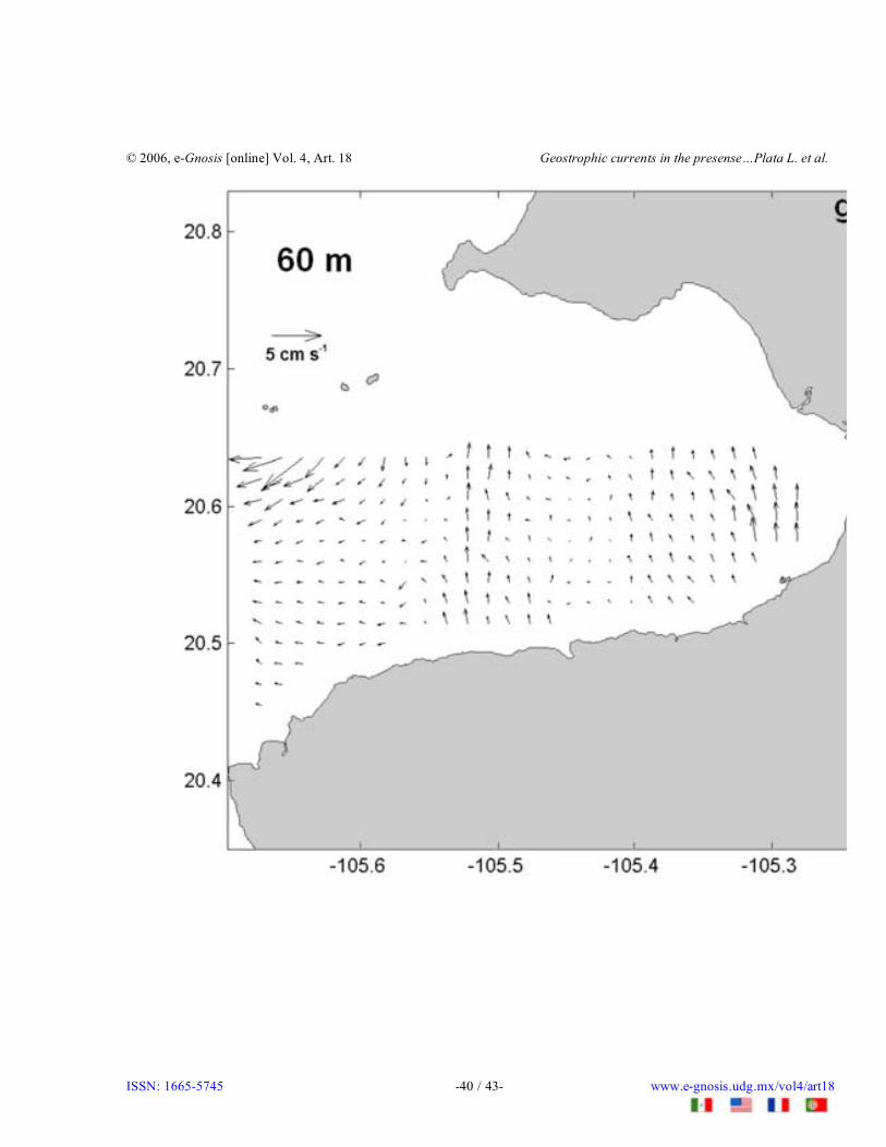
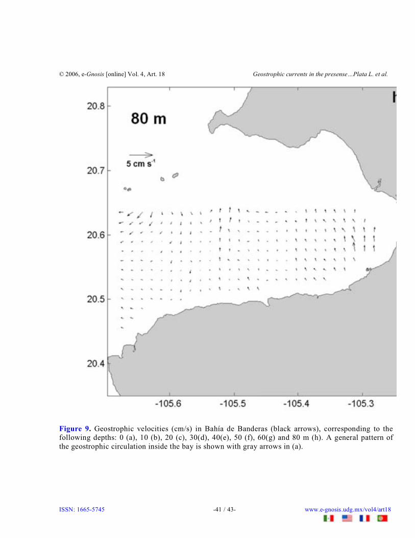
In Figure 9 there is a noticeable intensification of currents at the NW zone close to Islas Marietas and at theNE zone near the coast. In both cases, velocities are an order of magnitude greater than in the rest of the bayIn Figure 9 (a), a qualitative picture of the geostrophic circulation in the bay at the end of April 2001 isshown with large gray arrows. As we can see, the circulation consists of a very weak jet stream of oceanicwater; this might be a branch of the Costa Rica Coastal Current which reaches this region of the MexicanPacific at the end of spring [30]. The jet stream enters the bay close to Cabo Corrientes and then it movesinside the bay in an easterly direction parallel to the south coast. After approximately 10 km, this jet streamdivides itself into two branches. The first one, weaker and narrower of about 1-1.5 km in width, flows to thenorth and after arriving at the center of the bay, it rotates anticlockwise. Near the southern part of IslasMarietas, it then flows out of the bay to the open ocean. The second jet stream branch moves farther from theseparation point towards the east, increasing its width and intensity. Later, it flows along the east and northcoasts of the bay and then between Punta de Mita and Islas Marietas and finally out of the bay to the openocean. We can assume that in general terms the character of the geostrophic circulation has not changed withdepth, but its values decreased significantly and at levels deeper than 70 m where current values were lessthan 0.5 cm/s.
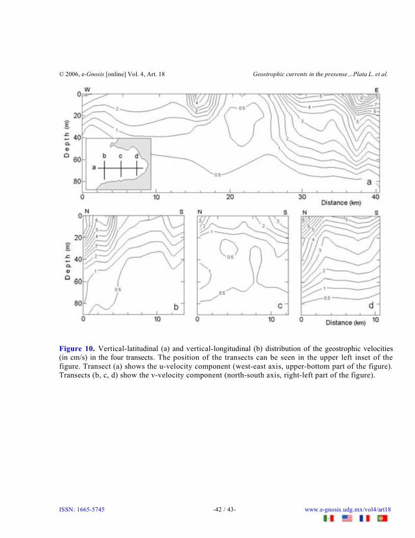
Spatial and vertical structure of the geostrophic currents in Bahía de Banderas is shown in Figure 10. Thesetransects complement the circulation sketch and show that the strongest currents were present south of IslasMarietas and at the east zone of the bay, where they appeared down to 50 and 70 m of depth, respectivelyThe flow in a northerly direction towards the center of the bay had its maximum velocity at the surface (5cm/s) and it reached a depth of just 20 m.
The results obtained have shown that the geostrophic circulation in the bay in the months of spring can play avery important role in the water masses exchange between the regions close to the east coast of the bay whichare always more contaminated, and the clean water masses from the open ocean. If we take the main gyre of
© 2006, e-Gnosis [online] Vol. 4, Art. 18 Geostrophic currents in the presense…Plata L. et al.
ISSN: 1665-5745 -7 / 43- www.e-gnosis.udg.mx/vol4/art18
geostrophic currents shown above, which has a mean velocity of 5 cm/s, we find that this flow can follow itsentire route in the bay of approximately 70 km during just 16 days, and it can transport to the open ocean asignificant volume of surface water which is more contaminated than water at the deeper levels.
Conclusion
Internal tide plays a very important role in the vertical mixing and pollutant dispersal processes. Filtering ofinternal waves is indispensable for the use of the geostrophic method in currents calculation; without it,values one order of magnitude greater (>20 cm/s) than the expected and measured for more dynamicalzones than Bahía de Banderas, like the Gulf of California, are obtained. We should point out that themethod used in this work offered the possibility of filtering the random variations of the hydrophysicalfields caused by internal waves on the continental shelf. As well, the smoothed fields obtained after filteringwere used to calculate the geostrophic currents in Bahía de Banderas. Geostrophic currents are not thedominant currents in the bay. Here, in a partially enclosed place, drift currents caused by marine breezepredominate, buy they play a fundamental roll in the water masses exchange between the bay and the openocean.
Appendix A: Analytical forms of temperature and salinity fields
Because the oceanographic survey was carried out using the fast technique described by [3], it can beassumed that the temperature and salinity oscillations fields include just three main components: the lowfrequency component – which depends on its mean gradients in the bay; the random component – causedby pulses originated by disintegration of internal tide waves inside the bay; and the daily behaviorcomponent, which depends on the heat exchange at the upper layer of the ocean [4].
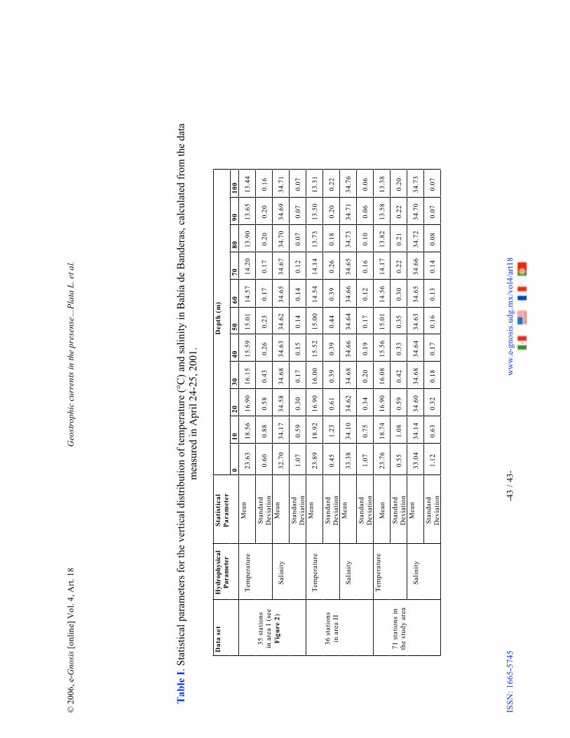
To test the homogeneity of the initial data measured during the oceanographic survey in Bahía de Banderas,the vertical casts were divided in two sets of 36 and 35 stations (see Figure 3). Statistical parameters (meanand standard deviation) for each set were calculated for each horizon of analyzed depth (Table I). Acomparison of the resultant values corresponding to the salinity and temperature fields, for each horizon,between the three considered sets, show that both of them are significantly homogenous in theirfluctuations. The largest differences belong, as it was expected, to the mixing layer (0 to 10 m depth),because numerous dynamical processes (diurnal cooling/heating, wind stress, drift currents) manifest there.However, all the differences are very small (e.g., 0.23°C in temperature, and 0.32 in salinity, at 10 m depth)and they are not significant, therefore, we can consider the temperature and salinity fields as homogeneous.
From this point on we will talk only about the temperature field, because the explanations corresponding tothe salinity field are the same. Temperature distribution for a constant level in the bay can be expressed as afunction of x, y, and t coordinates, represented by the form:
( ) ( ) ( ) ( )tTtyxTyxTtyxT c++= ,,',,, (A1)
where is the term that describes the low frequency component; ( )tyxT ,,' is the random
spatial-temporal caused by short waves generated by the internal tide; is the daily temperaturevariability, which can be considered as insignificant compared to the random term [4].
© 2006, e-Gnosis [online] Vol. 4, Art. 18 Geostrophic currents in the presense…Plata L. et al.
ISSN: 1665-5745 -8 / 43- www.e-gnosis.udg.mx/vol4/art18
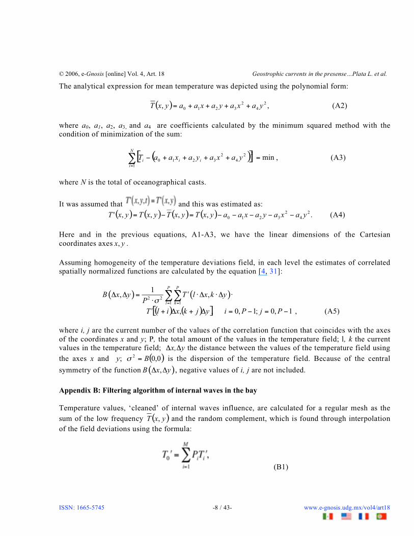
The analytical expression for mean temperature was depicted using the polynomial form:
( ) ,, 24
23210 yaxayaxaayxT ++++= (A2)
where a0, a1, a2, a3, and a4 are coefficients calculated by the minimum squared method with thecondition of minimization of the sum:
( )[ ]�=
=++++�N
i
iii yaxayaxaaT1
224
23210 min , (A3)
where N is the total of oceanographical casts.
It was assumed that and this was estimated as:
( ) ( ) ( ) ( ) .,,,,' 24
23210 yaxayaxaayxTyxTyxTyxT �����=�= (A4)
Here and in the previous equations, A1-A3, we have the linear dimensions of the Cartesiancoordinates axes yx, .
Assuming homogeneity of the temperature deviations field, in each level the estimates of correlatedspatially normalized functions are calculated by the equation [4, 31]:
( ) ( )2 21 1
1, ,
P P
l k
B x y T l x k yP � = =
� � = � �� �� ����
( ) ( )[ ],, yjkxilT �+�+� 1,0;1,0 �=�= PjPi , (A5)
where i, j are the current number of the values of the correlation function that coincides with the axesof the coordinates x and y; P, the total amount of the values in the temperature field; l, k the currentvalues in the temperature field; �x,�y the distance between the values of the temperature field using
the axes x and y; ( )0,02 B=� is the dispersion of the temperature field. Because of the central
symmetry of the function ( ),B x y� � , negative values of i, j are not included.
Appendix B: Filtering algorithm of internal waves in the bay
Temperature values, ‘cleaned’ of internal waves influence, are calculated for a regular mesh as the
sum of the low frequency ( )yxT , and the random complement, which is found through interpolationof the field deviations using the formula:
(B1)
© 2006, e-Gnosis [online] Vol. 4, Art. 18 Geostrophic currents in the presense…Plata L. et al.
ISSN: 1665-5745 -9 / 43- www.e-gnosis.udg.mx/vol4/art18
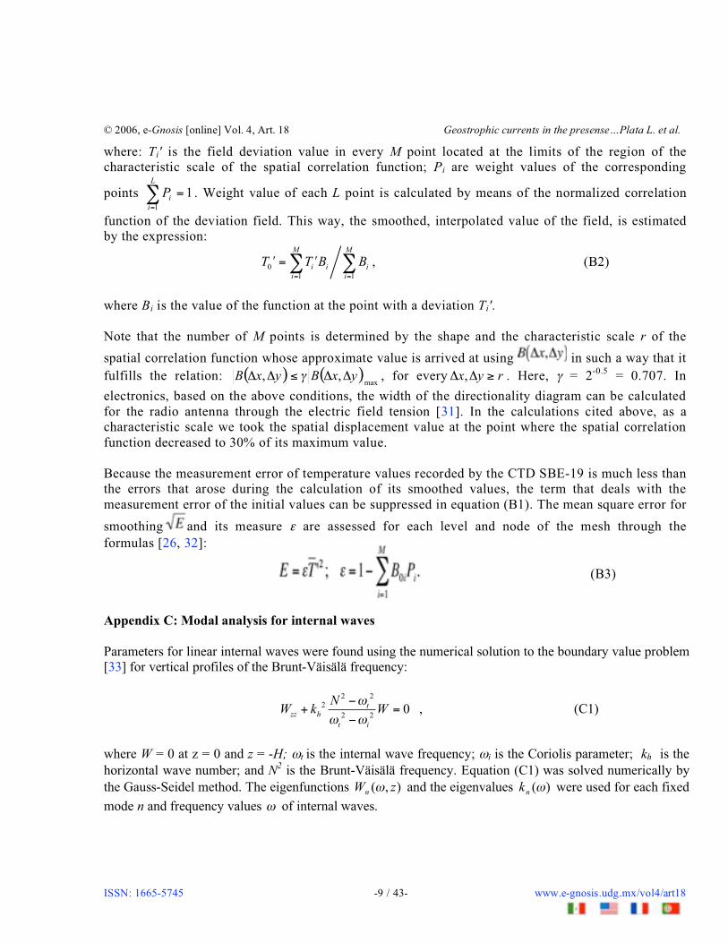
where: Ti' is the field deviation value in every M point located at the limits of the region of thecharacteristic scale of the spatial correlation function; Pi are weight values of the corresponding
points 11
=�=
L
i
iP . Weight value of each L point is calculated by means of the normalized correlation
function of the deviation field. This way, the smoothed, interpolated value of the field, is estimatedby the expression:
01 1
M M
i i i
i i
T T B B= =
� = �� � , (B2)
where Bi is the value of the function at the point with a deviation Ti'.
Note that the number of M points is determined by the shape and the characteristic scale r of the
spatial correlation function whose approximate value is arrived at using in such a way that itfulfills the relation: ( ) ( )
max,, yxByxB ����� � , for every ryx ��� , . Here, � = 2-0.5 = 0.707. In
electronics, based on the above conditions, the width of the directionality diagram can be calculatedfor the radio antenna through the electric field tension [31]. In the calculations cited above, as acharacteristic scale we took the spatial displacement value at the point where the spatial correlationfunction decreased to 30% of its maximum value.
Because the measurement error of temperature values recorded by the CTD SBE-19 is much less thanthe errors that arose during the calculation of its smoothed values, the term that deals with themeasurement error of the initial values can be suppressed in equation (B1). The mean square error for
smoothing and its measure � are assessed for each level and node of the mesh through theformulas [26, 32]:
(B3)
Appendix C: Modal analysis for internal waves
Parameters for linear internal waves were found using the numerical solution to the boundary value problem[33] for vertical profiles of the Brunt-Väisälä frequency:
2 22
2 20t
zz h
t i
NW k W
�
� �
�+ =
�, (C1)
where W = 0 at z = 0 and z = -H; �t is the internal wave frequency; �i is the Coriolis parameter; kh is thehorizontal wave number; and N2 is the Brunt-Väisälä frequency. Equation (C1) was solved numerically bythe Gauss-Seidel method. The eigenfunctions ),( zWn � and the eigenvalues )(�nk were used for each fixed
mode n and frequency values � of internal waves.
© 2006, e-Gnosis [online] Vol. 4, Art. 18 Geostrophic currents in the presense…Plata L. et al.
ISSN: 1665-5745 -10 / 43- www.e-gnosis.udg.mx/vol4/art18
References
1. Seiwell, J. (1939). The effect of short period variations of temperature and salinity on calculation in dynamicstopography. Pap. Phys. Ocean. and Meteor. Woods Hole: 110.
2. Defant, A. (1950). Reality and illusion in oceanographic surveys. J. of Mar. Res. (9): 15-31.3. Filonov, A. E., Monzón, C.O., Tereshchenko, I.E. (1996b). A technique for fast conductivity-temperature-depth oceanographic
surveys. Geofís. Internacional. (35): 415-420.4. Filonov, A. E. (2000b). Spatial structure of the temperature and salinity fields in the presence of internal waves on the
continental shelf of the states of Jalisco and Colima (Mexico). Cs . Mar. (6): 1-21.5. Baines, P. G. (1982). On internal tide generation models. Deep-Sea Res. (29): 307-338.6. Craig, P. D. (1987). Solution for internal tide generation over coastal topography. J. of Mar. Res. (45): 83-105.7. Holloway, P. E. (1987). Internal hydraulic jumps and solitons at a Shelf Break Region on the Australian North West Shelf. J. ofGeophys. Res. (92): 5405-5416.
8. Ostrovsky, L. A., Strepanyants, Yu. A. (1989). Do Internal Solitons exist in the Ocean? Rev. of Geophys. (27): 293-310.9. Filonov, A.E., Trasviña, A. (2000). Internal waves on the continental shelf of the Gulf of Tehuantepec, Mexico. Estuar.,Coastal and Shelf Sci. (50): 531-548.
10. Filonov, A.E., Lavin, M.F. (2003). Internal tides in the Northern Gulf of California. J. of Geophys. Res. 108(C5), 3151, doi:10.1029/2002JC001460.
11. Filonov, A. E., Monzón, C.O., Tereshchenko, I.E. (1996a). On the conditions of internal wave generation along the west coastof Mexico. Cs. Mar. (22): 255-272.
12. Filonov, A.E., Tereshchenko, I.E., Monzón C.O. (1998). Structure of the spatial and temporal temperature variations on thewestern part of Mexico continental shelf. Russ. Meteor. and Hydrology 6, 51-60.
13. Filonov, A.E. (1999). October 9, 1995, Tsunami waves measured at the open continental shelf near Barra de Navidad,Mexico. Izvestia. Atmos. and Ocean Phys. (35): 45-55.
14. Filonov, A.E., Tereshchenko, I.E., Monzón, C.O., González-Ruelas, M.E, Godínez-Domínguez, E. (2000). Seasonalvariability of the temperature and salinity fields in the coastal zone of the states of Jalisco and Colima, Mexico. Cs. Mar. (26):303-321.
15. Filonov, A.E., Tereshchenko, I.E. (2000). El Niño 1997-98 Monitoring in Mixed Layer of the Western Coast of Mexico.Geophys. Res. Letters, (27): 705-710.
16. Konyaev, K.V., Filonov, A.E. (2002). Internal tide near Pacific coast of Mexico. Izvestia. Atmos. and Ocean Phys. (38): 259-266.
17. Filonov, A.E., Konyaev, K.V. (2003). Nonlinear Internal Waves near the Mexico’s central pacific Coast. In NonlinearProcesses in Geophysical Fluid Dynamics. Velasco-Fuentes, O.U., Scheimbaum, J., Ochoa, J. (Eds), 377-386. KluwerAcademic Publishers,
18. Sandstrom, H., Elliott, J. A. (1984). Internal tide and solitons on the Scotian Shelf: A nutrient pump at work. J. of Geophys.Res. (89): 6415-6426.
19. Filonov, A. E. (2000a). Internal tide and tsunami waves in the continental shelf of the Mexican western coast. Ocean. of theEastern Pacif. (1): 31-45.
20. Secretaría de Marina. (1994). Carta Batimétrica de Bahía de Banderas, Jalisco, México. Dirección General de Oceanografía,Instituto Oceanográfico del Pacífico.
21. Fofonoff, N.P., Millard, J.R. (1983). Algorithms for computation of fundamental properties of sea water. Unesco TechnicalPapers in Mar. Sci., (44): 53.
22. Trasviña, A. (1999). Procesamiento de datos de CTD ondulante. GEOS, Unión Geofís. Mex. (19): 1-11.23. Emery, W.J., Thomson, R.E. (1997). Data Analysis Methods in Physical Oceanography, 114, 271. Elsevier, Amsterdan.24. Konyaev, K. V., Sabinin, K. D. (1992). Waves inside the Ocean, 272. Hydrometeoizdat. Sankt-Petersburg.25. Kolmogorov, A.N. 1941. Interpolation and extrapolation of stationary random sequences. Izv. Akad. Nauk SSSR Ser. Mat. 5,
5(1), 3-11 (in Russian).26. Gandin, L.S., Kagan, P.L. (1976). Métodos estocásticos de interpretación de datos meteorológicos, 360.
Hydrometeoizdat, Leningrado.27. CNA-SEMARNAT. (1999). Régimen de almacenamientos hasta 1999. Banco Nacional de Datos de Aguas Superficiales.28. Mamaev, O.I. (1957). T, S Analysis of the World Ocean.Hidrometeoizdat, Leningrad (in Russian).29. Pond, S., Pickard, G.L. (1978). Introductory Dynamic Oceanography, 71-78. Pergamon Press, New York.30. Badan, A. (1997). La corriente Costera de Costa Rica en el Pacifico Mexicano. Contribuciones a la Oceanografía Física en
México. Monografía No.3, Unión Geofís. Mex., 99-112.
© 2006, e-Gnosis [online] Vol. 4, Art. 18 Geostrophic currents in the presense…Plata L. et al.
ISSN: 1665-5745 -11 / 43- www.e-gnosis.udg.mx/vol4/art18
31. Konyaev, K.V. (1990). Spectral Analysis of Physical Oceanographic Data. National Science Foundation,Washington, D.C.32. Gandin, L.S. (1965). Objective Analysis of Meteorological Fields. Israel Program for Scientific Translations, Jerusalem.33. Krauss, W. (1966). Interne Wellen. Gebrüder Bornträger, Berlin.
© 2006, e-Gnosis [online] Vol. 4, Art. 18 Geostrophic currents in the presense…Plata L. et al.
ISSN: 1665-5745 -12 / 43- www.e-gnosis.udg.mx/vol4/art18
Figures
Figure 1. Observation area and bathymetric features of Bahía de Banderas, Mexico.
© 2006, e-Gnosis [online] Vol. 4, Art. 18 Geostrophic currents in the presense…Plata L. et al.
ISSN: 1665-5745 -13 / 43- www.e-gnosis.udg.mx/vol4/art18
Figure 2. Ship route and distribution of the profiles made with the oscillating CTD during the fastoceanographic survey of Bahía de Banderas, April 24-25, 2001. The transects are numbered from 1 to 8.(Upper left inset) Sea level variations in Puerto Vallarta during the days of the measurements. (Upper right)The circle shows 30-100% of the spatial correlation function used to smooth the initial temperature andsalinity fields. (Bottom right) Position of the polygon and the moorings: the moorings were deployed forten days with the HOBO autonomous thermographs. (Area within dotted lines) All numerical calculationswere done inside the dotted line area. The red line divides the cast in two sets indicated by Roman numbers.
© 2006, e-Gnosis [online] Vol. 4, Art. 18 Geostrophic currents in the presense…Plata L. et al.
ISSN: 1665-5745 -14 / 43- www.e-gnosis.udg.mx/vol4/art18
Figure 3. Spatial distribution of the wavelength (in km) of the semidiurnal internal tide in Bahía deBanderas, calculated with the linear model from the data of the oceanographical survey of April 24-25,2001.
© 2006, e-Gnosis [online] Vol. 4, Art. 18 Geostrophic currents in the presense…Plata L. et al.
ISSN: 1665-5745 -15 / 43- www.e-gnosis.udg.mx/vol4/art18
Figure 4. Vertical profiles curves for temperature and salinity from the oceanographical survey of Bahía deBanderas for the period April 24-25, 2001.
© 2006, e-Gnosis [online] Vol. 4, Art. 18 Geostrophic currents in the presense…Plata L. et al.
ISSN: 1665-5745 -16 / 43- www.e-gnosis.udg.mx/vol4/art18
Figure 5. Mean vertical profiles of temperature, salinity and Brunt-Väisälä frequency, calculated from 71vertical casts in Bahía de Banderas for the period of April 24-25, 2001.
© 2006, e-Gnosis [online] Vol. 4, Art. 18 Geostrophic currents in the presense…Plata L. et al.
ISSN: 1665-5745 -17 / 43- www.e-gnosis.udg.mx/vol4/art18
Figure 6. Vertical-longitudinal (a) and vertical-latitudinal (b) views of the correlationfunction of the temperature field, from the oceanographical survey data, April 24-25, 2001. (c, d)Mean function ( )yxB �� , in the 0-90 m layer and its approximate value ( )yxB ��� , calculated byequation (1). Isolines are given in percentages of the maximum value. Shaded area points out thecharacteristic scale of spatial correlation in the bay.
© 2006, e-Gnosis [online] Vol. 4, Art. 18 Geostrophic currents in the presense…Plata L. et al.
ISSN: 1665-5745 -18 / 43- www.e-gnosis.udg.mx/vol4/art18
© 2006, e-Gnosis [online] Vol. 4, Art. 18 Geostrophic currents in the presense…Plata L. et al.
ISSN: 1665-5745 -19 / 43- www.e-gnosis.udg.mx/vol4/art18
© 2006, e-Gnosis [online] Vol. 4, Art. 18 Geostrophic currents in the presense…Plata L. et al.
ISSN: 1665-5745 -20 / 43- www.e-gnosis.udg.mx/vol4/art18

© 2006, e-Gnosis [online] Vol. 4, Art. 18 Geostrophic currents in the presense…Plata L. et al.
ISSN: 1665-5745 -21 / 43- www.e-gnosis.udg.mx/vol4/art18

© 2006, e-Gnosis [online] Vol. 4, Art. 18 Geostrophic currents in the presense…Plata L. et al.
ISSN: 1665-5745 -22 / 43- www.e-gnosis.udg.mx/vol4/art18
© 2006, e-Gnosis [online] Vol. 4, Art. 18 Geostrophic currents in the presense…Plata L. et al.
ISSN: 1665-5745 -23 / 43- www.e-gnosis.udg.mx/vol4/art18
© 2006, e-Gnosis [online] Vol. 4, Art. 18 Geostrophic currents in the presense…Plata L. et al.
ISSN: 1665-5745 -24 / 43- www.e-gnosis.udg.mx/vol4/art18
© 2006, e-Gnosis [online] Vol. 4, Art. 18 Geostrophic currents in the presense…Plata L. et al.
ISSN: 1665-5745 -25 / 43- www.e-gnosis.udg.mx/vol4/art18
Figure 7. (a to d) Temperature distribution in Bahía de Banderas for the four upper depths of 0, 10,20 and 30 m from the oceanographical survey carried out on April 24-25, 2001. (e to h) Sametemperature fields after filtering of fluctuations caused by internal waves.
© 2006, e-Gnosis [online] Vol. 4, Art. 18 Geostrophic currents in the presense…Plata L. et al.
ISSN: 1665-5745 -26 / 43- www.e-gnosis.udg.mx/vol4/art18
© 2006, e-Gnosis [online] Vol. 4, Art. 18 Geostrophic currents in the presense…Plata L. et al.
ISSN: 1665-5745 -27 / 43- www.e-gnosis.udg.mx/vol4/art18
© 2006, e-Gnosis [online] Vol. 4, Art. 18 Geostrophic currents in the presense…Plata L. et al.
ISSN: 1665-5745 -28 / 43- www.e-gnosis.udg.mx/vol4/art18

© 2006, e-Gnosis [online] Vol. 4, Art. 18 Geostrophic currents in the presense…Plata L. et al.
ISSN: 1665-5745 -29 / 43- www.e-gnosis.udg.mx/vol4/art18

© 2006, e-Gnosis [online] Vol. 4, Art. 18 Geostrophic currents in the presense…Plata L. et al.
ISSN: 1665-5745 -30 / 43- www.e-gnosis.udg.mx/vol4/art18
© 2006, e-Gnosis [online] Vol. 4, Art. 18 Geostrophic currents in the presense…Plata L. et al.
ISSN: 1665-5745 -31 / 43- www.e-gnosis.udg.mx/vol4/art18
© 2006, e-Gnosis [online] Vol. 4, Art. 18 Geostrophic currents in the presense…Plata L. et al.
ISSN: 1665-5745 -32 / 43- www.e-gnosis.udg.mx/vol4/art18
© 2006, e-Gnosis [online] Vol. 4, Art. 18 Geostrophic currents in the presense…Plata L. et al.
ISSN: 1665-5745 -33 / 43- www.e-gnosis.udg.mx/vol4/art18
Figure 8. (a to d) Salinity distribution in Bahía de Banderas for the four upper depths of 0, 10, 20 and30 m from the oceanographical survey carried out on April 24-25, 2001. (e to h) Same salinity fieldsafter filtering of fluctuations caused by internal waves.
© 2006, e-Gnosis [online] Vol. 4, Art. 18 Geostrophic currents in the presense…Plata L. et al.
ISSN: 1665-5745 -34 / 43- www.e-gnosis.udg.mx/vol4/art18

© 2006, e-Gnosis [online] Vol. 4, Art. 18 Geostrophic currents in the presense…Plata L. et al.
ISSN: 1665-5745 -35 / 43- www.e-gnosis.udg.mx/vol4/art18
© 2006, e-Gnosis [online] Vol. 4, Art. 18 Geostrophic currents in the presense…Plata L. et al.
ISSN: 1665-5745 -36 / 43- www.e-gnosis.udg.mx/vol4/art18

© 2006, e-Gnosis [online] Vol. 4, Art. 18 Geostrophic currents in the presense…Plata L. et al.
ISSN: 1665-5745 -37 / 43- www.e-gnosis.udg.mx/vol4/art18
© 2006, e-Gnosis [online] Vol. 4, Art. 18 Geostrophic currents in the presense…Plata L. et al.
ISSN: 1665-5745 -38 / 43- www.e-gnosis.udg.mx/vol4/art18
© 2006, e-Gnosis [online] Vol. 4, Art. 18 Geostrophic currents in the presense…Plata L. et al.
ISSN: 1665-5745 -39 / 43- www.e-gnosis.udg.mx/vol4/art18
© 2006, e-Gnosis [online] Vol. 4, Art. 18 Geostrophic currents in the presense…Plata L. et al.
ISSN: 1665-5745 -40 / 43- www.e-gnosis.udg.mx/vol4/art18
© 2006, e-Gnosis [online] Vol. 4, Art. 18 Geostrophic currents in the presense…Plata L. et al.
ISSN: 1665-5745 -41 / 43- www.e-gnosis.udg.mx/vol4/art18
Figure 9. Geostrophic velocities (cm/s) in Bahía de Banderas (black arrows), corresponding to thefollowing depths: 0 (a), 10 (b), 20 (c), 30(d), 40(e), 50 (f), 60(g) and 80 m (h). A general pattern ofthe geostrophic circulation inside the bay is shown with gray arrows in (a).
© 2006, e-Gnosis [online] Vol. 4, Art. 18 Geostrophic currents in the presense…Plata L. et al.
ISSN: 1665-5745 -42 / 43- www.e-gnosis.udg.mx/vol4/art18
Figure 10. Vertical-latitudinal (a) and vertical-longitudinal (b) distribution of the geostrophic velocities(in cm/s) in the four transects. The position of the transects can be seen in the upper left inset of thefigure. Transect (a) shows the u-velocity component (west-east axis, upper-bottom part of the figure).Transects (b, c, d) show the v-velocity component (north-south axis, right-left part of the figure).
©20
06,e
-Gnosis
[onl
ine]
Vol
.4,A
rt.1
8Geostrophiccurrentsinthepresense…PlataL.etal.
ISS
N:
1665
-574
5-4
3/
43-
ww
w.e
-gno
sis.
udg.
mx/
vol4
/art
18
TableI.
Sta
tist
ical
para
met
ers
for
the
vert
ical
dist
ribu
tion
ofte
mpe
ratu
re(°
C)
and
sali
nity
inB
ahía
deB
ande
ras,
calc
ulat
edfr
omth
eda
tam
easu
red
inA
pril
24-2
5,20
01.
Dataset
Hydrophysical
Parameter
Statistical
Parameter
Depth(m)
010
2030
4050
6070
8090
100
Tem
pera
ture
Mea
n23
.63
18.5
616
.90
16.1
515
.59
15.0
114
.57
14.2
013
.90
13.6
513
.44
35st
atio
nsin
area
I(s
eeS
tand
ard
Dev
iati
on0.
600.
880.
580.
430.
260.
230.
170.
170.
200.
200.
16
Figure2
)S
alin
ity
Mea
n32
.70
34.1
734
.58
34.6
834
.63
34.6
234
.65
34.6
734
.70
34.6
934
.71
Sta
ndar
dD
evia
tion
1.07
0.59
0.30
0.17
0.15
0.14
0.14
0.12
0.07
0.07
0.07
Tem
pera
ture
Mea
n23
.89
18.9
216
.90
16.0
015
.52
15.0
014
.54
14.1
413
.73
13.5
013
.31
36st
atio
nsin
area
IIS
tand
ard
Dev
iati
on0.
451.
230.
610.
390.
390.
440.
390.
260.
180.
200.
22
Sal
init
yM
ean
33.3
834
.10
34.6
234
.68
34.6
634
.64
34.6
634
.65
34.7
334
.71
34.7
6
Sta
ndar
dD
evia
tion
1.07
0.75
0.34
0.20
0.19
0.17
0.12
0.16
0.10
0.06
0.06
Tem
pera
ture
Mea
n23
.76
18.7
416
.90
16.0
815
.56
15.0
114
.56
14.1
713
.82
13.5
813
.38
71st
atio
nsin
the
stud
yar
eaS
tand
ard
Dev
iati
on0.
551.
080.
590.
420.
330.
350.
300.
220.
210.
220.
20
Sal
init
yM
ean
33.0
434
.14
34.6
034
.68
34.6
434
.63
34.6
534
.66
34.7
234
.70
34.7
3
Sta
ndar
dD
evia
tion
1.12
0.63
0.32
0.18
0.17
0.16
0.13
0.14
0.08
0.07
0.07