geometry of lagrangian first-order classical field theories

arX

iv:d

g-ga

/950

5004

v1 1

7 M

ay 1

995

Geometry of Lagrangian First-order Classical Field Theories

Arturo Echeverria-Enriquez,

Miguel C. Munoz-Lecanda∗,

Narciso Roman-Roy†,

Departamento de Matematica Aplicada y TelematicaUniversidad Politecnica de Cataluna

Campus Nord, Modulo C-3C/ Gran Capitan s.n.

E-08071 BARCELONASPAIN

February 7, 2008

DMAT 04-0194

Abstract

We construct a lagrangian geometric formulation for first-order field theories using the canon-ical structures of first-order jet bundles, which are taken as the phase spaces of the systems inconsideration. First of all, we construct all the geometric structures associated with a first-order jet bundle and, using them, we develop the lagrangian formalism, defining the canonicalforms associated with a lagrangian density and the density of lagrangian energy, obtaining theEuler-Lagrange equations in two equivalent ways: as the result of a variational problem anddeveloping the jet field formalism (which is a formulation more similar to the case of mechanicalsystems). A statement and proof of Noether’s theorem is also given, using the latter formalism.

Finally, some classical examples are briefly studied.

Key words: Jet bundle, first order field theory, lagrangian formalism.

AMS s. c. (1980): 53C80, 58A20. PACS: 0240, 0350

∗e-mail: [email protected]

†e-mail: [email protected]

http://arXiv.org/abs/dg-ga/9505004v1

A. Echeverria et al , Geometry of Lagrangian First-order Classical Field Theories. 2

Contents

1 Introduction 3

2 Elements of differential geometry for first-order lagrangian field theories 5

2.1 Geometrical structures of first-order jet bundles . . . . . . . . . . . . . . . . . . . . . 5

2.1.1 First-order jet bundles . . . . . . . . . . . . . . . . . . . . . . . . . . . . . . . 5

2.1.2 Vertical differential. Canonical form . . . . . . . . . . . . . . . . . . . . . . . 7

2.1.3 Contact module (Cartan distribution) . . . . . . . . . . . . . . . . . . . . . . 8

2.1.4 Vertical endomorphisms . . . . . . . . . . . . . . . . . . . . . . . . . . . . . . 10

2.2 Canonical prolongations . . . . . . . . . . . . . . . . . . . . . . . . . . . . . . . . . . 11

2.2.1 Prolongation of sections and diffeomorphisms . . . . . . . . . . . . . . . . . . 11

2.2.2 Relation with the affine structure . . . . . . . . . . . . . . . . . . . . . . . . . 12

2.2.3 Relation with the geometric elements . . . . . . . . . . . . . . . . . . . . . . . 13

2.2.4 Prolongation of projectable vector fields . . . . . . . . . . . . . . . . . . . . . 16

2.2.5 Generalization to non-projectable vector fields . . . . . . . . . . . . . . . . . 18

3 Lagrangian formalism of first-order field theories 18

3.1 Lagrangian systems. Variational problems and critical sections . . . . . . . . . . . . 18

3.1.1 Lagrangian densities . . . . . . . . . . . . . . . . . . . . . . . . . . . . . . . . 18

3.1.2 Lagrangian canonical forms. Properties . . . . . . . . . . . . . . . . . . . . . 20

3.1.3 Density of lagrangian energy . . . . . . . . . . . . . . . . . . . . . . . . . . . 21

3.1.4 Variational problem associated with a lagrangian density . . . . . . . . . . . 24

3.1.5 Characterization of critical sections . . . . . . . . . . . . . . . . . . . . . . . . 24

3.2 Lagrangian formalism with jet fields . . . . . . . . . . . . . . . . . . . . . . . . . . . 28

3.2.1 1-jet fields in the bundle J1J1E . . . . . . . . . . . . . . . . . . . . . . . . . . 28

3.2.2 The S.O.P.D.E. condition . . . . . . . . . . . . . . . . . . . . . . . . . . . . . 29

3.2.3 Action of jet fields on forms . . . . . . . . . . . . . . . . . . . . . . . . . . . . 30

3.2.4 Lagrangian and Energy functions. Euler-Lagrange equations . . . . . . . . . 32


4 Lagrangian symmetries and Noether’s theorem 33

4.1 Symmetries. Noether’s theorem . . . . . . . . . . . . . . . . . . . . . . . . . . . . . . 33

4.1.1 Symmetries of lagrangian systems . . . . . . . . . . . . . . . . . . . . . . . . 33

4.1.2 Infinitesimal symmetries . . . . . . . . . . . . . . . . . . . . . . . . . . . . . . 35

4.1.3 Noether’s theorem . . . . . . . . . . . . . . . . . . . . . . . . . . . . . . . . . 36

4.1.4 Noether’s theorem for jet fields . . . . . . . . . . . . . . . . . . . . . . . . . . 37

5 Examples 38

5.1 Electromagnetic field (with fixed background) . . . . . . . . . . . . . . . . . . . . . . 38

5.2 Bosonic string . . . . . . . . . . . . . . . . . . . . . . . . . . . . . . . . . . . . . . . . 39

5.3 WZWN model . . . . . . . . . . . . . . . . . . . . . . . . . . . . . . . . . . . . . . . 40

6 Conclusions and outlook 41

A Connections and jet fields in a first-order jet bundle 41

A.1 Basic definition and properties . . . . . . . . . . . . . . . . . . . . . . . . . . . . . . 42

A.2 Other relevant features . . . . . . . . . . . . . . . . . . . . . . . . . . . . . . . . . . . 45

A.3 Integrability of jet fields . . . . . . . . . . . . . . . . . . . . . . . . . . . . . . . . . . 45

B Glossary of notation 47

1 Introduction

Nowadays, it is well known that jet bundles are the appropriate domain for the description ofclassical field theory, both in lagrangian and hamiltonian formalisms. In recent years much workhas been done in that domain with the aim of establishing the suitable geometrical structures forfield theories in general [21], [17], [14], [2], [15], [23], [20], [30], [5], [31], [18], [7], [10], [28] and forgauge and Yang-Mills field theories in particular [9], [3], [6], [8], [13], [4], [16], [25]. Nevertheless,there is no definitive consensus about which are the most relevant geometrical structures whendealing with first-order lagrangian field theory and the role they play [31], [21], [14], [15], [30], [5].In addition, many authors have emphasized the importance of the hamiltonian formulation of fieldtheories in the construction of the lagrangian formalism [20], [18], [7], [10], [29], [27] (in the sameway that certain geometric formulations of mechanics are made [1]). However, even in these cases,an external element to the problem, such as a bundle connection, is needed in order to develop thehamiltonian field equations [7], [10].

Our aim in this work is to construct a lagrangian geometric formulation for first-order field


theories using only the canonical structures of the jet bundle J1E representing the system, ina way analogous to Klein’s formalism for classical mechanics [22]. A forthcoming paper will bedevoted to a hamiltonian formalism for these theories [12].

A brief description of the content of the work now follows:

• The motivation of section 2 is the construction of the relevant geometric structures of first-order jet bundles. Following [14], the vertical differential will be used as the fundamentaltool in the build up of the other elements: the canonical form, the Cartan distribution,and the vertical endomorphisms. We also study the canonical prolongations of sections,diffeomorphisms and vector fields and the invariance of the geometric elements by theseprolongations. Much of this section is well known in the usual literature, but it is includedhere in order to make this work more self-contained. However, a new contribution is theconstruction of the vertical endomorphisms (which play a most relevant role in the theory)using the affine structure of the first-order jet bundle and the canonical form. Anothercontribution is the proof of the invariance of the geometric elements by the prolongation ofdiffeomorphisms and vector fields above mentioned.

• In the first part of section 3 we develop the lagrangian formalism. Using one of the verticalendomorphisms we construct intrinsically the canonical forms associated with the lagrangian

density: the Poincare-Cartan forms. A deep study is made about the geometrical aspectsof the variational problem posed by a lagrangian density and we obtain the Euler-Lagrange

equations, both their local and global expressions, for sections of the configuration bundle.

A particularly interesting point is the introduction of the notion of the energy density associ-ated with a lagrangian density and a connection. We give an intrinsic definition of the energydensity which, as expected, coincides with the usual one when the configuration bundle is adirect product and then a natural flat connection exists. Furthermore, for a given lagrangiandensity we give the structure of the set of all the possible energy densities associated withit. We also establish the formula for the linear variation of the energy density with respectto change on the connection. We would like to point out that the need for a connection forthe definition of an energy density indicates a close relationship, not developed in this work,between the energy and the hamiltonian associated with the lagrangian and the connection(see [12]).

One of the main goals in this section is to establish the Euler-Lagrange equations for jet fields

In order to sattisfy this aim, the problem of integrability and the second order condition

for jet fields are briefly treated. Moreover, the solutions of such equations (if they exist)are integrable second-order jet fields whose integral manifolds are the critical sections of thevariational problem associated with the lagrangian. In this sense, jet fields and their integralmanifolds play the same role as vector fields and their integral curves in mechanics. So, inthis language, field equations have a structural similarity with the usual ones in mechanics.We believe this formulation will, in due course, provide us with a good opportunity to tacklethe study of singular lagrangian field theories.

• A subject of great interest in field theory is the study of symmetries. Another section ofthe work is devoted to studying the Noether symmetries of a lagrangian problem by meansof the jet field formalism just developed. We state and prove the Noether’s theorem in thisformalism.

• A further section contains some typical examples, such as: the electromagnetic field, thebosonic string and the West-Zumino-Witten-Novikov model. For all of these we specifywhich is the corresponding first-order jet bundle and its geometrical elements, as well as thelagrangian density of the problem.


• The last section is devoted to discussion and outlook.

• The first appendix covers the main features on the theory of connections on jet bundles andjet fields which are used in some parts of the work. Finally, since the notation on jet bundlesis not unified, a glosary of notation is also included at the end of the paper.

All the manifolds are real, second countable and C∞. The maps are assumed to be C∞. Sumover repeated indices is understood.

2 Elements of differential geometry for first-order lagrangian fieldtheories

2.1 Geometrical structures of first-order jet bundles

In this first paragraph we introduce the basic definitions and properties concerning to first-orderjet bundles, as well as the canonical structures defined therein. For more details regarding some ofthem see [31].

2.1.1 First-order jet bundles

Let M be an orientable manifold and π:E −→ M a differentiable fiber bundle with typical fibreF . We denote by Γ(M,E) or Γ(π) the set of global sections of π. In the same way, if U ⊂M is anopen set, let ΓU (π) be the set of local sections of π defined on U . Let dimM = n+ 1, dimF = N .

Remarks:

• The dimension of M is taken to be n+ 1 because, in many cases, this manifold is space-time.The bundle π:E −→ M is called the covariant configuration bundle. The physical fields arethe sections of this bundle.

• The orientability of M is not used in this first part of the work. It is relevant when dealingwith variational problems.

We denote by J1E the bundle of 1-jets of sections of π, or 1-jet bundle, which is endowed withthe natural projection π1:J1E −→ E. For every y ∈ E, the fibers of J1E are denoted J1

yE andtheir elements by y. If φ:U → E is a representative of y ∈ J1

yE, we write φ ∈ y or y = Tπ(y)φ.

In addition, the map π1 = π π1:J1E −→M defines another structure of differentiable bundle.We denote by V(π) the vertical bundle associated with π, that is V(π) = Ker Tπ, and by V(π1)the vertical bundle associated with π1, that is V(π1) = Ker Tπ1. XV(π)(E) and XV(π1)(J1E) willdenote the corresponding sections or vertical vector fields. Then, it can be proved (see [26]) thatπ1:J1E −→ E is an affine bundle modelled on the vector bundle E = π∗T∗M⊗EV(π) 1. Therefore,the rank of π1:J1E −→ E is (n + 1)N .

1 This notation denotes the tensor product of two vector bundles over E.


Sections of π can be lifted to J1E in the following way: let φ:U ⊂M → E be a local section ofπ. For every x ∈ U , the section φ defines an element of J1E: the equivalence class of φ in x, whichis denoted (j1φ)(x). Therefore we can define a local section of π1

j1φ : U −→ J1E

x 7−→ (j1φ)(x)

and so we have defined a map

ΓU(M,E) −→ ΓU (M,J1E)φ 7−→ j1(φ) ≡ j1φ

j1φ is called the canonical lifting or the canonical prolongation of φ to J1E. A section of π1 whichis the canonical extension of a section of π is called a holonomic section.

Let xµ, µ = 1, . . . , n, 0, be a local system in M and yA, A = 1, . . . , N a local system in thefibers; that is, xµ, yA is a coordinate system adapted to the bundle. In these coordinates, a localsection φ:U → E is writen as φ(x) = (xµ, φA(x)), that is, φ(x) is given by functions yA = φA(x).These local systems xµ, yA allows us to construct a local system (xµ, yA, vAµ ) in J1E, where vAµare defined as follows: if y ∈ J1E, with π1(y) = y and π(y) = x, let φ:U → E, yA = φA, be arepresentative of y, then

vAµ (y) =

(

∂φA

∂xµ

)

x

These systems are called natural local systems in J1E. In one of them we have

j1φ(x) =

(

xµ(x), φA(x),∂φA

∂xµ(x)

)

Remarks:

• If y ∈ J1yE, with x = π(y), and φ:U → E is a representative of y we have the split

TyE = Im Txφ⊕ Vy(π)

hence the sections of π1 are identified with connections in the bundle π:E −→M , since theyinduce a horizontal subbundle of TE.

Observe that it is reasonable to write Im y for an element y ∈ J1E.

• Giving a global section of an affine bundle, this one can be identified with its associated vectorbundle. In our case we have:

– If π:E −→ M is a trivial bundle, that is E = M × F , a section of π1 can be chosenin the following way: denoting by π1:M × F → M and π2:M × F → F the canonicalprojections, for a given yo ∈ M × F , yo = (xo, vo) = (π1(yo), π2(yo)), we define thesection φyo(x) = (x, π2(yo)), for every x ∈ M . With these sections of π we constructanother one z of π1 as follows:

z(y) := (j1φy)(π1(y)) ; y ∈ E

which is taken as the zero section of π1. So, in this case, J1E is a vector bundle over E.

– If π:E −→M is a vector bundle with typical fiber F , let φ : M → E be the zero sectionof π and j1φ:M → J1E its canonical lifting. We construct the zero section of π1 in thefollowing way:

z(y) := (j1φ)(π(y)) ; y ∈ E

thereby, in this case π1:J1E −→ E is a vector bundle.


2.1.2 Vertical differential. Canonical form

(Following [14]).

We are now going to define the canonical geometric structures with which J1E is endowedwith. The first one is the canonical form. Firstly we need to introduce the concept of vertical

differentiation:

Definition 1 Let φ:M → E be a section of π, x ∈ M and y = φ(x). The vertical differential ofthe section φ at the point y ∈ E is the map

dvyφ : TyE −→ Vy(π)

u 7−→ u− Ty(φ π)u

Notice that dvyφ is well defined since Tyπ dvyφ = 0, so the image is in Vy(π) and it dependsonly on (j1φ)(x).

If (xµ, yA) is a natural local system of E and φ = (xµ, φA(xµ)), then

dvyφ

(

∂

∂xµ

)

y

= −

(

∂φA

∂xµ

)

y

(

∂

∂yA

)

y

, dvyφ

(

∂

∂yA

)

y

=

(

∂

∂yA

)

y

Observe that the vertical differential splits TyE into a vertical component and another onewhich is tangent to the imagen of φ at the point y. In addition, dvyφ(u) is the projection of u onthe vertical part of this splitting.

As dvyφ depends only on (j1φ)(π(y)), the vertical differential can be lifted to J1E in the followingway:

Definition 2 Consider y ∈ J1E with yπ1

7→ yπ7→ x and u ∈ TyJ

1E. The structure canonical formof J1E is a 1-form θ in J1E with values on V(π) which is defined by

θ(y; u) := (dvyφ)(Tyπ1(u))

where the section φ is a representative of y.

This expression is well defined and does not depend on the representative φ of y.

If (xµ, yA, vAµ ) is a natural local system of J1E and xµ(y) = αµ, yA(y) = βA, vAµ (y) = γAµ , then:

θ

(

y;

(

∂

∂xµ

)

y

)

= −γAµ

(

∂

∂yA

)

y

, θ

(

y;

(

∂

∂yA

)

y

)

=

(

∂

∂yA

)

y

, θ

y;

(

∂

∂vAµ

)

y

= 0

where φ is a representative of y. As one may observe, the images can be placed in the point ylifting them to this point from y, by means of the pull-back of bundles.

From the above calculations we conclude that θ is diferentiable and its expression in a naturallocal system is

θ = (dyA − vAµ dxµ) ⊗∂

∂yA(1)


According to this, θ is a differential 1-form defined in J1E with values on π1∗V(π), hence it is anelement of Ω1(J1E, π1∗V(π)) = Ω1(J1E) ⊗J1E Γ(J1E, π1∗V(π)), where Ω1(J1E) denotes the setof differential 1-forms in J1E.

Holonomic sections can be characterized using the structure canonical form as follows:

Proposition 1 Let ψ:M → J1E be a section of π1. The necessary and sufficient condition for ψto be a holonomic section is that ψ∗θ = 0

( Proof ) (⇐=) Consider ψ = j1φ. If x ∈M and v ∈ TxM , we have

(ψ∗θ)(x; v) = ((j1φ)∗θ)(x; v) = θ((j1φ)(x); (Txj1φ)v)

= (dvφ(x)φ)((T(j1φ)(x)π1)(Txj

1φ(v))) = (dvφ(x)φ)((Txφ)(v))

= (Txφ)(v) − Tφ(x)(φ π)((Txφ)(v)) = 0

(=⇒) Now, let ψ:M → J1E be a section of π1 such that ψ∗θ = 0. If x ∈ M and(xµ, yA, vAµ ) is a natural system of coordinates in a neighbourhood U of ψ(x); then we have ψ|U =

(xµ, gA(xµ), fAρ (xµ)) and therefore

0 = ψ∗θ =

(

∂gA

∂xµdxµ − fAµ dx

µ

)

⊗∂

∂yA

then fAµ (xρ) =∂gA

∂xµ(xρ) and ψ is the canonical prolongation of a section of π.

We will use this canonical form in order to construct some other geometric elements on J1E.

2.1.3 Contact module (Cartan distribution)

The second canonical structure of J1E is defined in the following way:

Definition 3 Let θ be the structure canonical form of J1E. As we have seen, it is an element ofΩ1(J1E) ⊗J1E Γ(J1E, π1∗V(π)); then it can be considered as a C∞(J1E)-linear map

θ: Γ(J1E, π1∗V(π))∗ −→ Ω1(J1E)

The image of this map is called the contact module or Cartan distribution of J1E. It is denotedby Mc.

Proposition 2 Mc is a locally finite generated module. If (xµ, yA, vAµ ) is a local natural system of

coordinates in an open set of J1E, then Mc is generated by the forms θA = dyA − vAµ dxµ in thisopen set.

( Proof ) The local expression of θ in this local system is θ =(

dyA − vAµ dxµ)

⊗∂

∂yA. Let ξA

be the local basis of Γ(J1E, π1∗V(π))∗ which is dual of

∂

∂yA

, therefore the image of θ has as a

local basis the above mentioned forms.


Remark:

• Observe that there is no identification of V(π)∗ as a subbundle of T∗E unless we have a

connection on π:E →M . So the elements ξA are defined by ξA(

∂

∂yB

)

= δAB .

Now, using the Cartan distribution, we have another characterization of holonomic sections:

Proposition 3 Let ψ:M → J1E be a section of π1. The necessary and sufficient condition for ψto be a holonomic section is that ψ∗α = 0, for every α ∈ Mc.

( Proof ) (=⇒) Let ψ = j1φ be an holonomic section and α ∈ Mc. By definition α = θ(ϕ),where ϕ:J1E → π1∗V(π) is a section. If x ∈M and v ∈ TxM , we have

(ψ∗α)(x; v) = α(ψ(x); (Txψ)v) = θ(ϕ)(ψ(x); (Txψ)v)

= θ(ψ(x); (Txψ)v, ϕ) = θ(ψ(x); (Txψ)v)(ϕ) = ((ψ∗θ)(x; v)(ϕ) = 0

since ψ∗θ = 0, because ψ is holonomic.

(⇐=) It suffices to see it in an open set of coordinates. Let (xµ, yA, vAµ ) be a local naturalsystem of coordinates in (π1)−1(U), with U an open set in M . Let ψ:M → J1E be a section suchthat ψ∗α = 0, for every α ∈ Mc. In particular, in U , we have ψ|U = (xµ, gA(xµ), fBρ (xµ)), and ψ

vanishes on θA, hence fBρ =∂gB

∂xρand ψ is holonomic.

Conversely, the forms belonging to Mc can be characterized by means of holonomic sections,which is the classical definition of Mc:

Proposition 4 Consider α ∈ Ω1(J1E). The necessary and sufficient condition for α ∈ Mc is that(j1φ)∗α = 0, for every section φ:M → E.

( Proof ) We define the set

M0 := α ∈ Ω1(J1E) | (j1φ)∗α = 0, ∀φ:M → E, section of π

It is clear that Mc ⊂ M0. Now we are able to see that M0 coincides with Mc locally.

Consider y ∈ J1E with π1(y) = y and π(y) = x, and let φ:M → E be a section of π withφ(x) = y and (j1φ)(x) = y. If (xµ, yA, vAµ )) is a local system of coordinates and φ = (xµ, φA(xµ) inthis local system, we have

(Txj1φ)

∂

∂xµ

∣

∣

∣

x=

∂

∂xµ

∣

∣

∣

y+∂φA

∂xµ

∣

∣

∣

x

∂

∂yA

∣

∣

∣

y+

∂2φA

∂xµ∂xρ

∣

∣

∣

x

∂

∂vAρ

∣

∣

∣

y

=∂

∂xµ

∣

∣

∣

y+ vAµ (y)

∂

∂yA

∣

∣

∣

y+

∂2φA

∂xµ∂xρ

∣

∣

∣

x

∂

∂vAρ

∣

∣

∣

y

Therefore, varying the section φ, we obtain all the vectors in TyJ1E which are tangent to the image

of the canonical extension of sections of π. They are all the vectors of the subspace generated by

∂

∂xµ

∣

∣

∣

y+ vAµ (y)

∂

∂yA

∣

∣

∣

y;

∂

∂vAρ

∣

∣

∣

y


A basis of the subspace of T∗yJ

1E which is incident to the last one is

θAy = (dyA − vAµ (y)dxµ)|y

thereby M0 is locally generated by θA = dyA − vAµ dxµ and, hence, it coincides with Mc.

2.1.4 Vertical endomorphisms

Finally, we have two geometrical elements which generalize the notion of the canonical endomor-phism of a tangent bundle [22].

As we have seen, J1(E) is an affine bundle over E with associated vector bundle π∗T∗M ⊗E

V(π). Therefore, if y ∈ J1yE, the tangent space to the fiber J1

yE at y is canonically isomorphic toT∗π(y)M ⊗ Vy(π). Moreover, TyJ

1yE is just VyJ

1E, that is, the vertical tangent space of J1E with

respect to the projection π1. Then:

Definition 4 For every y ∈ J1E, consider the canonical isomorphism

Sy: T∗π1(y)M ⊗ Vπ1(y)(π) −→ Vy(π

1)

which consists in associating with an element α⊗v ∈ T∗π1(y)M⊗Vπ1(y)(π) the directional derivative

in y with respect to α⊗ v. Taking into account that α⊗ v acts in J1yE by translation

Sy(α⊗ v) := Dα⊗v(y): f 7→ limt→0

f(y + t(α⊗ v)) − f(y)

t

for f ∈ C∞(J1yE). Then we have the following isomorphism of C∞(J1E)-modules

S: Γ(J1E, π1∗T∗M) ⊗ Γ(J1E, π1∗V(π)) −→ Γ(J1E,V(π1))

which is called the vertical endomorphism S.

If (xµ, yA, vAµ ) is a natural system of coordinates, the local expression of S is given, in this localsystem, by

S

(

dxµ ⊗∂

∂yA

)

=∂

∂vAµ

and, therefore,

S = ξA ⊗∂

∂vAµ⊗

∂

∂xµ

where ξA is the local basis of Γ(J1E, π1∗V(π))∗ which is dual of

∂

∂yA

as we have pointed out

in the remark following proposition 2. So we have:

Proposition 5 S ∈ Γ(J1E, (π1∗V(π))∗) ⊗ Γ(J1E,V(π1)) ⊗ Γ(J1E, π1∗TM) (where all the tensorproducts are on C∞(J1E)).

In addition, S is a canonical section of (π1∗V(π))∗ ⊗ V(π1) ⊗ π1∗TM over J1E (canonical inthe sense that it is associated with the initial structure π:E →M).


Moreover, we have the canonical form θ ∈ Ω1(J1E)⊗J1E Γ(J1E, π1∗V(π)), then we can define:

Definition 5 The vertical endomorphism V arises from the natural contraction between the factorsΓ(J1E, (π1∗V(π))∗) of S and Γ(J1E, π1∗V(π)) of θ; that is

V = i(S)θ ∈ Ω1(J1E) ⊗ Γ(J1E,V(π1)) ⊗ Γ(J1E, π1∗TM)

Taking into account the local expression of θ (eq. (1)), it is clear that the local expression of Vin a natural system of coordinates is

V =(

dyA − vAµ dxµ)

⊗∂

∂vAν⊗

∂

∂xν

J1E is also endowed with other canonical structures, namely: the total differentiation and themodule of total derivatives (see [31]). Nevertheless we are not going to use them in this work.

2.2 Canonical prolongations

Consider J1Eπ1

−→ Eπ

−→ M as above. Geometric objects in E (namely, differential forms andvector fields) can be canonically lifted to J1E. Next, we study the way this is done, as well as themain properties of these liftings, because they will be used later in order to characterize criticalsections starting from variational principles and in the study of symmetries.

2.2.1 Prolongation of sections and diffeomorphisms

Let φ:U ⊂M → E be a local section. In the above paragraphs we have seen that this section canbe prolonged to a section j1φ:U → J1E with the following properties

1. π1 j1φ = φ 2. (j1φ)∗θ = 0

In order to evaluate j1φ in a point x ∈ U , it suffices to take the equivalence class of φ in x, as wehave described in the construction of J1E.

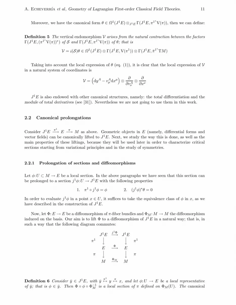
Now, let Φ:E → E be a diffeomorphism of π-fiber bundles and ΦM :M →M the diffeomorphisminduced on the basis. Our aim is to lift Φ to a diffeomorphism of J1E in a natural way; that is, insuch a way that the following diagram commutes:

J1Ej1Φ−→ J1E

π1

y

y π1

EΦ

−→ E

π

y

y π

MΦM−→ M

Definition 6 Consider y ∈ J1E, with yπ1

7→ yπ7→ x, and let φ:U → E be a local representative

of y; that is φ ∈ y. Then Φ φ Φ−1M is a local section of π defined on ΦM(U). The canonical


prolongation or the canonical lifting of the diffeomorphism Φ is the map j1Φ:J1E −→ J1E definedby

(j1Φ)(y) := j1(Φ φ Φ−1M )(ΦM (x))

It is clear that this definition does not depend on the representative φ ∈ y; that is, (j1Φ)(y) is welldefined and, moreover, it depends differentiably on y.

We can check that this definition has the predicted properties. In fact:

Proposition 6 Let Φ:E → E be a diffeomorphism of fiber bundles. Then

1. π1 j1Φ = Φ π1, π1 j1Φ = ΦM π1.

2. If Φ′:E → E is another fiber bundle diffeomorphism, then

j1(Φ′ Φ1) = j1Φ′ j1Φ

3. j1Φ is a diffeomorphism of π1-bundles and π1-bundles, and (j1Φ)−1 = j1Φ−1.

4. If φ:U → E is a local section of π, then

j1(Φ φ Φ−1M ) = j1Φ j1φ Φ−1

M

5. If ψ:U → J1E is a holonomic section, with ψ = j1φ for some φ:U → E, then j1Φ j1φ Φ−1M : ΦM (U) → J1E is a holonomic section.

( Proof ) See [31].

Remark:

• If Φ:E → E induces the identity in M (that is a strong diffeomorphism), then j1Φ is definedby

(j1Φ)(y) = j1(Φ φ)(x) ; (φ ∈ y , π1(y) = x)

since Φ φ is a section of π defined in the same open set as the section φ. In the same way, inthis case, j1Φ j1φ = j1(Φ φ), and hence canonical prolongations of strong diffeomorphismstransform holonomic sections defined in an open set into holonomic sections defined in thesame open set.

2.2.2 Relation with the affine structure

Now we want to describe the relations between the canonical prolongations of diffeomorphisms andthe canonical structures of J1E introduced in the above section.

First of all we study the relation with the affine structure of J1E.

Proposition 7 The canonical prolongations of diffeomorphisms Φ:E → E over π preserve theaffine structure of π1:J1E → E.


( Proof ) Consider y ∈ J1E and φ ∈ y, we have

(j1Φ)(y) = (j1(Φ φ Φ−1M ) ΦM )(π1(y))

Consider now α ⊗ v ∈ T∗π1(y)M ⊗ Vπ1(y)(π) and the point y + α ⊗ v. Let φ′:M → E be a local

section with φ′(π1(y)) = π1(y) and Tπ1(y)φ′ = Tπ1(y)φ+ α⊗ v. We have

(j1Φ)(y + α⊗ v) = (j1(Φ φ′ Φ−1M ) ΦM )(π1(y + α⊗ v))

= (j1(Φ φ′ Φ−1M ) ΦM )(π1(y))

= Tφ′(π1(y))Φ Tπ1(y)φ′ TΦM (π1(y))Φ

−1M

= Tφ(π1(y))Φ (Tπ1(y)φ+ α⊗ v) TΦM (π1(y))Φ−1M

= Tφ(π1(y))Φ Tπ1(y)φ TΦM (π1(y))Φ−1M + Tφ(π1(y))Φ α⊗ v TΦM (π1(y))Φ

−1M

= j1(Φ φ Φ−1M )(ΦM (π1(y)) + (T∗

ΦM (π1(y))Φ−1M ⊗ Tπ1(y))Φ(α⊗ v)

= (j1Φ)(y) + ϕ(α ⊗ v)

where ϕ: T∗π1(y)M ⊗ Vπ1(y)(π) → T∗

ΦM (π1(y))M ⊗ VΦ(π1(y))(π) is the map ϕ := T∗ΦM (π1(y))Φ

−1M ⊗

Tπ1(y)Φ and hence it is linear, therefore j1Φ is an affine mapping.

Remarks:

• See [31] for a local version of this proof.

• Consider y ∈ J1E with π1(y) = y. Since J1yE is an affine bundle over E with typical fiber

π1∗T∗M ⊗ π1∗V(π), the tangent space to one fiber at each point is canonically isomorphic tothe vector space where the fiber is modelled on; that is

T∗yJ

1yE ≃ T∗

π1(y)M ⊗ Vy(π)

If Φ:E → E is a π-diffeomorphism, we have seen that j1Φ preserves the affine structure,hence the tangent of j1Φ is just its linear part; that is, Tyj

1Φ acts on TyJ1E in the following

way:TyJ

1E −−−−−−−−−−−−−−−−→ Tj1Φ(y)J1Φ(y)E

Tyj1Φ

≃x

y

x

y ≃

T∗ΦM (π1(y))Φ

−1M ⊗ TyΦ

T∗yM ⊗ Vy(π) −−−−−−−−−−−−−−−−→ T∗

π1(j1Φ(y))M ⊗ VΦ(y)(π)

with the canonical identifications.

2.2.3 Relation with the geometric elements

Next we analyze the relation between the canonical prolongation of diffeomorphisms and the contactmodule, the structure canonical form and the canonical isomorphisms, proving that all of them areinvariant under the action of these prolongations.

Proposition 8 Let Φ:E → E be a diffeomorphism and j1Φ:J1E → J1E its canonical prolonga-tion. Then

1. (j1Φ)∗Mc = Mc 2. (j1Φ)∗θ = θ


( Proof )

1. Consider α ∈ Mc. In order to see that (j1Φ)∗α ∈ Mc we have to prove that it vanishes onevery holonomic section. Let φ:U → E be a local section and j1φ:U → J1E its canonicalprolongation, we have

(j1φ)∗((j1Φ)∗α) = (j1Φ j1φ)∗α = (j1(Φ φ Φ−1M ) ΦM)∗α = (Φ∗

M j1(Φ φ Φ−1M )∗)α = 0

because j1(Φ φ Φ−1M )∗α = 0 since α ∈ Mc and Φ φ Φ−1

M is a section of π.

We have proved that (j1Φ)∗Mc ⊂ Mc and the converse inclusion is a direct consequence ofthe third item of proposition 6.

2. Consider θ as a C∞(J1E)-linear map between X (J1E) and Γ(J1E, π1∗V(π)). Then we have

X (J1E) −−−−→ X (J1E)(j1Φ)∗

(j1Φ)∗θ

y

y θ

(j1Φ)∗Γ(J1E, π1∗V(π)) −−−−→ Γ(J1E, π1∗V(π))

therefore(j1Φ)∗θ = (j1Φ)−1

∗ θ (j1Φ)∗

and (j1Φ)∗θ = θ is equivalent to

(j1Φ)∗ θ = θ (j1Φ)∗ (2)

In order to prove this, let y ∈ J1E, u ∈ TyJ1E and φ ∈ y, (φ:U → E). Taking into account

the action of j1Φ on π1∗V(π), we have

(Tj1Φ θ)(y;u) = Tj1Φ(θ(y;u)) = Tj1Φ(dvyφ(Tyπ1(u)))

= (j1Φ)∗(Tyπ1(u) − Ty(φ π1)(u))

= Ty(Φ π1)(u) − Ty(Φ φ π1)(u)

however, since a representative of (j1Φ)(y) is ψ = Φ φ Φ−1M , we obtain

(θ Tj1Φ)(y;u) = θ((j1Φ)(y); Ty(u))

= (dvΦ(y)ψ)((T(j1Φ)(y)π1 Tyj

1Φ)(u))

= (dvΦ(y)ψ)(Ty(π1 j1Φ)(u))

= Ty(π1 j1Φ)(u) − (Ty(ψ π) Ty(π

1 j1Φ))(u)

= Ty(π1 j1Φ)(u) − Ty(Φ φ Φ−1

M π1 j1Φ)(u)

= Ty(π1 j1Φ)(u) − Ty(Φ φ π1)(u)

Conversely, we can characterize the diffeomorphisms in J1E which are canonical prolongationsas follows:

Proposition 9 Let Φ:E → E be a diffeomorphism of π-fiber bundles and ΦM :M → M the dif-feomorphism induced on the basis. Let Φ:J1E → J1E be a diffeomorphism verifying the followingconditions:

1. π1 Φ = Φ π1 2. Φ∗θ = θ

Then Φ = j1Φ.


( Proof ) Let y ∈ J1E and φ ∈ y, with φ:U → E, U ⊂ M . The second condition implies that(j1φ)∗(Φ∗θ) = (j1φ)∗θ = 0, then

(Φ−1M

∗ (j1φ)∗ Φ∗)θ = (Φ j1φ Φ−1

M )∗θ = 0

However,

π1 Φ j1φ Φ−1M = π π1 Φ j1φ Φ−1

M = π Φ π1 j1φ Φ−1M

= ΦM π φ Φ−1M = ΦM IdU Φ−1

M = IdΦM (U)

then the map Φ j1φ Φ−1M : ΦM (U) → J1E is a section of π1 such that θ vanishes on it, so it is a

holonomic section and there exists ϕ: ΦM (U) → E, with Φ j1φ Φ−1M = j1ϕ. Therefore

ϕ = π1 j1ϕ = π1 Φ j1φ Φ−1M = Φ π1 j1φ Φ−1

M = Φ φ Φ−1M

and we have

Φ(y) = Φ(j1φ(π1(y))) = (Φ j1φ Φ−1M )(ΦM (π1(y)))

= (j1ϕ)(ΦM (π1(y))) = j1(Φ j1φ Φ−1M )(ΦM (π1(y))) = (j1Φ)(y)

so Φ = j1Φ.

The last two results can be summarized in the following assertion:

Proposition 10 Let Φ:J1E → J1E be a diffeomorphism of fiber bundles over E and over M ,which induces Φ:E → E and ΦM :M →M . The necessary and sufficient condition for Φ to be thecanonical prolongation to J1E of the induced diffeomorphism Φ on E is that Φ∗θ = θ.

Finally, for the vertical endomorphisms we have:

Proposition 11 Let Φ:E → E be a diffeomorphism and j1Φ:J1E → J1E its canonical prolonga-tion. Then

1. (j1Φ)∗S = S 2. (j1Φ)∗V = V

( Proof ) We are going to interpret (j1Φ)∗S as a morphism of sections over J1E. Remember that,if y ∈ J1E with y 7→ y 7→ x and α⊗ v ∈ Vy(π)⊗T∗

xM , then S(y;α⊗ v) = Dα⊗v(y), the directionalderivative in J1

yE at the point y in the direction given by α⊗ v. According to this we can displaythe following diagram

Γ(J1E, π1∗T∗M) ⊗ Γ(J1E, π1∗V(π)) −−−−−−−−−−−−−→ Γ(J1E, π1∗T∗M) ⊗ Γ(J1E, π1∗V(π))(j1Φ−1)∗ ⊗ (j1Φ)∗

(j1Φ)∗S

y

yS

(j1Φ)∗Γ(J1E,V(π1)) −−−−−−−−−−−−−→ Γ(J1E,V(π1))

therefore, as in the above proposition of invariance of the structure form θ, we have

(j1Φ)∗S = ((j1Φ−1)∗ ⊗ (j1Φ)∗)−1 S (j1Φ)∗

and the statement of the theorem is equivalent to

S ((j1Φ−1)∗ ⊗ (j1Φ)∗) = (j1Φ)∗ S


We have

(S ((j1Φ−1)∗ ⊗ (j1Φ)∗))(y;α⊗ v) = S((j1Φ)(y); T∗j1Φ−1α⊗ Tj1Φv)

= DT∗j1Φ−1α⊗Tj1Φv(j1Φ(y))

However((j1Φ)∗ S)(y;α⊗ v) = (Tyj

1Φ)(Dα⊗v(y))

but, if f ∈ C∞(J1E), then

DT∗j1Φ−1α⊗Tj1Φv(j1Φ(y))f = lim

t→0

1

t(f(j1Φ)(y) + t(T∗j1Φ−1α⊗ Tj1Φv)) − f(j1Φ)(y)))

and

(Tj1Φ(Dα⊗v(y))f = limt→0

1

t(f((j1Φ)(y + tα⊗ v)) − f(j1Φ)(y)))

then it must be proved that

(j1Φ)(y + tα⊗ v) = (j1Φ)(y) + t(T∗j1Φ−1α⊗ Tj1Φv)

But this is proposition 7.

Since V = i(S)θ, the second item obviously holds.

2.2.4 Prolongation of projectable vector fields

Let Z ∈ X (E) a π-projectable vector field and τt:W → W , (W ⊂ E being an open set), a localone-parameter group of diffeomorphisms of Z. τt are bundle-diffeomorphisms, hence there existtheir prolongations j1τt to J1E. From the properties of τt, we deduce that j1τt is also a localone-parameter group of diffeomorphisms defined in (π1)−1(W ), so they are associated to a vectorfield. Since the prolongations can be done on every open set where a local one-parameter group ofdiffeomorphisms of Z exists, we can extend this vector field everywhere in its domain.

Definition 7 Let Z ∈ X (E) be a π-projectable vector field. The canonical prolongation of Z is thevector field j1Z ∈ X (J1E) whose associated local one-parameter groups of diffeomorphisms are thecanonical prolongations j1τt of the local one-parameter groups of diffeomorphisms of Z.

The most relevant properties of these prolongations are:

Proposition 12 Let Z ∈ X (E) be a π-projectable vector field. Then:

1. j1Z is well defined and it is a π1-projectable vector field, satisfying that π1∗(j

1Z) = Z.

2. L(j1Z)Mc ⊂ Mc.

3. The canonical prolongation of Z is the only vector field j1Z ∈ X (J1E) verifying the twofollowing conditions:

(a) j1Z is π1-projectable and π1∗(j

1Z) = Z.

(b) j1Z lets the contact module invariant: L(j1Z)Mc ⊂ Mc.


( Proof )

1. It is a direct consequence of the theorem of existence and unicity of the local one-parametergroups.

2. Since the canonical prolongations of diffeomorphisms preserve the contact module, the resultfollows straightforwardly.

3. It suffices to see that these conditions allow us to calculate the coordinates of j1Z in any localcanonical system of J1E. So, let (xµ, yA, vAµ ) be a local natural system in (π1)−1(W ) ⊂ J1E,

and Z = αµ∂

∂xµ+ βA

∂

∂yAa π-projectable vector field; that is,

∂αµ

∂yA= 0 . Since j1Z is

π1-projectable and π1∗(j

1Z) = Z, we have

j1Z = αµ∂

∂xµ+ βA

∂

∂yA+ γAµ

∂

∂vAµ

and the only problem is to calculate the coefficients γAµ . But we know that j1Z preserves the

contact module and this is generated by the forms θA = dyA − vAµ dxµ, then we have

L(j1Z)θA = ζABθB

where ζAB ∈ C∞(W ). We obtain

ζABθB = L(j1Z)θA = (d i(j1Z) + i(j1Z)d)θA

= d(βA − vAµ αµ) + i(j1Z)(dvAµ ∧ dxµ)

=∂βA

∂xµdxµ +

∂βA

∂yBdyB − αµdvAµ − vAµ

∂αµ

∂xρdxρ − γAµ dxµ + αµdvAµ

=

(

∂βA

∂xµ− vAρ

∂αρ

∂xµ− γAµ

)

dxµ +∂βA

∂yBdyB

Then, by identification of terms

ζAB =∂βA

∂yB, −ζABv

Bµ =

∂βA

∂xµ− vAρ

∂αρ

∂xµ− γAµ

therefore

γAµ =∂βA

∂xµ− vAρ

∂αρ

∂xµ+ vBµ

∂βA

∂yB

which completes the local coordinate expression of j1Z.

As a particular case, if Z ∈ X (E) is a vertical vector field; that is, π∗Z = 0, then if τt is alocal one-parameter group associated with Z, it induces the identity on M . In this case, in a local

natural system of coordinates, Z = βA∂

∂yAand its canonical prolongation is

j1Z = βA∂

∂yA+

(

∂βA

∂xµ+∂βA

∂yBvBµ

)

∂

∂vAµ


2.2.5 Generalization to non-projectable vector fields

If Z ∈ X (E) is not a π-projectable vector field, we can define its prolongation by means of thecharacterization given in proposition 12. Thus we define:

Definition 8 Let Z ∈ X (E) be a vector field. The canonical prolongation of Z is the only vectorfield j1Z ∈ X (J1E) verifying the following conditions:

1. j1Z is π1-projectable and π1∗(j

1Z) = Z.

2. The contact module is invariant under the action of j1Z: L(j1Z)Mc ⊂ Mc.

A vector field X ∈ X (J1E) satisfying these conditions is called an infinitesimal contact transfor-mation.

In a local system of coordinates, (xµ, yA, vAµ ), with Z = αµ∂

∂xµ+ βA

∂

∂yA, doing an analogous

calculation as in the above section and taking into account that, in general,∂αµ

∂yA6= 0 , we obtain

finally

j1Z = αµ∂

∂xµ+ βA

∂

∂yA+

(

∂βA

∂xµ− vAρ

(

∂αρ

∂xµ+ vBµ

∂αρ

∂yB

)

+ vBµ∂βA

∂yB

)

∂

∂vAµ

For further points of view on this subject, see [14] or [18].

3 Lagrangian formalism of first-order field theories

3.1 Lagrangian systems. Variational problems and critical sections

This section is devoted to the introduction of lagrangian densities and, using them, to defining thegeometrical objects that allow us to study the dynamical behaviour of field theories.

Let us consider again the initial situation π:E →M and the jet bundle π1:J1E → E, M beingan orientable manifold.

3.1.1 Lagrangian densities

Dynamics of classical field theories is given from lagrangian densities. A lagrangian density dependson the fields and their first derivatives with respect to the space-time variables, and it can beintegrated on the images of the fields.

First of all, it is important to point out that the following C∞(J1E)-modules are canonicallyisomorphic:


1. C∞(J1E) ⊗M Ωn+1(M).

2. Γ(J1E, π1∗Λn+1T∗M).

3. The set of semibasic (n+ 1)-forms on J1E with respect to the projection π1:

α ∈ Ωn+1(J1E) | i(X)α = 0 , ∀X ∈ Γ(J1E,V(π1))

4. The sections of the bundle Λn+1T∗M along the mapping π1:J1E →M .

(Proofs of this proposition can be found in [19] and [24]).

This assertion allow us a free ride on the notion of lagrangian density. Then we define:

Definition 9 A lagrangian density L is a π1-semibasic (n+ 1)-form in J1E.

Remarks:

1. After the above proposition, the lagrangian densities will be considered indistinctly as ele-ments of any one of those C∞(J1E)-modules when necessary.

2. The expression of a lagrangian density L is

L = fi ⊗ π1∗ωi = fi ⊗ ωi ; fi ∈ C∞(J1E) , ωi ∈ Ωn+1(M)

Since we suppose that M is an oriented manifold, suppose ω ∈ Ωn+1(M) is a fixed volume(n+ 1)-form on M , then from now on we will write a lagrangian density as

L = £ω ; £ ∈ C∞(J 1E ) , ω ∈ Ωn+1 (M )

If (xµ, yA, vAµ ) is a natural system of coordinates, we use the expression

L = £(xµ, yA, vAµ )dx1 ∧ . . . ∧ dxn ∧ dx0 ≡ £dn+1x

Then:

Definition 10 The function £ is called the lagrangian function associated with L and ω.

3. Bearing this in mind, the exterior differential of L is dL = d£ ∧ ω, which is an element ofΩn+2(J1E) or an element of Ω1(J1E) ∧ Γ(J1E, π1∗Λn+1T∗M), with the exterior product asC∞(J1E)-modules.

Observe that, if X1,X2 are π1-vertical vector fields, then i(X1) i(X2)dL = 0.

Finally, we establish the following terminology:

Definition 11 A lagrangian system is a pair ((E,M ;π),L) where

1. π:E →M is a differentiable bundle with M an orientable manifold.

2. L is a lagrangian density.


3.1.2 Lagrangian canonical forms. Properties

Now we can define the canonical forms induced by a lagrangian density. Given a lagrangian densityL which we write in the form L = £ω, we are going to associate it with some differential forms inorder to use them for studying variational problems.

The standpoint objects are

V ∈ Ω1(J1E) ⊗ Γ(J1E,V(π1)) ⊗ Γ(J1E, π1∗TM)

dL ∈ Ω1(J1E) ∧ Γ(J1E, π1∗Λn+1T∗M)

and we can contract the factors Γ(J1E,V(π1)) of V with Ω1(J1E) of dL, and Γ(J1E, π1∗TM)with Γ(J1E, π1∗Λn+1T∗M), obtaining a factor in Γ(J1E, π1∗ΛnT∗M). So we have an element ofΩ1(J1E) ∧ Γ(J1E, π1∗ΛnT∗M) which is also an element of Ωn+1(J1E) in a natural way. Then

Definition 12 Let ((E,M ;π),L) be a lagrangian system.

1. The (n+ 1)-form in J1E

ϑL := i(V)dL

(obtained after doing the above-mentioned contractions) is called the lagrangian canonicalform associated with the lagrangian density L.


ΘL := ϑL + L

is called the Poincare-Cartan (n + 1)-form associated with the lagrangian density L.


ΩL := −dΘL

is called the Poincare-Cartan (n + 2)-form associated with the lagrangian density L.

In a natural system of coordinates (xµ, yA, vAµ ) the expressions of these elements are:

V = θA ⊗∂

∂vAµ⊗

∂

∂xµ

θA = dyA − vAρ dxρ

dL = d£ ∧ ω

ω = dx1 ∧ . . . dxn ∧ dx0 ≡ dn+1x

ϑL := i(V)dL =∂£

∂vAµθA ∧ i

(

∂

∂xµ

)

ω =∂£

∂vAµθA ∧ dnxµ

≡∂£

∂vAµθA ∧ (−1)µ+1dx1 ∧ . . . dxµ−1 ∧ dxµ+1 ∧ . . . dx0

=∂£

∂vAµdyA ∧ dnxµ −

∂£

∂vAµvAµ dn+1x

ΘL =∂£

∂vAµdyA ∧ dnxµ −

(

∂£

∂vAµvAµ − £

)

dn+1x

ΩL = −d

(

∂£

∂vAµ

)

∧ dyA ∧ dnxµ + d

(

∂£

∂vAµvAµ − £

)

∧ dn+1x


As a direct consequence of the definition and the above local expressions, the relation betweenthese canonical forms and the prolongation of sections is the following:

Proposition 13 Let φ:U ⊂M → E be a local section of π. If L is a lagrangian density then

1. (j1φ)∗ϑL = 0.

2. (j1φ)∗ΘL = (j1φ)∗L.

3.1.3 Density of lagrangian energy

In the last paragraph we have seen how, in the local expression of the Poincare-Cartan (n+2)-form,appears the factor

E£ ≡∂£

∂vAµvAµ − £ (3)

which is recognized as the classical expression of the lagrangian energy associated with the la-grangian function £. Is there any global function on J1E having this local expression?. We aregoing to prove that, in order to give an intrinsic construction of this function and, by extension, ofa density of lagrangian energy, it is necessary to choose a connection in the bundle π:E → M 2.This dependence is hidden in the given local expression because any local systems of coordinatesin this bundle induces a local connection with vanishing Christoffel symbols.

First of all, we refer to the appendix A in order to take into account the basic concepts aboutconnections in the bundle π:E → M . Then we will see how the identifications made in thisappendix influence the vertical endomorphisms and the lagrangian forms.

Consider the bundle sequenceJ1E −→ E −→M

and the bundle π1∗TE → J1E. If ∇ is a connection in π:E → M inducing the splitting TE =V(π) ⊕ H(∇), we also have that

π1∗TE = π1∗V(π) ⊕ π1∗H(∇)

and therefore we obtainπ1∗T∗E = π1∗V∗(π) ⊕ π1∗H∗(∇)

as a splitting in the dual bundle. Hence π1∗V∗(π) is identified as a subbundle of π1∗T∗E.

If ξ is a section of π1∗T∗E → J1E; that is, ξ ∈ Γ(J1E, π1∗T∗E), then ξ is an element ofΩ1(J1E), that is, a 1-form on J1E, in the following way: let y 7→ y 7→ x and X ∈ X (J1E). Wewrite

ξ(y;X) = ξy((Tyπ1)(Xy))

where ξy is the value of ξ at y, translated to y = π1(y) by means of the natural identificationbetween the corresponding fibers of π1∗T∗E and T∗E.

In the same way, as every connection induces an injection π1∗V∗(π) → π1∗T∗E, then everyζ ∈ Γ(J1E, π1∗V∗(π)) is a 1-form in J1E. We then have

Γ(J1E, π1∗V∗(π)) → Ω1(J1E)2 In a forthcomming work [12], we will prove that this density of lagrangian energy allows us to construct a

hamiltonian density and a formulation of the theory in hamiltonian terms.


Consider now the vertical endomorphisms S and V, which, as we know, are sections of thebundles

S ∈ Γ(J1E, (π1∗V(π))∗) ⊗ Γ(J1E,V(π1)) ⊗ Γ(J1E, π1∗TM)

V ∈ Ω1(J1E) ⊗ Γ(J1E,V(π1)) ⊗ Γ(J1E, π1∗TM)

(remember that (π1∗V(π))∗ = π1∗V∗(π)). Taking into account the above identifications, the fol-lowing operation holds

S − V ∈ Ω1(J1E) ⊗ Γ(J1E,V(π1)) ⊗ Γ(J1E, π1∗TM)

Consequently we are able to achieve the contraction of this difference with differential forms in J1E

such as dL, obtaining

i(S − V)dL ∈ Ωn+1(J1E)

which is a semibasic form with respect to π1. Then we can define:

Definition 13 Let ((E,M ;π),L) be a lagrangian system and ∇ be a connection in π:E → M .The density of lagrangian energy associated with the lagrangian density L and the connection ∇ isthe semibasic (n+ 1)-form in J1E given by

E∇L := i(S − V)dL − L

As in the case of the lagrangian density, the expression of the density of lagrangian energy is

E∇L = Fi ⊗ π1∗ωi = Fi ⊗ ωi ; Fi ∈ C∞(J1E) , ωi ∈ Ωn+1(M)

and, if ω ∈ Ωn+1(M) is the volume (n + 1)-form on M , from now on we will write the density oflagrangian energy as

E∇L = E∇

L π1∗ω ≡ E∇

Lω ; E∇L ∈ C∞(J1E) , ω ∈ Ωn+1(M)

Then:

Definition 14 The function E∇L is called the lagrangian energy function associated with L, ∇ and

ω.

In order to see the local expressions of these elements, let (xµ, yA, vAµ ) be a natural system ofcoordinates. We have

∇ = dxµ ⊗

(

∂

∂xµ+ ΓAµ

∂

∂yA

)

E∇L = E∇

Ldn+1x

S = (dyA − ΓAµ dxµ) ⊗∂

∂vAν⊗

∂

∂xν

V =(

dyA − vAµ dxµ)

⊗∂

∂vAν⊗

∂

∂xν

where, in the expression of S, we have taken dyA − ΓAµ dxµ as a local basis of the sections of

π1∗V∗(π) over J1E, associated with the connection ∇. This basis is well defined because π1∗V∗(π)

is the incident submodule to π1∗H(∇), which is locally generated by

∂

∂xµ+ ΓAµ

∂

∂yA

. Hence

S − V = (vAµ − ΓAµ )dxµ ⊗∂

∂vAν⊗

∂

∂xν


and then the density of lagrangian energy is

E∇L := i(S − V)dL − L =

(

∂£

∂vAµ(vAµ − ΓAµ ) − £

)

dn+1x

where

E∇L =

∂£

∂vAµ(vAµ − ΓAµ ) − £

is the expression of the lagrangian energy. As one may observe, the definition of the density oflagrangian energy associated with L and ∇ depends only on these elements.

Remark:

• If the bundle π:E →M is trivial, that is E = F ×M , then we have a natural connection onE given by the splitting TE = TF × TM , and the density of lagrangian energy associatedwith this natural connection is just (3), since ΓAµ = 0.

As a final remark, we will compare the densities of lagrangian energy corresponding to twodifferent connections.

First of all, as is described in appendix A, given a connection ∇ and γ ∈ Γ(E, π∗T∗M) ⊗Γ(E,V(π)), then ∇ + γ is also a connection and, conversely, if ∇ and ∇′ are connections then∇−∇′ = γ ∈ Γ(E, π∗T∗M) ⊗ Γ(E,V(π)); that is, the difference between two connections is not aconnection. Hence, for a given connection ∇, the construction of the density of lagrangian energyallows us to define a map

Γ(E, π∗T∗M) ⊗ Γ(E,V(π)) −→ Γ(J1E, π1∗Λn+1T∗M)

γ 7→ E∇+γL − E∇

L

which is a C∞(E)-morphism of modules. This is the so-called Legendre transformation form in[14].

In another way, if we denote by S∇ and S∇+γ the “vertical endomorphisms corresponding to∇ and ∇ + γ” respectivelly, we have

E∇+γL − E∇

L = i(S∇+γ − S∇)dL

In a local system of coordinates we have

γ = γAµ dxµ ⊗∂

∂yA

E∇+γL − E∇

L = −γAµ∂£

∂vAνdn+1x

Note that this difference does not depend on the connection but only on γ.

This expression of the difference of densities of lagrangian energy corresponding to two differentconnections is recognized by stating that the density of lagrangian energy depends linearly on theconnection.


3.1.4 Variational problem associated with a lagrangian density

If φ:M → E is a section of π and j1φ:M → J1E is its canonical prolongation, since L is a(n+ 1)-form on J1E, then (j1φ)∗L ∈ Ωn+1(M). Taking this into account we can define:

Definition 15 Let ((E,M ;π),L) be a lagrangian system. Let Γc(M,E) be the set of compactsupported sections of π and consider the map

L : Γc(M,E) −→ Rφ 7→

∫

M (j1φ)∗L

The variational problem posed by the lagrangian density L is the problem of searching for the critical(or stationary) sections of the functional L.

Remark:

• The sections must be “stationary” with respect to the variations of φ given by φt = τt φ,where τt is a local one-parameter group of any vector field Z ∈ X (E) which is π-vertical;that is,

d

dt

∣

∣

∣

t=0

∫

M(j1φt)

∗L = 0

Z is required to be vertical in order to assure that φt is a section defined in the same openset as φ (except for some problems in the domain of τt), since τt induces the identity on M .

3.1.5 Characterization of critical sections

In this paragraph we suppose that a lagrangian density L is given and we are going to study theconditions for a section of π with compact support to be a critical section of the variational problemassociated with this lagrangian density. For other approaches see [17]. [14], [18].

Theorem 1 Let ((E,M ;π),L) be a lagrangian system. The following assertions on a sectionφ ∈ Γc(M,E) are equivalent 3.

1. φ is a critical section for the variational problem posed by L.

2.

∫

M(j1φ)∗ L(j1Z)L = 0 , for every Z ∈ XV(π)(E).

3.

∫

M(j1φ)∗ L(j1Z)ΘL = 0 , for every Z ∈ XV(π)(E).

4. (j1φ)∗ i(j1Z)ΩL = 0, for every Z ∈ XV(π)(E).

5. (j1φ)∗ i(X)ΩL = 0, for every X ∈ X (J1E).

6. If (xµ, yA, vAµ ) is a local natural system of coordinates and L = £ω = £dn+1 x , the coordinatesof φ in that system satisfy the Euler-Lagrange equations:

∂£

∂yA

∣

∣

∣

j1φ−

∂

∂xµ

(

∂£

∂vAµ

∣

∣

∣

j1φ

)

= 0 ; (A = 1, . . . , N)

3 In the Lie derivatives and contractions, L must be understood as a (n + 1)-form on J1E.


( Proof ) (1 ⇔ 2) If Z ∈ XV(π)(E) and τt is a one-parameter local group of Z, according tothe results in the paragraph 2.2, we have

j1(τt φ) = j1τt j1φ

therefore

d

dt

∣

∣

∣

t=0

∫

M(j1(τt φ))∗L = lim

t→0

1

t

(∫

M(j1(τt φ))∗L −

∫

M(j1φ)∗L

)

= limt→0

1

t

(∫

M(j1φ)∗(j1τt)

∗L −

∫

M(j1φ)∗L

)

= limt→0

1

t

(∫

M(j1φ)∗[(j1τt)

∗L − L]

)

=

∫

M(j1φ)∗ L(j1Z)L

and the results follows immediatelly.

(2 ⇔ 3) Taking into account that (j1φ)∗L = (j1φ)∗ΘL, for every section of π, we haveφ is a critical section if, and only if, for every Z ∈ XV(π)(E).

d

dt

∣

∣

∣

t=0

∫

M(j1(τt φ))∗ΘL =

∫

M(j1φ)∗ L(j1Z)ΘL

where τt is the one-parameter local group associated with Z.

(3 ⇔ 4) Taking into account the last item, we have φ is a critical section if, and only if,∫

M(j1φ)∗ L(j1Z)ΘL = 0 , for every Z ∈ XV(π)(E). But

L(j1Z)ΘL = d i(j1Z)ΘL + i(j1Z)dΘL = d i(j1Z)ΘL − i(j1Z)ΩL

and as φ has compact support, using Stoke’s theorem we obtain∫

M(j1φ)∗d i(j1Z)ΘL =

∫

Md(j1φ)∗ i(j1Z)ΘL = 0

and hence φ is a critical section if, and only if,∫

M(j1φ)∗ i(j1Z)ΩL = 0

and therefore, according to the fundamental theorem of variational calculus (see the comment atthe end of the proof), the section is critical if, and only if,

(j1φ)∗ i(j1Z)ΩL = 0

(4 ⇔ 5) The sufficency is a consequence of the above theorem.

We will attempt to prove that the condition is necessary. Suppose φ ∈ Γc(M,E) is stationary;that is,

(j1φ)∗ i(j1Z)ΩL = 0 ∀Z ∈ XV(π)(E)

and consider X ∈ X (J1E), which can be writen as X = Xφ + Xv where Xφ is tangent to theimage of j1φ and Xv is vertical in relation to π1, both in the points of the image of j1φ. However,Xv = (Xv − j1(π1

∗Xv)) + j1(π1∗Xv), where j1(π1

∗Xv) is understood as the prolongation of a vectorfield which coincides with π1

∗Xv on the image of φ. Observe that π1∗(Xv − j1(π1

∗Xv)) = 0 on thepoints of the image of j1φ. Therefrom

(j1φ)∗ i(X)ΩL = (j1φ)∗ i(Xφ)ΩL + (j1φ)∗ i(Xv − j1(π1∗Xv))ΩL + (j1φ)∗ i(j1(π1

∗Xv))ΩL


However, (j1φ)∗ i(Xφ)ΩL = 0 because Xφ is tangent to the image of j1φ, hence ΩL acts on linearlydependent vector fields. Nevertheless, (j1φ)∗ i(Xv−j

1(π1∗Xv))ΩL = 0 because Xv−j

1(π1∗Xv) is π1-

vertical and ΩL vanishes on these vector fields, when it is restricted to j1φ (again, see the commentat the end of the proof). Therefore

∫

M(j1φ)∗ i(X)ΩL =

∫

M(j1φ)∗ i(j1(π1

∗Xv))ΩL = 0

since φ is stationary and π1∗Xv ∈ XV(π)(E).

(2 ⇔ 6) φ is a stationary section if, and only if,

∫

M(j1φ)∗ L(j1Z)L = 0 , ∀Z ∈ XV(π)(E)

If Z = βA∂

∂yAthen

j1Z = βA∂

∂yA+

(

∂βA

∂xµ+∂βA

∂yBvBµ

)

∂

∂vAµ

and hence

i(j1Z)dL = i(j1Z)(d£ ∧ ω) = i(j 1Z )(d£ ∧ dn+1ω) = βA ∂£

∂yA+

(

∂βA

∂xµ+∂βA

∂yBvBµ

)

∂£

∂vAµ

therefore we have

(j1φ)∗ i(j1Z)dL =

[

(βA φ)∂£

∂yA j1φ+

(

∂βA

∂xµ φ+

(

∂βA

∂yB φ

)

∂φB

∂xµ∂£

∂vAµ j1φ

)]

dn+1x (4)

Now we will calculate the integral. Firstly, one may observe that the last term gives

∫

M

(

∂βA

∂yB φ

)

∂φB

∂xµ

(

∂£

∂vAµ j1φ

)

dn+1x =

∫

M

[

∂

∂xµ(βA φ) −

∂βA

∂xµ φ

](

∂£

∂vAµ j1φ

)

dn+1x

and the second term of this last expression cancels the second one in (4).Whereas for the first one,taking into account that the section is compact supported and integrating by parts, we have

∫

M

∂βA φ

∂xµ

(

∂£

∂vAµ j1φ

)

dxn+1x = −

∫

M(βA φ)

∂

∂xµ

(

∂£

∂vAµ j1φ

)

dxn+1x

therefore

∫

Mi(j1Z)dL =

∫

M

(

∂£

∂yA j1φ−

∂

∂xµ

(

∂£

∂vAµ j1φ

))

(βA φ)dxn+1x = 0

and since βA are arbitrary functions, we obtain

∂£

∂yA j1φ−

∂

∂xµ

(

∂£

∂vAµ j1φ

)

= 0

as set out to prove.

Remark:


• In this context, the fundamental theorem of variational calculus is applied in the followingway: let φ ∈ Γc(M,E) be a section for which there exists Z ∈ XV(π)(E) and x ∈M such that

((j1φ)∗ i(j1Z)ΩL)(x) 6= 0

we will see that, in this case, the section is not critical. In order to do this, it suffices to finda vector field Z ′ ∈ XV(π)(E) such that

∫

M(j1φ)∗ i(j1Z ′)ΩL 6= 0

This vector field Z ′ is constructed as follows: let W be a coordinate open set with x ∈W andsuch that (j1φ)∗ i(j1Z)ΩL|W = gdn+1x with g > 0, and let f :M → R be a function verifyingthat

1. f |W ≤ 0.

2. There exists V ⊂W such that f |V > 0.

3. f |M−W = 0.

Consider the vector field Z ′ = fZ. Since f vanishes out of the coordinate neighbourhood,the integral involving Z ′ vanishes there. Consequently, on W , we have

Z = βA∂

∂yA⇒ j1Z = βA

∂

∂yA+ Z = βA

∂

∂yA

(

∂βA

∂xµ+ vBµ

∂βA

∂yB

)

∂

∂vAµ

Z ′ = fZ ⇒ j1Z ′ = j1(fZ) = fj1Z + βA∂f

∂xµ∂

∂vAµ

therefore i(j1Z ′) = f i(j1Z) + i(X), where X = βA∂f

∂xµ∂

∂vAµ, but since

ΩL = −d∂£

∂vAµ∧ dyA ∧ dnxµ + dE ∧ dn+1x

we obtain

i(X)ΩL = −βBd∂f

∂xρ∂2£

∂vBρ ∂vAµ

∧ dyA ∧ dnxµ + βB∂f

∂xρ∂E

∂vBρ∧ dn+1x

−βBd∂f

∂xρ∂2£

∂vBρ ∂vAµ

∧ dyA ∧ dnxµ + βB∂f

∂xρ∂2£

∂vBρ ∂vAµ

∧ dn+1x

If φ = (xµ, φA(xµ)), we have

(j1φ) i(X)ΩL = −βB∂f

∂xρ∂2£

∂vBρ ∂vAµ

∣

∣

∣

j1φ

∂φA

∂xµdn+1x+ βB

∂f

∂xρ∂2£

∂vBρ ∂vAµ

∣

∣

∣

j1φ

∂φA

∂xµdn+1x = 0

therefore(j1φ) i(j1Z ′)ΩL = (j1φ)f i(j1Z)ΩL

and, taking into account the conditions on W and f , we conclude that

∫

M(j1φ)∗ i(j1Z ′)ΩL =

∫

W(j1φ)∗f i(j1Z)ΩL =

∫

Wf(j1φ)∗ i(j1Z)ΩL > 0


3.2 Lagrangian formalism with jet fields

The lagrangian formalism for field theories can also be established in a more analogous way than inthe case of mechanical systems using 1-jet fields. We devote the following paragraps to developingthese topics and review the main results obtained in the above sections.

First, we will introduce the kind of geometrical objects which are relevant in order to providethis particular formulation of dynamics of field theories. Once again, we refer to the appendix Afor the basic concepts related to jet fields in a jet bundle.

3.2.1 1-jet fields in the bundle J1J1E

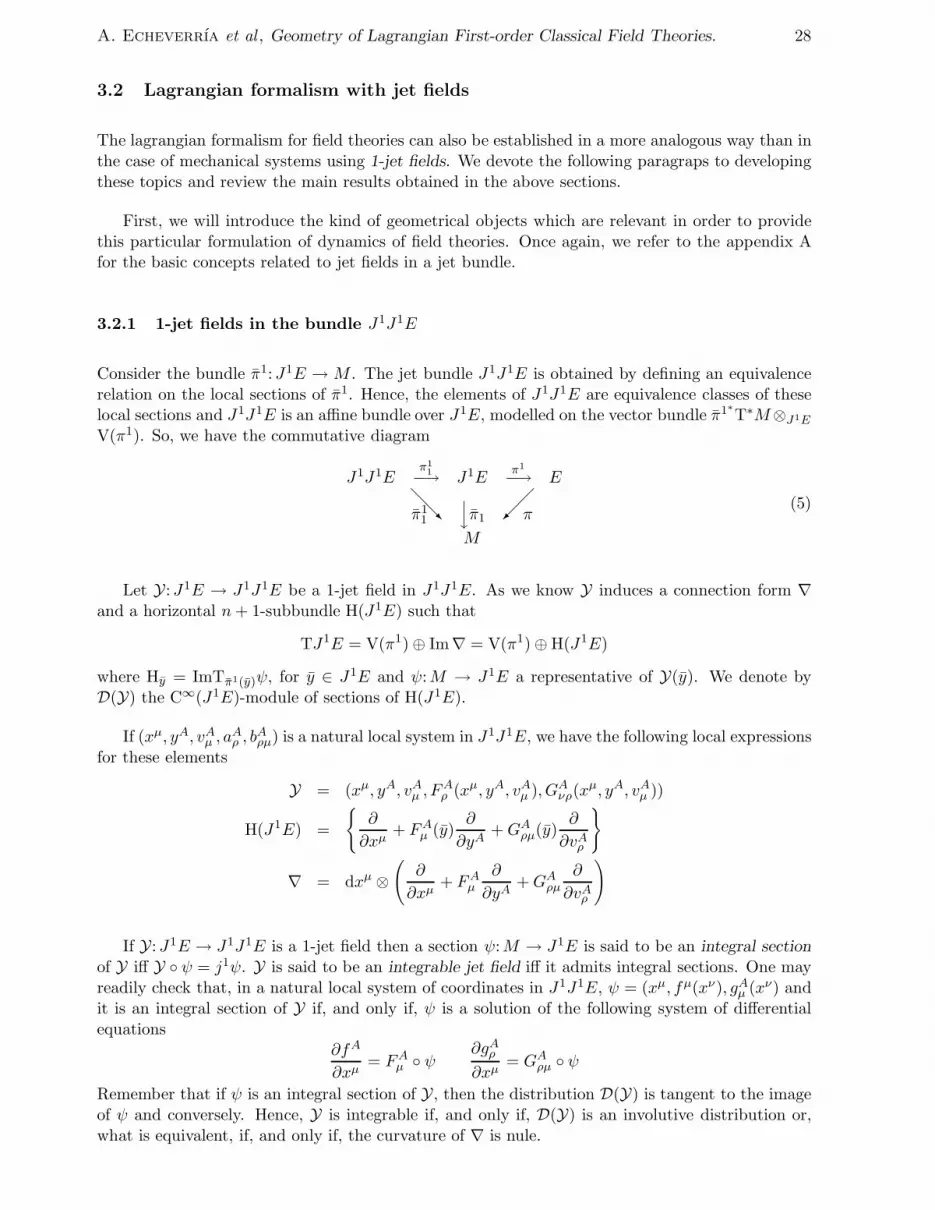
Consider the bundle π1:J1E → M . The jet bundle J1J1E is obtained by defining an equivalencerelation on the local sections of π1. Hence, the elements of J1J1E are equivalence classes of theselocal sections and J1J1E is an affine bundle over J1E, modelled on the vector bundle π1∗T∗M⊗J1E

V(π1). So, we have the commutative diagram

J1J1Eπ1

1−→ J1Eπ1

−→ E

π11

@@R

yπ1 π

M

(5)

Let Y:J1E → J1J1E be a 1-jet field in J1J1E. As we know Y induces a connection form ∇and a horizontal n+ 1-subbundle H(J1E) such that

TJ1E = V(π1) ⊕ Im∇ = V(π1) ⊕ H(J1E)

where Hy = ImTπ1(y)ψ, for y ∈ J1E and ψ:M → J1E a representative of Y(y). We denote byD(Y) the C∞(J1E)-module of sections of H(J1E).

If (xµ, yA, vAµ , aAρ , b

Aρµ) is a natural local system in J1J1E, we have the following local expressions

for these elements

Y = (xµ, yA, vAµ , FAρ (xµ, yA, vAµ ), GAνρ(x

µ, yA, vAµ ))

H(J1E) =

∂

∂xµ+ FAµ (y)

∂

∂yA+GAρµ(y)

∂

∂vAρ

∇ = dxµ ⊗

(

∂

∂xµ+ FAµ

∂

∂yA+GAρµ

∂

∂vAρ

)

If Y:J1E → J1J1E is a 1-jet field then a section ψ:M → J1E is said to be an integral section

of Y iff Y ψ = j1ψ. Y is said to be an integrable jet field iff it admits integral sections. One mayreadily check that, in a natural local system of coordinates in J1J1E, ψ = (xµ, fµ(xν), gAµ (xν) andit is an integral section of Y if, and only if, ψ is a solution of the following system of differentialequations

∂fA

∂xµ= FAµ ψ

∂gAρ

∂xµ= GAρµ ψ

Remember that if ψ is an integral section of Y, then the distribution D(Y) is tangent to the imageof ψ and conversely. Hence, Y is integrable if, and only if, D(Y) is an involutive distribution or,what is equivalent, if, and only if, the curvature of ∇ is nule.


3.2.2 The S.O.P.D.E. condition

The idea of this paragraph is to characterize the integrable jet fields in J1J1E such that theirintegral sections are canonical prolongations of sections from M to E.

It is well known that there are two natural projections from TTQ to TQ. In the same way,if we consider the diagram (5), we are going to see that there is another natural projection from

J1J1E to J1E. Let y ∈ J1J1E with yπ1

17→ yπ1

7→ yπ7→ x , and ψ:M → J1E a representative of y,

that is, y = Txψ. Consider now the section φ = π1 ψ:M → E, then j1φ(x) ∈ J1E and we have:

Proposition 14 The projection

j1π1 : J1J1E −→ J1E

y 7→ j1(π1 ψ)(π11(y))

is differentiable.

( Proof ) Let (xµ, yA, vAµ , aAρ , b

Aµρ) be a natural local system in a neigbourhood of y0 ∈ J1J1E

and y0 = (xµ0 , yA0 , v

Aµ 0, aAρ 0

, bAµρ0). We have π1

1(y0) = (xµ0, yA

0, vAµ 0

). Let ψ:M → J1E be a

representative of y0; locally ψ = (xµ, fA(xν), gAµ (xν)) with

fA(xν0) = yA0 , gAµ (xν0) = vAµ 0;

∂fA(xν0)

∂xρ= aAρ 0

,∂gAµ (xν0)

∂xρ= bAρµ0

then φ = π1 ψ = (xµ, fA(xν)), and

j1φ =

(

xµ, fA(xν),∂fA

∂xµ(xν)

)

Hence j1π1(y0) = (xµ0 , yA0 , a

Aρ 0

) and the result follows.

Remark:

• Observe that j1π1 and π11 exchange the coordinates vAµ and aAµ .

Corolary 1 If ψ:M → J1E is a section of π1, then j1π1 j1ψ = j1(π1 ψ).

( Proof ) In a local coordinate system (xµ, yA, vAµ , aAρ , b

Aµρ), we have ψ = (xµ, fA(xν), gAρ (xν))

and j1ψ =

(

xµ, fA(xν), gAρ (xν),∂fA

∂xρ(xν),

∂gAµ

∂xρ(xν)

)

, but j1π1 j1ψ =

(

xµ, fA(xν),∂fA

∂xρ(xν)

)

=

j1(π1 ψ) .

Definition 16 A 1-jet field Y:J1E → J1J1E is said to be a Second Order Partial DifferentialEquation (SOPDE), or also that verifies the SOPDE condition, iff it is a section of the projectionj1π1 or, what is equivalent,

j1π1 Y = IdJ1E


This kind of jet fields can be characterized in the following way:

Proposition 15 Let Y:J1E → J1J1E be an integrable 1-jet field. The necessary and sufficientcondition for Y to be a SOPDE is that its integral sections are canonical prolongations of sectionsφ:M → E.

( Proof ) (=⇒) If Y is a SOPDE then j1π1 Y = IdJ1E . Let ψ:M → J1E be an integralsection of Y; that is, Y ψ = j1ψ, then

ψ = j1π1 Y ψ = j1π1 j1ψ = j1(π1 ψ) ≡ j1φ

and ψ is a canonical prolongation.

(⇐=) Now, let Y be an integrable jet field whose integral sections are canonical prolon-gations. Take y ∈ J1E and φ:M → E a section such that j1φ:M → J1E is an integral section ofY with j1φ(π1(y)) = y. We have

(j1π1 Y)(y) = (j1π1 Y)(j1φ(π1(y))) = (j1π1 Y j1φ)(π1(y)) = (j1π1 Y ψ)(π1(y))

= (j1π1 j1ψ)(π1(y)) = j1(π1 ψ)(π1(y)) = j1φ(π1(y)) = y

and Y is a SOPDE.

Remark:

• In coordinates, the condition j1π1 Y = IdJ1E is expressed as follows: the jet field Y =(xµ, yA, vAµ , F

Aρ , G

Aνρ) is a SOPDE if, and only if, FAρ = vAρ .

• If Y = (xµ, yA, vAµ , vAρ , G

Aνρ) is a SOPDE and j1φ =

(

xµ, fA,∂fA

∂xµ

)

is an integral section of

Y, then the differential equations for φ are

GAνρ

(

xν , fA,∂fA

∂xγ

)

=∂2fA

∂xρ∂xν

which justifies the nomenclature. y

3.2.3 Action of jet fields on forms

Let Y:J1E → J1J1E be a 1-jet field. A map Y :X (M) → X (J1E) can be defined in the followingway: Let Z ∈ X (M), Y(Z) ∈ X (J1E) is the vector field defined as

Y(Z)(y) := (Tπ1(y)ψ)(Zπ1(y))

for every y ∈ J1E and ψ ∈ Y(y). This map is an element of Ω1(M) ⊗M X (J1E) and its localexpression is

Y

(

fµ∂

∂xµ

)

= fµ

(

∂

∂xµ+ FAµ

∂

∂yA+GAρµ

∂

∂vAρ

)

(We can recover the connection form using this map, as follows: ∇ = Y π1∗).


This map induces an action of Y on the forms on J1E. In fact, let ξ ∈ Ωn+m+1(J1E), with

m ≥ 0, we define i(Y)ξ:X (M)× (n+1). . . ×X (M) −→ Ωm(J1E) given by

((i(Y)ξ)(Z1, . . . , Zn+1))(y;X1, . . . ,Xm) := ξ(y; Y(Z1), . . . , Y(Zn+1),X1, . . . ,Xm)

for Z1, . . . , Zn+1 ∈ X (M) and X1, . . . ,Xm ∈ X (J1E). It is a C∞(M)-linear and alternate map onthe vector fields Z1, . . . , Zn+1.

Definition 17 Let Y:J1E → J1J1E be a 1-jet field and ξ ∈ Ωp(J1E). The C∞(J1E)-linear map

i(Y)ξ just defined, extended by zero to forms of degree p < n+ 1, is called the inner contraction ofthe jet field Y and the differential form ξ.

An important result related with the action of integrable jet fields is:

Theorem 2 Let Y be an integrable jet field and ξ ∈ Ωn+2(J1E). The necessary and sufficientcondition for the integral sections of Y, ψ:M → J1E, to verify the relation ψ∗ i(X)ξ = 0, for everyX ∈ X (J1E), is i(Y)ξ = 0.

( Proof ) (⇐=) If i(Y)ξ = 0 then ((i(Y)ξ)(Z1, . . . , Zn+1))(y;X) = 0, for every Zi ∈ X (M),y ∈ J1E and X ∈ X (J1E). Let ψ:M → J1E be an integral section of Y with ψ(x) = y, then

0 = ((i(Y)ξ)(Z1, . . . , Zn+1))(ψ(x);X) = ξ(ψ(x); Txψ(Z1), . . . ,Txψ(Zn+1),X)

= (i(X)ξ)(ψ(x); Txψ(Z1), . . . ,Txψ(Zn+1)) = (ψ∗i(X)ξ)(x;Z1, . . . , Zn+1)

for every X ∈ X (J1E), x ∈M , Zi ∈ X (M). And then the result follows.

(=⇒) If ψ∗ i(X)ξ = 0, for every X ∈ X (J1E), then, let Z1, . . . , Zn+1 ∈ X (M), y ∈ J1E

and ψ:M → E an integral section of Y with ψ(x) = y. We have

((i(Y)ξ)(Z1, . . . , Zn+1))(ψ(x);X) = (i(X)ξ)(ψ(x); Txψ(Z1), . . . ,Txψ(Zn+1))

= (ψ∗i(X)ξ)(x;Z1, . . . , Zn+1) = 0

for every X ∈ X (J1E), x ∈M , Zi ∈ X (M). Hence i(Y)ξ = 0.

From the definition, one may readily prove the following properties for this map:

Proposition 16 1. i(Y)(ξ1 + ξ2) = i(Y)(ξ1) + i(Y)(ξ2).

2. i(Y)(fξ) = f i(Y)(ξ), for every f ∈ C∞(J1E).

3. i(Y)(ξ) ∈ Ωn+1(M) ⊗M Ωm(J1E).

The above definition rules also for jet fields in J1E and differential forms ξ ∈ Ωp(E), in ananalogous way. So, every 1-jet field Ψ defines a map Ψ:X (M) −→ X (E) as follows: if y ∈ E

then, to every Z ∈ X (M), Ψ associates the vector field Ψ(Z) ∈ X (E) defined as Ψ(Z)(y) :=

(Tπ1(y)φ)(Zπ1(y)) (φ ∈ Ψ(y)). Then, if ξ ∈ Ωn+m+1(E) (m ≥ 0), we define i(Ψ)ξ:X (M)× (n+1). . .

×X (M) −→ Ωm(E) given by

((i(Ψ)ξ)(Z1, . . . , Zn+1))(y;X1, . . . ,Xm) := ξ(y; Ψ(Z1), . . . , Ψ(Zn+1),X1, . . . ,Xm)

for Z1, . . . , Zn+1 ∈ X (M) and X1, . . . ,Xm ∈ X (E).


3.2.4 Lagrangian and Energy functions. Euler-Lagrange equations

Now we are ready to establish the lagrangian formulation of field theories using 1-jet fields inJ1J1E.

First of all, you can check (using the corresponding local expressions) that the lagrangian andenergy functions can be characterized using jet fields as follows:

Proposition 17 Let ((E,M ;π),L) be a lagrangian system and ω the volume form in M . SetZ1, . . . , Zn+1 ∈ X (M) such that ω(Z1, . . . , Zn+1) = 1.

1. If ∇ is a connection form in J1E, the lagrangian energy function can be equivalently obtainedas:

(a) For any 1-jet field Ψ in J1E

E∇L = −ΘL(j1(Ψ(Z1), . . . , j

1(Ψ(Zn+1))

(b) For any 1-jet vector Y in J1J1E,

E∇L = (i(Y)E∇

L )(Z1, . . . , Zn+1)

2. For any 1-jet field Y in J1J1E, the lagrangian function can be recover as

£ = (i(Y)L)(Z1 , . . . ,Zn+1 )

On the other hand, it is known that the critical section of the associated variational problemsatisfies the following conditions:

1. They are sections φ:M → E.

2. (j1φ)∗ i(j1Z)ΩL = 0, for every Z ∈ X (J1E).

then, taking into account the statements and comments in the above sections, it is evident that:

Proposition 18 Let ((E,M ;π),L) be a lagrangian system. The critical section of the variationalproblem posed by L are the integral sections of a jet field Y, if and only if, Y satisfies the followingconditions:

1. Y is integrable; that is, R(Y) = 0.

2. Y is a SOPDE; that is, j1π1 Y = IdJ1E.

3. i(Y)ΩL = 0.

This is the version of the Euler-Lagrange equations in terms of jet fields.


4 Lagrangian symmetries and Noether’s theorem

4.1 Symmetries. Noether’s theorem

We are going to consider the question of symmetries in the lagrangian formalism of field theories.The most common and meaningful way to treat this subject is by using the theory of actions of

Lie groups and algebras. However, in this chapter, we will give a brief and simple introduction tothis question and we reserve the study of symmetries as actions of Lie groups for further research.

4.1.1 Symmetries of lagrangian systems

In Mechanics, a symmetry of a lagrangian dynamical system is a diffeomorphism in the phasespace of the system (the tangent bundle) which leaves the lagrangian function invariant. Thus, itis usual to speak about natural or physical symmetries, that is, those which are canonical liftingsof diffeomorphisms in the basis of the tangent bundle: the configuration space of the system (oralso vertical diffeomorphisms). These preserve the canonical structures of the tangent bundle and,also, as a consequence, the dynamical geometric structures induced by the lagrangian.

Nevertheless, diffeomorphisms in the tangent bundle which leave the lagrangian invariant, butwhich are not canonical liftings of diffeomorphisms in the basis, do not preserve either the naturalor the dynamical structures of the tangent bundle. Thus, in the lagrangian formalism, these kindsof symmetries are usually considered as pathological or undesired from the physical point of viewand in general they are not considered (although the situation is not the same in the hamiltonianformalism, where symmetries which are not canonical liftings play a relevant role in some theories).

Taking these comments as our standpoint, and in order to establish a more general concept ofsymmetry for field theories, we define:


1. A natural symmetry of the lagrangian system is a diffeomorphism Φ:E → E such that itscanonical prolongation j1Φ:J1E → J1E leaves L invariant.

2. A (general) symmetry of the lagrangian system is a diffeomorphism Υ:J1E → J1E such that

(a) Υ leaves the canonical geometric structures of J1E (θ, Mc, S, V) invariant.

(b) Υ leaves L invariant.

It is evident that every natural symmetry is also a (general) symmetry, but the converse is nottrue. At present, we are interested only in natural symmetries, although all the comments andresults we obtain for them also hold for (general) symmetries.

Remarks:

• Since L is a (n+ 1)-form on J1E, j1Φ acts on it by pull-back. Then, for L to be invariant byj1Φ means that (j1Φ)∗L = L. Hence, one way to obtain the explicit expression of (j1Φ)∗L


consists in considering the diagram

(X (J1E))n+1 −−−−−−−−→ (X (J1E))n+1

((j1Φ)∗)n+1

(j1Φ)∗L

y

y L

((j1Φ)∗)−1

C∞(J1E) −−−−−−−−→ C∞(J1E)

where L is understood as an element of Ωn+1(J1E), we have

(j1Φ)∗L = (j1Φ)∗ L ((j1Φ)∗)n+1

that is, if Xi ∈ X (J1E) and y ∈ J1E,

((j1Φ)∗L)(y;X1, . . . ,Xn+1) = L(j1Φ(y); (j1Φ)∗X1, . . . , (j1Φ)∗Xn+1)

• Another way to obtain explicit expression of (j1Φ)∗L consists in considering L as an elementof Γ(J1E, π1∗Λn+1T∗M, ), then we have the diagram

π1∗Λn+1T∗M −−−−−−−−−−−−−→ π1∗Λn+1T∗M

(j1Φ,Λn+1Φ∗M

−1)

(j1Φ)∗L

y

y L

j1ΦJ1E −−−−−−−−−−−−−→ J1E

and then we obtain that

(j1Φ)∗L = (j1Φ,Λn+1Φ∗M

−1)−1 L j1Φ = (j1Φ−1,Λn+1Φ∗M) L j1Φ

that is, the same expression as above, taking into account that L is a (n+1)-form on M withcoefficients in C∞(J1E).

• Finally, for the last interpretation we consider the diagram

(X (E))n+1 −−−−−−−→ (X (E))n+1

(ΦM )n+1∗

(j1Φ)∗L

y

y L

((j1Φ)∗)−1

C∞(J1E) −−−−−−−→ C∞(J1E)

and therefore(j1Φ)∗L = (j1Φ) L (ΦM )n+1

∗

As predicted, we have the following relevant property:

Proposition 19 If Φ:E → E is a natural symmetry of the lagrangian system ((E,M ;π),L) then

1. (j1Φ)∗ϑL = ϑL.

2. (j1Φ)∗ΘL = ΘL.

( Proof ) Since j1Φ:J1E → J1E is a natural prolongation, it verifies that

(j1Φ)∗θ = θ , (j1Φ)∗S = S , (j1Φ)∗ΘL = ΘL

and, since the pull-back commutes with the contractions and (j1Φ)∗dL = dL, the desired resultsfollow immediately.


4.1.2 Infinitesimal symmetries

A symmetry of a lagrangian system can be thought of being generated by a vector fied. This is thestandpoint for the following definition:


1. An infinitesimal natural symmetry of the lagrangian system is a vector field Z ∈ X (E) suchthat its canonical prolongation leaves L invariant:

L(j1Z)L = 0

2. An infinitesimal (general) symmetry of the lagrangian system is a vector field X ∈ X (J1E)such that:

(a) The canonical geometric structures of J1E (θ, Mc, S, V) are invariant under the actionof X.

(b) X leaves L invariant.

In these cases L is said to be invariant by j1Z or X respectively.

As in the above paragraph we will limit ourselves to natural symmetries.

Remarks:

• L(j1Z)L is calculated in the usual way, once L is understood as a (n+ 1)-form on J1E; thatis

L(j1Z)L = i(j1Z)dL + d i(j1Z)L

• The statement that Z ∈ X (E) is an infinitesimal symmetry is equivalent to stating that thelocal one-parameter groups of Z are symmetries of the lagrangian system (in the sense ofdefinition 18).

• This kind of symmetries, as well as those in the above paragraph, are said to be dynamical

symmetries (in order to distinguish them from other kinds of symmetries), because they arecanonical prolongations of diffeomorphisms or vector fields on E, which is the configurationspace of the physical fields.

In order to obtain the local coordinate expression, suppose that

Z = αµ∂

∂xµ+ βA

∂

∂yA

j1Z = αµ∂

∂xµ+ βA

∂

∂yA+

(

∂βA

∂xµ−∂αρ

∂xµvAρ +

∂βA

∂yBvBµ

)

∂

∂vAµ

and, taking L = £ω, we have dL = d£ ∧ ω, hence

i(j1Z)dL = ((j1Z)£)ω − d£ ∧ i(j 1Z )ω

i(j1Z)L = £ i(j 1Z )ω

d i(j1Z)L = d£ ∧ i(j 1Z )ω + £d i(j 1Z )ω


therefore

L(j1Z)L = ((j1Z)£)ω + £d i(j 1Z )ω = ((j 1Z )£)ω + £d

(

αµ i

(

∂

∂xµ

)

ω

)

= ((j1Z)£)ω + £∑

µ

∂αµ

∂xµω =

(

(j 1Z )£ + £∑

µ

∂αµ

∂xµ

)

ω

therefore, if L is invariant by Z we obtain

δZ£ ≡ (j 1Z )£ + £∑

µ

∂αµ

∂xµ= 0

where δZ£ is usually called the total variation of £.

In the particular case that Z is a vertical vector field, αµ = 0 and L is invariant by Z if, andonly if, (j1Z)£ = 0 .

In relation to infinitesimal symmetries, we have the following relevant property:

Proposition 20 If Z ∈ X (E) is an infinitesimal natural symmetry of the lagrangian system((E,M ;π),L) then:

1. L(j1Z)∗ϑL = 0.

2. L(j1Z)∗ΘL = 0.

( Proof ) It is a direct consequence of proposition 19.

4.1.3 Noether’s theorem

Closely related to the problem of symmetries is the question of conserved quantities. The mainresult is:

Theorem 3 (Noether): Let Z be an infinitesimal symmetry of the system ((E,M ;π),L). Then,the n-form J(Z) := i(j1Z)ΘL is constant on the critical sections of the variational problem posedby L.

( Proof ) Let φ:M → E be a critical section of the variational problem, that is,

(j1φ)∗ i(X)dΘL = 0 , ∀X ∈ X (J1E)

Since L is invariant under Z we have

0 = L(j1Z)ΘL = d i(j1Z)ΘL + i(j1Z)dΘL

therefore

0 = (j1φ)∗[L(j1Z)ΘL] = (j1φ)∗[d i(j1Z)ΘL] + (j1φ)∗[i(j1Z)dΘL]

= (j1φ)∗[d i(j1Z)ΘL] = d[(j1φ)∗ i(j1Z)ΘL]

and the resulst follows.


Definition 20 Let ((E,M ;π),L) be a lagrangian system. If φ is a critical section for the vari-ational problem posed by L, then the expression (j1φ)∗J(Z) is called Noether’s current associatedwith Z.

In order to give an interpretation of this current, let N ⊂M be a manifold with boundary ∂N ,such that dimN = dimM and φ a critical section. Since d[(j1φ)∗ i(j1Z)ΘL] = 0, we obtain

0 =

∫

Nd[(j1φ)∗ i(j1Z)ΘL] =

∫

Nd[(j1φ)∗ i(j1Z)ΘL] =

∫

∂N(j1φ)∗ i(j1Z)ΘL

4.1.4 Noether’s theorem for jet fields

Next we are going to interpret the idea of conserved quantity in terms of jet fields. In analogy withtime-dependent lagrangian mechanical systems and taking into account how a jet field Y acts on thedifferential forms, it seems reasonable to find invariants which are differential n-forms ζ ∈ Ωn(J1E)such that i(Y)dζ = 0.

Then, in order to state Noether’s theorem in this context, we must first recall the conceptsof natural symmetry and infinitesimal natural symmetry given in definitions 18 and 19 and theirproperties. At this point, the following result is required:

Lemma 1 Let Y:J1E → J1J1E be an integrable jet field such that it is a SOPDE. If ζ ∈Ωn+1(J1E) belongs to the ideal generated by the contact module, (which is denoted by I(Mc)),then

i(Y)ζ = 0

( Proof ) Consider y ∈ J1E and let φ:M → E be a section such that j1φ is an integral section ofY passing through y. In this case we have the map

i(Y)ζ:X (M)× n+1. . . X (M) −→ C∞(J1E)

such that

(i(Y)ζ)(y;Z1, . . . , Zn+1) = ζ(y; (j1φ)∗Z1, . . . , (j1φ)∗Zn+1) = ((j1φ)∗ζ)(π1(y);Z1, . . . , Zn+1) = 0

because ζ belongs to the ideal generated by the contact module and then (j1φ)∗ζ = 0.

Now we are ready to prove that:

Theorem 4 (Noether): Let ((E,M ;π),L) be a lagrangian system and Y:J1E → J1J1E a jet fieldverifying the Euler-Lagrange equations for the lagrangian density L. Let X ∈ X (J1E) be a vectorfield satisfying the following conditions:

1. X preserves the contact module: L(X)Mc ⊂ Mc.

2. There exist ξ ∈ Ωn(J1E), and α ∈ I(Mc) ⊂ Ωn+1(J1E), such that L(X)L = dξ + α.

Then the following relation holds

i(Y)d(ξ − i(X)ΘL) = 0


( Proof ) On the one hand we have

L(X)ΘL = i(X)dΘL + d i(X)ΘL

however

L(X)ΘL = L(X)(ϑL + L) := β + dξ + α

where β ∈ I(Mc) because ϑL ∈ I(Mc). Therefrom

d(ξ − i(X)ΘL) = i(X)dΘL + ζ

with ζ ∈ I(Mc). Hence

i(Y)d(ξ − i(X)ΘL) = 0

since i(Y) i(X)dΘL = 0, for every X ∈ X (J1E), because Y is a solution of the Euler-Lagrangeequations, and i(Y)ζ = 0 as a consequence of the last lemma.

5 Examples

5.1 Electromagnetic field (with fixed background)

In this case M is space-time endowed with a semi-riemannian metric g, E = T∗M is a vectorbundle over M and πM : T∗M → M denotes the natural projection. Sections of πM are the so-called electromagnetic potentials. Using the linear connection associated with the metric g, one canbe sure that J1E → T∗M is a vector bundle. It then coincides with its associated vector bundle,and, since VE = π∗MT∗M , we have J1E = π∗MT∗M ⊗E π

∗MT∗M .

Coordinates in J1E are usually denoted (xµ, Aν , vµν)4. The coordinates A1, A2, A3 constitute

the vector potential and A4 is the scalar potential, if M = R4 and the metric is + + +−.

Let φ:M → T∗M be a section of π. Then j1φ:M → π∗T∗M × π∗T∗M is just j1φ = Tφ.

Locally φ = φνdxν , therefore j1φ =

∂φν

∂xµdxµ ⊗ dxν . Then, one may observe that j1φ is a metric

tensor on M .

The lagrangian density is the following: consider y ∈ J1E and let φ:M → T∗M be a represen-tative of y; that is, y = Tπ(y)φ, then

L =1

2‖dφ‖2dVg

where dφ is the exterior differential of φ, ‖ ‖ is the norm induced by the metric g on the 2-formson M and dVg is the volume element associated with the metric g. Observe that dφ is the skew-symmetric part of the matrix giving Tφ or, in other words, the skew-symmetric part of the metricTφ on M . It is usual to write φ in the form A = Aµdx

µ and dA = Aµ,νdxν ∧ dxµ, as we stated

above.

The symmetries of the problem arise from the isometries of g and from the fact that thesymmetric part of Tφ has not been taken into account in order to construct the lagrangian density.

Finally, if f ∈ C∞(M), then f acts on T∗M in the following way:

f : T∗M −→ T∗M

(x, α) 7→ (x, α + df(x))4 Sometimes, the notation Aν,µ is used instead of vµν .


f being a diffeomorphism which induces the identity on M . Moreover, if y ∈ J1E, the equalityL(j1f(y)) = L(y) holds trivially. This is the so-called gauge invariance of the electromagnetic field.

5.2 Bosonic string

Let M be a two-dimensional manifold and B a d + 1-dimensional manifold endowed with a givenmetric g, with signature (+, . . . ,+,−), that is, a Lorentz metric. A bosonic string in B is a mapφ:M −→ B.

Furthermore, in order to construct the lagrangian function we need a metrics on M , we takethe bundle

E = M ×B × S1,12 (M)

where S1,12 (M) is the bundle over M whose sections are the 2-covariant tensors with signature

(+,−). In this case we have:

J1E = J1(M ×B) × J1(S1,12 (M))

and we have obtained the so-called Polyakov approach where the metrics on M is dynamics.

In this approach, a field ψ is a couple (φ, h), where φ:M → B is a differentiable map (thestring) and h is a Lorentz metric in M . If y ∈ J1E and ψ = (φ, h) is a representative of y; that is,(j1ψ)(π1(y)) = y, the lagrangian density at the point y is given by

L(y) = −1

2i(h∗)φ∗gdVh

where h∗ is the dual metric of h, i(h∗)φ∗g denotes the total contraction of the 2-covariant tensorφ∗g with the 2-contravariant tensor h∗ and dVh is the volume element associated with the metrich.

Denoting by xµ the coordinates on M , by yA the ones in B and by hσρ the coordinates in the

fiber of S1,12 (M), then the coordinates in J1E are (xµ, yA, hσρ, v

Aµ , wσρµ), µ = 1, 2, A = 1, . . . , d, 0.

In such a local system, if φ = φA, g = gABdyA ⊗ dyB h = hσρdxσ ⊗ dxρ and h∗ = hσρ

∂

∂xσ⊗

∂

∂xρ,

the linear expression of L is

L = −1

2hσρgABv

Aσ v

Bρ

√

|deth|d2x

In the Nambu approach we use the metric induced on M by the string itself; that is, h = φ∗g,where g is the metric over B. In this case, E = M×B and the rest are as in the Polyakov approachwith the appropriate changes in the coordinates.

In this last case, a field is a map φ:M → B. Then, if y ∈ J1E and φ is a representative of it,the lagrangian density is

L(y) =1

2dVφ∗g

A local system of canonical coordinates is now (xµ, yA, vAµ ) and if we write φ = φA and g =

gABdyA ⊗ dyB, we have

L =1

2

√

∣

∣

∣det

(

gAB∂φA

∂x1

∂φB

∂x2

)

∣

∣

∣dx1dx2

thus it is easy to see that this expression is the infinitesimal “area” of the parallelogram generated

by Tφ

(

∂

∂x1

)

and Tφ

(

∂

∂x2

)

in B.


5.3 WZWN model

ConsiderM = S2 endowed with a riemannian metric h. Let G be a Lie group, then take E = M×Gas the manifold of configuration. If g is the Lie algebra of G, let Ω ∈ Ω1(G) ⊗ g be the Maurer-Cartan form of G and denote K the Killing metrics on g. A section of E is given by a mapg:M → G and defines the function (h∗ ⊗ K)(g∗Ω, g∗Ω) ∈ C∞(M), h∗ being the dual metrics ofh. This function is used in order to define another one in the 1-jet bundle J1E = J1(M × G) ina natural way as follows: if y ∈ J1E, with π1(y) = x, and g:M → G is a representative of it, wehave that the map

x 7−→ (h∗ ⊗K)(g∗xΩ, g∗xΩ)

does not depend on the chosen representative and hence we can define a function

y 7−→ (h∗ ⊗K)(g∗π1(y)Ω, g∗π1(y)Ω)

The first approach to the WZWN theory takes SU(2) as the Lie group, that is

SU(2) = SL(2,C) ∩U(2) = A ∈ GL(2,C) | AA† = I, detA = 1

(Observe that SU(2) is diffeomorphic to S3). In this case the fields are maps g:S2 → SU(2).

The second approach consists in considering that the metrics h on S2 is dynamical too. In thatcase the configuration bundle is E′ = (S2×G)×S2S2(S

2), where S2(S2) is the bundle over S2 whose

sections are the riemannian metrics on S2. A section of E′ is given by a pair (g, h), where g:S2 → G

is a map and h is a riemannian metrics on S2. The 1-jet bundle is J1E′ = J1(S2×G)×J1(S2(S2)).

Like in the first case we have a function defined in a natural way in J1E′. In fact, let y ∈ J1E′

and let (g, h) be a representative of y. The map

y 7−→ (h∗π1(y) ⊗K)(g∗π1(y)Ω, g∗π1(y)Ω)

is independent of the representative. We use this function in order to construct the lagrangiandensity of this model which is

L(y) := y 7−→ (h∗π1(y) ⊗K)(g∗π1(y)Ω, g∗π1(y)Ω)dVh

(This corresponds only to the so-called non topological or dynamical term of the lagrangian of theWZWN model).

The systems of natural coordinates are (xµ, gA, hρσ , vAµ , hρσµ), where xµ are coordinates in S2

(µ = 1, 2), gA are coordinates in G and hρσ makes up a local basis of sections of S2(S2).

A comment about SU(2):

• SU(2) is the universwal covering of SO(3), the group of rotations in the euclidean space ofdimension 3. Thus, SU(2) is simply connected. An element of this group is a matrix A asthe following

A =

(

α β

−β α

)

‖α‖2 + ‖β‖2 = 1 α, β ∈ C

Therefrom, it is obvious that SU(2) is diffeomorphic to S3 ⊂ R4.

The Lie algebra su(2) of SU(2) is generated by

E1 =1

2

(

0 −i−i 0

)

; E2 =1

2

(

0 −11 0

)

; E3 =1

2

(

−i 00 i

)

Observe that Ej = −12 iσj, σj being the Pauli matrices. If these matrices σj are used as a

basis of SU(2) then the coefficients are imaginary numbers.


6 Conclusions and outlook

In this work we have formulated a purely geometric theory of the lagrangian formalism of first-orderclassical field theories. The main goals we have achieved are the following:

1. We give an intrinsic definition of all the geometric elements associated with 1-jet bundles: thevertical diferential, the canonical form, the contact module and the vertical endomorphisms.Some of them, namely the structure canonical form, have been defined previously [14]; but inother cases, such as the vertical endomorphisms, the construction presented here is original.In addition, we have given a detailed description of the canonical prolongations of sections,difeomorphisms and vector fields, as well as the properties of invariance of all the abovedefined geometric elements by these prolongations.

2. Using some of the previously introduced geometric elements, we have constructed the la-

grangian forms in an intrinsic way, with no use of connections [14]. Neither is the Legendretransformation used to obtain lagrangian forms from the dual (hamiltonian) formalism of thetheory, as is the case in other works [17], [18].

3. Nevertheless, this is not the case when we define the density of lagrangian energy and thelagrangian energy function in an intrinsic way since, as we have specified, such a constructionnecessarily requires the use of a connection. We also need this connection when we wish todualize the theory; that is, in order to obtain the hamiltonian formalism, as will be seen in aforthcoming work [12].

4. After analyzing the variational problem obtaining the critical sections, another outstandingpoint is that we achieve a unified presentation of the field equations in field theories andthe dynamical equations for non-autonomous mechanical systems, by means of the 1-jetfield formulation. The problem of the integrability of the evolution equations and the factthat these equations are second-order partial differential equations is clearly interpreted in ageometrical way using this formalism.

5. Furthermore, we have carried out an introduction to the study of lagrangian symmetries,classifying them in several ways and stating and proving a geometrical version of Noether’s

theorem based on the 1-jet field formalism.

6. As a final remark, we have briefly dealt with some classical examples, making the geometricalstructure of each one of them evident.

Among the problems we will study in forthcoming papers, in which we hope to provide anoriginal treatment, we draw attention to the following:

• How to construct the hamiltonian formalism of first-order classical field theories.

• An investigation of non-regular classical field theories.

• To make a detailed analysis of symmetries in field theories.

A Connections and jet fields in a first-order jet bundle

In this appendix, we summarize some elements of the theory of jet fields and connections in fiberbundles (see [31] for details).


A.1 Basic definition and properties

In order to set the main definition of this appendix, first we prove the following statement:

Proposition 21 Let π:E → M be a fiber bundle and π1:J1E → E the corresponding first-orderjet bundle. The following elements can be canonically constructed one from the other:

1. A π-semibasic 1-form ∇ on E with values in TE (that is, an element of Γ(E, π∗T∗M) ⊗Γ(E,TE)), such that ∇∗α = α, for every π1-semibasic form α ∈ Ω1(E).

2. A subbundle H(E) of TE such that

TE = V(π) ⊕ H(E) (6)

3. A (global) section of π1:J1E → E; that is, a mapping Ψ:E → J1E such that π1 Ψ = IdE.

( Proof ) (1 ⇒ 2) First of all, observe that ∇:X (E) → X (E) is a C∞(E)-map which vanisheswhen it acts on the vertical vector fields. Its transposed map is ∇∗:Ω1(E) → Ω1(E), which isdefined as usually by ∇∗β := β ∇, for every β ∈ Ω1(E). Moreover, since ∇ is π-semibasic, so is∇∗β, then ∇∗(∇∗β) = ∇∗β and hence ∇ ∇ = ∇. Therefore, ∇ and ∇∗ are projection operatorsin X (E) and Ω1(E) respectively. So we have the splittings

X (E) = Im∇⊕ Ker∇ ; Ω1(E) = Im∇∗ ⊕ Ker∇∗

with the natural identifications

(Im∇)′ = Ker∇∗ ; (Ker∇)′ = Im∇∗ (7)

(where, if S is a submodule of X (E), the incident or annihilator of S is defined as S′ := α ∈Ω1(E) | α(X) = 0 , ∀X ∈ S). Taking this into account, for every y ∈ E, ∇y: TyE → TyE inducesthe splittings

TyE = Im∇y ⊕ Ker∇y ; T∗yE = Im∇∗

y ⊕ Ker∇∗y (8)

Next we must prove that Vy(π) = Ker∇y. But Vy(π) ⊆ Ker∇y and Im∇∗y is the set of π-semibasic

forms at y ∈ E, then we have Vy(π) = Ker∇y and, hence,

Ker∇ = Γ(E,V(π)) ≡ XV(π)(E) ; Im∇∗ = Γ(E, π∗T∗M)

So we defineH(E) :=

⋃

y∈E

∇y(u) | u ∈ TyE

As a consequence of this, the first of the splittings (8) leads to

TE = H(E) ⊕ V(π) (9)

and it allows us to introduce the projections

h: TE −→ H(E) ; v: TE −→ V(π)

whose transposed maps

h∗: H∗(∇) −→ T∗E ; v∗: V∗(π) −→ T∗E


are injections which lead to the spliting

T∗E = H∗(E) ⊕ V∗(π) (10)

and, taking into account the second equality of (8) and (7), in a natural way we have the identifi-cations H(E)′ with V∗(π) and V(π)′ with H∗(E).

(2 ⇒ 1) Given the subbundle H(E) and the splitting TE = V(π)⊕H(E), let h: TE → TEand v : TE → TE be the projections over H(E) and V(π) respectively, which induce the splittingX = h(X) + v(X), for every X ∈ X (E). Then we can define the map

∇ : X (E) −→ X (E)X 7→ h(X)

which is a C∞(E)-morphism and satisfies trivially the following properties:

1. ∇ vanishes on the vertical vector fields and therefore ∇ ∈ Γ(E, π∗T∗M) ⊗X (E).

2. ∇ ∇ = ∇, since ∇ is a projection.

3. if α ∈ Γ(E, π∗T∗M) and X ∈ X (E) we have

(∇∗α)X = α(∇(X)) = α(h(X)) = α(h(X) + v(X)) = α(X)

because α is semibasic. Therefore ∇∗α = α.

(2 ⇒ 3) Suppose that TE splits into TE = H(E) ⊕ V(π). Then there is a natural wayof constructing a section of π1:J1E → E. In fact, consider y ∈ E with π(y) = x, we haveTyE = Hy(E)⊕Vy(π) and Tyπ|Hy(E) is an isomorphism between Hy(E) and TxM . Let φy:U → E

be a local section defined in a neigbourhood of x, such that

φy(x) = y , Txφy = (Tyπ|Hy(E))−1

then we have a sectionΨ : E −→ J1E

y 7→ (j1φy)(π(y))

which is differentiable because the splitting TyE = Hy(E) ⊕ Vy(π) depends differentiabily on y.

(3 ⇒ 2) Let Ψ:E → J1E be a section and y ∈ J1E with yπ1

→ yπ→ x. Observe that Ψ(y) ∈ J1E

is an equivalence class of sections φ:M → E with φ(x) = y, but the subspace ImTxφ does notdepend on the representative φ, provided it is in this class. Then, for every y ∈ J1E and φ arepresentative of y = Ψ(y), we define

Hy(E) := ImTxφ and H(E) :=⋃

y∈E

Hy(E)

Definition 21 A connection in the bundle π:E → M is one of the above mentioned equivalentelements.

Then a (global) section Ψ:E → J1E is said to be a 1-jet field in the bundle π1:J1E → E. Theπ-semibasic form ∇ is called the connection form or Ehresmann connection. The subbundle H(E)is called the horizontal subbundle of TE associated with the connection. The set of sections ofH(E) will be denoted by D(Ψ) and its elements are the horizontal vector fields.


Let (xµ, yA) be a local system of coordinates in an open set U ⊂ E. The most general localexpression of a semibasic 1-form on E with values in TE would be

∇ = fµdxµ ⊗

(

gν∂

∂xν+ hA

∂

∂yA

)

As ∇∗ is the identity on semibasic forms, it follows that ∇∗dxµ = dxµ, so the local expression ofthe connection form ∇ is

∇ = dxµ ⊗

(

∂

∂xµ+ ΓAµ

∂

∂yA

)

where ΓAµ ∈ C∞(U). In this system the 1-jet field Ψ is expressed as

Ψ = (xµ, yA, ΓAρ (xµ, yA))

Let φ be a representative of Ψ(y) with φ = (xµ, fA(xµ)). Therefrom φ(x) = y, Txφ = Ψ(y) andwe have

y = φ(x) = (xµ, fA(xµ)) = (xµ, yA)

The matrix of Txφ is

(

Id(

∂fA

∂xµ

)

x

)

, therefore∂fA

∂xν

∣

∣

∣

x= ΓAν (xµ, yA) . Now, taking

∂

∂xµ

∣

∣

∣

xas a basis

of TxM , we obtain

ImTxφ =

(Txφ)

(

∂

∂xµ

)

=

∂

∂xµ

∣

∣

∣

y+ ΓAµ (y)

∂

∂yA

∣

∣

∣

y

hence, H(E) is locally spaned by

∂

∂xµ+ ΓAµ (y)

∂

∂yA

As final remarks, notice that the splitting (9) induces a further one

X (E) = Im∇⊕ Γ(E,V(π))

so every vector field X ∈ X (E) splits into its horizontal and vertical components:

X = XH +XV = ∇(X) + (X −∇(X))

Locally, this splitting is given by

X = fµ∂

∂xµ+ gA

∂

∂yA= fµ

(

∂

∂xµ+ ΓAµ

∂

∂yA

)

+(

gA − fµΓAµ

) ∂

∂yA

since∂

∂xµ+ ΓAµ

∂

∂yAand

∂

∂yAgenerate locally Γ(E,H(E)) and Γ(E,V(π)), respectivelly. Observe

that, if X is an horizontal vector field, then ∇(X) = X.

In an analogous way the splitting (10) induces the following one

Ω1(E) = Γ(E, π∗T∗M) ⊕ Ker∇∗ = Γ(E, π∗T∗M) ⊕ (Im∇)′

then, for every α ∈ Ω1(E), we have

α = αH + αB = ∇∗α+ (α−∇∗α)

whose local expression is

α = Fµdxµ +GAdyA = (Fµ +GAΓ

Aµ )dxµ +GA(dyA − ΓAµ dxµ)

since dxµ and dyA − ΓAµ dxµ generate locally Γ(E,H∗(E)) and Γ(E,V∗(π)), respectivelly.


A.2 Other relevant features

As an interesting remark, we analyze the structure of the set of connections in π:E → M . Then,let ∇1,∇2 be two connection forms. The condition ∇∗

1α = ∇∗2α = 0, for every semibasic 1-form α,

means that (∇1 −∇2)∗α = 0; that is ∇1 −∇2 ∈ Γ(E, π∗T∗M) ⊗E Γ(E,V(π)).

However, let ∇ be a connection on π:E →M and γ ∈ Γ(E, π∗T∗M)⊗E Γ(E,V(π)), then ∇+γ

is another connection form. So we have:

Proposition 22 The set of connection forms on π:E → M is an affine “space” over the moduleof semibasic differential 1-forms on E with values in V(π).

In a local canonical system, if ∇ = dxµ ⊗

(

∂

∂xµ+ ΓAµ

∂

∂yA

)

and γ = γAµ dxµ ⊗∂

∂yAthen

∇ + γ = dxµ ⊗

(

∂

∂xµ+ (ΓAµ + γAµ )

∂

∂yA

)

Finally, another important concept related with connections is:

Definition 22 The curvature of a connection ∇ is defined as:

R(Z1, Z2) := (Id −∇)([∇(Z1),∇(Z2)]) = i([∇(Z1),∇(Z2)])(Id −∇)

for every Z1, Z2 ∈ X (M).

Using the coordinate expressions of the connection form ∇ and the 1-jet field Ψ, a simplecalculation leads to

R =1

2

(

∂ΓBη

∂xµ−∂ΓBµ

∂xη+ ΓAµ

∂ΓBη

∂yA− ΓAη

∂ΓBµ

∂yA

)

(dxµ ∧ dxη) ⊗∂

∂yB

A.3 Integrability of jet fields

Definition 23 Let Ψ:E → J1E be a 1-jet field.

1. A section φ:M → E is said to be an integral section of Ψ iff Ψ φ = j1φ.

2. Ψ is said to be an integrable jet field iff it admits integral sections.

One may readily check that, if (xµ, yA, vAµ ) is a natural local system in J1E and, in this system,

Ψ = (xµ, yA, ΓAρ (xµ, yA)) and φ = (xµ, fA(xν)), then φ is an integral section of Ψ if, and only if, φis a solution of the following system of partial differential equations

∂fA

∂xµ= ΓAµ φ (11)

The integrable jet fields can be characterized as follows:


Proposition 23 The following assertions on a 1-jet field Ψ are equivalent:

1. The 1-jet field Ψ is integrable.

2. The curvature of the connection form ∇ associated with Ψ is nule.

3. D(Ψ) is an involutive distribution.

( Proof ) (1 ⇔ 2) Notice that if φ is an integral section of Ψ, then the distribution D(Ψ) istangent to the image of Ψ and conversely.

(2 ⇔ 3) From the definition (22) we obtain that, if R = 0, then

∇([∇(Z1),∇(Z2)]) = [∇(Z1),∇(Z2)]

hence, the horizontal distribution D(Ψ) is involutive.

Conversely, if D(Ψ) is involutive, as ∇ is the identity on D(Ψ), the last equation follows, soR = 0.

Remark:

• According to this proposition, from the local expression of R we obtain the local integrabilityconditions of the equations (11).


B Glossary of notation

C∞(A) Smooth functions in the manifold A.X (A) Vector fields in the manifold A.Ωp(A) Differential p-forms in the manifold A.A′ Incident set to A.Hom(A,B) Homomorphisms from A to B.

i(X)α Contraction of the elements X and α.

L(X)α Lie derivative of the element α along the vector field X.Dvα Directional derivative of α along the direction of v.π:E →M Differentiable fiber bundle over a (orientable) manifold M .Γ(A,B) , Γ(pr) Sections of the bundle pr:B → A.ΓU (A,B) Local sections (in an open set U ⊂ A).Γc(A,B) Compact supported sections .Ωp(A,B) = Ωp(A) ⊗A Γ(B) Differential p-forms in the manifold A with values in the bundle B.π1:J1E → E 1-jet bundle.π1:J1E →M Fiber bundle induced by π1 = π π1.J1yE Fiber of J1E at y ∈ E.

y ∈ J1E 1-jet (element of J1E).(xµ, yA, vAµ ) Local coordinate system in J1E.

V(pr) Vertical subbundle with respect to the projection pr:A→M .

XV(pr)(B) Vertical vector fields in B with respect to the projection pr:B → A.φ:M → E Section of π.ψ:M → J1E Section of π1.dvyφ Vertical differential of φ at y ∈ E.

θ Structure canonical form of J1E.Mc Contact module or Cartan distribution.θA Element of a local basis of Mc.I(Mc) Ideal generated by the contact module.V , S Vertical endomorphisms in J1E.j1φ, (jψ) Canonical prolongation of φ (ψ) to J1E (J1J1E).j1Φ Canonical prolongation of a diffeomorphism Φ:E → E to J1E.j1Z Canonical prolongation of a vector field Z ∈ X (E) to J1E.∇ Connection form (Ehresmann connection).H(E) Horizontal subbundle (induced by a connection).Ψ:E → JE (Global) section of π1. (1-jet field in J1E).D(Ψ) Set of sections of H(E) (horizontal vector fields).R Curvature of a connection.L Lagrangian density.£ Lagrangian function.L Lagrangian functional.ϑL Lagrangian canonical form.ΘL Poincare-Cartan (n + 1)-form.ΩL Poincare-Cartan (n + 2)-form.((E,M ;π),L) Lagrangian systemE∇L Density of lagrangian energy associated with L and ∇.

E∇L Energy associated with L and ∇.

π11 :J

1J1E → J1E Repeated 1-jet bundle.y ∈ J1J1E Element of J1J1E.Y:J1E → J1J1E (Global) section of π1

1 (1-jet field in J1J1E).δZ£ Total variation of £ (under the action of Z ∈ X (E)).(j1φ)∗JZ := (j1φ)∗(i(j1Z)ΘL) Noether’s current associated with Z (for a critical section φ).


Acknowledgments

We thank Dr. X. Gracia-Sabate (U.P.C.) for discussions concerning some subjects on DifferentialGeometry and Dr. L.A. Ibort (U.C.M.) for his comments and suggestions. We also thank Mr. JeffPalmer for his assistance in preparing the English version of the manuscript.

References

[1] R. Abraham, J.E. Marsden, Foundations of Mechanics (2nd ed.), Addison-Wesley,Reading Ma., 1978.

[2] V. Aldaya, J.A. de Azcarraga, “Geometric formulation of classical mechanics andfield theory”, Riv. Nuovo Cimento 3 (1980) 1-66.

[3] M.F. Atiyah, Geometry of Yang-Mills Fields, Academia Nazionale dei Lincei, ScuolaNormale Superiore, 1979.

[4] M.J. Bergvelt, E.A. de Kerf, “Yang-Mills theories as constrained hamiltonian sys-tems”, Physica A 139 (1986) 101-124.

[5] E. Binz, J. Sniatycki, H. Fisher, The Geometry of Classical fields, North Holland,Amsterdam, 1988.

[6] D. Bleecker, Gauge theory and variational principles, Addison-Wesley, Reading, 1980.

[7] J.F. Carinena, M. Crampin, L.A. Ibort, “On the multisymplectic formalism for firstorder field theories”, Diff Geom. Appl. 1 (1991) 345-374.

[8] M. Daniel, C. Viallet, “The geometrical setting of gauge theories of the Yang-Millstype”, Rev. Mod. Phys. 52(1) (1980) 175-197.

[9] W. Drechsler, M.E. Mayer, Fiber Bundle Techniques in Gauge Theories, LecturesNotes in Physics 67, Springer-Verlag, New York, 1977.

[10] A. Echeverrıa-Enrıquez, M.C. Munoz-Lecanda, “Variational calculus in severalvariables: a hamiltonian approach”, Ann. Inst. Henri Poincare 56(1) (1992) 27-47.

[11] A. Echeverrıa-Enrıquez, M.C. Munoz-Lecanda, N. Roman-Roy, “Geometricalsetting of time-dependent regular systems. Alternative models”, Rev. Math. Phys. 3(3)(1991) 301-330.

[12] A. Echeverrıa-Enrıquez, M.C. Munoz-Lecanda, N. Roman-Roy, “Geometry ofHamiltonian First-order Classical Field Theories”, Preprint DMAT-UPC (1995) (In prepa-ration).

[13] T. Eguchi, P.B. Gilkey, A. Hanson, “Gravitation, gauge theories and DifferentialGeometry”, Phys. Rep. 66 (1980) 213-393.

[14] P.L. Garcia, “The Poincare-Cartan invariant in the calculus of variations”, Symp. Math.

14 (1974) 219-246.

[15] P.L. Garcia, J. Munoz, “On the geometrical structure of higher order variational calcu-lus”, Proc. IUTAM-ISIMM Symposyum on Modern Developments in Analytical Mechanics

M. Francaviglia, A. Lichnerowicz eds., Atti della Academia della Scienze di Torino 117(1983) 127-147.

[16] M. Gockeler, T. Schucker, Differential Geometry, Gauge Theories and Gravity, Cam-bridge Univ. Press, New York, 1987.


[17] H. Goldschmidt, S. Sternberg, “The Hamilton-Cartan formalism in the calculus ofvariations”, Ann. Inst. Fourier Grenoble 23 (1) (1973) 203-267.

[18] M.J. Gotay, J.Isenberg, J.E. Marsden, R. Montgomery, J. Sniatycki, P.B.

Yasskin, Momentum maps and classical relativistic fields, GIMMSY, 1990.

[19] W. Greub, S. Halpering, S. Vanstone, Connections, curvature and cohomology,Acad. Press, New York, 1972.

[20] C Gunther, “The polysymplectic hamiltonian formalism in the field theory and thecalculus of variations I: the local case”, J. Diff. Geom. 25 (1987) 23-53.

[21] R. Hermann, Differential Geometry and the Calculus of Variations, Academic Press, 2nd

ed., Math. Sci. Press, Brookline Ma., 1968.

[22] J. Klein, “Espaces variationnels et mecanique”, Ann. Inst. Fourier, Grenoble 12 (1962)1-124.

[23] M. de Leon, P.R. Rodrigues, Generalized Classical Mechanics and Field Theory,North-Holland Math. Studies 112, Elsevier, Amsterdam, 1985.

[24] P. Libermann, C.M. Marle, Symplectic geometry and analytical dynamics, D. ReidelPublisging Company, Dordrecht, 1987.

[25] K.B. Marathe, G. Martucci, “The geometry of gauge fields”, J. Geom. Phys. 6 (1),(1989) 1-106.

[26] R. Ouzilou, “Expression symplectique des problemes variationels”, Symp. Math. 14,(1973) 85-98.

[27] G. Sardanashvily, “Multimomentum Hamiltonian Formalism in Field Theory, Preprinthep-th/9403172 (1994).

[28] G. Sardanashvily, “Five Lectures on Jet Manifold Methods in Field Theory”, Preprinthep-th/9411089 (1994).

[29] G. Sardanashvily O. Zakharov, “The Multimomentum Hamiltonian Formalism forField Systems, Int. J. Theor. Phys. 31 (1992) 1477-1504.

[30] D.J. Saunders, “The Cartan form in Lagrangian field theories”, J. Phys. A: Math. Gen.

20 (1987) 333-349.

[31] D.J. Saunders, The Geometry of Jet Bundles, London Math. Soc. Lect. Notes Ser. 142,Cambridge, Univ. Press, 1989.

http://arXiv.org/abs/hep-th/9403172

http://arXiv.org/abs/hep-th/9411089

geometry of lagrangian first-order classical field theories

Documents