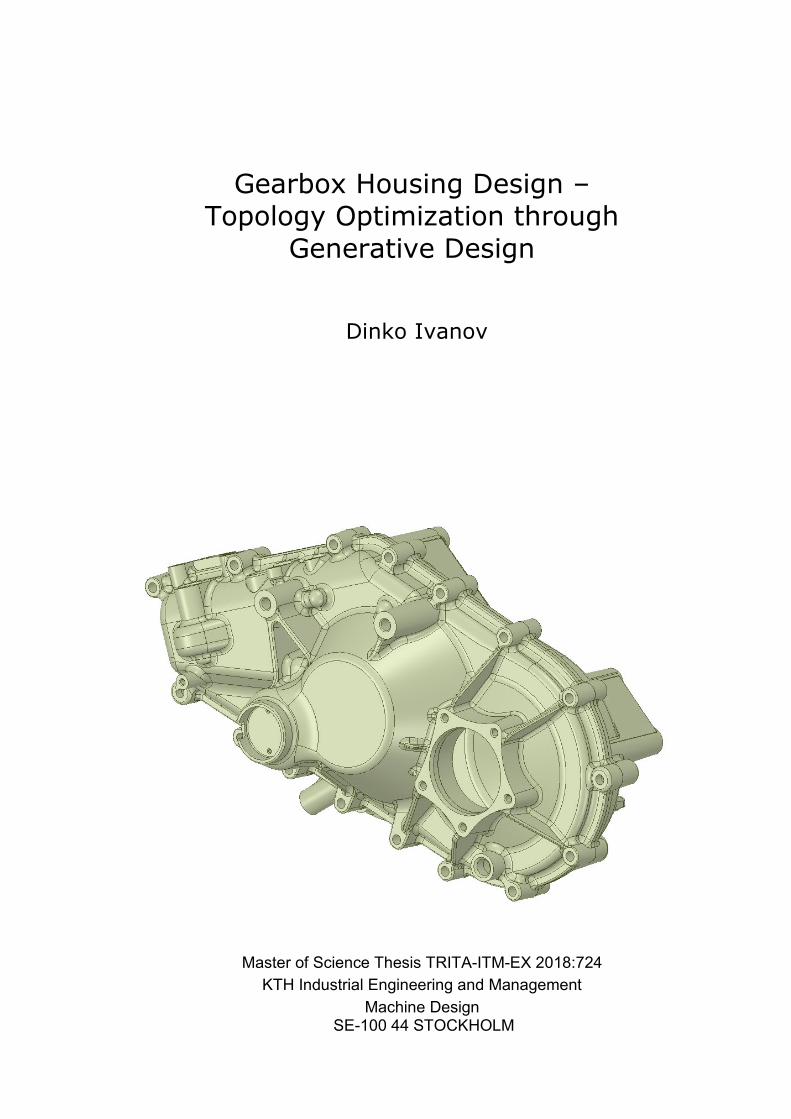
gearbox housing design – topology optimization ... - diva
TRANSCRIPT
1
Dinko Ivanov
Gearbox Housing Design – Topology Optimization through
Generative Design
Master of Science Thesis TRITA-ITM-EX 2018:724 KTH Industrial Engineering and Management
Machine Design SE-100 44 STOCKHOLM

2

3
Examensarbete TRITA-ITM-EX 2018:724
Optimering av växellådshus
Dinko Ivanov
Godkänt
2018-12-05Examinator
Ulf SellgrenHandledare Ulf Sellgren
Uppdragsgivare
AVL Sweden Kontaktperson
Minoo Nakhjiri
Sammanfattning:
Detta examensarbete använder ett systematiskt tillvägagångssätt för att omkonstruera ett växellådshus till ett elektriskt fordon med avsikt att förbättra prestanda med avseende på hållfasthet, livslängd och styvhet. I examensarbetet ges även en kort beskrivning av hur växellådan fungerar, vilken roll den spelar i de elektriska fordonen, samt grundläggande teori som används vid konstruktion av liknande växellådor. Den huvudsakliga arbetsmetoden som använts för att nå målen är topologioptimering och olika lösningar har simulerats för att förenkla den framtida omkonstruktionen. Analyser av de olika resultaten har lett fram till ett grovt förslag på hur växellådshuset kan utformas. Det resultatet förkastades efter det att några extra simuleringar gjorts. Även om inget slutgiltigt förslag hittades, har detta examensarbete tagit fram en bra grund och vägvisning för att senare lyckas med uppdraget.
Nyckelord: Abaqus,CATIA, Tillverkningsbarhet, Tosca, Topologisk optimering,

4
5
Master of Science Thesis TRITA-ITM-EX 2018:724
Gearbox housing design – topology optimization through generative design
Dinko Ivanov
Approved
2018-12-05 Examiner
Ulf Sellgren Supervisor Ulf Sellgren
Commissioner
AVL Sweden Contact person
Minoo Nakhjiri
Abstract
This thesis targets a systematic approach for redesign of the gearbox housing for an electrical vehicle, with an intention to improve its performance in terms of structural integrity, durability and compliance. Throughout the work, a brief overview of gearbox purpose, position and significance in context of electric vehicles has been presented, some theoretical background concerning design of similar gearboxes is presented and underlying theoretical fundamentals are reviewed. Topology optimization has been utilized as the main method for achieving the goals and various solving runs were performed in order to ease the subsequent redesign. Interpretations of multiple result sets led to a rough outline guess of a possible solution candidate. After supplementary studies, that solution was later discarded. In the end, although no final redesign was generated, clear and comprehensive directions for achieving the targeted goal have been formulated.
Keywords: Abaqus,CATIA, Manufacturability, Tosca, Topology optimization

6

7
FOREWORD
I would like to express gratefulness towards all my KTH teachers – Ulf Sellgren, Stefan Björklund, Ulf Olofsson, Kjell Anderson and the rest who willingly spread their vast knowledge and constantly tried to spark wisdom within us.
Great thanks towards all AVL staff in Sweden who gave me a chance to be a part of an outstanding team: my manager Joakim Karlson for thrusting me, Minoo Nakhjiri for being patient as supervisor, Samuel Brauer for being supportive fellow engineer and all the other colleagues who are real professionals and genuine collaborators. You inspire me!
Finally – my family for their support and understanding!
Dinko Ivanov
Stockholm, 2018-11-25

8
9
TABLE OF CONTENTS
SAMMANFATTNING (SWEDISH) 3
ABSTRACT 5
FOREWORD 7
NOMENCLATURE 13
1 INTRODUCTION 13
1.1 Background 13
1.2 Purpose and goals 16
1.3 Assumptions and delimitations 16
2 FRAME OF REFERENCE 19
2.1 Load formulation and lifespan 19
2.1.1 Load cases 19
2.1.2 Service life, fatigue and corresponding material considerations 20 2.2 Helical gears and forces in shaft bearings 22
2.3 Transmission error and mesh stiffness 25
2.4 Eigenfrequencies and eigenmodes 28
2.5 NVH and periodic loads 30
2.6 Topology optimization 30
3 IMPLEMENTATION 35
3.1 Initial housing design 35
3.2 The geartrain 37
3.3 The load inputs 39
3.3.1 The cruising speed estimation 39
3.3.2 The maximum torque 39
3.4 The multibody models load calculations 39
10
3.4.1 Abusive loads in time domain 41
3.4.2 Periodic loads 42
3.5 Mesh and FEA optimization model setup 42
3.5.1 The initial geometry 43
3.5.2 The “chunk” 46
3.5.3 The “stripped” model 48
3.5.4 The “noribs” model 49
4 RESULTS 51
4.1 Initial geometry analysis 51
4.1.1 Modal analysis 51
4.1.2 Von Mises stress and deformations 53
4.2 The ”Stripped” model results 55
4.2.1 Modal analysis 55
4.2.2 Stress and deformations 56
4.3 The ”Chunk” optimization output 57
4.4 The ”Noribs” optimization output 59
5 Interpretations, redesign and evaluation 63
5.1 Results interpretation 63
5.2 The proposal 64
5.3 Proposal evaluation 64
5.4 Conclusions 66
6 RECOMMENDATIONS AND FUTURE WORK 67
6.1 Recommendations 67
6.2 Future work 68
7 REFERENCES 69
APPENDIX 71
11
NOMENCLATURE
Used abbreviations
Abbreviations AB Aktiebolag AC Alternating Current BEV Battery Electric Vehicle CPU Central Processing Unit DC Direct Current DOF Degree of Freedom EV Electric Vehicle FEA Finite Element Analysis FEM Finite Element Methods FFT Fast Fourier Transform HEV Hybrid Electric Vehicle ICE Internal Combustion Engine KTH Kungliga Tekniska Högskolan MBS Multibody System NVH Noise, Vibration & Harshness PHEV Plug – in Hybrid Electric Vehicle RAMP Rational Approximation of Material Properties RPM Revolutions Per Minute SIMP Solid Isotropic Microstructure with Penalization STEP Standard for the Exchange of Product model data STL Stereolithography TE Transmission Error

12
13
1 INTRODUCTION This chapter contains a brief overview of electric vehicles, their drivetrain configurations and economic perspectives.
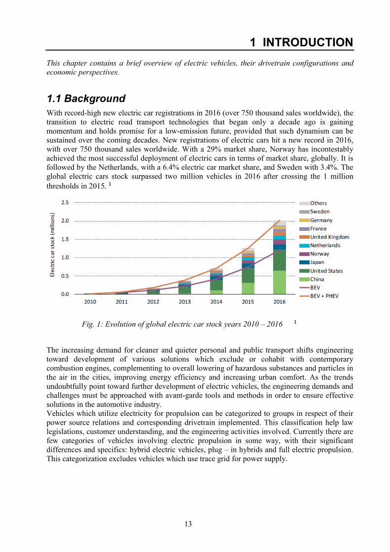
1.1 Background With record-high new electric car registrations in 2016 (over 750 thousand sales worldwide), the transition to electric road transport technologies that began only a decade ago is gaining momentum and holds promise for a low-emission future, provided that such dynamism can be sustained over the coming decades. New registrations of electric cars hit a new record in 2016, with over 750 thousand sales worldwide. With a 29% market share, Norway has incontestably achieved the most successful deployment of electric cars in terms of market share, globally. It is followed by the Netherlands, with a 6.4% electric car market share, and Sweden with 3.4%. The global electric cars stock surpassed two million vehicles in 2016 after crossing the 1 million thresholds in 2015.[1]
Fig. 1: Evolution of global electric car stock years 2010 – 2016 [1]
The increasing demand for cleaner and quieter personal and public transport shifts engineering toward development of various solutions which exclude or cohabit with contemporary combustion engines, complementing to overall lowering of hazardous substances and particles in the air in the cities, improving energy efficiency and increasing urban comfort. As the trends undoubtfully point toward further development of electric vehicles, the engineering demands and challenges must be approached with avant-garde tools and methods in order to ensure effective solutions in the automotive industry. Vehicles which utilize electricity for propulsion can be categorized to groups in respect of their power source relations and corresponding drivetrain implemented. This classification help law legislations, customer understanding, and the engineering activities involved. Currently there are few categories of vehicles involving electric propulsion in some way, with their significant differences and specifics: hybrid electric vehicles, plug – in hybrids and full electric propulsion. This categorization excludes vehicles which use trace grid for power supply.
14
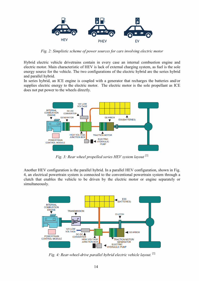
Fig. 2: Simplistic scheme of power sources for cars involving electric motor
Hybrid electric vehicle drivetrains contain in every case an internal combustion engine and electric motor. Main characteristic of HEV is lack of external charging system, as fuel is the sole energy source for the vehicle. The two configurations of the electric hybrid are the series hybrid and parallel hybrid. In series hybrid, an ICE engine is coupled with a generator that recharges the batteries and/or supplies electric energy to the electric motor. The electric motor is the sole propellant as ICE does not put power to the wheels directly.
Fig. 3: Rear wheel propelled series HEV system layout [2]
Another HEV configuration is the parallel hybrid. In a parallel HEV configuration, shown in Fig. 4, an electrical powertrain system is connected to the conventional powertrain system through a clutch that enables the vehicle to be driven by the electric motor or engine separately or simultaneously.
Fig. 4: Rear-wheel-drive parallel hybrid electric vehicle layout. [2]
15
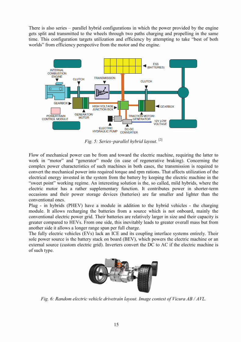
There is also series – parallel hybrid configurations in which the power provided by the engine gets split and transmitted to the wheels through two paths charging and propelling in the same time. This configuration targets utilization and efficiency by attempting to take “best of both worlds” from efficiency perspective from the motor and the engine.
Fig. 5: Series–parallel hybrid layout. [2]
Flow of mechanical power can be from and toward the electric machine, requiring the latter to work in “motor” and “generator” mode (in case of regenerative braking). Concerning the complex power characteristics of such machines in both cases, the transmission is required to convert the mechanical power into required torque and rpm rations. That affects utilization of the electrical energy invested in the system from the battery by keeping the electric machine in the “sweet point” working regime. An interesting solution is the, so called, mild hybrids, where the electric motor has a rather supplementary function. It contributes power in shorter-term occasions and their power storage devices (batteries) are far smaller and lighter than the conventional ones. Plug - in hybrids (PHEV) have a module in addition to the hybrid vehicles - the charging module. It allows recharging the batteries from a source which is not onboard, mainly the conventional electric power grid. Their batteries are relatively larger in size and their capacity is greater compared to HEVs. From one side, this inevitably leads to greater overall mass but from another side it allows a longer range span per full charge. The fully electric vehicles (EVs) lack an ICE and its coupling interface systems entirely. Their sole power source is the battery stack on board (BEV), which powers the electric machine or an external source (custom electric grid). Inverters convert the DC to AC if the electric machine is of such type.
Fig. 6: Random electric vehicle drivetrain layout. Image contest of Vicura AB / AVL.
16
1.2 Purpose and goals The purpose of the thesis is to study an existing design of an electric vehicle gearbox housing and through topology optimization deliver design improvement suggestions for the geometry. Conditions for such optimization are stemming from the significant operational abusive and periodic loads. Criteria for successful optimization redesign are improved structural performance in terms of lifetime, or diminished weight with sufficient performance in terms of the former three. Since the optimization of a design is a trade - off between different factors (see the end of 3.1 chapter), two possible strategies are available: 1. Improved performance: by having the same weight as the initial design, one can try to reduce stress and deformations of the structure, as latter stem from the abusive loads. In other words – redistributing the same amount of material to achieve greater robustness from structural point of view. 2. Diminished weight: delivering a lighter design, but one which does not trespass critical levels for stress, strain and does not trigger eigenmodes. In such strategy, essential is the safety factor definitions for each parameter (maximum deformations, cycles to failure, maximum noise level, etc.)
In this thesis the first strategy is followed, as it does not involve uncertainty of the safety factors and it is less sensitive towards input (loads) accuracy as the second one. Comparing the structural response between initial and proposals, rather than observing misconduct of certain property / parameter levels has less requirements toward unknown design details. To paraphrase: the ultimate goal is to have a structure, which being subjected to the same peak loads diminish the stress levels the initial one exerts, and at the same time has no significant excitation from periodic components of the transient loads stemming from a given operational case. Decreased stress levels under operating conditions mean extension of operational life. Studying design proposals, placed under the same load conditions, can help to discover potential improvements in the structure of the housing and provide insights for further design enhancements.
1.3 Assumptions and delimitations Some assumptions were made about various unknown parameters (for example mass of the vehicle, size of the rims and so forth). These assumptions are reasoned and motivated by rational approaches - observation of similarity, brief calculations, AVL expert recommendations and experience. Such assumptions are explained deeper in context of the topic throughout the thesis. Since there is a lack of empirical data, external structural loads used in the thesis work come from simulations with the MBS AVL EXCITE software and a model in Kisssoft software. Such assumption by itself present a whole set of limitations, as the MBS model has its own set of approximations representing the cases. These are discussed also further down in this document. When possible, finite element models are simplified in certain ways (discretization, boundary condition assumptions, neglecting various phenomena such as bolt head local stress concentrations etc.) to diminish computing power required, solving times and user input. In general, the complexity level of the models differ from industrial practices and this results in
17
lesser accuracy. The simplifications will be discussed in focus during implementation of the methods. The electric machine parameters and characteristics were lacking initially and have been investigated throughout and assumed after observation of various AVL materials and theses involving a similar gearbox. The exact model of the vehicle(s), wheel diameter etc. is also outside of the scope, as there are just functional parameters assumed. The actual values for input mechanical / electrical power can differ. The motor flange part (see further) optimization has not been included in the optimization. It is considered ”as-is” throughout the project and its change is out of scope. Nevertheless, it plays an important role as it is a part of the housing structure, alongside with the motor mount and the fasteners used. The parking lock mechanism is excluded, since there is a lack of information about its geometry. Parking stillness preservation presents a different set of load cases (on flat, down or up on a slope) which affect the housing structure significantly. However due to a lack of input data and for reducing complexity it was left outside the scope of the thesis work.

18
19
2 FRAME OF REFERENCE Theoretical fundamentals, current state design and available knowledge concerning the project are revealed in the following chapter.
2.1 Load formulation and lifespan 2.1.1 Load cases. Operational: Operational loads within the geartrain are caused by various common usage scenarios of the vehicle. They can be further categorized with respect to their occurrence: - stochastic: happen during casual usage of the gearbox. Example: forward / backward acceleration of the vehicle, regenerative braking - periodic: Their main cause is the rotational motion of the geartrain components and their sources are geometric imperfections of gears and shafts, meshing stiffness and frequency of tooth flanks, damage of contact surfaces and other less contributing phenomena. Usually frequencies of the periodic loads are related to the input frequency of the system (in our case the rotational speed of the motor’s rotor) – the so called harmonic multiples. They a play major role in NVH aspects and spectrum analysis is needed for prediction of the dynamic performance of the structure. As the loads act in the time domain, Fourier transformation can be used to convert the recorded data signal into a frequency domain representation, hence a frequency spectrum of loads. This frequency domain map presents the system excitation inputs and one can observe the static preload and more importantly the frequency and related magnitude of each dynamic component. Inertia, stiffness and damping of the system determine its response to the dynamic loads. Avoiding a possible match between periodic load components with a given frequency and an eigenmode of the structure with a similar eigenfrequency is important! Matches between those cause negative effects which vary from noise and vibration to high stresses, fatigue and deformation in the structure. Abusive: Abusive loads can happen in rare cases with sudden application of maximum torque within the geartrain system at high rpm. Superposition of maximum torque input and inertia forces lead to the largest load magnitudes. Their significance in the design phase play a role for material selection, geometry design and lifetime prediction / computation. Despite their comparably rareness of occurrence, they must be very carefully considered, calculated and proved as their estimation is important for meeting the endurance limits and safety factors. Full torque impact due to backlash play is an example of an abusive load. Worst case scenarios: Worst case scenarios are actual or imagined (but possible) combinations of abusive loads during operation, which are crucial for the gearbox structure boundary conditions. They can be exaggerated and / or formed by collection of mismatching peaks into a single set (artificial peaks). Misunderstanding, inaccurate prediction or neglecting a worst-case scenario can lead to catastrophic failure in case of an under-dimensioned structure, or terrible energy utilization in an over-dimensioned structure.
20
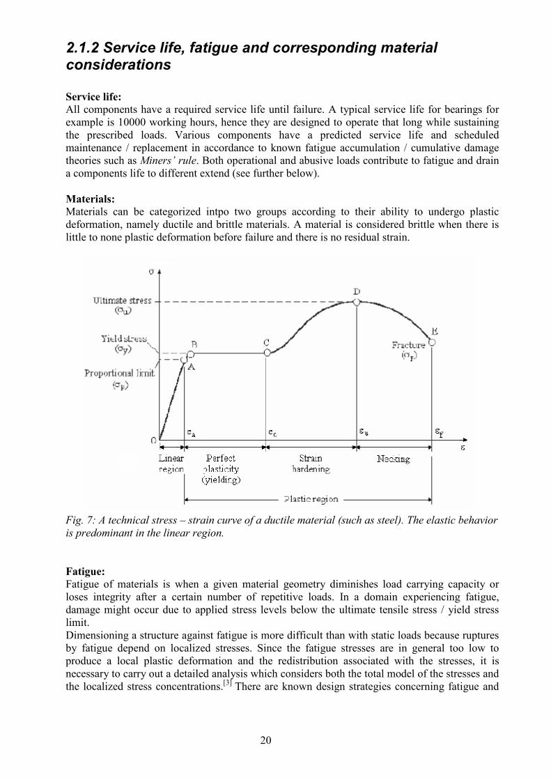
2.1.2 Service life, fatigue and corresponding material considerations Service life: All components have a required service life until failure. A typical service life for bearings for example is 10000 working hours, hence they are designed to operate that long while sustaining the prescribed loads. Various components have a predicted service life and scheduled maintenance / replacement in accordance to known fatigue accumulation / cumulative damage theories such as Miners’ rule. Both operational and abusive loads contribute to fatigue and drain a components life to different extend (see further below). Materials: Materials can be categorized intpo two groups according to their ability to undergo plastic deformation, namely ductile and brittle materials. A material is considered brittle when there is little to none plastic deformation before failure and there is no residual strain.
Fig. 7: A technical stress – strain curve of a ductile material (such as steel). The elastic behavior is predominant in the linear region. Fatigue: Fatigue of materials is when a given material geometry diminishes load carrying capacity or loses integrity after a certain number of repetitive loads. In a domain experiencing fatigue, damage might occur due to applied stress levels below the ultimate tensile stress / yield stress limit. Dimensioning a structure against fatigue is more difficult than with static loads because ruptures by fatigue depend on localized stresses. Since the fatigue stresses are in general too low to produce a local plastic deformation and the redistribution associated with the stresses, it is necessary to carry out a detailed analysis which considers both the total model of the stresses and the localized stress concentrations.[3] There are known design strategies concerning fatigue and
21
these strategies are based upon known criteria. Criteria from their side rely on corresponding fatigue life models that takes into account the material behavior. These strategies are:
- Infinite life design: local stresses are below the fatigue limit in the materials S–N curve and local strains are entirely in the elastic part of the Stress–Strain curve. This approach ensures fatigue proof operation of the component but might be impractical due to excessive weight and / or cost. However, it is not possible for all types of materials. Safe–Life design: during the design phase, a life span is assumed and the component is designed to safely operate throughout it. Scheduled replacement is necessary, since failure is highly probable. Calculations are based on stress-life, strain-life, or crack growth relations.
- Fail–safe design: the aim is to guarantee system integrity and nominal performance. Even crack formations and certain propagation will not cause complete failure. Alternative load paths and crack preventing are implemented, scheduled maintenance checks must assess component condition. This strategy utilizes the Fatigue crack growth method for criteria definition.
- Damage–tolerant design: assumes the existence of cracks in the structure. This strategy is based on the Fail–Safe design approach, extending it by applying crack formation and propagation predictions as a two-stage method.
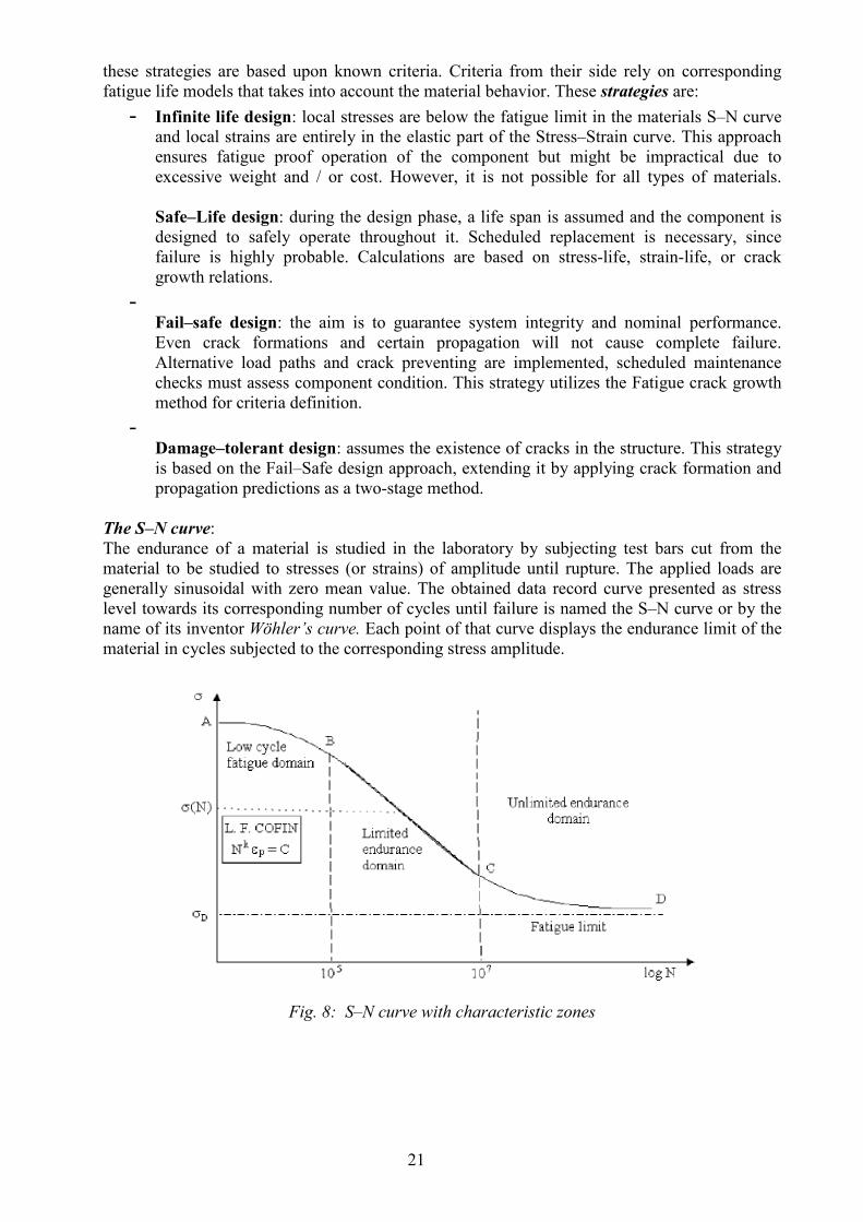
The S–N curve: The endurance of a material is studied in the laboratory by subjecting test bars cut from the material to be studied to stresses (or strains) of amplitude until rupture. The applied loads are generally sinusoidal with zero mean value. The obtained data record curve presented as stress level towards its corresponding number of cycles until failure is named the S–N curve or by the name of its inventor Wöhler’s curve. Each point of that curve displays the endurance limit of the material in cycles subjected to the corresponding stress amplitude.
Fig. 8: S–N curve with characteristic zones
22
As seen from figure 8, different zones define different fatigue behaviour models, such as low cycle fatigue and high cycle fatigue. Often the axis where the number of cycles to failure are marked is logarithmic, in sake of a more comprehensive visual representation. A side notion concerning endurance limits is that the brittle materials do not have a well-defined fatigue limit. Also, for extra-hardened tempered steels (certainly titanium, copper or aluminium alloys), or when there is corrosion, this limit remains theoretical and without interest since the fatigue life is never infinite. [3] The Palmgren-Miner rule: Statistical analysis takes into account the reliability treatments of dispersion causes, which imply that life expectancy on the Wöhler’s curve cannot be represented by a point, but by the distribution of 𝑁𝑁𝑐𝑐𝑐𝑐𝑐𝑐𝑐𝑐𝑐𝑐𝑐𝑐 with respect to the stress levels and the corresponding duration/cycles the part has been subjected to. Miner proposed a cumulative damage model as follows: 𝑛𝑛𝑖𝑖 the number of cycles at the level of stresses 𝜎𝜎𝑝𝑝 for which the average number of cycles to fracture is 𝑁𝑁𝑖𝑖 which drives an increase in damage equal to (𝑛𝑛𝑖𝑖/𝑁𝑁𝑖𝑖). The fracture occurs when:
𝐷𝐷 = 𝑛𝑛𝑖𝑖
𝑘𝑘
𝑖𝑖=1
𝑁𝑁1 = 1
If the fraction (𝑛𝑛𝑖𝑖/𝑁𝑁𝑖𝑖) of life expectancy is carried out at a certain level of stress 𝐶𝐶𝑖𝑖, the remaining endurance at another level 𝐶𝐶𝑧𝑧 will be (𝑛𝑛𝑧𝑧/𝑁𝑁𝑧𝑧 = 1 − 𝑧𝑧). Miner’s law is very simple, but not very precise. It considers what is called understressing and overstressing. [4]
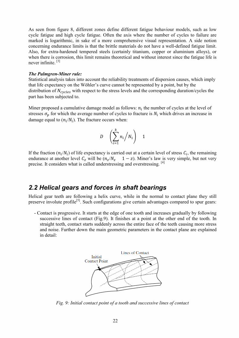
2.2 Helical gears and forces in shaft bearings Helical gear teeth are following a helix curve, while in the normal to contact plane they still preserve involute profile[5]. Such configurations give certain advantages compared to spur gears:
- Contact is progressive. It starts at the edge of one tooth and increases gradually by following successive lines of contact (Fig.9). It finishes at a point at the other end of the tooth. In straight teeth, contact starts suddenly across the entire face of the teeth causing more stress and noise. Further down the main geometric parameters in the contact plane are explained in detail:
Fig. 9: Initial contact point of a tooth and successive lines of contact
23
- Due to its progressive contact, process performance is smoother and produces less noise.
Dynamic loads are also reduced. - This type of gears can work at higher speeds than spur gears. - The contact ratio is higher. - The transmitted load is spread along an angled line making bending loads smaller. - Tooth wear is reduced, and they can transmit more power than spur gears with teeth of the
same size.
There are also few known drawbacks of theirs, compared to spurs:
- Load is transmitted perpendicularly to the tooth profile which generates an axialcomponent of the load that must be taken into consideration when designing the shaft supports.
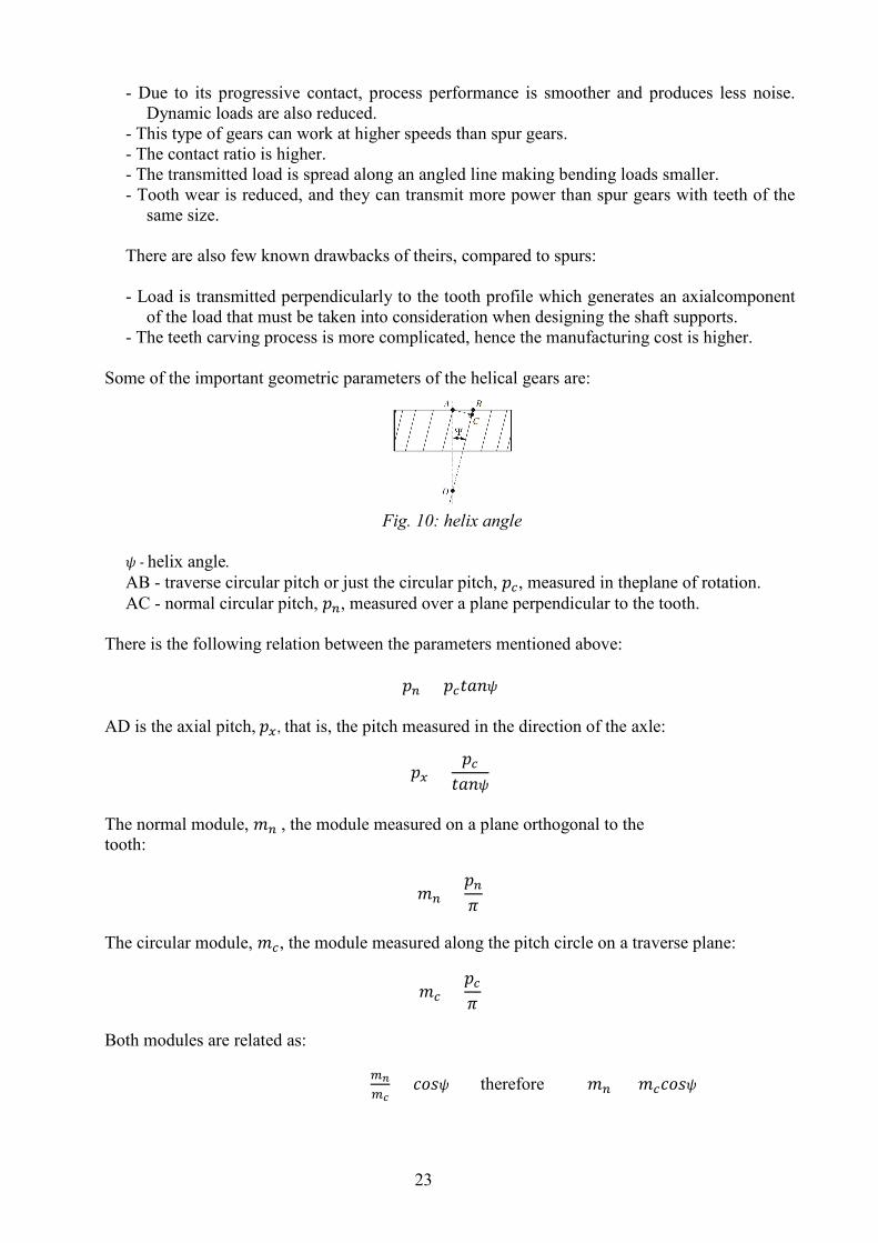
- The teeth carving process is more complicated, hence the manufacturing cost is higher. Some of the important geometric parameters of the helical gears are:
Fig. 10: helix angle
𝜓𝜓 - helix angle. AB - traverse circular pitch or just the circular pitch, 𝑝𝑝𝑐𝑐, measured in theplane of rotation. AC - normal circular pitch, 𝑝𝑝𝑛𝑛, measured over a plane perpendicular to the tooth.
There is the following relation between the parameters mentioned above:
𝑝𝑝𝑛𝑛 = 𝑝𝑝𝑐𝑐𝑡𝑡𝑡𝑡𝑛𝑛𝜓𝜓 AD is the axial pitch, 𝑝𝑝𝑥𝑥, that is, the pitch measured in the direction of the axle:
𝑝𝑝𝑥𝑥 =𝑝𝑝𝑐𝑐𝑡𝑡𝑡𝑡𝑛𝑛𝜓𝜓
The normal module, 𝑚𝑚𝑛𝑛 , the module measured on a plane orthogonal to the tooth:
𝑚𝑚𝑛𝑛 =𝑝𝑝𝑛𝑛𝜋𝜋
The circular module, 𝑚𝑚𝑐𝑐, the module measured along the pitch circle on a traverse plane:
𝑚𝑚𝑐𝑐 =𝑝𝑝𝑐𝑐𝜋𝜋
Both modules are related as:
𝑚𝑚𝑛𝑛𝑚𝑚𝑐𝑐
= 𝑐𝑐𝑐𝑐𝑐𝑐𝜓𝜓 therefore 𝑚𝑚𝑛𝑛 = 𝑚𝑚𝑐𝑐𝑐𝑐𝑐𝑐𝑐𝑐𝜓𝜓
24
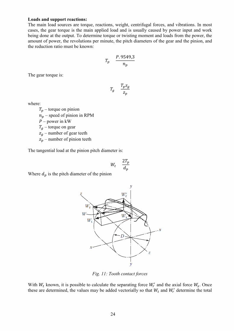
Loads and support reactions: The main load sources are torque, reactions, weight, centrifugal forces, and vibrations. In most cases, the gear torque is the main applied load and is usually caused by power input and work being done at the output. To determine torque or twisting moment and loads from the power, the amount of power, the revolutions per minute, the pitch diameters of the gear and the pinion, and the reduction ratio must be known:
𝑇𝑇𝑝𝑝 =𝑃𝑃. 9549,3
𝑛𝑛𝑝𝑝
The gear torque is:
𝑇𝑇𝑔𝑔 =𝑇𝑇𝑝𝑝𝑧𝑧𝑔𝑔𝑧𝑧𝑝𝑝
where:
𝑇𝑇𝑝𝑝 – torque on pinion 𝑛𝑛𝑝𝑝 – speed of pinion in RPM 𝑃𝑃 – power in kW 𝑇𝑇𝑔𝑔 – torque on gear 𝑧𝑧𝑔𝑔 – number of gear teeth 𝑧𝑧𝑝𝑝 – number of pinion teeth
The tangential load at the pinion pitch diameter is:
𝑊𝑊𝑡𝑡 =2𝑇𝑇𝑝𝑝𝑑𝑑𝑝𝑝
Where 𝑑𝑑𝑝𝑝 is the pitch diameter of the pinion
Fig. 11: Tooth contact forces
With 𝑊𝑊𝑡𝑡 known, it is possible to calculate the separating force 𝑊𝑊𝑟𝑟
′ and the axial force 𝑊𝑊𝑥𝑥. Once these are determined, the values may be added vectorially so that 𝑊𝑊𝑡𝑡 and 𝑊𝑊𝑟𝑟
′ determine the total
25
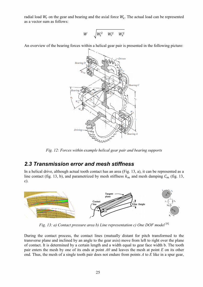
radial load 𝑊𝑊𝑟𝑟 on the gear and bearing and the axial force 𝑊𝑊𝑥𝑥. The actual load can be represented as a vector sum as follows:
𝑊𝑊 = 𝑊𝑊𝑡𝑡2 + 𝑊𝑊𝑟𝑟
2 + 𝑊𝑊𝑥𝑥2
An overview of the bearing forces within a helical gear pair is presented in the following picture:
Fig. 12: Forces within example helical gear pair and bearing supports
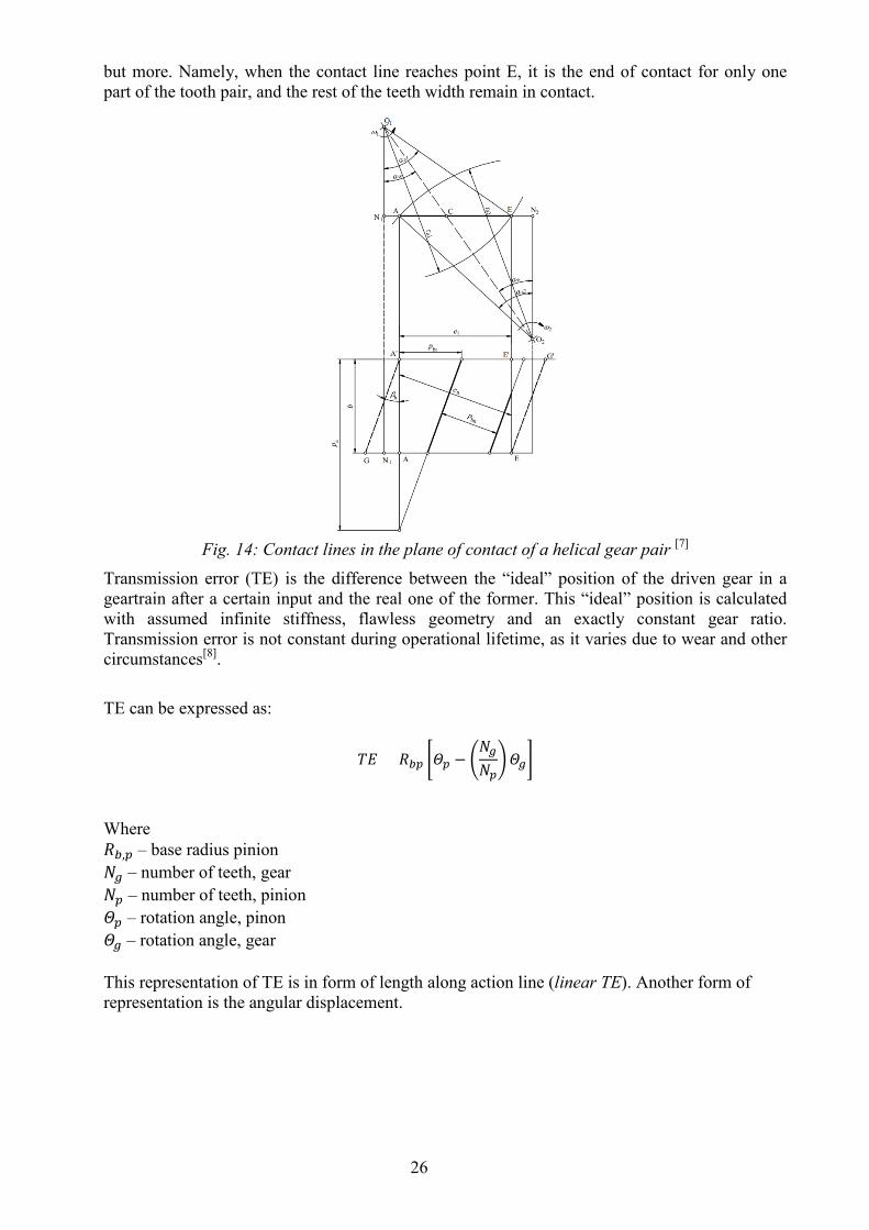
2.3 Transmission error and mesh stiffness In a helical drive, although actual tooth contact has an area (Fig. 13, a), it can be represented as a line contact (fig. 13, b), and parametrized by mesh stiffness 𝑘𝑘𝑚𝑚 and mesh damping 𝐶𝐶𝑚𝑚 (fig. 13, c).
Fig. 13: a) Contact pressure area b) Line representation c) One DOF model [6]
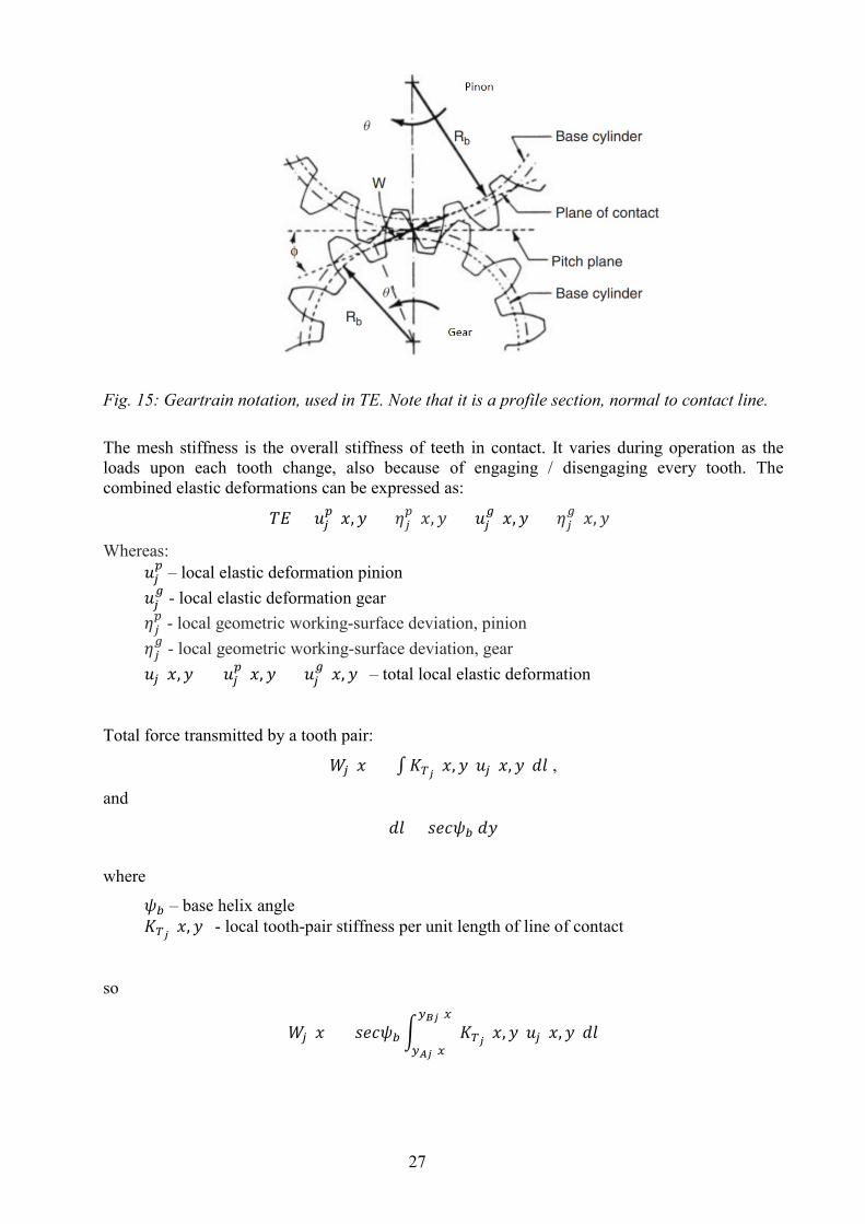
During the contact process, the contact lines (mutually distant for pitch transformed to the transverse plane and inclined by an angle to the gear axis) move from left to right over the plane of contact. It is determined by a certain length and a width equal to gear face width b. The tooth pair enters the mesh by one of its ends at point A0 and leaves the mesh at point E on its other end. Thus, the mesh of a single tooth pair does not endure from points A to E like in a spur gear,
26
but more. Namely, when the contact line reaches point E, it is the end of contact for only one part of the tooth pair, and the rest of the teeth width remain in contact.
Fig. 14: Contact lines in the plane of contact of a helical gear pair [7]
Transmission error (TE) is the difference between the “ideal” position of the driven gear in a geartrain after a certain input and the real one of the former. This “ideal” position is calculated with assumed infinite stiffness, flawless geometry and an exactly constant gear ratio. Transmission error is not constant during operational lifetime, as it varies due to wear and other circumstances[8].
TE can be expressed as:
𝑇𝑇𝑇𝑇 = 𝑅𝑅𝑏𝑏𝑝𝑝 𝛩𝛩𝑝𝑝 − 𝑁𝑁𝑔𝑔𝑁𝑁𝑝𝑝𝛩𝛩𝑔𝑔
Where 𝑅𝑅𝑏𝑏,𝑝𝑝 – base radius pinion 𝑁𝑁𝑔𝑔 – number of teeth, gear 𝑁𝑁𝑝𝑝 – number of teeth, pinion 𝛩𝛩𝑝𝑝 – rotation angle, pinon 𝛩𝛩𝑔𝑔 – rotation angle, gear This representation of TE is in form of length along action line (linear TE). Another form of representation is the angular displacement.
27
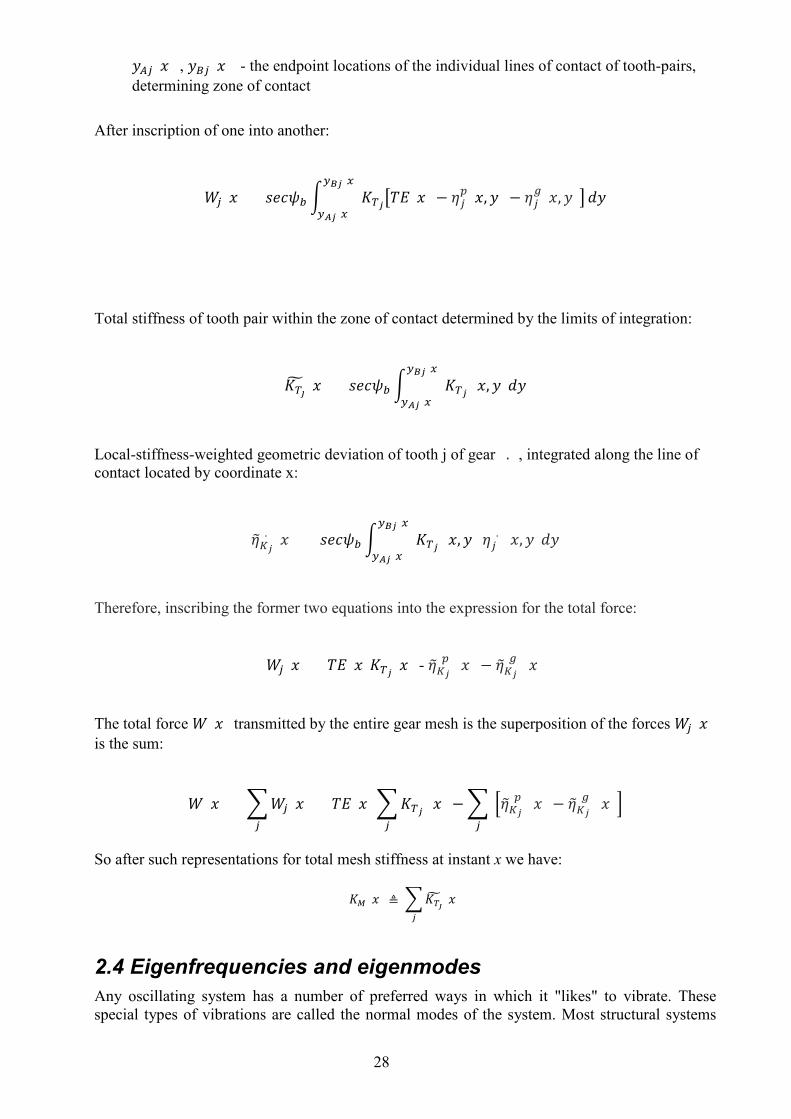
Fig. 15: Geartrain notation, used in TE. Note that it is a profile section, normal to contact line. The mesh stiffness is the overall stiffness of teeth in contact. It varies during operation as the loads upon each tooth change, also because of engaging / disengaging every tooth. The combined elastic deformations can be expressed as:
𝑇𝑇𝑇𝑇 = 𝑢𝑢𝑗𝑗𝑝𝑝(𝑥𝑥,𝑦𝑦) + 𝜂𝜂𝑗𝑗
𝑝𝑝(𝑥𝑥,𝑦𝑦) + 𝑢𝑢𝑗𝑗𝑔𝑔(𝑥𝑥,𝑦𝑦) + 𝜂𝜂𝑗𝑗
𝑔𝑔(𝑥𝑥, 𝑦𝑦)
Whereas: 𝑢𝑢𝑗𝑗𝑝𝑝 – local elastic deformation pinion 𝑢𝑢𝑗𝑗𝑔𝑔 - local elastic deformation gear
𝜂𝜂𝑗𝑗𝑝𝑝 - local geometric working-surface deviation, pinion 𝜂𝜂𝑗𝑗𝑔𝑔 - local geometric working-surface deviation, gear 𝑢𝑢𝑗𝑗(𝑥𝑥,𝑦𝑦) = 𝑢𝑢𝑗𝑗
𝑝𝑝(𝑥𝑥, 𝑦𝑦) + 𝑢𝑢𝑗𝑗𝑔𝑔(𝑥𝑥, 𝑦𝑦) – total local elastic deformation
Total force transmitted by a tooth pair:
𝑊𝑊𝑗𝑗(𝑥𝑥) = ∫𝐾𝐾𝑇𝑇𝑗𝑗(𝑥𝑥,𝑦𝑦)𝑢𝑢𝑗𝑗(𝑥𝑥, 𝑦𝑦)𝑑𝑑𝑑𝑑 ,
and
𝑑𝑑𝑑𝑑 = 𝑐𝑐𝑠𝑠𝑐𝑐𝜓𝜓𝑏𝑏 𝑑𝑑𝑦𝑦
where
𝜓𝜓𝑏𝑏 – base helix angle 𝐾𝐾𝑇𝑇𝑗𝑗(𝑥𝑥, 𝑦𝑦) - local tooth-pair stiffness per unit length of line of contact
so
𝑊𝑊𝑗𝑗(𝑥𝑥) = 𝑐𝑐𝑠𝑠𝑐𝑐𝜓𝜓𝑏𝑏 𝐾𝐾𝑇𝑇𝑗𝑗(𝑥𝑥,𝑦𝑦)𝑢𝑢𝑗𝑗(𝑥𝑥, 𝑦𝑦)𝑑𝑑𝑑𝑑𝑐𝑐𝐵𝐵𝑗𝑗(𝑥𝑥)
𝑐𝑐𝐴𝐴𝑗𝑗(𝑥𝑥)
28
𝑦𝑦𝐴𝐴𝑗𝑗(𝑥𝑥) , 𝑦𝑦𝐵𝐵𝑗𝑗(𝑥𝑥) - the endpoint locations of the individual lines of contact of tooth-pairs, determining zone of contact
After inscription of one into another:
𝑊𝑊𝑗𝑗(𝑥𝑥) = 𝑐𝑐𝑠𝑠𝑐𝑐𝜓𝜓𝑏𝑏 𝐾𝐾𝑇𝑇𝑗𝑗𝑇𝑇𝑇𝑇(𝑥𝑥) − 𝜂𝜂𝑗𝑗𝑝𝑝(𝑥𝑥,𝑦𝑦) − 𝜂𝜂𝑗𝑗
𝑔𝑔(𝑥𝑥,𝑦𝑦)𝑐𝑐𝐵𝐵𝑗𝑗(𝑥𝑥)
𝑐𝑐𝐴𝐴𝑗𝑗(𝑥𝑥)𝑑𝑑𝑦𝑦
Total stiffness of tooth pair within the zone of contact determined by the limits of integration:
𝐾𝐾𝑇𝑇𝚥𝚥 (𝑥𝑥) = 𝑐𝑐𝑠𝑠𝑐𝑐𝜓𝜓𝑏𝑏 𝐾𝐾𝑇𝑇𝑗𝑗𝑐𝑐𝐵𝐵𝑗𝑗(𝑥𝑥)
𝑐𝑐𝐴𝐴𝑗𝑗(𝑥𝑥)(𝑥𝑥,𝑦𝑦)𝑑𝑑𝑦𝑦
Local-stiffness-weighted geometric deviation of tooth j of gear (. ), integrated along the line of contact located by coordinate x:
𝜂𝜂𝐾𝐾𝑗𝑗(.) (𝑥𝑥) = 𝑐𝑐𝑠𝑠𝑐𝑐𝜓𝜓𝑏𝑏 𝐾𝐾𝑇𝑇𝑗𝑗
𝑐𝑐𝐵𝐵𝑗𝑗(𝑥𝑥)
𝑐𝑐𝐴𝐴𝑗𝑗(𝑥𝑥)(𝑥𝑥,𝑦𝑦) 𝜂𝜂𝑗𝑗
(.)(𝑥𝑥,𝑦𝑦)𝑑𝑑𝑦𝑦
Therefore, inscribing the former two equations into the expression for the total force:
𝑊𝑊𝑗𝑗(𝑥𝑥) = 𝑇𝑇𝑇𝑇(𝑥𝑥)𝐾𝐾𝑇𝑇𝑗𝑗(𝑥𝑥) - 𝜂𝜂𝐾𝐾𝑗𝑗(𝑝𝑝)(𝑥𝑥) − 𝜂𝜂𝐾𝐾𝑗𝑗
(𝑔𝑔)(𝑥𝑥)
The total force 𝑊𝑊(𝑥𝑥) transmitted by the entire gear mesh is the superposition of the forces 𝑊𝑊𝑗𝑗(𝑥𝑥) is the sum:
𝑊𝑊(𝑥𝑥) = 𝑊𝑊𝑗𝑗(𝑥𝑥)𝑗𝑗
= 𝑇𝑇𝑇𝑇(𝑥𝑥)𝐾𝐾𝑇𝑇𝑗𝑗𝑗𝑗
(𝑥𝑥) − 𝜂𝜂𝐾𝐾𝑗𝑗(𝑝𝑝)(𝑥𝑥) − 𝜂𝜂𝐾𝐾𝑗𝑗
(𝑔𝑔)(𝑥𝑥)𝑗𝑗
So after such representations for total mesh stiffness at instant x we have:
𝐾𝐾𝑀𝑀(𝑥𝑥) ≜ 𝐾𝐾𝑇𝑇𝚥𝚥 (𝑥𝑥)𝑗𝑗
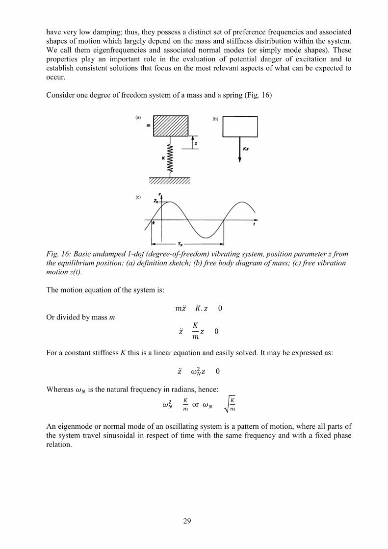
2.4 Eigenfrequencies and eigenmodes Any oscillating system has a number of preferred ways in which it "likes" to vibrate. These special types of vibrations are called the normal modes of the system. Most structural systems
29
have very low damping; thus, they possess a distinct set of preference frequencies and associated shapes of motion which largely depend on the mass and stiffness distribution within the system. We call them eigenfrequencies and associated normal modes (or simply mode shapes). These properties play an important role in the evaluation of potential danger of excitation and to establish consistent solutions that focus on the most relevant aspects of what can be expected to occur. Consider one degree of freedom system of a mass and a spring (Fig. 16)
Fig. 16: Basic undamped 1-dof (degree-of-freedom) vibrating system, position parameter z from the equilibrium position: (a) definition sketch; (b) free body diagram of mass; (c) free vibration motion z(t). The motion equation of the system is:
𝑚𝑚𝑧 + 𝐾𝐾. 𝑧𝑧 = 0 Or divided by mass m
𝑧 +𝐾𝐾𝑚𝑚𝑧𝑧 = 0
For a constant stiffness K this is a linear equation and easily solved. It may be expressed as:
𝑧 + ω𝑁𝑁2 𝑧𝑧 = 0
Whereas 𝜔𝜔𝑁𝑁 is the natural frequency in radians, hence:
𝜔𝜔𝑁𝑁2 = 𝐾𝐾
𝑚𝑚 or 𝜔𝜔𝑁𝑁 = 𝐾𝐾
𝑚𝑚
An eigenmode or normal mode of an oscillating system is a pattern of motion, where all parts of the system travel sinusoidal in respect of time with the same frequency and with a fixed phase relation.
30
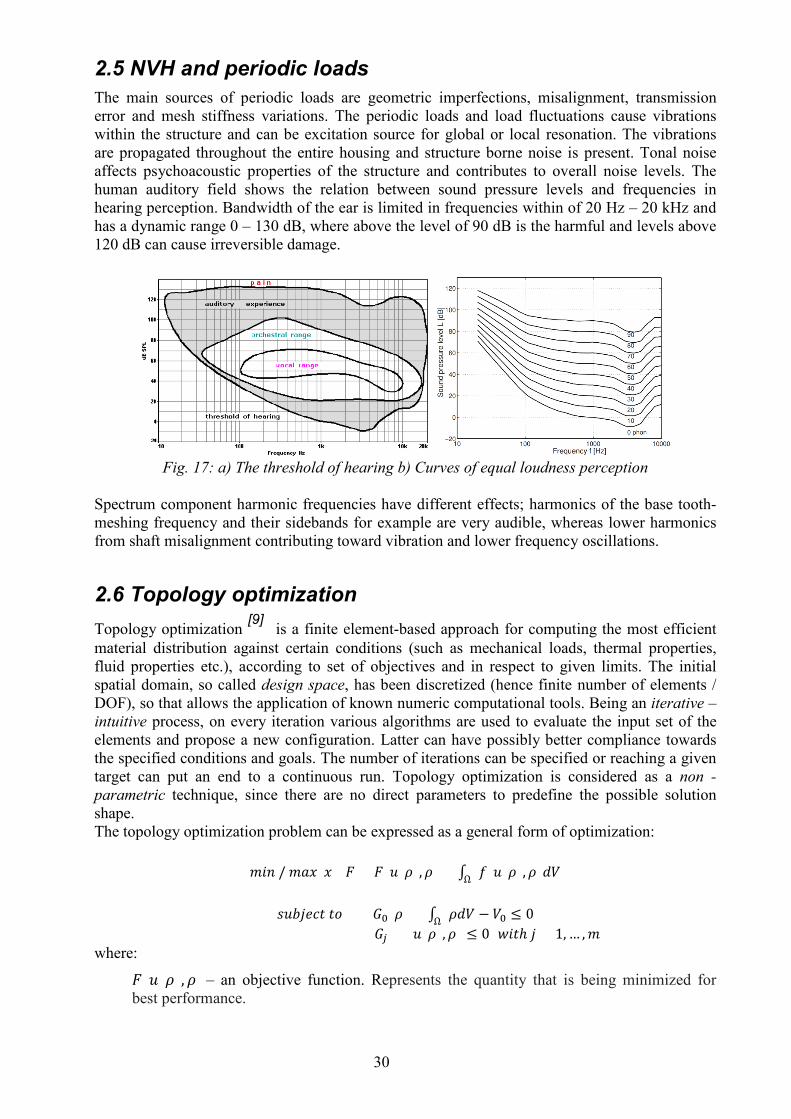
2.5 NVH and periodic loads The main sources of periodic loads are geometric imperfections, misalignment, transmission error and mesh stiffness variations. The periodic loads and load fluctuations cause vibrations within the structure and can be excitation source for global or local resonation. The vibrations are propagated throughout the entire housing and structure borne noise is present. Tonal noise affects psychoacoustic properties of the structure and contributes to overall noise levels. The human auditory field shows the relation between sound pressure levels and frequencies in hearing perception. Bandwidth of the ear is limited in frequencies within of 20 Hz – 20 kHz and has a dynamic range 0 – 130 dB, where above the level of 90 dB is the harmful and levels above 120 dB can cause irreversible damage.
Fig. 17: a) The threshold of hearing b) Curves of equal loudness perception
Spectrum component harmonic frequencies have different effects; harmonics of the base tooth-meshing frequency and their sidebands for example are very audible, whereas lower harmonics from shaft misalignment contributing toward vibration and lower frequency oscillations.
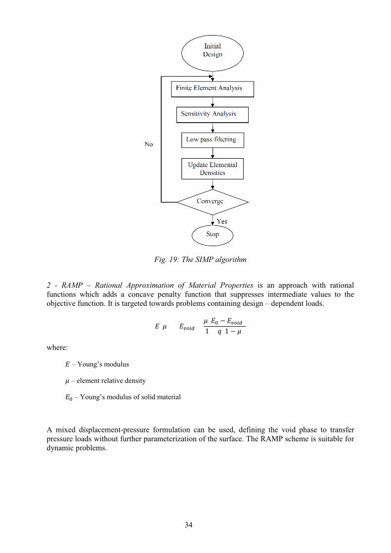
2.6 Topology optimization Topology optimization [9] is a finite element-based approach for computing the most efficient material distribution against certain conditions (such as mechanical loads, thermal properties, fluid properties etc.), according to set of objectives and in respect to given limits. The initial spatial domain, so called design space, has been discretized (hence finite number of elements / DOF), so that allows the application of known numeric computational tools. Being an iterative – intuitive process, on every iteration various algorithms are used to evaluate the input set of the elements and propose a new configuration. Latter can have possibly better compliance towards the specified conditions and goals. The number of iterations can be specified or reaching a given target can put an end to a continuous run. Topology optimization is considered as a non - parametric technique, since there are no direct parameters to predefine the possible solution shape. The topology optimization problem can be expressed as a general form of optimization:
𝑚𝑚𝑚𝑚𝑛𝑛 / 𝑚𝑚𝑡𝑡𝑥𝑥 𝑥𝑥 𝐹𝐹 = 𝐹𝐹(𝑢𝑢(𝜌𝜌),𝜌𝜌) = ∫ 𝑓𝑓(𝑢𝑢(𝜌𝜌),𝜌𝜌)𝑑𝑑𝑑𝑑Ω
𝑐𝑐𝑢𝑢𝑠𝑠𝑠𝑠𝑠𝑠𝑐𝑐𝑡𝑡 𝑡𝑡𝑐𝑐 𝐺𝐺0(𝜌𝜌) = ∫ 𝜌𝜌𝑑𝑑𝑑𝑑 − 𝑑𝑑0Ω ≤ 0 𝐺𝐺𝑗𝑗 = (𝑢𝑢(𝜌𝜌),𝜌𝜌) ≤ 0 𝑤𝑤𝑚𝑚𝑡𝑡ℎ 𝑠𝑠 = 1, … ,𝑚𝑚
where:
𝐹𝐹(𝑢𝑢(𝜌𝜌),𝜌𝜌) – an objective function. Represents the quantity that is being minimized for best performance.
31
𝐹𝐹𝑚𝑚𝑖𝑖𝑛𝑛 = min𝑊𝑊𝑖𝑖(𝜑𝜑𝑖𝑖 − 𝜑𝜑𝑖𝑖𝑟𝑟𝑐𝑐𝑟𝑟)
𝑁𝑁
𝑖𝑖=1
𝐹𝐹𝑚𝑚𝑚𝑚𝑥𝑥 = max𝑊𝑊𝑖𝑖(𝜑𝜑𝑖𝑖 − 𝜑𝜑𝑖𝑖𝑟𝑟𝑐𝑐𝑟𝑟)
𝑁𝑁
𝑖𝑖=1
𝜑𝜑𝑖𝑖 – design response, 𝑊𝑊𝑖𝑖 – assigned weight, 𝜑𝜑𝑖𝑖𝑟𝑟𝑐𝑐𝑟𝑟 – objective value
𝜌𝜌 – material density 𝑢𝑢(𝜌𝜌) – displacement vector of given density Ω – design space domain. The maximum allowable spatial limits a possible solution can occupy
𝐺𝐺𝑗𝑗 – constraint function
In case of the existence of more than one objective function, optimization is considered as multi–objective. The problem can be formulated as:
𝑚𝑚𝑚𝑚𝑛𝑛 [(𝑓𝑓1(𝑥𝑥),𝑓𝑓2(𝑥𝑥), … ,𝑓𝑓𝑛𝑛(𝑥𝑥)]𝑥𝑥 ∈ X
Where X is feasible set of solution vectors
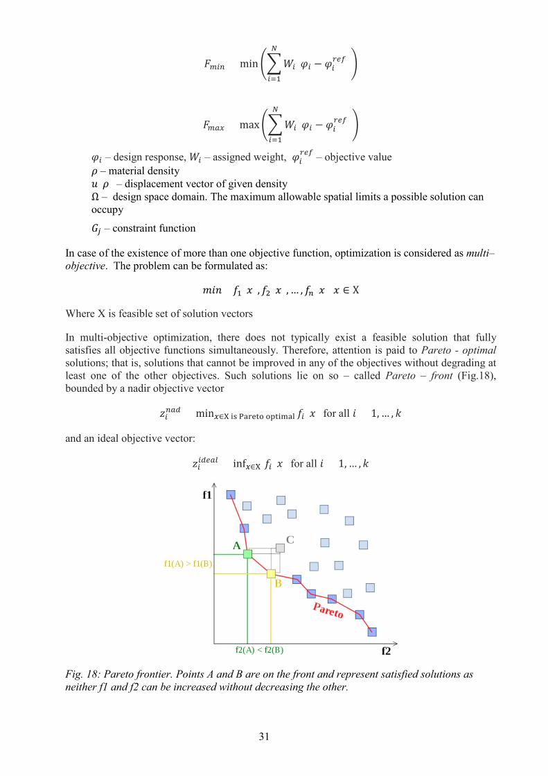
In multi-objective optimization, there does not typically exist a feasible solution that fully satisfies all objective functions simultaneously. Therefore, attention is paid to Pareto - optimal solutions; that is, solutions that cannot be improved in any of the objectives without degrading at least one of the other objectives. Such solutions lie on so – called Pareto – front (Fig.18), bounded by a nadir objective vector
𝑧𝑧𝑖𝑖𝑛𝑛𝑚𝑚𝑛𝑛 = min𝑥𝑥∈X is Pareto optimal 𝑓𝑓𝑖𝑖(𝑥𝑥) for all 𝑚𝑚 = 1, … , 𝑘𝑘
and an ideal objective vector:
𝑧𝑧𝑖𝑖𝑖𝑖𝑛𝑛𝑐𝑐𝑚𝑚𝑐𝑐 = inf𝑥𝑥∈X 𝑓𝑓𝑖𝑖(𝑥𝑥) for all 𝑚𝑚 = 1, … ,𝑘𝑘
Fig. 18: Pareto frontier. Points A and B are on the front and represent satisfied solutions as neither f1 and f2 can be increased without decreasing the other.
32
Optimization algorithms: Concerning the application in this thesis, two different topology optimization approaches are available in Abaqus/Tosca. These are implemented in the optimization module and are available in many industry widespread packages. In this part there will be an overview of the features and their theoretical background from user’s point of view. Sources for further deeper theoretical insights concerning optimization are mentioned on the spot and listed in the “References” chapter at the end. Condition–based optimality: Homogenization of stress distribution by adding material at points of high stress and removing material at points of low stress. Based upon the Neuber hypothesis, the optimum form of a component is achieved when the stresses running along the considered surface zone is fully constant. This concept is known as stress homogenization. A desired stress level is declared as a reference and algorithm reach convergence when the design space geometry is stressed as many elements possible with the reference level. It is more efficient and takes less computing effort compared to other available approach, as usually it reaches results for around 15 iterations in most of the cases. However, it has known limitations: it can only have the compliance as objective and the material volume as a constraint. Since in many practical cases, the main goal of the designers is to maximize the global stiffness of the part (hence minimize the compliance as latter being the inverse of the former 𝑐𝑐 = 1
𝑘𝑘), the usage of this approach is
widespread. Sensitivity–based optimality: The underlying mathematical tool behind sensitivity-based optimization is the Method of the Moving Asymptotes or MMA [10]. This approach supports different types of design responses, such as volume, reaction forces, displacements, eigenvalues, stresses, etc. hence it is considered as General optimization method in Tosca. It also allows multiple constraints and performs quite well with that. The sensitivity-based algorithm relies on semi-analytical sensitivities of the response of design variables, based on a finite difference of the stiffness and mass element matrices:
𝑛𝑛𝐾𝐾𝑛𝑛𝑥𝑥≈ 𝛥𝛥𝐾𝐾∗ = 𝛥𝛥𝐾𝐾 + 𝑡𝑡𝑗𝑗𝑘𝑘 with 𝛥𝛥𝐾𝐾 = 𝐾𝐾0+𝑝𝑝−𝐾𝐾0
𝛥𝛥𝑥𝑥
Where:
𝐾𝐾 – Stiffness matrix 𝐾𝐾0 – Original matrix 𝐾𝐾0+𝑝𝑝 – Perturbed matrix when a node is moved
The first part calculates the sensitivity hence derivatives for the design responses. The second part, the design variable response matrix. The versatility of this approach comes with computational efforts – around 45 iterations are necessary to a reach convergent solution. Nevertheless, it is a widely used optimization approach as it is very powerful supporting different types of design variables. Material interpolation methods: Topology optimization determines the optimal placement of a given isotropic material in space, as it discretizes the design space and spares/discards a set of voxels by representing the relative densitiy by the state variable vector 𝑥𝑥. For structural optimization, a voxel has a material relative density of 1, then it is fully contributing to global stiffness matrix. In case of relative density of 0, i.e. 0%, its material property does not affect the global matrix. Since the design vector is not continuous, it is not possible do derive the sensitivities needed for solving numerically (see above) but allowing intermediate values of relative density (making a voxel partly contributing
33
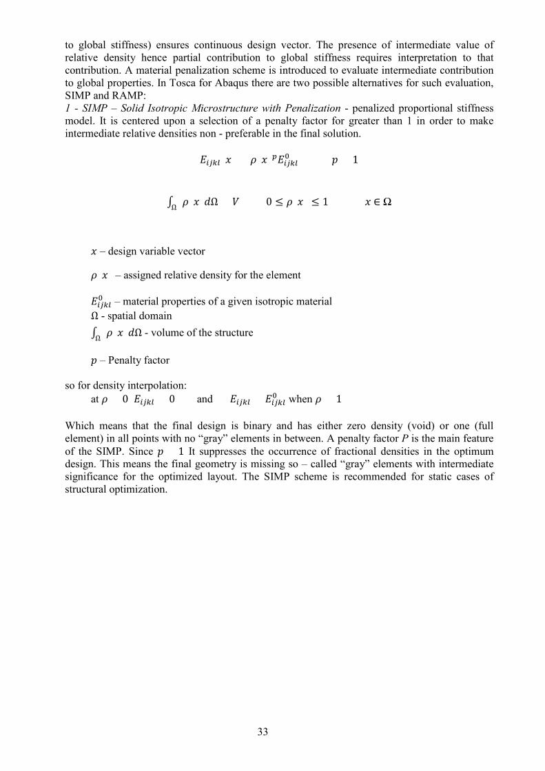
to global stiffness) ensures continuous design vector. The presence of intermediate value of relative density hence partial contribution to global stiffness requires interpretation to that contribution. A material penalization scheme is introduced to evaluate intermediate contribution to global properties. In Tosca for Abaqus there are two possible alternatives for such evaluation, SIMP and RAMP: 1 - SIMP – Solid Isotropic Microstructure with Penalization - penalized proportional stiffness model. It is centered upon a selection of a penalty factor for greater than 1 in order to make intermediate relative densities non - preferable in the final solution.
𝑇𝑇𝑖𝑖𝑗𝑗𝑘𝑘𝑐𝑐(𝑥𝑥) = 𝜌𝜌(𝑥𝑥)𝑝𝑝𝑇𝑇𝑖𝑖𝑗𝑗𝑘𝑘𝑐𝑐0 𝑝𝑝 > 1
∫ 𝜌𝜌(𝑥𝑥)𝑑𝑑ΩΩ < 𝑑𝑑 0 ≤ 𝜌𝜌(𝑥𝑥) ≤ 1 𝑥𝑥 ∈ Ω
𝑥𝑥 – design variable vector
𝜌𝜌(𝑥𝑥) – assigned relative density for the element 𝑇𝑇𝑖𝑖𝑗𝑗𝑘𝑘𝑐𝑐0 – material properties of a given isotropic material Ω - spatial domain ∫ 𝜌𝜌(𝑥𝑥)𝑑𝑑ΩΩ - volume of the structure 𝑝𝑝 – Penalty factor
so for density interpolation:
at 𝜌𝜌 = 0 𝑇𝑇𝑖𝑖𝑗𝑗𝑘𝑘𝑐𝑐 = 0 and 𝑇𝑇𝑖𝑖𝑗𝑗𝑘𝑘𝑐𝑐 = 𝑇𝑇𝑖𝑖𝑗𝑗𝑘𝑘𝑐𝑐0 when 𝜌𝜌 = 1
Which means that the final design is binary and has either zero density (void) or one (full element) in all points with no “gray” elements in between. A penalty factor P is the main feature of the SIMP. Since 𝑝𝑝 > 1 It suppresses the occurrence of fractional densities in the optimum design. This means the final geometry is missing so – called “gray” elements with intermediate significance for the optimized layout. The SIMP scheme is recommended for static cases of structural optimization.
34
Fig. 19: The SIMP algorithm
2 - RAMP – Rational Approximation of Material Properties is an approach with rational functions which adds a concave penalty function that suppresses intermediate values to the objective function. It is targeted towards problems containing design – dependent loads.
𝑇𝑇(𝜇𝜇) = 𝑇𝑇𝑣𝑣𝑣𝑣𝑖𝑖𝑛𝑛 +𝜇𝜇(𝑇𝑇0 − 𝑇𝑇𝑣𝑣𝑣𝑣𝑖𝑖𝑛𝑛)1 + 𝑞𝑞(1 − 𝜇𝜇)
where:
𝑇𝑇 – Young’s modulus
𝜇𝜇 – element relative density
𝑇𝑇0 – Young’s modulus of solid material
A mixed displacement-pressure formulation can be used, defining the void phase to transfer pressure loads without further parameterization of the surface. The RAMP scheme is suitable for dynamic problems.
35
3 IMPLEMENTATION In this chapter, the initial state and methods applied to reach the goals are explained in detail. Model setup has been reviewed and explanations and reasoning behind the methodology are given.
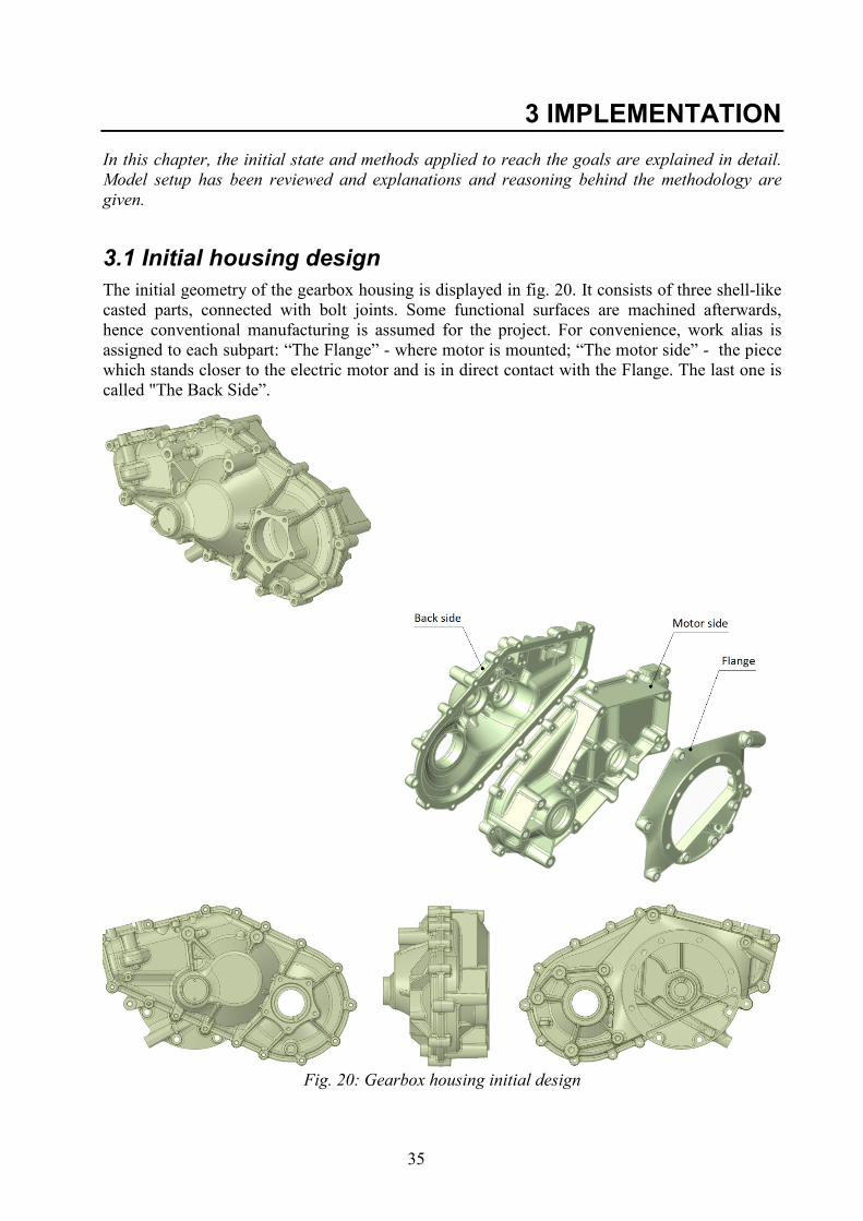
3.1 Initial housing design The initial geometry of the gearbox housing is displayed in fig. 20. It consists of three shell-like casted parts, connected with bolt joints. Some functional surfaces are machined afterwards, hence conventional manufacturing is assumed for the project. For convenience, work alias is assigned to each subpart: “The Flange” - where motor is mounted; “The motor side” - the piece which stands closer to the electric motor and is in direct contact with the Flange. The last one is called "The Back Side”.
Fig. 20: Gearbox housing initial design
36
The housing itself has following main purposes (in order of the importance):
1. Hold and support gear train at working position, ensuring proper torque transmission and axle alignment. Accommodate shafts bearings into bearing beds and cups.
2. Contain the lubricant and preserve gear train from outer affects (foreign objects, dust etc.) 3. Reduce noise from gear pair and minimize vibrations (though not being directly
dedicated to damping) thus not acting itself as a noise emitter. Contributes to smoothness of operation of gears.
4. Allow modular packaging and mounting, contributing to lowering and centralizing both its own and the overall mass centers.
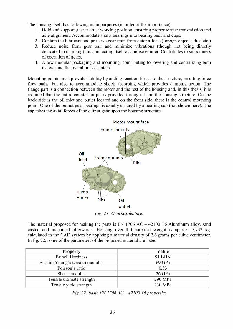
Mounting points must provide stability by adding reaction forces to the structure, resulting force flow paths, but also to accommodate shock absorbing which provides damping action. The flange part is a connection between the motor and the rest of the housing and, in this thesis, it is assumed that the entire counter torque is provided through it and the housing structure. On the back side is the oil inlet and outlet located and on the front side, there is the control mounting point. One of the output gear bearings is axially ensured by a bearing cap (not shown here). The cap takes the axial forces of the output gear upon the housing structure.
Fig. 21: Gearbox features
The material proposed for making the parts is EN 1706 AC – 42100 T6 Aluminum alloy, sand casted and machined afterwards. Housing overall theoretical weight is approx. 7,732 kg. calculated in the CAD system by applying a material density of 2,6 grams per cubic centimeter. In fig. 22, some of the parameters of the proposed material are listed.
Property Value Brinell Hardness 91 BHN
Elastic (Young’s tensile) modulus 69 GPa Poisson’s ratio 0,33 Shear modulus 26 GPa
Tensile ultimate strength 290 MPa Tensile yield strength 230 MPa
Fig. 22: basic EN 1706 AC – 42100 T6 properties
37
To summarize, the gearbox design is created according to the following design considerations:
1. Strength towards applied loads incl. contact strength in the faces / areas of contact like the bearing beds, bolt joints etc. Lifetime in accordance to fatigue accumulation estimation (see chapter 2.1.2).
2. Stiffness to ensure proper shaft axis alignments and maintaining intended gear meshing. Stiffness is also linked to the noise emitting and transmitting and NVH (noise vibration harshness) performance.
3. Oiling system – preserve the oil (watertight), minimum squashing and wall dipping effects; accessible oil inlet on highest point and drain at the lowest.
4. Lightweight and mass distribution: minimizing weight is vital. Keeping the mass center as close as possible to the midplane and as low as possible in the overall assembly.
5. Manufacturability: design for accessible conventional manufacturing, in accordance with the operations requirements for molding, milling, threatening and strengthening, finishing etc. This is a major key point in the design!
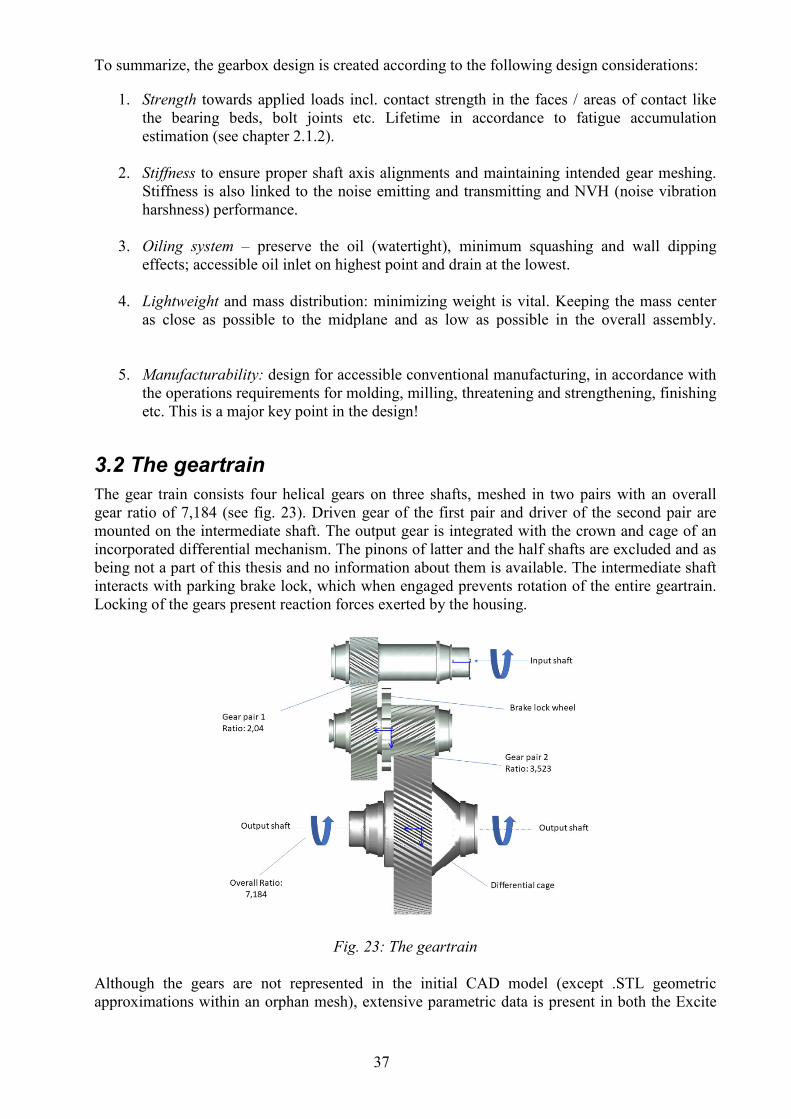
3.2 The geartrain The gear train consists four helical gears on three shafts, meshed in two pairs with an overall gear ratio of 7,184 (see fig. 23). Driven gear of the first pair and driver of the second pair are mounted on the intermediate shaft. The output gear is integrated with the crown and cage of an incorporated differential mechanism. The pinons of latter and the half shafts are excluded and as being not a part of this thesis and no information about them is available. The intermediate shaft interacts with parking brake lock, which when engaged prevents rotation of the entire geartrain. Locking of the gears present reaction forces exerted by the housing.
Fig. 23: The geartrain
Although the gears are not represented in the initial CAD model (except .STL geometric approximations within an orphan mesh), extensive parametric data is present in both the Excite
38
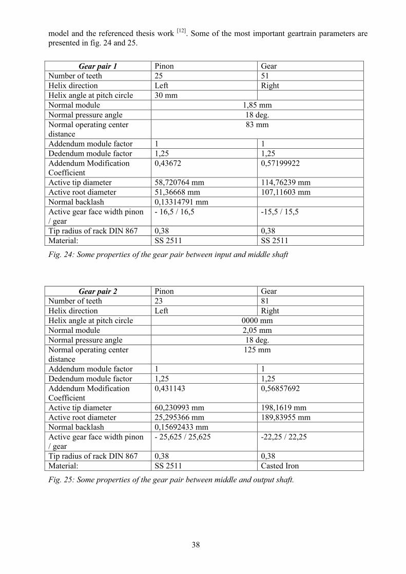
model and the referenced thesis work [12]. Some of the most important geartrain parameters are presented in fig. 24 and 25.
Gear pair 1 Pinon Gear
Number of teeth 25 51 Helix direction Left Right Helix angle at pitch circle 30 mm Normal module 1,85 mm Normal pressure angle 18 deg. Normal operating center distance
83 mm
Addendum module factor 1 1 Dedendum module factor 1,25 1,25 Addendum Modification Coefficient
0,43672 0,57199922
Active tip diameter 58,720764 mm 114,76239 mm Active root diameter 51,36668 mm 107,11603 mm Normal backlash 0,13314791 mm Active gear face width pinon / gear
- 16,5 / 16,5 -15,5 / 15,5
Tip radius of rack DIN 867 0,38 0,38 Material: SS 2511 SS 2511
Fig. 24: Some properties of the gear pair between input and middle shaft
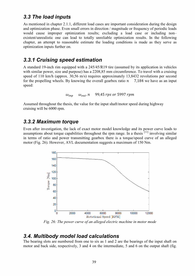
Gear pair 2 Pinon Gear
Number of teeth 23 81 Helix direction Left Right Helix angle at pitch circle 0000 mm Normal module 2,05 mm Normal pressure angle 18 deg. Normal operating center distance
125 mm
Addendum module factor 1 1 Dedendum module factor 1,25 1,25 Addendum Modification Coefficient
0,431143 0,56857692
Active tip diameter 60,230993 mm 198,1619 mm Active root diameter 25,295366 mm 189,83955 mm Normal backlash 0,15692433 mm Active gear face width pinon / gear
- 25,625 / 25,625 -22,25 / 22,25
Tip radius of rack DIN 867 0,38 0,38 Material: SS 2511 Casted Iron
Fig. 25: Some properties of the gear pair between middle and output shaft.
39
3.3 The load inputs As mentioned in chapter 2.1.1, different load cases are important consideration during the design and optimization phase. Even small errors in direction / magnitude or frequency of periodic loads would cause improper optimization results; excluding a load case or including non–existent/unrealistic one can lead to totally unreliable optimization results. In the following chapter, an attempt to reasonable estimate the loading conditions is made as they serve as optimization inputs further on.
3.3.1 Cruising speed estimation A standard 19-inch rim equipped with a 245/45/R19 tire (assumed by its application in vehicles with similar power, size and purpose) has a 2208,85 mm circumference. To travel with a cruising speed of 110 km/h (approx. 30,56 m/s) requires approximately 13,8432 revolutions per second for the propelling wheels. By knowing the overall gearbox ratio 𝑛𝑛 = 7,184 we have as an input speed:
𝜔𝜔𝑖𝑖𝑛𝑛𝑝𝑝 = 𝜔𝜔𝑣𝑣𝑜𝑜𝑡𝑡.𝑛𝑛 = 99,45 𝑟𝑟𝑝𝑝𝑐𝑐 𝑐𝑐𝑟𝑟 5997 𝑟𝑟𝑝𝑝𝑚𝑚
Assumed throughout the thesis, the value for the input shaft/motor speed during highway cruising will be 6000 rpm.
3.3.2 Maximum torque Even after investigation, the lack of exact motor model knowledge and its power curve leads to assumptions about torque capabilities throughout the rpm range. In a thesis [11] involving similar in terms of ratio and power transmitting gearbox there is a torque/speed curve of an alleged motor (Fig. 26). However, AVL documentation suggests a maximum of 150 Nm.
Fig. 26: The power curve of an alleged electric machine in motor mode
3.4. Multibody model load calculations The bearing slots are numbered from one to six as 1 and 2 are the bearings of the input shaft on motor and back side, respectively, 3 and 4 on the intermediate, 5 and 6 on the output shaft (fig.
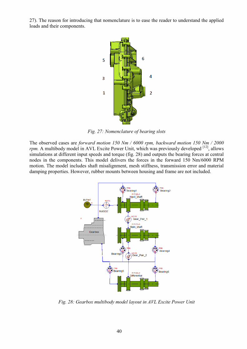
40
27). The reason for introducing that nomenclature is to ease the reader to understand the applied loads and their components.
Fig. 27: Nomenclature of bearing slots
The observed cases are forward motion 150 Nm / 6000 rpm, backward motion 150 Nm / 2000 rpm. A multibody model in AVL Excite Power Unit, which was previously developed [12], allows simulations at different input speeds and torque (fig. 28) and outputs the bearing forces at central nodes in the components. This model delivers the forces in the forward 150 Nm/6000 RPM motion. The model includes shaft misalignment, mesh stiffness, transmission error and material damping properties. However, rubber mounts between housing and frame are not included.
Fig. 28: Gearbox multibody model layout in AVL Excite Power Unit
41
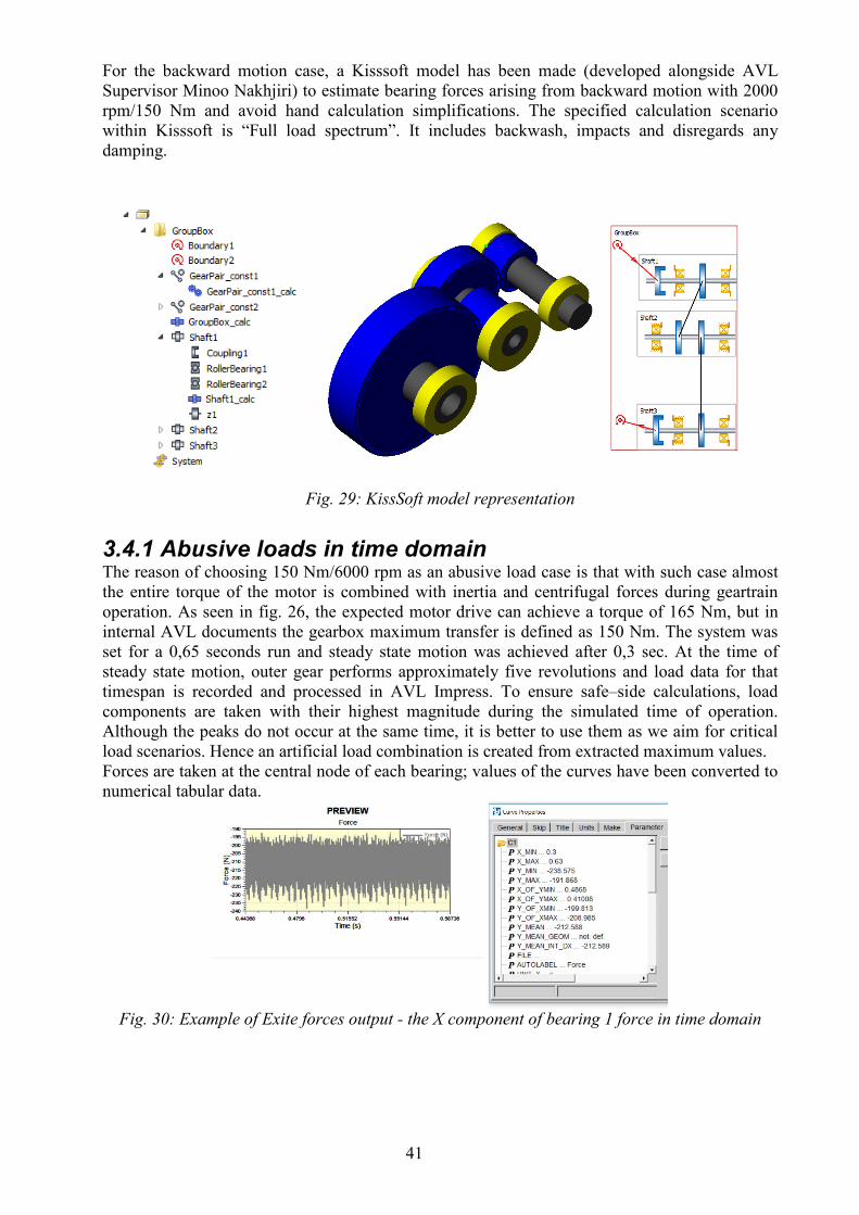
For the backward motion case, a Kisssoft model has been made (developed alongside AVL Supervisor Minoo Nakhjiri) to estimate bearing forces arising from backward motion with 2000 rpm/150 Nm and avoid hand calculation simplifications. The specified calculation scenario within Kisssoft is “Full load spectrum”. It includes backwash, impacts and disregards any damping.
Fig. 29: KissSoft model representation 3.4.1 Abusive loads in time domain The reason of choosing 150 Nm/6000 rpm as an abusive load case is that with such case almost the entire torque of the motor is combined with inertia and centrifugal forces during geartrain operation. As seen in fig. 26, the expected motor drive can achieve a torque of 165 Nm, but in internal AVL documents the gearbox maximum transfer is defined as 150 Nm. The system was set for a 0,65 seconds run and steady state motion was achieved after 0,3 sec. At the time of steady state motion, outer gear performs approximately five revolutions and load data for that timespan is recorded and processed in AVL Impress. To ensure safe–side calculations, load components are taken with their highest magnitude during the simulated time of operation. Although the peaks do not occur at the same time, it is better to use them as we aim for critical load scenarios. Hence an artificial load combination is created from extracted maximum values. Forces are taken at the central node of each bearing; values of the curves have been converted to numerical tabular data.
Fig. 30: Example of Exite forces output - the X component of bearing 1 force in time domain
42
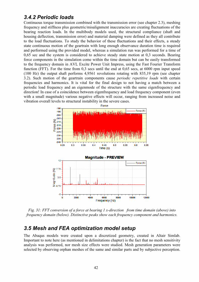
3.4.2 Periodic loads Continuous torque transmission combined with the transmission error (see chapter 2.3), meshing frequency and stiffness plus geometric/misalignment inaccuracies are creating fluctuations of the bearing reaction loads. In the multibody models used, the structural compliance (shaft and housing deflection, transmission error) and material damping were defined as they all contribute to the load fluctuations. To study the behavior of these fluctuations and their effects, a steady state continuous motion of the geartrain with long enough observance duration time is required and performed using the provided model, whereas a simulation run was performed for a time of 0,65 sec and the system is considered to achieve steady state motion at 0,3 seconds. Bearing force components in the simulation come within the time domain but can be easily transformed to the frequency domain in AVL Excite Power Unit Impress, using the Fast Fourier Transform function (FFT). For the time from 0,3 secs until the end at 0,65 secs, at 6000 rpm input speed (100 Hz) the output shaft performs 4,9561 revolutions rotating with 835,19 rpm (see chapter 3.2). Such motion of the geartrain components cause periodic repetitive loads with certain frequencies and harmonics. It is vital for the final design to not having a match between a periodic load frequency and an eigenmode of the structure with the same eigenfrequency and direction! In case of a coincidence between eigenfrequency and load frequency component (even with a small magnitude) various negative effects will occur, ranging from increased noise and vibration overall levels to structural instability in the severe cases.
Fig. 31: FFT conversion of a force at bearing 1 x-direction from time domain (above) into frequency domain (below). Distinctive peaks show each frequency component and harmonics.
3.5 Mesh and FEA optimization model setup The Abaqus models were created upon a discretized geometry, created in Altair Simlab. Important to note here (as mentioned in delimitations chapter) is the fact that no mesh sensitivity analysis was performed, nor mesh size effects were studied. Mesh generation parameters were selected by observing orphan meshes of the same and similar parts and by subjective perception.
43
The three main models: “initial”, “chunk” and “noribs” serve different purposes and have been the basis of different optimization setups. Each one is discussed in the following subchapters.
3.5.1 The initial geometry FEM analysis of the initial geometry has been performed to giv important information on stress distribution and levels, strain and deformation, eigenmodes and eigenvalues. All these are needed as they will serve as a reference for the design proposals. By knowing these values, they can be used as design performance guides and by that way “to include” the assumed design safety factors that are not determined. In other words, if two different geometries made of the same material results in the same maximum von Mises stress under the same loads and conditions, this means they have the same design safety factor too. Since there is a lack of information about the required safety factors, it's been necessary to perform Modal, Structural and Frequency response analysis upon the gearbox housing using the loads from chapter 3.3. So the FEA model must be prepared, solved and post-processed in that context. Displacement of bearing centroid orphan nodes is important, as it corresponds to shaft misalignment that is a major contributor for reduced NVH performance and diminishing the absolute displacement of these nodes will positively affect the smoothness of operation. To summarize, minimizing bearing bed relative displacement is a condition for NVH improvement as it diminishes vibration excitation sources of the structure. First, the exterior of the geometry was meshed with following parameters:
Property:
Value:
Element type Tri6 2nd Order (see fig. 30) Average element size 6 𝑚𝑚𝑚𝑚2
Minimum element size 0,6 𝑚𝑚𝑚𝑚2 Grade factor 1,5
Maximum angle per element 45º Curvature minimum element size 3 𝑚𝑚𝑚𝑚2
Aspect ratio 10 Refinements, like merging small geometric faces and increasing the number of elements in some local areas and, thus, reducing their average size was performed to create an acceptable surface mesh. This mesh will serve as the basis for creating the volumetric 3D discretization of the housing geometry. 2nd order elements are chosen despite their increased computation demands, because of better curvature approximation abilities. The following properties are used for the volume mesh generation:
Property:
Value:
Element type TET10 2nd Order (see fig.30) or C3D10 Average element size 6 𝑚𝑚𝑚𝑚3
Internal grading 2 Stretch coefficient minimum 0.1
Jacobian normalized factor minimum 0.001
44
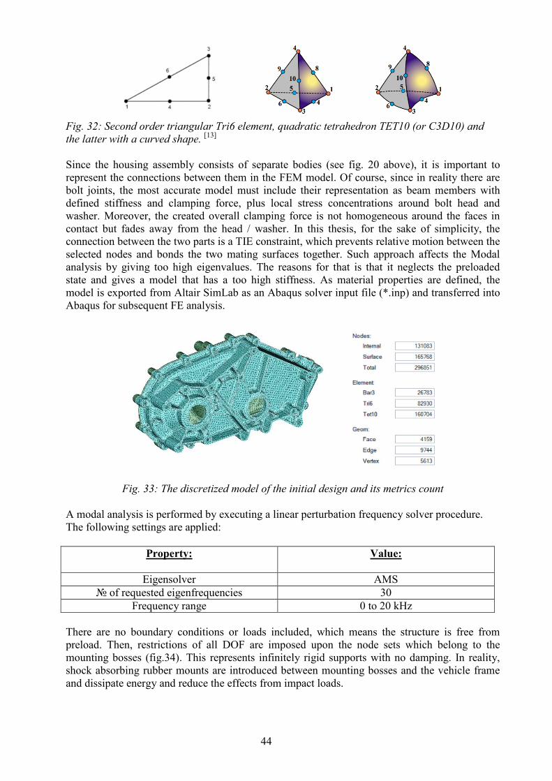
Fig. 32: Second order triangular Tri6 element, quadratic tetrahedron TET10 (or C3D10) and the latter with a curved shape. [13] Since the housing assembly consists of separate bodies (see fig. 20 above), it is important to represent the connections between them in the FEM model. Of course, since in reality there are bolt joints, the most accurate model must include their representation as beam members with defined stiffness and clamping force, plus local stress concentrations around bolt head and washer. Moreover, the created overall clamping force is not homogeneous around the faces in contact but fades away from the head / washer. In this thesis, for the sake of simplicity, the connection between the two parts is a TIE constraint, which prevents relative motion between the selected nodes and bonds the two mating surfaces together. Such approach affects the Modal analysis by giving too high eigenvalues. The reasons for that is that it neglects the preloaded state and gives a model that has a too high stiffness. As material properties are defined, the model is exported from Altair SimLab as an Abaqus solver input file (*.inp) and transferred into Abaqus for subsequent FE analysis.
Fig. 33: The discretized model of the initial design and its metrics count
A modal analysis is performed by executing a linear perturbation frequency solver procedure. The following settings are applied:
Property:
Value:
Eigensolver AMS of requested eigenfrequencies 30
Frequency range 0 to 20 kHz There are no boundary conditions or loads included, which means the structure is free from preload. Then, restrictions of all DOF are imposed upon the node sets which belong to the mounting bosses (fig.34). This represents infinitely rigid supports with no damping. In reality, shock absorbing rubber mounts are introduced between mounting bosses and the vehicle frame and dissipate energy and reduce the effects from impact loads.
45
Fig. 34: Fixed supports for the static structural study step
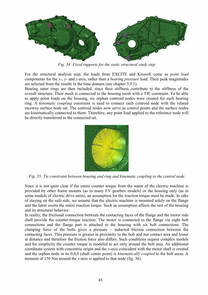
For the structural analysis step, the loads from EXCITE and Kisssoft come as point load components for the x-, y- and z-axis, rather than a bearing pressure load. Their peak magnitudes are selected from the results in the time domain (see chapter 3.3.1). Bearing outer rings are then included, since their stiffness contribute to the stiffness of the overall structure. Their mesh is connected to the housing mesh with a TIE constraint. To be able to apply point loads on the housing, six orphan centroid nodes were created for each bearing ring. A kinematic coupling constraint is used to connect each centroid node with the related raceway surface node set. The centroid nodes now serve as control points and the surface nodes are kinematically connected to them. Therefore, any point load applied to the reference node will be directly transferred to the connected set.
Fig. 35: Tie constraint between housing and ring and kinematic coupling to the central node
Since it is not quite clear if the entire counter torque from the stator of the electric machine is provided by other frame mounts (as in many EV gearbox models) or the housing only (as in some models of electric drive units), an assumption for the reaction torque must be made. In sake of staying on the safe side, we assume that the electric machine is mounted solely on the flange and the latter exerts the entire reaction torque. Such an assumption affects the rest of the housing and its structural behavior. In reality, the frictional connection between the contacting faces of the flange and the motor side shell provide the counter-torque reaction. The motor is connected to the flange via eight bolt connections and the flange part is attached to the housing with six bolt connections. The clamping force of the bolts gives a pressure – inducted friction connection between the contacting faces. This pressure is greater in proximity to the bolt and nut contact area and lesser at distance and therefore the friction force also differs. Such conditions require complex models and for simplicity the counter torque is modeled to act only around the bolt area. An additional coordinate system with concentric origin and the x-axis coincident with the motor shaft is created and the orphan node in its 0,0,0 (shaft center point) is kinematically coupled to the bolt areas. A moment of 150 Nm around the x-axis is applied to that node (fig. 36).
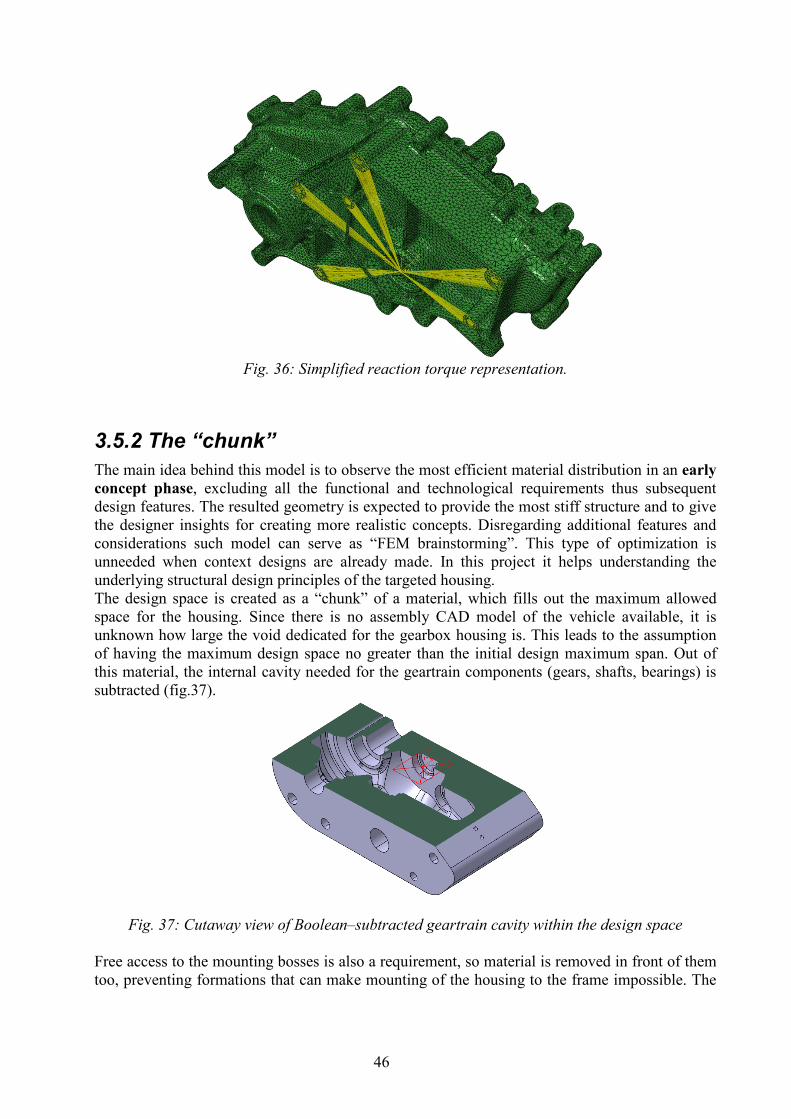
46
Fig. 36: Simplified reaction torque representation.
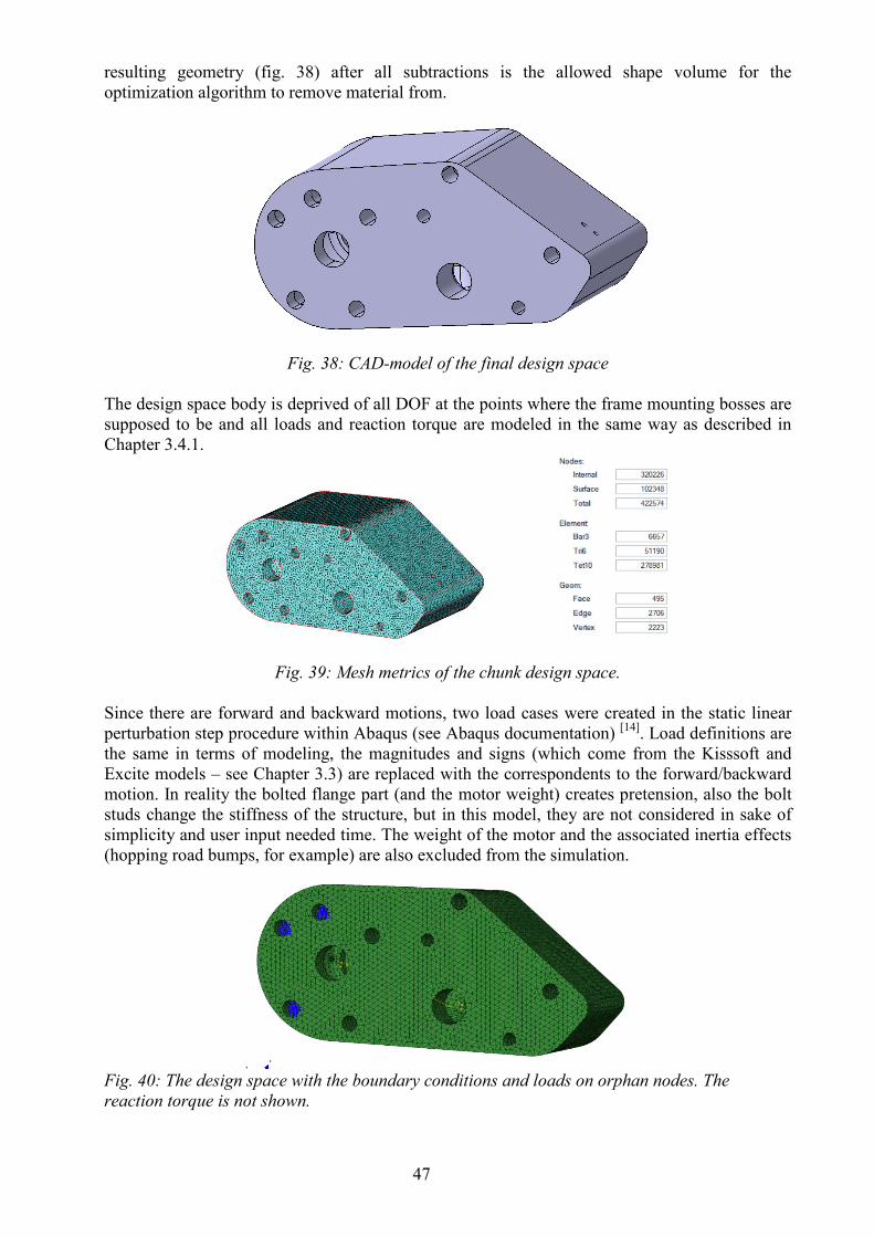
3.5.2 The “chunk” The main idea behind this model is to observe the most efficient material distribution in an early concept phase, excluding all the functional and technological requirements thus subsequent design features. The resulted geometry is expected to provide the most stiff structure and to give the designer insights for creating more realistic concepts. Disregarding additional features and considerations such model can serve as “FEM brainstorming”. This type of optimization is unneeded when context designs are already made. In this project it helps understanding the underlying structural design principles of the targeted housing. The design space is created as a “chunk” of a material, which fills out the maximum allowed space for the housing. Since there is no assembly CAD model of the vehicle available, it is unknown how large the void dedicated for the gearbox housing is. This leads to the assumption of having the maximum design space no greater than the initial design maximum span. Out of this material, the internal cavity needed for the geartrain components (gears, shafts, bearings) is subtracted (fig.37).
Fig. 37: Cutaway view of Boolean–subtracted geartrain cavity within the design space Free access to the mounting bosses is also a requirement, so material is removed in front of them too, preventing formations that can make mounting of the housing to the frame impossible. The
47
resulting geometry (fig. 38) after all subtractions is the allowed shape volume for the optimization algorithm to remove material from.
Fig. 38: CAD-model of the final design space The design space body is deprived of all DOF at the points where the frame mounting bosses are supposed to be and all loads and reaction torque are modeled in the same way as described in Chapter 3.4.1.
Fig. 39: Mesh metrics of the chunk design space.
Since there are forward and backward motions, two load cases were created in the static linear perturbation step procedure within Abaqus (see Abaqus documentation) [14]. Load definitions are the same in terms of modeling, the magnitudes and signs (which come from the Kisssoft and Excite models – see Chapter 3.3) are replaced with the correspondents to the forward/backward motion. In reality the bolted flange part (and the motor weight) creates pretension, also the bolt studs change the stiffness of the structure, but in this model, they are not considered in sake of simplicity and user input needed time. The weight of the motor and the associated inertia effects (hopping road bumps, for example) are also excluded from the simulation.
Fig. 40: The design space with the boundary conditions and loads on orphan nodes. The reaction torque is not shown.
48
As for optimization settings, the condition-based method explained in chapter 2.5.1 is selected, since it suits the goals of the study well. Minimization of total strain energy is defined as the optimization objective function. A constraint on the percentage of used volume is applied. The value of this constraint 𝑑𝑑 ≤ 0.084𝑑𝑑𝑐𝑐ℎ𝑜𝑜𝑛𝑛𝑘𝑘 presents the same amount of material used for the initial design. A geometric restriction of a minimum member size of 10mm is applied to ensure no too small material formations will be present in the result geometry. The SIMP method for material interpolation was selected and maximum of 50 iterations in the search of a convergent solution has been defined. A new set of elements on the bearing beds surfaces and mounting bosses is defined as frozen areas. This action ensures these elements will be preserved in the optimization design process. The expected outcome of the model is the stiffest distribution of a material volume equal to the initial design. Knowing such material distribution towards just the specific set of bearing loads answer the question “how the most rigid material arrangement looks like regarding these loads”. Results of this study are present in Chapter 4.3.
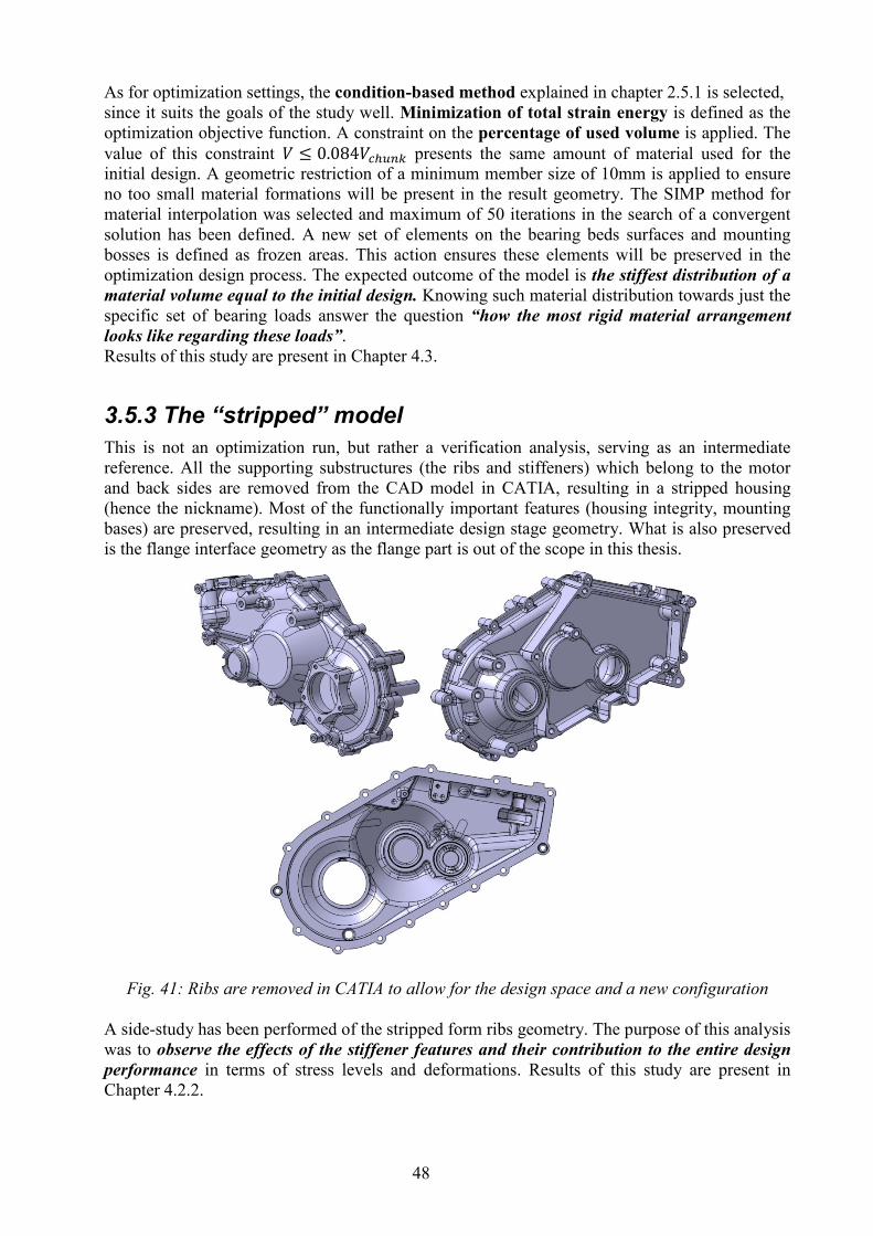
3.5.3 The “stripped” model This is not an optimization run, but rather a verification analysis, serving as an intermediate reference. All the supporting substructures (the ribs and stiffeners) which belong to the motor and back sides are removed from the CAD model in CATIA, resulting in a stripped housing (hence the nickname). Most of the functionally important features (housing integrity, mounting bases) are preserved, resulting in an intermediate design stage geometry. What is also preserved is the flange interface geometry as the flange part is out of the scope in this thesis.
Fig. 41: Ribs are removed in CATIA to allow for the design space and a new configuration A side-study has been performed of the stripped form ribs geometry. The purpose of this analysis was to observe the effects of the stiffener features and their contribution to the entire design performance in terms of stress levels and deformations. Results of this study are present in Chapter 4.2.2.
49
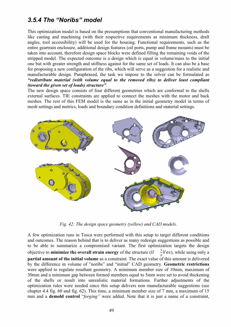
3.5.4 The “Noribs” model This optimization model is based on the presumptions that conventional manufacturing methods like casting and machining (with their respective requirements as minimum thickness, draft angles, tool accessibility) will be used for the housing. Functional requirements, such as the entire geartrain enclosure, additional design features (oil ports, pump and frame mounts) must be taken into account, therefore design space blocks were defined filling the remaining voids of the stripped model. The expected outcome is a design which is equal in volume/mass to the initial one but with greater strength and stiffness against for the same set of loads. It can also be a base for proposing a new configuration of the ribs, which will serve as a suggestion for a realistic and manufacturable design. Paraphrased, the task we impose to the solver can be formulated as “redistribute material (with volume equal to the removed ribs) to deliver least compliant (toward the given set of loads) structure”. The new design space consists of four different geometries which are conformal to the shells external surfaces. TIE constraints are applied to connect the meshes with the motor and back meshes. The rest of this FEM model is the same as in the initial geometry model in terms of mesh settings and metrics, loads and boundary condition definitions and material settings.
Fig. 42: The design space geometry (yellow) and CAD models.
A few optimization runs in Tosca were performed with this setup to target different conditions and outcomes. The reason behind that is to deliver as many redesign suggestions as possible and to be able to summarize a compromised variant. The first optimization targets the design objective to minimize the overall strain energy of the structure (𝑈𝑈 = 1
2𝑑𝑑𝜎𝜎𝑉𝑉), while using only a
partial amount of the initial volume as a constraint. The exact value of this amount is delivered by the difference in volume of ”noribs” and “initial” CAD geometry. Geometric restrictions were applied to regulate resultant geometry. A minimum member size of 10mm, maximum of 30mm and a minimum gap between formed members equal to 5mm were set to avoid thickening of the shells or result into unrealistic material formations. Further adjustments of the optimization rules were needed since this setup delivers non–manufacturable suggestions (see chapter 4.4 fig. 60 and fig. 62). This time, a minimum member size of 7 mm, a maximum of 15 mm and a demold control “forging” were added. Note that it is just a name of a constraint,
50
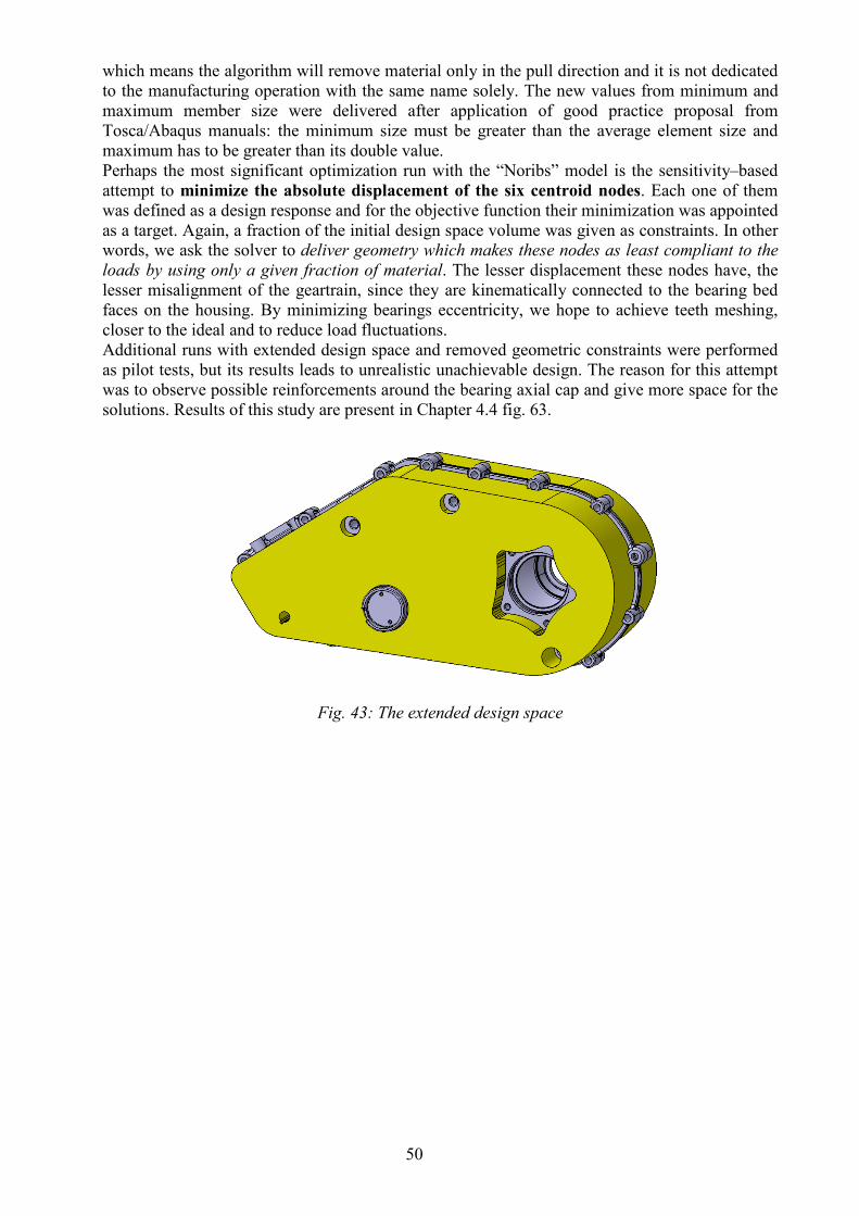
which means the algorithm will remove material only in the pull direction and it is not dedicated to the manufacturing operation with the same name solely. The new values from minimum and maximum member size were delivered after application of good practice proposal from Tosca/Abaqus manuals: the minimum size must be greater than the average element size and maximum has to be greater than its double value. Perhaps the most significant optimization run with the “Noribs” model is the sensitivity–based attempt to minimize the absolute displacement of the six centroid nodes. Each one of them was defined as a design response and for the objective function their minimization was appointed as a target. Again, a fraction of the initial design space volume was given as constraints. In other words, we ask the solver to deliver geometry which makes these nodes as least compliant to the loads by using only a given fraction of material. The lesser displacement these nodes have, the lesser misalignment of the geartrain, since they are kinematically connected to the bearing bed faces on the housing. By minimizing bearings eccentricity, we hope to achieve teeth meshing, closer to the ideal and to reduce load fluctuations. Additional runs with extended design space and removed geometric constraints were performed as pilot tests, but its results leads to unrealistic unachievable design. The reason for this attempt was to observe possible reinforcements around the bearing axial cap and give more space for the solutions. Results of this study are present in Chapter 4.4 fig. 63.
Fig. 43: The extended design space
51
4 RESULTS In this chapter, the results that are obtained with the process/methods described above are presented, analyzed and commented.
4.1 Initial geometry analysis The following results are the output of the model setup explained in chapter 3.5.1.
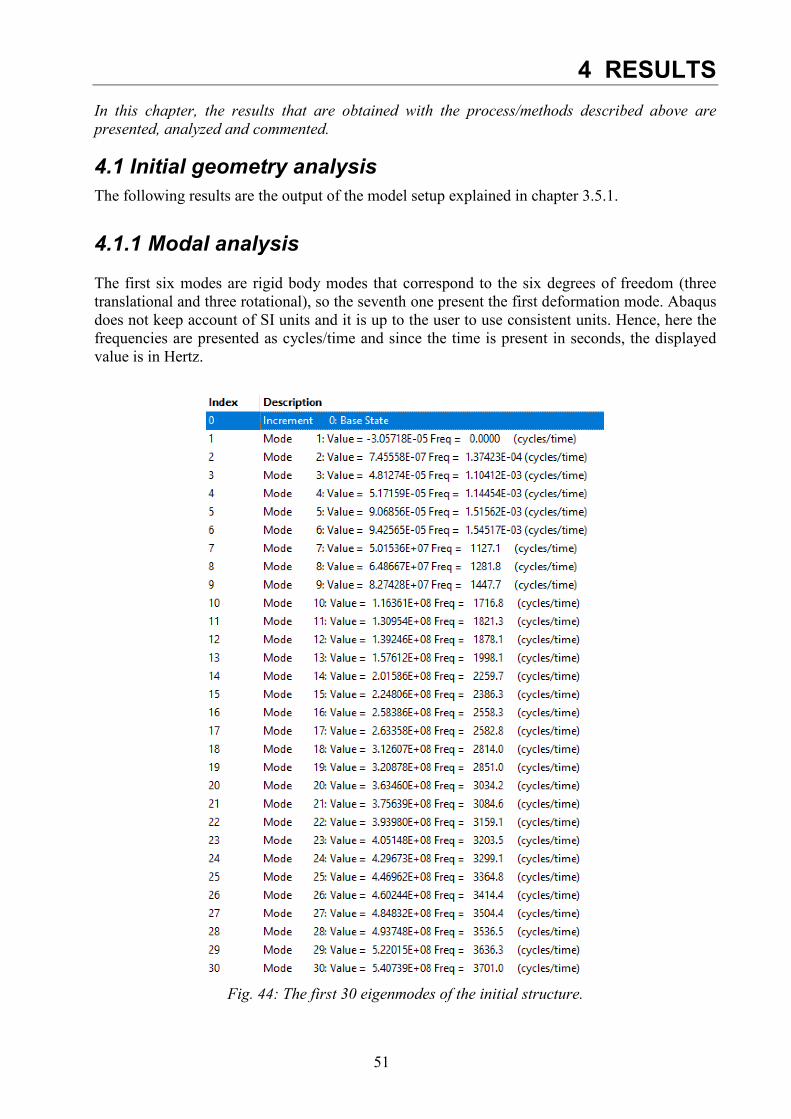
4.1.1 Modal analysis The first six modes are rigid body modes that correspond to the six degrees of freedom (three translational and three rotational), so the seventh one present the first deformation mode. Abaqus does not keep account of SI units and it is up to the user to use consistent units. Hence, here the frequencies are presented as cycles/time and since the time is present in seconds, the displayed value is in Hertz.
Fig. 44: The first 30 eigenmodes of the initial structure.
52
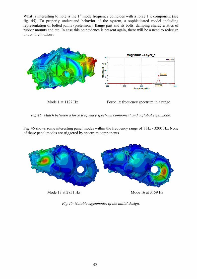
What is interesting to note is the 1st mode frequency coincides with a force 1 x component (see fig. 45). To properly understand behavior of the system, a sophisticated model including representation of bolted joints (pretension), flange part and its bolts, damping characteristics of rubber mounts and etc. In case this coincidence is present again, there will be a need to redesign to avoid vibrations.
Mode 1 at 1127 Hz Force 1x frequency spectrum in a range
Fig.45: Match between a force frequency spectrum component and a global eigenmode.
Fig. 46 shows some interesting panel modes within the frequency range of 1 Hz - 3200 Hz. None of these panel modes are triggered by spectrum components.
Mode 13 at 2851 Hz Mode 16 at 3159 Hz
Fig.46: Notable eigenmodes of the initial design.
53
4.1.2 Von Misses stress and deformations
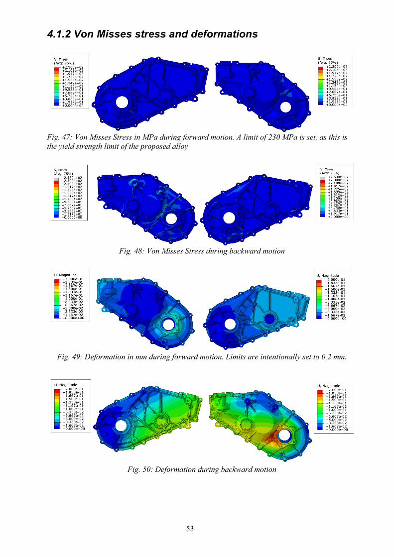
Fig. 47: Von Misses Stress in MPa during forward motion. A limit of 230 MPa is set, as this is the yield strength limit of the proposed alloy
Fig. 48: Von Misses Stress during backward motion
Fig. 49: Deformation in mm during forward motion. Limits are intentionally set to 0,2 mm.
Fig. 50: Deformation during backward motion
54
Slot Displacement in mm
Forward Displacement in mm Backward
1 0,0384193 0.107566
2 0,00790404 0.123605
3 0,0348692 0.0671581
4 0,00847785 0.11
5 0,0111417 0.0218948
6 0,0522123 0.138033
Fig. 51: Absolute displacement of the bearing beds centroid nodes (see chapter 3.3 for slot nomenclature). What is visible from this study is that even on unrealistic peak load combinations, stresses and deformations are far below critical for the assumed material. This tells us of underlying high safety factors and a long lifespan of the component assumed by its designers. As expected, it performs better and stays “more solid” during forward motion and is relatively weaker during backward motion, since scenarios with high loads (torque) on backward are less frequent throughout operational life. Deflections of the bearing centroid nodes are of great interest for us, as they give some insights into misalignment effects due to external factors. A parametric filed plot, tracking their overall absolute displacement (disregarding direction) was done and its results are presented in fig. 51. In figure 52 an interesting phenomenon is observed – a stress singularity is present in a single “edgy” element causing local stress concentration. In the model the bearing outer rings are “bonded” with the housing with TIE connection type of kinematic couplings, which means “pull” forces in the normal direction are also transferred. In reality, the forces transferred from the bearing ring towards the housing are actually normal pressure on the contact area, hence bearing beds of the housing cannot “be pulled” by the bearings. As such model representation is most probably the reason for the occurring singularity, it will be considered as a synthetic stress concentration and will be disregarded further on. Another possible reason can be the relatively lower element quality (skewness, Jacobian ratio) in that area. Further investigation is needed and in case of its presence in a properly constructed model, the local mesh resolution must be increased to check if this is actual stress concentration rather than a numerical issue.
Fig. 52: Nodes with stress singularity cause unrealistically high values
55
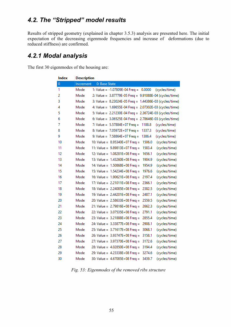
4.2. The “Stripped” model results Results of stripped geometry (explained in chapter 3.5.3) analysis are presented here. The initial expectation of the decreasing eigenmode frequencies and increase of deformations (due to reduced stiffness) are confirmed. 4.2.1 Modal analysis The first 30 eigenmodes of the housing are:
Fig. 53: Eigenmodes of the removed ribs structure
56
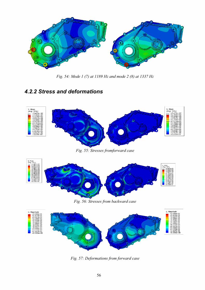
Fig. 54: Mode 1 (7) at 1189 Hz and mode 2 (8) at 1337 Hz
4.2.2 Stress and deformations
Fig. 55: Stresses fromforward case
Fig. 56: Stresses from backward case
Fig. 57: Deformations from forward case
57
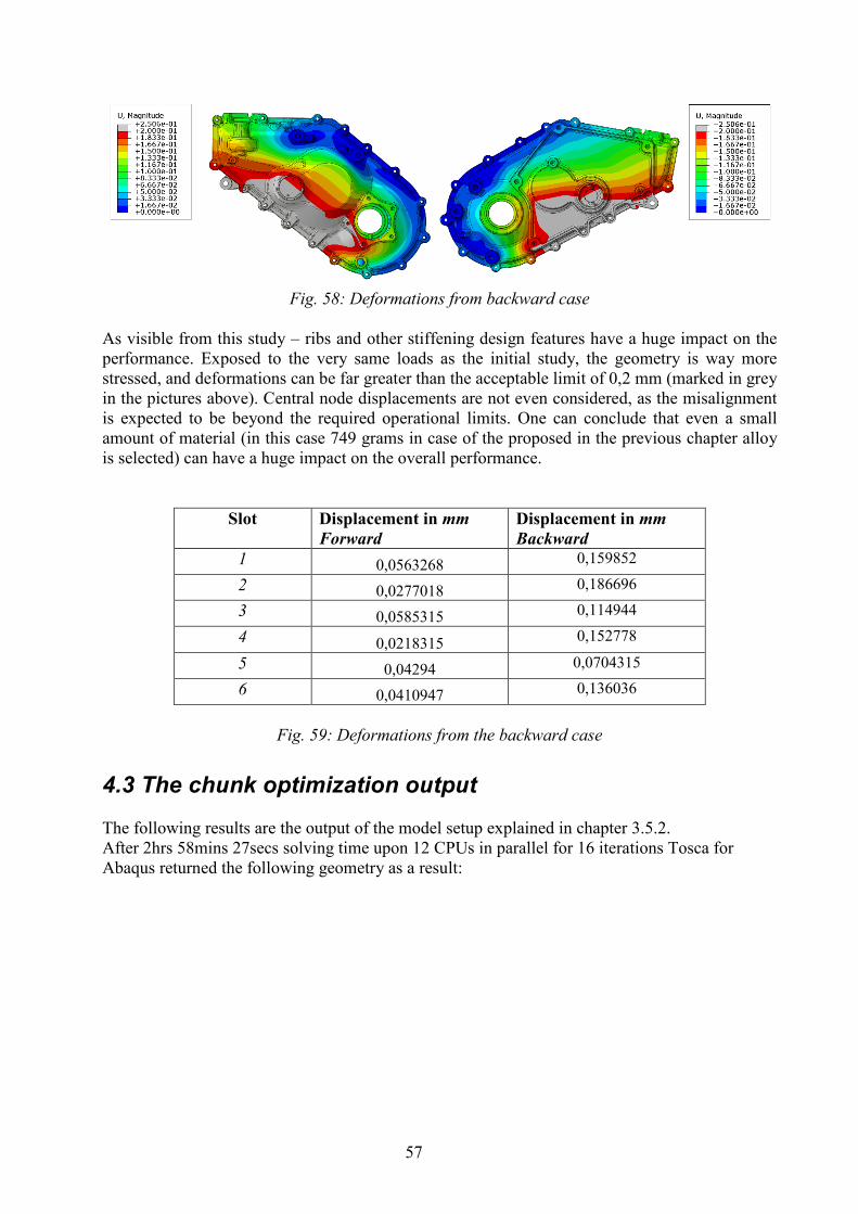
Fig. 58: Deformations from backward case
As visible from this study – ribs and other stiffening design features have a huge impact on the performance. Exposed to the very same loads as the initial study, the geometry is way more stressed, and deformations can be far greater than the acceptable limit of 0,2 mm (marked in grey in the pictures above). Central node displacements are not even considered, as the misalignment is expected to be beyond the required operational limits. One can conclude that even a small amount of material (in this case 749 grams in case of the proposed in the previous chapter alloy is selected) can have a huge impact on the overall performance.
Slot Displacement in mm Forward
Displacement in mm Backward
1 0,0563268 0,159852
2 0,0277018 0,186696
3 0,0585315 0,114944
4 0,0218315 0,152778
5 0,04294 0,0704315
6 0,0410947 0,136036
Fig. 59: Deformations from the backward case
4.3 The chunk optimization output The following results are the output of the model setup explained in chapter 3.5.2. After 2hrs 58mins 27secs solving time upon 12 CPUs in parallel for 16 iterations Tosca for Abaqus returned the following geometry as a result:

58
Fig. 60: a) All views of the optimized chunk in 1st angle of projection.
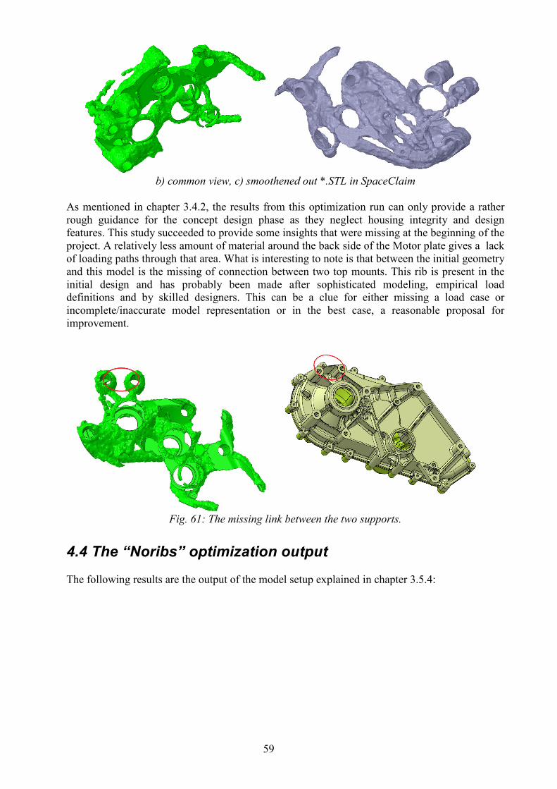
59
b) common view, c) smoothened out *.STL in SpaceClaim
As mentioned in chapter 3.4.2, the results from this optimization run can only provide a rather rough guidance for the concept design phase as they neglect housing integrity and design features. This study succeeded to provide some insights that were missing at the beginning of the project. A relatively less amount of material around the back side of the Motor plate gives a lack of loading paths through that area. What is interesting to note is that between the initial geometry and this model is the missing of connection between two top mounts. This rib is present in the initial design and has probably been made after sophisticated modeling, empirical load definitions and by skilled designers. This can be a clue for either missing a load case or incomplete/inaccurate model representation or in the best case, a reasonable proposal for improvement.
Fig. 61: The missing link between the two supports.
4.4 The “Noribs” optimization output The following results are the output of the model setup explained in chapter 3.5.4:
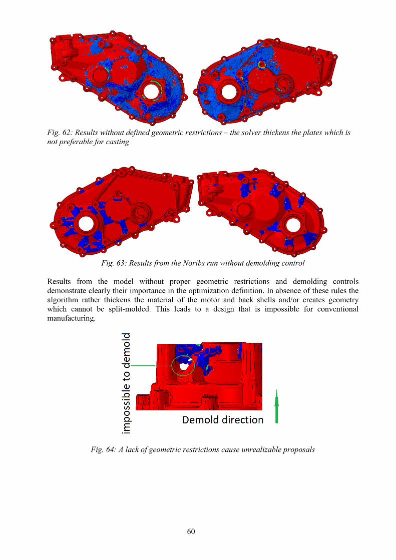
60
Fig. 62: Results without defined geometric restrictions – the solver thickens the plates which is not preferable for casting
Fig. 63: Results from the Noribs run without demolding control
Results from the model without proper geometric restrictions and demolding controls demonstrate clearly their importance in the optimization definition. In absence of these rules the algorithm rather thickens the material of the motor and back shells and/or creates geometry which cannot be split-molded. This leads to a design that is impossible for conventional manufacturing.
Fig. 64: A lack of geometric restrictions cause unrealizable proposals
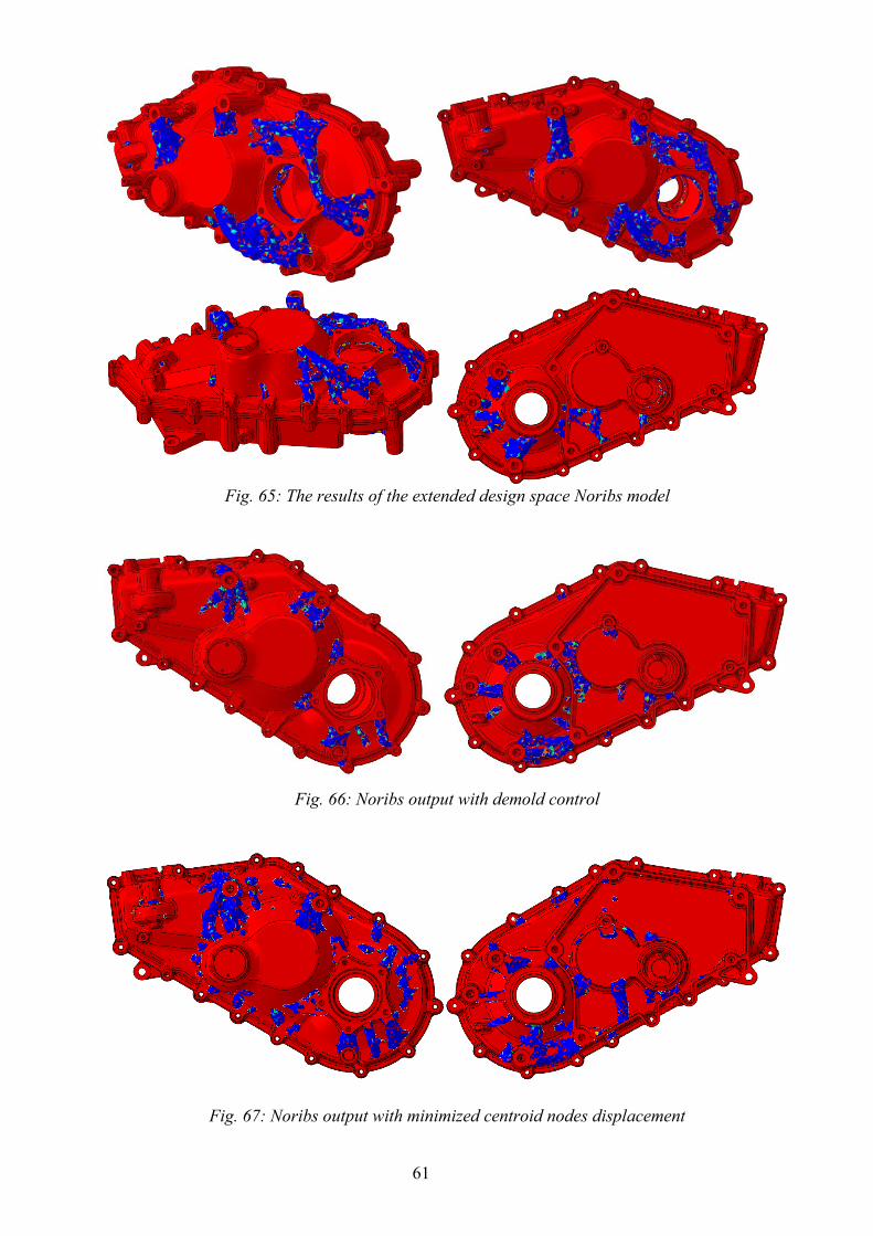
61
Fig. 65: The results of the extended design space Noribs model
Fig. 66: Noribs output with demold control
Fig. 67: Noribs output with minimized centroid nodes displacement
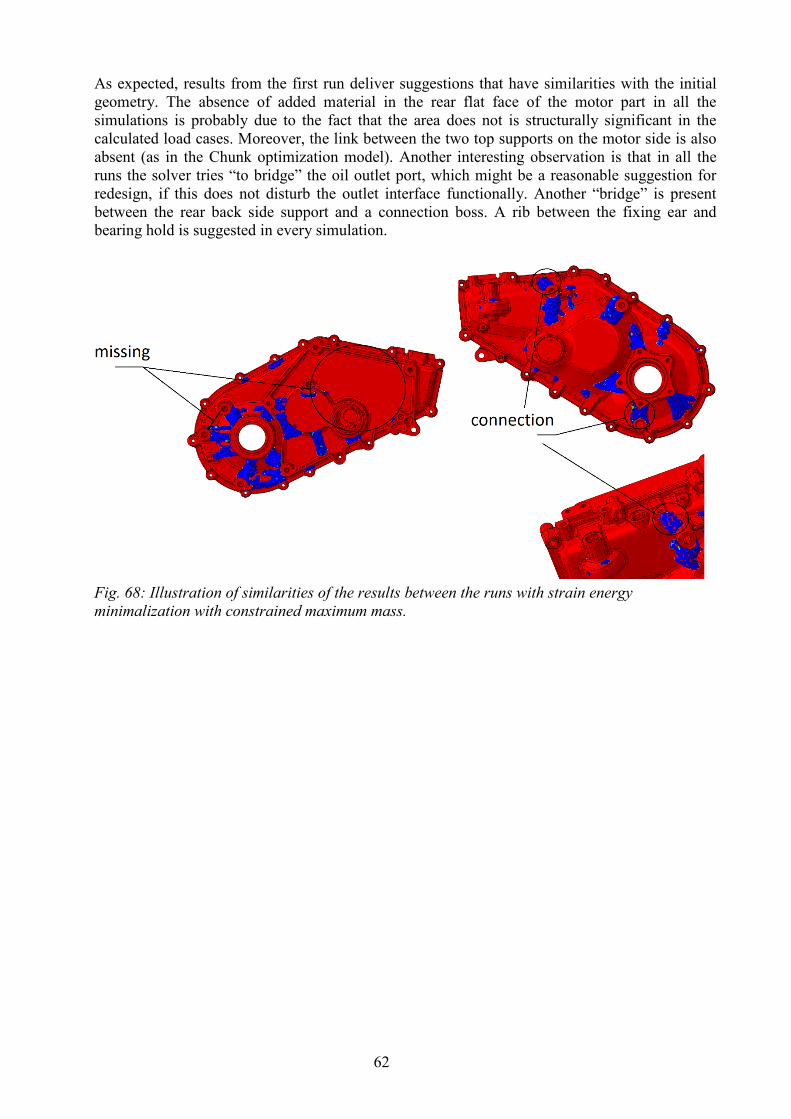
62
As expected, results from the first run deliver suggestions that have similarities with the initial geometry. The absence of added material in the rear flat face of the motor part in all the simulations is probably due to the fact that the area does not is structurally significant in the calculated load cases. Moreover, the link between the two top supports on the motor side is also absent (as in the Chunk optimization model). Another interesting observation is that in all the runs the solver tries “to bridge” the oil outlet port, which might be a reasonable suggestion for redesign, if this does not disturb the outlet interface functionally. Another “bridge” is present between the rear back side support and a connection boss. A rib between the fixing ear and bearing hold is suggested in every simulation.
Fig. 68: Illustration of similarities of the results between the runs with strain energy minimalization with constrained maximum mass.
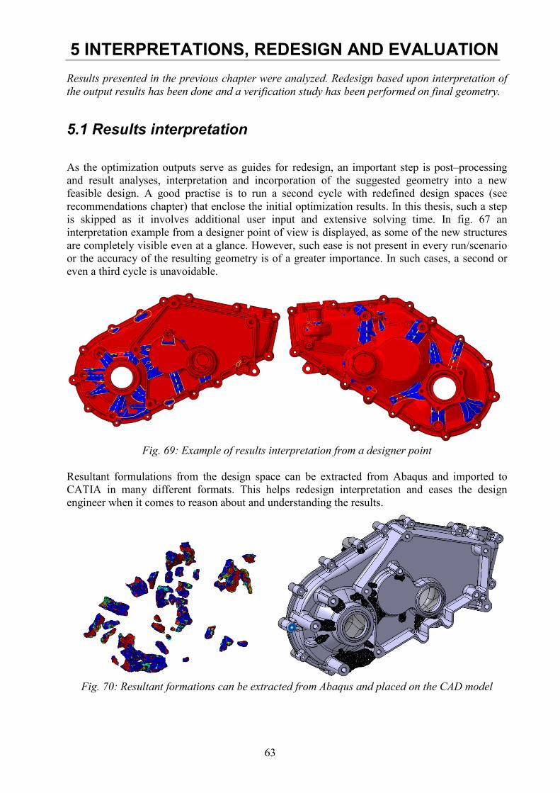
63
5 INTERPRETATIONS, REDESIGN AND EVALUATION Results presented in the previous chapter were analyzed. Redesign based upon interpretation of the output results has been done and a verification study has been performed on final geometry.
5.1 Results interpretation As the optimization outputs serve as guides for redesign, an important step is post–processing and result analyses, interpretation and incorporation of the suggested geometry into a new feasible design. A good practise is to run a second cycle with redefined design spaces (see recommendations chapter) that enclose the initial optimization results. In this thesis, such a step is skipped as it involves additional user input and extensive solving time. In fig. 67 an interpretation example from a designer point of view is displayed, as some of the new structures are completely visible even at a glance. However, such ease is not present in every run/scenario or the accuracy of the resulting geometry is of a greater importance. In such cases, a second or even a third cycle is unavoidable.
Fig. 69: Example of results interpretation from a designer point
Resultant formulations from the design space can be extracted from Abaqus and imported to CATIA in many different formats. This helps redesign interpretation and eases the design engineer when it comes to reason about and understanding the results.
Fig. 70: Resultant formations can be extracted from Abaqus and placed on the CAD model
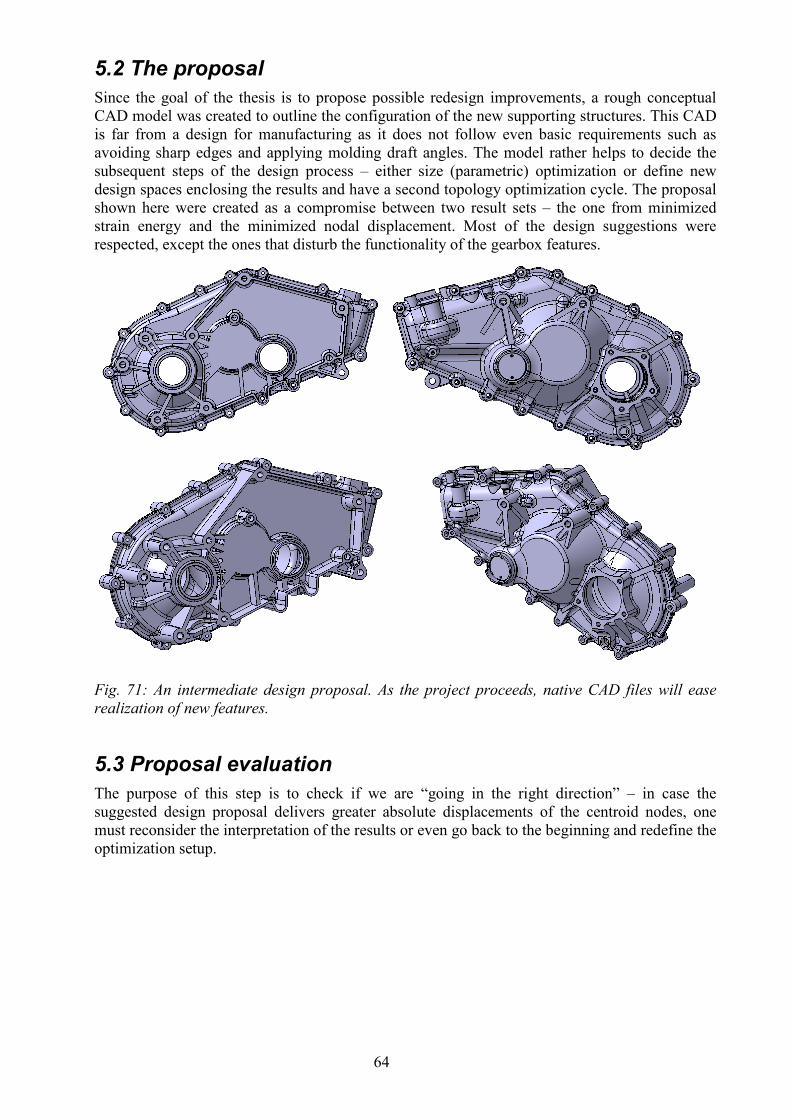
64
5.2 The proposal Since the goal of the thesis is to propose possible redesign improvements, a rough conceptual CAD model was created to outline the configuration of the new supporting structures. This CAD is far from a design for manufacturing as it does not follow even basic requirements such as avoiding sharp edges and applying molding draft angles. The model rather helps to decide the subsequent steps of the design process – either size (parametric) optimization or define new design spaces enclosing the results and have a second topology optimization cycle. The proposal shown here were created as a compromise between two result sets – the one from minimized strain energy and the minimized nodal displacement. Most of the design suggestions were respected, except the ones that disturb the functionality of the gearbox features.
Fig. 71: An intermediate design proposal. As the project proceeds, native CAD files will ease realization of new features.
5.3 Proposal evaluation The purpose of this step is to check if we are “going in the right direction” – in case the suggested design proposal delivers greater absolute displacements of the centroid nodes, one must reconsider the interpretation of the results or even go back to the beginning and redefine the optimization setup.
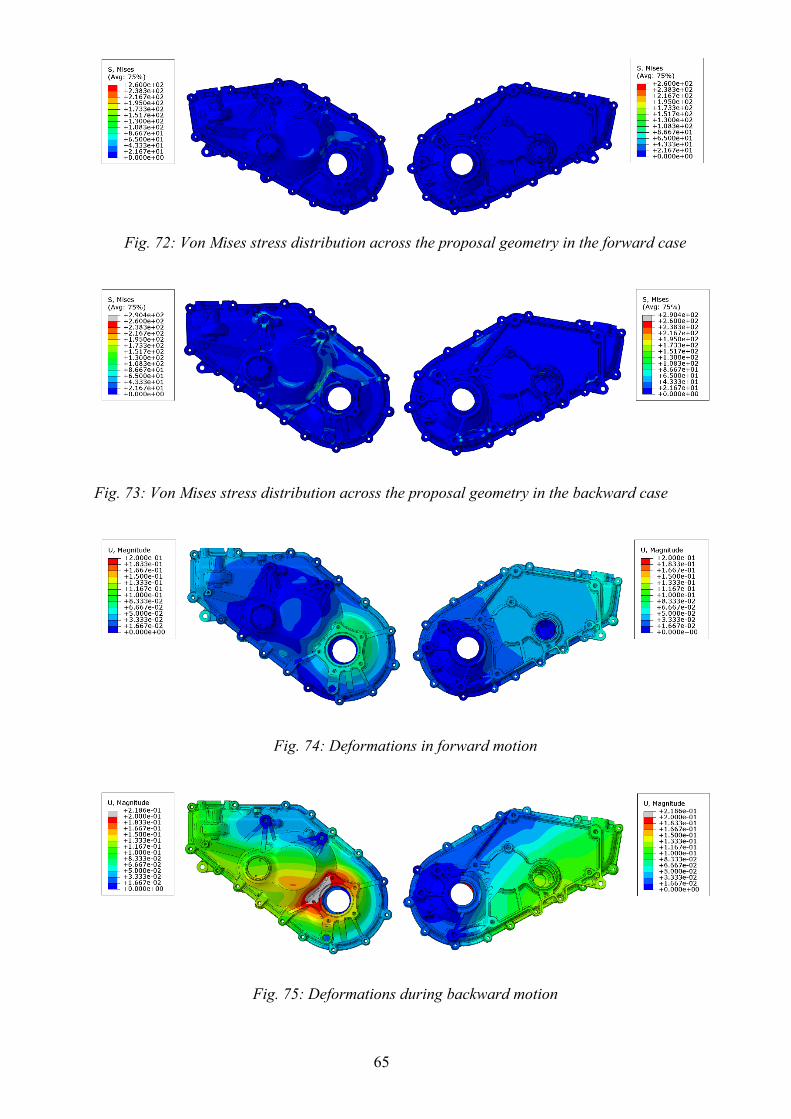
65
Fig. 72: Von Mises stress distribution across the proposal geometry in the forward case
Fig. 73: Von Mises stress distribution across the proposal geometry in the backward case
Fig. 74: Deformations in forward motion
Fig. 75: Deformations during backward motion
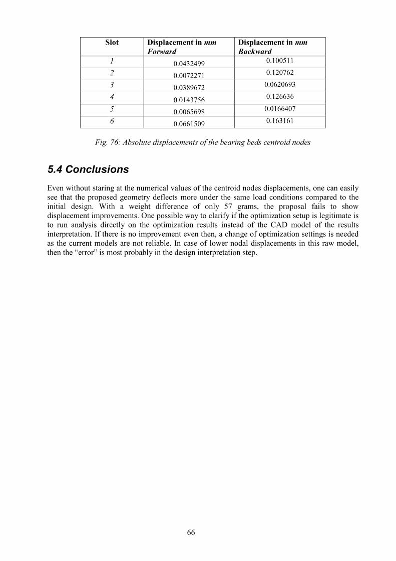
66
Slot Displacement in mm
Forward Displacement in mm Backward
1 0.0432499 0.100511
2 0.0072271 0.120762
3 0.0389672 0.0620693
4 0.0143756 0.126636
5 0.0065698 0.0166407
6 0.0661509 0.163161
Fig. 76: Absolute displacements of the bearing beds centroid nodes
5.4 Conclusions Even without staring at the numerical values of the centroid nodes displacements, one can easily see that the proposed geometry deflects more under the same load conditions compared to the initial design. With a weight difference of only 57 grams, the proposal fails to show displacement improvements. One possible way to clarify if the optimization setup is legitimate is to run analysis directly on the optimization results instead of the CAD model of the results interpretation. If there is no improvement even then, a change of optimization settings is needed as the current models are not reliable. In case of lower nodal displacements in this raw model, then the “error” is most probably in the design interpretation step.
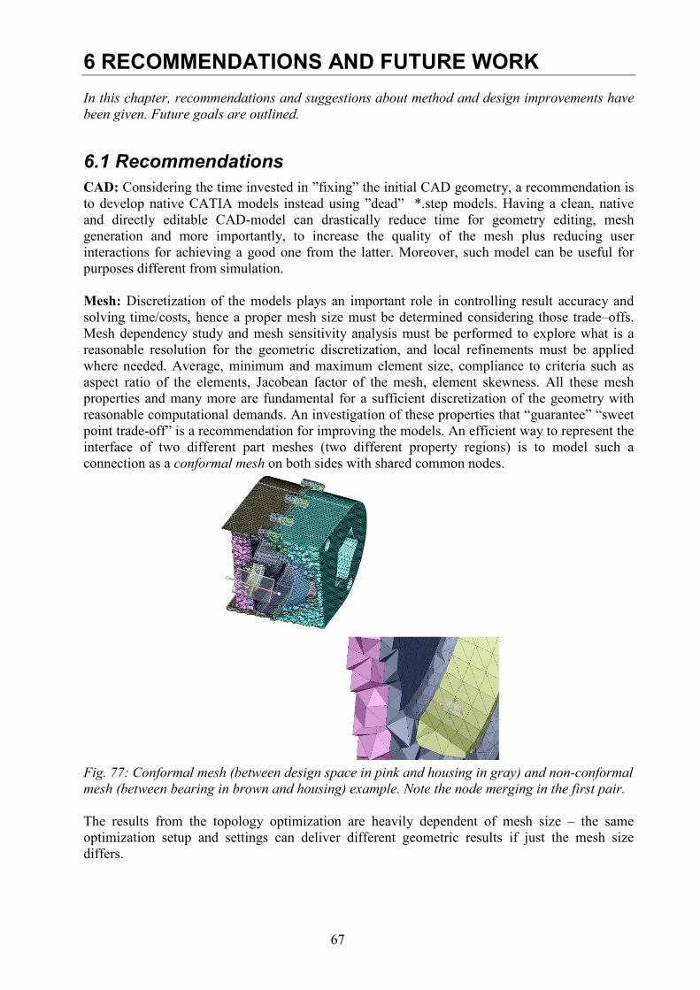
67
6 RECOMMENDATIONS AND FUTURE WORK In this chapter, recommendations and suggestions about method and design improvements have been given. Future goals are outlined.
6.1 Recommendations CAD: Considering the time invested in ”fixing” the initial CAD geometry, a recommendation is to develop native CATIA models instead using ”dead” *.step models. Having a clean, native and directly editable CAD-model can drastically reduce time for geometry editing, mesh generation and more importantly, to increase the quality of the mesh plus reducing user interactions for achieving a good one from the latter. Moreover, such model can be useful for purposes different from simulation. Mesh: Discretization of the models plays an important role in controlling result accuracy and solving time/costs, hence a proper mesh size must be determined considering those trade–offs. Mesh dependency study and mesh sensitivity analysis must be performed to explore what is a reasonable resolution for the geometric discretization, and local refinements must be applied where needed. Average, minimum and maximum element size, compliance to criteria such as aspect ratio of the elements, Jacobean factor of the mesh, element skewness. All these mesh properties and many more are fundamental for a sufficient discretization of the geometry with reasonable computational demands. An investigation of these properties that “guarantee” “sweet point trade-off” is a recommendation for improving the models. An efficient way to represent the interface of two different part meshes (two different property regions) is to model such a connection as a conformal mesh on both sides with shared common nodes.
Fig. 77: Conformal mesh (between design space in pink and housing in gray) and non-conformal mesh (between bearing in brown and housing) example. Note the node merging in the first pair. The results from the topology optimization are heavily dependent of mesh size – the same optimization setup and settings can deliver different geometric results if just the mesh size differs.
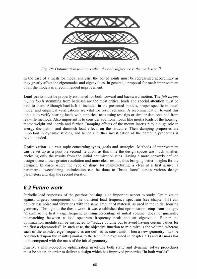
68
Fig. 78: Optimization solutions when the only difference is the mesh size [9] In the case of a mesh for modal analysis, the bolted joints must be represented accordingly as they greatly affect the eigenmodes and eigenvalues. In general, a proposal for mesh improvement of all the models is a recommended improvement. Load peaks must be properly estimated for both forward and backward motion. The full torque impact loads stemming from backlash are the most critical loads and special attention must be paid to them. Although backlash is included in the presented models, proper specific in-detail model and empirical verifications are vital for result reliance. A recommendation toward this topic is to verify bearing loads with empirical tests using test rigs or similar data obtained from real–life methods. Also important is to consider additional loads like inertia loads of the housing, motor weight and inertia and further. Damping effects of the mount inserts play a huge role in energy dissipation and diminish load effects on the structure. Their damping properties are important in dynamic studies, and hence a further investigation of the damping properties is recommended. Optimization is a vast topic concerning types, goals and strategies. Methods of improvement can be set up as a possible second iteration, as this time the design spaces are much smaller, enclosing only the results from the initial optimization runs. Having a more narrowly defined design space allows greater resolution and more clear results, thus bringing better insights for the designer. In cases where the type of shape for manufacturing is clear at a first glance, a parametric sweep/sizing optimization can be done to “brute force” across various design parameters and skip the second iteration.
6.2 Future work Periodic load responses of the gearbox housing is an important aspect to study. Optimization against targeted components of the transient load frequency spectrum (see chapter 3.3) can deliver less noise and vibrations with the same amount of material, as used in the initial housing geometry. Throughout the thesis work, it was established that optimization setup from the type “maximize the first n eigenfrequencies using percentage of initial volume” does not guarantee mismatching between a load spectrum frequency peak and an eigenvalue. Rather the optimization module can be instructed to “reduce volume but to avoid having certain values for the first n eigenmodes”. In such case, the objective function to minimize is the volume, whereas each of the avoided eigenfrequencies are defined as constraints. Then a new geometry must be constructed upon the results (similar to the technique explained in chapter 5.1) and its mass has to be compared with the mass of the initial geometry.
Finally, a multi–objective optimization involving both static and dynamic solver procedures must be set up, in order to deliver a design which has improved properties “in both worlds”.
69
7 REFERENCES
[1] International Energy Agency, “Global Electric Vehicles Outlook 2017 – Two Million and Counting”, https://www.iea.org/publications/freepublications/publication/GlobalEVOutlook2017.pdf [2] Wey L., “Introduction to Hybrid Vehicle System Modeling and Control”, John Wiley & Sons, 2013, New Jersey ISBN: 978-1-118-30840-0 [3] Lalanne C., “Fatigue Damage”, 3rd edition, Vol.3, John Wiley & Sons, 2017, Croydon ISBN: 978-1-84821-647-1 [4] Grous A., “Fracture Mechanics”, Vol.2., John Wiley & Sons, 2013, London, ISBN: 978-1-84821-441-5 [5] Radzevich S., “Handbook of Practical Gear Design and Manufacture”, Taylor & Francis Group, 2012, Ranton ISBN: 978-1-4398-6602-3 [6] Henrikson M., “On Noise Generation and Dynamic Transmission Error of Gears”, KTH, Department of Aeronautical and Vehicle Engineering, 2009, Stockholm ISBN: 978-91-7415-537-2 [7] Jelaska D., “Gears and Gear Drives”, John Wiley & Sons, Chichester, 2012. ISBN: 978-1-119-94130-9 [8] Welbourn D.B., “Fundamental Knowledge of Gear Noise – A Survey”, Proc. Noise &Vib. of Eng. and Trans., I Mech E., 1979, Cranfield [9] Brendsøe M. and Sigmund O., “Topology Optimization. Theory Methods and Applicaitons”, Second Edition., Springer, 2004, Heidelberg. ISBN 978-3-662-05086-6 [10] Svanberg K., “The Method of Moving Asymptotes – A New Method Of Structural Optimization”, KTH, International Journal for Numerical Methods in Engineering, Vol 24, 1987, Stockholm [11] Nilsson I., “Gear Whine Noise Excitation Model”, Chalmers, Department of Applied Mechanics, 2013, Göteborg [12] Brauer S., “High Speed Electric Vehicle Transmission”, Karlstad University, Faculty of Health, science and Technology, 2017, Karlstad

70
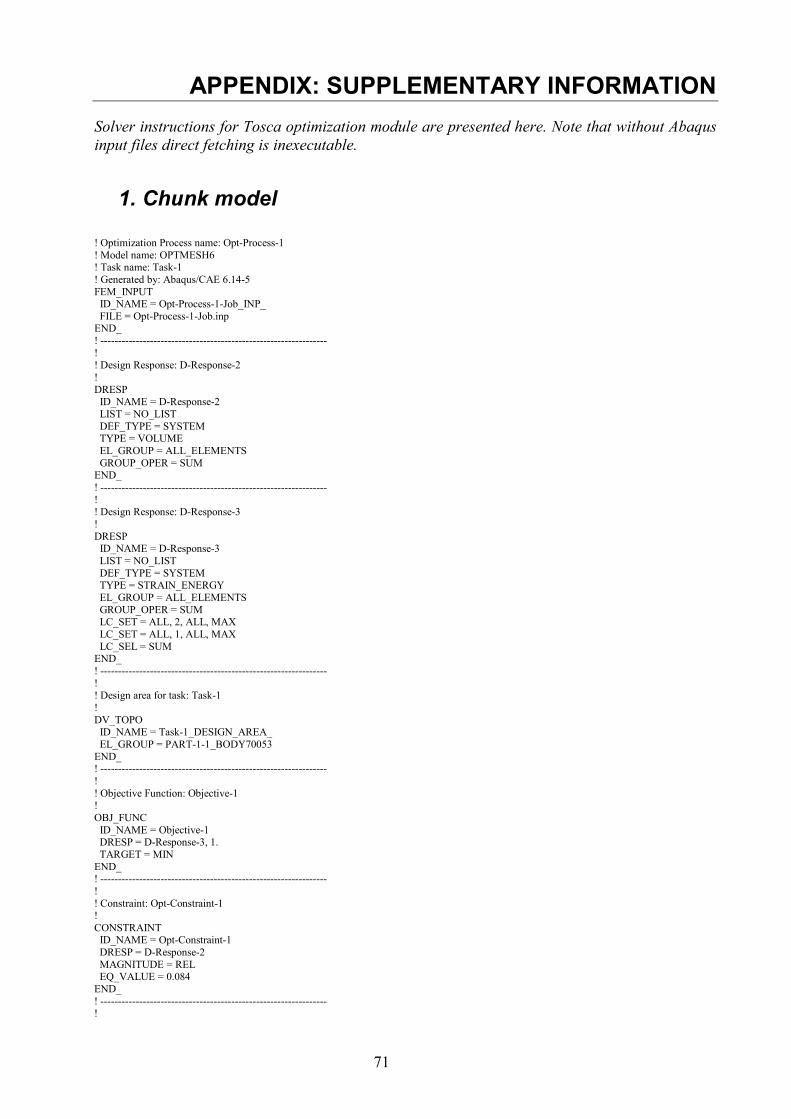
71
APPENDIX: SUPPLEMENTARY INFORMATION Solver instructions for Tosca optimization module are presented here. Note that without Abaqus input files direct fetching is inexecutable.
1. Chunk model ! Optimization Process name: Opt-Process-1 ! Model name: OPTMESH6 ! Task name: Task-1 ! Generated by: Abaqus/CAE 6.14-5 FEM_INPUT ID_NAME = Opt-Process-1-Job_INP_ FILE = Opt-Process-1-Job.inp END_ ! ---------------------------------------------------------------- ! ! Design Response: D-Response-2 ! DRESP ID_NAME = D-Response-2 LIST = NO_LIST DEF_TYPE = SYSTEM TYPE = VOLUME EL_GROUP = ALL_ELEMENTS GROUP_OPER = SUM END_ ! ---------------------------------------------------------------- ! ! Design Response: D-Response-3 ! DRESP ID_NAME = D-Response-3 LIST = NO_LIST DEF_TYPE = SYSTEM TYPE = STRAIN_ENERGY EL_GROUP = ALL_ELEMENTS GROUP_OPER = SUM LC_SET = ALL, 2, ALL, MAX LC_SET = ALL, 1, ALL, MAX LC_SEL = SUM END_ ! ---------------------------------------------------------------- ! ! Design area for task: Task-1 ! DV_TOPO ID_NAME = Task-1_DESIGN_AREA_ EL_GROUP = PART-1-1_BODY70053 END_ ! ---------------------------------------------------------------- ! ! Objective Function: Objective-1 ! OBJ_FUNC ID_NAME = Objective-1 DRESP = D-Response-3, 1. TARGET = MIN END_ ! ---------------------------------------------------------------- ! ! Constraint: Opt-Constraint-1 ! CONSTRAINT ID_NAME = Opt-Constraint-1 DRESP = D-Response-2 MAGNITUDE = REL EQ_VALUE = 0.084 END_ ! ---------------------------------------------------------------- !

72
! Geometric Restriction: Restrict-1 ! DVCON_TOPO ID_NAME = Restrict-1 EL_GROUP = PART-1-1_BODY70053 CHECK_TYPE = MIN_MEMBER THICKNESS = 10. END_ ! ---------------------------------------------------------------- ! ! Geometric Restriction: Restrict-2 ! DVCON_TOPO ID_NAME = Restrict-2 EL_GROUP = Set-17 CHECK_TYPE = FROZEN END_ ! ---------------------------------------------------------------- ! ! Task: Task-1 ! OPTIMIZE ID_NAME = Task-1 DV = Task-1_DESIGN_AREA_ OBJ_FUNC = Objective-1 DVCON = Restrict-1 DVCON = Restrict-2 CONSTRAINT = Opt-Constraint-1 STRATEGY = TOPO_CONTROLLER END_ OPT_PARAM ID_NAME = Task-1_OPT_PARAM_ OPTIMIZE = Task-1 AUTO_FROZEN = BOTH SPEED = ITER, 15 END_ STOP ID_NAME = Task-1_GLOBAL_STOP_CONDITION_ ITER_MAX = 50 END_ CONFIG $fe_solver_add_call = " memory=90% cpus=12"; add_move_per_iter_list("0,1,last", "SAVE.odb", "*.odb"); add_move_per_iter_list("0,1,last", "SAVE.msg", "*.msg"); add_move_per_iter_list("0,1,last", "SAVE.dat", "*.dat"); add_move_per_iter_list("0,1,last", "SAVE.sta", "*.sta"); END_ EXIT STOP_CRITERION_LEVEL = BOTH STOP_CRITERION_OBJ = 0.001 STOP_CRITERION_DENSITY = 0.005 STOP_CRITERION_ITER = 4 SUM_Q_FACTOR = 6. END_ STOP ID_NAME = Task-1_GLOBAL_STOP_CONDITION_ ITER_MAX = 50 END_ CONFIG $fe_solver_add_call = " memory=90% cpus=12"; add_move_per_iter_list("0,1,last", "SAVE.odb", "*.odb"); add_move_per_iter_list("0,1,last", "SAVE.msg", "*.msg"); add_move_per_iter_list("0,1,last", "SAVE.dat", "*.dat"); add_move_per_iter_list("0,1,last", "SAVE.sta", "*.sta"); END_ EXIT

73
2. Noribs model with diminished design space, geometric restrictions and direction / pull control – strain energy minimalization
! Optimization Process name: Opt-Process-1 ! Model name: awe ! Task name: Task-1 ! Generated by: Abaqus/CAE 6.14-5 FEM_INPUT ID_NAME = Opt-Process-1-Job_INP_ FILE = Opt-Process-1-Job.inp END_ ! ---------------------------------------------------------------- ! ! Design Response: D-Response-1 ! DRESP ID_NAME = D-Response-1 LIST = NO_LIST DEF_TYPE = SYSTEM TYPE = STRAIN_ENERGY EL_GROUP = ALL_ELEMENTS GROUP_OPER = SUM LC_SET = ALL, 2, ALL, MAX LC_SET = ALL, 1, ALL, MAX LC_SEL = SUM END_ ! ---------------------------------------------------------------- ! ! Design Response: D-Response-2 ! DRESP ID_NAME = D-Response-2 LIST = NO_LIST DEF_TYPE = SYSTEM TYPE = VOLUME EL_GROUP = DesignSpace GROUP_OPER = SUM END_ ! ---------------------------------------------------------------- ! ! Design area for task: Task-1 ! DV_TOPO ID_NAME = Task-1_DESIGN_AREA_ EL_GROUP = DesignSpace END_ ! ---------------------------------------------------------------- ! ! Objective Function: Objective-1 ! OBJ_FUNC ID_NAME = Objective-1 DRESP = D-Response-1, 1. TARGET = MIN END_ ! ---------------------------------------------------------------- ! ! Constraint: Opt-Constraint-1 ! CONSTRAINT ID_NAME = Opt-Constraint-1 DRESP = D-Response-2 MAGNITUDE = REL LE_VALUE = 0.03458 END_ ! ---------------------------------------------------------------- ! ! Geometric Restriction: Restrict-1 ! DVCON_TOPO ID_NAME = Restrict-1 EL_GROUP = DesignSpace CHECK_TYPE = MAX_MEMBER THICKNESS = 15.
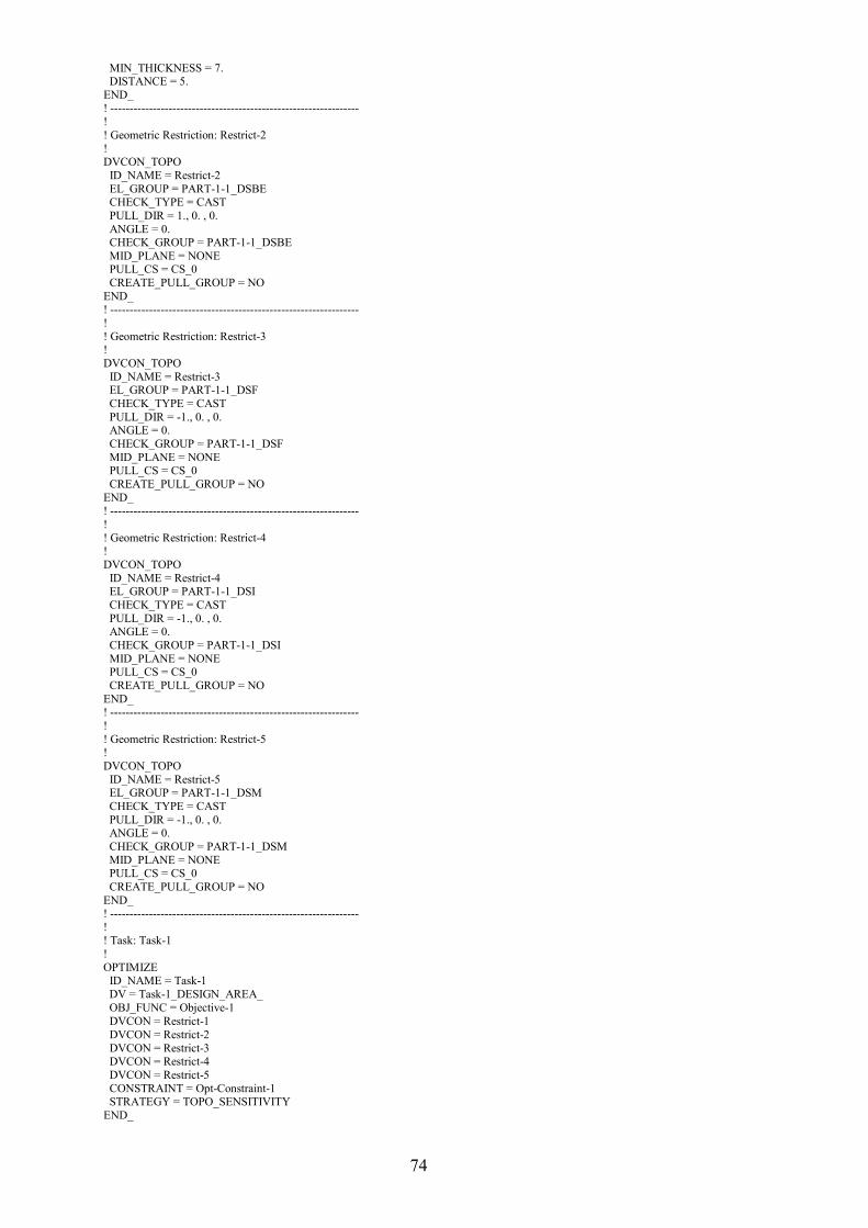
74
MIN_THICKNESS = 7. DISTANCE = 5. END_ ! ---------------------------------------------------------------- ! ! Geometric Restriction: Restrict-2 ! DVCON_TOPO ID_NAME = Restrict-2 EL_GROUP = PART-1-1_DSBE CHECK_TYPE = CAST PULL_DIR = 1., 0. , 0. ANGLE = 0. CHECK_GROUP = PART-1-1_DSBE MID_PLANE = NONE PULL_CS = CS_0 CREATE_PULL_GROUP = NO END_ ! ---------------------------------------------------------------- ! ! Geometric Restriction: Restrict-3 ! DVCON_TOPO ID_NAME = Restrict-3 EL_GROUP = PART-1-1_DSF CHECK_TYPE = CAST PULL_DIR = -1., 0. , 0. ANGLE = 0. CHECK_GROUP = PART-1-1_DSF MID_PLANE = NONE PULL_CS = CS_0 CREATE_PULL_GROUP = NO END_ ! ---------------------------------------------------------------- ! ! Geometric Restriction: Restrict-4 ! DVCON_TOPO ID_NAME = Restrict-4 EL_GROUP = PART-1-1_DSI CHECK_TYPE = CAST PULL_DIR = -1., 0. , 0. ANGLE = 0. CHECK_GROUP = PART-1-1_DSI MID_PLANE = NONE PULL_CS = CS_0 CREATE_PULL_GROUP = NO END_ ! ---------------------------------------------------------------- ! ! Geometric Restriction: Restrict-5 ! DVCON_TOPO ID_NAME = Restrict-5 EL_GROUP = PART-1-1_DSM CHECK_TYPE = CAST PULL_DIR = -1., 0. , 0. ANGLE = 0. CHECK_GROUP = PART-1-1_DSM MID_PLANE = NONE PULL_CS = CS_0 CREATE_PULL_GROUP = NO END_ ! ---------------------------------------------------------------- ! ! Task: Task-1 ! OPTIMIZE ID_NAME = Task-1 DV = Task-1_DESIGN_AREA_ OBJ_FUNC = Objective-1 DVCON = Restrict-1 DVCON = Restrict-2 DVCON = Restrict-3 DVCON = Restrict-4 DVCON = Restrict-5 CONSTRAINT = Opt-Constraint-1 STRATEGY = TOPO_SENSITIVITY END_
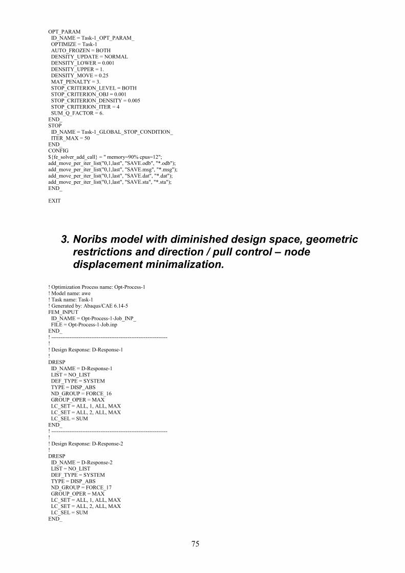
75
OPT_PARAM ID_NAME = Task-1_OPT_PARAM_ OPTIMIZE = Task-1 AUTO_FROZEN = BOTH DENSITY_UPDATE = NORMAL DENSITY_LOWER = 0.001 DENSITY_UPPER = 1. DENSITY_MOVE = 0.25 MAT_PENALTY = 3. STOP_CRITERION_LEVEL = BOTH STOP_CRITERION_OBJ = 0.001 STOP_CRITERION_DENSITY = 0.005 STOP_CRITERION_ITER = 4 SUM_Q_FACTOR = 6. END_ STOP ID_NAME = Task-1_GLOBAL_STOP_CONDITION_ ITER_MAX = 50 END_ CONFIG $fe_solver_add_call = " memory=90% cpus=12"; add_move_per_iter_list("0,1,last", "SAVE.odb", "*.odb"); add_move_per_iter_list("0,1,last", "SAVE.msg", "*.msg"); add_move_per_iter_list("0,1,last", "SAVE.dat", "*.dat"); add_move_per_iter_list("0,1,last", "SAVE.sta", "*.sta"); END_ EXIT
3. Noribs model with diminished design space, geometric restrictions and direction / pull control – node displacement minimalization.
! Optimization Process name: Opt-Process-1 ! Model name: awe ! Task name: Task-1 ! Generated by: Abaqus/CAE 6.14-5 FEM_INPUT ID_NAME = Opt-Process-1-Job_INP_ FILE = Opt-Process-1-Job.inp END_ ! ---------------------------------------------------------------- ! ! Design Response: D-Response-1 ! DRESP ID_NAME = D-Response-1 LIST = NO_LIST DEF_TYPE = SYSTEM TYPE = DISP_ABS ND_GROUP = FORCE_16 GROUP_OPER = MAX LC_SET = ALL, 1, ALL, MAX LC_SET = ALL, 2, ALL, MAX LC_SEL = SUM END_ ! ---------------------------------------------------------------- ! ! Design Response: D-Response-2 ! DRESP ID_NAME = D-Response-2 LIST = NO_LIST DEF_TYPE = SYSTEM TYPE = DISP_ABS ND_GROUP = FORCE_17 GROUP_OPER = MAX LC_SET = ALL, 1, ALL, MAX LC_SET = ALL, 2, ALL, MAX LC_SEL = SUM END_
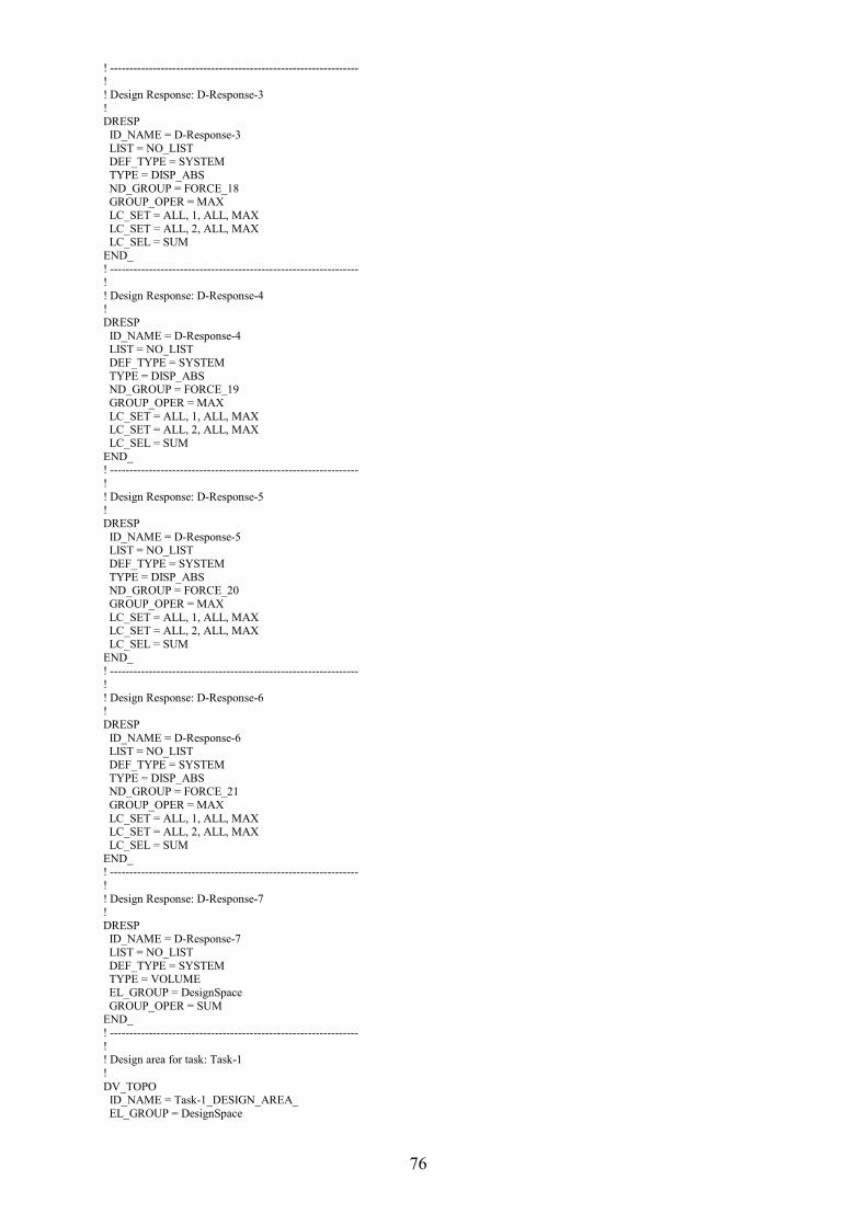
76
! ---------------------------------------------------------------- ! ! Design Response: D-Response-3 ! DRESP ID_NAME = D-Response-3 LIST = NO_LIST DEF_TYPE = SYSTEM TYPE = DISP_ABS ND_GROUP = FORCE_18 GROUP_OPER = MAX LC_SET = ALL, 1, ALL, MAX LC_SET = ALL, 2, ALL, MAX LC_SEL = SUM END_ ! ---------------------------------------------------------------- ! ! Design Response: D-Response-4 ! DRESP ID_NAME = D-Response-4 LIST = NO_LIST DEF_TYPE = SYSTEM TYPE = DISP_ABS ND_GROUP = FORCE_19 GROUP_OPER = MAX LC_SET = ALL, 1, ALL, MAX LC_SET = ALL, 2, ALL, MAX LC_SEL = SUM END_ ! ---------------------------------------------------------------- ! ! Design Response: D-Response-5 ! DRESP ID_NAME = D-Response-5 LIST = NO_LIST DEF_TYPE = SYSTEM TYPE = DISP_ABS ND_GROUP = FORCE_20 GROUP_OPER = MAX LC_SET = ALL, 1, ALL, MAX LC_SET = ALL, 2, ALL, MAX LC_SEL = SUM END_ ! ---------------------------------------------------------------- ! ! Design Response: D-Response-6 ! DRESP ID_NAME = D-Response-6 LIST = NO_LIST DEF_TYPE = SYSTEM TYPE = DISP_ABS ND_GROUP = FORCE_21 GROUP_OPER = MAX LC_SET = ALL, 1, ALL, MAX LC_SET = ALL, 2, ALL, MAX LC_SEL = SUM END_ ! ---------------------------------------------------------------- ! ! Design Response: D-Response-7 ! DRESP ID_NAME = D-Response-7 LIST = NO_LIST DEF_TYPE = SYSTEM TYPE = VOLUME EL_GROUP = DesignSpace GROUP_OPER = SUM END_ ! ---------------------------------------------------------------- ! ! Design area for task: Task-1 ! DV_TOPO ID_NAME = Task-1_DESIGN_AREA_ EL_GROUP = DesignSpace
77
END_ ! ---------------------------------------------------------------- ! ! Objective Function: Objective-1 ! OBJ_FUNC ID_NAME = Objective-1 DRESP = D-Response-1, 1. DRESP = D-Response-2, 1. DRESP = D-Response-3, 1. DRESP = D-Response-4, 1. DRESP = D-Response-5, 1. DRESP = D-Response-6, 1. TARGET = MIN END_ ! ---------------------------------------------------------------- ! ! Constraint: Opt-Constraint-1 ! CONSTRAINT ID_NAME = Opt-Constraint-1 DRESP = D-Response-7 MAGNITUDE = REL LE_VALUE = 0.040412 END_ ! ---------------------------------------------------------------- ! ! Geometric Restriction: Restrict-1 ! DVCON_TOPO ID_NAME = Restrict-1 EL_GROUP = DesignSpace CHECK_TYPE = MAX_MEMBER THICKNESS = 20. MIN_THICKNESS = 10. DISTANCE = 5. END_ ! ---------------------------------------------------------------- ! ! Geometric Restriction: Restrict-2 ! DVCON_TOPO ID_NAME = Restrict-2 EL_GROUP = PART-1-1_DSBE CHECK_TYPE = CAST PULL_DIR = 1., 0. , 0. ANGLE = 0. CHECK_GROUP = PART-1-1_DSBE MID_PLANE = NONE PULL_CS = CS_0 CREATE_PULL_GROUP = NO END_ ! ---------------------------------------------------------------- ! ! Geometric Restriction: Restrict-3 ! DVCON_TOPO ID_NAME = Restrict-3 EL_GROUP = PART-1-1_DSF CHECK_TYPE = CAST PULL_DIR = -1., 0. , 0. ANGLE = 0. CHECK_GROUP = PART-1-1_DSF MID_PLANE = NONE PULL_CS = CS_0 CREATE_PULL_GROUP = NO END_ ! ---------------------------------------------------------------- ! ! Geometric Restriction: Restrict-4 ! DVCON_TOPO ID_NAME = Restrict-4 EL_GROUP = PART-1-1_DSI CHECK_TYPE = CAST PULL_DIR = -1., 0. , 0. ANGLE = 0. CHECK_GROUP = PART-1-1_DSI MID_PLANE = NONE

78
PULL_CS = CS_0 CREATE_PULL_GROUP = NO END_ ! ---------------------------------------------------------------- ! ! Geometric Restriction: Restrict-5 ! DVCON_TOPO ID_NAME = Restrict-5 EL_GROUP = PART-1-1_DSM CHECK_TYPE = CAST PULL_DIR = -1., 0. , 0. ANGLE = 0. CHECK_GROUP = PART-1-1_DSM MID_PLANE = NONE PULL_CS = CS_0 CREATE_PULL_GROUP = NO END_ ! ---------------------------------------------------------------- ! ! Task: Task-1 ! OPTIMIZE ID_NAME = Task-1 DV = Task-1_DESIGN_AREA_ OBJ_FUNC = Objective-1 DVCON = Restrict-1 CONSTRAINT = Opt-Constraint-1 STRATEGY = TOPO_SENSITIVITY END_ OPT_PARAM ID_NAME = Task-1_OPT_PARAM_ OPTIMIZE = Task-1 AUTO_FROZEN = BOTH DENSITY_UPDATE = NORMAL DENSITY_LOWER = 0.001 DENSITY_UPPER = 1. DENSITY_MOVE = 0.25 MAT_PENALTY = 3. STOP_CRITERION_LEVEL = BOTH STOP_CRITERION_OBJ = 0.001 STOP_CRITERION_DENSITY = 0.005 STOP_CRITERION_ITER = 4 SUM_Q_FACTOR = 6. END_ STOP ID_NAME = Task-1_GLOBAL_STOP_CONDITION_ ITER_MAX = 50 END_ CONFIG $fe_solver_add_call = " memory=90% cpus=12"; add_move_per_iter_list("0,1,last", "SAVE.odb", "*.odb"); add_move_per_iter_list("0,1,last", "SAVE.msg", "*.msg"); add_move_per_iter_list("0,1,last", "SAVE.dat", "*.dat"); add_move_per_iter_list("0,1,last", "SAVE.sta", "*.sta"); END_ EXIT