gas retention and release behavior in hanford double-shell
TRANSCRIPT
PNNL-11536 Rev. 1UC-2030
Gas Retention and ReleaseBehavior in HanfordDouble-Shell Waste Tanks
P. A. MeyerM. E. BrewsterS. A. BryanG. ChenL. R. PedersonC. W. StewartG. Terrones
May 1997
Prepared for the U.S. Department of Energyunder Contract DE-AC06-76RLO 1830
Pacific Northwest National LaboratoryRichland, Washington 99352
WSTRIBUTION OF THIS DOCUMEINfT IS UNLIMITED
DISCLAIMER
Portions of this document may be fllegiblein electronic image products* Images arcproduced from the best available originalDocument.
Preface
This report was prepared to satisfy the Defense Nuclear Facilities Safety Board(DNFSB) Recommendation 93-5 Implementation Plan (DOE 1996), Milestone 5.4.3.5.1,"Letter reporting refinement of flammable gas generation/retention models using void meterand retained gas sampling data."
The data obtained from operating the void fraction instrument (VFI) (Stewart et al. 1996a),and retained gas sampler (RGS) (Shekarriz et al. 1997) have determined the amount and com-position of gas retained in the wastes in the six double-shell tanks on the Flammable Gas WatchList (Johnson et all 1997). The interpretation of those data and the models for gas retention andrelease developed or improved as a result represent significant progress toward an adequateunderstanding of the mechanisms of gas generation, retention, and release. This report sum-marizes the VFI and RGS data and presents the models these data have enabled us to develop.
in

Abstract
This report describes the current understanding of flammable gas retention and release inHanford double-shell waste tanks AN-103, AN-104, AN-105, AW-101, SY-101, and SY-103.This knowledge is based on analyses, experimental results, and observations of tank behavior.The applicable data available from the void fraction instrument, retained gas sampler, ballrheometer, tank characterization, and field monitoring are summarized. Retained gas volumes andvoid fractions are updated with these new data. Using the retained gas compositions from theretained gas sampler, peak dome pressures during a gas burn are calculated as a function of thefraction of retained gas hypothetically released instantaneously into the tank head space. Modelsand criteria are given for gas generation, initiation of buoyant displacement, and resulting gasrelease; and predictions are compared with observed tank behavior.

Summary
The gas retention and release behaviors of Hanford double-shell tanks (DSTs) on the Flam-mable Gas Watch List (FGWL), AN-103, AN-104, AN-105, AW-101, SY-101, and SY-103,were characterized in detail using the ball rheometer and void fraction instrument (VFI) fromDecember 1994 to May 1996. These are reported in Stewart et al. (1996a). Additional data on gascomposition and void fraction have since become available on four of these tanks (AW-101,AN-103, AN-104, and AN-105) using the retained gas sampler (RGS) from March throughSeptember 1996 and are described in Shekarriz et al. (1997).
The main objective of the work presented in this report is improving the models for gasretention and release based on these data and updating the original gas retention and releasecalculations with the new RGS and core sample data. Because of this extensive characterizationeffort, we have a better knowledge and understanding of these DSTs than of any other Hanfordtanks. We include models that help explain current gas retention and release behavior and examinethe potential for other tanks to exhibit hazardous episodic gas releases. The models developed forgas generation based on waste sample testing are also summarized. While none of these modelshave been formally verified and validated for safety analysis, they are consistent with the extantbody of data and observations. The updates to earlier calculations and improvements to gasgeneration, retention, and release models are summarized below.
Gas Generation Models and Results
The three most important mechanisms for gas generation are 1) radiation-induced chemicaldecomposition of water and some organic species; 2) thermally induced chemical decomposition,mainly involving organic complexants and solvents; and 3) chemical decomposition of the steeltank walls. The first two clearly dominate, and the yield from radiolysis of the organic compoundsis especially important.
Recent studies on gas evolution from tank waste samples and prior mechanistic studieswith simulants have advanced our understanding of gas generation processes significantly. Acti-vation energies for overall gas generation as well as for hydrogen, nitrogen, and nitrous oxide arenow well established for the waste from Tank SY-103 (Bryan et al. 1996). The relative magnitudeof the thermal and radiolytic components of gas generation are known as a function of temperaturefor wastes from SY-101 and SY-103, and a predictive model for gas generation based on thebehavior of SY-103 waste has been developed. The gas composition in SY-103 has been revisedaccording to the experimental generation rates.
Though we know how to study gas generation effectively, and we understand the gasgeneration behavior of SY-101 and SY-103 waste reasonably well, we cannot yet extrapolate toother waste types with confidence and precision. We must be able to do this to predict the long-term gas generation behavior. To this end, gas generation tests are being performed on wastesamples from Tanks S-102 (a single-shell tank), AW-101, and AN-105.
Gas Retention Models and Results
Updating the retained gas volume calculation with the additional data from the RGSproduced only minor adjustments in the average void fraction, void distribution, and total storedvolume. The crust gas volume calculation model was modified as a result of the new information.The original calculation derived for SY-101 conservatively assumed a crust void fraction of 0.25.The best information now available indicates that the crust consists of the same material as the
vn
nonconvective layer and that its void fraction is approximately the neutral buoyancy value. Con-sistent with these observations, the new model assumes the crust void fraction is slightly aboveneutral buoyancy such that a large fraction of its thickness is submerged below the free liquidsurface. This change reduces the estimated crust gas volume by as much as half in some tanks.
The barometric pressure effect (BPE) model, which estimates the retained gas volume fromthe response of waste level to barometric pressure fluctuations, is derived in detail and its resultscompared with the gas volumes calculated from VFI and RGS void fractions. The assumptionsmade during the derivation require that the BPE model be applied to tanks with relatively deep, wetwaste in which the vertical gas distribution can be estimated. Currently, this includes the DSTsand a few of the single-shell tanks (SSTs). The difference between the BPE and VFI gas volumeestimates is well within the standard deviation of the VFI results. Good results are also obtainedwhere the vertical gas distribution has a high uncertainty.
Gas Release Models and Results
The large episodic gas release events (GREs) historically observed in the DSTs on theFGWL are believed to be caused by the buoyant displacement mechanism (Stewart 1996b). In abuoyant displacement, a portion, or "gob," of the nonconvective layer near the tank bottomaccumulates gas until it becomes sufficiently buoyant to overcome the weight and strength ofmaterial restraining it. At that point it suddenly breaks away and rises through the supernatantliquid layer. The hydrostatic pressure decreases as the gob rises, causing the stored gas bubbles toexpand. Where bubble expansion is sufficient to fail the surrounding material, gas is released fromthe gob and, if not trapped by existing crust, may escape into the head space.
Buoyancy tends to destabilize the nonconvective layer, while the material strength stabilizesit. A buoyant displacement can occur when local void fraction is high enough to produce a netupward force in the nonconvective layer (exceeds "neutral buoyancy"). However, the strength ofthe bulk solids will keep the gob from rising until the buoyant force causes the material yield stressto be exceeded. Therefore, the void fraction must be significantly greater than the neutralbuoyancy value before a buoyant displacement can begin.
The effect of the material strength depends on the shape of the gob as well as its size. Theshape effect depends on the ratio of the surface area to volume. For large gobs, the effect ofmaterial strength is minimal, and the critical void fraction is approximately equal to the neutralbuoyancy value. However, small gobs have a higher surface-to-volume ratio and require a muchhigher void fraction. To first order, gobs with a diameter approximately equal to the nonconvec-tive layer depth may be the most probable. Better estimates are obtained with a detailed stabilityanalysis.
At the onset of a buoyant displacement, the yield stress of the nonconvective material isexceeded, and the material around the participating gob begins to flow. Assuming that at this pointthe entire nonconvective layer behaves as a viscous fluid, the length scale can be estimated from theRayleigh-Taylor theory for superposed fluid layers of different densities and viscosities. Thisanalysis allows both the size and critical void fraction of a gob to be determined and leads to amethod to predict the gas release volume and frequency of buoyant displacements in the six FGWLDSTs. The estimates compare quite well with actual tank behavior as derived from the waste levelhistory.
Basic energy conservation principles can be applied to the buoyant displacement process todetermine the conditions required for it to release gas. A simple predictive model is derived thatdescribes the energy requirements of buoyant displacement in terms of estimated or measurableparameters. The model establishes a criterion for gas release by a buoyant displacement. The total
vni
amount of energy stored in a gob of gas-bearing solids must exceed the energy required to yield thegas-retaining matrix. The model is compared with data from scaled experiments and applied to thesix DSTs on the FGWL. The conclusion is that a relatively deep layer of supernatant liquid isrequired for buoyant displacement to release gas. This condition currently exists only in the DSTs.
The calculation of the peak dome pressure resulting from a postulated deflagration has alsobeen updated with actual gas compositions from RGS data for AW-101, AN-103, AN-104, andAN-105. SY-103 compositions were derived from recent gas generation experiments (Bryan et al.1996). The SY-101 compositions are unchanged. The new data slightly reduced the predictedpressures in the AN tanks. The peak pressure in SY-103 increased because the new compositionhas about twice the hydrogen. Only SY-101 demonstrated a clear potential for a flammable gasburn that could fail the dome structure. None of the other tanks appear capable of producing peakpressures exceeding the 3.08-atm limit at 99% confidence for even a very large release of 50% oftheir stored gas, which is far larger than any observed to date. Tanks SY-103 and AW-101 remainincapable of exceeding the pressure limit even if they were to release 100% of their stored gas.
The models discussed above, and the data on which they are based, allow us to evaluatethese tanks' gas release potential. To within reasonable uncertainty, we now know how much gasthey contain, its composition, and where it is stored; we also understand how the gas is released,and we can estimate approximately how much gas will be released and how often. Though thesemodels are not, and possibly cannot be formally validated, they represent our best understandingand are consistent with the available knowledge base.
ReferencesBryan S, CM King, LR Pederson, SV Forbes, and RL Sell. 1996. Gas Generation fromTank241-SY-103 Waste. PNNL-10978, Pacific Northwest National Laboratory, Richland,Washington.
Johnson GD. 1997 Flammable Gas Project Topical Report. HNF-SP-1193 Rev. 2, DukeEngineering Services Hanford, Richland, Washington.
Shekarriz A, DR Rector, LA Mahoney, MA Chieda, JM Bates, RE Bauer, NS Cannon, BE Hey,CG Linschooten, FJ Reitz, and ER Siciliano. 1997. Composition and Quantities of Retained GasMeasured in Hanford Waste Tanks 241-AW-101, A-101, AN-105, AN-104, and AN-103.PNNL-11450 Rev. 1, Pacific Northwest National Laboratory, Richland, Washington.
Stewart CW, JM Alzheimer, ME Brewster, G Chen, RE Mendoza, HC Reid, CL Shepard, andG Terrones. 1996a. In Situ Rheology and Gas Volume in Hanford Double-Shell Waste Tanks.PNNL-11296, Pacific Northwest National Laboratory, Richland, Washington.
Stewart CW, ME Brewster, PA Gauglitz, LA Mahoney, PA Meyer, KP Recknagle, and HC Reid.1996b. Gas Retention and Release Behavior in Hanford Single-Shell Waste Tanks.PNNL-11391, Pacific Northwest National Laboratory, Richland, Washington.
IX
Acknowledgments
The authors gratefully thank Lenna Mahoney, Reza Shekarriz, and Dave Rector, whosupplied the RGS data and help us understand it. Thanks also to Blaine Barton and Steve Barker(both of LMHC) for providing us helpful suggestions and encouragement on the gas releasemodel.
Thanks to Jerry Johnson (DESH) and to John Gray and Craig Groendyke (DOE-RL) forassistance in seeing the document through the formal review process.
We appreciate the efforts of Sheila Bennett who edited this report several times throughfinal publication. Thanks to Kathy Rightmire for preparing the core extrusion and waste surfacephotos.
XI

Contents
Preface iii
Abstract v
Summary vii
Acknowledgments xi
1.0 Introduction 1.1
2.0 Gas Generation Models 2.1
2.1 Studies Using Actual Waste 2.1
2.2 Kinetics of Gas Generation 2.5
2.3 Recommendations for Improving Gas Generation Models 2.5
3.0 Gas Retention Models 3.1
3.1 Retained Gas Volume 3.1
3.1.1 Average Void Fraction 3.1
3.1.2 Gas Retention Model 3.3
3.1.3 Gas Volume Uncertainties 3.8
3.1.4 Retained Gas Volume Summary 3.9
3.2 Individual Tank Gas Retention Summaries 3.12
3.2.1 SY-101 Void Distribution and Gas Volume 3.12
3.2.2 SY-103 Void Distribution and Gas Volume 3.14
3.2.3 AW-101 Void Distribution and Gas Volume 3.15
3.2.4 AN-103 Void Distribution and Gas Volume 3.17
3.2.5 AN-104 Void Distribution and Gas Volume 3.19
3.2.6 AN-105 Void Distribution and Gas Volume 3.21
3.3 Surface Level Effect Models for Retained Gas Volume 3.22
3.3.1 Barometric Pressure Effect Model 3.23
XHl
3.3.2 Surface Level Effect Model 3.33
3.4 Visual Study of Core Extrusions and Waste Surface 3.35
3.4.1 Core Extrusion Photographs 3.35
3.4.2 Waste Surface Appearance 3.38
3.5 Recommendations for Improving Gas Retention Models 3.48
4.0 Prediction of Gas Release Behavior 4.1
4.1 Historic Gas Release Behavior 4.2
4.2 Waste Configuration and Properties 4.14
4.3 Material Strength Effects on Initial Buoyancy 4.21
4.3.1 Buoyancy of Plane Layers 4.22
4.3.2 Effect of Geometry on Buoyant Gobs 4.24
4.4 Stability of Buoyant Nonconvective Layers. 4.25
4.4.1 Rayleigh-Taylor Stability Analysis 4.26
4.4.2 Gob Size and Critical Void Fraction 4.30
4.5 Predictive Models 4.32
4.5.1 Size and Frequency of Gas Release Events 4.32
4.5.2 Evaluation of GRE Model for DSTs 4.34
4.5.3 A Simplified Model 4.36
4.6 A Criterion for Gas Release During Buoyant Displacement 4.37
4.6.1 Buoyant Energy of Nonconvective Layer 4.37
4.6.2 Energy Required to Release Gas 4.39
4.6.3 The Gas Release Criterion 4.40
4.7 Recommendations for Improving Gas Release Models 4.42
5.0 Potential Consequences of Gas Releases 5.1
5.1 Gas Composition 5.1
5.2 Peak Pressure Model 5.2
xiv
5.3 Peak Pressure Predictions 5.7
5.4 Recommendations for Improving Peak Pressure Models 5.11
6.0 References 6.1
xv
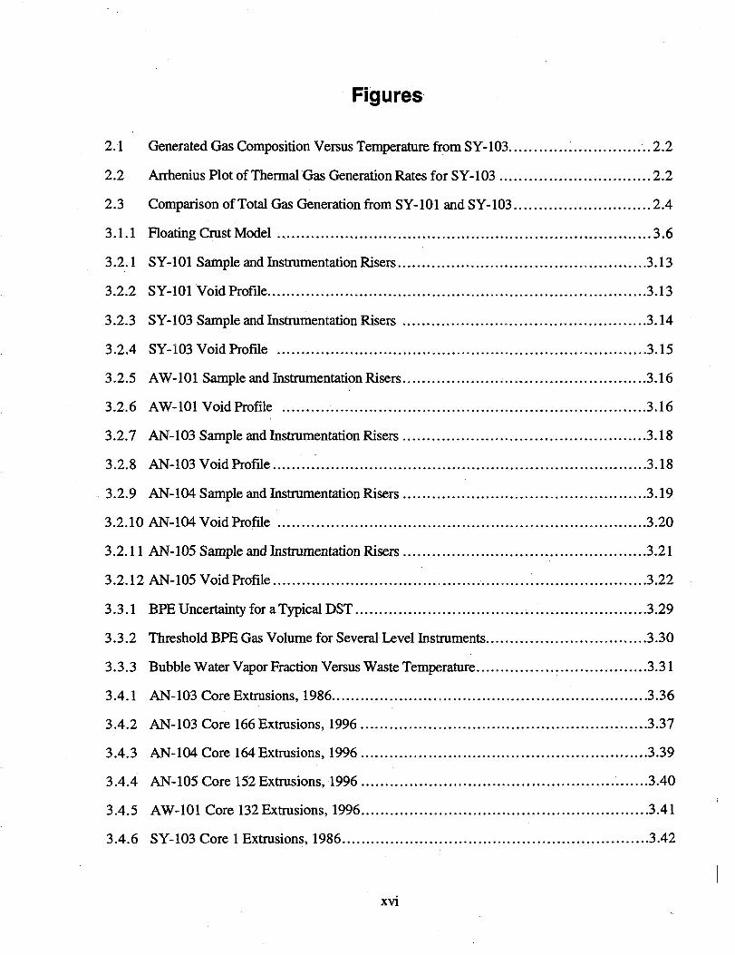
Figures
2.1 Generated Gas Composition Versus Temperature from SY-103 2.2
2.2 Arrhenius Plot of Thermal Gas Generation Rates for SY-103 2.2
2.3 Comparison of Total Gas Generation from SY-101 and SY-103 2.4
3.1.1 Floating Crust Model 3.6
3.2.1 SY-101 Sample and Instrumentation Risers 3.13
3.2.2 SY-101 Void Profile 3.13
3.2.3 SY-103 Sample and Instrumentation Risers 3.14
3.2.4 SY-103 Void Profile 3.15
3.2.5 AW-101 Sample and Instrumentation Risers 3.16
3.2.6 AW-101 Void Profile 3.16
3.2.7 AN-103 Sample and Instrumentation Risers 3.18
3.2.8 AN-103 Void Profile 3.18
3.2.9 AN-104 Sample and Instrumentation Risers 3.19
3.2.10 AN-104 Void Profile 3.20
3.2.11 AN-105 Sample and Instrumentation Risers 3.21
3.2.12 AN-105 Void Profile 3.22
3.3.1 BPE Uncertainty for a Typical DST 3.29
3.3.2 Threshold BPE Gas Volume for Several Level Instruments 3.30
3.3.3 Bubble Water Vapor Fraction Versus Waste Temp*;rature 3.31
3.4.1 AN-103 Core Extrusions, 1986 3.36
3.4.2 AN-103 Core 166 Extrusions, 1996 3.37
3.4.3 AN-104 Core 164 Extrusions, 1996 3.39
3.4.4 AN-105 Core 152 Extrusions, 1996 3.40
3.4.5 AW-101 Core 132 Extrusions, 1996 3.41
3.4.6 SY-103 Core 1 Extrusions, 1986 3.42
xv i
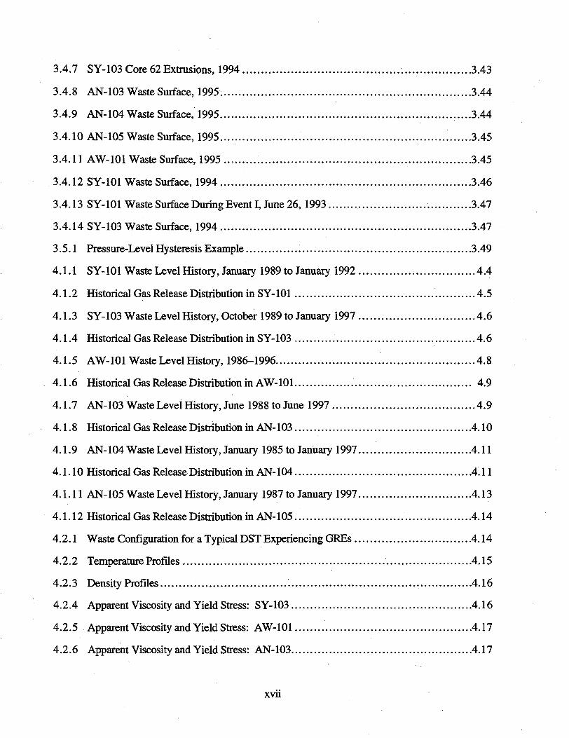
3.4.7 SY-103 Core 62 Extrusions, 1994 3.43
3.4.8 AN-103 Waste Surface, 1995. 3.44
3.4.9 AN-104 Waste Surface, 1995 3.44
3.4.10 AN-105 Waste Surface, 1995 3.45
3.4.11 AW-101 Waste Surface, 1995 3.45
3.4.12 SY-101 Waste Surface, 1994 3.46
3.4.13 SY-101 Waste Surface During Event I, June 26,1993 3.47
3.4.14 SY-103 Waste Surface, 1994 3.47
3.5.1 Pressure-Level Hysteresis Example 3.49
4.1.1 SY-101 Waste Level ffistory, January 1989 to January 1992 4.4
4.1.2 Historical Gas Release Distribution in SY-101 4.5
4.1.3 SY-103 Waste Level ffistory, October 1989 to January 1997 4.6
4.1.4 Historical Gas Release Distribution in SY-103 4.6
4.1.5 AW-101 Waste Level History, 1986-1996 4.8
4.1.6 Historical Gas Release Distribution in AW-101 4.9
4.1.7 AN-103 Waste Level History, June 1988toJune 1997 4.9
4.1.8 Historical Gas Release Distribution in AN-103 4.10
4.1.9 AN-104 Waste Level ffistory, January 1985 to January 1997 4.11
4.1.10 Historical Gas Release Distribution in AN-104 4.11
4.1.11 AN-105 Waste Level History, January 1987 to January 1997 4.13
4.1.12 Historical Gas Release Distribution in AN-105 4.14
4.2.1 Waste Configuration for a Typical DST Experiencing GREs 4.14
4.2.2 Temperature Profiles 4.15
4.2.3 Density Profiles 4.16
4.2.4 Apparent Viscosity and Yield Stress: SY-103 4.16
4.2.5 Apparent Viscosity and Yield Stress: AW-101 4.17
4.2.6 Apparent Viscosity and Yield Stress: AN-103 4.17
xvn
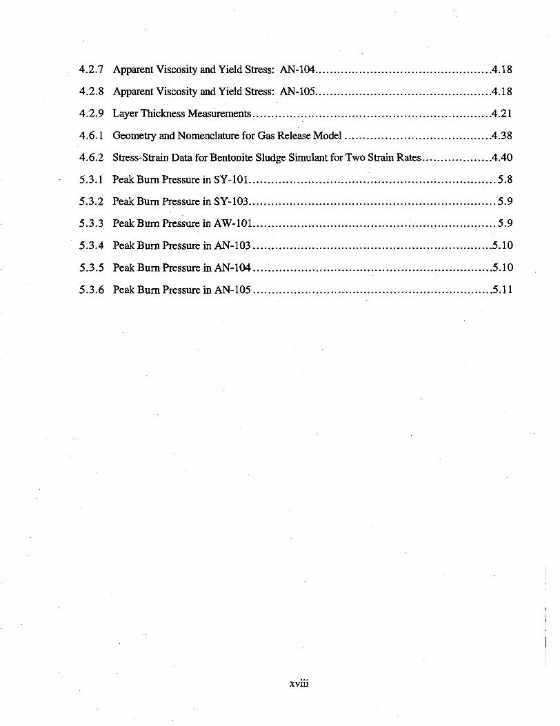
4.2.7 Apparent Viscosity and Yield Stress: AN-104 4.18
4.2.8 Apparent Viscosity and Yield Stress: AN-105 4.18
4.2.9 Layer Thickness Measurements 4.21
4.6.1 Geometry and Nomenclature for Gas Release Model 4.38
4.6.2 Stress-Strain Data for Bentonite Sludge Simulant for Two Strain Rates 4.40
5.3.1 Peak Burn Pressure in SY-101 5.8
5.3.2 Peak Burn Pressure in SY-103 5.9
5.3.3 PeakBurn Pressure in AW-101 5.9
5.3.4 Peak Burn Pressure in AN-103 5.10
5.3.5 Peak Burn Pressure in AN-104 5.10
5.3.6 Peak Bum Pressure in AN-105 5.11
xvm
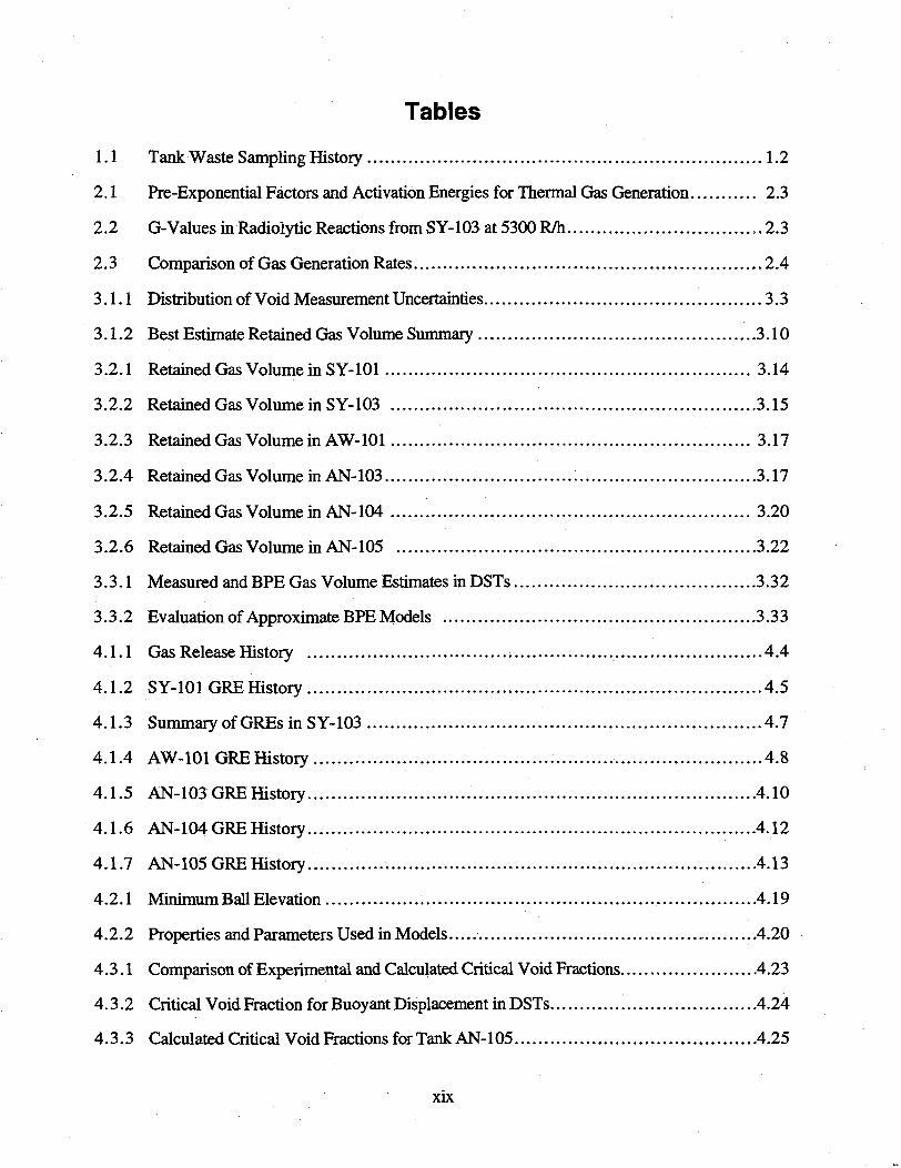
Tables
1.1 Tank Waste Sampling History 1.2
2.1 Pre-Exponential Factors and Activation Energies for Thermal Gas Generation 2.3
2.2 G-Values in Radiolytic Reactions from SY-103 at 5300 R/h 2.3
2.3 Comparison of Gas Generation Rates 2.4
3.1.1 Distribution of Void Measurement Uncertainties 3.3
3.1.2 Best Estimate Retained Gas Volume Summary 3.10
3.2.1 Retained Gas Volume in SY-101 3.14
3.2.2 Retained Gas Volume in SY-103 3.15
3.2.3 Retained Gas Volume in AW-101 3.17
3.2.4 Retained Gas Volume in AN-103 3.17
3.2.5 Retained Gas Volume in AN-104 3.20
3.2.6 Retained Gas Volume in AN-105 3.22
3.3.1 Measured and BPE Gas Volume Estimates in DSTs 3.32
3.3.2 Evaluation of Approximate BPE Models 3.33
4.1.1 Gas Release History 4.4
4.1.2 SY-101 GRE History 4.5
4.1.3 Summary of GREs in SY-103 4.7
4.1.4 AW-101 GRE History 4.8
4.1.5 AN-103 GRE History 4.10
4.1.6 AN-104 GRE History 4.12
4.1.7 AN-105 GRE History. 4.13
4.2.1 Minimum Ball Elevation 4.19
4.2.2 Properties and Parameters Used in Models 4.20
4.3.1 Comparison of Experimental and Calculated Critical Void Fractions, 4.23
4.3.2 Critical Void Fraction for Buoyant Displacement in DSTs 4.24
4.3.3 Calculated Critical Void Fractions for Tank AN-105 4.25
xix
4.5.1 Buoyant Displacement Model Results 4.35
4.5.2 Comparison of GRE Volume Predictions 4.37
4.6.1 The Energy Model Applied to Scaled Buoyant Displacement Experiments 4.41
4.6.2 Energy Ratio Calculated for Six DSTs.... ......: 4.41
5.1.1 Waste Gas Composition and Flammability Summary 5.3
5.2.1 Combustion Energies of Different Fuel-Oxidizer Pedrs 5.5
xx
1.0 Introduction
The primary purpose of this report is to present models developed or updated using the datafrom the retained gas sampler (RGS), void fraction instrument (VFI), and ball rheometer to predictgas retention and release behavior. Models have been developed for determining stored gasvolume, predicting peak pressure resulting from burning a specified fraction of stored gas volume,and predicting the potential size and frequency of buoyant displacement and whether a displace-ment event will release gas. A second major objective is to update the gas retention and releasecalculations given in Stewart et al. (1996a) with the new RGS and core sample data in Shekarriz etal. (1997). The models developed for gas generation based on waste sample testing by Bryan etal. (1996) are also summarized.
The flammable gas hazard in Hanford waste tanks was first recognized in the behavior ofdouble-shell tank (DST) 241-SY-101 (SY-101). The waste level in this tank began periodicallyrising and suddenly dropping shortly after it was filled in 1980. The large, "sawtooth" level dropswere taken as an indication of episodic gas releases that might pose a safety hazard. A period ofintense study of this tank's behavior in 1990-1992 revealed that these releases were, in fact,hazardous; the gas was indeed occasionally flammable, and the releases were quite large. Some ofthem had sufficient volume to exceed the lower flammability limit (LFL) in the entire head spaceand would probably have damaged the tank if the gas had been ignited.
The major concern in SY-101 was mitigated in late 1993 with the installation of a mixerpump that has prevented gas retention (Allemann et al. 1994; Stewart et al. 1994; Brewster et al.1995). But the experience with SY-101 created anxiety that other tanks might have similar largegas releases or the potential to do so, associating a perception of imminent danger with all 177waste tanks. We know now that this perception was not correct. The large episodic gas releasesin SY-101 were truly unique in size and hazard.
The historic gas releases in SY-101 prior to mixing were buoyancy-induced displacementevents, at one time called "rollovers" (Allemann et al. 1993). In a buoyant displacement, a portion,or "gob," of the nonconvective layer near the tank bottom accumulates gas until it becomessufficiently buoyant to overcome the weight and strength of material restraining it. At that point itsuddenly breaks away and rises through the supernatant liquid layer. The stored gas bubblesexpand as the gob rises, failing the surrounding matrix so a portion of the gas can escape from thegob into the head space.
Theory, experiment, and experience indicate that only the waste configuration found in theDSTs has the potential for significant gas releases by buoyant displacements. Only SY-103,AW-101, AN-103, AN-104, and AN-105 now actually exhibit this kind of episodic gas release,but these releases are typically less than 30 cubic meters in volume, compared with over 100 cubicmeters in SY-101.
These five tanks, plus SY-101, represent the six DSTs on the 25-tank Flammable GasWatch List (FGWL). The FGWL tanks were identified in response to Public Law 101-510,Section 3133 (the Wyden Amendment), as having a "serious potential for release of high levelwaste due to uncontrolled increases in temperature or pressure" from a flammable gas burn. Thisstatus has provided a powerful impetus for experiments, characterization, monitoring, and analyti-cal studies sufficient to fully understand the risk involved. Accordingly, the void fraction instru-ment (VFI), ball rheometer, and the RGS were developed and deployed in the FGWL DSTsstarting in December 1994. Gas generation tests on SY-103 waste samples were also performed in1996.
1.1
The gas retention and release behaviors of Hanford DSTs AN-103, AN-104, AN-105,AW-101, SY-101, and SY-103 have been characterized in detail by the ball rheometer and VFIduring operations from December 1994 to May 1996. The results of this testing campaign, givenin Stewart et al. (1996a), include the following:
• Waste configuration (thickness of the crust, convective, and nonconvective layers)• Rheology of the convective and nonconvective layers (viscosity and yield stress as a
function of shear rate, and density)• Retained gas volume and distribution (void fraction profile, effective pressure, and gas
volume of each waste layer)• Gas release behavior (gas release history, distribution of release volume and release
fraction, peak dome pressure during a hypothetical burn).
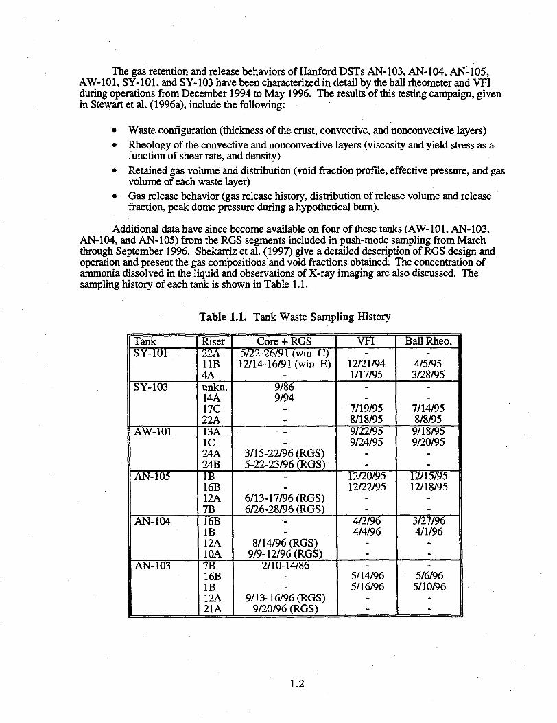
Additional data have since become available on four of these tanks (AW-101, AN-103,AN-104, and AN-105) from the RGS segments included in push-mode sampling from Marchthrough September 1996. Shekarriz et al. (1997) give a detailed description of RGS design andoperation and present the gas compositions and void fractions obtained: The concentration ofammonia dissolved in the liquid and observations of X-ray imaging are also discussed. Thesampling history of each tank is shown in Table 1.1.
Table 1.1. Tank Waste Sampling History
TankSY-101
SY-103
AW-101
AN-105
AN-104
AN-103
Riser22A11B4Aunkn.14A17C22A13A1C24A24BIB16B12A7B16BIB12A10A7B16BIB12A21A
Core + RGS5/22-26/91 (win. C)12/14-16/91 (win. E)
9/869/94
3/15-22/96 (RGS)5-22-23/96 (RGS)
6/13-17/96 (RGS)6/26-28/96 (RGS)
8/14/96 (RGS)9/9-12/96 (RGS)
2/10-14/86
9/13-16/96 (RGS)9/20/96 (RGS)
VFI
12/21/941/17/95
7/19/958/18/959/22/959/24/95
12/20/9512/22/95
4/2/964/4/96
5/14/965/16/96
Ball Rheo.
4/5/953/28/95
7/14/958/8/959/18/959/20/95
12/15/9512/18/95
3/27/964/1/96
5/6/965/10/96
1.2
The balance of this report is organized into four categories consistent with the importantaspects of the flammable gas safety issue: gas generation, retention, release, and the immediateconsequences of gas release, should the gas be ignited. Each is discussed in a separate section asindicated below.
An understanding of gas generation is important to successful operation of the waste tanksfor several reasons. First a knowledge of the gas generation rate is needed to verify mat any giventank has sufficient ventilation to keep flammable gas concentration at a safe level in the dome spacein the steady state (i.e., gas release equals generation rate). Understanding the generationmechanisms of the various gases is important for estimating the stored gas composition and inpredicting long-term effects. The results of recent gas generation testing on SY-103 waste samples(Bryan et al. 1996) and the current model for flammable gas generation are discussed in Section 2.
The gas retention calculations given in Stewart et al. (1996a) are updated with the newRGS and core sample data in Shekarriz et al. (1997) in Section 3. Except for the crust layer, theupdate did not change the gas volumes significantly. Recent photos of AN-103 and AN-104 coreextrusions and representative video frames of the waste surface in all six tanks complete the visualdata set. Since the gas distribution is now known in these six tanks, the stored gas volume can becalculated at any time from the waste level or barometric pressure response. These models are alsodescribed in Section 3.
Models that predict how a buoyant displacement event is initiated have been developedusing the waste rheology and configuration data as well as the observed gas release behavior.These models not only explain the gas releases in the six tanks tested but can also be used topredict whether other tanks (e.g., newly filled via transfers) will experience buoyant displacement.It has also been determined that only tanks with a waste configuration similar to these six DSTshave the potential for significant gas releases by buoyant displacement (Stewart et al. 1996b).These models are derived in Section 4.
Given the stored gas volume and its composition, the peak pressure during a hypotheticalburn can be estimated as a function of release fraction. The peak pressure model and the results aredescribed in Section 5. References cited can be found in Section 6.
The data acquired and the models developed to date are neither perfect nor complete. Wehave few data on the floating crust layer and on the particle shape and size distributions, forexample. However, we believe the current understanding is sufficient to assess the potentialflammable gas risk in the tanks studied in this report, under storage operations, for the foreseeablefuture. In any event, since no new waste-intrusive measurements are planned in these tanks,temperature profiles, waste level, and head-space gas monitoring represent the only new dataavailable for a long time to come.
1.3
2.0 Gas Generation Models
The current knowledge of gas generation has been summarized by Pederson and Bryan(1996). While the VFI and RGS data do not directly support gas generation studies, the gascompositions from the RGS provide an independent, though indirect, measure of the relative gasgeneration rates of the various species. This section provides a brief overview of the models forthe kinetics of gas generation and current laboratory results to measure and predict gas generation.
Gas generation in the waste results from radiation-induced chemical decomposition ofwater and some organic species and from thermally induced chemical decomposition, mainlyinvolving organic complexants and solvents. The effects of radiation on the generation of gases(Meisel et al. 1993) and the thermal degradation of the organic species (Barefield et al. 1995,1996)have been evaluated through studies of synthetic waste mixtures. More recently, the focus hasbeen on testing actual tank waste samples (Bryan et al. 1996; Person 1996).
2.1 Studies Using Actual Waste
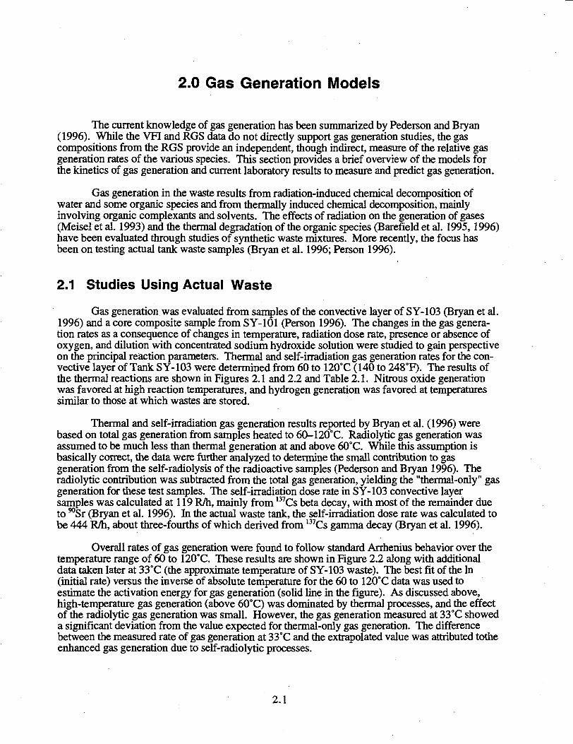
Gas generation was evaluated from samples of the convective layer of SY-103 (Bryan et al.1996) and a core composite sample from SY-101 (Person 1996). The changes in the gas genera-tion rates as a consequence of changes in temperature, radiation dose rate, presence or absence ofoxygen, and dilution with concentrated sodium hydroxide solution were studied to gain perspectiveon die principal reaction parameters. Thermal and self-irradiation gas generation rates for the con-vective layer of Tank SY-103 were determined from 60 to 120°C (140 to 248°F). The results ofthe thermal reactions are shown in Figures 2.1 and 2.2 and Table 2.1. Nitrous oxide generationwas favored at high reaction temperatures, and hydrogen generation was favored at temperaturessimilar to those at which wastes are stored.
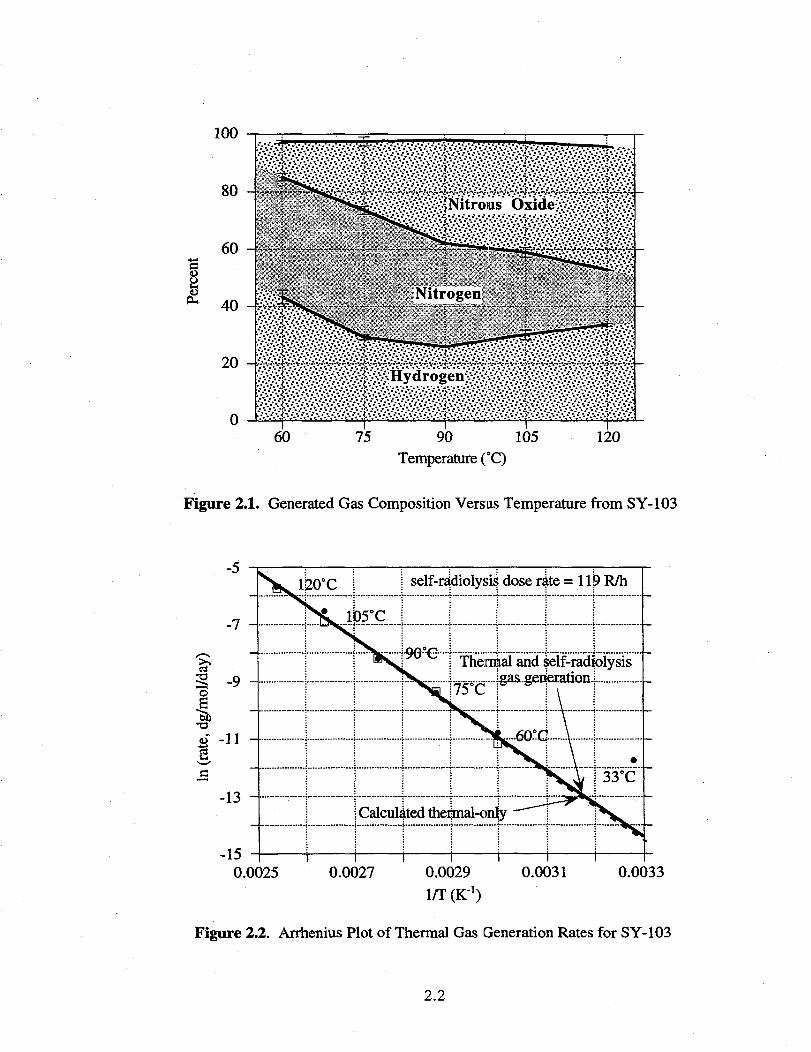
Thermal and self-irradiation gas generation results reported by Bryan et al. (1996) werebased on total gas generation from samples heated to 60-120°C. Radiolytic gas generation wasassumed to be much less than thermal generation at and above 60°C. While this assumption isbasically correct, the data were further analyzed to determine the small contribution to gasgeneration from the self-radiolysis of the radioactive samples (Pederson and Bryan 1996). Theradiolytic contribution was subtracted from the total gas generation, yielding the "thermal-only" gasgeneration for these test samples. The self-irradiation dose rate in SY-103 convective layersamples was calculated at 119 R/h, mainly from 137Cs beta decay, with most of the remainder dueto ^Sr (Bryan et al. 1996). In the actual waste tank, the self-irradiation dose rate was calculated tobe 444 R/h, about three-fourths of which derived from 137Cs gamma decay (Bryan et al. 1996).
Overall rates of gas generation were found to follow standard Arrhenius behavior over thetemperature range of 60 to 120°C. These results are shown in Figure 2.2 along with additionaldata taken later at 33°C (the approximate temperature of SY-103 waste). The best fit of the In(initial rate) versus the inverse of absolute temperature for the 60 to 120°C data was used toestimate the activation energy for gas generation (solid line in the figure). As discussed above,high-temperature gas generation (above 60°C) was dominated by thermal processes, and the effectof the radiolytic gas generation was small. However, the gas generation measured at 33°C showeda significant deviation from the value expected for thermal-only gas generation. The differencebetween the measured rate of gas generation at 33°C and the extrapolated value was attributed totheenhanced gas generation due to self-radiolytic processes.
2.1
gIOk
100
80 -
60
40 -
20 -
060 75 105 120
Temperature (°C)
Figure 2.1. Generated Gas Composition Versus Temperature from SY-103
i self-rajdiolysis; dose r^te = 1 lp R/h
Thenaal and self-radiolysisIgas-geEierationi
-13 —
-15
! Calculated theijmal-oniy, — * ™.,
T i l l
0.0025 0.0027 0.00291 r
0.0031 0.0033
Figure 2.2. Arrhenius Plot of Thermal Gas Generation Rates for SY-103
2.2
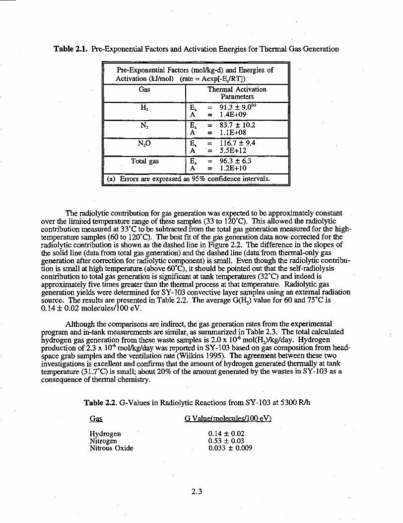
Table 2.1. Pre-Exponential Factors and Activation Energies for Thermal Gas Generation
Pre-Exponential Factors (mol/kg-d) and Energies ofActivation (kJ/mol) (rate = Aexp[-Ea/RT])
Gas
H2
N2
N2O
Total gas
Thermal ActivationParameters
Ea = 91.3 ± 9.0<a)
A = 1.4E+09Ea = 83.7 ± 10.2A = 1.1E+08Ea = 116.7 ±9.4A = 5.5E+12Ea = 96.3 + 6.3A = 1.2E+10
(a) Errors are expressed as 95% confidence intervals.
The radiolytic contribution for gas generation was expected to be approximately constantover the limited temperature range of these samples (33 to 120°C). This allowed the radiolyticcontribution measured at 33 °C to be subtracted from the total gas generation measured for die high-temperature samples (60 to 120°C). The best fit of the gas generation data now corrected for theradiolytic contribution is shown as the dashed line in Figure 2.2. The difference in the slopes ofthe solid line (data from total gas generation) and the dashed line (data from thermal-only gasgeneration after correction for radiolytic component) is small. Even though the radiolytic contribu-tion is small at high temperature (above 60°C), it should be pointed out that the self-radiolysiscontribution to total gas generation is significant at tank temperatures (32°C) and indeed isapproximately five times greater than the thermal process at that temperature. Radiolytic gasgeneration yields were determined for SY-103 convective layer samples using an external radiationsource. The results are presented in Table 2.2. The average G(H2) value for 60 and 75°C is0.14 + 0.02 molecules/100 eV.
Although the comparisons are indirect, the gas generation rates from the experimentalprogram and in-tank measurements are similar, as summarized in Table 2.3. The total calculatedhydrogen gas generation from these waste samples is 2.0 x 10"6 mol(H2)/kg/day. Hydrogenproduction of 2.3 x 10"6 mol/kg/day was reported in SY-103 based on gas composition from head-space grab samples and the ventilation rate (Wilkins 1995). The agreement between these twoinvestigations is excellent and confirms that the amount of hydrogen generated thermally at tanktemperature (31.7°C) is small; about 20% of the amount generated by the wastes in SY-103 as aconsequence of thermal chemistry.
Table 2.2. G-Values in Radiolytic Reactions from SY-103 at 5300 R/h
G Value(molecules/100 eV)
0.14 ± 0.020.53 ± 0.030.033 ± 0.009
HydrogenNitrogenNitrous Oxide
2.3
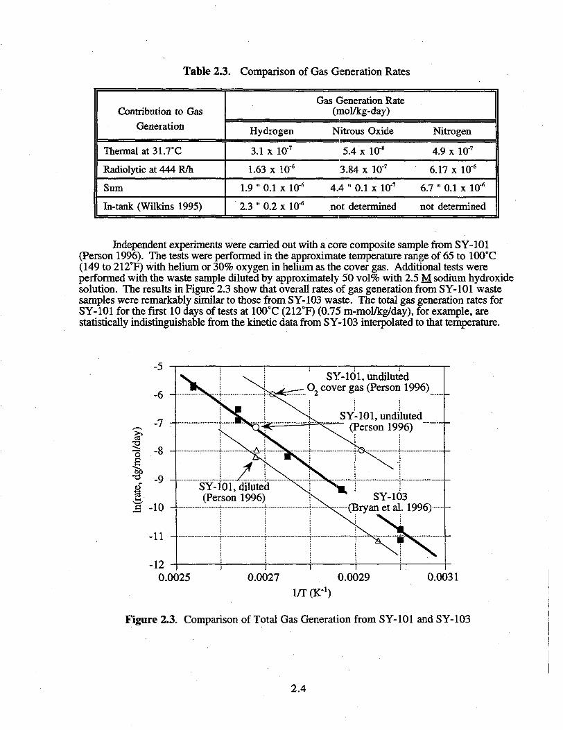
Table 2.3. Comparison of Gas Generation Rates
Contribution to Gas
Generation
Thermal at 31.7°C
Radiolytic at 444 R/h
Sum
In-tank (Wilkins 1995)
Hydrogen
3.1 x 10'
1.63 x 10⁶
1.9 " 0.1 x 10*
2.3 " 0.2 x 10*
Gas Generation Rate(mol/kg-day)
Nitrous Oxide
5.4 x Iff*
3.84 x 10'
4.4 " 0.1 x Iff7
not determined
Nitrogen
4.9 x Iff7
6.17 x Iff6
6.7 " 0.1 x 10*
not determined
Independent experiments were carried out with a core composite sample from SY-101(Person 1996). The tests were performed in the approximate temperature range of 65 to 100°C(149 to 212°F) with helium or 30% oxygen in helium as the cover gas. Additional tests wereperformed with the waste sample diluted by approximately 50 vol% with 2.5 M sodium hydroxidesolution. The results in Figure 2.3 show that overall rates of gas generation from SY-101 wastesamples were remarkably similar to those from SY-103 waste. The total gas generation rates forSY-101 for the first 10 days of tests at 100°C (212°F) (0.75 m-mol/kg/day), for example, arestatistically indistinguishable from the kinetic data from SY-103 interpolated to that temperature.
SY-101, undilutedO cover gas (Person 1996)
SY-101,(Person
SY-101, diluted(Person 1996) SY-103
^Bryan et al. 1996)
-120.0025
1/T (K"1)
Figure 2.3. Comparison of Total Gas Generation from SY-101 and SY-103
2.4
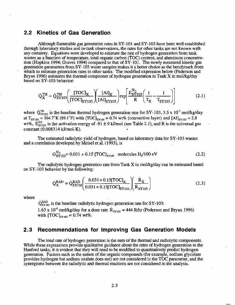
2.2 Kinetics of Gas Generation
Although flammable gas generation rates in SY-101 and SY-103 have been well establishedthrough laboratory studies and in-tank observations, the rates for other tanks are not known withany certainty. Equations were developed to estimate the rate of hydrogen generation from tankwastes as a function of temperature, total organic carbon (TOC) content, and aluminum concentra-tion (Hopkins 1994; Graves 1994) compared to that of SY-101. The newly measured kinetic gasgeneration parameters from SY-103 waste samples makes it a better choice as the benchmark fromwhich to estimate generation rates in other tanks. The modified expression below (Pederson andBryan 1996) estimates the thermal component of hydrogen generation in Tank X in mol/kg/daybased on SY-103 behavior:
Q l f l _X -
_ ATH^SY103
[TQC]X Y [Ai]
l[TOC]SY103JjAl] expS Y 1 0 3
ESY103
R lSY103.
(2.1)
where Q™103 is the baseline thermal hydrogen generation rate for SY-103, 3.5 x 10'7 mol/kg/daya t Tsvio3 = 304.7°K (89.1°F) with [TOC]SY103 = 0.74 wt% (convective layer) and [A1]SY1O3 = 2.8wt%, EsY103 is the activation energy of -91 + 9 kJ/mol (see Table 2.1), and R is the universal gasconstant (0.008314 kJ/mol-K).
The estimated radiolytic yield of hydrogen, based on laboratory data for SY-103 wastesand a correlation developed by Meisel et al. (1993), is
GSYi03= ° - 0 3 1 + 0 J 5 [TOC]SYIO3 molecules H/lOO eV (2.2)
The radiolytic hydrogen generation rate from Tank X in mol/kg/day can be estimated basedon SY-103 behavior by the following:
ARAD _ ARAD ( 0.031 + 0.15[TOC]X Y R x
-.031 + 0.15[TOC]S Y 1 0 3 | i^703 _(2.3)
whereQSYIO3 ^s m e baseline radiolytic hydrogen generation rate for SY-103:
1.63 x 10'6 mol/kg/day for a dose rate RSY103 = 444 R/hr (Pederson and Bryan 1996)with [TOC]SY103 = 0.74 wt%.
2.3 Recommendations for Improving Gas Generation Models
The total rate of hydrogen generation is the sum of the thermal and radiolytic components.While these expressions provide qualitative guidance about the rates of hydrogen generation in theHanford tanks, it is evident that they will need to be modified to quantitatively predict hydrogengeneration. Factors such as the nature of the organic compounds (for example, sodium glycolateprovides hydrogen but sodium oxalate does not) are not considered in the TOC parameter, and thesynergisms between the radiolytic and thermal reactions are not considered in the analysis.
2.5
Significant differences exist in composition among Hanford waste tanks. As a result, gasgeneration behaviors are expected to vary considerably. Most of the technical work has focused onchelator and chelator fragments, which dissolve in the liquid fraction. Other wastes contain sol-vents that are largely insoluble in the liquid fraction and may decompose by totally different path-ways. Laboratory gas generation studies using actual waste mixtures that represent different wasteclasses will significantly enhance our ability to predict gas generation behavior in Hanford wastes.
2.6
TWSFG97.51
Pacific Northwest National LaboratoryOperated by Battelle for the U.S. Department of Energy
July 15,1997
Distribution
Holders of PNNL-11536,
PNNL-11536, Gas Retention and Release Behavior in Hanford Double-Shell Waste Tanks, published by PacificNorthwest National Laboratory in May 1997, contained errors. Please replace the erroneous pages with theidentically numbered attached corrected versions.
The layer dimensions listed on the void fraction profile plots have been corrected and are now consistent with thoselisted in the corresponding tables. Equation 2.1 has also been corrected.
Also of importance, note that these corrections are to be made to PNNL-11536 Rev 1, which supercedes Rev 0.
Thanks,
Joe Brothers
jwb
Attachment
cc: File/LB
OSTI
MASTERatSTRIBUTlQN OF THIS DOCUMENT IS UNLlMfT
Battelle Boulevard • P.O. Box 999 • Richland, WA 99352
Telephone (509) 375-2396 • Email [email protected] • Fax (509) 372-4600
3.0 Gas Retention Models
This section of the report gives the current estimates of the retained gas volume, itsdistribution, and its composition from data obtained with the VFI and RGS over the past twoyears. The gas volume and distribution in each tank are provided in Section 3.1 (the gas compo-sitions derived from RGS data and gas generation studies are given in Section 5). The barometricpressure effect (BPE) and surface level effect (SLE) models for determining the retained gasvolume indirectly are derived and evaluated in Section 3.3. The collection of extrusion and wastesurface photos is presented in Section 3.4. Recommendations for improving gas retention modelsand data are given in Section 3.5.
3.1 Retained Gas Volume
The gas volume of each waste in SY-101, SY-103, AW-101, AN-103, AN-104, andAN-105 was calculated from VFI measurements in Stewart et al. (1996a). Since then, the RGShas provided additional void fraction data in AN-103, AN-104, AN-105, and AW-101 that arenow included in the overall data set. The non-RGS core samples also provided current noncon-vective layer densities in AN-103 and AN-104 that were not available when the initial volumecalculations were performed.00 The revised data are
1. Void fractions determined from the RGS segments are included in gas volumecalculations in AN-103,00 AN-104, AN-105, and AW-101.
2. Nonconvective layer densities measured from 1996 cores from AN-103 and AN-104are used in pressure and volume calculations (recent cores from AW-101 and AN-105were already available for Stewart et al. [1996a]).
This section describes the updated volume calculations and the method by which the RGS voiddata were combined with the existing VFI measurements.
3.1.1 Average Void Fraction
The RGS void fractions are ascribed to their own risers to correctly capture the effect ofimproved spatial coverage. Because the RGS waste sample is 48 cm in length, which is approxi-mately the vertical spacing between VFI measurements (30-60 cm), one RGS segment coversapproximately the same vertical distance as two VFI samples.(c) Accordingly, each RGS result wasconverted to two data points: one at the reported value, the other allowed to vary randomly aboutthe reported value to maintain the variance structure among the original RGS void data. Therandom variation was modeled by a normal distribution with zero mean and standard deviationequal to 10% of the data value, which is the approximate uncertainty ascribed to the RGS voidmeasurement (Shekarriz et al. 1997). The elevation of both data points was set to the midpoint ofthe 48-cm (19-in.) sample. A single location was used because the distribution of gas in thesegment is not known, and it is reasonable to use the midpoint for the average void.
(a) Density values were obtained from the LABCOR database by RL Bechtold on 12/18/96.(b) The AN-103 RGS void fractions were corrected to account for changes in the extraction
procedure for that tank and do not match the values given in Shekarriz et al. (1997).(c) However, the 367-cm3 VFI sample volume is actually larger than the 243 cm of waste
contained in a full RGS segment.
3.1
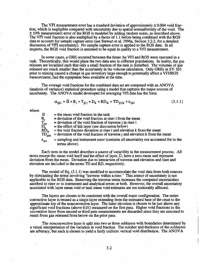
The VH measurement error has a standard deviation of approximately ± 0.004 void frac-tion, which is negligible compared with uncertainty due to spatial nonuniformity of the void. The±10% measurement error of the RGS is modeled by adding random noise, as described above.The VH void fraction is also multiplied by a factor of 1.1 before being combined with the RGSdata to account for sample capture error (see Stewart et al. 1996a, Section 3.2.2, for a detaileddiscussion of VFI uncertainty). No sample capture error is applied to the RGS data. In allrespects, the RGS void fraction is assumed to be equal in quality to a VFI measurement.
In some cases, a GRE occurred between the times the VFI and RGS were operated in atank. Theoretically, this would place the two data sets in different populations. In reality, the gasreleases are localized such that only a small fraction of the tank is disturbed. The volumes of gasreleased are much smaller than the uncertainty in the volume calculation. Only GREs in SY-101prior to mixing caused a change in gas inventory large enough to potentially affect a VFI/RGSmeasurement, had the equipment been available at the time.
The average void fractions for the combined data set are computed with an ANOVA(analysis of variance) statistical procedure using a model mat captures the major sources ofuncertainty. The ANOVA model developed for averaging VFI data has the form
am = a + R i +T j ( i ) +D k +RD i k +TD j ( i ) k +e i j k l (3.1.1)
where __a = the mean void fraction in the tankR. = deviation of the void fraction at riser i from the meanTCl) = deviation of the void fraction of traverse j in riser iD k = the effect of kth layer (see discussion below)RD i k = the void fraction deviation at riser i and elevation k from the meanTD j0)k = deviation of the void fraction of traverse j and elevation k from the meane.jkl = sampling and instrument error (contains all uncertainty not accounted for in the
terms above).
Each term in the model describes a source of variability in the measurement process. Allterms except the mean void itself and the effect of layer, D, have a zero mean and representdeviation from the mean. Deviation due to interaction of traverse and elevation and riser andelevation are included in the terms TD and RD, respectively.
The model of Eq. (3.1.1) was modified to accommodate the void data from both sourcesby eliminating the terms involving "traverse within a riser." This source of uncertainty is notapplicable to the RGS data. Removing the traverse terms increases the computed uncertaintiesascribed to riser or to instrument and analytical errors or both. However, the overall uncertaintyassociated with layer mean void or tank mean void estimates are not noticeably affected.
The layers are chosen to be consistent with the overall waste configuration. The entireconvective layer is treated as a single layer extending from the estimated base of the crust to theapproximate top of the nonconvective layer. The latter elevation is chosen to be just above anysignificant void fractions (above 0.01) measured on the first pass. Higher void fractions in theconvective layer from second or third pass measurements are discarded since they are assumed toresult from gas released from below on the prior pass.
The nonconvective layer is split into two or three sublayers with boundaries determined bya visual interpretation of the variation in void fraction. The number and thickness of the sublayersare arbitrary, but each is chosen to yield a fairly uniform vertical void distribution. The ANOVA
3.2
model emphasizes predicting the mean void fraction in each layer of a tank. For estimating the totalgas volume stored in a tank, this is more important than predicting the exact void fraction profile.
Although measurements are made in only a few risers (two VFI and two RGS), it islegitimate to estimate horizontal variation based on the data. There remains a potential for missingimportant horizontal variation, but if the void profile in the two risers is nearly the same, the chanceof an undetected nonuniformity is small. Likewise, if the two risers show a very different voidprofile, it is unlikely that the uncertainty due to any undetected void variation would be larger.This procedure has been used to estimate the horizontal variation of tank chemical contents basedon core samples from two risers (Hartley et al. 1995).
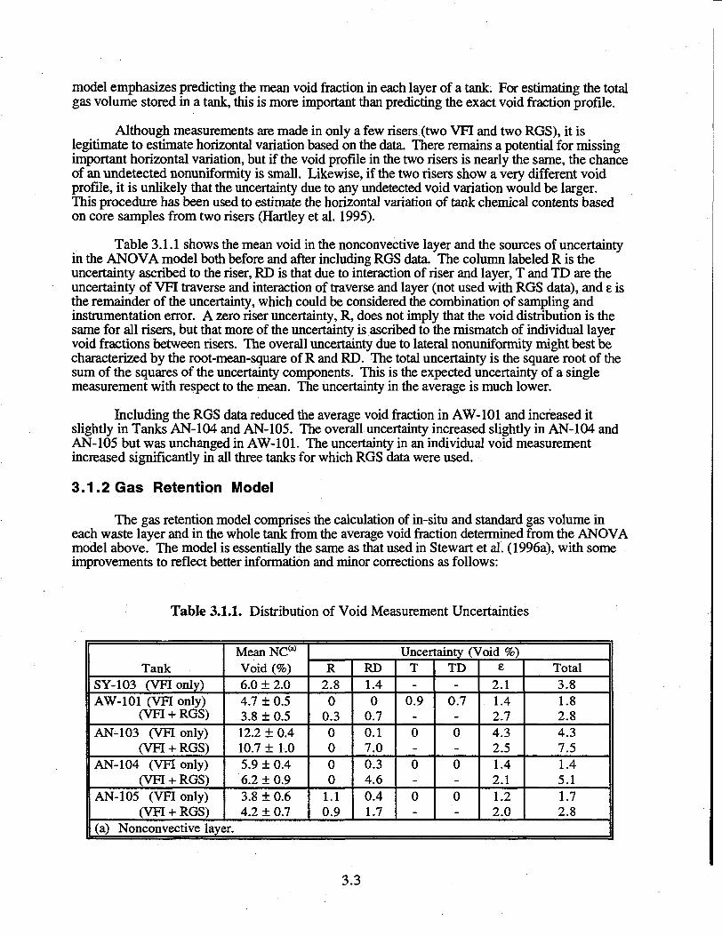
Table 3.1.1 shows the mean void in the nonconvective layer and the sources of uncertaintyin the ANOVA model both before and after including RGS data. The column labeled R is theuncertainty ascribed to the riser, RD is that due to interaction of riser and layer, T and TD are theuncertainty of VFI traverse and interaction of traverse and layer (not used with RGS data), and e isthe remainder of the uncertainty, which could be considered the combination of sampling andinstrumentation error. A zero riser uncertainty, R, does not imply that the void distribution is thesame for all risers, but that more of the uncertainty is ascribed to the mismatch of individual layervoid fractions between risers. The overall uncertainty due to lateral nonuniformity might best becharacterized by the root-mean-square of R and RD. The total uncertainty is the square root of thesum of the squares of the uncertainty components. This is the expected uncertainty of a singlemeasurement with respect to the mean. The uncertainty in the average is much lower.
Including the RGS data reduced the average void fraction in AW-101 and increased itslightly in Tanks AN-104 and AN-105. The overall uncertainty increased slightly in AN-104 andAN-105 but was unchanged in AW-101. The uncertainty in an individual void measurementincreased significantly in all three tanks for which RGS data were used.
3.1.2 Gas Retention Model
The gas retention model comprises the calculation of in-situ and standard gas volume ineach waste layer and in the whole tank from the average void fraction determined from the ANOVAmodel above. The model is essentially the same as that used in Stewart et al. (1996a), with someimprovements to reflect better information and minor corrections as follows:
Table 3.1.1. Distribution of Void Measurement Uncertainties
TankSY-103 (VFI only)AW-101 (VFI only)
(VFI + RGS)AN-103 (VFI only)
(VFI + RGS)AN-104 (VFI only)
(VFI + RGS)AN-105 (VFI only)
(VFI + RGS)
Mean NC(a)
Void (%)6.0 ± 2.04.7 + 0.53.8 ± 0.512.2 ± 0.410.7 + 1.05.9 ± 0.46.2 + 0.93.8 ± 0.64.2 ± 0.7
Uncertainty (Void %)R
2.80
0.30000
1.10.9
RD1.40
0.70.17.00.34.60.41.7
T-
0.9
0
0
0
TD-
0.7
0
0
0
e2.11.42.74.32.51.42.11.22.0
Total3.81.82.84.37.51.45.11.72.8
(a) Nonconvective layer.
3.3
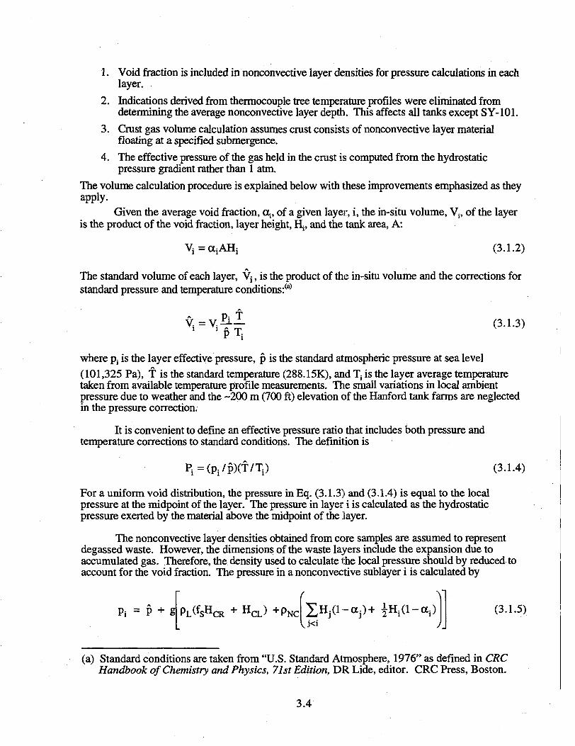
1. Void fraction is included in nonconvective layer densities for pressure calculations in eachlayer.
2. Indications derived from thermocouple tree temperature profiles were eliminated fromdetermining the average nonconvective layer depth. This affects all tanks except SY-101.
3. Crust gas volume calculation assumes crust consists of nonconvective layer materialfloating at a specified submergence.
4. The effective pressure of the gas held in the crust is computed from the hydrostaticpressure gradient rather than 1 atm.
The volume calculation procedure is explained below with these improvements emphasized as theyapply.
Given the average void fraction, a,, of a given layer, i, the in-situ volume, Vj, of the layeris the product of the void fraction, layer height, Hj, and the tank area, A:
V^ctiAHi (3.1.2)
The standard volume of each layer, Vj, is the product of the in-situ volume and the corrections forstandard pressure and temperature conditions:(a)
V ^ V ^ ^ (3.1.3)
where Pj is the layer effective pressure, p is the standard atmospheric pressure at sea level
(101,325 Pa), T is the standard temperature (288.15K), and T, is the layer average temperaturetaken from available temperature profile measurements. The small variations in local ambientpressure due to weather and the ~200 m (700 ft) elevation of the Hanford tank farms are neglectedin the pressure correction.
It is convenient to define an effective pressure ratio that includes both pressure andtemperature corrections to standard conditions. The definition is
P i =(P i / p ) ( t /T i ) (3.1.4)
For a uniform void distribution, the pressure in Eq. (3.1.3) and (3.1.4) is equal to the localpressure at the midpoint of the layer. The pressure in layer i is calculated as the hydrostaticpressure exerted by the material above the midpoint of the layer.
The nonconvective layer densities obtained from core samples are assumed to representdegassed waste. However, the dimensions of the waste layers include the expansion due toaccumulated gas. Therefore, the density used to calculate the local pressure should by reduced toaccount for the void fraction. The pressure in a nonconvective sublayer i is calculated by
Pi = P + g pL(fsHCR + HCL) +pN CXH j<1-cx j>+ ±11, (3.1.5)
(a) Standard conditions are taken from "U.S. Standard Atmosphere, 1976" as defined in CRCHandbook of Chemistry and Physics, 71st Edition, DR Lide, editor. CRC Press, Boston.
3.4
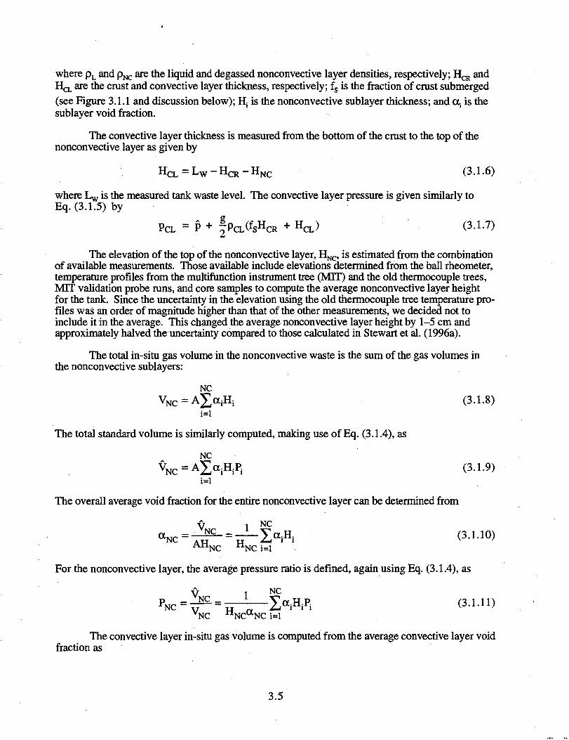
where pL and pNC are the liquid and degassed nonconvective layer densities, respectively; H ^ andHCL are the crust and convective layer thickness, respectively; fs is the fraction of crust submerged(see Figure 3.1.1 and discussion below); H; is the nonconvective sublayer thickness; and a, is thesublayer void fraction.
The convective layer thickness is measured from the bottom of the crust to the top of thenonconvective layer as given by
HQL = Lw ~ HQR — H N C (3.1.6)
where L^ is the measured tank waste level. The convective layer pressure is given similarly toEq. (3.1.5) by
PCL = P + f PcL(fsHCR + H CL> C3-1-7)
The elevation of the top of the nonconvective layer, HNC, is estimated from the combinationof available measurements. Those available include elevations determined from the ball rheometer,temperature profiles from the multifunction instrument tree (MTT) and the old thermocouple trees,MTT validation probe runs, and core samples to compute the average nonconvective layer heightfor the tank. Since the uncertainty in the elevation using the old thermocouple tree temperature pro-files was an order of magnitude higher than that of the other measurements, we decided not toinclude it in the average. This changed the average nonconvective layer height by 1-5 cm andapproximately halved the uncertainty compared to those calculated in Stewart et al. (1996a).
The total in-situ gas volume in the nonconvective waste is the sum of the gas volumes inthe nonconvective sublayers:
NC
xiHi (3.1.8)
The total standard volume is similarly computed, making use of Eq. (3.1.4), as
NC
(3.1.9)
The overall average void fraction for the entire nonconvective layer can be determined from
V i NC(3.1-10)
C n NC i=l
For the nonconvective layer, the average pressure ratio is defined, again using Eq. (3.1.4), as
V 1 N C
VNC n N C U N C i=l
The convective layer in-situ gas volume is computed from the average convective layer voidfraction as
3.5
CL (3.1.12)
The standard volume in the convective layer is the product of the in-situ volume and the pressureratio derived from Eq. (3.1.4) and (3.1.7) as
rCL (3.1.13)
The crust volume calculation is the most significant change from the calculations in Stewartet al. (1996a), reducing the estimated gas volume in the crust by about half. The original calcula-tion was derived for SY-101 (Brewster et al. 1995) and conservatively assumed a crust density of2.0 g/cc floating on a liquid with a density of 1.46 g/cc (approximately that of centrifuged liquidfrom Window E samples). A void fraction of 0.25 was required to float this crust.
Observations from recent core samples indicate that the crust probably consists of the samematerial as the nonconvective layer. The extrusion photos from the few recent DST core samplesthat included crust material show that the crust and nonconvective layer have a very similarappearance (see Figures 3.4.2, 3.4.5, and 3.4.6). At the same time, the single RGS void fractionmeasurement from the crust of AN-103 indicates a void fraction of about 0.15, which is close tothe estimated neutral buoyancy value and of the same magnitude as the peak void fraction in thenonconvective layer.
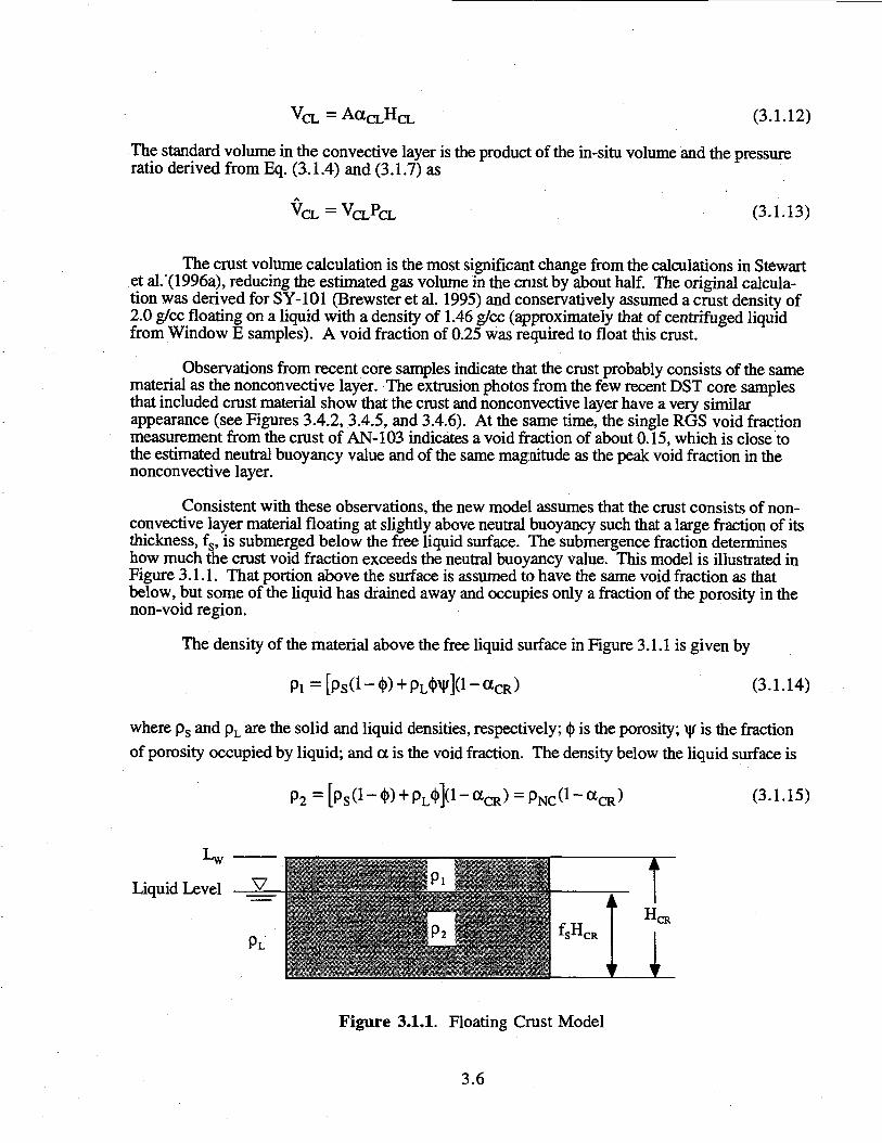
Consistent with these observations, the new mode! assumes that the crust consists of non-convective layer material floating at slightly above neutral buoyancy such that a large fraction of itsthickness, fs, is submerged below the free liquid surface. The submergence fraction determineshow much the crust void fraction exceeds the neutral buoyancy value. This model is illustrated inFigure 3.1.1. That portion above the surface is assumed to have the same void fraction as thatbelow, but some of the liquid has drained away and occupies only a fraction of the porosity in thenon-void region.
The density of the material above the free liquid surface in Figure 3.1.1 is given by
(3.1.14)
where p s and pL are the solid and liquid densities, respectively; <(> is the porosity; \j/ is the fraction
of porosity occupied by liquid; and a is the void fraction. The density below the liquid surface is
p2 = [ps(l - = pNC(l - a (3.1.15)
Liquid Level
PL
Figure 3.1.1. Floating Crust Model
3.6
Balancing the weight of the crust with buoyancy using Archimedes' principle and solving for thecrust void fraction yields
^ ( 3 . 1 . 1 6 )pN C-(l-fs)(l-¥)pL<t>
With fs = 1, Eq. (3.1.16) degenerates to the expression for the neutral buoyancy void fraction.
As yet we have no reliable data on porosity or the moisture fraction, \|f, in the unsubmergedportion. However, with the (l-fs) coefficient, Eq. (3.1.16) is not very sensitive to the choice ofvalues for these parameters. Assuming a porosity of 0.4{a) and that capillary forces pull sufficient
moisture into the unsubmerged portion that half of its porosity is occupied by liquid (\|f=0.5),Eq. (3.1.16) becomes
^ £ ( 3 . 1 . 1 7 )lp N C -0 .2 (1 - f s )p L
where <|>(l-i|0=0.4*(l-0.5)=0.2.
The value of the submergence fraction is quite subjective since there is a void measurementin only one tank. A submergence fraction of 0.95 was chosen for AN-103 so that the crust voidfraction given by Eq. (3.1.17) agrees with the RGS measurement of 0.15. The difference betweenthe two level instruments in SY-101 is about 18 cm, which indicates that only 82-85% of the crustis submerged. However, this yields a void fraction of over 0.20, which is far above neutralbuoyancy. Thus we arbitrarily chose a 90% submergence, for a void fraction of 0.16. Thesubmergence fraction in other tanks was chosen in the same subjective way.
The effective pressure is the hydrostatic pressure at the midpoint of the submerged portionof the crust:
PCR = P + rPcLfsHCR (3.1.18)
The gas in the crust was assumed to be held at 1 atm in the original model. While this is a goodapproximation, a better estimate is obtained using the hydrostatic pressure gradient.
The in-situ crust gas volume calculated using the void fraction from Eq. (3.1.17). Thestandard crust volume corrects the in-situ volume to standard conditions using Eq. (3.1.18) alongwith Eq. (3.1.4). The crust in-situ and standard volumes are given, respectively, by
VcR=AaC R f sHC R (3.1.19)
V C R - V C R P C R (3.1.20)
The total in-situ and standard gas volumes in the entire tank are the sums of thecontributions of individual layers. They are given, respectively, by
(a) Saltcake porosity was estimated at 0.3 to 0.4 in an unpublished report on BY-107 pumpingtests by WP Metz in 1976: "A topical report on interstitial liquid removal from Hanford saltcakes," ARH-CD-545. The "drainable porosity" from saltwell pumping records in Caley et al.(1996) shows a range from <0.1 to 0.66 with an average around 0.4.
3.7
V G = V N C + V C L + V C R C3-
V G = V N C + V C L + V C R (3.1.22)
The overall tank effective pressure ratio is computed as the ratio of standard volume to in-situvolume.
^r (3-L23)
G
The degassed level represents the waste level after all the in-situ retained gas in the nonconvectivelayer was removed. It is computed by
LNO-GAS = LW - V N C / A (3.1.24)
3.1.3 Gas Volume Uncertainties
In general, uncertainties given represent one standard deviation and are estimated by linearpropagation through their defining equations, assuming each parameter was independent. If y is afunction of N variables, y = F(x,, x2,...xN), each with uncertainty, a;, the standard error isexpressed as
(3.1.25)
The uncertainties in the in-situ and standard gas volume in each layer depend mainly on theuncertainty of mean void fraction in that layer. However, the uncertainties of layer height,pressure, and temperature are included for completeness. Based on Eq. (3.1.2), (3.1.3), and(3.1.25), these are expressed as
^ (3.1.26)
and
]2 +[Vj /pOVT^Cpj]2 + [Vi(Pi /p)(f / T ^ O T , ] 2 (3.1.27)
where the uncertainty in the void fraction is provided by the statistical model described in Sec-tion 3.2.3. Except for the convective layer, the layer heights are assigned and their uncertainty iszero. In the former, the uncertainties of the waste surface level and crust thickness are included.
The uncertainties of total in-situ and standard gas volumes in the nonconvective layerinclude the covariances of the layer void fractions. The covariances exist because the estimates ofmean void fraction in each layer are not independent; they share a common deviation due to riser(horizontal variability). The uncertainties, derived from Eq. (3.1.26) and (3.1.27), are given by
3.8
a v N C =N C
(3.1.28)
and
NCr2.+A222(HP)i(HP)j (3.1.29)
where cov(a],aj) represents the covariance of mean void fraction between layers i and j , calculatedfrom the estimate of riser variability and the structure of the ANOVA model. Covariances of thelayer pressures and temperatures are considered to be negligible and are not included.
3.1.4 Retained Gas Volume Summary
The input values and results of the volume calculations for all six tanks are summarized inTable 3:1.2. All uncertainties in the table represent one standard deviation. The effect of episodicGREs on any of the waste parameters shown in Table 3.1.2 is insignificant. The typical GRE inSY-101 before mixing released a major fraction of the stored gas inventory and rearranged much ofthe waste. This is not the case in any other tank. The typical GRE is very small and local; wastetemperatures are usually not measurably affected,(a) and die gas release volumes are much less thanthe uncertainty in the standard gas volume estimates.
The following is an explanation of the nomenclature used in Table 3.1.2:
1. Input Data
Waste Level (cm)
Dome Vol. (m3)
CL Den. (kg/m3)
NC Den. (kg/m3)
2. Nonconvective Layer
Thickness (cm)
Mean Void (%)
Waste level measured by Enraf or Food Instrument Corporation(FIC) gauge at approximately the time of the VFI measurements.
Volume of the head space above the waste level.
Mean convective layer density determined from ball rheometermeasurements.
Mean nonconvective layer density determined from core samples.
Thickness of the nonconvective layer as determined from averagingindications from the ball rheometer, temperature profiles (MITonly), and core samples, as available.
Average gas volume fraction computed from VFI and RGS datausing the ANOVA model represented by Eq. (3.1.1). Only VFIdata are available for SY-101 and SY-103.
(a) The temperature profiles in AN-105 and SY-103 have occasionally showed small changesbefore and after GREs.
3.9
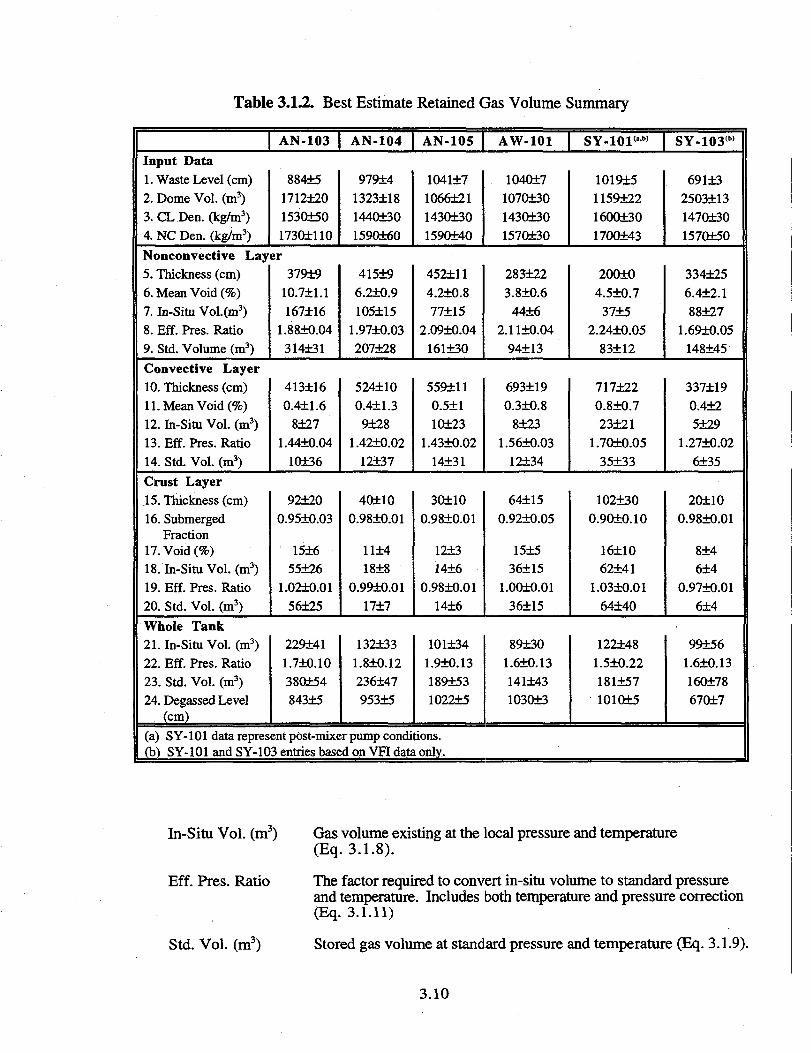
Table 3.1.2. Best Estimate Retained Gas Volume Summary
Input Data1. Waste Level (cm)2. Dome Vol. (m3)3. CL Den. (kg/m3)4. NC Den. (kg/m3)
AN-103
884±51712±201530±501730+110
Nonconvective Layer5. Thickness (cm)6. Mean Void (%)7. In-Situ Vol.(m3)8. Eff. Pres. Ratio9. Std. Volume (m3)Convective Layer10. Thickness (cm)11. Mean Void (%)12. In-Situ Vol. (m3)13. Eff. Pres. Ratio14. Std. Vol. (m3)Crust Layer15. Thickness (cm)16. Submerged
Fraction17. Void (%)18. In-Situ Vol. (m3)19. Eff. Pres. Ratio20. Std. Vol. (m3)Whole Tank21. In-Situ Vol. (m3)22. Eff. Pres. Ratio23. Std. Vol. (m3)24. Degassed Level
(cm)
379+910.7+1.1167±16
1.88+0.04314+31
413±160.4+1.6
8±271.44+0.04
10+36
92+200.95±0.03
15±655±26
1.02+0.0156±25
229+411.7+0.10380+54843±5
AN-104
979±41323±181440+301590±60
415±96.2+0.9105+15
1.97±0.03207+28
524+100.4±1.39±28
1.42±0.0212+37
40±100.98±0.01
11+418±8
0.99±0.0117±7
132±331.8±0.12236±47953±5
AN-105
1041±71066+211430+301590+40
452+114.2±0.877±15
2.09+0.04161±30
559+110.5+110+23
1.43±0.0214+31
30±100.98±0.01
12±314+6
O.98±O.O1
14±6
101+341.9±0.13189+531022±5
(a) SY-101 data represent post-mixer pump conditions.(b) SY-101 and SY-103 entries based on VFI data only.
AW-101
1040±71070+301430+301570+30
283+223.8±0.6
44+62.11±0.04
94±13
693+190.3±0.8
8±231.56+0.03
12±34
64+150.9210.05
15±536±15
1.0010.0136115
89+301.610.131411431030+3
SY-101(ab)
1019151159+221600+301700143
200104.510.737+5
2.24+0.0583112
717+220.8+0.723121
1.7010.0535+33
1021300.90+0.10
1611062141
1.0310.0164+40
1221481.5+0.221811571010+5
SY-103""
691132503+131470+301570150
3341256.412.188+27
1.69+0.05148145
3371190.4125129
1.27+0.026135
201100.9810.01
814614
0.97+0.01614
991561.610.13160178670+7
In-Situ Vol. (m3)
Eff. Pres. Ratio
Std. Vol. (m3)
Gas volume existing at the local pressure and temperature(Eq. 3.1.8).
The factor required to convert in-situ volume to standard pressureand temperature. Includes both temperature and pressure correction(Eq. 3.1.11)
Stored gas volume at standard pressure and temperature (Eq. 3.1.9).
3.10
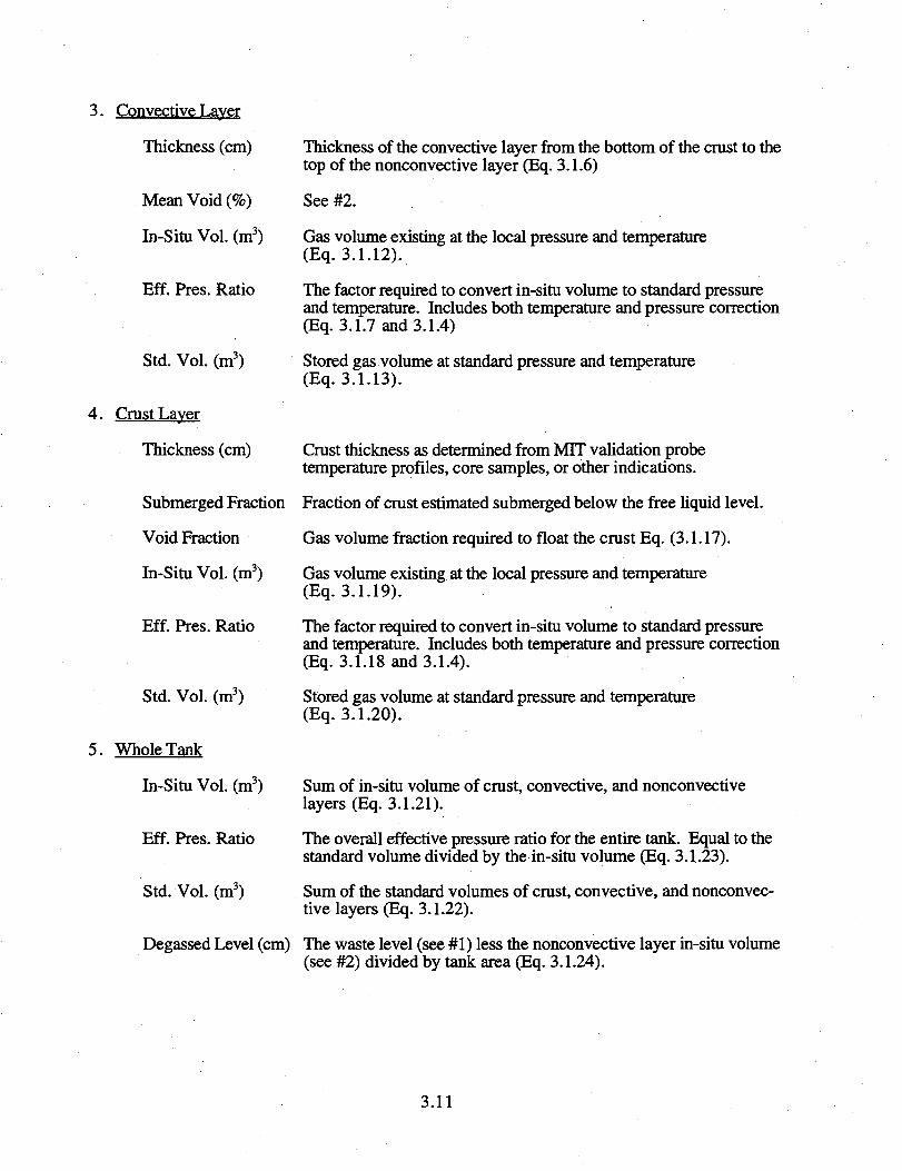
3. Convective Layer
Thickness (cm)
Mean Void (%)
In-Situ Vol. (m3)
Eff. Pres. Ratio
Std. Vol. (m3)
4. Crust Layer
Thickness (cm)
Submerged Fraction
Void Fraction
In-Situ Vol. (m3)
Eff. Pres. Ratio
Std. Vol. (m3)
5. Whole Tank
In-Situ Vol. (m3)
Eff. Pres. Ratio
Std. Vol. (m3)
Degassed Level (cm)
Thickness of the convective layer from the bottom of the crust to thetop of the nonconvective layer (Eq. 3.1.6)
See #2.
Gas volume existing at the local pressure and temperature(Eq. 3.1.12).
The factor required to convert in-situ volume to standard pressureand temperature. Includes both temperature and pressure correction(Eq. 3.1.7 and 3.1.4)
Stored gas volume at standard pressure and temperature(Eq. 3.1.13).
Crust thickness as determined from MIT validation probetemperature profiles, core samples, or other indications.
Fraction of crust estimated submerged below the free liquid level.
Gas volume fraction required to float the crust Eq. (3.1.17).
Gas volume existing at the local pressure and temperature(Eq. 3.1.19).
The factor required to convert in-situ volume to standard pressureand temperature. Includes both temperature and pressure correction(Eq. 3.1.18 and 3.1.4).
Stored gas volume at standard pressure and temperature(Eq. 3.1.20).
Sum of in-situ volume of crust, convective, and nonconvectivelayers (Eq. 3.1.21).
The overall effective pressure ratio for the entire tank. Equal to thestandard volume divided by the in-situ volume (Eq. 3.1.23).
Sum of the standard volumes of crust, convective, and nonconvec-tive layers (Eq. 3.1.22).
The waste level (see #1) less the nonconvective layer in-situ volume(see #2) divided by tank area (Eq. 3.1.24).
3.11
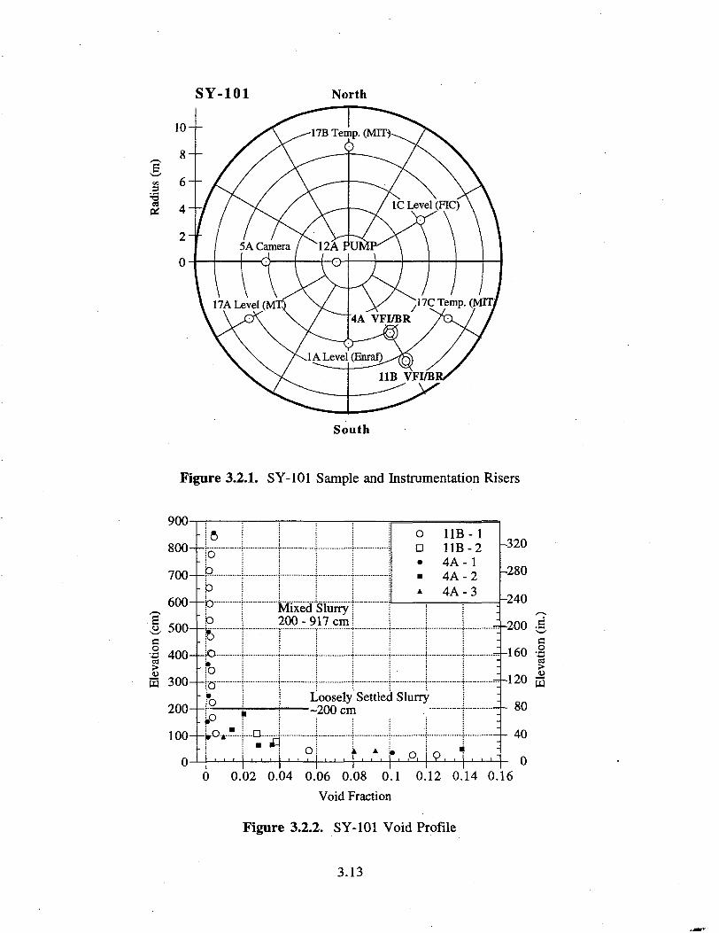
3.2 Individual Tank Gas Retention Summaries
Retained gas volume calculations for each tank are given in Sections 3.2.1 through 3.2.6.The local void fraction measurements are plotted along with the location of risers from which themeasurements were made and other important instrumentation. The detailed gas volume calcu-lations are given for each waste layer in a table for each tank. Note that, since no RGS voidmeasurements were made in SY-101 and SY-103, the data for these two tanks are unchanged fromStewart et al. (1996a) except for crust volume estimates.
Many of the void distributions plotted in the subsections that follow reveal regions in whichthe local void fraction exceeds the neutral buoyancy void fraction. This could be taken to indicatethat a buoyant displacement ("rollover") is imminent. But only comparing the local void to theneutral buoyancy void does not predict incipient buoyant displacements for three main reasons.First, there is considerable uncertainty in the neutral buoyancy void fraction. The neutral buoyancyvoid fraction is the gas fraction necessary to make the density of nonconvective layer materiallocally equal to the supernatant liquid above it. It can be expressed as
aNB = 1 ~ — (3-2-1)PNC
Eq. (3.2.1) amplifies the uncertainties in the layer densities resulting in 50-60% uncertainty in theneutral buoyancy void (see row 8 in Table 4.2.2). Second, the yield strength of the nonconvectivelayer material makes the void fraction required for an instability higher than the neutral buoyancyvalue, as discussed in Section 4.3.
Third, and most importantly, the net buoyancy integrated from the top down, not the localvoid fraction, determines whether a buoyant displacement can occur. For example, Figure 3.2.9shows that AN-103 has a 200-cm layer in which the local void far exceeds the neutral buoyancyvoid fraction of 12 ± 6%. But this region lies beneath a layer in which the local void fraction isconsiderably lower. The integration of net buoyancy confirms that AN-103 is stable by a smallmargin considering only neutral buoyancy and by a more comfortable margin considering theadditional effect of material strength.
3.2.1 SY-101 Void Distribution and Gas Volume
No further core sampling or RGS data are available for SY-101. The only changes in thegas volume result from revisions to the model, as discussed above, with the most significant beinga reduction in estimated crust gas volume. The locations of important instruments and VFI and ballrheometer tests are shown in Figure 3.2.1, and the void profile is given in Figure 3.2.2. The gasvolume calculations in each sublayer are summarized in Table 3.2.1.
3.12
SY-101 North
lALevelQSnraf)11B VFI/B
South
Figure 3.2.1. SY-101 Sample and Instrumentation Risers
900-
800-
700-
600-
500-
155 300-
200-
100-
0-
iobp-pP
;O
-P
Mixed200-
Slurrycm917
o
Loosely-200 cm
oD
11B- 111B-24A- 14A-24A-3
Settled Slurry
-320
-280
-240
- I 1 I 1 I 1 1 I 1 1 1 I I I I I LA I P . . 1 • , •
4-200 .9,c
-160 - |
-120 S
- 80
- 40
00 0.02 0.04 0.06 0.08 0.1 0.12 0.14 0.16
Void Fraction
Figure 3.2.2. SY-101 Void Profile
3.13
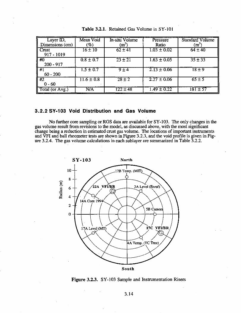
Table 3.2.1. Retained Gas Volume in SY-1O1
Layer ID,Dimensions (cm)Crust
917-1019#0
200-917#1
60 - 200#2
0-60Total (or Avg.)
Mean Void(%)
16 ±10
0.8 ± 0.7
1.5 ± 0.7
11.6 ±0.8
N/A
In-situ Volume(m3)
62 ±41
23 ±21
9±4
28 ± 2
122 ± 48
PressureRatio
1.03 ±0.02
1.63 ±0.05
2.13 ± 0.06
2.27 ± 0.06
1.49 ±0.22
Standard Volume(m3)
64 ±40
35 ± 33
18±9
65 ±5
181 ±57
3.2.2 SY-103 Void Distribution and Gas Volume
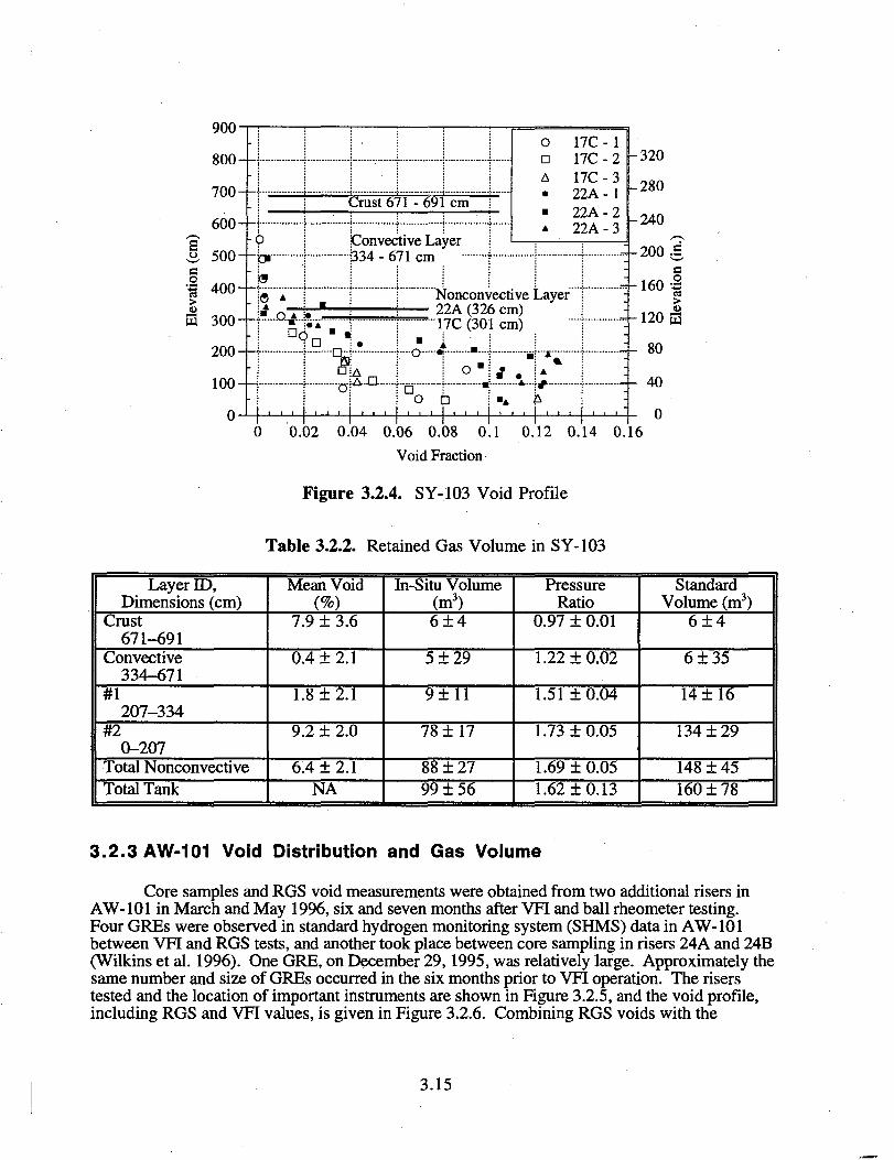
No further core sampling or RGS data are available for SY-103. The only changes in thegas volume result from revisions to the model, as discussed above, with the most significantchange being a reduction in estimated crust gas volume. The locations of important instrumentsand VFI and ball rheometer tests are shown in Figure 3.2.3, and the void profile is given in Fig-ure 3.2.4. The gas volume calculations in each sublayer are summarized in Table 3.2.2.
SY-103 North
South
Figure 3.2.3. SY-103 Sample and Instrumentation Risers
3.14
900-
800-
700-
600-
500-
400-
300-
200-
100-
0-
uW 300-f
9pr-ies
Crust 671-691
iConvective Layer•1334 - 671 cm
...*...
i Q-A4 o^A.n...
cm
onA
17C-117C-217C-322A- 122A-222A - 3
Nonconvective Layer- 22A (326 cm)""17C (301 cm)
-o 4-
no .* •
..:-200:s
0.02 0.04 0.06 0.08 0.1
Void Fraction
-320
-280
-240
160 I
120 S
80
40
00.12 0.14 0.16
Figure 3.2.4. SY-103 Void Profile
Table 3.2.2. Retained Gas Volume in SY-103
Layer ED,Dimensions (cm)
Crust671-691
Convective334-671
#1207-334
#20-207
Total NonconvectiveTotal Tank
Mean Void(%)
7.9 ± 3.6
0.4 ± 2.1
1.8 ±2.1
9.2 ± 2.0
6.4 ± 2.1NA
In-Situ Volume(m3)6±4
5 ±29
9±11
78 ±17
88 ±2799 ±56
PressureRatio
0.97 ± 0.01
1.22 ±0.02
1.51 ±0.04
1.73 ±0.05
1.69 ±0.051.62 ±0.13
StandardVolume (m3)
6±4
6 ±35
14 ±16
134 ±29
148 ± 45160 ±78
3.2.3 AW-101 Void Distribution and Gas Volume
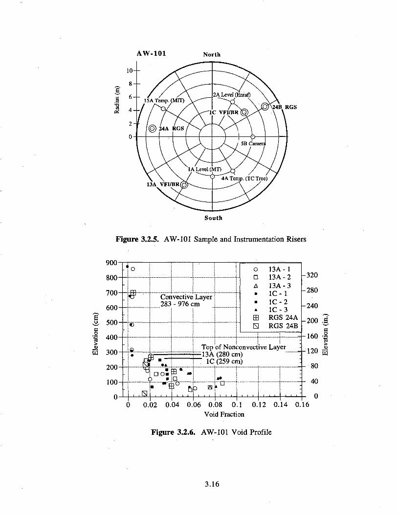
Core samples and RGS void measurements were obtained from two additional risers inAW-101 in March and May 1996, six and seven months after VFI and ball rheometer testing.Four GREs were observed in standard hydrogen monitoring system (SHMS) data in AW-101between VFI and RGS tests, and another took place between core sampling in risers 24A and 24B(Wilkins et al. 1996). One GRE, on December 29,1995, was relatively large. Approximately thesame number and size of GREs occurred in the six months prior to VFI operation. The riserstested and the location of important instruments are shown in Figure 3.2.5, and the void profile,including RGS and VFI values, is given in Figure 3.2.6. Combining RGS voids with the
3.15
AW-101 North
4B RGS
2A Level (Enraf)
1C VFI/BR
South
Figure 3.2.5. AW-101 Sample and Instramentation Risers
900-
800-
700-
600-
500-
•f 400-
3 3 0 0 ^
200-
ioo-h
Convective283 - 976 cm
DO*
Layer
oD
ffl
13A-113A-213A - 31C- 11C-21C-3RGS 24ARGS 24B
Top of Nonconvective Layer-13A (280 cm)" lC(259cm)
-320
-280
-240
-200 'S
-160 -2
-120 |
- 80
- 40
- 00 0.02 0.04 0.06 0.08 0.1 0.12 0.14 0
Void Fraction
Figure 3.2.6. AW-101 Void Profile
.16
3.16
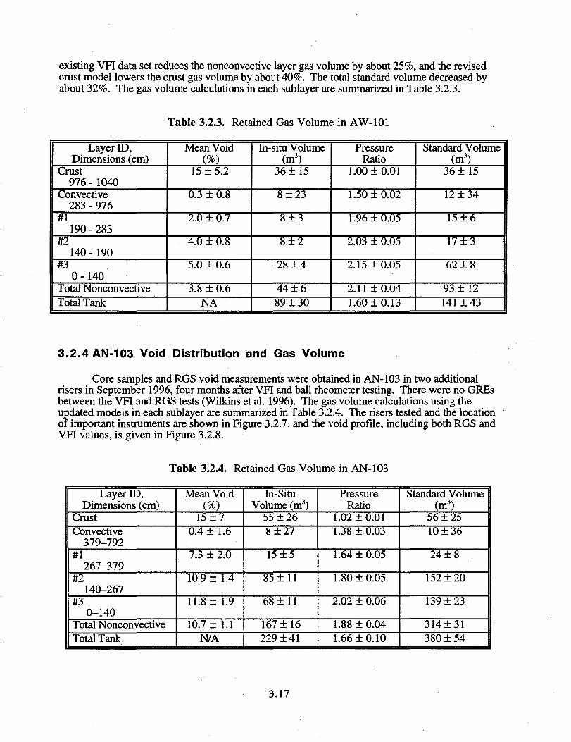
existing VFI data set reduces the nonconvective layer gas volume by about 25%, and the revisedcrust model lowers the crust gas volume by about 40%. The total standard volume decreased byabout 32%. The gas volume calculations in each sublayer are summarized in Table 3.2.3.
Table 3.2.3. Retained Gas Volume in AW-101
Layer ID,Dimensions (cm)
Crust976 -1040
Convective283 - 976
#1190 - 283
#2140 - 190
#30-140
Total NonconvectiveTotal Tank
Mean Void(%)
15 ±5.2
0.3 ± 0.8
2.0 ± 0.7
4.0 ±0.8
5.0 ± 0.6
3.8 ± 0.6NA
In-situ Volume(m3)
36 ±15
8 ±23
8±3
8±2
28 ±4
44±689 ±30
PressureRatio
1.00 ± 0.01
1.50 ±0.02
1.96 ±0.05
2.03 ± 0.05
2.15 ±0.05
2.11 ±0.041.60 ±0.13
Standard Volume(m3)
36 ±15
12 ±34
15 ±6
17 ±3
62 ±8
93 ± 12141 ±43
3.2.4 AN-103 Void Distribution and Gas Volume
Core samples and RGS void measurements were obtained in AN-103 in two additionalrisers in September 1996, four months after VFI and ball rheometer testing. There were no GREsbetween the VFI and RGS tests (Wilkins et al. 1996). The gas volume calculations using theupdated models in each sublayer are summarized in Table 3.2.4. The risers tested and the locationof important instruments are shown in Figure 3.2.7, and the void profile, including both RGS andVFI values, is given in Figure 3.2.8.
Table 3.2.4. Retained Gas Volume in AN-103
Layer ID,Dimensions (cm)
CrustConvective
379-792#1
267-379#2
140-267#3
0-140Total NonconvectiveTotal Tank
Mean Void(%)
15 ±70.4 ± 1.6
7.3 ± 2.0
10.9 ± 1.4
11.8 ± 1.9
10.7 ±1.1N/A
In-SituVolume (m3)
55 ±268 ±27
15 ±5
85 ±11
68 ±11
167 ± 16229 ±41
PressureRatio
1.02 ±0.011.38 ±0.03
1.64 ±0.05
1.80 ±0.05
2.02 ± 0.06
1.88 ± 0.041.66 ±0.10
Standard Volume(m3)
56 + 2510 ±36
24 ±8
152 ±20
139 ±23
314±31380 ± 54
3.17
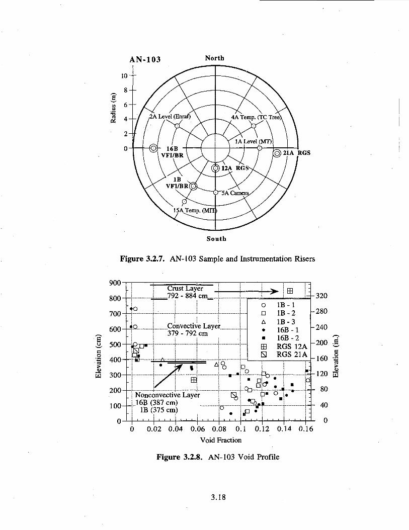
AN-103 North
10
C5)21A RGS
South
Figure 3.2.7. AN-103 Sample and Instrumentation Risers
900-
800-
700-
600-
J, 500-s
• | 400-
W 300-
200-
100
0
*o.
Crust LayerJ92 - 884 crn .."
.Convective Layer379 - 792
m
cm
Nonconvective Layer16B (387 cm)
IB (375 cm)
ffl
oDA
ffl
1B-1IB-2IB-316B-116B-2RGS 12ARGS 21A
ino
o
,p
320
280
240
200 5,
160 - |
•120 a
- 80
- 40
• 0
0 0.02 0.04 0.06 0.08 0.1 0.12 0.14 0.16
Void Fraction
Figure 3.2.8. AN-103 Void Profile
3.18
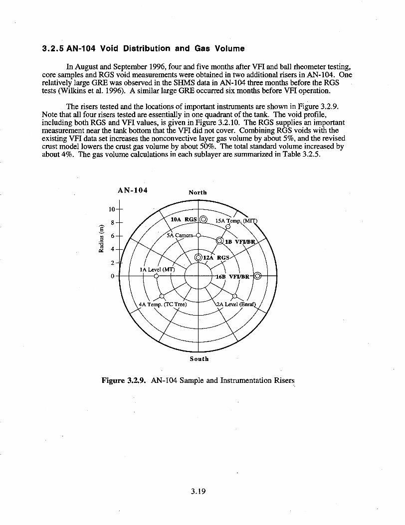
3.2.5 AN-104 Void Distribution and Gas Volume
In August and September 1996, four and five months after VFI and ball rheometer testing,core samples and RGS void measurements were obtained in two additional risers in AN-104. Onerelatively large GRE was observed in the SHMS data in AN-104 three months before the RGStests (Wilkins et al. 1996). A similar large GRE occurred six months before VFI operation.
The risers tested and the locations of important instruments are shown in Figure 3.2.9.Note that all four risers tested are essentially in one quadrant of the tank. The void profile,including both RGS and VFI values, is given in Figure 3.2.10. The RGS supplies an importantmeasurement near the tank bottom that the VFI did not cover. Combining RGS voids with theexisting VFI data set increases the nonconvective layer gas volume by about 5%, and the revisedcrust model lowers the crust gas volume by about 50%. The total standard volume increased byabout 4%. The gas volume calculations in each sublayer are summarized in Table 3.2.5.
AN-104 North
South
Figure 3.2.9. AN-104 Sample and Instrumentation Risers
3.19
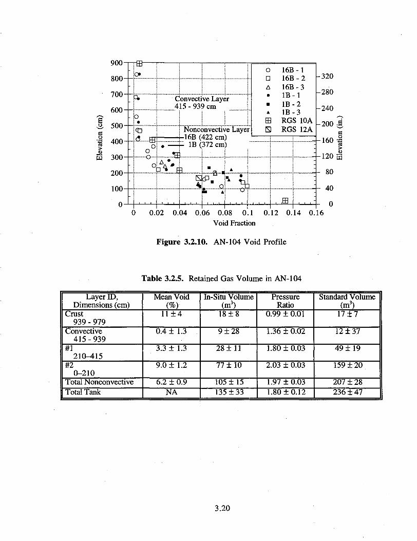
900-rjffi-
800-{>
700
600- !O
500-
••§ 400-h
53 300-h|
200--!
loo-H
0
en
ooO--
Oj
Convective Layer415 - 939 cm
Nonconvective Layer-16B(422cm)- IB (372 cm)
•Q--
C Bi
o 16B - 1D 16B - 2A 16B - 3• 1B-1• I B - 2A I B - 3
EB RGS 10AS RGS 12A
-320
-280
-240
-200
160
120
80
40
00 0.02 0.04 0.06 0.08 0.1 0.12 0.14 0.
Void Fraction
Figure 3.2.10. AN-104 Void Profile
16
Table 3.2.5. Retained Gas Volume in AN-104
Layer ID,Dimensions (cm)
Crust939 - 979
Convective415 - 939
#1210-415
#20-210
Total NonconvectiveTotal Tank
Mean Void(%)
11 ±4
0.4 ± 1.3
3.3 ± 1.3
9.0 ± 1.2
6.2 ± 0.9NA
In-Situ Volume(m3)
18±8
9 ±28
28 ±11
77 ±10
105 ± 15135 ±33
PressureRatio
0.99 ± 0.01
1.36 ±0.02
1.80 ±0.03
2.03 ± 0.03
1.97 ± 0.031.80 ±0.12
Standard Volume(m3)
17±7
12 ±37
49 ±19
159 ± 20
207 ± 28236 ±47
3.20
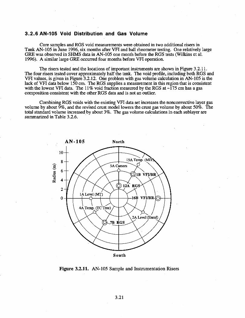
3.2.6 AN-105 Void Distribution and Gas Volume
Core samples and RGS void measurements were obtained in two additional risers inTank AN-105 in June 1996, six months after VFI and ball rheometer testing. One relatively largeGRE was observed in SHMS data in AN-105 one month before the RGS tests (Wilkins et al.1996). A similar large GRE occurred four months before VFI operation.
The risers tested and the locations of important instruments are shown in Figure 3.2.11.The four risers tested cover approximately half the tank. The void profile, including both RGS andVFI values, is given in Figure 3.2.12. One problem with gas volume calculation in AN-105 is thelack of VFI data below 150 cm. The RGS supplies a measurement in this region that is consistentwith the lowest VFI data. The 11% void fraction measured by the RGS at -175 cm has a gascomposition consistent with the other RGS data and is not an outlier.
Combining RGS voids with the existing VFI data set increases the nonconvective layer gasvolume by about 9%, and the revised crust model lowers the crust gas volume by about 50%. Thetotal standard volume increased by about 3%. The gas volume calculations in each sublayer aresummarized in Table 3.2.6.
AN-105 North
14
12A RGS
16B VFI/BR
South
Figure 3.2.11. AN-105 Sample and Instrumentation Risers
3.21
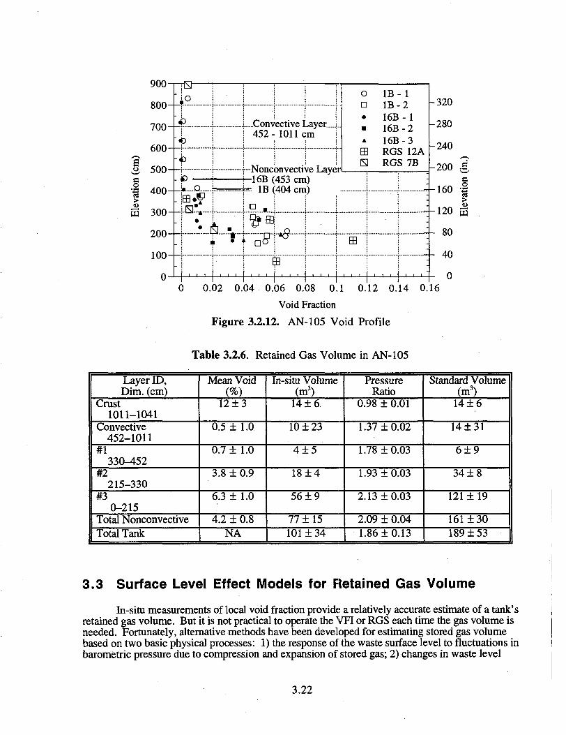
900-rrS
53
800-
700-
600-
500-
400-
300-
200-
100-
0-
o
...0.
TT
452-Convective Layer....!
1011 cm
•Nonconvective Layer-16B (453 cm)= IB (404 cm)
OD
IB- 1IB-216B-116B-216B-3RGS 12ARGS 7B
a
•<
-320
-280
-240
-200 •£,
160 |
120 s
80
40
00 0.02 0.04 0.06 0.08 0.1 0.12 0.14 0.16
Void Fraction
Figure 3.2.12. AN-105 Void Profile
Table 3.2.6. Retained Gas Volume in AN-105
Layer ID,Dim. (cm)
Crust1011-1041
Convective452-1011
#1330-452
#2215-330
#30-215
Total NonconvectiveTotal Tank
Mean Void(%)
12 ± 3
0.5 ± 1.0
0.7 ± 1.0
3.8 ± 0.9
6.3 ± 1.0
4.2 ± 0.8NA
In-situ Volume(m3)
14 ±6.
10 ±23
4±5
18±4
56 + 9
77 ±15101 ± 34
PressureRatio
0.98 ± 0.01
1.37 ±0.02
1.78 ± 0.03
1.93 + 0.03
2.13 + 0.03
2.09 ± 0.041.86 ±0.13
Standard Volume(m3)
14 ±6
14 ±31
6±9
34 ±8
121 + 19
161 ±30189 ±53
3.3 Surface Level Effect Models for Retained Gas Volume
In-situ measurements of local void fraction provide a relatively accurate estimate of a tank'sretained gas volume. But it is not practical to operate the VFI or RGS each time the gas volume isneeded. Fortunately, alternative methods have been developed for estimating stored gas volumebased on two basic physical processes: 1) the response of the waste surface level to fluctuations inbarometric pressure due to compression and expansion of stored gas; 2) changes in waste level
3.22
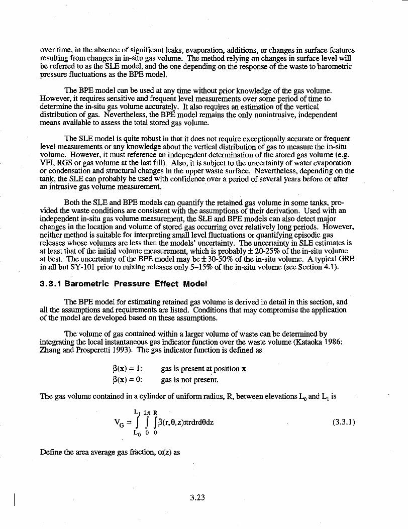
over time, in the absence of significant leaks, evaporation, additions, or changes in surface featuresresulting from changes in in-situ gas volume. The method relying on changes in surface level willbe referred to as the SLE model, and the one depending on the response of the waste to barometricpressure fluctuations as the BPE model.
The BPE model can be used at any time without prior knowledge of the gas volume.However, it requires sensitive and frequent level measurements over some period of time todetermine the in-situ gas volume accurately. It also requires an estimation of the verticaldistribution of gas. Nevertheless, the BPE model remains the only nonintrusive, independentmeans available to assess the total stored gas volume.
The SLE model is quite robust in that it does not require exceptionally accurate or frequentlevel measurements or any knowledge about the vertical distribution of gas to measure the in-situvolume. However, it must reference an independent determination of the stored gas volume (e.g.VFI, RGS or gas volume at the last fill). Also, it is subject to the uncertainty of water evaporationor condensation and structural changes in the upper waste surface. Nevertheless, depending on thetank, the SLE can probably be used with confidence over a period of several years before or afteran intrusive gas volume measurement.
Both the SLE and BPE models can quantify the retained gas volume in some tanks, pro-vided the waste conditions are consistent with the assumptions of their derivation. Used with anindependent in-situ gas volume measurement, the SLE and BPE models can also detect majorchanges in the location and volume of stored gas occurring over relatively long periods. However,neither method is suitable for interpreting small level fluctuations or quantifying episodic gasreleases whose volumes are less than the models' uncertainty. The uncertainty in SLE estimates isat least that of the initial volume measurement, which is probably ± 20-25% of the in-situ volumeat best. The uncertainty of the BPE model may be ± 30-50% of the in-situ volume. A typical GREin all but SY-101 prior to mixing releases only 5-15% of the in-situ volume (see Section 4.1).
3.3.1 Barometric Pressure Effect Model
The BPE model for estimating retained gas volume is derived in detail in this section, andall the assumptions and requirements are listed. Conditions that may compromise the applicationof the model are developed based on these assumptions.
The volume of gas contained within a larger volume of waste can be determined byintegrating the local instantaneous gas indicator function over the waste volume (Kataoka 1986;Zhang and Prosperetti 1993). The gas indicator function is defined as
|3(x) = 1: gas is present at position x
P(x) = 0: gas is not present.
The gas volume contained in a cylinder of uniform radius, R, between elevations Lo and Lx is
Li 2K R
V G = j J Jp(r,9,z)7trdrdedz (3.3.1)Lo 0 0
Define the area average gas fraction, ot(z) as
3.23
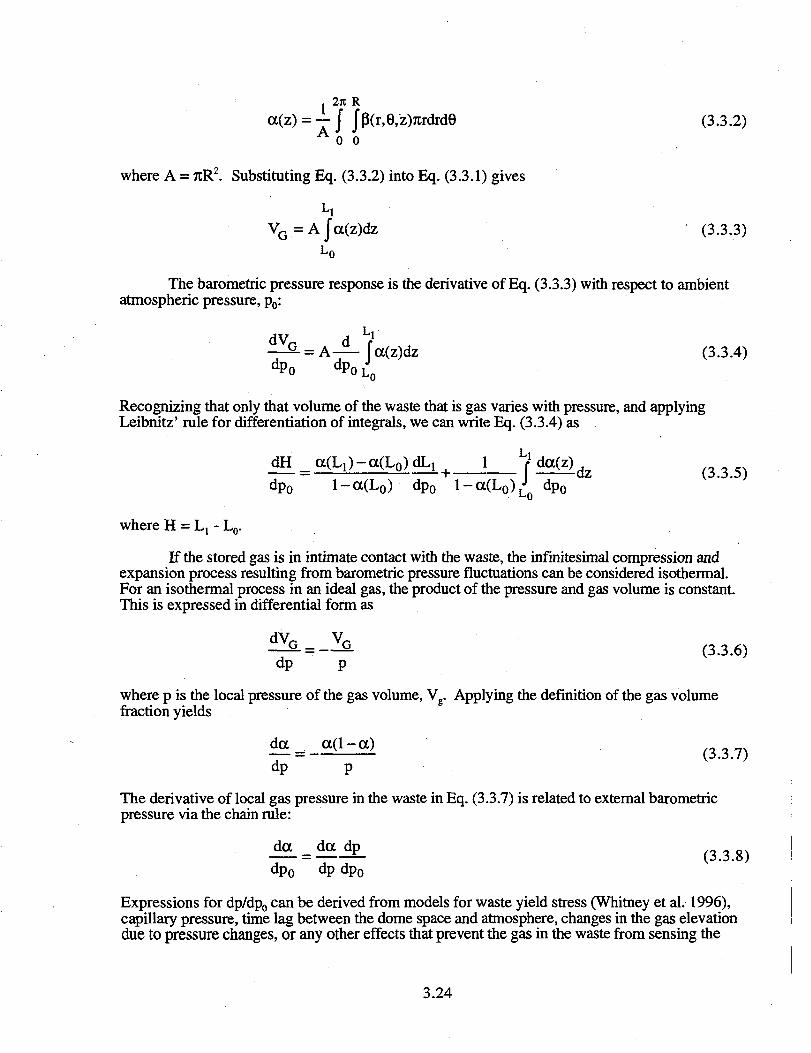
oc(z) = — J Jp(r,0,z)7trdrd8 (3.3.2)0 0
whereA = 7tR2. Substituting Eq. (3.3.2) into Eq. (3.3.1) gives
V G =Aja (z )dz (3.3.3)Lo
The barometric pressure response is the derivative of Eq. (3.3.3) with respect to ambientatmospheric pressure, p0:
dVr d LlQ A ja(z)dz (3.3.4)
Recognizing that only that volume of the waste that is gas varies with pressure, and applyingLeibnitz' rule for differentiation of integrals, we can write Eq. (3.3.4) as
dH=a(L1)-a(L0)dL1 | 1 V^)^ ( 3 3 5 )
dp0 l -a(L 0 ) dp0 l-a(L0)lo dp0
where H = Lj - Lo.
If the stored gas is in intimate contact with the waste, the infinitesimal compression andexpansion process resulting from barometric pressure fluctuations can be considered isothermal.For an isothermal process in an ideal gas, the product of the pressure and gas volume is constant.This is expressed in differential form as
dVr V r—2- = — 2 - (3.3.6)dp p
where p is the local pressure of the gas volume, Vg. Applying the definition of the gas volumefraction yields
( 3 .dp p
The derivative of local gas pressure in the waste in Eq. (3.3.7) is related to external barometricpressure via the chain rule:
dp0 dp dp0
(3.3.8)
Expressions for dp/dp0 can be derived from models for waste yield stress (Whitney et al. 1996),capillary pressure, time lag between the dome space and atmosphere, changes in the gas elevationdue to pressure changes, or any other effects that prevent the gas in the waste from sensing the
3.24
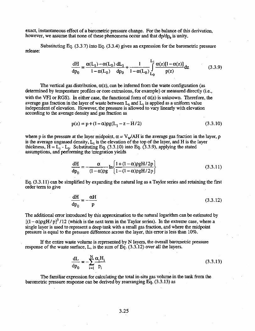
exact, instantaneous effect of a barometric pressure change. For the balance of this derivation,however, we assume that none of these phenomena occur and that dp/dp0 is unity.
Substituting Eq. (3.3.7) into Eq. (3.3.4) gives an expression for the barometric pressurerelease:
dH = a ( L t ) - a ( L 0 ) dl^ ( 1 Lr1 a(z)[l - a(z)] ( 3 3
dp0 l - a ( L 0 ) dp0 l - a C L , , ) ^ p(z)
The vertical gas distribution, a(z), can be inferred from the waste configuration (asdetermined by temperature profiles or core extrusions, for example) or measured directly (i.e.,with the VFI or RGS). In either case, the functional form of a(z) is unknown. Therefore, theaverage gas fraction in the layer of waste between Lo and L, is applied as a uniform valueindependent of elevation. However, the pressure is allowed to vary linearly with elevationaccording to the average density and gas fraction as
p(z) = p + ( l - a ) p g ( L 1 - z - H / 2 ) (3.3.10)
where p is the pressure at the layer midpoint, a = V^/AH is the average gas fraction in the layer, pis the average ungassed density, L, is the elevation of the top of the layer, and H is the layerthickness, H = L, - Lo. Substituting Eq. (3.3.10) into Eq. (3.3.9), applying the statedassumptions, and performing the integration yields
J**L = 2 inJ - ' ^ -/K&— -* i (3.3.11)
dp0 (l-a)pg ll-(l-a)pgH/2pJ
Eq. (3.3.11) can be simplified by expanding the natural log as a Taylor series and retaining the firstorder term to give
(3.3.12)
The additional error introduced by this approximation to the natural logarithm can be estimated by[(1 - a)pgH/p]3 /12 (which is the next term in the Taylor series). In the extreme case, where asingle layer is used to represent a deep tank with a small gas fraction, and where the midpointpressure is equal to the pressure difference across the layer, this error is less than 10%.
If the entire waste volume is represented by N layers, the overall barometric pressureresponse of the waste surface, L, is the sum of Eq. (3.3.12) over all the layers.
* S5 (3.3.13)ydPo S Pi
The familiar expression for calculating the total in-situ gas volume in the tank from thebarometric pressure response can be derived by rearranging Eq, (3.3.13) as
3.25
dPo
where the effective pressure is defined by
i N
P,EFF i=l LPiJ(3.3.15)
and fj is the fraction of the total in-situ gas stored in layer i
Eq. (3.3.13) provides an estimate of the barometric pressure response when the gas distributionand its pressure are known. If a suitable measurement of the barometric response and an estimateof the gas distribution are available, Eq. (3.3.14) gives the in-situ gas volume.
All gas volumes discussed up to now were at their local pressure and temperature. The truemeasure of the total amount of stored gas is the standard volume, which brings the in-situ volumeto standard pressure and temperature. The in-situ gas volume is given by Eq. (3.3.2). Includingthe pressure and temperature correction yields the standard volume as
Lj 2% R
VG = j J JP(r,e,z)P(r,e,z)7irdrd6dz (3.3.17)Lo 0 0
The pressure ratio, P(r,9,z), is defined by
P ( , e , 2 )p T(r,6,z)
where p(r,q,z) and T(r,q,z) are the local pressure and temperature, respectively; p is the standardatmospheric pressure of 101320 Pa; and T is the standard temperature, 288K. Define the areaaverage gas pressure ratio, Poc(z), as
2% R
P<x(z) = —J |P(r,6,z)p(r,e,z)ra-drd0 (3.3.18)A o o
and an area average pressure ratio, P(z), by
1 In RP(z) = — J JP(r,e,z)7trdrd9 (3.3.19)
A 0 0
If the pressure is uniform over area A, or if the pressure and local gas indicator are uncorrelated,the product of the average gas fraction and pressure is equal to the average of the product so that
3.26
Poc(z) = P(z)a(z) (3.3.20)
Substituting Eq. (3.3.20) and (3.3.18) into Eq. (3.3.17) gives the standard volume betweenelevations Lo and Lj as
L i
VG = A Jp(z)cc(z)dz (3.3.21)Lo
The total standard volume in the tank is obtained by summing over N layers represented bya uniform average gas fraction as in Eq. (3.3.10). Let the pressure ratio vary linearly within eachlayer according to the layer average density, gas fraction, and temperature as
(3.3.22)a ) ( L i zpT
where P is the pressure ratio at the layer midpoint. Summing Eq. (3.3.21) over all layers with theabove assumptions, performing the integration of Eq. (3.3.22) for P(z), and applying thedefinition of layer gas fraction yields this familiar expression for standard volume:
% = VGPEFF
where the effective pressure ratio, P ^ , is defined as
where Pj is the pressure ratio at the midpoint of layer i, and fj is defined by Eq. (3.3.16). Sub-stituting Eq. (3.3.14) for the in-situ volume yields the final result for estimating the standardvolume from a measured barometric pressure response:
1 t (3-3.24)
io
The assumptions that were made in the above derivations are summarized below. Thoughnot part of the derivation, it is essential to assume the response of the waste surface can bemeasured with sufficient precision and frequency. Assumptions 1-5 apply to the in-situ volumedetermined from Eq. (3.3.14). Additional assumption 6 applies to the standard volume computedfrom Eq. (3.3.24):
1. The gas-bearing waste is contained entirely in a cylinder of fixed radius and uniformbut temporally variable height (true for a radially stiff tank structure whose waste andgas fraction are relatively uniform radially and azimuthaUy).
2. The process of expansion and compression due to barometric pressure fluctuation isisothermal (true for expected large gas surface-to-volume ratio and very slow pressurechanges).
3. The gas stored in the waste behaves as an ideal gas (true for small pressure changes andrelatively low temperatures with the expected gas composition and local pressures).
3.27
4. The local pressure of all the gas in the waste changes as the barometric pressure (truefor relatively weak waste in which the gas elevation does not change measurably withpressure).
5. Vertical waste configuration and in-situ gas volume distribution can be estimated or isknown to within an appropriate level of uncertainty (depends on information available).
6. The local pressure is radially and azimuthally uniform, or the radial and azimuthalvariation of the pressure and gas fraction are uncorrelated (true if assumption 4 is met).
From these assumptions it can be inferred that, without careful consideration, the BPEmodel should not be applied to tanks
• in which a high lithostatic load results from an interstitial liquid level well below thewaste surface where the gas is stored as pore-filling bubbles (potentially violatesassumptions 1 and 4)
• with a very low waste level (potentially violates assumptions 1 and 4)• that have been salt-well pumped (potentially violates assumptions 1,4, and 5)• with a forest of suspended hardware such as airlift circulators, cooling coils, etc.
(potentially violates assumptions 1 and 4)• in which the waste is periodically disturbed by mixing, specifically SY-101 (violates
assumption 4)• in which the gas elevation changes during the time of the barometric pressure response
measurement (violates assumption 5)• in which an appropriately precise waste level instrument is not available, or readings are
not taken with sufficient frequency.
The best prospects for an accurate volume determination with the BPE model are tanks withrelatively deep, wet waste, where the vertical gas distribution can be estimated with fair confi-dence. Currently, this includes the DSTs and few of the SSTs. More confidence will be gained inapplying the model to SSTs as more are assayed with the RGS.
Nevertheless, it is almost impossible to attribute a correlation of waste level and barometricpressure to anything but the presence of stored gas. Therefore, while a negligible barometricpressure response does not necessarily indicate the absence of gas, a strong measured barometricpressure response should always be taken as an indication of stored gas, regardless of how well atank satisfies all the above requirements.
The BPE model has a significant inherent uncertainty in the best of conditions. The smallerthe retained gas volume, the less accurately the BPE model can estimate it. We can derive theminimum detectable volume for a given uncertainty threshold and measurement error. Thebarometric response in Eq. (3.3.14) can be rewritten in finite difference form as
APowhere AL is the specific level change in response to a corresponding barometric pressure change ofApo.
(a) Assuming the uncertainties in the barometric pressure change and tank area are small, therelative uncertainty in the volume in Eq. (3.3.25) can be estimated by linear error propagation as
(a) The pressure fluctuation should be only the amount that exceeds twice the yield stress of thematerial according to Whitney et al. (1996). However, the yield stress in the DSTs is small,-150 Pa, compared with barometric pressure changes.
3.28
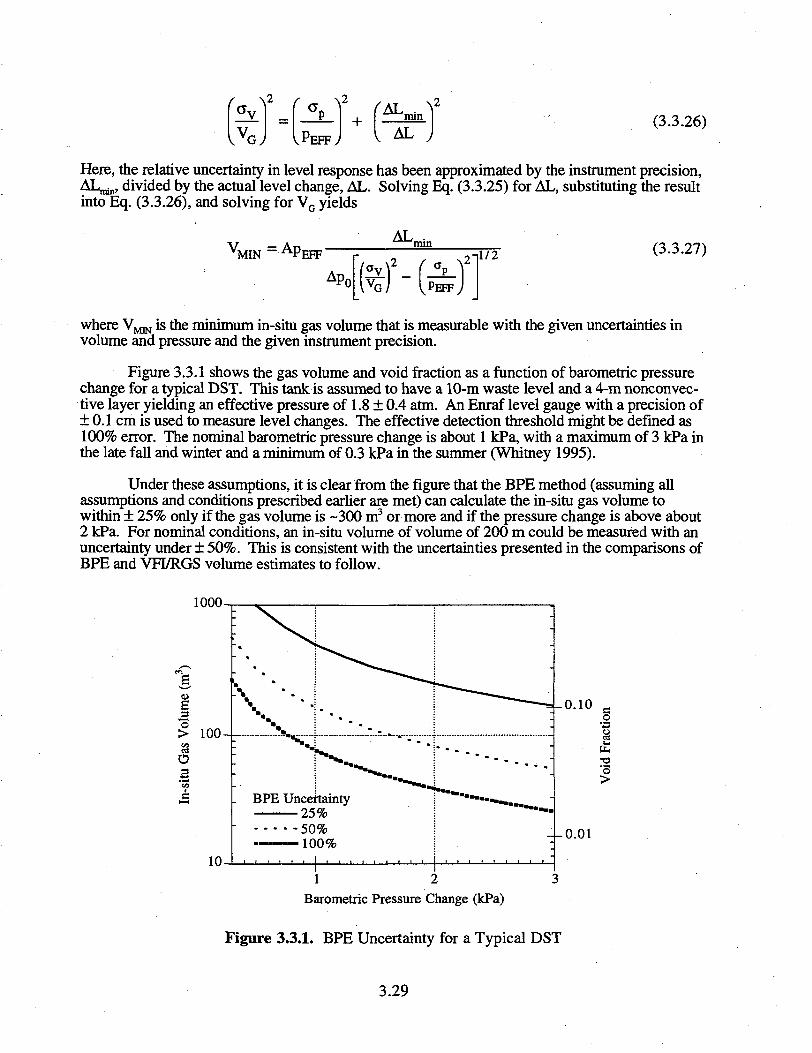
(3.3.26)
Here, the relative uncertainty in level response has been approximated by the instrument precision,AI^min, divided by the actual level change, AL. Solving Eq. (3.3.25) for AL, substituting the resultinto Eq. (3.3.26), and solving for VG yields
VMIN = A P EFF^ ^ m i n
APo
1/2 (3.3.27)
where V , ^ is the minimum in-situ gas volume that is measurable with the given uncertainties involume and pressure and the given instrument precision.
Figure 3.3.1 shows the gas volume and void fraction as a function of barometric pressurechange for a typical DST. This tank is assumed to have a 10-m waste level and a 4-m nonconvec-tive layer yielding an effective pressure of 1.8 ± 0.4 atm. An Enraf level gauge with a precision of± 0.1 cm is used to measure level changes. The effective detection threshold might be defined as100% error. The nominal barometric pressure change is about 1 kPa, with a maximum of 3 kPa inthe late fall and winter and a minimum of 0.3 kPa in the summer (Whitney 1995).
Under these assumptions, it is clear from the figure that the BPE method (assuming allassumptions and conditions prescribed earlier are met) can calculate the in-situ gas volume towithin ± 25% only if the gas volume is -300 m3 or more and if the pressure change is above about2 kPa. For nominal conditions, an in-situ volume of volume of 200 m could be measured with anuncertainty under ± 50%. This is consistent with the uncertainties presented in the comparisons ofBPE and VFI/RGS volume estimates to follow.
1000-
> 100-CO
o
10-
0.10
'5
BPE Uncertainty25%
•50%•100%
0.01
1 2Barometric Pressure Change (kPa)
Figure 3.3.1. BPE Uncertainty for a Typical DST
3.29
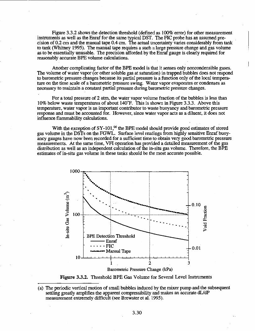
Figure 3.3.2 shows the detection threshold (defined as 100% error) for other measurementinstruments as well as the Enraf for the same typical DST. The FIC probe has an assumed pre-cision of 0.2 cm and the manual tape 0.4 cm. The actual uncertainty varies considerably from tankto tank (Whitney 1995). The manual tape requires a such a large pressure change and gas volumeas to be essentially unusable. The precision afforded by the Enraf gauge is clearly required forreasonably accurate BPE volume calculations.
Another complicating factor of the BPE model is that it senses only noncondensible gases.The volume of water vapor (or other soluble gas at saturation) in trapped bubbles does not respondto barometric pressure changes because its partial pressure is a function only of the local tempera-ture on the time scale of a barometric pressure swing. Water vapor evaporates or condenses asnecessary to maintain a constant partial pressure during barometric pressure changes.
For a total pressure of 2 arm, the water vapor volume fraction of the bubbles is less than10% below waste temperatures of about 140°F. This is shown in Figure 3.3.3. Above thistemperature, water vapor is an important contributor to waste buoyancy and barometric pressureresponse and must be accounted for. However, since water vapor acts as a diluent, it does notinfluence flammability calculations.
With the exception of SY-101 ,(a) the BPE model should provide good estimates of storedgas volume in the DSTs on the FGWL. Surface level readings from highly sensitive Enraf buoy-ancy gauges have now been recorded for a sufficient time to obtain very good barometric pressuremeasurements. At the same time, VFI operation has provided a detailed measurement of the gasdistribution as well as an independent calculation of the in-situ gas volume. Therefore, the BPEestimates of in-situ gas volume in these tanks should be the most accurate possible.
1000-
I5
S3
os
100-
10-
. BPE Detection ThresholdEnrafFIC
....... . . . Manual Tape
- - 0 . 1 0
•en
O
•a2ISo
- - 0 . 0 1
1 2 3Barometric Pressure Change (kPa)
Figure 3.3.2. Threshold BPE Gas Volume for Several Level Instruments
(a) The periodic vertical motion of small bubbles induced by the mixer pump and the subsequentsettling greatly amplifies the apparent compressibility and makes an accurate dL/dPmeasurement extremely difficult (see Brewster et al. 1995).
3.30
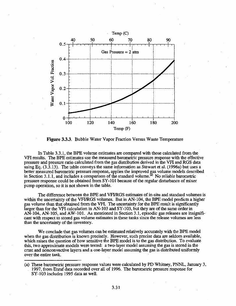
40 50
Temp (C)
60 70 80
Figure 3.3.3. Bubble Water Vapor Fraction Versus Waste Temperature
In Table 3.3.1, the BPE volume estimates are compared with those calculated from theVFI results. The BPE estimates use the measured barometric pressure response with the effectivepressure and pressure ratio calculated from the gas distribution derived in the VFI and RGS datausing Eq. (3.3.13). The table conveys the same information as Stewart et al. (1996a) but uses abetter measured barometric pressure response, applies the improved gas volume models describedin Section 3.1.1, and includes a comparison of the standard volume. No reliable barometricpressure response could be obtained from SY-101 because of the regular disturbance of mixerpump operation, so it is not shown in the table.
The difference between the BPE and VFI/RGS estimates of in-situ and standard volumes iswithin the uncertainty of the VFI/RGS volumes. But in AN-104, the BPE model predicts a highergas volume than that obtained from the VFI. The uncertainty for the BPE result is significantlylarger than for the VFI calculation in AN-103 and SY-103, but they are of the same order inAN-104, AN-105, and AW-101. As mentioned in Section 3.1, episodic gas releases are insignifi-cant with respect to stored gas volume estimates in these tanks since the release volumes are lessthan the uncertainty of the inventory.
We conclude that gas volumes can be estimated relatively accurately with the BPE modelwhen the gas distribution is known precisely. However, such precise data are seldom available,which raises the question of how sensitive the BPE model is to the gas distribution. To evaluatethis, two approximate models were tested: a two-layer model assuming the gas is stored in thecrust and nonconvective layers and a one-layer model assuming the gas is distributed uniformlyover the entire tank.
(a) These barometric pressure response values were calculated by PD Whitney, PNNL, January 3,1997, from Enraf data recorded over all of 1996. The barometric pressure response forSY-103 includes 1995 data as well.
3.31
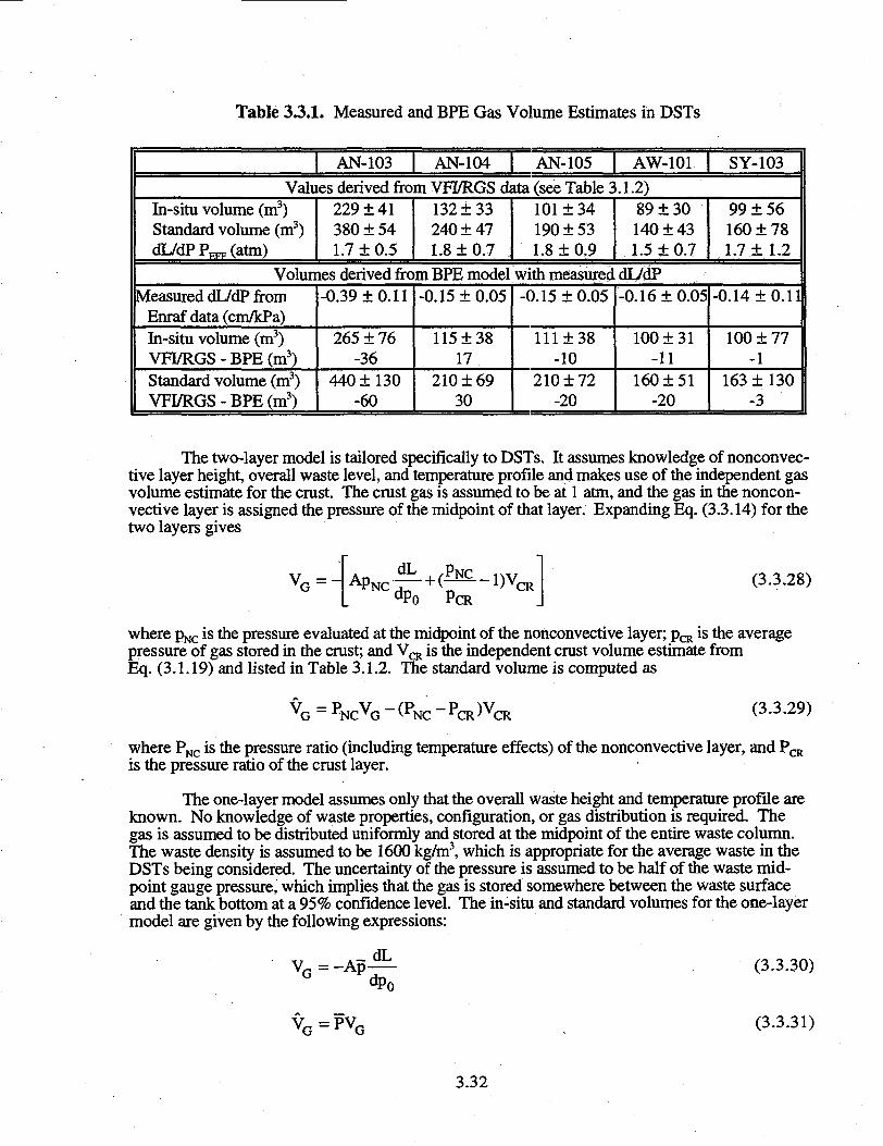
Table 3.3.1. Measured and BPE Gas Volume Estimates in DSTs
AN-103 AN-104 AN-105 AW-101 SY-103Values derived from VH/RGS data (see Table 3.1.2)
In-situ volume (m3)Standard volume (m3)dL/dPP^Catm)
229 ±41380 ± 541.7 ± 0.5
132 + 33240 ± 471.8 ±0.7
101 ± 34190 ±531.8 + 0.9
89130140 ±431.5 ±0.7
99 + 56160 ±781.7 ± 1.2
Volumes derived from BPE model with measured dL/dPMeasured dL/dP from
Enraf data (cm/kPa)In-situ volume (m3)VFI/RGS - BPE (m3)Standard volume (m3)VFI/RGS-BPE(m3)
-0.39 ±0.11
265 ±76-36
440 ± 130-60
-0.15 ± 0.05
115 ±3817
210 ±6930
-0.15 ± 0.05
111 ±38-10
210 ±72-20
-0.16 ±0.05
100 ±31-11
160 ±51-20
-0.14 ±0.11
100 + 77-1
163 ±130-3
The two-layer model is tailored specifically to DSTs. It assumes knowledge of nonconvec-tive layer height, overall waste level, and temperature profile and makes use of the independent gasvolume estimate for the crust. The crust gas is assumed to be at 1 atm, and the gas in the noncon-vective layer is assigned the pressure of the midpoint of that layer. Expanding Eq. (3.3.14) for thetwo layers gives
V G = "PCR
(3.3.28)
where pNC is the pressure evaluated at the midpoint of the nonconvective layer; p ^ is the averagepressure of gas stored in the crust; and V ^ is the independent crust volume estimate fromEq. (3.1.19) and listed in Table 3.1.2. The standard volume is computed as
' NC (3.3.29)
where PNC is the pressure ratio (including temperature effects) of the nonconvective layer, and P,is the pressure ratio of the crust layer.
CR
The one-layer model assumes only that the overall waste height and temperature profile areknown. No knowledge of waste properties, configuration, or gas distribution is required. Thegas is assumed to be distributed uniformly and stored at the midpoint of the entire waste column.The waste density is assumed to be 1600 kg/m3, which is appropriate for the average waste in theDSTs being considered. The uncertainty of the pressure is assumed to be half of the waste mid-point gauge pressure, which implies that the gas is stored somewhere between the waste surfaceand the tank bottom at a 95% confidence level. The in-situ and standard volumes for the one-layermodel are given by the following expressions:
Vo = -Ap_ d L (3.3.30)
VG = P V G (3.3.31)
3.32
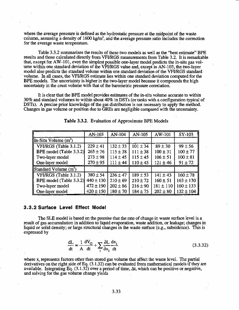
where the average pressure is defined as the hydrostatic pressure at the midpoint of the wastecolumn, assuming a density of 1600 kg/m3, and the average pressure ratio includes the correctionfor the average waste temperature.
Table 3.3.2 summarizes the results of these two models as well as the "best estimate" BPEresults and those calculated directly from VFI/RGS measurements from Table 3.2. It is remarkablethat, except for AW-101, even the simplest possible one-layer model predicts the in-situ gas vol-ume within one standard deviation of the VH/RGS value and, except in AN-103, the two-layermodel also predicts the standard volume within one standard deviation of the VFI/RGS standardvolume. In all cases, the VFI/RGS estimate lies within one standard deviation computed for theBPE models. The uncertainty is higher in the two-layer model because it compounds the highuncertainty in the crust volume with that of the barometric pressure correlation.
It is clear that the BPE model provides estimates of the in-situ volume accurate to within30% and standard volumes to within about 40% in DSTs (or tanks with a configuration typical ofDSTs). A precise prior knowledge of the gas distribution is not necessary to apply the method.Changes in gas volume or position due to GREs are negligible compared with the uncertainty.
Table 3.3.2. Evaluation of Approximate BPE Models
In-Situ Volume (m3)VFI/RGS (Table 3.1.2)BPE model (Table 3.3.2)Two-layer modelOne-layer model
Standard Volume (m3)VFI/RGS (Table 3.1.2)BPE model (Table 3,3.2)Two-layer modelOne-layer model
AN-103
229 ±41265 ± 76273 ± 98270 ±95
380 ±54440 ±130472 ±190420 ±150
AN-104
132 ±33115 ±38114±45111 ±44
236 ± 47210 ±69202 ± 86180 ±70
AN-105
101 ± 34111 ± 38115 ±45110±45
189 ±53210 ±72216 ±90184 ±75
AW-101
89 ±30100 ±31106 ±51121 ±46
141 ± 43160 ±51
181 ±110202 ± 80
SY-103
99 ±56100 ±77100 ±8191 ±72
160 ±78163 ±130160 ±133132 ±104
3.3.2 Surface Level Effect Model
The SLE model is based on the premise that the rate of change in waste surface level is aresult of gas accumulation in addition to liquid evaporation, waste addition, or leakage; changes inliquid or solid density; or large structural changes in the waste surface (e.g., subsidence). This isexpressed by
dt A dt
9L dx-.
dx: dt(3.3.32)
where X; represents factors other than stored gas volume that affect the waste level. The partialderivatives on the right side of Eq. (3.1.32) can be evaluated from mathematical models if they areavailable. Integrating Eq. (3.1.32) over a period of time, At, which can be positive or negative,and solving for the gas volume change yields
3.33
VG(t + At) = VG(t) + A[L(t + At) - L(t) - J dt(3.3.33)
where VG(t) is the total in-situ gas volume at time t. The in-situ gas volume and waste level thatcomprise this required starting point can be determined relatively accurately from the local gasvolume fractions measured with the VH/RGS. The last tank fill can also be a suitable startingpoint if the level and the gas volume are known at that time.
The major sources of uncertainty in the gas volume can be estimated by rearrangingEq. (3.1.33) to represent the change in gas volume over a given time period, At, to yield
= A[ALW-ALE-ALA] (3.3.34)
where AVG is the change in in-situ gas volume, A is the tank cross-sectional area, AL^ is themeasured surface level change, ALg is the equivalent level rise due to evaporation, and ALA is thelevel rise due to net waste addition, removal, or other similar effects. The relative uncertainty inthe gas retention can be expressed by linear combination of uncertainties in Eq. (3.1.34) as
= AALw + A
AL+ A
AL,
AVGIAL.(3.3.35)
where ci represents the standard error in each quantity.
The SLE model does not require a high-accuracy level measurement. Waste level changein DSTs is now typically measured by an Enraf buoyancy gauge to within a precision (CTJ of± 0.1 cm or better. This small error represents less than half a cubic meter of in-siru gas reten-tion. Even the relatively low precision of a manual tape measurement that is on the order of ± 1 cmrepresents an error of less than 5 m3 of gas. Therefore, if any significant volume of gas is beingretained, the first term of Eq. (3.1.35) quickly becomes small as gas accumulates.
Large waste transfers may invalidate subsequent SLE model predictions. Waste transfersoccur over a relatively short time. The resulting net level change, ALA, then remains fixed, and thelast term in the right side of Eq. (3.1.35) decreases with time as the retained gas volume grows.But the magnitude of the uncertainty (<JA/ALA) may be large if a large amount of waste is trans-ferred, or if the remaining waste is disturbed. A large waste addition increases the hydrostaticpressure and reduces the volume of the existing stored gas by a predictable amount. The incomingwaste is assumed to have no gas, which may not be exactly true. A large waste removal producesa reverse change in hydrostatic pressure but is also likely to cause a significant gas release that isdifficult to measure accurately. We conclude that the SLE model can probably be applied acrossmoderate waste additions but only for small volumes of waste removal. However, complete wasteremoval can serve as a new starting point if the gas content of the following addition is known.
In the absence of waste transfers, the major source of uncertainty in Eq. (3.1.35) can bethe effect of evaporation. Long-term (1994-1997) evaporation effects have only been measured inSY-101.(a) The head-space water vapor mass balance indicates that this tank is very slowly
(a) Net water gain or loss is reported in informal quarterly reviews of SY-101 mixer pump dataprepared by PNNL.
3.34
accumulating water. There is net water loss only occasionally during the winter when the ambientair is driest. The high salt concentration (especially sodium hydroxide) reduces the water vaporpressure and therefore inhibits evaporation. One could expect the error to be similarly negligible inother DSTs with a crust layer; however, evaporation could be significant in tanks that do not have acrust layer and that contain dilute waste at a relatively high temperature.
The evaporation rate is difficult to estimate unless the ventilation rate and the head-spacehumidity are well established. If both quantities are measured to within + 20%, the relativeuncertainty in evaporation (oyAL,;) could be as low as 30%. The uncertainty is much higher ifevaporation is estimated indirectly (e.g., waste heat load, mass transfer correlations, numericalsimulation, etc.).
If the level change due to evaporation can be shown to be small relative to gas retention(AALE/AVQ*!), the overall uncertainty contribution will also be small, regardless of the uncertaintyin evaporation. Also, since both evaporation loss and retained gas volume increase linearly overtime, the relative uncertainty does not accumulate with time. On the other hand, if little gas is beingretained compared with evaporation (AALB/AVQ>1), the overall uncertainty may be large enough todisqualify it even with a relatively accurate evaporation estimate.
We conclude that the SLE model provides a reasonable estimate of long-term retained gasaccumulation when gas retention is the dominant influence on waste level change. This isdemonstrably the case in the six DSTs on the FGWL. Evidence of this condition would be asteady rise in waste level over several years, periods of steady level rise interrupted by suddendrops due to episodic gas releases, or seasonal level variation with a maximum in September andOctober and a minimum in March and April.00 A constant or declining waste level would indicateconstant or declining gas volume only if evaporation and other effects can be specifically shown tobe negligible.
3.4 Visual Study of Core Extrusions and Waste Surface
Core sample extrusion photographs were shown in Stewart et al. (1996a) for SY-103,AW-101, AN-103, and AN-105, but only those from SY-103, AW-101, and AN-105 were fromthe most recent sampling. In this section, photographs from the most recent cores from AN-103and AN-104 are added (Figures 3.4.1 to 3.4.7). Waste surface photos for all six tanks are alsogiven to complete the picture (see Figures 3.4.8 through 3.4.14), including one of GRE Event I(June 26, 1993) in progress in SY-101 (Figure 3.4.13).
3.4.1 Core Extrusion Photographs
Extrusion photographs of AN-103 core samples from 1986 and 1996 are shown in Figures3.4.1 and 3.4.2. The 1986 core was taken only a few months after the last fill, in February 1986,before most of the gas accumulation had occurred. Bubbles are clearly visible in all segments ofthe 1996 cores but only in segment 12 of the 1986 core. Segment 15 (1996 core) is in the locationof the maximum void of 12-15%. The 1996 core appears dryer and stiffer than the 1986 core.1996 segments 16 and 17 are especially dry compared with 1986 segments at the same level (15and 16). The ball rheometer stopped at elevations represented by segment 16. In Figure 3.4.2,note the similarity of the crusts in segments 1 and 13 at the top of the nonconvective layer.
(a) This indicates a significant gas volume that changes cyclically in response to the average wastetemperature. Thermal inertia creates the time lag between the waste and ambient temperatureseasonal maxima.
3.35
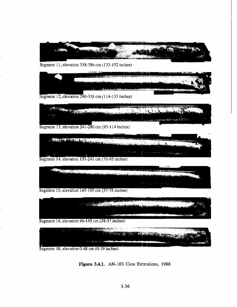
Segment 11, elevation 338-386 cm (133-152 inches)
Segment 12, elevation 290-338 cm (114-133 inches)
Segment 13, elevation 241-290 cm (95-114 inches)
Segment 14, elevation 193-241 cm (76-95 inches)
Segment 15, elevation 145-193 cm (57-76 inches)
Segment 16, elevation 96-145 cm (38-57 inches)
;gment 18, elevation 0-48 cm (0-19 inches)
Figure 3.4.1. AN-103 Core Extrusions, 1986
3.36
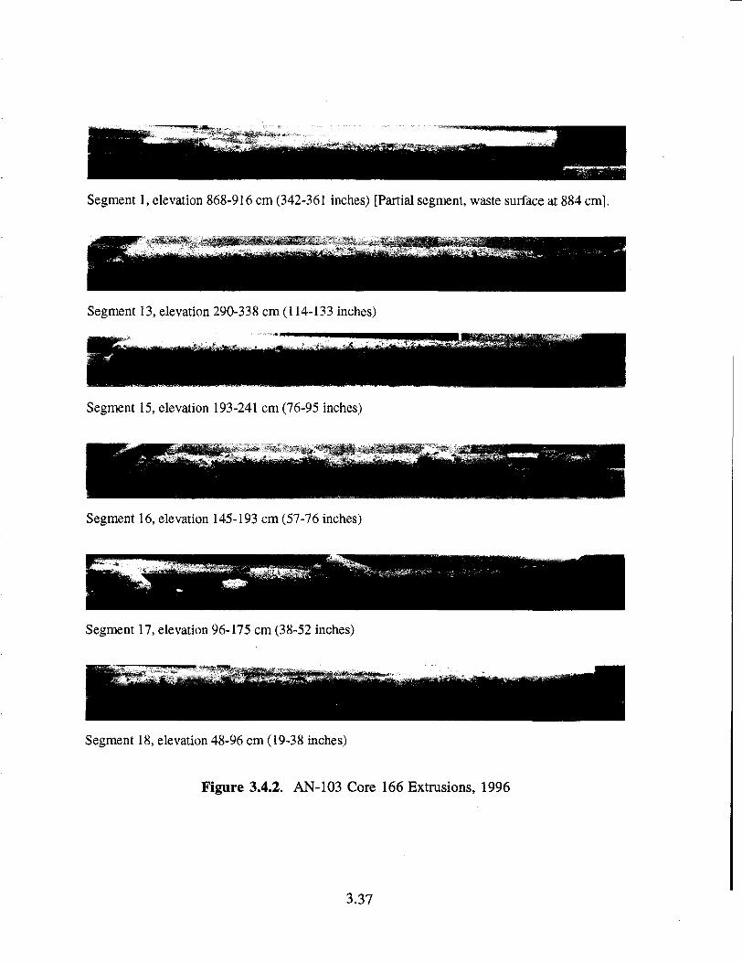
Segment 1, elevation 868-916 cm (342-361 inches) [Partial segment, waste surface at 884 cm].
Segment 13, elevation 290-338 cm (114-133 inches)
Segment 15, elevation 193-241 cm (76-95 inches)
Segment 16, elevation 145-193 cm (57-76 inches)
Segment 17, elevation 96-175 cm (38-52 inches)
Segment 18, elevation 48-96 cm (19-38 inches)
Figure 3.4.2. AN-103 Core 166 Extrusions, 1996
3.37
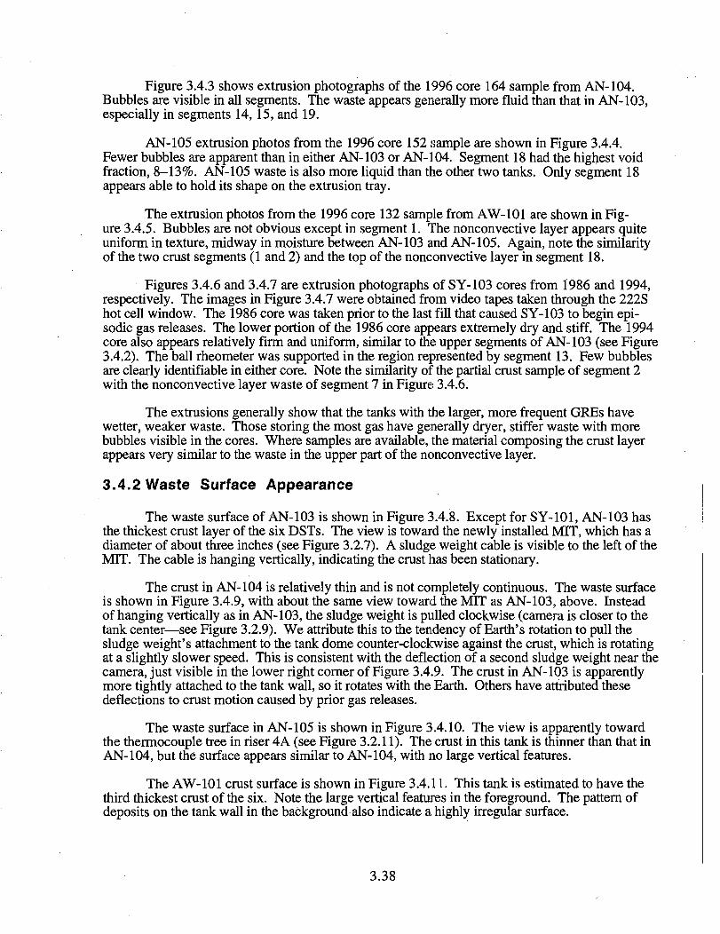
Figure 3.4.3 shows extrusion photographs of the 1996 core 164 sample from AN-104.Bubbles are visible in all segments. The waste appears generally more fluid than that in AN-103,especially in segments 14,15, and 19.
AN-105 extrusion photos from the 1996 core 152 sample are shown in Figure 3.4.4.Fewer bubbles are apparent than in either AN-103 or AN-104. Segment 18 had the highest voidfraction, 8-13%. AN-105 waste is also more liquid than the other two tanks. Only segment 18appears able to hold its shape on the extrusion tray.
The extrusion photos from the 1996 core 132 sample from AW-101 are shown in Fig-ure 3.4.5. Bubbles are not obvious except in segment 1. The nonconvective layer appears quiteuniform in texture, midway in moisture between AN-103 and AN-105. Again, note the similarityof the two crust segments (1 and 2) and the top of the nonconvective layer in segment 18.
Figures 3.4.6 and 3.4.7 are extrusion photographs of SY-103 cores from 1986 and 1994,respectively. The images in Figure 3.4.7 were obtained from video tapes taken through the 222Shot cell window. The 1986 core was taken prior to the last fill that caused SY-103 to begin epi-sodic gas releases. The lower portion of the 1986 core appears extremely dry and stiff. The 1994core also appears relatively firm and uniform, similar to the upper segments of AN-103 (see Figure3.4.2). The ball rheometer was supported in the region represented by segment 13. Few bubblesare clearly identifiable in either core. Note the similarity of the partial crust sample of segment 2with the nonconvective layer waste of segment 7 in Figure 3.4.6.
The extrusions generally show that the tanks with the larger, more frequent GREs havewetter, weaker waste. Those storing the most gas have generally dryer, stiffer waste with morebubbles visible in the cores. Where samples are available, the material composing the crust layerappears very similar to the waste in the upper part of the nonconvective layer.
3.4.2 Waste Surface Appearance
The waste surface of AN-103 is shown in Figure 3.4.8. Except for SY-101, AN-103 hasthe thickest crust layer of the six DSTs. The view is toward the newly installed MIT, which has adiameter of about three inches (see Figure 3.2.7). A sludge weight cable is visible to the left of theMIT. The cable is hanging vertically, indicating the crust has been stationary.
The crust in AN-104 is relatively thin and is not completely continuous. The waste surfaceis shown in Figure 3.4.9, with about the same view toward the MIT as AN-103, above. Insteadof hanging vertically as in AN-103, the sludge weight is pulled clockwise (camera is closer to thetank center—see Figure 3.2.9). We attribute this to the tendency of Earth's rotation to pull thesludge weight's attachment to the tank dome counter-clockwise against the crust, which is rotatingat a slightly slower speed. This is consistent with the deflection of a second sludge weight near thecamera, just visible in the lower right corner of Figure 3.4.9. The crust in AN-103 is apparentlymore tightly attached to the tank wall, so it rotates with the Earth. Others have attributed thesedeflections to crust motion caused by prior gas releases.
The waste surface in AN-105 is shown in Figure 3.4.10. The view is apparently towardthe thermocouple tree in riser 4A (see Figure 3.2.11). The crust in this tank is thinner than that inAN-104, but the surface appears similar to AN-104, with no large vertical features.
The AW-101 crust surface is shown in Figure 3.4.11. This tank is estimated to have thethird thickest crust of the six. Note the large vertical features in the foreground. The pattern ofdeposits on the tank wall in the background also indicate a highly irregular surface.
3.38
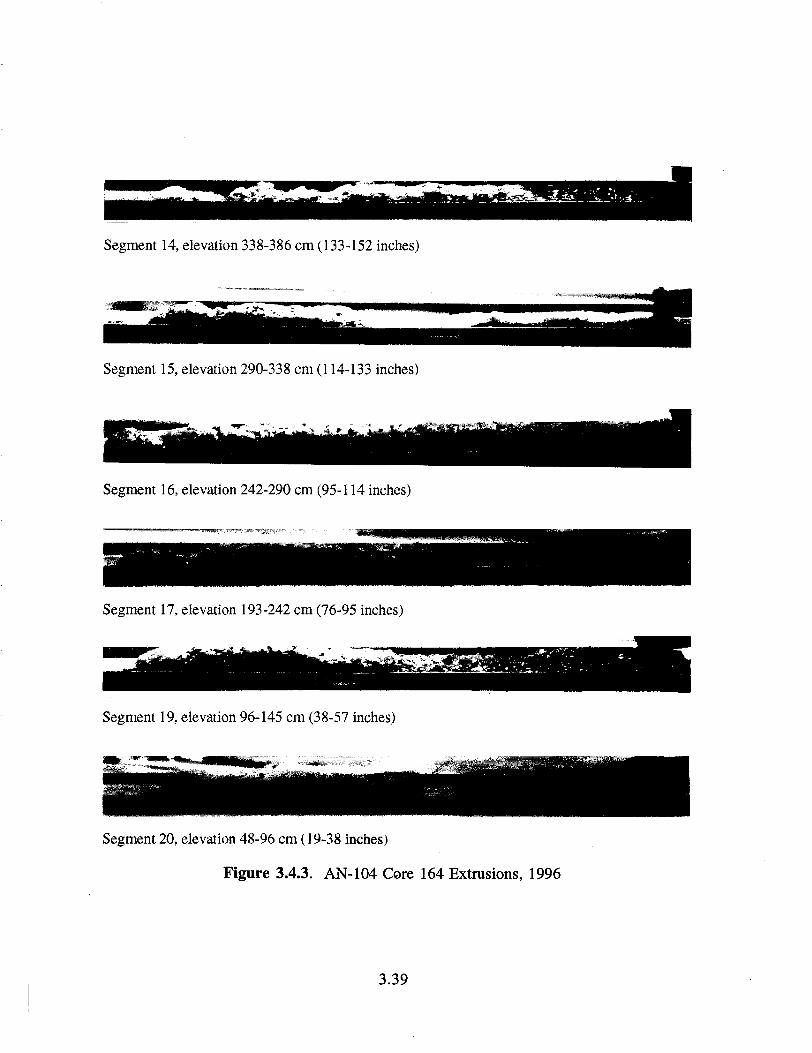
Segment 14, elevation 338-386 cm (133-152 inches)
Segment 15, elevation 290-338 cm (114-133 inches)
Segment 16, elevation 242-290 cm (95-114 inches)
Segment 17, elevation 193-242 cm (76-95 inches)
Segment 19, elevation 96-145 cm (38-57 inches)
Segment 20, elevation 48-96 cm (19-38 inches)
Figure 3.4.3. AN-104 Core 164 Extrusions, 1996
3.39
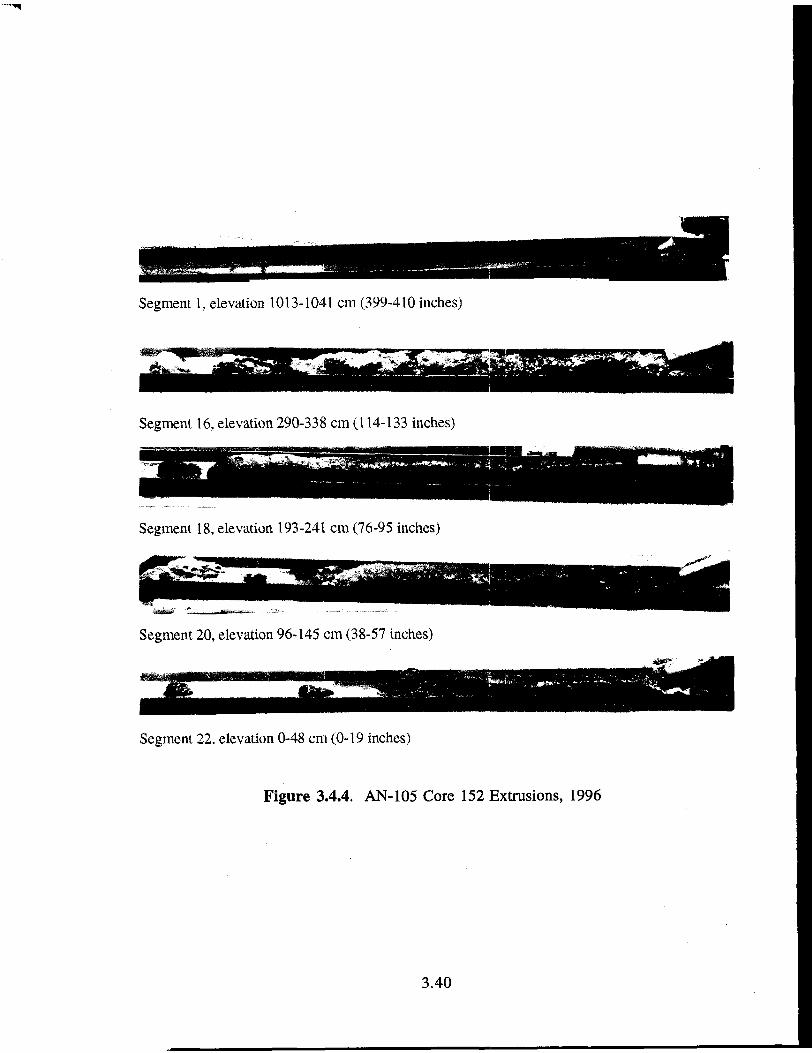
Segment 1, elevation 1013-1041 cm (399-410 inches.)
Segment 16, elevation 290-338 cm (114-133 inches)
Segment 18, elevation 193-241 cm (76-95 inches)
Segment 20, elevation 96-145 cm (38-57 inches)
Segment 22, elevation 0-48 cm (0-19 inches)
Figure 3.4.4. AN-105 Core 152 Extrusions, 1996
3.40
«**
Segment 1, elevation 1013-1040 cm (399-409 inches)
Segment 2, elevation 965-1013 cm (380-399 inches)
Segment 16, elevation 290-338 cm (114-133 inches)
Segment 18, elevation 193-241 cm (76-95 inches)
Segment 20, elevation 96-145 cm (38-57 inches)
Segment 22, elevation 0-48 cm (0-19 inches)
Figure 3.4.5. AW-101 Core 132 Extrusions, 1996
3.41
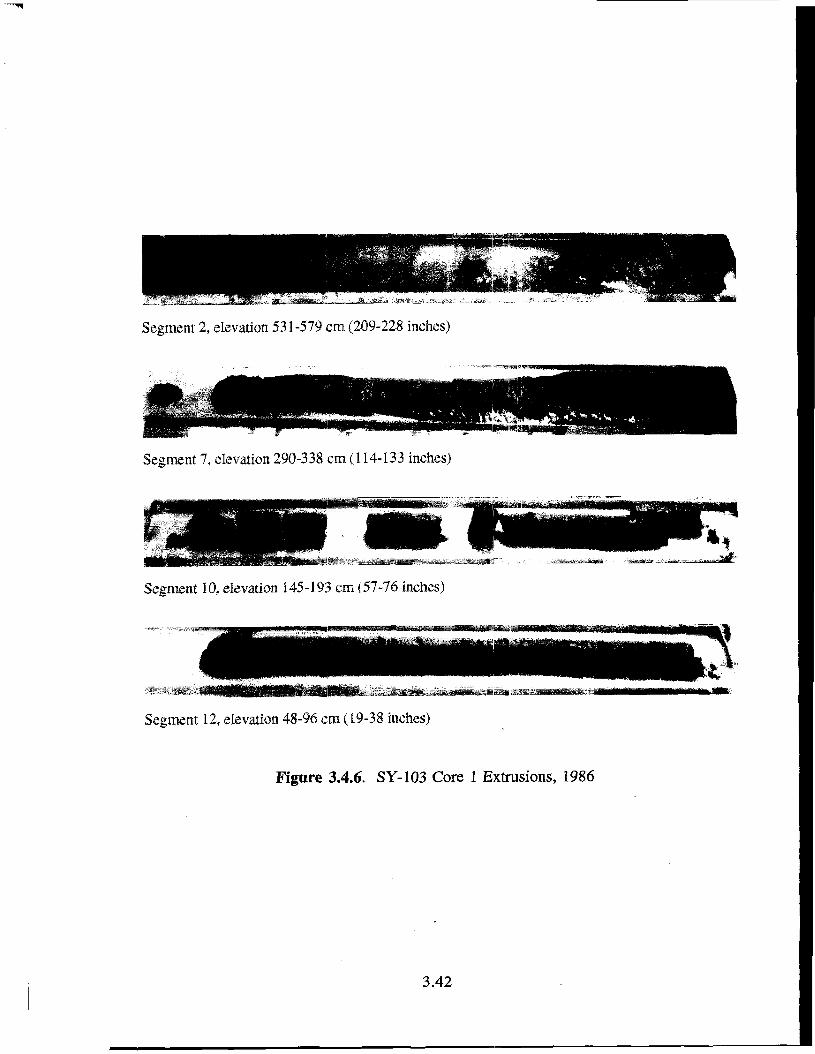
Segment 2, elevation 531-579 cm (209-228 inches)
Segment 7, elevation 290-338 cm (114-133 inches)
Segment 10, elevation 145-193 cm (57-76 inches)
Segment 12, elevation 48-96 cm (19-38 inches)
Figure 3.4.6. SY-103 Core 1 Extrusions, 1986
3.42
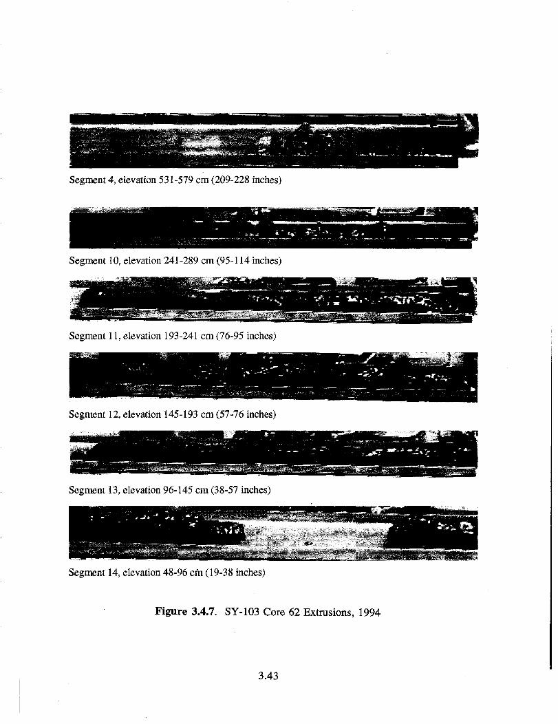
Segment 4, elevation 531-579 cm (209-228 inches)
Segment 10, elevation 241-289 cm (95-114 inches)
Segment 11, elevation 193-241 cm (76-95 inches)
Segment 12, elevation 145-193 cm (57-76 inches)
Segment 13, elevation 96-145 cm (38-57 inches)
Segment 14, elevation 48-96 cm (19-38 inches)
Figure 3.4.7. SY-103 Core 62 Extrusions, 1994
3.43
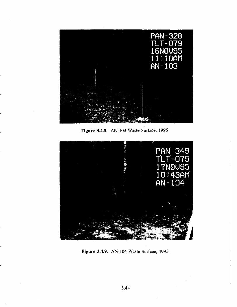
PAN-328TLT-07916N0U9511:10AMAN-103
Figure 3.4.8. AN-103 Waste Surface, 1995
Figure 3.4.9. AN-104 Waste Surface, 1995
3.44
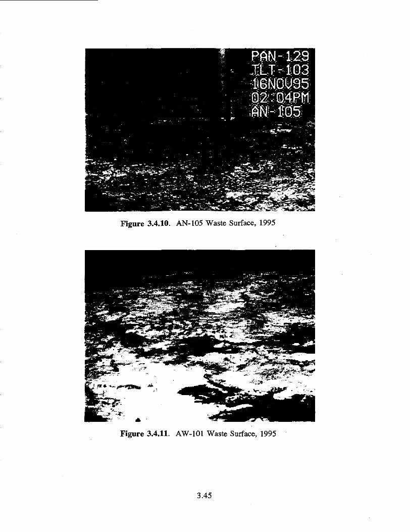
Figure 3.4.10. AN-105 Waste Surface, 1995
Figure 3.4.11. AW-101 Waste Surface, 1995
3.45
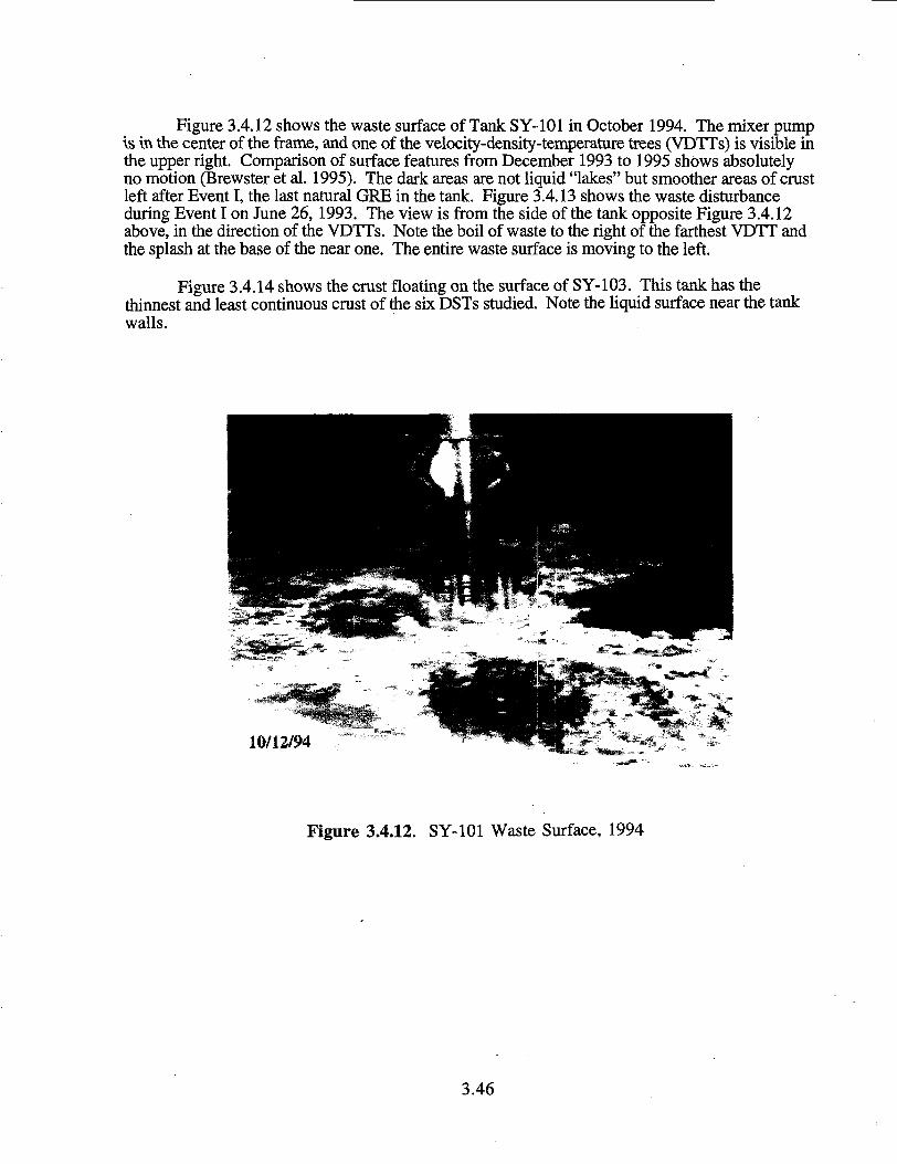
Figure 3.4.12 shows the waste surface of Tank SY-101 in October 1994. The mixer pumpis in the center of the frame, and one of the velocity-density-temperature trees (VDTTs) is visible inthe upper right. Comparison of surface features from December 1993 to 1995 shows absolutelyno motion (Brewster et al. 1995). The dark areas are not liquid "lakes" but smoother areas of crustleft after Event I, the last natural GRE in the tank. Figure 3.4.13 shows the waste disturbanceduring Event I on June 26, 1993. The view is from the side of the tank opposite Figure 3.4.12above, in the direction of the VDTTs. Note the boil of waste to the right of the farthest VDTT andthe splash at the base of the near one. The entire waste surface is moving to the left.
Figure 3.4.14 shows the crust floating on the surface of SY-103. This tank has thethinnest and least continuous crust of the six DSTs studied. Note the liquid surface near the tankwalls.
10/12/94
Figure 3.4.12. SY-101 Waste Surface, 1994
3.46
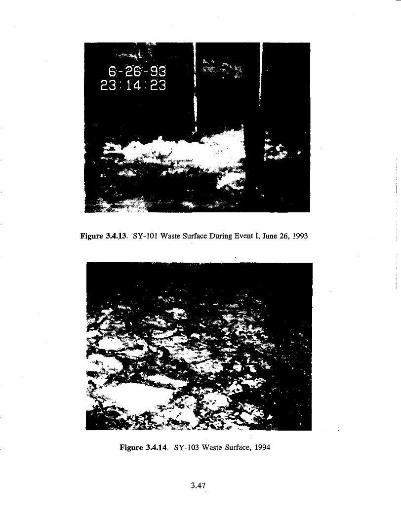
Figure 3.4.13. SY-101 Waste Surface During Event I, June 26, 1993
Figure 3.4.14. SY-103 Waste Surface, 1994
3.47
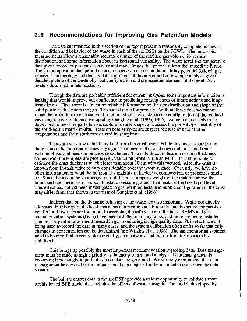
3.5 Recommendations for Improving Gas Retention Models
The data summarized in this section of the report present a reasonably complete picture ofthe condition and behavior of the waste in each of the six DSTs on the FGWL. The local voidmeasurements allow a reasonably accurate estimate of the retained gas volume, its verticaldistribution, and some information about its horizontal variability. The waste level and temperaturedata give a record of past tank behavior and reveal trends that predict at least the immediate future.The gas composition data permit an accurate assessment of the flammability potential following arelease. The rheology and density data from the ball rheometer and core sample analysis give adetailed picture of the waste physical configuration and are essential elements of the predictivemodels described in later sections.
Though the data are probably sufficient for current analyses, some important information islacking that would improve our confidence in predicting consequences of future actions and long-term effects. First, there is almost no reliable information on the size distribution and shape of thesolid particles that retain the gas. The same is true for porosity. Without these data we cannotrelate the other data (e.g., local void fraction, yield stress, etc.) to the configuration of the retainedgas using the correlations developed by Gauglitz et al. (1995, 1996). Some means needs to bedeveloped to measure particle size, capture particle shape, and assess the porosity/permeability ofthe solid-liquid matrix in-situ. Tests on core samples are suspect because of uncontrolledtemperatures and the disturbance caused by sampling.
There are very few data of any kind from the crust layer. While this layer is stable, andthere is no indication that it poses any significant hazard, the crust does contain a significantvolume of gas and needs to be understood better. The only direct indication of crust thicknesscomes from the temperature profile (i.e., validation probe run in an MIT). It is impossible toestimate the crust thickness much closer than about 10 cm with this method. Also, the crust isknown from in-tank video to vary considerably over the waste surface. Currently, we have noother information of what the horizontal variability in thickness, composition, or properties mightbe. Since the gas in the submerged part of the crust supports weight of the material above theliquid surface, there is an inverse lithostatic pressure gradient that peaks at the free liquid level.This effect has not yet been investigated in gas retention tests, and bubble configuration in the crustmay differ from that shown in the tests of Gauglitz et al. (1996).
Indirect data on the dynamic behavior of the waste are also important. While not directlyaddressed in this report, the head-space gas composition and humidity and the active and passiveventilation flow rates are important in assessing the safety state of the tank. SHMS and gascharacterization systems (GCS) have been installed on many tanks, and more are being installed.The most urgent improvement needed in gas monitoring is high-quality data. Strip charts are stillbeing used to record the data in many cases, and the system calibration often drifts so far that onlychanges in concentration can be determined (see Wilkins et al. 1996). The gas monitoring systemsneed to be modified to record data digitally, on a network, and their calibration needs to bestabilized.
This brings up possibly the most important recommendation regarding data. Data manage-ment must be made as high a priority as the measurement and analysis. Data management isbecoming increasingly important as more data are generated. We strongly recommend that datamanagement be elevated in importance and that a major effort be mounted to modernize the datastream.
The ball rheometer data in the six DSTs provide a unique opportunity to validate a moresophisticated BPE model that includes the effects of waste strength. The model, developed by
3.48
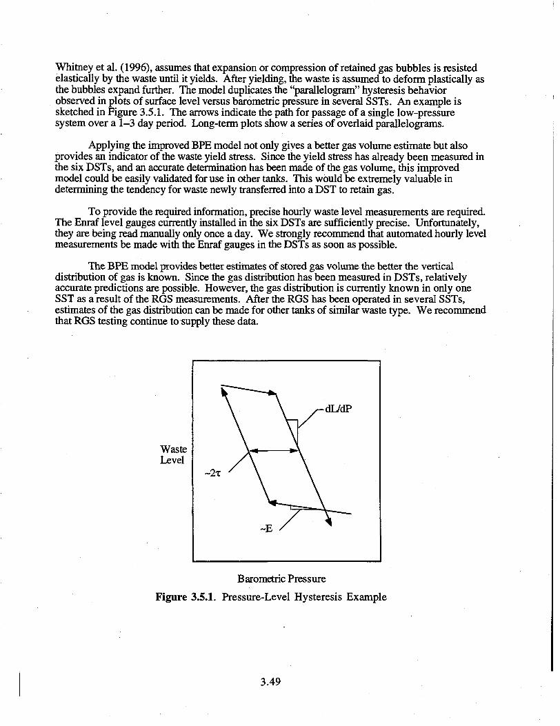
Whitney et al. (1996), assumes that expansion or compression of retained gas bubbles is resistedelastically by the waste until it yields. After yielding, the waste is assumed to deform plastically asthe bubbles expand further. The model duplicates the "parallelogram" hysteresis behaviorobserved in plots of surface level versus barometric pressure in several SSTs. An example issketched in Figure 3.5.1. The arrows indicate the path for passage of a single low-pressuresystem over a 1-3 day period. Long-term plots show a series of overlaid parallelograms.
Applying the improved BPE model not only gives a better gas volume estimate but alsoprovides an indicator of the waste yield stress. Since the yield stress has already been measured inthe six DSTs, and an accurate determination has been made of the gas volume, this improvedmodel could be easily validated for use in other tanks. This would be extremely valuable indetermining the tendency for waste newly transferred into a DST to retain gas.
To provide the required information, precise hourly waste level measurements are required.The Enraf level gauges currently installed in the six DSTs are sufficiently precise. Unfortunately,they are being read manually only once a day. We strongly recommend that automated hourly levelmeasurements be made with the Enraf gauges in the DSTs as soon as possible.
The BPE model provides better estimates of stored gas volume the better the verticaldistribution of gas is known. Since the gas distribution has been measured in DSTs, relativelyaccurate predictions are possible. However, the gas distribution is currently known in only oneSST as a result of the RGS measurements. After the RGS has been operated in several SSTs,estimates of the gas distribution can be made for other tanks of similar waste type. We recommendthat RGS testing continue to supply these data.
WasteLevel
-B/
y-dL/dP
VBarometric Pressure
Figure 3.5.1. Pressure-Level Hysteresis Example
3.49
4.0 Prediction of Gas Release Behavior
Section 3 presented the retained gas volume derived from local void measurements obtainedfrom the six DSTs on the FGWL. Section 5 discusses the potential consequences in terms of peakdome pressure resulting from a deflagration involving all or part of the gas inventory. This sectiondescribes the historical gas release behavior of the six tanks and presents new models to predict gasrelease volume. An important consideration in flammable gas safety is the potential for theexpected gas release volume to vary with long-term changes in the waste. It is also highlydesirable to be able to predict the size of potential GREs following waste transfers. The data haveenabled us to develop models that can predict how large a gas release to expect in these situations.
As discussed in Section 1, the episodic GREs historically observed in the six DSTs on theFGWL are believed to occur by the process of buoyant displacement. In a buoyant displacement,the nonconvective layer near the tank bottom accumulates gas until it becomes lighter than theconvective layer above it. At this point, a portion, or gob, of nonconvective material suddenlybreaks away and rises through the supernatant liquid layer. The stored gas bubbles may expand asthe gob rises. Where bubble expansion is sufficient to fail the ambient matrix, gas will be releasedfrom the gob and, if not trapped by existing crust, may escape into the head space
We hypothesize that the characteristic size of a buoyant gob (and the subsequent gascontent) is controlled by two competing physical phenomena. The first phenomenon relates tostatic forces and buoyancy. Since the nonconvective layer is a viscoplastic material, the concept ofbuoyancy is somewhat modified from the familiar meaning in Newtonian fluids. The forcesresulting from normal stresses around a region of low-density viscoplastic material must overcomeboth the weight of the region and the material strength on the boundaries of the region. Hence, alarger buoyant force is required to achieve an instability. The amount of gas accumulation requiredfor buoyancy will depend on the size and shape (surface area) of a gob as well as the yield strengthof the material.
The second phenomenon relates to dynamic instabilities. A viscoplastic material behaveslike a fluid once the yield stress is surpassed. We know that when a heavier fluid layer is super-posed on a lighter fluid layer, regions of heavier fluid will fall and regions of lighter fluid will riseaccording to the well-known Rayleigh Taylor instability theory. The wavelength, or characteristicsize of the moving regions, depends on the relative densities and viscosities of the two layers.Hence, if we view the nonconvective layer as a viscous fluid, the size of an unstable gob willdepend on density (gas accumulation) as well as viscosity.
The average size of an unstable gob undergoing buoyant displacement is dictated by thecombined effects of the mechanisms described above. The actual size of a GRE will be determinedby the size of the gob, the volume of gas within the gob, and the fraction of gas that escapes duringa buoyant displacement. After a buoyant displacement occurs, we assume the gob sinks back tothe nonconvective layer with a reduced gas inventory. Over time, heterogeneities develop in thenonconvective layer as buoyant gobs rise, release gas, sink, then repeat the process. This dynamiccycle could provide slow mixing in the nonconvective layer over time. The average time requiredfor a single GRE is dictated by a gob's initial gas content (immediately after a GRE), the amountof gas required to initiate buoyant displacement, and the gas generation rate. The average GREfrequency in a given tank is related to the total number of gobs possible and the GRE frequency foreach gob.
The physical processes described above form the basis of the analytical models presented inthis section. The modeling approach is to capture the first-order effects of the assumed physicalprocesses by making heuristic arguments and simplifying assumptions wherever possible. We do
4.1
not deny the complexity of the dynamic physical situations in the DSTs, and we recognize thatsimple models will not accurately represent all the details of the actual heterogeneous wastebehavior. However, we believe a simplified approach is appropriate for understanding andpredicting basic GRE behavior.
This section is organized in the following way: Section 4.1 summarizes the historical GREbehavior of each tank, and Section 4.2 addresses waste properties and the assumed waste config-uration to be modeled. Section 4.3 examines the essential mechanism of buoyancy, the stabilizingeffect of material yield strength, and the geometry of the buoyant gob. Section 4.4 presents resultsof a stability analysis for the buoyant nonconvective layer. In Section 4.5, the results of theprevious two sections are combined to obtain predictive models for the size and frequency ofGREs. Section 4.6 presents a criterion for gas release during buoyant displacement. This is acomplementary analysis that considers the energetics of the buoyant displacement process. Sec-tion 4.7 provides recommendations for improving gas release models.
4.1 Historic Gas Release Behavior
This section describes the historical gas releases in the six tanks studied in this report asobserved in the waste level history. The GRE history for a typical tank prior to the mid-1990smust be derived from the waste level history, usually as measured by an FIC contact probe orEnraf buoyancy gauge (since about 1995). The manual tape or other devices are suitable foridentifying but not quantifying some of the larger releases. GREs are identified by a sudden leveldrop following a long period of steady level rise. The initial drop is usually followed by a slowerdecline to a minimum level several days or even a couple of weeks after the main event. Oftenthere is an accelerated or even abrupt level rise just before the event.
During a buoyant displacement event, the expansion of the gas in the rising gob willproduce a level rise if it occurs slowly or if the gas is not released immediately. At the surface, gasis released until the gob returns to approximately neutral buoyancy at the surface. This causes thesudden level drop that is the signature of a classic "rollover." Then the gob may disintegrate aspieces sink back to the bottom, compressing the gas that remains trapped. This final processproduces the slower level decline that occurs days or even weeks after the actual release. Only theinitial level drop should be used to compute the release since only this phase of the GRE isaccompanied by a rapid release of gas into the head space.
A gas release is assumed to be indicated by a sharp level drop of at least 0.75 cm, which isessentially the limit of detection, or a sharp rise immediately followed by a sudden drop. Toensure that all level drops were evaluated, a procedure was applied that locates statisticallysignificant breaks in the level history (rises or drops) that might indicate a GRE (Whitney et al.1996). Once the level breaks are identified, the waste level history must be screened to weed outfalse positives resulting from occasional FIC flushes or spurious readings recorded in the opera-tions log. The validated list of breaks in each tank must then be evaluated one by one, by inspect-ing the daily level data with a generous application of human judgment. There is a good bit of artin this step, and different analysts could record different sets of GREs.(a) There is no doubt aboutthe larger ones (e.g., SY-101 prior to mixing), but there is considerable doubt about the barelydetectable drops in AN-101 and AW-101, for example.
(a) The GREs listed in this section were identified by CW Stewart. Use of the procedure inWhitney et al. (1996) produced slightly different list than given in Stewart et al. (1996a),which was also identified by Stewart directly from the level data.
4.2
Once the list of GREs is selected, the gas release is calculated from the difference betweenthe peak waste level immediately before the drop and the level on the next day, even if the level onsubsequent days is lower. The gas release is assumed to originate in the nonconvective layer,because the convective layer contains essentially no gas and the gas stored in the crust apparentlydoes not participate heavily, as evidenced by the quick re-establishment of the crust layer inSY-101 following large releases. The standard gas release volume is computed as
VREL = ALGREAPNC (4.1.1)
where ALGRE is the initial level drop, A is the tank area, and PNC is the average pressure ratio(includes both temperature and pressure effects) of the gas stored in the nonconvective layerdefined by Eq. (3.1.15). In some tanks, gas releases occur with no surface level change, or thereleases are so small as to challenge the resolution of the level measurement—this is particularlytrue of AW-101 and AN-103.
The gas inventory in the nonconvective layer immediately before the GRE is calculatedfrom the difference between the pre-GRE waste level and the effective waste level if all the gas inthe nonconvective layer were removed. The pre-GRE standard volume in the nonconvective layeris given by
VPre-GRE =(LGRE~LNO-GAS)APNC (4.1-2)
where LGRE is the pre-GRE waste level, and LNCWJAS is the waste level that would exist if all gas inthe nonconvective layer were removed. The degassed level was derived from the local voidmeasurements in Section 3.1 (see Eq. (3.1.24). Note that volumes calculated by Eq. (4.1.2) willdiffer from those given in Table 3.1.2, row 9 because LGRE differs from the level at the time thevoid measurements were made.
The release fraction is estimated from the tank level history as the ratio of gas volumereleased to the gas volume in the nonconvective layer immediately prior to the GRE. The releasefraction is calculated by
N0-GAS
where ALGRE is the level drop from immediately prior to one day following the GRE. Note that therelease fraction is independent of gas pressure.
The gas release history of each of the six DSTs on the FGWL was given earlier in Stewartet al. (1996a).(a) We had hoped to be able to add a list of GREs derived from the SHMS, particu-larly for AW-101 and AN-103, whose level history is not a good indicator of gas release. How-ever, calculating gas release volumes from SHMS data requires assuming the head space is fullymixed at all times (unless a detailed computational simulation is performed). Since the mixing timeis on the order of one hour, it is clear that this assumption is not valid for the initial stages of smallreleases, and the gas release volumes so calculated would be highly uncertain, although SHMSdata remain the clearest evidence that a GRE has occurred. Therefore, we believe that level dropremains the best characterization of historic GRE behavior at this time.
(a) All gas release parameters for SY-101 represent conditions prior to installation of the mixerpump July 4, 1993.
4.3
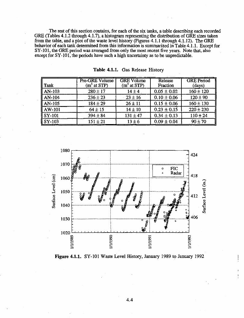
The rest of this section contains, for each of the six tanks, a table describing each recordedGRE (Tables 4.1.2 through 4.1.7), a histogram representing the distribution of GRE sizes takenfrom the table, and a plot of the waste level history (Figures 4.1.1 through 4.1.12). The GREbehavior of each tank determined from this information is summarized in Table 4.1.1. Except forSY-101, the GRE period was averaged from only the most recent five years. Note that, alsoexcept for SY-101, the periods have such a high uncertainty as to be unpredictable.
Table 4.1.1. Gas Release History
TankAN-103AN-104AN-105AW-101SY-101SY-103
Pre-GRE Volume(m3atSTP)280 ± 17236123184 ±2964+15394 ± 84151 ±21
GRE Volume(m3atSTP)
14±423 ±1626±1114 ±10131 ±4713 ±6
ReleaseFraction
0.05 ± 0.020.10 ±0.060.15 ± 0.060.23 ± 0.150.34 ±0.130.09 ± 0.04
GRE Period(days)
160 ±120120 ±90160 ±130220 ±230110 ±2490 ±70
1080
1070
(cm
"5>
o
rfa
CO
1060
1050
1040
1030 -
1 0 2 0 ' • • ' • • '
- 424
- 418
- 4 1 2
406
ICO
Figure 4.1.1. SY-101 Waste Level History, January 1989 to January 1992
4.4
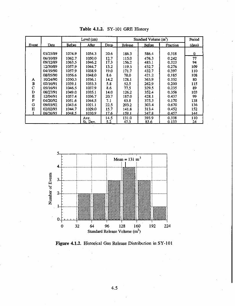
Table 4.1.2. SY-101 GRE History
Event
ABCDEFGHI
Date
03/25/8906/10/8909/12/8912/30/8904/19/9008/05/9010/24/9002/16/9105/16/9108/27/9112/04/9104/20/9209/03/9202/02/9306/26/93
Level (cm)
Before
1074.91062.71063.51057.91057.91056.61050.31039.11046.51049.01057.41051.61043.61044.71048.5
After
1054.31050.01046.21044.71038.91048.01036.11033.31037.91035.11036.71044.51021.11029.01030.9
Ave.St. Dev.
Droo
20.612.717.313.219.08.614.25.88.614.020.77.122.515.717.614.55.2
Standard Volume (m3)
Release
186.3115.0156.2119.3171.778.0128.152.577.5126.2187.063.8
203.2141.8159.1131.047.3
Before
586.4476.3483.1432.7432.7421.2363.9262.9329.5352.4428.1375.3303.4313.4347.8393.983.6
Fraction
0.3180.2420.3230.2760.3970.1850.3520.2000.2350.3580.4370.1700.6700.4520.4570.3380.133
Period
fdavs)
077941091101088011589
1039913813615214411024
0 32 64 96 128 160 192 224Standard Release Volume (m3)
Figure 4.1.2. Historical Gas Release Distribution in SY-101
4.5
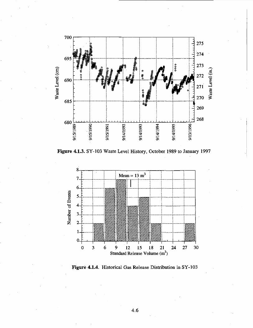
2
I
700
695
690 -
685
680 b ^
ON
ON
<?>ON
8i
ON
992
O\99
3S\
994
ON
ON
cn
ON
Figure 4.1.3. SY-103 Waste Level History, October 1989 to January 1997
1
12
9 12 15 18 21 24 27 30Standard Release Volume (m3)
Figure 4.1.4. Historical Gas Release Distribution in SY-103
4.6
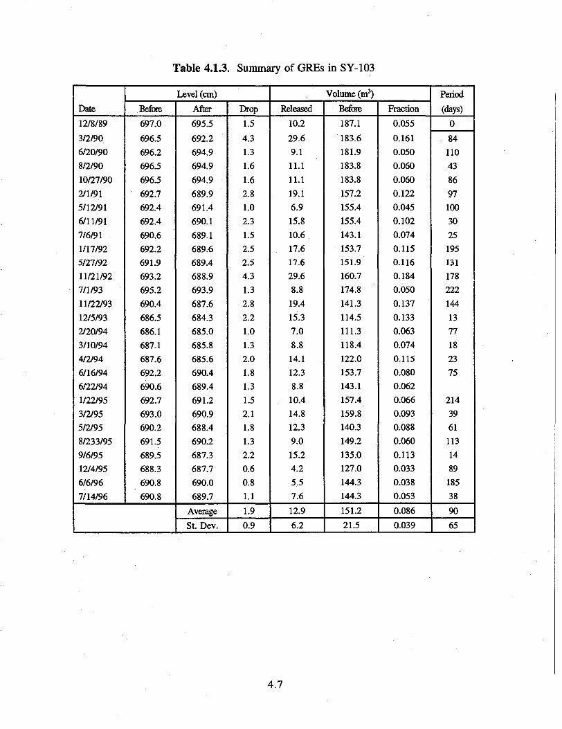
Table 4.13. Summary of GREs in SY-103
Date
12/8/89
3/2/906/20/908/2/9010/27/90
2/1/915/12/916/11/917/6/911/17/925/27/9211/21/927/1/9311/22/9312/5/932/20/943/10/944/2/946/16/946/22/941/22/953/2/955/2/958/233/959/6/9512/4/956/6/967/14/96
Before
697.0
696.5696.2696.5696.5692.7692.4692.4
690.6692.2691.9693.2695.2690.4686.5686.1687.1687.6692.2690.6692.7693.0690.2691.5689.5688.3690.8690.8
Level (cm)
After
695.5
692.2694.9694.9
694.9689.9691.4690.1689.1689,6689.4
688.9693.9687.6684.3685.0685.8685.6690.4689.4691.2690.9688.4690.2687.3687.7690.0689.7
Average
St. Dev.
Drop
1.5
4.3
1.3
1.6
1.6
2.8
1.0
2.3
1.5
2.5
2.5
4.3
1.3
2.8
2.2
1.0
1.3
2.0
1.8
1.3
1.5
2.11.8
1.3
2.2
0.6
0.8
1.1
1.9
0.9
Released
10.2
29.69.1
11.111.1
19.16.915.810.617.617.629.68.8
19.415.37.0
8.8
14.112.38.8
10.414.812.39.0
15.24.2
5.5
7.6
12.9
6.2
Volume (m3)
Before
187.1
183.6181.9183.8183.8157.2155.4155.4143.1153.7151.9160.7174.8141.3114.5111.3118.4122.0153.7143.1157.4159.8140.3149.2135.0127.0144.3144.3
151.2
21.5
Fraction
0.055
0.1610.0500.0600.0600.1220.0450.1020.0740.1150.1160.1840.0500.1370.1330.0630.0740.1150.0800.0620.0660.0930.0880.0600.1130.0330.0380.053
0.086
0.039
Period
(days)
0
84
110
43
86
97
100
30
25
195
131
178
222
144
13
77
18
23
75
214
39
61
113
14
89
185
38
90
65
4.7
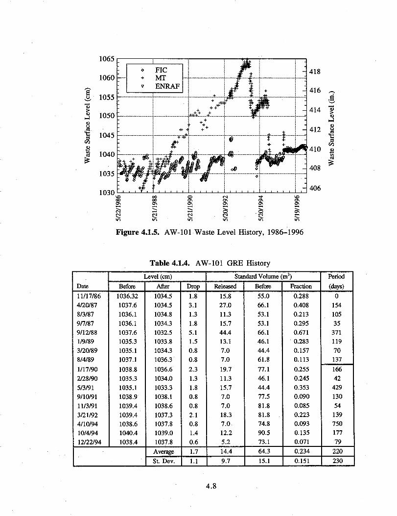
4J."5
i03
418
416
414
412
410
13
•s3
a
- 408
- 406
Figure 4.1.5. AW-101 Waste Level History, 1986-1996
Date
11/17/864/20/878/3/879/7/879/12/881/9/893/20/898/4/891/17/902/28/905/3/919/10/9111/3/913/21/924/10/9410/4/9412/22/94
Table 4.1.4. AW-101 GRELevel (cm)
Before
1036.321037.61036.11036.11037.61035.31035.11037.1
1038.81035.31035.11038.91039.41039.41038.61040.41038.4
After
1034.51034.51034.81034.31032.51033.81034.31036.31036.61034.01033.31038.11038.61037.31037.81039.01037.8
AverageSt. Dev.
Drop1.83.1
1.31.85.11.5
0.80.8
2.3
1.31.80.8
0.82.10.81.40.6
1.71.1
HistoryStandard Volume (m3)
Released
15.827.011.315.744.413.17.07.0
19.711.315.77.07.018.37.012.25.2
14.49.7
Before
55.066.153.153.166.146.144.461.877.146.144.477.581.881.874.890.573.164.315.1
Fraction
0.2880.4080.2130.2950.6710.2830.1570.1130.2550.2450.3530.0900.0850.2230.0930.1350.0710.2340.151
Period(days)
0154
105
35371119
70137
166
4242913054139750177
79
220230
4.8
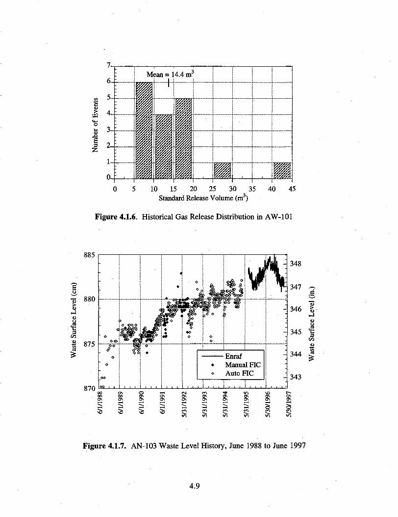
1
o.0 5 10 15 20 25 30 35 40 45
Standard Release Volume (m3)
Figure 4.1.6. Historical Gas Release Distribution in AW-101
885
Eo^ 880
I
870
-
-
-
o
<?o
o
>o <
« M
<K
o o i , i t
DOO
J8&
~"im—c"o*»
•
, , i , ,
^ *^ »
>
••
, i i ,
*
m<>
*?v•0o
• i i
o
<>0
SJFV tact o s y
* ^ * <
oo
«
O
j
j A O
>
A • J
w
EnrafManual FICAuto FIC
4M:. 7:—_----
, , , i , , , i , , , -
348
347
346
345
344
343
0)
<L>
ooooON
ONOOON
OONON Si O N
ONONOv
ONON
ONON
<n
a
Figure 4.1.7. AN-103 Waste Level History, June 1988 to June 1997
4.9
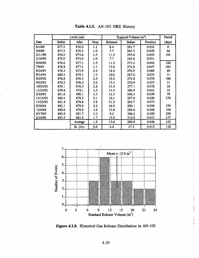
Table 4.1.5. AN-103 GRE History
Date
6/1/898/4/892/11/902/18/909/26/907/6/918/24/919/14/918/25/929/25/9210/23/9211/23/922/10/9311/15/9311/23/938/20/9412/4/948/17/952/10/96
Before
877.1877.3876.3875.0878.6878.8878.3880.4878.8878.3879.1879.6881.6880.4881.4882.1880.6882.9883.5
l evel (cm)
After
876.0876.3874.8874.0877.1877.1875.9879.1876.3876.3876.3878.1880.1878.3878.6879.9878.8881.7881.8
Average
St. Dev.
Drop
1.11.01.51.01.51.72.41.32.52.02.81.51.52.12.82.21.81.21.71.8
0.6
Standard Volume (m3)
Released
8.47.711.57.711.513.018.410.019.215.421.511.511.516.121.516.913.89.213.013.6
4.4
Before
261.7263.3255.6245.6273.2274.8270.9287.0274.8270.9277.1280.9296.3287.0294.7300.1288.6306.2310.8280.0
17.3
Fraction
0.0320.0290.0450.0310.0420.0470.0680.0350.0700.0570.0780.0410.0390.0560.0730.0560.0480.0300.0420.048
0.015
Period
(days)
064191
2202834921
34631283179
278
270106256177155
118
i
1
0 3 6 9 12 15 18 21 24Standard Release Volume (m3)
Figure 4.1.8. Historical Gas Release Distribution in AN-103
4.10
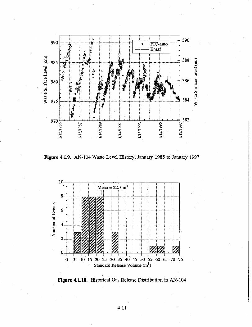
I
Ixn
990 J -
985
980
975
970
- 390
oo oo 0 0
Figure 4.1.9. AN-104 Waste Level History, January 1985 to January 1997
10-
>
8 I
4—
0-
j Mean = 22.7 m
IIi 1
Ii
t ^
10 5 10 15 20 25 30 35 40 45 50 55 60 65 70 75
Standard Release Volume (m3)
Figure 4.1.10. Historical Gas Release Distribution in AN-104
4.11
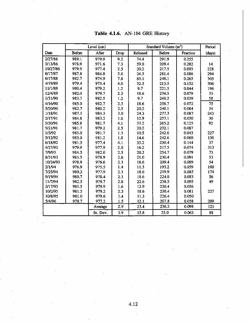
Table 4.1.6. AN-104 GRE History
Date
2/27/863/13/8610/27/868/17/876/17/884/19/8911/1/8912/4/891/31/904/16/905/20/901/18/912/17/915/20/915/21/911/3/925/12/926/18/924/27/937/9/938/31/9310/24/932/1/947/25/949/19/9411/7/942/17/9510/2/9510/8/955/4/96
]
Before
989.1978.9979.9987.8982.7979.4980.4982.0983.7985.0982.7987.3984.8985.8981.7983.0983.0981.5979.9984.5981.5978.9976.9980.2980.7982.5981.5981.5981.0978.7
^vel (cm)
After
979.9971.6977.4984.8974.9975.4979.2979.7982.5982.7980.2984.3983.2981.7979.2981.7981.2977.4977.9982.0978.9976.6975.5977.9978.4979.7979.9979.2979.6977.2
Average
St. Dev.
Drop
9.27.32.53.07.84.01.22.31.22.32.53.01.64.12.51.31.84.12.02.52.62.31.42.32.32.81.62.31.41.52.91.9
Standard Volume (m3)
Released
74.459.020.224.363.132.39.718.69.718.620.224.312.933.220.210.514.633.216.220.221.018.611.318.618.622.612.918.611.312.123.4
15.8
Before
291.9209.4217.5281.4240.1213.5221.5234.5248.2258.7240.1277.3257.1265.2232.1242.6242.6230.4217.5254.7230.4209.4193.2219.9224.0238.5230.4230.4226.4207.8236.2
23.0
Fraction
0.2550.2820.0930.0860.2630.1520.0440.0790.0390.0720.0840.0870.0500.1250.0870.0430.0600.1440.0740.0790.0910.0890.0590.0850.0830.0950.0560.0810.0500.0580.098
0.063
Period
(days)
1422829430530619633587534
2433092
22713037
3137353541001745649
227
209121
88
4.12
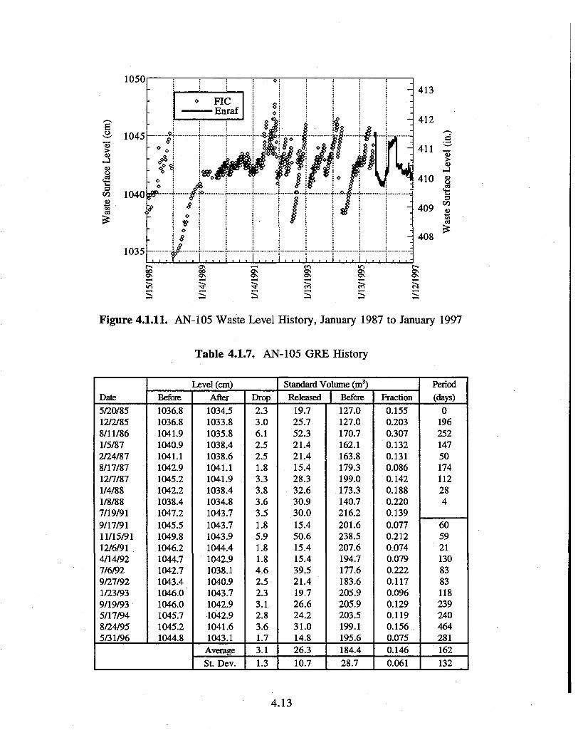
1050
"33
I00p.
1045 -
1040
1035 —
Figure 4.1.11. AN-105 Waste Level History, January 1987 to January 1997
Table 4.1.7. AN-105 GRE History
Date
5/20/8512/2/858/11/861/5/872/24/878/17/8712/7/871/4/881/8/887/19/919/17/9111/15/9112/6/914/14/927/6/929/27/921/23/939/19/935/17/948/24/955/31/96
Before
1036.81036.81041.91040.91041.11042.91045.21042.21038.41047.21045.51049.81046.21044.71042.71043.41046.01046.01045.71045.21044.8
Level (cm)After
1034.51033.81035.81038.41038.61041.11041.91038.41034.81043.71043.71043.91044.41042.91038.11040.91043.71042.91042.91041.61043.1
AverageSt. Dev.
Drop
2.33.06.12.52.51.83.33.83.63.51.85.91.81.84.62.52.33.12.83.61.73.11.3
Standard Volume (m3)Released
19.725.752.321.421.415.428.332.630.930.015.450.615.415.439.521.419.726.624.231.014.826.310.7
| Before
127.0127.0170.7162.1163.8179.3199.0173.3140.7216.2201.6238.5207.6194.7177.6183.6205.9205.9203.5199.1195.6184.428.7
Fraction
0.1550.2030.3070.1320.1310.0860.1420.1880.2200.1390.0770.2120.0740.0790.2220.1170.0960.1290.1190.1560.0750.1460.061
Period(days)
019625214750174112284
6059211308383118239240464281162132
4.13
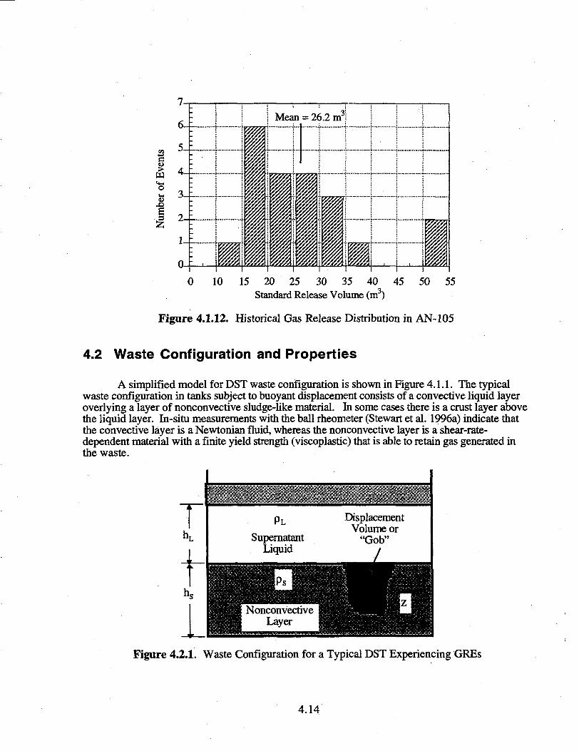
0 10 15 20 25 30 35 40 45 50 55Standard Release Volume (m )
Figure 4.1.12. Historical Gas Release Distribution in AN-105
4.2 Waste Configuration and Properties
A simplified model for DST waste configuration is shown in Figure 4.1.1. The typicalwaste configuration in tanks subject to buoyant displacement consists of a convective liquid layeroverlying a layer of nonconvective sludge-like material. In some cases there is a crust layer abovethe liquid layer. In-situ measurements with the ball rheometer (Stewart et al. 1996a) indicate thatthe convective layer is a Newtonian fluid, whereas the nonconvective layer is a shear-rate-dependent material with a finite yield strength (viscoplastic) that is able to retain gas generated inthe waste.
PL
SupernatantLiquid
DisplacementVolume or
"Gob"
NonconvectiveLayer
Figure 4.2.1. Waste Configuration for a Typical DST Experiencing GREs
4.14
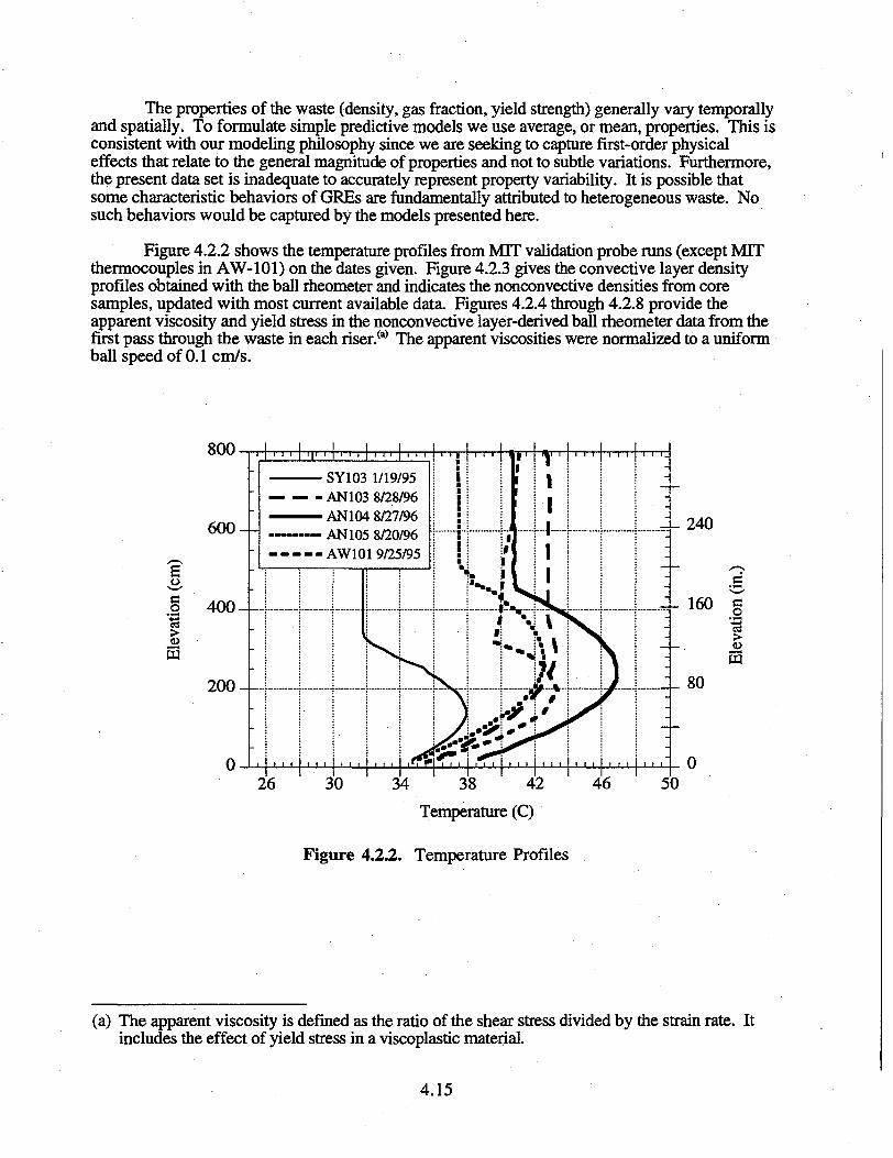
The properties of the waste (density, gas fraction, yield strength) generally vary temporallyand spatially. To formulate simple predictive models we use average, or mean, properties. This isconsistent with our modeling philosophy since we are seeking to capture first-order physicaleffects that relate to the general magnitude of properties and not to subtle variations. Furthermore,the present data set is inadequate to accurately represent property variability. It is possible thatsome characteristic behaviors of GREs are fundamentally attributed to heterogeneous waste. Nosuch behaviors would be captured by the models presented here.
Figure 4.2.2 shows the temperature profiles from MTT validation probe runs (except MITthermocouples in AW-101) on the dates given. Figure 4.2.3 gives the convective layer densityprofiles obtained with the ball rheometer and indicates the nonconvective densities from coresamples, updated with most current available data. Figures 4.2.4 through 4.2.8 provide theapparent viscosity and yield stress in the nonconvective layer-derived ball rheometer data from thefirst pass through the waste in each riser.00 The apparent viscosities were normalized to a uniformball speed of 0.1 cm/s.
800
6 0 0 - -
,0,
g5 4 0 0 - -
w2 0 0 - - U -
_LL_
SY103 1/19/95— — - AN103 8/28/96
AN104 8/27/96. . . . . . AN105 8/20/96
AW101 9/25/95
30 34 38 42
Temperature (C)
46
240
050
Figure 4.2.2. Temperature Profiles
(a) The apparent viscosity is defined as the ratio of the shear stress divided by the strain rate. Itincludes the effect of yield stress in a viscoplastic material.
4.15
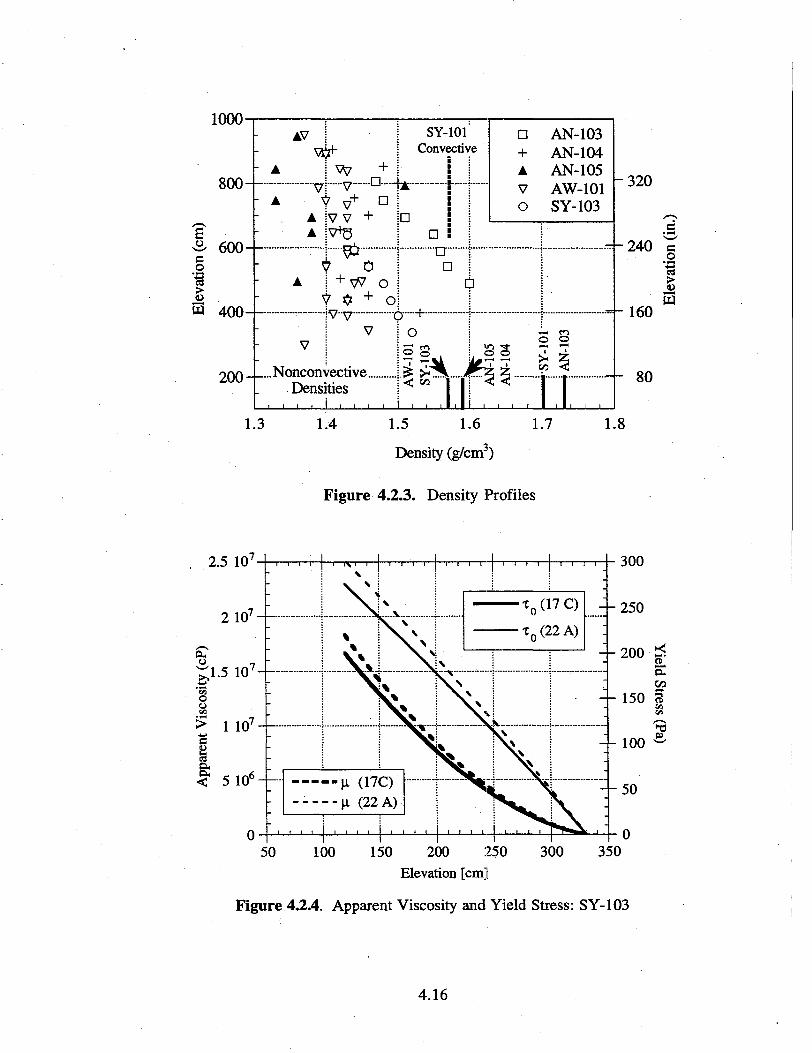
1000-
8 0 0 - -
o
1600--
W 4 0 0 - -
2 0 0 - - -
Vt +
+
~\*
D
..Nonconvective..Densities
SY-101Convective
•
n
- & • • -
28.
+•VO
AN-103AN-104AN-105AW-101SY-103
§
1 1 1 1 [ I ,
1.3 1.4 1.5 1.6
Density (g/cm3)
1.7
Figure 4.2.3. Density Profiles
2.5 107
-320
240
160
80
o
2
1.8
300
50 100 150 200 250 300 350Elevation [cm]
Figure 4.2.4. Apparent Viscosity and Yield Stress: SY-103
4.16
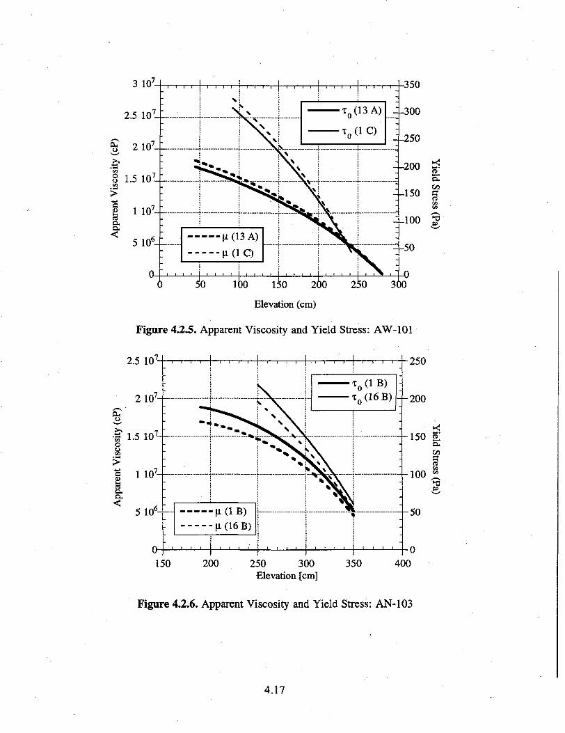
3 107- 350
300
6 50 100 150 200 250 300
Elevation (cm)
Figure 4.2.5. Apparent Viscosity and Yield Stress: AW-101
2.5 107- 250
0 0150 200 250 300 350
Elevation [cm]400
Figure 4.2.6. Apparent Viscosity and Yield Stress: AN-103
4.17
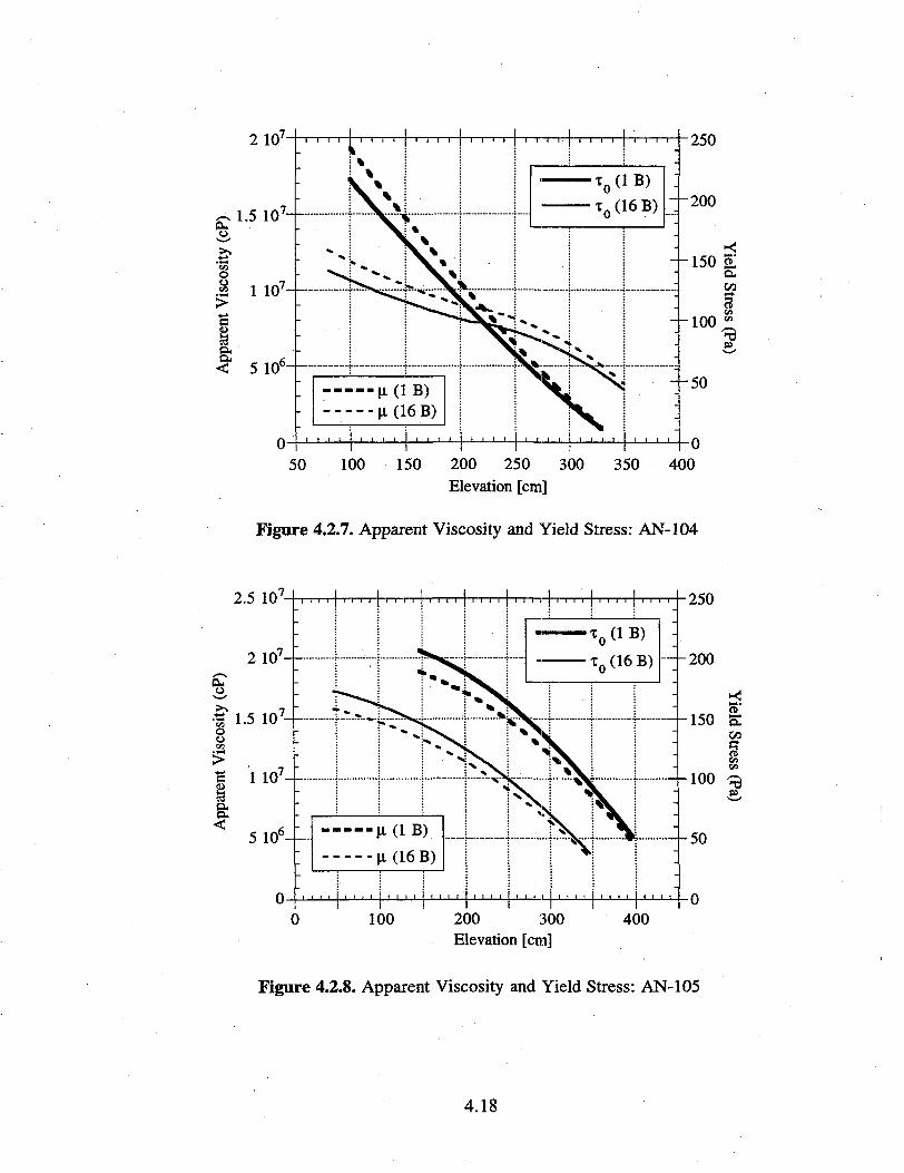
2 10 250
0 050 100 150 200 250 300 350 400
Elevation [cm]
Figure 4.2.7. Apparent Viscosity and Yield Stress: AN-104
2.5 107250
0 100 200 300Elevation [cm]
400
Figure 4.2.8. Apparent Viscosity and Yield Stress: AN-105
4.18
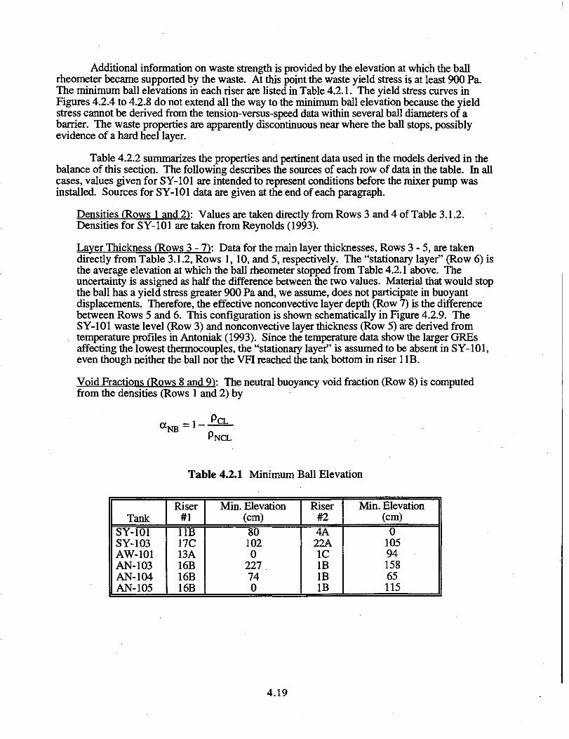
Additional information on waste strength is provided by the elevation at which the ballrheometer became supported by the waste. At this point the waste yield stress is at least 900 Pa.The minimum ball elevations in each riser are listed in Table 4.2.1. The yield stress curves inFigures 4.2.4 to 4.2.8 do not extend all the way to the minimum ball elevation because the yieldstress cannot be derived from the tension-versus-speed data within several ball diameters of abarrier. The waste properties are apparently discontinuous near where the ball stops, possiblyevidence of a hard heel layer.
Table 4.2.2 summarizes the properties and pertinent data used in the models derived in thebalance of this section. The following describes the sources of each row of data in the table. In allcases, values given for SY-101 are intended to represent conditions before the mixer pump wasinstalled. Sources for SY-101 data are given at the end of each paragraph.
Densities (Hows 1 and 2"): Values are taken directly from Rows 3 and 4 of Table 3.1.2.Densities for SY-101 are taken from Reynolds (1993).
Layer Thickness (Rows 3 - 7): Data for the main layer thicknesses, Rows 3 - 5, are takendirectly from Table 3.1.2, Rows 1,10, and 5, respectively. The "stationary layer" (Row 6) isthe average elevation at which the ball rheometer stopped from Table 4.2.1 above. Theuncertainty is assigned as half the difference between the two values. Material that would stopthe ball has a yield stress greater 900 Pa and, we assume, does not participate in buoyantdisplacements. Therefore, the effective nonconvective layer depth (Row 7) is the differencebetween Rows 5 and 6. This configuration is shown schematically in Figure 4.2.9. TheSY-101 waste level (Row 3) and nonconvective layer thickness (Row 5) are derived fromtemperature profiles in Antoniak (1993). Since the temperature data show the larger GREsaffecting the lowest thermocouples, the "stationary layer" is assumed to be absent in SY-101,even though neither the ball nor the VFI reached the tank bottom in riser 1 IB.
Void Fractions (Rows 8 and 9): The neutral buoyancy void fraction (Row 8) is computedfrom the densities (Rows 1 and 2) by
.1 PCL
PNCL
Table 4.2.1 Minimum Ball Elevation
TankSY-101SY-103AW-101AN-103AN-104AN-105
Riser#111B17C13A16B16B16B
Min. Elevation(cm)801020
227740
Riser#24A22A1CIBIBIB
Min. Elevation(cm)
01059415865115
4.19
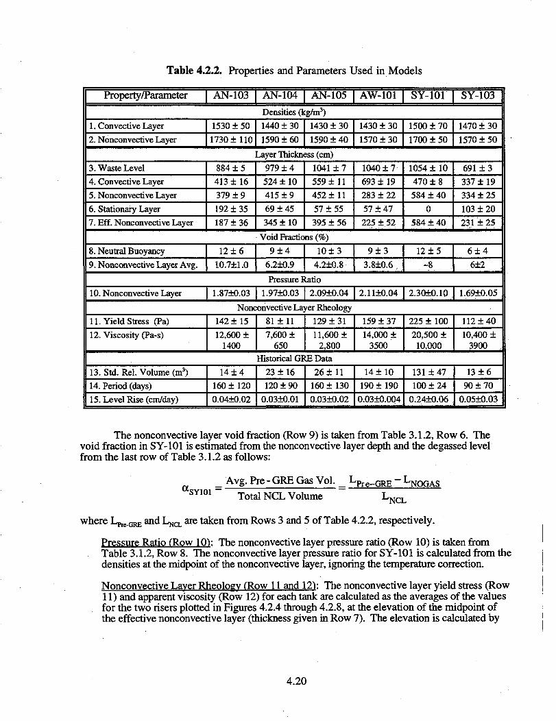
Table 4.2.2. Properties and Parameters Used in Models
Property/Parameter AN-103 AN-104 AN-105 AW-101 SY-101 SY-103
Densities (kg/m3)1. Convective Layer2. Nonconvective Layer
3. Waste Level4. Convective Layer5. Nonconvective Layer6. Stationary Layer7. Eff. Nonconvective Layer
1530 ± 501730+110
884 + 5413 + 16379 ±9192 + 35187 ±36
1440 ± 301590 ± 60
1430 ± 301590 + 40
Layer Thickness (cm)979 ±4524 ± 10415 ±969 + 45345 + 10
1041 ± 7559 ±11452+1157 + 55395 ± 56
1430 ± 301570 + 30
1040 ± 7693 + 19283 ± 2257 + 47225+52
1500 ± 701700 ± 50
1054 ± 10470 ± 8584 ± 40
0584 ± 40
1470 ± 301570 ± 50
691 ± 3337 ± 19334 ± 25
103 ± 20231 ± 25
Void Fractions (%)
8. Neutral Buoyancy9. Nonconvective Layer Avg.
12 ±6
10.7+1.0
9 ± 4
6.2±0.910 ± 3
4.2±0.89±3
3.8+.0.612 ±5
~86±46+2
Pressure Ratio10. Nonconvective Layer 1.87+0.03 1.97±0.03 2.09±0.04 2.11±0.04 2.30±0.10 1.69±0.05
Nonconvective Layer Rheology11. Yield Stress (Pa)12. Viscosity (Pa-s)
142 ± 1512,600 +
1400
81 ±117,600 +
650
129 ± 3111,600 ±
2,800
159 ± 3714,000 +
3500
225 ± 10020,500 ±10,000
112 ±4010,400 ±
3900Historical GRE Data
13. Std. Rel. Volume (m3)14. Period (days)15. Level Rise (cm/day)
14 ± 4160+1200.04±0.02
23 ±16120 ±90
0.03±0.01
26+11160 ± 1300.03±0.02
14 ±10190 ± 190
0.03±0.004
131 ± 47100 ±24
0.24±0.06
13 ± 690 ±70
0.05*0,03
The nonconvective layer void fraction (Row 9) is taken from Table 3.1.2, Row 6. Thevoid fraction in SY-101 is estimated from the nonconvective layer depth and the degassed levelfrom the last row of Table 3.1.2 as follows:
^SYlOl_ Avg. Pre - GRE Gas Vol. _ LPre-GRE ~ L
NOGAS
Total NCL Volume 'NCL
where an are taken from Rows 3 and 5 of Table 4.2.2, respectively.
Pressure Ratio CRow 10): The nonconvective layer pressure ratio (Row 10) is taken fromTable 3.1.2, Row 8. The nonconvective layer pressure ratio for SY-101 is calculated from thedensities at the midpoint of the nonconvective layer, ignoring the temperature correction.
Nonconvective Layer Rheology (Row 11 and 12): The nonconvective layer yield stress (Row11) and apparent viscosity (Row 12) for each tank are calculated as the averages of the valuesfor the two risers plotted in Figures 4.2.4 through 4.2.8, at the elevation of the midpoint ofthe effective nonconvective layer (thickness given in Row 7). The elevation is calculated by
4.20
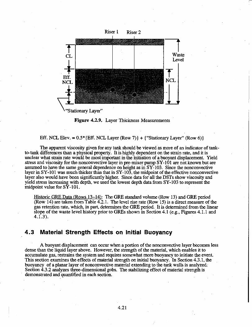
Riser 1 Riser 2
WasteLevel
'Stationary Layer"
Figure 4.2.9. Layer Thickness Measurements
Eff. NCL Elev. = 0.5*{Eff. NCL Layer (Row 7)} + {"Stationary Layer" (Row 6)}
The apparent viscosity given for any tank should be viewed as more of an indicator of tank-to-tank differences than a physical property. It is highly dependent on the strain rate, and it isunclear what strain rate would be most important in the initiation of a buoyant displacement. Yieldstress and viscosity for the nonconvective layer in pre-mixer pump SY-101 are not known but areassumed to have the same general dependence on height as in SY-103. Since the nonconvectivelayer in SY-101 was much thicker than that in SY-103, the midpoint of the effective nonconvectivelayer also would have been significantly higher. Since data for all the DSTs show viscosity andyield stress increasing with depth, we used the lowest depth data from SY-103 to represent themidpoint value for SY-101.
Historic GRE Data fRows 13-U): The GRE standard volume (Row 13) and GRE period(Row 14) are taken from Table 4.2.1. The level rise rate (Row 15) is a direct measure of thegas retention rate, which, in part, determines the GRE period. It is determined from the linearslope of the waste level history prior to GREs shown in Section 4.1 (e.g., Figures 4.1.1 and4.1.3).
4.3 Material Strength Effects on Initial Buoyancy
A buoyant displacement can occur when a portion of the nonconvective layer becomes lessdense than the liquid layer above. However, the strength of the material, which enables it toaccumulate gas, restrains the system and requires somewhat more buoyancy to initiate the event.This section examines the effects of material strength on initial buoyancy. In Section 4.3.1, thebuoyancy of a planar layer of nonconvective material extending to the tank walls is analyzed.Section 4.3.2 analyzes three-dimensional gobs. The stabilizing effect of material strength isdemonstrated and quantified in each section.
4.21
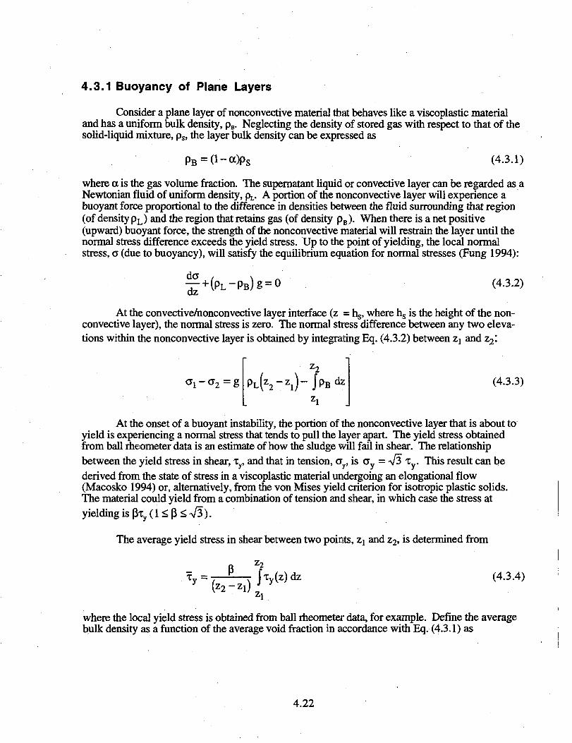
4.3.1 Buoyancy of Plane Layers
Consider a plane layer of nonconvective material that behaves like a viscoplastic materialand has a uniform bulk density, pB. Neglecting the density of stored gas with respect to that of thesolid-liquid mixture, ps, the layer bulk density can be expressed as
pB=(l-OC)p s (4.3.1)
where a is the gas volume fraction. The supernatant liquid or convective layer can be regarded as aNewtonian fluid of uniform density, pL. A portion of the nonconvective layer will experience abuoyant force proportional to the difference in densities between the fluid surrounding that region(of density pL) and the region that retains gas (of density pB). When there is a net positive(upward) buoyant force, the strength of the nonconvective material will restrain the layer until thenormal stress difference exceeds the yield stress. Up to the point of yielding, the local normalstress, a (due to buoyancy), will satisfy the equilibrium equation for normal stresses (Fung 1994):
= O (4-3.2)
At the convective/nonconvective layer interface (z = hs, where hs is the height of the non-convective layer), the normal stress is zero. The normal stress difference between any two eleva-tions within the nonconvective layer is obtained by integrating Eq. (4.3.2) between Zj and z2l
a1-a2 = P L ( Z 2 " Z I ) -
Z2
z l
(4.3.3)
At the onset of a buoyant instability, the portion of the nonconvective layer that is about toyield is experiencing a normal stress that tends to pull the layer apart. The yield stress obtainedfrom ball rheometer data is an estimate of how the sludge will fail in shear. The relationshipbetween the yield stress in shear, Ty, and that in tension, oy, is a y = *J3 i . This result can bederived from the state of stress in a viscoplastic material undergoing an elongational flow(Macosko 1994) or, alternatively, from the von Mises yield criterion for isotropic plastic solids.The material could yield from a combination of tension and shear, in which case the stress atyielding is p \ ( l < (3 <V3) .
The average yield stress in shear between two points, Z\ and z2, is determined from
R Z2
T y= P , f t (z)dz (4.3.4)zl
where the local yield stress is obtained from ball rheometer data, for example. Define the averagebulk density as a function of the average void fraction in accordance with Eq. (4.3.1) as
4.22
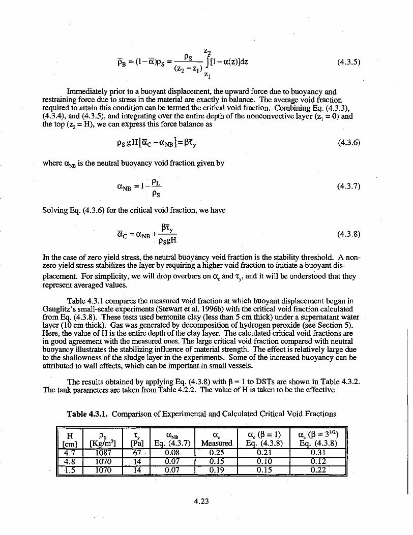
pB = ( l - a )p s =(z2-z,)
- cc(z)]dz (4.3.5)
Immediately prior to a buoyant displacement, the upward force due to buoyancy andrestraining force due to stress in the material are exactly in balance. The average void fractionrequired to attain this condition can be termed the critical void fraction. Combining Eq. (4.3.3),(4.3.4), and (4.3.5), and integrating over the entire depth of the nonconvective layer (Zj = 0) andthe top (Zj = H), we can express this force balance as
p s gH[a c -a N B ] = p'cy
where a ^ is the neutral buoyancy void fraction given by
(4.3.6)
(4.3.7)
Solving Eq. (4.3.6) for the critical void fraction, we have
PsgH(4.3.8)
In the case of zero yield stress, the neutral buoyancy void fraction is the stability threshold. A non-zero yield stress stabilizes the layer by requiring a higher void fraction to initiate a buoyant dis-placement. For simplicity, we will drop overbars on occ and ty, and it will be understood that theyrepresent averaged values.
Table 4.3.1 compares the measured void fraction at which buoyant displacement began inGauglitz's small-scale experiments (Stewart et al. 1996b) with the critical void fraction calculatedfrom Eq. (4.3.8). These tests used bentonite clay (less than 5 cm thick) under a supernatant waterlayer (10 cm thick). Gas was generated by decomposition of hydrogen peroxide (see Section 5).Here, the value of H is the entire depth of the clay layer. The calculated critical void fractions arein good agreement with the measured ones. The large critical void fraction compared with neutralbuoyancy illustrates the stabilizing influence of material strength. The effect is relatively large dueto the shallowness of the sludge layer in the experiments. Some of the increased buoyancy can beattributed to wall effects, which can be important in small vessels.
The results obtained by applying Eq. (4.3.8) with p = 1 to DSTs are shown in Table 4.3.2.The tank parameters are taken from Table 4.2.2. The value of H is taken to be the effective
Table 4.3.1. Comparison of Experimental and Calculated Critical Void Fractions
H[cm]4.74.81.5
Ps ,[Kg/m3]
108710701070
[Pa]671414
Eq. (4.3.7)0.080.070.07
Measured0.250.150.19
<xc (P = 1)Eq. (4.3.8)
0.210.100.15
a c (P = 31/2)Eq. (4.3.8)
0.310.120.22
4.23
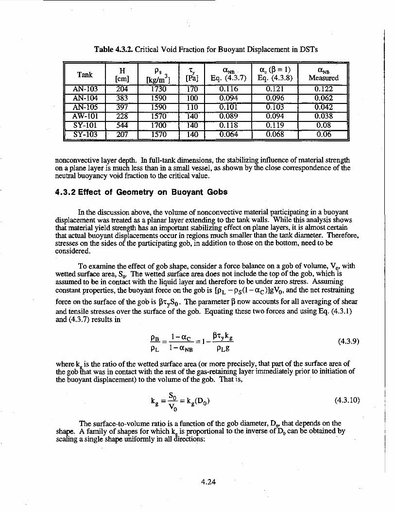
Table 4.3.2. Critical Void Fraction for Buoyant Displacement in DSTs
Tank
AN-103AN-104AN-105AW-101SY-101SY-103
H[cm]
204383397228544207
P s 3tkg/m3]
173015901590157017001570
Xy[Pa]170100110140140140
«NBEq. (4.3.7)
0.1160.0940.1010.0890.1180.064
ae(p = l)Eq. (4.3.8)
0.1210.0960.1030.0940.1190.068
ONEMeasured
0.1220.0620.0420.0380.080.06
nonconvective layer depth. In full-tank dimensions, the stabilizing influence of material strengthon a plane layer is much less than in a small vessel, as shown by the close correspondence of theneutral buoyancy void fraction to the critical value.
4.3.2 Effect of Geometry on Buoyant Gobs
In the discussion above, the volume of nonconvective material participating in a buoyantdisplacement was treated as a planar layer extending to the tank walls. While this analysis showsthat material yield strength has an important stabilizing effect on plane layers, it is almost certainthat actual buoyant displacements occur in regions much smaller than the tank diameter. Therefore,stresses on the sides of the participating gob, in addition to those on the bottom, need to beconsidered.
To examine the effect of gob shape, consider a force balance on a gob of volume, Vo, withwetted surface area, So. The wetted surface area does not include the top of the gob, which isassumed to be in contact with the liquid layer and therefore to be under zero stress. Assumingconstant properties, the buoyant force on the gob is [pL - p s(l - ac)]gV0, and the net restraining
force on the surface of the gob is fkyS0 . The parameter |3 now accounts for all averaging of shearand tensile stresses over the surface of the gob. Equating these two forces and using Eq. (4.3.1)and (4.3.7) results in
p B = l - a c = 1 PTykg
PL 1 - « N B PLE(4.3.9)
where kg is the ratio of the wetted surface area (or more precisely, that part of the surface area ofthe gob that was in contact with the rest of the gas-retaining layer immediately prior to initiation ofthe buoyant displacement) to the volume of the gob. That is,
k g =-f = kg(D0) (4.3.10)
The surface-to-volume ratio is a function of the gob diameter, Do, that depends on theshape. A family of shapes for which k is proportional to the inverse of Do can be obtained byscaling a single shape uniformly in all directions:
4.24
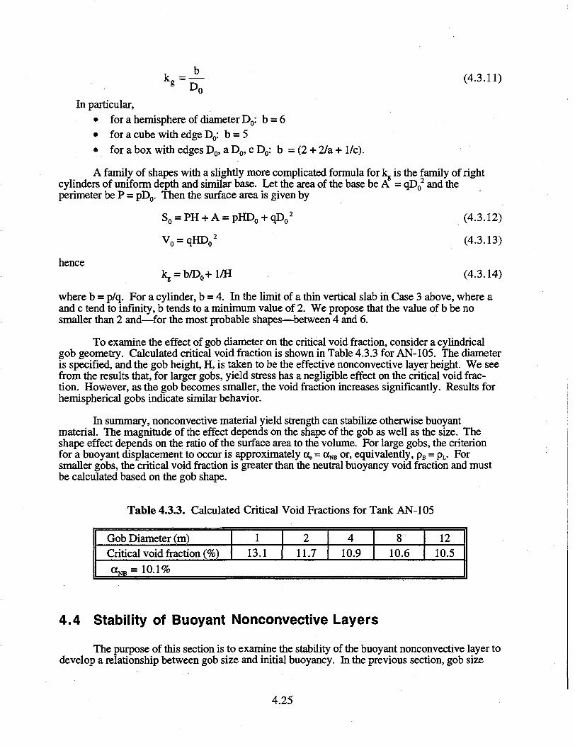
(4.3.11)
In particular,• for a hemisphere of diameter Do: b = 6• for a cube with edge Do: b = 5• for a box with edges Do, a Do, c Do: b = (2 + 2/a + 1/c).
A family of shapes with a slightly more complicated formula for kg is the family of rightf if d t h d i i l bas L t th f th b b A D 2 d thcylinders of uniform depth and similar base. Let the area of the base be A = qD0 and the
perimeter be P = pD0. Then the surface area is given by
So = PH + A = pHD0 + qD02
= qHD0
hence= b/D0+l/H
(4.3.12)
(4.3.13)
(4.3.14)
where b = p/q. For a cylinder, b = 4. In the limit of a thin vertical slab in Case 3 above, where aand c tend to infinity, b tends to a minimum value of 2. We propose that the value of b be nosmaller than 2 and—for the most probable shapes—between 4 and 6.
To examine the effect of gob diameter on the critical void fraction, consider a cylindricalgob geometry. Calculated critical void fraction is shown in Table 4.3.3 for AN-105. The diameteris specified, and the gob height, H, is taken to be the effective nonconvective layer height. We seefrom the results that, for larger gobs, yield stress has a negligible effect on the critical void frac-tion. However, as the gob becomes smaller, the void fraction increases significantly. Results forhemispherical gobs indicate similar behavior.
In summary, nonconvective material yield strength can stabilize otherwise buoyantmaterial. The magnitude of the effect depends on the shape of the gob as well as the size. Theshape effect depends on the ratio of the surface area to the volume. For large gobs, the criterionfor a buoyant displacement to occur is approximately occ = oc , or, equivalently, pB = pL. Forsmaller gobs, the critical void fraction is greater than the neutral buoyancy void fraction and mustbe calculated based on the gob shape.
Table 4.3.3. Calculated Critical Void Fractions for Tank AN-105
Gob Diameter (m)Critical void fraction (%)
113.1
211.7
410.9
810.6
1210.5
o ^ = 10.1%
4.4 Stability of Buoyant Nonconvective Layers
The purpose of this section is to examine the stability of the buoyant nonconvective layer todevelop a relationship between gob size and initial buoyancy. In the previous section, gob size
4.25
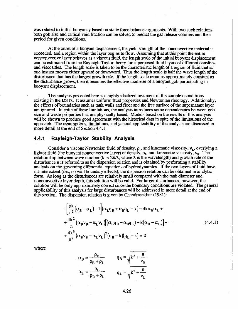
was related to initial buoyancy based on static force balance arguments. With two such relations,both gob size and critical void fraction can be solved to predict the gas release volumes and theirperiod for given conditions.
At the onset of a buoyant displacement, the yield strength of the nonconvective material isexceeded, and a region within the layer begins to flow. Assuming that at this point the entirenonconvective layer behaves as a viscous fluid, the length scale of the initial buoyant displacementcan be estimated from the Rayleigh-Taylor theory for superposed fluid layers of different densitiesand viscosities. The length scale is taken to be the characteristic length of a region of fluid that atone instant moves either upward or downward. Thus the length scale is half the wave length of thedisturbance that has the largest growth rate. If the length scale remains approximately constant asthe disturbance grows, then it becomes the effective diameter of a buoyant gob participating inbuoyant displacement.
The analysis presented here is a highly idealized treatment of the complex conditionsexisting in the DSTs. It assumes uniform fluid properties and Newtonian rheology. Additionally,the effects of boundaries such as tank walls and floor and the free surface of the supernatant layerare ignored. In spite of these limitations, the analysis introduces some dependencies between gobsize and waste properties that are physically based. Models based on the results of this analysiswill be shown to produce good agreement with the historical data in spite of the limitations of theapproach. The assumptions, limitations, and general applicability of the analysis are discussed inmore detail at the end of Section 4.4.1.
4.4.1 Rayleigh-Taylor Stability Analysis
Consider a viscous Newtonian fluid of density, pL, and kinematic viscosity, vL, overlying alighter fluid (the buoyant nonconvective layer) of density, pB, and kinematic viscosity, vB. Therelationship between wave number (k = 2%IX, where X is the wavelength) and growth rate of thedisturbance n is referred to as the dispersion relation and is obtained by performing a stabilityanalysis on the governing differential equations of hydrodynamics. If the two layers of fluid haveinfinite extent (i.e., no wall boundary effects), the dispersion relation can be obtained in analyticform. As long as the disturbances are relatively small compared with the tank diameter andnonconvective layer depth, this solution will be valid. For larger disturbances, however, thesolution will be only approximately correct since the boundary conditions are violated. The generalapplicability of this analysis for large disturbances will be addressed in more detail at the end ofthis section. The dispersion relation is given by Chandrasekhar (1981):
- k ) - 4 k a R a T +
4k2
n
4k3
n
where
_ PB
PB + PL
- k) = o
aB =
P B + P L
4.26
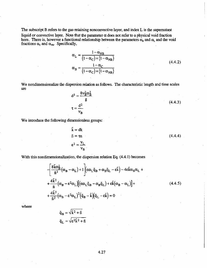
The subscript B refers to the gas-retaining nonconvective layer, and index L is the supernatantliquid or convective layer. Note that the parameter a does not refer to a physical void fractionhere. There is, however a functional relationship between the parameters Og and ct and the voidfractions Oc and ONB. Specifically,
aB =l - a
(4.4.2)
We nondimensionalize the dispersion relation as follows. The characteristic length and time scalesare
(4.4.3)
V B
We introduce the following dimensionless groups:
k = dk
VB
(4.4.4)
With this nondimensionalization, the dispersion relation Eq. (4.4.1) becomes
-(aB - a L ) +1 (£aLqB + aBqL - sk) - 4ekaBaL +8ka|
fi2
n
T - ek) = 0
where
qL = + n
4.27
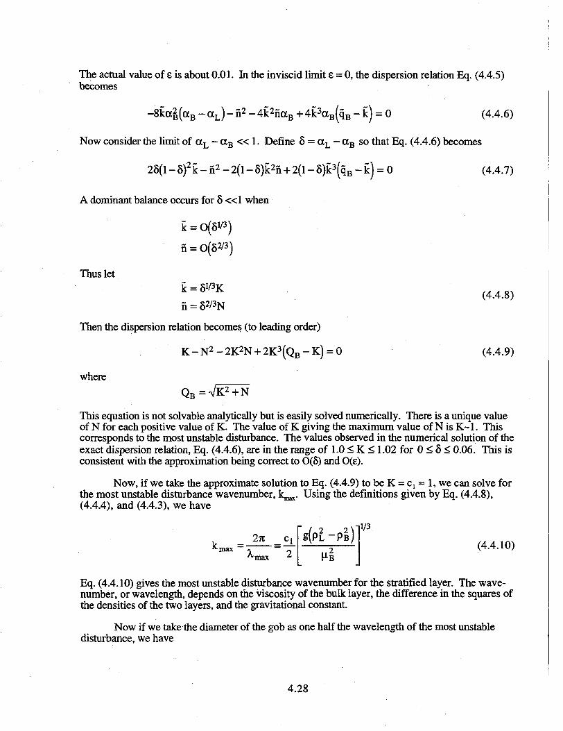
The actual value of 8 is about 0.01. In the inviscid limit £ = 0, the dispersion relation Eq. (4.4.5)becomes
-8koc|(aB - a L ) - fi2 - 4k2fiaB + 4k3aB(qB - k) = 0 (4.4.6)
Now consider the limit of a L - a B « 1 . Define 8 = a L — a B so that Eq. (4.4.6) becomes
28(1 - 8)2 k - r i 2 - 2(1 -8)k2fi + 2(1 - S ) k 3 ( q B - k ) = O (4.4.7)
A dominant balance occurs for 8 « 1 when
k = O(8V3)
n = O(82/3)
Thus let
(4.4.8)fi = 82/3N
Then the dispersion relation becomes (to leading order)
K - N 2 - 2 K 2 N + 2K 3 (Q B -K) = 0 (4.4.9)
where
This equation is not solvable analytically but is easily solved numerically. There is a unique valueof N for each positive value of K. The value of K giving the maximum value of N is K~l. Thiscorresponds to the most unstable disturbance. The values observed in the numerical solution of theexact dispersion relation, Eq. (4.4.6), are in the range of 1.0 < K < 1.02 for 0 < 8 <; 0.06. This isconsistent with the approximation being correct to 0(8) and O(E).
Now, if we take the approximate solution to Eq. (4.4.9) to be K = c : = 1, we can solve forthe most unstable disturbance wavenumber, k,^. Using the definitions given by Eq. (4.4.8),(4.4.4), and (4.4.3), we have
V32% C i * L B' (4.4.10)
Xmax
Eq. (4.4.10) gives the most unstable disturbance wavenumber for the stratified layer. The wave-number, or wavelength, depends on the viscosity of the bulk layer, the difference in the squares ofthe densities of the two layers, and the gravitational constant.
Now if we take the diameter of the gob as one half the wavelength of the most unstabledisturbance, we have
4.28
D o =2TC
gl(pi-Pi)
V3
(4.4.11)
Several points need to be made regarding the general applicability of Eq. (4.4.11). First ofall, Eq. (4.4.11) predicts the diameter of the most unstable gob; however, larger and smaller gobsare also unstable and may occur with lower probability.
The second point relates to the shape of disturbances. The stability analysis assumedlongitudinal disturbances at the interface between the convective and nonconvective layers. Inreality, disturbances are likely to be more cylindrical. Based on similarity arguments, one canshow that the solution for wavenumber for cylindrical disturbances has the same functional form asEq. (4.4.10). The only difference would be the constant multiplier, c r Therefore, Do can beassumed to be the effective diameter of a gob with cylindrical symmetry if the constant c2 isadjusted appropriately.
The third point relates to boundary conditions. The stability analysis is for a doubly infinitestratified layer. The presence of tank walls, tank floor, and supernatant liquid free surface allviolate the boundary conditions of the analysis. If disturbances are found to be small comparedwith tank length scales (i.e., diameter, nonconvective or convective layer height), the effects of theviolation should be negligible. If disturbances are predicted to be very large compared with thetank length scales, the assumptions are severely violated and the analysis does not hold. If thedisturbances are comparable to tank length scales, however, the analysis may still hold approx-imately. The primary functional dependence of wavelength on viscosity and density differencemight still be the dominant controlling factor. If the stability analysis were performed for thebounded case (a difficult analysis) one would most likely find that the wavelength has additionalfunctional dependencies on tank diameter and waste levels. The predicted disturbance wavelengthshave similar magnitudes for all cases considered. Given that all tank diameters are the same, andnonconvective layer depths do not vary by large factors, we suspect that the dependencies on theadditional length scales are approximately the same for each tank considered. This point, ofcourse, cannot be proven without completing the analysis with the correct boundary conditions.
The final point relates to waste properties. While convective layer densities are nearlyuniform, nonconvective layer densities vary with depth. Nonconvective layer viscosities and yieldstresses also vary strongly with depth (Figures 4.2.4-4.2.8). However, if predicted gobdiameters are large compared with regions of vertical property variation, the effects of the variationshould be minimal. Waste properties are also seen to vary depending on the riser used for thesample or test. Additionally, nonconvective layer viscosities are strongly shear-rate dependent andare clearly non-Newtonian. Hence, the nonuniform, non-Newtonian waste properties clearlyviolate the assumptions of the stability analysis. Consistent with our overall modeling approach,however, we simplify by using mean or average properties in the models.
In spite of its limitations and idealizations, the stability analysis does provide a simple,physically based relationship between gob size and average waste properties. To quantify thelimitations of the approach, a rigorous analysis that accounts for three-dimensional disturbances,tank boundaries, and nonuniforrn/non-Newtonian properties would be required. Such an analysiswould be an enormous undertaking and is likely intractable. Our hope is that the simplistic stabilityanalysis has captured the most dominant functional dependence of gob size on waste properties.The degree to which the model predicts the historical tank behavior is one test of its merits (and isthe only one currently available). Additional testing is desirable to refine the model and verify itspredictive capability.
4.29
4.4.2 Gob Size and Critical Void Fraction
The diameter of the most unstable gob is given by Eq. (4.4.11) as a function of theviscosity and bulk density of the nonconvective layer and the supernatant liquid. Eq. (4.3.9)provides an additional relation between gob diameter and waste properties. These two relationscan be combined to solve for the gob diameter and the critical void fraction independently.Returning to Eq. (4.3.9) and rearranging it gives
l -£B = _e_ k (D ) ( 4 A 1 2 )PL PLE
S
Also, using the assumption that the density difference is small, we have
(4.4.13)
Substituting Eq. (4.4.13) into Eq. (4.4.11) we obtain
D o = — (4.4.14)2pLPxkg(D)
To solve for Do we rewrite (4.4.14) as
:^%^L,2 (4.4.15)
Note that the grouping 1^ has dimensions of length. This is one natural-length scale of the systemunder consideration. Once Do is solved from Eq. (4.4.14), the critical void fraction can be deter-mined from Eq. (4.3.9) according to
io (4.4.16)
where L2 is another natural-length scale given by
L2=(5x/pLg (4.4.17)
In the particular cases discussed in Section 4.3 we have, for the case of similar shapes, where kg =b/D0
D 03k g (D 0 ) = b D 0
2 = L 12 (4.4.18)
henceD 0 = b - 1 / 2 L ! (4.4.19)
The maximum value of Do occurs when b is its minimum value; b = 2, therefore,
wo (4.4.20)D 0 < 2 " 1 / / L 1
4.30
The volume of the gob must be determined according to the applicable formula for each particularshape. For example, in the case of a hemisphere, b = 6, so
D 0 = 6 " 1 / 2 L ! (4.4.21)
and
The critical void fraction for similar gobs with any value of b is given by
(4.4.23)
For the case of right cylinders, kg = b/ D0+l/H, so
D 3*=L , 2 (4.4.24)
Letting x = D(/H, we have the cubic equation
x 3 + b x 2 - a = O (4.4.25)
wherea=Lj2/H2. The analytic solution to this cubic equation is
Dn in b2
x = —o. = y1 / 3
+ _ ^ _ _ I b (4.4.26)
where
y = l a _ J _ b 3 + ^V81a 2-12ab 3 (4.4.27)
There are two significant limiting cases for this formula, corresponding to the dominance ofeither the third- or second-order term in Eq. (4.4.25). In the first case, x is large compared with b,and x ~ a1 '3 » b . This parameter regime is identified by the relation a » b3 . The intermediatevalue y is real-valued in this case. Geometrically, we have a gob of shallow depth. In the secondcase, where x is small compared with b, x ~ (a/b)1 / 2 « b . This parameter regime is identifiedby the relation a « b3 . The intermediate value y is complex in this case, although the solution xis still real and positive. Geometrically we have a gob of narrow width and large depth. In theintermediate parameter regime, when a = O(b3), all three terms of the polynomial equation areequally important, and the full solution given by Eq. (4.4.26) and (4.4.27) is necessary. Theintermediate value y is either real or complex, with a transition when a = (4/27)b3. Geometrically,the gob is of similar width and depth.
Finally, once Do is determined from Eq. (4.4.26), the cylindrical gob volume is
V 0 = TCD02H/4 (4.4.28)
and the critical void fraction is calculated according to Eq. (4.4.16).
4.31
4.5 Predictive Models
The gob volume and critical void fraction have been solved by the analysis of the previoussections. We can now use these key results to develop models that predict the frequency of buoy-ant displacements and the size of resulting gas release volumes. The models are applied to the sixDSTs, and the results are compared with historical data. Finally, an approximate model ispresented that gives good results and has a relatively simple analytic form.
4.5.1 Size and Frequency of Gas Release Events
Since we have solved for the gob volume and critical void fraction, the in-situ volume ofgas within the gob is known. If the fraction of this gas released during a buoyant displacement canbe calculated, the volume of gas actually released can be determined.
The fraction of gas within a gob that is released during a buoyant displacement can beestimated by a simple model. We assume that gas is released until the nonconvective material,which is now near the surface of the waste, returns to neutral buoyancy. After the release, the gobsettles back through the supernatant liquid to the nonconvective layer.
Recall the definition of void fraction, a = VG/(Vq+ Vs), where Vs is the gas volume and Vois the volume of solids and liquids. By rearranging, the initial gas volume in the gob just prior tobuoyant displacement is V ^ = 0^(1-a^Vg. As the gob rises to the waste surface, the retainedgases expand so that the volume of gas within the gob is VG, = ps Vw, where p s is the averagepressure of the gas in the nonconvective layer in atmospheres. After the gas is released, neutralbuoyancy at the surface dictates that VG2 = 0 ^ ( 1 - 0 ^ ) ^ . The fraction of the gas in the gobreleased is f j ^ = (VG1 - VG2)/VG1. Substituting for VG1 and VG2, we find that
( 4 5 I )
The amount of gas released during a GRE (at standard conditions) is therefore
VREL = fRELcxcVoPs (4.5.2)
For right circular cylindrical gobs (b = 4) we have
f2 (4.5.3)
where occ is given by Eq. (4.4.16), and Do is given by solution of Eq. (4.4.26).
For hemispherical gobs we have
VREL = fRELaC YJ
where a^, is given by Eq. (4.4.23), and Do is given by Eq. (4.4.21).
4.32
We now propose a simple model for GRE frequency that is a straightforward extension ofthe concepts developed so far in this study. The model assumes that gas is generated within thenonconvective layer at a constant rate. While some gas is released due to nonepisodic transport,there is a net accumulation until the nonconvective material becomes unstable, at which time abuoyant displacement occurs. Since the average volume of a buoyant displacement is generallysignificantly less than the total volume of the nonconvective layer, we assume that there are manysuch gas generation/buoyant displacement processes occurring independently. Gas accumulationrates can be obtained from long-term level rise data. The number of independent buoyant displace-ment processes occurring in a tank can be estimated from the results discussed in this section.
According to our model, a buoyant displacement will occur when the void fraction in thenonconvective material is equal to the critical void fraction. After a previous buoyant displacement,the volume of gas within the gob increases with time according to
foA (4.5.5)dt
where VG(0) is the initial volume of gas at time t = 0; AQ is the cross-sectional area of the gob(Ao= 7cDQ /4 for a cylindrical or semispherical gob); and dh/dt is the long-term waste level rise rate.The fraction of gas that is released by small, undetected GREs or other mechanisms betweenmajor, recorded GREs is fo.
(a) Since the initial gas volume is equal to the amount of gas left in thegob after the previous buoyant displacement, we have
VG(0) = (l-fREL)acV0 (4.5.6)
If we define the time to initiation of a buoyant displacement as tc, then V Q ^ ) = O(N0, andEq. (4.5.5) can be evaluated at ^ to yield
«cvo =a-fra>cvo+Ao(l-fo)fLtc (4-5.7)
Solving Eq. (4.5.7) for t,. yields
t r = « — W a r (4-5-8)c A 0 ( l - f 0 ) U t J **L C
Eq. (4.5.8) gives the average time between buoyant displacements for a given gob. Forcylindrical gobs, "VyAg = H, where H is the height of the gob. For semispherical gobs,V0/A0 = D0/3.
The total number of gobs, Ng, that can act independently is equal to Vs /Vo, whereVs = hgAj. is the total volume of nonconvective material that retains gas. Therefore, we have
N g = H A T / V 0 (4.5.9)
(a) This factor is important since a particular methodology was applied when counting historicalGREs. GREs below about 7 m and occurring over periods longer than 24 hours were notcounted. Therefore, to accurately compare with historical data, this factor is needed.
4.33
Since the gobs are acting independently of one another, the average time between any two GREswill be TREL = tc / Ng so that
A 0ATH(l-f 0)
For cylindrical gobs we have
_ 7iD02H 1 / J u W
ZT){^«L«C (4-5..0)
REL=—TT / t - J - fREL«C (4.5.11)4AT ( l - f o ) v d t y
For hemispherical gobs we have
1 rdhw
TREL = £ 7 ^ 7 ^ ~ fREL«c (4-5.12)
The modeling approach presented in this section also allows us to estimate the averageamount of gas retained in the nonconvective layer. For a given gob, the void fraction just prior to abuoyant displacement is 0^. The void fraction after buoyant displacement is (1-fREL) Oe- Since thevoid fraction increases nearly linearly in time, the average gob void fraction is approximately(occ + (1 -fREL) occ )/2, so that we can write
a N C » ( 2 - f R E L ) a c (4.5.13)
Eq. (4.5.13) represents the long-term spatial and temporal average for nonconvective layer voidfraction. It is the mass balance of gas being generated versus gas released by multiple gobs actingindependently.
4.5.2 Evaluation of GRE Model for DSTs
In this section, we evaluate the models' predictions of GRE size and frequency under theconditions corresponding to the FGWL DSTs, and we identify the gob geometry that produces thebest predictive agreement with the data. The hemisphere showed poor agreement with the data,and gob diameters were predicted to be larger than the depth of the nonconvective layers—a clearviolation of the assumed geometry. However, the form of the hemisphere model is used todevelop a simplified model in the next section.
For right circular cylinder gobs (b =4), the gas release volume is given by Eq. (4.5.3).The formulas were evaluated for the parameter values shown in Table 4.2.2. Additionally, theconstants Cj and p were both set equal to their default value of 1. The value for the viscosity usedin the formulas was \iB = c-ji, where jx is the value derived from the ball rheometer data. The ballrheometer instrument produces indicator (as opposed to absolute) values for dynamic viscosity thatare known to be strongly shear-rate dependent. The important information for the models pre-sented is not the absolute value of the viscosity but rather how the viscosity varies from tank totank. The constant c2 is the sole adjustable parameter in the model and has the same value for eachtank. The value c2 = 0.077 gave the best results.
4.34
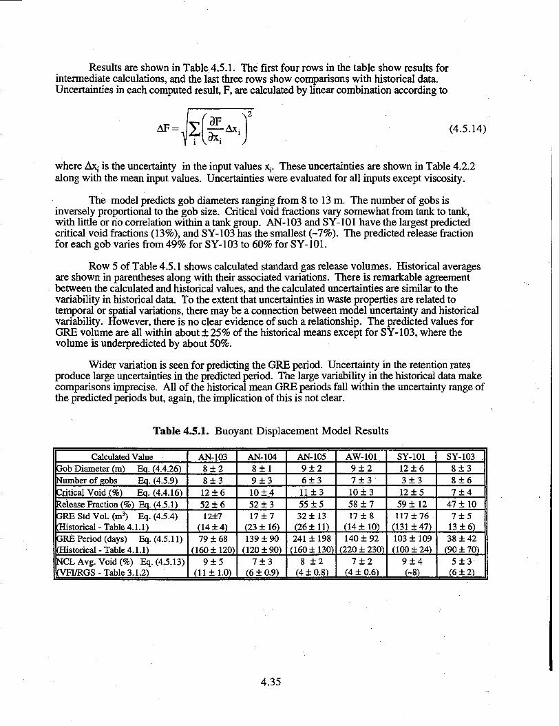
Results are shown in Table 4.5.1. The first four rows in the table show results forintermediate calculations, and the last three rows show comparisons with historical data.Uncertainties in each computed result, F, are calculated by linear combination according to
(4.5.14)
where Ax- is the uncertainty in the input values x;. These uncertainties are shown in Table 4.2.2along with the mean input values. Uncertainties were evaluated for all inputs except viscosity.
The model predicts gob diameters ranging from 8 to 13 m. The number of gobs isinversely proportional to the gob size. Critical void fractions vary somewhat from tank to tank,with little or no correlation within a tank group. AN-103 and SY-101 have the largest predictedcritical void fractions (13%), and SY-103 has the smallest (-7%). The predicted release fractionfor each gob varies from 49% for SY-103 to 60% for SY-101.
Row 5 of Table 4.5.1 shows calculated standard gas release volumes. Historical averagesare shown in parentheses along with their associated variations. There is remarkable agreementbetween the calculated and historical values, and the calculated uncertainties are similar to thevariability in historical data. To the extent that uncertainties in waste properties are related totemporal or spatial variations, there may be a connection between model uncertainty and historicalvariability. However, there is no clear evidence of such a relationship. The predicted values forGRE volume are all within about ± 25% of the historical means except for SY-103, where thevolume is underpredicted by about 50%.
Wider variation is seen for predicting the GRE period. Uncertainty in the retention ratesproduce large uncertainties in the predicted period. The large variability in the historical data makecomparisons imprecise. All of the historical mean GRE periods fall within the uncertainty range ofthe predicted periods but, again, the implication of this is not clear.
Table 4.5.1. Buoyant Displacement Model Results
Calculated ValueGob Diameter (m) Eq. (4.4.26)Number of gobs Eq. (4.5.9)Critical Void (%) Eq. (4.4.16)Release Fraction (%) Eq. (4.5.1)GRE Std Vol. (m3) Eq. (4.5.4)(Historical - Table 4.1.1)GRE Period (days) Eq. (4.5.11)(Historical - Table 4.1.1)NCL Avg. Void (%) Eq. (4.5.13)(VFI/RGS - Table 3.1.2)
AN-1038 ± 28 ± 312 ± 652 + 612+7
(14 ±4)79 ±68
(160 ± 120)9 + 5
(11 + L0)
AN-1048 ± 19 ± 310 ± 452 ± 317 ± 7
(23 ± 16)139 ± 90
(120 ±90)7 + 3
(6 ± 0.9)
AN-1059±26 ± 311 ±355 ±532 ±13
(26+11)241 ± 198
(160 ±130)8 ±2
(4 ± 0.8)
AW-1019 ± 27 ± 310 + 358 ±717 + 8
(14 ± 10)140 ± 92
(220 ±230)7 + 2
(4 ± 0.6)
SY-10112 ± 63 ± 312 ± 5
59 ±12117 + 76
(131 ±47)103 ± 109(100 ±24)
9±4(~8)
SY-1038 ± 38 + 67 ± 4
47+107±5
13 ±6)38 ±42
(90 ± 70)5±3
(6 ±2)
4.35
4.5.3 A Simplified Model
The above model for cylindrical gobs produces very good agreement with the historicaldata for the six DSTs. However, it is cumbersome to apply because Eq. (4.4.26) does not have asimple closed-form solution. We want to find an approximate model that retains the essentialfeatures of the exact solution while simplifying the algebra.
The model for hemispherical gobs has a simple analytical form but does not produceacceptable results, since the predicted diameter exceeds the depth of the nonconvective layer. Thediameter of the hemispherical gob has a simple analytical form. We attempt to find an approximatemodel by assuming that predicted diameter is that of a cylindrical gob even though it was notderived under that assumption. Then the volume of a GRE would be given by Eq. (4.5.3), whereDo is given by Eq. (4.4.21) so that
^ (4.5.15)
Eq. (4.5.15) can be simplified further by noting that the critical void fraction is very nearly equal tothe neutral buoyant void fraction for the six tanks considered. Therefore, if we let occ = cc^ thenW = P s ' 1 d Eq- (4.5.15) can be written with the aid of Eq. (4.4.15) as
V«L ~ (Ps - DaNBHfi2 /pLry (4.5.16)
To simplify further, we take advantage of the fact that the kinematic viscosity can berelated to the yield strength. The methodology for deriving viscosity and yield strength from ballrheometer data is discussed in Stewart et al. (1996a). For very low shear rates, the viscosity isproportional to the yield stress to first order. The constant of proportionality is the ball shear rate.We take advantage of this fact and write n - xy in Eq. (4.5.16) to obtain
V R E L «75O(p s - l ) a N B H(x y / p L ) (4.5.17)
The leading constant in Eq. (4.5.17) was chosen to give the best fit with the data.
Table 4.5.2 compares the GRE volumes predicted by the approximate formula given byEq. (4.5.17) with those of the full solution and the historical data. The approximate solution doesa reasonable job of matching the data; however, it is not as accurate as the full solution, and itsuncertainty is higher.
Eq. (4.5.17) can serve as a predictive model for evaluating the propensity for GREs inother tanks. However, caution is strongly advised for three reasons. First, as well-characterizedas the six FGWL DSTs are, uncertainties in their waste properties produce significant uncertaintiesin predicted volume. Uncertainties would be even higher in cases where properties were less well-defined. Second, while the general scaling of Eq. (4.5.17) is probably correct over some range ofconditions, the model has not been evaluated for small GREs, which would be of most interest inits application. Third, additional verification against new data is needed to build confidence in thegeneral applicability of the model.
Finally, it is important to emphasize that the model predicts the most probable gob size, notthe largest or smallest. The largest possible gob, in principle, is one with diameter equal to thetank diameter since all scales are potentially unstable.
4.36
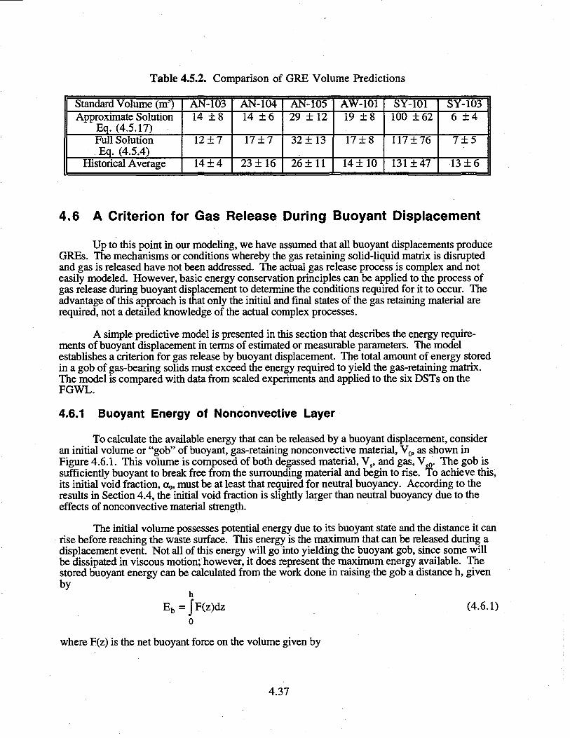
Table 4.5.2. Comparison of GRE Volume Predictions
Standard Volume (mJ)Approximate Solution
Eq. (4.5.17)Full SolutionEq. (4.5.4)
Historical Average
AN-10314 ± 8
12 ± 7
14 ±4
AN-10414 ±6
17 + 7
23 ±16
AN-10529 ±12
32 ±13
26 ±11
AW-10119 ±8
17 ±8
14 ±10
SY-101100 ±62
117 ±76
131 ±47
SY-1036 ±4
7±5
13 ±6
4.6 A Criterion for Gas Release During Buoyant Displacement
Up to this point in our modeling, we have assumed that all buoyant displacements produceGREs. The mechanisms or conditions whereby the gas retaining solid-liquid matrix is disruptedand gas is released have not been addressed. The actual gas release process is complex and noteasily modeled. However, basic energy conservation principles can be applied to the process ofgas release during buoyant displacement to determine the conditions required for it to occur. Theadvantage of this approach is that only the initial and final states of the gas retaining material arerequired, not a detailed knowledge of the actual complex processes.
A simple predictive model is presented in this section that describes the energy require-ments of buoyant displacement in terms of estimated or measurable parameters. The modelestablishes a criterion for gas release by buoyant displacement. The total amount of energy storedin a gob of gas-bearing solids must exceed the energy required to yield the gas-retaining matrix.The model is compared with data from scaled experiments and applied to the six DSTs on theFGWL.
4.6.1 Buoyant Energy of Nonconvective Layer
To calculate the available energy that can be released by a buoyant displacement, consideran initial volume or "gob" of buoyant, gas-retaining nonconvective material, Vo, as shown inFigure 4.6.1. This volume is composed of both degassed material, Vs, and gas, V^. The gob issufficiently buoyant to break free from the surrounding material and begin to rise. To achieve this,its initial void fraction, oto, must be at least that required for neutral buoyancy. According to theresults in Section 4.4, the initial void fraction is slightly larger than neutral buoyancy due to theeffects of nonconvective material strength.
The initial volume possesses potential energy due to its buoyant state and the distance it canrise before reaching the waste surface. This energy is the maximum that can be released during adisplacement event. Not all of this energy will go into yielding the buoyant gob, since some willbe dissipated in viscous motion; however, it does represent the maximum energy available. Thestored buoyant energy can be calculated from the work done in raising the gob a distance h, givenby
h
Eb=jF(z)dz (4.6.1)
where F(z) is the net buoyant force on the volume given by
4.37
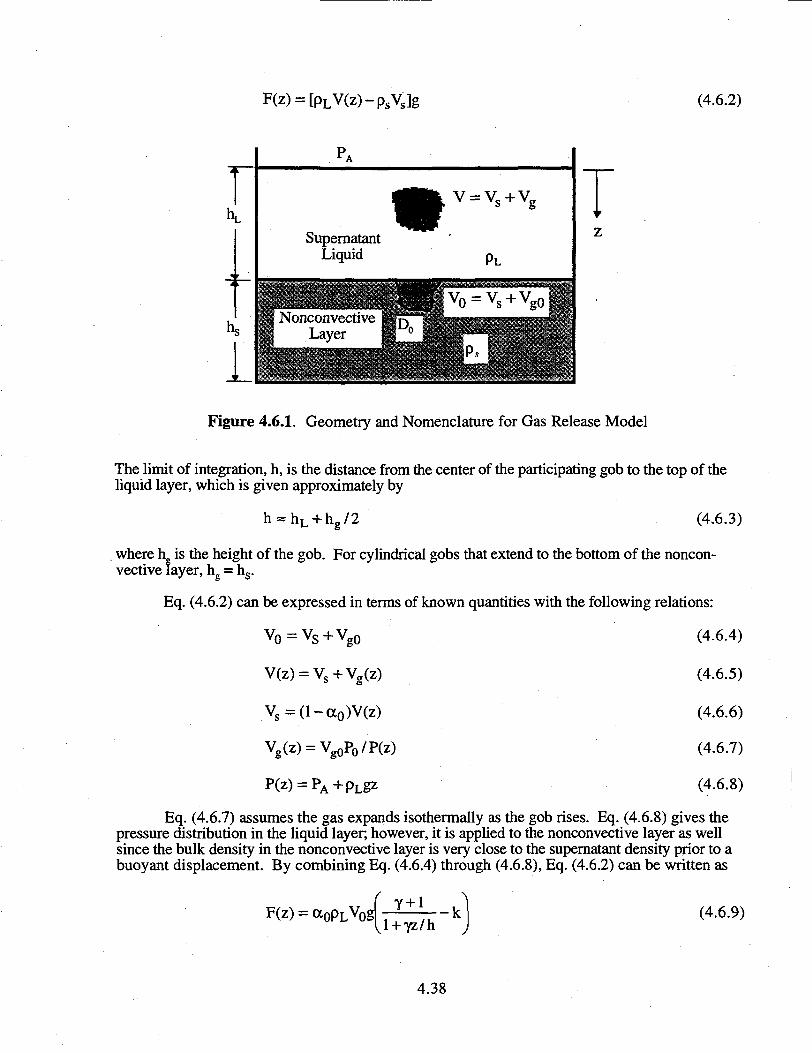
= [pLV(z)-PsV s]g (4.6.2)
SupernatantLiquid
vs+vg
PL
NonconvectiveLayer
Figure 4.6.1. Geometry and Nomenclature for Gas Release Model
The limit of integration, h, is the distance from the center of the participating gob to the top of theliquid layer, which is given approximately by
h = hL + h g / 2 (4.6.3)
. where h is the height of the gob. For cylindrical gobs that extend to the bottom of the noncon-vective layer, h = hs.
V o = V s + V g O
Eq. (4.6.2) can be expressed in terms of known quantities with the following relations:
(4.6.4)
V(z) = Vs+Vg(z) (4.6.5)
V s=(l-a<>)V(z) (4.6.6)
Vg(z) = Vg0P0/P(z) (4.6.7)
P(z) = PA+pLgz (4.6.8)
Eq. (4.6.7) assumes the gas expands isothermally as the gob rises. Eq. (4.6.8) gives thepressure distribution in the liquid layer; however, it is applied to the nonconvective layer as wellsince the bulk density in the nonconvective layer is very close to the supernatant density prior to abuoyant displacement. By combining Eq. (4.6.4) through (4.6.8), Eq. (4.6.2) can be written as
] (4.6.9)U
4.38
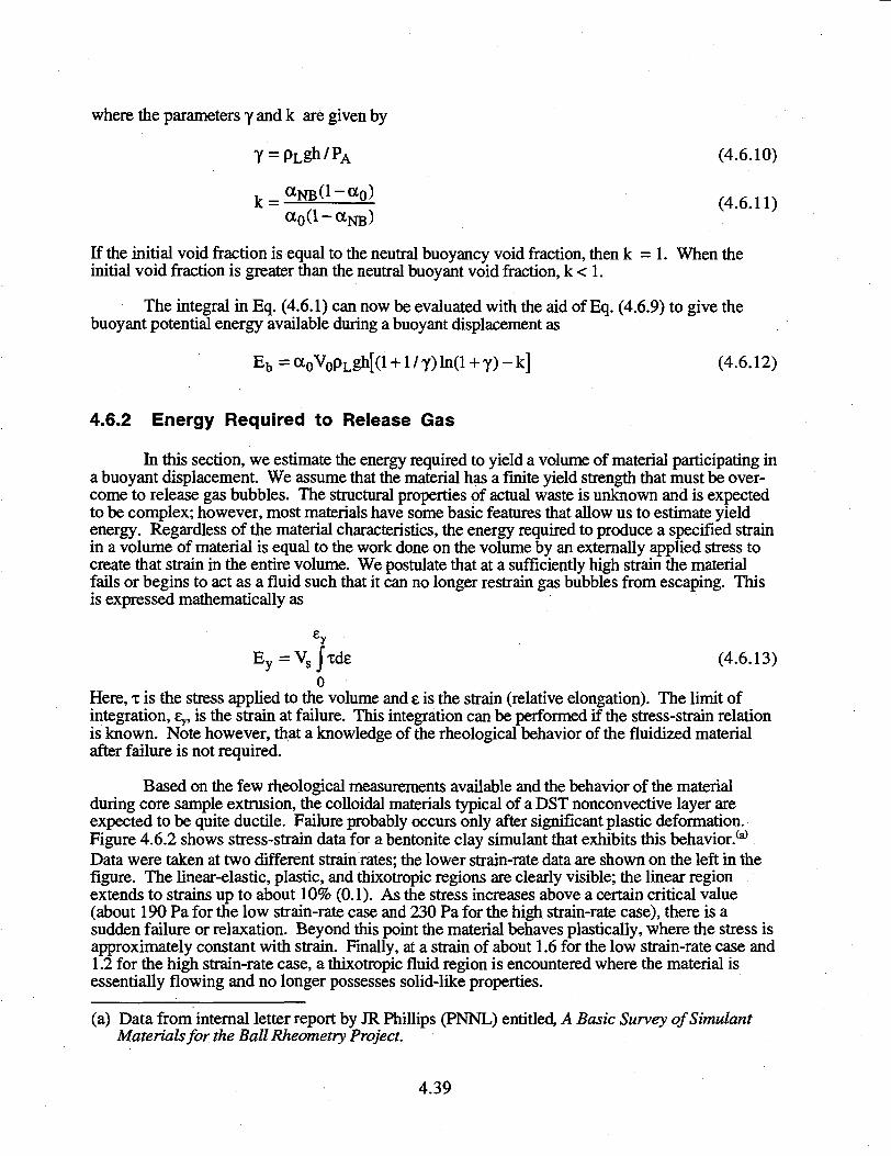
where the parameters y and k are given by
Y = pLgh/PA (4.6.10)
If the initial void fraction is equal to the neutral buoyancy void fraction, then k = 1. When theinitial void fraction is greater than the neutral buoyant void fraction, k < 1.
The integral in Eq. (4.6.1) can now be evaluated with the aid of Eq. (4.6.9) to give thebuoyant potential energy available during a buoyant displacement as
E b = a0V0pLgh[(l +1 / y) ln(l + y) - k] (4.6.12)
4.6.2 Energy Required to Release Gas
In this section, we estimate the energy required to yield a volume of material participating ina buoyant displacement. We assume that the material has a finite yield strength that must be over-come to release gas bubbles. The structural properties of actual waste is unknown and is expectedto be complex; however, most materials have some basic features that allow us to estimate yieldenergy. Regardless of the material characteristics, the energy required to produce a specified strainin a volume of material is equal to the work done on the volume by an externally applied stress tocreate that strain in the entire volume. We postulate that at a sufficiently high strain the materialfails or begins to act as a fluid such that it can no longer restrain gas bubbles from escaping. Thisis expressed mathematically as
ey
Ey=VsJxde (4.6.13)0
Here, x is the stress applied to the volume and £ is the strain (relative elongation). The limit ofintegration, £>,, is the strain at failure. This integration can be performed if the stress-strain relationis known. Note however, that a knowledge of the rheological behavior of the fluidized materialafter failure is not required.
Based on the few rheological measurements available and the behavior of the materialduring core sample extrusion, the colloidal materials typical of a DST nonconvective layer areexpected to be quite ductile. Failure probably occurs only after significant plastic deformation.Figure 4.6.2 shows stress-strain data for a bentonite clay simulant that exhibits this behavior.(a)
Data were taken at two different strain rates; the lower strain-rate data are shown on the left in thefigure. The linear-elastic, plastic, and thixotropic regions are clearly visible; the linear regionextends to strains up to about 10% (0.1). As the stress increases above a certain critical value(about 190 Pa for the low strain-rate case and 230 Pa for the high strain-rate case), there is asudden failure or relaxation. Beyond this point the material behaves plastically, where the stress isapproximately constant with strain. Finally, at a strain of about 1.6 for the low strain-rate case and1.2 for the high strain-rate case, a thixotropic fluid region is encountered where the material isessentially flowing and no longer possesses solid-like properties.
(a) Data from internal letter report by JR Phillips (PNNL) entitled, A Basic Survey of SimulantMaterials for the Ball Rheometry Project.
4.39
200
1 TT5
nominal strain
250
shea
r st
ress
(P
a)
Bentode day -13.5% by «tT=25°C,Sh<arnla*0.0091S30 1ft
V -X —--—.
• — *
0 1 2 3 4 5 6 7nominal strain
Figure 4.6.2. Stress-Strain Data for Bentonite Sludge Simulant for Two Strain Rates
Assuming the waste behaves similarly, the stress-strain model is simplified to consist oflinear-elastic behavior up to 10% strain followed by a plastic region where the stress is equal to theyield stress up to a strain of 1.0, where failure is assumed to occur and the material becomes fluid.With this model, the energy required to yield the material is approximately Ey = syVsTy, whereey ~ 1 is the strain at thixotropic transition. With Vs = (1 - ao)VQ and using Eq. (4.6.12), the energyrequired to yield the sludge is approximately
E y =V 0 £ y T y ( l - a 0 )
4.6.3 The Gas Release Criterion
(4.6.14)
The criterion states that gas release will not occur if the buoyant energy available is lessthan that required to yield the gas-bearing gob participating in the buoyant displacement. The ratioof the two energies given by Eq. (4.6.11) and (4.6.13) is
= <xopLgh(4.6.15)
If E/Ey> 1, we expect a buoyant displacement to release at least some of the retained gas. Other-wise, we expect little or no gas to be released. But a large fraction of the buoyant energy is dis-sipated in processes other than yielding the rising gob, so more energy is required than just enoughto bring the ratio to 1.0.
To find out how much greater than 1.0 the ratio needs to be, we can evaluate the criterionof Eq. (4.6.15) with the results of scaled buoyant displacement experiments (Stewart et al. 1996b).These experiments used a bentonite clay simulant with gas produced in situ by decomposition ofhydrogen peroxide. The model inputs and results are shown in Table 4.6.1. In the first test, a
4.40
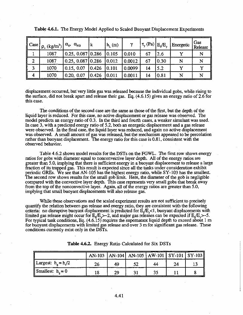
Table 4.6.1. The Energy Model Applied to Scaled Buoyant Displacement Experiments
Case
1
2
3
4
ps (kg/m3)
1087
1087
1070
1070
0.25, 0.087
0.25, 0.087
0.15, 0.07
0.20, 0.07
k
0.286
0.286
0.426
0.426
hL(m)
0.105
0.012
0.101
0.011
Y
0.010
0.0012
0.0099
0.0011
*y(Pa)
67
67
14
14
E,/Ey
2.6
0.30
5.2
0.81
Energetic
Y
N
Y
N
GasRelease
N
N
Y
N
displacement occurred, but very little gas was released because the individual gobs, while rising tothe surface, did not break apart and release their gas. Eq. (4.6.15) gives an energy ratio of 2.6 forthis case.
The conditions of the second case are the same as those of the first, but the depth of theliquid layer is reduced. For this case, no active displacement or gas release was observed. Themodel predicts an energy ratio of 0.3. In the third and fourth cases, a weaker simulant was used.In case 3, with a predicted energy ratio of 5.2, both an energetic displacement and a gas releasewere observed. In the final case, the liquid layer was reduced, and again no active displacementwas observed. A small amount of gas was released, but the mechanism appeared to be percolationrather than buoyant displacement. The energy ratio for this case is 0.81, consistent with theobserved behavior.
Table 4.6.2 shows model results for the DSTs on the FGWL. The first row shows energyratios for gobs with diameter equal to nonconvective layer depth. All of the energy ratios aregreater than 5.0, implying that mere is sufficient energy in a buoyant displacement to release a largefraction of its trapped gas. This result is expected since all the tanks under consideration exhibitperiodic GREs. We see that AN-105 has the highest energy ratio, while SY-103 has the smallest.The second row shows results for the small gob limit. Here, the diameter of the gob is negligiblecompared with the convective layer depth. This case represents very small gobs mat break awayfrom the top of the nonconvective layer. Again, all of the energy ratios are greater than 5.0,implying that small buoyant displacements will also release gas.
While these observations and the scaled experiment results are not sufficient to preciselyquantify the relation between gas release and energy ratio, they are consistent with the followingcriteria: no disruptive buoyant displacement is predicted for E,/Ey<l, buoyant displacements withlimited gas release might occur for E,/Ey>~2, and major gas releases can be expected if Eb/E^-5.For typical tank conditions, Eq. (4.6.15) requires the supernatant liquid depth to exceed about 1 mfor buoyant displacements with limited gas release and over 3 m for significant gas release. Theseconditions currently exist only in the DSTs.
Table 4.6.2. Energy Ratio Calculated for Six DSTs
Largest: h g=h/2
Smallest: h g =0
AN-103
26
18
AN-104
49
29
AN-105
52
31
AW-101
44
35
SY-101
24
11
SY-103
13
8
4.41
4.7 Recommendations for Improving Gas Release Models
Given measurements or estimates of the waste properties, configuration, and gas volume,the models discussed in the preceding sections can predict the size and frequency of gas releasesfrom tanks with a waste configuration representing current DSTs. These calculations assume thatgas can accumulate in the waste up to the point of neutral buoyancy. However, there is clearevidence that the maximum void fraction is limited, and many tanks simply do not retain a signifi-cant volume of gas. Therefore, the predicted gas releases may not occur at all.
Unfortunately, we cannot yet predict the gas retention ability based on waste properties anddimensions. This capability is most urgently needed to assess the potential flammable gas hazardresulting from waste transfers. Theoretical studies at Los Alamos National Laboratory aimed atpredicting the steady-state background gas release rate are beginning to make progress.**0 If thebackground release rate is known as a function of void fraction, the maximum void fraction willoccur when the background release is equal to the total generation rate. These studies need to bepursued.
Laboratory experiments have been performed on simulants and real waste samples thatshow a maximum void fraction of 0.25 to 0.35 (Gauglitz et al. 1996). However, these tests weredone in very small vessels with extremely fast gas generation rates relative to tank conditions.Wall effects and the absence of correct hydrostatic pressure difference undoubtedly affect theresults. A long-term, large-scale experiment on real waste material to resolve these difficultiesshould be given high priority.
Even given the capability to predict the maximum void fraction and gas release volume, thetank data set available to validate such models is very limited. We only have data on tanks that areknown to release significant volumes of gas regularly. We have essentially no data on DSTs thatdo not show episodic releases. The VFI is scheduled to be run in one riser of AN-107 inFY 1997. We also recommend that the VFI and ball rheometer be operated in AW-104 at theearliest convenient time. This will provide vital information on the conditions required to preventgas retention and release.
(a) Presentation by K Pasamehmetoglu, LANL, to the Flammable Gas Project, March 4,1997.
4.42
5.0 Potential Consequences of Gas Releases
The peak head-space pressure resulting from a postulated deflagration has been calculatedfor each of the six tanks using a probabilistic model that assumes a release of an arbitrary fractionof the gas retained in the nonconvective layer at random times. The procedure for estimating theburn pressure uses the best estimates available for the required input and the associated uncertainty,including the uncertainty in the gas volume itself, in its composition, and in the variation in the gasvolume with time according to the tanks' level history. Section 5.1 discusses the gas composition,Section 5.2 describes the combustion model and calculational procedure, and Section 5.3 presentsthe results. Recommendations for improving the peak pressure model are given in Section 5.4.
5.1 Gas Composition
The composition of the gas released from the waste must be known to determine thevolume of flammable gas as a function of time following a release. The released gas compositionhas been estimated from the head-space gas concentrations after large GREs in SY-101 (Sullivan1997) and also inferred from the ratios of steady-state head-space concentrations (Van Vleet 1996).Only SY-101 has released sufficiently large gas volumes that the head-space concentrationaccurately represents the concentration of the gas released from the waste. Inferring release gasconcentrations from the steady-state head space requires assumptions about the concentrations ofnitrogen and any important species not measured by the installed monitoring system. The steady-state head-space concentration ratios are also quite variable and do not match the actual waste gasconcentrations obtained with the RGS.
We believe that the composition of gas found in the waste is the best representation of thecomposition of the released gas. The RGS is the only instrument in use that provides in-situ wastegas composition directly. These measurements are used for AN-103, AN-104, AN-105, andAW-101.
The waste gas compositions in SY-101 prior to mixing are derived from the values given inthe mixer pump safety assessment (Sullivan 1997). The composition given in the safety assess-ment represents the released gas, including the ammonia co-release, not the waste gas. The wastegas concentrations are derived by reducing the ammonia concentration from the reported 11% to6%, which is the estimated ammonia concentration in the bubbles, and normalizing the otherspecies accordingly. The uncertainties are computed as the difference between the "conservativeestimate" and "best estimate" values given in the safety assessment.
The waste gas composition for SY-103 is derived from gas generation tests on actual wastesamples that were described in Section 2. No other tank has as yet been tested in this way. Theresults allow estimates to be made of the generation rates of hydrogen, nitrous oxide, and nitrogenat tank conditions. The estimated gas generation rates for SY-103 at 33°C and 441 R/hour are®
Hydrogen 2.1(10"6) ± 10% mol/kg/dayNitrous Oxide 4.3(10"7) ± 30% mol/kg/dayNitrogen 7.8(107) mol/kg/day
(a) Electronic message, CM King (PNNL) to CW Stewart (PNNL), May 5,1997, "SY-103 gasgeneration rates under tank conditions."
5.1
The uncertainty for nitrogen is not specified but is stated to be high. The fraction of each ofthese gases in the waste is assumed to be proportional to the above generation rates. This givesrelative concentrations of 63 ± 6% for hydrogen, 13 ± 4% for nitrous oxide, and 24 ± 7% fornitrogen. The uncertainty for nitrogen is assumed to be the square root of the sum of the squaresof the hydrogen and nitrous oxide uncertainties. Concentrations of ammonia, methane, and othergases are assumed to be the same as SY-101. The hydrogen, nitrous oxide, and nitrogenconcentrations are reduced accordingly to make the total 100%.
Given the composition, the mixture concentration in the head space at the lower LFL isdetermined from LeChatelier's rule:
[H2] | [CH4] [ [NH3] ] [CO]
FL LFLLFLMIX LFLH2 LFLCH4 LFLNH;j LFLCO
where the LFL concentrations of hydrogen, methane, ammonia, and carbon monoxide are 4,5.5,15, and 12.5%, respectively. The ammonia concentration in Eq. (5.1.1) includes both that in theescaping gas bubbles plus an additional amount assumed to evaporate from the waste surface as itis disturbed by the gas release. Assuming the volume of ammonia that evaporates from the surfacecan be expressed as a co-release fraction, F ^ ^ , of the total gas release volume, the mixture LFLcan be related to the waste gas composition by
1 1 [H9] [CHJ [NH.] + FFVAP [CO]L F L H 2
L F L C H 4 L F L N H 3
L F L C O(5.1.2)
The ammonia co-release fraction in SY-101 and SY-103 was established as 0.06 (Stewartet al. 1996a). The evaporation rate, and therefore the co-release fraction, should be approximatelyproportional to the dissolved ammonia concentration in the liquid. Since the other tanks have atleast an order of magnitude lower dissolved ammonia concentration in the liquid, their co-releasefraction is deemed insignificant and is set to zero.
The volume of waste gas that would need to be released to bring the head space just to theLFL is the product of the tank head space and the mixture LFL concentration. Dividing thisvolume by the stored gas volume in the nonconvective layer (see Tables 3.1.2 and 4.1.1 forSY-101) gives the gas release fraction necessary to bring the head space to LFL.
Table 5.1.1 summarizes the gas compositions and flammability information derived above.Note that there is insufficient stored gas in AW-101 and SY-103 to make the entire domeflammable even if all of the gas were released. Also, the required release fractions for the othertanks (except for SY-101) are much higher than those of observed GREs to date (see Table 4.1.1).
5.2 Peak Pressure Model
The peak head-space pressure resulting from a postulated deflagration is determined inorder to assess the potential safety consequences of releasing part or all of a tank's stored gasvolume. The hazard is evaluated by comparing the predicted peak pressure with the maximumallowable pressure, which is assumed to be 3.08-atm gauge (3.0 bar). We do not consider specific
5.2
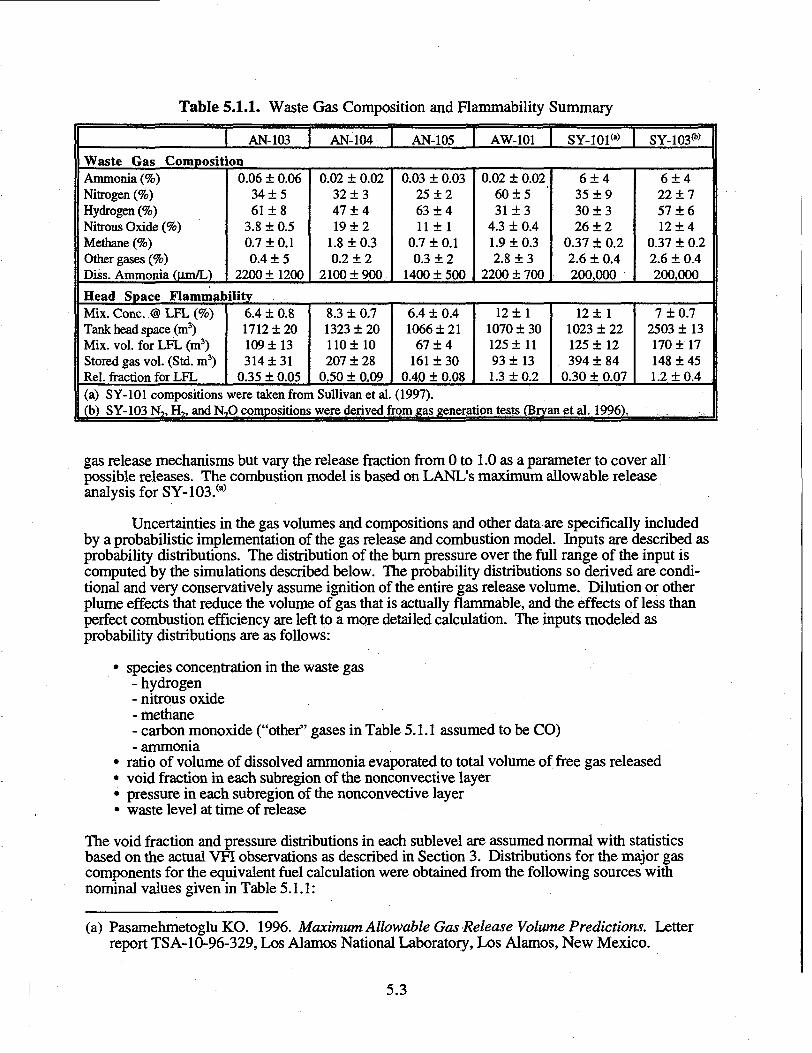
Table i5.1.1. Waste
AN-103
Waste Gas CompositionAmmonia (%)Nitrogen (%)Hydrogen (%)Nitrous Oxide (%)Methane (%)Other gases (%)Diss. Ammonia (jxm/L)
0.06 ± 0.0634 ± 561 ±8
3.8 ± 0.50.7 ± 0.10.4 ± 5
220011200
Gas Composition and Flammability Summary
AN-104
0.02 ± 0.0232 ± 347 ±419 + 2
1.8 ± 0.30.2 ± 2
2100 ±900
AN-105
0.03 + 0.0325 ± 263 + 411 + 1
0.7 ± 0.10.3 ± 2
1400 ± 500
AW-101
0.02 ± 0.0260 ± 531 ± 3
4.3 ± 0.41.9 ± 0.32.8 ± 3
2200 ± 700
SY-101(a)
6±435 ±930 ±326 ±2
0.37 ± 0.22.6 ± 0.4200,000
SY-103^
6±422 ±757 ±612 ±4
0.37 ± 0.22.6 ± 0.4200,000
Head Space FlammabilityMix. Cone. @ LFL (%)Tank head space (m3)Mix. vol. for LFL (m3)Stored gas vol. (Std. m3)Rel. fraction for LFL(a) SY-101 compositions
6.4 ± 0.81712 ± 20109 ±13314 + 31
0.35 ± 0.05
8.3 ± 0.71323 ± 20110 ±10207 ± 28
0.50 ± 0.09were taken from Sullivan et al.
6.4 ± 0.41066 ± 21
67 ± 4161 ± 30
0.40 ± 0.08(1997).
12 ± 11070 ± 30125 ±1193 ±131.3 ±0.2
12 ±11023 ± 22125 ± 12394 ±84
0.30 ± 0.07
(b) SY-103 N7, H,, and N,0 compositions were derived from gas generation tests (Bryan et al. 1996).
7 + 0.72503 ± 13170 ± 17148 ± 451.2 ± 0.4
gas release mechanisms but vary the release fraction from 0 to 1.0 as a parameter to cover allpossible releases. The combustion model is based on LANL's maximum allowable releaseanalysis for SY-103.(a)
Uncertainties in the gas volumes and compositions and other data are specifically includedby a probabilistic implementation of the gas release and combustion model. Inputs are described asprobability distributions. The distribution of the burn pressure over the full range of the input iscomputed by the simulations described below. The probability distributions so derived are condi-tional and very conservatively assume ignition of the entire gas release volume. Dilution or otherplume effects that reduce the volume of gas that is actually flammable, and the effects of less thanperfect combustion efficiency are left to a more detailed calculation. The inputs modeled asprobability distributions are as follows:
• species concentration in the waste gas- hydrogen- nitrous oxide-methane- carbon monoxide ("other" gases in Table 5.1.1 assumed to be CO)-ammonia
• ratio of volume of dissolved ammonia evaporated to total volume of free gas released• void fraction in each subregion of the nonconvective layer• pressure in each subregion of the nonconvective layer• waste level at time of release
The void fraction and pressure distributions in each sublevel are assumed normal with statisticsbased on the actual VFI observations as described in Section 3. Distributions for the major gascomponents for the equivalent fuel calculation were obtained from the following sources withnominal values given in Table 5.1.1:
(a) Pasamehmetoglu KO. 1996. Maximum Allowable Gas Release Volume Predictions. Letterreport TSA-10-96-329, Los Alamos National Laboratory, Los Alamos, New Mexico.
5.3
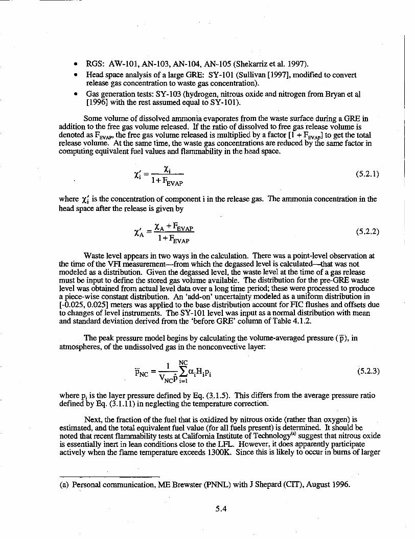
• RGS: AW-101, AN-103, AN-104, AN-105 (Shekarriz et al. 1997).• Head space analysis of a large GRE: SY-101 (Sullivan [1997], modified to convert
release gas concentration to waste gas concentration).• Gas generation tests: SY-103 (hydrogen, nitrous oxide and nitrogen from Bryan et al
[1996] with the rest assumed equal to SY-101).
Some volume of dissolved ammonia evaporates from the waste surface during a GRE inaddition to the free gas volume released. If the ratio of dissolved to free gas release volume isdenoted as F ^ ^ , the free gas volume released is multiplied by a factor [1 + F^^] to get the totalrelease volume. At the same time, the waste gas concentrations are reduced by the same factor incomputing equivalent fuel values and flammability in the head space.
EVAP
where %,' is the concentration of component i in the release gas. The ammonia concentration in thehead space after the release is given by
EVAP
Waste level appears in two ways in the calculation. There was a point-level observation atthe time of the VFI measurement—from which the degassed level is calculated—that was notmodeled as a distribution. Given the degassed level, the waste level at the time of a gas releasemust be input to define the stored gas volume available. The distribution for the pre-GRE wastelevel was obtained from actual level data over a long time period; these were processed to producea piece-wise constant distribution. An 'add-on' uncertainty modeled as a uniform distribution in[-0.025,0.025] meters was applied to the base distribution account for FIC flushes and offsets dueto changes of level instruments. The SY-101 level was input as a normal distribution with meanand standard deviation derived from the 'before GRE' column of Table 4.1.2.
The peak pressure model begins by calculating the volume-averaged pressure (p), inatmospheres, of the undissolved gas in the nonconvective layer:
1 NC
where p; is the layer pressure defined by Eq. (3.1.5). This differs from the average pressure ratiodefined by Eq. (3.1.11) in neglecting the temperature correction.
Next, the fraction of the fuel that is oxidized by nitrous oxide (rather than oxygen) isestimated, and the total equivalent fuel value (for all fuels present) is determined. It should benoted that recent flammability tests at California Institute of Technology00 suggest that nitrous oxideis essentially inert in lean conditions close to the LFL. However, it does apparently participateactively when the flame temperature exceeds 1300K. Since this is likely to occur in burns of larger
(a) Personal communication, ME Brewster (PNNL) with J Shepard (CIT), August 1996.
5.4
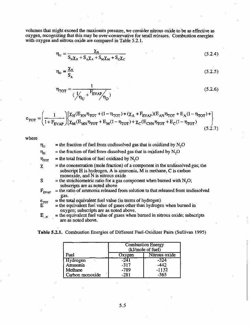
volumes that might exceed the maximum pressure, we consider nitrous oxide to be as effective asoxygen, recognizing that this may be over-conservative for small releases. Combustion energieswith oxygen and nitrous oxide are compared in Table 5.2.1.
XN
= —
1
EVAP/ \/v
(5.2.4)
(5.2.5)
(5.2.6)
eTOT ~
where
X
EVAP
eTOTE
-'...N
0- - + FEVAP)(EANT1TOT
(5.2.7)
the fraction of fuel from undissolved gas that is oxidized by N2O
the fraction of fuel from dissolved gas that is oxidized by N2O
the total fraction of fuel oxidized by N2Othe concentration (mole fraction) of a component in the undissolved gas; thesubscript H is hydrogen, A is ammonia, M is methane, C is carbonmonoxide, and N is nitrous oxidethe stoichiometric ratio for a gas component when burned with N2O;subscripts are as noted abovethe ratio of ammonia released from solution to that released from undissolvedgas.
the total equivalent fuel value (in terms of hydrogen)the equivalent fuel value of gases other than hydrogen when burned inoxygen; subscripts are as noted above.the equivalent fuel value of gases when burned in nitrous oxide; subscriptsare as noted above.
Table 5.2.1. Combustion Energies of Different Fuel-Oxidizer Pairs (Sullivan 1995)
FuelHydrogenAmmoniaMethaneCarbon monoxide
Combustion Energy(kJ/moleoffuel)
Oxygen-241-317-789-281
Nitrous oxide-324-442-1132-365
5.5
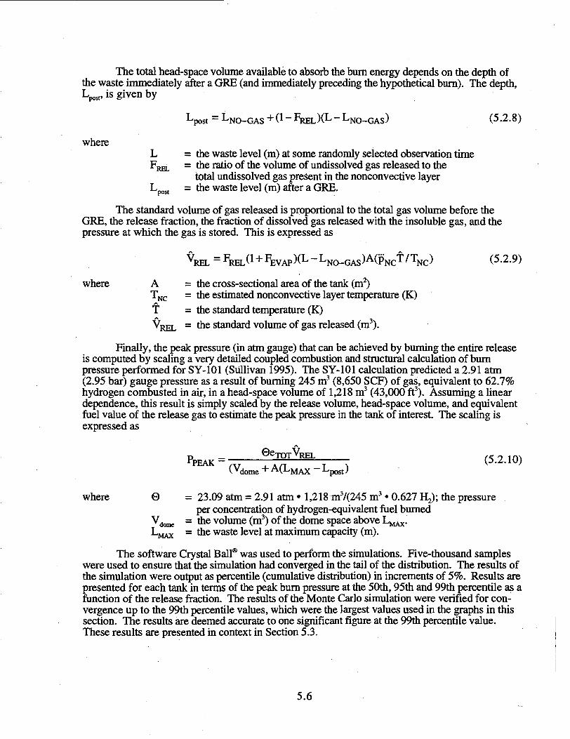
The total head-space volume available to absorb the burn energy depends on the depth ofthe waste immediately after a GRE (and immediately preceding the hypothetical burn). The depth,L ^ , is given by
p + 0 ~ FREL )(L - LN O_GAS ) (5.2.8)
whereL = the waste level (m) at some randomly selected observation timeFREL = the ratio of the volume of undissolved gas released to the
total undissolved gas present in the nonconvective layerLpos( = the waste level (m) after a GRE.
The standard volume of gas released is proportional to the total gas volume before theGRE, the release fraction, the fraction of dissolved gas released with the insoluble gas, and thepressure at which the gas is stored. This is expressed as
where A = the cross-sectional area of the tank (m2)TNC = the estimated nonconvective layer temperature (K)T = the standard temperature (K)VRFT = the standard volume of gas released (m3).
Finally, the peak pressure (in atm gauge) that can be achieved by burning the entire releaseis computed by scaling a very detailed coupled combustion, and structural calculation of burnpressure performed for SY-101 (Sullivan 1995). The SY-101 calculation predicted a 2.91 atm(2.95 bar) gauge pressure as a result of burning 245 m3 (8,650 SCF) of gas, equivalent to 62.7%hydrogen combusted in air, in a head-space volume of 1,218 m3 (43,000 ft3). Assuming a lineardependence, this result is simply scaled by the release volume, head-space volume, and equivalentfuel value of the release gas to estimate the peak pressure in the tank of interest. The scaling isexpressed as
P. PTOT REL /C o i r\\PEAK ~ (J.ZAV)
(Vdome + A(LMAX ~ Lpost)
where 0 = 23.09 atm = 2.91 atm • 1,218 nr7(245 m3 • 0.627 H2); the pressureper concentration of hydrogen-equivalent fuel burned
Vdome = the volume (m3) of the dome space above Lj^x.LMAX = the waste level at maximum capacity (m).
The software Crystal Ball® was used to perform the simulations. Five-thousand sampleswere used to ensure that the simulation had converged in the tail of the distribution. The results ofthe simulation were output as percentile (cumulative distribution) in increments of 5%. Results arepresented for each tank in terms of the peak burn pressure at the 50th, 95th and 99th percentile as afunction of the release fraction. The results of the Monte Carlo simulation were verified for con-vergence up to the 99th percentile values, which were the largest values used in the graphs in thissection. The results are deemed accurate to one significant figure at the 99th percentile value.These results are presented in context in Section 5.3.
5.6
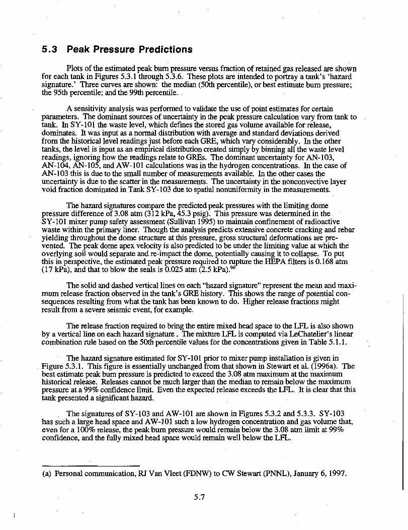
5.3 Peak Pressure Predictions
Plots of the estimated peak burn pressure versus fraction of retained gas released are shownfor each tank in Figures 5.3.1 through 5.3.6. These plots are intended to portray a tank's 'hazardsignature.' Three curves are shown: the median (50th percentile), or best estimate burn pressure;the 95th percentile; and the 99th percentile.
A sensitivity analysis was performed to validate the use of point estimates for certainparameters. The dominant sources of uncertainty in the peak pressure calculation vary from tank totank. In SY-101 the waste level, which defines the stored gas volume available for release,dominates. It was input as a normal distribution with average and standard deviations derivedfrom the historical level readings just before each GRE, which vary considerably. In the othertanks, the level is input as an empirical distribution created simply by binning all the waste levelreadings, ignoring how the readings relate to GREs. The dominant uncertainty for AN-103,AN-104, AN-105, and AW-101 calculations was in the hydrogen concentrations. In the case ofAN-103 this is due to the small number of measurements available. In the other cases theuncertainty is due to the scatter in the measurements. The uncertainty in the nonconvective layervoid fraction dominated in Tank SY-103 due to spatial nonuniformity in the measurements.
The hazard signatures compare the predicted peak pressures with the limiting domepressure difference of 3.08 arm (312 kPa, 45.3 psig). This pressure was determined in theSY-101 mixer pump safety assessment (Sullivan 1995) to maintain confinement of radioactivewaste within the primary liner. Though the analysis predicts extensive concrete cracking and rebaryielding throughout the dome structure at this pressure, gross structural deformations are pre-vented. The peak dome apex velocity is also predicted to be under the limiting value at which theoverlying soil would separate and re-impact the dome, potentially causing it to collapse. To putthis in perspective, the estimated peak pressure required to rupture the HEP A filters is 0.168 atm(17 kPa), and that to blow the seals is 0.025 atm (2.5 kPa).(a)
The solid and dashed vertical lines on each "hazard signature" represent the mean and maxi-mum release fraction observed in the tank's GRE history. This shows the range of potential con-sequences resulting from what the tank has been known to do. Higher release fractions mightresult from a severe seismic event, for example.
The release fraction required to bring the entire mixed head space to the LFL is also shownby a vertical line on each hazard signature. The mixture LFL is computed via LeChatelier's linearcombination rule based on the 50th percentile values for the concentrations given in Table 5.1.1.
The hazard signature estimated for SY-101 prior to mixer pump installation is given inFigure 5.3.1. This figure is essentially unchanged from that shown in Stewart et al. (1996a). Thebest estimate peak burn pressure is predicted to exceed the 3.08 atm maximum at the maximumhistorical release. Releases cannot be much larger than the median to remain below the maximumpressure at a 99% confidence limit. Even the expected release exceeds the LFL. It is clear that thistank presented a significant hazard.
The signatures of SY-103 and AW-101 are shown in Figures 5.3.2 and 5.3.3. SY-103has such a large head space and AW-101 such a low hydrogen concentration and gas volume that,even for a 100% release, the peak burn pressure would remain below the 3.08 atm limit at 99%confidence, and the fully mixed head space would remain well below the LFL.
(a) Personal communication, RJ Van Vleet (FDNW) to CW Stewart (PNNL), January 6,1997.
5.7
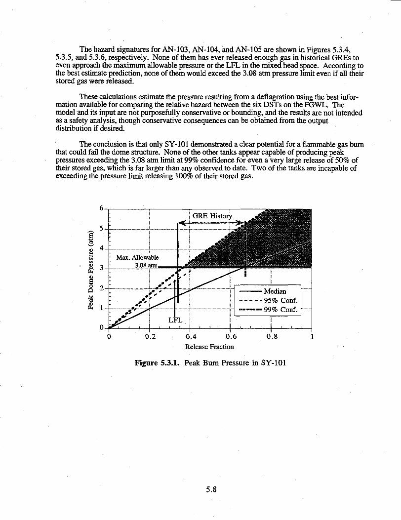
The hazard signatures for AN-103, AN-104, and AN-105 are shown in Figures 5.3.4,5.3.5, and 5.3.6, respectively. None of them has ever released enough gas in historical GREs toeven approach the maximum allowable pressure or the LFL in the mixed head space. According tothe best estimate prediction, none of them would exceed the 3.08 atm pressure limit even if all theirstored gas were released.
These calculations estimate the pressure resulting from a deflagration using the best infor-mation available for comparing the relative hazard between the six DSTs on the FGWL. Themodel and its input are not purposefully conservative or bounding, and the results are not intendedas a safety analysis, though conservative consequences can be obtained from the outputdistribution if desired.
The conclusion is that only SY-101 demonstrated a clear potential for a flammable gas burnthat could fail the dome structure. None of the other tanks appear capable of producing peakpressures exceeding the 3.08 atm limit at 99% confidence for even a very large release of 50% oftheir stored gas, which is far larger than any observed to date. Two of the tanks are incapable ofexceeding the pressure limit releasing 100% of their stored gas.
Max. Allowable3.08 atm
Median95% Conf
- 99% Conf
0.4 0.6Release Fraction
Figure 5.3.1. Peak Burn Pressure in SY-101
5.8
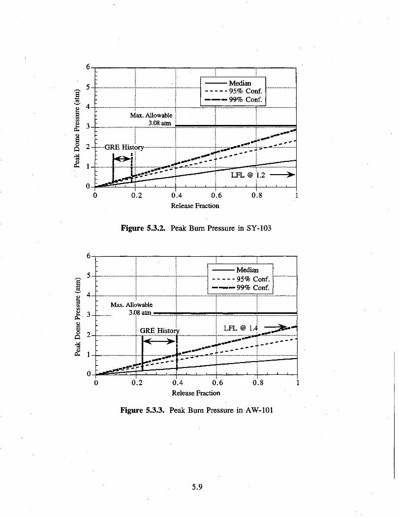
Median95% Conf.
——«. 99% Conf.
0.2 0.4 0.6Release Fraction
0.8
Figure 5.3.2. Peak Burn Pressure in SY-103
Median95% Conf.99% Conf.
0.4 0.6Release Fraction
Figure 5.3.3. Peak Burn Pressure in AW-101
5.9
senCO
2
Median95% Conf.
. . . . . 99% Conf.
Max. Allowable3.08 atm
& 1-C.
0.4 0.6Release Fraction
Figure 5.3.4. Peak Bum Pressure in AN-103
5 - -
0
Mean95% Conf.
— — 99% Conf.
0.4 0.6Release Fraction
Figure 5.3.5. Peak Bum Pressure in AN-104
5.10