future satellite gravimetry for geodesy

FUTURE SATELLITE GRAVIMETRY FOR GEODESY

J. FLURY and R. RUMMELInstitut fur Astronomische und Physikalische Geodasie, TU Munchen

(E-mail: [email protected]; [email protected])

(Received 4 October 2004; Accepted 14 March 2005)

Abstract. After GRACE and GOCE there will still be need and room for improvement of the knowledge

(1) of the static gravity field at spatial scales between 40 km and 100 km, and (2) of the time varying

gravity field at scales smaller than 500 km. This is shown based on the analysis of spectral signal power of

various gravity field components and on the comparison with current knowledge and expected perfor-

mance of GRACE and GOCE. Both, accuracy and resolution can be improved by future dedicated gravity

satellite missions. For applications in geodesy, the spectral omission error due to the limited spatial

resolution of a gravity satellite mission is a limiting factor. The recommended strategy is to extend as far as

possible the spatial resolution of future missions, and to improve at the same time the modelling of the

very small scale components using terrestrial gravity information and topographic models. We discuss the

geodetic needs in improved gravity models in the areas of precise height systems, GNSS levelling, inertial

navigation and precise orbit determination. Today global height systems with a 1 cm accuracy are required

for sea level and ocean circulation studies. This can be achieved by a future satellite mission with higher

spatial resolution in combination with improved local and regional gravity field modelling. A similar

strategy could improve the very economic method of determination of physical heights by GNSS levelling

from the decimeter to the centimeter level. In inertial vehicle navigation, in particular in sub-marine,

aircraft and missile guidance, any improvement of global gravity field models would help to improve

reliability and the radius of operation.

Keywords: Geodesy, gravity field, heights, GNSS levelling, inertial navigation

1. Introduction

All currently available geoid or gravity models are based on satellite orbitanalysis, satellite radar altimetry in ocean areas, terrestrial and shipbornegravimetry and topographic models. Long-term observation and analysisresulted in global gravity field models such as the Earth Gravity ModelEGM96 (Lemoine et al., 1998). Despite of the wealth of input data andsophistication of the computational processes these models are still ratherheterogeneous in terms of resolution and accuracy. At present, a major stepforward in gravity field knowledge is achieved by a first generation of dedi-cated gravity field satellite missions, CHAMP (Reigber et al., 2003), GRACE(Tapley et al., 2004b) and GOCE (ESA, 1999).

Earth, Moon, and Planets (2005) 94: 13–29 � Springer 2005

DOI 10.1007/s11038-005-3756-7

In geodesy the requirements of geoid and gravity field are particularlyhigh. Highly accurate and homogeneous gravity field information is neededfor the establishment of unified global height systems and for the calculationof physical heights from ellipsoidal GNSS heights. Precise and homogeneousheight systems are important for engineering purposes as well as for Earthsciences, e.g. for sea level studies. With GRACE and GOCE, considerableimprovements will be achieved, but the requirements in terms of accuracyand spatial resolution will not be fully met. Inertial navigation and preciseorbit determination are other geodetic fields requiring very accurate gravityfield knowledge.

A new and very challenging field is the observation and analysis of thetime variable gravity field due to mass variations in atmosphere, oceans,continental water cycle, ice covered areas and solid Earth (Committee, 1997;Ilk et al., 2005). The satellite mission GRACE enables a first view on thisfield, but many open questions will remain. With GRACE, and even morewith future satellite gravity missions, temporal gravity field variations willbecome an important subject of geodetic research. For adequate analysis andmodelling, a close cooperation between geodesy, geophysics, oceanography,glaciology, hydrology and other Earth sciences is mandatory.

There exist reliable mathematical ‘‘rules’’ about the average behaviour ofthe gravity field and geoid under the assumption of stationarity and isotropy.These rules are power spectra of average signal power, expressed in terms ofspherical harmonic degree variances or degree rms. We use such powerspectra as a starting point for a discussion of the state-of-the-art, of short-comings and future needs in gravity field knowledge, cf. Section 2.1. At shortwavelengths gravity information is insufficient or non-existent. For wave-lengths smaller than 100 km, this situation will remain unchanged even afterthe completion of the first generation of dedicated gravity field satellitemissions. Statistically, the unknown small-scale gravity signal is dealt with asomission error, cf. Section 2.2. Much more uncertain than the stationarygravity field characteristics is the signal size and behaviour of the time var-iable gravity field, cf. Section 2.3. The stationary and time variable gravityfield signal amplitudes and length scales give the background for the sub-sequent analysis of future geodetic requirements and possible improvementsby future satellite missions, cf. Section 3.

2. Gravity Field and Geoid: State-of-the-Art

2.1. STATIONARY GEOID

In the following we discuss the signal amplitudes of the Earth’s gravity fieldat various wavelengths and spatial scales, respectively. The discussion is

14 J. FLURY AND R. RUMMEL

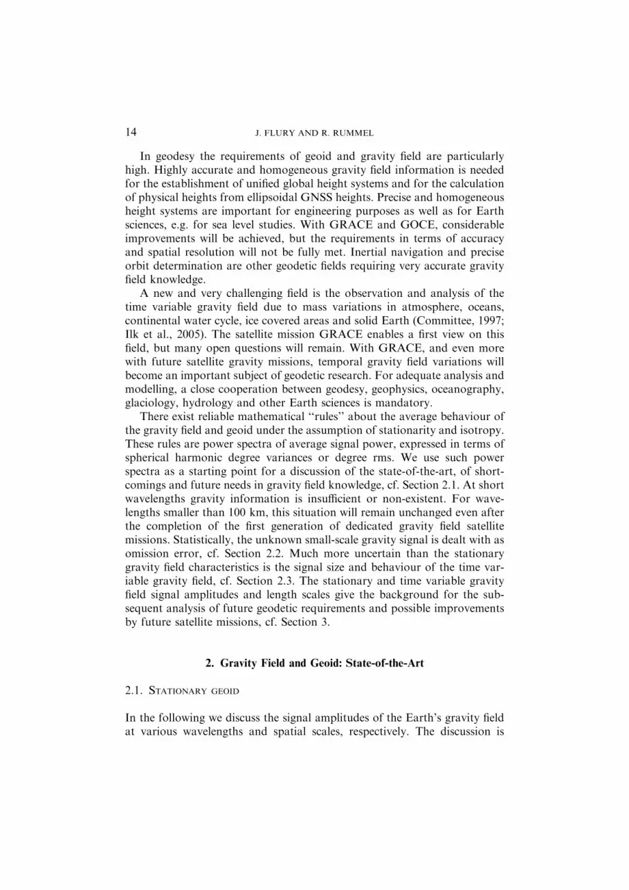
based on Figure 1 where degree rms values from spherical harmonic geoidexpansions are shown. The figure also explains where the current geoidinformation comes from and where there is room and need for improvement.

– The two central lines are those denoted ‘‘Tscherning-Rapp’’ and ‘‘Kaula’’.They represent models of the geoid signal size (in meters) as a function ofspherical harmonic degree or average spatial scale (half-wavelength inkilometers). They are based on satellite and terrestrial data translated intoa simple mathematical expression (rule of thumb). At small length scalesthese curves are extrapolated and pure speculation. In addition, theyassume homogeneous signal characteristics all over the globe. Neverthe-less, the two rules give an excellent impression of the overall (logarithmic)signal strength decrease with increasing spherical harmonic degree.

– The line for the Earth Gravity Model EGM96 shows the signal decrease ofthe geoid based on real data. It is derived from satellite, terrestrial andaltimetric gravity information. Its maximum spherical harmonic degree is360 (about 60 km). It fits well between the Tscherning-Rapp and Kaulalines.

102 103

geoi

d de

gree

rm

s [m

]

local data alps (incl. top.)

local data flat land

local data alps

(top. reduced)

Tscherning/Rapp

Kaula

global topography

compensated topography

EGM96

GRACEerror

GOCE error

200 km 100 km 50 km 20 km

Figure 1. Single content of the static gravity field, shown between spherical harmonics degree100 and 2000, in terms of geoid signal degree rms-values, as well as GRACE and GOCE errorrms-values. See the explanation in the text.

15FUTURE SATELLITE GRAVIMETRY FOR GEODESY

– The ‘‘global topography’’ line is based on a geoid computation from thegravity potential of all visible topographic masses (and ocean depths)assuming constant density. It seriously overestimates the geoid signalstrength because it neglects any isostatic compensation of topographicmasses.

– Therefore, in a second computation, mass compensation has been takeninto account using a simple Airy compensation model. Now the ‘‘com-pensated topography’’ line fits well to the measured EGM96 line. One canalso observe that at smaller length scales, say below 50 km, topographicmasses are not compensated anymore according to this model.

– From the GRACE and GOCE error curves one can deduce the state-of-artof geoid knowledge after GRACE and GOCE, respectively.

– At short wavelengths (10–40 km) two representative areas were selectedwith very good terrestrial gravity data coverage: a local test area in theAlps, which results in the geoid spectral line ‘‘local data Alps’’ and an areaof similar size but flat, resulting in the spectral line ‘‘local data flat land’’.One observes the large difference in amplitude (one order of magnitude).

– Finally, for the Alpine test area, the geoid spectrum has been computedafter subtracting the effect of the topographic masses; this is the ‘‘local dataAlps (top. reduced)’’ line. It is much closer to the Kaula model spectrum,but more important, it demonstrates that at short wavelengths the majorpart of the observed geoid can be explained by the visible topographicmasses of the area and its surroundings (cf. Flury, 2002, 2005).

Improving the static gravity field by means of a new gravity field satellitemission means to penetrate into spatial scales between 40 and 100 km. Scaleslarger than 100 km will be very well resolved by GOCE; at scales smaller than40 km the signal amplitude is quite small, and a major part of it can be com-puted from topographic models. In between, neither sufficient global gravitydata (of good quality) nor adequate topographic data are currently available.

The degree rms curves in Figure 1 are derived as follows: For globalmodels, degree variances cl are obtained from spherical harmonic coefficientsof degree l and order m

cl ¼X

m

ðc2lm þ s2lmÞ;

their square roots give the degree rms values. For the local data sets (gravityanomalies), empirical signal autocovariance models C(w) related to thespherical distance w have been determined and converted to degree variances(Wenzel and Arabelos, 1981; Forsberg, 1984):

cl ¼Z W

w¼0CðwÞPlðcoswÞ sinwdw:


Pl (cos w) are Legendre polynomials. The integration is performed up to anappropriate maximum distance w. The gravity anomaly degree variancesobtained from local data can be represented by simple power laws (cf. Flury,2005) and converted to geoid heights. The GRACE and GOCE error modelsare obtained from mission simulations, cf. Sneeuw et al., this issue.

2.2. GEOID OMISSION PART

Any satellite gravity field mission will measure the global geoid with a certainprecision and a certain spatial resolution. The size of the signal not resolvedby the measurements constitutes the so-called omission part. For most geo-physical science applications a certain finite spatial resolution is sufficient,corresponding e.g. to the grid spacing of a finite element model. Then theomission part does not enter into considerations as long as the geoid reso-lution fits to the model resolution. For some other applications, the full geoidinformation is needed at individual points on earth, i.e. the full spectralcontent from zero to infinity. In those cases the omission part enters into theerror budget. The omission part can be reduced by improving the spatialresolution of a space mission or by adding local geoid information as derivede.g. from local gravity surveys and topographic data.

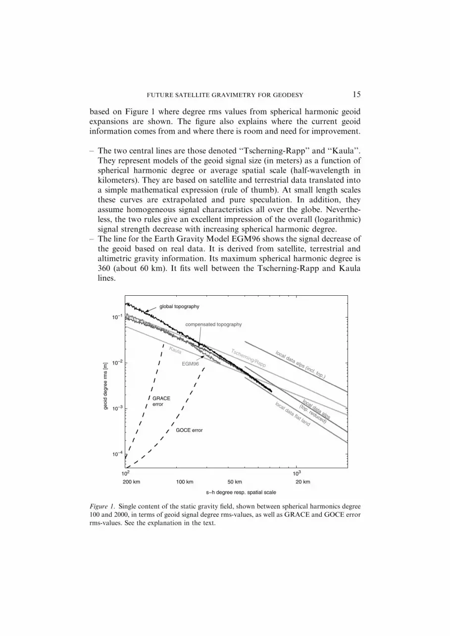
Figure 2 shows the geoid omission part in centimetres as a function ofspherical harmonic degree in the window between degree 300, which rep-resents the situation after GOCE, and degree 700, which a future missioncould possibly resolve, corresponding to the range of 70–30 km half-wavelength, respectively. The full omission error, shown by the black line, isstill rather high, decreasing from 28 cm at degree 300 to 10 cm at degree700. It should be noted, however, that by adding local gravity informationin a circle of radius 0.5�, 1�, 2� or 5� (50 km, 100 km, 200 km, 500 km)around the computation point the omission error can be reduced signifi-cantly. The error for a 0.5� radius cap is of special interest: such an areacould – even if no local data were available – be filled up with about 100terrestrial gravity measurements very fast and economically in sufficientaccuracy.

2.3. TIME VARIABLE GRAVITY FIELD

The geoid and gravity are changing with time due to the tides of sun, moonand planets, due to mass movements and mass exchange in Earth system and,as a secondary effect, due to deformation of the Earth’s surface as a conse-quence to such mass motions. The changes are small, ranging from below a


mm to a few dm for the geoid, they occur at all time scales from secular tosudden and at all spatial scales from global to very local. From terrestrialgravity measurements the global pattern of Earth tides is known rather well;also temporal changes due to postglacial rebound or secular crustal move-ments are nowadays well measurable. All other effects, such as changes ingroundwater level or ocean or atmospheric loading are so far difficult toidentify and quantify by in-situ measurements. From satellite orbit analysistime variations in the very low degree zonal spherical harmonic coefficientscan be determined rather well. Their physical interpretation proves difficult,however (Cazenave and Nerem, 2002; Cox and Chao, 2002). The situation isexpected to improve significantly with the monthly sets of spherical harmoniccoefficients from GRACE, from which changes in atmospheric pressure,ocean bottom pressure or in the hydrological cycle will be derived, compareWahr et al. (1998) and Tapley et al. (2004a, b).

Like it is done for the static gravity field, it is common practice to rep-resent the signal strength of the various contributions of temporal geoidvariations in terms of signal degree variances. On the one hand, this allows tocompare the spectral signal characteristics of the individual geophysicalsignals; on the other hand, one can compare the various signals with the

300 350 400 450 500 550 600 650 700

100

101

102

omis

sion

err

or [c

m]

full omission error

local data cap size ψ=0.5°

ψ=1°

ψ=2°

ψ=5°

70 km 30 km

Figure 2. Omission error modeled using Tscherning/Rapp degree variance model. For eachspherical harmonic degree the omission part up to infinity is shown, assuming that the signalup to this degree is covered by a geopotential model. The omission error reduces greatly whenlocal gravity data for a relatively small cap size is added, with spherical cap radii of 0.5�, 1�, 2�or 5�.


expected spectral characteristics of the measurement noise of space missionsand deduce thereof indications about their observability. There are two dif-ficulties with this approach. First, for some of the geophysical signalsknowledge about their temporal and spatial behaviour is rather poor; con-sequently the degree variance lines may be unrepresentative. Second, some ofthe considered phenomena are confined to land or ocean or certain geo-graphical regions, which makes the use of spherical harmonic degree vari-ances somewhat problematic. Thus, the spectra are to be seen with a certain‘‘grain of salt’’.

In essence, the temporal variations can be divided into two classes: thosethat need to be studied by future gravity field satellite missions and thosethat are to be considered as ‘‘disturbances’’. A special class of disturbancesarises from periodic, high frequency geophysical phenomena that map as‘‘alias’’ into the spectral range of interest due to the peculiar space-timesampling of a satellite. In particular, semi-diurnal and diurnal phenomenasuch as the tides of the solid Earth, oceans and atmosphere belong to thiscategory.

Figures 3 and 4 give an impression of the spectral geoid signal of somegeophysical effects. Comparison with the geoid degree rms-values of the

Degree

Deg

ree

Sta

nd

ard

Dev

iati

on

in G

eoid

Hei

gh

t [m

]

10

10

20

20

30

30

40

40

50

50

10-6 10-6

10-5 10-5

10-4 10-4

10-3 10-3

Ocean semi-annualOcean annualGRACE Error PredictionAtmosphere annual

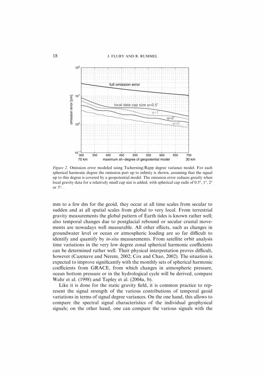
Figure 3. Geoid degree rms-values of the annual variations in atmospheric density of theannual and semi-annual ocean mass changes. For comparison, the expected GRACE noisespectrum is added.


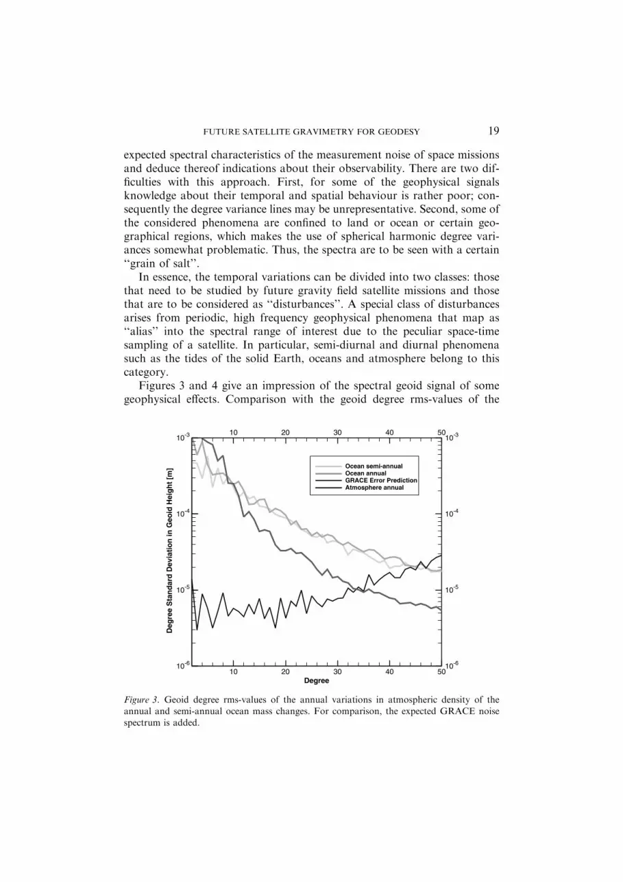
static field, Figure 1, explains the smallness of the time variable signals.Figure 3 shows the geoid degree rms-values of the annual variations of theatmosphere and of the annual and semi-annual variations of the oceans. Allthree spectra are derived from corresponding time series of daily data. Theiruncertainty is rather large. In order to get an impression of their observabilitythe expected noise spectrum of GRACE is included as well (see Wahr et al.,1998; Wunsch et al., 2001). It can be seen that time variable signals can bederived by GRACE up to about degree and order 35, or at length scales ofabout 500–600 km. Figure 4 shows some daily and monthly geoid variations(daily atmosphere from ECMWF, daily ocean from MIT ocean circulationmodel, and – with a high uncertainty – monthly changes in the hydrologicalwater cycle). These three time series may cause aliasing problems, dependingon the sampling strategy of future gravity field satellite missions (see Gruber,2001; Wunsch et al., 2001). The GRACE expected noise spectrum is addedfor completeness.

Based on this analysis of the signal behaviour of stationary and time-variable gravity and geoid and the current state-of-the-art of commission andomission error one can now turn to gravity and geoid applications in geodesyand (in the following articles) in Earth sciences.

Degree

Deg

ree

Sta

nd

ard

Dev

iati

on

in G

eoid

Hei

gh

t [m

]

10

10

20

20

30

30

40

40

50

50

10-6 10-6

10-5 10-5

10-4 10-4

10-3 10-3

Atmosphere daily ECMWFOcean daily MITHydrology monthly EuropeGRACE Error Prediction

Figure 4. Geoid degree rms-values of the daily variations in atmospheric density, the dailymass changes of the oceans monthly changes in the hydrological cycle. For comparison, the

expected GRACE noise spectrum is added.


3. Geodetic Requirements

It is common to all applications of gravity and geoid information in geodesy,mapping, geomatics and engineering that point values or differences of pointvalues are needed. The only exception is orbit determination. This impliesthat the band limited geoid and gravity information deduced from satellitemeasurements is only part of the required total geoid and gravity pointvalues. The missing complementary, small scale part has to come from localairborne, shipborne or terrestrial gravimetric surveys and from topographicmodels. After GOCE this is the signal part above spherical harmonic degree250, see Rummel (2004, this issue). If the small scale geoid and gravitycontribution is neglected, a rather high omission error has to be accepted, aswas discussed in Section 2. While after GOCE the geoid error at degree andorder 250 will amount to a few cm only, the omission part is about 30 cm 1 rerror.

Thus, what would be the proper strategy in these fields for the future?

(1) An improvement of GOCE precision without any improvement inresolution would reduce the geoid commission error from a few cmafter GOCE to the sub-cm level. However, this will not result in majorbreakthroughs in view of the large omission error.

(2) An improvement in spatial resolution from a maximum degree of 250to, say, degree 700 (or 30 km) would decrease the remaining omissionerror from 30 to 10 cm. This would help considerably, but it may provevery difficult to get such high resolution from space techniques.

(3) Reduction of the omission error by means of local gravimetric surveysand topographic models: In a concerted effort – based on new, wellcontrolled measurement campaigns, re-analysis of existing data setsand new high resolution terrain models – the local omission error canbe reduced to the cm-level.

As a consequence, the strategy must be: (a) Extension of the spatial res-olution of future dedicated satellite missions, beyond degree 250 without lossof accuracy, and (b) reduction of the omission error for selected regions andapplications to the cm-level.

3.1. HEIGHTS

In most countries, well defined and official ‘‘heights above sea level’’ aremade available and maintained for use in engineering, mapping, cadastre,geo-referencing as well as for use in science. These are so-called physicalheights which means they carry information about the direction of flow of


water. National height systems usually refer to sea level and are tied to a tidegauge at an arbitrarily selected point. This results in offsets between heightsystems at borders and across oceans or ocean straits. For Europe, the offsetsare in the order of some decimetres and are rather well known, with anaccuracy of 1–10 cm (Figure 5, from Sacher et al., 1999). For somecontinents they are unknown and may be much larger. Physical heights arederived by spirit levelling plus gravimetry. This approach has the tendencyto accumulate systematic errors that may amount to several cm or even dmon a continental scale (Haines et al., 2003), in addition to the tide gaugeoffsets.

Ideally, ‘‘heights above sea level’’ should be ‘‘heights above the geoid’’,i.e. in an ideal case all height systems should refer to one and the samelevel surface. Only then physical heights all over the earth would becomecomparable, which would lead to the establishment of a world heightreference system. One would be able to decide whether an arbitrary coastal

Figure 5. Offsets between national height systems in Europe (in cm), from Sacher et al. (1999).Countries in the same colour are connected to the same datum point (tide gauge). By courtesyof Bundesamt fur Kartographie und Geodasie, Frankfurt.


point in Australia would be higher or lower than a second point some-where in Europe. This is of some importance for regional and globalmapping, geo-referencing and geo-information, and it is of great impor-tance for global sea level and ocean circulation studies. Tidal recordswould become comparable globally, too (see Figure 6). The required geoidaccuracy is below 10 cm (commission plus omission part) or on the longterm below 1 cm. Official institutions like the US National Geospatial-Intelligence Agency NGA strive for a continental or global accuracy of2 cm. After GOCE, a height system accuracy of approximately 5–10 cm –commission and omission error – will be achievable for all areas where asufficient coverage of local gravity data is available to deal with theomission part (see Section 2; Arabelos and Tscherning, 2001; Rummel,2002). For a 1 cm accuracy, however, one has to take into account localdata up to much larger distances, and a satellite mission with higherresolution is needed.

For engineering purposes (construction of bridges, long tunnels, canals)precise physical height differences and deflections of the vertical are needed.The local character of these applications emphasizes the need for veryprecise local gravimetric and topographic information and relaxes therequirement for very precise global (satellite derived) geoid and gravitymodels. However, for these applications an increased resolution of thegeopotential models would lead to cost reduction in the sense that less effortwould be required to check and refine the geoid and height reference locally,e.g. that the amount of required local gravity observations would decreasesubstantially.

Figure 6. Examples for links between tide gauges (crossing the Antarctic Circumpolar

Current), for which high precision geoid differences are required for ocean circulationmodelling.


It has to be noted that for areas with considerable vertical land move-ments the time variability of the geoid has to be taken into account tomaintain the well defined height reference. This applies especially to Canada,Scandinavia and Antarctica, where the geoid variation due to postglacialrebound reaches up to 2 mm/year corresponding to a 20 cm change over acentury, but it also applies to low land countries (see Vermeersen, 2004, thisissue). Vertical tectonic movements – typically up to some mm/year (Lam-beck, 1988) – are expected to cause considerably smaller geoid changes(Marti et al., 2003). However, on the long run it may also be necessary toconsider geoid variations due to tectonics for precise height systems.Therefore, geodesy would also benefit from an improved determination ofsecular geoid time variations.

3.2. GNSS LEVELLING

Nowadays, by means of GPS and other space positioning methods,absolute point positions or position differences can be derived at the cm-level or sub-cm level, respectively, depending on the sophistication of themeasurement setup. There is a clear trend to even higher precisions oncethe next generation of satellite navigation systems with more precise clocksas well as better atmospheric monitoring become available. 3-D pointpositions or position differences can be directly transformed into geo-graphical coordinates or coordinate differences and ellipsoidal heights orheight differences. In combination with a precise geoid model, ellipsoidalheights can be conveniently translated into physical heights (heights abovethe geoid). This technique circumvents the tedious, time-consuming tradi-tional geodetic levelling and avoids the systematic errors inherent to thismethod. Precondition is, however, the availability of absolute geoid heightsor height differences with a precision comparable to that of the ellipsoidalheights derived by means of GNSS. This is to say the required geoidprecision (commission and omission part) has to be at the cm or sub-cmlevel.

Already now the technique of GPS-levelling is applied worldwide at amuch more moderate level of accuracy. The fields of application are engi-neering (construction of streets, bridges, tunnels, canals), mapping and geo-information, exploration and many more. The method is the only economicway to get a well defined height reference in unsurveyed areas, be it indeveloping countries or in the polar regions. It is of special interest for areaswhere permanent height benchmarks cannot be built, e.g. for inundationzones, where the benchmarks get destroyed by every flood.

Where no local gravity data in good quality are available, GNSS levelling isaffected by the full geoid error (commission and omission) of a geopotential


model. This error will be – depending on the distance between stations – at afew cm after GOCE. It could be lowered down to the centimeter level by asatellite mission resolving spatial scales of the geoid up to spherical harmonicdegree 700.

Figure 7 (from Ihde et al., 2002; see also Denker and Torge, 1998) showstoday’s state-of-the-art, where even in a well surveyed area like Europe thegeoid errors amount to several dm in general, in some cases even to morethan 1 m.

Figure 7. Errors for GNSS Levelling using the geoid model EGG97 (Denker and Torge,1998), based on EGM96 geopotential model and a very large terrestrial gravity data base. By

courtesy of Bundesamt fur Kartographie und Geodasie, Frankfurt.


3.3. INERTIAL NAVIGATION

The core sensors of any inertial measurement unit (IMU) are a set of threeorthogonally mounted accelerometers and gyroscopes. The IMU may berigidly fixed to the moving platform (strapped down system); then theaccelerometers and gyroscopes must be able to cope with the full dynamics ofthe platform motion. Alternatively the IMU may be isolated from therotational degrees of freedom of the motion by means of a gimbal system(space fixed or local level system). In any case, the accelerometers measurethe sum of vehicle motion and gravitational attraction.

In order to isolate the accelerations due to vehicle motion, which arethen integrated once or twice to give vehicle velocity or position differ-ences, respectively, the gravitational accelerations have to be subtracted.As there is no way to measure them independently they have to be pro-vided by some gravity model. Any imperfection in this model will result ina systematic error, and after integration this error will quickly accumulateto large drifts in the calculated velocities and positions. In vehicle navi-gation, where many zero-velocity updates (ZUPT’s) can be incorporated inthe survey, a rather simple ellipsoidal gravity model suffices. In sub-mar-ine, borehole, aircraft and missile guidance no ZUPT’s are possible andrequirements for precise gravity information are very high. They are typ-ically at the 0.1–1 mGal level in terms of gravity and 0.1 arcsec in terms ofdeflections of the vertical (DOV’s). Again, such errors comprise commis-sion and omission errors (Chatfield, 1997). Any improvement of globalgravity field models towards these numbers – in particular by increasingthe spatial resolution – would help (Schwarz et al., 1992). It wouldimprove reliablility, reduce navigation drift and consequently increase theradius of operation.

3.4. SATELLITE ORBIT DETERMINATION

After GRACE and GOCE a very good Earth gravity model will be availablefor the determination of satellite orbits. However, even then a gravity modelbased on only one or two missions may exhibit some specific weaknesses.This can be seen when using the current CHAMP only solutions for orbitdetermination of other satellites (Schrama, 2003). Complementary missionsmay therefore still prove to be of importance, in particular missions at higheraltitude or with different orbit inclinations. For this, inexpensive missions ofthe type LAGEOS or high orbiting satellites equipped with continuoustracking devices such as GPS receivers could serve. For the determination oflow zonal coefficients and their secular variations, long mission durations(>10 years) may remain important.


On the long term, from a perfect knowledge of the gravity field in con-junction with orbits derived from high–low SST using a GNSS (e.g. using thekinematic method), the influence of the non-gravitational forces could bestudied, which could be of value for atmosphere physics. In summary, there isno immediate need from the point of view of orbit determination for afollow-on dedicated gravity mission.

4. Conclusions

Geodesy, including navigation, mapping, engineering and geo-referencingrequires geoid, gravity anomaly or deflections of the vertical (DOV) values inthe absolute sense. Thus, not only the (commission) error of these quantitiesdeduced from potential future satellite gravity missions has to be taken intoaccount. At least as important is the reduction of the omission error, i.e. thesignal part that cannot be resolved from space.

A medium (and long) term accuracy goal (commission and omission part)is:

– 10 cm (1 cm) for geoid heights,– 1 mGal (0.1 mGal) for gravity anomalies,– 1 arcsec (0.1 arcsec) for DOV’s.

The corresponding strategy must be:

– Without loss of precision extend the spatial resolution of a future gravitysatellite mission from sperical harmonic degree lmax=250 (correspondingto 80 km half-wavelength) to lmax=400 (50 km) or may be even lmax=700(35 km).

– Reduction of the remaining omission part by means of local gravimetricsurveys (airborne, shipborne, terrestrial), re-analysis of existing gravitydata sets and new high resolution digital terrain models.

Acknowledgements

This work was funded in part by Deutsches Zentrum fur Luft- undRaumfahrt (DLR) which is gratefully acknowledged.

References

Arabelos, D. and Tscherning, C. C.: 2001, J. Geodesy. 75, 308–312.Cazenave, A. and Nerem, R. S.: 2002, Science. 297, 783–784.


Chatfield, A. B.: 1997, Fundamentals of high accuracy inertial navigation, in Progress inAstronautics and Aeronautics, Vol. 174, AIAA Reston.

Committee on Earth Gravity from Space (1997). Satellite Gravity and the Geosphere. Wash-ington, D.C: National Academy Press.

Cox, C. M. and Chao, B. F.: 2002, Science. 297, 831–833.Denker, H. and Torge, W.: 1998, The European Gravimetric Quasigeoid EGG97, in Inter-

national Association of Geodesy Symposia, Vol. 119, Geodesy on the Move, Springer.ESA, European Space Agency: 1999, Gravity Field and Steady-State Ocean Circulation

Mission (GOCE), Report for mission selection, SP-1233 (1), Noordwijk.

Flury, J.: 2002, Schwerefeldfunktionale im Gebirge: Modellierungsgenauigkeit, Mess-punktdichte und Darstellungsfehler am Beispiel des Testnetzes Estergebirge, DeutscheGeodaetische Kommission, Series C 557, Munchen.

Flury, J.: 2005, J. Geodesy, in revision.Forsberg, R.: 1984, Local covariance functions and density distributions, Dep. of Geodetic

Science Report 356, Ohio State Univ. Columbus.

Gruber, Th.: 2001, Identification of Processing and Product Synergies for Gravity Missions inView of the CHAMP and GRACE Science Data System Developments, in Proceedings of1st International GOCE User Workshop, ESA Publication Division, Report WPP-188.

Haines, K., Hipkin R., Beggan C., Bingley R., Hernandez F., Holt J., Baker T. and BinghamR.

J.: 2003, in G. Beutler, M. Drinkwater, R. Rummel and R. von Steiger (eds.), Earth GravityField from Space: From Sensors to Earth Sciences, Space Sciences Series of ISSI Vol. 18,Kluwer, pp. 205–216.

Ihde, J., Adam J., Gurtner W., Harsson B. G., Sacher M., Schluter W. and Woppelmann G.:2002, The Height Solution of the European Vertical Reference Network (EUVN), inEUREF-Publication Nr. 11/I pp. 53–70, Mitteilungen des Bundesamtes fur Kartographie

und Geodasie, 25, Frankfurt am Main.Ilk,K.H., Flury ,RummelR., Schwintzer P., BoschW.,HaasC., Schroter J., StammerD., Zahel

W., Miller H., Dietrich R., Huybrechts P., Schmeling H., Wolf D., Gotze H.J., Riegger J.,Bardossy A., Guntner A. and Gruber T.: 2005,Mass Transport andMass Distribution in the

Earth System, Contribution of the new generation of satellite gravity and altimetry missionsto geosciences, 2nd edn, GOCE Projektburo TU Munchen, GFZ Potsdam.

Lambeck, K.: 1988, Geophysical Geodesy: The Slow Deformation of the Earth. Oxford Uni-

versity Press.Lemoine, F. G., Kenyon S. C., Factor J. K., Trimmer R. G., Pavlis N. K., Chinn D. S., Cox C.

M., Klosko S. M., Luthcke S. B., Torrence M. H., Wang Y. M., Williamson R. G., Pavlis

E. C., Rapp R. H. and Olson T. R.: 1998, The development of the joint NASA GSFC andthe National Imagery and Mapping Agency (NIMA) geopotential model EGM96. NASATechnical Paper NASA/TP-1998-206861, Goddard Space Flight Center, Greenbelt.

Marti, U., Schlatter A. and Brockmann E.: 2003, Analysis of vertical movements in Swit-zerland, Presentation EGS-AGU-EUG general assembly Nice 2003.

Reigber, C.Schwintzer, P.Neumayer, K.-H.Barthelmes, F.Konig, R.Forste, C.Balmino,G.Biancale, R.Lemoine, J.-M.Loyer, S.Bruinsma, S.Perosanz, F. and Fayard, T.: 2003,

Adv. Space Res. 31(8), 1883–1888.Rummel, R.: 2002, Global unification of height systems and GOCE, in M. Sideris (eds.),

Gravity, geoid and geodynamics, IAG symposium Banff 2000, Springer, pp. 13–20.

Rummel, R.: 2004, Earth, Moon and Planets, this issue.Sacher, M., Ihde, J. and Seeger, H.: 1999, Preliminary Transformation Relations between

National European Height Systems and the United European Levelling Network (UELN),

in Report on the Symposium of the IAG Subcommission for Europe (EUREF), pp. 80–86,


Prague, 2–5 June 1999, Veroffentlichung der Bayer. Komm. fur die Internationale Erd-messung, Munchen.

Schwarz, K. P., Colombo, O., Hein, G., Knickmeyer, E. T.: 1992, Requirements for airbornevector gravimetry, in From Mars to Greenland, IAG symposium 1991, Springer, pp. 273–283.

Schrama, E. J. O.: 2003, in: G. Beutler, M. Drinkwater, R. Rummel and R. von Steiger (eds.),

Earth Gravity Field from Space: From Sensors to Earth Sciences, Space Sciences Series ofthe ISSI 18, Kluwer, pp. 179–194.

Tapley, B. D., Bettadpur, S., Ries, J. C., Thompson, P. F. and Watkins, M. M.: 2004a, Science

305 503–505.Tapley, B. D., Bettadpur, S., Watkins, M. and Reigber, C.: 2004b, Geophys. Res. Lett. 31,

L09607.

Vermeersen, B.: 2004, Earth, Moon Planets, this issue.Wahr, J.Molenaar, M. and Bryan, F.: 1998, J. Geophys. Res. 103(B12), 30205–30230.Wenzel, H. G. and Arabelos, D.: 1981, Zeitschrift fur Vermessungswesen. 106, 234–243.

Wunsch, J.Thomas, M. and Gruber, Th.: 2001, Geophys. J. Int. 147, 28–434.


future satellite gravimetry for geodesy

Documents