FURIA: An Algorithm For Unordered Fuzzy RuleInduction

Jens Hühn and Eyke HüllermeierPhilipps-Universität Marburg

Department of Mathematics and Computer Science{huehnj,eyke}@informatik.uni-marburg.de

To appear in: Data Mining and Knowledge Discovery

Abstract

This paper introduces a novel fuzzy rule-based classification method called FURIA,which is short for Fuzzy Unordered Rule Induction Algorithm. FURIA extends thewell-known RIPPER algorithm, a state-of-the-art rule learner, while preserving itsadvantages, such as simple and comprehensible rule sets. In addition, it includesa number of modifications and extensions. In particular, FURIA learns fuzzy rulesinstead of conventional rules and unordered rule sets instead of rule lists. More-over, to deal with uncovered examples, it makes use of an efficient rule stretchingmethod. Experimental results show that FURIA significantly outperforms the orig-inal RIPPER, as well as other classifiers such as C4.5, in terms of classificationaccuracy.

1 Introduction

The learning of rule-based classification models has been an active area of research fora long time. In fact, the interest in rule induction goes far beyond the field of machinelearning itself and also includes other fields, notably fuzzy systems (Hüllermeier, 2005).This is hardly surprising, given that rule-based models have always been a cornerstone offuzzy systems and a central aspect of research in that field. To a large extent, the popu-larity of rule-based models can be attributed to their comprehensibility, a distinguishingfeature and key advantage in comparison to many other (black-box) classification models.Despite the existence of many sound algorithms for rule induction, the field still enjoysgreat popularity and, as shown by recent publications (Ishibuchi and Yamamoto, 2005;Cloete and Van Zyl, 2006; Juang et al., 2007; Fernández et al., 2007), offers scope forfurther improvements.

1

This paper proposes a novel fuzzy rule-based classification method called Fuzzy Un-ordered Rule Induction Algorithm, or FURIA for short, which is a modification and ex-tension of the state-of-the-art rule learner RIPPER (Cohen, 1995). In particular, FURIAlearns fuzzy rules instead of conventional rules and unordered rule sets instead of rulelists. Moreover, to deal with uncovered examples, it makes use of an efficient rule stretch-ing method.

Fuzzy rules are more general than conventional rules and have a number of advantages.For example, conventional (non-fuzzy) rules produce models with “sharp” decision bound-aries and, correspondingly, abrupt transitions between different classes. This property isquestionable and not very intuitive. Instead, one would expect the support for a classprovided by a rule to decrease from “full” (inside the core of the rule) to “zero” (nearthe boundary) in a gradual rather than an abrupt way. Fuzzy rules have “soft” bound-aries, which is one of their main characteristics. Admittedly, if a definite classificationdecision has to be made, soft boundaries have again to be turned into crisp boundaries.Interestingly, however, these boundaries are potentially more flexible in the fuzzy case.For example, by using suitable aggregation operators for combining fuzzy rules, they arenot necessarily axis-parallel (Press et al., 1992).

The result of most conventional rule learners is a decision list. To produce such a list,rules are learned for each class in turn, starting with the smallest (in terms of relativefrequency of occurrence) and ending with the second largest one. Finally, a default rule isadded for the majority class. A new query instance is then classified by the first rule in thelist by which it is covered.1 This approach has advantages but some some disadvantages.For example, it may come along with an unwanted bias since classes are no longer treatedin a symmetric way. Moreover, sorting rules by priority compromises comprehensibility(the condition part of each rule implicitly contains the negated conditions of all previousrules). To avoid these problems, FURIA learns an unordered set of rules, namely a setof rules for each class in a one-vs-rest scheme. This, however, means that the resultingmodel is not necessarily complete, i.e., it may happen that a new query is not coveredby any rule (in this regard, decision lists are obviously less problematic). To deal withsuch cases, we propose a novel rule stretching method which is based on (Eineborg andBoström, 2001). The idea is to generalize the existing rules until they cover the example.As an advantage over the use of a default rule, note that rule stretching is a local strategythat exploits information in the vicinity of the query.

In the next section, we recall the basics of the RIPPER algorithm. In Section 3, we intro-duce FURIA and give a detailed explanation of its novelties. An experimental evaluationis presented in Section 4. Here, it is shown that FURIA significantly outperforms the orig-inal RIPPER, as well as other classifiers such as C4.5, in terms of classification accuracy.Besides, the impact of the different modifications distinguishing FURIA from RIPPERare investigated. Section 5 is devoted to related work. The paper ends with a summaryand concluding remarks in Section 6.

1An interesting probabilistic interpretation of rules in a rule list was recently proposed by Fawcett(2008).

2

2 Outline of RIPPER

RIPPER was introduced by Cohen (1995) as a successor of the IREP algorithm for ruleinduction (Fürnkranz and Widmer, 1994). Even though the key principles remained un-changed, RIPPER improves IREP in many details and is also able to cope with multi-classproblems.

Consider a polychotomous classification problem with m classes Ldf= {λ1 . . .λm}. Sup-

pose instances to be represented in terms of attributes Ai, i = 1 . . .n, which are eithernumerical (real-valued) or nominal, and let Di denote the corresponding domains. Thus,an instance is represented as an n-dimensional attribute vector

x = (x1 . . .xn) ∈ Ddf= D1× . . .×Dn.

A single RIPPER rule is of the form r = 〈rA |rC〉, consisting of a premise part rA and aconsequent part rC. The premise part rA is a conjunction of predicates (selectors) whichare of the form (Ai = vi) for nominal and (Ai θ vi) for numerical attributes, where θ ∈ {≤,=,≥} and vi ∈Di. The consequent part rC is a class assignment of the form (class = λ ),where λ ∈ L. A rule r = 〈rA |rC〉 is said to cover an instance x = (x1 . . .xn) if the attributevalues xi satisfy all the predicates in rA.

RIPPER learns such rules in a greedy manner, following a separate-and-conquer strategy(Fürnkranz, 1999). Prior to the learning process, the training data is sorted by class la-bels in ascending order according to the corresponding class frequencies. Rules are thenlearned for the first m− 1 classes, starting with the smallest one. Once a rule has beencreated, the instances covered by that rule are removed from the training data, and thisis repeated until no instances from the target class are left. The algorithm then proceedswith the next class. Finally, when RIPPER finds no more rules to learn, a default rule(with empty antecedent) is added for the last (and hence most frequent) class.

Rules for single classes are learned until either all positive instances are covered or the lastrule r that has been added was “too complicated”. The latter property is implemented interms of the total description length (Quinlan, 1995): The stopping condition is fulfilledif the description length of r is at least d bits longer than the shortest description lengthencountered so far; Cohen suggests choosing d = 64.2

2.1 Learning Individual Rules

Each individual rule is learned in two steps. The training data, which has not yet beencovered by any rule, is therefore split into a growing and a pruning set. In the first step,the rule will be specialized by adding antecedents which were learned using the growingset. Afterward, the rule will be generalized by removing antecedents using the pruningset.

2Essentially, the description length of a rule depends on the number selectors in its premise part; seeQuinlan (1993) for more details.

3

When RIPPER learns a rule for a given class, the examples of that class are denotedas positive instances, whereas the examples from the remaining classes are denoted asnegative instances.

Rule growing: A new rule is learned on the growing data, using a propositional ver-sion of the FOIL algorithm (Quinlan, 1990; Quinlan and Cameron-Jones, 1993).3 It startswith an empty conjunction and adds selectors until the rule covers no more negative in-stances, i.e., instances not belonging to the target class. The next selector to be added ischosen so as to maximize FOIL’s information gain criterion (IG), which is a measure ofimprovement of the rule in comparison with the default rule for the target class:

IGrdf= pr×

(

log2

(

pr

pr +nr

)

− log2

(

pp+n

))

,

where pr and nr denote, respectively, the number of positive and negative instances cov-ered by the rule; likewise, p and n denote the number of positive and negative instancescovered by the default rule.

Rule pruning: The above procedure typically produces rules that overfit the trainingdata. To remedy this effect, a rule is simplified so as to maximize its performance on thepruning data.

For the pruning procedure, the antecedents are considered in the order in which they werelearned, and pruning actually means finding a position at which that list of antecedents iscut. The criterion to find that position is the rule-value metric:

V (r) df=

pr−nr

pr +nr

Therewith, all those antecedents will be pruned that were learned after the antecedentmaximizing V (r); shorter rules are preferred in the case of a tie.

2.2 Rule Optimization

The ruleset RS produced by the learning algorithm outlined so far, called IREP*, is takenas a starting point for a subsequent optimization process. This process re-examines therules ri ∈ RS in the order in which they were learned. For each ri, two alternative rules r′iand r′′i are created. The replacement rule r′i is an empty rule, which is grown and prunedin a way that minimizes the error of the modified ruleset (RS∪{r′i})\{ri}. The revisionrule r′′i is created in the same way, except that it starts from ri instead of the empty rule. Todecide which version of ri to retain, the MDL (Minimum Description Length (Quinlan,

3Apart from RIPPER, several other rule learners have been built upon FOIL, for example the HYDRAalgorithm by Kamal and Pazzani (1993).

4

1993)) criterion is used. Afterward, the remaining positives are covered using the IREP*algorithm.

The RIPPERk algorithm iterates the optimization of the ruleset and the subsequent cov-ering of the remaining positive examples with IREP* k times, hence the name RIPPER(Repeated Incremental Pruning to Produce Error Reduction).

3 FURIA

This section presents the novel FURIA algorithm. Since FURIA builds upon the RIPPERalgorithm, the corresponding modifications and extensions will be especially highlighted.

3.1 Learning Unordered Rule Sets

A first modification of RIPPER concerns the type of rule model that is learned and, re-lated to this, the use of default rules. As already mentioned in the introduction, learninga decision list and using one class as a default prediction has some disadvantages. In par-ticular, it comes along with a systematic bias in favor of the default class. To avoid thisproblem, Boström (2004) has proposed an unordered version of RIPPER’s predecessorIREP (Fürnkranz and Widmer, 1994). Likewise, we propose to learn a rule set for everysingle class, using a one-vs-rest decomposition. Consequently, FURIA learns to separateeach class from all other classes, which means that no default rule is used and the orderof the classes is irrelevant.4

When using an unordered rule set without default rule, two problems can occur in con-nection with the classification of a new query instance: First, a conflict may occur sincethe instance is equally well covered by rules from different classes. As will be seen inSection 3.5, this problem is rather unlikely to occur and, in case it still does, can eas-ily be resolved. Second, it may happen that the query is not covered by any rule. Tosolve this problem, we propose a novel rule stretching method. The idea, to be detailedin Section 3.6, is to modify the rules in a local way so as to make them applicable to thequery.

3.2 Pruning Modifications

The RIPPER algorithm can be divided into the building and the optimization phase. Therule building is done via the IREP* algorithm, which essentially consists of a proposi-tional FOIL algorithm, the pruning strategy (cf. Section 2.1) and the stopping conditions.Interestingly, we found that the pruning strategies in IREP* have a negative influence onthe performance of FURIA. We therefore omitted the pruning step and instead learned

4It is worth mentioning that, while Release 1 based on (Cohen, 1995) only supported ordered rule lists,an unordered approach is also included in a more recent RIPPER implementation of Cohen (Release 2.5).

5

the initial ruleset on the whole training data directly. To explain this finding, note that,without pruning, IREP* produces more specific rules that better fit the data. More im-portantly, small rules provide a better starting point for our fuzzification procedure, to bedetailed in Section 3.4, in which rules can be made more general but not more specific.

In the optimization phase, the pruning was retained, as its deactivation was not beneficial.This is in agreement with the goal to minimize the MDL. The coverage of the remainingpositive instances, which is again accomplished by IREP*, also benefited from omittingthe pruning, just like IREP* in the building phase.

FURIA still applies pruning when it comes to creating the replacement and the revisionrule. Here, the original pruning strategy is applied, except in case the pruning strategytries to remove all antecedents from a rule, thereby generating a default rule. In this case,the pruning will be aborted, and the unpruned rule will be used for the MDL comparisonin the optimization phase. We found that those pruning strategies are still sufficient toavoid overfitting. Thus, the removal of the pruning in the IREP* part has no negativeimpact on classification accuracy.

3.3 Representation of Fuzzy Rules

A selector constraining a numerical attribute Ai (with domain Di = R) in a RIPPER rulecan obviously be expressed in the form (Ai ∈ I), where I ⊆ R is an interval: I = (−∞,v]if the rule contains a selector (Ai ≤ v), I = [u,∞) if it contains a selector (Ai ≥ u), andI = [u,v] if it contains both (in the last case, two selectors are combined).

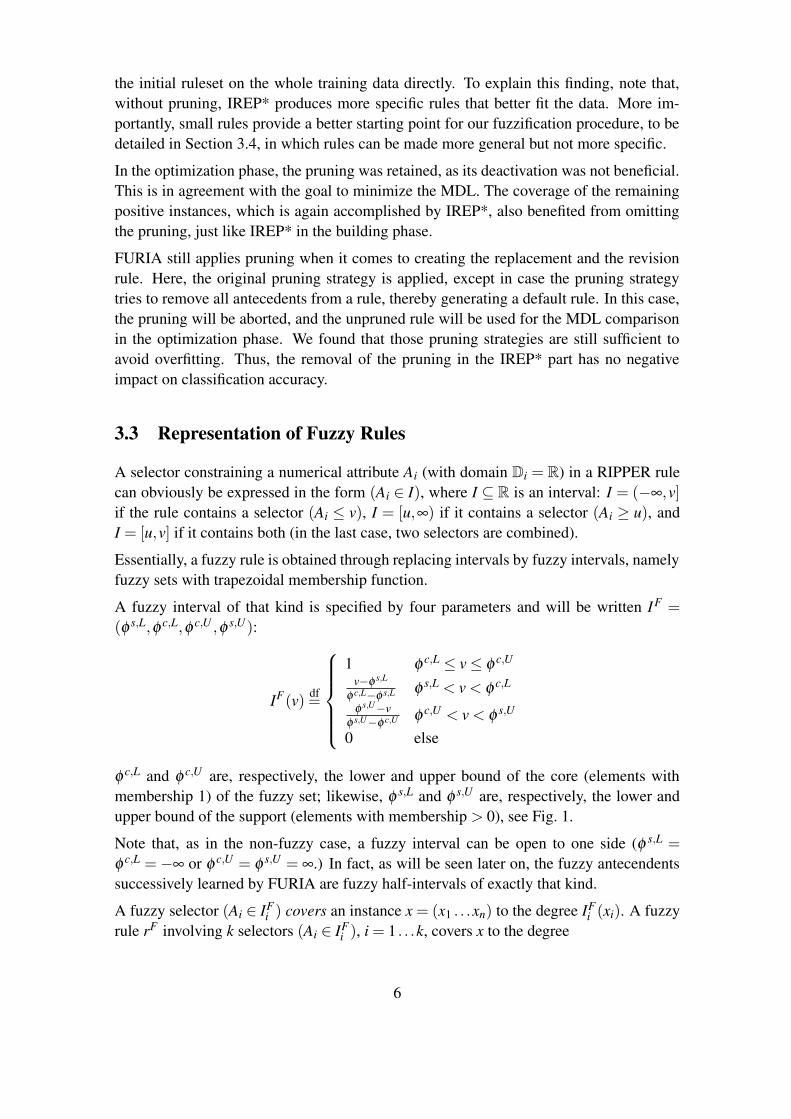
Essentially, a fuzzy rule is obtained through replacing intervals by fuzzy intervals, namelyfuzzy sets with trapezoidal membership function.

A fuzzy interval of that kind is specified by four parameters and will be written IF =

(φ s,L,φ c,L,φ c,U ,φ s,U):

IF(v) df=

1 φ c,L ≤ v≤ φ c,U

v−φ s,L

φ c,L−φ s,L φ s,L < v < φ c,L

φ s,U−vφ s,U−φ c,U φ c,U < v < φ s,U

0 else

φ c,L and φ c,U are, respectively, the lower and upper bound of the core (elements withmembership 1) of the fuzzy set; likewise, φ s,L and φ s,U are, respectively, the lower andupper bound of the support (elements with membership > 0), see Fig. 1.

Note that, as in the non-fuzzy case, a fuzzy interval can be open to one side (φ s,L =

φ c,L = −∞ or φ c,U = φ s,U = ∞.) In fact, as will be seen later on, the fuzzy antecendentssuccessively learned by FURIA are fuzzy half-intervals of exactly that kind.

A fuzzy selector (Ai ∈ IFi ) covers an instance x = (x1 . . .xn) to the degree IF

i (xi). A fuzzyrule rF involving k selectors (Ai ∈ IF

i ), i = 1 . . .k, covers x to the degree

6

φ s,L φ c,L φ c,U φ s,U

0

IF

1

Figure 1: A fuzzy interval IF .

µrF (x) = ∏i=1...k

IFi (xi) . (1)

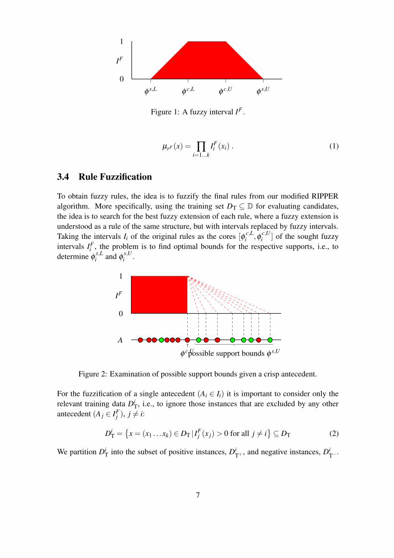
3.4 Rule Fuzzification

To obtain fuzzy rules, the idea is to fuzzify the final rules from our modified RIPPERalgorithm. More specifically, using the training set DT ⊆ D for evaluating candidates,the idea is to search for the best fuzzy extension of each rule, where a fuzzy extension isunderstood as a rule of the same structure, but with intervals replaced by fuzzy intervals.Taking the intervals Ii of the original rules as the cores [φ c,L

i ,φ c,Ui ] of the sought fuzzy

intervals IFi , the problem is to find optimal bounds for the respective supports, i.e., to

determine φ s,Li and φ s,U

i .

A

possible support bounds φ s,Uφ c,U

0

IF

1

Figure 2: Examination of possible support bounds given a crisp antecedent.

For the fuzzification of a single antecedent (Ai ∈ Ii) it is important to consider only therelevant training data Di

T, i.e., to ignore those instances that are excluded by any otherantecedent (A j ∈ IF

j ), j 6= i:

DiT =

{

x = (x1 . . .xk) ∈ DT | IFj (x j) > 0 for all j 6= i

}

⊆ DT (2)

We partition DiT into the subset of positive instances, Di

T+ , and negative instances, DiT− .

7

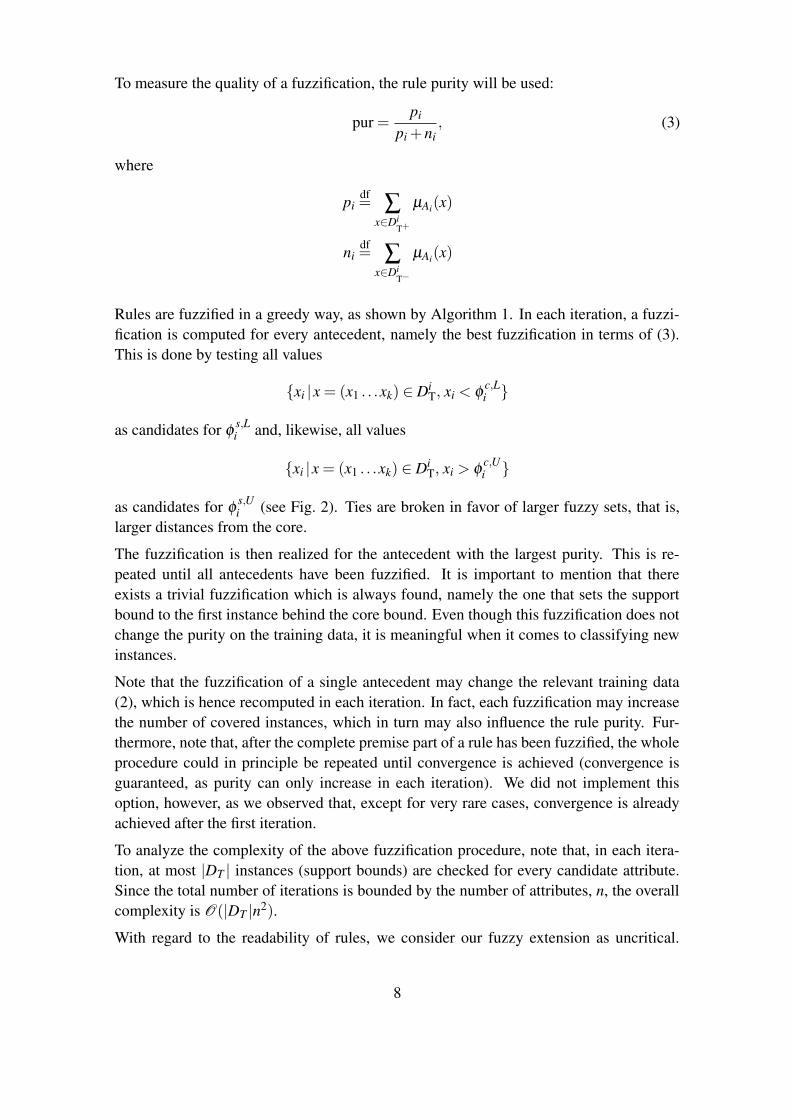
To measure the quality of a fuzzification, the rule purity will be used:

pur =pi

pi +ni, (3)

where

pidf= ∑

x∈DiT+

µAi(x)

nidf= ∑

x∈DiT−

µAi(x)

Rules are fuzzified in a greedy way, as shown by Algorithm 1. In each iteration, a fuzzi-fication is computed for every antecedent, namely the best fuzzification in terms of (3).This is done by testing all values

{xi |x = (x1 . . .xk) ∈ DiT, xi < φ c,L

i }

as candidates for φ s,Li and, likewise, all values

{xi |x = (x1 . . .xk) ∈ DiT, xi > φ c,U

i }

as candidates for φ s,Ui (see Fig. 2). Ties are broken in favor of larger fuzzy sets, that is,

larger distances from the core.

The fuzzification is then realized for the antecedent with the largest purity. This is re-peated until all antecedents have been fuzzified. It is important to mention that thereexists a trivial fuzzification which is always found, namely the one that sets the supportbound to the first instance behind the core bound. Even though this fuzzification does notchange the purity on the training data, it is meaningful when it comes to classifying newinstances.

Note that the fuzzification of a single antecedent may change the relevant training data(2), which is hence recomputed in each iteration. In fact, each fuzzification may increasethe number of covered instances, which in turn may also influence the rule purity. Fur-thermore, note that, after the complete premise part of a rule has been fuzzified, the wholeprocedure could in principle be repeated until convergence is achieved (convergence isguaranteed, as purity can only increase in each iteration). We did not implement thisoption, however, as we observed that, except for very rare cases, convergence is alreadyachieved after the first iteration.

To analyze the complexity of the above fuzzification procedure, note that, in each itera-tion, at most |DT | instances (support bounds) are checked for every candidate attribute.Since the total number of iterations is bounded by the number of attributes, n, the overallcomplexity is O(|DT |n2).

With regard to the readability of rules, we consider our fuzzy extension as uncritical.

8

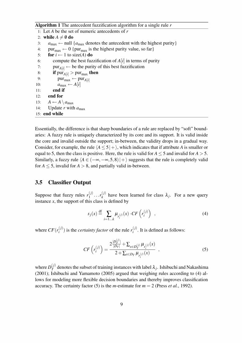
Algorithm 1 The antecedent fuzzification algorithm for a single rule r1: Let A be the set of numeric antecedents of r2: while A 6= /0 do3: amax← null {amax denotes the antecedent with the highest purity}4: purmax← 0 {purmax is the highest purity value, so far}5: for i← 1 to size(A) do6: compute the best fuzzification of A[i] in terms of purity7: purA[i]← be the purity of this best fuzzification8: if purA[i] > purmax then9: purmax← purA[i]

10: amax← A[i]11: end if12: end for13: A← A\amax14: Update r with amax15: end while

Essentially, the difference is that sharp boundaries of a rule are replaced by “soft” bound-aries: A fuzzy rule is uniquely characterized by its core and its support. It is valid insidethe core and invalid outside the support; in-between, the validity drops in a gradual way.Consider, for example, the rule 〈A≤ 5 |+〉, which indicates that if attribute A is smaller orequal to 5, then the class is positive. Here, the rule is valid for A≤ 5 and invalid for A > 5.Similarly, a fuzzy rule 〈A ∈ (−∞,−∞,5,8) |+〉 suggests that the rule is completely validfor A≤ 5, invalid for A > 8, and partially valid in-between.

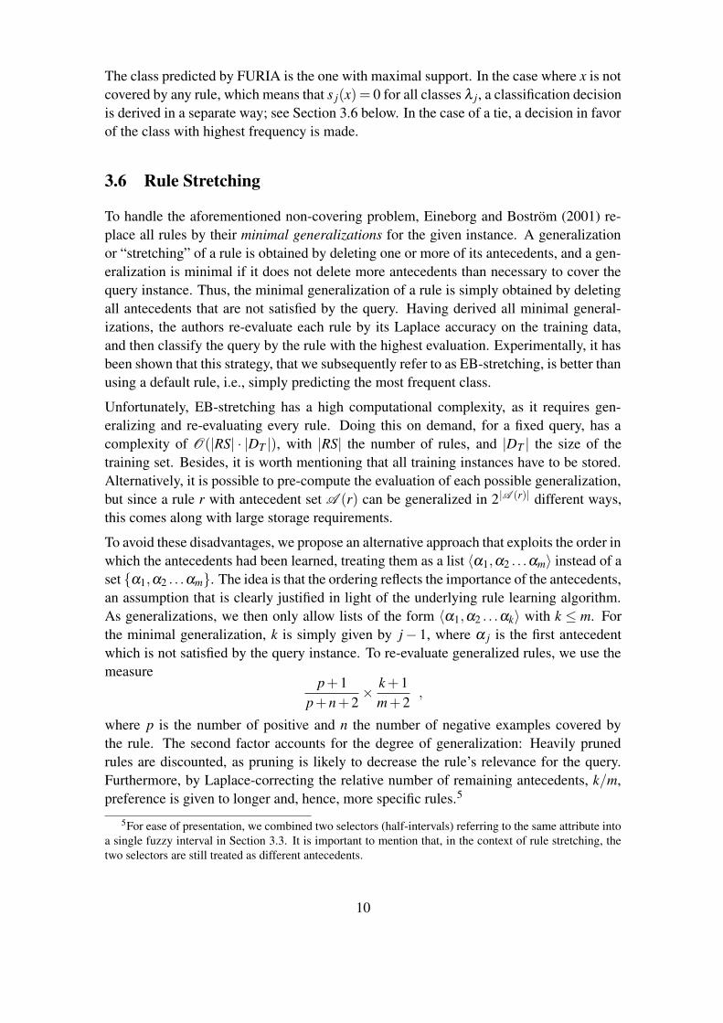
3.5 Classifier Output

Suppose that fuzzy rules r( j)1 . . .r( j)

k have been learned for class λ j. For a new queryinstance x, the support of this class is defined by

s j(x)df= ∑

i=1...kµ

r( j)i

(x) ·CF(

r( j)i

)

, (4)

where CF(r( j)i ) is the certainty factor of the rule r( j)

i . It is defined as follows:

CF(

r( j)i

)

=2 |D

( j)T ||DT | +∑x∈D( j)

Tµ

r( j)i

(x)

2+∑x∈DT µr( j)

i(x)

, (5)

where D( j)T denotes the subset of training instances with label λ j. Ishibuchi and Nakashima

(2001); Ishibuchi and Yamamoto (2005) argued that weighing rules according to (4) al-lows for modeling more flexible decision boundaries and thereby improves classificationaccuracy. The certainty factor (5) is the m-estimate for m = 2 (Press et al., 1992).

9

The class predicted by FURIA is the one with maximal support. In the case where x is notcovered by any rule, which means that s j(x) = 0 for all classes λ j, a classification decisionis derived in a separate way; see Section 3.6 below. In the case of a tie, a decision in favorof the class with highest frequency is made.

3.6 Rule Stretching

To handle the aforementioned non-covering problem, Eineborg and Boström (2001) re-place all rules by their minimal generalizations for the given instance. A generalizationor “stretching” of a rule is obtained by deleting one or more of its antecedents, and a gen-eralization is minimal if it does not delete more antecedents than necessary to cover thequery instance. Thus, the minimal generalization of a rule is simply obtained by deletingall antecedents that are not satisfied by the query. Having derived all minimal general-izations, the authors re-evaluate each rule by its Laplace accuracy on the training data,and then classify the query by the rule with the highest evaluation. Experimentally, it hasbeen shown that this strategy, that we subsequently refer to as EB-stretching, is better thanusing a default rule, i.e., simply predicting the most frequent class.

Unfortunately, EB-stretching has a high computational complexity, as it requires gen-eralizing and re-evaluating every rule. Doing this on demand, for a fixed query, has acomplexity of O(|RS| · |DT |), with |RS| the number of rules, and |DT | the size of thetraining set. Besides, it is worth mentioning that all training instances have to be stored.Alternatively, it is possible to pre-compute the evaluation of each possible generalization,but since a rule r with antecedent set A (r) can be generalized in 2|A (r)| different ways,this comes along with large storage requirements.

To avoid these disadvantages, we propose an alternative approach that exploits the order inwhich the antecedents had been learned, treating them as a list 〈α1,α2 . . .αm〉 instead of aset {α1,α2 . . .αm}. The idea is that the ordering reflects the importance of the antecedents,an assumption that is clearly justified in light of the underlying rule learning algorithm.As generalizations, we then only allow lists of the form 〈α1,α2 . . .αk〉 with k ≤ m. Forthe minimal generalization, k is simply given by j− 1, where α j is the first antecedentwhich is not satisfied by the query instance. To re-evaluate generalized rules, we use themeasure

p+1p+n+2

× k +1m+2

,

where p is the number of positive and n the number of negative examples covered bythe rule. The second factor accounts for the degree of generalization: Heavily prunedrules are discounted, as pruning is likely to decrease the rule’s relevance for the query.Furthermore, by Laplace-correcting the relative number of remaining antecedents, k/m,preference is given to longer and, hence, more specific rules.5

5For ease of presentation, we combined two selectors (half-intervals) referring to the same attribute intoa single fuzzy interval in Section 3.3. It is important to mention that, in the context of rule stretching, thetwo selectors are still treated as different antecedents.

10

Computationally, the above rule stretching strategy is much more efficient than EB-stretching.The complexity for re-evaluating a rule r is O(|A (r)|). Moreover, since the evaluationsof all generalizations of a rule can be calculated and stored directly in the course of therule learning process, in which antecedents are learned in a successive way, there is noneed for storing the training data.

4 Experimental Results

To analyze the performance of our FURIA approach, we conducted several experimentalstudies under the WEKA 3.5.5 framework (Witten and Frank, 2005). As a starting point,we used the RIPPER implementation of WEKA (“JRip”) for re-implementing FURIA.

4.1 Classification Accuracy

In a first study, we compared FURIA to other classifiers with respect to classificationaccuracy. The minimum number of covered instances per premise was set to 2, and forthe number of folds and the number of optimizations in FURIA and RIPPER we used,respectively, values 3 and 2 (which is the default setting in WEKA and leads to RIPPER2).

Additionally, we also included the C4.5 decision tree learner (Quinlan, 1993) as a well-known benchmark classifier and, moreover, added two fuzzy rule-based classifiers fromthe KEEL suite (Alcalá-Fernandez et al., 2008): The CHI algorithm is based on Chi et al.(1995, 1996) and uses rule weighing as proposed by Ishibuchi and Yamamoto (2005).6

The SLAVE algorithm makes use of genetic algorithms to learn a fuzzy classifier (Gon-zalez and Perez, 1999, 2001).7 Both algorithms are frequently used for experimentalpurposes (e.g., (Fernández et al., 2007; Ishibuchi and Yamamoto, 2003; Cordon et al.,2004; Zolghadri and Mansoori, 2007)).

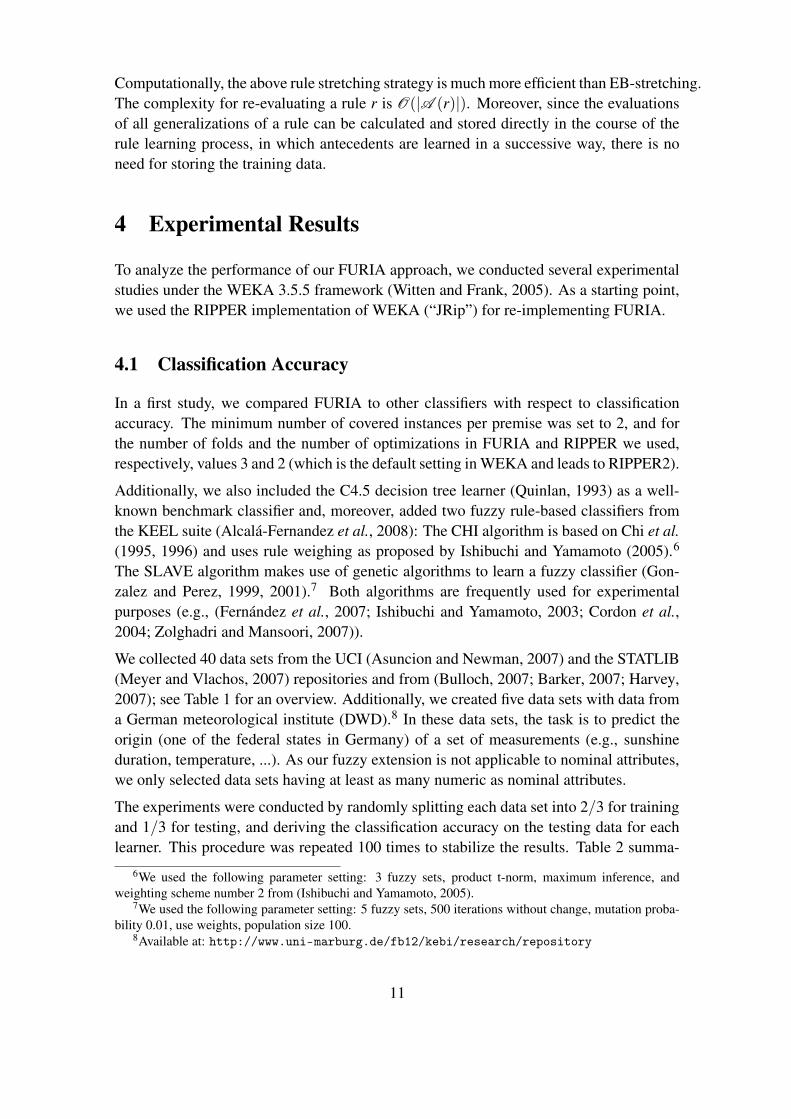
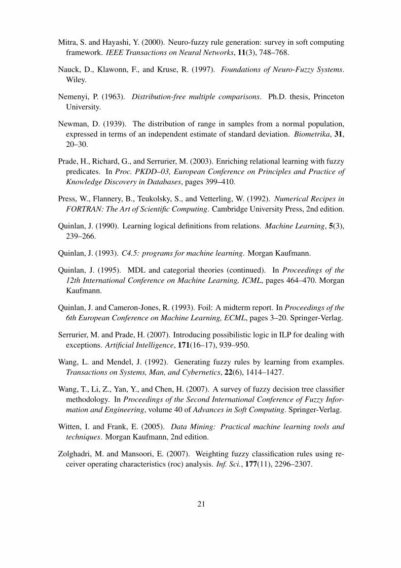
We collected 40 data sets from the UCI (Asuncion and Newman, 2007) and the STATLIB(Meyer and Vlachos, 2007) repositories and from (Bulloch, 2007; Barker, 2007; Harvey,2007); see Table 1 for an overview. Additionally, we created five data sets with data froma German meteorological institute (DWD).8 In these data sets, the task is to predict theorigin (one of the federal states in Germany) of a set of measurements (e.g., sunshineduration, temperature, ...). As our fuzzy extension is not applicable to nominal attributes,we only selected data sets having at least as many numeric as nominal attributes.

The experiments were conducted by randomly splitting each data set into 2/3 for trainingand 1/3 for testing, and deriving the classification accuracy on the testing data for eachlearner. This procedure was repeated 100 times to stabilize the results. Table 2 summa-

6We used the following parameter setting: 3 fuzzy sets, product t-norm, maximum inference, andweighting scheme number 2 from (Ishibuchi and Yamamoto, 2005).

7We used the following parameter setting: 5 fuzzy sets, 500 iterations without change, mutation proba-bility 0.01, use weights, population size 100.

8Available at: http://www.uni-marburg.de/fb12/kebi/research/repository

11

rizes the classification accuracies.9 The overall picture conveyed by the results is clearlyin favor of FURIA, which outperforms the other methods on most data sets. To analyzethe differences between the classifiers more closely, we followed the two-step procedurerecommended by Demšar (2006): First, a Friedman Test is conducted to test the null hy-pothesis of equal classifier performance (Friedman, 1937, 1940). In case this hypothesis isrejected, which means that the classifiers’ performance differs in a statistically significantway, a posthoc test is conducted to analyze these differences in more detail.

The Friedman test is a non-parametric test which is based on the relative performanceof classifiers in terms of their ranks: For each data set, the methods to be compared aresorted according to their performance, i.e., each method is assigned a rank (in case of ties,average ranks are assigned); see Table 3. Let k be the number of classifiers and N thenumber of data sets. Let r j

i be the rank of classifier j on data set i, and R j = 1N ∑N

i=1 r ji the

average rank of classifier j. Under the null-hypothesis, the Friedman statistic

χ2F =

12Nk(k +1)

[

k

∑j=1

(R j)2− k · (k +1)2

4

]

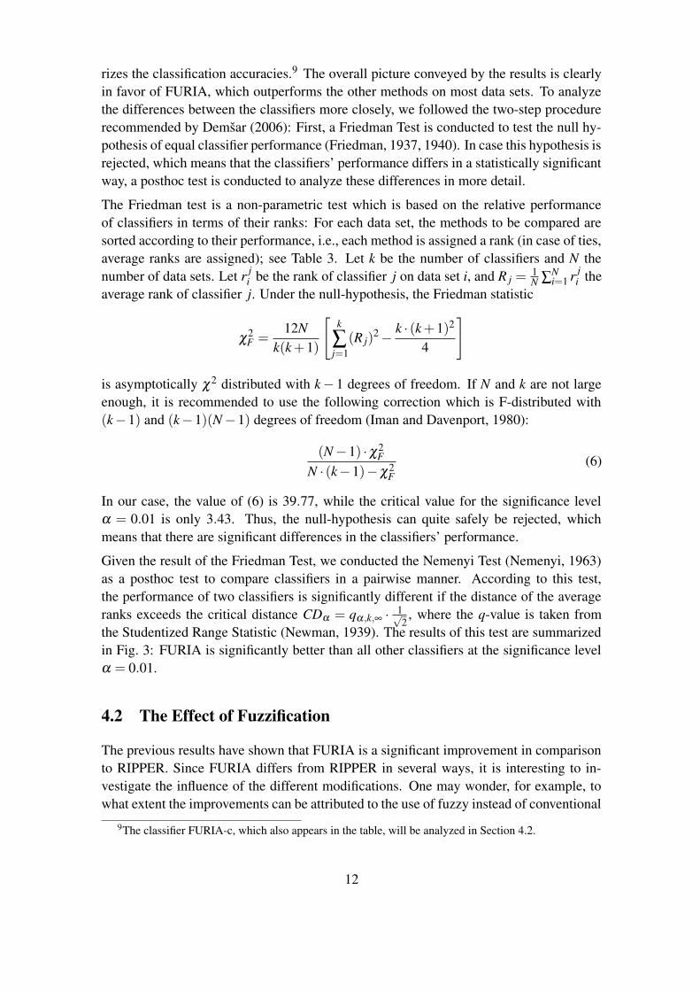
is asymptotically χ2 distributed with k− 1 degrees of freedom. If N and k are not largeenough, it is recommended to use the following correction which is F-distributed with(k−1) and (k−1)(N−1) degrees of freedom (Iman and Davenport, 1980):

(N−1) ·χ2F

N · (k−1)−χ2F

(6)

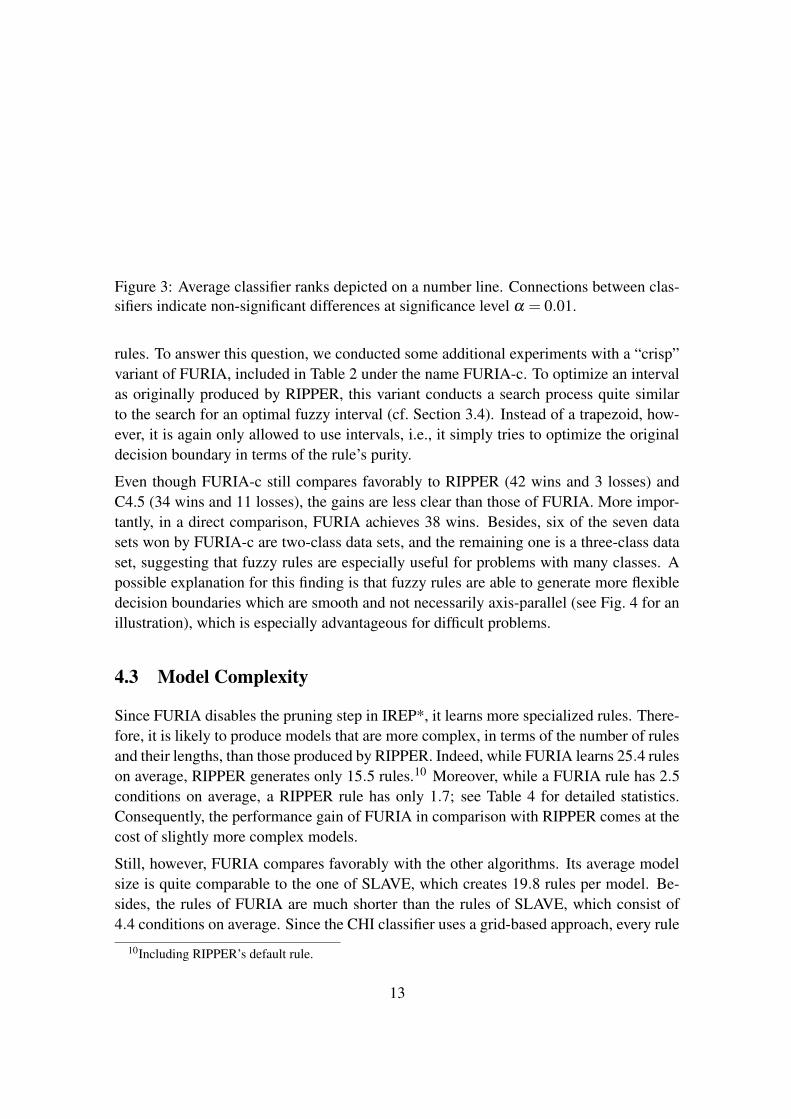
In our case, the value of (6) is 39.77, while the critical value for the significance levelα = 0.01 is only 3.43. Thus, the null-hypothesis can quite safely be rejected, whichmeans that there are significant differences in the classifiers’ performance.

Given the result of the Friedman Test, we conducted the Nemenyi Test (Nemenyi, 1963)as a posthoc test to compare classifiers in a pairwise manner. According to this test,the performance of two classifiers is significantly different if the distance of the averageranks exceeds the critical distance CDα = qα,k,∞ · 1√

2, where the q-value is taken from

the Studentized Range Statistic (Newman, 1939). The results of this test are summarizedin Fig. 3: FURIA is significantly better than all other classifiers at the significance levelα = 0.01.

4.2 The Effect of Fuzzification

The previous results have shown that FURIA is a significant improvement in comparisonto RIPPER. Since FURIA differs from RIPPER in several ways, it is interesting to in-vestigate the influence of the different modifications. One may wonder, for example, towhat extent the improvements can be attributed to the use of fuzzy instead of conventional

9The classifier FURIA-c, which also appears in the table, will be analyzed in Section 4.2.

12

3 4 51 2

FURIA CH I

SLAVEC4.5

RIPPER

CD α = 0.01

Figure 3: Average classifier ranks depicted on a number line. Connections between clas-sifiers indicate non-significant differences at significance level α = 0.01.

rules. To answer this question, we conducted some additional experiments with a “crisp”variant of FURIA, included in Table 2 under the name FURIA-c. To optimize an intervalas originally produced by RIPPER, this variant conducts a search process quite similarto the search for an optimal fuzzy interval (cf. Section 3.4). Instead of a trapezoid, how-ever, it is again only allowed to use intervals, i.e., it simply tries to optimize the originaldecision boundary in terms of the rule’s purity.

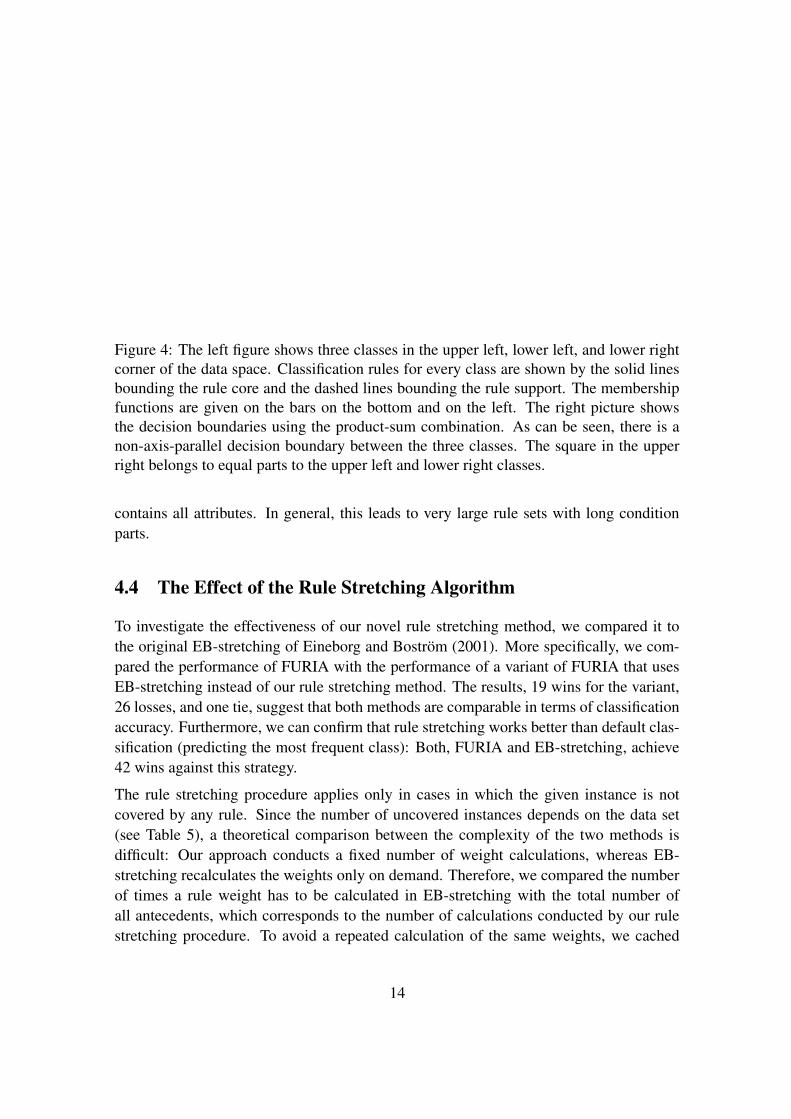
Even though FURIA-c still compares favorably to RIPPER (42 wins and 3 losses) andC4.5 (34 wins and 11 losses), the gains are less clear than those of FURIA. More impor-tantly, in a direct comparison, FURIA achieves 38 wins. Besides, six of the seven datasets won by FURIA-c are two-class data sets, and the remaining one is a three-class dataset, suggesting that fuzzy rules are especially useful for problems with many classes. Apossible explanation for this finding is that fuzzy rules are able to generate more flexibledecision boundaries which are smooth and not necessarily axis-parallel (see Fig. 4 for anillustration), which is especially advantageous for difficult problems.

4.3 Model Complexity

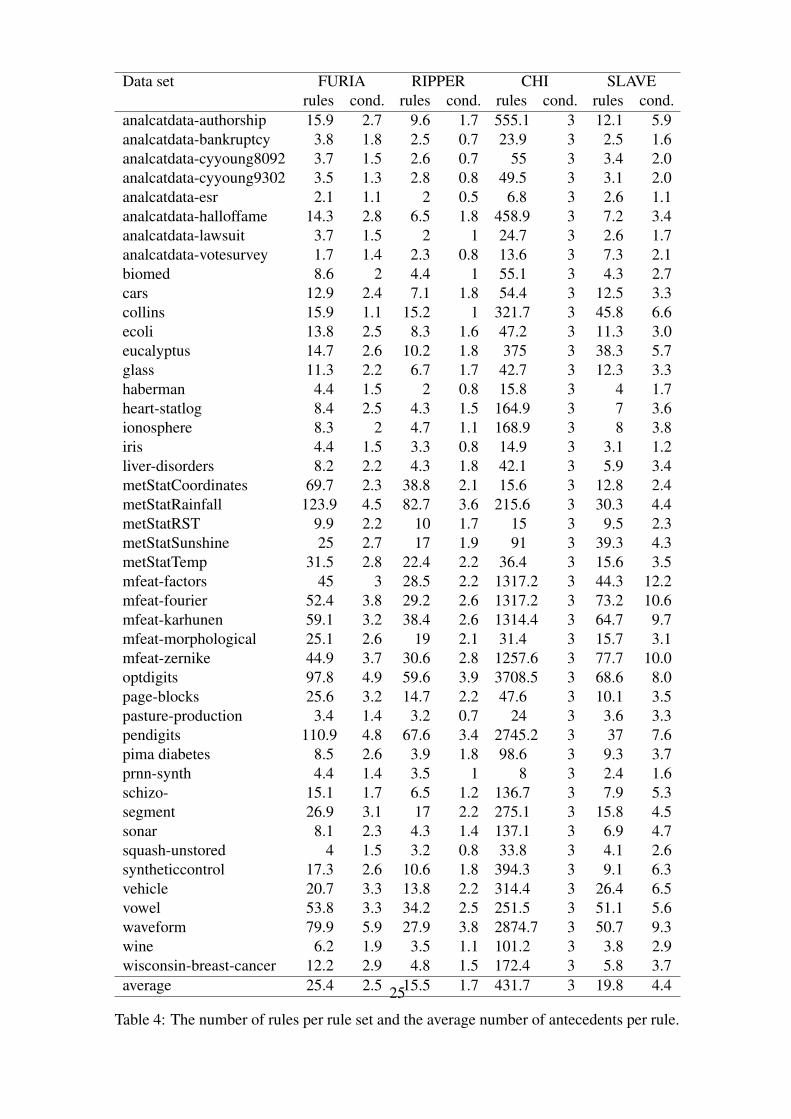
Since FURIA disables the pruning step in IREP*, it learns more specialized rules. There-fore, it is likely to produce models that are more complex, in terms of the number of rulesand their lengths, than those produced by RIPPER. Indeed, while FURIA learns 25.4 ruleson average, RIPPER generates only 15.5 rules.10 Moreover, while a FURIA rule has 2.5conditions on average, a RIPPER rule has only 1.7; see Table 4 for detailed statistics.Consequently, the performance gain of FURIA in comparison with RIPPER comes at thecost of slightly more complex models.

Still, however, FURIA compares favorably with the other algorithms. Its average modelsize is quite comparable to the one of SLAVE, which creates 19.8 rules per model. Be-sides, the rules of FURIA are much shorter than the rules of SLAVE, which consist of4.4 conditions on average. Since the CHI classifier uses a grid-based approach, every rule

10Including RIPPER’s default rule.

13

μ μ

Figure 4: The left figure shows three classes in the upper left, lower left, and lower rightcorner of the data space. Classification rules for every class are shown by the solid linesbounding the rule core and the dashed lines bounding the rule support. The membershipfunctions are given on the bars on the bottom and on the left. The right picture showsthe decision boundaries using the product-sum combination. As can be seen, there is anon-axis-parallel decision boundary between the three classes. The square in the upperright belongs to equal parts to the upper left and lower right classes.

contains all attributes. In general, this leads to very large rule sets with long conditionparts.

4.4 The Effect of the Rule Stretching Algorithm

To investigate the effectiveness of our novel rule stretching method, we compared it tothe original EB-stretching of Eineborg and Boström (2001). More specifically, we com-pared the performance of FURIA with the performance of a variant of FURIA that usesEB-stretching instead of our rule stretching method. The results, 19 wins for the variant,26 losses, and one tie, suggest that both methods are comparable in terms of classificationaccuracy. Furthermore, we can confirm that rule stretching works better than default clas-sification (predicting the most frequent class): Both, FURIA and EB-stretching, achieve42 wins against this strategy.

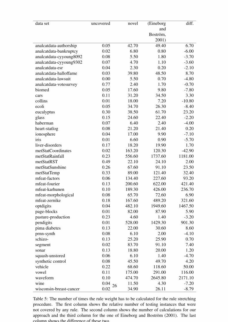
The rule stretching procedure applies only in cases in which the given instance is notcovered by any rule. Since the number of uncovered instances depends on the data set(see Table 5), a theoretical comparison between the complexity of the two methods isdifficult: Our approach conducts a fixed number of weight calculations, whereas EB-stretching recalculates the weights only on demand. Therefore, we compared the numberof times a rule weight has to be calculated in EB-stretching with the total number ofall antecedents, which corresponds to the number of calculations conducted by our rulestretching procedure. To avoid a repeated calculation of the same weights, we cached

14

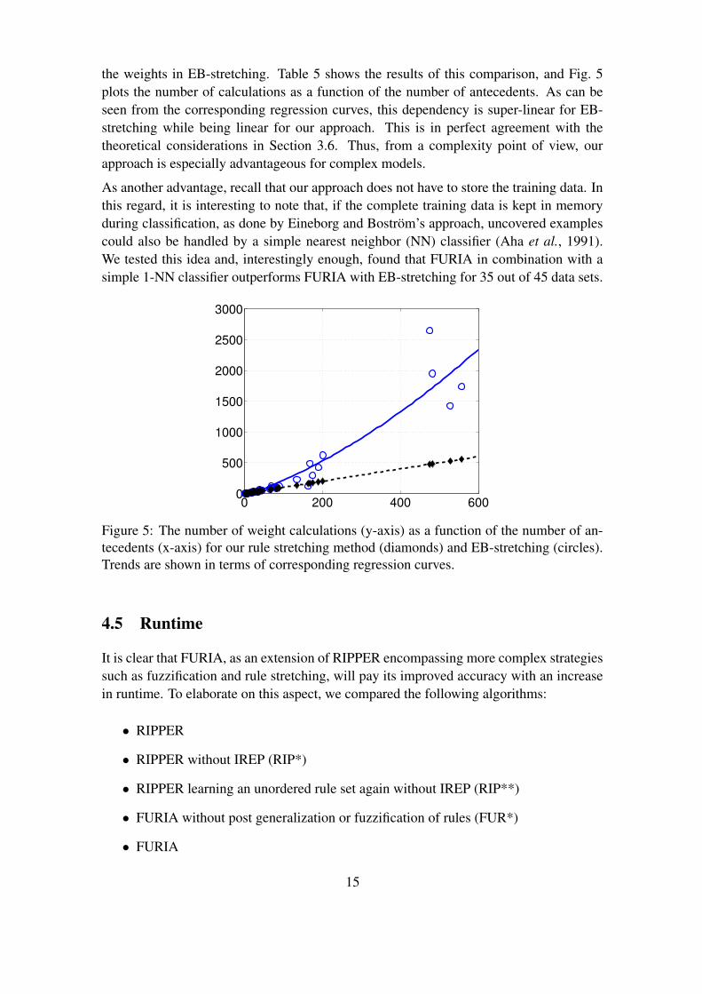
the weights in EB-stretching. Table 5 shows the results of this comparison, and Fig. 5plots the number of calculations as a function of the number of antecedents. As can beseen from the corresponding regression curves, this dependency is super-linear for EB-stretching while being linear for our approach. This is in perfect agreement with thetheoretical considerations in Section 3.6. Thus, from a complexity point of view, ourapproach is especially advantageous for complex models.

As another advantage, recall that our approach does not have to store the training data. Inthis regard, it is interesting to note that, if the complete training data is kept in memoryduring classification, as done by Eineborg and Boström’s approach, uncovered examplescould also be handled by a simple nearest neighbor (NN) classifier (Aha et al., 1991).We tested this idea and, interestingly enough, found that FURIA in combination with asimple 1-NN classifier outperforms FURIA with EB-stretching for 35 out of 45 data sets.

0 200 400 6000

500

1000

1500

2000

2500

3000

Figure 5: The number of weight calculations (y-axis) as a function of the number of an-tecedents (x-axis) for our rule stretching method (diamonds) and EB-stretching (circles).Trends are shown in terms of corresponding regression curves.

4.5 Runtime

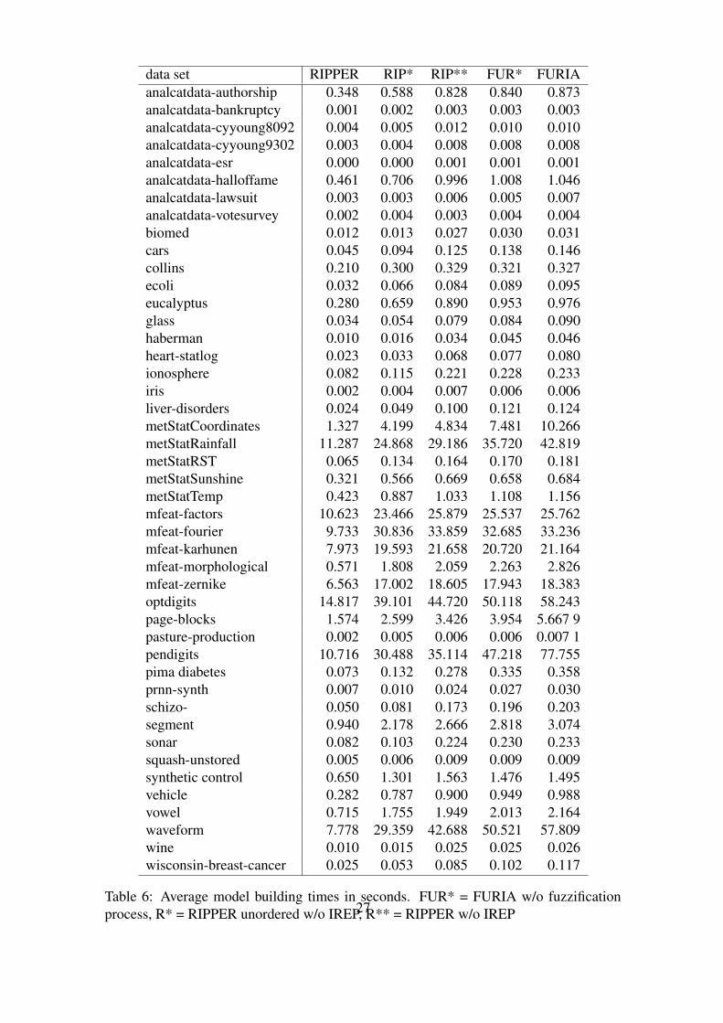
It is clear that FURIA, as an extension of RIPPER encompassing more complex strategiessuch as fuzzification and rule stretching, will pay its improved accuracy with an increasein runtime. To elaborate on this aspect, we compared the following algorithms:

• RIPPER

• RIPPER without IREP (RIP*)

• RIPPER learning an unordered rule set again without IREP (RIP**)

• FURIA without post generalization or fuzzification of rules (FUR*)

• FURIA

15

Table 6 shows the runtime results in seconds (all measurements were performed on a In-tel Core2Duo 2.4Ghz). As expected, RIPPER is the most efficient variant. Disabling theIREP procedure (RIP*) does indeed slow down the algorithm (keep in mind that, since thepruning set is now empty, growing data is larger at the beginning). A further increase inruntime is caused by changing from an ordered rule list to the unordered rule set (RIP**).This is also expected since the unordered version learns rules in a one-vs-all fashion,while for the ordered variant, the training data becomes successively smaller (training in-stances from already covered classes are dropped). There is not much difference betweenthe unordered RIPPER without IREP (RIP**) to FURIA without fuzzification or crispgeneralization after rule learning (FUR*). The difference between RIP** and FUR* canbe explained by the rule stretching procedure that needs additional time to determine theweights during classification.

The quintessence of this study is that, compared to RIPPER, the extensions and modifi-cations of FURIA (disabling of the IREP procedure, the change from an ordered rule listto an unordered list, the calculation of the rule stretching weights, and the fuzzificationprocedure) cause an increase of runtime by a factor between 1.5 and 7.7 (average 3.4).

5 Related Work

Since the literature on (fuzzy) rule learning abounds, a comprehensive survey of this fieldis clearly beyond the scope of this paper. Nevertheless, this section is meant to convey arough picture of the field and to briefly mention some related work.

The field of fuzzy rule learning can be roughly separated into several subfields. Firstly,there are fuzzy extensions of conventional rule learning techniques, not only for the propo-sitional case but also for the case of first-order logic (Drobics et al., 2003; Prade et al.,2003; Serrurier and Prade, 2007). Quite popular in the fuzzy field are grid-based ap-proaches as popularized by Wang and Mendel (1992), which proceed from fixed fuzzypartitions of the individual dimensions. They are not very flexible and suffer from the“curse of dimensionality” in the case of many input variables but may have advantageswith respect to interpretability (Guillaume, 2001). A well-known representative of thiskind of approach is the CHI algorithm that we also used in our experiments (Chi et al.,1995, 1996). It proceeds from a fuzzy partition for each attribute and learns a rule forevery grid cell. This is done by searching the training instance with maximal degree ofmembership in this cell (matching degree of the rule premise) and adopting the corre-sponding class attribute as the rule consequent. Another approach of this subfield, whichprevails the literature on conventional rule learning but has received less attention in thefuzzy field so far, is rule covering algorithms (Cloete and Van Zyl, 2006). In this category,the FR3 rule learner that has recently been proposed by Hühn and Hüllermeier (2009) de-serves special mentioning. Just like FURIA, FR3 draws on the RIPPER algorithm andmodifies it in a quite similar way. However, FR3 has a completely different focus andembeds the modified RIPPER algorithm in a round robin learning scheme, i.e., it learnsan ensemble of binary classification models, one for each pair of classes. As opposed to

16

this, FURIA learns a single multi-class model.

Secondly, several fuzzy variants of decision tree learning, following a divide-and-conquerstrategy and producing rule sets of a special (hierarchical) structure, have been proposed(Wang et al., 2007). As this direction is only indirectly related to our work, we do not gointo further details.

Thirdly, hybrid methods that combine fuzzy set theory with other (soft computing) method-ologies, notably evolutionary algorithms and neural networks, are especially important inthe field of fuzzy rule learning. For example, evolutionary algorithms are often used tooptimize (“tune”) a fuzzy rule base or for searching the space of potential rule bases ina (more or less) systematic way (Cordon et al., 2004). One of these classifiers, whichwas also included in our experimental comparison, is the SLAVE classifier (Gonzalezand Perez, 1999, 2001). It uses a genetic learning approach to create a fuzzy rule-basedsystem by following a covering scheme. SLAVE represents each rule as a single chromo-some. It uses an iterative approach, which means that the result of the genetic algorithm isnot meant to cover all positive examples. Instead, the genetic algorithm is repeated untilthe iteratively generated set of rules is sufficient to represent the training set. Anotherinteresting approach in this area is the one proposed by del Jesus et al. (2004), whichapplies the idea of boosting (Kearns, 1988) to the evolutionary learning of rule-basedclassifiers. Neuro-fuzzy methods (Mitra and Hayashi, 2000; Nauck et al., 1997) encode afuzzy system as a neural network and apply corresponding learning methods (like back-propagation). Fuzzy rules are then extracted from a trained network.

Finally, with regard to the idea of rule stretching that we proposed in this paper, it isworth mentioning that some other approaches have been proposed in the literature that areclosely related, in particular the idea to combine instance-based and rule learning. Thisidea has been realized in the RISE system (Domingos, 1995), in which single instancesare considered as maximally specific rules. The learning procedure essentially tries toaggregate specific rules into more general ones. At classification time, an instance isclassified by the nearest rule. Another combination of instance-based and rule learning isproposed by Hendrickx and van den Bosch (2005), who make use of the rule set to createnew features, indicating whether or not a rule is activated for an instance. A classificationis made by searching the query’s nearest neighbor in the novel feature space and assigningits class.

6 Concluding Remarks

In this paper, we introduced a fuzzy rule-based classifier called FURIA, which is an ad-vancement of the famous RIPPER algorithm. FURIA differs from RIPPER in severalrespects, notably in the use of fuzzy instead of conventional rules. This way, it becomespossible to model decision boundaries in a more flexible way. Besides, FURIA makesuse of a novel rule stretching technique which is computationally less complex than ahitherto existing alternative and improves performance in comparison to the use of a de-

17

fault rule. Combined with the sophisticated rule induction techniques employed by theoriginal RIPPER algorithm, these improvements have produced a rule learner with a su-perb classification performance, which comes at the price of an acceptable increase inruntime. In fact, extensive experiments on a large number of benchmark data sets haveshown that FURIA significantly outperforms the original RIPPER, as well as other fuzzyrule learning methods included for comparison purpose.

A Java implementation of FURIA, running under the open-source machine learning toolkitWEKA, can be downloaded at http://www.uni-marburg.de/fb12/kebi/research/.

Acknowledgements: This research was supported by the German Research Foundation(DFG). The CHI and SLAVE classifiers were made available to us by the developersof the KEEL software (Alberto Fernández). We gratefully acknowledge this support.We also thank Johannes Fürnkranz for insightful discussions about rule fuzzification andgeneralization.

ReferencesAha, D., Kibler, D., and Albert, M. (1991). Instance-based learning algorithms. Machine

Learning, 6(1), 37–66.

Alcalá-Fernandez, J., Sánchez, L., García, S., del Jesus, M., Ventura, S., Garrell, J., Otero,J., Romero, C., Bacardit, J., Rivas, V., Fernández, J., and Herrera, F. (2008). KEEL:A Software Tool to Assess Evolutionary Algorithms to Data Mining Problems. SoftComputing (in press).

Asuncion, A. and Newman, D. (2007). UCI machine learning repository. http:

//archive.ics.uci.edu/ml/index.html.

Barker, D. (2007). Dataset: Pasture production. http://weka.sourceforge.net/

wiki/index.php/Datasets. Obtained on 20th of October 2007.

Boström, H. (2004). Pruning and exclusion criteria for unordered incremental reducederror pruning. Proceedings of the Workshop on Advances in Rule Learning, ECML,pages 17–29.

Bulloch, B. (2007). Dataset: Eucalyptus soil conservation. http://weka.

sourceforge.net/wiki/index.php/Datasets. Obtained on 20th of October 2007.

Chi, Z., Wu, J., and Yan, H. (1995). Handwritten numeral recognition using self-organizing maps and fuzzy rules. Pattern Recognition, 28(1), 59–66.

Chi, Z., Yan, H., and Pham, T. (1996). Fuzzy Algorithms: With Applications to ImageProcessing and Pattern Recognition. World Scientific Publishing Co., Inc.

Cloete, I. and Van Zyl, J. (2006). Fuzzy rule induction in a set covering framework. IEEETransactions Fuzzy Systems, 14(1), 93–110.

18

Cohen, W. (1995). Fast effective rule induction. In A. Prieditis and S. Russell, editors,Proceedings of the 12th International Conference on Machine Learning, ICML, pages115–123. Morgan Kaufmann.

Cordon, O., Gomide, F., Herrera, F., Hoffmann, F., and Magdalena, L. (2004). Ten yearsof genetic fuzzy systems: current framework and new trends. Fuzzy Sets and Systems,141(1), 5–31.

del Jesus, M., Hoffmann, F., Navascues, L., and Sánchez, L. (2004). Induction of fuzzy-rule-based classifiers with evolutionary boosting algorithms. IEEE Transactions onFuzzy Systems, 12(3), 296–308.

Demšar, J. (2006). Statistical comparisons of classifiers over multiple data sets. Journalof Machine Learning Research, 7, 1–30.

Domingos, P. (1995). Rule induction and instance-based learning: A unified approach. InProceedings of the Fourteenth International Joint Conference on Artificial Intelligence,IJCAI, pages 1226–1232. Morgan Kaufmann.

Drobics, M., Bodenhofer, U., and Klement, E. (2003). FS-FOIL: an inductive learningmethod for extracting interpretable fuzzy descriptions. International Journal of Ap-proximative Reasoning, 32(2–3), 131–152.

Eineborg, M. and Boström, H. (2001). Classifying uncovered examples by rule stretch-ing. In ILP ’01: Proceedings of the 11th International Conference on Inductive LogicProgramming, pages 41–50. Springer-Verlag.

Fawcett, T. (2008). Prie: a system for generating rulelists to maximize roc performance.Data Mining and Knowledge Discovery, 17(2), 207–224.

Fernández, A., García, S., Herrera, F., and del Jesus, M. (2007). An analysis of the ruleweights and fuzzy reasoning methods for linguistic rule based classification systemsapplied to problems with highly imbalanced data sets. In Applications of Fuzzy SetsTheory, volume 4578 of Lecture Notes in Computer Science, pages 170–178. Springer.

Friedman, M. (1937). The use of ranks to avoid the assumption of normality implicitin the analysis of variance. Journal of the American Statistical Association, 32(200),675–701.

Friedman, M. (1940). A comparison of alternative tests of significance for the problem ofm rankings. The Annals of Mathematical Statistics, 11(1), 86–92.

Fürnkranz, J. (1999). Separate-and-conquer rule learning. Artificial Intelligence Review,13(1), 3–54.

Fürnkranz, J. and Widmer, G. (1994). Incremental reduced error pruning. In Proceedingsof the 11th International Conference on Machine Learning, ICML, pages 70–77.

19

Gonzalez, A. and Perez, R. (1999). Slave: a genetic learning system based on an iterativeapproach. IEEE Transactions on Fuzzy Systems, 7(2), 176–191.

Gonzalez, A. and Perez, R. (2001). Selection of relevant features in a fuzzy geneticlearning algorithm. IEEE Transactions on Systems, Man, and Cybernetics, Part B,31(3), 417–425.

Guillaume, S. (2001). Defining fuzzy inference systems from data: An interpretability-oriented review. IEEE Transactions on Fuzzy Systems, 9(3), 426–443.

Harvey, W. (2007). Dataset: Squash harvest stored / unstored. http://weka.

sourceforge.net/wiki/index.php/Datasets. Obtained on 20th of October 2007.

Hendrickx, I. and van den Bosch, A. (2005). Hybrid algorithms for instance-based classi-fication. In J. Gama, R. Camacho, P. Brazdil, A. Jorge, and L. Torgo, editors, Proceed-ings of the Sixteenth European Conference on Machine Learning, ECML, pages 158 –169. Springer.

Hühn, J. and Hüllermeier, E. (2009). FR3: A fuzzy rule learner for inducing reliableclassifiers. IEEE Transactions Fuzzy Systems, 17(1), 138–149.

Hüllermeier, E. (2005). Fuzzy sets in machine learning and data mining: Status andprospects. Fuzzy Sets and Systems, 156(3), 387–406.

Iman, R. and Davenport, J. (1980). Approximations of the critical region of the friedmanstatistic. Communications in Statistics, 9(6), 571–595.

Ishibuchi, H. and Nakashima, T. (2001). Effect of rule weights in fuzzy rule-based clas-sification systems. IEEE Transactions on Fuzzy Systems, 9(4), 506–515.

Ishibuchi, H. and Yamamoto, T. (2003). Performance evaluation of three-objective geneticrule selection. In The 12th IEEE International Conference on Fuzzy Systems, volume 1,pages 149–154.

Ishibuchi, H. and Yamamoto, T. (2005). Rule weight specification in fuzzy rule-basedclassification systems. IEEE Transactions on Fuzzy Systems, 13(4), 428–436.

Juang, C., Chiu, S., and Chang, S. (2007). A self-organizing ts-type fuzzy network withsupport vector learning and its application to classification problems. IEEE Transac-tions on Fuzzy Systems, 15(5), 998–1008.

Kamal, M. and Pazzani, M. (1993). Hydra: A noise-tolerant relational concept learningalgorithm. In Proceedings of the Thirteenth International Joint Conference on ArtificialIntelligence, IJCAI, pages 1064–1071. Morgan Kaufmann.

Kearns, M. (1988). Thoughts on hypothesis boosting. ML class project.

Meyer, M. and Vlachos, P. (2007). Statlib. http://lib.stat.cmu.edu/.

20

Mitra, S. and Hayashi, Y. (2000). Neuro-fuzzy rule generation: survey in soft computingframework. IEEE Transactions on Neural Networks, 11(3), 748–768.

Nauck, D., Klawonn, F., and Kruse, R. (1997). Foundations of Neuro-Fuzzy Systems.Wiley.

Nemenyi, P. (1963). Distribution-free multiple comparisons. Ph.D. thesis, PrincetonUniversity.

Newman, D. (1939). The distribution of range in samples from a normal population,expressed in terms of an independent estimate of standard deviation. Biometrika, 31,20–30.

Prade, H., Richard, G., and Serrurier, M. (2003). Enriching relational learning with fuzzypredicates. In Proc. PKDD–03, European Conference on Principles and Practice ofKnowledge Discovery in Databases, pages 399–410.

Press, W., Flannery, B., Teukolsky, S., and Vetterling, W. (1992). Numerical Recipes inFORTRAN: The Art of Scientific Computing. Cambridge University Press, 2nd edition.

Quinlan, J. (1990). Learning logical definitions from relations. Machine Learning, 5(3),239–266.

Quinlan, J. (1993). C4.5: programs for machine learning. Morgan Kaufmann.

Quinlan, J. (1995). MDL and categorial theories (continued). In Proceedings of the12th International Conference on Machine Learning, ICML, pages 464–470. MorganKaufmann.

Quinlan, J. and Cameron-Jones, R. (1993). Foil: A midterm report. In Proceedings of the6th European Conference on Machine Learning, ECML, pages 3–20. Springer-Verlag.

Serrurier, M. and Prade, H. (2007). Introducing possibilistic logic in ILP for dealing withexceptions. Artificial Intelligence, 171(16–17), 939–950.

Wang, L. and Mendel, J. (1992). Generating fuzzy rules by learning from examples.Transactions on Systems, Man, and Cybernetics, 22(6), 1414–1427.

Wang, T., Li, Z., Yan, Y., and Chen, H. (2007). A survey of fuzzy decision tree classifiermethodology. In Proceedings of the Second International Conference of Fuzzy Infor-mation and Engineering, volume 40 of Advances in Soft Computing. Springer-Verlag.

Witten, I. and Frank, E. (2005). Data Mining: Practical machine learning tools andtechniques. Morgan Kaufmann, 2nd edition.

Zolghadri, M. and Mansoori, E. (2007). Weighting fuzzy classification rules using re-ceiver operating characteristics (roc) analysis. Inf. Sci., 177(11), 2296–2307.

21

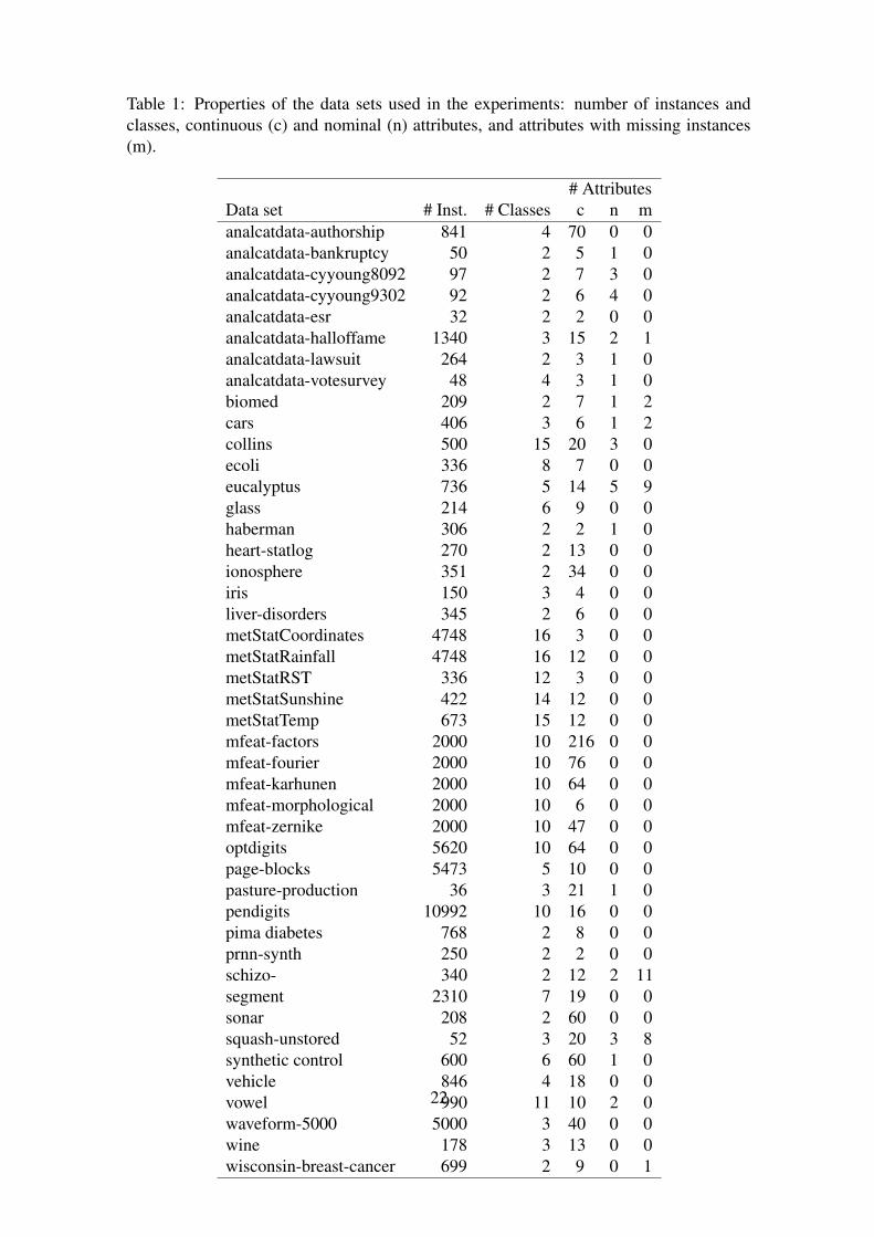
Table 1: Properties of the data sets used in the experiments: number of instances andclasses, continuous (c) and nominal (n) attributes, and attributes with missing instances(m).

# AttributesData set # Inst. # Classes c n manalcatdata-authorship 841 4 70 0 0analcatdata-bankruptcy 50 2 5 1 0analcatdata-cyyoung8092 97 2 7 3 0analcatdata-cyyoung9302 92 2 6 4 0analcatdata-esr 32 2 2 0 0analcatdata-halloffame 1340 3 15 2 1analcatdata-lawsuit 264 2 3 1 0analcatdata-votesurvey 48 4 3 1 0biomed 209 2 7 1 2cars 406 3 6 1 2collins 500 15 20 3 0ecoli 336 8 7 0 0eucalyptus 736 5 14 5 9glass 214 6 9 0 0haberman 306 2 2 1 0heart-statlog 270 2 13 0 0ionosphere 351 2 34 0 0iris 150 3 4 0 0liver-disorders 345 2 6 0 0metStatCoordinates 4748 16 3 0 0metStatRainfall 4748 16 12 0 0metStatRST 336 12 3 0 0metStatSunshine 422 14 12 0 0metStatTemp 673 15 12 0 0mfeat-factors 2000 10 216 0 0mfeat-fourier 2000 10 76 0 0mfeat-karhunen 2000 10 64 0 0mfeat-morphological 2000 10 6 0 0mfeat-zernike 2000 10 47 0 0optdigits 5620 10 64 0 0page-blocks 5473 5 10 0 0pasture-production 36 3 21 1 0pendigits 10992 10 16 0 0pima diabetes 768 2 8 0 0prnn-synth 250 2 2 0 0schizo- 340 2 12 2 11segment 2310 7 19 0 0sonar 208 2 60 0 0squash-unstored 52 3 20 3 8synthetic control 600 6 60 1 0vehicle 846 4 18 0 0vowel 990 11 10 2 0waveform-5000 5000 3 40 0 0wine 178 3 13 0 0wisconsin-breast-cancer 699 2 9 0 1

22

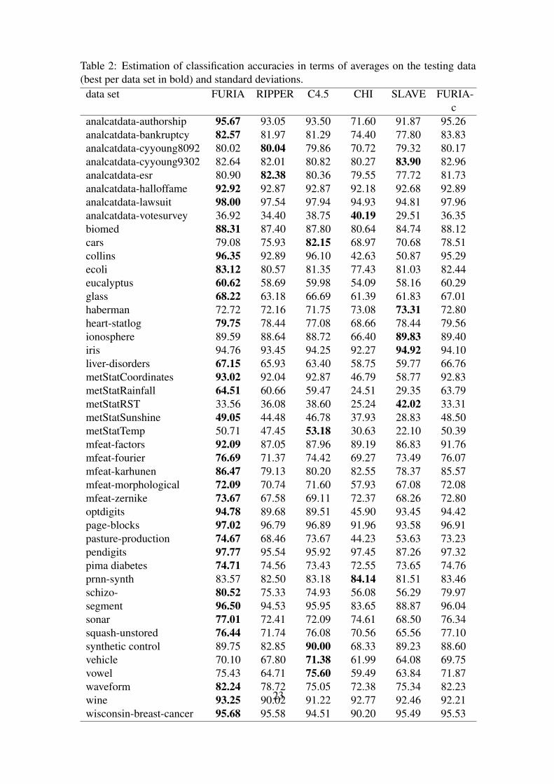
Table 2: Estimation of classification accuracies in terms of averages on the testing data(best per data set in bold) and standard deviations.data set FURIA RIPPER C4.5 CHI SLAVE FURIA-

canalcatdata-authorship 95.67 93.05 93.50 71.60 91.87 95.26analcatdata-bankruptcy 82.57 81.97 81.29 74.40 77.80 83.83analcatdata-cyyoung8092 80.02 80.04 79.86 70.72 79.32 80.17analcatdata-cyyoung9302 82.64 82.01 80.82 80.27 83.90 82.96analcatdata-esr 80.90 82.38 80.36 79.55 77.72 81.73analcatdata-halloffame 92.92 92.87 92.87 92.18 92.68 92.89analcatdata-lawsuit 98.00 97.54 97.94 94.93 94.81 97.96analcatdata-votesurvey 36.92 34.40 38.75 40.19 29.51 36.35biomed 88.31 87.40 87.80 80.64 84.74 88.12cars 79.08 75.93 82.15 68.97 70.68 78.51collins 96.35 92.89 96.10 42.63 50.87 95.29ecoli 83.12 80.57 81.35 77.43 81.03 82.44eucalyptus 60.62 58.69 59.98 54.09 58.16 60.29glass 68.22 63.18 66.69 61.39 61.83 67.01haberman 72.72 72.16 71.75 73.08 73.31 72.80heart-statlog 79.75 78.44 77.08 68.66 78.44 79.56ionosphere 89.59 88.64 88.72 66.40 89.83 89.40iris 94.76 93.45 94.25 92.27 94.92 94.10liver-disorders 67.15 65.93 63.40 58.75 59.77 66.76metStatCoordinates 93.02 92.04 92.87 46.79 58.77 92.83metStatRainfall 64.51 60.66 59.47 24.51 29.35 63.79metStatRST 33.56 36.08 38.60 25.24 42.02 33.31metStatSunshine 49.05 44.48 46.78 37.93 28.83 48.50metStatTemp 50.71 47.45 53.18 30.63 22.10 50.39mfeat-factors 92.09 87.05 87.96 89.19 86.83 91.76mfeat-fourier 76.69 71.37 74.42 69.27 73.49 76.07mfeat-karhunen 86.47 79.13 80.20 82.55 78.37 85.57mfeat-morphological 72.09 70.74 71.60 57.93 67.08 72.08mfeat-zernike 73.67 67.58 69.11 72.37 68.26 72.80optdigits 94.78 89.68 89.51 45.90 93.45 94.42page-blocks 97.02 96.79 96.89 91.96 93.58 96.91pasture-production 74.67 68.46 73.67 44.23 53.63 73.23pendigits 97.77 95.54 95.92 97.45 87.26 97.32pima diabetes 74.71 74.56 73.43 72.55 73.65 74.76prnn-synth 83.57 82.50 83.18 84.14 81.51 83.46schizo- 80.52 75.33 74.93 56.08 56.29 79.97segment 96.50 94.53 95.95 83.65 88.87 96.04sonar 77.01 72.41 72.09 74.61 68.50 76.34squash-unstored 76.44 71.74 76.08 70.56 65.56 77.10synthetic control 89.75 82.85 90.00 68.33 89.23 88.60vehicle 70.10 67.80 71.38 61.99 64.08 69.75vowel 75.43 64.71 75.60 59.49 63.84 71.87waveform 82.24 78.72 75.05 72.38 75.34 82.23wine 93.25 90.02 91.22 92.77 92.46 92.21wisconsin-breast-cancer 95.68 95.58 94.51 90.20 95.49 95.53

23

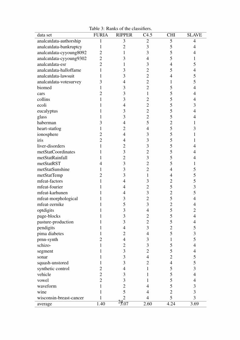
Table 3: Ranks of the classifiers.data set FURIA RIPPER C4.5 CHI SLAVEanalcatdata-authorship 1 3 2 5 4analcatdata-bankruptcy 1 2 3 5 4analcatdata-cyyoung8092 2 1 3 5 4analcatdata-cyyoung9302 2 3 4 5 1analcatdata-esr 2 1 3 4 5analcatdata-halloffame 1 3 2 5 4analcatdata-lawsuit 1 3 2 4 5analcatdata-votesurvey 3 4 2 1 5biomed 1 3 2 5 4cars 2 3 1 5 4collins 1 3 2 5 4ecoli 1 4 2 5 3eucalyptus 1 3 2 5 4glass 1 3 2 5 4haberman 3 4 5 2 1heart-statlog 1 2 4 5 3ionosphere 2 4 3 5 1iris 2 4 3 5 1liver-disorders 1 2 3 5 4metStatCoordinates 1 3 2 5 4metStatRainfall 1 2 3 5 4metStatRST 4 3 2 5 1metStatSunshine 1 3 2 4 5metStatTemp 2 3 1 4 5mfeat-factors 1 4 3 2 5mfeat-fourier 1 4 2 5 3mfeat-karhunen 1 4 3 2 5mfeat-morphological 1 3 2 5 4mfeat-zernike 1 5 3 2 4optdigits 1 3 4 5 2page-blocks 1 3 2 5 4pasture-production 1 3 2 5 4pendigits 1 4 3 2 5pima diabetes 1 2 4 5 3prnn-synth 2 4 3 1 5schizo- 1 2 3 5 4segment 1 3 2 5 4sonar 1 3 4 2 5squash-unstored 1 3 2 4 5synthetic control 2 4 1 5 3vehicle 2 3 1 5 4vowel 2 3 1 5 4waveform 1 2 4 5 3wine 1 5 4 2 3wisconsin-breast-cancer 1 2 4 5 3average 1.40 3.07 2.60 4.24 3.6924

Data set FURIA RIPPER CHI SLAVErules cond. rules cond. rules cond. rules cond.

analcatdata-authorship 15.9 2.7 9.6 1.7 555.1 3 12.1 5.9analcatdata-bankruptcy 3.8 1.8 2.5 0.7 23.9 3 2.5 1.6analcatdata-cyyoung8092 3.7 1.5 2.6 0.7 55 3 3.4 2.0analcatdata-cyyoung9302 3.5 1.3 2.8 0.8 49.5 3 3.1 2.0analcatdata-esr 2.1 1.1 2 0.5 6.8 3 2.6 1.1analcatdata-halloffame 14.3 2.8 6.5 1.8 458.9 3 7.2 3.4analcatdata-lawsuit 3.7 1.5 2 1 24.7 3 2.6 1.7analcatdata-votesurvey 1.7 1.4 2.3 0.8 13.6 3 7.3 2.1biomed 8.6 2 4.4 1 55.1 3 4.3 2.7cars 12.9 2.4 7.1 1.8 54.4 3 12.5 3.3collins 15.9 1.1 15.2 1 321.7 3 45.8 6.6ecoli 13.8 2.5 8.3 1.6 47.2 3 11.3 3.0eucalyptus 14.7 2.6 10.2 1.8 375 3 38.3 5.7glass 11.3 2.2 6.7 1.7 42.7 3 12.3 3.3haberman 4.4 1.5 2 0.8 15.8 3 4 1.7heart-statlog 8.4 2.5 4.3 1.5 164.9 3 7 3.6ionosphere 8.3 2 4.7 1.1 168.9 3 8 3.8iris 4.4 1.5 3.3 0.8 14.9 3 3.1 1.2liver-disorders 8.2 2.2 4.3 1.8 42.1 3 5.9 3.4metStatCoordinates 69.7 2.3 38.8 2.1 15.6 3 12.8 2.4metStatRainfall 123.9 4.5 82.7 3.6 215.6 3 30.3 4.4metStatRST 9.9 2.2 10 1.7 15 3 9.5 2.3metStatSunshine 25 2.7 17 1.9 91 3 39.3 4.3metStatTemp 31.5 2.8 22.4 2.2 36.4 3 15.6 3.5mfeat-factors 45 3 28.5 2.2 1317.2 3 44.3 12.2mfeat-fourier 52.4 3.8 29.2 2.6 1317.2 3 73.2 10.6mfeat-karhunen 59.1 3.2 38.4 2.6 1314.4 3 64.7 9.7mfeat-morphological 25.1 2.6 19 2.1 31.4 3 15.7 3.1mfeat-zernike 44.9 3.7 30.6 2.8 1257.6 3 77.7 10.0optdigits 97.8 4.9 59.6 3.9 3708.5 3 68.6 8.0page-blocks 25.6 3.2 14.7 2.2 47.6 3 10.1 3.5pasture-production 3.4 1.4 3.2 0.7 24 3 3.6 3.3pendigits 110.9 4.8 67.6 3.4 2745.2 3 37 7.6pima diabetes 8.5 2.6 3.9 1.8 98.6 3 9.3 3.7prnn-synth 4.4 1.4 3.5 1 8 3 2.4 1.6schizo- 15.1 1.7 6.5 1.2 136.7 3 7.9 5.3segment 26.9 3.1 17 2.2 275.1 3 15.8 4.5sonar 8.1 2.3 4.3 1.4 137.1 3 6.9 4.7squash-unstored 4 1.5 3.2 0.8 33.8 3 4.1 2.6syntheticcontrol 17.3 2.6 10.6 1.8 394.3 3 9.1 6.3vehicle 20.7 3.3 13.8 2.2 314.4 3 26.4 6.5vowel 53.8 3.3 34.2 2.5 251.5 3 51.1 5.6waveform 79.9 5.9 27.9 3.8 2874.7 3 50.7 9.3wine 6.2 1.9 3.5 1.1 101.2 3 3.8 2.9wisconsin-breast-cancer 12.2 2.9 4.8 1.5 172.4 3 5.8 3.7average 25.4 2.5 15.5 1.7 431.7 3 19.8 4.4

Table 4: The number of rules per rule set and the average number of antecedents per rule.

25

data set uncovered novel (Eineborgand

Boström,2001)

diff.

analcatdata-authorship 0.05 42.70 49.40 6.70analcatdata-bankruptcy 0.02 6.80 0.80 -6.00analcatdata-cyyoung8092 0.08 5.50 1.80 -3.70analcatdata-cyyoung9302 0.07 4.70 1.10 -3.60analcatdata-esr 0.04 2.30 0.20 -2.10analcatdata-halloffame 0.03 39.80 48.50 8.70analcatdata-lawsuit 0.00 5.50 0.70 -4.80analcatdata-votesurvey 0.77 2.40 1.70 -0.70biomed 0.05 17.60 9.80 -7.80cars 0.11 31.20 34.50 3.30collins 0.01 18.00 7.20 -10.80ecoli 0.05 34.70 26.30 -8.40eucalyptus 0.30 38.50 61.70 23.20glass 0.15 24.60 22.40 -2.20haberman 0.07 6.40 2.40 -4.00heart-statlog 0.08 21.20 21.40 0.20ionosphere 0.04 17.00 9.90 -7.10iris 0.01 6.60 0.90 -5.70liver-disorders 0.17 18.20 19.90 1.70metStatCoordinates 0.02 163.20 120.30 -42.90metStatRainfall 0.23 556.60 1737.60 1181.00metStatRST 0.49 22.10 24.10 2.00metStatSunshine 0.26 67.60 91.10 23.50metStatTemp 0.33 89.00 121.40 32.40mfeat-factors 0.06 134.40 227.60 93.20mfeat-fourier 0.13 200.60 622.00 421.40mfeat-karhunen 0.10 189.30 426.00 236.70mfeat-morphological 0.08 65.70 72.60 6.90mfeat-zernike 0.18 167.60 489.20 321.60optdigits 0.04 482.10 1949.60 1467.50page-blocks 0.01 82.00 87.90 5.90pasture-production 0.23 4.60 1.40 -3.20pendigits 0.01 528.00 1429.30 901.30pima diabetes 0.13 22.00 30.60 8.60prnn-synth 0.08 6.10 2.00 -4.10schizo- 0.13 25.20 25.90 0.70segment 0.02 83.70 91.10 7.40sonar 0.13 18.80 20.00 1.20squash-unstored 0.06 6.10 1.40 -4.70synthetic control 0.08 45.50 49.70 4.20vehicle 0.22 68.60 118.60 50.00vowel 0.11 175.00 291.00 116.00waveform 0.10 474.70 2645.80 2171.10wine 0.04 11.50 4.30 -7.20wisconsin-breast-cancer 0.02 34.90 26.11 -8.79

Table 5: The number of times the rule weight has to be calculated for the rule stretchingprocedure. The first column shows the relative number of testing instances that werenot covered by any rule. The second column shows the number of calculations for ourapproach and the third column for the one of Eineborg and Boström (2001). The lastcolumn shows the difference of these two.

26

data set RIPPER RIP* RIP** FUR* FURIAanalcatdata-authorship 0.348 0.588 0.828 0.840 0.873analcatdata-bankruptcy 0.001 0.002 0.003 0.003 0.003analcatdata-cyyoung8092 0.004 0.005 0.012 0.010 0.010analcatdata-cyyoung9302 0.003 0.004 0.008 0.008 0.008analcatdata-esr 0.000 0.000 0.001 0.001 0.001analcatdata-halloffame 0.461 0.706 0.996 1.008 1.046analcatdata-lawsuit 0.003 0.003 0.006 0.005 0.007analcatdata-votesurvey 0.002 0.004 0.003 0.004 0.004biomed 0.012 0.013 0.027 0.030 0.031cars 0.045 0.094 0.125 0.138 0.146collins 0.210 0.300 0.329 0.321 0.327ecoli 0.032 0.066 0.084 0.089 0.095eucalyptus 0.280 0.659 0.890 0.953 0.976glass 0.034 0.054 0.079 0.084 0.090haberman 0.010 0.016 0.034 0.045 0.046heart-statlog 0.023 0.033 0.068 0.077 0.080ionosphere 0.082 0.115 0.221 0.228 0.233iris 0.002 0.004 0.007 0.006 0.006liver-disorders 0.024 0.049 0.100 0.121 0.124metStatCoordinates 1.327 4.199 4.834 7.481 10.266metStatRainfall 11.287 24.868 29.186 35.720 42.819metStatRST 0.065 0.134 0.164 0.170 0.181metStatSunshine 0.321 0.566 0.669 0.658 0.684metStatTemp 0.423 0.887 1.033 1.108 1.156mfeat-factors 10.623 23.466 25.879 25.537 25.762mfeat-fourier 9.733 30.836 33.859 32.685 33.236mfeat-karhunen 7.973 19.593 21.658 20.720 21.164mfeat-morphological 0.571 1.808 2.059 2.263 2.826mfeat-zernike 6.563 17.002 18.605 17.943 18.383optdigits 14.817 39.101 44.720 50.118 58.243page-blocks 1.574 2.599 3.426 3.954 5.667 9pasture-production 0.002 0.005 0.006 0.006 0.007 1pendigits 10.716 30.488 35.114 47.218 77.755pima diabetes 0.073 0.132 0.278 0.335 0.358prnn-synth 0.007 0.010 0.024 0.027 0.030schizo- 0.050 0.081 0.173 0.196 0.203segment 0.940 2.178 2.666 2.818 3.074sonar 0.082 0.103 0.224 0.230 0.233squash-unstored 0.005 0.006 0.009 0.009 0.009synthetic control 0.650 1.301 1.563 1.476 1.495vehicle 0.282 0.787 0.900 0.949 0.988vowel 0.715 1.755 1.949 2.013 2.164waveform 7.778 29.359 42.688 50.521 57.809wine 0.010 0.015 0.025 0.025 0.026wisconsin-breast-cancer 0.025 0.053 0.085 0.102 0.117

Table 6: Average model building times in seconds. FUR* = FURIA w/o fuzzificationprocess, R* = RIPPER unordered w/o IREP, R** = RIPPER w/o IREP27