fundamentals of reservoir fluid behavior classification of reservoirs and reservoir fluids

C H A P T E R 1

FUNDAMENTALS OF RESERVOIR FLUID

BEHAVIOR

Naturally occurring hydrocarbon systems found in petroleum reservoirs are mixtures of organic compounds that exhibit multiphase behavior over wide ranges of pressures and temperatures. These hydrocarbon accumulations may occur in the gaseous state, the liquid state, the solid state, or in various combinations of gas, liquid, and solid.

These differences in phase behavior, coupled with the physical properties of reservoir rock that determine the relative ease with which gas and liquid are transmitted or retained, result in many diverse types of hydrocarbon reservoirs with complex behaviors. Frequently, petroleum engi- neers have the task to study the behavior and characteristics of a petroleum reservoir and to determine the course of future development and production that would maximize the profit.

The objective of this chapter is to review the basic principles of reservoir fluid phase behavior and illustrate the use of phase diagrams in classifying types of reservoirs and the native hydrocarbon systems.

CLASSIFICATION OF RESERVOIRS AND RESERVOIR FLUIDS

Petroleum reservoirs are broadly classified as oil or gas reservoirs. These broad classifications are further subdivided depending on:

2 Reservoir Engineering Handbook

�9 The composition of the reservoir hydrocarbon mixture �9 Initial reservoir pressure and temperature �9 Pressure and temperature of the surface production

The conditions under which these phases exist are a matter of consid- erable practical importance. The experimental or the mathematical deter- minations of these conditions are conveniently expressed in different types of diagrams commonly called phase diagrams. One such diagram is called the pressure-temperature diagram.

Pressure-Temperature D i a g r a m

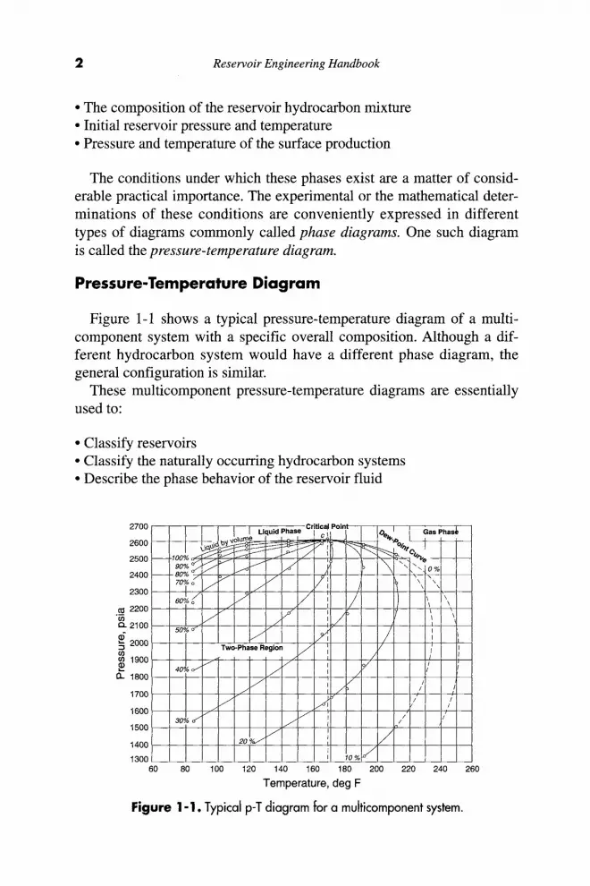
Figure 1-1 shows a typical pressure-temperature diagram of a multicomponent system with a specific overall composition. Although a different hydrocarbon system would have a different phase diagram, the general configuration is similar.

These multicomponent pressure-temperature diagrams are essentially used to:

�9 Classify reservoirs �9 Classify the naturally occurring hydrocarbon systems �9 Describe the phase behavior of the reservoir fluid

270O

2600

2500

2400

2300

2200 . m

co CL 2100

' - 2000 u) co 1900 (9 Q- 1800

1700

1600

1500

1400

1300 60

I I Liquid Phase ~,r~ .... !r'ol.z Gas I)has~ ~ e - ~ ~ ~ ~ - ~ ! % 1 0 0 % P~.i" . . ~ ' ~ l I ~ I J '. I/ I

70% o~ / i l ) \\\\ 60; ~o / j 7

J ,0,, o/ / 'I

Two-Phase Region / J / ' o//

J / / I / / / / J,<

1 / // /" / " i i ~~ <~ ~ I " '

20 ~ ~ I I i

I , o , J 80 100 120 140 160 180 200 220 240

Temperature, deg F

Figure 1- ! . Typical p-T diagram for a muJticomponent system.

260

Fundamentals of Reservoir Fluid Behavior 3

To fully understand the significance of the pressure-temperature diagrams, it is necessary to identify and define the following key points on these diagrams:

�9 Cricondentherm (Tct)~The Cricondentherm is defined as the maximum temperature above which liquid cannot be formed regardless of pressure (point E). The corresponding pressure is termed the Cricon- dentherm pressure Pct-

�9 Cr icondenbar (Pcb)~The Cricondenbar is the maximum pressure above which no gas can be formed regardless of temperature (point D). The corresponding temperature is called the Cricondenbar temperature Tcb.

�9 Cr i t i ca l point---The critical point for a multicomponent mixture is referred to as the state of pressure and temperature at which all inten- sive properties of the gas and liquid phases are equal (point C). At the critical point, the corresponding pressure and temperature are called the critical pressure Pc and critical temperature Tc of the mixture.

�9 Phase enve lope ( two-phase region)~The region enclosed by the bubble-point curve and the dew-point curve (line BCA), wherein gas and liquid coexist in equilibrium, is identified as the phase envelope of the hydrocarbon system.

�9 Quality l ines~The dashed lines within the phase diagram are called quality lines. They describe the pressure and temperature conditions for equal volumes of liquids. Note that the quality lines converge at the critical point (point C).

�9 B u b b l e - p o i n t curve---The bubble-point curve (line BC) is defined as the line separating the liquid-phase region from the two-phase region.

�9 D e w - p o i n t curve~The dew-point curve (line AC) is defined as the line separating the vapor-phase region from the two-phase region.

In general, reservoirs are conveniently classified on the basis of the location of the point representing the initial reservoir pressure Pi and temperature T with respect to the pressure-temperature diagram of the reservoir fluid. Accordingly, reservoirs can be classified into basically two types. These are:

�9 Oil reservoirs--If the reservoir temperature T is less than the critical temperature Tc of the reservoir fluid, the reservoir is classified as an oil reservoir.


�9 Gas reservoirs---If the reservoir temperature is greater than the critical temperature of the hydrocarbon fluid, the reservoir is considered a gas reservoir.

Oil Reservoirs

Depending upon initial reservoir pressure Pi, oil reservoirs can be sub- classified into the following categories:

1. Undersaturated oil reservoir. If the initial reservoir pressure Pi (as represented by point 1 on Figure 1-1), is greater than the bubble-point pressure Pb of the reservoir fluid, the reservoir is labeled an undersaturated oil reservoir.

2. Saturated oil reservoir. When the initial reservoir pressure is equal to the bubble-point pressure of the reservoir fluid, as shown on Figure 1-1 by point 2, the reservoir is called a saturated oil reservoir.

3. Gas-cap reservoir. If the initial reservoir pressure is below the bubble- point pressure of the reservoir fluid, as indicated by point 3 on Figure 1-1, the reservoir is termed a gas-cap or two-phase reservoir, in which the gas or vapor phase is underlain by an oil phase. The appropriate quality line gives the ratio of the gas-cap volume to reservoir oil volume.

Crude oils cover a wide range in physical properties and chemical compositions, and it is often important to be able to group them into broad categories of related oils. In general, crude oils are commonly classified into the following types:

�9 Ordinary black oil �9 Low-shrinkage crude oil �9 High-shrinkage (volatile) crude oil �9 Near-critical crude oil

The above classifications are essentially based upon the properties exhibited by the crude oil, including physical properties, composition, gas-oil ratio, appearance, and pressure-temperature phase diagrams.

1. Ordinary black oil. A typical pressure-temperature phase diagram for ordinary black oil is shown in Figure 1-2. It should be noted that quality lines, which are approximately equally spaced characterize this black oil phase diagram. Following the pressure reduction path as indicated by the vertical line EF on Figure 1-2, the liquid shrinkage curve, as shown in Figure 1-3, is prepared by plotting the liquid volume percent as a function of pressure. The liquid shrinkage curve approxi-


Ordinary Black Oil

Gas Phase

Pressure path ~ Dew-p , in reservoir ~ C Dew-Point Curve

Liquid Phase / / ) /

Temperature

Figure 1-2. A typical p-T diagram for an ordinary black oil.

(l) E :3 0

>

.'9_ :3 ET

._1

f Residual Oil F,(

0%

100%

Pressure >

Figure | -3 . Liquid-shrinkage curve for black oil.

mates a straight line except at very low pressures. When produced, ordinary black oils usually yield gas-oil ratios between 200-700 scf/STB and oil gravities of 15 to 40 API. The stock tank oil is usually brown to dark green in color.

2. Low-shrinkage oil. A typical pressure-temperature phase diagram for low-shrinkage oil is shown in Figure 1-4. The diagram is characterized by quality lines that are closely spaced near the dew-point curve. The liquid-shrinkage curve, as given in Figure 1-5, shows the shrinkage characteristics of this category of crude oils. The other associated properties of this type of crude oil are:


A

~) i ._

r O) .=

n

Liquid ..,role E

. ~\e-gd'~ - ~ ~ ~ Critical Point /

Separator Conditions. i i i f ~ / / /

\ I / f I I I \. I I I / , / ~ r

. " , " , ' / ' /C),~ ~' ii / / / ." /~-q,"

85~ / / . / / / - / / / ~ , q u

/ I i Ii I/<3~ Gas

75% " / 0 % 650/0 " B

F

Temperature �9

Figure ! -4. A typical phase diagram for a low-shrinkage oil.

100%

E o > "o ==,,=

O" , m

0%

I

F ~ ~ Residual Oil

Pressure Figure 1-5. Oil-shrinkage curve for low-shrinkage oil.

�9 Oil formation volume factor less than 1.2 bbl/STB

�9 Gas-oil ratio less than 200 scf/STB

�9 Oil gravity less than 35 ~ API

�9 Black or deeply colored �9 Substantial liquid recovery at separator conditions as indicated by

point G on the 85% quality line of Figure 1-4.


3. Volatile crude oil. The phase diagram for a volatile (high-shrinkage) crude oil is given in Figure 1-6. Note that the quality lines are close together near the bubble-point and are more widely spaced at lower pressures. This type of crude oil is commonly characterized by a high liquid shrinkage immediately below the bubble-point as shown in Fig- ure 1-7. The other characteristic properties of this oil include:

�9 Oil formation volume factor less than 2 bbl/STB �9 Gas-oil ratios between 2,000-3,200 scf/STB �9 Oil gravities between 45-55 ~ API

Pressure path 1 �9 in r e ~

Volatile Oil Ip~ ~~~70~~~

/ _ _

_,o.,y////// .

~/~~~~~/////Separator ~ o , ~

4O

J

100%

E _= 0 > .9_ ._o- ...I

0%

~ R e s i d u a l Oil F

Temperature Figure 1-6. A typical p-T diagram for a volatile crude oil.

Pressure ~-

Figure 1-7. A typical liquid-shrinkage curve for a volatile crude oil.


�9 Lower liquid recovery of separator conditions as indicated by point G on Figure 1-6

�9 Greenish to orange in color

Another characteristic of volatile oil reservoirs is that the API gravity of the stock-tank liquid will increase in the later life of the reservoirs.

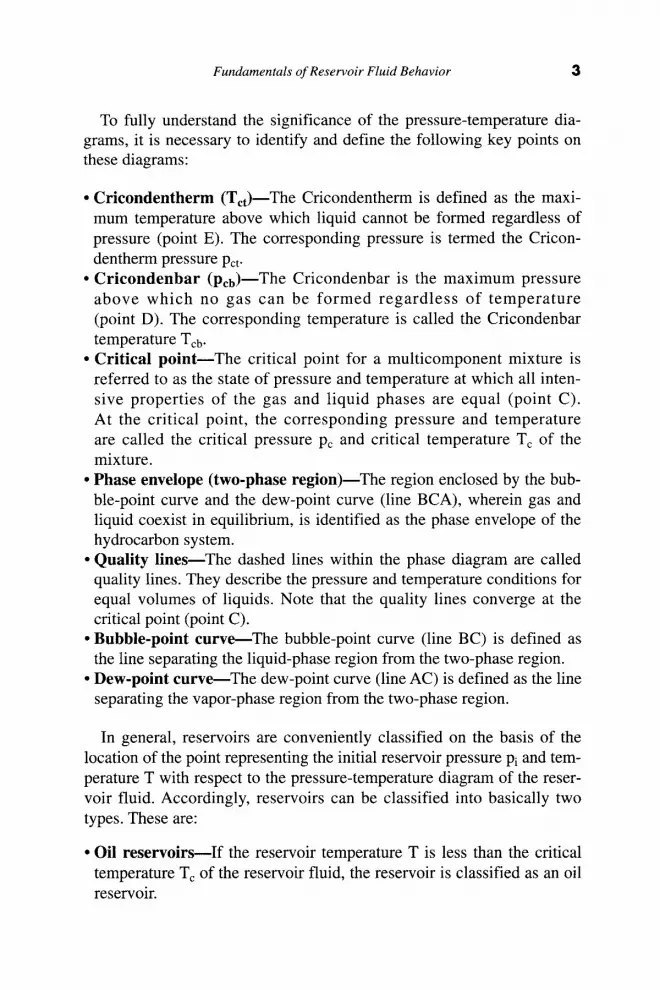
4. Near-critical crude oil. If the reservoir temperature T is near the critical temperature Tc of the hydrocarbon system, as shown in Figure 1-8, the hydrocarbon mixture is identified as a near-critical crude oil. Because all the quality lines converge at the critical point, an isothermal pressure drop (as shown by the vertical line EF in Figure 1-8) may shrink the crude oil from 100% of the hydrocarbon pore volume at the bubble-point to 55% or less at a pressure 10 to 50 psi below the bubble-point. The shrinkage characteristic behavior of the near-critical crude oil is shown in Figure 1-9. The near-critical crude oil is characterized by a high GOR in excess of 3,000 scf/STB with an oil formation volume factor of 2.0 bbl/STB or higher. The compositions of near- c r i t ica l oils are usua l ly cha rac t e r i zed by 12.5 to 20 mol% heptanes-plus, 35% or more of ethane through hexanes, and the remainder methane.

Figure 1-10 compares the characteristic shape of the liquid-shrinkage curve for each crude oil type.

I Pressure path t~ in r e ~

I \ \ \ \

Temperature

Figure 1-8. A schematic phase diagram for the near-critical crude oil


100%

(D E :3

, , . = .

0 :=

13 . . _

:3 O"

. . m /

0% Pressure ~-

Figure 1-9. A typical liquid-shrinkage curve for the near-critical crude oil.

100

f

/

A - Low- Shri nkage Oil

B-Ordinary Black Oil

C-High-Shrinkage Oil

D- Near-Critical Oil

Pressure

Figure 1-10. Liquid shrinkage for crude oil systems.

Gas Reservoirs

In general, if the reservoir temperature is above the critical temperature of the hydrocarbon system, the reservoir is classified as a natural gas reservoir. On the basis of their phase diagrams and the prevailing reservoir conditions, natural gases can be classified into four categories:

| 0 Reservoir Engineering Handbook

�9 Retrograde gas-condensate �9 Near-critical gas-condensate �9 Wet gas �9 Dry gas

Retrograde gas-condensate reservoir. If the reservoir temperature T lies between the critical temperature T~ and cricondentherm Tct of the reservoir fluid, the reservoir is classified as a retrograde gas- condensate reservoir. This category of gas reservoir is a unique type of hydrocarbon accumulation in that the special thermodynamic behavior of the reservoir fluid is the controlling factor in the development and the depletion process of the reservoir. When the pressure is decreased on these mixtures, instead of expanding (if a gas) or vaporizing (if a liquid) as might be expected, they vaporize instead of condensing.

Consider that the initial condition of a retrograde gas reservoir is represented by point 1 on the pressure-temperature phase diagram of Figure 1-11. Because the reservoir pressure is above the upper dew-point pressure, the hydrocarbon system exists as a single phase (i.e., vapor phase) in the reservoir. As the reservoir pressure declines isothermally during production from the initial pressure (point 1) to the upper dew- point pressure (point 2), the attraction between the molecules of the light and heavy components causes them to move further apart further apart.

I Pressure path 1 �9 in reservoir 2 ~

Retrograde gas / . ~ ~

...... ;/ / /

Temperature

Figure 1- ! 1. A typical phase diagram of a retrograde system.

Fundamentals of Reservoir Fluid Behavior | |

As this occurs, attraction between the heavy component molecules becomes more effective; thus, liquid begins to condense.

This retrograde condensation process continues with decreasing pressure until the liquid dropout reaches its maximum at point 3. Further reduction in pressure permits the heavy molecules to commence the normal vaporization process. This is the process whereby fewer gas molecules strike the liquid surface and causes more molecules to leave than enter the liquid phase. The vaporization process continues until the reservoir pressure reaches the lower dew-point pressure. This means that all the liquid that formed must vaporize because the system is essentially all vapors at the lower dew point.

Figure 1-12 shows a typical liquid shrinkage volume curve for a condensate system. The curve is commonly called the liquid dropout curve. In most gas-condensate reservoirs, the condensed liquid volume seldom exceeds more than 15%-19% of the pore volume. This liquid saturation is not large enough to allow any liquid flow. It should be recognized, however, that around the wellbore where the pressure drop is high, enough liquid dropout might accumulate to give two-phase flow of gas and retrograde liquid.

The associated physical characteristics of this category are:

�9 Gas-oil ratios between 8,000 and 70,000 scf/STB. Generally, the gas-oil ratio for a condensate system increases with time due to the liquid dropout and the loss of heavy components in the liquid.

100

> "0

"n

Maximum Liquid Dropout

I Pressure ~-

Figure I - 12. A typical liquid dropout curve.

| 2 Reservoir Engineering Handbook

�9 Condensate gravity above 50 ~ API �9 Stock-tank liquid is usually water-white or slightly colored.

There is a fairly sharp dividing line between oils and condensates from a compositional standpoint. Reservoir fluids that contain heptanes and are heavier in concentrations of more than 12.5 mol% are almost always in the liquid phase in the reservoir. Oils have been observed with heptanes and heavier concentrations as low as 10% and condensates as high as 15.5%. These cases are rare, however, and usually have very high tank liquid gravities.

Near-crit ical gas-condensate reservoir. If the reservoir temperature is near the critical temperature, as shown in Figure 1-13, the hydrocarbon mixture is classified as a near-critical gas-condensate. The volumetric behavior of this category of natural gas is described through the isothermal pressure declines as shown by the vertical line 1-3 in Figure 1-13 and also by the corresponding liquid dropout curve of Figure 1-14. Because all the quality lines converge at the critical point, a rapid liquid buildup will immediately occur below the dew point (Figure 1-14) as the pressure is reduced to point 2.

This behavior can be justified by the fact that several quality lines are crossed very rapidly by the isothermal reduction in pressure. At the point where the liquid ceases to build up and begins to shrink again, the

Pressure path in reservoir ~

I Near-Critical Gas / J ~ \

~" iauid I . /

~ a r a ~ ~ ~ O ~

Temperature

Figure 1-13. A typical phase diagram for a near-critical gas condensate reservoir.

Fundamentals of Reservoir Fluid Behavior | 3

100

E

0 > "13 :3 ET

._i

50 2

3 1

Pressure ~-

Figure 1-14. Liquid-shrinkage curve for a near-critical gas-condensate system.

reservoir goes from the retrograde region to a normal vaporization region.

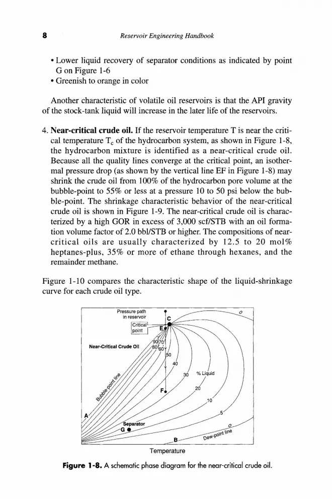
Wet-gas reservoir. A typical phase diagram of a wet gas is shown in Figure 1-15, where reservoir temperature is above the cricondentherm of the hydrocarbon mixture. Because the reservoir temperature exceeds the cricondentherm of the hydrocarbon system, the reservoir fluid will always remain in the vapor phase region as the reservoir is depleted isothermally, along the vertical line A-B.

As the produced gas flows to the surface, however, the pressure and temperature of the gas will decline. If the gas enters the two-phase region, a liquid phase will condense out of the gas and be produced from the surface separators. This is caused by a sufficient decrease in the kinetic energy of heavy molecules with temperature drop and their subsequent change to liquid through the attractive forces between molecules.

Wet-gas reservoirs are characterized by the following properties:

�9 Gas oil ratios between 60,000 to 100,000 scf/STB �9 Stock-tank oil gravity above 60 ~ API �9 Liquid is water-white in color �9 Separator conditions, i.e., separator pressure and temperature, lie within

the two-phase region

Dry-gas reservoir. The hydrocarbon mixture exists as a gas both in the reservoir and in the surface facilities. The only liquid associated


T G) L . _

:3 (/)

t _ _

Q.

Pressure Depletion at Reservoir Temperature

C I \ \ ~ A J 1 I

Liquid I I I

Tw~/7///~/wo--~/se?~phase Region

/ / ~ / / . , . l ,

! Temperature > B

Figure 1 - 15. Phase diagram for a wet gas. (After Clark, N.J. Elements of Petroleum Reservoirs, SPE, 1969.)

with the gas from a dry-gas reservoir is water. A phase diagram of a dry-gas reservoir is given in Figure 1-16. Usually a system having a gas-oil ratio greater than 100,000 scf/STB is considered to be a dry gas.

Kinetic energy of the mixture is so high and attraction between molecules so small that none of them coalesce to a liquid at stock-tank conditions of temperature and pressure.

It should be pointed out that the classification of hydrocarbon fluids might be also characterized by the initial composition of the system. McCain (1994) suggested that the heavy components in the hydrocarbon mixtures have the strongest effect on fluid characteristics. The ternary diagram, as shown in Figure 1-17, with equilateral triangles can be conveniently used to roughly define the compositional boundaries that separate different types of hydrocarbon systems.


Figure 1-16. Phase diagram for a dry gas. (After Clark, N.J. Elements of Petroleum Reservoirs, SPE, 1969.)

From the foregoing discussion, it can be observed that hydrocarbon mixtures may exist in either the gaseous or liquid state, depending on the reservoir and operating conditions to which they are subjected. The qualitative concepts presented may be of aid in developing quantitative analyses. Empirical equations of state are commonly used as a quantitative tool in describing and classifying the hydrocarbon system. These equations of state require:

�9 Detailed compositional analyses of the hydrocarbon system �9 Complete descriptions of the physical and critical properties of the mix-

ture individual components

Many characteristic properties of these individual components (in other words, pure substances) have been measured and compiled over the years. These properties provide vital information for calculating the

! 6 Reservoir Engineering Handbook

Figure 1 - 17. Compositions of various reservoir fluid types.

thermodynamic properties of pure components, as well as their mixtures. The most important of these properties are:

�9 Critical pressure, p~ �9 Critical temperature, Tc �9 Critical volume, Vc �9 Critical compressibility factor, Zc �9 Acentric factor, T �9 Molecular weight, M

Table 1-2 documents the above-listed properties for a number of hydrocarbon and nonhydrocarbon components.

Katz and Firoozabadi (1978) presented a generalized set of physical properties for the petroleum fractions C6 through C45. The tabulated properties include the average boiling point, specific gravity, and molecular weight. The authors' proposed a set of tabulated prop-


erties that were generated by analyzing the physical properties of 26 condensates and crude oil systems. These generalized properties are given in Table 1-1.

Ahmed (1985) correlated Katz-Firoozabadi-tabulated physical properties with the number of carbon atoms of the fraction by using a regres- sion model. The generalized equation has the following form:

0 = a 1 + a2 n + a 3 n 2 + a 4 n 3 + (as/n) (1-1)

where 0 = any physical property n - number of carbon atoms, i.e., 6.7 . . . . . ,45

al-a5 = coefficients of the equation and are given in Table 1-3

Undefined Petroleum Fractions

Nearly all naturally occurring hydrocarbon systems contain a quantity of heavy fractions that are not well defined and are not mixtures of dis- cretely identified components. These heavy fractions are often lumped together and identified as the plus fraction, e.g., C7+ fraction.

A proper description of the physical properties of the plus fractions and other undefined petroleum fractions in hydrocarbon mixtures is essential in performing reliable phase behavior calculations and compositional modeling studies. Frequently, a distillation analysis or a chromatographic analysis is available for this undefined fraction. Other physical properties, such as molecular weight and specific gravity, may also be measured for the entire fraction or for various cuts of it.

To use any of the thermodynamic property-prediction models, e.g., equation of state, to predict the phase and volumetric behavior of complex hydrocarbon mixtures, one must be able to provide the acentric factor, along with the critical temperature and critical pressure, for both the defined and undefined (heavy) fractions in the mixture. The problem of how to adequately characterize these undefined plus fractions in terms of their critical properties and acentric factors has been long recognized in the petroleum industry. Whitson (1984) presented an excellent documen- tation on the influence of various heptanes-plus (C7+) characterization schemes on predicting the volumetric behavior of hydrocarbon mixtures by equations-of-state.

(text continued on page 24)

~ g

Table 1 - 1 Genera l i zed Physical Propert ies

Group Tb (~ M Tc (~ P c

(psia) %

(~/Ib) Group

C6

C7 C8 C9

C1o C]] C12 C13 C14 C15 C16 C17 C18 C19 C2o C21 C22 C23 C24

607 658 702 748 791 829 867 901 936 971

1,002 1,032 1,055 1,077 1,101 1,124 1,146 1,167 1,187

0.690 0.727 0.749 0.768 0.782 0.793 0.804 0.815 0.826 0.836 0.843 0.851 0.856 0.861 0.866 0.871 0.876 0.881 0.885

12.27 11.96 11.87 11.82 11.83 11.85 11.86 11.85 11.84 11.84 11.87 11.87 11.89 11.91 11.92 11.94 11.95 11.95 11.96

84 923 483 0.250 96 985 453 0.280

107 1,036 419 0.312 121 1,085 383 0.348 134 1,128 351 0.385 147 1,166 325 0.419 161 1,203 302 0.454 175 1,236 286 0.484 190 1,270 270 0.516 206 1,304 255 0.550 222 1,332 241 0.582 237 1,360 230 0.613 251 1,380 222 0.638 263 1,400 214 0.662 275 1,421 207 0.690 291 1,442 200 0.717 300 1,461 193 0.743 312 1,480 188 0.768 324 1,497 182 0.793

0.06395 0.06289 0.06264 0.06258 0.06273 0.06291 0.06306 0.06311 0.06316 0.06325 0.06342 0.06350 0.06362 0.06372 0.06384 0.06394 0.06402 0.06408 0.06417

C6

C7

C8 C9

Clo C11 C12 C13 C14 C15 C16 C17 C18 C19 Ceo C21 C22 C23 Ce4

r..,. o

t%

Fundam

entals of Reservoir F

luid Behavior

|

Table 1-2 Physical Properties for Pure Components 0

L

E D

Z

1 2 3 4 5

9 I0 11 12 13

14 15 16 17 18 19 20 21

221

i i ~L ,

See Note No. -> . . . . . . . .

Compound

Methane" Ethane Propane ] eobutane n-Butane

! eopent one n-Pen t one Neopentane

n-Hexane 2-Methy I pentone 3-Me t hy I pentane Neohexane 2,3-O imet hy I butane

n-~eptane 2--Me t hy I hexane 3-Methy I hexane 3-Et hy I pent one 2,2-O imet hy ! pen t one 2 ,4 -0 Imethy t pent one 3,3--0 t methy I pentane T r i p tane

n-Octane Di I eobuty l

oooctane

o

CH cz~

Cs CsH

C6

C6 C6H

c,~ C7 c,~ C~ c,~ C~ c,~ C~

c,~ Ce Celt

6 $

10 SO

12

I Z

13

14

14

14

14

14

16

16 ] 6

] 6

16

| 6

16

16

18

18

18

Phys ica l C o n s t a n t s i

.. B .

o

, i ~ ~.o

2258.73 (.5000), -127.49 1~880. ~ ,

-43 .75 10.78 31.08

82.12 96.92 49.10

155.72 140.47 145.89 121.52 136.38

.209.16 194.09 197.33 200.25 174.54 176.89 186.91 177.58

258.21 228.39 210.63

72.581 51.706

20.445 15.574 36.69

4.9597 6.769 6.103 9.859 7.406

1.620 2.272 2.131 2.013 3.494 3.293 2.774 3.375

0.53694 1.102 1. 709

i C r i t i c a l conetan

o..

. . . . . . . o. > J z -296 .44* -297.04e -305.73* -255.28 --217.05

-255.82 -201.51

2.17

-139 .58 -244.62

-147.72 -199.38

-131.O5 --180.89

-181.48 -190.86 -182.63 -210.01

-12.81

-70 .18 -132 .11 -161.27

.00042e

.20971e

.29480e

.3245,

.3,~)88e

.35631

.35992

.342*

.37708

.37387

.37888

.37126

.37730

.38989

.38714 �9 39091 .39566 .38446 .38379 .38564 .39168

.39956 �9 39461 .38624

666.4 706.5 6 t6 .0 527.9 650~6

4 9 0 . 4 488.6 464.0

436.9 436.6 453.1 446.8 453.5

396.8 396.5 408.1 419.3 402.2 396.9 427.2 428.4

360.7 360.6 372.4

- i 16.67 89.92

206.06 274.46 305.62

369.10 385.8 321.13

453.6 435.83 448.4 420.13 440.29

512.7 495.00 503.80 513.39 477.23 475.95 505.87 496.44

564.22 530.44 519.46

9 10 11 12 13

14 15 16 17 18 19 20 21

22 23 24

(%

(%

e.,.

(% (%

2 n -Non ,n . 2 n-Decone 2 Cyc I opent ane 2 Methy | c yc l open tone

Cyr I ohexane .I kip. t hy I cyr I ohexone

E thene(E thy I e n e ) _ .1 Propene(Propy I ene) .~ 1 -Bu tene(Bu ty tene)

c i s--2-But ene t r ons -2 -Bu t ene I eobut erie

.~ 1- -Pent ,n ,

. ~ 1,2--Butodi ene I 1 . 3 - B u t o d i ene i Isoprene

Ace ~ y I ene i i Benzene 'i Toluene

a Ethy I benzene ,~ , o -Xy lene

.. m-Xy I ene ' D--Xy I one

, i S ty rene ~ I 8op ropy l benzene

! ; Methy l o l coho l ' E thy l o l coho l ' ~ Corbon monoxide ' i Corbon d i o x i d e .' , Hydrogen sul f i d e ' , S u l f u r d i o x i d e

t l ' , , Ammonia ' ' A i r ' ~ Hydrogen , i Oxygen I ~ N i t rogen .l C h l o r i n e I ! iWoter tl ; He| ium ;~ ; Hydrogen c h l o r i d e

CgHzo CloHzz CsHlo C~Hlz C6Hlz C?Hl4

CzH4 C3H6 C4He C4H8 C4H8 C4H# CsHIo C4H6 C4H6 CsH8

CzHz C~H6 CvH8 CsH]o CsHso CsHso CeHso C8H8 C9H12

CH40 CzH60 CO COz HzS SOz

NH3 Nz+Oz Hz Oz Nz Clz HzO He HCl

! 128.258 142.285 70.134 84.161 84.161 98.188

28.054 42.081 56.108 56.108 56.108 56.108 70.134 54.O92 54.092 68.119

26.038 78. 114 92. 141

106.167 106.167 106.167 104.152 120.194

32.042 46.069 28.010 44.010 34. O8 64.O6

17. 030,1 28.962:

2.015~

70. 906

4. 002 36.461

~ 345.48 0 .06088 - 2 1 . 3 6 120.65 9 .915 -136.91 161.25 4 .503 -224 .40 177.29 3. 266 43.77 213.68 1.609 -195 .87

-154 .73 ( 1400 ) * - 272 .47 * - 5 3 . 8 4 227.7 - 301 .45 *

20.79 62.10 - 3 0 1 . 6 3 � 9 38.69 45.95 -218 .06 33.58 49.87 -157 .96 19.59 63.02 -220.6,5 85.93 19.12 -265 .39 51.53 36.53 -213 .16 24.06 59.46 -164 .~)2 93.31 16.68 -230 .73

-120 .49* . . . . 114.5* 176.18 3. 225 41.95 231.13 1.033 -139 .00 277.16 0 .3716 -138 .966 291.97 0 .-2643 - 1 3 . 5 9 282.41 O. 3265 - 5 4 . 1 8 281.07 O. 3424 55.83 293.25 O. 2582 -23 . t0 306.34 0 .1884 -140 .814 ""! ' ' ! 172.90 2.312 - 1 7 3 . 4

-312 .68 -337. O0 �9 - 109.257, ' --69.83 �9

-76 .497 394.59 - 1 2 1 . 8 8 � 9 14.11 85 .46 -103.86e

-27 .99 211.9 - 1 0 7 . 8 8 * - 3 1 7 . 8 - - - ' - - - -422 .955* �9 - 435 .26 * - 2 9 7 . 3 3 2 , . * -361 .820 -320.451 - 3 4 6 . 0 0 ,

- 2 , 1:5 ls?;3 - , 4 9 ?:3. 212.000,, 0.9501 32.00

-452 .09 -121 .27 906.71 - 1 7 3 . 5 2 ,

1.40746 331.8 61o. 1.41385 305.2 652. 1.40896. 653.8 461. 1. 41210 548.9 499. 1.42862 590 .8 536. 1.42538 503 .5 570.

I . 228)* 731.0 48. I . 3130, 668.6 197. 1 .3494* 583.5 295. 1 .3665* 612.1 324. 1 .3563* 587.4 311. I . 3512- 580.2 292. ~.37426 s ~ . a ~76. ~--..~9~5 ( ~ " ) " ( ~ o .

627.5 305. 1.42498 (5 ,58 . ) . (412.

.5o39"----6 890 .4 95. I 71o. 4 552. 1 . 49942 595.5 605. 1 . 49826 523. o 651 . 1 . 50767 541 . 6 674. 1 . 49951 512.9 651 . 1 . 4981o 509.2 649. 1.54937 587.8 (703. 1 . 49372 465.4 676.

1.36346 890.1 465. 1 .ooo36e 5o7.5 -22o . 1 .ooo48, lO71. 87. 1 .ooo6oe 1300. 212. 1 .ooo62, 1143. 315.

1 .ooo36* 1646. 270. 1. ooo28* 546.9 -22-- 1. 1. ooo13* 188.1 !4-399" 1 .ooo27* 731.4 - t 8 1 . 1 .ooo28o 493.1 -232. 1. 3878, 1157. 290. 1.33335 3198.8 705. 1. oooo3, 32.99 50. 1.00o42* 1205. 124.

(ml 0 .0684 0 i 0 .0579 2 I 0 .0594 35 0.06O7 6 0.0586 271 0.O6OO

54"] 0.0746 17t O.O689 481 0.O685 37 0.O668 86 0.0679 551 0.0682 93 O. 0676 ).Ko.o~).

10.0654 ) " K O . O ~ ) -

34 O. 0695 22 0.0531 57 O. 0550 29 0.0565 92 0.0557 02 0.0567 54 0.0570 , o 0.0534 - O. 0572

081 0.0590 39! 0.054~1 431 0.0532 91 0.0344 45, 0.0461 8 0 . 0305

2 0.0681 31 0.0517 9 0.516.5 43 0.0367 51 0.0510 75 O. 0280 16 0.04975 31 0.2300 77 0.0356

(table continued on next page) ml

H.

t , . o

8 o

T a b l e 1 - 2 (continued)

11 12 13

14 15 16 17 18

21

22 23 24 25~ 26'

I I I i l l

E. . . . . . .

Oenol ty of l i q u l d 14.696 po lo . 60OF

" i .... -

., ~ . 16.~172)*

(~3 ~.~;19. 10. 26. O. 50699e 10. 433e O. 56287* 0.58401"

O. 62470 0.63112 0.59666"

0.66383 O. 65785 O. 66901 D. _KS_~'~_ 5 0.65631

O. 68820 0.68310 0.69165 O. 70276 0.67829 0.67733 O. 69772 0.69457

O. 70696 O. 69793 0.69624 0.72187 0.73421

12.386" 11.937e

13.853 13.712 14.504*

15.571 15.713 15.451 15.809 15.513

17.464 17.595 t7.377 17.103 17.720 17.745 17.226 17.304

19.381 19.632 19.679 2t .311 23.245

F

2 ~ .,=-

X "

mll l l

-"0 . - ~ ' 6 2 , -0.00119* "-0.00106*

-0.00090 --0.00088 -0.00106*,

-0.00075 --0.00076 -0.00076 --0.00076 --0.00076

-0.00068 -.0.00070 --0.00070 -0.00069 -0.00070 -0.00073 -0.00087 -0.00068

-0.00064 -0.00067 -0.00065 -0.00061 -0.00057

Phys ica l Cons tan t s

G. , .

�9 -

u

~ o , -

,3494 ,3298 ,3232 ,3105 ,2871 ,3026 ,2674 ,2503

,3977 3564 3035 4445 4898

*See the Table of Notes and References. �9 . . . .

xo j . !

Ideal gas S p e c i f i c Heat 14.696 p l i a . 60~ 60~ �9 _

14.696 p I i a "~ ~ o" B t u / ( I b ~ ' O F )

P m

= e ~ o ~" Cp Cp "~ = Ideal L i q u i d =

~ ~ ~ E . ~ - gas =

- - Z . . . .

,9755 9755 9755 9755 9755

.4598 4598 4598 4598 4598 4598 4598 4598

,9441 9441 9441 4284 9127

.4035

.4035 �9 4035 .4035 �9 4035

�9 7872 .7872 �9 7872 �9 7872 .7872 .7872 .7872 �9 7872

.3220

.3220

.3220

.9588 �9 6671

24.371 24.152 24.561 24.005 24.462

21.729 21 . ~ 21 22:189 21.418

21:930

19 19: 1728~? 16: 326

0

o o

0

o o

o o

0 ,

o o

0

.53327

.52732 ~ . 51876

.51367 0.513O8

2.

D. 75050 D. 75349 0.78347 0.77400

0.52095, 0.60107, 0.62717�9 0.60996. 0.60040. 0.64571 0.65799. 0 .62723, 0.68615

:0.41796) 0.88448 0.87190 0.87168 0.88467 0.86875 0.86578 0.91108 0.86634

0.79626 0.79399 0.78939�9 0.81802. 0.80144. 1.3974*

0 .61832, O. 87476. 0.071070, 1.1421�9 O. 80940�9 1. 4244�9 1.00000 O. 12510�9 0.85129�9

S.2570 5.281

S. 4529

5.0112�9 5 .2288, 5 .0853, 5 .0056. 5.3834 5 .4857. 5.2293* 5.7205

(~:4842) 374O

7.2691 7.2673 7.3756 7.2429 7.2181 7.5958 7.2228

6.6385 6.6196 6 .5812, 6. 8199* 6 .6817�9

11.650�9

5 1550. 7 2930�9 0 59252 9 5221�9 16 7481.

875�9 33712 0430 .

7 0973.

11.209 13.397 12.885 15.216

9 . - " ~ . 11.197* 10.731 * 11. 033* 11. 209* 13.028 9. 8605* 10.344, 11.908

C7.473) 10 593 12.676 t 4 . 609 14.394 14.658 14.708 13.712 16.641

4.8267 6.9595 4 .2561. 6 .4532. 5 .1005, 5 .4987,

3 .3037, 3 .9713, 3 .4022, 3 .3605, 4. 1513. 5 .9710. 2.1609 3.8376, 5 .1373.

,

-o. 00073 -O. 00069 -O. 00065 --0.00062

-O.00173�9 -0 .00112. -0 .00105. -0.00106. i --0. 00117,i -0.00089 ,',-0. 00101* -"0.00110" --0. 00082

-0 . 00067 "-0.0O059 -0 . 00056 --0. OO052 -0 . 00053 -0 . 00056 - 0 . OOO53 - 0 . OO055

-0.00066 --0.00058

-0.00583. --0.00157"

-O.OOOO9

-0.00300, i

o. 1950 D. 2302 D. 2096 0.2358

0.0865 O. 1356 O. 1941 0.2029 0.2128 O. 1999 0.2333 0.2540 0.20O7 O. 1568

O. 1949 O. 2093 O. 2633 0.3027 O. 3942 0.3257 0.3216 0.2412 0.3260

O. 5649 0.6438 0.0484 O. 2667 O. 0948 O. 2548

0.2557

0.0216 O.0372 0 .0878

O: 1259.

0�9 0.9844 0�9 0.9665 0.9667 0.9700

o.969) o.9651

0 .gg30 . _ _

0.9959 0.9943 0.9846 0.9802

0.9877 I . 0000 1 .0006 O. 9992 O. 9997 0.98751

i i0oo6 0.9923

2. 4215 2.9O59 2.9059 3.3902

3.9686 I . 4529 1.9373 1 �9 1.9373 I .9373 2.4215 I . 8677 1.8677 2.3520

I). 8990 2.6971 3.1814 3.6657 3.6657 3. 6657 3. 6657 3.5961 4.1500

I . 1063 1.5906 0.9671 1.5196 I . 1767 2.2118

0.5880 1.0000 O. 0696 1.1048 0.9672 2. 4482 O. 6220 O. 1382 1.2589

, , ,

5.4110 4. 5090 4.5090 3.8649

13.527 9.0179 6.7636 6.7636 6.7636 6.7636 5.4110 7.0156 7�9 5.5710

14.574 4.8581 4. 1184 3.5744 3.5744 3.5744 3.5744 3.6435 3.1573

11.843 8.2372

13.548 8. 6229

11.135 5.9238

22. 283 13. 103

188.25 11.859 13. 546 5.3519

21.065 94.814 10.408

~98 8",'6 325 452

24 940

39.167�9 33. 894* 35.366* 34.395�9 33. 856�9 29.129 38. 485* 36.687, 31.869

35.824 29.937 25.976 26.363 25.889 25.80O 27.675 22.8O4

78.622 54.527 89 .163" 58.807* 74.401 �9 69.012*

114.87" 95.557*

111.54. 112.93. 91.413* 63. 554�9

175.62 98.891 �9 73.869.

_

.27199

.30100

.28817

.31700

.35697

.35714

.35446

.33754 �9 35574 .37690 .36351 .34347 .3412O .35O72

.39754

.24296

.26370

.27792

.28964 �9 .27471 �9 .29170

.32316

.33222

.2r �9 19911 �9 23827 .14804

.49677

.23988 �9 4038 �9 21892 �9 24828 .11377 �9 44457 .2404 �9 19086

D. 42182 0.44126 0.43584 0.44012

D.5:;i16 0.54533 0.52980 D.54215 0.54839 D. 51782 D .54029 D. 53447 B.51933

I). 40989 ~. 40095 [ .41139 D. 41620 I). 40545 D. 40255 D. 41220 I). 42053

D.59187 0.56610

. . . .

0.50418 0.32460

I �9 1209

O. 99974

27 28 29 3o

31 32 33 34 35 36 37 38 39 4O

41 42 43 44 45 46 47 48 49

5O 51 52 53 54 55

56 57 58 59 60 61 62 63 54

- 1 - 2 . 2 , . , s

r

C,)


(text continued from page 17)

Table 1-3 Coefficients of Equation 1-1

0 al a2 a3 a4 a5

M -131.11375 24.96156 -0.34079022 2.4941184 x 10- 3 468.32575

Tc, ~ 915.53747 41.421337 -0.7586859 5.8675351 • 10 -3 -1.3028779 x 103

Pc, psia 275.56275 -12.522269 0.29926384 -2.8452129 • 10 -3 1.7117226 • 10 -3

T b, ~ 434.38878 50.125279 -0.9097293 7.0280657 x 10 -3 -601.85651

T -0.50862704 8.700211 • 10- 2 -1.8484814 • 10- 3 1.4663890 • 10 -5 1.8518106

y 0.86714949 3.4143408 • 10 -3 -2.839627 x 10 -5 2.4943308 x 10 -8 -1.1627984

Vc, ft3/lb 5.223458 x 10 -2 7.87091369 • 10- 4 -1.9324432 x 10- 5 1.7547264 x 10 -7 4.4017952 x 10 -2

Riazi and Daubert (1987) developed a simple two-parameter equation for predicting the physical properties of pure compounds and undefined hydrocarbon mixtures. The proposed generalized empirical equation is based on the use of the molecular weight M and specific gravity ~/of the undefined petroleum fraction as the correlating parameters. Their mathematical expression has the following form:

0 - a (M) b ~ EXP [d (M) + e y + f (M) ~t] (1-2)

where 0 = any physical property a-f = constants for each property as given in Table 1-4

T= specific gravity of the fraction M = molecular weight T c - critical temperature, ~ P c - critical pressure, psia (Table 1-4)

Table 1-4 Correlation Constants for Equation 1-2

0 a b c d e f

To, ~ 544.4 0.2998 1.0555 -1.3478 • 10 -4 -0.61641

Pc, psia 4.5203 • 104 -0.8063 1.6015 -1.8078 • 10- 3 -0.3084

V e ft3/lb 1.206 • 10- 2 0.20378 -1.3036 -2.657 • 10 -3 0.5287

Tb, ~ 6.77857 0.401673 -1.58262 3.77409 • 10 -3 2.984036

0.0

0.0

2.6012 • 10- 3

-4.25288 • 10 -3

Fundamentals of Reservoir Fluid Behavior 2 5

T b = boiling point temperature, ~ Vc = critical volume, ft3/lb

Edmister (1958) proposed a correlation for estimating the acentric fac, tor T of pure fluids and petroleum fractions. The equation, widely used in the petroleum industry, requires boiling point, critical temperature, and critical pressure. The proposed expression is given by the following relationship:

3 [log (Pc/14.70)] 03 = - 1 (1-3)

7 [(T/T b -1)]

where T = acentric factor Pc- critical pressure, psia T c - critical temperature, ~ Tb = normal boiling point, ~

If the acentric factor is available from another correlation, the Edmis- ter equation can be rearranged to solve for any of the three other properties (providing the other two are known).

The critical compressibility factor is another property that is often used in thermodynamic-property prediction models. It is defined as the component compressibility factor calculated at its critical point. This property can be conveniently computed by the real gas equation-of-state at the critical point, or

pc V M z (1-4) c R T

C

where R = universal gas constant, 10.73 psia-ft3/lb-mol. ~ Vc = critical volume, ft3/lb M = molecular weight

The accuracy of Equation 1-4 depends on the accuracy of the values of Pc, Tc, and Vc used in evaluating the critical compressibility factor. Table 1-5 presents a summary of the critical compressibility estimation methods.


Table 1-5 Critical Compressibility Estimation Methods

Method Year Zc Equation No.

Haugen 1959

Reid, Prausnitz, and

Sherwood 1977

Salerno, et al. 1985

Nath 1985

z c = 1/(1.28 0) + 3.41)

Zc = 0.291 - 0.080 0)

Zc = 0.291 - 0.080 0) - 0.016 0) 2

Zc = 0.2918 - 0.0928

1-5

1-6

1-7

1-8

Example 1-1

Estimate the critical properties and the acentric factor of the heptanes- plus fraction, i.e., C7+, with a measured molecular weight of 150 and specific gravity of 0.78.

Solution

Step 1. Use Equation 1-2 to estimate Tc, p~, Vc, and Tb:

�9 T z - 544.2 ( 1 5 0 ) .2998 (.78) 1"~ exp[-1.3478 x 10 . 4 ( 1 5 0 ) -

0.61641 (.78) + 0] - 1139.4 ~ �9 P c - 4.5203 x 10 4 ( 1 5 0 ) -.8063 ( . 7 8 ) 1-6015 exp[-1.8078 x 10 -3

(150) - 0.3084 (.78) + 0] =320.3 psia �9 V c - 1.206 x 10 -2 ( 1 5 0 ) .20378 ( . 7 8 ) -1"3036 exp[-2.657 x 10 -3

(150) + 0.5287 (.78) - 2.6012 x 10 -3 (150) (.78)] - . 06035 ft3/lb �9 T b - 6 . 7 7 8 5 7 ( 1 5 0 ) .401673 ( . 7 8 ) -1"58262 exp[3.77409 x 10 -3 (150)

+ 2.984036 (0 .78) - 4.25288 x 10 .3 (150) (0.78)] - 825.26 OR

Step 2. Use Edmister's Equation (Equation 1-3) to estimate the acentric factor:

3[log (320.3/14.7)] 1 0.5067

711139 .4 /825 .26-1]


PROBLEMS

1. The following is a list of the compositional analysis of different hydrocarbon systems. The compositions are expressed in the terms of mol%.

Component System #1 System #2 System #3 System #4

C 1 68.00 25.07 60.00 12.15 C2 9.68 11.67 8.15 3.10 C3 5.34 9.36 4.85 2.51 C4 3.48 6.00 3.12 2.61 C5 1.78 3.98 1.41 2.78 C6 1.73 3.26 2.47 4.85 C7+ 9.99 40.66 20.00 72.00

Classify these hydrocarbon systems. 2. If a petroleum fraction has a measured molecular weight of 190 and a

specific gravity of 0.8762, characterize this fraction by calculating the boiling point, critical temperature, critical pressure, and critical volume of the fraction. Use the Riazi and Daubert correlation.

3. Calculate the acentric factor and critical compressibility factor of the component in the above problem.

REFERENCES

1. Ahmed, T., "Composition Modeling of Tyler and Mission Canyon Formation Oils with CO2 and Lean Gases," final report submitted to the Montana's on a New Track for Science (MONTS) program (Montana National Science Foun- dation Grant Program), 1985.

2. Edmister, W. C., "Applied Hydrocarbon Thermodynamic, Part 4: Compress- ibility Factors and Equations of State," Petroleum Refiner, April 1958, Vol. 37, pp. 173-179.

3. Haugen, O. A., Watson, K. M., and Ragatz R. A., Chemical Process Princi- ples, 2nd ed. New York: Wiley, 1959, p. 577.

4. Katz, D. L. and Firoozabadi, A., "Predicting Phase Behavior of Condensate/Crude-oil Systems Using Methane Interaction Coefficients," JPT, Nov. 1978, pp. 1649-1655.

5. McCain, W. D., "Heavy Components Control Reservoir Fluid Behavior," JPT, September 1994, pp. 746-750.

6. Nath, J., "Acentric Factor and Critical Volumes for Normal Fluids," Ind. Eng. Chem. Fundam., 1985, Vol. 21, No. 3, pp. 325-326.


7. Reid, R., Prausnitz, J. M., and Sherwood, T., The Properties of Gases and Liquids, 3rd ed., pp. 21. McGraw-Hill, 1977.

8. Riazi, M. R. and Daubert, T. E., "Characterization Parameters for Petroleum Fractions," Ind. Eng. Chem. Res., 1987, Vol. 26, No. 24, pp. 755-759.

9. Salerno, S., et al., "Prediction of Vapor Pressures and Saturated Vol.," Fluid Phase Equilibria, June 10, 1985, Vol. 27, pp. 15-34.

fundamentals of reservoir fluid behavior classification of reservoirs and reservoir fluids

Documents