arX

iv:c

ond-

mat

/050

8111

v2 [

cond

-mat

.str

-el]

27

Mar

200

6

Full configuration interaction approach to the few-electron problem in artificial atoms

Massimo Rontani,1, ∗ Carlo Cavazzoni,1, 2 Devis Bellucci,1, 3 and Guido Goldoni1, 3

1CNR-INFM National Research Center on nanoStructures and bioSystems at Surfaces (S3), Modena, Italy2CINECA, Via Magnanelli 6/3, 40033 Casalecchio di Reno BO, Italy

3Dipartimento di Fisica, Universita degli Studi di Modena e Reggio Emilia, Via Campi 213/A, 41100 Modena MO, Italy(Dated: February 2, 2008)

We present a new high-performance configuration interaction code optimally designed for thecalculation of the lowest energy eigenstates of a few electrons in semiconductor quantum dots (alsocalled artificial atoms) in the strong interaction regime. The implementation relies on a single-particle representation, but it is independent of the choice of the single-particle basis and, therefore,of the details of the device and configuration of external fields. Assuming no truncation of the Fockspace of Slater determinants generated from the chosen single-particle basis, the code may tackleregimes where Coulomb interaction very effectively mixes many determinants. Typical stronglycorrelated systems lead to very large diagonalization problems; in our implementation, the secularequation is reduced to its minimal rank by exploiting the symmetry of the effective-mass interactingHamiltonian, including square total spin. The resulting Hamiltonian is diagonalized via parallelimplementation of the Lanczos algorithm. The code gives access to both wave functions and energiesof first excited states. Excellent code scalability in a parallel environment is demonstrated; accuracyis tested for the case of up to eight electrons confined in a two-dimensional harmonic trap as thedensity is progressively diluted up to the Wigner regime, where correlations become dominant.Comparison with previous Quantum Monte Carlo simulations in the Wigner regime demonstratespower and flexibility of the method.

Keywords: configuration interaction; correlated electrons; artificial atoms; Wigner crystal

I. INTRODUCTION

Semiconductor quantum dots1,2,3,4 (QDs) are nanome-ter sized regions of space where free carriers are confinedby electrostatic fields. Typically, the confining field maybe provided by compositional design (e.g., the QD isformed by a small gap material embedded in a larger-gap matrix) or by gating an underlying two-dimensional(2D) electron gas. Different techniques lead to nanome-ter size QDs with different shapes and strengths of theconfinement. As the typical de Broglie wavelength insemiconductors is of the order of 10 nm, nanometer con-finement leads to a discrete energy spectrum, with energysplittings ranging from fractions to several tens of meV.

The similarity between semiconductor QDs and nat-ural atoms, ensuing from the discreteness of theenergy spectrum, is often pointed out.5,6,7,8,9 Shellstructure7,8,10 and correlation effects9,11,12 are amongthe most striking experimental demonstrations. Morerecently, the interest in new classes of devices has fu-elled investigations of QDs which are coupled by quantumtunneling.13 In addition to their potential for promisingapplications, these systems extend the analogy betweennatural and artificial atoms to the molecular realm (fora review of both theoretical and experimental work seeRef. 14).

Maybe the most prominent feature of artificial atoms isthe possibility of a fine control of a variety of parametersin the laboratory. The nature of ground and excited few-electron states has been shown to vary with artificiallytunable quantities such as confinement potential, den-sity, magnetic field, inter-dot coupling.1,4,9,14,15,16,17 Suchflexibility allows for envisioning a vast range of appli-

cations in optoelectronics (single-electron transistors,18

lasers,19,20 micro-heaters and micro-refrigerators basedon thermoelectric effects21), life sciences,22,23 as well asin several quantum information processing schemes in thesolid-state environment.24,25,26

Almost all QD-based applications rely on (or are influ-enced by) electronic correlation effects, which are promi-nent in these systems. The dominance of interactionin artificial atoms and molecules is evident from themultitude of strongly correlated few-electron states mea-sured or predicted under different regimes: Fermi liquid,Wigner molecule (the precursor of Wigner crystal in 2Dbulk), charge and spin density wave, incompressible statereminescent of fractional quantum Hall effect in 2D (forreviews see Refs. 14,16).

It is important to understand where the dominant cor-relation effects arise from. In QDs the “external” con-finement potential originates either from band mismatchor from the self-consistent field (SCF) due to dopingcharges. In both cases, the total field modulation whichconfines a few free carriers is smooth and can often be ap-proximated by a parabolic potential in two dimensions.Therefore, the single-particle (SP) energy gaps of the freecarrier states are uniform in a broad energy range. This isin contrast with natural atoms, where the electron con-finement is provided by the singular nuclear potential.Furthermore, while the kinetic energy term scales as r−2

s ,rs being the dimensionless parameter measuring the av-erage distance between electrons, the Coulomb energyscales as r−1

s . Contrary to natural atoms, in semicon-ductor QDs the Coulomb-to-kinetic-energy ratio can berather large (even larger than one order of magnitude),the smaller the carrier density the larger the ratio. This

2

causes Coulomb correlation to severely mix many dif-ferent SP configurations, or Slater determinants (SDs).Therefore, we expect that any successful robust compu-tational strategy in QDs, if flexible enough to addressdifferent correlation regimes, must not rely on trunca-tion of the Fock space of SDs obtained by filling a givenSP basis with N electrons.

The theoretical understanding of QD electronic statesin a vaste class of devices is based on the envelope func-tion and effective mass model.27,28 Here, changes in theBloch states, the eigenfunctions of the bulk semiconduc-tor, brought about by “external” potentials other thanthe perfect crystal potential, are taken into account by aslowly varying (envelope) function which multiplies thefast oscillating periodic part of the Bloch states. Thisdecoupling of fast and slow Fourier components of thewave function is valid provided the modulation of theexternal potential is slow on the scale of the lattice con-stant. Then, the theory allows for calculating such enve-lope functions from an “effective” Schrodinger equationwhere only the external potentials appear, while the un-perturbed crystalline potential enters as a renormalizedelectron mass, i.e. the “effective” value m∗ replaces thefree electron mass. Therefore, SP states can be calculatedin a straightforward way once compositional and geomet-rical parameters are known. This approach was proved tobe remarkably accurate by spectroscopy experiments forweakly confined QDs;13,16 for strongly confined systems,such as certain classes of self-assembled QDs, atomisticmethods might be necessary.29

Several different theoretical approaches have been em-ployed in the solution of the few-electron, fully interact-ing effective-mass Hamiltonian of the QD system14,16

H =

N∑

i

H0(i) +1

2

∑

i6=j

e2

κ|ri − rj |, (1)

with

H0(i) =1

2m∗

[p − e

cA(r)

]2+ V (r). (2)

Here, N is the number of free conduction band elec-trons (or free valence band holes) localized in the de-vice “active” area, e, m∗, and κ are respectively the car-rier charge, effective mass, and static relative dielectricconstant of the host semiconductor, r is the position ofthe electron, p is its canonically conjugated momentum,A(r) is the vector potential associated with an externalmagnetic field. The effective potential V (r) describes thecarrier confinement due to the electrostatic interactionwith the environment. We ignore the (usually small) Zee-man term coupling spin with magnetic field; this smallperturbation can always be added a posteriori.

The eigenvalue problem associated to the Hamilto-nian (1) has been tackled mainly via Hartree-Fock (HF)method, density functional theory, configuration inter-action (CI), and quantum Monte Carlo (QMC) (for re-views see Refs. 1,4,14,16). Each method has its own mer-its and drawbacks; mean-field methods, for example, are

simple and may treat a large number of carriers, a com-mon situation in many experimental situations. On theother hand, CI and QMC methods allow for the treat-ment of Coulomb correlation with arbitrary numericalprecision, and, therefore, represent the natural choice forstudies interested in strongly correlated (low density orhigh magnetic field) regimes which are nowadays attain-able in very high quality samples. In addition, CI is astraightforward approach with respect to QMC, and givesaccess to both ground and lowest excited states at thesame time and with comparable accuracy, which allowsfor the calculation of various response functions to be di-rectly compared with experiments. The main limitationswithin the CI approach, when applied to the stronglycorrelated regimes attainable in artificial atoms, are thattruncation of the Fock space — one of the standard pro-cedures in traditional CI methods of quantum chemistry(the so-called CI with singles, doubles, etc.30,31,32,33,34,35)— generally gives large errors or even qualitatively wrongresults, and that the Fock space dimension grows expo-nentially with N .

Here we present a newly developed CI code36 with per-formances comparable to QMC calculations for a broadrange of electron densities, covering the transition fromliquid to solid electron phases. The implementation isindependent of the SP orbital basis and, therefore, of thedetails of the device. We do not assume any truncation ofthe Fock space of SDs generated from the chosen SP basis[full-CI30,31,32,33,34,35 (FCI)]. The large eigenvalue prob-lem is reduced to its minimal size by exploiting the sym-metry of the effective-mass interacting Hamiltonian (1),including square total spin (S2).37 The resulting Hamil-tonian, which represents the Coulomb interaction in themany-electron basis, is diagonalized via a parallel versionof the Lanczos algorithm.

The motivation for developing a new code, instead ofusing CI codes already available in the computationalquantum chemistry literature, was the difficulty ofhandling such codes, optimized for traditional ab initioapplications, to treat effective or model problems suchas a few electrons in artificial atoms. Therefore, ourcode has been developed entirely from scratch andspecifically designed for quantum dot applications. Onepeculiar feature is that it builds the whole Hamiltonianin the many-electron basis and it stores it in computermemory (see Sec. II). This procedure presently con-stitutes a limitation with respect to state-of-the-art CIalgorithms30,31,32,33,34,35,38,39,40,41,42,43,44,45,46,47,48,49,50,51,52,53,54,55,56

of Quantum Chemistry based on the direct tech-nique, which avoids the storage of the Hamiltonian(cf. Sec. VII). The implementation of the direct CIalgorithm is left to future work.

In order to demonstrate the effectiveness of our code,we present a benchmark calculation in the strongly corre-lated regime par excellence, namely the crossover regionbetween Fermi liquid and Wigner crystallization, and wecompare results with available QMC data. Since the FCIcode gives access to both wave functions and energies of

3

the first excited states, we analize the signatures of crys-tallization in the excitation spectrum. We also discussthe performance of the algorithm in a parallel environ-ment.

The paper is organized as follows: First the generalcode structure is illustrated (Sec. II), then possible SPbases and related convergence problems are considered(Sec. III). Section IV analyzes the code performance in aparallel environment. A benchmark physical applicationin demanding correlation regimes is considered in Sec. V,where results are compared with QMC and CI data takenfrom literature. Section VI discusses the peculiar fea-tures of the excitation spectrum in the strongly corre-lated regime. Finally, some general considerations areaddressed (Sec. VII), followed by the concluding sectionVIII. Appendix A reviews the construction of the many-electron Hilbert space and related issues, while AppendixB provides the explicit expression of the 2D Coulomb ma-trix elements for the so-called Fock-Darwin SP orbitals.

II. CODE STRUCTURE

The interacting Hamiltonian (1) can be written in sec-ond quantized form59 on the basis of a complete and or-thonormal set of SP orbitals φa(r):

H =∑

abσ

εab c†aσcbσ +

1

2

∑

abcd

∑

σσ′

Vabcd c†aσc

†

bσ′ ccσ′ cdσ. (3)

Here c†aσ (caσ) creates (destroys) an electron in the spin-orbital φa(r)χσ(s), χσ(s) is the spinor eigenvector of thespin z-component with eigenvalue σ (σ = ±1/2), the la-bel a stands for a certain set of orbital quantum numbers,εab and Vabcd are the one- and two-body matrix elements,respectively, of the Hamiltonian (1). The latter are de-fined as follows:

εab =

∫d r φ∗a(r)H0(r)φb(r), (4a)

Vabcd =

∫d r

∫d r

′

φ∗a(r)φ∗b(r′

)

× e2

κ|r − r′ |φc(r

′

)φd(r). (4b)

The adopted FCI strategy to find the ground- andexcited-state energies and wave functions of N interact-ing electrons, described by the Hamiltonian (1) or (3),proceeds in three separate steps:

step 1 A specific set of NSP single-particle orbitals,φa(r), is chosen. NSP should be large enough toguarantee as much completeness of the SP space aspossible. The parameters εab and Vabcd for a givendevice [Eqs. (4)] are computed numerically onlyonce, and then stored on disk. In case φa(r) is aneigenfunction of the SP Hamiltonian (2) the matrixεab acquires a diagonal form, εab = εaδab. In a few

(but important) cases, the SP orbitals are eigen-functions of a particularly simple SP HamiltonianH0, and analytic expressions for εab and Vabcd canbe derived; one example is discussed in Sec. III A.

step 2 The many-electron Hilbert (Fock) space is builtup. The N -electron wave function, |ΨN〉, is ex-panded as a linear combination of configurationalstate functions34,35,60,61 (CSFs), |ψi〉, namely prim-itive combinations of SDs which are simultane-ously eigenvectors of the spatial symmetry groupof Hamiltonian (1), the square total spin S2, andthe projection of the spin along the z-axis Sz:

|ΨN〉 =∑

i

ai |ψi〉 . (5)

On such a basis set, the matrix representation ofthe Hamiltonian (3) acquires a block diagonal form,where each block is identified by a different irre-ducible representation of the spatial and spin sym-metry group (the latter is labeled by S2, Sz). Thealgorithm for building the whole set of CSFs start-ing from the SP basis set is described in detailin App. A; here we are only concerned with thefact that CSFs are linear combination of SDs, |Φj〉,obtained by filling in, in all possible ways consis-tent with symmetry requirements, the 2NSP spin-orbitals with N electrons:

|ψi〉 =∑

j

bij |Φj〉 , (6)

the bij ’s being the Clebsch-Gordan coefficients.These do not depend on the device, and can becalculated once (see App. A) and stored on disk.

step 3 Hamiltonian matrix elements in the CSF represen-tation are calculated. Since several CSFs |ψi〉 mayconsist of different linear combinations of the sameSDs |Φj〉, it is convenient to compute and store onceand for all the non-null matrix elements of Hamil-tonian (3) between all possible SDs, 〈Φj |H |Φj′ 〉;subsequently, the matrix elements between CSFs,〈ψi|H |ψi′〉, can be simply evaluated using the co-efficients bij previously stored:

〈ψi|H |ψi′〉 =∑

jj′

b∗ij bi′j′ 〈Φj |H |Φj′〉 . (7)

Then, the secular equation

(H−ENI) |ΨN 〉 = 0, (8)

where I is the identity operator, is solved by meansof the Lanczos package ARPACK,62 designed tohandle the eigenvalue problem of large size sparsematrices. Eventually, eigenenergies EN and eigen-vectors ai are found and saved, ready for post-processing (wave function analysis, computation ofcharge density, pair correlation functions, responsefunctions, etc).

4

abεabcdV

V(r) φ( )ra

INPUT

maineigenvectors

eigenvalues

INPUT/OUTPUT

INPUT

bij

Clebsh−Gordon

INPUT/OUTPUTpost−

processing

κ m*

innominato

FIG. 1: Pictorial synopsis of the DONRODRIGO suite of FCIcodes.

step 1-3 are implemented in the suite of programsDONRODRIGO,36 named after the characters of AlessandroManzoni’s literary masterpiece I promessi sposi. Eachstep corresponds to a different high-level routine, pro-viding maximum code flexibility. Specifically, step 1is an independent program on its own, the INNOMINATO

code: The idea is that, to describe different QD devices,it is sufficient to modify only the form of the confine-ment potential, V (r), and field components appearingin the SP Hamiltonian (2). Indeed, the confinement po-tential and the SP basis set only affect parameters εab

and Vabcd. Such parameters are passed, as input data,to step 2-3 (cf. Fig. 1) which constitute the core of themain program, and do not depend on the form of theSP Hamiltonian and basis set. step 2-3 are by far themost intensive computational parts and are parallelizedvia the MPI interface: the Hamiltonian matrix elements〈Φj |H |Φj′〉 are distributed among all processors. Onlynon-null elements are allocated in local memory, and theparallel version of ARPACK routine is used for diagonal-ization. Matrix element computation is optimized by im-plementing a binary representation for CSFs: each CSFcorresponds to a couple of 64-bit integers, where each bitrepresent the occupation of a SP orbital (App. A2), andhighly efficient bit-per-bit logical operations are used todetermine the sign of the matrix element, depending onthe anti-commuting behavior of fermionic operators. Anexample is given in Sec. A3 of the Appendix.

Figure 1 is the graphical synopsis of the interfacebetween codes belonging to the suite DONRODRIGO, in-cluding post-processing routines, which actually consi-tute a rich collection of codes capable of calculatingexperimentally accessible quantities and response func-tions. Presently, we have already implemented wavefunction analysis, computation of charge density and paircorrelation functions,9,14,15,63 dynamical form factor,15

purely electronic Raman excitation spectrum,12,15 single-electron excitation transport spectrum,13,63 spectral den-

sity weight (one-particle Green’s function),13,64,65 re-laxation time of excited states via acoustic phononemission.66,67

III. SINGLE PARTICLE BASIS

So far, in applications, among all possible SP basis setsφa(r) we chose the eigenfunctions of the SP Hamilto-nian H0(r). In this section we review the two most com-mon cases.

A. Fock-Darwin states

Two common classes of QD devices are the so-called“planar” and “vertical” QDs. Planar QDs are obtainedstarting from a quantum well semiconductor heterostruc-ture, where conduction electrons are free to move in theplane parallel to the interfaces, therefore realizing a twodimensional electron gas. The second step is to depositelectrodes on top of the structure, which laterally de-plete the electron gas forming a puddle of carriers, i.e.,the dot7. By appropriate engineering the top gates, morethan one QD can also be formed, coupled by quantummechanical tunneling. Vertical QDs are included in cylin-drical mesa pillars built by laterally etching a quantumwell or a heterojunction.8,13 In this case, devices withtwo or more tunnel coupled QDs can be obtained start-ing from coupled quantum wells or heterojunctions.

In the above devices, the in-plane confinement is muchweaker than the confinement in the underlying quantumwell or heterojunction. It is commonly accepted16 thatthe confinement potential for the above devices is accu-rately described by

V (r) =1

2m∗ω2

0

(x2 + y2

)+ V (z), (9)

where ω0 is the natural frequency of a 2D harmonic trapand V (z) describes the profile of a single or multiplequantum well along the growth axis z. The eigenfunc-tions of the Hamiltonian (2), with the potential givenby (9) and possibly a homogeneous static magnetic fieldapplied parallel to z, are of the type

φnmi(r) = ϕnm(x, y)χi(z), (10)

namely the motion is decoupled between the x− y planeand the z axis. Here, the ϕnm’s, known as Fock-Darwinorbitals1 (see below), are eigenfunctions of the in-planepart of the SP Hamiltonian with eigenvalues

εnm = hΩ (2n+ |m| + 1) − hωc/2, (11)

n and m being respectively the radial and azimuthalquantum numbers (n = 0, 1, 2, . . . m = 0,±1,±2, . . .),Ω = (ω2

0 +ω2c/4)1/2, ωc = eB/m∗c, B being the magnetic

field, and the χi(z)’s (i = 1, 2, 3, . . .) are eigenfunctionsof the confinement potential along z. At zero field the

5

(2,0)(0,-4) (1,-2) (1,2)

(1,-1)

(0,-2)

(0,3)(1,1)(0,-3)

(0,4)

3

4

5

degeneracy

2

...... ...

1

(1,0)

(0,0)

(0,1)(0,-1)

(0,2)

FIG. 2: Shell structure of the SP Fock-Darwin energy spec-trum, and associated degeneracies. Each shell corresponds tothe energy hω0(Nshell + 1), where Nshell = 2n + |m| is fixed,and (n,m) are the radial and azimuthal quantum numbers,respectively. The degeneracy of each shell (not taking intoaccount the spin) is Nshell + 1.

Fock-Darwin energies (11) display a characteristic shellstructure, the orbital degeneracy increasing linearly withthe shell number (Fig. 2).

The explicit expression of Fock Darwin orbitals is

ϕnm(ρ, ϑ) = ℓ−(|m|+1)/4

√n!

π (n+ |m|)! ρ|m| e−(ρ/ℓ)2/2

× L|m|n

[(ρ/ℓ)

2]e−imϑ, (12)

where (ρ, ϑ) are polar coordinates and L|m|n (ξ) is a Gener-

alized Laguerre Polynomial. The typical lateral extensionis given by the characteristic dot radius ℓ = (h/m∗ω0)

1/2,ℓ being the mean square root of ρ on the Fock-Darwinground state ϕ00.

In usual applications only the first one or two con-fined states along z are important, since the localiza-tion in the growth direction is much stronger than in theplane,9,13,14,15 and it is often possible to assume a mirrorsymmetry with respect to the plane crossing the origin,13

V (z) = V (−z). In the above simple model the spa-tial symmetry group of the device, D∞h, is abelian andtherefore SDs (CSFs) transforming according to its irre-ducible representations may be straightforwardly built.68

The presence of a vertical magnetic field makes the sys-tem chiral and reduces the symmetry to C∞h.

The most obvious advantage for choosing as SP ba-sis orbitals the eigenfunctions of the SP Hamiltonian it-self is that they represent a natural and simple startingpoint with regards to the physics of the problem, allow-ing for both fast convergence in SP space and easy sym-metrization of many-electron wave functions. Besides, inthe two dimensional case Coulomb matrix elements areknown analytically (cf. App. B), while in the three di-

mensional case [Eq. (9)] one can limit the effort of a sixdimensional integral evalutation to only a three dimen-sional numerical integration, two variables being alongthe z-axis and one along the radial relative coordinate,respectively, after transformation to cylindrical coordi-nates in the in-plane center-of-mass frame. Therefore,the evalutation of the Coulomb integrals (4b) is easilyfeasible — the serial version of the INNOMINATO routinecontributes a negligible part to the total computationtime — and makes the usage of Fock-Darwin orbitalsin the QD context competitive with the implementation,e.g., of a gaussian basis.69,70

B. Numerical single particle states

Exploiting spatial symmetry and nearly parabolicconfinemente is not always possible. For example,self-assembled QDs grown by the Stranski-Krastanovmechanism in strained materials, like in several III-Vmaterials71, grow in highly non symmetric shapes. An-other case where symmetry is lost is by application ofa magnetic field with arbitrary direction.63,72,73 In bothcases, the no analytic solutions are available. In these un-favorable cases we solve in a completely numerical waythe SP Schrodinger equation and obtain Coulomb matrixelements via Fourier transformation of (4b) in the recip-rocal space (for more details see Ref. 73). Note that theCoulomb integrals in (4b) become complex as far as thefield is tilted with respect to the z axis. In this generalcase the algorithm is computationally demanding alreadyat the SP level, requiring extensive code parallelization.

C. A test case — Convergence issues

In order to assess quantitatively both completeness andconvergence rates for the Fock-Darwin SP basis, we setup a test case, which we will systematically refer to in theremainder of the paper. We therefore consider N elec-trons in a 2D harmonic trap [Eq. (9) with V (z) = 0] asthe density is progressively reduced, namely the lateraldimension ℓ increases as N is kept fixed. This test caseis a significant benchmark since: (i) path integral QMCcalculations are available,74,75,76 providing “exact” dataconcerning energies and wave functions of the groundstate; (ii) as far as ℓ increases, the dot goes progressivelyinto a strong correlation regime, which is more and moredemanding with respect to the size of the many-electronspace needed; (iii) the model is simple and the parame-ters of Eqs. (4) may be computed analytically.

We measure the strength of correlation by means of thedimensionless parameter74 λ = ℓ/a∗B [a∗B = h2κ/(m∗e2)is the effective Bohr radius of the dot], which is the QDanalog to the density parameter rs in extended systems.As a rough indication, consider that for λ ≈ 2 or lower theelectronic ground state is liquid, while well above λ = 8electrons form a “crystallized” phase, reminescent of the

6

5 10 15 20 25 30single-particle basis size

0.01%

0.1%

1%

10%

100%

grou

nd-s

tate

ene

rgy

rela

tive

erro

r

N = 2 λ = 2 N = 5 λ = 2 N = 5 λ = 8

FIG. 3: Relative error of the ground state energy for thetest case defined in Sec. IIIC, as a function of the size ofthe SP basis, for different values of the number of electrons,N , and the dimensionless interaction strength, λ, for a twodimensional harmonic trap. The reference values are takenfrom Refs. 75,76.

Wigner crystal in the bulk. In the latter phase electronsare localized in space and arrange themselves in a geo-metrically ordered configuration such that electrostaticrepulsion is minimized.74

In Fig. 3 we study the completeness of the SP basis,plotting the relative error of the ground state energy, as afunction of the basis size, in different correlation regimes.The “exact” reference values are taken to be the QMCdata,75,76 and the calculated values correspond to addingsuccessive Fock-Darwin orbital shells of increasing energyto the SP basis (for a total amount of 3, 6, 10, 15, 21, 28orbitals, respectively). We see that, in the liquid phase(λ = 2), a basis made of 15 orbitals is sufficient to guar-antee a precision of one part over one hundred. The er-ror, however, depends sensitively on N : the smaller theelectron number, the higher the precision. The reasonis that, since the confinement potential is soft, electronstend to move towards the outer QD region asN increases,and therefore higher energy orbital shells are needed tobuild wave functions with larger lateral extension. A ba-sis made of 21 orbitals, however, is enough to obtain asimilar precision for both two- and five-electron groundstates (around 0.1%). Figure 3 also shows that, as wemove towards the high correlation regime, i.e., as λ in-creases, the error rapidly increases if the SP basis size iskept fixed. For example, when λ = 8 the error for theN = 5 ground state using 21 orbitals is about 2%, anorder-of-magnitude larger than for the liquid regime atλ = 2. Therefore, λ turns out to be a crucial parameterfor the convergence of the SP basis.

IV. CODE PARALLELIZATION ANDPERFORMANCES

Since the main program of DONRODRIGO (here referredto as DONRODRIGO itself) is the most computationally in-tensive part of the suite (cf. Sec. II), it has been par-allelized to take advantage of parallel architectures. Inthis section the parallelization strategies and the resultsof parallel benchmark are discussed.

As anticipated in Sec. II, the code has been parallelizedusing the message passing paradigm based on MPI inter-face. This choice has been guided both by the possibilityof having a portable code, that could run from small de-partmental clusters to large supercomputers, and, mostof all, by the possibility of using the PARPACK library,namely the parallel version of the ARPACK library62

used in the scalar code to solve the eigenproblem, whichin turn uses MPI. The package is designed to computea few eigenvalues and eigenvectors of a general squarematrix, and it is most appropriate for sparse matrices(see the ARPACK user guide62). The algorithm reducesto a Lanczos process (the Implicitly Restarted LanczosMethod) in the present case of a symmetric matrix, andonly requires the action of the matrix on a vector. Fora comparative analysis of the algorithm and its perfor-mances with regards to other methods see Ref. 77.

Specifically, DONRODRIGO has been parallelized as fol-lows: In the first part of the code the matrix elementsof the Hamiltonian 〈ψi|H |ψi′〉 to be computed are dis-tributed to the available processes, which then computeall the elements in parallel. Once the distributed Hamil-tonian matrix has been built, the eigenvalues and eigen-vectors are computed using the PARPACK library. Notethat in the computation of the Hamiltonian no commu-nication is needed between processors. The PARPACKlibrary manages the communications between processorsby its own, and the calling code DONRODRIGO has onlyto handle the distribution of data as required by thePARPACK itself. Together with the data distribution,PARPACK requires that the user writes a few parallelsupport subroutines. Specifically, the computation of theproduct between the Hamiltonian matrix and a vector isneeded. Within this scheme both data and computationsare distributed among all processes, and then the parallelversion of DONRODRIGO scales as the number of processors,in terms of both wallckock time and local memory allo-cation.

To evaluate the performance of the code a benchmarkhas been run on two parallel machines, with very differentarchitectures: a Linux cluster (CLX, equipped with IBMx335, PIV 3.06 GHz, dual processor nodes and Myri-com interconnection) and an IBM AIX parallel super-computer (SP4, equipped with p690 nodes, containing32 Power4 1.3 GHz processors each, and IBM “Federa-tion” high performance switch interconnections).

The test case chosen for the benchmark is the prob-lem of N = 4 and N = 5 electrons in a 2D harmonictrap (see Sec. III C), with NSP = 36. Requirements of

7

subspace non-nullS

size 〈ψi| H |ψi′〉

0 8018 3338976

1 11461 7090087

2 3493 709953

TABLE I: Subspace dimensions and non-null matrix elementsfor the M = 0 sector of the N = 4 problem with NSP = 36.

1 10 10010

100

1000

CPUs

Exe

cu

tion

Tim

e(s

econ

ds)

CLX

SP4

FIG. 4: Overall execution time of DONRODRIGO on CLX andSP4, as a function of the number of processors, for a test casewith N = 4, NSP = 36, M = 0, NSD = 22972. The sizeand number of non-null matrix elements 〈ψi| H |ψi′〉 of eachsubspace is given in Table I.

such test in terms of memory and computations are farfrom typical needs of our most demanding applications(see, e.g., Refs. 64,65 and Sec. V). A first small testcalculation has been chosen where the effect of commu-nications over the computations is maximized. It is thecase of the M = 0 subspace for N = 4, where the initialSD space with linear size NSD = 22972, correspondingto Sz = 0, is rearranged giving three CSF subspaces forS = 0, 1, 2. The sizes and numbers of non-null matrix el-ements 〈ψi|H |ψi′〉 are given in Table I. The job is smallenough to run on a single processor. Even if commu-nications between processes dominate, nevertheless theexecution time (Fig. 4) displays a good scalability up to64 processors on both machines, giving the user a largeflexibility in the choice of the number of processors.

The speedup (see Fig. 5) of the computation of theHamiltonian elements (H) scales almost linearly as ex-pected, since there are no communications but those usedto collect the data. For 64 processors the speedup shownin Fig. 5 is sublinear because the data distribution acrossprocessors turns out to be unbalanced, since the size ofthe job becomes unrealistically small. The computationof the eigenvalues and eigenvectors (L) for this test case ismuch less expensive than the computation of the Hamil-tonian (roughly 1:10), and its scalability (especially onCLX) is very small, since the execution time is already

0 10 20 30 40 50 60 700

10

20

30

40

50

60

70

CPUs

sp

eed

up

H (CLX)

L (CLX)

H (SP4)

L (SP4)

FIG. 5: Speedup vs number of CPUs (ratio of the executiontime when running on one processor to the time when using xCPUs) on CLX and SP4, for the computation of the Hamilto-nian elements (H), including I/O, and for the computation ofeigenvalues and eigenvectors using PARPACK libraries (L),respectively. Same test case as in Fig. 4.

S subspace size non-null 〈ψi|H |ψi′〉

M = 9 M = 0 M = 9 M = 0

1/2 63077 123418 72197095 1.889862·108

3/2 46062 91896 46136336 1.118364·108

5/2 9896 20370 2507738 6212517

TABLE II: Subspace dimensions and non-null matrix ele-ments for the M = 0 and M = 9 sectors of the N = 5 Hilbertspace with NSP = 36.

very small on one processor.

In order to evaluate the parallel performance as thecomputational load of jobs increases, we consider two ad-ditional test jobs for N = 5, corresponding, in order ofincreasing computational load, to M = 9 and M = 0,respectively. In both cases DONRODRIGO rearranges theSD space into three CSF subspaces corresponding toS = 1/2, 3/2, 5/2, respectively. The size of each CSFsubspace and the number of non-null Hamiltonian ma-trix elements is given in Table II. In Fig. 6 the executiontime on eight SP4 CPUs for the three jobs mentionedabove is displayed as a function of the job size. The ex-ecution time as a function of the linear size of the SDspace scales roughly as a power law, with exponent closeto two. Note that both the computation of the Hamilto-nian matrix (H) and the solution of the eigenproblem (L)have similar behavior. This is possible because the Lanc-zos method is applied, which scales with a lower exponentthan a direct diagonalization method. The ratio betweenthe eigenproblem part (L) and the Hamiltonian part (H)slowly decreases as the size of the system increases. Thisimplies that the parallelism becomes progressively more

8

10000 100000 10000001

10

100

1000

10000

SD space linear size

Exe

cu

tion

Tim

e(s

econ

ds)

Total

H

L

FIG. 6: Execution time on 8 SP4 CPUs vs SD space lin-ear size for selected jobs (see text and Table II). The threelines refer to the overall execution time (Total), the timespent to compute Hamiltonian matrix elements (H), includingI/O, and that to compute eigenvalues and eigenvectors usingPARPACK libraries (L).

effective as the system size increases, since part H dis-plays a better speedup than part L when the number ofprocessors increases (cf. Fig. 5).

V. TWO-DIMENSIONAL QUANTUM DOT INVERY STRONG CORRELATION REGIMES

In this section we demonstrate the powerand reliability of DONRODRIGO in treating thefew-electron problem in QDs for our test case(cf. Sec. III C). There have been many CI calcula-tions for few-electron QDs in different geometries andconditions.5,9,11,12,13,14,15,63,64,65,69,70,72,78,79,80,81,82,83,84,85,86,87,88,89,90,91,92,93,94,95,96,97,98,99,100,101,102,103,104,105,106,107,108,109,110,111

Here we consider N electrons in a 2D harmonic trap, asthe density is progressively diluted, namely going froma Fermi liquid behavior (small λ) to a Wigner moleculeregime (large λ). Such a case is particularly interestingsince it is the object of a querelle between differenttheoretical methods (HF,123 QMC,74 CI93) about whatvalue of λ corresponds to the onset of “crystallization”and what the spin polarization of the six-electron groundstate is (see the introduction of Ref. 93 for a discussionof the physics behind this problem).

A complete analysis of the physics emerging from ourresults is beyond the aim of this paper. In this sectionwe just focus on the convergence and accuracy of groundstate energies, for different N and Hilbert space sectors,in a wide range of λ. A possible source of confusionin the above querelle is the fact that different authorsuse different conventions to identify density values, likeλ74,76,95,96 or rs

93,123 or other.124 Therefore, it is not al-ways clear which energy values, taken from different pa-pers, should be compared. Here we consider path integralQMC data74,75,76 for 2 ≤ N ≤ 8 and 2 ≤ λ ≤ 10 and CIdata obtained from a cutoff procedure applied to the SD

λ M S SP set dimension Ref. 74,75 Ref. 76

N=

2

21 28 36

2 0 0 3.7338 3.7312 3.72951 2 4.1437 4.1431 4.1427

4 0 0 4.8502 4.893(7)1 2 5.1203 5.118(8)

6 0 0 5.78501 2 5.9910

8 0 0 6.6185 6.6185 6.61851 2 6.7873 6.7873 6.7873

10 0 0 7.38401 2 7.5286

N=

3

21 36

2 1 1 8.1755 8.1671 8.16(3)0 3 8.3244 8.3224 8.37(1)

4 1 1 11.046 11.043 11.05(1) 11.055(8)0 3 11.055 11.053 11.05(2) 11.050(10)

6 1 1 13.468 13.4670 3 13.439 13.438 13.43(1)

8 1 1 15.641 15.6340 3 15.597 15.595 15.59(1)

10 1 1 17.652 17.6300 3 17.600 17.588 17.60(1)

N=

4

21 36

2 0 2 13.626 13.78(6)2 0 13.7710 0 13.8482 4 14.256 14.30(5)

4 0 2 19.035 19.15(4) 19.104(6)0 0 19.1462 0 19.1702 4 19.359 19.42(1) 19.34(1)

6 0 2 23.641 23.598 23.62(2)0 0 23.691 23.6502 4 23.870 23.805 23.790(12)

32 36

8 0 2 27.677 27.675 27.72(1)0 0 27.702 27.6992 4 27.828 27.823(11)

10 0 2 31.429 31.48(2)0 0 31.4412 4 31.553 31.538(12)

TABLE III: Comparison between FCI ground-states energies(units of hω0) obtained via DONRODRIGO and QMC resultstaken from the literature for 2 ≤ N ≤ 4 electrons in a 2Dharmonic trap. Few-electron states belong to different Hilbertspace sectors classified according to their total orbital an-gular momentum hM (z-component) and total square spinh2S(S + 1) (units of 1/2). The parameter λ is the ratio be-tween the characteristic dot radius ℓ and the effective Bohrradius (see text). In the middle column, we report results cor-responding to diferent SP basis set, as indicated in the cellswith gray background.

space95,96 for N = 3, 4 and 2 ≤ λ ≤ 20. Note that theextreme values of density and N considered here cannotbe reached simultaneously, since they are well beyond thelimits of FCI calculations performed until now for QDs.For example, the lower density limit for the N = 6 CIcalculation of Ref. 93 was λ ≈ 3.5, while Mikhailov95,96

considered a large density range but only up to N = 4.

In Tables III and IV we compare our FCI results forground state energies, for 2 ≤ λ ≤ 10 and 2 ≤ N ≤ 8and different values of S and M , with QMC data takenfrom Refs. 74,75,76. The energies are given in units ofhω0. Progressively larger sets of SP orbitals are consid-

9

λ M S SP set dimension Ref. 74,75 Ref. 76

N=

5

21 28 36

2 1 1 20.36 20.34 20.33 20.30(8)2 3 20.64 20.62 20.61 20.71(8)1 3 20.92 20.90 20.900 5 21.15 21.13 21.13 21.29(6)

4 1 1 29.01 28.96 28.94 29.09(6) 29.01(2)2 3 29.21 29.11 29.10 29.15(6) 29.12(2)0 5 29.44 29.31 29.30 29.22(7) 29.33(2)

6 1 1 36.22 36.26(4)2 3 36.34 36.35(4)0 5 36.42 36.44(3)

28 32 36

8 1 1 42.98 42.80 42.77 42.77(4)2 3 43.04 42.91 42.86 42.82(2)0 5 43.01 42.93 42.88 42.86(4)

10 1 1 48.84 48.76(2)1 3 48.91 48.78(3)2 3 48.930 5 48.91 48.79(2)

N=

6

21 28 36

2 0 0 28.03 27.981 2 28.36 28.300 4 28.54 28.480 6 28.98 28.93

4 0 0 40.74 40.54 40.45 40.53(1)1 2 40.96 40.62(2)0 4 41.06 40.71 40.66 40.69(2)0 6 41.29 40.88 40.85 40.83(4)

6 0 0 51.35 51.020 4 51.38 51.150 6 51.46 51.25

26 28 36

8 0 0 61.44 61.35 60.641 2 61.53 61.37 60.71 60.37(2)0 4 61.43 61.32 60.730 6 61.47 61.38 60.80 60.42(2)

10 0 0 69.740 4 69.810 6 69.86

N=

7

15 21

4 3 7 57.02 55.200 5 56.53 54.93 53.93(5)1 3 56.55 54.78 53.80(2)0 1 56.60 54.692 1 54.68 53.71(2)

N=

8

15 21

2 0 2 47.14 46.5(2)0 0 47.260 4 47.58 46.9(3)0 6 48.19 47.4(3)0 8 48.48 48.3(2)

4 0 2 73.54 70.48 68.44(1)0 0 73.63 70.57 68.52(2)0 4 73.72 70.65 68.3(2)0 6 74.17 70.73 68.5(2)0 8 74.15 70.83 69.2(1)1 0 73.441 2 73.44 68.44(1)

TABLE IV: Same comparison as in Table III for 5 ≤ N ≤ 8electrons.

ered. Note that, contrary to available QMC energies,which only refer to different values of S, here in addi-tion we are able to assign values of M . QMC data fora given value of S are compared with FCI data with Mcorresponding to the lowest energy for the same valueof S. For 2 ≤ N ≤ 5 we find an almost perfect agree-ment between FCI and QMC data in the full range of λ;in several cases FCI results are slightly lower in energythan corresponding QMC data. Since the FCI calcula-

2 4 6 8 10dimensionless interaction strength λ

0%

20%

40%

60%

80%

wei

ght o

f do

min

ant C

SF

N = 2N = 3 singletN = 3 tripletN = 4N = 5

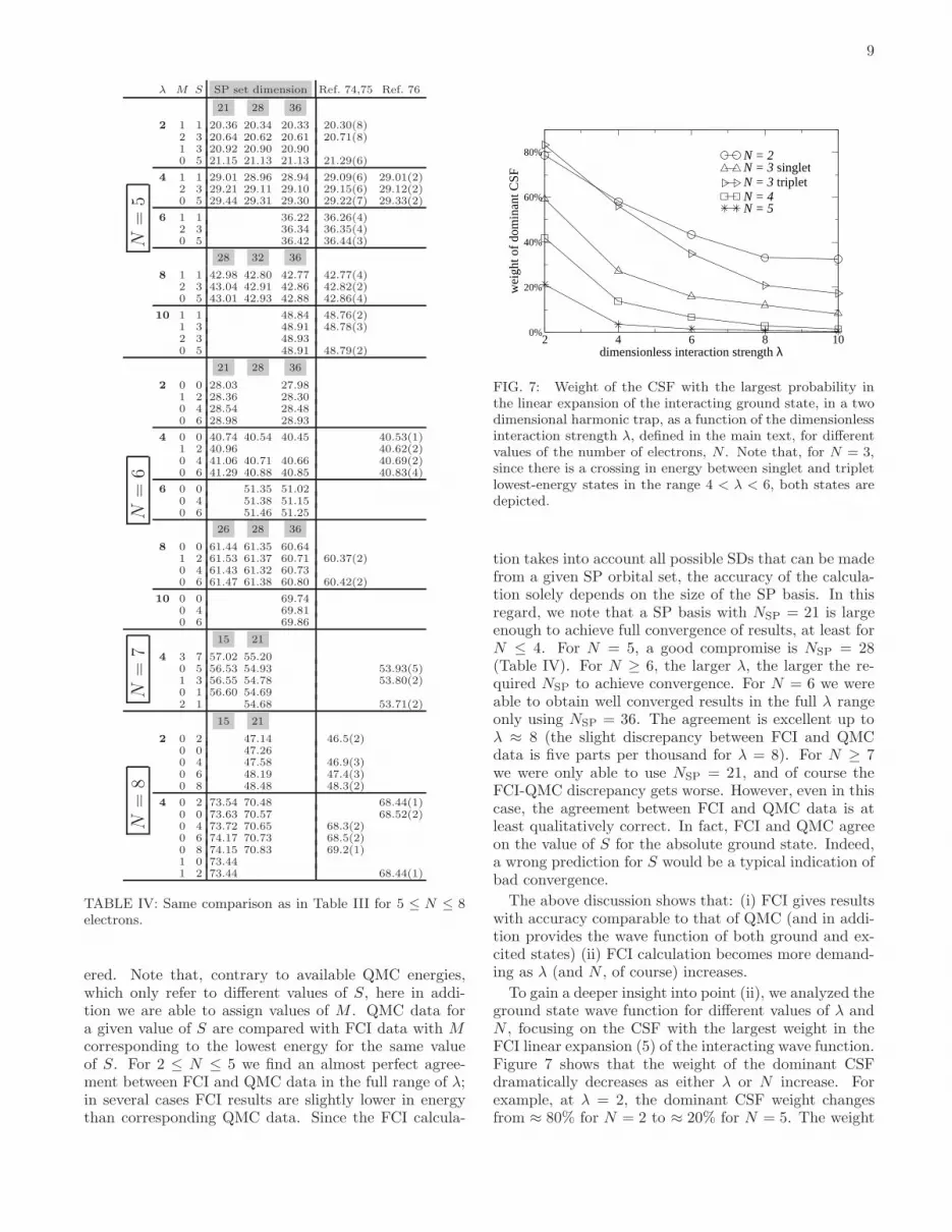
FIG. 7: Weight of the CSF with the largest probability inthe linear expansion of the interacting ground state, in a twodimensional harmonic trap, as a function of the dimensionlessinteraction strength λ, defined in the main text, for differentvalues of the number of electrons, N . Note that, for N = 3,since there is a crossing in energy between singlet and tripletlowest-energy states in the range 4 < λ < 6, both states aredepicted.

tion takes into account all possible SDs that can be madefrom a given SP orbital set, the accuracy of the calcula-tion solely depends on the size of the SP basis. In thisregard, we note that a SP basis with NSP = 21 is largeenough to achieve full convergence of results, at least forN ≤ 4. For N = 5, a good compromise is NSP = 28(Table IV). For N ≥ 6, the larger λ, the larger the re-quired NSP to achieve convergence. For N = 6 we wereable to obtain well converged results in the full λ rangeonly using NSP = 36. The agreement is excellent up toλ ≈ 8 (the slight discrepancy between FCI and QMCdata is five parts per thousand for λ = 8). For N ≥ 7we were only able to use NSP = 21, and of course theFCI-QMC discrepancy gets worse. However, even in thiscase, the agreement between FCI and QMC data is atleast qualitatively correct. In fact, FCI and QMC agreeon the value of S for the absolute ground state. Indeed,a wrong prediction for S would be a typical indication ofbad convergence.

The above discussion shows that: (i) FCI gives resultswith accuracy comparable to that of QMC (and in addi-tion provides the wave function of both ground and ex-cited states) (ii) FCI calculation becomes more demand-ing as λ (and N , of course) increases.

To gain a deeper insight into point (ii), we analyzed theground state wave function for different values of λ andN , focusing on the CSF with the largest weight in theFCI linear expansion (5) of the interacting wave function.Figure 7 shows that the weight of the dominant CSFdramatically decreases as either λ or N increase. Forexample, at λ = 2, the dominant CSF weight changesfrom ≈ 80% for N = 2 to ≈ 20% for N = 5. The weight

10

loss is even more dramatic as λ increases: e.g., for N ≥ 4the decrease is larger than one order of magnitude asλ goes from 2 to 10. This trend clearly illustrates theevolution between two limiting cases: as λ → 0, the dotturns into a non-interacting system, and just one CSF isthe exact eigenstate of the ideal Fermi gas, with weightequal to 100%. What CSF is the ground state is dictatedby the Aufbau principle, according to which the lowest-energy SP orbitals are filled in with N electrons. Asλ → ∞, the system evolves into the limit of completecrystallization: electrons are perfectly localized in space,therefore the SP basis, and consequently the CSF basis,turn out to be extremely ineffective in representing theWigner molecule, unless one uses a special SP basis oflocalized gaussians, or similar kinds of orbitals.

The loss of weight shown in Fig. 7 depends of courseon the chosen SP basis. Therefore we expect that, bymeans of a proper unitary transformation of SP orbitals,like that provided by a self-consistent HF calculation,weights of dominant CSFs will be in general larger thanthose shown in Fig. 7. However, except for a shift ofweight values, the above discussion will not be qualita-tively affected. Note that past experience in HF calcula-tions showed that convergence of the HF self-consistentcycle is not necessarily achieved at low densities.125

Figure 7 also shows that the triplet ground state, forN = 3, is relatively less affected by interaction than thesinglet ground state (see also Fig. 8), namely less CSFsare needed for the triplet than for the singlet in the FCIlinear expansion (5) of the wave function. The reasonis that in the triplet exchange interaction is sufficient tokeep electrons far apart as Coulomb repulsion betweenelectrons increases; the same effect can be obtained forthe singlet only in virtue of a deeper correlation holearound each electron. Such behavior is obtained by mix-ing more CSFs, namely the singlet increases its correla-tion with respect to the triplet.

Not only the dominant CSF loses weight as λ → ∞,but also more and more CSFs are needed to build upthe exact wave function. This is illustrated by Fig. 8,where we show the sum of weights of “significant” CSFsas a function of λ and for different values of N . Hereby “significant CSF” we mean a configuration |ψi〉 whose

weight |ai|2 is larger than 1% [cf. Eq. (5)]. Figure 8clearly demonstrates that, as λ increases, the set of sig-nificant CSFs is progressively emptied. From such resultwe infer that, in regimes of strong correlation, only thefull CI approach is a reliable algorithm. Therefore, cut-off procedures like those of Ref. 93, where the full spaceof SDs is filtered and truncated by considering the ki-netic energy per single SD, are potentially dangerous instrong correlation regimes where they might not be ableto warrant convergence.126

This is illustrated in Table V, where we compare CIresults obtained via two different algorithms. The firstcolumn in Table V shows ground state energies, for2 ≤ λ ≤ 20 andN = 3, 4, obtained from FCI DONRODRIGOruns. Here NSP = 55 was considered, and no cutoff pro-

2 4 6 8 10dimensionless interaction strength λ

0%

20%

40%

60%

80%

100%

tota

l wei

ght o

f C

SFs

abov

e 1%

thre

shol

d

N = 2N = 3 singletN = 3 tripletN = 4N = 5

FIG. 8: Total weight of CSFs whose probability in the linearexpansion of the ground state is larger than 1% as a functionof the dimensionless interaction strength λ for different valuesof N . The system is the same as in Fig. 7.

λ M S DONRODRIGO Refs. 95,96

N=

3

2 1 1 8.1633 8.1651

0 3 8.3217 8.3221

4 1 1 11.0423 11.0422

0 3 11.0527 11.0527

6 1 1 13.4666 13.4658

0 3 13.4380 13.4373

8 1 1 15.6344 15.6334

0 3 15.5948 15.5938

10 1 1 17.6293 17.6279

0 3 17.5877 17.5863

15 1 1 22.1127

0 3 22.0754

20 1 1 26.1184

0 3 26.0863

N=

4

2 0 2 13.6195 13.6180

2 4 14.2544 14.2535

4 0 2 19.0335 19.0323

2 4 19.3578 19.3565

6 0 2 23.5975 23.5958

2 4 23.8041 23.8025

8 0 2 27.6715 27.6696

2 4 27.8222 27.8203

10 0 2 31.4148 31.4120

2 4 31.5352 31.5323

15 0 2 39.8197 39.8163

2 4 39.9054 39.8970

20 0 2 47.3443 47.4002

2 4 47.4153 47.4013

TABLE V: Comparison between different CI calculations forN = 3, 4. FCI ground-state energies (units of hω0) fromDONRODRIGO were obtained using a SP basis set correspondingto the first ten lowest-energy Fock-Darwin shells (55 orbitals)and no truncation of the many-electron space. Results takenfrom Refs. 95,96 were obtained considering a larger number ofSP orbitals but with a cutoff procedure on the kinetic energyper single SD. S is given in units of 1/2.

11

cedure was implemented. The second column collectsdata taken from Refs. 95,96. In those papers NSP > 55but only certain SDs are retained, namely those whosekinetic energy per single SD is smaller than a certaincutoff. For example, in Ref. 95 the largest size of theSD space with N = 4, S = 1, M = 0 (S = 2, M = 2)considered was 24348 (8721) while in our calculation was67225 (15659). The comparison between the two sets ofdata gives excellent agreement, since results systemati-cally have at least four significant digits identical (ener-gies in the second column tend to have a slightly lowerenergy due to the larger NSP which could be used forsuch a small number of electrons). However, there is oneimportant exception, namely at very low density (λ = 20,N = 4, S = 1, M = 0), where our result is 47.34 against47.40. This can be explained by the loss of angular cor-relation once one truncates the SD space as it is done inRef. 95.

VI. NORMAL MODES OF THE WIGNERMOLECULE

In order to illustrate the wealth of information pro-vided by the FCI method with respect to QMC tech-niques, in this section we give an example of excita-tion spectrum calculation. In fact, the access to excitedstates is a difficult task for QMC calculations, which rou-tinely focus on ground-state properties.16 Nevertheless,the knowledge of excited-state energies and wave func-tions is of the utmost interest from both the theoreticaland experimental points of view. Indeed, several usefuldynamical response functions can be computed from ex-cited states. Moreover, many experimental techniquesallow nowadays to access QD excitation spectrum, suchas single-electron non-linear tunneling experiments,13,122

far-infrared spctroscopy,1 inelastic light scattering.12 Inaddition, the theoretical analysis of the energy spectrumgives a precious insight into QD physics.

Figure 9 displays our FCI results for the low-energy re-gion of the excitation spectrum of a six-electron quantumdot in the Wigner regime (λ = 8), for different values ofthe total orbital angular momentum and spin multiplic-ities. The plot of the lowest energies as a function ofthe angular momentum is known as yrast line in nuclearphysics,16 and provides several hints on the crystallizedelectron phase.

We see from Fig. 9 that the ground state is the non-degenerate spin singlet state with M = 0, which isfound to be the lowest-energy state in the whole range0 ≤ λ ≤ 10. The absence of any level crossing as the den-sity is progressively diluted (i.e. λ increases) implies thatthe crystallization process evolves in a continuos manner,consistently with the finite-size character of the system.Nevertheless, several features of Fig. 9 demonstrate theformation of a Wigner molecule in the dot.

First, the three possible spin multiplets other thanS = 0, namely S = 1, 2, 3, lie very close in energy to

0 1 2 3 4 5 6orbital angular momentum M

61

62

ener

gy (

hω0/2

π)

S = 0S = 1S = 2S = 3

FIG. 9: Excitation energies of a six-electron quantum dot inthe Wigner regime (λ = 8) for different values of the totalorbital angular momentum, M , and total spin, S. Energiesare in units of hω0.

the ground state. In general, at the lowest energies forany given M , several spin multiplets in Fig. 9 appear asalmost degenerate.

The overall behavior is well explained by invoking elec-tron crystallization. In the Wigner limit, the Hamilto-nian of the system turns into a classical quantity, sincethe kinetic energy term in it may be neglected with re-spect to the Coulomb term. Therefore, only commutingoperators (the electron positions) appear in the Hamil-tonian. In this regime the spin, which has no classicalcounterpart, becomes irrelevant:109 spin-dependent ener-gies show a tendency to degeneracy. This can also beunderstood in the following way: if electrons sit at somelattice sites with unsubstatial overlap of their localizedwave functions, then the total energy must not dependon the relative orientation of neighboring spins.

Note also that the proximity of the four possible spinmultiplets at the lowest energies occurs for both M = 0and for M = 5. Such a period of five units on the M axisidentifies a magic number,5,127 whose origin is broughtabout by the internal spatial symmetry of the interactingwave function.128 In fact, when electrons form a stableWigner molecule, they arrange themselves into a five-fold

symmetry configuration, where charges are localized atthe corners of a regular pentagon plus one electron at thecenter.15,129,130

A second distinctive signature of crystallization is theappearance of rotational bands,127 which we identify inFig. 9 as those bunches of levels, separated by energygaps of about 0.2hω0, that increase monotonically as Mincreases. We are able to distinguish in Fig. 9 at leastthree bands, where each band is composed of differentspin multiplets. Such bands are called “rotational” sincethey can be identified with the quantized levels Erot(M)

12

of a rigid two-dimensional top, given by the formula

Erot(M) =h2

2IM2,

where I is the moment of inertia of the top.127 Theseexcitations may be thought of as the “normal modes” ofthe Wigner molecule rotating as a whole in the xy planearound the vertical symmetry axis parallel to z.

VII. DISCUSSION

In the previous sections we demonstrated thatDONRODRIGO is a flexible and well performing code, suit-able to treat strongly-correlated few-electron problems inquantum dots to the same degree of accuracy as QMCcalculations. With respect to the latter, the FCI methodalso provides full access to excited states.

A major achievement of DONRODRIGO is the indepen-dence of core routines from both Hamiltonian and SPbasis. Differently from other CI codes, the SP basis isnot optimized by a SCF calculation, before the actualFCI calculation. Of course the FCI results are indepen-dent from the SP basis, but the question arises whethera proper SP basis could improve the efficiency of the FCIcalculation, at the time cost of a preliminary SCF cal-culation. However, the usage of non self-consistent SPorbitals does not seem to be a serious drawback, sinceDONRODRIGO was designed to treat a wide range of differ-ent correlation regimes, especially those for which SCFcalculations are not expected to converge. An exampleof the latter circumstance is the case of very large dots(λ large). Of course in such regime a large SP basis anda full CI diagonalization are both necessary requirements(see discussion in Secs. III and V). Another major advan-tage is the code simple and transparent structure, whichallowed for easy parallelization and straightforward cod-ing of post-processing routines.

Although very efficient also in highly correlatedregimes and with very good scaling properties in parallelarchitectures, our code still lacks some smartnessesof pre-existing quantum chemistry CI codes. Onemajor drawback is the requirement of large amountsof memory, since, for each Hilbert space sector, allmatrix elements 〈Φj |H |Φj′〉 are stored (cf. Sec. II).An alternative strategy is given by so-called direct

methods,30,31,32,33,34,35,38,39,40,41,42,43,44,45,46,47,48,49,50,51,52,53,54,55,56,57,58

where required matrix elements are computed on the

fly during each step of recursive diagonalization ofthe many-electron Hamiltonian. The latter approachconstitutes an interesting direction for future work,together with possible interfaces with other CI codes.

VIII. CONCLUSION

We presented a new high performance full CI codespecifically designed for quantum dot applications. With

respect to previous CI codes, DONRODRIGO is powerfulenough to treat demanding correlation regimes with thesame degree of accuracy as QMC method. In addition,the code provides full information about ground and ex-cited states, its only limitation being the number of elec-trons. Its flexible structure allows for inclusion of dif-ferent device geometries and external fields, plus easypost-processing code development.

DONRODRIGO is available, upon request andon the basis of scientific collaboration, athttp://www.s3.infm.it/donrodrigo.

ACKNOWLEDGMENTS

Andrea Bertoni and Filippo Troiani contributed in arelevant way to the implementation of the SP basis inan arbitrary magnetic field. We acknowledge valuablediscussions with Stefano Corni. This paper is supportedby MIUR-FIRB RBAU01ZEML, miur-cofin 2003020984,INFM Supercomputing Project 2004 and 2005 (Inizia-tiva Trasversale INFM per il Calcolo Parallelo), ItalianMinistry of Foreign Affairs (Ministero degli Affari Esteri,Direzione Generale per la Promozione e la CooperazioneCulturale).

APPENDIX A: CONFIGURATIONAL STATEFUNCTIONS

In this Appendix we illustrate how CSFs are built. Themethod is straightforward, namely one writes the S2 op-erator in a suitable matrix form and diagonalizes it nu-merically, storing the eigenvectors (the Clebsch-Gordancoefficients bij) once and for all. This approach is men-tioned for example in Ref. 60, together with other possi-ble strategies. However, it turns out that the approachis non standard for actual CI code implementations35,and we summarize here the algorithm for completeness.By means of simple examples we show how it is imple-mented in DONRODRIGO, following Slater.68 In this sectionwe distinguish operators from eigenvalues by means of the“hat” symbol.

1. Building the configurational state function space

Let us consider a SP basis made of NSP orbitals. Thecorresponding SDs are built occupying such orbitals withN electrons in all possible ways, taking the two possiblespin orientations into account. NSD =

(2NSP

N

)is the total

number of SDs so obtained; each SD is trivially asso-ciated with an eigenvalue of Sz. Note that many SDsmay be associated to the same value of Sz. The SD set|Φi〉 ≡ |i〉, i = 1, 2, . . . , NSD constitutes a basis for both

operators Sz and H. Therefore, the energy eigenvalues

13

can be obtained by diagonalization of

〈j, Szj | H |i, Szi〉 i, j = 1, . . . , NSD. (A1)

If Szi 6= Szj the matrix element (A1) is zero, i.e., H isblock diagonal in the different Sz sectors. Since bothoperators Sz and S2 commute with the Hamiltonian, aswell as with each other, it is also possible to build a Fockspace whose basis vectors are simultaneously eigenstatesof operators Sz and S2. In this new basis, H has a blockdiagonal representation, labelled by (Sz , S), with dimen-sions of the blocks smaller than in the previous case. Be-low we show how one can find simultaneous eigenstatesof both Sz and S2.

The search of the eigenstates of S2 starting from thoseof Sz can be traced to that of a unitary transformation

|i〉 → |i〉, (A2)

where |i〉 are eigenstates of Sz and |i〉 of Sz and S2 simul-taneously. It is possible to represent the vectors of thesecond basis on those of the first through a suitable linearcombination with (Clebsch-Gordan) coefficients bij ,

|i〉 =

NSD∑

j=1

bij |j〉 , (A3)

under the unitariness condition

NSD∑

j=1

b∗ijblj = δil. (A4)

The problem of finding the Clebsch-Gordan coefficientscan be greatly reduced by considering only the spins ofsingly occupied orbitals, which, in general, are much lessthan the total number of electrons. This is based on thefollowing property: the SDs with only empty or doublyoccupied orbitals are eigenstates of S2 with S = 0. Tosee this, consider the identity (h = 1)

S2 = (Sx + iSy)(Sx − iSy) + S2z − Sz, (A5)

which does not depend on N . Furthermore, let |↑〉 ≡c†↑|0〉 and |↓〉 ≡ c†↓|0〉 denote the spinors related to ageneric orbital. Then the following relations hold:

(Sx − iSy) |↑〉 = |↓〉 ,(Sx + iSy) |↓〉 = |↑〉 ,(Sx − iSy) |↓〉 = 0,

(Sx + iSy) |↑〉 = 0,

Sz |↑〉 = 1/2 |↑〉 ,Sz |↓〉 = −1/2 |↓〉 .

The operator (Sx − iSy) is a step-down operator: whenacting on a given SD, the result is a sum of SDs each

having one of the original up spins turned down. Forexample,

(Sx − iSy) |↑↑↓〉 = |↓↑↓〉 + |↑↓↓〉 , (A6)

where |↑↑↓〉 ≡ c†a↑c†b↑c

†c↓|0〉. Analogously, the operator

(Sx + iSy) is a step-up operator, turning ↓ spins into ↑spins. The above operators in second quantized form, forjust one orbital, are:

(Sx + iSy) ≡ S+ = c†↑c↓,

(Sx − iSy) ≡ S− = c†↓c↑,

Sz = 1/2[c†↑c↑ − c†↓c↓

].

We now consider two electrons on the same orbital. Thecorresponding SD, c†↑c

†↓ |0〉, is an eigenstate of Sz with

Sz = 0. To see that it is also an eigenstate of S2 withS = 0 it is sufficient to apply (A5) using the definition of

S+ and S−. One verifies immediately that

S+S−c†↑c†↓ |0〉 = c†↑c↓c

†↓c↑c

†↑c

†↓ |0〉 = 0. (A7)

In the general case, N electrons are distributed over NSP

orbitals, so that N ≤ 2NSP. The operator S is

S = S(1) + S(2) + . . .+ S(NSP), (A8)

where S(a) ≡ [Sx(a), Sy(a), Sz(a)] acts on the a-th or-bital. Therefore, we can write

S2 =

NSP∑

a,b=1

c†b↑cb↓c†a↓ca↑ + S2

z − Sz. (A9)

Again, we ask whether a generic SD, which is eigenstateof Sz with some orbitals a doubly occupied or otherwiseempty, is also eigenstate of S2. The answer is affirmative,since, in the term S+S− explicited in Eq. (A9), when

first S− acts on the SD, it destroys a spin ↑ in the fulla-th orbital and creates a spin ↓ on the same orbital;

the total contribution of S+S−, however, is zero, sincethe a-th orbital is already occupied by a spin ↓ electron.Therefore, it is proved that the SD is eigenstate of S2

with S = 0.

2. Examples

Let us consider the case of SDs having some singlyoccupied orbitals. For definiteness, let us focus on theexample N = 4 and NSP = 4 (a = 0, . . . , 3), with twoelectrons in orbital 0, zero in 2, and one in each orbital1 and 3, with opposite spin:

|i1〉 = c†0↑c†0↓c

†1↑c

†3↓ |0〉 . (A10)

The operator Sz, explicitly, is

Sz =1

2

3∑

a=0

(c†a↑ca↑ − c†a↓ca↓

). (A11)

14

Evidently, Sz |i1〉 = 0 |i1〉. The goal is to build linearcombinations of SDs, including |i1〉, that are eigenstates

of S2. To this aim one needs to identify all the SDs whichcouple to |i1〉 through the operator S2 and represent S2

in this set. In the present case, it is sufficient to consideronly SDs with Sz = 0. It is possible to establish a prioriwhat these SDs are since they differ from |i1〉 only forthe spin orientation of the electrons on the same singlyoccupied orbitals (1 and 3 in the present example), whilethe doubly occupied or empty orbitals (0 and 2, respec-tively) remain unchanged. This is evident from Eq. (A9),using similar arguments as above; for a formal proof see,e.g., Ref. 35. This way, starting from |i1〉, we build theequivalence class S (of which |i1〉 is the representative)of all SDs having the same doubly occupied and emptyorbitals, and differing only in the spin configurations ofsame singly occupied orbitals, with the same value of Sz.In our example, the only other SD belonging to S is

|i2〉 = c†0↑c†0↓c

†1↓c

†3↑ |0〉 . (A12)

The idea is that we only need to find the Clebsch-Gordan coefficients of the SDs belonging to the sameequivalence class S. In this way we reduce the problemto the vectorial sum of n angular momenta of value 1/2,where n is the number of unpaired electrons, and usuallyn≪ N . We approach this problem by first writing downS2 as a matrix, and then diagonalizing it numerically:the eigenvectors are the requested Clebsch-Gordan coef-ficients. In the case considered above, the two elementsbelonging to S are

|1

↑3

↓ 〉 , |1

↓3

↑ 〉 ,(A13)

where according to the above prescription we only re-fer to the spins of singly occupied orbitals, 1 and 3, asindicated. On this basis, the matrix form of S2, usingEq. (A9), is

(1 1

1 1

), (A14)

whose eigenvalues correspond to the singlet (S = 0) andtriplet (S = 1) states. The corresponding eigenvectorsprovide us the desired Clebsch-Gordan coefficients bij ,i, j = 1, 2 [cf. Eq. (A3)]. Specifically, the eigenstates of

S2 obtained from the SDs belonging to the equivalenceclass S are:

|i1〉 =1√2|i1〉 +

1√2|i2〉 (S = 1), (A15)

|i2〉 =1√2|i1〉 −

1√2|i2〉 (S = 0). (A16)

Note that, for the triplet state S = 1, there are otherCSFs degenerate in energy with Sz = ±1, namely |↑↑〉

and |↓↓〉 (incidentally, the CSFs with S = ±n are alwayssingle SDs). Such CSFs are redundant in applicationsand are ignored by DONRODRIGO. In general, the subspacediagonalization with Sz = 0 (or Sz = 1/2 if n is odd)provides all spin eigenvalues allowed by symmetry. Suchsectors are the only ones considered by the code.

As another example, let us consider the case withNSP = 15 (the SP orbital index runs from 0 to 14) andn = 3 singly occupied orbitals (N can be, of course, muchlarger). Let us now focus on a given SD, e.g.,

c†0↑c†0↓c

†3↑c

†5↑c

†7↑c

†7↓c

†14↓ |0〉

(N = 7). The above SD corresponds to a state withtwo doubly occupied orbitals (0 and 7), two singly oc-cupied orbitals with spin up (3 and the 5), one singlyoccupied orbital with spin down (14). In DONRODRIGO aSD is uniquely identified by a couple of 8-byte integers inbinary representation. The first (second) integer labelsthe spin-up (-down) orbitals: each of the 64 bits repre-sents a SP orbital; if a bit is set to 1 then the orbitalis occupied by one electron. Therefore, the above SD iscoded as

0

1

1

1

0

0

2

0

0

3

1

0

4

0

0

5

1

0

6

0

0

7

1

1

8

0

0

9

0

0

10

0

0

11

0

0

12

0

0

13

0

0

14

0

1

. (A17)

The corresponding equivalence class S uniquely associ-ated to (A17) is coded as

0

0

1

1

0

0

2

0

0

3

1

0

4

0

0

5

1

0

6

0

0

7

0

1

8

0

0

9

0

0

10

0

0

11

0

0

12

0

0

13

0

0

14

1

0

, (A18)

where the first integer labels the singly occupied orbitals:if a bit is set to 1 then the orbital is occupied by oneelectron. The second integer represents doubly occupiedorbitals, using the same convention.

Independently from the number of doubly occupied or-bitals, it will be sufficient to solve the equivalent Clebsch-Gordan problem for the following three determinants,

|3

↑5

↑14

↓ 〉 |3

↓5

↑14

↑ 〉 |3

↑5

↓14

↑ 〉,(A19)

where the first ket, |↑↑↓〉, represents (A17). Note that for

all kets Sz = 1/2. Therefore, we need to diagonalize S2

— a 3 × 3 matrix — as we did with (A14). One obtains3 eigenvalues, 1/2, 1/2, 3/2, and the associated Clebsch-Gordan eigenvectors. Eventually, the equivalence class(A18) is associated with an additional index labellingthe pertinent Clebsch-Gordan eigenspace (in this case,either the quadruplet or one of the two doublets). Thesetwo entities — the equivalence class (A18) and the lattermultiplet index — identify the CSFs.

More generally, a N -electron SD, |i〉, with n′ electronsin doubly occupied orbitals and n in singly occupied or-bitals (n+n′ = N), is uniquely associated with an equiv-alence class Si. The class Si is the same for all and only

15

M S = 0 S = 1 S = 2 S = 3 NSD Si

0 661300 1131738 568896 97976 2459910 190380

1 656476 1123952 564697 97221 2442346 189000

2 643242 1100391 552661 95043 2391337 185624

3 621112 1062496 532877 91493 2307978 179728

4 591897 1011245 506545 86741 2196428 172093

5 555754 949079 474285 80960 2060078 162429

6 514945 877805 437690 74407 1904847 151662

TABLE VI: Partitioning of the SD space into CSF subspacesfor selected values of the total orbital angular momentum M .We consider N = 6 and a SP basis made of Fock-Darwinorbitals corresponding to the first 8 shells (NSP = 36). S isthe total spin, NSD is the dimension of the SD space, and Si isthe number of equivalence classes from which CSFs are built.

those SDs which differ from |i〉 for the spin orientation ofthe n electrons, keeping Sz constant. DONRODRIGO scansthe whole SD space |i〉i exhaustively (i = 1, . . . , NSD),rearranging it as a set of different equivalence classes Si.Within each class Si, the problem is now equivalent tothe vectorial sum of n spins, the maximum possible valueof n (S) being N (N/2). For large values of n, where thesolution of matrices like (A14) is not possible by sim-

ple analytical methods, S2 is diagonalized by a standardnumerical routine. In such a way Clebsch-Gordan coef-ficients up to n = 15 (corresponding to a 6435 × 6435matrix) were obtained and stored. By means of associ-ating each class Si with all possible multiplet indices, allCSFs are built.

As an example taken from an actualapplication,64,65,109 we consider the reduction of themany-electron Hilbert space in our test case (Sec. IIIC)of a 2D harmonic trap with N = 6. Truncating theSP basis to the first 8 shells of Fock-Darwin orbitals(NSP = 36), we first reduce the SD space in blockscorresponding to different values of the total orbitalangular momentum, M (see Table VI). Focusing onM = 0, the dimension of the SD space correspondingto Sz = 0 is NSD = 2459910. From such startingpoint DONRODRIGO extracts 190380 equivalence classes,allowing to build a CSF space divided in singlet (S = 0,dimension 661300), triplet (S = 1, dimension 1131738),quintuplet (S = 2, dimension 568896), and septuplet(S = 3 dimension 97976) sectors, respectively. The sumof sector dimensions is equal to NSD. Table VI is alarger list of CSF subspaces partitioning the initial SDspace for different values of M .

3. Computing matrix elements

Since any state may be written as a linear combina-tion of CSFs |ψi〉, any matrix element of the generic op-

erator O is a linear combination of the matrix elements〈ψi| O |ψi′ 〉. Such elements in turn are computed by ex-

panding the CSFs on the SD basis |Φj〉 [Eq. (7)]:

〈ψi| O |ψi′〉 =∑

jj′

b∗ij bi′j′ 〈Φj | O |Φj′〉 . (A20)

The usage of the binary representation of SDs, as inEq. (A17), allows for extremely efficient bit-per-bit oper-ations when evaluating matrix elements. Consider, e.g.,the matrix element

〈Φf | c†a↑c†b↓cc↓cd↑ |Φi〉 , (A21)

which might represent a term in the Coulomb interaction.The ket

c†a↑c†b↓cc↓cd↑ |Φi〉 (A22)

will differ from |Φi〉 at most in the occupancy of one or-bital with spin up and one with spin down. Translatedinto the binary representation, this implies that in eitherthe spin-up or -down integers identifying the ket (A22),a couple of bits at most will be swapped with respect to|Φi〉, their values being changed from (01) to (10) or viceversa (or no change at all). The matrix element (A21)will differ from zero only if the ket (A22) is equal to |Φf 〉,but for the sign: this is efficiently checked by performinga bit-per-bit xor operation between the same-spin inte-gers representing |Φi〉 and |Φf 〉, respectively. Only if thenumber of resulting bits set to true (after the xor opera-tion per each spin) is equal to 0 or 2, the matrix element(A21) may be non null. Eventually, the sign of (A21)is determined by counting how many bits set to 1 occurbetween those swapped. With those and similar tricksall types of matrix elements are easily evaluated.

The above procedure is especially advantageous forpost-processing,9,12,13,14,15,63,64,65,66,67,109 since the eva-lutation of various matrix elements is particularly trans-parent and simple once physical operators are expressedin their second quantized form.

APPENDIX B: COULOMB MATRIX ELEMENTSOF FOCK-DARWIN STATES FOR THE 2D

HARMONIC TRAP

We report, for the sake of completeness, the explicitexpressions of the Coulomb matrix elements Vabcd re-ferred to Fock-Darwin orbitals (Sec. IIIA), which havebeen used in the calculations of few-electron states in a2D harmonic trap presented in the this paper (Sec. V).For a full derivation see Refs. 131,132.

Since each Fock-Darwin orbital [Eq. (12)] is identifiedby the radial and azimuthal quantum numbers n and m,respectively, the generic Coulomb matrix element is iden-tified by eight indices: Vn1m1,n2m2,n3m3,n4m4

. Amongsuch indices, only seven are independent, in virtue of to-tal orbital angular momentum conservation. The explicit

16

expression is:

Vn1m1,n2m2,n3m3,n4m4= δm1+m2,m3+m4

e2

κℓ

×[

4∏

i=1

ni!

(ni + |mi|)!

]1/2 n∑

(4)j=0

(−1)j1+j2+j3+j4

j1!j2!j3!j4!

×4∏

l=1

(nl + |ml|nl − jl

)2−G/2−1/2

γ∑

(4)ℓ=0

δℓ1+ℓ2,ℓ3+ℓ4

×4∏

t=1

(γt

ℓt

)(−1)γ2+γ3−ℓ2−ℓ3 Γ(Λ/2 + 1)

× Γ([G− Λ + 1] /2) . (B1)

Here, Γ(ξ) denotes the Gamma function and we use thefollowing conventions:

(i) The shorthand

n∑

(4)j=0

≡n1∑

j1=0

n2∑

j2=0

n3∑

j3=0

n4∑

j4=0

has been used.

(ii) The γ’s are defined as:

γ1 = j1 + j4 + (|m1| +m1) /2 + (|m4| −m4) /2,

γ2 = j2 + j3 + (|m2| +m2) /2 + (|m3| −m3) /2,

γ3 = j2 + j3 + (|m2| −m2) /2 + (|m3| +m3) /2,

γ4 = j1 + j4 + (|m1| −m1) /2 + (|m4| +m4) /2.

(iii) G and Λ are defined as:

G = γ1 + γ2 + γ3 + γ4,

Λ = ℓ1 + ℓ2 + ℓ3 + ℓ4.

∗ Electronic address: rontani@unimore.it;URL: http://www.nanoscience.unimo.it/max_index.html

1 L. Jacak, P. Hawrylak, and A. Wojs, Quantum dots(Springer, Berlin, 1998).

2 D. Bimberg, M. Grundmann, and N. N. Ledentsov, Quan-tum dot heterostructures (Wiley, Chichester, 1998).

3 U. Woggon, Optical properties of semiconductor quantumdots (Springer, Berlin, 1997).

4 T. Chakraborty, Quantum dots - A survey of the prop-erties of artificial atoms (North-Holland, Amsterdam,1999).

5 P. A. Maksym and T. Chakraborty, Phys. Rev. Lett. 64,108 (1990).

6 M. A. Kastner, Phys. Today 46, 24 (1993).7 R. Ashoori, Nature (London) 379, 413 (1996).8 S. Tarucha, D. G. Austing, T. Honda, R. J. van der Hage,

and L. P. Kouwenhoven, Phys. Rev. Lett. 77, 3613 (1996).9 M. Rontani, G. Goldoni, and E. Molinari, in New direc-

tions in mesoscopic physics (towards nanoscience), editedby R. Fazio, V. F. Gantmakher, and Y. Imry (Kluwer,Dordrecht, 2003), vol. 125 of NATO Science Series II:Physics and Chemistry, p. 361.

10 M. Rontani, F. Rossi, F. Manghi, and E. Molinari,Appl. Phys. Lett. 72, 957 (1998).

11 G. W. Bryant, Phys. Rev. Lett. 59, 1140 (1987).12 C. P. Garcıa, V. Pellegrini, A. Pinczuk, M. Rontani,

G. Goldoni, E. Molinari, B. S. Dennis, L. N. Pfeiffer, andK. W. West, Phys. Rev. Lett. 95, 266806 (2005).

13 M. Rontani, S. Amaha, K. Muraki, F. Manghi, E. Moli-nari, S. Tarucha, and D. G. Austing, Phys. Rev. B 69,85327 (2004).

14 M. Rontani, F. Troiani, U. Hohenester, and E. Molinari,Solid State Commun. 119, 309 (2001), special Issue onSpin Effects in Mesoscopic Systems.

15 M. Rontani, G. Goldoni, F. Manghi, and E. Molinari,

Europhys. Lett. 58, 555 (2002).16 S. M. Reimann and M. Manninen, Rev. Mod. Phys. 74,

1283 (2002).17 G. Goldoni, F. Troiani, M. Rontani, D. Bellucci, E. Moli-

nari, and U. Hohenester, in Quantum Dots: Fundamen-tals, Applications, and Frontiers, edited by B. A. Joyce,P. Kelires, A. Naumovets, and D. D. Vvedensky (Springer,2005), vol. 190 of NATO Science Series II: Mathematics,Physics and Chemistry, p. 269.

18 H. Grabert and M. H. Devoret, Single charge tunneling:Coulomb blockade phenomena in nanostructures (Plenum,New York, 1992), vol. 294 of NATO ASI series B: physics.

19 Y. Arakawa and H. Sakaki, Appl. Phys. Lett. 40, 939(1982).

20 N. Kirstaedter, N. N. Ledentsov, M. Grundmann, D. Bim-berg, V. M. Ustinov, S. S. Ruvimov, M. V. Maximov, P. S.Kopev, Z. I. Alferov, U. Richter, et al., Electron. Lett. 30,1416 (1994).

21 H. L. Edwards, Q. Niu, G. A. Georgakis, and A. L.de Lozanne, Phys. Rev. B 52, 5714 (1995).

22 X. Michalet, F. F. Pinaud, L. A. Bentolila, J. M. Tsay,S. Doose, J. J. Li, G. Sundaresan, A. M. Wu, S. S. Gamb-hir, and S. Weiss, Science 307, 538 (2005).

23 R. E. Bailey, A. M. Smith, and S. Nie, Physica E 25, 1(2004).

24 D. Loss and D. P. DiVincenzo, Phys. Rev. A 57, 120(1998).

25 F. Troiani, U. Hohenester, and E. Molinari, Phys. Rev. B62, RC2263 (2000).

26 E. Biolatti, R. C. Iotti, P. Zanardi, and F. Rossi, Phys.Rev. Lett. 85, 5647 (2000).

27 G. Bastard, Wave mechanics applied to semiconductorheterostructures (Les Editions de Physique, Les Ulis,France, 1998).

28 P. Y. Yu and M. Cardona, Fundamentals of semiconduc-

17

tors (Springer, Berlin, 1996).29 L.-W. Wang and A. Zunger, Phys. Rev. B 59, 15806

(1999).30 C. W. Bauschlicher, S. R. Langhoff, and P. R. Taylor,

Adv. Chem. Phys. 77, 103 (1990).31 K. Raghavachari and J. B. Anderson, J. Phys. Chem. 100,

12960 (1996).32 I. Shavitt, Mol. Phys. 94, 3 (1998).33 C. D. Sherril and H. F. Schaefer, Advances in Quantum

Chemistry 34, 143 (1999).34 F. Jensen, Introduction to computational chemistry (Wi-

ley, Chichester, 1999).35 T. Helgaker, P. Jørgensen, and J. Olsen, Molecular

electronic-structure theory (Wiley, Chichester, 2000).36 DONRODRIGO is available, upon request and

on the basis of scientific cooperation, athttp://www.s3.infm.it/donrodrigo.

37 The only CI calculation in QDs exploting S2 symmetrywe are aware of is Ref. 133.

38 B. Roos, Chem. Phys. Lett. 15, 153 (1972).39 P. E. M. Siegbahn, Chem. Phys. Lett. 109, 417 (1984).40 P. J. Knowles and N. C. Handy, Chem. Phys. Lett. 111,

315 (1984).41 C. W. Bauschlicher, Theo. Chim. Acta 71, 263 (1987).42 J. Olsen, B. O. Roos, P. Jørgensen, and H. J. A. Jensen,

J. Chem. Phys. 89, 2185 (1988).43 P. J. Knowles and N. C. Handy, J. Chem. Phys. 91, 2396

(1989).44 R. J. Harrison, J. Chem. Phys. 94, 5021 (1991).45 R. Caballol and J. P. Malrieu, Chem. Phys. Lett. 188,

543 (1992).46 A. Povill, R. Caballol, J. Rubio, and J. P. Malrieu,

Chem. Phys. Lett. 209, 126 (1993).47 T. Sakai and K. Tanaka, Theo. Chim. Acta 85, 451 (1993).48 J. P. Daudey, J. L. Heully, and J. P. Malrieu,

J. Chem. Phys. 99, 1240 (1993).49 P. G. Szalay and R. J. Bartlett, J. Chem. Phys. 103, 3600

(1995).50 M. Hanrath and B. Engels, Chem. Phys. 225, 197 (1997).51 F. Stephan and W. Wenzel, J. Chem. Phys. 108, 1015

(1998).52 N. Ben Amor and D. Maynau, Chem. Phys. Lett. 286,

211 (1998).53 P. Stampfuß, W. Wenzel, and H. Keiter, J. Comp. Chem.

20, 1559 (1999).54 P. Stampfuß, K. Hamacher, and W. Wenzel,

J. Mol. Struct. 506, 99 (2000).55 R. Ansaloni, G. L. Bendazzoli, S. Evangelisti, and

E. Rossi, Comp. Phys. Commun. 128, 496 (2000).56 H. Lischka, R. Shepard, R. M. Pitzer, I. Shavitt, M. Dal-

los, T. Muller, P. G. Szalay, M. Seth, G. S. Kedziora,S. Yabushita, et al., Phys. Chem. Chem. Phys. 3, 664(2001).

57 J. Ivanic, J. Chem. Phys. 119, 9364 (2003).58 P. Stampfuß and W. Wenzel, J. Chem. Phys. 122, 024110

(2005).59 L. D. Landau and E. M. Lifshitz, Quantum mechanics –

Non relativistic theory (Pergamon Press, Oxford, 1958).60 R. Pauncz, Spin eigenfunctions – Construction and use

(Plenum Press, New York, 1979).61 R. McWeeny, Methods of molecular quantum mechanics

(Academic Press, London, 1992).62 R. B. Lehoucq, K. Maschhoff, D. C. Sorensen, and

C. Yang, ARPACK computer code (1997), available at

http://www.caam.rice.edu/software/ARPACK/.63 D. Bellucci, M. Rontani, F. Troiani, G. Goldoni, and

E. Molinari, Phys. Rev. B 69, RC201308 (2004).64 M. Rontani and E. Molinari, Phys. Rev. B 71, 233106

(2005).65 M. Rontani and E. Molinari, Jp. J. Appl. Phys. 45 (2006),

available as cond-mat/0507688.66 A. Bertoni, M. Rontani, G. Goldoni, F. Troiani, and

E. Molinari, Appl. Phys. Lett. 85, 4729 (2004).67 A. Bertoni, M. Rontani, G. Goldoni, and E. Molinari,

Phys. Rev. Lett. 95, 066806 (2005).68 J. C. Slater, Quantum theory of molecules and solids,

Vol. 1 (McGraw-Hill, New York, 1963).69 M. Brasken, M. Lindberg, D. Sundholm, and J. Olsen,

Phys. Rev. B 61, 7652 (2000).70 S. Corni, M. Brasken, M. Lindberg, J. Olsen, and

D. Sundholm, Phys. Rev. B 67, 45313 (2003).71 B. R. Bennett, B. V. Shanabrook, P. M. Thibado, L. J.

Whitman, and R. Magno, J. Cryst. Growth 175/176, 888(1997).

72 D. Bellucci, M. Rontani, G. Goldoni, F. Troiani, andE. Molinari, Physica E 22, 482 (2004).

73 D. Bellucci, F. Troiani, G. Goldoni, and E. Molinari,Phys. Rev. B 70, 205332 (2004).

74 R. Egger, W. Hausler, C. H. Mak, and H. Grabert, Phys.Rev. Lett. 82, 3320 (1999).

75 R. Egger, W. Hausler, C. H. Mak, and H. Grabert, Phys.Rev. Lett. 83, E462 (1999).

76 B. Reusch and R. Egger, Europhys. Lett. 64, 84 (2003).77 R. B. Lehoucq and J. A. Scott (1996), preprint MCS-

P547-1195, Argonne National Laboratory, available atftp://info.mcs.anl.gov/pub/tech reports/reports/P547.ps.Z.

78 U. Merkt, J. Huser, and M. Wagner, Phys. Rev. B 43,7320 (1991).

79 D. Pfannkuche, V. Gudmundsson, and P. A. Maksym,Phys. Rev. B 47, 2244 (1993).

80 P. Hawrylak, Phys. Rev. Lett. 71, 3347 (1993).81 A. H. MacDonald and M. D. Johnson, Phys. Rev. Lett.

70, 3107 (1993).82 S.-R. E. Yang, A. H. MacDonald, and M. D. Johnson,

Phys. Rev. Lett. 71, 3194 (1993).83 J. J. Palacios, L. Martın-Moreno, G. Chiappe, E. Louis,

and C. Tejedor, Phys. Rev. B 50, 5760 (1993).84 D. Pfannkuche and S. E. Ulloa, Phys. Rev. Lett. 74, 1194

(1995).85 A. Wojs and P. Hawrylak, Phys. Rev. B 53, 10841 (1996).86 P. A. Maksym, Phys. Rev. B 53, 10871 (1996).87 N. A. Bruce and P. A. Maksym, Phys. Rev. B 61, 4718

(2000).88 L. P. Kouwenhoven, T. H. Oosterkamp, M. W. S. Danoe-

sastro, M. Eto, D. G. Austing, T. Honda, and S. Tarucha,Science 278, 1788 (1997).

89 M. Eto, Jpn. J. Appl. Phys. 36, 3924 (1997).90 T. Ezaki, N. Mori, and C. Hamaguchi, Phys. Rev. B 56,

6428 (1997).91 E. Goldmann and S. R. Renn, Phys. Rev. B 60, 16611

(1999).92 C. E. Creffield, W. Hausler, J. H. Jefferson, and S. Sarkar,

Phys. Rev. B 59, 10719 (1999).93 S. M. Reimann, M. Koskinen, and M. Manninen, Phys.

Rev. B 62, 8108 (2000).94 M. Manninen, M. Koskinen, S. M. Reimann, and B. Mot-

telson, Eur. Phys. J. D 16, 381 (2001).95 S. A. Mikhailov, Phys. Rev. B 66, 153313 (2002).

18

96 S. A. Mikhailov, Phys. Rev. B 65, 115312 (2002).97 S.-R. E. Yang and A. H. MacDonald, Phys. Rev. B 66,

R041304 (2002).98 A. D. Guclu, Q. F. Sun, H. Guo, and R. Harris, Phys.

Rev. B 66, 195327 (2002).99 A. D. Guclu, J.-S. Wang, and H. Guo, Phys. Rev. B 68,

035304 (2003).100 M.-C. Cha and S.-R. E. Yang, Phys. Rev. B 67, 205312

(2003).101 M. B. Tavernier, E. Anisimovas, F. M. Peeters, B. Szafran,

J. Adamowski, and S. Bednarek, Phys. Rev. B 68, 205305(2003).

102 C. Yannouleas and U. Landman, Phys. Rev. B 68, 035326(2003).

103 M.-H. Chung, Phys. Rev. B 70, 113302 (2004).104 E. Anisimovas, A. Matulis, M. B. Tavernier, and F. M.

Peeters, Phys. Rev. B 69, 075305 (2004).105 B. Szafran, F. M. Peeters, S. Bednarek, and

J. Adamowski, Phys. Rev. B 69, 125344 (2004).106 B. Szafran, F. M. Peeters, and S. Bednarek, Phys. Rev.

B 70, 205318 (2004).107 M. Korkusinski, P. Hawrylak, M. Ciorga, M. Pioro-

Ladriere, and A. S. Sachrajda, Phys. Rev. Lett. 93,206806 (2004).

108 M. Manninen, S. M. Reimann, M. Koskinen, Y. Yu, andM. Toreblad, Phys. Rev. Lett. 94, 106405 (2005).

109 M. Rontani, C. Cavazzoni, and G. Goldoni, ComputerPhysics Commun. 169, 430 (2005).

110 J. J. Palacios and P. Hawrylak, Phys. Rev. B 51, 1769(1995).

111 J. H. Oh, K. J. Chang, G. Ihm, and S. J. Lee, Phys. Rev.B 53, R13264 (1996).

112 H. Imamura, P. A. Maksym, and H. Aoki, Phys. Rev. B53, 12613 (1996).

113 H. Imamura, H. Aoki, and P. A. Maksym, Phys. Rev. B57, R4257 (1998).

114 H. Imamura, P. A. Maksym, and H. Aoki, Phys. Rev. B59, 5817 (1999).

115 Y. Tokura, D. G. Austing, and S. Tarucha, J. Phys.: Con-dens. Matter 11, 6023 (1999).

116 Y. Tokura, S. Sasaki, D. G. Austing, and S. Tarucha,Physica E 6, 676 (2000).

117 L. Martın-Moreno, L. Brey, and C. Tejedor, Phys. Rev. B62, R10633 (2000).

118 H. Hu and S. Das Sarma, Physical Review A 64, 042312(2001).

119 A. Harju, S. Siljamaki, and R. M. Nieminen, Phys. Rev.Lett. 88, 226804 (2002).

120 D. Jacob, B. Wunsch, and D. Pfannkuche, Phys. Rev. B70, R081314 (2004).

121 B. Wunsch, D. Jacob, and D. Pfannkuche, Physica E 26,464 (2005).

122 T. Ota, M. Rontani, S. Tarucha, Y. Nakata, H. Z. Song,T. Miyazawa, T. Usuki, M. Takatsu, and N. Yokoyama,Phys. Rev. Lett. 95, 236801 (2005).

123 C. Yannouleas and U. Landman, Phys. Rev. Lett. 82,5325 (1999).

124 F. Pederiva, C. J. Umrigar, and E. Lipparini, Phys. Rev.B 62, 8120 (2000).

125 M. Rontani, F. Rossi, F. Manghi, and E. Molinari, Phys.Rev. B 59, 10165 (1999).

126 Indeed, authors of Ref. 93 were not able to investigate thefull λ range since they used a serial CI code with strongpower and memory limitations.

127 M. Koskinen, M. Manninen, B. Mottelson, and S. M.Reimann, Phys. Rev. B 63, 205323 (2001).

128 W. Y. Ruan, Y. Y. Liu, C. G. Bao, and Z. Q. Zhang,Phys. Rev. B 51, 7942 (1995).

129 F. Bolton and U. Rossler, Superlatt. Microstruct. 13, 139(1993).

130 V. M. Bedanov and F. M. Peeters, Phys. Rev. B 49, 2667(1994).

131 E. Anisimovas and A. Matulis, J. Phys.: Condens. Matter10, 601 (1998).

132 M. Rontani, Ph.D. thesis, University of Modena and Reg-gio Emilia, Via Campi 213A 41100 Modena Italy (1999),available at http://www.nanoscience.unimo.it.

133 A. Wensauer, M. Korkusinski, and P. Hawrylak, SolidState Commun. 130, 115 (2004).