from photos to models - sparc
TRANSCRIPT
From Photos to Models
Strategies for using digital photogrammetry in your project
Adam Barnes Katie Simon Adam Wiewel
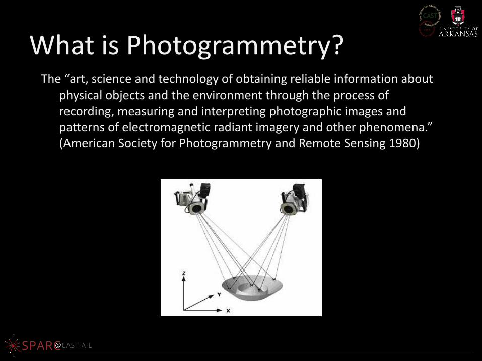
What is Photogrammetry? The “art, science and technology of obtaining reliable information about
physical objects and the environment through the process of recording, measuring and interpreting photographic images and patterns of electromagnetic radiant imagery and other phenomena.” (American Society for Photogrammetry and Remote Sensing 1980)
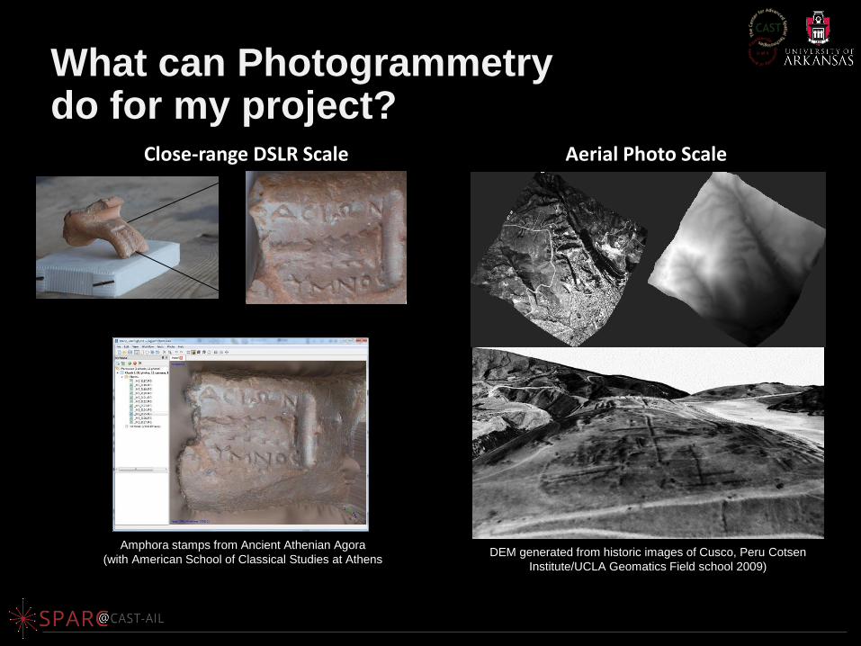
DEM generated from historic images of Cusco, Peru Cotsen
Institute/UCLA Geomatics Field school 2009)
Aerial Photo Scale Close-range DSLR Scale
Amphora stamps from Ancient Athenian Agora
(with American School of Classical Studies at Athens
What can Photogrammetry do for my project?
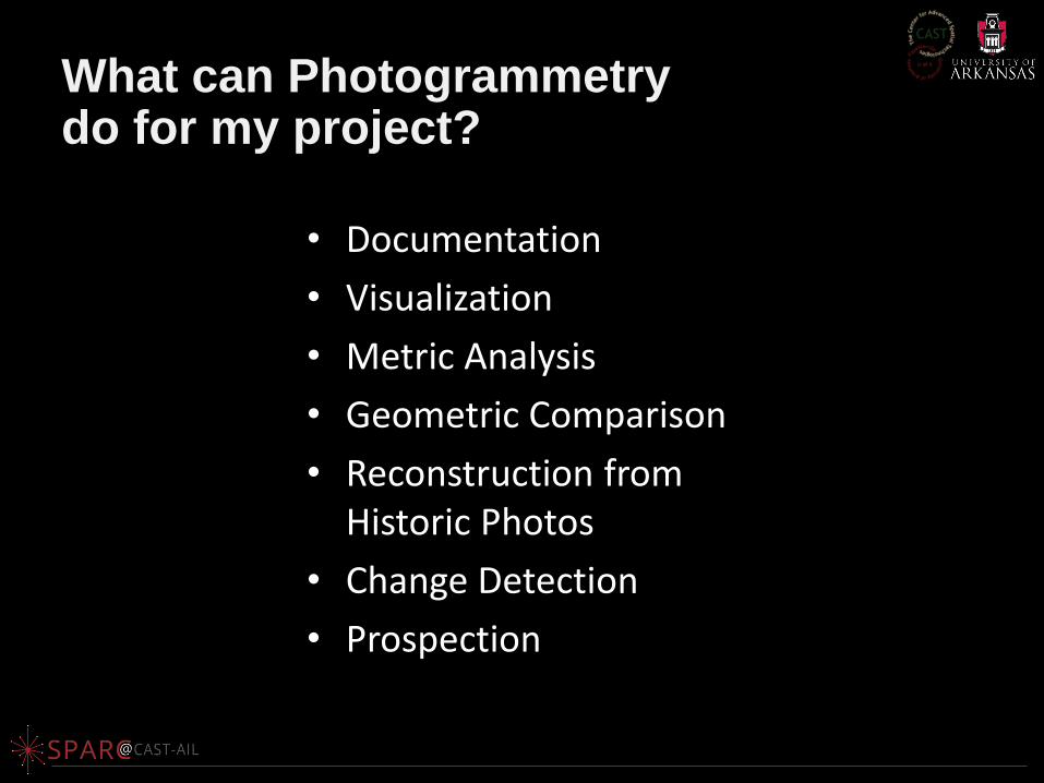
What can Photogrammetry do for my project?
• Documentation
• Visualization
• Metric Analysis
• Geometric Comparison
• Reconstruction from Historic Photos
• Change Detection
• Prospection
A LITTLE BACKGROUND
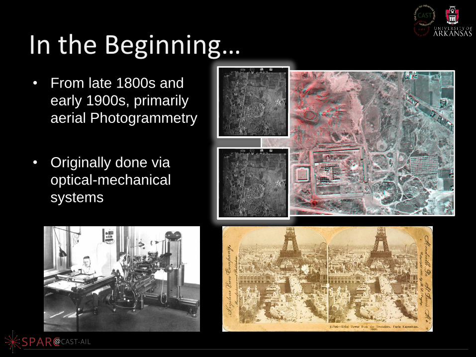
In the Beginning… • From late 1800s and
early 1900s, primarily
aerial Photogrammetry
• Originally done via
optical-mechanical
systems
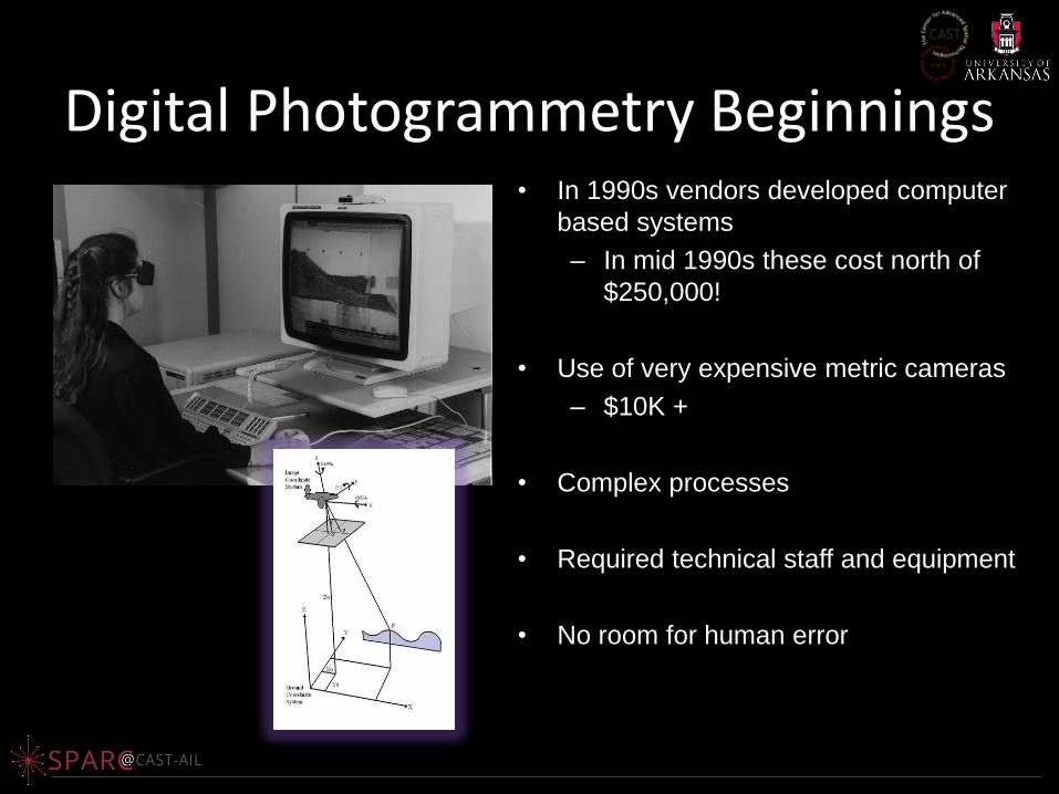
Digital Photogrammetry Beginnings • In 1990s vendors developed computer
based systems
– In mid 1990s these cost north of
$250,000!
• Use of very expensive metric cameras
– $10K +
• Complex processes
• Required technical staff and equipment
• No room for human error
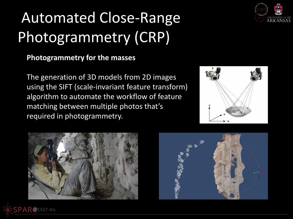
Automated Close-Range Photogrammetry (CRP)
Photogrammetry for the masses The generation of 3D models from 2D images using the SIFT (scale-invariant feature transform) algorithm to automate the workflow of feature matching between multiple photos that’s required in photogrammetry.
How does automated CRP it work?
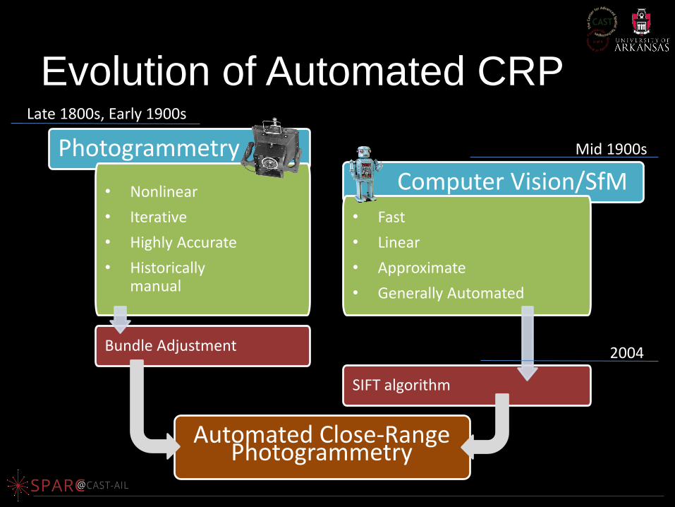
Automated Close-Range
Photogrammetry
• Nonlinear
• Iterative
• Highly Accurate
• Historically manual
Bundle Adjustment
Late 1800s, Early 1900s
Mid 1900s
• Fast
• Linear
• Approximate
• Generally Automated
Evolution of Automated CRP
SIFT algorithm
2004
Computer Vision/SfM
Photogrammetry
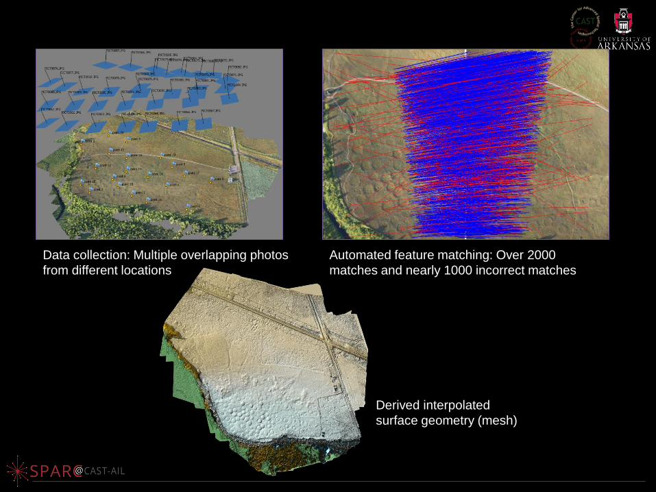
Automated feature matching: Over 2000
matches and nearly 1000 incorrect matches
Data collection: Multiple overlapping photos
from different locations
Derived interpolated
surface geometry (mesh)
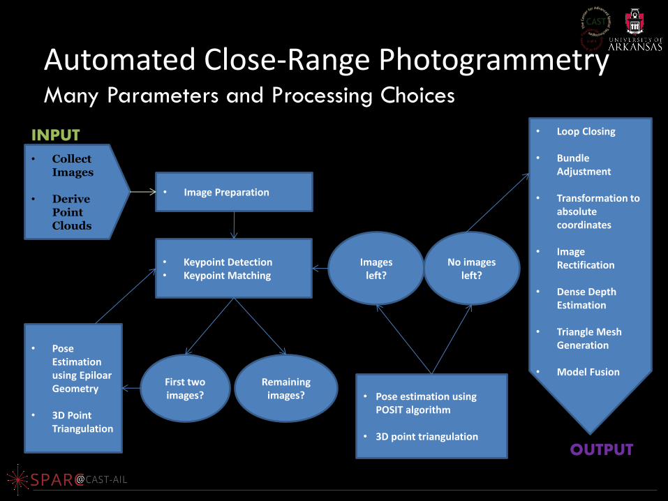
• Collect Images
• Derive Point Clouds
• Image Preparation
• Keypoint Detection • Keypoint Matching
• Pose Estimation using Epiloar Geometry
• 3D Point Triangulation
First two images?
Images left?
No images left?
• Pose estimation using POSIT algorithm
• 3D point triangulation
Remaining images?
• Loop Closing
• Bundle
Adjustment
• Transformation to absolute coordinates
• Image Rectification
• Dense Depth Estimation
• Triangle Mesh Generation
• Model Fusion
INPUT
OUTPUT
Automated Close-Range Photogrammetry Many Parameters and Processing Choices
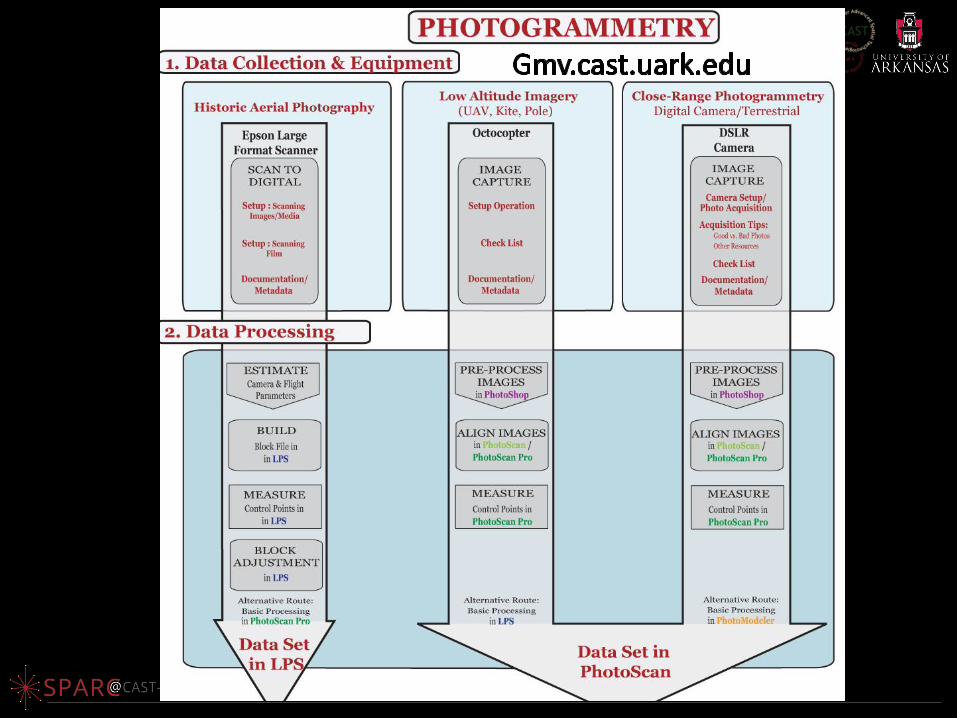
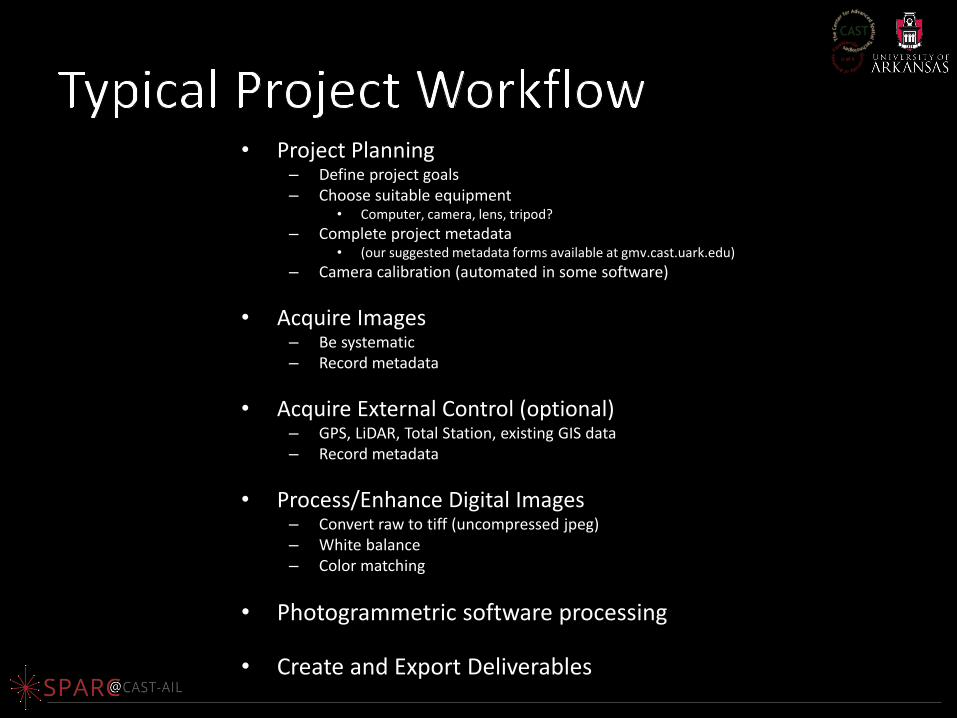
• Project Planning
– Define project goals – Choose suitable equipment
• Computer, camera, lens, tripod?
– Complete project metadata • (our suggested metadata forms available at gmv.cast.uark.edu)
– Camera calibration (automated in some software)
• Acquire Images – Be systematic – Record metadata
• Acquire External Control (optional) – GPS, LiDAR, Total Station, existing GIS data – Record metadata
• Process/Enhance Digital Images – Convert raw to tiff (uncompressed jpeg) – White balance – Color matching
• Photogrammetric software processing
• Create and Export Deliverables
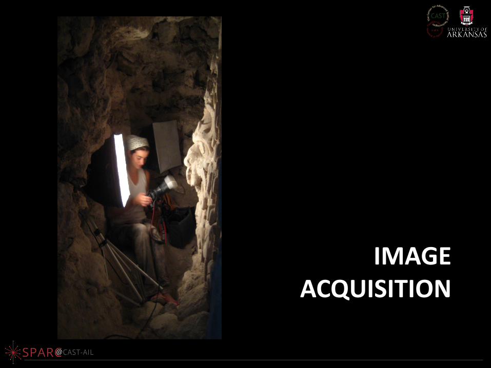
IMAGE ACQUISITION
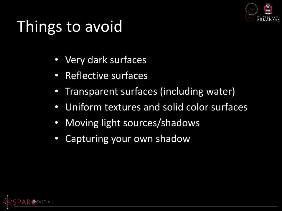
Things to avoid
• Very dark surfaces
• Reflective surfaces
• Transparent surfaces (including water)
• Uniform textures and solid color surfaces
• Moving light sources/shadows
• Capturing your own shadow
• Contiguous photos with 80% overlap
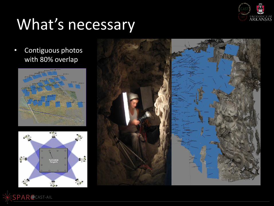
What’s necessary
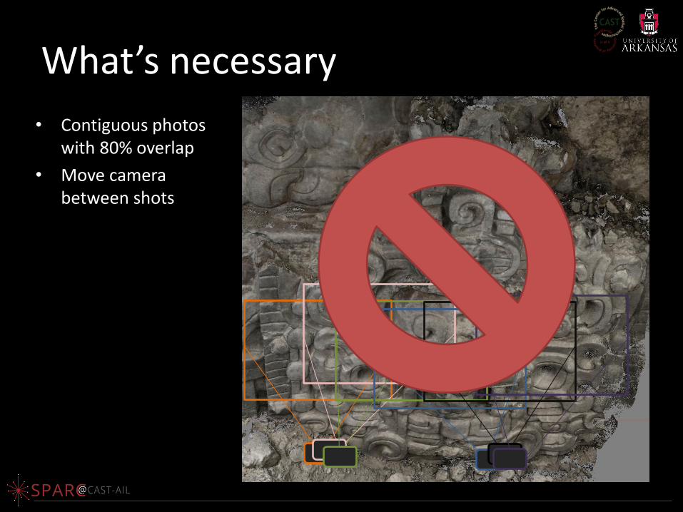
• Contiguous photos with 80% overlap
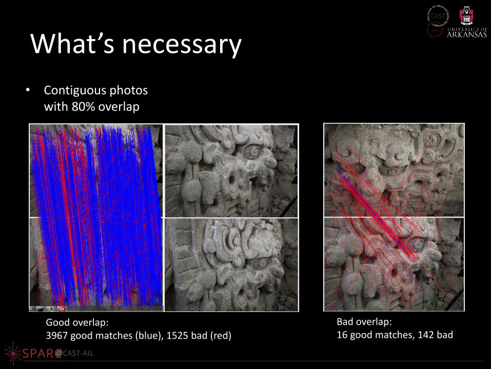
What’s necessary
Good overlap: 3967 good matches (blue), 1525 bad (red)
Bad overlap: 16 good matches, 142 bad
• Contiguous photos with 80% overlap
• Move camera between shots
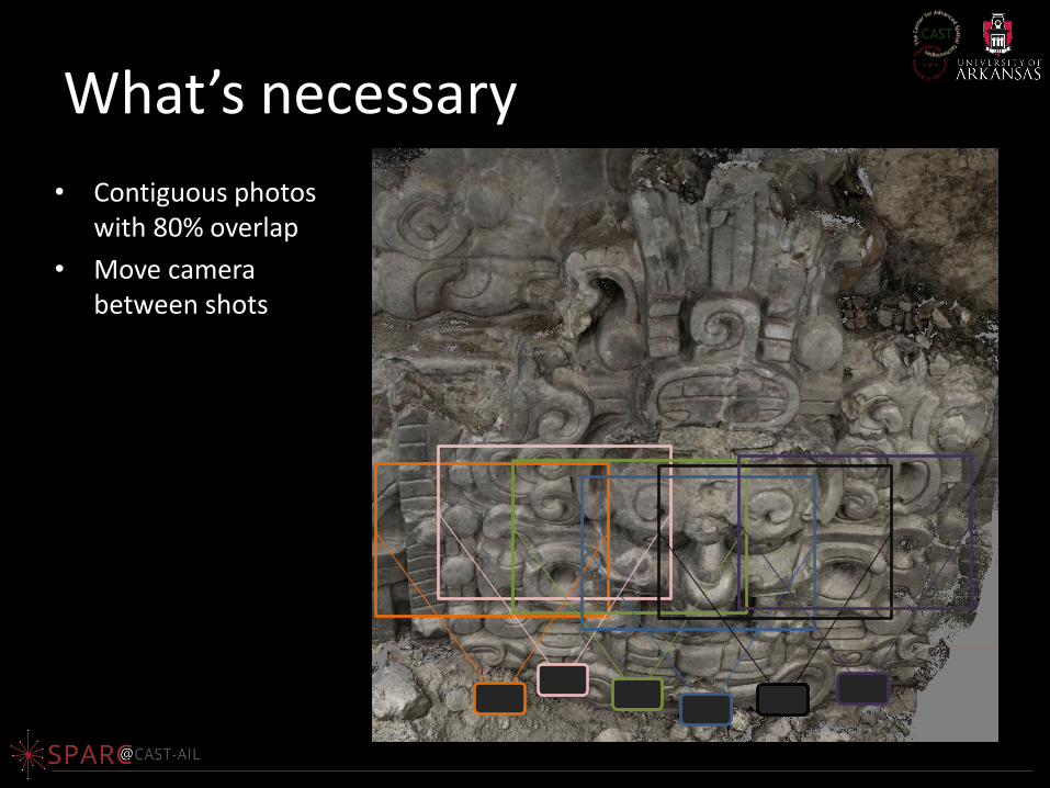
What’s necessary
• Contiguous photos with 80% overlap
• Move camera between shots
What’s necessary
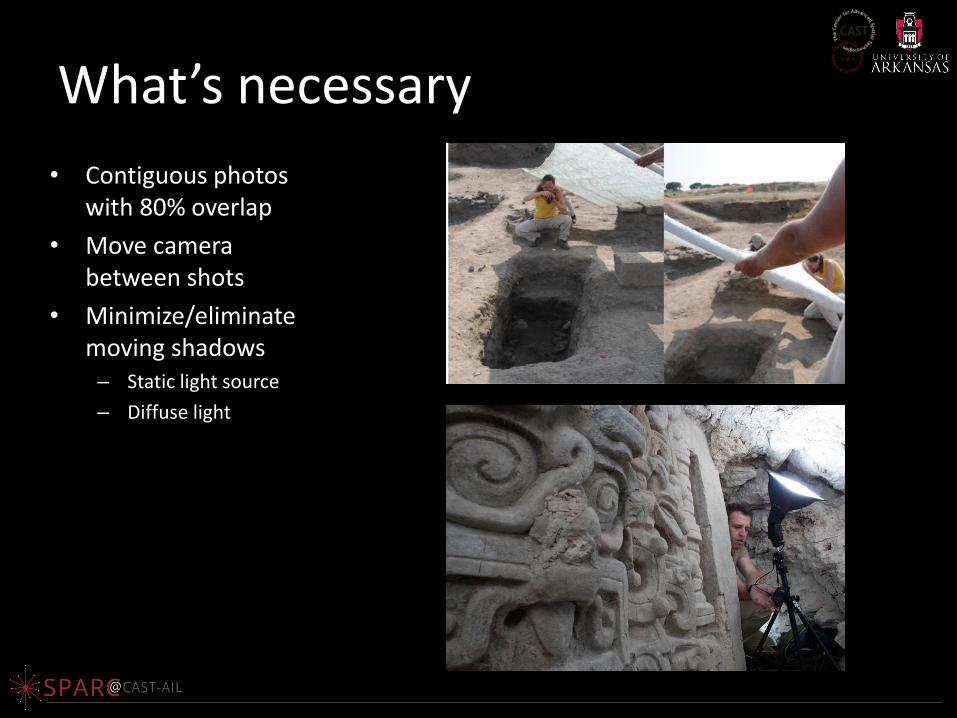
• Contiguous photos with 80% overlap
• Move camera between shots
• Minimize/eliminate moving shadows
– Static light source
– Diffuse light
What’s necessary
• Contiguous photos with 80% overlap
• Move camera between shots
• Minimize/eliminate moving shadows
– Static light source
– Diffuse light
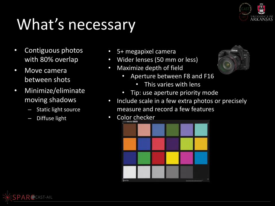
What’s necessary
• 5+ megapixel camera • Wider lenses (50 mm or less) • Maximize depth of field
• Aperture between F8 and F16 • This varies with lens
• Tip: use aperture priority mode • Include scale in a few extra photos or precisely
measure and record a few features • Color checker
Will my camera work?
“A metric camera is a general term applicable to a camera which has been designed as a survey camera and possessing a well defined inner orientation. That is a camera possessing a good lens with a wide field of view and small distortion, a calibrated principal distance and in which the position of the principal point can be located in the image plane by reference to fiducial marks. The picture format is normally fairly large and the film is flattened in the focal plane at the instant of photography. Cameras not possessing these characteristics can be defined as simple or non metric Cameras.”
– Adams, L.P., 1980. The Use of Non Metric Cameras in Short Range Photogrammetry. 14th Congress of the
International Society for Photogrammetry, Commission V, Hamburg, Germany.
It is around this time (1980) that non-metric cameras were established as a suitable tool for close-range photogrammetry, and that the accuracy of projects using non-metric cameras could equal those using metric cameras.
– Karara, H.M., and W. Faig, 1980. An Expose on Photographic Data Aquisition Systems in Close-Range
Photogrammetry. 14th Congress of the International Society for Photogrammetry, Commission V, Hamburg, Germany.
Metric vs Non-Metric
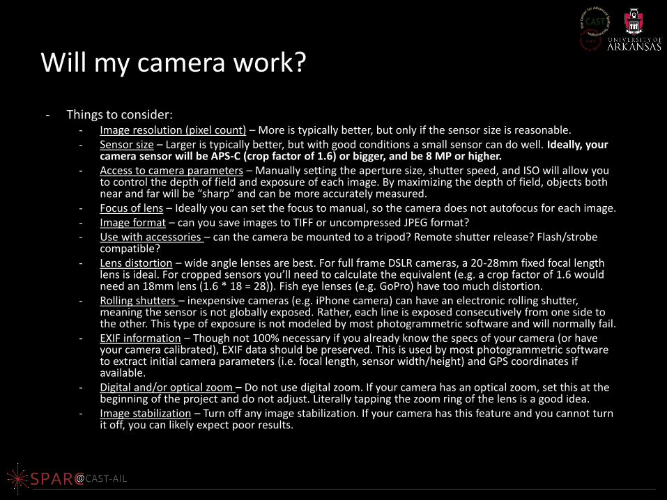
Will my camera work?
- Things to consider: - Image resolution (pixel count) – More is typically better, but only if the sensor size is reasonable. - Sensor size – Larger is typically better, but with good conditions a small sensor can do well. Ideally, your
camera sensor will be APS-C (crop factor of 1.6) or bigger, and be 8 MP or higher. - Access to camera parameters – Manually setting the aperture size, shutter speed, and ISO will allow you
to control the depth of field and exposure of each image. By maximizing the depth of field, objects both near and far will be “sharp” and can be more accurately measured.
- Focus of lens – Ideally you can set the focus to manual, so the camera does not autofocus for each image. - Image format – can you save images to TIFF or uncompressed JPEG format? - Use with accessories – can the camera be mounted to a tripod? Remote shutter release? Flash/strobe
compatible? - Lens distortion – wide angle lenses are best. For full frame DSLR cameras, a 20-28mm fixed focal length
lens is ideal. For cropped sensors you’ll need to calculate the equivalent (e.g. a crop factor of 1.6 would need an 18mm lens (1.6 * 18 = 28)). Fish eye lenses (e.g. GoPro) have too much distortion.
- Rolling shutters – inexpensive cameras (e.g. iPhone camera) can have an electronic rolling shutter, meaning the sensor is not globally exposed. Rather, each line is exposed consecutively from one side to the other. This type of exposure is not modeled by most photogrammetric software and will normally fail.
- EXIF information – Though not 100% necessary if you already know the specs of your camera (or have your camera calibrated), EXIF data should be preserved. This is used by most photogrammetric software to extract initial camera parameters (i.e. focal length, sensor width/height) and GPS coordinates if available.
- Digital and/or optical zoom – Do not use digital zoom. If your camera has an optical zoom, set this at the beginning of the project and do not adjust. Literally tapping the zoom ring of the lens is a good idea.
- Image stabilization – Turn off any image stabilization. If your camera has this feature and you cannot turn it off, you can likely expect poor results.
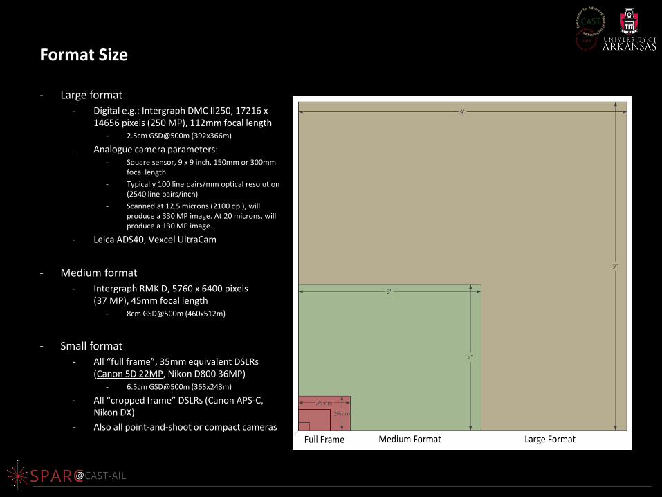
Format Size
- Large format
- Digital e.g.: Intergraph DMC II250, 17216 x 14656 pixels (250 MP), 112mm focal length
- 2.5cm GSD@500m (392x366m)
- Analogue camera parameters: - Square sensor, 9 x 9 inch, 150mm or 300mm
focal length
- Typically 100 line pairs/mm optical resolution (2540 line pairs/inch)
- Scanned at 12.5 microns (2100 dpi), will produce a 330 MP image. At 20 microns, will produce a 130 MP image.
- Leica ADS40, Vexcel UltraCam
- Medium format
- Intergraph RMK D, 5760 x 6400 pixels (37 MP), 45mm focal length
- 8cm GSD@500m (460x512m)
- Small format
- All “full frame”, 35mm equivalent DSLRs (Canon 5D 22MP, Nikon D800 36MP)
- 6.5cm GSD@500m (365x243m)
- All “cropped frame” DSLRs (Canon APS-C, Nikon DX)
- Also all point-and-shoot or compact cameras
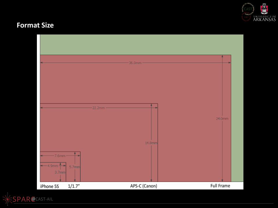
Format Size
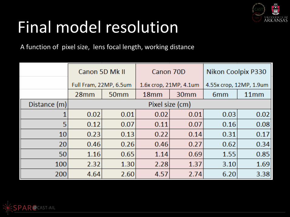
Final model resolution A function of pixel size, lens focal length, working distance
DATA PROCESSING
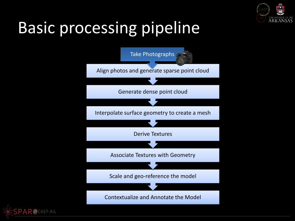
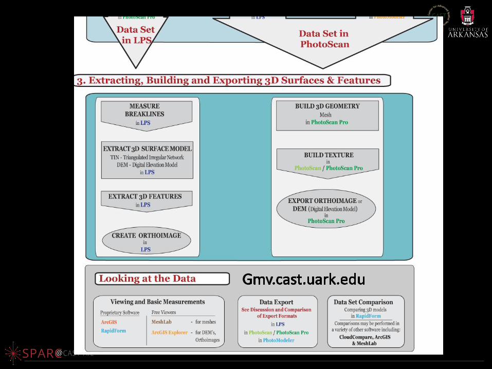
Basic processing pipeline
Contextualize and Annotate the Model
Scale and geo-reference the model
Associate Textures with Geometry
Derive Textures
Interpolate surface geometry to create a mesh
Generate dense point cloud
Align photos and generate sparse point cloud
Take Photographs
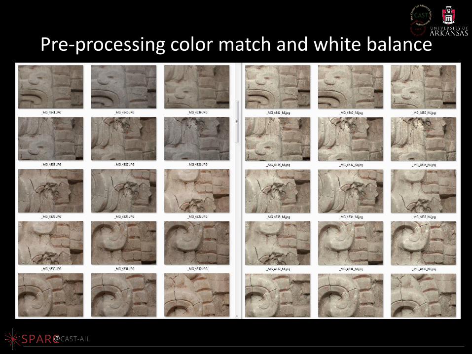
Pre-processing color match and white balance
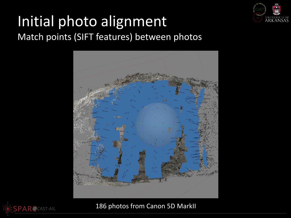
Initial photo alignment Match points (SIFT features) between photos
186 photos from Canon 5D MarkII
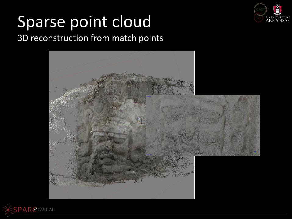
Sparse point cloud 3D reconstruction from match points
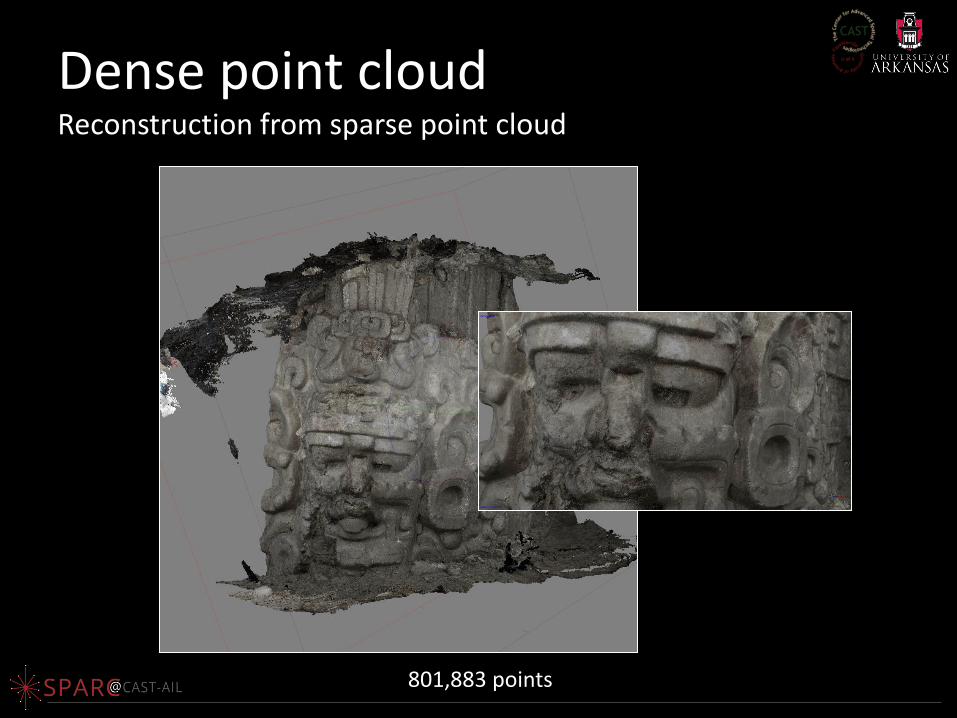
Dense point cloud Reconstruction from sparse point cloud
801,883 points
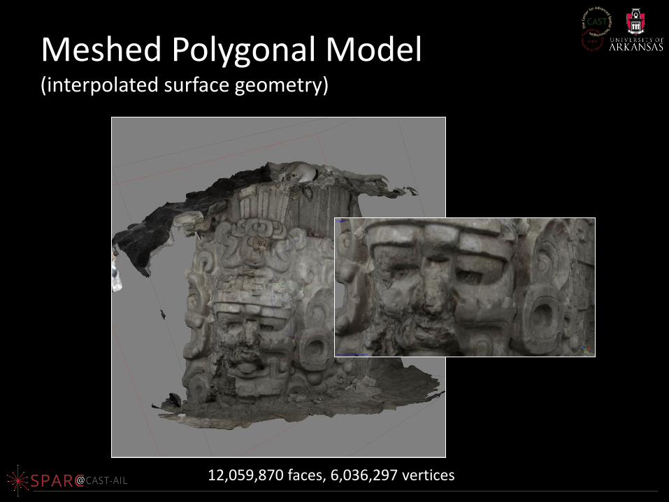
Meshed Polygonal Model (interpolated surface geometry)
12,059,870 faces, 6,036,297 vertices
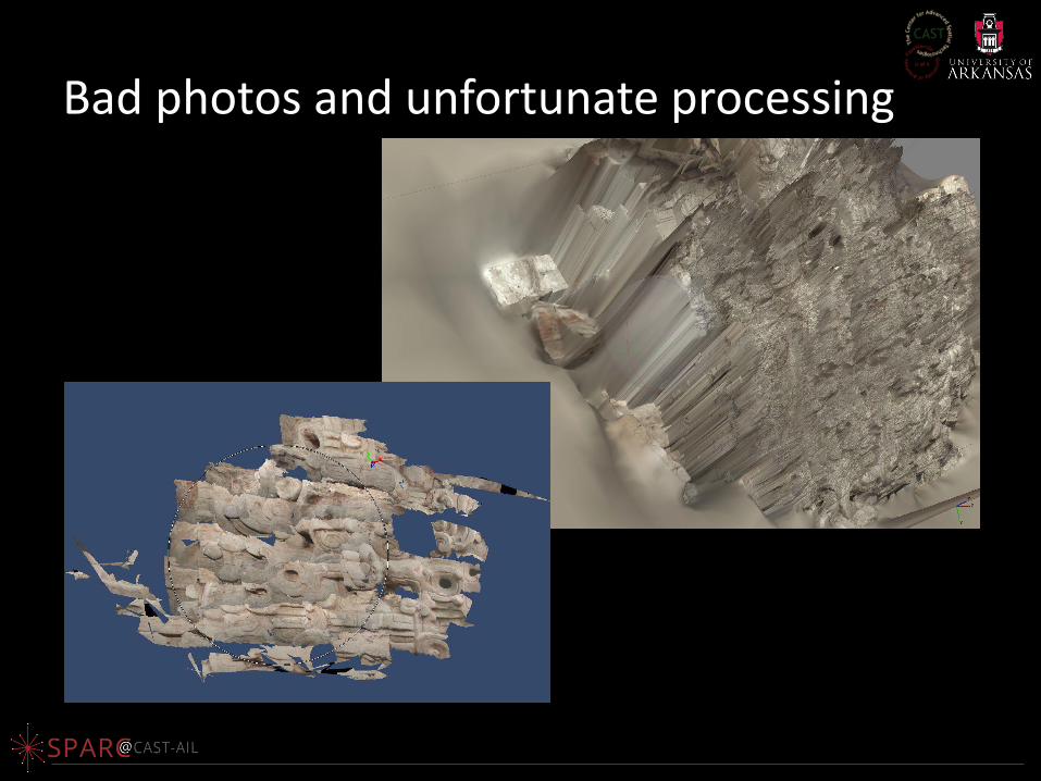
Bad photos and unfortunate processing
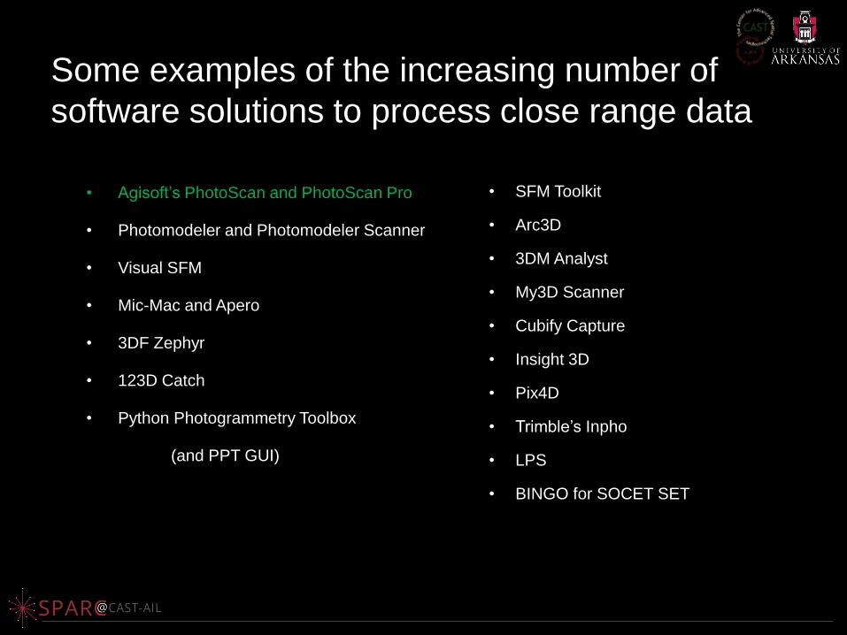
Some examples of the increasing number of
software solutions to process close range data
• Agisoft’s PhotoScan and PhotoScan Pro
• Photomodeler and Photomodeler Scanner
• Visual SFM
• Mic-Mac and Apero
• 3DF Zephyr
• 123D Catch
• Python Photogrammetry Toolbox
(and PPT GUI)
• SFM Toolkit
• Arc3D
• 3DM Analyst
• My3D Scanner
• Cubify Capture
• Insight 3D
• Pix4D
• Trimble’s Inpho
• LPS
• BINGO for SOCET SET
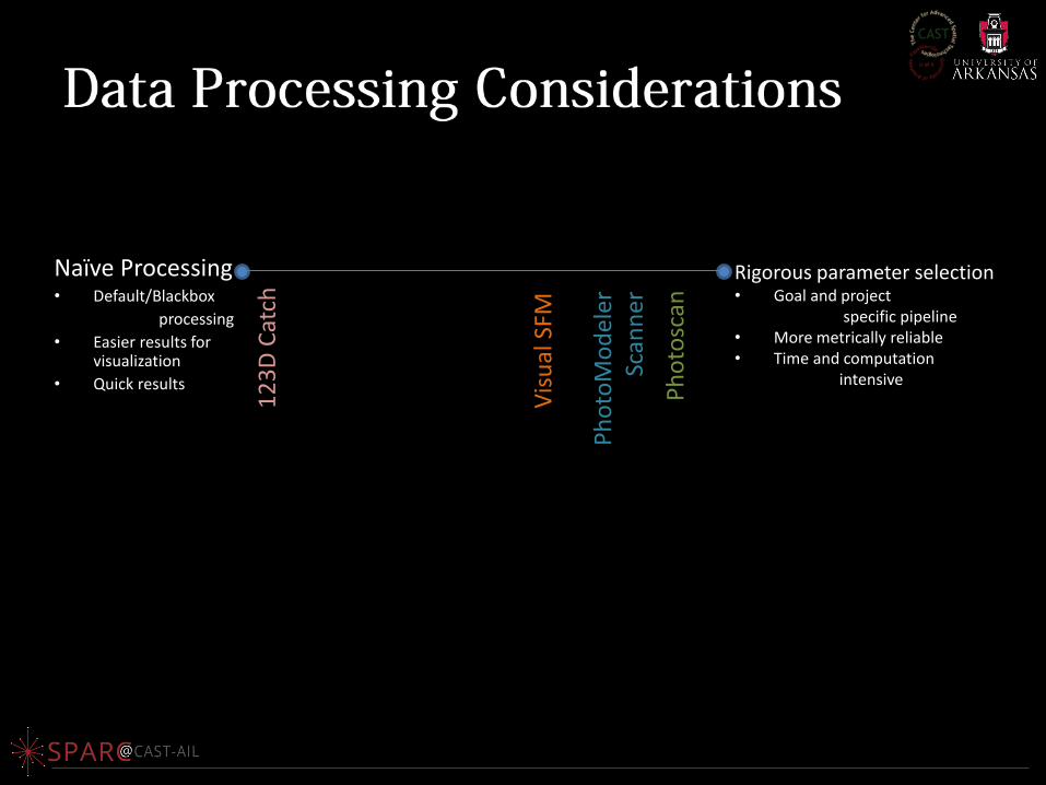
Naïve Processing • Default/Blackbox
processing
• Easier results for visualization
• Quick results
Rigorous parameter selection • Goal and project specific pipeline • More metrically reliable • Time and computation intensive
Vis
ual
SFM
Ph
oto
scan
12
3D
Cat
ch
Ph
oto
Mo
del
er
Scan
ner
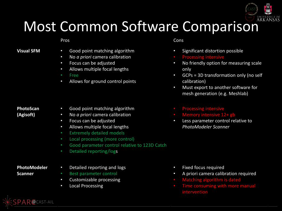
Most Common Software Comparison Pros Cons
Visual SFM • Good point matching algorithm • No a priori camera calibration • Focus can be adjusted • Allows multiple focal lengths • Free • Allows for ground control points
• Significant distortion possible • Processing intensive • No friendly option for measuring scale
only • GCPs = 3D transformation only (no self
calibration) • Must export to another software for
mesh generation (e.g. Meshlab)
PhotoScan (Agisoft)
• Good point matching algorithm • No a priori camera calibration • Focus can be adjusted • Allows multiple focal lengths • Extremely detailed models • Local processing (more control) • Good parameter control relative to 123D Catch • Detailed reporting/logs
• Processing intensive • Memory intensive 12+ gb • Less parameter control relative to
PhotoModeler Scanner
PhotoModeler Scanner
• Detailed reporting and logs • Best parameter control • Customizable processing • Local Processing
• Fixed focus required • A priori camera calibration required • Matching algorithm is dated • Time consuming with more manual
intervention
HOW ACCURATE IS IT? SOFTWARE COMPARISONS
With high precision 3D scanner model comparisons
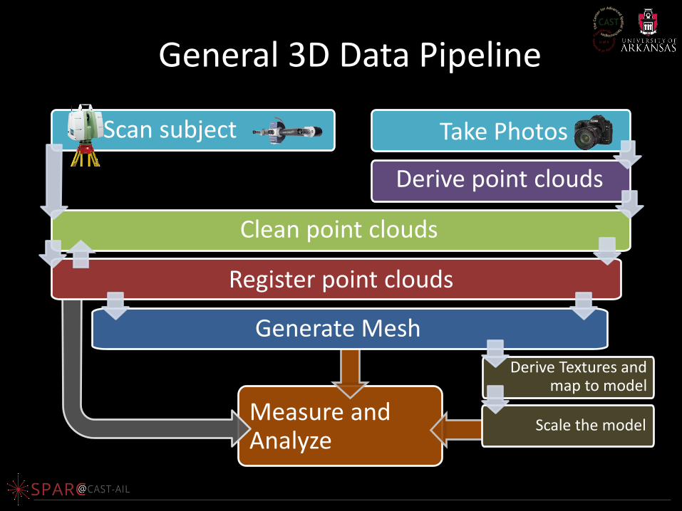
Measure and Analyze
Scan subject
Generate Mesh
General 3D Data Pipeline
Derive point clouds
Clean point clouds
Register point clouds
Derive Textures and map to model
Scale the model
Take Photos
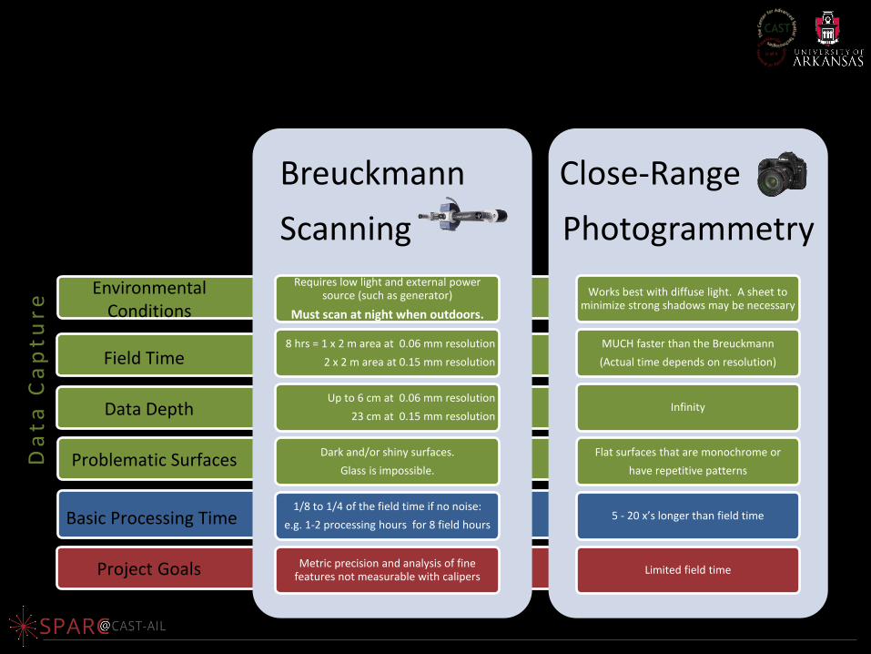
Breuckmann
Scanning
Requires low light and external power source (such as generator)
Must scan at night when outdoors.
8 hrs = 1 x 2 m area at 0.06 mm resolution
2 x 2 m area at 0.15 mm resolution
Up to 6 cm at 0.06 mm resolution
23 cm at 0.15 mm resolution
Dark and/or shiny surfaces.
Glass is impossible.
1/8 to 1/4 of the field time if no noise:
e.g. 1-2 processing hours for 8 field hours
Metric precision and analysis of fine features not measurable with calipers
Close-Range
Photogrammetry
Works best with diffuse light. A sheet to minimize strong shadows may be necessary
MUCH faster than the Breuckmann
(Actual time depends on resolution)
Infinity
Flat surfaces that are monochrome or
have repetitive patterns
5 - 20 x’s longer than field time
Limited field time
Field Time
Project Goals
Problematic Surfaces Da
ta C
ap
ture
Basic Processing Time
Environmental Conditions
Data Depth
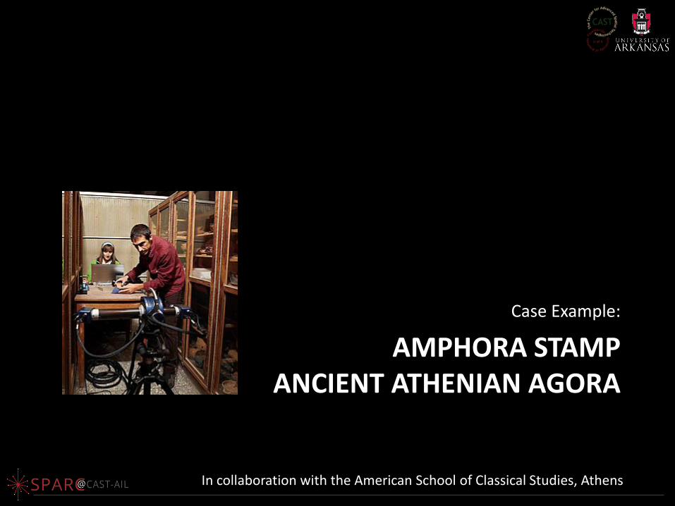
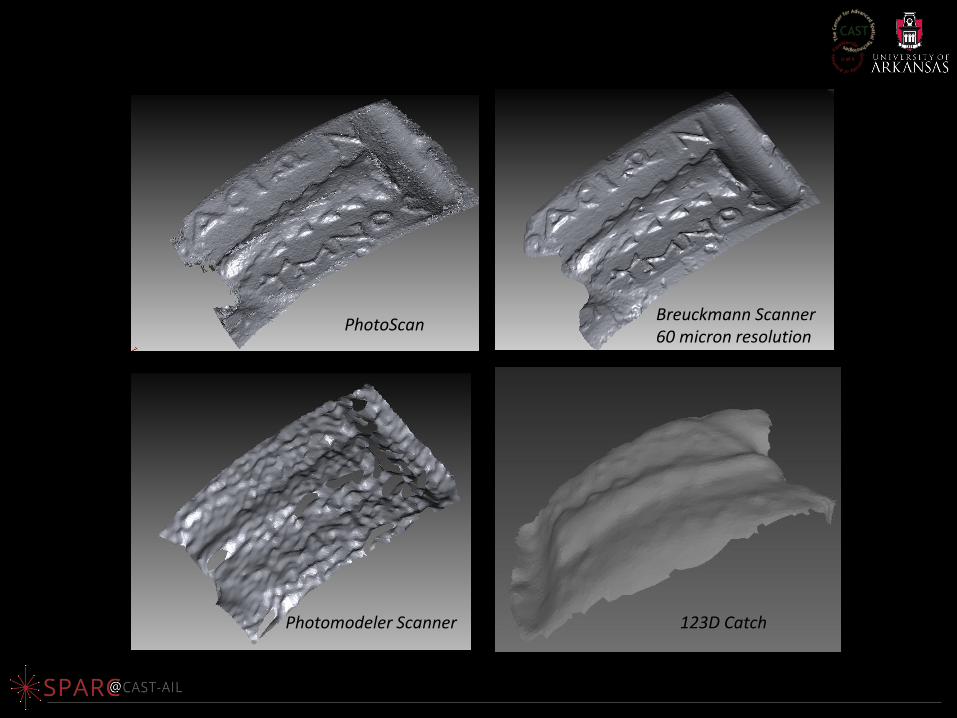
AMPHORA STAMP ANCIENT ATHENIAN AGORA
Case Example:
In collaboration with the American School of Classical Studies, Athens
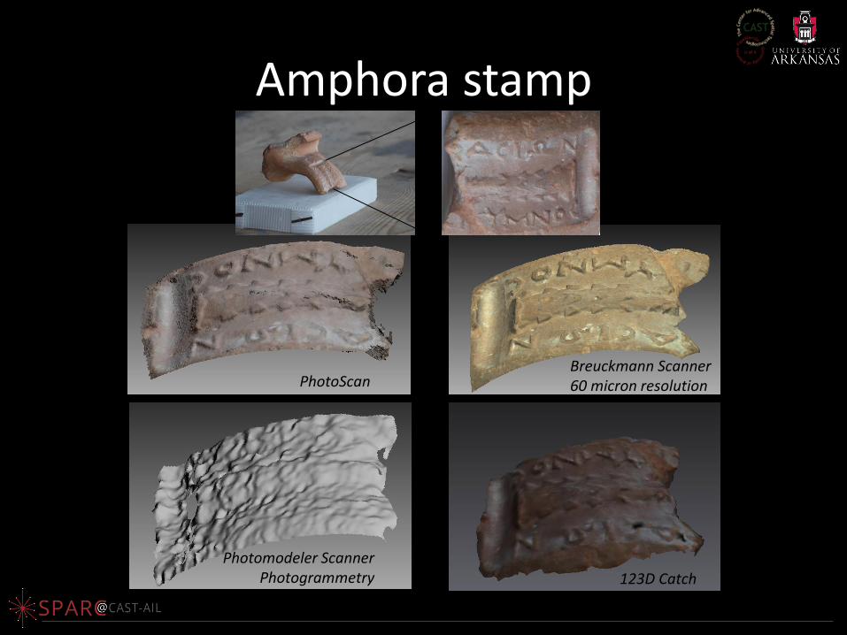
Amphora stamp
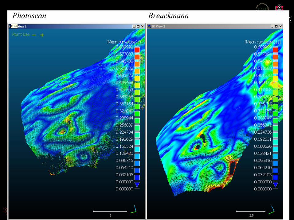
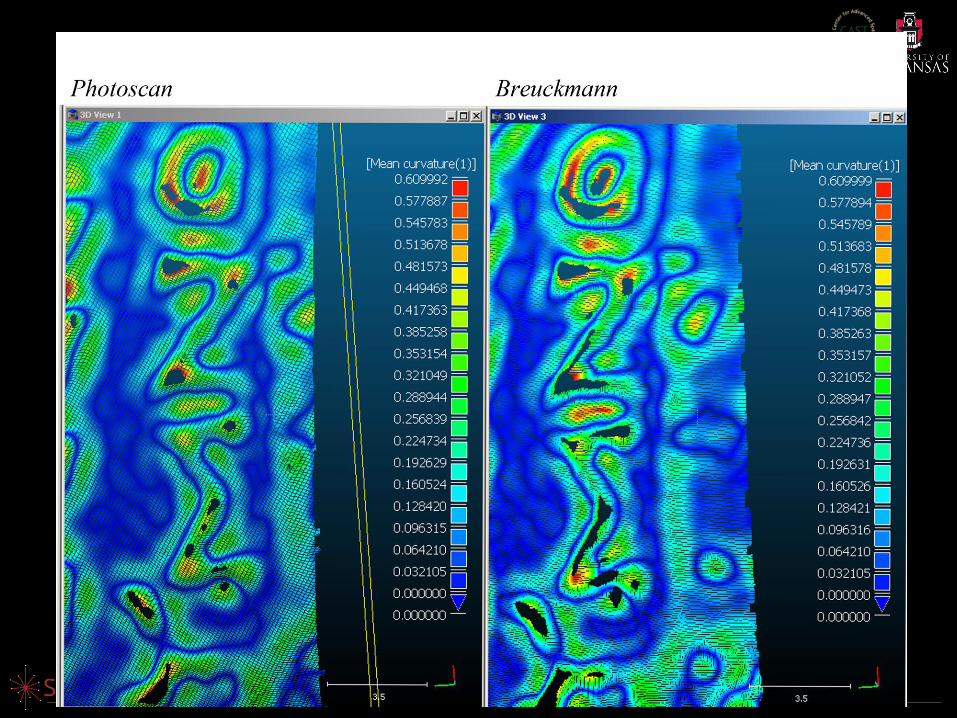
PhotoScan Breuckmann Scanner 60 micron resolution
Photomodeler Scanner Photogrammetry 123D Catch
123D Catch
PhotoScan
Photomodeler Scanner
Color Stripped Meshes
Breuckmann Scanner 60 micron resolution
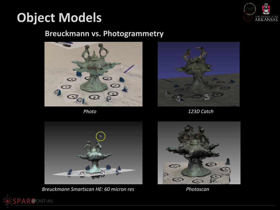
Breuckmann Smartscan HE: 60 micron res Photoscan
123D Catch
Object Models Breuckmann vs. Photogrammetry
Photo
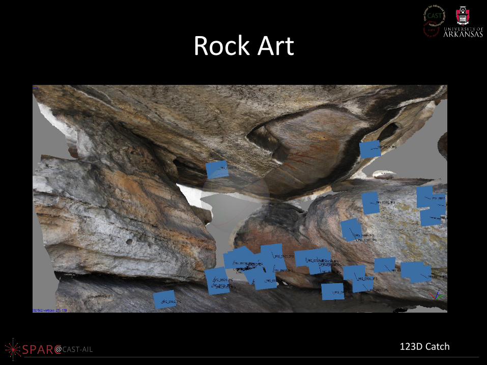
Rock Art
123D Catch
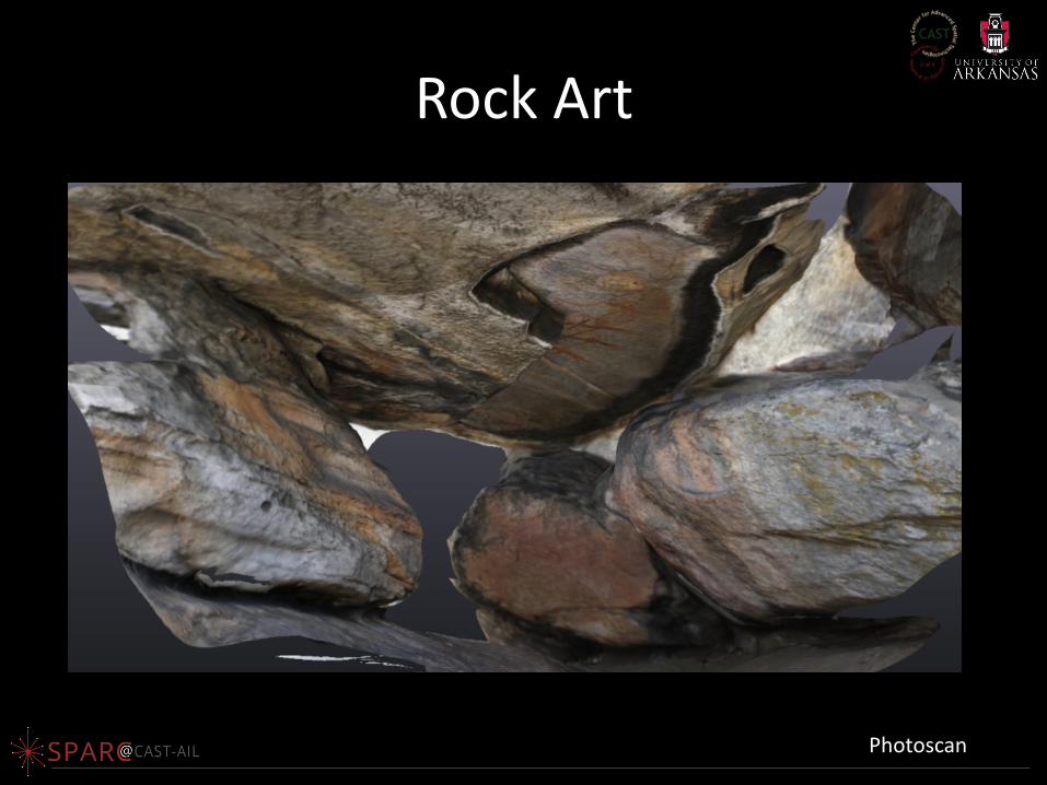
Rock Art
Photoscan
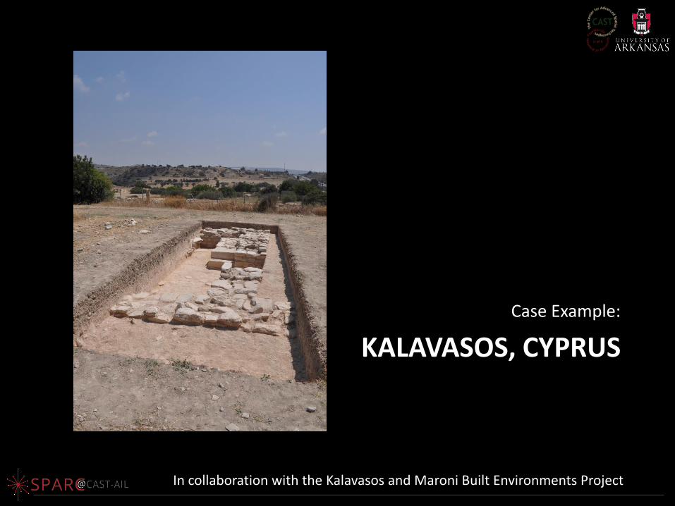
KALAVASOS, CYPRUS
Case Example:
In collaboration with the Kalavasos and Maroni Built Environments Project
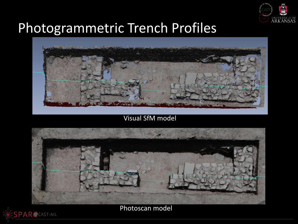
Photogrammetric Trench Profiles
Photoscan model
Visual SfM model
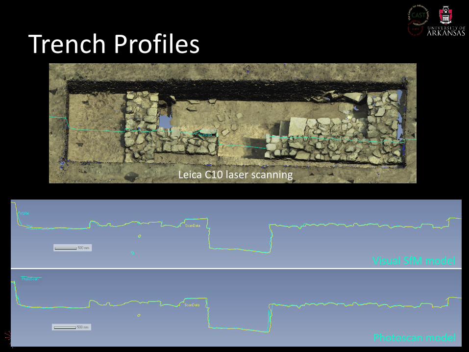
Trench Profiles
Photoscan model
Visual SfM model
Leica C10 laser scanning
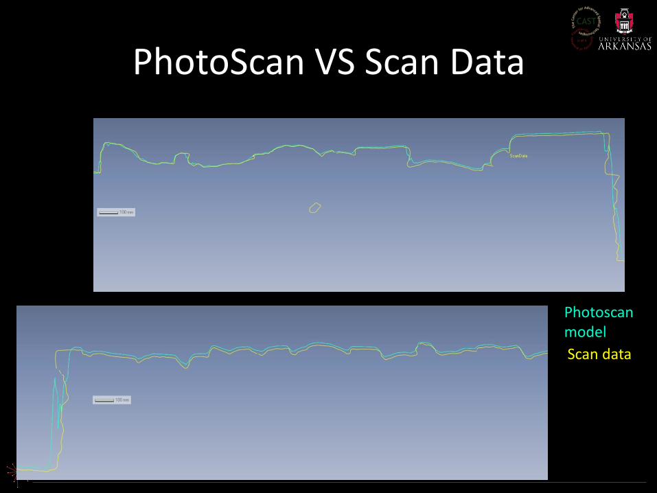
PhotoScan VS Scan Data
Photoscan model
Scan data
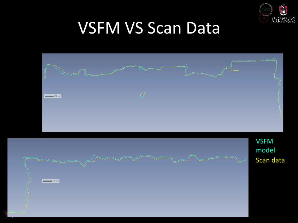
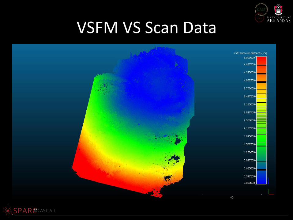
VSFM VS Scan Data
VSFM model
Scan data
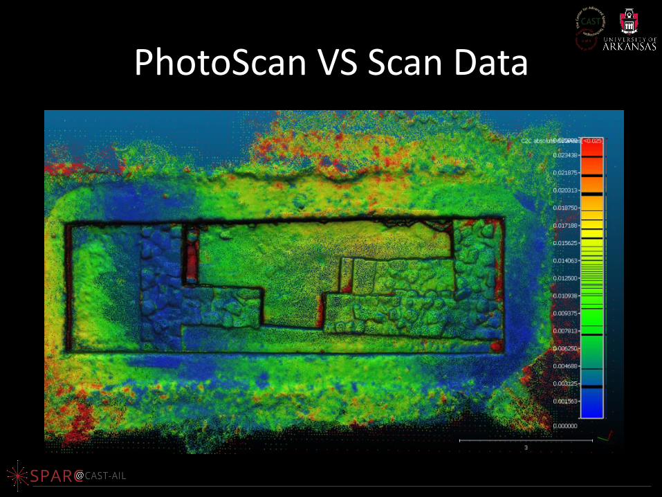
PhotoScan VS Scan Data
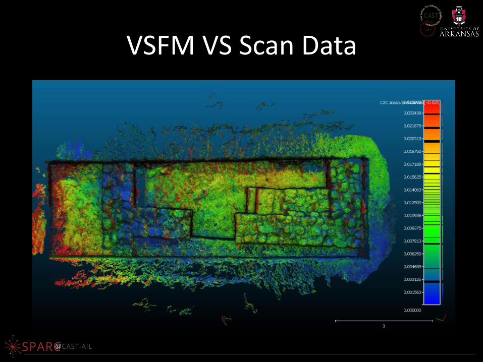
VSFM VS Scan Data
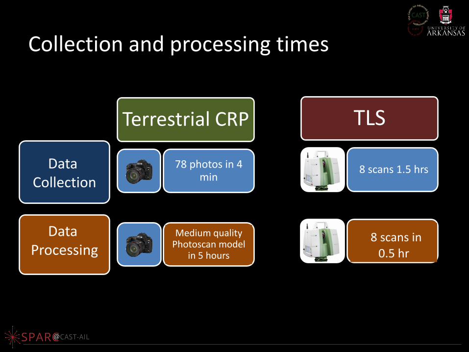
Collection and processing times
Terrestrial CRP
78 photos in 4 min
TLS
8 scans 1.5 hrs
Medium quality Photoscan model
in 5 hours
8 scans in 0.5 hr
Data Collection
Data Processing
HISTORIC PHOTO CASE EXAMPLES
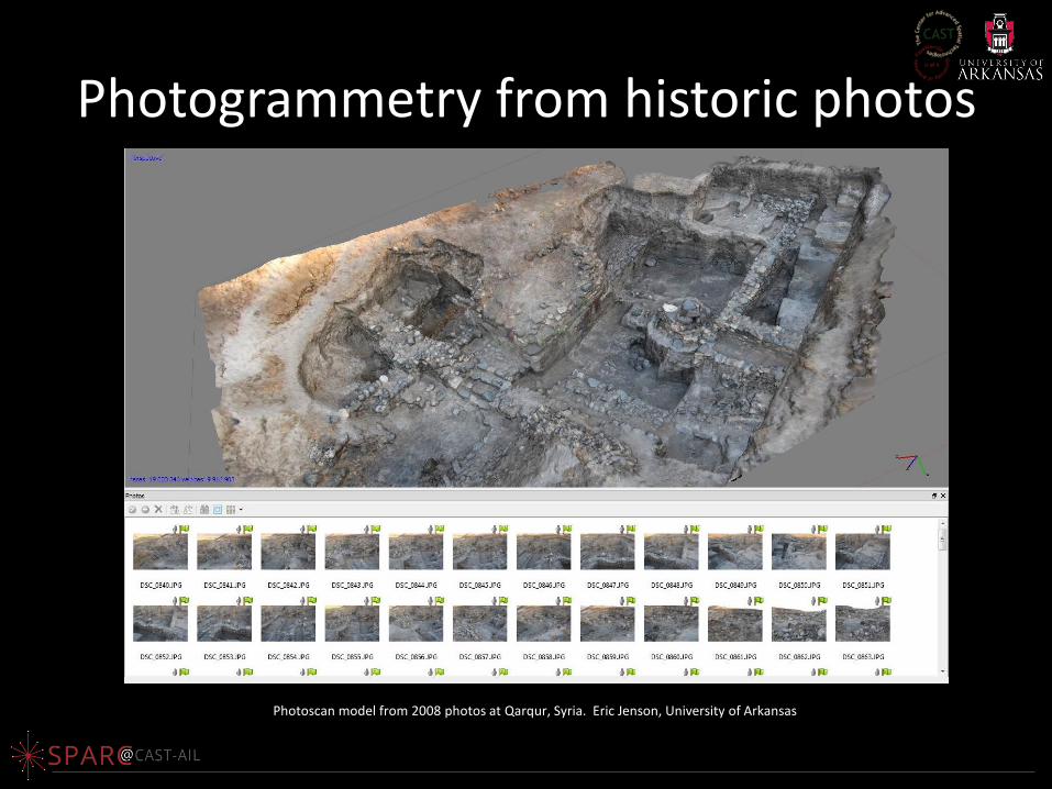
Photogrammetry from historic photos
Photoscan model from 2008 photos at Qarqur, Syria. Eric Jenson, University of Arkansas
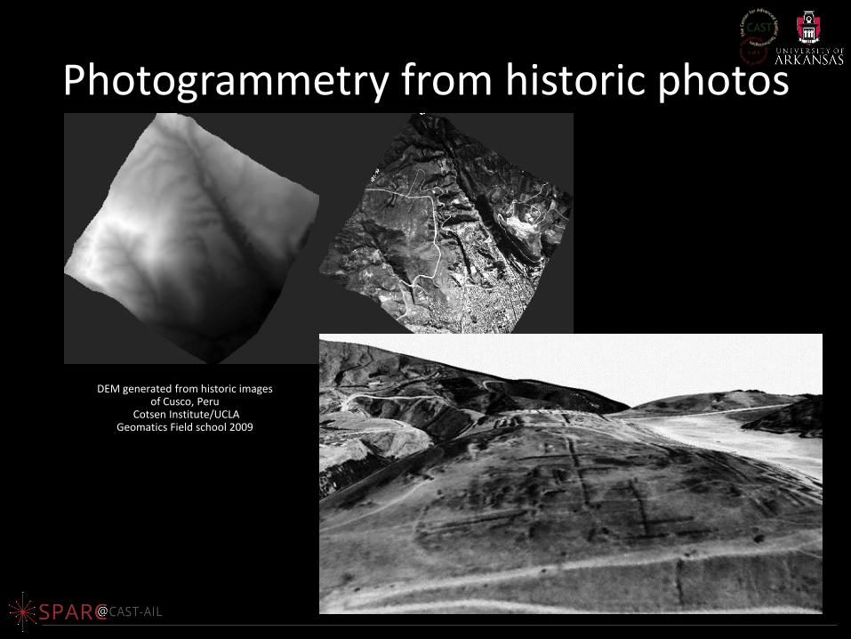
Photogrammetry from historic photos
DEM generated from historic images of Cusco, Peru
Cotsen Institute/UCLA Geomatics Field school 2009
FORT CLARK STATE HISTORIC SITE, NORTH DAKOTA
Archaeological Prospecting Case Example:
In collaboration with …
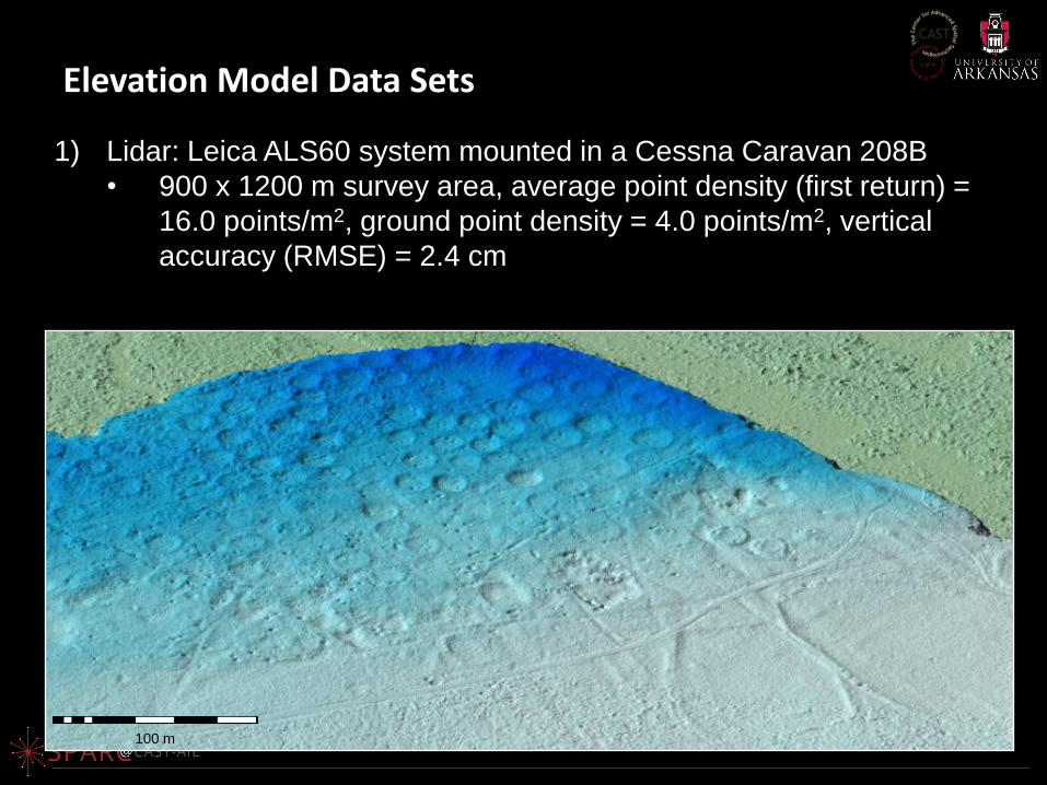
Elevation Model Data Sets
1) Lidar: Leica ALS60 system mounted in a Cessna Caravan 208B
• 900 x 1200 m survey area, average point density (first return) =
16.0 points/m2, ground point density = 4.0 points/m2, vertical
accuracy (RMSE) = 2.4 cm
100 m
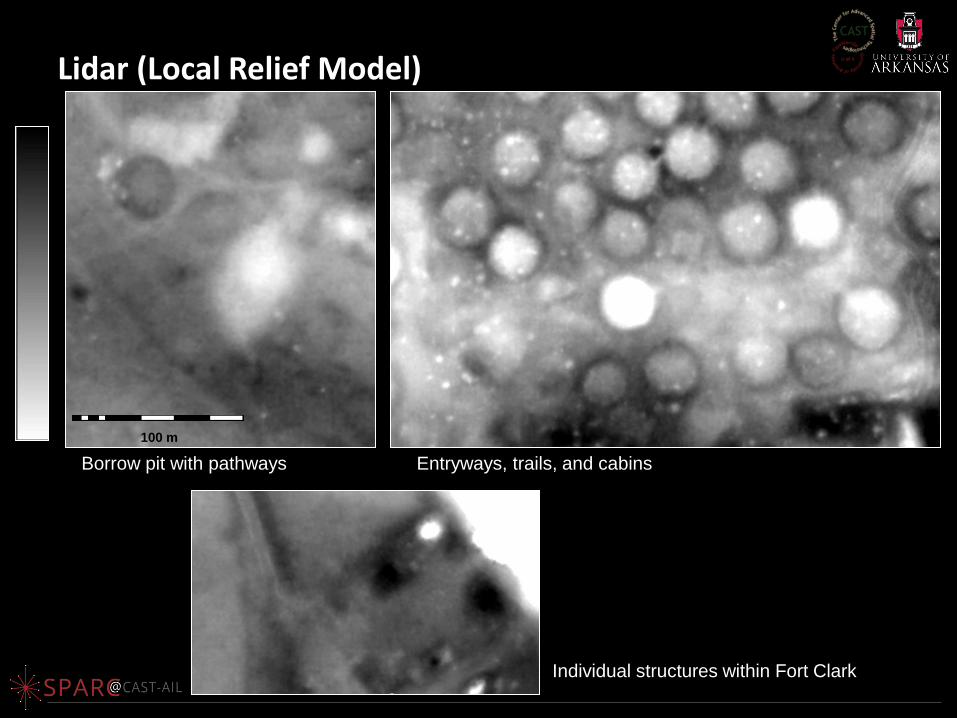
Lidar (Local Relief Model)
Borrow pit with pathways
Individual structures within Fort Clark
Entryways, trails, and cabins
100 m
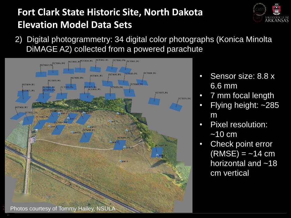
Fort Clark State Historic Site, North Dakota Elevation Model Data Sets
2) Digital photogrammetry: 34 digital color photographs (Konica Minolta
DiMAGE A2) collected from a powered parachute
• Sensor size: 8.8 x
6.6 mm
• 7 mm focal length
• Flying height: ~285
m
• Pixel resolution:
~10 cm
• Check point error
(RMSE) = ~14 cm
horizontal and ~18
cm vertical
Photos courtesy of Tommy Hailey, NSULA
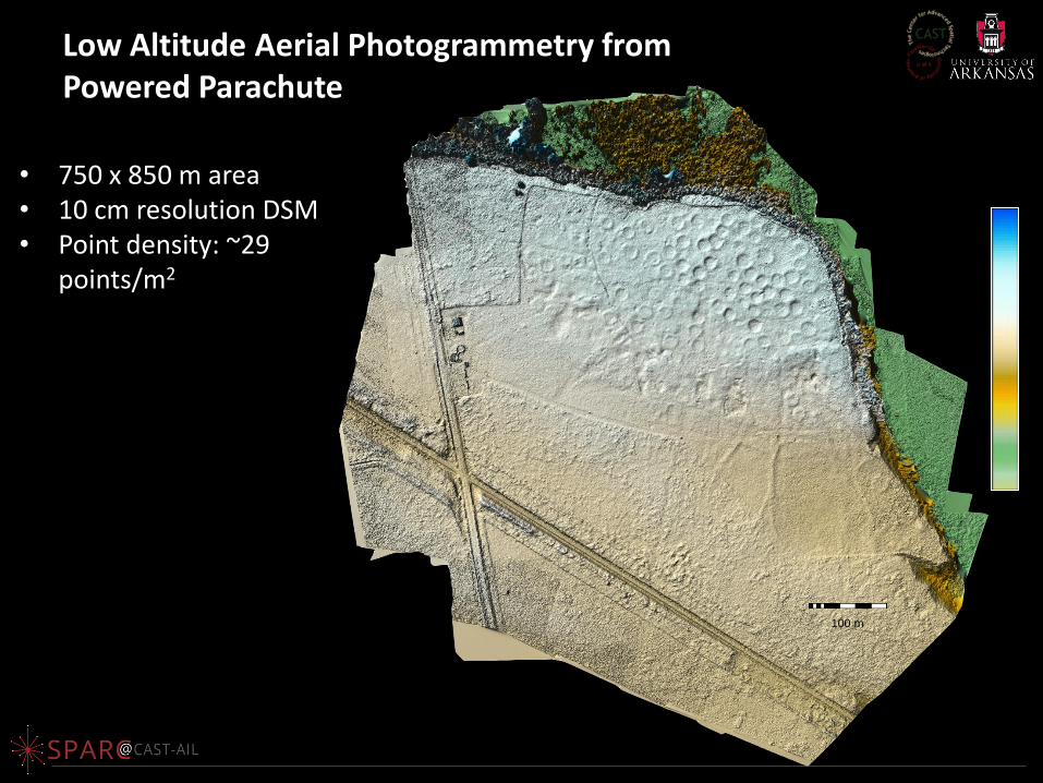
Low Altitude Aerial Photogrammetry from Powered Parachute
• 750 x 850 m area • 10 cm resolution DSM • Point density: ~29
points/m2
100 m
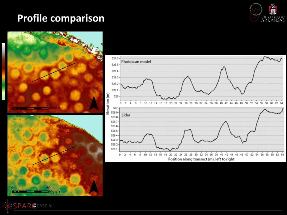
Profile comparison
Lidar
2004 color
1985 B/W
Lidar
2004 color
1985 B/W
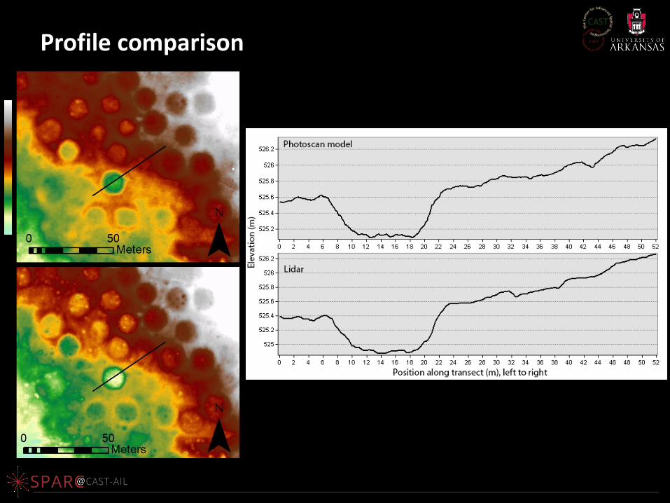
Profile comparison
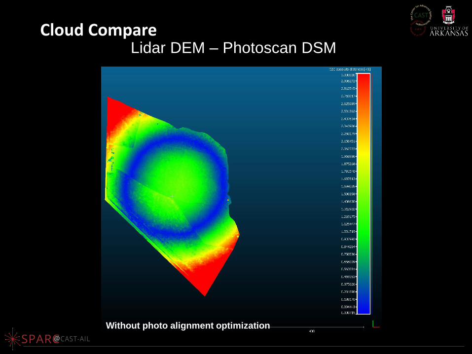
Cloud Compare Lidar DEM – Photoscan DSM
Without photo alignment optimization
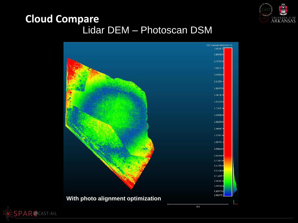
Lidar DEM – Photoscan DSM
With photo alignment optimization
Cloud Compare
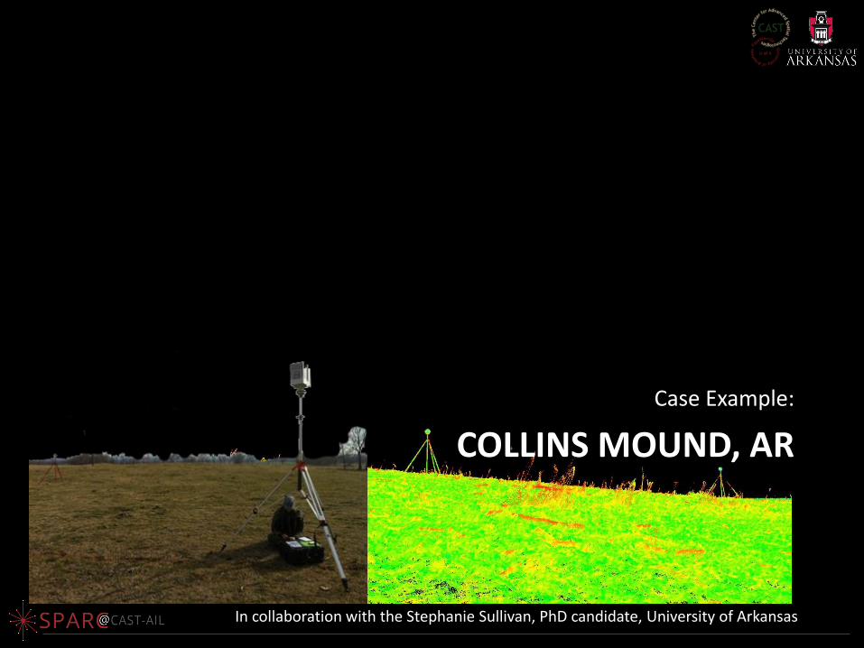
COLLINS MOUND, AR
Case Example:
In collaboration with the Stephanie Sullivan, PhD candidate, University of Arkansas
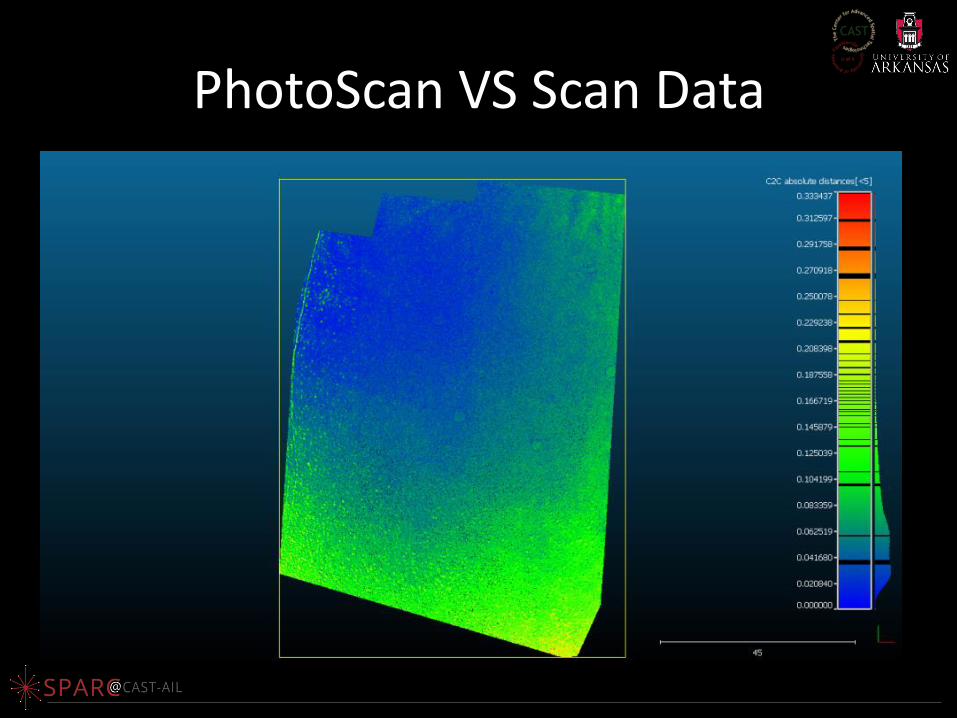
PhotoScan VS Scan Data
VSFM VS Scan Data
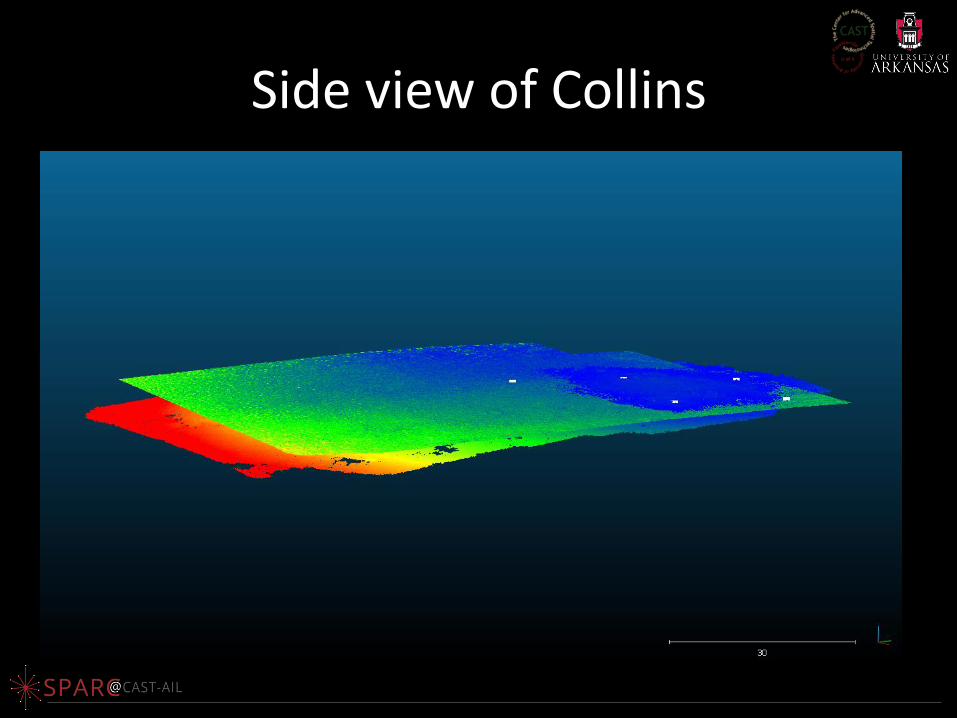
Side view of Collins
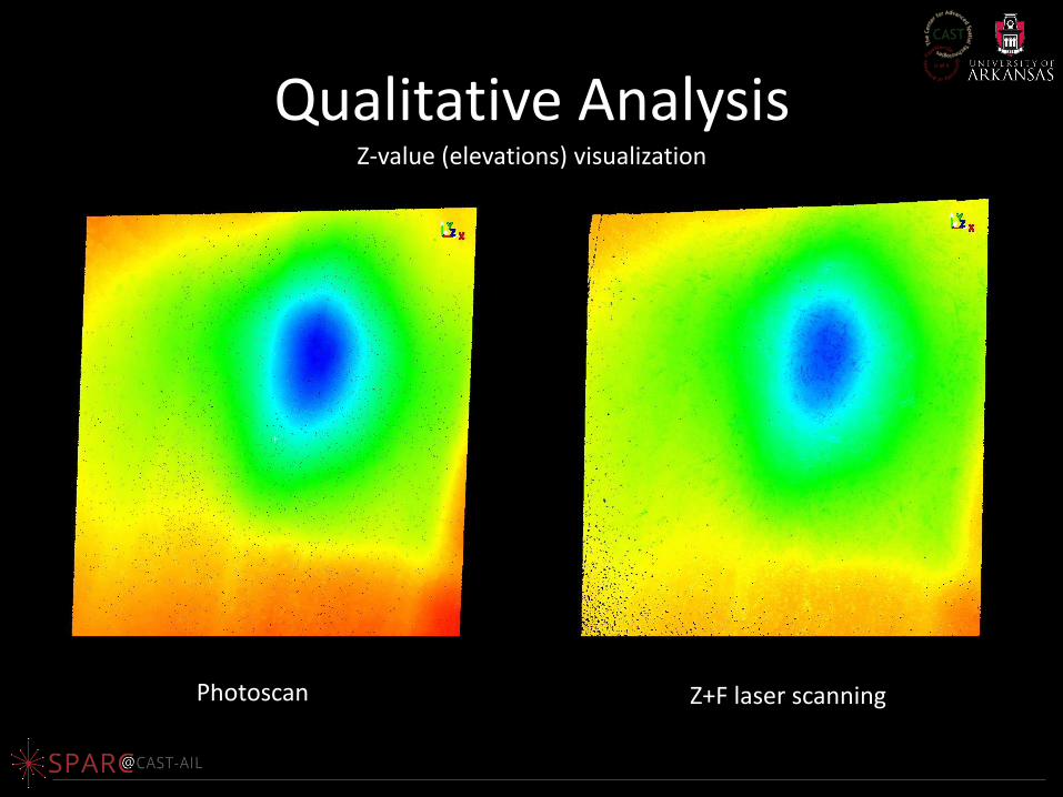
Qualitative Analysis
• Which datasets reveal which types of features
Photoscan Z+F laser scanning
Z-value (elevations) visualization
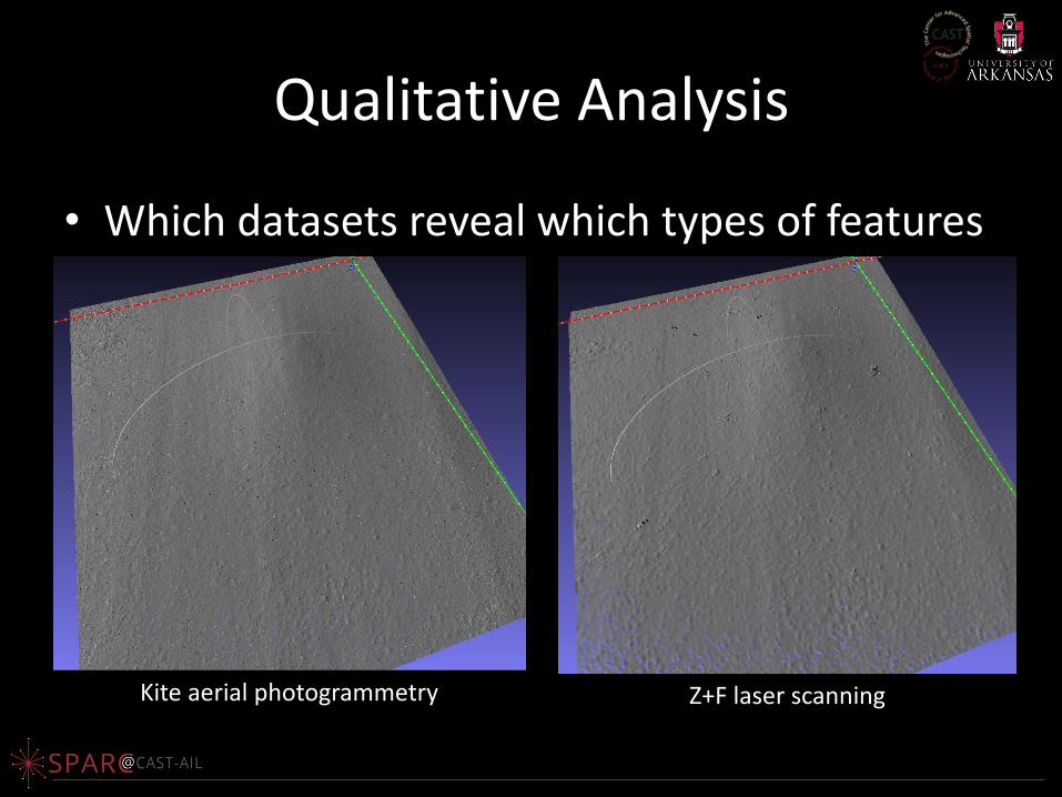
Qualitative Analysis
• Which datasets reveal which types of features
Kite aerial photogrammetry Z+F laser scanning
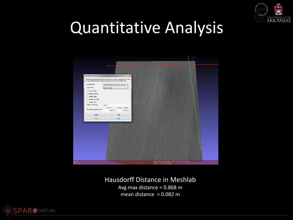
Quantitative Analysis
Hausdorff Distance in Meshlab Avg max distance = 0.868 m mean distance = 0.082 m
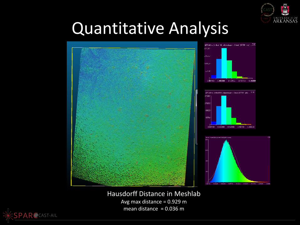
Quantitative Analysis
Hausdorff Distance in Meshlab Avg max distance = 0.929 m mean distance = 0.036 m
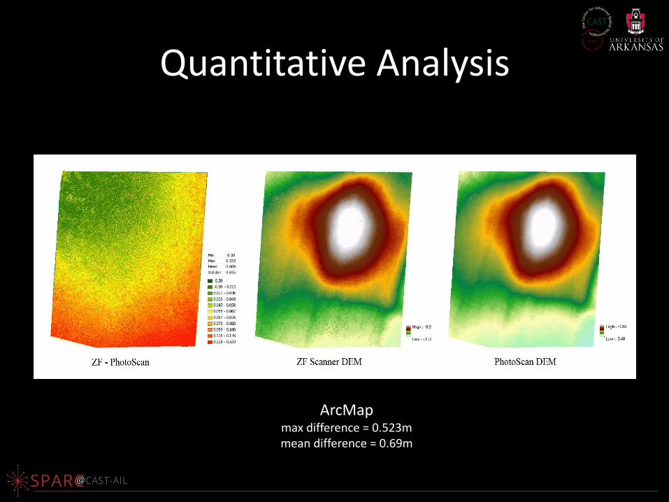
Quantitative Analysis
ArcMap max difference = 0.523m mean difference = 0.69m
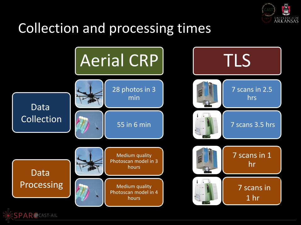
Collection and processing times
Aerial CRP
28 photos in 3 min
55 in 6 min
TLS
7 scans in 2.5 hrs
7 scans 3.5 hrs
Medium quality Photoscan model in 3
hours
Medium quality Photoscan model in 4
hours
7 scans in 1 hr
7 scans in 1 hr
Data Collection
Data Processing
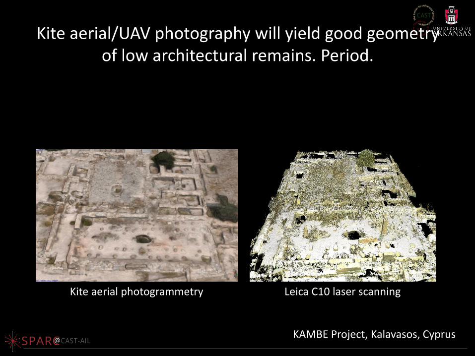
Kite aerial/UAV photography will yield good geometry of low architectural remains. Period.
Kite aerial photogrammetry Leica C10 laser scanning
KAMBE Project, Kalavasos, Cyprus
Conclusions • Keep your project goals in focus at all times
• Know your camera and lenses
• Know the basics of photogrammetry and how that relates to your software settings – You can get by with leaving default settings and
pressing just a few buttons—will that meet your project goals?
• Photogrammetry can be good solution – Great for visualization
– Must be executed with great care for metric analysis