from biogeochemical to ecological models of marine microplankton

Ž .Journal of Marine Systems 25 2000 431–446www.elsevier.nlrlocaterjmarsys

From biogeochemical to ecological models ofmarine microplankton

Paul Tett a,), Hilary Wilson a,b

a Department of Biological Sciences, Napier UniÕersity, 10 Colinton Road, Edinburgh EH10 5NT, UKb School of Ocean Sciences, UniÕersity of Wales, Bangor, Ireland

Received 15 December 1998; accepted 17 June 1999

Abstract

Models must simplify the complexity of real marine pelagic ecosystems. How much simplicity is needed? A series ofŽ .increasing numbers of state variables is used to illuminate this issue and to illustrate biogeochemical element-conserving

Ž .and ecological semi-freely dynamically interacting models of the marine microplankton, defined as all organisms less thanw200 mm. The models are those of Riley Riley, 1946. Factors controlling phytoplankton populations on Georges Bank, J.

x Ž .Marine Res., 6, 54–73. for phytoplankton, a nitrogen-conserving version of Riley, the microplankton model MP of TettwTett, P., 1990. A three layer vertical and microbiological processes model for shelf seas. Proudman Oceanographic

x Ž .Laboratory, Report 14, 85 pp. with a constant ratio h of microheterotrophs to total microplankton, a related model AHŽ .with Lotka–Volterra dynamics for interacting autotrophs and heterotrophs, and a simple microbial loop model ML . It is

Ž .argued that models must be at least biogeochemical. The biogeochemical model MP simulated changes during amicrocosm experiment better than the simplest ecological–biogeochemical model AH, which is, as here parameterised, anunstable system. ML, with protozoans able to switch food sources, is more stable than AH, and satisfactorily simulates theseasonal cycle of chlorophyll in the North-East Atlantic. MP performed well when forced with a time-series of h taken fromML. Time-varying h is one way of providing the smallest amount of microbial ‘ecology’ needed in biogeochemical pelagicmodels without introducing instability. q 2000 Elsevier Science B.V. All rights reserved.

Keywords: ecosystem-stability; microbial-loop; microplankton; model

1. Introduction

Models of biological–physical interactions in theŽsea must take account of physical transports which

) Corresponding author. Tel.: q44-131-455-2633; fax: q44-131-455-2291.

Ž .E-mail address: [email protected] P. Tett .

.conserve the total quantity of transported variablesand of non-conservative biological or chemical pro-

Ž .cesses which convert one variable into another .Ž .Fransz et al. 1991 review progress with such mod-

els. The development of computing power has in thepresent decade begun to allow the coupling of mod-els of biological processes with increasingly realistic

Žthree-dimensional physical models Sarmiento et al.,1993; Aksnes et al., 1995; Gregoire et al., 1998,

.Luytens et al., 1999 . Although horizontal transports

0924-7963r00r$ - see front matter q 2000 Elsevier Science B.V. All rights reserved.Ž .PII: S0924-7963 00 00032-4

( )P. Tett, H. WilsonrJournal of Marine Systems 25 2000 431–446432

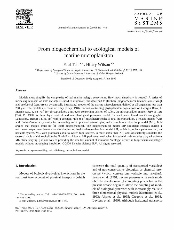
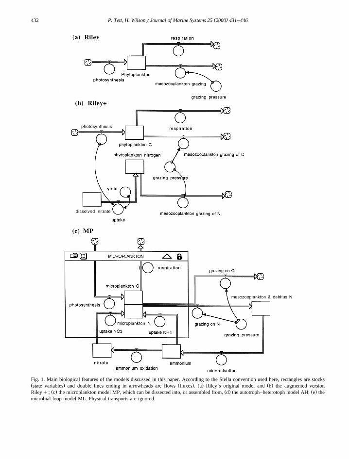
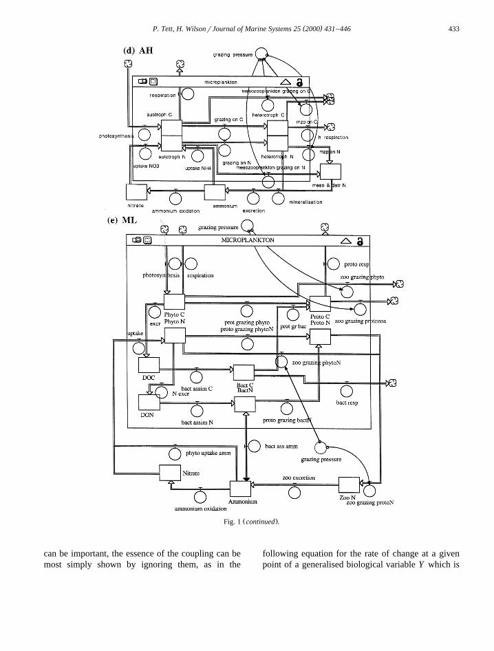
Fig. 1. Main biological features of the models discussed in this paper. According to the Stella convention used here, rectangles are stocksŽ . Ž . Ž . Ž .state variables and double lines ending in arrowheads are flows fluxes . a Riley’s original model and b the augmented version

Ž . Ž . Ž .Rileyq ; c the microplankton model MP, which can be dissected into, or assembled from, d the autotroph–heterotoph model AH; e themicrobial loop model ML. Physical transports are ignored.

( )P. Tett, H. WilsonrJournal of Marine Systems 25 2000 431–446 433

Ž .Fig. 1 continued .

can be important, the essence of the coupling can bemost simply shown by ignoring them, as in the

following equation for the rate of change at a givenpoint of a generalised biological variable Y which is


a function of time t and of height z above the seabed:

EYrEts yEw rEzYvertical transport flux divergence

q b 1Ž .Ynonconservative processes

The vertical flux includes transport due to meanwater w, water fluctuation wX and particle sinkingw velocities, acting on mean Y and fluctuation Y X,Y

with the effects of the fluctuations approximated aseddy mixing along a gradient:

² X X :w s wqw yw YqYŽ . Ž .Y Y

w fy K EYrEz q wyw YŽ . Ž .Y z Yeddy mixing water advection and particle sinking

This paper concerns the nonconservative componentb , which can be dealt with separately from theY

physical component so long as numerical integrationŽ .of Eq. 1 employs short time-steps, and so long as

second-order effects of physics on biology, such asthe role of turbulent shear on nutrient diffusion at the

Žsub-Kolmogorov scale Lazier and Mann, 1989;.Kiørboe, 1993 , can be neglected. Our objectives are

to exemplify classes of model we call biogeochemi-Ž .cal and ecological and to discuss but not resolve

some issues relating to the complexity of biologicalmodels of marine pelagic ecosystems. We do this

Ž .with the aid of results from a series Fig. 1 ofmodels of increasing biological complexity; which isto say: of increasing numbers of state variables.

2. Data and methods

Models presented here used the generalised equa-tion:

dYrd tsE Y yY q w rh B qb 2Ž . Ž . Ž .0 Y Y

Ž .which results from integration of Eq. 1 over auniform domain with one open boundary. The sink-

Ž .ing rate w was zero in our simulations. Eq. 2 wasYŽ .applied to the dynamics of a pelagic ecosystem in i

Ž .a surface mixed layer SML of thickness h metresŽ .and b a well-stirred laboratory microcosm.

SML models were implemented using the soft-Ž .ware Stella II Wilson, 2000 . The mixed layer was

that of the waters over the continental slope west of

Scotland, observed during six cruises of the UKŽ .LOIS Shelf-Edge-Study SES in 1995–1996. CTD-

fluorometer profiles, used to estimate chlorophyllconcentration, and h from the depth at which tem-perature was 0.18C below that at the surface, weretaken from data banked at the British Oceanographic

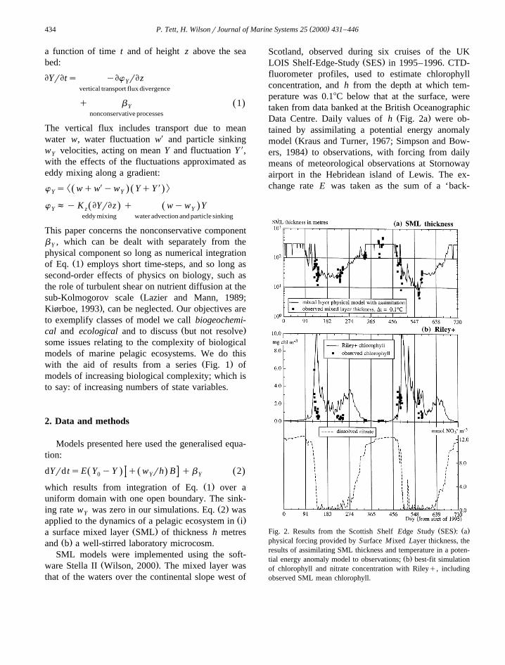
Ž .Data Centre. Daily values of h Fig. 2a were ob-tained by assimilating a potential energy anomaly

Žmodel Kraus and Turner, 1967; Simpson and Bow-.ers, 1984 to observations, with forcing from daily

means of meteorological observations at Stornowayairport in the Hebridean island of Lewis. The ex-change rate E was taken as the sum of a ‘back-

Ž . Ž .Fig. 2. Results from the Scottish Shelf Edge Study SES : aphysical forcing provided by Surface M ixed Layer thickness, theresults of assimilating SML thickness and temperature in a poten-

Ž .tial energy anomaly model to observations; b best-fit simulationof chlorophyll and nitrate concentration with Rileyq, includingobserved SML mean chlorophyll.


Ž .Ž .ground mixing’ term plus entrainment dhrd t 1rhfor dhrd t)0. Y was the value of the appropriate0

variable just below the SML. PhotosyntheticallyŽ .available radiation PAR for these models was also

based on measurements at Stornoway. Mesozoo-Žplankton grazing pressures were calculated Tett and

.Walne, 1995 from monthly mean copepod abun-Ždances supplied by Dr. A.W. Walne SAHFOS, Ply-

.mouth, UK from long-term CPR observations in theSES region.

The microcosm was that used for experiment H ofŽ .Jones Jones et al., 1978a,b; Jones, 1979 , who en-

closed 19 l of 200 mm-filtered seawater taken in July1975 from the small Scottish fjord, Loch Creran,under natural conditions of light and temperature.The contents of the microcosm were continuouslydiluted at Es0.21 dayy1 with nutrient-enrichedsterile seawater. Microscopical and chemical analy-ses were carried out on samples drawn from themicrocosm, and the resulting values used to estimatethe concentrations of particulate organic carbon dueto autotrophs and heterotrophs less than 200 mm.Simulations of these data were numerically inte-

Ž .grated by a Pascal program Tett, 1998 .In all cases, numerical integrations were carried

Ž .out by Euler forward difference, as the fasterRunga–Kutta method can cause numerical problemswhen used with equations containing discontinuitiesŽ .Anon, 1994 , as some of ours did. The reliability ofnumerical integration was checked by varying thetime step, and with test cases. Agreement betweensimulations Y X and observations Y was measured inthe case of the microcosm data by calculating a fit

Ž Ž X . Ž ..2statistic derived from Ý ln Y y ln Y , summedover all observed variables. In the case of the SES

Ž .data the fitting criteria were i a comparison of theŽ .sum of squared deviations SOSD of simulated from

observed values compared with the SOSD due to aŽ .null model in which dYrd ts0; and ii the extent

of agreement between simulations and observationsof the phase and amplitude of the Spring bloom andthe amount of chlorophyll in Autumn.

3. Riley’s model

Ž . Ž .The model of Riley 1946 Fig. 1a containedonly one state variable, phytoplankton biomass, given

in g C my2 and estimated by Riley from plantpigment concentration. Rewritten in our symbols, interms of concentration, and in a way that corre-sponds to the separation of physical and biological

Ž . Ž .terms in Eqs. 1 and 2 , the characterising equationis:

b s myryG BŽ .B

in mmol phytoplankton-C my3dayy1 3Ž .

Ž . y1where relative growth rate msa If S day , a

being photosynthetic efficiency, I the 24-h meanŽ .photosynthetically active irradiance PAR in the

Ž .SML, and f S is a saturation function of seawaterphosphate concentration. The other terms are relativerespiration rate r and zooplankton grazing pressureG, both defined as the instantaneous rate at whichbiomass is consumed divided by existing biomass.

Although Riley’s simulation of the seasonal cyclewas close to observed amounts of phytoplankton onGeorges Bank, there is nothing in principle in hismodel to stop sustained exponential increase leadingto an enormous biomass. That is, there is nothingbuilt into the equation for rate of change of biomassthat causes growth rate to slow as a finite ‘carryingcapacity’ is approached: such restriction must besupplied in the forcing data by increasing severity ofnutrient limitation, and increasing zooplankton graz-ing, during summer.

We augmented Riley’s model by adding two moreŽ .state variables, for seawater nitrate S and phyto-

Ž . Ž .plankton nitrogen N Fig. 1b . Nitrate replacedRiley’s phosphate as the limiting nutrient.

b syqmB in mmol nitrate-N my3 dayy1 4Ž .S

b sqmByGNN

in mmol phytoplankton-N my3dayy1 5Ž .

where q is the reciprocal of the yield, taken as 5Ž .y1mmol C mmol N , of phytoplankton organic car-

Žbon from assimilated nitrogen. The yield was madelower than the Redfield value in order to be compati-ble with the value of Q in the more elaboratemax a

.models. The extra equations make Rileyq into abiogeochemical model. This means that, if account is

Žtaken of boundary exchange including losses due to


. Ž . Ž .zooplankton grazing the system of Eqs. 2 – 5conserves the total of nitrogen, and constrains phyto-plankton biomass to an upper limit set by the supplyof nitrogen. For comparison with observations,chlorophyll was calculated from phytoplankton car-

Ž .y1bon at a ratio of 0.44 mg chl mmol C .When forced by realistic physics in the form of

SML thickness and actual daily irradiance, Rileyqsimulated some typical features of the seasonal cycle

Ž .of phytoplankton in the SES region Fig. 2b . Thesimulated spring bloom was, however, late, and au-tumn chlorophyll levels too high, in comparison withobservations.

4. Microplankton

An impression of the complexity of trophic rela-tionships amongst plankton and nekton was given,

Ž .for the North Sea, by Hardy 1924 . His ‘diagram-matic representation of the relation of the Herring tothe Plankton Community as a whole’ contained at

Ž .least a dozen genera of mainly crustacean herbi-vores and as many of phytoplankton. The subsequentdiscovery of the ‘microbial loop’ linking hetero-trophic and photosynthetic bacteria and small eu-

Žkaryotic algae with protistan grazers Williams, 1981;.Azam et al., 1983 increased the number of species

that must be taken into consideration. Although someŽmodels of freshwater phytoplankton e.g., Reynolds

.and Irish, 1997 describe the simultaneous dynamicsof numerous species, models of marine pelagic

Žecosystems Fasham et al., 1990; Taylor and Joint,1990; Taylor et al., 1993; Baretta-Bekker et al.,

.1995; Varela et al., 1995 have sought to compressthe diversity of the system into a small number ofcompartments, which may represent higher-level taxaŽ . Žsuch as ‘diatoms’ or trophic groups such as ‘zoo-

.plankton’ .The general issue concerns the number of state

variables, or the number of b-terms, in a model.Each simulated compartment entails writing and pa-rameterising at least one b-term, more if the modelconcerns the cycling of several chemical elements,and solving the resulting sets of differential equa-tions. It is desirable to minimise the list of statevariables, not only in order to minimise computer

Žstorage and calculation especially in 2D or 3D

models, or during the repeated simulations necessary.for parameter optimisation , but also because of Oc-

Žcam’s Razor ‘do not unnecessarily multiply expla-.nations’ and on account of practical and theoretical

Ždifficulties in estimating parameters which, in gen-.eral, increase with variable number .

Taking into account this need for parsimony inŽ .state variables, Tett 1990 proposed a microbiologi-

cal model with three pelagic compartments and sixindependent state variables:

ŽØ microplankton organic carbon and nitrogen and.non-independent chlorophyll ;

Ø detrital organic carbon and nitrogen;ŽØ dissolved ammonium and nitrate and non-inde-

.pendent oxygen .

Ž .The microbiological or microplankton-detritusŽ .model Fig. 1c was embedded in a three-layer phys-

ical framework, and the combination named L3VMPŽ .Tett and Walne, 1995 . As in the case of Riley,mesozooplankton were represented as a grazing pres-sure rather than a dynamic compartment.

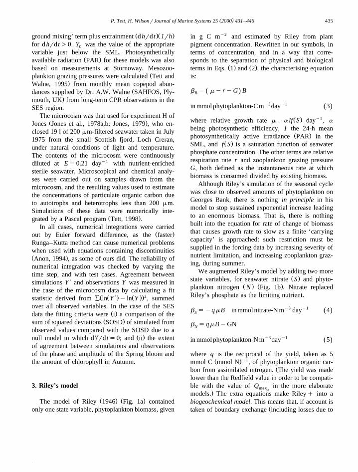
Fig. 3 is a conceptual diagram of the microplank-ton box in this model. The model of the microplank-ton compartment on its own is called MP. It isdeemed to contain all pelagic microorganisms lessthan 200 mm, including heterotrophic bacteria and

Žprotozoa zooflagellates, ciliates, heterotrophic di-.noflagellates, etc. as well as photo-autotrophic

Fig. 3. Conceptual diagram of the contents of the microplanktonbox in MP.


Žcyanobacteria and micro-algae diatoms, dinoflagel-.lates, flagellates, etc. . This definition of microplank-

ton, as including all pelagic micro-organisms lessŽ .than 200 mm, employs an earlier use Dussart, 1965

of the term ‘microplankton’ than that of SieburthŽ .1979 who contrasted microplankton to picoplank-ton and nanoplankton. The purpose of the mi-croplankton compartment is to provide a simpleparameterisation of pelagic photo-autotrophic andmicro-heterotrophic processes, with less emphasison the organisms. The microplankton may be seenfrom a functional viewpoint as a suspension of

Ž .chloroplasts and cyanobacteria and mitochondria

Ž .and heterotrophic bacteria with associated organiccarbon and nutrient elements.

The microplankton compartment in MP has twostate variables, for carbon biomass B and nitrogenN. The defining equations are:

b s myG BŽ .B

in mmol microplankton-C my3dayy1 6Ž .b s uyGQ BŽ .N

in mmol microplankton-N my3dayy1 7Ž .where microplankton: nutrient quota QsNrB andis variable; growth rate m is a ‘threshold’ function

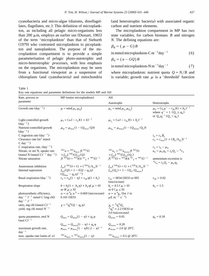
Table 1Key rate equations and parameter definitions for the models MP and AH

Ž .Rate, process or MP entire microplankton AHparameter Autotrophs Heterotrophs

y1 ) y1Ž . � 4 � 4 Ž .Ž .Growth rate day msmin m ,m m smin m ,m m s i q yr 1qbI Q a I Q h h 0h ha a) Ž .where q s1 Q Gqa h

y1 Ž .or Q q Q -qa h a hy1 y1Ž .Ž . Ž .Ž .Light-controlled growth m s a Iyr 1qb m s a Iyr 1qbI 0 I 0a aa

y1Ž .dayŽ Ž .. Ž Ž ..Nutrient-controlled growth m sm 1y Q rQ m sm 1y Q rQQ max min Q maxa mina aa

y1Ž .dayy1Ž .C ingestion rate day i sc Bh h a

3 y1Ž Ž Ž ..Clearance rate m mmol c sc 1q B rkh max a Bay1 .C day

y1Ž .C respiration rate, day r s i ymh h hNO NO NO NO NO NO NŽ . Ž .Nitrate, or net N, uptake rate us u f S u s u f S u sm q s i Q y rmax a maxa h h h h a h

y1 y1 NH NHŽ Ž . . Ž . Ž . Ž . Ž .mmol N mmol C day =f S f Q =f S f Qin1 in2 in1 in2 aNO NO NO NO y1 NO NO NO NO y1Ž . Ž . Ž . Ž .Nitrate saturation f S s S k q S f S s S k q S ammonium excretion isS S

Nr s i Q ym qh h a h hNH NH y1 NH NH y1Ž . Ž Ž .. Ž . Ž Ž ..Ammonium inhibition f S s 1q Srk f S s 1q Srkin1 in in1 inŽ . ŽŽ . Ž . Ž .Internal supression f Q s1y Qyq h f Q s1y Q rQin2 h in2 a a maxa

y1Ž . .Q yq hmax hy1Ž . Ž . Ž . Ž .Basal respiration day r sr 1yh qr h 1qb r s0034 SES or 005 r s0.020 0a 0h a 0a 0h

Ž .microcosmŽ . Ž . Ž .Respiration slope bsb 1q b h qb h m)0 b s0.5 m)0 b s1.5a h h a h

Ž . Ž .or 0 mG0 or 0 mF0X X XŽ . Žphotosynthetic efficiency, asa x a s0.069 microcosm asa x for I ina

y1 y1 y2 y1Ž . Ž . .day I mmol C mg chl 0.101 SES mE m sy1 y1day I

y1 X N X NŽ . Ž .ratio, mg chl mmol C xs q Qyq h x s q Qa h a a ay1 X N Ž .yield, mg chl mmol N q s2.2 SES ora

Ž .3.0 microcosmŽ .quota parameters, mol N Q sQ 1yh qq h Q s0.05 q s0.18min mina h mina h

y1Ž .mol CŽ .Q sQ 1yh qq h Q s0.20max maxa h maxa

y1Ž .Ž .maximum growth rate, m sm 1yh 1.2yh m s2.0 @ 208Cmax max maxaay1day

NO NO NOŽ . Ž .max. uptake rate units of u u s u 1yh u s0.5 @ 208Cmax maxa maxa


Ž .including respiration of light or internal nutrientŽ .limitation Droop, 1983 ; and nutrient uptake rate u

is a saturation function of seawater nitrate or ammo-nium concentration with some inhibition by internalnutrient. Chlorophyll concentration was calculatedfrom biomass by way of a cell-quota dependentchlorophyll:carbon ratio x .

ŽNO .The model also includes nitrate S and ammo-ŽNH .nium S as state variables:

NO w NH NH xb sy uB q r SNO S

in mmol nitrate-N my3dayy1 8Ž .

NH NH NHb sy uB y r Sqeg GNNH S

in mmol NHq my3dayy1 9Ž .4

The nitrification term NH rNH S and the mesozoo-plankton grazing mineralisation term eg GN were setto zero in the case of the microcosm simulations, butwere allowed to be positive in the SES simulations.

‘Parameterisation’ of rates such as m is theirexpansion in terms of state variables and ‘parame-ters’ — terms which have a constant value during asingle numerical simulation. In the case of MP, wemade this parameterisation with the aid of three

Ž .assumptions: i mesozooplankton grazing impactedŽ .equally on all autotrophs and microheterotrophs; ii

any dissolved organic carbon or any ammoniumexcreted or leaked by any micro-organism was com-pletely internally cycled within the microplankton;

Ž .and iii autotrophs were in constant ratio to het-erotrophs. The last of these assumptions was ex-pressed as a constant value of a parameter called the‘heterotroph fraction’:

hsB r B qB 10Ž . Ž .a a h

where the subscripts ‘a’ and ‘h’ refer to autotrophsŽ .and micro heterotrophs, respectively. The parameter

h was used to derive MP rate equations from thelarger set AH containing separate autotroph and het-

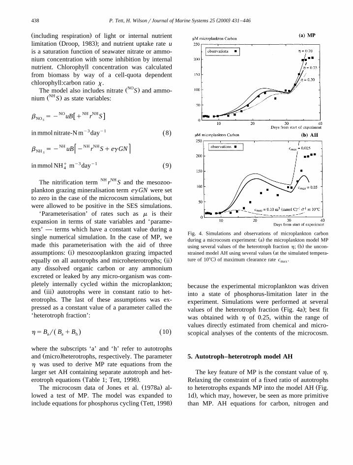
Ž .erotroph equations Table 1; Tett, 1998 .Ž .The microcosm data of Jones et al. 1978a al-

lowed a test of MP. The model was expanded toŽ .include equations for phosphorus cycling Tett, 1998

Fig. 4. Simulations and observations of microplankton carbonŽ .during a microcosm experiment: a the microplankton model MP

Ž .using several values of the heterotroph fraction h; b the uncon-Žstrained model AH using several values at the simulated tempera-

.ture of 108C of maximum clearance rate c .max

because the experimental microplankton was driveninto a state of phosphorus-limitation later in theexperiment. Simulations were performed at several

Ž .values of the heterotroph fraction Fig. 4a ; best fitwas obtained with h of 0.25, within the range ofvalues directly estimated from chemical and micro-scopical analyses of the contents of the microcosm.

5. Autotroph–heterotroph model AH

The key feature of MP is the constant value of h.Relaxing the constraint of a fixed ratio of autotrophs

Žto heterotrophs expands MP into the model AH Fig..1d , which may, however, be seen as more primitive

than MP. AH equations for carbon, nitrogen and


ammonium are given here; see Table 1, and TettŽ .1998 for further details.

b s m yc B B in mmol C my3 dayy1 11Ž . Ž .B a h h aa

b s c B yr B in mmol C my3 dayy1 12Ž . Ž .B h a h hh

b s u Qy1 yc B N in mmol N my3 dayy1Ž .N a a h h aa

13Ž .

b s c N yNr B in mmol N my3 dayy1Ž .N h h a h h

14Ž .

b syNH u B qNr B in mmol N my3 dayy1NH a a h hS

15Ž .

The most important of the new rate variables is themicroheterotroph volume clearance or transfer ratec . In order to increase the potential for stability inh

the relationship between microheterotrophs and au-Ž .totrophs, it was made a Holling 1959 type II

Ž .saturation function of food concentration:

y1c sc 1q B rKŽ .Ž .h max a Ba

y13 y1in m day mmol C 16Ž . Ž .

with half-saturation at K s50 mmol C my3. Re-Ba

sults of simulations carried out for the microcosmexperiment, and using several values of c , aremax

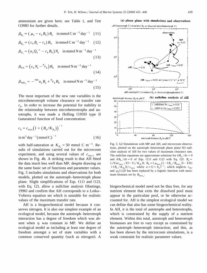
shown in Fig. 4b. A striking result is that AH fittedthe data much less well than MP, despite drawing onthe same basic set of functions and parameter values.Fig. 5 includes simulations and observations for bothmodels, plotted on the autotroph–heterotroph phase

Ž . Ž .plane. Slight simplifications of Eqs. 11 and 12 ,Ž . Žwith Eq. 2 , allow a nullcline analysis Hastings,

.1996 and confirm that AH corresponds to a Lotka–Volterra equation set which is unstable for realisticvalues of the maximum transfer rate.

AH is a biogeochemical model because it con-serves nitrogen. It is also our simplest example of anecological model, because the autotroph–heterotrophinteraction has a degree of freedom which was ab-sent when h was constant in MP. We define anecological model as including at least one degree offreedom amongst a set of state variables with a

Ž .common conserved quantity such as nitrogen . A

Ž .Fig. 5. a Simulations with MP and AH, and microcosm observa-Ž .tions, plotted on the autotroph–heterotroph phase plane b null-

cline analysis of AH for two values of maximum clearance rate.The nullcline equations are approximate solutions for d B rd ts0a

Ž . Ž . Ž .and d B rd ts0 of Eqs. 11 and 12 with Eq. 2 : B sh aŽŽ . Ž .. Ž Ž Ž .. .Ž1r ac rE y 1rK ; B s m 1y B rB y E 1max B h max a maxa a aŽ .. Ž .y1q B rK rc where as 1q b , which neglects r ,a B max h 0ha

Ž .and m I,Q has been replaced by a logistic function with maxi-a

mum biomass set by B .max a

biogeochemical model need not be thus free, for anynutrient element that exits the dissolved pool mustappear in the particulate pool, or be otherwise ac-counted for. AH is the simplest ecological model wecan define that also has some biogeochemical reality.In AH, it is the total of autotrophs and heterotrophs,which is constrained by the supply of a nutrientelement. Within this total, autotroph and heterotrophbiomasses are free to vary except as constrained bythe autotroph–heterotroph interaction; and this, ashas been shown by the microcosm simulations, is aweak constraint for realistic parameter values.


The consequence of these features of AH is that asystem simulated by MP is more predictable thanone simulated by AH. For example, given a knowl-edge of total nitrogen and the information that thereis adequate light, then it can be predicted that the MP

Ž .system will evolve to a point in state variable spaceŽwhere the majority of nitrogen is in biomass. This

ignores mesozooplankton grazing, but that will not( ) .change the outcome unless G)m I . Such a defi-

nite prediction cannot be made of AH without know-ing exact initial conditions and duration of simula-tion, for the AH system can repeatedly pass throughmany states including those of low microplanktonbiomass. AH is an example of what may be called a‘billiard-table’ model. Apparently precisely definedby a small set of differential equations, and withbehaviour that is highly predictable in the short term,its long-term behaviour can be chaotic, as illustratedfor a comparable 3-step food chain by Hastings and

Ž .Powell 1991 .

6. Microbial Loop model ML

Ž .Our most complicated model, ML Wilson, 2000 ,includes four components of the microbial loop:phytoplankton, dissolved organic matter, bacteria,

Žand protozoa, each with carbon and nitrogen Fig..1e . However, bacteria and protozoa have constant

Ž .y1N:C ratios of 0.18 mol N mol C , the same as thevalue used for heterotrophs in AH. Only the carbonequations are presented below, as the nitrogen equa-tions are little different from those used in AH. Anexception concerns bacterial uptake of dissolved or-ganic nitrogen. This can be supplemented by ammo-nium uptake if the N:C ratio of the assimilated DOMis less than the optimum bacterial ratio, or bacteriacan excrete ammonium if the assimilated DOM isnitrogen-rich.

phytoplankton: b s m y l yc B yG BŽ .B a a p h aa

in mmol C my3dayy1 17Ž .

protozoa: b s c B qB yr yG BŽ .Ž .B p a b p pp

mmol C my3 dayy1 18Ž .

bacteria: b s u yr yc B BŽ .B b b p h bb

mmol C my3 dayy1 19Ž .DOC: b s l B yu BOCS a a b b

mmol C my3 dayy1 20Ž .The new term l gives the relative rate of DOCa

excretion by phytoplankton, a proportion of itsgrowth rate.

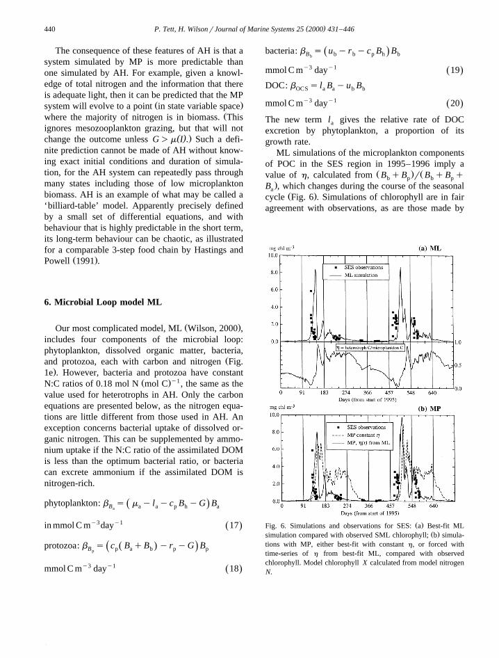
ML simulations of the microplankton componentsof POC in the SES region in 1995–1996 imply a

Ž . Žvalue of h, calculated from B qB r B qB qb p b p.B , which changes during the course of the seasonala

Ž .cycle Fig. 6 . Simulations of chlorophyll are in fairagreement with observations, as are those made by

Ž .Fig. 6. Simulations and observations for SES: a Best-fit MLŽ .simulation compared with observed SML chlorophyll; b simula-

tions with MP, either best-fit with constant h, or forced withtime-series of h from best-fit ML, compared with observedchlorophyll. Model chlorophyll X calculated from model nitrogenN.


the simpler model MP modified to include, as aforcing variable, a time-series of h output from ML.Including variable h corrects the overestimation of

ŽAutumn chlorophyll made by standard MP with.fixed h .

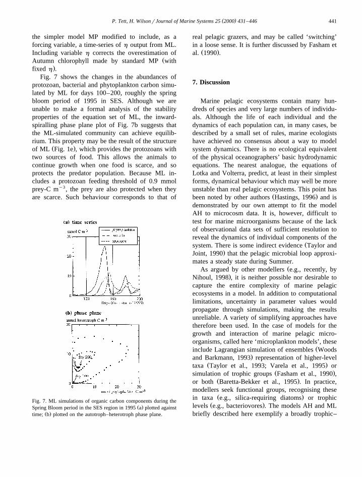
Fig. 7 shows the changes in the abundances ofprotozoan, bacterial and phytoplankton carbon simu-lated by ML for days 100–200, roughly the springbloom period of 1995 in SES. Although we areunable to make a formal analysis of the stabilityproperties of the equation set of ML, the inward-spiralling phase plane plot of Fig. 7b suggests thatthe ML-simulated community can achieve equilib-rium. This property may be the result of the structure

Ž .of ML Fig. 1e , which provides the protozoans withtwo sources of food. This allows the animals tocontinue growth when one food is scarce, and soprotects the predator population. Because ML in-cludes a protozoan feeding threshold of 0.9 mmolprey-C my3, the prey are also protected when theyare scarce. Such behaviour corresponds to that of

Fig. 7. ML simulations of organic carbon components during theŽ .Spring Bloom period in the SES region in 1995 a plotted against

Ž .time; b plotted on the autotroph–heterotroph phase plane.

real pelagic grazers, and may be called ‘switching’in a loose sense. It is further discussed by Fasham et

Ž .al. 1990 .

7. Discussion

Marine pelagic ecosystems contain many hun-dreds of species and very large numbers of individu-als. Although the life of each individual and thedynamics of each population can, in many cases, bedescribed by a small set of rules, marine ecologistshave achieved no consensus about a way to modelsystem dynamics. There is no ecological equivalentof the physical oceanographers’ basic hydrodynamicequations. The nearest analogue, the equations ofLotka and Volterra, predict, at least in their simplestforms, dynamical behaviour which may well be moreunstable than real pelagic ecosystems. This point has

Ž .been noted by other authors Hastings, 1996 and isdemonstrated by our own attempt to fit the modelAH to microcosm data. It is, however, difficult totest for marine microorganisms because of the lackof observational data sets of sufficient resolution toreveal the dynamics of individual components of the

Žsystem. There is some indirect evidence Taylor and.Joint, 1990 that the pelagic microbial loop approxi-

mates a steady state during Summer.ŽAs argued by other modellers e.g., recently, by

.Nihoul, 1998 , it is neither possible nor desirable tocapture the entire complexity of marine pelagicecosystems in a model. In addition to computationallimitations, uncertainty in parameter values wouldpropagate through simulations, making the resultsunreliable. A variety of simplifying approaches havetherefore been used. In the case of models for thegrowth and interaction of marine pelagic micro-organisms, called here ‘microplankton models’, these

Žinclude Lagrangian simulation of ensembles Woods.and Barkmann, 1993 representation of higher-level

Ž .taxa Taylor et al., 1993; Varela et al., 1995 orŽ .simulation of trophic groups Fasham et al., 1990 ,

Ž .or both Baretta-Bekker et al., 1995 . In practice,modellers seek functional groups, recognising these

Ž .in taxa e.g., silica-requiring diatoms or trophicŽ .levels e.g., bacteriovores . The models AH and ML

briefly described here exemplify a broadly trophic–

()

P.T

ett,H.W

ilsonr

JournalofM

arineSystem

s25

2000431

–446

442

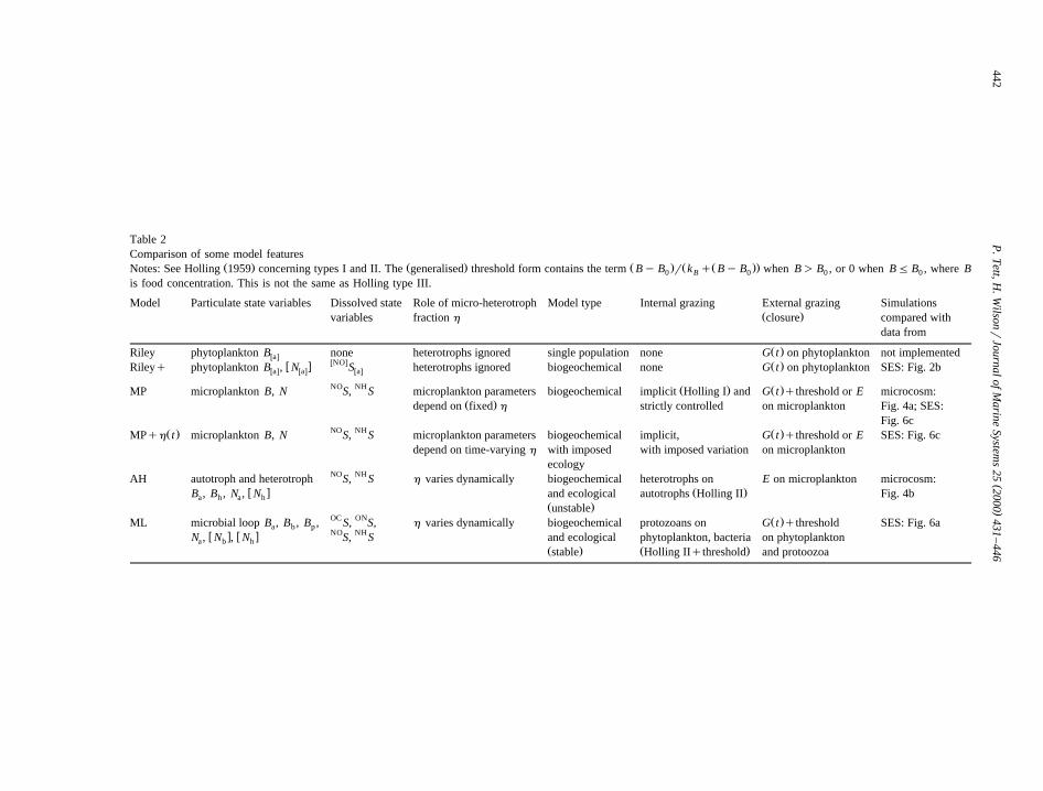
Table 2Comparison of some model features

Ž . Ž . Ž . Ž Ž ..Notes: See Holling 1959 concerning types I and II. The generalised threshold form contains the term By B r k q By B when B) B , or 0 when BF B , where B0 B 0 0 0

is food concentration. This is not the same as Holling type III.

Model Particulate state variables Dissolved state Role of micro-heterotroph Model type Internal grazing External grazing SimulationsŽ .variables fraction h closure compared with

data from

Ž .Riley phytoplankton B none heterotrophs ignored single population none G t on phytoplankton not implementedwaxwNOxw x Ž .Rileyq phytoplankton B , N S heterotrophs ignored biogeochemical none G t on phytoplankton SES: Fig. 2bwax wax wax

NO NH Ž . Ž .MP microplankton B, N S, S microplankton parameters biogeochemical implicit Holling I and G t qthreshold or E microcosm:Ž .depend on fixed h strictly controlled on microplankton Fig. 4a; SES:

Fig. 6cNO NHŽ . Ž .MPqh t microplankton B, N S, S microplankton parameters biogeochemical implicit, G t qthreshold or E SES: Fig. 6c

depend on time-varying h with imposed with imposed variation on microplanktonecology

NO NHAH autotroph and heterotroph S, S h varies dynamically biogeochemical heterotrophs on E on microplankton microcosm:w x Ž .B , B , N , N and ecological autotrophs Holling II Fig. 4ba h a h

Ž .unstableOC ON Ž .ML microbial loop B , B , B , S, S, h varies dynamically biogeochemical protozoans on G t qthreshold SES: Fig. 6aa b pNO NHw x w xN , N , N S, S and ecological phytoplankton, bacteria on phytoplanktona b h

Ž . Ž .stable Holling IIqthreshold and protoozoa


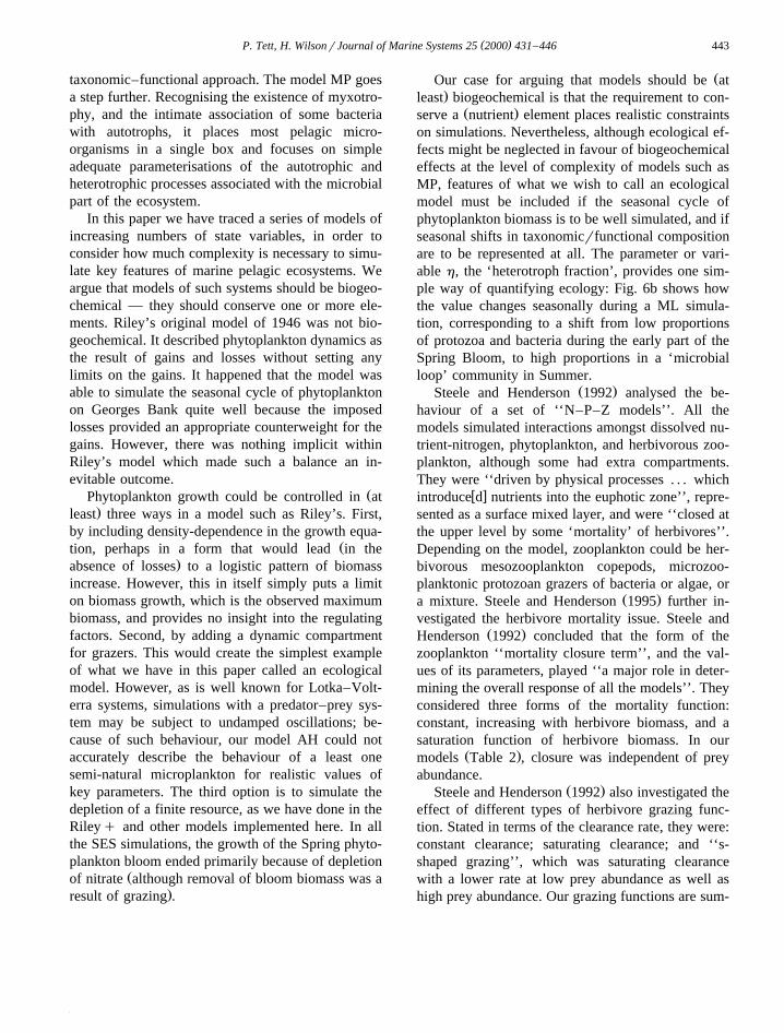
taxonomic–functional approach. The model MP goesa step further. Recognising the existence of myxotro-phy, and the intimate association of some bacteriawith autotrophs, it places most pelagic micro-organisms in a single box and focuses on simpleadequate parameterisations of the autotrophic andheterotrophic processes associated with the microbialpart of the ecosystem.

In this paper we have traced a series of models ofincreasing numbers of state variables, in order toconsider how much complexity is necessary to simu-late key features of marine pelagic ecosystems. Weargue that models of such systems should be biogeo-chemical — they should conserve one or more ele-ments. Riley’s original model of 1946 was not bio-geochemical. It described phytoplankton dynamics asthe result of gains and losses without setting anylimits on the gains. It happened that the model wasable to simulate the seasonal cycle of phytoplanktonon Georges Bank quite well because the imposedlosses provided an appropriate counterweight for thegains. However, there was nothing implicit withinRiley’s model which made such a balance an in-evitable outcome.

ŽPhytoplankton growth could be controlled in at.least three ways in a model such as Riley’s. First,

by including density-dependence in the growth equa-Žtion, perhaps in a form that would lead in the

.absence of losses to a logistic pattern of biomassincrease. However, this in itself simply puts a limiton biomass growth, which is the observed maximumbiomass, and provides no insight into the regulatingfactors. Second, by adding a dynamic compartmentfor grazers. This would create the simplest exampleof what we have in this paper called an ecologicalmodel. However, as is well known for Lotka–Volt-erra systems, simulations with a predator–prey sys-tem may be subject to undamped oscillations; be-cause of such behaviour, our model AH could notaccurately describe the behaviour of a least onesemi-natural microplankton for realistic values ofkey parameters. The third option is to simulate thedepletion of a finite resource, as we have done in theRileyq and other models implemented here. In allthe SES simulations, the growth of the Spring phyto-plankton bloom ended primarily because of depletion

Žof nitrate although removal of bloom biomass was a.result of grazing .

ŽOur case for arguing that models should be at.least biogeochemical is that the requirement to con-

Ž .serve a nutrient element places realistic constraintson simulations. Nevertheless, although ecological ef-fects might be neglected in favour of biogeochemicaleffects at the level of complexity of models such asMP, features of what we wish to call an ecologicalmodel must be included if the seasonal cycle ofphytoplankton biomass is to be well simulated, and ifseasonal shifts in taxonomicrfunctional compositionare to be represented at all. The parameter or vari-able h, the ‘heterotroph fraction’, provides one sim-ple way of quantifying ecology: Fig. 6b shows howthe value changes seasonally during a ML simula-tion, corresponding to a shift from low proportionsof protozoa and bacteria during the early part of theSpring Bloom, to high proportions in a ‘microbialloop’ community in Summer.

Ž .Steele and Henderson 1992 analysed the be-haviour of a set of ‘‘N–P–Z models’’. All themodels simulated interactions amongst dissolved nu-trient-nitrogen, phytoplankton, and herbivorous zoo-plankton, although some had extra compartments.They were ‘‘driven by physical processes . . . which

w xintroduce d nutrients into the euphotic zone’’, repre-sented as a surface mixed layer, and were ‘‘closed atthe upper level by some ‘mortality’ of herbivores’’.Depending on the model, zooplankton could be her-bivorous mesozooplankton copepods, microzoo-planktonic protozoan grazers of bacteria or algae, or

Ž .a mixture. Steele and Henderson 1995 further in-vestigated the herbivore mortality issue. Steele and

Ž .Henderson 1992 concluded that the form of thezooplankton ‘‘mortality closure term’’, and the val-ues of its parameters, played ‘‘a major role in deter-mining the overall response of all the models’’. Theyconsidered three forms of the mortality function:constant, increasing with herbivore biomass, and asaturation function of herbivore biomass. In our

Ž .models Table 2 , closure was independent of preyabundance.

Ž .Steele and Henderson 1992 also investigated theeffect of different types of herbivore grazing func-tion. Stated in terms of the clearance rate, they were:constant clearance; saturating clearance; and ‘‘s-shaped grazing’’, which was saturating clearancewith a lower rate at low prey abundance as well ashigh prey abundance. Our grazing functions are sum-


marised in Table 2. Steele and Henderson concludedw xthat, even ‘‘with s-shaped grazing . . . a limit cycle

w xresponse occurs with certain parameter values. Forw xsystems with constant herbivore mortality , a nutri-

ent limitation may be necessary to prevent limitwcycle behaviour. For herbivore-biomass dependent

xmortality with appropriate choice of coefficients,large values of nutrient concentration relative to thehalf-saturation value can be obtained’’. In these nu-trient-limited cases biomasses of phytoplankton andzooplankton remained fairly constant throughout thesimulated year.

All the models considered by Steele and Hender-Ž .son 1992 were biogeochemical according to our

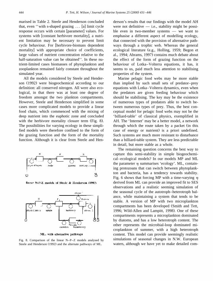
definition: all conserved nitrogen. All were also eco-logical, in that there was at least one degree offreedom amongst the two plankton compartments.However, Steele and Henderson simplified in somecases more complicated models to provide a linearfood chain, which commenced with the mixing ofdeep nutrient into the euphotic zone and concluded

Ž .with the herbivore mortality closure term Fig. 8 .The possibilities for varying ecology in these simpli-fied models were therefore confined to the form ofthe grazing function and the form of the mortalityfunction. Although it is clear from Steele and Hen-

Fig. 8. Comparison of the linear N–P–Z models analysed byŽ .Steele and Henderson 1992 and the alternate pathways of ML.

derson’s results that our findings with the model AHwere not definitive — i.e., stability might be possi-ble even in two-member systems — we want toemphasise a different aspect of modelling ecology,that connected with the provision of alternative path-ways through a trophic web. Whereas the general

Žecological literature e.g., Holling, 1959; Begon et.al., 1994; Abrams, 1997 contains much debate about

the effect of the form of grazing function on thebehaviour of Lotka–Volterra equations, it has, itseems to us, paid much less attention to stabilisingproperties of the system.

Marine pelagic food webs may be more stablethan implied by such small sets of predator–preyequations with Lotka–Volterra dynamics, even whenthe predators are given feeding behaviour whichshould be stabilising. The key may be the existenceof numerous types of predators able to switch be-tween numerous types of prey. Thus, the best con-ceptual model for pelagic food webs may not be the‘billiard-table’ of classical physics, exemplified inAH. The ‘Internet’ may be a better model, a network

Žthrough which the route taken by a packet in this.case of energy or nutrient is a priori undefined.

Such systems are much more resistant to disturbancethan a billiard-table system. They are less predictablein detail, but more stable as a whole.

The remaining question concerns the best way tocapture this semi-stability in simple biogeochemi-cal–ecological models? In our models MP and MLthe parameter h summarises ‘ecology’. ML, contain-ing protozoans that can switch between phytoplank-ton and bacteria, has a tendency towards stability.Fig. 6 shows that forcing MP with a time-varying h

derived from ML can provide an improved fit to SESobservations and a realistic seeming simulation ofthe seasonal cycle of the autotroph–heterotroph bal-ance, while maintaining a system that tends to bestable. A version of MP with two microplankton

Žcompartments has been developed Smith and Tett,.1996; Wild-Allen and Lampitt, 1998 . One of these

compartments represents a microplankton dominatedby diatoms, and has a low heterotroph content. Theother represents the microbial-loop dominated mi-croplankton of summer, with a high heterotrophcontent. This model can provide seemingly realisticsimulations of seasonal changes in N.W. Europeanwaters, although we have yet to make detailed com-


parisons of its predictions with observations of thetaxonomic composition of microplankton.

Acknowledgements

HW was funded for part of this work by a NERCstudentship, part of SES Special Topic grant GSTr02r746. The studies relating to the models MP andAH and the microcosm data were part of the EUCOHERENS project, MAS2-CT97-0088. PT isgrateful to IOW for the invitation to present thispaper at the Baltic Sea Conference, and to Dr. M.Huxham and several anonymous reviewers for help-ful comments. This is LOIS publication 735.

References

Aksnes, D.L., Ulvestad, K.B., Balino, B.M., Berntsen, J., Egge,˜J.K., Svendsen, E., 1995. Ecological modelling in coastalwaters: towards predictive physical–chemical–biological sim-ulation models. Ophelia 41, 5–36.

Anon, 1994. Stella II. Technical Documentation. High Perfor-mance Systems, Hanover, NH.

Azam, F., Fenchel, T., Field, J.G., Gray, J.S., Meyer-Reil, L.A.,Thingstad, F., 1983. The ecological role of water-columnmicrobes in the sea. Marine Ecol. Prog. Ser. 10, 257–263.

Baretta-Bekker, J.G., Baretta, J.W., Rasmussen, E.K., 1995. Themicrobial food web in the European Regional Seas Ecosystemmodel. Neth. J. Sea Res. 33, 363–379.

Begon, M., Harper, J.L., Townsend, C.R., 1994. Ecology. Black-well.

Droop, M.R., 1983. 25 years of algal growth kinetics — apersonal view. Bot. Mar. 26, 99–112.

Dussart, B.M., 1965. Les differentes categories de plancton. Hy-´ ´drobiologia 26, 72–74.

Fasham, M.J.R., Ducklow, H.W., McKelvie, S.M., 1990. A nitro-gen-based model of plankton dynamics in the oceanic mixedlayer. J. Mar. Res. 48, 591–639.

Fransz, H.G., Mommaerts, J.P., Radach, G., 1991. Ecologicalmodelling of the North Sea. Neth. J. Sea Res. 28, 67–140.

Gregoire, M., Beckers, J.M., Nihoul, J.C.J., Stabev, E., 1998.Reconnaissance of the main Black Sea’s ecohydrodynamics bymeans of a 3D interdisciplinary model. J. Mar. Syst. 16,85–105.

Hardy, A.C., 1924. The herring in relation to its animate environ-ment. Part I. The food and feeding habits of the herring withspecial reference to the east coast of England. Fish. Invest.,

Ž .Series II 7 3 , 1–53.Hastings, A., 1996. Population Biology: Concepts and Models.

Springer, New York.

Hastings, A., Powell, T., 1991. Chaos in a three-species foodchain. Ecology 72, 896–903.

Holling, C.S., 1959. Some characteristics of simple types ofpredation and parasitism. Can. Entomol. 91, 385–398.

Jones, K.J., 1979. Studies on nutrient levels and phytoplanktongrowth in a Scottish Sea Loch. PhD thesis, University ofStrathclyde.

Jones, K.J., Tett, P., Wallis, A.C., Wood, B.J.B., 1978a. Investiga-tion of a nutrient-growth model using a continuous culture ofnatural phytoplankton. J. Mar. Biol. Assoc. UK 58, 923–941.

Jones, K.J., Tett, P., Wallis, A.C., Wood, B.J.B., 1978b. The useof small, continuous and multispecies cultures to investigatethe ecology of phytoplankton in a Scottish sea-loch. Mitt. -Int.Ver. Theor. Angew. Limnol. 21, 398–412.

Kiørboe, T., 1993. Turbulence, phytoplankton cell size and thestructure of pelagic food webs. Adv. Mar. Biol. 29, 1–72.

Kraus, E.B., Turner, J.S., 1967. A one-dimensional model of theseasonal thermocline: II. The general theory and its conse-quences. Tellus 19, 98–106.

Lazier, J.R.N., Mann, K.H., 1989. Turbulence and the diffusivelayer around small organisms. Deep-Sea Res. 36, 1721–1733.

Luytens, P.J., Jones, J.E., Proctor, R., Tabor, A., Tett, P., Wild-Allen, K., 1999. COHERENS — A Coupled Hydrodynami-cal–Ecological Model for Regional and Shelf Seas: UserDocumentation. MUMM Internal report, Managament Unit ofthe Mathematical Models of the North Sea, Brussels.

Nihoul, J.C.J., 1998. Modelling marine ecosystems as a disciplinein Earth Sciences. Earth Sci. Rev. 44, 1–13.

Reynolds, C.S., Irish, A.E., 1997. Modelling phytoplankton dy-namics in lakes and reservoirs: the problems of in-situ growthrates. Hydrobiologica 349, 5–17.

Riley, 1946. Factors controlling phytoplankton populations onGeorges Bank. J. Mar. Res. 6, 54–73.

Sarmiento, J.L., Slater, R.D., Fasham, M.J.R., Ducklow, H.W.,Ducklow, J.R., Ducklow, T., Evans, G.T., 1993. A seasonalthree-dimensional ecosystem model of nitrogen cycling in theNorth Atlantic euphotic zone. Global Biogeochem. Cycles 7,417–450.

Sieburth, J.M., 1979. Sea Microbes. Oxford Univ. Press, Oxford.Simpson, J.H., Bowers, D.B., 1984. The role of tidal stirring in

controlling the seasonal heat cycle in shelf seas. Ann. Geo-phys. 2, 411–416.

Smith, C.L., Tett, P.B., 1996. Development of one and twomicroplankton compartment models to simulate conditions on

Ž .the Goban Spur abstract . UK Oceanography 96. Universityof Wales, Bangor, p. 30, Programme and Abstracts.

Steele, J.H., Henderson, E.W., 1992. The role of predation inplankton models. J. Plankton Res. 14, 157–172.

Steele, J.H., Henderson, E.W., 1995. Predation control of planktondemography. ICES J. Mar. Sci. 52, 565–573.

Taylor, A.H., Joint, I., 1990. A steady-state analysis of themicrobial loop in stratified systems. Marine Ecol. Prog. Ser.59, 1–17.

Taylor, A.H., Harbour, D.S., Harris, R.P., Burkhill, P.H., Ed-wards, E.S., 1993. Seasonal succession in the pelagic ecosys-tem of the North Atlantic and the utilization of nitrogen. J.Plankton Res. 15, 875–891.


Tett, P., 1990. A three layer vertical and microbiological pro-cesses model for shelf seas. Proudman Oceanographic Labora-tory, Report 14, 85 pp.

Tett, P., 1998. Parameterising a microplankton model. Report,Napier University, Edinburgh.

Tett, P., Walne, A., 1995. Observations and simulations of hy-drography, nutrients and plankton in the southern North Sea.Ophelia 42, 371–416.

Varela, R.A., Cruzado, A., Gabaldon, J.E., 1995. Modelling pri-´mary production in the North Sea using the European Re-gional Seas Ecosystem Model. Neth. J. Sea Res. 33, 337–361.

Wild-Allen, K.A., Lampitt, R.S., 1998. Modelling and observation

Ž .of marine snow on the continental slope abstract . UKOceanography ’98, Southampton, Programme and Abstracts,p. 62.

Williams, P.J. leB., 1981. Incorporation of microheterotrophicprocesses into the classical paradigm of the plankton foodweb. Kiel. Meeresforsch. 5, 1–28.

Wilson, H., 2000. Modelling the microplankton: a comparativestudy. PhD thesis, University of Wales, Bangor.

Woods, J., Barkmann, W., 1993. Diatom demography in winter— simulated by the Lagrangian Ensemble method. Fish.Oceanogr. 2, 202–222.

from biogeochemical to ecological models of marine microplankton

Documents