REVIEW OF SCIENTIFIC INSTRUMENTS 82, 064702 (2011)

Frequency-shift vs phase-shift characterization of in-liquid quartzcrystal microbalance applications

Y. J. Montagut,1 J. V. García,1 Y. Jiménez,1 C. March,2 A. Montoya,2 and A. Arnau1,a)

1Grupo de Fenómenos Ondulatorios, Departamento de Ingeniería Electrónica, Universitat Politècnicade València, Spain2Instituto Interuniversitario de Investigación en Bioingeniería y Tecnología Orientada al Ser Humano,Universitat Politècnica de València, Spain

(Received 16 March 2011; accepted 16 May 2011; published online 10 June 2011)

The improvement of sensitivity in quartz crystal microbalance (QCM) applications has been ad-dressed in the last decades by increasing the sensor fundamental frequency, following the incrementof the frequency/mass sensitivity with the square of frequency predicted by Sauerbrey. However, thissensitivity improvement has not been completely transferred in terms of resolution. The decrease offrequency stability due to the increase of the phase noise, particularly in oscillators, made impossibleto reach the expected resolution. A new concept of sensor characterization at constant frequency hasbeen recently proposed. The validation of the new concept is presented in this work. An immunosen-sor application for the detection of a low molecular weight contaminant, the insecticide carbaryl, hasbeen chosen for the validation. An, in principle, improved version of a balanced-bridge oscillatoris validated for its use in liquids, and applied for the frequency shift characterization of the QCMimmunosensor application. The classical frequency shift characterization is compared with the newphase-shift characterization concept and system proposed. © 2011 American Institute of Physics.[doi:10.1063/1.3598340]

I. INTRODUCTION

Acoustic sensing has taken advantage of the progressmade in the last decades in piezoelectric resonators forradio-frequency (RF) telecommunication technologies. Theso-called gravimetric technique is based on the change inthe resonance frequency experimented by the resonator dueto a mass attached on the sensor surface;1 it has openeda great deal of applications in bio-chemical sensing inboth gaseous and liquid media.2–10 This characteristic al-lows using the gravimetric techniques based on acousticsensors for a label-free and a quantitative time-dependentdetection.

The classical quartz crystal microbalance (QCM) hasbeen the most used acoustic device for sensor applications.However, other acoustic devices such as surface generatedacoustic wave (SGAW) (Ref. 4) and film bulk acoustic res-onators (FBAR) (Refs. 8 and 11–14) have been, and are beingused, for the implementation of nano-gravimetric techniquesdue to the feasibility of obtaining much higher resonantfrequency in these devices than in classical QCM resonators.The absolute frequency/mass sensitivity, given by the ratiobetween the resonant frequency-shift �f and the surfacemass density shift �m: Sa = �f/�m, theoretically increaseswith the square of the fundamental frequency;1 absolutesensitivities of a 30 MHz QCM reach 2 Hz cm2 ng−1, withtypical mass resolutions around 10 ng cm-2.15 A resolutionimprovement down to 1 ng cm−2 seems to be feasible byoptimizing the characterization electronic interface as wellas the fluidic system. Consequently, much higher sensitivity

a)Author to whom correspondence should be addressed. Electronic mail:aarnau@eln.upv.es.

is expected at higher resonant frequencies. However, the in-crease in frequency-shift/mass sensitivity has not been pairedwith the expected improvement in terms of limit of detection(LOD). Effectively, thin film electroacoustic technology hasmade possible to fabricate quasi-shear mode thin FBAR,operating with a sufficient electromechanical coupling forbeing used in liquid media at 1–2 GHz;12, 16 however, thehigher frequency and the smaller size of the resonator resultin that the boundary conditions have a much stronger effecton the FBAR performance than on the QCM response. Ahigher mass sensitivity is attained, but with an increased noiselevel as well, thus moderating the gain in resolution.13, 17

So far only publications of network analyzer based FBARsensor measurements have been published in the literature,which show that the FBAR mass resolution is very similar ifnot better than for oscillator based QCM sensors.14, 18 On theother hand, the mass sensitivity of Love mode SGAW sensorshas been evaluated.19–21 Kalantar and coworkers reported asensibility of 95 Hz cm2 ng−1 for a 100 MHz Love modesensor, which is much better than the typical values reportedfor low frequency QCM technology.22 However, Moll andcoworkers reported a LOD for a Love sensor of 400 ng cm−2,this reveals once again that an increase in the sensitivity doesnot mean, necessarily, an increase in the LOD.23 Moreover,these results have been compared with typical 10 MHzQCM sensors; recently, an electrodeless QCM biosensorfor 170 MHz fundamental frequency, with a sensitivity of67 Hz cm−2 ng−1, has been reported;24 this shows thatthe classical QCM technique still remains as a promisingtechnique. The main challenges remain on the improvementof the sensitivity, but with the aim of getting a higher massresolution, multi-analysis, and integration capabilities andreliability.

0034-6748/2011/82(6)/064702/14/$30.00 © 2011 American Institute of Physics82, 064702-1

Author complimentary copy. Redistribution subject to AIP license or copyright, see http://rsi.aip.org/rsi/copyright.jsp

064702-2 Montagut et al. Rev. Sci. Instrum. 82, 064702 (2011)

This analysis makes clear that increasing the resonant fre-quency of the sensor is not the only aspect to keep in mindfor resolution improvement; the configuration setup has animportant role, including the fluidic system and electroniccharacterization interface. Once all the care has been takenin optimizing the fluidic aspects, the role of the electronic in-terface is of maximum relevance.

In practice, focusing on in-liquid QCM applications,the sensor characterization techniques provide, among otherrelevant parameters, the resonance frequency shift of thesensor:25, 26 network or impedance analysis is used to sweepthe resonance frequency range of the resonator and deter-mine the maximum conductance frequency,27, 28 which is al-most equivalent to the motional series resonance frequencyof the resonator-sensor; impulse excitation and decay methodtechniques are used to determine the series-resonance or theparallel-resonance frequency depending on the measuring set-up;29, 30 oscillator techniques are used for a continuous mon-itoring of a frequency which corresponds to a specific phaseshift of the sensor in the resonance bandwidth,31–35 this fre-quency can be used, in many applications, as reference of theresonance frequency of the sensor; and the lock-in techniques,which can be considered as sophisticated oscillators, are de-signed for a continuous monitoring of the motional series res-onance frequency or the maximum conductance frequency ofthe resonator-sensor.36–42 In order to assure that the frequencyshift is the only parameter of interest, a second parameter pro-viding information of the constancy of the properties of liquidmedium is important, for instance, in piezoelectric biosensors;this parameter depends on the characterization system being:the maximum conductance or the conductance bandwidth inimpedance analysis, the dissipation factor in decay methods,and a voltage associated with the sensor damping in oscillatortechniques.

For high frequency resonators only impedance analysisprovides accurate results, but its high cost and large dimen-sions prevent its use for sensor applications. Consequently,oscillators are taken as alternative for sensor resonance fre-quency monitoring; the low cost of their circuitry as well asthe integration capability and continuous monitoring are somefeatures which make the oscillators to be the most commonalternative for high resonance frequency QCM sensors. How-ever, in spite of the efforts carried out to design oscillatorconfigurations suitable for in-liquid applications43–51 the poorstability of high frequency QCM systems based on oscilla-tors has prevented increasing the limit of detection despite thehigher sensitivity reported.52–56

A higher sensitivity is necessary when a higher resolutionis required. This happens in those applications where very tinychanges in the sensor resonant frequency, due to the perturba-tion process to be monitored, are expected. These very smallfrequency shifts, in the order of tens of hertz, and mainly dueto a mass transfer effect over different kind of coatings withdifferent contacting media, must be monitored under very dif-ferent damping conditions which depend on the physical andgeometrical properties of the coating and contacting media.For instance, in piezoelectric biosensors the coating can beconsidered, in general, like an acoustically thin layer and thecontacting media is a water-like solution which provides a

relatively small damping on the sensor. On the contrary, inother cases like, for example, in some electrochemical appli-cations where polymer coatings are involved, these tiny fre-quency shifts must be monitored under much higher dampingconditions. Continuous monitoring of very small frequencyshifts at very high resonance frequencies can be easily per-formed with well-designed oscillators; however, when thequality factor of the resonator-sensor is relatively low, cir-cuits able to oscillate under these special conditions have to beperformed.

A phase-shift monitoring at a constant frequency in thesensor resonance bandwidth has been recently proposed as analternative characterization method for high resolution QCMapplications.57 In the present article this alternative method isvalidated in a real application, and compared with an, in prin-ciple, improved version of a balanced-bridge oscillator.25, 51

The comparison is made with relatively low frequency sen-sors (10 MHz), where the performance of the oscillator circuitcan be considered nearly ideal.

II. THEORETICAL ASPECTS

For a great deal of in-liquid QCM applications, as itis the case of QCM biosensors, Martin’s equation (Eq. (1))is generally applied,58 which combines the additive contri-bution of the mass effect (Sauerbrey1) and the liquid effect(Kanazawa):59

� f = −2 f 2o

Zcq(mc + mL ). (1)

In the former equation, fo is the fundamental resonantfrequency, Zcq is the characteristic acoustic impedance of thequartz, mc is the surface mass density of the coating and mL

= ρLδL/2 where ρL and δL = (ηL/π foρL)1/2, ηL being the liq-uid viscosity, are respectively, the liquid density and the wavepenetration depth of the acoustic wave in the liquid: mL is, infact, the equivalent surface mass density of the liquid, whichmoves in an exponentially damped sinusoidal profile, due tothe oscillatory movement of the surface of the sensor.

According to Eq. (1), the frequency shift, associatedwith a certain mass change, increases directly proportional tothe square of the fundamental resonance frequency. Conse-quently, the most relevant parameter used up to date for thecharacterization of microbalance sensors has been the sen-sor resonance frequency-shift. However, the great efforts per-formed to improve the sensitivity of the sensor are useless ifthey are not accompanied with an increase in the limit of de-tection. As mentioned, the increase of the sensor frequencyhas not carried a parallel improvement in the mass resolu-tion. Effectively, the sensitivity will not be improved if thefrequency stability is not improved as well. In oscillators, theorigin of the frequency instability is the phase instability,25, 57

and a direct relationship can be obtained between a phase shiftand the corresponding frequency shift, through the definitionof the stability factor SF of a crystal resonator operating at itsseries resonance frequency fo:

SF = �ϕ

� ffo = 2 Q, (2)

Author complimentary copy. Redistribution subject to AIP license or copyright, see http://rsi.aip.org/rsi/copyright.jsp

064702-3 Montagut et al. Rev. Sci. Instrum. 82, 064702 (2011)

where �f is the frequency shift necessary to provide a phaseshift �ϕ in the phase-frequency response of the resonator,around fo, and Q is the series quality factor of the resonator.

According to Eq. (2) the frequency noise �fn associatedwith a phase noise in the circuitry �ϕn is

� fn = fo

2 Q�ϕn. (3)

Consequently, because the quality factor of the unper-turbed resonator is normally reduced proportionally to 1/fo,the frequency instability is increased in relation to the squareof frequency. Moreover, the phase response of the electroniccomponents of an oscillator gets worse with increasing thefrequency, which increases, even more, the noise. Further-more, if the limit of the detection is assumed to be three timesthe level of noise (�ϕmin = 3�ϕn), the minimum detectablesurface mass density change of a QCM, according to thedefinition of the absolute frequency/mass sensitivity Sa andEq. (3), will be

�mmin = fo

2 QSa�ϕmin. (4)

The former equation seems to indicate that for a givenminimum detectable phase of the measuring system, the sur-face mass limit of detection does not depend on the frequency.Fortunately this is not completely true; the liquid medium hasnot been taken into account in the obtaining of the previousequation.

III. FREQUENCY-SHIFT VS PHASE-SHIFT

Following a similar mathematical development describedelsewhere,57 the next generalized approximated equation forthe phase-shift of a signal, of constant frequency very closeto the motional series resonant frequency of the resonator-sensor, to small changes both in the coating mass and liquidproperties, is found:

�ϕ (rad) = −�mc + �mL

mq + mL. (5)

In the former equation mq = Zcq/4foQo and mL, pre-viously defined in Eq. (1), can be written as follows mL

= Zcq/4foQL, where Qo = c66/ωoηq is the series quality factorof the unperturbed resonator, c66 and ηq being, respectively,the shear modulus and the effective viscosity of the quartzcrystal, and ωo the angular resonant frequency; and QL is theseries quality factor of the resonator under liquid loading con-ditions, which is given by the following equation:

QL = Zcq√

π

2

1√fo

1√ρLηL

.

In many in-liquid QCM applications mL can be assumedto be constant and in most of them mq � mL; thus Eq. (5)reduces to

�ϕ ≈ −�mc

mL, (6)

which was previously obtained by the authors elsewhere.57

According to Eq. (6) the limit of mass-change detection�mmin corresponding to the phase-shift detection limit of thesystem �ϕmin will be given by: �mmin ≈ −mL�ϕmin. Con-sequently, the mass resolution increases (�mmin decreases)with the decrease of mL; therefore, because mL decreases pro-portionally to 1/f 1/2, the resolution in the detection of surfacemass density changes increases with f 1/2 for a given �ϕmin.

This is not in contradiction with Eq. (4); simply the ef-fective reduction of the quality factor of the sensor is propor-tional to 1/f 1/2 instead of to 1/f when the contacting liquid isconsidered. This is not true in air because the approximationmq � mL made in Eq. (5) to obtain Eq. (6) is not acceptable. Inair, an increase in frequency does not improve the limit of de-tection unless the stability and the phase detection limit of themeasuring system are improved. Curiously, this also happenswhen only changes in the liquid properties occur. Effectively,when the aim is to monitor changes in the properties of theliquid in contact with the sensor: �(ηLρL)1/2, the phase shiftrelated to these changes is, according to Eq. (5), given by

�ϕ ≈ −�mL

mL= −�

√ρLηL√

ρLηL. (7)

Therefore, it is not possible to increase the resolution inthe detection of changes in the liquid properties by increasingthe frequency. According to the previous considerations, it isimportant to check the limits for which the approximation mq

� mL is acceptable:The parameter mq is independent of the frequency, and

a reference value of mq = 2.2·10−6 kg m−2 is obtained for areal 10 MHz AT-cut quartz crystal sensor with a typical Qo

around 105 (see definition below Eq. (5) with Zcq = 8.838833106 N s m−3). The approximation can be considered accept-able for ratios of mq/mL ≤ 0.1. This ratio is given by

mq

mL= 2.2 · 10−6

√4π

√f√

ρLηL≤ 0.1. (8)

The former equation indicates that for a given liquid theratio mq/mL only depends on the frequency; the worst caseoccurs for low density-viscosity liquids like, for instance,water where ηLρL = 1. In this case the maximum frequencyfor which the approximation mq � mL is acceptable is around165 MHz. Moreover, Eq. (5) also indicates that when mL

decreases to a value much smaller than mq, no furtherimprovement in the resolution can be obtained by increasingthe frequency; this happens for ratios mq/mL ≥ 0.9 whichare obtained, under the previous conditions, for frequencieshigher than 10 GHz.

The previous analysis allows concluding the followingimportant remarks: (1) the sensitivity of a QCM always in-creases with increasing the frequency; however, the mass res-olution, which is the parameter of interest, only increases withthe frequency if the noise is, at least, maintained constant orreduced. Moreover, this increase in the mass resolution is onlyvalid for in-liquid QCM and not for in-gas QCM; and (2) onceall the cares have been taken into account to reduce the pertur-bations on the resonator-sensor such as temperature and pres-sure fluctuations, etc., the mass resolution is only depending

Author complimentary copy. Redistribution subject to AIP license or copyright, see http://rsi.aip.org/rsi/copyright.jsp

064702-4 Montagut et al. Rev. Sci. Instrum. 82, 064702 (2011)

FIG. 1. (a) Description of the phase-shift characterization versus thefrequency-shift method, (b) implementation block diagram.

on the interface system, its stability, and its phase detectionlimit.

Consequently, unlike in oscillators for RF applications,in oscillators based on QCM sensors, the resonator is not in-cluded in the circuitry with the aim of stabilizing the oscillatorsystem, although evidently it does it; just on the contrary, theoscillator circuitry should be as ideal as possible for not in-fluencing the shifts in the sensor phase due to the monitoringprocesses. Unfortunately, the implementation of an ideal os-cillator for high frequency QCM sensors, keeping in mind thelow quality factors reached by these sensors under liquid con-ditions, and the very low phase noise that it is necessary, isnot an easy task.

By keeping in mind the previous considerations, a dif-ferent approach was recently proposed:57 taking into accountthat the expected frequency shifts in those QCM applica-tions where a high resolution is necessary, for example, inbiosensors, are very small, it could be possible to interrogatethe sensor with an appropriate constant frequency signal, inthe sensor resonance bandwidth, and then measure the changein the phase response of the sensor, while maintaining thefrequency of the testing signal in the resonance bandwidth;Fig. 1(a) depicts the frequency-shift versus the phase-shiftcharacterization methods.

A similar approach has been already applied under dif-ferent conditions by some authors.60, 61 The advantage of thisapproach is that the sensor is interrogated with an externalsource which can be designed to be very stable and with ex-tremely low phase and frequency noises, even at very highfrequencies. Moreover, a very simple circuit can be usedfor the phase-mass characterization approach as depicted inFig. 1(b), where a mixer based phase detector is used. In thenext paragraph two practical systems are described which willbe useful for validating the phase-shift against the frequency-shift characterization. An improved version of the balanced-bridge oscillator proposed elsewhere25 is extensively testedunder different damping conditions showing the effects of the

FIG. 2. Schematics of the balanced-bridge oscillator proposed.

non-ideal behaviour of oscillators to monitor the frequency-shifts under different damping conditions. Nonetheless, forconstant damping conditions and low frequency sensors(10 MHz AT-cut quartz resonators), the oscillator can be usedfor resonance frequency shift monitoring and therefore beused to validate the phase-shift method by comparison of theresults.

IV. DESCRIPTION OF THE SYSTEMS

A. Improved balanced-bridge oscillator

The proposed interface is shown in Fig. 2, and is based onthe balanced-bridge oscillator presented elsewhere,51 wherethe transistors have been replaced by operational transconduc-tance amplifiers or diamond transistors (OTA 1-2). The mixercircuit based on the integrated circuit (IC) AD835, with twodifferential inputs, allows the implementation of a differen-tial amplification with automatic gain control (AGC), whichminimizes the nonlinearities of the active devices and pro-vides information about the sensor damping. This configura-tion allows, in principle, a parallel capacitance compensationwhich ideally provides oscillation at zero-phase loop condi-tion; the parallel circuit LC-CC is included to drastically re-duce the loop-gain for undesired frequencies. For ideal com-ponents and parallel capacitance compensation the oscillationfrequency should be the motional series resonant frequency ofthe sensor under different damping conditions, and the AGCvoltage would provide information about the resonator mo-tional resistance.

Effectively, the input voltage ui is transferred to theemitters and the emitter currents are non-inverted voltage-converted to the collectors into u1 and u2 as follows:

u1 = ui YX ZC , (9a)

u2 = ui YCv ZC , (9b)

where YX = jωCo+1/Zm is the admittance of the QCM sensorformed by the so-called static capacitance Co in parallel withthe so-called motional branch whose impedance Zm is formedby a Rm, Lm, Cm series equivalent circuit, being Zm = Rm

+ j(Lmω − 1/ωCm); YCv = jωCv, ZC = RC + j(LCω − 1/ωCC)and ω is the angular frequency.

Author complimentary copy. Redistribution subject to AIP license or copyright, see http://rsi.aip.org/rsi/copyright.jsp

064702-5 Montagut et al. Rev. Sci. Instrum. 82, 064702 (2011)

The voltages at the collectors are differentially amplifiedwith one of the high input impedance differential amplifiersof the AD835, and the output signal is level controlled witha multiplier giving the following output signal u′

i which isfed-back to the input:

u′i = ADk

(1

Zm+ jω(Co − Cv )

)ZC ui . (10)

Because u′i = ui the final loop condition results:

ADk

(1

Zm+ jω(Co − Cv )

)ZC = 1. (11)

Under ideal conditions, it is assumed that the parallelcircuit ZC has been designed to resonate at the oscillationfrequency, therefore ZC ≈ RC; the parallel capacitance hasbeen compensated, Co = CV; and the OTAs and the multi-plier do not produce phase-shifts, it is to say AD and k are realnumbers. Consequently, the loop-phase condition given byEq. (11) indicates that, under the previous conditions, the os-cillation frequency corresponds to the motional series reso-nant frequency at which Zm = Rm, and the loop-gain at theoscillation frequency reduces to

ADkRC

Rm= 1. (12)

Therefore the automatic gain control voltage, k= Rm/ADRC, is proportional to the value of the motionalresistance Rm for given values of the differential gain AD andthe resistance RC. The objective of the AGC is to maintainconstant the amplitude of the signal u1; with this purpose a dcsignal, associated with the amplitude of the sinusoidal signalu1, is obtained by low pass filtering the output of a multiplierwhose inputs are connected to u1.

Experimental results will provide the level of fulfilmentof the previous equations regarding the degree of ideal perfor-mance of the components of the oscillator.

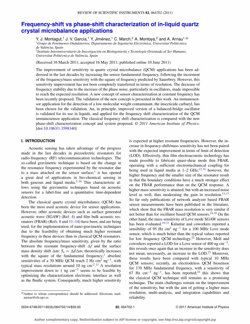
B. Phase-shift characterization interface

A schematic interface for the phase-shift characteriza-tion method was proposed elsewhere57 and it has been im-plemented now for its validation. The core of the interfaceis the sensor circuit which is depicted in Fig. 3. Two paral-lel branches form a differential circuit. Because the testingsignal ut has constant frequency ft, the only element in thecircuit which contributes to a change in the phase shift be-tween the reference signal u1 and the signal u2 is the change inthe phase-frequency response due to the sensor perturbation.Therefore, this phase-shift can be continuously monitored bya phase-detector. The IC AD8302 from Analog Devices hasbeen used for this purpose; it includes a mixer and the low-pass filter (LPF), connected in series behind the signals u1 andu2, which act as a phase detector for small phase-shifts around90o between the input signals.62 Thus, for a proper operationit is convenient to phase-shift 90o the testing signals in eachbranch of the sensor circuit; for this purpose the networksformed by Ri and Ci at the inputs of the sensor circuit havebeen included. The phase-shifting networks formed by Ri andCi must be designed coherently with the resonant frequency of

FIG. 3. Schematics of the phase-shift characterization system.

the sensor in order to obtain two signals 90o phase-shifted andof similar amplitude. The IC-AD8302 additionally includesa block, formed by logarithmic amplifiers, which provides avoltage proportional to the decibel ratio of the input signals u1

and u2. Both the phase detector and the logarithmic amplifierblock have responses VPHS and VMAG, centred at 900 mV for90o phase-shift and 0 dB power ratio between the signals u1

and u2. These transfer functions are re-centred around 0 mVwith additional differential amplifiers with appropriate volt-ages at the reference inputs Vref1 and Vref2, obtained from avery stable and low noise voltage reference; this allows pro-viding an additional amplification of signals VPHS and VMAG.

Wide bandwidth operational amplifiers OPA1-4 are usedto isolate the sensor and the reference network RC-CC fromthe rest of the circuit. At motional series resonance frequency(MSRF) the sensor reduces to a motional resistance Rm in par-allel with the so-called static capacitance C0; therefore for op-timum operation it is convenient to select RC and CC similarto Rm and C0, respectively. Effectively, under these conditionsand at the MSRF of the sensor, the voltages uϕ and uA cor-responding to the phase-shift and to the decibel ratio of theinput signals u1 and u2, respectively, should be, ideally, zero;this provides a way to calibrate the system.

Additionally, far from resonance the sensor behaves likethe parallel capacitance C0, and the network formed by theresistance Rt and the sensor reduces to a low-pass filterRt-C0 of very high cutoff frequency around several megahertz.Consequently slow phase noises in the input testing signal areequally transferred to both branches and eliminated by the dif-ferential system, and then improving the stability.

V. MATERIALS AND METHOD

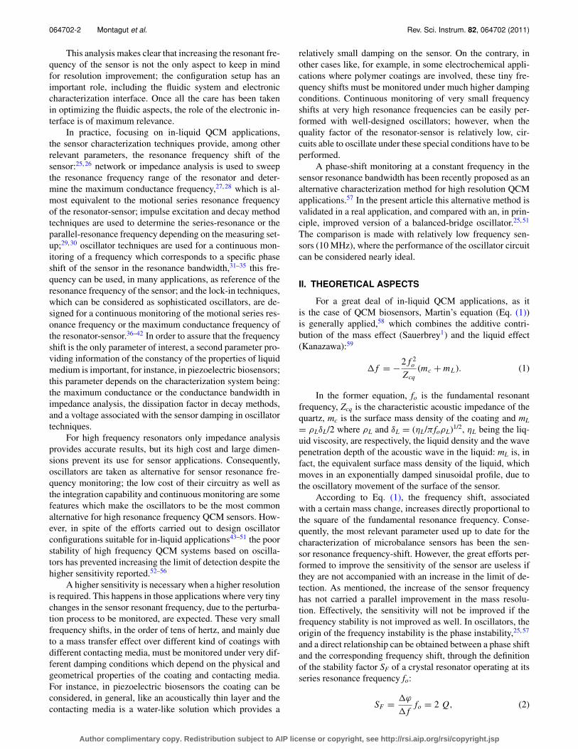
A. Sensors and accessories

10 MHz fundamental frequency AT-cut quartz sensors,with 13.67 mm blank diameter and 5.11 mm of Cr/Au elec-trode diameter (100 Å of Cr and 1000 Å of Au), were used inthe experiments. Two home-made cells were used, one witha volume capacity of 200 μl for the experiments done in-batch with different concentrations of glycerol in water, de-scribed elsewhere,42 and a different one for the experimentsin flow with 30 μl volume capacity (Fig. 4). Other instru-ments associated with the experiment were: Impedance An-alyzer HP4291A, frequency meter HP53181A, multimeter

Author complimentary copy. Redistribution subject to AIP license or copyright, see http://rsi.aip.org/rsi/copyright.jsp

064702-6 Montagut et al. Rev. Sci. Instrum. 82, 064702 (2011)

FIG. 4. (Color online) Flow cell.

HP34401A, RF signal generator model HP8664A, and dataacquisition system AWSense IP/AQ-1 from AWSensors Inc.

B. Circuit implementation

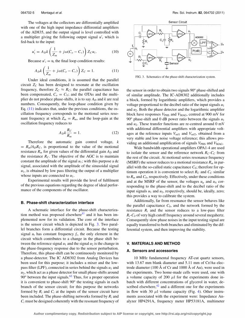
The circuits for both systems were made follow-ing recommendations applicable to high frequency layoutdesign63, 64 and implemented in four-layer surface-mounttechnology. The following ICs for the main parts of the os-cillator were used: OPA860 for the OTAs and AD835 for theimplementation of the automatic gain control and differentialamplification. The value of RC must be appropriately selectedto assure the fulfilment of the loop-gain condition, accordingto Eq. (12), for given values of AD and k, and for the expectedrange of values of Rm, which mainly depends on the dampingmedia in contact with the sensor. In this particular case a valueof RC = 1 K has been selected for an Rm range between10 and 1.2 K, keeping in mind the reachable values of k(0 � 1,2) and AD ≈ 1. LC-CC filters have been selectedmatched and for a resonance at 10 MHz when using 10 MHzAT-cut quartz resonators. The implemented design is shownin Figs. 5(a) and 5(b).

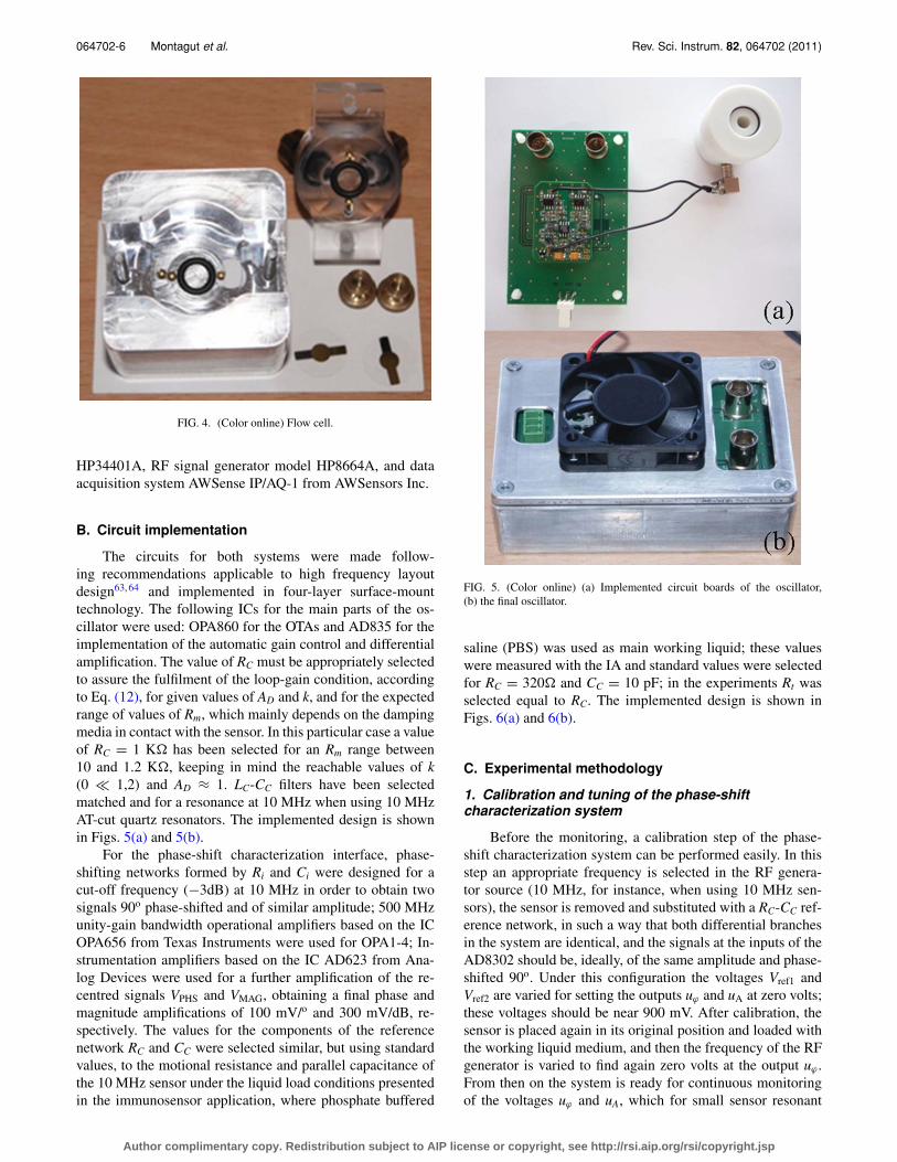
For the phase-shift characterization interface, phase-shifting networks formed by Ri and Ci were designed for acut-off frequency (−3dB) at 10 MHz in order to obtain twosignals 90o phase-shifted and of similar amplitude; 500 MHzunity-gain bandwidth operational amplifiers based on the ICOPA656 from Texas Instruments were used for OPA1-4; In-strumentation amplifiers based on the IC AD623 from Ana-log Devices were used for a further amplification of the re-centred signals VPHS and VMAG, obtaining a final phase andmagnitude amplifications of 100 mV/o and 300 mV/dB, re-spectively. The values for the components of the referencenetwork RC and CC were selected similar, but using standardvalues, to the motional resistance and parallel capacitance ofthe 10 MHz sensor under the liquid load conditions presentedin the immunosensor application, where phosphate buffered

FIG. 5. (Color online) (a) Implemented circuit boards of the oscillator,(b) the final oscillator.

saline (PBS) was used as main working liquid; these valueswere measured with the IA and standard values were selectedfor RC = 320 and CC = 10 pF; in the experiments Rt wasselected equal to RC. The implemented design is shown inFigs. 6(a) and 6(b).

C. Experimental methodology

1. Calibration and tuning of the phase-shiftcharacterization system

Before the monitoring, a calibration step of the phase-shift characterization system can be performed easily. In thisstep an appropriate frequency is selected in the RF genera-tor source (10 MHz, for instance, when using 10 MHz sen-sors), the sensor is removed and substituted with a RC-CC ref-erence network, in such a way that both differential branchesin the system are identical, and the signals at the inputs of theAD8302 should be, ideally, of the same amplitude and phase-shifted 90o. Under this configuration the voltages Vref1 andVref2 are varied for setting the outputs uϕ and uA at zero volts;these voltages should be near 900 mV. After calibration, thesensor is placed again in its original position and loaded withthe working liquid medium, and then the frequency of the RFgenerator is varied to find again zero volts at the output uϕ .From then on the system is ready for continuous monitoringof the voltages uϕ and uA, which for small sensor resonant

Author complimentary copy. Redistribution subject to AIP license or copyright, see http://rsi.aip.org/rsi/copyright.jsp

064702-7 Montagut et al. Rev. Sci. Instrum. 82, 064702 (2011)

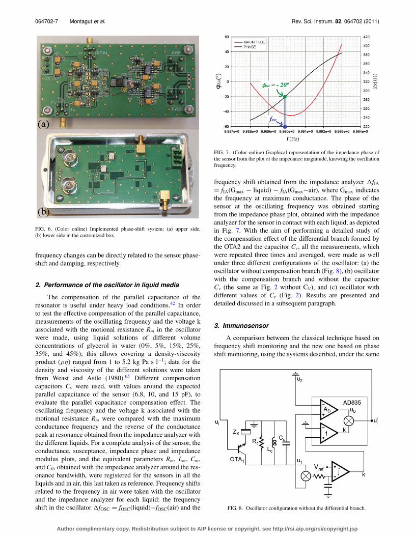
FIG. 6. (Color online) Implemented phase-shift system: (a) upper side,(b) lower side in the customized box.

frequency changes can be directly related to the sensor phase-shift and damping, respectively.

2. Performance of the oscillator in liquid media

The compensation of the parallel capacitance of theresonator is useful under heavy load conditions.42 In orderto test the effective compensation of the parallel capacitance,measurements of the oscillating frequency and the voltage kassociated with the motional resistance Rm in the oscillatorwere made, using liquid solutions of different volumeconcentrations of glycerol in water (0%, 5%, 15%, 25%,35%, and 45%); this allows covering a density-viscosityproduct (ρη) ranged from 1 to 5.2 kg Pa s l−1; data for thedensity and viscosity of the different solutions were takenfrom Weast and Astle (1980).65 Different compensationcapacitors Cv were used, with values around the expectedparallel capacitance of the sensor (6.8, 10, and 15 pF), toevaluate the parallel capacitance compensation effect. Theoscillating frequency and the voltage k associated with themotional resistance Rm were compared with the maximumconductance frequency and the reverse of the conductancepeak at resonance obtained from the impedance analyzer withthe different liquids. For a complete analysis of the sensor, theconductance, susceptance, impedance phase and impedancemodulus plots, and the equivalent parameters Rm, Lm, Cm,and C0, obtained with the impedance analyzer around the res-onance bandwidth, were registered for the sensors in all theliquids and in air, this last taken as reference. Frequency shiftsrelated to the frequency in air were taken with the oscillatorand the impedance analyzer for each liquid: the frequencyshift in the oscillator �fOSC = fOSC(liquid)−fOSC(air) and the

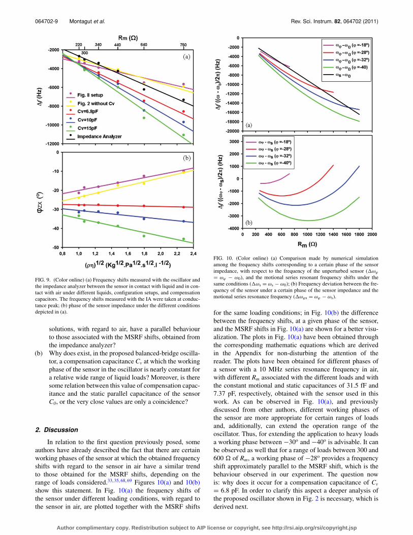
FIG. 7. (Color online) Graphical representation of the impedance phase ofthe sensor from the plot of the impedance magnitude, knowing the oscillationfrequency.

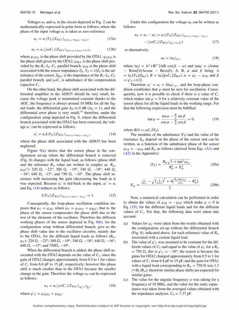
frequency shift obtained from the impedance analyzer �fIA= fIA(Gmax − liquid) − fIA(Gmax−air), where Gmax indicatesthe frequency at maximum conductance. The phase of thesensor at the oscillating frequency was obtained startingfrom the impedance phase plot, obtained with the impedanceanalyzer for the sensor in contact with each liquid, as depictedin Fig. 7. With the aim of performing a detailed study ofthe compensation effect of the differential branch formed bythe OTA2 and the capacitor Cv, all the measurements, whichwere repeated three times and averaged, were made as wellunder three different configurations of the oscillator: (a) theoscillator without compensation branch (Fig. 8), (b) oscillatorwith the compensation branch and without the capacitorCv (the same as Fig. 2 without CV), and (c) oscillator withdifferent values of Cv (Fig. 2). Results are presented anddetailed discussed in a subsequent paragraph.

3. Immunosensor

A comparison between the classical technique based onfrequency shift monitoring and the new one based on phaseshift monitoring, using the systems described, under the same

FIG. 8. Oscillator configuration without the differential branch.

Author complimentary copy. Redistribution subject to AIP license or copyright, see http://rsi.aip.org/rsi/copyright.jsp

064702-8 Montagut et al. Rev. Sci. Instrum. 82, 064702 (2011)

experimental conditions, was performed by implementing areal application based on the detection of low molecularweight pollutants; only with this purpose, a piezoelectric im-munosensor for the detection of the pesticide carbaryl, asa validation model, was developed. The following protocoldescribed elsewhere was followed:3 the AT-cut quartz crys-tals were functionalized by immobilizing BSA-CNH carbarylhapten conjugate on the sensor surface through the forma-tion of a thioctic acid self-assembled monolayer. The crys-tal was placed in a custom-made flow cell (Fig. 4) and in-cluded in a flow-through setup, controlled by a peristalticpump (Minipuls 3, Gilson), with the injection loop and solu-tions at the input of the flow cell exchanged by manual Rheo-dyne valves (models 5020 and 5011, Supelco), according tothe flow system described elsewhere.66 The whole fluidic sys-tem and the sensor characterization circuit with the sensor cellwere placed in a custom made thermostatic chamber and allthe experiments were performed at 25 oC ± 0.1 oC. To avoidunwanted disturbances the chamber was placed on an anti-vibration table.

The immunoassay developed to determine carbaryl wasan inhibition test based on the conjugate coated format, inwhich the hapten-conjugate was immobilized on the sensorsurface. A fixed amount of a specific monoclonal antibodywas mixed with standard solutions of the analyte and pumpedover the sensor surface. Since the analyte inhibits antibodybinding to the immobilized conjugate, increasing concentra-tions of analyte will reduce the phase shift induced on thepiezoelectric sensor and the corresponding demodulated volt-age.

Different standard concentrations of carbaryl were pre-pared by serial dilutions in PBS, from a 1 mM stock so-lution in dimetylformamide at −20 oC. The standards weremixed with a fixed concentration of the monoclonal antibodyLIB-CNH45 (from I3BH-UPV (Ref. 67)) in PBS. Analyte-antibody solutions were incubated for 1 h at ambient tem-perature, then loaded (250 μl) into the injection loop in thechamber, and finally, when tempered, injected onto the sensorsurface. The phase-shift was monitored in real-time for eachanalyte concentration during 12 min, as the binding betweenfree antibody and the immobilized conjugate took place. Re-generation of the sensing surface was performed using dilutedhydrochloric acid, 0.1M HCl, to break the antibody-haptenlinkage, at a flow rate of 280 μl/min for 4 min, and thenwith the working buffer solution – phosphate buffered saline– 0.005% tween 20 (PBST) – for 2 min at the same flow rate.Stabilization of the initial signal was achieved again at a flowrate of 30 μl/min for 2 min. A complete assay cycle took20 min. This protocol was performed with both characteri-zation systems and the results are discussed in a subsequentparagraph.

VI. RESULTS AND DISCUSSION

A. Performance of the oscillator in liquid media

1. Results

A linear correlation was found between the motional re-sistance Rm values, obtained from the impedance analyzer,

and the voltage k values, obtained from the oscillator, with acorrelation coefficient higher than 0.998 in all the cases. Aver-age deviations between the value of Rm obtained from the lin-eal regression, under the restricted condition of Rm being 0 fork = 0, to be coherent with Eq. (12), and those obtained fromthe IA, were smaller that 5.5%, reaching the value of 1.1% forthe highest values of Rm; a uniform reduction of the deviationis observed as the Rm values increase. This can be explainedtaking into account that the OTA1 operates at higher currentgains for smaller liquid loads, and that the operation of theamplifier gets farther from the ideal behaviour as the gain in-creases.

Figure 9(a) collects the frequency shifts obtained withthe oscillator (�fOSC = fOSC(liquid)−fOSC(air)) and theimpedance analyzer (�fIA = fIA(Gmax−liquid)−fIA(Gmax

−air)) for all the liquids and with the different circuit set-ups and compensation capacitors Cv. Figure 9(b) shows theimpedance working phase of the sensor, obtained as ex-plained, under the different liquid loads and for the differentoscillator set-ups and compensation capacitors Cv depicted inFig. 9(a). The Rm values in Figs. 9(a) and 9(b) are only in-cluded as reference and are near but not necessarily equal tothe corresponding Rm values obtained from the impedance an-alyzer with the corresponding liquids; however these valuesfor Rm were used in the numerical calculations performed inthe discussion below.

The main objective of using the balanced-bridge os-cillator is the parallel capacitance compensation under theideal assumptions made in Sec. IV A. The results shown inFigs. 9(a) and 9(b) allow making the following remarks:

(a) If the parallel capacitance was compensated with an ap-propriate value of compensation capacitance Cv, the os-cillation frequency shift should be in coincidence, orat least to be very near to the MSRF shift given bythe impedance analyzer; however the results depicted inFig. 9(a) show that none of sets of the oscilla-tor frequency shifts for the different liquids fits theMSRF shifts of the analyzer, only the set of frequencyshifts corresponding to the compensation capacitor Cv

= 6.8 pF seems to be parallel to the results obtained withthe impedance analyzer which are taken as reference.The averaged value of the static parallel capacitance C0

obtained from the impedance analyzer for all the liquidswas 7.37 pF, with a maximum deviation of 1.5%, it is tosay very near to 6.8 pF. This could make to think that akind of compensation occurs; however this is not reason-able by taking into account the following remark.

(b) According to Fig. 9(b), the sensor working phase for Cv

= 6.8 pF shows nearly a constant working phase for thewhole range of liquid loads (average of −28o with a de-viation of 0.4o). This is in contradiction with the trackingof the MSRF, since different sensor phases correspond todifferent MSRFs associated with different liquid loads.

In any case, the behaviour depicted in Figs. 9(a) and 9(b)should be explained in the following aspects:

(a) Why is there a sensor working phase at which theoscillation frequency shifts in the working liquid

Author complimentary copy. Redistribution subject to AIP license or copyright, see http://rsi.aip.org/rsi/copyright.jsp

064702-9 Montagut et al. Rev. Sci. Instrum. 82, 064702 (2011)

FIG. 9. (Color online) (a) Frequency shifts measured with the oscillator andthe impedance analyzer between the sensor in contact with liquid and in con-tact with air under different liquids, configuration setups, and compensationcapacitors. The frequency shifts measured with the IA were taken at conduc-tance peak; (b) phase of the sensor impedance under the different conditionsdepicted in (a).

solutions, with regard to air, have a parallel behaviourto those associated with the MSRF shifts, obtained fromthe impedance analyzer?

(b) Why does exist, in the proposed balanced-bridge oscilla-tor, a compensation capacitance Cv at which the workingphase of the sensor in the oscillator is nearly constant fora relative wide range of liquid loads? Moreover, is theresome relation between this value of compensation capac-itance and the static parallel capacitance of the sensorC0, or the very close values are only a coincidence?

2. Discussion

In relation to the first question previously posed, someauthors have already described the fact that there are certainworking phases of the sensor at which the obtained frequencyshifts with regard to the sensor in air have a similar trendto those obtained for the MSRF shifts, depending on therange of loads considered.33, 35, 68, 69 Figures 10(a) and 10(b)show this statement. In Fig. 10(a) the frequency shifts ofthe sensor under different loading conditions, with regard tothe sensor in air, are plotted together with the MSRF shifts

FIG. 10. (Color online) (a) Comparison made by numerical simulationamong the frequency shifts corresponding to a certain phase of the sensorimpedance, with respect to the frequency of the unperturbed sensor (�ωϕ

= ωϕ − ω0), and the motional series resonant frequency shifts under thesame conditions (�ωs = ωs − ω0); (b) Frequency deviation between the fre-quency of the sensor under a certain phase of the sensor impedance and themotional series resonance frequency (�ωϕs = ωϕ − ωs).

for the same loading conditions; in Fig. 10(b) the differencebetween the frequency shifts, at a given phase of the sensor,and the MSRF shifts in Fig. 10(a) are shown for a better visu-alization. The plots in Fig. 10(a) have been obtained throughthe corresponding mathematic equations which are derivedin the Appendix for non-disturbing the attention of thereader. The plots have been obtained for different phases ofa sensor with a 10 MHz series resonance frequency in air,with different Rm associated with the different loads and withthe constant motional and static capacitances of 31.5 fF and7.37 pF, respectively, obtained with the sensor used in thiswork. As can be observed in Fig. 10(a), and previouslydiscussed from other authors, different working phases ofthe sensor are more appropriate for certain ranges of loadsand, additionally, can extend the operation range of theoscillator. Thus, for extending the application to heavy loadsa working phase between −30o and −40o is advisable. It canbe observed as well that for a range of loads between 300 and600 of Rm, a working phase of −28o provides a frequencyshift approximately parallel to the MSRF shift, which is thebehaviour observed in our experiment. The question nowis: why does it occur for a compensation capacitance of Cv

= 6.8 pF. In order to clarify this aspect a deeper analysis ofthe proposed oscillator shown in Fig. 2 is necessary, which isderived next.

Author complimentary copy. Redistribution subject to AIP license or copyright, see http://rsi.aip.org/rsi/copyright.jsp

064702-10 Montagut et al. Rev. Sci. Instrum. 82, 064702 (2011)

Voltages u1 and u2 in the circuit depicted in Fig. 2 can bemathematically expressed in polar form as follows, where thephase of the input voltage ui is taken as zero reference:

u1 = ui |YX ||Z RLC |〈ϕOT A1+ϕRLC −ϕZ X 〉, (13a)

u2 = ui | jωCv ||Z RLC |〈ϕOT A2+ϕRLC +π/2〉, (13b)

where ϕOTA1 is the phase shift provided by the OTA1, ϕOTA2 isthe phase shift given by the OTA2, ϕRLC is the phase shift pro-vided by the RC-LC-CC parallel branch, ϕZX is the phase shiftassociated with the sensor impedance ZX, YX = 1/ZX is the ad-mittance of the sensor, ZRLC is the impedance of the RC-LC-CC

parallel branch, and jωCv is admittance of the compensationcapacitor Cv.

On the other hand, the phase shift associated with the dif-ferential amplifier in the AD835 should be very small, be-cause the voltage peak is maintained constant thanks to theAGC, the frequency is always around 10 MHz for all the liq-uid loads, the differential gain AD is 0 dB (AD = 1), and thedifferential error phase is very small;70 therefore, under theconfiguration setup depicted in Fig. 8, where the differentialbranch associated with the OTA2 has been removed, the volt-age ui

′ can be expressed as follows:

u′i = ui k|YX ||Z RLC |〈ϕOT A1+ϕRLC −ϕZ X 〉, (14)

where the phase shift associated with the AD835 has beenneglected.

Figure 9(a) shows that the sensor phase in the con-figuration set-up where the differential branch is removed(Fig. 8) changes with the liquid load, as follows (phase shiftand the reference Rm value are written in couples as: Rm,ϕZX

o): 220 , −22o; 300 , −19o; 340 , −18o; 440 ,−16o; 640 , –13o; and 750 , −10o. The phase shift in-creases with increasing the gain (decreasing the load) as itwas expected. Because ui

′ is fed-back to the input, ui′ = ui

and Eq. (14) reduces as follows:

k|YX ||Z RLC |〈ϕOT A1+ϕRLC −ϕZ X 〉 = 1. (15)

Consequently, the loop-phase oscillation condition im-poses that ϕC = ϕZX, where ϕC = ϕOTA1 + ϕRLC; that is, thephase of the sensor compensates the phase shift due to therest of the elements of the oscillator. Therefore the differentworking phases of the sensor depicted in Fig. 9(b), for theconfiguration setup without differential branch, give us thephase shift value due to the oscillator circuitry, mainly dueto the OTA1, for the different liquid loads as follows (Rm,ϕC): 220 , −22o; 300 , −19o; 340 , −18o; 440 , −16o;640 , −13o; and 750, −10o.

When the differential branch is added, the phase shift as-sociated with the OTA2 depends on the value of Cv, since thegain of OTA2 changes approximately from 0.5 to 1 for valuesof Cv from 6.8 pF to 15 pF, respectively; however this phaseshift is much smaller than in the OTA1 because the smallerchange in the gain. Therefore the voltage u2 can be expressedas follows:

u2 = ui | jωCv ||Z RLC |〈ϕ′C +π/2〉, (16)

where ϕ′C = ϕOTA2 + ϕRLC

Under this configuration the voltage u0 can be written asfollows:

u0 = u1 − u2 = ui (|YX ||Z RLC |〈ϕOT A1+ϕRLC −ϕZ X 〉

− | jωCv ||Z RLC |〈ϕ′C +π/2〉) (17)

or alternatively:

u0 = |u0|〈ϕ〉, (18)

where |u0| = A2+B2–2AB cos(β − α) and tanϕ = (Asinα

− Bsinβ)/(Acosα − Bcosβ); A, B, α and β being: A= |ui‖YX‖ZRLC|, B = |ui‖jωCv‖ZRLC|, α = ϕC − ϕZX and β

= ϕ′C+π /2.Therefore ui

′ = ui = k|u0|<ϕ> and the loop-phase con-dition establishes that ϕ must be zero for oscillation. Conse-quently, now it is possible to check if there is a value of Cv

which makes tan ϕ = 0 for a relatively constant value of thesensor phase for all the liquid loads in the working range. Forthat the following expression must be fulfilled:

tan ϕ = sin α − BA sin β

cos α − BA cos β

= 0, (19)

where B/A = ωCv/|YX|.The modulus of the admittance |YX| and the value of the

reactance Xm depend on the phase of the sensor and can bewritten, as a function of the admittance phase of the sensorϕYX = −ϕZX and Rm as follows (derived from Eqs. (A1) and(A2) in the Appendix):

|YX | = Rm

√1 + tan2 ϕYX

R2m + X2

m

, (20a)

Xm =1

ωC0−

√(1

ωC0

)2 + 4( Rm tan ϕYX

ωC0− R2

m

)2

. (20b)

Now, a numerical calculation can be performed in orderto obtain the values of ϕZX = −ϕYX which make ϕ = 0 inEq. (19), for the different liquid loads and for the differentvalues of Cv. For that, the following data were taken intoaccount:

(a) Values for ϕC were taken from the results obtained withthe configuration set-up without the differential branch(Fig. 8), indicated above, for each reference value of Rm

associated with a certain liquid load.(b) The value of ϕ′

C was assumed to be constant for the dif-ferent values of CV and equal to the value of ϕC for a Rm

= 750 , this is ϕ′C = −10o; the reason is because the

gains for OTA2 changed approximately from 0.5 to 1 forvalues of Cv from 6.8 pF to 15 pF, and the gain for OTA1with a liquid load corresponding to Rm = 750 was 1.3(≈RC/Rm); therefore similar phase shifts are expected forsimilar gains.

(c) The value for the angular frequency ω was taking for afrequency of 10 MHz, and the value for the static capac-itance was taken from the averaged values obtained withthe impedance analyzer, C0 = 7.37 pF.

Author complimentary copy. Redistribution subject to AIP license or copyright, see http://rsi.aip.org/rsi/copyright.jsp

064702-11 Montagut et al. Rev. Sci. Instrum. 82, 064702 (2011)

FIG. 11. (Color online) Results of the numerical simulation derived fromEq. (19).

The results of this analysis are presented in Fig. 11. Asit can be observed they follow almost the same trend as theones obtained in Fig. 9(b) for the different values of Cv; aphase ϕZX = −26.8o with a deviation of 0.5o, very close to theone obtained in our experiment, results for all the values of Rm

FIG. 12. Results obtained with the oscillator and IA, for a compensationcapacitor Cv = 6.8 pF, under the same conditions as in Fig. 9(a) but with aparallel capacitance of the sensor purposely increased to 12 pF by adding aparallel capacitor.

FIG. 13. (Color online) (a) Evolution of the frequency shift in the oscillator,at different flow rates, under the appropriate conditions for maximum signal,and (b) evolution of the voltage associated with the phase-shift in the phase-shift characterization system, at different flow rates, under the appropriateconditions for maximum signal.

with the compensation capacitor Cv = 6.8 pF, while the sensorphase changes, with the same trend, for a different value of Cv.

In order to confirm the previous results and to demon-strate that the very close values between the value of Cv

= 6.8 pF, at which frequency shifts for a constant phase ofthe sensor are nearly parallel to MSRF shifts, and the valueof C0 was only a coincidence, an additional experiment wasperformed in which the parallel capacitance of the sensor waschanged to 12 pF by an external parallel capacitor. Fig. 12(a)shows how the results for the oscillation frequency shifts leavethe parallelism to those from the MSRF shift obtained fromthe IA, while the sensor phase is maintained relatively con-stant for all the liquid loads (Fig. 12(b)).

These results indicate that the expected compensation ofthe parallel capacitance is not provided by the implementedbalanced bridge oscillator; the non-ideal behaviour of the os-cillator elements and mainly of the OTAs, despite their ex-pected good performance at 10 MHz, prevailed on the ex-pected ideal operation of the oscillator circuit. However, thedifferential branch with the compensation capacitor can beused to compensate the non-ideal behaviour of the oscillatorcircuit, in such a way that the phase of the sensor can remainrelatively constant in a certain range of liquid loads. The valueof the capacitor CV for this purpose depends on the sensor and

Author complimentary copy. Redistribution subject to AIP license or copyright, see http://rsi.aip.org/rsi/copyright.jsp

064702-12 Montagut et al. Rev. Sci. Instrum. 82, 064702 (2011)

FIG. 14. (Color online) Real time piezoelectric immunosensor response to different concentrations of analyte: (a) with the balanced-bridge oscillator, and(b) with the phase-shift characterization system.

on the behaviour of the oscillator circuit and can be obtainedif the phase responses of the OTAs versus the gain are known.

On the other hand, the results show that the oscillatordesigned can maintain the oscillation under relatively highdamping loads, and therefore can be used for frequency shiftmonitoring in in-liquid microgravimetric applications like, forinstance, in piezoelectric biosensors, where the characteristicsof the fluid medium remain constant. Therefore the imple-mented oscillator was used, with Cv = 6.8 pF, for continuousmonitoring the resonance frequency shift of the sensor in theimmunosensor application performed to validate the phase-shift characterization method.

B. Immunosensor

1. Results

Figures 13(a) and 13(b) show the real time monitoring ofdifferent experiments made with both systems, with the aimof optimizing the flow rate under maximum signal condition;i.e., when the sample is a solution of a reference antibodyconcentration without antigen.3 Because the flow cell was thesame in both cases, and the optimized flow rate depends onthe cell volume, the same speed of 30 μl/min was obtained forboth systems. As it can be observed a very close response wasfound for both systems keeping in mind the different mag-nitudes involved. A real time signal of the voltage uϕ , asso-ciated with the phase-shift, showed an exponential decay assoon as the molecular interaction occurred after the sampleinjection; a similar behaviour was observed when the reso-nant frequency shift was monitored.

Figures 14(a) and 14(b) show a comparison between thereal-time signals obtained for the piezoelectric immunosen-

sor, for the same experiment, with the frequency-shift(Fig. 14(a)) and phase-shift (Fig. 14(b)) monitoring systems.During the experiments, different concentrations of pesticidein the sample were tested after cyclic regeneration stages de-scribed. Only a representative part of the signals obtained inthe immunoassay, corresponding to analyte concentrations of10, 20, 100, and 500 μg/l, are shown. As it can be observedthe resistance Rm (voltage k) measured with the oscillatortechnique (Fig. 14(a)) remained constant as expected in theseapplications.

2. Discussion

These results validate the new characterization conceptand the implemented interface. Moreover, a reduction of thenoise in the new system was observed as well. Effectively, thenoise level in the oscillator technique was of 2 Hz for a max-imum signal of 137 Hz, while for the phase-shift interfacewas of 1 mV for a maximum signal of 200 mV, this indicatesan improvement of three times the maximum signal to noiseratio. Furthermore, it is important to notice that this improve-ment has been got even with relative low frequency sensors(10 MHz), where electronic components and circuits have avery good performance in both, the oscillator and the phase-detector system. Therefore a much more significant improve-ment is expected to be found with very high fundamental fre-quency resonators.

VII. CONCLUSIONS AND FUTURE LINES

A new characterization concept, particularly useful forhigh resolution QCM applications, based on the phase-shift

Author complimentary copy. Redistribution subject to AIP license or copyright, see http://rsi.aip.org/rsi/copyright.jsp

064702-13 Montagut et al. Rev. Sci. Instrum. 82, 064702 (2011)

monitoring has been compared with the classical conceptof frequency shift monitoring. A balanced bridge oscillatorhas been proposed for in-liquid QCM applications andproved to be valid for working with sensors under relativelyheavy loading conditions. It has been demonstrated that thenon-ideal behaviour of the active components which formpart of the oscillator prevent making any preliminary idealtheoretical presumption of the expected performance underreal conditions; however, despite of the non-ideal behaviourof the oscillators they can follow being used for QCM appli-cations under liquid conditions, and specially for relativelylow frequency resonators. Alternatively, the following ad-vantages are expected with the new characterization conceptbased on the phase-shift monitoring at constant frequency:(a) the sensor is interrogated passively with an externalsource, which can be designed with high frequency stabilityan very low phase noise, even at very high frequencies, (b)the sensor circuit is very simple with high level of integrationcapabilities, (c) the open loop configuration, in contrast tothe typical feedback configuration of the oscillator, allows astraightforward noise analysis and minimization, simplifyingthe design and implementation of the electronics, (d) sensorsworking at the same fundamental resonance frequency couldbe characterized, in principle, with only one source, openingthe possibility of working with sensor arrays for multianalysisdetection.

Following the results presented here, the next step is toperform experiments with the new systems using high fun-damental frequency BAW resonators based on inverted mesatechnology.

ACKNOWLEDGMENTS

The authors are grateful to the Spanish Ministry of Sci-ence and Technology for the financial support to this researchunder contract reference AGL2009-13511, and to the com-pany Advanced Wave Sensors S.L. (www.awsensors.com) forthe help provided in the development of some parts of thiswork.

APPENDIX: DERIVATION OF THE FREQUENCY SHIFTBETWEEN THE FREQUENCY OF THE SENSOR AT ACERTAIN PHASE AND THE MSRF

The admittance of the sensor can be expresses as follows:

YX = jωC0 + 1

Rm + j Xm= Rm

R2m + X2

m

+ jωC0

(R2

m + X2m

) − Xm

R2m + X2

m

. (A1)

Therefore, the phase of the admittance ϕYx complies withthe following expression:

tan ϕYX = ωC0(R2

m + X2m

) − Xm

Rm. (A2)

The reactance Xm at a certain angular frequency ωϕ cor-responding to a sensor operating phase ϕ can be written as

follows:

Xm = Lmωϕ − 1

Cmωϕ

= (Lq + �L)ωϕ − 1

Cqωϕ

= �Lωϕ + 1

Cqωϕ

(ω2

ϕ

ω20

− 1

), (A3)

where it has been assumed that the change in the reactancedue to the liquid load is due to an inertial effect associatedwith the increase in the motional inductance �Lω, the mo-tional capacitance is assumed to be constant and equal to thevalue in the unperturbed state, Cq; Lq is the motional induc-tance in air; and ω0 = 1/(LqCq)1/2 is the resonance angularfrequency in the unperturbed state (air).

For liquid loads �Lω ≈ Rm, assuming the motional resis-tance in air is small, and the former equation can be approxi-mated as follows:

Xm ≈ Rm + 2

Cqω20

�ωϕ, (A4)

where �ωϕ = ωϕ − ω0.By using Eq. (A4) in Eq. (A2), the following relationship

is obtained, which relates �ωϕ , with the sensor admittancephase, the motional resistance Rm corresponding to a liquidload, the static parallel capacitance C0, the motional capaci-tance Cq, and the unperturbed resonance frequency ω0:

tan ϕYX = 4C0

C2qω3

0 Rm�ω2

ϕ + 4C0ω0 Rm − 2

Cq Rmω20

�ωϕ

+ 2ω0C0 Rm − 1. (A5)

The frequency at conductance peak, obtained from IAmeasurements, corresponds, with negligible error in most ofcases, to the MSRF where Xm = 0; therefore, from Eq. (A4),the angular frequency shift corresponding to the MSRF for acertain liquid load with respect to the unperturbed state �ωs

= ωs − ω0, where ωs is the angular MSRF, results as follows:

�ωs = −Cqω20 Rm

2. (A6)

Consequently, the angular frequency shift between theMSRF and the angular frequency corresponding to a certainsensor admittance phase, �ωϕs = ωϕ − ωs, can be obtainedfrom the previous equations as �ωϕs = �ωϕ − �ωs (�fϕs

= �ωϕs/2π ). The previous equations have been used, for10 MHz resonance frequency, Cq = 31.5 fF and C0 = 7.37pF corresponding to the sensor used, and for different valuesof the sensor admittance phase, in the derivation of the resultsshown in Figs. 10(a) and 10(b).

1G. Sauerbrey, Z. Phys. 155, 206 (1959).2A. Janshoff, H. J. Galla, and C. Steinem, Angew. Chem., Int. Ed. 39, 4004(2000).

3C. March, J. J. Manclús, Y. Jiménez, A. Arnau, and A. Montoya, Talanta78, 827 (2009).

4M. I. Rocha, C. March, A. Montoya, and A. Arnau, Sensors 9, 5740(2009).

5L. Richert, P. Lavalle, D. Vaultier, B. Senger, F. Stoltz, P. Schaaf, J. C.Voegel, and C. Picart, Biomacromolecules 3, 1170 (2002).

6F. Hook, A. Ray, B. Norden, and B. Kasemo, Langmuir 17, 8305 (2001).7I. BenDov, I. Willner, and E. Zisman, Anal. Chem. 69, 3506 (1997).

Author complimentary copy. Redistribution subject to AIP license or copyright, see http://rsi.aip.org/rsi/copyright.jsp

064702-14 Montagut et al. Rev. Sci. Instrum. 82, 064702 (2011)

8M. Nirschl, A. Blüher, C. Erler, B. Katzschner, I. Vikholm-Lundin, S. Auer,J. Vörös, W. Pompe, M. Schreiter, and M. Mertig, Sens. Actuators A 156,180 (2009).

9Y. S. Fung and Y. Y. Wong, Anal. Chem. 73, 5302 (2001).10X. D. Zhou, L. J. Liu, M. Hu, L. Wang, and J. Hu, J. Pharm. Biomed. Anal.

27, 341 (2002).11R. Gabl, M. Schreiter, E. Green, H. D. Feucht, H. Zeininger, J. Runck, W.

Reichl, R. Primig, D. Pitzer, G. Eckstein, and W. Wersing, Proc. IEEE Sens.2, 1184 (2003).

12R. Gabl, H. D. Feucht, H. Zeininger, G. Eckstein, M. Schreiter, R. Primig,D. Pitzer, and W. Wersing, Biosens. Bioelectron. 19, 615 (2004).

13G. Wingqvist, V. Yantchev, and I. Katardjiev, Sens. Actuators A 148, 88(2008).

14J. Weber, W. M. Albers, J. Tuppurainen, M. Link, R. Gabl, W. Wersing,and M. Schreiter, Sens. Actuators A 128, 84 (2006).

15Z. Lin, C. M. Yip, I. S. Joseph, and M. D. Ward, Anal. Chem. 65, 1546(1993).

16J. Bjurstrom, G. Wingqvist, and I. Katardjiev, IEEE Trans. Ultrason. Ferro-electr. Freq. Control 53, 2095 (2006).

17G. Wingqvist, J. Bjurstrom, L. Liljeholm, V. Yantchev, and I. Katardjiev,Sens. Actuators B 123, 466 (2007).

18G. Wingqvist, H. Anderson, C. Lennartsson, T. Weissbach, V. Yanchtev,and A. Lloyd Spetz, Biosens. Bioelectron. 24, 3387 (2009).

19L. A. Francis, J. M. Friedt, R. De Palma, C. Zhou, C. Bartic, A. Campitelli,and P. Bertrand, Frequency Control Symposium and Exposition, 2004. Pro-ceedings of the 2004 IEEE International, pp. 241–249 (2004).

20G. L. Harding, Sens. Actuators A 88, 20 (2001).21Z. Wang, J. D. N. Cheeke, and C. K. Jen, Appl. Phys. Lett. 64, 2940

(1994).22K. Kalantar-Zadeh, W. Wlodarski, Y. Y. Chen, B. N. Fry, and K. Galatsis,

Sens. Actuators B 91, 143 (2003).23N. Moll, E. Pascal, D. H. Dinh, J. L. Lachaud, L. Vellutini, J. P. Pillot, D.

Rebière, D. Moynet, J. Pistré, D. Mossalayi, Y. Mas, B. Bennetau, and C.Déjous, ITBM-RBM 29, 155 (2008).

24H. Ogi, H. Nagai, Y. Fukunishi, M. Hirao, and M. Nishiyama, Anal. Chem.81, 8068 (2009).

25A. Arnau, V. Ferrari, D. Soares, and H. Perrot, in Piezoelectric Transduc-ers and Applications, edited by A. Arnau, 2nd ed. (Springer Verlag, BerlinHeidelberg, 2008), ch. 5, pp. 117–186.

26F. Eichelbaum, R. Borngräber, J. Schröder, R. Lucklum, and P. Hauptmann,Rev. Sci. Instrum. 70, 2537 (1999).

27J. Schröder, R. Borngräber, R. Lucklum, and P. Hauptmann, Rev. Sci. In-strum. 72(6), 2750 (2001).

28S. Doerner, T. Schneider, J. Schröder, and P. Hauptmann “Universalimpedance spectrum analyzer for sensor applications” in Proceedings ofIEEE Sensors 1, pp. 596–594 (2003).

29M. Rodahl and B. Kasemo, Rev. Sci. Instrum. 67, 3238 (1996).30M. Rodahl and B. Kasemo, Sens. Actuators B 37, 111 (1996).31C. Barnes, Sens. Actuators A 30(3), 197 (1992).32K. O. Wessendorf, “The lever oscillator for use in high resistance resonator

applications,” in Proceedings of the 1993 IEEE International FrequencyControl Symposium, pp. 711–717 (1993).

33R. Borngräber, J. Schröder, R. Lucklum, and P. Hauptmann, IEEE Trans.Ultrason. Ferroelectr. Freq. Control 49(9), 1254 (2002).

34H. Ehahoun, C. Gabrielli, M. Keddam, H. Perrot, and P. Rousseau, Anal.Chem. 74, 1119 (2002).

35S. J. Martin, J. J. Spates, K. O. Wessendorf, T. W. Schneider, and R. J.Huber, Anal. Chem. 69, 2050 (1997).

36V. Ferrari, D. Marioli, and A. Taroni, IEEE Trans. Instrum. Meas. 50, 1119(2001).

37A. Arnau, T. Sogorb, Y. Jiménez, Rev. Sci. Instrum. 73(7), 2724(2002).

38B. Jakoby, G. Art, and J. Bastemeijer, IEEE Sens. J. 5(5), 1106(2005).

39M. Ferrari, V. Ferrari, D. Marioli, A. Taroni, M. Suman, and E. Dalcanale,IEEE Trans. Instrum. Meas. 55(3), 828 (2006).

40M. Ferrari, V. Ferrari, and K. K. Kanazawa, Sens. Actuators A 145, 131(2008).

41C. Riesch and B. Jakoby, IEEE Sens. J. 7(3) 464 (2007).42A. Arnau, J. V. García, Y. Jimenez, V. Ferrari, and M. Ferrari, Rev. Sci.

Instrum. 79, 075110 (2008).43C. Barnes, Sens. Actuators A 29(1), 59 (1991).44J. Auge, P. Hauptmann, F. Eichelbaum, and S. Rösler, Sens. Actuators B

18–19, 518 (1994).45J. Auge, P. Hauptmann, J. Hartmann, S. Rösler, and R. Lucklum, Sens.

Actuators B 24–25, 43 (1995).46C. Chagnard, P. Gilbert, A. N. Watkins, T. Beeler, and D. W. Paul, Sens.

Actuators B 32, 129 (1996).47D. W. Paul and T. L. Beeler, Piezoelectric sensor Q-loss compensation.

U.S. Patent No. 4,788,466 (1998).48L. Rodríguez-Pardo, J. Fariña, C. Gabrielli, H. Perrot, and R. Brendel, Sens.

Actuators B 103, 318 (2004).49L. Rodríguez-Pardo, J. Fariña, C. Gabrielli, H. Perrot, and R. Brendel, Elec-

tron. Lett. 42(18), 1065 (2006).50K. O. Wessendorf, The active-bridge oscillator for use with liquid loaded

QCM sensors. Proceedings of IEEE International Frequency Control Sym-posium and PDA Exhibition, pp. 400–407 (2001).

51E. Benes, M. Schmid, M. Gröschl, P. Berlinger, H. Nowotny, and K. C.Harms, Proceedings of the Joint Meeting of the European Frequency andTime Forum and the IEEE International Frequency Control Symposium,Vol. 2, p. 1023–1026 (1999).

52J. Rabe, S. Büttgenbach, B. Zimmermann, and P. Hauptmann, 2000IEEE/EIA International Frequency Control Symposium and Exhibition,pp. 106–112 (2000).

53E. Uttenthaler, M. Schräml, J. Mandel, and S. Drost, Biosens. Bioelectron.16, 735 (2001).

54B. Zimmermann, R. Lucklum, and P. Hauptmann, Sens. Actuators B 76, 47(2001).

55B. P. Sagmeister, I. M. Graz, R. Schwödiauer, H. Gruber, and S. Bauer,Biosens. Bioelectron. 24, 2643 (2009).

56E. A. Bustabad, G. García, L. Rodriguez-Pardo, J. Fariña, H. Perrot, C.Gabrielli, B. Bucur, M. Lazerges, D. Rose, C. Compere, and A. Arnau,Sensors, 2009 IEEE, pp. 687–690 (2009).

57A. Arnau, Y. Montagut, J. V. García, and Y. Jimenez, Meas. Sci. Technol.20, 124004 (2009).

58S. J. Martin, V. E. Granstaff, and G. C. Frye, Anal. Chem. 63, 2272(1991).

59K. K. Kanazawa and J. G. Gordon II, Anal. Chim. Acta 175, 99(1985).

60D. M. Dress, H. R. Shanks, R. A. Van Deusen, and A. R. Landin, Methodand system for detecting material using piezoelectric resonators. U.S.Patent 5,932,953 (1999).

61M. Pax, J. Rieger, R. H. Eibl, C. Thielemann, and D. Johannsmann, Analyst130, 1474 (2005).

62Analog Devices, LF-2.7GHz, RF/IF Gain and Phase Detector, AD8302Data Sheet (2002).

63H. Johnson, High-Speed Digital Design: A Handbook of Black Magic(Prentice Hall, Englewood Cliffs, NJ, 1993).

64M. Montrose, Emc & the Printed Circuit Board: Design, Theory, & LayoutMade Simple (IEEE Press, New York, 1998).

65R. C. Weast and M. J. Astle, CRC Handbook of Chemistry and Physics,60th ed. (CRC Press, Inc., Boca Raton, FL, 1980).

66A. Montoya, A. Ocampo, and C. March, in Piezoelectric Transducersand Applications, edited by A. Arnau, 2nd ed. (Springer-Verlag, Berlin,Heidelberg, 2008), Ch 12, pp. 289–306.

67A. Abad, J. Primo, and A. Montoya, J. Agric. Food Chem. 45, 1486(1997).

68D. Soares, Meas. Sci. Technol. 4, 549 (1993).69C. Fruböse, K. Doblhofer and D. M. Soares, Ber. Bunsenges. Phys. Chem.

97(3), 475 (1993).70Analog Devices, 250MHz, Voltage Output, 4-quadrant multiplier, AD835

Data Sheet (1994–2010).

Author complimentary copy. Redistribution subject to AIP license or copyright, see http://rsi.aip.org/rsi/copyright.jsp