forte tutorials - ansys learning forum
TRANSCRIPT
Forte Tutorials
Release 19.2ANSYS, Inc.August 2018Southpointe
2600 ANSYS DriveCanonsburg, PA 15317 ANSYS, Inc. and
ANSYS Europe,[email protected]. are UL
http://www.ansys.com registered ISO(T) 724-746-3304(F) 724-514-9494
9001: 2015companies.

Copyright and Trademark Information
© 2018 ANSYS, Inc. Unauthorized use, distribution or duplication is prohibited.
ANSYS, ANSYS Workbench, AUTODYN, CFX, FLUENT and any and all ANSYS, Inc. brand, product, service and featurenames, logos and slogans are registered trademarks or trademarks of ANSYS, Inc. or its subsidiaries located in theUnited States or other countries. ICEM CFD is a trademark used by ANSYS, Inc. under license. CFX is a trademarkof Sony Corporation in Japan. All other brand, product, service and feature names or trademarks are the propertyof their respective owners. FLEXlm and FLEXnet are trademarks of Flexera Software LLC.
Disclaimer Notice
THIS ANSYS SOFTWARE PRODUCT AND PROGRAM DOCUMENTATION INCLUDE TRADE SECRETS AND ARE CONFID-ENTIAL AND PROPRIETARY PRODUCTS OF ANSYS, INC., ITS SUBSIDIARIES, OR LICENSORS. The software productsand documentation are furnished by ANSYS, Inc., its subsidiaries, or affiliates under a software license agreementthat contains provisions concerning non-disclosure, copying, length and nature of use, compliance with exportinglaws, warranties, disclaimers, limitations of liability, and remedies, and other provisions. The software productsand documentation may be used, disclosed, transferred, or copied only in accordance with the terms and conditionsof that software license agreement.
ANSYS, Inc. and ANSYS Europe, Ltd. are UL registered ISO 9001: 2015 companies.
U.S. Government Rights
For U.S. Government users, except as specifically granted by the ANSYS, Inc. software license agreement, the use,duplication, or disclosure by the United States Government is subject to restrictions stated in the ANSYS, Inc.software license agreement and FAR 12.212 (for non-DOD licenses).
Third-Party Software
See the legal information in the product help files for the complete Legal Notice for ANSYS proprietary softwareand third-party software. If you are unable to access the Legal Notice, contact ANSYS, Inc.
Published in the U.S.A.

Table of Contents
1. Introduction . . . . . . . . . . . . . . . . . . . . . . . . . . . . . . . . . . . . . . . . . . . . . . . . . . . . . . . . . . . . . . . . . . . . . . . . . . . . . . . . . . . . . . . . . . . . . . . . . . . . . . . . . . . . . . . . . . . . . . . . . . . . . . . . . . . . . . . . . . . . 12. Simulating a Diesel Engine Using a Sector Mesh . . . . . . . . . . . . . . . . . . . . . . . . . . . . . . . . . . . . . . . . . . . . . . . . . . . . . . . . . . . . . . . . . . . . . . . . . . . . . . . . . . . . 3
2.1. Data Provided .... . . . . . . . . . . . . . . . . . . . . . . . . . . . . . . . . . . . . . . . . . . . . . . . . . . . . . . . . . . . . . . . . . . . . . . . . . . . . . . . . . . . . . . . . . . . . . . . . . . . . . . . . . . . . . . . . . . . . . . . . . . . . . . . 32.1.1. Files Used in This Tutorial ... . . . . . . . . . . . . . . . . . . . . . . . . . . . . . . . . . . . . . . . . . . . . . . . . . . . . . . . . . . . . . . . . . . . . . . . . . . . . . . . . . . . . . . . . . . . . . . . . . . . . . . . 32.1.2. Project Comparison Utility ... . . . . . . . . . . . . . . . . . . . . . . . . . . . . . . . . . . . . . . . . . . . . . . . . . . . . . . . . . . . . . . . . . . . . . . . . . . . . . . . . . . . . . . . . . . . . . . . . . . . . . 32.1.3. Time Estimate .... . . . . . . . . . . . . . . . . . . . . . . . . . . . . . . . . . . . . . . . . . . . . . . . . . . . . . . . . . . . . . . . . . . . . . . . . . . . . . . . . . . . . . . . . . . . . . . . . . . . . . . . . . . . . . . . . . . . . . . 4
2.2. Generating the Sector Mesh .... . . . . . . . . . . . . . . . . . . . . . . . . . . . . . . . . . . . . . . . . . . . . . . . . . . . . . . . . . . . . . . . . . . . . . . . . . . . . . . . . . . . . . . . . . . . . . . . . . . . . . . . . . . 42.2.1. Define the Engine Parameters ... . . . . . . . . . . . . . . . . . . . . . . . . . . . . . . . . . . . . . . . . . . . . . . . . . . . . . . . . . . . . . . . . . . . . . . . . . . . . . . . . . . . . . . . . . . . . . . . 42.2.2. Select the Mesh Topology .... . . . . . . . . . . . . . . . . . . . . . . . . . . . . . . . . . . . . . . . . . . . . . . . . . . . . . . . . . . . . . . . . . . . . . . . . . . . . . . . . . . . . . . . . . . . . . . . . . . . . 52.2.3. Specify the Mesh-Size Parameters ... . . . . . . . . . . . . . . . . . . . . . . . . . . . . . . . . . . . . . . . . . . . . . . . . . . . . . . . . . . . . . . . . . . . . . . . . . . . . . . . . . . . . . . . . . . 62.2.4. Generate the Mesh and Review .... . . . . . . . . . . . . . . . . . . . . . . . . . . . . . . . . . . . . . . . . . . . . . . . . . . . . . . . . . . . . . . . . . . . . . . . . . . . . . . . . . . . . . . . . . . . . 62.2.5. Import the Mesh into the Open ANSYS Forte Project ... . . . . . . . . . . . . . . . . . . . . . . . . . . . . . . . . . . . . . . . . . . . . . . . . . . . . . . . . . . . . . . 72.2.6. Set Up the Case .... . . . . . . . . . . . . . . . . . . . . . . . . . . . . . . . . . . . . . . . . . . . . . . . . . . . . . . . . . . . . . . . . . . . . . . . . . . . . . . . . . . . . . . . . . . . . . . . . . . . . . . . . . . . . . . . . . . . . 7
2.2.6.1. Run the Case Using Defaults ... . . . . . . . . . . . . . . . . . . . . . . . . . . . . . . . . . . . . . . . . . . . . . . . . . . . . . . . . . . . . . . . . . . . . . . . . . . . . . . . . . . . . . . . 122.2.6.2. Problem Results ... . . . . . . . . . . . . . . . . . . . . . . . . . . . . . . . . . . . . . . . . . . . . . . . . . . . . . . . . . . . . . . . . . . . . . . . . . . . . . . . . . . . . . . . . . . . . . . . . . . . . . . . . . . 13
2.3. Reference .... . . . . . . . . . . . . . . . . . . . . . . . . . . . . . . . . . . . . . . . . . . . . . . . . . . . . . . . . . . . . . . . . . . . . . . . . . . . . . . . . . . . . . . . . . . . . . . . . . . . . . . . . . . . . . . . . . . . . . . . . . . . . . . . . . . . 133. Simulating Dual Fuel Combustion . . . . . . . . . . . . . . . . . . . . . . . . . . . . . . . . . . . . . . . . . . . . . . . . . . . . . . . . . . . . . . . . . . . . . . . . . . . . . . . . . . . . . . . . . . . . . . . . . . . . . . . . 15
3.1. Data Provided .... . . . . . . . . . . . . . . . . . . . . . . . . . . . . . . . . . . . . . . . . . . . . . . . . . . . . . . . . . . . . . . . . . . . . . . . . . . . . . . . . . . . . . . . . . . . . . . . . . . . . . . . . . . . . . . . . . . . . . . . . . . . . . 153.1.1. Files Used in This Tutorial ... . . . . . . . . . . . . . . . . . . . . . . . . . . . . . . . . . . . . . . . . . . . . . . . . . . . . . . . . . . . . . . . . . . . . . . . . . . . . . . . . . . . . . . . . . . . . . . . . . . . . . 153.1.2. Project Comparison Utility ... . . . . . . . . . . . . . . . . . . . . . . . . . . . . . . . . . . . . . . . . . . . . . . . . . . . . . . . . . . . . . . . . . . . . . . . . . . . . . . . . . . . . . . . . . . . . . . . . . . . 163.1.3. Time Estimate .... . . . . . . . . . . . . . . . . . . . . . . . . . . . . . . . . . . . . . . . . . . . . . . . . . . . . . . . . . . . . . . . . . . . . . . . . . . . . . . . . . . . . . . . . . . . . . . . . . . . . . . . . . . . . . . . . . . . . 16
3.2. Pre-Processing the Chemistry Set ... . . . . . . . . . . . . . . . . . . . . . . . . . . . . . . . . . . . . . . . . . . . . . . . . . . . . . . . . . . . . . . . . . . . . . . . . . . . . . . . . . . . . . . . . . . . . . . . . . 163.3. Importing the Mesh .... . . . . . . . . . . . . . . . . . . . . . . . . . . . . . . . . . . . . . . . . . . . . . . . . . . . . . . . . . . . . . . . . . . . . . . . . . . . . . . . . . . . . . . . . . . . . . . . . . . . . . . . . . . . . . . . . . . . . 17
3.3.1. Set Up the Case .... . . . . . . . . . . . . . . . . . . . . . . . . . . . . . . . . . . . . . . . . . . . . . . . . . . . . . . . . . . . . . . . . . . . . . . . . . . . . . . . . . . . . . . . . . . . . . . . . . . . . . . . . . . . . . . . . . . 173.3.1.1. Save the Project ... . . . . . . . . . . . . . . . . . . . . . . . . . . . . . . . . . . . . . . . . . . . . . . . . . . . . . . . . . . . . . . . . . . . . . . . . . . . . . . . . . . . . . . . . . . . . . . . . . . . . . . . . . . 233.3.1.2. Run the Case Using Defaults ... . . . . . . . . . . . . . . . . . . . . . . . . . . . . . . . . . . . . . . . . . . . . . . . . . . . . . . . . . . . . . . . . . . . . . . . . . . . . . . . . . . . . . . . 233.3.1.3. Visualizing the Results ... . . . . . . . . . . . . . . . . . . . . . . . . . . . . . . . . . . . . . . . . . . . . . . . . . . . . . . . . . . . . . . . . . . . . . . . . . . . . . . . . . . . . . . . . . . . . . . . . 24
3.4. Reference .... . . . . . . . . . . . . . . . . . . . . . . . . . . . . . . . . . . . . . . . . . . . . . . . . . . . . . . . . . . . . . . . . . . . . . . . . . . . . . . . . . . . . . . . . . . . . . . . . . . . . . . . . . . . . . . . . . . . . . . . . . . . . . . . . . . . 244. Spray Bomb Modeling . . . . . . . . . . . . . . . . . . . . . . . . . . . . . . . . . . . . . . . . . . . . . . . . . . . . . . . . . . . . . . . . . . . . . . . . . . . . . . . . . . . . . . . . . . . . . . . . . . . . . . . . . . . . . . . . . . . . . . . . . . . 27
4.1. Data Provided .... . . . . . . . . . . . . . . . . . . . . . . . . . . . . . . . . . . . . . . . . . . . . . . . . . . . . . . . . . . . . . . . . . . . . . . . . . . . . . . . . . . . . . . . . . . . . . . . . . . . . . . . . . . . . . . . . . . . . . . . . . . . . . 274.1.1. Files Used in This Tutorial ... . . . . . . . . . . . . . . . . . . . . . . . . . . . . . . . . . . . . . . . . . . . . . . . . . . . . . . . . . . . . . . . . . . . . . . . . . . . . . . . . . . . . . . . . . . . . . . . . . . . . . 274.1.2. Project Comparison Utility ... . . . . . . . . . . . . . . . . . . . . . . . . . . . . . . . . . . . . . . . . . . . . . . . . . . . . . . . . . . . . . . . . . . . . . . . . . . . . . . . . . . . . . . . . . . . . . . . . . . . 274.1.3. Time Estimate .... . . . . . . . . . . . . . . . . . . . . . . . . . . . . . . . . . . . . . . . . . . . . . . . . . . . . . . . . . . . . . . . . . . . . . . . . . . . . . . . . . . . . . . . . . . . . . . . . . . . . . . . . . . . . . . . . . . . . 27
4.2. Modeling Solid-Cone Spray Injection .... . . . . . . . . . . . . . . . . . . . . . . . . . . . . . . . . . . . . . . . . . . . . . . . . . . . . . . . . . . . . . . . . . . . . . . . . . . . . . . . . . . . . . . . . . . . 284.2.1. Spray Bomb ..... . . . . . . . . . . . . . . . . . . . . . . . . . . . . . . . . . . . . . . . . . . . . . . . . . . . . . . . . . . . . . . . . . . . . . . . . . . . . . . . . . . . . . . . . . . . . . . . . . . . . . . . . . . . . . . . . . . . . . . 29
4.2.1.1. Problem Description .... . . . . . . . . . . . . . . . . . . . . . . . . . . . . . . . . . . . . . . . . . . . . . . . . . . . . . . . . . . . . . . . . . . . . . . . . . . . . . . . . . . . . . . . . . . . . . . . . . . 294.2.1.2. Mesh Setup .... . . . . . . . . . . . . . . . . . . . . . . . . . . . . . . . . . . . . . . . . . . . . . . . . . . . . . . . . . . . . . . . . . . . . . . . . . . . . . . . . . . . . . . . . . . . . . . . . . . . . . . . . . . . . . . . 314.2.1.3. Models Setup .... . . . . . . . . . . . . . . . . . . . . . . . . . . . . . . . . . . . . . . . . . . . . . . . . . . . . . . . . . . . . . . . . . . . . . . . . . . . . . . . . . . . . . . . . . . . . . . . . . . . . . . . . . . . . 32
4.2.1.3.1. Boundary Conditions .... . . . . . . . . . . . . . . . . . . . . . . . . . . . . . . . . . . . . . . . . . . . . . . . . . . . . . . . . . . . . . . . . . . . . . . . . . . . . . . . . . . . . . . . . 344.2.1.3.2. Initial Conditions .... . . . . . . . . . . . . . . . . . . . . . . . . . . . . . . . . . . . . . . . . . . . . . . . . . . . . . . . . . . . . . . . . . . . . . . . . . . . . . . . . . . . . . . . . . . . . . . . 344.2.1.3.3. Parameter Study on Pressure .... . . . . . . . . . . . . . . . . . . . . . . . . . . . . . . . . . . . . . . . . . . . . . . . . . . . . . . . . . . . . . . . . . . . . . . . . . . . . . 354.2.1.3.4. Simulation Controls ... . . . . . . . . . . . . . . . . . . . . . . . . . . . . . . . . . . . . . . . . . . . . . . . . . . . . . . . . . . . . . . . . . . . . . . . . . . . . . . . . . . . . . . . . . . . 354.2.1.3.5. Chemistry Solver ... . . . . . . . . . . . . . . . . . . . . . . . . . . . . . . . . . . . . . . . . . . . . . . . . . . . . . . . . . . . . . . . . . . . . . . . . . . . . . . . . . . . . . . . . . . . . . . . . 354.2.1.3.6. Transport Terms .... . . . . . . . . . . . . . . . . . . . . . . . . . . . . . . . . . . . . . . . . . . . . . . . . . . . . . . . . . . . . . . . . . . . . . . . . . . . . . . . . . . . . . . . . . . . . . . . . 35
4.2.1.4. Output Controls ... . . . . . . . . . . . . . . . . . . . . . . . . . . . . . . . . . . . . . . . . . . . . . . . . . . . . . . . . . . . . . . . . . . . . . . . . . . . . . . . . . . . . . . . . . . . . . . . . . . . . . . . . . 364.2.1.5. Save Project ... . . . . . . . . . . . . . . . . . . . . . . . . . . . . . . . . . . . . . . . . . . . . . . . . . . . . . . . . . . . . . . . . . . . . . . . . . . . . . . . . . . . . . . . . . . . . . . . . . . . . . . . . . . . . . . . . 364.2.1.6. Run Settings .... . . . . . . . . . . . . . . . . . . . . . . . . . . . . . . . . . . . . . . . . . . . . . . . . . . . . . . . . . . . . . . . . . . . . . . . . . . . . . . . . . . . . . . . . . . . . . . . . . . . . . . . . . . . . . . 364.2.1.7. Run Simulation .... . . . . . . . . . . . . . . . . . . . . . . . . . . . . . . . . . . . . . . . . . . . . . . . . . . . . . . . . . . . . . . . . . . . . . . . . . . . . . . . . . . . . . . . . . . . . . . . . . . . . . . . . . . 364.2.1.8. Results ... . . . . . . . . . . . . . . . . . . . . . . . . . . . . . . . . . . . . . . . . . . . . . . . . . . . . . . . . . . . . . . . . . . . . . . . . . . . . . . . . . . . . . . . . . . . . . . . . . . . . . . . . . . . . . . . . . . . . . . . 37
4.3. Reference .... . . . . . . . . . . . . . . . . . . . . . . . . . . . . . . . . . . . . . . . . . . . . . . . . . . . . . . . . . . . . . . . . . . . . . . . . . . . . . . . . . . . . . . . . . . . . . . . . . . . . . . . . . . . . . . . . . . . . . . . . . . . . . . . . . . . 39
iiiRelease 19.2 - © ANSYS, Inc. All rights reserved. - Contains proprietary and confidential information
of ANSYS, Inc. and its subsidiaries and affiliates.

5. Port-Injected Spark Ignition Engine . . . . . . . . . . . . . . . . . . . . . . . . . . . . . . . . . . . . . . . . . . . . . . . . . . . . . . . . . . . . . . . . . . . . . . . . . . . . . . . . . . . . . . . . . . . . . . . . . . . . . 415.1. Data Provided .... . . . . . . . . . . . . . . . . . . . . . . . . . . . . . . . . . . . . . . . . . . . . . . . . . . . . . . . . . . . . . . . . . . . . . . . . . . . . . . . . . . . . . . . . . . . . . . . . . . . . . . . . . . . . . . . . . . . . . . . . . . . . . 41
5.1.1. Files Used in This Tutorial ... . . . . . . . . . . . . . . . . . . . . . . . . . . . . . . . . . . . . . . . . . . . . . . . . . . . . . . . . . . . . . . . . . . . . . . . . . . . . . . . . . . . . . . . . . . . . . . . . . . . . . 415.1.2. Project Comparison Utility ... . . . . . . . . . . . . . . . . . . . . . . . . . . . . . . . . . . . . . . . . . . . . . . . . . . . . . . . . . . . . . . . . . . . . . . . . . . . . . . . . . . . . . . . . . . . . . . . . . . . 415.1.3. Time Estimate .... . . . . . . . . . . . . . . . . . . . . . . . . . . . . . . . . . . . . . . . . . . . . . . . . . . . . . . . . . . . . . . . . . . . . . . . . . . . . . . . . . . . . . . . . . . . . . . . . . . . . . . . . . . . . . . . . . . . . 41
5.2. Port-Injected Spark Ignition Engine .... . . . . . . . . . . . . . . . . . . . . . . . . . . . . . . . . . . . . . . . . . . . . . . . . . . . . . . . . . . . . . . . . . . . . . . . . . . . . . . . . . . . . . . . . . . . . . 425.2.1. Problem Description .... . . . . . . . . . . . . . . . . . . . . . . . . . . . . . . . . . . . . . . . . . . . . . . . . . . . . . . . . . . . . . . . . . . . . . . . . . . . . . . . . . . . . . . . . . . . . . . . . . . . . . . . . . . 42
5.2.1.1. Import the Geometry .... . . . . . . . . . . . . . . . . . . . . . . . . . . . . . . . . . . . . . . . . . . . . . . . . . . . . . . . . . . . . . . . . . . . . . . . . . . . . . . . . . . . . . . . . . . . . . . . . . 425.2.1.2. Subvolume Creation .... . . . . . . . . . . . . . . . . . . . . . . . . . . . . . . . . . . . . . . . . . . . . . . . . . . . . . . . . . . . . . . . . . . . . . . . . . . . . . . . . . . . . . . . . . . . . . . . . . . 435.2.1.3. Automatic Mesh Generation Setup .... . . . . . . . . . . . . . . . . . . . . . . . . . . . . . . . . . . . . . . . . . . . . . . . . . . . . . . . . . . . . . . . . . . . . . . . . . . . . 435.2.1.4. Models Setup .... . . . . . . . . . . . . . . . . . . . . . . . . . . . . . . . . . . . . . . . . . . . . . . . . . . . . . . . . . . . . . . . . . . . . . . . . . . . . . . . . . . . . . . . . . . . . . . . . . . . . . . . . . . . . 455.2.1.5. Boundary Conditions: ... . . . . . . . . . . . . . . . . . . . . . . . . . . . . . . . . . . . . . . . . . . . . . . . . . . . . . . . . . . . . . . . . . . . . . . . . . . . . . . . . . . . . . . . . . . . . . . . . . 465.2.1.6. Initialization .... . . . . . . . . . . . . . . . . . . . . . . . . . . . . . . . . . . . . . . . . . . . . . . . . . . . . . . . . . . . . . . . . . . . . . . . . . . . . . . . . . . . . . . . . . . . . . . . . . . . . . . . . . . . . . . 485.2.1.7. Simulation Controls ... . . . . . . . . . . . . . . . . . . . . . . . . . . . . . . . . . . . . . . . . . . . . . . . . . . . . . . . . . . . . . . . . . . . . . . . . . . . . . . . . . . . . . . . . . . . . . . . . . . . . 495.2.1.8. Output Controls ... . . . . . . . . . . . . . . . . . . . . . . . . . . . . . . . . . . . . . . . . . . . . . . . . . . . . . . . . . . . . . . . . . . . . . . . . . . . . . . . . . . . . . . . . . . . . . . . . . . . . . . . . . 505.2.1.9. Preview Simulation .... . . . . . . . . . . . . . . . . . . . . . . . . . . . . . . . . . . . . . . . . . . . . . . . . . . . . . . . . . . . . . . . . . . . . . . . . . . . . . . . . . . . . . . . . . . . . . . . . . . . . 525.2.1.10. Run Simulation .... . . . . . . . . . . . . . . . . . . . . . . . . . . . . . . . . . . . . . . . . . . . . . . . . . . . . . . . . . . . . . . . . . . . . . . . . . . . . . . . . . . . . . . . . . . . . . . . . . . . . . . . . 525.2.1.11. Run Settings .... . . . . . . . . . . . . . . . . . . . . . . . . . . . . . . . . . . . . . . . . . . . . . . . . . . . . . . . . . . . . . . . . . . . . . . . . . . . . . . . . . . . . . . . . . . . . . . . . . . . . . . . . . . . . 52
5.2.2. Results ... . . . . . . . . . . . . . . . . . . . . . . . . . . . . . . . . . . . . . . . . . . . . . . . . . . . . . . . . . . . . . . . . . . . . . . . . . . . . . . . . . . . . . . . . . . . . . . . . . . . . . . . . . . . . . . . . . . . . . . . . . . . . . . . . 536. Tracking Soot Particles Evolution in a Diesel Engine . . . . . . . . . . . . . . . . . . . . . . . . . . . . . . . . . . . . . . . . . . . . . . . . . . . . . . . . . . . . . . . . . . . . . . . . . . . . 57
6.1. Data Provided .... . . . . . . . . . . . . . . . . . . . . . . . . . . . . . . . . . . . . . . . . . . . . . . . . . . . . . . . . . . . . . . . . . . . . . . . . . . . . . . . . . . . . . . . . . . . . . . . . . . . . . . . . . . . . . . . . . . . . . . . . . . . . . 576.1.1. Files Used in This Tutorial ... . . . . . . . . . . . . . . . . . . . . . . . . . . . . . . . . . . . . . . . . . . . . . . . . . . . . . . . . . . . . . . . . . . . . . . . . . . . . . . . . . . . . . . . . . . . . . . . . . . . . . 576.1.2. Project Comparison Utility ... . . . . . . . . . . . . . . . . . . . . . . . . . . . . . . . . . . . . . . . . . . . . . . . . . . . . . . . . . . . . . . . . . . . . . . . . . . . . . . . . . . . . . . . . . . . . . . . . . . . 576.1.3. Time Estimate .... . . . . . . . . . . . . . . . . . . . . . . . . . . . . . . . . . . . . . . . . . . . . . . . . . . . . . . . . . . . . . . . . . . . . . . . . . . . . . . . . . . . . . . . . . . . . . . . . . . . . . . . . . . . . . . . . . . . . 586.1.4. Prerequisites for This Tutorial ... . . . . . . . . . . . . . . . . . . . . . . . . . . . . . . . . . . . . . . . . . . . . . . . . . . . . . . . . . . . . . . . . . . . . . . . . . . . . . . . . . . . . . . . . . . . . . . . 58
6.2. Project Setup .... . . . . . . . . . . . . . . . . . . . . . . . . . . . . . . . . . . . . . . . . . . . . . . . . . . . . . . . . . . . . . . . . . . . . . . . . . . . . . . . . . . . . . . . . . . . . . . . . . . . . . . . . . . . . . . . . . . . . . . . . . . . . . . 586.2.1. Sector Mesh Details ... . . . . . . . . . . . . . . . . . . . . . . . . . . . . . . . . . . . . . . . . . . . . . . . . . . . . . . . . . . . . . . . . . . . . . . . . . . . . . . . . . . . . . . . . . . . . . . . . . . . . . . . . . . . . . 586.2.2. Chemistry Set Details ... . . . . . . . . . . . . . . . . . . . . . . . . . . . . . . . . . . . . . . . . . . . . . . . . . . . . . . . . . . . . . . . . . . . . . . . . . . . . . . . . . . . . . . . . . . . . . . . . . . . . . . . . . . 596.2.3. Transport Property Settings .... . . . . . . . . . . . . . . . . . . . . . . . . . . . . . . . . . . . . . . . . . . . . . . . . . . . . . . . . . . . . . . . . . . . . . . . . . . . . . . . . . . . . . . . . . . . . . . . . 606.2.4. Spray Model Settings .... . . . . . . . . . . . . . . . . . . . . . . . . . . . . . . . . . . . . . . . . . . . . . . . . . . . . . . . . . . . . . . . . . . . . . . . . . . . . . . . . . . . . . . . . . . . . . . . . . . . . . . . . . 606.2.5. Soot Model Settings .... . . . . . . . . . . . . . . . . . . . . . . . . . . . . . . . . . . . . . . . . . . . . . . . . . . . . . . . . . . . . . . . . . . . . . . . . . . . . . . . . . . . . . . . . . . . . . . . . . . . . . . . . . . . 616.2.6. Boundary Conditions .... . . . . . . . . . . . . . . . . . . . . . . . . . . . . . . . . . . . . . . . . . . . . . . . . . . . . . . . . . . . . . . . . . . . . . . . . . . . . . . . . . . . . . . . . . . . . . . . . . . . . . . . . . 626.2.7. Initial Conditions .... . . . . . . . . . . . . . . . . . . . . . . . . . . . . . . . . . . . . . . . . . . . . . . . . . . . . . . . . . . . . . . . . . . . . . . . . . . . . . . . . . . . . . . . . . . . . . . . . . . . . . . . . . . . . . . . . 626.2.8. Simulation Control ... . . . . . . . . . . . . . . . . . . . . . . . . . . . . . . . . . . . . . . . . . . . . . . . . . . . . . . . . . . . . . . . . . . . . . . . . . . . . . . . . . . . . . . . . . . . . . . . . . . . . . . . . . . . . . . 626.2.9. Output Control ... . . . . . . . . . . . . . . . . . . . . . . . . . . . . . . . . . . . . . . . . . . . . . . . . . . . . . . . . . . . . . . . . . . . . . . . . . . . . . . . . . . . . . . . . . . . . . . . . . . . . . . . . . . . . . . . . . . . . 63
6.3. Project Results ... . . . . . . . . . . . . . . . . . . . . . . . . . . . . . . . . . . . . . . . . . . . . . . . . . . . . . . . . . . . . . . . . . . . . . . . . . . . . . . . . . . . . . . . . . . . . . . . . . . . . . . . . . . . . . . . . . . . . . . . . . . . . . 637. Gasoline Direct Injection Engine Simulation . . . . . . . . . . . . . . . . . . . . . . . . . . . . . . . . . . . . . . . . . . . . . . . . . . . . . . . . . . . . . . . . . . . . . . . . . . . . . . . . . . . . . . . . 69
7.1. Data Provided .... . . . . . . . . . . . . . . . . . . . . . . . . . . . . . . . . . . . . . . . . . . . . . . . . . . . . . . . . . . . . . . . . . . . . . . . . . . . . . . . . . . . . . . . . . . . . . . . . . . . . . . . . . . . . . . . . . . . . . . . . . . . . . 697.1.1. Files Used in This Tutorial ... . . . . . . . . . . . . . . . . . . . . . . . . . . . . . . . . . . . . . . . . . . . . . . . . . . . . . . . . . . . . . . . . . . . . . . . . . . . . . . . . . . . . . . . . . . . . . . . . . . . . . 697.1.2. Project Comparison Utility ... . . . . . . . . . . . . . . . . . . . . . . . . . . . . . . . . . . . . . . . . . . . . . . . . . . . . . . . . . . . . . . . . . . . . . . . . . . . . . . . . . . . . . . . . . . . . . . . . . . . 697.1.3. Time Estimate .... . . . . . . . . . . . . . . . . . . . . . . . . . . . . . . . . . . . . . . . . . . . . . . . . . . . . . . . . . . . . . . . . . . . . . . . . . . . . . . . . . . . . . . . . . . . . . . . . . . . . . . . . . . . . . . . . . . . . 707.1.4. Prerequisites for This Tutorial ... . . . . . . . . . . . . . . . . . . . . . . . . . . . . . . . . . . . . . . . . . . . . . . . . . . . . . . . . . . . . . . . . . . . . . . . . . . . . . . . . . . . . . . . . . . . . . . . 70
7.2. Direct Injection Spark Ignition Engine .... . . . . . . . . . . . . . . . . . . . . . . . . . . . . . . . . . . . . . . . . . . . . . . . . . . . . . . . . . . . . . . . . . . . . . . . . . . . . . . . . . . . . . . . . . 707.2.1. Problem Description .... . . . . . . . . . . . . . . . . . . . . . . . . . . . . . . . . . . . . . . . . . . . . . . . . . . . . . . . . . . . . . . . . . . . . . . . . . . . . . . . . . . . . . . . . . . . . . . . . . . . . . . . . . . 70
7.2.1.1. Import the Geometry .... . . . . . . . . . . . . . . . . . . . . . . . . . . . . . . . . . . . . . . . . . . . . . . . . . . . . . . . . . . . . . . . . . . . . . . . . . . . . . . . . . . . . . . . . . . . . . . . . . 717.2.1.2. Subvolume Creation .... . . . . . . . . . . . . . . . . . . . . . . . . . . . . . . . . . . . . . . . . . . . . . . . . . . . . . . . . . . . . . . . . . . . . . . . . . . . . . . . . . . . . . . . . . . . . . . . . . . 727.2.1.3. Automatic Mesh Generation Setup .... . . . . . . . . . . . . . . . . . . . . . . . . . . . . . . . . . . . . . . . . . . . . . . . . . . . . . . . . . . . . . . . . . . . . . . . . . . . . 727.2.1.4. Models Setup .... . . . . . . . . . . . . . . . . . . . . . . . . . . . . . . . . . . . . . . . . . . . . . . . . . . . . . . . . . . . . . . . . . . . . . . . . . . . . . . . . . . . . . . . . . . . . . . . . . . . . . . . . . . . . 747.2.1.5. Boundary Conditions .... . . . . . . . . . . . . . . . . . . . . . . . . . . . . . . . . . . . . . . . . . . . . . . . . . . . . . . . . . . . . . . . . . . . . . . . . . . . . . . . . . . . . . . . . . . . . . . . . . 777.2.1.6. Initialization .... . . . . . . . . . . . . . . . . . . . . . . . . . . . . . . . . . . . . . . . . . . . . . . . . . . . . . . . . . . . . . . . . . . . . . . . . . . . . . . . . . . . . . . . . . . . . . . . . . . . . . . . . . . . . . . 807.2.1.7. Simulation Controls ... . . . . . . . . . . . . . . . . . . . . . . . . . . . . . . . . . . . . . . . . . . . . . . . . . . . . . . . . . . . . . . . . . . . . . . . . . . . . . . . . . . . . . . . . . . . . . . . . . . . . 817.2.1.8. Output Controls ... . . . . . . . . . . . . . . . . . . . . . . . . . . . . . . . . . . . . . . . . . . . . . . . . . . . . . . . . . . . . . . . . . . . . . . . . . . . . . . . . . . . . . . . . . . . . . . . . . . . . . . . . . 82
Release 19.2 - © ANSYS, Inc. All rights reserved. - Contains proprietary and confidential informationof ANSYS, Inc. and its subsidiaries and affiliates.iv
Tutorials
7.2.1.9. Preview Simulation .... . . . . . . . . . . . . . . . . . . . . . . . . . . . . . . . . . . . . . . . . . . . . . . . . . . . . . . . . . . . . . . . . . . . . . . . . . . . . . . . . . . . . . . . . . . . . . . . . . . . . 837.2.1.10. Run Simulation .... . . . . . . . . . . . . . . . . . . . . . . . . . . . . . . . . . . . . . . . . . . . . . . . . . . . . . . . . . . . . . . . . . . . . . . . . . . . . . . . . . . . . . . . . . . . . . . . . . . . . . . . . 837.2.1.11. Run Settings .... . . . . . . . . . . . . . . . . . . . . . . . . . . . . . . . . . . . . . . . . . . . . . . . . . . . . . . . . . . . . . . . . . . . . . . . . . . . . . . . . . . . . . . . . . . . . . . . . . . . . . . . . . . . . 84
7.2.2. Results ... . . . . . . . . . . . . . . . . . . . . . . . . . . . . . . . . . . . . . . . . . . . . . . . . . . . . . . . . . . . . . . . . . . . . . . . . . . . . . . . . . . . . . . . . . . . . . . . . . . . . . . . . . . . . . . . . . . . . . . . . . . . . . . . . 848. Two-Stroke Engine Simulation . . . . . . . . . . . . . . . . . . . . . . . . . . . . . . . . . . . . . . . . . . . . . . . . . . . . . . . . . . . . . . . . . . . . . . . . . . . . . . . . . . . . . . . . . . . . . . . . . . . . . . . . . . . . . . 89
8.1. Data Provided .... . . . . . . . . . . . . . . . . . . . . . . . . . . . . . . . . . . . . . . . . . . . . . . . . . . . . . . . . . . . . . . . . . . . . . . . . . . . . . . . . . . . . . . . . . . . . . . . . . . . . . . . . . . . . . . . . . . . . . . . . . . . . . 898.1.1. Files Used in This Tutorial ... . . . . . . . . . . . . . . . . . . . . . . . . . . . . . . . . . . . . . . . . . . . . . . . . . . . . . . . . . . . . . . . . . . . . . . . . . . . . . . . . . . . . . . . . . . . . . . . . . . . . . 898.1.2. Project Comparison Utility ... . . . . . . . . . . . . . . . . . . . . . . . . . . . . . . . . . . . . . . . . . . . . . . . . . . . . . . . . . . . . . . . . . . . . . . . . . . . . . . . . . . . . . . . . . . . . . . . . . . . 908.1.3. Time Estimate .... . . . . . . . . . . . . . . . . . . . . . . . . . . . . . . . . . . . . . . . . . . . . . . . . . . . . . . . . . . . . . . . . . . . . . . . . . . . . . . . . . . . . . . . . . . . . . . . . . . . . . . . . . . . . . . . . . . . . 908.1.4. Prerequisites for This Tutorial ... . . . . . . . . . . . . . . . . . . . . . . . . . . . . . . . . . . . . . . . . . . . . . . . . . . . . . . . . . . . . . . . . . . . . . . . . . . . . . . . . . . . . . . . . . . . . . . . 90
8.2. Two-Stroke Marine Engine Project Setup .... . . . . . . . . . . . . . . . . . . . . . . . . . . . . . . . . . . . . . . . . . . . . . . . . . . . . . . . . . . . . . . . . . . . . . . . . . . . . . . . . . . . . . 908.2.1. Problem Description .... . . . . . . . . . . . . . . . . . . . . . . . . . . . . . . . . . . . . . . . . . . . . . . . . . . . . . . . . . . . . . . . . . . . . . . . . . . . . . . . . . . . . . . . . . . . . . . . . . . . . . . . . . . 90
8.2.1.1. Two-Stroke Engine Details ... . . . . . . . . . . . . . . . . . . . . . . . . . . . . . . . . . . . . . . . . . . . . . . . . . . . . . . . . . . . . . . . . . . . . . . . . . . . . . . . . . . . . . . . . . . 928.2.1.2. Automatic Mesh Generation Setup .... . . . . . . . . . . . . . . . . . . . . . . . . . . . . . . . . . . . . . . . . . . . . . . . . . . . . . . . . . . . . . . . . . . . . . . . . . . . . 92
8.2.2. Chemistry Set Details ... . . . . . . . . . . . . . . . . . . . . . . . . . . . . . . . . . . . . . . . . . . . . . . . . . . . . . . . . . . . . . . . . . . . . . . . . . . . . . . . . . . . . . . . . . . . . . . . . . . . . . . . . . . 938.2.3. Transport Property Settings .... . . . . . . . . . . . . . . . . . . . . . . . . . . . . . . . . . . . . . . . . . . . . . . . . . . . . . . . . . . . . . . . . . . . . . . . . . . . . . . . . . . . . . . . . . . . . . . . . 948.2.4. Spray Model Settings .... . . . . . . . . . . . . . . . . . . . . . . . . . . . . . . . . . . . . . . . . . . . . . . . . . . . . . . . . . . . . . . . . . . . . . . . . . . . . . . . . . . . . . . . . . . . . . . . . . . . . . . . . . 948.2.5. Boundary Conditions .... . . . . . . . . . . . . . . . . . . . . . . . . . . . . . . . . . . . . . . . . . . . . . . . . . . . . . . . . . . . . . . . . . . . . . . . . . . . . . . . . . . . . . . . . . . . . . . . . . . . . . . . . . 958.2.6. Initial Conditions .... . . . . . . . . . . . . . . . . . . . . . . . . . . . . . . . . . . . . . . . . . . . . . . . . . . . . . . . . . . . . . . . . . . . . . . . . . . . . . . . . . . . . . . . . . . . . . . . . . . . . . . . . . . . . . . . . 998.2.7. Simulation Controls ... . . . . . . . . . . . . . . . . . . . . . . . . . . . . . . . . . . . . . . . . . . . . . . . . . . . . . . . . . . . . . . . . . . . . . . . . . . . . . . . . . . . . . . . . . . . . . . . . . . . . . . . . . . . 1018.2.8. Output Controls ... . . . . . . . . . . . . . . . . . . . . . . . . . . . . . . . . . . . . . . . . . . . . . . . . . . . . . . . . . . . . . . . . . . . . . . . . . . . . . . . . . . . . . . . . . . . . . . . . . . . . . . . . . . . . . . . . 1028.2.9. Preview Simulation .... . . . . . . . . . . . . . . . . . . . . . . . . . . . . . . . . . . . . . . . . . . . . . . . . . . . . . . . . . . . . . . . . . . . . . . . . . . . . . . . . . . . . . . . . . . . . . . . . . . . . . . . . . . . 1048.2.10. Run Settings .... . . . . . . . . . . . . . . . . . . . . . . . . . . . . . . . . . . . . . . . . . . . . . . . . . . . . . . . . . . . . . . . . . . . . . . . . . . . . . . . . . . . . . . . . . . . . . . . . . . . . . . . . . . . . . . . . . . . 1058.2.11. Run Simulation .... . . . . . . . . . . . . . . . . . . . . . . . . . . . . . . . . . . . . . . . . . . . . . . . . . . . . . . . . . . . . . . . . . . . . . . . . . . . . . . . . . . . . . . . . . . . . . . . . . . . . . . . . . . . . . . . 105
8.3. Project Results ... . . . . . . . . . . . . . . . . . . . . . . . . . . . . . . . . . . . . . . . . . . . . . . . . . . . . . . . . . . . . . . . . . . . . . . . . . . . . . . . . . . . . . . . . . . . . . . . . . . . . . . . . . . . . . . . . . . . . . . . . . . . 1069. Multi-Cylinder Four-Stroke Engine Simulation . . . . . . . . . . . . . . . . . . . . . . . . . . . . . . . . . . . . . . . . . . . . . . . . . . . . . . . . . . . . . . . . . . . . . . . . . . . . . . . . . . . 111
9.1. Data Provided .... . . . . . . . . . . . . . . . . . . . . . . . . . . . . . . . . . . . . . . . . . . . . . . . . . . . . . . . . . . . . . . . . . . . . . . . . . . . . . . . . . . . . . . . . . . . . . . . . . . . . . . . . . . . . . . . . . . . . . . . . . . . 1119.1.1. Accessing Tutorial Files ... . . . . . . . . . . . . . . . . . . . . . . . . . . . . . . . . . . . . . . . . . . . . . . . . . . . . . . . . . . . . . . . . . . . . . . . . . . . . . . . . . . . . . . . . . . . . . . . . . . . . . . 1119.1.2. Files Used in This Tutorial ... . . . . . . . . . . . . . . . . . . . . . . . . . . . . . . . . . . . . . . . . . . . . . . . . . . . . . . . . . . . . . . . . . . . . . . . . . . . . . . . . . . . . . . . . . . . . . . . . . . . 111
9.2. Engine Configuration and Problem Description .... . . . . . . . . . . . . . . . . . . . . . . . . . . . . . . . . . . . . . . . . . . . . . . . . . . . . . . . . . . . . . . . . . . . . . . . . . 1129.3. Multi-Cylinder Spark-Ignition Engine Project Setup .... . . . . . . . . . . . . . . . . . . . . . . . . . . . . . . . . . . . . . . . . . . . . . . . . . . . . . . . . . . . . . . . . . . . . 113
9.3.1. Geometry Import ... . . . . . . . . . . . . . . . . . . . . . . . . . . . . . . . . . . . . . . . . . . . . . . . . . . . . . . . . . . . . . . . . . . . . . . . . . . . . . . . . . . . . . . . . . . . . . . . . . . . . . . . . . . . . . . 1139.3.2. Defining Reference Frames and Time Frames .... . . . . . . . . . . . . . . . . . . . . . . . . . . . . . . . . . . . . . . . . . . . . . . . . . . . . . . . . . . . . . . . . . . . . 113
9.3.2.1. Reference Frames .... . . . . . . . . . . . . . . . . . . . . . . . . . . . . . . . . . . . . . . . . . . . . . . . . . . . . . . . . . . . . . . . . . . . . . . . . . . . . . . . . . . . . . . . . . . . . . . . . . . . . 1139.3.2.2. Time Frames .... . . . . . . . . . . . . . . . . . . . . . . . . . . . . . . . . . . . . . . . . . . . . . . . . . . . . . . . . . . . . . . . . . . . . . . . . . . . . . . . . . . . . . . . . . . . . . . . . . . . . . . . . . . . . 114
9.3.3. Automatic Mesh Generation Setup .... . . . . . . . . . . . . . . . . . . . . . . . . . . . . . . . . . . . . . . . . . . . . . . . . . . . . . . . . . . . . . . . . . . . . . . . . . . . . . . . . . . . 1159.3.4. Model Setup .... . . . . . . . . . . . . . . . . . . . . . . . . . . . . . . . . . . . . . . . . . . . . . . . . . . . . . . . . . . . . . . . . . . . . . . . . . . . . . . . . . . . . . . . . . . . . . . . . . . . . . . . . . . . . . . . . . . . . 1169.3.5. Boundary Conditions .... . . . . . . . . . . . . . . . . . . . . . . . . . . . . . . . . . . . . . . . . . . . . . . . . . . . . . . . . . . . . . . . . . . . . . . . . . . . . . . . . . . . . . . . . . . . . . . . . . . . . . . . . 1169.3.6. Initial Conditions .... . . . . . . . . . . . . . . . . . . . . . . . . . . . . . . . . . . . . . . . . . . . . . . . . . . . . . . . . . . . . . . . . . . . . . . . . . . . . . . . . . . . . . . . . . . . . . . . . . . . . . . . . . . . . . . 1189.3.7. Simulation Controls ... . . . . . . . . . . . . . . . . . . . . . . . . . . . . . . . . . . . . . . . . . . . . . . . . . . . . . . . . . . . . . . . . . . . . . . . . . . . . . . . . . . . . . . . . . . . . . . . . . . . . . . . . . . . 119
9.4. Result Visualization .... . . . . . . . . . . . . . . . . . . . . . . . . . . . . . . . . . . . . . . . . . . . . . . . . . . . . . . . . . . . . . . . . . . . . . . . . . . . . . . . . . . . . . . . . . . . . . . . . . . . . . . . . . . . . . . . . . . . 11910. Links to Third-Party Software . . . . . . . . . . . . . . . . . . . . . . . . . . . . . . . . . . . . . . . . . . . . . . . . . . . . . . . . . . . . . . . . . . . . . . . . . . . . . . . . . . . . . . . . . . . . . . . . . . . . . . . . . . . 121
10.1. Installing Forte and GT-SUITE for Coupling .... . . . . . . . . . . . . . . . . . . . . . . . . . . . . . . . . . . . . . . . . . . . . . . . . . . . . . . . . . . . . . . . . . . . . . . . . . . . . . . . 12110.2. Setting Up a GT-SUITE Model for CFD Coupling .... . . . . . . . . . . . . . . . . . . . . . . . . . . . . . . . . . . . . . . . . . . . . . . . . . . . . . . . . . . . . . . . . . . . . . . . . 12110.3. Setting Up a Forte Model for Coupling with GT-Power .... . . . . . . . . . . . . . . . . . . . . . . . . . . . . . . . . . . . . . . . . . . . . . . . . . . . . . . . . . . . . . . 12110.4. Restarting or Continuing a Co-simulation .... . . . . . . . . . . . . . . . . . . . . . . . . . . . . . . . . . . . . . . . . . . . . . . . . . . . . . . . . . . . . . . . . . . . . . . . . . . . . . . . . 12510.5. References .... . . . . . . . . . . . . . . . . . . . . . . . . . . . . . . . . . . . . . . . . . . . . . . . . . . . . . . . . . . . . . . . . . . . . . . . . . . . . . . . . . . . . . . . . . . . . . . . . . . . . . . . . . . . . . . . . . . . . . . . . . . . . . . 125
11. Combustion Simulation for a Sector in IC Engine System (ANSYS Workbench) . . . . . . . . . . . . . . . . . . . . . . . . . . . . . . 12711.1. Preparation .... . . . . . . . . . . . . . . . . . . . . . . . . . . . . . . . . . . . . . . . . . . . . . . . . . . . . . . . . . . . . . . . . . . . . . . . . . . . . . . . . . . . . . . . . . . . . . . . . . . . . . . . . . . . . . . . . . . . . . . . . . . . . . 12811.2. Step 1: Setting the Properties ... . . . . . . . . . . . . . . . . . . . . . . . . . . . . . . . . . . . . . . . . . . . . . . . . . . . . . . . . . . . . . . . . . . . . . . . . . . . . . . . . . . . . . . . . . . . . . . . . . . . 12911.3. Step 2: Performing the Decomposition .... . . . . . . . . . . . . . . . . . . . . . . . . . . . . . . . . . . . . . . . . . . . . . . . . . . . . . . . . . . . . . . . . . . . . . . . . . . . . . . . . . . . . 13111.4. Step 3: Meshing .... . . . . . . . . . . . . . . . . . . . . . . . . . . . . . . . . . . . . . . . . . . . . . . . . . . . . . . . . . . . . . . . . . . . . . . . . . . . . . . . . . . . . . . . . . . . . . . . . . . . . . . . . . . . . . . . . . . . . . . . 138
vRelease 19.2 - © ANSYS, Inc. All rights reserved. - Contains proprietary and confidential information
of ANSYS, Inc. and its subsidiaries and affiliates.
Tutorials
11.5. Step 4: Setting up the Simulation .... . . . . . . . . . . . . . . . . . . . . . . . . . . . . . . . . . . . . . . . . . . . . . . . . . . . . . . . . . . . . . . . . . . . . . . . . . . . . . . . . . . . . . . . . . . . . . 14211.6. Step 5: Running the Solution .... . . . . . . . . . . . . . . . . . . . . . . . . . . . . . . . . . . . . . . . . . . . . . . . . . . . . . . . . . . . . . . . . . . . . . . . . . . . . . . . . . . . . . . . . . . . . . . . . . . . 14411.7. Step 6: Obtaining the Results ... . . . . . . . . . . . . . . . . . . . . . . . . . . . . . . . . . . . . . . . . . . . . . . . . . . . . . . . . . . . . . . . . . . . . . . . . . . . . . . . . . . . . . . . . . . . . . . . . . . . . 14611.8. Summary .... . . . . . . . . . . . . . . . . . . . . . . . . . . . . . . . . . . . . . . . . . . . . . . . . . . . . . . . . . . . . . . . . . . . . . . . . . . . . . . . . . . . . . . . . . . . . . . . . . . . . . . . . . . . . . . . . . . . . . . . . . . . . . . . . 17211.9. Further Improvements .... . . . . . . . . . . . . . . . . . . . . . . . . . . . . . . . . . . . . . . . . . . . . . . . . . . . . . . . . . . . . . . . . . . . . . . . . . . . . . . . . . . . . . . . . . . . . . . . . . . . . . . . . . . . . 172
12. Gasoline Direct Injection Engine Simulation in IC Engine (ANSYS Workbench) . . . . . . . . . . . . . . . . . . . . . . . . . . . . . . . 17312.1. Preparation .... . . . . . . . . . . . . . . . . . . . . . . . . . . . . . . . . . . . . . . . . . . . . . . . . . . . . . . . . . . . . . . . . . . . . . . . . . . . . . . . . . . . . . . . . . . . . . . . . . . . . . . . . . . . . . . . . . . . . . . . . . . . . . 17412.2. Step 1: Setting the Properties ... . . . . . . . . . . . . . . . . . . . . . . . . . . . . . . . . . . . . . . . . . . . . . . . . . . . . . . . . . . . . . . . . . . . . . . . . . . . . . . . . . . . . . . . . . . . . . . . . . . . 17412.3. Step 2: Performing the Decomposition .... . . . . . . . . . . . . . . . . . . . . . . . . . . . . . . . . . . . . . . . . . . . . . . . . . . . . . . . . . . . . . . . . . . . . . . . . . . . . . . . . . . . . 17612.4. Step 3: Meshing .... . . . . . . . . . . . . . . . . . . . . . . . . . . . . . . . . . . . . . . . . . . . . . . . . . . . . . . . . . . . . . . . . . . . . . . . . . . . . . . . . . . . . . . . . . . . . . . . . . . . . . . . . . . . . . . . . . . . . . . . 18912.5. Step 4: Setting up the Simulation .... . . . . . . . . . . . . . . . . . . . . . . . . . . . . . . . . . . . . . . . . . . . . . . . . . . . . . . . . . . . . . . . . . . . . . . . . . . . . . . . . . . . . . . . . . . . . . 19012.6. Step 5: Running the Solution .... . . . . . . . . . . . . . . . . . . . . . . . . . . . . . . . . . . . . . . . . . . . . . . . . . . . . . . . . . . . . . . . . . . . . . . . . . . . . . . . . . . . . . . . . . . . . . . . . . . . 19112.7. Step 6: Obtaining the Results ... . . . . . . . . . . . . . . . . . . . . . . . . . . . . . . . . . . . . . . . . . . . . . . . . . . . . . . . . . . . . . . . . . . . . . . . . . . . . . . . . . . . . . . . . . . . . . . . . . . . . 19712.8. Summary .... . . . . . . . . . . . . . . . . . . . . . . . . . . . . . . . . . . . . . . . . . . . . . . . . . . . . . . . . . . . . . . . . . . . . . . . . . . . . . . . . . . . . . . . . . . . . . . . . . . . . . . . . . . . . . . . . . . . . . . . . . . . . . . . . 23912.9. Further Improvements .... . . . . . . . . . . . . . . . . . . . . . . . . . . . . . . . . . . . . . . . . . . . . . . . . . . . . . . . . . . . . . . . . . . . . . . . . . . . . . . . . . . . . . . . . . . . . . . . . . . . . . . . . . . . . 239
Release 19.2 - © ANSYS, Inc. All rights reserved. - Contains proprietary and confidential informationof ANSYS, Inc. and its subsidiaries and affiliates.vi
Tutorials
List of Figures
2.1. Sector Mesh Generator Utility with New Profile and Editor panel ... . . . . . . . . . . . . . . . . . . . . . . . . . . . . . . . . . . . . . . . . . . . . . . . . . . . . . . . . . . . 52.2. Template for Topology #3 .... . . . . . . . . . . . . . . . . . . . . . . . . . . . . . . . . . . . . . . . . . . . . . . . . . . . . . . . . . . . . . . . . . . . . . . . . . . . . . . . . . . . . . . . . . . . . . . . . . . . . . . . . . . . . . . . . . . . . 62.3. Diesel sector sample mesh as generated in the Sector Mesh Generator. .. . . . . . . . . . . . . . . . . . . . . . . . . . . . . . . . . . . . . . . . . . . . . . . . . . 72.4. Injection Profile Parameter Settings .... . . . . . . . . . . . . . . . . . . . . . . . . . . . . . . . . . . . . . . . . . . . . . . . . . . . . . . . . . . . . . . . . . . . . . . . . . . . . . . . . . . . . . . . . . . . . . . . . . . . 102.5. Run Simulation - Icon bar. .. . . . . . . . . . . . . . . . . . . . . . . . . . . . . . . . . . . . . . . . . . . . . . . . . . . . . . . . . . . . . . . . . . . . . . . . . . . . . . . . . . . . . . . . . . . . . . . . . . . . . . . . . . . . . . . . . . . . . 133.1. KIVA-3V geometry visualized in Simulate’s 3-D View after import. .. . . . . . . . . . . . . . . . . . . . . . . . . . . . . . . . . . . . . . . . . . . . . . . . . . . . . . . . . . 173.2. Spray cone shown after nozzle specification. ... . . . . . . . . . . . . . . . . . . . . . . . . . . . . . . . . . . . . . . . . . . . . . . . . . . . . . . . . . . . . . . . . . . . . . . . . . . . . . . . . . . . . . . 193.3. Injection profile parameter settings .... . . . . . . . . . . . . . . . . . . . . . . . . . . . . . . . . . . . . . . . . . . . . . . . . . . . . . . . . . . . . . . . . . . . . . . . . . . . . . . . . . . . . . . . . . . . . . . . . . . . 203.4. Gas Mixture Editor ... . . . . . . . . . . . . . . . . . . . . . . . . . . . . . . . . . . . . . . . . . . . . . . . . . . . . . . . . . . . . . . . . . . . . . . . . . . . . . . . . . . . . . . . . . . . . . . . . . . . . . . . . . . . . . . . . . . . . . . . . . . . . . 213.5. Simulation result in Visualizer. .. . . . . . . . . . . . . . . . . . . . . . . . . . . . . . . . . . . . . . . . . . . . . . . . . . . . . . . . . . . . . . . . . . . . . . . . . . . . . . . . . . . . . . . . . . . . . . . . . . . . . . . . . . . . . . 243.6. Pressure and net heat release rate vs. crank angle. ... . . . . . . . . . . . . . . . . . . . . . . . . . . . . . . . . . . . . . . . . . . . . . . . . . . . . . . . . . . . . . . . . . . . . . . . . . . . . . . . 253.7. CO and UHC emissions vs. crank angle. ... . . . . . . . . . . . . . . . . . . . . . . . . . . . . . . . . . . . . . . . . . . . . . . . . . . . . . . . . . . . . . . . . . . . . . . . . . . . . . . . . . . . . . . . . . . . . . . . 264.1. KH-RT spray model definitions. ... . . . . . . . . . . . . . . . . . . . . . . . . . . . . . . . . . . . . . . . . . . . . . . . . . . . . . . . . . . . . . . . . . . . . . . . . . . . . . . . . . . . . . . . . . . . . . . . . . . . . . . . . . . . 284.2. View injection profile. .. . . . . . . . . . . . . . . . . . . . . . . . . . . . . . . . . . . . . . . . . . . . . . . . . . . . . . . . . . . . . . . . . . . . . . . . . . . . . . . . . . . . . . . . . . . . . . . . . . . . . . . . . . . . . . . . . . . . . . . . . . 344.3. Spray - Parameter study on pressure. ... . . . . . . . . . . . . . . . . . . . . . . . . . . . . . . . . . . . . . . . . . . . . . . . . . . . . . . . . . . . . . . . . . . . . . . . . . . . . . . . . . . . . . . . . . . . . . . . . . . 354.4. Monitor ANSYS Forte run .... . . . . . . . . . . . . . . . . . . . . . . . . . . . . . . . . . . . . . . . . . . . . . . . . . . . . . . . . . . . . . . . . . . . . . . . . . . . . . . . . . . . . . . . . . . . . . . . . . . . . . . . . . . . . . . . . . . 374.5. Mesh sensitivity on spray penetration depth .... . . . . . . . . . . . . . . . . . . . . . . . . . . . . . . . . . . . . . . . . . . . . . . . . . . . . . . . . . . . . . . . . . . . . . . . . . . . . . . . . . . . . . 384.6. Mesh sensitivity on droplet mass and vapor mass .... . . . . . . . . . . . . . . . . . . . . . . . . . . . . . . . . . . . . . . . . . . . . . . . . . . . . . . . . . . . . . . . . . . . . . . . . . . . . . . 384.7. Spray bomb penetration for 2 mm mesh. ... . . . . . . . . . . . . . . . . . . . . . . . . . . . . . . . . . . . . . . . . . . . . . . . . . . . . . . . . . . . . . . . . . . . . . . . . . . . . . . . . . . . . . . . . . . . . 394.8. Results of automated parameter study on ambient pressure in the spray bomb. .... . . . . . . . . . . . . . . . . . . . . . . . . . . . . . . . . . 395.1. Port-injected engine geometry with valves and ports defined .... . . . . . . . . . . . . . . . . . . . . . . . . . . . . . . . . . . . . . . . . . . . . . . . . . . . . . . . . . . . . 435.2. Gas Mixture Editor: Defining Inlet gas composition .... . . . . . . . . . . . . . . . . . . . . . . . . . . . . . . . . . . . . . . . . . . . . . . . . . . . . . . . . . . . . . . . . . . . . . . . . . . . . 465.3. Output control panel - Spatially Resolved .... . . . . . . . . . . . . . . . . . . . . . . . . . . . . . . . . . . . . . . . . . . . . . . . . . . . . . . . . . . . . . . . . . . . . . . . . . . . . . . . . . . . . . . . . . . 515.4. User-defined spatially resolved output controls ... . . . . . . . . . . . . . . . . . . . . . . . . . . . . . . . . . . . . . . . . . . . . . . . . . . . . . . . . . . . . . . . . . . . . . . . . . . . . . . . . . . 515.5. Screen view of the solution file in Visualize .... . . . . . . . . . . . . . . . . . . . . . . . . . . . . . . . . . . . . . . . . . . . . . . . . . . . . . . . . . . . . . . . . . . . . . . . . . . . . . . . . . . . . . . . . 535.6. Pressure (blue line) and Net Heat Release Rate (red line) ... . . . . . . . . . . . . . . . . . . . . . . . . . . . . . . . . . . . . . . . . . . . . . . . . . . . . . . . . . . . . . . . . . . . . . 545.7. NOx and CO emissions index (g/kg-fuel) ... . . . . . . . . . . . . . . . . . . . . . . . . . . . . . . . . . . . . . . . . . . . . . . . . . . . . . . . . . . . . . . . . . . . . . . . . . . . . . . . . . . . . . . . . . . . . . 545.8. Iso-contours at 1000 K showing the progression of the flame front from CA 694-702 degrees .... . . . . . . . . . . . . . 556.1. Sector Mesh Generator settings for this tutorial ... . . . . . . . . . . . . . . . . . . . . . . . . . . . . . . . . . . . . . . . . . . . . . . . . . . . . . . . . . . . . . . . . . . . . . . . . . . . . . . . . . . 596.2. Calculated pressure and heat release rate curves .... . . . . . . . . . . . . . . . . . . . . . . . . . . . . . . . . . . . . . . . . . . . . . . . . . . . . . . . . . . . . . . . . . . . . . . . . . . . . . . . 636.3. Predicted spatially averaged soot as a function of crank angle .... . . . . . . . . . . . . . . . . . . . . . . . . . . . . . . . . . . . . . . . . . . . . . . . . . . . . . . . . . . . 646.4. A 2000K temperature isosurface showing the region of combustion at TDC.The cut plane shown hereis used to plot values in the next figure. ... . . . . . . . . . . . . . . . . . . . . . . . . . . . . . . . . . . . . . . . . . . . . . . . . . . . . . . . . . . . . . . . . . . . . . . . . . . . . . . . . . . . . . . . . . . . . . . . . . . . . 656.5. Soot particle number density (#particles/cm3), volume fraction (cm3/cm3) and average diameter (nm)shown on the cut plane from 0-40 CA degree ATDC .... . . . . . . . . . . . . . . . . . . . . . . . . . . . . . . . . . . . . . . . . . . . . . . . . . . . . . . . . . . . . . . . . . . . . . . . . . . . . . . . . . 666.6. Filter used in EnSight for average particle diameter ... . . . . . . . . . . . . . . . . . . . . . . . . . . . . . . . . . . . . . . . . . . . . . . . . . . . . . . . . . . . . . . . . . . . . . . . . . . . . . 676.7. Particle number count reported for various particle bins .... . . . . . . . . . . . . . . . . . . . . . . . . . . . . . . . . . . . . . . . . . . . . . . . . . . . . . . . . . . . . . . . . . . . . 687.1. Schematic of GDI engine .... . . . . . . . . . . . . . . . . . . . . . . . . . . . . . . . . . . . . . . . . . . . . . . . . . . . . . . . . . . . . . . . . . . . . . . . . . . . . . . . . . . . . . . . . . . . . . . . . . . . . . . . . . . . . . . . . . . . 707.2. Engine geometry with valves and ports defined .... . . . . . . . . . . . . . . . . . . . . . . . . . . . . . . . . . . . . . . . . . . . . . . . . . . . . . . . . . . . . . . . . . . . . . . . . . . . . . . . . 727.3. Subvolume for the chamber .... . . . . . . . . . . . . . . . . . . . . . . . . . . . . . . . . . . . . . . . . . . . . . . . . . . . . . . . . . . . . . . . . . . . . . . . . . . . . . . . . . . . . . . . . . . . . . . . . . . . . . . . . . . . . . . 727.4. Import injection profile from CSV dialog .... . . . . . . . . . . . . . . . . . . . . . . . . . . . . . . . . . . . . . . . . . . . . . . . . . . . . . . . . . . . . . . . . . . . . . . . . . . . . . . . . . . . . . . . . . . . . 757.5. Injection profile after import ... . . . . . . . . . . . . . . . . . . . . . . . . . . . . . . . . . . . . . . . . . . . . . . . . . . . . . . . . . . . . . . . . . . . . . . . . . . . . . . . . . . . . . . . . . . . . . . . . . . . . . . . . . . . . . . 767.6. Nozzles after specifying location and orientation .... . . . . . . . . . . . . . . . . . . . . . . . . . . . . . . . . . . . . . . . . . . . . . . . . . . . . . . . . . . . . . . . . . . . . . . . . . . . . . . . 777.7. Gas Mixture Editor: Defining inlet gas composition .... . . . . . . . . . . . . . . . . . . . . . . . . . . . . . . . . . . . . . . . . . . . . . . . . . . . . . . . . . . . . . . . . . . . . . . . . . . . . 787.8. Profile of spatially resolved output control data .... . . . . . . . . . . . . . . . . . . . . . . . . . . . . . . . . . . . . . . . . . . . . . . . . . . . . . . . . . . . . . . . . . . . . . . . . . . . . . . . . . 827.9. Pressure trace result from Forte .... . . . . . . . . . . . . . . . . . . . . . . . . . . . . . . . . . . . . . . . . . . . . . . . . . . . . . . . . . . . . . . . . . . . . . . . . . . . . . . . . . . . . . . . . . . . . . . . . . . . . . . . . . 837.10. Screen view of the solution file in CFD-Post ... . . . . . . . . . . . . . . . . . . . . . . . . . . . . . . . . . . . . . . . . . . . . . . . . . . . . . . . . . . . . . . . . . . . . . . . . . . . . . . . . . . . . . . 847.11. Creating surface groups in CFD-Post ... . . . . . . . . . . . . . . . . . . . . . . . . . . . . . . . . . . . . . . . . . . . . . . . . . . . . . . . . . . . . . . . . . . . . . . . . . . . . . . . . . . . . . . . . . . . . . . . . . 857.12. Turning on the spray particles ... . . . . . . . . . . . . . . . . . . . . . . . . . . . . . . . . . . . . . . . . . . . . . . . . . . . . . . . . . . . . . . . . . . . . . . . . . . . . . . . . . . . . . . . . . . . . . . . . . . . . . . . . . . 867.13. Spray particles in the combustion chamber .... . . . . . . . . . . . . . . . . . . . . . . . . . . . . . . . . . . . . . . . . . . . . . . . . . . . . . . . . . . . . . . . . . . . . . . . . . . . . . . . . . . . . . 87
viiRelease 19.2 - © ANSYS, Inc. All rights reserved. - Contains proprietary and confidential information
of ANSYS, Inc. and its subsidiaries and affiliates.

7.14. Iso-surface of the flame showing the flame location at 728CA .... . . . . . . . . . . . . . . . . . . . . . . . . . . . . . . . . . . . . . . . . . . . . . . . . . . . . . . . . . . 888.1. Components of direct-injection two-stroke engine simulation project ... . . . . . . . . . . . . . . . . . . . . . . . . . . . . . . . . . . . . . . . . . . . . . . . . 908.2.Two-stroke geometry after import ... . . . . . . . . . . . . . . . . . . . . . . . . . . . . . . . . . . . . . . . . . . . . . . . . . . . . . . . . . . . . . . . . . . . . . . . . . . . . . . . . . . . . . . . . . . . . . . . . . . . . . . 918.3. Composition editor specifying inlet Air mixture .... . . . . . . . . . . . . . . . . . . . . . . . . . . . . . . . . . . . . . . . . . . . . . . . . . . . . . . . . . . . . . . . . . . . . . . . . . . . . . . . . . 968.4. Import CSV data for pressure profile ... . . . . . . . . . . . . . . . . . . . . . . . . . . . . . . . . . . . . . . . . . . . . . . . . . . . . . . . . . . . . . . . . . . . . . . . . . . . . . . . . . . . . . . . . . . . . . . . . . . . 978.5. Importing the intake pressure profile ... . . . . . . . . . . . . . . . . . . . . . . . . . . . . . . . . . . . . . . . . . . . . . . . . . . . . . . . . . . . . . . . . . . . . . . . . . . . . . . . . . . . . . . . . . . . . . . . . . 978.6. TimeSteps profile for Max Time Step Profile ... . . . . . . . . . . . . . . . . . . . . . . . . . . . . . . . . . . . . . . . . . . . . . . . . . . . . . . . . . . . . . . . . . . . . . . . . . . . . . . . . . . . . . . 1028.7. Output CAs profile for Spatially Resolved output .... . . . . . . . . . . . . . . . . . . . . . . . . . . . . . . . . . . . . . . . . . . . . . . . . . . . . . . . . . . . . . . . . . . . . . . . . . . . . . . 1038.8. Preview mesh at 98 CA degrees, the start of the simulation .... . . . . . . . . . . . . . . . . . . . . . . . . . . . . . . . . . . . . . . . . . . . . . . . . . . . . . . . . . . . . . . 1058.9. Monitoring the pressure from Run Simulation .... . . . . . . . . . . . . . . . . . . . . . . . . . . . . . . . . . . . . . . . . . . . . . . . . . . . . . . . . . . . . . . . . . . . . . . . . . . . . . . . . . 1068.10. Screen view of the solution file in CFD-Post ... . . . . . . . . . . . . . . . . . . . . . . . . . . . . . . . . . . . . . . . . . . . . . . . . . . . . . . . . . . . . . . . . . . . . . . . . . . . . . . . . . . . . . 1078.11. Temperature contour plot on a plane through the centerline of the combustion chamber .... . . . . . . . . . . . . . . 1088.12. Spray particles in the chamber at 291 CA degrees .... . . . . . . . . . . . . . . . . . . . . . . . . . . . . . . . . . . . . . . . . . . . . . . . . . . . . . . . . . . . . . . . . . . . . . . . . . . 1098.13. Isosurface at 334 CA degrees showing the location of the flame front .... . . . . . . . . . . . . . . . . . . . . . . . . . . . . . . . . . . . . . . . . . . . . . 1109.1. Configuration of the inline four-stroke multi-cylinder engine .... . . . . . . . . . . . . . . . . . . . . . . . . . . . . . . . . . . . . . . . . . . . . . . . . . . . . . . . . . . . 1129.2. Tilt angles of intake and exhaust valve stems .... . . . . . . . . . . . . . . . . . . . . . . . . . . . . . . . . . . . . . . . . . . . . . . . . . . . . . . . . . . . . . . . . . . . . . . . . . . . . . . . . . . . 11410.1. GT-Power co-simulation panel under Simulation Controls ... . . . . . . . . . . . . . . . . . . . . . . . . . . . . . . . . . . . . . . . . . . . . . . . . . . . . . . . . . . . . . . . 12310.2. Species and boundaries extracted from the sample GT-Power project in Forte setup .... . . . . . . . . . . . . . . . . . . . . . . 12411.1. Problem Schematic ... . . . . . . . . . . . . . . . . . . . . . . . . . . . . . . . . . . . . . . . . . . . . . . . . . . . . . . . . . . . . . . . . . . . . . . . . . . . . . . . . . . . . . . . . . . . . . . . . . . . . . . . . . . . . . . . . . . . . . . . . 12811.2. Cylinder Face .... . . . . . . . . . . . . . . . . . . . . . . . . . . . . . . . . . . . . . . . . . . . . . . . . . . . . . . . . . . . . . . . . . . . . . . . . . . . . . . . . . . . . . . . . . . . . . . . . . . . . . . . . . . . . . . . . . . . . . . . . . . . . . . . . 13311.3. Valves .... . . . . . . . . . . . . . . . . . . . . . . . . . . . . . . . . . . . . . . . . . . . . . . . . . . . . . . . . . . . . . . . . . . . . . . . . . . . . . . . . . . . . . . . . . . . . . . . . . . . . . . . . . . . . . . . . . . . . . . . . . . . . . . . . . . . . . . . . . . . 13411.4. Valve Seats ... . . . . . . . . . . . . . . . . . . . . . . . . . . . . . . . . . . . . . . . . . . . . . . . . . . . . . . . . . . . . . . . . . . . . . . . . . . . . . . . . . . . . . . . . . . . . . . . . . . . . . . . . . . . . . . . . . . . . . . . . . . . . . . . . . . . . . 13511.5. Decomposed Geometry .... . . . . . . . . . . . . . . . . . . . . . . . . . . . . . . . . . . . . . . . . . . . . . . . . . . . . . . . . . . . . . . . . . . . . . . . . . . . . . . . . . . . . . . . . . . . . . . . . . . . . . . . . . . . . . . . . 13711.6. Mesh comparison .... . . . . . . . . . . . . . . . . . . . . . . . . . . . . . . . . . . . . . . . . . . . . . . . . . . . . . . . . . . . . . . . . . . . . . . . . . . . . . . . . . . . . . . . . . . . . . . . . . . . . . . . . . . . . . . . . . . . . . . . . . 14112.1. Problem Schematic ... . . . . . . . . . . . . . . . . . . . . . . . . . . . . . . . . . . . . . . . . . . . . . . . . . . . . . . . . . . . . . . . . . . . . . . . . . . . . . . . . . . . . . . . . . . . . . . . . . . . . . . . . . . . . . . . . . . . . . . . . 17312.2. Direction for Normal Defined by . . . . . . . . . . . . . . . . . . . . . . . . . . . . . . . . . . . . . . . . . . . . . . . . . . . . . . . . . . . . . . . . . . . . . . . . . . . . . . . . . . . . . . . . . . . . . . . . . . . . . . 18012.3. Spark, Beam and Footprint Points ... . . . . . . . . . . . . . . . . . . . . . . . . . . . . . . . . . . . . . . . . . . . . . . . . . . . . . . . . . . . . . . . . . . . . . . . . . . . . . . . . . . . . . . . . . . . . . . . . . . . 18112.4. Cylinder Face .... . . . . . . . . . . . . . . . . . . . . . . . . . . . . . . . . . . . . . . . . . . . . . . . . . . . . . . . . . . . . . . . . . . . . . . . . . . . . . . . . . . . . . . . . . . . . . . . . . . . . . . . . . . . . . . . . . . . . . . . . . . . . . . . . 18312.5. Symmetry Faces .... . . . . . . . . . . . . . . . . . . . . . . . . . . . . . . . . . . . . . . . . . . . . . . . . . . . . . . . . . . . . . . . . . . . . . . . . . . . . . . . . . . . . . . . . . . . . . . . . . . . . . . . . . . . . . . . . . . . . . . . . . . . . 18412.6. Intake Valve .... . . . . . . . . . . . . . . . . . . . . . . . . . . . . . . . . . . . . . . . . . . . . . . . . . . . . . . . . . . . . . . . . . . . . . . . . . . . . . . . . . . . . . . . . . . . . . . . . . . . . . . . . . . . . . . . . . . . . . . . . . . . . . . . . . . 18512.7. Intake Valve Seat ... . . . . . . . . . . . . . . . . . . . . . . . . . . . . . . . . . . . . . . . . . . . . . . . . . . . . . . . . . . . . . . . . . . . . . . . . . . . . . . . . . . . . . . . . . . . . . . . . . . . . . . . . . . . . . . . . . . . . . . . . . . . . 18512.8. Exhaust Valve Seat ... . . . . . . . . . . . . . . . . . . . . . . . . . . . . . . . . . . . . . . . . . . . . . . . . . . . . . . . . . . . . . . . . . . . . . . . . . . . . . . . . . . . . . . . . . . . . . . . . . . . . . . . . . . . . . . . . . . . . . . . . . 18612.9. Decomposed Geometry .... . . . . . . . . . . . . . . . . . . . . . . . . . . . . . . . . . . . . . . . . . . . . . . . . . . . . . . . . . . . . . . . . . . . . . . . . . . . . . . . . . . . . . . . . . . . . . . . . . . . . . . . . . . . . . . . . 18812.10. Meshed Geometry .... . . . . . . . . . . . . . . . . . . . . . . . . . . . . . . . . . . . . . . . . . . . . . . . . . . . . . . . . . . . . . . . . . . . . . . . . . . . . . . . . . . . . . . . . . . . . . . . . . . . . . . . . . . . . . . . . . . . . . . 189
Release 19.2 - © ANSYS, Inc. All rights reserved. - Contains proprietary and confidential informationof ANSYS, Inc. and its subsidiaries and affiliates.viii
Tutorials
List of Tables
4.1. Description of default ANSYS Forte spray constants. ... . . . . . . . . . . . . . . . . . . . . . . . . . . . . . . . . . . . . . . . . . . . . . . . . . . . . . . . . . . . . . . . . . . . . . . . . . . . 294.2. Spray bomb simulation case set-up and test conditions. ... . . . . . . . . . . . . . . . . . . . . . . . . . . . . . . . . . . . . . . . . . . . . . . . . . . . . . . . . . . . . . . . . . . . . . 304.3. Injector Settings .... . . . . . . . . . . . . . . . . . . . . . . . . . . . . . . . . . . . . . . . . . . . . . . . . . . . . . . . . . . . . . . . . . . . . . . . . . . . . . . . . . . . . . . . . . . . . . . . . . . . . . . . . . . . . . . . . . . . . . . . . . . . . . . . 324.4. Nozzle settings. ... . . . . . . . . . . . . . . . . . . . . . . . . . . . . . . . . . . . . . . . . . . . . . . . . . . . . . . . . . . . . . . . . . . . . . . . . . . . . . . . . . . . . . . . . . . . . . . . . . . . . . . . . . . . . . . . . . . . . . . . . . . . . . . . . . . 334.5. Injection settings. ... . . . . . . . . . . . . . . . . . . . . . . . . . . . . . . . . . . . . . . . . . . . . . . . . . . . . . . . . . . . . . . . . . . . . . . . . . . . . . . . . . . . . . . . . . . . . . . . . . . . . . . . . . . . . . . . . . . . . . . . . . . . . . . 336.1. Details of the diesel engine geometry used in this tutorial ... . . . . . . . . . . . . . . . . . . . . . . . . . . . . . . . . . . . . . . . . . . . . . . . . . . . . . . . . . . . . . . . . . . 586.2. Details of the bowl profile in the ANSYS Forte profile editor ... . . . . . . . . . . . . . . . . . . . . . . . . . . . . . . . . . . . . . . . . . . . . . . . . . . . . . . . . . . . . . . . . 586.3. Nozzle settings .... . . . . . . . . . . . . . . . . . . . . . . . . . . . . . . . . . . . . . . . . . . . . . . . . . . . . . . . . . . . . . . . . . . . . . . . . . . . . . . . . . . . . . . . . . . . . . . . . . . . . . . . . . . . . . . . . . . . . . . . . . . . . . . . . . 606.4. Details of nozzle (Nozzle-1) and fuel injection (Injection-1) ... . . . . . . . . . . . . . . . . . . . . . . . . . . . . . . . . . . . . . . . . . . . . . . . . . . . . . . . . . . . . . . . . . . 617.1. Details of the refinement types and settings .... . . . . . . . . . . . . . . . . . . . . . . . . . . . . . . . . . . . . . . . . . . . . . . . . . . . . . . . . . . . . . . . . . . . . . . . . . . . . . . . . . . . . . . 738.1. Details of the diesel engine geometry used in this tutorial ... . . . . . . . . . . . . . . . . . . . . . . . . . . . . . . . . . . . . . . . . . . . . . . . . . . . . . . . . . . . . . . . . . . 928.2. Settings for Mesh Control refinements .... . . . . . . . . . . . . . . . . . . . . . . . . . . . . . . . . . . . . . . . . . . . . . . . . . . . . . . . . . . . . . . . . . . . . . . . . . . . . . . . . . . . . . . . . . . . . . . 928.3. Injection settings used in this tutorial ... . . . . . . . . . . . . . . . . . . . . . . . . . . . . . . . . . . . . . . . . . . . . . . . . . . . . . . . . . . . . . . . . . . . . . . . . . . . . . . . . . . . . . . . . . . . . . . . . . 948.4. Nozzle settings used in this tutorial ... . . . . . . . . . . . . . . . . . . . . . . . . . . . . . . . . . . . . . . . . . . . . . . . . . . . . . . . . . . . . . . . . . . . . . . . . . . . . . . . . . . . . . . . . . . . . . . . . . . . . 958.5. Details of boundaries created from Copy and Paste operations .... . . . . . . . . . . . . . . . . . . . . . . . . . . . . . . . . . . . . . . . . . . . . . . . . . . . . . . . . . . 988.6. Specifications for Cut Planes in Mesh Preview Editor panels ... . . . . . . . . . . . . . . . . . . . . . . . . . . . . . . . . . . . . . . . . . . . . . . . . . . . . . . . . . . . . . . 1049.1. Origins of local reference frames for four cylinders .... . . . . . . . . . . . . . . . . . . . . . . . . . . . . . . . . . . . . . . . . . . . . . . . . . . . . . . . . . . . . . . . . . . . . . . . . . . . 1149.2. Piston positions and strokes to begin in each cylinder .... . . . . . . . . . . . . . . . . . . . . . . . . . . . . . . . . . . . . . . . . . . . . . . . . . . . . . . . . . . . . . . . . . . . . . . 118
ixRelease 19.2 - © ANSYS, Inc. All rights reserved. - Contains proprietary and confidential information
of ANSYS, Inc. and its subsidiaries and affiliates.

Release 19.2 - © ANSYS, Inc. All rights reserved. - Contains proprietary and confidential informationof ANSYS, Inc. and its subsidiaries and affiliates.x
Chapter 1: Introduction
The ANSYS Forte CFD™ software is designed for 3-D, multi-phase engine simulations with combustion.This manual consists of tutorials that illustrate how to use ANSYS Forte CFD to address a variety of enginedesigns including compression ignition and spark ignition. The tutorials generally represent realisticsituations that might be encountered by practicing scientists or engineers. They have been chosen todemonstrate the wide range of software capabilities, and the different ways ANSYS Forte can be used.
In this manual, we address two major categories of engine simulations: Diesel modeling with sectormesh generation is covered in Simulating a Diesel Engine Using a Sector Mesh (p. 3), modeling ofDual Fuels is covered in Simulating Dual Fuel Combustion (p. 15), Evaporating Spray modeling is coveredin Spray Bomb Modeling (p. 27), and Spark Ignition modeling with moving valves, and automatic meshgeneration in Port-Injected Spark Ignition Engine (p. 41). Soot particle tracking is demonstrated inTracking Soot Particles Evolution in a Diesel Engine (p. 57). In Gasoline Direct Injection Engine Simula-tion (p. 69), gasoline direct injection in an SI engine is modeled. In Two-Stroke Engine Simulation (p. 89),a two-stroke marine engine with intake and exhaust ports is described. This lesson also includes a restartfile, pressure profiles, plus an .stl file, to try starting from only the geometry. A four-stroke engine ismodeled in Multi-Cylinder Four-Stroke Engine Simulation (p. 111).
To learn about co-simulation with GT-SUITE, read Multi-Cylinder Four-Stroke Engine Simulation (p. 111).This includes installation and model set-up.
Running Forte in the ANSYS Workbench IC Engine environment is described in Gasoline Direct InjectionEngine Simulation in IC Engine (ANSYS Workbench) (p. 173) and Combustion Simulation for a Sector inIC Engine System (ANSYS Workbench) (p. 127).
Note
Before working with these tutorials, we recommend that you first review the Forte QuickStart Guide to become familiar with the operation of the ANSYS Forte interface and how toset up, run, and visualize results.
1Release 19.2 - © ANSYS, Inc. All rights reserved. - Contains proprietary and confidential information
of ANSYS, Inc. and its subsidiaries and affiliates.

Release 19.2 - © ANSYS, Inc. All rights reserved. - Contains proprietary and confidential informationof ANSYS, Inc. and its subsidiaries and affiliates.2

Chapter 2: Simulating a Diesel Engine Using a Sector Mesh
For diesel engines, the engine combustion is often simulated from intake valve closure (IVC) to exhaustvalve opening (EVO), rather than modeling the full air intake or exhaust flow processes involving theintake and exhaust ports, respectively. This is usually a reasonable approximation since the gas in thecylinder at IVC is a relatively homogeneous mixture of air and exhaust gas (due to internal residual orfrom exhaust-gas recycling), prior to fuel injection. Furthermore, the nozzle hole pattern of the fuel in-jection usually gives rise to a periodic symmetry, based on the number of nozzle holes. In this tutorialwe describe the use of a sector mesh that takes advantage of such symmetry for simulating a dieselengine operating in low-temperature-combustion (LTC) mode. The LTC mode involves an early injectiontiming, relative to more conventional diesel operation.
A sector can represent the full geometry, since we can take advantage of the periodicity of the cylinderand injector nozzle-hole pattern. For example, an eight-hole injector allows simulation using a 45° sector(360/8). By using the symmetry of the problem in this way, the mesh created is much smaller and thesimulation therefore runs faster than it would with a 360° mesh. Such a simplification usually cannotbe made for spark-ignited engine cases due to asymmetries introduced by spark plugs, piston shape,and possibly intake ports.
2.1. Data Provided
2.1.1. Files Used in This Tutorial
The files for this tutorial are obtained by downloading the diesel_sector_mesh.zip file here.
Unzip diesel_sector_mesh.zip to your working folder.
• sandia_bowl_profile.csv: Data describing the piston bowl shape. This profile can be imported or manuallyentered in the Profile Editor for use by the Sector Mesh Generator to define the bowl shape.
• InjectionProfile.csv: Data describing the spray injection. The data can be imported from this file throughthe User Interface or manually entered once you reach the Spray node on the Workflow tree through useof the Profile Editor.
• UserCrankAngleOutputs.csv: Table of data that contains crank angles going from -22 to +20.
• Sandia_Engine_LTC_EarlyInj.ftsim: A project file of the completed tutorial, for verification or comparisonof your progress in the tutorial set-up.
The sample files are provided as a download. You have the opportunity to select the location for thefiles when you download and uncompress the sample files.
2.1.2. Project Comparison Utility
The ANSYS Forte installation includes the cgns_util export command, which you can use to comparethe parameter settings in the project file generated at any point during your tutorial set-up against the
3Release 19.2 - © ANSYS, Inc. All rights reserved. - Contains proprietary and confidential information
of ANSYS, Inc. and its subsidiaries and affiliates.
provided .ftsim , which has the parameter settings for the final, completed tutorial. This command isdescribed in the ANSYS Forte User Guide.
Briefly, you can double-check project settings by saving your project and then running the cgns_utilto export your tutorial project, and then to export the provided final version of the tutorial. Save bothversions and compare them with your favorite diff tool, such as DIFFzilla. If all the parameters are inagreement, you have set up the project successfully. If there are differences, you can go back into thetutorial set-up, re-read the tutorial instructions, and change the setting of interest.
2.1.3. Time Estimate
As a guideline for your own simulations, this tutorial is estimated to take 19 minutes on a dual Intel®
Xeon® processor E5-2690 at 2.90 GHz (8 total cores).
2.2. Generating the Sector Mesh
The ANSYS Forte Sector Mesh Generator provides six different sample mesh topologies for differentpiston bowl shapes. The shape of the piston bowl determines which mesh topology is most appropriate.The overview of the process is:
1. Specify the bowl profile.
2. Enter engine parameters, such as bore, stroke, etc.
3. Select a topology for meshing.
4. Specify the control point locations for the mesh topology if necessary (for Topology 3, these are assumedand the profile must have exactly 3 points to define them).
5. Specify the number of cells between control points for the mesh.
6. Generate the mesh and import into ANSYS Forte.
Note
All Editor panel options that are not explicitly mentioned in this tutorial should be left attheir default values. Changed values on any Editor panel do not take effect until you pressthe Apply button.
2.2.1. Define the Engine Parameters
1. To begin creating a sector mesh, go to the Workflow tree and click Geometry. This opens the Geometry
icon bar. Click the Launch Sector Mesh Generator icon to open the Sector Mesh Generator Utility(SMG).
2. Start by clicking the Engine Parameters node in the SMG Project tree to open an Editor panel.
3. In that panel, the first step is to import the simple bowl profile that was provided with the sample. To do
this, go to the Bowl Profile pull-down menu and select Create New... and click the Pencil icon. Thisopens the Profile Editor window.
Release 19.2 - © ANSYS, Inc. All rights reserved. - Contains proprietary and confidential informationof ANSYS, Inc. and its subsidiaries and affiliates.4
Simulating a Diesel Engine Using a Sector Mesh
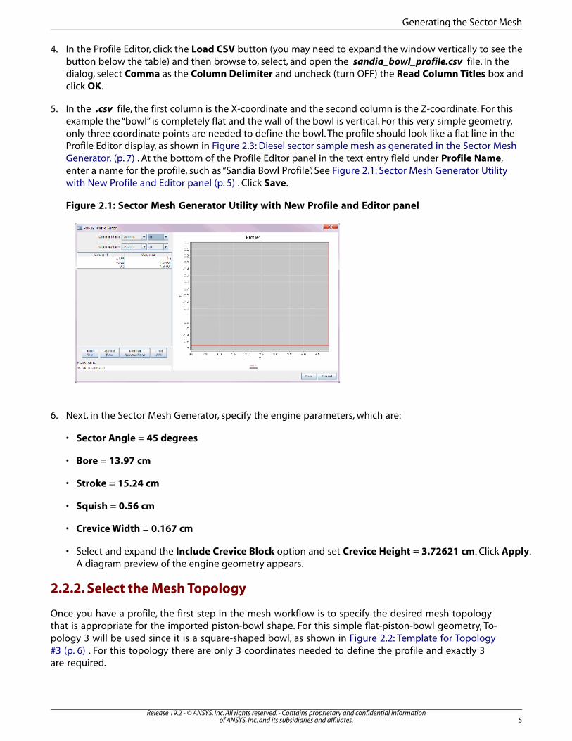
4. In the Profile Editor, click the Load CSV button (you may need to expand the window vertically to see thebutton below the table) and then browse to, select, and open the sandia_bowl_profile.csv file. In thedialog, select Comma as the Column Delimiter and uncheck (turn OFF) the Read Column Titles box andclick OK.
5. In the .csv file, the first column is the X-coordinate and the second column is the Z-coordinate. For thisexample the “bowl” is completely flat and the wall of the bowl is vertical. For this very simple geometry,only three coordinate points are needed to define the bowl. The profile should look like a flat line in theProfile Editor display, as shown in Figure 2.3: Diesel sector sample mesh as generated in the Sector MeshGenerator. (p. 7) . At the bottom of the Profile Editor panel in the text entry field under Profile Name,enter a name for the profile, such as “Sandia Bowl Profile”. See Figure 2.1: Sector Mesh Generator Utilitywith New Profile and Editor panel (p. 5) . Click Save.
Figure 2.1: Sector Mesh Generator Utility with New Profile and Editor panel
6. Next, in the Sector Mesh Generator, specify the engine parameters, which are:
• Sector Angle = 45 degrees
• Bore = 13.97 cm
• Stroke = 15.24 cm
• Squish = 0.56 cm
• Crevice Width = 0.167 cm
• Select and expand the Include Crevice Block option and set Crevice Height = 3.72621 cm. Click Apply.A diagram preview of the engine geometry appears.
2.2.2. Select the Mesh Topology
Once you have a profile, the first step in the mesh workflow is to specify the desired mesh topologythat is appropriate for the imported piston-bowl shape. For this simple flat-piston-bowl geometry, To-pology 3 will be used since it is a square-shaped bowl, as shown in Figure 2.2: Template for Topology#3 (p. 6) . For this topology there are only 3 coordinates needed to define the profile and exactly 3are required.
5Release 19.2 - © ANSYS, Inc. All rights reserved. - Contains proprietary and confidential information
of ANSYS, Inc. and its subsidiaries and affiliates.
Generating the Sector Mesh
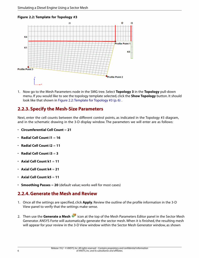
Figure 2.2: Template for Topology #3
1. Now go to the Mesh Parameters node in the SMG tree. Select Topology 3 in the Topology pull-downmenu. If you would like to see the topology template selected, click the Show Topology button. It shouldlook like that shown in Figure 2.2: Template for Topology #3 (p. 6) .
2.2.3. Specify the Mesh-Size Parameters
Next, enter the cell counts between the different control points, as indicated in the Topology #3 diagram,and in the schematic drawing in the 3-D display window. The parameters we will enter are as follows:
• Circumferential Cell Count = 21
• Radial Cell Count i1 = 16
• Radial Cell Count i2 = 11
• Radial Cell Count i3 = 3
• Axial Cell Count k1 = 11
• Axial Cell Count k4 = 21
• Axial Cell Count k5 = 11
• Smoothing Passes = 20 (default value; works well for most cases)
2.2.4. Generate the Mesh and Review
1. Once all the settings are specified, click Apply. Review the outline of the profile information in the 3-DView panel to verify that the settings make sense.
2. Then use the Generate a Mesh icon at the top of the Mesh Parameters Editor panel in the Sector MeshGenerator. ANSYS Forte will automatically generate the sector mesh. When it is finished, the resulting meshwill appear for your review in the 3-D View window within the Sector Mesh Generator window, as shown
Release 19.2 - © ANSYS, Inc. All rights reserved. - Contains proprietary and confidential informationof ANSYS, Inc. and its subsidiaries and affiliates.6
Simulating a Diesel Engine Using a Sector Mesh
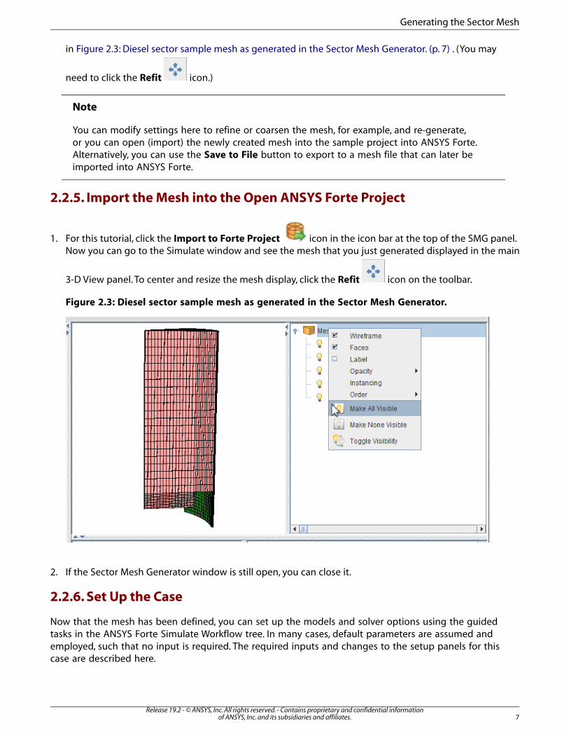
in Figure 2.3: Diesel sector sample mesh as generated in the Sector Mesh Generator. (p. 7) . (You may
need to click the Refit icon.)
Note
You can modify settings here to refine or coarsen the mesh, for example, and re-generate,or you can open (import) the newly created mesh into the sample project into ANSYS Forte.Alternatively, you can use the Save to File button to export to a mesh file that can later beimported into ANSYS Forte.
2.2.5. Import the Mesh into the Open ANSYS Forte Project
1. For this tutorial, click the Import to Forte Project icon in the icon bar at the top of the SMG panel.Now you can go to the Simulate window and see the mesh that you just generated displayed in the main
3-D View panel. To center and resize the mesh display, click the Refit icon on the toolbar.
Figure 2.3: Diesel sector sample mesh as generated in the Sector Mesh Generator.
2. If the Sector Mesh Generator window is still open, you can close it.
2.2.6. Set Up the Case
Now that the mesh has been defined, you can set up the models and solver options using the guidedtasks in the ANSYS Forte Simulate Workflow tree. In many cases, default parameters are assumed andemployed, such that no input is required. The required inputs and changes to the setup panels for thiscase are described here.
7Release 19.2 - © ANSYS, Inc. All rights reserved. - Contains proprietary and confidential information
of ANSYS, Inc. and its subsidiaries and affiliates.
Generating the Sector Mesh

In the Workflow tree, expand Models. In the following steps you will turn ON (check-mark) severalmodels and configure parameters for them in their Editor panels.
Note
You can change the display properties of items in the 3-D View by selecting the items in theVisibility tree and turning ON/OFF their visibility or right-clicking and selecting options fromthe context menu, such as display of the mesh or level of opacity.
1. Models > Chemistry: In the Workflow tree, under Models, select Chemistry. On the Chemistry icon bar, click
the Import Chemistry icon. This opens a file browser where you can navigate to and select a chemistryset file. For this project, however, we use a pre-installed chemistry set that comes with ANSYS Forte. Thisis a simplified, reduced n-heptane mechanism that can be used to represent the diesel fuel under conven-tional diesel-engine combustion conditions. To load this file, browse to the System Data directory andlocate the pre-installed Diesel_1comp_35sp.cks file. The System Data directory can be accessed fromthis file browser by clicking the data radio button in the upper right-hand sub-panel of the browser window.The chemistry file is a standard ANSYS Chemkin-Pro chemistry-set file. More information about the chemistryset and the files referenced within it can be found in the ANSYS Forte User Guide .
Note
You can respond Yes or No to the “View chemistry set information?” prompt. A Yes re-sponse displays the chemistry set file in a viewer.
2. Models > Transport: For this node, keep all the default settings.
3. Models > Spray Model: Since this is a direct-injection case, turn ON (check) Spray Model to display its iconbar (action bar) in the Editor panel.
a. For the basic Spray Properties, keep Radius of Influence Model for the Droplet Collision Model andset 0.2 cm as the Radius of Influence. The Use Vaporization Model option should be ON (checked,its default value).
b. Create Injector: Click Spray Model in the Workflow tree. The icon bar provides two spray-injector options:
Hollow Cone or Solid Cone. For the diesel injector, click the Solid Cone icon. In the dialog thatopens, name the Spray Model as “Injector 1”. This opens another icon bar and Editor panel for the newsolid-cone spray model. In the Editor panel, configure the model parameters for the solid-cone spraymodel.
• Composition: Select Create New... in the Composition drop-down menu under Settings and click
the Pencil icon to open the Fuel Mixture Editor. In the Fuel Mixture panel, click the Add Speciesbutton and select nc7h16 (i.e., n-heptane) as the Species, n-Tetradecane as the Physical Propertiesand 1.0 as the Mass Fraction. (Note that you must press ENTER after entering the values in thetable.)
• At the bottom of the panel, type a name such as “n-heptane”. Click Save and Close the window.
• Under the Injection Type, select Pulsed Injection and change the Parcel Specification to NumberOf Parcels and set Injected Parcel Count = 4,000.
Release 19.2 - © ANSYS, Inc. All rights reserved. - Contains proprietary and confidential informationof ANSYS, Inc. and its subsidiaries and affiliates.8
Simulating a Diesel Engine Using a Sector Mesh

• Set Inflow Droplet Temperature = 368.0 K.
• Set Spray Initialization to Constant Discharge Coefficient and Angle, and Discharge Coefficient= 0.7, and Mean Cone Angle = 15.0 degrees.
• Keep default values for Droplet Size Distribution and, under the Solid Cone Breakup Model Set-tings, the KH Model Constants, RT Model Constants, and Use Gas-Jet Model.
• Click Apply.
c. Create a Nozzle: Click the New Nozzle icon on the Spray icon bar and name the nozzle “Nozzle1”. Nozzle 1 then appears in the Workflow tree, and the Editor panel and icon bar transform to allowspecification of the Nozzle geometry and orientation. In the Editor panel, set the Reference Frameparameters to specify the nozzle location and direction. Keep the default Global Origin and use thefollowing settings:
• Location > Coord. System = Cylindrical, with R = 0.15 cm, θ = 22.5 degrees, and A = 19.368 cm.
• Spray Direction > Coord. System = Spherical, θ = 104.0 degrees, and ϕ = 22.5 degrees.
• Click Apply. You can see the nozzle appear at the top of the geometry. (You may wish to make theGeometry less opaque by right-clicking the Geometry item and selecting a lower value for Opacity,or change the color of the nozzle itself, both in the Visibility tree on the right side, to make the nozzleeasier to see in the interior.)
d. Create an Injection: In the Workflow tree, click Injector 1 again and click the New Injection iconon the Injector 1 icon bar and name the injection Injection 1. The new Injection item appears in theWorkflow tree, and the Editor panel and the icon bar transform to allow specification of the injectionproperties. In the Editor panel, keep the Pulsed Injection Type (default), select Crank Angle as theTiming option and then specify the Start of injection and Duration of injection as -22.5 and 7.75 de-grees ATDC, respectively. Set the Total Injected Mass = 0.0535 g. Click Apply.
e. Injection Profile: Click the Create new... option in the profile selection menu next to Velocity Profile,then click the pencil icon to open a new window with the Profile Editor. The new Injection Profile itemappears in the Workflow tree; also the Editor panel and the icon bar transform to the new InjectionProfile. In the Profile Editor window, make sure all the Units are set to None for both columns (the di-mensionless data is automatically scaled within ANSYS Forte to match the mass and duration of injection)and click the Load CSV button at the bottom of the panel (you may have to expand the panel size tosee the button). Navigate to the InjectionProfile.csv file (see Data Provided (p. 3) ). Select Commaas the Column delimiter and turn ON Read Column Titles and load the profile file. Alternatively, youcan type in the Injection Profile data in the table on the Editor panel or copy and paste from a spread-sheet or 3rd-party editor. Go to Profile Name at the bottom-left of the panel and name the new profileInjection Profile. Once the data is entered, click Save in the Profile Editor and then click Apply in theANSYS Forte Editor panel.
9Release 19.2 - © ANSYS, Inc. All rights reserved. - Contains proprietary and confidential information
of ANSYS, Inc. and its subsidiaries and affiliates.
Generating the Sector Mesh

Figure 2.4: Injection Profile Parameter Settings
4. Models > Soot Model: Turn ON the Soot Model. This creates the Settings item. In the Editor panel, acceptall the defaults.
5. Boundary Conditions: Under Boundary Conditions in the Workflow tree, specify the Boundary conditionsin the Editor panels associated with each of the four boundary conditions created by importing the mesh.By default the Wall Model for all of the wall boundaries will be set to Law of the Wall. Leave this defaultsetting as well as the default check box that turns ON heat transfer to the wall.
• Boundary Conditions > Piston: Set Piston Temperature = 500.0 K. Turn ON Wall Motion with MotionType set to Slider Crank. The other parameters should be:
• Stroke = 15.24
• Connecting Rod Length = 30.48
• Bore = 13.97 (pre-determined by the Sector Mesh Generator)
• Accept the defaults of Piston is Offset = unchecked (OFF) and Vertices to Transform = All.
• For Reference Frame, accept the default Global Origin and Direction parameters.
• Click Apply.
• Boundary Conditions > Periodicity: Set the Sector Angle = 45 degrees, and multi-select both PeriodicA and Periodic B boundaries on which to apply this boundary condition. Click Apply.
• Boundary Conditions > Head: Set Head Temperature = 470.0 K. Click Apply.
• Boundary Conditions > Liner: Set Liner Temperature = 420.0 K. Click Apply.
6. Initial Conditions > Region 1 Initialization: Specify the parameters for the initial conditions as follows:
Release 19.2 - © ANSYS, Inc. All rights reserved. - Contains proprietary and confidential informationof ANSYS, Inc. and its subsidiaries and affiliates.10
Simulating a Diesel Engine Using a Sector Mesh
• Composition: Select Constant and then Create New and click the Pencil icon and to launch theComposition Editor. Set these parameters: set the Composition = Mole Fraction (not the default MassFraction). Then click the Add Species button and select both o2 and n2 to add. When both o2 and n2are in the Species column in the Composition table, enter 0.126 for the o2 Fraction and 0.874 for n2.Name this “Composition 1” in the text field at the bottom of the Gas Mixture window. Click Save andclose the Composition Editor.
• Temperature = 362.0 K
• Pressure = 2.215 bar (Note: This is not the default unit.)
• Turbulence: Select Constant, and then in the pull-down menu for the initial Turbulence parameters,select Turbulent Kinetic Energy and Length Scale as the way in which we will specify the initial turbu-lence. For this option we provide an explicit value for the initial turbulent kinetic energy, but use a length-scale approximation to determine the turbulence dissipation energy. Use these values.
• Turbulent Kinetic Energy = 10,000cm2/sec2
• Turbulent Length Scale = 1.0 cm
• Velocity: Select Engine Swirl in the Velocity pull-down and then specify the swirl profile parameters:
– Initial Swirl Ratio = 0.5
– Initial Swirl Profile Factor = 3.11
– Initialize Velocity Components Normal to Piston = ON
Note
If you want to estimate the turbulent kinetic energy (TKE) as a fraction of the piston
speed, let the fraction be F and stroke is ms-1, the value you would enter then wouldbe
• Click Apply in the Region 1 Initialization Editor panel.
7. Simulation Controls: Under Simulation Limits, for the Simulation End Points, specify:
• Crank Angle Based
• Initial Crank Angle = -165.0
• Final Simulation Crank Angle = 125.0 degrees. (These two angles correspond to Intake Valve Openand Exhaust Valve Closing, respectively.)
• RPM = 1,200.0
• Cycle Type is 4-Stroke.
• Click Apply.
11Release 19.2 - © ANSYS, Inc. All rights reserved. - Contains proprietary and confidential information
of ANSYS, Inc. and its subsidiaries and affiliates.
Generating the Sector Mesh

8. Simulation Controls > Time Step: For the Advanced Time Step Control Options, specify:
• Rate of Strain Factor = 1.2
• Convection Factor = 0.5
• Click Apply.
9. Simulation Controls > Chemistry Solver:
• Turn ON (check) Use Dynamic Cell Clustering and accept its defaults.
• At the bottom of the panel, set Activate Chemistry to Conditionally, specifying When Temperatureis Reached, setting Threshold Temperature = 600.0 K. Click Apply.
10. Output Controls > Spatially Resolved: For the Spatially Resolved Output Control, specify:
• Crank Angle Output Control
• Output every = 5.0 degrees.
• Also check the box next to User Defined Crank Angle Outputs and then import the UserCrankAngleOut-puts.csv table of data using the Profile Editor that contains crank angles going from -22 to +20, withincrement 1, units of Angle and Degree, and file named UserCrankAngleOutputs. This assuresthat we get more resolved outputs around the spray, without requiring the same resolution throughoutthe simulation.
• For Spatially Resolved Species, move these species to the Selection list: nc7h16, o2, n2, co2, h2o, co,no, and no2. Click Apply.
11. Output Controls > Spatially Averaged:
• For the Spatially Averaged Output Control, select the Crank Angle option and specify Output Every= 1.0 degree.
• For Spatially Averaged Species, select all and move all species to the Selection list. Click Apply.
12. Output Controls > Restart Data: In the Workflow tree, check the box for Restart Data and then in the Restartpanel, check the box that says, Write Restart File at Last Simulation Step. Uncheck (turn OFF) any otherboxes on the panel. Click Apply.
2.2.6.1. Run the Case Using Defaults
1. In the Workflow tree, click the Run Simulation node to open the run control interface.
2. Click the green arrow under Start to start the case running. The Status changes to “Running.”
3. To interrupt the run, click the red button under Stop. Then the Status becomes “Stopped”.
4. To start over or restart, click Start again.
5. The progress of the simulation can be monitored during a run. To monitor the averaged value of simulation
variables, click the Monitor Runs icon on the Run Simulation icon bar.
Release 19.2 - © ANSYS, Inc. All rights reserved. - Contains proprietary and confidential informationof ANSYS, Inc. and its subsidiaries and affiliates.12
Simulating a Diesel Engine Using a Sector Mesh
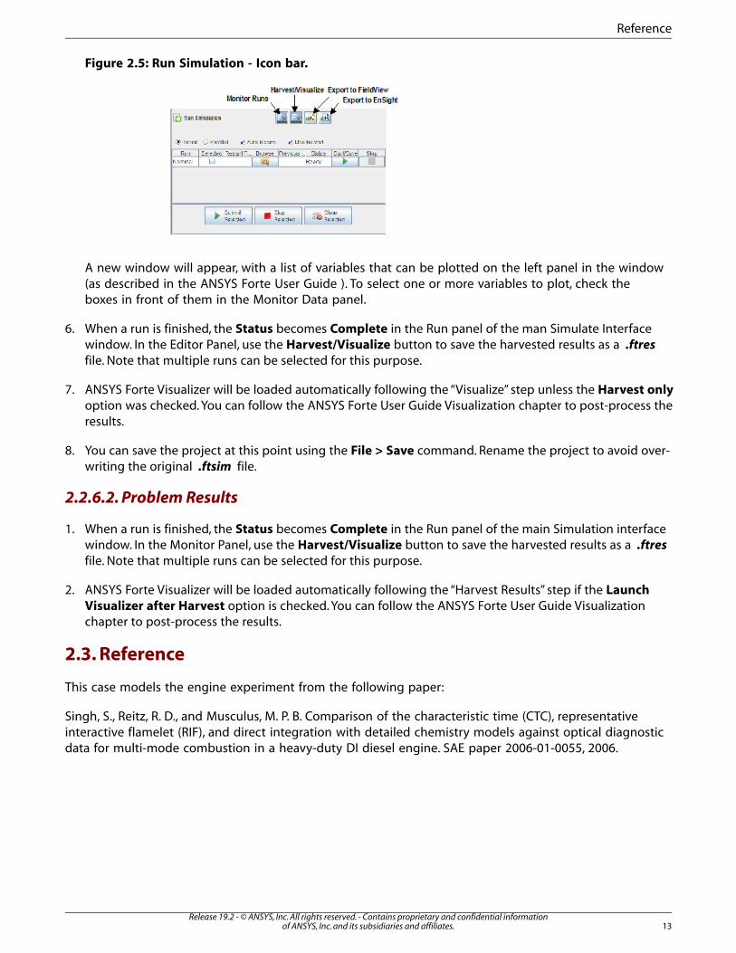
Figure 2.5: Run Simulation - Icon bar.
A new window will appear, with a list of variables that can be plotted on the left panel in the window(as described in the ANSYS Forte User Guide ). To select one or more variables to plot, check theboxes in front of them in the Monitor Data panel.
6. When a run is finished, the Status becomes Complete in the Run panel of the man Simulate Interfacewindow. In the Editor Panel, use the Harvest/Visualize button to save the harvested results as a .ftresfile. Note that multiple runs can be selected for this purpose.
7. ANSYS Forte Visualizer will be loaded automatically following the “Visualize” step unless the Harvest onlyoption was checked. You can follow the ANSYS Forte User Guide Visualization chapter to post-process theresults.
8. You can save the project at this point using the File > Save command. Rename the project to avoid over-writing the original .ftsim file.
2.2.6.2. Problem Results
1. When a run is finished, the Status becomes Complete in the Run panel of the main Simulation interfacewindow. In the Monitor Panel, use the Harvest/Visualize button to save the harvested results as a .ftresfile. Note that multiple runs can be selected for this purpose.
2. ANSYS Forte Visualizer will be loaded automatically following the “Harvest Results” step if the LaunchVisualizer after Harvest option is checked. You can follow the ANSYS Forte User Guide Visualizationchapter to post-process the results.
2.3. Reference
This case models the engine experiment from the following paper:
Singh, S., Reitz, R. D., and Musculus, M. P. B. Comparison of the characteristic time (CTC), representativeinteractive flamelet (RIF), and direct integration with detailed chemistry models against optical diagnosticdata for multi-mode combustion in a heavy-duty DI diesel engine. SAE paper 2006-01-0055, 2006.
13Release 19.2 - © ANSYS, Inc. All rights reserved. - Contains proprietary and confidential information
of ANSYS, Inc. and its subsidiaries and affiliates.
Reference

Release 19.2 - © ANSYS, Inc. All rights reserved. - Contains proprietary and confidential informationof ANSYS, Inc. and its subsidiaries and affiliates.14
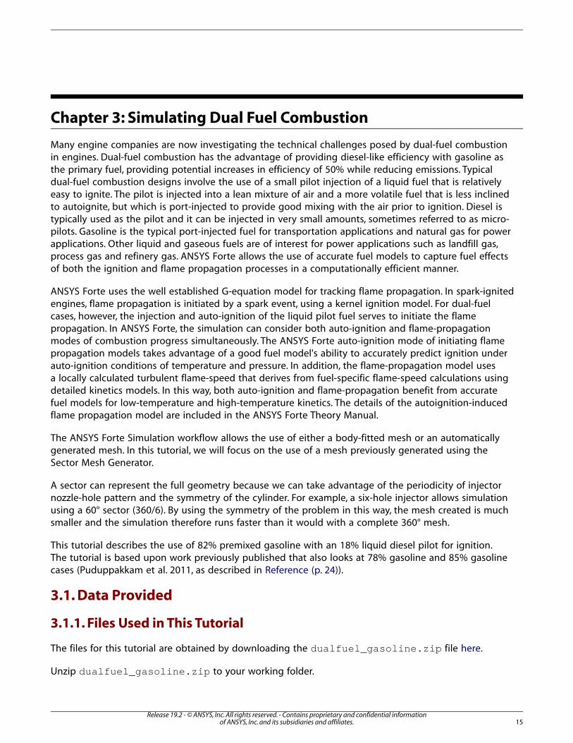
Chapter 3: Simulating Dual Fuel Combustion
Many engine companies are now investigating the technical challenges posed by dual-fuel combustionin engines. Dual-fuel combustion has the advantage of providing diesel-like efficiency with gasoline asthe primary fuel, providing potential increases in efficiency of 50% while reducing emissions. Typicaldual-fuel combustion designs involve the use of a small pilot injection of a liquid fuel that is relativelyeasy to ignite. The pilot is injected into a lean mixture of air and a more volatile fuel that is less inclinedto autoignite, but which is port-injected to provide good mixing with the air prior to ignition. Diesel istypically used as the pilot and it can be injected in very small amounts, sometimes referred to as micro-pilots. Gasoline is the typical port-injected fuel for transportation applications and natural gas for powerapplications. Other liquid and gaseous fuels are of interest for power applications such as landfill gas,process gas and refinery gas. ANSYS Forte allows the use of accurate fuel models to capture fuel effectsof both the ignition and flame propagation processes in a computationally efficient manner.
ANSYS Forte uses the well established G-equation model for tracking flame propagation. In spark-ignitedengines, flame propagation is initiated by a spark event, using a kernel ignition model. For dual-fuelcases, however, the injection and auto-ignition of the liquid pilot fuel serves to initiate the flamepropagation. In ANSYS Forte, the simulation can consider both auto-ignition and flame-propagationmodes of combustion progress simultaneously. The ANSYS Forte auto-ignition mode of initiating flamepropagation models takes advantage of a good fuel model's ability to accurately predict ignition underauto-ignition conditions of temperature and pressure. In addition, the flame-propagation model usesa locally calculated turbulent flame-speed that derives from fuel-specific flame-speed calculations usingdetailed kinetics models. In this way, both auto-ignition and flame-propagation benefit from accuratefuel models for low-temperature and high-temperature kinetics. The details of the autoignition-inducedflame propagation model are included in the ANSYS Forte Theory Manual.
The ANSYS Forte Simulation workflow allows the use of either a body-fitted mesh or an automaticallygenerated mesh. In this tutorial, we will focus on the use of a mesh previously generated using theSector Mesh Generator.
A sector can represent the full geometry because we can take advantage of the periodicity of injectornozzle-hole pattern and the symmetry of the cylinder. For example, a six-hole injector allows simulationusing a 60° sector (360/6). By using the symmetry of the problem in this way, the mesh created is muchsmaller and the simulation therefore runs faster than it would with a complete 360° mesh.
This tutorial describes the use of 82% premixed gasoline with an 18% liquid diesel pilot for ignition.The tutorial is based upon work previously published that also looks at 78% gasoline and 85% gasolinecases (Puduppakkam et al. 2011, as described in Reference (p. 24)).
3.1. Data Provided
3.1.1. Files Used in This Tutorial
The files for this tutorial are obtained by downloading the dualfuel_gasoline.zip file here.
Unzip dualfuel_gasoline.zip to your working folder.
15Release 19.2 - © ANSYS, Inc. All rights reserved. - Contains proprietary and confidential information
of ANSYS, Inc. and its subsidiaries and affiliates.
• itape.fmsh: This is the sector mesh file. It can only be used with body-fitted mesh calculations.
• Profile1.csv: Data describing the spray injections. These data can be entered using cut and paste or usingthe Import option within the Profile Editor tool, which can be opened in the context of the spray-injectionpanel on the Simulation User Interface.
• reduced-mech__RCCI-conditions_e.inp: This is the chemistry input file specifically assembled for this tutorial,using Reaction Design’s Model Fuels Consortium II (MFC II) database to assemble a multi-component mastermechanism. This mechanism was then reduced specifically for use in the dual fuels engine case. Details ofthe mechanism can be found in Puduppakkam et al. (2011). After downloading this file, it must be pre-pro-cessed (see Pre-Processing the Chemistry Set (p. 16)).
• Dual_Fuels_82percentGasoline_BFMesh_Tutorial.ftsim: A project file of the completed tutorial, for verific-ation or comparison of your progress in the tutorial set-up.
The sample files are provided as a download. You have the opportunity to select the location for thefiles when you download and uncompress the sample files.
3.1.2. Project Comparison Utility
The ANSYS Forte installation includes the cgns_util export command, which you can use to comparethe parameter settings in the project file generated at any point during your tutorial set-up against theprovided .ftsim , which has the parameter settings for the final, completed tutorial. This command isdescribed in the ANSYS Forte User Guide.
Briefly, you can double-check project settings by saving your project and then running the cgns_utilto export your tutorial project, and then to export the provided final version of the tutorial. Save bothversions and compare them with your favorite diff tool, such as DIFFzilla. If all the parameters are inagreement, you have set up the project successfully. If there are differences, you can go back into thetutorial set-up, re-read the tutorial instructions, and change the setting of interest.
3.1.3. Time Estimate
As a guideline for your own simulations, this tutorial is estimated to take approximately 3 hours on a
dual Intel® Xeon® processor E5-2690 at 2.90 GHz (8 total cores).
3.2. Pre-Processing the Chemistry Set
Note
All Editor panel options that are not explicitly mentioned in this tutorial should be left attheir default values. Changed values on any Editor panel do not take effect until you pressthe Apply button.
The mechanism has been encrypted for use only with ANSYS Forte and ANSYS Chemkin-Pro. The en-crypted mechanism .inp file must be pre-processed.
On the Utility menu, select Pre-Processing. Choose a Working Directory and select New ChemistrySet. Enter a Short Name for the chemistry set, such as DualFuels. For the Gas-Phase Kinetics Fileentry, browse to the directory where you saved the .inp file and select reduced-mech__RCCI-condi-tions_e.inp, and click the Open/Create button in the file browser. In the Pre-processing dialog, clickthe Save As button. The .cks file with the assigned Short Name should be in the File Name entry; click
Release 19.2 - © ANSYS, Inc. All rights reserved. - Contains proprietary and confidential informationof ANSYS, Inc. and its subsidiaries and affiliates.16
Simulating Dual Fuel Combustion
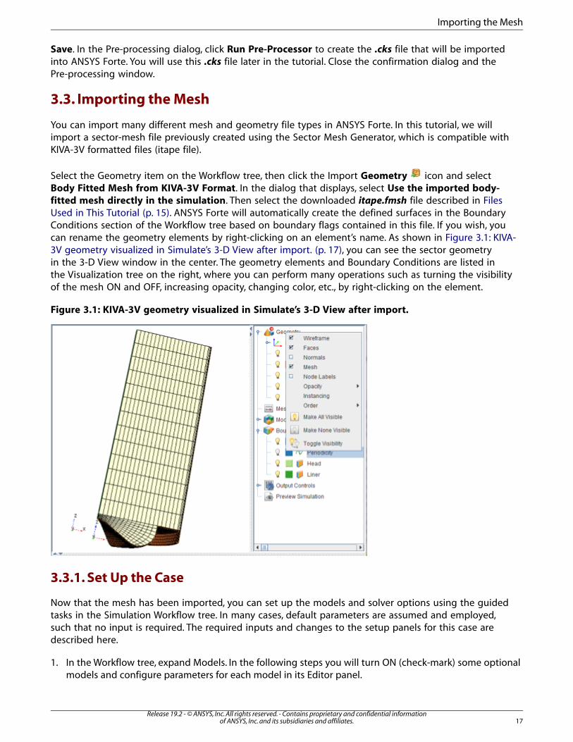
Save. In the Pre-processing dialog, click Run Pre-Processor to create the .cks file that will be importedinto ANSYS Forte. You will use this .cks file later in the tutorial. Close the confirmation dialog and thePre-processing window.
3.3. Importing the Mesh
You can import many different mesh and geometry file types in ANSYS Forte. In this tutorial, we willimport a sector-mesh file previously created using the Sector Mesh Generator, which is compatible withKIVA-3V formatted files (itape file).
Select the Geometry item on the Workflow tree, then click the Import Geometry icon and selectBody Fitted Mesh from KIVA-3V Format. In the dialog that displays, select Use the imported body-fitted mesh directly in the simulation. Then select the downloaded itape.fmsh file described in FilesUsed in This Tutorial (p. 15). ANSYS Forte will automatically create the defined surfaces in the BoundaryConditions section of the Workflow tree based on boundary flags contained in this file. If you wish, youcan rename the geometry elements by right-clicking on an element’s name. As shown in Figure 3.1: KIVA-3V geometry visualized in Simulate’s 3-D View after import. (p. 17), you can see the sector geometryin the 3-D View window in the center. The geometry elements and Boundary Conditions are listed inthe Visualization tree on the right, where you can perform many operations such as turning the visibilityof the mesh ON and OFF, increasing opacity, changing color, etc., by right-clicking on the element.
Figure 3.1: KIVA-3V geometry visualized in Simulate’s 3-D View after import.
3.3.1. Set Up the Case
Now that the mesh has been imported, you can set up the models and solver options using the guidedtasks in the Simulation Workflow tree. In many cases, default parameters are assumed and employed,such that no input is required. The required inputs and changes to the setup panels for this case aredescribed here.
1. In the Workflow tree, expand Models. In the following steps you will turn ON (check-mark) some optionalmodels and configure parameters for each model in its Editor panel.
17Release 19.2 - © ANSYS, Inc. All rights reserved. - Contains proprietary and confidential information
of ANSYS, Inc. and its subsidiaries and affiliates.
Importing the Mesh
2. Models > Chemistry: On the Chemistry icon bar, click the Import Chemistry icon. This opens a filebrowser where you can navigate to and select a chemistry set file. For this project, however, we use a pre-installed chemistry set that comes with ANSYS Forte. This is a reduced mechanism specifically for thesedual-fuel conditions. To load this file, browse to the directory where you saved pre-processed .cks file andlocate the .cks file you created from the reduced-mech__RCCI-conditions_e.inp file (see Pre-Processingthe Chemistry Set (p. 16)). The chemistry file (.cks ) is a standard ANSYS Chemkin-Pro chemistry-set file.More information about the chemistry set and the files referenced within it can be found in the ANSYSForte User Guide .
3. Models > Transport: For this node, keep all the default settings.
4. Models > Spray Model: Since this is a direct-injection case, turn ON (check) Spray Model to display its iconbar (action bar) in the Editor panel. In the panel, keep the defaults. Leave the Use Vaporization Model(default) check ON.
a. Add an Injector: The icon bar provides two spray-injector options: Hollow Cone or Solid Cone. For the
diesel injector, click the Solid Cone icon. In the dialog that opens, name the new solid-cone in-jector as “Solid Injector”. This opens another icon bar and Editor panel for the new solid-cone injector.In the Editor panel, configure the model parameters for the solid-cone injector.
• Composition: Select Create New... in the Composition drop-down menu under Settings and clickthe pencil icon to open the Fuel Mixture Editor. In the Fuel Mixture panel, click the Add Speciesbutton and select nc7h16 (i.e., n-heptane) as the Species, n-Tetradecane as the Physical Propertiesand enter 1.0 as the Mass Fraction. At the bottom of the panel, you can keep the default name of“Fuel Mixture 1”. Click Save and Close the window.
• Change the Parcel Specification to Number of Parcels, and the Injected Parcel Count = 3,000, itsdefault value.
• Set Inflow Droplet Temperature = 322.0 K.
• Set Spray Initialization to Constant Discharge Coefficient and Angle, and Discharge Coefficient= 0.7 and Mean Cone Angle = 10.0 degrees.
• The Droplet Size Distribution is set to Uniform Size by default.
• Under the Solid Cone Breakup Model Settings, leave the KH Model Constants, and RT ModelConstants, at their default values, except for the Size constant of RT Breakup; set this value to 0.1.
• Use the Gas Jet Model, with the default parameters.
• Click Apply.
b. Create a Nozzle: While Solid Injector is selected in the Workflow tree, click the New Nozzle iconon the icon bar and name the nozzle Nozzle.“Nozzle” then appears in the Workflow tree, and the Editorpanel and icon bar transform to allow specification of the Nozzle geometry and orientation. Set theparameters in the Editor panel to:
• Reference Frame: Select Global Origin from the drop-down menu. For Coord. System = Cylindrical,with R = 0.097 cm,Θ= 30.0 degrees, and A = 18.44 cm.
Release 19.2 - © ANSYS, Inc. All rights reserved. - Contains proprietary and confidential informationof ANSYS, Inc. and its subsidiaries and affiliates.18
Simulating Dual Fuel Combustion
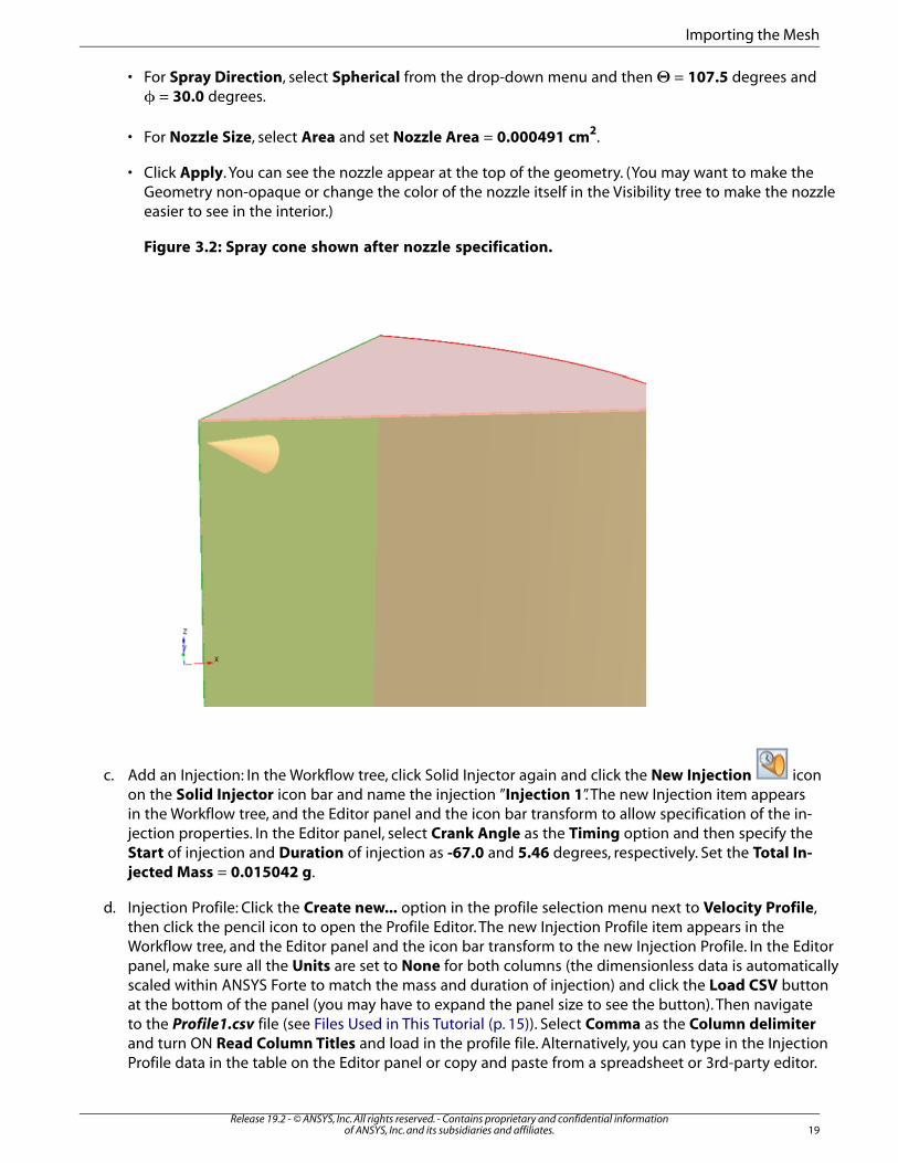
• For Spray Direction, select Spherical from the drop-down menu and then Θ = 107.5 degrees andφ = 30.0 degrees.
• For Nozzle Size, select Area and set Nozzle Area = 0.000491 cm2.
• Click Apply. You can see the nozzle appear at the top of the geometry. (You may want to make theGeometry non-opaque or change the color of the nozzle itself in the Visibility tree to make the nozzleeasier to see in the interior.)
Figure 3.2: Spray cone shown after nozzle specification.
c. Add an Injection: In the Workflow tree, click Solid Injector again and click the New Injection iconon the Solid Injector icon bar and name the injection ”Injection 1”. The new Injection item appearsin the Workflow tree, and the Editor panel and the icon bar transform to allow specification of the in-jection properties. In the Editor panel, select Crank Angle as the Timing option and then specify theStart of injection and Duration of injection as -67.0 and 5.46 degrees, respectively. Set the Total In-jected Mass = 0.015042 g.
d. Injection Profile: Click the Create new... option in the profile selection menu next to Velocity Profile,then click the pencil icon to open the Profile Editor. The new Injection Profile item appears in theWorkflow tree, and the Editor panel and the icon bar transform to the new Injection Profile. In the Editorpanel, make sure all the Units are set to None for both columns (the dimensionless data is automaticallyscaled within ANSYS Forte to match the mass and duration of injection) and click the Load CSV buttonat the bottom of the panel (you may have to expand the panel size to see the button). Then navigateto the Profile1.csv file (see Files Used in This Tutorial (p. 15)). Select Comma as the Column delimiterand turn ON Read Column Titles and load in the profile file. Alternatively, you can type in the InjectionProfile data in the table on the Editor panel or copy and paste from a spreadsheet or 3rd-party editor.
19Release 19.2 - © ANSYS, Inc. All rights reserved. - Contains proprietary and confidential information
of ANSYS, Inc. and its subsidiaries and affiliates.
Importing the Mesh
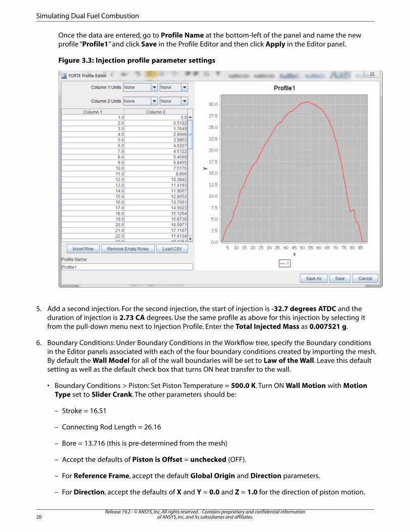
Once the data are entered, go to Profile Name at the bottom-left of the panel and name the newprofile “Profile1” and click Save in the Profile Editor and then click Apply in the Editor panel.
Figure 3.3: Injection profile parameter settings
5. Add a second injection. For the second injection, the start of injection is -32.7 degrees ATDC and theduration of injection is 2.73 CA degrees. Use the same profile as above for this injection by selecting itfrom the pull-down menu next to Injection Profile. Enter the Total Injected Mass as 0.007521 g.
6. Boundary Conditions: Under Boundary Conditions in the Workflow tree, specify the Boundary conditionsin the Editor panels associated with each of the four boundary conditions created by importing the mesh.By default the Wall Model for all of the wall boundaries will be set to Law of the Wall. Leave this defaultsetting as well as the default check box that turns ON heat transfer to the wall.
• Boundary Conditions > Piston: Set Piston Temperature = 500.0 K. Turn ON Wall Motion with MotionType set to Slider Crank. The other parameters should be:
– Stroke = 16.51
– Connecting Rod Length = 26.16
– Bore = 13.716 (this is pre-determined from the mesh)
– Accept the defaults of Piston is Offset = unchecked (OFF).
– For Reference Frame, accept the default Global Origin and Direction parameters.
– For Direction, accept the defaults of X and Y = 0.0 and Z = 1.0 for the direction of piston motion.
Release 19.2 - © ANSYS, Inc. All rights reserved. - Contains proprietary and confidential informationof ANSYS, Inc. and its subsidiaries and affiliates.20
Simulating Dual Fuel Combustion

– Click Apply.
• Boundary Conditions > Periodicity: Keep the default Sector Angle = 60 degrees. The periodic boundaries,Periodic A and Periodic B, for this boundary condition are automatically selected, based on theboundary flags contained in the imported mesh.
• Boundary Conditions > Head: Set Head Temperature = 500.0 K. Click Apply.
• Boundary Conditions > Liner: Set Liner Temperature = 430.0 K. Click Apply.
7. Initial Conditions > Region 1 Initialization (Main): Specify the parameters for the initial conditions as follows:
• In the Composition drop-down menu, select Create New... and click the pencil icon to open the GasMixture Editor. In the Gas Mixture panel, change the Composition setting to Mole Fraction (not thedefault Mass Fraction). Then click the Add Species button and select the species in the list indicatedin Figure 3.4: Gas Mixture Editor (p. 21). Once all the species are entered, provide the mole fraction valuesas indicated in Figure 3.4: Gas Mixture Editor (p. 21). Enter a name for the Mixture if you desire or leavethe default as Mixture 1 in the bottom left text box; click Save, then Close the window.
Figure 3.4: Gas Mixture Editor
• Temperature = 391.0 K
• Pressure = 3.34 bar (note this is not the default unit, so you need to use the pull-down next to the textbox to select the correct units option)
21Release 19.2 - © ANSYS, Inc. All rights reserved. - Contains proprietary and confidential information
of ANSYS, Inc. and its subsidiaries and affiliates.
Importing the Mesh
• In the pull-down menu for the initial Turbulence parameters, select Turbulence Intensity and LengthScale as the way in which we will specify the initial turbulence. For this option we leave the settingswith the default values:
• Turbulence Intensity Fraction = 0.1 (default value).
• Turbulent Length Scale = 1.0 cm (default value).
• Velocity is set to Constant.
• Select Engine Swirl in the Velocity pull-down and then specify the swirl profile parameters:
– Initial Swirl Ratio = -0.7
– Initial Swirl Profile Factor = 3.11
– Initialize Velocity Components Normal to Piston = ON (checked)
• Also keep other options at their defaults.
• Click Apply in the Region 1 Initialization Editor panel.
8. Simulation Controls: Under Simulation Limits, for the Simulation End Points, specify:
• Crank Angle Based
• Initial Crank Angle = -95.0
• RPM = 1,300.0
• Cycle Type is 4-Stroke.
• Final Simulation Crank Angle = 130.0 degrees. (These two angles correspond to Intake Valve Openand Exhaust Valve Closing, respectively.) Click Apply.
9. Simulation Controls > Time Step:
• Maximum Time Step Option = Constant and enter the value 1.0E-5 sec. (This value is selected so thetutorial example will run fast; the default value is 5.0E-6.)
• Leave other settings at their defaults. Click Apply.
10. Simulation Controls > Chemistry Solver:
• Accept the default state of ON (check) for Use Dynamic Cell Clustering and accept its defaults.
• Near the bottom of the panel, turn OFF (uncheck) When temperature is Reached. Set the ActivateChemistry drop-down menu to Conditionally, specifying During Crank Angle Interval, with Startingand Ending values of -45.0 and 40.0, respectively. Click Apply.
Note
More details about the chemistry solver options, such as Dynamic Cell Clustering andDynamic Adaptive Chemistry, are available in the ANSYS Forte User Guide.
Release 19.2 - © ANSYS, Inc. All rights reserved. - Contains proprietary and confidential informationof ANSYS, Inc. and its subsidiaries and affiliates.22
Simulating Dual Fuel Combustion
11. Output Controls > Spatially Resolved: For the Spatially Resolved Output Control, specify:
• Crank Angle Output Control.
• Output every = 5.0 degrees.
• For Spatially Resolved Species, move all the fuel-related and emissions species, such as these, to theSelection list: nc7h16, o2, co2, h2o, co, no, ic8h18, c6h12-1, c6h5ch3 and ic6h14. Click Apply.
12. Output Controls > Spatially Averaged:
• For the Spatially Averaged Output Control, select the Crank Angle option and specify Output Every= 1.0 degree.
• For Spatially Averaged Species, select o2, co2, co, no, nc7h16, ic8h18, c6h12-1, c6h5ch3, ic6h14,n2, h20, and move all species to the Selection list. Click Apply.
13. Output Controls > Restart Data: In the Workflow tree, check the box for Restart Data and then in the Restartpanel, check the box that says, Write Restart File at Last Simulation Step. Uncheck (turn OFF) any otherboxes on the panel. Click Apply.
3.3.1.1. Save the Project
1. In the File menu, use the Save As command to rename and save this project. The project must be savedbefore running.
3.3.1.2. Run the Case Using Defaults
1. In the Workflow tree, click the Run Simulation node to open the run control interface.
2. Click the green arrow “play” button under Start/Save to start the case running. The Status changes to“Running.”
3. To interrupt the run, click the red button under Stop. Then the Status becomes “Stopped”.
4. To start over or restart, first select the file from which you want to start, by clicking on the Browse buttonin the Run row. Once an appropriate ftrst file is selected, click the green Start again.
5. The progress of the simulation can be monitored during a run. To monitor the averaged value of simulation
variables, click the Monitor Runs icon in the Run Simulation icon bar. A new window will appear, witha list of variables that can be plotted on the left panel in the window. To select one or more variables toplot, check the boxes in front of them in the Monitor Data panel. These plots are shown inFigure 3.4: GasMixture Editor (p. 21) to Figure 3.7: CO and UHC emissions vs. crank angle. (p. 26).
Note
To change the units of the plotted variables, go back to the Simulation Interface, Edit menuand choose Edit Preferences. In the Preferences panel, select the units desired. The nexttime the Monitor window updates the plots, it will automatically reflect these updated unitpreferences.
23Release 19.2 - © ANSYS, Inc. All rights reserved. - Contains proprietary and confidential information
of ANSYS, Inc. and its subsidiaries and affiliates.
Importing the Mesh
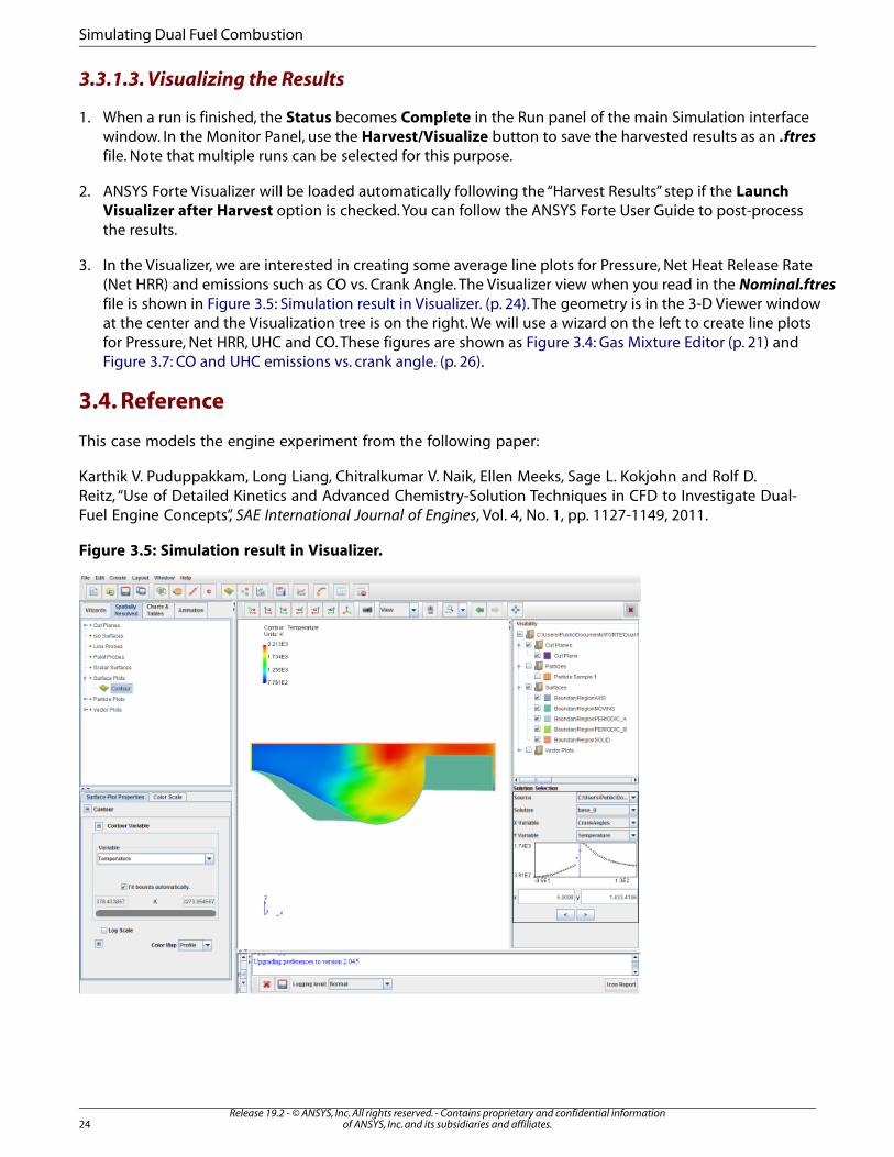
3.3.1.3. Visualizing the Results
1. When a run is finished, the Status becomes Complete in the Run panel of the main Simulation interfacewindow. In the Monitor Panel, use the Harvest/Visualize button to save the harvested results as an .ftresfile. Note that multiple runs can be selected for this purpose.
2. ANSYS Forte Visualizer will be loaded automatically following the “Harvest Results” step if the LaunchVisualizer after Harvest option is checked. You can follow the ANSYS Forte User Guide to post-processthe results.
3. In the Visualizer, we are interested in creating some average line plots for Pressure, Net Heat Release Rate(Net HRR) and emissions such as CO vs. Crank Angle. The Visualizer view when you read in the Nominal.ftresfile is shown in Figure 3.5: Simulation result in Visualizer. (p. 24). The geometry is in the 3-D Viewer windowat the center and the Visualization tree is on the right. We will use a wizard on the left to create line plotsfor Pressure, Net HRR, UHC and CO. These figures are shown as Figure 3.4: Gas Mixture Editor (p. 21) andFigure 3.7: CO and UHC emissions vs. crank angle. (p. 26).
3.4. Reference
This case models the engine experiment from the following paper:
Karthik V. Puduppakkam, Long Liang, Chitralkumar V. Naik, Ellen Meeks, Sage L. Kokjohn and Rolf D.Reitz, “Use of Detailed Kinetics and Advanced Chemistry-Solution Techniques in CFD to Investigate Dual-Fuel Engine Concepts”, SAE International Journal of Engines, Vol. 4, No. 1, pp. 1127-1149, 2011.
Figure 3.5: Simulation result in Visualizer.
Release 19.2 - © ANSYS, Inc. All rights reserved. - Contains proprietary and confidential informationof ANSYS, Inc. and its subsidiaries and affiliates.24
Simulating Dual Fuel Combustion
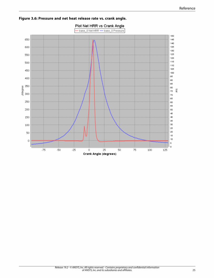
Figure 3.6: Pressure and net heat release rate vs. crank angle.
25Release 19.2 - © ANSYS, Inc. All rights reserved. - Contains proprietary and confidential information
of ANSYS, Inc. and its subsidiaries and affiliates.
Reference
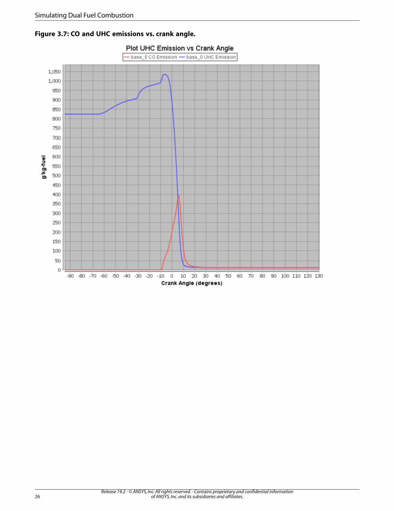
Figure 3.7: CO and UHC emissions vs. crank angle.
Release 19.2 - © ANSYS, Inc. All rights reserved. - Contains proprietary and confidential informationof ANSYS, Inc. and its subsidiaries and affiliates.26
Simulating Dual Fuel Combustion
Chapter 4: Spray Bomb Modeling
Accurately capturing fuel injection, spray breakup and spray vaporization are important aspects of engine-design simulations for direct-injection engines. However, it is difficult to isolate the effects of spray be-havior in a full engine simulation involving combustion, moving boundaries and complex turbulentflow. Spray bomb experiments are an excellent method for isolating the spray behavior prior to enginedesign and analysis. A spray bomb is a quiescent environment where liquid is injected without anymoving boundaries, such that the spray characteristics can be examined in detail. Any engine simulationinvolving liquid injection must account for the key aspects of atomization such as liquid-jet breakup,droplet formation, secondary breakup, droplet collisions, droplet coalescence and vaporization. Thistutorial describes how to use ANSYS Forte in spray bomb simulations that account for all of thesephenomena.
4.1. Data Provided
4.1.1. Files Used in This Tutorial
The files for this tutorial are obtained by downloading the spray_chamber.zip file here.
Unzip spray_chamber.zip to your working folder.
• Evaporating_Spray_Tutorial.fmsh: This is an ANSYS Forte body-fitted mesh file. This file will provide thespray bomb geometry for this Automatic Mesh Generator (AMG) tutorial.
• Evaporating_Spray_Tutorial.ftsim: A project file of the completed tutorial, for verification or comparisonof your progress in the tutorial set-up.
The tutorial sample files are provided as a download. You have the opportunity to select the locationfor the files when you download and unzip or untar the sample files.
4.1.2. Project Comparison Utility
The ANSYS Forte installation includes the cgns_util export command, which you can use to comparethe parameter settings in the project file generated at any point during your tutorial set-up against theprovided .ftsim , which has the parameter settings for the final, completed tutorial. This command isdescribed in the ANSYS Forte User Guide.
Briefly, you can double-check project settings by saving your project and then running the cgns_utilto export your tutorial project, and then to export the provided final version of the tutorial. Save bothversions and compare them with your preferred diff tool, such as DIFFzilla. If all the parameters are inagreement, you have set up the project successfully. If there are differences, you can go back into thetutorial set-up, re-read the tutorial instructions, and change the setting of interest.
4.1.3. Time Estimate
As a guideline for your own simulations, this tutorial is estimated to take 4 hours on a cluster of 16
nodes with Intel® Xeon® processor E5-2690 at 2.90 GHz (16 cores).
27Release 19.2 - © ANSYS, Inc. All rights reserved. - Contains proprietary and confidential information
of ANSYS, Inc. and its subsidiaries and affiliates.
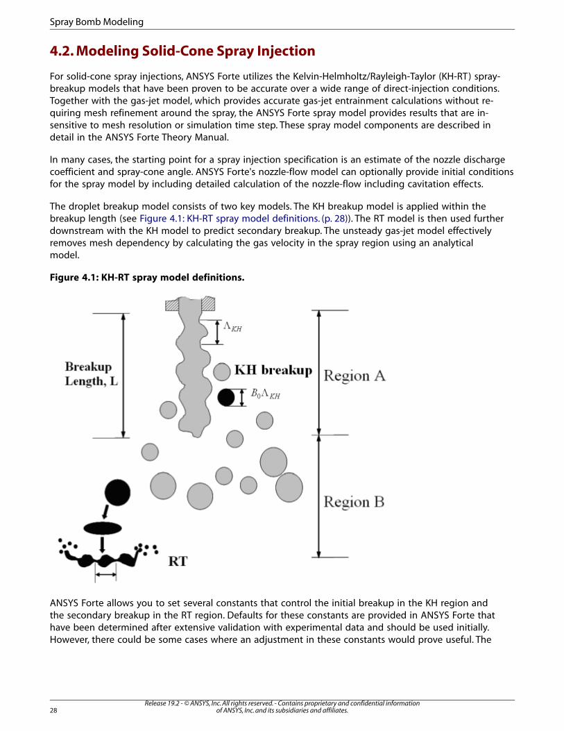
4.2. Modeling Solid-Cone Spray Injection
For solid-cone spray injections, ANSYS Forte utilizes the Kelvin-Helmholtz/Rayleigh-Taylor (KH-RT) spray-breakup models that have been proven to be accurate over a wide range of direct-injection conditions.Together with the gas-jet model, which provides accurate gas-jet entrainment calculations without re-quiring mesh refinement around the spray, the ANSYS Forte spray model provides results that are in-sensitive to mesh resolution or simulation time step. These spray model components are described indetail in the ANSYS Forte Theory Manual.
In many cases, the starting point for a spray injection specification is an estimate of the nozzle dischargecoefficient and spray-cone angle. ANSYS Forte's nozzle-flow model can optionally provide initial conditionsfor the spray model by including detailed calculation of the nozzle-flow including cavitation effects.
The droplet breakup model consists of two key models. The KH breakup model is applied within thebreakup length (see Figure 4.1: KH-RT spray model definitions. (p. 28)). The RT model is then used furtherdownstream with the KH model to predict secondary breakup. The unsteady gas-jet model effectivelyremoves mesh dependency by calculating the gas velocity in the spray region using an analyticalmodel.
Figure 4.1: KH-RT spray model definitions.
ANSYS Forte allows you to set several constants that control the initial breakup in the KH region andthe secondary breakup in the RT region. Defaults for these constants are provided in ANSYS Forte thathave been determined after extensive validation with experimental data and should be used initially.However, there could be some cases where an adjustment in these constants would prove useful. The
Release 19.2 - © ANSYS, Inc. All rights reserved. - Contains proprietary and confidential informationof ANSYS, Inc. and its subsidiaries and affiliates.28
Spray Bomb Modeling
following table describes the specific spray constant name, its default value, a suggested range of ad-justment and what the constant controls.
Table 4.1: Description of default ANSYS Forte spray constants.
DescriptionAdjustmentRange
DefaultValue
Constant Name
Affects radius of newdroplets formed frominitial breakup.
0.5 - 2.01.0Size Constant of KHBreakup
Most importantconstant for controlling
10 - 8040Time Constant of KHBreakup
spray penetrationlength.
Determines fraction atwhich new droplets can
N/A0.03Critical Mass Fractionfor New DropletGeneration leave their parent
parcel.
Affects the radius ofthe secondary droplets
0.1 - 0.30.15Size Constant of RTBreakup
arising from thecatastrophic breakup ofthe parent droplet
Affects thecharacteristic time
0.5 - 2.01.0Time Constant of RTBreakup
required to break theparent droplet
Affects the initialbreakup length when
1.5 - 3.01.9RT Distance Constant
the RT model isinitiated
4.2.1. Spray Bomb
4.2.1.1. Problem Description
This tutorial considers a cylindrical chamber with no moving walls and quiescent gas (see Table 4.2: Spraybomb simulation case set-up and test conditions. (p. 30)). In this case, pure n-heptane is injected intothe chamber. This single component, fuel is injected from a single solid-cone injector, where the nozzlehole is located on the wall and the injection is directed towards the center of the chamber. The initialgas in the chamber is a blend of N2, CO2, and H2O, such that the mixture is non-reacting. As the intention
of this example is to represent diesel-fuel injection, we use the physical properties of n-tetradecane torepresent the fuel. This combination of chemistry model being represented by one fuel surrogate (inthis case, n-heptane) while the physical model is represented by another fuel surrogate (in this case,n-tetradecane) is an approach often taken in simulating diesel engine combustion. In this way, thespray-bomb simulation comparisons to experiment can be used to verify the behavior of the surrogatemodel approach as it will be used in a combustion simulation. For this case, a square injection profileis used. Chemistry calculations are effectively stopped by setting the chemistry solver to begin at atemperature that will not be reached during the simulation.
29Release 19.2 - © ANSYS, Inc. All rights reserved. - Contains proprietary and confidential information
of ANSYS, Inc. and its subsidiaries and affiliates.
Modeling Solid-Cone Spray Injection

This tutorial shows the use of the Automatic Mesh Generator. We import a previously generated meshto provide the spray bomb geometry and select the option upon import to only import the geometrysurfaces for use with Automatic Mesh Generation. Mesh sizes of 1 mm, 2 mm and 3 mm are then usedto test mesh dependency. Results for penetration length of the three different mesh sizes are comparedagainst experimental data from SAE Technical Paper 960034 by J.D. Naber and D.L. Siebers [1 (p. 39)].
Note
All Editor panel options that are not explicitly mentioned in this tutorial should be left attheir default values. Changed values on any Editor panel do not take effect until you pressthe Apply button.
Table 4.2: Spray bomb simulation case set-up and test conditions.
Evaporating Spray CaseParameter
Disc-shaped constant-volume combustion chamber with 114.3 mmdiameter and 28.6 mm thickness
Mesh
Diesel DF2 (Experiment)Tetradecane (Surrogate)Fuel Type
436 KFuelTemperature
1,370 barInjectionPressure
4 msInjectionDuration
257 μmNozzleDiameter
Pa= 40; 83; and 170 barChamberConditions
Ta= 1,000 K
Release 19.2 - © ANSYS, Inc. All rights reserved. - Contains proprietary and confidential informationof ANSYS, Inc. and its subsidiaries and affiliates.30
Spray Bomb Modeling

4.2.1.2. Mesh Setup
In this tutorial, we will import an existing structured mesh with a size of 2 mm. Mesh sizes of 1 mm, 2mm, and 3 mm will be investigated to demonstrate mesh independence of the solution. The spraybomb geometry and test conditions are shown in Table 4.2: Spray bomb simulation case set-up andtest conditions. (p. 30).
• Import the mesh using Geometry on the Workflow tree. Click the Import Geometry icon. In the dialog,pull down and select Body Fitted mesh from Kiva-3Vformat, click OK and then select Only import thegeometry surfaces for use with Automatic Mesh Generation. In the dialog that opens, navigate to theEvaporating_Spray_Tutorial.fmsh file in the location where you saved the downloaded sample files.
• The imported file displays in the 3-D View area, but may not be ideally zoomed or centered. Click the Refit
icon to center and resize the mesh.
• Mesh Controls: Under Mesh Controls, we need to set the Material Point to a location that will always be“inside” the boundaries and should be located at least one unit cell length away from any boundaries. Tosee the coordinate values, select Geometry > Reference Frames > Solid.1 in the left-hand Workflow tree.The Editor panel below will show the min/max coordinates. From here we can see that the minimum andmaximum coordinate values are -5.724 and 5.714 cm for x- and y-axes, and 0 and 2.86 cm for the z-axis.So, return to Mesh Controls > Material Point, and in the Reference Frame = Global Origin options, set x=1cm, y=2 cm and z=1 cm, and click Apply. Once it is set, you can see the Material Point in the 3-D Viewpanel (as a small cube) and it can be made visible/invisible in the Visibility tree on the right, under MeshControls. (You may need to adjust the opacity of the Solid.1 Geometry item in the Visibility tree.)
• In the Workflow tree, set the Global Mesh Size to 0.2 cm. This will set the default size of cells to be 2 mmlong on each side of the cell cube. Click Apply.
• Note
This is within the recommended mesh range; a coarser setting of 0.3 cm could be usedfor tutorial purposes to produce a shorter runtime.
• Click the Mesh Controls node in the Workflow tree. In the icon bar, click the New Surface Refinement Depth
icon and name the new control “surfaces”. (This indicates that along the selected surface, cells of thissmaller size will be used.) A new SurfaceDepth item appears under Mesh Controls in the Workflow tree. Inthe panel that appears, select the Solid.1 surface from the Location list, set the mesh Size as Fraction ofGlobal Size to 1/2 with an extension of 1 layer. Click Apply.
• Click the Solution Adaptive Meshing icon on the Mesh Controls Editor panel and name the newcontrol SAM-Velocity. Set the Quantity Type = Gradient of Solution Field and Solution Variables = Ve-locityMagnitude. Bounds = Statistical and Sigma Threshold = 0.5. Set the Size as Fraction of GlobalSize = 1/4. The refinement is Active = Always, and the Location option is Entire Domain. Click Apply.
31Release 19.2 - © ANSYS, Inc. All rights reserved. - Contains proprietary and confidential information
of ANSYS, Inc. and its subsidiaries and affiliates.
Modeling Solid-Cone Spray Injection

4.2.1.3. Models Setup
Chemistry: After the mesh, the models are chosen. Chemistry is set with Models > Chemistry. Click the
Import Chemistry icon and import Diesel_1comp_35sp.cks from the installed ANSYS Forte datadirectory. An option is provided to view the chemistry details such as chemistry source, pre-processinglog, gas phase input, gas phase output, thermodynamic input, transport input and transport output.Note that in this case, the chemistry is effectively turned off, so the main reason to import the chemistryset is to obtain the chemical species nc7h16 that will represent the fuel and n2 for the gas in thechamber.
Transport: The default RNG k-Ε model turbulence settings are used in this tutorial. Those are specifiedin the Editor panel for Models > Transport > Turbulence. The default fluid properties are also used,which are at Models > Transport.
Spray Model: To set up the spray model, turn on (check-mark) Models > Spray Model. First, choose theglobal Spray Properties, which include using the Radius of Influence model for droplet collisions withthe default Radius of Influence set to 0.2 cm. Also check Use Vaporization Model to include the effectsof vaporization, since this case is into a relatively hot gas, where vaporization will occur.
• Create Injector: Add a solid-cone spray injector through the Models > Spray Model panel, by clicking on
the Solid Cone Spray Injector icon. Name the injector (Injector) and configure the injector and itsfuel. In the Injector Editor panel, select Create New... in the Composition drop-down menu and click thepencil icon to open the Fuel Mixture Editor. In the Fuel Mixture panel, click the Add Species button andselect nc7h16 (i.e., n-heptane) as the Species, n-Tetradecane as the Physical Properties and 1.0 as theMass Fraction. (Note that you must press ENTER after entering the values in the table.) At the bottom ofthe panel, type a name such as “n-heptane”. Click Save and Close the window.
• Using an Injection Type of Pulsed Injection, change the Parcel Specification to Number of Parcels, thenset Injected Parcel Count = 5,000.
• Set Inflow Droplet Temperature = 436.0 K.
• Set Spray Initialization to Constant Discharge Coefficient and Angle, and Discharge Coefficient = 0.78,and Mean Cone Angle = 19.04 degrees.
• Keep default values for Droplet Size Distribution and, under the Solid Cone Breakup Model Settings, forthe KH Model Constants, RT Model Constants, and Use Gas-Jet Model. Click Apply.
Next we will add the nozzle and specify the injection parameters under this new injector (seeTable 4.4: Nozzle settings. (p. 33) and Table 4.5: Injection settings. (p. 33)).
Table 4.3: Injector Settings
SettingParameter
5,000Injected Spray Parcels
436.0 KInflow Droplet Temperature
Constant Discharge Coefficientand Angle
Spray Initialization
0.78Discharge Coefficient
19.04Mean Cone Angle
Release 19.2 - © ANSYS, Inc. All rights reserved. - Contains proprietary and confidential informationof ANSYS, Inc. and its subsidiaries and affiliates.32
Spray Bomb Modeling
• Create a Nozzle: Click the New Nozzle icon on the Injector icon bar and name the nozzle “Nozzle”.The Nozzle item then appears in the Workflow tree, and the Editor panel and icon bar transform to allowspecification of the Nozzle geometry and orientation. Set the parameters in the Editor panel to use theReference Frame parameters to specify the nozzle location and direction. Keep the Global Origin and usethe following settings:
Table 4.4: Nozzle settings.
SettingParameter
Location
CylindricalCoordinate System
5.7 cmR
180.0 degrees•
1.43 cmA
Spray Direction
SphericalCoord. System
90.0 degreesθ
0.0 degrees•
Nozzle Size
257 micronsNozzle Diameter
• If you cannot see the nozzle in the 3-D View, you may need to adjust the opacity or color choice of the nozzleor the boundary conditions that may be blocking your view of it. Select the desired item in the Visualizationtree (on the right side) and right-click to turn ON/OFF visualization, change opacity levels, or change thecolor assigned to that item.
• Create an Injection: In the Workflow tree, click Injector again and click the New Injection icon on theInjector icon bar and name the injection Injection. The new Injection item appears in the Workflow tree,and the Editor panel and the icon bar transform to allow specification of the injection properties. In theEditor panel, use the following settings:
Table 4.5: Injection settings.
SettingParameter
TimeTiming
0.0 secStart
0.004 secDuration
Square ProfileVelocity Profile
0.058 gTotal Injected Mass
The resulting injection profile can be viewed by clicking on the pencil icon next to the Velocity Profileentry box. In this window, you can also import a new velocity profile for the injection from a .csv fileor make edits directly in the table (see Figure 4.2: View injection profile. (p. 34)).
33Release 19.2 - © ANSYS, Inc. All rights reserved. - Contains proprietary and confidential information
of ANSYS, Inc. and its subsidiaries and affiliates.
Modeling Solid-Cone Spray Injection
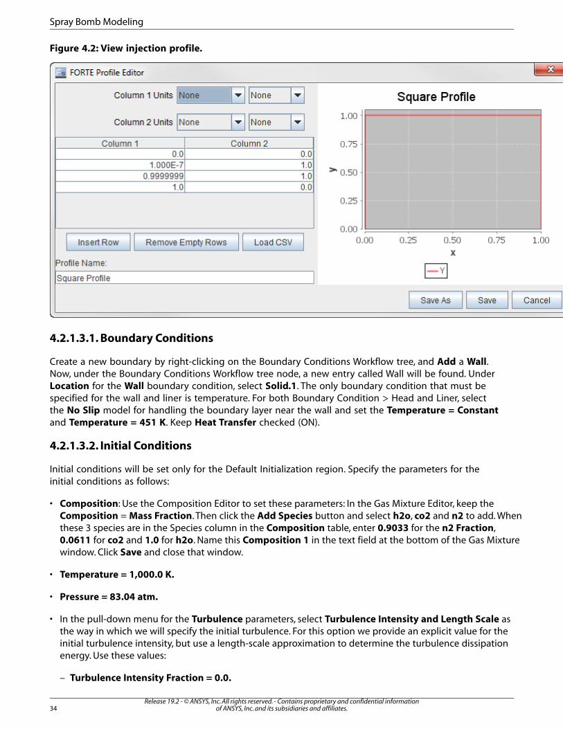
Figure 4.2: View injection profile.
4.2.1.3.1. Boundary Conditions
Create a new boundary by right-clicking on the Boundary Conditions Workflow tree, and Add a Wall.Now, under the Boundary Conditions Workflow tree node, a new entry called Wall will be found. UnderLocation for the Wall boundary condition, select Solid.1. The only boundary condition that must bespecified for the wall and liner is temperature. For both Boundary Condition > Head and Liner, selectthe No Slip model for handling the boundary layer near the wall and set the Temperature = Constantand Temperature = 451 K. Keep Heat Transfer checked (ON).
4.2.1.3.2. Initial Conditions
Initial conditions will be set only for the Default Initialization region. Specify the parameters for theinitial conditions as follows:
• Composition: Use the Composition Editor to set these parameters: In the Gas Mixture Editor, keep theComposition = Mass Fraction. Then click the Add Species button and select h2o, co2 and n2 to add. Whenthese 3 species are in the Species column in the Composition table, enter 0.9033 for the n2 Fraction,0.0611 for co2 and 1.0 for h2o. Name this Composition 1 in the text field at the bottom of the Gas Mixturewindow. Click Save and close that window.
• Temperature = 1,000.0 K.
• Pressure = 83.04 atm.
• In the pull-down menu for the Turbulence parameters, select Turbulence Intensity and Length Scale asthe way in which we will specify the initial turbulence. For this option we provide an explicit value for theinitial turbulence intensity, but use a length-scale approximation to determine the turbulence dissipationenergy. Use these values:
– Turbulence Intensity Fraction = 0.0.
Release 19.2 - © ANSYS, Inc. All rights reserved. - Contains proprietary and confidential informationof ANSYS, Inc. and its subsidiaries and affiliates.34
Spray Bomb Modeling
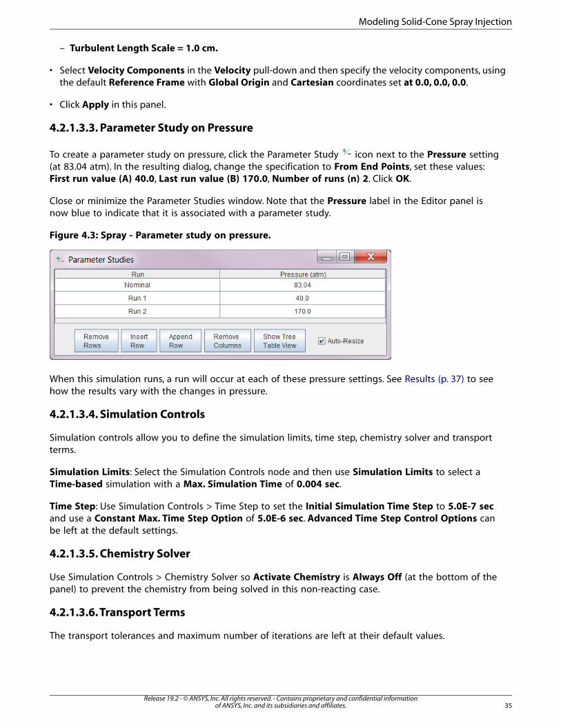
– Turbulent Length Scale = 1.0 cm.
• Select Velocity Components in the Velocity pull-down and then specify the velocity components, usingthe default Reference Frame with Global Origin and Cartesian coordinates set at 0.0, 0.0, 0.0.
• Click Apply in this panel.
4.2.1.3.3. Parameter Study on Pressure
To create a parameter study on pressure, click the Parameter Study icon next to the Pressure setting(at 83.04 atm). In the resulting dialog, change the specification to From End Points, set these values:First run value (A) 40.0, Last run value (B) 170.0, Number of runs (n) 2. Click OK.
Close or minimize the Parameter Studies window. Note that the Pressure label in the Editor panel isnow blue to indicate that it is associated with a parameter study.
Figure 4.3: Spray - Parameter study on pressure.
When this simulation runs, a run will occur at each of these pressure settings. See Results (p. 37) to seehow the results vary with the changes in pressure.
4.2.1.3.4. Simulation Controls
Simulation controls allow you to define the simulation limits, time step, chemistry solver and transportterms.
Simulation Limits: Select the Simulation Controls node and then use Simulation Limits to select aTime-based simulation with a Max. Simulation Time of 0.004 sec.
Time Step: Use Simulation Controls > Time Step to set the Initial Simulation Time Step to 5.0E-7 secand use a Constant Max. Time Step Option of 5.0E-6 sec. Advanced Time Step Control Options canbe left at the default settings.
4.2.1.3.5. Chemistry Solver
Use Simulation Controls > Chemistry Solver so Activate Chemistry is Always Off (at the bottom of thepanel) to prevent the chemistry from being solved in this non-reacting case.
4.2.1.3.6. Transport Terms
The transport tolerances and maximum number of iterations are left at their default values.
35Release 19.2 - © ANSYS, Inc. All rights reserved. - Contains proprietary and confidential information
of ANSYS, Inc. and its subsidiaries and affiliates.
Modeling Solid-Cone Spray Injection
4.2.1.4. Output Controls
Output controls determine what data are stored for viewing during the simulation and for creatingplots, graphs and animations in the ANSYS Forte Visualizer.
Spatially Resolved: Set the Temporal Output Control reporting every 0.004 sec. To create the SpatiallyResolved Species list, be sure to move nc7h16 to the Selection list. Also move n2, co2, and h2o. UnderRestart, clear (uncheck) the option Write Restart File at Last Simulation Step. Click Apply.
Spatially Averaged: Set the Temporal Output Control reporting every 4.0E-5 sec. To create theSpatially Averaged Species list, be sure to move nc7h16 to the Selection list. Also move co2, o2, andn2. Click Apply.
4.2.1.5. Save Project
Save your project with the Save command in the File menu, but choose a new name for the projectto avoid overwriting the original .ftsim file. The saving step includes validation of the project.
4.2.1.6. Run Settings
The settings here depend on the system and environment for your simulations. The default for the RunSettings panel is to have nothing selected.
Run Options: Under Job Script Options, change Default Run Type to Parallel and change the defaultMPI Arguments to 8. (If you do not have MPI installed and configured, keep the default of a serial run.)
4.2.1.7. Run Simulation
All that is needed to be done now is to select Run Simulation and click on Start once ANSYS Forte hasgiven you the green light and reports that it is ready for the simulation. You can monitor the resultsby clicking on the Monitor icon. In the Monitor window that opens, you can select which result youwant to monitor for the spray such as Mass Injected and Penetration Length.
Release 19.2 - © ANSYS, Inc. All rights reserved. - Contains proprietary and confidential informationof ANSYS, Inc. and its subsidiaries and affiliates.36
Spray Bomb Modeling

Figure 4.4: Monitor ANSYS Forte run
4.2.1.8. Results
This spray bomb case was run with three mesh sizes (1 mm, 2 mm and 3 mm) and then comparedagainst experimental data from Naber and Siebers 1 (p. 39). The experimental data provided consistedof penetration depth for the test spray. The experimental data show a penetration depth of 22.6 mmas is shown in Figure 4.5: Mesh sensitivity on spray penetration depth (p. 38). The simulation resultsshow good agreement with the spray penetration depth as is also seen in Figure 4.5: Mesh sensitivityon spray penetration depth (p. 38). It is important to note that ANSYS Forte defines the spray penetrationdepth that captures 95% of the liquid. These results also show that the spray is relatively insensitive tothe mesh for the three mesh sizes considered. The 1 mm and 2 mm results lie on top of each other.The diversion of the results for 3 mm, suggest that size is a little too large to resolve the fluid mechanicsoverall and so for these types of cases we would recommend the 2 mm resolution. However, even thecoarse mesh results are not far from the resolved-mesh solution, which is an important feature of theANSYS Forte simulations. Another interesting feature is to look at the how the droplet mass and vapormass evolve during the simulation time. These results are shown in Figure 4.6: Mesh sensitivity on dropletmass and vapor mass (p. 38), where the mesh is also shown to be insensitive to the mesh size, evenwith the coarsest mesh. Visualization of the spray results are shown in Figure 4.7: Spray bomb penetrationfor 2 mm mesh. (p. 39) at time = 0.0015 sec.
The results of the automated parameter study on ambient pressure in the spray bomb are shown asFigure 4.8: Results of automated parameter study on ambient pressure in the spray bomb. (p. 39). Thespray penetration is decreased as the ambient pressure increases due to the increased chamber gasdensity and drag.
37Release 19.2 - © ANSYS, Inc. All rights reserved. - Contains proprietary and confidential information
of ANSYS, Inc. and its subsidiaries and affiliates.
Modeling Solid-Cone Spray Injection
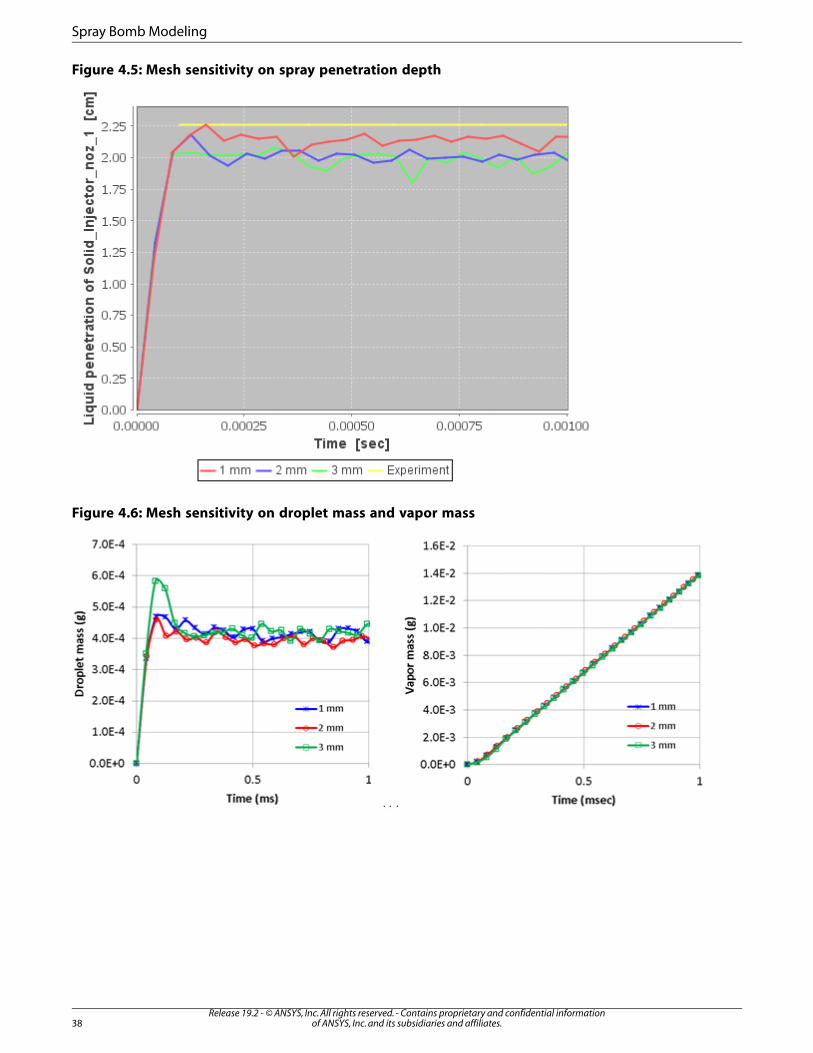
Figure 4.5: Mesh sensitivity on spray penetration depth
Figure 4.6: Mesh sensitivity on droplet mass and vapor mass
Release 19.2 - © ANSYS, Inc. All rights reserved. - Contains proprietary and confidential informationof ANSYS, Inc. and its subsidiaries and affiliates.38
Spray Bomb Modeling

Figure 4.7: Spray bomb penetration for 2 mm mesh.
Figure 4.8: Results of automated parameter study on ambient pressure in the spray bomb.
4.3. Reference
This tutorial is based on the work in this published paper:
1. Naber, J. D. and Siebers, D. L.,“Effects of Gas Density and Vaporization on Penetration and Dispersion ofDiesel Sprays”, SAE Technical Paper 9p60034, 1996.
39Release 19.2 - © ANSYS, Inc. All rights reserved. - Contains proprietary and confidential information
of ANSYS, Inc. and its subsidiaries and affiliates.
Reference

Release 19.2 - © ANSYS, Inc. All rights reserved. - Contains proprietary and confidential informationof ANSYS, Inc. and its subsidiaries and affiliates.40
Chapter 5: Port-Injected Spark Ignition Engine
This tutorial describes how to use ANSYS Forte CFD to simulate combustion in a port-injected sparkignition internal combustion engine with moving valves. Engine geometry is imported and ANSYSForte's automatic mesh generation is used to create the computational mesh on-the-fly during thesimulation.
5.1. Data Provided
5.1.1. Files Used in This Tutorial
The files for this tutorial are obtained by downloading the siengine_pfi_automesh.zip file here.
Unzip siengine_pfi_automesh.zip to your working folder.
• SIEngine_Sample.stl : This is the geometry file.
• ExhaustLift.csv and IntakeLift.csv: Two files of data describing the intake and exhaust valve lifts. Profilessuch as these can be imported (from .csv files) or manually entered in the Profile Editor.
• Spatial_Output_CAs.csv : Specifies when spatially resolved data such as velocity, temperature, speciesconcentrations, etc., will be output.
• SIEngine_PortInjected_AMG_Tutorial.ftsim: A project file of the completed tutorial, for verification orcomparison of your progress in the tutorial set-up.
The sample files are provided as a download. You have the opportunity to select the location for thefiles when you download and uncompress the sample files.
5.1.2. Project Comparison Utility
The ANSYS Forte installation includes the cgns_util export command, which you can use to comparethe parameter settings in the project file generated at any point during your tutorial set-up against theprovided .ftsim , which has the parameter settings for the final, completed tutorial. This command isdescribed in the ANSYS Forte User Guide.
Briefly, you can double-check project settings by saving your project and then running the cgns_utilto export your tutorial project, and then to export the provided final version of the tutorial. Save bothversions and compare them with your favorite diff tool, such as DIFFzilla. If all the parameters are inagreement, you have set up the project successfully. If there are differences, you can go back into thetutorial set-up, re-read the tutorial instructions, and change the setting of interest.
5.1.3. Time Estimate
As a guideline for your own simulations, this tutorial is estimated to take approximately 20.2 hours on
a cluster with 16 nodes with dual Intel® Xeon® processor E5-2690 at 2.90 GHz (8 total cores).
41Release 19.2 - © ANSYS, Inc. All rights reserved. - Contains proprietary and confidential information
of ANSYS, Inc. and its subsidiaries and affiliates.
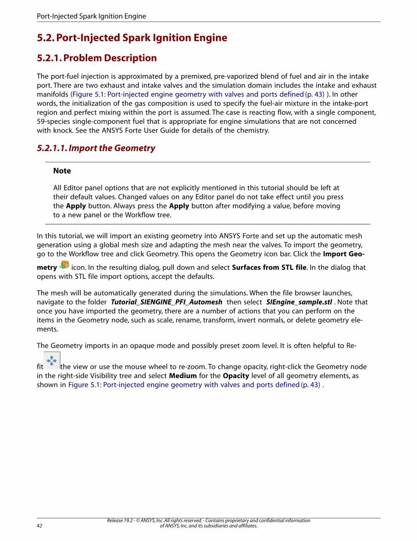
5.2. Port-Injected Spark Ignition Engine
5.2.1. Problem Description
The port-fuel injection is approximated by a premixed, pre-vaporized blend of fuel and air in the intakeport. There are two exhaust and intake valves and the simulation domain includes the intake and exhaustmanifolds (Figure 5.1: Port-injected engine geometry with valves and ports defined (p. 43) ). In otherwords, the initialization of the gas composition is used to specify the fuel-air mixture in the intake-portregion and perfect mixing within the port is assumed. The case is reacting flow, with a single component,59-species single-component fuel that is appropriate for engine simulations that are not concernedwith knock. See the ANSYS Forte User Guide for details of the chemistry.
5.2.1.1. Import the Geometry
Note
All Editor panel options that are not explicitly mentioned in this tutorial should be left attheir default values. Changed values on any Editor panel do not take effect until you pressthe Apply button. Always press the Apply button after modifying a value, before movingto a new panel or the Workflow tree.
In this tutorial, we will import an existing geometry into ANSYS Forte and set up the automatic meshgeneration using a global mesh size and adapting the mesh near the valves. To import the geometry,go to the Workflow tree and click Geometry. This opens the Geometry icon bar. Click the Import Geo-
metry icon. In the resulting dialog, pull down and select Surfaces from STL file. In the dialog thatopens with STL file import options, accept the defaults.
The mesh will be automatically generated during the simulations. When the file browser launches,navigate to the folder Tutorial_SIENGINE_PFI_Automesh then select SIEngine_sample.stl . Note thatonce you have imported the geometry, there are a number of actions that you can perform on theitems in the Geometry node, such as scale, rename, transform, invert normals, or delete geometry ele-ments.
The Geometry imports in an opaque mode and possibly preset zoom level. It is often helpful to Re-
fit the view or use the mouse wheel to re-zoom. To change opacity, right-click the Geometry nodein the right-side Visibility tree and select Medium for the Opacity level of all geometry elements, asshown in Figure 5.1: Port-injected engine geometry with valves and ports defined (p. 43) .
Release 19.2 - © ANSYS, Inc. All rights reserved. - Contains proprietary and confidential informationof ANSYS, Inc. and its subsidiaries and affiliates.42
Port-Injected Spark Ignition Engine
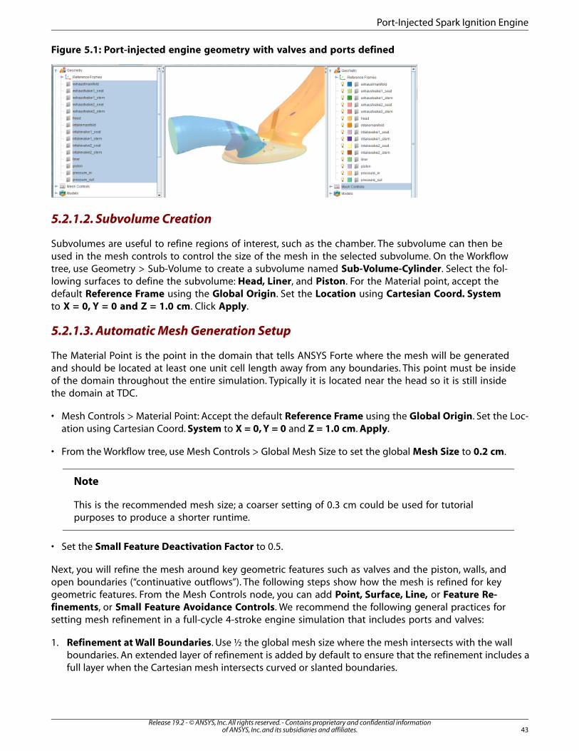
Figure 5.1: Port-injected engine geometry with valves and ports defined
5.2.1.2. Subvolume Creation
Subvolumes are useful to refine regions of interest, such as the chamber. The subvolume can then beused in the mesh controls to control the size of the mesh in the selected subvolume. On the Workflowtree, use Geometry > Sub-Volume to create a subvolume named Sub-Volume-Cylinder. Select the fol-lowing surfaces to define the subvolume: Head, Liner, and Piston. For the Material point, accept thedefault Reference Frame using the Global Origin. Set the Location using Cartesian Coord. Systemto X = 0, Y = 0 and Z = 1.0 cm. Click Apply.
5.2.1.3. Automatic Mesh Generation Setup
The Material Point is the point in the domain that tells ANSYS Forte where the mesh will be generatedand should be located at least one unit cell length away from any boundaries. This point must be insideof the domain throughout the entire simulation. Typically it is located near the head so it is still insidethe domain at TDC.
• Mesh Controls > Material Point: Accept the default Reference Frame using the Global Origin. Set the Loc-ation using Cartesian Coord. System to X = 0, Y = 0 and Z = 1.0 cm. Apply.
• From the Workflow tree, use Mesh Controls > Global Mesh Size to set the global Mesh Size to 0.2 cm.
Note
This is the recommended mesh size; a coarser setting of 0.3 cm could be used for tutorialpurposes to produce a shorter runtime.
• Set the Small Feature Deactivation Factor to 0.5.
Next, you will refine the mesh around key geometric features such as valves and the piston, walls, andopen boundaries (“continuative outflows”). The following steps show how the mesh is refined for keygeometric features. From the Mesh Controls node, you can add Point, Surface, Line, or Feature Re-finements, or Small Feature Avoidance Controls. We recommend the following general practices forsetting mesh refinement in a full-cycle 4-stroke engine simulation that includes ports and valves:
1. Refinement at Wall Boundaries. Use ½ the global mesh size where the mesh intersects with the wallboundaries. An extended layer of refinement is added by default to ensure that the refinement includes afull layer when the Cartesian mesh intersects curved or slanted boundaries.
43Release 19.2 - © ANSYS, Inc. All rights reserved. - Contains proprietary and confidential information
of ANSYS, Inc. and its subsidiaries and affiliates.
Port-Injected Spark Ignition Engine

• Surface Refinement: Click the Mesh Controls node in the Workflow tree. In the icon bar, click the New
Surface Refinement Depth icon and name the new control AllWalls. (This indicates that along theselected surfaces, cells of this smaller size and greater refinement will be used.) A new AllWalls item ap-pears under Mesh Controls in the Workflow tree. In the panel that appears, select all of the items in theLocation list, except be sure to exclude the Pressure_In and Pressure_Out open-boundary surfaces (wewill set up refinement along these surfaces separately). Be sure the list’s scroll bar is showing to ensureall the list items are displayed. Accept the default mesh Size as Fraction of Global Size as ½. Set theNumber of Cell Layers to Extend Refinement from Surface to 1. Keep the default of Active to Alwaysin the pull-down list below the refinement-layer entry. Click Apply. An initial refinement is applied overall wall boundaries with a ½ Size Fraction of Global Size.
2. Refinement at Open Boundaries (Continuative Outflows). Again, we will use ½ the global mesh size atcontinuative outflows, but use 2 extended layers of refinement, to make sure the continuative outflowshave smooth refinement where the inlet intersects walls.
• In the Mesh Controls icon bar, click the New Surface Refinement Depth icon and name the newcontrol OpenBoundaries. In the panel that appears, select all of the open-boundary surfaces (thePressure_In and Pressure_Out boundary surfaces) from the Location list. Accept the default mesh Sizeas Fraction of Global Size as 1/2. Set the Number of Cell Layers to Extend Refinement from Surfaceto 2. Click Apply. An initial refinement control is applied over all wall boundaries with a ½ Size Fractionof Global Size.
3. Refinement Around the Valve Stems. Here we want to make sure we have smaller cells in the regionsaround the valve stems, where velocities will be greatest during intake and exhaust portions of the cycle.
• Click the New Surface Refinement Depth icon (on the Mesh Controls icon bar) and name the newitem ValveStems. Select IntakeValve1_Stem, IntakeValve2_Stem, and ExhaustValve1_Stem, andExhasutValve2_Ste in the Location list. Set the Size as Fraction of Global Size to 1/2 and set theNumber of Cell Layers to Extend Refinement from Surface to 2. Make this Active = Always.
4. Refinement Around the Valve Ends that Seat to the Port. As above, we want to assure sufficient refine-ment where velocities will be greatest during valve opening and closing.
• Click the New Surface Refinement Depth icon and name the new item ValveSeats. Select Exhaust-Valve1_Seat, ExhaustValve2_Seat, IntakeValve1_Seat and IntakeValve2_Seat in the Location list.Set Size as Fraction of Global Size to 1/4 and set the Number of Cell Layers to Extend Refinementfrom Surface to 1. Make this Active = Always.
5. Refinement Near Piston and Head at TDC positions (Squish regions): The squish regions require refine-ment near TDC at the end of compression strokes to make sure that there are at least a couple of cellsseparating the head and piston surfaces in all locations. These controls are dynamic controls, since theyare only necessary near the TDC position of the crank.
• Click the New Surface Refinement Depth icon and name the new item Squish1. Select Head, Ex-haustValve1_Seat, ExhaustValve2_Seat, IntakeValve1_Seat, IntakeValve2_Seat, Linerand Pistonfrom the Location list. Change Size as Fraction of Global Size to 1/4. Set Number of Cell Layers toExtend Refinement from Surface to 1. Make this Active = During Crank Angle Interval and Startangle = 340.0 degrees and End angle = 380.0 degrees. Click Apply.
• Use the Copy and Paste icons in the icon bar of the Squish1 panel and name the new item Squish2.Make this Active = During Crank Angle Interval and set Start angle = 690.0 degrees and End angle= 790.0 degrees. Click Apply.
Release 19.2 - © ANSYS, Inc. All rights reserved. - Contains proprietary and confidential informationof ANSYS, Inc. and its subsidiaries and affiliates.44
Port-Injected Spark Ignition Engine
6. Add a Point Refinement Depth for the region of the spark: : Capture the chemistry around the spark.
• Click the Point Refinement Depth icon and name it SparkRegion. Set the Location as: X = -0.36cm, Y = 0 cm, Z = 0.33 cm, with the Radius of Application = 0.5 cm and the Refinement level = 1/4.The refinement is Active between Crank Angle 680 and 720 degrees. Click Apply.
7. Adaptive Refinements: Adaptively refine based on the solution variables temperature and velocity.
• Click the Solution Adaptive Meshing icon and name the new control SAM-Temperature. Set theQuantity Type = Gradient of Solution Field and Solution Variables = Temperature. Bounds Option= Statistical and Sigma Threshold = 0.5. Set the Size as fraction of Global Size = 1/4. The refinementis Active between Crank Angle 680 and 800 degrees, and the Location option is Sub-Volumes = Sub-volume-Cylinder. Click Apply.
• Click the Solution Adaptive Meshing icon and name the new control SAM-Velocity. Set theQuantity Type = Gradient of solution field and solution variable = VelocityMagnitude. BoundsOption = Statistical and Sigma Threshold = 0.5. Set the Refinement level = 1/2. The refinement isActive = Always, and the Location option is Entire Domain. Click Apply.
5.2.1.4. Models Setup
Chemistry: Now that the mesh has been set up, assigning models is next. Assign the chemistry with
Models > Chemistry and use the Import Chemistry icon and select the file Gasol-ine_1comp_49sp.cks from the ANSYS Forte data directory. If you are curious, you can view the chemistrydetails, such as chemistry source, pre-processing log, gas phase input, gas phase output, thermodynamicinput, transport input and transport output.
• Flame Speed Model: Use Models > Chemistry > Flame Speed Model to access the settings for the FlameSpeed model. Keep all the defaults, except under Turbulent Flame Speed (at the bottom of the Editorpanel), set Turbulent Flame Speed Ratio (b1) to 2.0. Click Apply.
Transport: The default RNG k-ε model turbulence settings are used in this tutorial. Those are specifiedin the Editor panel for Models > Transport > Turbulence. The default fluid properties are also used,which are at Models > Transport.
Spark Ignition: Turn on the spark ignition model by checking the box at Models > Spark Ignition.
The spark ignition model defaults include a Kernel Flame to G-Equation Switch Constant of 2.0 and theFlame Development Coefficient of 0.5.
Use the New Spark icon to create a new spark event and name it Spark.
Use Models > Spark Ignition > Spark to set up the details of the spark event. In the Reference Frame,use Global Origin and Cartesian coordinates for the Location, and set X= -0.36 cm, Y=1.0E-6 cm,and Z=0.33 cm. Select Crank Angle for Timing and Starting Angle = 688.0 degrees, Duration = 10.0degrees. Under Spark Energy, set Energy Release Rate = 20.0 J/sec. Accept the default 0.5 for EnergyTransfer Efficiency and 0.5 mm for Initial Kernel Radius. Click Apply.
45Release 19.2 - © ANSYS, Inc. All rights reserved. - Contains proprietary and confidential information
of ANSYS, Inc. and its subsidiaries and affiliates.
Port-Injected Spark Ignition Engine
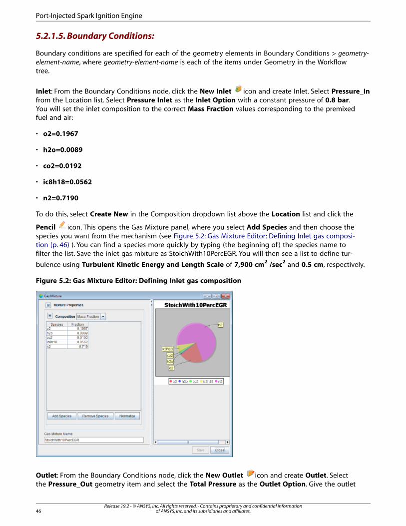
5.2.1.5. Boundary Conditions:
Boundary conditions are specified for each of the geometry elements in Boundary Conditions > geometry-element-name, where geometry-element-name is each of the items under Geometry in the Workflowtree.
Inlet: From the Boundary Conditions node, click the New Inlet icon and create Inlet. Select Pressure_Infrom the Location list. Select Pressure Inlet as the Inlet Option with a constant pressure of 0.8 bar.You will set the inlet composition to the correct Mass Fraction values corresponding to the premixedfuel and air:
• o2=0.1967
• h2o=0.0089
• co2=0.0192
• ic8h18=0.0562
• n2=0.7190
To do this, select Create New in the Composition dropdown list above the Location list and click the
Pencil icon. This opens the Gas Mixture panel, where you select Add Species and then choose thespecies you want from the mechanism (see Figure 5.2: Gas Mixture Editor: Defining Inlet gas composi-tion (p. 46) ). You can find a species more quickly by typing (the beginning of ) the species name tofilter the list. Save the inlet gas mixture as StoichWith10PercEGR. You will then see a list to define tur-
bulence using Turbulent Kinetic Energy and Length Scale of 7,900 cm2 /sec2 and 0.5 cm, respectively.
Figure 5.2: Gas Mixture Editor: Defining Inlet gas composition
Outlet: From the Boundary Conditions node, click the New Outlet icon and create Outlet. Selectthe Pressure_Out geometry item and select the Total Pressure as the Outlet Option. Give the outlet
Release 19.2 - © ANSYS, Inc. All rights reserved. - Contains proprietary and confidential informationof ANSYS, Inc. and its subsidiaries and affiliates.46
Port-Injected Spark Ignition Engine

a Pressure of 0.9 bar, which arises from the back-pressure of the exhaust system with an Offset Distanceto Apply Pressure of 0.1 cm. Set the Turbulence Boundary Conditions to Turbulent Kinetic Energy
and Length Scale of 7,900 cm2/sec2 and 0.5 cm,respectively.
Piston: From the Boundary Conditions node, click the New Wall icon and name it Piston. Select thePiston item in the Location list. Set the Temperature Option to Constant and 420 K. Turn ON theWall Motion option and set the piston Motion Type to use a Slider-Crank Model with a Stroke of7.95 cm and a Connecting Rod Length of 13.81 cm with 0.0 Piston Offset. Change the MovementType to Moving Surface and accept the default Global Origin Reference Frame.
Intake: Click the New Wall icon and name it Intake. Select the IntakeManifold item in the Locationlist and set the Temperature to 300 K.
Exhaust: Click the New Wall icon and name it Exhaust. Select the ExhaustManifold item in theLocation list and set the Temperature to 650 K.
Liner: Click the New Wall icon and name it Liner. Select the Liner item in the Location list and setthe Temperature to 385 K.
Head: Click the New Wall icon and name it Head. Select the Head item in the Location list and setthe Temperature to 385 K.
Intake Valves: Click the New Wall icon and name it IntakeValve 1. The valve specification is a littlemore complicated than the stationary walls, such that several steps are required within the wall panel.These steps specify the wall motion and the way we want the mesh to adapt to the gap opening nearthe valve seat when the valve opens or closes.
• Multiselect both the IntakeValve1_Seat and IntakeValve1_Stem items in the Location list.
• Check the Heat Transfer option and set the Temperature to the constant value of 385 K.
• Turn ON (check) the Wall Motion and set the Motion Type to Offset Table.
• Accept the default Global Origin for the Reference Frame. Select Spherical for the Coord. System under
Direction for the valve motion and set =199 degrees and =0.0 degrees.
• To import the lift profile (named IntakeLift.csv in the same location as the .stl file you started this tutorial
with), select Create New from the Lift Profile drop- down list and click the Pencil icon. In the ProfileEditor, click the Load CSV button and navigate to the IntakeLift.csv file. Accept the defaults in the importdialog and click OK. At the bottom of the Profile Editor window, name this IntakeValves. Ensure that theunits in the first column are set to Angle and the second column is set to cm. Save the Profile.
• For Movement Type, change the pull-down menu to Valve. Then select just the surface boundary portionof the valve that comes into contact with the valve seat on the port, as well as the surface boundary thatcontains the seat region. In this case, select both the IntakeManifold and the IntakeValve1_Seat.
• Finally, set the Valve Motion Activation Threshold to 0.15 cm. This indicates that the valve will not openuntil the lift value specified in the valve-lift profile exceeds this threshold. A smaller value will cause thevalves to open sooner, but the mesh refinement required to resolve the gap will be higher. This is a trade-off that will need to be determined based on the goals and outcomes desired from the simulation. In addition
47Release 19.2 - © ANSYS, Inc. All rights reserved. - Contains proprietary and confidential information
of ANSYS, Inc. and its subsidiaries and affiliates.
Port-Injected Spark Ignition Engine
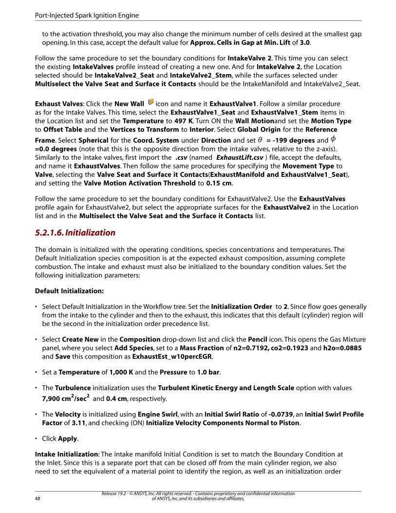
to the activation threshold, you may also change the minimum number of cells desired at the smallest gapopening. In this case, accept the default value for Approx. Cells in Gap at Min. Lift of 3.0.
Follow the same procedure to set the boundary conditions for IntakeValve 2. This time you can selectthe existing IntakeValves profile instead of creating a new one. And for IntakeValve 2, the Locationselected should be IntakeValve2_Seat and IntakeValve2_Stem, while the surfaces selected underMultiselect the Valve Seat and Surface it Contacts should be the IntakeManifold and IntakeValve2_Seat.
Exhaust Valves: Click the New Wall icon and name it ExhaustValve1. Follow a similar procedureas for the Intake Valves. This time, select the ExhaustValve1_Seat and ExhaustValve1_Stem items inthe Location list and set the Temperature to 497 K. Turn ON the Wall Motionand set the Motion Typeto Offset Table and the Vertices to Transform to Interior. Select Global Origin for the Reference
Frame. Select Spherical for the Coord. System under Direction and set = -199 degrees and =0.0 degrees (note that this is the opposite direction from the intake valves, relative to the z-axis).Similarly to the intake valves, first import the .csv (named ExhaustLift.csv ) file, accept the defaults,and name it ExhaustValves. Then follow the same procedures for specifying the Movement Type toValve, selecting the Valve Seat and Surface it Contacts(ExhaustManifold and ExhaustValve1_Seat),and setting the Valve Motion Activation Threshold to 0.15 cm.
Follow the same procedure to set the boundary conditions for ExhaustValve2. Use the ExhaustValvesprofile again for ExhaustValve2, but select the appropriate surfaces for the ExhaustValve2 in the Locationlist and in the Multiselect the Valve Seat and the Surface it Contacts list.
5.2.1.6. Initialization
The domain is initialized with the operating conditions, species concentrations and temperatures. TheDefault Initialization species composition is at the expected exhaust composition, assuming completecombustion. The intake and exhaust must also be initialized to the boundary condition values. Set thefollowing initialization parameters:
Default Initialization:
• Select Default Initialization in the Workflow tree. Set the Initialization Order to 2. Since flow goes generallyfrom the intake to the cylinder and then to the exhaust, this indicates that this default (cylinder) region willbe the second in the initialization order precedence list.
• Select Create New in the Composition drop-down list and click the Pencil icon. This opens the Gas Mixturepanel, where you select Add Species, set to a Mass Fraction of n2=0.7192, co2=0.1923 and h2o=0.0885and Save this composition as ExhaustEst_w10percEGR.
• Set a Temperature of 1,000 K and the Pressure to 1.0 bar.
• The Turbulence initialization uses the Turbulent Kinetic Energy and Length Scale option with values
7,900 cm2/sec2 and 0.4 cm, respectively.
• The Velocity is initialized using Engine Swirl, with an Initial Swirl Ratio of -0.0739, an Initial Swirl ProfileFactor of 3.11, and checking (ON) Initialize Velocity Components Normal to Piston.
• Click Apply.
Intake Initialization: The intake manifold Initial Condition is set to match the Boundary Condition atthe Inlet. Since this is a separate port that can be closed off from the main cylinder region, we alsoneed to set the equivalent of a material point to identify the region, as well as an initialization order
Release 19.2 - © ANSYS, Inc. All rights reserved. - Contains proprietary and confidential informationof ANSYS, Inc. and its subsidiaries and affiliates.48
Port-Injected Spark Ignition Engine
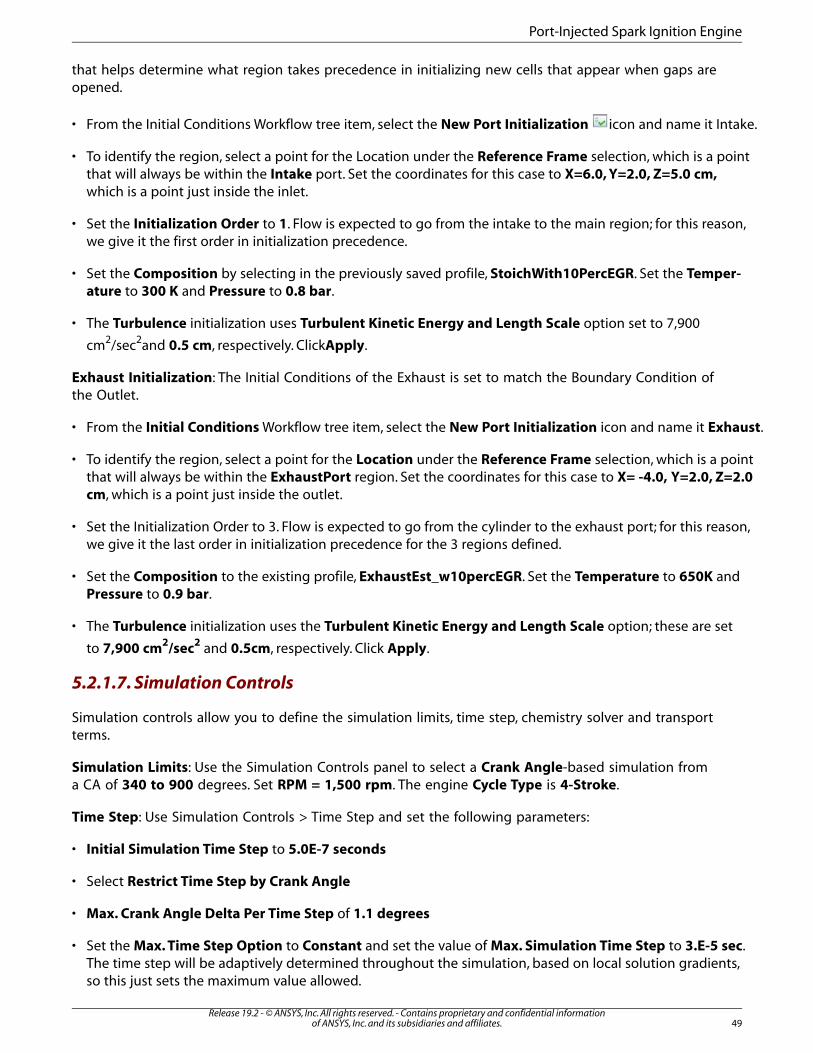
that helps determine what region takes precedence in initializing new cells that appear when gaps areopened.
• From the Initial Conditions Workflow tree item, select the New Port Initialization icon and name it Intake.
• To identify the region, select a point for the Location under the Reference Frame selection, which is a pointthat will always be within the Intake port. Set the coordinates for this case to X=6.0, Y=2.0, Z=5.0 cm,which is a point just inside the inlet.
• Set the Initialization Order to 1. Flow is expected to go from the intake to the main region; for this reason,we give it the first order in initialization precedence.
• Set the Composition by selecting in the previously saved profile, StoichWith10PercEGR. Set the Temper-ature to 300 K and Pressure to 0.8 bar.
• The Turbulence initialization uses Turbulent Kinetic Energy and Length Scale option set to 7,900
cm2/sec2and 0.5 cm, respectively. ClickApply.
Exhaust Initialization: The Initial Conditions of the Exhaust is set to match the Boundary Condition ofthe Outlet.
• From the Initial Conditions Workflow tree item, select the New Port Initialization icon and name it Exhaust.
• To identify the region, select a point for the Location under the Reference Frame selection, which is a pointthat will always be within the ExhaustPort region. Set the coordinates for this case to X= -4.0, Y=2.0, Z=2.0cm, which is a point just inside the outlet.
• Set the Initialization Order to 3. Flow is expected to go from the cylinder to the exhaust port; for this reason,we give it the last order in initialization precedence for the 3 regions defined.
• Set the Composition to the existing profile, ExhaustEst_w10percEGR. Set the Temperature to 650K andPressure to 0.9 bar.
• The Turbulence initialization uses the Turbulent Kinetic Energy and Length Scale option; these are set
to 7,900 cm2/sec2 and 0.5cm, respectively. Click Apply.
5.2.1.7. Simulation Controls
Simulation controls allow you to define the simulation limits, time step, chemistry solver and transportterms.
Simulation Limits: Use the Simulation Controls panel to select a Crank Angle-based simulation froma CA of 340 to 900 degrees. Set RPM = 1,500 rpm. The engine Cycle Type is 4-Stroke.
Time Step: Use Simulation Controls > Time Step and set the following parameters:
• Initial Simulation Time Step to 5.0E-7 seconds
• Select Restrict Time Step by Crank Angle
• Max. Crank Angle Delta Per Time Step of 1.1 degrees
• Set the Max. Time Step Option to Constant and set the value of Max. Simulation Time Step to 3.E-5 sec.The time step will be adaptively determined throughout the simulation, based on local solution gradients,so this just sets the maximum value allowed.
49Release 19.2 - © ANSYS, Inc. All rights reserved. - Contains proprietary and confidential information
of ANSYS, Inc. and its subsidiaries and affiliates.
Port-Injected Spark Ignition Engine

TheAdvanced Time Step Control Options settings are kept at the defaults:
• Time Step Growth Factor = 1.3
• Fluid Acceleration Factor = 0.5
• Rate of Strain Factor = 0.6
• Convection factor = 0.2
• Internal Energy Factor = 1.0
• Max. Convection Subcycles = 8
Chemistry Solver: Simulation Controls > Chemistry Solver is also kept at the defaults, with the followingparameters:
• Absolute Tolerance = 1.0E-12
• Relative Tolerance = 1.0E-5
• Use Dynamic Cell Clustering to take advantage of groups of cells with similar conditions. Select 2 featuresto introduce Dynamic Cell Clustering: 1) Max. Temperature Dispersion of 10 K and 2) a Max. EquilibriumRatio Dispersion of 0.05.
• To increase the time-to-solution speed, you have the ability to choose when chemistry is activated. In thistutorial, select Activate Chemistry Conditionally, and select When Temperature is Reached with ThresholdTemperature 600 K and also select During Crank Angle Interval between 650 and 850 crank angle. Thisensures that chemistry is active during the time that combustion is expected even if temperature does notrise above 600 K. Click Apply.
Transport Terms:Use the default transport tolerances and maximum number of iterations.
5.2.1.8. Output Controls
Output controls determine what data are stored for viewing during the simulation and for creatingplots, graphs and animations in ANSYS Forte Visualize.
Spatially Resolved: Allows you to control when spatially resolved data such as velocity, temperature,species concentrations, etc., will be output. In the Spatially Resolved panel, set theCrank Angle OutputControl to report every 20 degrees (to manage the size of the output file). You can optionally increasethe frequency of output during the cycle by selecting User Defined Output Control and importingthe Spatial_Output_CAs.csv file, which has a list of specific crank angles where spatially resolved outputwill occur (illustrated in Figure 5.3: Output control panel - Spatially Resolved (p. 51) ). Alternatively, youcould select User Defined Output Control, and use the Profile Editor to create some other file specifyingan output crank-angle profile (the provided profile is illustrated in Figure 5.4: User-defined spatially re-solved output controls (p. 51) ). Select the following species for Spatially Resolved Output: h2o, no,no2, co, co2, o2, ic8h18 and n2.
Release 19.2 - © ANSYS, Inc. All rights reserved. - Contains proprietary and confidential informationof ANSYS, Inc. and its subsidiaries and affiliates.50
Port-Injected Spark Ignition Engine
Figure 5.3: Output control panel - Spatially Resolved
Figure 5.4: User-defined spatially resolved output controls
Spatially Averaged:Allows you to control the output of values that are averaged across the domain.Spatially Averaged panels, set the Crank Angle Output Control to reporting every 1 degree. Selectthe following species for Spatially Averaged Output: h2o, no, no2, co, co2, o2, ic8h18 and n2.
Restart Data: If you anticipate that the case will be stopped and you want the ability to restart it fromthe last time step solved, select Output Controls > Restart Data. You can specify certain Restart Pointsusing a separate file. Turn on (check) User Defined Restart Points and use the Profile Editor to createa Restart profile. You can view, edit or import new Restart Points in this 1-D Profile Editor. Sometimesit is helpful in spark ignition cases to save a restart file after IVC but before the spark occurs (CA=687in this case) so you can use the compression portion of the cycle as a start point in additional runs.Create a new profile for this purpose called RestartOutput and add one line with CA value set to 650.
51Release 19.2 - © ANSYS, Inc. All rights reserved. - Contains proprietary and confidential information
of ANSYS, Inc. and its subsidiaries and affiliates.
Port-Injected Spark Ignition Engine
5.2.1.9. Preview Simulation
You can view the profiles for the Piston, Intake Valves, Exhaust Valves and Mesh Refinement during thesimulation by selecting Preview Simulation > Boundary Motion > Simulation Preview. This is an excellentway to check whether you have valve overlap and that the settings are correct.
As a method for checking the automatically generated mesh, you can generate a Preview Mesh. Select
Preview Simulation > Mesh Generation and then click the New Automatic Mesh Plot icon, namethis new automatic mesh generation plot “FTDC”, select Crank Angleas theTime Optionand set it to
720 CA. Then click Apply to save the settings and then on the Generate Mesh icon. ANSYS Fortewill generate the preview mesh and display it in the 3-D View window. It is a good practice to look atmeshes at key points in the cycle such as Firing Top Dead Center (FTDC), Exhaust Valve Opening (EVO),Intake Valve Closed (IVC), Intake Valve Open (IVO) and Exhaust Valve Closed (EVC). If you want to seethe cut plane where the mesh will be generated, click the Plane Filter box and specify an origin pointand normal direction for the cut plane.
Use the information in the following list to set up these New Automatic Mesh Plots.
1. FTDC @ CA=720: Point (X=0.0cm, Y=0.0cm, Z=0.0cm); Normal (X=0.0cm, Y=1.0cm, Z=0.0cm)
2. EVO @ CA=192: Point (X=0.0cm, Y=2.0cm, Z=0.0cm); Normal (X=0.0cm, Y=1.0cm, Z=0.0cm)
3. IVC @ CA=601: Point (X=0.0cm, Y=-2.0cm, Z=0.0cm); Normal (X=0.0cm, Y=1.0cm, Z=0.0cm)
4. IVO @ CA=363: Point (X=0.0cm, Y=-1.0cm, Z=0.0cm); Normal (X=0.0cm, Y=1.0cm, Z=0.0cm)
The visibility of the Automatic Mesh Plots is controlled in the Visibility tree under Preview Simulationand Mesh Generation.
5.2.1.10. Run Simulation
To complete the lesson, select Run Simulation on the Workflow tree and, once ANSYS Forte displaysthe green START button on the Run Simulation panel and reports a “Ready” status, click Start. You can
monitor the results by clicking on the Monitor Runs icon. In the Monitor window that opens, youcan select the run you wish to monitor.
5.2.1.11. Run Settings
The settings here depend on the system and environment for your simulations. The default for the RunSettings panel is to have nothing selected.
Run Options: This tutorial does not require changes to this panel’s defaults; adjust them as necessaryfor your environment.
Windows Settings: This tutorial does not require changes to this panel’s defaults; adjust them as ne-cessary for your environment.
Linux Settings: This tutorial does not require changes to this panel’s defaults; adjust them as necessaryfor your environment.
Release 19.2 - © ANSYS, Inc. All rights reserved. - Contains proprietary and confidential informationof ANSYS, Inc. and its subsidiaries and affiliates.52
Port-Injected Spark Ignition Engine
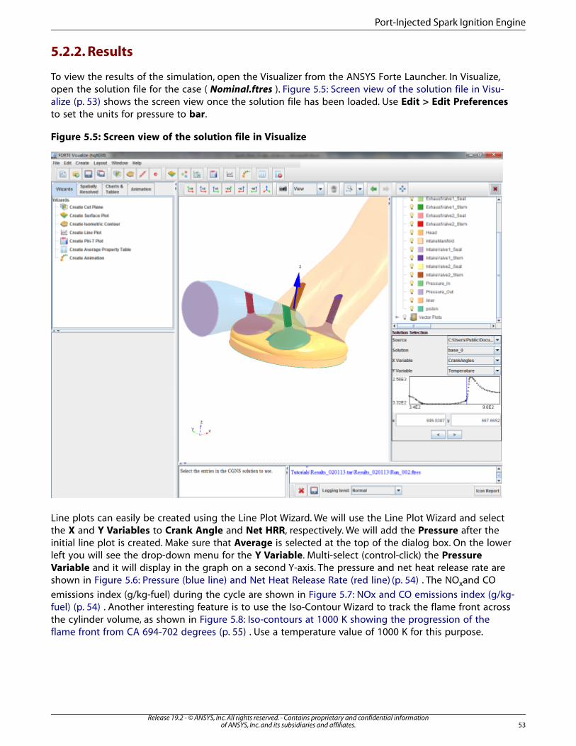
5.2.2. Results
To view the results of the simulation, open the Visualizer from the ANSYS Forte Launcher. In Visualize,open the solution file for the case ( Nominal.ftres ). Figure 5.5: Screen view of the solution file in Visu-alize (p. 53) shows the screen view once the solution file has been loaded. Use Edit > Edit Preferencesto set the units for pressure to bar.
Figure 5.5: Screen view of the solution file in Visualize
Line plots can easily be created using the Line Plot Wizard. We will use the Line Plot Wizard and selectthe X and Y Variables to Crank Angle and Net HRR, respectively. We will add the Pressure after theinitial line plot is created. Make sure that Average is selected at the top of the dialog box. On the lowerleft you will see the drop-down menu for the Y Variable. Multi-select (control-click) the PressureVariable and it will display in the graph on a second Y-axis. The pressure and net heat release rate areshown in Figure 5.6: Pressure (blue line) and Net Heat Release Rate (red line) (p. 54) . The NOxand CO
emissions index (g/kg-fuel) during the cycle are shown in Figure 5.7: NOx and CO emissions index (g/kg-fuel) (p. 54) . Another interesting feature is to use the Iso-Contour Wizard to track the flame front acrossthe cylinder volume, as shown in Figure 5.8: Iso-contours at 1000 K showing the progression of theflame front from CA 694-702 degrees (p. 55) . Use a temperature value of 1000 K for this purpose.
53Release 19.2 - © ANSYS, Inc. All rights reserved. - Contains proprietary and confidential information
of ANSYS, Inc. and its subsidiaries and affiliates.
Port-Injected Spark Ignition Engine

Figure 5.6: Pressure (blue line) and Net Heat Release Rate (red line)
Figure 5.7: NOx and CO emissions index (g/kg-fuel)
Release 19.2 - © ANSYS, Inc. All rights reserved. - Contains proprietary and confidential informationof ANSYS, Inc. and its subsidiaries and affiliates.54
Port-Injected Spark Ignition Engine
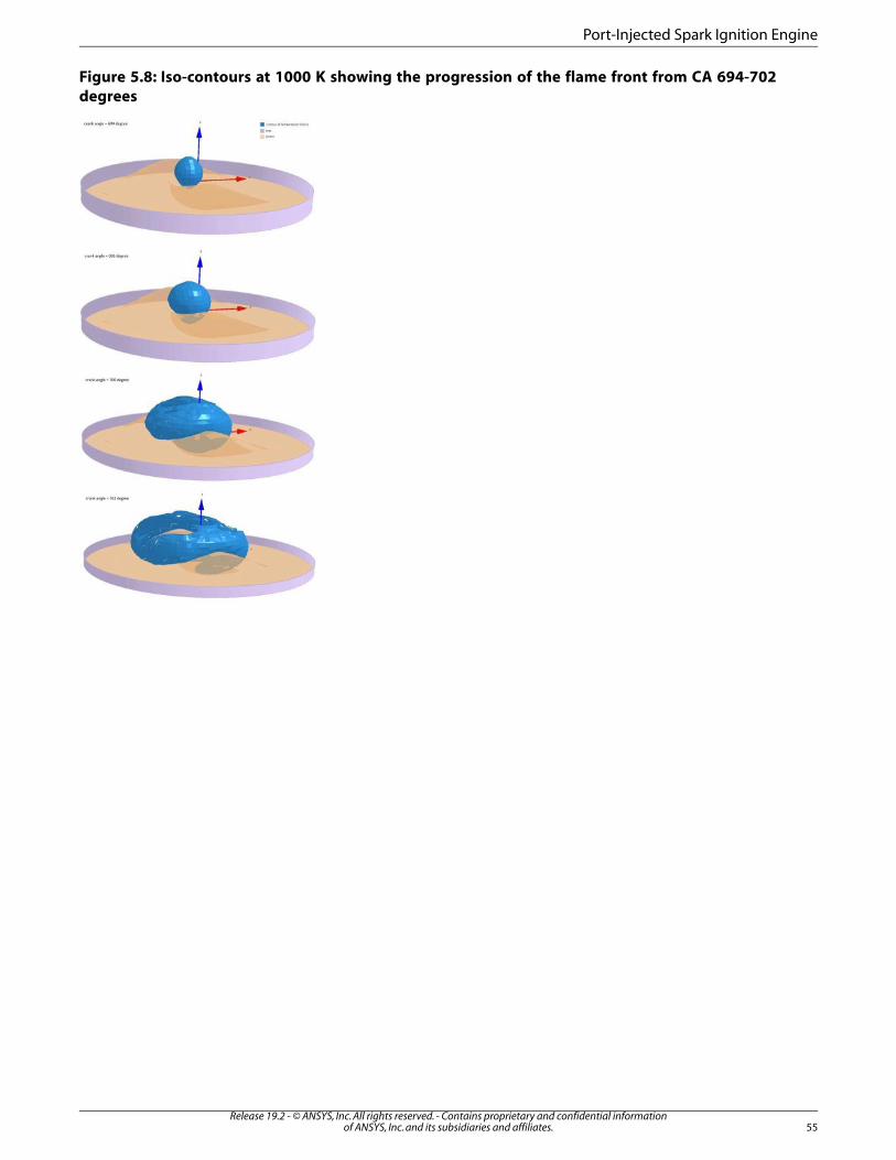
Figure 5.8: Iso-contours at 1000 K showing the progression of the flame front from CA 694-702degrees
55Release 19.2 - © ANSYS, Inc. All rights reserved. - Contains proprietary and confidential information
of ANSYS, Inc. and its subsidiaries and affiliates.
Port-Injected Spark Ignition Engine

Release 19.2 - © ANSYS, Inc. All rights reserved. - Contains proprietary and confidential informationof ANSYS, Inc. and its subsidiaries and affiliates.56

Chapter 6: Tracking Soot Particles Evolution in a Diesel Engine
This tutorial presents the soot particle tracking capability in ANSYS Forte, applying the method of mo-ments to a diesel engine case. With the soot particle tracking feature, several spatially resolved valuesof soot can be simulated, including particle number density, volume fraction and average diameter.The tutorial explains the setup for using the particle tracking capability, and presents visualizations ofsoot predictions.
6.1. Data Provided
6.1.1. Files Used in This Tutorial
The files for this tutorial are obtained by downloading the soot_particle_tracking.zip filehere.
Unzip soot_particle_tracking.zip to your working folder.
• Soot-particle-tracking__tutorial.ftsim: A project file of the completed tutorial, for verification or comparisonof your progress in the tutorial set-up. The project file includes all the relevant geometry, chemistry set andspray profile details.
The tutorial sample file is provided as a download. You have the opportunity to select the location forthe file when you download and uncompress the sample files.
Note
This tutorial is based on a fully configured sample project that contains the tutorial projectsettings. The description provided here covers the key points of the project set-up but is notintended to explain every parameter setting in the project. The .ftsim file has all custom anddefault parameters already configured; the text highlights only the significant points of thetutorial.
6.1.2. Project Comparison Utility
The ANSYS Forte installation includes the cgns_util export command, which you can use to comparethe parameter settings in the project file generated at any point during your tutorial set-up against theprovided .ftsim , which has the parameter settings for the final, completed tutorial. This command isdescribed in the ANSYS Forte User Guide.
Briefly, you can double-check project settings by saving your project and then running the cgns_utilto export your tutorial project, and then to export the provided final version of the tutorial. Save bothversions and compare them with your preferred diff tool, such as DIFFzilla. If all the parameters are inagreement, you have set up the project successfully. If there are differences, you can go back into thetutorial set-up, re-read the tutorial instructions, and change the setting of interest.
57Release 19.2 - © ANSYS, Inc. All rights reserved. - Contains proprietary and confidential information
of ANSYS, Inc. and its subsidiaries and affiliates.
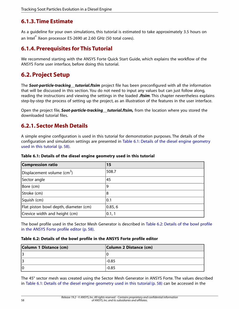
6.1.3. Time Estimate
As a guideline for your own simulations, this tutorial is estimated to take approximately 3.5 hours on
an Intel® Xeon processor E5-2690 at 2.60 GHz (50 total cores).
6.1.4. Prerequisites for This Tutorial
We recommend starting with the ANSYS Forte Quick Start Guide, which explains the workflow of theANSYS Forte user interface, before doing this tutorial.
6.2. Project Setup
The Soot-particle-tracking__tutorial.ftsim project file has been preconfigured with all the informationthat will be discussed in this section. You do not need to input any values but can just follow along,reading the instructions and viewing the settings in the loaded .ftsim. This chapter nevertheless explainsstep-by-step the process of setting up the project, as an illustration of the features in the user interface.
Open the project file, Soot-particle-tracking__tutorial.ftsim, from the location where you stored thedownloaded tutorial files.
6.2.1. Sector Mesh Details
A simple engine configuration is used in this tutorial for demonstration purposes. The details of theconfiguration and simulation settings are presented in Table 6.1: Details of the diesel engine geometryused in this tutorial (p. 58).
Table 6.1: Details of the diesel engine geometry used in this tutorial
15Compression ratio
508.7Displacement volume (cm3)
45Sector angle
9Bore (cm)
8Stroke (cm)
0.1Squish (cm)
0.85, 6Flat piston bowl depth, diameter (cm)
0.1, 1Crevice width and height (cm)
The bowl profile used in the Sector Mesh Generator is described in Table 6.2: Details of the bowl profilein the ANSYS Forte profile editor (p. 58).
Table 6.2: Details of the bowl profile in the ANSYS Forte profile editor
Column 2 Distance (cm)Column 1 Distance (cm)
03
-0.853
-0.850
The 45° sector mesh was created using the Sector Mesh Generator in ANSYS Forte. The values describedin Table 6.1: Details of the diesel engine geometry used in this tutorial (p. 58) can be accessed in the
Release 19.2 - © ANSYS, Inc. All rights reserved. - Contains proprietary and confidential informationof ANSYS, Inc. and its subsidiaries and affiliates.58
Tracking Soot Particles Evolution in a Diesel Engine
Soot-particle-tracking__tutorial.ftsim project file, by launching the Sector Mesh Generator, as shownin Figure 6.1: Sector Mesh Generator settings for this tutorial (p. 59). In the Sector Mesh Generator, To-pology 3 was deemed the most appropriate to represent this piston bowl geometry. The mesh parametersfor this topology were selected as follows:
1. ~1 mm resolution along the radial direction.
2. 3° along the azimuthal direction.
3. Along the z-direction:
• 0.7 mm in the piston bowl, to capture spray and events close to TDC accurately.
• 1.6 mm resolution in the squish region. Four minimum cells will be present, as specified in the MeshControls Editor panel, to ensure resolution close to TDC. Away from TDC, the mesh is set to be coarse inthe squish region, for the sake of faster simulation in this simplistic demonstration case.
These settings resulted in a sector mesh with 40,890 cells when the piston is at bottom dead center(BDC).
Figure 6.1: Sector Mesh Generator settings for this tutorial
In the Mesh Controls > Remeshing Editor panel, the Smooth check box is unchecked. All other controlsare left at default values.
6.2.2. Chemistry Set Details
On the Models > Chemistry Editor panel, the Diesel_2comp_189sp__soot-particle-tracking.cks chemistryset has been selected.
This chemistry set includes a gas-phase mechanism (Diesel_2comp_189sp__soot-particle-track-ing_chem.inp), and a surface mechanism file (surf_soot_chem.inp). The thermodynamic data are includedin the mechanism files.
59Release 19.2 - © ANSYS, Inc. All rights reserved. - Contains proprietary and confidential information
of ANSYS, Inc. and its subsidiaries and affiliates.
Project Setup
The gas-phase mechanism contains 189 species participating in 1392 reactions. This mechanism hasbeen generated for use with the 66.8/33.2 wt% n-decane/AMN diesel surrogate. It has reaction pathwaysto accurately predict soot precursors needed for the surface soot mechanism, all the way from smallhydrocarbons such as acetylene to polycyclic aromatic species such as pyrene and coronene.
If you were to create your own chemistry set for use with particle tracking, the surface mechanismswould have to conform to certain standards, as defined in the Chemkin-Pro Input Manual and Chemkin-Pro Theory Manual. The soot surface mechanism that is part of this tutorial's chemistry set includes:
1. Soot nucleation through multiple pathways.
2. HACA- and PAH-based soot growth pathways.
3. Soot oxidation through O2 and OH.
6.2.3. Transport Property Settings
The default values are used in the Transport property panel. In the Transport > Turbulence panel, theRANS RNG k-epsilon model is used, with default values.
6.2.4. Spray Model Settings
Under Models > Spray model, the spray models, nozzle and fuel injection values have been set.
The nozzle-1 settings are provided in Table 6.3: Nozzle settings (p. 60).
Table 6.3: Nozzle settings
Location
Global originReference frame
CylindricalCoordinate system
0.1 cmR
22.5 degreesq
9 cmA
Spray direction
Global originReference frame
SphericalCoordinate system
110 degreesq
22.5 degreesf
Nozzle size
150 micronNozzle diameter
The following spray models are being used in this project, with default ANSYS Forte settings:
1. KH droplet breakup model
2. RT droplet breakup model
Release 19.2 - © ANSYS, Inc. All rights reserved. - Contains proprietary and confidential informationof ANSYS, Inc. and its subsidiaries and affiliates.60
Tracking Soot Particles Evolution in a Diesel Engine
3. Gas-jet
4. Vaporization model
5. Adaptive Collision Mesh droplet collision model
The diesel fuel was simulated using a 2-component surrogate consisting (1) of 66.8 weight% n-decane/33.2weight% 1-methylnaphthalene. This particular surrogate was designed to model a European diesel fuelwith cetane number of 55. This surrogate has a threshold sooting index of 36, placing it on the higherend of the typical diesel fuel sooting index. Table 6.4: Details of nozzle (Nozzle-1) and fuel injection(Injection-1) (p. 61) provides details of the nozzle and the fuel injection. These values are entered underthe Models > Solid Injector-1 node. Specifically, the nozzle location and spray direction inputs are seton the Nozzle-1 Editor panel, and the fuel injection-related inputs are specified on the Injection-1 Editorpanel.
On the Solid Injector-1 panel, parcel specification has been set using the Number of parcels option. TheInjected parcel count has been set to 3000.
The Inflow Droplet Temperature has been set to 320 K.
Spray was initialized using the Constant Discharge Coefficient and Angle option. A Discharge Coef-ficient of 0.9 has been used, with a Mean Cone Angle of 15°.
Table 6.4: Details of nozzle (Nozzle-1) and fuel injection (Injection-1)
Nozzle details
150 μmDirect-injector nozzle hole
140Direct-injector included angle (°)
Fuel injection details
-10Start of injection (° ATDC)
10Duration of injection (°)
20Total Injected mass (mg)
A slightly modified square profile: (0,0), (1E-7,1),(0.999999,1), (1,0)
Injection velocity profile
6.2.5. Soot Model Settings
Under Models > Soot Model, choose Soot Model. There are three options for modeling soot in ANSYSForte. One option is to define a “pseudo-gas” soot model that is included in a different gas-phasechemistry mechanism input. In that case, you would not select Models > Soot Model. With the selectedchemistry in this example, you may either:
• Use a built-in 2-step model, which is one option on the Soot Model panel.
• Use the Method of Moments. This option enables the particle tracking capability. In this tutorial, Methodof Moments is selected.
1species names: n-decane is nc10h22; 1-methylnaphthalene is a2ch3.
61Release 19.2 - © ANSYS, Inc. All rights reserved. - Contains proprietary and confidential information
of ANSYS, Inc. and its subsidiaries and affiliates.
Project Setup
With the Method of Moments option selected in the Soot Model panel, four inputs are required. Detailsregarding these parameters can be found in the Chemkin-Pro Theory Manual.
1. Number of Moments: 3-6 moments can be used in the simulations. Typically, it is recommended that 3moments are sufficient; that value of 3 is used in this tutorial.
2. Scaling Factor for Moments: This value changes the units of the (internal) solution variable for particlemoments. A recommended value for typical problems is the default 1.0E+12, as the scaling helps preservethe positivity of the solution during computation.
3. Scaling Factor for Surface Species: This value changes the units of the (internal) solution variable forparticle surface species. For example, setting it to 1.0E+12 results in pico-moles, while a value of 1 wouldmean that the unit should be moles. A recommended value for typical problems is the default 1.0E+12,as the scaling helps preserve the positivity of the solution during numerical computation.
4. Coagulation is included in this tutorial, with a Coagulation Collision Efficiency of 1.0. This coagulationcollision efficiency term is a combined correction factor to the coalescent collision between particles. Thevan der Waals forces can enhance the collision frequency while non-coalescent collision can reduce thefrequency.
6.2.6. Boundary Conditions
Piston: The piston temperature is set to 500 K. The Law of the Wall model is used. Under Wall motion,the Bore is set to 9 cmand Stroke is set to 8 cm, and the Connecting Rod Length is set to 15 cm.
Periodicity: The Sector Angle is set to 45°.
Head: The Temperature is set to 470 K, and the Law of the Wall model is used.
Liner: The Temperature is set to 420 K, and the Law of the Wall model is used.
6.2.7. Initial Conditions
An ~10% EGR case is considered here. This results in an initial composition with a mass fraction of:
• O2=0.2055
• N2=0.7611
• CO2=0.0246
• H2O=0.0088
The initial Temperature and Pressure are set to values of 340 K and 2.0 bar. The initial Turbulent
Kinetic Energy is set to 10,000 cm2/sec2, and the Turbulent Length Scale = 1 cm. Under Velocity,Engine Swirl is chosen and an Initial Swirl Ratio of 1.0 is used. The Initial Swirl Profile factor is left atthe default value of 3.11.
6.2.8. Simulation Control
The simulation Start Crank Angle (i.e., Initial Crank Angle, under Simulation Controls in the Workflowtree) is set to -130 degrees ATDC, the Engine Speed is specified as 2000 RPM, and the simulation FinalSimulation Crank Angle is set to +130 degrees ATDC.
Release 19.2 - © ANSYS, Inc. All rights reserved. - Contains proprietary and confidential informationof ANSYS, Inc. and its subsidiaries and affiliates.62
Tracking Soot Particles Evolution in a Diesel Engine
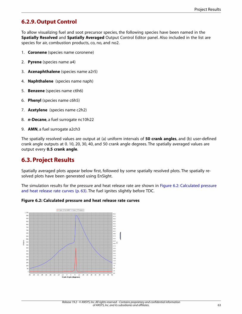
6.2.9. Output Control
To allow visualizing fuel and soot precursor species, the following species have been named in theSpatially Resolved and Spatially Averaged Output Control Editor panel. Also included in the list arespecies for air, combustion products, co, no, and no2.
1. Coronene (species name coronene)
2. Pyrene (species name a4)
3. Acenaphthalene (species name a2r5)
4. Naphthalene (species name naph)
5. Benzene (species name c6h6)
6. Phenyl (species name c6h5)
7. Acetylene (species name c2h2)
8. n-Decane, a fuel surrogate nc10h22
9. AMN, a fuel surrogate a2ch3
The spatially resolved values are output at (a) uniform intervals of 50 crank angles, and (b) user-definedcrank angle outputs at 0. 10, 20, 30, 40, and 50 crank angle degrees. The spatially averaged values areoutput every 0.5 crank angle.
6.3. Project Results
Spatially averaged plots appear below first, followed by some spatially resolved plots. The spatially re-solved plots have been generated using EnSight.
The simulation results for the pressure and heat release rate are shown in Figure 6.2: Calculated pressureand heat release rate curves (p. 63). The fuel ignites slightly before TDC.
Figure 6.2: Calculated pressure and heat release rate curves
63Release 19.2 - © ANSYS, Inc. All rights reserved. - Contains proprietary and confidential information
of ANSYS, Inc. and its subsidiaries and affiliates.
Project Results
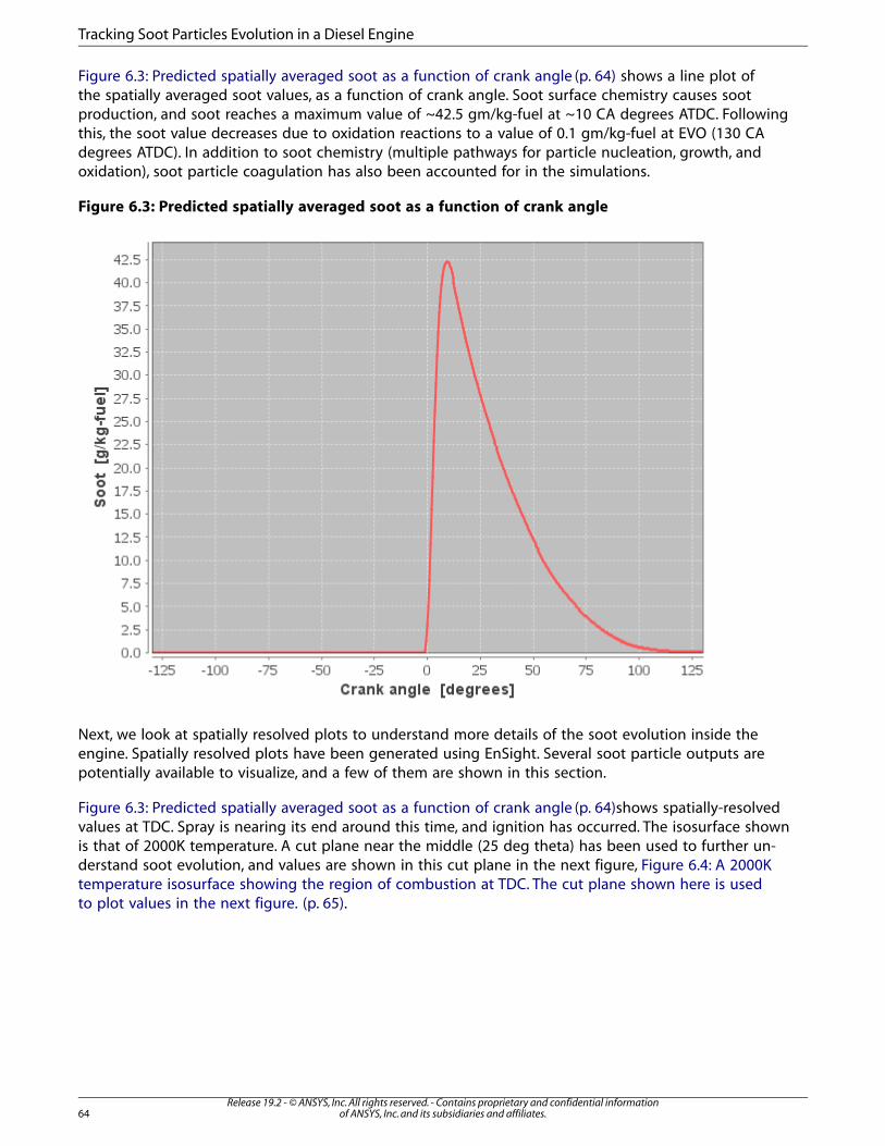
Figure 6.3: Predicted spatially averaged soot as a function of crank angle (p. 64) shows a line plot ofthe spatially averaged soot values, as a function of crank angle. Soot surface chemistry causes sootproduction, and soot reaches a maximum value of ~42.5 gm/kg-fuel at ~10 CA degrees ATDC. Followingthis, the soot value decreases due to oxidation reactions to a value of 0.1 gm/kg-fuel at EVO (130 CAdegrees ATDC). In addition to soot chemistry (multiple pathways for particle nucleation, growth, andoxidation), soot particle coagulation has also been accounted for in the simulations.
Figure 6.3: Predicted spatially averaged soot as a function of crank angle
Next, we look at spatially resolved plots to understand more details of the soot evolution inside theengine. Spatially resolved plots have been generated using EnSight. Several soot particle outputs arepotentially available to visualize, and a few of them are shown in this section.
Figure 6.3: Predicted spatially averaged soot as a function of crank angle (p. 64)shows spatially-resolvedvalues at TDC. Spray is nearing its end around this time, and ignition has occurred. The isosurface shownis that of 2000K temperature. A cut plane near the middle (25 deg theta) has been used to further un-derstand soot evolution, and values are shown in this cut plane in the next figure, Figure 6.4: A 2000Ktemperature isosurface showing the region of combustion at TDC. The cut plane shown here is usedto plot values in the next figure. (p. 65).
Release 19.2 - © ANSYS, Inc. All rights reserved. - Contains proprietary and confidential informationof ANSYS, Inc. and its subsidiaries and affiliates.64
Tracking Soot Particles Evolution in a Diesel Engine
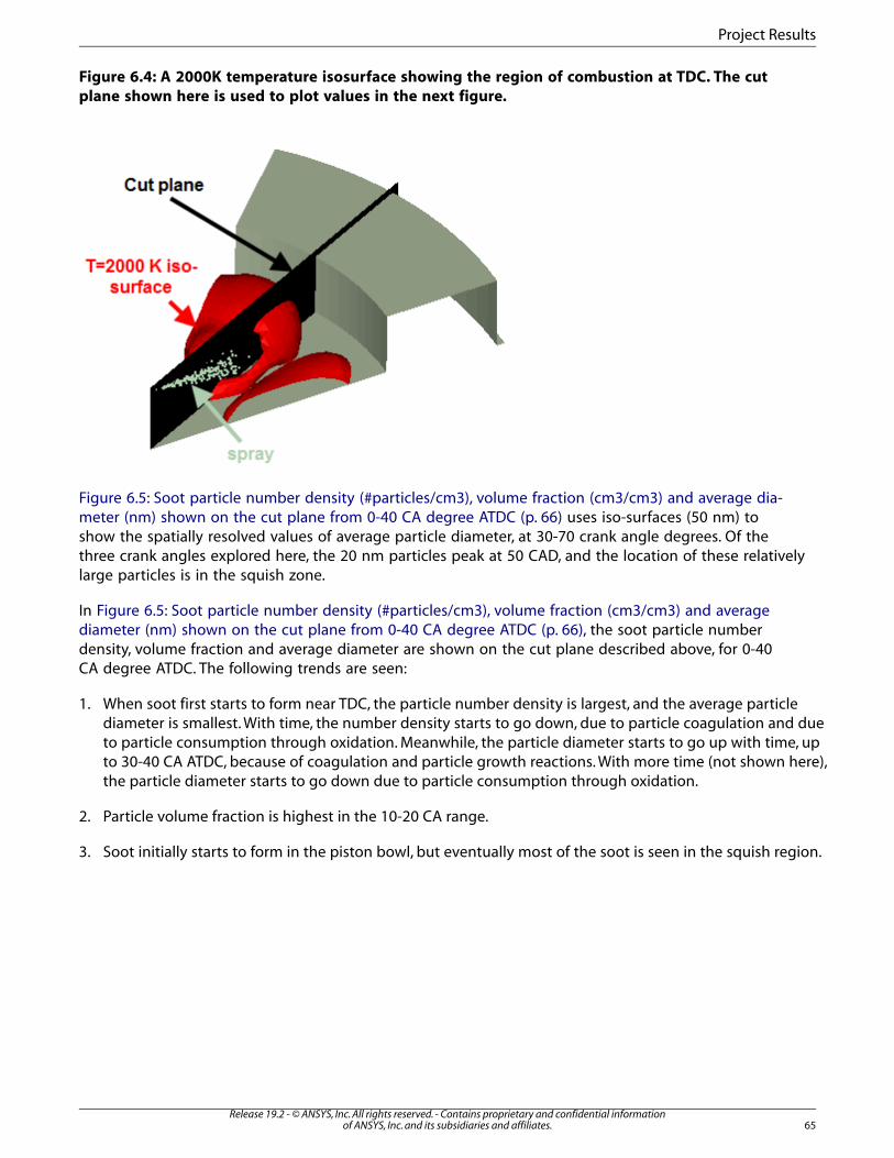
Figure 6.4: A 2000K temperature isosurface showing the region of combustion at TDC. The cutplane shown here is used to plot values in the next figure.
Figure 6.5: Soot particle number density (#particles/cm3), volume fraction (cm3/cm3) and average dia-meter (nm) shown on the cut plane from 0-40 CA degree ATDC (p. 66) uses iso-surfaces (50 nm) toshow the spatially resolved values of average particle diameter, at 30-70 crank angle degrees. Of thethree crank angles explored here, the 20 nm particles peak at 50 CAD, and the location of these relativelylarge particles is in the squish zone.
In Figure 6.5: Soot particle number density (#particles/cm3), volume fraction (cm3/cm3) and averagediameter (nm) shown on the cut plane from 0-40 CA degree ATDC (p. 66), the soot particle numberdensity, volume fraction and average diameter are shown on the cut plane described above, for 0-40CA degree ATDC. The following trends are seen:
1. When soot first starts to form near TDC, the particle number density is largest, and the average particlediameter is smallest. With time, the number density starts to go down, due to particle coagulation and dueto particle consumption through oxidation. Meanwhile, the particle diameter starts to go up with time, upto 30-40 CA ATDC, because of coagulation and particle growth reactions. With more time (not shown here),the particle diameter starts to go down due to particle consumption through oxidation.
2. Particle volume fraction is highest in the 10-20 CA range.
3. Soot initially starts to form in the piston bowl, but eventually most of the soot is seen in the squish region.
65Release 19.2 - © ANSYS, Inc. All rights reserved. - Contains proprietary and confidential information
of ANSYS, Inc. and its subsidiaries and affiliates.
Project Results

Figure 6.5: Soot particle number density (#particles/cm3), volume fraction (cm3/cm3) and averagediameter (nm) shown on the cut plane from 0-40 CA degree ATDC
Note that the particle diameter shown in Figure 6.6: Filter used in EnSight for average particle diamet-er (p. 67) is a filtered value. Even when soot volume fraction is very low (say, less than 1E-10), the averagediameter can potentially be a large value; however in this scenario, the average particle diameter doesnot have much meaning as it is essentially due to numerical noise. To filter this kind of values, the fil-tering shown in Figure 6.6: Filter used in EnSight for average particle diameter (p. 67)has been used.This filter shows only particle diameter when the local particle volume fraction is greater than 1E-10.
Release 19.2 - © ANSYS, Inc. All rights reserved. - Contains proprietary and confidential informationof ANSYS, Inc. and its subsidiaries and affiliates.66
Tracking Soot Particles Evolution in a Diesel Engine
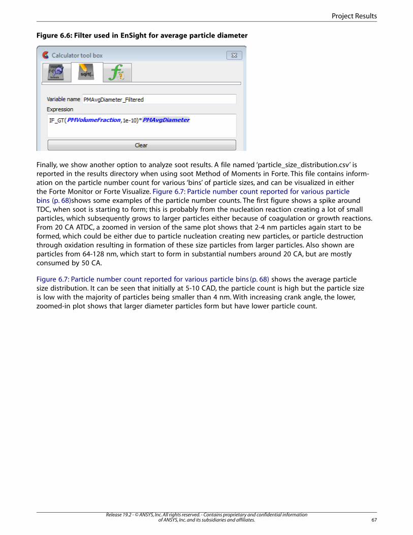
Figure 6.6: Filter used in EnSight for average particle diameter
Finally, we show another option to analyze soot results. A file named ‘particle_size_distribution.csv’ isreported in the results directory when using soot Method of Moments in Forte. This file contains inform-ation on the particle number count for various ‘bins’ of particle sizes, and can be visualized in eitherthe Forte Monitor or Forte Visualize. Figure 6.7: Particle number count reported for various particlebins (p. 68)shows some examples of the particle number counts. The first figure shows a spike aroundTDC, when soot is starting to form; this is probably from the nucleation reaction creating a lot of smallparticles, which subsequently grows to larger particles either because of coagulation or growth reactions.From 20 CA ATDC, a zoomed in version of the same plot shows that 2-4 nm particles again start to beformed, which could be either due to particle nucleation creating new particles, or particle destructionthrough oxidation resulting in formation of these size particles from larger particles. Also shown areparticles from 64-128 nm, which start to form in substantial numbers around 20 CA, but are mostlyconsumed by 50 CA.
Figure 6.7: Particle number count reported for various particle bins (p. 68) shows the average particlesize distribution. It can be seen that initially at 5-10 CAD, the particle count is high but the particle sizeis low with the majority of particles being smaller than 4 nm. With increasing crank angle, the lower,zoomed-in plot shows that larger diameter particles form but have lower particle count.
67Release 19.2 - © ANSYS, Inc. All rights reserved. - Contains proprietary and confidential information
of ANSYS, Inc. and its subsidiaries and affiliates.
Project Results
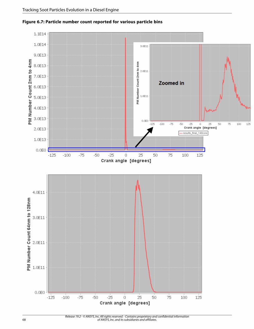
Figure 6.7: Particle number count reported for various particle bins
Release 19.2 - © ANSYS, Inc. All rights reserved. - Contains proprietary and confidential informationof ANSYS, Inc. and its subsidiaries and affiliates.68
Tracking Soot Particles Evolution in a Diesel Engine
Chapter 7: Gasoline Direct Injection Engine Simulation
This tutorial describes how to use ANSYS Forte to simulate combustion in a direct injection spark ignitioninternal combustion engine with moving valves. Engine geometry is imported and ANSYS Forte'sautomatic mesh generation is used to create the computational mesh on-the-fly during the simulation.
7.1. Data Provided
This section describes the provided files, time required, prerequisites, and a utility for comparing yourgenerated project file (.ftsim) with the one provided in the tutorial download.
7.1.1. Files Used in This Tutorial
The files for this tutorial are obtained by downloading the siengine_gdi_tutorial.zip file here.
Unzip siengine_gdi_tutorial.zip to your working folder.
• Forte_GDI_Tutorial.stl: This is the geometry file.
• exhaust_valve_lift.csv and intake_valve_lift.csv: Two files of data describing the intake and exhaust valvelifts. Profiles such as these can be imported (from .csv files) or manually entered in the Profile Editor
• spatial_output.csv: Specifies when spatially resolved data such as velocity, temperature, species concentra-tions, etc., will be output.
• Forte_GDI_Tutorial.ftsim: A project file of the completed tutorial, for verification or comparison of yourprogress in the tutorial set-up.
The tutorial sample file is provided as a download. You have the opportunity to select the location forthe file when you download and uncompress the sample files.
Note
This tutorial is based on a fully configured sample project that contains the tutorial projectsettings. The description provided here covers the key points of the project set-up but is notintended to explain every parameter setting in the project. The .ftsim file has all custom anddefault parameters already configured; the text highlights only the significant points of thetutorial.
7.1.2. Project Comparison Utility
The ANSYS Forte installation includes the cgns_util export command, which you can use to comparethe parameter settings in the project file generated at any point during your tutorial set-up against theprovided .ftsim , which has the parameter settings for the final, completed tutorial. This command isdescribed in the ANSYS Forte User Guide.
69Release 19.2 - © ANSYS, Inc. All rights reserved. - Contains proprietary and confidential information
of ANSYS, Inc. and its subsidiaries and affiliates.
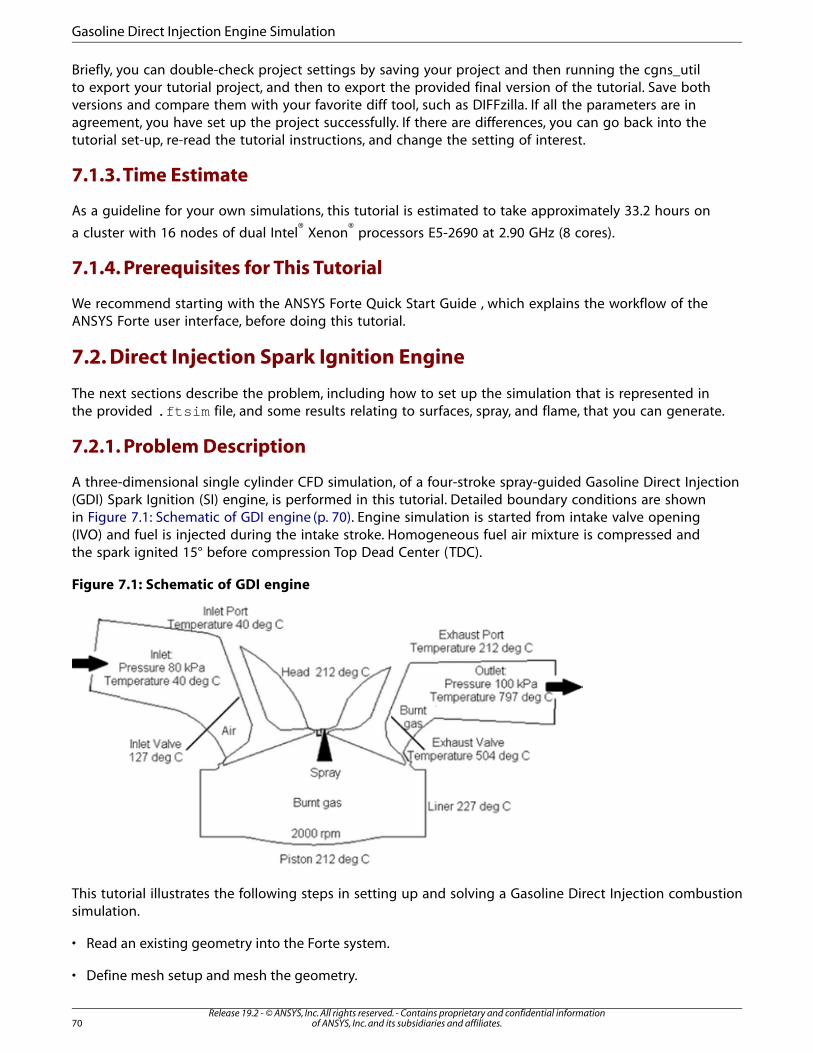
Briefly, you can double-check project settings by saving your project and then running the cgns_utilto export your tutorial project, and then to export the provided final version of the tutorial. Save bothversions and compare them with your favorite diff tool, such as DIFFzilla. If all the parameters are inagreement, you have set up the project successfully. If there are differences, you can go back into thetutorial set-up, re-read the tutorial instructions, and change the setting of interest.
7.1.3. Time Estimate
As a guideline for your own simulations, this tutorial is estimated to take approximately 33.2 hours on
a cluster with 16 nodes of dual Intel® Xenon® processors E5-2690 at 2.90 GHz (8 cores).
7.1.4. Prerequisites for This Tutorial
We recommend starting with the ANSYS Forte Quick Start Guide , which explains the workflow of theANSYS Forte user interface, before doing this tutorial.
7.2. Direct Injection Spark Ignition Engine
The next sections describe the problem, including how to set up the simulation that is represented inthe provided .ftsim file, and some results relating to surfaces, spray, and flame, that you can generate.
7.2.1. Problem Description
A three-dimensional single cylinder CFD simulation, of a four-stroke spray-guided Gasoline Direct Injection(GDI) Spark Ignition (SI) engine, is performed in this tutorial. Detailed boundary conditions are shownin Figure 7.1: Schematic of GDI engine (p. 70). Engine simulation is started from intake valve opening(IVO) and fuel is injected during the intake stroke. Homogeneous fuel air mixture is compressed andthe spark ignited 15° before compression Top Dead Center (TDC).
Figure 7.1: Schematic of GDI engine
This tutorial illustrates the following steps in setting up and solving a Gasoline Direct Injection combustionsimulation.
• Read an existing geometry into the Forte system.
• Define mesh setup and mesh the geometry.
Release 19.2 - © ANSYS, Inc. All rights reserved. - Contains proprietary and confidential informationof ANSYS, Inc. and its subsidiaries and affiliates.70
Gasoline Direct Injection Engine Simulation
• Set up the injection event.
• Set up the spark timing event.
• Set up the boundary and initial conditions.
• Specify the simulation controls.
• Specify the output variables and frequency.
• Run the simulation.
• Examine the results in the report.
7.2.1.1. Import the Geometry
Note
All Editor panel options that are not explicitly mentioned in this tutorial should be left attheir default values. Changed values on any Editor panel do not take effect until you pressthe Apply button. Always press the Apply button after modifying a value, before movingto a new panel or to the Workflow tree.
In this tutorial, we will import an existing geometry into ANSYS Forte and set up the automatic meshgeneration using a global mesh size and adapting the mesh near the valves. The geometry used willbe half symmetric. To import the geometry, go to the Workflow tree and click Geometry. This opens
the Geometry icon bar. Click the Import Geometry icon. In the resulting dialog, pull down and selectSurfaces from STL file. Browse to and select the file called Forte_GDI_Tutorial. In the dialog thatopens with STL file import options, accept the defaults for units and tolerances. Note that the geometryshould always be in centimeters units when read into ANSYS Forte. If it is not, the geometry can bescaled using the appropriate scaling factor to get it into centimeters. Note that once you have importedthe geometry, there are a number of actions that you can perform on the items in the Geometry node,such as scale, rename, transform, invert normals, or delete geometry elements.
Once the geometry is read in, you should see the following surfaces: liner, exhaust-port, inlet, outlet,intake-port, piston, head, exhaust-valve, intake-valve, intake-symmetry, cylinder-symmetry, ex-haust-symmetry, spark-plug.
The Geometry imports in an opaque mode and possibly preset zoom level. It is often helpful to Refit
the view or use the mouse wheel to re-zoom. To change opacity, right-click the Geometry nodein the right-side Visibility tree and select Medium for the Opacity level of all geometry elements, asshown in Figure 7.2: Engine geometry with valves and ports defined (p. 72).
71Release 19.2 - © ANSYS, Inc. All rights reserved. - Contains proprietary and confidential information
of ANSYS, Inc. and its subsidiaries and affiliates.
Direct Injection Spark Ignition Engine

Figure 7.2: Engine geometry with valves and ports defined
7.2.1.2. Subvolume Creation
Subvolumes are useful to refine regions of interest, such as the chamber. The subvolume can then beused in the mesh controls to control the size of the mesh in the selected subvolume. Select the followingsurfaces to define the subvolume: cylinder-symmetry, head, liner, piston, and spark_plug. You shouldsee a triangulated region as in Figure 7.3: Subvolume for the chamber (p. 72).
Figure 7.3: Subvolume for the chamber
7.2.1.3. Automatic Mesh Generation Setup
The Material Point is the point in the domain that tells ANSYS Forte where the mesh will be generatedand should be located at least one unit cell length away from any boundaries. This point must remaininside of the domain throughout the entire simulation. Typically it is located near the head so it is stillinside the domain at TDC.
• Mesh Controls ¬ Material Point: Accept the default Reference Frame using the Global Origin. Set theLocation using Cartesian Coord. System to X = 0.25, Y = 3.25, and Z = 0.25 cm. ClickApply.
• From the Workflow tree, use Mesh Controls ¬ Global Mesh Size to set the Global Mesh Size to 0.2 cm.
Note
This is the recommended mesh size; a coarser setting of 0.3 cm could be used for tutorialpurposes to produce a shorter runtime.
Release 19.2 - © ANSYS, Inc. All rights reserved. - Contains proprietary and confidential informationof ANSYS, Inc. and its subsidiaries and affiliates.72
Gasoline Direct Injection Engine Simulation
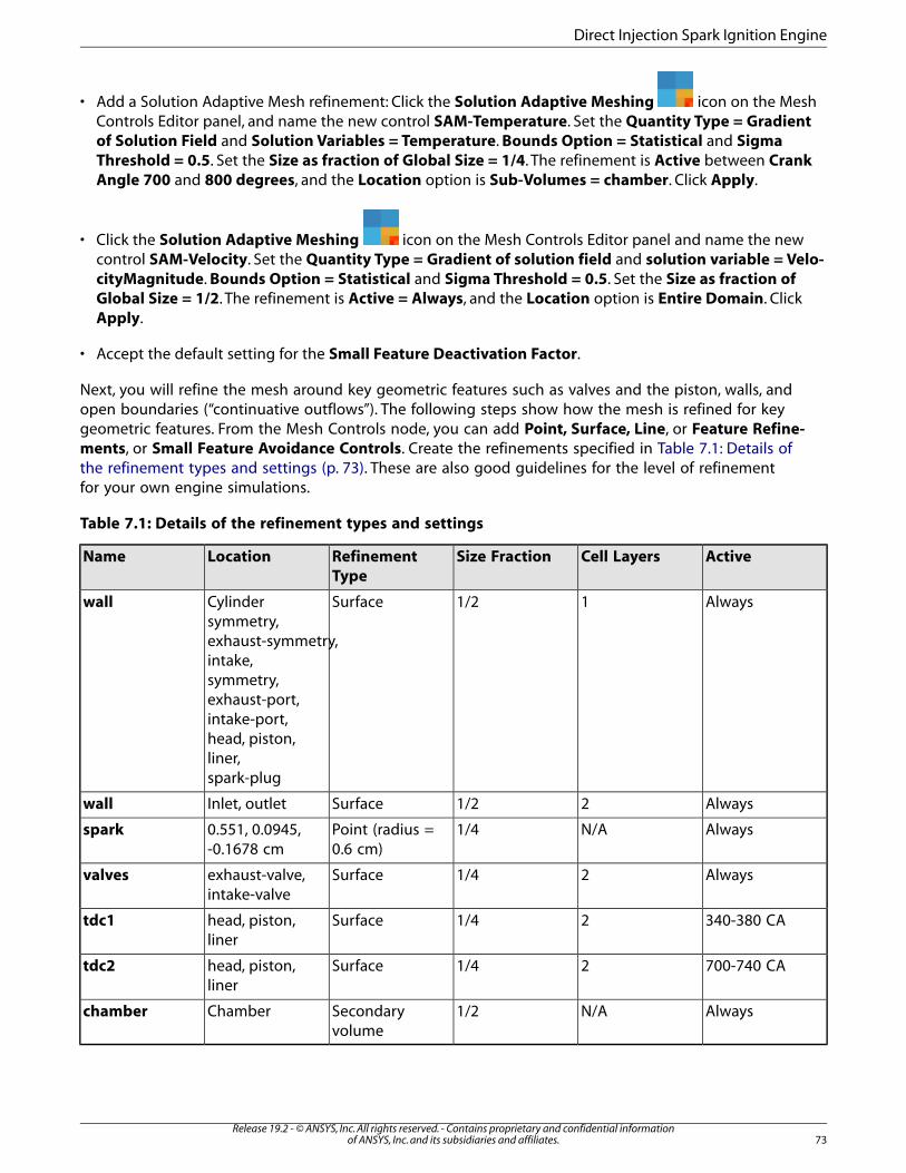
• Add a Solution Adaptive Mesh refinement: Click the Solution Adaptive Meshing icon on the MeshControls Editor panel, and name the new control SAM-Temperature. Set the Quantity Type = Gradientof Solution Field and Solution Variables = Temperature. Bounds Option = Statistical and SigmaThreshold = 0.5. Set the Size as fraction of Global Size = 1/4. The refinement is Active between CrankAngle 700 and 800 degrees, and the Location option is Sub-Volumes = chamber. Click Apply.
• Click the Solution Adaptive Meshing icon on the Mesh Controls Editor panel and name the newcontrol SAM-Velocity. Set the Quantity Type = Gradient of solution field and solution variable = Velo-cityMagnitude. Bounds Option = Statistical and Sigma Threshold = 0.5. Set the Size as fraction ofGlobal Size = 1/2. The refinement is Active = Always, and the Location option is Entire Domain. ClickApply.
• Accept the default setting for the Small Feature Deactivation Factor.
Next, you will refine the mesh around key geometric features such as valves and the piston, walls, andopen boundaries (“continuative outflows”). The following steps show how the mesh is refined for keygeometric features. From the Mesh Controls node, you can add Point, Surface, Line, or Feature Refine-ments, or Small Feature Avoidance Controls. Create the refinements specified in Table 7.1: Details ofthe refinement types and settings (p. 73). These are also good guidelines for the level of refinementfor your own engine simulations.
Table 7.1: Details of the refinement types and settings
ActiveCell LayersSize FractionRefinementType
LocationName
Always11/2SurfaceCylindersymmetry,
wall
exhaust-symmetry,intake,symmetry,exhaust-port,intake-port,head, piston,liner,spark-plug
Always21/2SurfaceInlet, outletwall
AlwaysN/A1/4Point (radius =0.6 cm)
0.551, 0.0945,-0.1678 cm
spark
Always21/4Surfaceexhaust-valve,intake-valve
valves
340-380 CA21/4Surfacehead, piston,liner
tdc1
700-740 CA21/4Surfacehead, piston,liner
tdc2
AlwaysN/A1/2Secondaryvolume
Chamberchamber
73Release 19.2 - © ANSYS, Inc. All rights reserved. - Contains proprietary and confidential information
of ANSYS, Inc. and its subsidiaries and affiliates.
Direct Injection Spark Ignition Engine

7.2.1.4. Models Setup
Chemistry: Now that the mesh has been set up, assigning models is next. Assign the chemistry with
Models ¬ Chemistry and use the Import Chemistry icon and select the file Gasol-ine_1comp_49sp.cks from the ANSYS Forte data directory. If you are curious, you can view the chemistrydetails, such as chemistry source, pre-processing log, gas phase input, gas phase output, thermodynamicinput, transport input, and transport output.
• Flame Speed Model: Use Models ¬ Chemistry ¬ Flame Speed Model and select the Table Library Option.Select Create New, then add ic8h18 as the fuel species and specify ic8h18_flame_library as the name. Forthe Turbulent Flame Speed settings, keep the defaults except for Turbulent Flame Speed Ratio (b1),which should be set to 2.0. Click Apply.
Transport: The default RNG k-epsilon model turbulence settings are used in this tutorial. Those arespecified in the Editor panel for Models ¬ Transport ¬ Turbulence. The default fluid properties are alsoused, which are at Models ¬ Transport.
Spray Model: Turn on the spray model by checking the box at Models ¬ Spray Model. For Spray mod-eling in ANSYS Forte, you will create an Injector first, then and Injection events and Nozzles to the in-jector. You can have multiple injectors in a ANSYS Forte model and they can have different fuels.
Create a new Solid Cone Injector and name it Solid Injector. Specify the following for the injector:
• For Composition, select Create New… then select ic8h18 as the fuel species and specify the mass fractionas 1.0. Specify gasoline as the name and click Save.
• Set Injection Type to Pulsed Injection and Parcel Specification to Droplet Density with a DropletNumber Density of 1.
• Set the Inflow Droplet Temperature to 400K.
• For Spray Initialization, select Constant Discharge Coefficient and Angle and specify the DischargeCoefficient as 0.7 and the Mean Cone Angle as 14.0 degrees.
• Select Rosin-Rammler Distribution for the Drop Size Distribution, use 3.5 for the Shape Parameter andspecify the Initial Sauter Mean Diameter as 120 micron.
• Specify the following for the KH and RT model constants:
– Size Constant of KH Breakup = 0.5
– Time Constant of KH Breakup = 10
– Critical Mass Fraction for New Droplet Generation = 0.03
– Activate the SMR Conservation in KH Breakup option (Note: This option is typically activated for gasolineinjections, but not for diesel injections.)
– Size Constant of RT Breakup = 0.1
– Time Constant of RT Breakup = 1.0
– RT Distance Constant = 1.9
Release 19.2 - © ANSYS, Inc. All rights reserved. - Contains proprietary and confidential informationof ANSYS, Inc. and its subsidiaries and affiliates.74
Gasoline Direct Injection Engine Simulation
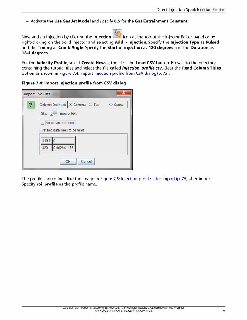
– Activate the Use Gas Jet Model and specify 0.5 for the Gas Entrainment Constant.
Now add an Injection by clicking the Injection icon at the top of the Injector Editor panel or byright-clicking on the Solid Injector and selecting Add > Injection. Specify the Injection Type as Pulsedand the Timing as Crank Angle. Specify the Start of injection as 420 degrees and the Duration as18.4 degrees.
For the Velocity Profile, select Create New…, the click the Load CSV button. Browse to the directorycontaining the tutorial files and select the file called injection_profile.csv. Clear the Read Column Titlesoption as shown in Figure 7.4: Import injection profile from CSV dialog (p. 75).
Figure 7.4: Import injection profile from CSV dialog
The profile should look like the image in Figure 7.5: Injection profile after import (p. 76) after import.Specify roi_profile as the profile name.
75Release 19.2 - © ANSYS, Inc. All rights reserved. - Contains proprietary and confidential information
of ANSYS, Inc. and its subsidiaries and affiliates.
Direct Injection Spark Ignition Engine

Figure 7.5: Injection profile after import
Now that the injection event has been added, we need to specify the nozzles. The nozzles require inputfor the location, direction, and nozzle hole diameter (or area). Since this is a half-symmetry model, threenozzles will be specified.
On the Solid Injector panel, click the New Nozzle icon or right-click Solid Injection and click Add> Nozzle. Name the new nozzle nozzle1.
For the Location, specify X = -5.296mm, Y = 0.634mm, and Z = 6.468mm and for Spray Directionspecify X = 3.0415mm, Y = 2.73735mm, and Z = -9.12449mm. For the Nozzle Size, select the Diameteroption and specify a nozzle diameter of 300 micron.
Now that the first nozzle has been created, copy and paste nozzle1 and name it nozzle2 using the
Copy and Paste icons. For the Location, specify X = -5.65mm, Y = 1.1885mm, and Z =6.5991mm and for Spray Direction specify X = 1.49781mm, Y = 5.08692mm, and Z = -8.4782mm.
Repeat the copy and paste process by copying nozzle2 and naming it nozzle3 to create the last nozzle.For the Location, specify X = -6.7647mm, Y = 0.72441mm, and Z = 6.1653mm and for Spray Directionspecify X = -2.90254mm, Y = 2.74977mm, and Z = -9.16592mm.
Now that all the nozzles have been created, they should appear similar to the model in Figure 7.6: Nozzlesafter specifying location and orientation (p. 77).
Release 19.2 - © ANSYS, Inc. All rights reserved. - Contains proprietary and confidential informationof ANSYS, Inc. and its subsidiaries and affiliates.76
Gasoline Direct Injection Engine Simulation
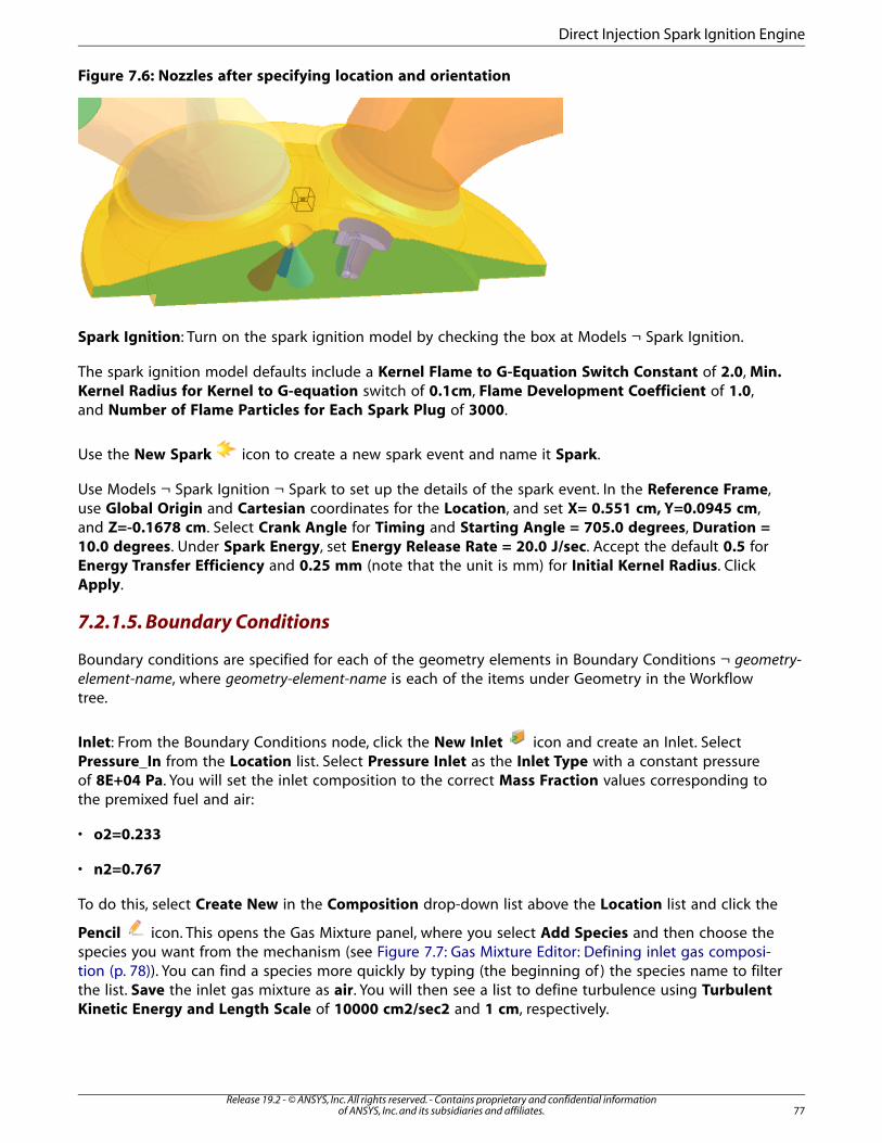
Figure 7.6: Nozzles after specifying location and orientation
Spark Ignition: Turn on the spark ignition model by checking the box at Models ¬ Spark Ignition.
The spark ignition model defaults include a Kernel Flame to G-Equation Switch Constant of 2.0, Min.Kernel Radius for Kernel to G-equation switch of 0.1cm, Flame Development Coefficient of 1.0,and Number of Flame Particles for Each Spark Plug of 3000.
Use the New Spark icon to create a new spark event and name it Spark.
Use Models ¬ Spark Ignition ¬ Spark to set up the details of the spark event. In the Reference Frame,use Global Origin and Cartesian coordinates for the Location, and set X= 0.551 cm, Y=0.0945 cm,and Z=-0.1678 cm. Select Crank Angle for Timing and Starting Angle = 705.0 degrees, Duration =10.0 degrees. Under Spark Energy, set Energy Release Rate = 20.0 J/sec. Accept the default 0.5 forEnergy Transfer Efficiency and 0.25 mm (note that the unit is mm) for Initial Kernel Radius. ClickApply.
7.2.1.5. Boundary Conditions
Boundary conditions are specified for each of the geometry elements in Boundary Conditions ¬ geometry-element-name, where geometry-element-name is each of the items under Geometry in the Workflowtree.
Inlet: From the Boundary Conditions node, click the New Inlet icon and create an Inlet. SelectPressure_In from the Location list. Select Pressure Inlet as the Inlet Type with a constant pressureof 8E+04 Pa. You will set the inlet composition to the correct Mass Fraction values corresponding tothe premixed fuel and air:
• o2=0.233
• n2=0.767
To do this, select Create New in the Composition drop-down list above the Location list and click the
Pencil icon. This opens the Gas Mixture panel, where you select Add Species and then choose thespecies you want from the mechanism (see Figure 7.7: Gas Mixture Editor: Defining inlet gas composi-tion (p. 78)). You can find a species more quickly by typing (the beginning of ) the species name to filterthe list. Save the inlet gas mixture as air. You will then see a list to define turbulence using TurbulentKinetic Energy and Length Scale of 10000 cm2/sec2 and 1 cm, respectively.
77Release 19.2 - © ANSYS, Inc. All rights reserved. - Contains proprietary and confidential information
of ANSYS, Inc. and its subsidiaries and affiliates.
Direct Injection Spark Ignition Engine

Figure 7.7: Gas Mixture Editor: Defining inlet gas composition
Outlet: From the Boundary Conditions node, click the New Outlet icon and create Outlet. Selectthe Pressure_Out geometry item and select the Pressure Outlet as the Outlet Type. Give the outleta Pressure of 1E+05 Pa, which arises from the back-pressure of the exhaust system with an OffsetDistance to Apply Pressure of 0.0 cm. Set the Turbulence Boundary Conditions to Turbulent KineticEnergy and Length Scale of 10000 cm2/sec2 and 1 cm, respectively.
Piston: From the Boundary Conditions node, click the New Wall icon and name it Piston. Selectthe Piston item in the Location list. Set the Temperature Option to Constant and 485 K. Turn ONthe Wall Motion option and set the piston Motion Type to use a Slider-Crank Model with a Strokeof 9.0 cm and a Connecting Rod Length of 14.43 cm with 0.0 Piston Offset. Change the MovementType to Moving Surface and accept the default Global Origin Reference Frame. For Direction, thepiston will move along the Z-direction, specify 1.0 for Z.
Intake: Click the New Wall icon and name it intake-port. Select the intake-port item in the Locationlist and set the Temperature to 313 K.
Exhaust: Click the New Wall icon and name it exhaust-port. Select the exhaust-port item in theLocation list and set the Temperature to 485 K.
Liner: Click the New Wall icon and name it liner. Select the liner item in the Location list and setthe Temperature to 500 K.
Release 19.2 - © ANSYS, Inc. All rights reserved. - Contains proprietary and confidential informationof ANSYS, Inc. and its subsidiaries and affiliates.78
Gasoline Direct Injection Engine Simulation
Head: Click the New Wall icon and name it head. Select the head item in the Location list and setthe Temperature to 485 K.
Intake Valves: Click the New Wall icon and name it intake-valve. The valve specification is a littlemore complicated than the stationary walls, such that several steps are required within the wall panel.These steps specify the wall motion and the way we want the mesh to adapt to the gap opening nearthe valve seat when the valve opens or closes.
• Select the intake-valve in the Location list.
• Check the Heat Transfer option and set the Temperature to the constant value of 400 K.
• Turn ON (check) the Wall Motion and set the Motion Type to Offset Table.
• Accept the default Global Origin for the Reference Frame. Select Cartesian for the Coord. System underDirection for the valve motion and set X = 0.241922 cm, Y = 0.0 cm, Z = −0.970296 cm.
• To import the lift profile (named intake_valve_lift.csv in the same location as the .stl file you started this
tutorial with), select Create New from the Lift Profile drop-down list and click the Pencil icon. In theProfile Editor, click the Load SV button and navigate to the intake_valve_lift.csv file. Clear the Read ColumnTitles option and press OK. At the bottom of the Profile Editor window, name this intake_valve_lift. Ensurethat the units in the first column are set to Angle and the second column for Distance is set to m. Save theProfile.
• For Movement Type, change the pull-down menu to Valve. Then select just the surface boundary portionof the valve that comes into contact with the valve seat on the head, as well as the surface boundary thatcontains the seat region. In this case, select both the head and the intake-valve.
• Finally, set the Valve Motion Activation Threshold to 0.02 cm. This indicates that the valve will not openuntil the lift value specified in the valve-lift profile exceeds this threshold. A smaller value will cause thevalves to open sooner, but the mesh refinement required to resolve the gap will be higher. This is a trade-off that will need to be determined based on the goals and outcomes desired from the simulation. In additionto the activation threshold, you may also change the minimum number of cells desired at the smallest gapopening. In this case, specify the Approx. Cells in Gap at Min. Lift as 1.5.
Exhaust Valves: Click the New Wall icon and name it exhaust-valve. New Wall icon and nameit exhaust-valve. Follow a similar procedure as for the Intake Valves. This time, select the exhaust-valveitem in the Location list and set the Temperature to 777 K Turn ON the Wall Motion and set theMotion Type to Offset Table and the Vertices to Transform to Interior. Select Global Origin for theReference Frame. Select Cartesian for the Coord. System under Direction and set X = -0.327218 cm,Y = 0.0 cm, and Z = -0.944949 cm. Similarly to the intake valves, first import the .csv (named ex-haust_valve_lift.csv) file, clear the Read Column Titles option, and name it exhaust_lift_profile. Thenfollow the same procedures for specifying the Movement Type to Valve, selecting the Valve Seat andSurface it Contacts (exhaust-valve and head), and setting the Valve Motion Activation Thresholdto 0.02 cm. Specify the Approx. Cells in Gap at Min. Lift as 1.5.
Symmetry: Click the New Symmetry icon and name it symmetry. Select the cylinder-symmetry,exhaust-symmetry, and intake-symmetry item in the Location list.
Spark Plug: Click the New Wall icon and name it exhaust-valve. New Wall icon and name itspark-plug. Select the head item in the Location list and set the Temperature to 485 K.
79Release 19.2 - © ANSYS, Inc. All rights reserved. - Contains proprietary and confidential information
of ANSYS, Inc. and its subsidiaries and affiliates.
Direct Injection Spark Ignition Engine

7.2.1.6. Initialization
The domain is initialized with the operating conditions, species concentrations and temperatures. TheDefault Initialization species composition is at the expected exhaust composition, assuming completecombustion. The intake and exhaust must also be initialized to the boundary condition values. Set thefollowing initialization parameters:
Default Initialization:
• Select Default Initialization in the Workflow tree. Set the Initialization Order to 2. Since flow goes generallyfrom the intake to the cylinder and then to the exhaust, this indicates that this default (cylinder) region willbe the second in the initialization order precedence list.
• We will use the ANSYS Forte Composition Calculator to compute the exhaust gas composition. Click theComposition Calculation button
in the Toolbar or go to Utility > Composition Calculation. In the Composition calculation, specify the FuelMass (27 mg), select the fuel mixture in the Liquid input, for Air Flow specify Phi and set Phi = 1.0, EGRFraction = 0.0, and for Internal EGR select the Estimate from CR and specify a CR of 10. Next, set theCalculate option to Exhaust and click Create Mixture. Specify a name of exhaust_gas. In the Initial Condi-tions, select exhaust_gas for the Composition.
• Set a Temperature of 1,070 K and the Pressure to 1.05359E+05 Pa.
• The Turbulence initialization uses the Turbulent Kinetic Energy and Length Scale option with values10,000 cm2/sec2 and 1.0 cm, respectively.
• The Velocity is initialized using Velocity Components and all the values are set to zero.
• Click Apply.
Intake Initialization: The intake manifold Initial Condition is set to match the Boundary Condition atthe Inlet. Since this is a separate port that can be closed off from the main cylinder region, we alsoneed to set the equivalent of a material point to identify the region, as well as an initialization orderthat helps determine what region takes precedence in initializing new cells that appear when gaps areopened.
• From the Initial Conditions Workflow tree item, select the New Port Initialization icon and name it intake.
• To identify the region, select a point for the Location under the Reference Frame selection, which is a pointthat will always be within the Intake port. Set the coordinates for this case to X=-5.6838, Y=1.4295,Z=4.2858 cm, which is a point just inside the inlet.
• Set the Initialization Order to 1. Flow is expected to go from the intake to the main region; for this reason,we give it the first order in initialization precedence.
• Set the Composition by selecting in the previously saved profile, air. Set the Temperature to 313 K andPressure to 8.0E+04 Pa. The Turbulence initialization uses Turbulent Kinetic Energy and Length Scaleoption set to 10,000 cm2/sec2 and 1.0 cm, respectively. Click Apply.
Exhaust Initialization: The Initial Condition of the Exhaust is set to match the Boundary Condition ofthe Outlet.
• From the Initial Conditions Workflow tree item, select the New Port Initialization icon and name it exhaust.
Release 19.2 - © ANSYS, Inc. All rights reserved. - Contains proprietary and confidential informationof ANSYS, Inc. and its subsidiaries and affiliates.80
Gasoline Direct Injection Engine Simulation

• To identify the region, select a point for the Location under the Reference Frame selection, which is a pointthat will always be within the ExhaustPort region. Set the coordinates for this case to X=4.7892, Y=1.5061,Z=3.1552 cm, which is a point just inside the outlet.
• Set the Initialization Order to 3. Flow is expected to go from the cylinder to the exhaust port; for thisreason, we give it the last order in initialization precedence for the 3 regions defined.
• Set the Composition to the existing profile, exhaust_gas. Set the Temperature to 1070K and Pressureto 1.0E+05 Pa.
• The Turbulence initialization uses the Turbulent Kinetic Energy and Length Scale option; these are setto 10,000 cm2/sec2 and 1.0 cm, respectively. Click Apply.
7.2.1.7. Simulation Controls
Simulation controls allow you to define the simulation limits, RPM, time step, chemistry solver, andtransport terms.
Simulation Limits: Use the Simulation Controls panel to select a Crank Angle- based simulation froma CA of 328 to 880.2 degrees. Set RPM = 2,000 rpm. The engine Cycle Type is 4-Stroke.
Time Step: Use Simulation Controls ¬ Time Step and set the following parameters:
• Initial Simulation Time Step to 5.0E-7 seconds
• Max. Crank Angle Delta Per Time Step of 1.1 degrees
• Set the Max. Time Step Option to Constant and set the value of Max. Simulation Time Step to 1.E-5 sec.The time step will be adaptively determined throughout the simulation, based on local solution gradients,so this just sets the maximum value allowed. You may also consider reducing the time-step using the TimeVarying option. This can be helpful for injection and spark events.
The Advanced Time Step Control Options settings are kept at the defaults:
• Time Step Growth Factor = 1.3
• Fluid Acceleration Factor = 0.5
• Rate of Strain Factor = 0.6
• Convection factor = 0.2
• Internal Energy Factor = 1.0
• Max. Convection Subcycles = 8
Chemistry Solver: Simulation Controls ¬ Chemistry Solver is also kept at the defaults, with the followingparameters:
• Absolute Tolerance = 1.0E-12
• Relative Tolerance = 1.0E-5
• Use Dynamic Cell Clustering to take advantage of groups of cells with similar conditions. Select 2 featuresto introduce Dynamic Cell Clustering: 1) Max. Temperature Dispersion of 10 K and 2) a Max. EquilibriumRatio Dispersion of 0.05.
81Release 19.2 - © ANSYS, Inc. All rights reserved. - Contains proprietary and confidential information
of ANSYS, Inc. and its subsidiaries and affiliates.
Direct Injection Spark Ignition Engine

• To increase the time-to-solution speed, you have the ability to choose when chemistry is activated. In thistutorial, select Activate Chemistry Conditionally, turn on (check) After First Spark Event, and select WhenTemperature is Reached with Threshold Temperature 600 K and also select During Crank Angle Intervalbetween 670 and 850 Crank Angle. This ensures that chemistry is active during the time that combustionis expected even if temperature does not rise above 600 K. Click Apply.
Transport Terms: Use the default transport tolerances and maximum number of iterations.
7.2.1.8. Output Controls
Output controls determine what data are stored for viewing during the simulation and for creatingplots, graphs, and animations in ANSYS Forte Visualize, CFD-Post, EnSight, or FieldView.
Spatially Resolved: Allows you to control when spatially resolved data such as velocity, temperature,species concentrations, etc., will be output. In the Spatially Resolved panel, set the Crank Angle OutputControl to report every 10 degrees (to manage the size of the output file). You can optionally increasethe frequency of output during the cycle by selecting User Defined Output Control and importingthe spatial_output.csv file, which has a list of specific crank angles where spatially resolved output willoccur. Alternatively, you could select User Defined Output Control, and use the Profile Editor to createsome other file specifying an output crank-angle profile (the provided profile is illustrated in Figure 7.8: Pro-file of spatially resolved output control data (p. 82)). Keep the default species and solution variablesselected for output. Reducing the variables selected will help reduce file sizes.
Figure 7.8: Profile of spatially resolved output control data
Spatially Averaged: Allows you to control the output of values that are averaged across the domain.On the Spatially Averaged panel, set the Crank Angle Output Control to reporting every 1 degree.Keep the default species and solution variables selected for output.
Restart Data: If you anticipate that the case will be stopped and you want the ability to restart it fromthe last time step solved, select Output Controls ¬ Restart Data. You can specify certain Restart Pointsusing a separate file. Turn on (check) User Defined Restart Points and use the Profile Editor to createa Restart profile. You can view, edit, or import new Restart Points in this 1-D Profile Editor. Sometimesit is helpful in spark ignition cases to save a restart file after IVC but before the spark occurs (CA=687in this case) so you can use the compression portion of the cycle as a start point in additional runs.
Release 19.2 - © ANSYS, Inc. All rights reserved. - Contains proprietary and confidential informationof ANSYS, Inc. and its subsidiaries and affiliates.82
Gasoline Direct Injection Engine Simulation
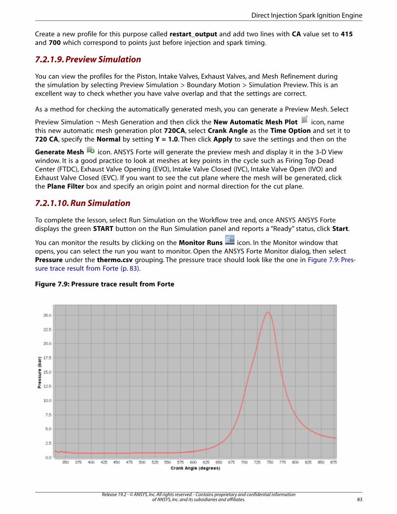
Create a new profile for this purpose called restart_output and add two lines with CA value set to 415and 700 which correspond to points just before injection and spark timing.
7.2.1.9. Preview Simulation
You can view the profiles for the Piston, Intake Valves, Exhaust Valves, and Mesh Refinement duringthe simulation by selecting Preview Simulation > Boundary Motion > Simulation Preview. This is anexcellent way to check whether you have valve overlap and that the settings are correct.
As a method for checking the automatically generated mesh, you can generate a Preview Mesh. Select
Preview Simulation ¬ Mesh Generation and then click the New Automatic Mesh Plot icon, namethis new automatic mesh generation plot 720CA, select Crank Angle as the Time Option and set it to720 CA, specify the Normal by setting Y = 1.0. Then click Apply to save the settings and then on the
Generate Mesh icon. ANSYS Forte will generate the preview mesh and display it in the 3-D Viewwindow. It is a good practice to look at meshes at key points in the cycle such as Firing Top DeadCenter (FTDC), Exhaust Valve Opening (EVO), Intake Valve Closed (IVC), Intake Valve Open (IVO) andExhaust Valve Closed (EVC). If you want to see the cut plane where the mesh will be generated, clickthe Plane Filter box and specify an origin point and normal direction for the cut plane.
7.2.1.10. Run Simulation
To complete the lesson, select Run Simulation on the Workflow tree and, once ANSYS ANSYS Fortedisplays the green START button on the Run Simulation panel and reports a “Ready” status, click Start.
You can monitor the results by clicking on the Monitor Runs icon. In the Monitor window thatopens, you can select the run you want to monitor. Open the ANSYS Forte Monitor dialog, then selectPressure under the thermo.csv grouping. The pressure trace should look like the one in Figure 7.9: Pres-sure trace result from Forte (p. 83).
Figure 7.9: Pressure trace result from Forte
83Release 19.2 - © ANSYS, Inc. All rights reserved. - Contains proprietary and confidential information
of ANSYS, Inc. and its subsidiaries and affiliates.
Direct Injection Spark Ignition Engine
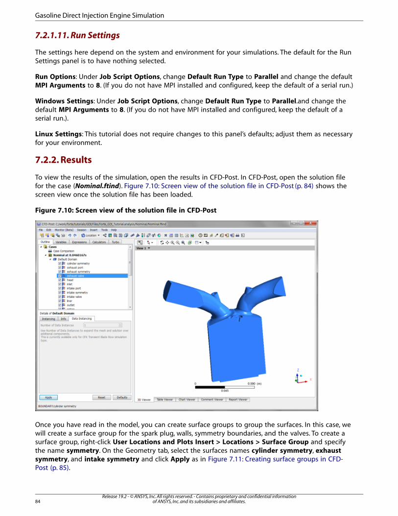
7.2.1.11. Run Settings
The settings here depend on the system and environment for your simulations. The default for the RunSettings panel is to have nothing selected.
Run Options: Under Job Script Options, change Default Run Type to Parallel and change the defaultMPI Arguments to 8. (If you do not have MPI installed and configured, keep the default of a serial run.)
Windows Settings: Under Job Script Options, change Default Run Type to Parallel.and change thedefault MPI Arguments to 8. (If you do not have MPI installed and configured, keep the default of aserial run.).
Linux Settings: This tutorial does not require changes to this panel’s defaults; adjust them as necessaryfor your environment.
7.2.2. Results
To view the results of the simulation, open the results in CFD-Post. In CFD-Post, open the solution filefor the case (Nominal.ftind). Figure 7.10: Screen view of the solution file in CFD-Post (p. 84) shows thescreen view once the solution file has been loaded.
Figure 7.10: Screen view of the solution file in CFD-Post
Once you have read in the model, you can create surface groups to group the surfaces. In this case, wewill create a surface group for the spark plug, walls, symmetry boundaries, and the valves. To create asurface group, right-click User Locations and Plots Insert > Locations > Surface Group and specifythe name symmetry. On the Geometry tab, select the surfaces names cylinder symmetry, exhaustsymmetry, and intake symmetry and click Apply as in Figure 7.11: Creating surface groups in CFD-Post (p. 85).
Release 19.2 - © ANSYS, Inc. All rights reserved. - Contains proprietary and confidential informationof ANSYS, Inc. and its subsidiaries and affiliates.84
Gasoline Direct Injection Engine Simulation
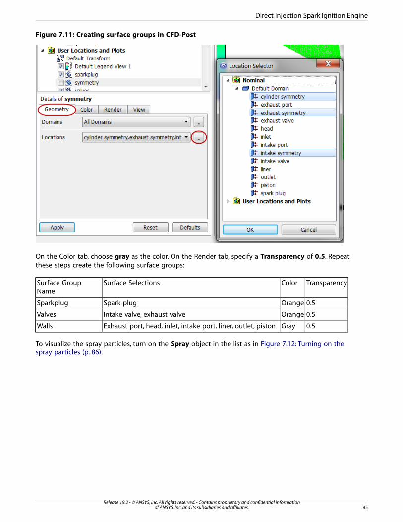
Figure 7.11: Creating surface groups in CFD-Post
On the Color tab, choose gray as the color. On the Render tab, specify a Transparency of 0.5. Repeatthese steps create the following surface groups:
TransparencyColorSurface SelectionsSurface GroupName
0.5OrangeSpark plugSparkplug
0.5OrangeIntake valve, exhaust valveValves
0.5GrayExhaust port, head, inlet, intake port, liner, outlet, pistonWalls
To visualize the spray particles, turn on the Spray object in the list as in Figure 7.12: Turning on thespray particles (p. 86).
85Release 19.2 - © ANSYS, Inc. All rights reserved. - Contains proprietary and confidential information
of ANSYS, Inc. and its subsidiaries and affiliates.
Direct Injection Spark Ignition Engine

Figure 7.12: Turning on the spray particles
When the spray is activated, all the particles will be a single color. You can use a variable to changethe color by going to the Color tab. Set the Mode to Variable and select Spray Particle Radius. Youcan also adjust the droplet size rendering on the Symbol tab; a value of 0.3 works well for this case.Go to Tools > Timestep Selector and select crank angle 436CA. With these changes, the spray shouldresemble Figure 7.13: Spray particles in the combustion chamber (p. 87).
Release 19.2 - © ANSYS, Inc. All rights reserved. - Contains proprietary and confidential informationof ANSYS, Inc. and its subsidiaries and affiliates.86
Gasoline Direct Injection Engine Simulation
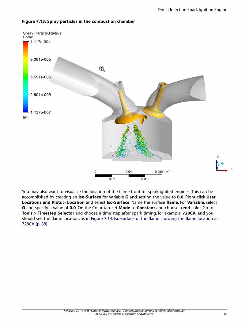
Figure 7.13: Spray particles in the combustion chamber
You may also want to visualize the location of the flame front for spark ignited engines. This can beaccomplished by creating an Iso-Surface for variable G and setting the value to 0.0. Right-click UserLocations and Plots > Location and select Iso-Surface. Name the surface flame. For Variable, selectG and specify a value of 0.0. On the Color tab, set Mode to Constant and choose a red color. Go toTools > Timestep Selector and choose a time step after spark timing, for example, 728CA, and youshould see the flame location, as in Figure 7.14: Iso-surface of the flame showing the flame location at728CA (p. 88).
87Release 19.2 - © ANSYS, Inc. All rights reserved. - Contains proprietary and confidential information
of ANSYS, Inc. and its subsidiaries and affiliates.
Direct Injection Spark Ignition Engine
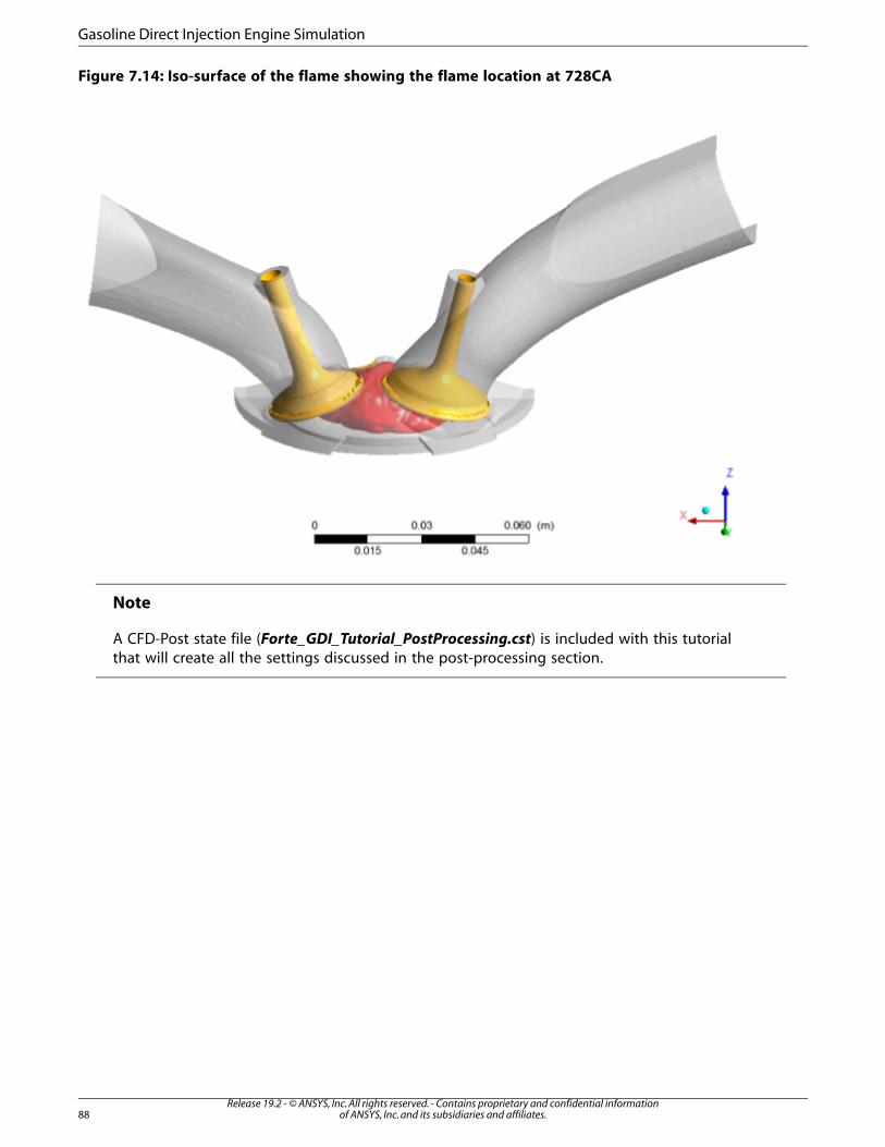
Figure 7.14: Iso-surface of the flame showing the flame location at 728CA
Note
A CFD-Post state file (Forte_GDI_Tutorial_PostProcessing.cst) is included with this tutorialthat will create all the settings discussed in the post-processing section.
Release 19.2 - © ANSYS, Inc. All rights reserved. - Contains proprietary and confidential informationof ANSYS, Inc. and its subsidiaries and affiliates.88
Gasoline Direct Injection Engine Simulation
Chapter 8: Two-Stroke Engine Simulation
This tutorial describes how to use ANSYS Forte CFD to simulate combustion for a two-stroke marineengine with intake and exhaust ports. Details on how to use ANSYS Forte's automatic mesh generationwith sliding interfaces, a requirement for 2-stroke engines, is discussed. The tutorial also demonstratesprofile creation and the import and loading of an .stl file to start the simulation from the geometry.
8.1. Data Provided
The following sections describe the provided files, time required, prerequisites, and a utility for comparingyour generated project file (.ftsim) with the one provided in the tutorial download.
8.1.1. Files Used in This Tutorial
The files for this tutorial are obtained by downloading the two_stroke.zip file here.
Unzip two_stroke.zip to your working folder.
• FORTE-2stroke .ftsim:A project file of the completed tutorial, for verification or comparison of your progressin the tutorial set-up. The project file includes all the relevant geometry, chemistry set, and spray profiledetails.
• intake_pressure_profile.csv and exhaust_pressure_profile.csv: Two files of data describing the profile ofthe time-varying pressure for the intake and exhaust.
• time_step_size.csv: Adaptive time-step profile.
• output_crank_angles.csv: Profile of crank-angle points for spatially resolved output.
• FORTE_2stoke.stl: Geometry file for the 2-stroke engine in this project without the chemistry set, sprayprofile, and other project details. (Optional)
• restart_crank_angles.csv: Profile defining restart points. (Optional)
• Nom-VelMag_Vector-Centerline.avi: An animation showing the velocity magnitude and piston motion ofthe meshed system. (Optional)
The tutorial sample file is provided as a download. You have the opportunity to select the location forthe file when you download and uncompress the sample files.
Note
This tutorial is based on a fully configured sample project that contains the tutorial projectsettings. The description provided here covers the key points of the project set-up but is notintended to explain every parameter setting in the project. The .ftsim file has all custom anddefault parameters already configured; the text highlights only the significant points of thetutorial.
89Release 19.2 - © ANSYS, Inc. All rights reserved. - Contains proprietary and confidential information
of ANSYS, Inc. and its subsidiaries and affiliates.
8.1.2. Project Comparison Utility
The ANSYS Forte installation includes the cgns_util export command, which you can use to comparethe parameter settings in the project file generated at any point during your tutorial set-up against theprovided .ftsim , which has the parameter settings for the final, completed tutorial. This command isdescribed in the ANSYS Forte User Guide.
Briefly, you can double-check project settings by saving your project and then running the cgns_utilto export your tutorial project, and then to export the provided final version of the tutorial. Save bothversions and compare them with your favorite diff tool, such as DIFFzilla. If all the parameters are inagreement, you have set up the project successfully. If there are differences, you can go back into thetutorial set-up, re-read the tutorial instructions, and change the setting of interest.
8.1.3. Time Estimate
As a guideline for your own simulations, this tutorial is estimated to take approximately 9.5 hours on
an Intel® Xenon® processor E5-2690 at 3.00 GHz (20 total cores).
8.1.4. Prerequisites for This Tutorial
We recommend starting with the ANSYS Forte Quick Start Guide , which explains the workflow of theANSYS Forte user interface, before doing this tutorial.
8.2. Two-Stroke Marine Engine Project Setup
The next sections describe the problem, including how to set up the simulation that is represented inthe provided .ftsim file, and some results relating to surfaces, spray, and flame, that you can generate.
8.2.1. Problem Description
In this case, a full 3-D geometry is used to simulate a 2-stroke marine engine, including combustion.The fuel in this engine is gasoline and is direct-injected into the combustion chamber.
Figure 8.1: Components of direct-injection two-stroke engine simulation project
Release 19.2 - © ANSYS, Inc. All rights reserved. - Contains proprietary and confidential informationof ANSYS, Inc. and its subsidiaries and affiliates.90
Two-Stroke Engine Simulation
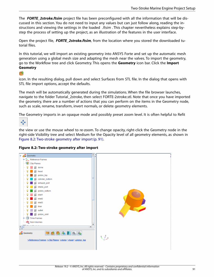
The FORTE_2stroke.ftsim project file has been preconfigured with all the information that will be dis-cussed in this section. You do not need to input any values but can just follow along, reading the in-structions and viewing the settings in the loaded .ftsim . This chapter nevertheless explains step-by-step the process of setting up the project, as an illustration of the features in the user interface.
Open the project file, FORTE_2stroke.ftsim, from the location where you stored the downloaded tu-torial files.
In this tutorial, we will import an existing geometry into ANSYS Forte and set up the automatic meshgeneration using a global mesh size and adapting the mesh near the valves. To import the geometry,go to the Workflow tree and click Geometry. This opens the Geometry icon bar. Click the ImportGeometry
icon. In the resulting dialog, pull down and select Surfaces from STL file. In the dialog that opens withSTL file import options, accept the defaults.
The mesh will be automatically generated during the simulations. When the file browser launches,navigate to the folder Tutorial_2stroke, then select FORTE-2stroke.stl. Note that once you have importedthe geometry, there are a number of actions that you can perform on the items in the Geometry node,such as scale, rename, transform, invert normals, or delete geometry elements.
The Geometry imports in an opaque mode and possibly preset zoom level. It is often helpful to Refit
the view or use the mouse wheel to re-zoom. To change opacity, right-click the Geometry node in theright-side Visibility tree and select Medium for the Opacity level of all geometry elements, as shown inFigure 8.2: Two-stroke geometry after import (p. 91).
Figure 8.2: Two-stroke geometry after import
91Release 19.2 - © ANSYS, Inc. All rights reserved. - Contains proprietary and confidential information
of ANSYS, Inc. and its subsidiaries and affiliates.
Two-Stroke Marine Engine Project Setup

8.2.1.1. Two-Stroke Engine Details
A simple engine configuration is used in this tutorial for demonstration purposes. The details of theconfiguration and simulation settings are presented here.
Table 8.1: Details of the diesel engine geometry used in this tutorial
UnitsValueItem
2-stokeCycle type
Direct injection, hollow coreFuel injection system
12.65Compression ratio
cm8.58Bore
cm6.73Stroke
cm13.97Squish
GasolineFuel
The mesh is created using the Automated Mesh Generator in ANSYS Forte. The values described inTable 8.1: Details of the diesel engine geometry used in this tutorial (p. 92) can be accessed from theFORTE_2stroke.ftsim project file. If you did not already have a pre-configured geometry, you could importa Fluent Mesh file, STL, KIVA-3V, or CGNS geometry file. Fluent Mesh files are the preferred format forimporting geometry because they are guaranteed to be water-tight. The Fluent Mesh file can be createdas a surface mesh for the geometry in ANSYS Meshing.
8.2.1.2. Automatic Mesh Generation Setup
Material Point: On this panel, we must set the point that defines where ANSYS Forte will mesh. Thispoint, the Material Point, must always lie inside the geometry during the entire cycle and should belocated at least one unit cell length away from any boundaries. On the Material Point Editor panel,define the point’s location as X = 0.0, Y = 0.0, Z = 6.9 cm.
Global Mesh Size: Set the Global Mesh Size to 2.0 mm. Other Mesh Controls should be set to thesevalues:
Table 8.2: Settings for Mesh Control refinements
Crank angleactive range
Refinementlayers
Refinementlevel
Refinementlocation
Refinementtype
Item
1/2All walls exceptinlets andoutlet
SurfaceRefinement
AllSurfaces
2 layers1/2Inlets andOutlet
SurfaceRefinement
OpenBoundar-ies
350° - 370°2 layers1/4Head andPiston Top
SurfaceRefinement
TDC
21/2Intake andExhaust Port
SurfaceRefinement
PortWalls2
274° - 400°1/2(0.0, 0.0,6.0) cm
PointCombustion
Release 19.2 - © ANSYS, Inc. All rights reserved. - Contains proprietary and confidential informationof ANSYS, Inc. and its subsidiaries and affiliates.92
Two-Stroke Engine Simulation
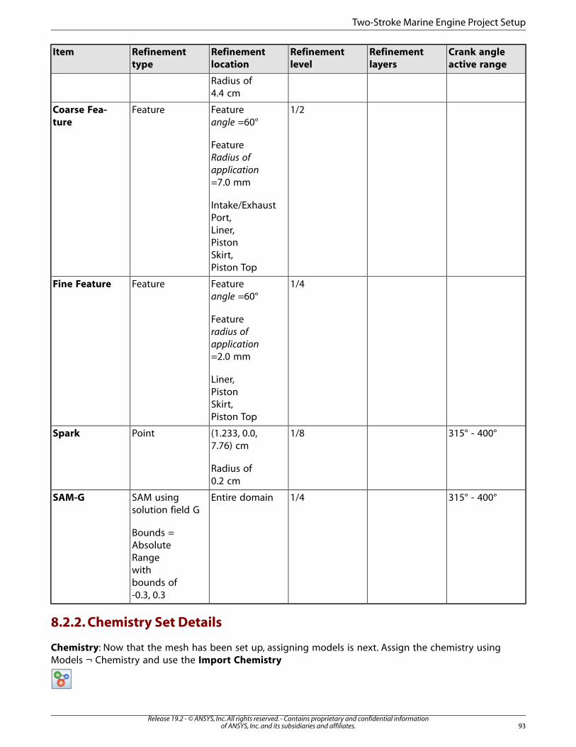
Crank angleactive range
Refinementlayers
Refinementlevel
Refinementlocation
Refinementtype
Item
Radius of4.4 cm
1/2Featureangle =60°
FeatureCoarse Fea-ture
FeatureRadius ofapplication=7.0 mm
Intake/ExhaustPort,Liner,PistonSkirt,Piston Top
1/4Featureangle =60°
FeatureFine Feature
Featureradius ofapplication=2.0 mm
Liner,PistonSkirt,Piston Top
315° - 400°1/8(1.233, 0.0,7.76) cm
PointSpark
Radius of0.2 cm
315° - 400°1/4Entire domainSAM usingsolution field G
Bounds =Absolute
SAM-G
Rangewithbounds of-0.3, 0.3
8.2.2. Chemistry Set Details
Chemistry: Now that the mesh has been set up, assigning models is next. Assign the chemistry usingModels ¬ Chemistry and use the Import Chemistry
93Release 19.2 - © ANSYS, Inc. All rights reserved. - Contains proprietary and confidential information
of ANSYS, Inc. and its subsidiaries and affiliates.
Two-Stroke Marine Engine Project Setup

icon and select the file Gasoline_1comp_49sp.cks from the ANSYS Forte data directory. If you arecurious, you can view the chemistry details, such as chemistry source, pre-processing log, gas phaseinput, gas phase output, thermodynamic input, transport input, and transport output.
Flame Speed Model: On the Workflow tree, use Models ¬ Chemistry ¬ Flame Speed Model and selectthe Table Library Option. Select Create New, then add ic8h18 as the fuel species and specify iso_octaneas the name. Click Save. Close the Library Editor panel. For the Turbulent Flame Speed settings, keepthe defaults. Click Apply.
8.2.3. Transport Property Settings
The default values are used in the Transport property panel. In the Transport ¬ Turbulence panel, theRNG k-epsilon model is used, with default values.
8.2.4. Spray Model Settings
Models ¬ Spray Model: Since this is a direct-injection case, turn ON (check) Spray Model in the Workflowtree to display its icon bar (action bar) in the Editor panel. In the panel, keep the defaults. Leave theUse Vaporization Model (default) check ON.
Add an Injector: The icon bar provides two spray-injector options: Hollow Cone or Solid Cone. For this
injector, click the Hollow Cone icon. In the dialog that opens, name the new hollow-cone injectoras Hollow Cone Injector. This opens another icon bar and Editor panel for the new hollow-cone injector.In the Workflow tree under the Hollow Cone Injector node, add a Nozzle and an Injection. You caneither right-click the Hollow Cone Injector node and select Add or select that Workflow tree item oruse the icons in the panel’s action bar.
On the Hollow Cone Injector panel, create a new Composition, select ic8h18 (iso-octane) in the Specieslist, specify the physical properties as iso-octane, and specify the Mass Fraction as 1.0. Use iso-octanefor the Vaporization properties and name the Composition gasoline. Click Save.
For the injection, specify the following parameters:
Table 8.3: Injection settings used in this tutorial
UnitsValueInput
-3000Injected Parcel Count
K363Inflow Droplet Temperature
bar51.7Injection Pressure
-Checked (ON)Inwardly Opening Nozzle
degrees54.0Mean Cone Angle
degrees15.0Liquid Jet Thickness
-Rosin-Rammler DistributionDroplet Size Distribution
-3.5Shape Parameter
-12.0Breakup Length Model Constant
With the Hollow Cone Injector selected, add a Nozzle to the injector by clicking the New Nozzle
Release 19.2 - © ANSYS, Inc. All rights reserved. - Contains proprietary and confidential informationof ANSYS, Inc. and its subsidiaries and affiliates.94
Two-Stroke Engine Simulation
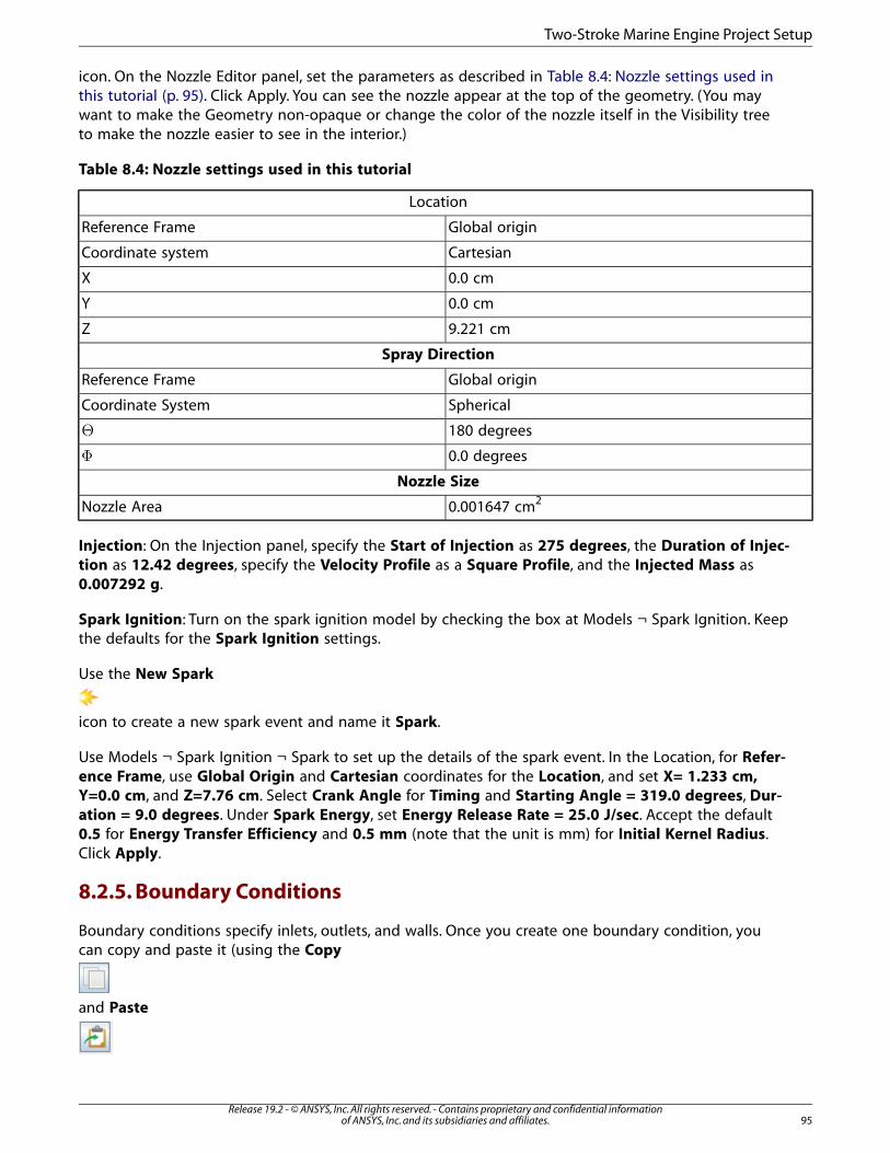
icon. On the Nozzle Editor panel, set the parameters as described in Table 8.4: Nozzle settings used inthis tutorial (p. 95). Click Apply. You can see the nozzle appear at the top of the geometry. (You maywant to make the Geometry non-opaque or change the color of the nozzle itself in the Visibility treeto make the nozzle easier to see in the interior.)
Table 8.4: Nozzle settings used in this tutorial
Location
Global originReference Frame
CartesianCoordinate system
0.0 cmX
0.0 cmY
9.221 cmZ
Spray Direction
Global originReference Frame
SphericalCoordinate System
180 degreesΘ
0.0 degreesΦ
Nozzle Size
0.001647 cm2Nozzle Area
Injection: On the Injection panel, specify the Start of Injection as 275 degrees, the Duration of Injec-tion as 12.42 degrees, specify the Velocity Profile as a Square Profile, and the Injected Mass as0.007292 g.
Spark Ignition: Turn on the spark ignition model by checking the box at Models ¬ Spark Ignition. Keepthe defaults for the Spark Ignition settings.
Use the New Spark
icon to create a new spark event and name it Spark.
Use Models ¬ Spark Ignition ¬ Spark to set up the details of the spark event. In the Location, for Refer-ence Frame, use Global Origin and Cartesian coordinates for the Location, and set X= 1.233 cm,Y=0.0 cm, and Z=7.76 cm. Select Crank Angle for Timing and Starting Angle = 319.0 degrees, Dur-ation = 9.0 degrees. Under Spark Energy, set Energy Release Rate = 25.0 J/sec. Accept the default0.5 for Energy Transfer Efficiency and 0.5 mm (note that the unit is mm) for Initial Kernel Radius.Click Apply.
8.2.5. Boundary Conditions
Boundary conditions specify inlets, outlets, and walls. Once you create one boundary condition, youcan copy and paste it (using the Copy
and Paste
95Release 19.2 - © ANSYS, Inc. All rights reserved. - Contains proprietary and confidential information
of ANSYS, Inc. and its subsidiaries and affiliates.
Two-Stroke Marine Engine Project Setup
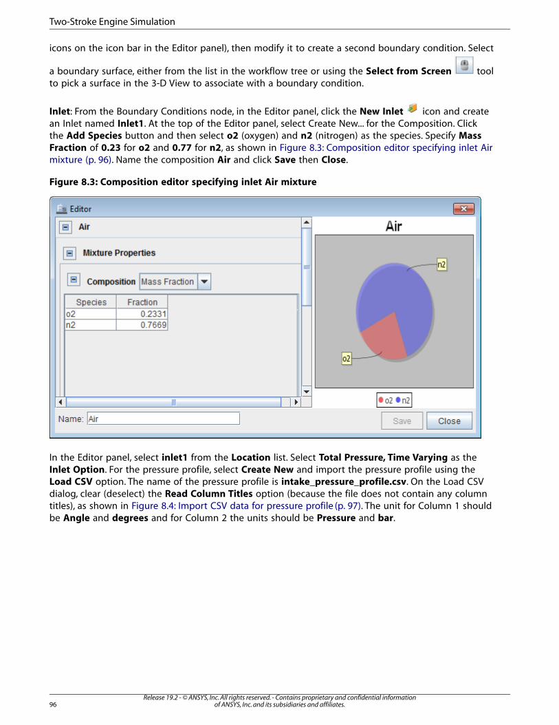
icons on the icon bar in the Editor panel), then modify it to create a second boundary condition. Select
a boundary surface, either from the list in the workflow tree or using the Select from Screen toolto pick a surface in the 3-D View to associate with a boundary condition.
Inlet: From the Boundary Conditions node, in the Editor panel, click the New Inlet icon and createan Inlet named Inlet1. At the top of the Editor panel, select Create New... for the Composition. Clickthe Add Species button and then select o2 (oxygen) and n2 (nitrogen) as the species. Specify MassFraction of 0.23 for o2 and 0.77 for n2, as shown in Figure 8.3: Composition editor specifying inlet Airmixture (p. 96). Name the composition Air and click Save then Close.
Figure 8.3: Composition editor specifying inlet Air mixture
In the Editor panel, select inlet1 from the Location list. Select Total Pressure, Time Varying as theInlet Option. For the pressure profile, select Create New and import the pressure profile using theLoad CSV option. The name of the pressure profile is intake_pressure_profile.csv. On the Load CSVdialog, clear (deselect) the Read Column Titles option (because the file does not contain any columntitles), as shown in Figure 8.4: Import CSV data for pressure profile (p. 97). The unit for Column 1 shouldbe Angle and degrees and for Column 2 the units should be Pressure and bar.
Release 19.2 - © ANSYS, Inc. All rights reserved. - Contains proprietary and confidential informationof ANSYS, Inc. and its subsidiaries and affiliates.96
Two-Stroke Engine Simulation

Figure 8.4: Import CSV data for pressure profile
The pressure profile should look like the profile shown in Figure 8.5: Importing the intake pressureprofile (p. 97).
Figure 8.5: Importing the intake pressure profile
Define Turbulence using values for Turbulent Kinetic Energy and Length Scale of 3,600 cm2/sec2and 1.0 cm, respectively. On the Editor panel, accept Assume Isentropic for the Temperature ValueType. Click Apply.
97Release 19.2 - © ANSYS, Inc. All rights reserved. - Contains proprietary and confidential information
of ANSYS, Inc. and its subsidiaries and affiliates.
Two-Stroke Marine Engine Project Setup

Now that the first inlet has been created, copy and paste inlet1 and name it inlet2 using the Copy
and Paste.
icons. Repeat this step to create inlet3. Update the Location to inlet2 and inlet3, respectively, for eachnew boundary condition, inlet2 and inlet3.
Outlet: From the Boundary Conditions node, go to the Editor panel and click the New Outlet iconand create Outlet. Select Total Pressure, Time Varying as the Outlet Option. For the pressure profile,select Create New and import the pressure profile using the Load CSV option. The name of the pressureprofile is exhaust_pressure_profile.csv. On the Load CSV dialog, deselect the Read Column Titlesoption, because the file does not contain any column titles. The unit for Column 1 should be Angleand degrees, and for Column 2 the units should be Pressure and bar. Set the Turbulence BoundaryConditions to Turbulent Kinetic Energy and Length Scale of 3600 cm2/sec2 and 1 cm, respectively.
Piston: From the Boundary Conditions node, go to the Editor panel and click the New Wall iconand name it Piston_Moving. Select the piston_top item in the Location list. Set the TemperatureOption to Constant and 450 K. Turn ON the Wall Motion option and set the piston Motion Type touse a Slider-Crank with a Stroke of 6.73 cm and a Connecting Rod Length of 13.97 cm with 0.0Piston Offset. To set the axis for translation, under Direction, the Reference Frame is Global Originand the Coordinate System is Cartesian. Set X=0.0 cm, Y=0.0 cm, Z=1.0 cm. Change the MovementType to Sliding Interface and select the liner and piston_skirt from the list of surfaces. For this setting,the moving piston should be selected along with the surface it is sliding/moving past.
Note
The RPM is specified on the Simulation Controls Editor panel.
Intake: Click the New Wall icon and name it IntakePort. Select the intake_port item in the Locationlist and turn ON the Heat Transfer option and set the Temperature to 300 K.
Now reproduce the Intake Port with Copy
and Paste
four times to create four new boundaries as detailed in the following table.
Table 8.5: Details of boundaries created from Copy and Paste operations
Boundary ConditionLocationBoundary NameItem
Wall Model=Law ofthe Wall
exhaust_portExhaustPort1
Twall=490 K
Heat Transfer=ON
Release 19.2 - © ANSYS, Inc. All rights reserved. - Contains proprietary and confidential informationof ANSYS, Inc. and its subsidiaries and affiliates.98
Two-Stroke Engine Simulation
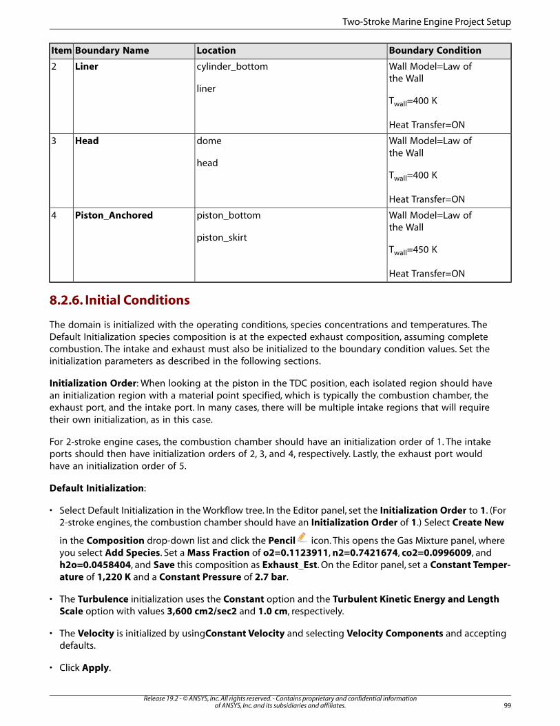
Boundary ConditionLocationBoundary NameItem
Wall Model=Law ofthe Wall
cylinder_bottom
liner
Liner2
Twall=400 K
Heat Transfer=ON
Wall Model=Law ofthe Wall
dome
head
Head3
Twall=400 K
Heat Transfer=ON
Wall Model=Law ofthe Wall
piston_bottom
piston_skirt
Piston_Anchored4
Twall=450 K
Heat Transfer=ON
8.2.6. Initial Conditions
The domain is initialized with the operating conditions, species concentrations and temperatures. TheDefault Initialization species composition is at the expected exhaust composition, assuming completecombustion. The intake and exhaust must also be initialized to the boundary condition values. Set theinitialization parameters as described in the following sections.
Initialization Order: When looking at the piston in the TDC position, each isolated region should havean initialization region with a material point specified, which is typically the combustion chamber, theexhaust port, and the intake port. In many cases, there will be multiple intake regions that will requiretheir own initialization, as in this case.
For 2-stroke engine cases, the combustion chamber should have an initialization order of 1. The intakeports should then have initialization orders of 2, 3, and 4, respectively. Lastly, the exhaust port wouldhave an initialization order of 5.
Default Initialization:
• Select Default Initialization in the Workflow tree. In the Editor panel, set the Initialization Order to 1. (For2-stroke engines, the combustion chamber should have an Initialization Order of 1.) Select Create New
in the Composition drop-down list and click the Pencil icon. This opens the Gas Mixture panel, whereyou select Add Species. Set a Mass Fraction of o2=0.1123911, n2=0.7421674, co2=0.0996009, andh2o=0.0458404, and Save this composition as Exhaust_Est. On the Editor panel, set a Constant Temper-ature of 1,220 K and a Constant Pressure of 2.7 bar.
• The Turbulence initialization uses the Constant option and the Turbulent Kinetic Energy and LengthScale option with values 3,600 cm2/sec2 and 1.0 cm, respectively.
• The Velocity is initialized by usingConstant Velocity and selecting Velocity Components and acceptingdefaults.
• Click Apply.
99Release 19.2 - © ANSYS, Inc. All rights reserved. - Contains proprietary and confidential information
of ANSYS, Inc. and its subsidiaries and affiliates.
Two-Stroke Marine Engine Project Setup
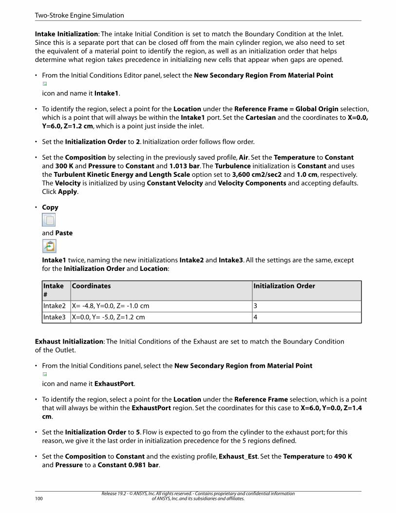
Intake Initialization: The intake Initial Condition is set to match the Boundary Condition at the Inlet.Since this is a separate port that can be closed off from the main cylinder region, we also need to setthe equivalent of a material point to identify the region, as well as an initialization order that helpsdetermine what region takes precedence in initializing new cells that appear when gaps are opened.
• From the Initial Conditions Editor panel, select the New Secondary Region From Material Point
icon and name it Intake1.
• To identify the region, select a point for the Location under the Reference Frame = Global Origin selection,which is a point that will always be within the Intake1 port. Set the Cartesian and the coordinates to X=0.0,Y=6.0, Z=1.2 cm, which is a point just inside the inlet.
• Set the Initialization Order to 2. Initialization order follows flow order.
• Set the Composition by selecting in the previously saved profile, Air. Set the Temperature to Constantand 300 K and Pressure to Constant and 1.013 bar. The Turbulence initialization is Constant and usesthe Turbulent Kinetic Energy and Length Scale option set to 3,600 cm2/sec2 and 1.0 cm, respectively.The Velocity is initialized by using Constant Velocity and Velocity Components and accepting defaults.Click Apply.
• Copy
and Paste
Intake1 twice, naming the new initializations Intake2 and Intake3. All the settings are the same, exceptfor the Initialization Order and Location:
Initialization OrderCoordinatesIntake#
3X= -4.8, Y=0.0, Z= -1.0 cmIntake2
4X=0.0, Y= -5.0, Z=1.2 cmIntake3
Exhaust Initialization: The Initial Conditions of the Exhaust are set to match the Boundary Conditionof the Outlet.
• From the Initial Conditions panel, select the New Secondary Region from Material Point
icon and name it ExhaustPort.
• To identify the region, select a point for the Location under the Reference Frame selection, which is a pointthat will always be within the ExhaustPort region. Set the coordinates for this case to X=6.0, Y=0.0, Z=1.4cm.
• Set the Initialization Order to 5. Flow is expected to go from the cylinder to the exhaust port; for thisreason, we give it the last order in initialization precedence for the 5 regions defined.
• Set the Composition to Constant and the existing profile, Exhaust_Est. Set the Temperature to 490 Kand Pressure to a Constant 0.981 bar.
Release 19.2 - © ANSYS, Inc. All rights reserved. - Contains proprietary and confidential informationof ANSYS, Inc. and its subsidiaries and affiliates.100
Two-Stroke Engine Simulation
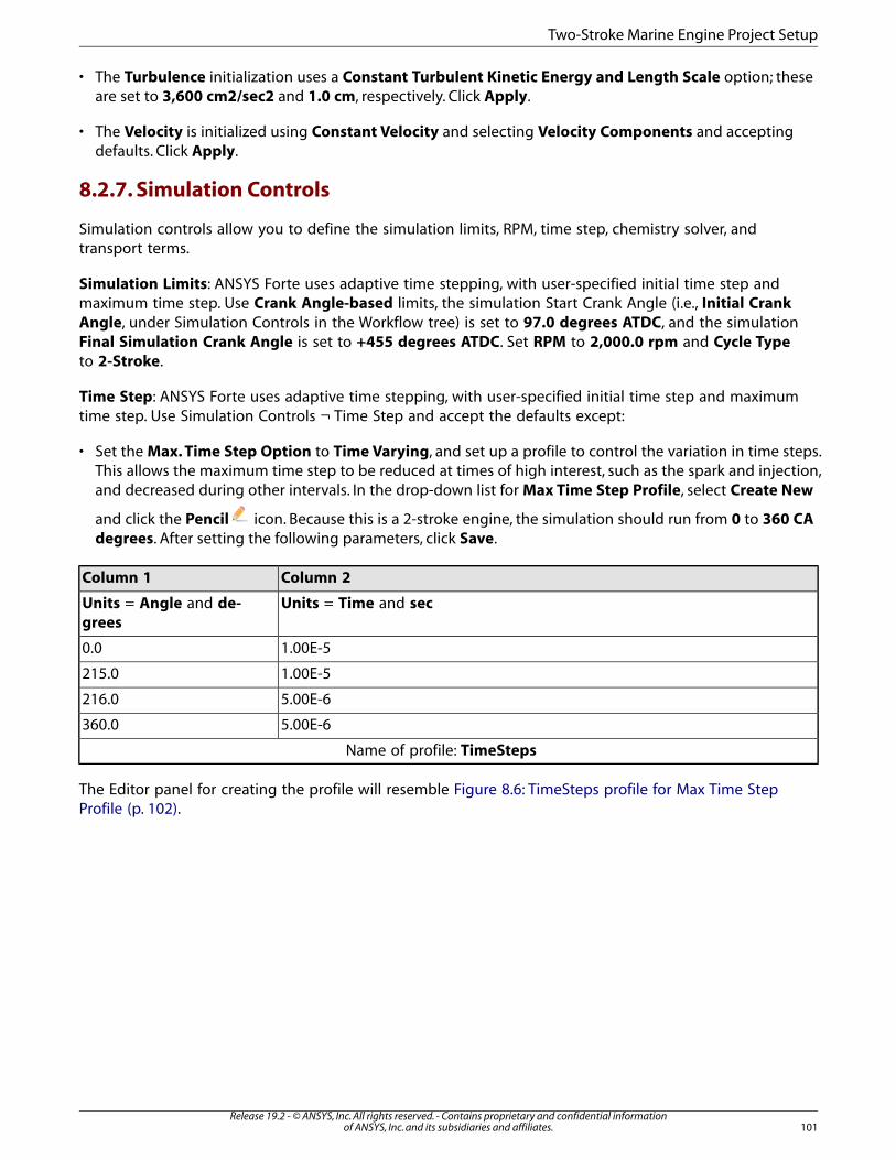
• The Turbulence initialization uses a Constant Turbulent Kinetic Energy and Length Scale option; theseare set to 3,600 cm2/sec2 and 1.0 cm, respectively. Click Apply.
• The Velocity is initialized using Constant Velocity and selecting Velocity Components and acceptingdefaults. Click Apply.
8.2.7. Simulation Controls
Simulation controls allow you to define the simulation limits, RPM, time step, chemistry solver, andtransport terms.
Simulation Limits: ANSYS Forte uses adaptive time stepping, with user-specified initial time step andmaximum time step. Use Crank Angle-based limits, the simulation Start Crank Angle (i.e., Initial CrankAngle, under Simulation Controls in the Workflow tree) is set to 97.0 degrees ATDC, and the simulationFinal Simulation Crank Angle is set to +455 degrees ATDC. Set RPM to 2,000.0 rpm and Cycle Typeto 2-Stroke.
Time Step: ANSYS Forte uses adaptive time stepping, with user-specified initial time step and maximumtime step. Use Simulation Controls ¬ Time Step and accept the defaults except:
• Set the Max. Time Step Option to Time Varying, and set up a profile to control the variation in time steps.This allows the maximum time step to be reduced at times of high interest, such as the spark and injection,and decreased during other intervals. In the drop-down list for Max Time Step Profile, select Create New
and click the Pencil icon. Because this is a 2-stroke engine, the simulation should run from 0 to 360 CAdegrees. After setting the following parameters, click Save.
Column 2Column 1
Units = Time and secUnits = Angle and de-grees
1.00E-50.0
1.00E-5215.0
5.00E-6216.0
5.00E-6360.0
Name of profile: TimeSteps
The Editor panel for creating the profile will resemble Figure 8.6: TimeSteps profile for Max Time StepProfile (p. 102).
101Release 19.2 - © ANSYS, Inc. All rights reserved. - Contains proprietary and confidential information
of ANSYS, Inc. and its subsidiaries and affiliates.
Two-Stroke Marine Engine Project Setup

Figure 8.6: TimeSteps profile for Max Time Step Profile
Chemistry Solver: Simulation Controls ¬ Chemistry Solver is also kept at the defaults for the followingsolver tolerances:
Do not activateDynamic Adaptive Chemistry. DAC should not be used for this case since there arefewer than 500 species. For cases with 500+ species, DAC may provide additional speedup in the simu-lation.
• Use Dynamic Cell Clustering to take advantage of groups of cells with similar conditions. Select 2 featuresto introduce Dynamic Cell Clustering: 1) Max. Temperature Dispersion of 10 K and 2) a Max. EquilibriumRatio Dispersion of 0.05.
• To increase the time-to-solution speed, you have the ability to choose when chemistry is activated. In thistutorial, select Activate Chemistry Conditionally, turn ON (check) After Fuel Injection Starts, and selectWhen Temperature is Reached with Threshold Temperature = 600 K. This ensures that chemistry is activeduring the time that combustion is expected. Click Apply.
8.2.8. Output Controls
Output controls determine what data are stored for viewing during the simulation and for creatingplots, graphs, and animations in ANSYS Forte Visualize, CFD-Post, EnSight, or FieldView.
The following species are named in both the Spatially Resolved and Spatially Averaged and SprayOutput Control Editor panels, to be written to the results file. Fuel, oxidizer, and common emissionsspecies are automatically added. Move these species into the Selection list.
• n2
• o2
• co2
• h2o
Release 19.2 - © ANSYS, Inc. All rights reserved. - Contains proprietary and confidential informationof ANSYS, Inc. and its subsidiaries and affiliates.102
Two-Stroke Engine Simulation
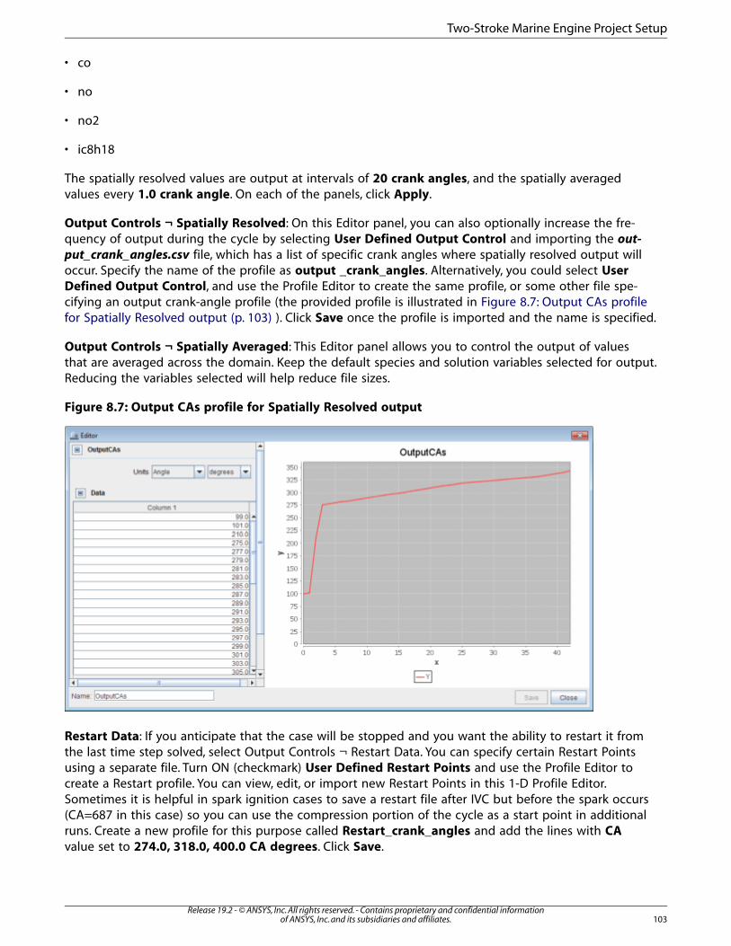
• co
• no
• no2
• ic8h18
The spatially resolved values are output at intervals of 20 crank angles, and the spatially averagedvalues every 1.0 crank angle. On each of the panels, click Apply.
Output Controls ¬ Spatially Resolved: On this Editor panel, you can also optionally increase the fre-quency of output during the cycle by selecting User Defined Output Control and importing the out-put_crank_angles.csv file, which has a list of specific crank angles where spatially resolved output willoccur. Specify the name of the profile as output _crank_angles. Alternatively, you could select UserDefined Output Control, and use the Profile Editor to create the same profile, or some other file spe-cifying an output crank-angle profile (the provided profile is illustrated in Figure 8.7: Output CAs profilefor Spatially Resolved output (p. 103) ). Click Save once the profile is imported and the name is specified.
Output Controls ¬ Spatially Averaged: This Editor panel allows you to control the output of valuesthat are averaged across the domain. Keep the default species and solution variables selected for output.Reducing the variables selected will help reduce file sizes.
Figure 8.7: Output CAs profile for Spatially Resolved output
Restart Data: If you anticipate that the case will be stopped and you want the ability to restart it fromthe last time step solved, select Output Controls ¬ Restart Data. You can specify certain Restart Pointsusing a separate file. Turn ON (checkmark) User Defined Restart Points and use the Profile Editor tocreate a Restart profile. You can view, edit, or import new Restart Points in this 1-D Profile Editor.Sometimes it is helpful in spark ignition cases to save a restart file after IVC but before the spark occurs(CA=687 in this case) so you can use the compression portion of the cycle as a start point in additionalruns. Create a new profile for this purpose called Restart_crank_angles and add the lines with CAvalue set to 274.0, 318.0, 400.0 CA degrees. Click Save.
103Release 19.2 - © ANSYS, Inc. All rights reserved. - Contains proprietary and confidential information
of ANSYS, Inc. and its subsidiaries and affiliates.
Two-Stroke Marine Engine Project Setup
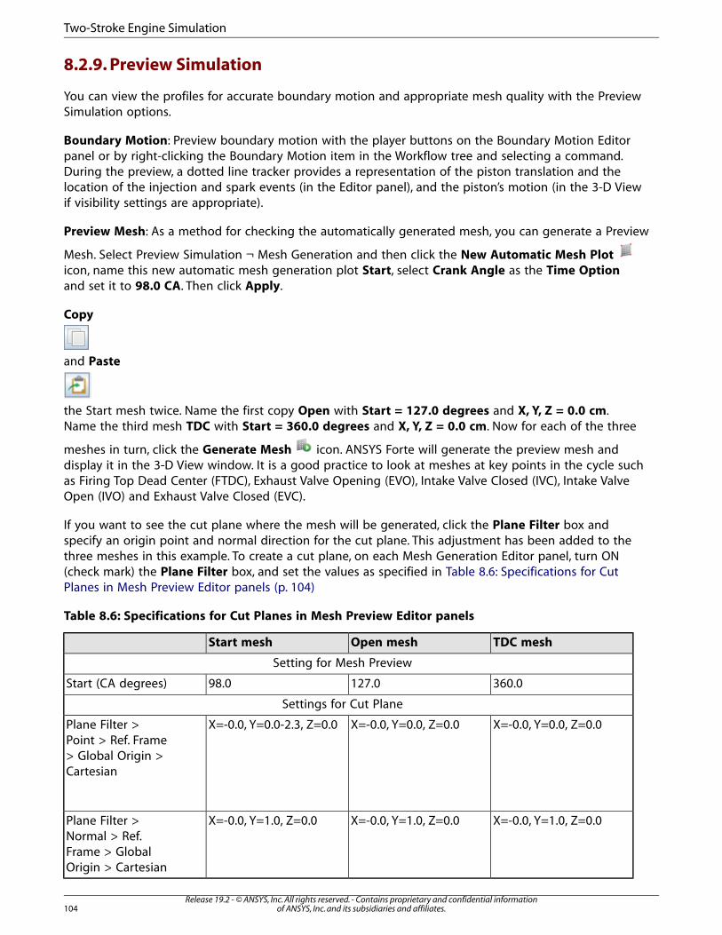
8.2.9. Preview Simulation
You can view the profiles for accurate boundary motion and appropriate mesh quality with the PreviewSimulation options.
Boundary Motion: Preview boundary motion with the player buttons on the Boundary Motion Editorpanel or by right-clicking the Boundary Motion item in the Workflow tree and selecting a command.During the preview, a dotted line tracker provides a representation of the piston translation and thelocation of the injection and spark events (in the Editor panel), and the piston’s motion (in the 3-D Viewif visibility settings are appropriate).
Preview Mesh: As a method for checking the automatically generated mesh, you can generate a Preview
Mesh. Select Preview Simulation ¬ Mesh Generation and then click the New Automatic Mesh Ploticon, name this new automatic mesh generation plot Start, select Crank Angle as the Time Optionand set it to 98.0 CA. Then click Apply.
Copy
and Paste
the Start mesh twice. Name the first copy Open with Start = 127.0 degrees and X, Y, Z = 0.0 cm.Name the third mesh TDC with Start = 360.0 degrees and X, Y, Z = 0.0 cm. Now for each of the three
meshes in turn, click the Generate Mesh icon. ANSYS Forte will generate the preview mesh anddisplay it in the 3-D View window. It is a good practice to look at meshes at key points in the cycle suchas Firing Top Dead Center (FTDC), Exhaust Valve Opening (EVO), Intake Valve Closed (IVC), Intake ValveOpen (IVO) and Exhaust Valve Closed (EVC).
If you want to see the cut plane where the mesh will be generated, click the Plane Filter box andspecify an origin point and normal direction for the cut plane. This adjustment has been added to thethree meshes in this example. To create a cut plane, on each Mesh Generation Editor panel, turn ON(check mark) the Plane Filter box, and set the values as specified in Table 8.6: Specifications for CutPlanes in Mesh Preview Editor panels (p. 104)
Table 8.6: Specifications for Cut Planes in Mesh Preview Editor panels
TDC meshOpen meshStart mesh
Setting for Mesh Preview
360.0127.098.0Start (CA degrees)
Settings for Cut Plane
X=-0.0, Y=0.0, Z=0.0X=-0.0, Y=0.0, Z=0.0X=-0.0, Y=0.0-2.3, Z=0.0Plane Filter >Point > Ref. Frame> Global Origin >Cartesian
X=-0.0, Y=1.0, Z=0.0X=-0.0, Y=1.0, Z=0.0X=-0.0, Y=1.0, Z=0.0Plane Filter >Normal > Ref.Frame > GlobalOrigin > Cartesian
Release 19.2 - © ANSYS, Inc. All rights reserved. - Contains proprietary and confidential informationof ANSYS, Inc. and its subsidiaries and affiliates.104
Two-Stroke Engine Simulation
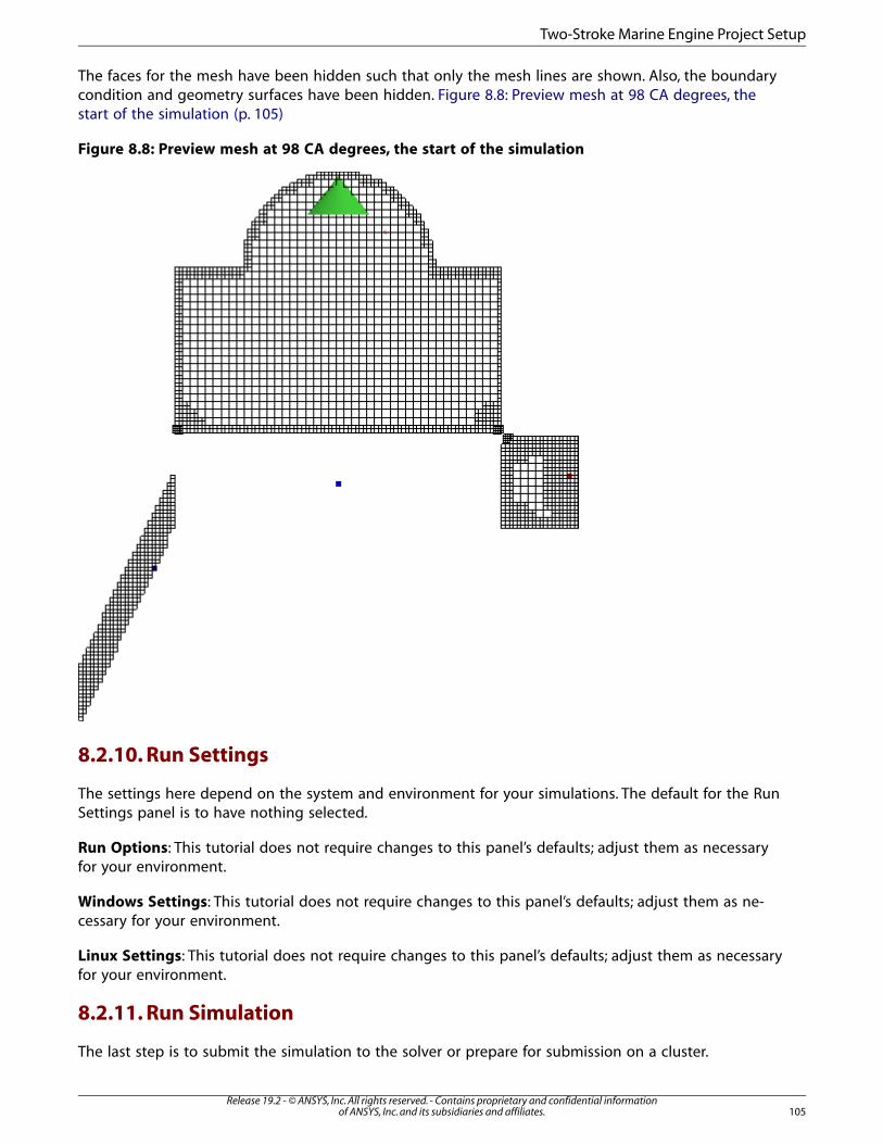
The faces for the mesh have been hidden such that only the mesh lines are shown. Also, the boundarycondition and geometry surfaces have been hidden. Figure 8.8: Preview mesh at 98 CA degrees, thestart of the simulation (p. 105)
Figure 8.8: Preview mesh at 98 CA degrees, the start of the simulation
8.2.10. Run Settings
The settings here depend on the system and environment for your simulations. The default for the RunSettings panel is to have nothing selected.
Run Options: This tutorial does not require changes to this panel’s defaults; adjust them as necessaryfor your environment.
Windows Settings: This tutorial does not require changes to this panel’s defaults; adjust them as ne-cessary for your environment.
Linux Settings: This tutorial does not require changes to this panel’s defaults; adjust them as necessaryfor your environment.
8.2.11. Run Simulation
The last step is to submit the simulation to the solver or prepare for submission on a cluster.
105Release 19.2 - © ANSYS, Inc. All rights reserved. - Contains proprietary and confidential information
of ANSYS, Inc. and its subsidiaries and affiliates.
Two-Stroke Marine Engine Project Setup
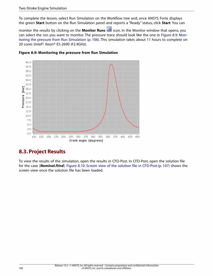
To complete the lesson, select Run Simulation on the Workflow tree and, once ANSYS Forte displaysthe green Start button on the Run Simulation panel and reports a “Ready” status, click Start. You can
monitor the results by clicking on the Monitor Runs icon. In the Monitor window that opens, youcan select the run you want to monitor. The pressure trace should look like the one in Figure 8.9: Mon-itoring the pressure from Run Simulation (p. 106). This simulation takes about 11 hours to complete on20 cores (Intel® Xeon® E5-2690 @2.9GHz).
Figure 8.9: Monitoring the pressure from Run Simulation
8.3. Project Results
To view the results of the simulation, open the results in CFD-Post. In CFD-Post, open the solution filefor the case (Nominal.ftind). Figure 8.10: Screen view of the solution file in CFD-Post (p. 107) shows thescreen view once the solution file has been loaded.
Release 19.2 - © ANSYS, Inc. All rights reserved. - Contains proprietary and confidential informationof ANSYS, Inc. and its subsidiaries and affiliates.106
Two-Stroke Engine Simulation

Figure 8.10: Screen view of the solution file in CFD-Post
Once you have read in the model, you can create surface groups to group the surfaces. In this case, wewill create a surface group for the spark plug, walls, symmetry boundaries, and the valves. To create asurface group, right-click User Locations and Plots Insert > Locations > Surface Group and specifythe name surfaces. On the Color and Render tab, you can change the color of the surfaces and thetransparency. In Figure 8.10: Screen view of the solution file in CFD-Post (p. 107), the surfaces are coloredgray and the transparency is set to a value of 0.5.
To visualize the solution in the combustion chamber, create a cut plane by right-clicking User Locationsand Plots > Insert > Location > Plane. Specify the Method as a ZX plane. On the Color tab, set theMode to Variable and specify the Variable as Temperature, click Apply. The temperature is now dis-played on the cut plane, as shown in Figure 8.11: Temperature contour plot on a plane through thecenterline of the combustion chamber (p. 108).
107Release 19.2 - © ANSYS, Inc. All rights reserved. - Contains proprietary and confidential information
of ANSYS, Inc. and its subsidiaries and affiliates.
Project Results
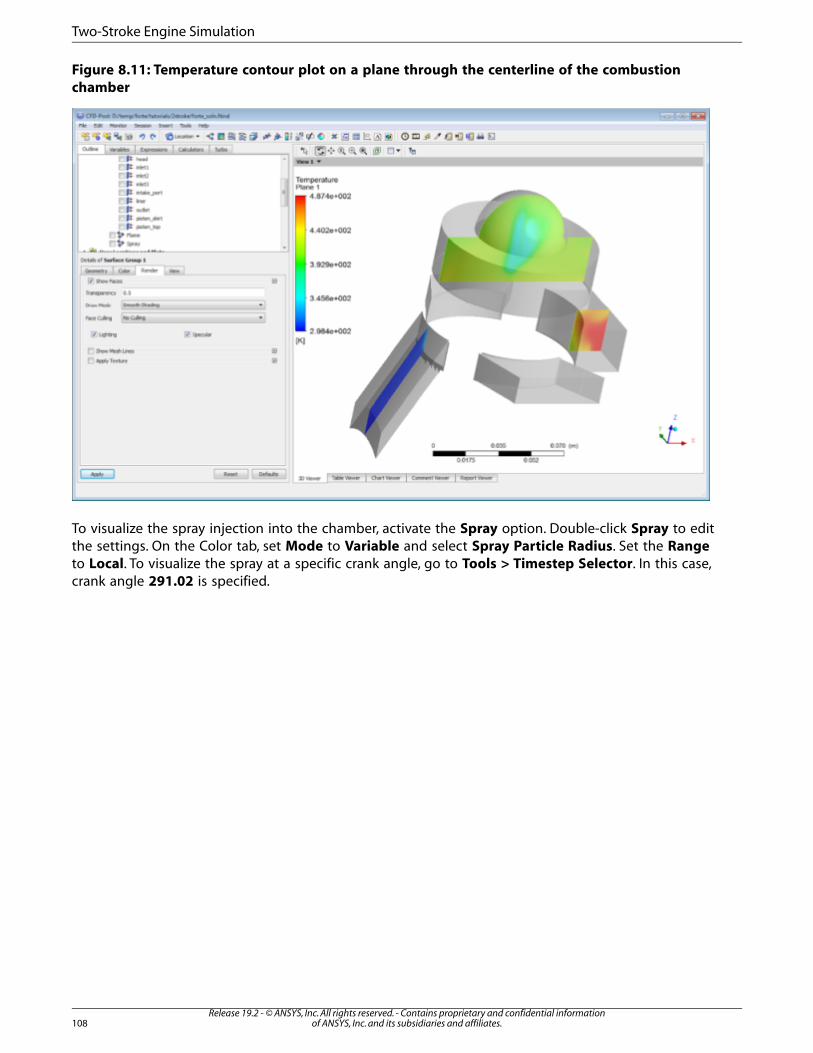
Figure 8.11: Temperature contour plot on a plane through the centerline of the combustionchamber
To visualize the spray injection into the chamber, activate the Spray option. Double-click Spray to editthe settings. On the Color tab, set Mode to Variable and select Spray Particle Radius. Set the Rangeto Local. To visualize the spray at a specific crank angle, go to Tools > Timestep Selector. In this case,crank angle 291.02 is specified.
Release 19.2 - © ANSYS, Inc. All rights reserved. - Contains proprietary and confidential informationof ANSYS, Inc. and its subsidiaries and affiliates.108
Two-Stroke Engine Simulation
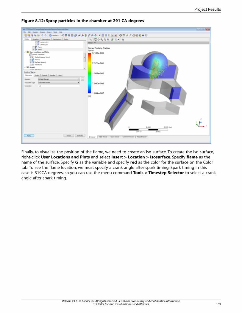
Figure 8.12: Spray particles in the chamber at 291 CA degrees
Finally, to visualize the position of the flame, we need to create an iso-surface. To create the iso-surface,right-click User Locations and Plots and select Insert > Location > Isosurface. Specify flame as thename of the surface. Specify G as the variable and specify red as the color for the surface on the Colortab. To see the flame location, we must specify a crank angle after spark timing. Spark timing in thiscase is 319CA degrees, so you can use the menu command Tools > Timestep Selector to select a crankangle after spark timing.
109Release 19.2 - © ANSYS, Inc. All rights reserved. - Contains proprietary and confidential information
of ANSYS, Inc. and its subsidiaries and affiliates.
Project Results
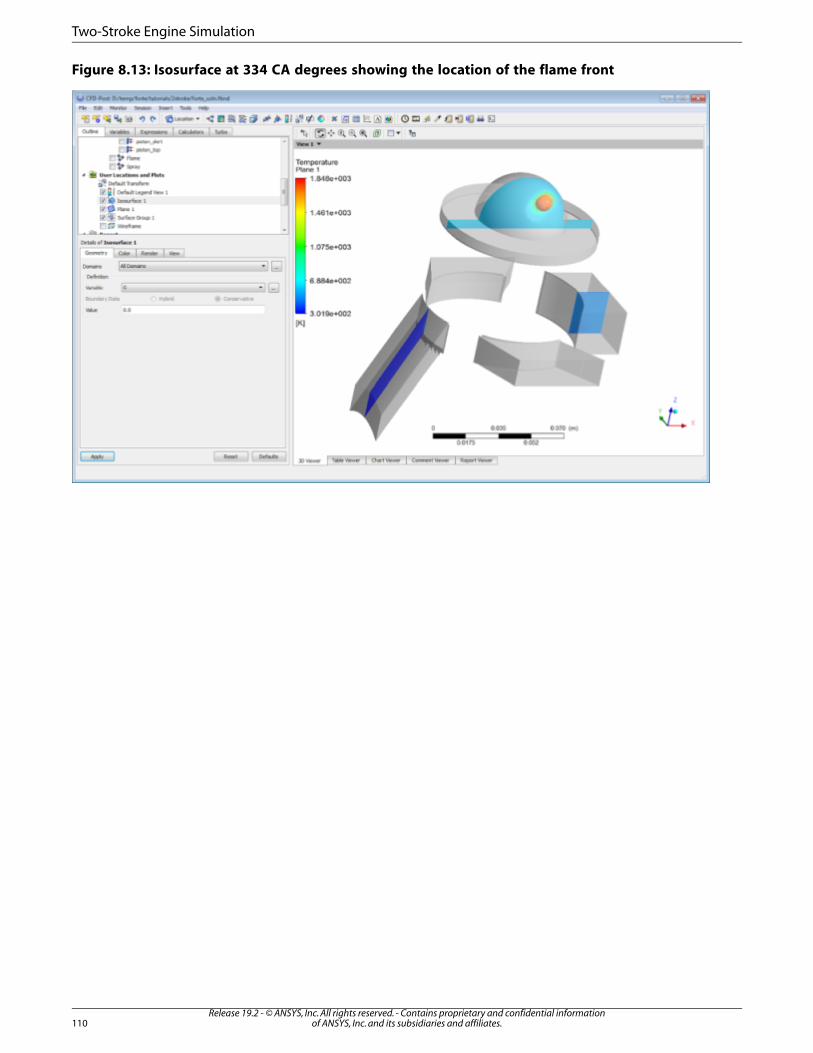
Figure 8.13: Isosurface at 334 CA degrees showing the location of the flame front
Release 19.2 - © ANSYS, Inc. All rights reserved. - Contains proprietary and confidential informationof ANSYS, Inc. and its subsidiaries and affiliates.110
Two-Stroke Engine Simulation
Chapter 9: Multi-Cylinder Four-Stroke Engine Simulation
This tutorial describes how to use ANSYS Forte CFD to simulate engine processes in an inline four-cyl-inder four-stroke spark-ignition engine. The purpose of this tutorial is to demonstrate several key pointsof project setup that are specific to multi-cylinder use cases:
• Use (spatial) Reference Frames to facilitate the setup of location and orientation parameters in each cylinder.
• Use Time Frames to facilitate the setup of timing parameters in each cylinder.
• Approximate initial conditions in each cylinder region for a given starting crank angle.
• Monitor output parameters that are averaged for each cylinder region.
Although the example used is an inline four-cylinder four-stroke spark-ignition engine, the concept andmethodology described in this tutorial are also applicable to other multi-cylinder configurations, suchas V-shaped arrangement, opposed piston engines, as well as other types of engine operations, suchas spray combustion in diesel engines, HCCI, etc.
This tutorial is based on a fully configured ANSYS Forte project (.ftsim) file. The steps described onlyhighlight the key points specific to multi-cylinder engines and are not intended to explain all the entiredetailed setup. The tutorial assumes that learner is already familiar with the fundamental steps for settingup a single-cylinder engine in ANSYS Forte. Such prerequisite knowledge can be obtained by studyingtutorials in previous chapters, such as the ANSYS Forte GDI tutorial,Gasoline Direct Injection EngineSimulation (p. 69).
9.1. Data Provided
9.1.1. Accessing Tutorial Files
The files for this tutorial are obtained by downloading the multicylinder_engine.zip file here.
Unzip multicylinder_engine.zip to your working folder.
9.1.2. Files Used in This Tutorial
The files for this tutorial include:
• multicylinder_4stroke_engine_tutorial.ftsim: A completely configured ANSYS Forte project file.
• intake_valve_lift_profile.csv: Lift profiles of the intake valves, tabulated for the crank angle range of [0,720] °CA ATDC.
• exhaust_valve_lift_profile.csv: Lift profiles of the exhaust valves, tabulated for the crank angle range of[0, 720] °CA ATDC.
111Release 19.2 - © ANSYS, Inc. All rights reserved. - Contains proprietary and confidential information
of ANSYS, Inc. and its subsidiaries and affiliates.

• multicylinder_4stroke_engine_tutorial.stl: An STL file that contains the multi-cylinder geometry. This isan optional file, which could be used as part of an exercise setting up this ANSYS Forte project without usingpreconfigured files.
9.2. Engine Configuration and Problem Description
The configuration of the inline four-cylinder engine is shown in Figure 9.1: Configuration of the inlinefour-stroke multi-cylinder engine (p. 112). The figure shows the numbering of the four cylinders, the intakemanifolds merging at a plenum, the inlet located on the side of the plenum, as well as two groups ofexhaust manifolds. One group of exhaust manifolds is connected to Cylinder-1 and Cylinder-4, theother is connected to Cylinder-2 and Cylinder-3. In this geometry, the crank shaft axis of the engine(not shown) is parallel to the Z-axis and the cylinder axes are parallel to the Y-axis. If you prefer, youcan rotate the geometry so the cylinder axes are parallel to the z-axis. To do the rotation, select all thegeometry surfaces under Geometry, right-click, select Transform Mesh, and then select Rotate X by90 degrees. The setup steps described below are based on the original orientation, not a transformedgeometry. The engine geometry will serve as the surface mesh for the automatic mesh generation.Automatic Mesh Generation requires that all the pistons are positioned at their top-dead-center (TDC)location and all valves are at their closed location in the initial surface mesh.
There is one spark per cylinder central-mounted near the top of each cylinder head. The firing order ofthis engine is 1-3-4-2, which means that there is a 180 °CA phase delay between any two consecutivespark events.
In this tutorial, the fuel/air mixture preparation process inside the intake manifolds is simplified and noport fuel injection is simulated. Instead, the fuel and air are treated as premixed stoichiometric mixture,which enters the computational domain through the inlet connected to the plenum.
Figure 9.1: Configuration of the inline four-stroke multi-cylinder engine
Release 19.2 - © ANSYS, Inc. All rights reserved. - Contains proprietary and confidential informationof ANSYS, Inc. and its subsidiaries and affiliates.112
Multi-Cylinder Four-Stroke Engine Simulation
9.3. Multi-Cylinder Spark-Ignition Engine Project Setup
This section will go over the simulation setup steps, with emphasis on several aspects that are specificto multi-cylinder simulation.
Note
Time frames can be added under Geometry > Time Frames. However, the default state forthe Time Frames node in the Workflow tree is hidden. To see it, use the Preferences com-mand in the Edit menu and check Enable Reference Time Frame Controls. Then Exit andrestart ANSYS Forte.
9.3.1. Geometry Import
(Optional) If you wish to set up the case without using the preconfigured files, you can start with im-
porting the supplied STL geometry file. On the Geometry Editor panel, click the Import Geometryicon, and choose the Surface from one or more STL files option, and then browse for the STL file.This step is needed only if you want the exercise of setting up the case from scratch. These steps arenot detailed here.
9.3.2. Defining Reference Frames and Time Frames
Reference frames and time frames in ANSYS Forte allow you to define transforms to apply in space andtime.
9.3.2.1. Reference Frames
Reference frames used in ANSYS Forte are spatially transformed coordinate systems. They can be definedin the Workflow tree under Geometry > Reference Frames. A new reference frame can be defined byreferring to its parent coordinate system and through transformation of either or both the origin andorientation. In a multi-cylinder geometry, by defining equivalent local reference frames for all cylinders,you can use the same set of location and orientation parameters for all cylinders.
To make it convenient to set up equivalent local coordinate systems for all the cylinders, the geometrymust meet some basic requirements relating to alignment with the coordinate axes in the global co-ordinate system. Generally, the minimum requirement is to let the crank shaft axis be parallel to oneof the coordinate axes in the global coordinate. This tutorial case satisfies this requirement because itscrank shaft axis is parallel to the Z-axis.
Now let us define a local reference frame for each cylinder. There are no fixed rules for setting the originof each cylinder’s own reference frame, but a convenient way is to use the center of the piston as thelocal origin. Using Cylinder-1 as an example, under Geometry, click surface piston_1. The piston_1Editor panel shows the Min and Max coordinate values along X-, Y-, Z-directions in the global referenceframe. The center of piston_1 on the X-Z plane can be calculated as
X_center = 0.5*(X_min + X_max) = 0.5*(-3.949 + 3.948) = 0 cm
Z_center = 0.5*(Z_min + Z_max) = 0.5* (31.15 + 39.05) = 35.1 cm
Since Y_min and Y_max are the same, you can pick Y_min as Y_center. In this specific example, it isbeneficial to let all four cylinders have the same Y_center value.
113Release 19.2 - © ANSYS, Inc. All rights reserved. - Contains proprietary and confidential information
of ANSYS, Inc. and its subsidiaries and affiliates.
Multi-Cylinder Spark-Ignition Engine Project Setup

In the fully configured .ftsim file, you can see four Reference Frames for the four cylinders: Frame-C1, Frame-C2, Frame-C3, and Frame-C4, listed in the Workflow tree. Their origins are calculated basedon the method described above and the values are listed in Table 9.1: Origins of local reference framesfor four cylinders (p. 114). We can see that the distance along the Z-direction between the axes of twoconsecutive cylinders is 9.5 cm. These four reference frames do not involve orientation transformation.Orientation transformation is needed in a V-type multi-cylinder engine.
Table 9.1: Origins of local reference frames for four cylinders
Frame-C4Frame-C3Frame-C2Frame-C1(cm)
0000Origin X
19.719.719.719.7Origin Y
6.616.125.635.1Origin Z
In this tutorial engine, all the intake valves are tilted on the X-Y plane by -11° relative to the Y-axis, andall the exhaust valves are tilted in a similar manner, but by 12°.The tilt angles are illustrated in Fig-ure 9.2: Tilt angles of intake and exhaust valve stems (p. 114). Two reference frames are created for intakevalves and exhaust valves, respectively, such that the Y-axes of these two reference frames are alignedwith the moving directions of the valves. The names are Frame_Intake_Valves_Dir andFlame_Exhaust_Valves_Dir. The transformation only involves rotation about the Z-axis. Thesetwo reference frames can be used to define the moving directions of the valves. They can also be usedto adjust the valve gaps at seated position if needed.
Figure 9.2: Tilt angles of intake and exhaust valve stems
9.3.2.2. Time Frames
Note
If you cannot see Time Frames listed under Geometry in the Workflow tree, edit your Pref-erences as described in the note in Note (p. 113) early in this tutorial.
Time frames are convenient tools for managing all the timing parameters in a multi-cylinder context.A time frame requires input of a crank angle offset. An event associated with the time frame will bedelayed by the offset value relative to the global crank angle. By defining an appropriate time framefor each cylinder, you can use the same set of timing parameters for all the cylinders in the configuration.
Release 19.2 - © ANSYS, Inc. All rights reserved. - Contains proprietary and confidential informationof ANSYS, Inc. and its subsidiaries and affiliates.114
Multi-Cylinder Four-Stroke Engine Simulation
Such timing parameters include, for example, piston motion specification and valve lift profiles, sparktiming, and injection timing.
The Global Time is a prepopulated item, which corresponds to the global crank angle and serves as areference. It cannot be edited. You can add four new time frames, one for each cylinder. Since the firingorder of this engine is 1-3-4-2, the crank angle offset values can be set as 0 °CA, 180 °CA, 360 °CA,540 °CA for Cylinder 1, 3, 4, 2, respectively. Note that Cylinder-1 is essentially associated with theglobal crank angle, and therefore it is used as a reference cylinder.
9.3.3. Automatic Mesh Generation Setup
A multi-cylinder case requires that one of the cylinders be defined as the reference cylinder and associatedwith the Default Initialization region under Initial Conditions. The Material Point under Mesh Controlsis expected to be a location inside the Default Initialization region. Since Cylinder-1 is assigned asthe reference cylinder in this tutorial, the material point should be inside Cylinder-1. As mentionedearlier, since the origin of the reference frame for Cylinder-1 is defined as the center of the pistonsurface at the piston’s TDC position, you can set the material point a distance above the local origin.The location selected should be able to remain inside the combustion chamber at all times while thepiston travels from its BDC to TDC and the valves move from a fully closed position to a fully liftedposition. In this sample, the Material Point is set to (X, Y, Z) = (0.0, 1.0, 0.0) cm in the Frame-C1 ref-erence frame. The Global Mesh Size is set to 4.0 mm.
Several refinement controls for surface or volume are used to obtain higher mesh resolution at systemboundaries and at various locations that are expected to see high gradients for velocity or temperature.
You can go through the refinement control items under Mesh Controls in the fully configured projectfile to check their detailed specifications.
Under Mesh Controls on the Workflow tree, AllWalls, OpenBoundaries, ValveStems, Chamber_BL,and ValveSeats are surface refinement controls that are applied at all times. ValveSeats specifies a 1/8refinement for all valve seat surfaces in all the cylinders. In a typical engine geometry, cells near thevalve gaps must be sufficiently refined (approximately 0.5 mm) to ensure that the computational domainof the intake/exhaust manifolds and the cylinders are cleanly separated when the corresponding valvesare closed.
IVO_n and EVO_n, in which n is a numeral, are interval-based surface refinements applied to thecombustion chamber walls during intake-valve opening or exhaust-valve opening processes. The cylinder-specific time frames are convenient when setting up these crank-angle-interval–based controls. By as-sociating such a control with a cylinder’s local time frame, you can specify the start angle and end anglevalues with respect to the cylinder’s local TDC, and the same crank angle values can be used for all thecylinders. For example, the crank angle interval for refinement controls IVO_1 to IVO_4 has the samevalue, [323, 563] °CA ATDC. The only difference for this timing control is the time-frame selection. Notethat the Location should point to the corresponding surfaces in each cylinder.
SparkPlug_1 to SparkPlug_4 are spherical volume refinement controls that specify 1/8 refinement ina small region surrounding each spark plug. The center of the refinement volume will be set at thespark location and the Radius of Application is 0.4 cm. By specifying the coordinates of the refinement
115Release 19.2 - © ANSYS, Inc. All rights reserved. - Contains proprietary and confidential information
of ANSYS, Inc. and its subsidiaries and affiliates.
Multi-Cylinder Spark-Ignition Engine Project Setup
center relative to the origin of each cylinder’s local reference frame, the same center coordinates canbe used for these four controls.
Note
As an option, you can limit this refinement to 10 °CA before spark and 60 °CA degreeafter spark in each cylinder.
9.3.4. Model Setup
Chemistry: The single-component 59-species gasoline chemical kinetics mechanism that is included inANSYS Forte’s chemistry mechanism database is used to simulate the combustion of gasoline/air mixture,in which gasoline is approximated by iso-octane. The chemistry set can be found in the data folderwithin the ANSYS Forte installation. The name of the chemistry set is Gasoline_1comp_49sp.cks.
Flame Speed: The Gülder formulation of the power law will be used to compute laminar flame speedsin the flame propagation model. For all the other model inputs on the Flame Speed Model panel, thedefault values are used.
Spark Ignition: Turn on the spark ignition model by checking the checkbox in front of Spark Ignitionin the Workflow tree. On the Spark Ignition > Settings panel, the checkbox in front of FlamePropagation Model is checked by default. This means the flame propagation will be modeled usingthe discrete particle ignition kernel (DPIK) model and the G-equation model. Keep the default valuesfor all the model constants.
Sparks: In this engine, each cylinder contains one spark plug. The spark plug structure is included inthe cylinder head surfaces. On the SparkIgnition Editor panel, you can create four spark plug items tospecify their location, spark duration, energy discharge rate, etc. Start with adding the spark plug for
the first cylinder by clicking the Spark icon on the SparkIgnition Editor panel. By specifying thespatial reference frame as Frame-C1, the coordinates of the spark plug’s location can be specified withrespect to this cylinder’s local reference frame. The coordinates of the spark gap are (-0.4, 1.35, 0.0)cm. Similarly, by linking this spark’s timing parameter to Time Frame Cylinder 1, the spark timing valuecan be specified with respect to this cylinder’s local TDC. The spark timing is 20°CA before the firingTDC, so the starting angle of spark is set to 700°CA ATDC. The default values are kept for spark energyand initial kernel radius. After the first spark, Spark 1, has been configured, you can then duplicate it
(Copy and Paste ) to create the spark plugs in the other three cylinders. After each copy andpaste, you can simply adjust the Time Frame and (spatial) Reference Frame to their respective localframes.
Spray: (Optional) This tutorial does not involve spray simulation, but fuel sprays within each cylinderor within the intake ports of each cylinder could be set up in a similar manner as the spark setup. Youcan start with configuring the injector for the reference cylinder, and then duplicate that injector forthe other cylinders. For each duplicated injector, you must adjust the time frame as well as the referenceframes for each nozzle to use the cylinder’s local frames. Note that the time frame is applied on theInjector level, that is, the injection timings of all the Injection pulses added under an injector are as-sumed to use the same time frame specified on the Injector Editor panel.
9.3.5. Boundary Conditions
In the context of multi-cylinder engines, the boundary conditions can be divided into two groups, oneis shared by all cylinders and the other is cylinder-specific. The cylinder-specific boundary conditions
Release 19.2 - © ANSYS, Inc. All rights reserved. - Contains proprietary and confidential informationof ANSYS, Inc. and its subsidiaries and affiliates.116
Multi-Cylinder Four-Stroke Engine Simulation
include head, liner, and moving surfaces (pistons and valves). For the cylinder-specific boundary condi-tions, you can first do the configuration for the reference cylinder, and then duplicate that for the restof the cylinders. For each duplicated boundary condition item, the only parameters that must be adjustedare the Ref. Frames (for locations or directions) and Time Frames (for timings). Of course, the Locationselection should be adjusted accordingly as well.
In this tutorial, boundary conditions shared by all the cylinders include Inlet, Outlet_1, Outlet_2, In-takeManifold, ExhaustManifold1, and ExhaustManifold2. The first three are open boundaries, whichinvolve time profiles for boundary pressure and temperature. The time frame associated with thesetime profiles should be set to Global Time. In this tutorial, port fuel injection will not be simulated. In-stead, the mixture coming into the domain through the inlet is assumed to be a premixed stoichiometricair/fuel mixture.
The boundary conditions head and liner are static wall boundaries. They are cylinder-specific, but donot require a time frame input, therefore the head surfaces of all cylinders are grouped as one boundarycondition and the same is done for the liner surfaces. If preferred, you can split each group into fourindividual boundary condition items. Such a split may be needed if you want to define different wallboundary temperatures for different cylinders.
Each moving surface requires the specification of a Wall Motion. The wall motion for pistons and valvesin different cylinders can easily be synchronized with the help of the cylinder-specific time frames. Inthe fully configured ANSYS Forte project file, Piston_1, IntakeValve1-1, IntakeValve2-1, ExhaustValve1-1, ExhaustValve2-1 are the moving boundary conditions for Cylinder_1 (the last numeral in the BCname indicates the cylinder index). If setting up the project on your own, you could first create thesefive boundary conditions, specify the Time Frame as Cylinder 1, and specify the Ref. Frame used bythe wall motion direction as Frame-C1. Then, duplicate these BCs for the other cylinders.
For a duplicated piston, adjust three items to reflect the local cylinder:
• Location selection;
• TimeFrame; and
• Ref. Frame (for motion direction).
For a duplicated valve, adjust four items:
• Location selection;
• Time Frame (for lift profiles);
• Ref. Frame (for motion direction); and
• the selection of Valve Seat and the Surface it Contacts.
All the other parameters can be kept the same for different cylinders, including the valve lift profiles.
Note that Frame-C1 to Frame-C4 are used to specify the valve motion direction in the current projectfile. An alternative (probably easier) way is to use the Ref. Frames mentioned earlier, Frame_In-take_Valves_Dir and Flame_Exhaust_Valves_Dir. For example, when using Frame_Intake_Valves_Dirto specify the moving direction of the intake valves, you can simply specify the Cartesian directionvector as (X, Y, Z) = (0, -1, 0). The same motion direction setting can be applied to all intake valves be-cause they all move along the same direction. The same approach can be applied to the exhaust valves.
117Release 19.2 - © ANSYS, Inc. All rights reserved. - Contains proprietary and confidential information
of ANSYS, Inc. and its subsidiaries and affiliates.
Multi-Cylinder Spark-Ignition Engine Project Setup
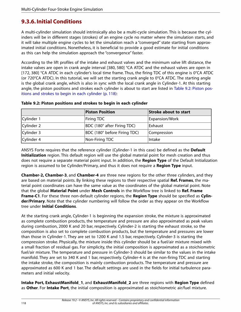
9.3.6. Initial Conditions
A multi-cylinder simulation should intrinsically also be a multi-cycle simulation. This is because the cyl-inders will be in different stages (strokes) of an engine cycle no matter where the simulation starts, andit will take multiple engine cycles to let the simulation reach a “converged” state starting from approx-imated initial conditions. Nonetheless, it is beneficial to provide a good estimate for initial conditionsas this can help the simulation approach the “convergence” faster.
According to the lift profiles of the intake and exhaust valves and the minimum valve lift distance, theintake valves are open in crank angle interval [380, 580] °CA ATDC and the exhaust valves are open in[172, 380] °CA ATDC in each cylinder’s local time frame. Thus, the firing TDC of this engine is 0°CA ATDC(or 720°CA ATDC). In this tutorial, we will set the starting crank angle to 0°CA ATDC. The starting angleis the global crank angle, which is also in sync with the local crank angle in Cylinder-1. At this startingangle, the piston positions and strokes each cylinder is about to start are listed in Table 9.2: Piston pos-itions and strokes to begin in each cylinder (p. 118):
Table 9.2: Piston positions and strokes to begin in each cylinder
Stroke about to startPiston Position
Expansion/WorkFiring TDCCylinder 1
ExhaustBDC (180° after Firing TDC)Cylinder 2
CompressionBDC (180° before Firing TDC)Cylinder 3
IntakeNon-Firing TDCCylinder 4
ANSYS Forte requires that the reference cylinder (Cylinder-1 in this case) be defined as the DefaultInitialization region. This default region will use the global material point for mesh creation and thusdoes not require a separate material point input. In addition, the Region Type of the Default Initializationregion is assumed to be Cylinder/Primary, and thus it does not require a Region Type input.
Chamber-2, Chamber-3, and Chamber-4 are three new regions for the other three cylinders, and theyare based on material points. By linking these regions to their respective spatial Ref. Frames, the ma-terial point coordinates can have the same value as the coordinates of the global material point. Notethat the global Material Point under Mesh Controls in the Workflow tree is linked to Ref. FrameFrame-C1. For these three non-default cylinder regions, the Region Type should be specified as Cylin-der/Primary. Note that the cylinder numbering will follow the order as they appear on the Workflowtree under Initial Conditions.
At the starting crank angle, Cylinder-1 is beginning the expansion stroke, the mixture is approximatedas complete combustion products, the temperature and pressure are also approximated as peak valuesduring combustion, 2000 K and 20 bar, respectively. Cylinder-2 is starting the exhaust stroke, so thecomposition is also set to complete combustion products, but the temperature and pressures are lowerthan those in Cylinder-1. They are set to 1200 K and 1.5 bar, respectively. Cylinder-3 is starting thecompression stroke. Physically, the mixture inside this cylinder should be a fuel/air mixture mixed witha small fraction of residual gas. For simplicity, the initial composition is approximated as a stoichiometricfuel/air mixture. The temperature and pressure in Cylinder-3 should be similar to the values in the intakemanifold. They are set to 340 K and 1 bar, respectively. Cylinder-4 is at the non-firing TDC and startingthe intake stroke, the composition is mainly combustion products. The temperature and pressure areapproximated as 600 K and 1 bar. The default settings are used in the fields for initial turbulence para-meters and initial velocity.
Intake Port, ExhaustManifold_1, and ExhaustManifold_2 are three regions with Region Type definedas Other. For Intake Port, the initial composition is approximated as stoichiometric air/fuel mixture.
Release 19.2 - © ANSYS, Inc. All rights reserved. - Contains proprietary and confidential informationof ANSYS, Inc. and its subsidiaries and affiliates.118
Multi-Cylinder Four-Stroke Engine Simulation
Temperature and Pressure are set to 313 K and 1.1 bar, respectively. For the two exhaust ports,composition is set to combustion products, and Temperature and Pressure are set to 500 K and 1bar, respectively. The material points can be placed anywhere inside the respective manifold geometry.
The Initialization Order values of all the initialization regions should be set following the “go-with-the-flow” rule. The order of the intake port should be 1, followed by the four cylinders, and finally the twoexhaust manifolds.
The Composition Calculation Utility contained in the ANSYS Forte Setup Interface can be used toprepare different mixtures required by the initial conditions.
9.3.7. Simulation Controls
A multi-cylinder engine simulation must use the Crank Angle Based option on the Simulation ControlsEditor panel. The initial and final crank angles exposed on the Simulation Controls panel are bothglobal values. In the fully configured project, the case is set up to run two complete engine cycles.
On the Time Step Editor panel, the Max Simulation Time Step, dtmax, uses a constant value (1.E-5s) in the current project. If a time varying dtmax profile is used instead, the profile is required to coverthe crank angle range of [0, 720] °CA ATDC. This profile will be applied to all cylinders within each cyl-inder’s local time frame. Specifically, a max time step value is first determined in each cylinder separatelybased on the profile and the cylinder’s local crank angle value. Then, the minimum value among all thecylinders will be used as the global Max Simulation Time Step.
For the chemistry activation control on the Chemistry Solver panel, it is recommended not to checkthe After First Spark Event and After Fuel Injection Starts boxes because these controls are not well-defined in the multi-cycle, multi-cylinder context. Instead, you can use the During Crank Angle Intervaloption to activate chemistry for a certain duration within an engine cycle. Similar to the Max SimulationTime Step control, the interval-based chemistry activation control is also assumed to be applied in allthe cylinders based on each cylinder’s local time frame. For example, in this tutorial, the interval is setto [-40, 100] °CA ATDC. This means chemistry will be activated 40°CA before the Firing TDC and deac-tivated 100°CA after the Firing TDC in all four cylinders.
9.4. Result Visualization
In a multi-cylinder calculation, cylinder-specific spatially-averaged solutions are reported on a per-cylinderbasis. The cylinder-specific CSV output files include:
• thermos.csv
• dynamic.csv
• flame.csv
• massfraction.csv
• molefraction.csv
• speciesmass.csv
The cylinder index will be appended to the file names to indicate which cylinder they are for. For example,you will see thermo1.csv, thermo2.csv, etc. These files include both the global crank angle andthe cylinder’s local crank angle. The local crank angles are always converted to values within the range
119Release 19.2 - © ANSYS, Inc. All rights reserved. - Contains proprietary and confidential information
of ANSYS, Inc. and its subsidiaries and affiliates.
Result Visualization

of [0, 720) °CA ATDC. For two-stroke engines, the local crank angles will be in the range of [0, 360) °CAATDC.
The rest of the CSV files are reported either based on the average over the whole computational domainor reported on a per-boundary-condition basis, and they have the same format as single-cylinder calcu-lations.
Release 19.2 - © ANSYS, Inc. All rights reserved. - Contains proprietary and confidential informationof ANSYS, Inc. and its subsidiaries and affiliates.120
Multi-Cylinder Four-Stroke Engine Simulation
Chapter 10: Links to Third-Party Software
ANSYS Forte version 19.0 can be used to perform co-simulation with GT-Power. It is useful to performsimulation of intake and exhaust manifolds as well as that including in-cylinder combustion. Refer tothe GT-SUITE's Fluent Coupling Manual and Tutorials document installed with GT-SUITE version 2017 [1]for general information about CFD coupling, basic requirements, scope, and coupling methodology.The GTLINK library template, provided through a partnership arrangement between ANSYS, Inc. andGamma-Technologies, has been used to enable coupling with Forte. The code to use the GTLINK libraryis included in Forte and invoked automatically when setting up and running Forte simulations, as de-scribed later in this section.
• To access tutorials and their input files, go to the ANSYS Help site and select the ANSYS Forte tutorials youwish to download.
10.1. Installing Forte and GT-SUITE for Coupling
Both GT-SUITE and ANSYS Forte must be independently installed and operating on the same platform.There is no need for any additional libraries. ANSYS Forte version 19.0 is compatible with GT-Powerversion 2017. Mutually compatible 64-bit Windows and Linux platforms are supported. The path to theGT-Power installation directory can be specified during Forte setup. An environment variable, GTIHOME,which is set by the GT-Power installation, is also used as an alternative method to invoke GT-Powerduring co-simulation.
10.2. Setting Up a GT-SUITE Model for CFD Coupling
We use the same example as shown in GT-SUITE's Fluent Coupling Manual and Tutorials document todemonstrate coupling with ANSYS Forte. In that document, refer to the section on “Tutorial 1: Settingup a GT-SUITE model for CFD Coupling,” for detailed instructions on setting up a GT-Power Enginemodel example in GT-SUITE. The example uses a 4-cylinder spark-ignition engine model with a resolvedEGR pipeline. CFD is used at the intake manifold to capture pulsation and mixing effects and the resultingcylinder-to-cylinder composition variation. Section 1.2 of that tutorial describes the steps to prepare aGT-Power model for CFD coupling.
• For coupling GT-Power with ANSYS Forte, only Velocity or Pressure boundary types may be used.
Note
ANSYS Forte simulations require regions to be contiguous. This restricts use of Forte with GT-Power for non-contiguous setup, such as a split exhaust manifold, as well as for modelingmultiple components in the system.
10.3. Setting Up a Forte Model for Coupling with GT-Power
The files for this tutorial are obtained by downloading the gtpower_intake_manifold.zip filehere.
121Release 19.2 - © ANSYS, Inc. All rights reserved. - Contains proprietary and confidential information
of ANSYS, Inc. and its subsidiaries and affiliates.
Unzip gtpower_intake_manifold.zip to your working folder.
The first step in setting up an ANSYS Forte model in the example is to import a surface mesh for thegeometry. For this example, we import the geometry STL file Intake_Manifold.stl located at%GTIHOME%\v2017\tutorials\Co-Simulation_And_UserCode\CFDcoupling\Intake-Manifold, or import the Fluent mesh file in the sub-folder FLUENT\IntakeManifold.msh. Moreinformation on setting up mesh controls for automatic meshing and boundary conditions is in the ForteQuick Start Guide and Forte User's Guide.
A pre-set Forte setup file (.ftsim) is available with this sample.
Cell size can be set according to the accuracy desired. Typically a cell size of 2 mm or smaller is recom-mended. ANSYS Forte also requires a reaction mechanism for fluid mixture. Since there is no chemistryin this intake manifold example, the chemistry set provided contains only species information withoutreactions. An estimate of initial conditions in the fluid domain of the manifold and of initial boundaryconditions are set in the Forte project. These values can be obtained by running GT-Power without CFDcoupling. They will impact the initial transient conditions but not the steady state at longer residencetimes.
For setting up boundary conditions in Forte, the following types should be used:
• Velocity Inlet Type: Use the Velocity option with the direction set normal to the boundary, a zero pressure-gradient assumption, and use the total-temperature option.
• Pressure Inlet Type: Use the Total Pressure option with the total temperature specification.
• Pressure Outlet Type: Use the Total Pressure option.
• Velocity Outlet Type: Use the Continuative Outlet option.
Simulation Controls in ANSYS Forte should be time-based. Simulation time should slightly exceed thetotal time for all cycles in the GT-Power setup. All the controls for coupling with GT-Power are locatedunder the GTI Model panel as shown in Figure 10.1: GT-Power co-simulation panel under SimulationControls (p. 123).
Note
The GT-SUITE license feature, version, and bin directories are specified as Preferences. If thebin directory is not available, the software will look for an alternate location using the%GTIHOME% environment variable.
Release 19.2 - © ANSYS, Inc. All rights reserved. - Contains proprietary and confidential informationof ANSYS, Inc. and its subsidiaries and affiliates.122
Links to Third-Party Software

Figure 10.1: GT-Power co-simulation panel under Simulation Controls
Link Time Step specifies the frequency for syncing the simulations of two codes through the updateof boundary conditions. Typically this is same as the Max Time Step specified in ANSYS Forte. However,the link time step can be greater than the Max Time Step to reduce the frequency of syncing, whichwill improve the simulation speed of Forte.
Next, the GT-Power project file (.gtm) should be specified and loaded by clicking the button next tothat entry box. This action will extract the species and boundary information using the GTLINK libraryin the background. Any unresolved issues from Step 1 or absence of a GT-SUITE installation may preventthis action. Note that the GT-SUITE bin path and version number are specified in Forte > Preferences> Preferred Applications. The default version for GT-SUITE is v2017. If the GTIHOME environmentvariable is defined, it will be used to load the appropriate GTLINK library. Once the GT-SUITE projectfile is read successfully, all the species and boundaries will be populated on the same setup panel asshown in Figure 10.2: Species and boundaries extracted from the sample GT-Power project in Fortesetup (p. 124).
123Release 19.2 - © ANSYS, Inc. All rights reserved. - Contains proprietary and confidential information
of ANSYS, Inc. and its subsidiaries and affiliates.
Setting Up a Forte Model for Coupling with GT-Power
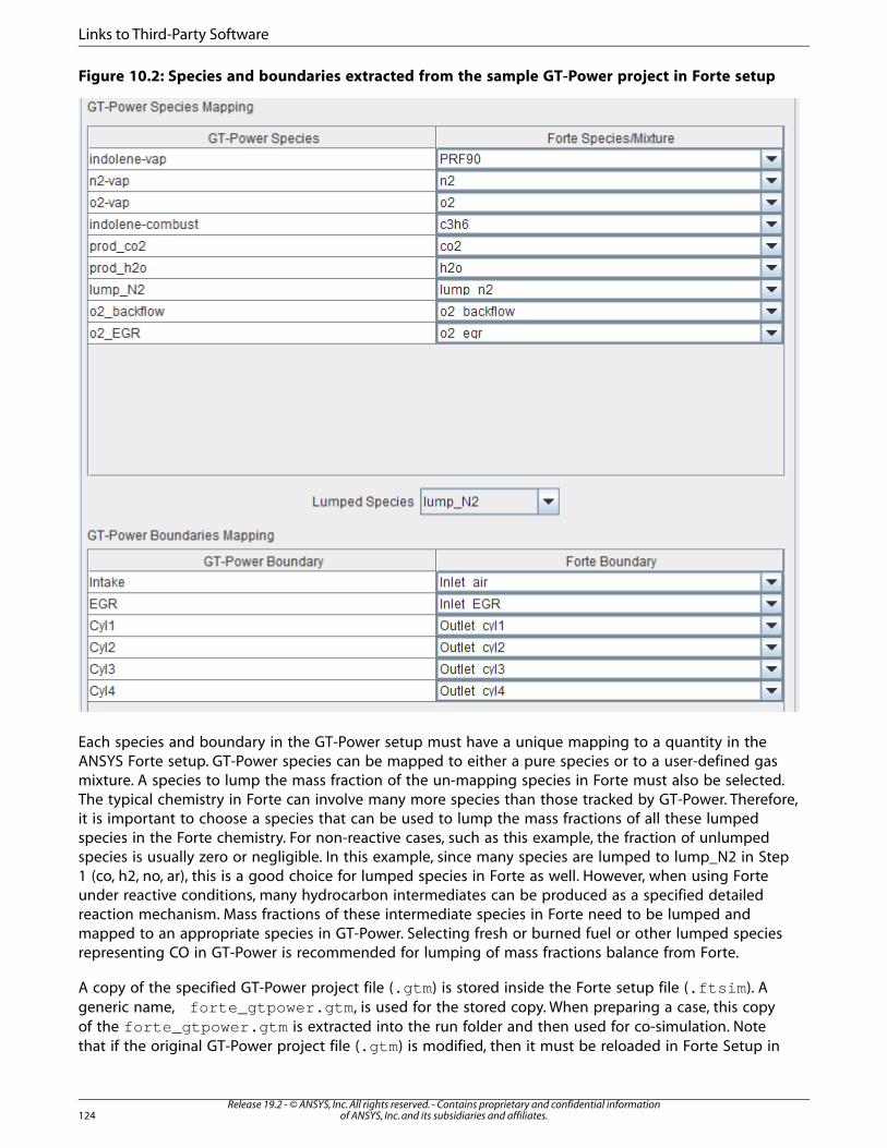
Figure 10.2: Species and boundaries extracted from the sample GT-Power project in Forte setup
Each species and boundary in the GT-Power setup must have a unique mapping to a quantity in theANSYS Forte setup. GT-Power species can be mapped to either a pure species or to a user-defined gasmixture. A species to lump the mass fraction of the un-mapping species in Forte must also be selected.The typical chemistry in Forte can involve many more species than those tracked by GT-Power. Therefore,it is important to choose a species that can be used to lump the mass fractions of all these lumpedspecies in the Forte chemistry. For non-reactive cases, such as this example, the fraction of unlumpedspecies is usually zero or negligible. In this example, since many species are lumped to lump_N2 in Step1 (co, h2, no, ar), this is a good choice for lumped species in Forte as well. However, when using Forteunder reactive conditions, many hydrocarbon intermediates can be produced as a specified detailedreaction mechanism. Mass fractions of these intermediate species in Forte need to be lumped andmapped to an appropriate species in GT-Power. Selecting fresh or burned fuel or other lumped speciesrepresenting CO in GT-Power is recommended for lumping of mass fractions balance from Forte.
A copy of the specified GT-Power project file (.gtm) is stored inside the Forte setup file (.ftsim). Ageneric name, forte_gtpower.gtm, is used for the stored copy. When preparing a case, this copyof the forte_gtpower.gtm is extracted into the run folder and then used for co-simulation. Notethat if the original GT-Power project file (.gtm) is modified, then it must be reloaded in Forte Setup in
Release 19.2 - © ANSYS, Inc. All rights reserved. - Contains proprietary and confidential informationof ANSYS, Inc. and its subsidiaries and affiliates.124
Links to Third-Party Software
order to update the internally stored copy of the file. Upon completion of the simulation, the GT-Powersolution (forte_gtpower.gdx) is written in the run folder for further analysis.
10.4. Restarting or Continuing a Co-simulation
A copy of the specified GT-Power project file (.gtm) is stored inside the ANSYS Forte setup file (.ftsim).A generic name, forte_gtpower.gtm, is used for the stored copy. When preparing a case, this copyof the forte_gtpower.gtm is extracted into the run folder and then used for co-simulation. Notethat if the original GT-Power project file (.gtm) is modified, it must be reloaded in Forte Simulate inorder to update the internally stored copy of the file. Oncethe simulation completes, the GT-Powersolution (forte_gtpower.gdx) is written in the run folder for further analysis.
10.5. References
1. Gamma Technologies, GT-SUITE 2017. 2017.
125Release 19.2 - © ANSYS, Inc. All rights reserved. - Contains proprietary and confidential information
of ANSYS, Inc. and its subsidiaries and affiliates.
References

Release 19.2 - © ANSYS, Inc. All rights reserved. - Contains proprietary and confidential informationof ANSYS, Inc. and its subsidiaries and affiliates.126

Chapter 11: Combustion Simulation for a Sector in IC Engine System(ANSYS Workbench)
Note
This tutorial is for working in the environment of ANSYS Workbench and using Forte forspecific steps.
In this tutorial a complete Direct injection (DI) compression ignition (CI) engine geometry is transformedinto 60° sector in order to reduce mesh size and solution time. Detailed boundary conditions are asshown in the Figure 11.1: Problem Schematic (p. 128). Sector simulation is started at intake valve Closing(IVC) with initial conditions as 3.45 bar and 404 K, species mass fraction of O2=0.1369, N2=0.7473,CO2=0.0789, H2O=0.0369. n-heptane (nc7h16) is used as surrogate for diesel fuel and is injected 8 degreesbefore compression (Top Dead Centre). This tutorial illustrates the following steps in setting up andsolving a combustion simulation for a sector.
• Launch IC Engine (Forte) system.
• Read an existing geometry into IC Engine (Forte) .
• Decompose the geometry.
• Mesh the geometry in FORTE Sector Mesh Generator.
• Define the solver setup.
• Run the simulation.
• Examine the results in the report.
127Release 19.2 - © ANSYS, Inc. All rights reserved. - Contains proprietary and confidential information
of ANSYS, Inc. and its subsidiaries and affiliates.

Figure 11.1: Problem Schematic
This tutorial is written with the assumption that you are familiar with the IC Engine system and thatyou have a good working knowledge of ANSYS Workbench. For more information on IC Engines referto the Fluent User's Guide, Forte User's Guide, and Fluent Workbench Tutorials.
11.1. Preparation11.2. Step 1: Setting the Properties11.3. Step 2: Performing the Decomposition11.4. Step 3: Meshing11.5. Step 4: Setting up the Simulation11.6. Step 5: Running the Solution11.7. Step 6: Obtaining the Results11.8. Summary11.9. Further Improvements
11.1. Preparation
The files for this tutorial are obtained by downloading the gasoline_direct_injection_en-gine.zip file here.
Unzip gasoline_direct_injection_engine.zip to your working folder.
1. Copy the files (tut_comb_sect.x_t and Sector_Setup.ftrpl) to your working folder.
To access tutorials and their input files, go to the ANSYS Help site and select the tutorials fromthe product you desire.
2. Start Workbench.
Release 19.2 - © ANSYS, Inc. All rights reserved. - Contains proprietary and confidential informationof ANSYS, Inc. and its subsidiaries and affiliates.128
Combustion Simulation for a Sector in IC Engine System (ANSYS Workbench)
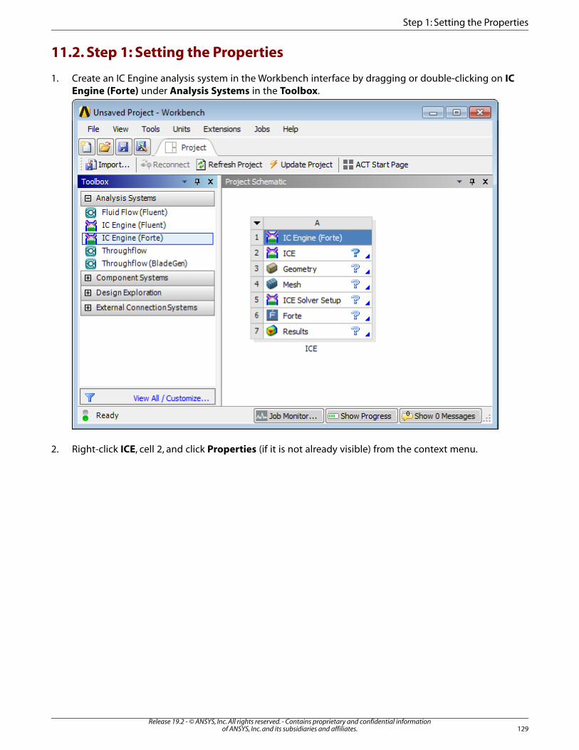
11.2. Step 1: Setting the Properties
1. Create an IC Engine analysis system in the Workbench interface by dragging or double-clicking on ICEngine (Forte) under Analysis Systems in the Toolbox.
2. Right-click ICE, cell 2, and click Properties (if it is not already visible) from the context menu.
129Release 19.2 - © ANSYS, Inc. All rights reserved. - Contains proprietary and confidential information
of ANSYS, Inc. and its subsidiaries and affiliates.
Step 1: Setting the Properties
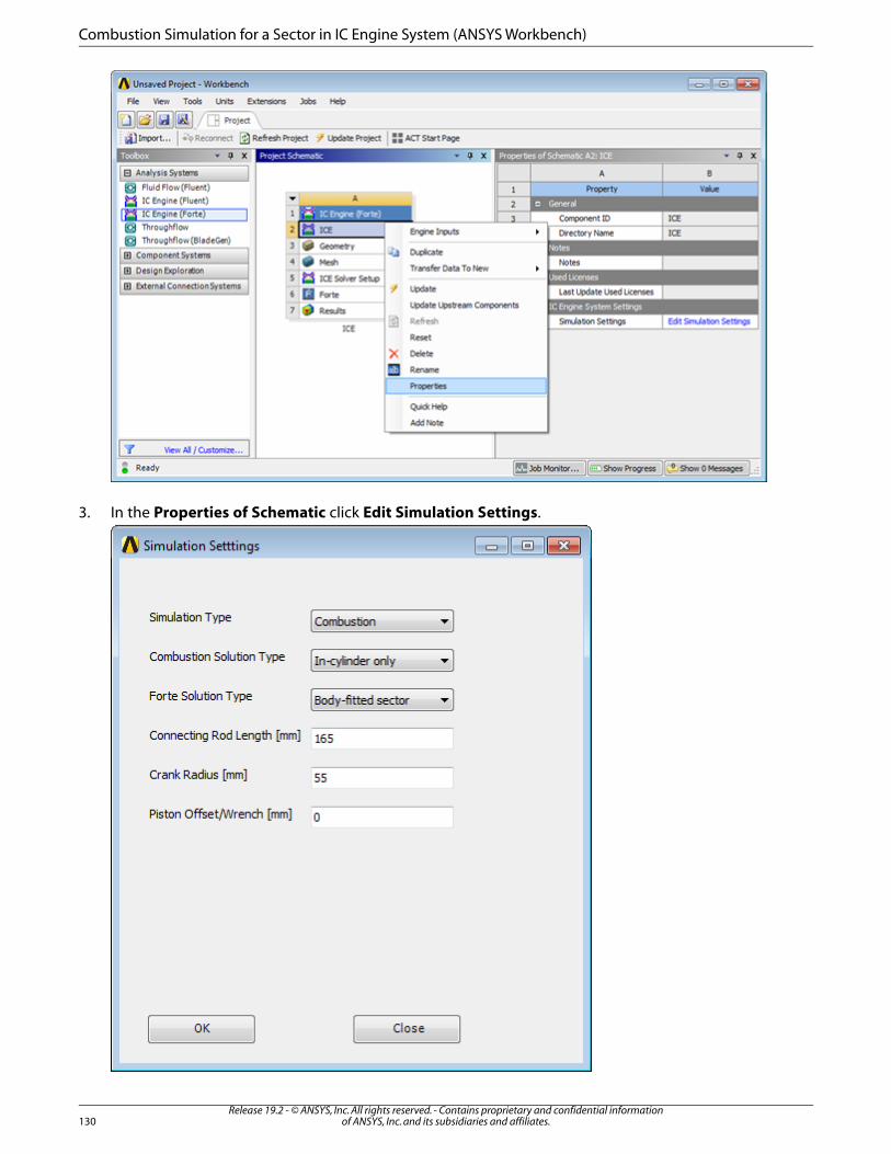
3. In the Properties of Schematic click Edit Simulation Settings.
Release 19.2 - © ANSYS, Inc. All rights reserved. - Contains proprietary and confidential informationof ANSYS, Inc. and its subsidiaries and affiliates.130
Combustion Simulation for a Sector in IC Engine System (ANSYS Workbench)
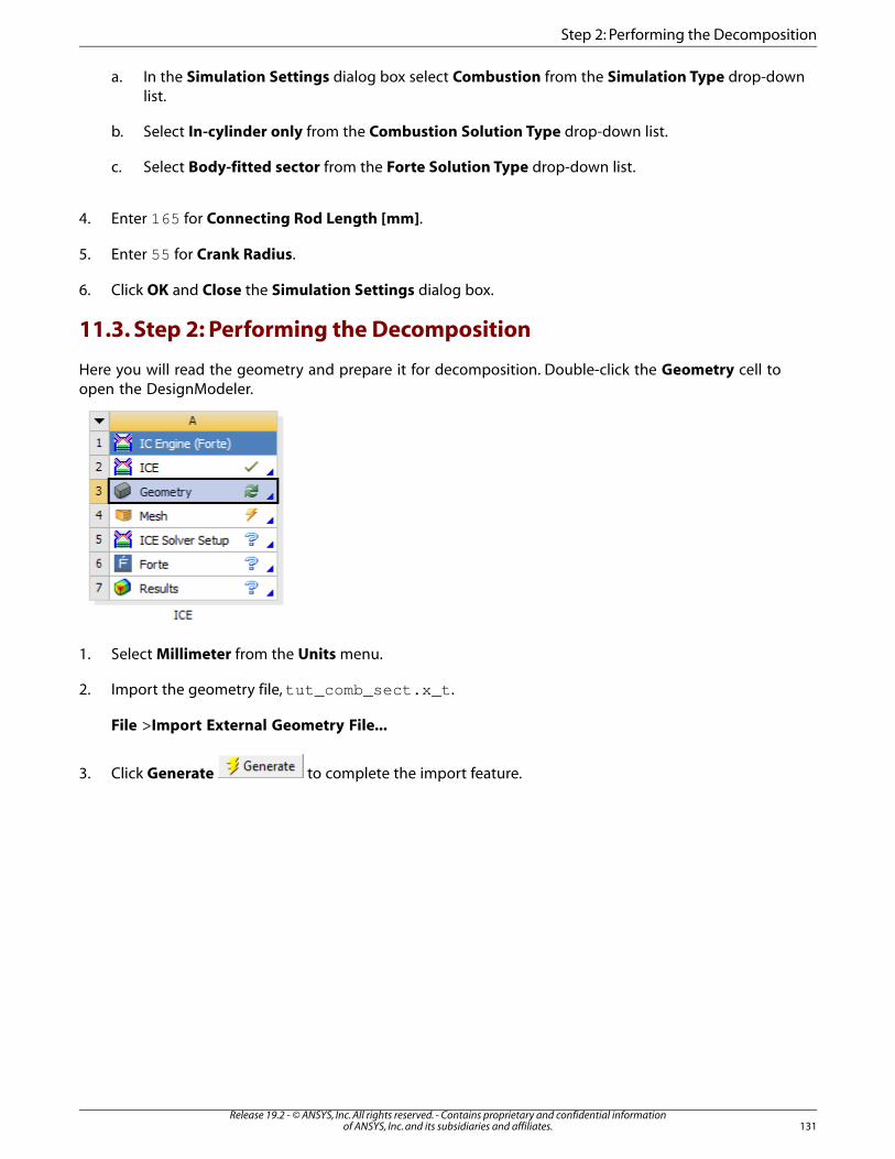
a. In the Simulation Settings dialog box select Combustion from the Simulation Type drop-downlist.
b. Select In-cylinder only from the Combustion Solution Type drop-down list.
c. Select Body-fitted sector from the Forte Solution Type drop-down list.
4. Enter 165 for Connecting Rod Length [mm].
5. Enter 55 for Crank Radius.
6. Click OK and Close the Simulation Settings dialog box.
11.3. Step 2: Performing the Decomposition
Here you will read the geometry and prepare it for decomposition. Double-click the Geometry cell toopen the DesignModeler.
1. Select Millimeter from the Units menu.
2. Import the geometry file,tut_comb_sect.x_t.
File >Import External Geometry File...
3. Click Generate to complete the import feature.
131Release 19.2 - © ANSYS, Inc. All rights reserved. - Contains proprietary and confidential information
of ANSYS, Inc. and its subsidiaries and affiliates.
Step 2: Performing the Decomposition

4. Click Input Manager located in the IC Engine toolbar.
a. Retain Complete Geometry from the Sector Decomposition Type drop-down list as the inputgeometry you have chosen is a complete geometry.
Release 19.2 - © ANSYS, Inc. All rights reserved. - Contains proprietary and confidential informationof ANSYS, Inc. and its subsidiaries and affiliates.132
Combustion Simulation for a Sector in IC Engine System (ANSYS Workbench)
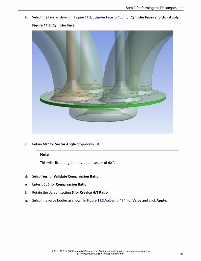
b. Select the face as shown in Figure 11.2: Cylinder Face (p. 133) for Cylinder Faces and click Apply.
Figure 11.2: Cylinder Face
c. Retain 60 ° for Sector Angle drop-down list.
Note
This will slice the geometry into a sector of 60 °.
d. Select Yes for Validate Compression Ratio.
e. Enter 15.5 for Compression Ratio.
f. Retain the default setting 3 for Crevice H/T Ratio.
g. Select the valve bodies as shown in Figure 11.3: Valves (p. 134) for Valve and click Apply.
133Release 19.2 - © ANSYS, Inc. All rights reserved. - Contains proprietary and confidential information
of ANSYS, Inc. and its subsidiaries and affiliates.
Step 2: Performing the Decomposition

Figure 11.3: Valves
h. Select the valve seat faces as shown in Figure 11.2: Cylinder Face (p. 133) for Valve Seat and clickApply.
Release 19.2 - © ANSYS, Inc. All rights reserved. - Contains proprietary and confidential informationof ANSYS, Inc. and its subsidiaries and affiliates.134
Combustion Simulation for a Sector in IC Engine System (ANSYS Workbench)
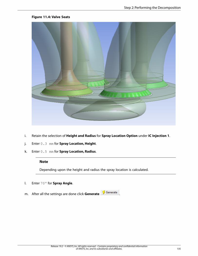
Figure 11.4: Valve Seats
i. Retain the selection of Height and Radius for Spray Location Option under IC Injection 1.
j. Enter 0.3 mm for Spray Location, Height.
k. Enter 0.5 mm for Spray Location, Radius.
Note
Depending upon the height and radius the spray location is calculated.
l. Enter 70° for Spray Angle.
m. After all the settings are done click Generate .
135Release 19.2 - © ANSYS, Inc. All rights reserved. - Contains proprietary and confidential information
of ANSYS, Inc. and its subsidiaries and affiliates.
Step 2: Performing the Decomposition
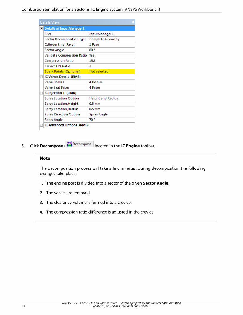
5. Click Decompose ( located in the IC Engine toolbar).
Note
The decomposition process will take a few minutes. During decomposition the followingchanges take place:
1. The engine port is divided into a sector of the given Sector Angle.
2. The valves are removed.
3. The clearance volume is formed into a crevice.
4. The compression ratio difference is adjusted in the crevice.
Release 19.2 - © ANSYS, Inc. All rights reserved. - Contains proprietary and confidential informationof ANSYS, Inc. and its subsidiaries and affiliates.136
Combustion Simulation for a Sector in IC Engine System (ANSYS Workbench)

Figure 11.5: Decomposed Geometry
6. During decomposition a warning pops up asking if you would like to compensate for the difference incompression ratio.
Click Yes.
7. After the geometry has been successfully decomposed click Show Spray Cone .
137Release 19.2 - © ANSYS, Inc. All rights reserved. - Contains proprietary and confidential information
of ANSYS, Inc. and its subsidiaries and affiliates.
Step 2: Performing the Decomposition
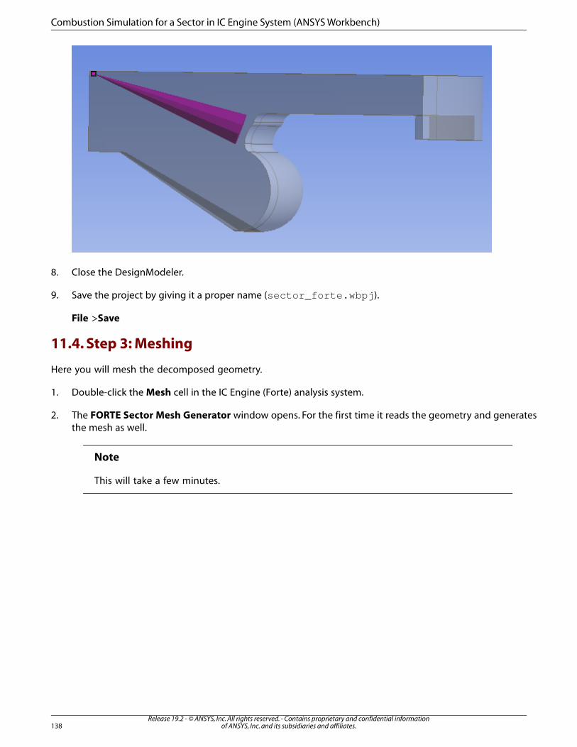
8. Close the DesignModeler.
9. Save the project by giving it a proper name (sector_forte.wbpj).
File >Save
11.4. Step 3: Meshing
Here you will mesh the decomposed geometry.
1. Double-click the Mesh cell in the IC Engine (Forte) analysis system.
2. The FORTE Sector Mesh Generator window opens. For the first time it reads the geometry and generatesthe mesh as well.
Note
This will take a few minutes.
Release 19.2 - © ANSYS, Inc. All rights reserved. - Contains proprietary and confidential informationof ANSYS, Inc. and its subsidiaries and affiliates.138
Combustion Simulation for a Sector in IC Engine System (ANSYS Workbench)
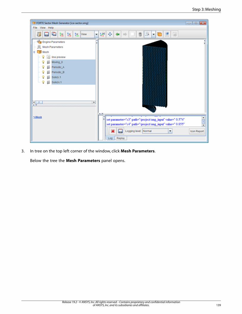
3. In tree on the top left corner of the window, click Mesh Parameters.
Below the tree the Mesh Parameters panel opens.
139Release 19.2 - © ANSYS, Inc. All rights reserved. - Contains proprietary and confidential information
of ANSYS, Inc. and its subsidiaries and affiliates.
Step 3: Meshing
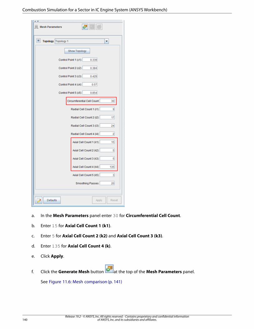
a. In the Mesh Parameters panel enter 30 for Circumferential Cell Count.
b. Enter 15 for Axial Cell Count 1 (k1).
c. Enter 5 for Axial Cell Count 2 (k2) and Axial Cell Count 3 (k3).
d. Enter 135 for Axial Cell Count 4 (k).
e. Click Apply.
f. Click the Generate Mesh button at the top of the Mesh Parameters panel.
See Figure 11.6: Mesh comparison (p. 141)
Release 19.2 - © ANSYS, Inc. All rights reserved. - Contains proprietary and confidential informationof ANSYS, Inc. and its subsidiaries and affiliates.140
Combustion Simulation for a Sector in IC Engine System (ANSYS Workbench)
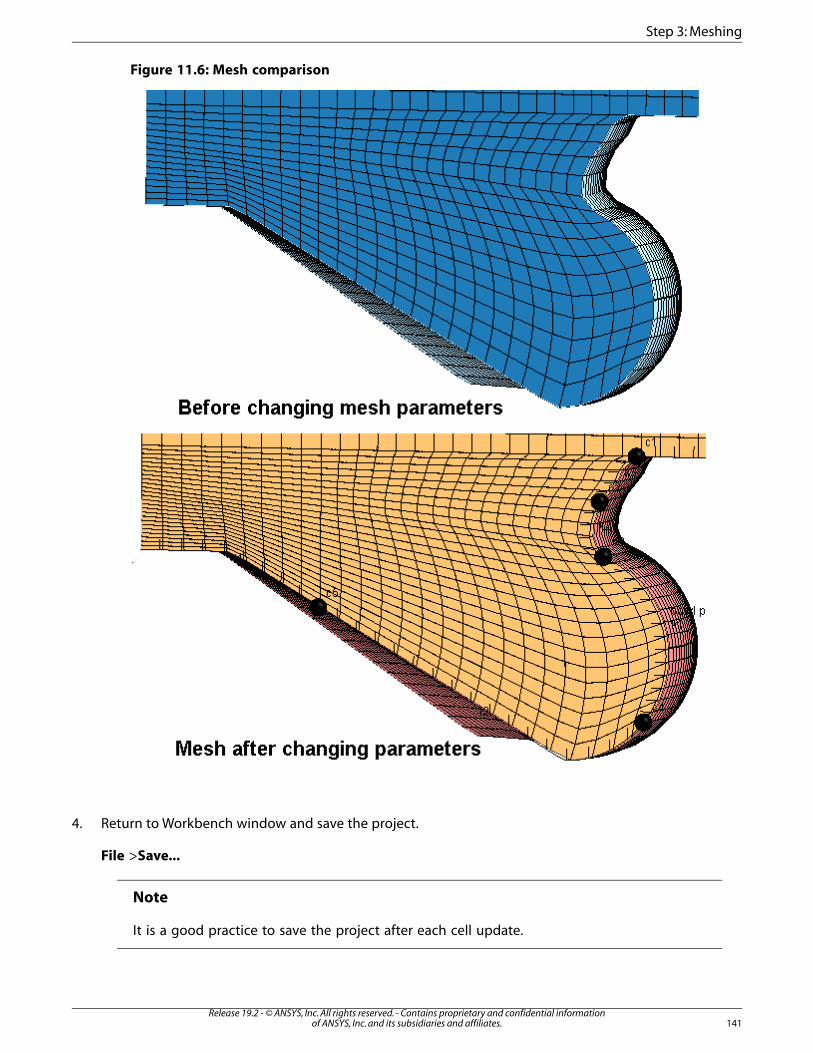
Figure 11.6: Mesh comparison
4. Return to Workbench window and save the project.
File >Save...
Note
It is a good practice to save the project after each cell update.
141Release 19.2 - © ANSYS, Inc. All rights reserved. - Contains proprietary and confidential information
of ANSYS, Inc. and its subsidiaries and affiliates.
Step 3: Meshing
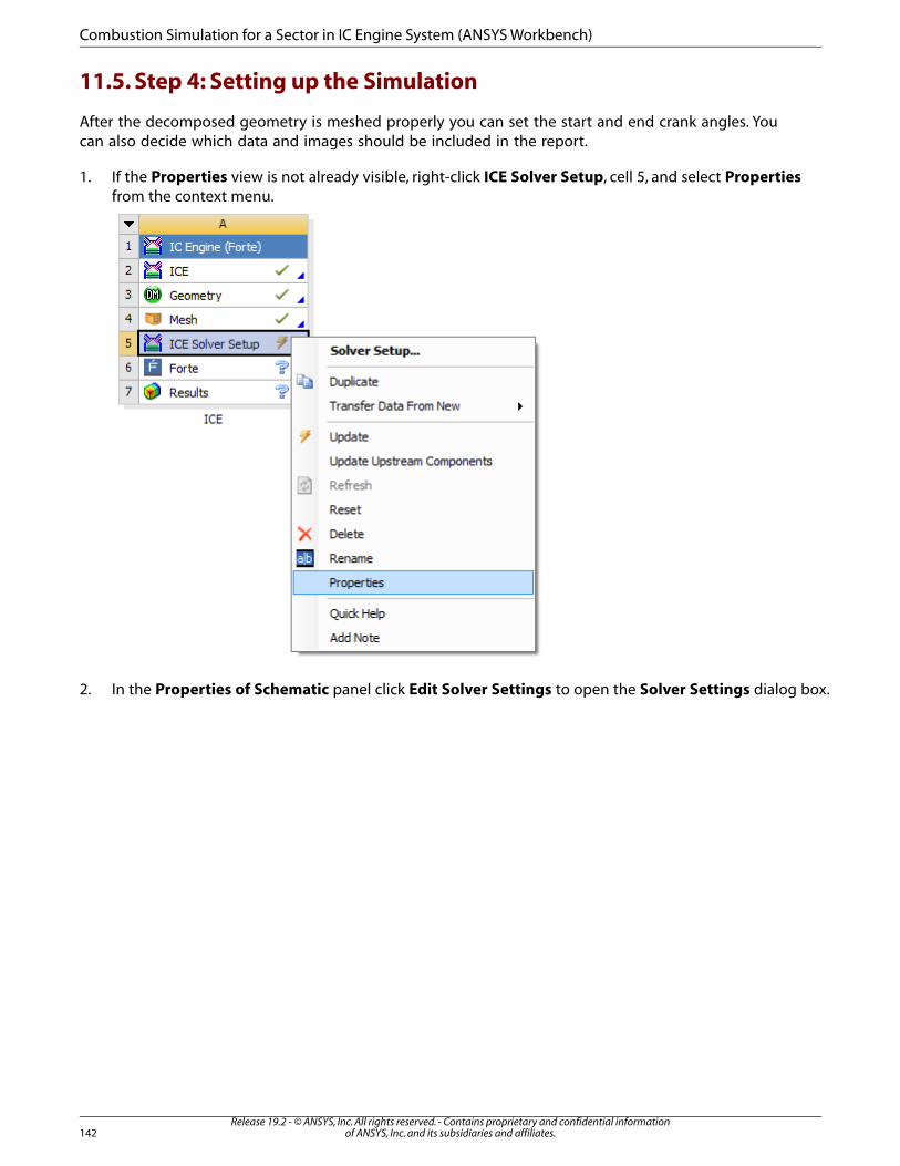
11.5. Step 4: Setting up the Simulation
After the decomposed geometry is meshed properly you can set the start and end crank angles. Youcan also decide which data and images should be included in the report.
1. If the Properties view is not already visible, right-click ICE Solver Setup, cell 5, and select Propertiesfrom the context menu.
2. In the Properties of Schematic panel click Edit Solver Settings to open the Solver Settings dialog box.
Release 19.2 - © ANSYS, Inc. All rights reserved. - Contains proprietary and confidential informationof ANSYS, Inc. and its subsidiaries and affiliates.142
Combustion Simulation for a Sector in IC Engine System (ANSYS Workbench)
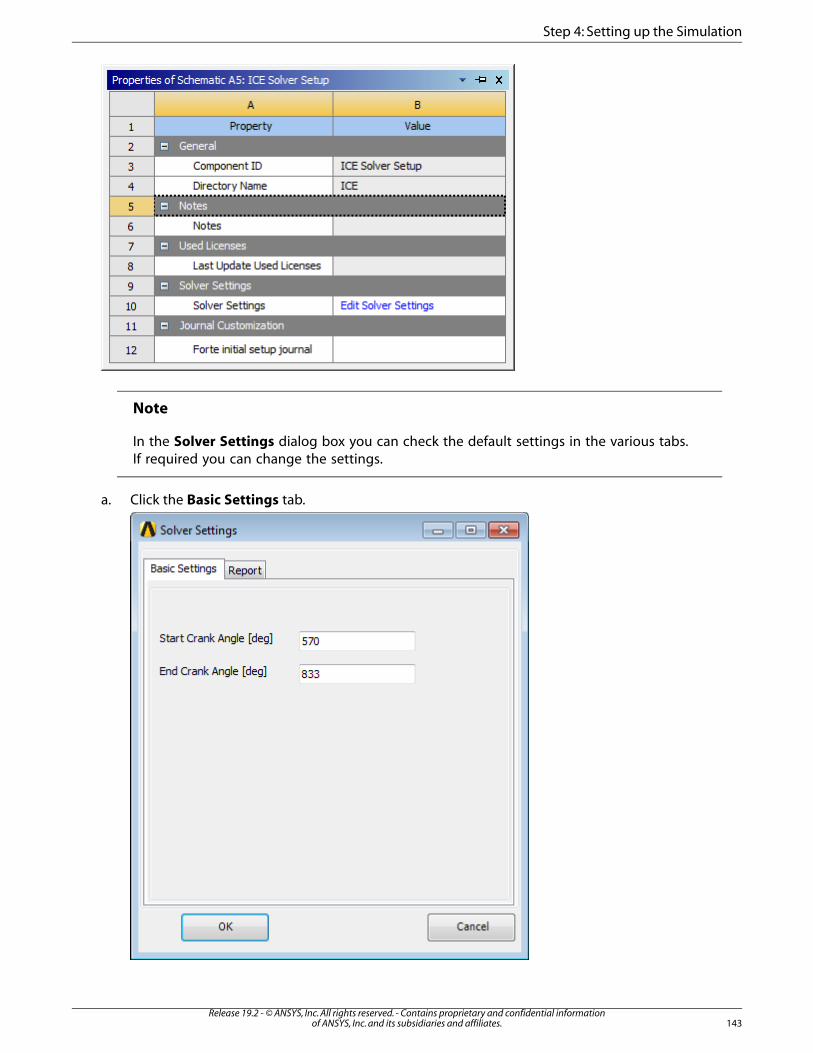
Note
In the Solver Settings dialog box you can check the default settings in the various tabs.If required you can change the settings.
a. Click the Basic Settings tab.
143Release 19.2 - © ANSYS, Inc. All rights reserved. - Contains proprietary and confidential information
of ANSYS, Inc. and its subsidiaries and affiliates.
Step 4: Setting up the Simulation
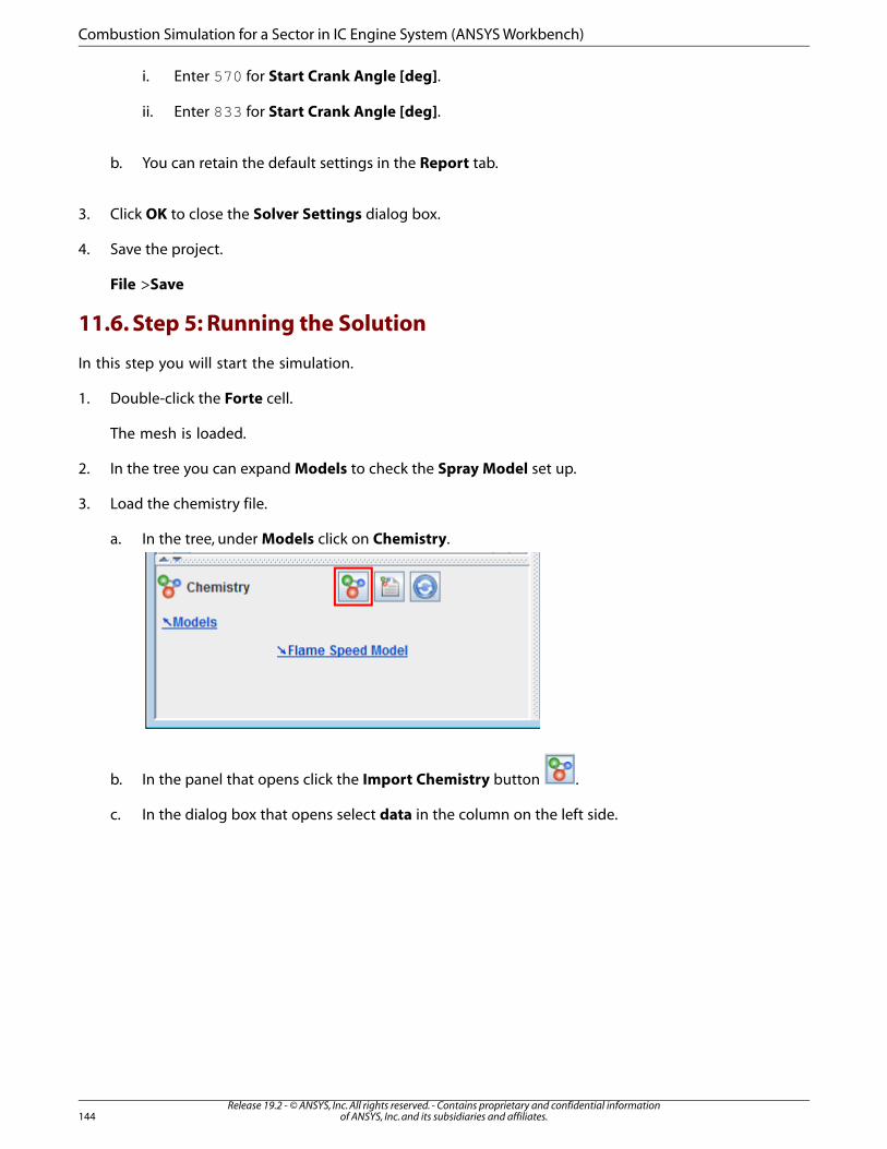
i. Enter 570 for Start Crank Angle [deg].
ii. Enter 833 for Start Crank Angle [deg].
b. You can retain the default settings in the Report tab.
3. Click OK to close the Solver Settings dialog box.
4. Save the project.
File >Save
11.6. Step 5: Running the Solution
In this step you will start the simulation.
1. Double-click the Forte cell.
The mesh is loaded.
2. In the tree you can expand Models to check the Spray Model set up.
3. Load the chemistry file.
a. In the tree, under Models click on Chemistry.
b. In the panel that opens click the Import Chemistry button .
c. In the dialog box that opens select data in the column on the left side.
Release 19.2 - © ANSYS, Inc. All rights reserved. - Contains proprietary and confidential informationof ANSYS, Inc. and its subsidiaries and affiliates.144
Combustion Simulation for a Sector in IC Engine System (ANSYS Workbench)
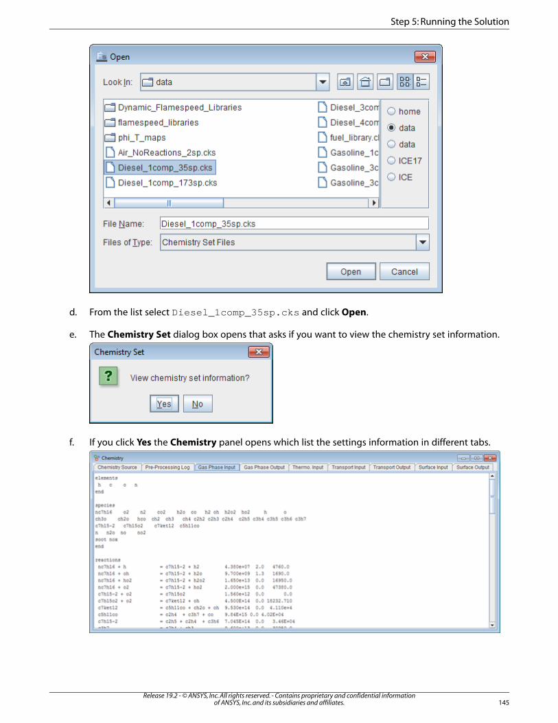
d. From the list select Diesel_1comp_35sp.cks and click Open.
e. The Chemistry Set dialog box opens that asks if you want to view the chemistry set information.
f. If you click Yes the Chemistry panel opens which list the settings information in different tabs.
145Release 19.2 - © ANSYS, Inc. All rights reserved. - Contains proprietary and confidential information
of ANSYS, Inc. and its subsidiaries and affiliates.
Step 5: Running the Solution
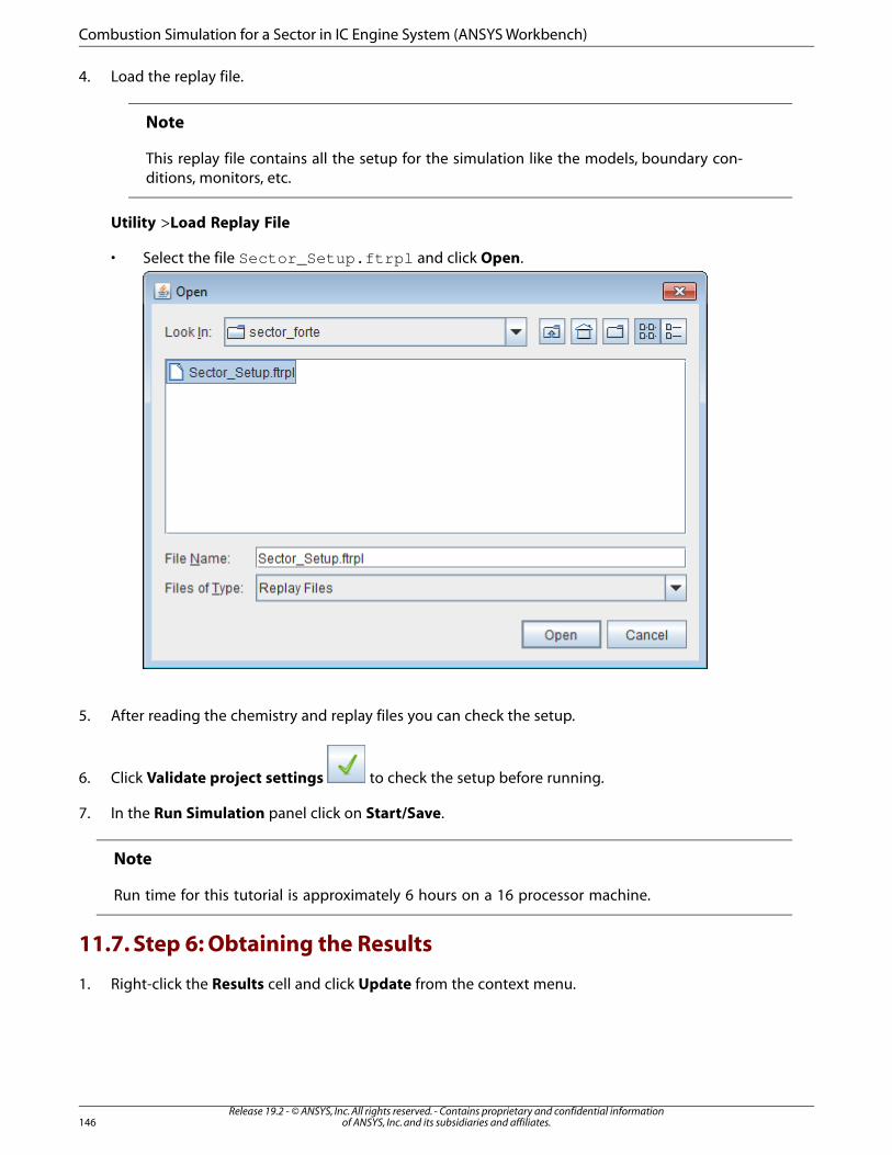
4. Load the replay file.
Note
This replay file contains all the setup for the simulation like the models, boundary con-ditions, monitors, etc.
Utility >Load Replay File
• Select the file Sector_Setup.ftrpl and click Open.
5. After reading the chemistry and replay files you can check the setup.
6. Click Validate project settings to check the setup before running.
7. In the Run Simulation panel click on Start/Save.
Note
Run time for this tutorial is approximately 6 hours on a 16 processor machine.
11.7. Step 6: Obtaining the Results
1. Right-click the Results cell and click Update from the context menu.
Release 19.2 - © ANSYS, Inc. All rights reserved. - Contains proprietary and confidential informationof ANSYS, Inc. and its subsidiaries and affiliates.146
Combustion Simulation for a Sector in IC Engine System (ANSYS Workbench)
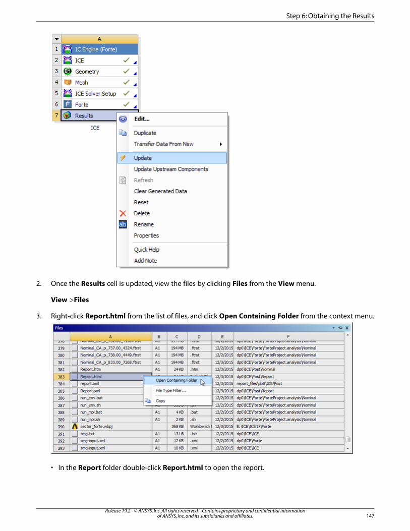
2. Once the Results cell is updated, view the files by clicking Files from the View menu.
View >Files
3. Right-click Report.html from the list of files, and click Open Containing Folder from the context menu.
• In the Report folder double-click Report.html to open the report.
147Release 19.2 - © ANSYS, Inc. All rights reserved. - Contains proprietary and confidential information
of ANSYS, Inc. and its subsidiaries and affiliates.
Step 6: Obtaining the Results
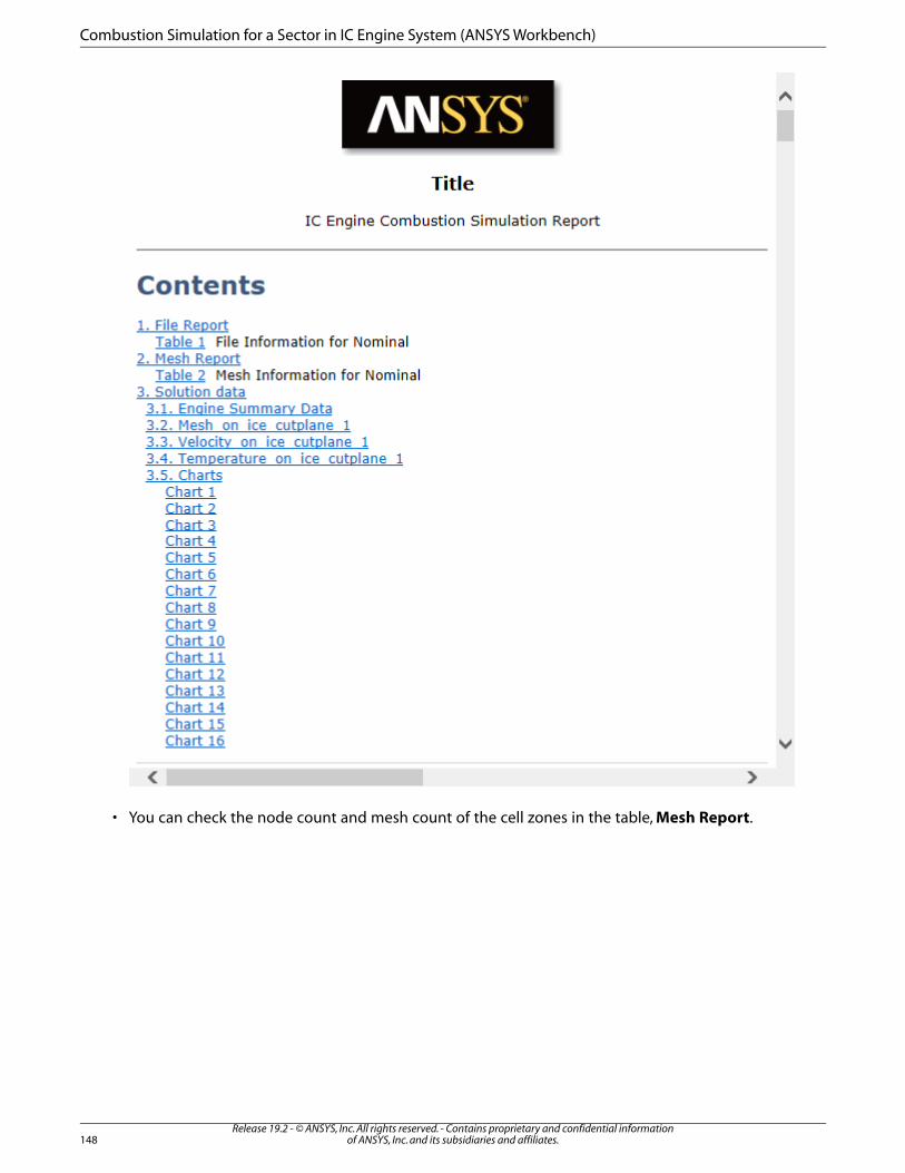
• You can check the node count and mesh count of the cell zones in the table, Mesh Report.
Release 19.2 - © ANSYS, Inc. All rights reserved. - Contains proprietary and confidential informationof ANSYS, Inc. and its subsidiaries and affiliates.148
Combustion Simulation for a Sector in IC Engine System (ANSYS Workbench)
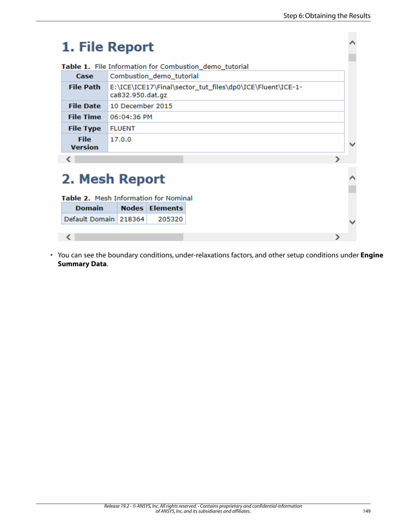
• You can see the boundary conditions, under-relaxations factors, and other setup conditions under EngineSummary Data.
149Release 19.2 - © ANSYS, Inc. All rights reserved. - Contains proprietary and confidential information
of ANSYS, Inc. and its subsidiaries and affiliates.
Step 6: Obtaining the Results
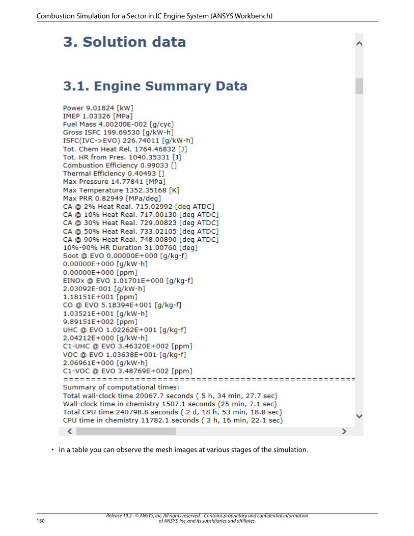
• In a table you can observe the mesh images at various stages of the simulation.
Release 19.2 - © ANSYS, Inc. All rights reserved. - Contains proprietary and confidential informationof ANSYS, Inc. and its subsidiaries and affiliates.150
Combustion Simulation for a Sector in IC Engine System (ANSYS Workbench)
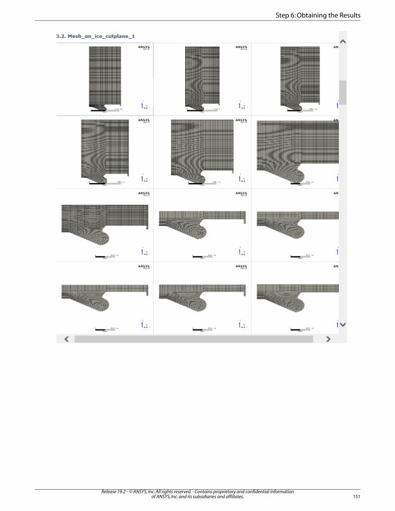
151Release 19.2 - © ANSYS, Inc. All rights reserved. - Contains proprietary and confidential information
of ANSYS, Inc. and its subsidiaries and affiliates.
Step 6: Obtaining the Results
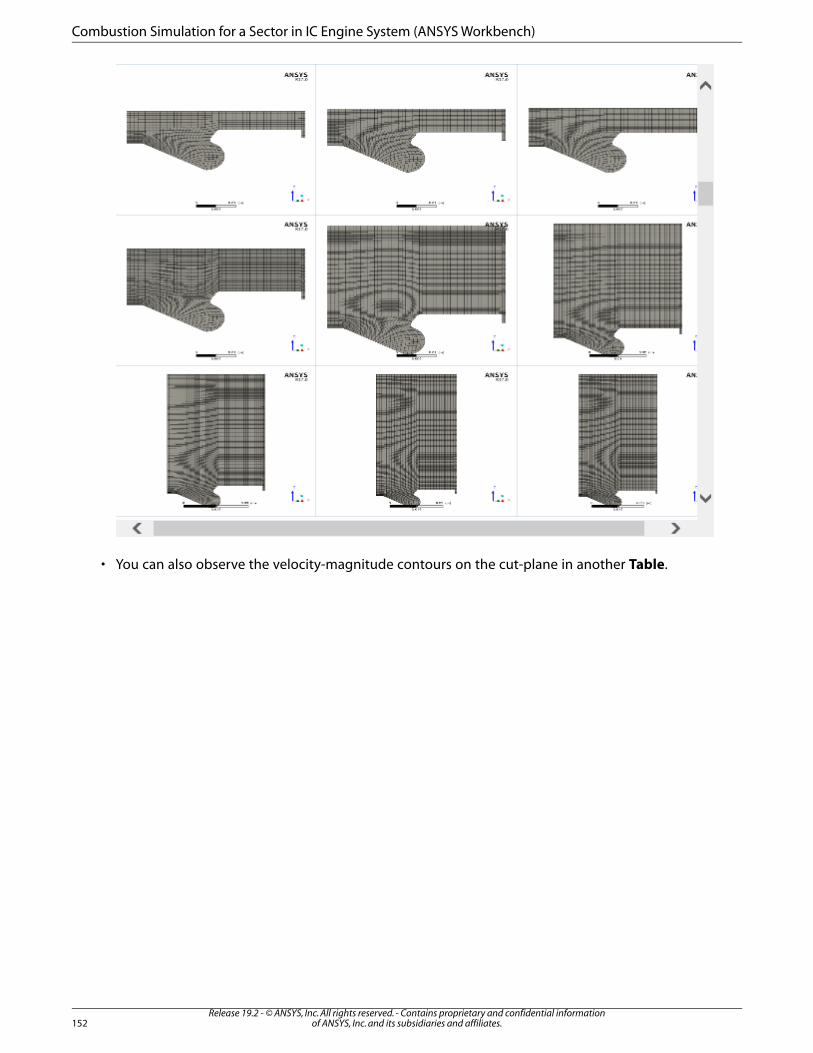
• You can also observe the velocity-magnitude contours on the cut-plane in another Table.
Release 19.2 - © ANSYS, Inc. All rights reserved. - Contains proprietary and confidential informationof ANSYS, Inc. and its subsidiaries and affiliates.152
Combustion Simulation for a Sector in IC Engine System (ANSYS Workbench)

153Release 19.2 - © ANSYS, Inc. All rights reserved. - Contains proprietary and confidential information
of ANSYS, Inc. and its subsidiaries and affiliates.
Step 6: Obtaining the Results
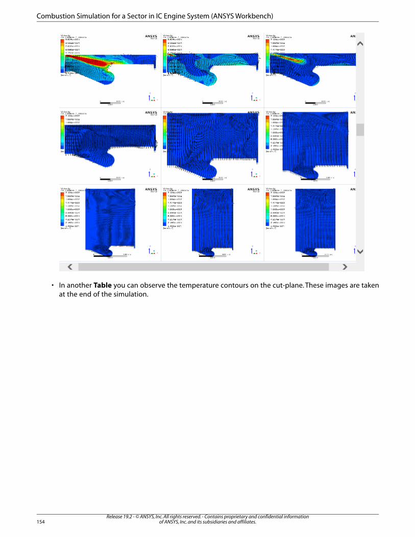
• In another Table you can observe the temperature contours on the cut-plane. These images are takenat the end of the simulation.
Release 19.2 - © ANSYS, Inc. All rights reserved. - Contains proprietary and confidential informationof ANSYS, Inc. and its subsidiaries and affiliates.154
Combustion Simulation for a Sector in IC Engine System (ANSYS Workbench)
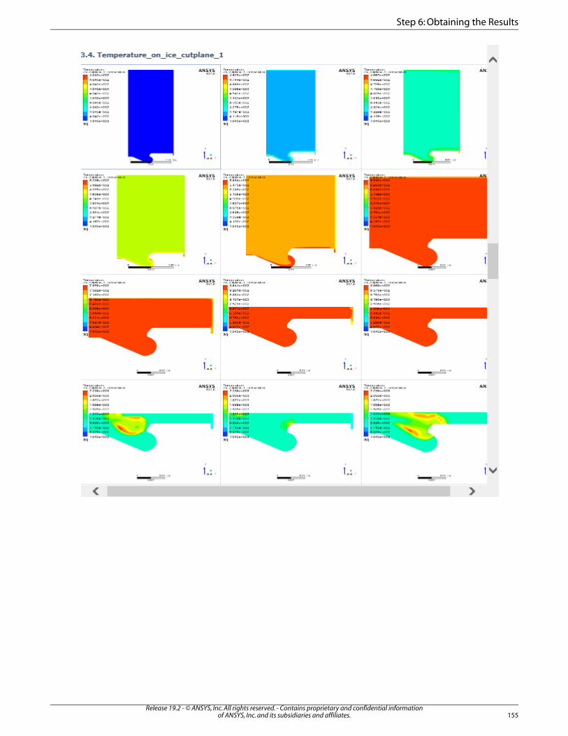
155Release 19.2 - © ANSYS, Inc. All rights reserved. - Contains proprietary and confidential information
of ANSYS, Inc. and its subsidiaries and affiliates.
Step 6: Obtaining the Results
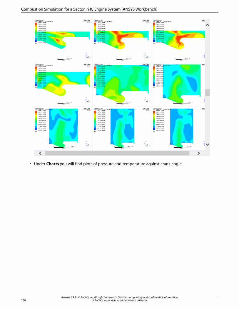
• Under Charts you will find plots of pressure and temperature against crank angle.
Release 19.2 - © ANSYS, Inc. All rights reserved. - Contains proprietary and confidential informationof ANSYS, Inc. and its subsidiaries and affiliates.156
Combustion Simulation for a Sector in IC Engine System (ANSYS Workbench)
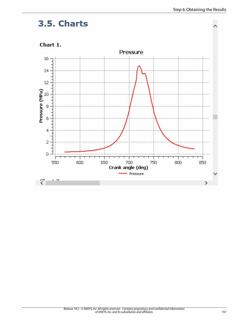
157Release 19.2 - © ANSYS, Inc. All rights reserved. - Contains proprietary and confidential information
of ANSYS, Inc. and its subsidiaries and affiliates.
Step 6: Obtaining the Results
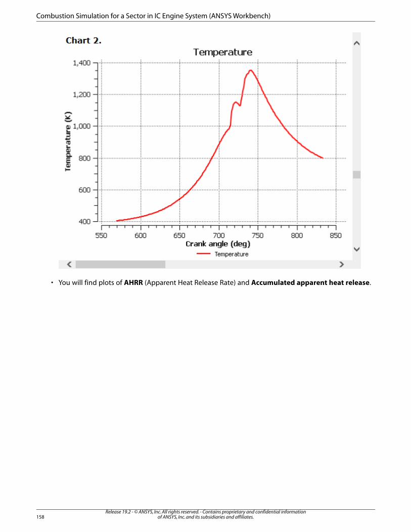
• You will find plots of AHRR (Apparent Heat Release Rate) and Accumulated apparent heat release.
Release 19.2 - © ANSYS, Inc. All rights reserved. - Contains proprietary and confidential informationof ANSYS, Inc. and its subsidiaries and affiliates.158
Combustion Simulation for a Sector in IC Engine System (ANSYS Workbench)
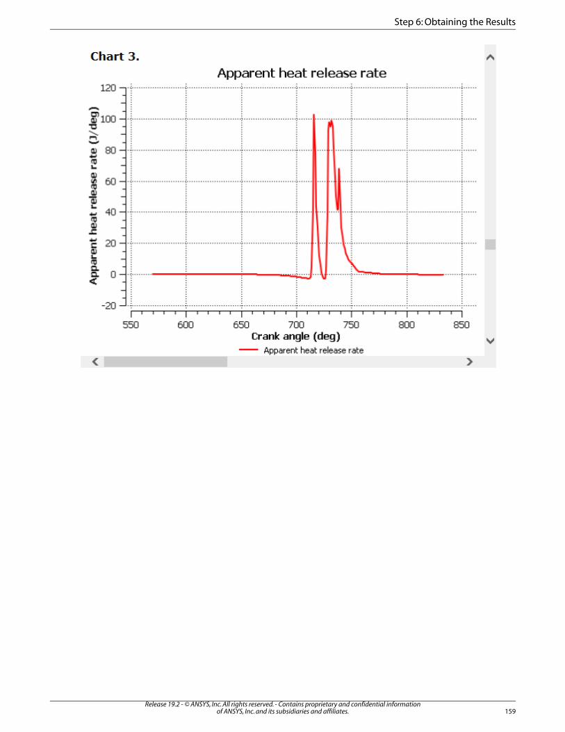
159Release 19.2 - © ANSYS, Inc. All rights reserved. - Contains proprietary and confidential information
of ANSYS, Inc. and its subsidiaries and affiliates.
Step 6: Obtaining the Results
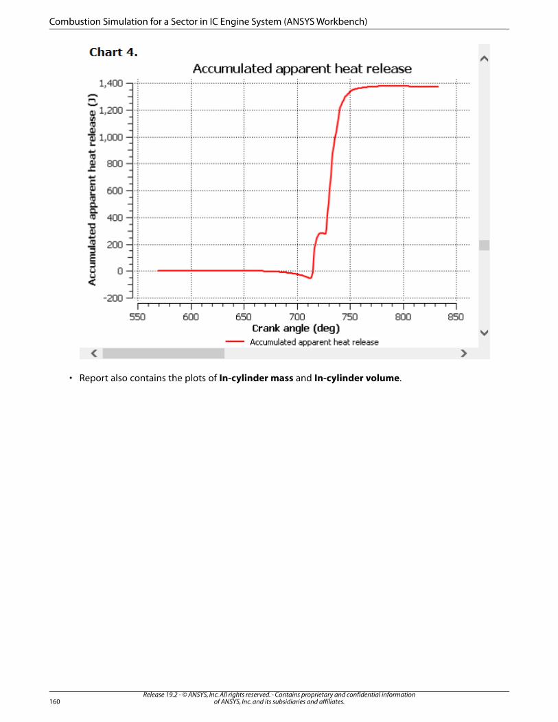
• Report also contains the plots of In-cylinder mass and In-cylinder volume.
Release 19.2 - © ANSYS, Inc. All rights reserved. - Contains proprietary and confidential informationof ANSYS, Inc. and its subsidiaries and affiliates.160
Combustion Simulation for a Sector in IC Engine System (ANSYS Workbench)
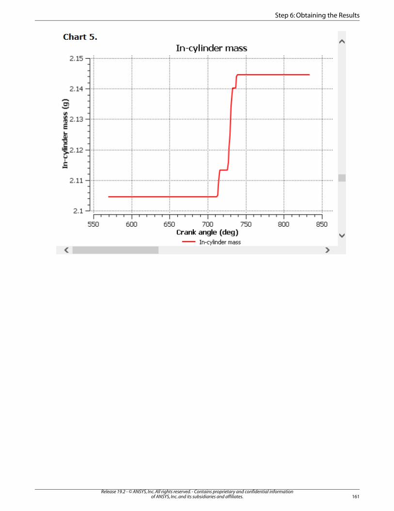
161Release 19.2 - © ANSYS, Inc. All rights reserved. - Contains proprietary and confidential information
of ANSYS, Inc. and its subsidiaries and affiliates.
Step 6: Obtaining the Results
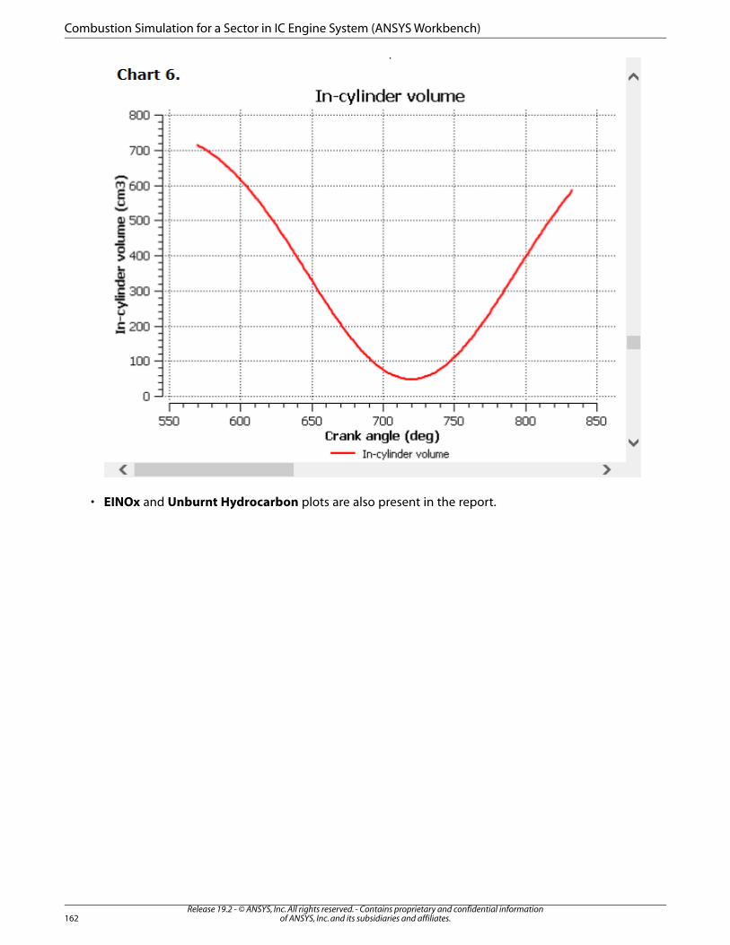
• EINOx and Unburnt Hydrocarbon plots are also present in the report.
Release 19.2 - © ANSYS, Inc. All rights reserved. - Contains proprietary and confidential informationof ANSYS, Inc. and its subsidiaries and affiliates.162
Combustion Simulation for a Sector in IC Engine System (ANSYS Workbench)
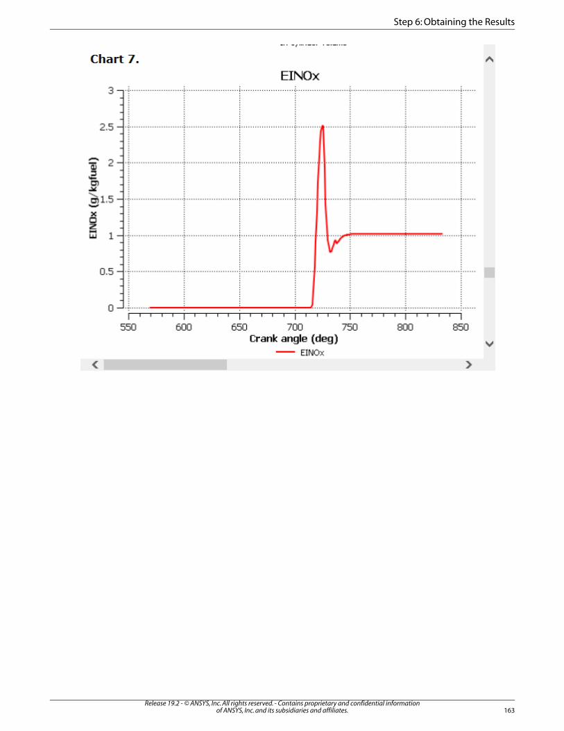
163Release 19.2 - © ANSYS, Inc. All rights reserved. - Contains proprietary and confidential information
of ANSYS, Inc. and its subsidiaries and affiliates.
Step 6: Obtaining the Results
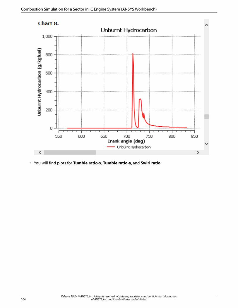
• You will find plots for Tumble ratio-x, Tumble ratio-y, and Swirl ratio.
Release 19.2 - © ANSYS, Inc. All rights reserved. - Contains proprietary and confidential informationof ANSYS, Inc. and its subsidiaries and affiliates.164
Combustion Simulation for a Sector in IC Engine System (ANSYS Workbench)

165Release 19.2 - © ANSYS, Inc. All rights reserved. - Contains proprietary and confidential information
of ANSYS, Inc. and its subsidiaries and affiliates.
Step 6: Obtaining the Results
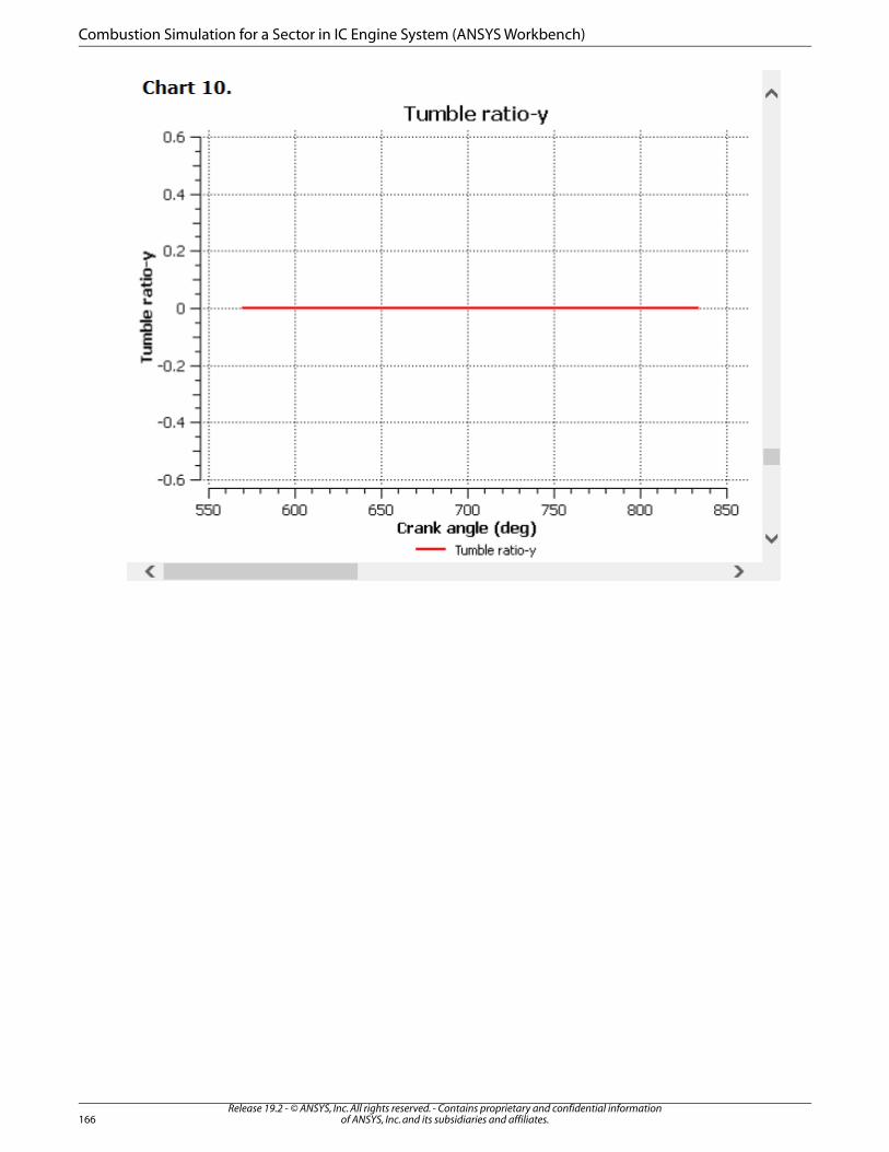
Release 19.2 - © ANSYS, Inc. All rights reserved. - Contains proprietary and confidential informationof ANSYS, Inc. and its subsidiaries and affiliates.166
Combustion Simulation for a Sector in IC Engine System (ANSYS Workbench)
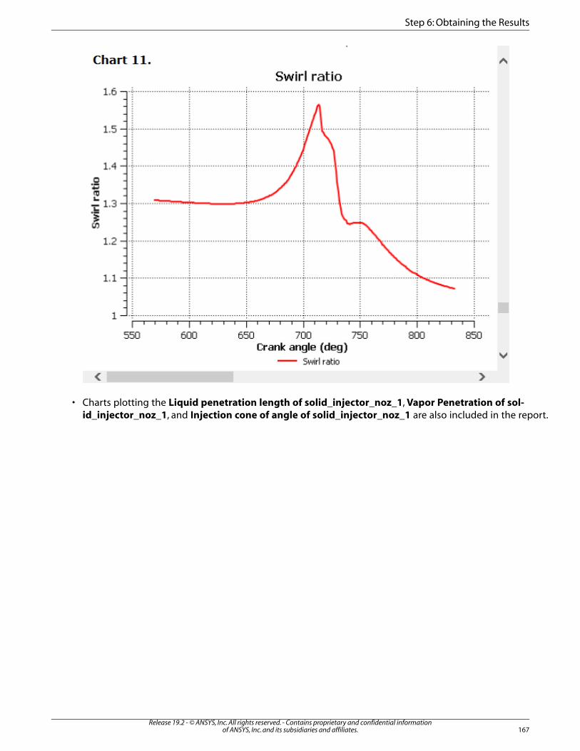
• Charts plotting the Liquid penetration length of solid_injector_noz_1, Vapor Penetration of sol-id_injector_noz_1, and Injection cone of angle of solid_injector_noz_1 are also included in the report.
167Release 19.2 - © ANSYS, Inc. All rights reserved. - Contains proprietary and confidential information
of ANSYS, Inc. and its subsidiaries and affiliates.
Step 6: Obtaining the Results
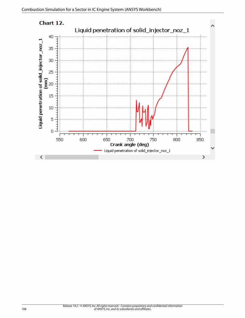
Release 19.2 - © ANSYS, Inc. All rights reserved. - Contains proprietary and confidential informationof ANSYS, Inc. and its subsidiaries and affiliates.168
Combustion Simulation for a Sector in IC Engine System (ANSYS Workbench)
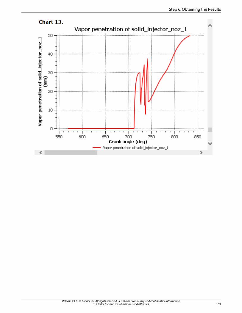
169Release 19.2 - © ANSYS, Inc. All rights reserved. - Contains proprietary and confidential information
of ANSYS, Inc. and its subsidiaries and affiliates.
Step 6: Obtaining the Results

• Lastly in the report you can see the charts of Average Sauter mean diameter and Mass averageddroplet velocity.
Release 19.2 - © ANSYS, Inc. All rights reserved. - Contains proprietary and confidential informationof ANSYS, Inc. and its subsidiaries and affiliates.170
Combustion Simulation for a Sector in IC Engine System (ANSYS Workbench)
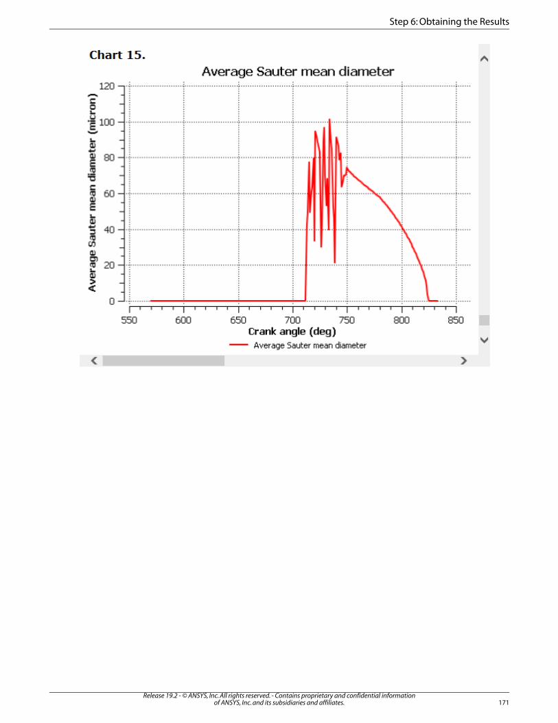
171Release 19.2 - © ANSYS, Inc. All rights reserved. - Contains proprietary and confidential information
of ANSYS, Inc. and its subsidiaries and affiliates.
Step 6: Obtaining the Results
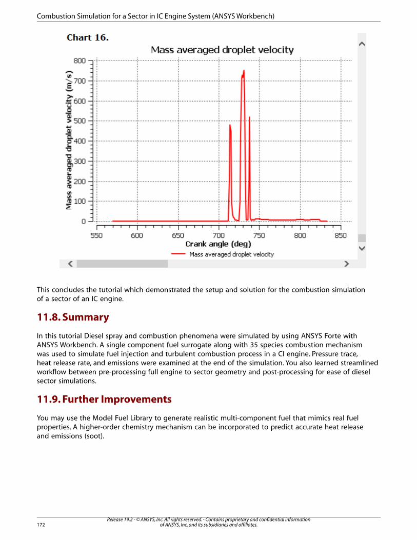
This concludes the tutorial which demonstrated the setup and solution for the combustion simulationof a sector of an IC engine.
11.8. Summary
In this tutorial Diesel spray and combustion phenomena were simulated by using ANSYS Forte withANSYS Workbench. A single component fuel surrogate along with 35 species combustion mechanismwas used to simulate fuel injection and turbulent combustion process in a CI engine. Pressure trace,heat release rate, and emissions were examined at the end of the simulation. You also learned streamlinedworkflow between pre-processing full engine to sector geometry and post-processing for ease of dieselsector simulations.
11.9. Further Improvements
You may use the Model Fuel Library to generate realistic multi-component fuel that mimics real fuelproperties. A higher-order chemistry mechanism can be incorporated to predict accurate heat releaseand emissions (soot).
Release 19.2 - © ANSYS, Inc. All rights reserved. - Contains proprietary and confidential informationof ANSYS, Inc. and its subsidiaries and affiliates.172
Combustion Simulation for a Sector in IC Engine System (ANSYS Workbench)
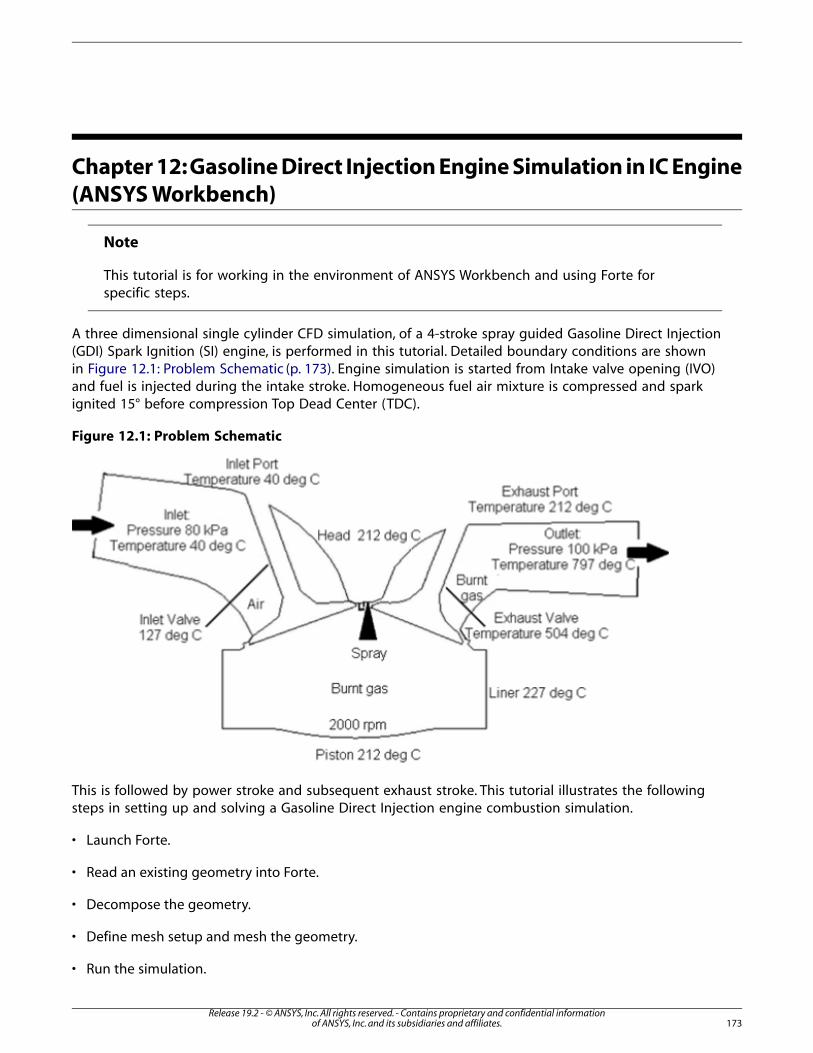
Chapter 12: Gasoline Direct Injection Engine Simulation in IC Engine(ANSYS Workbench)
Note
This tutorial is for working in the environment of ANSYS Workbench and using Forte forspecific steps.
A three dimensional single cylinder CFD simulation, of a 4-stroke spray guided Gasoline Direct Injection(GDI) Spark Ignition (SI) engine, is performed in this tutorial. Detailed boundary conditions are shownin Figure 12.1: Problem Schematic (p. 173). Engine simulation is started from Intake valve opening (IVO)and fuel is injected during the intake stroke. Homogeneous fuel air mixture is compressed and sparkignited 15° before compression Top Dead Center (TDC).
Figure 12.1: Problem Schematic
This is followed by power stroke and subsequent exhaust stroke. This tutorial illustrates the followingsteps in setting up and solving a Gasoline Direct Injection engine combustion simulation.
• Launch Forte.
• Read an existing geometry into Forte.
• Decompose the geometry.
• Define mesh setup and mesh the geometry.
• Run the simulation.
173Release 19.2 - © ANSYS, Inc. All rights reserved. - Contains proprietary and confidential information
of ANSYS, Inc. and its subsidiaries and affiliates.
• Examine the results in the report.
This tutorial is written with the assumption that you are familiar with the ANSYS Workbench IC Enginesystem and that you have a good working knowledge of ANSYS Workbench. For more information onIC Engines refer to the Fluent User's Guide, Forte User's Guide, and Fluent Workbench Tutorials.
12.1. Preparation12.2. Step 1: Setting the Properties12.3. Step 2: Performing the Decomposition12.4. Step 3: Meshing12.5. Step 4: Setting up the Simulation12.6. Step 5: Running the Solution12.7. Step 6: Obtaining the Results12.8. Summary12.9. Further Improvements
12.1. Preparation
The files for this tutorial are obtained by downloading the sector_combustion.zip file here.
Unzip sector_combustion.zip to your working folder.
1. Copy the files (tut_gdi_forte.x_t,Gdi-Setup.ftrpl,GDI_Engine.prof,WbIceRe-port_gdi_forte.cse and footprint_gdi_forte.txt) to your working folder.
To access tutorials and their input files, go to the ANSYS Help site and select the tutorials fromthe product you desire.
2. Start Workbench.
12.2. Step 1: Setting the Properties
1. Create an IC Engine analysis system in the Workbench interface by dragging or double-clicking on ICEngine under Analysis Systems in the Toolbox.
Release 19.2 - © ANSYS, Inc. All rights reserved. - Contains proprietary and confidential informationof ANSYS, Inc. and its subsidiaries and affiliates.174
Gasoline Direct Injection Engine Simulation in IC Engine (ANSYS Workbench)
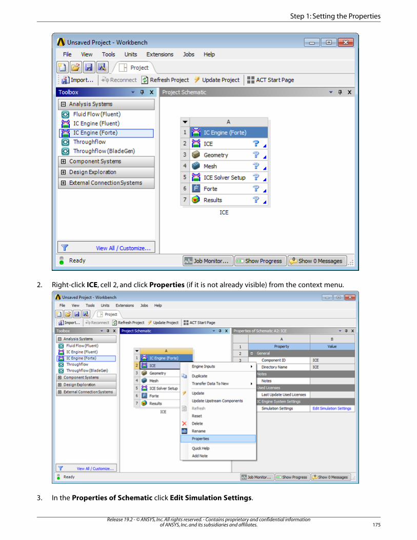
2. Right-click ICE, cell 2, and click Properties (if it is not already visible) from the context menu.
3. In the Properties of Schematic click Edit Simulation Settings.
175Release 19.2 - © ANSYS, Inc. All rights reserved. - Contains proprietary and confidential information
of ANSYS, Inc. and its subsidiaries and affiliates.
Step 1: Setting the Properties
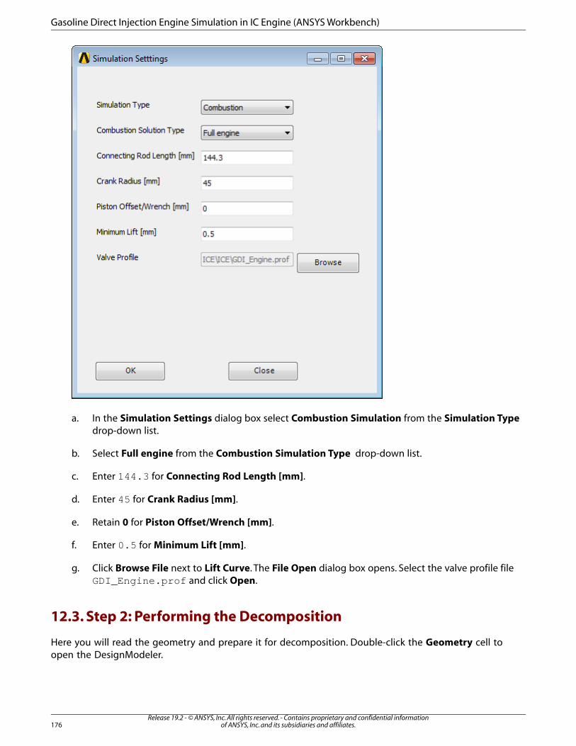
a. In the Simulation Settings dialog box select Combustion Simulation from the Simulation Typedrop-down list.
b. Select Full engine from the Combustion Simulation Type drop-down list.
c. Enter 144.3 for Connecting Rod Length [mm].
d. Enter 45 for Crank Radius [mm].
e. Retain 0 for Piston Offset/Wrench [mm].
f. Enter 0.5 for Minimum Lift [mm].
g. Click Browse File next to Lift Curve. The File Open dialog box opens. Select the valve profile fileGDI_Engine.prof and click Open.
12.3. Step 2: Performing the Decomposition
Here you will read the geometry and prepare it for decomposition. Double-click the Geometry cell toopen the DesignModeler.
Release 19.2 - © ANSYS, Inc. All rights reserved. - Contains proprietary and confidential informationof ANSYS, Inc. and its subsidiaries and affiliates.176
Gasoline Direct Injection Engine Simulation in IC Engine (ANSYS Workbench)
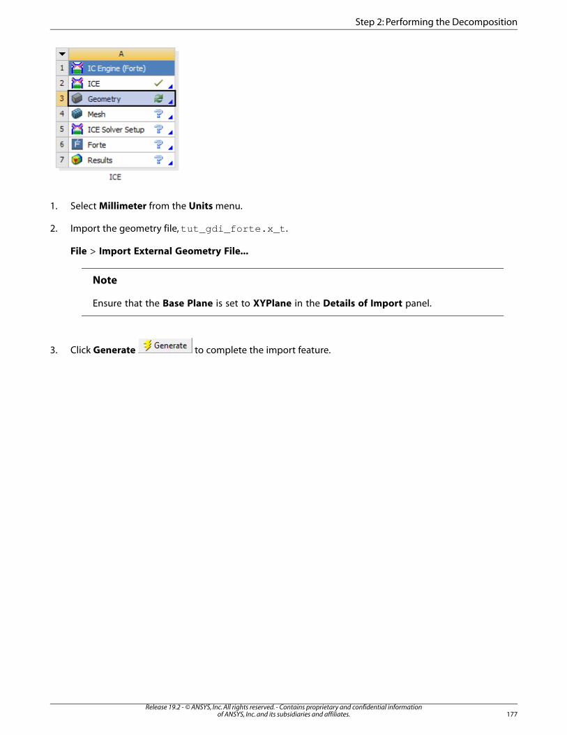
1. Select Millimeter from the Units menu.
2. Import the geometry file,tut_gdi_forte.x_t.
File > Import External Geometry File...
Note
Ensure that the Base Plane is set to XYPlane in the Details of Import panel.
3. Click Generate to complete the import feature.
177Release 19.2 - © ANSYS, Inc. All rights reserved. - Contains proprietary and confidential information
of ANSYS, Inc. and its subsidiaries and affiliates.
Step 2: Performing the Decomposition

4. Create a spark point.
Note
Before creating a point ensure that the Display Points button is pressed to enableyou to see the point created in the graphics window.
Create > Point
a. In the Details View enter Spark for Point.
b. Select Construction Point from the Type drop-down list.
Release 19.2 - © ANSYS, Inc. All rights reserved. - Contains proprietary and confidential informationof ANSYS, Inc. and its subsidiaries and affiliates.178
Gasoline Direct Injection Engine Simulation in IC Engine (ANSYS Workbench)
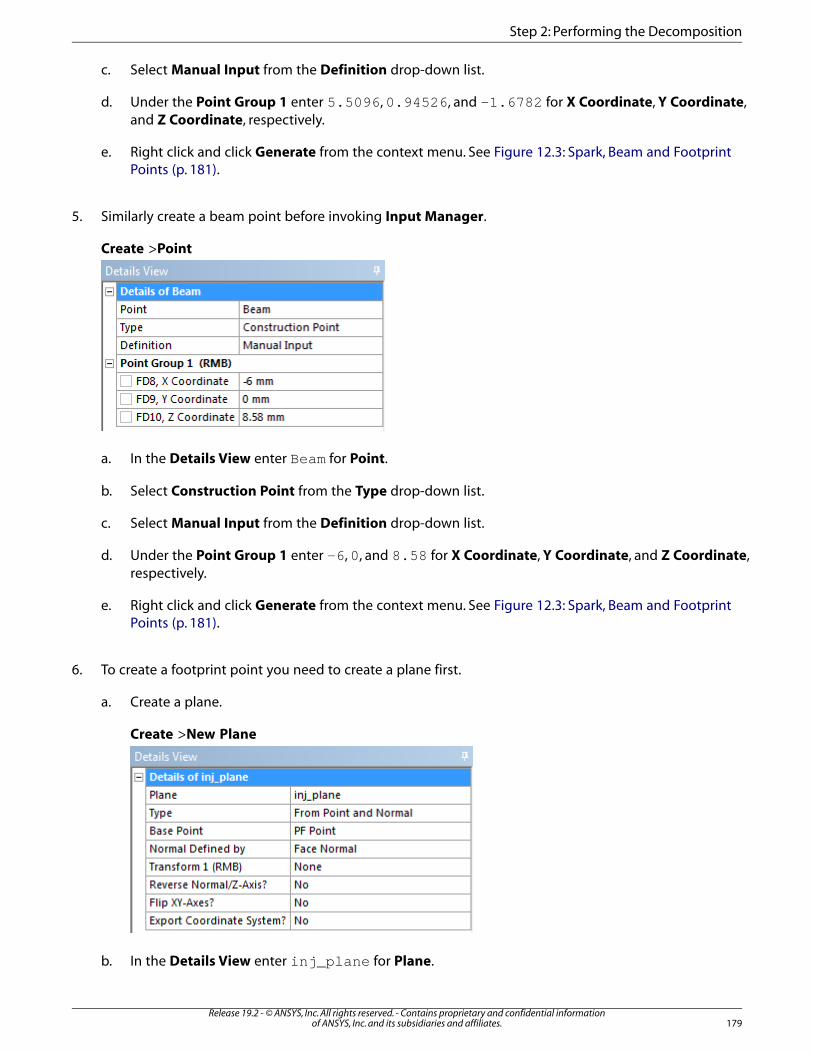
c. Select Manual Input from the Definition drop-down list.
d. Under the Point Group 1 enter 5.5096,0.94526, and -1.6782 for X Coordinate, Y Coordinate,and Z Coordinate, respectively.
e. Right click and click Generate from the context menu. See Figure 12.3: Spark, Beam and FootprintPoints (p. 181).
5. Similarly create a beam point before invoking Input Manager.
Create >Point
a. In the Details View enter Beam for Point.
b. Select Construction Point from the Type drop-down list.
c. Select Manual Input from the Definition drop-down list.
d. Under the Point Group 1 enter -6,0, and 8.58 for X Coordinate, Y Coordinate, and Z Coordinate,respectively.
e. Right click and click Generate from the context menu. See Figure 12.3: Spark, Beam and FootprintPoints (p. 181).
6. To create a footprint point you need to create a plane first.
a. Create a plane.
Create >New Plane
b. In the Details View enter inj_plane for Plane.
179Release 19.2 - © ANSYS, Inc. All rights reserved. - Contains proprietary and confidential information
of ANSYS, Inc. and its subsidiaries and affiliates.
Step 2: Performing the Decomposition
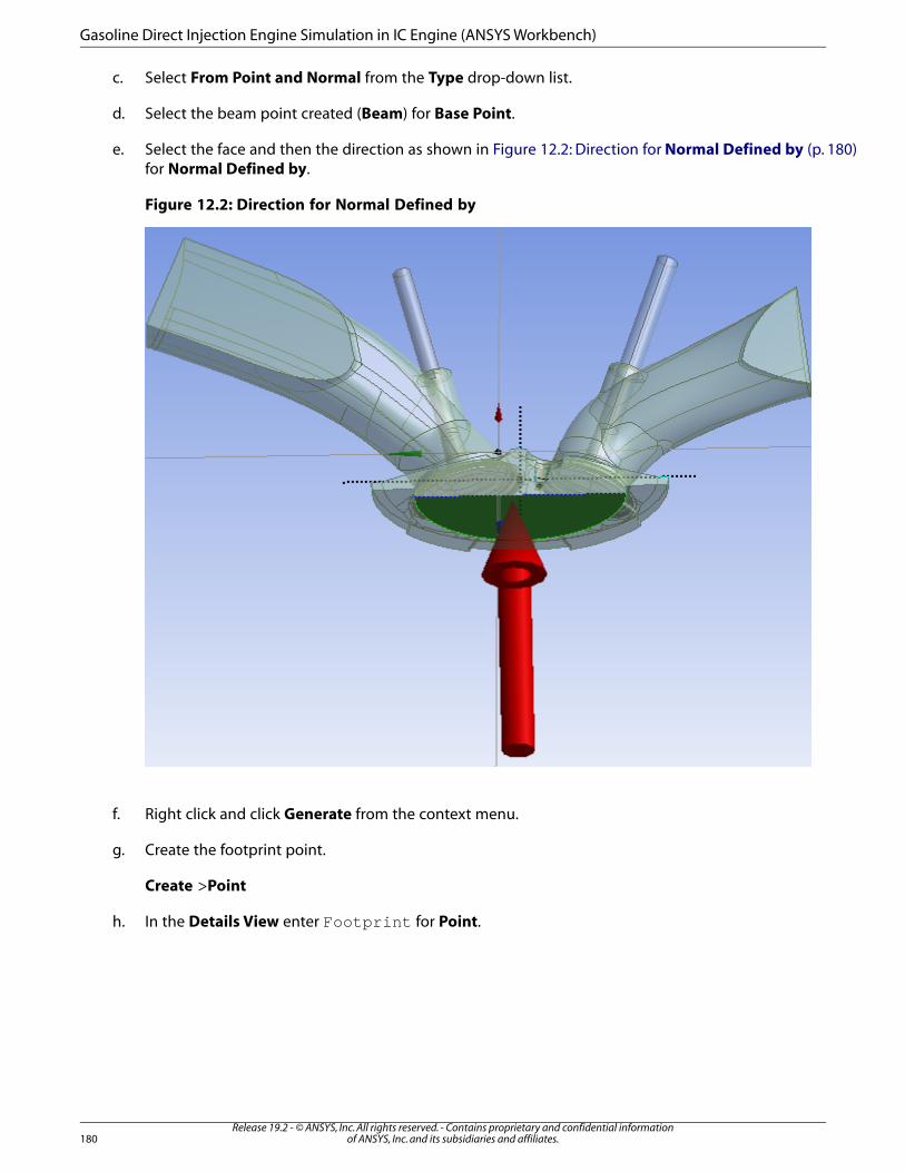
c. Select From Point and Normal from the Type drop-down list.
d. Select the beam point created (Beam) for Base Point.
e. Select the face and then the direction as shown in Figure 12.2: Direction for Normal Defined by (p. 180)for Normal Defined by.
Figure 12.2: Direction for Normal Defined by
f. Right click and click Generate from the context menu.
g. Create the footprint point.
Create >Point
h. In the Details View enter Footprint for Point.
Release 19.2 - © ANSYS, Inc. All rights reserved. - Contains proprietary and confidential informationof ANSYS, Inc. and its subsidiaries and affiliates.180
Gasoline Direct Injection Engine Simulation in IC Engine (ANSYS Workbench)
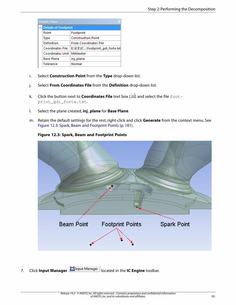
i. Select Construction Point from the Type drop-down list.
j. Select From Coordinates File from the Definition drop-down list.
k. Click the button next to Coordinates File text box ( ) and select the file foot-print_gdi_forte.txt.
l. Select the plane created, inj_plane for Base Plane.
m. Retain the default settings for the rest, right-click and click Generate from the context menu. SeeFigure 12.3: Spark, Beam and Footprint Points (p. 181).
Figure 12.3: Spark, Beam and Footprint Points
7. Click Input Manager located in the IC Engine toolbar.
181Release 19.2 - © ANSYS, Inc. All rights reserved. - Contains proprietary and confidential information
of ANSYS, Inc. and its subsidiaries and affiliates.
Step 2: Performing the Decomposition
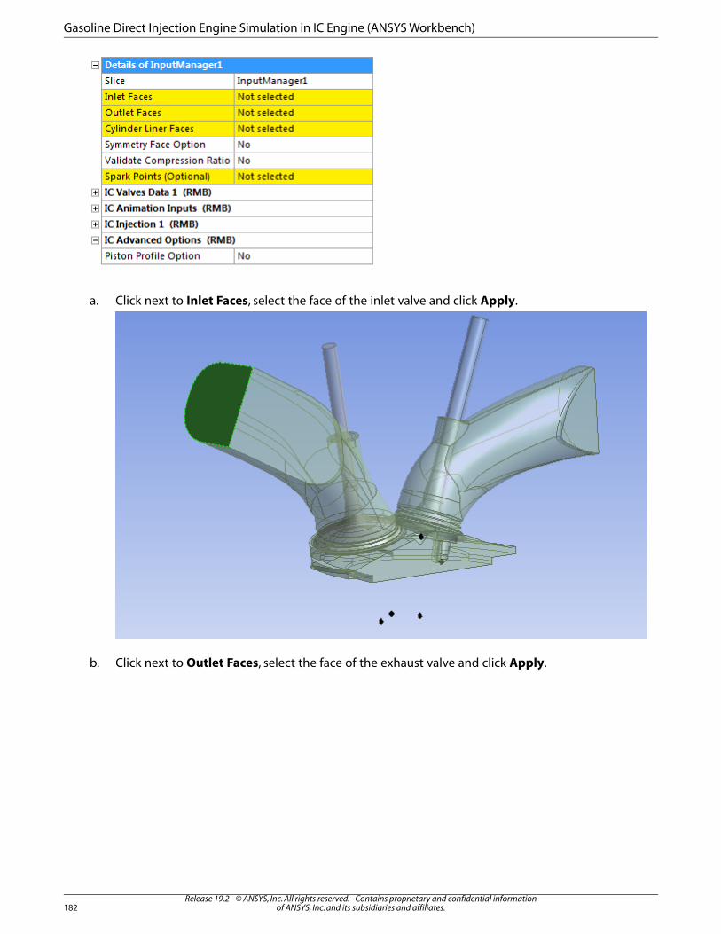
a. Click next to Inlet Faces, select the face of the inlet valve and click Apply.
b. Click next to Outlet Faces, select the face of the exhaust valve and click Apply.
Release 19.2 - © ANSYS, Inc. All rights reserved. - Contains proprietary and confidential informationof ANSYS, Inc. and its subsidiaries and affiliates.182
Gasoline Direct Injection Engine Simulation in IC Engine (ANSYS Workbench)
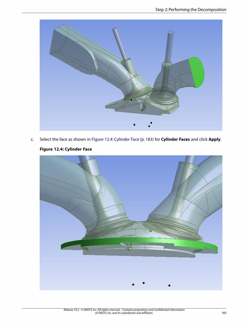
c. Select the face as shown in Figure 12.4: Cylinder Face (p. 183) for Cylinder Faces and click Apply.
Figure 12.4: Cylinder Face
183Release 19.2 - © ANSYS, Inc. All rights reserved. - Contains proprietary and confidential information
of ANSYS, Inc. and its subsidiaries and affiliates.
Step 2: Performing the Decomposition
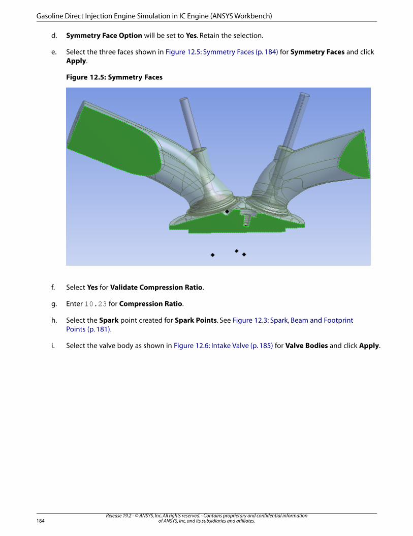
d. Symmetry Face Option will be set to Yes. Retain the selection.
e. Select the three faces shown in Figure 12.5: Symmetry Faces (p. 184) for Symmetry Faces and clickApply.
Figure 12.5: Symmetry Faces
f. Select Yes for Validate Compression Ratio.
g. Enter 10.23 for Compression Ratio.
h. Select the Spark point created for Spark Points. See Figure 12.3: Spark, Beam and FootprintPoints (p. 181).
i. Select the valve body as shown in Figure 12.6: Intake Valve (p. 185) for Valve Bodies and click Apply.
Release 19.2 - © ANSYS, Inc. All rights reserved. - Contains proprietary and confidential informationof ANSYS, Inc. and its subsidiaries and affiliates.184
Gasoline Direct Injection Engine Simulation in IC Engine (ANSYS Workbench)

Figure 12.6: Intake Valve
j. Select the valve seat face as shown in Figure 12.7: Intake Valve Seat (p. 185) for Valve Seat Faces andclick Apply.
Figure 12.7: Intake Valve Seat
k. Select invalve1 from the Valve Profile drop-down list.
185Release 19.2 - © ANSYS, Inc. All rights reserved. - Contains proprietary and confidential information
of ANSYS, Inc. and its subsidiaries and affiliates.
Step 2: Performing the Decomposition
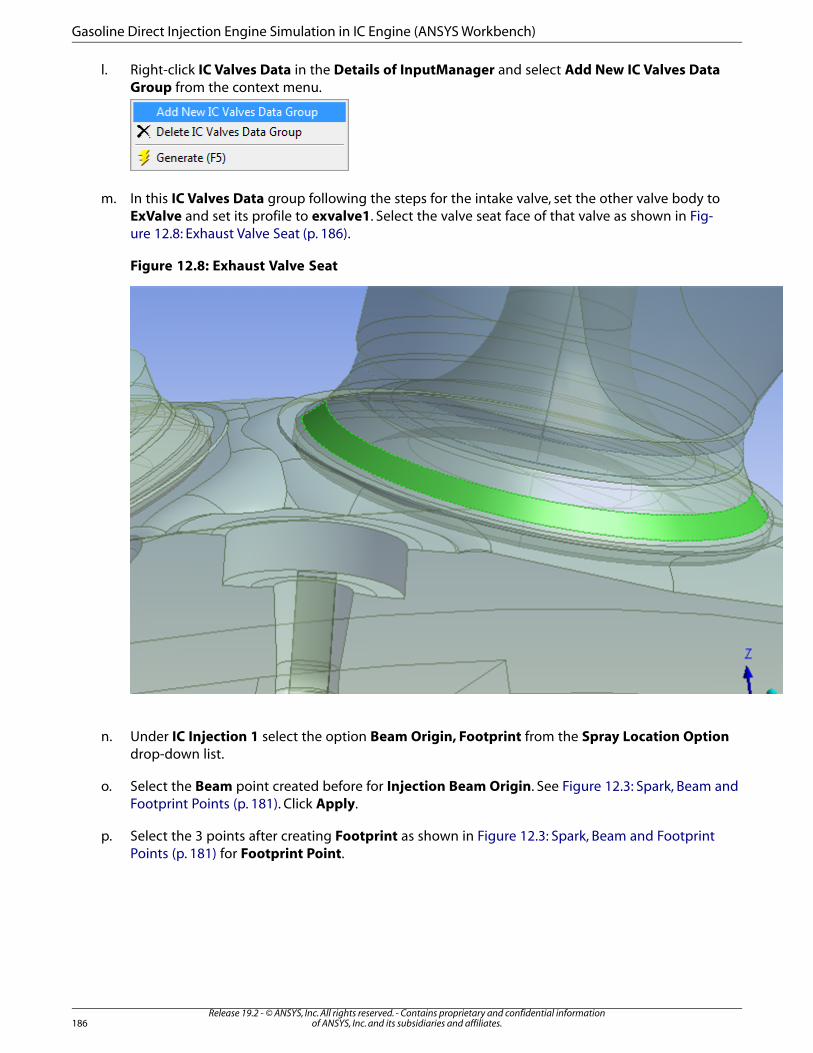
l. Right-click IC Valves Data in the Details of InputManager and select Add New IC Valves DataGroup from the context menu.
m. In this IC Valves Data group following the steps for the intake valve, set the other valve body toExValve and set its profile to exvalve1. Select the valve seat face of that valve as shown in Fig-ure 12.8: Exhaust Valve Seat (p. 186).
Figure 12.8: Exhaust Valve Seat
n. Under IC Injection 1 select the option Beam Origin, Footprint from the Spray Location Optiondrop-down list.
o. Select the Beam point created before for Injection Beam Origin. See Figure 12.3: Spark, Beam andFootprint Points (p. 181). Click Apply.
p. Select the 3 points after creating Footprint as shown in Figure 12.3: Spark, Beam and FootprintPoints (p. 181) for Footprint Point.
Release 19.2 - © ANSYS, Inc. All rights reserved. - Contains proprietary and confidential informationof ANSYS, Inc. and its subsidiaries and affiliates.186
Gasoline Direct Injection Engine Simulation in IC Engine (ANSYS Workbench)
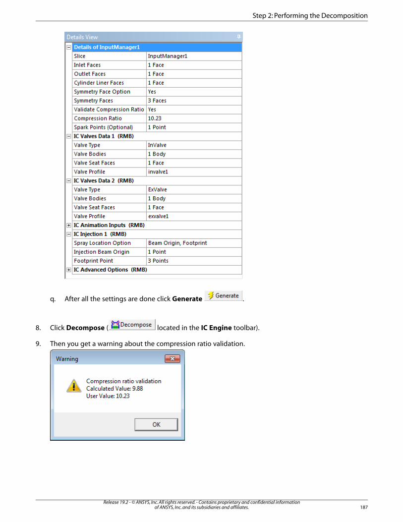
q. After all the settings are done click Generate .
8. Click Decompose ( located in the IC Engine toolbar).
9. Then you get a warning about the compression ratio validation.
187Release 19.2 - © ANSYS, Inc. All rights reserved. - Contains proprietary and confidential information
of ANSYS, Inc. and its subsidiaries and affiliates.
Step 2: Performing the Decomposition
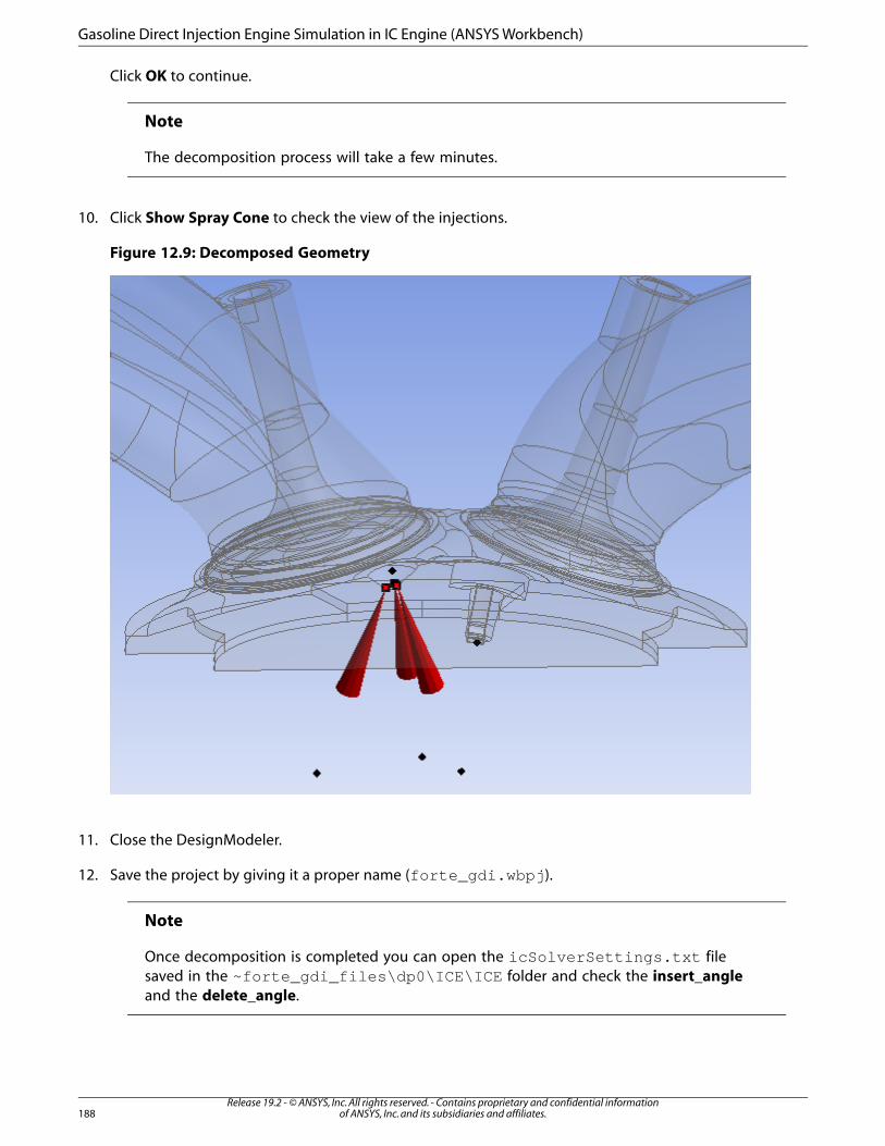
Click OK to continue.
Note
The decomposition process will take a few minutes.
10. Click Show Spray Cone to check the view of the injections.
Figure 12.9: Decomposed Geometry
11. Close the DesignModeler.
12. Save the project by giving it a proper name (forte_gdi.wbpj).
Note
Once decomposition is completed you can open the icSolverSettings.txt filesaved in the ~forte_gdi_files\dp0\ICE\ICE folder and check the insert_angleand the delete_angle.
Release 19.2 - © ANSYS, Inc. All rights reserved. - Contains proprietary and confidential informationof ANSYS, Inc. and its subsidiaries and affiliates.188
Gasoline Direct Injection Engine Simulation in IC Engine (ANSYS Workbench)
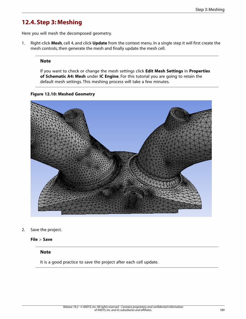
12.4. Step 3: Meshing
Here you will mesh the decomposed geometry.
1. Right-click Mesh, cell 4, and click Update from the context menu. In a single step it will first create themesh controls, then generate the mesh and finally update the mesh cell.
Note
If you want to check or change the mesh settings click Edit Mesh Settings in Propertiesof Schematic A4: Mesh under IC Engine. For this tutorial you are going to retain thedefault mesh settings. This meshing process will take a few minutes.
Figure 12.10: Meshed Geometry
2. Save the project.
File > Save
Note
It is a good practice to save the project after each cell update.
189Release 19.2 - © ANSYS, Inc. All rights reserved. - Contains proprietary and confidential information
of ANSYS, Inc. and its subsidiaries and affiliates.
Step 3: Meshing
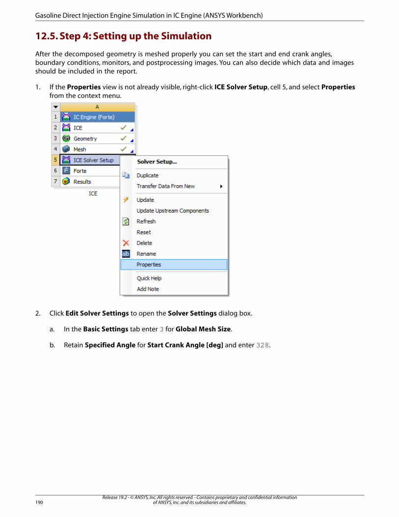
12.5. Step 4: Setting up the Simulation
After the decomposed geometry is meshed properly you can set the start and end crank angles,boundary conditions, monitors, and postprocessing images. You can also decide which data and imagesshould be included in the report.
1. If the Properties view is not already visible, right-click ICE Solver Setup, cell 5, and select Propertiesfrom the context menu.
2. Click Edit Solver Settings to open the Solver Settings dialog box.
a. In the Basic Settings tab enter 3 for Global Mesh Size.
b. Retain Specified Angle for Start Crank Angle [deg] and enter 328.
Release 19.2 - © ANSYS, Inc. All rights reserved. - Contains proprietary and confidential informationof ANSYS, Inc. and its subsidiaries and affiliates.190
Gasoline Direct Injection Engine Simulation in IC Engine (ANSYS Workbench)
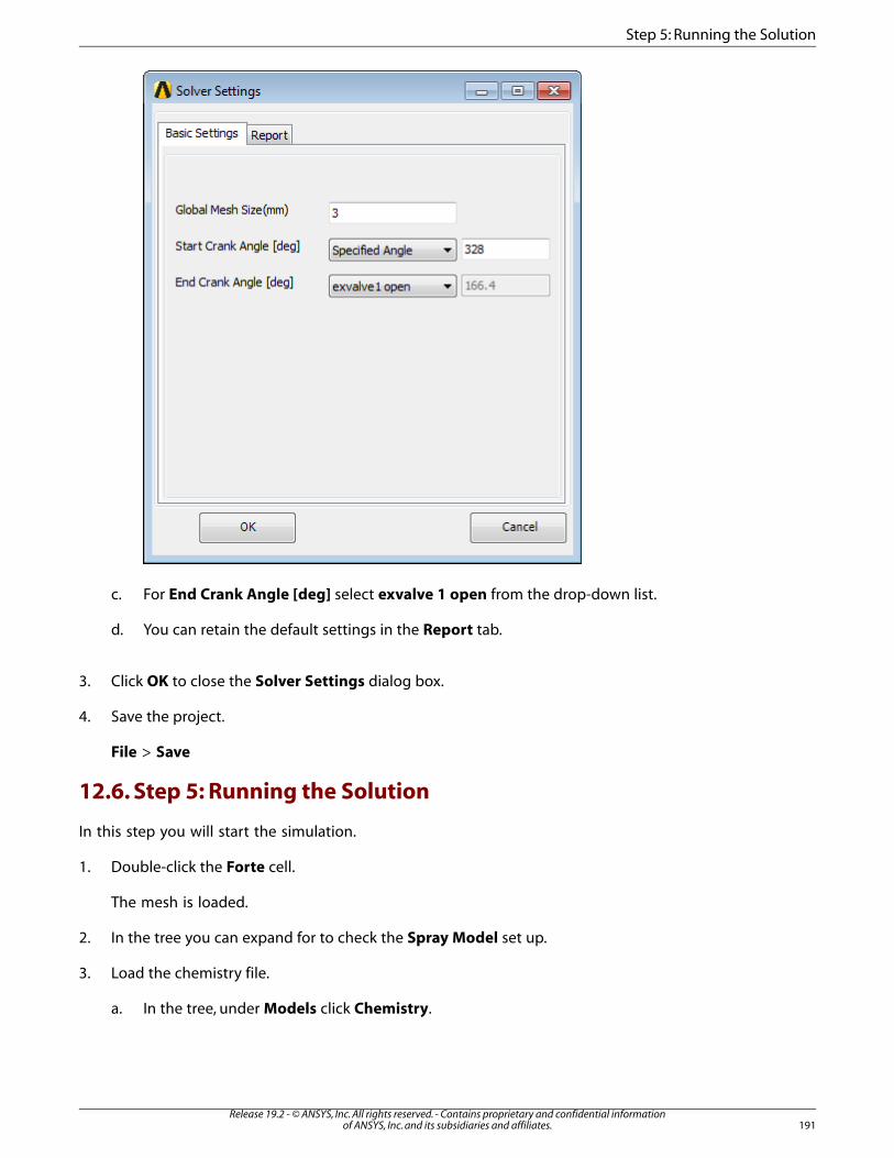
c. For End Crank Angle [deg] select exvalve 1 open from the drop-down list.
d. You can retain the default settings in the Report tab.
3. Click OK to close the Solver Settings dialog box.
4. Save the project.
File > Save
12.6. Step 5: Running the Solution
In this step you will start the simulation.
1. Double-click the Forte cell.
The mesh is loaded.
2. In the tree you can expand for to check the Spray Model set up.
3. Load the chemistry file.
a. In the tree, under Models click Chemistry.
191Release 19.2 - © ANSYS, Inc. All rights reserved. - Contains proprietary and confidential information
of ANSYS, Inc. and its subsidiaries and affiliates.
Step 5: Running the Solution
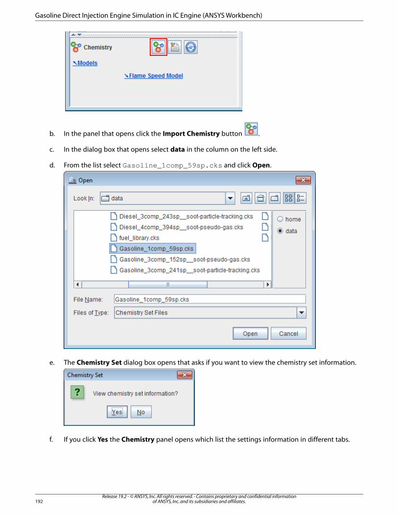
b. In the panel that opens click the Import Chemistry button .
c. In the dialog box that opens select data in the column on the left side.
d. From the list select Gasoline_1comp_59sp.cks and click Open.
e. The Chemistry Set dialog box opens that asks if you want to view the chemistry set information.
f. If you click Yes the Chemistry panel opens which list the settings information in different tabs.
Release 19.2 - © ANSYS, Inc. All rights reserved. - Contains proprietary and confidential informationof ANSYS, Inc. and its subsidiaries and affiliates.192
Gasoline Direct Injection Engine Simulation in IC Engine (ANSYS Workbench)
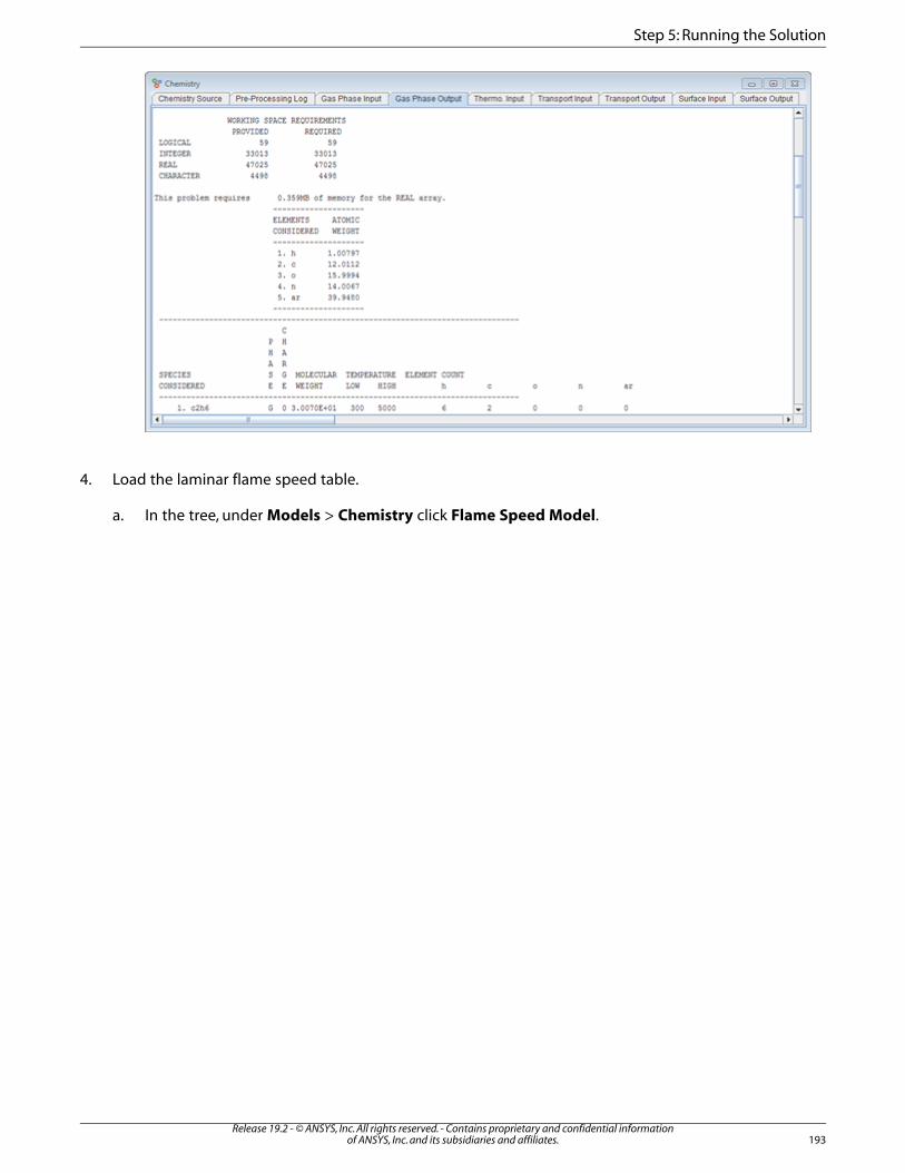
4. Load the laminar flame speed table.
a. In the tree, under Models > Chemistry click Flame Speed Model.
193Release 19.2 - © ANSYS, Inc. All rights reserved. - Contains proprietary and confidential information
of ANSYS, Inc. and its subsidiaries and affiliates.
Step 5: Running the Solution
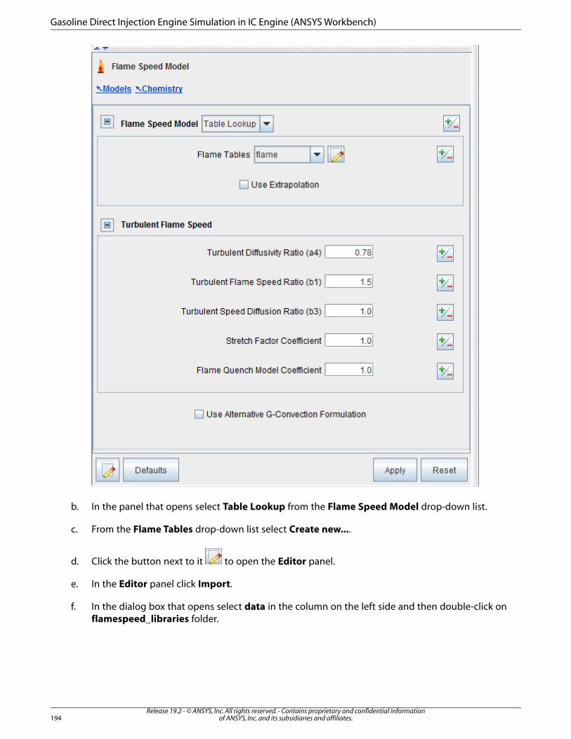
b. In the panel that opens select Table Lookup from the Flame Speed Model drop-down list.
c. From the Flame Tables drop-down list select Create new....
d. Click the button next to it to open the Editor panel.
e. In the Editor panel click Import.
f. In the dialog box that opens select data in the column on the left side and then double-click onflamespeed_libraries folder.
Release 19.2 - © ANSYS, Inc. All rights reserved. - Contains proprietary and confidential informationof ANSYS, Inc. and its subsidiaries and affiliates.194
Gasoline Direct Injection Engine Simulation in IC Engine (ANSYS Workbench)
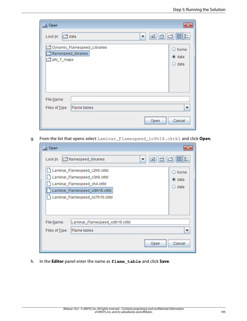
g. From the list that opens select Laminar_Flamespeed_ic8h18.cktbl and click Open.
h. In the Editor panel enter the name as flame_table and click Save.
195Release 19.2 - © ANSYS, Inc. All rights reserved. - Contains proprietary and confidential information
of ANSYS, Inc. and its subsidiaries and affiliates.
Step 5: Running the Solution
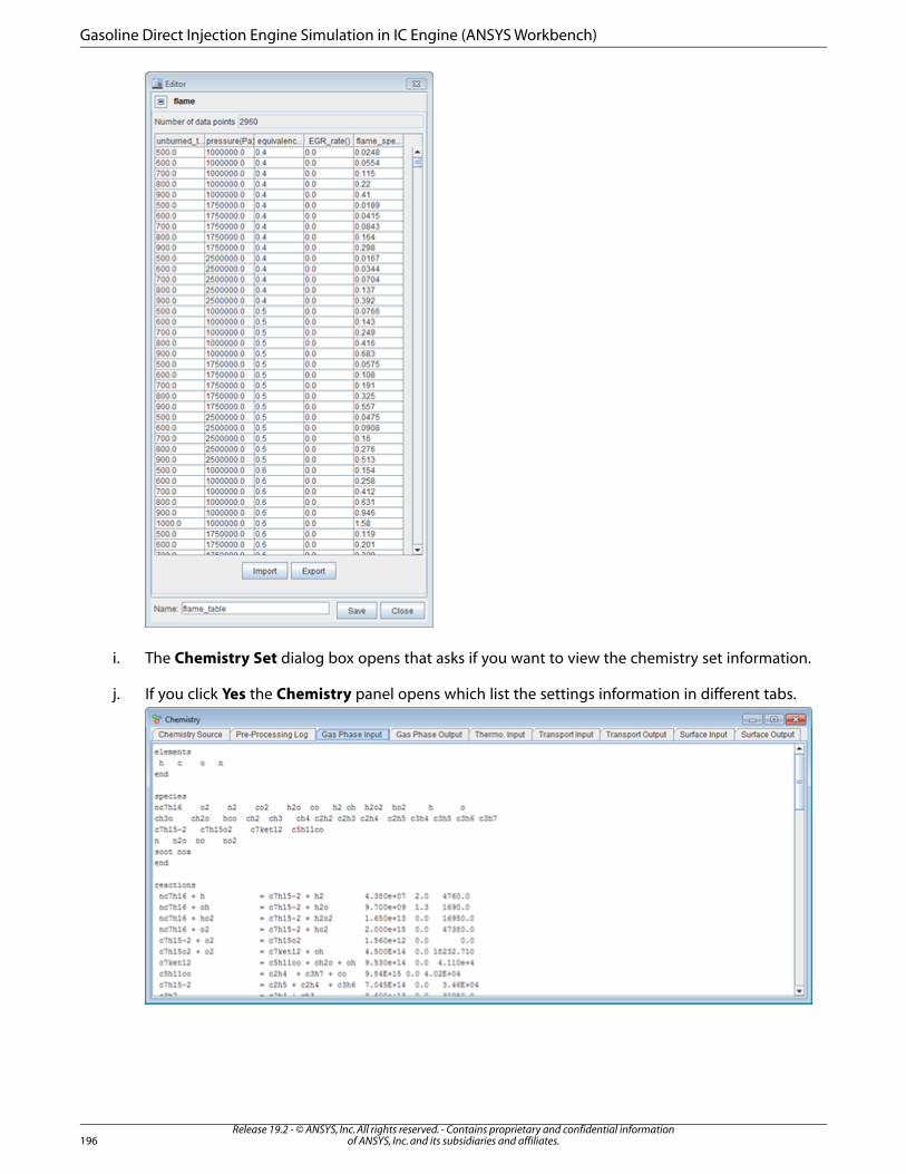
i. The Chemistry Set dialog box opens that asks if you want to view the chemistry set information.
j. If you click Yes the Chemistry panel opens which list the settings information in different tabs.
Release 19.2 - © ANSYS, Inc. All rights reserved. - Contains proprietary and confidential informationof ANSYS, Inc. and its subsidiaries and affiliates.196
Gasoline Direct Injection Engine Simulation in IC Engine (ANSYS Workbench)
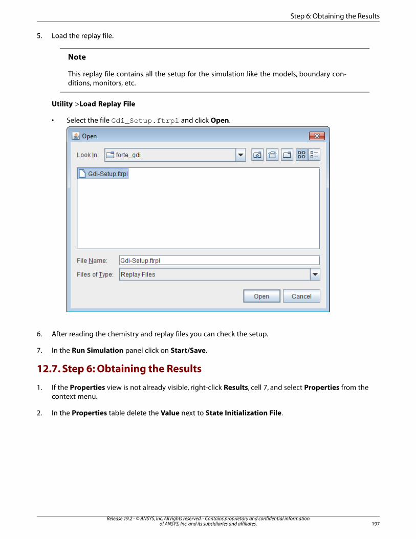
5. Load the replay file.
Note
This replay file contains all the setup for the simulation like the models, boundary con-ditions, monitors, etc.
Utility >Load Replay File
• Select the file Gdi_Setup.ftrpl and click Open.
6. After reading the chemistry and replay files you can check the setup.
7. In the Run Simulation panel click on Start/Save.
12.7. Step 6: Obtaining the Results
1. If the Properties view is not already visible, right-click Results, cell 7, and select Properties from thecontext menu.
2. In the Properties table delete the Value next to State Initialization File.
197Release 19.2 - © ANSYS, Inc. All rights reserved. - Contains proprietary and confidential information
of ANSYS, Inc. and its subsidiaries and affiliates.
Step 6: Obtaining the Results
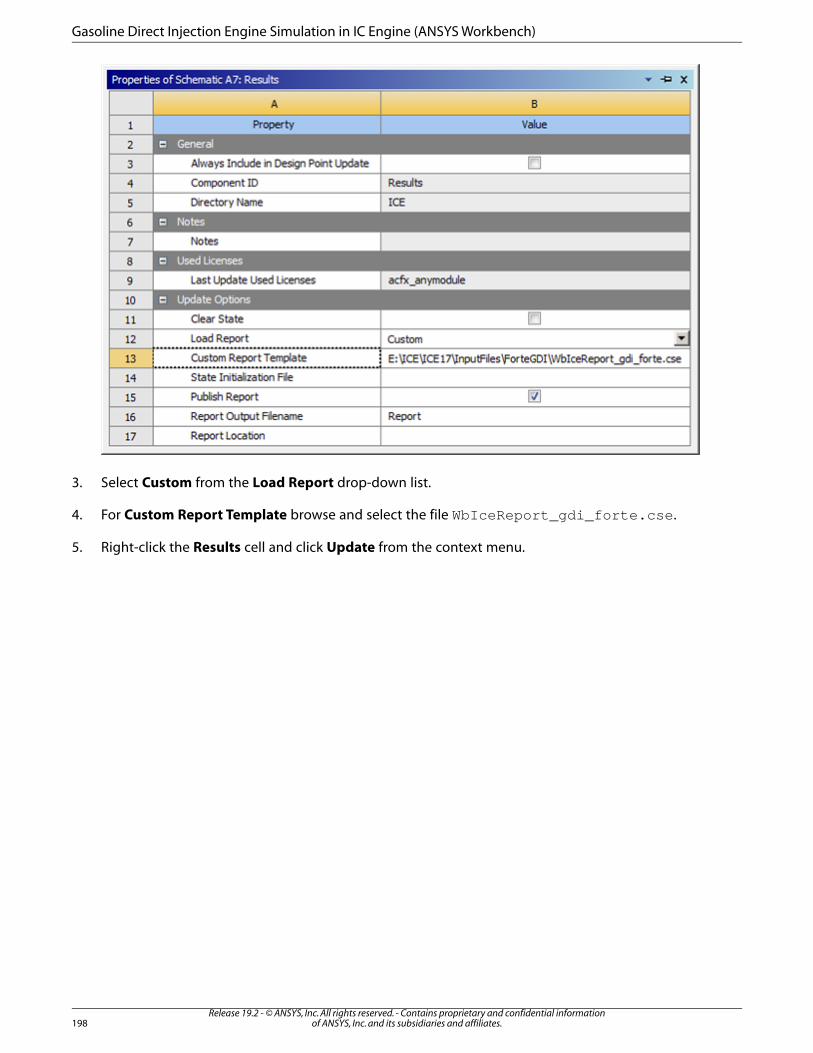
3. Select Custom from the Load Report drop-down list.
4. For Custom Report Template browse and select the file WbIceReport_gdi_forte.cse.
5. Right-click the Results cell and click Update from the context menu.
Release 19.2 - © ANSYS, Inc. All rights reserved. - Contains proprietary and confidential informationof ANSYS, Inc. and its subsidiaries and affiliates.198
Gasoline Direct Injection Engine Simulation in IC Engine (ANSYS Workbench)
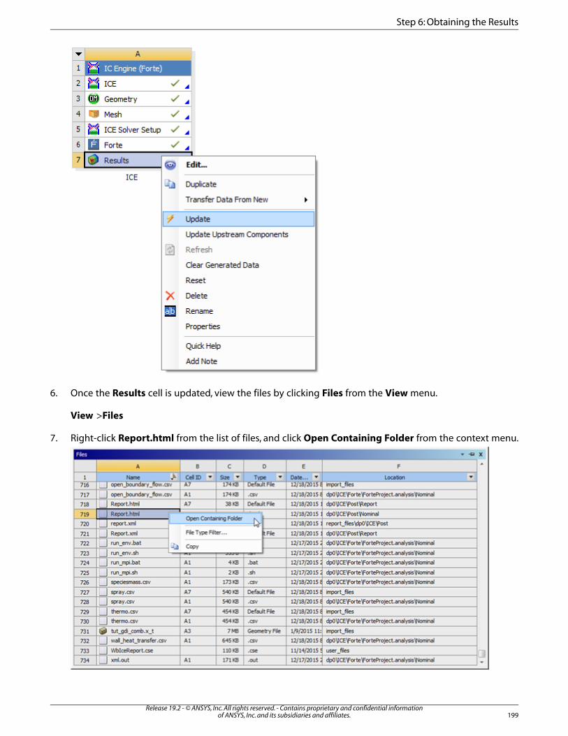
6. Once the Results cell is updated, view the files by clicking Files from the View menu.
View >Files
7. Right-click Report.html from the list of files, and click Open Containing Folder from the context menu.
199Release 19.2 - © ANSYS, Inc. All rights reserved. - Contains proprietary and confidential information
of ANSYS, Inc. and its subsidiaries and affiliates.
Step 6: Obtaining the Results
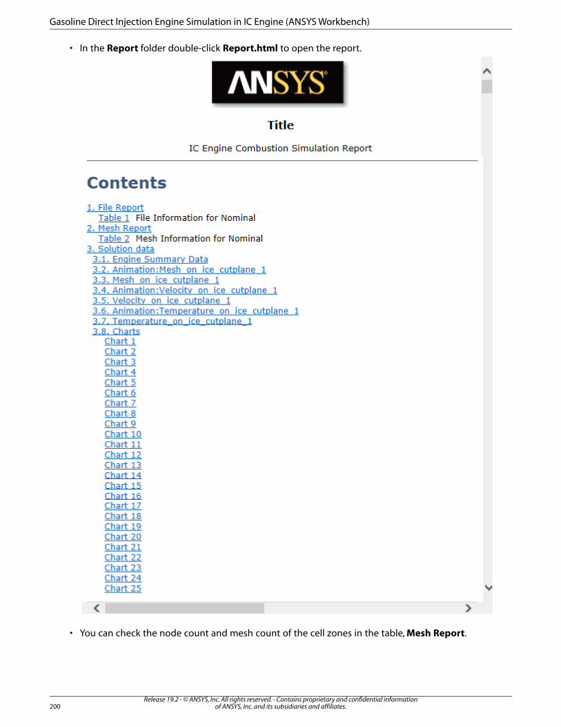
• In the Report folder double-click Report.html to open the report.
• You can check the node count and mesh count of the cell zones in the table, Mesh Report.
Release 19.2 - © ANSYS, Inc. All rights reserved. - Contains proprietary and confidential informationof ANSYS, Inc. and its subsidiaries and affiliates.200
Gasoline Direct Injection Engine Simulation in IC Engine (ANSYS Workbench)
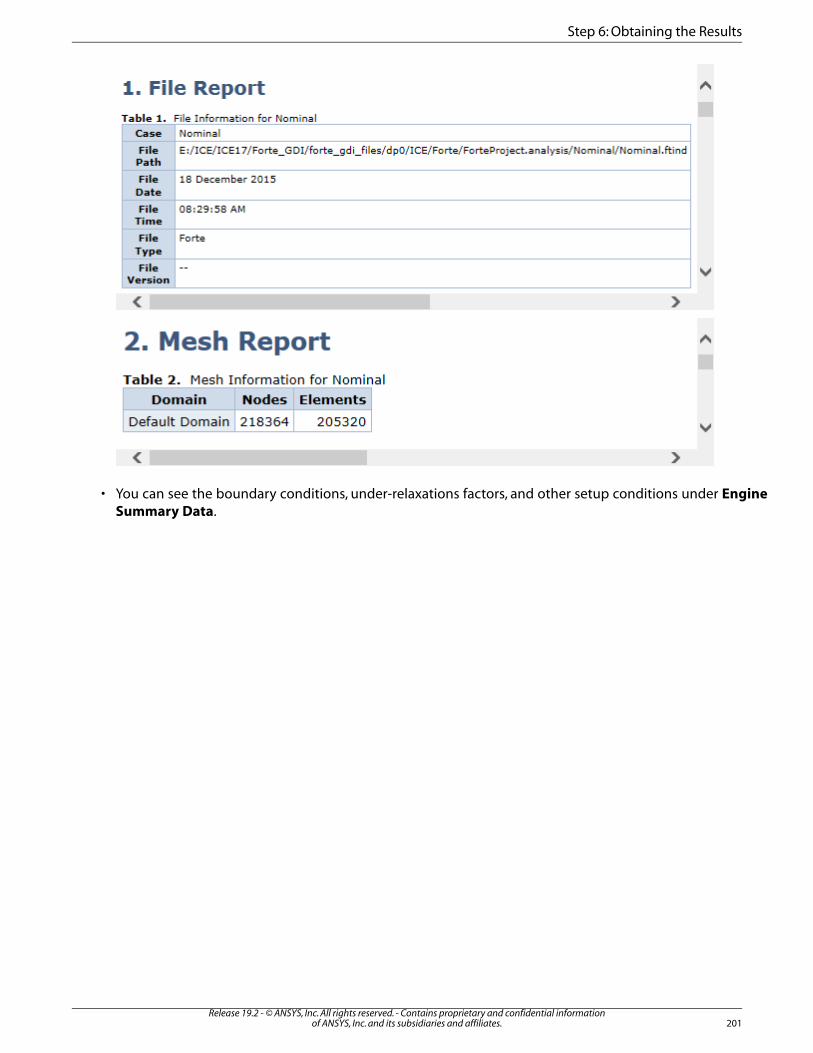
• You can see the boundary conditions, under-relaxations factors, and other setup conditions under EngineSummary Data.
201Release 19.2 - © ANSYS, Inc. All rights reserved. - Contains proprietary and confidential information
of ANSYS, Inc. and its subsidiaries and affiliates.
Step 6: Obtaining the Results

• Check the mesh animation on the cut-plane.
Release 19.2 - © ANSYS, Inc. All rights reserved. - Contains proprietary and confidential informationof ANSYS, Inc. and its subsidiaries and affiliates.202
Gasoline Direct Injection Engine Simulation in IC Engine (ANSYS Workbench)
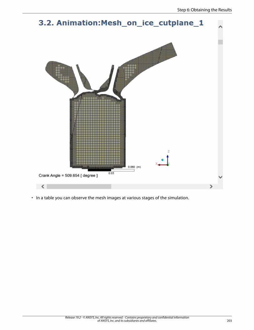
• In a table you can observe the mesh images at various stages of the simulation.
203Release 19.2 - © ANSYS, Inc. All rights reserved. - Contains proprietary and confidential information
of ANSYS, Inc. and its subsidiaries and affiliates.
Step 6: Obtaining the Results
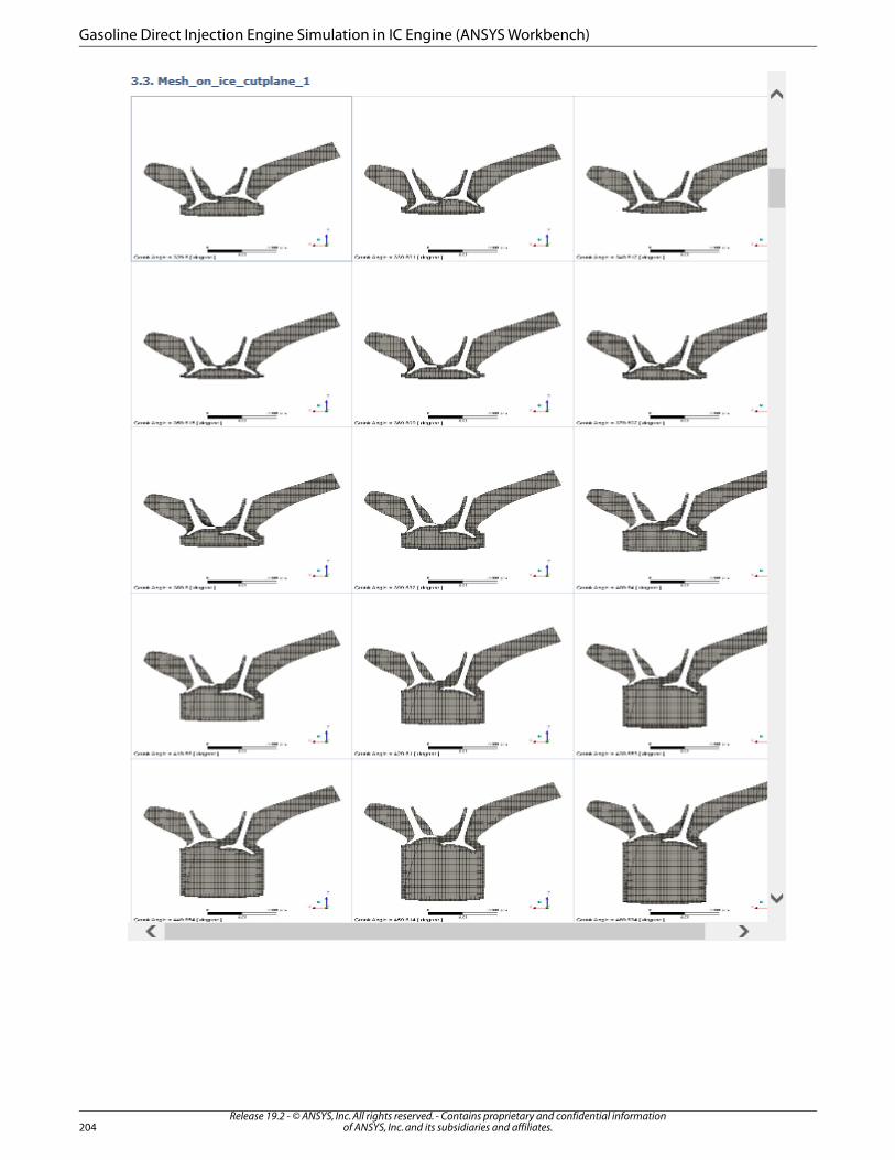
Release 19.2 - © ANSYS, Inc. All rights reserved. - Contains proprietary and confidential informationof ANSYS, Inc. and its subsidiaries and affiliates.204
Gasoline Direct Injection Engine Simulation in IC Engine (ANSYS Workbench)

205Release 19.2 - © ANSYS, Inc. All rights reserved. - Contains proprietary and confidential information
of ANSYS, Inc. and its subsidiaries and affiliates.
Step 6: Obtaining the Results
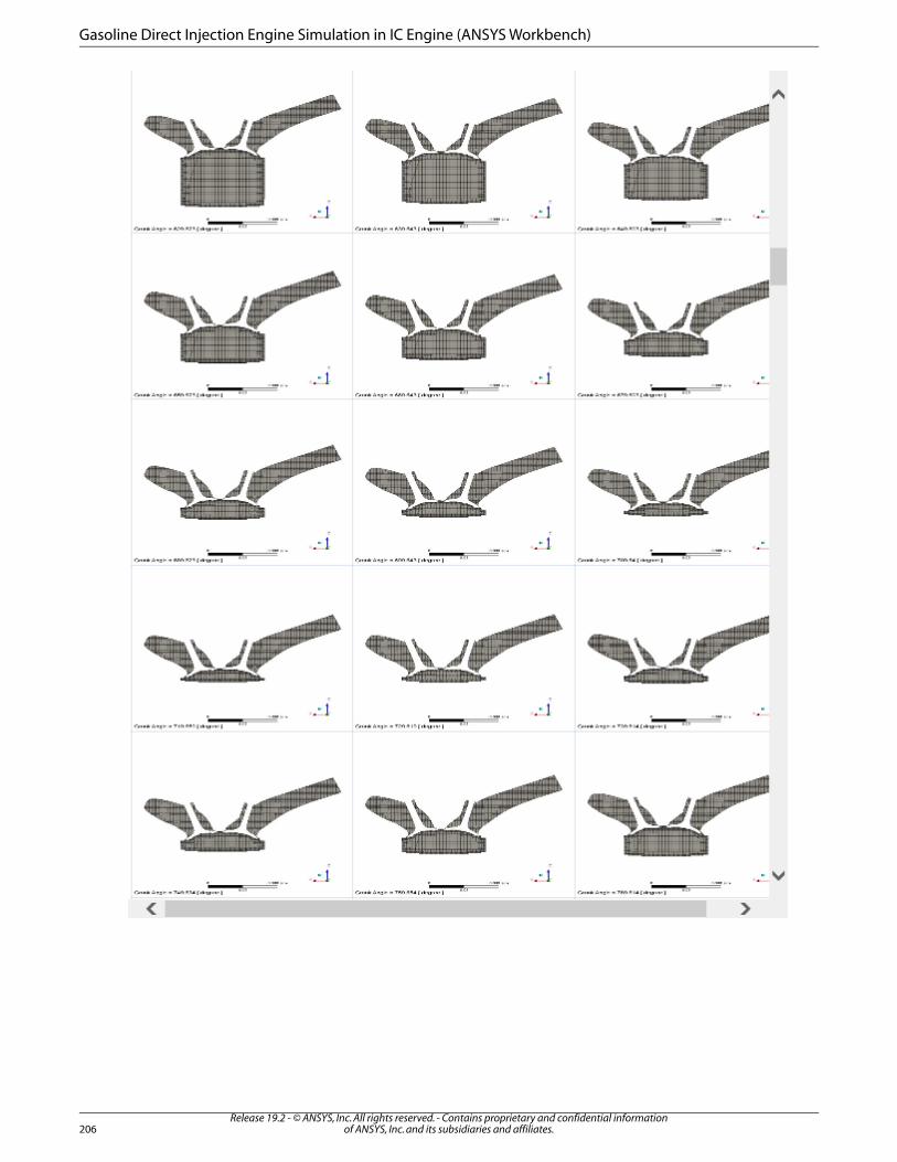
Release 19.2 - © ANSYS, Inc. All rights reserved. - Contains proprietary and confidential informationof ANSYS, Inc. and its subsidiaries and affiliates.206
Gasoline Direct Injection Engine Simulation in IC Engine (ANSYS Workbench)
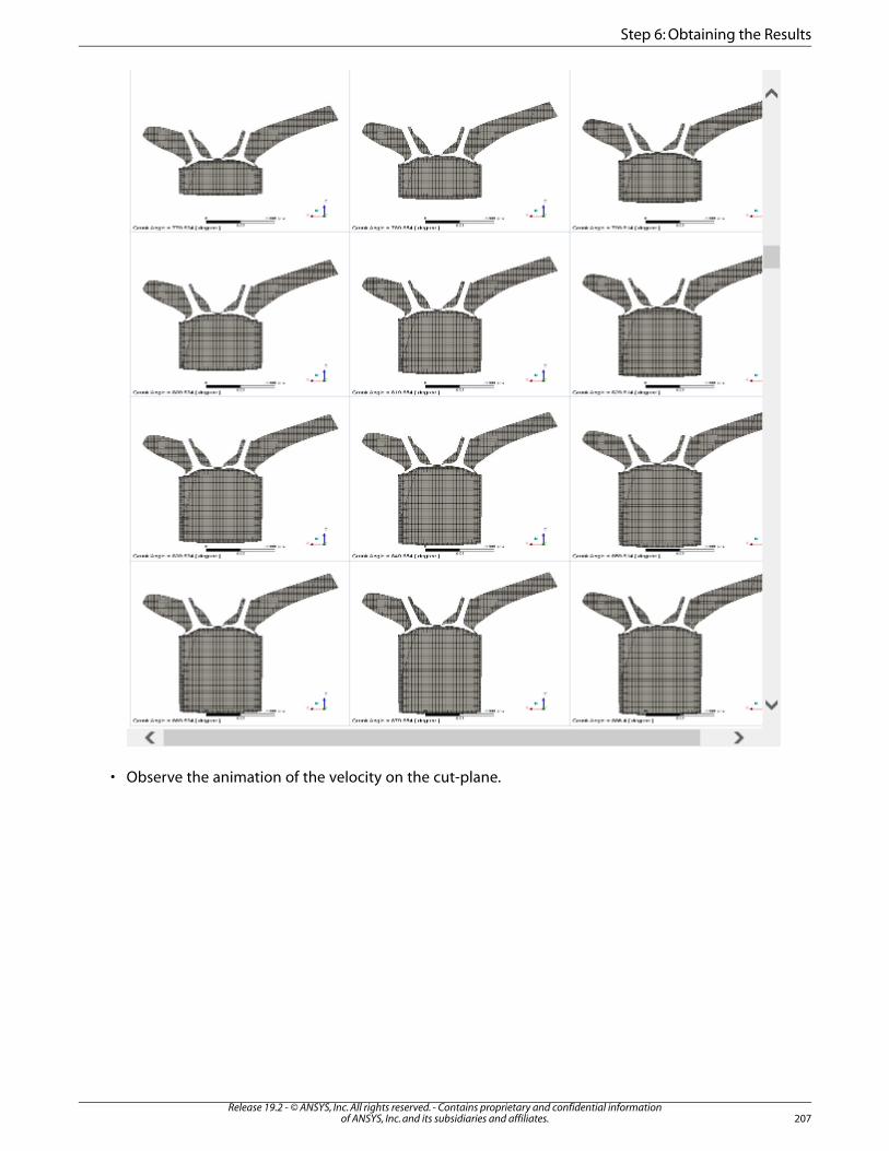
• Observe the animation of the velocity on the cut-plane.
207Release 19.2 - © ANSYS, Inc. All rights reserved. - Contains proprietary and confidential information
of ANSYS, Inc. and its subsidiaries and affiliates.
Step 6: Obtaining the Results
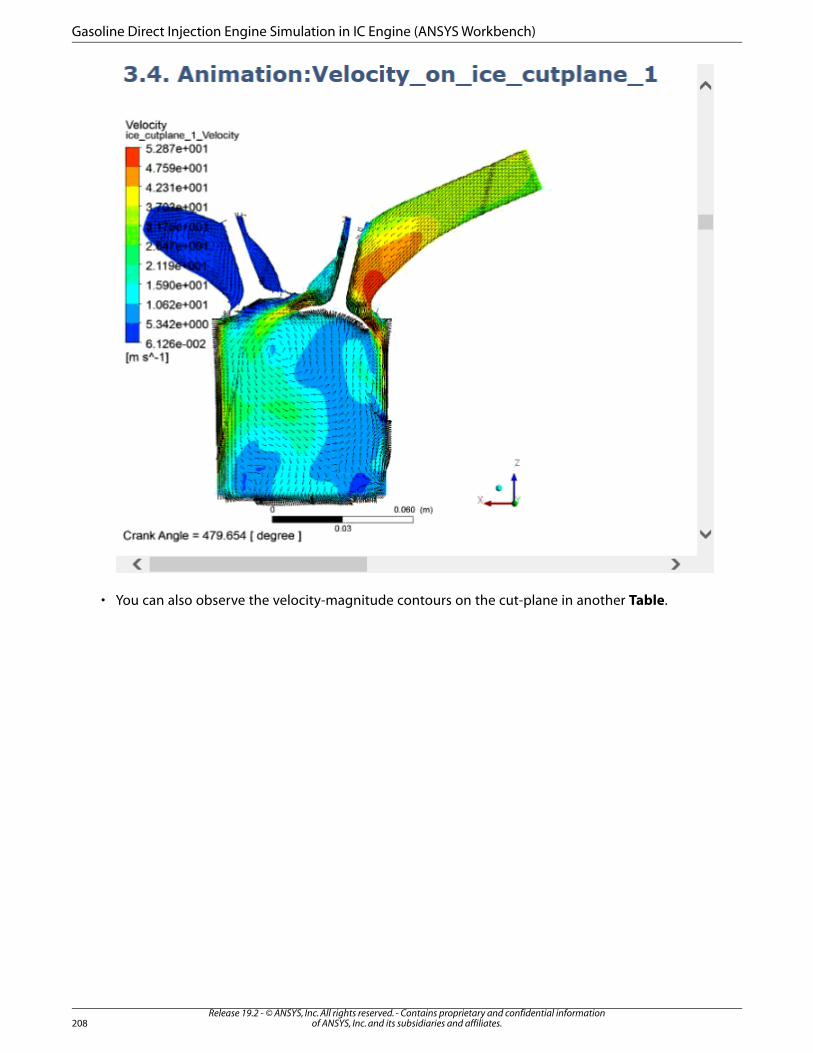
• You can also observe the velocity-magnitude contours on the cut-plane in another Table.
Release 19.2 - © ANSYS, Inc. All rights reserved. - Contains proprietary and confidential informationof ANSYS, Inc. and its subsidiaries and affiliates.208
Gasoline Direct Injection Engine Simulation in IC Engine (ANSYS Workbench)
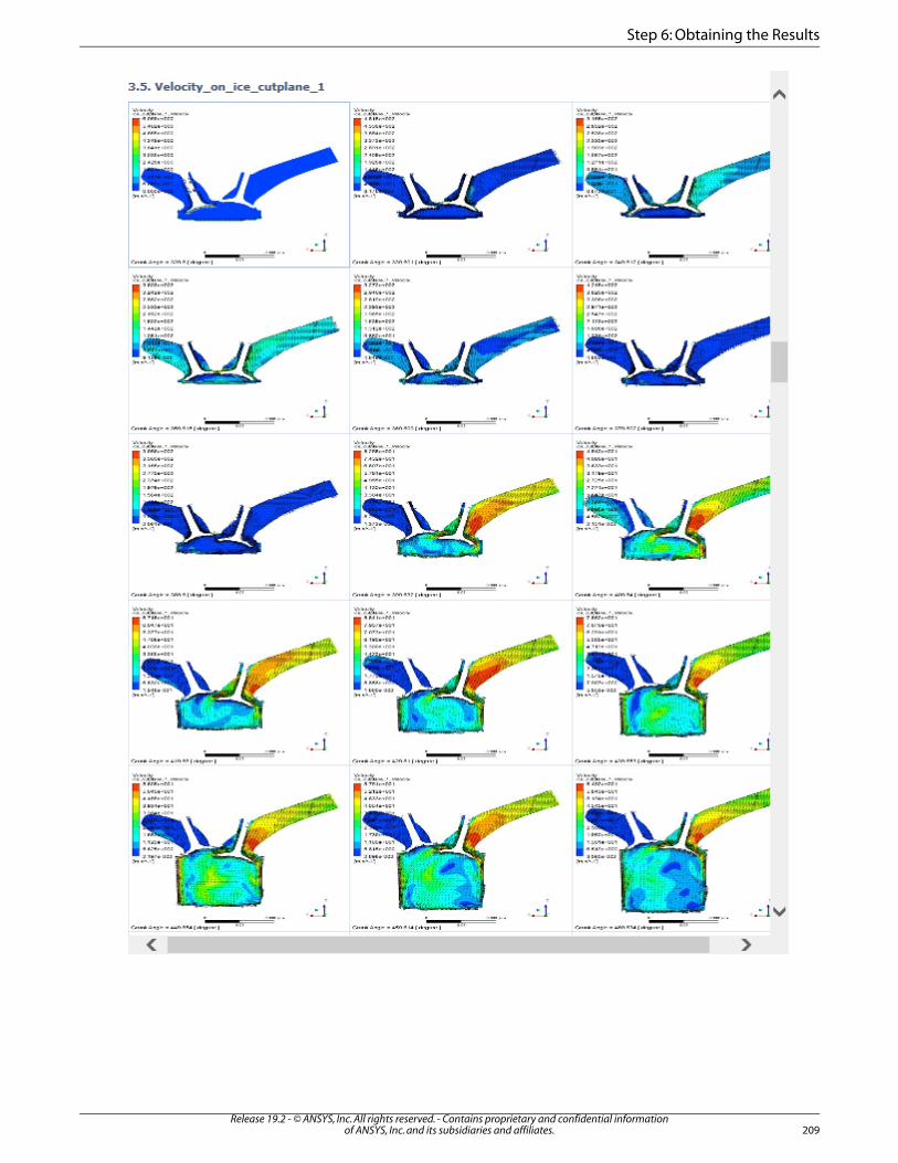
209Release 19.2 - © ANSYS, Inc. All rights reserved. - Contains proprietary and confidential information
of ANSYS, Inc. and its subsidiaries and affiliates.
Step 6: Obtaining the Results
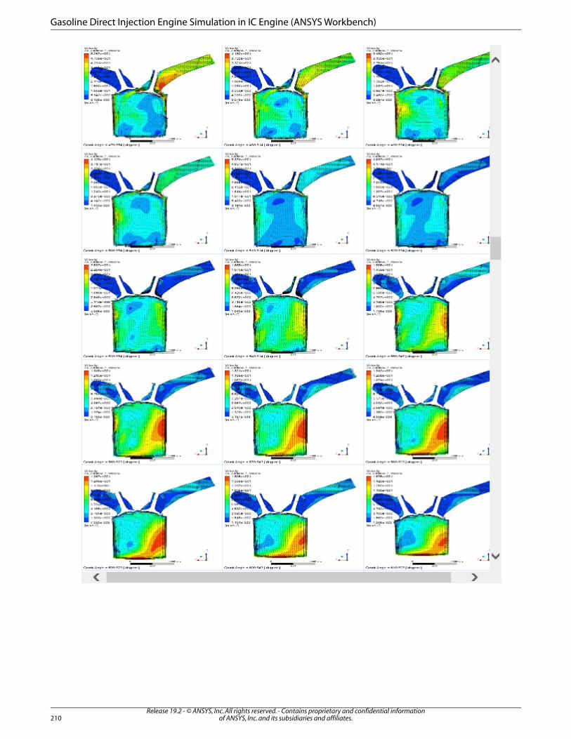
Release 19.2 - © ANSYS, Inc. All rights reserved. - Contains proprietary and confidential informationof ANSYS, Inc. and its subsidiaries and affiliates.210
Gasoline Direct Injection Engine Simulation in IC Engine (ANSYS Workbench)
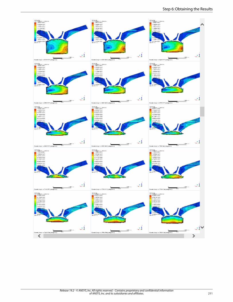
211Release 19.2 - © ANSYS, Inc. All rights reserved. - Contains proprietary and confidential information
of ANSYS, Inc. and its subsidiaries and affiliates.
Step 6: Obtaining the Results
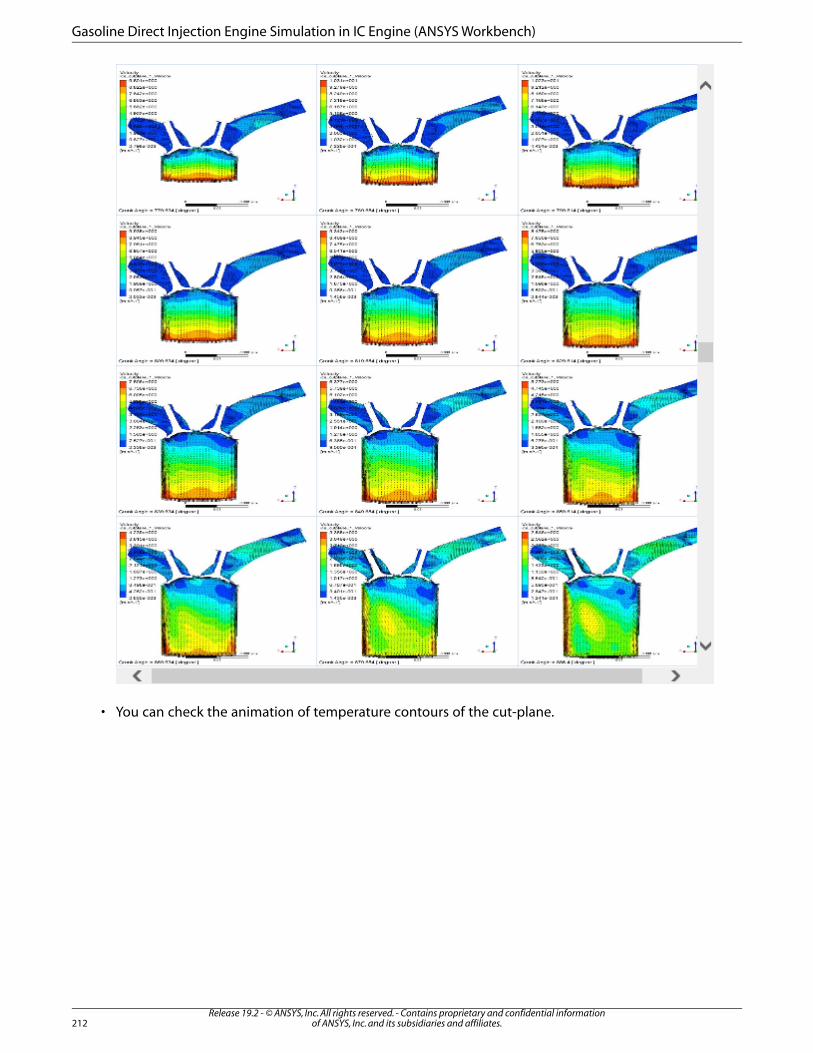
• You can check the animation of temperature contours of the cut-plane.
Release 19.2 - © ANSYS, Inc. All rights reserved. - Contains proprietary and confidential informationof ANSYS, Inc. and its subsidiaries and affiliates.212
Gasoline Direct Injection Engine Simulation in IC Engine (ANSYS Workbench)
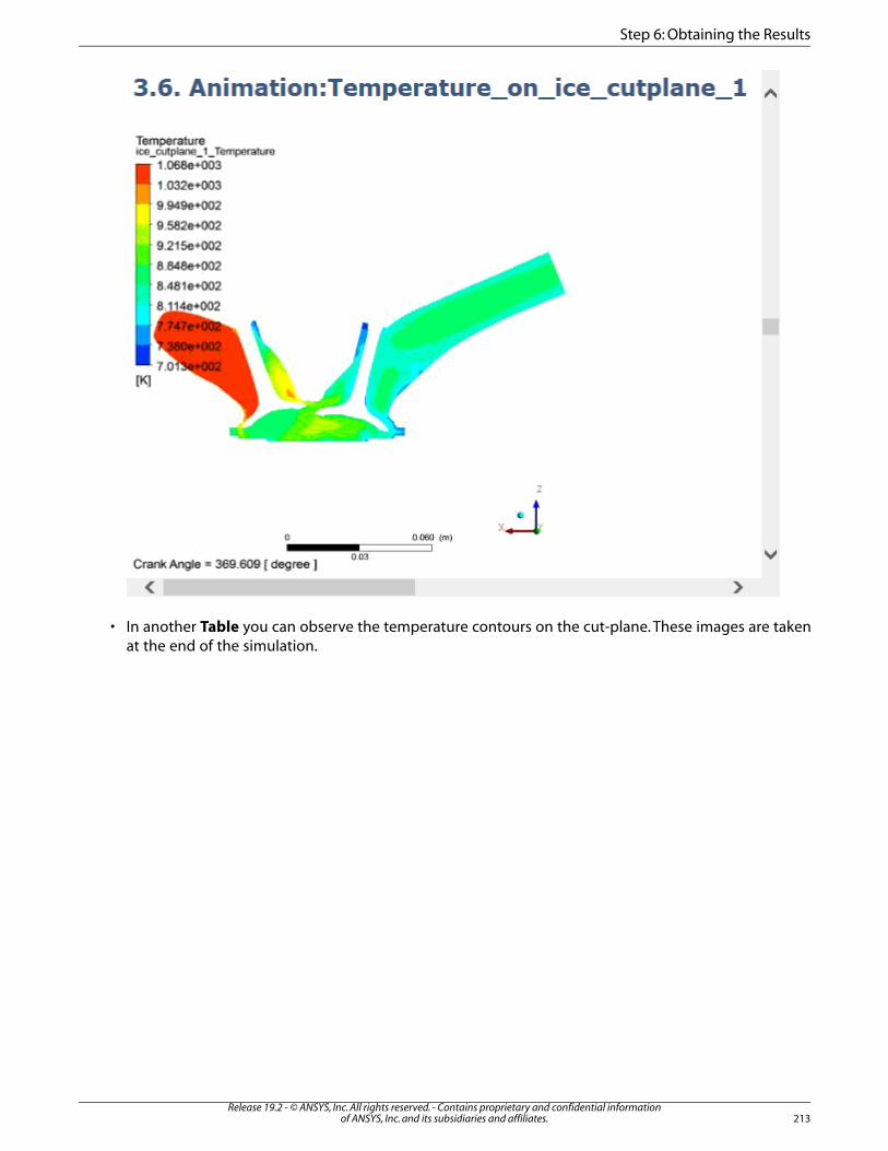
• In another Table you can observe the temperature contours on the cut-plane. These images are takenat the end of the simulation.
213Release 19.2 - © ANSYS, Inc. All rights reserved. - Contains proprietary and confidential information
of ANSYS, Inc. and its subsidiaries and affiliates.
Step 6: Obtaining the Results
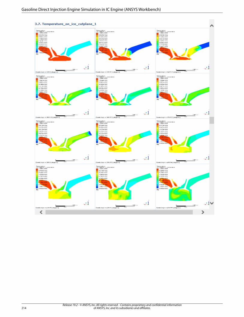
Release 19.2 - © ANSYS, Inc. All rights reserved. - Contains proprietary and confidential informationof ANSYS, Inc. and its subsidiaries and affiliates.214
Gasoline Direct Injection Engine Simulation in IC Engine (ANSYS Workbench)
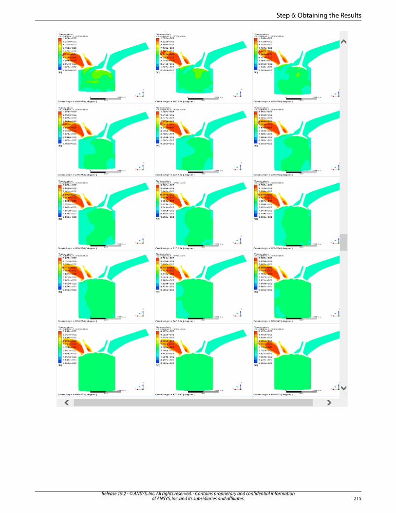
215Release 19.2 - © ANSYS, Inc. All rights reserved. - Contains proprietary and confidential information
of ANSYS, Inc. and its subsidiaries and affiliates.
Step 6: Obtaining the Results
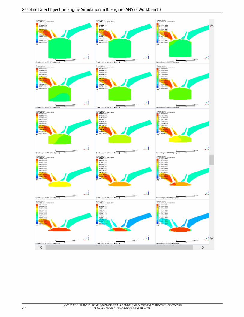
Release 19.2 - © ANSYS, Inc. All rights reserved. - Contains proprietary and confidential informationof ANSYS, Inc. and its subsidiaries and affiliates.216
Gasoline Direct Injection Engine Simulation in IC Engine (ANSYS Workbench)
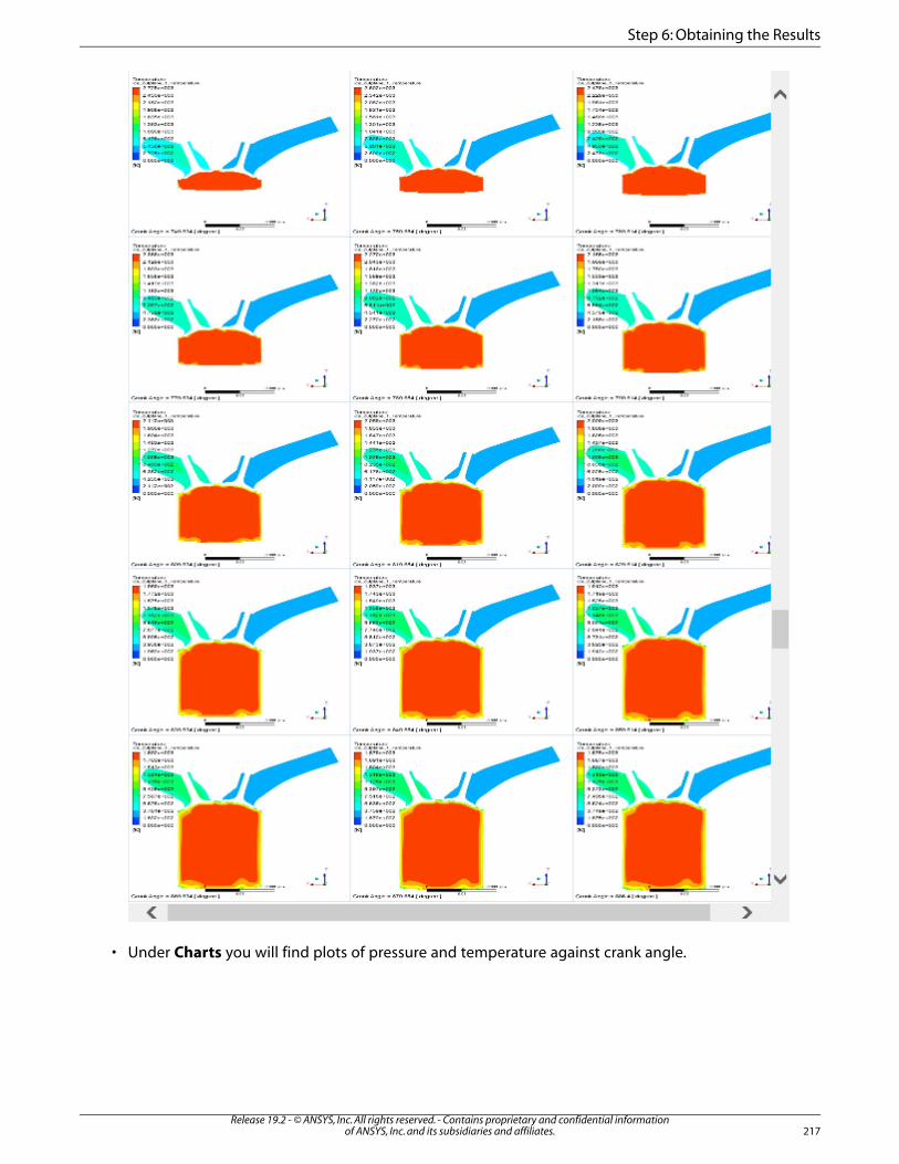
• Under Charts you will find plots of pressure and temperature against crank angle.
217Release 19.2 - © ANSYS, Inc. All rights reserved. - Contains proprietary and confidential information
of ANSYS, Inc. and its subsidiaries and affiliates.
Step 6: Obtaining the Results
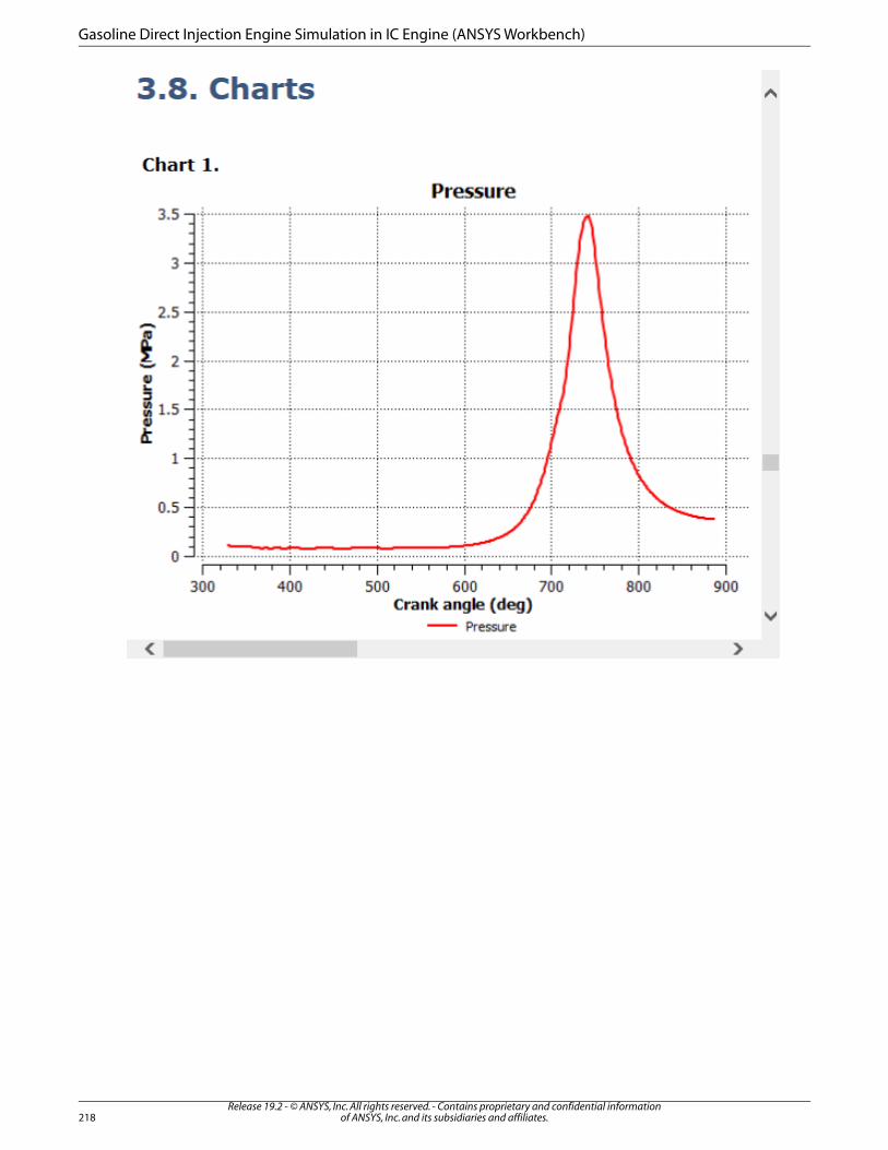
Release 19.2 - © ANSYS, Inc. All rights reserved. - Contains proprietary and confidential informationof ANSYS, Inc. and its subsidiaries and affiliates.218
Gasoline Direct Injection Engine Simulation in IC Engine (ANSYS Workbench)
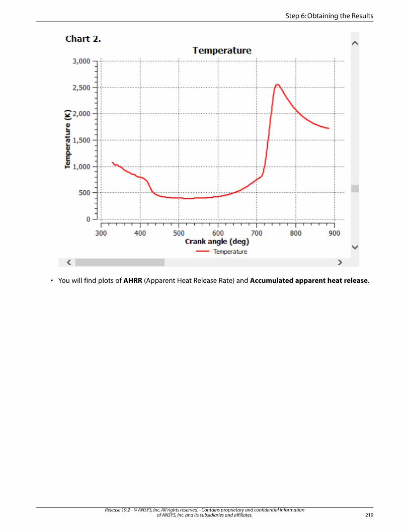
• You will find plots of AHRR (Apparent Heat Release Rate) and Accumulated apparent heat release.
219Release 19.2 - © ANSYS, Inc. All rights reserved. - Contains proprietary and confidential information
of ANSYS, Inc. and its subsidiaries and affiliates.
Step 6: Obtaining the Results
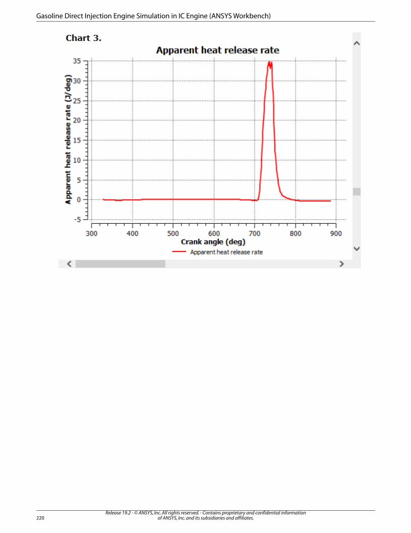
Release 19.2 - © ANSYS, Inc. All rights reserved. - Contains proprietary and confidential informationof ANSYS, Inc. and its subsidiaries and affiliates.220
Gasoline Direct Injection Engine Simulation in IC Engine (ANSYS Workbench)
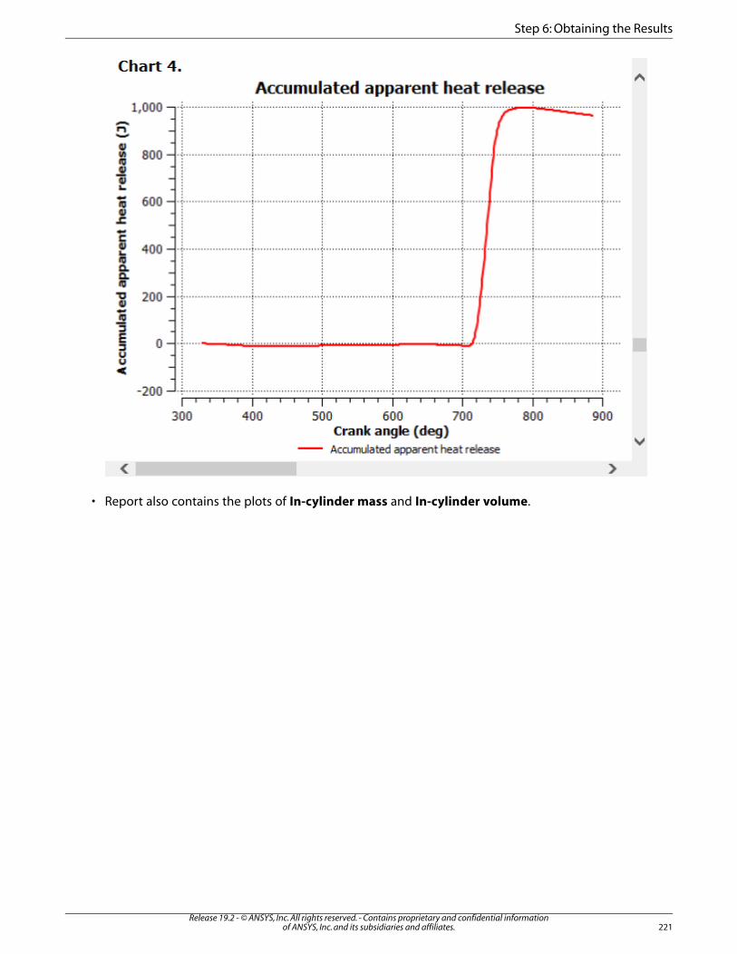
• Report also contains the plots of In-cylinder mass and In-cylinder volume.
221Release 19.2 - © ANSYS, Inc. All rights reserved. - Contains proprietary and confidential information
of ANSYS, Inc. and its subsidiaries and affiliates.
Step 6: Obtaining the Results
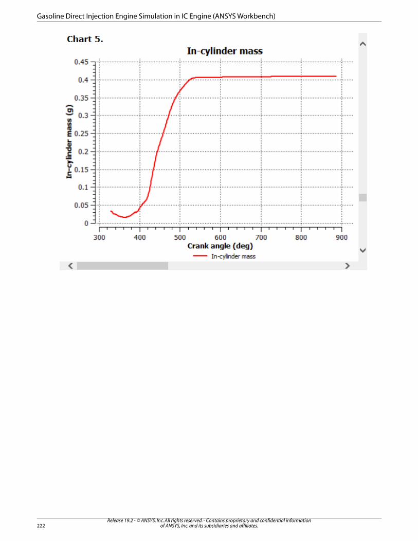
Release 19.2 - © ANSYS, Inc. All rights reserved. - Contains proprietary and confidential informationof ANSYS, Inc. and its subsidiaries and affiliates.222
Gasoline Direct Injection Engine Simulation in IC Engine (ANSYS Workbench)
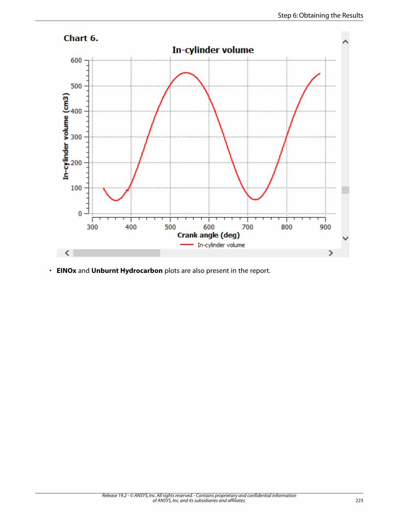
• EINOx and Unburnt Hydrocarbon plots are also present in the report.
223Release 19.2 - © ANSYS, Inc. All rights reserved. - Contains proprietary and confidential information
of ANSYS, Inc. and its subsidiaries and affiliates.
Step 6: Obtaining the Results
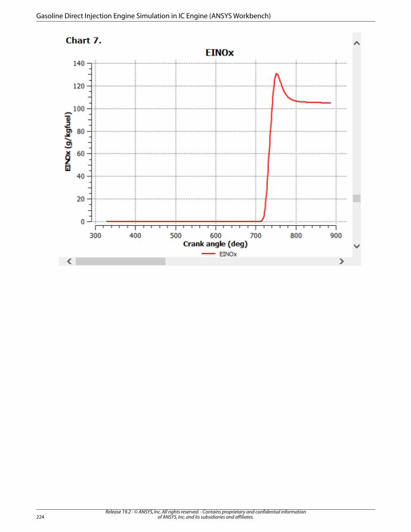
Release 19.2 - © ANSYS, Inc. All rights reserved. - Contains proprietary and confidential informationof ANSYS, Inc. and its subsidiaries and affiliates.224
Gasoline Direct Injection Engine Simulation in IC Engine (ANSYS Workbench)
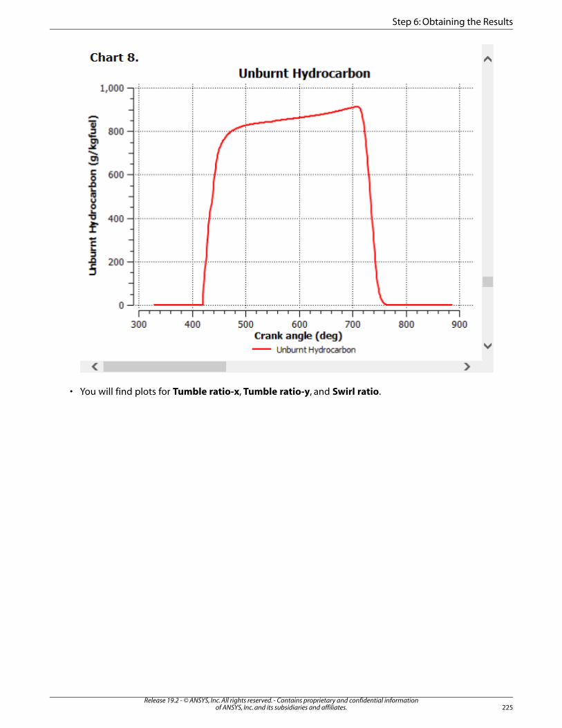
• You will find plots for Tumble ratio-x, Tumble ratio-y, and Swirl ratio.
225Release 19.2 - © ANSYS, Inc. All rights reserved. - Contains proprietary and confidential information
of ANSYS, Inc. and its subsidiaries and affiliates.
Step 6: Obtaining the Results
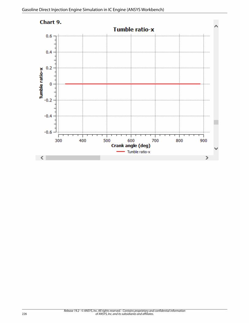
Release 19.2 - © ANSYS, Inc. All rights reserved. - Contains proprietary and confidential informationof ANSYS, Inc. and its subsidiaries and affiliates.226
Gasoline Direct Injection Engine Simulation in IC Engine (ANSYS Workbench)
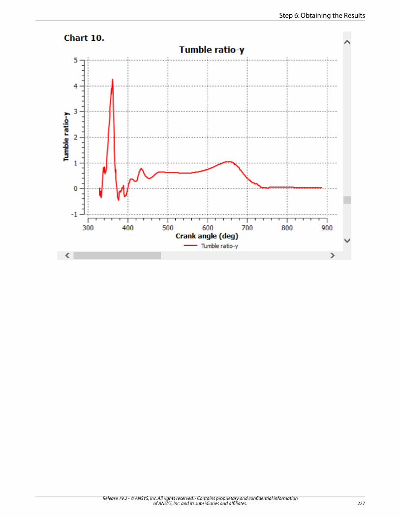
227Release 19.2 - © ANSYS, Inc. All rights reserved. - Contains proprietary and confidential information
of ANSYS, Inc. and its subsidiaries and affiliates.
Step 6: Obtaining the Results

• The report includes charts of mass inflow and outflow rate.
Release 19.2 - © ANSYS, Inc. All rights reserved. - Contains proprietary and confidential informationof ANSYS, Inc. and its subsidiaries and affiliates.228
Gasoline Direct Injection Engine Simulation in IC Engine (ANSYS Workbench)
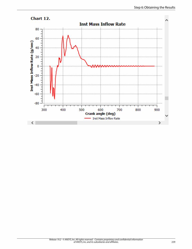
229Release 19.2 - © ANSYS, Inc. All rights reserved. - Contains proprietary and confidential information
of ANSYS, Inc. and its subsidiaries and affiliates.
Step 6: Obtaining the Results
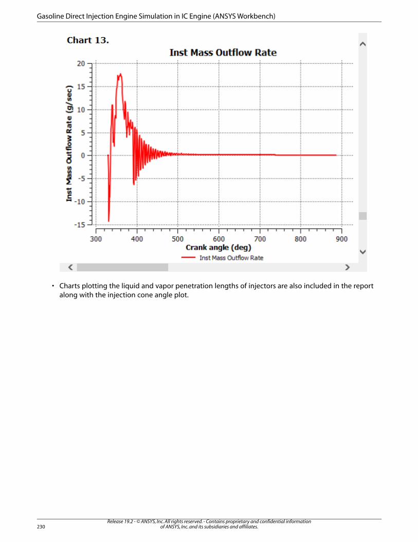
• Charts plotting the liquid and vapor penetration lengths of injectors are also included in the reportalong with the injection cone angle plot.
Release 19.2 - © ANSYS, Inc. All rights reserved. - Contains proprietary and confidential informationof ANSYS, Inc. and its subsidiaries and affiliates.230
Gasoline Direct Injection Engine Simulation in IC Engine (ANSYS Workbench)
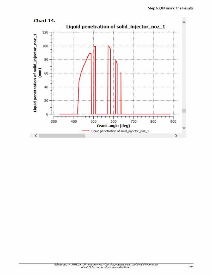
231Release 19.2 - © ANSYS, Inc. All rights reserved. - Contains proprietary and confidential information
of ANSYS, Inc. and its subsidiaries and affiliates.
Step 6: Obtaining the Results
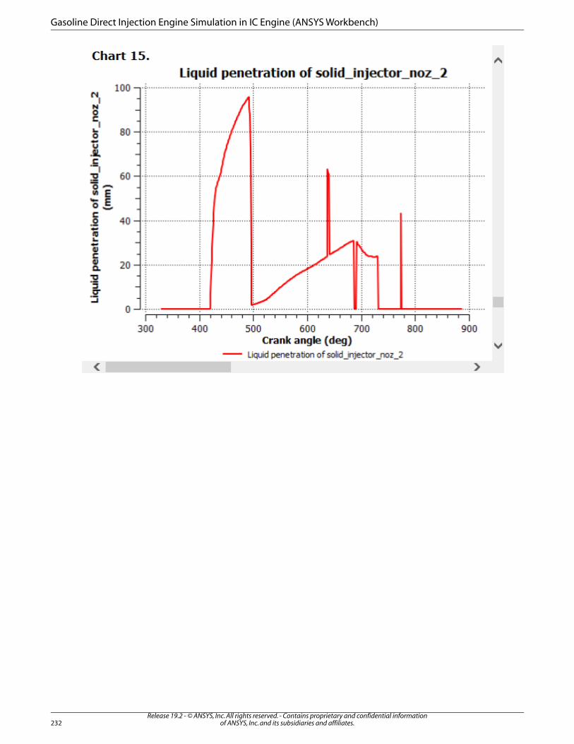
Release 19.2 - © ANSYS, Inc. All rights reserved. - Contains proprietary and confidential informationof ANSYS, Inc. and its subsidiaries and affiliates.232
Gasoline Direct Injection Engine Simulation in IC Engine (ANSYS Workbench)
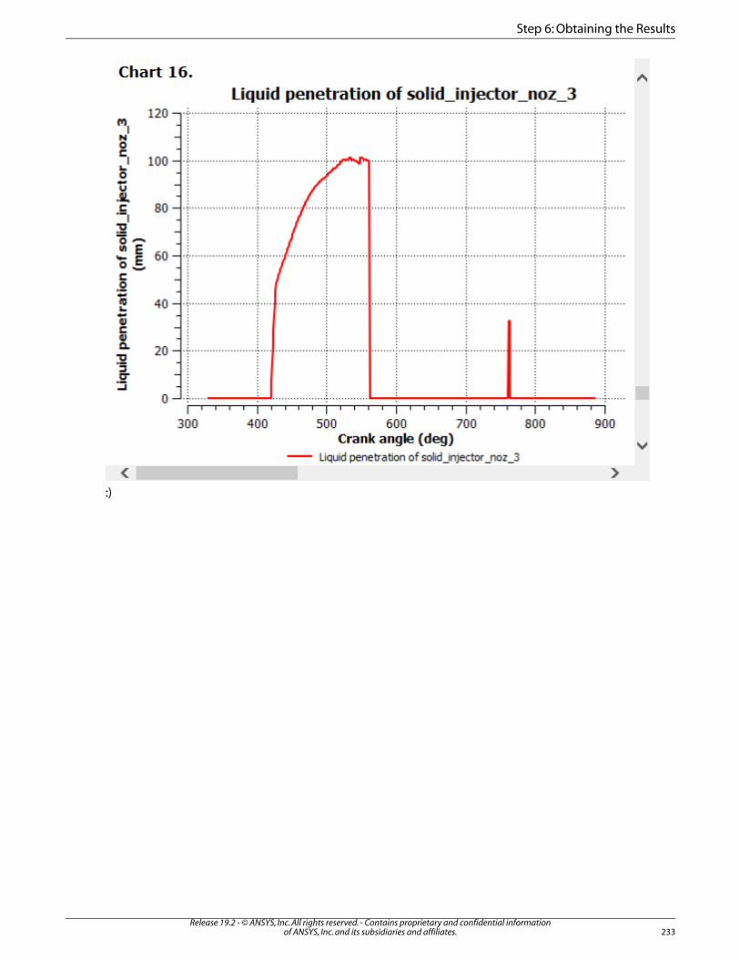
:)
233Release 19.2 - © ANSYS, Inc. All rights reserved. - Contains proprietary and confidential information
of ANSYS, Inc. and its subsidiaries and affiliates.
Step 6: Obtaining the Results
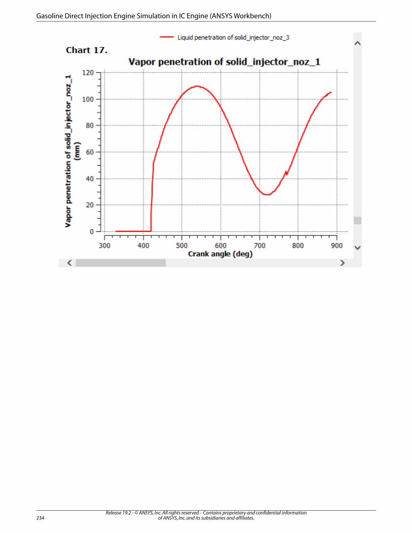
Release 19.2 - © ANSYS, Inc. All rights reserved. - Contains proprietary and confidential informationof ANSYS, Inc. and its subsidiaries and affiliates.234
Gasoline Direct Injection Engine Simulation in IC Engine (ANSYS Workbench)
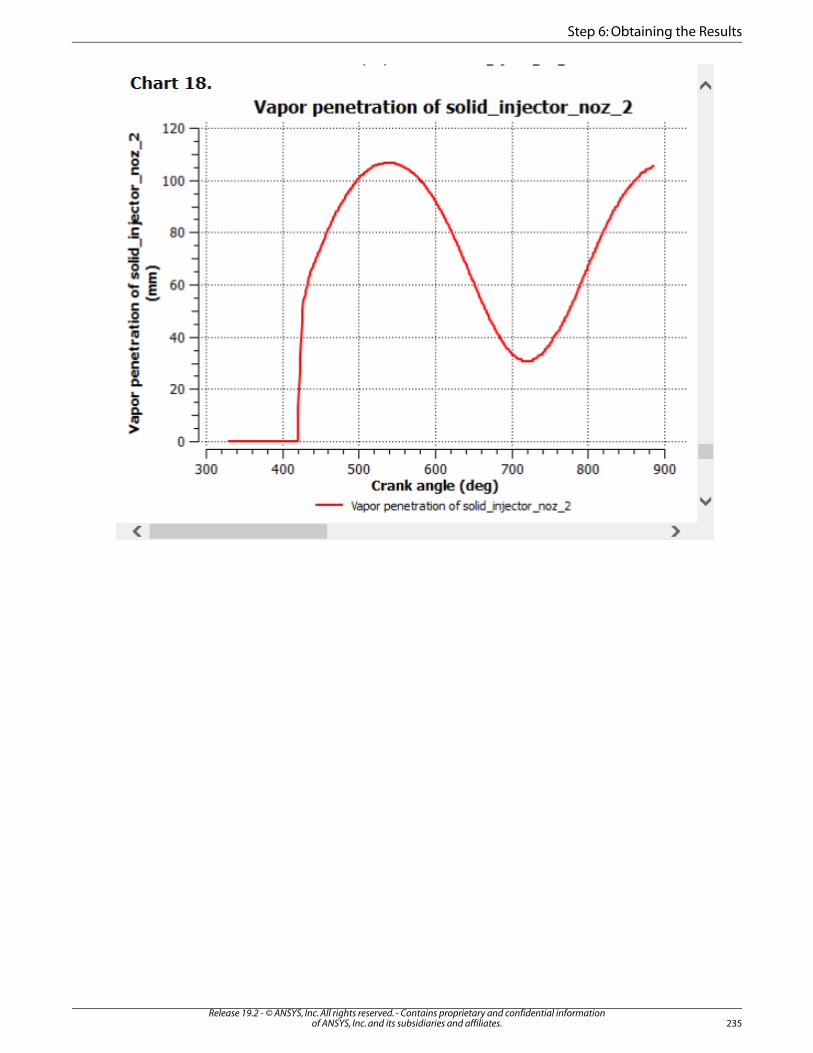
235Release 19.2 - © ANSYS, Inc. All rights reserved. - Contains proprietary and confidential information
of ANSYS, Inc. and its subsidiaries and affiliates.
Step 6: Obtaining the Results
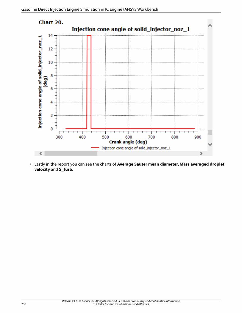
• Lastly in the report you can see the charts of Average Sauter mean diameter, Mass averaged dropletvelocity and S_turb.
Release 19.2 - © ANSYS, Inc. All rights reserved. - Contains proprietary and confidential informationof ANSYS, Inc. and its subsidiaries and affiliates.236
Gasoline Direct Injection Engine Simulation in IC Engine (ANSYS Workbench)
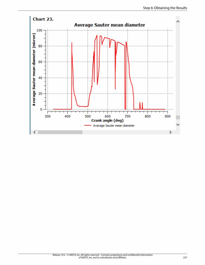
237Release 19.2 - © ANSYS, Inc. All rights reserved. - Contains proprietary and confidential information
of ANSYS, Inc. and its subsidiaries and affiliates.
Step 6: Obtaining the Results
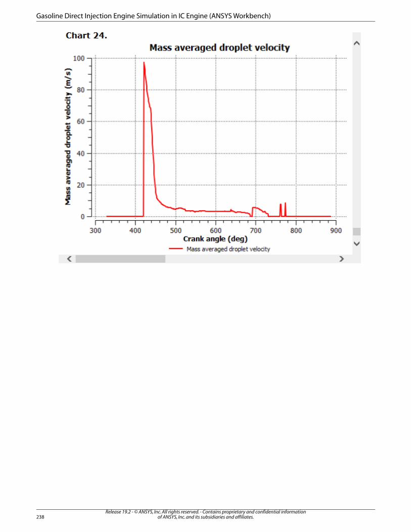
Release 19.2 - © ANSYS, Inc. All rights reserved. - Contains proprietary and confidential informationof ANSYS, Inc. and its subsidiaries and affiliates.238
Gasoline Direct Injection Engine Simulation in IC Engine (ANSYS Workbench)

This concludes the tutorial which demonstrated the setup and solution for the combustion simulationof an IC engine.
12.8. Summary
In this tutorial Gasoline spray and combustion phenomenon in a spark ignited engine were simulatedby using Forte. Single component fuel surrogate with 59 species combustion mechanism was used tosimulate fuel injection and combustion process in a SI engine. Pressure, heat release rate and emissionswere examined at the end of the simulation. You also learned streamlined workflow between pre-pro-cessing full engine and user defined post-processing for ease of GDI full engine simulations.
12.9. Further Improvements
You may use Model Fuel Library to generate realistic multi-component fuel that mimics real fuel prop-erties. Higher order chemistry mechanism can be incorporated to predict accurate heat release andemissions (soot).
239Release 19.2 - © ANSYS, Inc. All rights reserved. - Contains proprietary and confidential information
of ANSYS, Inc. and its subsidiaries and affiliates.
Further Improvements

Release 19.2 - © ANSYS, Inc. All rights reserved. - Contains proprietary and confidential informationof ANSYS, Inc. and its subsidiaries and affiliates.240