for academic use only - nit jamshedpur
TRANSCRIPT

ForAcademicuseONLY
DonotDistribute
Numerical Methods and Application
Code: MA 1404
Ramayan Singh
Department of Mathematics
NIT Jamshedpur

ForAcademicuseONLY
DonotDistribute
Contents
1 Introduction to Operator 1
1.1 Forward difference operator . . . . . . . . . . . . . . . . . . . . . . . . . . . . . . . . . . . . . . . . 1
1.2 Backward difference operator . . . . . . . . . . . . . . . . . . . . . . . . . . . . . . . . . . . . . . . 2
1.3 Central difference operator . . . . . . . . . . . . . . . . . . . . . . . . . . . . . . . . . . . . . . . . 2
1.4 Shift Operator . . . . . . . . . . . . . . . . . . . . . . . . . . . . . . . . . . . . . . . . . . . . . . . 3
1.5 Averaging Operator . . . . . . . . . . . . . . . . . . . . . . . . . . . . . . . . . . . . . . . . . . . . 4
2 Interpolation 6
2.1 Lagrange Interpolation . . . . . . . . . . . . . . . . . . . . . . . . . . . . . . . . . . . . . . . . . . . 6
2.3 Newton Interpolation polynomial . . . . . . . . . . . . . . . . . . . . . . . . . . . . . . . . . . . . . 9
2.5 Gregory-Newton Forward Difference Approach: . . . . . . . . . . . . . . . . . . . . . . . . . . . . . 13
2.6 Newton-Gregory Backward Difference Interpolation polynomiale . . . . . . . . . . . . . . . . . . . 15
3 Numerical differentiation 19
4 Numerical Integration 22
4.1 General Quadrature Formula . . . . . . . . . . . . . . . . . . . . . . . . . . . . . . . . . . . . . . . 22
4.2 Trapezoidal Rule . . . . . . . . . . . . . . . . . . . . . . . . . . . . . . . . . . . . . . . . . . . . . . 23
4.3 Simpson’s Rule . . . . . . . . . . . . . . . . . . . . . . . . . . . . . . . . . . . . . . . . . . . . . . . 24
4.4 Simpson’s 3/8 Rule . . . . . . . . . . . . . . . . . . . . . . . . . . . . . . . . . . . . . . . . . . . . . 25
4.5 Weddle’s Rule . . . . . . . . . . . . . . . . . . . . . . . . . . . . . . . . . . . . . . . . . . . . . . . . 25
5 Ordinary differential equation 26
5.1 Euler’s Method . . . . . . . . . . . . . . . . . . . . . . . . . . . . . . . . . . . . . . . . . . . . . . . 26
5.2 Modified Euler’s Method . . . . . . . . . . . . . . . . . . . . . . . . . . . . . . . . . . . . . . . . . . 28
5.4 Runga- Kutta Method . . . . . . . . . . . . . . . . . . . . . . . . . . . . . . . . . . . . . . . . . . . 30
5.6 Runge-Kutta Method of order 4 . . . . . . . . . . . . . . . . . . . . . . . . . . . . . . . . . . . . . . 32
6 System of linear equation 34
6.1 The Elimination Method . . . . . . . . . . . . . . . . . . . . . . . . . . . . . . . . . . . . . . . . . . 34
6.3 Jacobis Method . . . . . . . . . . . . . . . . . . . . . . . . . . . . . . . . . . . . . . . . . . . . . . . 36
6.4 Gauss Seidel Method . . . . . . . . . . . . . . . . . . . . . . . . . . . . . . . . . . . . . . . . . . . . 38

ForAcademicuseONLY
DonotDistribute
7 Partial differential equation 41
7.1 Order of partial differential equation . . . . . . . . . . . . . . . . . . . . . . . . . . . . . . . . . . . 41
7.2 Degree of partial differential equation . . . . . . . . . . . . . . . . . . . . . . . . . . . . . . . . . . 41
7.3 Classification of the first order partial differential equation . . . . . . . . . . . . . . . . . . . . . . . 41
7.4 Classification of the second order partial differential equation . . . . . . . . . . . . . . . . . . . . . 42
7.5 Classification of the second order semi-linear partial differential equation . . . . . . . . . . . . . . . 42

ForAcademicuseONLY
DonotDistribute
Introduction to Operator
Topic No. 1
Introduction to Operator
Learning Objectives At the end of this session students should be able to
1. recall forward and bacward difference operator.
2. know what is central diffetence and average operator.
3. know what is shift operator.
4. establish the relationship between above five operator.
Theoritical Part
1.1 Forward difference operator
Forward difference operator , denoted by ∆, and defined by
∆f(x) = f(x+ h)− f(x).
The expression f(x + h) − f(x) gives the First Forward difference of f(x) and the operator ∆ is called the
First Forward difference operator. Given the step size h, this formula uses the values at x and x + h, the
point at the next step. As it is moving in the forward direction, it is called the forward difference operator.
Similarly, the second forward difference operator, ∆2, is defined as
∆2f(x) = ∆(∆f(x)
)= ∆f(x+ h)−∆f(x).
We note that
∆2f(x) = ∆f(x+ h)−∆f(x)
=(f(x+ 2h)− f(x+ h)
)−(f(x+ h)− f(x)
)= f(x+ 2h)− 2f(x+ h) + f(x)
In particular, for x = xk, we get,
∆yk = yk+1 − yk
and
∆2yk = ∆yk+1 −∆yk = yk+2 − 2yk+1 + yk.
Now the rth forward difference operator, ∆r, is defined as
∆rf(x) = ∆r−1f(x+ h)−∆r−1f(x), r = 1, 2, . . . ,

ForAcademicuseONLY
DonotDistribute
1.2 Backward difference operator Introduction to Operator
with ∆0f(x) = f(x).
Remark:
• For a set of tabular values, the horizontal forward difference table is written as:
x0 y0
∆y0 = y1 − y0
x1 y1 ∆2y0 = ∆y1 −∆y0
∆y1 = y2 − y1
x2 y2 ∆2y1 = ∆y2 −∆y1
· · · · · · · · ·
xn−1 yn−1 ∆2yn−2 = ∆yn−1 −∆yn−2
∆yn−1 = yn − yn−1
xn yn
• In general, if f(x) = xn + a1xn−1 + a2x
n−2 + · · · + an−1x + an is a polynomial of degree n, then it can be
shown that ∆nf(x) = n!hn and ∆n+rf(x) = 0 for r = 1, 2, . . . .
1.2 Backward difference operator
The Backward difference operator, denoted by ∇, is defined as
∇f(x) = f(x)− f(x− h).
Given the step size h, note that this formula uses the values at x and x− h, the point at the previous step. As it
moves in the backward direction, it is called the backward difference operator.
The rth backward difference operator, ∇r, is defined as
∇rf(x) = ∇r−1f(x)−∇r−1f(x− h), r = 1, 2, . . . ,
with ∇0f(x) = f(x).
In particular, for x = xk, we get ∇yk = yk − yk−1 and ∇2yk = yk − 2yk−1 + yk−2.
Note: ∇2yk = ∆2yk−2.
1.3 Central difference operator
The The First Central difference operator, denoted by δ, is defined by
δf(x) = f(x+h
2)− f(x− h
2)
and the rth Central difference operator is defined as
δrf(x) = δr−1f(x+h
2)− δr−1f(x− h
2)

ForAcademicuseONLY
DonotDistribute
1.4 Shift Operator Introduction to Operator
with δ0f(x) = f(x).
Thus, δ2f(x) = f(x+ h)− 2f(x) + f(x− h).
In particular, for x = xk, define yk+ 12
= f(xk + h2 ), and yk− 1
2= f(xk − h
2 ), then
δyk = yk+ 12− yk− 1
2and δ2yk = yk+1 − 2yk + yk−1.
Example 1.3.1. the following set of tabular values (xi, yi), write the forward and backward difference tables.
xi 9 10 11 12 13 14
yi 5.0 5.4 6.0 6.8 7.5 8.1
Soln.
x y ∆y ∆2y ∆3y ∆4y ∆5y
9 5.0 0.4 0.2 0.0 -0.3 0.6
10 5.4 0.6 0.2 -0.3 0.3
11 6.0 0.8 -0.1 0.0
12 6.8 0.7 -0.1
13 7.5 0.6
14 8.1
x y ∇y ∇2y ∇3y ∇4y ∇5y
9 5
10 5.4 0.4
11 6 0.6 0.2
12 6.8 0.8 0.2 0.0
13 7.5 0.7 -0.1 - 0.3 -0.3
14 8.1 0.6 -0.1 0.0 0.3 0.6
1.4 Shift Operator
A Shift operator, denoted by E, is the operator which shifts the value at the next point with step h, i.e.,
Ef(x) = f(x+ h).
Thus,
Eyi = yi+1, E2yi = yi+2, and Ekyi = yi+k.
Example 1.4.1. Show that E ≡ 1 + ∆
Soln.
Ef(x) = f(x+ h)
= [f(x+ h)− f(x)] + f(x)
= ∆f(x) + f(x)
= (∆ + 1)f(x)
∴ E ≡ 1 + ∆
ForAcademicuseONLY
DonotDistribute
1.5 Averaging Operator Introduction to Operator
1.5 Averaging Operator
The Averaging Operator, denoted by µ, gives the average value between two central points, i.e., µf(x) =1
2
[f(x+
h
2) + f(x− h
2)]. Thus µ yi = 1
2(yi+ 12
+ yi− 12) and µ2 yi =
1
2
[µ yi+ 1
2+ µ yi− 1
2
]=
1
4[yi+1 + 2yi + yi−1] .
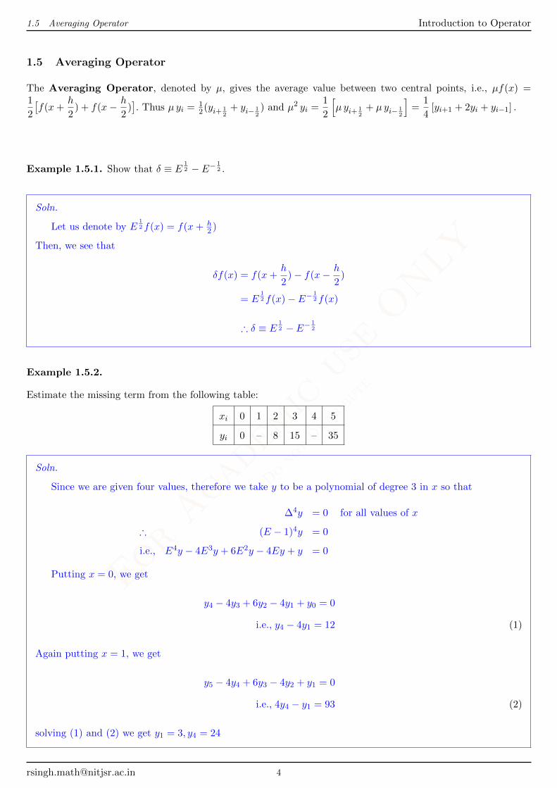
Example 1.5.1. Show that δ ≡ E12 − E−
12 .
Soln.
Let us denote by E12 f(x) = f(x+ h
2 )
Then, we see that
δf(x) = f(x+h
2)− f(x− h
2)
= E12 f(x)− E−
12 f(x)
∴ δ ≡ E12 − E−
12
Example 1.5.2.
Estimate the missing term from the following table:
xi 0 1 2 3 4 5
yi 0 – 8 15 – 35
Soln.
Since we are given four values, therefore we take y to be a polynomial of degree 3 in x so that
∆4y = 0 for all values of x
∴ (E − 1)4y = 0
i.e., E4y − 4E3y + 6E2y − 4Ey + y = 0
Putting x = 0, we get
y4 − 4y3 + 6y2 − 4y1 + y0 = 0
i.e., y4 − 4y1 = 12 (1)
Again putting x = 1, we get
y5 − 4y4 + 6y3 − 4y2 + y1 = 0
i.e., 4y4 − y1 = 93 (2)
solving (1) and (2) we get y1 = 3, y4 = 24

ForAcademicuseONLY
DonotDistribute
1.5 Averaging Operator Introduction to Operator
Practice Problems
Problem 1.6. 1. Prove that E ≡ ehD.
2. Prove that µ2 ≡ 14
(δ2 + 4
)3. Prove that hD ≡ sinh−1(µδ).
4. Prove that ∆−∇ ≡ δ2
5. Show that D ≡ 1h ln
(1
1−∇
).
6. Find ∆2(ax2 + bx+ c) Ans: 2ah2
7. Find ∆2 cos 2x Ans: −4 sinh cos 2(x+ h)
8. Estimate the missing term from the following table:
xi 0 1 2 3 4
yi 1 3 9 – 81
Ans: 31
9. Estimate the missing term from the following table:
xi 1 2 3 4 5 6 7
yi 2 4 8 – 32 64 128
Ans: 16.1
ForAcademicuseONLY
DonotDistribute
Interpolation
Topic No. 2
Interpolation
Learning Objectives At the end of this session students should be able to
1. know what is interpolation.
2. apply Lagrange method and divide difference method to find the unknown value from the given data set.
3. apply Newton forward and backward interpolation method.
Theoritical Part
Interpolation is a method of constructing new data points within the range of a discrete set of known data points.
In engineering and science, one often has a number of data points, obtained by sampling or experimentation,
which represent the values of a function for a limited number of values of the independent variable. It is often
required to interpolate, i.e., estimate the value of that function for an intermediate value of the independent
variable.
2.1 Lagrange Interpolation
Let us suppose that the given data points (xi, yi), i = 0, 1, 2...n is coming from a function f(x). Let us assume
that this function y = f(x) takes the values y0, y1.......yn at x0, x1, .......xn. Since there are (n + 1) data points
(xi, yi), we can represent the function f(x) by a polynomial of degree n
∴ f(x) = Cnxn + Cn−1x
n−1 + ...+ C1x+ C0 (3)
As we have assumed that f(xi) = yi, i = 0, 1, 2.......n i.e. the function f(x) passes through (xi, yi) can be rewritten
as:
y = f(x) = a0(x− x1)(x− x2)...(x− xn) + a1(x− x0)(x− x2)...(x− xn)+
a2(x− x0)(x− x1)(x− x3)...(x− xn) + .......+ an(x− x0)...(x− xn−1) (4)
But
yi = f(xi) i = 0, 1, .....n (5)
Using (3) for i=0, in (2) we get
y0 = f(x0) = a0(x0 − x1)...(x0 − xn) (6)
∴ a0 =y0
(x0 − x1)...(x0 − xn)(7)

ForAcademicuseONLY
DonotDistribute
2.1 Lagrange Interpolation Interpolation
For i = 1, we get
y1 = f(x1) = a1(x1 − xo)(x1 − x2)...(x1 − xn) (8)
a1 =y1
(x1 − x0)(x1 − x2)...(x1 − xn)(9)
Similarly for i = 2.......n− 1, we get
ai =yi
(xi − x0)(xi − x1)...(xi − xi−1)(xi − xi+1)...(xi − xn)(10)
and for i = n, we get
an =yn
(xn − x0)...(xn − xn−1)(11)
Using (5), (7), (8), (9) in (2) we get can be rewritten in a compact form as:
y = f(x) = L0(x)y0 + L1(x)y1 + ...........+ Ln(x)yn
=
n∑i=0
Li(x)yi
=
n∑i=0
Li(x)f(xi) (12)
where
Li(x) =(x− x0)(x− x1)...(x− xi−1)(x− xi+1)...(x− x......)(xi − x0)(xi − x1)...(xi − xi−1)(xi − xi+1)...(xi − xn)
(13)
It can be easily noted that Let us introduce the product notation as :
∏(x) =
n∏i=0
(x− xi) = (x− x0)(x− x1)....(x− xn)
Therefore, Lagrange interpolation polynomial of degree n can be written as
y = f(x) =n∑k=0
Lk(x)yk (14)
Note: Given a set of data points(xi, yi) i = 1, 2, · · · , n . Suppose we are interested in evaluating f(x) at
some intermediate point x to a desired level of accuracy. Directly using the entire data set of size n may not
only be computationally economical but may also turn out to be redundant. Naturally one would like to use an
interpolating polynomial of optimal degree. Since this is not known apriori, one may start with P0(x) and if it
was enough then move onto P1(x) and so on i.e. slowly increase the no. of the interpolating points (or) data
points x0, x1..xk so that Pk−1(x) will be close to f(x). In this context the biggest disadvantage with Lagrange
Interpolation is that we cannot use the work that has already been done i.e. we cannot make use of Pk−1(x)
while evaluating Pk(x). With the addition of each new data point, calculations have to be repeated. Newton
Interpolation polynomial overcomes this drawback.
Example 2.1.1. Given the following data table, construct the Lagrange interpolation polynomial f(x), to fit the
data and find f(1.25)

ForAcademicuseONLY
DonotDistribute
2.1 Lagrange Interpolation Interpolation
xi 0 1 2 3
yi 1 2.25 3.75 4.25
Soln. Lagrange interpolation polynomial is given by y=f(x) =
L0(x) =(x− x1)(x− x2)(x− x3)
(x0 − x1)(x0 − x2)(x0 − x3)=
(x− 1)(x− 2)(x− 3)
(0− 1)(0− 2)(0− 3)=x3 − 6x2 + 11x− 6
−6
L1(x) =(x− x0)(x− x2)(x− x3)
(x1 − x0)(x1 − x2)(x1 − x3)=
(x− 0)(x− 2)(x− 3)
(1− 0)(1− 2)(1− 3)=x3 − 5x2 + 6x
2
L2(x) =(x− 0)(x− 1)(x− 3)
(2− 0)(2− 1)(2− 3)=x3 − 4x2 + 3x
−2
L3(x) =(x− 0)(x− 1)(x− 2)
(3− 0)(3− 1)(3− 2)=x3 − 3x2 + 2x
6
f(1.25) = L0(1.25)y0 + L1(1.25)y1 + L2(1.25)y2 + L3(1.25)y3
= (−0.546875).1 + (0.8203125)2.25 + (0.2734375)3.75 + (−0.0390625)4.25
= 2.650390625
Example 2.1.2. Given the following data table, construct the Lagrange interpolation polynomial f(x), to fit the
data and find
xi 1980 1985 1990 1995 2000 2005
yi 440 510 525 571 500 600
Soln. Here n = 6, xk = 1998
Lagrange interpolation polynomial is given by
L0(x) =(x− x1)(x− x2)(x− x3)(x− x4)(x− x5)
(x0 − x1)(x0 − x2)(x0 − x3)(x0 − x4)(x0 − x5)
=(x− 1985)(x− 1990)(x− 1995)(x− 2000)(x− 2005)
(1980− 1985)(1980− 1990)(1980− 1995)(1980− 2000)(1980− 2005)
L0(xk) = L0(1998) =(1998− 1985)(1998− 1990)(1998− 1995)(1998− 2000)(1998− 2005)
(−5)(−10)(−15)(−20)(−25)
=13.8.3.(−2).(−7)
−(375000)= − 4368
375000= −0.011648
L1(xk) =(xk − x0)(xk − x2)(xk − x3)(xk − x4)(xk − x5)
(x1 − x0)(x1 − x2)(x1 − x3)(x1 − x4)(x1 − x5)
=(1998− 1980)(1998− 1990)(1998− 1995)(1998− 2000)(1998− 2005)
(1985− 1980)(1985− 1990)(1985− 1995)(1985− 2000)(1985− 2005)
=18.8.3.(−2).(−7)
5(−5)(−10)(−15)(−20)= 0.08064

ForAcademicuseONLY
DonotDistribute
2.3 Newton Interpolation polynomial Interpolation
L2(xk) =(1998− 1980)(1998− 1985)(1998− 1995)(1998− 2000)(1998− 2005)
(1990− 1980)(1990− 1985)(1990− 1995)(1990− 2000)(1990− 2005)
=18.13.3.(−2)(−7)
10.5.(−5)(−10).(−15)= −0.26208
L3(xk) =(1998− 1980)(1998− 1985)(1998− 1990)(1998− 2000)(1998− 2005)
(1995− 1980)(1995− 1985)(1995− 1990)(1995− 2000)(1995− 2005)
=18.13.8.(−2)(−7)
15.10.5(−5)(−10)= 0.69888
L4(xk) =(1998− 1980)(1998− 1985)(1998− 1990)(1998− 1995)(1998− 2005)
(2000− 1980)(2000− 1985)(2000− 1990)(2000− 1995)(2000− 2005)
=18.13.8.3.(−7)
20.15.10.5(−5)= 0.52416
L4(xk) =(1998− 1980(1998− 1985)(1998− 1990)(1998− 1995)(1998− 2000)
(2005− 1980)(2005− 1985)(2005− 1990)(2005− 1995)(2005− 2000)
=18.13.8.3.(−2)
25.20.15.10.5= −0.029952
∴ f(1998) =
5∑i=0
Li(1998)yi = 541.578560
Practice Problems
Problem 2.2. 1. Use Lagrange’s interpolation formula to find f(x), if f(1) = 2, f(2) = 4, f(3) = 8, f(4) =
16 andf(7) = 128.
2. Use Lagrange interpolation formula to fit a polynomial to the following data. Hence find f(4).
xi 1.140 1.145 1.150 1.155 1.160 1.165
f(x) 0.13103 0.135410 0.13976 0.14410 1.14842 0.15272
Ans: 1/6(7x3 − 31x2 + 28x+ 18),13.66
2.3 Newton Interpolation polynomial
Suppose that we are given a data set (xi, fi), i = 0, 1...n− 1. Let us assume that these are interpolating points of
Newton form of interpolating polynomial Pn(x) of degree n i.e
Pn(xi) = fi, i = 1, 2, · · · , n (15)
The Newton form of the interpolating polynomial Pn(x) is given by
Pn(x) = a0 +a1(x−x0)+a2(x−x0)(x−x1)+a3(x−x0)(x−x1)(x−x2)+ · · ·+an(x−x0)(x−x1) · · · (x−xn) (16)

ForAcademicuseONLY
DonotDistribute
2.3 Newton Interpolation polynomial Interpolation
For i = 0, from (13) & (14) we get
f0 = Pn(x0) = a0
For i = 1, from (1) & (2) we get
f1 = pn(x1) = a0 + a1(x1 − x0)
a1 =f1 − f0
x1 − x0
For i = 2, from(13) & (14) we get
f2 = pn(x2) = a0 + a1(x2 − x0) + a2(x2 − x0)(x2 − x1)
Using a0 & a1 we get
a2 =[(f2 − f1)/(x2 − x1)]− [(f1 − f0)/(x1 − x0)]
(x2 − x0)
Similarly we can find a3.....an−1. To express ai, i = 0......n−1 in a compact manner let us first define the following
notation called divided differences:
f [xk] = fk
f [xk, xk+1] =f [xk+1]− f [xk]
xk+1 − xk
f [xk, xk+1, xk+2] =f [xk+1, xk+2]− f [xk, xk+1]
xk+2 − xkNow the co-efficients can be expressed in terms of divided differences as follows:
a0 = f0 = f [x0]
a2 =
f2−f1x2−x1 −
f1−f0x1−x0
x2 − x0=f [x1, x2]− f [x0, x1]
x2 − x0
= f [x0, x1, x2]
an = f [x0, x1...xn]
Note that a1 is called as the first divided difference, a2 as the second divided difference and so on. Now the
polynomial (13) can be rewritten as:
This is called as Newton’s Divided Difference interpolation polynomial.
Example 2.3.1. Given the following data table, evaluate f(2.4) using 3rd order Newton’s Divided Difference
interpolation polynomial.
xi 0 1 2 3 4
yi = f(xi) 1 2.25 3.75 4.25 5.81

ForAcademicuseONLY
DonotDistribute
2.3 Newton Interpolation polynomial Interpolation
Soln. Here . For constructing 3rd order Newton Divided Difference polynomial we need only four points. Let
us use the first four points. The 3rd Newton Divided Difference polynomial is given by:
a0 = f [x0] = 1
∴ a1 = f [x0, x1] =f(x1)− f(x0)
(x1 − x0)=
2.25− 1
1− 0= 1.25
∴ a2 = f [x0, x1, x2] =f [x1, x2]− f [x0, x1]
x2 − x0=
1.5− 1.25
2− 0= 0.125
f [x2, x3] =f [x3]− f [x2]
x3 − x2=
4.25− 3.75
3− 2=
0.5
1= 0.5
f [x1, x2, x3] =f [x2, x3]− f [x1, x2]
x3 − x1=
0.5− 1.5
3− 1= −0.5
∴ a3 = f [x0, x1, x2, x3] =f [x1, x2, x3]− f [x0, x1, x2]
x3 − x0=−0.5− 0.125
3− 0=−0.625
3= −0.20833
∴ p3(x) = 1 + 1.25(x− 0) + 0.125(x− 0)(x− 1) + (−0.20833)(x− 0)(x− 1)(x− 2)
∴ f(2.4) = p3(2.4) = 1 + 1.25(2.4− 0) + 0.125(2.4− 0)(2.4− 1)
+ (−0.20833)(2.4− 0)(2.4− 1)(2.4− 2)
= 1 + (1.25)(2.4) + 0.125(2.4)(1.4)− 0.20833(2.4)(1.4)(0.4)
In this example it may be noted that for calculating the order polynomial, we first start with P0 = f [x0] = 1.
To it we add a1(x − x0) to get P1 and to P1 we add a2(x − x0)(x − x1) to get P2. Finally on adding
a3(x− x0)(x− x1)(x− x2) to P2 we get P3.
Newton Divided Difference Table
It may also be noted for calculating the higher order divided differences we have used lower order divided
differences. In fact starting from the given zeroth order differences ; one can systematically arrive at any of higher
order divided differences. For clarity the entire calculation may be depicted in the form of a table called

ForAcademicuseONLY
DonotDistribute
2.3 Newton Interpolation polynomial Interpolation
i xi f [xi]First order
differences
Second order
differences
Third order
differences
Fourth order
differences
0 x0 f [x0]
f [x0, x1]
1 x1 f [x0] f [x0, x1, x2]
f [x1, x2] f [x0, x1, x2, x3]
2 x2 f [x2] f [x1, x2, x3] f [x0, x1, x2, x3, x4]
f [x2, x3] f [x1, x2, x3, x4]
3 x3 f [x3] f [x2, x3, x4]
f [x3, x4]
4 x4 f [x4]
Again suppose that we are given the data set (xi, fi), i = 0.......5 and that we are interested in finding the 5th
order Newton Divided Difference interpolation polynomial. Let us first construct the Newton Divided Difference
Table. Wherein one can clearly see how the lower order differences are used in calculating the higher order Divided
Differences
Note: One may note that the given data corresponds to the cubic polynomial. To fit such a data 3rd order
polynomial is adequate. From the Newton Divided Difference table we notice that the fourth order difference
is zero. Further the divided differences in the table can be directly used for constructing the Newton Divided
Difference interpolation polynomial that would fit the data.
Example 2.3.2. Construct the Newton Divided Difference Table for generating Newton interpolation polynomial
with the following data set:
xi 0 1 2 3 4
yi = f(xi) 0 1 8 27 64
Soln. Here . One can fit a fourth order Newton Divided Difference interpolation polynomial to the given data.
Let us generate Newton Divided Difference Table; as requested.
i xi f [xi]1st order
differences
2nd order
differences
3rd order
differences
4th order
differences
0 0 0
1−01−0 = 1
1 1 1 7−12−0 = 3
8−12−1 = 7 6−3
3−0 = 1
2 2 8 19−73−1 = 6 1−1
4−0 = 0

ForAcademicuseONLY
DonotDistribute
2.5 Gregory-Newton Forward Difference Approach: Interpolation
27−83−2 = 19 9−6
4−1 = 1
3 3 27 37−194−2 = 9
64−274−3 = 37
4 4 64
Practice Problems
Problem 2.4. 1. Find f(8) using Newton’s divided difference formula given that.
xi 4 5 7 10 11 13
f(x) 48 100 294 900 1210 2028
Ans: 448
2. Find f(27) using Newton’s divided difference formula given that.
xi 14 17 31 35
f(x) 68.7 64.0 44.0 39.1
Ans: 49.3
2.5 Gregory-Newton Forward Difference Approach:
Very often it so happens in practice that the given data set correspond to a sequence {xi} of equally spaced points.
Here we can assume that
xi = x0 + ih i = 0, 1, 2, · · · , n
where x0 is the starting point (sometimes, for convenience, the middle data point is taken as x0 and in such a case
the integer i is allowed to take both negative and positive values.) and h is the step size. Further it is enough to
calculate simple differences rather than the divided differences as in the non-uniformly placed data set case. These
simple differences can be forward differences (∆fi) or backward differences (∇fi). We will first look at forward
differences and the interpolation polynomial based on forward differences.
The first order forward difference ∆fi is defined as
∆fi = fi+1 − fi
The second order forward difference ∆2fi is defined as
∆2fi = ∆fi+1 −∆fi

ForAcademicuseONLY
DonotDistribute
2.5 Gregory-Newton Forward Difference Approach: Interpolation
The kth order forward difference ∆kfi is defined as
∆kfi = ∆k−1fi+1 −∆k−1fi
Since we already know Newton interpolation polynomial in terms of divided differences, to derive or generate
Newton interpolation polynomial in terms of forward differences it is enough to express forward differences in
terms of divided differences.
Recall the definition of first divided difference f [x0, x1],
f [x0, x1] =f(x1)− f(x0)
x1 − x0=f1 − f0
h=
∆f0
h
∴ ∆f0 = hf [x0, x1]
Similarly we can get
∆f1 = hf [x1, x2]
By the definition of second order forward difference ∆2f0, we get
∆2f0 = ∆f1 −∆f0
= hf [x1, x2]− hf [x0, x1]
= h.2h (f [x1, x2]− f [x0, x1]/2h)
= 2h2f [x0, x1, x2]
In a similar way, in general, we can show that
∆kfi = k!hkf [xi, xi+1, xi+2...xi+k]
∴ f [xi, xi+1, ...xi+k] =∆kfik!hk
For i = 0,
f [x0, x1...xk] =∆kf0
k!hk
Now using Newton divide difference formula and above relation the Newton forward difference interpolation
polynomial may be written as follows:
Pn(x) =
n∑k=0
∆kf0
k!hk
k−1∏i=0
(x− xi) (17)
To rewrite (16) in a simpler way let us set
∵ xk = x0 + kh
x− xk = (s− k)h

ForAcademicuseONLY
DonotDistribute
2.6 Newton-Gregory Backward Difference Interpolation polynomiale Interpolation
Pn(x) = Pn(s) =
n∑k=0
∆kf0
k!hk
k−1∏i=0
(s− i)h
=
n∑k=0
∆kf0
k!hk[s(s− 1).......(s− k + 1)]hk
=
n∑k=0
s
k
∆kf0 (18)
This is known as Newton-Gregory forward difference interpolation polynomial. For convenience while constructing
(17) one can first generate a forward difference table and use the ∆kfi from the table. Suppose we have data set
(xifi), i = 0, 1, 2, 3, 4 then forward difference table looks as follows:
i xi f [xi] ∆f [xi] ∆2f [xi] ∆3f [xi] ∆3f [xi]
0 x0 f [x0]
∆f [x0]
1 x1 f [x1] ∆2f [x0]
∆f [x1] ∆3f [x0]
2 x2 f [x2] ∆2f [x1] ∆4f [x0]
∆f [x2] ∆3f [x1]
3 x3 f [x3] ∆2f [x2]
∆f [x3]
4 x4 f [x4]
2.6 Newton-Gregory Backward Difference Interpolation polynomiale
If the data size is big then the divided difference table will be too long. Suppose the desired intermediate value
(x̃) at which one needs to estimate the function (i.e.f(x̃)) falls towards the end or say in the second half of the
data set then it may be better to start the estimation process from the last data set point. For this we need
to use backward-differences and backward difference table. Let us first define backward differences and generate
backward difference table, say for the data set (xi, fi), i = 0, 1, 2, 3, 4.
First order backward difference ∇fi is defined as:
∇fi = fi − fi−1
Second order backward difference ∇2fi is defined as:
∇2fi = ∇fi −∇fi−1
In general, the kth order backward difference is defined as
∇kfi = ∇k−1fi −∇k−1fi−1

ForAcademicuseONLY
DonotDistribute
2.6 Newton-Gregory Backward Difference Interpolation polynomiale Interpolation
In this case the reference point is xn and therefore we can derive the Newton-Gregory backward difference inter-
polation polynomial as:
Pn(x) = Pn(s) =
n∑k=0
∇kfnk!hk
k−1∏i=0
(s+ i)h
=
n∑k=0
∇kf0
k!hk[s(s+ 1).......(s+ k − 1)]hk (19)
Where s =x− xnh
For constructing as given in Eqn.(18) it will be easier if we first generate backward-difference
table. The backward difference table for the data (xi, fi), i = 0, 1, 2, 3, 4.
i xi f [xi] ∇f [xi] ∇2f [xi] ∇3f [xi] ∇3f [xi]
0 x0 f [x0]
∇f [x1]
1 x1 f [x1] ∇2f [x2]
∇f [x2] ∇3f [x3]
2 x2 f [x2] ∇2f [x3] ∇4f [x4]
∇f [x3] ∇3f [x4]
3 x3 f [x3] ∇2f [x4]
∇f [x4]
4 x4 f [x4]
Example 2.6.1. Given the following data, estimate using Newton-Gregory forward difference interpolation poly-
nomial:
xi 1 3 5 7 9
yi = f(xi) 0 1.0986 1.6094 1.9459 2.1972
Soln. Here we have five data points i.e i = 0, 1, 2, 3, 4. Let us first generate the forward difference table.
i xi f [xi] ∆f [xi] ∆2f [xi] ∆3f [xi] ∆3f [xi]
0 1 0
1.0986
1 3 1.0986 −0.5878
0.5108 0.4135
2 5 1.6094 −0.1743 −0.3244
0.3365 0.0891
3 7 1.9459 −0.0852
0.2513
4 9 2.1972
h = 2, x = 1.83, x0 = 1.0, s =x− x0
h= 0.415

ForAcademicuseONLY
DonotDistribute
2.6 Newton-Gregory Backward Difference Interpolation polynomiale Interpolation
Newton Gregory forward difference interpolation polynomial is given by:
P1(0.415) = 0 + (0.415)(1.0986) = 0.455919
P2(0.415) = 0.455919 +0.415(0.415− 1)
2(−0.5878) = 0.455919 + 0.071352 = 0.527271
P4(0.415) = 0.527271 + 0.415(0.415−1)(0.415.2)6 (0.4135) + 0.415(0.415−1)(0.415−2)(0.415−3)
24 (−0.3244)
= 0.554157 + 0.013445 = 0.567602
Example 2.6.2. Given the following data estimate f(4.12) using Newton-Gregory forward difference interpolation
polynomial:
xi 0 1 2 3 4 5
yi = f(xi) 1 2 4 8 16 32
Soln. Let us first generate the Newton-Gregory forward difference table:
i xi f [xi] ∆f [xi] ∆2f [xi] ∆3f [xi] ∆4f [xi] ∆5f [xi]
0 0 1
1
1 1 2 1
2 1
2 2 4 2 1
4 2 1
3 3 8 4 2
8 4
4 4 16 8
16
5 5 32
Pn(4.12) = 1 + (4.12)1 + 4.12(4.12−1)2 1 + 4.12(4.12−1)(4.12−2)
6 1 + 4.12(4.12−1)(4.12−2)(4.12−3)24 1
+4.12(4.12−1)(4.12−2)(4.12−3)(4.12−4)120 1
= 1 + 4.12 + 6.4272 + 4.5419 + 1.2717 + 0.0305 = 17.3913
Example 2.6.3. Given the following data estimate f(4.12) using Newton-Gregory backward difference interpo-
lation polynomial:
xi 0 1 2 3 4 5
yi = f(xi) 1 2 4 8 16 32

ForAcademicuseONLY
DonotDistribute
2.6 Newton-Gregory Backward Difference Interpolation polynomiale Interpolation
Soln. Here
xn = 5, x = 4.12, h = 1
∴ s =x− xnh
=4.12− 5
1= −0.88
Newton Backward Difference polynomial P5(x) is given by
Pn(4.12) = 32 + (−0.88)16 + (−0.88)(−0.88+1)2 8 + (−0.88)(−0.88+1)(−0.88+2)
6 4+
(−0.88)(−0.88+1)(−0.88+2)(−0.88+3)24 2 + (−0.88)(−0.88+1)(−0.88+2)(−0.88+3)(−0.88+4)
120 1
= 32− 14.08− 0.4224− 0.07885− 0.0209− 0.0065 = 17.39135
i xi f [xi] ∇f [xi] ∇2f [xi] ∇3f [xi] ∇4f [xi] ∇5f [xi]
0 0 1
1
1 1 2 1
2 1
2 2 4 2 1
4 2 1
3 3 8 4 2
8 4
4 4 16 8
16
5 5 32
Now one may note from the above problem it is definitely advantageous of use backward difference approach
here, as in exactly the same number of steps we are relatively more close to the approximate solution.
Practice Problems
Problem 2.7. 1. Compute f(1.135) using suitable formula from the following table:
xi 1.140 1.145 1.150 1.155 1.160 1.165
f(x) 0.13103 0.135410 0.13976 0.14410 1.14842 0.15272
Ans: 6.65
2. Find the equation of the cubic curve that passes through the points (0, 5), (1, 10), (2,−9), (3, 4) and (4, 35)
Ans: x3 − 5x2 + 2x− 3
ForAcademicuseONLY
DonotDistribute
Numerical differentiation
Topic No. 3
Numerical differentiation
Learning Objectives At the end of this session students should be able to
1. apply Newton forward differentiation.
2. apply Newton backward differentiation.
Theoritical Part
In the case of differentiation, we first write the interpolating formula on the interval (x0, xn). and the differen-
tiate the polynomial term by term to get an approximated polynomial to the derivative of the function. When the
tabular points are equidistant, one uses either the Newton’s Forward/ Backward Formula otherwise Lagrange’s
formula is used. Newton’s Forward/ Backward formula is used depending upon the location of the point at which
the derivative is to be computed. We illustrate the process by taking Newton’s Forward formula
Recall, that the Newton’s forward interpolating polynomial is given by
f(x) = f(x0 + hu) ≈ y0 + ∆y0u+∆2y0
2!(u(u− 1)) + · · ·+ ∆ky0
k!{u(u− 1) · · · (u− k + 1)}
+ · · ·+ ∆ny0
n!{u(u− 1)...(u− n+ 1)}. (20)
Differentiating (1), we get the approximate value of the first derivative at x as
df
dx=
1
h
df
du≈ 1
h
[∆y0 +
∆2y0
2!(2u− 1) +
∆3y0
3!(3u2 − 6u+ 2) + · · ·
+∆ny0
n!
(nun−1 − n(n− 1)2
2un−2 + · · ·+ (−1)(n−1)(n− 1)!
)]. (21)
where, u =x− x0
h. Thus, an approximation to the value of first derivative at x = x0 i.e. u = 0 is obtained as :
df
dx
∣∣∣∣x=x0
=1
h
[∆y0 −
∆2y0
2+
∆3y0
3− · · ·+ (−1)(n−1) ∆ny0
n
].
Now higher derivatives can be found by successively differentiating the interpolating polynomials. Thus e.g.
using (2), we get the second derivative at x = x0 as
d2f
dx2
∣∣∣∣x=x0
=1
h2
[∆2y0 −∆3y0 +
2× 11
4!∆4y0 − · · ·
].
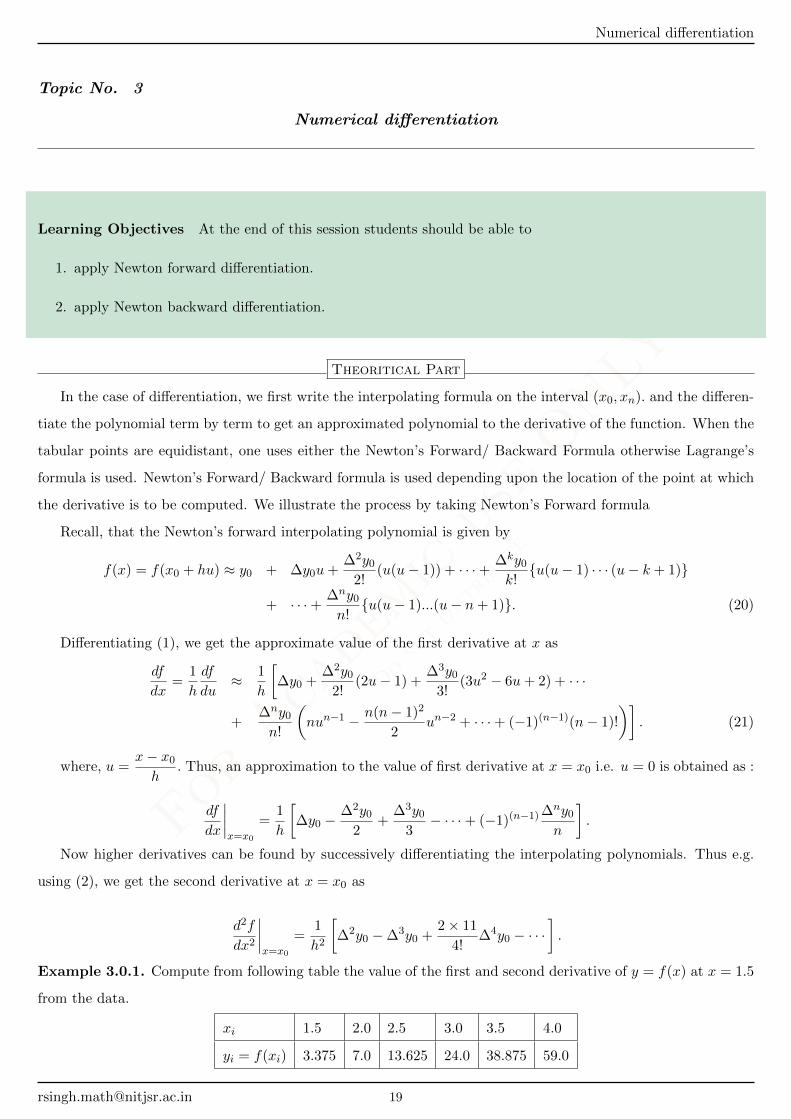
Example 3.0.1. Compute from following table the value of the first and second derivative of y = f(x) at x = 1.5
from the data.
xi 1.5 2.0 2.5 3.0 3.5 4.0
yi = f(xi) 3.375 7.0 13.625 24.0 38.875 59.0

ForAcademicuseONLY
DonotDistribute
Numerical differentiation
Soln.
xi f [xi] ∆f [xi] ∆2f [xi] ∆3f [xi] ∆3f [xi] ∆4f [xi]
1.5 3.375
3.625
2 7 3
6.625 0.75
2.5 13.625 3.75 0
10.375 0.75 0
3 24 4.5 0
14.875 0.75
3.5 38.875 5.25
20.125
4 59
f ′(1.5) =1
0.5
[3.625− 1
2× 3 +
1
3× 0.75
]= 4.75
f ′′(1.5) =1
0.52[3.625− 0.75] = 9
Example 3.0.2. Find the values of sin 18◦ and sin 45◦ from the following table using numerical differentiation
based on Newton’s forward interpolation formula
xi 0 10 20 30 40
cos(x◦) 1 0.9848 0.9397 0.8660 0.7660
Soln.
xi f [xi] ∆f [xi] ∆2f [xi] ∆3f [xi] ∆3f [xi]
0 1
-0.0152
10 0.9848 -0.0299
-0.0451 0.0013
20 0.9397 -0.0286 0.001
-0.0737 0.0023
30 0.866 -0.0263

ForAcademicuseONLY
DonotDistribute
Numerical differentiation
-1
40 0.766
df
dx=
1
h
df
du≈ 1
h
[∆y0 +
∆2y0
2!(2u− 1) +
∆3y0
3!(3u2 − 6u+ 2) +
∆4y0
4!(4u3 + 18u2 + 105u2 + 100u+ 24)
]
For x = 18◦u =18− 0
10= 1.8 For x = 45◦u =
45− 0
10= 4.5
cos(18◦) = −18
π
[−0.0152 + 1.3× (−0.0299) +
1
6× 0.92× 0.0013 +
1
24× (13.92)× 0.001
]= 0.3120
cos(45◦) = −18
π
[−0.0152− 4× (−0.0299) +
1
6× (35.75)× (0.0013) +
1
24× 93× (0.001)
]= 0.7058
Practice Problems
Problem 3.1. 1. Find the values of1
xand
1
x2at x = 9 from the following data of values of y = lnx
xi 1 2 3 4 5 6 7 8 9
y 0 0.6931 1.0986 1.3863 1.6094 1.79182 1.9459 2.0794 2.1972
Ans: 0.11, 0.0123

ForAcademicuseONLY
DonotDistribute
Numerical Integration
Topic No. 4
Numerical Integration
Learning Objectives At the end of this session students should be able to
1. apply Trapezoidal rule.
2. apply Simpsons 1/3 and 3/8 rule.
3. apply Weddle rule.
Theoritical Part
4.1 General Quadrature Formula
Let f(xk) = yk be the nodal value at the tabular point xk for k = 0, 1, · · · , xn, where x0 = a and xn = x0 + nh =
b. Now, a general quadrature formula is obtained by replacing the integrand by Newton’s forward difference
interpolating polynomial. Thus, we get,
b∫a
f(x)dx =
b∫a
[y0 +
∆y0
h(x− x0) +
∆2y0
2!h2(x− x0)(x− x1)
+∆3y0
3!h3(x− x0)(x− x1)(x− x2)
+∆4y0
4!h4(x− x0)(x− x1)(x− x2)(x− x3) + · · ·
]dx (22)
This on using the transformation x = x0 + hu gives:
b∫a
f(x)dx =
b∫a
[y0 + u∆y0 +
∆2y0
2!u(u− 1) +
∆3y0
3!u(u− 1)(u− 2)
+∆4y0
4!u(u− 1)(u− 2)(u− 3) + · · ·
]du (23)
which on term by term integration gives,
b∫a
f(x)dx =
[ny0 +
n2
2∆y0 +
∆2y0
2!
(n3
3− n2
2
)+
∆3y0
3!
(n4
4− n3 + n2
)
+∆4y0
4!
(n5
5− 3n4
2+
11n3
3− 3n2
)+ · · ·
](24)

ForAcademicuseONLY
DonotDistribute
4.2 Trapezoidal Rule Numerical Integration
For n = 1, i.e., when linear interpolating polynomial is used then, we have
b∫a
f(x)dx = h
[y0 +
∆y0
2
]=h
2[y0 + y1] (25)
Similarly, using interpolating polynomial of degree 2 (i.e. n = 2 ), we obtain,
b∫a
f(x)dx = h[2y0 + 2∆y0 +
(83 −
42
) ∆2y02
]= 2h
[y0 + (y1 − y0) + 1
3 ×y2−2y1+y0
2
]= h
3 [y0 + 4y1 + y2] (26)
In the above we have replaced the integrand by an interpolating polynomial over the whole interval [a, b] and then
integrated it term by term. However, this process is not very useful. More useful Numerical integral formulae are
obtained by dividing the interval [a, b] in n sub-intervals [xk, xk+1], where, xk = x0 + kh for k = 0, 1, · · · , n with
x0 = a, xn = x0 + nh = b.
4.2 Trapezoidal Rule
Here, the integral is computed on each of the sub-intervals by using linear interpolating formula, i.e. for n = 1
and then summing them up to obtain the desired integral. Note that
b∫a
f(x)dx =
x1∫x0
f(x)dx+
x2∫x1
f(x)dx+ · · ·+xk∫
xk+1
f(x)dx+ · · ·+xn−1∫xn
f(x)dx
Now using the formula (4) for n = 1 on the interval [xk, xk+1], we get,
xk+1∫xk
f(x)dx =h
2[yk + yk+1] .
Thus, we have,
b∫a
f(x)dx =h
2[y0 + y1] + · · · h
2[yn−2 + yn−1] +
h
2[yn−1 + yn]
=h
2[y0 + 2y1 + 2y2 + · · ·+ 2yk + · · ·+ 2yn−1 + yn]
= h
[y0 + yn
2+n−1∑i=1
yi
]This is called Trapezoidal Rule It is a simple quadrature formula, but is not very accurate.
Remark: An estimate for the error E1 in numerical integration using the Trapezoidal rule is given by
E1 = −b− a12
∆2y,
where ∆2y is the average value of the second forward differences. Recall that in the case of linear function, the
second forward differences is zero, hence, the Trapezoidal rule gives exact value of the integral if the integrand is
a linear function.

ForAcademicuseONLY
DonotDistribute
4.3 Simpson’s Rule Numerical Integration
4.3 Simpson’s Rule
If we are given odd number of tabular points,i.e. n is even, then we can divide the given integral of integration
in even number of sub-intervals [x2k, x2k+2]. Note that for each of these sub-intervals, we have the three tabular
points x2k, x2k+1, x2k+2 and so the integrand is replaced with a quadratic interpolating polynomial. Thus using
the formula (3), we get,x2k+2∫x2k
f(x)dx =h
3[y2k + 4y2k+1 + y2k+2] .
In view of this, we have
b∫a
f(x)dx =
x2∫x0
f(x)dx+
x4∫x2
f(x)dx+ · · ·+x2k+2∫x2k
f(x)dx+ · · ·+xn∫
xn−2
f(x)dx
=h
3[(y0 + 4y1 + y2) + (y2 + 4y3 + y4) + · · ·+ (yn−2 + 4yn−1 + yn)]
=h
3[y0 + 4y1 + 2y2 + 4y3 + 2y4 + · · ·+ 2yn−2 + 4yn−1 + yn]
=h
3[(y0 + yn) + 4× (y1 + y3 + · · ·+ y2k+1 + · · ·+ yn−1)
+2× (y2 + y4 + · · ·+ y2k + · · ·+ yn−2)]
=h
3
(y0 + yn) + 4×
n−1∑i=1, i is odd
yi
+ 2×
n−2∑i=2, i is even
yi
(27)
This is known as Simpson’s rule.
Remark: An estimate for the error E2 in numerical integration using the Simpson’s rule is given by
E2 = −b− a180
∆4y,
where ∆4y is the average value of the forth forward differences
Example 4.3.1. Using Trapezoidal rule compute the integral1∫0
ex2dx, where the table for the values of y = ex
2
is given below:
xi 0.0 0.1 0.2 0.3 0.4 0.5
y 1.00000 1.01005 1.04081 1.09417 1.17351 1.28402
xi 0.6 0.7 0.8 0.9 1.0
y 1.43332 1.63231 1.89648 2.2479 2.71828
Soln. Here, h = 0.1, n = 10,
y0 + y10
2=
1.0 + 2.71828
2= 1.85914,
and9∑i=1
yi = 12.81257.

ForAcademicuseONLY
DonotDistribute
4.4 Simpson’s 3/8 Rule Numerical Integration
Thus,1∫
0
ex2dx = 0.1× [1.85914 + 12.81257] = 1.467171
4.4 Simpson’s 3/8 Rule
If the number of sub-interval is multiple of three then
x3∫x0
f(x)dx =3h
8[y0 + 3y1 + 3y2 + y3] .
∴
b∫a
f(x)dx =3h
8
[(y0 + yn) + 3× (y1 + y2 + y4 + y5 + · · ·+ yn−1) + 2× (y2 + y6 + y9 · · ·+ yn−3)
]This is known as Simpson’s 3/8 rule.
4.5 Weddle’s Rule
If the number of sub-interval is multiple of six then
x6∫x0
f(x)dx =3h
10[y0 + 5y1 + y2 + 6y3 + y4 + 5y5 + y6] .
This is known as Weddle’s rule.
Practice Problems
Problem 4.6. 1. Solve the following using (i) Trapezoidal rule (ii) Simpson 1/3 rule (iii) Simpson 3/8 rule
(iv) Weddle rule.
(a)
∫ 1
0x3dx taking n = 6 Ans:
(b)
∫ 1.6
1.2(x+
1
x)dx taking n = 6 Ans:
(c)
∫ π/2
0esinxdx taking n = 6 Ans:
(d)
∫ 1.6
1.2(4x− 3x2)dx taking n = 6 Ans:
(e)
∫ π/2
0
√sinx dx taking n = 6 Ans:
(f)
∫ 1
0
dx
1 + x2taking n = 6 Ans:
(g)
∫ π/2
0
√1− 0.162 sin2 x dx taking n = 6 Ans:
(h)
∫ 2.2
1ln(x)dx taking n = 8 Ans:

ForAcademicuseONLY
DonotDistribute
Ordinary differential equation
Topic No. 5
Ordinary differential equation
Learning Objectives At the end of this session students should be able to
1. solve Initial Value Problems by Euler method and Eular modified method
2. solve Initial Value Problems by Runge-Kutta Method of order 2 and 4.
Theoritical Part
This lecture attempts to describe a few methods for finding approximate values of a solution of a initial value
problems. By no means, it is not an exhaustive study but can be looked upon as an introduction to numerical
methods. Again, we stress that no attempt is made towards a deeper analysis. A question may arise: why one
needs numerical methods for differential equations. Probably because, differential equations play an important role
in many problems of engineering and science. This is so because the differential equations arise in mathematical
modelling of many physical problems. The use of the numerical methods have become vital in the absence of
explicit solutions. Normally, numerical methods have two major roles:
1. the amicability of the method for easy implementation on a computer;
2. the method allows us to deal with the analysis of error estimates.
In this chapter, we do not enter into the aspect of error analysis. For the present, we deal with some of the
numerical methods to find approximate value of the solution of initial value problems (IVP’s) on finite intervals.
We also mention that no effort is made to study the boundary value problems. Let us consider an initial value
problem
y′ = f(x, y), a ≤ x ≤ b, y(a) = y0 (28)
where f : [a, b]−→R, a, b and y0 are prescribed real numbers and |b− a| <∞ .
5.1 Euler’s Method
For a small step size h , the derivative y′(h) is close enough to the ratioy(x+ h)− y(x)
h. In the Euler’s method,
such an approximation is attempted. To recall, we consider the problem (1). Let h =b− an
be the step size and
let xi = a+ ih, 0 ≤ i ≤ n with xn = b . Let yk be the approximate value of y at xk, k = 1, 2 . . . , n . We define
yk+1 = yk + hf(xk, yk), k = 0, 1, 2, . . . , n− 1 (29)

ForAcademicuseONLY
DonotDistribute
5.1 Euler’s Method Ordinary differential equation
The method of determination of yk by (2) is called the Eular’s Method. For convenience, the value f(xk, yk)
is denoted by fk , for k = 0, 1, 2, . . . , n .
Remark:
1. Euler’s method is an one-step method.
2. The Euler’s method has a few motivations.
(a) The derivative y′ at x = xi can be approximated byy(xi+1)− y(xi)
hif h is sufficiently small. Using
such an approximation in (1), we have
f(xi, y(xi)) = y′(xi) ∼=y(xi+1)− y(xi)
h.
(b) We can also look at (2) from the following point of view. The integration of (1) yields
y(xi+1) = y(xi) +
xi+1∫xi
f(x, y(x)) dx.
The integral on the right hand side is approximated, for sufficiently small value of h > 0 , by
xi+1∫xi
f(s, y(x)) dx ∼= f(xi, y(xi))h.
(c) Moreover, if y is differentiable sufficient number of times, we can also arrive at (2) by considering the
Taylor’s expansion
y(xi+1) = y(xi) + hf(xi, y(xi)) +h2
2f(xi, y(xi)) + · · ·
and neglecting terms that contain powers of h that are greater than or equal to 2.
3. A great disadvantage of the method lies in the fact that if h is not small enough then the method yields
erroneous result; on the other hand, if h is taken too small enough then the method becomes very slow.
Example 5.1.1. Use Euler’s algorithm to find an approximate value of y(1) , where y is the solution of the IVP
y′ = y2, y(0) = 1, 0 ≤ x ≤ 0.5
with step sizes (i) 0.1 and (ii) 0.05. The solution of the IVP is y(x) =1
1− x. Calculate the error at each step
and tabulate the results.
Soln.
f(x, y) = y2, a = 0, b = 0.5, and y0 = 1.
The Euler’s algorithm now reads as
yk+1 = yk + hy2k, k = 0, 1, 2, . . . and y0 = 1.

ForAcademicuseONLY
DonotDistribute
5.2 Modified Euler’s Method Ordinary differential equation
It is left as an exercise to verify that y(x) =1
1− xis a solution of the given IVP. So, the absolute value of the
error at the jth step is
Absolute Error = |y(xj)− yj | =∣∣∣∣ 1
1− xj− yj
∣∣∣∣.Initial x Initial y Step size h Approx y Exact y Error
1.00000 0.10000
1.00000 0.10000 1.10000 1.11111
0.20000 1.10000 0.10000 1.22100 1.25000 0.02900
0.30000 1.22100 0.10000 1.37008 1.42857 0.05849
0.40000 1.37008 0.10000 1.55780 1.66667 0.10887
0.50000 1.55780 0.10000 1.80047 2.00000 0.19953
5.2 Modified Euler’s Method
To remove the drawback to some extent, we shall discuss modified Eular’s Method starting with the initial value
y0 an approximate value for y1. From eular’s method the approximate value of y1 is as:
y(0)1 = y0 + hf(x0, y0) (30)
Then to get the second approximation for y1 we replace f(x0, y0) in(3) by average value of f(x0, y0) and f(x1, y(0)1 ).
Thus the second approximation for y1 is given by
y(1)1 = y0 +
h
2
[f(x0, y0) + f(x1, y
(0)1 )
](31)
similarly, third approximation for y1 is given by
y(2)1 = y0 +
h
2
[f(x0, y0) + f(x1, y
(1)1 )
]Thus, in general
y(k)n = y0 +
h
2
[f(x0, y0) + f(x1, y
(k−1)1 )
]k = 1, 2, 3, · · · (32)
is used to approximate yn.
Example 5.2.1. Use Modified Euler’s methods to find an approximate value of y(1.2) , where y is the solution
of the IVP
y′ +y
x=
1
x2, y(1) = 1,
correct upto 4 decimal place.

ForAcademicuseONLY
DonotDistribute
5.2 Modified Euler’s Method Ordinary differential equation
Soln.
f(x, y) =1
x2− y
x, x0 = 1, y0 = 1
Let h = 0.1 so thatx1 = 1 + 0.1 = 1.1
∴ y(0)1 = y0 + hf(x0, y0) = 1 + 0.1 = 1.1
now we modified the y1 as follows:
iteration (k) yk1 = 1 + 0.05
(1
1.12− y
(k−1)11.1
)1 0.99587
2 0.99606
3 0.99607
Hence y(1.1) = 0.9961
∴ y(0)2 = y1 + hf(x1, y1) = 0.9961 + 0.1(−0.079) = 0.98819
iteration (k) yk2 = 0.9961 + 0.05
(− 0.079 + 1
1.22− y
(k−1)11.2
)1 0.98569
2 0.98580
3 0.985797
Hence y(1.2) = 0.985797
Practice Problems
Problem 5.3. 1. Find the solution of the differential equation
dy
dx= x2 − y, y(0) = 1
for x = 0.3 taking h = 0.1 and using Eular’s method. Compare the result with the exact solution.
Ans: 0.7492, 0.0153
2. Using Euler’s method, find an approximate value of y at 0.5 given that
dy
dx= x+ y, y(0) = 1
Ans: 1.72
3. Solve the equation
5xdy
dx+ y2 − 2 = 0, y(4) = 1
for y(4.1), taking h = 0.1 and using modified Euler’s method. Ans: 1.005
ForAcademicuseONLY
DonotDistribute
5.4 Runga- Kutta Method Ordinary differential equation
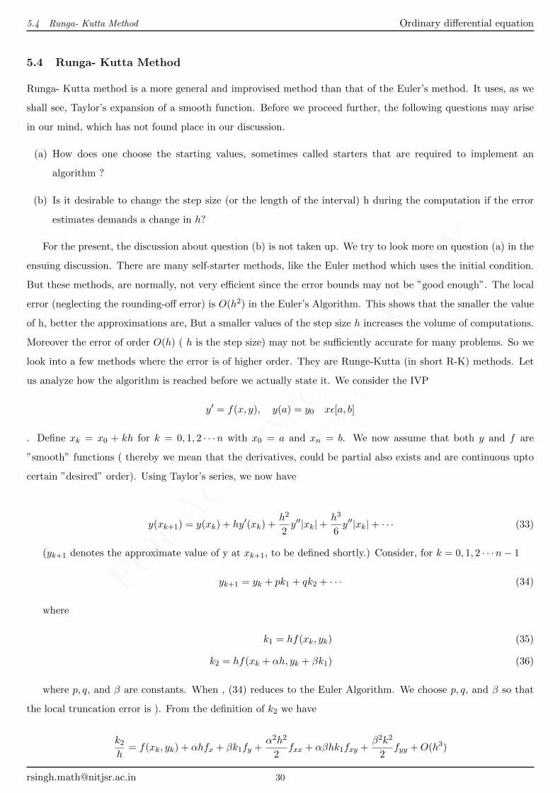
5.4 Runga- Kutta Method
Runga- Kutta method is a more general and improvised method than that of the Euler’s method. It uses, as we
shall see, Taylor’s expansion of a smooth function. Before we proceed further, the following questions may arise
in our mind, which has not found place in our discussion.
(a) How does one choose the starting values, sometimes called starters that are required to implement an
algorithm ?
(b) Is it desirable to change the step size (or the length of the interval) h during the computation if the error
estimates demands a change in h?
For the present, the discussion about question (b) is not taken up. We try to look more on question (a) in the
ensuing discussion. There are many self-starter methods, like the Euler method which uses the initial condition.
But these methods, are normally, not very efficient since the error bounds may not be ”good enough”. The local
error (neglecting the rounding-off error) is O(h2) in the Euler’s Algorithm. This shows that the smaller the value
of h, better the approximations are, But a smaller values of the step size h increases the volume of computations.
Moreover the error of order O(h) ( h is the step size) may not be sufficiently accurate for many problems. So we
look into a few methods where the error is of higher order. They are Runge-Kutta (in short R-K) methods. Let
us analyze how the algorithm is reached before we actually state it. We consider the IVP
y′ = f(x, y), y(a) = y0 xε[a, b]
. Define xk = x0 + kh for k = 0, 1, 2 · · ·n with x0 = a and xn = b. We now assume that both y and f are
”smooth” functions ( thereby we mean that the derivatives, could be partial also exists and are continuous upto
certain ”desired” order). Using Taylor’s series, we now have
y(xk+1) = y(xk) + hy′(xk) +h2
2y′′|xk|+
h3
6y′′|xk|+ · · · (33)
(yk+1 denotes the approximate value of y at xk+1, to be defined shortly.) Consider, for k = 0, 1, 2 · · ·n− 1
yk+1 = yk + pk1 + qk2 + · · · (34)
where
k1 = hf(xk, yk) (35)
k2 = hf(xk + αh, yk + βk1) (36)
where p, q, and β are constants. When , (34) reduces to the Euler Algorithm. We choose p, q, and β so that
the local truncation error is ). From the definition of k2 we have
k2
h= f(xk, yk) + αhfx + βk1fy +
α2h2
2fxx + αβhk1fxy +
β2k2
2fyy +O(h3)

ForAcademicuseONLY
DonotDistribute
5.4 Runga- Kutta Method Ordinary differential equation
where fx, fy, denotes the partial derivatives of f w.r.t. x, y, respectively. Substituting these values in (34), we
have
yk+1 = yk + h(p+ q)f + qh2(αfx + βffy) + qh3
(α2
2.fxxαβffxy +
p2
2f2fyy
)+O(h4) (37)
A comparison of (33) and (36), leads to the choice
p+ q = 1 (38)
q(q(αfx + βfy) =1
2y′′ (39)
in order that the powers of h upto match (in some sense) in the approximate values of yk+i. Here we note that
y′′ = fx + fyf
Now we choose α, β,p and q so that (38) and(39) are satisfied. One of the simplest solution is p = q =1
2and
α = β = 1 Thus, we are lead to define yk+i by
yk+1 = yk +h
2[f(xk, yk) + f(xk + h, yk + hf(xk))] (40)
Evaluation of yk+1 by (40) is called the Runge-Kutta method of order 2 (R-K method of order 2) .
A few things are worthwhile to be noted in the above discussion. Firstly, we need the existence of partial
derivatives of f upto third order for R-K method of order 2. For higher order methods, we need f to be more
smooth. Secondly we note that the local truncation error( in R-K method of order 2) is of the order O(h3). Again,
we remind the readers here that the round off error in the case of implementation has not been considered. Also
in (40), the partial derivatives of f do not appear. In short, we are likely to get a better accuracy in Runge-Kutta
method of order 2 in comparison with the Euler’s method. Formally, we state the Runge-Kutta method of order
2.
Example 5.4.1. Use the Runge-Kutta method of order 2 to find the approximate y(0.2) and y(0.4) of the IVP.
yy′ = y2 − x, y(0) = 2
Soln.
f(x, y) = y′ =y2 − xy
, x0 = 0, y0 = 2
consider h = 0.2
k1 = hf(x0, y0) = 0.2× 22 − 0
2= 0.4
k2 = 0.2× 2.42 − 0.2
2.4= 0.46333
Thus, y(0.2) = y1 = y0 +1
2(k1 + k2) = 2.43166
ForAcademicuseONLY
DonotDistribute
5.6 Runge-Kutta Method of order 4 Ordinary differential equation
k1 = hf(x1, y1) = 0.2× (0.432)2 − 0.2
0.432= −0.00633
k2 = 0.2× 22 − 0
2= −0.10302
Thus, y(0.4) = y2 = y1 +1
2(k1 + k2) = 2.37698
Practice Problems
Problem 5.5. 1. Find the solution of the differential equation
dy
dx= x− y2, y(0) = 1
for x = 0.2 taking h = 0.1 by using fourth order RK method. Ans: 0.851
2. Find the solution of the differential equation
dy
dx= −xy, y(0) = 1
for x = 0.2 taking h = 0.1 by using fourth order RK method. Ans: 0.9802
3. Find the solution of the differential equation
dy
dx= 1 + y2, y(0) = 0
for x = 0.4 taking h = 0.1 by using fourth order RK method. Ans: 0.4228
5.6 Runge-Kutta Method of order 4
There are generalization of R-K Method of order 2 to higher order methods. Without getting into analytical
details , we state the R-K method of order 4. It is a widely used algorithm. For the initial value problems (34),
set xi = a+ ih, i = i = 0, 1, 2 · · ·n and y0 = y0 for k = 0, 1, 2, · · ·n− 1, define yk+1 by
yk+1 = yk +1
6(k1 + 2k2 + 2k3 + k4)
where
k1 = hf(xk, yk) (41)
k2 = hf(xk +h
2, yk +
k1
2) (42)
k3 = hf(xk +h
2, yk +
k2
2) (43)
k2 = hf(xk + h, yk + k3) (44)
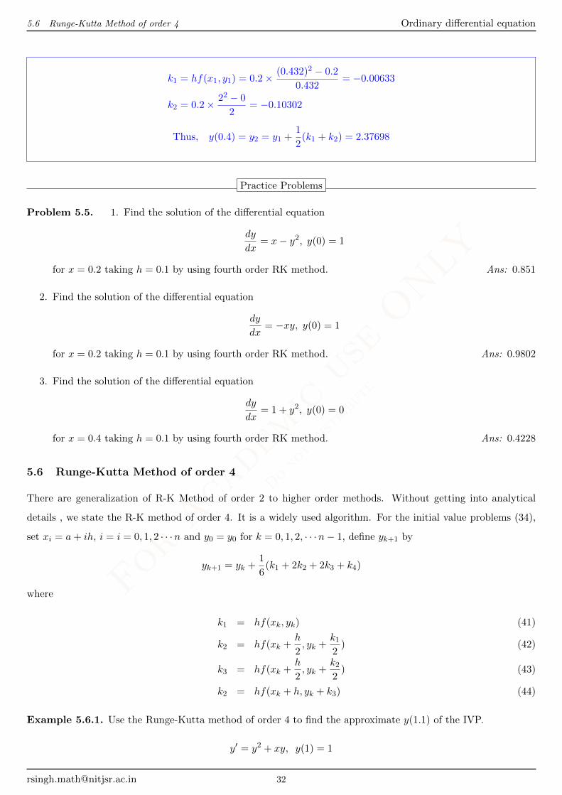
Example 5.6.1. Use the Runge-Kutta method of order 4 to find the approximate y(1.1) of the IVP.
y′ = y2 + xy, y(1) = 1
ForAcademicuseONLY
DonotDistribute
5.6 Runge-Kutta Method of order 4 Ordinary differential equation
Soln.
f(x, y) = y′ = y2 + xy, x0 = 1, y0 = 1
k1 = hf(x0, y0) = 0.1(12 + 1× 1) = 0.2
k2 = hf(x0 +h
2, y0 +
k1
2) = 0.1(1.12 + 1.05× 1.1) = 0.2365
k3 = hf(xk +h
2, y0 +
k2
2) = 0.1((1.11825)2 + 1.05× 1.11825) = 0.2425
k2 = hf(xk + h, yk + k3) = 0.1((1.2425)2 + 1.05× 1.2425) = 0.2910556
Thus, y(1.1) = y1 = y0 +1
6(k1 + 2k2 + 2k3 + k4) = 1.2415
Practice Problems
Problem 5.7. 1. Find the solution of the differential equation
dy
dx= 1 + y2, y(0) = 0
for x = 0.2 by using fourth order RK method. Ans: 0.2024
2. Using fourth order RK method, find an approximate value of y at 0.2 taking step size h = 0.1 given that
dy
dx= x+ y, y(0) = 1
Ans: 1.2205
3. Solve the equationdy
dx= xy + y2, y(0) = 1
for y(0.1), y(0.2) y(0.3), taking h = 0.1 using fourth order RK method. Ans: 0.1168, 1.2689, 1.4856

ForAcademicuseONLY
DonotDistribute
System of linear equation
Topic No. 6
System of linear equation
Learning Objectives At the end of this session students should be able to
1. recall the definition of moments of a random variable.
2. compute the kth moment about any fixed point.
3. recall the definition of central moments and compute kth central moment.
4. state the definition of moment generating functions and compute them.
Theoritical Part
6.1 The Elimination Method
Consider an upper-triangular system given by
5x1 + 3x2 − 2x3 = −3
6x2 + x3 = −1
2x3 = 10
It is very easy to obtain its solution. From the last equation, we see that x3 = 5 and substituting in the 2nd
equation gives x2 = −1. Finally, substituting these values in the first equation gives x1 = 2. Thus the solution is
x1 = 2, x2 = −1, x3 = 5.
The first objective of the elimination method is to reduce the matrix of coefficients to an upper-triangular form.
Consider this example of three equation:
4x1 − 2x2 + x3 = 15
−3x1 − x2 + 4x3 = 8
x1 − x2 + 3x3 = 13
We first eliminate x1 from the 2nd and 3rd equation. This is done by performing the calculations as 4R2 + 3R1
and 4R3 −R1 (where Ri stands for the ith row), we get
4x1 − 2x2 + x3 = 15
−10x2 + 19x3 = 77
−2x2 + 11x3 = 37

ForAcademicuseONLY
DonotDistribute
6.1 The Elimination Method System of linear equation
We now eliminate x2 from the third equation; this is done by performing the calculations as −10R3 + 2R2 to get
4x1 − 2x2 + x3 = 15 (45)
−10x2 + 19x3 = 77 (46)
−72x3 = −216 (47)
This yields solution, by backward substitution, as
x3 = 3, x2 = −2, x1 = 2
We now present the above problem, solved in exactly the same way, in matrix notation. We write the given system
as
4 −2 1
−3 −1 4
−1 1 3
x1
x2
x3
=
15
8
13
and form the augmented matrix
4 −2 1
−3 −1 4
−1 1 3
15
8
13
We carry out the elementary row transformations to convert A to upper triangular form. Using the transformation
as given above, we get 4 −2 1 15
0 −10 19 77
0 0 −72 −216
and using backward substitution yields the solution. Note that there exists the possibility that the set of equations
has no solution, or that the prior procedure will fail to find it. During the triangularization step, if a zero is
encountered on the diagonal, we cannot use that row to eliminate coefficients below that zero element. However, in
that case, we can continue by interchanging rows and eventually achieve an upper triangular matrix of coefficients.
The real stumbling block is finding a zero on the diagonal after we have triangularized. If that occurs, it means
that the determinat is zero and there is no solution. Let us now state what we mean by elementary row operations,
that we have used to solve the above system.
There are three of these operations:
1. We may multiply any row of the augmented matrix by a constant.
2. We can add a multiple of one row to a multiple of any other row.
3. We can inter change the order of any two rows.
It is intuitively obvious that all the three above operations do not change the solution of the system.
ForAcademicuseONLY
DonotDistribute
6.3 Jacobis Method System of linear equation
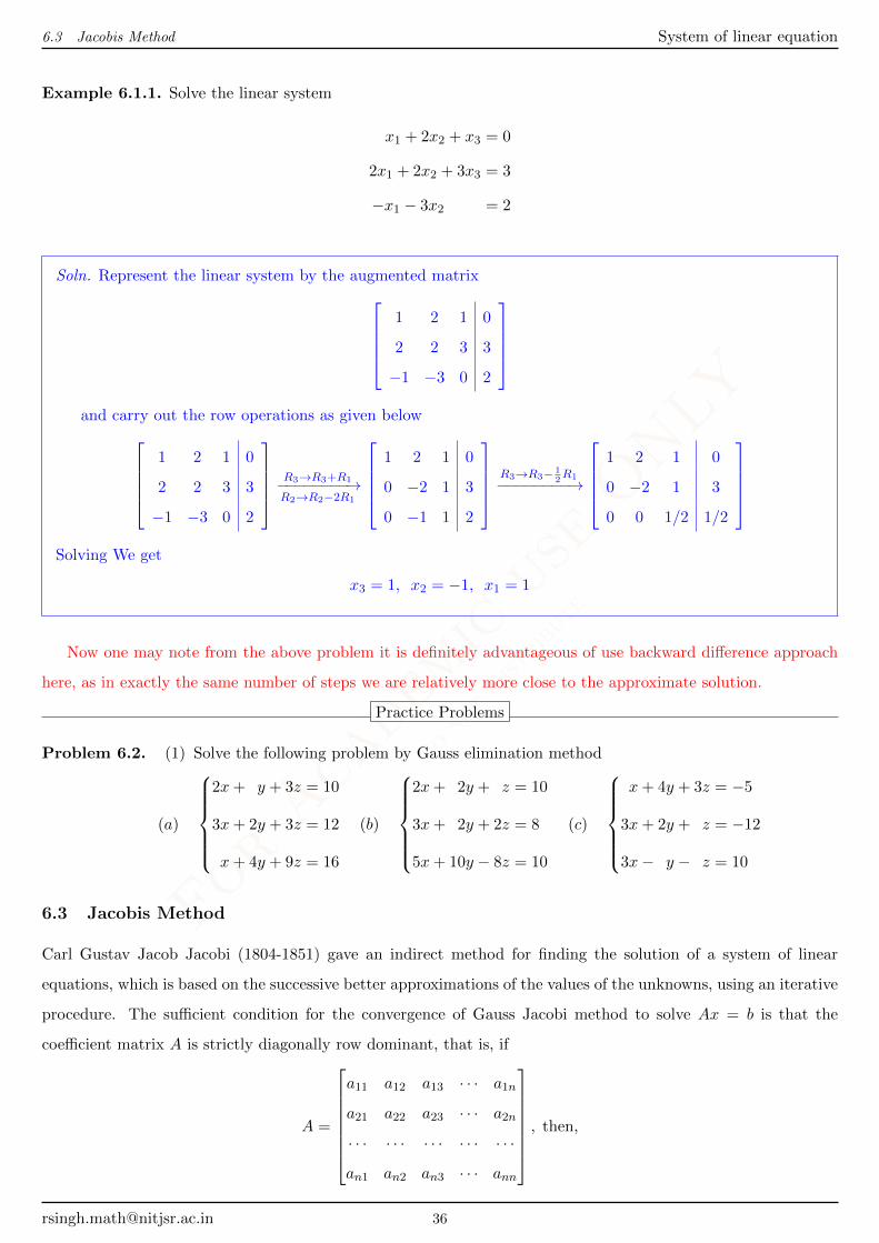
Example 6.1.1. Solve the linear system
x1 + 2x2 + x3 = 0
2x1 + 2x2 + 3x3 = 3
−x1 − 3x2 = 2
Soln. Represent the linear system by the augmented matrix1 2 1
2 2 3
−1 −3 0
0
3
2
and carry out the row operations as given below
1 2 1
2 2 3
−1 −3 0
0
3
2
R3→R3+R1−−−−−−−−→R2→R2−2R1
1 2 1
0 −2 1
0 −1 1
0
3
2
R3→R3− 12R1−−−−−−−−→
1 2 1
0 −2 1
0 0 1/2
0
3
1/2
Solving We get
x3 = 1, x2 = −1, x1 = 1
Now one may note from the above problem it is definitely advantageous of use backward difference approach
here, as in exactly the same number of steps we are relatively more close to the approximate solution.
Practice Problems
Problem 6.2. (1) Solve the following problem by Gauss elimination method
(a)
2x+ y + 3z = 10
3x+ 2y + 3z = 12
x+ 4y + 9z = 16
(b)
2x+ 2y + z = 10
3x+ 2y + 2z = 8
5x+ 10y − 8z = 10
(c)
x+ 4y + 3z = −5
3x+ 2y + z = −12
3x− y − z = 10
6.3 Jacobis Method
Carl Gustav Jacob Jacobi (1804-1851) gave an indirect method for finding the solution of a system of linear
equations, which is based on the successive better approximations of the values of the unknowns, using an iterative
procedure. The sufficient condition for the convergence of Gauss Jacobi method to solve Ax = b is that the
coefficient matrix A is strictly diagonally row dominant, that is, if
A =
a11 a12 a13 · · · a1n
a21 a22 a23 · · · a2n
· · · · · · · · · · · · · · ·
an1 an2 an3 · · · ann
, then,

ForAcademicuseONLY
DonotDistribute
6.3 Jacobis Method System of linear equation
aii >n∑
j=1j 6=i|aij |
It should be noted that this method makes two assumptions. First, the system of linear equations to be solved,
must have a unique solution and second, there should not be any zeros on the main diagonal of the coefficient
matrix A. In case, there exist zeros on its main diagonal, then rows must be interchanged to obtain a coefficient
matrix that does not have zero entries on the main diagonal. Consider a system of n linear equations in n
unknowns, which are strictly diagonally row dominant, as follows:
a11x1 + a12x2 + a13x3 + · · ·+ a1nxn = b1
a21x1 + a22x2 + a23x3 + · · ·+ a2nxn = b2
· · · · · · · · · · · · · · · · · · · · · · · · · · · · · · · · · · · · · · ·
an1x1 + an2x2 + an3x3 + · · ·+ annxn = bn
Since the system is strictly diagonally row dominant, aii 6= 0
Therefore, the system of equations is rewritten as
x1 =b1a11− 0 · x1 −
a12
a11x2 −
a13
a11x3 + · · · − a1n
a11xn
x2 =b2a22− a21
a22x1 − 0 · x2 −
a23
a22x3 + · · · − a2n
a22xn
· · · · · · · · · · · · · · · · · · · · · · · · · · · · · · · · · · · · · · · · · · · · · · · ·
xn =bnann− an1
annx1 −
an2
annx2 −
an3
annx3 + · · · − 0 · xn
We then consider an arbitrary initial guess of the solution as (x(0)1 , x
(0)2 , · · · , x(0)
n ). which are row substituted to
the right hand side of the rewritten equations to obtain the first approximation as
x(1)1 =
b1a11− 0 · x(0)
1 −a12
a11x
(0)2 −
a13
a11x
(0)3 + · · · − a1n
a11x(0)n
x(1)2 =
b2a22− a21
a22x
(0)1 − 0 · x(0)
2 −a23
a22x
(0)3 + · · · − a2n
a22x(0)n
· · · · · · · · · · · · · · · · · · · · · · · · · · · · · · · · · · · · · · · · · · · · · · · · · · · · · · · · ·
x(1)n =
bnann− an1
annx
(0)1 −
an2
annx
(0)2 −
an3
annx
(0)3 + · · · − 0 · x(0)
n
This process is repeated by substituting the first approximate solution (x(1)1 , x
(1)2 , · · · , x(1)
n ) to the r.h.s of the
rewritten equations. By repeated iteration, we get the required solution up to the desired level of the accuracy.
Example 6.3.1. solve the linear system
x1 + x2 + 4x3 = 9
8x1 − 3x2 + 2x3 = 20
4x1 + 11x2 − x3 = 33

ForAcademicuseONLY
DonotDistribute
6.4 Gauss Seidel Method System of linear equation
Soln. The given system of equations is not diagonally row dominant as |a22| < |a12| + |a13| . Therefore, we
re-arrange the system as
8x1 − 3x2 + 2x3 = 20
4x1 + 11x2 − x3 = 33
x1 + x2 + 4x3 = 9
Thus, the system is diagonally row dominant. We now re-write the system as:
x1 =1
8(20− 3x2 − 2x3)
x2 =1
11(33− 4x1 + x3)
x3 =1
4(9− x1 − x2)
Let the initial guess be x(0)1 = 1, x
(0)2 = 1, x
(0)3 = 0 Then, the first approximation to the solution is given by
x(1)1 =
1
8(20− 3× 1− 2× 0) = 2.875
x(1)2 =
1
11(33− 4× 1 + 0) = 2.636
x(1)3 =
1
4(9− 1− 1) = 1.75
2nd approx 3rd approx 4th approx 5th approx 6th approx
x(2)1 = 3.051 x
(3)1 = 3.075 x
(4)1 = 2.999 x
(5)1 = 2.991 x
(6)1 = 2.997
x(2)2 = 2.114 x
(3)2 = 1.969 x
(4)2 = 1.969 x
(5)2 = 1.999 x
(6)2 = 2.004
x(2)3 = 0.872 x
(3)3 = 0.981 x
(4)3 = 0.989 x
(5)3 = 0.989 x
(6)3 = 1.002
Therefore,x1 = 3.0, x2 = 2.0, x3 = 1 correct to two significant figures.
6.4 Gauss Seidel Method
Gauss Seidel iteration method for solving a system of n-linear equations in n- unknowns is a modified Jacobis
method. Therefore, all the conditions that is true for Jacobis method, also holds for Gauss Seidel method. As
before, the system of linear equations are rewritten as
x1 =b1a11− 0 · x1 −
a12
a11x2 −
a13
a11x3 + · · · − a1n
a11xn
x2 =b2a22− a21
a22x1 − 0 · x2 −
a23
a22x3 + · · · − a2n
a22xn
· · · · · · · · · · · · · · · · · · · · · · · · · · · · · · · · · · · · · · · · · · · · · · · ·
xn =bnann− an1
annx1 −
an2
annx2 −
an3
annx3 + · · · − 0 · xn

ForAcademicuseONLY
DonotDistribute
6.4 Gauss Seidel Method System of linear equation
If (x(0)1 , x
(0)2 , · · · , x(0)
n ) be the initial guess of the solution, which is arbitrary, then the first approximation to the
solution is obtained as.
x(1)1 =
b1a11− 0 · x(0)
1 −a12
a11x
(0)2 −
a13
a11x
(0)3 + · · · − a1n
a11x(0)n
x(1)2 =
b2a22− a21
a22x
(1)1 − 0 · x(0)
2 −a23
a22x
(0)3 + · · · − a2n
a22x(0)n
· · · · · · · · · · · · · · · · · · · · · · · · · · · · · · · · · · · · · · · · · · · · · · · · · · · · · · · · ·
x(1)n =
bnann− an1
annx
(1)1 −
an2
annx
(1)2 −
an3
annx
(1)3 + · · · − 0 · x(0)
n
Please note, while calculating x(1)2 the value of x1is replaced by x
(1)1 not by x
(0)1 . This is the basic difference of
Gauss Seidel with Jocobis method The successive iterations are generated by the scheme called iteration formulae
of Gauss-Seidel method, which is as follows:
x(k+1)1 =
b1a11− 0 · x(k)
1 −a12
a11x
(k)2 −
a13
a11x
(k)3 + · · · − a1 n−1
a11x
(k)n−1 −
a1n
a11x(k)n
x(k+1)2 =
b2a22− a21
a22x
(k+1)1 − 0 · x(k)
2 −a23
a22x
(k)3 + · · · − a2 n−1
a22x
(k)n−1 −
a2n
a22x(k)n
· · · · · · · · · · · · · · · · · · · · · · · · · · · · · · · · · · · · · · · · · · · · · · · · · · · · · · · · ·
x(k+1)n =
bnann− an1
annx
(k+1)1 − an2
annx
(k+1)2 − an3
annx
(k+1)3 + · · · − an−1 3
annx
(k+1)n−1 − 0 · x(k)
n
Example 6.4.1. solve the linear system Gauss Seidel method
x1 + x2 + 4x3 = 9
8x1 − 3x2 + 2x3 = 20
4x1 + 11x2 − x3 = 33
Soln. The given system of equations is not diagonally row dominant as |a22| < |a12| + |a13| . Therefore, we
re-arrange the system as
8x1 − 3x2 + 2x3 = 20
4x1 + 11x2 − x3 = 33
x1 + x2 + 4x3 = 9
Thus, the system is diagonally row dominant. We now re-write the system as:
x1 =1
8(20− 3x2 − 2x3)
x2 =1
11(33− 4x1 + x3)
x3 =1
4(9− x1 − x2)
ForAcademicuseONLY
DonotDistribute
6.4 Gauss Seidel Method System of linear equation
Let the initial guess be x(0)1 = 1, x
(0)2 = 1, x
(0)3 = 0 Then, the first approximation to the solution is given by
x(1)1 =
1
8(20− 3× 1− 2× 0) = 2.875
x(1)2 =
1
11(33− 4× 2.875 + 0) = 1.995
x(1)3 =
1
4(9− 2.875− 1.995) = 1.043
2nd approx 3rd approx 4th approx
x(2)1 = 2.972 x
(3)1 = 3.004 x
(4)1 = 3.00
x(2)2 = 2.014 x
(3)2 = 1.999 x
(4)2 = 2.00
x(2)3 = 1.004 x
(3)3 = 0.999 x
(4)3 = 1.00
Therefore,x1 = 3, x2 = 2, x3 = 1 correct to two significant figures.
Practice Problems
Problem 6.5. (1) Solve the following problem by Gauss Seidel and Jecobi method
(a)
6x+ 3y + 12z = 36
8x− 3y + 2z = 20
4x+ 11y − z = 33
(b)
9x− 3y + 2z = 23
6x+ 3y + 14z = 38
4x+ 12y − z = 35
(c)
5x+ 2y + z = −12
x+ 4y + 2z = 15
x+ 2y + 5z = 20
ForAcademicuseONLY
DonotDistribute
Partial differential equation
Topic No. 7
Partial differential equation
Learning Objectives At the end of this session students should be able to
1. Classified the partial differential equation of first and second order
Theoritical Part
A partial differential equation (or briefly a PDE) is a mathematical equation that involves two or more
independent variables, an unknown function (dependent on those variables), and partial derivatives of the unknown
function with respect to the independent variables.
1. ∂2z∂x2
+ ∂2z∂y2
= z, z = z(x, y)
2. ∂z∂x + 2∂z∂y = xy.
7.1 Order of partial differential equation
The order of a partial differential equation is the order of the highest derivative involved in the partial differential
equation.
7.2 Degree of partial differential equation
Highest power of the highest order derivative occurring in the given partial differential equation is referred as the
degree of the partial differential equation, after making it free from radicals, fractions and transcandal functions
as far as derivatives are concerned.
Notations
∂z∂x = p, ∂z
∂y = q, ∂2z∂x2
= r, ∂2z∂y2
= t, ∂2z∂x∂y = s.
7.3 Classification of the first order partial differential equation
1. Linear partial differential equation: A partial differential equation of the form
P (x, y)p+Q(x, y)q = R(x, y)z + S(x, y) is called the linear PDE of first order.
2. Semi-linear partial differential equation: A partial differential equation of the form
P (x, y)p+Q(x, y)q = R(x, y, z) is called the semi-linear PDE.
3. Quasi-linear partial differential equation: A partial differential equation of the form
P (x, y, z)p+Q(x, y, z)q = R(x, y, z) s called the quasi-linear PDE.

ForAcademicuseONLY
DonotDistribute
7.4 Classification of the second order partial differential equation Partial differential equation
4. Non-linear partial differential equation: A first order partial differential equation which does not come
under any of the above types is called the non-linear PDE.
7.4 Classification of the second order partial differential equation
1. Linear partial differential equation: If given second order partial differential equation (PDE) is of the
form
[R(x, y)r + S(x, y)s + T (x, y)t] + P (x, y)p + Q(x, y)q + M(x, y)z = N(x, y) is called the linear partial
differential equation of second order.
2. Semi-linear partial differential equation: If the PDE is of the form
R(x, y)r + S(x, y)s+ T (x, y)t+ f(x, y, z, p, q) = 0 is called the semi linear partial differential equation of
second order.
3. Quasi-linear partial differential equation: If the PDE is of the form
R(x, y, z, p, q)r + S(x, y, z, p, q)s+ T (x, y, z, p, q)t+ f(x, y, z, p, q) = 0 is called the quasi linear partial
differential equation of second order.
4. Non-linear partial differential equation: A second order partial differential equation which does not
come under any of the above types is called the non-linear PDE of second order.
7.5 Classification of the second order semi-linear partial differential equation
Consider the semi-linear partial differential equation
R(x, y)r + S(x, y)s+ T (x, y)t+ f(x, y, z, p, q) = 0 (48)
Or
Ar +Bs+ Ct+ f(x, y, z, p, q) = 0 (49)
(49) is called
Hyperbolic if B2 − 4AC > 0, (50)
Elliptic if B2 − 4AC < 0, (51)
Parabolic if B2 − 4AC = 0 (52)
Question If uxx + uyy + uzz + 2x2uxz = 0 then the given partial differential equation is
1. Parabolic for |x| = 1
2. Hyperbolic for |x| > 1

ForAcademicuseONLY
DonotDistribute
7.5 Classification of the second order semi-linear partial differential equation Partial differential equation
3. Elliptic for |x| < 1
4. Elliptic for |x| > 1
Ans: 2, 3