fluxes across parts of fractal boundaries
TRANSCRIPT

Milan j. math. 74 (2006), 1–45
c© 2006 Birkhauser Verlag Basel/Switzerland
1424-9286/010001-45, published online 21.6.2006
DOI 10.1007/s00032-006-0055-3 Milan Journal of Mathematics
Fluxes Across Parts of FractalBoundaries
M. Silhavy
Abstract. This paper determines the flux F (q, T ) of a physical quantityacross a part T of the boundary of a ‘rough body.’ The latter term meansthat the (measure theoretic) boundary ∂B of the body B is fractal in thesense that the outer normal n to B is not defined for almost every pointof ∂B with respect to the n− 1 dimensional Hausdorff measure Hn−1.
The quantity is represented by a bounded measurable flux vectorfieldq on R
n with bounded distributional divergence. Cauchy’s formula forregular surfaces T ,
F (q, T ) =∫
T
q · n dHn−1, (∗)
cannot be used because it requires the normal n to the surface. F (q, T )is defined using the divergence theorem provided T is a “trace,” i.e.,provided T = B ∩ ∂M where M is a properly normalized set of finiteperimeter. The definition reduces to (∗) if Hn−1(T ) <∞. The set B(B)of all traces is a boolean algebra and F (q, ·) is additive on it. Basicproperties of the functional F are examined. (1) It is shown that ifHn−1(∂B) = ∞, then F (q, ·) does not extend to a measure unless q
is in some sense trivial. (2) It is proved that a rough body B can beapproximated by a sequence Bk of sets of finite perimeter such that(∗) holds in some limiting sense. (3) Consequences are derived of thesituation when a given T ∈ B(B) insulates under q in the sense thatthe flux through each trace S ⊂ T vanishes. (4) Conditions are givenon ∂B for the locality of F (so that the value F (q, T ) depends on thevalues of q on T ).

2 M. Silhavy Vol. 74 (2006)
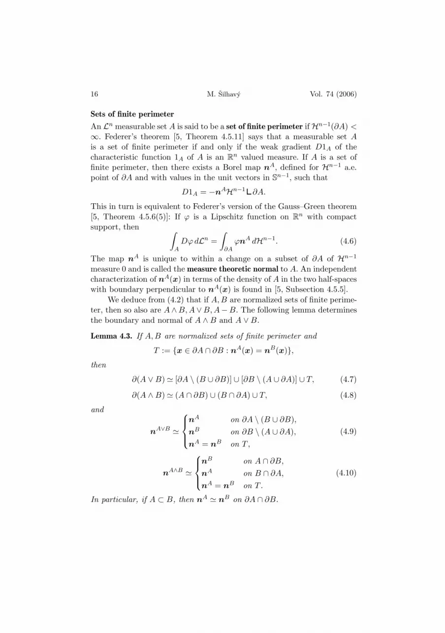
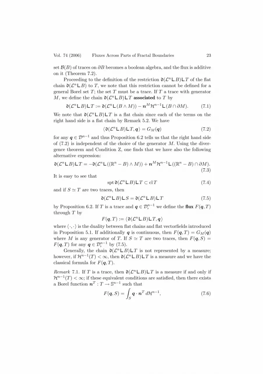
B
B ∩M
T
M
B ∩ ∂M
Figure 1.1. Trace T and sets B,M
1. Introduction
In this paper, bodies with fractal boundaries (rough bodies) are interpretedas subsets B of Rn whose (measure theoretic) boundary ∂B is complicatedto the extent that the normal cannot be defined for Hn−1 a.e. point of ∂B.Here Hn−1 denotes the n − 1 dimensional Hausdorff measure. Examplesof a rough sets are the von Koch snowflake B considered Section 2 and‘Whitney’s rough set’ considered in Section 3. In contrast to rough bodies,sets of finite perimeter have the normal defined for Hn−1 a.e. point of ∂B;these sets are interpreted as ‘regular bodies’ here.
The goal of the paper is to determine the flux of a physical quantityacross parts of the boundary of a rough body. Only scalar quantities areconsidered; these are represented by vector–valued, bounded and measur-able flux vectorfields q with bounded distributional divergence. The fluxesof vector valued quantities, such as the force, can be obtained by applyingthe scalar case to each component.

Vol. 74 (2006) Fluxes Across Parts of Fractal Boundaries 3
The reader is referred to [3, Section 6] and [2] for the discussion ofnonstandard bodies in continuum mechanics.
Suppose that B is a part of a rigid heat conductor extending over Rn
and that the heat flux vector q : Rn → R
n is assigned. What is the net fluxof heat F (q, T ) across T ⊂ ∂B? For a smooth surface T with normal n,F (q, T ) is given by
F (q, T ) =∫
Tq · n dHn−1. (1.1)
This cannot be used if T is fractal since n is not defined. This paper showsthat the flux F (q, T ) can be defined if T is a trace. For a fixed set B,a trace is a set of the form T = ∂B ∩M where M is a normalized set offinite perimeter and Hn−1(∂B∩∂M) = 0. See Figure 1.1. Here ‘normalized’means that the set of points of density of M coincides with M , see Section4. Then one can define, for a continuous q with an essentially boundedweak divergence,
F (q, T ) =∫
B∩Mdiv q dLn −
∫B∩∂M
q · nM dHn−1 (1.2)
where Ln is the Lebesgue measure in Rn and nM is the measure theoretic
outer normal to M. This reduces to (1.1) if Hn−1(T ) <∞ (Remark 7.1).It is shown that the definition (1.2) is independent of the choice of M.
Furthermore, two traces that differ by a Hn−1 negligible set give rise tothe same flux (Proposition 6.2). Identifying traces of negligible difference,we show that the set of all traces B(B) on ∂B is a boolean algebra underthe set theoretic operations and F (q, ·) is additive on B(B). One might betempted to conjecture that the values of F (q, ·) are obtained by integrationof some effective quantity over subsets of ∂B. For example if ∂B has theHausdorff dimension d, then one might be tempted to use the d dimensionalHausdorff measure Hd for such an integration. However, it is shown thatthe set function F (q, ·) generally does not generally extend to a measure ifHn−1(∂B) = ∞ (see Section 9 for a precise statement); thus F (q, ·) cannotbe obtained by integration at all.
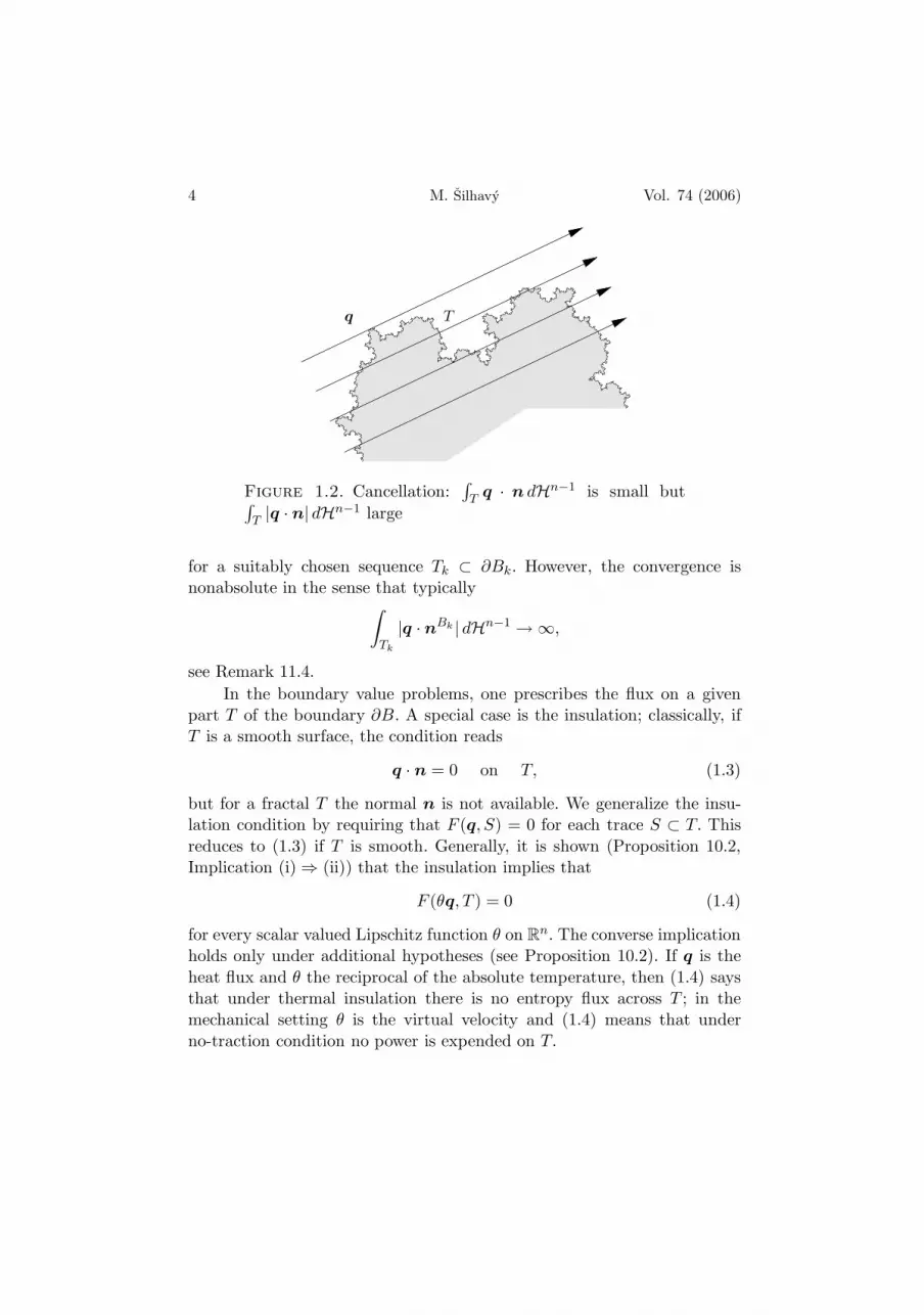
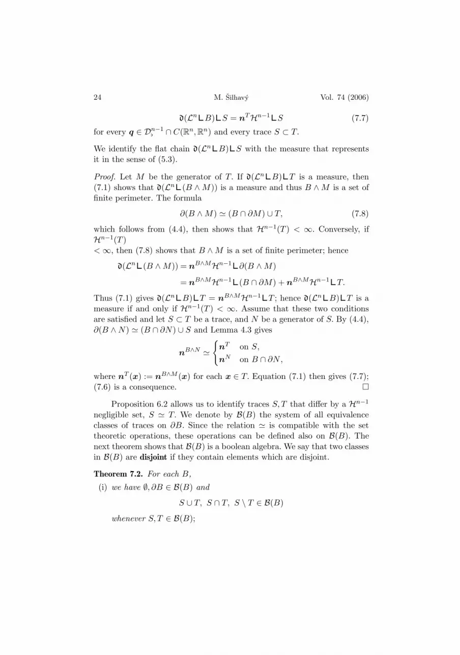
The quantity F (q, T ) is finite only due to a cancelation of infinitelymany contributions of opposite signs on the curly boundary of the body, seeFigure 1.2. This is best illustrated using the results of Section 11. Namely,each B can be approximated by a sequence Bk of sets of finite perimeterin such a way that
F (q, T ) = limk→∞
∫Tk
q · nBk dHn−1
4 M. Silhavy Vol. 74 (2006)
Tq
Figure 1.2. Cancellation:∫T q · n dHn−1 is small but∫
T |q · n| dHn−1 large
for a suitably chosen sequence Tk ⊂ ∂Bk. However, the convergence isnonabsolute in the sense that typically∫
Tk
|q · nBk | dHn−1 → ∞,
see Remark 11.4.In the boundary value problems, one prescribes the flux on a given
part T of the boundary ∂B. A special case is the insulation; classically, ifT is a smooth surface, the condition reads
q · n = 0 on T, (1.3)
but for a fractal T the normal n is not available. We generalize the insu-lation condition by requiring that F (q, S) = 0 for each trace S ⊂ T. Thisreduces to (1.3) if T is smooth. Generally, it is shown (Proposition 10.2,Implication (i) ⇒ (ii)) that the insulation implies that
F (θq, T ) = 0 (1.4)
for every scalar valued Lipschitz function θ on Rn. The converse implication
holds only under additional hypotheses (see Proposition 10.2). If q is theheat flux and θ the reciprocal of the absolute temperature, then (1.4) saysthat under thermal insulation there is no entropy flux across T ; in themechanical setting θ is the virtual velocity and (1.4) means that underno-traction condition no power is expended on T.
Vol. 74 (2006) Fluxes Across Parts of Fractal Boundaries 5
Intuitively, the values of F (q, T ) should depend only on the valuesof q on T, i.e., if q = 0 on T , then F (q, T ) = 0. For a smooth surfacethe locality follows from (1.1). However, Example 3 in [12] shows that thelocality property is not true generally even in the case when T = bdB(this example is presented in Section 3 in a slightly modified and moreexpanded form). It is shown (Proposition 12.1) that if the dimension d of Tsatisfies n− 1 ≤ d < n, then F (q, T ) behaves locally on the class of Holdercontinuous of exponent α satisfying d−n+1 < α ≤ 1. This establishes thecounterpart of the locality results in [12] for the case when T is the wholeboundary of B.
The paper also establishes the relationship of the presented materialto Whitney’s theory of flat chains [19] (see Section 5 for a brief summaryof that theory). Namely, it is shown that to each trace T corresponds ann− 1 dimensional flat chain T that represents T in the sense that
F (q, T ) = 〈T,q 〉where 〈 ·, · 〉 is the duality pairing between flat chains and flat forms. We heremention that it is automatic in Whitney’s theory that ∂B is representedby a flat chain T. However, the restriction of T to subsets of ∂B is notautomatic; the paper shows that T can be restricted to T if T is a trace.
Rodnay & Segev [14] establish the relationship of Cauchy’s theorem incontinuum mechanics to Whitney’s theory and also to the work of Harrison[7], [8], [9], [10], [11] which generalizes Whitney’s theory to include chainlets.We emphasize that the traces are flat chains, no matter how complicatedthe boundary.
2. Flux of heat across a snowflake
To provide a motivation for this paper, the flux of heat across parts of theboundary of the von Koch set (snowflake) is calculated. The basic propertiesof the Koch set can be deduced from [4, Example 9.5].
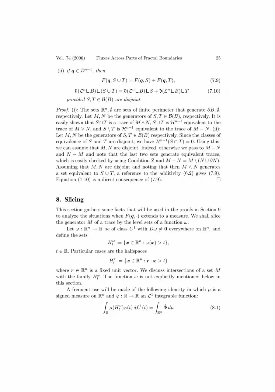
The von Koch set is a union B ⊂ R2 of an increasing sequence of open
equilateral polygons Bk ⊂ R2, k = 0, . . . , defined inductively as follows.
B0 is an open equilateral triangle of side length 1. The polygon Bk+1 isobtained from Bk by replacing the middle third of each side of Bk bythe other two sides of an equilateral triangle pointing out of Bk. ThusBk is enclosed by a (topological) boundary bdBk which is a union of 3 ·4k line segments of length 1/3k (see Figure 2.1); hence the length H1 of

6 M. Silhavy Vol. 74 (2006)
B3 B4
(a) (b)
Figure 2.1. Stages 3 and 4
bdBk satisfies H1(bdBk) = 3(4/3)k → ∞. The boundary bdBk can beparametrized by a continuous and piecewise linear map γk : [0, 3] → R
2
such that γ(0) is the lower left vertex of bdB0,
|γk(t)| = (4/3)k
for a.e. t ∈ [1, 3], and γk gives bdBk a counterclockwise orientation. Hereγk(t) is the derivative of γk at t. The maps γk form a Cauchy sequence inthe space C([0, 3],R2) of continuous maps on [0, 3] and thus there exists acontinuous map γ : [0, 3] → R
2 such that
γk → γ uniformly on [0, 3]. (2.1)
The map γ provides a continuous and nowhere differentiable parametriza-tion of bdB. One has H1(bdB) = ∞ and
0 < Hd(bdB) <∞where d = log 4/ log 3 is the dimension of bdB. One also finds that thevariation of γ is infinite, i.e.,
Var ts γ = ∞ (2.2)
whenever 0 ≤ s < t ≤ 3.Suppose that there is a flow of heat in R
2 described by a constant heatflux vector q ∈ R
2. Consider the segment T := γ([0, t)) of bdB where t ∈[1, 3] is arbitrary, see Figure 2.2. Let us determine the net heat through T.
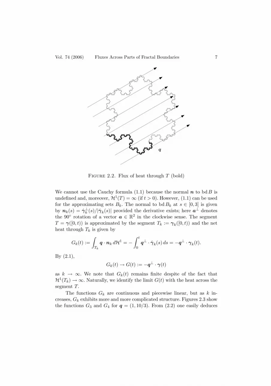
Vol. 74 (2006) Fluxes Across Parts of Fractal Boundaries 7
q
Figure 2.2. Flux of heat through T (bold)
We cannot use the Cauchy formula (1.1) because the normal n to bdB isundefined and, moreover, H1(T ) = ∞ (if t > 0). However, (1.1) can be usedfor the approximating sets Bk. The normal to bdBk at s ∈ [0, 3] is givenby nk(s) = γ⊥
k (s)/|γk(s)| provided the derivative exists; here a⊥ denotesthe 90◦ rotation of a vector a ∈ R
2 in the clockwise sense. The segmentT = γ([0, t)) is approximated by the segment Tk := γk([0, t)) and the netheat through Tk is given by
Gk(t) :=∫
Tk
q · nk dH1 = −∫ t
0q⊥ · γk(s) ds = −q⊥ · γk(t).
By (2.1),
Gk(t) → G(t) := −q⊥ · γ(t)
as k → ∞. We note that Gk(t) remains finite despite of the fact thatH1(Tk) → ∞. Naturally, we identify the limit G(t) with the heat across thesegment T.
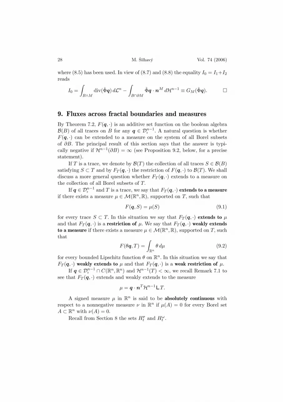
The functions Gk are continuous and piecewise linear, but as k in-creases, Gk exhibits more and more complicated structure. Figures 2.3 showthe functions G3 and G4 for q = (1, 10/3). From (2.2) one easily deduces

8 M. Silhavy Vol. 74 (2006)
G3
t0 1 2 3
G4
t0 1 2 3
(a) (b)
Figure 2.3. The distribution functions G3 and G4
that
Var tsG = ∞ (2.3)
whenever 0 ≤ s < t ≤ 3 and q �= 0. Also note that∫
Tk
q · nk ds→ G(t), but∫
Tk
|q · nk| dH1 → ∞,
which describes the cancellation effect mentioned in Introduction.The amount of heat through the general segment T := γ([s, t)), 0 ≤
s ≤ t ≤ 3, is given by
F (q, T ) = G(t) −G(s).
Clearly, the set function F (q, ·) can be extended to an additive function ona system of finite unions of segments in bdB. However, (2.3) shows thatF (q, ·) cannot be extended to a measure on bdB (unless q = 0).
To anticipate the development below, note that it can be shown thatthe topological and measure theoretic boundaries of B coincide and that Tas above is a trace in the sense of Section 7. Moreover, F (q, T ) coincideswith the flux across T according to the definition given in that section.That F (q, ·) does not extend to a measure is a typical situation wheneverbdB is fractal, see Section 9.

Vol. 74 (2006) Fluxes Across Parts of Fractal Boundaries 9
3. Whitney’s set and function
Formula (1.1) shows F (q, T ) = 0 whenever q = 0 on T. Following Example3 in [12], we here construct a subset T of a boundary of a rough set and acontinuous vectorfield q on R
2 such that q = 0 on T and yet F (q, T ) = 1.The example is based on Whitney’s [18] construction of a continuouslydifferentiable function f on R
2 and a connected set W ⊂ R2 such that the
derivative of f vanishes on W and yet f(W ) = [0, 1]. Whitney’s originalproof uses Whitney’s extension theorem; here an explicit construction of f[see (3.4)] is given.
Let Q be an open square of side 1 in R2. Let Q0, Q1, Q2, Q3 be open
squares of side 1/3 lying interior to Q in cyclical order, each a distance1/12 from the boundary of Q. Let A1, . . . , A4 be the closed line segmentswith endpoints at the centers of the sides of Q0, . . . , Q3 and let a, a′ be thecenters of two sides of Q as shown in Figure 3.1. We now shrink Figure 3.1to a third of its size, turn it around and upside down if necessary, and placeit into the squares Q0, . . . , Q3. We continue this process indefinitely, anddefine a curve W, function f, and region B determined by this process.
Let Si, i = 0, . . . , 3, be affine transformations in R2 of the form
Six =13Uix + ci
x ∈ R2, where Ui are orthogonal matrices and ci ∈ R
2, such that Si mapsQ to Qi and the points a, a′ to the endpoints of those two segments amongA1, . . . , A4 that touch bdQi. Moreover, we require that detU0 = −1 whiledetUi = 1, i = 1, 2, 3. This determines the maps Si uniquely.
Write Λk for the set of all k tuples I = (i1, . . . , ik) with integral entriessatisfying 0 ≤ ip ≤ 3. If I = (i1, . . . , ik) ∈ Λk, we write
SI := Si1 ◦ · · · ◦ Sik , S−1I := S−1
ik◦ · · · ◦ S−1
i1
andTI := SIT
for any T ⊂ R2. Let Λ∞ be the set of all sequences I = (i1, . . . ) with integral
elements satisfying 0 ≤ ik ≤ 3, k = 1, . . . If I = (i1, . . . ) ∈ Λ∞ let xI ≡xi1,... denote the unique element that belongs to all cubes Q(i1,...,ik), k =1, . . .
Define the sets Wk, k = 0, . . . , inductively as follows. Let W0 be theset consisting of the points a, a′ and of the bold path interior to Q shown inFigure 3.1. Let L be the bold path on the boundary of Q and let us agreethat the endpoints a, a′ do not belong to L. We observe that W0 contains

10 M. Silhavy Vol. 74 (2006)
Q
Q2 Q3
Q1 Q0
A0
A1
A2
A3
A4
a
a′
Figure 3.1. The sets W0 and B0
the right angles SiL, i = 0, . . . , 3. In the next step we remove these anglesform W0 and replace them with the scaled copies of W0; an analogousprocedure works for any k > 0. That is, we define
Wk =(Wk−1 \
⋃I∈Λk
LI
) ∪ ⋃I∈Λk
W0I (3.1)
if k > 0. The sets W1 and W2 are shown in Figure 3.2. As k increases,Wk gets more complicated near the points xI ,I ∈ Λ∞. We introduce aparametrization of Wk as follows. Consider a piecewise linear parametriza-tion γ0 : [0, 9] → R
2 of W0 such that each segment Aj corresponds tothe interval [2j, 2j + 1], j = 0, . . . , 4, and each path SiL to the interval[2i + 1, 2i + 2], i = 0, . . . , 3. Let Ti : R → R, i = 0, . . . , 3, be given byTi(t) = t/9 + 2i + 1 for each t ∈ R, so that Ti maps the interval [0, 9] to[2i+ 1, 2i + 2]. If I = (i1, . . . , ik) ∈ Λk, we write
TI := Ti1 ◦ · · · ◦ Tik , T−1I := T−1
ik◦ · · · ◦ T−1
i1
andMI := TIM
for any M ⊂ R. Guided by (3.1), we parametrize Wk inductively by
γk(t) =
{γk−1(t) if t ∈ [0, 9] \ ⋃
I∈ΛkTI [0, 9]
SIγ0(T−1I t) if t ∈ TI [0, 9] where I ∈ Λk.
t ∈ [0, 9].

Vol. 74 (2006) Fluxes Across Parts of Fractal Boundaries 11
(a) The sets W1 and B1 (b) The sets W2 and B2
Figure 3.2. Whitney’s set
The sequence of sets
Rk = [0, 9] \⋃
I∈Λk
TI [0, 9]
is increasing and the complement of its union in [0, 9] is the set of all tof the form t =
∑∞p=1(2ip + 1)/9p−1 where (i1, . . . ) ∈ Λ∞. We note that
γl Rk = γk Rk if l ≥ k and define a map γ : [0, 9] → R2 by
γ(t) =
{γk(t) if t ∈ Rk for some k = 1, . . . ,xi1,... if t =
∑∞p=1(2ip + 1)/9p−1 for some (i1, . . . ) ∈ Λ∞.
It can be shown that γ is continuous and injective and
γk → γ uniformly on [0, 9]
as k → ∞. We setW = γ([0, 9]).
Clearly, H1(W ) = ∞ and it can be shown that 0 < Hd(W ) < ∞ whered = ln 4/ ln 3.
To define the function f, denote
Σ := clQ \3⋃
i=0
clQi, E = R2 \
3⋃i=0
clQi.

12 M. Silhavy Vol. 74 (2006)
Let g : R2 → R be a class C2 function with bounded first and second
derivatives such that
g(Six) =14g(x) + i/4, Dg(Six) =
34UiDg(x); (3.2)
for each i = 0, . . . , 3,x ∈ bdQ, and
g = i/4 and Dg = 0 on Ai for each i = 0, . . . , 4. (3.3)
Clearly, the function g with the required properties exists. Let f : R2 → R
be defined by
f(x) =
g(x) if x ∈ E,
g(S−1I x)/4k +
∑kp=1 ip/4
p if x ∈ ΣI where k = 1, . . . , I ∈ Λk,∑kp=1 ip/4
p if x = xI where I = (i1, . . . ) ∈ Λ∞.(3.4)
for each x ∈ R2. We note that the three regimes in (3.4) are disjoint and
exhaust R2. The constraints (3.2) can be used to show that f is of class C1
and (3.3) implies that
Df = 0 on W and f(W ) = [0, 1].
Moreover, Df is locally Holder continuous of any exponent β satisfying0 ≤ β < ln 4/ ln 3 − 1.
For each k let Bk be the open region delimited by the closed curveWk ∪ L and let B be the open region delimited by W ∪ L. Consider nowthe vectorfield q = −(Df)⊥. The weak divergence of q satisfies div q =− curlDf = 0 and one has q = 0 on W. Determine the flux of q throughW ⊂ bdB. Similarly to Section 2, we approximate W by the sequenceWk ⊂ bdBk. The normal to Bk at Wk is given by nk = −γ⊥
k /|γk| and thus
F (q,Wk) =∫
Wk
q · nk dH1 =∫ 9
0Df(γk(t)) · γk(t) dt = f(a′) − f(a) = 1.
Thus the limit k → ∞ gives F (q,W ) = 1 despite the fact that q vanisheson W.
To anticipate, note that it can be shown that the topological andmeasure theoretic boundaries of B coincide and that W as above is a tracein the sense of Section 7. Moreover, F (q,W ) coincides with the flux acrossT according to the definition given in that section. The locality propertiesof F (q, T ) are treated in Section 12.

Vol. 74 (2006) Fluxes Across Parts of Fractal Boundaries 13
4. Sets, boundaries and measures
The normalized sets to be introduced below provide models of ‘rough bod-ies’ mentioned in the introduction; the measure theoretic boundary is iden-tified with the (generally fractal) boundary of a rough body. Also conven-tions about vector valued measures are introduced, and the last part of thesection deals with sets of finite perimeter; these are our models of ‘regularbodies’.
Normalized sets and the measure theoretic boundary
If k is a nonnegative number, we denote by Hk the k dimensional Hausdorffmeasure in R
n [5, Subsections 2.10.2–2.10.6]; recall that the n dimensionalLebesgue measure is Ln := Hn. If A is an Ln measurable subset of R
n andx ∈ R
n, the density Θn(x, A) of A at x is defined by
Θn(x, A) = limρ→0
Ln(A ∩ B(x, ρ))/κnρn
provided the limit exists; here B(x, ρ) is the open ball of center x andradius ρ and κn is the volume of the unit ball in R
n. An x ∈ Rn is said
to be a point of density of A if Θn(x, A) = 1. The set of all points ofdensity of A is denoted by A∗, which is a Borel set that differs by a set ofLebesgue measure 0 from A. If intA, clA denote the interior and closure ofA, respectively, then
intA ⊂ A∗ ⊂ clA.
The set A is said to be normalized if A = A∗. The measure theoreticboundary ∂A of a measurable set A is defined by
∂A := Rn \ [A∗ ∪ (Rn \ A)∗];
cf. [5, Subsection 4.5.12]. If bdA := clA ∩ cl(Rn \ A) is the topologicalboundary of A, then
∂A ⊂ bdA;
moreover, if A is normalized, then
cl ∂A = bdA (4.1)
[17, Lemma 4.1(i)].If A,B are normalized sets, then A∩B is a normalized and we define
the meet, join and difference by
A ∧B = A ∩B, A ∨B = (A ∪B)∗, A−B = (A \B)∗,
14 M. Silhavy Vol. 74 (2006)
respectively. If C stands for any of A ∧B,A ∨B,A−B, then
∂C ⊂ ∂A ∪ ∂B. (4.2)
A frequent use will be made of the following condition. We say that twonormalized sets A,B satisfy Condition Z if Hn−1(∂A ∩ ∂B) = 0. Let R beanother normalized set such that A,R and B,R satisfy Condition Z. If Cstands for any of the sets A∧B,A∨B,A−B, then (4.2) implies that C,Rsatisfy Condition Z.
If S, T are Borel sets in Rn we write S � T and say that S, T are Hn−1
equivalent if the Hn−1 measure of the symmetric difference of S, T is 0.Similarly, if f : S → P, g : T → P are maps defined on subsets of R
n andwith values in a set P we write f � g and say that f, g are Hn−1 equivalent
if S, T are Hn−1 equivalent and f = g for Hn−1 a.e. point of M.
Lemma 4.1. If A,B are normalized sets that satisfy Condition Z, then
∂(A ∨B) � (∂A \B) ∪ (∂B \A), (4.3)
∂(A ∧B) � (∂A ∩B) ∪ (∂B ∩A). (4.4)
Proof. This is an immediate consequence of [13, Proposition 2.1]. �
Measures
This subsection briefly introduces the conventions, notations and elemen-tary results on measures with values in a finite dimensional inner productspace V. Each such a measure can be identified with an m tuple of scalarvalued signed measures; the reader is referred to [15, Chapter 6] for thelatter. The results on V valued measures can be easily deduced from thosefor signed measures.
If V is a finite dimensional inner product space with the euclideannorm | · |, a V valued map µ defined on the system of all Borel subsets ofR
n is said to be a V valued measure if it is countably additive. The set ofall V valued measures is denoted by M(Rn, V ). If µ ∈ M(Rn, V ), thereexists a unique finite nonnegative measure ‖µ‖ and a ‖µ‖ almost uniqueBorel function k : R
n → V with |k(x)| = 1 for ‖µ‖ a.e. x ∈ Rn such that
µ(A) =∫
Ak d‖µ‖
for every Borel set A ⊂ Rn. The measure ‖µ‖ is called the total variation
measure of µ; the mass of µ is defined by M(µ) := ‖µ‖(Rn).We write a ·b for the scalar product of a, b ∈ V. If µ ∈ M(Rn, V ) and
a : M → V is a ‖µ‖ measurable function with∫M |a| d‖µ‖ < ∞, we say

Vol. 74 (2006) Fluxes Across Parts of Fractal Boundaries 15
that a is µ integrable and define the integral of a over M with respect toµ by ∫
Ma · dµ :=
∫M
a · k d‖µ‖,where k is as above.
If A is a Borel set and φ either a nonnegative measure or a V valuedmeasure on R
n, the restriction of φ to A is denoted by φ A, which is ameasure on R
n defined by
(φ A)(B) = φ(A ∩B),
for each Borel set B ⊂ Rn. If φ,ψ are either nonnegative measures or V
valued measures and A ⊂ Rn is a Borel set, one says that φ = ψ on A if
φ A = ψ A. In particular, one says that φ vanishes on A if φ A = 0,i.e., if φ(B) = 0 for each Borel set B ⊂ A. If A ⊂ R
n is a Borel set andf : R
n → V is a Borel function, integrable with respect to a nonnegativemeasure φ, then fφ denotes the V valued measure given by
(fφ)(B) =∫
Bf dφ
for every Borel subset B of Rn. If g : R
n → R and a : Rn → V are fφ
integrable maps, then ∫Bg d(fφ) =
∫Bgf dφ
and ∫B
a · d(fφ) =∫
Ba · f dφ
for any Borel subset B of Rn. If A is a Borel subset of R
n, then (fφ) A =f(φ A) and this measure is denoted by fφ A. If µ is a V valued measureand a : R
n → V a µ integrable function, then a ·µ denotes a scalar valuedmeasure defined by
(a · µ)(B) =∫
Ba · dµ
for every Borel set B in Rn.
Proposition 4.2 (Coarea formula, special case). If ω : Rn → R is a Lipschitz
function and f : A→ Rn an Ln integrable function, then∫
Af |Dω| dLn =
∫R
∫A∩ω−1(t)
f dHn−1dL1(t). (4.5)
See [5, Theorem 3.2.12].
16 M. Silhavy Vol. 74 (2006)
Sets of finite perimeter
An Ln measurable set A is said to be a set of finite perimeter if Hn−1(∂A) <∞. Federer’s theorem [5, Theorem 4.5.11] says that a measurable set Ais a set of finite perimeter if and only if the weak gradient D1A of thecharacteristic function 1A of A is an R
n valued measure. If A is a set offinite perimeter, then there exists a Borel map nA, defined for Hn−1 a.e.point of ∂A and with values in the unit vectors in S
n−1, such that
D1A = −nAHn−1 ∂A.
This in turn is equivalent to Federer’s version of the Gauss–Green theorem[5, Theorem 4.5.6(5)]: If ϕ is a Lipschitz function on R
n with compactsupport, then ∫
ADϕdLn =
∫∂AϕnA dHn−1. (4.6)
The map nA is unique to within a change on a subset of ∂A of Hn−1
measure 0 and is called the measure theoretic normal to A. An independentcharacterization of nA(x) in terms of the density of A in the two half-spaceswith boundary perpendicular to nA(x) is found in [5, Subsection 4.5.5].
We deduce from (4.2) that if A,B are normalized sets of finite perime-ter, then so also are A∧B,A∨B,A−B. The following lemma determinesthe boundary and normal of A ∧B and A ∨B.Lemma 4.3. If A,B are normalized sets of finite perimeter and
T := {x ∈ ∂A ∩ ∂B : nA(x) = nB(x)},then
∂(A ∨B) � [∂A \ (B ∪ ∂B)] ∪ [∂B \ (A ∪ ∂A)] ∪ T, (4.7)
∂(A ∧B) � (A ∩ ∂B) ∪ (B ∩ ∂A) ∪ T, (4.8)
and
nA∨B �
nA on ∂A \ (B ∪ ∂B),nB on ∂B \ (A ∪ ∂A),nA = nB on T ,
(4.9)
nA∧B �
nB on A ∩ ∂B,nA on B ∩ ∂A,nA = nB on T .
(4.10)
In particular, if A ⊂ B, then nA � nB on ∂A ∩ ∂B.
Vol. 74 (2006) Fluxes Across Parts of Fractal Boundaries 17
Proof. In [13, Proposition 2.2] are proved (4.7) and (4.8) with T replacedby
E := {x ∈ ∂A ∩ ∂B : nA(x) �= −nB(x)}.Thus (4.7) and (4.8) will be proved if we show that
nA(x) = nB(x) or nA(x) = −nB(x) for Hn−1 a.e. x ∈ ∂A ∩ ∂B.(4.11)
To prove (4.11), we proceed as follows (the author is indebted to M. De-giovanni for the following proof, which is shorter than the one originallyavailable to the author). By [6, Proposition 3.4], one has
Hn−1(∂M ∩ ∂N ∩ ∂O) = 0 (4.12)
for any three mutually disjoint sets M,N,O of finite perimeter. TakingM = A − B, N = B − A,O = A ∧ B and using [13, Proposition 2.2] onefinds that
F ⊂ ∂M, F ⊂ ∂N, E ⊂ ∂O
whereF := {x ∈ ∂A ∩ ∂B : nA(x) �= nB(x)}.
From (4.12) we obtain Hn−1(E ∩F ) = 0, which is (4.11). This proves (4.7)and (4.8). The formulas (4.9) and (4.10) are then proved directly using thecharacterization of the measure theoretic normal [5, Subsection 4.5.5]. Thedetails are omitted. �
5. Chains
This section introduces Whitney’s flat chains; for the present purposes itsuffices to consider flat chains of dimension n−1 in Rn. If B is a measurableset, there is a canonically associated flat chain to the boundary of B; inSection 7 we shall also associate a flat chain with each part of ∂B that is atrace in the sense of that section. The principal result stated in the presentsection is the duality pairing 〈 ·, · 〉 between flat chains and flat vectorfieldsdescribed in Proposition 5.1. If T is the flat chain associated to ∂B and qa flat vectorfield, then the number 〈T,q 〉 is the substitute of the ‘surfaceintegral’ of the normal component of q over ∂B. A remarkable fact is thatthe value 〈T,q 〉 is well defined even when q itself is undefined on ∂B.
The reader is referred to [5], [19] for details of the theory of flat chains.We denote by Dn−1 the set of all C∞ vectorfields q : R
n → Rn with
compact support and by C0(Rn,Rn) the set of all continuous vectorfieldswith compact support.
18 M. Silhavy Vol. 74 (2006)
An Ln measurable vectorfield q : Rn → R
n is said to be flat if q isLn essentially bounded and the weak divergence of q is represented by anessentially bounded function div q : R
n → R. Recall that the last meansthat there exists a bounded Ln measurable function div q such that∫
Rn
Dθ · q dLn = −∫
Rn
θ div q dLn
for any θ ∈ C∞0 (Rn,R). We identify flat vectorfields that are Ln almost
equal and denote by Dn−1� the set of all (classes of equivalence of) flat
vectorfields, endowed with the flat norm
|q|� = max{sup essx∈Rn
|q(x)|, sup essx∈Rn
|div q(x)|}
for each q ∈ Dn−1� . Note that if θ is a bounded Lipschitz function and
q ∈ Dn−1� , then θq ∈ Dn−1
� and
div(θq) = Dθ · q + θ div q.
We denote by Cn−1 the set of linear functionals T on Dn−1 continuousin the Schwartz topology of Dn−1 (see, e.g., [16, Chapter 6], [5, Subsection4.1.1]); the value of T on q ∈ Dn−1 is denoted by
〈T,q 〉, (5.1)
which gives a bilinear duality pairing
〈 ·, · 〉 : Cn−1 ×Dn−1 → R. (5.2)
The elements of Cn−1 are Rn valued distributions, which we call the n −
1 dimensional currents. We denote by sptT the support of T, i.e., thesmallest closed set C such that 〈T,q 〉 = 0 for each q ∈ Dn−1 such that thesupport sptq of q satisfies C ∩ sptq = ∅.
We define the mass M(T) of T ∈ Cn−1 by
M(T) = sup{〈T,q 〉 : q ∈ Dn−1, ‖q‖ ≤ 1}where ‖ · ‖ denotes the uniform norm. Thus M(T) < ∞ if and only if Tis representable by a measure, i.e., if and only if there exists a measureµ ∈ M(Rn,Rn) such that
〈T,q 〉 =∫
Rn
q · dµ (5.3)
for every q ∈ Dn−1; then M(T) = M(µ). Conversely, we can associatewith any vector valued measure µ ∈ M(Rn,Rn) a current T by (5.3). Since

Vol. 74 (2006) Fluxes Across Parts of Fractal Boundaries 19
T = 0 if and only if µ = 0, we identify µ with T, define 〈µ,q 〉 := 〈T,q 〉,interpret M(Rn,Rn) as a subset of Cn−1 and write M(Rn,Rn) ⊂ Cn−1.
If T ∈ Cn−1 we define |T|� by
|T|� = sup{〈T,q 〉 : q ∈ Dn−1, |q|� ≤ 1}and call |T|� the flat norm of T if |T|� <∞. We denote
Q�n−1 := {T ∈ Cn−1 : |T|� <∞}
and note that | · |� makes Q�n−1 a Banach space. Clearly,
|T|� ≤ M(T) (5.4)
for any T ∈ Cn−1,
M(Rn,Rn) ⊂ Q�n−1
and it can be shown that
Q�n−1 \M(Rn,Rn) �= ∅.
We say that a set C in Rn is an n − 1 dimensional cell if C can be
written as an intersection of an affine subspace of dimension n − 1 in Rn
with finitely many open halfspaces in Rn. We say that T ∈ Cn−1 is an
n−1 dimensional polyhedral chain if there exists a finite collection of n−1dimensional cells Ci ⊂ R
n, i = 1, . . . , k, and a corresponding collection ofvectors ai ∈ R
n tangent to Ci such that
T =k∑
i=1
aiHn−1 Ci.
Denoting by Pn−1 the set of all polyhedral chains we observe that Pn−1 ⊂Q�
n−1 and put
C�n−1 := the | · |� closure of Pn−1 in Q�
n−1.
The elements of C�n−1 are called n− 1 dimensional flat chains.
The space Cn−1 of n− 1 dimensional currents as defined above is iso-metrically isomorphic, via the Hodge duality, to the space of n−1 currentsdefined in [5, Subsection 4.1.7]; the same duality converts the above spacesPn−1, C�
n−1 into the spaces bearing the same names in [5, Chapter 4]; these,in turn, are isometrically isomorphic to the corresponding spaces in [19], asexplained in [5, pp. 377–378].
If L1(Rn,Rn) denotes the space of (classes of equivalence of) Ln inte-grable R
n valued functions on Rn, then
{αLn : α ∈ L1(Rn,Rn)} ⊂ C�n−1

20 M. Silhavy Vol. 74 (2006)
and the inclusion is | · |� dense in C�n−1. This can be deduced from the
considerations [5, Subsection 4.1.18]; cf. also [19, Chapter IX, Section 15].The following proposition introduces the basic duality between flat
chains and flat vectorfields. This allows us to extend the theory of Sections7–11 from continuous to flat vectorfields. Let C(Rn,Rn) be the set of allcontinuous vectorfields.
Proposition 5.1. The restriction of the duality pairing 〈 ·, · 〉 given by (5.1)and (5.2) to C�
n−1 ×Dn−1 has a unique | · |� continuous extension
〈 ·, · 〉 : C�n−1 ×Dn−1
� → R
such that
〈αLn,q 〉 =∫
Rn
α · q dLn
for every α ∈ L1(Rn,Rn) and q ∈ Dn−1� .
If µ ∈ C�n−1 ∩M(Rn,Rn) and q ∈ Dn−1
� ∩ C(Rn,Rn), then
〈µ,q 〉 =∫
Rn
q · dµ.
If q ∈ Dn−1� ,T ∈ C�
n−1 and q = 0 for Ln a.e. point of a neighborhoodof sptT, then 〈T,q 〉 = 0.
Proof. This is a basic result in Whitney’s theory. The detailed references tothe above particular form are found in [17, Proof of Proposition 5.2]. �
If µ is a scalar valued signed Radon measure (of finite mass) we definethe boundary dµ of µ to be an n− 1 dimensional current given by
〈dµ,q 〉 =∫
Rn
div q dµ
for each q ∈ Dn−1. Clearly,
|dµ|� ≤ M(µ). (5.5)
In particular, if B is a Lebesgue measurable set and µ := Ln B we denotethe boundary of µ by d(Ln B) and call it the boundary of B. If B is a setof finite perimeter, then
d(Ln B) = nBHn−1 ∂B.
Remark 5.2. IfB ⊂ Rn is a Lebesgue measurable set, then d(Ln B) ∈ C�
n−1
and|d(Ln B)|� ≤ Ln(B); (5.6)
Vol. 74 (2006) Fluxes Across Parts of Fractal Boundaries 21
ifM is a set of finite perimeter and T ⊂ ∂M a Borel set, then nMHn−1 T ∈C�
n−1 and|nMHn−1 T |� ≤ Hn−1(T ). (5.7)
The assertion d(Ln B) ∈ C�n−1 follows from the fact that Ln B is an n
dimensional flat chain [5, p. 375] and the operator d maps n dimensional flatchains into n− 1 dimensional flat chains. Inequality (5.6) is just (5.5). Theassertion nMHn−1 T ∈ C�
n−1 follows from the fact that nMHn−1 ∂M isa flat chain and that for any flat chain represented by a measure µ andany Borel set T also the current represented by µ T is a flat chain [5,Subsection 4.1.17]. Inequality (5.7) is just (5.4).
6. Traces
This section introduces traces, special subsets of the boundary of a roughset B; for traces T the flux F (q, T ) across T will be defined in Section 7.We also introduce the quantity GM (q) for continuous flat vectorfields q andnormalized sets of finite perimeter M and formulate some of its properties.The quantity GM (q) is closely related to the flux of q across ∂B.
For the rest of the paper, let B ⊂ Rn be a bounded normalized set,
which is not usually mentioned in the statements of the results.A Borel subset T of ∂B is said to be a trace (on ∂B) if there exists a
bounded normalized set of finite perimeter M such that T = B ∩ ∂M andB,M satisfy Condition Z. In this situation, we also say that T is a trace ofM and that M is a generator of T.
If q ∈ Dn−1� ∩C(Rn,Rn) we define
GM (q) :=∫
B∧Mdiv q dLn −
∫B∩∂M
q · nM dHn−1 (6.1)
We shall show that GM (q) depends on M only through the intersectionT = ∂B ∩M.
Lemma 6.1. Let M,N be two disjoint normalized sets of finite perimetersuch that M,B and N,B satisfy Condition Z and let q ∈ Dn−1
� ∩C(Rn,Rn).Then
GM∨N (q) = GM (q) +GN (q). (6.2)
Proof. Each of the two integrals on the right hand side of (6.1) is an addi-tive function of M. This is immediate for the volume integrals and for thesurface integrals one uses (4.7) and (4.9) to see that the integrals over theoverlapping parts of the boundaries cancel. �

22 M. Silhavy Vol. 74 (2006)
Proposition 6.2. If q ∈ Dn−1� ∩C(Rn,Rn) and S, T are traces with genera-
tors M,N, respectively, andS � T, (6.3)
thenGM (q) = GN (q). (6.4)
In particular, if T = ∂B ∩M = ∂B ∩N , then GM (q) = GN (q).
Proof. We shall proveGM (q) = GM∧N (q); (6.5)
by symmetry then also GN (q) = GM∧N (q), which gives (6.4). To prove(6.5), let Q := N −M and note that (6.2) gives
GN (q) = GM∧N (q) +GQ(q). (6.6)
We now prove that
GQ(q) ≡∫
B∧Qdiv q dLn −
∫B∩∂Q
q · nQ dHn−1 = 0. (6.7)
We denote P := B ∧ Q and prove that the middle expression in (6.7)vanishes by the divergence theorem for P. To this end, we note that (4.4)gives
∂P � (∂B ∩Q) ∪ (B ∩ ∂Q) � B ∩ ∂Q (6.8)
since ∂B ∩ Q ⊂ (∂B ∩ N) \ (B ∩ ∂M) � ∅ by (6.3) and by Q ⊂ N \M.By (6.8), P is a set of finite perimeter and moreover ∂P ∩ ∂Q � ∂P . Thesecond sentence of Lemma 4.3 then tells us that nP = nQ for Hn−1 a.e.point of ∂P. Thus the surface integral in (6.7) reduces to
∫∂P q ·nP dHn−1
and the middle expression in (6.7) vanishes by the divergence theorem forP. Hence (6.6) reduces to (6.5) and the proof of (6.4) is complete. �
7. Fluxes through traces
This section introduces a flux of a flat vectorfield q through a trace T. Wefirst associate with any trace T a flat chain d(Ln B) T, to be interpretedas the restriction of the flat chain d(Ln B) to T, and then define the flux ofq by the duality between flat chains and flat vectorfields from Proposition5.1. Using Proposition 6.2 one deduces that traces that differ by Hn−1
negligible sets give rise to the same associated chains and to the sameassociated fluxes; thus they can be identified. With this identification, the
Vol. 74 (2006) Fluxes Across Parts of Fractal Boundaries 23
set B(B) of traces on ∂B becomes a boolean algebra, and the flux is additiveon it (Theorem 7.2).
Proceeding to the definition of the restriction d(Ln B) T of the flatchain d(Ln B) to T, we note that this restriction cannot be defined for ageneral Borel set T ; the set T must be a trace. If T a trace with generatorM , we define the chain d(Ln B) T associated to T by
d(Ln B) T := d(Ln (B ∧M)) − nMHn−1 (B ∩ ∂M). (7.1)
We note that d(Ln B) T is a flat chain since each of the terms on theright hand side is a flat chain by Remark 5.2. We have
〈d(Ln B) T,q 〉 = GM (q) (7.2)
for any q ∈ Dn−1 and thus Proposition 6.2 tells us that the right hand sideof (7.2) is independent of the choice of the generator M. Using the diver-gence theorem and Condition Z, one finds that we have also the followingalternative expression:
d(Ln B) T = −d(Ln ((Rn −B) ∧M)) + nMHn−1 ((Rn −B) ∩ ∂M).(7.3)
It is easy to see thatsptd(Ln B) T ⊂ clT (7.4)
and if S � T are two traces, then
d(Ln B) S = d(Ln B) T (7.5)
by Proposition 6.2. If T is a trace and q ∈ Dn−1� we define the flux F (q, T )
through T byF (q, T ) := 〈d(Ln B) T,q 〉
where 〈 ·, · 〉 is the duality between flat chains and flat vectorfields introducedin Proposition 5.1. If additionally q is continuous, then F (q, T ) = GM (q)where M is any generator of T. If S � T are two traces, then F (q, S) =F (q, T ) for any q ∈ Dn−1
� by (7.5).Generally, the chain d(Ln B) T is not represented by a measure;
however, if Hn−1(T ) <∞, then d(Ln B) T is a measure and we have theclassical formula for F (q, T ).
Remark 7.1. If T is a trace, then d(Ln B) T is a measure if and only ifHn−1(T ) <∞; if these equivalent conditions are satisfied, then there existsa Borel function nT : T → S
n−1 such that
F (q, S) =∫
Sq · nT dHn−1, (7.6)
24 M. Silhavy Vol. 74 (2006)
d(Ln B) S = nTHn−1 S (7.7)
for every q ∈ Dn−1� ∩ C(Rn,Rn) and every trace S ⊂ T.
We identify the flat chain d(Ln B) S with the measure that representsit in the sense of (5.3).
Proof. Let M be the generator of T. If d(Ln B) T is a measure, then(7.1) shows that d(Ln (B ∧M)) is a measure and thus B ∧M is a set offinite perimeter. The formula
∂(B ∧M) � (B ∩ ∂M) ∪ T, (7.8)
which follows from (4.4), then shows that Hn−1(T ) < ∞. Conversely, ifHn−1(T )<∞, then (7.8) shows that B ∧M is a set of finite perimeter; hence
d(Ln (B ∧M)) = nB∧MHn−1 ∂(B ∧M)
= nB∧MHn−1 (B ∩ ∂M) + nB∧MHn−1 T.
Thus (7.1) gives d(Ln B) T = nB∧MHn−1 T ; hence d(Ln B) T is ameasure if and only if Hn−1(T ) < ∞. Assume that these two conditionsare satisfied and let S ⊂ T be a trace, and N be a generator of S. By (4.4),∂(B ∧N) � (B ∩ ∂N) ∪ S and Lemma 4.3 gives
nB∧N �{
nT on S,nN on B ∩ ∂N,
where nT (x) := nB∧M (x) for each x ∈ T. Equation (7.1) then gives (7.7);(7.6) is a consequence. �
Proposition 6.2 allows us to identify traces S, T that differ by a Hn−1
negligible set, S � T. We denote by B(B) the system of all equivalenceclasses of traces on ∂B. Since the relation � is compatible with the settheoretic operations, these operations can be defined also on B(B). Thenext theorem shows that B(B) is a boolean algebra. We say that two classesin B(B) are disjoint if they contain elements which are disjoint.
Theorem 7.2. For each B,
(i) we have ∅, ∂B ∈ B(B) and
S ∪ T, S ∩ T, S \ T ∈ B(B)
whenever S, T ∈ B(B);
Vol. 74 (2006) Fluxes Across Parts of Fractal Boundaries 25
(ii) if q ∈ Dn−1, then
F (q, S ∪ T ) = F (q, S) + F (q, T ), (7.9)
d(Ln B) (S ∪ T ) = d(Ln B) S + d(Ln B) T (7.10)
provided S, T ∈ B(B) are disjoint.
Proof. (i): The sets Rn, ∅ are sets of finite perimeter that generate ∂B, ∅,
respectively. Let M,N be the generators of S, T ∈ B(B), respectively. It iseasily shown that S∩T is a trace of M ∧N, S∪T is Hn−1 equivalent to thetrace of M ∨N, and S \ T is Hn−1 equivalent to the trace of M −N. (ii):Let M,N be the generators of S, T ∈ B(B) respectively. Since the classes ofequivalence of S and T are disjoint, we have Hn−1(S ∩ T ) = 0. Using this,we can assume that M,N are disjoint. Indeed, otherwise we pass to M −Nand N − M and note that the last two sets generate equivalent traces,which is easily checked by using Condition Z and M −N = M \ (N ∪ ∂N).Assuming that M,N are disjoint and noting that then M ∧ N generatesa set equivalent to S ∪ T, a reference to the additivity (6.2) gives (7.9).Equation (7.10) is a direct consequence of (7.9). �
8. Slicing
This section gathers some facts that will be used in the proofs in Section 9to analyze the situations when F (q, ·) extends to a measure. We shall slicethe generator M of a trace by the level sets of a function ω.
Let ω : Rn → R be of class C1 with Dω �= 0 everywhere on R
n, anddefine the sets
Hωt := {x ∈ R
n : ω(x) > t},t ∈ R. Particular cases are the halfspaces
Hrt := {x ∈ R
n : r · x > t}where r ∈ R
n is a fixed unit vector. We discuss intersections of a set Mwith the family Hω
t . The function ω is not explicitly mentioned below inthis section.
A frequent use will be made of the following identity in which µ is asigned measure on R
n and ϕ : R → R an L1 integrable function:∫R
µ(Hωt )ϕ(t) dL1(t) =
∫Rn
Φ dµ (8.1)

26 M. Silhavy Vol. 74 (2006)
where Φ : Rn → R is given by
Φ(x) =∫ ω(x)
−∞ϕ(t) dt, x ∈ R
n. (8.2)
This is obtained by an obvious integration by parts; the details are omitted.
Lemma 8.1. Let M be a bounded normalized set of finite perimeter suchthat B,M satisfy Condition Z and set M(t) = M ∧ Hω
t , t ∈ R. Then thefollowing statements hold for L1 a.e. t ∈ R: M(t) is a set of finite perimeter,
∂M(t) � (∂M ∩Hωt ) ∪ (M ∩ ∂Hω
t ), (8.3)
nM(t) �{
nM on ∂M ∩Hωt ,
−Dω/|Dω| on M ∩ ∂Hωt ;
(8.4)
and B,M(t) satisfy Condition Z.
Proof. Hωt is a normalized set and ∂Hω
t = bdHωt = ω−1(t) for every t ∈ R
since ω is continuously differentiable and Dω �= 0 everywhere on Rn. By
the coarea formula (4.5),
0 =∫
∂B|Dω| dLn =
∫R
Hn−1(ω−1(t) ∩ ∂B) dL1(t).
Thus Hn−1(ω−1(t) ∩ ∂B) = 0 for L1 a.e. t ∈ R and hence B,Hωt satisfy
Condition Z. Since B,M satisfy Condition Z, we see from (4.2) that alsoB,M(t) satisfy Condition Z. For any such a value of t we deduce (8.3) fromLemma 4.1. Since M is bounded, the coarea formula gives
∞ >
∫M
|Dω| dLn =∫
R
Hn−1(ω−1(t) ∩M) dL1(t).
Thus Hn−1(ω−1(t) ∩ M) < ∞ for L1 a.e. t ∈ Rn and (8.3) tells us that
M(t) is a set of finite perimeter. Moreover, the normal to Hωt is −Dω/|Dω|;
Equation (4.10) then gives (8.4). �
Lemma 8.2. Let Dω be bounded on Rn, let M be a bounded normalized
set of finite perimeter such that B,M satisfy Condition Z, let q ∈ Dn−1� ∩
C(Rn,Rn), and let ϕ : R → R be a bounded L1 integrable function. Thenthe function Φ given by (8.2) is bounded and Lipschitz and
GM (Φq) =∫
R
GM∧Hωt(q)ϕ(t) dL1(t).

Vol. 74 (2006) Fluxes Across Parts of Fractal Boundaries 27
Proof. Since ϕ is bounded and L1 integrable, the function Φ : R → R, givenby
Φ(t) =∫ t
−∞ϕdL1, t ∈ R,
is Lipschitz. Since Dω is bounded, we see that Φ = Φ ◦ ω is bounded andLipschitz and
DΦ = ϕ ◦ ωDω (8.5)
for Ln a.e. point of Rn. By Lemma 8.1, for L1 a.e. t ∈ R the set M(t) :=
M ∧Hωt is of finite perimeter and M(t), B satisfy Condition Z. Equations
(8.3) and (8.4) give
GM∧Hωt(q) =
∫B∧M∧Hω
t
div q dLn
+∫
B∩M∩∂Hωt
q ·Dω/|Dω| dHn−1 (8.6)
−∫
B∩∂M∩Hωt
q · nM dHn−1.
We multiply (8.6) by ϕ(t), integrate with respect to t over R and denote
µ := div qLn B ∧M − q · nMHn−1 B ∩ ∂Mto obtain I0 = I1 + I2 where
I0 =∫
R
GM∧Hωt(q)ϕ(t) dL1(t),
I1 :=∫
R
µ(Hωt )ϕ(t) dL1(t),
I2 :=∫
R
∫B∩M∩∂Hω
t
q ·Dω/|Dω| dHn−1ϕ(t) dL1(t).
Applying (8.1) we obtain
I1 =∫
B∧MΦ div q dLn −
∫B∩∂M
Φq · nM dHn−1. (8.7)
The coarea formula (4.5) with A = B∧M and f = ϕ◦ω q ·Dω/|Dω| yields
I2 =∫
B∧Mϕ ◦ ωDω · q dLn =
∫B∧M
DΦ · q dLn (8.8)
28 M. Silhavy Vol. 74 (2006)
where (8.5) has been used. In view of (8.7) and (8.8) the equality I0 = I1+I2reads
I0 =∫
B∧Mdiv(Φq) dLn −
∫B∩∂M
Φq · nM dHn−1 ≡ GM (Φq). �
9. Fluxes across fractal boundaries and measures
By Theorem 7.2, F (q, ·) is an additive set function on the boolean algebraB(B) of all traces on B for any q ∈ Dn−1
� . A natural question is whetherF (q, ·) can be extended to a measure on the system of all Borel subsetsof ∂B. The principal result of this section says that the answer is typi-cally negative if Hn−1(∂B) = ∞ (see Proposition 9.2, below, for a precisestatement).
If T is a trace, we denote by B(T ) the collection of all traces S ∈ B(B)satisfying S ⊂ T and by FT (q, ·) the restriction of F (q, ·) to B(T ). We shalldiscuss a more general question whether FT (q, ·) extends to a measure onthe collection of all Borel subsets of T.
If q ∈ Dn−1� and T is a trace, we say that FT (q, ·) extends to a measure
if there exists a measure µ ∈ M(Rn,R), supported on T, such that
F (q, S) = µ(S) (9.1)
for every trace S ⊂ T. In this situation we say that FT (q, ·) extends to µ
and that FT (q, ·) is a restriction of µ. We say that FT (q, ·) weakly extendsto a measure if there exists a measure µ ∈ M(Rn,R), supported on T, suchthat
F (θq, T ) =∫
Rn
θ dµ (9.2)
for every bounded Lipschitz function θ on Rn. In this situation we say that
FT (q, ·) weakly extends to µ and that FT (q, ·) is a weak restriction of µ.
If q ∈ Dn−1� ∩ C(Rn,Rn) and Hn−1(T ) < ∞, we recall Remark 7.1 to
see that FT (q, ·) extends and weakly extends to the measure
µ = q · nTHn−1 T.
A signed measure µ in Rn is said to be absolutely continuous with
respect to a nonnegative measure ν in Rn if µ(A) = 0 for every Borel set
A ⊂ Rn with ν(A) = 0.
Recall from Section 8 the sets Hrt and Hω
t .
Vol. 74 (2006) Fluxes Across Parts of Fractal Boundaries 29
Proposition 9.1. Let T be a trace, q ∈ Dn−1� ∩ C(Rn,Rn) and µ a measure
supported on T. Consider the following conditions:(i) FT (q, ·) extends to µ;(ii) FT (q, ·) weakly extends to µ;(iii) for every unit vector r we have
F (q, T ∩Hrt ) = µ(Hr
t ) (9.3)
for L1 a.e. t ∈ R;(iv) for every continuously differentiable function ω with a bounded deriv-
ative satisfying Dω �= 0 everywhere on Rn we have
F (q, T ∩Hωt ) = µ(Hω
t )
for L1 a.e. t ∈ R.
Then (i) ⇒ (ii) ⇔ (iii) ⇔ (iv).Moreover, if we consider T = ∂B and assume that bdB � ∂B and
that µ is absolutely continuous with respect to Hn−1 ∂B, then (i) ⇔ (ii) ⇔(iii) ⇔ (iv).
The implication (i) ⇒ (ii) says that the condition of weak extension toa measure is really weaker than the condition of extension to a measure.The implication (ii) ⇒ (iii) shows that even under the condition of weakextension we have the equality (9.1) of strong extension for traces of theforms S = T ∩Hr
t and (ii) ⇒ (iii) shows that the same holds for traces ofthe form S = T∩Hω
t . The condition bdB � ∂B is equivalent to cl ∂B � ∂Bby (4.1). We note that these two conditions are satisfied by the von Kochand Whitney sets.
Proof. Let Q be an open ball containing the closure of B, and let M be agenerator of T. We shall prove (i) ⇒ (iv) ⇒ (iii) ⇒ (ii) ⇒ (iv).
(i) ⇒ (iv) : It suffices to note that by Lemma 8.1, M(t) := M ∧Hωt is
a normalized set of finite perimeter such that B,M(t) satisfy Condition Zfor L1 a.e. t ∈ R. Thus T ∩Hω
t ≡ ∂B ∩M(t) is a trace for all such t and(9.1) implies (iv).
(iv) ⇒ (iii) is trivial.(iii) ⇒ (ii) : Let (iii) hold. Prove first that
∫B∧M
eip·x div q + ip · qeip·x dLn(x) −∫
B∩∂Meip·x · nM dHn−1
=∫
Rn
eip·x dµ(x) (9.4)
30 M. Silhavy Vol. 74 (2006)
for every p ∈ Rn. Let first p = 0. Let r be any unit vector. Since B and
T are bounded, we have T ∩ Hrt = T for all t sufficiently small; since µ
is supported on T, we have µ(Hrt ) = µ(Rn) for all such t. Thus (iii) gives
F (q, T ) = µ(Rn), which is (9.4) with p = 0. Next let p �= 0 and setr = p/|p| and M(t) = M ∧Hr
t for each t ∈ R. By Lemma 8.1, M(t) is a setof finite perimeter and M(t), B satisfy Condition Z for L1 a.e. t ∈ R. Thenfor every such a t we have ∂B ∩M(t) ≡ T ∩Hr
t ⊂ T and thus (9.3) holds.Letting ϕ : R → R be a bounded L1 integrable function, we multiply (9.3)by ϕ(t) and integrate over R. Invoking (8.1) and Lemma 8.2 we obtain
F (Φq, T ) =∫
Rn
Φ dµ (9.5)
where Φ is given by (8.2) with ω(x) = r ·x,x ∈ Rn. Extending the general
definition of F (q, T ) to complex vector valued vectorfields q in the obviousway, we apply (9.5) to ϕ : R → C given by ϕ(t) = i|p|1[t0,t1](t)ei|p|t, t ∈ R,
where t0 < t1 are such that t0 < r · x < t1 for each x ∈ B. One then findsthat
Φ(x) = eip·x + c (9.6)
for every x ∈ B where c = −ei|p|t0. Inserting (9.6) into (9.5) and subtractingcF (q, T ) = cµ(Rn) (see above) we obtain (9.4). We now prove (9.2) for anyθ ∈ C∞
0 (Rn,R). Write
θ(x) =∫
Rn
θ(p)eip·x dLn(p), Dθ(x) =∫
Rn
ip θ(p)eip·x dLn(p) (9.7)
for the Fourier decomposition of θ where θ belongs to the Schwartz’s spaceof infinitely differentiable functions with rapidly decaying derivatives. Wemultiply (9.4) by θ(p), integrate with respect to p, interchange the orderof integrations and use (9.7) to obtain∫
B∧Mθ div q +Dθ · q dLn(x) −
∫B∩∂M
θq · nM dHn−1 =∫
Tθ dµ(x)
which is (9.2) for θ ∈ C∞0 (Rn,R). The validity of (9.2) is then extended to
any bounded Lipschitz function by mollification. The details of this stepare omitted.
(ii) ⇒ (iv) : Let ϕ be a bounded L1 integrable function, let Φ bedefined by (8.2). Then Φ is a bounded Lipschitz function and we have (9.5)by (ii). By (8.1) and Lemma 8.2 this reads∫
R
µ(Hωt )ϕ(t) dL1(t) =
∫R
GM∧Hωt(q)ϕ(t) dL1(t).

Vol. 74 (2006) Fluxes Across Parts of Fractal Boundaries 31
Since ϕ is arbitrary, we have (iv). This completes the proof of the first partof the proposition.
We prove the second part by showing that (ii) ⇒ (i). Let (ii) hold andlet S ⊂ T ≡ ∂B be a trace with a generator P. Recalling that the set B isbounded, we can assume that q has compact support; otherwise we replaceq by q := ψq where ψ is a class C∞ function with compact support suchthat ψ = 1 on a neighborhood of clB. Let θρ be the mollifications (see, e.g.,[16, Subsection 6.31]) of 1P . We have
F (θρq, ∂B) =∫
BDθρ · q + θρ div q dLn.
Let ρ → 0. Applying (13.13) (see Lemma 13.3, below) to a continuousfunction ϕ with compact support such that ϕ = 1 on clB, we obtain∫
BDθρ · q dLn → −
∫B∩∂P
q · nP dHn−1. (9.8)
Furthermore, θρ → 1P for Ln a.e. point of Rn and thus the Lebesgue theo-
rem gives ∫Bθρ div q dLn →
∫B∧P
div q dLn. (9.9)
Relations (9.8), (9.9), and S = P ∩ ∂B thus give
F (θρq, ∂B) → F (q, S). (9.10)
Furthermore, since B,P satisfy Condition Z, we have θρ → 1P for Hn−1
point of ∂B. Since µ is absolutely continuous with respect to Hn−1 ∂B,
we obtain ∫Rn
θρ dµ→ µ(∂B ∩ P ) ≡ µ(S) (9.11)
by the Lebesgue theorem. The limit in F (q, θρq) =∫
Rn θρ dµ using (9.10)and (9.11) gives F (q, S) = µ(S). �
Let T be a trace and p1, . . . ,pn ∈ Dn−1 vectorfields. We say that pi
are linearly independent on T if there exists an open set G with clT ⊂ G
such that p1(x), . . . ,pn(x) are linearly independent for every x ∈ G.Proposition 9.2. Let T be a trace such that FT (pi, ·) weakly extends to ameasure for n linearly independent vectorfields p1, . . . ,pn ∈ Dn−1 on T.
Then Hn−1(T ) <∞.

32 M. Silhavy Vol. 74 (2006)
Proof. Let G ⊃ clT be the open set occurring in the definition of linearindependence. Let ϕ ∈ C∞(Rn,R) be any function such that ϕ = 1 in aneighborhood of clT and with support in G. There exist functions dij ∈C∞
0 (Rn,R), 1 ≤ i, j ≤ n, such that
ϕq =n∑
i,j=1
dijqjpi
for any q = (q1, . . . , qn) ∈ Dn−1. Using (7.4) we find that
F (q, T ) = 〈d(Ln B) T,q 〉 = F (ϕq, T );
denoting the extension of FT (pi, ·) by µi ∈ M(Rn,R), we find that
F (ϕq, T ) =n∑
i,j=1
F (dijqjpi, T ) =n∑
i,j=1
∫Rn
dijqj dµi =∫
Rn
q · dσ
where
σ = (σ1, . . . , σn), σj =n∑
i=1
dijµi.
Thus d(Ln B) T is represented by a measure and hence Hn−1(T ) < ∞by Remark 7.1. �
10. Insulation
Let q ∈ Dn−1� ∩ C(Rn,Rn) be a fixed flux vector and let T be a trace on
∂B. If q is the heat flux vector and Hn−1(T ) < ∞, we classically say thatT insulates under q if q · nT = 0 for Hn−1 a.e. point of T, where nT isthe normal to T. For fractal traces the normal nT is not available and thusother means have to be used. There are two not entirely equivalent ways todefine the insulation within the general framework. The goal of this sectionis to discuss their relationship.
We say that a trace T insulates under q ∈ Dn−1� if F (q, S) = 0 for
every trace S ⊂ T. We say that a trace T weakly insulates under q if
F (θq, T ) = 0 (10.1)
for each bounded Lipschitz function θ on Rn. If q is the heat flux and θ the
reciprocal of the absolute temperature, then equation (10.1) ensures thatunder thermal insulation also the entropy flux across T vanishes.
For traces T with Hn−1(T ) < ∞ these conditions are equivalent andreduce to the Condition q · n = 0:
Vol. 74 (2006) Fluxes Across Parts of Fractal Boundaries 33
Remark 10.1. If T is a trace with Hn−1(T ) <∞ and q ∈ Dn−1� ∩C(Rn,Rn),
then the following three conditions are equivalent:
(i) T insulates under q;(ii) T weakly insulates under q;(iii) we have q · nT = 0 for Hn−1 a.e. point of T.
In (iii), nT is the normal introduced in Remark 7.1.
Proof. (i) ⇒ (iii) : If T insulates under q and x ∈ T, then B,B(x, r)satisfy Condition Z for L1 a.e. r > 0 by Lemma 8.1. Thus for all such r,∂B ∩ B(x, r) is a trace, and hence also S := T ∩ B(x, r) ⊂ T is a trace byTheorem 7.2(ii). By Condition (i) and Remark 7.1,
F (q, S) ≡∫
Sq · nT dHn−1 = 0.
Standard differentiation theorems ([5]) can be used to assert that (iii) holds.(iii) ⇒ (ii) : The Condition q · nT = 0 for Hn−1 a.e. point of T impliesθq · nT = 0 for Hn−1 a.e. point of T. (ii) ⇒ (i) : From (ii),∫
Tθq · nT dHn−1 = 0
for every θ ∈ C∞0 (Rn,R); hence, by mollification, for every θ ∈ C0(Rn,R).
Thus q · nT Hn−1 T = 0, which gives F (q, S) = 0 for every trace S ⊂T. �
We now establish the relationships under general circumstances. Recallfrom Section 8 the sets Hr
t and Hωt .
Theorem 10.2. Let T be a trace and q ∈ Dn−1� ∩ C(Rn,Rn). Consider the
following conditions:
(i) T insulates under q;(ii) T weakly insulates under q;(iii) for every unit vector r we have
F (q, T ∩Hrt ) = 0
for L1 a.e. t ∈ R;(iv) for every continuously differentiable function ω with a bounded deriv-
ative satisfying Dω �= 0 everywhere on Rn we have
F (q, T ∩Hωt ) = 0
for L1 a.e. t ∈ R.
34 M. Silhavy Vol. 74 (2006)
Then (i) ⇒ (ii) ⇔ (iii) ⇔ (iv).Moreover, if we consider T = ∂B and assume that bdB � ∂B, then
(i) ⇔ (ii) ⇔ (iii) ⇔ (iv).
Condition (iv) extends the equality F (q, S) = 0 for a large class of tracesS ⊂ T. For example we have
F (q, T ∩ B(x, r)) = 0
for L1 a.e. r > 0.
Proof. This is a specialization of Proposition 9.1 to µ = 0. �Remark 10.3. The definition of insulation is also relevant to determiningwhen two flux vectors q, q induce the same flux across a trace T on ∂B.
In the classical setting this means that q · n = q · n on T . In the generalsituation we say that two flux vectors q, q induce the same flux across atrace T if T insulates under q − q.
11. Approximations by sets of finite perimeter
This section shows that a rough body B can be approximated by a sequenceBk of sets of finite perimeter such that the fluxes through traces on ∂B arelimits of fluxes through appropriate subsets of ∂Bk.
Throughout the section, k is a positive integer, and the statementk → ∞ is omitted in the limits below.
If Bk are normalized sets we say that Bk → B if 1Bk→ 1B for Hn−1
a.e. point of Rn \ ∂B and B,Bk satisfy Condition Z for all k. For example,
if B is the von Koch or Whitney set, then the approximations constructedin Sections 2 and 3 satisfy Bk → B.
Proposition 11.1. There exists a sequence of bounded normalized sets of fi-nite perimeter Bk such that Bk → B. If cl ∂B � ∂B, then Bk can be chosento form an increasing sequence with Bk ⊂ B or a decreasing sequence withBk ⊃ B.
Proof. Let θρ be the sequence of mollifications of 1B , choose arbitrarily adecreasing sequence ρk → 0, and set θk = θρk
. The coarea formula (4.5)gives
∞ >
∫Rn
|Dθk| dLn =∫
R
Hn−1(θ−1k (t)) dL1(t),
0 =∫
∂B|Dθk| dLn =
∫R
Hn−1(∂B ∩ θ−1k (t)) dL1(t),

Vol. 74 (2006) Fluxes Across Parts of Fractal Boundaries 35
which tells us that Hn−1(θ−1k (t)) < ∞ and Hn−1(∂B ∩ θ−1
k (t)) = 0 for L1
a.e. t ∈ R and all k. Choose any such a t with 0 < t < 1 and set
Uk := {x ∈ Rn : θk(x) > t}, Bk := (Uk)∗.
Thus Uk is an open set; moreover ∂Bk = ∂Uk ⊂ bdUk ⊂ θ−1k (t). Con-
sequently, Bk is a set of finite perimeter and B,Bk satisfy Condition Z.Since θk → 1B pointwise on R
n \ ∂B, one finds from 0 < t < 1 that1Bk
(x) = 1B(x) for every x ∈ Rn \ ∂B and all sufficiently large k. Thus
1Bk→ 1B pointwise everywhere on R
n \ ∂B, which completes the proof ofthe first part of the assertion.
To prove the second part of the assertion, let εk be any decreasingsequence of nonnegative numbers with εk → 0. Since cl ∂B is compact(recall that B is bounded), for any k there exists a covering of cl ∂B byballs B(xi, εk), i = 1, . . . , nk, of radius εk. Set
Nk :=nk∨i=1
B(xi, εk), Pk :=k∧
i=1
Ni, Bk := B − Pk
so that Bk is an increasing sequence of sets of finite perimeter containedin B. From
⋂ ∞k=1Pk = cl ∂B one deduces that 1Bk
→ 1B\cl ∂B pointwiseeverywhere on R
n.We have 1B � 1B\cl ∂B by cl ∂B � ∂B, and consequently,1Bk
→ 1B for Hn−1 a.e. point of Rn. Thus Bk is an increasing sequence
with the required properties. The decreasing sequence as in the statementof the proposition is obtained by applying the preceding part of the proofto R
n −B and by passing to the complements of Bk. �
Remark 11.2. If Hn−1(∂B) = ∞ and Bk → B, then Hn−1(∂Bk) → ∞. In-deed, if, on the contrary, Hn−1(∂Bk) < c <∞ for some c and some subse-quence, then by (4.6) we have | ∫Bk
DϕdLn| ≤ c‖ϕ‖ for each ϕ ∈ C∞0 (Rn,R)
where ‖ · ‖ denotes the uniform norm. The limit gives | ∫B DϕdLn| ≤ c‖ϕ‖and thus B is a set of finite perimeter, in contradiction to the hypothesis.
Proposition 11.3. If Bk is any sequence of bounded normalized sets of finiteperimeter such that Bk → B, then for each trace T ∈ B(B) there exists asequence of Borel sets Tk ⊂ ∂Bk such that
F (q, T ) = limk→∞
∫Tk
q · nBk dHn−1 (11.1)
for every q ∈ Dn−1� ∩ C(Rn,Rn) and
nBkHn−1 Tk → d(Ln B) T (11.2)
36 M. Silhavy Vol. 74 (2006)
in the | · |� norm.
Proof. Let T be a trace on ∂B and M the corresponding generator. ThenMk := Bk ∧M is a set of finite perimeter and by Lemma 4.3 we have
∂Mk = (Bk ∩ ∂M) ∪ (M ∩ ∂Bk) ∪ Tk
with disjoint summands, where Tk := {x ∈ ∂Bk ∩∂M : nBk(x) = nM(x)},and
nMk �{
nBk on (M ∩ ∂Bk) ∪ Tk,
nM on Bk ∩ ∂M.
SetTk = (M ∩ ∂Bk) ∪ Tk (11.3)
so that Tk ⊂ ∂Bk. The divergence theorem for Mk gives∫Tk
q · nBk dHn−1 =∫
Bk∧Mdiv q dLn −
∫Bk∩∂M
q · nM dHn−1. (11.4)
Since Bk → B and B,M satisfy Condition Z, the Lebesgue theorem impliesthat the right hand side of (11.4) converges to F (q, T ), which proves (11.1).
To prove (11.2), we note that
T � (T ∩Bk) ∪ (T ∩ (Rn −Bk))
since B,Bk satisfy Condition Z. Hence
d(Ln B) T = d(Ln B) (T ∩Bk)+ d(Ln B) (T ∩ (Rn −Bk)) (11.5)
by Theorem 7.2(ii). Since Bk ∧M is a generator of T ∩Bk, we have
d(Ln B) (T ∩Bk) = Qk + Rk (11.6)
whereQk := −d((Rn −B) ∧Bk ∧M)
andRk := nB∧MkHn−1 ((Rn −B) ∩ ∂(Bk ∧M))
by (7.3). Using (4.8), (4.10) and (11.3), we find that
Rk = nMHn−1 ((Rn−B)∩Bk∩∂M)+nBkHn−1 ((Rn−B)∩Tk). (11.7)
Similarly, M ∧ (Rn −Bk) is a generator of T ∩ (Rn −Bk) and hence
d(Ln B) (T ∩ (Rn −Bk)) = Sk + Tk (11.8)
whereSk := d(B ∧M ∧ (Rn −Bk))

Vol. 74 (2006) Fluxes Across Parts of Fractal Boundaries 37
and
Tk := −nM∧(Rn−Bk)Hn−1 (B ∩ ∂(M ∧ (Rn −Bk))).
By (4.8), (4.10) and (11.3) we have
Tk = −nMHn−1 (B ∩ ∂M ∩ (Rn −Bk)) + nBkHn−1 (B ∩ Tk). (11.9)
Combining (11.5)–(11.9) we obtain
d(Ln B) T − nBkHn−1 Tk = Qk + Sk
+ nMHn−1 ((Rn −B) ∩Bk ∩ ∂M) (11.10)
− nMHn−1 (B ∩ ∂M ∩ (Rn −Bk)).
By (5.6),
|Qk|� ≤ M((Rn −B) ∧Bk ∧M) ≤ Ln((Rn −B) ∧Bk) → 0,
|Sk|� ≤ M(B ∧M ∧ (Rn −Bk)) ≤ Ln(B ∧ (Rn −Bk)) → 0
since Bk → B. Similarly, by (5.7),
|nMHn−1 ((Rn −B) ∩Bk ∩ ∂M)|� ≤ Hn−1(∂M ∩Bk) → 0,
|nMHn−1 (B ∩ ∂M ∩ (Rn −Bk))|� ≤ Hn−1(∂M ∩ (Rn −Bk)) → 0.
Thus (11.10) gives |d(Ln B) T − nBkHn−1 Tk|� → 0. �
Remark 11.4. Let T be a trace, let Bk, Tk be as in Proposition 11.3 and letq ∈ Dn−1
� ∩C(Rn,Rn). Then∫Tk
|q · nBk | dHn−1 → ∞
unless FT (q, ·) weakly extends to a measure.
Proof. If∫Tk
|q · nBk | dHn−1 ≤ c < ∞ for some c and infinitely many k,then the sequence µk := q · nBkHn−1 Tk satisfies M(µk) ≤ c and thusthere exists a subsequence, still denoted µk, such that µk ⇀
∗µ where µ is
some measure on Rn. Here ⇀∗ denotes the weak∗ convergence of measures.
Proposition 11.3 then implies
F (θq, T ) = limk→∞
∫Tk
θq · nBk dHn−1 =∫
Rn
θ dµ
for any bounded Lipschitz function θ. �

38 M. Silhavy Vol. 74 (2006)
12. Locality
This section deals with the locality of F (q, T ): under what conditions twoflux vectorfields q, q that coincide on T give rise to F (q, T ) = F (q, T ). Bylinearity it suffices to examine under what conditions the equality q = 0 onT implies F (q, T ) = 0. The inclusion sptd(Ln B) T ⊂ clT and the thirdsentence of Proposition 5.1 shows that F (q, T ) is weakly local: if q ∈ Dn−1
�
and q = 0 for Ln a.e. point of a neighborhood of clT , then F (q, T ) = 0.However, the example in Section 3 gives a continuous q with q = 0 on atrace T with F (q, T ) �= 0.
Following [12], it will be shown here that if the dimension of T issufficiently small and q approaches 0 on T with sufficient rate, then F (q, T )is local. The dimension of T will be interpreted either as the box or as theHausdorff dimension [4, Chapter 2] and the rate of approach in the senseof the Holder continuity.
Given a bounded set M ⊂ Rn and ε > 0, let NM (ε) be the minimum
number of balls of radius ε needed to cover M. Then the (upper) boxdimension of M is defined by
dimB M = lim supε→0+
logNM (ε)− log ε
.
One hasdimB M = dimB clM ≤ n. (12.1)
The Hausdorff dimension dimH M of M is defined as the smallest d ≥ 0such that Hr(M) = 0 for all r > d. One has
dimH M ≤ dimB M. (12.2)
If B is a bounded Ln measurable set with Ln(B) > 0, then
n− 1 ≤ dimH ∂B ≤ n. (12.3)
Here (12.3)2 follows from (12.1) and (12.2). Inequality (12.3)1 is proved asfollows: assuming dimH ∂B < n − 1 we obtain that Hn−1(∂B) = 0; thusB is a set of finite perimeter. The isoperimetric inequality for sets of finiteperimeter [5] and Ln(B) > 0 and Ln(Rn\B) > 0 then imply Hn−1(∂B) > 0,a contradiction. We note that dimH ∂B = n− 1 for sets of finite perimeterand if ∂B is fractal, then typically dimH ∂B > n− 1.
If 0 < α ≤ 1, we say that q : Rn → R
n is Holder continuous ofexponent α if there exists a constant c such that
|q(x) − q(y)| ≤ c|x − y|α (12.4)

Vol. 74 (2006) Fluxes Across Parts of Fractal Boundaries 39
for every x,y ∈ Rn. We denote by Cα(Rn,Rn) the set of all Holder contin-
uous vectorfields of exponent α.
Proposition 12.1. Let T be a trace and let d, α be real numbers such thatd− n+ 1 < α ≤ 1. Assume that one of the following two conditions holds:
(i) d = dimB T ;(ii) Hd(clT ) <∞.
Then F (·, T ) is local on Dn−1� ∩Cα(Rn,Rn) in the sense that if q ∈ Dn−1
� ∩Cα(Rn,Rn) and q = 0 on T , then F (q, T ) = 0.
The reader is referred to [12, Theorems A and A’] for similar results in thecase T = bdB. We note that the assumption in (ii) implies that dimH T ≤dimH clT ≤ d. We also note that in the nonlocal example q = −(Df)⊥
of Section 3 we have Item (ii) satisfied with d − n + 1 = ln 4/ ln 3 − 1.We recall that Df and hence q is Holder continuous of every exponentα < ln 4/ ln 3− 1; the above proposition implies that Df cannot be Holdercontinuous of any exponent α > ln 4/ ln 3 − 1.
Proof. Let M be the generator of T.Assume that (i) holds. Let β be any number such that dimB T < β <
n−1+α. Then the minimum number N(ε) of balls of radius ε > 0 necessaryto cover T satisfies
N(ε) < ε−β (12.5)
if ε < 1. Let ε < 1 be fixed, and let A′i, i = 1, . . . , N(ε), be the covering of T
by balls of radius ε. By the assertion about Condition Z in Lemma 8.1, wecan slightly increase the radii of the balls A′
i to obtain balls Ai such thatAi, B satisfy Condition Z. Assume that the radii of Ai do not exceed 2ε.Let
A :=k∨
i=1
Ai (12.6)
where k := N(ε). By (4.4), M ∧A is a set of finite perimeter with
∂(M ∧A) ⊂ (∂M ∩A) ∪k⋃
i=1
∂Ai.
Moreover, M ∧A is a generator of T. We have
F (q, T ) =∫
B∧M∧Adiv q dLn −
∫B∩∂(M∧A)
q · nM∧A dHn−1.

40 M. Silhavy Vol. 74 (2006)
Since the collection {Ai : i = 1, . . . , k} covers B ∧ M ∧ A and since thecollection {∂M ∩A, ∂Ai : i = 1, . . . , k} covers ∂(M ∧A), we have
|F (q, T )| ≤k∑
i=1
[∫Ai
|div q| dLn +∫
∂Ai
|q| dHn−1]+
∫∂M∩A
|q| dHn−1.
(12.7)We estimate the volume integral in (12.7) by
κn‖div q‖L∞(Rn)(2ε)n (12.8)
where, it will be recalled, κn is the volume of the unit ball in Rn. Further,
since each Ai contains at least one point of T, we have |q| ≤ c(4ε)α on clAby (12.4). We thus estimate the surface integral in the square bracket in(12.7) by
cnκn(4ε)α(2ε)n−1. (12.9)The second surface integral in (12.7) is estimated by
cHn−1(∂M)(4ε)α. (12.10)
Collecting the estimates (12.8)–(12.10), using k = N(ε) and (12.5), weobtain
|F (q, T )| ≤ c1εn−β + c2ε
α−β+n−1 + c3εα
where c1, c2, c3 are positive constants independent of ε. Thus the limit ε→ 0gives F (q, T ) = 0.
Assume that (ii) holds. Let δ > 0. Then there exists a cover {Ai : i =1, . . . , k} of clT by open balls such that Ai ∩ clT �= ∅,diamAi < δ and
2−dκd
k∑i=1
diamAdi < Hd(clT ) + 1 (12.11)
where κd is the normalization factor for the d dimensional Hausdorff mea-sure. By the assertion about Condition Z in Lemma 8.1, we can slightlyincrease the radii of the balls Ai to obtain balls, equally denoted, such thatB,Ai satisfy Condition Z. Then the set A given by (12.6) is a set of fi-nite perimeter, M ∧ A is a generator of T and (12.7) holds. Abbreviating∆i = diamAi, we estimate the volume integral in (12.7) by
κn‖div q‖L∞(Rn)∆ni ≤ κn‖div q‖L∞(Rn)∆
di δ
n−d. (12.12)
Since q(x) = 0 for some x ∈ Ai we obtain from (12.4) that |q| ≤ c∆αi on
∂Ai. We can therefore estimate the surface integral in the square bracketin (12.7) by
ncκn∆α+n−1i ≤ ncκn∆d
i δα+n−1−d. (12.13)

Vol. 74 (2006) Fluxes Across Parts of Fractal Boundaries 41
Furthermore, we have |q| ≤ c∆αi ≤ cδα on A and thus we can estimate the
second surface integral in (12.7) by
cδαHn−1(∂M). (12.14)
Collecting the estimates (12.12)–(12.14) and using (12.11) we find that
|F (q, T )| ≤ c1δn−d + c2δ
α+n−1−d + c3δα
where c1, c2, c3 are positive constants independent of δ. The limit δ → 0gives F (q, T ) = 0. �
13. Appendix: mollifications of sets of finite perimeter
We here prove some statements needed in the proof of the second partof Proposition 9.1. The main result is Lemma 13.3, the two lemmas thatprecede are preparations. The symbol ⇀∗ denotes the weak∗ convergenceof measures, see, e.g., [1, Section 1.4].
Lemma 13.1. Let P be a set of finite perimeter, let θρ, ρ > 0, be the molli-fications of 1P , let q ∈ Dn−1
� ∩ C0(Rn,Rn), and let
µρ := Dθρ · qLn, µ := −q · nPHn−1 ∂P
for each ρ > 0. Then
µρ ⇀∗µ, M(µρ) → M(ν) (13.1)
as ρ→ 0.
Proof. The masses of µρ, µ are
M(µρ) =∫
Rn
|Dθρ · q| dLn, M(µ) =∫
∂P|q · nP | dHn−1. (13.2)
Let ϕ : Rn → [0,∞) be a mollifier and write ϕρ(z) = ρ−nϕ(z/ρ) for each
z ∈ Rn and ρ > 0. From
Dθρ(x) =∫
∂Pϕρ(x − y)nP (y) dHn−1(y)
we obtain
|Dθρ(x) · q(x)| ≤∫
∂Pϕρ(x − y)|q(x) · nP (y)| dHn−1(y).
Integrating with respect to x and using (13.2)1,
M(µρ) ≤∫
∂PIρ(y) dHn−1(y) (13.3)

42 M. Silhavy Vol. 74 (2006)
whereIρ(y) =
∫|x−y|<ρ
ϕρ(x − y)|q(x) · nP (y)| dLn(x)
for each y ∈ ∂P for which nP (y) exists. Let ε > 0. Since q is uniformlycontinuous, there exists an r > 0 such that |q(x) − q(y)| < ε whenever|x − y| < r. This gives
|q(x) · nP (y)| < |q(y) · nP (y)| + ε
for each x ∈ Rn,y ∈ ∂P such that |x − y| < r. Hence if ρ < r we have
Iρ(y) ≤ |q(y) · nP (y)| + ε
for each y ∈ ∂P for which nP (y) exists. Consequently M(µρ) ≤ M(µ) +Hn−1(∂P )ε for all ρ < r by (13.3) and (13.2)2. The arbitrariness of ε > 0provides
lim supρ→0
M(µρ) ≤ M(µ).
Combining with the general assertion M(µ) ≤ lim infρ→0 M(µρ) we obtain(13.1)2. Let f ∈ C∞
0 (Rn); then∫Rn
f dµρ =∫
Rn
Dθρ · qf dLn = −∫
Rn
θρ div(qf) dLn
and as θρ → 1P for Ln a.e. point of Rn, we have
limρ→0
∫Rn
f dµρ = −∫
Pdiv(qf) dLn = −
∫∂P
q · nPf dLn
Since the sequence M(µρ) is bounded, we have (13.1)1. �
Lemma 13.2. Let B ⊂ Rn, let µρ, ρ > 0, be a family of signed measures such
that, for some signed measure µ,
µρ ⇀∗µ as ρ→ 0,
M(µ) ≥ lim supρ→0 [M(µρ intB) + M(µρ int(R \B))],
µρ, µ vanish on bdB.
(13.4)
Thenµρ B ⇀
∗µ B as ρ→ 0. (13.5)
Proof. Suppose that (13.5) does bot hold. Then there exists a sequence ρk
with ρk → 0 such that the sequence µρkB contains no subsequence con-
verging weak∗ to µ B. Let µk := µρk, νk := µk intB,σk := µk int(Rn \
B) and note thatµk = νk + σk (13.6)

Vol. 74 (2006) Fluxes Across Parts of Fractal Boundaries 43
since µk vanish on bdB. By (13.4)2 the sequences of masses of νk, σk arebounded and thus there exist signed measures ν, σ and a subsequence, notdistinguished graphically, such that
νk ⇀∗ν, σk ⇀
∗σ (13.7)
as k → ∞. We haveµ = ν + σ (13.8)
by (13.6). Since
lim infk→∞
M(νk) ≥ M(ν), lim infk→∞
M(σk) ≥ M(σ),
Inequality (13.4)2 gives
M(µ) ≥ M(ν) + M(σ). (13.9)
Since νk, σk vanish on the open sets int(R \ B), intB, respectively, alsoν, σ vanish on int(R \B), intB, respectively. Consequently we obtain from(13.8),
σ int(R \B) = µ int(R \B), ν intB = µ intB (13.10)
and from Rn = intB ∪ bdB ∪ int(R \B) (disjointly)
M(ν) = M(ν intB) + M(ν bdB),
M(σ) = M(σ int(R \B)) + M(σ bdB).
}(13.11)
Since µ vanishes on bdB, we obtain from (13.10)
M(µ) = M(ν intB) + M(σ int(R \B)). (13.12)
Eliminating M(µ),M(ν),M(σ) from (13.9) via (13.11) and (13.12) we ob-tain M(ν bdB) = M(σ bdB) = 0. Thus ν vanishes on int(R \ B) andon bdB; hence ν = ν intB and (13.10)2 gives ν = µ intB. Equation(13.7)1 and the definition of νk then gives µk intB ⇀
∗µ intB. Since µ
and µk vanish on bdB, this gives µk B ⇀∗µ B, which is a contradic-
tion. �
Lemma 13.3. Let P,B be normalized sets which satisfy Condition Z, letP have finite perimeter, let bdB � ∂B, let θρ, ρ > 0, be a sequence ofmollifications of 1P and let q ∈ Dn−1
� ∩ C0(Rn,Rn). Then
Dθρ · qLn B ⇀∗ − q · nPHn−1 (B ∩ ∂P ) (13.13)
as ρ→ 0.

44 M. Silhavy Vol. 74 (2006)
Proof. Let µρ, µ be the measures introduced in Lemma 13.1, and show thatthe hypotheses (13.4) of Lemma 13.2 hold. We have (13.4)1 by (13.1)1. Toprove (13.4)2, let νρ be the measure on the left hand side of (13.13), andnote that νρ = µρ B. Let σρ := Dθρ · qLn (R \ B) ≡ µρ (R \ B). SincebdB � ∂B, we have Ln(bdB) = 0, and as µρ is absolutely continuous withrespect to Ln, we have
νρ = µρ intB, σρ = µρ int(R \B).
We have
M(νρ) + M(σρ) =∫
B|Dθρ · q| dLn +
∫R\B
|Dθρ · q| dLn = M(µρ)
and thuslimρ→0
[M(νρ) + M(σρ)] = limρ→0
M(µρ) = M(µ)
by (13.1)2 and thus (13.4)2 holds. To prove (13.4)3, we note that µρ vanisheson bdB since µρ is Ln absolutely continuous and Ln(bdB) = 0, whileµ vanishes on bdB since bdB � ∂B and B,M satisfy Condition Z. Tosummarize, the hypotheses of Lemma 13.2 hold and thus νρ ≡ µρ B⇀∗µ B ≡ −q · nPHn−1 (B ∩ ∂P ). �
References
[1] L. Ambrosio, N. Fusco and D. Pallara, Functions of bounded variation andfree discontinuity problems. Clarendon Press, Oxford, 2000.
[2] G. Capriz and G. Mazzini, A σ-algebra and a concept of limit for bodies. Math.Models Methods in Appl. Sci. 10 (2000), 801–813.
[3] G. Capriz and P. Podio-Guidugli, Whence the boundary conditions in moderncontinuum physics? Atti dei Convegni Lincei (2005), 19–42.
[4] K. Falconer, Fractal geometry. Wiley, Chichester, 1990.[5] H. Federer, Geometric measure theory. Springer, New York, 1969.[6] M. E. Gurtin, W. O. Williams and W. Ziemer, Geometric measure theory and
the axioms of continuum mechanics. Arch. Rational Mech. Anal. 92 (1985),1–22.
[7] J. Harrison, Stokes’ theorem for nonsmooth chains. Bulletin of the AmericanMath Society (1993).
[8] J. Harrison, Isomorphisms of differential forms and cochains. Journal of Geo-metric Analysis 8 (1998), 797–807.
[9] J. Harrison, Continuity of the integral as a function of the domain. Journal ofGeometric Analysis 8 (1998), 769–795.

Vol. 74 (2006) Fluxes Across Parts of Fractal Boundaries 45
[10] J. Harrison, Flux across nonsmooth boundaries and fractal Gauss/Green/-Stokes theorems. J. Phys. A 32 (1999), 5317–5327.
[11] J. Harrison, Geometric realizations of currents and distributions. Proceedingsof Fractal Geometry and Stochastics III. Birkhauser, 2004.
[12] J. Harrison and A. Norton, The Gauss-Green theorem for fractal boundaries.Duke Journal of Mathematics 67 (1992), 575–588.
[13] A. Marzocchi and A. Musesti, Decomposition and integral representation ofCauchy interactions associated with measures. Continuum Mech. Thermodyn.13 (2001), 149–169.
[14] G. Rodnay and R. Segev, Cauchy’s flux theorem in light of geometric integra-tion theory. J. Elasticity 71 (2003), 183–203. (Preprint, 2002).
[15] W. Rudin, Real and complex analysis. McGraw-Hill, New York, 1974.[16] W. Rudin, Functional analysis. McGraw-Hill, New York, 1991.[17] M. Silhavy, Normal traces of divergence measure vectorfields on fractal bound-
aries. 2005. (Preprint, Dipartimento di Matematica, University of Pisa, Oc-tober 2005.)
[18] H. Whitney, A function not constant on a connected set of critical points.Duke Math. J. 1 (1935), 514–517.
[19] H. Whitney, Geometric integration theory. Princeton University Press, Prince-ton, 1957.
Acknowledgment
The research has been supported by a grant of MIUR “Variational theory ofmicrostructure, semiconvexity, and complex materials.” The author thanksG. Capriz and A. DiCarlo for fruitful discussions.
M. SilhavyDipartimento di Matematica, Universita di Pisa, Largo Bruno Pontecorvo 556127 PisaItaliaandMathematical Institute of the AV CR, Zitna 25115 67 Prague 1Czech Republice-mail: [email protected]
Lecture held in the Seminario Matematico e Fisico on December 3, 2003Received: December 2005