Flow structure and variability in the subtropical Indian Ocean:

Instability of the South Indian Ocean Countercurrent

V. Palastanga,1 P. J. van Leeuwen,1 M. W. Schouten,2 and W. P. M. de Ruijter1

Received 16 November 2005; revised 18 August 2006; accepted 6 September 2006; published 3 January 2007.

[1] The origin of the eddy variability around the 25�S band in the Indian Ocean isinvestigated. We have found that the surface circulation east of Madagascar shows ananticyclonic subgyre bounded to the south by eastward flow from southwest Madagascar,and to the north by the westward flowing South Equatorial Current (SEC) between 15�and 20�S. The shallow, eastward flowing South Indian Ocean Countercurrent (SICC)extends above the deep reaching, westward flowing SEC to 95�E around the latitude of thehigh variability band. Applying a two-layer model reveals that regions of large verticalshear along the SICC-SEC system are baroclinically unstable. Estimates of the frequencies(3.5–6 times/year) and wavelengths (290–470 km) of the unstable modes are close toobservations of the mesoscale variability derived from altimetry data. It is likely then thatRossby wave variability locally generated in the subtropical South Indian Ocean bybaroclinic instability is the origin of the eddy variability around 25�S as seen, for example,in satellite altimetry.

Citation: Palastanga, V., P. J. van Leeuwen, M. W. Schouten, and W. P. M. de Ruijter (2007), Flow structure and variability in the

subtropical Indian Ocean: Instability of the South Indian Ocean Countercurrent, J. Geophys. Res., 112, C01001,

doi:10.1029/2005JC003395.

1. Introduction

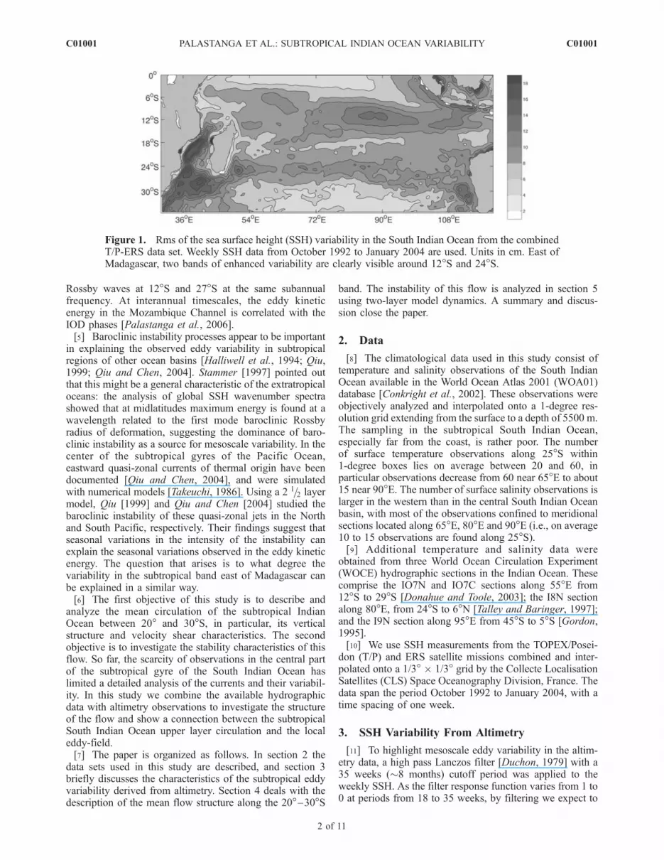
[2] It is well known from satellite altimetry that thevariability of the South Indian Ocean comprises a rangeof frequencies from interannual to subannual timescales[e.g., de Ruijter et al., 2005]. The rms of the sea surfaceheight (SSH) in the South Indian Ocean shows a localmaximum off Sumatra extending into the basin along 12�S,and a second area of high variability around 25�S extendingeastward to the Australian coast and westward to east ofMadagascar (Figure 1). The SSH variance off Java to 90�Eis related to baroclinic instability of the South EquatorialCurrent (SEC) at a period of 40–80 days [Feng andWijffels, 2002], while to the east the variance is attributedto annual Rossby waves [Perigaud and Delecluse, 1992;Morrow and Birol, 1998], interannual SSH anomaliesrelated to the Indian Ocean dipole (IOD) as well as ElNino–Southern Oscillation (ENSO) teleconnections [Xie etal., 2002]. In the latitude band 20�–30�S evidence forsemiannual [Morrow and Birol, 1998] and 4–5 times/year[Schouten et al., 2002] westward propagating Rossby waveswas found. Analyzing a simple two-layer model, Birol andMorrow [2001] concluded that the quasi-semiannualRossby waves (i.e., periods between 150 and 180 days)are connected to variations in the eastern boundary pycno-cline. Moreover, Birol and Morrow [2003] presumed thatthe semiannual coastal Kelvin waves along Australia might

be remotely forced, i.e., by equatorial Pacific wind anoma-lies. However, the forcing of the observed 4–5 times/yearwaves in the 25�S band east of Madagascar was notidentified. In the present study, we further investigate thecauses of the variability in this subtropical band.[3] The eastern part of the subtropical Indian Ocean is

also characterized by significant mesoscale eddy activityassociated with eddies pinched off from the LeeuwinCurrent west off Australia. Combining hydrographic obser-vations and altimetry data, Fang and Morrow [2003] couldtrack Leeuwin Current anticyclonic eddies propagatingwestward between 20�–32�S. Interaction with bottom to-pography seems to induce a slowing down and decay of theeddy amplitudes. Overall, the eddy signals are lost west of90�E.[4] South of Madagascar eddies have been tracked with

altimetry propagating (south) westward towards the Agul-has Current [Grundlingh, 1995; Schouten et al., 2002].Thereafter, they may have an impact on the shedding ofAgulhas Rings [Schouten et al., 2002]. Recently, large deep-reaching dipoles (i.e., vortex pairs) were discovered andmeasured hydrographically in this region [de Ruijter et al.,2004]. They also propagate into the Agulhas Retroflectionregion and trigger the shedding of Agulhas rings. Analyzing6 years of altimetry data, de Ruijter et al. [2004] could onlyfollow three of these dipoles upstream as pairs to thesouthern tip of the Mascarene ridge (23�S, 55�E); in mostcases, cyclonic vortices formed as lee eddies at the southerntip of Madagascar, whereas anticyclones were first observedin the region east or south of Madagascar. Schouten et al.[2002] detected a dominant frequency of 4–5 times/year inthe eddy variability around Madagascar, suggesting a mod-ulation in the eddy-formation processes by the arrival of

JOURNAL OF GEOPHYSICAL RESEARCH, VOL. 112, C01001, doi:10.1029/2005JC003395, 2007ClickHere

for

FullArticle

1Institute for Marine and Atmospheric Research, Utrecht University,Utrecht, Netherlands.

2Royal Netherlands Institute for Sea Research, Texel, Netherlands.

Copyright 2007 by the American Geophysical Union.0148-0227/07/2005JC003395$09.00

C01001 1 of 11

Rossby waves at 12�S and 27�S at the same subannualfrequency. At interannual timescales, the eddy kineticenergy in the Mozambique Channel is correlated with theIOD phases [Palastanga et al., 2006].[5] Baroclinic instability processes appear to be important

in explaining the observed eddy variability in subtropicalregions of other ocean basins [Halliwell et al., 1994; Qiu,1999; Qiu and Chen, 2004]. Stammer [1997] pointed outthat this might be a general characteristic of the extratropicaloceans: the analysis of global SSH wavenumber spectrashowed that at midlatitudes maximum energy is found at awavelength related to the first mode baroclinic Rossbyradius of deformation, suggesting the dominance of baro-clinic instability as a source for mesoscale variability. In thecenter of the subtropical gyres of the Pacific Ocean,eastward quasi-zonal currents of thermal origin have beendocumented [Qiu and Chen, 2004], and were simulatedwith numerical models [Takeuchi, 1986]. Using a 2 1=2 layermodel, Qiu [1999] and Qiu and Chen [2004] studied thebaroclinic instability of these quasi-zonal jets in the Northand South Pacific, respectively. Their findings suggest thatseasonal variations in the intensity of the instability canexplain the seasonal variations observed in the eddy kineticenergy. The question that arises is to what degree thevariability in the subtropical band east of Madagascar canbe explained in a similar way.[6] The first objective of this study is to describe and

analyze the mean circulation of the subtropical IndianOcean between 20� and 30�S, in particular, its verticalstructure and velocity shear characteristics. The secondobjective is to investigate the stability characteristics of thisflow. So far, the scarcity of observations in the central partof the subtropical gyre of the South Indian Ocean haslimited a detailed analysis of the currents and their variabil-ity. In this study we combine the available hydrographicdata with altimetry observations to investigate the structureof the flow and show a connection between the subtropicalSouth Indian Ocean upper layer circulation and the localeddy-field.[7] The paper is organized as follows. In section 2 the

data sets used in this study are described, and section 3briefly discusses the characteristics of the subtropical eddyvariability derived from altimetry. Section 4 deals with thedescription of the mean flow structure along the 20�–30�S

band. The instability of this flow is analyzed in section 5using two-layer model dynamics. A summary and discus-sion close the paper.

2. Data

[8] The climatological data used in this study consist oftemperature and salinity observations of the South IndianOcean available in the World Ocean Atlas 2001 (WOA01)database [Conkright et al., 2002]. These observations wereobjectively analyzed and interpolated onto a 1-degree res-olution grid extending from the surface to a depth of 5500 m.The sampling in the subtropical South Indian Ocean,especially far from the coast, is rather poor. The numberof surface temperature observations along 25�S within1-degree boxes lies on average between 20 and 60, inparticular observations decrease from 60 near 65�E to about15 near 90�E. The number of surface salinity observations islarger in the western than in the central South Indian Oceanbasin, with most of the observations confined to meridionalsections located along 65�E, 80�E and 90�E (i.e., on average10 to 15 observations are found along 25�S).[9] Additional temperature and salinity data were

obtained from three World Ocean Circulation Experiment(WOCE) hydrographic sections in the Indian Ocean. Thesecomprise the IO7N and IO7C sections along 55�E from12�S to 29�S [Donahue and Toole, 2003]; the I8N sectionalong 80�E, from 24�S to 6�N [Talley and Baringer, 1997];and the I9N section along 95�E from 45�S to 5�S [Gordon,1995].[10] We use SSH measurements from the TOPEX/Posei-

don (T/P) and ERS satellite missions combined and inter-polated onto a 1/3� � 1/3� grid by the Collecte LocalisationSatellites (CLS) Space Oceanography Division, France. Thedata span the period October 1992 to January 2004, with atime spacing of one week.

3. SSH Variability From Altimetry

[11] To highlight mesoscale eddy variability in the altim-etry data, a high pass Lanczos filter [Duchon, 1979] with a35 weeks (�8 months) cutoff period was applied to theweekly SSH. As the filter response function varies from 1 to0 at periods from 18 to 35 weeks, by filtering we expect to

Figure 1. Rms of the sea surface height (SSH) variability in the South Indian Ocean from the combinedT/P-ERS data set. Weekly SSH data from October 1992 to January 2004 are used. Units in cm. East ofMadagascar, two bands of enhanced variability are clearly visible around 12�S and 24�S.

C01001 PALASTANGA ET AL.: SUBTROPICAL INDIAN OCEAN VARIABILITY

2 of 11

C01001

remove the steric height annual variability (�52 weeks)[Stammer, 1997] and to reduce the semiannual signal(�25 weeks) observed along the latitude band 20�–30�S[Morrow and Birol, 1998]. The rms of the high passed SSHshows a band of high variability around 25�S like theunfiltered data (Figure 1), but with relative maxima moreclearly outstanding near 67�E, 80�E, 87�E, and 105�E(Figure 2). Inspection of the time-longitude diagram ofthe high passed SSH reveals wavelike westward propagat-ing features along this band (not shown).[12] To analyze the dominant frequencies of the SSH

variability along 25�S, a spectral analysis was performedaround 100�E, 80�E, and 65�E. Figure 3a shows that near100�E the dominant variability is found at around aperiod of 19 weeks (�2.5 times/year), while in the centraland western basin the spectral peak occurs at around 14–15 weeks (�4 times/year). In particular, this shorter periodappears to dominate the spectra over the areas of maximumvariability west of 90�E (Figure 2). The presence of vari-ability around 4–5 times/year is consistent with the obser-vations of Schouten et al. [2002]. Energy present at longerperiods (22–24 weeks) is probably related to the quasi-semiannual variability forced at the eastern boundary [Biroland Morrow, 2001].[13] To estimate the spatial scales associated with the

subtropical eddy variability, the data were high pass filteredwith a cut off wavelength of 700 km and SSH wavenumber-spectra along 25�S and between 50�E–110�E were com-puted. Figure 3b shows a dominant peak at a wavelength ofaround 440 km, whereas for higher wavenumbers theenergy closely follows a k�3 relation. Stammer [1997] notedthat this type of cutoff in the spectra is associated with thelength scale at which the maximum baroclinic instabilityoccurs. Moreover, the energy decay in the spectra as apower-function of the wavenumber k is consistent withtheories of baroclinic instability and geostrophic turbulence[Pedlosky, 1987]. In the Indian Ocean around 25�S thewavelength associated with the first baroclinic Rossbyradius of deformation is 2pR0 � 330 km [Chelton et al.,1998]. This is in good agreement with the SSH spectralmaximum, if one considers that real mesoscale features tend

to be larger than those predicted by linear theories ofbaroclinic instability [Pedlosky, 1987]. The peak in thespectra at a wavelength of around 590 km (Figure 3b)might be related to the quasi-semiannual waves (i.e., wave-lengths of 300–500 km) observed by Morrow and Birol[1998].

4. Mean Flow Structure

[14] Owing to the scarcity of observations in the center ofthe subtropical gyre, the flow structure between 20�–30�S

Figure 2. Rms of the high pass filtered SSH along 24�S inthe South Indian Ocean. A filter with a cutoff period of8 months was applied to the weekly SSH field from thecombined T/P-ERS data set.

Figure 3. (a) Frequency spectra of the high pass filteredSSH from the combined T/P-ERS data set in three regionsalong 25�S, namely, at 100�E (solid black line), 80�E(dashed line), and 65�E (solid gray line). The dominantfrequency changes from 2.5 times/year in the east to4 times/year in the central and western basin. (b) Wavenum-ber spectra of the SSH data along 25�S and between 50� and110�E. Weekly SSH were high pass filtered with a cut offwavelength of 700 km. Energy decays at high wavenumbersas the third power law of the wavenumber, k�3. Thedominant wavelength is found around 440 km, and a secondpeak appears around 590 km.

C01001 PALASTANGA ET AL.: SUBTROPICAL INDIAN OCEAN VARIABILITY

3 of 11

C01001

is not yet well known. On the basis of hydrographic data,Stramma and Lutjeharms [1997] estimated the idealizedtransport of the subtropical gyre over the upper 1000 m.They showed that the westward return flow in the gyre isfound in the subtropical basin from 40�S up to the SEClatitude, and as part of a recirculation cell in the southwestcorner of the basin (see their Figure 7). Dynamic topogra-phy maps in the atlas by Wyrtki [1971], as well as theanalysis by Reid [2003], indicates, however, that east ofMadagascar there is a surface eastward flow. In this sectionwe analyze in detail the structure of the flow in the SouthIndian Ocean around 25�S from the surface down to about1000 m. Although it is expected that seasonal changes canbe important in the near surface circulation, because of thelack of observations, we limit the description to the meanpattern. Comments related to the seasonal variability areincluded in the discussion section.[15] The climatological dynamic topography at the sur-

face relative to 2000 m (Figure 4a) shows the pattern of thesubtropical gyre with a recirculation cell in the southwesternbasin around 30�S [Stramma and Lutjeharms, 1997], and ananticyclonic cell east of Madagascar. The latter is boundedto the north by the westward flowing SEC, roughly between10�–20�S, and to the south by an eastward flow from southMadagascar up to 75�E. The eastward flow continues

between 20�–30�S from the central basin to Australia,and seems connected to the South Indian Ocean Current,which constitutes the southern limit of the subtropical gyreat around �40�S [Stramma, 1992]. This shallow, quasizonaleastward flow along 25�S has not been previously docu-mented in detail. It is noteworthy that the location of this jetis similar to that of the subtropical countercurrents observedin the North and South Pacific [Qiu, 1999; Qiu and Chen,2004], supporting the idea of a dynamically similar perma-nent current in the South Indian Ocean subtropical gyre. Byanalogy with the Pacific Ocean we will hereafter refer to theIndian Ocean eastward jet as the South Indian OceanCountercurrent (SICC). At 500 m (Figure 4b), the flowbetween 20�–30�S is westward in agreement with the largescale Sverdrup flow forced by the wind stress curl, and thesouthwestern recirculation cell extends up to 70�E.[16] A geostrophic velocity section at 65�E (Figure 5a)

based on climatology, shows the vertical structure of theflow east of Madagascar. The eastward jet is confined to theupper 250 m in the latitude band 20�–35�S, with its corearound 25�S and surface velocities up to 0.06 m/s. It flowsabove westward velocities of about �0.02 m/s associatedwith the southward extension of the SEC between depths of350 and 1100 m. This vertical structure characterizes theflow between 50� and 95�E. East of 75�E the eastward jet

Figure 4. Dynamic topography of the South Indian Ocean relative to 2000 m at (a) the surface and(b) 500 m, based on the climatological hydrographic data. Units in m2/s2. Contours every 0.1 units. Itshows a recirculation cell east of Madagascar and general eastward flow in the upper layer south of 20�S.At 500 m the flow between 20� and 30�S is westward, as a Sverdrupian flow.

C01001 PALASTANGA ET AL.: SUBTROPICAL INDIAN OCEAN VARIABILITY

4 of 11

C01001

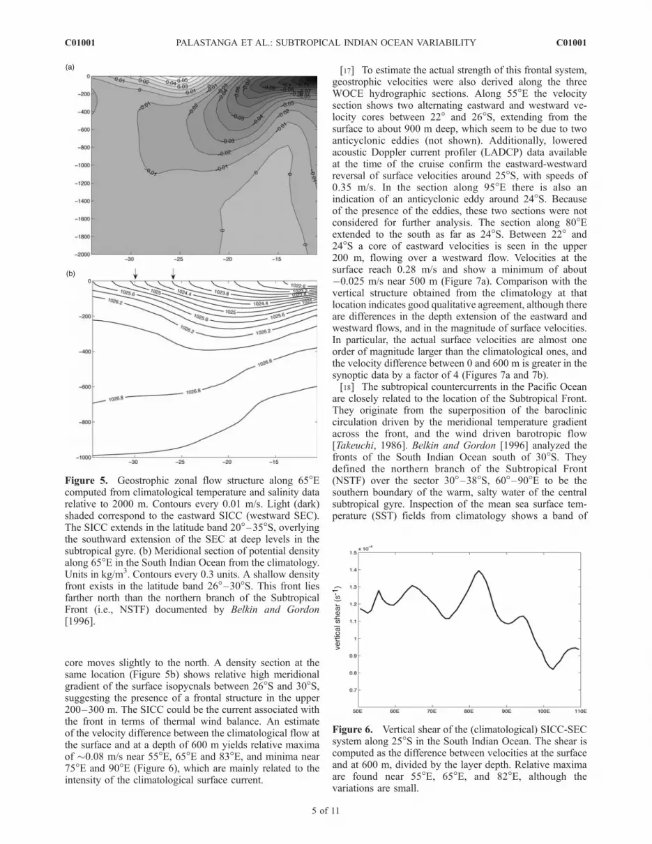
core moves slightly to the north. A density section at thesame location (Figure 5b) shows relative high meridionalgradient of the surface isopycnals between 26�S and 30�S,suggesting the presence of a frontal structure in the upper200–300 m. The SICC could be the current associated withthe front in terms of thermal wind balance. An estimateof the velocity difference between the climatological flow atthe surface and at a depth of 600 m yields relative maximaof �0.08 m/s near 55�E, 65�E and 83�E, and minima near75�E and 90�E (Figure 6), which are mainly related to theintensity of the climatological surface current.

[17] To estimate the actual strength of this frontal system,geostrophic velocities were also derived along the threeWOCE hydrographic sections. Along 55�E the velocitysection shows two alternating eastward and westward ve-locity cores between 22� and 26�S, extending from thesurface to about 900 m deep, which seem to be due to twoanticyclonic eddies (not shown). Additionally, loweredacoustic Doppler current profiler (LADCP) data availableat the time of the cruise confirm the eastward-westwardreversal of surface velocities around 25�S, with speeds of0.35 m/s. In the section along 95�E there is also anindication of an anticyclonic eddy around 24�S. Becauseof the presence of the eddies, these two sections were notconsidered for further analysis. The section along 80�Eextended to the south as far as 24�S. Between 22� and24�S a core of eastward velocities is seen in the upper200 m, flowing over a westward flow. Velocities at thesurface reach 0.28 m/s and show a minimum of about�0.025 m/s near 500 m (Figure 7a). Comparison with thevertical structure obtained from the climatology at thatlocation indicates good qualitative agreement, although thereare differences in the depth extension of the eastward andwestward flows, and in the magnitude of surface velocities.In particular, the actual surface velocities are almost oneorder of magnitude larger than the climatological ones, andthe velocity difference between 0 and 600 m is greater in thesynoptic data by a factor of 4 (Figures 7a and 7b).[18] The subtropical countercurrents in the Pacific Ocean

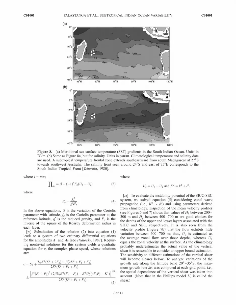
are closely related to the location of the Subtropical Front.They originate from the superposition of the barocliniccirculation driven by the meridional temperature gradientacross the front, and the wind driven barotropic flow[Takeuchi, 1986]. Belkin and Gordon [1996] analyzed thefronts of the South Indian Ocean south of 30�S. Theydefined the northern branch of the Subtropical Front(NSTF) over the sector 30�–38�S, 60�–90�E to be thesouthern boundary of the warm, salty water of the centralsubtropical gyre. Inspection of the mean sea surface tem-perature (SST) fields from climatology shows a band of

Figure 5. Geostrophic zonal flow structure along 65�Ecomputed from climatological temperature and salinity datarelative to 2000 m. Contours every 0.01 m/s. Light (dark)shaded correspond to the eastward SICC (westward SEC).The SICC extends in the latitude band 20�–35�S, overlyingthe southward extension of the SEC at deep levels in thesubtropical gyre. (b) Meridional section of potential densityalong 65�E in the South Indian Ocean from the climatology.Units in kg/m3. Contours every 0.3 units. A shallow densityfront exists in the latitude band 26�–30�S. This front liesfarther north than the northern branch of the SubtropicalFront (i.e., NSTF) documented by Belkin and Gordon[1996].

Figure 6. Vertical shear of the (climatological) SICC-SECsystem along 25�S in the South Indian Ocean. The shear iscomputed as the difference between velocities at the surfaceand at 600 m, divided by the layer depth. Relative maximaare found near 55�E, 65�E, and 82�E, although thevariations are small.

C01001 PALASTANGA ET AL.: SUBTROPICAL INDIAN OCEAN VARIABILITY

5 of 11

C01001

relatively high meridional SST gradients extending witha southeastward tilt from 45�E, 27�S towards Australia(Figure 8a). Analysis of SST from satellite data supportsthe existence of a similar basin temperature front between27� and 35�S. In the central basin, these temperaturegradients seem connected to the NSTF of Belkin and Gordon[1996]. The meridional salinity gradients from climatologyindicate a frontal zone east of 75�E between 20� and 26�S(Figure 8b) that corresponds to the South Indian TropicalFront [Tchernia, 1980], which separates salty waters of thecentral subtropical Indian Ocean from the fresher waters ofthe eastern tropical Indian Ocean. As a consequence, asecondary density front exists in the band 20�S–30�S (i.e.,north of the NSTF of Belkin and Gordon [1996]) extending

with a northeastward tilt from southeast Madagascar to theeastern subtropical basin. Whether (and how) this subtrop-ical frontal zone is linked to the origin of the SICC deservesfurther investigation that will be left for future studies.[19] Another important aspect of the SICC to be investi-

gated is its connection to the western boundary current thatcloses the surface anticyclonic circulation east of Madagas-car (Figure 4a), i.e., the East Madagascar Current (EMC).The fate of the EMC after separating from the Madagascarcoast has been a subject of discussion. Based on theavailable hydrographic observations Lutjeharms [1976]suggested that the surface flow south of Madagascarwas eastward, leading later to the suggestion of anEMC retroflection similar to that of the Agulhas current[Lutjeharms, 1988]. However, based on chlorophyll data,Quartly and Srokosz [2004] found indications of differentEMC regimes, sometimes corresponding to a retroflection,in other cases to a westward continuation towards theAfrican coast. The eastward flow we observed fromthe climatology near the southwestern tip of Madagascar(Figure 4a) seems consistent with the observations ofLutjeharms [1976]. Farther east, the SICC could supportthe existence of an EMC retroflection and/or an eastwardEMC return flow into the ocean interior. However, the SICCis shallow compared to the vertical extension of the EMC,so only the near-surface part of the EMC would be involvedin such a retroflection.[20] In summary, both climatology and WOCE data

reveal the SICC to be a shallow eastward current extendingalong the South Indian Ocean subtropical gyre over thewestward flow of the SEC. With this sheared flow structure,instabilities of the SICC-SEC that explain the observedsubtropical variability may be induced. To check this, inthe next section, we analyze the baroclinic instability of theSICC-SEC system in the context of a simple two-layermodel.

5. Stability Considerations

[21] A simple model to study baroclinic instability wasintroduced by Phillips [1954]. In this approximation theocean is represented by two layers of constant depth Hn anddensity rn, with meridionally independent zonal velocitiesUn in each layer (n = 1 and 2). This implies that the interfacebetween the two layers has a constant slope. Here we adoptthis approximation to represent the vertical structure of theSICC-SEC system. In the absence of friction and bottomtopography, the linearized version of the quasigeostrophicpotential vorticity equation [see Pedlosky, 1987] reads:

@

@tþ Un

@

@x

� �qn þ

@Pn

@y

@fn

@x¼ 0; ð1Þ

where qn is the perturbation potential vorticity, fn theperturbation stream function and Pn the mean potentialvorticity in layer n.[22] As U1 and U2 are independent of y, the normal mode

solutions to equation (1), fn, and the meridional gradient ofthe mean potential vorticity, Pny, have the form:

fn ¼ Re An sin lyð Þ exp i kx� wtð Þ½ ð2Þ

Figure 7. (a) Geostrophic zonal velocity profile at 80�E,24�S, in the upper 2000 m from a WOCE hydrographicsection. (b) Same as Figure 7a, but from climatological data.Note the difference in velocity scale. This shows thatclimatology underestimates significantly the magnitude ofthe surface, eastward velocities. The velocity differencecomputed between 0 and 600 m is about 0.3 m/s in theWOCE data, but lower by a factor 4 in the climatology(�0.08 m/s).

C01001 PALASTANGA ET AL.: SUBTROPICAL INDIAN OCEAN VARIABILITY

6 of 11

C01001

where l = mp; Yny¼ b � �1ð ÞnFn U1 � U2ð Þ ð3Þ

where

Fn ¼f 2o

g0Hn

: ð4Þ

In the above equations, b is the variation of the Coriolisparameter with latitude, fo is the Coriolis parameter at thereference latitude, g0 is the reduced gravity, and Fn is theinverse of the square of the Rossby deformation radius ineach layer.[23] Substitution of the solution (2) into equation (1)

leads to a system of two ordinary differential equationsfor the amplitudes A1 and A2 [see Pedlosky, 1987]. Requir-ing nontrivial solutions for this system yields a quadraticequation for c, the complex phase speed, whose solutionsare:

c ¼ U2 þUsK

2 K2 þ 2F2ð Þ � b 2K2 þ F1 þ F2ð Þ2K2 K2 þ F1 þ F2ð Þ

�b2 F1 þ F2ð Þ2þ2bUsK

4 F1 � F2ð Þ � K4U2s 4F1F2 � K4ð Þ

h i1=22K2 K2 þ F1 þ F2ð Þ

ð5Þ

where

Us ¼ U1 � U2 and K2 ¼ k2 þ l2:

[24] To evaluate the instability potential of the SICC-SECsystem, we solved equation (5) considering zonal wavepropagation (i.e., K2 � k2) and using parameters derivedfrom climatology. Inspection of the mean velocity profiles(see Figures 5 and 7) shows that values of H1 between 200–300 m and H2 between 400–700 m are good choices forthe depths of the upper and lower layers associated with theSICC and SEC, respectively. It is also seen from thevelocity profile (Figure 7b) that the flow exhibits littlevariation between 400–700 m; thus, U2 is estimated asthe average zonal flow over those depths, whereas U1

equals the zonal velocity at the surface. As the climatologyprobably underestimates the actual value of the verticalshear it is reasonable to consider an upper bound estimation.The sensitivity to different estimations of the vertical shearwill become clearer below. To analyze variations of thegrowth rate along the latitude band 20�–35�S, the maxi-mum growth rate kci was computed at each grid point, i.e.,the spatial dependence of the vertical shear was taken intoaccount. (Note that in the Phillips model Us is called theshear.)

Figure 8. (a) Meridional sea surface temperature (SST) gradients in the South Indian Ocean. Units in�C/m. (b) Same as Figure 8a, but for salinity. Units in psu/m. Climatological temperature and salinity dataare used. A subtropical temperature frontal zone extends southeastward from south Madagascar at 27�Stowards southwest Australia. The salinity front seen around 24�S and east of 75�E corresponds to theSouth Indian Tropical Front [Tchernia, 1980].

C01001 PALASTANGA ET AL.: SUBTROPICAL INDIAN OCEAN VARIABILITY

7 of 11

C01001

[25] Figure 9 shows the maximum growth rate, kci, whenH1 = 250 m and H2 = 400 m. Nonzero values are foundbetween 24� and 31�S and near the regions of maximumvertical shear (Figure 6). Comparison with Figure 2 showsthat the instability spots also lie close to the regions ofmaximum variability west of 90�E. The growth rates varybetween 0.004 and 0.014 day�1, or equivalently betweene-folding timescales from 70 to 250 days. The wavelengthsof the most unstable modes lie between 240 and 320 km,decreasing from north to south in agreement with thevariation of RO. The southeastward tilt seen in kci east of100�E coincides with a shift in the SICC core towards�29�S. The largest growth rates are found near 64�E, 26�Sand 82�E, 26�S (Figure 10). They show a window ofunstable wavelengths between 250 and 333 km, withmaxima around 297 km and 283 km, and e-folding time-scales between 75 and 80 days. The e-folding times pre-dicted from the Phillips model are of the same order as thosefound for the countercurrents in the Pacific Ocean duringthe winter-spring season [Qiu, 1999; Qiu and Chen, 2004].[26] The above results are quite sensitive to the thickness

of the second layer. For instance, a choice of H2 > 450 mmakes solutions of equation (5) stable over the subtropicaldomain. On the other hand, reducing the depth of the firstlayer tends to increase the instability potential of thesubtropical current system. The sensitivity to H2 is relatedto the necessary condition for instability in the Phillipsmodel. For instability to occur the meridional gradient of themean potential vorticity needs to change sign between thetwo layers, from equation (3) when U1 > U2 this reduces to:

Y2y< 0; or Us >

bF2

¼ bg0H2

f 20:

A slightly different criterion for baroclinic instability can bederived from the 2 1=2 layer quasigeostrophic modelequations. Qiu [1999] showed that when U1 > U2, thenecessary condition states that the vertical shear has to

overcome the beta effect plus a factor proportional to thestratification ratio, i.e.:

Us >bF2

þ gU2 ð6Þ

where

g ¼ r2 � r1r3 � r2

:

Results of equation (6) are similar to those in Figure 8,although there is a slight increase in the instability potential

Figure 9. Maximum growth rate of the unstable modes estimated from the two-layer Phillips modelequations (i.e., equation (5)), computed at each grid point over the South Indian Ocean. The model depthof the first and second layers is 250 m and 400 m, respectively, and the velocity shear is estimatedbetween the observed flow at the surface and the average flow between 400-600 m. Units in days�1.Results indicate that in the subtropical band between 24�-30�S the flow is baroclinically unstable.

Figure 10. Growth rate as a function of the zonalwavenumber k calculated from equation (5) at 64�E, 26�S(solid line) and at 80�E, 26�S (dash line). Both locationsshow similar e-folding times (between 75 days and 80 days)and wavelengths for the most unstable modes (�290 km).

C01001 PALASTANGA ET AL.: SUBTROPICAL INDIAN OCEAN VARIABILITY

8 of 11

C01001

over the subtropical latitude band 24�S–31�S. If H2

becomes larger than 450 m, the instability is also reduced.[27] Since the vertical shear from climatology is about 4

times smaller than that observed from synoptic hydro-graphic data (Figure 7), we estimated the Phillips growthrate using the zonal velocity profile available at 80�E,24�S (Figure 7a). To compute kci, U1 was estimated as thevelocity averaged over the first 100 m and U2 as thevelocity averaged over the second layer thickness. H1 wasset equal to 250 m, and H2 was varied between 250 and750 m. (Note that the change in the vertical shear dueto varying H2 is very small.) Figure 11 shows that thee-folding time of the most unstable waves varies slowlywhen H2 varies from 250 to 650 m, but it increasessharply from �30 to 63 days when H2 varies between650 and 750m. A depth of �750 m for H2 is probably themore realistic approximation of the vertical flow structurein this synoptic data set (see Figure 7a). In this case thewindow of unstable wavelengths is 390–470 km, withL � 430 km for the most unstable wave. This is inagreement with the dominant spatial scale of eddy vari-ability estimated from observations (i.e., �440 km,Figure 3b). In addition, the frequency of the most unstablemode turns out to be around 5 times/year, though it variesin the range 3.5–6 times/year with small variations of thevertical shear (i.e., the frequency increases when thevertical shear decreases).[28] In conclusion, the frequency range generated by the

baroclinic instability as detected near 80�E, 24�S is closeto the observed subtropical Rossby wave variability of 4–5 times/year [Schouten et al., 2002]. Although the resultswith synoptic hydrographic data are based on a singleobservation of the velocity profile, they support the hypoth-esis that regions of maximum vertical shear around 25�S arebaroclinically unstable. It is likely that the analysis using

climatology underestimates the vertical shear and therebythe expected instability along the subtropical band.

6. Summary and Discussion

[29] In this study, we have analyzed the flow structure inthe South Indian Ocean subtropical gyre between 20� and30�S. The climatology shows the existence of a shalloweastward jet with its core around 25�S, which flows over thedeep reaching westward SEC. The presence of this eastwardSouth Indian Ocean Countercurrent (SICC) is analogous tothe subtropical countercurrents in the Pacific Ocean [Qiu,1999; Qiu and Chen, 2004]. This suggests that the forcingof the SICC could be similar to that in the Pacific. Theposition of the northernmost branch of the Subtropical Frontin the South Indian Ocean lies farther south than that in thePacific [Belkin and Gordon, 1996]. From the climatologicaldata we have shown the existence of a secondary, subtrop-ical frontal zone extending across the basin between �26�–32�S in the west and between �20�–27�S in the east. TheSICC might be its associated frontal jet. The connection ofthe SICC to the western boundary current at that latitude,the East Madagascar current (EMC), is still unclear. Evi-dence for the existence of ‘‘events’’ of an EMC retroflectionhas been derived in the past from analyses of surface data[Lutjeharms, 1988; Quartly and Srokosz, 2004]. The shal-low SICC could provide the mean large-scale, eastwardflow to which a retroflection of the upper layers of the EMCcould connect. In the future, a combination of observationsand modeling studies is needed to better determine thecharacteristics of the SICC, its forcing and variability.[30] The stability of the SICC-SEC vertical flow structure

was analyzed using the Phillips two-layer model [Phillips,1954]. We have shown that the SICC-SEC system satisfiesthe condition for baroclinic instability in this model: themeridional gradient of the mean potential vorticity changessign around 200 m. In particular, areas of maximum verticalshear in the subtropical basin between 24� and 31�S arebaroclinically unstable. The findings are confirmed in astability analysis of the 2 1=2 layer quasi-geostrophic model[see, e.g., Qiu, 1999]. E-folding timescales found near 64�Eand 82�E (�80 days) compare well with baroclinic insta-bility timescales detected in the Pacific subtropical counter-currents [Qiu, 1999; Qiu and Chen, 2004]. Given thesimplicity of the two-layer model and the quality of thedatabase in this region of the South Indian Ocean, the rangeof unstable wavelengths (290–470 km) agrees surprisinglywell with estimations of the wavenumber spectra fromaltimetry (�440 km). Analysis of the stability using syn-optic hydrographic data along the 80�E section shows arange of unstable frequencies between 3.5 and 6 times/year.A similar subannual frequency is present in the SSH dataalong 25�S, consistent with the 4–5 times/year Rossbywave propagation detected by Schouten et al. [2002].Therefore, baroclinic instability of the SICC-SEC systemcan explain the eddy variability observed along the 25�Sband and the fact that a large part of the variance is in thesubannual frequency range. It is also worth noticing that thepossibility of barotropic instability across the SICC shearwas evaluated following Lipps [1963]. Assuming a simpli-fied profile for the SICC-SEC velocity, no change in themeridional gradient of potential vorticity was detected, in

Figure 11. E-folding timescale of the most unstable modeas a function of the second layer depth H2 using parametersfrom WOCE synoptic hydrographic data at 80�E, 24�S (asin Figure 7a). The sensitivity of the growth rate to changesin H2 is higher if the latter varies from 650 m to 750 m.

C01001 PALASTANGA ET AL.: SUBTROPICAL INDIAN OCEAN VARIABILITY

9 of 11

C01001

other words, the sufficient condition for barotropic stabilityis satisfied.[31] The altimetry data show high eddy kinetic energy

(EKE) levels in the center of the South Indian Oceansubtropical gyre analogous to those observed along thesubtropical Pacific Ocean (i.e., EKE ranges between 150and 300 cm2/s2). The region east of Madagascar between50� and 60�E (see Figure 1) is a particularly highlyenergetic area (i.e., EKE varies from 200 up to 1000 cm2/s2).EKE variations along 25�S may also represent changes inthe intensity and/or position of the SICC. Estimations of theEKE associated with the low frequency component of theSSH field (i.e., periods greater than 1 year) range between20 and 70 cm2/s2. This suggests that a high percentage ofthe total EKE variability is related to mesoscale processes.Halliwell et al. [1994] suggested that a baroclinicallyunstable system might convert initially wavelike perturba-tions into large eddy structures due to a nonlinear energycascade. It seems plausible that the variability generatedlocally by baroclinic instability in the subtropical IndianOcean is connected to the eddy activity observed east andsouth of Madagascar [Schouten et al., 2002; de Ruijter etal., 2004; Quartly and Srokosz, 2004].[32] High levels of EKE also exist in the South Indian

Ocean over the SEC path (i.e., EKE ranges between 100and 400 cm2/s2). The stability analysis based on the Phillipstwo-layer model shows that the SEC vertical shear is stable.However, an analysis of the continuously stratified systemshowed that the SEC in the eastern Indian Ocean isbaroclinically unstable, with the largest growth rates (e-folding timescales of less than 50 days) during the July–September season [Feng and Wijffels, 2002]. The SEC northof Madagascar is barotropically unstable at a period of50 days, inducing this frequency of variability in the eddyactivity drifting south into the Mozambique Channel [Schottet al., 1988; Schouten et al., 2003].[33] Finally, the EKE along 25�S shows a regular sea-

sonal variation, with maxima in November and minima inMay. Qiu [1999] and Qiu and Chen [2004] showed that theseasonal modulation of the EKE in the subtropical Pacificcountercurrents is related to seasonal variations in thegrowth rate of the baroclinic waves. Analysis of seasonalvelocity profiles from climatology reveals that the SICC isstronger (weaker) in summer (winter), while the SECweakens (strengthens) due to the large-scale wind variabil-ity [Tchernia, 1980]. As a consequence, the shear of theSICC-SEC system is high in summer and winter, leading tobaroclinic instability with e-folding timescales between 40and 50 days in both seasons. Future studies using betterquality observations of the seasonal velocity profiles as wellas density sections, will need to analyze these variations andtheir possible relation to the annual variability of the EKE.More accurate analyses of the continuously stratified systemwill also require an ensemble of hydrographic observationsthat is not currently available for the South Indian Ocean.

[34] Acknowledgments. This research was funded by the Foundationfor Earth and Life Sciences (ALW) of the Netherlands Foundation ofScientific Research (NWO) under grant 854.00.001.

ReferencesBelkin, I. M., and A. L. Gordon (1996), Southern Ocean fronts from theGreenwich Meridian to Tasmania, J. Geophys. Res., 101, 3675–3696.

Birol, F., and R. Morrow (2001), Source of the baroclinic waves in thesoutheast Indian Ocean, J. Geophys. Res., 106, 9145–9160.

Birol, F., and R. Morrow (2003), Separation of the quasi-semiannualRossby waves from the eastern boundary of the Indian Ocean, J. Mar.Res., 61, 707–723.

Chelton, D. B., R. A. deSzoeke, M. G. Schlax, K. E. Naggar, and N.Siwertz(1998), Geographical variability of the first baroclinic Rossby radius ofdeformation, J. Phys. Oceanogr., 28, 433–460.

Conkright, M. E., R. A. Locarnini, H. E. Garcia, T. D. O’Brien, T. P. Boyer,C. Stephens, and J. I. Antonov (2002), World Ocean Atlas 2001: Objec-tive analyses, data statistics, and figures, CD-ROM documentation, 17pp., Natl. Oceanogr. Data Cent., Silver Spring, Md.

de Ruijter, W. P. M., H. M. van Aken, E. J. Beier, J. R. E. Lutjeharms, R. P.Matano, and M. W. Schouten (2004), Eddies and dipoles around southMadagascar: Formation, pathways and large-scale impact, Deep Sea Res.,Part I, 51, 383–400.

de Ruijter, W. P. M., H. Ridderinkhof, and M. W. Schouten (2005), Varia-bility of the southwest Indian Ocean, Philos. Trans. Math. Phys. Eng.Sci., 363, 63–76.

Donahue, K. A., and J. M. Toole (2003), A near-synoptic survey of thesouthwest Indian Ocean, Deep Sea Res., 50, 1893–1931.

Duchon, C. E. (1979), Lanczos filtering in one and two dimensions, J. Appl.Meteorol., 18, 1016–1022.

Fang, F., and R. Morrow (2003), Evolution, movement and decay of warm-core Leeuwin Current eddies, Deep Sea Res., 50, 2245–2261.

Feng, F., and S. Wijffels (2002), Intraseasonal variability of the SouthEquatorial Current of the east Indian Ocean, J. Phys. Oceanogr., 32,265–277.

Gordon, A. L. (1995), WHP Indian Ocean I9N, Int. WOCE Newsl., 20, 26–27.

Grundlingh, M. L. (1995), Tracking eddies in the southeast Atlantic andsouthwest Indian oceans with TOPEX/Poseidon, J. Geophys. Res., 100,24,977–24,986.

Halliwell, G. R., Jr., G. Peng, and D. B. Olson (1994), Stability of theSargasso Sea Subtropical Frontal Zone, J. Phys. Oceanogr., 24, 1166–1183.

Lipps, F. B. (1963), Stability jets in a divergent bartropic fluid, J. Atmos.Sci., 20, 120–129.

Lutjeharms, J. R. E. (1976), The Agulhas Current system during the north-east monsoon season, J. Phys. Oceanogr., 6, 665–670.

Lutjeharms, J. R. E. (1988), Remote sensing corroboration of the retro-flection of the East Madagascar Current, Deep Sea Res., Part A, 35,2045–2050.

Morrow, R., and F. Birol (1998), Variability in the southeast Indian Oceanfrom altimetry: Forcing mechanisms for the Leeuwin Current, J. Geo-phys. Res., 103, 18,529–18,544.

Palastanga, V., P. J. van Leeuwen, and W. P. M. de Ruijter (2006), A linkbetween low-frequency mesoscale eddy variability around Madagascarand the large-scale Indian Ocean variability, J. Geophys. Res., 111,C09029, doi:10.1029/2005JC003081.

Pedlosky, J. (1987), Geophysical Fluid Dynamics, 710 pp., Springer, NewYork.

Perigaud, C., and P. Delecluse (1992), Annual sea level variations in thesouthern tropical Indian Ocean from Geosat and shallow water simula-tions, J. Geophys. Res., 97, 20,169–20,178.

Phillips, N. A. (1954), Energy transformations and meridional circulationsassociated with simple baroclinic waves in a two-level, quasi-geostrophicmodel, Tellus, 6, 273–286.

Qiu, B. (1999), Seasonal eddy field modulation of the North Pacific Sub-tropical Countercurrent: TOPEX/Poseidon observations and theory,J. Phys. Oceanogr., 29, 2471–2486.

Qiu, B., and S. Chen (2004), Seasonal modulations in the eddy field of theSouth Pacific Ocean, J. Phys. Oceanogr., 34, 1515–1527.

Quartly, G. D., and M. A. Srokosz (2004), Eddies in the southern Mozam-bique Channel, Deep Sea Res., Part II, 51, 69–83.

Reid, J. L. (2003), On the total geostrophic circulation of the Indian Ocean:Flow patterns, tracers, and transports, Prog. Oceanogr., 56, 137–186.

Schott, F., M. Fieux, J. Kindle, J. Swallow, and R. Zantopp (1988), Theboundary currents east and north of Madagascar: 2. Gesotrophic directmeasurements and model comparisons, J. Geophys. Res., 93, 4963–4974.

Schouten, M. W., W. P. M. de Ruijter, and P. J. van Leeuwen (2002),Upstream control of Agulhas Ring shedding, J. Geophys. Res.,107(C8), 3109, doi:10.1029/2001JC000804.

Schouten,M.W.,W. P.M. de Ruijter, P. J. van Leeuwen, andH. Ridderinkhof(2003), Eddies and variability in theMozambique Channel,Deep Sea Res.,Part II, 50, 1987–2003.

Stammer, D. (1997), Global characteristics of ocean variability estimatedfrom regional TOPEX/Poseidon altimeter measurements, J. Phys. Ocea-nogr., 27, 1743–1769.

C01001 PALASTANGA ET AL.: SUBTROPICAL INDIAN OCEAN VARIABILITY

10 of 11

C01001

Stramma, L. (1992), The South Indian Ocean Current, J. Phys. Oceanogr.,22, 421–430.

Stramma, L., and J. R. E. Lutjeharms (1997), The flow field of the sub-tropical gyre of the south Indian Ocean, J. Geophys. Res., 102, 5330–5513.

Takeuchi, K. (1986), Numerical study of the seasonal variations of theSubtropical Front and the Subtropical Countercurrent, J. Phys. Ocea-nogr., 16, 919–926.

Talley, L. D., and M. O. Baringer (1997), Preliminary results from WOCEhydrographic sections at 80�E and 32�S in the central Indian Ocean,Geophys. Res. Lett., 24, 2789–2792.

Tchernia, P. (1980), Descriptive Regional Oceanography, Pergamon Mar.Ser., vol. 3, 253 pp., Elsevier, New York.

Wyrtki, K. (1971), Oceanographic Atlas of the Interanational Indian OceanExpedition, 531 pp., Natl. Sci. Found., Washington, D. C.

Xie, S. P., H. Annamalai, F. A. Schott, and J. P. McCreary Jr. (2002),Structure and mechanisms of south Indian Ocean climate variability,J. Clim., 15, 864–878.

�����������������������W. P. M. de Ruijter, V. Palastanga, and P. J. van Leeuwen, Institute for

Marine and Atmospheric Research, Utrecht University, NL-3508 TAUtrecht, Netherlands. (v.palastanga@phys.uu.nl)M. W. Schouten, Royal Netherlands Institute for Sea Research, NL-1759

AB, Texel, Netherlands.

C01001 PALASTANGA ET AL.: SUBTROPICAL INDIAN OCEAN VARIABILITY

11 of 11

C01001