flow between time-periodically co-rotating cylinders

J. Fluid Mech. (1999), vol. 397, pp. 73–98. Printed in the United Kingdom

c© 1999 Cambridge University Press

73

Flow between time-periodicallyco-rotating cylinders

By P A T R I C I A E R N† AND J O S E E D U A R D O W E S F R E I DLaboratoire de Physique et Mecanique des Milieux Heterogenes, UMR CNRS 7636,

Ecole Superieure de Physique et Chimie Industrielles de Paris – ESPCI,10, rue Vauquelin, 75231 Paris cedex 05, France

(Received 28 October 1998 and in revised form 16 May 1999)

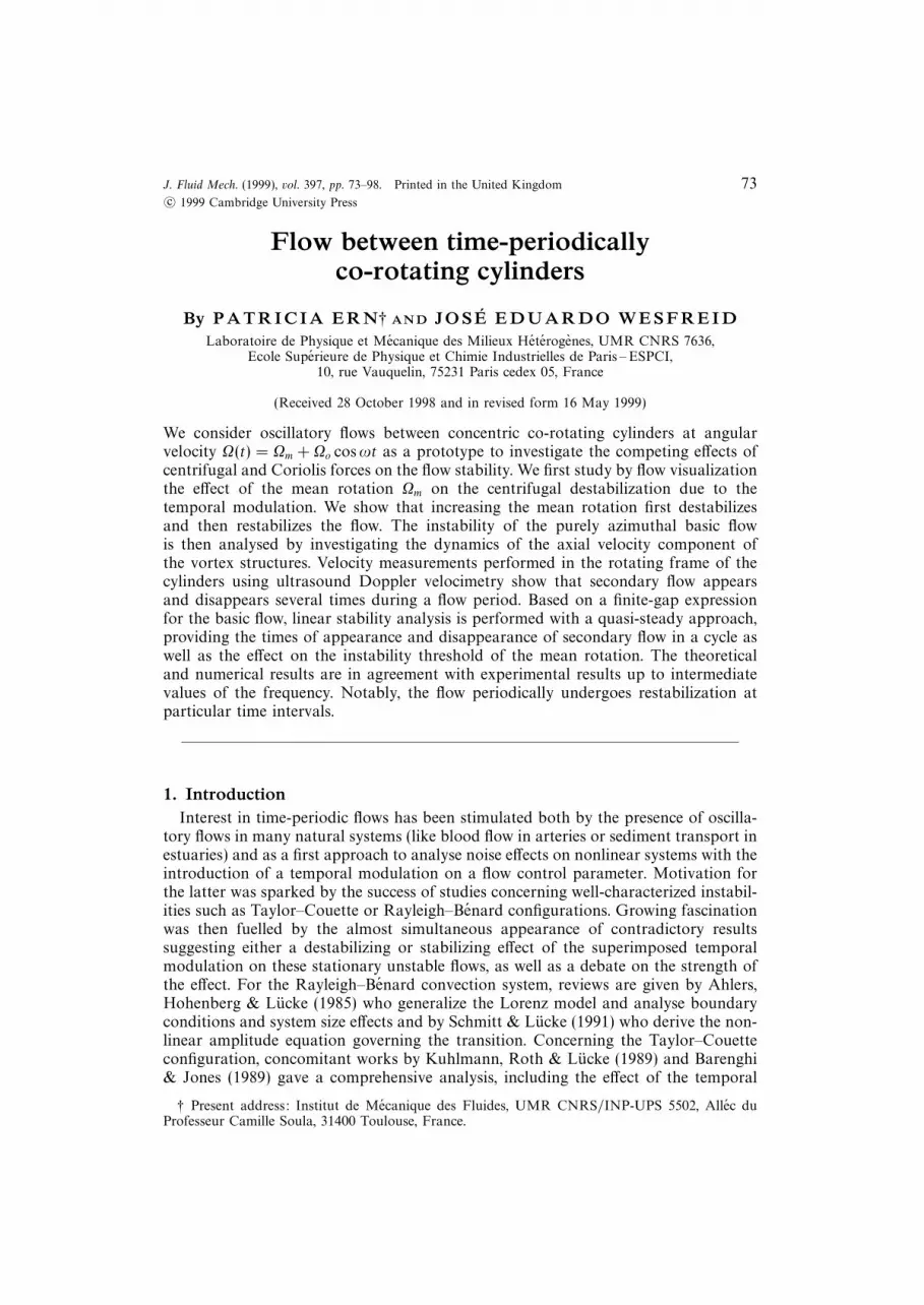
We consider oscillatory flows between concentric co-rotating cylinders at angularvelocity Ω(t) = Ωm + Ωo cosωt as a prototype to investigate the competing effects ofcentrifugal and Coriolis forces on the flow stability. We first study by flow visualizationthe effect of the mean rotation Ωm on the centrifugal destabilization due to thetemporal modulation. We show that increasing the mean rotation first destabilizesand then restabilizes the flow. The instability of the purely azimuthal basic flowis then analysed by investigating the dynamics of the axial velocity component ofthe vortex structures. Velocity measurements performed in the rotating frame of thecylinders using ultrasound Doppler velocimetry show that secondary flow appearsand disappears several times during a flow period. Based on a finite-gap expressionfor the basic flow, linear stability analysis is performed with a quasi-steady approach,providing the times of appearance and disappearance of secondary flow in a cycle aswell as the effect on the instability threshold of the mean rotation. The theoreticaland numerical results are in agreement with experimental results up to intermediatevalues of the frequency. Notably, the flow periodically undergoes restabilization atparticular time intervals.

1. IntroductionInterest in time-periodic flows has been stimulated both by the presence of oscilla-

tory flows in many natural systems (like blood flow in arteries or sediment transport inestuaries) and as a first approach to analyse noise effects on nonlinear systems with theintroduction of a temporal modulation on a flow control parameter. Motivation forthe latter was sparked by the success of studies concerning well-characterized instabil-ities such as Taylor–Couette or Rayleigh–Benard configurations. Growing fascinationwas then fuelled by the almost simultaneous appearance of contradictory resultssuggesting either a destabilizing or stabilizing effect of the superimposed temporalmodulation on these stationary unstable flows, as well as a debate on the strength ofthe effect. For the Rayleigh–Benard convection system, reviews are given by Ahlers,Hohenberg & Lucke (1985) who generalize the Lorenz model and analyse boundaryconditions and system size effects and by Schmitt & Lucke (1991) who derive the non-linear amplitude equation governing the transition. Concerning the Taylor–Couetteconfiguration, concomitant works by Kuhlmann, Roth & Lucke (1989) and Barenghi& Jones (1989) gave a comprehensive analysis, including the effect of the temporal

† Present address: Institut de Mecanique des Fluides, UMR CNRS/INP-UPS 5502, Allec duProfesseur Camille Soula, 31400 Toulouse, France.

74 P. Ern and J. E. Wesfreid

modulation on the onset of instability and the nonlinear behaviour of the instabilityrolls.

On the other hand, for purely oscillatory flow, there is no stationary unstableflow serving as a reference to quantify the modulation effect. Because of the non-separability of space and time variables, it is difficult to treat the instability analyticallyand the problem has to be solved numerically. The stability of oscillatory flows isrelated to the development and stability of Stokes layers at the boundaries. Theusual prototype of oscillatory flows is the plane Stokes layer (Davis 1976). In thepresent work, we are concerned with Stokes layers generated over curved walls,whose destabilization is induced by centrifugal effects (Seminara & Hall 1976, 1977;Papageorgiou 1987; Horseman, Bassom & Blennerhassett 1996). The instability thenappears as spatially periodic counter-rotating vortices aligned with the main flow, likeTaylor, Dean or Gortler vortices.

In this framework, it is interesting to come back to the Taylor–Couette configurationto study a flow where the destabilization is linked to the development of centrifugalStokes layers. We consider here the stability of the flow developing when both cylindersrotate jointly at the same angular velocity Ω(t) = Ωm + Ωo cosωt and for a range ofvalues of the mean velocity Ωm. Previous studies by flow visualization are those byAouidef et al. (1994) for Ωm = 0 and by Tennakoon et al. (1997) for one value of themean rotation Ωm and for counter-rotating cylinders for Ωm = 0. They also analysedtheir systems as the instability of the Stokes layer in the plane configuration. Inour study, we will consider the more realistic general case of Stokes layers includingcurvature effects. A first contribution of this paper is to present velocity measurementscharacterizing the temporal behaviour of this oscillatory flow. The instability of thepurely azimuthal basic flow is analysed by investigating the dynamics of the axialvelocity component of the vortex structures that appear and disappear during anoscillation cycle. Up to intermediate values of the forcing frequency, this behaviouris recovered with a quasi-steady finite-gap analysis even when mean rotation effectsare included.

Our second concern in this work is with the effect of rotation on centrifugalinstabilities, which is inferred here by the influence of the mean rotation term Ωmon the centrifugal destabilization due to the periodic rotation at Ωo cosωt. Interestin the problem of rotation–instability interaction stemmed from its occurrence ingeophysical (Tritton & Davies 1985) and industrial flows (such as Gortler flowaround rotating blades in turbines, see for instance Aouidef, Wesfreid & Mutabazi1992). A first step in the comprehension of these systems was given by the evidencethat the Coriolis force can generate instability in a stable flow, like in Poiseuilleflow (Alfredsson & Persson 1989). Further advances showed that rotation mightmodify turbulence (Bidokhti & Tritton 1992; Cambon et al. 1994) or instability,having either a stabilizing or destabilizing effect. For instance, destabilization may beobserved in the development of three-dimensional perturbations when rotation andflow vorticity vectors are parallel or anti-parallel, like in mixing layers or in boundarylayer flows. Other works have addressed the effect of rotation on Rayleigh–Benardconvection (Chandrasekhar 1981) or on a Taylor–Couette flow with the rotationaxis perpendicular to the cylinder axis (Wiener et al. 1990; Ning et al. 1991). Studiesconcerned specifically with the competing effects of Coriolis and centrifugal forces onflow stability have been reported for rotating Dean flow (Matsson & Alfredsson 1990,1994) or rotating Gortler flow (Zebib & Bottaro 1993; Pexieder 1996) showing thatdepending on its direction, the Coriolis force may inhibit or enhance the centrifugaldestabilization. In this paper, we investigate the effect of rotation on centrifugal Stokes

Flow between time-periodically co-rotating cylinders 75

layers. Moreover, in our experimental setup, thanks to its reduced size compared toa water channel in a rotating platform, this effect is explored over a large range offlow parameters.

The procedure adopted in the paper is the following. In § 2, we present the basicflow expression for a finite gap between the cylinders as well as the parameters ofthe system. Section 3 is devoted to the experimental setup and techniques. Flowvisualization results showing the effect of the mean rotation on flow stability areaddressed in § 4. Section 5 presents ultrasound Doppler velocimetry results concerningthe time behaviour of the vortex structure. Section 6 investigates the flow instabilityby means of a theoretical and numerical analysis.

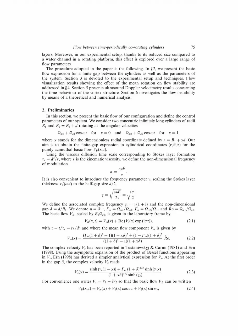
2. PreliminariesIn this section, we present the basic flow of our configuration and define the control

parameters of our system. We consider two concentric infinitely long cylinders of radiiR1 and R2 = R1 + d rotating at the angular velocities

Ωm1 + Ωo1 cosωt for x = 0 and Ωm2 + Ωo2 cosωt for x = 1,

where x stands for the dimensionless radial coordinate defined by r = R1 + xd. Ouraim is to obtain the finite-gap expression in cylindrical coordinates (r, θ, z) for thepurely azimuthal basic flow VB(x, t).

Using the viscous diffusion time scale corresponding to Stokes layer formationτν = d2/ν, where ν is the kinematic viscosity, we define the non-dimensional frequencyof modulation

σ =ωd2

ν.

It is also convenient to introduce the frequency parameter γ, scaling the Stokes layerthickness ν/(ωd) to the half-gap size d/2,

γ =

√ωd2

2ν=

√σ

2.

We define the associated complex frequency γc = γ(1 + i) and the non-dimensionalgap δ = d/R1. We denote µ = δ−1, Γm = Ωm2/Ωm1, Γo = Ωo2/Ωo1 and Ro = Ωm1/Ωo1.The basic flow VB , scaled by R1Ωo1, is given in the laboratory frame by

VB(x, t) = Vm(x) + Re (Vs(x) exp (iστ)), (2.1)

with τ = t/τν = tν/d2 and where the mean flow component Vm is given by

Vm(x) =(Γm(1 + δ)2 − 1)(1 + xδ)2 + (1− Γm)(1 + δ)2

((1 + δ)2 − 1)(1 + xδ)Ro. (2.2)

The complex velocity Vs has been reported in Tustaniwskyj & Carmi (1981) and Ern(1998). Using the asymptotic expansion of the product of Bessel functions appearingin Vs, Ern (1998) has derived a simpler analytical expression for Vs. At the first orderin the gap δ, the complex velocity Vs reads

Vs(x) =sinh (γc(1− x)) + Γo (1 + δ)3/2 sinh (γcx)

(1 + xδ)1/2 sinh (γc). (2.3)

For convenience one writes Vs = V1 − iV2 so that the basic flow VB can be written

VB(x, t) = Vm(x) + V1(x) cos στ+ V2(x) sin στ, (2.4)


with the following expressions for V1 and V2:

V1(x) =(A(x) + Γo (1 + δ)3/2C(x)) sinh γ cos γ + (B(x) + Γo(1 + δ)3/2D(x)) cosh γ sin γ

(1 + xδ)1/2(cosh2 γ − cos2 γ),

(2.5)

V2(x) =(A(x) + Γo (1 + δ)3/2C(x)) cosh γ sin γ − (B(x) + Γo(1 + δ)3/2D(x)) sinh γ cos γ

(1 + xδ)1/2(cosh2 γ − cos2 γ),

(2.6)where

A(x) = sinh (γ(1− x)) cos (γ(1− x)), B(x) = cosh (γ(1− x)) sin (γ(1− x)),

C(x) = sinh (γx) cos (γx) and D(x) = cosh (γx) sin (γx).

Expressions (2.5)–(2.6), valid at the first order in δ, will be termed the finite-gapapproximation. An estimate of the validity of this approximation is obtained whenthe second-order terms in δ can be neglected. Expressions (2.5)–(2.6) are valid as longas the condition (Ern 1998)

f(γ, δ) = δ2 3√

2γ2 − 2γ + 1

16γ2 1 (2.7)

holds. In our experimental configuration, the gap is δ = 0.112 so that we getf(γ, 0.112) 6 10−2 as long as γ > 0.41.

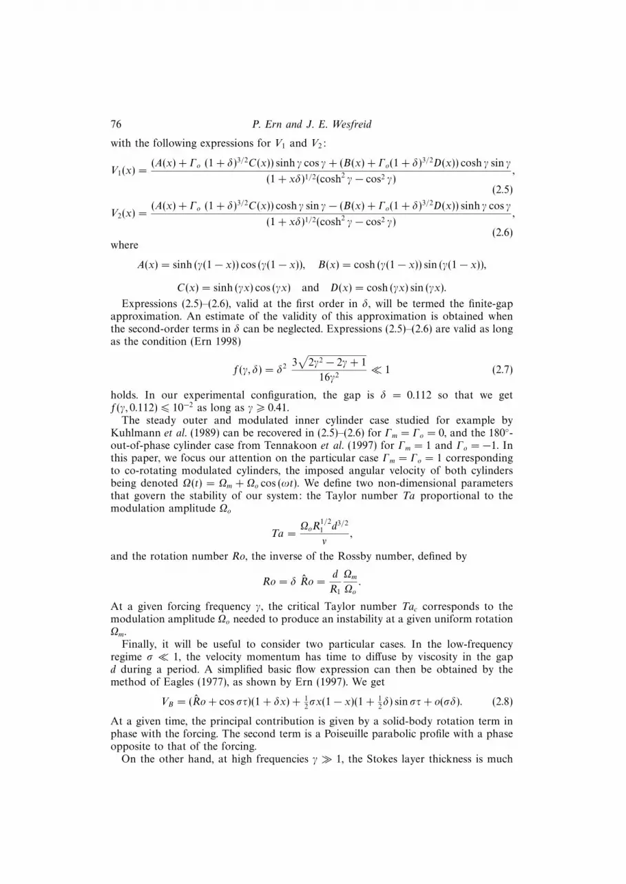
The steady outer and modulated inner cylinder case studied for example byKuhlmann et al. (1989) can be recovered in (2.5)–(2.6) for Γm = Γo = 0, and the 180-out-of-phase cylinder case from Tennakoon et al. (1997) for Γm = 1 and Γo = −1. Inthis paper, we focus our attention on the particular case Γm = Γo = 1 correspondingto co-rotating modulated cylinders, the imposed angular velocity of both cylindersbeing denoted Ω(t) = Ωm + Ωo cos (ωt). We define two non-dimensional parametersthat govern the stability of our system: the Taylor number Ta proportional to themodulation amplitude Ωo

Ta =ΩoR

1/21 d3/2

ν,

and the rotation number Ro, the inverse of the Rossby number, defined by

Ro = δ Ro =d

R1

Ωm

Ωo.

At a given forcing frequency γ, the critical Taylor number Tac corresponds to themodulation amplitude Ωo needed to produce an instability at a given uniform rotationΩm.

Finally, it will be useful to consider two particular cases. In the low-frequencyregime σ 1, the velocity momentum has time to diffuse by viscosity in the gapd during a period. A simplified basic flow expression can then be obtained by themethod of Eagles (1977), as shown by Ern (1997). We get

VB = (Ro+ cos στ)(1 + δx) + 12σx(1− x)(1 + 1

2δ) sin στ+ o(σδ). (2.8)

At a given time, the principal contribution is given by a solid-body rotation term inphase with the forcing. The second term is a Poiseuille parabolic profile with a phaseopposite to that of the forcing.

On the other hand, at high frequencies γ 1, the Stokes layer thickness is much


Servopack &function generator

Motor

Transducer

Displacement table

Instability rolls

Fluid

Rotation axis

BNC-SMC cables

Flexible joint

Faraday cagewith BNC head

Slip-ringcollectorUltrasound

Dopplervelocimeter

dL

Figure 1. Sketch of the experimental setup with ultrasound Doppler velocimetry. (Not to scale;L = 305 mm, d = 7.75 mm and inner cylinder radius Ri = 69.25 mm.)

smaller than the gap size d. The basic flow VB can then be written as

VB = Vm +e−γx

(1 + δx)1/2cos (γx− στ) + (1 + δ)3/2 e−γ(1−x)

(1 + δx)1/2cos (γ(1− x)− στ) (2.9)

and is the sum of two velocity profiles of Stokes layer type, with an amplitudedamped (amplified) spatially for the inner (outer) cylinder with respect to the planeconfiguration.

3. Experimental setup3.1. Apparatus

The experimental configuration is presented in figure 1. It consists of a Taylor–Couette cell of two concentric cylinders with gap d = 7.75 mm containing the fluid.The cylinders are closed by a top and bottom plate that rotate with the cylinders. Theheight of the cylinders is L = 305 mm so that the aspect ratio of the cell is L/d = 39and the central core of the fluid can be considered to be unaffected by end effects. Theinner cylinder of external radius Ri = 69.25 mm is made from black-anodized Duralin order to facilitate flow visualization. The external cylinder is made from Plexiglas,


with internal radius Ro = 77± 0.1 mm. The non-dimensional gap is δ = 0.112 and theradii of the cylinders have ratio 0.899.

The cylinders rotate jointly via a brushless servomotor Yaskawa USAREM 01-CE2K +MRC 300-1/20. A time-periodic signal is imposed on the motor by aHewlett Packard 33120A-15MHz function generator connected to a servopack CACR-SR01AC. Using the back signal from the motor tachometer to the servopack, we havechecked that the effective rotation of the motor and the cylinders corresponds to thesignal imposed by the function generator.

3.2. Flow detection techniques

3.2.1. Flow visualization

Flow visualization is performed using a de-ionized water solution with 2% Kalliro-scope rheoscopic concentrate AQ-1000 and 1% SQ-1000 bacterial stabilizer. Kalliro-scope flakes are a classical visualization tool for Taylor–Couette flows (Andereck,Liu & Swinney 1986), because of their properties of reflection and their tendency toalign along streamlines (Gauthier, Gondret & Rabaud 1998). At a given frequency γand mean rotation Ωm, the determination of the onset of instability is performed byincreasing the modulation amplitude Ωo by steps of 2.632×10−2 rad s−1 correspondingto a change in Taylor number of about 5 units. We wait for a sufficient period of timefor the flow to adapt to each new configuration. For instance, for γ = 1, we wait forten cycles T (about 15 min). As T = (π/γ2)τν where τν = d2/ν is the viscous diffusiontime, this interval is larger than 30 τν . We then examine the flow during five, or more,cycles to detect the instability.

By visualization, the instability appears as transient shadowed black and whitestreaks. As the amplitude Ωo of the forcing is increased, the instability appears moreclearly as pulsed Taylor–Couette rolls. We assume that in this system no long-termdevelopment of the instability is to be expected since the flow undergoes periodicrestabilization when the cylinders reverse their rotation, as will be described laterwith the velocity measurements. For this reason, we have also chosen to increasethe modulation amplitude when the forcing is decreasing in time and the flow isrestabilizing. In spite of its simplicity, eye observation is a very accurate detectiontool, far better than the observation obtained with a 256 grey levels CCD cameraor other systems as also indicated by Walsh (1988) in his experiment with a time-periodic inner cylinder rotation. Our determination of the instability threshold hasa reproductibility of 5%. Error in the Taylor number values, mainly due to thedetermination of the viscosity, is less than 3%.

3.2.2. Ultrasound Doppler velocimetry

Velocity measurements have been performed with a Signal Processing Dop 1000ultrasound Doppler velocimeter. In our case, this technique is particularly interestingas the reduced size of the transducer allows us to perform easily measurements in therotating frame of the cylinders. Moreover, the apparatus delivers a velocity profilequasi-instantaneously. We have measured the axial profile of the axial component ofthe velocity. This quantity is particularly relevant as it constitutes a direct indicationof the presence of the vortex structure and allows its characterization (see for instance,Ahlers et al. 1986; Heinrichs et al. 1988; Cooper et al. 1985; Kuhlmann et al. 1989and Takeda et al. 1993b).

As shown in figure 1, the measurements are performed in the rotating frame of thecylinders and transfered to the laboratory frame for analysis. On the top cover of thecylinders, and following their rotation, the ultrasound transducer is held vertically


on a micrometric displacement table which allows radial motion of the transducer.To avoid parasite reflections the transducer is directly in contact with the fluid. Thesignal is transfered to a slip-ring Litton Poly-Scientific AC 4023-12 protected in aFaraday cage. The cables of the slip-ring non-rotating part are connected to a BNChead located in the Faraday cage.

The operating principle of the ultrasound Doppler velocimeter has been givenby Willemetz (1990) and Takeda (1991). We used a transducer of 8 MHz emittingfrequency, shifting between an emission and reception state. The pulse repetitionfrequency fp was taken as small as possible (fp ≈ 488.3 Hz) in order to have thelowest possible velocity detection range (6 mm s−1). Data for a given time results fromaveraging the last six profiles. The induced acoustic field is composed of a cylindricalFresnel region of radius r = 2.5 mm which starts to expand conically at a distance of3 cm from the transducer with an angle of 2.9 for the Frauenhofer principal lobe. Ata given depth, the measured axial velocity is a mean over the section of this volume.Measurements are performed up to a distance of 9 cm from the transducer with anaxial resolution of 0.8 mm. For data analysis, we only considered the last 50 measuredspatial points, which correspond in depth to a distance from the transducer biggerthan 5 cm. This avoids the inclusion of the end effects of the cylinders. Dependingon the values of the parameters, 50 spatial points correspond to about 3 to 5 Taylorvortices. The working fluid is a de-ionized water solution with 30% by mass of glycerolseeded with 3 g l−1 of Griltex COPA 11P1 4104320/09 particles and containing 0.05%of Kalliroscope AQ-1000. Except for the mono-dispersity of the particles the samemixture was used in the Taylor–Couette experiments of Takeda, Fisher & Sakakibara(1993a). This mixture was found to be an appropriate ultrasound reflector whichallowed simultaneous flow visualization. Our particles have a maximum size of 80 µmand a density of 1.07 g cm−3. In this case, the error in the estimation of the Taylornumber is lower than 3.5%. For the velocity measurements, the noise level (orbackground signal) is estimated to be less than 0.15 mm s−1 thanks to the Faradaycage isolation.

4. Coriolis force effect: results by visualizationWhen Ωm = Ro = 0, the basic flow has no mean component and the instability is

generated by the phase lag of the flow with respect to its moving boundaries. Detailedlinear stability analysis of this flow has been carried out with Floquet calculations inthe small-gap approximation (δ → 0) and visualization experiments by Aouidef et al.(1994). Results showed that for all modulation frequencies γ, the flow is destabilized.Maximal destabilization (lower Tac(γ)) is achieved for intermediate frequencies γ ≈ 2,whereas the flow stability increases for lower and higher frequencies. The sametendency was observed for one value of the mean rotation (Ωm = 1.26 rad s−1)by Tennakoon et al. (1997). In this work, we are interested in the Coriolis forcecontribution to the flow instability. We thus study, at a given frequency, the amplitudeof the temporal modulation needed to destabilize different solid-body rotation flows.We investigate the behaviour of the threshold Tac as a function of the rotationnumber Ro for different frequencies γ.

4.1. Flow stability with mean rotation

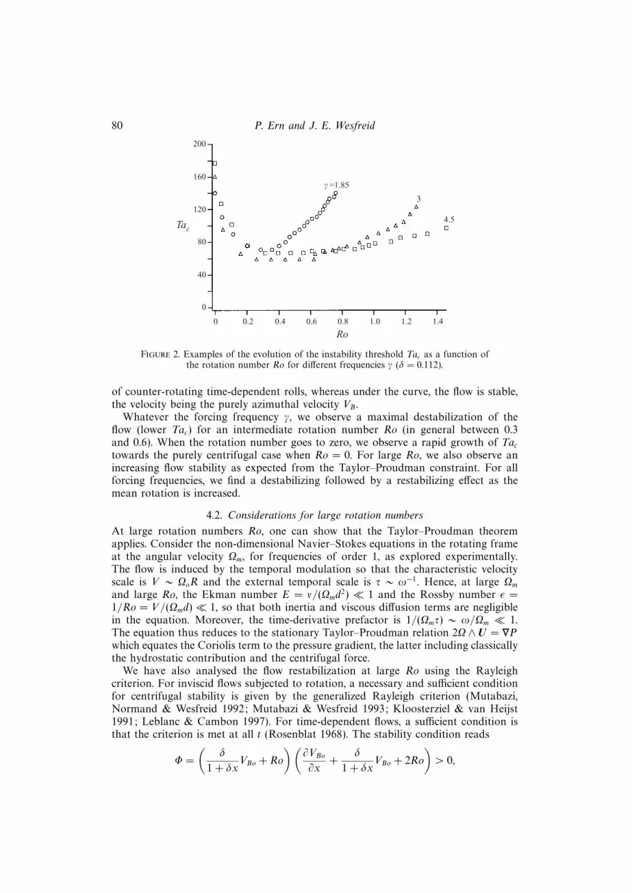
Figure 2 reports the evolution of the critical Taylor number Tac as a function of therotation number Ro for several frequencies γ. At a given frequency, the parameterregimes above the curve correspond to an unstable flow characterized by the presence


200

160

120

80

40

0

0 0.2 0.4 0.6 0.8 1.0 1.2 1.4

Ro

Tac

γ =1.85

3

4.5

Figure 2. Examples of the evolution of the instability threshold Tac as a function ofthe rotation number Ro for different frequencies γ (δ = 0.112).

of counter-rotating time-dependent rolls, whereas under the curve, the flow is stable,the velocity being the purely azimuthal velocity VB .

Whatever the forcing frequency γ, we observe a maximal destabilization of theflow (lower Tac) for an intermediate rotation number Ro (in general between 0.3and 0.6). When the rotation number goes to zero, we observe a rapid growth of Tactowards the purely centrifugal case when Ro = 0. For large Ro, we also observe anincreasing flow stability as expected from the Taylor–Proudman constraint. For allforcing frequencies, we find a destabilizing followed by a restabilizing effect as themean rotation is increased.

4.2. Considerations for large rotation numbers

At large rotation numbers Ro, one can show that the Taylor–Proudman theoremapplies. Consider the non-dimensional Navier–Stokes equations in the rotating frameat the angular velocity Ωm, for frequencies of order 1, as explored experimentally.The flow is induced by the temporal modulation so that the characteristic velocityscale is V ∼ ΩoR and the external temporal scale is τ ∼ ω−1. Hence, at large Ωmand large Ro, the Ekman number E = ν/(Ωmd

2) 1 and the Rossby number ε =1/Ro = V/(Ωmd) 1, so that both inertia and viscous diffusion terms are negligiblein the equation. Moreover, the time-derivative prefactor is 1/(Ωmτ) ∼ ω/Ωm 1.The equation thus reduces to the stationary Taylor–Proudman relation 2Ω ∧U = ∇Pwhich equates the Coriolis term to the pressure gradient, the latter including classicallythe hydrostatic contribution and the centrifugal force.

We have also analysed the flow restabilization at large Ro using the Rayleighcriterion. For inviscid flows subjected to rotation, a necessary and sufficient conditionfor centrifugal stability is given by the generalized Rayleigh criterion (Mutabazi,Normand & Wesfreid 1992; Mutabazi & Wesfreid 1993; Kloosterziel & van Heijst1991; Leblanc & Cambon 1997). For time-dependent flows, a sufficient condition isthat the criterion is met at all t (Rosenblat 1968). The stability condition reads

Φ =

(δ

1 + δxVBo + Ro

)(∂VBo

∂x+

δ

1 + δxVBo + 2Ro

)> 0,


10–1

γ

Ro

R lim

100

101

10–1 100 101

Slope 2

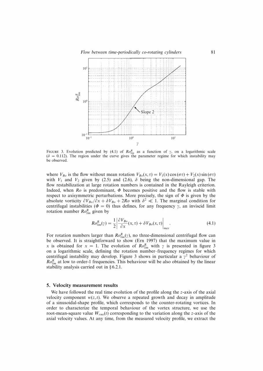
Figure 3. Evolution predicted by (4.1) of RoRlim as a function of γ, on a logarithmic scale(δ = 0.112). The region under the curve gives the parameter regime for which instability maybe observed.

where VBo is the flow without mean rotation VBo(x, τ) = V1(x) cos (στ) +V2(x) sin (στ)with V1 and V2 given by (2.5) and (2.6), δ being the non-dimensional gap. Theflow restabilization at large rotation numbers is contained in the Rayleigh criterion.Indeed, when Ro is predominant, Φ becomes positive and the flow is stable withrespect to axisymmetric perturbations. More precisely, the sign of Φ is given by theabsolute vorticity ∂VBo/∂x + δVBo + 2Ro with δ2 1. The marginal condition forcentrifugal instabilities (Φ = 0) thus defines, for any frequency γ, an inviscid limitrotation number RoRlim given by

RoRlim(γ) =1

2

∣∣∣∣∂VBo∂x(x, τ) + δVBo(x, τ)

∣∣∣∣max

. (4.1)

For rotation numbers larger than RoRlim(γ), no three-dimensional centrifugal flow canbe observed. It is straightforward to show (Ern 1997) that the maximum value inx is obtained for x = 1. The evolution of RoRlim with γ is presented in figure 3on a logarithmic scale, defining the rotation number–frequency regimes for whichcentrifugal instability may develop. Figure 3 shows in particular a γ2 behaviour ofRoRlim at low to order-1 frequencies. This behaviour will be also obtained by the linearstability analysis carried out in § 6.2.1.

5. Velocity measurement resultsWe have followed the real time evolution of the profile along the z-axis of the axial

velocity component w(z, t). We observe a repeated growth and decay in amplitudeof a sinusoidal-shape profile, which corresponds to the counter-rotating vortices. Inorder to characterize the temporal behaviour of the vortex structure, we use theroot-mean-square value Wrms(t) corresponding to the variation along the z-axis of theaxial velocity values. At any time, from the measured velocity profile, we extract the


t

Wrm

s (mm

s–1

)

1.5

0.2

1.0

0.5

0 0.4 0.6 0.8 1.0

Ta = 300

t

3

0.2

2

1

0 0.4 0.6 0.8 1.0

Ta = 600

Wrm

s (mm

s–1

)

0.25

0.2

0.20

0.15

0 0.4 0.6 0.8 1.0

Ta = 2602.5

0.2

2.0

1.5

0 0.4 0.6 0.8 1.0

Ta = 400

1.0

0.5

0.10

0.05

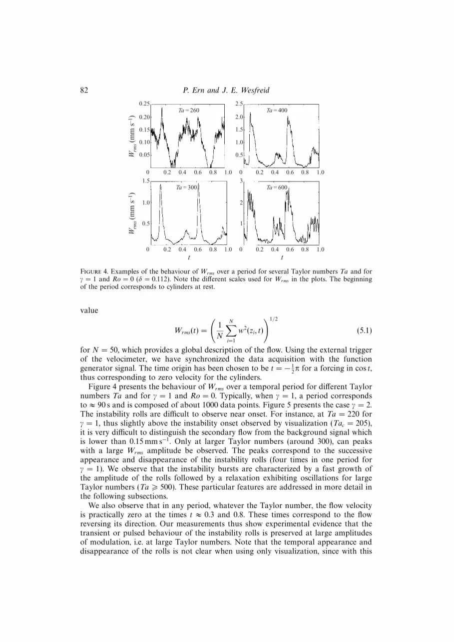
Figure 4. Examples of the behaviour of Wrms over a period for several Taylor numbers Ta and forγ = 1 and Ro = 0 (δ = 0.112). Note the different scales used for Wrms in the plots. The beginningof the period corresponds to cylinders at rest.

value

Wrms(t) =

(1

N

N∑i=1

w2(zi, t)

)1/2

(5.1)

for N = 50, which provides a global description of the flow. Using the external triggerof the velocimeter, we have synchronized the data acquisition with the functiongenerator signal. The time origin has been chosen to be t = − 1

2π for a forcing in cos t,

thus corresponding to zero velocity for the cylinders.Figure 4 presents the behaviour of Wrms over a temporal period for different Taylor

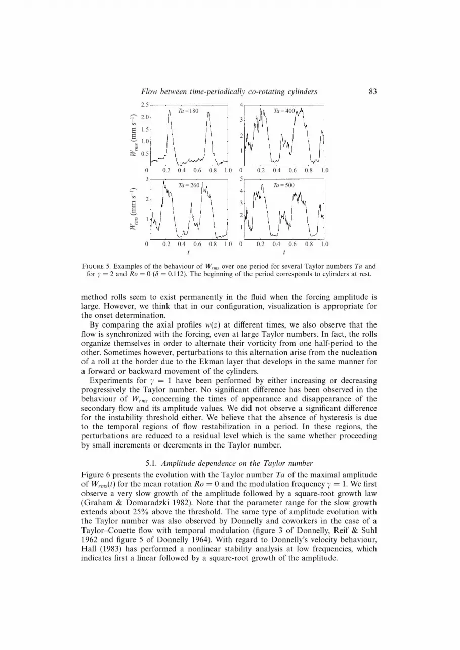
numbers Ta and for γ = 1 and Ro = 0. Typically, when γ = 1, a period correspondsto ≈ 90 s and is composed of about 1000 data points. Figure 5 presents the case γ = 2.The instability rolls are difficult to observe near onset. For instance, at Ta = 220 forγ = 1, thus slightly above the instability onset observed by visualization (Tac = 205),it is very difficult to distinguish the secondary flow from the background signal whichis lower than 0.15 mm s−1. Only at larger Taylor numbers (around 300), can peakswith a large Wrms amplitude be observed. The peaks correspond to the successiveappearance and disappearance of the instability rolls (four times in one period forγ = 1). We observe that the instability bursts are characterized by a fast growth ofthe amplitude of the rolls followed by a relaxation exhibiting oscillations for largeTaylor numbers (Ta > 500). These particular features are addressed in more detail inthe following subsections.

We also observe that in any period, whatever the Taylor number, the flow velocityis practically zero at the times t ≈ 0.3 and 0.8. These times correspond to the flowreversing its direction. Our measurements thus show experimental evidence that thetransient or pulsed behaviour of the instability rolls is preserved at large amplitudesof modulation, i.e. at large Taylor numbers. Note that the temporal appearance anddisappearance of the rolls is not clear when using only visualization, since with this


t

Wrm

s (mm

s–1

)

3

0.2

2

1

0 0.4 0.6 0.8 1.0

Ta = 260

t

5

0.2

4

3

0 0.4 0.6 0.8 1.0

Ta = 500

Wrm

s (mm

s–1

)

2.5

0.2

2.0

1.5

0 0.4 0.6 0.8 1.0

Ta =1804

0.2

3

0 0.4 0.6 0.8 1.0

Ta = 400

2

1

1.0

0.5

2

1

Figure 5. Examples of the behaviour of Wrms over one period for several Taylor numbers Ta andfor γ = 2 and Ro = 0 (δ = 0.112). The beginning of the period corresponds to cylinders at rest.

method rolls seem to exist permanently in the fluid when the forcing amplitude islarge. However, we think that in our configuration, visualization is appropriate forthe onset determination.

By comparing the axial profiles w(z) at different times, we also observe that theflow is synchronized with the forcing, even at large Taylor numbers. In fact, the rollsorganize themselves in order to alternate their vorticity from one half-period to theother. Sometimes however, perturbations to this alternation arise from the nucleationof a roll at the border due to the Ekman layer that develops in the same manner fora forward or backward movement of the cylinders.

Experiments for γ = 1 have been performed by either increasing or decreasingprogressively the Taylor number. No significant difference has been observed in thebehaviour of Wrms concerning the times of appearance and disappearance of thesecondary flow and its amplitude values. We did not observe a significant differencefor the instability threshold either. We believe that the absence of hysteresis is dueto the temporal regions of flow restabilization in a period. In these regions, theperturbations are reduced to a residual level which is the same whether proceedingby small increments or decrements in the Taylor number.

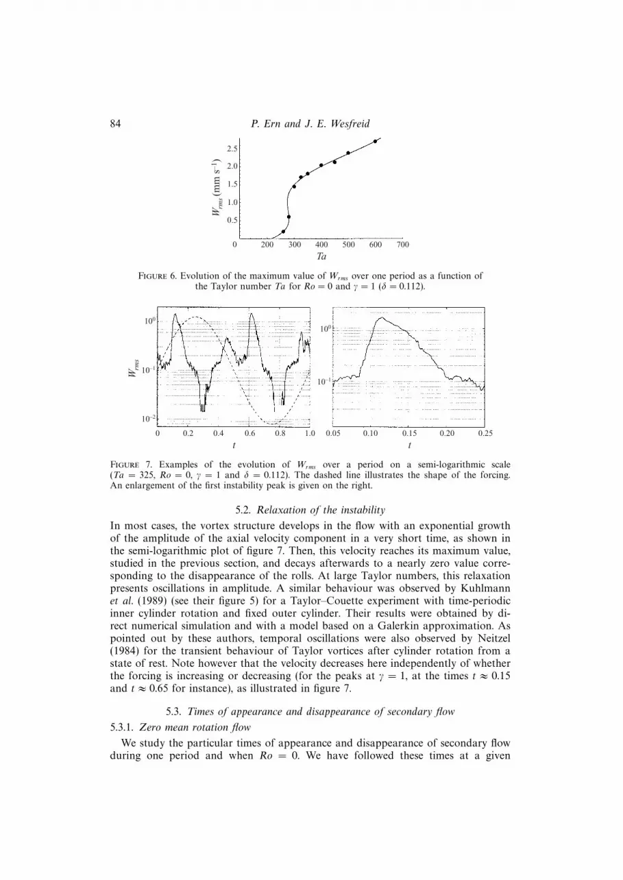
5.1. Amplitude dependence on the Taylor number

Figure 6 presents the evolution with the Taylor number Ta of the maximal amplitudeof Wrms(t) for the mean rotation Ro = 0 and the modulation frequency γ = 1. We firstobserve a very slow growth of the amplitude followed by a square-root growth law(Graham & Domaradzki 1982). Note that the parameter range for the slow growthextends about 25% above the threshold. The same type of amplitude evolution withthe Taylor number was also observed by Donnelly and coworkers in the case of aTaylor–Couette flow with temporal modulation (figure 3 of Donnelly, Reif & Suhl1962 and figure 5 of Donnelly 1964). With regard to Donnelly’s velocity behaviour,Hall (1983) has performed a nonlinear stability analysis at low frequencies, whichindicates first a linear followed by a square-root growth of the amplitude.


Ta

Wrm

s (mm

s–1

)

2.5

200

1.0

0.5

0 300 400 500 600 700

2.0

1.5

Figure 6. Evolution of the maximum value of Wrms over one period as a function ofthe Taylor number Ta for Ro = 0 and γ = 1 (δ = 0.112).

t

Wrm

s

100

0 0.2 0.4 0.6 0.8 1.0

10–1

10–2

t

100

0.05 0.10 0.15 0.20 0.25

10–1

Figure 7. Examples of the evolution of Wrms over a period on a semi-logarithmic scale(Ta = 325, Ro = 0, γ = 1 and δ = 0.112). The dashed line illustrates the shape of the forcing.An enlargement of the first instability peak is given on the right.

5.2. Relaxation of the instability

In most cases, the vortex structure develops in the flow with an exponential growthof the amplitude of the axial velocity component in a very short time, as shown inthe semi-logarithmic plot of figure 7. Then, this velocity reaches its maximum value,studied in the previous section, and decays afterwards to a nearly zero value corre-sponding to the disappearance of the rolls. At large Taylor numbers, this relaxationpresents oscillations in amplitude. A similar behaviour was observed by Kuhlmannet al. (1989) (see their figure 5) for a Taylor–Couette experiment with time-periodicinner cylinder rotation and fixed outer cylinder. Their results were obtained by di-rect numerical simulation and with a model based on a Galerkin approximation. Aspointed out by these authors, temporal oscillations were also observed by Neitzel(1984) for the transient behaviour of Taylor vortices after cylinder rotation from astate of rest. Note however that the velocity decreases here independently of whetherthe forcing is increasing or decreasing (for the peaks at γ = 1, at the times t ≈ 0.15and t ≈ 0.65 for instance), as illustrated in figure 7.

5.3. Times of appearance and disappearance of secondary flow

5.3.1. Zero mean rotation flow

We study the particular times of appearance and disappearance of secondary flowduring one period and when Ro = 0. We have followed these times at a given


t

Wrm

s (nm

s–1

)

0 0.2 0.4 0.6 0.8 1.0

1.2

0.8

0.2

Ro = 0.05

t0 0.2 0.4 0.6 0.8 1.0

0.5

0.4

0.3

Ro = 0.2

0.2

0.1

Wrm

s (nm

s–1

)

0 0.2 0.4 0.6 0.8 1.0

1.2

0.8

0.4

Ro = 0.15

0 0.2 0.4 0.6 0.8 1.0

1.2

0.8

Ro = 0.15

0.4

Wrm

s (nm

s–1

)

0 0.2 0.4 0.6 0.8 1.0

0.6

0.4

0.2

Ro = 0

0 0.2 0.4 0.6 0.8 1.0

1.2Ro = 0.1

0.8

0.4

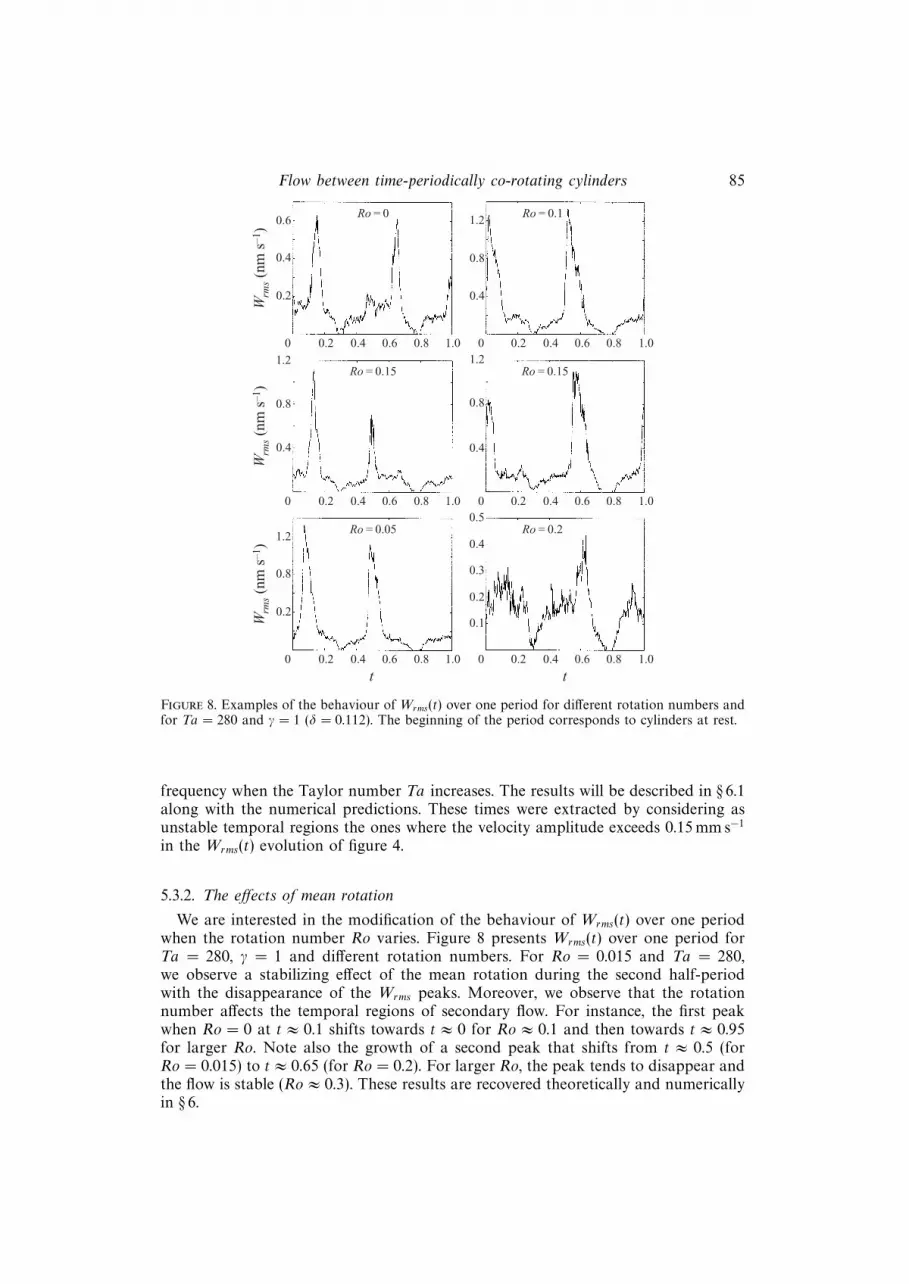
Figure 8. Examples of the behaviour of Wrms(t) over one period for different rotation numbers andfor Ta = 280 and γ = 1 (δ = 0.112). The beginning of the period corresponds to cylinders at rest.

frequency when the Taylor number Ta increases. The results will be described in § 6.1along with the numerical predictions. These times were extracted by considering asunstable temporal regions the ones where the velocity amplitude exceeds 0.15 mm s−1

in the Wrms(t) evolution of figure 4.

5.3.2. The effects of mean rotation

We are interested in the modification of the behaviour of Wrms(t) over one periodwhen the rotation number Ro varies. Figure 8 presents Wrms(t) over one period forTa = 280, γ = 1 and different rotation numbers. For Ro = 0.015 and Ta = 280,we observe a stabilizing effect of the mean rotation during the second half-periodwith the disappearance of the Wrms peaks. Moreover, we observe that the rotationnumber affects the temporal regions of secondary flow. For instance, the first peakwhen Ro = 0 at t ≈ 0.1 shifts towards t ≈ 0 for Ro ≈ 0.1 and then towards t ≈ 0.95for larger Ro. Note also the growth of a second peak that shifts from t ≈ 0.5 (forRo = 0.015) to t ≈ 0.65 (for Ro = 0.2). For larger Ro, the peak tends to disappear andthe flow is stable (Ro ≈ 0.3). These results are recovered theoretically and numericallyin § 6.


6. Theoretical analysisThe pulse-like behaviour of secondary flow observed experimentally in § 5 (see, for

instance, figure 4) induced us to consider the linear stability analysis of the flow usinga quasi-steady approach. This approach is valid as long as the rate of change ofthe flow is small compared to the growth rate of the perturbations. The sharp Wrms

peaks observed experimentally correspond to a fast growth of the instability withrespect to the flow period. Some previous theoretical studies dealt with the validity ofthe quasi-steady stability approach at low frequencies for time-dependent centrifugalflows. In particular, Seminara & Hall (1975) used a momentary stability criterion andcalculated that the correction due to the slow time evolution of the perturbations isweak. Hall (1983) studied the nonlinear stability of slowly varying time-dependentviscous flows. He showed that, in most cases, quasi-steady analysis leads to the correctform of the solution except in the neighbourhood of the bifurcation point.

The quasi-steady stability of our system is analysed in the following two ways. In§ 6.1, the linearized Navier–Stokes perturbation equations are recast as a first-orderdifferential system with six unknowns, which is solved numerically at any given timewith the corresponding velocity profile of the basic flow. In § 6.2, using the Navier–Stokes perturbation equations cast as a fourth-order differential system with twounknowns, we study analytically the dynamical similarity of our configuration toother systems in order to understand the instability development.

For convenience, we rescale the time by t→ (2π/ω)(t− 14) so that in the following

t = 0 corresponds to cylinders at rest.

6.1. Numerical calculations

We denote the dimensional velocity by

U = R1 Ωo (0, VB, 0) + (u, v, w),

and consider the velocity and pressure perturbations in the form

(u, v, w) = R1 Ωo ei(αt+mθ+λz) (u, v, w),

p =ρνΩo

δei(αt+mθ+λz) π(x),

(6.1)

with ρ being the density. Upon introducing the operators

D =∂

∂x, D∗ =

∂

∂x+ ξ(x) with ξ(x) =

δ

1 + xδ,

and q = λd, s = αd2/ν, X = D∗u(x) − π(x), the velocity perturbations are shown tobe the solution of the following first-order differential system:

D∗u = −imξv − iqw,

D∗v = Y ,

Dw = Z,

DX = M(x)u+ 2(imξ2 − ξVBTa δ−1/2)v,

DY = (M(x) + m2ξ2)v − 2(imξ2 − 12D∗VBTa δ−1/2)u− imξX + mqξw,

D∗Z = (M(x) + q2)w − iqX + mqξv,

(6.2)


t

Ta

0 0.2 0.4 0.6 0.8 1.0

600

400

200

Ro = 0.05

800

1000

t0 0.2 0.4 0.6 0.8 1.0

600

400

300

Ro = 0.3800

700

500

0 0.2 0.4 0.6 0.8 1.0

400

Ro = 0.03

800

1200

0 0.2 0.4 0.6 0.8 1.0

600

400

300

Ro = 0.2700

500

0 0.2 0.4 0.6 0.8 1.0

600

400

200

Ro = 0

800

1000

0 0.2 0.4 0.6 0.8 1.0

1000

Ro = 0.11500

500

Ta

Ta

200

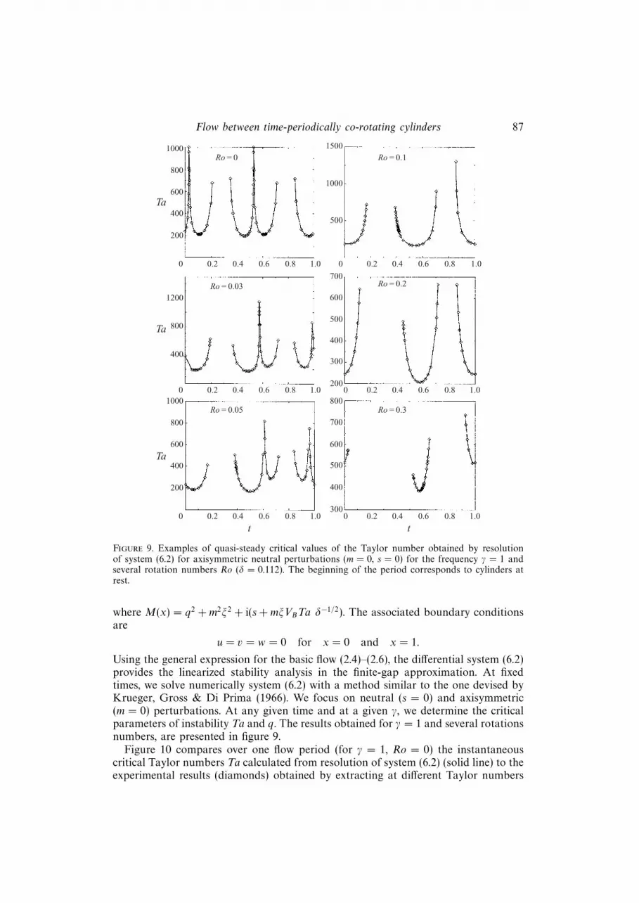
Figure 9. Examples of quasi-steady critical values of the Taylor number obtained by resolutionof system (6.2) for axisymmetric neutral perturbations (m = 0, s = 0) for the frequency γ = 1 andseveral rotation numbers Ro (δ = 0.112). The beginning of the period corresponds to cylinders atrest.

where M(x) = q2 + m2ξ2 + i(s+ mξVBTa δ−1/2). The associated boundary conditionsare

u = v = w = 0 for x = 0 and x = 1.

Using the general expression for the basic flow (2.4)–(2.6), the differential system (6.2)provides the linearized stability analysis in the finite-gap approximation. At fixedtimes, we solve numerically system (6.2) with a method similar to the one devised byKrueger, Gross & Di Prima (1966). We focus on neutral (s = 0) and axisymmetric(m = 0) perturbations. At any given time and at a given γ, we determine the criticalparameters of instability Ta and q. The results obtained for γ = 1 and several rotationsnumbers, are presented in figure 9.

Figure 10 compares over one flow period (for γ = 1, Ro = 0) the instantaneouscritical Taylor numbers Ta calculated from resolution of system (6.2) (solid line) to theexperimental results (diamonds) obtained by extracting at different Taylor numbers


t

Ta

0 0.2 0.4 0.6 0.8 1.0

600

400

200

800

1000

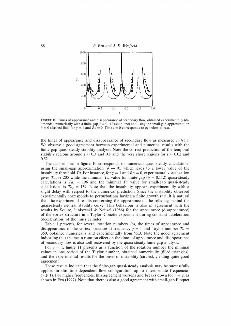
Figure 10. Times of appearance and disappearance of secondary flow, obtained experimentally (di-amonds), numerically with a finite gap δ = 0.112 (solid line) and using the small-gap approximationδ = 0 (dashed line) for γ = 1 and Ro = 0. Time t = 0 corresponds to cylinders at rest.

the times of appearance and disappearance of secondary flow as measured in § 5.3.We observe a good agreement between experimental and numerical results with thefinite-gap quasi-steady stability analysis. Note the correct prediction of the temporalstability regions around t ≈ 0.3 and 0.8 and the very short regions for t ≈ 0.02 and0.52.

The dashed line in figure 10 corresponds to numerical quasi-steady calculationsusing the small-gap approximation (δ → 0), which leads to a lower value of theinstability threshold Ta. For instance, for γ = 1 and Ro = 0, experimental visualizationgives Tac ≈ 205 while the minimal Ta value for finite-gap (δ = 0.112) quasi-steadycalculations is Tac = 196 and the minimal Ta value for small-gap quasi-steadycalculations is Tac = 139. Note that the instability appears experimentally with aslight delay with respect to the numerical prediction. Since the instability observedexperimentally corresponds to perturbations having a finite growth rate, it is naturalthat the experimental results concerning the appearance of the rolls lag behind thequasi-steady neutral stability curve. This behaviour is also in agreement with theresults by Squire, Jankowski & Neitzel (1986) for the appearance (disappearance)of the vortex structure in a Taylor–Couette experiment during constant acceleration(deceleration) of the inner cylinder.

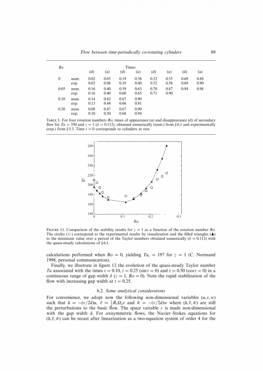
Table 1 presents, for several rotation numbers Ro, the times of appearance anddisappearance of the vortex structure at frequency γ = 1 and Taylor number Ta =350, obtained numerically and experimentally from § 5.3. Note the good agreementindicating that the mean rotation effect on the times of appearance and disappearanceof secondary flow is also well recovered by the quasi-steady finite-gap analysis.

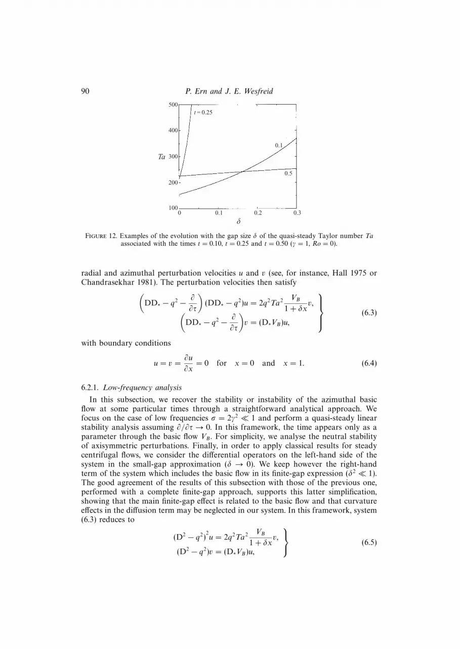
For γ = 1, figure 11 presents as a function of the rotation number the minimalvalues in one period of the Taylor number, obtained numerically (filled triangles),and the experimental results for the onset of instability (circles), yielding quite goodagreement.

These results indicate that the finite-gap quasi-steady analysis may be successfullyapplied in this time-dependent flow configuration up to intermediate frequencies(γ . 1). For higher frequencies, this agreement worsens and breaks down for γ ≈ 2, asshown in Ern (1997). Note that there is also a good agreement with small-gap Floquet


Ro Times(d) (a) (d) (a) (d) (a) (d) (a)

0 num. 0.02 0.05 0.19 0.38 0.52 0.55 0.69 0.88exp. 0.02 0.06 0.19 0.40 0.52 0.56 0.69 0.90

0.05 num. 0.16 0.40 0.59 0.63 0.70 0.87 0.94 0.98exp. 0.16 0.40 0.60 0.65 0.71 0.90

0.10 num. 0.14 0.42 0.67 0.90exp. 0.13 0.44 0.66 0.91

0.20 num. 0.08 0.47 0.67 0.90exp. 0.10 0.50 0.68 0.94

Table 1. For four rotation numbers Ro, times of appearance (a) and disappearance (d) of secondaryflow for Ta = 350 and γ = 1 (δ = 0.112), obtained numerically (num.) from § 6.1 and experimentally(exp.) from § 5.3. Time t = 0 corresponds to cylinders at rest.

Ro

Ta

0 0.1 0.2 0.3

240

180

160

260

280

220

140

200

Figure 11. Comparison of the stability results for γ = 1 as a function of the rotation number Ro.The circles ( d) correspond to the experimental results by visualization and the filled triangles (N)to the minimum value over a period of the Taylor numbers obtained numerically (δ = 0.112) withthe quasi-steady calculations of § 6.1.

calculations performed when Ro = 0, yielding Tac = 197 for γ = 1 (C. Normand1998, personal communication).

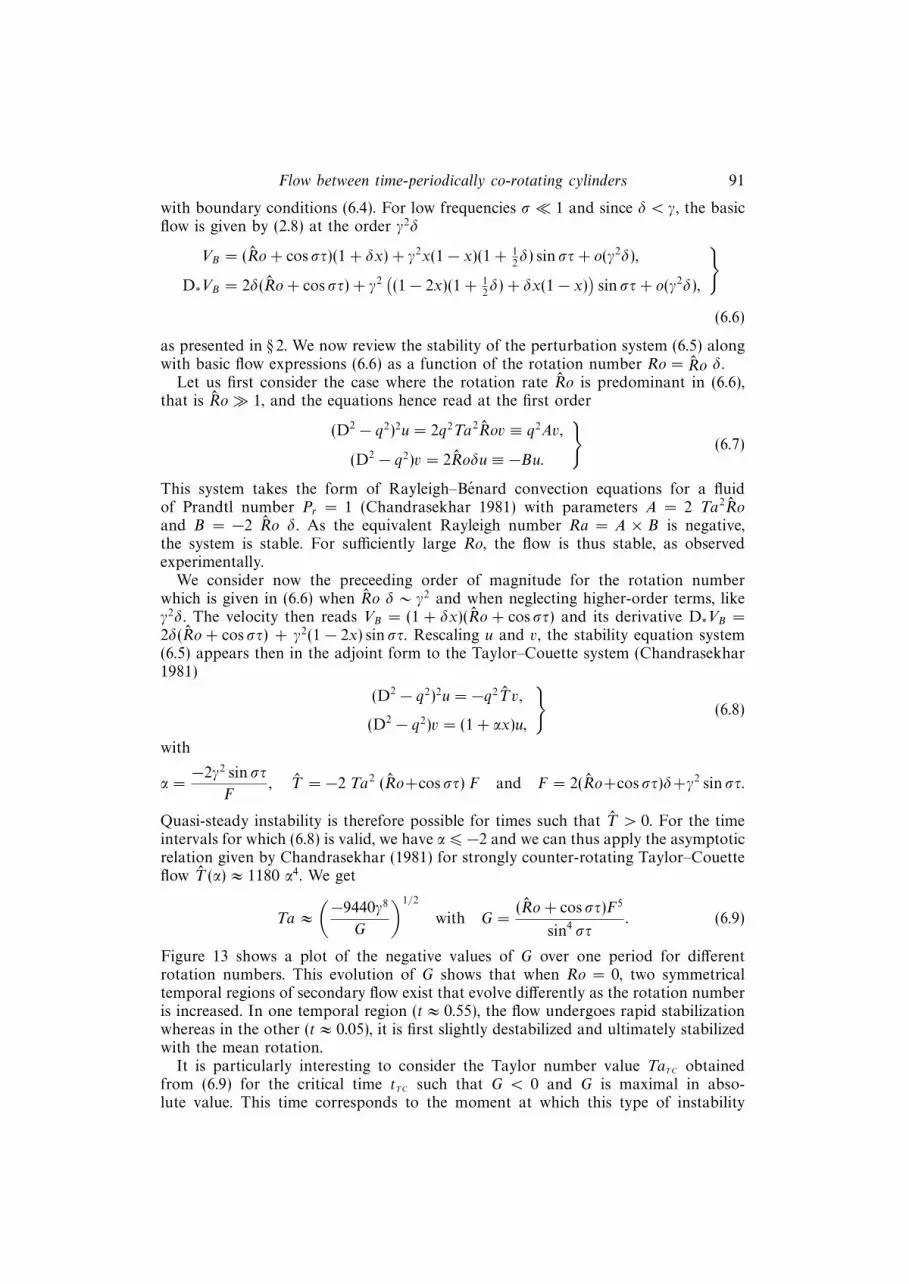
Finally, we illustrate in figure 12 the evolution of the quasi-steady Taylor numberTa associated with the times t = 0.10, t = 0.25 (sin t = 0) and t = 0.50 (cos t = 0) in acontinuous range of gap width δ (γ = 1, Ro = 0). Note the rapid stabilization of theflow with increasing gap width at t = 0.25.

6.2. Some analytical considerations

For convenience, we adopt now the following non-dimensional variables (u, v, w)such that u = −(ν/2d)u, v = 1

2R1Ωov and w = −(ν/2d)w where (u, v, w) are still

the perturbations to the basic flow. The space variable z is made non-dimensionalwith the gap width d. For axisymmetric flows, the Navier–Stokes equations for(u, v, w) can be recast after linearization as a two-equation system of order 4 for the


δ

Ta

0 0.1 0.2 0.3

200

100

300

400

500t = 0.25

0.1

0.5

Figure 12. Examples of the evolution with the gap size δ of the quasi-steady Taylor number Taassociated with the times t = 0.10, t = 0.25 and t = 0.50 (γ = 1, Ro = 0).

radial and azimuthal perturbation velocities u and v (see, for instance, Hall 1975 orChandrasekhar 1981). The perturbation velocities then satisfy(

DD∗ − q2 − ∂

∂τ

)(DD∗ − q2)u = 2q2Ta2 VB

1 + δxv,(

DD∗ − q2 − ∂

∂τ

)v = (D∗VB)u,

(6.3)

with boundary conditions

u = v =∂u

∂x= 0 for x = 0 and x = 1. (6.4)

6.2.1. Low-frequency analysis

In this subsection, we recover the stability or instability of the azimuthal basicflow at some particular times through a straightforward analytical approach. Wefocus on the case of low frequencies σ = 2γ2 1 and perform a quasi-steady linearstability analysis assuming ∂/∂τ → 0. In this framework, the time appears only as aparameter through the basic flow VB . For simplicity, we analyse the neutral stabilityof axisymmetric perturbations. Finally, in order to apply classical results for steadycentrifugal flows, we consider the differential operators on the left-hand side of thesystem in the small-gap approximation (δ → 0). We keep however the right-handterm of the system which includes the basic flow in its finite-gap expression (δ2 1).The good agreement of the results of this subsection with those of the previous one,performed with a complete finite-gap approach, supports this latter simplification,showing that the main finite-gap effect is related to the basic flow and that curvatureeffects in the diffusion term may be neglected in our system. In this framework, system(6.3) reduces to

(D2 − q2)2u = 2q2Ta2 VB

1 + δxv,

(D2 − q2)v = (D∗VB)u,

(6.5)


with boundary conditions (6.4). For low frequencies σ 1 and since δ < γ, the basicflow is given by (2.8) at the order γ2δ

VB = (Ro+ cos στ)(1 + δx) + γ2x(1− x)(1 + 12δ) sin στ+ o(γ2δ),

D∗VB = 2δ(Ro+ cos στ) + γ2((1− 2x)(1 + 1

2δ) + δx(1− x)

)sin στ+ o(γ2δ),

(6.6)

as presented in § 2. We now review the stability of the perturbation system (6.5) alongwith basic flow expressions (6.6) as a function of the rotation number Ro = Ro δ.

Let us first consider the case where the rotation rate Ro is predominant in (6.6),that is Ro 1, and the equations hence read at the first order

(D2 − q2)2u = 2q2Ta2Rov ≡ q2Av,

(D2 − q2)v = 2Roδu ≡ −Bu.

(6.7)

This system takes the form of Rayleigh–Benard convection equations for a fluidof Prandtl number Pr = 1 (Chandrasekhar 1981) with parameters A = 2 Ta2Roand B = −2 Ro δ. As the equivalent Rayleigh number Ra = A × B is negative,the system is stable. For sufficiently large Ro, the flow is thus stable, as observedexperimentally.

We consider now the preceeding order of magnitude for the rotation numberwhich is given in (6.6) when Ro δ ∼ γ2 and when neglecting higher-order terms, likeγ2δ. The velocity then reads VB = (1 + δx)(Ro + cos στ) and its derivative D∗VB =2δ(Ro + cos στ) + γ2(1 − 2x) sin στ. Rescaling u and v, the stability equation system(6.5) appears then in the adjoint form to the Taylor–Couette system (Chandrasekhar1981)

(D2 − q2)2u = −q2T v,

(D2 − q2)v = (1 + αx)u,

(6.8)

with

α =−2γ2 sin στ

F, T = −2 Ta2 (Ro+cos στ) F and F = 2(Ro+cos στ)δ+γ2 sin στ.

Quasi-steady instability is therefore possible for times such that T > 0. For the timeintervals for which (6.8) is valid, we have α 6 −2 and we can thus apply the asymptoticrelation given by Chandrasekhar (1981) for strongly counter-rotating Taylor–Couetteflow T (α) ≈ 1180 α4. We get

Ta ≈(−9440γ8

G

)1/2

with G =(Ro+ cos στ)F5

sin4 στ. (6.9)

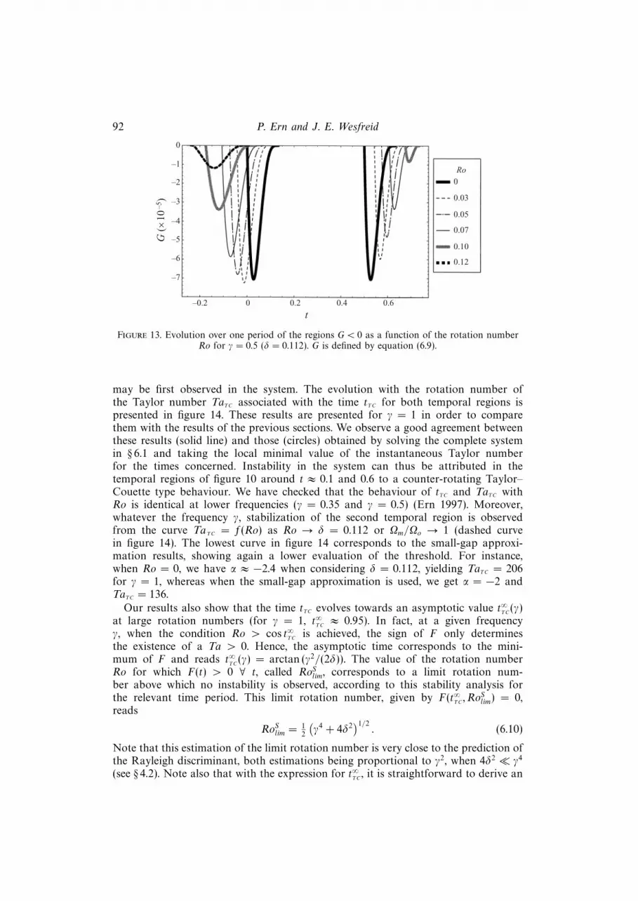
Figure 13 shows a plot of the negative values of G over one period for differentrotation numbers. This evolution of G shows that when Ro = 0, two symmetricaltemporal regions of secondary flow exist that evolve differently as the rotation numberis increased. In one temporal region (t ≈ 0.55), the flow undergoes rapid stabilizationwhereas in the other (t ≈ 0.05), it is first slightly destabilized and ultimately stabilizedwith the mean rotation.

It is particularly interesting to consider the Taylor number value TaTC obtainedfrom (6.9) for the critical time tTC such that G < 0 and G is maximal in abso-lute value. This time corresponds to the moment at which this type of instability


t

G (

×10

–5)

–0.2 0 0.2 0.4

–5

–2

–1

0

–3

–4

–6

–7

0.6

0

0.03

0.05

0.07

0.10

0.12

Ro

Figure 13. Evolution over one period of the regions G < 0 as a function of the rotation numberRo for γ = 0.5 (δ = 0.112). G is defined by equation (6.9).

may be first observed in the system. The evolution with the rotation number ofthe Taylor number TaTC associated with the time tTC for both temporal regions ispresented in figure 14. These results are presented for γ = 1 in order to comparethem with the results of the previous sections. We observe a good agreement betweenthese results (solid line) and those (circles) obtained by solving the complete systemin § 6.1 and taking the local minimal value of the instantaneous Taylor numberfor the times concerned. Instability in the system can thus be attributed in thetemporal regions of figure 10 around t ≈ 0.1 and 0.6 to a counter-rotating Taylor–Couette type behaviour. We have checked that the behaviour of tTC and TaTC withRo is identical at lower frequencies (γ = 0.35 and γ = 0.5) (Ern 1997). Moreover,whatever the frequency γ, stabilization of the second temporal region is observedfrom the curve TaTC = f(Ro) as Ro → δ = 0.112 or Ωm/Ωo → 1 (dashed curvein figure 14). The lowest curve in figure 14 corresponds to the small-gap approxi-mation results, showing again a lower evaluation of the threshold. For instance,when Ro = 0, we have α ≈ −2.4 when considering δ = 0.112, yielding TaTC = 206for γ = 1, whereas when the small-gap approximation is used, we get α = −2 andTaTC = 136.

Our results also show that the time tTC evolves towards an asymptotic value t∞TC

(γ)at large rotation numbers (for γ = 1, t∞

TC≈ 0.95). In fact, at a given frequency

γ, when the condition Ro > cos t∞TC

is achieved, the sign of F only determinesthe existence of a Ta > 0. Hence, the asymptotic time corresponds to the mini-mum of F and reads t∞

TC(γ) = arctan (γ2/(2δ)). The value of the rotation number

Ro for which F(t) > 0 ∀ t, called RoSlim, corresponds to a limit rotation num-ber above which no instability is observed, according to this stability analysis forthe relevant time period. This limit rotation number, given by F(t∞

TC, RoSlim) = 0,

reads

RoSlim = 12

(γ4 + 4δ2

)1/2. (6.10)

Note that this estimation of the limit rotation number is very close to the prediction ofthe Rayleigh discriminant, both estimations being proportional to γ2, when 4δ2 γ4

(see § 4.2). Note also that with the expression for t∞TC

, it is straightforward to derive an


Ro

TaTC

0 0.1 0.2 0.3

100

0.4

200

300

400

500

600

700

0δ

Figure 14. Evolution of TaTC corresponding to the minimum of expression (6.9) for both half-periods(solid and dashed lines) as a function of the rotation number Ro for γ = 1 (δ = 0.112). The circlesare the results obtained by solving the complete system of § 6.1 and taking the local minimum valueof the instantaneous Taylor number for the temporal region concerned. (The crosses denote theexperimental results of figure 11.) Results obtained using the small-gap approximation δ → 0 arealso presented, giving a lower value of the threshold.

asymptotic analytic expression for the Taylor number TaTC at large rotation numbers,as shown in Ern (1997).

Another interesting case in the stability equations (6.5) appears when Ro 6 1 andfor the times t0 such that Ro + cos t0 is sufficiently small to be negligible in theexpressions (6.6) for VB and D∗VB , as well as the terms of order γ2δ. Note that, forinstance for Ro = 0, these time values are t0 = 0.5 and 1 which belong to the secondand fourth unstable temporal regions of figure 10. We introduce T a2 = Ta2γ4 = O(1)so that system (6.5) now reads

(D2 − q2)2 u = 2q2T a2x(1− x) sin t0 v ≡ −q2Dx(1− x)v,

(D2 − q2)v = (1− 2x) sin t0 u ≡ (1− 2x)u.

(6.11)

After rescaling u and v, these equations correspond to Dean’s problem (Chandrasekhar1981), as shown on the right, thus giving the following dependence of the criticalTaylor number TaD on the rotation number: TaD ≈ 215 γ−2 (1− Ro2)−1/2. For Ro = 0and γ = 1, we get TaD = 215 and for γ = 0.5, TaD = 870. The dependence ofTaD on the rotation number shows a strong stabilizing effect of the mean rotationon this instability of Dean type. This instability may be observed for a time thatevolves, as the rotation number increases, from t0 = 0.5 to 0.75 and from t0 = 1 to0.75.

Finally, in the particular case when sin t = 0 and therefore cos t = ±1, the stabilityequation system (6.5) reduces to

(D2 − q2)2u = 2q2Ta2(Ro± 1)v,

(D2 − q2)v = 2δ(Ro± 1)u,

(6.12)

which is, as for equations (6.7), a stable Rayleigh–Benard convection system. Hence,whatever the rotation number Ro, the system is stable at the times such that sin t = 0,


λ0

Ro = 0.05

t0

2

4

6

8

10Ro = 0.2

λ0

0

2

4

6

8

10Ro = 0

0

0.2 0.4 0.8

2

4

6

8

10

0.6 1.0

Ro = 0.1

0

2

4

6

8

10

t0.2 0.4 0.80.6 1.0

0.2 0.4 0.80.6 1.00.2 0.4 0.80.6 1.0

Figure 15. Examples of the evolution over a period of the Taylor number coefficient λ0 for severalrotation numbers Ro and for γ = 1 (δ = 0.112), as obtained using the criterion of Hall (1982).Vertical lines represent asymptotes. The beginning of the period corresponds to cylinders at rest.Note the similarity with figure 9.

as is also observed experimentally in figure 8 where the axial velocity value Wrms

is zero at that times. Note that this effect can only be recovered using a finite-gapapproach.

6.2.2. Quasi-steady approach using the criterion of Hall (1982)

At higher frequencies, following the approach of Horseman et al. (1996), it maybe interesting to apply an analytical result of Hall (1982) concerning the asymptoticlinear stability analysis of centrifugal instabilities at large wavenumbers. At higherfrequencies, these authors considered that the growth rate of the perturbations isstill larger than the time scale associated with the modulation and also that thecharacteristic size of the vortex structures is given by the Stokes layer thicknesswhich is small with respect to the gap, thus corresponding to large wavenumbers.However, as observed in the previous sections, we have to consider finite-gap effects,which amounts only to considering the finite-gap expression for the Rayleigh dis-criminant (Ern 1997). We denote 2 Ta2 ≈ λ0ε

−4 at first order, with ε−1 = q 1the wavelength non-dimensionalized with the gap d and λ0 being a constant. Foracceptable solutions of the stability equations, we need Φ < 0 and λ0 > −Φ−1

min

where Φmin is the minimum value of the finite-gap Rayleigh discriminant Φ whichreads

Φ =VB

1 + δx(D∗VB).

For a given time t, we determine the position of the minimum value of Φ forthe associated velocity profile and then the Taylor number coefficient λ0. Figure 15presents the λ0 values over a period for different rotation numbers and for γ = 1.The results compare satisfactorily with figure 9 for the prediction of the times when


secondary flow exists, even for this intermediate frequency. However, we do notknow the wavenumbers so that the Ta values associated with the λ0 cannot bedetermined.

7. ConclusionsIn this paper, we have studied the stability of the flow induced by the time-periodic

co-rotation of two concentric cylinders at the angular velocity Ω(t) = Ωm + Ωo cosωtby visualization and ultrasound Doppler velocimetry. A first contribution of ourwork concerns the competing effects of the centrifugal and the Coriolis forceson the flow stability, which is analysed at a given frequency by progressively in-creasing the rotation number Ro = δΩm/Ωo. Over a large range of this parameterand for several forcing frequencies, we have shown by visualization that the flowis first destabilized as compared to the purely centrifugal case and then restabi-lized progressively until complete restabilization. This ultimate restabilization canbe analysed with the Rayleigh criterion and corresponds to a Taylor–Proudmaneffect. The most original contribution of this work is the analysis of the time-dependent behaviour of the secondary flow. Velocity field measurements in the ro-tating frame of the cylinders were performed by an ultrasound Doppler apparatus.The global axial velocity value Wrms(t) was used to analyse the evolution of thesecondary flow over a time period. We have observed that vortex structures ap-pear and disappear several times during one period, even at large Taylor numbers.The effect of the mean rotation on the time evolution of Wrms(t) has been alsoaddressed.

Our experimental observations of the transient flow behaviour and earlier theoret-ical studies (Seminara & Hall 1975; Hall 1983) on the validity of the quasi-steadystability analysis motivated us to analyse the linear stability of the basic flow with thisapproach, which allows us to obtain the times of appearance and disappearance ofthe secondary flow. We established an analytical solution of the basic flow, valid fora finite-gap and determined numerically the linear instability threshold for differenttimes. The quasi-steady linear stability analysis was compared to experimental velocitymeasurements. The good agreement obtained in this configuration is valid up to in-termediate frequencies (γ . 1). This agreement worsens at higher frequencies (γ > 1).The results obtained experimentally and with the quasi-steady approach are the fol-lowing: flow destabilization and restabilization when the mean rotation is increased;prediction of the particular times of appearance and disappearance of the secondaryflow for several Taylor numbers; and the effect of the mean rotation on these times.We have also shown by analytical considerations that our system is dynamically sim-ilar (same stability equations) at some particular times to well-documented systems(like counter-rotating Taylor–Couette, Dean or Rayleigh–Benard flows). This resultprovides an interpretation of the flow stability and instability at particular times, asobserved experimentally and numerically. We also point out that the quasi-steadyanalysis has to take into account the finite gap, as a lower evaluation of the in-stability threshold is obtained in our case when using the small-gap approximation(δ → 0).

In summary, we have shown that instability may be substantially modified bysolid-body rotation or time periodicity and that a simple theoretical analysis maygive valuable information on the flow behaviour. An interesting prospect for futurework is to use the technique of phase-averaging, in order to determine, at a givenphase-time, the unsteady characteristics of the root-mean-square value Wrms(t) over


different cycles. Phase-averaged values of the axial velocity component w(zi, t) mayalso be retrieved for spatial locations zi to characterize the spatio–temporal behaviourof the vortex structure.

The authors are indebted to A. Ern for useful comments and for developing thenumerical code used in § 6. Discussions with M. Lucke, D. Tritton, C. Normand, A.Stegner and A. Aouidef are gratefully acknowledged. We also would like to thank M.Willemetz for technical advice concerning the ultrasound Doppler velocimetry.

REFERENCES

Ahlers, G., Cannell, D., Dominguez-Lerma, M. & Heinrichs, R. 1986 Wavenumber selectionand Eckhaus instability in Couette–Taylor flow. Physica D 23, 202–219.

Ahlers, G., Hohenberg, P. & Lucke, M. 1985 Thermal convection under external modulation ofthe driving force. I: The Lorenz model- II: Experiments. Phys. Rev. A 32, 3493–3534.

Alfredsson, P. & Persson, H. 1989 Instabilities in channel flow with system rotation. J. FluidMech. 202, 543–557.

Andereck, D., Liu, S. & Swinney, H. 1986 Flow regimes in a circular Couette system withindependently rotating cylinders. J. Fluid Mech. 164, 155–183.

Aouidef, A., Normand, C., Stegner, A. & Wesfreid, J.-E. 1994 Centrifugal instability of pulsedflow. Phys. Fluids 6, 3665–3676.

Aouidef, A., Wesfreid, J.-E. & Mutabazi, I. 1992 Coriolis effects on Gortler vortices in theboundary layer flow on concave wall. AIAA J. 30, 2779–2782.

Barenghi, C. & Jones, C. 1989 Modulated Taylor–Couette flow. J. Fluid Mech. 208, 127–160.

Bidokhti, A. & Tritton, D. 1992 The structure of a turbulent free shear layer in a rotating fluid.J. Fluid Mech. 241, 469–502.

Cambon, C., Benoit, J. P., Shao, L. & Jacquin, L. 1994 Stability analysis and large-eddy simulationof rotating turbulence with organized eddies. J. Fluid Mech. 278, 175–200.

Carmi, S. & Tustaniwskyj, J. 1981 Stability of modulated finite-gap cylindrical Couette flow: lineartheory. J. Fluid Mech. 108, 19–42.

Chandrasekhar, S. 1981 Hydrodynamic and Hydromagnetic Instability. Dover.

Cooper, E., Jankowski, D., Neitzel, G. & Squire, T. 1985 Experiments on the onset of instabilityin unsteady circular Couette flow. J. Fluid Mech. 161, 97–113.

Davis, S. 1976 The stability of time-periodic flows. Ann. Rev. Fluid Mech. 8, 57–74.

Donnelly, R. 1964 Experiments on the stability of viscous flow between rotating cylinders. III.Enhancement of stability by modulation. Proc. R. Soc. Lond. A 281, 130–139.

Donnelly, R., Reif, F. & Suhl, H. 1962 Enhancement of hydrodynamic stability by modulation.Phys. Rev. Lett. 9, 363–365.

Eagles, P. 1977 On the stability of slowly varying flow between concentric cylinders. Proc. R. Soc.Lond. A 355, 209–224.

Ern, P. 1997 Instabilites d’ecoulements periodiques en temps avec effets de courbure et de rotation.These de Doctorat, Universite Paris VI, France.

Ern, P. 1998 A study on time-periodic finite-gap Taylor–Couette flows. C. R. Acad. Sci. Paris IIb326, 727–732.

Gauthier, G., Gondret, P. & Rabaud, M. 1998 Motions of anisotropic particles: application tovisualization of three-dimensional flows. Phys. Fluids 10, 2147–2154.

Graham, R. & Domaradzki, J. 1982 Local amplitude equation of Taylor vortices and its boundarycondition. Phys. Rev. A 26 (3), 1572–1579.

Hall, P. 1975 The stability of unsteady cylinder flows. J. Fluid Mech. 67, 29–63.

Hall, P. 1982 Taylor–Gortler vortices in fully developed or boundary layer flows: linear theory. J.Fluid Mech. 124, 475–494.

Hall, P. 1983 On the nonlinear stability of slowly varying time-dependent viscous flows. J. FluidMech. 126, 357–368.

Heinrichs, R., Cannell, W., Ahlers, G. & Jefferson, M. 1988 Experimental test of the perturba-tion expansion for the Taylor instability at various wavenumbers. Phys. Fluids 31, 250–255.


Horseman, N., Bassom, A. & Blennerhassett, P. 1996 Strongly nonlinear vortices in the Stokeslayer on an oscillating cylinder. Proc. R. Soc. Lond. A 452, 1087–1111.

Kloosterziel, R. & Heijst, G. van 1991 An experimental study of unstable barotropic vortices. J.Fluid Mech. 223, 1–24.

Krueger, E., Gross, A. & Di Prima, R. 1966 On the relative importance of Taylor-vortex andnon-axisymmetric modes in flow between rotating cylinders. J. Fluid Mech. 24, 521–538.

Kuhlmann, H., Roth, D. & Lucke, M. 1989 Taylor-vortex flow under harmonic modulation of thedriving force. Phys. Rev. A 39, 745–762.

Leblanc, S. & Cambon, C. 1997 On the three-dimensional instabilities of plane flows subjected toCoriolis force. Phys. Fluids 9, 1307–1316.

Matsson, O. & Alfredsson, P. 1990 Curvature- and rotation-induced instabilities in channel flow.J. Fluid Mech. 210, 537–563.

Matsson, O. & Alfredsson, P. 1994 The effect of spanwise system rotation on Dean vortices. J.Fluid Mech. 274, 243–265.

Mutabazi, I., Normand, C. & Wesfreid, J.-E. 1992 Gap size effects on centrifugally and rotationallydriven instabilities. Phys. Fluids A 4, 1199–1205.

Mutabazi, I. & Wesfreid, J.-E. 1993 Coriolis force and centrifugal force induced flow instabilities.In Mathematics and its Applications: Instabilities and Nonequilibrium Structures, vol. 4 (ed. E.Tirapegui & W. Zeller), pp. 301–316. Kluwer.

Neitzel, G. 1984 Numerical computation of time-dependent Taylor-vortex flows in finite-lengthgeometries. J. Fluid Mech. 141, 51–66.

Ning, L., Tveitereid, M., Ahlers, G. & Cannel, D. 1991 Taylor–Couette flow subjected to externalrotation. Phys. Rev. A 44, 2505–2513.

Papageorgiou, D. 1987 Stability of the unsteady viscous flow in a curved pipe. J. Fluid Mech. 182,209–233.

Pexieder, A. 1996 Effects of system rotation on the centrifugal instability of the boundary layer ona curved wall: an experimental study. PhD thesis no. 1507, Ecole Polytechnique Federale deLausanne, Switzerland.

Rosenblat, S. 1968 Centrifugal instability of time-dependent flows. Part 1. Inviscid, periodic flows.J. Fluid Mech. 33, 321–336.

Schmitt, S. & Lucke, M. 1991 Amplitude equation for modulated Rayleigh–Benard convection.Phys. Rev. A 44, 4986–5002.

Seminara, G. & Hall, P. 1975 Linear stability of slowly varying unsteady flows in a curved channel.Proc. R. Soc. Lond. A 346, 279–303.

Seminara, G. & Hall, P. 1976 Centrifugal instability of a Stokes layer: linear theory. Proc. R. Soc.Lond. A 350, 299–316.

Seminara, G. & Hall, P. 1977 The centrifugal instability of a Stokes layer: nonlinear theory. Proc.R. Soc. Lond. A 354, 119–126.

Squire, T., Jankowski, D. & Neitzel, G. 1986 Experiments with deceleration from a Taylor-vortexflow. Phys. Fluids 29, 2742–2743.

Takeda, Y. 1991 Development of an ultrasound velocity profile monitor. Nucl. Engng Des. 126,277–284.

Takeda, Y., Fischer, W. & Sakakibara, J. 1993a Measurement of energy spectral density of a flowin a rotating Couette system. Phys. Rev. Lett. 70, 3569–3571.

Takeda, Y., Fischer, W., Sakakibara, J. & Ohmura, K. 1993b Experimental observation of thequasiperiodic modes in a rotating Couette system. Phys. Rev. E 47, 4130–4134.

Tennakoon, S., Andereck, D., Aouidef, A. & Normand, C. 1997 Pulsed flow between concentricrotating cylinders. Eur. J. Mech. B 16, 227–248.

Tritton, D. & Davies, P. 1985 Instabilities in geophysical fluid dynamics. In Topics in AppliedPhysics, vol. 45: Hydrodynamic Instabilities and the Transition to Turbulence (ed. H. Swinney& J. Gollub), pp. 229–270. Springer.

Tustaniwskyj, J. & Carmi, S. 1980 Nonlinear stability of modulated finite-gap Taylor flow. Phys.Fluids 23, 1732–1739.

Walsh, T. 1988 The influence of external modulation on the stability of azimuthal Taylor–Couetteflow: an experimental investigation. PhD thesis, University of Oregon, USA.

Wiener, R., Hammer, P., Swanson, C. & Donnelly, R. 1990 Stability of Taylor–Couette flowsubject to an external Coriolis force. Phys. Rev. Lett. 64, 1115–1118.


Willemetz, J. 1990 Etude quantitative de l’hemodynamique de vaisseaux profonds par Echo-graphie Doppler Ultrasonore. These no. 893, Ecole Polytechnique Federale de Lausanne,Switzerland.

Zebib, A. & Bottaro, A. 1993 Gortler vortices with system rotation: linear theory. Phys. Fluids A5, 1206–1210.

flow between time-periodically co-rotating cylinders

Documents