flight data monitoring - easa
TRANSCRIPT
1
EUROPEAN OPERATORS FLIGHT DATA MONITORING FORUM (EOFDM) WORKING GROUP C
SAFETY PROMOTION
Good practice document
FLIGHT DATA MONITORING ANALYSIS TECHNIQUES AND PRINCIPLES
Initial issue
December 2021
EOFDM – Flight data monitoring, analysis techniques and principles (Initial issue, December 2021)
2
TABLE OF CONTENTS
NOTE ............................................................................................................................................................... 4
ABOUT THE AUTHORS ............................................................................................................................................... 4 WHOM IS THIS DOCUMENT FOR? ................................................................................................................................ 4 FDM DATA PROTECTION AND CONFIDENTIALITY ............................................................................................................ 4 FEEDBACK ON THIS DOCUMENT .................................................................................................................................. 4
EXECUTIVE SUMMARY ..................................................................................................................................... 5
ABBREVIATIONS AND SYMBOLS ...................................................................................................................... 6
DEFINITIONS .................................................................................................................................................... 7
I. IDENTIFYING THE RELEVANT FDM ALGORITHMS ..................................................................................... 8
1. IDENTIFYING AND PRIORITISING ISSUES TO BE MONITORED THROUGH FDM ................................................................ 8 FDM for safety performance monitoring and hazard identification .............................................................. 8 Identifying different types of safety risks ....................................................................................................... 8 Need for additional data sources ................................................................................................................... 8 Sources to identify risks .................................................................................................................................. 9 Describing an operational safety risk ............................................................................................................. 9
2. UNDERSTANDING THE POSSIBILITIES AND LIMITATIONS OF THE FDM PROGRAMME .................................................... 10 When is FDM relevant for the monitoring of an operational safety risk? .................................................... 10 Is there a reliable system for collecting flight data for the FDM programme? ............................................ 10 Is there enough information in the recorded flight parameters? ................................................................ 11 Is the flight data frame layout documentation clear and complete? .......................................................... 11 What does the quality of flight data allow for? ........................................................................................... 12 Is the performance of recorded flight parameters enough to program effective FDM algorithms? ........... 15
3. FDM ALGORITHMS ....................................................................................................................................... 16 Identifying an initial set of FDM algorithms ................................................................................................ 16 Using pre-defined FDM algorithms .............................................................................................................. 18 Maintaining the set of FDM algorithms ....................................................................................................... 19
II. DEFINING, TESTING, AND VALIDATING AN FDM ALGORITHM ................................................................ 20
1. DEFINING AN FDM ALGORITHM ...................................................................................................................... 20 Identifying the necessary data ..................................................................................................................... 20 Verifying the flight parameters .................................................................................................................... 20 Defining a search window ............................................................................................................................ 22 Defining the trigger logic of an FDM event algorithm ................................................................................. 22 Defining severity levels for FDM events ....................................................................................................... 22
2. TESTING AN FDM ALGORITHM ........................................................................................................................ 26 General considerations ................................................................................................................................ 26 Example of a testing plan for an FDM event algorithm ............................................................................... 27 Case of a low volume of operation .............................................................................................................. 27
3. PRODUCTION PHASE ...................................................................................................................................... 28 4. UPDATING .................................................................................................................................................. 28 5. EXAMPLES ................................................................................................................................................... 29
Example 1: Incorrect capture window ......................................................................................................... 29 Example 2 – Use of the radio-altitude in helicopter FDM programmes ....................................................... 30 Example 3 – Monitoring taxi speed during turns ......................................................................................... 31
III. PRODUCING MEANINGFUL FDM STATISTICS AND INTERPRETING THEM ............................................... 32
1. WHY USE STATISTICS? ................................................................................................................................... 32

EOFDM – Flight data monitoring, analysis techniques and principles (Initial issue, December 2021)
3
2. CONSIDERATIONS BEFORE ENGAGING INTO STATISTICS ......................................................................................... 32 3. BASIC MEASURES BASED ON FDM EVENTS ......................................................................................................... 34
Total number of FDM events or ‘FDM event count’ ..................................................................................... 34 FDM event rate ............................................................................................................................................ 34 Trends over time .......................................................................................................................................... 34 Including the severity level ........................................................................................................................... 35 Taking into account the age of the data ...................................................................................................... 35
4. STUDYING DISTRIBUTIONS .............................................................................................................................. 36 Visual assessment of a distribution .............................................................................................................. 36 Types of averaging ....................................................................................................................................... 36 Skewness of a distribution ........................................................................................................................... 36 Standard deviation and quartiles ................................................................................................................. 38 Central limit theorem, Z-scores, and confidence interval ............................................................................ 39 Analysis of variance ..................................................................................................................................... 43 Case of a discrete variable: the binomial distribution and the Poisson distribution .................................... 45
5. DEALING WITH OUTLIERS ................................................................................................................................ 46 General ......................................................................................................................................................... 46 Detection and assessment of outliers .......................................................................................................... 47
6. MONITORING TRENDS WITH STATISTICS ............................................................................................................. 56 Trend Evaluation Areas ................................................................................................................................ 56 Methodologies ............................................................................................................................................. 58
7. HOW TO PRESENT DATA ................................................................................................................................. 62 Preparing data for internal customers ......................................................................................................... 62 How can the data be visualized? .................................................................................................................. 62 Examples of visual presentation .................................................................................................................. 63
EOFDM – Flight data monitoring, analysis techniques and principles (Initial issue, December 2021)
4
Note
About the authors
This document was produced by the working group C of the European Operators Flight Data
Monitoring forum (EOFDM WG-C – Integration of an FDM programme into operator processes).
Unless otherwise indicated, all figures shown in this document were provided by members of working
group C.
According to its terms of reference, the EOFDM is a voluntary and independent safety initiative.
Therefore, this document should be considered as industry good practice which EASA promotes
actively. This document should not be considered as an alternative to any applicable regulatory
requirement, and should not be considered as official guidance from EASA.
Information on the EOFDM forum and other good practice documents produced by EOFDM can be
consulted on the EASA website (https://www.easa.europa.eu/).
Whom is this document for?
This document is primarily addressed to safety managers and flight data monitoring (FDM) specialists
working for organisations (air operators) that already run an FDM programme. Therefore, it does not
contain an introduction to FDM or guidance on performing the safety risk assessment.
Guidance and examples provided in this document are only meant to support the thinking process of
FDM specialists and the enhancement of their FDM programme. They are just indicative and not
exhaustive.
FDM data protection and confidentiality
The integrity of FDM programmes rests upon protection of the FDM data. Any disclosure of data that
reveals flight crew member identity for purposes other than safety management can compromise the
voluntary provision of safety data, thereby compromising flight safety. ICAO standards and
recommended practices on flight data monitoring are in ICAO Annex 6 Part I (aeroplanes) 3.3, and
Part III (helicopters) Section II, 1.3.
The data access and security policy should restrict access to FDM information to authorised persons.
In addition, when data access is required for airworthiness and maintenance purposes, a procedure
should be in place to prevent disclosure of flight crew member identity. This procedure should be
written in a document, which should be signed by all parties (detailed specifications regarding such
procedure can be found in Part-ORO of the EU rules for air operations1, AMC1 ORO.AOC.130).
Feedback on this document
In case you want to comment or give your feedback on this document, please contact:
1 The annexes to Commission Regulation (EU) 965/2012 contain the EU rules for air operations. A consolidated version of these rules can be consulted at: https://www.easa.europa.eu/document-library/easy-access-rules/easy-access-rules-air-operations

EOFDM – Flight data monitoring, analysis techniques and principles (Initial issue, December 2021)
5
Executive summary
This document provides industry good practice regarding common analysis techniques used by flight
data monitoring specialists. It also offers some principles to be aware of for successful implementation
of these analysis techniques.
Chapter 1 contains advice for identifying safety issues that can be monitored with the help of FDM
and for scoping the FDM algorithms.
Chapter 2 contains an overview of the design, testing, production, and maintenance phases of an FDM
algorithm. It also provides the reader with experience and practical guidance for each of these phases.
Chapter 3 is focussed on the use of statistics for analysing the output of FDM algorithms and
presenting the results of such analyses. Chapter 3 only introduces some statistical notions and tools
that are interesting for analysing flight data and it does not include advanced statistics.
EOFDM – Flight data monitoring, analysis techniques and principles (Initial issue, December 2021)
6
Abbreviations and symbols
ADS-B automatic dependent surveillance-broadcast
AFM aircraft flight manual
AMM aircraft maintenance manual
ATQP alternative training & qualification programme
ARINC Aeronautical Radio, Incorporated
AMC acceptable means of compliance
BI business intelligence
CAST Commercial Aviation Safety Team
CAT commercial air transport
CFIT controlled flight into terrain
CRM crew resource management
FATO final approach and take-off area
FDM flight data monitoring
FDR flight data recorder
ICAO International Civil Aviation Organization
LOC-I loss of control in flight
MAC mid-air collision
MOR mandatory occurrence report
MEL minimum equipment list
ORO organisation requirements for air operations
RE runway excursion
SD standard deviation
SID standard instrument departure
SMS safety management system
SOP(s) standard operating procedure(s)
TAWS terrain awareness & warning system
VOR voluntary occurrence report
EOFDM – Flight data monitoring, analysis techniques and principles (Initial issue, December 2021)
7
Definitions
Data snapshot (of an FDM event)
Data automatically extracted, processed, and recorded when defined conditions are detected.
Flight data Parametric data collected on-board the aircraft by a system dedicated for this purpose (for instance, a (wireless) quick-access recorder).
FDM algorithm An FDM event algorithm or an FDM measurement algorithm.
FDM data Flight data collected and data produced in the framework of an FDM programme.
FDM event An individual detection of defined conditions, either created by an FDM event algorithm, or obtained by applying an algorithm to detect such conditions on an FDM measurement.
FDM event algorithm Algorithm processing flight data to detect defined conditions (trigger logic) and extract data whenever these defined conditions are met (data snapshot).
FDM measurement Data created by applying an FDM measurement algorithm on the flight data of a batch of flights.
FDM measurement algorithm Algorithm processing flight data to extract data meeting certain defined conditions from each flight.
FDM programme Programme for routine collection and analysis of flight data to develop objective and predictive information for advancing safety, e.g. through improvements in flight crew performance, training effectiveness, operational procedures2.
Hazard A condition or an object with the potential to cause or contribute to an aircraft incident or accident3.
Safety risk The predicted probability and severity of the consequences or outcomes of a hazard4.
Threshold or trigger value Constant or condition-based value included in an algorithm, and beyond which an event is detected (e.g. by an FDM event algorithm) or an action is due.
Trigger logic (of an FDM event algorithm)
Part of the FDM event algorithm that contains the conditions triggering detection.
2 According to the definition of FDM in Annex I to Regulation (EU) 965/2012 (Definitions applicable to the rules for air operation), it is a non-punitive use of flight data. EOFDM document ‘Breaking the silos’ provides guidance on Just Culture and reconciling the non-punitive character of FDM with the identification of unacceptable behaviour. 3 Definition provided in ICAO doc 9859 (Safety Management Manual). 4 Definition provided in ICAO doc 9859.
EOFDM – Flight data monitoring, analysis techniques and principles (Initial issue, December 2021)
8
I. Identifying the relevant FDM algorithms
Note:
The ‘FDM specialist’ may be an internal resource (employed by the operator) or external resource (if
part of the FDM programme is subcontracted to a third party).
1. Identifying and prioritising issues to be monitored through FDM
FDM for safety performance monitoring and hazard identification
The FDM programme is an essential component of the SMS5 both in terms of hazard identification and
safety performance monitoring and measurement6 and operators often summarise their main
operational safety risks in a so-called ‘safety risk register’7. While the scope of the FDM programme
should be consistent with the risk register, it is advisable to not restrict the scope of work of the FDM
specialist to just transposing the safety risk register into FDM events and measurement algorithms.
Just like any other member of the safety manager’s team, the FDM specialist should be allowed to
pursue new analyses if he/she suspects or identifies a new threat for the safety of its operations. FDM
is not only a tool for monitoring known safety risks but should also be used to identify new hazards
and detect safety threats unknown or not quantifiable through other data sources.
Identifying different types of safety risks
Safety risk can be categorised as operational or non-operational. Operational safety risks are risks
associated to hazards that occur when the aircraft is operated and that may act as a precursor to an
incident or accident (e.g. icing conditions, bird strike, proximity with terrain, etc.). Non-operational
safety risks are related to other kinds of factors, such as organisational, related to training, company
safety culture, etc. and are mostly considered as contributing factors.
In practice, the FDM specialist will mostly focus on operational safety risks. This is because FDM
measures the actual operation of the aircraft. However, in some cases trends and events can be used
to find cues of non-operational issues, such as inadequate training (e.g. wrong take-off technique or
response to TCAS RA) or culture (e.g. non-adherence to stabilised approach criteria). In such cases it
is essential that the FDM specialists bring their findings to the attention of the safety manager and
that they can be combined with other data sources (e.g. occurrence reports, interviews, surveys,
weather & ADS-B data, etc.) to investigate the operational context and possible causes. Vice versa,
FDM can be used to assess threats identified by other means e.g. incident information from an internal
crew report or external safety publication (‘Does this happen in our company?’).
Need for additional data sources
Although FDM provides a wealth of data, it provides a limited understanding of the operation. Other
factors, such as weather conditions (e.g. visibility, the position of advective weather), factors affecting
5 According to the EU rules for air operations, Part-ORO, ORO.GEN.200 an operator shall identify, evaluate, and manage the
risks entailed by its activities, including taking actions to mitigate the risk and verify their effectiveness. 6 According to ICAO Annex 19, Appendix 2, Safety performance monitoring and measurement is one of the twelve elements that are part of SMS implementation. 7 A safety risk register is a tool to manage safety risks. How to establish a safety risk register is out of the scope of this document. Refer to ICAO doc 9859, Section 2.5.
EOFDM – Flight data monitoring, analysis techniques and principles (Initial issue, December 2021)
9
the individual and collective performance of flight crew members, distractions and disturbances,
workload, traffic situation, frequency congestion, etc. must be taken into account to build a more
complete picture. Therefore, it is important not to draw conclusions solely based on FDM data. Other
data should be consulted to understand the actions, inactions, or decisions which led to the operation
of the aircraft as logged by the on-board sensors. When identifying which issues to monitor, the
availability of necessary data sources should be taken into account.
Sources to identify risks
In addition to the safety risk register, the occurrences listed in Annex I to Commission Implementing
Regulation (EU) 2015/10188 (Occurrences related to the operation of the aircraft) may be considered,
as FDM algorithms related to some of these occurrences could be programmed.
EOFDM documents titled ‘Review of FDM precursors’ and ‘Guidance for the implementation of FDM
precursors’ cover the risks of runway excursion (RE), loss of control in flight (LOC-I), controlled flight
into terrain (CFIT) and mid-air collision (MAC) for aeroplanes and it is advised to consult these
documents9. However, it is not expected that an operator implements all the precursors proposed in
those documents. Guidance on establishing a relevant set of FDM algorithms (FDM event algorithms
and FDM measurement algorithms) is provided in this chapter.
With regards to helicopter offshore operations, Part-SPA of the EU rules for air operations10, GM2
SPA.HOFO.145, and HeliOffshore HFDM Recommended Practice11 contain examples of FDM events.
Describing an operational safety risk
In order to define a set of FDM algorithms related to a given operational safety risk, the FDM specialist
should be provided with an accurate and complete description of the related hazard. This implies the
following:
1. The safety manager team, including the FDM specialist should use a common taxonomy12 to
describe the occurrence category and flight phase.
2. The description of each operational safety risk should include, as a minimum:
• the flight phase(s) where the hazard may occur or is assumed to occur;
• the concerned inbound/outbound route, airport, and runways;
• environmental context (e.g. time of day/night, day of the week, season, etc.);
• the affected aircraft model(s) and, if applicable, the concerned airfield; and
• any additional factor that increases the probability of occurrence of this risk.
8 Commission Implementing Regulation (EU) 2015/1018 of 29 June 2015 laying down a list classifying occurrences in civil
aviation to be mandatorily reported according to Regulation (EU) No 376/2014 of the European Parliament and of the Council. 9 These documents are published on EASA website (see https://www.easa.europa.eu/domains/safety-management/safety-promotion/european-operators-flight-data-monitoring-eofdm-forum ) 10 The annexes to Commission Regulation (EU) 965/2012 contains the EU rules for air operations. A consolidated version of these rules can be consulted at: https://www.easa.europa.eu/document-library/easy-access-rules/easy-access-rules-air-operations 11 http://helioffshore.org/wp-content/uploads/2021/01/HFDM-RP-v1.0-1.pdf 12 For example, the CAST/ICAO common taxonomy team publishes common taxonomies and definitions for aviation accident and incident reporting systems (see http://www.intlaviationstandards.org )
EOFDM – Flight data monitoring, analysis techniques and principles (Initial issue, December 2021)
10
Example: ‘risk of runway overrun when taking off from a limitative runway with
aircraft model X’ instead of just ‘risk of runway excursion’.
3. The description of the operational safety risk should be refined by:
• an analysis of internal incident and hazard reports;
• research of published accident investigation reports or other guidance material relevant
to that safety risk; and
• a clear understanding of the operational reality (work-as-done) for example, by including
a practical explanation from a pilot on possible errors and their consequence.
Example: wrong setting of the horizontal stabiliser (trim) may translate into an
abnormal low pitch rate at lift-off or unusual and very strong inputs on flight
controls to get the aircraft airborne.
The FDM specialist may have to engage with the staff documenting the safety risks for the SMS, to
refine the description of an operational safety risk, until this description is clear and detailed enough.
This usually is an iterative process. This process should be documented for ensuring that the
programming of FDM algorithms is based on commonly understood needs. This documentation
should be retained as part of the SMS documentation of the operator.
The FDM specialist should have access to detailed description of standard operating procedures (SOPs)
and limitations to program the actual event. Refer to Chapter II.1 Defining an FDM algorithm.
2. Understanding the possibilities and limitations of the FDM programme
When is FDM relevant for the monitoring of an operational safety risk?
Flight data can provide accurate information about aircraft trajectory parameters, status of aircraft
systems, and human-machine interactions. However, flight data recording systems have very limited
capability to record information external to the aircraft such as other traffic, ATC communications and
weather (e.g. visibility, light conditions), human factors (e.g. crew resource management, fatigue) or
damage to the aircraft structure. Thus, it is advisable, where possible, to combine flight data with
other operational data (e.g., flight number, timestamp, etc.).
Is there a reliable system for collecting flight data for the FDM programme?
A flight collection rate of 80 % or more is advisable for making the FDM programme effective13 and it
is a condition for implementing an Alternative Training & Qualification Programme (ATQP)14. Wireless
transmission of flight data to the ground may be advantageous with this regard, as it avoids moving
recording media between the aircraft and maintenance facilities.
In addition, there should be procedures or means in place to ensure that flights are correctly identified
(tail number, date, and leg) in the FDM data. This is not only important for the FDM programme, but
also for linking FDM data with data from other sources.
13 Refer to EOFDM document titled ‘Key Performance Indicators for a Flight Data monitoring Programme’. This document is
published on EOFDM webpage. 14 In the EU rules for air operations, AMC1 ORO.FC.A.245 specifies a data collection rate of at least 60 % for a new ATQP and 80 % for an extension to an ATQP.
EOFDM – Flight data monitoring, analysis techniques and principles (Initial issue, December 2021)
11
Note:
Sufficient amount of flight data is needed to test an FDM algorithm definition (see also Chapter II).
Adequate flight collection rate is important for this purpose. However, collecting enough flight data
for testing purposes can be problematic for a small fleet or a rare event.
Is there enough information in the recorded flight parameters?
The minimum list of flight parameters required for crash-protected flight data recorders (FDRs) on
modern aeroplanes and helicopters can be used as a baseline for any FDM programme. This list can
be found in the EU rules for air operations, in the AMC to Part-CAT, CAT.IDE.A.190 (FDR, aeroplanes)
and CAT.IDE.H.190 (FDR, helicopters).
In case some flight parameters are not recorded by the quick access recorder (or equivalent):
• It might be possible to retrieve those flight parameters from the FDR. Using FDR recordings for the FDM programme is permitted, and some equipment manufacturers offer hand-held devices allowing the readout of the FDR on the aircraft. Keep in mind that the FDR is not intended for routine readouts and on some aircraft types it may be difficult to access the FDR. Furthermore, the FDR is a minimum equipment list (MEL) item affecting operational availability and it has a limited recording duration (usually not more than 25 hours). The use of the FDR for FDM purposes often requires dedicated procedures.
• Reconstructing missing flight parameters based on the recorded flight parameters is feasible, but may prove to be labour-intensive and it may produce inaccurate results. Possible errors introduced by the reconstruction method (noise, drift, offset) and the domain where the reconstructed flight parameter is valid should be carefully assessed, unless the reconstruction method has been approved by the aircraft manufacturer or is recommended by internationally recognised standard. In addition, it is important that the FDM tool clearly differentiates recorded parameters from reconstructed parameters.
The assessment of the available information in the recording should not be limited to the presence of
a corresponding flight parameter. The information content of each flight parameter should also be
reviewed and validated.
Example: If a discrete flight parameter is used to record TAWS warnings, it may mean that
only a TAWS warning was triggered but it may not provide details of the TAWS modes and the
severity of the TAWS alert (caution or warning).
Is the flight data frame layout documentation clear and complete?
If a flight parameter is intended to be used for programming FDM events, it is essential to be certain
about its meaning, source, units, and sign convention. All this information should be provided in the
flight data frame layout documentation.
The source of a given flight parameter recorded for flight data monitoring might not be the same as
the source of the information presented to the flight crew members.
Example: Only the flight parameters presented on one side of the cockpit might be recorded,
or the recorded flight parameter could come from a source that is not presented as such to
the flight crew members (for instance, the pitch attitude as provided by an inertial reference
EOFDM – Flight data monitoring, analysis techniques and principles (Initial issue, December 2021)
12
system is recorded, while the pitch attitude displayed to the flight crew takes into account the
values provided by all three inertial reference systems).
Sometimes the flight data frame layout documentation lacks clarity about the source of a flight
parameter. For instance, a parameter is named ‘flap position’ and it is not clear if this means the
flap/slats handle position or the actual position of the flaps. The FDM specialist should refer to
manufacturer documentation or request the support of maintenance staff in that case.
Note:
ARINC specification 647A, Flight Recorder Electronic Documentation, provides an internationally
recognised standard for the content and format of the flight data frame layout documentation.
Beside information on the flight parameter source, complete and correct information on the
engineering unit, sign convention and/or format of a flight parameter is essential for using it in an
FDM algorithm.
Example: the angle of attack parameter may be recorded in degrees, or as a ratio between
the angle of attack and a reference angle of attack (for instance for stall angle of attack);
Example: the air/ground status parameter is usually a binary parameter. Depending on flight
data frame layout, the value ‘0’ for this parameter may mean ‘on the ground’ or ‘airborne’.
What does the quality of flight data allow for?
Note:
Guidance related to flight data quality is also provided in Chapter 8 of CAA UK CAP739.
Understanding the quality of flight data used in the FDM programme is essential to avoid designing
FDM algorithms that work on paper and then fail during testing because of insufficient flight data
quality.
Flight parameter quality
When considering a flight parameter used by the FDM software it should be correctly recorded and
decoded (e.g. the sign convention is correct, the unit convention is correct). Typical quality problems
affecting flight parameters are:
• Spikes – sudden variation of flight parameters to abnormal values;
• Malfunction – a flight parameter is not recorded properly throughout a flight due to a system malfunction (either known or unknown);
• Freeze – at a given point of a flight, a parameter ‘freezes’ and it is no longer properly recorded (usually due to a system malfunction);
• Offset/bias – there is a constant difference between the flight parameter value and the actual physical value. This may occur to flight parameters that require calibration.
Note:
The case of ’outliers’ is discussed in Chapter III.
EOFDM – Flight data monitoring, analysis techniques and principles (Initial issue, December 2021)
13
The flight-phase splitting logic
Another source of flight data quality problems may be the flight-splitting logic or the flight-phase-
splitting logic programmed in the FDM software. A correct detection of flights and a correct transition
between two consecutive flight phases by the FDM software can be critical for the successful
implementation of FDM algorithms. Any inconsistency should be investigated.
Example 1: An FDM event algorithm designed to capture rejected take-offs may not work if
the software only recognises a flight when the aircraft is airborne.
Example 2: Detection of the transition from the landing phase to the taxi-in phase. In order to
correctly detect taxi-in when the aircraft uses a high-speed taxiway to exit the runway with an
aircraft speed above the usual taxi speed, a flight phase splitting logic should not only monitor
the groundspeed to initiate the taxi-in phase. If not properly implemented, the detection of
transition between landing roll and taxi-in might cause an FDM measurement algorithm
monitoring the taxi speed to provide wrong results.
Example 3: Some FDM software might wrongly detect a flight during maintenance activities
and generate undesired FDM events. False flight recordings should be flagged so that they do
not pollute any statistical analysis.
Assessing the overall quality of the flight data
Furthermore, the quality of the whole dataset needed for FDM-based analysis should be assessed and
not only the quality of individual flight parameters or the reliability of the flight-phase-splitting logic.
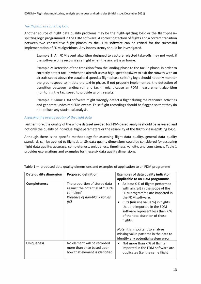
Although there is no specific methodology for assessing flight data quality, general data quality
standards can be applied to flight data. Six data quality dimensions could be considered for assessing
flight data quality: accuracy, completeness, uniqueness, timeliness, validity, and consistency. Table 1
provides explanations and examples for these six data quality dimensions.
Table 1 — proposed data quality dimensions and examples of application to an FDM programme
Data quality dimension Proposed definition Examples of data quality indicator applicable to an FDM programme
Completeness The proportion of stored data against the potential of ‘100 % complete’ Presence of non-blank values (%)
• At least X % of flights performed with aircraft in the scope of the FDM programme are imported in the FDM software.
• Cuts (missing value %) in flights that are imported in the FDM software represent less than X % of the total duration of those flights.
Note: it is important to analyse missing value patterns in the data to identify any potential system error.
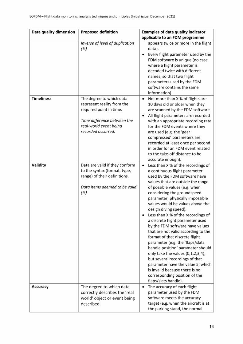
Uniqueness No element will be recorded more than once based upon how that element is identified.
• Not more than X % of flights imported in the FDM software are duplicates (i.e. the same flight
EOFDM – Flight data monitoring, analysis techniques and principles (Initial issue, December 2021)
14
Data quality dimension Proposed definition Examples of data quality indicator applicable to an FDM programme
Inverse of level of duplication (%)
appears twice or more in the flight data).
• Every flight parameter used by the FDM software is unique (no case where a flight parameter is decoded twice with different names, so that two flight parameters used by the FDM software contains the same information)
Timeliness The degree to which data represent reality from the required point in time. Time difference between the real-world event being recorded occurred.
• Not more than X % of flights are 10 days old or older when they are scanned by the FDM software.
• All flight parameters are recorded with an appropriate recording rate for the FDM events where they are used (e.g. the ‘gear compressed’ parameters are recorded at least once per second in order for an FDM event related to the take-off distance to be accurate enough).
Validity Data are valid if they conform to the syntax (format, type, range) of their definitions. Data items deemed to be valid (%)
• Less than X % of the recordings of a continuous flight parameter used by the FDM software have values that are outside the range of possible values (e.g. when considering the groundspeed parameter, physically impossible values would be values above the design diving speed).
• Less than X % of the recordings of a discrete flight parameter used by the FDM software have values that are not valid according to the format of that discrete flight parameter (e.g. the ‘flaps/slats handle position‘ parameter should only take the values {0,1,2,3,4}, but several recordings of that parameter have the value 5, which is invalid because there is no corresponding position of the flaps/slats handle).
Accuracy The degree to which data correctly describes the ’real world‘ object or event being described.
• The accuracy of each flight parameter used by the FDM software meets the accuracy target (e.g. when the aircraft is at the parking stand, the normal
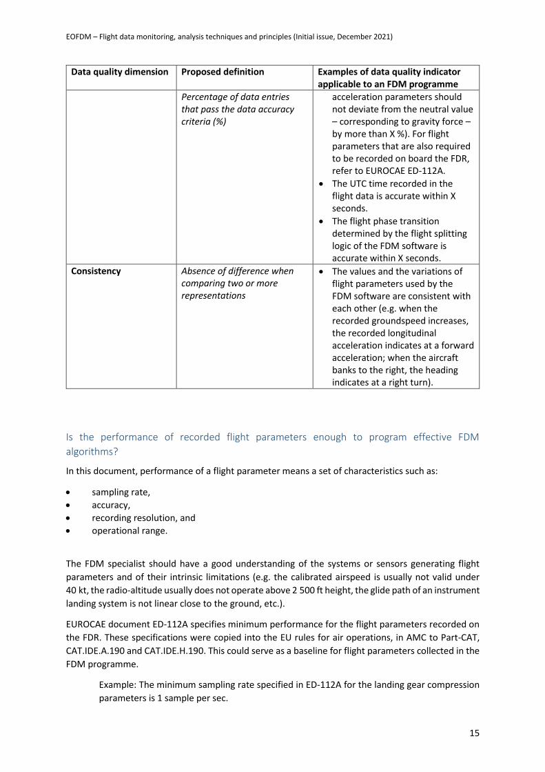
EOFDM – Flight data monitoring, analysis techniques and principles (Initial issue, December 2021)
15
Data quality dimension Proposed definition Examples of data quality indicator applicable to an FDM programme
Percentage of data entries that pass the data accuracy criteria (%)
acceleration parameters should not deviate from the neutral value – corresponding to gravity force – by more than X %). For flight parameters that are also required to be recorded on board the FDR, refer to EUROCAE ED-112A.
• The UTC time recorded in the flight data is accurate within X seconds.
• The flight phase transition determined by the flight splitting logic of the FDM software is accurate within X seconds.
Consistency
Absence of difference when comparing two or more representations
• The values and the variations of flight parameters used by the FDM software are consistent with each other (e.g. when the recorded groundspeed increases, the recorded longitudinal acceleration indicates at a forward acceleration; when the aircraft banks to the right, the heading indicates at a right turn).
Is the performance of recorded flight parameters enough to program effective FDM
algorithms?
In this document, performance of a flight parameter means a set of characteristics such as:
• sampling rate,
• accuracy,
• recording resolution, and
• operational range.
The FDM specialist should have a good understanding of the systems or sensors generating flight
parameters and of their intrinsic limitations (e.g. the calibrated airspeed is usually not valid under
40 kt, the radio-altitude usually does not operate above 2 500 ft height, the glide path of an instrument
landing system is not linear close to the ground, etc.).
EUROCAE document ED-112A specifies minimum performance for the flight parameters recorded on
the FDR. These specifications were copied into the EU rules for air operations, in AMC to Part-CAT,
CAT.IDE.A.190 and CAT.IDE.H.190. This could serve as a baseline for flight parameters collected in the
FDM programme.
Example: The minimum sampling rate specified in ED-112A for the landing gear compression
parameters is 1 sample per sec.
EOFDM – Flight data monitoring, analysis techniques and principles (Initial issue, December 2021)
16
In a dynamic flight phase where the values of a flight parameter are expected to vary rapidly (e.g. take
off, go-around, avoidance manoeuvres), the accuracy of that flight parameter might be lower than in
a stable flight phase. ED-112A specifies that data ‘shall be obtained from sources within the aircraft,
which provide the most accurate and reliable information under both static and normal dynamic
conditions.’. Hence, it is preferable to use the same flight parameters as those recorded on the FDR
for FDM algorithms when they are implemented on dynamic flight phases.
On some aircraft models, the flight data frame layout may be reconfigured without a retrofit. This
allows an operator to standardise the flight data frame layouts across the fleet, to modify sampling
rate of some flight parameters and/or record additional flight parameters. Enhancing the flight data
frame layout may generate savings for maintenance (by permitting a better monitoring of the
condition of systems and engines) and/or for operations (e.g. fuel savings).
Example: A flight parameter recording the status of passenger doors may be correlated with
the scheduled arrival time for accurately computing the delay at arrival of a given flight.
Note:
It is important to understand the limitations of discrete-time signals (which recorded flight
parameters are) and the effects of signal sampling. It is not within the scope of this document
to explore these aspects in detail, but generically speaking, if the sampling rate of a signal is
close to or lower than the signal’s highest possible frequency, then sampling may result in
significant loss of information. In the case of a flight parameter, too low sampling rate may
lead to erroneous results and/or missed FDM events.
Note:
Updating the flight data frame layout may have an unexpected impact on already-
implemented FDM algorithms (see Section I.3).
3. FDM algorithms
Identifying an initial set of FDM algorithms
Initially, it is recommended to implement a small set of ‘broad’ FDM algorithms (FDM event algorithms
and/or FDM measurement algorithms) covering all flight phases and the main categories of aviation
occurrences, and then to progressively complete this set with ‘specialised’ FDM algorithms that
address more peculiar operational safety risks.
• ‘Broad’ FDM algorithms are usually those that are designed to help capture unsafe outcomes, such as a risk of CFIT or of runway excursion. A broad FDM algorithm may potentially capture all occurrences related to a given operational safety risk.
Example: The FDM event algorithm15 ‘risk of runway overrun at landing’ detects that during the landing roll the aircraft is approaching the end of runway too fast (i.e. the groundspeed seems too high for the remaining distance). This FDM event algorithm is likely to reliably capture all landings with a higher risk of runway overrun.
Broad FDM algorithms are helpful for the initial assessment of safety issues. However, because a broad FDM algorithm is rather unspecific, the output data generated by such an algorithm need to be analysed to sort it out into smaller categories. A broad FDM algorithm is therefore not very suitable for monitoring specific safety issues, but can be a good starting point.
15 Examples in this section refer to FDM event algorithms, but the concepts of broad FDM algorithms and specialised FDM algorithms are also applicable to FDM measurement algorithms.
EOFDM – Flight data monitoring, analysis techniques and principles (Initial issue, December 2021)
17
Example: It would be desirable to sort out individual detections by the FDM event algorithm ‘risk of runway overrun at landing’ into subcategories such as ‘touchdown point far beyond the recommended touchdown zone’ and ‘too little/too late deceleration after touchdown’.
• ‘Specialised’ FDM algorithms are helpful for detecting specific deviations from the SOPs or accepted practice, even if they do not necessarily result in any unsafe outcome.
Example: A specialised FDM event algorithm could detect excessive groundspeed at landing (groundspeed is too high when the aircraft is passing the landing threshold). If the groundspeed at landing is excessive on a runway much longer than the landing distance, there is no immediate risk associated with this deviation.
A specialised FDM algorithm may be useful to track a specific safety issue e.g. related to a piloting technique or to the implementation of a particular SOP. However, the scope of a specialised FDM algorithm is rather narrow, so that unforeseen safety issues may not be detected if only specialised FDM algorithms are implemented in the FDM programme.
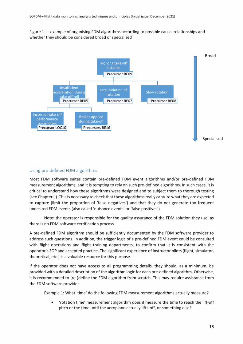
Example (see also Figure 1):
An excessively long take-off distance may have various causes, such as:
• insufficient acceleration during the take-off roll, which may be caused by o inadequate take-off thrust setting, or o the inadvertent application of brakes during the take-off roll; or
• the late initiation of the rotation; or
• a too slow rotation. In this example, an FDM algorithm monitoring the take-off distance could be
considered as ‘broad’ while an FDM algorithm capturing information about the
application of brakes during the take-off roll is rather ‘specialised’.
EOFDM – Flight data monitoring, analysis techniques and principles (Initial issue, December 2021)
18
Figure 1 — example of organising FDM algorithms according to possible causal relationships and whether they should be considered broad or specialised
Using pre-defined FDM algorithms
Most FDM software suites contain pre-defined FDM event algorithms and/or pre-defined FDM
measurement algorithms, and it is tempting to rely on such pre-defined algorithms. In such cases, it is
critical to understand how these algorithms were designed and to subject them to thorough testing
(see Chapter II). This is necessary to check that these algorithms really capture what they are expected
to capture (limit the proportion of ‘false negatives’) and that they do not generate too frequent
undesired FDM events (also called ‘nuisance events’ or ‘false positives’).
Note: the operator is responsible for the quality assurance of the FDM solution they use, as
there is no FDM software certification process.
A pre-defined FDM algorithm should be sufficiently documented by the FDM software provider to
address such questions. In addition, the trigger logic of a pre-defined FDM event could be consulted
with flight operations and flight training departments, to confirm that it is consistent with the
operator’s SOP and accepted practice. The significant experience of instructor pilots (flight, simulator,
theoretical, etc.) is a valuable resource for this purpose.
If the operator does not have access to all programming details, they should, as a minimum, be
provided with a detailed description of the algorithm logic for each pre-defined algorithm. Otherwise,
it is recommended to (re-)define the FDM algorithm from scratch. This may require assistance from
the FDM software provider.
Example 1: What ‘time’ do the following FDM measurement algorithms actually measure?
• ‘rotation time’ measurement algorithm does it measure the time to reach the lift-off pitch or the time until the aeroplane actually lifts-off, or something else?
Too long take-off distance
Precursor RE09
Insufficient acceleration during
take-off rollPrecursor RE05
Incorrect take-off performance parametersPrecursor LOC10
Brakes applied during take-off
Precursors RE16
Late initiation of rotation
Precursor RE07
Slow rotation
Precursor RE08
Broad
Specialised
EOFDM – Flight data monitoring, analysis techniques and principles (Initial issue, December 2021)
19
• ‘take-off distance’ measurement algorithm: does the measurement start when the aircraft turns onto the runway heading, or when a given power setting is selected, or other criteria?
• ‘TAWS alert’ event algorithm: what are the TAWS modes captured? And is the trigger logic of this algorithm consistent with the specific implementation of TAWS on the aircraft (for instance: is the bank angle threshold of the algorithm equal to the actual bank angle value that will trigger a ‘bank angle’ TAWS warning on that aircraft?).
Example 2: FDM event algorithm detecting the condition ‘unstable approach’: what are
exactly the deviations captured by this algorithm?
It is often necessary to adjust pre-defined FDM algorithms to specific operation. Unfortunately, some
FDM software offers only limited functionality to modify pre-defined algorithms. In addition, some
operators may not have sufficient internal knowledge to re-design these algorithms.
An FDM algorithm may work for a given aircraft model but not for another one, even when they belong
to the same family (for instance, because the applicable trigger value is not the same). In addition to
this, when aircraft have different flight data frame layouts (even if they are from the same make and
model), this might result in an FDM algorithm producing inconsistent data across that fleet. Therefore,
FDM algorithm testing should be performed for each flight data frame layout.
Maintaining the set of FDM algorithms
The safety risk register of an operator changes over time, with new safety threats emerging and the
frequency and severity of any given safety risk increasing or decreasing. This means that the FDM
event algorithms and FDM measurement algorithms should be checked against the operational safety
risks of the safety risk register at regular time intervals.
Examples of changes that could generate new operational safety risks:
• Operating on a new airfield or runway,
• Major changes in cockpit training,
• Change of operation area,
• Including new types of aircraft in the fleet, or
• New or revised SOPs.
EOFDM – Flight data monitoring, analysis techniques and principles (Initial issue, December 2021)
20
II. Defining, testing, and validating an FDM algorithm
The setting of an FDM event algorithm or an FDM measurement algorithm involves three
different phases, which can be identified as:
• Definition
• Testing
• Production
• Updating
1. Defining an FDM algorithm
Identifying the necessary data
In the phase of the definition of the FDM algorithm (FDM event algorithm or FDM measurement
algorithm), some initial assessment should be performed.
Based on the description of the operational safety risk (see Chapter I), define which event should be
captured through FDM.
Verify whether the data frames contain all the necessary flight parameters to address the event to be
captured. Verify if the frequency and the recording resolution of each needed flight parameter are
sufficient16.
Example: Case of an FDM event algorithm for detecting structural limit exceedance case such
as caused by overweight landing. During the initial assessment period the flight parameters
that will be used and the associated aircraft limitations should be identified in cooperation
with the engineering department.
Identify those additional flight parameters that could be helpful for testing and validation. The FDM
algorithm should also include the definition of a data snapshot.
Note:
If other data sources are available, which could be automatically linked with the FDM data (air safety
reports (ASR), weather, navigation data, etc.), it is advisable to already assess at this stage what data
could be used to enrich the data snapshot of the FDM event17.
Consider whether the FDM software uses automatic flight splitting or flight phase splitting. This may
have significant influence on the effectiveness of the FDM algorithm. See also Section I.2.
Verifying the flight parameters
For those flight parameters that have not yet been verified, check that their values, sign, and variations
are consistent. Verify whether there are some problems affecting flight parameter quality (refer to
16 Some parameters may be calculated from those recorded in the data frame, but care should be taken in this process. A typical example is computing the variations of a recorded parameter in order to assess its derivative, i.e. calculating the pitch angle rate from the recorded pitch attitude angle. This computation introduces noise. To cope with this, filtering could be added after performing the derivate calculation. 17 Refer also to EOFDM document ‘Breaking the silos’, Chapter I.
EOFDM – Flight data monitoring, analysis techniques and principles (Initial issue, December 2021)
21
Section I.2) that may have a negative effect on the final result. Start by examining flight parameters
plots for some sample flights. This is not an exhaustive check and some problems with the flight
parameters may only become obvious at a later stage.
Most FDM software allows to quickly review parameter values distributions over large amounts of
flights. This should be used as much as permitted by the available data and the computational power
of the software. As a minimum, such review should include looking for out-of-range values, for outliers
and extreme values, for missing values, abnormal distributions, etc.. Scatter plots and boxplots are
also helpful (see Chapter III).
Check whether the performance of some flight parameters may affect the accuracy of the trigger logic
or limit its domain of validity.
Examples:
• The airspeed is usually based on total pressure measurements provided by a pitot probe and therefore the airspeed is not accurate when the aircraft is taxying at lower speed;
• If the latitude and longitude parameters are provided by an individual inertial reference system, they will drift over time and provide an inaccurate position toward the end of the flight;
• The difference between the magnetic heading and the true heading is usually of several degrees at high latitudes, so that magnetic declination correction may be needed before using the magnetic heading.
Note:
It is also advisable to verify the quality of the data sources other than flight data.
Example: for computation of height at threshold, the position of the runway threshold is
necessary, and therefore an up-to-date database of airports and runways is required for an
accurate computation.
The following illustrates flight parameters checks that are recommended during the development
steps of an FDM event algorithm with the example of an algorithm monitoring flap speed limit
exceedance:
1. The first step ensures that the flight parameters needed are recorded: airspeed and aircraft flap configuration parameters.
2. Next, the recording rate and recording resolution of each of these flight parameters are checked, to ascertain if they can deliver the desired output. For instance, if one of these flight parameters is recorded only once every 4 seconds, this can have a considerable effect on the results. When an FDM algorithm relies on flight parameters with different recording rates, down-sampling and/or interpolating the values will be necessary, but, if not done properly, this might result in a misleading outcome.
3. Then, a quality check is performed. That is, if other flight parameters are recorded, such as airspeed from other aircraft sources, they are used to increase the robustness of the FDM event algorithm.
4. Then, a data snapshot of other relevant flight parameters values to be extracted when the FDM event is detected, is defined: altitude, rate of climb/descent, landing gear position, etc. These extracted values are checked for consistency.
EOFDM – Flight data monitoring, analysis techniques and principles (Initial issue, December 2021)
22
Defining a search window
Defining a ‘search window’ (i.e. conditions where the FDM algorithm is applicable) usually accelerates
data processing by reducing the amount of flight data to be processed by the FDM software.
Example: An FDM measurement algorithm monitoring the taxi speed does only needs to
be applied to those parts of the recording where the aircraft is on the ground. The search
window specifications of such an FDM event could be:
• ‘only applies to a taxi phase’ (if flight phase splitting is provided by the FDM software)’, or
• ‘only apply when the value of the air-ground status flight parameter is “ground”’.
Defining the trigger logic of an FDM event algorithm
To define the trigger logic of the FDM event algorithm, the ‘normal’ domain needs to be established.
Many limitations can be obtained from the AFM. In addition, the operator’s SOPs define operating
limits. When no indication is provided by available documentation and SOPs, a statistical distribution
of relevant FDM parameters may also be helpful to define the range of normal operation. Known
reference flights within the flight data may also be useful to help define the ‘normal’ domain.
If feasible, an algorithm that frequently triggers is preferable for the first stage of testing since it can
be tested with a limited amount of flight data. For instance, TAWS cautions are more frequent than
TAWS warnings and therefore a smaller flight data sample will be needed for testing the trigger logic.
To make the trigger logic more robust, a ‘confirmation time’ may be introduced: the FDM event
algorithm does not detect an event every time the trigger condition is met at a single point in time,
but only if it is met over a period exceeding a given duration (often designated as ‘confirmation time’,
‘persistence time’, or ‘time filter’). Another possibility to make the trigger logic definition more robust
is to base it on several simultaneous conditions (confirmation by several conditions).
Example 1: FDM event algorithm detecting excessive taxi speed (i.e. ground speed exceeding the maximum taxi speed permitted by the taxi SOPs). The introduction of a confirmation time of X seconds will make the trigger logic insensitive to spikes and very short deviations, while an excessive taxi speed sustained during X seconds will trigger an FDM event. Example 2: FDM event algorithm detecting TAWS cautions – double validation using the parameters corresponding to TAWS aural and visual signals. The FDM event is triggered only if the TAWS aural caution is active and the TAWS caution light is on. Example 3: FDM event algorithm detecting a high torque or a high rotation speed of the main rotor of a helicopter, such an FDM event usually requires a confirmation time.
Defining severity levels for FDM events
As explained in HeliOffshore good practice document on helicopter FDM18:
‘It is important to draw a distinction between the severity of an individual event and the operational
risk that event presented. Severity levels are assigned according to a numerical algorithm (in order to
18 HeliOffshore — Helicopter Flight Data Monitoring (HFDM) Recommended Practice for Oil and Gas Passenger Transport
Operations, Version 1.0, September 2020 (HO-HFDM-RPv1.0)

EOFDM – Flight data monitoring, analysis techniques and principles (Initial issue, December 2021)
23
assist analysts by highlighting certain events) but a high severity event does not imply high operational
risk. […]
Moving from event severity to event operational risk involves a further step in which an analyst
assesses the full context around an event. This process may be supported by additional procedures
including review groups, written criteria or a risk assessment matrix’.
Hence, the following distinction should be kept in mind:
• ‘FDM event severity level/score’ means a level/score that is allocated to an FDM event according to pre-defined criteria, and that is determined based on FDM data. The FDM event severity levels/scores may be used for supporting risk assessment, but FDM event severity levels/scores taken alone are not indications of actual risk.
• ‘assessed event risk level’= the assessed level of risk (of an undesired outcome e.g. catastrophic, hazardous) for a given event. This event may have been detected through FDM or not (e.g. a laser attack or a near-collision with a vehicle on the ground will leave no clear trace in the FDM data). The risk level should be assessed in view of all available data (occurrence report, FDM, weather data, traffic data, etc.), it should preferably follow a risk assessment method, and, where necessary, involve expert knowledge. Because of this, risk level assessment cannot be fully automatised. Assessing the risk level of events is part of the operator SRM, not just an FDM process.
When several severity levels are applied to FDM events, they should be defined according to a severity
level classification that is consistently applied across all FDM event algorithms. Otherwise, it will be
difficult to make meaningful indicators from FDM events.19
There can be many appropriate severity level classifications and Table 2 just provides an example.
In addition, FDM event algorithms could be used to produce either ‘leading’ or ‘lagging’ indicators,
depending on their definition or of their threshold values. For example, a leading indicator for the risk
of mid-air collision could be based on monitoring the vertical rate during climb, while a corresponding
lagging indicator would detect level busts.
Another example is the detection of hard landings.Assuming that the normal acceleration limit defined
by the aeroplane manufacturer for a given aircraft model is 2.1 g, the FDM event algorithm could be
designed in two ways:
1. By setting the threshold values below 2.1 g, an information about how close it is to the hard
landing limit is produced. This can be qualified as a leading indicator.
2. By defining threshold values above 2.1 g, an information about by how much the hard landing
limit has been exceeded is generated. The main advantage of this approach is that it only extract
events that require an action according to the maintenance instructions. But when the FDM
event algorithm triggers, the undesirable situation (hard landing, structural damage, etc.) has
already happened. This can be qualified as a lagging indicator.
Both approaches have their advantages and drawbacks.
Note:
Grouping flights according to an event severity classification may limit subsequent analyses (e.g.
19 If the flight data are also used for continuing airworthiness purposes, a severity level classification following different
principles may be needed, or even in some cases severity levels may not be relevant.

EOFDM – Flight data monitoring, analysis techniques and principles (Initial issue, December 2021)
24
because it might exclude certain flights), and the FDM specialist should remain aware of this. FDM
measurements may be more appropriate for finer analyses.
EOFDM – Flight data monitoring, analysis techniques and principles (Initial issue, December 2021)
25
Table 2 — example of a severity level classification applicable to FDM event definitions
Level Description Notes Examples
0 Thresholds at Level 0 should be:
• indicative of a deviation from SOP and/or accepted practice; and
• specific for the operation (fleet and/or operator) based on the equipment and operating environments.
Level 0 does not necessarily constitute a safety hazard; however, monitoring trends at this level can be used to:
• measure SOP adherence;
• compare an operation to the aggregate to identify outliers or potential areas of concern;
• assess the potential need to re-evaluate and/or update SOPs.
Momentary and limited exceedance of the recommended vertical speed during the approach.
1 Thresholds at Level 1 are indicative of having approached or exceeded at least one primary risk mitigation.
Level 1 events may occur frequently enough to provide statistically significant trends within an FDM program (depending on the volume of operation). Trends at this level should have mitigation plans and not just be monitored.
TAWS ‘sink rate’ alert
2 Thresholds at Level 2 are:
• indicative that safety margins have been consumed or reduced to the final safety barrier;
• at levels significant enough that a crew would likely notice the event and generate a voluntary safety report.
Level 2 events should be rare. A root cause analysis would typically be performed on each individual Level 2 event.
TAWS ‘pull up’ alert
3 Thresholds at Level 3 are indicative that the undesired state occurred.
Level 3 events should be extremely rare. Thresholds at Level 3 may have values set at points beyond which protection systems are intended to have activated. A full operator (and possibly State) investigation would typically be performed on each individual Level 3 event.
TAWS ‘pull up’ alert and the radio-height parameter show that the minimum height was less than X feet, i.e. this was a near collision with the terrain.
EOFDM – Flight data monitoring, analysis techniques and principles (Initial issue, December 2021)
26
2. Testing an FDM algorithm
After the FDM algorithm has been defined, some coding and testing has to be done (test phase).
Statistics and analysis about this algorithm should never be shared with third parties before it is
confirmed to work correctly.
General considerations
Note:
Some of the considerations provided in this section are focussed on FDM event algorithms. Other
considerations address ‘FDM algorithms’, i.e. they are applicable to FDM event algorithms and to FDM
measurement algorithms alike.
During the testing phase, the operator could use archived records in its occurrence reporting system
to identify flights that are relevant for a new FDM event algorithm to be tested. Such flights can for
instance help to validate the trigger logic of that algorithm.
Note:
The occurrence reporting system may include more than just flight crew reports. Maintenance reports
and operational flight plans could be also collected.
For testing purposes, the threshold value could be changed to trigger an FDM event for parameter
values that are frequently encountered in operation. After verifying that the FDM events are valid, the
threshold value could then be set to the appropriate value20.
Check flights and maintenance flights are likely to generate FDM events therefore they could be used
for testing the trigger logic of a new FDM event algorithm.
It could also be useful to build up a ‘control set’ composed of flights that do not contain the events
that a tested FDM event algorithm is meant to detect, and that possibly contains flight sequences or
flight manoeuvres that could trigger a false positive. This control set would be useful for ensuring that
the tested algorithm does not generate too frequent false positives.
With regards to the data used for test, there are two options:
• When it is technically possible, it is recommended to test on a separate platform which contains a sufficient number of historic flights, to ensure that operational statistics are not compromised. This usually allows to complete the testing faster. However, not all FDM software allows this option.
• If testing on a separate platform is not possible, the testing will need to be performed on ‘live’ flight data. In that case, the testing process could take a little longer depending on the amount of data received every day. The potential impact on the live data processing systems should be carefully considered, as it could affect historical analyses. However, this option may give more reliable results because the test has been performed on recent flight recordings.
Note:
When considering two aircraft of the same make and model that have different engine models or
slightly different airborne equipment, the same FDM algorithm may produce different results.
20 EOFDM WG-B document ‘Guidance for the implementation of FDM precursors’ provides guidance on setting a threshold.
EOFDM – Flight data monitoring, analysis techniques and principles (Initial issue, December 2021)
27
Therefore, it is important to test the FDM algorithm on all flight data frame layouts implemented on
the operator’s fleet.
Before an FDM algorithm is put into production (see Section 3), its testing results should be reviewed
and approved. The way this is organised depends on the internal organisation of each operator, but it
is recommended to establish a formalised approval process. To ensure that the FDM algorithm
definition is consistent with the operator’s SOP and what is considered acceptable piloting skills, it is
also helpful to include representatives of flight operations and flight training department in the
approval process.
Also, according to EU rules for air operations, the FDM programme is part of the operator’s SMS and
the safety manager should be responsible for the FDM programme21. Because of this, the safety
manager should verify whether new FDM algorithms are appropriate and relevant for addressing the
operational safety risk. This verification should be done before the algorithms are put into
productions.
Example of a testing plan for an FDM event algorithm
1. Test the FDM event algorithm against recordings of flights corresponding to known events (e.g. reports from the occurrence reporting system) to verify that the FDM event algorithm triggers for most of those flight recordings, that is to say the false negative rate or rate of ‘missed FDM events’ is low;.
2. Test the FDM event algorithm on a sample of flights corresponding to a week of operation, or a month of operation, so that a rate of nuisance FDM events per time period can be estimated; this rate has a direct impact on the workload of manually validating FDM events.
3. Incrementally increase the sample size and the number of aircraft models in the scope of the FDM event algorithm to progressively gain confidence in the trigger logic. The sample size should be sufficient to establish reliable statistics of nuisance FDM events.
Note:
If the new FDM event algorithm is linked to a specific departure or destination (e.g. an airfield with
peculiar procedures due to terrain or obstacles), the sample should obviously include these.
Case of a low volume of operation
If the fleet size is small or the flights are performed at irregular time intervals, it may take longer to
build a suitable data set to test the FDM algorithm. If aircraft utilisation is low, effective testing may
not be possible, because the amount of data produced by the FDM algorithm is likely to generate
unreliable statistics.
In that case, each flight may have to be reviewed in detail. To support analysis, a small set of flight
parameters could be collected at specific points, to progressively gain confidence in the FDM
algorithm.
In addition, certain types of maintenance or aircraft acceptance flights can provide a wealth of useful
capture points, to test event sets against.
21 For aeroplanes, refer to Part-ORO, ORO.AOC.130 and AMC1 ORO.AOC.130.
EOFDM – Flight data monitoring, analysis techniques and principles (Initial issue, December 2021)
28
With regard to analysing small data sets, refer to Chapter III.
3. Production phase
After successful testing and the FDM algorithm is considered compliant with the definition, it can be
used for daily operations. This is defined as the production phase.
Despite testing, nuisance FDM events can still occur in production. This may result of sensor failure or
other conditions that could not be anticipated during the testing phase. Therefore, a validation of the
FDM events is necessary so that nuisance FDM events can be removed from the final statistics and the
subsequent analysis process uses reliable data. This can be achieved by flagging each FDM event as
valid or invalid. A well-defined data snapshot is helpful for a quick validation of the FDM events.
For high-severity FDM events that are not expected to be frequent, this validation should be done for
every FDM event.
In the end, any FDM algorithm that is in production should be properly documented. Documentation
should include:
• reason(s) for implementation including detailed description of the safety risks that are intended to be monitored, and a link to the safety risk register of the operator;
• date of implementation;
• dataset(s) to which the FDM algorithm was applied (e.g. was it only applied to newly received data or also to some of the historical datasets?);
• (for an FDM event algorithm) the threshold values and the rationale for selecting these threshold values; and
• any other comments deemed relevant for the event programming.
This will ensure that pertinent details will be kept over time, assisting the interpretation of the output
of the FDM algorithm. This documentation can be provided in a dedicated manual, in controlled
documents or even as comments in the programming code of the FDM algorithm.
4. Updating
The thresholds of some FDM event algorithms such as those based on SOPs may need to be modified
from time to time. As such, a close interaction with the Flight Operations Department is paramount,
so that any change to the SOPs can be incorporated in the FDM algorithms as soon as possible,
otherwise the output of the FDM algorithms will lose their significance. Furthermore, a so-modified
FDM algorithm should be run on the flight data received since the new SOPs became effective.
Finally, all the event algorithm documentation shall be amended containing:
• the reason(s) for any change, including detailed description of the new safety risks that are intended to be monitored, and a link to the safety risk register of the operator;
• the change(s) made to the programming (e.g., modified trigger logic or thresholds, old-new variable encoding, metric changes etc…); and
• the date of this implementation.
This will permit to track the history of changes performed to an FDM event algorithm, which will in
turn assist interpretation of the related FDM events.
EOFDM – Flight data monitoring, analysis techniques and principles (Initial issue, December 2021)
29
5. Examples
Example 1: Incorrect capture window
The trigger logic below, originally used the groundspeed parameter to trigger an FDM event to
measure the pitch rotation rate at take-off for helicopters.
Where GROUNDSPEED <= 15 Knots, measure greatest change in pitch attitude
When this trigger logic was used on an aircraft that did not have a groundspeed parameter, many
flights had a pitch rate of 0 degrees per second: see Figure 2. This resulted in a large number of invalid
FDM events as well as incorrect statistical information.
Figure 2 — distribution of pitch rate at take-off that shows incorrect values
The trigger logic was corrected to use indicated airspeed parameter and the capture window was
expanded to the following:
Where INDICATED AIRSPEED <= 40 Knots, measure greatest change in pitch attitude
The revised trigger logic now captures the correct pitch rate and reduces the number of invalid FDM
events (see Figure 3).
EOFDM – Flight data monitoring, analysis techniques and principles (Initial issue, December 2021)
30
Figure 3 — distribution of pitch rate at take-off
Example 2 – Use of the radio-altitude in helicopter FDM programmes
Figure 4 shows the evolution over time of some flight parameters related to a helicopter approaching
an offshore installation. Pressure altitude and the integral of vertical speed are shown in blue and
green and the radio altimeter (radalt) parameter is shown in red.
The three values show good agreement until the clear step in radalt value that occurs as the helicopter
moves over the helideck. Any FDM algorithm using a radalt parameter in this situation must take
account of this effect. For instance, differencing the radalt parameter to synthesise a vertical speed
would produce erroneous values when the helicopter lands on a helideck.
EOFDM – Flight data monitoring, analysis techniques and principles (Initial issue, December 2021)
31
Figure 4 — pressure altitude (blue), integral of vertical speed (green) and radio-altitude (red) of a
helicopter approaching a helideck
Example 3 – Monitoring taxi speed during turns
Many manufacturers recommend limiting the taxi speeds during turns. E.g. the A320 FCTM
recommends a speed of less than 10 kt during turns of over 90°. Boeing has a similar recommendation
for the B737NG. When defining an FDM measurement algorithm to capture speed during turns, the
algorithm should compute heading change within a specific time interval. Otherwise, the algorithm
might identify a turn of over 90° at almost every flight cycle.
EOFDM – Flight data monitoring, analysis techniques and principles (Initial issue, December 2021)
32
III. Producing meaningful FDM statistics and interpreting them
Note:
The ambition of this chapter is limited to introducing a few statistical tools and practical examples of
their application to FDM data. Readers should keep in mind that explanations and examples in this
chapter have been simplified and are incomplete. Many publications are available on the internet for
further learning on statistics.
1. Why use statistics?
Much of the benefit of FDM comes from analysing very large numbers of flights to look for trends in
the operation. Statistics can help to achieve this. Statistics can also help to overcome biases.
When working with large amounts of data, statistical analysis methods are beneficial to highlight
useful information. By its nature, any FDM program involves working with large amount of data, thus
using correct statistical analysis methods is important to look for trends and emerging operational risk
areas.
In general, statistics can be separated into two branches – descriptive and inferential. Inferential
statistics draw conclusions about a whole population by studying a sample of that population, whereas
descriptive statistics looks to summarise, collect, analyse and present a complete set of data.
Inferential statistics are helpful especially if the flight collection rate is low. Descriptive statistics might
be more appropriate if a high flight collection rate is achieved for all individual aircraft and routes.
Note:
More advanced predictive analysis (e.g based on machine learning) is outside the scope of this
document.
The type of overarching questions that may be addressed using statistical analysis include:
• What has changed in the operation over certain time intervals?
• Is there a real trend, pattern, or correlation when considering a given FDM algorithm, airfield, runway, fleet, or pilot? How likely is it that a variation in the number or rate of FDM events just results from chance and not from a trend?
• Are there indications of the possible reasons for an observed trend or pattern?
• How can the information obtained from statistical analysis be turned into actionable solutions?
2. Considerations before engaging into statistics
Before applying statistics to the FDM programme, the context of the flight data should be understood,
as this may affect the relevance of any statistical computation. Below are a few questions that are
worth considering:
• Which individual aircraft are included in the FDM programme, and since when? Long-term statistics cannot be produced for recently introduced aircraft.
• Are flight data collected from non-revenue flights (e.g. ferry flights, training flights, and maintenance check flights), or solely from commercial flights? Beware that invalidating FDM
EOFDM – Flight data monitoring, analysis techniques and principles (Initial issue, December 2021)
33
events does not remove the flight data from non-revenue flights and these data could pollute future statistics if the flights are not properly identified as non-revenue flights.
• Are some areas of operation or airfields under-represented in the data collected by the FDM programme? Is this because of a technical reason (e.g. recovering flight data from the aircraft is challenging for some areas of operation)?
• What is the average time between the flight taking place and the data being analysed? What is the maximum time?
• Is the number of flights sufficient for statistical relevance and maintaining confidentiality? A minimum should be defined.
In addition, any FDM algorithm that is used for statistics should have been properly tested (refer to
Chapter II). In the case of an FDM event algorithm, most nuisance FDM events of that algorithm should
have been removed from the FDM events set prior to statistical analyses.
Furthermore, it is essential to clearly state the objective of a statistical calculation from the beginning.
In particular the questions to be addressed by that calculation should be written down, as well as any
simplification or assumption that was made to address those questions.
Example: In the last three months, there seem to have been more cases where the flight crews
requested priority landing for being short of fuel.
Question: how often has the remaining fuel quantity at the time of touchdown been
less than the final reserve fuel22 as prescribed by the SOPs?
Assumptions: on the considered aircraft model, the fuel quantity is computed by a
fuel quantity indication system, based on values taken from probes in each tank. The
tolerance of the fuel quantity indication system as indicated by the aircraft
manufacturer is ‘± (1 % of current FOB + 200 kg)’. This means that the expected
accuracy of the fuel quantity parameter will probably not be better than 200 kg, and
that this parameter will be less accurate at the beginning of the flight, when there is
more fuel on board, than at the end of the flight.
One should keep in mind the simplifications and assumptions made for a statistical analysis when
assessing the results. If some simplifications or assumptions are ignored during this assessment, this
can lead to inaccurate or even wrong conclusions, and in turn, to inadequate decisions
It is also important to ensure that any comparison is ‘like for like’. For example, a change in season
may bring a change in flight hours (which is accounted for by using the FDM event rate), but it may
also change the routes being operated (which may introduce other differences).
At the time this document was issued, most commercial FDM software offered only limited statistical
analysis capability. In addition, as explained in EOFDM document ‘Breaking the silos’, a safety analyst
needs to be able to bring FDM data together with other data sources (within a clear and robust
framework for protecting sensitive and personal data). In this context, it is more important that the
FDM software is capable of exporting output to formats that are compatible with other tools (such as
numerical-analysis software or business intelligence tools) rather than having complete statistical data
suites embedded in the FDM software.
Note:
Particular precautions regarding the sharing and dissemination of FDM-based indicators may be
22 According to ICAO Annex 6 Part I, the final reserve fuel for a turbine-engined aeroplane is ‘the amount of fuel required to fly for 30 minutes at holding speed at 450 m (1 500 ft) above aerodrome elevation in standard conditions.’
EOFDM – Flight data monitoring, analysis techniques and principles (Initial issue, December 2021)
34
needed in the case where the limited number of flights makes it possible to correlate such indicator
with identification data from external sources (e.g. scheduling system) and to re-identify flight crew
members.
3. Basic measures based on FDM events
Total number of FDM events or ‘FDM event count’
The FDM event count is a basic metric that can be used as a starting point for evaluation. However,
the absolute number of events is of limited use since a change in total number could be due to a
change in event rate or a change in flying hours or activity. Therefore, a normalisation process is
frequently considered.
FDM event rate
To compensate for changes in the volume of activity, calculating the FDM event rate is often used. To
calculate the event rate of an FDM event algorithm, sum up the number of detections of that event
(e.g. low rotation rate at take-off), and divide by the number of flights analysed. Rates are often
quoted as a value per 1 000 flights or per 10 000 flights (or flight hours) to make the numbers
manageable.
Note:
The format of the FDM event rate should be appropriate for tracking trends. Too small numbers might
not catch the attention they deserve, therefore presenting the FDM event rate per 1 000 flights or per
10 000 flights is more appropriate than per 100 flights.
If only a limited number of flights is available for analysis, the FDM event rate will be extremely
sensitive to small variations in numbers of FDM events (e.g. the influence of a single event on a data
sample of 1 000 flights compared to 100 000 flights is a hundred times larger).
Every individual FDM event that indicates a severe deviation should be verified, and if it is genuine,
analysed. Prioritisation between FDM events should not only rely on their rate, but also on their
severity.
Although the use of FDM event rates can compensate for changes in the volume of activity, variations
of the FDM event rate may be caused by many other factors such as meteorological conditions, route
differences, aircraft type differences, etc. In this case it may be advisable to group the data by key
factors such as fleet type, route, landing or take-off runway, etc.
Rates should be based on number of analysed flights instead of number of flights flown (often readily
available from an operational schedule). This is important to eliminate statistical errors introduced by
collection rate fluctuations (e.g. due to technical failure of flight data equipment or because of missing
recording equipment on a specific fleet).
Trends over time
It may be useful to track an FDM event rate over time to look for any developing trend: see Section
III.6.
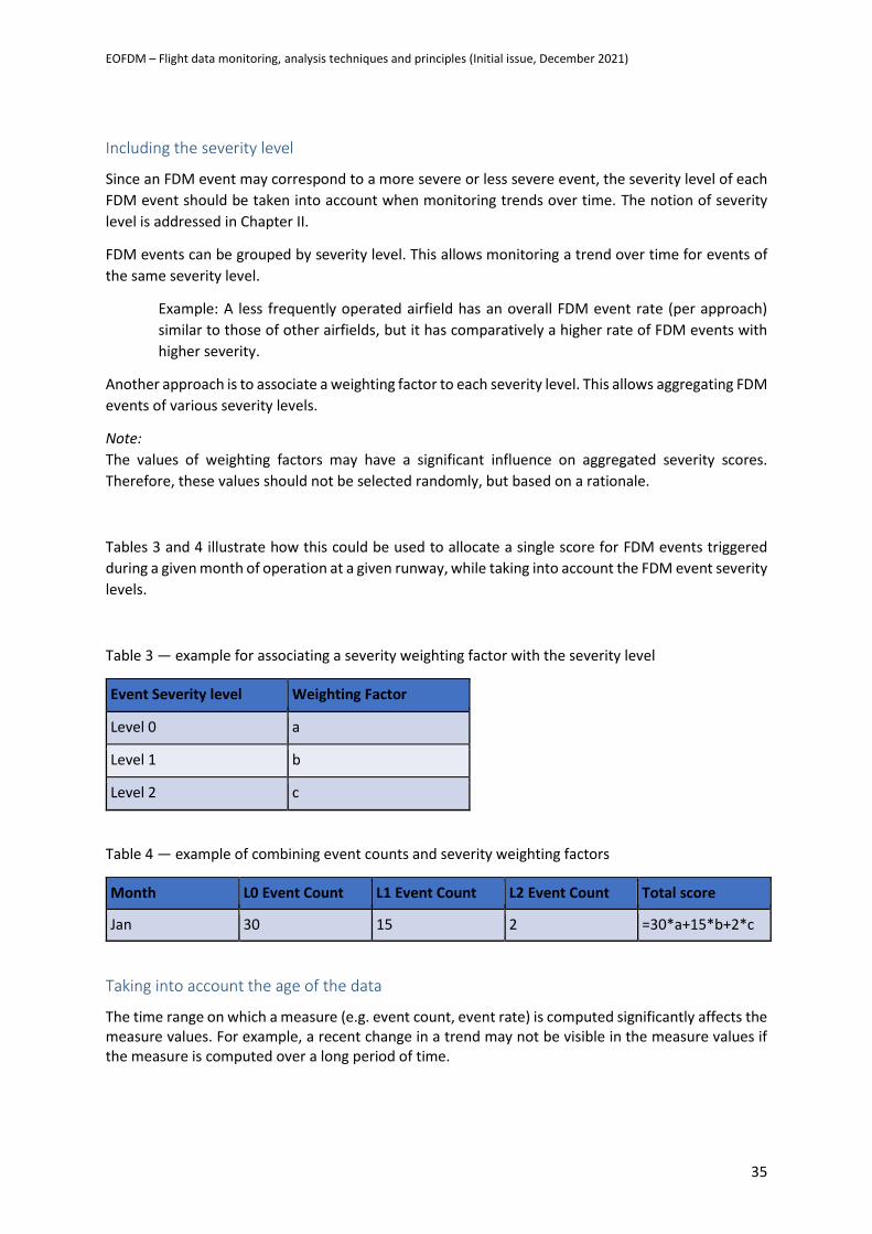
EOFDM – Flight data monitoring, analysis techniques and principles (Initial issue, December 2021)
35
Including the severity level
Since an FDM event may correspond to a more severe or less severe event, the severity level of each
FDM event should be taken into account when monitoring trends over time. The notion of severity
level is addressed in Chapter II.
FDM events can be grouped by severity level. This allows monitoring a trend over time for events of
the same severity level.
Example: A less frequently operated airfield has an overall FDM event rate (per approach)
similar to those of other airfields, but it has comparatively a higher rate of FDM events with
higher severity.
Another approach is to associate a weighting factor to each severity level. This allows aggregating FDM
events of various severity levels.
Note:
The values of weighting factors may have a significant influence on aggregated severity scores.
Therefore, these values should not be selected randomly, but based on a rationale.
Tables 3 and 4 illustrate how this could be used to allocate a single score for FDM events triggered
during a given month of operation at a given runway, while taking into account the FDM event severity
levels.
Table 3 — example for associating a severity weighting factor with the severity level
Event Severity level Weighting Factor
Level 0 a
Level 1 b
Level 2 c
Table 4 — example of combining event counts and severity weighting factors
Month L0 Event Count L1 Event Count L2 Event Count Total score
Jan 30 15 2 =30*a+15*b+2*c
Taking into account the age of the data
The time range on which a measure (e.g. event count, event rate) is computed significantly affects the measure values. For example, a recent change in a trend may not be visible in the measure values if the measure is computed over a long period of time.
EOFDM – Flight data monitoring, analysis techniques and principles (Initial issue, December 2021)
36
4. Studying distributions
Visual assessment of a distribution
This section introduces a few notions to help in studying a distribution of data points. However, before
computing any distribution measure, plotting the distribution can be helpful to visually identify some
important characteristics and avoid making wrong assumptions, such as assuming that the studied
distribution is Gaussian while it is not. For a one-dimensional distribution (i.e. each data point has just
one value), plotting the values on a histogram would allow spotting outliers or the presence of several
modes, or identifying that the distribution is skewed.
Types of averaging
Averaging, as a way of describing central tendency can be very useful when trying to summarise a
range of values. However, ‘average’ is a concept with multiple definitions that are worth
understanding. Before selecting an approach, it is important to understand the type and distribution
of data.
Mean This is the most common interpretation of ‘average’ and is defined as the sum of the
values divided by the number of values. The mean can only be calculated for numerical
(number-based) data. Although it is useful as a central tendency indicator, the mean is
easily skewed by extreme values (e.g. from erroneous data).
Median The median is defined as the central value of a sorted list of data. For this reason,
calculating a median value requires the data to be sortable (i.e. apply an order). This
implies that the median can be established for both numerical and ordinal data (Example:
assuming that the selected slats/flaps configuration can be {0; 1; 2; 3; FULL}, the median
of this list is ‘2’.). The median is less affected by outliers and skewed data than the mean.
Mode The mode is defined as the most commonly appearing value and can also be useful when
there is a need to ignore extreme values. However, the mode of a distribution is not
necessarily unique; some distributions may have more than one value that appears an
equal number of times (bi-modal or multi-modal). The mode can be determined for
numerical data, ordinal data, and so-called ‘nominal’ data (data with only a name value,
such as destination airport).
In a normal distribution (also designated as Gaussian distribution), the mean, median, and mode all
have identical values.
Skewness of a distribution
’Median‘ and ’mean‘ are good central tendency measures that can be easily calculated. Comparison
of these values will make us decide on the distribution of the data.
• If Mean <Median <Mode: the distribution is skewed to the left. In this case, there is a negative skew.
• If Mode <Median <Mean: the distribution is skewed to the right. In this case, there is a positive skew.
• If Mean = Median = Mode: the distribution is symmetrical.
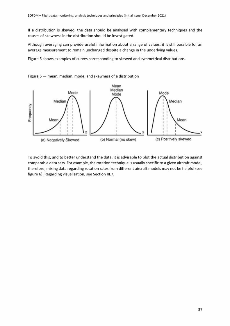
EOFDM – Flight data monitoring, analysis techniques and principles (Initial issue, December 2021)
37
If a distribution is skewed, the data should be analysed with complementary techniques and the
causes of skewness in the distribution should be investigated.
Although averaging can provide useful information about a range of values, it is still possible for an
average measurement to remain unchanged despite a change in the underlying values.
Figure 5 shows examples of curves corresponding to skewed and symmetrical distributions.
Figure 5 — mean, median, mode, and skewness of a distribution
To avoid this, and to better understand the data, it is advisable to plot the actual distribution against
comparable data sets. For example, the rotation technique is usually specific to a given aircraft model,
therefore, mixing data regarding rotation rates from different aircraft models may not be helpful (see
figure 6). Regarding visualisation, see Section III.7.
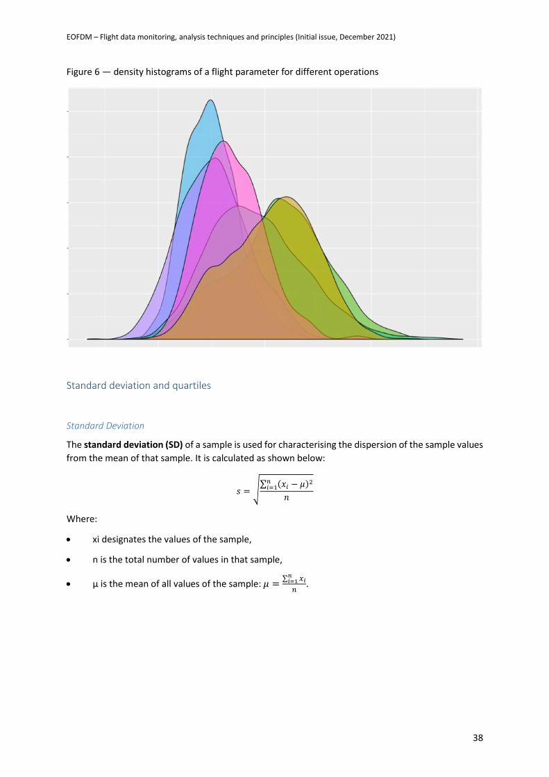
EOFDM – Flight data monitoring, analysis techniques and principles (Initial issue, December 2021)
38
Figure 6 — density histograms of a flight parameter for different operations
Standard deviation and quartiles
Standard Deviation
The standard deviation (SD) of a sample is used for characterising the dispersion of the sample values
from the mean of that sample. It is calculated as shown below:
𝑠 = √∑ (𝑥𝑖 − 𝜇)
2𝑛𝑖=1
𝑛
Where:
• xi designates the values of the sample,
• n is the total number of values in that sample,
• µ is the mean of all values of the sample: 𝜇 =∑ 𝑥𝑖𝑛𝑖=1
𝑛.
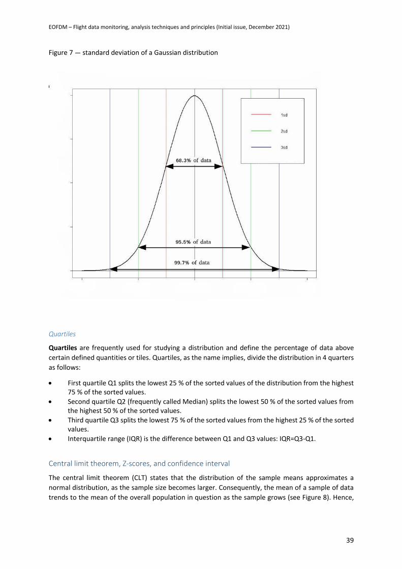
EOFDM – Flight data monitoring, analysis techniques and principles (Initial issue, December 2021)
39
Figure 7 — standard deviation of a Gaussian distribution
Quartiles
Quartiles are frequently used for studying a distribution and define the percentage of data above
certain defined quantities or tiles. Quartiles, as the name implies, divide the distribution in 4 quarters
as follows:
• First quartile Q1 splits the lowest 25 % of the sorted values of the distribution from the highest 75 % of the sorted values.
• Second quartile Q2 (frequently called Median) splits the lowest 50 % of the sorted values from the highest 50 % of the sorted values.
• Third quartile Q3 splits the lowest 75 % of the sorted values from the highest 25 % of the sorted values.
• Interquartile range (IQR) is the difference between Q1 and Q3 values: IQR=Q3-Q1.
Central limit theorem, Z-scores, and confidence interval
The central limit theorem (CLT) states that the distribution of the sample means approximates a
normal distribution, as the sample size becomes larger. Consequently, the mean of a sample of data
trends to the mean of the overall population in question as the sample grows (see Figure 8). Hence,
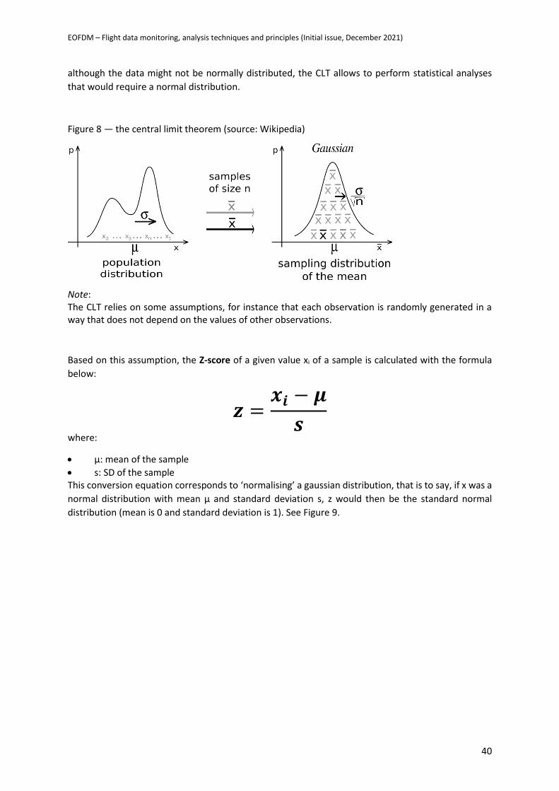
EOFDM – Flight data monitoring, analysis techniques and principles (Initial issue, December 2021)
40
although the data might not be normally distributed, the CLT allows to perform statistical analyses
that would require a normal distribution.
Figure 8 — the central limit theorem (source: Wikipedia)
Note: The CLT relies on some assumptions, for instance that each observation is randomly generated in a way that does not depend on the values of other observations.
Based on this assumption, the Z-score of a given value xi of a sample is calculated with the formula
below:
𝒛 =𝒙𝒊 − 𝝁
𝒔
where:
• μ: mean of the sample
• s: SD of the sample This conversion equation corresponds to ‘normalising’ a gaussian distribution, that is to say, if x was a
normal distribution with mean μ and standard deviation s, z would then be the standard normal
distribution (mean is 0 and standard deviation is 1). See Figure 9.
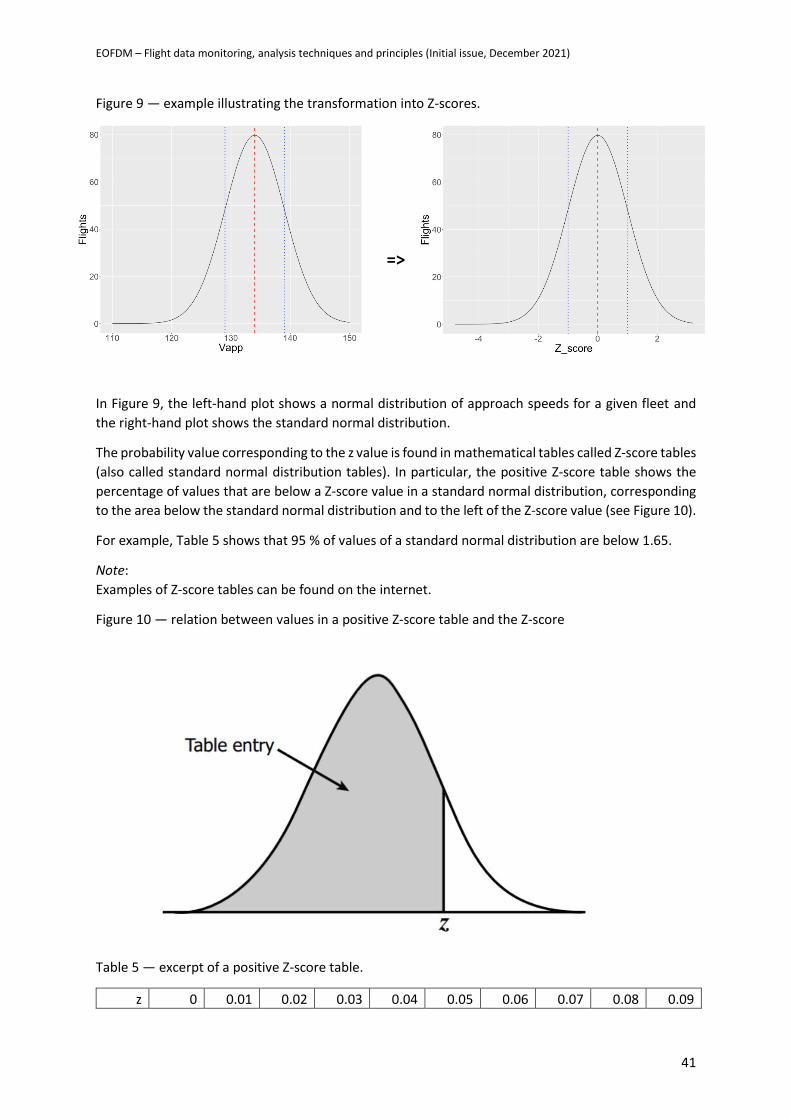
EOFDM – Flight data monitoring, analysis techniques and principles (Initial issue, December 2021)
41
Figure 9 — example illustrating the transformation into Z-scores.
=>
In Figure 9, the left-hand plot shows a normal distribution of approach speeds for a given fleet and
the right-hand plot shows the standard normal distribution.
The probability value corresponding to the z value is found in mathematical tables called Z-score tables
(also called standard normal distribution tables). In particular, the positive Z-score table shows the
percentage of values that are below a Z-score value in a standard normal distribution, corresponding
to the area below the standard normal distribution and to the left of the Z-score value (see Figure 10).
For example, Table 5 shows that 95 % of values of a standard normal distribution are below 1.65.
Note:
Examples of Z-score tables can be found on the internet.
Figure 10 — relation between values in a positive Z-score table and the Z-score
Table 5 — excerpt of a positive Z-score table.
z 0 0.01 0.02 0.03 0.04 0.05 0.06 0.07 0.08 0.09
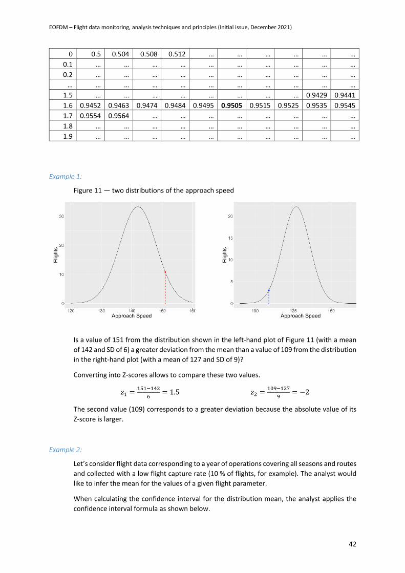
EOFDM – Flight data monitoring, analysis techniques and principles (Initial issue, December 2021)
42
0 0.5 0.504 0.508 0.512 … … … … … …
0.1 … … … … … … … … … …
0.2 … … … … … … … … … …
… … … … … … … … … … …
1.5 … … … … … … … … 0.9429 0.9441
1.6 0.9452 0.9463 0.9474 0.9484 0.9495 0.9505 0.9515 0.9525 0.9535 0.9545
1.7 0.9554 0.9564 … … … … … … … …
1.8 … … … … … … … … … …
1.9 … … … … … … … … … …
Example 1:
Figure 11 — two distributions of the approach speed
Is a value of 151 from the distribution shown in the left-hand plot of Figure 11 (with a mean
of 142 and SD of 6) a greater deviation from the mean than a value of 109 from the distribution
in the right-hand plot (with a mean of 127 and SD of 9)?
Converting into Z-scores allows to compare these two values.
𝑧1 =151−142
6= 1.5 𝑧2 =
109−127
9= −2
The second value (109) corresponds to a greater deviation because the absolute value of its
Z-score is larger.
Example 2:
Let’s consider flight data corresponding to a year of operations covering all seasons and routes
and collected with a low flight capture rate (10 % of flights, for example). The analyst would
like to infer the mean for the values of a given flight parameter.
When calculating the confidence interval for the distribution mean, the analyst applies the
confidence interval formula as shown below.
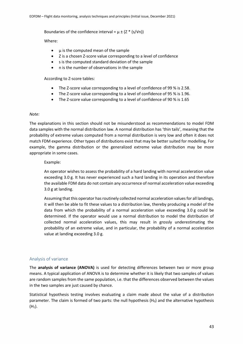
EOFDM – Flight data monitoring, analysis techniques and principles (Initial issue, December 2021)
43
Boundaries of the confidence interval = µ ± (Z * (s/√n))
Where:
• µ is the computed mean of the sample
• Z is a chosen Z-score value corresponding to a level of confidence
• s is the computed standard deviation of the sample
• n is the number of observations in the sample
According to Z-score tables:
• The Z-score value corresponding to a level of confidence of 99 % is 2.58.
• The Z-score value corresponding to a level of confidence of 95 % is 1.96.
• The Z-score value corresponding to a level of confidence of 90 % is 1.65
Note:
The explanations in this section should not be misunderstood as recommendations to model FDM
data samples with the normal distribution law. A normal distribution has ‘thin tails’, meaning that the
probability of extreme values computed from a normal distribution is very low and often it does not
match FDM experience. Other types of distributions exist that may be better suited for modelling. For
example, the gamma distribution or the generalized extreme value distribution may be more
appropriate in some cases.
Example:
An operator wishes to assess the probability of a hard landing with normal acceleration value
exceeding 3.0 g. It has never experienced such a hard landing in its operation and therefore
the available FDM data do not contain any occurrence of normal acceleration value exceeding
3.0 g at landing.
Assuming that this operator has routinely collected normal acceleration values for all landings,
it will then be able to fit these values to a distribution law, thereby producing a model of the
data from which the probability of a normal acceleration value exceeding 3.0 g could be
determined. If the operator would use a normal distribution to model the distribution of
collected normal acceleration values, this may result in grossly underestimating the
probability of an extreme value, and in particular, the probability of a normal acceleration
value at landing exceeding 3.0 g.
Analysis of variance
The analysis of variance (ANOVA) is used for detecting differences between two or more group
means. A typical application of ANOVA is to determine whether it is likely that two samples of values
are random samples from the same population, i.e. that the differences observed between the values
in the two samples are just caused by chance.
Statistical hypothesis testing involves evaluating a claim made about the value of a distribution
parameter. The claim is formed of two parts: the null hypothesis (H0) and the alternative hypothesis
(H1).
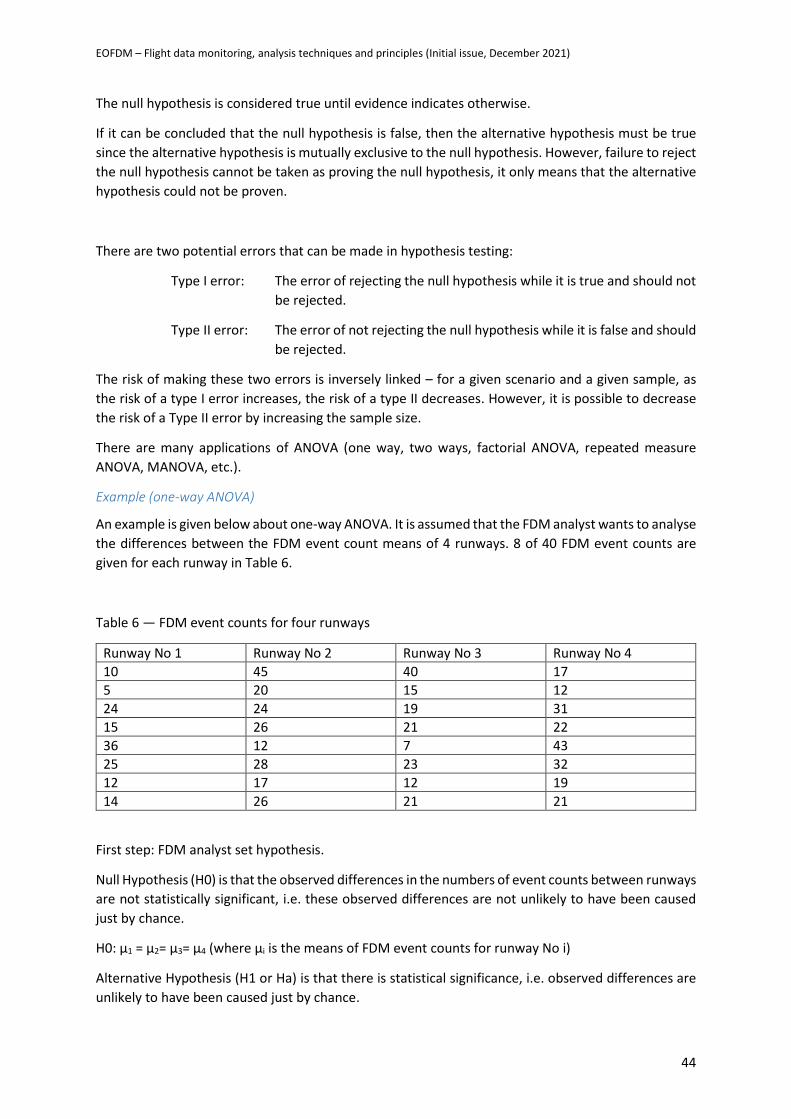
EOFDM – Flight data monitoring, analysis techniques and principles (Initial issue, December 2021)
44
The null hypothesis is considered true until evidence indicates otherwise.
If it can be concluded that the null hypothesis is false, then the alternative hypothesis must be true
since the alternative hypothesis is mutually exclusive to the null hypothesis. However, failure to reject
the null hypothesis cannot be taken as proving the null hypothesis, it only means that the alternative
hypothesis could not be proven.
There are two potential errors that can be made in hypothesis testing:
Type I error: The error of rejecting the null hypothesis while it is true and should not
be rejected.
Type II error: The error of not rejecting the null hypothesis while it is false and should
be rejected.
The risk of making these two errors is inversely linked – for a given scenario and a given sample, as
the risk of a type I error increases, the risk of a type II decreases. However, it is possible to decrease
the risk of a Type II error by increasing the sample size.
There are many applications of ANOVA (one way, two ways, factorial ANOVA, repeated measure
ANOVA, MANOVA, etc.).
Example (one-way ANOVA)
An example is given below about one-way ANOVA. It is assumed that the FDM analyst wants to analyse
the differences between the FDM event count means of 4 runways. 8 of 40 FDM event counts are
given for each runway in Table 6.
Table 6 — FDM event counts for four runways
Runway No 1 Runway No 2 Runway No 3 Runway No 4
10 45 40 17
5 20 15 12
24 24 19 31
15 26 21 22
36 12 7 43
25 28 23 32
12 17 12 19
14 26 21 21
First step: FDM analyst set hypothesis.
Null Hypothesis (H0) is that the observed differences in the numbers of event counts between runways
are not statistically significant, i.e. these observed differences are not unlikely to have been caused
just by chance.
H0: μ1 = μ2= μ3= μ4 (where μi is the means of FDM event counts for runway No i)
Alternative Hypothesis (H1 or Ha) is that there is statistical significance, i.e. observed differences are
unlikely to have been caused just by chance.
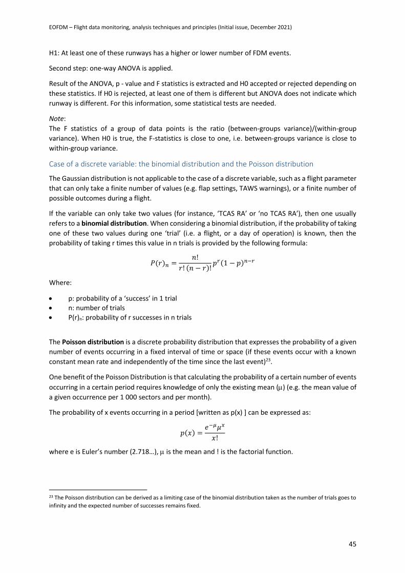
EOFDM – Flight data monitoring, analysis techniques and principles (Initial issue, December 2021)
45
H1: At least one of these runways has a higher or lower number of FDM events.
Second step: one-way ANOVA is applied.
Result of the ANOVA, p - value and F statistics is extracted and H0 accepted or rejected depending on
these statistics. If H0 is rejected, at least one of them is different but ANOVA does not indicate which
runway is different. For this information, some statistical tests are needed.
Note:
The F statistics of a group of data points is the ratio (between-groups variance)/(within-group
variance). When H0 is true, the F-statistics is close to one, i.e. between-groups variance is close to
within-group variance.
Case of a discrete variable: the binomial distribution and the Poisson distribution
The Gaussian distribution is not applicable to the case of a discrete variable, such as a flight parameter
that can only take a finite number of values (e.g. flap settings, TAWS warnings), or a finite number of
possible outcomes during a flight.
If the variable can only take two values (for instance, ‘TCAS RA’ or ‘no TCAS RA’), then one usually
refers to a binomial distribution. When considering a binomial distribution, if the probability of taking
one of these two values during one ‘trial’ (i.e. a flight, or a day of operation) is known, then the
probability of taking r times this value in n trials is provided by the following formula:
𝑃(𝑟)𝑛 =𝑛!
𝑟! (𝑛 − 𝑟)!𝑝𝑟(1 − 𝑝)𝑛−𝑟
Where:
• p: probability of a ‘success’ in 1 trial
• n: number of trials
• P(r)n: probability of r successes in n trials
The Poisson distribution is a discrete probability distribution that expresses the probability of a given
number of events occurring in a fixed interval of time or space (if these events occur with a known
constant mean rate and independently of the time since the last event)23.
One benefit of the Poisson Distribution is that calculating the probability of a certain number of events
occurring in a certain period requires knowledge of only the existing mean () (e.g. the mean value of
a given occurrence per 1 000 sectors and per month).
The probability of x events occurring in a period [written as p(x) ] can be expressed as:
𝑝(𝑥) =𝑒−𝜇𝜇𝑥
𝑥!
where e is Euler’s number (2.718…), is the mean and ! is the factorial function.
23 The Poisson distribution can be derived as a limiting case of the binomial distribution taken as the number of trials goes to
infinity and the expected number of successes remains fixed.
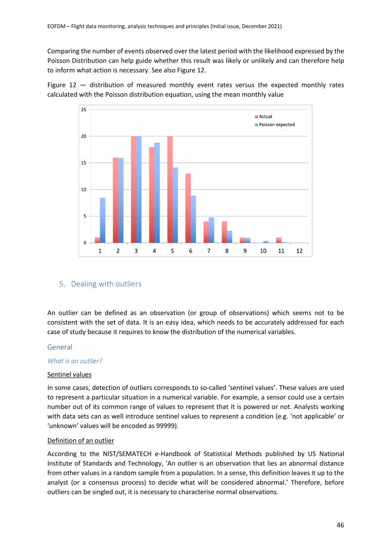
EOFDM – Flight data monitoring, analysis techniques and principles (Initial issue, December 2021)
46
Comparing the number of events observed over the latest period with the likelihood expressed by the
Poisson Distribution can help guide whether this result was likely or unlikely and can therefore help
to inform what action is necessary. See also Figure 12.
Figure 12 — distribution of measured monthly event rates versus the expected monthly rates
calculated with the Poisson distribution equation, using the mean monthly value
5. Dealing with outliers
An outlier can be defined as an observation (or group of observations) which seems not to be
consistent with the set of data. It is an easy idea, which needs to be accurately addressed for each
case of study because it requires to know the distribution of the numerical variables.
General
What is an outlier?
Sentinel values
In some cases, detection of outliers corresponds to so-called ‘sentinel values’. These values are used
to represent a particular situation in a numerical variable. For example, a sensor could use a certain
number out of its common range of values to represent that it is powered or not. Analysts working
with data sets can as well introduce sentinel values to represent a condition (e.g. ‘not applicable’ or
‘unknown’ values will be encoded as 99999).
Definition of an outlier
According to the NIST/SEMATECH e-Handbook of Statistical Methods published by US National
Institute of Standards and Technology, 'An outlier is an observation that lies an abnormal distance
from other values in a random sample from a population. In a sense, this definition leaves it up to the
analyst (or a consensus process) to decide what will be considered abnormal.’ Therefore, before
outliers can be singled out, it is necessary to characterise normal observations.
EOFDM – Flight data monitoring, analysis techniques and principles (Initial issue, December 2021)
47
Importance of addressing outliers
Performing an analysis with multiple outliers can result in a false outcome. However, the process of
dealing with outliers needs special attention because, if not correctly done, it might have a significant
impact on the analysis. There are multiple techniques to deal with outliers depending on how the data
looks like, explaining some of them would help.
Finally, an outlier might be a real value and some knowledge of the order of magnitude and/or sensor
limits is needed to distinguish between a real value, or an outlier caused by other reasons (e.g. sensor
reading error, integration of data, etc). If the outlier corresponds to a real event, then a corrective
action may need to be done urgently, e.g. a technical inspection after a hard landing.
Detection and assessment of outliers
Use of domain knowledge
Sometimes, the typical range of a value is known.
For example, when measuring the normal acceleration at landing, a typical range could be between 1 and 2 g. Therefore, normal accelerations values outside of the domain [1 g; 2 g] could be considered abnormal, whether they are outliers or not.
Another example is the typical airspeed during approach, for which the reference speed (Vref) in the flight crew operating manual provides indicative value.
Comparing the mean and the median
A histogram can be a helpful visual tool for a quick overlook of a distribution. However, the presence of outliers can be determined even without plotting data, by comparing the median and the mean of a distribution. The examples below illustrate the fact that the median is much less affected by outliers in a set of values than the mean. This feature may be used as a quick check of the data to identify outliers.
Example 1: Test data without outliers
A test set of 100 values was randomly generated by a function simulating a normal distribution with a mean of 10 and a standard deviation of 1. This test data is displayed in a histogram (see Figure 13) and in the below summary (see Table 7).
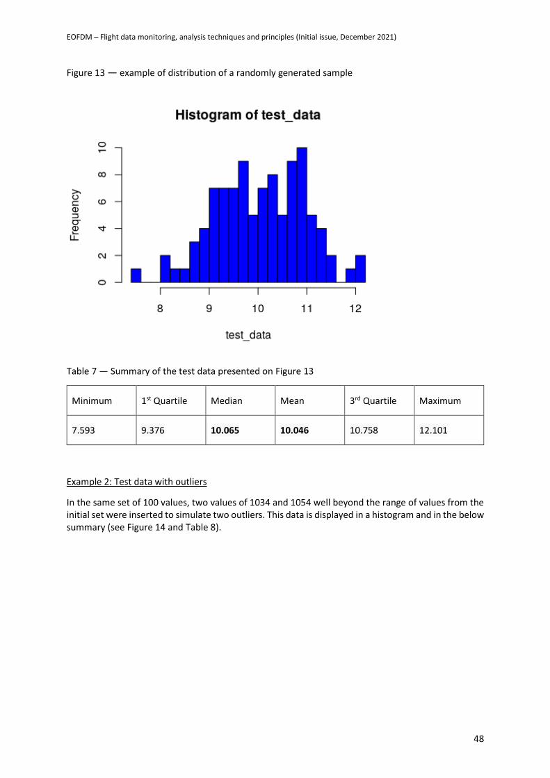
EOFDM – Flight data monitoring, analysis techniques and principles (Initial issue, December 2021)
48
Figure 13 — example of distribution of a randomly generated sample
Table 7 — Summary of the test data presented on Figure 13
Minimum 1st Quartile Median Mean 3rd Quartile Maximum
7.593 9.376 10.065 10.046 10.758 12.101
Example 2: Test data with outliers
In the same set of 100 values, two values of 1034 and 1054 well beyond the range of values from the initial set were inserted to simulate two outliers. This data is displayed in a histogram and in the below summary (see Figure 14 and Table 8).
EOFDM – Flight data monitoring, analysis techniques and principles (Initial issue, December 2021)
49
Figure 14 — example of of distribution of a randomly generated sample, in which two outlier values were inserted
Table 8 — summary of the test data presented on Figure 14
Minimum 1st Quartile Median Mean 3rd Quartile Maximum
7.593 9.386 10.069 30.319 10.831 1054
Examining the summary of the data in Table 8, the first observation is that the mean and the median values are not of the same magnitude and the second is that the median value was only slightly affected by the outliers when comparing to the median values obtained from the previous example. The mean value was significantly affected by introducing outliers in the dataset.
To conclude, a summary of the data containing the mean and the median can be very helpful to identify that outliers may be present in the sample.
Using boxplots
When some outliers have been detected, two questions may come to mind. Is the outlier value
stemming from a data quality issue or a programming error, or is it genuine? If it is a genuine value,
the analyst should analyse this outlier value.
For detecting outlier values, a boxplot could also be used.

EOFDM – Flight data monitoring, analysis techniques and principles (Initial issue, December 2021)
50
According to the NIST/SEMATECH e-Handbook of Statistical Methods, a boxplot is ‘constructed by
drawing a box between the upper and lower quartiles with a solid line drawn across the box to locate
the median. The following quantities (called fences) are needed for identifying extreme values in the
tails of the distribution:
• lower inner fence: Q1 - 1.5*IQ
• upper inner fence: Q3 + 1.5*IQ
• lower outer fence: Q1 - 3*IQ
• upper outer fence: Q3 + 3*IQ’
In addition, the NIST/SEMATECH e-Handbook of Statistical Methods proposes that ‘a point beyond an
inner fence on either side is considered a mild outlier. A point beyond an outer fence is considered
an extreme outlier.’
As shown in Figure 15, in the case of a normal distribution, 99.3 % of the values are between the lower
and inner fences, i.e. 0.7 % of the values would be considered outliers according to the
NIST/SEMATECH e-Handbook of Statistical Methods.
EOFDM – Flight data monitoring, analysis techniques and principles (Initial issue, December 2021)
51
Figure 15 — boxplot of a normal distribution (Author: Michael Galarnyk, source: towards data
science)
Example of use of boxplots
Consider that the event rates of all FDM event algorithms are compared to each other using a boxplot
chart. This would allow visually identify FDM event algorithms with a non-typical FDM event rate.
Figure 16 shows a boxplot example for an operator. In this example FDM event rates (y axis – values
in %) based on the severity level have been compared to each other for different flight cycles and
different FDM event algorithms. Every red dot represents an individual outlier FDM event rate for the
selected severity and the number of flights considered.
Figure 16 gives an overall picture of those FDM event algorithms that seem to have a much higher
rate. This could be used for:
• monitoring any emerging trend in the FDM event set;
EOFDM – Flight data monitoring, analysis techniques and principles (Initial issue, December 2021)
52
• calibrating/standardising the severity levels of FDM event algorithms (in view of creating a composite index);
• benchmarking against other operators that would use the same FDM event algorithms.
While dealing FDM event count and FDM event rate cannot have negative values, therefore lower
boundaries are statistically not represented.
Figure 16 — an operator example for using boxplot
To illustrate the boxplot methodology, Figures 17 and 18 below might be helpful. Figure 18 shows 20 data points lined up on a blank numerical axis and illustrates the terms that are used for calculations of boundaries.
Figure 17 — factors of boxplot
−
LOWERQUARTILE
(Q1)
UPPERQUARTILE
(Q3)
MEDIANLOWESTSAMPLEVALUE
HIGHESTSAMPLEVALUE
INTERQUARTILERANGE(IQR)
EOFDM – Flight data monitoring, analysis techniques and principles (Initial issue, December 2021)
53
Figure 18 shows an example of use of the boxplot formula to calculate boundaries and identify the
outliers. In this example, the two FDM event algorithms No 15 and No 20 are defined as outliers due
to their high number of event counts.
Figure 18 — example of using boxplot to identify FDM event counts that seem to be outliers
Note: When working with FDM event counts and rates there is no need to calculate the lower boundaries. However, if the boxplot method is applied to a recorded or calculated FDM parameter such as ‘Airspeed at Touchdown’ or ‘Landing Distance,’ then lower boundaries should be considered as well to see the lower value outliers.
Using scatter plots
Figure 19 illustrates the benefit potentially brought by a scatter plot for the visual identification of outliers. Each point of the scatter plot corresponds to a data snapshot that consists of the maximum groundspeed value and the maximum pitch attitude value that were collected during the approach phase of an individual flight. The point colour is used to identify the aircraft operator.
In Figure 19, at least three data snapshots can be visually identified as outliers because their maximum pitch attitude value and/or maximum groundspeed bring them far away from the rest of the points on the scatter plot. The histogram shows that these outliers cannot be visually identified when the distributions of max groundspeed or max pitch attitude of these data snapshots are plotted separately.
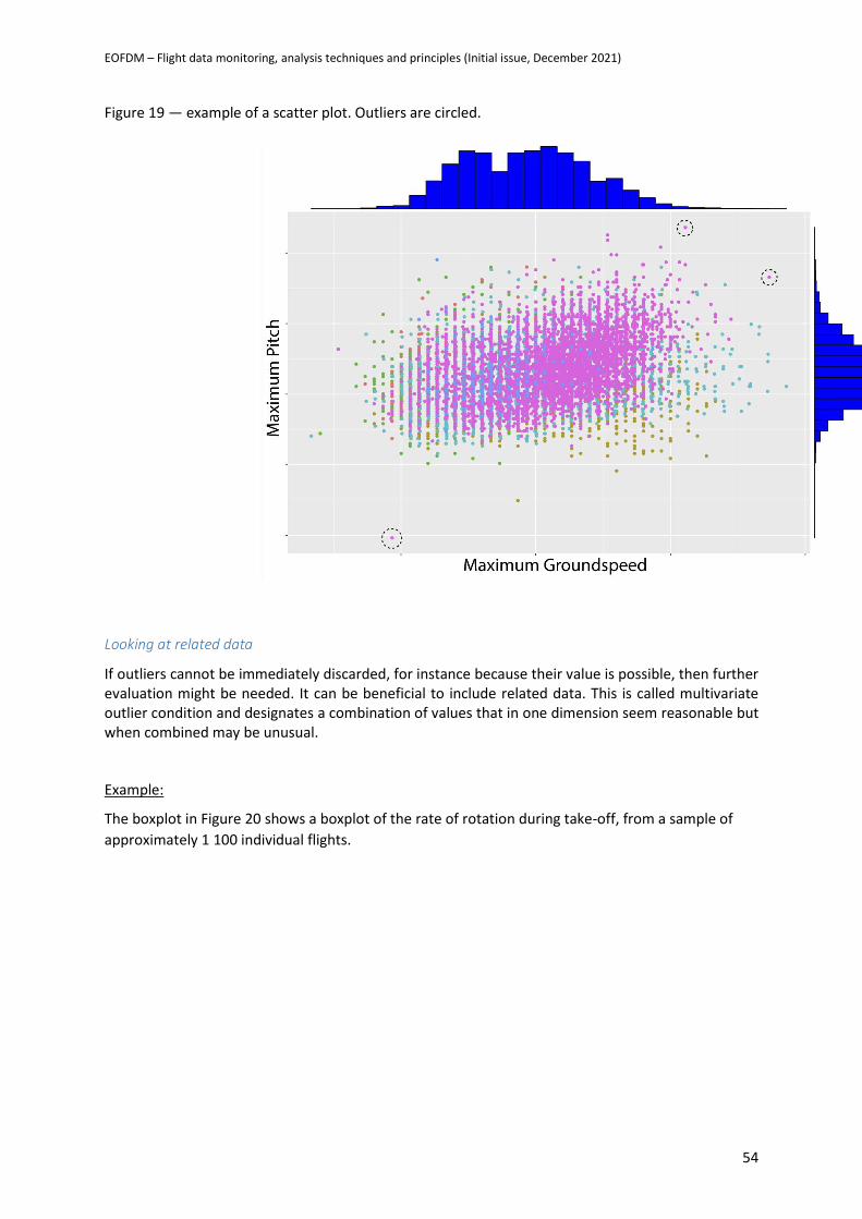
EOFDM – Flight data monitoring, analysis techniques and principles (Initial issue, December 2021)
54
Figure 19 — example of a scatter plot. Outliers are circled.
Looking at related data
If outliers cannot be immediately discarded, for instance because their value is possible, then further evaluation might be needed. It can be beneficial to include related data. This is called multivariate outlier condition and designates a combination of values that in one dimension seem reasonable but when combined may be unusual.
Example:
The boxplot in Figure 20 shows a boxplot of the rate of rotation during take-off, from a sample of
approximately 1 100 individual flights.
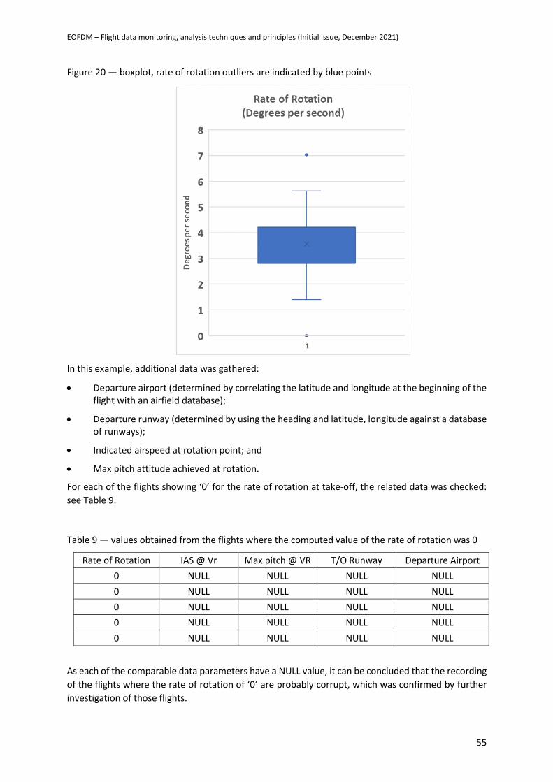
EOFDM – Flight data monitoring, analysis techniques and principles (Initial issue, December 2021)
55
Figure 20 — boxplot, rate of rotation outliers are indicated by blue points
In this example, additional data was gathered:
• Departure airport (determined by correlating the latitude and longitude at the beginning of the flight with an airfield database);
• Departure runway (determined by using the heading and latitude, longitude against a database of runways);
• Indicated airspeed at rotation point; and
• Max pitch attitude achieved at rotation.
For each of the flights showing ‘0’ for the rate of rotation at take-off, the related data was checked:
see Table 9.
Table 9 — values obtained from the flights where the computed value of the rate of rotation was 0
Rate of Rotation IAS @ Vr Max pitch @ VR T/O Runway Departure Airport
0 NULL NULL NULL NULL
0 NULL NULL NULL NULL
0 NULL NULL NULL NULL
0 NULL NULL NULL NULL
0 NULL NULL NULL NULL
As each of the comparable data parameters have a NULL value, it can be concluded that the recording
of the flights where the rate of rotation of ‘0’ are probably corrupt, which was confirmed by further
investigation of those flights.
EOFDM – Flight data monitoring, analysis techniques and principles (Initial issue, December 2021)
56
The remaining outlier values appear to have valid values for the related data parameters: see Table 10.
Table 10 — values obtained from the flights
Rate of Rotation IAS @ Vr Max pitch @ VR T/O Runway Departure Airport
7 112 15.1 07 XXX
7 112 14.8 14 YYY
6. Monitoring trends with statistics
Statistics should include areas where the safety risk has been successfully reduced, not only the
problematic areas. This can contribute to encouraging efforts of flight crew members and other staff
members.
Trend Evaluation Areas
General Evaluation
Overall assessment is important to see the full picture. Details should be avoided at this stage. The
aim is to identify general trends. On the other hand, this method can also be used to see the results
of past changes (changes in training method, newly recruited pilot groups, procedure changes, etc.).
It may be considered to regularly share the general evaluation results with internal stakeholders (such
as FDM Board members, flight operations, training departments).
The overall assessment will show where to focus (negative trend in unstable approaches, increase in
hard landings, etc.). With detailed evaluations to be made after that, it is necessary to try to find
answers to more detailed questions such as when (which phase), where (which runway), how (which
event), etc.
For example, an FDM event rate may be tracked over time to look for any developing trend, which can
be used for prediction. A simple time series can help to highlight any seasonality in the data.
When there is enough data, it can be useful to make year-on-year comparisons of the time series as
shown in Figure 21.
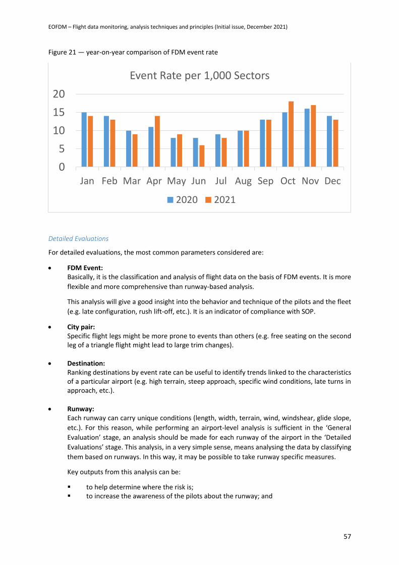
EOFDM – Flight data monitoring, analysis techniques and principles (Initial issue, December 2021)
57
Figure 21 — year-on-year comparison of FDM event rate
Detailed Evaluations
For detailed evaluations, the most common parameters considered are:
• FDM Event: Basically, it is the classification and analysis of flight data on the basis of FDM events. It is more
flexible and more comprehensive than runway-based analysis.
This analysis will give a good insight into the behavior and technique of the pilots and the fleet
(e.g. late configuration, rush lift-off, etc.). It is an indicator of compliance with SOP.
• City pair: Specific flight legs might be more prone to events than others (e.g. free seating on the second leg of a triangle flight might lead to large trim changes).
• Destination: Ranking destinations by event rate can be useful to identify trends linked to the characteristics of a particular airport (e.g. high terrain, steep approach, specific wind conditions, late turns in approach, etc.).
• Runway: Each runway can carry unique conditions (length, width, terrain, wind, windshear, glide slope,
etc.). For this reason, while performing an airport-level analysis is sufficient in the ‘General
Evaluation’ stage, an analysis should be made for each runway of the airport in the ‘Detailed
Evaluations’ stage. This analysis, in a very simple sense, means analysing the data by classifying
them based on runways. In this way, it may be possible to take runway specific measures.
Key outputs from this analysis can be:
▪ to help determine where the risk is; ▪ to increase the awareness of the pilots about the runway; and
0
5
10
15
20
Jan Feb Mar Apr May Jun Jul Aug Sep Oct Nov Dec
Event Rate per 1,000 Sectors
2020 2021
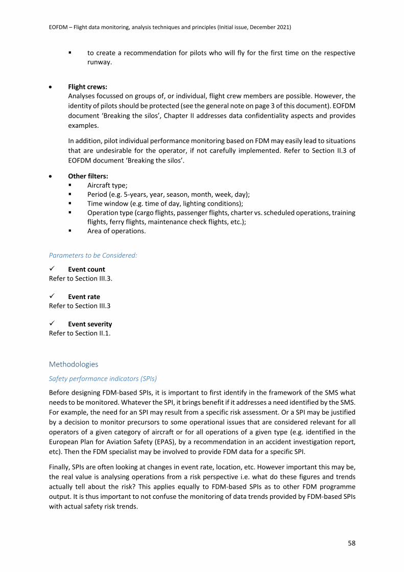
EOFDM – Flight data monitoring, analysis techniques and principles (Initial issue, December 2021)
58
▪ to create a recommendation for pilots who will fly for the first time on the respective runway.
• Flight crews: Analyses focussed on groups of, or individual, flight crew members are possible. However, the
identity of pilots should be protected (see the general note on page 3 of this document). EOFDM
document ‘Breaking the silos’, Chapter II addresses data confidentiality aspects and provides
examples.
In addition, pilot individual performance monitoring based on FDM may easily lead to situations
that are undesirable for the operator, if not carefully implemented. Refer to Section II.3 of
EOFDM document ‘Breaking the silos’.
• Other filters: ▪ Aircraft type; ▪ Period (e.g. 5-years, year, season, month, week, day); ▪ Time window (e.g. time of day, lighting conditions); ▪ Operation type (cargo flights, passenger flights, charter vs. scheduled operations, training
flights, ferry flights, maintenance check flights, etc.); ▪ Area of operations.
Parameters to be Considered:
✓ Event count Refer to Section III.3. ✓ Event rate Refer to Section III.3 ✓ Event severity Refer to Section II.1.
Methodologies
Safety performance indicators (SPIs)
Before designing FDM-based SPIs, it is important to first identify in the framework of the SMS what
needs to be monitored. Whatever the SPI, it brings benefit if it addresses a need identified by the SMS.
For example, the need for an SPI may result from a specific risk assessment. Or a SPI may be justified
by a decision to monitor precursors to some operational issues that are considered relevant for all
operators of a given category of aircraft or for all operations of a given type (e.g. identified in the
European Plan for Aviation Safety (EPAS), by a recommendation in an accident investigation report,
etc). Then the FDM specialist may be involved to provide FDM data for a specific SPI.
Finally, SPIs are often looking at changes in event rate, location, etc. However important this may be,
the real value is analysing operations from a risk perspective i.e. what do these figures and trends
actually tell about the risk? This applies equally to FDM-based SPIs as to other FDM programme
output. It is thus important to not confuse the monitoring of data trends provided by FDM-based SPIs
with actual safety risk trends.
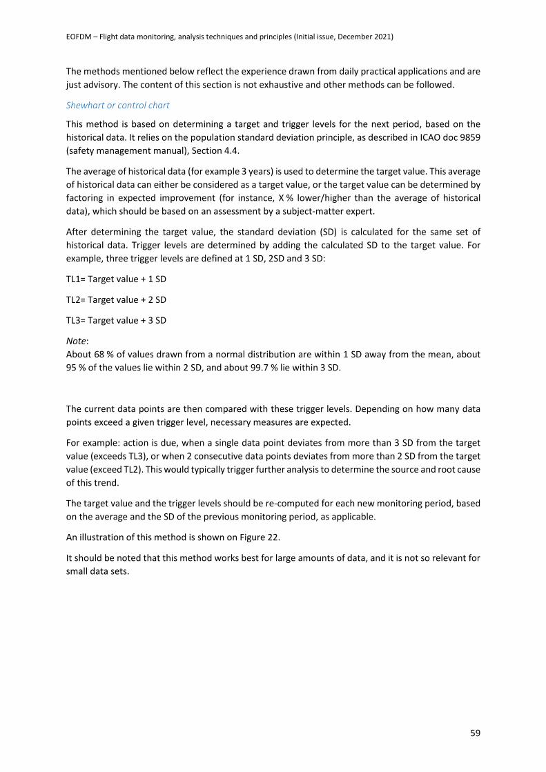
EOFDM – Flight data monitoring, analysis techniques and principles (Initial issue, December 2021)
59
The methods mentioned below reflect the experience drawn from daily practical applications and are
just advisory. The content of this section is not exhaustive and other methods can be followed.
Shewhart or control chart
This method is based on determining a target and trigger levels for the next period, based on the
historical data. It relies on the population standard deviation principle, as described in ICAO doc 9859
(safety management manual), Section 4.4.
The average of historical data (for example 3 years) is used to determine the target value. This average
of historical data can either be considered as a target value, or the target value can be determined by
factoring in expected improvement (for instance, X % lower/higher than the average of historical
data), which should be based on an assessment by a subject-matter expert.
After determining the target value, the standard deviation (SD) is calculated for the same set of
historical data. Trigger levels are determined by adding the calculated SD to the target value. For
example, three trigger levels are defined at 1 SD, 2SD and 3 SD:
TL1= Target value + 1 SD
TL2= Target value + 2 SD
TL3= Target value + 3 SD
Note:
About 68 % of values drawn from a normal distribution are within 1 SD away from the mean, about
95 % of the values lie within 2 SD, and about 99.7 % lie within 3 SD.
The current data points are then compared with these trigger levels. Depending on how many data
points exceed a given trigger level, necessary measures are expected.
For example: action is due, when a single data point deviates from more than 3 SD from the target
value (exceeds TL3), or when 2 consecutive data points deviates from more than 2 SD from the target
value (exceed TL2). This would typically trigger further analysis to determine the source and root cause
of this trend.
The target value and the trigger levels should be re-computed for each new monitoring period, based
on the average and the SD of the previous monitoring period, as applicable.
An illustration of this method is shown on Figure 22.
It should be noted that this method works best for large amounts of data, and it is not so relevant for
small data sets.
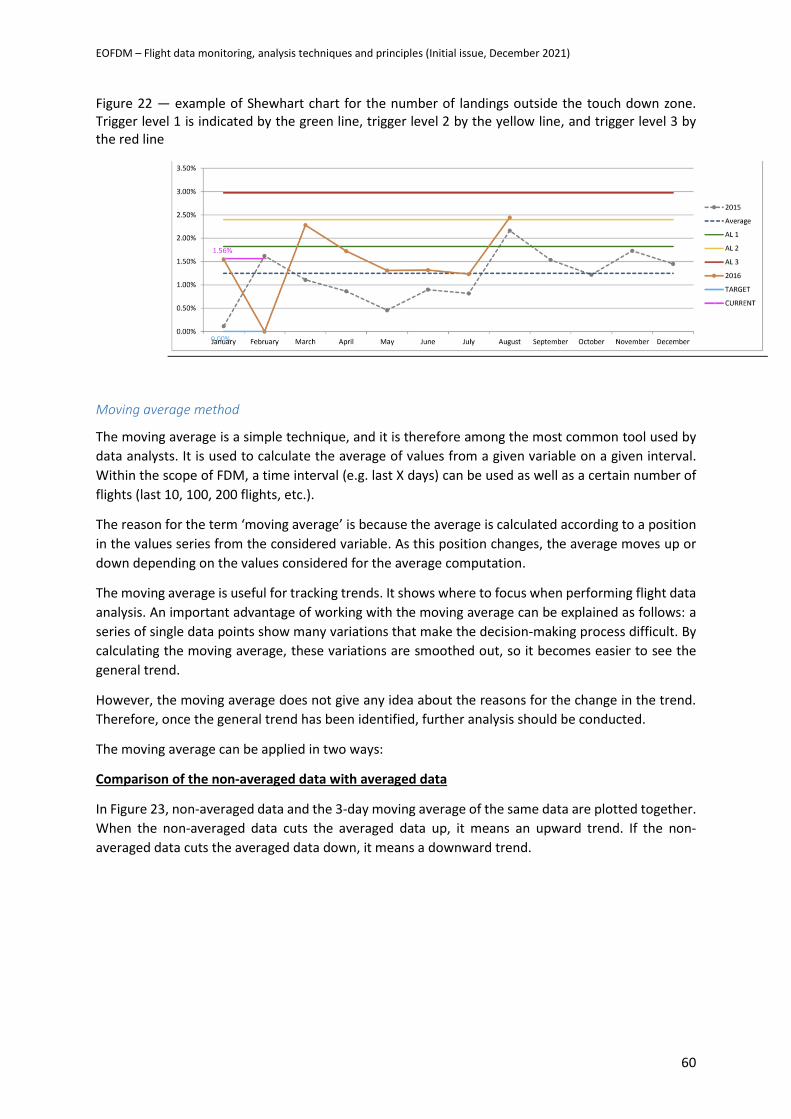
EOFDM – Flight data monitoring, analysis techniques and principles (Initial issue, December 2021)
60
Figure 22 — example of Shewhart chart for the number of landings outside the touch down zone. Trigger level 1 is indicated by the green line, trigger level 2 by the yellow line, and trigger level 3 by the red line
Moving average method
The moving average is a simple technique, and it is therefore among the most common tool used by
data analysts. It is used to calculate the average of values from a given variable on a given interval.
Within the scope of FDM, a time interval (e.g. last X days) can be used as well as a certain number of
flights (last 10, 100, 200 flights, etc.).
The reason for the term ‘moving average’ is because the average is calculated according to a position
in the values series from the considered variable. As this position changes, the average moves up or
down depending on the values considered for the average computation.
The moving average is useful for tracking trends. It shows where to focus when performing flight data
analysis. An important advantage of working with the moving average can be explained as follows: a
series of single data points show many variations that make the decision-making process difficult. By
calculating the moving average, these variations are smoothed out, so it becomes easier to see the
general trend.
However, the moving average does not give any idea about the reasons for the change in the trend.
Therefore, once the general trend has been identified, further analysis should be conducted.
The moving average can be applied in two ways:
Comparison of the non-averaged data with averaged data
In Figure 23, non-averaged data and the 3-day moving average of the same data are plotted together.
When the non-averaged data cuts the averaged data up, it means an upward trend. If the non-
averaged data cuts the averaged data down, it means a downward trend.
EOFDM – Flight data monitoring, analysis techniques and principles (Initial issue, December 2021)
61
Figure 23 — time series including a moving average
Comparison between moving averages made on different periods
The moving averages on different periods are shown on the same graph. Depending on the relative
positions taken by these different moving averages, a trend can be identified. In Figure 24, the moving
averages over 3, 5, 10 days of the same data are plotted together. If the curve of the moving average
with the shortest period (Mavg-3 in the example) is below the curves of the other moving averages (in
the example; Mavg-5, Mavg-10), it means a downward trend. On the contrary, if the curve of the
moving average with the shortest period is above the other curves, this means an upward trend. If the
shortest period is between the other two periods, there is a possibility of trend change.
The size of the intervals considered for computing a moving average will vary according to the scope
of the analysis to be made. For example, if long term trend analysis is made on 3 years of data, 180-,
90-, 30-day periods can be used. However, if a shorter-term trend analysis is made on 6-month data,
90, 30, 10 days periods can be used.
Figure 24— plot with three moving averages computed from the same time series, over 3, 5, and 10
points
Blind benchmarking
This consists in presenting individual results compared with a global average.
Refer also to EOFDM document ‘Breaking the silos’, Section I.3.
0
5
10
15
20
25
1 2 3 4 5 6 7 8 9 10 11 12 13 14 15 16 17 18 19 20
Val
ue
Period
Data Mavg(3)
0
5
10
15
20
1 2 3 4 5 6 7 8 9 10 11 12 13 14 15 16 17 18 19 20
Val
ue
Period
Mavg(3) Mavg(5) Mavg(10)
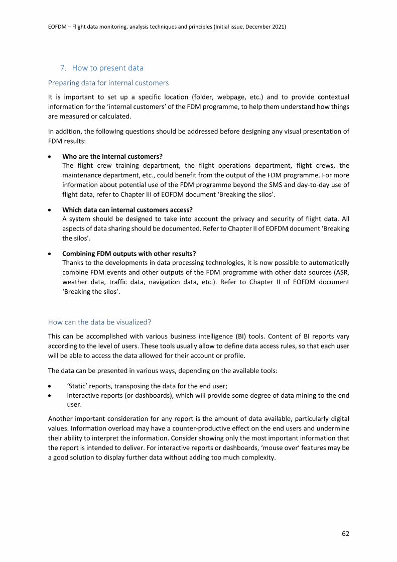
EOFDM – Flight data monitoring, analysis techniques and principles (Initial issue, December 2021)
62
7. How to present data
Preparing data for internal customers
It is important to set up a specific location (folder, webpage, etc.) and to provide contextual
information for the ‘internal customers’ of the FDM programme, to help them understand how things
are measured or calculated.
In addition, the following questions should be addressed before designing any visual presentation of
FDM results:
• Who are the internal customers? The flight crew training department, the flight operations department, flight crews, the
maintenance department, etc., could benefit from the output of the FDM programme. For more
information about potential use of the FDM programme beyond the SMS and day-to-day use of
flight data, refer to Chapter III of EOFDM document ‘Breaking the silos’.
• Which data can internal customers access? A system should be designed to take into account the privacy and security of flight data. All
aspects of data sharing should be documented. Refer to Chapter II of EOFDM document ‘Breaking
the silos’.
• Combining FDM outputs with other results? Thanks to the developments in data processing technologies, it is now possible to automatically
combine FDM events and other outputs of the FDM programme with other data sources (ASR,
weather data, traffic data, navigation data, etc.). Refer to Chapter II of EOFDM document
‘Breaking the silos’.
How can the data be visualized?
This can be accomplished with various business intelligence (BI) tools. Content of BI reports vary
according to the level of users. These tools usually allow to define data access rules, so that each user
will be able to access the data allowed for their account or profile.
The data can be presented in various ways, depending on the available tools:
• ‘Static’ reports, transposing the data for the end user;
• Interactive reports (or dashboards), which will provide some degree of data mining to the end user.
Another important consideration for any report is the amount of data available, particularly digital
values. Information overload may have a counter-productive effect on the end users and undermine
their ability to interpret the information. Consider showing only the most important information that
the report is intended to deliver. For interactive reports or dashboards, ‘mouse over’ features may be
a good solution to display further data without adding too much complexity.
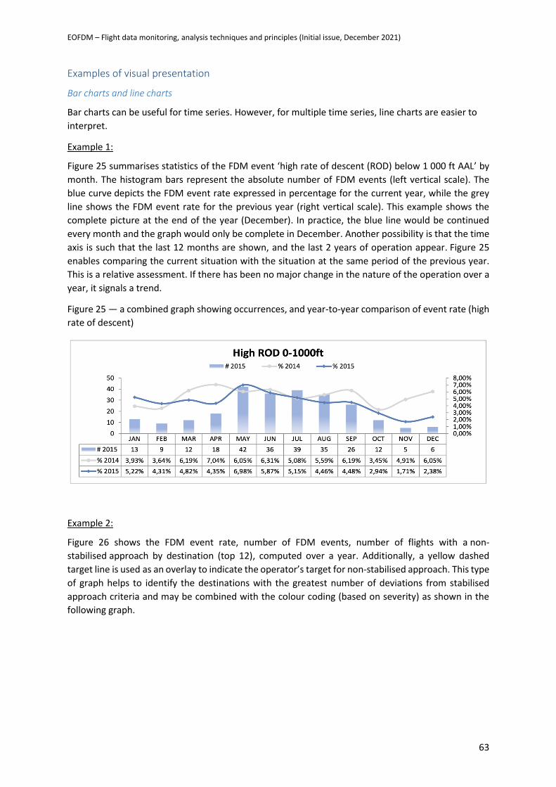
EOFDM – Flight data monitoring, analysis techniques and principles (Initial issue, December 2021)
63
Examples of visual presentation
Bar charts and line charts
Bar charts can be useful for time series. However, for multiple time series, line charts are easier to
interpret.
Example 1:
Figure 25 summarises statistics of the FDM event ‘high rate of descent (ROD) below 1 000 ft AAL’ by
month. The histogram bars represent the absolute number of FDM events (left vertical scale). The
blue curve depicts the FDM event rate expressed in percentage for the current year, while the grey
line shows the FDM event rate for the previous year (right vertical scale). This example shows the
complete picture at the end of the year (December). In practice, the blue line would be continued
every month and the graph would only be complete in December. Another possibility is that the time
axis is such that the last 12 months are shown, and the last 2 years of operation appear. Figure 25
enables comparing the current situation with the situation at the same period of the previous year.
This is a relative assessment. If there has been no major change in the nature of the operation over a
year, it signals a trend.
Figure 25 — a combined graph showing occurrences, and year-to-year comparison of event rate (high
rate of descent)
Example 2:
Figure 26 shows the FDM event rate, number of FDM events, number of flights with a non-
stabilised approach by destination (top 12), computed over a year. Additionally, a yellow dashed
target line is used as an overlay to indicate the operator’s target for non-stabilised approach. This type
of graph helps to identify the destinations with the greatest number of deviations from stabilised
approach criteria and may be combined with the colour coding (based on severity) as shown in the
following graph.
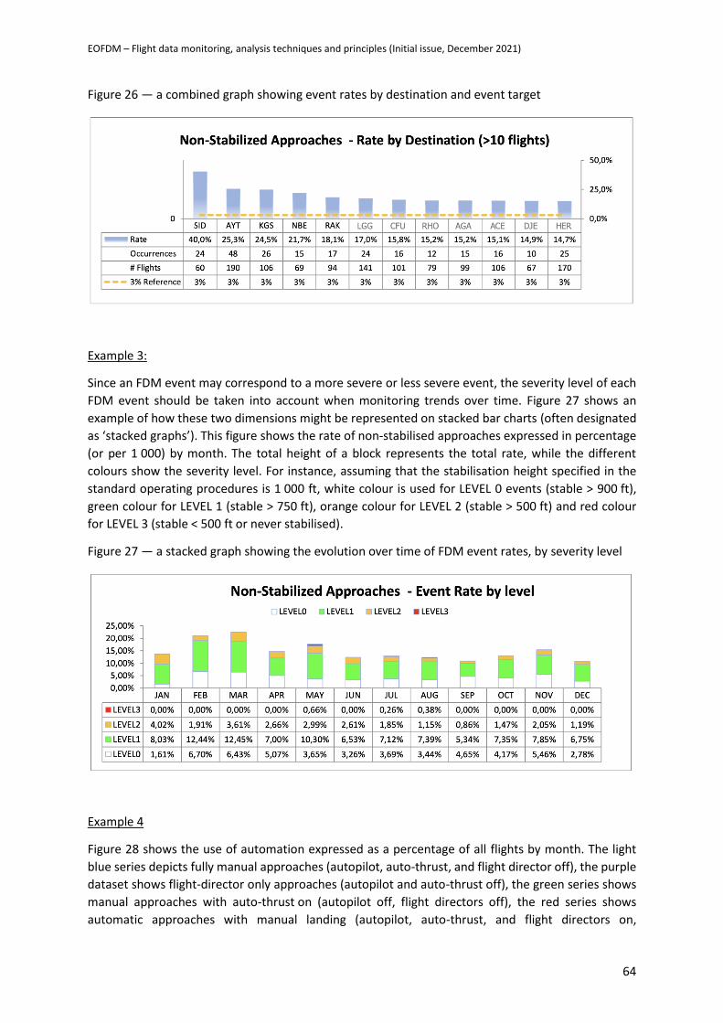
EOFDM – Flight data monitoring, analysis techniques and principles (Initial issue, December 2021)
64
Figure 26 — a combined graph showing event rates by destination and event target
Example 3:
Since an FDM event may correspond to a more severe or less severe event, the severity level of each
FDM event should be taken into account when monitoring trends over time. Figure 27 shows an
example of how these two dimensions might be represented on stacked bar charts (often designated
as ‘stacked graphs’). This figure shows the rate of non-stabilised approaches expressed in percentage
(or per 1 000) by month. The total height of a block represents the total rate, while the different
colours show the severity level. For instance, assuming that the stabilisation height specified in the
standard operating procedures is 1 000 ft, white colour is used for LEVEL 0 events (stable > 900 ft),
green colour for LEVEL 1 (stable > 750 ft), orange colour for LEVEL 2 (stable > 500 ft) and red colour
for LEVEL 3 (stable < 500 ft or never stabilised).
Figure 27 — a stacked graph showing the evolution over time of FDM event rates, by severity level
Example 4
Figure 28 shows the use of automation expressed as a percentage of all flights by month. The light
blue series depicts fully manual approaches (autopilot, auto-thrust, and flight director off), the purple
dataset shows flight-director only approaches (autopilot and auto-thrust off), the green series shows
manual approaches with auto-thrust on (autopilot off, flight directors off), the red series shows
automatic approaches with manual landing (autopilot, auto-thrust, and flight directors on,
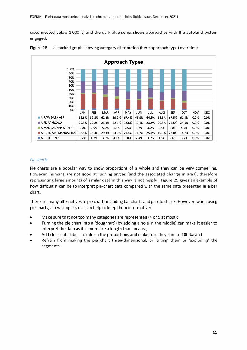
EOFDM – Flight data monitoring, analysis techniques and principles (Initial issue, December 2021)
65
disconnected below 1 000 ft) and the dark blue series shows approaches with the autoland system
engaged.
Figure 28 — a stacked graph showing category distribution (here approach type) over time
Pie charts
Pie charts are a popular way to show proportions of a whole and they can be very compelling.
However, humans are not good at judging angles (and the associated change in area), therefore
representing large amounts of similar data in this way is not helpful. Figure 29 gives an example of
how difficult it can be to interpret pie-chart data compared with the same data presented in a bar
chart.
There are many alternatives to pie charts including bar charts and pareto charts. However, when using
pie charts, a few simple steps can help to keep them informative:
• Make sure that not too many categories are represented (4 or 5 at most);
• Turning the pie chart into a ‘doughnut’ (by adding a hole in the middle) can make it easier to interpret the data as it is more like a length than an area;
• Add clear data labels to inform the proportions and make sure they sum to 100 %; and
• Refrain from making the pie chart three-dimensional, or ‘tilting’ them or ‘exploding’ the segments.
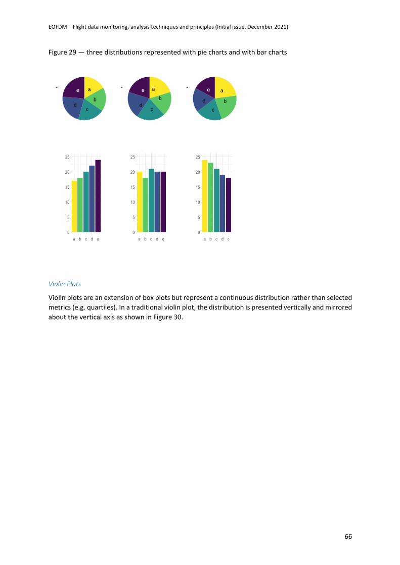
EOFDM – Flight data monitoring, analysis techniques and principles (Initial issue, December 2021)
66
Figure 29 — three distributions represented with pie charts and with bar charts
Violin Plots
Violin plots are an extension of box plots but represent a continuous distribution rather than selected
metrics (e.g. quartiles). In a traditional violin plot, the distribution is presented vertically and mirrored
about the vertical axis as shown in Figure 30.
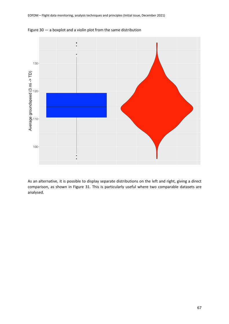
EOFDM – Flight data monitoring, analysis techniques and principles (Initial issue, December 2021)
67
Figure 30 — a boxplot and a violin plot from the same distribution
As an alternative, it is possible to display separate distributions on the left and right, giving a direct
comparison, as shown in Figure 31. This is particularly useful where two comparable datasets are
analysed.
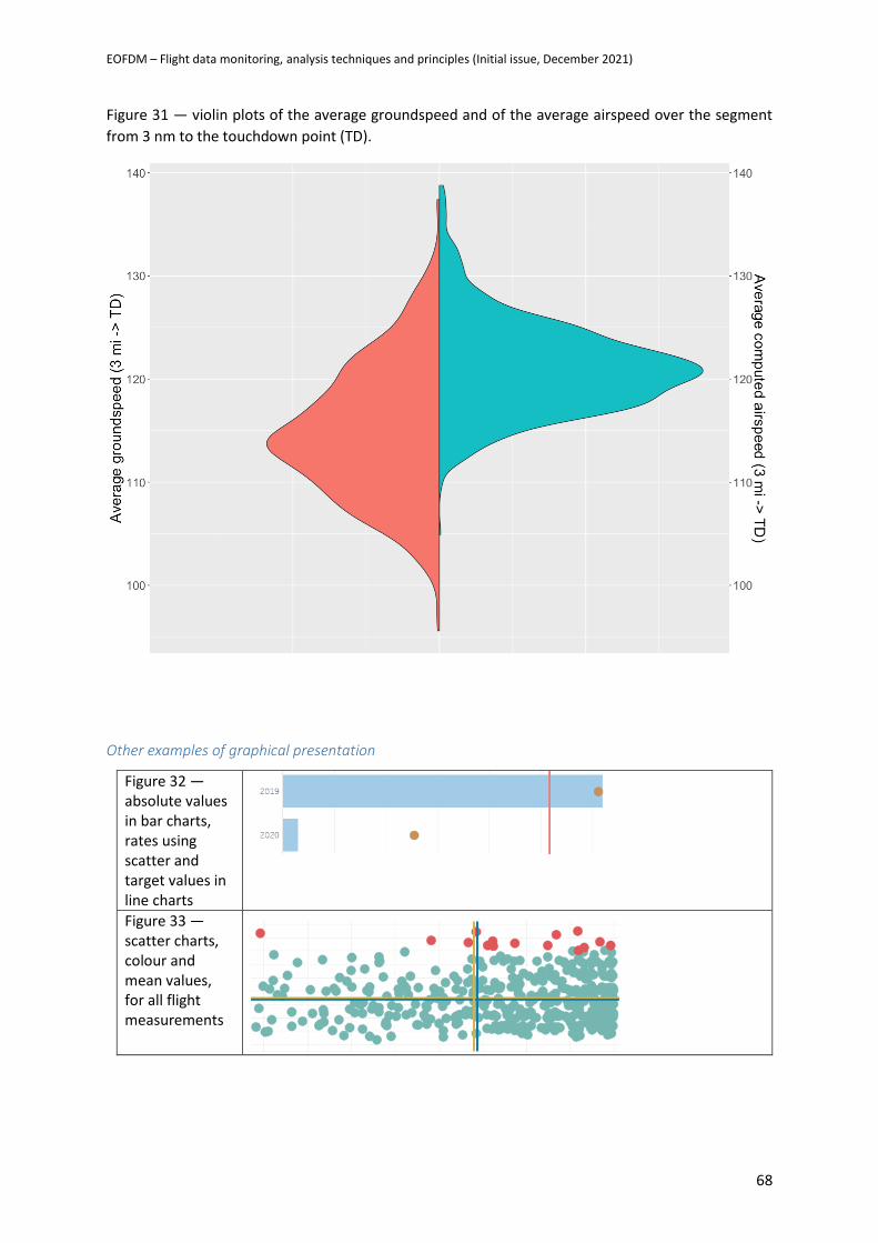
EOFDM – Flight data monitoring, analysis techniques and principles (Initial issue, December 2021)
68
Figure 31 — violin plots of the average groundspeed and of the average airspeed over the segment
from 3 nm to the touchdown point (TD).
Other examples of graphical presentation
Figure 32 — absolute values in bar charts, rates using scatter and target values in line charts
Figure 33 — scatter charts, colour and mean values, for all flight measurements
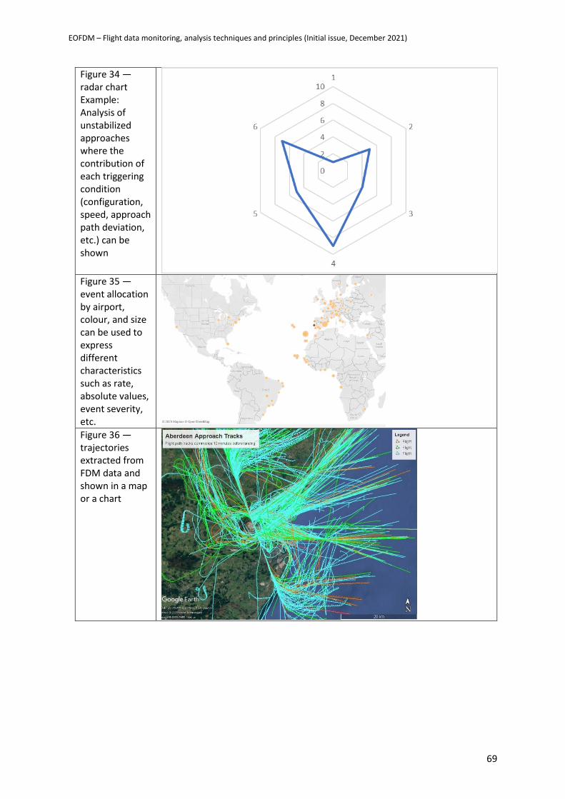
EOFDM – Flight data monitoring, analysis techniques and principles (Initial issue, December 2021)
69
Figure 34 — radar chart Example: Analysis of unstabilized approaches where the contribution of each triggering condition (configuration, speed, approach path deviation, etc.) can be shown
Figure 35 — event allocation by airport, colour, and size can be used to express different characteristics such as rate, absolute values, event severity, etc. Figure 36 — trajectories extracted from FDM data and shown in a map or a chart