finite element modeling of cyclically loaded frp
TRANSCRIPT
FINITE ELEMENT MODELING OF CYCLICALLY LOADED FRP-RETROFITTED RC SQUAT SHEAR
WALLS
ALI REZAIEFAR
A Thesis
in
The Department
of
Building, Civil, and Environmental Engineering
Presented in Partial Fulfillment of the Requirements
For the Degree of Master of Applied Science (Civil Engineering) at
Concordia University
Montréal, Québec, Canada
April 2013
© Ali Rezaiefar, 2013
CONCORDIA UNIVERSITY School of Graduate Studies
This is to certify that the thesis prepared
By: Ali Rezaiefar
Entitled: Finite Element Modeling of Cyclically Loaded FRP-Retrofitted RC Squat
Shear Walls
and submitted in partial fulfillment of the requirements for the degree of
Master of Applied Science (Civil Engineering)
complies with the regulations of the University and meets the accepted standards with
respect to originality and quality.
Signed by the final examining committee:
Lucia Tirca
Chair, Examiner
Lan Lin
Examiner
Ramin Sedaghati
Examiner
Khaled Galal
Supervisor
Approved by Chair of Department or Graduate Program Director April 2013 Dean of Faculty
iii
ABSTRACT
FINITE ELEMENT MODELING OF CYCLICALLY LOADED FRP-RETROFITTED RC SQUAT SHEAR
WALLS
ALI REZAIEFAR
Establishing effective retrofit methods for upgrading the seismic performance of
existing reinforced concrete (RC) shear walls requires reliable means for estimating the
behaviour of RC shear walls with various geometry and reinforcement configurations.
Generally, experimental testing of retrofitted RC shear walls is considered as the most
reliable method of performance evaluation, yet this requires great efforts in terms of the
testing equipment and time in addition to the high cost. On the other hand, a numerical
model that would consider the main parameters that influence the complex performance
of original and retrofitted RC shear walls is seen to be an effective tool for parametric
studies and development of code provisions for the design or evaluation purposes. A
number of experimental tests are available in the literature which could be used for the
primary verification of possible numerical analyses. Similarly, a number of numerical
and analytical approaches are available with a great potential for improvements in order
to converge into a precise and usable analytical approach.
In this thesis, numerical modeling of RC shear walls using general purpose finite
element analysis package ANSYS is explored. A total of seven wall specimens from four
experimental programs were modeled and analysed under monotonic and reversed cyclic
loading and the numerical predictions were in good correlation with the experimental
data. One of the experimentally tested models was then selected for further detailed
iv
investigation on the influence of the concrete compressive strength and the addition of
externally-bonded carbon fibre-reinforced polymer (CFRP) composite sheet on the
behaviour of the squat RC shear walls and their modes of failure.

v
To Mahsa

vi
AKNOWLEGMENT
It is with sincere gratitude that I thank my advisor Dr. Khaled Galal for positively
believing in my work. It would not be possible for me to accomplish any of my research
goals without his financial and academic support.
I would like to thank Mr. Krzysztof Rosiak and CADes Structures Inc. for helping me
realize the relations between the academic research and the real world industry and the
financial support during my research.
There were always great people in my life to learn from namely; Dr. Morteza Aboutalebi,
Dr. Hossam El-Sokkary, Dr. Hossein Azimi, and Mr. Hamid Arabzadeh that I can’t thank
them with the words I know. I also would like to extend my gratitude to my friends and
colleagues at Concordia University namely; Ihab, Javad, Nima, Farzad, Arash, Babak,
Hani, Ahmad and others who provided a friendly environment for me where I could
follow my research. I would like to thank the special people of my life, my parents, my
family and friends.
Finally, I dedicate this thesis to my wife for her patience, love and passion during my
studies. Without her support, my life would have had a different definition.
vii
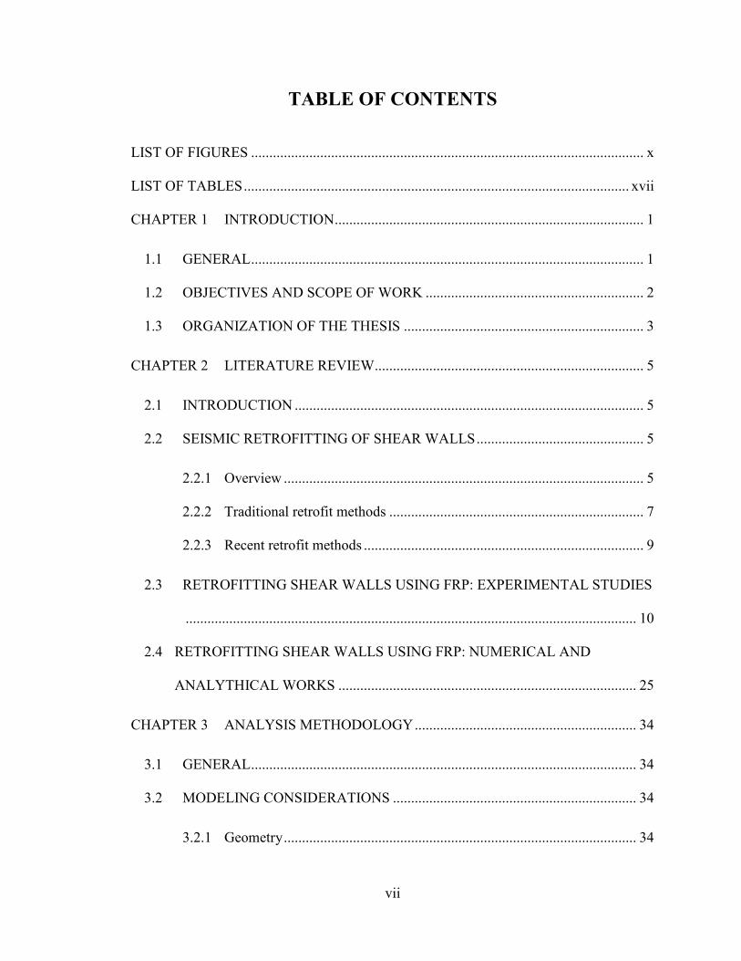
TABLE OF CONTENTS
LIST OF FIGURES ............................................................................................................ x
LIST OF TABLES .......................................................................................................... xvii
CHAPTER 1 INTRODUCTION ..................................................................................... 1
1.1 GENERAL ............................................................................................................ 1
1.2 OBJECTIVES AND SCOPE OF WORK ............................................................ 2
1.3 ORGANIZATION OF THE THESIS .................................................................. 3
CHAPTER 2 LITERATURE REVIEW .......................................................................... 5
2.1 INTRODUCTION ................................................................................................ 5
2.2 SEISMIC RETROFITTING OF SHEAR WALLS .............................................. 5
2.2.1 Overview ................................................................................................... 5
2.2.2 Traditional retrofit methods ...................................................................... 7
2.2.3 Recent retrofit methods ............................................................................. 9
2.3 RETROFITTING SHEAR WALLS USING FRP: EXPERIMENTAL STUDIES
............................................................................................................................ 10
2.4 RETROFITTING SHEAR WALLS USING FRP: NUMERICAL AND
ANALYTHICAL WORKS .................................................................................. 25
CHAPTER 3 ANALYSIS METHODOLOGY ............................................................. 34
3.1 GENERAL .......................................................................................................... 34
3.2 MODELING CONSIDERATIONS ................................................................... 34
3.2.1 Geometry ................................................................................................. 34
viii
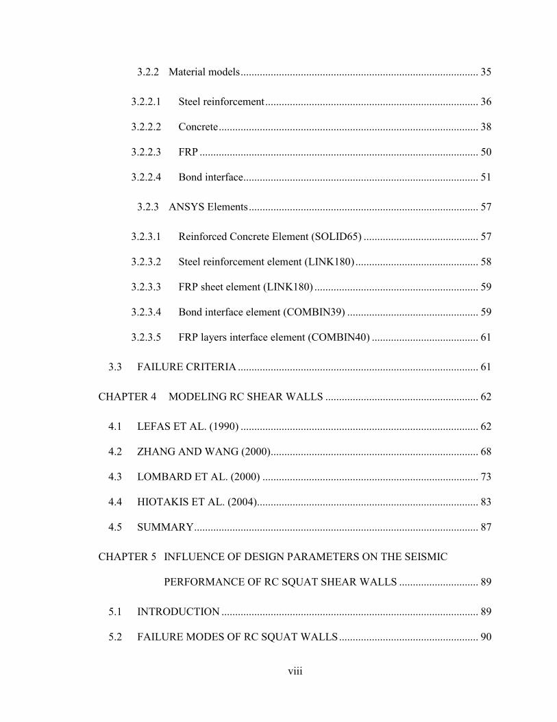
3.2.2 Material models ....................................................................................... 35
3.2.2.1 Steel reinforcement .............................................................................. 36
3.2.2.2 Concrete ............................................................................................... 38
3.2.2.3 FRP ...................................................................................................... 50
3.2.2.4 Bond interface ...................................................................................... 51
3.2.3 ANSYS Elements .................................................................................... 57
3.2.3.1 Reinforced Concrete Element (SOLID65) .......................................... 57
3.2.3.2 Steel reinforcement element (LINK180) ............................................. 58
3.2.3.3 FRP sheet element (LINK180) ............................................................ 59
3.2.3.4 Bond interface element (COMBIN39) ................................................ 59
3.2.3.5 FRP layers interface element (COMBIN40) ....................................... 61
3.3 FAILURE CRITERIA ........................................................................................ 61
CHAPTER 4 MODELING RC SHEAR WALLS ........................................................ 62
4.1 LEFAS ET AL. (1990) ....................................................................................... 62
4.2 ZHANG AND WANG (2000) ............................................................................ 68
4.3 LOMBARD ET AL. (2000) ............................................................................... 73
4.4 HIOTAKIS ET AL. (2004) ................................................................................. 83
4.5 SUMMARY ........................................................................................................ 87
CHAPTER 5 INFLUENCE OF DESIGN PARAMETERS ON THE SEISMIC
PERFORMANCE OF RC SQUAT SHEAR WALLS ............................. 89
5.1 INTRODUCTION .............................................................................................. 89
5.2 FAILURE MODES OF RC SQUAT WALLS ................................................... 90
ix
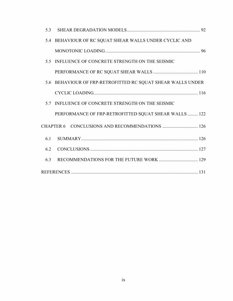
5.3 SHEAR DEGRADATION MODELS ................................................................ 92
5.4 BEHAVIOUR OF RC SQUAT SHEAR WALLS UNDER CYCLIC AND
MONOTONIC LOADING ................................................................................... 96
5.5 INFLUENCE OF CONCRETE STRENGTH ON THE SEISMIC
PERFORMANCE OF RC SQUAT SHEAR WALLS ....................................... 110
5.6 BEHAVIOUR OF FRP-RETROFITTED RC SQUAT SHEAR WALLS UNDER
CYCLIC LOADING ........................................................................................... 116
5.7 INFLUENCE OF CONCRETE STRENGTH ON THE SEISMIC
PERFORMANCE OF FRP-RETROFITTED SQUAT SHEAR WALLS ......... 122
CHAPTER 6 CONCLUSIONS AND RECOMMENDATIONS ............................... 126
6.1 SUMMARY ...................................................................................................... 126
6.2 CONCLUSIONS .............................................................................................. 127
6.3 RECOMMENDATIONS FOR THE FUTURE WORK .................................. 129
REFERENCES ............................................................................................................... 131
x
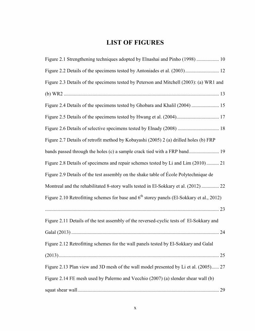
LIST OF FIGURES
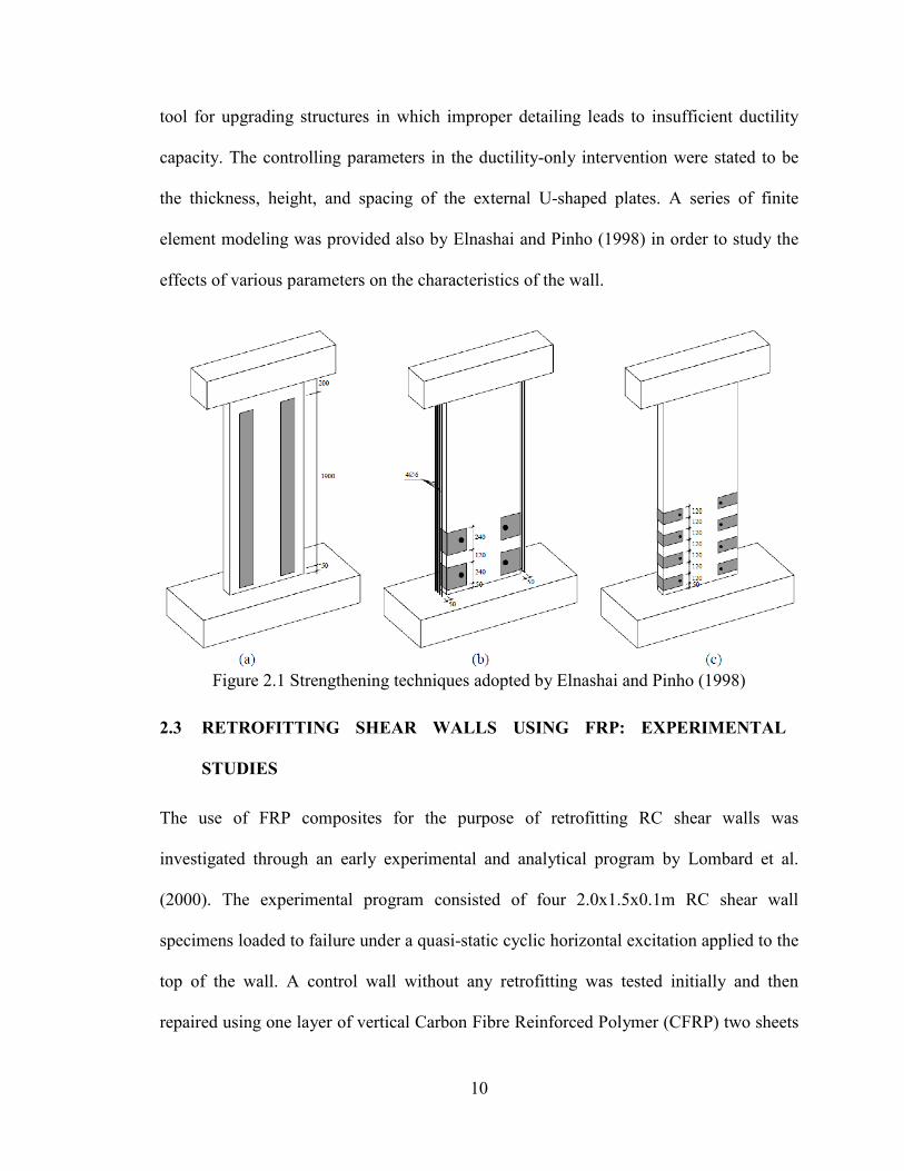
Figure 2.1 Strengthening techniques adopted by Elnashai and Pinho (1998) .................. 10
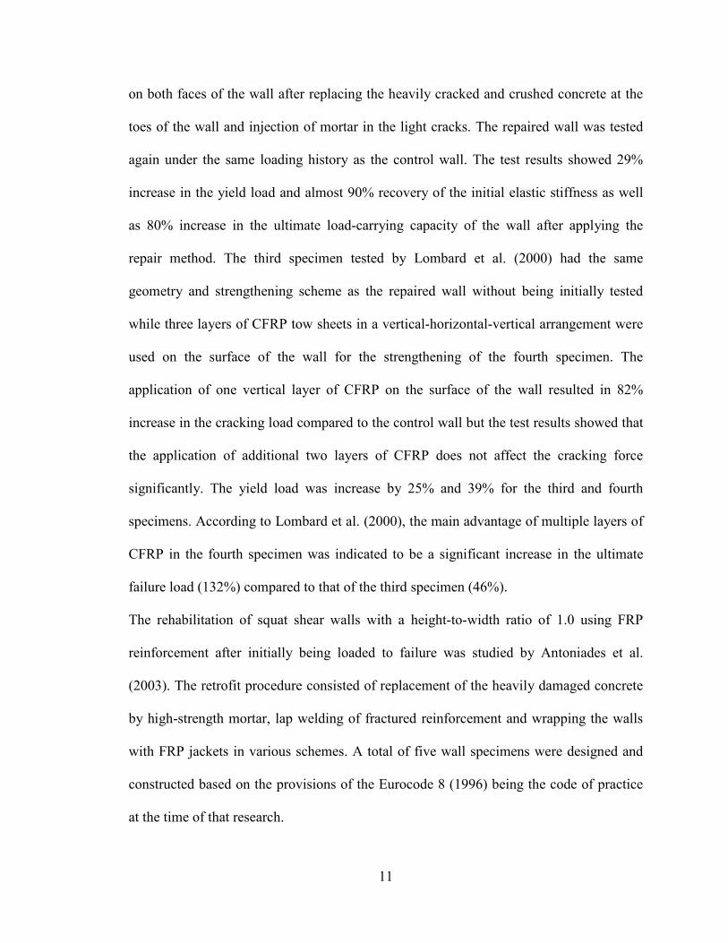
Figure 2.2 Details of the specimens tested by Antoniades et al. (2003) ........................... 12
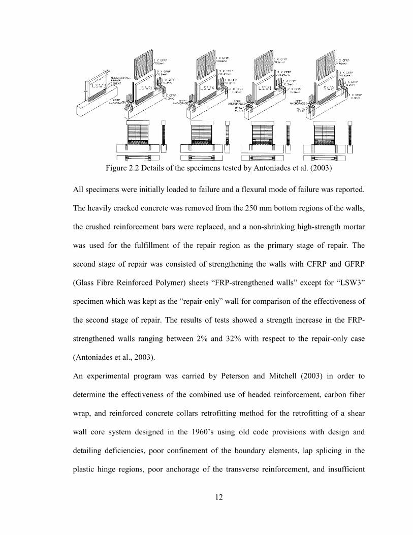
Figure 2.3 Details of the specimens tested by Peterson and Mitchell (2003): (a) WR1 and
(b) WR2 ............................................................................................................................ 13
Figure 2.4 Details of the specimens tested by Ghobara and Khalil (2004) ...................... 15
Figure 2.5 Details of the specimens tested by Hwang et al. (2004) .................................. 17
Figure 2.6 Details of selective specimens tested by Elnady (2008) ................................. 18
Figure 2.7 Details of retrofit method by Kobayashi (2005) 2 (a) drilled holes (b) FRP
bands passed through the holes (c) a sample crack tied with a FRP band ........................ 19
Figure 2.8 Details of specimens and repair schemes tested by Li and Lim (2010) .......... 21
Figure 2.9 Details of the test assembly on the shake table of École Polytechnique de
Montreal and the rehabilitated 8-story walls tested in El-Sokkary et al. (2012) .............. 22
Figure 2.10 Retrofitting schemes for base and 6th storey panels (El-Sokkary et al., 2012)
........................................................................................................................................... 23
Figure 2.11 Details of the test assembly of the reversed-cyclic tests of El-Sokkary and
Galal (2013) ...................................................................................................................... 24
Figure 2.12 Retrofitting schemes for the wall panels tested by El-Sokkary and Galal
(2013) ................................................................................................................................ 25
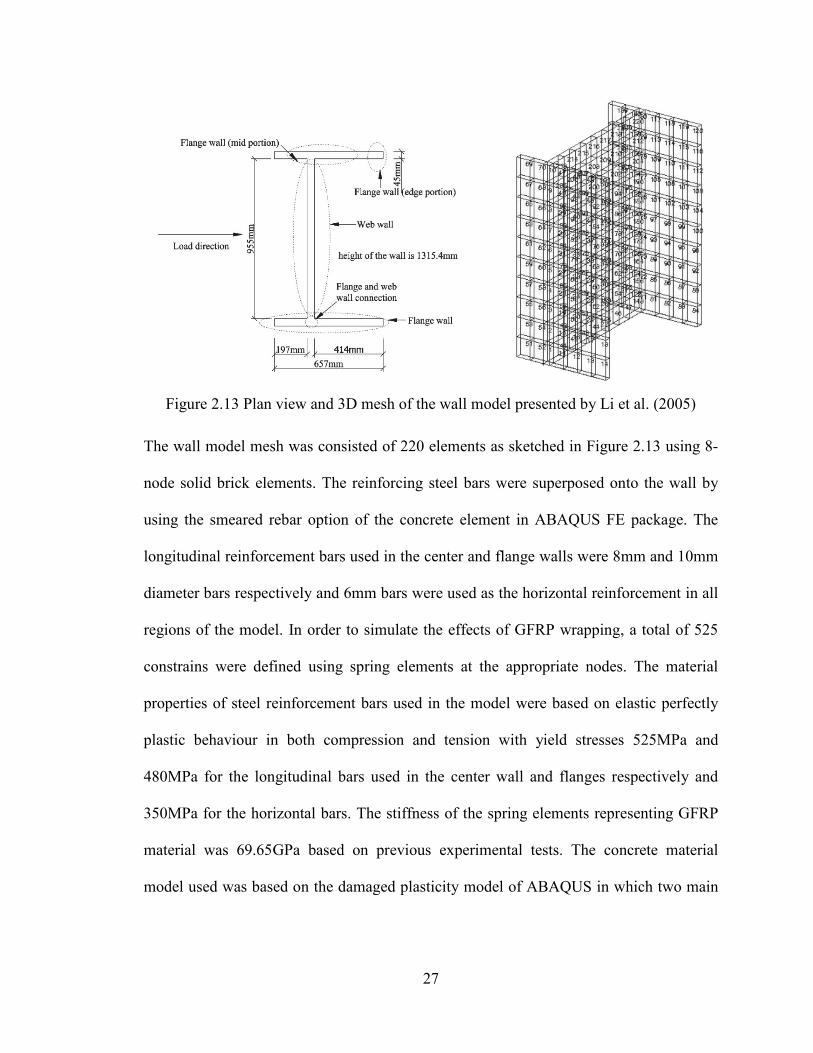
Figure 2.13 Plan view and 3D mesh of the wall model presented by Li et al. (2005) ...... 27
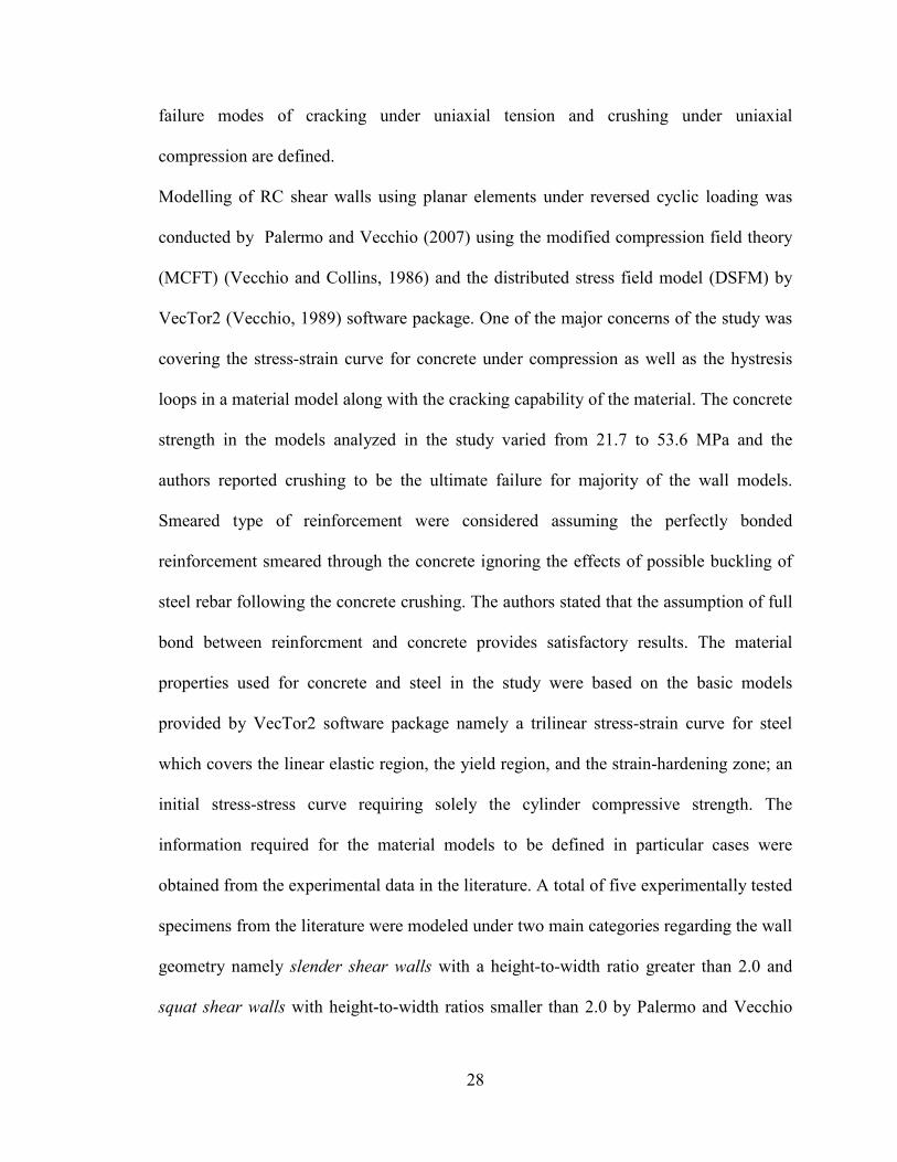
Figure 2.14 FE mesh used by Palermo and Vecchio (2007) (a) slender shear wall (b)
squat shear wall ................................................................................................................. 29
xi
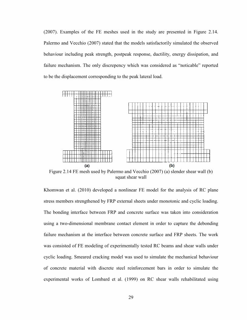
Figure 2.15 FE mesh of RC shear walls modeled by Khomwan et al. (2010) .................. 30
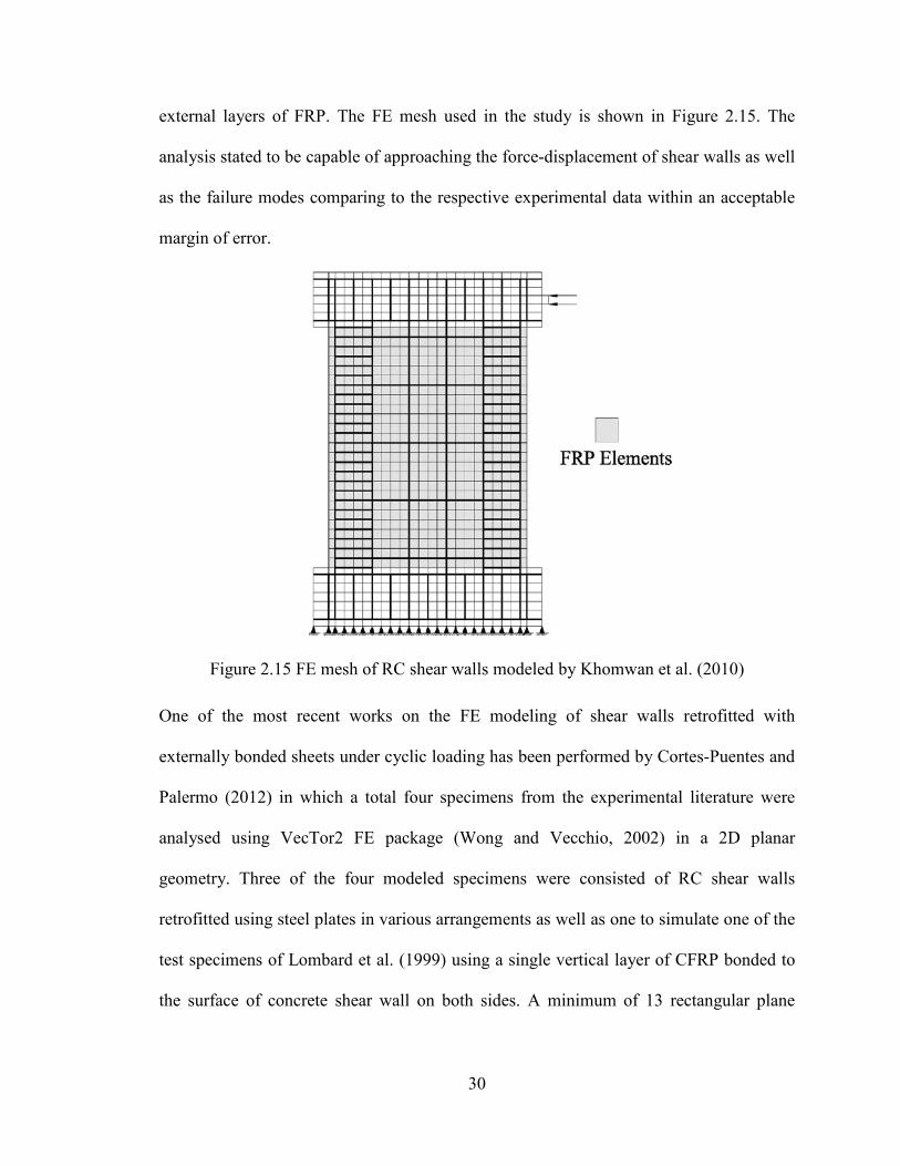
Figure 2.16 FE mesh of the shear wall model by Cortes-Puentes and Palermo (2012) ... 31
Figure 2.17 FE mesh and material properties used by Cruz-Noguez et al. (2012) ........... 32
Figure 3.1 Typical geometry of a wall specimen .............................................................. 35
Figure 3.2 Reinforcing steel stress-strain relationship ...................................................... 36
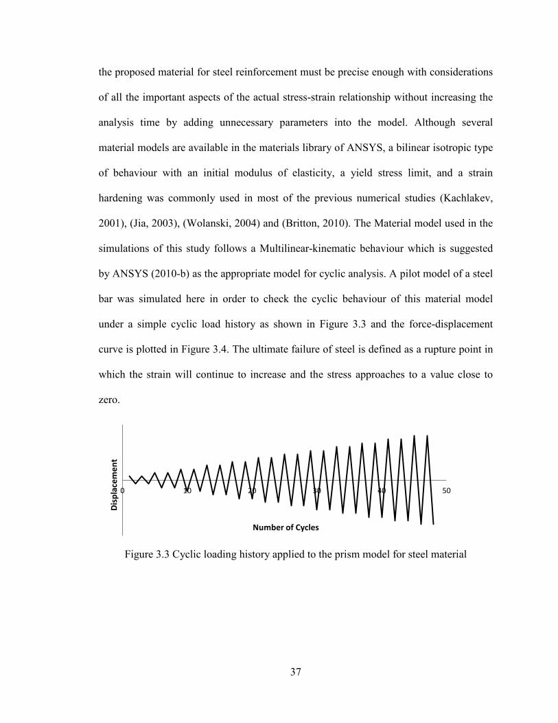
Figure 3.3 Cyclic loading history applied to the prism model for steel material .............. 37
Figure 3.4 Load-Displacement of a steel prism under cyclic loading .............................. 38
Figure 3.5. Compressive stress-strain curves for concrete with various strengths ........... 42
Figure 3.6. Range of tensile strength based on compressive strength for concrete .......... 43
Figure 3.7. Concrete failure mode under nearly biaxial stress state (ANSYS, 2010-b) ... 44
Figure 3.8. Cyclic load history applied to the test prism model for concrete material ..... 46
Figure 3.9. Stress-strain output for concrete prism model excluding smeared cracking
material model .................................................................................................................. 46
Figure 3.10. Geometry of a SOLID65 element (ANSYS, 2010-a) ................................... 47
Figure 3.11. Strength of a cracked section (ANSYS, 2010-b) .......................................... 49
Figure 3.12. Stress-strain output for the test concrete prism model including smeared
cracking material model .................................................................................................... 50
Figure 3.13 A typical unidirectional composite ply (Vasiliev and Morozov, 2007) ........ 51
Figure 3.14 Bond slip relation based on concrete fracture energy model (Sato and
Vecchio, 2003) .................................................................................................................. 54
Figure 3.15 Typical bond-slip relation based on the Italian Code (CNR DT/200, 2004)
model ................................................................................................................................. 55
xii
Figure 3.16 Bond-slip relationship considering IC debonding failure mechanism (Lu et
al., 2005-a) ........................................................................................................................ 56
Figure 3.17 Geometry of LINK180 element (ANSYS, 2010-a) ....................................... 59
Figure 3.18 COMBIN39 element geometry and input function (ANSYS, 2010-a) ......... 60
Figure 4.1. Details of the wall specimens tested by Lefas et al. (1990) ........................... 63
Figure 4.2 Details of the FE model FE-LSW14 (a) elements mesh (b) elements
arrangement ....................................................................................................................... 64
Figure 4.3. Crack pattern and rebars axial stresses in different stages of the analysis; (a):
cracking, (b) yielding, (c) failure resulted from FE-LSW14 ............................................ 65
Figure 4.4. Lateral load-deformation resulted from FE-LSW14 ..................................... 65
Figure 4.5 Details of the FE model FE-LSW26 (a) elements mesh (b) elements
arrangement ....................................................................................................................... 66
Figure 4.6. Crack pattern and rebars axial stresses in different stages of the analysis; (a):
cracking, (b) yielding, (c) failure resulted from FE-LSW26 ............................................ 67
Figure 4.7. Lateral load-deformation for LSW26 ............................................................. 68
Figure 4.8 Details of Specimen ZSW7 (Zhang and Wang, 2000) .................................... 69
Figure 4.9 Details of the FE model FE-ZSW7 (a) elements mesh (b) elements
arrangement ....................................................................................................................... 69
Figure 4.10 Crack pattern for SW7 (a) first cracks initiated in FE model (b) cracks in FE
model at cracking load of experimental tests (c) cracks at cracking load in experimental
tests (Zhang and Wang, 2000) .......................................................................................... 70
Figure 4.11. Crack pattern and rebars axial stresses at different stages of the analysis
resulted from FE-ZSW7 .................................................................................................... 71
xiii
Figure 4.12 Cracks at failure for SW7 (a) experimental (Zhang and Wang, 2000) (b) FE
analysis .............................................................................................................................. 72
Figure 4.13. Lateral load-deformation curve of ZSW7 and FE-ZSW7 ............................ 73
Figure 4.14. Geometry and reinforcement details of shear wall specimens (Lombard et
al., 2000) ........................................................................................................................... 74
Figure 4.15. Stress-strain relationship for (a) reinforcement steel (b) concrete ............... 75
Figure 4.16 FE mesh and elements arrangement of FE models based on the specimens of
Lombard et al. (2000) ....................................................................................................... 75
Figure 4.17. Lateral load-deformation curve of LCW (Lombard et al., 2000) and FE-
LCW model ....................................................................................................................... 76
Figure 4.18. Crack pattern and rebars axial stresses at different stages of the analysis
resulted from FE-LCW model .......................................................................................... 78
Figure 4.19. Specification of the FRP external reinforcement and the bond interface ..... 79
Figure 4.20. FRP anchor device (Lombard et al., 2000) ................................................... 79
Figure 4.21. Bond-Slip relationships for various regions of the wall model FE-SW1 ..... 80
Figure 4.22. Lateral load- top displacement curve of LSW1 (Lombard et al., 2000) and
FE-LSW1 model ............................................................................................................... 82
Figure 4.23. Lateral load- mid displacement curve of LSW1 (Lombard et al., 2000) and
FE-LSW1 model ............................................................................................................... 83
Figure 4.24. Lateral load-deformation curve of HCW (Hiotakis et al., 2004) and FE-
HCW model ...................................................................................................................... 84
Figure 4.25 The anchorage device used for the anchoring of CFRP sheets (Hiotakis et al.,
2004) ................................................................................................................................. 85
xiv
Figure 4.26. Lateral load-deformation curve of HSW1 (Hiotakis et al., 2004) and FE-
HSW1 model ..................................................................................................................... 86
Figure 5.1 Shear failure modes in squat walls (Paulay and Priestley, 1992) .................... 92
Figure 5.2 Lateral load-displacement results of the FE-HCW model under monotonic and
cyclic loading .................................................................................................................... 97
Figure 5.3. Loading scheme in the displacement-controlled cyclic analysis .................... 98
Figure 5.4. Crack pattern and vertical rebar axial stress at various stages of monotonic
analysis of the FE-HCW wall model ................................................................................ 99
Figure 5.5. Horizontal rebar axial stress at various stages of monotonic analysis of the
FE-HCW wall model ........................................................................................................ 99
Figure 5.6. Stress distribution in the model at various stages of monotonic analysis of the
FE-HCW wall model ...................................................................................................... 100
Figure 5.7. Stress in various layers of vertical reinforcement during the monotonic
analysis of FE-HCW ....................................................................................................... 101
Figure 5.8. Maximum axial stress in various layers of horizontal reinforcement during the
monotonic analysis of FE-HCW ..................................................................................... 101
Figure 5.9. In-plane deformations in mid-height of the wall at 4 loading stages during the
monotonic analysis of FE-HCW ..................................................................................... 102
Figure 5.10. In-plane deformations in 1/8-height of the wall at 4 loading stages during the
monotonic analysis of FE-HCW ..................................................................................... 103
Figure 5.11. Vertical displacement of 5 selective points in different heights during the
monotonic analysis of FE-HCW ..................................................................................... 104
xv
Figure 5.12. Crack pattern and vertical rebar axial stress at various stages of cyclic
analysis of the FE-HCW wall model .............................................................................. 105
Figure 5.13. Horizontal rebar axial stress at various stages of cyclic analysis of the FE-
HCW wall model ............................................................................................................ 106
Figure 5.14. Stress distribution in the model at various stages of cyclic analysis of the FE-
HCW wall model ............................................................................................................ 107
Figure 5.15. Lateral load vs. maximum rebar axial strain for the six vertical rebar layers
of FE-HCW model .......................................................................................................... 108
Figure 5.16. Lateral load vs. maximum rebar axial strain for the five horizontal rebar
layers of FE-HCW model ............................................................................................... 109
Figure 5.17 Compressive stress-strain relationship of concrete for different values of f’c
......................................................................................................................................... 110
Figure 5.18 Tensile strength of concrete for range of f’c<50 .......................................... 111
Figure 5.19. Load-Displacement ductility and nominal shear capacities of walls with
various f’c values ............................................................................................................. 112
Figure 5.20. Wall cracking load for different values of f’c resulted from cyclic and
monotonic analysis .......................................................................................................... 113
Figure 5.21. Load corresponding to the yielding of the first vertical rebar for different
values of f’c resulted from cyclic and monotonic analysis ............................................. 114
Figure 5.22. Effect of the fc’ on the displacement ductility capacity of the studied walls
when subjected to cyclic and monotonic lateral loads .................................................... 114
Figure 5.23. Effect of f’c on the wall’s energy dissipation capacity for cyclically loaded
walls ................................................................................................................................ 115
xvi
Figure 5.24. Lateral force-deflection relationships of the studied walls with various f’c
values along with the seismic performance levels .......................................................... 116
Figure 5.25. Crack pattern and rebar axial stress at various stages of cyclic analysis of the
FE-HSW1 wall model ..................................................................................................... 117
Figure 5.26. FRP axial stress at various stages of cyclic analysis of the FE-HSW1 wall
model ............................................................................................................................... 118
Figure 5.27. Stress distribution in the model at various stages of cyclic analysis of the FE-
HSW1 wall model ........................................................................................................... 119
Figure 5.28. Lateral load vs. maximum rebar axial strain for the six vertical rebar layers
of FE-HSW1 model ........................................................................................................ 120
Figure 5.29. Lateral load vs. maximum rebar axial strain for the five horizontal rebar
layers of FE-HSW1 model .............................................................................................. 121
Figure 5.30. Load-Displacement ductility and nominal shear capacities of FRP-retrofitted
walls with various f’c values ........................................................................................... 123
Figure 5.31. Effect of f’c on the FRP-retrofitted wall’s ultimate load carrying capacity 124
Figure 5.32. Effect of the f’c on the displacement ductility capacity of the FRP-retrofitted
walls when subjected to cyclic and monotonic lateral loads .......................................... 124
xvii
LIST OF TABLES
Table 2.1 Details of the wall specimens tested by Elnady (2008) .................................... 18
Table 3.1 Effect of aggregates type on the modulus of elasticity of concrete (FIB, 2010)
........................................................................................................................................... 39
Table 3.2. Secant modulus of elasticity (Ec) of concrete for various strengths [MPa] ..... 41
Table 3.3. Tangent modulus of elasticity (Eci) of concrete for various strengths [MPa] .. 41
Table 4.1. Summary of loading and geometry of the modeled specimens ....................... 62
Table 4.2. FRP and bond elements real constants ............................................................ 80
Table 4.3. Material properties of FRP and the bond interface (Lombard et al., 2000) ..... 81
Table 4.4 Comparison of the FEA and experimental results of RC shear walls at the key
performance points (cracking, yielding, and ultimate) ..................................................... 88
1
CHAPTER 1
INTRODUCTION
1.1 GENERAL
Reinforced concrete (RC) shear walls are the main lateral force resisting system in
many RC structures. Several factors affect the seismic behaviour and ductility of a RC
shear wall, particularly its shear span-to-depth ratio and its shear capacity in relation to
the flexural capacity. Squat shear walls are found in many existing low-rise RC buildings
such as nuclear power plant facilities, airport buildings and office/residential buildings
that use a flat plate system for gravity loads. RC squat shear walls are characterised by
their low height-to-length ratio or low shear span-to-depth ratio. As such, the response of
RC squat shear walls to lateral loads will be dominated by shear behaviour, with reduced
contribution from the classic beam theory and the plane-sections hypothesis. Shear
behaviour of RC squat elements is a complex phenomenon, especially when considering
the cyclic nature of acting lateral loads.
Last decades witnessed the development of several retrofitting methods for shear
deficient RC shear walls towards improving their seismic performance in terms of the
overall strength, ductility, and energy dissipation capacities. Among these, fiber-
reinforced polymer (FRP) composite materials have received increasing attention in the
past few years as a potential material for retrofitting of existing RC structures. Despite
the various research efforts reported in the literature in proposing different FRP-
retrofitting methods for existing RC squat walls, there is still a need to thoroughly
2
investigate the effect of major design parameters, such as the material properties,
geometry, arrangement of reinforcement bars and additional external reinforcement on
the overall seismic performance of the system.
Typically, the seismic performance of a retrofitted RC shear walls is evaluated
experimentally through assessing its hysteretic lateral force displacement relationships.
Although experimental testing is seen to be the most evident approach to assess the
performance of a shear wall, numerical simulations would provide valuable tools for
parametric studies and assessments of the seismic response of RC squat shear walls.
This thesis investigates the details of numerical modeling of RC squat shear walls
using Finite Element (FE) method. Amongst many general purpose FE analysis packages
available in the market, ANSYS is adopted for the simulations of this research
considering its extensive materials and elements library and the global reputation for the
accuracy of the results of analyses performed previously.
The study adopts three-dimensional geometry modeling approach while addressing
the most effective parts of the geometry along with major failure criteria of the
constituent materials namely concrete, steel reinforcement bars, FRP sheets and the bond
interface to improve the accuracy of the results. On the other hand, the use of symmetry
and a special meshing technique helped reducing the analysis time consumption.
1.2 OBJECTIVES AND SCOPE OF WORK
The main objective of this research is to investigate, numerically, the effect of shear
capacity on the ductility of RC squat shear walls, both existing and FRP-retrofitted, when
subjected to cyclic load excitations simulating seismic effects.
In order to achieve the objective of this research, the scope of work is to:
3
- Outline an appropriate numerical modeling approach for the analysis of RC shear
walls under monotonic and cyclic loading that best describes the geometry and
failure criteria using a widely accepted general purpose FE package.
- Apply the numerical modeling to study the failure modes of RC squat shear walls
in more details.
- Evaluate the effect of externally bonded FRP reinforcement content on the failure
mode and seismic performance of unretrofitted and FRP-retrofitted RC squat shear
walls using the numerical modeling.
- Evaluate the effects of concrete strength on the shear capacity and seismic
performance of unretrofitted and FRP-retrofitted RC squat shear walls.
1.3 ORGANIZATION OF THE THESIS
This thesis is composed of six chapters. Chapter 2 reviews the available literature in
order to generate the basis of the modeling i.e. geometry, loading, supports, etc. and to
identify relevant experimental works in the area of FRP-retrofit of RC squat shear walls.
In Chapter 3, the modeling procedure in terms of the geometry, elements, boundary
conditions and failure criteria is described. Pilot modeling and sensitivity analyses are
conducted whenever needed in order to identify the validity of the material properties and
failure criteria. As for Chapter 4, it is mainly concerned with comparing and correlating
the FE results with the relevant experimental data and quantifying the difference. A final
calibration of the analysis considerations is performed by comparing the results of FE
analysis with those of related experimental tests in order to measure the scope and
amount of error at various stages of the analysis. In Chapter 5, the behaviour of a squat
shear wall model from the cases studied in Chapter 4 is explained in details under
4
monotonic and cyclic loading in terms of stress distribution and internal forces of the
various parts and constitutes of the wall model. Appropriate shear degradation models
available in the literature are used to evaluate the mode of failure of the wall. A series of
models are developed in order to study the effects of concrete compressive strength on
the seismic performance of existing RC squat shear walls. The effects of an additional
layer of FRP external wrap on the type of behaviour, overall performance and the mode
of failure of the walls with various concrete compressive strengths are discussed and
conclusions are made. Finally, Chapter 6 provides the conclusions drawn from the
findings of Chapters 3, 4 and 5 and proposes areas for future research.
5
CHAPTER 2
LITERATURE REVIEW
2.1 INTRODUCTION
From the various studies available in the field of seismic retrofitting of reinforced
concrete (RC) structures and structural members, a review of the references related to the
field of numerical nonlinear modeling of the seismic retrofitting of RC shear walls is
presented in this chapter.
2.2 SEISMIC RETROFITTING OF SHEAR WALLS
2.2.1 Overview
Reinforced concrete shear walls are commonly used in concrete buildings to resist the
lateral forces acting on them due to their high in-plane stiffness. These lateral forces are
caused by earthquake or wind excitations. The term “structural wall” is used instead of
“shear wall” by Paulay and Priestley (1992) to emphasize on the significance of the in-
plane bending moments and axial forces on the behaviour of this structural element, in
addition to the shear forces. Brittle behaviour of shear walls caused by undesirable modes
of failure is prevented in the modern seismic codes of design by providing special
design/detailing practices. A well-designed/detailed wall provides high energy
dissipation, ductility, and strength to the building structure. Walls designed based on the
older versions of the seismic codes −prior to the enforcement of ductile energy
dissipation seismic performance− fail to undergo a ductile behaviour due to the poor
design and detailing.
6
In general, the seismic performance of a building structure that is damaged by a minor
earthquake or that is not damaged but vulnerable to future earthquakes, could be
upgraded using two different schemes: global and local retrofitting. Additional structural
members provide the strength and ductility in a globally upgraded structure while local
upgrading aims to improve the capacity of structural members separately in a way that
the upgraded structure passes the requirements of the up-to-date codes (Moehle,
2000).Various methods of retrofitting have been proposed and tested by researchers
based on the modes of failure of the shear walls. Most of these tests normally consider
the plastic hinge region as the vulnerable or damaged part of the entire wall. For brittle
failure modes with minimum or no ductility, the retrofit intervention aims at eliminating
the non-ductile behaviour and modifying it to ductile modes. For original walls that have
limited ductility with low energy dissipation capacity, the retrofit aims to modify the
performance to be more ductile with higher energy dissipation capacity. Pauley and
Priestley (1992) state that the principal source of energy dissipation in a laterally loaded
cantilever wall should be yielding of the flexural reinforcement in the plastic hinge
regions, normally located at the base of the wall.
A flexural mode of failure of RC shear walls occurs when there is a sufficient shear
capacity that develops yielding of the wall’s flexural reinforcement. Flexural failure
mode is necessary to ensure a ductile performance for RC shear walls subjected to in-
plane bending moments, shear and axial forces. Lack of sufficient shear capacity causes a
shear failure, which is brittle in nature. Modern seismic design codes adopt a capacity
design philosophy by ensuring that the shear capacity of the wall exceeds its flexural
capacity along the wall height. Besides the two main failure modes of shear and flexural,
7
there are three other possible modes of failure based on the instability of thin-walled
sections (local buckling of web), in-plane splitting failure, and rocking failure (Galal and
El-Sokkary, 2008). The three latter cases will not be considered in this study as they are
not as common as the main two failure modes of the RC shear walls. Seismic upgrade is
defined as “an improvement in the seismic performance of the shear walls based on the
prevention of brittle failure modes or improving their ductile performance by enhancing
their stiffness, strength, ductility, or a combination of them”. A repair is defined as
restoring the original state of a damaged structure without aiming for increasing its
capacity. If the repair of damaged walls improves the performance of the structure
comparing to its original state, the repair process is called rehabilitation. Strengthening
describes increasing the capacity and/or ductility of an undamaged structural element.
Retrofit is commonly used to describe an intervention that could be either one of the three
above described techniques, or a combination of them (Galal and El-Sokkary, 2008).
2.2.2 Traditional retrofit methods
Fiorato et al. (1983) used the replacement of concrete as a repair method for shear wall
specimens with barbell sections with a height-to-width ratio of 2.4. The walls were
subjected to reverse monotonic cyclic loading and axial loads simultaneously up to
failure. The concrete replacement method resulted in a lower stiffness for the repaired
specimens comparing to the original ones but the lateral strength and ductility were
reported to be fully restored by the repair technique (Fiorato et al., 1983).
Replacement of concrete in the damaged parts of shear walls was studied by Lefas et al.
(1990) where four slender rectangular walls were tested to damage and three of them
repaired by replacing the concrete and strengthening the buckled reinforcement bars in a
8
150x100mm region of the compressive toes of the walls. The flexural cracks on the body
of the walls were also filled with epoxy injection. The repaired specimens were subjected
again to a monotonic reverse cyclic loading and exhibited lower stiffness and less
ductility but a full restoration of wall strength was stated. Completely filling the cracks
by epoxy injection had a marginal effect on the improvement of the structural
characteristics of the repaired walls. A comparison between the crack patterns and failure
modes of the original and repaired walls implied a marginal effect of the repair method
on these structural characteristics.
Vecchio et al. (2002) repaired two damaged wide-flanged squat shear walls by replacing
the crushed concrete and re-tested the walls by subjecting them to the lateral loading that
caused the original damage. The barbell-sectioned shear wall specimens had a 2020mm
height and 2885mm width with a web thickness of 75mm, also the flange parts of the
specimens were consisted of 3045x100mm shells. The concrete used as the fulfillment
material had approximately double the strength of the original walls concrete. The first
repair scenario was to replace the damaged parts of the web only while in the second
repair scenario the crushed concrete replacement technique was done to the flanges. The
effectiveness of this repair method was assessed through the test results that showed that
the seismic efficiency indicators of the wall such as strength, stiffness, and energy
dissipation capacity were almost restored in the repaired walls.
In addition to the above studies, there has been several other research works done in the
field of traditional repair of shear walls using similar techniques. They are not included in
this chapter as they are out of the scope of this study.
9
2.2.3 Recent retrofit methods
In addition to the traditional methods applicable to the repair cases, improving the
performance of damaged or non-damaged wall structures by applying external layers of
bar or plate elements was studied by a number of authors considering the material for the
bonding elements to be steel or FRP where the latter case will be discussed in the next
part of this chapter.
The use of steel plates and bars as external bonding materials to shear wall was studied
by Elnashai and Pinho (1998). Experimental tests followed by analytical and numerical
analyses on 1:2.5 scale shear wall specimen were conducted to study the effects of
various methods of application of steel plates and bars on stiffness, strength, and ductility
as the three main parameters of wall seismic performance. In the stiffness-only phase,
steel plates were glued to the surface of the wall to cover the area of expected plastic
hinge region for the non-damaged walls and the heavily cracked regions for the damaged
specimen on the two boundary regions of the walls as shown in Figure 2.1(a). The
experimental results indicated an increase in the level of stiffness to be controlled totally
by the position of the bonded plates, and their dimensions. In the strength-only phase,
two main strengthening methods of adding external unbounded steel reinforcement bars
and external unbounded steel plates were conducted in order to increase the strength of
the wall without influencing the stiffness as shown in Figure 2.1(b). The level of strength
was stated to be controllable by the area and position of the steel plates or the re-bars. In
the ductility-only interventions, U-shaped external confinement steel plates were added to
the area where additional ductility was required as shown in Figure 2.1(c). The proposed
ductility-only intervention technique was stated to be externally efficient to be used as
10
tool for upgrading structures in which improper detailing leads to insufficient ductility
capacity. The controlling parameters in the ductility-only intervention were stated to be
the thickness, height, and spacing of the external U-shaped plates. A series of finite
element modeling was provided also by Elnashai and Pinho (1998) in order to study the
effects of various parameters on the characteristics of the wall.
Figure 2.1 Strengthening techniques adopted by Elnashai and Pinho (1998)
2.3 RETROFITTING SHEAR WALLS USING FRP: EXPERIMENTAL
STUDIES
The use of FRP composites for the purpose of retrofitting RC shear walls was
investigated through an early experimental and analytical program by Lombard et al.
(2000). The experimental program consisted of four 2.0x1.5x0.1m RC shear wall
specimens loaded to failure under a quasi-static cyclic horizontal excitation applied to the
top of the wall. A control wall without any retrofitting was tested initially and then
repaired using one layer of vertical Carbon Fibre Reinforced Polymer (CFRP) two sheets
11
on both faces of the wall after replacing the heavily cracked and crushed concrete at the
toes of the wall and injection of mortar in the light cracks. The repaired wall was tested
again under the same loading history as the control wall. The test results showed 29%
increase in the yield load and almost 90% recovery of the initial elastic stiffness as well
as 80% increase in the ultimate load-carrying capacity of the wall after applying the
repair method. The third specimen tested by Lombard et al. (2000) had the same
geometry and strengthening scheme as the repaired wall without being initially tested
while three layers of CFRP tow sheets in a vertical-horizontal-vertical arrangement were
used on the surface of the wall for the strengthening of the fourth specimen. The
application of one vertical layer of CFRP on the surface of the wall resulted in 82%
increase in the cracking load compared to the control wall but the test results showed that
the application of additional two layers of CFRP does not affect the cracking force
significantly. The yield load was increase by 25% and 39% for the third and fourth
specimens. According to Lombard et al. (2000), the main advantage of multiple layers of
CFRP in the fourth specimen was indicated to be a significant increase in the ultimate
failure load (132%) compared to that of the third specimen (46%).
The rehabilitation of squat shear walls with a height-to-width ratio of 1.0 using FRP
reinforcement after initially being loaded to failure was studied by Antoniades et al.
(2003). The retrofit procedure consisted of replacement of the heavily damaged concrete
by high-strength mortar, lap welding of fractured reinforcement and wrapping the walls
with FRP jackets in various schemes. A total of five wall specimens were designed and
constructed based on the provisions of the Eurocode 8 (1996) being the code of practice
at the time of that research.
12
Figure 2.2 Details of the specimens tested by Antoniades et al. (2003)
All specimens were initially loaded to failure and a flexural mode of failure was reported.
The heavily cracked concrete was removed from the 250 mm bottom regions of the walls,
the crushed reinforcement bars were replaced, and a non-shrinking high-strength mortar
was used for the fulfillment of the repair region as the primary stage of repair. The
second stage of repair was consisted of strengthening the walls with CFRP and GFRP
(Glass Fibre Reinforced Polymer) sheets “FRP-strengthened walls” except for “LSW3”
specimen which was kept as the “repair-only” wall for comparison of the effectiveness of
the second stage of repair. The results of tests showed a strength increase in the FRP-
strengthened walls ranging between 2% and 32% with respect to the repair-only case
(Antoniades et al., 2003).
An experimental program was carried by Peterson and Mitchell (2003) in order to
determine the effectiveness of the combined use of headed reinforcement, carbon fiber
wrap, and reinforced concrete collars retrofitting method for the retrofitting of a shear
wall core system designed in the 1960’s using old code provisions with design and
detailing deficiencies, poor confinement of the boundary elements, lap splicing in the
plastic hinge regions, poor anchorage of the transverse reinforcement, and insufficient
13
shear strength to develop the plastic hinge. A total of four specimens were constructed
and tested under reversed cyclic loading in two pairs of as-built and retrofitted walls. The
location of lap splice of the vertical reinforcement in the first pair (W1 and WR1) of
walls was at the bottom of the wall while for the second pair (W2 and WR2), the lap
splicing was at a height of 600mm from the bottom of the wall.
Figure 2.3 Details of the specimens tested by Peterson and Mitchell (2003): (a) WR1 and
(b) WR2
Retofit strategies for WR1, and WR2 are shown in Figure 2.3 where the use of headed
reinforcement, and carbon fibers to improve the seismic performance of the walls was
adopted. The displacement ductility of the wall was improved from 1.5 for W1 to 3.8 for
WR1, and from 4.0 for W2 to 6.3 for WR2; also, WR1 and WR2 specimens absorbed
over seven and three times respectively as much energy as W1 and W2 during the tests.
The combination of headed reinforcement and carbon fiber wrap was shown to be
14
effective in increasing the confinement of the wall boundary element regions and the
anchorage of the transverse reinforcement (Peterson and Mitchell, 2003).
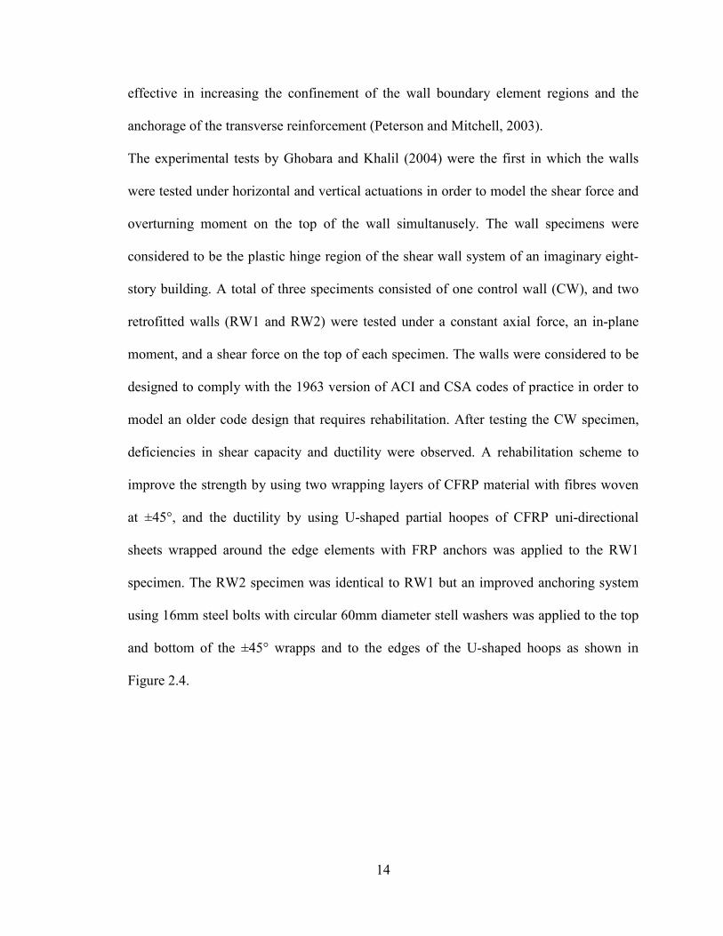
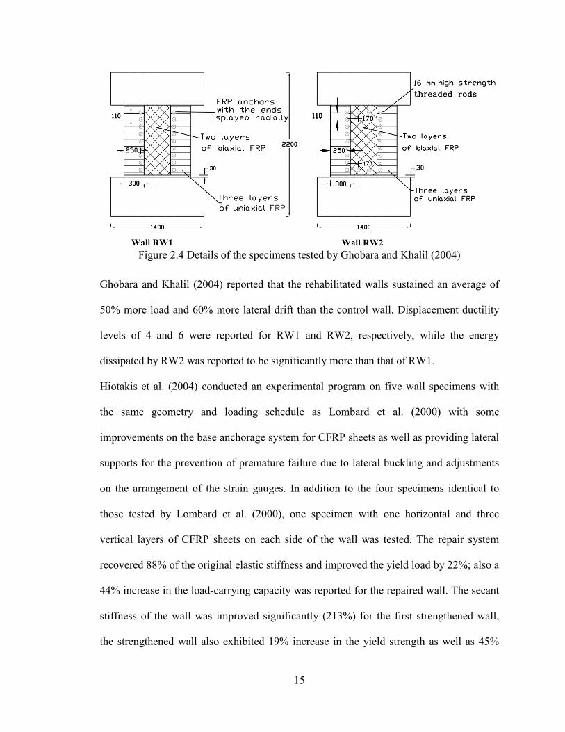
The experimental tests by Ghobara and Khalil (2004) were the first in which the walls
were tested under horizontal and vertical actuations in order to model the shear force and
overturning moment on the top of the wall simultanusely. The wall specimens were
considered to be the plastic hinge region of the shear wall system of an imaginary eight-
story building. A total of three speciments consisted of one control wall (CW), and two
retrofitted walls (RW1 and RW2) were tested under a constant axial force, an in-plane
moment, and a shear force on the top of each specimen. The walls were considered to be
designed to comply with the 1963 version of ACI and CSA codes of practice in order to
model an older code design that requires rehabilitation. After testing the CW specimen,
deficiencies in shear capacity and ductility were observed. A rehabilitation scheme to
improve the strength by using two wrapping layers of CFRP material with fibres woven
at ±45°, and the ductility by using U-shaped partial hoopes of CFRP uni-directional
sheets wrapped around the edge elements with FRP anchors was applied to the RW1
specimen. The RW2 specimen was identical to RW1 but an improved anchoring system
using 16mm steel bolts with circular 60mm diameter stell washers was applied to the top
and bottom of the ±45° wrapps and to the edges of the U-shaped hoops as shown in
Figure 2.4.
15
Figure 2.4 Details of the specimens tested by Ghobara and Khalil (2004)
Ghobara and Khalil (2004) reported that the rehabilitated walls sustained an average of
50% more load and 60% more lateral drift than the control wall. Displacement ductility
levels of 4 and 6 were reported for RW1 and RW2, respectively, while the energy
dissipated by RW2 was reported to be significantly more than that of RW1.
Hiotakis et al. (2004) conducted an experimental program on five wall specimens with
the same geometry and loading schedule as Lombard et al. (2000) with some
improvements on the base anchorage system for CFRP sheets as well as providing lateral
supports for the prevention of premature failure due to lateral buckling and adjustments
on the arrangement of the strain gauges. In addition to the four specimens identical to
those tested by Lombard et al. (2000), one specimen with one horizontal and three
vertical layers of CFRP sheets on each side of the wall was tested. The repair system
recovered 88% of the original elastic stiffness and improved the yield load by 22%; also a
44% increase in the load-carrying capacity was reported for the repaired wall. The secant
stiffness of the wall was improved significantly (213%) for the first strengthened wall,
the strengthened wall also exhibited 19% increase in the yield strength as well as 45%
16
increase in the cracking strength of the control wall. the results obtained from the second
strengthened wall corresponded to a 64% increase in the yield strength and 57% in the
stiffness compared to the control wall. the strengthening method used in the third
strengthened wall resulted in 55% increase in the yield strength, 148% in the secant
stiffness, and 160% in the maximum lateral load resistance of the control wall.
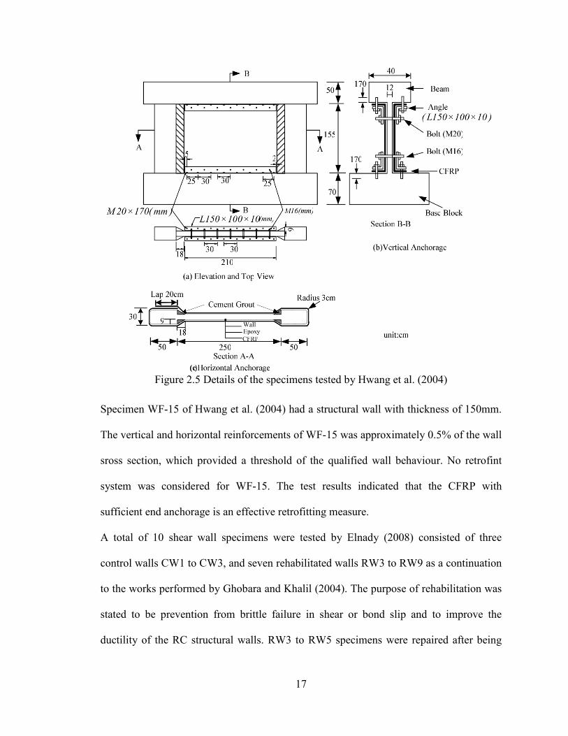
Experimental tests on RC frames with partition walls were conducted by Hwang et al.
(2004) in which five large-sclae isolated specimens, one frame and four walls were
tested. Three of the four wall specimens were identical with different retrofit schemes
while the fourth wall specimen was designed with higher amount of reinforcement and
wall thickness. Specimen PF was a pure frame, which intended to draw a comparison
between frame and wall, the details of frame in all four wall specimens were identical to
PF. The test wall of specimen WF-12 was consisted of a 120mm thickness, with
300x500mm boundary elements (columns of the frame); an overal length of 3500mm,
and height of 1500mm without retrofitting in order to use as the control specimen. Only
thermal reinforcements were used in the wall specimen WF-12 and similar specimens.
SpecimenWF-12-FV was strengthened with four layers of CFRP laminates of 0.1375mm
thickness, two layers at each side of the wall in vertical direction. Total of eight layers of
CFRP laminates with same properties as of those used for WF-12-FV were attached to
the surface of WF-12-FHV, two horizontally and two vertically on each side. The
retrofitting scheme and end anchorages of the specimens are shown in Figure 2.5.
17
Figure 2.5 Details of the specimens tested by Hwang et al. (2004)
Specimen WF-15 of Hwang et al. (2004) had a structural wall with thickness of 150mm.
The vertical and horizontal reinforcements of WF-15 was approximately 0.5% of the wall
sross section, which provided a threshold of the qualified wall behaviour. No retrofint
system was considered for WF-15. The test results indicated that the CFRP with
sufficient end anchorage is an effective retrofitting measure.
A total of 10 shear wall specimens were tested by Elnady (2008) consisted of three
control walls CW1 to CW3, and seven rehabilitated walls RW3 to RW9 as a continuation
to the works performed by Ghobara and Khalil (2004). The purpose of rehabilitation was
stated to be prevention from brittle failure in shear or bond slip and to improve the
ductility of the RC structural walls. RW3 to RW5 specimens were repaired after being

18
tested as control walls CW1 to CW3. The rehabilitation schemes for the specimens tested
by Elnady (2008) are listed in table 2-1 and selected specimens are shown in Figure 2.6.
The seismic retrofit was involved the use of steel anchor bolts, CFRP wraps, and fillet
weld of the lap spliced reinforcement at the base of the wall.
Figure 2.6 Details of selective specimens tested by Elnady (2008)
Elnady (2008) stated that the experimental program was successful in duplicating failure
modes observed in earthquakes. Based on the experimental results of Elnady (2008), the
moment to shear ratio is a significant factor that affects the behaviour of the structural
walls and influences their failure mode, retrofitting the walls using CFRP sheets
eliminated the brittle shear failure mode, the CFRP confined end column elements
showed a significant contribution to to the tested walls ductile response, and confinement
of concrete using steel anchor bolts successfully improved the ductile behaviour.
Table 2.1 Details of the wall specimens tested by Elnady (2008)
19
Specimen Steel Reinforcement Confinement Shear
CFRP layers
Steel anchors Flexural Shear steel CFRP
layers CW2 6-15M 6mm@180mm - - - -
CW3 6-15M 6mm@180mm - - - -
RW3 6-15M 6mm@50 mm 6mm@50mm 5 2 12.5@100mm
RW4 6-15M 6mm@100mm 6mm@50mm 2 2 12.5@100mm
RW5 6-15M 6mm@50 mm 6mm@50mm 2 2 12.5@100mm
RW6 8-20M 6mm@100mm 6mm@50mm 4 4 12.5@100mm
RW7 8-20M 6mm@100mm 6mm@50mm 4 4 12.5@100mm
RW8 6-20M 10M@100mm 6mm@50mm 3 - 10.0@100mm
RW9 6-20M 10M@100mm 6mm@50mm 3 - 10.0@100mm
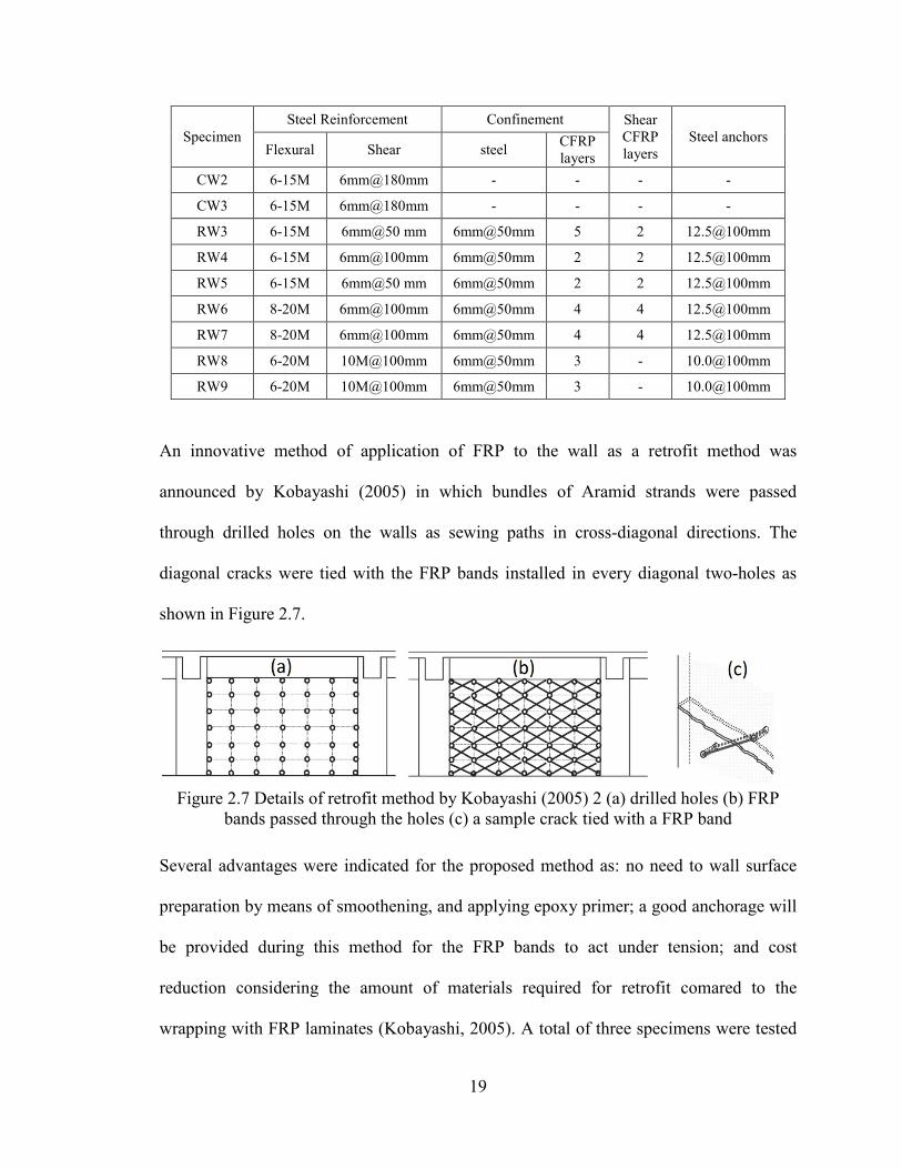
An innovative method of application of FRP to the wall as a retrofit method was
announced by Kobayashi (2005) in which bundles of Aramid strands were passed
through drilled holes on the walls as sewing paths in cross-diagonal directions. The
diagonal cracks were tied with the FRP bands installed in every diagonal two-holes as
shown in Figure 2.7.
Figure 2.7 Details of retrofit method by Kobayashi (2005) 2 (a) drilled holes (b) FRP
bands passed through the holes (c) a sample crack tied with a FRP band
Several advantages were indicated for the proposed method as: no need to wall surface
preparation by means of smoothening, and applying epoxy primer; a good anchorage will
be provided during this method for the FRP bands to act under tension; and cost
reduction considering the amount of materials required for retrofit comared to the
wrapping with FRP laminates (Kobayashi, 2005). A total of three specimens were tested
20
by Kobayashi (2005) in terms of a control wall “W03N” without strengthening, a
strengthened wall “W02R” using the proposed method; and a repaired wall “W03N-R”
which was previousely tested as the control wall and repaired by removing the crushed
parts of concrete and replacing them with new mortar, and strengthened by FRP bands.
The results of experimental tests were proofs of effectiveness of the proposed method of
strengthening using FRP bands by improving the shear capacity and deformability of the
wall panel.
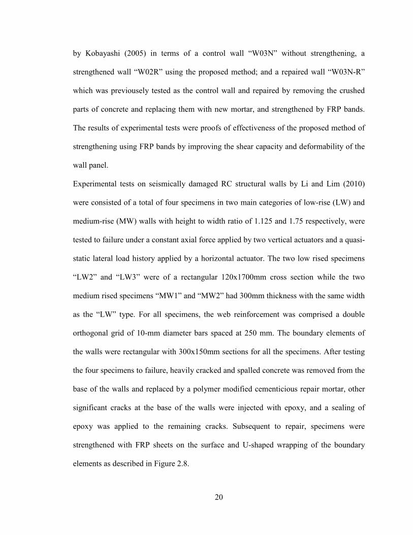
Experimental tests on seismically damaged RC structural walls by Li and Lim (2010)
were consisted of a total of four specimens in two main categories of low-rise (LW) and
medium-rise (MW) walls with height to width ratio of 1.125 and 1.75 respectively, were
tested to failure under a constant axial force applied by two vertical actuators and a quasi-
static lateral load history applied by a horizontal actuator. The two low rised specimens
“LW2” and “LW3” were of a rectangular 120x1700mm cross section while the two
medium rised specimens “MW1” and “MW2” had 300mm thickness with the same width
as the “LW” type. For all specimens, the web reinforcement was comprised a double
orthogonal grid of 10-mm diameter bars spaced at 250 mm. The boundary elements of
the walls were rectangular with 300x150mm sections for all the specimens. After testing
the four specimens to failure, heavily cracked and spalled concrete was removed from the
base of the walls and replaced by a polymer modified cementicious repair mortar, other
significant cracks at the base of the walls were injected with epoxy, and a sealing of
epoxy was applied to the remaining cracks. Subsequent to repair, specimens were
strengthened with FRP sheets on the surface and U-shaped wrapping of the boundary
elements as described in Figure 2.8.
21
Figure 2.8 Details of specimens and repair schemes tested by Li and Lim (2010)
Li and Lim (2010) indicated that the repair method was not capable of restoring the full
stiffness capacity but the specimen strengthened by CFRP exhibitted a better
performance regarding the stiffness compared to the GFRP strengthened walls, Also the
dissipated energy of the repaired specimens was stated to be significantly larger than
those of the original counterparts for both the “LW” and “MW” specimens.
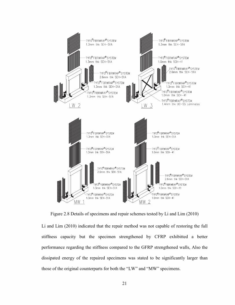
22
Figure 2.9 Details of the test assembly on the shake table of École Polytechnique de
Montreal and the rehabilitated 8-story walls tested in El-Sokkary et al. (2012)
El-Sokkary et al. (2012) studied the effects of rehabilitation of shear walls by CFRP
laminates through a shake table test program on two 8-storey cantilevered shear walls of
1:0.429 scale. The program was consisted of testing the walls under several levels of
ground motion excitations and then retrofitting the walls using CFRP laminates and
23
subject them again to the same excitation histories in order to study the effectiveness of
the rehabilitation techniques.
The test assembly and specimens details are shown in Figure 2.9. The results of tests on
the original walls showed severe inelastic deformations at the 6th storey level due to the
effects of higher modes of vibration; also, the base plastic hinge of the walls experienced
significant inelastic deformations. A rehabilitation scheme was proposed by El-Sokkary
et al. (2012) in order to enhance the overal seismic behaviour of the original walls by
strengthening the two locations with nonlinear response.
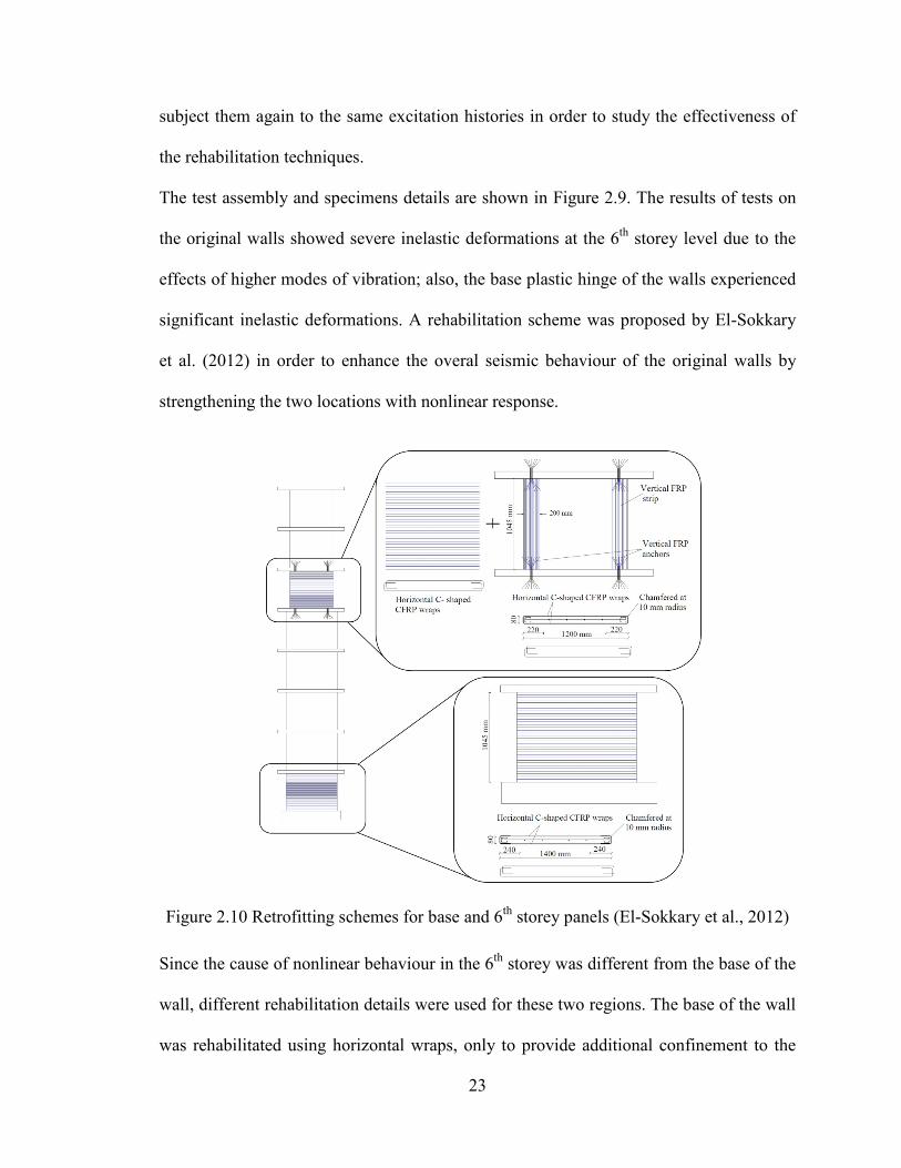
Figure 2.10 Retrofitting schemes for base and 6th storey panels (El-Sokkary et al., 2012)
Since the cause of nonlinear behaviour in the 6th storey was different from the base of the
wall, different rehabilitation details were used for these two regions. The base of the wall
was rehabilitated using horizontal wraps, only to provide additional confinement to the
24
boundary zones in order to improve the ductility without increasing the flexural capacity
of the wall. The target of rehabilitation at the sixth storey level was to increase the
flexural strength of the wall in order to prevent the plastic deformations. The boundary
zones of the panel at sixth storey elevation were wrapped by vertical CFRP sheets
providing additional flexural strength; also, the shear capacity of the panel was improved
by providing horizontal wraps in order to prevent shear failure prior to reach the flexural
capacity. Following rehabilitation, the overal performance of the walls was proven to be
satisfactorily improved.
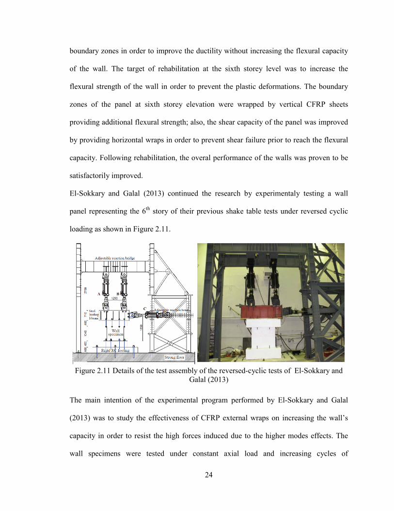
El-Sokkary and Galal (2013) continued the research by experimentaly testing a wall
panel representing the 6th story of their previous shake table tests under reversed cyclic
loading as shown in Figure 2.11.
Figure 2.11 Details of the test assembly of the reversed-cyclic tests of El-Sokkary and
Galal (2013)
The main intention of the experimental program performed by El-Sokkary and Galal
(2013) was to study the effectiveness of CFRP external wraps on increasing the wall’s
capacity in order to resist the high forces induced due to the higher modes effects. The
wall specimens were tested under constant axial load and increasing cycles of
25
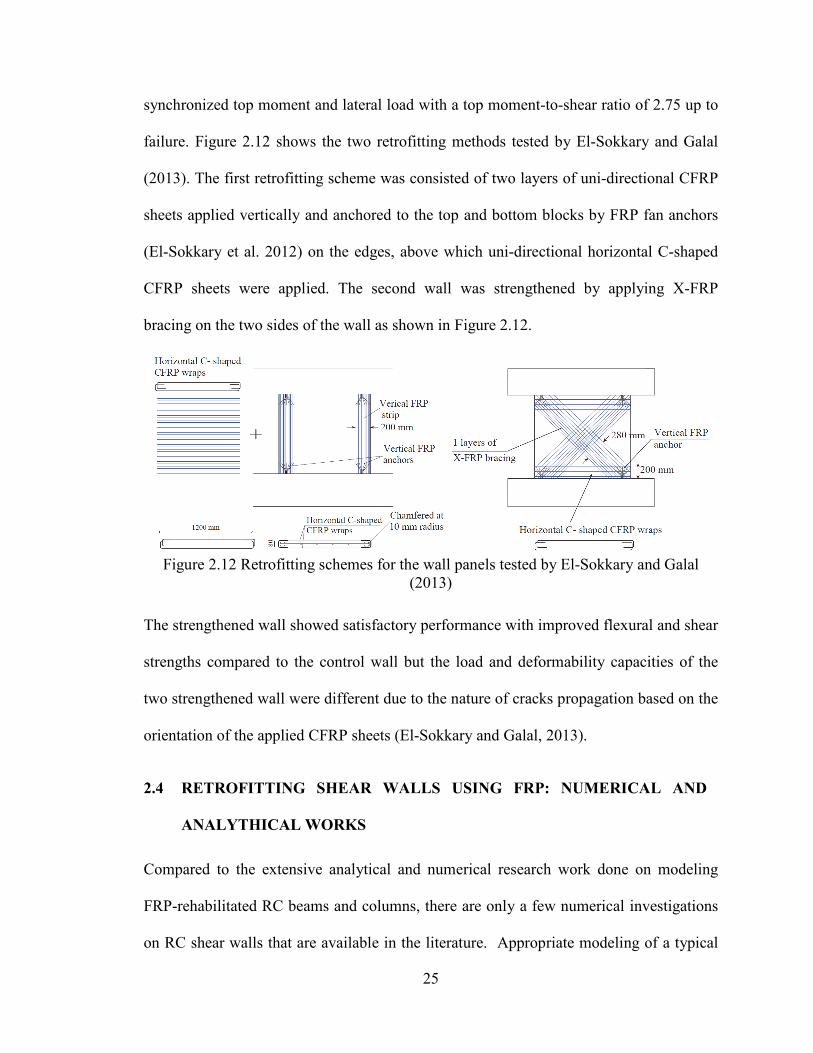
synchronized top moment and lateral load with a top moment-to-shear ratio of 2.75 up to
failure. Figure 2.12 shows the two retrofitting methods tested by El-Sokkary and Galal
(2013). The first retrofitting scheme was consisted of two layers of uni-directional CFRP
sheets applied vertically and anchored to the top and bottom blocks by FRP fan anchors
(El-Sokkary et al. 2012) on the edges, above which uni-directional horizontal C-shaped
CFRP sheets were applied. The second wall was strengthened by applying X-FRP
bracing on the two sides of the wall as shown in Figure 2.12.
Figure 2.12 Retrofitting schemes for the wall panels tested by El-Sokkary and Galal
(2013)
The strengthened wall showed satisfactory performance with improved flexural and shear
strengths compared to the control wall but the load and deformability capacities of the
two strengthened wall were different due to the nature of cracks propagation based on the
orientation of the applied CFRP sheets (El-Sokkary and Galal, 2013).
2.4 RETROFITTING SHEAR WALLS USING FRP: NUMERICAL AND
ANALYTHICAL WORKS
Compared to the extensive analytical and numerical research work done on modeling
FRP-rehabilitated RC beams and columns, there are only a few numerical investigations
on RC shear walls that are available in the literature. Appropriate modeling of a typical
26
RC shear wall retrofitted with FRP sheets envolves capturing the major characteristics of
reinforced concrete, FRP laminates, and bond interface between FRP and shear wall
surface. One of the first significant studies on the behaviour of RC shear walls using
numerical methods was performed by Sittipunt and Wood (1993) in which a FE modeling
approach was developed and verified using available experimental data. They studied the
effects of various parameters such as material models and reinforcement arrangement on
the cyclic behaviour of RC shear walls. The main effort of the study was on the
comparison of various available material models for concrete and steel and initial tests
were done in order to use the most useful material models respecting important factors
namely; simplicity, stability and reliability. The material model used for concrete was
based on the smeared crack model with fixed orthogonal cracks using the strength
criterion for crack initiation and propagation. Reliability of the material model has been
proved through cyclic analysis of slender shear walls and the results were compared to
appropriate experimental data.
Li et al. (2005) proposed a nonlinear 3D FE model in order to perform cyclic analysis on
an I-shaped wall representing the lower portion of the shear wall system of a 25-story
building in Singapore. The geometry of the model was consisted of two flange walls
with lenghts of 657mm and one center wall with a length of 955mm and 45mm thickness
overall as shown in Figure 2.13. The height of the walls were 1314mm which was equal
to 2.6 times the story height of the building in a 1/5 scale.
27
Figure 2.13 Plan view and 3D mesh of the wall model presented by Li et al. (2005)
The wall model mesh was consisted of 220 elements as sketched in Figure 2.13 using 8-
node solid brick elements. The reinforcing steel bars were superposed onto the wall by
using the smeared rebar option of the concrete element in ABAQUS FE package. The
longitudinal reinforcement bars used in the center and flange walls were 8mm and 10mm
diameter bars respectively and 6mm bars were used as the horizontal reinforcement in all
regions of the model. In order to simulate the effects of GFRP wrapping, a total of 525
constrains were defined using spring elements at the appropriate nodes. The material
properties of steel reinforcement bars used in the model were based on elastic perfectly
plastic behaviour in both compression and tension with yield stresses 525MPa and
480MPa for the longitudinal bars used in the center wall and flanges respectively and
350MPa for the horizontal bars. The stiffness of the spring elements representing GFRP
material was 69.65GPa based on previous experimental tests. The concrete material
model used was based on the damaged plasticity model of ABAQUS in which two main
28
failure modes of cracking under uniaxial tension and crushing under uniaxial
compression are defined.
Modelling of RC shear walls using planar elements under reversed cyclic loading was
conducted by Palermo and Vecchio (2007) using the modified compression field theory
(MCFT) (Vecchio and Collins, 1986) and the distributed stress field model (DSFM) by
VecTor2 (Vecchio, 1989) software package. One of the major concerns of the study was
covering the stress-strain curve for concrete under compression as well as the hystresis
loops in a material model along with the cracking capability of the material. The concrete
strength in the models analyzed in the study varied from 21.7 to 53.6 MPa and the
authors reported crushing to be the ultimate failure for majority of the wall models.
Smeared type of reinforcement were considered assuming the perfectly bonded
reinforcement smeared through the concrete ignoring the effects of possible buckling of
steel rebar following the concrete crushing. The authors stated that the assumption of full
bond between reinforcment and concrete provides satisfactory results. The material
properties used for concrete and steel in the study were based on the basic models
provided by VecTor2 software package namely a trilinear stress-strain curve for steel
which covers the linear elastic region, the yield region, and the strain-hardening zone; an
initial stress-stress curve requiring solely the cylinder compressive strength. The
information required for the material models to be defined in particular cases were
obtained from the experimental data in the literature. A total of five experimentally tested
specimens from the literature were modeled under two main categories regarding the wall
geometry namely slender shear walls with a height-to-width ratio greater than 2.0 and
squat shear walls with height-to-width ratios smaller than 2.0 by Palermo and Vecchio
29
(2007). Examples of the FE meshes used in the study are presented in Figure 2.14.
Palermo and Vecchio (2007) stated that the models satisfactorily simulated the observed
behaviour including peak strength, postpeak response, ductility, energy dissipation, and
failure mechanism. The only discrepency which was considered as “noticable” reported
to be the displacement corresponding to the peak lateral load.
Figure 2.14 FE mesh used by Palermo and Vecchio (2007) (a) slender shear wall (b)
squat shear wall
Khomwan et al. (2010) developed a nonlinear FE model for the analysis of RC plane
stress members strengthened by FRP external sheets under monotonic and cyclic loading.
The bonding interface between FRP and concrete surface was taken into consideration
using a two-dimensional membrane contact element in order to capture the debonding
failure mechanism at the interface between concrete surface and FRP sheets. The work
was consisted of FE modeling of experimentally tested RC beams and shear walls under
cyclic loading. Smeared cracking model was used to simulate the mechanical behaviour
of concrete material with discrete steel reinforcement bars in order to simulate the
experimental works of Lombard et al. (1999) on RC shear walls rehabilitated using
30
external layers of FRP. The FE mesh used in the study is shown in Figure 2.15. The
analysis stated to be capable of approaching the force-displacement of shear walls as well
as the failure modes comparing to the respective experimental data within an acceptable
margin of error.
Figure 2.15 FE mesh of RC shear walls modeled by Khomwan et al. (2010)
One of the most recent works on the FE modeling of shear walls retrofitted with
externally bonded sheets under cyclic loading has been performed by Cortes-Puentes and
Palermo (2012) in which a total four specimens from the experimental literature were
analysed using VecTor2 FE package (Wong and Vecchio, 2002) in a 2D planar
geometry. Three of the four modeled specimens were consisted of RC shear walls
retrofitted using steel plates in various arrangements as well as one to simulate one of the
test specimens of Lombard et al. (1999) using a single vertical layer of CFRP bonded to
the surface of concrete shear wall on both sides. A minimum of 13 rectangular plane
31
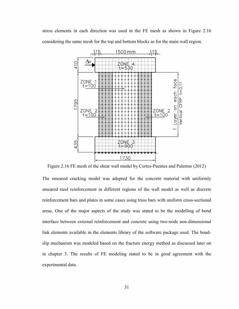
stress elements in each direction was used in the FE mesh as shown in Figure 2.16
considering the same mesh for the top and bottom blocks as for the main wall region.
Figure 2.16 FE mesh of the shear wall model by Cortes-Puentes and Palermo (2012)
The smeared cracking model was adopted for the concrete material with uniformly
smeared steel reinforcement in different regions of the wall model as well as discrete
reinforcement bars and plates in some cases using truss bars with uniform cross-sectional
areas. One of the major aspects of the study was stated to be the modelling of bond
interface between external reinforcement and concrete using two-node non-dimensional
link elements available in the elements library of the software package used. The bond-
slip mechanism was modeled based on the fracture energy method as discussed later on
in chapter 3. The results of FE modeling stated to be in good agreement with the
experimental data.
32
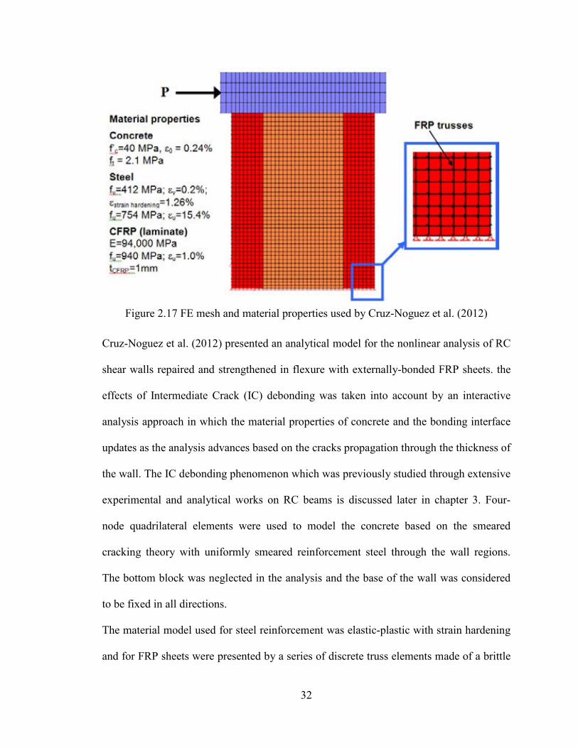
Figure 2.17 FE mesh and material properties used by Cruz-Noguez et al. (2012)
Cruz-Noguez et al. (2012) presented an analytical model for the nonlinear analysis of RC
shear walls repaired and strengthened in flexure with externally-bonded FRP sheets. the
effects of Intermediate Crack (IC) debonding was taken into account by an interactive
analysis approach in which the material properties of concrete and the bonding interface
updates as the analysis advances based on the cracks propagation through the thickness of
the wall. The IC debonding phenomenon which was previously studied through extensive
experimental and analytical works on RC beams is discussed later in chapter 3. Four-
node quadrilateral elements were used to model the concrete based on the smeared
cracking theory with uniformly smeared reinforcement steel through the wall regions.
The bottom block was neglected in the analysis and the base of the wall was considered
to be fixed in all directions.
The material model used for steel reinforcement was elastic-plastic with strain hardening
and for FRP sheets were presented by a series of discrete truss elements made of a brittle
33
material with zero compressive strength. The bond-slip relationship between concrete and
FRP was modeled by a tri-linear approximation of the IC debonding model proposed by
Lu et al. (2005-a). The IC debonding was stated to be of major importance in the
behaviour of RC shear walls retrofitted with FRP external layers under cyclic loads. The
debonding criterion used was stated to be a simple approach and easy to implement into
FE packages where user-defined elements to define the bond-slip model is not available.
34
CHAPTER 3
ANALYSIS METHODOLOGY
3.1 GENERAL
This chapter describes the FE modeling approach used for the simulation of reinforced
concrete (RC) shear walls retrofitted by external layers of fibre-reinforced polymer (FRP)
composites and the analysis methodology. The FE models are developed using general
purpose finite elements program package ANSYS13.0 (2010). The chapter describes the
geometry, meshing, element attributes, materials behaviour, and interface considerations.
In order to verify the material models used and failure criteria, pilot analysis on prism
models are conducted where necessary.
3.2 MODELING CONSIDERATIONS
3.2.1 Geometry
The geometry of the FE models used in this study consists of typical main parts that form
the tested wall specimens in the reported literature. The geometry of specimens in almost
all of the reported experimental programs described in the previous chapter consists of
three main parts, namely, the loading block, support block, and the main wall region. The
loading and support blocks are made of reinforced concrete with additional width and
length compare to the main wall region in order to transfer the loads from the loading
devices to the wall region without stress concentrations and from the wall region to the
supporting floor. Typical wall specimen geometry is shown in Figure 3.1 where B-B, H-
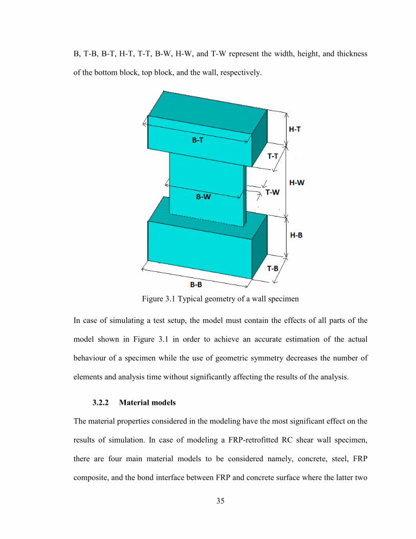
35
B, T-B, B-T, H-T, T-T, B-W, H-W, and T-W represent the width, height, and thickness
of the bottom block, top block, and the wall, respectively.
Figure 3.1 Typical geometry of a wall specimen
In case of simulating a test setup, the model must contain the effects of all parts of the
model shown in Figure 3.1 in order to achieve an accurate estimation of the actual
behaviour of a specimen while the use of geometric symmetry decreases the number of
elements and analysis time without significantly affecting the results of the analysis.
3.2.2 Material models
The material properties considered in the modeling have the most significant effect on the
results of simulation. In case of modeling a FRP-retrofitted RC shear wall specimen,
there are four main material models to be considered namely, concrete, steel, FRP
composite, and the bond interface between FRP and concrete surface where the latter two
36
models do not exist in the modeling of existing shear walls. ANSYS offers an extensive
materials library to simulate the behaviour of various materials based on the mechanical
stress-strain relationship and other phenomena (ANSYS, 2010-a).
3.2.2.1 Steel reinforcement
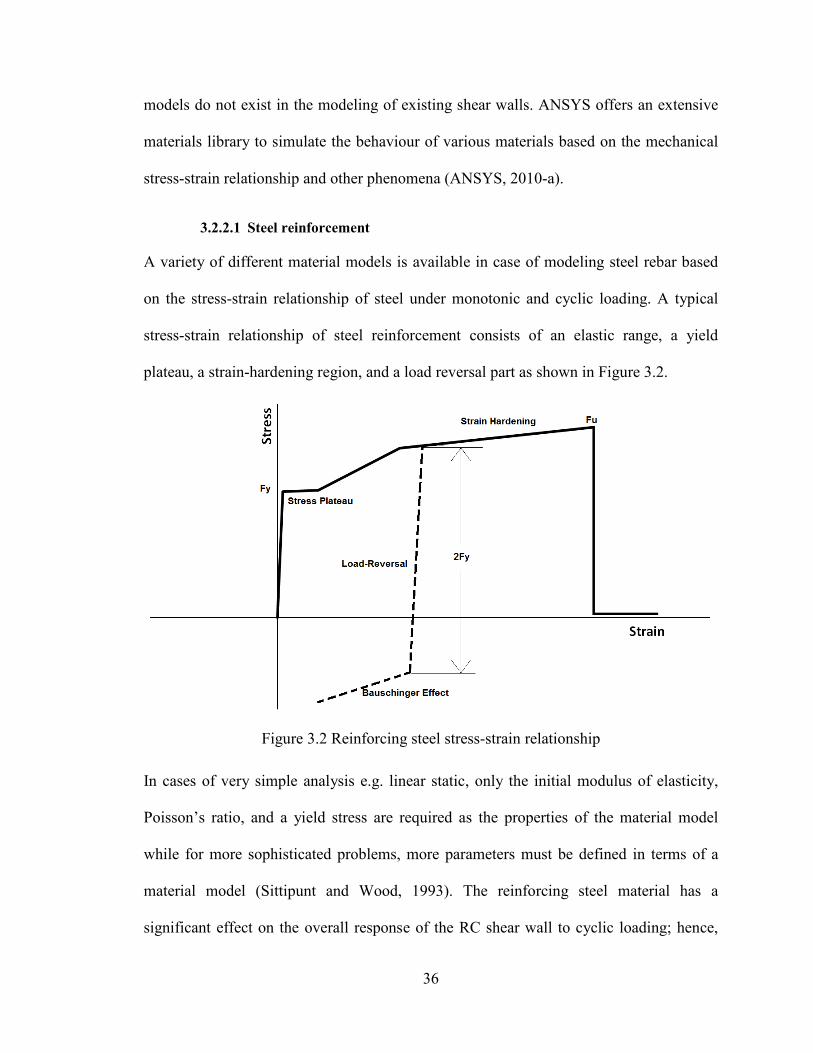
A variety of different material models is available in case of modeling steel rebar based
on the stress-strain relationship of steel under monotonic and cyclic loading. A typical
stress-strain relationship of steel reinforcement consists of an elastic range, a yield
plateau, a strain-hardening region, and a load reversal part as shown in Figure 3.2.
Figure 3.2 Reinforcing steel stress-strain relationship
In cases of very simple analysis e.g. linear static, only the initial modulus of elasticity,
Poisson’s ratio, and a yield stress are required as the properties of the material model
while for more sophisticated problems, more parameters must be defined in terms of a
material model (Sittipunt and Wood, 1993). The reinforcing steel material has a
significant effect on the overall response of the RC shear wall to cyclic loading; hence,
37
the proposed material for steel reinforcement must be precise enough with considerations
of all the important aspects of the actual stress-strain relationship without increasing the
analysis time by adding unnecessary parameters into the model. Although several
material models are available in the materials library of ANSYS, a bilinear isotropic type
of behaviour with an initial modulus of elasticity, a yield stress limit, and a strain
hardening was commonly used in most of the previous numerical studies (Kachlakev,
2001), (Jia, 2003), (Wolanski, 2004) and (Britton, 2010). The Material model used in the
simulations of this study follows a Multilinear-kinematic behaviour which is suggested
by ANSYS (2010-b) as the appropriate model for cyclic analysis. A pilot model of a steel
bar was simulated here in order to check the cyclic behaviour of this material model
under a simple cyclic load history as shown in Figure 3.3 and the force-displacement
curve is plotted in Figure 3.4. The ultimate failure of steel is defined as a rupture point in
which the strain will continue to increase and the stress approaches to a value close to
zero.
Figure 3.3 Cyclic loading history applied to the prism model for steel material
0 10 20 30 40 50
Disp
lace
men
t
Number of Cycles
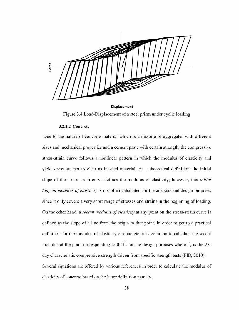
38
Figure 3.4 Load-Displacement of a steel prism under cyclic loading
3.2.2.2 Concrete
Due to the nature of concrete material which is a mixture of aggregates with different
sizes and mechanical properties and a cement paste with certain strength, the compressive
stress-strain curve follows a nonlinear pattern in which the modulus of elasticity and
yield stress are not as clear as in steel material. As a theoretical definition, the initial
slope of the stress-strain curve defines the modulus of elasticity; however, this initial
tangent modulus of elasticity is not often calculated for the analysis and design purposes
since it only covers a very short range of stresses and strains in the beginning of loading.
On the other hand, a secant modulus of elasticity at any point on the stress-strain curve is
defined as the slope of a line from the origin to that point. In order to get to a practical
definition for the modulus of elasticity of concrete, it is common to calculate the secant
modulus at the point corresponding to 0.4f’c for the design purposes where f’
c is the 28-
day characteristic compressive strength driven from specific strength tests (FIB, 2010).
Several equations are offered by various references in order to calculate the modulus of
elasticity of concrete based on the latter definition namely,
Forc
e
Displacement
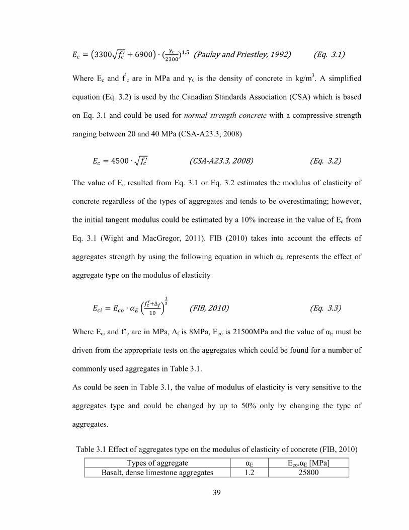
39
𝐸𝑐 = �3300�𝑓𝑐′ + 6900� ∙ ( 𝛾𝑐
2300)1.5 (Paulay and Priestley, 1992) (Eq. 3.1)
Where Ec and f’c are in MPa and γc is the density of concrete in kg/m3. A simplified
equation (Eq. 3.2) is used by the Canadian Standards Association (CSA) which is based
on Eq. 3.1 and could be used for normal strength concrete with a compressive strength
ranging between 20 and 40 MPa (CSA-A23.3, 2008)
𝐸𝑐 = 4500 ∙ �𝑓𝑐′ (CSA-A23.3, 2008) (Eq. 3.2)
The value of Ec resulted from Eq. 3.1 or Eq. 3.2 estimates the modulus of elasticity of
concrete regardless of the types of aggregates and tends to be overestimating; however,
the initial tangent modulus could be estimated by a 10% increase in the value of Ec from
Eq. 3.1 (Wight and MacGregor, 2011). FIB (2010) takes into account the effects of
aggregates strength by using the following equation in which αE represents the effect of
aggregate type on the modulus of elasticity
𝐸𝑐𝑖 = 𝐸𝑐𝑜 ∙ 𝛼𝐸 �𝑓𝑐′+∆𝑓
10�
13 (FIB, 2010) (Eq. 3.3)
Where Eci and f’c are in MPa, Δf is 8MPa, Eco is 21500MPa and the value of αE must be
driven from the appropriate tests on the aggregates which could be found for a number of
commonly used aggregates in Table 3.1.
As could be seen in Table 3.1, the value of modulus of elasticity is very sensitive to the
aggregates type and could be changed by up to 50% only by changing the type of
aggregates.
Table 3.1 Effect of aggregates type on the modulus of elasticity of concrete (FIB, 2010)
Types of aggregate αE Eco.αE [MPa] Basalt, dense limestone aggregates 1.2 25800
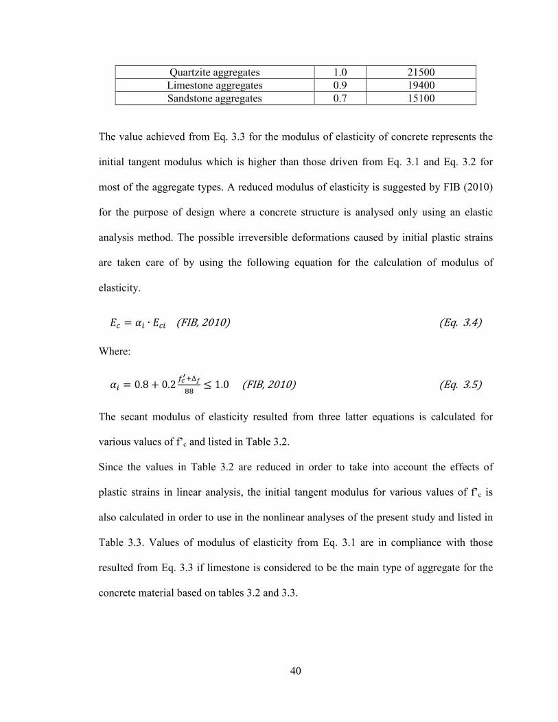
40
Quartzite aggregates 1.0 21500 Limestone aggregates 0.9 19400 Sandstone aggregates 0.7 15100
The value achieved from Eq. 3.3 for the modulus of elasticity of concrete represents the
initial tangent modulus which is higher than those driven from Eq. 3.1 and Eq. 3.2 for
most of the aggregate types. A reduced modulus of elasticity is suggested by FIB (2010)
for the purpose of design where a concrete structure is analysed only using an elastic
analysis method. The possible irreversible deformations caused by initial plastic strains
are taken care of by using the following equation for the calculation of modulus of
elasticity.
𝐸𝑐 = 𝛼𝑖 ∙ 𝐸𝑐𝑖 (FIB, 2010) (Eq. 3.4)
Where:
𝛼𝑖 = 0.8 + 0.2 𝑓𝑐′+∆𝑓
88≤ 1.0 (FIB, 2010) (Eq. 3.5)
The secant modulus of elasticity resulted from three latter equations is calculated for
various values of f’c and listed in Table 3.2.
Since the values in Table 3.2 are reduced in order to take into account the effects of
plastic strains in linear analysis, the initial tangent modulus for various values of f’c is
also calculated in order to use in the nonlinear analyses of the present study and listed in
Table 3.3. Values of modulus of elasticity from Eq. 3.1 are in compliance with those
resulted from Eq. 3.3 if limestone is considered to be the main type of aggregate for the
concrete material based on tables 3.2 and 3.3.
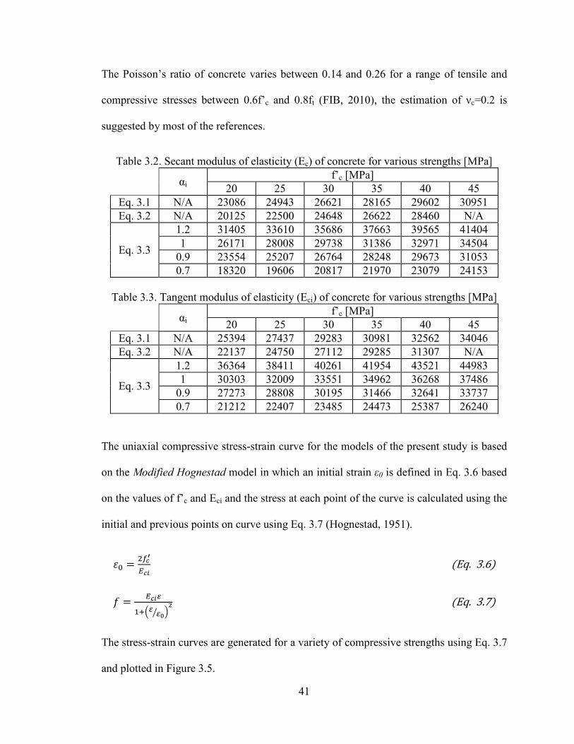
41
The Poisson’s ratio of concrete varies between 0.14 and 0.26 for a range of tensile and
compressive stresses between 0.6f’c and 0.8ft (FIB, 2010), the estimation of νc=0.2 is
suggested by most of the references.
Table 3.2. Secant modulus of elasticity (Ec) of concrete for various strengths [MPa]
αi f’c [MPa]
20 25 30 35 40 45 Eq. 3.1 N/A 23086 24943 26621 28165 29602 30951 Eq. 3.2 N/A 20125 22500 24648 26622 28460 N/A
Eq. 3.3
1.2 31405 33610 35686 37663 39565 41404 1 26171 28008 29738 31386 32971 34504
0.9 23554 25207 26764 28248 29673 31053 0.7 18320 19606 20817 21970 23079 24153
Table 3.3. Tangent modulus of elasticity (Eci) of concrete for various strengths [MPa]
αi f’c [MPa]
20 25 30 35 40 45 Eq. 3.1 N/A 25394 27437 29283 30981 32562 34046 Eq. 3.2 N/A 22137 24750 27112 29285 31307 N/A
Eq. 3.3
1.2 36364 38411 40261 41954 43521 44983 1 30303 32009 33551 34962 36268 37486
0.9 27273 28808 30195 31466 32641 33737 0.7 21212 22407 23485 24473 25387 26240
The uniaxial compressive stress-strain curve for the models of the present study is based
on the Modified Hognestad model in which an initial strain ε0 is defined in Eq. 3.6 based
on the values of f’c and Eci and the stress at each point of the curve is calculated using the
initial and previous points on curve using Eq. 3.7 (Hognestad, 1951).
𝜀0 = 2𝑓𝑐′
𝐸𝑐𝑖 (Eq. 3.6)
𝑓 = 𝐸𝑐𝑖𝜀
1+�𝜀 𝜀0� �2 (Eq. 3.7)
The stress-strain curves are generated for a variety of compressive strengths using Eq. 3.7
and plotted in Figure 3.5.
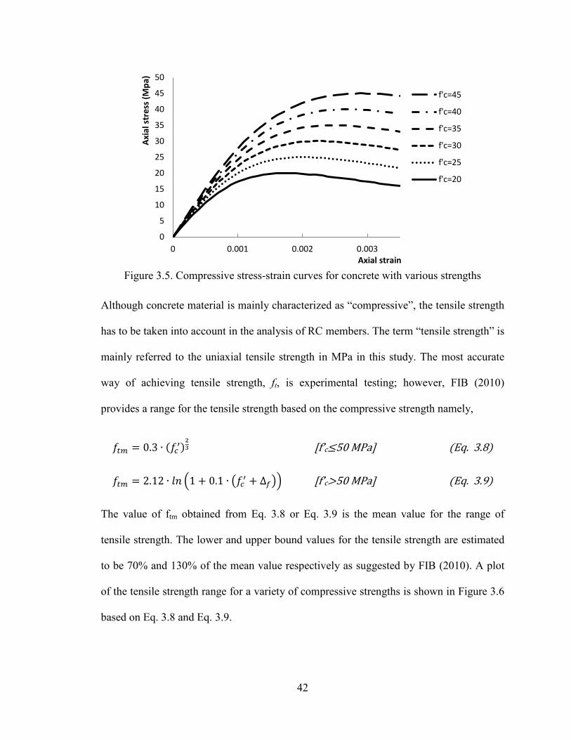
42
Figure 3.5. Compressive stress-strain curves for concrete with various strengths
Although concrete material is mainly characterized as “compressive”, the tensile strength
has to be taken into account in the analysis of RC members. The term “tensile strength” is
mainly referred to the uniaxial tensile strength in MPa in this study. The most accurate
way of achieving tensile strength, ft, is experimental testing; however, FIB (2010)
provides a range for the tensile strength based on the compressive strength namely,
𝑓𝑡𝑚 = 0.3 ∙ (𝑓𝑐′)
23 [f’c≤50 MPa] (Eq. 3.8)
𝑓𝑡𝑚 = 2.12 ∙ 𝑙𝑛 �1 + 0.1 ∙ �𝑓𝑐′ + ∆𝑓�� [f’c>50 MPa] (Eq. 3.9)
The value of ftm obtained from Eq. 3.8 or Eq. 3.9 is the mean value for the range of
tensile strength. The lower and upper bound values for the tensile strength are estimated
to be 70% and 130% of the mean value respectively as suggested by FIB (2010). A plot
of the tensile strength range for a variety of compressive strengths is shown in Figure 3.6
based on Eq. 3.8 and Eq. 3.9.
0
5
10
15
20
25
30
35
40
45
50
0 0.001 0.002 0.003
Axia
l str
ess (
Mpa
)
Axial strain
f'c=45
f'c=40
f'c=35
f'c=30
f'c=25
f'c=20
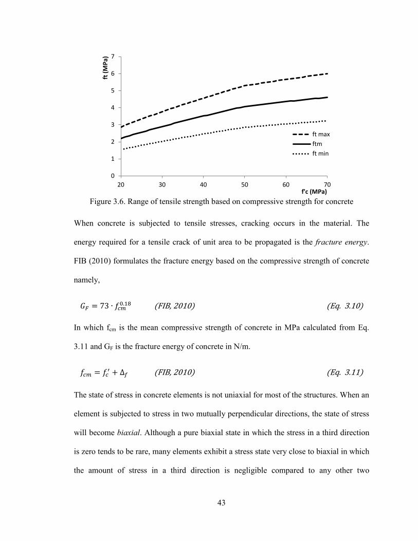
43
Figure 3.6. Range of tensile strength based on compressive strength for concrete
When concrete is subjected to tensile stresses, cracking occurs in the material. The
energy required for a tensile crack of unit area to be propagated is the fracture energy.
FIB (2010) formulates the fracture energy based on the compressive strength of concrete
namely,
𝐺𝐹 = 73 ∙ 𝑓𝑐𝑚0.18 (FIB, 2010) (Eq. 3.10)
In which fcm is the mean compressive strength of concrete in MPa calculated from Eq.
3.11 and GF is the fracture energy of concrete in N/m.
𝑓𝑐𝑚 = 𝑓𝑐′ + ∆𝑓 (FIB, 2010) (Eq. 3.11)
The state of stress in concrete elements is not uniaxial for most of the structures. When an
element is subjected to stress in two mutually perpendicular directions, the state of stress
will become biaxial. Although a pure biaxial state in which the stress in a third direction
is zero tends to be rare, many elements exhibit a stress state very close to biaxial in which
the amount of stress in a third direction is negligible compared to any other two
0
1
2
3
4
5
6
7
20 30 40 50 60 70
ft (M
Pa)
f'c (MPa)
ft max ftm ft min
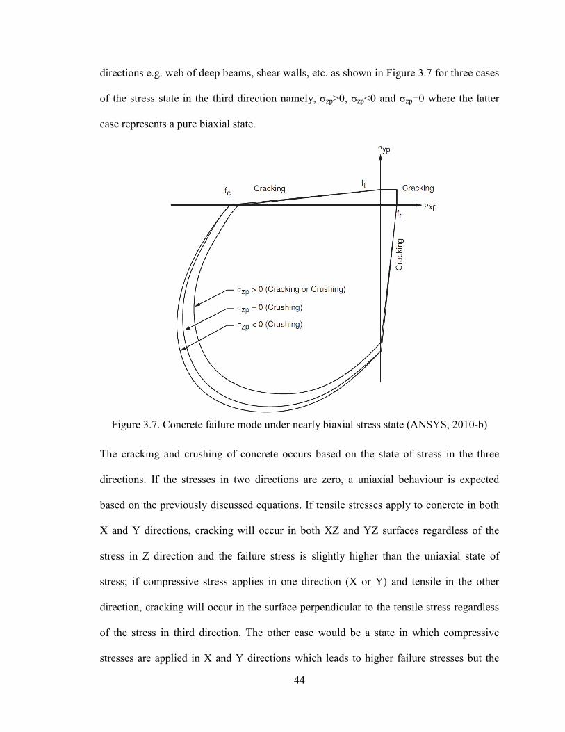
44
directions e.g. web of deep beams, shear walls, etc. as shown in Figure 3.7 for three cases
of the stress state in the third direction namely, σzp>0, σzp<0 and σzp=0 where the latter
case represents a pure biaxial state.
Figure 3.7. Concrete failure mode under nearly biaxial stress state (ANSYS, 2010-b)
The cracking and crushing of concrete occurs based on the state of stress in the three
directions. If the stresses in two directions are zero, a uniaxial behaviour is expected
based on the previously discussed equations. If tensile stresses apply to concrete in both
X and Y directions, cracking will occur in both XZ and YZ surfaces regardless of the
stress in Z direction and the failure stress is slightly higher than the uniaxial state of
stress; if compressive stress applies in one direction (X or Y) and tensile in the other
direction, cracking will occur in the surface perpendicular to the tensile stress regardless
of the stress in third direction. The other case would be a state in which compressive
stresses are applied in X and Y directions which leads to higher failure stresses but the
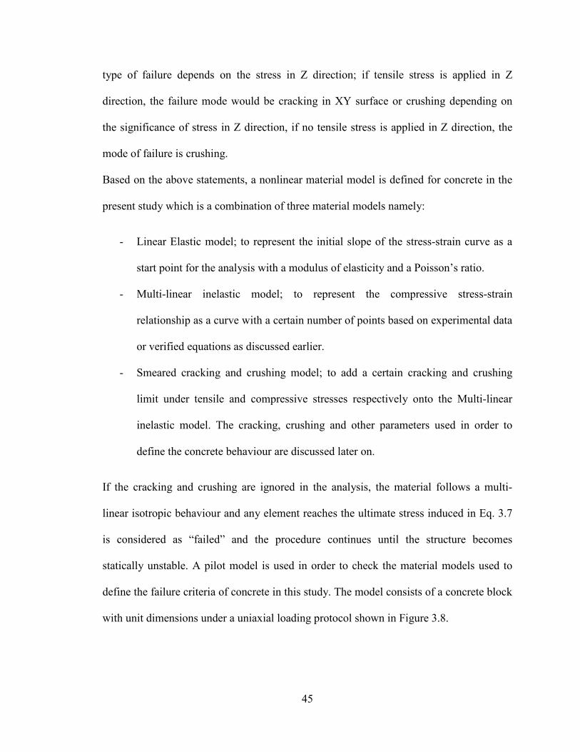
45
type of failure depends on the stress in Z direction; if tensile stress is applied in Z
direction, the failure mode would be cracking in XY surface or crushing depending on
the significance of stress in Z direction, if no tensile stress is applied in Z direction, the
mode of failure is crushing.
Based on the above statements, a nonlinear material model is defined for concrete in the
present study which is a combination of three material models namely:
- Linear Elastic model; to represent the initial slope of the stress-strain curve as a
start point for the analysis with a modulus of elasticity and a Poisson’s ratio.
- Multi-linear inelastic model; to represent the compressive stress-strain
relationship as a curve with a certain number of points based on experimental data
or verified equations as discussed earlier.
- Smeared cracking and crushing model; to add a certain cracking and crushing
limit under tensile and compressive stresses respectively onto the Multi-linear
inelastic model. The cracking, crushing and other parameters used in order to
define the concrete behaviour are discussed later on.
If the cracking and crushing are ignored in the analysis, the material follows a multi-
linear isotropic behaviour and any element reaches the ultimate stress induced in Eq. 3.7
is considered as “failed” and the procedure continues until the structure becomes
statically unstable. A pilot model is used in order to check the material models used to
define the failure criteria of concrete in this study. The model consists of a concrete block
with unit dimensions under a uniaxial loading protocol shown in Figure 3.8.
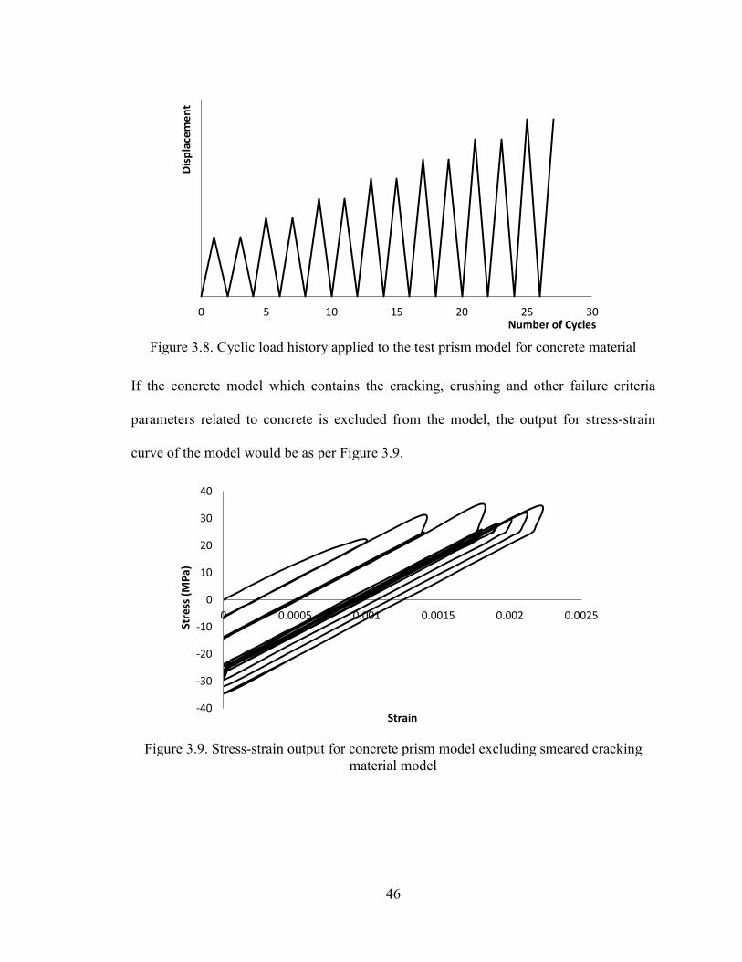
46
Figure 3.8. Cyclic load history applied to the test prism model for concrete material
If the concrete model which contains the cracking, crushing and other failure criteria
parameters related to concrete is excluded from the model, the output for stress-strain
curve of the model would be as per Figure 3.9.
Figure 3.9. Stress-strain output for concrete prism model excluding smeared cracking
material model
0 5 10 15 20 25 30
Disp
lace
men
t
Number of Cycles
-40
-30
-20
-10
0
10
20
30
40
0 0.0005 0.001 0.0015 0.002 0.0025
Stre
ss (M
Pa)
Strain
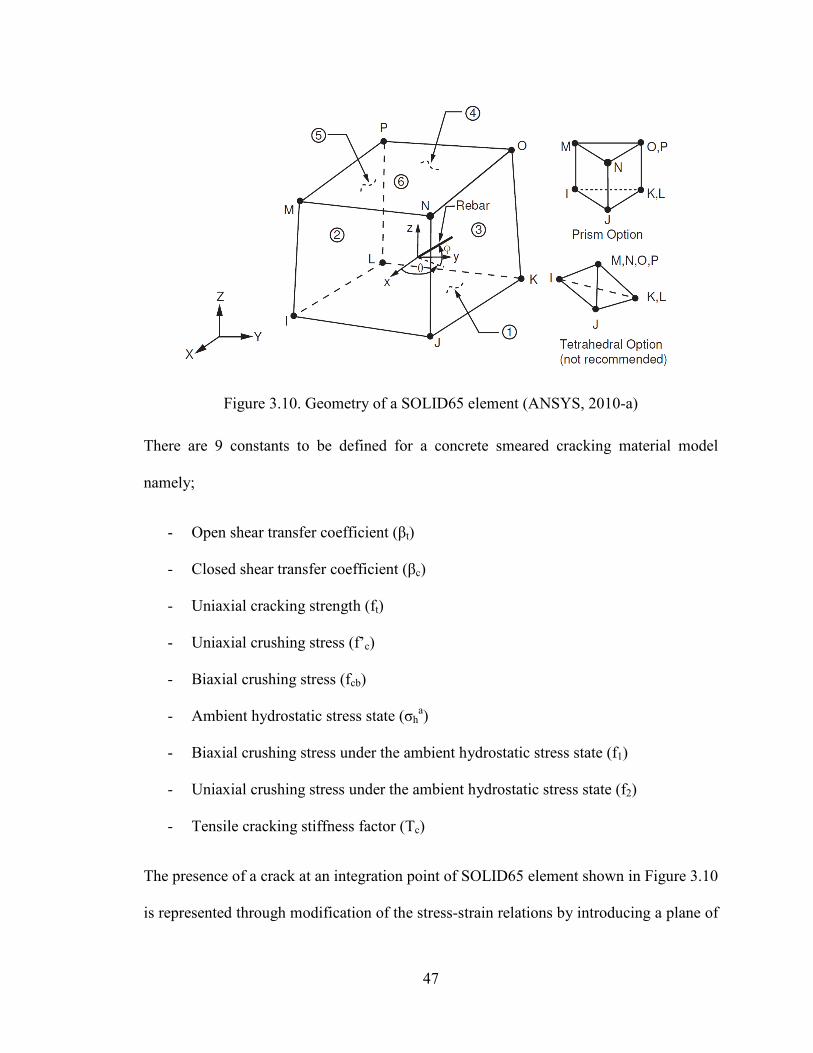
47
Figure 3.10. Geometry of a SOLID65 element (ANSYS, 2010-a)
There are 9 constants to be defined for a concrete smeared cracking material model
namely;
- Open shear transfer coefficient (βt)
- Closed shear transfer coefficient (βc)
- Uniaxial cracking strength (ft)
- Uniaxial crushing stress (f’c)
- Biaxial crushing stress (fcb)
- Ambient hydrostatic stress state (σha)
- Biaxial crushing stress under the ambient hydrostatic stress state (f1)
- Uniaxial crushing stress under the ambient hydrostatic stress state (f2)
- Tensile cracking stiffness factor (Tc)
The presence of a crack at an integration point of SOLID65 element shown in Figure 3.10
is represented through modification of the stress-strain relations by introducing a plane of
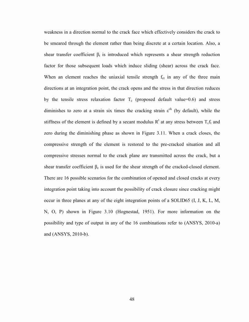
48
weakness in a direction normal to the crack face which effectively considers the crack to
be smeared through the element rather than being discrete at a certain location. Also, a
shear transfer coefficient βt is introduced which represents a shear strength reduction
factor for those subsequent loads which induce sliding (shear) across the crack face.
When an element reaches the uniaxial tensile strength fct in any of the three main
directions at an integration point, the crack opens and the stress in that direction reduces
by the tensile stress relaxation factor Tc (proposed default value=0.6) and stress
diminishes to zero at a strain six times the cracking strain εck (by default), while the
stiffness of the element is defined by a secant modulus Rt at any stress between Tcft and
zero during the diminishing phase as shown in Figure 3.11. When a crack closes, the
compressive strength of the element is restored to the pre-cracked situation and all
compressive stresses normal to the crack plane are transmitted across the crack, but a
shear transfer coefficient βc is used for the shear strength of the cracked-closed element.
There are 16 possible scenarios for the combination of opened and closed cracks at every
integration point taking into account the possibility of crack closure since cracking might
occur in three planes at any of the eight integration points of a SOLID65 (I, J, K, L, M,
N, O, P) shown in Figure 3.10 (Hognestad, 1951). For more information on the
possibility and type of output in any of the 16 combinations refer to (ANSYS, 2010-a)
and (ANSYS, 2010-b).
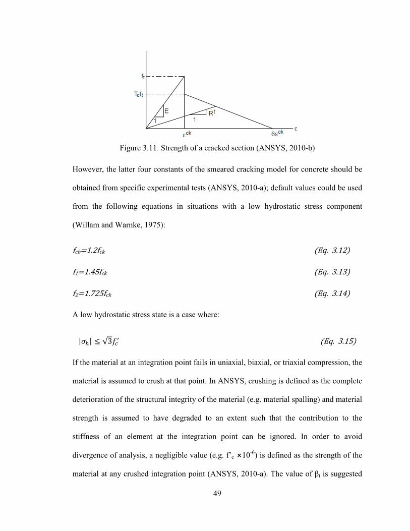
49
Figure 3.11. Strength of a cracked section (ANSYS, 2010-b)
However, the latter four constants of the smeared cracking model for concrete should be
obtained from specific experimental tests (ANSYS, 2010-a); default values could be used
from the following equations in situations with a low hydrostatic stress component
(Willam and Warnke, 1975):
fcb=1.2fck (Eq. 3.12)
f1=1.45fck (Eq. 3.13)
f2=1.725fck (Eq. 3.14)
A low hydrostatic stress state is a case where:
|𝜎ℎ| ≤ √3𝑓𝑐′ (Eq. 3.15)
If the material at an integration point fails in uniaxial, biaxial, or triaxial compression, the
material is assumed to crush at that point. In ANSYS, crushing is defined as the complete
deterioration of the structural integrity of the material (e.g. material spalling) and material
strength is assumed to have degraded to an extent such that the contribution to the
stiffness of an element at the integration point can be ignored. In order to avoid
divergence of analysis, a negligible value (e.g. f’c ⨯10-6) is defined as the strength of the
material at any crushed integration point (ANSYS, 2010-a). The value of βt is suggested
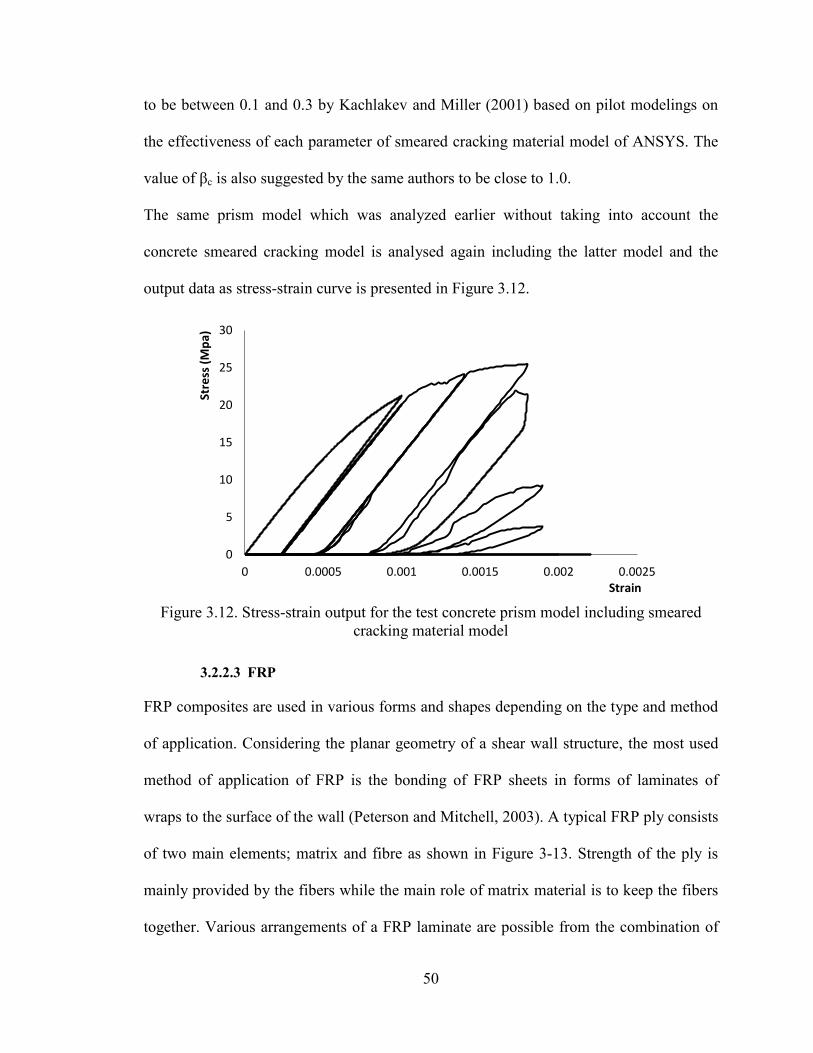
50
to be between 0.1 and 0.3 by Kachlakev and Miller (2001) based on pilot modelings on
the effectiveness of each parameter of smeared cracking material model of ANSYS. The
value of βc is also suggested by the same authors to be close to 1.0.
The same prism model which was analyzed earlier without taking into account the
concrete smeared cracking model is analysed again including the latter model and the
output data as stress-strain curve is presented in Figure 3.12.
Figure 3.12. Stress-strain output for the test concrete prism model including smeared
cracking material model
3.2.2.3 FRP
FRP composites are used in various forms and shapes depending on the type and method
of application. Considering the planar geometry of a shear wall structure, the most used
method of application of FRP is the bonding of FRP sheets in forms of laminates of
wraps to the surface of the wall (Peterson and Mitchell, 2003). A typical FRP ply consists
of two main elements; matrix and fibre as shown in Figure 3-13. Strength of the ply is
mainly provided by the fibers while the main role of matrix material is to keep the fibers
together. Various arrangements of a FRP laminate are possible from the combination of
0
5
10
15
20
25
30
0 0.0005 0.001 0.0015 0.002 0.0025
Stre
ss (M
pa)
Strain
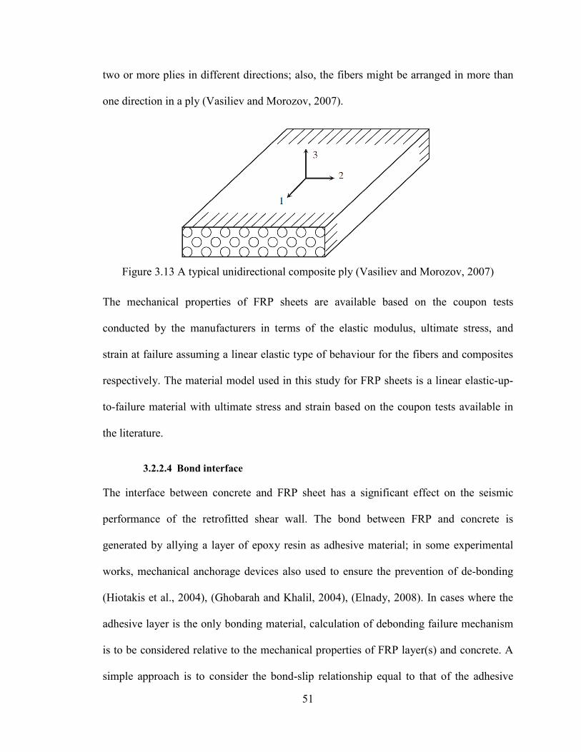
51
two or more plies in different directions; also, the fibers might be arranged in more than
one direction in a ply (Vasiliev and Morozov, 2007).
Figure 3.13 A typical unidirectional composite ply (Vasiliev and Morozov, 2007)
The mechanical properties of FRP sheets are available based on the coupon tests
conducted by the manufacturers in terms of the elastic modulus, ultimate stress, and
strain at failure assuming a linear elastic type of behaviour for the fibers and composites
respectively. The material model used in this study for FRP sheets is a linear elastic-up-
to-failure material with ultimate stress and strain based on the coupon tests available in
the literature.
3.2.2.4 Bond interface
The interface between concrete and FRP sheet has a significant effect on the seismic
performance of the retrofitted shear wall. The bond between FRP and concrete is
generated by allying a layer of epoxy resin as adhesive material; in some experimental
works, mechanical anchorage devices also used to ensure the prevention of de-bonding
(Hiotakis et al., 2004), (Ghobarah and Khalil, 2004), (Elnady, 2008). In cases where the
adhesive layer is the only bonding material, calculation of debonding failure mechanism
is to be considered relative to the mechanical properties of FRP layer(s) and concrete. A
simple approach is to consider the bond-slip relationship equal to that of the adhesive
52
layer but since the adhesive layer has a specific strength in terms of modulus of elasticity
(Eepx) and rapture stress (fepx) significantly greater than that of concrete, the failure of
concrete at the bonding surface by means of fracture energy must be considered as the
strength of the bonding layer.
In addition to the fracture energy method which is resulted from direct pullout tests,
another failure criterion based on the intermediate cracking (IC) in concrete at the
bonding surface is stated to be of significant importance (Teng et al., 2003), (Yao et al.,
2005), (Dai et al., 2005), (Lu et al., 2007) , (Rosenboom and Rizkalla, 2008), (Ombres,
2010). Various models are proposed in order to properly address the debonding failure
criterion in flexural RC members strengthened with FRP layers, in some models the
debonding mechanism is stated to be a function of FRP material properties while some
others used the concrete fracture energy as the failure criterion to address the debonding
mechanism, some more sophisticated models considered the IC debonding as the mode of
failure and more behaviour parameters have involved. The following is a brief review of
the most significant models available for the prediction of bond-slip relationship.
a) ACI model
A simple relationship was proposed by ACI (2002) in order to evaluate the design
debonding strain of the FRP material (εdeb).
𝜀𝑑𝑒𝑏 = 𝐾𝑚𝜀𝑓𝑢 (ACI, 2002) (Eq. 3.16)
Where εfu is the ultimate rupture strain of the FRP and Km is a reduction factor as
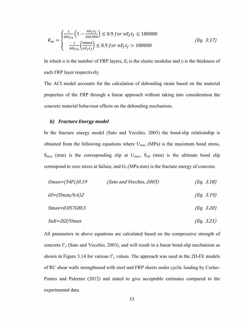
53
𝐾𝑚 = �
160𝜀𝑓𝑢
�1 − 𝑛𝐸𝑓𝑡𝑓
360,000� ≤ 0.9 𝑓𝑜𝑟 𝑛𝐸𝑓𝑡𝑓 ≤ 180000
160𝜀𝑓𝑢
�90000𝑛𝐸𝑓𝑡𝑓
� ≤ 0.9 𝑓𝑜𝑟 𝑛𝐸𝑓𝑡𝑓 > 180000� (Eq. 3.17)
In which n is the number of FRP layers, Ef is the elastic modulus and tf is the thickness of
each FRP layer respectively.
The ACI model accounts for the calculation of debonding strain based on the material
properties of the FRP through a linear approach without taking into consideration the
concrete material behaviour effects on the debonding mechanism.
b) Fracture Energy model
In the fracture energy model (Sato and Vecchio, 2003) the bond-slip relationship is
obtained from the following equations where Umax (MPa) is the maximum bond stress,
Smax (mm) is the corresponding slip at Umax, Sult (mm) is the ultimate bond slip
correspond to zero stress at failure, and Gf (MPa.mm) is the fracture energy of concrete.
Umax=(54f’c)0.19 (Sato and Vecchio, 2003) (Eq. 3.18)
Gf=(Umax/6.6)2 (Eq. 3.19)
Smax=0.057Gf0.5 (Eq. 3.20)
Sult=2Gf/Umax (Eq. 3.21)
All parameters in above equations are calculated based on the compressive strength of
concrete f’c (Sato and Vecchio, 2003), and will result in a linear bond-slip mechanism as
shown in Figure 3.14 for various f’c values. The approach was used in the 2D-FE models
of RC shear walls strengthened with steel and FRP sheets under cyclic loading by Cortes-
Puntes and Palermo (2012) and stated to give acceptable estimates compared to the
experimental data.
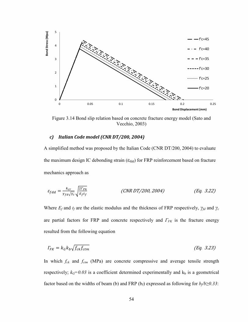
54
Figure 3.14 Bond slip relation based on concrete fracture energy model (Sato and
Vecchio, 2003)
c) Italian Code model (CNR DT/200, 2004)
A simplified method was proposed by the Italian Code (CNR DT/200, 2004) to evaluate
the maximum design IC debonding strain (εfdd) for FRP reinforcement based on fracture
mechanics approach as
𝜀𝑓𝑑𝑑 = 𝑘𝑐𝑟𝛾𝑓𝑑�𝛾𝑐
�2𝛤𝐹𝑘𝐸𝑓𝑡𝑓
(CNR DT/200, 2004) (Eq. 3.22)
Where Ef and tf are the elastic modulus and the thickness of FRP respectively, γfd and γc
are partial factors for FRP and concrete respectively and ΓFK is the fracture energy
resulted from the following equation
𝛤𝐹𝐾 = 𝑘𝐺𝑘𝑏�𝑓𝑐𝑘𝑓𝑐𝑡𝑚 (Eq. 3.23)
In which fck and fctm (MPa) are concrete compressive and average tensile strength
respectively; kG=0.03 is a coefficient determined experimentally and kb is a geometrical
factor based on the widths of beam (b) and FRP (bf) expressed as following for bf/b≥0.33:
0
1
2
3
4
5
0 0.05 0.1 0.15 0.2 0.25
Bond
Str
ess (
Mpa
)
Bond Displacement (mm)
f'c=45
f'c=40
f'c=35
f'c=30
f'c=25
f'c=20
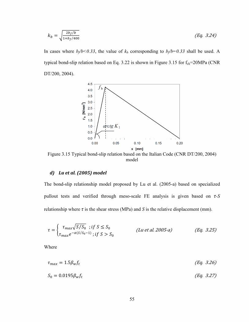
55
𝑘𝑏 = �2𝑏𝑓 𝑏⁄
1+𝑏𝑓 400⁄ (Eq. 3.24)
In cases where bf/b<0.33, the value of kb corresponding to bf/b=0.33 shall be used. A
typical bond-slip relation based on Eq. 3.22 is shown in Figure 3.15 for fck=20MPa (CNR
DT/200, 2004).
Figure 3.15 Typical bond-slip relation based on the Italian Code (CNR DT/200, 2004)
model
d) Lu et al. (2005) model
The bond-slip relationship model proposed by Lu et al. (2005-a) based on specialized
pullout tests and verified through meso-scale FE analysis is given based on τ-S
relationship where τ is the shear stress (MPa) and S is the relative displacement (mm).
𝜏 = � 𝜏𝑚𝑎𝑥�𝑆 𝑆0⁄ ; 𝑖𝑓 𝑆 ≤ 𝑆0
𝜏𝑚𝑎𝑥𝑒−𝛼(𝑆 𝑆0−1⁄ ) ; 𝑖𝑓 𝑆 > 𝑆0
� (Lu et al. 2005-a) (Eq. 3.25)
Where
𝜏𝑚𝑎𝑥 = 1.5𝛽𝑤𝑓𝑡 (Eq. 3.26)
𝑆0 = 0.0195𝛽𝑤𝑓𝑡 (Eq. 3.27)
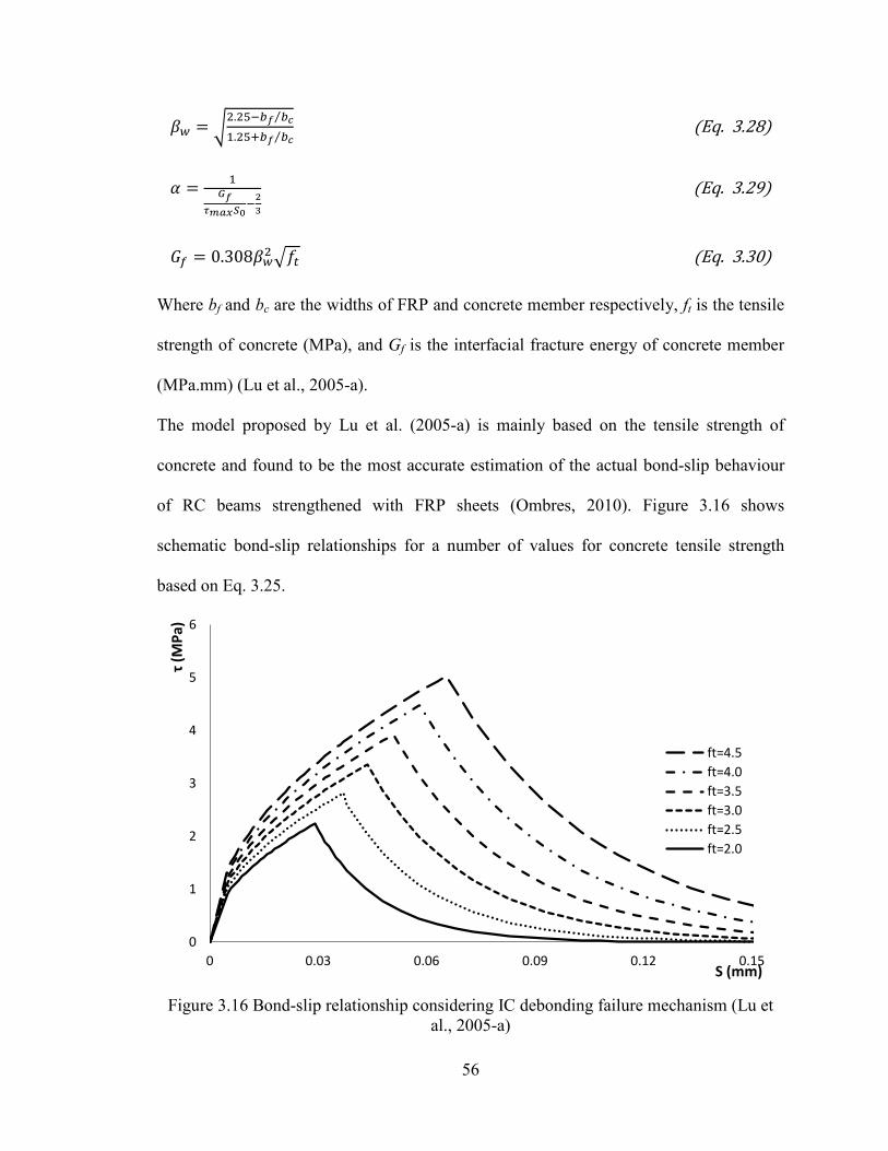
56
𝛽𝑤 = �2.25−𝑏𝑓 𝑏𝑐⁄1.25+𝑏𝑓 𝑏𝑐⁄ (Eq. 3.28)
𝛼 = 1𝐺𝑓
𝜏𝑚𝑎𝑥𝑆0−2
3
(Eq. 3.29)
𝐺𝑓 = 0.308𝛽𝑤2 �𝑓𝑡 (Eq. 3.30)
Where bf and bc are the widths of FRP and concrete member respectively, ft is the tensile
strength of concrete (MPa), and Gf is the interfacial fracture energy of concrete member
(MPa.mm) (Lu et al., 2005-a).
The model proposed by Lu et al. (2005-a) is mainly based on the tensile strength of
concrete and found to be the most accurate estimation of the actual bond-slip behaviour
of RC beams strengthened with FRP sheets (Ombres, 2010). Figure 3.16 shows
schematic bond-slip relationships for a number of values for concrete tensile strength
based on Eq. 3.25.
Figure 3.16 Bond-slip relationship considering IC debonding failure mechanism (Lu et
al., 2005-a)
0
1
2
3
4
5
6
0 0.03 0.06 0.09 0.12 0.15
τ (M
Pa)
S (mm)
ft=4.5 ft=4.0 ft=3.5 ft=3.0 ft=2.5 ft=2.0
57
3.2.3 ANSYS Elements
The elements used for the modeling of every part of the shear wall specimens of this
study are selected from the elements library of ANSYS. Types of elements and the DOFs
must meet the required boundary conditions for the failure criteria to be met. The
elements are listed based on their relevance in the models.
3.2.3.1 Reinforced Concrete Element (SOLID65)
SOLID65 is a general solid element defined by eight nodes with three translational
degrees of freedom at each node. The element is capable of modeling the cracking in
tension and crushing in compression and it is well suited for the 3D modeling of solids
with or without reinforcement materials. The main purpose of the element is to model the
concrete behaviour based on the criteria described previously. Other cases in which the
element is used for, are the modeling of the reinforced composites and geological
materials (ANSYS, 2010-a). The element is also capable of modeling plastic deformation
and creep. The geometry of SOLID65 is shown earlier in Figure 3.10 where the three
possible shapes of cube, prism and tetrahedral are described with details on the rebar
directions and the coordinate system of the element. Each of the eight nodes (I-O) has
three translational DOFs in X, Y, and Z direction respectively. Cracking is supported at
any surface in any direction by means of the angle between the normal of the crack
surface to the global directions.
SOLID65 allows the presence of four different materials in each element; one matrix
element which could be considered as a brittle material such as concrete and a maximum
of three different reinforcing materials each with its own direction and volume as a ratio
of the matrix material. The concrete material (if assigned to the matrix for SOLID65) is
58
capable of directional integration point cracking and crushing besides incorporating
plastic behaviour as discussed previously. The reinforcement supports uniaxial stiffness
only and is assumed to be smeared throughout the element (ANSYS, 2010-a). Although
the reinforcement capability of SOLID65 is proved to be useful, the rebar could be
modeled separately using link elements bonded to the concrete elements. In this case, the
nodes of the “discrete” rebar elements are to be coincident with the nodes of concrete
elements in all degrees of freedom; in this study, the steel reinforcement bars are modeled
as combination of smeared and discrete elements.
3.2.3.2 Steel reinforcement element (LINK180)
There are two different elements used in this study to simulate the embedded
reinforcement bars in concrete, a smeared reinforcement in the boundary regions of the
wall in the direction of wall thickness “Global Z” by means of the embedded smeared
reinforcement capability of SOLID65, and a discrete type of reinforcement bars in all
other directions. The element used for the discrete reinforcement bars is LINK180
(ANSYS, 2010-a) which is a 3D spar type element with two nodes and three translational
DOFs at each node. Since no rotational DOF is considered at the nodes of LINK180, no
bending or shear strength is provided. The element supports the material behaviour and
failure criteria specified for steel material described previously in case of nonlinear
analysis. Geometry of LINK180 element is shown in Figure 3.17. There are three real
constants to be defined for every LINK180 element, the cross-sectional area, possibility
of change in the cross-sectional area due to poison’s ratio and strain hardening, and the
type of behaviour as per compression/tension only or both (ANSYS, 2010-a). Another
capability of LINK180 is the initial stress state in which a pre-stressed bar could be
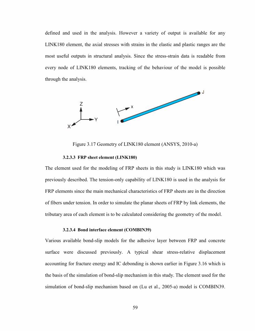
59
defined and used in the analysis. However a variety of output is available for any
LINK180 element, the axial stresses with strains in the elastic and plastic ranges are the
most useful outputs in structural analysis. Since the stress-strain data is readable from
every node of LINK180 elements, tracking of the behaviour of the model is possible
through the analysis.
Figure 3.17 Geometry of LINK180 element (ANSYS, 2010-a)
3.2.3.3 FRP sheet element (LINK180)
The element used for the modeling of FRP sheets in this study is LINK180 which was
previously described. The tension-only capability of LINK180 is used in the analysis for
FRP elements since the main mechanical characteristics of FRP sheets are in the direction
of fibers under tension. In order to simulate the planar sheets of FRP by link elements, the
tributary area of each element is to be calculated considering the geometry of the model.
3.2.3.4 Bond interface element (COMBIN39)
Various available bond-slip models for the adhesive layer between FRP and concrete
surface were discussed previously. A typical shear stress-relative displacement
accounting for fracture energy and IC debonding is shown earlier in Figure 3.16 which is
the basis of the simulation of bond-slip mechanism in this study. The element used for the
simulation of bond-slip mechanism based on (Lu et al., 2005-a) model is COMBIN39.
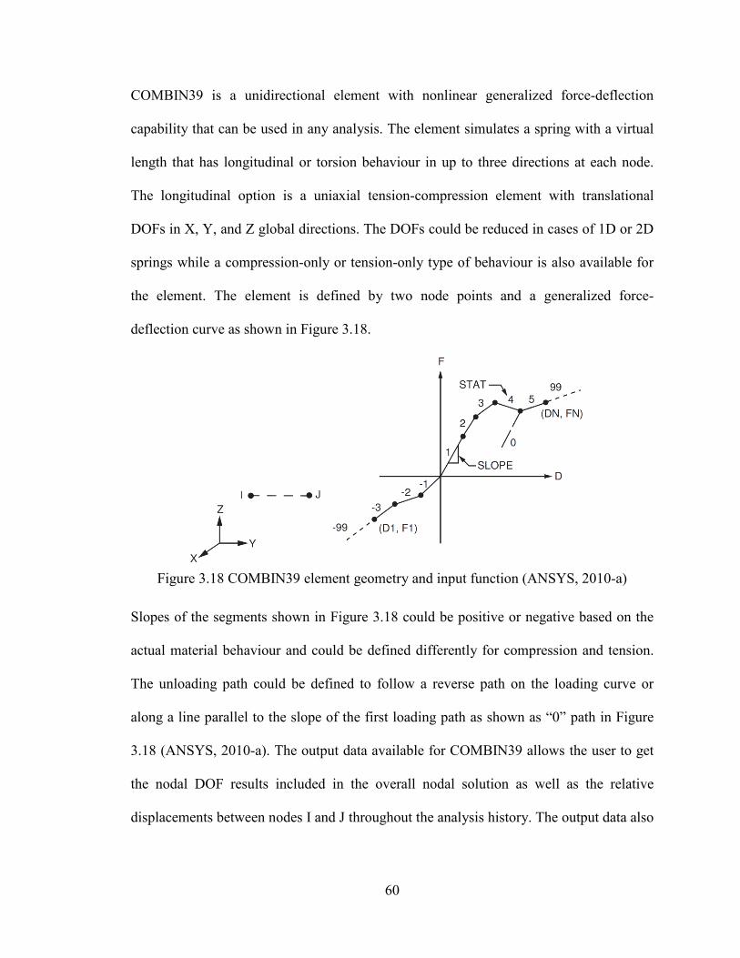
60
COMBIN39 is a unidirectional element with nonlinear generalized force-deflection
capability that can be used in any analysis. The element simulates a spring with a virtual
length that has longitudinal or torsion behaviour in up to three directions at each node.
The longitudinal option is a uniaxial tension-compression element with translational
DOFs in X, Y, and Z global directions. The DOFs could be reduced in cases of 1D or 2D
springs while a compression-only or tension-only type of behaviour is also available for
the element. The element is defined by two node points and a generalized force-
deflection curve as shown in Figure 3.18.
Figure 3.18 COMBIN39 element geometry and input function (ANSYS, 2010-a)
Slopes of the segments shown in Figure 3.18 could be positive or negative based on the
actual material behaviour and could be defined differently for compression and tension.
The unloading path could be defined to follow a reverse path on the loading curve or
along a line parallel to the slope of the first loading path as shown as “0” path in Figure
3.18 (ANSYS, 2010-a). The output data available for COMBIN39 allows the user to get
the nodal DOF results included in the overall nodal solution as well as the relative
displacements between nodes I and J throughout the analysis history. The output data also
61
gives the status of each element at any instant of the loading history as well as the status
of the force-deflection curve and current slope on the curve (ANSYS, 2010-a).
3.2.3.5 FRP layers interface element (COMBIN40)
Although the case of FRP layers interface failure is unlikely to occur as a failure
criterion, in cased where multiple layers of FRP sheets are used by applying epoxy resin
between adjacent layers a bond-slip relation is desirable for the persistence of the model.
COMBIN40 element is used in such cases where a linear-up-to-failure with a sliding
force and a spring constant define the bond interface between adjacent layers of FRP
sheets based on the material properties of epoxy resin.
3.3 FAILURE CRITERIA
The failure criteria are dictated by the mechanical characteristics of the constituent
materials (including the FRP-Concrete bond interface element) and the interactions
between them. As previously stated, a typical FE assembly in this study is consisted of
four different sub-assemblies namely, concrete, steel reinforcement, FRP composite, and
the bonding interface. Each of these sub-assemblies is modeled by a material model
assigned to appropriate meshes of elements in various regions of the geometry. The
material model represents the failure criterion of the material in terms of mechanical
properties and certain limitations. The nonlinear analysis continues while elements in
various regions of the assembly are reaching their limits defined by material models,
when an element fails, it is considered to be fully unloaded and the analysis continues
until the unloading of failed elements causes geometric instability (ANSYS, 2010-b).
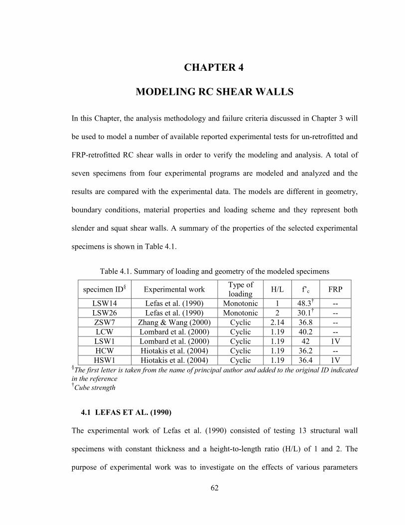
62
CHAPTER 4
MODELING RC SHEAR WALLS
In this Chapter, the analysis methodology and failure criteria discussed in Chapter 3 will
be used to model a number of available reported experimental tests for un-retrofitted and
FRP-retrofitted RC shear walls in order to verify the modeling and analysis. A total of
seven specimens from four experimental programs are modeled and analyzed and the
results are compared with the experimental data. The models are different in geometry,
boundary conditions, material properties and loading scheme and they represent both
slender and squat shear walls. A summary of the properties of the selected experimental
specimens is shown in Table 4.1.
Table 4.1. Summary of loading and geometry of the modeled specimens
specimen ID§ Experimental work Type of loading H/L f’c FRP
LSW14 Lefas et al. (1990) Monotonic 1 48.3† -- LSW26 Lefas et al. (1990) Monotonic 2 30.1† -- ZSW7 Zhang & Wang (2000) Cyclic 2.14 36.8 -- LCW Lombard et al. (2000) Cyclic 1.19 40.2 -- LSW1 Lombard et al. (2000) Cyclic 1.19 42 1V HCW Hiotakis et al. (2004) Cyclic 1.19 36.2 -- HSW1 Hiotakis et al. (2004) Cyclic 1.19 36.4 1V
§The first letter is taken from the name of principal author and added to the original ID indicated in the reference †Cube strength
4.1 LEFAS ET AL. (1990)
The experimental work of Lefas et al. (1990) consisted of testing 13 structural wall
specimens with constant thickness and a height-to-length ratio (H/L) of 1 and 2. The
purpose of experimental work was to investigate on the effects of various parameters
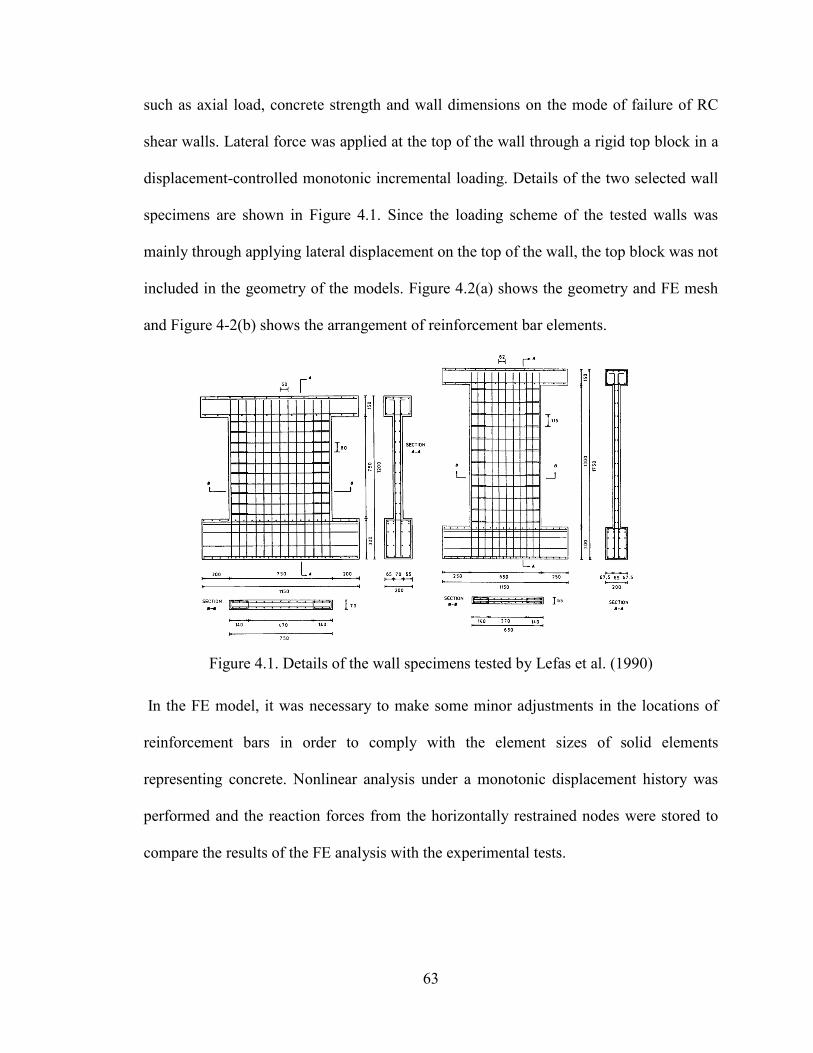
63
such as axial load, concrete strength and wall dimensions on the mode of failure of RC
shear walls. Lateral force was applied at the top of the wall through a rigid top block in a
displacement-controlled monotonic incremental loading. Details of the two selected wall
specimens are shown in Figure 4.1. Since the loading scheme of the tested walls was
mainly through applying lateral displacement on the top of the wall, the top block was not
included in the geometry of the models. Figure 4.2(a) shows the geometry and FE mesh
and Figure 4-2(b) shows the arrangement of reinforcement bar elements.
Figure 4.1. Details of the wall specimens tested by Lefas et al. (1990)
In the FE model, it was necessary to make some minor adjustments in the locations of
reinforcement bars in order to comply with the element sizes of solid elements
representing concrete. Nonlinear analysis under a monotonic displacement history was
performed and the reaction forces from the horizontally restrained nodes were stored to
compare the results of the FE analysis with the experimental tests.
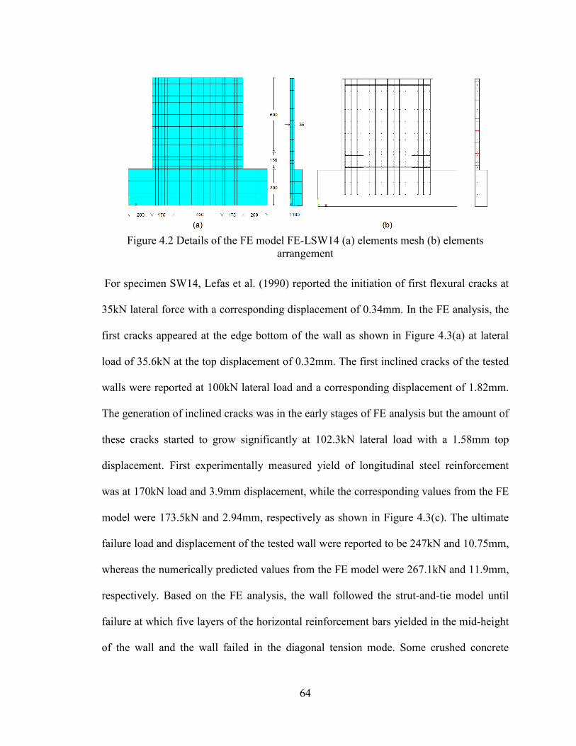
64
Figure 4.2 Details of the FE model FE-LSW14 (a) elements mesh (b) elements
arrangement
For specimen SW14, Lefas et al. (1990) reported the initiation of first flexural cracks at
35kN lateral force with a corresponding displacement of 0.34mm. In the FE analysis, the
first cracks appeared at the edge bottom of the wall as shown in Figure 4.3(a) at lateral
load of 35.6kN at the top displacement of 0.32mm. The first inclined cracks of the tested
walls were reported at 100kN lateral load and a corresponding displacement of 1.82mm.
The generation of inclined cracks was in the early stages of FE analysis but the amount of
these cracks started to grow significantly at 102.3kN lateral load with a 1.58mm top
displacement. First experimentally measured yield of longitudinal steel reinforcement
was at 170kN load and 3.9mm displacement, while the corresponding values from the FE
model were 173.5kN and 2.94mm, respectively as shown in Figure 4.3(c). The ultimate
failure load and displacement of the tested wall were reported to be 247kN and 10.75mm,
whereas the numerically predicted values from the FE model were 267.1kN and 11.9mm,
respectively. Based on the FE analysis, the wall followed the strut-and-tie model until
failure at which five layers of the horizontal reinforcement bars yielded in the mid-height
of the wall and the wall failed in the diagonal tension mode. Some crushed concrete
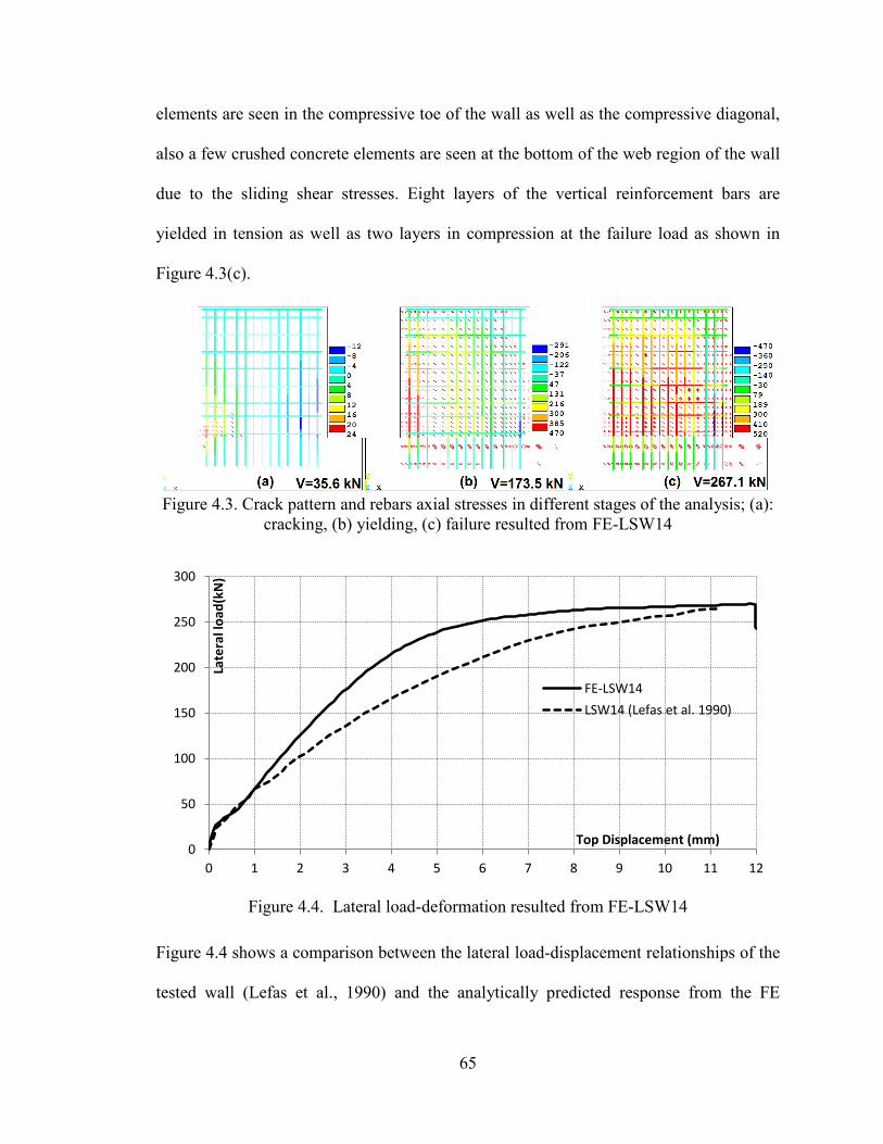
65
elements are seen in the compressive toe of the wall as well as the compressive diagonal,
also a few crushed concrete elements are seen at the bottom of the web region of the wall
due to the sliding shear stresses. Eight layers of the vertical reinforcement bars are
yielded in tension as well as two layers in compression at the failure load as shown in
Figure 4.3(c).
Figure 4.3. Crack pattern and rebars axial stresses in different stages of the analysis; (a):
cracking, (b) yielding, (c) failure resulted from FE-LSW14
Figure 4.4. Lateral load-deformation resulted from FE-LSW14
Figure 4.4 shows a comparison between the lateral load-displacement relationships of the
tested wall (Lefas et al., 1990) and the analytically predicted response from the FE
0
50
100
150
200
250
300
0 1 2 3 4 5 6 7 8 9 10 11 12
Late
ral l
oad(
kN)
Top Displacement (mm)
FE-LSW14 LSW14 (Lefas et al. 1990)
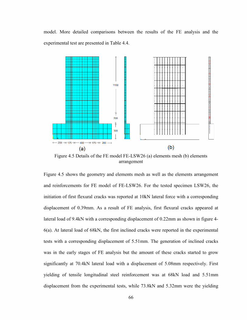
66
model. More detailed comparisons between the results of the FE analysis and the
experimental test are presented in Table 4.4.
Figure 4.5 Details of the FE model FE-LSW26 (a) elements mesh (b) elements
arrangement
Figure 4.5 shows the geometry and elements mesh as well as the elements arrangement
and reinforcements for FE model of FE-LSW26. For the tested specimen LSW26, the
initiation of first flexural cracks was reported at 10kN lateral force with a corresponding
displacement of 0.39mm. As a result of FE analysis, first flexural cracks appeared at
lateral load of 9.4kN with a corresponding displacement of 0.22mm as shown in figure 4-
6(a). At lateral load of 68kN, the first inclined cracks were reported in the experimental
tests with a corresponding displacement of 5.51mm. The generation of inclined cracks
was in the early stages of FE analysis but the amount of these cracks started to grow
significantly at 70.4kN lateral load with a displacement of 5.08mm respectively. First
yielding of tensile longitudinal steel reinforcement was at 68kN load and 5.51mm
displacement from the experimental tests, while 73.8kN and 5.32mm were the yielding
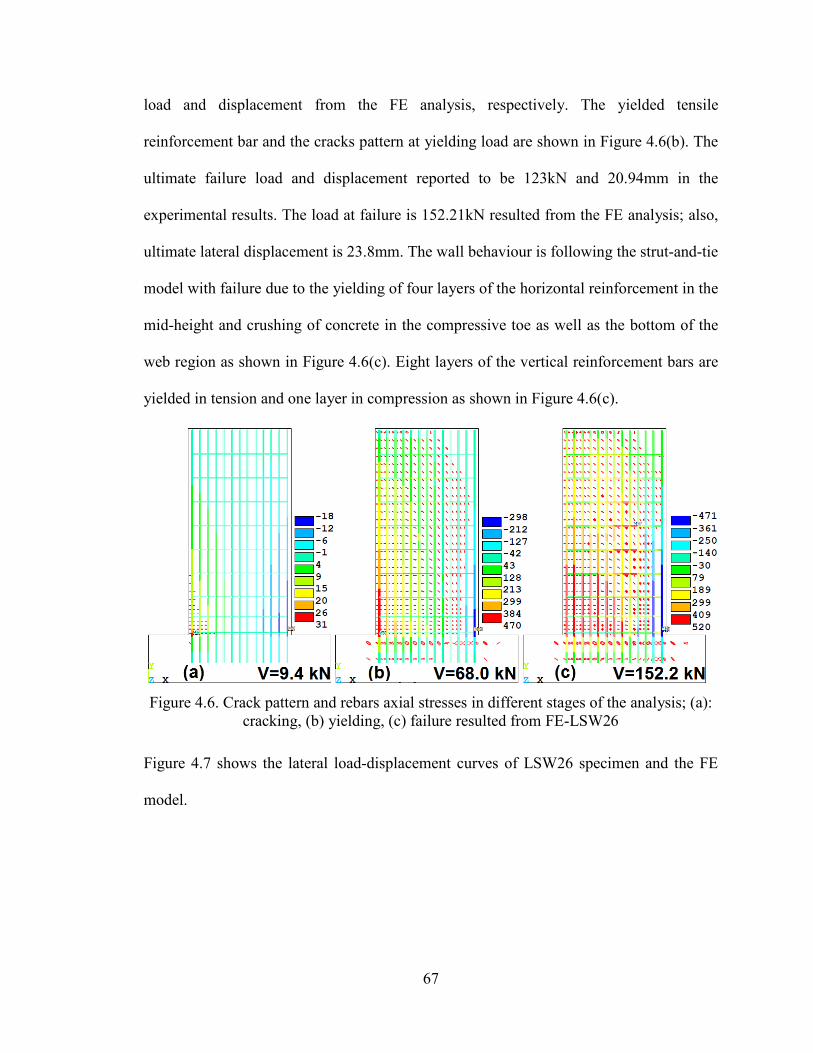
67
load and displacement from the FE analysis, respectively. The yielded tensile
reinforcement bar and the cracks pattern at yielding load are shown in Figure 4.6(b). The
ultimate failure load and displacement reported to be 123kN and 20.94mm in the
experimental results. The load at failure is 152.21kN resulted from the FE analysis; also,
ultimate lateral displacement is 23.8mm. The wall behaviour is following the strut-and-tie
model with failure due to the yielding of four layers of the horizontal reinforcement in the
mid-height and crushing of concrete in the compressive toe as well as the bottom of the
web region as shown in Figure 4.6(c). Eight layers of the vertical reinforcement bars are
yielded in tension and one layer in compression as shown in Figure 4.6(c).
Figure 4.6. Crack pattern and rebars axial stresses in different stages of the analysis; (a):
cracking, (b) yielding, (c) failure resulted from FE-LSW26
Figure 4.7 shows the lateral load-displacement curves of LSW26 specimen and the FE
model.
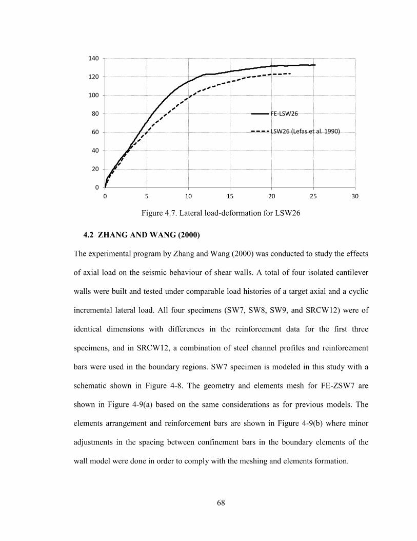
68
Figure 4.7. Lateral load-deformation for LSW26
4.2 ZHANG AND WANG (2000)
The experimental program by Zhang and Wang (2000) was conducted to study the effects
of axial load on the seismic behaviour of shear walls. A total of four isolated cantilever
walls were built and tested under comparable load histories of a target axial and a cyclic
incremental lateral load. All four specimens (SW7, SW8, SW9, and SRCW12) were of
identical dimensions with differences in the reinforcement data for the first three
specimens, and in SRCW12, a combination of steel channel profiles and reinforcement
bars were used in the boundary regions. SW7 specimen is modeled in this study with a
schematic shown in Figure 4-8. The geometry and elements mesh for FE-ZSW7 are
shown in Figure 4-9(a) based on the same considerations as for previous models. The
elements arrangement and reinforcement bars are shown in Figure 4-9(b) where minor
adjustments in the spacing between confinement bars in the boundary elements of the
wall model were done in order to comply with the meshing and elements formation.
0
20
40
60
80
100
120
140
0 5 10 15 20 25 30
FE-LSW26
LSW26 (Lefas et al. 1990)
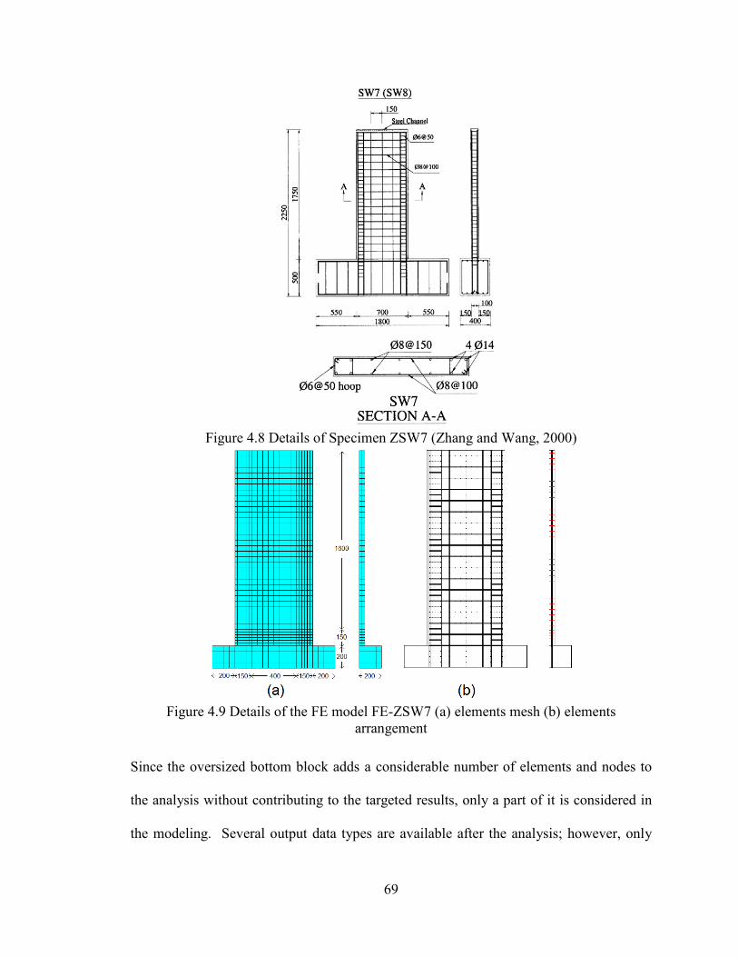
69
Figure 4.8 Details of Specimen ZSW7 (Zhang and Wang, 2000)
Figure 4.9 Details of the FE model FE-ZSW7 (a) elements mesh (b) elements
arrangement
Since the oversized bottom block adds a considerable number of elements and nodes to
the analysis without contributing to the targeted results, only a part of it is considered in
the modeling. Several output data types are available after the analysis; however, only
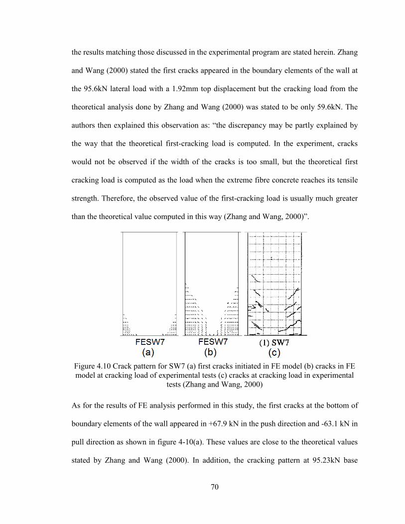
70
the results matching those discussed in the experimental program are stated herein. Zhang
and Wang (2000) stated the first cracks appeared in the boundary elements of the wall at
the 95.6kN lateral load with a 1.92mm top displacement but the cracking load from the
theoretical analysis done by Zhang and Wang (2000) was stated to be only 59.6kN. The
authors then explained this observation as: “the discrepancy may be partly explained by
the way that the theoretical first-cracking load is computed. In the experiment, cracks
would not be observed if the width of the cracks is too small, but the theoretical first
cracking load is computed as the load when the extreme fibre concrete reaches its tensile
strength. Therefore, the observed value of the first-cracking load is usually much greater
than the theoretical value computed in this way (Zhang and Wang, 2000)”.
Figure 4.10 Crack pattern for SW7 (a) first cracks initiated in FE model (b) cracks in FE model at cracking load of experimental tests (c) cracks at cracking load in experimental
tests (Zhang and Wang, 2000)
As for the results of FE analysis performed in this study, the first cracks at the bottom of
boundary elements of the wall appeared in +67.9 kN in the push direction and -63.1 kN in
pull direction as shown in figure 4-10(a). These values are close to the theoretical values
stated by Zhang and Wang (2000). In addition, the cracking pattern at 95.23kN base
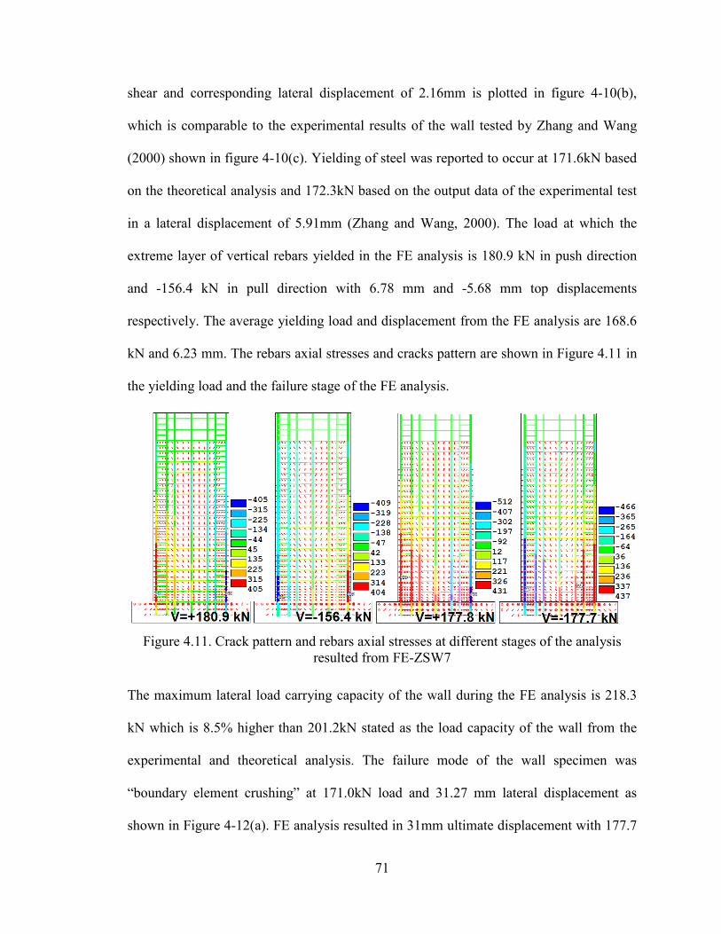
71
shear and corresponding lateral displacement of 2.16mm is plotted in figure 4-10(b),
which is comparable to the experimental results of the wall tested by Zhang and Wang
(2000) shown in figure 4-10(c). Yielding of steel was reported to occur at 171.6kN based
on the theoretical analysis and 172.3kN based on the output data of the experimental test
in a lateral displacement of 5.91mm (Zhang and Wang, 2000). The load at which the
extreme layer of vertical rebars yielded in the FE analysis is 180.9 kN in push direction
and -156.4 kN in pull direction with 6.78 mm and -5.68 mm top displacements
respectively. The average yielding load and displacement from the FE analysis are 168.6
kN and 6.23 mm. The rebars axial stresses and cracks pattern are shown in Figure 4.11 in
the yielding load and the failure stage of the FE analysis.
Figure 4.11. Crack pattern and rebars axial stresses at different stages of the analysis
resulted from FE-ZSW7
The maximum lateral load carrying capacity of the wall during the FE analysis is 218.3
kN which is 8.5% higher than 201.2kN stated as the load capacity of the wall from the
experimental and theoretical analysis. The failure mode of the wall specimen was
“boundary element crushing” at 171.0kN load and 31.27 mm lateral displacement as
shown in Figure 4-12(a). FE analysis resulted in 31mm ultimate displacement with 177.7
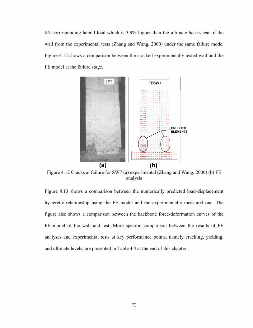
72
kN corresponding lateral load which is 3.9% higher than the ultimate base shear of the
wall from the experimental tests (Zhang and Wang, 2000) under the same failure mode.
Figure 4.12 shows a comparison between the cracked experimentally tested wall and the
FE model at the failure stage.
Figure 4.12 Cracks at failure for SW7 (a) experimental (Zhang and Wang, 2000) (b) FE
analysis
Figure 4.13 shows a comparison between the numerically predicted load-displacement
hysteretic relationship using the FE model and the experimentally measured one. The
figure also shows a comparison between the backbone force-deformation curves of the
FE model of the wall and test. More specific comparison between the results of FE
analyses and experimental tests at key performance points, namely cracking, yielding,
and ultimate levels, are presented in Table 4.4 at the end of this chapter.
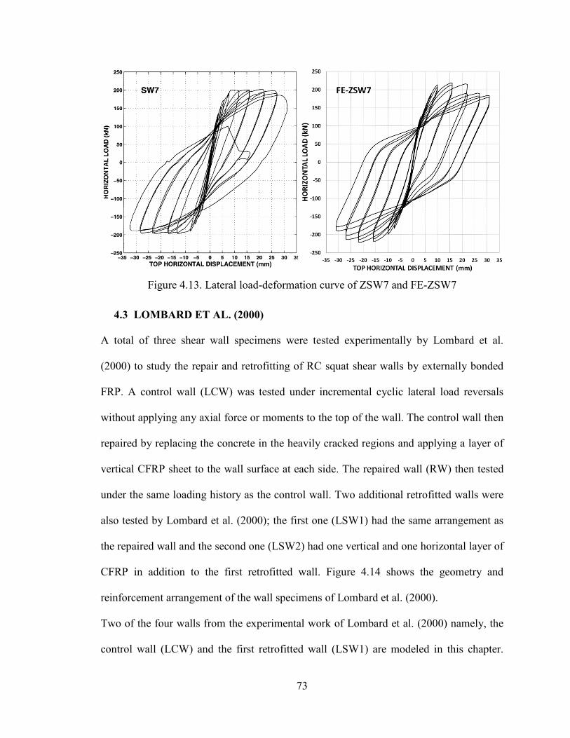
73
Figure 4.13. Lateral load-deformation curve of ZSW7 and FE-ZSW7
4.3 LOMBARD ET AL. (2000)
A total of three shear wall specimens were tested experimentally by Lombard et al.
(2000) to study the repair and retrofitting of RC squat shear walls by externally bonded
FRP. A control wall (LCW) was tested under incremental cyclic lateral load reversals
without applying any axial force or moments to the top of the wall. The control wall then
repaired by replacing the concrete in the heavily cracked regions and applying a layer of
vertical CFRP sheet to the wall surface at each side. The repaired wall (RW) then tested
under the same loading history as the control wall. Two additional retrofitted walls were
also tested by Lombard et al. (2000); the first one (LSW1) had the same arrangement as
the repaired wall and the second one (LSW2) had one vertical and one horizontal layer of
CFRP in addition to the first retrofitted wall. Figure 4.14 shows the geometry and
reinforcement arrangement of the wall specimens of Lombard et al. (2000).
Two of the four walls from the experimental work of Lombard et al. (2000) namely, the
control wall (LCW) and the first retrofitted wall (LSW1) are modeled in this chapter.
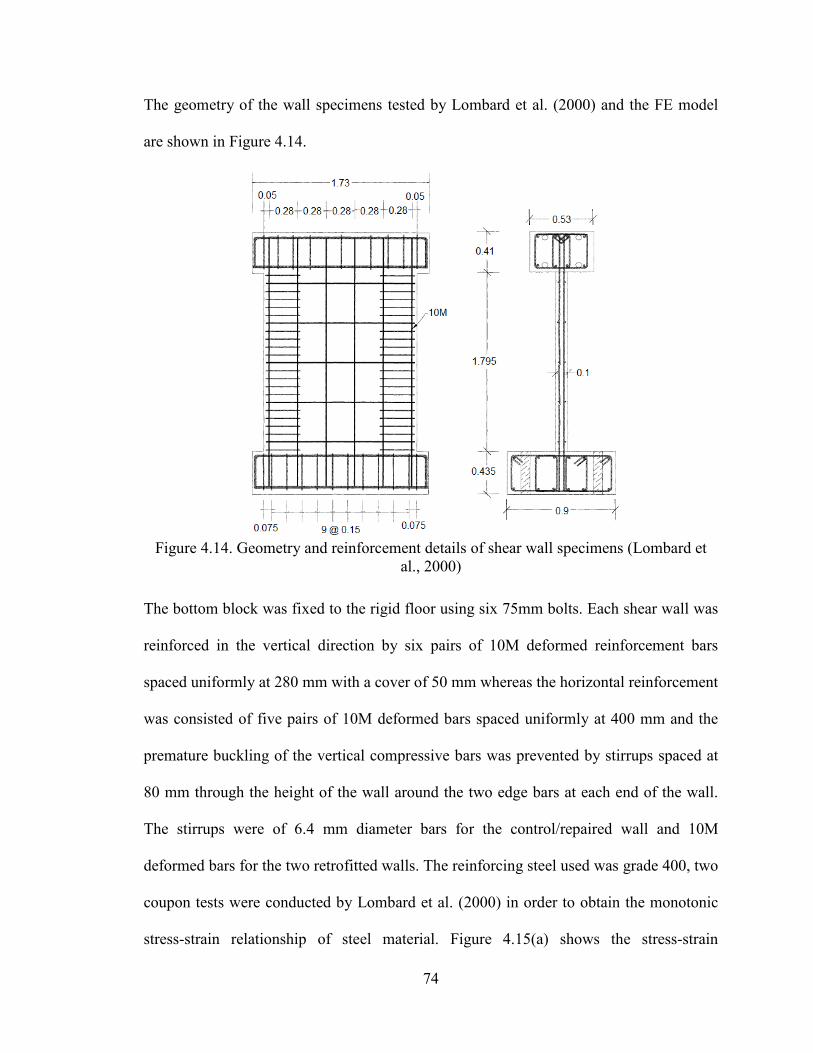
74
The geometry of the wall specimens tested by Lombard et al. (2000) and the FE model
are shown in Figure 4.14.
Figure 4.14. Geometry and reinforcement details of shear wall specimens (Lombard et
al., 2000)
The bottom block was fixed to the rigid floor using six 75mm bolts. Each shear wall was
reinforced in the vertical direction by six pairs of 10M deformed reinforcement bars
spaced uniformly at 280 mm with a cover of 50 mm whereas the horizontal reinforcement
was consisted of five pairs of 10M deformed bars spaced uniformly at 400 mm and the
premature buckling of the vertical compressive bars was prevented by stirrups spaced at
80 mm through the height of the wall around the two edge bars at each end of the wall.
The stirrups were of 6.4 mm diameter bars for the control/repaired wall and 10M
deformed bars for the two retrofitted walls. The reinforcing steel used was grade 400, two
coupon tests were conducted by Lombard et al. (2000) in order to obtain the monotonic
stress-strain relationship of steel material. Figure 4.15(a) shows the stress-strain
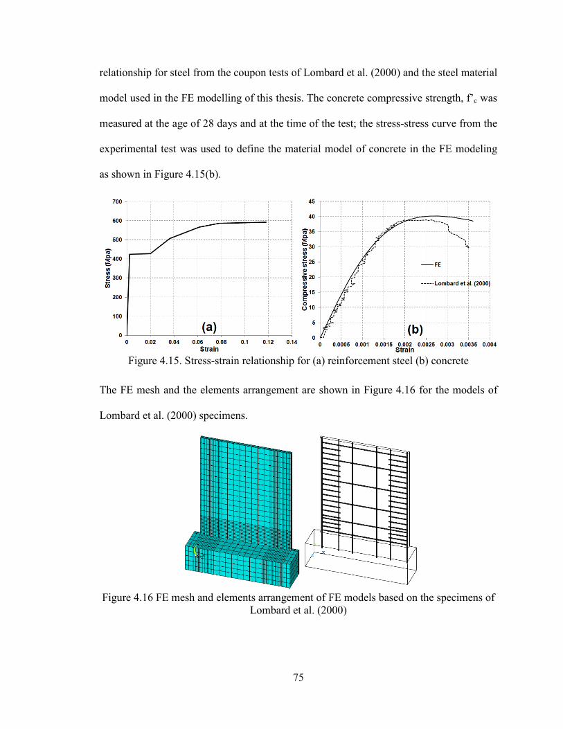
75
relationship for steel from the coupon tests of Lombard et al. (2000) and the steel material
model used in the FE modelling of this thesis. The concrete compressive strength, f’c was
measured at the age of 28 days and at the time of the test; the stress-stress curve from the
experimental test was used to define the material model of concrete in the FE modeling
as shown in Figure 4.15(b).
Figure 4.15. Stress-strain relationship for (a) reinforcement steel (b) concrete
The FE mesh and the elements arrangement are shown in Figure 4.16 for the models of
Lombard et al. (2000) specimens.
Figure 4.16 FE mesh and elements arrangement of FE models based on the specimens of
Lombard et al. (2000)
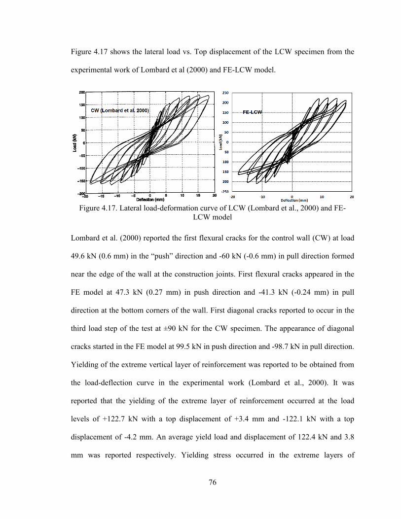
76
Figure 4.17 shows the lateral load vs. Top displacement of the LCW specimen from the
experimental work of Lombard et al (2000) and FE-LCW model.
Figure 4.17. Lateral load-deformation curve of LCW (Lombard et al., 2000) and FE-
LCW model
Lombard et al. (2000) reported the first flexural cracks for the control wall (CW) at load
49.6 kN (0.6 mm) in the “push” direction and -60 kN (-0.6 mm) in pull direction formed
near the edge of the wall at the construction joints. First flexural cracks appeared in the
FE model at 47.3 kN (0.27 mm) in push direction and -41.3 kN (-0.24 mm) in pull
direction at the bottom corners of the wall. First diagonal cracks reported to occur in the
third load step of the test at ±90 kN for the CW specimen. The appearance of diagonal
cracks started in the FE model at 99.5 kN in push direction and -98.7 kN in pull direction.
Yielding of the extreme vertical layer of reinforcement was reported to be obtained from
the load-deflection curve in the experimental work (Lombard et al., 2000). It was
reported that the yielding of the extreme layer of reinforcement occurred at the load
levels of +122.7 kN with a top displacement of +3.4 mm and -122.1 kN with a top
displacement of -4.2 mm. An average yield load and displacement of 122.4 kN and 3.8
mm was reported respectively. Yielding stress occurred in the extreme layers of
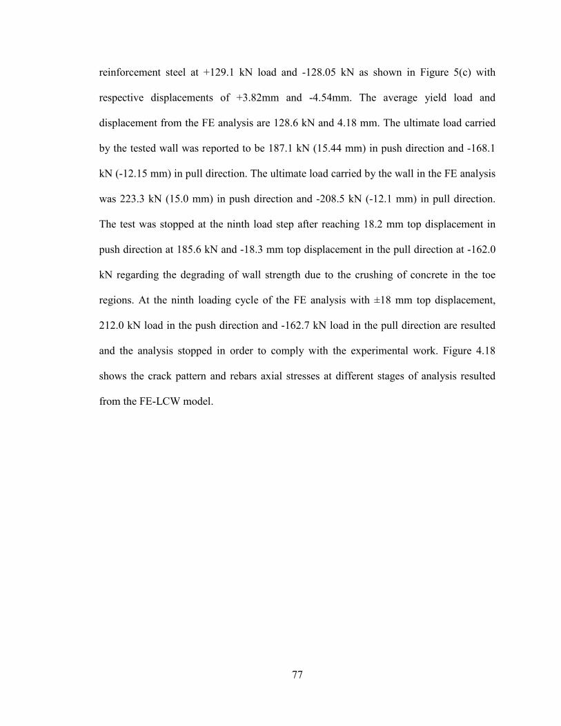
77
reinforcement steel at +129.1 kN load and -128.05 kN as shown in Figure 5(c) with
respective displacements of +3.82mm and -4.54mm. The average yield load and
displacement from the FE analysis are 128.6 kN and 4.18 mm. The ultimate load carried
by the tested wall was reported to be 187.1 kN (15.44 mm) in push direction and -168.1
kN (-12.15 mm) in pull direction. The ultimate load carried by the wall in the FE analysis
was 223.3 kN (15.0 mm) in push direction and -208.5 kN (-12.1 mm) in pull direction.
The test was stopped at the ninth load step after reaching 18.2 mm top displacement in
push direction at 185.6 kN and -18.3 mm top displacement in the pull direction at -162.0
kN regarding the degrading of wall strength due to the crushing of concrete in the toe
regions. At the ninth loading cycle of the FE analysis with ±18 mm top displacement,
212.0 kN load in the push direction and -162.7 kN load in the pull direction are resulted
and the analysis stopped in order to comply with the experimental work. Figure 4.18
shows the crack pattern and rebars axial stresses at different stages of analysis resulted
from the FE-LCW model.
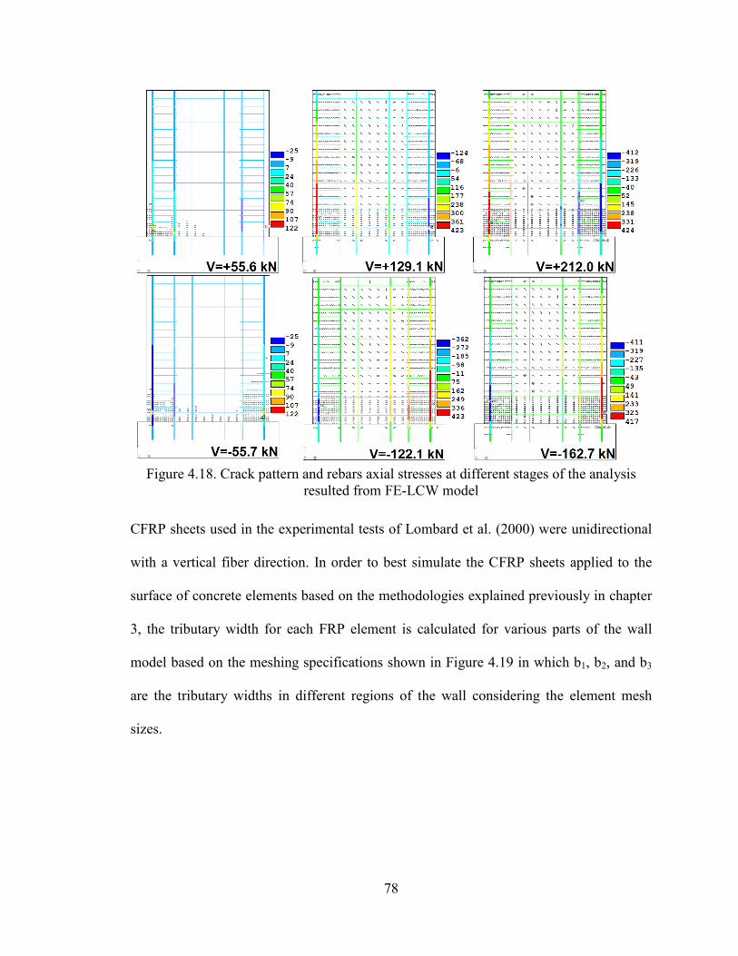
78
Figure 4.18. Crack pattern and rebars axial stresses at different stages of the analysis
resulted from FE-LCW model
CFRP sheets used in the experimental tests of Lombard et al. (2000) were unidirectional
with a vertical fiber direction. In order to best simulate the CFRP sheets applied to the
surface of concrete elements based on the methodologies explained previously in chapter
3, the tributary width for each FRP element is calculated for various parts of the wall
model based on the meshing specifications shown in Figure 4.19 in which b1, b2, and b3
are the tributary widths in different regions of the wall considering the element mesh
sizes.
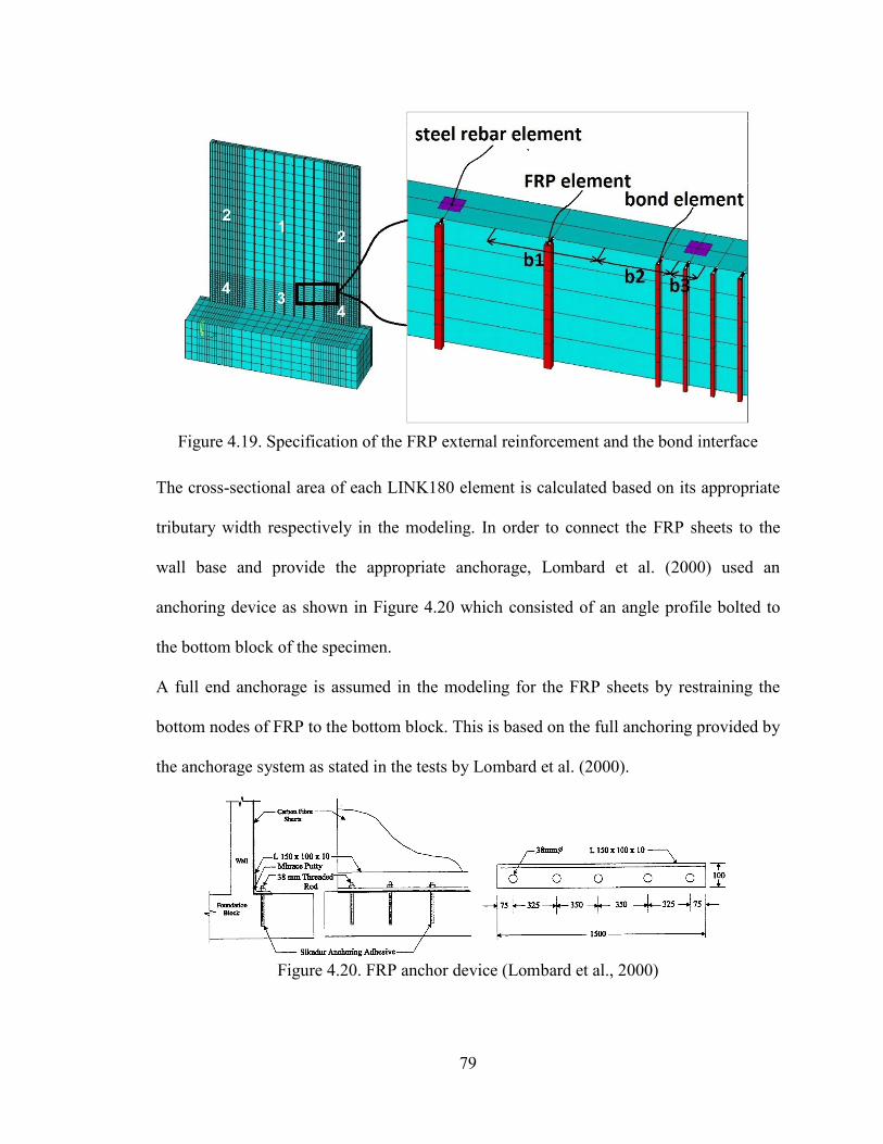
79
Figure 4.19. Specification of the FRP external reinforcement and the bond interface
The cross-sectional area of each LINK180 element is calculated based on its appropriate
tributary width respectively in the modeling. In order to connect the FRP sheets to the
wall base and provide the appropriate anchorage, Lombard et al. (2000) used an
anchoring device as shown in Figure 4.20 which consisted of an angle profile bolted to
the bottom block of the specimen.
A full end anchorage is assumed in the modeling for the FRP sheets by restraining the
bottom nodes of FRP to the bottom block. This is based on the full anchoring provided by
the anchorage system as stated in the tests by Lombard et al. (2000).
Figure 4.20. FRP anchor device (Lombard et al., 2000)
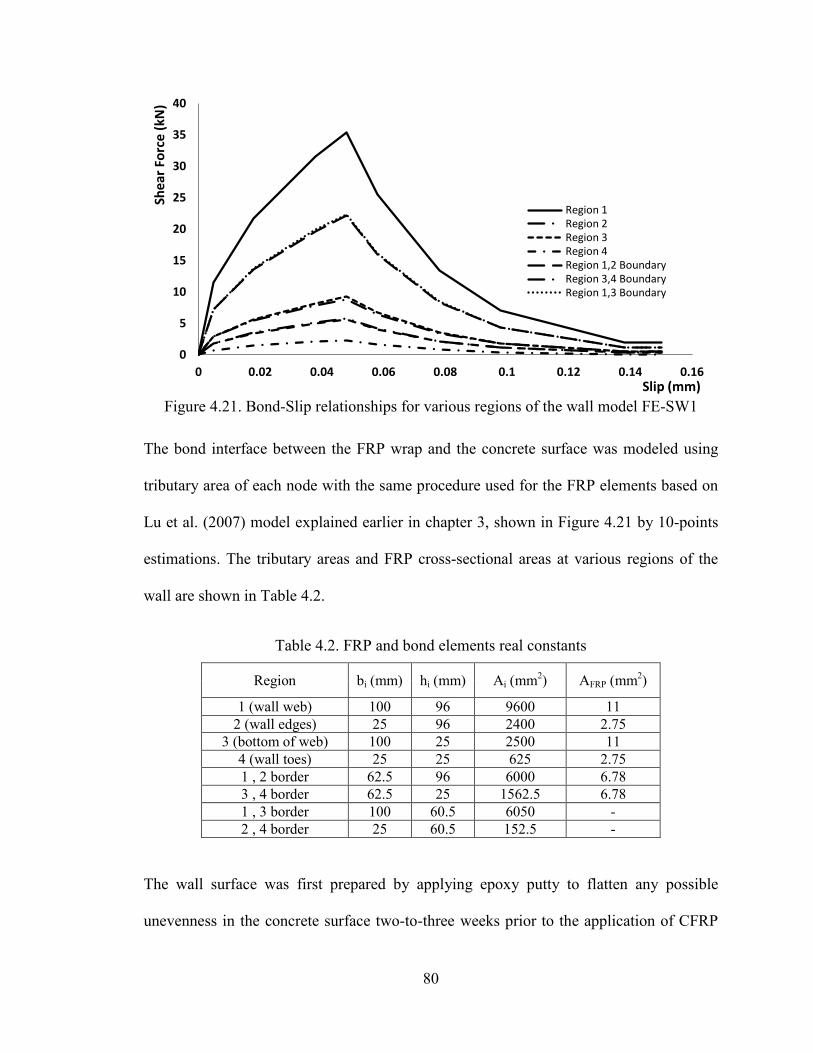
80
Figure 4.21. Bond-Slip relationships for various regions of the wall model FE-SW1
The bond interface between the FRP wrap and the concrete surface was modeled using
tributary area of each node with the same procedure used for the FRP elements based on
Lu et al. (2007) model explained earlier in chapter 3, shown in Figure 4.21 by 10-points
estimations. The tributary areas and FRP cross-sectional areas at various regions of the
wall are shown in Table 4.2.
Table 4.2. FRP and bond elements real constants
Region bi (mm) hi (mm) Ai (mm2) AFRP (mm2)
1 (wall web) 100 96 9600 11 2 (wall edges) 25 96 2400 2.75
3 (bottom of web) 100 25 2500 11 4 (wall toes) 25 25 625 2.75 1 , 2 border 62.5 96 6000 6.78 3 , 4 border 62.5 25 1562.5 6.78 1 , 3 border 100 60.5 6050 - 2 , 4 border 25 60.5 152.5 -
The wall surface was first prepared by applying epoxy putty to flatten any possible
unevenness in the concrete surface two-to-three weeks prior to the application of CFRP
0
5
10
15
20
25
30
35
40
0 0.02 0.04 0.06 0.08 0.1 0.12 0.14 0.16
Shea
r For
ce (k
N)
Slip (mm)
Region 1 Region 2 Region 3 Region 4 Region 1,2 Boundary Region 3,4 Boundary Region 1,3 Boundary
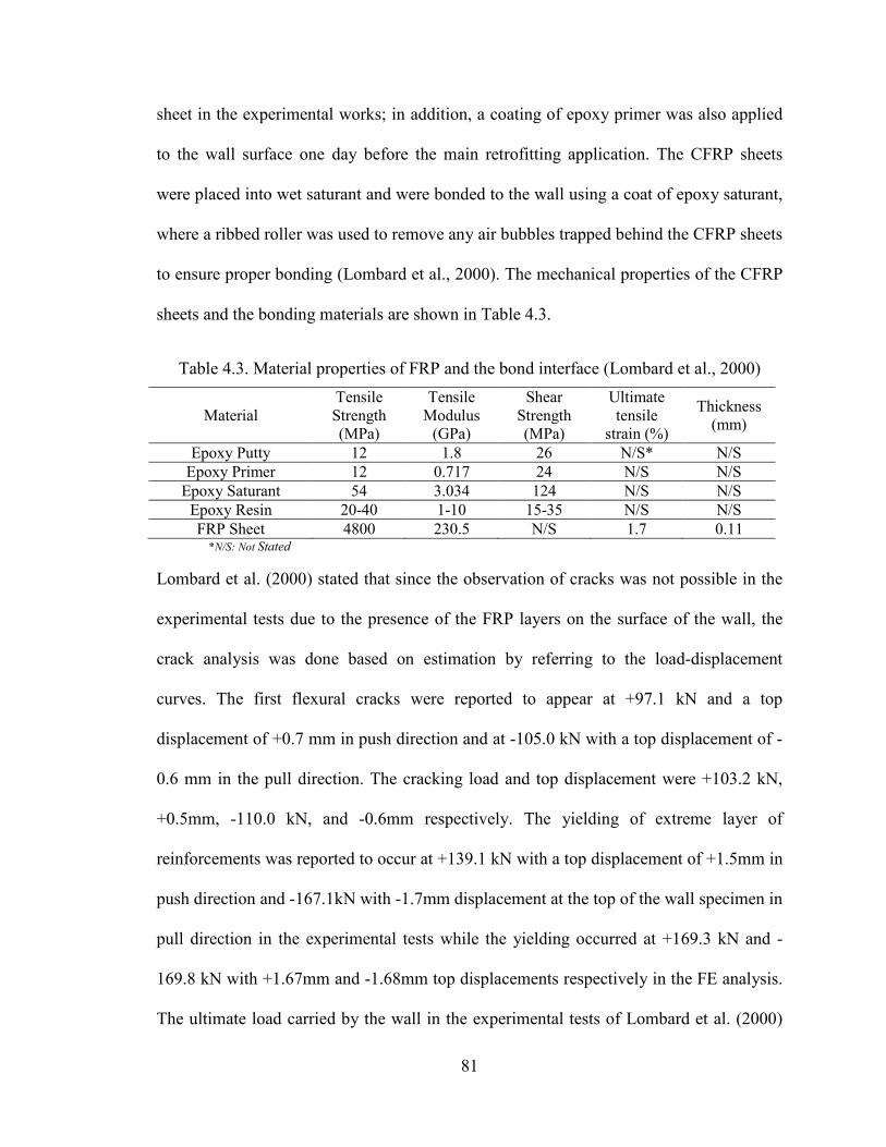
81
sheet in the experimental works; in addition, a coating of epoxy primer was also applied
to the wall surface one day before the main retrofitting application. The CFRP sheets
were placed into wet saturant and were bonded to the wall using a coat of epoxy saturant,
where a ribbed roller was used to remove any air bubbles trapped behind the CFRP sheets
to ensure proper bonding (Lombard et al., 2000). The mechanical properties of the CFRP
sheets and the bonding materials are shown in Table 4.3.
Table 4.3. Material properties of FRP and the bond interface (Lombard et al., 2000)
Material Tensile Strength (MPa)
Tensile Modulus
(GPa)
Shear Strength (MPa)
Ultimate tensile
strain (%)
Thickness (mm)
Epoxy Putty 12 1.8 26 N/S* N/S Epoxy Primer 12 0.717 24 N/S N/S
Epoxy Saturant 54 3.034 124 N/S N/S Epoxy Resin 20-40 1-10 15-35 N/S N/S FRP Sheet 4800 230.5 N/S 1.7 0.11
*N/S: Not Stated
Lombard et al. (2000) stated that since the observation of cracks was not possible in the
experimental tests due to the presence of the FRP layers on the surface of the wall, the
crack analysis was done based on estimation by referring to the load-displacement
curves. The first flexural cracks were reported to appear at +97.1 kN and a top
displacement of +0.7 mm in push direction and at -105.0 kN with a top displacement of -
0.6 mm in the pull direction. The cracking load and top displacement were +103.2 kN,
+0.5mm, -110.0 kN, and -0.6mm respectively. The yielding of extreme layer of
reinforcements was reported to occur at +139.1 kN with a top displacement of +1.5mm in
push direction and -167.1kN with -1.7mm displacement at the top of the wall specimen in
pull direction in the experimental tests while the yielding occurred at +169.3 kN and -
169.8 kN with +1.67mm and -1.68mm top displacements respectively in the FE analysis.
The ultimate load carried by the wall in the experimental tests of Lombard et al. (2000)
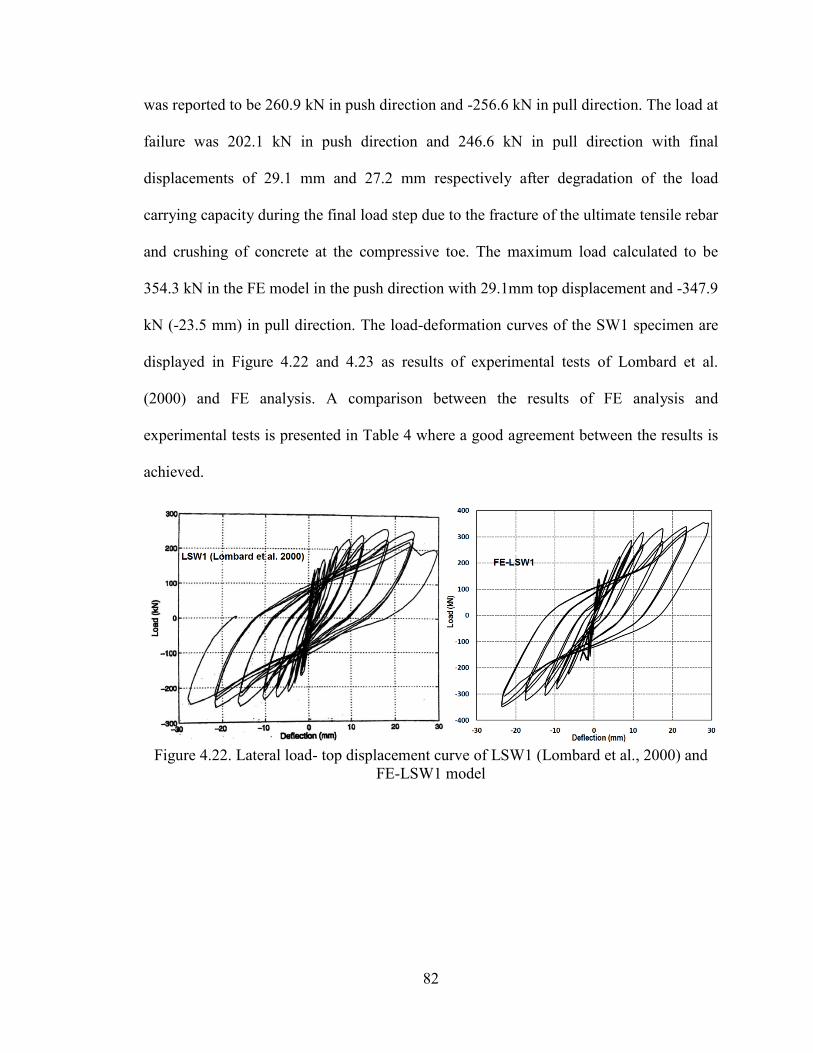
82
was reported to be 260.9 kN in push direction and -256.6 kN in pull direction. The load at
failure was 202.1 kN in push direction and 246.6 kN in pull direction with final
displacements of 29.1 mm and 27.2 mm respectively after degradation of the load
carrying capacity during the final load step due to the fracture of the ultimate tensile rebar
and crushing of concrete at the compressive toe. The maximum load calculated to be
354.3 kN in the FE model in the push direction with 29.1mm top displacement and -347.9
kN (-23.5 mm) in pull direction. The load-deformation curves of the SW1 specimen are
displayed in Figure 4.22 and 4.23 as results of experimental tests of Lombard et al.
(2000) and FE analysis. A comparison between the results of FE analysis and
experimental tests is presented in Table 4 where a good agreement between the results is
achieved.
Figure 4.22. Lateral load- top displacement curve of LSW1 (Lombard et al., 2000) and
FE-LSW1 model
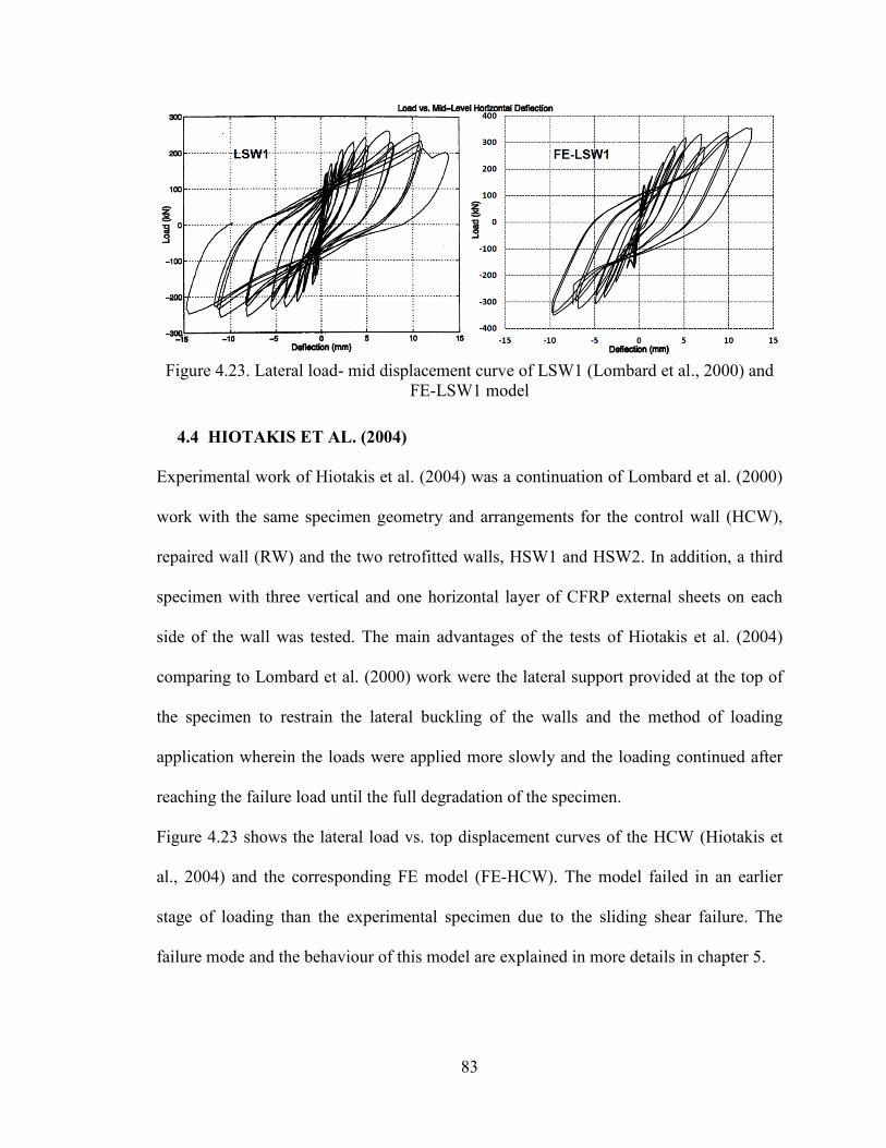
83
Figure 4.23. Lateral load- mid displacement curve of LSW1 (Lombard et al., 2000) and
FE-LSW1 model
4.4 HIOTAKIS ET AL. (2004)
Experimental work of Hiotakis et al. (2004) was a continuation of Lombard et al. (2000)
work with the same specimen geometry and arrangements for the control wall (HCW),
repaired wall (RW) and the two retrofitted walls, HSW1 and HSW2. In addition, a third
specimen with three vertical and one horizontal layer of CFRP external sheets on each
side of the wall was tested. The main advantages of the tests of Hiotakis et al. (2004)
comparing to Lombard et al. (2000) work were the lateral support provided at the top of
the specimen to restrain the lateral buckling of the walls and the method of loading
application wherein the loads were applied more slowly and the loading continued after
reaching the failure load until the full degradation of the specimen.
Figure 4.23 shows the lateral load vs. top displacement curves of the HCW (Hiotakis et
al., 2004) and the corresponding FE model (FE-HCW). The model failed in an earlier
stage of loading than the experimental specimen due to the sliding shear failure. The
failure mode and the behaviour of this model are explained in more details in chapter 5.
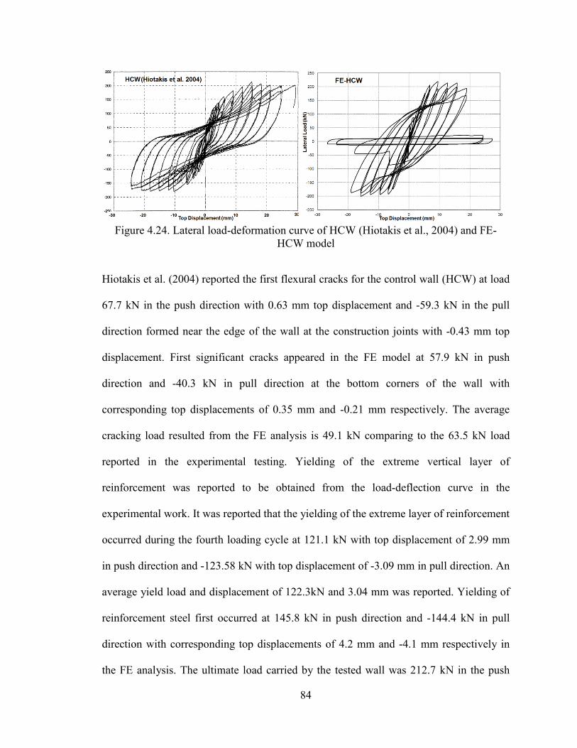
84
Figure 4.24. Lateral load-deformation curve of HCW (Hiotakis et al., 2004) and FE-
HCW model
Hiotakis et al. (2004) reported the first flexural cracks for the control wall (HCW) at load
67.7 kN in the push direction with 0.63 mm top displacement and -59.3 kN in the pull
direction formed near the edge of the wall at the construction joints with -0.43 mm top
displacement. First significant cracks appeared in the FE model at 57.9 kN in push
direction and -40.3 kN in pull direction at the bottom corners of the wall with
corresponding top displacements of 0.35 mm and -0.21 mm respectively. The average
cracking load resulted from the FE analysis is 49.1 kN comparing to the 63.5 kN load
reported in the experimental testing. Yielding of the extreme vertical layer of
reinforcement was reported to be obtained from the load-deflection curve in the
experimental work. It was reported that the yielding of the extreme layer of reinforcement
occurred during the fourth loading cycle at 121.1 kN with top displacement of 2.99 mm
in push direction and -123.58 kN with top displacement of -3.09 mm in pull direction. An
average yield load and displacement of 122.3kN and 3.04 mm was reported. Yielding of
reinforcement steel first occurred at 145.8 kN in push direction and -144.4 kN in pull
direction with corresponding top displacements of 4.2 mm and -4.1 mm respectively in
the FE analysis. The ultimate load carried by the tested wall was 212.7 kN in the push
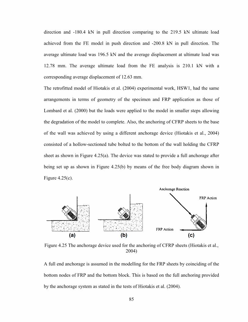
85
direction and -180.4 kN in pull direction comparing to the 219.5 kN ultimate load
achieved from the FE model in push direction and -200.8 kN in pull direction. The
average ultimate load was 196.5 kN and the average displacement at ultimate load was
12.78 mm. The average ultimate load from the FE analysis is 210.1 kN with a
corresponding average displacement of 12.63 mm.
The retrofitted model of Hiotakis et al. (2004) experimental work, HSW1, had the same
arrangements in terms of geometry of the specimen and FRP application as those of
Lombard et al. (2000) but the loads were applied to the model in smaller steps allowing
the degradation of the model to complete. Also, the anchoring of CFRP sheets to the base
of the wall was achieved by using a different anchorage device (Hiotakis et al., 2004)
consisted of a hollow-sectioned tube bolted to the bottom of the wall holding the CFRP
sheet as shown in Figure 4.25(a). The device was stated to provide a full anchorage after
being set up as shown in Figure 4.25(b) by means of the free body diagram shown in
Figure 4.25(c).
Figure 4.25 The anchorage device used for the anchoring of CFRP sheets (Hiotakis et al.,
2004)
A full end anchorage is assumed in the modelling for the FRP sheets by coinciding of the
bottom nodes of FRP and the bottom block. This is based on the full anchoring provided
by the anchorage system as stated in the tests of Hiotakis et al. (2004).
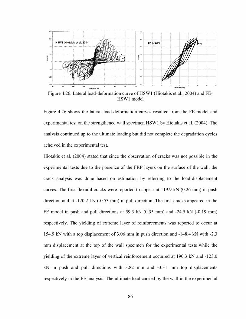
86
Figure 4.26. Lateral load-deformation curve of HSW1 (Hiotakis et al., 2004) and FE-
HSW1 model
Figure 4.26 shows the lateral load-deformation curves resulted from the FE model and
experimental test on the strengthened wall specimen HSW1 by Hiotakis et al. (2004). The
analysis continued up to the ultimate loading but did not complete the degradation cycles
acheived in the experimental test.
Hiotakis et al. (2004) stated that since the observation of cracks was not possible in the
experimental tests due to the presence of the FRP layers on the surface of the wall, the
crack analysis was done based on estimation by referring to the load-displacement
curves. The first flexural cracks were reported to appear at 119.9 kN (0.26 mm) in push
direction and at -120.2 kN (-0.53 mm) in pull direction. The first cracks appeared in the
FE model in push and pull directions at 59.3 kN (0.35 mm) and -24.5 kN (-0.19 mm)
respectively. The yielding of extreme layer of reinforcements was reported to occur at
154.9 kN with a top displacement of 3.06 mm in push direction and -148.4 kN with -2.3
mm displacement at the top of the wall specimen for the experimental tests while the
yielding of the extreme layer of vertical reinforcement occurred at 190.3 kN and -123.0
kN in push and pull directions with 3.82 mm and -3.31 mm top displacements
respectively in the FE analysis. The ultimate load carried by the wall in the experimental
87
tests of Hiotakis et al. (2004) was reported to be 313.24 kN (18.69 mm) in push direction
and -255.26 kN (-27.38 mm) in pull direction. The ultimate loads achieved during the FE
analysis were 328.4 kN (19.01 mm) in push direction and -252.0 kN (-19.01 mm) in pull
direction.
4.5 SUMMARY
A total of seven experimentally tested specimens were modeled based on the analysis
methodology discussed in chapter 3 and the results were compared to those of the
experimental tests and good agreements achieved. The case of RC shear walls without
any additional strengthening elements was studied in all of the available experimental
studies in order to setup reference results by means of control specimens. A summary of
the results of FE analyses of this chapter with the experimental data is shown in Table 4-
4. The error percentage in table 4.4 is calculated using the following equation for
applicable results.
Error % = (FE-EXP)/EXP*100 (Eq. 3.31)
In which “FE” is the output from analysis and “EXP” is the output from experimental
data regardless of their sign.
In Table 4.4, the cracking load and deformation are not compared between the FE and
EXP because of the fundamental difference between the method of measuring these
values in the experimental and FE analysis as discussed before.
The overall average of error for the analysis of RC shear walls of this chapter could be
estimated as 11.69% which is an acceptable error percentage for the analysis considering
the sophisticated failure criteria and other modeling assumptions explained in chapter 3.
From the results presented in Table 4.4, it can be seen that the FE analysis was able to
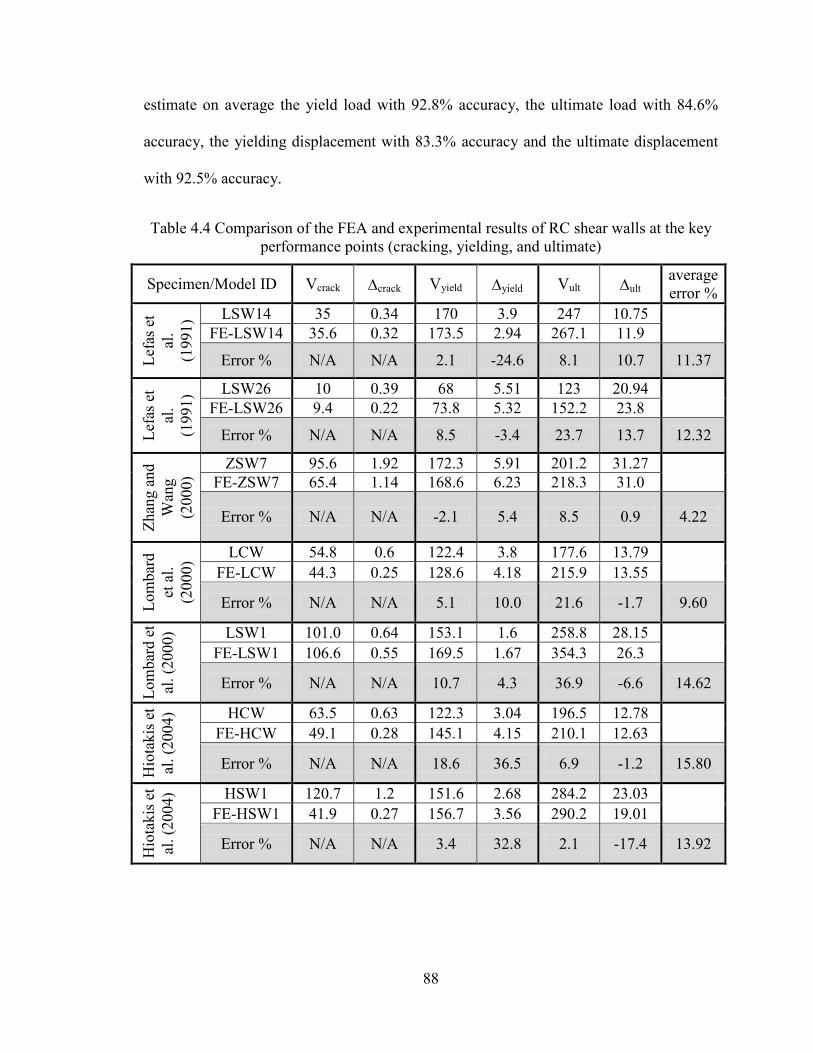
88
estimate on average the yield load with 92.8% accuracy, the ultimate load with 84.6%
accuracy, the yielding displacement with 83.3% accuracy and the ultimate displacement
with 92.5% accuracy.
Table 4.4 Comparison of the FEA and experimental results of RC shear walls at the key performance points (cracking, yielding, and ultimate)
Specimen/Model ID Vcrack ∆crack Vyield ∆yield Vult ∆ult average error %
Lefa
s et
al.
(199
1) LSW14 35 0.34 170 3.9 247 10.75 FE-LSW14 35.6 0.32 173.5 2.94 267.1 11.9
Error % N/A N/A 2.1 -24.6 8.1 10.7 11.37
Lefa
s et
al.
(199
1) LSW26 10 0.39 68 5.51 123 20.94 FE-LSW26 9.4 0.22 73.8 5.32 152.2 23.8
Error % N/A N/A 8.5 -3.4 23.7 13.7 12.32
Zhan
g an
d W
ang
(200
0) ZSW7 95.6 1.92 172.3 5.91 201.2 31.27 FE-ZSW7 65.4 1.14 168.6 6.23 218.3 31.0
Error % N/A N/A -2.1 5.4 8.5 0.9 4.22
Lom
bard
et
al.
(200
0) LCW 54.8 0.6 122.4 3.8 177.6 13.79 FE-LCW 44.3 0.25 128.6 4.18 215.9 13.55
Error % N/A N/A 5.1 10.0 21.6 -1.7 9.60
Lom
bard
et
al. (
2000
) LSW1 101.0 0.64 153.1 1.6 258.8 28.15 FE-LSW1 106.6 0.55 169.5 1.67 354.3 26.3 Error % N/A N/A 10.7 4.3 36.9 -6.6 14.62
Hio
taki
s et
al. (
2004
) HCW 63.5 0.63 122.3 3.04 196.5 12.78 FE-HCW 49.1 0.28 145.1 4.15 210.1 12.63 Error % N/A N/A 18.6 36.5 6.9 -1.2 15.80
Hio
taki
s et
al. (
2004
) HSW1 120.7 1.2 151.6 2.68 284.2 23.03 FE-HSW1 41.9 0.27 156.7 3.56 290.2 19.01
Error % N/A N/A 3.4 32.8 2.1 -17.4 13.92
89
CHAPTER 5
INFLUENCE OF DESIGN PARAMETERS ON THE
SEISMIC PERFORMANCE OF RC SQUAT SHEAR WALLS
5.1 INTRODUCTION
Reinforced Concrete (RC) walls are classified according to CSA (2004) as bearing walls,
non-bearing walls, and shear walls: including flexural shear walls and squat shear walls.
Many design codes refer to slender shear walls (or simply, shear walls) as a vertical
cantilever structural element that is loaded axially and laterally at the story levels of the
buildings with a potential plastic hinge region located at the base of the wall (Paulay and
Priestley, 1992). There is a conceptual difference in the behaviour of such slender shear
walls dominated by the flexure response of the wall and other non-slender (squat) shear
walls, where the response is mainly driven by the strut-and-tie model (Yanez et al.,
1989). The definition of squat shear walls differs from one reference to the other. Some
references use the height-to-length ratio and identify those walls with Hw/Lw less than 2
or 3 as squat walls (Paulay and Priestley, 1992) where Hw and Lw are the wall height and
length, respectively. Whereas other researchers refer squat walls to the walls with a low
shear span-to-length ratio namely M/VLw less than 1.5 (Salonikios et al., 1996) as squat
walls where M and V are the equivalent applied moment and shear force and the
maximum moment located at the bottom of the wall, respectively (thus M/V represents
the shear span of the wall). Aside from the categorizing method, an agreement on the
difference between the type of behaviour of squat and slender shear walls exist in all
90
references which mainly is the failure of the wall to be dominated by flexure in the
slender shear walls and shear in the squat ones.
In this chapter, the behaviour of squat shear walls under applied lateral loads is explained
and the influence of some major parameters on its response will be discussed using the
experimental data available in the literature and the results of performed FE analyses.
5.2 FAILURE MODES OF RC SQUAT WALLS
Loading a RC squat shear wall beyond its cracking limit would make the wall undergo a
nonlinear behaviour with extensive cracking in concrete and the post-yield stains in the
reinforcing steel until the wall reaches its failure limit (Paulay and Priestley, 1992). In
this case, four possible modes of failure exist for a typical RC squat wall as follows:
Diagonal tension mode: In walls with insufficient horizontal reinforcement, if the shear
forces at the top of the wall are not evenly distributed by means of a rigid top beam or
a slab with sufficient in-plan rigidity, the concrete in the web region subjects to tensile
stresses and a corner-to-corner tensile failure plane may develop as shown in Figure
5.1(a). Paulay and Priestly (1992) indicate that such failure may also occur along a
steeper failure plane in cases where there are paths existing to transfer the shear forces
through the wall (Figure 5.1(b)).
Flexural failure: When the diagonal tension mechanism is restricted by providing
sufficient horizontal reinforcement, the concrete at the compressive toe may crush
under the high axial loads resulted by the bending moments and the extreme layers of
vertical reinforcement bars in the tensile edge may yield and undergo plastic
deformations. This failure mode is the result of well design and detailing with a ductile
91
manner but it would only occur if the geometry of the wall permits the high bending
moments to be generated during the lateral loading history.
Diagonal compression failure: In cases where the flexural mode does not occur due to
the low moment-to-shear ratio and the horizontal reinforcement is sufficient, the
concrete in the compressive diagonal region may crush as shown in Figure 5.1(c). This
mode of failure is more likely in cases of cyclic loading reversals that result in two sets
of shear cracks in the diagonals wherein the overall concrete strength reduces by the
closing and reopening of the cracks (Paulay and Priestley, 1992). The crushing of
concrete may spread through the length of the wall in the last reversals of a cyclic
loading as shown in Figure 5.1(d). If a wall undergoes such a failure mechanism
during a loading event, the loss of strength is almost irrecoverable and such failure
mode must be avoided in cases where the repairing of the wall is regarded. Although
this mechanism is more desirable comparing to the diagonal tension, it is to be avoided
because of its brittle manner.
Sliding Shear failure:
If both diagonal tension and compression modes are restricted in a RC squat shear
wall, a flexural behaviour causes the horizontal cracking of concrete under the tensile
stresses at each load reversal. The sliding resistance of the wall at base region in the
first load reversals where the concrete strength in the compressive toe is not yet
affected significantly by the closing and reopening of the horizontal cracks occurred in
the previous reversal of each cycle is mainly provided by concrete. As the concrete in
the boundary of the wall and foundation cracks throughout the entire wall length, the
main resistance against the sliding forces at this region is provided by the dowel action
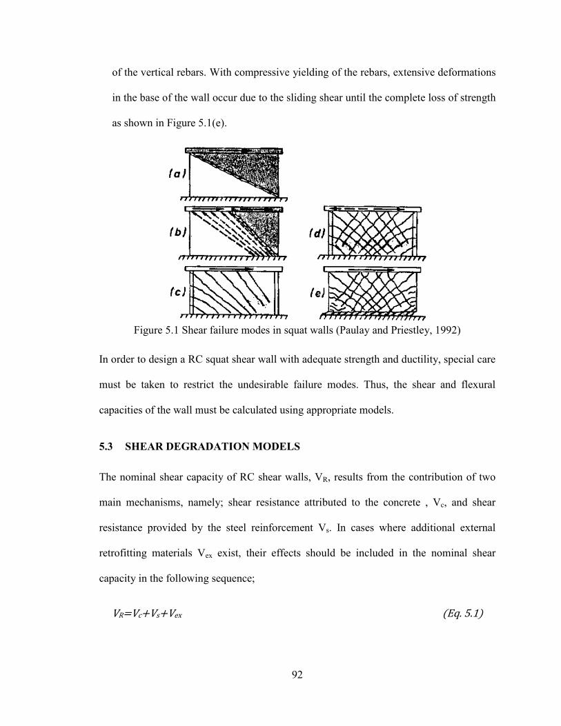
92
of the vertical rebars. With compressive yielding of the rebars, extensive deformations
in the base of the wall occur due to the sliding shear until the complete loss of strength
as shown in Figure 5.1(e).
Figure 5.1 Shear failure modes in squat walls (Paulay and Priestley, 1992)
In order to design a RC squat shear wall with adequate strength and ductility, special care
must be taken to restrict the undesirable failure modes. Thus, the shear and flexural
capacities of the wall must be calculated using appropriate models.
5.3 SHEAR DEGRADATION MODELS
The nominal shear capacity of RC shear walls, VR, results from the contribution of two
main mechanisms, namely; shear resistance attributed to the concrete , Vc, and shear
resistance provided by the steel reinforcement Vs. In cases where additional external
retrofitting materials Vex exist, their effects should be included in the nominal shear
capacity in the following sequence;
VR=Vc+Vs+Vex (Eq. 5.1)
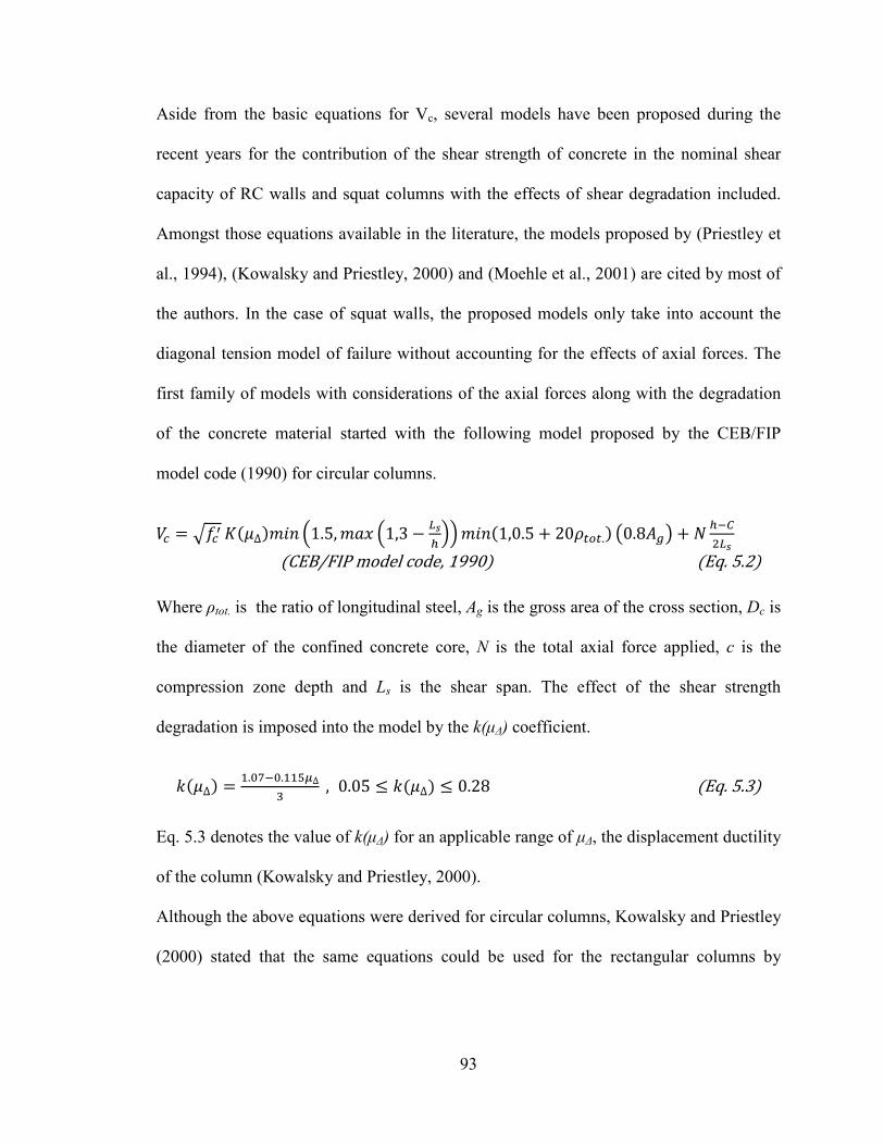
93
Aside from the basic equations for Vc, several models have been proposed during the
recent years for the contribution of the shear strength of concrete in the nominal shear
capacity of RC walls and squat columns with the effects of shear degradation included.
Amongst those equations available in the literature, the models proposed by (Priestley et
al., 1994), (Kowalsky and Priestley, 2000) and (Moehle et al., 2001) are cited by most of
the authors. In the case of squat walls, the proposed models only take into account the
diagonal tension model of failure without accounting for the effects of axial forces. The
first family of models with considerations of the axial forces along with the degradation
of the concrete material started with the following model proposed by the CEB/FIP
model code (1990) for circular columns.
𝑉𝑐 = �𝑓𝑐′ 𝐾(𝜇∆)𝑚𝑖𝑛 �1.5, 𝑚𝑎𝑥 �1,3 − 𝐿𝑠
ℎ�� 𝑚𝑖𝑛(1,0.5 + 20𝜌𝑡𝑜𝑡.) �0.8𝐴𝑔� + 𝑁 ℎ−𝐶
2𝐿𝑠
(CEB/FIP model code, 1990) (Eq. 5.2)
Where ρtot. is the ratio of longitudinal steel, Ag is the gross area of the cross section, Dc is
the diameter of the confined concrete core, N is the total axial force applied, c is the
compression zone depth and Ls is the shear span. The effect of the shear strength
degradation is imposed into the model by the k(μΔ) coefficient.
𝑘(𝜇∆) = 1.07−0.115𝜇∆3
, 0.05 ≤ 𝑘(𝜇∆) ≤ 0.28 (Eq. 5.3)
Eq. 5.3 denotes the value of k(μΔ) for an applicable range of μΔ, the displacement ductility
of the column (Kowalsky and Priestley, 2000).
Although the above equations were derived for circular columns, Kowalsky and Priestley
(2000) stated that the same equations could be used for the rectangular columns by
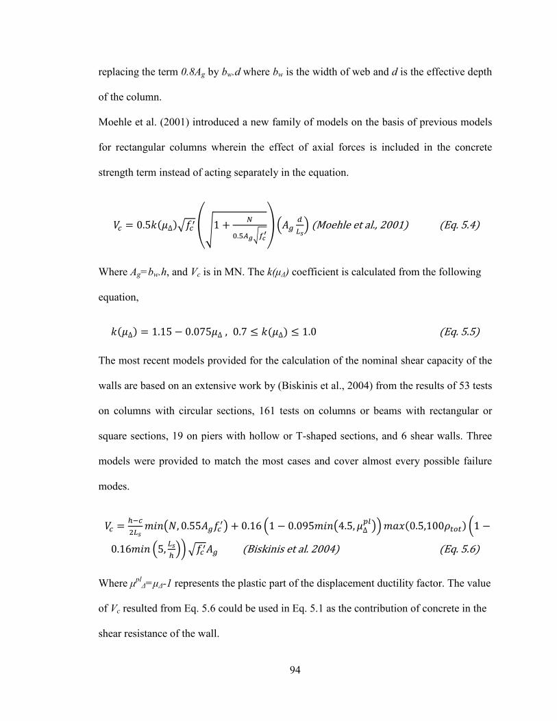
94
replacing the term 0.8Ag by bw.d where bw is the width of web and d is the effective depth
of the column.
Moehle et al. (2001) introduced a new family of models on the basis of previous models
for rectangular columns wherein the effect of axial forces is included in the concrete
strength term instead of acting separately in the equation.
𝑉𝑐 = 0.5𝑘(𝜇∆)�𝑓𝑐′ ��1 + 𝑁
0.5𝐴𝑔�𝑓𝑐′� �𝐴𝑔
𝑑𝐿𝑠
� (Moehle et al., 2001) (Eq. 5.4)
Where Ag=bw.h, and Vc is in MN. The k(μΔ) coefficient is calculated from the following
equation,
𝑘(𝜇∆) = 1.15 − 0.075𝜇∆ , 0.7 ≤ 𝑘(𝜇∆) ≤ 1.0 (Eq. 5.5)
The most recent models provided for the calculation of the nominal shear capacity of the
walls are based on an extensive work by (Biskinis et al., 2004) from the results of 53 tests
on columns with circular sections, 161 tests on columns or beams with rectangular or
square sections, 19 on piers with hollow or T-shaped sections, and 6 shear walls. Three
models were provided to match the most cases and cover almost every possible failure
modes.
𝑉𝑐 = ℎ−𝑐2𝐿𝑠
𝑚𝑖𝑛�𝑁, 0.55𝐴𝑔𝑓𝑐′� + 0.16 �1 − 0.095𝑚𝑖𝑛�4.5, 𝜇∆
𝑝𝑙�� 𝑚𝑎𝑥(0.5,100𝜌𝑡𝑜𝑡) �1 −
0.16𝑚𝑖𝑛 �5, 𝐿𝑠ℎ
�� �𝑓𝑐′𝐴𝑔 (Biskinis et al. 2004) (Eq. 5.6)
Where μplΔ=μΔ-1 represents the plastic part of the displacement ductility factor. The value
of Vc resulted from Eq. 5.6 could be used in Eq. 5.1 as the contribution of concrete in the
shear resistance of the wall.
95
All of the above models calculate the value of Vc to be used separately in Eq. 5.1
indicating the fact that in all of them the shear degradation only affects the concrete
strength and the contribution of transverse steel reinforcement is calculated as:
𝑉𝑠 = 𝜌𝑤𝑏𝑤(𝑑 − 𝑐)𝑓𝑦𝑤𝑐𝑜𝑡𝜃 (Eq. 5.7)
Where ρw denotes the ratio of transverse steel and θ indicates the truss inclination in the
strut-and-tie model with the suggested value of 45 degrees (Moehle et al., 2001).
As a complimentary to Eq.5.6, Biskinis et al. (2004) suggested a more accurate model
wherein both Vc and Vs degrade with inelastic cyclic displacements.
𝑉𝑅 = ℎ−𝑐2𝐿𝑠
𝑚𝑖𝑛�𝑁, 0.55𝐴𝑔𝑓𝑐′� + �1 − 0.05𝑚𝑖𝑛�5, 𝜇∆
𝑝𝑙�� �0.16𝑚𝑎𝑥(0.5,100𝜌𝑡𝑜𝑡) �1 −
0.16𝑚𝑖𝑛 �5, 𝐿𝑠ℎ
�� �𝑓𝑐′𝐴𝑔 + 𝑉𝑆� (Biskinis et al., 2004) (Eq. 5.8)
The shear strengths resulted from equations 5.6 and 5.8 fit the experimental data for a
vast range of parameters at their right hand side with the suggested range for the axial
load ratio, N/Agf’c, from -0.01 to 0.85; shear span ratio, Ls/h, from 0.5 to 6.0; total
longitudinal reinforcement ratio, ρtot, from 0.55% to 5.5%; concrete compressive strength,
f’c, from 13.0 to 113.0 MPa; and displacement ductility ratio, μΔ, from 1.0 to 9.5 (Biskinis
et al., 2004).
All of the previously discussed models refer to the diagonal tension as the principal mode
of failure, the only model available in the literature that empirically calculates the shear
degradation model for shear walls and columns with diagonal compression failure mode
is the third model offered by Biskinis et al. (2004).
96
𝑉𝑅 = 0.85 �1 − 0.06𝑚𝑖𝑛�5, 𝜇∆𝑝𝑙�� �1 + 1.8𝑚𝑖𝑛 �0.15,
𝑁𝐴𝑐𝑓𝑐
,�� �1
+ 0.25𝑚𝑎𝑥(1.75,100𝜌𝑡𝑜𝑡)� �1 − 0.2𝑚𝑖𝑛 �2,𝐿𝑠
ℎ�� �𝑚𝑖𝑛(𝑓𝑐
′, 100)𝑏𝑤𝑍
(Biskinis et al. 2004) (Eq. 5.9)
Where Z=0.8Lw for the rectangular walls and Z=d-d’ for the barbell sectioned walls.
The research on the externally applied retrofitting material e.g. FRP wraps or steel plates
on the shear degradation model of columns and walls is still on the early stages. Up to the
author’s knowledge at the date of preparing this thesis, no model was found in the
reported literature indicating the effect of external FRP wraps on the shear degradation
model.
5.4 BEHAVIOUR OF RC SQUAT SHEAR WALLS UNDER CYCLIC AND
MONOTONIC LOADING
As seen in the previous section, there are two possible methods of analysis considering
the loading scheme when modeling RC squat shear walls namely, incremental monotonic
and incremental reversed (cyclic analysis). In case of cyclic analysis, the main output
resulted from the analysis would be the load-displacement cyclic loops giving a general
idea about the type of behaviour and the quality of performance of the wall. One other
significant data achievable from the cyclic analysis is the total energy dissipation which
is the area occupied by the load-displacement loops. On the other hand, a monotonic
analysis also gives a general view of the overall behaviour and performance of the wall
but the data is only based on a one-step loading where the degradation of the strength of
materials through cyclic loading may not be considered. A detailed study on the output
resulted from the cyclic and monotonic analysis of FE-HCW (Hiotakis et al., 2004) is
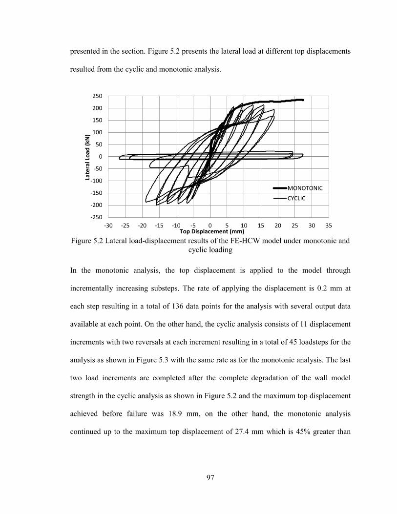
97
presented in the section. Figure 5.2 presents the lateral load at different top displacements
resulted from the cyclic and monotonic analysis.
Figure 5.2 Lateral load-displacement results of the FE-HCW model under monotonic and
cyclic loading
In the monotonic analysis, the top displacement is applied to the model through
incrementally increasing substeps. The rate of applying the displacement is 0.2 mm at
each step resulting in a total of 136 data points for the analysis with several output data
available at each point. On the other hand, the cyclic analysis consists of 11 displacement
increments with two reversals at each increment resulting in a total of 45 loadsteps for the
analysis as shown in Figure 5.3 with the same rate as for the monotonic analysis. The last
two load increments are completed after the complete degradation of the wall model
strength in the cyclic analysis as shown in Figure 5.2 and the maximum top displacement
achieved before failure was 18.9 mm, on the other hand, the monotonic analysis
continued up to the maximum top displacement of 27.4 mm which is 45% greater than
-250
-200
-150
-100
-50
0
50
100
150
200
250
-30 -25 -20 -15 -10 -5 0 5 10 15 20 25 30 35
Late
ral L
oad
(kN
)
Top Displacement (mm)
MONOTONIC CYCLIC
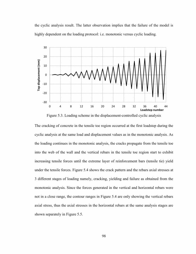
98
the cyclic analysis result. The latter observation implies that the failure of the model is
highly dependent on the loading protocol: i.e. monotonic versus cyclic loading.
Figure 5.3. Loading scheme in the displacement-controlled cyclic analysis
The cracking of concrete in the tensile toe region occurred at the first loadstep during the
cyclic analysis at the same load and displacement values as in the monotonic analysis. As
the loading continues in the monotonic analysis, the cracks propagate from the tensile toe
into the web of the wall and the vertical rebars in the tensile toe region start to exhibit
increasing tensile forces until the extreme layer of reinforcement bars (tensile tie) yield
under the tensile forces. Figure 5.4 shows the crack pattern and the rebars axial stresses at
3 different stages of loading namely, cracking, yielding and failure as obtained from the
monotonic analysis. Since the forces generated in the vertical and horizontal rebars were
not in a close range, the contour ranges in Figure 5.4 are only showing the vertical rebars
axial stress, thus the axial stresses in the horizontal rebars at the same analysis stages are
shown separately in Figure 5.5.
-30
-20
-10
0
10
20
30
0 4 8 12 16 20 24 28 32 36 40 44
Top
disp
lace
men
t (m
m)
Loadstep number
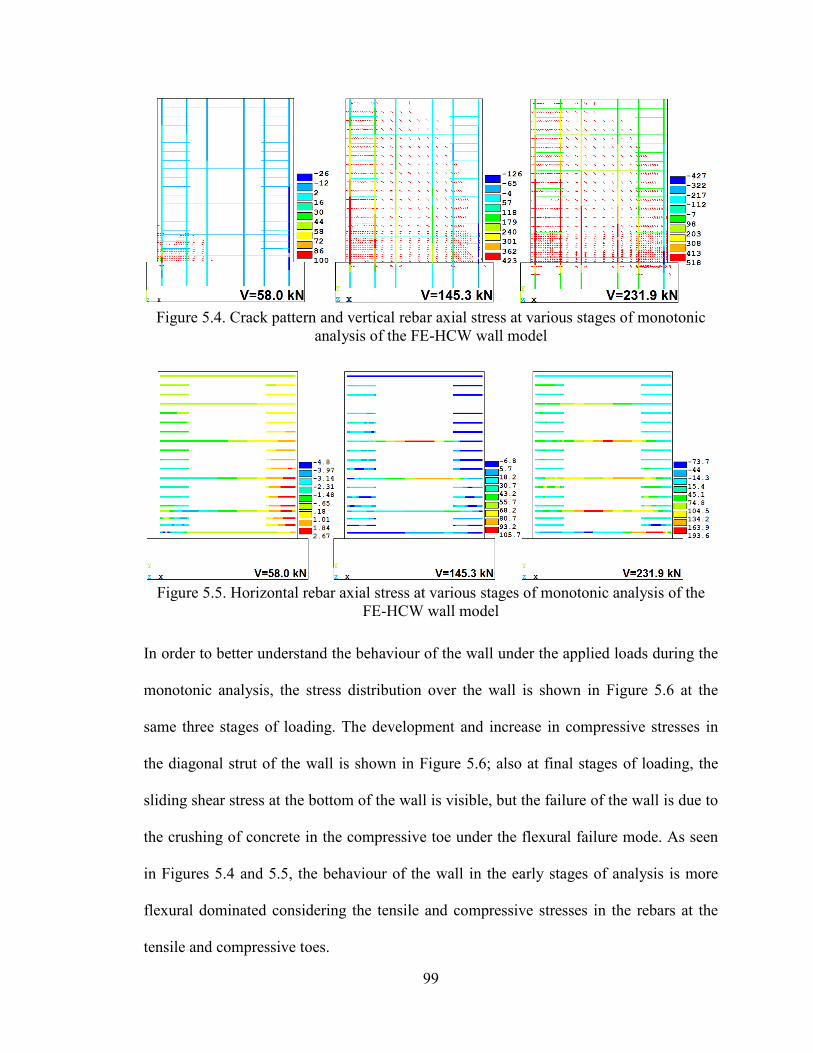
99
Figure 5.4. Crack pattern and vertical rebar axial stress at various stages of monotonic
analysis of the FE-HCW wall model
Figure 5.5. Horizontal rebar axial stress at various stages of monotonic analysis of the
FE-HCW wall model
In order to better understand the behaviour of the wall under the applied loads during the
monotonic analysis, the stress distribution over the wall is shown in Figure 5.6 at the
same three stages of loading. The development and increase in compressive stresses in
the diagonal strut of the wall is shown in Figure 5.6; also at final stages of loading, the
sliding shear stress at the bottom of the wall is visible, but the failure of the wall is due to
the crushing of concrete in the compressive toe under the flexural failure mode. As seen
in Figures 5.4 and 5.5, the behaviour of the wall in the early stages of analysis is more
flexural dominated considering the tensile and compressive stresses in the rebars at the
tensile and compressive toes.
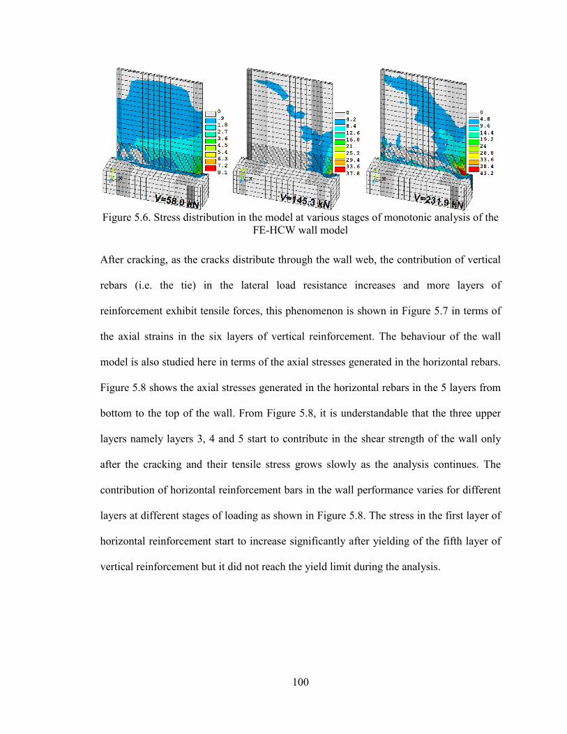
100
Figure 5.6. Stress distribution in the model at various stages of monotonic analysis of the
FE-HCW wall model
After cracking, as the cracks distribute through the wall web, the contribution of vertical
rebars (i.e. the tie) in the lateral load resistance increases and more layers of
reinforcement exhibit tensile forces, this phenomenon is shown in Figure 5.7 in terms of
the axial strains in the six layers of vertical reinforcement. The behaviour of the wall
model is also studied here in terms of the axial stresses generated in the horizontal rebars.
Figure 5.8 shows the axial stresses generated in the horizontal rebars in the 5 layers from
bottom to the top of the wall. From Figure 5.8, it is understandable that the three upper
layers namely layers 3, 4 and 5 start to contribute in the shear strength of the wall only
after the cracking and their tensile stress grows slowly as the analysis continues. The
contribution of horizontal reinforcement bars in the wall performance varies for different
layers at different stages of loading as shown in Figure 5.8. The stress in the first layer of
horizontal reinforcement start to increase significantly after yielding of the fifth layer of
vertical reinforcement but it did not reach the yield limit during the analysis.
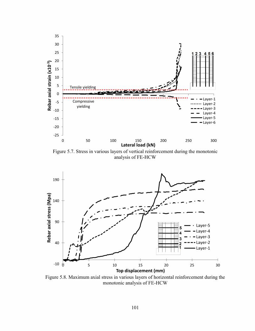
101
Figure 5.7. Stress in various layers of vertical reinforcement during the monotonic
analysis of FE-HCW
Figure 5.8. Maximum axial stress in various layers of horizontal reinforcement during the
monotonic analysis of FE-HCW
Tensile yielding
Compressive yielding
-25
-20
-15
-10
-5
0
5
10
15
20
25
30
35
0 50 100 150 200 250 300
Reba
r axi
al st
rain
(x10
-3)
Lateral load (kN)
Layer-1 Layer-2 Layer-3 Layer-4 Layer-5 Layer-6
-10
40
90
140
190
0 5 10 15 20 25 30
Reba
r axi
al st
ress
(Mpa
)
Top displacement (mm)
Layer-5 Layer-4 Layer-3 Layer-2 Layer-1
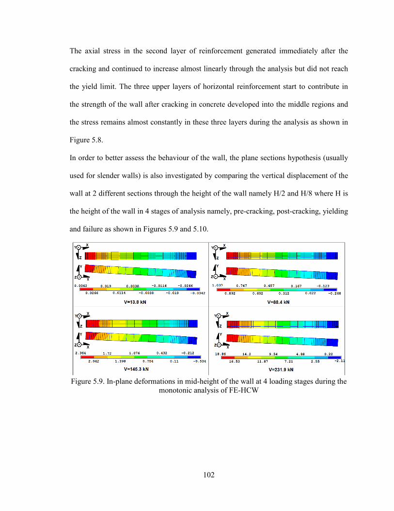
102
The axial stress in the second layer of reinforcement generated immediately after the
cracking and continued to increase almost linearly through the analysis but did not reach
the yield limit. The three upper layers of horizontal reinforcement start to contribute in
the strength of the wall after cracking in concrete developed into the middle regions and
the stress remains almost constantly in these three layers during the analysis as shown in
Figure 5.8.
In order to better assess the behaviour of the wall, the plane sections hypothesis (usually
used for slender walls) is also investigated by comparing the vertical displacement of the
wall at 2 different sections through the height of the wall namely H/2 and H/8 where H is
the height of the wall in 4 stages of analysis namely, pre-cracking, post-cracking, yielding
and failure as shown in Figures 5.9 and 5.10.
Figure 5.9. In-plane deformations in mid-height of the wall at 4 loading stages during the
monotonic analysis of FE-HCW
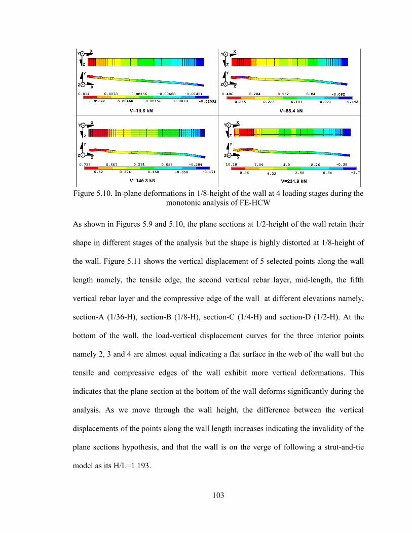
103
Figure 5.10. In-plane deformations in 1/8-height of the wall at 4 loading stages during the
monotonic analysis of FE-HCW
As shown in Figures 5.9 and 5.10, the plane sections at 1/2-height of the wall retain their
shape in different stages of the analysis but the shape is highly distorted at 1/8-height of
the wall. Figure 5.11 shows the vertical displacement of 5 selected points along the wall
length namely, the tensile edge, the second vertical rebar layer, mid-length, the fifth
vertical rebar layer and the compressive edge of the wall at different elevations namely,
section-A (1/36-H), section-B (1/8-H), section-C (1/4-H) and section-D (1/2-H). At the
bottom of the wall, the load-vertical displacement curves for the three interior points
namely 2, 3 and 4 are almost equal indicating a flat surface in the web of the wall but the
tensile and compressive edges of the wall exhibit more vertical deformations. This
indicates that the plane section at the bottom of the wall deforms significantly during the
analysis. As we move through the wall height, the difference between the vertical
displacements of the points along the wall length increases indicating the invalidity of the
plane sections hypothesis, and that the wall is on the verge of following a strut-and-tie
model as its H/L=1.193.
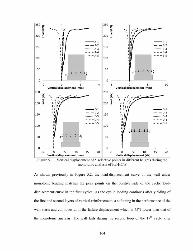
104
Figure 5.11. Vertical displacement of 5 selective points in different heights during the
monotonic analysis of FE-HCW
As shown previously in Figure 5.2, the load-displacement curve of the wall under
monotonic loading matches the peak points on the positive side of the cyclic load-
displacement curve in the first cycles. As the cyclic loading continues after yielding of
the first and second layers of vertical reinforcement, a softening in the performance of the
wall starts and continues until the failure displacement which is 45% lower than that of
the monotonic analysis. The wall fails during the second loop of the 17th cycle after
0
50
100
150
200
250
-2 0 2 4
Load
(kN
)
Vertical displacement (mm)
A-1 A-2 A-3 A-4 A-5
0
50
100
150
200
250
-5 0 5 10
Load
(kN
)
Vertical displacement (mm)
B-1 B-2 B-3 B-4 B-5
0
50
100
150
200
250
-5 0 5 10 15 20
Load
(kN
)
Vertical displacement (mm)
C-1 C-2 C-3 C-4 C-5
0
50
100
150
200
250
-5 0 5 10 15 20
Load
(kN
)
Vertical displacement (kN)
D-1 D-2 D-3 D-4 D-5
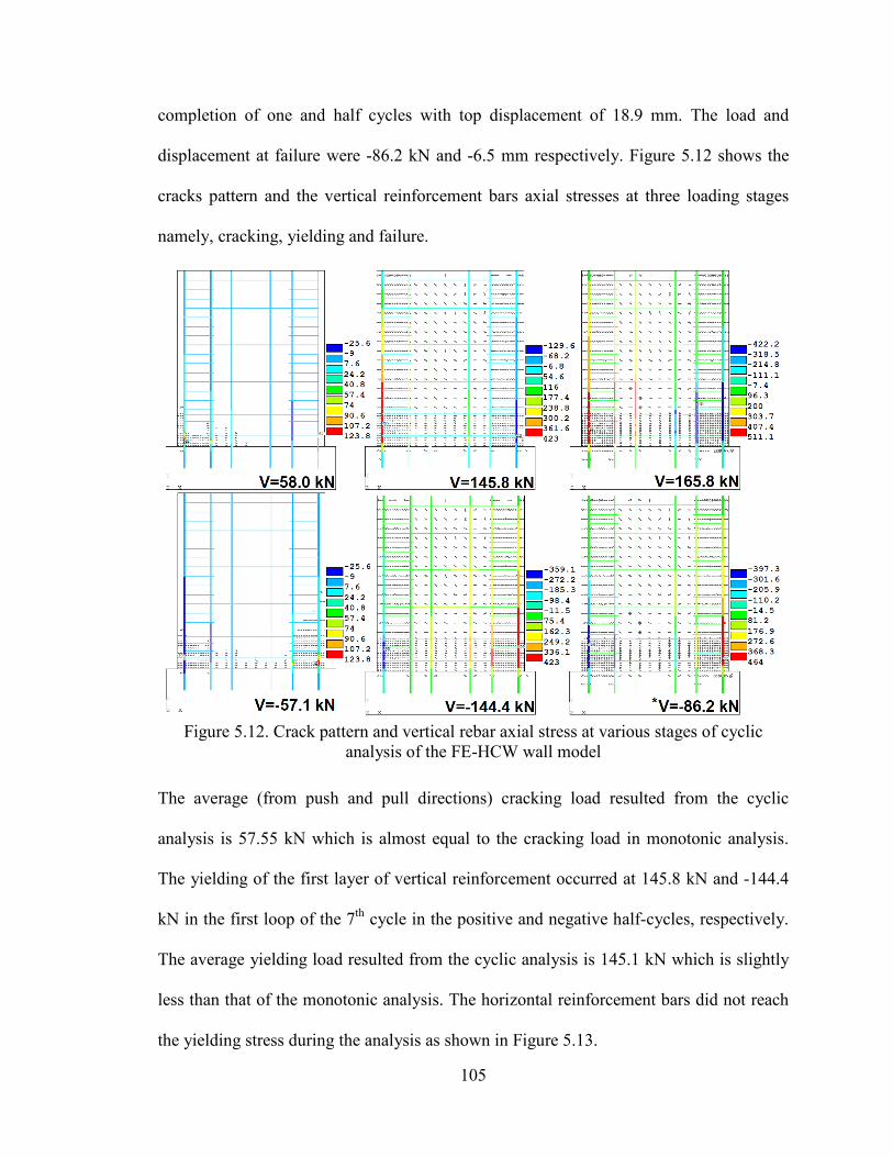
105
completion of one and half cycles with top displacement of 18.9 mm. The load and
displacement at failure were -86.2 kN and -6.5 mm respectively. Figure 5.12 shows the
cracks pattern and the vertical reinforcement bars axial stresses at three loading stages
namely, cracking, yielding and failure.
Figure 5.12. Crack pattern and vertical rebar axial stress at various stages of cyclic
analysis of the FE-HCW wall model
The average (from push and pull directions) cracking load resulted from the cyclic
analysis is 57.55 kN which is almost equal to the cracking load in monotonic analysis.
The yielding of the first layer of vertical reinforcement occurred at 145.8 kN and -144.4
kN in the first loop of the 7th cycle in the positive and negative half-cycles, respectively.
The average yielding load resulted from the cyclic analysis is 145.1 kN which is slightly
less than that of the monotonic analysis. The horizontal reinforcement bars did not reach
the yielding stress during the analysis as shown in Figure 5.13.
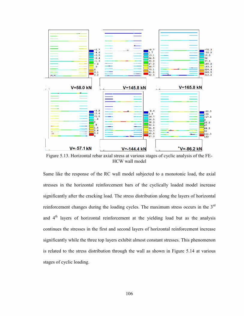
106
Figure 5.13. Horizontal rebar axial stress at various stages of cyclic analysis of the FE-
HCW wall model
Same like the response of the RC wall model subjected to a monotonic load, the axial
stresses in the horizontal reinforcement bars of the cyclically loaded model increase
significantly after the cracking load. The stress distribution along the layers of horizontal
reinforcement changes during the loading cycles. The maximum stress occurs in the 3rd
and 4th layers of horizontal reinforcement at the yielding load but as the analysis
continues the stresses in the first and second layers of horizontal reinforcement increase
significantly while the three top layers exhibit almost constant stresses. This phenomenon
is related to the stress distribution through the wall as shown in Figure 5.14 at various
stages of cyclic loading.
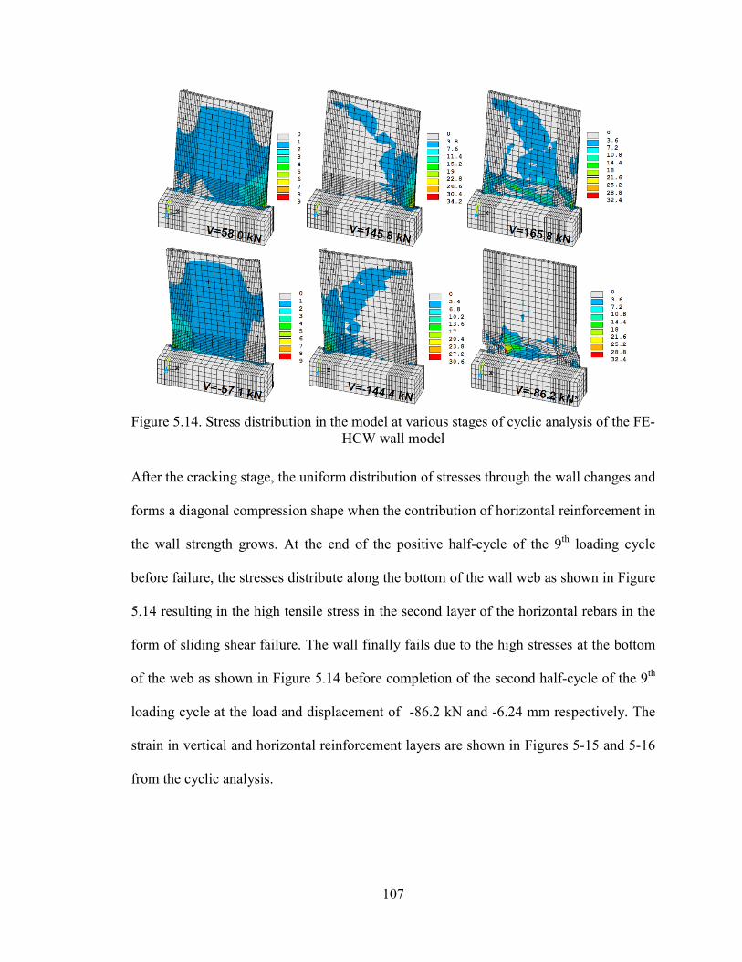
107
Figure 5.14. Stress distribution in the model at various stages of cyclic analysis of the FE-
HCW wall model
After the cracking stage, the uniform distribution of stresses through the wall changes and
forms a diagonal compression shape when the contribution of horizontal reinforcement in
the wall strength grows. At the end of the positive half-cycle of the 9th loading cycle
before failure, the stresses distribute along the bottom of the wall web as shown in Figure
5.14 resulting in the high tensile stress in the second layer of the horizontal rebars in the
form of sliding shear failure. The wall finally fails due to the high stresses at the bottom
of the web as shown in Figure 5.14 before completion of the second half-cycle of the 9th
loading cycle at the load and displacement of -86.2 kN and -6.24 mm respectively. The
strain in vertical and horizontal reinforcement layers are shown in Figures 5-15 and 5-16
from the cyclic analysis.
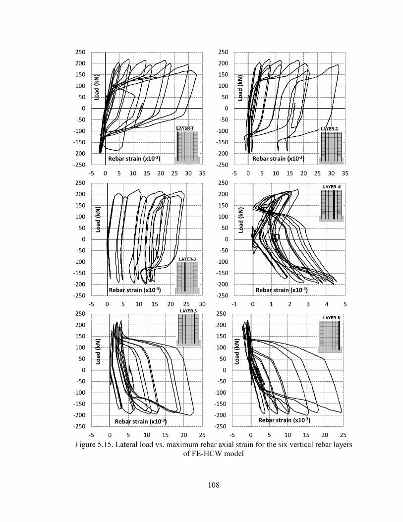
108
Figure 5.15. Lateral load vs. maximum rebar axial strain for the six vertical rebar layers
of FE-HCW model
-250
-200
-150
-100
-50
0
50
100
150
200
250
-5 0 5 10 15 20 25 30 35
Load
(kN
)
Rebar strain (x10-3)
-250
-200
-150
-100
-50
0
50
100
150
200
250
-5 0 5 10 15 20 25 30 35
Load
(kN
)
Rebar strain (x10-3)
-250
-200
-150
-100
-50
0
50
100
150
200
250
-5 0 5 10 15 20 25 30
Load
(kN
)
Rebar strain (x10-3)
-250
-200
-150
-100
-50
0
50
100
150
200
250
-1 0 1 2 3 4 5
Load
(kN
)
Rebar strain (x10-3)
-250
-200
-150
-100
-50
0
50
100
150
200
250
-5 0 5 10 15 20 25
Load
(kN
)
Rebar strain (x10-3) -250
-200
-150
-100
-50
0
50
100
150
200
250
-5 0 5 10 15 20 25
Load
(kN
)
Rebar strain (x10-3)
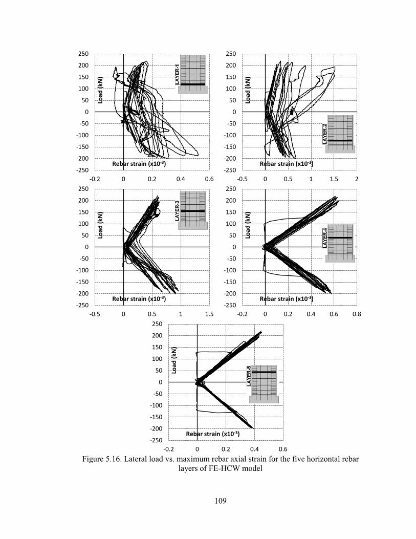
109
Figure 5.16. Lateral load vs. maximum rebar axial strain for the five horizontal rebar
layers of FE-HCW model
-250
-200
-150
-100
-50
0
50
100
150
200
250
-0.2 0 0.2 0.4 0.6
Load
(kN
)
Rebar strain (x10-3)
-250
-200
-150
-100
-50
0
50
100
150
200
250
-0.5 0 0.5 1 1.5 2
Load
(kN
)
Rebar strain (x10-3)
-250
-200
-150
-100
-50
0
50
100
150
200
250
-0.5 0 0.5 1 1.5
Load
(kN
)
Rebar strain (x10-3)
-250
-200
-150
-100
-50
0
50
100
150
200
250
-0.2 0 0.2 0.4 0.6 0.8
Load
(kN
)
Rebar strain (x10-3)
-250
-200
-150
-100
-50
0
50
100
150
200
250
-0.2 0 0.2 0.4 0.6
Load
(kN
)
Rebar strain (x10-3)
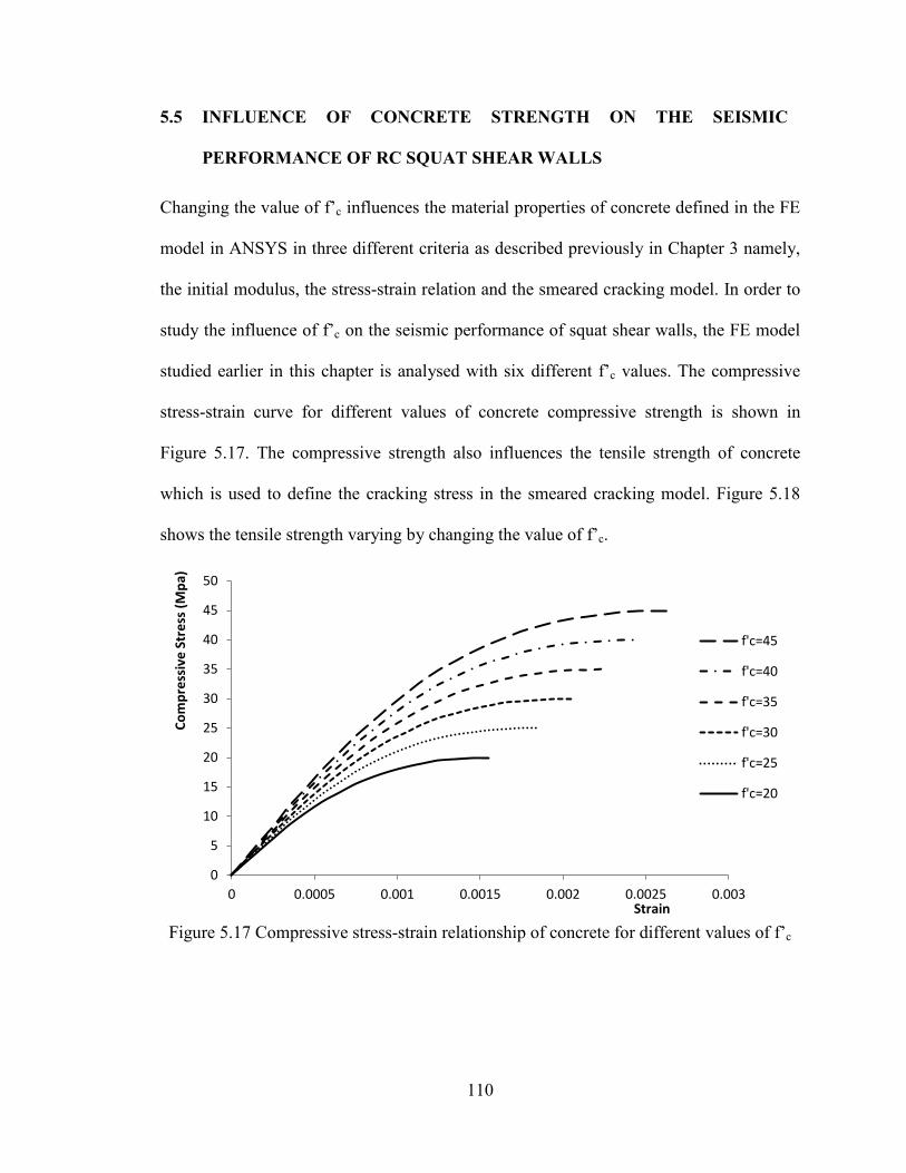
110
5.5 INFLUENCE OF CONCRETE STRENGTH ON THE SEISMIC
PERFORMANCE OF RC SQUAT SHEAR WALLS
Changing the value of f’c influences the material properties of concrete defined in the FE
model in ANSYS in three different criteria as described previously in Chapter 3 namely,
the initial modulus, the stress-strain relation and the smeared cracking model. In order to
study the influence of f’c on the seismic performance of squat shear walls, the FE model
studied earlier in this chapter is analysed with six different f’c values. The compressive
stress-strain curve for different values of concrete compressive strength is shown in
Figure 5.17. The compressive strength also influences the tensile strength of concrete
which is used to define the cracking stress in the smeared cracking model. Figure 5.18
shows the tensile strength varying by changing the value of f’c.
Figure 5.17 Compressive stress-strain relationship of concrete for different values of f’c
0
5
10
15
20
25
30
35
40
45
50
0 0.0005 0.001 0.0015 0.002 0.0025 0.003
Com
pres
sive
Str
ess (
Mpa
)
Strain
f'c=45
f'c=40
f'c=35
f'c=30
f'c=25
f'c=20
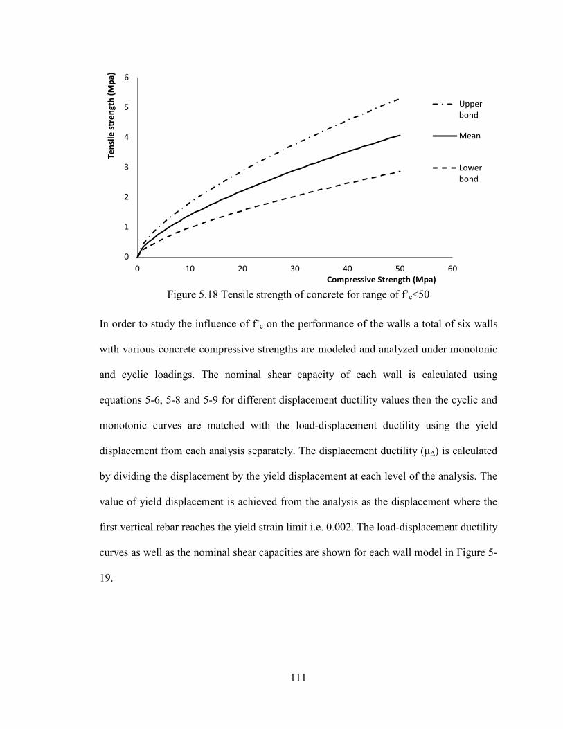
111
Figure 5.18 Tensile strength of concrete for range of f’c<50
In order to study the influence of f’c on the performance of the walls a total of six walls
with various concrete compressive strengths are modeled and analyzed under monotonic
and cyclic loadings. The nominal shear capacity of each wall is calculated using
equations 5-6, 5-8 and 5-9 for different displacement ductility values then the cyclic and
monotonic curves are matched with the load-displacement ductility using the yield
displacement from each analysis separately. The displacement ductility (μΔ) is calculated
by dividing the displacement by the yield displacement at each level of the analysis. The
value of yield displacement is achieved from the analysis as the displacement where the
first vertical rebar reaches the yield strain limit i.e. 0.002. The load-displacement ductility
curves as well as the nominal shear capacities are shown for each wall model in Figure 5-
19.
0
1
2
3
4
5
6
0 10 20 30 40 50 60
Tens
ile st
reng
th (M
pa)
Compressive Strength (Mpa)
Upper bond
Mean
Lower bond
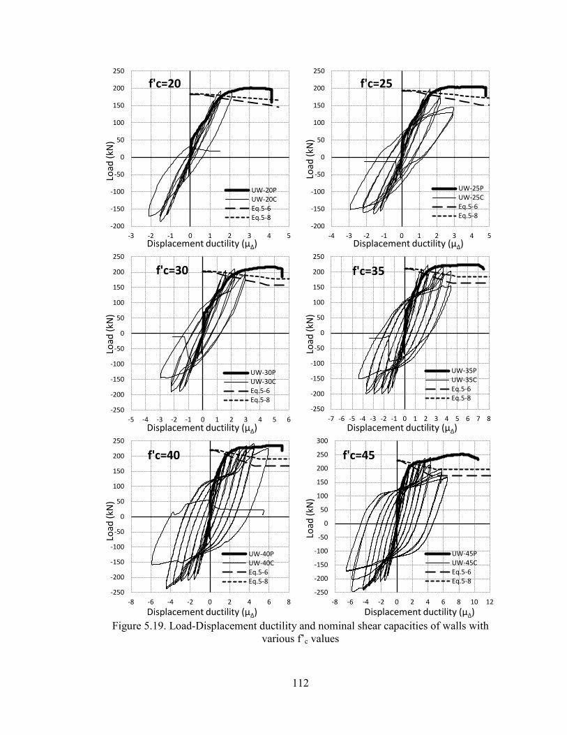
112
Figure 5.19. Load-Displacement ductility and nominal shear capacities of walls with
various f’c values
-200
-150
-100
-50
0
50
100
150
200
250
-3 -2 -1 0 1 2 3 4 5
Load
(kN
)
Displacement ductility (μΔ)
f'c=20
UW-20P UW-20C Eq.5-6 Eq.5-8
-200
-150
-100
-50
0
50
100
150
200
250
-4 -3 -2 -1 0 1 2 3 4 5
Load
(kN
)
Displacement ductility (μΔ)
f'c=25
UW-25P UW-25C Eq.5-6 Eq.5-8
-250
-200
-150
-100
-50
0
50
100
150
200
250
-5 -4 -3 -2 -1 0 1 2 3 4 5 6
Load
(kN
)
Displacement ductility (μΔ)
f'c=30
UW-30P UW-30C Eq.5-6 Eq.5-8
-250
-200
-150
-100
-50
0
50
100
150
200
250
-7 -6 -5 -4 -3 -2 -1 0 1 2 3 4 5 6 7 8
Load
(kN
)
Displacement ductility (μΔ)
f'c=35
UW-35P UW-35C Eq.5-6 Eq.5-8
-250
-200
-150
-100
-50
0
50
100
150
200
250
-8 -6 -4 -2 0 2 4 6 8
Load
(kN
)
Displacement ductility (μΔ)
f'c=40
UW-40P UW-40C Eq.5-6 Eq.5-8
-250
-200
-150
-100
-50
0
50
100
150
200
250
300
-8 -6 -4 -2 0 2 4 6 8 10 12
Load
(kN
)
Displacement ductility (μΔ)
f'c=45
UW-45P UW-45C Eq.5-6 Eq.5-8
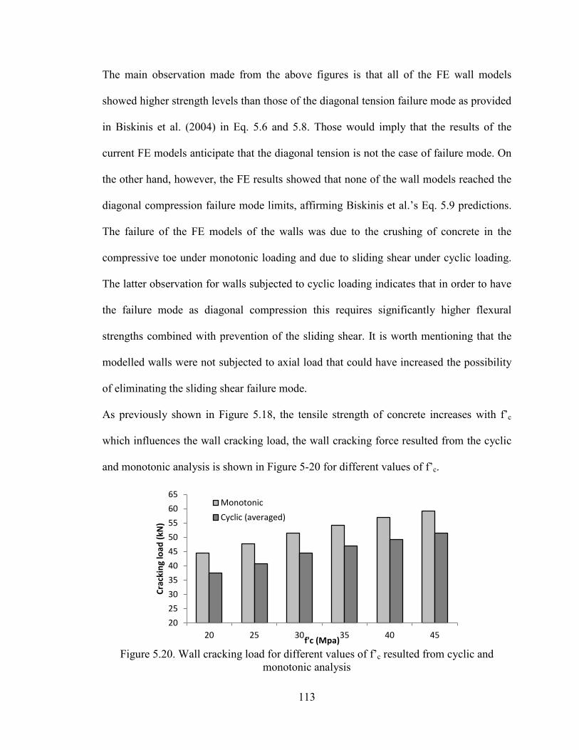
113
The main observation made from the above figures is that all of the FE wall models
showed higher strength levels than those of the diagonal tension failure mode as provided
in Biskinis et al. (2004) in Eq. 5.6 and 5.8. Those would imply that the results of the
current FE models anticipate that the diagonal tension is not the case of failure mode. On
the other hand, however, the FE results showed that none of the wall models reached the
diagonal compression failure mode limits, affirming Biskinis et al.’s Eq. 5.9 predictions.
The failure of the FE models of the walls was due to the crushing of concrete in the
compressive toe under monotonic loading and due to sliding shear under cyclic loading.
The latter observation for walls subjected to cyclic loading indicates that in order to have
the failure mode as diagonal compression this requires significantly higher flexural
strengths combined with prevention of the sliding shear. It is worth mentioning that the
modelled walls were not subjected to axial load that could have increased the possibility
of eliminating the sliding shear failure mode.
As previously shown in Figure 5.18, the tensile strength of concrete increases with f’c
which influences the wall cracking load, the wall cracking force resulted from the cyclic
and monotonic analysis is shown in Figure 5-20 for different values of f’c.
Figure 5.20. Wall cracking load for different values of f’c resulted from cyclic and
monotonic analysis
20 25 30 35 40 45 50 55 60 65
20 25 30 35 40 45
Crac
king
load
(kN
)
f'c (Mpa)
Monotonic Cyclic (averaged)
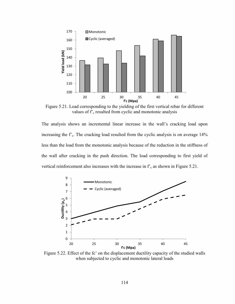
114
Figure 5.21. Load corresponding to the yielding of the first vertical rebar for different
values of f’c resulted from cyclic and monotonic analysis
The analysis shows an incremental linear increase in the wall’s cracking load upon
increasing the f’c. The cracking load resulted from the cyclic analysis is on average 14%
less than the load from the monotonic analysis because of the reduction in the stiffness of
the wall after cracking in the push direction. The load corresponding to first yield of
vertical reinforcement also increases with the increase in f’c as shown in Figure 5.21.
Figure 5.22. Effect of the fc’ on the displacement ductility capacity of the studied walls
when subjected to cyclic and monotonic lateral loads
100
110
120
130
140
150
160
170
20 25 30 35 40 45
Yiel
d lo
ad (k
N)
f'c (Mpa)
Monotonic
Cyclic (averaged)
0
1
2
3
4
5
6
7
8
9
20 25 30 35 40 45
Duct
ility
(μu)
f'c (Mpa)
Monotonic
Cyclic (averaged)
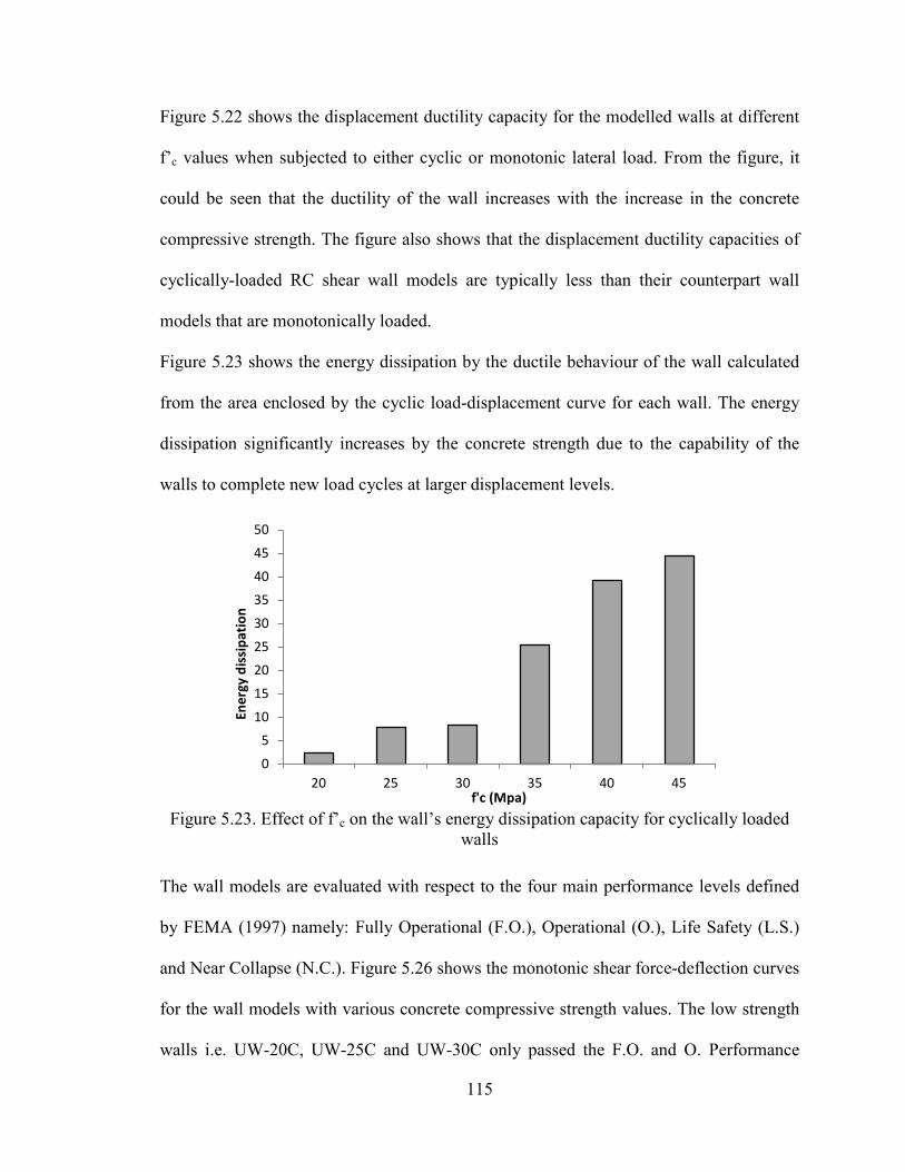
115
Figure 5.22 shows the displacement ductility capacity for the modelled walls at different
f’c values when subjected to either cyclic or monotonic lateral load. From the figure, it
could be seen that the ductility of the wall increases with the increase in the concrete
compressive strength. The figure also shows that the displacement ductility capacities of
cyclically-loaded RC shear wall models are typically less than their counterpart wall
models that are monotonically loaded.
Figure 5.23 shows the energy dissipation by the ductile behaviour of the wall calculated
from the area enclosed by the cyclic load-displacement curve for each wall. The energy
dissipation significantly increases by the concrete strength due to the capability of the
walls to complete new load cycles at larger displacement levels.
Figure 5.23. Effect of f’c on the wall’s energy dissipation capacity for cyclically loaded
walls
The wall models are evaluated with respect to the four main performance levels defined
by FEMA (1997) namely: Fully Operational (F.O.), Operational (O.), Life Safety (L.S.)
and Near Collapse (N.C.). Figure 5.26 shows the monotonic shear force-deflection curves
for the wall models with various concrete compressive strength values. The low strength
walls i.e. UW-20C, UW-25C and UW-30C only passed the F.O. and O. Performance
0
5
10
15
20
25
30
35
40
45
50
20 25 30 35 40 45
Ener
gy d
issi
patio
n
f'c (Mpa)
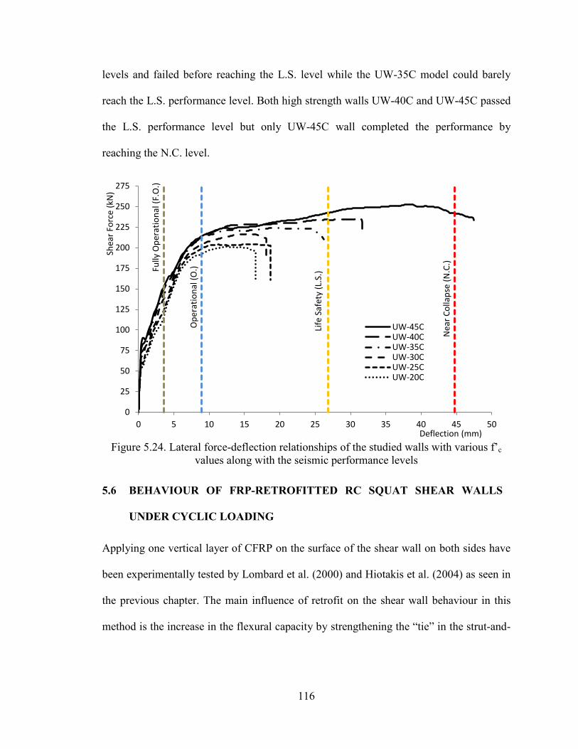
116
levels and failed before reaching the L.S. level while the UW-35C model could barely
reach the L.S. performance level. Both high strength walls UW-40C and UW-45C passed
the L.S. performance level but only UW-45C wall completed the performance by
reaching the N.C. level.
Figure 5.24. Lateral force-deflection relationships of the studied walls with various f’c
values along with the seismic performance levels
5.6 BEHAVIOUR OF FRP-RETROFITTED RC SQUAT SHEAR WALLS
UNDER CYCLIC LOADING
Applying one vertical layer of CFRP on the surface of the shear wall on both sides have
been experimentally tested by Lombard et al. (2000) and Hiotakis et al. (2004) as seen in
the previous chapter. The main influence of retrofit on the shear wall behaviour in this
method is the increase in the flexural capacity by strengthening the “tie” in the strut-and-
Fully
Ope
ratio
nal (
F.O
.)
Ope
ratio
nal (
O.)
Life
Saf
ety
(L.S
.)
Nea
r Col
laps
e (N
.C.)
0
25
50
75
100
125
150
175
200
225
250
275
0 5 10 15 20 25 30 35 40 45 50
Shea
r For
ce (k
N)
Deflection (mm)
UW-45C UW-40C UW-35C UW-30C UW-25C UW-20C
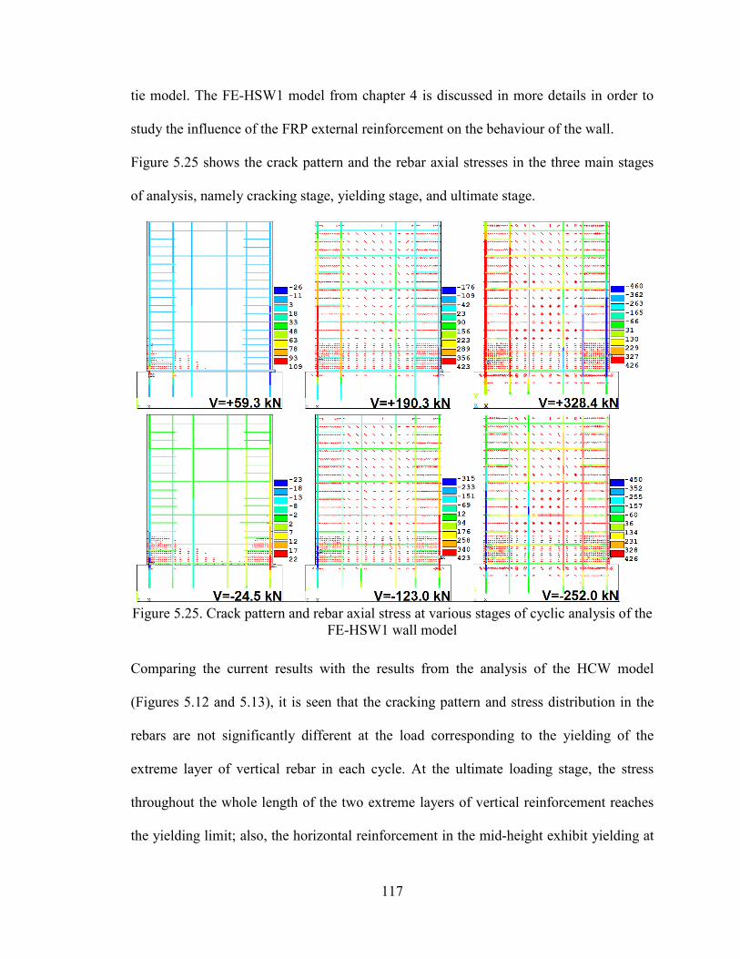
117
tie model. The FE-HSW1 model from chapter 4 is discussed in more details in order to
study the influence of the FRP external reinforcement on the behaviour of the wall.
Figure 5.25 shows the crack pattern and the rebar axial stresses in the three main stages
of analysis, namely cracking stage, yielding stage, and ultimate stage.
Figure 5.25. Crack pattern and rebar axial stress at various stages of cyclic analysis of the
FE-HSW1 wall model
Comparing the current results with the results from the analysis of the HCW model
(Figures 5.12 and 5.13), it is seen that the cracking pattern and stress distribution in the
rebars are not significantly different at the load corresponding to the yielding of the
extreme layer of vertical rebar in each cycle. At the ultimate loading stage, the stress
throughout the whole length of the two extreme layers of vertical reinforcement reaches
the yielding limit; also, the horizontal reinforcement in the mid-height exhibit yielding at
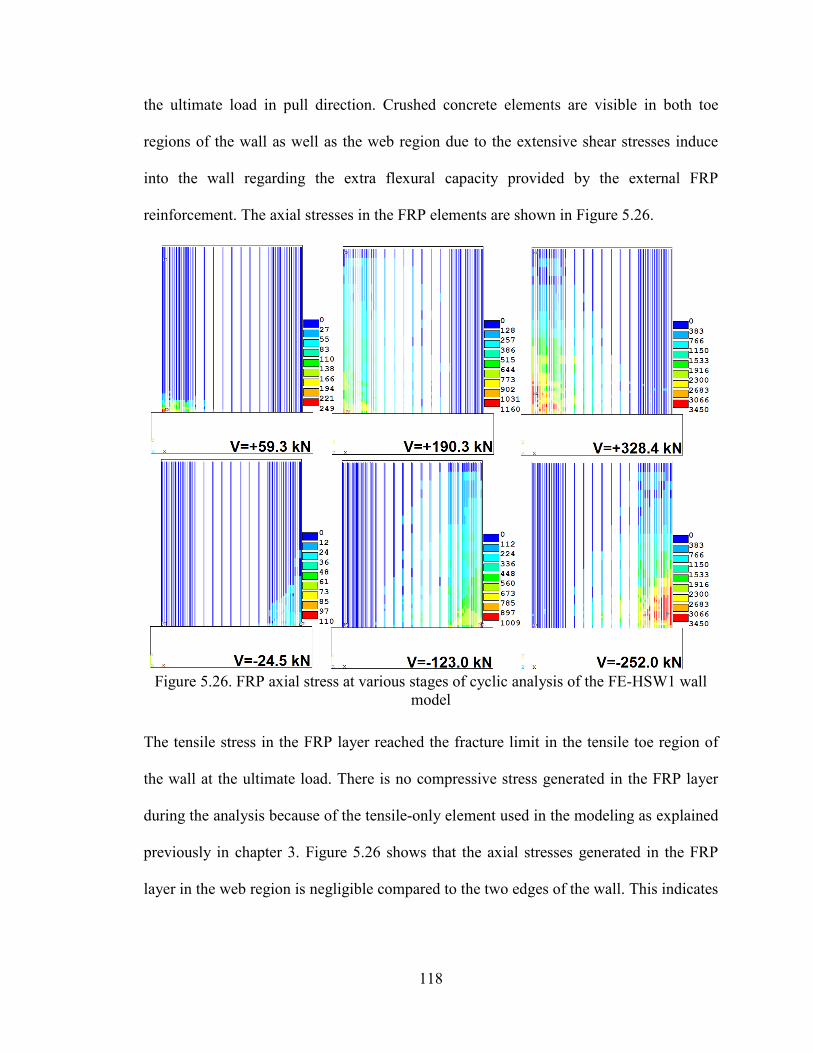
118
the ultimate load in pull direction. Crushed concrete elements are visible in both toe
regions of the wall as well as the web region due to the extensive shear stresses induce
into the wall regarding the extra flexural capacity provided by the external FRP
reinforcement. The axial stresses in the FRP elements are shown in Figure 5.26.
Figure 5.26. FRP axial stress at various stages of cyclic analysis of the FE-HSW1 wall
model
The tensile stress in the FRP layer reached the fracture limit in the tensile toe region of
the wall at the ultimate load. There is no compressive stress generated in the FRP layer
during the analysis because of the tensile-only element used in the modeling as explained
previously in chapter 3. Figure 5.26 shows that the axial stresses generated in the FRP
layer in the web region is negligible compared to the two edges of the wall. This indicates
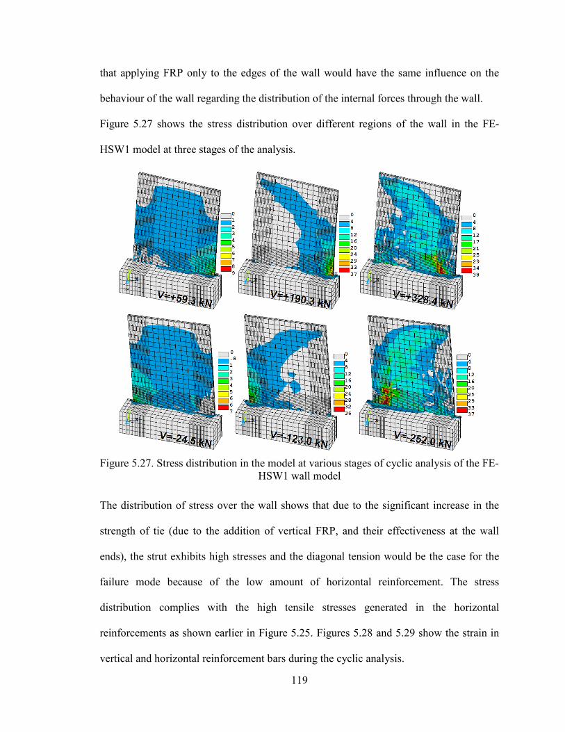
119
that applying FRP only to the edges of the wall would have the same influence on the
behaviour of the wall regarding the distribution of the internal forces through the wall.
Figure 5.27 shows the stress distribution over different regions of the wall in the FE-
HSW1 model at three stages of the analysis.
Figure 5.27. Stress distribution in the model at various stages of cyclic analysis of the FE-
HSW1 wall model
The distribution of stress over the wall shows that due to the significant increase in the
strength of tie (due to the addition of vertical FRP, and their effectiveness at the wall
ends), the strut exhibits high stresses and the diagonal tension would be the case for the
failure mode because of the low amount of horizontal reinforcement. The stress
distribution complies with the high tensile stresses generated in the horizontal
reinforcements as shown earlier in Figure 5.25. Figures 5.28 and 5.29 show the strain in
vertical and horizontal reinforcement bars during the cyclic analysis.
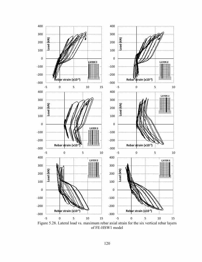
120
Figure 5.28. Lateral load vs. maximum rebar axial strain for the six vertical rebar layers
of FE-HSW1 model
-300
-200
-100
0
100
200
300
400
-5 0 5 10 15
Load
(kN
)
Rebar strain (x10-3)
-300
-200
-100
0
100
200
300
400
-5 0 5 10
Load
(kN
)
Rebar strain (x10-3)
-300
-200
-100
0
100
200
300
400
-5 0 5 10
Load
(kN
)
Rebar strain (x10-3)
-300
-200
-100
0
100
200
300
400
-5 0 5 10
Load
(kN
)
Rebar strain (x10-3)
-300
-200
-100
0
100
200
300
400
-5 0 5 10 15
Load
(kN
)
Rebar strain (x10-3)
-300
-200
-100
0
100
200
300
400
-5 0 5 10 15
Load
(kN
)
Rebar strain (x10-3)
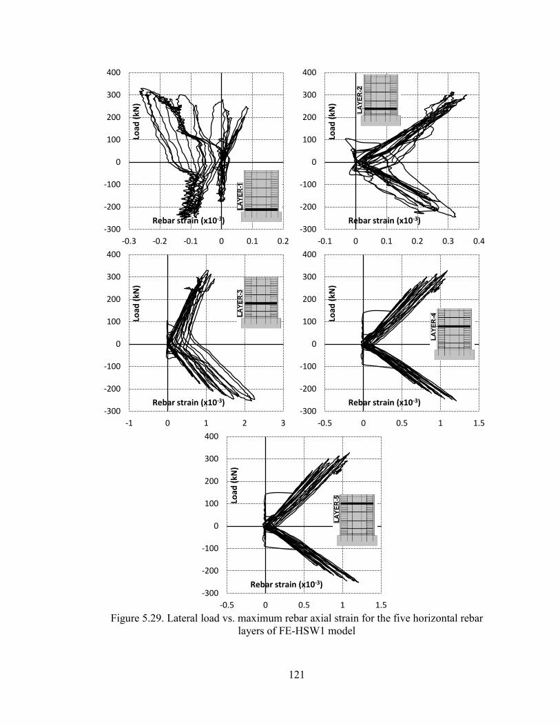
121
Figure 5.29. Lateral load vs. maximum rebar axial strain for the five horizontal rebar
layers of FE-HSW1 model
-300
-200
-100
0
100
200
300
400
-0.3 -0.2 -0.1 0 0.1 0.2
Load
(kN
)
Rebar strain (x10-3)
-300
-200
-100
0
100
200
300
400
-0.1 0 0.1 0.2 0.3 0.4
Load
(kN
)
Rebar strain (x10-3)
-300
-200
-100
0
100
200
300
400
-1 0 1 2 3
Load
(kN
)
Rebar strain (x10-3)
-300
-200
-100
0
100
200
300
400
-0.5 0 0.5 1 1.5
Load
(kN
)
Rebar strain (x10-3)
-300
-200
-100
0
100
200
300
400
-0.5 0 0.5 1 1.5
Load
(kN
)
Rebar strain (x10-3)
122
Although the vertical reinforcement bars exhibit yielding but the strains did not go well
beyond the yielding strain compared to the strains resulted from the unretrofitted wall
(HCW) due to the low flexibility of the FRP layers which also resulted in limited top
displacement. Unlike the vertical rebars, the strains in the horizontal reinforcement layers
increases compared to the HCW model. The third layer of horizontal reinforcement
yielded during the analysis but the strains in the other four layers remain within the
elastic limits.
5.7 INFLUENCE OF CONCRETE STRENGTH ON THE SEISMIC
PERFORMANCE OF FRP-RETROFITTED SQUAT SHEAR WALLS
The influence of f’c on the performance of retrofitted walls is discussed in the section. In
order to compare the results of FRP-retrofitted RC shear wall models with those of the
unretrofitted walls, the same loading history is used. The retrofit method used complies
with the HSW1 specimen from the experimental works of Hiotakis et al. (2004). Since
the bonding interface model (Lu et al., 2005-a) depends on the tensile strength of
concrete, the bond interface elements are updated in each model based on the f’c of the
model accordingly.
Figure 5.30 shows the lateral load-displacement ductility curves of the FRP-retrofitted
walls with various values of f’c between 20 MPa and 45 MPa. The concrete compressive
strength influences the performance of the FRP-retrofitted walls in two ways by affecting
the overall strength and ductility of the wall as shown previously for the unretrofitted
walls and also influencing the strength of the bond interface between FRP and concrete
surface.
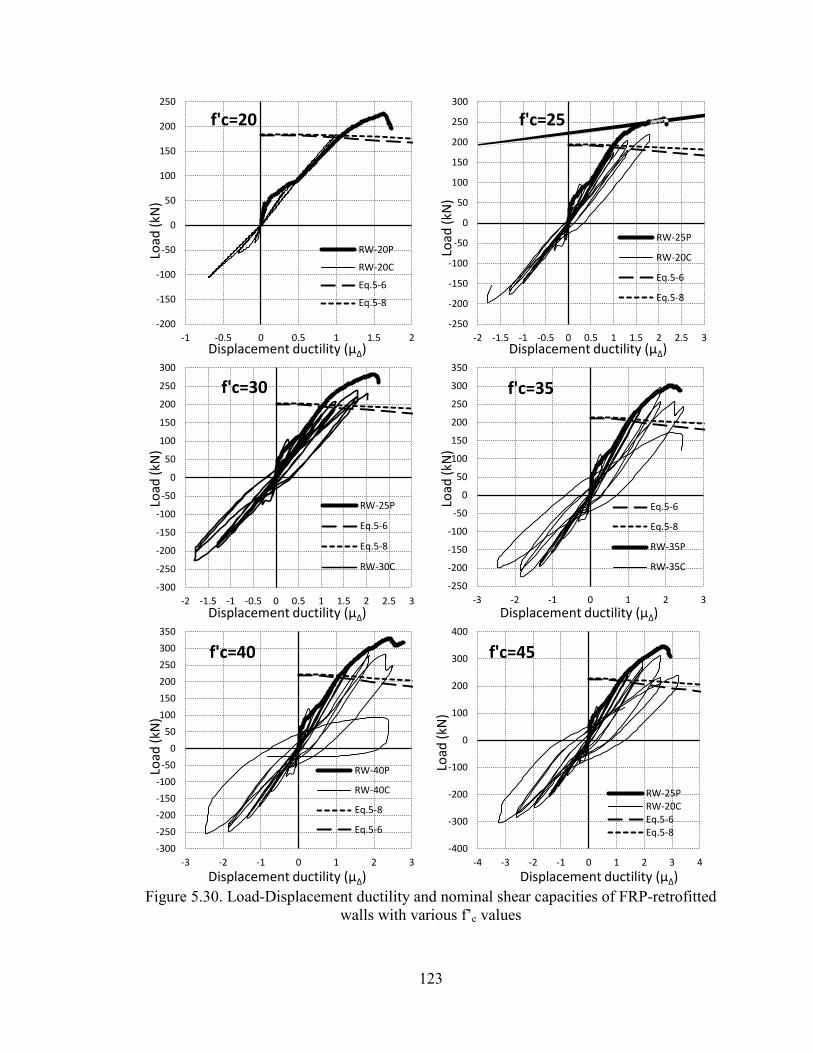
123
Figure 5.30. Load-Displacement ductility and nominal shear capacities of FRP-retrofitted
walls with various f’c values
-200
-150
-100
-50
0
50
100
150
200
250
-1 -0.5 0 0.5 1 1.5 2
Load
(kN
)
Displacement ductility (μΔ)
f'c=20
RW-20P
RW-20C
Eq.5-6
Eq.5-8
-250
-200
-150
-100
-50
0
50
100
150
200
250
300
-2 -1.5 -1 -0.5 0 0.5 1 1.5 2 2.5 3
Load
(kN
)
Displacement ductility (μΔ)
f'c=25
RW-25P
RW-20C
Eq.5-6
Eq.5-8
-300
-250
-200
-150
-100
-50
0
50
100
150
200
250
300
-2 -1.5 -1 -0.5 0 0.5 1 1.5 2 2.5 3
Load
(kN
)
Displacement ductility (μΔ)
f'c=30
RW-25P
Eq.5-6
Eq.5-8
RW-30C
-250
-200
-150
-100
-50
0
50
100
150
200
250
300
350
-3 -2 -1 0 1 2 3
Load
(kN
)
Displacement ductility (μΔ)
f'c=35
Eq.5-6
Eq.5-8
RW-35P
RW-35C
-300 -250 -200 -150 -100
-50 0
50 100 150 200 250 300 350
-3 -2 -1 0 1 2 3
Load
(kN
)
Displacement ductility (μΔ)
f'c=40
RW-40P
RW-40C
Eq.5-8
Eq.5-6
-400
-300
-200
-100
0
100
200
300
400
-4 -3 -2 -1 0 1 2 3 4
Load
(kN
)
Displacement ductility (μΔ)
f'c=45
RW-25P RW-20C Eq.5-6 Eq.5-8
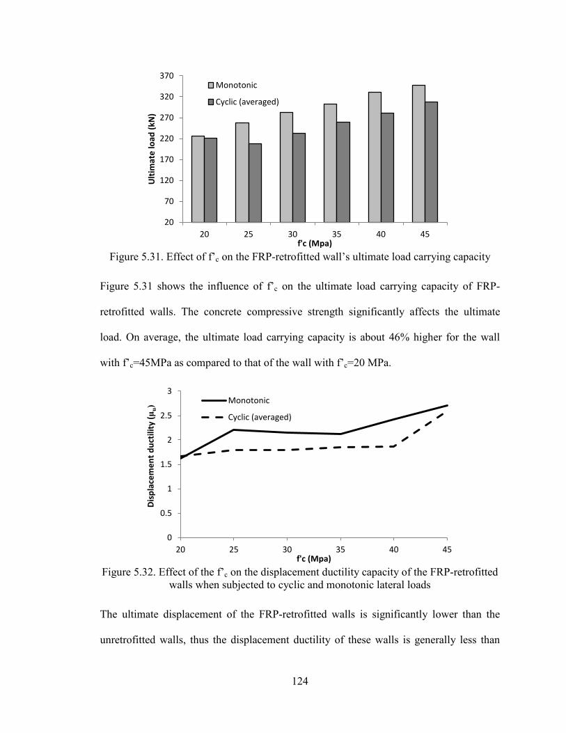
124
Figure 5.31. Effect of f’c on the FRP-retrofitted wall’s ultimate load carrying capacity
Figure 5.31 shows the influence of f’c on the ultimate load carrying capacity of FRP-
retrofitted walls. The concrete compressive strength significantly affects the ultimate
load. On average, the ultimate load carrying capacity is about 46% higher for the wall
with f’c=45MPa as compared to that of the wall with f’c=20 MPa.
Figure 5.32. Effect of the f’c on the displacement ductility capacity of the FRP-retrofitted
walls when subjected to cyclic and monotonic lateral loads
The ultimate displacement of the FRP-retrofitted walls is significantly lower than the
unretrofitted walls, thus the displacement ductility of these walls is generally less than
20
70
120
170
220
270
320
370
20 25 30 35 40 45
Ulti
mat
e lo
ad (k
N)
f'c (Mpa)
Monotonic
Cyclic (averaged)
0
0.5
1
1.5
2
2.5
3
20 25 30 35 40 45
Disp
lace
men
t duc
tility
(μu)
f'c (Mpa)
Monotonic
Cyclic (averaged)
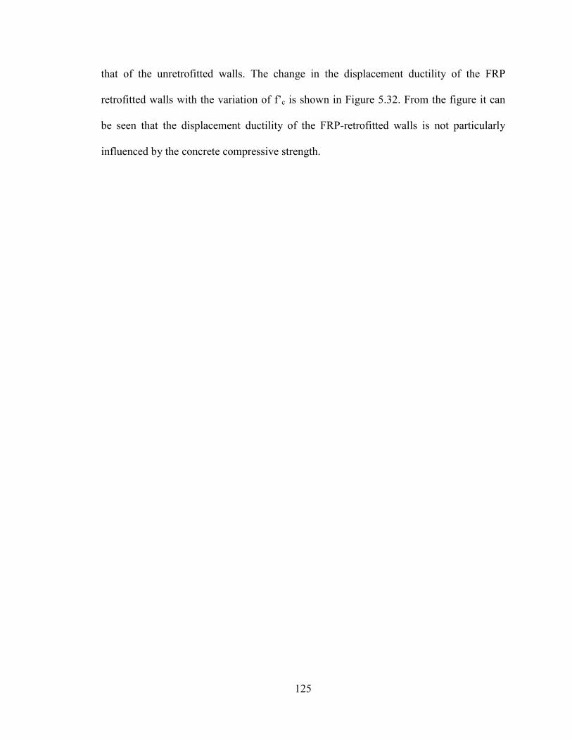
125
that of the unretrofitted walls. The change in the displacement ductility of the FRP
retrofitted walls with the variation of f’c is shown in Figure 5.32. From the figure it can
be seen that the displacement ductility of the FRP-retrofitted walls is not particularly
influenced by the concrete compressive strength.
126
CHAPTER 6
CONCLUSIONS AND RECOMMENDATIONS
6.1 SUMMARY
Establishing effective retrofit methods for upgrading the seismic performance of existing
reinforced concrete (RC) shear walls requires a reliable means for estimating the
behaviour of RC shear walls with various geometry and internal reinforcement
configurations when subjected to different combinations of axial and lateral loads.
Generally, experimental testing of retrofitted RC shear walls is considered as the most
reliable method of performance evaluation, yet this requires great efforts in terms of the
testing equipment and time in addition to the high cost. On the other hand, a numerical
model that would consider the main parameters that influence the complex performance
of original and retrofitted RC shear walls is seen to be an effective and promising tool.
Such analytical approach would be particularly useful for parametric studies and
development of code provisions for the design or evaluation purposes. Despite the wealth
in research information in the area of retrofitting RC bridges using fibre-reinforced
polymer (FRP) composite materials, yet the experimental and analytical research in the
area of assessing the seismic performance of FRP-retrofitted RC shear walls is still in its
early stages. A number of experimental tests are available in the literature which could be
used for the primary verification of possible numerical analyses. Similarly, a number of
numerical and analytical approaches are available with a great potential for
improvements in order to converge into a precise and usable analytical approach. Finite
127
Element (FE) modeling of reinforced concrete structural elements deals with the
composite behaviour of concrete material with the embedded steel reinforcement and
possible additional externally bonded/anchored retrofit reinforcement, such as FRP.
Appropriate use of elements and meshing techniques that closely represents the
composite nature of the steel-reinforced concrete with or without FRP is a key factor in
numerical simulations for the predicted behaviour of RC shear walls.
In this thesis, the FE modeling of RC shear walls using general purpose FE package
ANSYS were explored. A total of seven experimentally tested wall models from four
experimental programs were selected and analysed under monotonic and reversed cyclic
loading and the numerical predictions were in good correlation with the experimental
data. One of the experimentally tested models was selected for further detailed
investigation on the effect of various design parameters on the behaviour of the squat
walls and their modes of failure, namely the influence of the concrete compressive
strength and the addition of one layer of externally-bonded vertical CFRP sheet.
6.2 CONCLUSIONS
Based on the results of the FE analysis on the modeled shear walls and the extended
parametric study investigation, the following conclusions were drawn:
General conclusions on FE modeling of RC shear walls
1. The SOLID65 element provided in the elements library of ANSYS is capable of
simulating the behaviour of shear walls under the applied monotonic and cyclic
loading with a good precision.
128
2. The LINK180 element provided in the elements library of ANSYS is capable of
simulating the behaviour of embedded rebars and external reinforcement with
good precision and convenient output data capabilities, but it does not simulate
the rebar dowel action along the element’s normal plane which results in a
premature failure in some cases under cyclic loading.
3. The COMBIN39 element provided in the elements library of ANSYS is capable
of simulating the bond-interface between external reinforcement and the surface
of concrete with good precision.
For the studied unretrofitted squat shear wall FE model
1. The performance of unretrofitted shear wall model is sensitive to the loading
protocol on the wall. The monotonically loaded wall model exhibits higher
ultimate displacement and higher displacement ductility compared to the
cyclically loaded model.
2. If the diagonal tension mode of failure is prevented by sufficient providing
horizontal reinforcement, the failure mode of the squat wall will become flexural
in the absence of axial compressive force.
3. The concrete compressive strength significantly influences the displacement
ductility of the wall model.
4. The concrete compressive strength significantly influences the seismic energy
dissipation capacity of the model.
5. The concrete compressive strength significantly influences the loads correspond
to the first cracking of concrete and first yielding of the reinforcement bars.
129
6. The sliding shear was the dominating failure mode for the wall models subjected
to cyclic loading in the absence of axial compressive forces due to the incapability
of the used reinforcement elements in providing the extra shear resistance by
means of the rebars dowel action.
For the studied FRP-retrofitted RC squat shear wall FE model
1. Addition of an external layer of vertical FRP to the wall model significantly
influences the failure mode of the wall by providing a great additional flexural
strength to the wall. The model mode of failure migrates from the sliding shear
failure mode to diagonal tension after strengthening by vertical FRP
reinforcement.
2. The concrete compressive strength does not significantly influence the
performance of the FRP-retrofitted wall models. However, the ultimate load
carrying capacity of the wall significantly increases by the concrete compressive
strength.
6.3 RECOMMENDATIONS FOR THE FUTURE WORK
The author strongly recommends further numerical modeling of a bigger group of
experimental work in order to achieve the following objectives:
1. In the case of squat shear walls, the axial forces significantly influence the
behaviour of the wall; this phenomenon should be investigated through a series of
models subjected to different axial load levels.
130
2. The effect of horizontal reinforcement ratio on the failure mode of unretrofitted
and retrofitted walls should be investigated through a series of models with
different horizontal reinforcement ratios.
3. The use of beam elements with rotational degrees of freedom for the vertical
reinforcement bars could resemble the rebar dowel action and solve the premature
failure of the model under cyclic loading but it may affect the other results of the
analysis and impose additional sophistications into the analysis; this could be
studied through a comparative modeling.
4. Other methods of application of FRP sheets to the surface of the walls should be
modeled and the most efficient methods would be introduced by comparing the
different aspects of the influence of each method on the performance of the wall.
5. The case of wall panels with top moments, axial and lateral forces would be a
major achievement in the modeling.
6. The use of steel plates as the externally bonded reinforcement as a retrofit method
through a series of numerical modeling and experimental testing.
131
REFERENCES
ACI Committee, 4. (2002). Guide for the design and construction of externally bonded
FRP systems for strengthening concrete structures. USA: American Concrete
Institute.
ANSYS, Inc. (2010-a). ANSYS Element Reference. Canonsburg, PA: SAS IP, Inc.
ANSYS, Inc. (2010-b). Theory Reference for the Mechanical APDL and Mechanical
Applications. Canonsburg, PA: SAS IP, Inc.
Antoniades, K., Thomas, K., Salonikios, N. and Kappos, A. J. (2003). Cyclic Tests on
Seismically Damaged Reinforced Concrete Walls Strengthened Using Fiber-
Reinforced Polymer Reinforcement. ACI Structural Journal, 100(4), 510-518.
Biskinis, D. E., Roupakias, G. K., and Fardi, M. N. (2004). Degradation of Shear
Strength of Reinforced Concrete Members with Inelastic Cyclic Displacements.
ACI Structural Journal-Technical Paper, 101(6), 773-783.
British Standards Institution. (1996). Eurocode 8: Design provisions for earthquake
resistance of structures. London: British Standards Institution.
CNR DT/200. (2004). Guide for the design and construction of externally bonded FRP
systems for strengthening existing structures. Rome, Italy: National Research
Council, Italy.
CAN/CSA-A23.3 Concrete Design Handbook (3rd ed. 2008). Canadian Standard
Association.
132
Cortés-Puentes, L. W., and Palermo. D. (2012). Modeling of RC Shear Walls Retrofitted
with Steel Plates or FRP Sheets. JOURNAL OF STRUCTURAL
ENGINEERING, ASCE 138(5) 602-612.
Cruz-Noguez, C. A., Lau, D. T. and Sherwood, E. T. (2012). Analythical modeling of
shear walls flexurally-reinforced with carbon fibre sheets. 6th International
Conference on Advanced Composite Materials in Bridges and Structures.
Kingston, ON, Queen's University.
Dai, J., Ueda, T., and Sato, Y. (2005). Development of the Nonlinear Bond Stress–Slip
Model of Fiber Reinforced Plastics Sheet–Concrete Interfaces with a Simple
Method. Journal of Composites for Construction, ASCE, 9(1), 52-62.
Elnady, M. M. (2008). Seismic Rehabilitation of RC Structural Walls. Hamilton, ON,
Canada: PhD Thesis, McMaster University.
Elnashai, A. S., and Pinho, R. (1998). Repair and Retrofitting of RC Walls using
Selective Techniques. Journal of Earthquake Engineering, 2(4), 525-568.
El-Sokkary, H., Galal, K., Ghorbanirenani, I., Léger, P. and Tremblay, R., (2012). Shake
Table Tests on FRP-Rehabilitated RC Shear Walls. Journal of Composites for
Construction, 17(1), 79–90.
El-Sokkary, H. and Galal, K. (2013). Seismic Behavior of FRP-Strengthened RC Shear
Walls. Journal of Composites for Construction, 10.1061/(ASCE) CC.1943-
5614.0000364
fib Model Code 2010 first complete draft (2010), Volume1. Lausanne, Switzerland: DCC
Document Competence Center Siegmar Kästl e.K., Germany.
133
Fiorato, A.E., Oesterle, R.G. and Corley, W.G. (1983). Behavior of Earthquake Resistant
Structural Walls Before and After Repair. ACI Advancing concrete knowledge,
80(5), 403-413.
Galal, K., and El-Sokkary, H. (2008). RECENT ADVANCEMENTS IN RETROFIT OF
RC SHEAR WALLS. The 14th World Conference on Earthquake Engineering .
Beijing, China.
Ghobara, A., and Khalil, A. A. (2004). Seismic Rehabilitation of Reinforced Concrete
Walls using Fibre Composites. 13th World Conference on Earthquake
Engineering. Vancouver, B.C, Canada: WCEE, 3316 1-14.
Hiotakis, S., Lau, D. T., and Londono, N. (2004). Research on Seismic Retrofit and
Rehabilitation of Reinforced Concrete Shear Walls using FRP Materials. Ottawa,
ON, Canada: Carlton University.
Hognestad, E. (1951). A Study of Combined Bending and Axial Load in Reinforced
Concrete Members. Bulletin 399, University of Illinois Engineering Experiment
Stations, Urbana Ill., 128 pp.
Hwang, S. J., Chiou, T. C. and Tu, Y. S. (2004). Reinforced Concrete Squat Walls
Retrofitted With Carbon Fiber Reinforced Polymer. Proceedings of 2nd
International Conference on Frp Composites in Civil Engineering - CICE.
Adelaide, Australia, 47-56.
Kobayashi, K. (2005). Innovative application of FRPs for seismic strengthening of RC
shear wall. Fiber-Reinforced Polymer (FRP) Reinforcement for Concrete
Structures. Framington Hills, Mi, USA, ACI, 1269-1288.
134
Kong, K. H., Tan, K. H. and Balendra, T. (2003). Retrofitting of Shear Walls Designed to
BS 8110 for Seismic Loads using FRP. Proceedings of Sixth International
Symposium on FRP Reinforcement for Concrete Structures (FRPRCS-6).
Singapore, 2003. 1127-1136.
Kowalsky, M. J., and Priestley, M. J. (2000). Improved Analythical Model for Shear
Strength of Circular Reinforced Concrete Columns in Seismic Regions. ACI
Structural Journal, 97(3), 388-396.
Lefas, I. D. and Kotsovos, M. D. (1990). Strength and Deformation Characteristics of
Reinforced Concrete Walls under Load Reversals. ACI Structural Journal, 87(1),
716-726.
Lefas, I. D., Kotsovos, M. D. and Ambraseys, N. N.(1990). Behavior of Reinforced
Concrete Structural Walls: Strength, Deformation Characteristics, and Failure
Mechanism. ACI Structural Journal 87(1), 23-31.
Li, B., and Lim, C. L. (2010). Tests on Seismically Damaged Reinforced Concrete
Structural Walls Repaired Using Fiber-Reinforced Polymers. ASCE Journal of
Composites for Construction, 10.1061 ASCE CC.1943-5614.0000110, 597-608.
Li, Z. J., Balendra, T. Tan, K. H. and Kong. K. H. (2005). Finite element modelling of
cyclic behaviour of shear wall structure retrofitted using GFRP. Proceedings of
7th International Symposium on Fiber-Reinforced Polymer (FRP) Reinforcement
for Concrete Structures. Farmington Hills, MI, ACI Symposium Publication,
1305-1324.
Lombard, J., Lau, D. T., Humar, J. L., Foo, S. and Cheung, M. S. (2000). Seismic
Strengthening and Repair of Reinforced Concrete Shear Walls. Proceedings of
135
12th World Conference on Earthquake Engineering. Aukland, Silverstream, N.Z.,
New Zealand Society for Earthquake Engineering, 2032 1-8.
Lu, X. Z., Teng, J. G., Ye, L. P., and Jiang, J. (2007). Intermediate Crack Debonding in
FRP-Strengthened RC Beams: FE Analysis and Strength Model. Journal Of
Composites For Construction, ASCE, 11(2), 161-175.
Lu, X. Z., Teng, J. G., Ye, L. P., and Jiang, J. J. (2005-a). Bond-slip models for FRP
sheets/plates bonded to concrete. Journal of Engineering Structures, 27(6), 920-
937.
Lu, X. Z., Teng, J. G., Ye, L. P., and Jiang, J. J. (2005-b). Meso-scale finite-element
model for FRP sheets/plates externally boned to concrete. Journal of Engineering
Structures, 27(4), 564-575.
Moehle, J. P. (2000). State of Research on Seismic Retrofit of Concrete Building
Structures in the US. US-Japan Symposium and Workshop on Seismic Retrofit of
Concrete Structures-State of Research and Practice.
Moehle, J., Lynn, A., Elwood, K., and Sezen, H. (2001). Gravity Load Collapse of
Building Frames During Earthquakes. Richmond, California: Pacific Earthquake
Engineering Research Center.
Ombres, L. (2010). Prediction of Intermediate Crack Debonding Failure in FRP-
Strengthened Reinforced Concrete Beams. Journal of Composite Structures, 92,
322-329.
Palermo, D. and Vecchio, F. J. (2007). Simulation of cyclically loaded concrete structures
based on the finite-element method. Journal of Structural Engineering, 133(5),
728-738.
136
Paulay, T., and Priestley, M. (1992). Seismic Design of Reinforced Concrete and
Masonry Buildings. Wiley.
Peterson, J. and Mitchell, D. (2003). Seismic Retrofit of Shear Walls with Headed Bars
and Carbon Fiber Wrap. ASCE Journal of Structural Engineering, 129(5), 606-
614.
Priestley, M. J., Verma, R., and Xiao, Y. (1994). Seismic Shear Strength of Reinforced
Concrete Columns. Journal of the Structural Devision, ASCE, 120(8).
Rosenboom, O., and Rizkalla, S. (2008). Experimental Study of Intermediate Crack
Debonding in Fiber-Reinforced Polymer Strengthened Beams. ACI Structural
Journal, 105(1), 41-50.
Salonikios, T., Tegos, I., Kappos, A., and Penelis, G. (1996). Squat R/C Walls Under
Inelastic Shear Reversals. Paper No. 749.: Elsevier Science Ltd.
Sato, Y., and Vecchio, F. J. (2003). Tension Stiffening and Crack Formation in
Reinforced Concrete Members with Fiber-Reinforced Polymer Sheets. Journal of
Structural Engineering, ASCE, 129(6), 717-724.
Sittipunt, C. and Wood, S. L. (1993). Finite Element Analysis of Reinforced Concrete
Shear Walls. Department of Civil Engineering, University of Illinois at Urbana -
Champaign, Urbana, Illinois.
137
Teng, J. G., Smith, S. T., Yao, J., and Chen, J. F. (2003). Intermediate crack-induced
debonding in RC beams and slabs. Journal of Construction and Building
Materials, 17, 447-462.
Ueda, T., Dai, J. G. and Sato, Y. (2005). Development of non-linear bond stress slip
model of fiber reinfored plastics sheet-concrete interfaces with a simple method.
Journal of Composite Construction, 9(1), 52-62.
Vasiliev, V. V., and Morozov, E. V. (2007). Advanced Mechanics of Composite
Materials (2nd ed.). Oxford: Elsevier Ltd. .
Vecchio, F. J. (1989). Nonlinear finite element analysis of reinforced concrete
membranes. ACI Structural Journal, 26-35.
Vecchio, F. J., and Collins, M. P. (1986). The modified compression field theory for
reinforced concrete elelments subjected to shear. Journal of American Concrete
Institute, 219-231.
Wight, J. K. and MacGregor, J. G. (2011). Reinforced Concrete Mechanics and Design
6th Edition. Pearson Education Inc., Upper Saddle River, NJ.
Willam, K. J., and Warnke, E. D. (1975). Constitutive Model for the Triaxial Behavior of
Concrete. International Association for Bridge and Structural Engineering.
Bergamo, Italy.
Wong, P. S., and Vecchio, F. J. (2002). VecTor2 and FormWorks user's manual. Toronto:
University of Toronto.
Yanez, F. A., Park, R., and Paulay, T. (1989). Strut and Tie Models for Reinforced
Concrete Design and Analysis. New Zealand Concrete Society Silver Jubilee
Conference, (pp. 43-45). Wairakei, New Zealand.
138
Yao, J., Teng, J. G., and Lam, L. (2005). Experimental Study on Intermediate Crack
Debonding in FRP-Strengthened RC Flexural Members. Journal of Advanced in
Structural Engineering, ASE, 8(4), 365-396.
Yuzugullu, O. (1972). Finite Element Approach for the Prediction of Inelastic Behavior
of Shear Wall-Frame System. Department of Civil Engineering, University of
Illinois at Urbana-Champaign, Urbana, Illinois.
Zhang, Y., and Wang, Z. (2000). Seismic Behavior of Reinforced Concrete Shear Walls
Subjected to High Axial Loading. ACI Structural Journal 97(5), 739-750.