final method for lca of plastic articles
TRANSCRIPT

Comparative Life Cycle Assessment (LCA) of Alternative Feedstock for Plastics Production
Draft report for stakeholder consultation - Part 1
- Final method for LCA of plastic articles
Nessi S., Sinkko T., Bulgheroni C., Garcia-Gutierrez P., Giuntoli J., Konti A., Sanye-Mengual E., Tonini D., Pant R., Marelli L. (project leader)
EUR XXXXX XX
Deadline for consultation comments: June 30, 2020

This publication is a Technical report by the Joint Research Centre (JRC), the European Commission’s science and knowledge service. It aims to provide evidence-based scientific support to the European policymaking process. The scientific output expressed does not imply a policy position of the European Commission. Neither the European Commission nor any person acting on behalf of the Commission is responsible for the use that might be made of this publication. Contact information [optional element] Name: Address: Email: Tel.: EU Science Hub https://ec.europa.eu/jrc JRCxxxxx EUR xxxxx xx
Print ISBN XXX-XX-XX-XXXXX-X ISSN XXXX-XXXX doi:XX.XXXX/XXXXXX
PDF ISBN XXX-XX-XX-XXXXX-X ISSN XXXX-XXXX doi:XX.XXXX/XXXXXX
Ispra: European Commission, 2020 © European Union, 2020 The reuse policy of the European Commission is implemented by Commission Decision 2011/833/EU of 12 December 2011 on the reuse of Commission documents (OJ L 330, 14.12.2011, p. 39). Reuse is authorised, provided the source of the document is acknowledged and its original meaning or message is not distorted. The European Commission shall not be liable for any consequence stemming from the reuse. For any use or reproduction of photos or other material that is not owned by the EU, permission must be sought directly from the copyright holders. All content © European Union, 2020 (unless otherwise specified) How to cite this report: Nessi S., Sinkko T., Bulgheroni C., Garcia-Gutierrez P., Giuntoli J., Konti A., Sanye-Mengual E., Tonini D., Pant R., Marelli L., Comparative Life Cycle Assessment (LCA) of Alternative Feedstock for Plastics Production – Part 1, European Commission, Ispra, 2020, ISBN 978-92-79-XXXXX-X, doi:10.2760/XXXXX, JRCXXXXXX. Printed in XXX


i
Administrative Arrangement
JRC. 34854-2017
DG GROW N SI2.762599
"Comparative Life-Cycle Assessment of Alternative Feedstock for Plastics Production"
Draft report for stakeholder consultation - Part I
- Final method for LCA of plastic articles
Status: June 3, 2020
Deadline for consultation comments: June 30, 2020
Authors: Nessi S., Sinkko T., Bulgheroni C., Garcia-Gutierrez P., Giuntoli J., Konti A., Sanye-Mengual E., Tonini D., Pant R., Marelli L. (project leader)

Comparative LCA of Alternative Feedstock for Plastics Production – DRAFT FOR STAKEHOLDER CONSULTATION –Part I
i
Contents
Foreword .............................................................................................................. 7
Acknowledgements ................................................................................................ 8
Abstract ............................................................................................................... 9
1 Context and objectives ..................................................................................... 10
2 Method for LCA of plastic articles ....................................................................... 12
2.1 Target audience ......................................................................................... 13
2.2 Relationship to other methods and standards ................................................ 13
2.3 Terminology used: shall, should and may ..................................................... 14
2.4 How to use this document........................................................................... 14
2.5 Principles for LCA studies ............................................................................ 15
2.6 Phases of a LCA study ................................................................................ 15
3 Defining the goal(s) and scope of the LCA study .................................................. 18
3.1 Goal definition ........................................................................................... 18
3.2 Scope Definition ........................................................................................ 18
3.2.1 Description/characteristics of the studied product(s) .............................. 19
3.2.2 Functional unit and reference flow........................................................ 20
3.2.3 System boundary ............................................................................... 25
3.2.3.1 System boundary diagram ............................................................ 25
3.2.3.2 Indirect effects ............................................................................ 25
3.2.4 Impact Categories and Assessment methods ......................................... 27
3.2.5 Additional information to be included in the LCA study ............................ 29
3.2.5.1 Additional environmental information ............................................. 30
3.2.5.2 Additional technical information ..................................................... 32
3.2.6 Assumptions/limitations ...................................................................... 32
4 Life Cycle Inventory ......................................................................................... 33
4.1 Screening step .......................................................................................... 34
4.2 Life Cycle Stages ....................................................................................... 34
4.2.1 Raw Material Acquisition and Pre-processing (Cradle-to-Gate) ................. 35
4.2.2 Manufacturing ................................................................................... 36
4.2.3 Distribution stage .............................................................................. 36
4.2.4 Use stage ......................................................................................... 37
4.2.5 End of Life (including product recovery and recycling) ............................ 40
4.3 Nomenclature for the Life Cycle Inventory .................................................... 40
4.4 Modelling requirements .............................................................................. 41
4.4.1 Fossil-based feedstock supply .............................................................. 41
4.4.2 Agricultural production ....................................................................... 42

Comparative LCA of Alternative Feedstock for Plastics Production – DRAFT FOR STAKEHOLDER CONSULTATION –Part I
ii
4.4.2.1 Handling multi-functional processes ............................................... 43
4.4.2.2 Crop type-specific and country-, region- or climate-specific data ........ 43
4.4.2.3 Averaging data ............................................................................ 43
4.4.2.4 Fertilisers .................................................................................... 44
4.4.2.5 Pesticides .................................................................................... 46
4.4.2.6 Heavy metal emissions ................................................................. 47
4.4.2.7 Rice cultivation ............................................................................ 47
4.4.2.8 Peat soils .................................................................................... 47
4.4.2.9 Other activities ............................................................................ 48
4.4.3 Use of (bio-based) waste or by-products as a feedstock ......................... 48
4.4.4 Use of captured CO2 as a feedstock ...................................................... 49
4.4.4.1 General considerations on the modelling of the use of captured CO2 as a feedstock ................................................................................................ 49
4.4.4.2 Modelling recommendations .......................................................... 52
4.4.5 Handling of emerging and maturing technologies/products...................... 56
4.4.6 Electricity use .................................................................................... 59
4.4.6.1 General guidelines ....................................................................... 59
4.4.6.2 Set of minimal criteria to ensure contractual instruments for suppliers 59
4.4.6.3 How to model ‘country-specific residual grid mix, consumption mix’ ... 61
4.4.6.4 A single location with multiple products and more than one electricity mix …………………………………………………………………………………………………………………62
4.4.6.5 Multiple locations producing one product ......................................... 63
4.4.6.6 Electricity use at the use stage ...................................................... 63
4.4.6.7 How to deal with on site electricity generation? ............................... 63
4.4.7 Transport and logistics ....................................................................... 63
4.4.7.1 Allocation of impacts from transport – truck transport ...................... 65
4.4.7.1.1 Truck transport .................................................................... 65
4.4.7.2 Allocation of impacts from transport – Van transport ........................ 66
4.4.7.3 Allocation of impacts from transport – Consumer transport ............... 66
4.4.7.4 Default scenarios – from supplier to factory .................................... 66
4.4.7.5 Default scenarios – from factory to final client ................................ 67
4.4.7.6 Default scenarios – from EoL waste collection to EoL treatment ......... 68
4.4.7.7 Transport processes for cooled and frozen product ........................... 68
4.4.8 Capital goods - infrastructures and equipment ....................................... 68
4.4.9 Packaging ......................................................................................... 69
4.4.9.1 Packaging datasets ...................................................................... 69
4.4.10 Storage at distribution centres or retail ................................................. 69
4.4.11 Sampling procedure ........................................................................... 70
4.4.11.1 How to define homogenous sub-populations (stratification) ............ 70

Comparative LCA of Alternative Feedstock for Plastics Production – DRAFT FOR STAKEHOLDER CONSULTATION –Part I
iii
4.4.11.2 How to define sub-sample size at sub-population level .................. 72
4.4.11.2.1 First approach ..................................................................... 73
4.4.11.2.2 Second approach ................................................................. 73
4.4.11.3 How to define the sample for the population ................................ 73
4.4.11.4 What to do in case rounding is necessary ..................................... 73
4.4.12 Use stage ......................................................................................... 74
4.4.12.1 Types for use stage processes .................................................... 74
4.4.12.2 Main function approach or Delta approach.................................... 75
4.4.12.3 Modelling requirements ............................................................. 75
4.4.13 End of Life modelling .......................................................................... 77
4.4.13.1 End of Life scenarios ................................................................. 78
4.4.13.2 Waste-specific parameters relevant for End of Life modelling ......... 79
4.4.13.3 Modelling of mechanical recycling processes ................................. 79
4.4.13.4 Modelling of composting processes .............................................. 80
4.4.13.5 Modelling of anaerobic digestion processes .................................. 83
4.4.13.6 Modelling of incineration processes ............................................. 86
4.4.13.7 Modelling of organic material use-on-land .................................... 89
4.4.13.8 Modelling of in-situ biodegradation of bioplastic products ............... 91
4.4.13.9 Modelling of landfilling ............................................................... 92
4.4.13.10 Macro-plastics generation (including product litter) ..................... 97
4.4.13.11 Handling multi-functionality in reuse, recycling and energy recovery …………………………………………………………………………………………………………………97
4.4.13.12 The Circular Footprint Formula .................................................. 98
4.4.13.12.1 The A factor ................................................................... 99
4.4.13.12.2 The B factor ................................................................. 100
4.4.13.12.3 The point of substitution ................................................ 100
4.4.13.12.4 The quality ratios: Qsin/Qp and Qsout/Qp .......................... 101
4.4.13.12.5 Recycled content (R1) .................................................... 102
4.4.13.12.6 Guidelines when using supply chain specific R1 values ....... 102
4.4.13.12.7 Guidelines when using default R1 values .......................... 102
4.4.13.12.8 Guidelines how to deal with pre-consumer scrap ............... 102
4.4.13.12.9 Recycling output rate (R2) .............................................. 104
4.4.13.12.10 Erecycled (Erec) and ErecyclingEoL (ErecEoL) ................................ 105
4.4.13.12.11 The E*v ..................................................................... 105
4.4.13.12.12 How to apply the formula to intermediate products (cradle-to-gate studies) ……………………………………………………………………………………………..106
4.4.13.12.13 How to deal with specific aspects .................................. 106
4.4.13.12.14 Packaging .................................................................. 107
4.4.14 Extended product lifetime ................................................................. 111

Comparative LCA of Alternative Feedstock for Plastics Production – DRAFT FOR STAKEHOLDER CONSULTATION –Part I
iv
4.4.14.1 Reuse rates (situation 1) ......................................................... 112
4.4.14.2 How to apply and model the ‘reuse rate’ (situation 1) .................. 112
4.4.14.3 Packaging reuse rates ............................................................. 112
4.4.14.3.1 Average reuse rates for company owned pools ...................... 114
4.4.14.3.2 Average reuse rates for third party operated pools ................. 114
4.4.15 Greenhouse gas emissions and removals ............................................ 115
4.4.15.1 Sub-category 1: Climate Change – fossil.................................... 115
4.4.15.2 Sub-category 2: Climate Change – biogenic ............................... 115
4.4.15.3 Sub-category 3: Climate Change – land use and land use change (LULUCF) ……………………………………………………………………………………………………………118
4.4.15.4 (Temporary) carbon storage and delayed emissions .................... 119
4.4.16 Offsets ........................................................................................... 120
4.4.17 Land Use Changes and respective (GHG) emissions ............................. 120
4.4.17.1 Land use changes: direct and indirect (dLUC/iLUC) ..................... 120
4.4.17.2 Modelling guidelines to quantify GHG emissions from direct land use change (dLUC) ...................................................................................... 121
4.4.17.3 Overview of models available for quantification of iLUC GHG emissions ………………………………………………………………………………………………………………122
4.4.17.4 Modelling guidelines to quantify GHG emissions form indirect land use change (iLUC) ....................................................................................... 126
4.5 Handling multi-functional processes ........................................................... 127
4.6 Data collection requirements ..................................................................... 128
4.6.1 Company-specific data ..................................................................... 128
4.6.2 Secondary data ............................................................................... 129
4.6.3 Which datasets to use ...................................................................... 130
4.6.4 Data gaps ....................................................................................... 130
4.6.5 Cut off ............................................................................................ 130
4.6.6 Data collection: summary of requirement and relation to the next methodological phases in a LCA study .......................................................... 131
4.7 Data quality assessment and quality requirements ....................................... 132
4.7.1 Data quality criteria ......................................................................... 133
4.7.2 Semi-quantitative assessment of data quality ...................................... 133
4.7.3 Data quality assessment of company-specific datasets ......................... 137
4.7.3.1 DQR tables for processes with company-specific data ..................... 139
4.7.4 Data quality assessment of secondary datasets ................................... 141
4.7.5 The Data Quality Rating (DQR) of the study ........................................ 141
4.7.6 Data quality requirements ................................................................. 141
4.7.7 The data needs matrix (DNM)............................................................ 142
4.7.7.1 DNM, situation 1 ........................................................................ 143
4.7.7.2 DNM, situation 2 ........................................................................ 143

Comparative LCA of Alternative Feedstock for Plastics Production – DRAFT FOR STAKEHOLDER CONSULTATION –Part I
v
4.7.7.3 DNM, situation 3 ........................................................................ 144
4.7.7.4 DQR of the LCA study ................................................................. 144
5 Life Cycle Impact Assessment ......................................................................... 145
5.1 Classification and Characterisation ............................................................. 145
5.1.1 Classification ................................................................................... 145
5.1.1.1 Classification for the Climate Change impact category .................... 146
5.1.2 Characterisation .............................................................................. 146
5.1.2.1 Characterisation factors for the Climate Change impact category ..... 147
5.2 Normalisation and Weighting ..................................................................... 148
5.2.1 Normalisation of Life Cycle Impact Assessment Results ........................ 148
5.2.2 Weighting of Life Cycle Impact Assessment Results .............................. 149
6 Interpretation phase ...................................................................................... 150
6.1 Assessment of the robustness of the LCA model .......................................... 150
6.2 Identification of Hotspots: most relevant impact categories, life cycle stages, processes and elementary flows ...................................................................... 150
6.2.1 Procedure to identify the most relevant impact categories..................... 151
6.2.2 Procedure to identify the most relevant life cycle stages ....................... 151
6.2.3 Procedure to identify the most relevant processes ................................ 151
6.2.4 Procedure to identify the most relevant elementary flows ..................... 152
6.2.5 Dealing with negative numbers .......................................................... 152
6.2.6 Summary of requirements ................................................................ 152
6.2.7 Example ......................................................................................... 153
6.3 Conclusions, Recommendations and Limitations........................................... 155
7 Reporting ..................................................................................................... 156
7.1 Introduction ............................................................................................ 156
7.2 Summary ............................................................................................... 156
7.3 Main report ............................................................................................. 156
7.4 Aggregated EF compliant dataset ............................................................... 156
7.5 Validation statement ................................................................................ 156
7.6 Annexes ................................................................................................. 156
7.7 Confidential report ................................................................................... 157
8 Verification and validation of LCA studies and reports ......................................... 158
8.1 Defining the scope of the verification .......................................................... 158
8.2 Verification procedure .............................................................................. 159
8.3 Verifier(s) ............................................................................................... 159
8.3.1 Minimum requirements for verifier(s) ................................................. 159
8.3.2 Role of the lead verifier in the verification team ................................... 162
8.4 Verification / validation requirements ......................................................... 162

Comparative LCA of Alternative Feedstock for Plastics Production – DRAFT FOR STAKEHOLDER CONSULTATION –Part I
vi
8.4.1 Minimum requirements for the verification and validation of the LCA study ……………………………………………………………………………………………………………………..163
8.4.2 Verification and validation techniques ................................................. 163
8.4.3 Data confidentiality .......................................................................... 164
8.5 Outputs of the verification/ validation process ............................................. 164
8.5.1 Content of the verification and validation report .................................. 164
8.5.2 Content of the validation statement ................................................... 165
8.5.3 Validity of the verification and validation report and the validation statement ……………………………………………………………………………………………………………………..165
References ....................................................................................................... 166
List of abbreviations ........................................................................................... 179
List of definitions ............................................................................................... 181
List of figures .................................................................................................... 193
List of tables ..................................................................................................... 195
Annexes ........................................................................................................... 198
Annex A: Default loss rates per type of product during distribution and at consumer ………………………………………………………………………………………………………………………………199
Annex B: Preliminary framework to quantify macro-and microplastic generation throughout the life cycle (including product litter) .............................................. 202
Annex C: List of default values for CFF parameters (A, R1, R2, R3 and Qs/Qp) ...... 217
Annex D: Background information to calculate R2 for packaging materials ............ 218
Annex E: Method applicable to quantify the effects temporary carbon storage in products and delayed carbon emissions in LCA of plastic articles ......................... 220
Annex F: Alternative method applicable to quantify iLUC GHG emissions in LCA of plastic articles ............................................................................................... 228
Annex G: Example of rating criteria for semi-quantitative assessment of data quality ……………………………………………………………………………………………………………………………….231
Annex H: LCA report template ......................................................................... 233
Annex I: Discussion on the relevance of potential indirect effects from fossil-based feedstock supply............................................................................................ 241
Annex J: Modelling of crude oil supply in the LCA case studies accompanying this method ........................................................................................................ 244

Comparative LCA of Alternative Feedstock for Plastics Production – DRAFT FOR STAKEHOLDER CONSULTATION –Part I
7
Foreword

Comparative LCA of Alternative Feedstock for Plastics Production – DRAFT FOR STAKEHOLDER CONSULTATION –Part I
8
Acknowledgements
Authors
List of authors

Comparative LCA of Alternative Feedstock for Plastics Production – DRAFT FOR STAKEHOLDER CONSULTATION –Part I
9
Abstract

Comparative LCA of Alternative Feedstock for Plastics Production – DRAFT FOR STAKEHOLDER CONSULTATION –Part I
10
1 Context and objectives 1
This project is developed under the framework of the European Strategy for Plastics in a 2 Circular Economy (COM(2018 28 final) (EC, 2018a), adopted by the European 3 Commission on January 2018. This strategy proposes a vision where innovative materials 4 and alternative feedstock sources are applied for plastics production where evidence 5 clearly shows that they are more sustainable compared to traditional non-renewable 6 alternatives. Moreover, the Strategy also urges the identification of those applications 7 where the use of plastics with biodegradable properties provides clear environmental 8 benefits. Therefore, the Commission has engaged to investigate the potential 9 environmental impacts of alternative feedstock sources for plastics production, as well as 10 to develop life cycle assessment studies to identify the conditions under which the use of 11 biodegradable or compostable plastics is beneficial (1). 12
In this framework, the Joint Research Centre (JRC) has been entrusted by DG GROW 13 with the project “Environmental sustainability assessment comparing through the means 14 of lifecycle assessment the potential environmental impacts of the use of alternative 15 feedstock (biomass, recycled plastics, CO2) for plastic articles in comparison to using 16 current feedstocks (oil and gas)”. The main purpose of this project is to: 17
1. elaborate a consistent and appropriate LCA-based method to compare the 18 potential environmental impacts of the use of alternative feedstock sources for 19 plastic article production, taking also into account differences in biodegradability 20 properties of the materials obtained from such feedstock, and 21
2. to demonstrate the applicability of the developed methodological framework to a 22 number of detailed LCA case studies for ten (10) selected plastic articles. 23
The project is articulated into the following main steps: 24
A systematic review of selected existing studies related to LCA in the field of 25 plastics; 26
The development of a draft method applicable to comparative LCAs of plastics 27 from alternative feedstock sources (taking into account the outcome of the former 28 step); 29
The selection of relevant plastic articles to be investigated in the 10 demonstrative 30 LCA case studies; 31
Conduction of 5 screening case studies to test the draft method (addressed in a 32 separate report); 33
A first technical stakeholder consultation on the draft method and the results of 34 the screening case studies (held in November-December 2018); 35
Refinement of the draft method, accounting for the outcome of the consultation; 36
Detailed LCA analysis of 10 selected plastic articles (addressed in a separate 37 report); 38
A second technical stakeholder consultation, further refinement of the method, 39 and finalisation of the case studies; 40
A peer-review of the refined method and its subsequent finalisation. 41
This report addresses the outcome of the systematic review of selected relevant studies 42 (first step), and the refined method for comparative LCA of the use alternative feedstock 43 sources for plastic articles production. The selection of relevant articles and the five 44 screening case studies are addressed in a separate document (which only had the 45 purpose to inform the first stakeholder consultation and as such has not been changed 46
(1) However, it should be noted that there could also be drawbacks, e.g. increased perception of less risks
when dispersed in the environment.

Comparative LCA of Alternative Feedstock for Plastics Production – DRAFT FOR STAKEHOLDER CONSULTATION –Part I
11
compared to the original version submitted for consultation). The ten final LCA case 1 studies are documented as well in a dedicated report. 2
Note that the description and the results of the systematic review are not reported in this 3 version of the document, since no changes have been introduced compared to the 4 version submitted to the first stakeholder consultation and no additional comments are 5 hence required at this stage on it. The main purpose of the review was indeed to inform 6 the initial development of the (draft) method, and no further updates were foreseen 7 within the framework of this project. However, comments received during the first 8 consultation step regarding the systematic review have been taken into account, as far 9 as relevant, in the refinement of the method. 10

Comparative LCA of Alternative Feedstock for Plastics Production – DRAFT FOR STAKEHOLDER CONSULTATION –Part I
12
2 Method for LCA of plastic articles 1
The method described in this report provides methodological guidance on how to conduct 2 life cycle assessment (LCA) studies to compare the use of alternative feedstock sources 3 (including biomass, plastic waste and CO2) and traditional fossil-based feedstock (e.g. oil 4 and natural gas) for the production of plastic articles at the EU level. The aim of the 5 method is to enable as far as possible consistent and reliable comparisons at the level of 6 specific products, focusing on the function(s) provided by them (as quantified in the 7 respective functional unit). It does not aim at addressing the effects of strategies 8 implying large-scale variations in the type of feedstock or polymer used to manufacture a 9 given plastic product at the EU level or at any other large geographical scale (e.g. as a 10 consequence of policy initiatives). While focusing more specifically on changes in 11 feedstock, the method described in this report can also be applied to plastic articles and 12 polymers with different biodegradability properties2, regardless of the feedstock used for 13 their production (bio-based or not). 14
Life cycle assessment (LCA) is a method to calculate the potential environmental impacts 15 of products from a supply-chain perspective, i.e. by accounting for the impacts 16 associated with the emissions and resource consumption taking place throughout the 17 whole life cycle of a product, from raw material acquisition and pre-processing through 18 product manufacturing, distribution, use and waste management of the product at End of 19 Life. Moreover, a broad range of potential environmental impacts, health effects and 20 resource-related threats are accounted for. This is in contrast to focusing only on site-21 specific impacts or on individual impact categories, in order to reduce the unintended 22 shifting of environmental burdens and impacts (“burden shifting”) from one stage of the 23 life cycle to another, from one impact category to another, between 24 environmental/human health impacts and resource efficiency, and/or between countries. 25
The method presented in this report builds upon the general structure, requirements and 26 recommendations of the latest suggestions for updating the Product Environmental 27 Footprint (PEF) method (EC, 2013), as reported in Zampori and Pant (2019). Product 28 Environmental Footprint is a specific method based on Life Cycle Assessment, providing a 29 multi-criteria measure of the environmental-performance of a good or service throughout 30 its entire life cycle. It has been developed by the European Commission, which in 2013 31 recommended it as a common method to measure and communicate the life cycle 32 environmental performances of products. The method is complemented by a technical 33 guidance to develop Product Category Rules (PEFCRs), which includes additional 34 modelling requirements and recommendations for specific processes and life cycle stages 35 in the supply chain of specific product categories, and for implementing PEF studies 36 under such specific PEFCRs. 37
Compared to the PEF method and the related requirements for PEFCR development, the 38 method presented in this section provides further guidance to specifically address 39 relevant aspects for plastic articles and the related variety of feedstock sources. 40 Additional aspects covered include, for instance, general modelling requirements or 41 recommendations to handle specific types of feedstock (e.g. waste/residual feedstock or 42 captured CO2), the modelling of end-of-life options for biodegradable and non-43 biodegradable plastics (including biological treatment and biodegradation on/into the 44 soil), the assessment of the contribution from indirect Land Use Change (iLUC) to the 45 Climate Change impact (as additional environmental information), as well as a 46 preliminary framework to quantify macro- and micro-plastics generation throughout the 47 product life cycle (as additional environmental information). 48
It is important to note that the purpose of the method is not to provide exhaustive 49 (umbrella) Product Environmental Footprint Category Rules for PEF studies of plastic-50 based products, as this would require a different process and different efforts. 51
2 See the list of definitions for a more detailed description of how biodegradable plastics and biodegradability
are intended for the purpose of this method.

Comparative LCA of Alternative Feedstock for Plastics Production – DRAFT FOR STAKEHOLDER CONSULTATION –Part I
13
2.1 Target audience 1
This technical guidance is primarily aimed at experts who need to develop comparative or 2 non-comparative LCA studies for plastic articles. A background in LCA is needed to apply 3 this method to perform a compliant LCA study. 4
2.2 Relationship to other methods and standards 5
The guidelines provided in this method have been partly developed by taking into 6 account the requirements and recommendations of similar, widely recognised 7 environmental accounting methods and guidance documents. Specifically, the following 8 documents were considered: 9
— PEF Guide, Annex to the Commission Recommendation 2013/179/EU on the use of 10 common methods to measure and communicate the life cycle environmental 11 performance of products and organisations (EC, 2013b); 12
— ISO standards (3): 13
ISO 14040:2006 Environmental management — Life cycle assessment —Principles 14 and framework, 15
ISO 14044:2006 Environmental management — Life cycle assessment —16 Requirements and guidelines, 17
ISO 14046:2014 Environmental management -- Water footprint -- Principles, 18 requirements and guidelines, 19
ISO 14067:2018 Greenhouse gases -- Carbon footprint of products -- 20 Requirements and guidelines for quantification and communication, 21
ISO 14025:2006 Environmental labels and declarations – Type III environmental 22 declarations – Principles and procedures (ISO), 23
ISO 14020:2000 Environmental labels and declarations – General principles, 24
ISO TS 14071:2014 Environmental management – Life Cycle Assessment – 25 Critical reviewer competences: additional requirements and guidelines to ISO 26 14044:2006; 27
— EN standards: 28
EN 16760:2015 Bio-based products – Life Cycle Assessment, 29
CEN TR 16957:2016 Bio-based products – Guidelines for Life Cycle Inventory 30 (LCI) for the End-of-life phase, 31
EN 13432:2000 Packaging - Requirements for packaging recoverable through 32 composting and biodegradation - Test scheme and evaluation criteria for the final 33 acceptance of packaging, 34
EN 14995:2006 Plastics - Evaluation of compostability - Test scheme and 35 specifications, 36
EN 17033:2018 Plastics - Biodegradable mulch films for use in agriculture and 37 horticulture - Requirements and test methods; 38
— ILCD (International Reference Life Cycle Data System) Handbook (EC-JRC, 2010a); 39
— Ecological Footprint Standards (4); 40
— Greenhouse Gas Protocol - Product Life Cycle Accounting and Reporting Standard 41 (WRI, 2011b); 42
(3) Available online at http://www.iso.org/iso/iso_catalogue.htm (4) “Ecological Footprint Standards 2009” – Global Footprint Network. Available online at
http://www.footprintnetwork.org/images/uploads/Ecological_Footprint_Standards_2009.pdf

Comparative LCA of Alternative Feedstock for Plastics Production – DRAFT FOR STAKEHOLDER CONSULTATION –Part I
14
— BP X30-323-0:2011 - General principles for an environmental communication on 1 mass market products (AFNOR, 2011) (5); 2
— PAS 2050:2011 Specification for the assessment of the life cycle greenhouse gas 3 emissions of goods and services (BSI, 2011); and 4
— ENVIFOOD PROTOCOL - Food SCP RT (2013), ENVIFOOD Protocol, Environmental 5 Assessment of Food and Drink Protocol, European Food Sustainable Consumption and 6 Production Round Table (SCP RT), Working Group 1, Brussels, Belgium. 7
— LEAP (Livestock Environmental Assessment and Performance Partnership) Guidelines 8
• Environmental performance of animal feed supply chains – Guidelines for 9 quantification (FAO, 2015); 10
• Environmental performance of large ruminant supply chains: Guidelines for 11 assessment (FAO 2016); 12
• Greenhouse gas emissions and fossil energy demand from small ruminant supply 13 chains. Guidelines for quantification (FAO, 2015) 14
Whereas most existing methods may provide several alternatives for a given 15 methodological decision point, the intention of this method is (wherever feasible and in 16 line with the approach adopted in the PEF framework) to identify a single requirement for 17 each decision point, or to provide additional guidance/recommendations that will support 18 more consistent, robust and reproducible LCA studies for the product scope of this 19 method. Thus, comparability is given priority over flexibility. This should anyway not be 20 taken to restrict or limit the need for relevant and appropriate sensitivity analysis to test 21 the robustness of results in an LCA study used, for instance, to compare alternative 22 feedstock sources for a given plastic article. 23
2.3 Terminology used: shall, should and may 24
This guide uses precise terminology to indicate the requirements, the recommendations 25 and the options that may be chosen when developing a LCA study in accordance with this 26 method. 27
The term “shall” is used to indicate what is required in order for a LCA study to be in 28 conformance with the method specified in this guide. 29
The term “should” is used to indicate a recommendation rather than a requirement. Any 30 deviation from a “should” requirement has to be justified when developing a LCA study in 31 compliance with this method, and made transparent. 32
The term “may” is used to indicate an option that is permissible. Whenever options are 33 available, the LCA study shall include adequate argumentation to justify the chosen 34 option. 35
2.4 How to use this document 36
This guide provides methodological guidance to conduct as far as possible consistent and 37 robust LCA study. Information in this guide is presented in a sequential manner, in the 38 order of the methodological phases that shall be completed when conducting a LCA 39 study. Each section normally includes a first general description of the corresponding 40 methodological phase or issue, followed by the methodological requirements and/or 41 recommendations that “shall / should” be followed in order to comply with the 42 methodology described in this document. Supporting examples and “Tips” are also 43 provided where appropriate. “Tips” describe non-mandatory but recommended best 44 practices. 45
(5) Replaced by new standard: http://www.base-
impacts.ademe.fr/gestdoclist/download?url=/documents/Environmentallabelling0Generalprinciplesandmethodologicalframework.pdf

Comparative LCA of Alternative Feedstock for Plastics Production – DRAFT FOR STAKEHOLDER CONSULTATION –Part I
15
2.5 Principles for LCA studies 1
To produce consistent, robust and reproducible LCA studies, a core suite of analytical 2 principles shall be strictly adhered to. They provide overarching guidance in the 3 application of the present method, and shall be considered with respect to each phase of 4 LCA studies (see the next section). 5
The following principles shall be observed by users of this method in conducting a LCA 6 study: 7
(1) Relevance 8
All methods used and data collected for the purpose of the LCA study shall be as 9 relevant to the study as possible. 10
(2) Completeness 11
LCA studies shall include all environmentally relevant material/energy flows and 12 other environmental burdens as required for adherence to the defined system 13 boundary, the data requirements, and the impact assessment methods applied. 14
(3) Consistency 15
Strict conformity to this guide shall be observed in all steps of the LCA study so as 16 to ensure internal consistency and comparability with similar analyses. 17
(4) Accuracy/Quality 18
All reasonable efforts shall be taken to increase quality of the inventory data 19 applied for product system modelling (i.e. their technological, time-related (age) 20 and geographical representativeness, and reduced uncertainty) and in the 21 reporting of results. 22
(5) Transparency 23
LCA information shall be disclosed in such a way as to provide intended users with 24 the necessary basis for decision making, and for stakeholders to assess its 25 robustness and reliability. Confidentiality concerns and protection of proprietary 26 data shall be considered and can be solved, for instance, via review under 27 confidentiality agreements. 28
2.6 Phases of a LCA study 29
A number of phases shall be completed to carry out a LCA study in line with this method, 30 and conforming with small deviations to the overall structure of PEF studies (Figure 1): 31 Goal Definition, Scope Definition, Life Cycle Inventory, Life Cycle Impact Assessment, 32 Interpretation of LCA results and Reporting. 33

Comparative LCA of Alternative Feedstock for Plastics Production – DRAFT FOR STAKEHOLDER CONSULTATION –Part I
16
1
Figure 1. Phases of a LCA study in line with this method (based on the Product Environmental 2 Footprint (PEF) method; Zampori & Pant, 2019). 3
In the goal definition phase, the aims of the study are defined, including the intended 4 application, the reasons for carrying out the study and the intended audience (Section 5 3.1). 6
Main methodological choices are made in the scope definition phase, derived from and in 7 line with the goal phase. These include, for example, the definition of the functional unit, 8 the identification of the system boundary, the selection of additional environmental and 9 technical information considered in the study, as well as the main assumptions and 10 limitations6. 11
The life cycle inventory (LCI) phase involves data collection and the calculation procedure 12 for the quantification of relevant inputs and outputs of the studied system(s). Inputs and 13 outputs concern energy, raw materials and other physical inputs, products and co-14 products, any generated waste, as well as emissions to air/water/soil. Data collected 15 refer to both foreground processes and background processes. Data are put in 16 relationship to the intended input or output of process units, and then to the functional 17 unit of the study. The LCI is an iterative process. In fact, as data are collected and more 18 is learned about the system, new data requirements or limitations may be identified that 19
6 Note that a comprehensive list of assumptions and limitations can normally be made only after having
completed the next life cycle inventory phase, so that any gaps or limitations in terms of data and/or methods are known for the studied systems.
Define the goal of the LCA study
Compile the Life Cycle Inventory (LCI)
Conduct Life Cycle Impact Assessment (LCIA)
Interpretation and Reporting
Verification
Define the scope of the LCA study

Comparative LCA of Alternative Feedstock for Plastics Production – DRAFT FOR STAKEHOLDER CONSULTATION –Part I
17
require a change in the data collection procedures so that the goal of the study will still 1 be met. 2
In the impact assessment phase, LCI results are associated to environmental impact 3 categories and indicators. This is done through LCIA methods, which first classify 4 emissions into impact categories and then characterize (i.e. convert) them to common 5 units (e.g. CO2 and CH4 emissions are both expressed in CO2-equivalent emissions by 6 means of their global warming potential). Examples of impact categories are climate 7 change, acidification or resource use. 8
Finally, in the interpretation phase, results from both LCI and LCIA are interpreted in 9 accordance to the stated goal and scope. In this phase, most relevant impact categories, 10 life cycle stages, processes and elementary flows are identified. Conclusions and 11 recommendations can be drawn, based on the analytical results. All relevant items of the 12 study phases are finally documented in a study report. 13
Critical review is mandatory whenever the LCA study, or part of the information therein, 14 is used for any type of external communication (i.e. communication to any interested 15 party other than the commissioner or the user of the LCA study). 16

Comparative LCA of Alternative Feedstock for Plastics Production – DRAFT FOR STAKEHOLDER CONSULTATION –Part I
18
3 Defining the goal(s) and scope of the LCA study 1
3.1 Goal definition 2
Goal definition is the first step of a LCA study, and sets the overall context for the study 3 itself. The purpose of clearly defining goals is to ensure that the analytical aims, 4 methods, results and intended applications are optimally aligned, and that a shared 5 vision is in place to guide participants in the study. Therefore, it is important to take the 6 time to carefully consider and articulate goals in order to ensure the success of the LCA 7 study. 8
In defining goals, it is important to identify the intended applications and the degree of 9 analytical depth and rigour of the study. This should also be reflected in the defined 10 study limitations (scope definition phase, Section 3.2). In particular, the goal definition of 11 the LCA study shall address the following aspects, which are further exemplified in Table 12 1: 13
Intended application(s); 14
Reasons for carrying out the study and decision context; 15
Target audience; 16
Whether any comparisons and/or comparative assertions are to be disclosed to 17 the public; 18
Commissioner of the study; 19
Identity of the verifier (if applicable). 20
Table 1. Example of goal definition (LCA of disposable shopping bags). 21
Aspect Detail
Intended application(s): Compare the lifecycle environmental impacts of a new type of biodegradable and partly bio-based shopping bag with those of conventional non-biodegradable bags
Reasons for carrying out the study and decision context:
Understand the environmental implications of material substitution by a bag manufacturer
Target audience: External technical audience, business-to-business
Comparisons or comparative assertions intended to be disclosed to the public:
Yes, the results of the comparative study will be disclosed to the public
Commissioner of the study: Bags&Bags limited
Verifier: Independent external verifier (Mr. Name Surname)
22
3.2 Scope Definition 23
In defining the scope of the LCA study, the system to be evaluated and the associated 24 technical specifications are described in detail. 25
The scope definition shall be in line with the defined goals of the LCA study and shall 26 include the following elements (see subsequent sections for a more detailed description): 27
Description and characteristics of the studied product(s) and of the respective life 28 cycle (supply chain, Use Stage and End of Life); 29

Comparative LCA of Alternative Feedstock for Plastics Production – DRAFT FOR STAKEHOLDER CONSULTATION –Part I
19
Functional unit and reference flow; 1
System boundary; 2
Impact categories; 3
Additional information included; 4
Assumptions/Limitations. 5
3.2.1 Description/characteristics of the studied product(s) 6
A general description of the studied product(s) and of its relevant function(s) shall be 7 included in the study. Moreover, the chemical and physical properties reported in Table 2 8 shall be specified for all the products under comparison, along with the respective source. 9 This ensures transparency and enables comparability and reproducibility, as the reported 10 parameters are essential for a proper life cycle inventory modelling. 11
The Bill-of-materials (BOM) of the product (including packaging), i.e. its breakdown by 12 mass, shall be provided, differentiated between the actual product and any packaging. 13 The BOM of the actual product should be further differentiated by each part or 14 component, if data is available. 15
Table 2. Chemical and physical properties of the analysed product(s) that shall be specified in the 16 LCA study. This information should be differentiated per each plastic component included in the 17
product (excluding packaging), if data is available, and it shall always exclude any other attached 18 material (such as paper labels on bottles etc.). For composite materials, information should be 19
provided for each single material. 20
Parameter Recommended unit
Energy content -as lower heating value (LHV)-
MJ/kg
Water content % Volatile Solids (VS) % Ash % Density kg/m3 Molecular weight g/mol Main functional groups in the polymers (e.g. esters, alkyls, carbonates, etc.)
-
Compostabilitya (Y/N) specifying the standard of referenceb and the corresponding biodegradation rate (%) Anaerobic treatability
Biodegradability -terrestrial- (Y/N) specifying any standard of reference, type of biodegradability (ready or inherent) and the corresponding biodegradation rate (%) Biodegradability -marine-
Main constituents Main polymer
g/kgc
Co-monomer/Co-polymer 1 - Co-monomer 1 - Co-monomer 2 - Co-monomer n Co-monomer/Co-polymer n - Co-monomer 1 - Co-monomer n Additive 1 (type of additive, e.g. plasticiser, filler, flame retardant, stabiliser)d Additive 2 (type of additive, e.g. plasticiser, filler, flame retardant, stabiliser)d Additive n (type of additive, e.g. plasticiser, filler, flame retardant, stabiliser)d 21

Comparative LCA of Alternative Feedstock for Plastics Production – DRAFT FOR STAKEHOLDER CONSULTATION –Part I
20
Parameter Recommended unit
Chemical compositione Carbon -fossil- (C)
g/kgc
Carbon -biogenic- (C) Hydrogen (H) Oxygen (O) Nitrogen (N) Phosphorus (P) Potassium (K) Sulphur (S) Chlorine (Cl) Fluorine (F) Arsenic (As) Cadmium (Cd) Cobalt (Co) Chromium (Cr) Copper (Cu) Lead (Pb) Manganese (Mg) Mercury (Hg) Nickel (Ni) Zinc (Zn) Other elements (e.g. Se and Mo) (a) Including, but not limited to, inherent and ultimate biodegradability under aerobic conditions. 1 (b) For instance EN 13432 or EN 14995. 2 (c) On total weight. 3 (d) While the type of additive used shall always be reported (e.g. plasticiser, filler, flame retardant, stabilisers), 4
the specific substance used should also be reported whenever this cannot be disclosed for confidentiality 5 reasons. 6
(e) While the chemical composition may be difficult to know without a specific analysis, it is essential to carry 7 out a proper life cycle inventory and especially for calculation of emissions from the end-of-life stage (but 8 not limited to this). 9
3.2.2 Functional unit and reference flow 10
The functional unit (FU) is the quantified performance of a product system, to be used as 11 a reference to calculate the Life Cycle inventory of a product and to express its potential 12 environmental impacts. The functional unit provides a quantification of the selected 13 relevant product function(s), of the respective level of quality, and of the duration over 14 which they are to be ensured. For instance, the FU of a wall paint could be described as 15 “providing protection of 1 m2 of substrate for 20 years, with a minimum 98% opacity, in 16 Europe” (further examples are provided below for selected plastic products). Meaningful 17 comparisons can only be made when products can fulfil the same function. 18
The reference flow is the amount of product needed to provide the defined functional 19 unit. All input and output flows of processes and activities included in the analysis 20 quantitatively relate to it. For instance, the reference flow for a wall paint could be the 21 volume or mass of paint needed to fulfil the functional unit reported above. 22
The function(s) of the compared products that are selected as relevant for the LCA study, 23 and are retained in the functional unit, shall be clearly specified. A product may indeed 24 perform more than one function over the life cycle, and the one(s) selected as relevant 25 for the study depend on its goal and scope. For instance, a wall paint can provide both 26 surface protection and colouring/decoration. If the LCA study focuses on interior paints, 27 surface protection may be considered unnecessary (or secondary) for the specific goal 28 and scope, while colouring/decoration could be selected as the relevant function. 29
Any omissions of the functions of the product in the definition of the functional unit shall 30 be explained and documented. Any relevant additional product function that is not taken 31 into account in the definition of the functional unit should be listed, and its exclusion 32 should be justified when this has an influence on the resulting reference flow. 33

Comparative LCA of Alternative Feedstock for Plastics Production – DRAFT FOR STAKEHOLDER CONSULTATION –Part I
21
If additional or secondary functions are included in the study, full functional equivalence 1 shall be ensured among the compared alternatives or scenarios (7). For instance, 2 biodegradable (i.e. compostable) shopping bags could also be used for organic waste 3 collection after their first use for transport of goods, depending on the location, and 4 provided they are designed to provide suitable technical performances (e.g. preventing 5 breakage during product transport). This additional function may be included in the FU, 6 provided that an equivalent additional function is also provided in any compared 7 scenarios where conventional, non-biodegradable bags are used. If the use of non-8 biodegradable shopping bags for organic waste collection is permitted in the reference 9 geography, this additional function is directly provided by the non-biodegradable bags 10 themselves. If this is not the case, it will have to be provided by the alternative type of 11 bags that would otherwise be used in the absence of biodegradable plastic bags (e.g. 12 paper bags), whose life cycle have to be included into the analysed system as well. 13
Additional functions should not be included in the LCA study and in the related functional 14 unit, if there is no clear and robust evidence that a specific product may realistically 15 provide such functions. This can be for instance the case of (biodegradable) shopping 16 bags with unsuitable technical performances to be used for a second purpose (e.g. -17 organic- waste collection), or of studies focusing on regions where further use is 18 restricted for the geography in scope (e.g. only dedicated waste bags distributed by 19 municipalities can be used for collection). 20
Users of this method shall specify the function(s) of the compared products considered as 21 relevant for the LCA study, and to define the corresponding functional unit and reference 22 flow. 23
The functional unit of the LCA study shall describe qualitatively and quantitatively the 24 function(s) of the product and the duration over which they are to be provided, according 25 to the following aspects (further exemplified in Table 3): 26
— The function(s)/service(s) provided: “what”; 27
— The extent of the function or service: “how much”; 28
— The expected level of quality: “how well”; 29
— The duration of the function or service (or the product lifetime if both are the same): 30 “how long”; 31
— The location/geography where the function or service is provided: “where”. 32
— The beneficiary of the function or service, e.g. a consumer/citizen, a professional, a 33 pet animal, etc.: “for whom” 34
Notes: the “how well” attribute (expected level of quality) may not always be possible to 35 incorporate in the FU. Particularly, subjective and non-objectifiable quality aspects such 36 as fashion, taste shall therefore not be included in the “how well” attribute. These 37 relevant quality aspect shall in contrast be reported as aspects that are not captured in 38 the functional unit, but where equivalence is to be judged by the product user. The “how 39 long” attribute (duration/life time of the product or number of (re)uses) shall be 40 quantified if technical standards or agreed procedures exist at sectoral level. In 41 comparative studies, technical performance of compared products should be assumed 42 identical, unless clear and robust evidence of the opposite is available. User behaviour 43 and possibly shorter “how long” values in reality shall be included in defining the “how 44 long”; for example, an extremely durable shopping bag may technically be reusable tens 45 of thousands of times, but such would not reflect use reality. 46
(7) Note that the provisions given here for multiple product functions does not refer to the handling of process
multi-functionality (which is dealt with in Section 4.5), although similar approaches may be partly applied, depending on the goal and scope of the study (i.e. system expansion -adding missing functions to the alternatives/products that do not provide them- and substitution –subtracting additional functions from the alternatives/products where they are not needed).

Comparative LCA of Alternative Feedstock for Plastics Production – DRAFT FOR STAKEHOLDER CONSULTATION –Part I
22
In case applicable standards exist, when defining the FU they shall be used and cited in 1 the LCA study. 2
Table 3. Example of functional unit definition (LCA of shopping bags). 3
Aspect Example
“What” (function(s) or service(s) provided) Carrying of shopping from supermarket to home
“How much” (extent of the function or service provided)
An average volume of 22 litres and an average weight of 12 kg of purchased goods
“How well” (expected level of quality of the function or service)
Without breaking during the shopping trips (due to tension)
“How long” (duration of the function or service / product lifetime) Ten times
“Where” (location/geography of the function or service)
In the EU
“For whom” (beneficiary of the function or service) By consumers
Note 1: For intermediate products (e.g. polymers), the FU is more difficult to define 4 because they can often be converted into a variety of final products, fulfilling multiple 5 functions and whose downstream life cycle is not known. Therefore, a declared unit 6 should be applied to such products, and based, for example, on a unit mass (kilogram) or 7 volume (cubic meter) of product. In this case, the reference flow may correspond to the 8 FU. A proper comparison among intermediate products is only not possible if they are 9 identical in all their physical, mechanical, chemical and biological characteristics (and also 10 in their downstream processing, transport, use, End of Life, etc.). If these conditions are 11 not met, intermediate products shall not be compared in a LCA study conforming to this 12 method (8). 13
Note 2: For LCA studies of specific food packaging products, the FU shall be defined 14 at the food consumption level (i.e. at the end-consumer level), to allow accounting for 15 potential wastage of food and of the related packaging also during the Use Stage 16 (beyond preceding ones) (9). 17
An appropriate reference flow shall be determined in relation to the defined functional 18 unit. The quantitative input and output data collected for each lifecycle process and 19 activity included in the analysis shall be calculated in relation to this flow. 20
Example of reference flow (LCA of shopping bags): number of bags (and respective 21 mass) required to carry for ten times the quantity of purchased goods reported in the 22 functional unit, without breaking during transport by one consumer in the EU. 23
The LCA study should describe (i) how each aspect of the product performance reflected 24 in the functional unit can affect the environmental performance of the product, (ii) how 25
(8) Technical properties of materials (e.g. mechanical properties) normally determine their ability to provide
specific (mechanical) functions or performances, ultimately affecting the reference flow. Materials with poorer properties may indeed need to be used in larger quantities to provide a given performance (as far as this can be achieved by adjusting the final product dimensions as a function of relevant properties of the specific material). A comparison between alternative intermediate products or materials is hence appropriate only if they are always used in the same quantity (mass or volume) in all possible kinds of final application, and if the respective dowstream life cycles are also identical. However, this can only be ensured if the compared materials have the same technical, physical, chemical and biological properties, as reported in the text.
9 For instance, the functional unit could be defined as “delivering 1 kg of a specific food item for actual consumption by the final consumer in Europe”.

Comparative LCA of Alternative Feedstock for Plastics Production – DRAFT FOR STAKEHOLDER CONSULTATION –Part I
23
to include this effect in the LCA calculations and (iii) how an appropriate reference flow 1 will be calculated. 2
For example, the type of packaging used for a given food product might affect the shelf-3 life (or even the total product life) of the packed food, and hence the amount of food 4 (e.g. salad) potentially wasted at the retail and use stage. As a consequence, the type of 5 packaging may affect the amount of salad (and thus of packaging) which is needed to 6 fulfil the “how much” and “how long” attributes of the FU (e.g. “delivering 1 kg of salad 7 for final consumption with an average product life of 7 days”). The LCA study report 8 should describe the potential effects of the packaging type on food waste, and provide a 9 table with the % of salad wasted (at each lifecycle stage and as a whole) for each type of 10 packaging applied. Finally, the report should describe how the % of salad waste from the 11 table is integrated in the calculation of the reference flow (i.e. the amount of packaging 12 items and respective packaging material) needed to fulfil the FU. All quantitative input 13 and output data related to the packaging life cycle shall be calculated in relation to this 14 reference flow of packaging needed to deliver 1 kg consumed salad + X kg salad waste. 15 The duration (“how long”) specified in the FU is hence NOT the shelf-life but the total 16 product life before the food/drink is consumed (and hence extending beyond the shelf life 17 during distribution and retail). 18
Note that, if the compared packaging alternatives involve the generation of different 19 amounts of food waste (e.g. due to different product/shelf lives), then the life cycle of 20 this waste (or at least of the difference among the compared solutions) should be 21 included in the assessment (and captured as appropriate in the reference flow). However, 22 estimates of food waste levels associated with specific packaging solutions in absolute 23 terms are often not available or associated with high uncertainties. Therefore, if such an 24 assessment is undertaken, the corresponding results shall be reported and discussed 25 separately in the LCA report. 26
Default loss and waste rates per type of product during distribution and at consumer are 27 provided in Annex A and shall be used in case no specific and more representative 28 information is available, keeping in mind that in the case of food products they are not 29 packaging-specific and refer to broad product categories. Therefore, they are not suitable 30 to capture any differences among specific packaging solutions for specific food products. 31
Note also that food packaging shall not be seen in itself as a unique possible solution to 32 the food waste problem, while a comprehensive set of solutions is generally needed, 33 targeting causes and consequences of root causes such as overproduction and 34 undervaluing. 35
Additional examples are provided below regarding the definition of the functional unit and 36 of the corresponding reference flow for selected plastic articles from the three most 37 relevant market sectors (packaging, building & construction and “others”10; 38 PlasticsEurope, 2019) 39
40
Example 1 41
Product to be assessed: single-use plastic bottles for carbonated beverages. 42
The functional unit can be defined as: “delivering 1 litre of carbonated beverage by 43 means of single-use bottles to an average consumer in the EU, without breaking (e.g. 44 collapsing) during transport and ensuring a minimum specified shelf (or product) life for 45 the beverage”. 46
What: delivering carbonate beverage, 47
How much: 1 litre, 48
10 Including appliances, mechanical engineering, furniture, medical devices. Here furniture is selected as a
representative example for this sector.

Comparative LCA of Alternative Feedstock for Plastics Production – DRAFT FOR STAKEHOLDER CONSULTATION –Part I
24
How well: without breaking (e.g. collapsing) during transport, and ensuring a minimum 1 specified shelf (or product) life for the beverage, 2
How long: one time (single-use bottles), 3
Where: in the EU, 4
For whom: to an average consumer. 5
Reference flow: amount of plastic packaging material needed to fulfil the defined 6 function, which shall be measured in kg of material (including polymer and any 7 additives). 8
9
Example 2 10
Product to be assessed: thermal insulation boards for buildings. 11
The functional unit can be defined as: “providing thermal insulation for 1 m2 of external 12 wall or roof of residential buildings located in temperate EU regions, ensuring a thermal 13 resistance (R) equal to 0.14 W m-2K-1 throughout the entire board life time”. 14
What: Providing thermal insulation to buildings, 15
How much: for 1 m2 of external wall or roof, 16
How well: with a thermal resistance (R) of 0.14 W m-2K-1, 17
How long: throughout the life time of the board (e.g. 50 years on average), 18
Where: in temperate EU regions, 19
For whom: for residential buildings. 20
Reference flow: amount of insulation material needed to fulfil the defined function, 21 which shall be measured in kg of material (including polymer and any additives). 22
23
Example 3 24
Product to be assessed: outdoor stacking chairs. 25
The functional unit can be defined as: “providing free seating support to one person, by 26 means of one chair without armrests and cushioning, with a seat height of 50 cm and 27 which does not break or excessively discolour during outdoor use at households or events 28 over a minimum lifespan of 10 years”. 29
What: Providing a free seating support without armrests and cushioning in outdoor 30 spaces, 31
How much: for 1 person, 32
How well: through monobloc chairs with a seat height of 45 cm from the ground, which 33 does not break or excessively discolour during the product lifespan, 34
How long: over a minimum lifespan of 10 years, 35
Where: in the EU, 36
For whom: for households or public/private events, 37
Reference flow: amount of chair material needed to fulfil the defined function, which 38 shall be measured in kg of material (including polymer and any additives). 39

Comparative LCA of Alternative Feedstock for Plastics Production – DRAFT FOR STAKEHOLDER CONSULTATION –Part I
25
3.2.3 System boundary 1
The system boundary defines which parts of the product life cycle and which associated 2 life cycle stages and processes belong to the analysed system (i.e. are required to carry 3 out its function as defined by the functional unit). 4
The system boundary shall be defined following a general supply-chain logic for the 5 analysed product and the related functional unit, including all stages from raw material 6 extraction and processing, through manufacturing, distribution and storage, use stage 7 and end-of-life of the product (i.e. from cradle-to-grave), as appropriate to the intended 8 application of the study. The system boundary shall include all relevant processes linked 9 to these stages, except for those processes excluded based on the cut-off rule (see 10 Section 4.6.5). Any deviation from the default cradle-to-grave approach, as well as the 11 reason for and potential significance of any other exclusion shall be explicitly documented 12 and justified. The co-products, by-products and waste streams of at least the foreground 13 system shall be clearly identified. 14
The processes included in the system boundary shall be divided into “core processes” 15 (i.e. processes in the product life cycle for which direct access to information is available 16 to the practitioner conducting the LCA study (11)) and “other processes” (i.e. those 17 processes in the product life cycle for which no direct access to information is possible 18 (12)). 19
3.2.3.1 System boundary diagram 20
A system boundary diagram (or flow diagram) is a schematic representation of the 21 analysed system. It details which parts of the product life cycle are included or excluded 22 from the analysis. A system boundary diagram can be a useful tool in defining the 23 system boundary and organising subsequent data collection activities, and is hence 24 highly recommended. 25
A system boundary diagram shall be included in the scope definition and in the LCA study 26 report. The names of processes and activities in the system boundary diagram shall be 27 aligned with those used throughout the LCA report. Processes and activities where 28 company-specific data are used shall be highlighted. 29
3.2.3.2 Indirect effects 30
In general, indirect effects are here intended as the expected or potential consequences 31 of the investigated product supply chain on other product systems. Such effects may 32 include either market-mediated effects generated by significant changes in product 33 demand and price, or effects that may not be (easily) put in direct relation with the 34 throughput of a specific supply-chain activity. Even though the quantification of many 35 indirect effects may not be undertaken in an LCA context, or may be subject to a too 36 large level of uncertainty to be used for a reliable comparison among different products, 37 it was considered appropriate to at least mention and briefly evaluate the available 38 information. 39
One of the most commonly acknowledged indirect effects for bio-based (plastic) products 40 is indirect Land Use Change (iLUC), which is indeed taken into account in this method, 41 and discussed separately along with other (direct) land use change effects (see Section 42 4.4.17). 43
In the case of bio-degradable plastic products, other expected or potential indirect effects 44 reported in the literature (beyond iLUC in the case of bio-based plastics) include: 45
(11) For example, processes run on the producer’s site (when this is the commissioner of the study) and other
processes operated by the producer or its contractors such as transport of goods, head-office services, etc. (12) For example, most of the upstream life cycle processes – such as those associated with raw material
acquisition and processing or part manufacturing - and generally all processes further downstream (e.g. end-of-life treatment or disposal).

Comparative LCA of Alternative Feedstock for Plastics Production – DRAFT FOR STAKEHOLDER CONSULTATION –Part I
26
— Effects on the collection and management of other (closely linked) waste streams 1 (e.g. organic waste). Examples in this respect are: i) a potential reduction of non-2 biodegradable plastic impurities in separately collected organic waste when 3 biodegradable waste/shopping bags or food packaging13 are used, and subsequent 4 improvement of downstream biological treatment and quality of produced compost, 5 (Müller, 2012; Müller and Müller, 2017); ii) a possible increase in the separate 6 collection rate of household organic waste when biodegradable waste bags are used 7 in place of non-biodegradable ones14 (Müller, 2012; Müller and Müller, 2017); and iii) 8 on the opposite, a possible reduction in recycling efficiencies and/or in the quality of 9 recycled conventional plastics due to the presence of extraneous biodegradable and 10 non-recyclable plastics (if these cannot be properly sorted out). 11
— Effects on crop production systems affected by the use of biodegradable plastic 12 products. For instance, in those situations where proper removal of mulch film cannot 13 be ensured, the use of a biodegradable material may prevent a possible yield 14 decrease of the affected crop, compared to a non-biodegradable film that may 15 accumulate into soil over the years with possible detrimental effects on its quality. 16
Attempts to the quantification of some of these effects in a LCA context, related 17 challenges, and possible consequences on the results were addressed in systematic 18 review conducted to inform the development of this method (Nessi et al., 2018) and are 19 not reiterated here. 20
Regarding fossil-based plastics, a number of (potential) indirect effects are discussed in 21 the literature with reference to fossil-based feedstock supply (especially focusing on fossil 22 fuels for transport). According to Unnasch et al. (2009) such effects include: 23
iLUC caused by agricultural expansion on afforested areas due to road 24 construction for accessing oil fields on previously occupied agricultural land; 25
Emissions and impacts linked to military operations required for the protection of 26 petroleum supply, as well as impacts linked to military conflicts to secure access 27 to oil resources (and possible need for reconstruction); 28
Effects potentially induced by possible changes in production and market 29 availability of refinery co-products due to a reduced fossil fuel demand to 30 refineries when alternative fuels are used, leading to a decreased crude oil 31 consumption and subsequent production of refinery output15. In the case of fossil-32 based polymers being replaced by bio-based ones, such effects may be generated 33 by a reduced demand for naphtha rather than fuels; 34
Macro-economic effects due to changes in petroleum usage and price (also 35 referred to as rebound effect). 36
An attempt to the quantification of the potential impact of such indirect effects has been 37 conducted, for instance, by Malins et al. (2015) limiting to GHG emissions and the 38 resulting climate change impact (as better discussed in Annex I). Based on these 39 estimates, the contribution of each single effect to the total, average climate change 40 impact of fossil-based transportation fuels is in most cases very low (less than 1%), and 41 anyway never exceeding 6% (see Annex I for further details). 42
Due to the even considerable uncertainty, and the high risk of not ensuring a reliable, 43 consistent and reproducible assessment or comparison, indirect effects such as those 44
(13) In case non-biodegradable (food-contaminated) packaging is improperly discarded with any food residues
along with organic waste. 14 Although such an increase is most likely a consequence of communication and awareness raising campaigns
normally conducted to promote separate collection of such a waste stream, rather than a merit of the material used for organic waste bags. Similar results may also be achieved by using biodegradable paper bags, provided they are suitable for the area where organic waste is to be collected.
15 For instance, a reduced crude oil processing in refineries would lead to a reduced production and availability of residual oil and petroleum coke, thereby increasing their price. This could in turn lead to a reduced consumption or to a more likely shift to other alternative fuels that can either be “dirtier” (e.g. coal) or “cleaner” (e.g. natural gas), with all the resulting environmental implications.

Comparative LCA of Alternative Feedstock for Plastics Production – DRAFT FOR STAKEHOLDER CONSULTATION –Part I
27
reported above shall not be included in life cycle inventory calculations related to LCA 1 studies conforming to this Method, nor for reporting of additional environmental 2 information. 3
3.2.4 Impact Categories and Assessment methods 4
Impact categories represent specific environmental issues of concern considered in the 5 LCA study, whose aim is just quantifying the contribution of the investigated product life 6 cycle with respect to such issues. These issues are generally related to resource use and 7 emissions of environmentally damaging substances (e.g. greenhouse gases and toxic 8 chemicals) occurring throughout the life cycle, which may as well affect human health. 9 The contribution of the latter to each impact category is quantified by means of impact 10 assessment (or characterisation) methods, which apply specific characterisation factors 11 to the resource inputs and emissions from the product life cycle (compiled in the Life 12 Cycle Inventory). Characterisation factors are calculated through specific impact 13 assessment (or characterisation) models, quantify the environmental mechanism 14 between relevant Life Cycle Inventory flows and the potential environmental impact in 15 each impact category. Each category hence relies on a specific impact assessment model, 16 which is used to calculate an impact category indicator quantitatively representing such 17 category. 18
During life cycle impact assessment (section 6), Life Cycle Inventory data are grouped 19 and aggregated according to the respective contributions to each impact category, based 20 on characterisation methods and the corresponding characterisation factors. This 21 subsequently provides the necessary basis for interpretation of the LCA results relative to 22 the goals of the LCA study (for example, identification of supply chain “hotspots” and 23 “options” for improvement). The selection of impact categories shall therefore be 24 comprehensive in the sense that they cover a broad range of relevant environmental 25 issues related to the product supply chain of interest, following the general requirement 26 of completeness for LCA studies conforming to this method. 27
Table 4 provides a default list of impact categories and related impact assessment 28 methods (including impact assessment models and related impact category indicators) 29 that shall be applied, without exclusions, in a LCA study following this method. Such 30 categories and methods entirely conform to those currently prescribed in the Product 31 Environmental Footprint context, which were defined considering the need of ensuring a 32 sufficient robustness of the underlying models, while covering the broadest possible 33 range of impact categories. 34
The set of Characterisation Factors (CFs) to be used for each impact category is the one 35 reported in the most recent version of the EF reference package released at the time of 36 developing the LCA study (currently the EF 3.0 package has been released). The full list 37 of CFs is constantly updated and is available at 38 http://eplca.jrc.ec.europa.eu/LCDN/developer.xhtml. Users of this method shall report in 39 the LCA report the version of the EF reference package used in the LCA study. Further 40 instructions on calculations related to the impact assessment phase are provided in 41 Section 5. 42
More details on how the CFs were calculated is available at: 43 http://eplca.jrc.ec.europa.eu/LCDN/developerEF.xhtml (see also Fazio et al., 2018a and 44 Fazio et al. 2018b). For the LCA impact categories Human Toxicity - cancer, Human 45 Toxicity – non-cancer and Ecotoxicity - freshwater, all CFs have been recalculated 46 through the USEtox 2.1 model, relying on new input data for physicochemical properties, 47 aquatic ecotoxicity and human toxicity of each substance (see Saouter et al., 201816). 48
49
16 CFs calculated according to this technical report shall not be mixed with existing CFs based on USEtox 2.1
(applied until the EF 2.0 reference package) as the method used to calculate some of the input parameters has changed. The report is available at http://eplca.jrc.ec.europa.eu/LCDN/developerEF.xhtml.

Comparative LCA of Alternative Feedstock for Plastics Production – DRAFT FOR STAKEHOLDER CONSULTATION –Part I
28
Table 4. Default impact categories with respective impact category indicators and impact 1 assessment models that shall be considered and applied in LCA studies conforming to this method. 2
The CFs from the latest EF reference package (currently 3.0) that shall be used for each impact 3 category are available at: http://eplca.jrc.ec.europa.eu/LCDN/developerEF.xhtml. 4
Impact Category
Impact Category indicators
Unit Impact Assessment Model
Robust-ness
Climate Change, total (1)
Radiative forcing as Global Warming Potential (GWP100)
kg CO2 eq
Baseline model of the IPCC over a 100 year time horizon (IPCC, 2013)
I
Ozone Depletion
Increase of stratospheric ozone breakdown as Ozone Depletion Potential (ODP)
kg CFC-11 eq
Steady-state model of the World Meteorological Organization over an infinite time horizon (WMO, 2014 + integrations)
I
Human Toxicity –cancer (5)
Comparative Toxic Unit for humans (CTUh)
CTUh USEtox model 2.1 (Fankte et al., 2017) III
Human Toxicity –non-cancer
Comparative Toxic Unit for humans (CTUh)
CTUh USEtox model 2.1 (Fankte et al., 2017)
III
Particulate Matter
Impact on human health
Disease incidence
PM method recommended by UNEP (UNEP, 2016)
I
Ionising Radiation –human health
Human exposure efficiency relative to U235
kBq U235 eq Human Health effect model (Dreicer et al., 1995)
II
Photochemical Ozone Formation - human health
Tropospheric ozone concentration increase
kg NMVOC eq
LOTOS-EUROS model (Van Zelm et al., 2008) as implemented in ReCiPe 2008
II
Acidification Accumulated Exceedance (AE) of the critical load
mol H+ eq
Accumulated Exceedance model (Seppälä et al., 2006; Posch et al., 2008)
II
Eutrophication –terrestrial
Accumulated Exceedance (AE) of the critical load
mol N eq
Accumulated Exceedance model (Seppälä et al., 2006; Posch et al., 2008)
II
Eutrophication – freshwater
Fraction of nutrients (P) reaching freshwater end compartment
Kg P eq EUTREND model (Struijs et al., 2009) as implemented in ReCiPe
II
Eutrophication –marine
Fraction of nutrients (N) reaching marine end compartment
Kg N eq EUTREND model (Struijs et al., 2009) as implemented in ReCiPe
II
Ecotoxicity –freshwater
Comparative Toxic Unit for ecosystems (CTUe)
CTUe USEtox model 2.1 (Fankte et al, 2017)
III

Comparative LCA of Alternative Feedstock for Plastics Production – DRAFT FOR STAKEHOLDER CONSULTATION –Part I
29
Impact Category
Impact Category indicators Unit
Impact Assessment Model
Robust-ness
Land Use
• Soil quality index (2)
• Biotic production
• Erosion resistance
• Mechanical filtration
• Groundwater replenishment
• Dimension less (pt)
• kg biotic production
• kg soil
• m3 water
• m3 ground-water
Soil quality index based on LANCA (Beck et al., 2010 and Bos et al., 2016)
III
Water Use
User deprivation potential (deprivation-weighted water consumption)
m3 world eq
Available WAter REmaining (AWARE) as recommended by UNEP, 2016
III
Resource use – minerals and metals (3)
Abiotic resource depletion (ADP, based on ultimate reserves)
Kg Sb eq
CML 2002 (Guinée et al., 2002) as updated in Van Oers et al. (2002)
III
Resource use –fossils
Abiotic resource depletion –fossil fuels (ADP-fossil) (4)
MJ
CML 2002 (Guinée et al., 2002) as updated in Van Oers et al. (2002)
III
(1) The indicator “Climate Change, total” consists of three sub-indicators: Climate Change – fossil; Climate 1 Change – biogenic; and Climate Change – land use and land use change. The sub-indicators are further 2 described in section 4.4.14. The contribution of each sub-indicator shall be reported separately if it is larger 3 than 5% of the total Climate Change score, as also specified in section 4.4.14. 4
(2) This index is the result of the aggregation, performed by JRC, of the 4 indicators provided by LANCA model 5 as indicators for land use. 6
(3) The results of this impact category shall be interpreted with caution, because the results of ADP after 7 normalization may be overestimated. The European Commission intends to develop a new method moving 8 from depletion to dissipation model to better quantify the potential for conservation of resources. 9
(4) In the EF flow list, and for the current recommendation, Uranium is included in the list of energy carriers, 10 and it is measured in MJ. 11
3.2.5 Additional information to be included in the LCA study 12
Relevant potential environmental impacts of a product may go beyond the more widely 13 accepted life-cycle-based impact categories (including the default categories considered 14 in this method). It is important to consider and report such additional impacts, whenever 15 feasible, as additional environmental information. 16
For example, biodiversity impacts due to human-induced land use changes or other 17 supply-chain activities may occur in a specific site. This may require the application of 18 additional impact categories (with the underlying impact assessment methods) that are 19 not included in the default list provided in this guide (Section 3.2.4), or even additional 20 qualitative descriptions where impacts cannot be linked to the product supply chain in a 21 quantitative manner. Such additional categories and methods should be viewed as 22 complementary to the default list of impact categories, (and shall be presented 23 separately) but shall be addressed whenever relevant and feasible. 24
Similarly, potential toxicological of physical impacts on (aquatic) ecosystems from non-25 biodegradable plastics released to the environment (due e.g. to product littering) are 26 currently not captured within existing (toxicity-related) impact categories. The same 27 holds true for biodegradable plastics over the (more or less long) timeframe between 28 their release and (full) degradation. Additional categories addressing qualitatively or 29 semi-quantitatively the impact of littered plastic products (e.g. physical damage to 30

Comparative LCA of Alternative Feedstock for Plastics Production – DRAFT FOR STAKEHOLDER CONSULTATION –Part I
30
wildlife or aesthetic effects) may hence be included as additional information. The same 1 would apply to any estimate of potential (eco)-toxicity impacts calculated through new 2 possible sets of characterisation factors, developed as far as new information become 3 available on the fate, exposure and effects of plastics leaked to the environment and any 4 subsequent micro plastics formation. 5
Some products might be produced in companies that are located close to, and directly 6 emitting into the sea. More in general, specific product supply chains may include 7 activities generating direct emissions to seawater. Such emissions might therefore 8 directly impact marine ecosystems instead of fresh water ones. Since the default set of 9 impact categories only include ecotoxicity resulting from emissions to fresh water, it is 10 important to also consider emissions that occur directly into marine water. These need to 11 be included at the elementary flow (i.e. at the inventory) level because no sufficiently 12 reliable impact assessment model is currently available for such emissions. 13
Beyond these additional environmental issues and impacts, relevant technical aspects 14 and/or physical properties of the product in scope may need to be considered. These 15 aspects shall be reported as additional technical information. 16
3.2.5.1 Additional environmental information 17
Additional environmental information shall be: 18
Based on information that is substantiated and has been reviewed or verified in 19 accordance with the requirements of ISO 14020:2000 and Clause 5 of ISO 20 14021:2016; 21
Specific, accurate and not misleading; 22
Relevant to the particular product category. 23
Life cycle based information additional to the mandatory impact categories (listed 24 in Section 3.2.4). 25
Additional environmental information shall only be related to environmental aspects. 26 Information and instructions (e.g. product safety sheets), which are not directly related 27 to the environmental performance of the product shall not be part of additional 28 environmental information. 29
Additional environmental information shall not reflect the same or similar impact 30 categories as those considered by default in this method (Section 3.2.4), shall not 31 substitute the underlying characterisation models, and shall not report any results 32 obtained by applying any new CFs to such impact categories (unless those factors refer 33 to new relevant substances for the product in scope, such as micro-plastics or plastic 34 additives, which are not already covered in the default list of factors for the affected 35 category). 36
Additional environmental information should include (closed list): 37
(a) Potential impacts due to indirect Land Use Change (iLUC), e.g. in terms of Climate 38 Change caused by the related GHG emissions; 39
(b) Potential impacts on biodiversity; 40
(c) Contribution of the investigated product to litter formation at End of Life and 41 secondary micro-plastics generation throughout the whole life cycle17; 42
(d) Qualitative or semi-quantitative information related to the potential impact from 43 littering of the investigated product (e.g. through additional indicators addressing 44 physical or aesthetic damage from littered plastics); 45
(e) Qualitative or semi-quantitative information related to the potential impact from 46 secondary micro-plastics generation. 47
17 Quantified with reference to the functional unit of the study.

Comparative LCA of Alternative Feedstock for Plastics Production – DRAFT FOR STAKEHOLDER CONSULTATION –Part I
31
Additional environmental information may include (closed list): 1
(a) Information on local/site-specific impacts; 2
(b) Offsets; 3
(c) Noise impacts; 4
(d) Effects of biogenic carbon taken up in products and not released after 100 years 5 from disposal (i.e. landfilling) on the Climate Change impact indicator; 6
(e) Effects of temporary carbon storage in products and (resulting) delayed emissions 7 on the Climate Change impact indicator. 8
Overall emissions of substances released directly into marine water shall also be included 9 in the additional environmental information (at the inventory flow level and separately for 10 each substance). 11
The supporting models of any additional information shall be clearly referenced and 12 documented together with the corresponding indicators. 13
If additional environmental information is used to support the interpretation phase of a 14 LCA study, then all data needed to produce such information shall be assessed against 15 the same quality requirements established for the data used to calculate the LCA results 16 for the default impact categories covered in this method (see section 4.7). 17
Biodiversity 18
This method does not include any impact category explicitly covering potential 19 biodiversity impacts (i.e. named as “Biodiversity”), as currently there is no international 20 consensus on a life cycle impact assessment method capturing such impacts. However, 21 the method includes at least eight impact categories that have a key effect on 22 biodiversity (i.e., Climate Change, Eutrophication – freshwater, Eutrophication – marine, 23 Eutrophication – terrestrial, Acidification, Water Use, Land Use, Ecotoxicity – freshwater). 24 Also Photochemical Ozone Formation and (stratospheric) Ozone Depletion directly and 25 relevantly impact plant and animal life. 26
Considering the high relevance of biodiversity for many product groups, biodiversity 27 should also be addressed separately (in addition to the default impact categories), 28 despite these broadly cover a number of “midpoint” impact drivers. Each LCA study shall 29 explain whether biodiversity is relevant for the product in scope. If that is the case, the 30 user of this method shall include biodiversity indicators under additional environmental 31 information. 32
The following suggestions may be taken into account to cover biodiversity: 33
• To express the (avoided) impact on biodiversity as the percentage of 34 material that comes from ecosystems that have been managed to maintain 35 or enhance conditions for biodiversity, as demonstrated by regular 36 monitoring and reporting of biodiversity levels and gains or losses (e.g. less 37 than 15% loss of species richness due to disturbance, but the studies may 38 set their own level provided this is well justified and not in contradiction to 39 a relevant existing PEFCR, if any). The assessment should refer to 40 materials that end up in the final product and to materials that have been 41 used during the production process of the latter. For example, charcoal that 42 is used in steel production, or soy that is used to feed cows that produce 43 dairy, etc. 44
• To report additionally the percentage of such materials for which no chain 45 of custody or traceability information can be found. 46
• To use a certification system as a proxy. The user of this method should 47 determine which certification schemes provide sufficient evidence for 48

Comparative LCA of Alternative Feedstock for Plastics Production – DRAFT FOR STAKEHOLDER CONSULTATION –Part I
32
ensuring biodiversity maintenance and describe the criteria used. A useful 1 overview of standards is available on http://www.standardsmap.org/. 2
3.2.5.2 Additional technical information 3
Additional technical information may include (closed list): 4
(a) Bill of materials data; 5
(b) Information of dismantleability or reparability; 6
(c) Information and data related to the functional unit and technical 7 performance of the product. 8
When the product in scope is an intermediate product, additional technical 9 information shall include: 10
(a) The biogenic carbon content at factory gate (physical content and allocated 11 content); 12
(b) Recycled content (R1) of the product itself, (followed by an explicit 13 clarification statement that the environmental implications of using 14 recycled material are already fully considered in the LCA results); 15
(c) Results with application-specific A-values of the Circular Footprint Formula, 16 if relevant. 17
3.2.6 Assumptions/limitations 18
In LCA studies, several limitations to carrying out the analysis may arise and therefore 19 assumptions need to be made. For example, applied secondary data may not completely 20 represent the reality of the analysed product supply chain (e.g. in terms of technology or 21 geography) and it may have not been possible to adapt them for better representation. 22
All limitations and assumptions shall be transparently reported in the LCA study. 23

Comparative LCA of Alternative Feedstock for Plastics Production – DRAFT FOR STAKEHOLDER CONSULTATION –Part I
33
4 Life Cycle Inventory 1
An inventory of all material and energy inputs, waste outputs, and emissions into air, 2 water and soil throughout the whole product life cycle shall be compiled as a basis for 3 calculating the potential environmental impacts of the analysed product. This is called 4 Life Cycle Inventory. 5
Ideally, the inventory of the product life cycle should be constructed using facility- or 6 product-specific data (i.e. modelling the exact life cycle depicting the supply chain, use, 7 and end-of-life stages, as appropriate). In practice, and as a general rule, directly 8 collected, facility-specific inventory data should be used wherever possible, especially for 9 facilities operated by the producer of the product in scope. For processes where no direct 10 access to (company-) specific data is possible (e.g. background processes related to the 11 supply of energy and material inputs), secondary data will typically be used. However, it 12 is good practice to access and apply data collected directly from suppliers of the most 13 relevant input materials/products when possible, unless secondary data are more 14 representative or appropriate. 15
Detailed data requirements and quality requirements are described in Section 4.6 and 16 4.7. 17
The Life Cycle Inventory shall adopt the following classification of the flows included: 18
Elementary flows, which are “material or energy entering the system being 19 studied that has been drawn from the environment without previous human 20 transformation, or material or energy leaving the system being studied that is 21 released into the environment without subsequent human transformation.” (ISO 22 14040:2006, 3.12). Elementary flows are, for example, resources extracted from 23 nature or emissions into air, water, soil (which are directly linked to the 24 characterisation factors of impact assessment models, as better described in 25 Section 5); 26
Non-elementary (or complex) flows, which are all the remaining inputs (e.g. 27 electricity, materials, transports) and outputs (e.g. waste, by-products) in a 28 system that require further modelling efforts to be transformed into elementary 29 flows. 30
All non-elementary flows in the Life Cycle Inventory shall be transformed into elementary 31 flows, apart from the product flow of the product in scope. For example, waste flows shall 32 not only be reported as kg of household waste or hazardous waste, but shall also include 33 the emissions into water, air and soil and resource consumption due to the treatment or 34 disposal of the solid waste (via e.g. incineration or landfilling). The compilation of the Life 35 Cycle Inventory is therefore completed when all non-elementary flows are expressed as 36 elementary flows, with exclusively the final product or service flow (“reference flow”) 37 remaining in the inventory (and representing the product to which all other data 38 quantitatively relate). If developed, the LCI dataset including the inventory of the whole 39 LCA study shall only contain elementary flows, apart from the product flow of the product 40 in scope. 41
Compiling the Life Cycle Inventory of a LCA study may be completed following a 2-step 42 procedure, as detailed in Figure 2. The first step (“screening step”) is not mandatory, but 43 is highly recommended, because it helps focussing data collection activities and data 44 quality priorities for the final Life Cycle Inventory. Further requirements on how to 45 conduct the screening step are provided in section 4.1. 46

Comparative LCA of Alternative Feedstock for Plastics Production – DRAFT FOR STAKEHOLDER CONSULTATION –Part I
34
1
Figure 2. Two-step procedure recommended to compile the Life Cycle Inventory. 2
3
TIP: Documenting the data collection process is useful to improve the data quality over 4 time, facilitate the verification, and to revise future product inventories to reflect changes 5 in production practices. 6
4.1 Screening step 7
An initial “screening” step is highly recommended because it helps focussing data 8 collection activities and data quality priorities for the final Life Cycle Inventory. A 9 screening step shall include the LCIA phase and allow to further refine the life cycle 10 model of the product in scope in an iterative way, as more information becomes 11 available. 12
If a screening step is conducted, all relevant processes and activities in the product life 13 cycle shall be included, and no cut-off is allowed. Readily available, company-specific or 14 secondary data may be used for the screening step, fulfilling the data quality 15 requirements defined in Section 4.7 to the extent possible. 16
After the screening step is performed, the initial scope settings may be refined. Any 17 exclusion of life cycle stages or processes based on the screening step shall be explicitly 18 documented and justified, and the respective influence on the LCA results shall be 19 discussed. Any exclusion shall be submitted to the verification process, where conducted. 20
4.2 Life Cycle Stages 21
The following life cycle stages shall be considered, as a minimum, for inclusion in the Life 22 Cycle Inventory: 23
Raw material acquisition and pre-processing (including agricultural and forestry 24 production, as well as production of parts and unspecific components); 25
Manufacturing (production of the main product); 26
Distribution (covering product distribution, storage and related logistics); 27
Use stage; 28
End of Life (including product recycling or recovery). 29

Comparative LCA of Alternative Feedstock for Plastics Production – DRAFT FOR STAKEHOLDER CONSULTATION –Part I
35
In case the naming of the default life cycle stages is changed, the user shall specify 1 which default life cycle stage it corresponds to. 2
If justified, the user of this method may decide to split or add life cycle stages .The 3 justification shall be included in the LCA report. For example, the life cycle stage 'Raw 4 material acquisition and pre-processing' may be split into 'Raw material acquisition', 'pre-5 processing', and 'transport of processed raw materials'. 6
For intermediate products (e.g. polymers), the following life cycle stages shall be 7 excluded: 8
Use stage; 9
End of life (including product, recycling / recovery). 10
4.2.1 Raw Material Acquisition and Pre-processing (Cradle-to-Gate) 11
The “Raw Material Acquisition and Pre-processing” stage starts when resources are 12 extracted from nature and ends when the product components enter (through the gate 13 of) the product’s manufacturing facility. Processes that may occur in this stage include 14 (non-exhaustive list): 15
Mining and extraction of resources (e.g. oil and natural gas); 16
Pre-processing of all material inputs to the studied product, such as: 17
o Forming of metals into ingots; 18
o Cleaning coal; 19
o Sorting/pre-processing and recycling of recyclable waste/materials; 20
Agricultural and forestry activities (including plant photosynthesis, where 21 relevant); 22
Transportation within and between extraction and pre-processing facilities, and to 23 the production facility. 24
For fossil-based polymers and plastic products, the following processes and 25 activities shall be included under this stage, as far as relevant to the specific supply chain 26 investigated: 27
Oil & natural gas exploration and extraction; 28
Oil refining into naphtha or any other relevant hydrocarbon used in the supply 29 chain; 30
Naphtha cracking into the relevant monomer(s) (e.g. Ethylene, Propylene or 31 Butadiene) or into other intermediates/precursors used in the supply chain; 32
Naphtha or natural gas (catalytic) reforming; 33
Conversion of any intermediates/precursors into the relevant monomer(s) or final 34 precursor(s) used for polymer production; 35
Polymerisation and possible compounding; 36
Transport within and between all the listed activities. 37
For plastic waste-based polymers and plastic products, the following processes and 38 activities shall be included, as far as relevant to the specific supply chain investigated: 39
Collection and transport of plastic waste; 40
Sorting or pre-treatment of plastic waste; 41
Recycling of sorted plastic waste into new polymer granulate); 42
Transport within and between all the listed activities. 43

Comparative LCA of Alternative Feedstock for Plastics Production – DRAFT FOR STAKEHOLDER CONSULTATION –Part I
36
For bio-based polymers and plastic products, the following processes and activities 1 shall be included, as far as relevant to the specific supply chain investigated: 2
Crop/Plant (biomass) cultivation; 3
Biomass processing into the relevant intermediate(s)/precursor(s) (e.g. sugarcane 4 milling and fermentation to bioethanol and wet milling of maize into starch); 5
Conversion of intermediate(s)/precursor(s) into the relevant monomer (e.g. 6 bioethanol to bio-Ethylene, starch into glucose and lactic acid); 7
Polymerisation and possible compounding; 8
Transport within and between all the listed activities. 9
The activities reported above may be split into two different, mode disaggregated stages, 10 such as “Feedstock Supply” and “Polymer Production”. 11
Packaging production (for the product in scope) shall be modelled as part of the “Raw 12 material acquisition and pre-processing” life cycle stage. When packaging is the product 13 in scope, the respective production shall be part of the Manufacturing stage (Section 14 4.2.2). 15
4.2.2 Manufacturing 16
The product Manufacturing stage begins when the product components or constituting 17 material(s) enter the manufacturing site and ends when the finished product leaves the 18 manufacturing facility. Examples of manufacturing-related activities include (non-19 exhaustive list): 20
Chemical processing; 21
Manufacturing; 22
Transport of semi-finished products between manufacturing processes; 23
Assembly of material components. 24
For plastic products and articles, the Manufacturing stage typically includes the 25 conversion of raw polymer granulate into a finished item with a defined shape and size. 26 Common conversion processes applied to plastic polymers are injection moulding, 27 different versions of blow moulding (e.g. stretch-blow moulding or extrusion-blow 28 moulding), extrusion (e.g. blown film extrusion) and thermoforming. Any assembly step 29 of products made of different plastic parts shall also be included in the Manufacturing 30 stage. 31
The waste of products used during manufacturing shall be included in the modelling of 32 the Manufacturing stage. The Circular Footprint Formula shall be applied to such waste 33 (Section 4.4.13.11). 34
4.2.3 Distribution stage 35
Products are distributed to users and may be stored at various points along the supply 36 chain. The distribution stage includes transport from the factory gate (manufacturing 37 site) to warehouses and/or retail stores, storage at these premises, and transport from 38 the latter to the place of use or consumption (e.g. consumer home). Examples of 39 processes related to distribution and storage that shall be included in the LCA study are 40 (non-exhaustive list): 41
Energy inputs for warehouse lighting, heating, and refrigeration; 42
Use of refrigerants in warehouses and vehicles; 43
Fuel use by vehicles. 44
For LCA studies of plastic products used as packaging for items requiring refrigerated 45 storage, the burdens from refrigeration at warehouses or retail stores shall not be 46

Comparative LCA of Alternative Feedstock for Plastics Production – DRAFT FOR STAKEHOLDER CONSULTATION –Part I
37
accounted for in the inventory (being totally assigned to the life cycle of the packaged 1 product). Only burdens related to other relevant activities such as lighting and heating 2 shall be accounted. However, if the possibly compared packaging solutions imply 3 significantly different refrigeration requirements for the packaged product (e.g. due to 4 significantly different product shelf-lives), refrigeration shall be accounted (at least in 5 terms of differences among the compared solutions). 6
The loss or waste of products during distribution and storage shall be included in the 7 modelling of the Distribution stage. The Circular Footprint Formula shall be applied to 8 such waste. Default loss or waste rates per type of product during distribution (and at 9 consumer) are provided in Annex A and shall be used in case no specific and more 10 representative information is available. Allocation rules on energy consumption at 11 storage are presented in Section 4.4.10, while for transport see Section 4.4.7. 12
For LCA studies of packaging products (e.g. food packaging), losses and waste during 13 distribution and storage shall be normally accounted only for the packaging, and not also 14 for the respective product content (e.g. food). However, if different packaging 15 alternatives with different loss or waste rates are compared, losses and waste shall also 16 be included for the packaged product (or at least differences among the compared 17 alternatives shall be accounted). Estimates of food loss/waste rates associated with 18 specific packaging solutions are often not available, and normally affected by high 19 uncertainties. Therefore, if such an assessment is undertaken, the corresponding results 20 shall be reported and discussed separately in the LCA report. 21
4.2.4 Use stage 22
The use stage describes how the product is expected to be used by the end user (e.g. the 23 consumer). It begins at the moment the end user starts using the product and ends 24 when the used product leaves its place of use and enters the End of Life stage (e.g. it is 25 collected for recycling or disposal). Transport to such End of Life options is excluded from 26 the Use stage, while it is part of the End of Life stage. Similarly, the waste of the product 27 in scope being used, such as food waste and its primary packaging or the product left at 28 its end of use, is excluded from the Use stage and shall be part of the End of Life stage of 29 the product. 30
The use stage includes all activities and products that are needed for a proper use of the 31 product (i.e. such that the provision of its original function is kept throughout its lifetime, 32 see Figure 3). Examples of use-stage activities and input or output flows to be included 33 are: 34
Refrigeration at the location of use (only if required by the product in scope -e.g. 35 food- and not for LCA studies focusing on packaging of products requiring 36 refrigeration, unless the possibly compared packaging solutions imply significantly 37 different refrigeration requirements for the packaged product18); 38
Preparation for use (e.g. provision of tap water and wastewater treatment when 39 cooking pasta); 40
Direct resource and product consumption during use (e.g. detergent, energy and 41 water used to run a washing machine; manufacturing, distribution and waste 42 management of paper filters for coffee making19); 43
Manufacturing, distribution and waste management of materials needed for 44 maintenance, repair or refurbishment of the product during the Use Stage (e.g. 45 spare parts needed to repair the product, coolant production and waste 46 management due to losses). 47
18 Due to, e.g., significantly different shelf lives. 19 Note that the End of life of paper filters used for coffee making shall be part of the Use Stage (when coffee it
the product in scope). Conversely, the End of Life of coffee capsules, residues for coffee making and packaging of ground coffee belong to the End of Life stage.

Comparative LCA of Alternative Feedstock for Plastics Production – DRAFT FOR STAKEHOLDER CONSULTATION –Part I
38
Application of agricultural mulching film to soil; 1
Application of insulation materials to buildings (especially if relevant differences 2 exist among any compared alternatives); 3
Release of any additives, micro-plastics or any other degradation compounds to 4 air, water or soil (limited to any release taking place during the Use Stage, not 5 from the product after use). 6
The waste of ancillary products used during the Use Stage shall be included in the 7 modelling of the Use Stage itself. The Circular Footprint Formula (Section 4.4.13.13) shall 8 be applied to such waste. 9
The loss of the product in scope (e.g. food waste), taking place during the Use Stage, 10 shall also be included in the modelling of such stage. Default loss rates per type of 11 product during distribution and at consumer are provided in Annex A, and shall be used 12 in case no specific information is available. The Circular Footprint Formula (Section 13 4.4.13.13) shall again be applied to such waste. 14
For LCA studies of packaging products (e.g. food packaging), losses and waste during the 15 Use Stage shall be normally accounted only for the packaging, and not also for the 16 respective product content (e.g. food). However, if different packaging alternatives with 17 different loss or waste rates are compared, losses and waste shall also be included for 18 the packaged product (or at least differences among the compared alternatives shall be 19 accounted). Estimates of food loss/waste rates associated with specific packaging 20 solutions are often not available, and normally affected by high uncertainties. Moreover, 21 the contribution of the used packaging to (food) loos/waste generation can generally be 22 hardly distinguished by the role of consumer’s behaviour. Therefore, if such an 23 assessment is undertaken, the corresponding results shall be reported and discussed 24 separately in the LCA report. 25
In some cases, specific products are needed to allow a proper use of the product in 26 scope, which then become physically integrated with it: in this case, the waste treatment 27 of such products belongs to the End of Life stage of the product in scope. For example, 28 when the product in scope is a detergent, the wastewater treatment of the water used to 29 fulfil the function of the detergent belongs to the End of Life stage. 30
The following processes are excluded from the Use Stage: 31
If a product is reused (see also Section 4.4.14.2), the processes needed to collect 32 the product and make it ready for the new use cycle are excluded (e.g. the 33 impacts from collection and cleaning of reusable bottles). These processes are 34 included in the End of Life stage if the product is reused into a product with 35 different specifications (see Section 4.4.14 for further details). If the product 36 lifetime is extended into a product with original product specifications (providing 37 the same function) these processes shall be included in the FU and reference flow 38 (affecting all life cycle stages). 39
Transport from retail to consumer home shall be excluded from the Use Stage and 40 shall be included in the Distribution Stage. 41
42

Comparative LCA of Alternative Feedstock for Plastics Production – DRAFT FOR STAKEHOLDER CONSULTATION –Part I
39
1
Figure 3. Processes included and excluded from the Use Stage. 2
The use scenario also needs to reflect whether or not the use of the analysed products 3 might lead to changes in the systems in which they are used, i.e. whether a system-4 system or part-system relationship exists. For example, some energy-using products 5 might affect the energy needed for heating/cooling in a building (system-system), while 6 the weight of a car battery or of a car panel might affect the fuel consumption of the car 7 (part-system). More in general, any plastic part used in mobile applications may 8 significantly affect the respective total mass and hence the related energy (e.g. fuel) 9 consumption. Similarly, the use of a given (plastic) material for specific component in 10 electronic applications may affect its energy consumption during use. Inputs or activities 11 of such systems, which are significantly affected by the analysed product, shall be 12 included in the Use Stage, especially if relevant differences exist among the compared 13 product alternatives. 14
The following sources of technical information on the use scenario should be taken into 15 account (non-exhaustive list): 16
Published international standards that specify guidance and requirements for the 17 development of scenarios for the Use Stage and scenarios for (i.e. estimation of) 18 the service life of the product; 19
Published national guidelines for the development of scenarios for the Use Stage 20 and scenarios for (i.e. estimation of) the service life of the product; 21
Published industry guidelines for the development of scenarios for the Use Stage 22 and scenarios for (i.e. estimation of) the service life of the product; 23
Market surveys or other market data. 24
NOTE: The method recommended by the manufacturer to be applied in the Use Stage 25 (e.g. cooking in an oven at a specified temperature for a specified time) should be used 26 (if provided) to provide a basis for determining the use stage of a product. The actual 27 usage pattern may, however, differ from those recommended and should be used if this 28 information is available. 29
Where no method for determining the Use Stage of products has been established in 30 accordance with the techniques specified in this method, the approach taken in 31 determining the Use Stage of products shall be established by the organisation carrying 32 out the study. 33
Documentation of methods and assumptions shall be provided. All relevant assumptions 34 for the Use Stage shall be documented. 35
The use stage shall be excluded for intermediate products (e.g. polymers). 36

Comparative LCA of Alternative Feedstock for Plastics Production – DRAFT FOR STAKEHOLDER CONSULTATION –Part I
40
4.2.5 End of Life (including product recovery and recycling) 1
The End of Life stage begins when the product in scope (and its packaging) is discarded 2 by the user and ends when the product is returned to nature as a waste product or 3 enters another product’s life cycle (i.e. as a recycled material input). 4
In general, the End of Life stage includes the waste of the product in scope and the 5 respective primary packaging, if used. Other waste streams (different from the product in 6 scope) generated during the manufacturing, distribution, retail, use stage or after use 7 shall be included in the life cycle of the product and modelled at the life cycle stage 8 where they occur. 9
All End of Life options and processes applied to the product in scope shall be considered 10 in the LCA study through suitable End of Life scenarios, as detailed in Section 4.4.13.1. 11 For innovative or emerging products (or products relying on innovative or emerging 12 materials), potentially applicable End of Life options shall be considered. 13
Examples of End of Life processes that shall be included, where applicable, in the End of 14 Life stage include: 15
Collection and transport of the product in scope and its packaging to End of Life 16 treatment facilities; 17
Dismantling of components; 18
Shredding and sorting; 19
Conversion into recycled material; 20
Composting or other biological treatment options (e.g. anaerobic digestion); 21
Incineration and disposal of process residues (e.g. bottom ash); 22
Landfilling (including landfill emissions, operation and maintenance); 23
In-situ (bio)-degradation (e.g. biodegradation on/into the soil of agricultural 24 mulching film) 25
Wastewater treatment of products used dissolved in or with water (e.g. 26 detergents, shower gels, etc.); 27
Any waste mismanagement option (e.g. open burning, unsanitary landfilling, 28 product littering20), if relevant for the geographical scope of the study. 29
For intermediate products, the End of Life of the main product in scope shall be excluded. 30
The End of Life stage shall be modelled using the Circular Footprint Formula and 31 requirements provided in section 4.4.14. 32
4.3 Nomenclature for the Life Cycle Inventory 33
LCI data shall be compliant with EF requirements: 34
For the elementary flows, the nomenclature shall be aligned with the most recent 35 version of the EF reference package (currently EF 3.0) available on the EF 36 developer’s page at the following link: 37 http://eplca.jrc.ec.europa.eu/LCDN/developerEF.xhtml. 38
Details to fulfil this aspect are available at: 39
20 Littering does not represent an intended End of Life option for (plastic) products, but rather a
mismanagement practice, which similarly to accidents is normally not considered in LCA. However, due to the (current) relevance of this environmental issues for plastic products, the End of Life stage shall also account for product littering, with the respective burdens and impacts (as far as suitable methods are developed to address these). The estimated quantity of product ending up as littering into the environment at End of Life (per functional unit) should also be reported as “additional environmental information” (as discussed in Section 3.2.5).

Comparative LCA of Alternative Feedstock for Plastics Production – DRAFT FOR STAKEHOLDER CONSULTATION –Part I
41
http://eplca.jrc.ec.europa.eu/uploads/MANPROJPR-ILCD-Handbook-1 Nomenclature-and-other-conventions-first-edition-ISBN-finv1.0-E.pdf. 2
However, please assure that the process datasets and the latest EF LCIA methods 3 and characterisation factors are consistently implemented in the LCA software 4 that may be used in the study. 5
For the process datasets, product flows and waste flows, the nomenclature shall 6 be compliant with the “ILCD Handbook – Nomenclature and other conventions” 7 (available at: https://eplca.jrc.ec.europa.eu/uploads/MANPROJ-PR-ILCD-8 Handbook-Nomenclature-and-other-conventions-first-edition-ISBN-fin-v1.0-9 E.pdf). 10
4.4 Modelling requirements 11
This section provides detailed guidance and requirements or recommendations on how to 12 model specific stages, processes or other aspects of the product life cycle, in order to 13 compile the Life Cycle Inventory. Covered aspects include: 14
Fossil-based feedstock supply 15
Agricultural production; 16
Use of (bio-based) waste or by-products as a feedstock 17
Use of captured CO2 as a feedstock 18
Electricity use; 19
Transport and logistics; 20
Capital goods (infrastructures and equipment); 21
Packaging; 22
Storage at distribution centres or retail; 23
Sampling procedure; 24
Use stage; 25
End of Life modelling; 26
Extended product lifetime; 27
Greenhouse gas emissions and removals (including carbon storage); 28
Offsets. 29
Other aspects relevant to the compilation of the Life Cycle Inventory are also addressed 30 in Sections 4.5, 4.6 and 4.7, including: 31
Handling of multi-functional processes; 32
Data collection requirements and quality requirements; 33
Cut-off; 34
Data quality assessment 35
4.4.1 Fossil-based feedstock supply 36
This section addresses relevant activities and aspects that shall be considered, as a 37 general rule, when modelling the supply of fossil-based feedstock sources used for 38 polymer production (i.e. mainly crude oil and naphtha). Usually, however, such aspects 39 are fully considered in available background datasets for fossil-based feedstock supply, 40 and does not directly concern the practitioner implementing a LCA study on plastic 41 products, except for rare cases where these activities are part of the core model (e.g. if 42 directly operated by a supplier that makes available specific process data). 43

Comparative LCA of Alternative Feedstock for Plastics Production – DRAFT FOR STAKEHOLDER CONSULTATION –Part I
42
Relevant activities that shall be considered include: 1
Oil exploration (especially for oil coming from most recent sources); 2
Oil extraction/production; 3
Oil transport via pipeline and/or vessels (accounting for any losses into the 4 environment and compensation of these with additional oil input to provide the 5 intended unit output); 6
Oil refining (naphtha production); 7
Naphtha transport to users (e.g. cracking facilities). 8
Crude oil supply shall reflect, as far as possible, the average supply mix to refineries in 9 the relevant geography, in terms of origin and corresponding types of source (including 10 conventional and unconventional sources). 11
Oil exploration and drilling activities should also be taken into account in the burdens 12 associated with crude oil supply, especially for new (off-shore) oil fields requiring ongoing 13 (and generally deep-water) exploration and drilling activities compared to sources placed 14 in locations established from decades (Unnasch et al, 2009). 15
LCA typically looks at normal production conditions, disregarding potential impacts from 16 accidents or disasters, such as oil spills and oil fires during extraction activities21. 17 However, “structural” oil losses during transport are normally taken into account and 18 should be modelled in terms of direct oil emissions into the environment and of increased 19 oil production to supply the intended oil output. Physical and toxicological effects of oil 20 directly emitted to seawater on animals or other (marine) ecosystems are not captured 21 within traditional LCA impact categories (including the default categories adopted in the 22 PEF context and in this method). They should be reported as “additional environmental 23 information” (e.g. as part of biodiversity impacts). Toxicological impacts on freshwater 24 ecosystems are instead captured in the Ecotoxicity – freshwater impact category 25 considered in this method after the release of the 3.0 version of the EF reference 26 package (i.e. the most recent currently available ant to be applied for LCA studies). 27
Providing more detailed guidance on the modelling of individual processes related to 28 fossil-based feedstock supply is beyond the scope of the project where this method is 29 developed. However, Annex J provides further details on how some of these activities 30 and aspects have been modelled in the LCA case studies accompanying this method, 31 focusing especially on the crude oil mix considered as an input to refineries and on its 32 representativeness of the current average situation in the EU. 33
4.4.2 Agricultural production 34
Agricultural production is an essential part of the life cycle of food, feed and other bio-35 based products (e.g. bio-polymers). Activities related to agricultural production (as well 36 as to plantation, forestry and other open production systems) are specific cases where 37 more detailed modelling guidance is needed to ensure a sufficient level of 38 representativeness and reproducibility. This is because, in contrast to industrial 39 production systems, emissions and net water consumption from such activities cannot be 40 practically measured, but need to be modelled or calculated on purpose, thus requiring 41 specific modelling provisions. 42
The following input and output flows and activities shall be considered, where applicable, 43 when developing Life Cycle Inventories for agricultural production processes (for more 44 details see the subsections below): 45
Seeds and/or seedlings; 46
Fertilisers (synthetic and organic); 47
21 Similarly to the burdens from improper production conditions or cultivation practices, such as misuse of
pesticides and fertilisers in agriculture.

Comparative LCA of Alternative Feedstock for Plastics Production – DRAFT FOR STAKEHOLDER CONSULTATION –Part I
43
Peat; 1
Lime; 2
Pesticides; 3
Mulch film and its fate after use; 4
Irrigation (and associated water and energy input); 5
Use of agricultural machinery (and associated fuel consumption and emissions); 6
Input N from crop residues that stay on the field or are burned; 7
Field emissions of N, P and heavy metals from fertilisers, and pesticides 8 application; 9
Emissions from burning of residues; 10
Drying and storage of products. 11
The modelling guidelines in this chapter shall be followed by the user of this method 12 when modelling and creating a new dataset for agricultural production processes. 13
4.4.2.1 Handling multi-functional processes 14
The rules described in the LEAP Guideline (FAO, 2015) shall be followed: Environmental 15 performance of animal feeds supply chains (pages 36-43), available at: 16 http://www.fao.org/partnerships/leap/publications/en/. 17
The rules described in the LEAP Guideline shall be followed: Environmental performance 18 of animal feeds supply chains (pages 36-43), FAO (2016), available at: 19 http://www.fao.org/partnerships/leap/publications/en/. 20
4.4.2.2 Crop type-specific and country-, region- or climate-specific data 21
Crop type specific and country-region-or-climate specific data should be used for the 22 following parameters (per hectare and per year): yield, net water use (loss through 23 evaporation and transpiration), land use, land use change, fertiliser (synthetic or organic) 24 amount applied (N, P, K amount and specific compounds applied, others as applicable), 25 and pesticide amount applied (per active ingredient). 26
Country- or region-specific averages should be preferred over climate-specific averages. 27 Marginal crops should be considered only if it is known that they are used as a feedstock 28 for the product in scope. 29
4.4.2.3 Averaging data 30
When company-specific data are used, cultivation data shall be collected over a period of 31 time sufficient to develop an average life cycle inventory of the inputs and outputs of 32 cultivation, which will offset fluctuations due to seasonal differences. This shall be 33 undertaken as described in the LEAP guidelines (FAO, 2015), set out below: 34
For annual crops, an assessment period of at least three years shall be used (to 35 level out differences in crop yields related to fluctuations in growing conditions 36 over the years such as climate, pests and diseases, etc.). Where data covering a 37 three-year period is not available i.e. due to starting up a new production system 38 (e.g. a new greenhouse, newly cleared land, shift to other crop), the assessment 39 may be conducted over a shorter period, but shall not be less than 1 year. 40 Crops/plants grown in greenhouses shall be considered as annual crops/plants, 41 unless the cultivation cycle is significantly shorter than a year and another crop is 42 cultivated consecutively within that year. Tomatoes, peppers and other crops 43 which are cultivated and harvested over a longer period through the year are 44 considered as annual crops. 45

Comparative LCA of Alternative Feedstock for Plastics Production – DRAFT FOR STAKEHOLDER CONSULTATION –Part I
44
For perennial plants (including entire plants and edible portions of perennial 1 plants) a steady state situation (i.e. where all development stages are 2 proportionally represented in the studied time period) shall be assumed and a 3 three-year period shall be used to estimate the inputs and outputs (22). 4
Where the different stages in the cultivation cycle are known to be disproportional 5 in the studied time period (e.g. high share of area is just renewed and do not 6 provide yield), a correction shall be made by adjusting the crop areas allocated to 7 different development stages in proportion to the crop areas expected in a 8 theoretical steady state. The application of such correction shall be justified and 9 recorded. The life cycle inventory of perennial plants and crops shall not be 10 undertaken until the production system actually yields output. 11
For crops that are grown and harvested in less than one year (e.g. lettuce 12 produced in 2 to 4 months) data shall be gathered in relation to the specific time 13 period for production of a single crop, from at least three recent consecutive 14 cycles. Averaging over three years can best be done by first gathering annual 15 data and calculating the life cycle inventory per year and then determine the three 16 years average. 17
4.4.2.4 Fertilisers 18
Fertiliser (and manure) emissions shall be differentiated per fertiliser type and cover as a 19 minimum: 20
NH3, to air (from N-fertiliser application) 21
N2O, to air (direct and indirect (indirect from NH3, NOx and from NO3- 22
leaching/runoff)) (from N-fertiliser application) 23
CO2, to air (from lime, urea and urea-compounds application) 24
NO3, to water unspecified (leaching from N-fertiliser application) 25
PO4, to water unspecified or freshwater (leaching and run-off of soluble phosphate 26 from P-fertiliser application) 27
P, to water unspecified or freshwater (runoff of soil particles containing 28 phosphorous, from P-fertiliser application). 29
The default impact assessment model for freshwater eutrophication can start (i) when P 30 leaves the agricultural field (via leaching or run off) or (ii) from manure or fertiliser 31 application on agricultural field. However, within LCI modelling, the agricultural field 32 (soil) is typically seen as belonging to the technosphere and thus included in the LCI 33 model. This aligns with approach (i) where the impact assessment model starts after 34 leaching or run-off, i.e. when P leaves the agricultural field. Therefore, the LCI should be 35 normally modelled as the amount of P emitted to water after leaching or run-off, and the 36 emission compartment 'water' shall be used. When this amount is not available, the LCI 37 may be modelled as the amount of P directly applied on the agricultural field (through 38 manure or fertilisers) and the emission compartment 'soil' shall be used. In this case, the 39 run-off and leaching from soil to water is part of the impact assessment method and 40 included in the provided CF for soil. This approach comes however with a higher 41 uncertainty, and is less specific for the actual field management, climate setting and so 42 on. 43
(22) The underlying assumption in the cradle-to-gate life cycle inventory of horticultural products is that the
inputs and outputs of the cultivation are in a ‘steady state’, which means that all development stages of perennial crops (with different quantities of inputs and outputs) shall be proportionally represented in the time period of cultivation that is studied. This approach gives the advantage that inputs and outputs of a relatively short period can be used for the calculation of the cradle-to-gate life cycle inventory from the perennial crop product. Studying all development stages of a horticultural perennial crop can have a lifespan of 30 years and more (e.g. in case of fruit and nut trees).

Comparative LCA of Alternative Feedstock for Plastics Production – DRAFT FOR STAKEHOLDER CONSULTATION –Part I
45
The default impact assessment model for marine eutrophication starts after N leaves the 1 field (soil). Therefore, N emissions shall not be modelled as bare emissions to 2 (agricultural) soil. Conversely, the amount of nitrogen ending up in the different air and 3 water end compartments per amount of fertilisers applied on the field shall be modelled 4 within the LCI. Nitrogen emissions shall be calculated from nitrogen applications by the 5 farmer on the field, excluding any external sources (e.g. rain deposition), respectively by 6 balancing the overall N input and output with harvest plus storage-change. 7
To avoid strong inconsistencies among different LCA studies, a number of emission 8 factors are fixed, by following a simplified approach. For nitrogen-based fertilisers, the 9 Tier 1 emissions factors of IPCC (2006) (Tables 2-4) should be used, as presented in 10 Table 5. Note that the values provided are of little accuracy and shall not be used to 11 compare different types of synthetic fertilisers and are unsuitable to differentiate better 12 and worse N management of the field. More detailed modelling shall be used for that 13 purpose. In case better data is available, a more comprehensive nitrogen field model 14 may be used by the LCA developer, provided (i) it covers at least the emissions 15 requested above, (ii) N shall be balanced in inputs and outputs and (iii) it shall be 16 described in a transparent way. 17
Table 5. Tier 1 emission factors of IPCC for nitrogen emissions from fertilisers application (adapted 18 from IPCC, 2006). 19
Substance Compartment Emission factor to be applied
N2O (synthetic fertilisers and manure; direct and indirect) Air 0.022 kg N2O/ kg N in the fertiliser applied
NH3 (synthetic fertilisers) Air kg NH3= kg N * FracGASFf (1)= 1*0.1* (17/14)= 0.12 kg NH3/ kg N in the fertiliser applied
NH3 (manure) Air kg NH3= kg N*FracGASFm (2)= 1*0.2* (17/14)= 0.24 kg NH3/ kg N in the manure applied
NO3- (synthetic fertilisers and
manure) Water
kg NO3- = kg N*FracLEACH (3) =
1*0.3*(62/14) = 1.33 kg NO3-/ kg N in the
fertiliser or manure applied
(1) FracGASFf: fraction of nitrogen contained in synthetic fertilisers that is emitted as ammonia to air. 20 (2) FracGAFm: fraction of nitrogen contained in manure that is emitted as ammonia to air. 21 (3) FracLEACH: fraction of nitrogen contained in synthetic fertilisers and/or manure that is leached as nitrate to 22
groundwater in regions where Σ (rain in rainy season – Σ (PE in same period > soil water holding capacity, 23 OR where irrigation (except drip irrigation) is employed. 24
It is recognized that the above nitrogen field model has its limitations and shall be 25 improved in the future. Therefore, the following alternative approach shall be tested. The 26 N-balance is calculated using the parameters in Table 6 and the Equation 1 reported 27 below. The latter calculates the total NO3-N emission to water (which is considered a 28 variable) as: 29
𝛴𝑁𝑂 −𝑁 = 𝑁𝑂 , + 𝑁𝑂 −𝑁 [Equation 1] 30
Where ΣNO3-NW is total NO3-N emission to water, NO3,-BL is NO3
- base loss, and NO3-NATW 31 is additional NO3-N emissions to water. 32
Additional NO3-N emissions to water is calculated using the equation 2: 33
𝑁𝑂 −𝑁 = 𝛴𝑁 + 𝑁 , − 𝑁 − 𝑁𝐻 , − 𝑁 𝑂 − 𝑁 , − 𝑁𝑂 , [Equation 2] 34
Where ΣNf is N input of all fertilisers, N2,fix is N2 fixation by crop, NR is N-removal with the 35 harvest, NH3,air is NH3 emissions to air, N2Oair is N2O emissions to air, N2,air is N2 emissions 36 to air and NO3,
-BL is NO3
- base loss. 37

Comparative LCA of Alternative Feedstock for Plastics Production – DRAFT FOR STAKEHOLDER CONSULTATION –Part I
46
If in certain low-input schemes the value for “additional NO3-N emissions to water” is 1 negative, the value is to be set to “0”. Moreover, in such cases the absolute value of the 2 calculated “additional NO3-N emissions to water” is to be inventoried as additional N-3 fertiliser input into the system, using the same combination of N-fertilisers as employed 4 to the analysed crop. This last step serves to avoid fertility-depletion schemes by 5 capturing the N-depletion by the analysed crop that is assumed to lead to the need for 6 additional fertiliser later on and to keep the same soil fertility level. 7
Table 6. Alternative approach to nitrogen modelling. 8
Emission Compartment Value to be applied
NO3- base loss (synthetic
fertiliser and manure) Water kg NO3
-= kg N*FracLEACH (1) = 1*0.1*(62/14) = 0.44 kg NO3
-/ kg N in the fertiliser or manure applied
N2O (synthetic fertiliser and manure; direct and indirect) Air 0.022 kg N2O/ kg N in the fertilizer applied
NH3 - Urea (synthetic fertiliser) Air
kg NH3= kg N * FracGASFu (2) = 1*0.15* (17/14)= 0.18 kg NH3/ kg N in the fertilizer applied
NH3 - Ammonium nitrate (synthetic fertiliser)
Air kg NH3= kg N * FracGASFan (3) = 1*0.1* (17/14)= 0.12 kg NH3/ kg N in the fertilizer applied
NH3 - others (synthetic fertiliser) Air
kg NH3= kg N * FracGASFf (4) = 1*0.02* (17/14)= 0.024 kg NH3/ kg N in the fertilizer applied
NH3 (manure) Air kg NH3= kg N*FracGASFm (5)= 1*0.2* (17/14)= 0.24 kg NH3/ kg N in the manure applied
N2-fixation by crop For crops with symbiotic N2-fixation: the fixed amount is assumed to be identical to the N-content in the harvested crop
N2 Air 0.09 kg N2 / kg N in the fertiliser or manure applied
(1) FracLEACH: fraction of nitrogen contained in synthetic fertilisers and/or manure that is leached as nitrogen 9 to groundwater. 10
(2) FracGASFu: fraction of nitrogen contained in urea that is emitted as ammonia to air 11 (3) FracGASFan: fraction of nitrogen contained in ammonium nitrate that is emitted as ammonia to air. 12 (4) FracGASFf: fraction of nitrogen contained in other types of synthetic fertilise that is emitted as ammonia to 13
air. 14 (5) FracGASFm: fraction of nitrogen contained in manure that is emitted as ammonia to air. 15
4.4.2.5 Pesticides 16
Pesticide emissions shall be modelled as specific active ingredients. The default life cycle 17 impact assessment model for toxicity-related impact categories (USEtox, Table 4) has a 18 built-in multimedia fate model that simulates the fate of the pesticides starting from the 19 different emission compartments. Therefore, default emission fractions are needed in the 20 LCI modelling, to split the amount of pesticides applied on the field among the different 21 environmental emission compartments (Rosenbaum et al., 2015). As default approach, 22 the pesticides applied on the field shall be modelled as 90% emitted to the agricultural 23 soil compartment, 9% emitted to air and 1% emitted to water (based on expert 24

Comparative LCA of Alternative Feedstock for Plastics Production – DRAFT FOR STAKEHOLDER CONSULTATION –Part I
47
judgement due to current limitations (23)). More specific data may be used if available, 1 and shall be adequately justified and documented. 2
A robust model to assess the link between the amount of pesticides applied on the field 3 and the amount ending up in the different emission compartments is still missing today. 4 The PESTLCI model might fill in this gap in the future, but is currently still under testing. 5
4.4.2.6 Heavy metal emissions 6
Heavy metal emissions from field inputs shall be modelled as emission to soil and/or 7 leaching or erosion (run-off) to water. The inventory to water shall specify the oxidation 8 state of the metal (e.g., Cr+3, Cr+6), if the corresponding elementary flows are part of 9 the EF 3.0 elementary flow list. As crops assimilate part of the heavy metal emissions 10 during their cultivation, clarification is needed on how to model crops that act as a sink. 11 Two different modelling approaches are allowed, with a preference for option 1: 12
The final fate (emission compartment) of the heavy metal elementary flows is 13 considered within the system boundary: the inventory does account for the final 14 emissions of the heavy metals in the environment and therefore shall also account 15 for the uptake of heavy metals by the crop. For example, heavy metals in 16 agricultural crops cultivated for feed will mainly end up in the animal digestion 17 and used as manure back on the field where the metals are released in the 18 environment and their impacts captured by the impact assessment methods. 19 Therefore, the inventory of the agricultural stage shall account for the uptake of 20 heavy metals by the crop. A limited amount ends up in the animal (=sink), which 21 may be neglected for simplification. 22
The final fate of the heavy metals elementary flows are not further considered 23 within the system boundary: the inventory does not account for the final 24 emissions of the heavy metals and therefore shall not account for the uptake of 25 heavy metals by the crop. For example, heavy metals in agricultural crops 26 cultivated for human consumption end up in the plant. Within this context human 27 consumption is not modelled, the final fate is not further modelled and the plant 28 acts as a heavy metal sink. Therefore, the uptake of heavy metals by the crop 29 shall not be modelled. Note that wherever organic fertiliser such as cow or pig 30 manure etc. is applied to the field, this approach leads to higher-than-correct 31 emissions, as the withdrawal of the heavy metals from the field via animal 32 fodder/feed is not considered. 33
4.4.2.7 Rice cultivation 34
Methane emissions from rice cultivation shall be included on the calculation rules of IPCC 35 (2006) (Volume 4, Chapter 5.5, page 44-53). 36
4.4.2.8 Peat soils 37
Drained peat soils shall include carbon dioxide emissions based on a model that relates 38 the drainage levels to annual carbon oxidation. Default values, which should be used for 39 CO2 emissions from drained peat soils, are presented in Table 7, unless defensible, more 40 specific values are available. 41
(23) Several databases consider a 100% emitted to soil out of simplification (e.g. Agribalyse and Ecoinvent). It
is recognized that emissions to freshwater and air do occur. However, emission fractions vary significantly depending on the type of pesticide, the geographical location, time of application and application technique (ranging from 0% to 100%). Especially the % emitted to water can be strongly debated, however, overall it seems that 1% indicates a reasonable average (e.g. WUR-Alterra, 2016). On the other hand, emissions to groundwater can be significant for some pesticides and some soil conditions, reaching 10-30% of applied active ingredients (Fantin et al., 2019). Please note that these are temporary values until future modelling fills this gap.

Comparative LCA of Alternative Feedstock for Plastics Production – DRAFT FOR STAKEHOLDER CONSULTATION –Part I
48
Table 7. Default values for CO2 emissions from drained peat soils (in tonnes CO2/ha/year) (FAO, 1 2015). 2
Forest land / Agroforestry
Cropland Grassland Extraction sites
Tropical 40 40 40 30
Subtropical 30 35 30 25
Temperate 20 25 20 15
Boreal 7 25 10 10
4.4.2.9 Other activities 3
The following activities shall be included in agricultural modelling, if applicable, unless 4 their exclusion is allowed based on the cut-off criteria: 5
Input of seed material (kg/ha), 6
Input of peat to soil (kg/ha + C/N ratio), 7
Input of lime (kg /ha, type), 8
Machinery use (hours, type), 9
Input N from crop residues that stay on the field or are burned (kg residue/ha + N 10 content). Including emissions from residues burning. 11
Input of synthetic and organic fertilisers (kg/ha + nutrient content), 12
Input of pesticides (kg/ha + composition as active substance), 13
Mulching film (input + fate after use), 14
Irrigation (water + any related energy inputs), 15
Drying and storage of products (shall always be included, unless its exclusion is 16 clearly justified based on the cut-off criteria). 17
Unless it is clearly documented that agricultural operations are carried out manually, they 18 shall be considered to take place through agricultural machines. The respective burdens 19 shall be accounted in terms of total fuel consumption and resulting airborne emissions 20 (as input or output of the overall agricultural inventory), or through specific background 21 datasets modelling the burdens of each single field operation (possibly covering other 22 burdens such as machinery construction and end of life and soil emissions from tyre 23 abrasion). Similarly, irrigation shall be modelled through the respective water 24 consumption and energy/fuel demand (e.g. for pumping), or through a more 25 comprehensive specific background dataset. Transport to/from the field shall also be 26 accounted for, where relevant. 27
4.4.3 Use of (bio-based) waste or by-products as a feedstock 28
A range of waste, by-products or residual materials may be used as a feedstock for (bio-29 based and fossil-based) polymer production. Some of these feedstock sources have 30 already been explored, others may be in the future. For bio-based polymers, they 31 include, for instance, agricultural residues (e.g. wheat straw or corn stover), forestry 32 products' processing residues/waste (e.g. sawmill wood chips, wood bark, sawdust), 33 organic waste or by-products/residues from industry (e.g. orange peels, shrimp shells, 34 sugarcane bagasse, reclaimed starch from potato processing wastewater, residual 35 fats/oils from animal or plant processing), organic fraction of municipal waste, used 36 cooking oil, or organic matter from (municipal) wastewater. For fossil-based polymers, 37

Comparative LCA of Alternative Feedstock for Plastics Production – DRAFT FOR STAKEHOLDER CONSULTATION –Part I
49
post-consumer plastic waste for recycling is the most common waste-based feedstock 1 that may be used for polymer production. 2
The appropriate Life Cycle Inventory modelling of these feedstock materials depends on 3 whether they stem from: 4
a) joint production with other products (e.g. wheat straw, sugarcane bagasse, saw 5 dust, reclaimed starch from potato processing, shrimp shells, residual fats/oils 6 from industrial processing, etc.); or whether they are 7
b) an actual End of Life product (e.g. organic municipal waste, waste fats/oils after 8 use, post-consumer plastic waste, etc.). 9
In the case of joint production, two situations are to be distinguished: 10
a.1) they do have a positive economic value (market price) above 0 at the point 11 where they occur (i.e. excluding storage, transport, additional processing, etc.): 12 in this case they are to be modelled as any other co-product, i.e. applying the 13 multi-functionality decision hierarchy reported in Section 4.5. 14
a.2) they have a market value of 0 or below: in this case they are a waste and their 15 further processing, handling, storage, transport etc. is to be modelled until the 16 first product is obtained that can and in practice will replace an alternative 17 material (or energy carrier) that regularly is produced from primary resources. 18 Substitution at the point of substitution and the Circular Footprint Formula are 19 then be applied as in any other recycling/material recovery situation (Section 20 4.4.13.1). No burdens from any upstream activity occurring before the feedstock 21 material is generated are assigned to it. 22
If the feedstock material is in contrast an end-of-life product (situation b), it equally has 23 to be modelled until the point of substitution and the Circular Footprint Formula is to be 24 applied. 25
4.4.4 Use of captured CO2 as a feedstock 26
This section provides general methodological recommendations on the modelling of the 27 use of CO2 as a feedstock for polymer production via Carbon Capture and Utilisation 28 (CCU) processes. Capture can take place from both point emission sources (e.g. power 29 plants, cement kilns, ammonia production facilities, hydrogen production plants, etc.) or 30 directly from air (Direct Air Capture – DAC). The most up-to-date literature on relevant 31 methodological aspects for CO2 utilisation systems was considered (Dammer et al., 2018; 32 Giegrich et al., 2018; Zimmermann et al., 2018; Von der Assen et al., 2014; Von der 33 Assen et al, 2013), leading to the recommendations detailed below. Due to the 34 innovative nature of CO2-based pathways for polymer production (and of CCU systems in 35 general), the following recommendations are to be intended as first general guidelines for 36 an appropriate and consistent modelling. However, they may be revised in the future, as 37 far as such routes and the market of captured CO2 and CO2-based polymers/products 38 possibly becomes more established. Providing more specific modelling requirements is 39 not feasible at the current stage. 40
4.4.4.1 General considerations on the modelling of the use of captured CO2 as a 41 feedstock 42
Most CCU systems are of a multi-functional nature, i.e. the CO2 source (CO2-generating 43 process) usually provides a main product (e.g. electricity or ammonia) as well as CO2. In 44 a broader “system perspective”, the whole CCU system is multi-functional, as providing 45 both the main product from the CO2 source (e.g. electricity or ammonia), as well as the 46 product deriving from CO2 utilisation (e.g. methanol, propylene, or polyols). Furthermore, 47 the CO2 conversion (utilisation) process may produce multiple products itself. Multi-48 functionality in LCA of CO2 utilisation systems is an issue that has been discussed quite 49 extensively in the literature (Giegrich et al., 2018; Zimmermann et al., 2018; Von der 50 Assen et al., 2014; Von der Assen et al, 2013). Sub-division is the preferred way of 51

Comparative LCA of Alternative Feedstock for Plastics Production – DRAFT FOR STAKEHOLDER CONSULTATION –Part I
50
dealing with the multi-functionality problem according to ISO 14044, however it is 1 normally not applicable to the CO2-source (industrial plant) since CO2 is produced jointly 2 with the main product (electricity, chemicals, etc.). 3
A first alternative could be to study a CCU system as a whole, considering all the co-4 products (or functions) it provides (e.g. electricity and CO2-based propylene, or ammonia 5 and CO2-based polyols), according to the so-called “system expansion” approach (or 6 anyway in an overall system perspective). This expanded system could then be 7 compared with a reference system where such products are individually produced in two 8 separate industrial systems. This approach allows to evaluate the effects of providing the 9 products in a coupled (integrated) system (the CCU system), rather than in two separate 10 (uncoupled) systems. Its application is always recommended to evaluate whether 11 establishing a CCU system for polymer production makes sense from an environmental 12 point of view. It also allows to evaluate the potential benefits or drawbacks of process or 13 system integration or coupling in an industrial symbiosis perspective. Figure 4 below 14 depicts the expanded system of a CCU process and the corresponding reference system 15 including two separate production processes. 16
By including all products and functions of the overall CCU system, the systemic approach 17 described above does not provide product-specific results, which are required for 18 comparison at the product level (as it is the case of the present method). One option to 19 undertake a product-specific assessment focusing on the sole CO2-based product could 20 be to apply system expansion via substitution (also referred to as “avoided burden 21 approach”) to the whole CCU system. This approach would be in line with the 22 requirement from ISO 14044 to avoid allocation, and with the general hierarchy to 23 handle multi-functionality adopted in the present method, which sets “direct substitution” 24 as a first alternative (Section 4.5). The latter consists of crediting the overall (expanded), 25 multi-functional CCU system with the production of the non-relevant co-product (i.e. the 26 main product from the CO2 source such as electricity or ammonia) as carried out in an 27 uncoupled system without CO2 capture. For instance, in the case of ammonia and polyol 28 production in a coupled CCU system, substitution would imply subtracting the burdens 29 from the production of sole ammonia in an uncoupled system without CO2 capture. 30 Similarly, in the case of CO2 capture from a power plant, the process of electricity 31 generation without CO2 capture would be credited to the overall, expanded CCU system 32 providing both electricity and the CO2-based product. However, with this approach a 33 product system may result in negative emissions, which may be misleading in that the 34 system seems beneficial to the environment (uptake of emissions). Moreover, an 35 uncoupled “mono-functional” production process may not be available for all CO2 36 sources, while if more processes exist the selection is not straightforward (Von der Assen 37 et al., 2013). 38
In a slightly different (supply-chain) perspective, direct substitution may also be applied 39 at the level of the CO2 source (e.g. a power plant delivering both electricity and captured 40 CO2) rather than at the CCU system level with its co-products, thus focusing on the 41 multi-functionality of the CO2-providng process in the specific product supply-chain 42 (rather than on the multi-functionality of the CCU system as a whole). In this case, the 43 CO2 source (and not the CCU system) would be credited with the production of the non-44 relevant co-product (e.g. electricity or ammonia) as carried out in a process without CO2 45 capture. However, considering the typical main product of a CO2 source (e.g. electricity) 46 as the co-product for substitution, and captured CO2 as the main product, can be deemed 47 unrealistic under current production conditions, which can lead to further 48 misinterpretations. The use of system expansion via substitution as the only way of 49 dealing with multi-functionality of CCU systems is therefore discouraged (also considering 50 the above mentioned issues). 51
52

Comparative LCA of Alternative Feedstock for Plastics Production – DRAFT FOR STAKEHOLDER CONSULTATION –Part I
51
Referenceproduction
CCU system
Reference systemCO2 CO2
CO2 source(no capture)
Main product Reference product
CO2-basedproduction
CO2 CO2
CO2 source
Main product CO2-based product
CO2
1
Figure 4 System expansion approach to compare a CCU system with a conventional (reference) 2 system. The main product of the CO2 source (with capture) is included in the functional unit and 3 the reference system is expanded with the production of the main product without CO2 capture. 4
Adapted from Zimmermann et al. (2018) 5
An alternative to system expansion via substitution is the allocation of environmental 6 burdens between co-products based on a common underlying relationship. Similarly to 7 direct substitution, allocation could be either applied at the overall CCU system level with 8 its co-products (e.g. ammonia and polyols, or electricity and methanol; as discussed 9 above) or at the level of the CO2 source as the actual multi-functional process in a 10 specific CO2-based supply chain. Indeed, in the second case, CO2 utilisation processes 11 (e.g. methanol or polyol synthesis) can generally be clearly attributed to the relevant 12 CO2-based product. The same also reasonably applies to purification and compression 13 activities performed after capture of CO2 from the considered emission source24, and to 14 its subsequent transport to downstream users. Therefore, allocation would apply at the 15 level of the CO2 source, between its main product (e.g. electricity or ammonia) and 16 captured/isolated CO2 for subsequent use. This inherently implies considering that CO2 is 17 a co-product (or by-product) of the CO2 source, which is not straightforward to establish 18 (as briefly discussed below, and more widely in Giecrich et al., 2018). However, if a 19 demand exist for captured CO2 (as it is the case once a CCU system is in place) it can be 20 reasonably considered a co-product, and the following considerations on how allocation 21 could be performed refer to this situation. According to ISO 14044, a common underlying 22 physical relationship among co-products should be applied as a first option for allocation, 23 such as mass or energy relationships. Only when a common physical relationship cannot 24 be identified, e.g. when a process produces CO2 and electricity (as in a fossil-fired power 25 plant with CO2 capture) or when a CCU system produces electricity and methanol, 26 another appropriate relationship among co-products should be identified and applied, 27 such as their economic value. For many CO2 sources (e.g. power plants or waste 28 incineration plants), no common physical relationships exist among co-products (energy 29 and captured CO2), and the same applies to the overall CCU systems relying on such 30 sources (providing e.g. electricity and methanol). Similarly, no physical relationships that 31 24 Or applied to the pure CO2 stream arising from e.g. the ammonia production process, where
separation/extraction from the mixture with hydrogen generated in the process itself is necessarily carried out to allow the use of hydrogen for ammonia production (regardless of whether CO2 is further used downstream or simply emitted to air). Conversely, in many other sources (e.g. power plants, cement kilns or incineration plants) CO2 capture is purposefully carried (in the same facility where CO2 is generated) in order to allow downstream utilisation.

Comparative LCA of Alternative Feedstock for Plastics Production – DRAFT FOR STAKEHOLDER CONSULTATION –Part I
52
properly reflect the relative inherent value of such co-products can frequently be 1 identified (e.g. ammonia and CO2 currently have a very different economic value). 2 Therefore, physical allocation is usually not appropriate for those sources and systems, 3 while economic allocation appears a better alternative to reflect differences in the value 4 of co-products. However, due to the innovative nature of CCU pathways and systems, 5 and hence to the uncertainty attached to them in terms of their future status, choosing 6 an appropriate economic value for the different co-products may prove challenging 7 (especially if allocation is to be performed at the level of the CO2 source). An alternative 8 may be to rely on production costs of each co-product, but information on these are 9 difficult to derive for captured CO2 (and are potentially equal to zero for several sources). 10 For this reason, the use of economic allocation cannot be currently recommended. 11
All the alternatives discussed above to deal with the burdens of the feedstock CO2 (i.e. 12 direct substitution and allocation) are based on the assumption that it is as a co-product 13 of the CO2 source. However, in the current situation of large CO2 availability and absence 14 of an established market and demand, it is not straightforward to establish whether 15 (captured) CO2 should be considered a co-product or a waste of the CO2 source itself. 16 According to a report published by Ifeu (Giegrich et al., 2018), CO2 can be considered as 17 a waste if it has no economic value before capturing or if its supply is much larger than 18 its demand in the context of the CO2 emitter (power plant, cement kiln, etc.). 19
When raw gaseous CO2 emitted by the source is considered a waste, the question 20 whether it is a waste for disposal or for recycling/recovery arises, along with the issue of 21 which product systems should carry the burdens from common process across different 22 life cycles (e.g. supply of carbon-providing feedstock sources and final disposal of the 23 CO2-tranferred to the CO2-based product). However, the option of CO2 being a waste 24 from disposal is automatically excluded by its subsequent utilisation, which inherently 25 implies that some form of recycling/recovery is undertaken. Based on current availability 26 and demand, at present CO2 could thus be considered as a waste for recycling which is 27 offered in much larger quantities than its current demand (in line with the discussion in 28 Giegrich et al., 2018). However, this assumption may need to be reconsidered in a 29 possible future situation of lower availability of CO2 from point emission sources (thanks, 30 for instance, to energy decarbonisation) and wider use of CO2 as a valuable resource for 31 a broader range of applications (although being thermodynamically not advantageous). 32
4.4.4.2 Modelling recommendations 33
In line with the general provisions for system boundary setting (Section 4.2.3), the scope 34 of any LCA of CO2-based polymers and related plastic articles should be from "cradle to 35 grave". This means that the CO2 source (power plant, cement production plant, etc.) 36 shall be fully considered for inclusion in the system boundary, although the latter will 37 ultimately depend on the methodological approach applied to handle the multi-38 functionality of such CO2-providing process (or of the CCU system as a whole, as better 39 detailed below). In addition, the end-of-life of the CO2-based plastic article shall be 40 considered. 41
As a general rule, the source of captured CO2 shall be clearly specified. Similarly, the CO2 42 conversion technology should be clearly described, specifying either its technology 43 readiness level or at least its development level (research, pilot scale, etc.). To allow a 44 clear comparison between the assessed CO2-based polymer and its conventional, fossil-45 derived counterpart, the non-CCU reference system shall also be clearly described. 46
For modelling purposes, raw gaseous CO2 arising from point emission sources should be 47 currently considered as a waste for recycling that is offered in much larger quantities 48 than its current demand. This assumption is based on the discussion reported in Section 49 4.4.4.1, and especially considering that CO2 has no economic value before capturing (i.e. 50 at the point of arising), and that its current availability is much higher compared to its 51 present demand (for polymer production and in general) in the context of the CO2 52 emitter (as it is currently the case for many CO2 sources). However, this 53

Comparative LCA of Alternative Feedstock for Plastics Production – DRAFT FOR STAKEHOLDER CONSULTATION –Part I
53
recommendation may need to be reconsidered in the future to reflect any change in 1 availability of CO2 sources and demand for utilisation purposes. 2
If raw CO2 is as a waste of recycling, the subsequent processes of capture, purification, 3 compression/liquefaction, transport and (depending on the situation) also utilisation 4 constitute the components of a recycling chain aimed at converting waste CO2 into a 5 useful CO2-based product (e.g. methanol or polyols), ultimately replacing an equivalent 6 product from primary resources (e.g. conventional fossil-based sources). In other words, 7 the CO2-based synthesis pathway (starting with capture or purification, depending on the 8 CO2 source25) can be assimilated to an "extended” recycling process (recycling chain), 9 which turns waste CO2 into a useful, more or less proximate CO2-based product. 10
As in any recycling situation, the Circular Footprint Formula (CFF) should be applied as 11 the main modelling approach (Section 4.4.13.11), consistently with the provisions given 12 in Section 4.4.3 for the handling of any other waste feedstock26. The CFF shall be applied 13 considering the most proximate and suitable point of substitution within the product 14 supply chain (Section 4.4.13.11). In the identification of the point of substitution, any 15 relevant differences between the CO2-based synthesis pathway and the conventional 16 route should be carefully evaluated and taken into account, as appropriate, in the 17 modelling (as discussed below). No CO2 uptakes from air shall be modelled for captured 18 CO2 used in the investigated supply chain, if the considered CO2 source relies on fossil-19 based feedstock. 20
The point of substitution could be in principle identified in correspondence of the input to 21 the first utilisation process, with captured CO2 (which may be considered to represent the 22 very first “recycled” product), directly replacing a specific substance or product regularly 23 produced from primary (fossil-based) resources. For instance, in the case of CO2-based 24 polyols, captured CO2 may be assumed to totally or partially replace fossil-based 25 propylene oxide conventionally used, along with other raw materials, for polyols 26 production. Similarly, in the case of CO2-based methanol used as a building block for 27 CO2-based olefins (ethylene and propylene) production, replacement of carbon monoxide 28 from natural gas reforming as an input to methanol production may be assumed. 29 However, CO2-based synthesis pathways normally differ at least partially from 30 conventional (fossil-based) pathways in terms of material and energy inputs and outputs 31 (as in the case of CO2-based polyols) or of applied conversion routes/technology (as in 32 the case of CO2-based methanol, which is mostly derived from direct CO2 hydrogenation 33 rather than the complex of reactions involved when CO/CO2-containing synthesis gas is 34 used as an input). In some cases, differences exist also in further downstream 35 conversion/synthesis processes, such as in the case of CO2-based olefins, whose 36 alternative synthesis from (CO2-based) methanol completely differs from the 37 conventional synthesis route relying on cracking of naphtha and/or other hydrocarbons. 38 In all these situations, it may hence be deemed more appropriate to consider the point of 39 substitution in correspondence of the input to the first identical conversion/synthesis 40 process between the CO2-based supply chain and the conventional (fossil-based) one27. 41 This would mean considering that the CO2-based “recycling chain” extends until the 42 process delivering the first useful CO2-based product that actually replaces an equivalent 43 conventional product from primary (fossil-based) resources as an input to a same 44
25 Capture shall be considered as the first step of the recycling chain in those cases where it is purposefully
carried out to make CO2 available for downstream utilisation (e.g. in the case of power plants, cement kils, incineration plants). When CO2 separation from the gaseous stream it is part of is necessarily performed as an integral part of the process delivering the main product of the CO2 source (e.g. Ammonia), the first step of the recycling chain shall coincide with purification of the concentrated CO2 flows generated as a waste from the considered production process.
26 Note that the same approach would apply even if raw CO2 is considered a co-product or by-product from joint production with the main product of the CO2 source (as it is the case of most sources), as far as it has an economic value equal to zero or below at the point of arising (see Section 4.4.3).
27 A similar situation applies, for instance, to aluminium recycling, where secondary aluminium production is based on a process having a different energy consumption compared to primary aluminium. The point of substitution is hence frequently identified at the level of finished secondary aluminium ingots, replacing primary ingots as an input to manufacturing processes.

Comparative LCA of Alternative Feedstock for Plastics Production – DRAFT FOR STAKEHOLDER CONSULTATION –Part I
54
identical conversion/synthesis process in the supply chain. For instance, CO2-based 1 polyols may be assumed to replace fossil-based ones, while CO2-based propylene from 2 the methanol-to-olefin route may be considered to replace conventional propylene from 3 naphtha cracking. 4
The CFF applies the “A factor” to allocate the burdens from the recycling chain and from 5 the production of the replaced primary material between the system supplying and the 6 one using the recycled material (i.e. captured CO2 or the CO2-based product). The value 7 of the “A factor” aims to reflect market realities, taking into account the relation between 8 demand and offer of the recycled material. Since there is currently no established market 9 for captured/feedstock CO2 and CO2-based products (or no market is still in place), the 10 evaluation should be currently conducted considering a “neutral” situation of equilibrium 11 between the supply and demand of captured CO2 or of the CO2-based products, i.e. by 12 assuming a value of the A factor equal to 0.5. Alternative assumptions may be evaluated 13 as a sensitivity analysis, provided that they are adequately justified. 14
Beyond the application of the CFF recommended above, alternative approaches may also 15 be applied as a sensitivity analysis for the modelling of captured/feedstock CO2, and 16 evaluate robustness of the results. The following approaches may be considered, still 17 assuming that raw gaseous CO2 generated from the considered emission source is a 18 waste for recycling: 19
i) “Cut-off” approach28 20
According to this approach (also referred to as “zero burden” approach), waste CO2 21 leaves the emitting system (i.e. the CO2 source) without any burdens from its previous 22 life cycle (e.g. supply and conversion of the CO2-providing feedstock) but does not share 23 with that system any credits or burdens from being utilised downstream. The utilising 24 system gets waste CO2 free from any upstream burden, but as a result does not share 25 any credit or burden with the delivering system (Figure 5). Note that no CO2 uptakes 26 from air shall be assigned to the utilising system for taking up CO2 from the delivering 27 system, if the considered CO2 source relies on fossil-based feedstock. 28
29
28 This approach may be more appropriate in a situation of a much lower demand of waste CO2 compared to its
availability. For this situation, Giegrich et al. (2018) suggest a “100-0” waste allocation approach to the modelling of feedstock CO2, where the CO2 delivering system stays fully responsible for all the burdens associated with the supply and final disposal of the utilised CO2. However, this approach is considered overly beneficial for the CO2-based product, which is also leveraged from a part of the burdens from its disposal at end of life.

Comparative LCA of Alternative Feedstock for Plastics Production – DRAFT FOR STAKEHOLDER CONSULTATION –Part I
55
1
Extraction of raw materials
CO2 source
Main product use
Main product waste disposal
CO2 capture CO2-based production
Flue-gas (containing X kg CO2)
Extraction of raw materials
CO2-based product use
CO2-based product waste
disposal
CO2 source system CO2-based production
CO2-based product waste disposal (X
kg CO2 eq.)
2
Figure 5. Examples of application of the “cut-off” approach for the modelling of the use of 3 captured CO2 as a feedstock for polymer production (example of CO2-based polyols). 4
ii) “50 : 50” waste allocation approach 5
According to this approach (Figure 6), the upstream activities associated with the supply 6 of the CO2-providing feedstock (e.g. coal or natural gas) and final disposal (incineration 7 or landfilling) of the CO2-based product derived from it are equally shared between the 8 CO2 delivering system (i.e. the CO2 source) and the CO2 user (50:50 approach). A very 9 similar approach is also discussed in Giegrich et al. (2018), for a situation of higher 10 equilibrium between the availability of CO2 and its demand as a valuable raw material for 11 CO2-based products. The only difference compared to the approach described above is in 12 that only the downstream burdens from disposal of the sole CO2 incorporated in the CO2-13 based product are shared between the two systems. However, this cannot be easily 14 implemented to model the benefits from avoided energy generation (e.g. from 15 incineration) as only the portion of energy recovered from CO2 embodied in the disposed 16 product should be shared. Therefore, it is here suggested to share disposal burdens of 17 the CO2-based product as a whole. Note that no CO2 uptakes from air shall be assigned 18 to the utilisation system for taking up CO2 from the delivering system, if the considered 19 CO2 source relies on fossil-based feedstock. 20
21

Comparative LCA of Alternative Feedstock for Plastics Production – DRAFT FOR STAKEHOLDER CONSULTATION –Part I
56
Main product waste disposal
CO2 capture CO2-based production
Flue-gas (containing X kg CO2)
Extraction of raw materials
CO2-based product use
CO2-based product waste
disposal
CO2 source system
CO2 source
Main product use
Extraction of raw materials
CO2-based product waste disposal (X
kg CO2 eq.)
CO2-based production
1
Figure 6. Examples of application of the “50-50” waste allocation approach for the modelling of 2 the use of captured CO2 use as a feedstock for polymer production (example of CO2-based polyols). 3
4.4.5 Handling of emerging and maturing technologies/products 4
A popular formulation of the progress principle states that “the cost input per unit (of 5 product) declines at a uniform rate with cumulative production” (Dutton & Thomas, 6 1984). Moreover, it is by now proven that companies and industries generally go through 7 a learning curve, meaning that their efficiency and productivity increase as their 8 experience (i.e. cumulative production) increases. While the shape of the learning curves 9 varies depending on several parameters, the rate of improvement appears often to be 10 higher at the beginning of production (i.e. progress is faster) than for mature industries. 11 For instance, Dutton & Thomas (1984) analysed data from many different industries and 12 found a distribution of progress ratios with a mode between 81% and 82%. This implies 13 that for every doubling in cumulative output, unit costs decrease to 81% or 82% of their 14 former value, or also that the learning rate of the technology is equal to 18-19%. These 15 values have been further substantiated; for instance, Junginger et al. (2010) found a 16 range of progress ratios similarly centred around 83-85% for various energy 17 technologies, but with strong variations across the spectrum of technologies analysed. 18
The learning rates depend on several factors, including (Figure 7): technological 19 improvements, organizational practices, organizational characteristics, and the type of 20 learning in which an organization engages (EPA, 2016). 21

Comparative LCA of Alternative Feedstock for Plastics Production – DRAFT FOR STAKEHOLDER CONSULTATION –Part I
57
1
Figure 7. Exogenous and endogenous factors that affect learning rates in the manufacturing 2 industry (Weiss et al., 2010). 3
Expanding further on this concept is beyond the scope of this work, however, it is 4 important to acknowledge the importance of learning curves when comparing products 5 relying on technologies or processes at an early stage of development (e.g. production of 6 Hydroxymethylfurfural29) or running at smaller scales of production (e.g. PLA 7 production), with products relying on mature technologies produced at larger scales (e.g. 8 PET). 9
For instance, over the last 40-50 years, PTA production has benefited from improvements 10 in chemical conversion yields (up to 96%), energy efficiency across the process, solvent 11 consumption, purity of the output, as well as in the valorisation of by-products and 12 recycling rates of catalyst materials. Overall, it is thus safe to assume that the 13 environmental impacts of PTA have decreased with the cumulative production of the 14 polymer. 15
While broad ranges of learning rates can be assigned to different industries, these values 16 are subject to wide volatility and uncertainty. For instance, far from being constant 17 values, learning rates can also be subject to discontinuities and strongly influenced by 18 knowledge depreciation and knowledge forgetting (EPA, 2016). For these reasons, it is 19 often difficult to predict future learning rates (Daugaard, 2015), or extrapolate existing 20 rates to newer products or industries. 21 (29) Hydroxymethylfurfural is a precursor to PEF (Polyethylene Furanoate), a polymer obtained from
polymerisation of Furandicarboxylic Acid (FDCA) and Mono-Ethylene Glycol (MEG).

Comparative LCA of Alternative Feedstock for Plastics Production – DRAFT FOR STAKEHOLDER CONSULTATION –Part I
58
It is acknowledged that the production of polymers from alternative feedstock sources 1 relies in several cases on processes which are at the on-set or in the middle of their 2 learning curves, and that may undergo (important) optimisation and scale effects in the 3 future (which is likely to improve their environmental profile). Further, it is also likely 4 that fossil-based polymer production processes offer much more limited options for 5 improvement. 6
For polymers or products relying on emerging (early-stage) technologies (e.g. PEF or 7 CO2-based polymers), Life Cycle Inventory data from real (full-scale) production plants 8 are normally not available. In many cases, data from process simulation are available, 9 especially for chemical synthesis processes, normally referring to production capacities 10 comparable to those of pilot plants (in the order of thousands tons per year). While these 11 data are normally generated taking into account some process optimisation strategies 12 (e.g. energy integration), they normally do not account for possible (efficiency) 13 improvements due to upscaling, further process integration, experience and so on. 14 Moreover, they may also provide only a partial coverage of the environmental burdens of 15 the process (e.g. waste flows and certain direct emissions may be excluded from the 16 simulation), although energy and material flows that are most relevant in a LCA context 17 are generally covered. When such data are applied, a fully consistent and reliable 18 comparison with products relying on (more) mature technologies cannot be 19 accomplished, and this shall be clearly acknowledged in the interpretation of the LCA 20 results. 21
In some cases, emerging conversion/production pathways are similar to those applied in 22 more established processes, so that data related to the latter may be applied as a proxy 23 in the modelling of the process of interest. While this has the advantage to account for 24 the effects of process optimisation and efficiency improvement, the applied data may not 25 be sufficiently representative of the process to be modelled, which shall be taken into 26 account as well in the interpretation of the study results. 27
For polymers or products relying on more established but still evolving or maturing 28 production technologies (e.g. Bio-PBS, PLA, starch-based polymers), Life Cycle Inventory 29 data are generally available, although these normally refer to processes running at lower 30 scales, and still showing a potential for further optimisation and (efficiency) improvement 31 (with a subsequent possible reduction of the respective potential impacts). In this case, 32 possible “scaling factors” (or learning rates) reflecting potential future improvements 33 may be ideally applied, based, for instance, on historical improvement experienced in 34 similar, more established conversion processes (e.g. for conventional polymer 35 production), and provided that the potentially affected input(s) or output(s) is known. 36
However, reliable data in this respect are hardly available, and it is believed that applying 37 any learning rate from the literature to such processes would be mostly arbitrary and 38 introduce additional uncertainty, as identified above. Moreover, it would not be possible 39 to (consistently) apply such rates across the investigated polymers, because many 40 production inventories are only available in an aggregated form, and thus learning rates 41 could not be applied to the specific processes or parameters potentially affected by the 42 expected improvement. 43
Instead, the approach chosen in this project is to reflect this issue within the 44 interpretation phase of each case study, by properly acknowledging the potential for 45 future improvement (and possible impact reduction) in case the underlying production 46 technology further develops and production capacity is further increased. Moreover, 47 where appropriate (e.g. for products relying or emerging/early stage technologies) we 48 present a “gap analysis” of the impact reduction required for the alternative (bio-based) 49 product to outperform its conventional (fossil-based) counterpart considered for 50 comparison. This will not prevent interested readers to apply learning rates to the results 51 found in this project. 52

Comparative LCA of Alternative Feedstock for Plastics Production – DRAFT FOR STAKEHOLDER CONSULTATION –Part I
59
4.4.6 Electricity use 1
This section provides guidelines on how to model electricity use from processes and 2 activities included in the system boundary. 3
4.4.6.1 General guidelines 4
The following chapter introduces two types of electricity mixes: (i) the consumption grid 5 mix which reflects the total electricity mix transferred over a defined grid including green 6 claimed or tracked electricity, and (ii) the residual grid mix, consumption mix (also 7 named residual consumption mix), which characterizes the unclaimed, untracked or 8 publicly shared electricity only. The residual grid mix hence also excludes all claimed or 9 tracked “green” electricity production. 10
The following electricity mix shall be used, in hierarchical order, to model electricity from 11 the grid consumed within the defined system boundary: 12
a) Supplier-specific electricity product (30) shall be used if: 13
available, and 14
the set of minimum criteria to ensure the contractual instruments are 15 reliable is met. 16
b) The supplier-specific total electricity mix shall be used if: 17
available, and 18
the set of minimum criteria to ensure the contractual instruments are 19 reliable is met. 20
c) The 'country-specific residual grid mix, consumption mix' shall be used 21 (http://lcdn.thinkstep.com/Node/). Country-specific means the country in which 22 the life cycle stage occurs. This may be an EU country or non-EU country. The 23 residual grid mix characterizes the unclaimed, untracked or publicly shared 24 electricity. This prevents double counting with the use of supplier-specific 25 electricity mixes in (a) and (b). 26
d) As a last option, the average EU residual grid mix, consumption mix (EU-28 27 +EFTA), or region representative residual grid mix, consumption mix, shall be 28 used 29
The environmental integrity of the use of supplier-specific electricity mix depends on 30 ensuring that contractual instruments (for tracking) reliably and uniquely convey 31 claims to consumers. Without this, the LCA study lacks the accuracy and consistency 32 necessary to drive product/corporate electricity procurement decisions and accurate 33 consumer (buyer of electricity) claims. Therefore, a set of minimum criteria that relate to 34 the integrity of the contractual instruments as reliable conveyers of environmental 35 footprint information has been identified (see the following sections). They represent the 36 minimum features necessary to use supplier-specific mix within LCA studies. 37
4.4.6.2 Set of minimal criteria to ensure contractual instruments for suppliers 38
A supplier-specific electricity product/mix shall only be used when the applicant ensures 39 that any contractual instrument meets the criteria specified below. If contractual 40 instruments do not meet the criteria, then country-specific residual electricity 41 consumption-mix shall be used in the modelling. 42
The list of criteria below is based on the criteria of the GHG Protocol Scope 2 Guidance – 43 An amendment to the GHG Protocol Corporate Standard (Mary Sotos, World Resource 44 Institute). A contractual instrument used for electricity modelling shall: 45
(30) Electricity delivered to the grid by a specific supplier (see ISO 14067).

Comparative LCA of Alternative Feedstock for Plastics Production – DRAFT FOR STAKEHOLDER CONSULTATION –Part I
60
Criterion 1: Convey attributes 1
Convey the energy type mix associated with the unit of electricity produced. 2
The energy type mix shall be calculated based on delivered electricity, incorporating 3 certificates sourced and retired on behalf of its customers. Electricity from facilities for 4 which the attributes have been sold off (via contracts or certificates) shall be 5 characterised as having the environmental attributes of the country residual consumption 6 mix where the facility is located. 7
Criterion 2: Be a unique claim 8
Be the only instruments that carry the environmental attribute claim associated with that 9 quantity of electricity generated. 10
Be tracked and redeemed, retired, or cancelled by or on behalf of the company (e.g. by 11 an audit of contracts, third party certification, or may be handled automatically through 12 other disclosure registries, systems, or mechanisms). 13
Criterion 3: Be as close as possible to the period to which the contractual 14 instrument is applied 15
Table 8 gives guidance on how to fulfil each criterion. 16
Table 8. Minimal criteria to ensure contractual instruments from electricity suppliers. 17
Criterion 1 CONVEY ENVIRONMENTAL ATTRIBUTES AND GIVE EXPLANATION ABOUT THE CALCULATION METHOD
— Convey the energy type mix (or other related environmental attributes) associated with the unit of electricity produced.
— Give explanation about the calculation method used to determine this mix
Context Each program or policy will establish their own eligibility criteria and the attributes to be conveyed. These criteria specify energy resource type and certain energy generation facility characteristics, such as type of technologies, facility ages, or facility locations (but differ from one program/policy to another one). These attributes specify the energy resource type and sometimes some energy generation facility characteristics.
Conditions for satisfying the criterion
1) Convey the energy mix: If there is no energy type mix specified in the contractual instruments, ask your supplier to receive this information or other environmental attributes (GHG emission rate…). If no answer is received, use the 'country-specific residual grid mix, consumption mix'. If an answer is received, go to step 2).
2) Give explanation about the calculation method used: Ask your supplier to receive calculation method details in order to ensure he follow the above principle. If no information is received, apply the supplier-specific electricity mix, include the information received and document it was not possible to check for double counting.
Criterion 2 UNIQUE CLAIMS
— Be the only instrument that carry the environmental attribute claim associated with that quantity of electricity generation.
— Be tracked and redeemed, retired, or cancelled by or on behalf of the company (e.g. by an audit of contracts, third party certification, or may be handled automatically through other disclosure registries, systems, or mechanisms).

Comparative LCA of Alternative Feedstock for Plastics Production – DRAFT FOR STAKEHOLDER CONSULTATION –Part I
61
Context Certificates generally serve four main purposes, including (i) supplier disclosure, (ii) supplier quotas for the delivery or sales of specific energy sources, (iii) tax exemption, (iv) voluntary consumer programs.
Each program or policy will establish their own eligibility criteria. These criteria specify certain energy generation facility characteristics, such as type of technologies, facility ages, or facility locations (but differ from one program/policy to another one). Certificates must come from facilities meeting these criteria in order to be eligible for use in that program. In addition, individual country markets or policy-making bodies may accomplish these different functions using a single certificate system or a multi-certificate system.
Conditions for satisfying the criterion
1. Is the plant located in a country with no tracking system? Consult RE-DISS II (2015) Table 2:
If yes, use the 'country-specific residual grid mix, consumption mix'
If no, go to the second question
2. Is the plant located in a country with a part of untracked consumption > 95%?
If yes, use the 'country-specific residual grid mix, consumption mix' as the best data available to approximate the residual consumption mix
If no, go to the 3rd question
3. Is the plant located in a country with a single certificate system or a multi-certificate system? Consult Draeck (20090. Then:
If the plant is located in a region/country with a single certificate system the unique claim criteria is met. Use energy type mix mentioned on the contractual instrument.
If the plant is located in a region/country with a multi-certificate system, the unique claim is not ensured. Contact the country-specific Issuing Body (The European organization which governs the European Energy Certificate System, http://www.aib-net.org) to identify if there is a need to ask for more than one contractual instrument(s) to be sure there is no risk of double counting
o If more than one contractual instruments is needed, request all contractual instruments at the supplier to avoid double counting
o If it is not possible to avoid double counting, report this risk of double counting in the LCA study and use the 'country-specific residual grid mix, consumption mix'.
Criteria 3 Be issued and redeemed as close as possible to the period of electricity consumption to which the contractual instrument is applied.
1
4.4.6.3 How to model ‘country-specific residual grid mix, consumption mix’ 2
Datasets for residual grid mix, per energy type, per country and per voltage have been 3 purchased by the European Commission and are available in the dedicated node 4 (http://lcdn.thinkstep.com/Node/). In case the necessary dataset is not available, an 5 alternative dataset shall be chosen according to the procedure described in section 6 4.4.6.1. If no dataset is available, the following approach should be used: 7

Comparative LCA of Alternative Feedstock for Plastics Production – DRAFT FOR STAKEHOLDER CONSULTATION –Part I
62
Determine the country consumption mix (e.g. X% of MWh produced with hydro energy, 1 Y% of MWh produced with coal power plant) and combine it with LCI datasets per energy 2 type and country/region (e.g. LCI dataset for the production of 1MWh hydro energy in 3 Switzerland): 4
— Activity data related to non-EU country consumption mix per detailed energy type 5 shall be determined based on: 6
o Domestic production mix per production technologies 7
o Import quantity and from which neighbouring countries 8
o Transmission losses 9
o Distribution losses 10
o Type of fuel supply (share of resources used, by import and / or domestic 11 supply) 12
These data may be found in the publications of the International Energy Agency (IEA). 13
— Available LCI datasets per fuel technologies in the node 14 (http://lcdn.thinkstep.com/Node/). The LCI datasets available are generally specific 15 to a country or a region in terms of: 16
o fuel supply (share of resources used, by import and / or domestic supply), 17
o energy carrier properties (e.g. element and energy contents), 18
o technology standards of power plants regarding efficiency, firing technology, 19 flue-gas desulphurisation, NOx removal and de-dusting. 20
4.4.6.4 A single location with multiple products and more than one electricity 21 mix 22
How to proceed if only a part of the electricity use is covered by a supplier-specific mix or 23 by on-site electricity generation? And how to attribute the electricity mix among products 24 produced at the same location? 25
In general, the subdivision of electricity supply used among multiple products is based on 26 a physical relationship (e.g. number of pieces or kg of product). If the consumed 27 electricity comes from more than one electricity mix, each mix source shall be used in 28 terms of its proportion in the total kWh consumed. For example, if a fraction of this total 29 kWh consumed is coming from a specific supplier, a supplier-specific electricity mix shall 30 be used for this part. See below for on-site electricity generation (section 4.4.6.7). 31
A specific electricity type may be allocated to one specific product in the following 32 conditions: 33
The production (and related electricity consumption) of a product occurs in a separate 34 site (building) of the same facility; the energy type physically related to this 35 separated site may be used. 36
The production (and related electricity consumption) of a product occurs in a shared 37 space with specific energy metering or purchase records or electricity bills; the 38 product specific information (measure, record, bill) may be used. 39
All the products produced in the specific plant are supplied with a public available LCA 40 study. The company who wants to make the claim shall make all LCA studies 41 available. The allocation rule applied shall be described in the LCA study, consistently 42 applied in all LCA studies connected to the site and verified. An example is the 100% 43 allocation of a greener electricity mix to a specific product; this relates to specific 44 supply contracts, not to calculatory differentiating a purchased grid mix electricity 45 into different energy sources. 46

Comparative LCA of Alternative Feedstock for Plastics Production – DRAFT FOR STAKEHOLDER CONSULTATION –Part I
63
4.4.6.5 Multiple locations producing one product 1
In case a product is produced in different locations or sold in different countries, the 2 electricity mix shall reflect the ratios of production or ratios of sales between EU 3 countries/regions. To determine the ratio, a relevant physical unit shall be used, the 4 choice be explained and be subject to the review (e.g. number of pieces or kg of 5 product). If such data are not available, the average EU residual consumption mix (EU-28 6 +EFTA), or region representative residual mix, shall be used. The same general 7 guidelines mentioned above shall be applied. 8
4.4.6.6 Electricity use at the use stage 9
For electricity consumed during the use stage of products, the consumption grid mix shall 10 be used. The electricity mix shall reflect the ratios of sales between EU countries/regions. 11 To determine the ratio, a relevant physical unit shall be used, the choice be explained 12 and be subject to the review (e.g. number of pieces or kg of product). Where such data 13 are not available, the average EU consumption mix (EU-28 +EFTA), or region 14 representative consumption mix, shall be used. 15
4.4.6.7 How to deal with on site electricity generation? 16
If on-site electricity production is equal to the site own consumption, two situations 17 apply: 18
No contractual instruments have been sold to a third party: the applicant shall 19 model its own electricity mix (combined with LCI datasets per production 20 technology). 21
Contractual instruments have been sold to a third party: the applicant shall use 22 'country-specific residual grid mix, consumption mix' (combined with LCI datasets 23 per production technology). 24
If electricity is produced in excess of the amount consumed on-site within the defined 25 system boundary and is sold to, for example, the electricity grid, this system can be seen 26 as a multifunctionality situation. The system will provide two functions (e.g. product 27 function + electricity provision) and the following rules shall be followed: 28
If possible, apply subdivision. Subdivision applies either to (i) separate electricity 29 productions, or (ii) to a common electricity production process where you may 30 allocate the related upstream and direct emissions to on-site consumption and to 31 the share that is sold out of the company based on the corresponding amount of 32 electricity consumed or sold. For instance, if a company has a wind mill on its 33 production site and export 30% of the produced electricity, upstream and direct 34 emissions related to 70% of produced electricity should be accounted in the LCA 35 study. 36
If not possible, direct substitution shall be used. The country-specific residual 37 consumption electricity mix shall be used as substitution (31). 38
Subdivision is considered as not possible when upstream impacts or direct 39 emissions are closely related to the product itself. 40
4.4.7 Transport and logistics 41
Important parameters that shall be taken into account when modelling transport include: 42
1. Transport type: The type of transport, e.g. by land (truck, rail, pipe), by water 43 (boat, ferry, barge), or air (airplane); 44
(31) For some countries, this option is a best case rather than a worst case.

Comparative LCA of Alternative Feedstock for Plastics Production – DRAFT FOR STAKEHOLDER CONSULTATION –Part I
64
2. Vehicle type & fuel consumption: The type of vehicle by transport type, as well 1 as the fuel consumption when fully loaded and empty. An adjustment shall be 2 applied to the consumption of a fully-loaded vehicle according to loading rate; 3
3. Loading rate (=utilisation ratio): Environmental impacts are directly linked to 4 the actual loading rate, which shall therefore be considered; 5
4. Number of empty returns: The number of empty returns (i.e. the ratio of the 6 distance travelled to collect the next load after unloading the product to the 7 distance travelled to transport the product), when applicable and relevant. The 8 kilometres travelled by the empty vehicle shall be allocated to the product. 9 Specific values shall be developed by country and by type of transported product; 10
5. Transport distance: Average transport distances specific to the context being 11 considered shall be applied and documented; 12
6. Calculation of impacts from transport: A fraction of the impacts from 13 transportation activities shall be allocated to the considered product based on the 14 load-limiting factor. The following modelling principles should be considered: 15
o Goods transport: time or distance AND mass or volume (or in specific cases: 16 pieces/pallets) of the transported good: 17
a) If the maximum authorised weight is reached before the vehicle has 18 reached its maximum physical load at 100% of its volume (high density 19 products), then allocation shall be based on the mass of transported 20 products; 21
b) If the vehicle is loaded at 100% of the volume but it does not reach the 22 authorised maximum weight (low density products), then allocation shall be 23 based on the volume of the transported products; 24
o Personal transport: time or distance; 25
o Staff business travel: time, distance or economic value; 26
7. Fuel production: Fuel production shall be taken into account; 27
8. Infrastructure: The transport infrastructure, that of road, rail and water, unless 28 they should be excluded based on section Capital goods – infrastructure and 29 equipment or the cut-off criteria;; 30
9. Resources and tools: The amount and type of additional resources and tools 31 needed for logistic operations such as cranes and transporters, unless they may 32 be excluded based on the cut-off criteria. 33
The impacts of transport activities shall be expressed in the default reference units, i.e. 34 t∙km for goods, and Vehicle∙km for passenger transport. Any deviation from these default 35 reference units shall be justified and reported. 36
The environmental impact due to transport within the product life cycle shall be 37 calculated by multiplying the impact per reference unit of each vehicle type by: 38
a) for goods: the distance and load (mass for high density products or volume for 39 low density products); 40
b) for persons: the distance and number of persons based on the defined 41 transport scenarios. 42
In case no company-specific and supply chain-specific data and information is available, 43 the default transport scenarios and values outlined in the sections below shall be used. 44 Replacement of the default values below with case-specific values shall be clearly 45 mentioned and justified in the LCA study. 46

Comparative LCA of Alternative Feedstock for Plastics Production – DRAFT FOR STAKEHOLDER CONSULTATION –Part I
65
The (final and intermediate) client of the product shall also be defined in the LCA study 1 (32). The final client may be a consumer (i.e. a person who purchases goods and services 2 for personal use) or a company that uses the product for final use, such as restaurants, 3 professional painters, or a construction site. Re-sellers and importers are intermediate 4 clients and not final clients. 5
Emissions from tyre abrasion, including micro-plastic particles, should be modelled and 6 accounted for in transport-related burdens. These emissions may be included in 7 background (EF-compliant) LCI datasets for transport, and in that case do not need to be 8 modelled separately. However, if separate modelling is needed, recommendations on 9 how to conduct such an estimate are provided in Annex B. 10
4.4.7.1 Allocation of impacts from transport – truck transport 11
4.4.7.1.1 Truck transport 12
EF-compliant LCI datasets for truck transport refer to a functional unit of 1 tkm 13 (tonne*km), expressing the environmental impact for 1 tonne of product that covers a 14 distance of 1km in a truck with a certain load. The transport payload (=maximum mass 15 allowed) is indicated in the dataset. For example, a truck of 28-32t has a payload of 22t. 16 The corresponding LCI dataset for 1tkm (fully loaded) expresses the environmental 17 impact for 1 ton of product that covers 1km within a 22t loaded truck. The overall 18 transport burdens are allocated to the reference unit of 1 tkm based on the payload, so 19 that only 1/22 share of the overall burdens of the truck are assigned to it. 20
When the mass of a full freight in the product life cycle is lower than the load capacity of 21 the truck (e.g. 10t), the transport of the product may be considered volume limited. In 22 this case, the truck has less fuel consumption per total load transported and the 23 environmental impact per ton of product is 1/10 share of the total burdens of the volume 24 limited truck. Within the EF-compliant transport datasets available at 25 http://lcdn.thinkstep.com/Node/, the transport payload is modelled in a parameterised 26 way through the utilisation ratio. The utilisation ratio is calculated as the kg real load 27 divided by the kg payload and shall be adjusted upon the use of the dataset. In case the 28 real load is 0 kg, a real load of 1 kg shall be used to allow the calculation. Note that 29 default truck volumes cannot be provided as this strongly depends on the type of 30 material transported. In case truck volumes are needed to calculate the volume limited 31 transport load, case-specific data should be used. 32
The following utilisation ratio shall be used in LCA studies: 33
— If the load is mass limited: a default utilisation ratio of 64% (33) shall be used. This 34 utilisation ratio includes empty return trips. Therefore, empty returns shall not be 35 modelled separately. However, the user shall check and possibly adapt the utilisation 36 factor as appropriate. 37
— If the load is volume limited and the full volume is used: the LCA study report shall 38 indicate the company-specific utilisation ratio calculated as the kg real load/kg 39 payload of the dataset and indicate how empty returns are modelled. 40
— If the load is delicate (e.g. flowers): the full truck volume might not be used. The 41 most appropriate load factor to be applied shall be evaluated on a case-by-case basis. 42
Bulk transport (e.g. gravel transport from mining pit to concrete plant) shall be modelled 43 with a default utilisation ratio of 50% (100% loaded outbound and 0% loaded inbound). 44
(32) A clear definition of the final client facilitates a correct interpretation of the LCA study, which will enhance
the comparability of results. (33) Eurostat 2015 indicates that 21% of the kms truck transport are driven with empty load and 79% are
driven loaded (with an unknown load). In Germany only, the average truck load is 64%.

Comparative LCA of Alternative Feedstock for Plastics Production – DRAFT FOR STAKEHOLDER CONSULTATION –Part I
66
Reusable products and packaging shall be modelled with case-specific utilisation ratios. 1 The default value of 64% (including empty return) cannot be used because the return 2 transport is modelled separately for reusable products. 3
When default data cannot be used, the LCA study report shall specify the utilisation ratio 4 used for each truck transport modelled, as well clearly indicate whether the utilisation 5 ratio includes empty return trips. 6
4.4.7.2 Allocation of impacts from transport – Van transport 7
Vans are often used for home delivery products like books and clothes or home delivery 8 from retailers. For vans the mass is usually not the limiting factor, but rather the volume, 9 where often the van is half empty. If no specific information is available to perform the 10 LCA study, a lorry of <1.2t with a default utilisation ratio of 50% shall be used. In case 11 no datasets of a lorry of <1.2t are available, a lorry of <7.5t shall be used as 12 approximation, with an utilisation ratio of 20%. A lorry of <7.5t with a payload of 3.3t 13 and an utilisation ratio of 20%, comes to the same load as a van with payload of 1.2t and 14 utilisation ratio of 50%. 15
4.4.7.3 Allocation of impacts from transport – Consumer transport 16
EF-compliant LCI datasets for consumer transport (typically, passenger car) refer to a 17 reference unit of 1 km. In this context, the allocation of the car impact shall be based on 18 volume. The maximum volume to be considered for consumer transport is 0.2 m3 19 (around 1/3 of a trunk of 0.6 m3). For products larger than 0.2 m3 the full car transport 20 impact shall be considered. For products sold through supermarkets or shopping malls, 21 the product volume (including packaging and empty spaces such as between fruits or 22 bottles) shall be used to allocate the transport burdens over the product transported. The 23 allocation factor shall be calculated as the volume of the product transported divided by 24 0.2 m3. For simplification, all other types of consumer transport (like buying in 25 specialised shops or using combined trips) shall be modelled as through supermarket. 26 The LCA study report shall specify the default allocation value to be used. 27
4.4.7.4 Default scenarios – from supplier to factory 28
If no company-specific and supply chain-specific data are available, the default data 29 provided below shall be used to determine the transport distance for the transport of 30 product from supplier to factory. 31
For suppliers located within Europe: 32
For packaging materials from manufacturing plants to filler plants (beside glass; values 33 based on Eurostat 2015 (34)), the following scenario shall be used: 34
230 km by truck (>32 t, EURO 4); 35
280 km by train (average freight train); and 36
360 km by ship (barge). 37
For transport of empty bottles, the following scenario shall be used: 38
350 km by truck (>32 t, EURO 4); 39
39 km by train (average freight train); and 40
87 km by ship (barge). 41
For all other products from supplier to factory (values based on Eurostat 2015 (35)), the 42 following scenario shall be used: 43
(34) Calculated as the mass weighted average of the goods categories 06, 08 and 10 using the Ramon goods
classification for transport statistics after 2007. The category 'non-metallic mineral products' are excluded as they can double count with glass.

Comparative LCA of Alternative Feedstock for Plastics Production – DRAFT FOR STAKEHOLDER CONSULTATION –Part I
67
130 km by truck (>32 t, EURO 4); 1
240 km by train (average freight train); and 2
270 km by ship (barge). 3
For all suppliers located outside Europe, the following scenario shall be used: 4
1000 km by truck (>32 t, EURO 4), for the sum of distances from harbour/airport 5 to factory outside and inside Europe. case-specific utilisation ratio; and 6
18000 km by ship (transoceanic container) or 10’000 km by plane (cargo). 7
If producers country (origin) is known: the adequate distance for ship and airplane 8 should be determined using http://www.searates.com/services/routes-explorer or 9 https://co2.myclimate.org/en/flight_calculators/new 10
In case it is unknown if the supplier is located within or outside Europe, the transport 11 shall be modelled as supplier being located outside Europe. 12
4.4.7.5 Default scenarios – from factory to final client 13
In case no company-specific and supply chain-specific information is available to define a 14 transport scenario, the default scenario outlined below shall be used as a basis (see 15 Figure 8): 16
Ratio between products sold through retail, distribution centre (DC) and directly to 17 the final client; 18
From factory to final client: Ratio between local, intracontinental and international 19 supply chains; 20
From factory to retail: distribution between intracontinental and international 21 supply chains. 22
23
24
Figure 8. Default transport scenario. 25
The following transport modes and vehicle types/settings as well as transport distances 26 are to be used as default: 27
(1) X% from factory to final client: 28
X% local supply chain: 1'200 km by truck (>32 t, EURO 4) 29
X% intracontinental supply chain: 3'500 km by truck (>32 t, EURO 4) 30
(35) Calculated as the mass weighted average of the goods of all categories.

Comparative LCA of Alternative Feedstock for Plastics Production – DRAFT FOR STAKEHOLDER CONSULTATION –Part I
68
X% international supply chain: 1'000 km by truck (>32 t, EURO 4) and 18'000 km 1 by ship (transoceanic container). Note that for specific cases, plane or train may 2 be used instead of ship. 3
(2) X% from factory to retail/distribution centre (DC): 4
X% local supply chain: 1'200 km by truck (>32 t, EURO 4) 5
X% intracontinental supply chain: 3'500 km by truck (>32 t, EURO 4) 6
X% international supply chain: 1'000 km truck (>32 t, EURO 4), and 18’000 km 7 by ship (transoceanic container). Note that for specific cases, plane or train may 8 be used instead of ship. 9
(3) X% from DC to final client: 10
100% Local: 250 km round trip by van (lorry <7.5t, EURO 3, utilisation ratio of 11 20%) 12
(4) X% from retail to final client: 13
62%: 5 km, by passenger car (average) 14
5%: 5 km round trip, by van (lorry <7.5t, EURO 3 with utilisation ratio of 20%) 15
33%: no impact modelled 16
Note that for reusable products the return transport from retail/DC to factory shall be 17 modelled in addition to the transport needed to go to retail/DC. The same transport 18 distances as from product factory to final client shall be used (see above), however the 19 truck utilisation ratio might be volume limited depending on the type of product. The 20 utilisation ratio to be used for the return transport shall be case-specific. 21
4.4.7.6 Default scenarios – from EoL waste collection to EoL treatment 22
The transport of collected waste from the place of collection to End of Life treatment is 23 normally included in the landfill, incineration and recycling EF-compliant datasets 24 provided by the EC. However, this shall be checked case by case, and there may be 25 cases where additional default data might be needed by the practitioner. The following 26 values shall be used in case no better data is available: 27
Consumer transport from home to sorting place: 1 km by passenger car) (36) 28
Transport from collection place to methanisation: 100 km by truck (>32 t, EURO 29 4) 30
Transport from collection place to composting: 30 km by truck (lorry <7.5t, EURO 31 3) 32
4.4.7.7 Transport processes for cooled and frozen product 33
Note that the transport processes from factory to final client, DC and retail suggested 34 above are for products at ambient temperature only. Products frozen or cooled are to be 35 transported in freezers or coolers. These datasets are available at 36 http://lcdn.thinkstep.com/Node/. 37
4.4.8 Capital goods - infrastructures and equipment 38
Capital goods (including infrastructures) and their end of life should be excluded, unless 39 there is evidence from previous studies that they are relevant. If capital goods are 40
(36) Assumption (Justification: 75% of households do not need to "move" their waste, or can simply do it by
walking. However 25% of the households do about 4 km by car to bring their waste to a local collection place (whether for trash or for recycling), which corresponds in average for all waste to 1 km by car).

Comparative LCA of Alternative Feedstock for Plastics Production – DRAFT FOR STAKEHOLDER CONSULTATION –Part I
69
included, the study report shall include a clear and extensive explanation, reporting all 1 assumptions made. As a general rule, the modelling of capital goods shall be based on 2 linear depreciation (i.e. the respective environmental burdens shall be evenly distributed 3 throughout the useful life of the good, or production/processing amount, as applicable). 4 The expected service life of capital goods shall be taken into account (and not the 5 duration to evolve to an economic book value of 0). 6
4.4.9 Packaging 7
This section provides guidance on: (i) datasets to be used for the modelling of packaging 8 used throughout the life cycle of the main product in scope; (ii) how to calculate reuse 9 rates for returnable packaging (used both as main product and as ancillary product); and 10 (iii) recommended reuse rates to be considered for specific types of packaging when they 11 are not the main product in scope. 12
4.4.9.1 Packaging datasets 13
A large number of EF-compliant packaging related datasets are available on the node 14 (http://lcdn.thinkstep.com/Node). These European average packaging datasets shall be 15 used in case no company-specific data or supplier-specific information is available, or the 16 packaging is not relevant within the product life cycle. For some multi-material 17 packaging, additional information are however needed to perform a correct modelling. 18 This is the case for, e.g., beverage cartons and bag-in-box packaging. 19
4.4.10 Storage at distribution centres or retail 20
Storage activities consume energy and potentially refrigerant gases. The following default 21 data shall be used, unless more specific data is available: 22
Energy consumption at distribution centre: the storage energy consumption is 30 23 kWh/m2·year and 360 MJ bought (= burnt in boiler) or 10 Nm3 natural gas/m2·year plus 24 related emissions from combustion. For centres that contain cooling systems, the 25 additional energy use for the chilled or frozen storage is 40 kWh/m3·year (with an 26 assumption of 2m high for the fridges and freezers). For centres with both ambient and 27 cooled storage: 20% of the area of the DC is chilled or frozen. Note: the energy for 28 chilled or frozen storage is only the energy to maintain the temperature. 29
Energy consumption at retail: A general energy consumption of 300 kWh/m2·year for the 30 entire building surface shall be considered as default. For retail specialized in non-food/ 31 non-beverage products a 150 kWh/m2·year for the entire building surface shall be 32 considered. For retail specialized in food/ beverage products a 400 kWh/m2·year for the 33 entire building surface plus energy consumption for chilled and frozen storage of 1,900 34 kWh/m2·year and 2700 kWh/m2·year respectively is to be considered (PERIFEM and 35 ADEME, 2014). 36
Refrigerant gases consumption and leakages at DCs with cooling systems: gas content in 37 fridges and freezers is 0.29 kg R404A per m2 (retail OEFSR; Humbert et al., 201837). A 38 10% annual leakage is considered (Palandre 2003). For the portion of refrigerant gases 39 remaining in the equipment at end of life, 5% is emitted at end of life and the remaining 40 fraction is treated as hazardous waste. 41
Only part of the emissions and resources emitted or used at storage systems shall be 42 allocated to the product stored. This allocation shall be based on the space (in m3) and 43 time (in weeks) occupied by the product stored. For this the total storage capacity of the 44 system shall be known, and the product specific volume and storage time shall be used to 45 calculate the allocation factor (as the ratio between product-specific volume*time and 46 storage capacity volume*time). 47
37 The OEFSR of the retail sector (v 1.0) is available at:
http://ec.europa.eu/environment/eussd/smgp/pdf/OEFSR-Retail_15052018.pdf.

Comparative LCA of Alternative Feedstock for Plastics Production – DRAFT FOR STAKEHOLDER CONSULTATION –Part I
70
An average DC is assumed to store 60,000 m3 of product, out of which 48,000 m3 for 1 ambient storage and 12,000 m3 for chilled or frozen storage. For a storage time of 52 2 weeks, a default total storage capacity of 3,120,000 m3*weeks/year shall be assumed. 3
An average retail place is assumed to store 2000 m3 of products (assuming 50% of the 4 2000 m2 building is covered by shelves of 2 m high) during 52 weeks, i.e. 104,000 m3 * 5 weeks/year. 6
4.4.11 Sampling procedure 7
In some cases, a sampling procedure is needed in order to limit the collection of specific 8 data only to a representative sample of plants/farms etc. Examples of cases when the 9 sampling procedure may be needed are in case multiple production sites are involved in 10 the production of the same Stock Keeping Unit (SKU). For instance, in case the same raw 11 material/input material comes from multiple sites or in case the same process is 12 outsourced to more than one subcontractor/supplier. 13
Different procedures exist to derive a representative sample. In this context, a stratified 14 sample shall be used, i.e. a sample ensuring that sub-populations (strata) of a given 15 population are each adequately represented within the whole sample of the study. With 16 this type of sampling, it is guaranteed that subjects from each sub-population are 17 included in the final sample, whereas simple random sampling does not ensure that sub-18 populations are represented equally or proportionately within the sample. 19
Using a stratified sample will always achieve greater precision than a simple random 20 sample, provided that the sub-populations have been chosen so that the items of the 21 same sub-population are as similar as possible in terms of the characteristics of interest. 22 In addition, a stratified sample guarantees better coverage of the population. The 23 practitioner has control over the sub-populations that are included in the sample, 24 whereas simple random sampling does not guarantee that sub-populations (strata) of a 25 given population are each adequately represented within the final sample. However, one 26 main disadvantage of stratified sampling is that it can be difficult to identify appropriate 27 sub-populations for a population. 28
The following procedure shall be applied in order to select a representative sample as a 29 stratified sample: 30
1. define the population 31
2. define homogenous sub-populations (stratification) 32
3. define the sub-samples at sub-population level 33
4. define the sample for the population starting from sub-samples at sub-population 34 level. 35
4.4.11.1 How to define homogenous sub-populations (stratification) 36
Stratification is the process of dividing members of the population into homogeneous 37 subgroups (sub-populations) before sampling. The sub-populations should be mutually 38 exclusive: every element in the population shall be assigned to only one sub-population. 39
Aspects at least to be taken into consideration in the identification of the sub-populations 40 are: 41
Geographical distribution of sites 42
Technologies/farming practices involved 43
Production capacity of the companies/sites taken into consideration 44
Additional aspects to be taken into consideration may be added for a specific product 45 category. 46
The number of sub-populations may be identified as: 47

Comparative LCA of Alternative Feedstock for Plastics Production – DRAFT FOR STAKEHOLDER CONSULTATION –Part I
71
𝑁𝑠𝑝 = 𝑔 ∗ 𝑡 ∗ 𝑐 [Equation 3] 1
— Nsp: number of sub-populations 2
— g : number of countries in which the sites/plants/farms are located 3
— t : number of technologies/farming practices 4
— c : number of classes of production capacity of companies 5
In case additional aspects are taken into account, the number of sub-populations is 6 calculated using Equation 3 and multiplying the result with the numbers of classes 7 identified for each additional aspect (e.g. those sites which have an environmental 8 management or reporting systems in place). 9
Example 1 10
Identify the number of sub-populations for the following population: 11
350 farms located in the same region in Spain, all the farms have more or less the same 12 annual production and apply the same farming techniques. 13
In this case: 14
g=1 : all the farmers are located in the same country 15
t=1 : all the farmers are using the same cultivation techniques 16
c=1 : the capacity of the companies is almost the same (i.e. they have the same annual 17 production) 18
𝑁𝑠𝑝 = 𝑔 ∗ 𝑡 ∗ 𝑐 = 1 ∗ 1 ∗ 1 = 1 19
Only one sub-population may be identified, which coincides with the (main) population. 20
Example 2 21
350 farms are distributed in three different countries (100 in Spain, 200 in France and 50 22 in Germany). Two different harvesting techniques are used overall, which differ in a 23 relevant way (Spain: 70 technique A, 30 technique B; France: 100 technique A, 100 24 technique B; Germany: 50 technique A). The capacity of the farms in terms of annual 25 production varies between 10.000 t and 100.000 t. According to expert 26 judgement/relevant literature, it has been estimated that farmers with an annual 27 production lower than 50.000 t are completely different in terms of efficiency compared 28 to the farmers with an annual production higher than 50000 t. Two classes of companies 29 are thus defined, based on the annual production: class 1, if production is lower than 30 50.000 t and class 2, if production if higher than 50.000 t (Spain: 80 class 1, 20 class 2; 31 France: 50 class 1, 150 class 2; Germany: 50 class 1). Table 9 summarises the details of 32 the population. 33
Table 9. Features of the population for example 2. 34
Sub-population
Country Technology Capacity
1 Spain
100
Technique A 70
Class 1 50
2 Spain Technique A Class 2 20
3 Spain Technique B 30
Class 1 30
4 Spain Technique B Class 2 0
5 France
200
Technique A 100
Class 1 20
6 France Technique A Class 2 80
7 France Technique B 100 Class 1 30

Comparative LCA of Alternative Feedstock for Plastics Production – DRAFT FOR STAKEHOLDER CONSULTATION –Part I
72
Sub-population Country Technology Capacity
8 France Technique B Class 2 70
9 Germany
50
Technique A 50
Class 1 50
10 Germany Technique A Class 2 0
11 Germany Technique B 0
Class 1 0
12 Germany Technique B Class 2 0
1
In this case: 2
g=3 : three countries 3
t=2 : two different harvesting techniques are identified 4
c=2 : two classes of production are identified 5
𝑁𝑠𝑝 = 𝑔 ∗ 𝑡 ∗ 𝑐 = 3 ∗ 2 ∗ 2 = 12 6
It is thus possible to identify maximum 12 sub-populations, which are summarized in 7 Table 10. 8
Table 10. Summary of the sub-populations for example 2. 9
Sub-population Country Technology Capacity
Number of companies in
the sub-population
1 Spain Technique A Class 1 50
2 Spain Technique A Class 2 20
3 Spain Technique B Class 1 30
4 Spain Technique B Class 2 0
5 France Technique A Class 1 20
6 France Technique A Class 2 80
7 France Technique B Class 1 30
8 France Technique B Class 2 70
9 Germany Technique A Class 1 50
10 Germany Technique A Class 2 0
11 Germany Technique B Class 1 0
12 Germany Technique B Class 2 0
10
4.4.11.2 How to define sub-sample size at sub-population level 11
Once the sub-populations have been identified, the size of sample shall be calculated for 12 each sub-population (the sub-sample size). Two approaches are possible: 13
1. based on the total production of the sub-population 14
2. based on the number of sites /farms/plants involved in the sub-population 15
The chosen approach shall be specified in the LCA study. The same approach shall be 16 used for all the sub-populations selected. 17

Comparative LCA of Alternative Feedstock for Plastics Production – DRAFT FOR STAKEHOLDER CONSULTATION –Part I
73
4.4.11.2.1 First approach 1
In case the first approach is chosen, the unit of measure for the production (t, m3, m2, 2 value) shall be established. The percentage of production to be covered by each sub-3 population shall be also identified, and shall not be lower than 50%, expressed in the 4 relevant unit. This percentage determines the sample size within the sub-population. 5
4.4.11.2.2 Second approach 6
In case the second approach is chosen: 7
The required sub-sample size shall be calculated using the square root of the sub-8 population size. 9
𝑛 = 𝑛 [Equation 4] 10
nSS: required sub-sample size 11
nSP: sub-population size 12
An example of the approach is provided in Table 11. 13
Table 11. Example – how to calculate the number of companies in each sub-sample based on sub-14 population size. 15
Sub-population
Country Technology Capacity
Number of companies in the sub-population (size)
Number of companies in the sample (sub-sample size, [nSS])
1 Spain Technique A Class 1 50 7
2 Spain Technique A Class 2 20 5
3 Spain Technique B Class 1 30 6
4 Spain Technique B Class 2 0 0
5 France Technique A Class 1 20 5
6 France Technique A Class 2 80 9
7 France Technique B Class 1 30 6
8 France Technique B Class 2 70 8
9 Germany Technique A Class 1 50 7
10 Germany Technique A Class 2 0 0
11 Germany Technique B Class 1 0 0
12 Germany Technique B Class 2 0 0
16
4.4.11.3 How to define the sample for the population 17
The representative sample of the population corresponds to the sum of the sub-samples 18 at sub-population level. 19
4.4.11.4 What to do in case rounding is necessary 20
In case rounding is necessary, the general rule used in mathematics shall be applied: 21
If the number you are rounding is followed by 5, 6, 7, 8, or 9, round the number up. 22

Comparative LCA of Alternative Feedstock for Plastics Production – DRAFT FOR STAKEHOLDER CONSULTATION –Part I
74
If the number you are rounding is followed by 0, 1, 2, 3, or 4, round the number 1 down. 2
4.4.12 Use stage 3
The use stage is a life cycle stage that can result in a high overall environmental 4 contribution for many product categories. As the use stage is generally calculated based 5 on many modelling assumptions, the real contribution is affected by potentially very high 6 uncertainties. 7
In cradle-to-grave LCA studies, the use stage shall always be included for final products 8 by following the guidelines outlined below. For final products the LCIA results of the use 9 stage shall be reported separately and as sum with all other life cycle stages (total life 10 cycle). The use stage shall be excluded for intermediate products. 11
The use stage of plastic products in many or most cases adds no major burdens to the 12 overall lifecycle impacts, as it normally does not directly involve relevant energy 13 consumption or direct emissions to the environment. However, relevant material-14 dependent aspects that may substantially affect use-stage impacts of the product or 15 service where the plastic product is used should be taken into account in comparative 16 assessments. This is the case, for instance, of car panels affecting total fuel consumption 17 of a vehicle, or insulation boards affecting usage of construction materials (due e.g. to 18 different wall thickness required to ensure the same thermal resistance). If different 19 materials are compared, which imply relevant differences in the ultimate mass of a car 20 panel (and hence in fuel consumption), use-stage impacts related to fuel use (production 21 and emissions from use) shall be taken into account, as well as specific materials and 22 masses of connection parts to the rest of the vehicle. The same would apply to the 23 lifecycle impacts of building materials for wall construction, if these would be used in 24 significantly different quantities when different insulation materials as analysed product 25 are used, as well as net changes in energy consumption for heating and cooling, if the 26 analysed product affects the energetic system. 27
4.4.12.1 Types for use stage processes 28
The use stage often involves multiple processes (see section 5.2.6). A distinction shall be 29 made between (i) product independent and (ii) product dependent processes. 30
Product dependent processes shall be included in the system boundary of the LCA study. 31 Product independent processes shall be excluded from the system boundary and 32 qualitative information may be provided. 33
(i) Product independent processes have no relationship with the way the analysed 34 product is designed or distributed. The use stage process impacts will remain the same 35 for all products in this product (sub) category even if the producer changes the product's 36 characteristics. Therefore, they don’t contribute to any form of differentiation between 37 two products. Examples are the use of a glass for drinking wine (considering that the 38 product doesn’t determine a difference in glass use); frying time when using olive oil; 39 energy use for boiling one litre of water to be used for preparing coffee made from bulk 40 instant coffee; the washing machine used for heavy laundry detergents (capital good). 41
(ii) Product dependent processes are directly or indirectly determined or influenced by 42 the product design or are related to instructions for use of the product. These processes 43 depend on the product characteristics and therefore contribute to differentiation between 44 two products. All instructions provided by the producer and directed towards the 45 consumer (through labels, websites or other media) shall be considered as product 46 dependent. Examples of instruction are indications on how long the food must be cooked, 47 how much water must be used, or in the case of drinks the recommended serving 48 temperature and storage conditions. An example of a direct dependent process is the 49 energy use of electric equipment when used in normal conditions. 50

Comparative LCA of Alternative Feedstock for Plastics Production – DRAFT FOR STAKEHOLDER CONSULTATION –Part I
75
4.4.12.2 Main function approach or Delta approach 1
Modelling of the use stage may be done in different ways. Very often the related impacts 2 and activities are modelled fully. For example, the total electricity consumption when 3 using a coffee machine, or the total cooking time and related gas consumption when 4 boiling pasta. In these cases, the use stage processes for drinking coffee or eating pasta 5 are related to the main function of the product (referred to as "main function approach"). 6
In some cases, the use of one product can influence the environmental impact of another 7 product. Some examples are: 8
i. A toner cartridge is not held responsible for the paper it prints. But if 9 remanufactured toner cartridge works less efficiently and causes more paper loss 10 compared to an original cartridge, the total cartridge-related paper loss shall be 11 considered. In that case, the paper loss is a dependent process of the use stage of 12 a remanufactured cartridge. The use stage involves processes and activities which 13 are not 100% related to the product. 14
ii. The energy consumption during the use stage of the battery/charger system is 15 not related to the amount of energy stored and released from the battery. It only 16 refers to the energy loss in each loading cycle. That energy loss can be caused by 17 the loading system or the internal losses in the battery and is hence to be 18 included within the system boundary. 19
In these cases, only the additional activities and processes shall be allocated to the 20 product (e.g. paper and energy loss caused by remanufactured toner cartridge and 21 battery). The method to deal with multifunctionality consists in taking all associated 22 products in the system (here paper and energy), and allocating the excess consumption 23 of these associated products to the product which is considered responsible for this 24 excess. This requires a reference consumption to be defined for each associated product 25 in the LCA study (e.g. of energy and materials). The reference consumption refers to the 26 minimum consumption that is essential for providing the function. E.g. it will be 0 in case 27 of the cartridge and paper loss and equally 0 for the battery. The consumption above this 28 reference (the delta) will then be allocated to the product (Delta approach). This 29 approach should only be used for increasing impacts and to account for additional 30 consumptions above the reference. 31
To define the reference situation, the following source shall be considered when existing: 32
Regulations applicable to the product category 33
Standards or harmonised standards 34
Recommendations from manufacturers or manufacturers' organisations 35
Use agreements established by consensus in sector-specific working groups. 36
It is up to the practitioner to decide the approach to be taken (main function approach or 37 Delta approach), which shall be described in the LCA study report. 38
4.4.12.3 Modelling requirements 39
For all processes belonging to the use stage, the practitioner shall decide and describe in 40 the LCA report whether the main function approach or Delta approach shall be applied. 41
If the main function approach is applied, the developed or used dataset shall reflect as 42 much as possible the reality of market situations. In case the Delta approach is applied, a 43 reference consumption to be used shall be provided. 44
Table 12 and Table 13 provide default data and assumptions to be used by the 45 practitioner to model use stage activities that might be crosscutting for several product 46

Comparative LCA of Alternative Feedstock for Plastics Production – DRAFT FOR STAKEHOLDER CONSULTATION –Part I
76
categories. Better data may be used, but shall be justified in the LCA report. Moreover, a 1 sensitivity analysis on selected relevant assumptions is recommended. 2
Table 12. Default data to model crosscutting use stage activities for several product categories 3 (note: data based on assumptions, except if specified otherwise). 4
Product Use stage assumptions per product category
Meat, fish, eggs
Chilled storage. Cooking: 10 minutes in frying pan (75% on gas and 25% electricity), 5 gram sunflower oil (incl. its life cycle) per kg product. Dishwashing of frying pan.
Milk Chilled storage, drunk cold in 200 ml glass (i.e., 5 glasses per L milk), incl. glass life cycle and dishwashing.
Frozen dishes Frozen storage. Cooked in oven 15 minutes at 200°C (incl. a fraction of a stove, a fraction of a baking sheet). Baking sheet rinsing: 5 L water.
Beer Cooling, drunk in 33 cl glass (i.e., 3 glasses per L beer), glass production, end-of-life and dishwashing.
Bottled water Chilled storage. Storage duration: 1 day. 2.7 glasses per L water drunk, 260 gram glass production, end-of-life and dishwashing.
Laundry detergent
Use of a washing machine (see T-shirt data for washing machine model). 70 ml laundry detergent assumed per cycle, i.e., 14 cycles per kg detergent.
Automotive oil
10% losses during use assessed as hydrocarbons emissions to water.
5
Table 13. Default data to model storage during the use stage (note: data based on assumptions, 6 except if specified otherwise). 7
Product Assumptions common for several product categories
Ambient storage (at home)
Ambient storage at home is considered, for the sake of simplification, as having no impact.
Chilled storage (in a fridge, at home)
Storage time: product dependent. As default 7 days storage in fridge (ANIA and ADEME 2012).
Storage volume: assumed to be 3x the actual product volume
Energy consumption: 0.0037 kWh/L (i.e., “the storage volume”) - day (ANIA and ADEME 2012).
Fridge production and end-of-life considered (assuming 15 years of lifetime).
Chilled storage (at the pub/restaurant)
The fridge at the pub is assumed to consume 1400 kWh/ yr (Communication with Heineken green cooling expert, 2015). 100% of this energy consumption is assumed to be for the cooling of beer.

Comparative LCA of Alternative Feedstock for Plastics Production – DRAFT FOR STAKEHOLDER CONSULTATION –Part I
77
Product Assumptions common for several product categories
The throughput of the fridge is assumed to be 40hl/ yr. This means 0.035 kWh/ l for pub / supermarket cooling for the full storage time.
Fridge production and end-of-life considered (assuming 15 years of lifetime).
Frozen storage (in a freezer, at home)
Storage time: 30 days in freezer (based on ANIA and ADEME 2012).
Storage volume: assumed to be 2x the actual product volume.
Energy consumption: 0.0049 kWh/L (i.e., “the storage volume”) - day (ANIA and ADEME 2012).
Freezer production and end-of-life considered (assuming 15 years of lifetime): assumed similar to fridge.
Cooking (at home) Cooking: 1 kWh/h use (derived from consumptions for induction stove (0.588 kWh/h), ceramic stove (0.999 kWh/h) and electric stove (1.161 kWh/h) all from (ANIA and ADEME 2012).
Backing in oven: electricity considered: 1.23 kWh/h (ANIA and ADEME 2012).
Dishwashing (at home) Dishwasher use: 15 L water, 10 g soap and 1.2 kWh per washing cycle (Kaenzig and Jolliet 2006).
Dishwasher production and end-of-life considered (assuming 1500 cycle per lifetime).
When dishwashing is done by hand, one assumes an equivalent of 0.5 L of water and 1 g of soap for the value above of 2.5% (with a scaling in terms of water use and soap, using the % above). The water is assumed to be warmed by natural gas, considering a delta T of 40 °C and an efficiency of energy from natural gas heating to water heat of 1/1.25 (meaning that to heat the 0.5 L of water one needs to use 1.25 * 0.5 * 4186 * 40 = 0.1 MJ of “Heat, natural gas, at boiler”).
1
4.4.13 End of Life modelling 2
A general differentiation can be made between: (i) End of Life of the main product in 3 scope once it has reached its End of Life and has been discarded by the user; and (ii) End 4 of Life of the waste flows generated across the different stages of the life cycle (i.e. 5 during the manufacturing, distribution, retail and use stage of the main product, and 6 within all the related background activities such as manufacturing of ingoing 7 materials/parts, consumables and product packaging materials). 8
End of Life of the waste flows generated during the manufacturing, distribution, retail, 9 and use stage (and in the supply of the inputs related to such stages) shall be included in 10 the modelling of the product life cycle. Overall, it shall be modelled and reported at the 11 specific life cycle stage where the waste occurs. For example, End of Life of waste flows 12 generated during manufacturing shall be modelled and reported at the manufacturing 13 stage. End of Life of any product losses at the different stages shall also be included in 14 the modelling and attributed to the life cycle stage where they occur. Default loss rates 15 per type of product during distribution and at consumer are provided in Annex A. These 16 values shall be used in case no supply chain-specific information is available. 17

Comparative LCA of Alternative Feedstock for Plastics Production – DRAFT FOR STAKEHOLDER CONSULTATION –Part I
78
End of Life of the main product in scope shall be modelled at the End of Life stage of the 1 product life cycle. In general, the End of Life stage includes handling of the product in 2 scope generated as a waste after use, of the product left at its end of use (such as food 3 waste), and of any primary packaging of the product. For cradle-to-gate studies of 4 intermediate products (e.g. polymers), the End of Life of the product in scope itself shall 5 be excluded from the system boundary. 6
All waste flows arising from processes included in the system boundary (and belonging to 7 both of the abovementioned categories) shall be modelled to the level of elementary 8 flows. This means that waste flows shall not represent, per se, an emission to the 9 environment, while the emissions and resource consumption resulting from their End of 10 Life management (e.g. recycling, incineration or landfilling) shall be modelled in the Life 11 Cycle Inventory. 12
The following sections provide specific requirements and recommendations for the 13 modelling of End of Life scenarios and specific End of Life options applicable to both non-14 biodegradable and biodegradable plastic products. The general guidelines reported in 15 CEN TR 16957 (CEN, 2016) (38) were taken into account, as far as relevant, for this 16 purpose. 17
4.4.13.1 End of Life scenarios 18
As it is often not known exactly what will happen at the End of Life of a product, End of 19 Life scenarios shall be defined. These scenarios shall be based on most recent (year of 20 analysis) practice, technology and data. 21
Frequently, a combination of End of Life options is applied, especially to the main product 22 in scope, when it is delivered to an advanced waste management system including 23 separate collection of recoverable materials. As a consequence, an appropriate End of 24 Life scenario should be modelled, based on most recent European, national or regional 25 waste statistics (depending on the geographical scope of the study), and/or data supplied 26 by the operators of extended producer responsibility schemes (e.g. packaging material 27 consortia). The share of each option should be determined as the average of shares 28 individually calculated for each of the three most recent years for which data are 29 available (or for any lower number of years over which they may be provided). If no 30 suitable information is available to calculate (average) End of Life shares for the different 31 applied options, alternative End of Life scenarios covering the different viable (or 32 potentially viable) End of Life options for the product should be modelled in the study. At 33 least an expected best-case and worst-case scenario should be considered in this 34 situation (e.g. recycling and disposal), although all viable options should be preferably 35 covered. 36
At End of Life, a certain share of the product in scope may end up as littered into the 37 environment, either on-land or (directly or indirectly) into the marine and/or riverine 38 environment. Littering does not represent an intended End of Life option for (plastic) 39 products, but rather a mismanagement practice, which similarly to accidents is normally 40 not considered in LCA. However, due to the (current) relevance of this environmental 41 issues for plastic products, End of Life scenarios should also account for the portion of 42 product being littered, with the respective burdens and impacts (as far as suitable 43 methods are developed to address these). The estimated quantity of product ending up 44 as littering into the environment at End of Life (per functional unit) should also be 45 reported as “additional environmental information” (as discussed in Section 3.2.5). Few 46 data are currently available to estimate product-specific littering rates and the resulting 47 amount of product being littered into the marine or terrestrial environment. However, for 48 plastic products, estimates can be attempted based on available aggregated results from 49 beach litter surveys (e.g. Addamo et al., 2018, Hanke et al., 2019) and the apparent 50 consumption of the product over an appropriate timeframe (e.g. the 5 years preceding 51
(38) CEN TR 16957 (2016) Bio-based products – Guidelines for Life Cycle Inventory (LCI) for the End-of-life
phase.

Comparative LCA of Alternative Feedstock for Plastics Production – DRAFT FOR STAKEHOLDER CONSULTATION –Part I
79
the beach observation period. Further preliminary guidelines and recommendations on 1 how this estimate can be approached are provided in Annex B. 2
4.4.13.2 Waste-specific parameters relevant for End of Life modelling 3
The physico-chemical properties considered for product waste when modelling the 4 applied End of Life options shall reflect those of the specific analysed products, as defined 5 in the scope definition phase (section 3.2.1). While elemental composition data referring 6 to the product once used and discarded into the specific waste stream are preferable 7 (and often applied in existing life cycle inventory datasets for waste treatment or 8 disposal), the composition of the product as obtained from manufacturing is considered a 9 suitable approximation, especially when innovative or emerging materials are used. In 10 this case, composition data may also be derived from stoichiometric calculations. 11
The physical carbon content in (bio-based) products shall be considered for calculations 12 related to the modelling of the End of Life stage, regardless of any allocation performed 13 upstream in the product life cycle. For instance, if the (fossil) carbon content in waste 14 PET is estimated to equal 0.625 kg C/kg PET, based on elemental composition analyses 15 (or stoichiometry in the absence of more specific analytical values), such value shall be 16 used for calculation purposes (e.g. to quantify CO2 emissions from incineration). 17
4.4.13.3 Modelling of mechanical recycling processes 18
In mechanical recycling, waste material is reclaimed in order to enable its use for 19 manufacturing a new product. During mechanical recycling, plastic waste is for example 20 ground, cleaned and eventually recycled (e.g. into flakes or pellets). The quality of the 21 recycled material differs depending on original material properties and on the recycling 22 processes applied. 23
This waste treatment pathway can also be applied to bio-based products. Prerequisite for 24 a valuable mechanical recycling of the latter is, as for any other product, a source-25 separated (mono-material or multi-material) collection (depending on local conditions) 26 and subsequent sorting into homogeneous material streams. For recyclable bio-based 27 plastic products, the same collection schemes as those currently applied to conventional 28 (fossil-based) plastics could be applied, provided that proper sorting into specific polymer 29 streams is then performed. However, for products consisting of “drop-in” bio-based 30 polymers (e.g. bio-PET, bio-PE, and bio-PP), which are chemically identical to their fossil-31 based counterparts, no additional sorting is required as they can be mixed regardless of 32 the feedstock used for production. 33
Material-specific recycling datasets shall be applied to model mechanical recycling of the 34 product in scope in the relevant geography. The selected dataset shall be EF-compliant 35 or, in the absence of this, ILCD entrly level (EL)-compliant (in line with the dataset 36 selection requirements reported in Section 4.6.3). If no material-specific datasets are 37 available, material-unspecific (EF-compliant or ILCD EL-compliant) recycling datasets 38 shall be applied as a proxy, provided that the single unit operations modelled in the 39 dataset are sufficiently representative for the recycling of products made of the studied 40 material. When no suitable datasets are available to be used as a proxy, a new EF-41 compliant dataset may be developed based on the general modelling guidance reported 42 below, while relying on data collected from specific plants, the literature or other suitable 43 data sources. 44
The key parameters for modelling mechanical recycling are listed in Table 14. Additional 45 guidance on how to handle multi-functionality of product recycling is provided in Section 46 4.4.13.12 (Circular Footprint Formula). For this purpose, additional parameters on the 47 quality of the recycled material and of the replaced (primary) material are needed, as 48 better specified in Section 4.4.13.12.1. 49
Recycling of bio-based products maintains the CO2 taken up from the atmosphere during 50 biomass growth within the recycled material until (after one or more recycling “loops”) it 51 ends up in other treatment or disposal options (e.g. incineration or landfilling) where it is 52

Comparative LCA of Alternative Feedstock for Plastics Production – DRAFT FOR STAKEHOLDER CONSULTATION –Part I
80
totally or partially released back. As better detailed in Section 4.4.14.2, recycling of 1 biogenic carbon taken up in bio-based plastic products shall be considered to be entirely 2 transferred to the next product life cycle. When the uptake of biogenic CO2 is not 3 modelled in the inventory (according to the simplified accounting approach discussed in 4 Section 4.4.14.2), no product-related carbon (CO2) emissions shall be modelled in case 5 of recycling. If the uptake of biogenic carbon (CO2) embodied in the product is modelled 6 in the inventory (according to its biogenic carbon content), it shall be modelled as 7 entirely “released” to the next product life cycle (i.e. as an emission of biogenic CO2 to 8 air, which will be then taken up from the next life cycle). 9
Collecting non-recyclable biodegradable plastics along with conventional plastics for 10 further recycling may increase contamination of the latter with biodegradable material, 11 and ultimately affect the final quality of recycled conventional polymers. To prevent level 12 of contaminations of 13
Table 14. Main parameters required to model mechanical recycling processes of specific plastic 14 products when developing a new inventory dataset and related requirements and 15
recommendations. 16
Parameter Unit Requirement / recommendation
Type of recycling technology -
Shall reflect the relevant technology (or mix of technologies) for the geography and time period in scope
Recycling efficiency % of input waste ultimately obtained as recycled material
Should be representative of the specific product or of products made of the same material (targeted for recycling)
Energy demand -electricity-
kWh/kg input waste
Should be based on process-specific consumption of the reference technology (or mix of technologies)
Energy demand -thermal- MJ/kg input waste
Energy demand -mechanical- (e.g. fuel consumption)
MJ/kg input waste
Water m3/kg input waste Should be based on process-specific consumption of the reference technology (or mix of technologies)
Ancillary materials (e.g. detergents, chemicals) kg/kg input waste
Should be based on process-specific consumption of the reference technology (or mix of technologies)
Production of rejects (non-recycled material) -and respective fate-
kg/kg input waste Should be representative of the specific product or of products made of the same material (targeted for recycling)
Wastewater production –and respective characteristics- (1)
m3/kg input waste Should be based on process-specific consumption of the reference technology (or mix of technologies)
(1) E.g. concentrations of main pollutants such as BOD, COD, TOC, Total Solids, TKN, NH4-N, NO3
--N, NO2--N, 17
PO43-P, etc. 18
4.4.13.4 Modelling of composting processes 19
Composting is a biological treatment process where biodegradable waste is typically 20 converted, under aerobic conditions, into carbon dioxide, water, smaller amounts of 21 methane and Non-Methane Volatile Organic Compounds (NMVOC), and into a residual 22

Comparative LCA of Alternative Feedstock for Plastics Production – DRAFT FOR STAKEHOLDER CONSULTATION –Part I
81
solid fraction of simpler organic compounds (the compost), which is the main output of 1 the process. Compost produced can serve as a soil amendment, maintaining soil carbon 2 content and possibly replacing mineral fertilisers. 3
Composting can be classified into a) industrial composting and b) home composting. 4 Industrial composting is a managed process, typically consisting of two stages (main 5 oxidation and a maturation phase), where the main process conditions (temperature, 6 humidity, oxygen level, availability of microorganisms and residence time), are 7 controlled. The composting performance is thus generally stable and constantly 8 guaranteed. Moreover, process emissions are normally controlled (e.g. through bio-filters 9 in encapsulated systems). A separation of non-composted materials (e.g. plastic 10 residues, films, etc.) is often performed as a final step. Conversely, home composting is 11 a simple, one-stage and open-pile composting process where operating parameters can 12 vary widely, resulting in a process where the average composting rate and performance 13 is less predictable. Moreover, no emission control or final material separation is carried 14 out in home composting. This section specifically focuses on industrial composting, being 15 home composting normally an unsuitable option for biodegradable plastic products. 16
Often, such as in the case of biodegradable plastic materials, the degradation process 17 starts with a chemical/physical degradation (e.g. hydrolysis) of the material into simpler 18 and smaller organic compounds (e.g. monomers). These are then subject to 19 biodegradation by microorganisms available in the composting environment. 20
Prerequisite for considering composting a viable treatment option for the product in 21 scope is its compostability, which can be assessed according to specific standards, such 22 as EN 13432 (for packaging products) and EN 14995 (for plastics in generals). 23
The modelling of the composting process of suitable plastic materials or products shall be 24 carried out by reflecting, as far as possible, the specific scope of the LCA study in terms 25 of analysed material/product, geography and reference period. The actual biodegradation 26 rate (biodegradability) of the product in scope shall be considered, while the use of 27 generic, product-unspecific data shall be avoided. The biodegradation rate determined in 28 accordance with the standardised testing methods (e.g. ISO 14855-1:2012) 29 recommended by the abovementioned European standards on compostability shall be 30 preferably used, if available. Alternatively, a 90% biodegradation rate (39) shall be 31 considered as default value, according to the minimum biodegradability (percentage of 32 biodegradation) required by such standards. If composting is considered as an end of life 33 option, it is expected that the material complies with such requirement. 34
Biodegradation rates shall refer to the composition of the material actually used in the 35 formulation of the final product, including any additives (which may affect the overall 36 degradation rate). If additives are not biodegradable, or only partly biodegrade, the 37 respective non-biodegraded portion shall be assumed to be entirely transferred to the 38 residual composted organic material, and their subsequent fate shall be properly 39 modelled (i.e. entirely emitted to soil if residual material is applied on agricultural land). 40 The same applies to any other non-biodegradable element in the product composition 41 (e.g. metals). 42
The assumed (product-specific) biodegradation rate shall be interpreted as the rate at 43 which carbon in the composted product is mineralised to CO2 and CH4, and shall be 44 applied in the modelling accordingly (see below). The same rate should also be applied to 45 degradation of volatile solids in the product, unless more specific and representative data 46 are available in this respect (which if applied should be properly justified and 47 documented). 48
(39) The biodegradation rate (biodegradability) determined according to testing methods recommended in
compostability standards refers to the percentage of carbon converted to CO2 (i.e. mineralised) during the biodegradation test. However, for modelling purposes, such rate can also be considered a reasonable approximation of the overall percentage of degradation of the material/product (i.e. of the volatile solids contained in it).

Comparative LCA of Alternative Feedstock for Plastics Production – DRAFT FOR STAKEHOLDER CONSULTATION –Part I
82
Direct process emissions, production of residual composted material (if any) and its 1 composition shall be determined taking into account the actual elemental composition of 2 the product sent to composting and the assumed biodegradation rate, by applying, where 3 relevant, suitable element-specific transfer coefficients (emission factors; such as those 4 reported in Table 15). Emissions of substances which are not contained in the product 5 shall not be assigned to the composting process (e.g. nitrogen emissions shall not be 6 considered if the nitrogen content of the product in scope is equal to zero). Similarly, no 7 credits for replacing any mineral fertilisers shall be assigned to any residual organic 8 material from composting if no nutrients that can be potentially transferred to it are 9 included in the composition of the product in scope (as it is the case for most 10 biodegradable plastics). Table 15 specifies a list of relevant parameters and data typically 11 required for the modelling of industrial composting of biodegradable plastic products and, 12 where appropriate, provides requirements or recommendations on how they shall be 13 determined. 14
Table 15. List of requirements or recommendations on the main parameters and data required to 15 model industrial composting of biodegradable plastic products (1). 16
Parameter Unit Requirement / recommendation
Type of composting technology(ies) -
Shall reflect the relevant technology (or mix of technologies) suitable for bioplastic composting in the geography and time period in scope
Biodegradation rate (carbon mineralisation rate)
% of C in the waste
Shall be product-specific and preferably determined in accordance with the testing methods recommended in compostability standards for plastics (2, 3). Alternatively, a 90% biodegradation rate shall be considered (according to the minimum requirement from EN 13432/EN 14995)
Biodegradation rate (for VS in the product/material)
% of VS in the waste
Should be the same as the applied carbon mineralisation rate, unless more specific and representative values are available (to be properly justified and documented, if applied)
Production of residual composted material
kg/kg waste ww Shall be consistent with the applied biodegradation rate for VS (e.g. Residual material = non-degraded VS + Initial Ash & Water content)
Energy demand (waste handling, aeration, etc.)
Electricity kWh/kg waste ww Shall be based on the process-specific consumption
of the reference technology (or mix of technologies) Fuel (e.g. diesel) l/kg waste ww
Water consumption m3/kg waste ww
Shall be based on the process-specific consumption of the reference technology (or mix of technologies)
Emissions to air
CO2 (biogenic/fossil) (4) kg/kg waste ww 99.99% of mineralised carbon in the material/product (5)
CH4 (biogenic/fossil) (4) kg/kg waste ww 0.01% of mineralised carbon in the material/product (5)
NH3 kg/kg waste ww 98.5% of N content in the material/product (5)

Comparative LCA of Alternative Feedstock for Plastics Production – DRAFT FOR STAKEHOLDER CONSULTATION –Part I
83
N2O kg/kg waste ww 1.4% of N content in the material/product (5)
N2 kg/kg waste ww 0.1% of N content in the material/product (5)
H2S
kg/kg waste ww Should be based on process-specific emissions of the reference technology (or mix of technologies)
Terpenes
NMVOC
Leachate production (if any)
m3/kg waste ww
Should be based on process-specific production of the reference technology (or mix of technologies)
Emissions to water (if any)
BOD kg/kg waste ww
Should be calculated as % of non-mineralised carbon, or based on process-specific emissions of the reference technology (or mix of technologies) (6)
NO3-—N kg/kg waste ww Should be calculated as % of N/P content in the
material/product, or based on process-specific emissions of the reference technology (or mix of technologies) (6) PO4
3-—P kg/kg waste ww
Characteristics and fertilising value of residual composted material (C, N, P, K and water content)
g/kg DM
Shall be based on the specific product composition, taking into account the applied biodegradation / mineralisation rate and the amount of each substance emitted to the environment during the composting process
(1) Not all the listed parameters may be relevant across all possible composting technologies. 1 (2) For instance EN 13432 for plastic packaging and EN 14995 for plastic materials in general. 2 (3) Shall reflect the composition of the material actually used in the formulation of the final product, including 3
additives (which may affect the overall biodegradation rate). 4 (4) Depending on the origin of carbon in the polymer. 5 (5) For enclosed tunnel composting facilities. Other composting technologies may apply different emission 6
factors. These values should be applied for modelling unless more representative data are available for the 7 reference technology. 8
(6) Net of any removal at wastewater treatment facilities. 9
4.4.13.5 Modelling of anaerobic digestion processes 10
Anaerobic digestion is a biological treatment process where biodegradable waste (or 11 other feedstock) is converted, under anaerobic conditions, into biogas, water, and a 12 residual fraction called digestate. Biogas is typically a mixture of Methane, Carbon 13 Dioxide, NMVOC, N2, H2S and NH3, depending on the composition of the input waste. 14 Carbon Dioxide and Methane are, however, the main components. Due to its high 15 greenhouse gas potential, biogas needs to be properly managed in order to avoid its 16 release to the atmosphere (e.g. during digestion, storage and combustion). Energy may 17 be recovered from the generated biogas, through combustion in cogeneration units, after 18 removal of water vapour and acid gases. Biogas can also be upgraded to bio-methane for 19 use together with natural gas, as fuel for vehicles, for electricity generation, or 20 distribution into the grid. The digestate may undergo a subsequent (aerobic) composting 21 process, where it is converted to soil conditioner (in this case, the provisions reported in 22 Section 4.4.13.4 are also valid for composting of digestate). This is often the case of 23 separately collected municipal organic waste. Alternatively, the digestate may be directly 24 applied on field (as such or after dehydration). Abatement of air emissions in 25 encapsulated digestion plants may be achieved by biofilters and/or scrubbers. 26
Prerequisite for considering anaerobic digestion a viable treatment option for the product 27 in scope is at least its anaerobic biodegradability. The property can be currently assessed 28

Comparative LCA of Alternative Feedstock for Plastics Production – DRAFT FOR STAKEHOLDER CONSULTATION –Part I
84
according to compostability standards covering also aspects relevant to anaerobic 1 treatability, such as EN 13432 (for packaging products) and EN 14995 (for plastics in 2 general). However, these standards only provides minimum requirements for 3 biodegradability (i.e. mineralisation) under anaerobic conditions, while other aspects 4 relevant to anaerobic processability (e.g. disintegration, quality of the resulting material, 5 etc.) are not covered. Moreover, testing of biodegradability under anaerobic conditions is 6 not mandatory according to such standards when evaluating compostability and 7 biodegradability. Therefore, a product certified according to EN 13432 or EN 14995 is not 8 necessarily suitable for processing within anaerobic digestion facilities (e.g. the product 9 may remain intact or degrade to a very low extent). No standards specifying criteria and 10 requirements for products suitable for anaerobic digestion are currently available. 11
Anaerobic digestion of suitable plastic materials or products shall be modelled by 12 reflecting, as far as possible, the specific scope of the LCA study in terms of analysed 13 material/product, geography and reference period. The actual biodegradation rate 14 (biodegradability) of the product in scope under anaerobic conditions shall be considered, 15 as well as the corresponding biogas production. The biodegradation rate and 16 corresponding biogas production determined according to the standardised testing 17 methods (e.g. ISO 15985 and ISO 14853) recommended by the abovementioned 18 European standards shall be preferably used, if available. Alternatively, a 50% 19 biodegradation rate shall be considered as a default value, according to the minimum 20 biodegradability (percentage of biodegradation) required by such standards, which 21 expresses the share of anaerobically gasified carbon in the digested product. However, in 22 both cases the applied value should be reduced to account for the fact that it refers to 23 laboratory conditions, and may be hardly achieved in real, full-scale plants. The typical 24 conversion yield of anaerobically biodegradable carbon in organic waste into biogas is 25 70% (as the average of the range 50-90%; Angelidaki and Batstone, 2010). Therefore, 26 in the absence of more specific and representative data, the application of this 27 conversion factor is recommended also for biodegradable plastic products, which would 28 imply considering an overall biodegradation rate equal to 35% (i.e. 70% of the 29 biodegradation rate achievable under ideal laboratory conditions). 30
Biodegradation rates shall refer to the composition of the material actually used in the 31 formulation of the final product, including any additives (which may affect the overall 32 degradation rate). If additives are not digestible, or can only be partially digested, the 33 respective non-biodegraded portion shall be assumed to be entirely transferred to the 34 residual, non-digested or partially digested material output, and their subsequent fate 35 shall be properly modelled (i.e. entirely emitted to soil if residual material is directly 36 applied on agricultural land or if it undergoes further composting but additives are not 37 biodegradable). The same applies to any other non-biodegradable element in the product 38 composition (e.g. metals). 39
The assumed (product-specific) biodegradation rate shall be interpreted as the rate at 40 which carbon in the digested product is mineralised to CO2 and CH4 (i.e. converted into 41 biogas), and shall be applied in the modelling accordingly (see below). Biodegradation of 42 Volatile Solids (VS) in the product should be calculated considering a ratio between 43 degraded VS and degraded Carbon equal to 1.89, unless more specific and 44 representative values are available in this respect (which if applied should be properly 45 justified). 46
Direct process emissions (e.g. fugitive Methane emissions), biogas composition, 47 production of residual material in the output digestate, and its composition shall be 48 determined by taking into account the actual elemental composition of the product sent 49 to digestion, and the considered biodegradation rate (see Table 29 for further details). 50 Waste-specific emissions of substances which are not contained in the product shall not 51 be assigned to the digestion process. For instance, no nitrogen emissions shall be 52 modelled if the nitrogen content of the product is equal to zero. Similarly, no fertilising 53 value shall be assigned to the residual material in the output digestate if the composition 54

Comparative LCA of Alternative Feedstock for Plastics Production – DRAFT FOR STAKEHOLDER CONSULTATION –Part I
85
of the product in scope does not include any nutrient that can be transferred to it (as it is 1 the case for most biodegradable plastics). 2
Table 16 specifies a list of relevant parameters and data typically required for the 3 modelling of anaerobic digestion of biodegradable plastic products and, where 4 appropriate, provides requirements or recommendations on how they shall be 5 determined. 6
Table 16. List of requirements or recommendations on the main parameters and data required to 7 model anaerobic digestion of biodegradable plastic products. 8
Parameter Unit Requirement / recommendation
Type of anaerobic digestion technology(ies)
- Shall reflect the relevant technology (or mix of technologies) suitable for bioplastic digestion in the geography and time period in scope
Biodegradation rate (carbon mineralisation rate)
% of C in the waste
Shall be product-specific and preferably determined in accordance with the testing methods recommended in compostability/biodegradability standards for plastics (1, 2). Alternatively, a 50% biodegradation rate shall be considered (3). A net biodegradation rate should then be calculated considering a conversion efficiency of anaerobically biodegradable carbon into biogas equal to 70% (4)
Biogas production (total) Nm3
CH4/kg waste ww
Shall be based on the carbon content in the product and the applied biodegradation rate
Biogas composition (CH4, CO2, N2, H2S, NH3, NMVOC)
% Shall be based on the stoichiometry of the anaerobic degradation reaction and the C, H, O and N content in the product (5)
Production of residual material in the output digestate
kg/kg waste ww
Shall be consistent with the applied carbon biodegradation rate, and should be calculated considering a ratio VSdegraded/Cdegraded equal to 1.89 (6) (e.g. Residual material = non-degraded VS + Initial Ash & Water content)
Energy demand (waste handling, capture equipment, etc.)
Electricity kWh/kg waste ww
Shall be based on the process-specific consumption for the reference technology (or mix of technologies) Thermal energy
MJ/kg waste ww
Fuel (e.g. diesel) l/kg waste ww
Water consumption m3/kg waste ww
Shall be based on the process-specific consumption for the reference technology (or mix of technologies)
Energy recovery
Electricity generation kWh/kg waste ww Shall be based on the actual energy (i.e. Methane)
content of the generated biogas and on the energy efficiency of utilisation units for the relevant geography Heat generation
MJ/kg waste ww

Comparative LCA of Alternative Feedstock for Plastics Production – DRAFT FOR STAKEHOLDER CONSULTATION –Part I
86
Direct emissions to air (e.g. fugitive emissions)
CH4, CO2, N2O, NH3, etc. g/kg waste ww
Shall be consistent with the actual composition of the product (no waste-specific emissions related to substances excluded from the product composition shall be included)
Leachate production (if any)
m3/kg waste ww
Should be based on process-specific production for the reference technology (or mix of technologies)
Emissions to water (if any)
BOD g/kg waste ww
Should be calculated as % of non-mineralised carbon, or based on process-specific emissions for the reference technology (or mix of technologies) (7)
N
g/kg waste ww
Should be calculated as % of N/P content in the material/product, or based on process-specific emissions for the reference technology (or mix of technologies) (7) P
Characteristics and fertilising value of residual material in the output digestate (C, N, P, K and water content)
g/kg DM
Shall be based on the specific product composition, taking into account the applied biodegradation rate and the amount of each substance emitted to the environment during the digestion process
(1) For instance EN 13432 for plastic packaging and EN 14995 for plastic materials in general. 1 (2) Shall reflect the composition of the material actually used in the formulation of the final product, including 2
additives (which may affect the overall biodegradation rate). 3 (3) According to the minimum biodegradability (biodegradation percentage) required from EN 13432 and EN 4
14995 (i.e. 50%). 5 (4) According to the typical conversion yield of anaerobically biodegradable carbon in organic waste into biogas 6
(Angelidaki and Batstone, 2010), which should be applied unless more specific and representative data are 7 available. 8
(5) Limited to CH4, CO2, N2 and NH3. For other components (e.g. NMVOC and H2S) typical average composition 9 values for organic waste-derived biogas can be applied (where relevant). 10
(6) Unless a better and more representative value is available. 11 (7) Net of any removal at wastewater treatment facilities. 12
4.4.13.6 Modelling of incineration processes 13
During incineration the waste material or product undergoes a combustion (oxidation) 14 process, where it is fully or partially converted into a number of gaseous combustion 15 products, including CO2, water vapour, SOx (if the material contains sulphur), NOx (both 16 from nitrogen in the material and in combustion air), etc. If the waste also includes 17 metals in its composition, these are also released in the combustion process, while metal 18 wastes are normally mostly transferred to solid incineration residues (e.g. bottom ash 19 and/or slag). Similarly, other inert wastes such as glass or ceramic products, or inert 20 fractions or components of the waste material itself (e.g. sand, metal parts) end up in 21 such residual fraction. Flue gases with combustion products normally undergo a number 22 of cleaning steps, where air pollutants are removed with efficiencies depending on the 23 type of air pollution control device used. The energy content of the waste material (i.e. 24 its lower heating value) is generally recovered as electricity, heat, or both (depending on 25 the applied incineration technology). 26
The modelling of the incineration process of waste materials or products shall be carried 27 out by reflecting, as far as possible, the specific scope of the LCA study in terms of 28 analysed product, geography and reference period. 29

Comparative LCA of Alternative Feedstock for Plastics Production – DRAFT FOR STAKEHOLDER CONSULTATION –Part I
87
Material-specific, EF-compliant inventory datasets (or ILCD-Entry Level compliant 1 datasets in the absence of these) shall be applied to model incineration of the product in 2 scope in the geography of reference. If no EF-compliant or ILCD-EL-compliant datasets 3 are available, material-specific inventories from other existing life cycle inventory 4 databases shall be applied, provided that these can be consistently used in combination 5 with the impact assessment methods reported in the latest available version of the EF 6 reference package (currently 3.0). If this is not the case, or no material-specific 7 incineration datasets are available, a new EF-compliant and material-specific inventory 8 dataset shall be developed, based on the general modelling guidelines reported below. 9 The development can be supported by dedicated modelling tools conforming to such 10 principles. 11
Any new incineration inventory shall be developed by taking into account the actual 12 chemical composition and energy content (Lower Heating Value; LHV) of the product in 13 scope (or of the respective material, if no product-specific data are available). These data 14 shall be applied to determine, via element-specific transfer coefficients, direct process 15 emissions, recovered energy, and more in general the distribution of each element in the 16 waste composition among the different process outputs (flue gas, ash or slag, and air 17 pollution control residues). However, the ultimate emission of several substances 18 (pollutants) that are subject to abatement (e.g. NOx, HCl, HF, SO2, particulate matter, 19 some metals, dioxins and other organic compounds, etc.) depend on the respective 20 concentration in flue gas achievable through the applied cleaning technologies, rather 21 than on product composition. Similar considerations apply to intermediate oxidation 22 products (e.g. CO and VOC), to substances originating (or used) during flue gas cleaning 23 (e.g. NH3), and to N2O emissions. Such emissions shall thus be modelled as process-24 specific, taking into account the average concentrations in flue gas achieved thanks to 25 the average cleaning technology applied in the geography of reference, and the waste-26 specific flue gas production (m3/kg waste). Emissions related to substances that are not 27 included in the product composition (and that cannot be originated from other sources -28 e.g. thermal NOx originating from nitrogen in combustion air, or NH3 used for cleaning-) 29 shall not be attributed, however, to the incineration process. 30
Technical parameters and assumptions used in the modelling (e.g. energy efficiencies, 31 configuration of the flue gas treatment line and related inputs and removal efficiencies, 32 fate of process outputs, etc.) shall reflect the average technology or mix of technologies 33 applied in the geography of reference. 34
Table 17 specifies a list of relevant parameters and data typically required for 35 incineration modelling and, where appropriate, provides requirements or 36 recommendations on how they shall be determined when developing a new landfilling 37 dataset. 38
Table 17. List of requirements or recommendations on the main parameters and data required to 39 model incineration of waste materials or products when developing a new inventory dataset. 40
Parameter Unit Requirement / recommendation
Type of incineration technology
- Shall reflect the relevant technology (or mix of technologies) for the geography and time period in scope
Energy recovery
Electricity (1) kWh/kg waste ww
Shall be based on the net energy content (LHV) of the product and on process-specific energy efficiencies (%LHVww) for the reference technology (or mix of technologies) (2). Heat (1) MJ/kg waste ww
Air emissions

Comparative LCA of Alternative Feedstock for Plastics Production – DRAFT FOR STAKEHOLDER CONSULTATION –Part I
88
CO2 (fossil, biogenic) (3) kg/kg waste ww Shall be calculated based on the Carbon content of the product and on the respective origin (fossil or biogenic)
CO
kg/kg waste ww Shall be based on process-specific emissions for the reference technology (or mix of technologies)
VOC
NOx (thermal)
N2O
NH3
Particulate matter
Dioxins
HCl
kg/kg waste ww
Shall be based on process-specific emissions for the reference technology, consistently with product composition (i.e. no emission shall be accounted if the substance of origin is not included in the product composition)
HF
SO2
Metals (e.g. As, Cd, Cr, Hg, Ni, Pb, Zn)
kg/kg waste ww Shall be based on the metal content in the product composition and the respective transfer coefficient to air (4)
Production of residues (and respective fate)
Bottom ash kg/kg waste ww
Shall be based on the ash (or inert) content of the product, or on process-specific production for the reference technology. Fate shall be in line with practices adopted in the reference geography
Fly ash / Boiler ash
Shall be based on process-specific production for the reference technology. Fate shall be in line with practices adopted in the reference geography Slag
Ancillary inputs
Chemicals for air pollution control (e.g. Lime, Sodium Bicarbonate, Ammonia, Urea) kg/kg waste ww
Shall be based on the process-specific consumption for the reference technology (or mix of technologies)
Activated carbon
Fuel (e.g. diesel)
(1) Amount exported from the incineration plant, net of any internal consumption. 1 (2) Average gross energy efficiencies that should be currently applied for incineration at the EU level are 2
13.7% electricity efficiency, and 31.8% heat efficiency, unless more representative data are available. 3 (3) Depending on the origin of carbon in the incinerated material. 4 (4) Emissions of some metals (e.g. As, Cd, Co, Cr, Ni and Pb) may also be modelled as being process-specific, 5
taking into account their actual presence in the product composition (no emission shall be modelled if the 6 specific metal is not part of the product composition). 7

Comparative LCA of Alternative Feedstock for Plastics Production – DRAFT FOR STAKEHOLDER CONSULTATION –Part I
89
4.4.13.7 Modelling of organic material use-on-land 1
The resource use (e.g. diesel for tractors) and emissions associated with the application 2 on agricultural land of residual organic material from biological treatment of 3 biodegradable plastic products can be quantified based on state-of-the-art literature data 4 and emission factors, considering a 100 year time horizon after application. The base 5 assumption is that biological processes (i.e. composting or post-composting of 6 anaerobically digested material) are properly operated, so that the treated bio-plastic 7 material is either mineralised (e.g. to CO2), metabolised by microorganisms, or converted 8 into new biomass or simpler organic compounds (i.e. no residues of non-biodegraded 9 plastic are present in the resulting organic material). 10
Diesel consumption for spreading operations was estimated at 0.00042 L/kg for compost 11 and 0.00063 L/kg for digestate (Yoshida et al., 2016). The values estimated for compost 12 should also be applied to residual organic material from composting of biodegradable 13 plastic products or post-composting of the partially digested material from their 14 anaerobic treatment. More representative data may be applied, if available, which shall 15 be documented and justified in the LCA study. Direct on-land application of partially 16 digested material is generally not relevant for biodegradable plastic products, which 17 typically shows a (very) limited biodegradation under anaerobic conditions (e.g. UBA, 18 2018), and further aerobic processing is needed. 19
For compost derived from municipal organic waste, the mineralisation of carbon to CO2-C 20 within 100 years from on-land application, simulated via agro-ecosystem modelling, 21 equalled on average 88.8% of the carbon applied with the material (Bruun et al., 2006; 22 average of values for all types of temperate soil). Emission as CH4-C was 0.01% of the 23 carbon applied, in line with the same source. These values should be extended as well to 24 organic material from bio-plastics composting or post-composting after anaerobic 25 treatment, unless more specific data are available (which should be documented and 26 justified). Carbon not mineralised within 100 years after application can be considered 27 associated with stable organic compounds, and hence no longer released (back) to the 28 atmosphere (see Section 4.4.14.2 for more details on the modelling of this flow). 29 Nitrogen emissions are normally not relevant for bioplastic-derived organic material, 30 being the nitrogen content in bioplastics typically equal to zero or very low. However, 31 where relevant, emissions to air of N2O-N and NH3-N, can be assumed as 1.5% and 32 0.21% of the N applied on-land with the residual material, respectively (Yoshida et al., 33 2015; average of values for all types of soil). Emissions of NO3-N to water bodies can be 34 estimated as 30% (10% to groundwater, 20% runoff) of the N applied on-land with the 35 residual material, according to the same source. These values should be applied in the 36 modelling, unless more representative data are available. 37
For digestate, the mineralisation of carbon to CO2-C within 100 years equalled 89.5% of 38 the carbon applied with the digested material in Bruun et al., 2006 (average of 39 simulation results for all types of temperate soil). Emission as CH4-C was 0.05% of the 40 applied carbon, in line with the same source. Emissions of N2O-N to air, NH3-N to air, and 41 NO3-N to water bodies can be assumed as 1.4%, 0.98%, and 36% (11% to groundwater 42 and 25% runoff) of the N applied on-land with the material, respectively (Yoshida et al., 43 2015; average of all types of soil). As discussed above, digested material from bio-plastic 44 treatment would be unsuitable for direct on-land application, being anaerobic 45 biodegradation of most bio-plastics currently (very) low. Further treatment of the 46 partially digested material through an aerobic post-composting stage is hence typically 47 needed, and the emission factors reported above apply to on-land application of the 48 residual material from such treatment. 49
No substitution of conventional NPK synthetic fertilisers shall be modelled to take place 50 through the use of residual material from composting or digestion of bioplastic products, 51 due to the typically low nutrient content in bio-plastics (which in most cases is equal to 52 zero). Therefore, no avoided emissions from the application of such fertilisers shall be 53 modelled. 54

Comparative LCA of Alternative Feedstock for Plastics Production – DRAFT FOR STAKEHOLDER CONSULTATION –Part I
90
Non-biodegradable elements in the product composition, including any metals and 1 additives, shall be assumed to be entirely emitted to soil, with their fate-exposure-effect 2 accounted in underlying LCIA models for affected impact categories (e.g. toxicity-related 3 ones). The same applies to any intermediate degradation product that is not ultimately 4 mineralised to CO2/CH4, water and biomass. 5
Table 18 summarises the main parameters and data relevant to the modelling of on-land 6 application of organic material from biological treatment of biodegradable plastic 7 products and provides, where appropriate, requirements and recommendations on how 8 they shall be determined. 9
Table 18. Requirements or recommendations on the determination of the main parameters 10 required to model on-land application of residual organic material from composting or anaerobic 11
digestion of biodegradable plastic products. 12
Parameter Unit Requirement / recommendation
Energy consumption (spreading operations) (1, 2)
Diesel (tractors) l/kg waste ww RMcomposting: 0.00042 litres
RMdigestion: 0.00063 litres
Air emissions (1, 2)
CO2 (biogenic/fossil) (3) kg/kg waste ww
RMcomposting: 88.8% of C applied on land
RMdigestion: 89.5% of C applied on land
CH4 (biogenic/fossil) kg/kg waste ww
RMcomposting: 0.01% of C applied on land
RMdigestion: 0.05% of C applied on land
N2O kg/kg waste ww
RMcomposting: 1.5% of N applied on land
RMdigestion: 1.4% of N applied on land
NH3 kg/kg waste ww
RMcomposting: 0.21% of N applied on land
RMdigestion: 0.98% of N applied on land
Water emissions (1, 2)
NO3- (to groundwater via
leaching) kg/kg waste ww
RMcomposting: 10% of N applied on land
RMdigestion: 11% of N applied on land
NO3- (to surface water via
runoff) kg/kg waste ww
RMcomposting: 20% of N applied on land
RMdigestion: 36% of N applied on land
Soil emissions
Metals (e.g. Cd, Cr, Cu, Hg, Ni, Pb, Zn) and other non-biodegradable elements (e.g. additives) (4)
kg/kg waste ww
Shall be equal to 100% of the amount applied on land with compost or digestate
(1) The reported values should be applied unless more specific and representative data are available. 13 (2) RMcomposting: Residual Material from composting or post-composting; RMdigestion: Residual Material from 14
anaerobic digestion. 15 (3) Depending on the origin of carbon in the polymer. 16 (4) Including any intermediate degradation product that is not ultimately mineralised to CO2/CH4, water and 17
biomass. 18

Comparative LCA of Alternative Feedstock for Plastics Production – DRAFT FOR STAKEHOLDER CONSULTATION –Part I
91
4.4.13.8 Modelling of in-situ biodegradation of bioplastic products 1
In-situ biodegradation represents a possible End of Life option for biodegradable 2 agricultural products, such as biodegradable mulching film, which after use are left to 3 biodegrade on or into the soil, after being possibly incorporated in it during the next 4 tillage. Also portions of non-biodegradable agricultural products (especially mulching 5 film) may be left on the field due to difficult removal conditions (e.g. after tearing of 6 thinner films or due to inefficiency of collection equipment). In this case, in-situ 7 degradation is not an appropriate End of Life option, but rather represents a littering or 8 waste mismanagement phenomenon, which is addressed in a separate section of this 9 report (4.4.13.10). 10
In-situ biodegradation should be modelled considering a timeframe of 100 years after 11 product use has terminated, consistently with the time horizon considered for on-land 12 application of residual organic material from (post)-composting or anaerobic digestion 13 (Section 4.4.13.7). 14
In principle, a complete (100%) biodegradation (i.e. mineralisation) of the product could 15 be assumed within the 100-years timeframe. However, this is an optimistic assumption, 16 which would unlikely take place in reality, and is not recommended to be adopted for 17 modelling. For mulching film, a standard specifying the biodegradability requirements 18 and the corresponding testing method is available (EN 17033). The biodegradation rate 19 (percentage) determined in accordance with the specified testing method (ISO 17556) 20 shall be considered for modelling purposes, if quantified. Alternatively, a 90% 21 biodegradation rate shall be considered, according to the minimum requirement by EN 22 17033 (expressing the percentage of organic carbon in the product that is converted to 23 CO2, i.e. the carbon mineralisation rate). For products with no biodegradability standard 24 of reference, the same minimum biodegradation (mineralisation) rate required for 25 mulching film should be applied, unless more representative and product-specific data 26 from real testing are available (which shall be documented and justified). 27
Mineralised carbon can be reasonably assumed (and should be considered) to be entirely 28 converted into CO2 and subsequently released to the atmosphere. However, CH4 29 production may also take place after the product is incorporated into the soil, where 30 anaerobic conditions are more likely to occur. This possibility shall be fully considered in 31 the modelling and properly reflected in the inventory, as long as better knowledge is 32 gained on biodegradation pathways of plastic products on/into the soil. Any carbon not 33 degraded within 100 years from application and use can be considered to be no longer 34 released (back) to the atmosphere (see Section 4.4.15.2 for further details on the 35 modelling of this flow). 36
Biodegradation pathways of polymers and plastic products in soil are not yet completely 37 understood. However, from a theoretical point of view, if all polymer and product 38 components are ultimately biodegradable by soil microorganisms, and no hazardous or 39 toxic substances are included in the respective composition, the biodegradation process 40 ultimately leads to the sole formation of CO2 (biogenic or fossil, depending on carbon 41 origin in the polymer), water and new soil biomass. On the other hand, non-degraded 42 plastic fragments (including any microplastics), or any intermediate biodegradation 43 products may be generated over time and transferred to other environmental 44 compartments before full biodegradation occurs. Such releases (both to soil or other 45 compartments) shall be properly taken into account in the inventory, as long as better 46 knowledge is gained in this respect. 47
Any non-biodegradable elements present in the material composition, such as metals and 48 additives, shall be assumed to be entirely emitted to the soil during the 100-years time 49 horizon considered for modelling. The same applies to any final or intermediate 50 biodegradation product (beyond CO2, water and biomass) remaining in the soil at the end 51 of such a timeframe, including any intermediate compound from (partial) additive (bio)-52 degradation. 53

Comparative LCA of Alternative Feedstock for Plastics Production – DRAFT FOR STAKEHOLDER CONSULTATION –Part I
92
Table 19 summarises the main parameters and data relevant to the modelling of in-situ 1 biodegradation of biodegradable plastic products and provides, where appropriate, 2 requirements and recommendations on how they shall be determined. 3
Table 19. Requirements or recommendations on the determination of the main parameters 4 required to model in-situ biodegradation of biodegradable plastic products. 5
Parameter Unit Requirement / recommendation
Biodegradation rate (carbon mineralisation rate)
% of C (and VS) in the waste
For mulch film: the percentage of biodegradation determined according to the testing method recommended in the standard EN 17033 shall be applied (if available). Otherwise, a 90% biodegradation rate shall be considered (according to the minimum requirement from EN 17033)
For products with no biodegradability standards of reference: a 90% biodegradation rate should be assumed, unless more representative and product-specific data is available (which shall be documented and justified)
Air emissions (during biodegradation)
CO2 (biogenic/fossil) (1)
kg/kg waste ww 100% of mineralised carbon in the product (2)
Soil emissions (during/after biodegradation)
Metals (e.g. Cd, Cr, Cu, Hg, Ni, Pb, Zn)
kg/kg waste ww 100% of the amount of substance contained in the product
Non-biodegradable additives (3)
kg/kg waste ww 100% of the amount of substance contained in the product
Any final or intermediate biodegradation product (4) remaining in the soil after 100 years from product use
kg/kg waste ww Shall be calculated based on the product composition and biodegradation dynamics (as long as these are better understood)
Other emissions to soil and/or other compartments (during biodegradation)
Non-degraded plastic fragments (including any microplastics)
kg/kg waste ww Shall be calculated based on biodegradation dynamics (as long as these are better understood)
Any intermediate biodegradation products
kg/kg waste ww Shall be calculated based on the product composition and biodegradation dynamics (as long as these are better understood)
(1) Depending on the origin of carbon in the polymer. 6 (2) The possibility that also CH4 emissions occur once the product is incorporated into the soil shall be fully 7
considered in the modelling and properly reflected in the inventory, as long as better knowledge is gained 8 on biodegradation pathways of plastic products on/into the soil. 9
(3) Or any intermediate compound from their partial (bio)-degradation. 10 (4) Beyond CO2, water and biomass. 11
4.4.13.9 Modelling of landfilling 12
A landfill is a site where waste products are buried in the ground. It can be either a 13 managed (sanitary) or an unmanaged (unsanitary) landfill, although in Europe many 14

Comparative LCA of Alternative Feedstock for Plastics Production – DRAFT FOR STAKEHOLDER CONSULTATION –Part I
93
landfills are of the managed type. In managed landfills, a number of technical measures 1 are typically undertaken to prevent emissions of landfill gas and leachate to the 2 environment, and energy recovery from landfill gas is generally carried out. Examples of 3 such measures include application of a bottom liner, a leachate collection system and its 4 subsequent treatment in a wastewater treatment plant prior to discharge to surface 5 waterbodies, as well as top soil cover, and a landfill gas collection system with flaring 6 equipment. 7
The modelling of the landfilling process of waste materials or products shall be carried 8 out by reflecting, as far as possible, the specific scope of the LCA study in terms of 9 analysed product, geography and reference period. 10
Material-specific, EF-compliant inventory datasets (or ILCD-Entry Level compliant 11 datasets in the absence of these) shall be applied to model landfilling of the product in 12 scope in the geography of reference. If no EF-compliant or ILCD-EL-compliant datasets 13 are available, material-specific landfilling inventories from other existing life cycle 14 inventory databases shall be applied, provided that these can be consistently used in 15 combination with the impact assessment methods reported in the latest available version 16 of the EF reference package (currently 3.0). If this is not the case, or no material-specific 17 landfilling datasets are available, a new EF-compliant and material-specific inventory 18 dataset shall be developed, based on the general modelling guidelines reported below. 19 The development can be supported by dedicated modelling tools conforming to such 20 principles. 21
In landfills, a mix of inert, aerobic and anaerobic conditions can be found, so that aerobic 22 and anaerobic biodegradation processes may take place depending on the characteristics 23 of the landfilled waste material (i.e. its biodegradability), site-specific landfill conditions 24 (temperature, rainfall, level of coverage, microbial activity) and the applied processes 25 (e.g. technical measures to stimulate biodegradation). Biodegradation and decomposition 26 processes lead to the generation of landfill gas, whose main components are Methane 27 and Carbon Dioxide. As the landfill gas moves upwards through over heading waste and 28 cover layers, methane can partly undergo oxidation to carbon dioxide. Besides being 29 released with landfill gas, decomposition products are also transferred to leachate 30 originating via rainwater infiltration through the landfill body, and ultimately emitted to 31 surface water (if leachate is collected and until the capture system does not fail) or 32 leached to groundwater. As mentioned above, technical measures can be undertaken in 33 managed landfills to capture landfill gas, to minimise the formation of leachate, and to 34 capture landfill leachate. If landfill gas is captured, it can be combusted for energy 35 recovery (e.g. in a gas engine) or flared (to at least oxidise Methane to Carbon Dioxide). 36 Both processes generate combustion products that are fully or partly released as air 37 emissions. Captured leachate can be treated in dedicated or existing plants to reduce the 38 concentration of pollutants, before being released to surface waterbodies. Additional 39 environmental burdens from landfilling are associated with fuel and electricity supply to 40 the landfill system itself. 41
Any new landfilling inventories shall be developed by taking into account the specific 42 chemical composition and (bio)-degradation (decomposition/mineralisation) rate of the 43 product in scope (or of the respective material, if no product-specific data are available). 44 These data shall be used to determine, via element-specific transfer coefficients, the 45 distribution of degradation products (originating from the elements in the input waste) 46 between the generated landfill gas and leachate, and their ultimate emissions to air and 47 waterbodies. Emissions of substances originating from elements not included in the 48 composition of the input waste shall not be accounted in the inventory. For 49 biodegradation (decomposition/mineralisation) rates over the considered timeframe (see 50 below), values determined in accordance with available standardised testing methods 51 (e.g. ASTM D5526 – 1840, or other appropriate tests) shall be preferably used, if 52
40 Standard Test Method for Determining Anaerobic Biodegradation of Plastic Materials Under Accelerated
Landfill Conditions.

Comparative LCA of Alternative Feedstock for Plastics Production – DRAFT FOR STAKEHOLDER CONSULTATION –Part I
94
available. Alternatively, proper values from the literature may be applied, and adequately 1 documented and justified. 2
Technical parameters and assumptions relevant to the modelling (e.g. landfill gas capture 3 rate, utilisation rate of captured gas, energy efficiency of engines, lifetime of the leachate 4 capture system, etc.) shall reflect the average technology (or mix of technologies) 5 applied in the geography of reference. Relevant meteorological parameters (e.g. mean 6 annual precipitation, temperature and evapotranspiration) shall also be representative of 7 such a geography. Table 20 specifies a list of relevant parameters and data typically 8 required for landfilling modelling and, where appropriate, provides requirements or 9 recommendations on how they shall be determined when developing a new landfilling 10 dataset. 11
A time horizon of 100 years after waste deposition is typically considered when modelling 12 waste degradation/decomposition in landfills and the resulting emissions with biogas and 13 leachate, to develop waste-specific Life Cycle Inventories (e.g. Doka, 2009; Kupfer et al., 14 2020). This is mainly because, in managed municipal solid waste landfills, most biological 15 activity and hence material (bio-)degradation comes to an end within approximately the 16 first 80 years after deposition (with a duration of the actual methane/active phase up to 17 30 years from deposition; Doka, 2009). As a consequence, laboratory tests conducted to 18 determine material (bio)-degradability under landfill conditions (e.g. Accelerated Landfill 19 Conditions tests) are normally operated so as to simulate a period of 100 years from 20 disposal. However, the situation may be different for unmanaged landfills (where 21 biodegradation can extend for longer periods), and for specific (bioplastic) products 22 differing from average municipal solid waste, whose (bio)-degradation may further 23 advance even beyond such a timeframe (e.g. for certain biodegradable plastic materials, 24 which showed a still ongoing biodegradation at the end of the test, such as in Vermeulen, 25 2007). Moreover, over an infinite time horizon (which is typically looked at in LCA) 26 additional product (bio)-degradation may take place (to an extent depending on the 27 material type), While the use of a different time horizon is not recommended in this 28 method, for reasons of consistency with traditional LCA practice, such specific situations 29 shall be properly taken into account in the interpretation of the LCA results, as far as 30 these are significantly affected by the applied 100-years’ time horizon. 31
In these conditions, the portion of material that is not degraded within 100 years from 32 deposition, can be assumed to undergo no further degradation, and carbon not 33 mineralised within such a timeframe to be permanently sequestered in the landfill body. 34 However, the situation may be different for unmanaged landfills (where biodegradation 35 can extend for longer periods). Moreover, over an infinite time horizon (which is typically 36 looked at in LCA), additional material degradation and carbon mineralisation may take 37 place (to an extent depending on the material type), so that sequestration of carbon may 38 be questioned. This aspect shall be highlighted in the discussion of LCA results when 39 landfilling is considered. 40
Due to storage mechanisms in the landfill body, substances originating from product 41 decomposition over the first 100 years from disposal may actually be released (to 42 leachate only) after such a timeframe. This is, for instance, the case of metals liberated 43 from a decomposed waste matrix and then re-precipitated in secondary solid phases, 44 leading to delayed (or long-term) emissions of such substances (after 100 years form 45 deposition). Delayed emissions shall not be inventoried when developing landfilling 46 dataset conforming to the present method (41). 47
The share of landfilled material or product that is not (bio)-degraded within 100 years 48 from deposition can be assumed to undergo no further degradation, and carbon not 49 mineralised within such a timeframe can be considered to be no longer released (back) to 50 the atmosphere (see Section 4.4.15.2 for more details on the modelling of this flow). 51
(41) Note also that characterisation factors are set to zero for long-term emissions of toxic substances in the
impact assessment model to be applied to Human Toxicty and Ecotoxicity impact categories in accordance with this method.

Comparative LCA of Alternative Feedstock for Plastics Production – DRAFT FOR STAKEHOLDER CONSULTATION –Part I
95
When the Climate Change effects of non-released biogenic carbon are calculated as 1 “additional environmental information” (see Section 4.4.15.2), the results shall be 2 complemented by specific considerations on whether the applied (bio)-degradation rates 3 properly reflect the long-term degradation potential of the product, or if further 4 degradation (and hence carbon release) can be expected even beyond the applied 100-5 years’ time horizon (according to the discussion reported above). 6
For products made of non-biodegradable polymers such as both fossil-based and bio-7 based PET, PE and PP, as well as ABS, PC, etc., a mineralisation rate equal to 1% of the 8 carbon originally disposed of with the material should be considered within a 100 year 9 time horizon (in line with the overall degradation rate applied by Doka (2009) for 10 conventional, non-biodegradable polymers such as PET, PE and PP). For products relying 11 on biodegradable polymers (e.g. PLA, Starch-based polymer, PBS) the material-specific 12 mineralisation rates reported in Table 21 should be applied, unless more representative, 13 product-specific data are available. 14
Table 20. List of requirements or recommendation on the main parameters and data required to 15 model landfilling of waste materials or products when developing a new inventory dataset. 16
Parameter Unit Requirement / recommendation
Type of landfill technology -
Shall reflect the relevant technology (or mix of technologies) for the geography and time period in scope
Time horizon (for emission modelling) years
100 years (long-term emissions beyond 100 years shall not be inventoried)
(Bio)-degradation (decomposition) rate (Carbon mineralisation rate) in 100 years
%
(% of C)
Shall be product-specific (or material-specific) and preferably determined in accordance with standardised testing methods (e.g. ASTM D5526 – 18)
Technological parameters
Landfill height / area m / m2
Shall reflect the characteristics of the average technology (or mix of technologies) applied for the geography and time period in scope
Capture rate of landfill gas (active phase)
% of generated landfill gas
Utilisation rate of captured landfill gas
% of captured landfill gas
Energy efficiencies in landfill gas utilisation
% of LHVlandfill gas
Oxidation of CH4 in non-captured landfill gas (surface layers)
% of CH4 in landfill gas
Leachate capture efficiency (and duration of capture)
% of generated leachate
(years)
Meteorological parameters
Mean annual precipitation mm/year
Shall reflect the average meteorological conditions for the geography in scope

Comparative LCA of Alternative Feedstock for Plastics Production – DRAFT FOR STAKEHOLDER CONSULTATION –Part I
96
Mean annual temperature °C
Mean annual actual evapotranspiration
mm/year
Landfill gas generation
Landfill gas production Nm3/kg waste ww
Shall be based on the actual product composition and specific transfer coefficients of decomposition products into landfill gas Landfill gas composition
(CH4, CO2, CO, NMVOC, NO2, particles, etc.)
%
Leachate generation
Leachate production m3/kg waste ww
Shall be based on average infiltration rate (mm/m2y) for the relevant geography and technology, and on landfill site characteristics (height, waste density, residence time of leachate etc.) for the relevant technology
Leachate composition (e.g. COD, NH4
+, NO3-,
PO43-, metals, etc.)
% Shall be based on the actual product composition and specific transfer coefficients of decomposition products to landfill leachate
Energy demand (waste handling, equipment operation, etc.)
Electricity kWh/kg waste ww
Shall be based on the process-specific consumption for the reference technology (or mix of technologies)
Thermal energy MJ/kg waste ww
Fuel (e.g. diesel for vehicles) l/kg waste ww
Energy recovery
Electricity kWh/kg waste ww
Shall be based on the specific energy content (LHV) of landfill gas and on process-specific energy efficiencies (%LHV) for the reference technology. Heat MJ/kg waste ww
Material demand (infrastructure and operation)
Lining materials (e.g. polyethylene) kg/kg waste ww
Shall be based on estimated requirements for the applied technology (or mix of technologies) in the reference geography
Pipes for leachate collection (PE or PVC)
kg/kg waste ww
Cover material (e.g. soil and clay) kg/kg waste ww
1

Comparative LCA of Alternative Feedstock for Plastics Production – DRAFT FOR STAKEHOLDER CONSULTATION –Part I
97
Table 21. Biodegradation (Carbon mineralisation) rates for selected biodegradable and non-1 biodegradable polymers over the first 100 years from disposal in a managed (sanitary) landfill for 2
municipal solid waste. The reported values should be considered in the modelling unless more 3 representative product-specific data are available (to be documented and justified). 4
Polymer Degradability (%) Source
Conventional non-biodegradable polymers (1): PET, PE, PP, PS, EPS, PUR, ABS, PC, PVC, etc.
1 Doka (2009)
PEF 1 As conventional non-biodegradable polymers (Doka, 2009)
PLA 1 Kolstad et al. (2012)
TPS blends 11 (2) Vermeulen (2007)
PLA blends 11 As TPS blends (3)
PBS / Bio-PBS 1 As conventional non-biodegradable polymers (Doka, 2009) (4)
(1) Both fossil-based and bio-based, as far as relevant for the specific polymer. 5 (1) This value is observed at the end of an Accelerated Landfill Conditions test where biodegradation was still 6
ongoing (i.e. the biodegradation curve has not yet reached a plateau). Therefore, a higher biodegradation 7 rate can be actually expected over a 100years’ timeframe or beyond. 8
(3) In the current absence of more representative data, which shall be applied if available. 9 (4) In the current absence of specific data and considering the very low biodegradability under anaerobic 10
digestion conditions (UBA, 2018). More representative, product-specific data shall be applied if available. 11
4.4.13.10 Macro-plastics generation (including product litter) 12
At present, no sufficient knowledge and data are available to model the burdens of 13 plastics products (macro-plastics) discarded into the environment (e.g. from product 14 littering) in a proper and reliable manned. Such burdens may include, for instance, the 15 release of additives, micro-plastics from subsequent fragmentation, or any other organic 16 compound from further degradation (be it biodegradation, oxidation, or light-17 degradation). No specific requirements or recommendations can hence be given in this 18 method on the modelling of the latter. 19
Nevertheless, the contribution of the analysed product(s) to macro-plastics generation 20 and release into the terrestrial and/or marine environment should at least be estimated, 21 and reported as “additional environmental information” in the LCA study. A preliminary 22 framework to address such an estimate is described in Annex B, and may be applied for 23 calculation purposes, keeping in mind that no generally agreed methods and data are still 24 available in this respect. 25
Beyond addressing macro-plastics generation and release at End of Life (from product 26 littering by consumers and mismanagement of collected plastic waste), the framework 27 also addresses micro-plastics generation and release from different sources throughout 28 the upstream life cycle (e.g. pellet losses from processes and tyre abrasion). It may 29 hence also be applied to provide an estimate of the potential micro-plastics release from 30 the product supply chain, which should be included as well in the LCA study as 31 “additional environmental information”. 32
4.4.13.11 Handling multi-functionality in reuse, recycling and energy 33 recovery 34
The current PEF Guide (Recommendation 2013/179/EU) requires the use of a formula, 35 commonly known as End-of-Life (EoL) formula, available in Annex V of the PEF Guide 36 (EC, 2013a), to deal with multi-functionality in recycling, re-use and energy recovery 37 situations. 38
The initial feedbacks received during the EF pilot phase (2013-2018) and the further 39 experience gathered during five years of pilot phase, led the Commission to re-consider 40

Comparative LCA of Alternative Feedstock for Plastics Production – DRAFT FOR STAKEHOLDER CONSULTATION –Part I
98
the EoL formula available in the Annex V and, together with interested stakeholders, to 1 come up with an alternative proposal. 2
The new formula has been renamed to “Circular Footprint Formula” (CFF) and shall be 3 used in this method instead of the original "End-of-Life" formula to model the End of Life 4 Stage. The formula applies both to products including recycled material and to products 5 that are recycled at their end of life (or a combination of both). 6
The following Section (4.4.13.12) describes the formula and the parameters to be used, 7 and how the formula and the respective parameter shall be applied to final products and 8 to intermediate products. 9
4.4.13.12 The Circular Footprint Formula 10
The Circular Footprint Formula (CFF) shall be applied to model the End of Life Stage. 11
The CFF is a combination of "material recovery + energy recovery+ disposal", i.e.: 12
Material recovery: 13
(𝟏 − 𝑹𝟏)𝑬𝑽 + 𝑹𝟏 × 𝑨𝑬𝒓𝒆𝒄𝒚𝒄𝒍𝒆𝒅 + (𝟏 − 𝑨)𝑬𝑽 ×𝑸𝑺𝒊𝒏
𝑸𝒑
+ (𝟏 − 𝑨)𝑹𝟐 × 𝑬𝒓𝒆𝒄𝒚𝒄𝒍𝒊𝒏𝒈𝑬𝒐𝑳 − 𝑬𝑽∗ ×
𝑸𝑺𝒐𝒖𝒕
𝑸𝑷
14
Energy recovery: 15
(𝟏 − 𝑩)𝑹𝟑 × (𝑬𝑬𝑹 − 𝑳𝑯𝑽 × 𝑿𝑬𝑹,𝒉𝒆𝒂𝒕 × 𝑬𝑺𝑬,𝒉𝒆𝒂𝒕 − 𝑳𝑯𝑽 × 𝑿𝑬𝑹,𝒆𝒍𝒆𝒄 × 𝑬𝑺𝑬,𝒆𝒍𝒆𝒄) 16
Disposal: 17
(𝟏 − 𝑹𝟐 − 𝑹𝟑) × 𝑬𝑫 18
The Parameters of the CFF 19
A: Allocation factor of burdens and credits between supplier and user of recycled 20 materials. 21
B: Allocation factor of energy recovery processes: it applies both to burdens and credits. 22
Qsin: Quality of the ingoing secondary material, i.e. the quality of the recycled material 23 at the point of substitution. 24
Qsout: Quality of the outgoing secondary material, i.e. the quality of the recyclable 25 material at the point of substitution. 26
Qp: Quality of the primary material, i.e. quality of the virgin material. 27
R1: The proportion of material in the input to the production that has been recycled from 28 a previous system. 29
R2: The proportion of the material in the product that will be recycled (or reused) in a 30 subsequent system. R2 shall therefore take into account the inefficiencies in the 31 collection and recycling (or reuse) processes. R2 shall be measured at the output of the 32 recycling plant. 33
R3: The proportion of the material in the product that is used for energy recovery at EoL. 34
Erecycled (Erec): Specific emissions and resources consumed (per functional unit) arising 35 from the recycling process of the recycled (reused) material, including collection, sorting 36 and transportation process. 37
ErecyclingEoL (ErecEoL): Specific emissions and resources consumed (per functional unit) 38 arising from the recycling process at EoL, including collection, sorting and transportation 39 process. 40

Comparative LCA of Alternative Feedstock for Plastics Production – DRAFT FOR STAKEHOLDER CONSULTATION –Part I
99
Ev: Specific emissions and resources consumed (per functional unit) arising from the 1 acquisition and pre-processing of virgin material. 2
E*v: Specific emissions and resources consumed (per functional unit) arising from the 3 acquisition and pre-processing of virgin material assumed to be substituted by recyclable 4 materials. 5
EER: Specific emissions and resources consumed (per functional unit) arising from the 6 energy recovery process (e.g. incineration with energy recovery, landfill with energy 7 recovery, …). 8
ESE,heat and ESE,elec: Specific emissions and resources consumed (per functional unit) that 9 would have arisen from the specific substituted energy source, heat and electricity 10 respectively. 11
ED: Specific emissions and resources consumed (per functional unit) arising from 12 disposal of waste material at the EoL of the analysed product, without energy recovery. 13
XER,heat and XER,elec: The efficiency of the energy recovery process for both heat and 14 electricity. 15
LHV: Lower Heating Value of the material in the product that is used for energy 16 recovery. 17
Users of this method shall report all the parameters used. Default values for some 18 parameters (A, R1, R2, R3 and Qs/Qp for packaging) are available in Annex C of the PEF 19 guide and of this document (see the following sections for further details): users of this 20 method shall report the version of Annex C they are referring to in the LCA study. Annex 21 C is also available at http://eplca.jrc.ec.europa.eu/LCDN/developerEF.xhtml. 22
If a default value for R1 and R2 is not included in Annex C, users of this method may 23 provide new values to the Commission. Such values shall be part of a study that has 24 been reviewed by an external independent third party reviewer. The Commission will 25 take the decision if the new values are acceptable and can be implemented in an updated 26 version of Annex C. 27
4.4.13.12.1 The A factor 28
The A factor allocates burdens and credits from recycling and primary material 29 production between two life cycles (i.e. the one supplying and the one using recycled 30 material) and it aims to reflect market realities. 31
The A factor values shall be in the range 0.2 ≤ A ≤ 0.8, to always capture both aspects 32 of recycling (recycled content and recyclability at end-of-life). 33
The driver to determine the values of the A factor is the analysis of the market situation. 34 This means: 35
A=0.2. Low offer of recyclable materials and high demand: the formula focus on 36 recyclability at End-of-Life. 37
A=0.8. High offer of recyclable materials and low demand: the formula focus on recycled 38 content. 39
A=0.5. Equilibrium between offer and demand: the formula focuses both on recyclability 40 at EoL and recycled content. 41
The list of A values is available in Annex C. Proposals to include new or updated values of 42 A will be evaluated by the EC. The list of A values in the Annex C will be periodically 43 reviewed and updated by the European Commission; practitioners are thus invited to 44 check and use the most updated values. 45
The following procedure shall be applied to select the value of A to be used in the study: 46

Comparative LCA of Alternative Feedstock for Plastics Production – DRAFT FOR STAKEHOLDER CONSULTATION –Part I
100
Check in the list in Annex C the availability of an application specific A value which fits 1 the analysed product, 2
If an application specific A value is not available, the material specific A value in the list 3 in Annex C shall be used, 4
If a material specific A value is not available, the A value shall be set equal to 0.5. 5
4.4.13.12.2 The B factor 6
The B factor is used as an allocation factor of energy recovery processes. It applies both 7 to burdens and credits. Credits refer to the amount of heat and electricity sold, not to the 8 total produced, taking into account relevant variations over a 12-months period, e.g. for 9 heat. 10
The B value shall be equal to 0 as default. 11
To avoid double-counting between the current and the subsequent system (i.e. between 12 the system producing energy from waste incineration and the one using such energy) in 13 case of energy recovery, the subsequent system shall model its own energy use 14 (electricity mix) as primary energy. 15
Proposals to include new or updated values of B in Annex C will be evaluated by the 16 Commission. The list of B values will be periodically reviewed and updated by the 17 European Commission; the practitioner is thus invited to check and use the most updated 18 values. 19
4.4.13.12.3 The point of substitution 20
It is necessary to determine the point of substitution to apply the “material” part of the 21 formula. The point of substitution corresponds to the point in the supply chain where 22 secondary materials substitute primary materials. 23
The point of substitution shall be identified in correspondence to the process where input 24 flows are coming from 100% primary sources and 100% secondary sources (level 1 in 25 Figure 9). This corresponds to, e.g. metal scrap, glass cullet and pulp. However, in some 26 cases, the point of substitution may be identified after some mixing of primary and 27 secondary material flows has occurred (level 2 in Figure 9), which corresponds to e.g. 28 metal ingots, glass and paper. The point of substitution at level 2 may be applied only if 29 the datasets used to model e.g. Erec and Ev take into account the real (average) flows 30 regarding primary and secondary materials: for example, if Erec corresponds to the 31 “production of 1 t of secondary material” (see Figure 9) and it has an average input of 32 10% from primary raw materials, the amount of primary materials, together with their 33 environmental burdens, shall be included in the Erec dataset. 34 35
36
Figure 9. Point of substitution at level 1 and at level 2. 37

Comparative LCA of Alternative Feedstock for Plastics Production – DRAFT FOR STAKEHOLDER CONSULTATION –Part I
101
Figure 9 is a schematic representation of a generic situation (flows are 100% primary 1 and 100% secondary). In practice in some situations, more than one point of substitution 2 can be identified at different steps in the value chain, as represented in Figure 10, where 3 e.g. scrap of two different qualities is processed at different steps. 4
5
Figure 10. Example of point of substitutions at different steps in the value chain. 6
7
4.4.13.12.4 The quality ratios: Qsin/Qp and Qsout/Qp 8
Two quality ratios are used in the CFF, to take into account the quality of both the 9 ingoing and the outgoing recycled materials. 10
Two further cases can be distinguished: 11
a) If Ev=E*v the two quality ratios are needed: Qsin/Qp associated to the recycled 12 content, and Qsout/Qp associated to recyclability at EoL; the quality factors are there to 13 capture down cycling of a material compared to the original primary material and, in 14 some cases, may capture the effect of multiple recycling loops. 15
b) If Ev≠E*v one quality ratio is needed: Qsin/Qp associated to the recycled content. In 16 this case E*v refers to the functional unit of the material substituted in a specific 17 application. For example, plastic recycled to produce a bench modelled via substitution of 18 cement, shall take into account also how much, how long, how well. Therefore, the E*v 19 parameter indirectly integrates the Qsout/Qp parameter, and therefore the Qsout and Qp 20 parameters are not part of the CFF. 21
The quality ratios shall be determined at the point of substitution and per application or 22 material. The quality ratios are material specific and for packaging materials the values in 23 section 5.5.8.22 shall be applied. 24
The quantification of the quality ratios shall be based on: 25
Economical aspects: i.e. price ratio of secondary compared to primary materials at 26 the point of substitution. In case the price of secondary materials is higher than 27 the primary ones, the quality ratios shall be set equal to 1. 28

Comparative LCA of Alternative Feedstock for Plastics Production – DRAFT FOR STAKEHOLDER CONSULTATION –Part I
102
When economic aspects are less relevant than physical aspects, the latter may be 1 used. 2
Packaging materials used by industry are often the same within different sectors and 3 product groups: Annex C provides one worksheet with Qsin/Qp and Qsout/Qp values 4 applicable to packaging materials. The company performing a LCA study conforming to 5 this method may use different values and they shall be made transparent and justified in 6 the LCA report. 7
4.4.13.12.5 Recycled content (R1) 8
The R1 values applied shall be supply-chain or application specific. The R1 value shall be 9 set to 0% when no application-specific data is available. Material-specific values based on 10 supply market statistics are not accepted as a proxy. 11
The applied R1 values shall be subject to verification, if applicable. 12
4.4.13.12.6 Guidelines when using supply chain specific R1 values 13
When using supply-chain specific R1 values other than 0, traceability throughout the 14 supply chain is necessary. The following general guidelines shall be followed when using 15 supply-chain specific R1 values: 16
The supplier information (through e.g. statement of conformity or delivery note) shall be 17 maintained during all stages of production and delivery at the converter; 18
Once the material is delivered to the converter for production of the end products, the 19 converter shall handle information through their regular administrative procedures; 20
The converter for production of the end products claiming recycled content shall 21 demonstrate through his management system the [%] of recycled input material into the 22 respective end product(s). 23
The latter demonstration shall be transferred upon request to the user of the end 24 product. 25
Industry- or company-owned traceability systems may be applied as long as they cover 26 the general guidelines outlined above. If not, they shall be supplemented with the 27 general guidelines above. 28
4.4.13.12.7 Guidelines when using default R1 values 29
Default R1 values are available in Annex C and are application specific. Default R1 values 30 shall be used if there is an application specific value available in Annex C. If no 31 application-specific value is available in Annex C, the R1 value shall be set equal to 0. 32
4.4.13.12.8 Guidelines how to deal with pre-consumer scrap 33
When dealing with pre-consumer scrap, two options may be applied: 34
● Option 1: The impacts to produce the input material that lead to the pre-35 consumer scrap in question have to be allocated to the product system that 36 generated this scrap. Scrap is claimed as pre-consumer recycled content. Process 37 boundaries and modelling requirements applying the Circular Footprint Formula 38 are shown in Figure 11. 39

Comparative LCA of Alternative Feedstock for Plastics Production – DRAFT FOR STAKEHOLDER CONSULTATION –Part I
103
1
Figure 11. Modelling option when pre-consumer scrap is claimed as pre-consumer recycled 2 content. 3
● Option 2: Any material that circulates within a process chain or pool of process 4 chains is excluded from being defined as recycled content and it is not included in 5 R1. Scrap is not claimed as pre-consumer recycled content. Process boundaries 6 and modelling requirements applying the Circular Footprint Formula are shown in 7 Figure 12. 8
9
10
Figure 12. Modelling option when pre-consumer scrap is not claimed as pre-consumer recycled 11 content. 12
13

Comparative LCA of Alternative Feedstock for Plastics Production – DRAFT FOR STAKEHOLDER CONSULTATION –Part I
104
4.4.13.12.9 Recycling output rate (R2) 1
Default R2 values are available in Annex C and shall be used by the applicant in case no 2 company-specific values are available. If an R2 value is not available for a specific 3 application in Annex C, material-specific values shall be used (e.g. materials average). In 4 case no R2 values are available in Annex C, R2 shall be set equal to 0 or new statistics 5 may be generated in order to assign an R2 value. Proposals to include new or updated 6 values of R2 in Annex C will be evaluated by the Commission. The list of R2 values in the 7 Annex C will be periodically reviewed and updated by the Commission; the practitioner is 8 thus invited to check and use the most updated values. 9
The following procedure shall be followed by the applicant to select the right R2 value: 10
Company-specific values shall be used when available. 11
If no company-specific values are available and the criteria for evaluation of recyclability 12 are fulfilled (see below), application-specific R2 values shall be used as listed in Annex C, 13
o If an R2 value is not available for a specific country, then the European 14 average shall be used. 15
o If an R2 value is not available for a specific application, the R2 values of the 16 material shall be used (e.g. materials average). 17
o In case no R2 values are available, R2 shall be set equal to 0 or new statistics 18 may be generated in order to assign an R2 value in the specific situation. 19
The applied R2 values shall be subject to the LCA study verification. 20
A visual representation of the output recycling rate is given in Figure 13. Often, values 21 are available for point 8 in Figure 13, therefore such values shall be corrected to the 22 actual output recycling rate (point 10). In Figure 13 the output recycling rate (R2) is in 23 correspondence of point 10. 24
25
Figure 13. Simplified collection recycling scheme of a material. 26
27

Comparative LCA of Alternative Feedstock for Plastics Production – DRAFT FOR STAKEHOLDER CONSULTATION –Part I
105
The product design and composition will determine if the material in the specific product 1 is actually suitable for recycling and thus falls within the values available in Annex C. 2 Therefore, before selecting the appropriate R2 value, an evaluation for recyclability of the 3 material shall be done and the LCA study shall include a statement on the recyclability of 4 the materials/products. 5
The statement on the recyclability shall be provided together with an evaluation for 6 recyclability that includes evidence for the following three criteria (as described by ISO 7 14021:1999, section 7.7.4 'Evaluation methodology'): 8
1. The collection, sorting and delivery systems to transfer the materials from the 9 source to the recycling facility are conveniently available to a reasonable 10 proportion of the purchasers, potential purchasers and users of the product; 11
2. The recycling facilities are available to accommodate the collected materials; 12
3. Evidence is available that the product for which recyclability is claimed is being 13 collected and recycled. 14
Points 1 and 3 can be proven by recycling statistics (country specific) derived from 15 industry associations or national bodies. Approximation to evidence at point 3 can be 16 provided by applying for example the design for recyclability evaluation outlined in EN 17 13430 Material recycling (Annexes A and B) or other sector-specific recyclability 18 guidelines if available (42). 19
Following the evaluation for recyclability, the appropriate R2 values (supply-chain specific 20 or provided in Annex C) shall be used. 21
If one criterion is not fulfilled or the sector-specific recyclability guidelines indicate a 22 limited recyclability: an R2 value of 0% shall be applied. 23
4.4.13.12.10 Erecycled (Erec) and ErecyclingEoL (ErecEoL) 24
The system boundary of Erec and ErecEoL shall consider all the emissions and resources 25 consumed starting from collection up to the defined point of substitution. 26
If the point of substitution is identified at “level 2” Erec and ErecEoL shall be modelled using 27 the real input flows. Therefore, if a portion of the input flows are from primary raw 28 materials, they shall be included in the datasets used to model Erec and ErecEoL. 29
In some cases Erec can correspond to ErecEoL, for example in cases where close loops 30 occurs. 31
4.4.13.12.11 The E*v 32
When E*v equals Ev, it is assumed that a recyclable material at end-of-life is replacing 33 the same virgin material as the one the recyclable material is produced from (at input 34 side). 35
In some cases, E*v will be different from Ev, when evidence is provided that a recyclable 36 material is substituting a different virgin material than the one the recyclable material is 37 produced from. 38
When E*v ≠ Ev, E*v refers to the actual amount of virgin material substituted by the 39 recyclable material. In such cases E*v is not multiplied by Qsout/Qp, because this 40 parameter is indirectly taken into account when calculating the “actual amount” of virgin 41 material substituted: such amount shall be calculated taking into account that the virgin 42 material substituted and the recyclable material shall fulfil the same function, in terms of 43 “how long” and “how well”. E*v shall be determined based on evidence of actual 44 substitution of the selected virgin material. 45 (42) E.g. the EPBP design guidelines (http://www.epbp.org/design-guidelines), or Recyclability by design
(http://www.recoup.org/)

Comparative LCA of Alternative Feedstock for Plastics Production – DRAFT FOR STAKEHOLDER CONSULTATION –Part I
106
4.4.13.12.12 How to apply the formula to intermediate products (cradle-to-gate 1 studies) 2
In LCA studies for intermediate products, the end-of-life of the product (i.e. recyclability 3 at end-of-life, energy recovery, disposal) shall also be included, based on scenarios 4 considering 100% of the viable end-of-life options for the relevant material(s), 5 Incineration and landfilling shall at least be individually considered. 6
Therefore, when the formula is applied in LCA studies of intermediate products: 7
The parameters R2 and R3 shall be alternatively set equal to 1, depending on the scenario 8 (end-of-life option) being assessed. 9
Results shall be calculated and reported considering two A values for the product in 10 scope: 11
o Setting A = 1: to be used as default in the LCA calculation. 12
o Setting A = the application- or material-specific default values as listed in 13 Annex C 14
These results shall be reported as 'additional technical information'. 15
4.4.13.12.13 How to deal with specific aspects 16
Biogenic carbon 17
When modelling bio-based products, biogenic carbon shall be modelled according to the 18 requirements listed in section 4.4.15. 19
Recovery bottom ashes/slag from incineration 20
Recovery of bottom ashes/slag shall be included in the R2 value (recycling output rate) of 21 the original product/material. Emissions from their treatment is within the ErecEoL. 22
Landfill and incineration with energy recovery 23
Whenever a process, such as landfill with energy recovery or municipal solid waste 24 incineration with energy recovery, is leading to an energy recovery, it shall be modelled 25 under the “energy” part of CFF. The credit is calculated based on the amount of output 26 energy that is sold. 27
Municipal solid waste 28
Default values per country are provided in Annex C and shall be used to quantify the 29 share to landfill and the share to incineration, unless supply-chain specific values are 30 available. 31
Compost and anaerobic digestion/sewage treatment 32
Compost, including digestate coming out of the anaerobic digestion, shall be treated in 33 the “material” part of CFF like a case of recycling with A = 0.5, and with E*v representing 34 the (virgin) production burdens of the product(s) replaced from compost (if any, e.g. 35 mineral fertilisers or peat). The actual amount of product replaced shall be considered for 36 the calculation of E*v (based on e.g. the content of available nutrients in compost or 37 digestate compared to replaced mineral fertilisers). The energy part of the anaerobic 38 digestion shall be treated as a normal process of energy recovery under the “energy” 39 part of CFF. 40
Waste materials used as a fuel 41
When a waste material is used as a fuel (e.g. waste plastic used as fuel in cement kilns), 42 it shall be treated as an energy recovery process under the “energy” part of CFF. 43
44

Comparative LCA of Alternative Feedstock for Plastics Production – DRAFT FOR STAKEHOLDER CONSULTATION –Part I
107
Modelling complex products 1
When considering complex products (e.g. printed wiring boards PWB) with complex End 2 of Life management, the default values of the parameters shall refer to the ones in 3 Annex C. The Bill of Material (BoM) should be taken as a starting point for calculations if 4 no default data is available. 5
Reuse and refurbishment 6
If the reuse/refurbishment of a product results into a product with different product 7 specifications (providing another function), this shall be considered as part of the CFF, as 8 a form of recycling (see section 4.4.14). Also, old parts that have been changed during 9 refurbishment shall be modelled under the CFF. 10
In this case, reuse/refurbishment activities are part of the ErecEoL parameter, while the 11 alternative function provided (or the avoided production of parts or components) falls 12 under the E*v parameter. 13
4.4.13.12.14 Packaging 14
Qs/Qp values for packaging 15
Packaging materials used by industry are often the same within different sectors and 16 product groups. Therefore, consistency is also needed in the quality ratios used within 17 the CFF. Annex C provides one worksheet with Qs/Qp values applicable to packaging 18 materials, which shall be used in LCA studies. The company performing a PEF study may 19 use different values and they shall be made transparent and justified in the PEF report. 20
Recycled content (R1) for packaging 21
When using supply-chain-specific R1 values, traceability throughout the supply chain is 22 necessary and supplementary information is required. For the packaging industry, the 23 following industry-specific guidelines are recommended: 24
For the container glass industry (FEVE - The European Container Glass 25 Federation): the European Commission regulation no 1179/2012 (EC, 2012). This 26 regulation requests a statement of conformity delivered by the cullet producer. 27
For the paper industry: European Recovered Paper Identification System (CEPI, 28 2008). This document prescribes rules and guidance on necessary information and 29 steps, with a delivery note that shall be received at the reception of the mill. 30
For beverage cartons no recycled content is used so far and thus sector specific 31 rules are redundant so far. However, if needed, the same guidelines as paper shall 32 be used as being most suitable (beverage cartons are covered by a recovered 33 paper grade category under EN643). 34
For the plastics industry: EN standard 15343:2007. This standard prescribes rules 35 and guidelines on traceability. The supplier of the recyclate is requested to 36 provide specific information. 37
Recycling output rate (R2) for packaging 38
Background information used to calculate R2 values for packaging is reported in Annex D. 39 It presents, per packaging application, the corresponding material and default R2 data 40 source to be used, as available in Annex C. The R2 values may only be used after making 41 an evaluation for recyclability based on three criteria (as described by ISO 14021:1999 42 and in section 4.4.13.12.9). Sector-specific recyclability guidelines may be used to show 43 that a certain product is collected and recycled. For PET bottles the EPBP guidelines 44 should be used (epbp.org/design-guidelines), while for generic plastics the recyclability 45 by design should be used (www.recoup.org). Table 22 specifies, for most common 46 packaging applications, which data source reported in Annex C shall be considered to 47 determine R2. 48

Comparative LCA of Alternative Feedstock for Plastics Production – DRAFT FOR STAKEHOLDER CONSULTATION –Part I
108
Table 22. Data source for R2 per packaging application. 1
Packaging application Material Data source R2 (see Annex C)
Bag in Box - High barrier EVOH Packaging film Generic plastic packaging
Bag in Box - High barrier EVOH HDPE tap PET bottle
Bag in Box - High barrier EVOH Corrugated board Paper and cardboard
Aseptic beverage carton Aluminium foil Aluminium, Liquid beverage carton
Aseptic beverage carton LDPE film Generic plastics, Liquid beverage carton
Aseptic beverage carton Liquid Packaging Board
Paper and cardboard, Liquid beverage carton
Beverage carton LDPE film Generic plastics, Liquid beverage carton
Beverage carton Liquid Packaging Board
Paper and cardboard, Liquid beverage carton
Closure - Plastic cap PP PP granulates Generic plastic packaging
Closure - Plastic cap HDPE HDPE granulates PET bottle
Closure - Alu-Ring pull Aluminium sheet Aluminium cans
Closure - Alu-Screw cap Aluminium foil Aluminium cans
Closure - Tin plated steel Tin plated steel (ETP) Steel for packaging
Closure - ESSC steel-Pry off Tin free steel (ECCS) Steel for packaging
Closure - plastic cork stopper LDPE cork Generic plastic packaging
Crates - Plastic, HDPE HDPE granulates Generic plastic packaging
Crates - Plastic, PP PP granulates Generic plastic packaging
Packaging film - High barrier PET/ALU/PE film Generic plastic packaging
Packaging film - Medium barrier PP film
PP film
Generic plastic packaging
Packaging film - Low barrier PP film
PP film
Generic plastic packaging
Packaging film - High barrier PE film Generic plastic packaging

Comparative LCA of Alternative Feedstock for Plastics Production – DRAFT FOR STAKEHOLDER CONSULTATION –Part I
109
Packaging application Material Data source R2 (see Annex C)
PE/EVOH/PE EVOH film
LDPE film
Flexible paper packaging Kraft paper - uncoated Paper and cardboard
Glass bottle, unspecified colour Glass, unspecified colour
Container glass, unspecified colour
Glass bottle, colourless (flint) Glass, unspecified colour
Container glass, colourless (flint)
Glass bottle, green colour Glass, unspecified colour
Container glass, green colour
Glass bottle, amber colour Glass, unspecified colour
Container glass, amber colour
Label - Plastic self adhesive PP film PET bottle
Label - Plastic wrap around OPP film PET bottle
Label - Alu label Neck Foil Aluminium foil Aluminium cans
Label - Paper Kraft paper - uncoated Paper and cardboard
Label - Plastic PE film Generic plastic packaging
Plastic - Shrink Sleeve PET PET film PET bottle
Plastic - Shrink Sleeve PVC PVC film PET bottle
Plastic - Shrink Sleeve OPS PS film PET bottle
Can beverage - sanitary end aluminium
Aluminium sheet Aluminium cans
Can beverage - body aluminium Aluminium sheet Aluminium cans
Can beverage - body steel Tin plated steel (ETP) Steel for packaging
Can Food - sanitary end aluminium
Aluminium sheet Aluminium cans
Can Food - sanitary end tin plated steel
Tin plated steel (ETP) Steel for packaging
Can Food - body ESSC Tin free steel (ECCS) Steel for packaging
Can Food - body aluminium Aluminium sheet Aluminium cans

Comparative LCA of Alternative Feedstock for Plastics Production – DRAFT FOR STAKEHOLDER CONSULTATION –Part I
110
Packaging application Material Data source R2 (see Annex C)
Can Food - body tin plated steel Tin plated steel (ETP) Steel for packaging
Can - body ECCS PET coated Tin free steel (ECCS) Steel for packaging
Can - sanitary end ECCS PET coated
Tin free steel (ECCS) Steel for packaging
Can non food - body tin plated steel - coated
Tin plated steel (ETP) Steel for packaging
Can non food - sanitary end tin plated steel
Tin plated steel (ETP) Steel for packaging
Can non food - body tin plated steel
Tin plated steel (ETP) Steel for packaging
Aluminium tray Aluminium foil Aluminium cans
Pallet - Plastic, 80x120 HDPE granulates Generic plastic packaging
Pallet - Plastic, 100x120 HDPE granulates Generic plastic packaging
Pallet - Plastic, half HDPE granulates Generic plastic packaging
Paper sack Sack kraft paper Paper, Paper sack
Paper bag Kraft paper - uncoated Paper, Paper bag
Carton - box / inserts Cartonboard Paper, Carton - box / inserts
Solid board box Solid board Paper, Solid board box
Solid board box - bleached Solid bleached board Paper, Solid board box - bleached
Corrugated - pads / box / inserts
Corrugated board Paper, Corrugated - pads / box / inserts
PET bottle transparent PET granulates, bottle grade
PET bottle
PET Preform transparent PET granulates, bottle grade
PET bottle
Plastic film - PET PET film Generic plastic packaging
Plastic film - PE PE film Generic plastic packaging
Plastic film - PP PP film Generic plastic packaging

Comparative LCA of Alternative Feedstock for Plastics Production – DRAFT FOR STAKEHOLDER CONSULTATION –Part I
111
Packaging application Material Data source R2 (see Annex C)
Plastic film - OPP PP film Generic plastic packaging
Plastic film - PP strapping PP film Generic plastic packaging
Plastic film - PE wrapping PE film Generic plastic packaging
Plastic - Shrink wrap LDPE film Generic plastic packaging
Plastic - Stretch film LLDPE film Generic plastic packaging
Plastic bag - PE bag PE film Generic plastic packaging
Plastic bag - Dry food PP film Generic plastic packaging
Plastic bag - Dry food LDPE film Generic plastic packaging
Slipsheet / Plastic divider LDPE granulates Generic plastic packaging
Plastic Can - body PP PP granulates Generic plastic packaging
Plastic Can - sanitary end PP PP granulates Generic plastic packaging
Plastic Can - body HDPE HDPE granulates Generic plastic packaging
Plastic Can - sanitary end HDPE HDPE granulates Generic plastic packaging
Plastic tray - Polypropylene PP granulates Generic plastic packaging
Corner foam - polyethylene LDPE granulates Generic plastic packaging
Corner foam - polystyrene EPS beads Generic plastic packaging
HDPE tap HDPE granulates Generic plastic packaging
4.4.14 Extended product lifetime 1
Extended product lifetime, due to reuse or refurbishment of a product, can be split into 2 two situations: 3
1. Reuse/refurbishment into a product with original product specifications (providing 4 the same function) 5
2. In situation 1, the product lifetime is extended into a product with original product 6 specifications (providing the same function) and shall be included in the FU and 7 reference flow. The practitioner shall describe how reuse or refurbishment is 8 included in the calculations of the reference flow and full life cycle model, taking 9 into account the “how long” of the FU. 10
3. Reuse/refurbishment into a product with different product specifications 11 (providing another function) 12

Comparative LCA of Alternative Feedstock for Plastics Production – DRAFT FOR STAKEHOLDER CONSULTATION –Part I
112
In situation 2, the reuse/refurbishment of a product results into a product with different 1 product specifications (providing another function). This shall be considered as part of 2 the CFF, as a form of recycling (see section 5.5.8.10). Also, old parts that have been 3 changed during refurbishment shall be modelled under the CFF. 4
4.4.14.1 Reuse rates (situation 1) 5
Reuse rate is the number of times a material is used at the factory. This is often also 6 called trip rates, reuse time or number of rotations. This may be expressed as the 7 absolute number of reuse or as % of reuse rate. For example: a reuse rate of 80% 8 equals 5 reuses. Equation 5 describes the conversion: 9
𝑁𝑢𝑚𝑏𝑒𝑟 𝑜𝑓 𝑟𝑒𝑢𝑠𝑒 =% %
[Equation 5] 10
The number of reuse applied here refers to the total number of uses during the life of the 11 material. It includes both the first use and all the following reuses. 12
Specific calculation rules for reusable packaging as well as average reuse rates for 13 company or third party operated packaging pools can be found in section 4.4.14.3. 14
4.4.14.2 How to apply and model the ‘reuse rate’ (situation 1) 15
The number of times a material is reused affects the environmental profile of the product 16 at different life cycle stages. The following 5 steps explain how the different life cycle 17 stages with reusable materials shall be modelled, using packaging as an example: 18
1. Raw material acquisition: The reuse rate determines the quantity of packaging 19 material consumed per product sold. The raw material consumption shall be 20 calculated by dividing the actual weight of the packaging by the number of times 21 this packaging is reused. For example: A 1l glass bottle weights 600 grams and is 22 reused 10 times. The raw material use per litre is 60 gram (= 600 gram per bottle 23 / 10 reuses). 24
2. Transport from packaging manufacturer to the product factory (where the 25 products are packed): The reuse rate determines the quantity of transport that is 26 needed per product sold. The transport impact shall be calculated by dividing the 27 one-way trip impact by the number of times this packaging is reused. 28
3. Transport from product factory to final client and back: additional to the transport 29 needed to go to the client, the return transport shall also be taken into account. 30 To model the total transport, section 4.4.7 on modelling transport shall be 31 followed. 32
4. At product factory: once the empty packaging is returned to the product factory, 33 energy and resource use shall be accounted for cleaning, repairing or refilling (if 34 applicable). 35
5. Packaging End of Life: the reuse rate determines the quantity of packaging 36 material (per product sold) to be treated at End-of-Life. The amount of packaging 37 treated at End of Life shall be calculated by dividing the actual weight of the 38 packaging by the number of times this packaging was reused. 39
4.4.14.3 Packaging reuse rates 40
Reuse rate refers to the number of times a packaging material is used (e.g. filled) at the 41 factory. This is often also called trip rate, reuse time or number of rotations. This may be 42 expressed as the total number of reuse cycles or as % reuse rate. For example: a reuse 43 rate of 80% equals 5 reuse cycles. Equation 6 describes the conversion: 44

Comparative LCA of Alternative Feedstock for Plastics Production – DRAFT FOR STAKEHOLDER CONSULTATION –Part I
113
𝑁𝑢𝑚𝑏𝑒𝑟 𝑜𝑓 𝑟𝑒𝑢𝑠𝑒 𝑐𝑦𝑐𝑙𝑒𝑠 =% %
[Equation 6] 1
The number of reuse cycles applied here refers to the total number of uses during the life 2 of a packaging. It includes both the first use and all the following reuses. The application 3 of the concept of reuse cycles should be preferred over that of reuse rate for modelling 4 and reporting purposes. Reuse cycles considered for packaging included in the life cycle 5 shall be specified in the LCA study report (for both the product in scope or packaging 6 used in the background system). 7
A packaging return system can be organized by the company owning the packaging 8 material (company owned pools) or at a higher level by a third party, e.g. the 9 government or a pooler (third party operated pools). This may have an influence on the 10 lifetime of the material as well as the data source to be used. Therefore, it is important to 11 separate these two return systems. 12
For company owned packaging pools the reuse rate shall be calculated using supply-13 chain-specific data. Depending on the data available within the company, two different 14 calculation approaches may be used (see Options a and b presented below). Returnable 15 glass bottles are used as an example, but the calculations also apply for other types of 16 company owned reusable packaging. 17
Option a: Use of supply-chain-specific data, based on accumulated experience over the 18 lifetime of the previous glass bottle pool. This is the most accurate way to calculate the 19 reuse rate of bottles for the previous bottle pool and can be a proper estimate for the 20 current bottle pool. The following supply-chain-specific data is collected: 21
Number of bottles filled during the lifetime of the bottle pool (#Fi) 22
Number of bottles at initial stock plus purchased over the lifetime of the bottle pool 23 (#B) 24
𝑅𝑒𝑢𝑠𝑒 𝑟𝑎𝑡𝑒 𝑜𝑓 𝑡ℎ𝑒 𝑏𝑜𝑡𝑡𝑙𝑒 𝑝𝑜𝑜𝑙 =#
# [Equation 7] 25
𝑇ℎ𝑒 𝑛𝑒𝑡 𝑔𝑙𝑎𝑠𝑠 𝑢𝑠𝑒
=
# ×( / )
# [Equation 8] 26
This calculation option shall be used: 27
i. With data of the previous bottle pool when the previous and current bottle pool 28 are comparable. This implies the same product category, similar bottle 29 characteristics (e.g. size), comparable return systems (e.g. way of collection, 30 consumer group and outlet channels), etc. 31
ii. With data of the current bottle pool when future estimations/extrapolations are 32 available on (i) the bottle purchases, (ii) the volumes sold, and (iii) the lifetime of 33 the bottle pool. 34
The data shall be supply-chain-specific and shall be verified by an external verification, 35 including the reasoning of this method choice. 36
Option b: When no real data is tracked, the calculation shall be done partly based on 37 assumptions. This option is less accurate due to the assumptions made and therefore 38 conservative/safe estimates shall be used. The following data is needed: 39
Average number of rotations of a single bottle, during one calendar year (if not broken). 40 One loop consists of filling, delivery, use, back to brewer for washing (#Rot) 41
Estimated lifetime of the bottle pool (LT, in years) 42

Comparative LCA of Alternative Feedstock for Plastics Production – DRAFT FOR STAKEHOLDER CONSULTATION –Part I
114
Average percentage of loss per rotation. This refers to the sum of losses at consumer and 1 the bottles scrapped at filling sites (%Los) 2
𝑅𝑒𝑢𝑠𝑒 𝑟𝑎𝑡𝑒 𝑜𝑓 𝑡ℎ𝑒 𝑏𝑜𝑡𝑡𝑙𝑒 𝑝𝑜𝑜𝑙 =( ×% )
#
[Equation 9] 3
This calculation option shall be used when option a) is not applicable (e.g. the previous 4 pool is not usable as reference). The data used shall be verified by an external 5 verification, including the reasoning of this method choice. Reuse rates can significantly 6 impact study outcomes and where there is any uncertainty or where default rates are 7 used a sensitivity analysis shall be conducted. 8
4.4.14.3.1 Average reuse rates for company owned pools 9
The following average reuse rates shall be applied when company owned reusable 10 packaging pools are used, unless data of better quality is available: 11
Glass bottles: 20 trips for beer and water bottles (43), 2 trips for wine (44) 12
Plastic crates for bottles: 30 trips (45) 13
Plastic pallets: 30 trips (Nederlands Instituut voor Bouwbiologie en Ecologie, 2014 14 (46)) 15
If other values are used, they shall be clearly justified and the data source shall be 16 provided. In case a specific packaging type is not present in the list above, sector-specific 17 data shall be used. New values shall be subject to review, if applicable. 18
4.4.14.3.2 Average reuse rates for third party operated pools 19
Average reuse rates provided by literature vary a lot, are not usable as such or are too 20 country specific. Some data sources are outdated (more than 15 years old) and thus not 21 representative for the current situation (EC, 1999). Some others are biased due to a 22 significant change in consumer behaviour. For example, the return rate of beer bottles in 23 Denmark is higher than 100% due to a decrease of this packaging in sales (Årsrapport, 24 2013). One recent study is valid for Germany only and provides reuse rates for reusable 25 glass bottles in third party operated pools and company owned pools (Deloitte, 2014). 26
The following reuse rates shall be used by LCA studies that have third party operated 27 reusable packaging pools in scope, unless data of better quality is available: 28
Glass bottles: 30 trips for beer and water (47), 5 trips for wine (48) 29
Plastic crates for bottles: 30 trips (49) 30
(43) Agreement from packaging working group members (including beer and packed water pilot). (44) Estimation: http://ec.europa.eu/environment/waste/studies/packaging/belgium.pdf (45) Technical approximation as no data source could be found. Technical specifications guarantee a lifetime of
10 years. A return of 3 times per year (between 2 to 4) is taken as first approximation. (46) Most conservative number is used. (47) The reuse rates for third party operated glass bottle pools was largely discussed within the packaging
working group. Literature provides values between 5 and 50 reuse rates, but is mainly outdated. The study of Deloitte (2014) is most recent but provides values within the German context only. It can be questioned if these results are directly applicable for the European context. However, the study provides results for both company owned pools (23 trips, considering all foreign bottles as exchanged) and third party operated pools (36 trips, considering all foreign bottles as exchanged). It shows that the reuse rates for third party operated pools are ±1.5 times higher than for company owned pools. As first approximation the packaging working group proposes to use this ratio to extrapolate the average reuse rates for company owned pools (20 trips) towards average reuse rates for third party operated pools (20*1.5= 30 trips).
(48) Assumption based on monopoly system of Finland: http://ec.europa.eu/environment/waste/studies/packaging/finland.pdf
(49) Technical approximation as no data source could be found. Technical specifications guarantee a lifetime of 10 years. A return of 3 times per year (between 2 to 4) is taken as first approximation.

Comparative LCA of Alternative Feedstock for Plastics Production – DRAFT FOR STAKEHOLDER CONSULTATION –Part I
115
Plastic pallets: 50 trips (Nederlands Instituut voor Bouwbiologie en Ecologie, 1 2014) (50) 2
Wooden pallets: 25 trips (Nederlands Instituut voor Bouwbiologie en Ecologie, 3 2014) (51) 4
If other values are used in the study, they shall be clearly justified and the data source 5 shall be provided. In case a specific packaging type is not present in the list above, 6 sector-specific data shall be collected and applied. New values shall be subject to review, 7 if applicable. 8
4.4.15 Greenhouse gas emissions and removals 9
Three main categories of greenhouse gas (GHG) emissions and removals can be 10 distinguished, each contributing to a specific sub-category of the impact category 11 'Climate Change': 12
1. Fossil GHG emissions and removals (contributing to the sub-category ‘Climate 13 Change – fossil’); 14
2. Biogenic carbon emissions and removals (contributing to the sub-category 15 ‘Climate Change – biogenic’); 16
3. Carbon emissions from land use and land use change (contributing to the sub-17 category ‘Climate Change – land use and land use change’). 18
The contribution of each of the three listed sub-categories to the total Climate Change 19 impact indicator shall be reported separately if it is larger than 5% (52). 20
4.4.15.1 Sub-category 1: Climate Change – fossil 21
This sub-category covers GHG (carbon) emissions to any media originating from the 22 oxidation and/or reduction of fossil fuels by means of their transformation or degradation 23 (e.g. combustion, composting, digestion, landfilling, etc). This category also includes 24 emissions from peat mineralisation, and emissions/uptakes due to 25 calcination/carbonation of limestone. 26
Fossil CO2 uptake and the corresponding emissions (e.g. due to carbonation) shall be 27 modelled in a simplified way in the Life Cycle Inventory (meaning, no emissions or 28 uptakes shall be modelled). When the amount of fossil CO2 uptake is required for 29 additional environmental information, the CO2 uptake may be modelled with the flow 30 “CO2 (fossil), uptake from air”. 31
Modelling requirements: The flows falling under this definition shall be modelled 32 consistently with the list of elementary flows in the most recent version of the EF 33 reference package (53). The names ending with '(fossil)' (e.g., 'Carbon dioxide (fossil)' 34 and 'Methane (fossil)') shall be used, if available. 35
4.4.15.2 Sub-category 2: Climate Change – biogenic 36
This sub-category covers carbon emissions to air (CO2, CO and CH4) originating from the 37 oxidation and/or reduction of aboveground biomass by means of its transformation or 38 degradation (e.g. combustion, digestion, composting, landfilling), as well as CO2 uptake 39 from the atmosphere through photosynthesis during biomass growth (54). Carbon 40
(50) The less conservative number is used. (51) Half of plastic pallets is used as approximation. (52) For example, if 'Climate change - biogenic' contributes with 7% to the total climate change impact and
'Climate change – land use and land use change' contributes with 3%, only the former contribution ('Climate change – biogenic') shall be reported, along with the total value of the climate change impact and with the contribution of ‘Climate change – fossil’.
(53) https://eplca.jrc.ec.europa.eu/LCDN/developerEF.xhtml (54) CO2 uptake from the atmosphere contributes to define the carbon content of products, biofuels and
aboveground plant residues such as litter and dead wood.

Comparative LCA of Alternative Feedstock for Plastics Production – DRAFT FOR STAKEHOLDER CONSULTATION –Part I
116
exchanges from native forests (55) shall be modelled under sub-category 3 (including 1 connected soil emissions, derived products or residues). 2
Modelling requirements: The flows falling under this definition shall be modelled 3 consistently with the list of elementary flows in the most recent version of the EF 4 reference package and using the flow names ending with '(biogenic)', e.g. 'Carbon 5 dioxide (biogenic)' and ‘Methane (biogenic)’. A mass allocation shall be applied to model 6 the biogenic carbon flows. 7
A simplified modelling approach is often applied, where only those flows that influence 8 the climate change impact results (namely biogenic methane emissions) are modelled. 9 This option may apply, for instance, to LCAs of food products, as it avoids modelling 10 human digestion while arriving eventually at a zero balance56. However, this approach 11 may not be the most appropriate for bio-based plastic products, as it prevents the 12 possibility to automatically quantify the effects of any temporary imbalance between 13 uptakes and emissions of carbon, including for instance the one created by (temporary) 14 storage of carbon in the product itself or at the End of Life. Therefore, all biogenic carbon 15 emissions and removals shall be preferably modelled in the inventory of a LCA study on 16 bio-based plastic articles, including biogenic CO2 uptakes and releases. Still, the 17 modelling should be simplified by especially focusing on uptakes related to the biogenic 18 carbon content in the product and on the corresponding releases at End of Life, to avoid 19 potential inconsistencies in the carbon balance when any emissions from feedstock 20 processing or CO2 flows related to any co-product, by-product or residue cannot be 21 properly or completely tracked throughout the life cycle. Note, however, that the default 22 characterisation factors for biogenic CO2 uptakes and releases are set to zero (0) in this 23 method (see section 6.1.2.1), fully conforming to the most recent version of the EF 24 reference package. Therefore, the application of a simplified modelling approach as 25 described above does not alter the Climate Change results of the study. 26
For intermediate products such as polymers (cradle-to-gate studies), the biogenic carbon 27 content at factory gate (physical content) shall always be reported as ‘additional 28 technical information’. 29
Handling biogenic carbon emissions at End-of-Life (EoL): a time horizon of 100 years is 30 typically applied in LCA when modelling emissions from end-of-life options such as 31 landfilling57 and on-land application of residual organic material from composting and 32 anaerobic digestion of biodegradable products58. This implies that any biogenic carbon 33 taken up from the atmosphere, embodied in the product, and not released (i.e. not 34 mineralised) within 100 years from its disposal (or from on-land application of any 35
(55) Native forests – represents native or long-term, non-degraded forests. Definition adapted from table 8 in
Annex V C(2010)3751 to Directive 2009/28/EC. In principle, this definition excludes short-term forests, degraded forests, managed forests, and forests with short-term or long-term rotations.
(56) In this case, the following rules apply: (i) Only biogenic methane emissions are modelled (through the elementary flow ‘methane (biogenic)’; (ii) No further biogenic emissions to and uptakes from the atmosphere are modelled; (iii) If methane emissions are both fossil or biogenic, the release of biogenic methane shall be modelled first, and then the remaining release of fossil methane.
(57) This is mainly because a 100-years’ time frame is normally simulated when testing material (bio)-degradability under landfill conditions (e.g. in Accelerated Landfill Conditions tests). Over such a time frame, most of the potential (bio)-degradation (mineralisation) typically occurs for average municipal solid waste deposited in a managed landfill (i.e. an asymptotic value is achieved by the degradation curve describing e.g. methane generation over time). However, this does not automatically exclude that (bio)-degradation of specific (plastic) products or materials (and hence mineralisation of the respective carbon content) may be still ongoing at the end of the (simulated) 100-years’ time horizon (i.e. stabilisation is not yet reached) and that it may thus advance to a non-negligible extent even beyond such a threshold (see Section 4.4.13.9).
(58) Formation of stable humic compounds (carbon) normally occurs after 3-5 years from on-land application of compost/digestate from organic waste treatment (nearly 75% of Carbon in the applied material is mineralised into CO2 and stable, non-degradable humic Carbon over such timeframe). A portion of the remaining Carbon (10-20% of that initially applied) is then mineralized to humic Carbon within 100 years from application. A 100-years’ time horizon is hence normally considered when testing and simulating biodegradation/mineralisation of residual organic material applied on-land (e.g. through dedicated agro-ecosystem models). However, while extensive research has been conducted on compost/digestate from organic wastes, yet little is specifically known concerning residual material from bioplastics treatment.

Comparative LCA of Alternative Feedstock for Plastics Production – DRAFT FOR STAKEHOLDER CONSULTATION –Part I
117
residual material derived from its biological treatment) is considered to be never released 1 back to the atmosphere itself. In the case of bio-based plastic products, this especially 2 applies when only a portion of biogenic carbon in the landfilled product is mineralised to 3 CH4 or CO2
within 100 years from disposal. This is for instance the case of products 4 relying on non-biodegradable bio-based polymers such as bio-PE and bio-PP, for which a 5 carbon mineralisation in the order of only 1% within 100 years from disposal is normally 6 considered (Doka, 2009b). To a much lower extent, this also applies to any residual 7 organic material from composting or anaerobic digestion of biodegradable plastic 8 products, after on-land application. In this case, residual carbon in such material may be 9 assumed to mineralise at a rate of about 86-96% within 100 years from application, if 10 the typical values estimated for compost and digestate from municipal organic waste are 11 considered (Bruun et al., 2006), in the absence of more specific data for residual material 12 from the treatment of bioplastic products. This means that approximately 0.5-4% of the 13 biogenic carbon in the original product is not released back to the atmosphere after 100 14 years from its biological treatment and on-land application of the resulting organic 15 material59. 16
When a simplified approach is applied to the modelling of biogenic carbon emissions and 17 removals (as described above), biogenic carbon taken up as CO2 during biomass growth, 18 incorporated into the product, and not released (as CO2 or CH4) after 100 years from 19 landfilling or on-land application is not quantified in the product inventory (as uptakes of 20 biogenic CO2 are not modelled). The effects of non-released carbon (CO2) uptakes are 21 further not reflected in climate change impact results, as far as the characterization 22 factors of biogenic CO2 flows are set equal to zero (as it is the case of the latest EF 23 reference package to be applied for impact assessment according to this method). 24
The effects on the Climate Change impact indicator due to biogenic carbon uptakes not 25 released within 100 years from product end of life may only be separately quantified for 26 the studied product, and reported in the LCA study as “additional environmental 27 information”. In this case, two modelling approaches are possible, with a preference for 28 the first one in the list below: 29
(i) If a simplified modelling approach has been applied to biogenic carbon flows: a 30 specific CO2 uptake shall be modelled in the inventory, quantifying the share 31 or biogenic CO2 taken up in the product which is not (bio)-degraded 32 (mineralised) to CO2 or CH4 within 100 years from disposal or biological 33 treatment and subsequent on-land application. The uptake shall be calculated 34 based on the biogenic carbon content of the product (expressed as CO2) and 35 the respective mineralisation rate in the specific end of life option (landfilling 36 or on-land application60). The calculated uptake shall be modelled in the 37 inventory as 'resource from air', using (or creating) the elementary flow 38 'carbon dioxide (biogenic-100yr)'. This flow shall then be characterised with a 39 characterisation factor equal to -1 kg CO2 eq. per kg CO2-C not released. 40
(ii) If biogenic CO2 uptakes and releases related to the biogenic carbon content of 41 the product are modelled in the inventory: characterisation factors for such 42 flows shall be set equal to -1 and +1 kg CO2 eq. per kg CO2-C taken up or 43 released, respectively. This approach is not recommended, as CO2 flows 44 beyond those related to the biogenic carbon content in the product may have 45 been (unintentionally) modelled throughout the life cycle inventory, while not 46 checking correctness of the whole carbon balance, and thus leading to 47 distorted results. 48
Handling of biogenic carbon emissions in recycling situations: when recycling is applied 49 as an end of life option for bio-based products, biogenic carbon (CO2) taken up in the 50
(59) Considering that mineralisation during the previous biological treatment steps normally ranges between
70% and 90%. 60 Mineralisation occurring during the previous composting or anaerobic digestion step shall also be taken into
account.

Comparative LCA of Alternative Feedstock for Plastics Production – DRAFT FOR STAKEHOLDER CONSULTATION –Part I
118
product itself shall be considered to be entirely transferred to the next (product) life cycle 1 (regardless of any allocation performed to the burdens of the recycling process by 2 applying the Circular Footprint Formula; Section 4.4.13.12). 3
If biogenic CO2 uptakes and releases are not modelled in the inventory (according to the 4 simplified modelling approach discussed above) no product-related carbon (CO2) 5 emissions (to the next life cycle) shall be modelled in case of recycling. 6
If the uptake of biogenic carbon (CO2) embodied in the product is accounted for 7 (according to its biogenic carbon content), in case of recycling it shall be modelled as 8 entirely “released” to the next life cycle (i.e. as an emission of biogenic CO2 to air, which 9 will be then taken up from the next life cycle). 10
4.4.15.3 Sub-category 3: Climate Change – land use and land use change 11 (LULUCF) 12
This sub-category accounts for carbon uptakes and emissions (CO2, CO and CH4), as well 13 as other GHG emissions (e.g. N2O), originating from carbon stock changes caused by 14 land use and land use change. This sub-category includes biogenic carbon exchanges 15 from deforestation, road construction or other soil activities (including soil carbon 16 emissions). All CO2 emissions related to the conversion of native forests are included and 17 modelled under this sub-category (including connected soil emissions, products derived 18 from native forest (61) and residues), while their CO2 uptake is excluded. 19
A distinction is made between direct and indirect land use change. Direct land use change 20 occurs as the result of a transformation from one land use type into another, which takes 21 place in a unique land cover, possibly incurring changes in the carbon stock of that 22 specific land, but not leading to a change in other systems. Examples of direct land use 23 change are the conversion from forestland to cropland, or of land used for growing crops 24 to industrial use. Emissions from direct land use change shall be considered in the LCA 25 study. All forms of land use change that result in emissions or removals shall be included. 26
Indirect land use change occurs when a certain (direct) change in land use, or in the use 27 of the feedstock grown on a given piece of land, induces changes in land use outside the 28 system boundary, i.e. in other land use types. While indirect land use change is 29 addressed in this method, it shall not be taken into account in the calculation of the 30 environmental profile of the studied product, due to lack of scientific consensus on a 31 quantification method to be applied. However, its effects should be evaluated and 32 reported as additional environmental information. 33
Modelling requirements: The flows falling under this definition shall be modelled 34 consistently with the list of elementary flows in the most recent version of the EF 35 reference package, and using the flow names ending with '(land use change)'. Biogenic 36 carbon uptakes and emissions shall be inventoried separately through the respective 37 elementary flows. 38
For land use change: detailed modelling guidelines for land use changes and related 39 carbon emissions and removals are provided in section 4.4.17. 40
Intermediate products such as polymers (cradle-to-gate studies) derived from native 41 forest shall always report as meta-data (in the ‘additional technical information’ section 42 of the LCA study report): (i) their carbon content (physical content and allocated 43 content) and (ii) that corresponding carbon emissions shall be modelled with ‘(land use 44 change)’ elementary flows. 45
For soil carbon stock: carbon emissions from changes in soil carbon stock shall be 46 included and modelled under this sub-category (e.g. from rice fields). Soil carbon 47 emissions derived from aboveground residues (except from native forest) shall be 48 modelled under sub-category 2, such as the application of non-native forest residues or 49 straw. Soil carbon uptake (accumulation) shall be excluded from the LCA results, as it is 50
(61) Following the instantaneous oxidation approach in IPCC 2013 (Chapter 2).

Comparative LCA of Alternative Feedstock for Plastics Production – DRAFT FOR STAKEHOLDER CONSULTATION –Part I
119
highly questionable how the long term uptakes (beyond 100 years) can be guaranteed in 1 practice. This include, for example, carbon uptake from grasslands or from improved land 2 management through tilling techniques or other management actions taken in relation to 3 agricultural land. Soil carbon storage may only be included in the LCA study as additional 4 environmental information and if proof is provided. If legislation has different modelling 5 requirements for the sector, such as the EU Decision on greenhouse gas accounting from 6 2013 (Decision 529/2013/EU), which indicates carbon stock accounting, it shall be 7 modelled according to the relevant legislation and provided under additional 8 environmental information. 9
4.4.15.4 (Temporary) carbon storage and delayed emissions 10
Temporary carbon storage takes place when (biogenic) carbon removed from the 11 atmosphere during biomass growth is embodied in a (bio-based) product and is stored in 12 it for a limited amount of time. A consequence of this storage are delayed emissions, i.e. 13 emissions that are released over time (e.g. during/after long-use or final disposal 14 phases), compared to instantaneous emissions at a specific time t closer to the uptake. 15 For instance, let us assume the fictional case of a wood-derived plastic furniture with an 16 estimated life span of 120 years (starting from the year of harvest/production), at the 17 end of which it is disposed of through incineration. The CO2 is taken up by the plant used 18 for the production of the furniture, is stored in the furniture itself for 60 years, and is 19 released only when the furniture is incinerated at its end of life. Related CO2 emissions 20 are thus delayed by 60 years with respect to the harvest/production year, as they occur 21 only at the end of the product life span rather than at a very early stage from uptake, 22 which could be the case if that wood was instead harvested and used for energy 23 purposes. 24
The overall impact on climate associated with temporary storage of biogenic carbon 25 and/or delayed carbon emissions shall not be considered in the inventory nor in the 26 calculation of the Climate Change impact indicator (in line with ISO 14067:2018). This 27 means that all emissions and removals occurring over the product life cycle shall be 28 accounted for as emitted at the same point in time (t=0), regardless of their distance 29 from uptake. Moreover, no discounting of emissions/removals over time shall be 30 performed, neither at the inventory nor at the impact assessment level. The effects on 31 the overall impact on climate deriving from temporary storage of biogenic carbon in 32 plastic products and delayed carbon emissions, may only be separately quantified to be 33 reported as “additional environmental information”. For quantification purposes, the 34 approach outlined in Annex E may be followed to calculate the Climate Change impact 35 indicator. Any result presented in this respect shall be accompanied by the following 36 disclaimer: 37
“This indicator expresses the short-term climate impact of the product over a fixed time 38 horizon of 100 years after biomass harvesting and/or product manufacturing. The impact 39 of CO2 emissions is evaluated from the moment they occur during the product life cycle, 40 accounting for temporary storage of biogenic carbon and delayed emissions of fossil-41 based carbon in products. Note, however, that such carbon will continue to contribute to 42 the climate impact also beyond the applied time horizon.” 43
For cradle-to-gate studies of bio-based intermediate products (e.g. bio-polymers), no 44 credits shall be modelled in the inventory for the CO2 uptake corresponding to the 45 biogenic carbon content of the product. The biogenic carbon content at factory gate 46 (physical content) shall always be reported as ‘additional technical information’. 47
No permanent carbon storage in products shall be considered in the assessment, 48 regardless of the storage duration (or product lifetime). No carbon credits or uptakes 49 shall thus be modelled, unless they are uniquely needed for calculation of the following 50 additional environemental information: i) Climate Change impact indicator accounting for 51 the effects of biogenic carbon uptakes not released within 100 years from product End of 52 Life (landfilling or on-land application, as discussed in Section 4.4.14.2), or ii) Climate 53

Comparative LCA of Alternative Feedstock for Plastics Production – DRAFT FOR STAKEHOLDER CONSULTATION –Part I
120
Change impact indicator accounting for the effects of temporary storage of biogenic 1 carbon and delayed carbon emissions. 2
For Carbon Capture and Sequestration (CCS) activities, permanent carbon storage shall 3 be considered only if it can be proven to take place beyond 10,000 years. 4
4.4.16 Offsets 5
The term “offset” is frequently used with reference to third-party greenhouse gas 6 mitigation activities, e.g. regulated schemes in the framework of the Kyoto Protocol (CDM 7 – Clean Development Mechanism, JI – Joint Implementation, ETS - Emissions Trading 8 Schemes), or voluntary schemes. Offsets are discrete greenhouse gas (GHG) reductions 9 used to compensate for (i.e., offset) GHG emissions elsewhere, for example to meet a 10 voluntary or mandatory GHG target or cap. Offsets are calculated relative to a baseline 11 that represents a hypothetical scenario for what emissions would have been in the 12 absence of the mitigation project that generates the offsets. Examples are carbon 13 offsetting by the Clean Development Mechanism, carbon credits, and other system-14 external offsets. 15
Offsets shall not be included in the impact assessment of a LCA study on plastic products, 16 but may be reported separately as additional environmental information. 17
4.4.17 Land Use Changes and respective (GHG) emissions 18
Section 4.4.17.1 provides a broader definition of direct and indirect land use change 19 (dLUC/iLUC) compared to those given in Section 4.4.15.3, while the modelling guidelines 20 that shall be followed to quantify dLUC (conforming to PAS2050-1:2012; BSI, 2012) are 21 reported in section 4.4.17.2. As for indirect land use change (iLUC), whose effects should 22 be included as “additional environmental information” in LCA studies of bio-based plastic 23 products, there is no agreed method on how to calculate such effects. Therefore, this 24 section provides some more background and discussion compared to other sections of 25 this document, by illustrating the different models available for quantification of iLUC and 26 applicable to LCA, highlighting pros and cons (Section 4.4.17.3). Finally, section 4.4.17.4 27 provides modelling recommendations that should be followed to address the effects of 28 iLUC. 29
4.4.17.1 Land use changes: direct and indirect (dLUC/iLUC) 30
Different but somehow aligned definitions of dLUC and iLUC exist in the literature. ISO 31 (2013) defines direct land use change (dLUC) as a “change in human use or 32 management of land within the boundaries of the product system being assessed” while 33 iLUC as “change in the use or management of land which is a consequence of direct land 34 use change, but which occurs outside the product system being assessed”. Another study 35 by Schmidt et al. (2015) defines dLUC as ”those changes that occur on the same land as 36 the land use” and iLUC as “the upstream life cycle consequences of the land use 37 regardless of the purpose of the land use”, i.e. a change in land use caused indirectly as 38 an upstream consequence of a dLUC but taking place somewhere else in the World. 39 Marelli et al. (2015) define a land use change to be direct when "the demanded crops are 40 grown on uncultivated land" while indirect "when the demanded crops are grown on 41 already cultivated or used land". In the scientific literature, dLUC has also been defined 42 as “all changes in above- and below-ground flows of carbon, nitrogen and phosphorus 43 flows on a particular site, as one land use takes place instead of another” (e.g. Hamelin 44 et al., 2012; Tonini et al., 2012). In a nutshell, dLUC refers to the changes occurring on 45 the same land where the land use for the product under assessment takes place. The 46 iLUC refers instead to market-driven consequences incurred (somewhere else) by the 47 dLUC taking place in the very first place (Figure 14). The point of departure for iLUC to 48 occur is when arable land, already-in-use for cropping or grazing activities, is used for 49 supplying the feedstock under assessment. In other words, iLUC arises as changes in 50 overall land demand occur. The pre-condition for iLUC to occur is that the global 51

Comparative LCA of Alternative Feedstock for Plastics Production – DRAFT FOR STAKEHOLDER CONSULTATION –Part I
121
agricultural area is still expanding because of increased population, GDP increase of some 1 countries, etc. and that its capacity is inherently limited/constrained. For example, if the 2 feedstock needed for a bio-based product or biofuel is cultivated at the expense of 3 another crop, the service this formerly-cultivated crop provided to the food/feed market 4 will still be demanded on the World’s market. The main underlying postulate of iLUC is 5 that this relative drop in supply is likely to cause a relative increase in agricultural prices, 6 which in turn provides incentives to increase production elsewhere. This in principle can 7 incur: i) agricultural land expansion (at the expenses of nature), ii) production 8 intensification and iii) crop-displacement mechanisms (reduced consumption). The latter 9 is supported by some studies arguing that in the short-to-medium term not 100% of the 10 displaced feedstock may need to be compensated by increased production as reduced 11 consumption may also occur (e.g. Edwards et al., 2010). This hypothesis is however 12 contrasted by other authors (e.g. Schmidt et al., 2015) arguing that this effect should 13 not be included in LCAs, since it is the long-term effect of the demand that should be 14 guiding for decisions (Weidema et al., 2013). According to these authors, the supply of 15 goods and services should be assumed fully elastic, i.e. an increase in demand is to be 16 met by a corresponding (1:1) increase in supply. 17
18
Figure 14. Schematic representation of direct and indirect land use changes considering biofuel 19 production as an example. Adapted from CE Delft, 2010). 20
4.4.17.2 Modelling guidelines to quantify GHG emissions from direct land 21 use change (dLUC) 22
CO2 emissions and removals from dLUC shall be modelled following the guidelines of PAS 23 2050:2011 (BSI, 2011) and the supplementary document PAS2050-1:2012 (BSI, 2012) 24 for horticultural products. The provision given in Section 4.4.15.3 on the modelling of 25 changes in soil carbon stock shall also be taken into account. According to the latter, soil 26 carbon uptake (accumulation)62 shall be excluded from the LCA results, as it is highly 27 questionable how the long term uptakes (beyond 100 years) can be guaranteed in 28 practice. 29
In PAS2050:2011 (Appendix C), two main types of previous land use are considered for 30 the modelling of dLUC: i) transformation from grassland (to annual or perennial crop) 31 and ii) transformation from forest land (to annual or perennial crop). Quoting (with small 32 adjustments) the Standard, the following provisions are given: 33
The GHG emissions and removals arising from dLUC shall be assessed for any input to 34 the life cycle of the product originating from land and shall be included in the Life Cycle 35 Inventory. The emissions arising from the product shall be assessed on the basis of the 36 default land use change values provided in PAS 2050:2011 Annex C, unless better data is 37 available. For countries and land use change types not covered in Annex C, the emissions 38 arising from the product shall be assessed using the GHG emissions and removals 39
(62) Including, for example, carbon uptake from grasslands or from improved land management through tilling
techniques or other management actions taken in relation to agricultural land.

Comparative LCA of Alternative Feedstock for Plastics Production – DRAFT FOR STAKEHOLDER CONSULTATION –Part I
122
occurring as a result of direct land use change in accordance with the relevant sections of 1 the IPCC Guidelines for National Greenhouse Gas Inventories (IPCC, 2006). 2
The assessment of the impact of land use change shall include all direct land use change 3 occurring not more than 20 years, or a single harvest period, prior to undertaking the 4 assessment (whichever is the longer). The total GHG emissions and removals arising 5 from dLUC over the period shall be included in the Life Cycle Inventory of products 6 arising from this land on the basis of equal allocation to each year of the period (63). 7 Where it can be demonstrated that the land use change occurred more than 20 years 8 prior to the assessment being carried out, no emissions from land use change should be 9 included in the assessment, i.e. dLUC should be set to zero (no dLUC occurs). Where the 10 timing of land use change cannot be demonstrated to be more than 20 years, or a single 11 harvest period, prior to making the assessment (whichever is the longer), it shall be 12 assumed that the land use change occurred on 1 January of either: 13
The earliest year in which it can be demonstrated that the land use change had 14 occurred; or 15
On 1st of January of the year in which the assessment of GHG emissions and 16 removals is being carried out for the purpose of developing the LCA study. 17
The following hierarchy shall apply when determining the GHG emissions and removals 18 arising from land use change occurring not more than 20 years or a single harvest 19 period, prior to making the assessment (whichever is the longer): 20
1. Where the country of production is known and the previous land use is known, the 21 GHG emissions and removals arising from land use change shall be those resulting 22 from the change in land use from the previous land use to the current land use in 23 that country (additional guidelines on the calculation can be found in PAS 2050-24 1:2012); 25
2. Where the country of production is known, but the former land use is not known, 26 the GHG emissions arising from land use change shall be the estimate of the 27 average emissions from the land use change for the specific crop under 28 assessment in that country (additional guidelines on the calculation can be found 29 in PAS 2050-1:2012); 30
3. Where neither the country of production nor the former land use is known, the 31 GHG emissions arising from land use change shall be the weighted average of the 32 average land use change emissions of that commodity in the countries in which it 33 is grown. 34
Knowledge of the prior land use can be demonstrated using a number of sources of 35 information, such as satellite imagery and land survey data. Where records are not 36 available, local knowledge of prior land use can be used. Countries in which a crop is 37 grown can be determined from import statistics, and a cut-off threshold of not less than 38 90% of the weight of imports may be applied. Data sources, location and timing of land 39 use change associated with inputs to products shall be reported. 40
4.4.17.3 Overview of models available for quantification of iLUC GHG 41 emissions 42
A number of approaches and models have been proposed in recent years to quantify 43 iLUCs in LCA, but a broad consensus on what to apply still needs to be reached (Warner 44 et al., 2014). According to De Rosa et al. (2016) the main challenges are: i) the 45 identification of the affected (in consequential LCA often referred as to marginal) land; ii) 46 establishing the relationship between the demand for agricultural products and the 47 occurring land use changes; iii) including the effect of by-products; iv) the overall level of 48 uncertainty caused by the multiple modelling assumptions involved as highlighted in 49 Marelli et al. (2011). The LUC models are typically distinguished into 3 types (De Rosa et 50
(63) In case of variability of production over the years, a mass allocation should be applied.

Comparative LCA of Alternative Feedstock for Plastics Production – DRAFT FOR STAKEHOLDER CONSULTATION –Part I
123
al., 2016): economic equilibrium models (EEMs), causal-descriptive models (CDMs) and 1 role-based normative models (NMs). 2
EEMs are based on the theory of economic equilibrium: changes in supply and demand 3 induce fluctuations of the price of goods until a new equilibrium “supply=demand” is 4 reached, with a new price. Any variation in goods demand incurs changes in land 5 requirement and occupation from which LUC between the former and new equilibriums 6 can be estimated. Two main types of EEMs models exist: partial equilibrium models (PE), 7 restricting the modelling to selected sectors of the economy (e.g. CAPRI, 2012), and 8 computable general equilibrium models (CGE) striving to include and link all the sectors 9 of the global (or regional) economy (e.g. GTAP, IMAGE, LEITAP; among others see Britz 10 and Hertel, 2011). 11
CDMs (sometimes also referred to as biophysical or deterministic) are simpler and 12 conceptually easier than EEMs (Nassar et al., 2011), reducing computational efforts and 13 data needs. They describe future states of a system establishing cause-effect 14 relationships. These can be determined from a combination of biological and physical 15 land characteristics, own and cross-price elasticities, statistical data, etc. (De Rosa et al., 16 2016). CDMs do not exclude economic aspects that drive the supply-demand patterns; 17 rather, they forecast future production and consumption patterns based on current or 18 historical market trends and assumptions on agriculture supply-demand trajectories. 19 Based on this, future land uses and their geographic origin (i.e. land areas affected by a 20 change in demand/supply) can be identified. Recent examples of CDMs are Bauen et al. 21 (2010), Schmidt et al. (2015), and Tonini et al. (2016). 22
Normative models attempt to establish assumptions or LUC factors based on statistical 23 metadata (Audsley et al., 2009). Often, they de facto exclude iLUC, avoiding the most 24 controversial aspect, and only focus on the quantification of dLUCs GHG emissions; an 25 example is the approach proposed in the PAS 2050 (BSI, 2011) also used by EC (2016), 26 and that from Flynn et al. (2012). Another NM is that proposed by (Fritsche et al., 2010), 27 where the bioproduct is assumed to come by 25% from set-free land with no iLUC risk 28 and by 75% from new land incurring iLUCs. The iLUC GHG factors reported in EU 29 2015/1513 (EC 2015) can also be classified under this category. In EU 2015/1513 a 30 number of default iLUC GHG factors are provided for biofuels obtained from sugar-, 31 starch-, and oil-rich crops. The figures were derived from a meta-analysis of the iLUC 32 GHG factors reported in the scientific literature and are originally reported as g CO2-eq. 33 MJ-1, as intended to be applied to biofuels assessment studies. An overview of the main 34 differences between EEMs (e.g. Valin et al., 2015) and CDMs (e.g. Schmidt et al., 2015) 35 is reported in Table 23. 36
37

Comparative LCA of Alternative Feedstock for Plastics Production – DRAFT FOR STAKEHOLDER CONSULTATION –Part I
124
Table 23. Main differences between EEMs (economic equilibrium models) and CDMs (causal 1 descriptive models). 2
EEMs (e.g. Valin et al., 2015) CDMs (e.g. Schmidt et al., 2015; Tonini et al., 2016; Bauen et al., 2010)
Model type EEM (Global equilibrium model) targeted to economic analyses
CDM (causal-effect/deterministic) specifically targeted to application in LCA
Type of iLUC factor
Crop- and location-specific Global, independent on crop type and location of occupation
What iLUC includes?
iLUC + all the substitution of co-products at farm and biorefinery level (in terms of land avoided)
iLUC only
Land suppliers Transformation, intensification, reduced consumption
Transformation, intensification
Identification of affected lands (i.e. marginal)
Estimated using price and price elasticities that are implemented as model functions
Estimated with historical patterns using transformation matrices that can be changed/updated (mainly FAO data)
Intensification effects
Accounted for as reduced land needs, but without accounting for associated GHG impacts due to increased fertilizers use
Accounted for both as reduced land needs and as GHG emissions due to increased fertiliser use
GW assessment of LUC-deforestation GHGs
Annual amortisation of the initial C-emissions using a 20yr period
Schmidt et al. (2015):
After 1-year of occupation, land is released back to other product systems (uses). This equals to speed up the emission by one year. Follows using Bern C-Cycle and IPCC-GWP (Forster et al., 2007) to calculate the change in radiative forcing.
Tonini et al. (2016)/Bauen et al. (2010): Annual amortisation
Previous applications
A number of studies on biofuels
(e.g. Valin et al., 2015)
A number of Danish Energy Agency, Danish EPA, private companies and peer-review studies on food, biofuels, and bioproducts
Pros and cons of these models, in the endeavour of their application to LCA, have been 3 highlighted in two recent reviews by Warner et al. (2014) and De Rosa et al. (2016). In 4 particular, De Rosa et al. (2016) performed a pairwise comparison, based on a number of 5 criteria, between: a PE model (CAPRI, 2012), a CGE model (GTAP-AEZ), a hybrid CGE/PE 6 model developed by JRC (integrating data from the CGE model IFPRI-MIRAGE and the PE 7 model AGLINK-COSIMO), a NM (BSI, 2011), and two CDMs (Bauen et al., 2010; Schmidt 8 et al., 2015). The criteria of the comparison were: i) completeness of scope, ii) impact 9 assessment relevance, iii) scientific robustness and certainty, and iv) transparency, 10 reproducibility and applicability. The main results of the analysis are summarised herein: 11
Completeness of scope: generally, GTAP-AEZ and JRC have more complete datasets 12 and land classification maps to derive the origin of the affected (marginal) land compared 13 to CDMs. Yet, the uncertainty around this is high as it depends upon the assumptions 14 regarding the competition for land; this is described by the function of elasticity of land 15 transformation σ (Hertel et al., 2009). Land transformation elasticity distributes the 16 productivity-adjusted land to its alternative uses. Regarding the distribution of the GHG 17 emissions, only Schmidt et al. (2015) model suggests a methodology for handling this. 18

Comparative LCA of Alternative Feedstock for Plastics Production – DRAFT FOR STAKEHOLDER CONSULTATION –Part I
125
Other EEMs leave this aspect to the users or consider the issue outside the scope of LUC 1 modelling. EEMs have usually a (rough) national level of GHG data aggregation. A 2 common limit of all LUC models, regardless of the approach and resolution of GHG 3 emissions, is the amortisation of the emission over an arbitrary period of time, generally 4 20 years (Fritsche et al., 2010; Valin et al., 2015) or 30 years (Bauen et al., 2010). 5 Schmidt et al. (2015) propose an alternative approach that avoids in toto amortisation. 6
Impact assessment relevance: all these models only focus on GHG emissions and lack 7 a more broad coverage of the iLUC environmental effects. 8
Scientific robustness and certainty: all these models do not assess nor propagate 9 uncertainties. Regarding updates, GTAP-AEZ and CAPRI are constantly updated. Schmidt 10 et al. (2015) is updated with a biannual frequency. Bauen et al. (2010) and JRC provide 11 suggestions for future developments, but are not regularly updated. PAS 2050 has not 12 been updated. PAS 2050 and Bauen et al. (2010) are the only ones not been peer-13 reviewed. 14
Transparency, reproducibility, and applicability: All are well documented. CAPRI 15 and JRC have a limited focus on agriculture, their analyses mostly focus on biofuels, a 16 regional scope (EU) only is available. Bauen et al. (2010) is limited to biofuels analyses. 17 In contrast, GTAP-AEZ, Schmidt et al. (2015) and PAS 2050 models are designed to be 18 applied regardless of location and economic sector, thus having a larger applicability. It 19 should be borne in mind that in LCA it is common practice to assume long-term full 20 elasticity of supply under a competitive unconstrained market. In this respect, EEMs-21 derived results may instead reflect fluctuations of market prices due to a short-term 22 inelastic supply where a sudden demand increase (or supply decrease) induces a higher 23 price (new equilibrium) and vice versa. This may ultimately generate incongruences in 24 the LCA. 25
The main conclusions from the reviews of Warner et al. (2014) and De Rosa et al. 26 (2016), can be summarised as follows: 27
CDMs specifically developed for application to LCAs may be more suitable than 28 applying more complex and computation-wise intensive EEMs. 29
EEMs, however, appear useful for identifying the affected (i.e. marginal) land. 30
EEMs address iLUC by attempting to capture all crop displacements at the specific 31 crop and country level (including intensification). EEMs identify the affected crops 32 by price and price elasticity information, and specific crop markets are assumed 33 (e.g. rapeseed displaced in one country is compensated with the quantity of 34 another crop producing an equivalent amount of oil, using elasticities of 35 substitutions). This leads to iLUC factor crop- and country-specific. 36
EEMs describe land competition and transformation through mathematical 37 functions (elasticities), difficult to calibrate with real data. When calibration is 38 made, it is not free from uncertainties and may ultimately only reflect case-39 specific scenarios. 40
EEMs may include the effect of co-products, potentially incurring double counting 41 in LCAs; these should not be included in LUC models for LCAs, as they belong to a 42 part of the product system not related to the actual provision of land. 43
The iLUC factors derived with EEMs represent the sum of direct and indirect 44 effects; in principle, double counting (e.g. for dLUC) should be avoided. 45
A careful combination of the two modelling approaches, whenever possible, is 46 ultimately encouraged. 47
Time allocation of GHG emissions over an arbitrary period of time (e.g. 20yr) 48 should be avoided. 49

Comparative LCA of Alternative Feedstock for Plastics Production – DRAFT FOR STAKEHOLDER CONSULTATION –Part I
126
To avoid arbitrary allocation, alternative time-dynamic formulations exist (among 1 the others see: (Cherubini et al., 2011, 2016; Kloverpris and Mueller, 2013; 2 Schmidt et al., 2015). 3
Incongruences may be generated when using EEMs, as their results reflect prices 4 fluctuations following short-term inelasticity of supply, while LCA typically 5 assumes long-term full elasticity of supply. 6
4.4.17.4 Modelling guidelines to quantify GHG emissions form indirect land 7 use change (iLUC) 8
The iLUC contribution due to GHG emissions derived from land clearing should be 9 quantified by applying the iLUC factors proposed in the EU 2015/1513 Directive, annex V 10 and VIII (EC, 2015). These iLUC factors were originally reported per type of crop 11 required (differing between starch-rich, sugar-rich, and oil-rich) as gCO2-eq. MJ-1 and 12 intended to be applied to the assessment of energy-rich products, e.g. biofuels. In order 13 to apply these figures to the non-energy products targeted in this method, it is necessary 14 to first recalculate these factors as kg CO2-eq. ha-1 a-1. This may be done by applying 15 typical yields for each individual crop-type based on the figures reported in a recent 16 study by (Valin et al., 2015). The results are reported in Table 24. Once this is done, the 17 agricultural (arable and pasture) land demanded by the (fully or partly) bio-based plastic 18 article in each individual LCA scenario needs to be quantified as ha∙a∙FU-1 (i.e. this value 19 is scenario-specific, depending on the amount and type of crop used as feedstock). By 20 multiplying the land demanded per FU with the appropriate iLUC factors derived after EU 21 2015/1513, the iLUC GHG contribution can be finally quantified (Equation 10). 22
iLUC contribution [𝑘𝑔𝐶𝑂2 ∙ 𝐹𝑈 ] = land demand [ℎ𝑎 ∙ 𝑎 ∙ 𝐹𝑈 ] ∙ iLUC [𝑘𝑔𝐶𝑂 ∙ ℎ𝑎 ∙ 𝑎 ] 23
[Equation 10] 24
Table 24. iLUC GHG contribution recalculated on the basis of the figures in EU 2015/1513 (EC 25 2015). 26
Unit Starch-
rich Sugar-rich
Oil-rich
iLUC factor
(energy basis) gCO2-eq. MJ-1 12 13 55
Yield MJ ha-1 a-1 51000 135000 37000
iLUC factor
(land basis) kgCO2-eq. ha-1 a-1 612 1755 2035
Amortisation time a 20 20 20
iLUC factor
(land basis, non-amortised) kgCO2-eq ha-1 12240 35100 40700
As an alternative approach, the iLUC model described in Annex F (Schmidt et al., 2015) 27 may be applied as a sensitivity analysis, to explore and illustrate the variability 28 associated with the iLUC GHG contribution. While no consensus exists on which iLUC 29 model to apply, the results obtained applying alternative models should not be used as a 30 replacement for those obtained by means of the iLUC factors described above. This 31 recommendation may however be subject to changes in the future, in light of the 32 ongoing research on the topic. 33

Comparative LCA of Alternative Feedstock for Plastics Production – DRAFT FOR STAKEHOLDER CONSULTATION –Part I
127
4.5 Handling multi-functional processes 1
If a process or facility provides more than one function, i.e. it delivers several goods 2 and/or services ("co-products"), it is “multifunctional”. In these situations, all inputs and 3 emissions linked to the process must be partitioned between the product of interest and 4 the other co-products in a principled manner. Systems involving multi-functionality of 5 processes shall be modelled in accordance with the following general decision hierarchy. 6 However, for activities at farm and at slaughterhouse, the allocation approach to be used 7 shall be the one described in Section 4.5.1 of the updated PEF guide (Zampori & Pant, 8 2019). 9
Decision hierarchy 10
I) Subdivision or system expansion 11
Wherever possible, subdivision or system expansion should be used to avoid allocation. 12 Subdivision refers to disaggregating multifunctional processes or facilities to isolate the 13 input flows directly associated with each process or facility output. System expansion 14 refers to expanding the system by including additional functions related to the co-15 products. It shall be investigated first whether the analysed process can be subdivided or 16 expanded. Where subdivision is possible, inventory data should be collected only for 17 those unit processes directly attributable to the goods/services of concern. If the system 18 can be expanded, the additional functions shall be included in the analysis with results 19 communicated for the expanded system as a whole rather than on an individual co-20 product level. If this is not compatible with the scope of the assessment, the system can 21 be modelled using direct substitution if a product can be identified that is directly 22 substituted. 23
Can a direct substitution-effect be robustly modelled? This can be demonstrated by 24 proving that (1) there is a direct, empirically demonstrable substitution effect, AND (2) 25 the substituted product can be modelled and the life cycle inventory data subtracted in a 26 directly representative manner: 27
— If yes (i.e. both conditions are verified), model the substitution effect. 28
— If no direct substitutions can be identified, the system can be modelled using indirect 29 substitution. 30
Can an indirect substitution effect be identified? AND can the substituted product be 31 modelled and the inventory subtracted in a reasonably representative manner? 32
— If yes (i.e. both conditions are verified), model the indirect substitution effect. 33
II) Allocation based on a relevant underlying physical relationship 34
Where subdivision or system expansion cannot be applied, allocation should be applied: 35 the inputs and outputs of the system should be partitioned between its different products 36 or functions in a way that reflects relevant underlying physical relationships between 37 them. (ISO 14044:2006, 14) 38
Allocation based on a relevant underlying physical relationship refers to partitioning the 39 input and output flows of a multi-functional process or facility in accordance with a 40 relevant, quantifiable physical relationship between the process inputs and co-product 41 outputs (for example, a physical property of the inputs and outputs that is relevant to the 42 function provided by the co-product of interest). 43
Can input/output flows be allocated based on some other relevant underlying physical 44 relationship that relates the inputs and outputs to the function provided by the system? 45 This can be demonstrated by proving that a relevant physical relationship can be defined 46 by which to allocate the flows attributable to the provision of the defined function of the 47 product system: 48
— If yes, allocate based on this physical relationship. 49
50

Comparative LCA of Alternative Feedstock for Plastics Production – DRAFT FOR STAKEHOLDER CONSULTATION –Part I
128
III) Allocation Based on Some Other Relationship 1
Allocation based on some other relationship may be possible. For example, economic 2 allocation refers to allocating inputs and outputs associated with multi-functional 3 processes to the co-product outputs in proportion to their relative market values. The 4 market price of the co-functions should refer to the specific condition and point at which 5 the co-products are produced. Allocation based on economic value shall only be applied 6 when options (I) and (II) are not possible. In any case, a clear justification for having 7 discarded options (I) and (II) and for having selected a certain allocation rule in step 8 (III) shall be provided, to ensure the physical representativeness of the LCA results as far 9 as possible. 10
Dealing with multi-functionality of products is particularly challenging when recycling or 11 energy recovery of one (or more) of these products is involved as the systems tend to 12 get rather complex. The Circular Footprint Formula (see section 5.5.8.10) provides an 13 approach that shall be used to estimate the overall emissions associated to a certain 14 process involving recycling and/or energy recovery. These moreover also relate to waste 15 flows generated within the system boundary. 16
In short, the following multi-functionality decision hierarchy shall be applied for resolving 17 multi-functionality problems: (1) subdivision or system expansion (including direct 18 substitution or indirect substitution); (2) allocation based on a relevant underlying 19 physical relationship; (3) allocation based on some other relationship. 20
All choices made to address multi-functionality (chosen solution, corresponding 21 assumptions and parameters, e.g. allocation factors) shall be reported and justified with 22 respect to the overarching goal of ensuring physically representative, environmentally 23 relevant results. 24
For multi-functionality of products in recycling or energy recovery situations, the 25 equation described in Section 4.4.13 shall be applied. The abovementioned decision 26 process also applies for End of Life multi-functionality. 27
4.6 Data collection requirements 28
This section addresses the data sources to be used to compile the life cycle inventory of 29 processes included in the system boundary, the corresponding data collection 30 procedures, how to fill any data gaps and how to apply cut-off. 31
4.6.1 Company-specific data 32
This section describes the collection of company-specific Life Cycle Inventory data, which 33 are data directly measured or collected at a specific facility or set of facilities, and 34 representative of one or more activities or processes in the system boundary. The data 35 should include all known inputs and outputs for the processes. Inputs are (for example) 36 use of energy, water, materials, etc. but also direct resource elementary flows, such as 37 e.g. land use, groundwater etc. Outputs are the products, co-products, waste generated, 38 and emissions. Emissions are emitted into any one of the three main compartments (or 39 sub-compartments of these): emissions to air, to water, to soil. 40
Company-specific product, waste and resource/emission data can be collected, measured 41 or calculated using company-specific activity data (64) and related emission factors (e.g. 42 litre of fuel consumption and emission factors for combustion in a vehicle or boiler). It 43 should be noted that emission factors may be derived from secondary data that are 44 equally subject to data quality requirements. 45
Data collection - measurement and tailored questionnaires 46
In theory, the most representative sources of data for specific processes are 47 measurements directly performed on the process, while often the measurement 48
(64) Activity data are data that are specific to the process being considered, as opposed to secondary data.

Comparative LCA of Alternative Feedstock for Plastics Production – DRAFT FOR STAKEHOLDER CONSULTATION –Part I
129
frequency may render those data less representative than other ways to obtain them, 1 e.g. calculations, modelling, from purchase information etc. and obtained from operators 2 via interviews or questionnaires. The data may need scaling, aggregation or other forms 3 of mathematical treatment to bring them in line with the functional unit and reference 4 flow of the process. 5
For complex products, the bill of materials (BoM)65 is a valuable information source as 6 well; it is constituted of two parts: the list of materials/ingredients – best broken down 7 per assembly, subassembly and/or part or component - and the quantity used for each of 8 them. 9
The activity data of the BoM shall be specific to the product in scope and modelled with 10 company-specific data. For companies producing more than one product the activity data 11 used (including the BoM) shall be specific to the product in scope of the study. 12
The modelling of the manufacturing processes shall be based on company-specific data 13 (e.g. energy needed for the assembly of the materials/ components of the product in 14 scope). For companies producing more than one product the activity data used (including 15 the BoM) shall be specific to the product in scope of the study. 16
Typical specific sources of company-specific data are: 17
Process- or plant-level consumption data; 18
Bills and stock/inventory changes of consumables; 19
Emission measurements and calculations (amounts and concentrations of 20 emissions from flue gas and wastewater); 21
Composition of products and waste; 22
Procurement and sale department(s)/unit(s). 23
Company-specific data (66) shall be obtained for all foreground processes and for 24 background processes (from suppliers), where appropriate. However, if secondary data 25 are more representative or appropriate than specific data for foreground processes (to be 26 justified and reported), secondary data shall also be used for the foreground processes. 27
All new datasets created when conducting a LCA study conforming to this method shall 28 be EF-compliant (see http://eplca.jrc.ec.europa.eu/LCDN/developerEF.xhtml for further 29 details). 30
4.6.2 Secondary data 31
Secondary data refers to data that are not based on direct measurements or calculation 32 of the respective processes in the system boundary. Secondary data can be either 33 sector-specific, i.e. specific to the sector being considered for the LCA study, or multi-34 sector. Examples of secondary data include: 35
Industry-average life-cycle data from life-cycle-inventory databases, industry 36 association reports, government statistics, etc. 37
Data from literature or scientific papers; 38
Secondary data should be used only for processes in the background system, unless 39 (secondary data) are more representative or appropriate than company-specific data for 40 foreground processes. In this case, secondary data shall also be used for processes in the 41 foreground system. When available, sector-specific secondary data shall be used instead 42 of multi-sector secondary data. All secondary data shall fulfil the data quality 43 requirements specified in this document (section 4.7.4). The sources of the data used 44 shall be clearly documented and reported in the LCA report. 45
65 In some sectors it is equivalent to the bill of components. (66) Including average data representing multiple sites. Average data refers to a production-weighted average
of specific data.

Comparative LCA of Alternative Feedstock for Plastics Production – DRAFT FOR STAKEHOLDER CONSULTATION –Part I
130
4.6.3 Which datasets to use 1
LCA studies shall use secondary datasets that are EF compliant, when available. In case 2 an EF compliant secondary dataset does not exist, the selection of the datasets to be 3 used shall be done according to the following rules, provided below in hierarchical order: 4
Use an EF-compliant dataset available on one of the following nodes: 5
o http://eplca.jrc.ec.europa.eu/EF-node 6 o http://lcdn.blonkconsultants.nl 7 o http://ecoinvent.lca-data.com 8 o http://lcdn-cepe.org 9 o https://lcdn.quantis-software.com/PEF/ 10 o http://lcdn.thinkstep.com/Node 11
Use an EF-compliant dataset available in a free or commercial source/database; 12
Use another EF-compliant dataset that can be considered a good proxy for the 13 relevant process or activity. In such case this information shall be included in the 14 "limitation" section of the LCA study report. Be aware that the proxy has to be 15 sufficiently close to the actually needed dataset; the data quality requirements 16 apply. 17
Use an ILCD-entry level-compliant dataset. In such case this information shall be 18 included in the "data gap" section of the LCA study report. 19
If no EF-compliant or ILCD-EL compliant proxy is available, then the process shall be 20 excluded from the model. This shall be clearly stated in the in the “limitations” section of 21 the LCA report as a data gap and validated by the verifier. 22
4.6.4 Data gaps 23
Data gaps exist when there is no company-specific or secondary data available that is 24 sufficiently representative of the given process in the system boundary. For many 25 processes where data may be missing, it should be possible to obtain sufficient 26 information to provide a sufficiently representative estimate of the missing data. Missing 27 information can be of different types and have different characteristics, each requiring 28 separate resolution approaches. 29
Data gaps may exist when: 30
i. Data does not exist for a specific input/output or product, or 31
ii. Data exists for a similar process but: 32
o The data refer to a different region; 33
o The data refer to a different technology and/or product and/or feedstock; 34
o The data refer to a different time period. 35
Any data gaps may only be filled using sufficiently representative secondary or 36 extrapolated data, and be at least ILCD DN entry level compliant. The contribution of 37 such data (including gaps in secondary data) shall not account for more than 10% of the 38 overall contribution to each impact category considered. This is reflected in the data 39 quality requirements (section 4.7), according to which 10% of the data can be chosen 40 from the best available ILCD DN entry-level compliant datasets. 41
4.6.5 Cut off 42
Any cut-off shall be avoided, but if unavoidable it is permissible under the following rules: 43
Processes and elementary flows may be excluded up to a total combined contribution of 44 up to 3.0%, based on mass and energy flows and the level of environmental significance 45 (single overall score, approximated by temporarily using the best available proxy dataset 46

Comparative LCA of Alternative Feedstock for Plastics Production – DRAFT FOR STAKEHOLDER CONSULTATION –Part I
131
in the LCI model, only for the purpose of determining this 3%). The processes subject to 1 cut-off shall be made explicit and justified in the LCA report, in particular with reference 2 to the environmental significance of the cut-off applied. 3
This cut-off has to be considered additionally to the cut-off already included in the 4 background datasets. This rule is valid for both intermediate and final products. 5
The processes that in total account less than 3.0% of the material and energy flow and 6 environmental impact for each impact category may be excluded from LCA studies 7 (starting from the less relevant). 8
A screening study is recommended to identify processes that may be subject to cut-off. 9
4.6.6 Data collection: summary of requirement and relation to the next 10 methodological phases in a LCA study 11
Figure 15 summarises the “shall/should/may” requirements for the collection of both 12 specific and generic data when developing a LCA study. Moreover, the figure illustrates 13 the link between the data collection step and the development of the Life Cycle Inventory 14 and the subsequent Life Cycle Impact Assessment phases. 15

Comparative LCA of Alternative Feedstock for Plastics Production – DRAFT FOR STAKEHOLDER CONSULTATION –Part I
132
1
Figure 15. Relationship between data collection, Life Cycle Inventory and Life Cycle Impact 2 Assessment. 3
4.7 Data quality assessment and quality requirements 4
This section describes how the data quality shall be assessed, as well as data quality 5 requirements. Data quality requirements are established according to the “materiality” 6 approach, which aims at “focusing on where it really matters”. This means that most 7 relevant lifecycle processes, leading the environmental profile of a product, shall be 8 modelled by using data with higher quality compared to less relevant processes 9 (regardless of where these processes take place in the life cycle of the product). 10

Comparative LCA of Alternative Feedstock for Plastics Production – DRAFT FOR STAKEHOLDER CONSULTATION –Part I
133
Within this context, a semi-quantitative assessment of data quality shall be performed 1 and reported for the processes or activities (i.e. the respective inventory datasets) 2 accounting for at least 70% of contributions to each considered impact category. The 3 data quality of the overall LCA study shall also be calculated and reported. Data quality 4 shall be evaluated against four quality criteria (section 4.7.1), according to the semi-5 quantitative assessment method described in section 4.7.2. 6
Note that discussion on data quality requirements is still ongoing, so that the provisions 7 and recommendations in this section may be subject to refinement and changes, 8 compared to this draft version of the method. 9
4.7.1 Data quality criteria 10
Data quality shall be evaluated against four quality criteria, including: (i) Technological-11 Representativeness (TeR), (ii) Geographical-Representativeness (GR), (iii) Time-12 Representativeness (TiR), and (iv) Parameter uncertainty (P). The representativeness 13 (technological, geographical and time-related) characterises to what degree the 14 processes and products selected are adequately depicting the system analysed, while the 15 precision indicates the way the data is derived and related level of uncertainty. Data 16 quality criteria apply to both company-specific, and secondary data. 17
Besides these criteria, three additional aspects are included in the quality assessment, 18 when an EF-compliant life cycle inventory dataset is to be developed: documentation 19 (compliance with the ILCD format), nomenclature (compliance with ILCD nomenclature), 20 and review. The latter three are not included within the semi-quantitative assessment of 21 the data quality as described in the following paragraphs, but shall however be fulfilled 22 by any EF-compliant inventory dataset. Table 25 summarises data quality criteria and 23 data quality aspects relevant for LCA studies. 24
Table 25. Data quality criteria (for company-specific and secondary data), as well as additional 25 documentation, nomenclature and review criteria for EF-compliant datasets. 26
Data quality criteria
Technological representativeness (1) Geographical representativeness (2) Time-related representativeness (3) Parameter uncertainty (4)
Documentation Compliant with ILCD format
Nomenclature Compliant with ILCD nomenclature (e.g. use of ILCD reference elementary
flows for IT compatible inventories)
Review Review by "Qualified reviewer” Separate review report
(1) The term “technological representativeness” is used throughout this Guide instead of “technological 27 coverage” used in ISO14044 28
(2) The term “geographical representativeness” is used throughout this Guide instead of “geographical 29 coverage” used in ISO14044. 30
(3) The term “time-related representativeness” is used throughout this Guide instead of “time-related 31 coverage” used in ISO14044. 32
(4) The term “parameter uncertainty” is used throughout this Guide instead of “precision” used in ISO14044. 33
4.7.2 Semi-quantitative assessment of data quality 34
A semi-quantitative assessment of the quality level associated with the four data quality 35 criteria shall be performed first, according to the rating criteria reported in Table 26 (note 36 that some criteria are context-specific and further guidance is provided in section 4.7.3 37 and 4.7.4 for company-specific and secondary datasets respectively). An example of 38 rating criteria for semi-quantitative assessment is reported in Annex G. The overall data 39 quality of the dataset (Data Quality Rating; DQR) shall then be calculated by summing up 40 the achieved quality rating for each of the quality criteria, divided by the total number of 41 criteria (i.e. four), as reported in Equation 11. Finally, the Data Quality Rating (DQR) 42 result is used to identify the corresponding quality level, as specified in Table 27. 43

Comparative LCA of Alternative Feedstock for Plastics Production – DRAFT FOR STAKEHOLDER CONSULTATION –Part I
134
𝐷𝑄𝑅 = [Equation 11] 1
— DQR : Data Quality Rating of the dataset 2
— TeR: Technological Representativeness 3
— GR: Geographical Representativeness 4
— TiR: Time-related Representativeness 5
— P: Parameter uncertainty 6
Equation 11 shall be used to identify the overall data quality level according to the 7 achieved data quality rating. 8
9

Comparative LCA of Alternative Feedstock for Plastics Production – DRAFT FOR STAKEHOLDER CONSULTATION –Part I
135
Table 26. Rating criteria for semi-quantitative assessment of overall data quality of Life Cycle Inventory datasets used in the LCA study. 1
Quality level
Quality rating
Definition Technological representativeness
Geographical representativeness
Time representativeness
Parameter uncertainty
Degree to which the dataset reflects the true population of interest regarding technology, including for included background datasets, if any.
Comment: i.e. of the technological characteristics including operating conditions.
Degree to which the dataset reflects the true population of interest regarding geography, including background datasets, if any.
Comment: i.e. of the given location / site, region, country, market, continent, etc.
Degree to which the dataset reflects the specific conditions of the system being considered regarding the time / age of the data, and including background datasets, if any.
Comment: i.e. of the given year (and, if applicable, of intra-annual or intra-daily differences).
Qualitative expert judgement or relative standard deviation as a % if a Monte Carlo simulation is used.
Comment: The uncertainty assessment is related to the resource use and emission data only; it does not cover the life cycle impact assessment.
Very good
1
Meets the criterion to a very high degree, without need for improvement.
Context–specific Context–specific Context–specific
Very low uncertainty
Very low uncertainty ( 10%)
Good 2
Meets the criterion to a high degree, with little significant need for improvement.
Context–specific Context–specific Context–specific
Low uncertainty
Low uncertainty (10% to 20%]
Fair 3 Meets the criterion to an
Context–specific Context–specific Context–specific Fair uncertainty
Fair uncertainty

Comparative LCA of Alternative Feedstock for Plastics Production – DRAFT FOR STAKEHOLDER CONSULTATION –Part I
136
Quality level
Quality rating
Definition Technological representativeness
Geographical representativeness
Time representativeness
Parameter uncertainty
acceptable degree, but merits improvement.
(20% to 30%]
Poor 4
Does not meet the criterion to a sufficient degree. Requires improvement.
Context–specific Context–specific Context–specific
High uncertainty
High uncertainty
(30% to 50%]
Very poor
5
Does not meet the criterion. Substantial improvement is necessary OR:
This criterion was not judged / reviewed or its quality could not be verified / is unknown.
Context–specific Context–specific Context–specific
Very high uncertainty
Very high uncertainty ( 50%)
1
2

Comparative LCA of Alternative Feedstock for Plastics Production – DRAFT FOR STAKEHOLDER CONSULTATION –Part I
137
Table 27. Overall data quality level of the LCI datasets according to the achieved data quality 1 rating. 2
Overall data quality rating (DQR)
Overall data quality level
DQR 1.5 “Excellent quality”
1.5 < DQR 2.0 "Very good quality"
2.0 < DQR 3.0 “Good quality”
3.0 < DQR 4.0 "Fair quality"
DQR > 4.0 “Poor quality”
The DQR formula is applicable to: 3
1. Company-specific datasets: section 4.7.3 describes the procedure to calculate the DQR 4 of company-specific datasets; 5
2. Secondary datasets: when using a secondary EF compliant dataset in a LCA study 6 (procedure described in section 4.7.4); 7
3. The LCA study (procedure described in section 4.7.5). 8
Table 28. Example for determining the data quality rating of LCI datasets. 9
Component Achieved quality level
Corresponding quality rating
Technological representativeness (TeR) good 2
Geographical representativeness (GR) good 2
Time-related representativeness (TiR) fair 3
Parameter uncertainty (P) good 2
10
DQR =TeR + GR + TiR + P
4=
2 + 2 + 3 + 2
4= 2.2 11
A DQR of 2.2 corresponds to an overall “good quality” rating. 12
The data quality requirements for technological, geographical and time-related 13 representativeness shall be subject to review as part of the LCA study, if appropriate. 14
4.7.3 Data quality assessment of company-specific datasets 15
Data quality of company-specific datasets accounting for at least 70% of contributions to 16 each considered impact category shall be separately assessed for (i) the company-17 specific activity data (type and magnitude of non-elementary flows), (ii) the company-18 specific emission data (type and magnitude of elementary flows) and (iii) the secondary 19 sub-processes used to model non-elementary flows. When creating a company-specific 20 dataset, the data quality of i) the company-specific activity data and ii) the company-21 specific direct elementary flows (i.e. emission data) shall be assessed separately. The 22 DQR of the sub-processes linked to the activity data (see Figure 16) are evaluated 23 through the requirements provided in the Data Needs Matrix (section 4.7.7). 24
25

Comparative LCA of Alternative Feedstock for Plastics Production – DRAFT FOR STAKEHOLDER CONSULTATION –Part I
138
Figure 16. Graphical representation of a company-specific dataset. A company-specific dataset is 1 a partially disaggregated one: the DQR of the activity data and direct elementary flows shall 2 assessed. The DQR of the sub-processes shall be assessed through the Data Needs Matrix. 3
The DQR of the newly developed dataset shall be calculated as follow: 4
1) Select the most relevant sub-processes and direct elementary flows that account for 5 at least 80% of the total (weighted) environmental impact of the company-specific 6 dataset, listing them from the most contributing to the least contributing one. 7
2) Calculate the data quality (DQR) criteria TeR, TiR, GR and P for each most relevant 8 sub-process and each most relevant direct elementary flow. The value of each DQR 9 criteria shall be assigned based on Table 29 (see section 4.7.5). 10
2.a) Each most relevant elementary flow consists of the amount and elementary 11 flow naming (e.g. 40 g carbon dioxide). For each most relevant elementary flow, 12 the practitioner shall evaluate the 4 DQR criteria named TeR-EF, TiR-EF, GR-EF, PEF 13 (where EF stands for elementary flow). For example, the practitioner shall 14 evaluate the timing of the flow measured, for which technology the flow was 15 measured and in which geographical area. 16
2.b) Each most relevant process is a combination of activity data (quantifying the 17 magnitude of each non-elementary flow) and the secondary dataset used to model 18 such flows. For each most relevant process, the DQR is calculated by the 19 practitioner as a combination of the 4 DQR criteria for activity data and the 20 corresponding secondary dataset: (i) TiR and P shall be evaluated at the level of 21 the activity data (named TiR-AD, PAD) and (ii) TeR, TiR and GR shall be evaluated at 22 the level of the secondary dataset used (named TeR-SD , TiR-SD and GR-SD). As TiR is 23 evaluated twice, the arithmetic average of TiR-AD and TiR-SD represents the TiR of 24 the most relevant process. 25
3) Calculate the contribution of each most-relevant sub-process and direct elementary 26 flow to the total (weighted) environmental impact of all most-relevant processes and 27 elementary flows of the dataset, in %. For example, if the newly developed dataset has 28 only two most relevant processes, contributing in total to 80% of the total environmental 29 impact of the dataset, and: 30
— Process 1 carries 30% of the total dataset environmental impact. The contribution of 31 this process to the total of 80% is 37.5% (30/0.8). 32
— Process 2 carries 50% of the total dataset environmental impact. The contribution of 33 this process to the total of 80% is 62.5% (50/0.8). 34

Comparative LCA of Alternative Feedstock for Plastics Production – DRAFT FOR STAKEHOLDER CONSULTATION –Part I
139
The calculated values (37.5% and 62.5%) are the weight to be used in the following 1 point 4. 2
4) Calculate the TeR, TiR, GR and P criteria of the newly developed dataset as the 3 weighted average of each criteria of the most relevant processes and direct elementary 4 flows. The weight is the relative contribution (in %) of each most relevant process and 5 direct elementary flow calculated in step 3. 6
5) Calculate the total DQR of the newly developed dataset using Equation 12, where 7 𝑇𝑒 , 𝐺 , 𝑇𝚤 , 𝑃 are the weighted average calculated as specified in point (4). 8
𝐷𝑄𝑅 = [Equation 12] 9
NOTE: in case the newly developed dataset has most relevant sub-processes filled in by 10 non-EF compliant datasets (and thus without DQR), then these datasets cannot be 11 included in step 4 and 5 of the DQR calculation. In this situation: (1) The weight of step 3 12 shall be recalculated for the EF-compliant datasets only. Calculate the environmental 13 contribution of each most-relevant EF compliant process and elementary flow to the total 14 environmental impact of all most-relevant EF compliant processes and elementary flows, 15 in %. Continue with step 4 and 5. (2) The weight of the non-EF compliant dataset 16 (calculated in step 3) shall be used to increase the DQR criteria and total DQR 17 accordingly. For example: 18
Process 1 carries 30% of the total dataset environmental impact and is ILCD entry level 19 compliant. The contribution of this process to the total of 80% is 37.5% (the latter is the 20 weight to be used). 21
Process 1 carries 50% of the total dataset environmental impact and is EF compliant. The 22 contribution of this process to all most-relevant EF compliant processes is 100%. The 23 latter is the weight to be used in step 4. 24
After step 5, the parameters Te , G , Tı , P and the total DQR shall be multiplied with 25 1.375. 26
4.7.3.1 DQR tables for processes with company-specific data 27
To assess the value of the DQR criteria of processes for which company-specific data are 28 used (i.e. company-specific datasets), the scoring criteria reported in Table 29 shall be 29 used. Only the reference years criteria TiR (TiR-EF and TiR-AD and TiR-SD) might be adapted 30 by the practitioner. It is not allowed to modify the text for the other criteria 31
32

Comparative LCA of Alternative Feedstock for Plastics Production – DRAFT FOR STAKEHOLDER CONSULTATION –Part I
140
Table 29. How to assign the values to DQR criteria when using company-specific datasets. 1
Value PEF and PAD TiR-EF and TiR-AD TiR-SD TeR-EF and TeR-SD GR-EF and GR-SD
1 Measured/calculated and externally verified
The data refers to the most recent annual administration period with respect to the timing of the LCA study
The LCA study is carried out within the time validity of the dataset
The elementary flows and the secondary dataset reflect exactly the technology of the newly developed dataset
The data(set) reflects the exact geography where the process modelled in the newly created dataset takes place
2 Measured/calculated and internally verified, plausibility checked by reviewer
The data refers to maximum 2 annual administration periods with respect to the timing of the LCA study
The LCA study is carried out not later than 2 years beyond the time validity of the dataset
The elementary flows and the secondary dataset is a proxy of the technology of the newly developed dataset
The data(set) partly reflects the geography where the process modelled in the newly created dataset takes place
3
Measured/calculated/literature and plausibility not checked by reviewer OR Qualified estimate based on calculations plausibility checked by reviewer
The data refers to maximum three annual administration periods with respect to the timing of the LCA study
Not applicable Not applicable Not applicable
4-5 Not applicable Not applicable Not applicable Not applicable Not applicable
PEF: Precision for elementary flows; PAD: Precision for activity data; TiR-EF: Time Representativeness for elementary flows; TiR-AD: Time 2 representativeness for activity data; TiR-SD: Time representativeness for secondary datasets; TeR-EF: Technology representativeness for elementary 3 flows; TeR-SD: Technology representativeness for secondary datasets; GR-EF: Geographical representativeness for elementary flows; GR-SD: 4 Geographical representativeness for secondary datasets. 5
6

Comparative LCA of Alternative Feedstock for Plastics Production – DRAFT FOR STAKEHOLDER CONSULTATION –Part I
141
4.7.4 Data quality assessment of secondary datasets 1
To assess the value of context-specific data quality (DQR) criteria TeR, TiR and GR for most 2 relevant processes modelled based on secondary datasets, the scoring criteria reported in 3 Table 30 shall be used. Only the reference year for criteria TiR might be adapted by the 4 practitioner, per process. It is not allowed to modify the text for the other criteria. 5
Table 30. How to assign the values to DQR criteria when using secondary datasets. 6
TiR TeR GR
1
The LCA study is conducted within the time validity of the dataset
The technology used in the LCA study is exactly the same as the one in scope of the dataset
The process modelled in the LCA study takes place in the country the dataset is valid for
2
The LCA study is conducted not later than 2 years beyond the time validity of the dataset
The technologies used in the LCA study is included in the mix of technologies in scope of the dataset
The process modelled in the LCA study takes place in the geographical region (e.g. Europe) the dataset is valid for
3
The LCA study is conducted not later than 4 years beyond the time validity of the dataset
The technologies used in the LCA study are only partly included in the scope of the dataset
The process modelled in the LCA study takes place in one of the geographical regions the dataset is valid for
4
The LCA study is conducted not later than 6 years beyond the time validity of the dataset
The technologies used in the LCA study are similar to those included in the scope of the dataset
The process modelled in the LCA study takes place in a country that is not included in the geographical region(s) the dataset is valid for, but sufficient similarities are estimated based on expert judgement
5
The LCA study is conducted later than 6 years after the time validity of the dataset
The technologies used in the LCA study are different from those included in the scope of the dataset
The process modelled in the LCA study takes place in a different country than the one the dataset is valid for
TiR: Time representativeness; TeR: Technology representativeness; GR: Geographic 7 representativeness. 8
4.7.5 The Data Quality Rating (DQR) of the study 9
The DQR of the LCA study (i.e. of the overall dataset related to the analysed product) 10 shall be calculated and reported in the LCA study report. 11
In order to calculate the DQR of the LCA study, the applicant shall calculate separately 12 the TeR, TiR, GR and P for the LCA study as the weighted average of the values of TeR, 13 TiR and GR related to all most relevant processes (67). Weighting factors shall be based 14 on the relative environmental contribution (in %) of each process to the total weighted 15 impact (single score) of all most relevant processes. The detailed DQR calculation rules of 16 section 4.7.3 shall be followed. 17
4.7.6 Data quality requirements 18
Data quality requirements specified below shall be met by LCA studies intended for 19 external communication, i.e. B2B and B2C. For LCA studies (claiming to be in line with 20 this method) intended for in-house applications, the specified data quality requirements 21 (67) Most relevant processes are those that collectively contribute with at least 80% to any of the considered
impact categories.

Comparative LCA of Alternative Feedstock for Plastics Production – DRAFT FOR STAKEHOLDER CONSULTATION –Part I
142
should be met (i.e. are recommended, but are not mandatory). Any deviations from the 1 requirements shall be documented. Data quality requirements apply to both company-2 specific (68) and secondary data (69). 3
In the optional screening step (section 4.1) a minimum “fair quality” level (i.e. data 4 quality rating ranging from 3 to 4) is required for datasets contributing to at least 90% of 5 the impact estimated for each impact category, as assessed via a qualitative expert 6 judgement. 7
In the final Life Cycle Inventory, for the processes or activities accounting for at least 8 70% of contributions to each impact category, both company-specific and generic data 9 shall achieve at least an overall “good quality” level. At least 2/3 of the remaining 30% 10 (i.e. 20% to 30%) shall be modelled with at least “fair quality” data. Data of less than 11 “fair quality” level shall not account for more than 10% contributions to each impact 12 category. Note that the 70% threshold is chosen to balance the goal of achieving a 13 robust assessment with the need to keep it feasible and accessible. 14
4.7.7 The data needs matrix (DNM) 15
The Data Needs Matrix shall be used to evaluate all processes required to model the 16 product in scope on their data requirements (see Table 31). It indicates for which 17 processes company-specific data or secondary data shall or may be used, depending on 18 the level of influence the company has on the process. The following three cases are 19 found in the DNM and explained below: 20
1. Situation 1: the process is run by the company performing the LCA study. 21
2. Situation 2: the process is not run by the company performing the LCA study, but the 22 company has access to (company-)specific information. 23
3. Situation 3: the process is not run by the company performing the LCA study and this 24 company does not have access to (company-)specific information. 25
The user of this method shall: 26
1. Determine the level of influence (Situation 1, 2 or 3) the company has for each 27 process in its supply chain. This decision determines which of the options in Table 31 28 is pertinent for each process; 29
2. Provide a table in the LCA report listing all processes and their situation according to 30 the DNM; 31
3. Follow the data requirements indicated in Table 31; 32
4. Calculate/ re-evaluate the DQR values (for each criterion + total) for the datasets of 33 most relevant processes and the new ones created, as indicated in sections 4.7.3 – 34 4.7.4. 35
36
37
(68) Most relevant processes are those that collectively contribute with at least 80% to any of the considered
impact categories. (69) Refers to data that is not directly collected, measured, or estimated, but rather sourced from a third-party
life-cycle-inventory database or other source that complies with the data quality requirements of the PEF method.

Comparative LCA of Alternative Feedstock for Plastics Production – DRAFT FOR STAKEHOLDER CONSULTATION –Part I
143
Table 31. Data Needs Matrix (DNM) – Requirements for a company performing a LCA study 1 according to this method. The options indicated for each situation are not listed in hierarchical 2
order. 3
4
4.7.7.1 DNM, situation 1 5
For all processes run by the company and where the company performing the LCA study 6 uses company-specific data, the DQR of the newly developed EF compliant dataset shall 7 be evaluated as described in Section 4.7.7.2. 8
4.7.7.2 DNM, situation 2 9
When a process is in situation 2 (i.e. the company performing the LCA study is not 10 running the process but has access to company-specific data) there are two possible 11 options: 12
The user of this method has access to extensive supplier-specific information and 13 wants to create a new EF-compliant dataset (Option 1); 14
The company has some supplier-specific information and wants to make some 15 minimum changes (Option 2); 16
Situation 2/Option 1 17
For all processes not run by the company and where the company performing the LCA 18 study uses company-specific data, the DQR of the newly developed EF compliant dataset 19 shall be evaluated as described in Section 4.7.3. 20
Situation 2/Option 2 21
A disaggregated secondary EF compliant dataset is used for processes in Situation 22 2/Option 2. The company performing the LCA study shall: 23

Comparative LCA of Alternative Feedstock for Plastics Production – DRAFT FOR STAKEHOLDER CONSULTATION –Part I
144
Use company-specific activity data for transport; 1
Substitute the sub-processes for the electricity mix and transport used in the 2 disaggregated secondary EF compliant dataset with supply chain specific EF compliant 3 datasets. 4
Supply-chain specific R1 values may be used. The user of this method shall recalculate 5 the DQR criteria for the processes in Situation 2, Option 2. It shall make the DQR 6 context-specific by re-evaluating TeR and TiR using the table(s) provided in Table 29. 7 The criterion GeR shall be lowered by 30% and the criterion P shall keep the original 8 value. 9
4.7.7.3 DNM, situation 3 10
If a process is in situation 3 (i.e. the company performing the LCA study is not running 11 the process and this company does not have access to company-specific data), the 12 company performing the LCA study shall use EF compliant secondary datasets. 13
If the process is a most relevant one, following the procedure described in section 6.2.3, 14 the user of this method shall make the DQR criteria context-specific by re-evaluating 15 TeR, TiR and GeR using Table 29. The parameter P shall keep the original value. 16
For the non-most relevant processes, following the procedure described in section 6.2.3, 17 the company performing the LCA study shall take the DQR values from the original 18 dataset. 19
4.7.7.4 DQR of the LCA study 20
To calculate the DQR of the LCA study, the user of this method shall calculate separately 21 the TeR, TiR, GeR and P. They shall be calculated as the weighted average of the DQR 22 scores of all most relevant processes, based on their relative environmental contribution 23 to the single overall score, using Equation 12. 24
25

Comparative LCA of Alternative Feedstock for Plastics Production – DRAFT FOR STAKEHOLDER CONSULTATION –Part I
145
5 Life Cycle Impact Assessment 1
Once the Life Cycle Inventory has been compiled, the life cycle impact assessment shall 2 be undertaken to calculate the environmental performance of the product, using the 3 selected impact categories and models (section 3.2.4). Life cycle impact assessment 4 includes two mandatory and two optional steps. The Life Cycle Impact Assessment does 5 not intend to replace other (regulatory) tools that have a different scope and objective 6 such as (Environmental) Risk Assessment ((E)RA), site specific Environmental Impact 7 Assessment (EIA) or Health and Safety regulations at product level or related to safety at 8 the workplace. Especially, the Life Cycle Impact Assessment has not the objective to 9 predict if at any specific location at any specific time thresholds are exceeded and actual 10 impacts occur. In contrast it describes the existing pressures on the environment. Thus, 11 the Life Cycle Impact Assessment is complementary to other well-proven tools, adding 12 the life cycle perspective. 13
5.1 Classification and Characterisation 14
As a requirement for any LCA study, life cycle impact assessment shall include a 15 classification and characterisation of the life cycle inventory flows. 16
5.1.1 Classification 17
Classification requires assigning the material/energy inputs and outputs compiled in the 18 Life Cycle Inventory to the relevant impact category. For example, during the 19 classification phase, all inputs/outputs that result in greenhouse gas emissions are 20 assigned to the Climate Change category. Similarly, those that result in emissions of 21 ozone-depleting substances are classified accordingly to the Ozone Depletions category. 22 In some cases, an input/output may contribute to more than one impact category (for 23 example, chlorofluorocarbons (CFCs) contribute to both Climate Change and Ozone 24 Depletion). An example of classification is reported below. 25
All inputs/outputs inventoried during the compilation of the Life Cycle Inventory shall be 26 assigned to the impact categories to which they contribute (“classification”), using the 27 classification data available at http://eplca.jrc.ec.europa.eu/LCDN/. 28
As part of the classification of the Life Cycle Inventory, data should be expressed in 29 terms of constituent substances for which characterisation factors (see Section 5.1.2) are 30 available. 31
For example, data for a composite NPK fertiliser should be disaggregated and classified 32 according to its N, P, and K fractions, because each constituent element will contribute to 33 different impact categories. In practice, much of the Life Cycle Inventory data may be 34 drawn from existing public or commercial life-cycle-inventory databases, where 35 classification has already been implemented. In such cases, it must be assured, for 36 example by the provider that the classification and linked impact assessment pathways 37 correspond to the requirements of this guide. 38
39

Comparative LCA of Alternative Feedstock for Plastics Production – DRAFT FOR STAKEHOLDER CONSULTATION –Part I
146
Example: classification of life cycle inventory data 1
Classification of data in the climate change impact category: 2
CO2 Yes 3
CH4 Yes 4
SO2 No 5
NOx No 6
Classification of data in the acidification impact category: 7
CO2 No 8
CH4 No 9
SO2 Yes 10
NOx Yes 11
5.1.1.1 Classification for the Climate Change impact category 12
The 'climate change' impact category normally consists of three main sub-categories, 13 each one referring to a specific category of greenhouse gas (GHG) emissions and 14 removals: 15
1. ‘Climate Change –fossil’, accounting for fossil GHG emissions and removals; 16
2. ‘Climate Change – biogenic’, accounting for biogenic carbon emissions and 17 removals; 18
3. ‘Climate Change – land use and land transformation’, accounting for carbon 19 emissions associated with land use and land transformation. 20
The contribution of each sub-category to the total climate change impact shall be 21 reported separately if it is larger than 5% (70). 22
5.1.2 Characterisation 23
Characterisation refers to the calculation of the magnitude of the contribution of each 24 classified input/output to their respective impact categories, and aggregation of the 25 contributions within each category. This is carried out by multiplying the values in the 26 Life Cycle Inventory by the relevant characterisation factor for each impact category. 27
The characterisation factors are substance- or resource-specific. They represent the 28 impact intensity of a substance relative to a common reference substance for an impact 29 category (impact category indicator). For example, in the case of calculating climate 30 change impacts, all greenhouse gas emissions inventoried in the Life Cycle Inventory are 31 weighted in terms of their impact intensity relative to carbon dioxide, which is the 32 reference substance for this category. This allows for the aggregation of impact potentials 33 and expression in terms of a single equivalent substance (in this case, CO2 equivalents) 34 for each impact category. For example, the CF expressed as global warming potential for 35 methane equals 25 CO2 – equivalents and its impact on global warming is thus 25 times 36 higher than of CO2 (i.e. CF of 1 CO2-equivalent). An example of characterisation is 37 reported below. 38
All classified inputs/outputs in each impact category shall be assigned characterisation 39 factors representing the contribution per unit of input/output to the category, using the 40 provided characterisation factors available online at http://eplca.jrc.ec.europa.eu/EF-41 node/LCIAMethodList.xhtml?stock=default. Life cycle impact assessment results shall 42 subsequently be calculated for each impact category by multiplying the amount of each 43 input/output by its characterisation factor and summing the contributions of all 44
(70) For example, if 'Climate change - biogenic' contributes with 7% (using absolute values) to the total climate
change impact and 'Climate change – land use and land transformation' contributes with 3%, the Total climate change impact and the 'Climate change – biogenic' shall be reported.

Comparative LCA of Alternative Feedstock for Plastics Production – DRAFT FOR STAKEHOLDER CONSULTATION –Part I
147
inputs/outputs within each category in order to obtain a single measure expressed in the 1 appropriate reference unit. 2
If characterisation factors (CFs) from the default model are not available for certain flows 3 (e.g. a group of chemicals) of the Life Cycle Inventory, then other approaches may be 4 used for characterising these flows. In such circumstances, this shall be reported under 5 “additional environmental information”. The characterisation models shall be scientifically 6 and technically valid, and based upon distinct, identifiable environmental mechanisms 7 (71) or reproducible empirical observations. 8
Example: calculation of life cycle impact assessment results 9
Global warming 10
CF 11
CO2, fossil g 5.132 x 1 = 5.132 kg CO2 eq 12
CH4, fossil g 8.2 x 36.8 = 301.76 kg CO2 eq 13
SO2 g 3.9 x 0 = 0 kg CO2 eq 14
NOx g 26.8 x 0 = 0 kg CO2 eq 15
Total = 306.892 kg CO2 eq 16
Acidification (unspecified emission location) 17
CF 18
CO2 g 5.132 x 0 = 0 Mol H+ eq 19
CH4 g 8.2 x 0 = 0 Mol H+ eq 20
SO2 g 3.9 x 1.31 = 0.005 Mol H+ eq 21
NOx g 26.8 x 0.74 = 0.019 Mol H+ eq 22
Total = 0.024kg Mol H+ eq 23
5.1.2.1 Characterisation factors for the Climate Change impact category 24
The global warming potentials (GWPs) of the Fifth Assessment Report of IPCC (IPCC, 25 2013) are applied. GWPs including climate-change carbon feedbacks for both CO2 and 26 non-CO2 substances shall be specifically used (following the UNEP/SETAC 27 recommendations of the Pellston Workshop, January 2016). The values with feedbacks 28 are applied to ensure consistency, as feedbacks are already included for CO2. The GWPs 29 of well-mixed GHGs can be found in chapter 8 of the Scientific basis report, Tables 8.7 30 and 8.SM.16. The GWPs for near term GHGs are not recommended for use due to their 31 complexity and high uncertainty. Near term GHGs refer to substances that are not well-32 mixed once emitted to the atmosphere because of their very rapid decay (black carbon, 33 organic carbon, nitrogen oxides, sulphur oxides, volatile organic compounds, and carbon 34 monoxide). 35
The third assessment IPCC report (2007) estimated the global warming potential for 36 methane at 25 for a time period of 100 years. This value accounts for the indirect climate 37 effects of methane emissions (such as the positive feedback on the methane lifetime and 38 on the concentrations of ozone and stratospheric water vapour) but excludes the 39 oxidation of methane into carbon dioxide. The Fifth assessment report of IPCC (2013) 40 reports a global warming potential for methane at 34, still with the exclusion of methane 41 oxidation into carbon dioxide and which is valid for biogenic methane only (IPCC 2013, 42 Table 8.7). IPCC (2013) refers to Boucher et al. (2009) to add the methane oxidation for 43 fossil methane, resulting in a GWP of 36. The added value of +2 includes only a partial 44 oxidation of methane into CO2. Boucher et al. (2009) calculated an upper limit of +2.5 45
(71) An environmental mechanism is defined as a system of physical, chemical and biological processes for a
given EF impact category linking the Life Cycle Inventory results to EF category indicators. (based on ISO 14040:2006).

Comparative LCA of Alternative Feedstock for Plastics Production – DRAFT FOR STAKEHOLDER CONSULTATION –Part I
148
when considering that all methane is converted into CO2 and up to +2.75 with a longer 1 time horizon. Within the context of this method, a simple stoichiometric calculation is 2 used to compensate the avoided CO2 uptake within the released methane (+2.75). It can 3 be discussed which correction factor should be applied, (i) +2 following IPCC, (ii) +2.5 4 following the upper margin of Boucher et al. (2009) for a time horizon of 100 years or 5 (iii) +2.75 using the stoichiometric balance (all emissions happens "now"). The last 6 approach is chosen, as a GWP of 36.75 ensures the same outcome between a detailed 7 modelling (modelling all biogenic carbon uptakes and releases) and a simplified modelling 8 approach (only modelling the biogenic CH4 release). In the context of this method, the 9 same result between a detailed modelling approach or the proposed simplified modelling 10 approach is considered to be essential. This means that for fossil methane a GWP of 11 36.75 shall be used. For biogenic carbon modelling, the list of ILCD elementary flows and 12 CFs shall be applied. Table 32 summarises CFs to be applied for fossil and biogenic 13 carbon emissions. 14
Table 32. CFs (in CO2-equivalents, with carbon feedbacks). 15
Substance Compartment GWP100
Carbon dioxide (fossil) Emission to air 1
Methane (fossil) Emission to air 36.75
Carbon monoxide (fossil) Emission to air 1.57 (1)
Carbon dioxide (biogenic) Resources from air 0
Carbon dioxide (biogenic) Emission to air 0
Methane (biogenic) Emission to air 34
Carbon monoxide (biogenic) Emission to air 0
Carbon dioxide (land use change) Resources from air -1
Carbon dioxide (land use change) Emission to air 1
Methane (land use change) Emission to air 36.75
Carbon monoxide (land use change) Emission to air 1.57
(1) The effects of near term climate forcers are uncertain and therefore excluded (following the UNEP/SETAC 16 recommendations of the Pellston Workshop, January 2016). The GWP presented here represents only the 17 effects from degradation of CO into CO2 (stoichiometric calculation). 18
5.2 Normalisation and Weighting 19
Following the steps of classification and characterisation, the life cycle impact assessment 20 shall be complemented with normalisation and weighting 21
5.2.1 Normalisation of Life Cycle Impact Assessment Results 22
Normalisation is the step in which the life cycle impact assessment results are multiplied 23 by normalisation factors, to calculate and compare the magnitude of their contributions 24 to the life cycle impact categories relative to a reference unit (such as the potential 25 impact caused over one year in a specific country or region, or from an average person in 26

Comparative LCA of Alternative Feedstock for Plastics Production – DRAFT FOR STAKEHOLDER CONSULTATION –Part I
149
such country or region). As a result, dimensionless, normalised life cycle impact 1 assessment results are obtained. These reflect the impacts attributable to a product 2 relative to the reference unit, such as per capita for a given year and region. This allows 3 the relevance of the contributions made by individual processes to be compared to the 4 reference unit of the impact categories considered. For example, life cycle impact 5 assessment results may be compared to the same life cycle impact assessment results 6 for a given region such as the EU-27 and on a per-person basis. In this case they would 7 reflect person-equivalents relative to the emissions associated with the EU-27. 8 Normalised results do not, however, indicate the severity or relevance of the respective 9 impacts. 10
Normalisation is a required step for LCA studies applying this method. Within this 11 method, the normalisation factors are expressed per capita, based on global values. The 12 set of normalisation factors that shall be applied is those reported in the most recent 13 version of the EF reference package at the time of developing the study (currently 3.0), 14 and available at: http://eplca.jrc.ec.europa.eu/LCDN/developerEF.xhtml. 15
Normalised LCA results shall not be aggregated as such, since this implicitly applies 16 weighting. Results from the life cycle impact assessment prior to normalisation (i.e. 17 characterised results) shall be reported alongside the normalised results. 18
5.2.2 Weighting of Life Cycle Impact Assessment Results 19
Weighting is a mandatory step in LCA studies conforming to this method, and it supports 20 the interpretation and communication of the results of the analysis. In this step, 21 normalised results are multiplied by a set of weighting factors (in %) which reflect the 22 perceived relative importance of the life cycle impact categories considered. Weighted 23 results of different impact categories may then be compared to assess their relative 24 importance. They may also be aggregated across the different life cycle impact 25 categories to obtain a single overall score. 26
To develop weighting factors, value judgements are required as to the respective 27 importance of the life cycle impact categories considered. The weighting factors72 that 28 shall be used in LCA studies applying this method are those provided in the most recent 29 version of the EF reference package (currently 3.0), available at: 30 http://eplca.jrc.ec.europa.eu/LCDN/developerEF.xhtml. 31
The results of life cycle impact assessment prior to weighting (i.e. characterised and 32 normalised results) shall be reported alongside weighted results in the LCA report. 33
72 For more information on existing weighting approaches in PEF, please refer to the reports developed by the
JRC available online at: http://ec.europa.eu/environment/eussd/smgp/documents/2018_JRC_Weighting_EF.pdf

Comparative LCA of Alternative Feedstock for Plastics Production – DRAFT FOR STAKEHOLDER CONSULTATION –Part I
150
6 Interpretation phase 1
Interpretation of the results of the LCA (73) study serves two purposes: 2
The first is to ensure that the LCA model corresponds to the goals of the study and fulfil 3 its quality requirements. In this sense, result interpretation may inform iterative 4 improvements of the LCA model until all goals and requirements are met; 5
The second purpose is to derive robust conclusions and recommendations from the 6 analysis, for example in support of environmental improvements. 7
To meet these objectives, the result interpretation phase shall include four key steps, as 8 outlined in this chapter: (i) assessment of the robustness of the LCA model; (ii) 9 identification of hotspots; and (iii) conclusions, limitations and recommendations. 10
6.1 Assessment of the robustness of the LCA model 11
The assessment of the robustness of the LCA model assesses the extent to which 12 methodological choices such as the system boundary, data sources, allocation choices, 13 and coverage of impact categories influence the analytical outcomes. 14
Tools that should be used to assess the robustness of the LCA model include: 15
Completeness checks: assess the Life Cycle Inventory data to ensure that it is 16 complete relative to the defined goals, scope, system boundary and quality 17 criteria. This includes completeness of process coverage (i.e. all processes at each 18 supply-chain stage considered have been included) and input/output coverage 19 (i.e. all relevant material and/or energy inputs and emissions associated with each 20 process have been included). 21
Sensitivity checks: assess the extent to which the results are determined by 22 specific methodological choices, and the impact of implementing alternative 23 choices where these are identifiable. It is useful to structure sensitivity checks for 24 each phase of the LCA study, including goal and scope definition, the Life Cycle 25 Inventory, and the life cycle impact assessment. 26
Consistency checks: assess the extent to which assumptions, methods, and data 27 quality considerations have been applied consistently throughout the LCA study. 28
Any issues flagged in this evaluation may be used to inform iterative improvements to 29 the LCA study. 30
Within the present method, the assessment of the robustness of the LCA model shall 31 include a sensitivity check to assess the extent to which methodological choices (made in 32 accordance with the requirement of this guide) influence the results. Other tools that 33 shall be used to assess the robustness of the LCA model are completeness checks and 34 consistency checks. 35
6.2 Identification of Hotspots: most relevant impact categories, 36 life cycle stages, processes and elementary flows 37
Once it has been ensured that the LCA model is robust and conforms to all aspects 38 defined in the goal and scope definition phases, the next step is to identify the main 39 contributing elements to the LCA results. This step may also be referred to as “hotspot” 40 or “weak point” analysis. Contributing elements may be specific life-cycle stages, 41 processes, or individual material/energy inputs/outputs associated with a given stage or 42 process in the product supply chain. These are identified by systematically reviewing the 43 LCA study results. Graphical tools may be particularly useful in this context. Such 44 analyses provide the necessary basis to identify improvement potentials of the 45 environmental performance of the product, associated with specific management 46 interventions. 47 (73) The term “life cycle interpretation” is used in ISO 14044 to refer to this stage.

Comparative LCA of Alternative Feedstock for Plastics Production – DRAFT FOR STAKEHOLDER CONSULTATION –Part I
151
In the interpretation phase, the performer of a LCA study shall identify the most 1 relevant: 2
1. Impact categories, 3
2. Life cycle stages 4
3. Processes 5
The procedure that shall be followed to identify the most relevant impact categories, life 6 cycle stages, processes and direct elementary flows is described in the following sections. 7
6.2.1 Procedure to identify the most relevant impact categories 8
The identification of the most relevant impact categories shall be based on the 9 normalised and weighted results. The most relevant impact categories shall be identified 10 as all impact categories that cumulatively contribute to at least 80% to the total 11 environmental impact. This should start from the largest to the smallest contributions. At 12 least three relevant impact categories shall be identified as most relevant ones. The 13 performer of the LCA study may add more impact categories to the list of the most 14 relevant ones but none shall be deleted. 15
6.2.2 Procedure to identify the most relevant life cycle stages 16
The most relevant life cycle stages are the ones that together contribute to at least 80% 17 to any of the most relevant impact categories identified. This should start from the 18 largest to the smallest contributions. The performer of the LCA study may add more life 19 cycle stages to the list of the most relevant ones but none shall be deleted. As a 20 minimum, the following life cycle stages shall be considered: 21
Raw material acquisition and pre-processing (including production of parts and 22 unspecific components); 23
Production of the main product; 24
Product distribution and storage; 25
Use stage (if in scope); 26
End-of-life (including product, recovery / recycling, if in scope). 27
If the use stage accounts for more than 50% of the total impact then the procedure shall 28 be re-run by excluding the use stage. In this case, the list of most relevant life cycle 29 stages shall be those selected through the latter procedure plus the use stage. 30
6.2.3 Procedure to identify the most relevant processes 31
Each most relevant impact category shall be further investigated to identify the most 32 relevant processes used to model the product life cycle. Similar/identical processes 33 taking place in different life cycle stages (e.g. transportation, electricity use) shall be 34 accounted for separately. They shall be reported in the LCA study report together with 35 the respective life cycle stage or multiple life cycle stages if relevant. The identification of 36 the most relevant processes shall be done according to Table 33. 37
38

Comparative LCA of Alternative Feedstock for Plastics Production – DRAFT FOR STAKEHOLDER CONSULTATION –Part I
152
Table 33. Criteria to select at which life cycle stage level to identify the most relevant processes. 1
Contribution of the use stage to the total impact
Most relevant processes identified at the level of
≥ 50% Whole life cycle excluding use stage, and
Use stage
< 50% Whole life cycle
The most relevant processes are those that collectively contribute to at least 80% to any 2 of the most relevant impact categories identified. The performer of the LCA study may 3 add more processes to the list of the most relevant ones but none shall be deleted. 4
6.2.4 Procedure to identify the most relevant elementary flows 5
The most relevant elementary flows are defined as those elementary flows contributing 6 cumulatively at least with 80% to the total impact for each most relevant processes, 7 starting from the most contributing to the less contributing ones. This analysis shall be 8 reported separately for each most relevant impact category. 9
Elementary flows belonging to the background system of a most relevant process may 10 dominate the total impact, therefore, if disaggregated datasets are available, the user of 11 the Plastic LCA method should in addition identify the most relevant direct elementary 12 flows for each most relevant process 13
Most relevant direct elementary flows are defined as those direct elementary flows 14 contributing cumulatively at least with 80% to the total impact of the direct elementary 15 flows of the process, for each most relevant impact category. The analysis shall be 16 limited to the direct emissions of the level-1 disaggregated datasets (see 17 http://eplca.jrc.ec.europa.eu/LCDN/developerEF.xhtml) for description of level-1 18 disaggregated datasets). This means that the 80% cumulative contribution shall be 19 calculated against the impact caused by the direct emissions only, and not against the 20 total impact of the process. 21
The user of the Plastic LCA method may add more elementary flows to the list of the 22 most relevant ones but none shall be deleted. The list of most relevant elementary flows 23 (or, if applicable, direct elementary flows) per most relevant process shall be reported in 24 the LCA report. 25
6.2.5 Dealing with negative numbers 26
When identifying the percentage impact contribution for any process or flow, it is 27 important that absolute values are used (i.e. the minus sign is ignored). This allows the 28 relevance of any credits (e.g., from recycling) to be identified. In case of flows with a 29 negative impact score, (i) you should consider those flows to have a plus sign, namely a 30 positive score, (ii) the total impact score needs to be recalculated including the converted 31 negative scores, (iii) the total impact score is set to 100% and (iv) the percentage impact 32 contribution for any life cycle stage, process or flow is assessed to this new total. 33
6.2.6 Summary of requirements 34
In Table 34 the requirements to define most relevant contributions are summarized. 35

Comparative LCA of Alternative Feedstock for Plastics Production – DRAFT FOR STAKEHOLDER CONSULTATION –Part I
153
Table 34. Summary of requirements to define most relevant contributions. 1
Item At what level does
relevance need to be identified?
Threshold
Most relevant impact categories
Normalised and weighted results
Impact categories cumulatively contributing at least 80% of the total environmental impact (excluding toxicity related impact categories)
Most relevant life cycle stages
For each most relevant impact category
All life cycle stages contributing cumulatively more than 80% to that impact category
Most relevant processes
For each most relevant impact category
All processes contributing cumulatively (along the entire life cycle) more than 80% to that impact category
Most relevant elementary flows
For each most relevant process and most relevant impact categories
All elementary flows contributing cumulatively at least to 80% to the total impact for each most relevant processes.
If disaggregated data are available: for each most relevant process, all direct elementary flows contributing cumulatively at least to 80% to that impact category (caused by the direct elementary flows only)
2
6.2.7 Example 3
Following is a fictitious example, not based on any specific LCA study results (Tables 35-4 37). 5
Most relevant impact categories 6
Table 35. Contribution of different impact categories based on normalised and weighted results. 7
Impact Category Contribution to the total impact (%)
Climate Change 21.5
Ozone Depletion 3.0
Human Toxicity - cancer 6.0
Human Toxicity - non-cancer 0.1
Particulate Matter 14.9
Ionizing Radiation 0.5
Photochemical Ozone Formation 2.4
Acidification 1.5

Comparative LCA of Alternative Feedstock for Plastics Production – DRAFT FOR STAKEHOLDER CONSULTATION –Part I
154
Impact Category Contribution to the total impact (%)
Eutrophication - terrestrial 1.0
Eutrophication - freshwater 1.0
Eutrophication - marine 0.1
Ecotoxicity - freshwater 0.1
Land Use 14.3
Water Use 18.6
Resource Use - minerals and metals 6.7
Resource Use - fossils 8.3
Total most relevant Impact Categories 84.3
Based on the normalised and weighted results, and excluding the toxicity related 1 impacts, the most relevant impact categories are: climate change, water use, land use, 2 and resource use (minerals and metals and fossils) for a cumulative contribution of 3 87.4% of the total impact. 4
Most relevant life cycle stages 5
Table 36. Contribution of different life cycle stages to the Climate Change impact category (based 6 on the characterised inventory results). 7
Life cycle stage (LCS) Contribution (%)
Raw material acquisition and pre-processing 46.3
Production of the main product 21.2
Product distribution and storage 16.5
Use stage 5.9
End-of-Life 10.1
Total most relevant LCS 88.0
The three life cycle stages in yellow will be the ones identified as "most relevant" for 8 climate change as they are contributing to more than 80%. Ranking shall start from the 9 highest contributors. 10
This procedure shall be repeated for all the selected most relevant impact categories. 11
12

Comparative LCA of Alternative Feedstock for Plastics Production – DRAFT FOR STAKEHOLDER CONSULTATION –Part I
155
Most relevant processes 1
Table 37. Contribution of different processes to the Climate Change impact category (based on the 2 characterised inventory results). 3
Life cycle stage Unit process Contribution (%)
Raw material acquisition and pre-processing
Process A 4.9
Process B 41.4
Production of the main product
Process C 18.4
Process D 2.8
Product distribution and storage Process E 16.5
Use stage Process F 5.9
End of Life Process G 10.1
Total most relevant processes 86.4
According to the proposed procedure the processes B, C, E and G shall be selected as 4 “most relevant”. 5
This procedure shall be repeated for all the selected most relevant impact categories. 6
6.3 Conclusions, Recommendations and Limitations 7
The final step of the result interpretation phase is to draw conclusions based on the 8 analytical results, answer the questions posed at the outset of the LCA study (goal 9 definition), and advance recommendations appropriate to the intended audience and 10 context while explicitly taking into account any limitations to the robustness and 11 applicability of the results. The LCA study needs to be seen as complementary to other 12 assessments and instruments such as site-specific environmental impact assessments or 13 chemical risk assessments. 14
Potential improvement options can also be identified, such as cleaner technology or 15 techniques, changes in product design, implementation of environmental management 16 systems (e.g. Eco-Management and Audit Scheme (EMAS) or ISO 14001), or other 17 systematic approaches. 18
Conclusions, recommendations and limitations shall be described in accordance with the 19 defined goals and scope of the LCA study. LCA studies intended to support comparative 20 assertions or non-assertive comparisons to be disclosed to the public (i.e. claims about 21 the environmental superiority or equivalence of the product) shall fulfil the requirement 22 of this guide. 23
Where appropriate, the conclusions should include a summary of identified supply chain 24 “hotspots” and the potential improvement in the environmental performance of the 25 product(s) associated with management interventions. 26

Comparative LCA of Alternative Feedstock for Plastics Production – DRAFT FOR STAKEHOLDER CONSULTATION –Part I
156
7 Reporting 1
7.1 Introduction 2
A LCA report complements the LCA study and it provides a relevant, comprehensive, 3 consistent, accurate, and transparent summary of the LCA study itself. It reflects the 4 best possible information in such a way as to maximise its usefulness to intended current 5 and future users, whilst transparently communicating the limitations. Effective reporting 6 requires that several criteria, both procedural (report quality) and substantive (report 7 content), are met. A LCA report template is available in Annex H. The template includes 8 the minimum information to be reported in a LCA report. 9
A LCA report consists of at least: a summary, the main report, the aggregated EF 10 compliant dataset and an annex. Confidential and proprietary information may be 11 documented in a fourth element - a complementary confidential report. Review reports 12 are annexed. 13
7.2 Summary 14
The summary shall be able to stand alone without compromising the results and 15 conclusions/ recommendations (if included). The summary shall fulfil the same criteria 16 about transparency, consistency, etc. as the detailed report. To the extent possible, the 17 summary should be written targeting a non-technical audience. 18
7.3 Main report 19
The main report74 shall, as a minimum, include the following components: 20
General information, 21
Goal of the study, 22
Scope of the study, 23
Life cycle inventory analysis, 24
Life cycle impact assessment results, 25
Interpreting results. 26
7.4 Aggregated EF compliant dataset 27
For each product in scope of the LCA study, the company shall make available an 28 aggregated EF compliant dataset to the European Commission. The details related to the 29 use and intellectual property rights related to this data are available at the link: 30 http://ec.europa.eu/environment/eussd/smgp/pdf/IPR_PEFCR_OEFSR.pdf 31
If the user of this method publishes such an EF compliant dataset, the LCA report on the 32 basis of which the dataset is generated shall also be made public. 33
7.5 Validation statement 34
See section verification 35
7.6 Annexes 36
The annexes serve to document supporting elements to the main report which are 37 of a more technical nature (e.g detailed calculations for data quality assessment, 38 alternative approach for nitrogen field model when a LCA study has agricultural 39
74 The main report, as defined here, is insofar as possible in line with ISO 14044 requirements on reporting for
studies which do not contain comparative assertions to be disclosed to the public.

Comparative LCA of Alternative Feedstock for Plastics Production – DRAFT FOR STAKEHOLDER CONSULTATION –Part I
157
modelling in scope, results of sensitivity analysis, assessment of the robustness of 1 the LCA model, bibliographic references). 2
7.7 Confidential report 3
The confidential report is an optional reporting element that shall contain all data 4 (including raw data) and information that are confidential or proprietary and may not be 5 made externally available. The confidential report shall be made available for the 6 verification and validation procedure of the LCA study (see section 8.4.3). 7
8

Comparative LCA of Alternative Feedstock for Plastics Production – DRAFT FOR STAKEHOLDER CONSULTATION –Part I
158
8 Verification and validation of LCA studies and reports 1
In case policies implementing the method define specific requirements regarding 2 verification and validation of studies and reports, the requirements in said policies shall 3 prevail. 4
8.1 Defining the scope of the verification 5
The verification and validation of the LCA study is mandatory whenever the LCA study, or 6 part of the information therein, is used for any type of external communication (i.e. 7 communication to any interested party other than the commissioner of the study or the 8 used of this method). 9
Verification means the conformity assessment process carried out by an environmental 10 footprint verifier to check whether the LCA study has been carried out in compliance with 11 the most updated version of the Commission LCA method. 12
Validation means the confirmation by the environmental footprint verifier who carried out 13 the verification, that the information and data included in the LCA study LCA report and 14 the communication vehicles are reliable, credible and correct. 15
The verification and validation shall cover the following three areas: 16
1. the LCA study (including, but not limited to the data collected, calculated, 17 and estimated and the underlying model); 18 2. the LCA report; 19 3. the technical content of the communication vehicles, if applicable. 20
The verification of the LCA study shall ensure that the LCA study is conducted in 21 compliance with the most recent version of the Plastic LCA method. 22
The validation of information in the LCA study shall ensure that: 23
the data and information used for the LCA study are consistent, reliable and 24 traceable; 25
the calculations performed do not include significant75 mistakes. 26
The verification and validation of the LCA report shall ensure that: 27
the LCA report is complete, consistent, and compliant with the LCA report template 28 provided in the most recent version of the Plastic LCA method; 29
the information and data included are consistent, reliable and traceable; 30
the mandatory information and sections are included and appropriately filled in; 31
all the technical information that could be used for communication purposes, 32 independently from the communication vehicle to be used, are included in the 33 report. 34
Note: confidential information shall be subject to validation, whilst they may be excluded 35 from the LCA report. 36
The validation of the technical content of the communication vehicle content shall 37 ensure that: 38
The technical information and data included are reliable and consistent with the 39 information included in the LCA study and in the LCA report; 40
That the information is compliant with the requirements of the Unfair Commercial 41 Practices Directive76; 42
75Mistakes are significant if they change the final result by more than 5% for any of the impact categories, or
the identified most relevant impact categories, life cycle stages and processes 76 Directive 2005/29/EC of the European Parliament and of the Council of 11 May 2005 concerning unfair
business-to-consumer commercial practices in the internal market and amending Council Directive

Comparative LCA of Alternative Feedstock for Plastics Production – DRAFT FOR STAKEHOLDER CONSULTATION –Part I
159
That the communication vehicle fulfils the principles of transparency, availability and 1 accessibility, reliability, completeness, comparability and clarity, as described in the 2 Commission Communication on Building the Single Market for Green Products77. 3
8.2 Verification procedure 4
The verification procedure covers the following steps: 5
1. The commissioner shall select the verifier or verification team following the rules 6 outlined in section 9.3.1; 7
2. The verification shall be performed following the verification process described in 8 section 9.4; 9
3. The verifier shall communicate to the commissioner any misstatements, 10 nonconformities and need for clarifications (section 9.3.2), and draft the validation 11 statement (section 9.5.2); 12
4. The commissioner shall respond to the verifier's comments and introduce necessary 13 corrections and changes (if needed) to ensure the final compliance of the LCA study, 14 LCA report and technical content of LCA communication vehicles. If, in the verifier's 15 judgement, the commissioner does not respond appropriately within a reasonable 16 time period, the verifier shall issue a modified validation statement; 17
5. The final validation statement is provided, considering (if needed) the corrections and 18 changes introduced by the commissioner; 19
6. Surveillance that the LCA report is available during the validity of the validation 20 statement (as defined in 9.5.3). 21
If a matter comes to the verifier's attention that causes the verifier to believe in the 22 existence of fraud or noncompliance with laws or regulations, the verifier shall 23 communicate this immediately to the commissioner of the study. 24
8.3 Verifier(s) 25
The verification/ validation may be performed by a single verifier or by a verification 26 team. The independent verifier(s) shall be external to the organisation that conducted 27 the LCA study. 28
In all cases the independence of the verifiers shall be guaranteed, i.e. they shall fulfil the 29 intentions in the requirements of ISO/IEC 17020:2012 regarding a 3rd party verifier, 30 they shall not have conflicts of interests on concerned products. 31
The minimum requirements and score for the verifier(s) as specified below shall be 32 fulfilled. If the verification/ validation is performed by a single verifier, he or she shall 33 satisfy all the minimum requirements and the minimum score (see chapter 8.3.1); if the 34 verification/validation is performed by a team, the team as a whole shall satisfy all the 35 minimum requirements and the minimum score. The documents proving the 36 qualifications of the verifier(s) shall be provided as annex to the verification report or 37 they shall be made available electronically. 38
In case a verification team is established, one of the members of the verification team 39 shall be appointed as lead verifier. 40
8.3.1 Minimum requirements for verifier(s) 41
The assessment of the competences of verifier or verification team is based on a scoring 42 system that takes into account (i) verification and validation experience, (ii) LCA 43
84/450/EEC, Directives 97/7/EC, 98/27/EC and 2002/65/EC of the European Parliament and of the Council and Regulation (EC) No 2006/2004 of the European Parliament and of the Council (‘Unfair Commercial Practices Directive’)
77 https://eur-lex.europa.eu/legal-content/EN/TXT/?uri=CELEX:52013DC0196

Comparative LCA of Alternative Feedstock for Plastics Production – DRAFT FOR STAKEHOLDER CONSULTATION –Part I
160
methodology and practice, and (iii) knowledge of relevant technologies, processes or 1 other activities included in the product(s)/organisation(s) in scope of the study. Table 38 2 below presents the scoring system for each relevant competence and experience topic. 3
Unless otherwise specified in the context of the intended application, the 4 verifier’s selfdeclaration on the scoring system constitutes the minimum requirement. 5 Verifier(s) shall provide a self-declaration of their qualifications (e.g. university diploma, 6 working experience, certifications, etc), stating how many points they achieved for each 7 criterion and the total points achieved. This self-declaration shall form part of the LCA 8 verification report. 9
A verification of a LCA study shall be conducted as per the requirements of the intended 10 application. Unless otherwise specified, the minimum necessary score to qualify as a 11 verifier or a verification team is six points, including at least one point for each of the 12 three mandatory criteria (i.e. verification and validation practice, LCA methodology and 13 practice, and knowledge of technologies or other activities relevant to the LCA study). 14
15

Comparative LCA of Alternative Feedstock for Plastics Production – DRAFT FOR STAKEHOLDER CONSULTATION –Part I
161
Table 38. Scoring system for each relevant competence and experience topic for the assessment of the competences of verifier(s). 1
Score (points)
Topic Criteria 0 1 2 3 4
Verification and validation practice
Years of experience (1)
<2 2 ≤ x < 4 4 ≤ x < 8 8≤ x < 14 ≥14
Number of verifications (2)
≤5 5 < x ≤ 10 11 ≤ x ≤ 20 21 ≤ x ≤ 30 >30
LCA methodlogy and practice
Years of experience (3)
<2 2 ≤ x < 4 4 ≤ x < 8 8≤ x < 14 ≥14
Number of LCA studies or reviews (4)
≤5 5 < x ≤ 10 11 ≤ x ≤ 20 21 ≤ x ≤ 30 >30
Knowledge of the specific sector Years of experience (5)
<1 1 ≤ x < 3 3 ≤ x < 6 6≤ x < 10 ≥10
Additional criteria
Review, verification/ validation practice
Optional scores relating to verification/ validation
— 2 points: Accreditation as third party verifier for EMAS — 1 point: Accreditation as third party reviewer for at least one EPD Scheme, ISO 14001, or other EMS
(1) Years of experience in the field of environmental verifications and/or review of LCA/PEF/EPD studies. 2 (2) Number of verifications for EMAS, ISO 14001, International EPD scheme or other EMS. 3 (3) Years of experience in the field of LCA modelling. Work done during master and bachelor degrees shall be excluded. Work done during a relevant Ph.D./Doctorate course 4
shall be accounted for. Experience in LCA modelling includes, among others: 5 LCA modelling in commercial and non-commercial software 6 Datasets and database development 7
(4) Studies compliant with one of the following standards/methods: PEF, OEF, ISO 14040-44, ISO 14067, ISO 14025 8 (5) Years of experience in a sector related to the studied product(s). The experience in the sector may be gained through LCA studies or through other types of activities. 9
The LCA studies shall be done on behalf of and with access to primary data of the producing/operating industry. The qualification of knowledge about technologies or 10 other activities is assigned according to the classification of NACE codes (Regulation (EC) No 1893/2006 of the European Parliament and of the Council of 20 December 11 2006 establishing the statistical classification of economic activities - NACE Revision 2). Equivalent classifications of other international organisations may also be used. 12 Experience gained with technologies or processes in a whole sector are considered valid for any of its sub-sectors. 13

Comparative LCA of Alternative Feedstock for Plastics Production – DRAFT FOR STAKEHOLDER CONSULTATION –Part I
162
1
8.3.2 Role of the lead verifier in the verification team 2
The lead verifier is a team member with additional tasks. The lead verifier shall: 3
distribute the tasks to be fulfilled between the team members according to the 4 specific competencies of the team members, to get the full coverage of the tasks to 5 be done and to use in the best manner the specific competencies of the team 6 members; 7
coordinate the whole verification/validation process and ensure that all team 8 members have a common understanding of the tasks they need to fulfil; 9
assemble all comments and ensure they are communicated to the commissioner of 10 the LCA study in a clear and comprehensible way; 11
resolve any conflicting statements between team members; 12
ensure that the verification report and validation statement are generated and are 13 signed by each member of the verification team. 14
8.4 Verification / validation requirements 15
The verifier(s) shall describe all the outcomes related to the verification of the LCA study, 16 LCA report and give the commissioner of the LCA study the opportunity to improve the 17 work, if necessary. Depending on the nature of the outcomes, additional iterations of 18 comments and responses may be necessary. Any changes made in response to the 19 verification outcomes shall be documented in the verification report. 20
The verification/validation shall be done by combining documental review and model 21 validation. 22
the documental review includes the LCA report, the technical content of any 23 communication vehicle, and the data used in the calculations through requested 24 underlying documents. Verifier(s) may organise the documental review either as an 25 “at desk” or “on site” exercise, or as a mix of the two. The verification of the 26 company-specific data should always be organised through a visit of the production 27 site(s) the data refer to. 28
the validation of the model may take place at the production site of the commissioner 29 of the study or be organised remotely. The verifier(s) shall access the model to verify 30 its structure, the data used, and its consistency with the LCA report. The details about 31 how the verifier(s) accesses the model shall be agreed by the commissioner of the 32 LCA study and the verifier(s). 33
The verification may take place at the end of the LCA study or in parallel (concurrent) to 34 the study. 35
The verifier(s) shall ensure that data verification/validation includes: 36
a) coverage, precision, completeness, representativeness, consistency, reproducibility, 37 sources and uncertainty; 38
b) plausibility, quality and accuracy of the LCA-based data; 39
c) quality and accuracy of additional environmental and technical information; 40 (d) quality and accuracy of the supporting information. 41
The validation of the LCA report shall be carried out by checking enough information to 42 provide reasonable assurance that the LCA report fulfils all the conditions listed in section 43 8.4.1. 44
The verification and validation of the LCA study shall be carried out by following the 45 minimum requirements listed below. 46

Comparative LCA of Alternative Feedstock for Plastics Production – DRAFT FOR STAKEHOLDER CONSULTATION –Part I
163
8.4.1 Minimum requirements for the verification and validation of the 1 LCA study 2
The verifier(s) shall validate the accuracy and reliability of the quantitative information 3 used in the calculation of the study. As this may be highly resource intensive, the 4 following requirements shall be followed: 5
the verifier shall check if the correct version of all impact assessment methods was 6 used. For each of the most relevant impact categories (ICs), at least 50% of the 7 characterisation shall be verified, while all normalisation and weighting factors of all 8 ICs shall be verified. In particular, the verifier shall check that the characterisation 9 factors correspond to those included in the impact assessment method the study 10 declares compliance with78; 11
cut-off applied (if any) fulfils the requirements at section 4.6.5; 12
all the newly created datasets shall be checked on their EF compliance (for the 13 meaning of EF compliant datasets refer 14 to http://eplca.jrc.ec.europa.eu/LCDN/developerEF.xhtml). All their underlying data 15
(elementary flows, activity data and sub processes) shall be validated; 16
the aggregated EF compliant dataset of the product in scope is made available to the 17 European Commission; 18
for at least 70% of the most relevant processes (by number) in situation 2 option 2 of 19 the DNM, 70% of the underlying numbers shall be validated. The 70% data shall 20 include all energy and transport sub-processes for processes in situation 2 option 2; 21
for at least 60% of the most relevant processes (by number) in situation 3 of the 22 DNM, 60% of the underlying data shall be validated; 23
for at least 50% of the other processes (by number) in situation 1, 2 and 3 of the 24 DNM, 50% of the underlying data shall be validated. 25
The verifier shall put together in a single list all the most relevant processes coming from 26 all the most relevant impact categories, together with their situation in the DNM. 27
For all processes to be validated, it shall be checked if the DQR satisfies the minimum 28 DQR as specified in the Plastic LCA method. 29
These data checks shall include, but should not be limited to, the activity data used, the 30 selection of secondary sub-processes, the selection of the direct elementary flows and 31 the CFF parameters. For example, if there are 5 processes and each one of them includes 32 5 activity data, 5 secondary datasets and 10 CFF parameters, then the verifier(s) has to 33 check at least 4 out of 5 processes (70%) and, for each process, (s)he shall check at 34 least 4 activity data (70% of the total amount of activity data), 4 secondary datasets 35 (70% of the total amount of secondary datasets), and 7 CFF parameters (70% of the 36 total amount of CFF parameters), i.e. the 70% of each of data that could be possible 37 subject of check. 38
8.4.2 Verification and validation techniques 39
The verifier shall assess and confirm whether the calculation methodologies applied are 40 of acceptable accuracy, reliable, are appropriate and performed in accordance to the 41 plastic LCA method. The verifier shall confirm the correct application of conversion of 42 measurement units. 43
The verifier shall check if applied sampling procedures are in accordance with the 44 sampling procedure defined in the plastic LCA method. The data reported shall be 45 checked against the source documentation in order to check their consistency. 46
78 Available at: http://eplca.jrc.ec.europa.eu/LCDN/developer.xhtml

Comparative LCA of Alternative Feedstock for Plastics Production – DRAFT FOR STAKEHOLDER CONSULTATION –Part I
164
The verifiers shall evaluate whether the methods for making estimates are appropriate 1 and have been applied consistently. 2
The verifier may assess alternatives to estimations or choices made, in the assertion to 3 determine whether a conservative choice has been selected. 4
The verifier may identify uncertainties that are greater than expected and assess the 5 effect of the identified uncertainty on the final LCA results. 6
The verifier shall have access to the models on their own computers and do the 7 verifications/reviews there, i.e. to exclude a screen sharing remote session as way to 8 verify the models. 9
8.4.3 Data confidentiality 10
Data for validation shall be presented in a systematic and comprehensive way, all the 11 project documentation supporting the validation of a LCA study shall be provided to the 12 verifier(s), including the model, the confidential information and data. This data and 13 information shall be treated as confidential and shall be used only during the verification 14 process. 15
Confidential information may be excluded from the report, provided that: 16
the request for non-disclosure only cover input information, not any output 17 information; 18
the commissioner of the LCA study provides the verifier with sufficient information of 19 the nature of the data and information, and the reason for the request of excluding 20 the data or information from the study report; 21
the verifier accept the non-disclosure and include in the verification report the 22 reasons for doing so; 23
the commissioner of the LCA study keep a file of the non-disclosed information for 24 possible future re-evaluation of the decision of non-disclosure. 25
Business data could be of confidential nature because of competition aspects, intellectual 26 property rights or similar legal restrictions. Therefore, business data identified as 27 confidential and provided during validation process shall be kept confidential. Hence, 28 verifiers shall not disseminate or otherwise retain for use, without the permission of the 29 organisation, any information disclosed to them during the course of the review work. 30 The commissioner of the LCA study may ask to the verifier(s) to sign a non-disclosure 31 agreement (NDA). 32
8.5 Outputs of the verification/ validation process 33
8.5.1 Content of the verification and validation report 34
The verification and validation report79 shall include all findings of the verification/ 35 validation process, the actions taken by the commissioner to answer the comments of 36 the verifier(s), and the final conclusion. The report is mandatory, but it may be 37 confidential. 38
The final conclusion may be of different nature: 39
“compliant” if the documental or on-site information proves that the requirements of 40 this chapter are fulfilled. 41
“not compliant” if the documental or on-site information proves that the requirements 42 of this chapter are not fulfilled. 43
79The two aspects, validation and verification, are included in one report.

Comparative LCA of Alternative Feedstock for Plastics Production – DRAFT FOR STAKEHOLDER CONSULTATION –Part I
165
“complementary information needed” if the documental or on-site information cannot 1 allow the verifier to conclude on compliance. This may happen if the information is 2 not transparently or sufficiently documented or registered. 3
8.5.2 Content of the validation statement 4
The validation statement is mandatory and shall always be provided as an annex to the 5 LCA report. Therefore, from each communication vehicle it shall be possible to have 6 access to the complete LCA report (except any confidential annexes), including the 7 validation statement. 8
The following elements and aspects shall be included in the validation statement, as a 9 minimum: 10
title of the LCA study under verification/validation, together with the exact version of 11 the report to which the validation statement belongs; 12
the commissioner of the LCA study; 13
the user of the Plastic LCA method; 14
the verifier(s) or, in the case of a verification team, the team members with the 15 identification of the lead verifier; 16
absence of conflicts of interest of the verifier(s) with respect to concerned products 17 and for other relevant reasons, such as a dependent relationship to the 18 commissioner of the LCA study); 19
a description of the objective of the verification/ validation; 20
a statement of the result of the verification /validation; 21
any limitations of the verification/ validation outcomes; date in which the validation 22 statement has been issued; signature by the verifier(s). 23
8.5.3 Validity of the verification and validation report and the validation 24 statement 25
A verification/ validation report and a validation statement shall refer only to one specific 26 LCA report. The verification and validation report and a validation statement shall 27 unambiguously identify the specific LCA study under verification (e.g. by including the 28 title, the commissioner of the LCA study, the user of the LCA method, etc.), together with 29 the explicit version of the final LCA report to which the verification and validation report 30 and a validation statement apply (e.g. by including the report date, the version number, 31 etc.). 32
Both the verification and validation report and the validation statement shall be 33 completed on the basis of the final LCA report, after the implementation of all the 34 corrective actions requested by the verifier(s). They shall carry the handwritten or 35 electronic signature of the verifier(s). 36
The maximum validity of the verification and validation report and of the validation 37 statement should not exceed three years starting from their first issue date. 38
Regardless of the validity, the LCA study (and consequently the LCA report) shall be 39 updated during the surveillance period if the results of one of the impact categories 40 communicated has worsened by more than 10.0% compared to the verified data, or if 41 the total aggregated score has worsened by more than 5.0% compared to the verified 42 data. 43
If these changes affect also the communication content, it shall be updated accordingly. 44

Comparative LCA of Alternative Feedstock for Plastics Production – DRAFT FOR STAKEHOLDER CONSULTATION –Part I
166
References 1
2.0 LCA consultants (2020). iLUC club website. Available at: https://lca-2 net.com/clubs/iluc. 3
ADEME (2011). General principles for an environmental communication on mass market 4 products BPX 30-323-0. Available online at: 5 http://www2.ademe.fr/servlet/getDoc?id=38480&m=3&cid=96 6
AFRC (1993). Energy and Protein Requirements of Ruminants. Agricultural and Food 7 Research Council (AFRC) Technical Committee on Responses to Nutrients. 24-159, CAB 8 International, Wallingford, U.K. 9
Angelidaki, I., Batstone, D.J. (2010). Anaerobic Digestion: Process 583 in Christensen, T. 10 (ed.) (2010). Solid Waste Technology and Management, 2 Volume Set. Wiley. 11
ANIA and ADEME (2012). Projet de référentiel transversal d’évaluation de l’impact 12 environnemental des produits alimentaires (mainly annexe 4) (« GT1 »), 23/04/12. 13
Audsley, E., Brander, M., Chatterton, J., Murphy-Bokern, D., Webster, C., Williams, A. 14 (2009). How long can we go? An Assessment of Greenhouse Gas Emissions from the UK 15 Food System and the Scope Reduction by 2050. 16
Baffes, J., Dennis, A. (2013). Long-term Drivers of Food Prices. The World Bank, 17 Washington DC. Policy Research Working Paper 6455. 18
Bauen, A., Chudziak, C., Vad, K., Watson, P. (2010). In: E4tech (Ed.) (2009) A Causal 19 Descriptive Approach to Modelling the GHG Emissions Associated with the Indirect Land 20 Use Impacts of Biofuels: a Study for the UK Department for Transport. London, UK 21
Beck, T., Bos, U., Wittstock, B., Baitz, M., Fischer, M., Sedlbauer, K. (2010). LANCA Land 22 Use Indicator Value Calculation in Life Cycle Assessment – Method Report. Fraunhofer 23 Institute for Building Physics. 24
Bos, U., Horn, R., Beck, T., Lindner, J.P., Fischer, M. (2016). LANCA® - Characterisation 25 Factors for Life Cycle Impact Assessment, Version 2.0, 978-3-8396-0953-8Fraunhofer 26 Verlag, Stuttgart. 27
Boucher, O., Friedlingstein, P., Collins, B., Shine, K.P. (2009). The indirect global 28 warming potential and global temperature change potential due to methane oxidation. 29 Environ. Res. Lett., 4, 044007. 30
Boucher, J., Friot, D. (2017). Primary microplastics in the oceans: a global evaluation of 31 sources. Gland, Switzerland: IUCN. 32
Bruun, S., Hansen T.L., Christensen, T.H., Magid, J. and L.S. Jensen (2006) Application 33 of processes organic municipal solid waste on agricultural land – a scenario analysis. 34 Environmental Modeling and Assessment 11: 251-265. 35
Britz, W., Hertel, T. (2011). Impacts of EU biofuels directives on global markets and EU 36 environmental quality: an integrated PE, global CGE analysis, Agric. Ecosyst. Environ., 37 142, 102–109. doi: (1e2), 102e109. http://dx.doi.org/10.1016/ j.agee.2009.11.003 38
BSI (2008). PAS 2050:2008. Specification for the assessment of the life cycle 39 greenhouse gas emissions of goods and services. British Standards Institution, London, 40 UK: BSI. 41
BSI (2011). PAS 2050:2011 Specification for the assessment of the life cycle greenhouse 42 gas emissions of goods and services. British Standards Institution, London, 38 pp. 43
BSI (2012). PAS 2050-1:2012. Assessment of life cycle greenhouse gas emissions from 44 horticultural products - Supplementary requirements for the cradle to gate stages of GHG 45 assessments of horticultural products undertaken in accordance with PAS 2050. London, 46 British Standards Institution. 47

Comparative LCA of Alternative Feedstock for Plastics Production – DRAFT FOR STAKEHOLDER CONSULTATION –Part I
167
CAPRI (2012). CAPRI Model Documentation, in Britz, W., Witzke, P. (ed.) Agricultural 1 Policy Regional Impact. Bonn. 2
Carnegie Endowment for International Peace (2019). Oil Climate Index. Available at: 3 https://oci.carnegieendowment.org/#supply-chain 4
CE Delft (2010). Biofuels: GHG impact of indirect land use change. Available online at: 5 http://www.birdlife.org/eu/pdfs/PPT_carbon_bomb_CE_delft.pdf 6
CEN TR 16957:2016. Bio-based products – Guidelines for the Life Cycle Inventory (LCI) 7 for the End-of life phase. 8
CEPI (2008). European Recovered Paper Identification System. 9
Christensen, T.H., Gentil, E., Boldrin, A., Larsen, A.W., Weidema, B.P., Hauschild, M. 10 (2009). C balance, carbon dioxide emissions and global warming potentials in LCA-11 modelling of waste management systems. Waste Management & Research, 27: 707–715. 12
Cherubini, F., Peters, G.B., Bernsten, T., Strømman, A.H., Hertwich, E. (2011). CO2 13 emissions from biomass combustion for bioenergy: Atmospheric decay and contribution 14 to global warming. GCB Bioenergy 3(5): 413–426. 15
Cherubini, F., Bright, R.M., Strømman, A.H. (2013). Global climate impacts of forest 16 bioenergy: what, when and how to measure? Environ. Res. Lett. 8. https://doi.org/ 17 10.1088/1748-9326/8/2/029503. 18
Cherubini, F., Huijbregts, M., Kindermann, G., Van Zelm, R., Van Der Velde, M., Stadler, 19 K., Strømman, A.H. (2016a). Global spatially explicit CO2emission metrics for forest 20 bioenergy. Sci. Rep. 6, pp. 1–12. https://doi.org/10.1038/srep20186. 21
Cherubini, F., Fuglestvedt, J., Gasser, T., Reisinger, A., Cavalett, O., Huijbregts, M.A.J., 22 Johansson, D.J.A., Jørgensen, S.V., Raugei, M., Schivley, G., Strømman, A.H., Tanaka, 23 K., Levasseur, A. (2016b). Bridging the gap between impact assessment methods and 24 climate science. Environ. Sci. Pol. 64, 129–140. 25 https://doi.org/10.1016/j.envsci.2016.06.019. 26
Clift, R., Brandao, M. (2008). Carbon storage and timing of emissions. Technical note. 27 Centre for Environmental Strategy, University of Surrey, Surry, UK. Available at: 28 www.surrey.ac.uk/ces/files/pdf/0208_CES_WP_Carbon_storage_and_timing_of_emission29 s.pdf 30
Cole, G., Sherrington, C. (2016). Study to quantify pellet emission in the UK, Eunomia, 31 March 2016. 32
Dammer, L., Carus, M., vom Berg, C., Raschka, A., Rhiemeier, J.-M., Achtelik, C., 33 Schwarz, M. (2018). Support for the revision of the Monitoring and Reporting Regulation 34 for the 4th trading period (focus: Carbon Capture and Utilisation (CCU)), 35 Umweltbundesamt, Dessau-Roßlau, Germany. 36
Daugaard, T., Mutti, L.A., Wright, M.M., Brown, R.C., Componation, P. (2015). Learning 37 rates and their impacts on the optimal capacities and production costs of biorefineries. 38 Biofuels, Bioprod. Bioref., Vol. 9, pp. 82-94. 39
De Rosa, M., Knudsen, M. T., Hermansen, J. E. (2016). A comparison of Land Use 40 Change models: challenges and future developments. Journal of Cleaner Production, 113, 41 183–193. doi: 10.1016/j.jclepro.2015.11.097. 42
Draeck, M. (2009). The state of implementation of electricity disclosure and Guarantees 43 of Origin across Europe. D1 of WP 2 from the E-TRACK II project. Annex I – Country 44 Monitoring Reports. Available online at: 45 https://ec.europa.eu/energy/intelligent/projects/sites/iee-46 projects/files/projects/documents/e-track_ii_guarantees_of_origin_in_europe.pdf 47

Comparative LCA of Alternative Feedstock for Plastics Production – DRAFT FOR STAKEHOLDER CONSULTATION –Part I
168
Deloitte (2014). Trippage rates and transportation distances in the beverage industry. 1 Commissioned by the Federation of German Food and Drink Industries and the 2 Association of German Retailers. 3
Deudero, S., Alomar, C. (2015). Mediterranean marine biodiversity under threat: 4 reviewing influence of marine litter on species. Marine Pollution Bulletin, 98(1-2), 58-68. 5
DiGiulio, D.C., Jackson, R.B. (2016). Impact to Underground Sources of Drinking Water 6 and Domestic Wells from Production Well Stimulation and Completion Practices in the 7 Pavillion, Wyoming, Field’. Environ. Sci. Technol., Vol. 50, pp. 4524-4536. 8
Doka G. (2009). Life Cycle Inventories of Waste Treatment Services - Part III "Landfills - 9 Underground deposits - Landfarming". ecoinvent report No. 13. Swiss Centre for Life 10 Cycle Inventories, St. Gallen. 11
Dreicer, M., Tort, V., Manen, P. (1995). ExternE, Externalities of Energy, Vol. 5 Nuclear, 12 Centre d'étude sur l'Evaluation de la Protection dans le domaine nucléaire (CEPN), edited 13 by the European Commission DGXII, Science, Research and development JOULE, 14 Luxembourg. 15
Dutton, J.M., Thomas, A.(1984). Treating Progress Functions as a Managerial 16 Opportunity. Academy of Management Review 9(2), pp. 235-247. 17
EC (2012). Regulation no 1179/2012: Establishing criteria determining when glass cullet 18 ceases to be waste under Directive 2008/98/EC of the European Parliament and of the 19 Council. 20
EC (1999). Reuse of Primary Packaging. Available online at: 21 http://ec.europa.eu/environment/waste/studies/reuse.htm 22
EC (2013a). Commission recommendation of 9 April 2013 on the use of common 23 methods to measure and communicate the life cycle environmental performance of 24 products and organisations (2013/179/EU). Official Journal of the European Union 25 4.5.2013 26
EC (2013b). Annex II: Product Environmental Footprint (PEF) Guide in Commission 27 Recommendation of 9 April 2013 on the use of common methods to measure and 28 communicate the life cycle environmental performance of products and organisations 29 (2013/179/EU). Official Journal of the European Union 56(L 124): 6-106. 30
EC (2013c). Decision No 529/2013/EU of the European Parliament and of the Council of 31 21 May 2013 on accounting rules on greenhouse gas emissions and removals resulting 32 from activities relating to land use, land-use change and forestry and on information 33 concerning actions relating to those activities. Official Journal of the European Union L 34 165, pp. 80-97. 35
EC (2015). Directive (EU) 2015/1513 of the European Parliament and of the Council of 9 36 September 2015 amending Directive 98/70/EC relating to the quality of petrol and diesel 37 fuels and amending Directive 2009/28/EC on the promotion of the use of energy from 38 renewable sources. Official Journal of the European Union L 239, pp. 1-29. 39
EC (2016). Guidance for the implementation of the EU Product Environmental Footprint 40 (PEF) during the Environmental Footprint (EF) pilot phase, (February), pp. 1–95. 41
EC (2018). Product Environmental Footprint Category Rules Guidance. Version 6.3 – May 42 2018. Available online: 43 http://ec.europa.eu/environment/eussd/smgp/pdf/PEFCR_guidance_v6.3.pdf 44
EC (2020). EU Crude Oil Imports and supply cost. European Commission. Available at: 45 https://ec.europa.eu/energy/en/data-analysis/eu-crude-oil-imports#content-heading-0 46
EC-JRC (2010a). International Reference Life Cycle Data System (ILCD) Handbook - 47 General guide for Life Cycle Assessment - Detailed guidance. First edition March 2010. 48 ISBN 978-92-79-19092-6, doi: 10.2788/38479. Publications Office of the European 49 Union, Luxembourg. 50

Comparative LCA of Alternative Feedstock for Plastics Production – DRAFT FOR STAKEHOLDER CONSULTATION –Part I
169
EC-JRC (2010b). International Reference Life Cycle Data System (ILCD) Handbook - 1 Framework and Requirements for Life Cycle Impact Assessment Models and Indicators. 2 First edition March 2010. ISBN 978-92-79-17539-8, doi: 10.2788/38719. Publications 3 Office of the European Union, Luxembourg. 4
EC-JRC (2010c). International Reference Life Cycle Data System (ILCD) Handbook - 5 Recommendations based on existing environmental impact assessment models and 6 factors for Life Cycle Assessment in a European context. Publications Office of the 7 European Union. 8
EC-JRC (2010d). International Reference Life Cycle Data System (ILCD) Handbook – 9 Nomenclature and other conventions. First edition March 2010. ISBN 978-92-79-15861-10 2, doi: 10.2788/96557. Publications Office of the European Union, Luxembourg. 11
EC-JRC (2011). Analysis of Existing Environmental Footprint Methodologies for Products 12 and Organizations: Recommendations, Rationale, and Alignment. Available online at: 13 http://ec.europa.eu/environment/eussd/corporate_footprint.htm 14
Edwards, R., Mulligan, D., Marelli, L. (2010). Indirect land use change from increased 15 biofuels demand. Comparison of models and results for marginal biofuels production from 16 different feedstocks, Joint Research Center of the EU (JRC): Ispra, Italy. European 17 Commission Joint Research Centre. Available at: http://www.eac-18 quality.net/fileadmin/eac_quality/user_documents/3_pdf/Indirect_land_use_change_fro19 m_increased_biofuels_demand_-_Comparison_of_models.pdf. 20
Edwards, C., Parker, G. (2012). A Life Cycle Assessment of Oxo-biodegradable, 21 Compostable and Conventional Bags. Interetek Expert Services Report on behalf of 22 Symphony Environmental Ltd. 46pp. 23
Elliott, R. (2019). Frackers, Chasing Fast Oil Output, Are on a Treadmill. The Wall Street 24 Journal. Available at: https://www.wsj.com/articles/frackers-chasing-fast-oil-output-are-25 on-a-treadmill-11554721202 26
Elliott, E.G., Ettinger, A.S., Leaderer, B.P., Bracken, M.B., Deziel, N.C. (2017). A 27 systematic evaluation of chemicals in hydraulic-fracturing fluids and wastewater for 28 reproductive and developmental toxicity. Journal of Exposure Science and Environmental 29 Epidemiology, Vol 27, pp. 90-99. 30
EN 643:2014. Paper and board - European list of standard grades of paper and board for 31 recycling. European Committee for Standardization. 32
EN 13432:2000. Packaging – Requirements for packaging recoverable through 33 composting and biodegradation – Test scheme and evaluation criteria for the final 34 acceptance of packaging. European standards. 35
EN 14995:2006. Plastics – Evaluation of compostability – Test scheme and specifications. 36 European standards. 37
EN 15343:2007. Plastics – Recycled plastics – Plastics recycling traceability and 38 assessment of conformity and recycled content. European Committee for 39 Standardization. 40
EN 15804:2013. Sustainability of construction works – Environmental product 41 declarations – Core rules for the product category of construction products. European 42 standards. 43
EN 16760:2015. Bio-based products – Life Cycle Assessment. European standards. 44
EN 17033:2018. Plastics – Biodegradable mulch films for use in agriculture and 45 horticulture – Requirements and test methods. European Committee for Standardization. 46
EPA (2016). Cost Reduction through Learning in Manufacturing Industries and in the 47 Manufacture of Mobile Sources. Final Report and Peer Review Report, US Environmental 48 Protection Agency, EPA-420-R-16-018, 2016. Available at: 49

Comparative LCA of Alternative Feedstock for Plastics Production – DRAFT FOR STAKEHOLDER CONSULTATION –Part I
170
https://19january2017snapshot.epa.gov/sites/production/files/2016-1 11/documents/420r16018.pdf 2
Essel, R., Engel, R., Carus, M., Ahrens, R. H. (2015). Sources of microplastics relevant to 3 marine protection in Germany. Texte, 64, 2015. 4
ETRMA (2012). Report for the year 2011. Available from:/www.etrma.org, (accessed 5 25.03.12). 6
EU (2009). Directive 2009/28/EC of the European Parliament and of the Council of 23 7 April 2009 on the promotion of the use of energy from renewable sources and amending 8 and subsequently repealing Directives 2001/77/EC and 2003/30/EC, Official Journal of 9 the European Union, Brussels. 10
EU (2013). Decision No 529/2013/EU of the European Parliament and of the Council of 11 21 May 2013 on accounting rules on greenhouse gas emissions and removals resulting 12 from activities relating to land use, land-use change and forestry and on information 13 concerning actions relating to those activities. Official Journal of the European Union 14 18.6.2013. 15
EUROSTAT (2015). European statistics database. Available online: 16 http://ec.europa.eu/eurostat/data/database 17
Eurostat (2018). Sold production, exports and imports by PRODCOM list (NACE Rev. 2) - 18 annual data (DS-066341). Available online: 19 https://ec.europa.eu/eurostat/web/prodcom/data/database 20
EUROSTAT (2020). Energy Flow – Sankey Diagram Data. Eurostat table nrg_bal_sd. 21
Fantin, V., Buscaroli, A., Dijkman, T., Zamagni, A., Garavini, G., Bonoli, A., Righi, S. 22 (2019). PestLCI 2.0 sensitivity to soil variations for the evaluation of pesticide 23 distribution in Life Cycle Assessment studies. Science of the Total Environment 656, 24 1021-1031. 25
Fantke, P., Bijster, M., Guignard, C., Hauschild, M., Huijbregts, M., Jolliet, O., Kounina, 26 A., Magaud, V., Margni, M., McKone, T.E., Posthuma, L., Rosenbaum, R.K., van de Meet, 27 D., van Zelm, R. (2017). Usetox®2.0 Documentation (Version 1).Available at: 28 http://usetox.org 29
FAO (2011). Global food losses and food waste – Extent, causes and prevention. FAO, 30 Rome, Italy. 31
FAO (2014). Greenhouse gas emissions and fossil energy demand from small ruminant 32 supply chains. Guidelines for quantification. Livestock Environmental Assessment and 33 Performance Partnership. FAO, Rome, Italy. 34
FAO (2015). Environmental performance of animal feeds supply chains: Guidelines for 35 assessment. Livestock Environmental Assessment and Performance Partnership. FAO, 36 Rome, Italy. 37
FAO (2016). Environmental performance of large ruminant supply chains: Guidelines for 38 assessment. Livestock Environmental Assessment and Performance Partnership. FAO, 39 Rome, Italy. 40
Faraca, G., Tonini, D., Astrup, T.F. (2019). Dynamic accounting of greenhouse gas 41 emissions from cascading utilisation of wood waste. Science of the total environment, 42 651, pp. 2689–2700. 43
Fazio, S. Castellani, V. Sala, S., Schau, EM. Secchi, M. Zampori, L. (2018a). Supporting 44 information to the characterisation factors of recommended EF Life Cycle Impact 45 Assessment methods. EUR 28888 EN, European Commission, Ispra. ISBN 978-92-79-46 76742-5. 47
Fazio, S. Biganzioli, F. De Laurentiis, V., Zampori, L., Sala, S. Diaconu, E. (2018b). 48 Supporting information to the characterisation factors of recommended EF Life Cycle 49

Comparative LCA of Alternative Feedstock for Plastics Production – DRAFT FOR STAKEHOLDER CONSULTATION –Part I
171
Impact Assessment methods, version 2, from ILCD to EF 3.0. EUR 29600 EN, European 1 Commission, Ispra. ISBN 978-92-79-98584-3. 2
Flynn, H.C., Canals, L.M.I., Keller, E., King, H., Sim, S., Hastings, A., Wang, S., Smith, P. 3 (2012). Quantifying global greenhouse gas emissions from land-use change for crop 4 production, Glob. Change Biol., 18(5), 1622–1635. 5
Food SCP RT (2013). ENVIFOOD Protocol, Environmental Assessment of Food and Drink 6 Protocol, European Food Sustainable Consumption and Production Round Table (SCP RT), 7 Working Group 1, Brussels, Belgium. 8
Forster, P. et al. (2007). Changes in Atmospheric Constituents and in Radiative Forcing, 9 in Solomon, S. et al. (eds) Climate Change 2007: The Physical Science Basis. 10 Contribution of Working Group I to the Fourth Assessment Report of the 11 Intergovernmental Panel on Climate Change. Cambridge, United Kingdom and New York, 12 NY, USA.51: Cambridge University Press, 130–234. 13
Frischknecht, R., Braunschweig, A., Hofstetter P., Suter P. (2000). Modelling human 14 health effects of radioactive releases in Life Cycle Impact Assessment. Environmental 15 Impact Assessment Review, 20 (2) pp. 159-189. 16
Fritsche, U. R. (2008). The ‘iLUC Factor’ as a Means to Hedge Risks of GHG Emissions 17 from Indirect Land-Use Change Associated with Bioenergy Feedstock Provision. Working 18 paper prepared for BMU, Darmstadt (forthcoming), Oeko-Institute. 19
Giegrich, J., Liebich, A., Fröhlich, T., Fehrenbach, H. (2018). Methodological 20 Considerations for the Impact Assessment of CO2 as Raw Material, ifeu – Institut für 21 Energie- und Umweltforschung Heidelberg gGmbH, Heidelberg, Germany. 22
Global Footprint Network (2009). Ecological Footprint Standards 2009. Available online 23 at: 24 http://www.footprintnetwork.org/images/uploads/Ecological_Footprint_Standards_2009.25 pdf 26
Goñi, U. (2019). Indigenous Mapuche pay high price for Argentina's fracking dream. 27 Guardian. Available at: 28 https://www.theguardian.com/environment/2019/oct/14/indigenous-mapuche-argentina-29 fracking-communities 30
Government of Canada (2019). Crude oil facts. Natural Resources Canada. Available at: 31 https://www.nrcan.gc.ca/science-data/data-analysis/energy-data-analysis/energy-32 facts/crude-oil-facts/20064#L6 33
Guinée, J.B. (Ed.), Gorrée, M., Heijungs, R., Huppes, G., Kleijn, R., de Koning, A., Van 34 Oers, L., Wegener Sleeswijk, A., Suh, S.,. Udo de Haes, H.A, De Bruijn, J.A., Van Duin 35 R., Huijbregts, M.A.J. (2002). Handbook on Life Cycle Assessment: Operational Guide to 36 the ISO Standards. Series: Eco-efficiency in industry and science. Kluwer Academic 37 Publishers. Dordrecht (Hardbound, ISBN 1-4020-0228-9; Paperback, ISBN 1-4020-0557-38 1). 39
Haberl, H. et al. (2007). Quantifying and mapping the human appropriation of net 40 primary production in earth’s terrestrial ecosystems. Proceedings of the National 41 Academy of Sciences, 104(31), 12942–12947. doi: 10.1073/pnas.0704243104. 42
Hamelin, L., Joergensen, U., Petersen, B.M., Olesen, J.E., Wenzel, H. (2012). Modelling 43 the carbon and nitrogen balances of direct land use changes from energy crops in 44 Denmark: a consequential life cycle inventory. GCB Bioenergy, 4(6), 889-907. 45
Hanke, G. (2016). Marine Beach Litter in Europe – Top Items A Short Draft Summary. 46 JRC Technical reports. European Commission. 47
Heino, E., Lettenmeier, M. Reuse of Primary Packaging. Report Finland. Available online 48 at: http://ec.europa.eu/environment/waste/studies/packaging/finland.pdf 49

Comparative LCA of Alternative Feedstock for Plastics Production – DRAFT FOR STAKEHOLDER CONSULTATION –Part I
172
Hertel, T.W., Lee, H.L., Rose, S., Sohngen, B. (2009). Modeling land-use related 1 greenhouse gas sources and sinks and their mitigation potential. In Economic Analysis of 2 Land Use in Global Climate Change Policy. Routledge, New York, 123–153. 3
Humbert, S., Dubois, C., Guignard, C., Pedrazzini, S., Adams, A. (2018). Organisation 4 Environmental Footprint Sector Rules (OEFSR), Retail. Version 1.0 of April 20, 2018. 5 Valid until December 31, 2020. Quantis. Available online at: 6 https://ec.europa.eu/environment/eussd/smgp/pdf/OEFSR-Retail_15052018.pdf 7
Huppes, G., van Oers, L. (2011a). Background Review of Existing Weighting Approaches 8 in Life Cycle Impact Assessment (LCIA). JRC Scientific and Technical Reports. EUR 24997 9 EN. Publication Office of the European Union. 10
Huppes, G., van Oers, L. (2011b). Evaluation of Weighting Methods for Measuring the 11 EU-27 Overall Environmental Impact. JRC Scientific and Technical Reports. EUR 24985 12 EN. Publication Office of the European Union. 13
IDF (2015). A common carbon footprint approach for the dairy sector. The IDF guide to 14 standard life cycle assessment methodology. Bulletin of the International Dairy 15 Federation 479/2015. 16
IPCC (2013). IPCC Climate Change Fifth Assessment Report: Climate Change 2013. 17 Available online at: http://www.ipcc.ch/ipccreports/assessments-reports.htm 18
IPCC (2007). IPCC Climate Change Fourth Assessment Report: Climate Change 2007. 19 Available online at: http://www.ipcc.ch/ipccreports/assessments-reports.htm 20
IPCC (2006). IPCC Guidelines for National Greenhouse Gas Inventories: Volume 4 21 Agriculture, Forestry and Other Land Use, IGES, Japan. 22
ISO (2018). ISO 14067:2018. Greenhouse gases – Carbon footprint of products – 23 Requirements and guidelines for quantification and communication. International 24 Organization for Standardization. Geneva, Switzerland. 25
ISO (2016a). ISO 14021:2016. International Standard – Environmental labels and 26 declarations – Self-declared environmental claims (Type II environmental labelling). 27 Geneva, Switzerland. 28
ISO (2016b). ISO 14046:2016. Environmental management – Water footprint – 29 Principles, requirements and guidelines. International Organization for Standardization. 30 Geneva, Switzerland. 31
ISO (2016c). ISO 14853:2016. International Standard – Plastics – Determination of the 32 ultimate anaerobic biodegradation of plastic materials in an aqueous system – Method by 33 measurement of biogas production. International Organization for Standardization. 34 Geneva, Switzerland. 35
ISO (2015). ISO 14001:2015. International Standard – Environmental management 36 systems – Requirements with guidance for use. Geneva, Switzerland. 37
ISO (2014a). ISO 14071:2014. International Standard – Environmental management – 38 Life cycle assessment – Critical reviewer competences: additional requirements and 39 guidelines to ISO 14044:2006. International Organization for Standardization. Geneva, 40 Switzerland. 41
ISO (2014b). ISO 15985:2014. International Standard – Plastics – Determination of the 42 ultimate anaerobic biodegradation under high-solids anaerobic-digestion conditions – 43 Method by analysis of released biogas. International Organization for Standardization. 44 Geneva, Switzerland. 45
ISO (2013). ISO/TS-14067:2013. Greenhouse Gases - Carbon Footprint of Products - 46 Requirements and Guidelines for Quantification and Communication. Geneva, 47 Switzerland. 48

Comparative LCA of Alternative Feedstock for Plastics Production – DRAFT FOR STAKEHOLDER CONSULTATION –Part I
173
ISO (2012a). ISO 14855-1:2012. International Standard – Determination of the ultimate 1 aerobic biodegradability of plastic materials under controlled composting conditions – 2 Method by analysis of evolved carbon dioxide – Part 1: General method. International 3 Organization for Standardization. Geneva, Switzerland. 4
ISO (2012b). ISO 17556:2012. International Standard – Plastics – Determination of the 5 ultimate aerobic biodegradability of plastic materials in soil by measuring the oxygen 6 demand in a respirometer or the amount of carbon dioxide evolved. International 7 Organization for Standardization. Geneva, Switzerland. 8
ISO (2006a). ISO 14025:2006. International Standard – Environmental labels and 9 declarations – Type III environmental declarations – Principles and procedures. 10 International Organization for Standardization. Geneva, Switzerland. 11
ISO (2006b). ISO 14040:2006. International Standard – Environmental management – 12 Life cycle assessment – Principles and framework. International Organization for 13 Standardization. Geneva, Switzerland. 14
ISO (2006c). ISO 14044:2006. International Standard – Environmental management – 15 Life cycle assessment – Requirements and guidelines. International Organization for 16 Standardization. Geneva, Switzerland. 17
ISO (2001). ISO 14020:2000. International Standard – Environmental labels and 18 declarations – General principles Geneva, Switzerland. 19
Jansen, R. Reuse of Primary Packaging. Report Belgium. Available online at: 20 http://ec.europa.eu/environment/waste/studies/packaging/belgium.pdf 21
Johnson, I.R., France, J., Thornley, J.H., Bell, M.J., Eckard, R.J. (2012). A generic model 22 of growth, energy metabolism, and body composition for cattle and sheep. Journal of 23 Animal Science 90(13)4741-51. 24
Jordaan, S.M. (2012). Land and Water Impacts of Oil Sands Production in Alberta. 25 Environ. Sci. Technol., Vol 46, No 7, pp. 3611-3617. Available at: 26 https://pubs.acs.org/doi/abs/10.1021/es203682m 27
Junginger, M., van Saark, W., Faaij, A. (2010). Technological learning in the Energy 28 Sector. Lessons for Policy, Industry and Science, edited by Edward Elgar Publishing, 29 Cheltenham, UK. 30
Kaenzig, J., Jolliet, O. (2006). Consommation respectueuse de l’environnement: 31 de´cisions et acteurs cle´s, mode`les de consommation. Connaissance de 32 l’environnement no 0616. Berne, Switzerland: Office fe´de´ ral de l’environnement; 33 2006. 34
Kazantzidis, Ch. (2011). Tires Recycling for Energy and Materials in EU and Greece. M.Sc. 35 Thesis. International HellenicUniversity, Thessaloniki, Greece. 36
Kim, J. S., Lee, H. J., Kim, S. K., Kim, H. J. (2018). Global Pattern of Microplastics (MPs) 37 in Commercial Food-Grade Salts: Sea Salt as an Indicator of Seawater MP Pollution. 38 Environmental science & technology. 39
Kloverpris, J. H., Mueller, S. (2013). Baseline time accounting: Considering global land 40 use dynamics when estimating the climate impact of indirect land use change caused by 41 biofuels. International Journal of Life Cycle Assessment, 18(2), 319–330. doi: 42 10.1007/s11367-012-0488. 43
Kupfer, T., Baitz, M., Makishi Colodel, C., Kokborg, M., Schöll, S., Rudolf, M., Bos, U., 44 Bosch, F., Gonzalez, M., Sxhuller, O., Hengstler, J., Stoffregen, A., Thylman, D. (2020). 45 GaBi Databases & Modelling Principles 2020. Sphera. Available at: http://www.gabi-46 software.com/fileadmin/GaBi_Databases/Modeling_Principles_-47 _GaBi_Databases_2020.pdf 48

Comparative LCA of Alternative Feedstock for Plastics Production – DRAFT FOR STAKEHOLDER CONSULTATION –Part I
174
Lassen, C., Hansen, S. F., Magnusson, K., Hartmann, N. B., Jensen, P. R., Nielsen, T. G., 1 Brinch, A. (2015). Microplastics: occurrence, effects and sources of releases to the 2 environment in Denmark. 3
Leahy, S. (2019). This is the world's most destructive oil operation—and it's growing. 4 Can Canada develop its climate leadership and its lucrative oil sands too?. National 5 Geographic. Available at: 6 https://www.nationalgeographic.com/environment/2019/04/alberta-canadas-tar-sands-7 is-growing-but-indigenous-people-fight-back/ 8
Liggio, J., Li, S.-M., Staebler, R.M. et al. (2019). Measured Canadian oil sands CO2 9 emissions are higher than estimates made using internationally recommended methods. 10 Nature Communication, Vol 10, pp. 1863. Available at: 11 https://www.nature.com/articles/s41467-019-09714-9 12
Malins, C., Galarza, S., Baral, A. et al. (2014). Upstream Emissions of Fossil Fuel 13 Feedstocks for Transport Fuels Consumed in the European Union. International Council 14 on Cleant Transportation, Washington D.C. Available at: 15 https://circabc.europa.eu/sd/a/6215286e-eb5f-4870-b92f-16 26acff386156/ICCT_Upstream-emissions-of-EU-crude_May2014.pdf 17
Malins, C., Searle, S., Pavlenko, N. (2015). Assessment of the scale of potential indirect 18 emissions due to higher oil use. White Paper. The International Council on Clean 19 Transportation, icct. Available at: 20 https://theicct.org/sites/default/files/publications/Indirect_emissions_%20oil_use_2015121 0.pdf 22
Marelli, L. Padella, M., R. Edwards, A. Moro, M. Kousoulidou, J. Giuntoli, D. Baxter, V. 23 Vorkapic, A. Agostini, A. O’Connell, L. Lonza (2015). The impact of biofuels on transport 24 and environment, and their connection to the agricultural development in Europe. JRC 25 report for the European Parliament. doi: 10.2861/775. 26
Marelli, L., Mulligan, D., Edwards, R. (2011). Critical issues in estimating ILUC emissions. 27 Outcomes of an expert consultation 9-10 November 2010, Joint Research Centre of the 28 EU (JRC): Ispra, Italy. Available at: https://ec.europa.eu/jrc/en/publication/eur-29 scientific-and-technical-research-reports/critical-issues-estimating-iluc-emissions-30 outcomes-expert-consultation. 31
Meili, C., Jungbluth, N., Annaheim, J. (2018) Life cycle inventories of crude oil extraction. 32 Final report. ESU Services. Available at: http://esu-services.ch/publications/energy/ 33
Meyer, G. (2019). US is net exporter of oil for first time in decades. Financial Times. 34 Available at: https://www.ft.com/content/9cbba7b0-12dd-11ea-a7e6-62bf4f9e548a 35
Müller B. (2012). Eco-Efficiency Analysis; Comparative study of bags; Eco-Efficiency 36 Analysis of bags made of different materials for transportation of staple goods, reuse and 37 disposal of organic waste 38
Müller B., Müller D. (2017) Comparative Life Cycle Assessment for Fruit and Vegetable 39 Bags in France 40
Nederlands Instituut voor Bouwbiologie en Ecologie (2014). Vergelijkend LCA onderzoek 41 houten en kunststof pallets. 42
Nessi, S., Bulgheroni, C., Konti, A., Sinkko, T., Tonini, D., Pant, R. (2018). Environmental 43 sustainability assessment comparing through the means of lifecycle assessment the 44 potential environmental impacts of the use of alternative feedstock (biomass, recycled 45 plastics, CO2) for plastic articles in comparison to using current feedstock (oil and gas). 46 Draft report for stakeholder consultation (part 1): Meta-analysis of selected existing 47 studies, Draft method for LCA of plastics. 48
NRC (2007). Nutrient requirements of small ruminants: Sheep, goats, cervids, and new 49 world camelids. National Academy Press, 384 p. 50

Comparative LCA of Alternative Feedstock for Plastics Production – DRAFT FOR STAKEHOLDER CONSULTATION –Part I
175
OECD (2009). Emission Scenario documents on coating industry (Paints, Laquers and 1 Varnishes). 2
PAS 2050 (2011). Specifications for the assessment of the life cycle greenhouse gas 3 emissions of goods and services. Available online at: 4 http://www.bsigroup.com/en/Standards-and-Publications/How-we-can-help-5 you/Professional-Standards-Service/PAS-2050/ 6
PlasticsEurope (2019). Plastics – the Facts 2019. An analysis of European plastics 7 production demand and waste data. Available online at: 8 https://www.plasticseurope.org/download_file/force/3183/181 9
Posch, M., Seppälä, J., Hettelingh, J.P., Johansson, M., Margni M., Jolliet, O. (2008). The 10 role of atmospheric dispersion models and ecosystem sensitivity in the determination of 11 characterisation factors for acidifying and eutrophying emissions in LCIA. International 12 Journal of Life Cycle Assessment (13) pp.477–486 13
RE-DISS II (2015). European Residual Mixes 2014. Results of the calculation of residual 14 Mixes for purposes of electricity disclosure in Europe for the calendar year 2014. Version 15 1.0corr2. Available online at: http://www.reliable-disclosure.org/upload/161-RE-16 DISS_2014_Residual_Mix_Results_2015-05-15_corrected2.pdf 17
Rosa, L., Davis, K.F., Rulli, M.C., D’Odorico, P. (2016). Environmental consequences of oil 18 production from oil sands. Earth’s Future, Vol 5, No 2, pp. 158-170. Available at: 19 https://agupubs.onlinelibrary.wiley.com/doi/full/10.1002/2016EF000484 20
Rosenbaum, R.K., Anton, A., Bengoa, X. et al. (2015). The Glasgow consensus on the 21 delineation between pesticide emission inventory and impact assessment for LCA. 22 International Journal of Life Cycle Assessment, 20:765. 23
Rosenbaum, R.K., Bachmann, T.M., Gold, L.S., Huijbregts, M.A.J., Jolliet, O., Juraske, R., 24 Köhler, A., Larsen, H.F., MacLeod, M., Margni, M., McKone, T.E., Payet, J., Schuhmacher, 25 M., van de Meent, D., Hauschild, M.Z. (2008). USEtox - The UNEP-SETAC toxicity model: 26 recommended characterisation factors for human toxicity and freshwater ecotoxicity in 27 Life Cycle Impact Assessment. International Journal of Life Cycle Assessment 13(7): 532-28 546, 2008. 29
Sala, S., Cerutti, A.K., Pant, R. (2018). Development of a weighting approach for the 30 Environmental Footprint. JRC Technical Reports. Publication Office of the European Union. 31
Samolada, M. C., Zabaniotou, A. A. (2012). Potential application of pyrolysis for the 32 effective valorisation of the end of life tires in Greece. Environmental Development, 4, 33 73-87. 34
Saouter, E., Biganzoli, F., Ceriani, L., Versteeg, D., Crenna, E., Zampori, L., Sala, S, 35 Pant, R. (2018). Environmental Footprint: Update of Life Cycle Impact Assessment 36 Methods –Ecotoxicity freshwater, human toxicity cancer, and non-cancer. EUR 29495 EN, 37 Publications Office of the European Union, Luxembourg. ISBN 978-92-79-98183-8. 38
Scanlon, B.R., Reedy, R.C., Nicot, J.-P. (2014). Comparison of Water Use for Hydraulic 39 Fracturing for Unconventional Oil and Gas versus Conventional Oil. Environ Sci. Technol., 40 Vol 48, pp. 12386-12393. 41
Schmidt, J. H., Weidema, B. P., Brandao, M. (2015). A framework for modelling indirect 42 land use changes in Life Cycle Assessment. Journal of Cleaner Production, 99(15), 230-43 238. 44
Schmidt, J.H., Munoz, I. (2014). The carbon footprint of Danish production and 45 consumption Schmidt. Aalborg University, Aalborg, Denmark. 46
Seppälä J., Posch M., Johansson M., Hettelingh J.P. (2006). Country-dependent 47 Characterisation Factors for Acidification and Terrestrial Eutrophication Based on 48 Accumulated Exceedance as an Impact Category Indicator. International Journal of Life 49 Cycle Assessment 11(6): 403-416. 50

Comparative LCA of Alternative Feedstock for Plastics Production – DRAFT FOR STAKEHOLDER CONSULTATION –Part I
176
Sotos, M. (2015). GHG Protocol Scope 2 Guidance. An amendment to the GHG Protocol 1 Corporate Standard. World Resources Institute, WRI. 2
Stanford University (2018). OPGEE: The Oil Production Greenhouse gas Emissions 3 Estimator. Stanford School of Earth, Energy & Environmental Sciences. Available at: 4 https://eao.stanford.edu/research-areas/opgee 5
Struijs J., Beusen A., van Jaarsveld H., Huijbregts M.A.J. (2009). Aquatic Eutrophication. 6 Chapter 6 in: Goedkoop M., Heijungs R., Huijbregts M.A.J., De Schryver A., Struijs J., 7 Van Zelm R. (2009): ReCiPe 2008 - A life cycle impact assessment method which 8 comprises harmonised category indicators at the midpoint and the endpoint level. Report 9 I: Characterisation factors, first edition. 10
Swift, A., Droitsch, D. (2014). The Tar Sands Threat to Europe: How Canadian Industry 11 Plans Could Undermine Europe’s Climate Goals. NRDC. Available at: 12 https://www.foeeurope.org/sites/default/files/nrdc_tar_sands_threat_europe_january2013 14.pdf 14
TC Energy (2020). Keystone XL Pipeline. Available at: 15 https://www.tcenergy.com/operations/oil-and-liquids/keystone-xl/ 16
Thoma, G., Jolliet, O., Wang, Y. (2013). A biophysical approach to allocation of life cycle 17 environmental burdens for fluid milk supply chain analysis. Int. Dairy J. 31(S1):41-49. 18
Tonini, D., Hamelin, L., Astrup, T. F. (2016). Environmental implications of the use of 19 agro-industrial residues for biorefineries: application of a deterministic model for indirect 20 land-use changes. GCB Bioenergy, 8(4), 690–706. doi: 10.1111/gcbb.12290. 21
Tonini, D., Hamelin, L., Wenzel, H., Astrup, T. (2012). Bioenergy Production from 22 Perennial Energy Crops: A Consequential LCA of 12 Bioenergy Scenarios including Land 23 Use Changes. Environmental Science & Technology, 46, 13521-13530. 24
Tuttle, R., Kassai, L. (2019). Repsol said to look to Alberta to replace Mexican and 25 Venezuelan oil. Bloomberg Canada. Available at: https://www.bnnbloomberg.ca/repsol-26 looks-to-alberta-to-replace-mexican-and-venezuelan-oil-1.1346590 27
UBA (2018) Gutachten zur Behandlung biologisch abbaubarer Kunststoffe. UBA Texte 28 57/2018, Dessau-Rosslau, Germany. Available at: 29 https://www.umweltbundesamt.de/publikationen/gutachten-zur-behandlung-biologisch-30 abbaubarer 31
UNEP (2016). Global guidance for life cycle impact assessment indicators. Volume 1. 32 ISBN: 978-92-807-3630-4. Available online at: http://www.lifecycleinitiative.org/life-33 cycle-impact-assessment-indicators-and-characterization-factors/ 34
UNFCC (2007). The Kyoto Protocol Mechanisms. International Emission Trading. Clean 35 Development Mechanism. Joint Implementation. United Nations Framework Convention 36 on Climate Change. 37
Unnasch, S., Wiesenberg, R., Sanchez, S.T., Brandt, A., Mueller, S., Plevin, R. (2009). 38 Assessment of direct and indirect GHG emissions associated with petroleum fuels. Life 39 Cycle Associates Report LCA-6004-3P. Prepared for New Fuels Alliance. 40
Valin, H. et al. (2015). The land use change impact of biofuels in the EU: Quantification 41 of area and greenhouse gas impacts. Available at: 42 https://ec.europa.eu/energy/sites/ener/files/documents/Final 43 Report_GLOBIOM_publication.pdf. 44
Van Oers L., de Koning A., Guinee J.B., Huppes G. (2002). Abiotic Resource Depletion in 45 LCA. Road and Hydraulic Engineering Institute, Ministry of Transport and Water, 46 Amsterdam. 47
Van Zelm R., Huijbregts M.A.J., Den Hollander H.A., Van Jaarsveld H.A., Sauter F.J., 48 Struijs J., Van Wijnen H.J., Van de Meent D. (2008). European characterisation factors 49

Comparative LCA of Alternative Feedstock for Plastics Production – DRAFT FOR STAKEHOLDER CONSULTATION –Part I
177
for human health damage of PM10 and ozone in life cycle impact assessment. 1 Atmospheric Environment 42, 441-453. 2
Vermeulen J (2007) Anaerobic Biodegradation Test Under Accelerated Landfill Conditions 3 of Mater-Bi NF 803. O.W.S Study FDI-41 – Final Report. 4
Wackernagel, M., Rees, W.E. (1996). Our Ecological Footprint: Reducing Human Impact 5 on the Earth. Gabriola Press New Society Publishing, B.C. 6
Warner, E. et al. (2014). Challenges in the estimation of greenhouse gas emissions from 7 biofuel-induced global land-use change. Biofuels, Bioproducts and Biorefining. John Wiley 8 & Sons, Ltd, 8(1), 114–125. doi: 10.1002/bbb.1434. 9
Weidema B.P., Bauer C., Hischier R., Mutel C., Nemecek T., Reinhard J., Vadenbo C.O., 10 Wernet G. (2013). Overview and methodology - Data quality guideline for the ecoinvent 11 database version 3. St. Gallen, Switzerland. 12
Weidema, B. (2003): Market information in life cycle assessment. Copenhagen, 13 Denmark: Ministry of the Environment, Danish Environmental Protection Agency; 14 Environmental project 863. 15
Weiss, M., Junginger, M., Patel, M.K., Blok, K. (2010). A review of experience curve 16 analyses for energy demand technologies. Technological Forecasting and Social Change, 17 Vol. 77, pp. 411-428. 18
Wiedemann, S.G., Ledgard, S.F., Henry, B.K., Yan, M-J., Mao, N., Russell, S.J. (2015). 19 Application of life cycle assessment to sheep production systems: investigating co-20 production of wool and meat using case studies from major global producers. The 21 International Journal of Life Cycle Assessment 20(4):463-476. 22
WMO (1999). Scientific Assessment of Ozone Depletion: 1998. Global Ozone Research 23 and Monitoring Project - Report No. 44, ISBN 92-807-1722-7, Geneva. 24
von der Assen, N. Bardow, A. (2014). Life cycle assessment of polyols for polyurethane 25 production using CO2 as feedstock: insights from an industrial case study. Green Chem. 26 https://doi.org/10.1039/C4GC00513A. 27
von der Assesn, N., Jung, J., Bardow, A. (2013). Life-cycle assessment of carbon dioxide 28 capture and utilization: avoiding the pitfalls. Energy & Environmental Science 6, pp. 29 2721-2734. 30
WRI (2011a). Greenhouse Gas Protocol Corporate Value Chain (Scope 3) Accounting and 31 Reporting Standard. World Resources Institute and World Business Council for 32 Sustainable Development WBCSD. 33
WRI (2011b). Product Life Cycle Accounting and Reporting Standard. Greenhouse Gas 34 Protocol. World Resources Institute and World Business Council for Sustainable 35 Development WBCSD, 144 pp. 36
WUR-Alterra (2016). Emissies landbouwbestrijdingsmiddelen. Versie mei 2016. 37 Emissiechattingen Diffuse bronnen Emissieregistratie. Available online at: 38 http://www.emissieregistratie.nl/erpubliek/documenten/Water/Factsheets/Nederlands/E39 missies%20landbouwbestrijdingsmiddelen.pdf 40
Yoshida, H., Nielsen, M.P., Scheutz, C., Jensen, L.S., Bruun, S., Christensen, T.H. 41 (2016). Long-term emission factors for land application of treated organic municipal 42 waste. Environ. Modell. Assess. 21 (1), 111–124. 43
Zampori, L., Pant, R. (2019). Suggestions for updating the Product Environmental 44 Footprint (PEF) method. JRC Technical Reports. Publications Office of the European 45 Union. 46
Zimmermann, A., Wunderlich, J., Buchner, G., Müller, L., Armstrong, K., Michailos, S., 47 Marxen, A., Naims, H. (2018). Techno-Economic Assessment & Life Cycle Assessment 48 Guidelines for CO2 Utilization, CO2Chem Media and Publishing Ltd, Sheffield, UK. 49

Comparative LCA of Alternative Feedstock for Plastics Production – DRAFT FOR STAKEHOLDER CONSULTATION –Part I
178
Årsrapport (2013). Dansk retursystem. 1
2

Comparative LCA of Alternative Feedstock for Plastics Production – DRAFT FOR STAKEHOLDER CONSULTATION –Part I
179
List of abbreviations 1
A Article 2 ADEME Agence de l'Environnement et de la Maîtrise de l'Energie 3 B2B Business to Business 4 B2C Business to Consumer 5 Bio-PE (Bio-based) PolyEthylene 6 Bio-PET (Bio-based) PolyEthylene Terephatalate 7 Bio-PP (Bio-based) PolyPropylene 8 Bio-PVC (Bio-based) PolyVinyl Chloride 9 Bio-PUR (Bio-based) PolyURethane 10 BSI British Standards Institution 11 C Cradle 12 CF Characterisation Factor 13 CFCs Chlorofluorocarbons 14 CPA Statistical Classification of Products by Activity 15 dLUC direct Land Use Change 16 DQR Data Quality Rating 17 EC European Commission 18 EIA Environmental Impact Assessments 19 ELCD European Reference Life Cycle Database 20 EF Environmental Footprint 21 EMAS Eco-Management and Audit Schemes 22 EMS Environmental Management Schemes 23 EoL End-of-Life 24 EPD Environmental Product Declaration 25 FG Factory Gate 26 GHG Greenhouse Gas 27 GR Grave 28 GRI Global Reporting Initiative 29 I Intermediate 30 ILCD International Reference Life Cycle Data System 31 iLUC Indirect Land Use Change 32 IPCC Intergovernmental Panel on Climate Change 33 ISIC International Standard Industrial Classification 34 ISO International Organization for Standardization 35 IUCN International Union for Conservation of Nature and Natural 36
Resources 37 LCA Life Cycle Assessment 38 LCI Life Cycle Inventory 39 LCIA Life Cycle Impact Assessment 40 LCT Life Cycle Thinking 41 M Monomer 42 NACE Nomenclature Générale des Activités Economiques dans les 43
Communautés Européennes 44 OEF Organisation Environmental Footprint 45 P Polymer 46 PAS Publicly Available Specification 47 PBAT Polybutylene adipate co-terephthalate 48 PBS Polybutylene succinate 49 PBSA Polybutylene succinate adipate 50 PCR Product Category Rule 51 PEF Polyethylene furanoate 52 PEFCR Product Environmental Footprint Category Rule 53 PHAs Polyhydroxyalkanoates 54 PLA Polylactic acid 55 PTT Polytrimethylene terephthalate 56

Comparative LCA of Alternative Feedstock for Plastics Production – DRAFT FOR STAKEHOLDER CONSULTATION –Part I
180
TPS Thermoplastic starch 1 WRI World Resources Institute 2 WBCSD World Business Council for Sustainable Development 3
4

Comparative LCA of Alternative Feedstock for Plastics Production – DRAFT FOR STAKEHOLDER CONSULTATION –Part I
181
List of definitions 1
Acidification – Impact category that addresses impacts due to acidifying substances in 2 the environment. Emissions of NOx, NH3 and SOx lead to releases of hydrogen ions (H+) 3 when the gases are mineralised. The protons contribute to the acidification of soils and 4 water when they are released in areas where the buffering capacity is low, resulting in 5 forest decline and lake acidification. 6
Activity data - This term refers to information which is associated with processes while 7 modelling Life Cycle Inventories (LCI). In the PEF Guide it is also called “non-elementary 8 flows”. The aggregated LCI results of the process chains that represent the activities of a 9 process are each multiplied by the corresponding activity data (WRI, 2011a) and then 10 combined to derive the environmental footprint associated with that process (See Figure 11 17). Examples of activity data include quantity of kilowatt-hours of electricity used, 12 quantity of fuel used, output of a process (e.g. waste), number of hours equipment is 13 operated, distance travelled, floor area of a building, etc. In the context of PEF the 14 amounts of ingredients from the bill of material (BOM) shall always be considered as 15 activity data. 16
Additional Environmental Information – Impact categories and other environmental 17 indicators that are calculated and communicated alongside LCA results. 18
Additive – Substance added to a plastic polymer or product in order to modify its 19 properties and to improve its performance (e.g. rigidity, flexibility, colour, durability 20 etc.). Examples of additives include stabilisers, colorants, fillers, and plasticisers. 21
Aggregated dataset - This term is defined as a life cycle inventory of multiple unit 22 processes (e.g. material or energy production) or life cycle stages (cradle-to-gate), but 23 for which the inputs and outputs are provided only at the aggregated level. Aggregated 24 datasets are also called "LCI results", “cumulative inventory” or “system processes” 25 datasets. The aggregated dataset can have been aggregated horizontally and/or 26 vertically. Depending on the specific situation and modelling choices a "unit process" 27 dataset can also be aggregated. See Figure 17. 28
29
Figure 17. Definition of a unit process dataset and an aggregated process dataset (UNEP, 2016). 30

Comparative LCA of Alternative Feedstock for Plastics Production – DRAFT FOR STAKEHOLDER CONSULTATION –Part I
182
Allocation – An approach to solving multi-functionality problems. It refers to 1 “partitioning the input or output flows of a process or a product system between the 2 product system under study and one or more other product systems” (ISO 14040:2006). 3
Application specific – It refers to the generic aspect of the specific application in which 4 a material is used. For example, the average recycling rate of PET in bottles. 5
Attributional – Refers to process-based modelling intended to provide a static 6 representation of average conditions, excluding market-mediated effects. 7
Average Data – Refers to a production-weighted average of specific data. 8
Background processes – Refers to those processes in the product life cycle for which 9 no direct access to information is possible. For example, most of the upstream life-cycle 10 processes and generally all processes further downstream will be considered part of the 11 background processes. 12
Benchmark – A standard or point of reference against which any comparison can be 13 made. In the context of PEF, the term ‘benchmark’ refers to the average environmental 14 performance of the representative product sold in the EU market. A benchmark may 15 eventually be used, if appropriate, in the context of communicating environmental 16 performance of a product belonging to the same category. 17
Bill of materials – A bill of materials or product structure (sometimes bill of material, 18 BOM or associated list) is a list of the raw materials, sub-assemblies, intermediate 19 assemblies, sub-components, parts and the quantities of each needed to manufacture an 20 end product. 21
Bio-based plastic / polymer or plastic product – A plastic, polymer or plastics 22 product that is totally or partially derived from biomass. 23
Biodegradable plastic / polymer or plastic product – A plastic, polymer or plastic 24 product capable of undergoing physical and biological decomposition by microorganisms, 25 such that it ultimately decomposes, in the presence of Oxygen, to Carbon Dioxide (CO2), 26 water, mineral salts of any other elements present (mineralisation) and new biomass, or, 27 in the absence of Oxygen, to Carbon Dioxide, Methane, mineral salts and new biomass. 28 Biodegradable polymers and plastic products are recoverable through composting and/or 29 anaerobic digestion in accordance with European standards for packaging or plastic 30 materials (EN 13432, EN 14995). 31
Biodegradation – Intended as Ultimate Biodegradation, i.e. the complete breakdown of 32 an organic chemical compound (e.g. polymers) by microorganisms in the presence of 33 oxygen to CO2, water, mineral salts of any other element present (mineralisation) and 34 new biomass, or in the absence of oxygen to CO2, methane, mineral salts and new 35 biomass. 36
Biodegradation rate (biodegradability) – share of carbon in biodegradable polymers 37 or plastic products which is converted (mineralised) to Carbon Dioxide (CO2) and biomass 38 in the specific conditions where biodegradability is claimed (e.g. composting, anaerobic 39 digestion or soil). The biodegradation rate is determined according to testing procedures 40 recommended in different standards, depending on the conditions where it needs to be 41 proven, e.g. ISO 14855-1 (composting conditions); ISO 15985 (high solids anaerobic 42 digestion conditions); ISO 17556 (in soil); as well as ISO 14851 ISO 14852, and ISO 43 14853 (aqueous medium/systems). 44
Biomass – Material produced by the growth of microorganisms, plants or animals. 45

Comparative LCA of Alternative Feedstock for Plastics Production – DRAFT FOR STAKEHOLDER CONSULTATION –Part I
183
Bioplastic / Biopolymer or bioplastic product – A plastic, polymer or plastic product 1 that is totally or partially bio-based, biodegradable, or both. 2
Business to Business (B2B) – Describes transactions between businesses, such as 3 between a manufacturer and a wholesaler, or between a wholesaler and a retailer. 4
Business to Consumers (B2C) – Describes transactions between business and 5 consumers, such as between retailers and consumers. According to ISO 14025:2006, a 6 consumer is defined as “an individual member of the general public purchasing or using 7 goods, property or services for private purposes”. 8
Characterisation – Calculation of the magnitude of the contribution of each classified 9 input/output to their respective impact categories, and aggregation of contributions 10 within each category. This requires a linear multiplication of the inventory data with 11 characterisation factors for each substance and impact category of concern. 12
Characterisation factor – Factor derived from a characterisation model which is applied 13 to convert an assigned Life Cycle Inventory result to the common unit of the impact 14 category indicator (based on ISO 14040:2006). 15
Classification – Assigning the material/energy inputs and outputs tabulated in the 16 Resource and Emissions Profile to EF impact categories according to each substance’s 17 potential to contribute to each of the EF impact categories considered. 18
Co-function - Any of two or more functions resulting from the same unit process or 19 product system. 20
Commissioner of the LCA study - Organisation (or group of organisations) that 21 finances the LCA study in accordance with the LCA Guide (definition adapted from ISO 22 14071/2014, point 3.4). 23
Company-specific data – It refers to directly measured or collected data from one or 24 multiple facilities (site-specific data) that are representative for the activities of the 25 company. It is synonymous to “primary data”. To determine the level of 26 representativeness a sampling procedure can be applied. 27
Comparative Assertion - An environmental claim regarding the superiority or 28 equivalence of one product versus a competing product that performs the same function 29 (adapted from ISO 14025:2006). 30
Consequential approach - Activities in a product system are linked so that activities 31 are included in the product system to the extent that they are expected to change as a 32 consequence of a change in demand for the functional unit. 33
Co-product – Any of two or more products resulting from the same unit process or 34 product system (ISO 14040:2006). 35
Cradle to Gate – A partial product supply chain, from the extraction of raw materials 36 (cradle) up to the manufacturer’s “gate”. The distribution, use stage and end-of-life 37 stages of the supply chain are omitted. 38
Cradle to Grave – A product’s life cycle that includes raw material extraction, 39 processing, distribution, storage, use, and disposal or recycling stages. All relevant inputs 40 and outputs are considered for all of the stages of the life cycle. 41
Critical review – Process intended to ensure consistency between a LCA study and the 42 principles and requirements of this Guide (based on ISO 14040:2006). 43
Data Quality – Characteristics of data that relate to their ability to satisfy stated 44 requirements (ISO 14040:2006). Data quality covers various aspects, such as 45

Comparative LCA of Alternative Feedstock for Plastics Production – DRAFT FOR STAKEHOLDER CONSULTATION –Part I
184
technological, geographical and time-related representativeness, as well as completeness 1 and precision of the inventory data. 2
Data Quality Rating (DQR) - Semi-quantitative assessment of the quality criteria of a 3 dataset based on Technological representativeness, Geographical representativeness, 4 Time-related representativeness, and Precision. The data quality shall be considered as 5 the quality of the dataset as documented. 6
Delayed emissions - Emissions that are released over time, e.g. through long use or 7 final disposal stages, versus a single emission at time t. 8
Direct elementary flows (also named elementary flows) – All output emissions and 9 input resource use that arise directly in the context of a process. Examples are emissions 10 from a chemical process, or fugitive emissions from a boiler directly onsite. See Figure 11 18. 12
13
Figure 18. An example of a partially aggregated dataset, at level 1. The activity data and direct 14 elementary flows are to the left, and the complementing sub-processes in their aggregated form 15
are to the right. The grey text indicates elementary flows. 16
17
Direct Land Use Changes (dLUC) – The transformation from one land use type into 18 another, which takes place in a unique land area and does not lead to a change in 19 another system. 20
Direct substitution - Occurs when product is directly substituting other product, e.g. 21 when manure nitrogen is applied to agricultural land, directly substituting an equivalent 22 amount of the specific fertiliser nitrogen that the farmer would otherwise have applied. In 23 this case, the animal husbandry system from which the manure is derived is credited for 24 the displaced fertiliser production and use (taking into account differences in 25 transportation, handling, and emissions). 26
Directly attributable – Refers to a process, activity or impact occurring within the 27 defined system boundary. 28
Downstream – Occurring along a product supply chain after the point of referral. 29
Ecotoxicity – Impact category that addresses the toxic impacts on an ecosystem, which 30 damage individual species and change the structure and function of the ecosystem. 31

Comparative LCA of Alternative Feedstock for Plastics Production – DRAFT FOR STAKEHOLDER CONSULTATION –Part I
185
Ecotoxicity is a result of a variety of different toxicological mechanisms caused by the 1 release of substances with a direct effect on the health of the ecosystem. 2
Elementary flows – In the Life Cycle Inventory, elementary flows include “material or 3 energy entering the system being studied that has been drawn from the environment 4 without previous human transformation, or material or energy leaving the system being 5 studied that is released into the environment without subsequent human transformation” 6 (ISO 14040:2006, 3.12). Elementary flows include, for example, resources taken from 7 nature or emissions into air, water, soil that are directly linked to the characterisation 8 factors of the impact categories. 9
Environmental aspect – An element of an organisation’s activities or products or 10 services that interacts or can interact with the environment (ISO 14001:2015). 11
Environmental impact – Any change to the environment, whether adverse or 12 beneficial, that wholly or partially results from an organisation’s activities, products or 13 services (EMAS regulation). 14
Environmental mechanism – System of physical, chemical and biological processes for 15 a given impact category linking the Life Cycle Inventory results to category indicators 16 (based on ISO 14040:2006). 17
Environmental profile – The quantified results of a LCA study. It includes the 18 quantification of the impacts for the various impact categories and the additional 19 environmental information considered necessary to be reported. 20
Eutrophication – Nutrients (mainly nitrogen and phosphorus) from sewage outfalls and 21 fertilised farmland accelerate the growth of algae and other vegetation in water. The 22 degradation of organic material consumes oxygen resulting in oxygen deficiency and, in 23 some cases, fish death. Eutrophication translates the quantity of substances emitted into 24 a common measure expressed as the oxygen required for the degradation of dead 25 biomass. 26
External Communication – Communication to any interested party other than the 27 commissioner or the practitioner of the study. 28
Extrapolated Data – Refers to data from a given process that is used to represent a 29 similar process for which data is not available, on the assumption that it is reasonably 30 representative. 31
Flow diagram – Schematic representation of the flows occurring during one or more 32 process stages within the life cycle of the product being assessed. 33
Foreground elementary flows - Direct elementary flows (emissions and resources) for 34 which access to primary data (or company-specific information) is available. 35
Foreground Processes – Refer to those processes in the product life cycle for which 36 direct access to information is available. For example, the producer’s site and other 37 processes operated by the producer or its contractors (e.g. goods transport, head-office 38 services, etc.) belong to the foreground processes. 39
Fossil-based plastic / polymer or plastic product – A plastic, polymer or plastics 40 product that is totally derived from fossil resources such as oil and natural gas. 41
Fragmentation – The process by which plastics break into pieces over time. A plastic 42 can fragment into microscopic pieces while not being biodegradable. 43
Functional unit – The functional unit defines the qualitative and quantitative aspects of 44 the function(s) and/or service(s) provided by the product being evaluated; the functional 45 unit definition answers the questions “what?”, “how much?”, “how well?”, and “for how 46 long?” 47

Comparative LCA of Alternative Feedstock for Plastics Production – DRAFT FOR STAKEHOLDER CONSULTATION –Part I
186
Generic Data – Refers to data that is not directly collected, measured, or estimated, but 1 rather sourced from a third-party life-cycle-inventory database or other source that 2 complies with the data quality requirements of the PEF method. 3
Global Warming Potential – Capacity of a greenhouse gas to influence radiative 4 forcing, expressed in terms of a reference substance (for example, CO2-equivalent units) 5 and specified time horizon (e.g. GWP 20, GWP 100, GWP 500, for 20, 100, and 500 years 6 respectively). It relates to the capacity to influence changes in the global average 7 surface-air temperature and subsequent change in various climate parameters and their 8 effects, such as storm frequency and intensity, rainfall intensity and frequency of 9 flooding, etc. 10
Human Toxicity – cancer – Impact category that accounts for the adverse health 11 effects on human beings caused by the intake of toxic substances through inhalation of 12 air, food/water ingestion, penetration through the skin insofar as they are related to 13 cancer. 14
Human Toxicity – non-cancer – Impact category that accounts for the adverse health 15 effects on human beings caused by the intake of toxic substances through inhalation of 16 air, food/water ingestion, penetration through the skin insofar as they are related to non-17 cancer effects that are not caused by particulate matter/respiratory inorganics or ionising 18 radiation. 19
Impact Assessment Method – Protocol for quantitative translation of Life Cycle 20 Inventory data into contributions to an environmental impact of concern. 21
Impact Category – Class of resource use or environmental impact to which the Life 22 Cycle Inventory data are related. 23
Impact category indicator – Quantifiable representation of an impact category (based 24 on ISO 14040:2006). 25
Indirect Land Use Changes (iLUC) – Occur when a demand for a certain land use 26 leads to changes, outside the system boundary, i.e. in other land use types. These 27 indirect effects can be mainly assessed by means of economic modelling of the demand 28 for land or by modelling the relocation of activities on a global scale. The main drawbacks 29 of such models are their reliance on trends, which might not reflect future developments. 30 The iLUC modelling is commonly used as the basis for political decisions. 31
Indirect substitution - Occurs when a product is substituted but you don’t know by 32 which products exactly (i.e. more technically, when a co-product is assumed to displace a 33 marginal or average market-equivalent product via market-mediated processes). For 34 example, when animal manure is packaged and sold for use in home gardening, the 35 animal husbandry system from which the manure is derived is credited for the production 36 and use of the market-average home gardening fertiliser that is assumed to have been 37 displaced (taking into account differences in transportation, handling, and emissions). 38
Input – Product, material or energy flow that enters a unit process. Products and 39 materials include raw materials, intermediate products and co-products (ISO 40 14040:2006). 41
Intermediate product – An intermediate product is a product that requires further 42 processing before it is saleable to the final consumer. 43
Ionising Radiation – Impact category that accounts for the adverse health effects on 44 human health caused by radioactive releases. 45
Land Use – Impact category related to use (occupation) and conversion 46 (transformation) of land area by activities such as agriculture, roads, housing, mining, 47

Comparative LCA of Alternative Feedstock for Plastics Production – DRAFT FOR STAKEHOLDER CONSULTATION –Part I
187
etc. Land occupation considers the effects of the land use, the amount of area involved 1 and the duration of its occupation (changes in quality multiplied by area and duration). 2 Land transformation considers the extent of changes in land properties and the area 3 affected (changes in quality multiplied by the area). 4
LCA report – Document that summarises the results of the LCA study. In case the 5 commissioner of the LCA study decides to communicate the results (independently from 6 the communication vehicle (80) used), the LCA report shall be made available for free 7 through the commissioner’s website. The LCA report shall not contain any information 8 that is considered as confidential by the commissioner, however the confidential 9 information shall be provided to the verifier(s). 10
LCA study – Term used to identify the totality of actions needed to calculate the LCA 11 results. It includes the modelisation, the data collection, and the analysis of the results. 12
Life cycle – Consecutive and interlinked stages of a product system, from raw material 13 acquisition or generation from natural resources to final disposal (ISO 14040:2006). 14
Life-Cycle Approach – Takes into consideration the spectrum of resource flows and 15 environmental interventions associated with a product from a supply-chain perspective, 16 including all stages from raw material acquisition through processing, distribution, use, 17 and end-of-life processes, and all relevant related environmental impacts (instead of 18 focusing on a single issue). 19
Life-Cycle Assessment (LCA) – Compilation and evaluation of the inputs, outputs and 20 the potential environmental impacts of a product system throughout its life cycle 21 according to specified method (ISO 14040:2006). 22
Life-Cycle Impact Assessment (LCIA) – Phase of life cycle assessment that aims at 23 understanding and evaluating the magnitude and significance of the potential 24 environmental impacts for a system throughout the life cycle (ISO 14040:2006). The 25 LCIA methods used provide impact characterisation factors for elementary flows to in 26 order to aggregate the impact to obtain a limited number of midpoint and/or damage 27 indicators. 28
Life Cycle Inventory Analysis (LCI) – Phase of LCA involving the compilation and 29 quantification of inputs and outputs for a product throughout its life cycle (ISO 30 14040:2006). 31
Life Cycle Inventory (LCI) dataset - A document or file with life cycle information of a 32 specified product or other reference (e.g. site, process), covering descriptive metadata 33 and quantitative life cycle inventory. A LCI dataset could be a unit process dataset, 34 partially aggregated or an aggregated dataset. 35
Life Cycle Inventory results – Outcome of a Life Cycle Inventory that catalogues the 36 flows crossing the system boundary and provides the starting point for the life cycle 37 impact assessment. 38
Litter - Regardless of the size, any persistent, manufactured or processed solid material 39 discarded, disposed of or abandoned improperly, without consent, at an inappropriate 40 location. 41
Littering – Discarding, disposing of or abandoning improperly any persistent, 42 manufactured or processed solid material, without consent, at an inappropriate location. 43
(80) Communication vehicles includes all the possible ways that can be used to communicate the results of the
LCA study to the stakeholders. The list of communication vehicles includes, but it is not limited to, labels, environmental product declarations, green claims, websites, infographics, etc.

Comparative LCA of Alternative Feedstock for Plastics Production – DRAFT FOR STAKEHOLDER CONSULTATION –Part I
188
Loading rate – Ratio of actual load to the full load or capacity (e.g. mass or volume) 1 that a vehicle carries per trip. 2
Macroplastics – solid synthetic-polymer-containing particles greater than 5 mm in their 3 longest dimension. 4
Material-specific – It refers to a generic aspect of a material. For example, the 5 recycling rate of PET. 6
Microplastics – solid synthetic-polymer-containing particles of no more than five 7 millimeters in their longest dimension (i.e. with a diameter Φ ≤ 5 mm) and which may 8 contain additives or other substances. 9
Monomer - A substance which is capable of forming covalent bonds with a sequence of 10 additional like or unlike molecules under the conditions of the relevant polymer-forming 11 reaction used for the particular process (Regulation (EC) No 1907/2006). In other words 12 a monomer is a molecule making up the smallest repeating unit in a polymer. Monomers 13 undergo chemical conversion to form the bonds holding them together in a polymer. 14
Multi-functionality – If a process or facility provides more than one function, i.e. it 15 delivers several goods and/or services ("co-products"), it is “multifunctional”. In these 16 situations, all inputs and emissions linked to the process must be partitioned between the 17 product of interest and the other co-products in a principled manner. 18
Non-elementary (or complex) flows – In the Life Cycle Inventory, non-elementary 19 flows include all the inputs (e.g. electricity, materials, transport processes) and outputs 20 (e.g. waste, by-products) in a system that need further modelling efforts to be 21 transformed into elementary flows. These are flows not directly linked to the 22 environment, thus not contributing directly to any environmental impact. 23
Normalisation – After the characterisation step, normalisation is an optional step in 24 which the life cycle impact assessment results are multiplied by normalisation factors 25 that represent the overall inventory of a reference unit (e.g. a whole country or an 26 average citizen). Normalised life cycle impact assessment results express the relative 27 shares of the impacts of the analysed system in terms of the total contributions to each 28 impact category per reference unit. When displaying the normalised life cycle impact 29 assessment results of the different impact topics next to each other, it becomes evident 30 which impact categories are affected most and least by the analysed system. Normalised 31 life cycle impact assessment results reflect only the contribution of the analysed system 32 to the total impact potential, not the severity/relevance of the respective total impact. 33 Normalised results are dimensionless, but not additive. 34
Output – Product, material or energy flow that leaves a unit process. Products and 35 materials include raw materials, intermediate products, co-products and releases (ISO 36 14040:2006). 37
Ozone Depletion – Impact category that accounts for the degradation of stratospheric 38 ozone due to emissions of ozone-depleting substances, for example long-lived chlorine 39 and bromine containing gases (e.g. CFCs, HCFCs, Halons). 40
Particulate Matter/Respiratory Inorganics – Impact category that accounts for the 41 adverse health effects on human health caused by emissions of Particulate Matter (PM) 42 and its precursors (NOx, SOx, NH3) 43
Photochemical Ozone Formation – Impact category that accounts for the formation of 44 ozone at the ground level of the troposphere caused by photochemical oxidation of 45 Volatile Organic Compounds (VOCs) and carbon monoxide (CO) in the presence of 46 nitrogen oxides (NOx) and sunlight. High concentrations of ground-level tropospheric 47

Comparative LCA of Alternative Feedstock for Plastics Production – DRAFT FOR STAKEHOLDER CONSULTATION –Part I
189
ozone damage vegetation, human respiratory tracts and manmade materials through 1 reaction with organic materials. 2
Plastic – A material consisting of a polymer as defined in point 5 of Article 3 of 3 Regulation (EC) No 1907/2006, to which additives or other substances may have been 4 added, and which can function as a main structural component of final products, with the 5 exception of natural polymers that have not been chemically modified (conforming to 6 Directive 2019/904 EU). 7
Polymer - A substance consisting of molecules characterised by the sequence of one or 8 more types of monomer units. Such molecules must be distributed over a range of 9 molecular weights wherein differences in the molecular weight are primarily attributable 10 to differences in the number of monomer units. A polymer comprises the following: (a) a 11 simple weight majority of molecules containing at least three monomer units which are 12 covalently bound to at least one other monomer unit or other reactant; (b) less than a 13 simple weight majority of molecules of the same molecular weight (Definition according 14 to Regulation (EC) No 1907/2006). In other words a polymer is a substance consisting of 15 molecules characterised by the sequence of one or more types of monomers. 16
Population - Any finite or infinite aggregation of individuals, not necessarily animate, 17 subject to a statistical study. 18
Practitioner of the LCA study – Individual, organisation or group of organisations that 19 performs the LCA study in accordance with the LCA Guide. The practitioner of the LCA 20 study can belong to the same organisation as the commissioner of the LCA study 21 (adapted from ISO 14071/2014, point 3.6). 22
Primary data - This term refers to data from specific processes within the supply-chain 23 of the company applying the LCA Guide. Such data may take the form of activity data, or 24 foreground elementary flows (life cycle inventory). Primary data are site-specific, 25 company-specific (if multiple sites for the same product) or supply-chain-specific. 26 Primary data may be obtained through meter readings, purchase records, utility bills, 27 engineering models, direct monitoring, material/product balances, stoichiometry, or other 28 methods for obtaining data from specific processes in the value chain of the company 29 applying the LCA Guide (WRI, 2011a). In this Guidance, primary data is synonym of 30 "company-specific data" or "supply-chain specific data". 31
Processing residue - A substance that is not the end product(s) that a production 32 process directly seeks to produce; it is not a primary aim of the production process and 33 the process has not been deliberately modified to produce it. LCA is limited to impacts 34 starting from the generation of the residue. 35
Product – Any goods or services (ISO 14040:2006). 36
Product category – Group of products (or services) that can fulfil equivalent functions 37 (ISO 14025:2006). 38
Product Category Rules (PCR) – Set of specific rules, requirements and guidelines for 39 developing Type III environmental declarations (81) for one or more product categories 40 (ISO 14025:2006). 41
Product Environmental Footprint Category Rules (PEFCRs) – Product-category-42 specific, life-cycle-based rules that complement general methodological guidance for PEF 43
(81) An environmental declaration providing quantified environmental data using predetermined parameters
and, where relevant, additional environmental information (ISO 14025:2006). The predetermined parameters are based on the ISO 14040 series of standards, which is made up of ISO 14040 and ISO 14044.

Comparative LCA of Alternative Feedstock for Plastics Production – DRAFT FOR STAKEHOLDER CONSULTATION –Part I
190
studies by providing further specification at the level of a specific product category. 1 PEFCRs can help to shift the focus of the PEF study towards those aspects and 2 parameters that matter the most, and hence contribute to increased relevance, 3 reproducibility and consistency of the results by reducing costs versus a study based on 4 the comprehensive requirements of the PEF guide. 5
Product flow – Products entering from or leaving to another product system (ISO 6 14040:2006). 7
Product system – Collection of unit processes with elementary and product flows, 8 performing one or more defined functions, and which models the life cycle of a product 9 (ISO 14040:2006). 10
Raw material – Primary or secondary material that is used to produce a product (ISO 11 14040:2006). 12
Reference Flow – Measure of the outputs from processes in a given product system 13 required to fulfil the function expressed by the functional unit (based on ISO 14 14040:2006). 15
Refurbishment – It is the process of restoring components to a functional and/or 16 satisfactory state to the original specification (providing the same function), using 17 methods such as resurfacing, repainting, etc. Refurbished products may have been 18 tested and verified to function properly. 19
Releases – Emissions to air and discharges to water and soil (ISO 14040:2006). 20
Representative sample – A representative sample with respect to one or more 21 variables is a sample in which the distribution of these variables is exactly the same (or 22 similar) as in the population from which the sample is a subset 23
Resource Depletion – Impact category that addresses use of natural resources, either 24 renewable or non-renewable, biotic or abiotic. 25
Sample – A sample is a subset containing the characteristics of a larger population. 26 Samples are used in statistical testing when population sizes are too large for the test to 27 include all possible members or observations. A sample should represent the whole 28 population and not reflect bias toward a specific attribute. 29
Secondary data - It refers to data not from specific process within the supply-chain of 30 the company applying this methodology. This refers to data that is not directly collected, 31 measured, or estimated by the company, but sourced from a third party life-cycle-32 inventory database or other sources. Secondary data includes industry-average data 33 (e.g., from published production data, government statistics, and industry associations), 34 literature studies, engineering studies and patents, and can also be based on financial 35 data, and contain proxy data, and other generic data. Primary data that go through a 36 horizontal aggregation step are considered as secondary data. (WRI, 2011a) 37
Secondary microplastics – Microplastics originating from the fragmentation and/or 38 degradation of larger plastic items (macroplastics) into smaller plastic particles once 39 released to the environment (terrestrial or marine). Microplastics generation takes place 40 through photodegradation, oxidation, and other weathering processes. 41
Sensitivity analysis – Systematic procedures for estimating the effects of the choices 42 made regarding methods and data on the results of a LCA study (based on ISO 14040: 43 2006). 44
Site-specific data – It refers to directly measured or collected data from one facility 45 (production site). It is synonymous to “primary data”. 46

Comparative LCA of Alternative Feedstock for Plastics Production – DRAFT FOR STAKEHOLDER CONSULTATION –Part I
191
Soil Organic Matter (SOM) – Is the measure of the content of organic material in soil. 1 This derives from plants and animals and comprises all of the organic matter in the soil 2 exclusive of the matter that has not decayed. 3
Specific Data – Refers to directly measured or collected data representative of activities 4 at a specific facility or set of facilities. Synonymous with “primary data.” 5
Subdivision – Subdivision refers to disaggregating multifunctional processes or facilities 6 to isolate the input flows directly associated with each process or facility output. The 7 process is investigated to see whether it can be subdivided. Where subdivision is 8 possible, inventory data should be collected only for those unit processes directly 9 attributable to the products/services of concern. 10
Sub-population – In this document this term indicates any finite aggregation of 11 individuals, not necessarily animate, subject to a statistical study that constitutes a 12 homogenous sub-set of the whole population. Sometimes the word "stratum" can be 13 used as well. 14
Sub-processes - Those processes used to represent the activities of the level 1 15 processes (=building blocks). Sub-processes can be presented in their (partially) 16 aggregated form (see Figure 2). 17
Sub-sample - In this document this term indicates a sample of a sub-population. 18
Supply-chain – It refers to all of the upstream and downstream activities associated 19 with the operations of the company applying this methodology, including the use of sold 20 products by consumers and the end-of-life treatment of sold products after consumer 21 use. 22
Supply-chain specific – It refers to a specific aspect of the specific supply-chain of a 23 company. For example the recycled content value of an aluminium can produced by a 24 specific company. 25
System Boundary – Definition of aspects included or excluded from the study. For 26 example, for a “cradle-to-grave” analysis, the system boundary should include all 27 activities from the extraction of raw materials through the processing, distribution, 28 storage, use, and disposal or recycling stages. 29
System boundary diagram – Graphic representation of the system boundary defined 30 for the LCA study. 31
Temporary carbon storage - happens when a product “reduces the GHGs in the 32 atmosphere” or creates “negative emissions”, by removing and storing carbon for a 33 limited amount of time. 34
Uncertainty analysis – Procedure to assess the uncertainty introduced into the results 35 of a LCA study due to data variability and choice-related uncertainty. 36
Unit process – Smallest element considered in the Life Cycle Inventory for which input 37 and output data are quantified (based on ISO 14040:2006). 38
Upstream – Occurring along the supply chain of purchased goods/services prior to 39 entering the system boundary. 40
Waste – Substances or objects which the holder intends or is required to dispose of (ISO 41 14040:2006). 42
Weighting – Weighting is an additional, but not mandatory, step that may support the 43 interpretation and communication of the results of the analysis. LCA results are 44 multiplied by a set of weighting factors, which reflect the perceived relative importance of 45

Comparative LCA of Alternative Feedstock for Plastics Production – DRAFT FOR STAKEHOLDER CONSULTATION –Part I
192
the impact categories considered. Weighted results can be directly compared across 1 impact categories, and also summed across impact categories to obtain a single-value 2 overall impact indicator. Weighting requires making value judgements as to the 3 respective importance of the impact categories considered. These judgements may be 4 based on expert opinion, social science methods, cultural/political viewpoints, or 5 economic considerations. 6
7

Comparative LCA of Alternative Feedstock for Plastics Production – DRAFT FOR STAKEHOLDER CONSULTATION –Part I
193
List of figures 1
Figure 1. Phases of a LCA study in line with this method (based on the Product 2 Environmental Footprint (PEF) method; Zampori & Pant, 2019). .................................16 3
Figure 2. Two-step procedure recommended to compile the Life Cycle Inventory. .......34 4
Figure 3. Processes included and excluded from the Use Stage. ................................39 5
Figure 4 System expansion approach to compare a CCU system with a conventional 6 (reference) system. The main product of the CO2 source (with capture) is included in the 7 functional unit and the reference system is expanded with the production of the main 8 product without CO2 capture. Adapted from Zimmermann et al. (2018) .......................51 9
Figure 5. Examples of application of the “cut-off” approach for the modelling of the use 10 of captured CO2 as a feedstock for polymer production (example of CO2-based polyols).11 ..........................................................................................................................55 12
Figure 6. Examples of application of the “50-50” waste allocation approach for the 13 modelling of the use of captured CO2 use as a feedstock for polymer production (example 14 of CO2-based polyols). ..........................................................................................56 15
Figure 7. Exogenous and endogenous factors that affect learning rates in the 16 manufacturing industry (Weiss et al., 2010). ...........................................................57 17
Figure 8. Default transport scenario. ......................................................................67 18
Figure 9. Point of substitution at level 1 and at level 2. .......................................... 100 19
Figure 10. Example of point of substitutions at different steps in the value chain. ..... 101 20
Figure 11. Modelling option when pre-consumer scrap is claimed as pre-consumer 21 recycled content. ................................................................................................ 103 22
Figure 12. Modelling option when pre-consumer scrap is not claimed as pre-consumer 23 recycled content. ................................................................................................ 103 24
Figure 13. Simplified collection recycling scheme of a material. .............................. 104 25
Figure 14. Schematic representation of direct and indirect land use changes considering 26 biofuel production as an example. Adapted from CE Delft, 2010). ............................. 121 27
Figure 15. Relationship between data collection, Life Cycle Inventory and Life Cycle 28 Impact Assessment. ........................................................................................... 132 29
Figure 16. Graphical representation of a company-specific dataset. A company-specific 30 dataset is a partially disaggregated one: the DQR of the activity data and direct 31 elementary flows shall assessed. The DQR of the sub-processes shall be assessed 32 through the Data Needs Matrix. ............................................................................ 138 33
Figure 17. Definition of a unit process dataset and an aggregated process dataset 34 (UNEP, 2016). .................................................................................................... 181 35
Figure 18. An example of a partially aggregated dataset, at level 1. The activity data 36 and direct elementary flows are to the left, and the complementing sub-processes in their 37 aggregated form are to the right. The grey text indicates elementary flows. .............. 184 38
Figure B.1. Generation of macro- and microplastics along the life cycle of products. .. 202 39
Figure B.2. Macro- and microplastics loss and release events considered in the different 40 levels and sensitivity analyses of the framework. .................................................... 205 41
Figure E.1. Biogenic-C emission and uptake dynamics of 1 kg CO2. Two biomass growth 42 curves are represented with different rotation times (1 year = annual crop and 80 year = 43 forest feedstock), and emission of CO2 due to disposal through incineration after 20 years 44 of use. .............................................................................................................. 220 45

Comparative LCA of Alternative Feedstock for Plastics Production – DRAFT FOR STAKEHOLDER CONSULTATION –Part I
194
Figure E.2. GWPs dependent upon storage and rotation period (taken from Guest et al., 1 2012)................................................................................................................ 222 2
Figure E.3. Curves representing the AGWP for a pulse emission of 1 kg CO2 at different 3 time steps. The blue curve represents a biogenic-C cycle where an annual crop is 4 harvested at t = 0, fully regrows at t = 1, while the harvested biogenic-C is stored in a 5 product with a use phase of 20 years and incinerated at t = 20, thus fully releasing the 6 CO2 contained. The red curve represents the AGWP for a fossil plastic which is used for 7 20 years and incinerated. The grey line represents the AGWP for a pulse emission of CO2 8 at t = 0. The latter curve is used by the IPCC as the denominator for the definition of all 9 GWP factors (see Eq. 6 in part 2 of this annex). ..................................................... 223 10
Figure E.4. GWP value for delayed fossil CO2 emissions when applying a fixed end-point 11 method. The time on the x-axis is interpreted as the time that the fossil CO2 spends in 12 the atmosphere with regard to the fixed end-point. ................................................ 224 13
Figure F.1. Markets for land. Taken from Schmidt et al. (2015). ............................. 229 14
Figure F.2. Effect of LUC on the timing of deforestation CO2 emissions. From Schmidt et 15 al. (2015). ......................................................................................................... 229 16
Figure J.1. Crude oil Mix in the EU-27 in the year 2014, as considered in the Sphera 17 (formerly thinkstep) EF dataset. ........................................................................... 245 18
Figure J.2. Mix of import and deliveries of crude oil in EU-28 in 2014 and 2018. Source: 19 https://ec.europa.eu/energy/en/data-analysis/eu-crude-oil-imports#content-heading-020 ........................................................................................................................ 246 21
Figure J.3. Share of origin of crude oil imports and deliveries to EU-28 in 2014 and 2018 22 (left axis), and relative changes in share between 2014 and 2018 (right axis). ........... 247 23
Figure J.4. Trend in imports of US crude to EU 28. ................................................ 248 24
Figure J.5. Trend in imports of Canadian crude oil to EU 28. ................................... 248 25
Figure J.6. GHG intensity of the crude oil mix imported to the EU in 2014 and 2018, 26 considering the variation of maximum and minimum values for the intensities of US shale 27 oil and Canada heavy crudes as reported in Table J.1. ............................................. 253 28
29

Comparative LCA of Alternative Feedstock for Plastics Production – DRAFT FOR STAKEHOLDER CONSULTATION –Part I
195
List of tables 1
Table 1. Example of goal definition (LCA of disposable shopping bags). ......................18 2
Table 2. Chemical and physical properties of the analysed product(s) that shall be 3 specified in the LCA study. This information should be differentiated per each plastic 4 component included in the product (excluding packaging), if data is available, and it shall 5 always exclude any other attached material (such as paper labels on bottles etc.). For 6 composite materials, information should be provided for each single material. .............19 7
Table 3. Example of functional unit definition (LCA of shopping bags). .......................22 8
Table 4. Default impact categories with respective impact category indicators and impact 9 assessment models that shall be considered and applied in LCA studies conforming to this 10 method. The CFs from the latest EF reference package (currently 3.0) that shall be used 11 for each impact category are available at: 12 http://eplca.jrc.ec.europa.eu/LCDN/developerEF.xhtml. ............................................28 13
Table 5. Tier 1 emission factors of IPCC for nitrogen emissions from fertilisers 14 application (adapted from IPCC, 2006). ...................................................................45 15
Table 6. Alternative approach to nitrogen modelling. ................................................46 16
Table 7. Default values for CO2 emissions from drained peat soils (in tonnes 17 CO2/ha/year) (FAO, 2015). ....................................................................................48 18
Table 8. Minimal criteria to ensure contractual instruments from electricity suppliers. ..60 19
Table 9. Features of the population for example 2. ..................................................71 20
Table 10. Summary of the sub-populations for example 2. .......................................72 21
Table 11. Example – how to calculate the number of companies in each sub-sample 22 based on sub-population size. ................................................................................73 23
Table 12. Default data to model crosscutting use stage activities for several product 24 categories (note: data based on assumptions, except if specified otherwise). ...............76 25
Table 13. Default data to model storage during the use stage (note: data based on 26 assumptions, except if specified otherwise). ............................................................76 27
Table 14. Main parameters required to model mechanical recycling processes of specific 28 plastic products when developing a new inventory dataset and related requirements and 29 recommendations. ................................................................................................80 30
Table 15. List of requirements or recommendations on the main parameters and data 31 required to model industrial composting of biodegradable plastic products (1). .............82 32
Table 16. List of requirements or recommendations on the main parameters and data 33 required to model anaerobic digestion of biodegradable plastic products. .....................85 34
Table 17. List of requirements or recommendations on the main parameters and data 35 required to model incineration of waste materials or products when developing a new 36 inventory dataset. ................................................................................................87 37
Table 18. Requirements or recommendations on the determination of the main 38 parameters required to model on-land application of residual organic material from 39 composting or anaerobic digestion of biodegradable plastic products. ..........................90 40
Table 19. Requirements or recommendations on the determination of the main 41 parameters required to model in-situ biodegradation of biodegradable plastic products. 92 42
Table 20. List of requirements or recommendation on the main parameters and data 43 required to model landfilling of waste materials or products when developing a new 44 inventory dataset. ................................................................................................95 45
Table 21. Biodegradation (Carbon mineralisation) rates for selected biodegradable and 46 non-biodegradable polymers over the first 100 years from disposal in a managed 47

Comparative LCA of Alternative Feedstock for Plastics Production – DRAFT FOR STAKEHOLDER CONSULTATION –Part I
196
(sanitary) landfill for municipal solid waste. The reported values should be considered in 1 the modelling unless more representative product-specific data are available (to be 2 documented and justified). ....................................................................................97 3
Table 22. Data source for R2 per packaging application. ......................................... 108 4
Table 23. Main differences between EEMs (economic equilibrium models) and CDMs 5 (causal descriptive models).................................................................................. 124 6
Table 24. iLUC GHG contribution recalculated on the basis of the figures in EU 7 2015/1513 (EC 2015). ........................................................................................ 126 8
Table 25. Data quality criteria (for company-specific and secondary data), as well as 9 additional documentation, nomenclature and review criteria for EF-compliant datasets.10 ........................................................................................................................ 133 11
Table 26. Rating criteria for semi-quantitative assessment of overall data quality of Life 12 Cycle Inventory datasets used in the LCA study. .................................................... 135 13
Table 27. Overall data quality level of the LCI datasets according to the achieved data 14 quality rating. .................................................................................................... 137 15
Table 28. Example for determining the data quality rating of LCI datasets. ............... 137 16
Table 29. How to assign the values to DQR criteria when using company-specific 17 datasets. ........................................................................................................... 140 18
Table 30. How to assign the values to DQR criteria when using secondary datasets. .. 141 19
Table 31. Data Needs Matrix (DNM) – Requirements for a company performing a LCA 20 study according to this method. The options indicated for each situation are not listed in 21 hierarchical order. .............................................................................................. 143 22
Table 32. CFs (in CO2-equivalents, with carbon feedbacks). .................................... 148 23
Table 33. Criteria to select at which life cycle stage level to identify the most relevant 24 processes. ......................................................................................................... 152 25
Table 34. Summary of requirements to define most relevant contributions. .............. 153 26
Table 35. Contribution of different impact categories based on normalised and weighted 27 results. ............................................................................................................. 153 28
Table 36. Contribution of different life cycle stages to the Climate Change impact 29 category (based on the characterised inventory results). ......................................... 154 30
Table 37. Contribution of different processes to the Climate Change impact category 31 (based on the characterised inventory results). ...................................................... 155 32
Table 38. Scoring system for each relevant competence and experience topic for the 33 assessment of the competences of verifier(s). ........................................................ 161 34
Table A.1. Default loss rates per type of product during distribution and at consumer 35 (including restaurant, etc.) (assumptions if not specified otherwise). Out of simplification, 36 the values for restaurant are considered the same as for consumer at home. ............. 199 37
Table B.1. Sources of macro- and microplastics littering considered in the framework, 38 including both the PLP method and the modified PLP method (Microplastics sources based 39 on Boucher & Friot, 2017). .................................................................................. 206 40
Table B.2. Values, including default values, and sources for the parameters in Equations 41 B.1 and B.2. ...................................................................................................... 208 42
Table B.3. Parameters for estimating the microplastics loss from tire abrasion by vehicle 43 type (Source: PLP method). ................................................................................. 209 44
Table B.4. Values, including default values, and sources for the parameters in Equations 45 B.3 and B.4. ...................................................................................................... 209 46

Comparative LCA of Alternative Feedstock for Plastics Production – DRAFT FOR STAKEHOLDER CONSULTATION –Part I
197
Table B.5. Values, including default values, and sources for the parameters in Equations 1 B.5 and B.6. ...................................................................................................... 210 2
Table B.6. Values, including default values, and sources for the parameters in Equations 3 B.7, B.8 and B.9. ................................................................................................ 211 4
Table B.7. Default values for the parameters in Equations B.10 and B.11. ................ 213 5
Table B.8. Values, including default values, and sources for the parameters in Equations 6 B.12 and B.13. ................................................................................................... 214 7
Table B.9. Examples of littering event probabilities in closed and open system in the 8 GreenDelta framework (*System is closed but not for the use phase). ...................... 214 9
Table B.10. Examples of littering event probabilities in closed and open system in the 10 GreenDelta framework (*System is closed but not for the use phase). ...................... 215 11
Table B.11. Values, including default values, and sources for the parameters in 12 Equations B.15 and B.16. .................................................................................... 216 13
Table D.1. Recycling rates for different packaging categories, including the source, the 14 data collection point and the recommended correction factor. Please note that the data 15 sources used for the correction factor are not always reviewed reports but may also be 16 surveys or standards........................................................................................... 218 17
Table E.1. A selection of GWPs time-dependent; GWP 20y, GWP 100y, and GWP 500y.18 ........................................................................................................................ 225 19
Table G.1. Example of rating criteria for the semi-quantitative assessment of data 20 quality required for key Life Cycle Inventory datasets. Process: dyeing process. ......... 231 21
Table I.1.. Summary of the estimated climate change impact of (potential) indirect and 22 accident-related effects associated with the supply of fossil transportation fuels, 23 compared to the respective average lifecycle impact (i.e. 83.8 g CO2 eq/MJ fuel -24 Directive 2009/28/EC). Estimates are based on Malins et al. (2015). ........................ 243 25
Table J.1. Upstream GHG intensities taken from OCI values for crudes from Canada and 26 US (not provided by Malins et al., 2014). Source: 27 https://oci.carnegieendowment.org/#supply-chain ................................................. 249 28
Table J.2. Upstream GHG intensity of the crude oil mix imported to the EU in 2014. 29 Coverage of crude oils considered = 91% of the import mix. .................................... 250 30
Table J.3. Upstream GHG intensity of the crude oil mix imported to the EU in 2018. 31 Coverage of crude oils considered = 95% of the import mix. .................................... 251 32
Table J.4. Comparison of GHG emission results for crude oil production datasets in 33 Ecoinvent 3.6 and with literature ranges................................................................ 254 34
35

Comparative LCA of Alternative Feedstock for Plastics Production – DRAFT FOR STAKEHOLDER CONSULTATION –Part I
198
Annexes 1
2

Comparative LCA of Alternative Feedstock for Plastics Production – DRAFT FOR STAKEHOLDER CONSULTATION –Part I
199
Annex A: Default loss rates per type of product during distribution and at 1 consumer 2
Table A.1. Default loss rates per type of product during distribution and at consumer 3 (including restaurant, etc.) (assumptions if not specified otherwise). Out of simplification, the 4
values for restaurant are considered the same as for consumer at home. 5
Retail trade sector
Category Loss rate (incl. broken products but not products returned to manufacturer) during distribution (overall consolidated value for transportation, storage and retail place)
Loss rate at consumer (including restaurant, etc.)
Food Fruits and vegetables 10% (FAO 2011) 19% (FAO 2011)
Meat and meat alternatives
4% (FAO 2011) 11% (FAO 2011)
Dairy products 0.5% (FAO 2011) 7% (FAO 2011)
Grain products 2% (FAO 2011) 25% (FAO 2011)
Oils and fats 1% (FAO 2011) 4% (FAO 2011)
Prepared/processed meals (ambient)
10% 10%
Prepared/processed meals (chilled)
5% 5%
Prepared/processed meals (frozen)
0.6% (primary data based on Picard – oral communication from Arnaud Brulaire)
0.5% (primary data based on Picard – oral communication from Arnaud Brulaire)
Confectionery 5% 2%
Other foods 1% 2%
Beverages Coffee and tea 1% 5%
Alcoholic beverages 1% 5%
Other beverages 1% 5%

Comparative LCA of Alternative Feedstock for Plastics Production – DRAFT FOR STAKEHOLDER CONSULTATION –Part I
200
Retail trade sector
Category Loss rate (incl. broken products but not products returned to manufacturer) during distribution (overall consolidated value for transportation, storage and retail place)
Loss rate at consumer (including restaurant, etc.)
Tobacco 0% 0%
Pet food 5% 5%
Live animals 0% 0%
Clothing and textile 10% 0%
Footwear and leather goods 0% 0%
Personal accessories
Personal accessories 0% 0%
Home and professional supplies
Home hardware supplies 1% 0%
Furniture, furnishings and decor
0% 0%
Electrical household appliances
1% 0%
Kitchen merchandise 0% 0%
Information and communication equipment
1% 0%
Office machinery and supplies
1% 0%
Cultural and recreational goods
Books, newspapers and paper/paper supplies
1% 0%
Music and videos 1% 0%
Sporting equipment and gadgets
0% 0%

Comparative LCA of Alternative Feedstock for Plastics Production – DRAFT FOR STAKEHOLDER CONSULTATION –Part I
201
Retail trade sector
Category Loss rate (incl. broken products but not products returned to manufacturer) during distribution (overall consolidated value for transportation, storage and retail place)
Loss rate at consumer (including restaurant, etc.)
Other cultural and recreational goods
1% 0%
Healthcare 5% 5%
Cleaning/hygiene products, cosmetics and toiletries
5% 5%
Fuels, gases, lubricants and oils 1% 0%
Batteries and power 0% 0%
Plants and garden supplies
Flowers, plants and seeds 10% 0%
Other garden supplies 1% 0%
Other goods 0% 0%
Gas station Gas station products 1% 0%
Food losses at distribution center, during transport and at retail place, and at 1 home: assumed to be 50% trashed (i.e., incinerated and landfilled), 25% 2 composting, 25% methanisation. 3
Product losses (excluding food losses) and packing/repacking/unpacking at 4 distribution center, during transport and at retail place: Assumed to be 100% 5 recycled. 6
Other waste generated at distribution center, during transport and at retailer 7 (outside food and product losses) such as repacking/unpacking are assumed to 8 follow the same EoL treatment as for home waste. 9
Liquid food wastes (as for instance milk) at consumer (including restaurant, etc.) 10 are assumed to be poured in the sink and therefore treated in the wastewater 11 treatment plant. 12

Comparative LCA of Alternative Feedstock for Plastics Production – DRAFT FOR STAKEHOLDER CONSULTATION –Part I
202
Annex B: Preliminary framework to quantify macro-and microplastic 1 generation throughout the life cycle (including product litter) 2
Plastic littering and debris are becoming of increasing concern due to the potential 3 impacts on ecosystems (e.g. biodiversity) and human health (Thevenon and Carroll 4 2014; Arroyo Schnell et al. 2017). As a result, the LCA community launched the 5 Declaration of Medellin (Sonnemann & Valdivia, 2017) setting the necessity to work 6 on integrating marine litter into LCA. 7
Macro- and microplastics can be littered along the life cycle of products due to 8 direct (e.g., beverage bottles on the beach) or indirect actions (e.g., littering from 9 mismanaged landfill), leading to an emission to the marine environment. 10 Furthermore, macroplastics can eventually become microplastics once in the marine 11 environment due to erosion, thereby generating secondary microplastics (Figure). 12 These macro- and microplastics can have a negative environmental impact to 13 marine ecosystems, including biodiversity (e.g., entanglement) (Deudero & Alomar, 14 2015) as well as to human health through diets (e.g., microplastics presence in 15 marine salt) (Yang et al., 2015). 16
17
Figure B.1. Generation of macro- and microplastics along the life cycle of products. 18
The framework to address plastic losses and release to the environment is 19 based on the state-of-the-art methodological approaches to address marine 20 litter in the LCA community. On the one hand, the Plastic Leak Project82 21 (PLP) (Peano et al., 2020) defined a framework to quantify the plastic 22 leakage along the supply-chain of products with the aim of mapping, 23 measuring and forecasting plastic leakage. The project was a multi-24 stakeholder initiative including 35 public, private and scientific organizations. 25 To date, this is the first project quantifying the plastic loss and release to the 26 environment along the life cycle of products at the inventory level. However, 27 not all the identified sources of microplastics have been included in the PLP 28 method. On the other hand, GreenDelta (Ciroth & Kouame, 2019) 29 elaborated a framework to include plastic litter emissions in the ecoinvent 30 3.5 database (Wernet et al., 2016) based on available literature on plastic 31 littering, thereby providing the possibility for LCA practitioners to quantify 32 the plastic litter emissions to the environment by employing background 33 processes from this life cycle inventories database. 34
Furthermore, some available studies tackling with plastic litter and marine 35 litter can be adapted to a life cycle perspective. First, Boucher & Friot (2017) 36 estimated the global generation of microplastics by developing a 37
82 https://quantis-intl.com/metrics/initiatives/plastic-leak-project/

Comparative LCA of Alternative Feedstock for Plastics Production – DRAFT FOR STAKEHOLDER CONSULTATION –Part I
203
quantification basis that can be related to the life cycle of products. Second, 1 the supporting study of the Directive (EU) 2019/904 on Single Use Plastics 2 (SUPs) (European Union, 2019) compiled data regarding the littering 3 potential of SUP products, which can be of interest for the modelling of the 4 End of Life of plastic products. Finally, data on beach litter are available for 5 the EU (Addamo et al., 2018; Hanke et al., 2019) and can be employed to 6 estimate the share of consumed products that can become marine litter. 7
The proposed framework includes a quantitative estimate of the potential 8 contribution of the supply chains of plastic products to plastic loss and 9 release to the environment (including both macro- and microplastics) for 10 comparative purposes. The quantitative estimates of loss and release are 11 performed at the inventory level towards comparing the contribution of the 12 supply-chain of different plastic polymers. In this sense, the proposed 13 littering estimates are not intended to provide accurate and conclusive 14 quantifications of macro- and microplastics generation from the investigated 15 product supply chains. 16
At this stage, no impact assessment models have been developed to 17 evaluate the potential impacts due to plastic littering and leakages (e.g. 18 microplastic emissions), and therefore no recommendations are provided in 19 these guidelines. This is mainly due to incomplete understanding of the 20 underlying mechanism governing the full fate, exposure, and subsequent 21 (physical and toxicological) effects of on ecosystems and humans of plastic 22 product released into the environment, which makes the development of a 23 suitable impact assessment method challenging. Regarding fate, while some 24 information on degradation and bio-degradation is available for plastic 25 polymers, data do not cover fossil- and bio-based polymers in a 26 comprehensive manner and cannot therefore be employed in the present 27 study, aiming at comparing polymer scenarios for plastic products. 28
Overview of the framework: underlying methods, sources and littering 29 coverage 30
The presented framework includes two levels and two sensitivity analysis with 31 alternative approaches on plastic loss quantification (including both macro- and 32 microplastics) and estimation of macroplastics release to the marine environment 33 at the End of Life (Figure): 34
First level: implementation of the PLP method, as in Peano et al. (2020), a 35 method developed and validated following a multi-stakeholder approach. 36 The PLP method addresses emissions of microplastics from tire abrasion 37 (MiLt), plastic pellets (MiLp) and textile fibres (this source has been excluded 38 from the analysis as no textile elements are present in the assessed case 39 studies), from relevant supply-chain stages (Table). Moreover, it addresses 40 the emission of macroplastics at the End of Life due to littering of products 41 by consumers (MaLl) and waste mismanagement (MaLm). The method 42 differentiates between plastic loss from the “technosphere” (i.e. from 43 processes or consumers) and their actual release to environment (both 44 terrestrial and marine). The latter accounts for possible take-back from the 45 technosphere (e.g. through capture systems or littering collection) and for 46 the redistribution of released plastics among the different environmental 47 compartments. 48
Second level: Expanded PLP method, where the following additional 49 aspects have been included, although offering a lower level of reliability and 50 accuracy compared to aspects covered in the original method: 51
— The microplastics generation from road markings and marine coatings 52 d, based on Boucher & Friot (2017) (MiLmc; MiLrm). 53

Comparative LCA of Alternative Feedstock for Plastics Production – DRAFT FOR STAKEHOLDER CONSULTATION –Part I
204
— The export of plastic waste for recycling outside the EU and the 1 different quality of waste management operations in the importing 2 countries, affecting the macroplastics loss rate due to waste 3 mismanagement (MaL*m). 4
Sensitivity analysis: two different approaches are considered as sensitivity 5 for the overall plastic loss along the product life cycle, and the release of 6 macroplastics to the marine environment at End of Life. 7
— Plastic loss quantification: this sensitivity analysis applies an 8 alternative approach to estimate the total loss of plastic (particles) 9 along the life cycle (supply chain) of products. The estimate is based 10 on the probability of plastic littering calculated for background 11 process included in the ecoinvent 3.5 database by Ciroth & Kouame 12 (2019) are employed to calculate the overall plastic litter probability 13 of a given supply-chain. 14
— Macroplastics release to the marine environment at End of Life 15 (from product littering): a bottom-up estimate of the probability of 16 a consumed product to be littered and ultimately released to the 17 marine environment has been performed based on data from beach 18 litter surveys (Addamo et al., 2018; Hanke et al., 2019) and 19 consumption statistics (Eurostat, 2020b). An approach to calculate 20 product-specific marine litter rates (MRL, %) is applied.21

Comparative LCA of Alternative Feedstock for Plastics Production – DRAFT FOR STAKEHOLDER CONSULTATION –Part I
205
1 Note: The PLP method distinguishes release to ocean (i.e. the marine environment) and to terrestrial environment. 2
Figure B.2. Macro- and microplastics loss and release events considered in the different levels and sensitivity analyses of the framework. 3

Comparative LCA of Alternative Feedstock for Plastics Production – DRAFT FOR STAKEHOLDER CONSULTATION –Part I
206
Table B.1 summarises the sources of macro- and microplastics loss that are considered in 1 the first and second level of the framework: the PLP method and the expanded PLP 2 method, respectively. The sources of microplastics are based on the study by Boucher & 3 Friot (2017), which have different relevance in the life cycle stages of products (Table 4 B.1). 5
Table B.1. Sources of macro- and microplastics littering considered in the framework, including 6 both the PLP method and the modified PLP method (Microplastics sources based on Boucher & 7
Friot, 2017). 8
Plastic litter sources
(life cycle stage(s))
Framework
First level:
PLP method
Second level:
Expanded PLP method
Macroplastics
𝑴𝒂𝑹𝒍,𝒎
(Littering, End of Life)
X
X
(incl. Plastic waste for recycling exported to non-EU countries)
Plastic pellets
𝑴𝒊𝑹𝒑
(Manufacturing, Transport, End of Life)
X X
Tyres
𝑴𝒊𝑹𝒕
(Transport -wheel)
X X
Marine coatings
𝑴𝒊𝑹𝒎𝒄
(Transport –water)
(not considered)
X
Road markings
𝑴𝒊𝑹𝒓𝒎
(Transport –wheel)
(not considered)
X
Synthetic textiles
(Use)
(excluded) (1) (excluded) (1)
Personal care products (not considered) (not considered)
City dust (not considered) (not considered)
(1) While the PLP method considers plastic leakage from textiles, it has been excluded as the case studies do 9 not have textile elements in their life cycles. 10
11
First level: the PLP method 12
This report summarizes the main methodological aspects of the PLP method regarding 13 the plastic loss pathways considered in this framework as first level (Peano et al., 2020). 14 A complete description of the method, parameters and limitations is reported in the 15 official Plastic Leak Project report (Peano et al., 2020). 16
17

Comparative LCA of Alternative Feedstock for Plastics Production – DRAFT FOR STAKEHOLDER CONSULTATION –Part I
207
Macroplastics loss and release to the environment due to plastic waste 1
The mass of plastic waste that is considered a loss at the End of Life (MPWl) is calculated 2 as the share of plastic waste associated to littering events and mismanaged waste 3 practices (e.g. direct discharge of waste to waterways, uncollected waste, poor 4 management). Littering rates (LRlit) are estimated based on product size – small or 5 detachable (<5cm), medium size (5-25 cm) and large size (>25cm) – and use – in-6 house (non-flushable), in-house (flushable) and on-the-go –, ranging from 0% to 5% 7 (Peano et al., 2020; p. 75). The share of mismanaged waste (MWI) is a country-specific 8 parameter calculated based on World Bank data referring to national waste management 9 practices (Kaza et al., 2018) (as reported in the Plastic Leak Project Sectorial Guidances 10 Generic Data v1.0). For the implementation to an EU context, a weighted average of 11 mismanaged waste according to the population of each country was calculated. 12
𝑀𝑃𝑊 (𝑘𝑔) = 𝑚 (𝑘𝑔) ∗ (𝐿𝑅 (%) + (1 − 𝐿𝑅 (%)) ∗ 𝑀𝑊𝐼 (%)) 13
Equation B.1 – Macroplastics loss due to plastic littering and waste mismanagement formula. 14
15
According to the PLP method, not all the mass of plastic waste littered to the 16 environment (MPWl) is eventually released to the environment, as plastic waste has a 17 residual waste value leading to potential collection through informal waste collection (e.g 18 waste pickers). Defined release rates to ocean (RelRocean) and freshwater environment 19 (RelRfrw) and to terrestrial environment (RelRterenv) are defined based on the size of the 20 product – small (<5cm), medium (5-25 cm) and large (>25cm) – and the residual value 21 of the material – low, medium or high (Peano et al., 2020; p. 79). Release rates range 22 from 1% to 95%, and the remaining share of the product after release is considered to 23 be informally collected. Fossil-based and bio-based polymers are not differentiated and, 24 therefore, the same release rate is considered for the different polymers employed for a 25 given plastic product. 26
Once the plastic has been released to the environment, the PLP method proposes 27 redistribution rates as a partial fate, where plastic released to freshwater and ocean 28 eventually reach the ocean, while the plastic released to terrestrial environment remains 29 there. For this calculation, a redistribution rate (RedR = 100%) is applied. Applying these 30 release and redistribution rates, the macroplastics release (MaR) to the environment is 31 calculated as follows: 32
𝑀𝑎𝑅 = 𝑀𝑃𝑊 (𝑘𝑔) ∗ (𝑅𝑒𝑙𝑅 (%) + 𝑅𝑒𝑙𝑅 (%)) ∗ 𝑅𝑒𝑑𝑅 (%) 33
𝑀𝑎𝑅 = 𝑀𝑃𝑊 (𝑘𝑔) ∗ 𝑅𝑒𝑙𝑅 (%) ∗ 𝑅𝑒𝑑𝑅 (%) 34
Equation B.2 – Microplastics release to ocean and terrestrial environments due to plastic waste formula. 35
The parameters of the equations and default values are reported in Table B.2. 36 37

Comparative LCA of Alternative Feedstock for Plastics Production – DRAFT FOR STAKEHOLDER CONSULTATION –Part I
208
Table B.2. Values, including default values, and sources for the parameters in Equations B.1 and 1 B.2. 2
Variable Value Source
m LCI data
LRlit Product-specific Peano et al. (2020)
MWI 9.25% Peano et al. (2020)
Relocean Product-specific Peano et al. (2020)
Relfrw
Relterenv Product-specific Peano et al. (2020)
RedR 100% Peano et al. (2020)
3
Microplastics loss and release from tire abrasion during transport 4
The PLP method considers the tire abrasion emission as a share of the tire and road wear 5 particles (TRWP) generated due to the friction between tires and pavement in road 6 transportation events. The PLP method details calculation rules for tire-related and non-7 tire-related studies. For the purpose of this framework, the main considerations for non-8 tire-related studies are reported. 9
The mass of tire that is considered a loss during transportation processes (MRAl) is 10 calculated based on the transported mass (mt), the average vehicle load (AVL), the share 11 of rubber in tire tread (SR) and the loss rate of the tire (LRtire). 12
𝑀𝑇𝐴 (𝑘𝑔) =𝑚 (𝑘𝑔 · 𝑘𝑚)
𝐴𝑉𝐿 (𝑘𝑔)∗ 𝑆𝑅(%) ∗ 𝐿𝑅 (
𝑚𝑔
𝑘𝑚) 13
Equation B.3 – Microplastics loss due to tire abrasion formula. 14
While the transported mass and the average vehicle load are parameters related to the 15 specific life cycle inventory of the product, the PLP method reports default parameters for 16 the parameters related to tires, which depend on the type of vehicle (Peano et al., 2020; 17 p. 123-124). 18
According to the PLP method, not all the mass from tire abrasion lost to the environment 19 (MTAl) is eventually released to the environment, the release of microplastics from tire 20 abrasion to the different environmental compartments depends on the characteristics of 21 the microplastics (e.g. size), the location of the emission (e.g. type of road – rural, 22 urban, highway) and the treatment of the waterflow with microplastics content (e.g. 23 retention or conversion to sludge). Release rates range from 0% to 66%, depending on 24 the compartment. Once the microplastics have been released to the environment, the 25 PLP method proposes redistribution rates as a partial fate, where microplastics released 26 to ocean eventually reach the ocean, while the microplastics released to terrestrial 27 environment remains there. Microplastics emission to freshwater is partially redistributed 28 to the ocean, as 90% is considered to remain in freshwater sediments. For simplification, 29 the release rates reported in this framework already consider this aspect. For this 30 calculation, a redistribution rate (RedR = 100%) is applied. Applying these release and 31 redistribution rates, the microplastics from tire abrasion release (MiRt) to the 32 environment is calculated as follows: 33
34
𝑀𝑖𝑅 , = 𝑀𝑇𝐴 (𝑘𝑔) ∗ 𝑅𝑒𝑙𝑅 (%) ∗ 𝑅𝑒𝑑𝑅 (%) 35

Comparative LCA of Alternative Feedstock for Plastics Production – DRAFT FOR STAKEHOLDER CONSULTATION –Part I
209
𝑀𝑖𝑅 , = 𝑀𝑇𝐴 (𝑘𝑔) ∗ 𝑅𝑒𝑙𝑅 (%) ∗ 𝑅𝑒𝑑𝑅 (%) 1
Equation B.4 – Microplastics release to ocean and terrestrial environments due to plastic waste formula. 2
A summary on parameters per vehicle type is reported in Table B.3. Detailed parameters 3 and assumptions are reported in the official Plastic Leak Project report (Peano et al., 4 2020). 5
Table B.3. Parameters for estimating the microplastics loss from tire abrasion by vehicle type 6 (Source: PLP method). 7
Vehicle type
SR (%)
AVL (kg)
LRtire
(mg/km)
Heavy truck 60 12000 517
Light truck 36 3500 142
Car 35 640 102
8
The parameters of the equations and default values are reported in Table B.4. 9
Table B.4. Values, including default values, and sources for the parameters in Equations B.3 and 10 B.4. 11
Variable Value Source
mt LCI data
SR See Table B.3 Peano et al. (2020)
AVL
LRtire
RelRocean 2% Peano et al. (2020)
RelRfrw
Relterenv 84% Peano et al. (2020)
RedR 100% Peano et al. (2020)
12
Microplastics loss and release from plastic production 13
The PLP method considers the potential plastic loss and release from plastic pellets 14 during plastic production, as the most common form of plastic raw material are pellets. 15 The plastic loss and release to the environment in form of plastic pellets considers the 16 share of plastic pellets emitted to the environment, while excludes the share of plastic 17 pellets waste and material loss during the production process which are not emitted to 18 the environment. 19
The mass of microplastics from plastic pellets loss during the production process of 20 plastic products (MPPl) is calculated based on the input plastic mass to the production 21 process (m) and the loss rate of plastic pellets (LRpp). According to the reviewed 22 literature, the PLP method suggests a loss rate for plastic pellets of 0.01%. 23

Comparative LCA of Alternative Feedstock for Plastics Production – DRAFT FOR STAKEHOLDER CONSULTATION –Part I
210
𝑀𝑃𝑃 (𝑘𝑔) = 𝑚 (𝑘𝑔) ∗ 𝐿𝑅 (%) 1
Equation B.5 – Microplastics loss due to plastic waste formula. 2
According to the PLP method, not all the mass of microplastics from plastic pellets lost to 3 the environment (MTAl) is eventually released to the environment. Retention rates for 4 freshwater sediments of 6% and for soil of 100% are considered. The release and 5 distribution behaviour of microplastics from pellets is similar to the microplastics from 6 tire abrasion, as described above. The final release rates (FinalRelR) to ocean terrestrial 7 environment are 12% and 74%, respectively. 8
𝑀𝑖𝑅 , = 𝑀𝑃𝑃 (𝑘𝑔) ∗ 𝐹𝑖𝑛𝑎𝑙𝑅𝑒𝑙𝑅 (%) 9
𝑀𝑖𝑅 , = 𝑀𝑃𝑃 (𝑘𝑔) ∗ 𝐹𝑖𝑛𝑎𝑙𝑅𝑒𝑙𝑅 (%) 10
Equation B.6 – Microplastics release to ocean and terrestrial environments due to plastic waste formula. 11
The parameters of the equations and default values are reported in Table B.5. 12
Table B.5. Values, including default values, and sources for the parameters in Equations B.5 and 13 B.6. 14
Variable Value Source
m LCI data
LRpp 0.01% Peano et al. (2020)
FinalRelocean 10% Peano et al. (2020)
FinalRelterenv 5% Peano et al. (2020)
15
Second level: Expanded PLP method 16
The second level of the framework evaluates the loss and release of macro- and 17 microplastics by estimating additional sources to the PLP method. Regarding 18 macroplastics, the expanded PLP method considers the variation on the waste 19 mismanagement share due to the plastic for recycling that has been exported to non-EU 20 countries. As well, two sources of microplastics in transport events have been added to 21 the estimation: road markings and marine coatings. 22
Additional mismanaged waste due to trade of plastic waste 23
One of the limitations of the PLP method is the exclusion of plastic waste trade in the 24 estimation of waste mismanagement rates (Peano et al., 2020). Although the authors 25 argue that it would be inaccurate to assess imported plastic waste as conventional waste 26 in these countries due to the high value for recycling of this traded good, Brooks et al. 27 (2018) indicated that trading plastic waste increases the pressure in the waste 28 management infrastructure of the importing countries thereby highlighting the potential 29 mismanagement of domestic plastic waste. 30
In the second level of the framework, the mass of plastic waste that is considered a loss 31 at the End of Life (MPWl) is calculated as the share of plastic waste that due to littering 32 events and mismanaged waste practices (e.g. direct discharge of waste to waterways, 33 uncollected waste, poor management). While Littering rates (LRlit) follow the PLP method 34 (Peano et al., 2020; p. 75), the share of mismanaged waste considers the additional loss 35 related to the mismanaged waste of exported plastic waste for recycling to extra-EU 36 countries (MWIi,trade). This share of mismanaged waste is estimated based on the specific 37 recycling rate of each product and scenario (RRi), the share of exported plastic waste for 38 recycling outside EU countries (ExpEU) (average for years 2016 and 2018; PlasticsEurope, 39
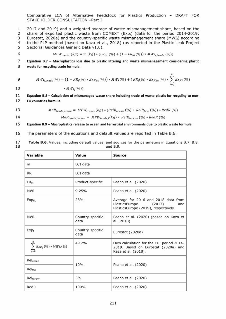
Comparative LCA of Alternative Feedstock for Plastics Production – DRAFT FOR STAKEHOLDER CONSULTATION –Part I
211
2017 and 2019) and a weighted average of waste mismanagement share, based on the 1 share of exported plastic waste from COMEXT (Expj) (data for the period 2014-2019; 2 Eurostat, 2020a) and the country-specific waste mismanagement share (MWIj) according 3 to the PLP method (based on Kaza et al., 2018) (as reported in the Plastic Leak Project 4 Sectorial Guidances Generic Data v1.0). 5
𝑀𝑃𝑊 , (𝑘𝑔) = 𝑚 (𝑘𝑔) ∗ (𝐿𝑅 (%) + (1 − 𝐿𝑅 (%)) ∗ 𝑀𝑊𝐼 , (%)) 6
Equation B.7 – Macroplastics loss due to plastic littering and waste mismanagement considering plastic 7 waste for recycling trade formula. 8
𝑀𝑊𝐼 , (%) = 1 − 𝑅𝑅 (%) ∗ 𝐸𝑥𝑝 (%) ∗ 𝑀𝑊𝐼(%) + ( 𝑅𝑅 (%) ∗ 𝐸𝑥𝑝 (%) ∗ 𝐸𝑥𝑝 (%)9
∗ 𝑀𝑊𝐼 (%)) 10
Equation B.8 – Calculation of mismanaged waste share including trade of waste plastic for recycling to non-11 EU countries formula. 12
𝑀𝑎𝑅 , = 𝑀𝑃𝑊 , (𝑘𝑔) ∗ (𝑅𝑒𝑙𝑅 (%) + 𝑅𝑒𝑙𝑅 (%)) ∗ 𝑅𝑒𝑑𝑅 (%) 13
𝑀𝑎𝑅 , = 𝑀𝑃𝑊 , (𝑘𝑔) ∗ 𝑅𝑒𝑙𝑅 (%) ∗ 𝑅𝑒𝑑𝑅 (%) 14
Equation B.9 – Macroplastics release to ocean and terrestrial environments due to plastic waste formula. 15
The parameters of the equations and default values are reported in Table B.6. 16
Table B.6. Values, including default values, and sources for the parameters in Equations B.7, B.8 17 and B.9. 18
Variable Value Source
m LCI data
RRi LCI data
LRlit Product-specific Peano et al. (2020)
MWI 9.25% Peano et al. (2020)
ExpEU 28% Average for 2016 and 2018 data from PlasticsEurope (2017) and PlasticsEurope (2019), respectively.
MWIj Country-specific data
Peano et al. (2020) (based on Kaza et al., 2018)
Expj Country-specific data
Eurostat (2020a)
𝐸𝑥𝑝 (%) ∗ 𝑀𝑊𝐼 (%)
49.2% Own calculation for the EU, period 2014-2019. Based on Eurostat (2020a) and Kaza et al. (2018).
Relocean 10% Peano et al. (2020)
Relfrw
Relterenv 5% Peano et al. (2020)
RedR 100% Peano et al. (2020)

Comparative LCA of Alternative Feedstock for Plastics Production – DRAFT FOR STAKEHOLDER CONSULTATION –Part I
212
The proposed estimation of the potential additional waste mismanagement associated to 1 plastic waste collected for recycling in the EU that has been exported into non-EU 2 countries has two main sources of uncertainty. Firstly, COMEXT data indicate the 3 destination country for the trade event (i.e. export) between EU and non-EU countries, 4 but further trade events that can occur are not tracked (e.g. EU exports to China, latter 5 exported to Vietnam). As a result, the estimation considers the characteristics of the 6 waste management system of the first destination country (i.e. waste mismanagement 7 share) and might overlook differences with the waste management system of the 8 ultimate destination. Secondly, the estimation considers the pressure put on the waste 9 management system of the countries importing plastic waste for recycling from the EU, 10 while the plastic waste originated in the EU might be properly recycled, other domestic 11 plastic waste might be emitted due to pressure on the system. Therefore, while the 12 additional waste mismanagement due to trade might not occur in the plastic waste 13 stream of the EU product, the estimation follows a precautionary principle in order to 14 consider the overall effects of current practices and the worst-case scenario. 15
Microplastics loss and release due to road marking 16
According to Boucher & Friot (2017), there is a release of plastic from the erosion of road 17 markings associated to road transportation. The mass of microplastics from the erosion 18 of road markings that is lost to the environment (MRMl) can be calculated based on the 19 road transport by vehicle type (mt,i), the road required per functional unit by vehicle type 20 (ri), the content of plastic of the road marking (rmr) and the estimated loss rate of road 21 marking to the environment (LRrm). 22
𝑀𝑅𝑀 (𝑘𝑔) = 𝑚 , (𝑡𝑘𝑚) ∗ 𝑟 𝑚 · 𝑦
𝑡𝑘𝑚∗ 𝑟𝑚
𝑘𝑔
𝑚 · 𝑦∗ 𝐿𝑅 (%) 23
Equation B.10 – Microplastics loss due to road markings formula. 24
As reported in Boucher & Friot (2017), microplastics emission from road markings may 25 behave similar to microplastics from tyre abrasion. In this sense, the release and 26 redistribution of plastic loss to the environment have been modelled as in the PLP 27 method for tire abrasion (Peano et al., 2020). 28
𝑀𝑖𝑅 , = 𝑀𝑅𝑀 (𝑘𝑔) ∗ 𝑅𝑒𝑙𝑅 (%) ∗ 𝑅𝑒𝑑𝑅 (%) 29
𝑀𝑖𝑅 , = 𝑀𝑅𝑀 (𝑘𝑔) ∗ 𝑅𝑒𝑙𝑅 (%) ∗ 𝑅𝑒𝑑𝑅 (%) 30
Equation B.11 – Microplastics release to ocean due to marine coatings formula. 31
While the transported mass depends on the LCI of the system under assessment, the 32 other parameters can use the following default values (Table B.7). 33
34

Comparative LCA of Alternative Feedstock for Plastics Production – DRAFT FOR STAKEHOLDER CONSULTATION –Part I
213
Table B.7. Default values for the parameters in Equations B.10 and B.11. 1
Variable Value Source
mt,i LCI data, by vehicle type
ri
Passenger car
6.966·10-4
m·y·km-1
“transport, passenger car, small size, petrol, EURO 5” dataset of ecoinvent 3.5 (Wernet et al., 2016)
Lorry
>32t
1.09·10-2
m·y·tkm-1
“transport, freight, lorry >32 metric ton, EURO5” dataset of ecoinvent 3.5 (Wernet et al., 2016)
Lorry
16-32t
1.05·10-2
m·y·tkm-1
“transport, freight, lorry 16-32 metric ton, EURO5” dataset of ecoinvent 3.5 (Wernet et al., 2016)
Lorry
3.5-7.5
1.95·10-2
m·y·tkm-1
“transport, freight, lorry 3.5-7.5 metric ton, EURO5” dataset of ecoinvent 3.5 (Wernet et al., 2016)
Light commercial vehicle
1.8499·10-3
m·y·tkm-1
“transport, freight, light commercial vehicle, unregulated” dataset of ecoinvent 3.5 (Wernet et al., 2016)
rmr 0.0513 kg·my-1 Cruz et al. (2016)
Lr 43% Lassen et al. (2015) (central scenario)
RelRocean 2% Peano et al. (2020)
RelRfrw
Relterenv 84% Peano et al. (2020)
RedR 100% Peano et al. (2020)
2
Microplastics loss and release due to marine coatings 3
According to Boucher & Friot (2017), there is a release of plastic from the erosion of 4 marine coatings during maritime transportation. The mass of microplastics from the 5 erosion of marine coatings that is lost to the environment (MMPl) can be calculated based 6 on the overall maritime transport (Tm), the content of plastic of the marine coating (mmc), 7 the share of plastic of the marine coating (pmc) and the loss rate of the marine coating 8 (LRmc). 9
𝑀𝑀𝐶 (𝑘𝑔) = 𝑇 (𝑘𝑔 · 𝑘𝑚) ∗ 𝑚 𝑘𝑔
𝑘𝑔 · 𝑘𝑚∗ 𝑝 (%) ∗ 𝐿𝑅 (%) 10
Equation B.12 – Microplastics loss to environment due to marine coatings formula. 11
Since the loss of microplastics from marine coating takes place in the ocean, the release 12 and redistribution among environmental compartments are considered as a final release 13 (FinalRelocean) as 100%. No release to terrestrial environment is considered. 14
𝑀𝑖𝑅 , = 𝑀𝑀𝐶 (𝑘𝑔) ∗ 𝐹𝑖𝑛𝑎𝑙𝑅𝑒𝑙𝑅 (%) 15
Equation B.13 – Microplastics release to ocean due to marine coatings formula. 16
17

Comparative LCA of Alternative Feedstock for Plastics Production – DRAFT FOR STAKEHOLDER CONSULTATION –Part I
214
The parameters of the equations and default values are reported inTable B.8. 1
Table B.8. Values, including default values, and sources for the parameters in Equations B.12 and 2 B.13. 3
Variable Value Source
Tm LCI data
mmc 7.34·10-10 kg·kgkm-1
Calculated based on “transport, freight, sea, container ship” dataset of ecoinvent 3.5 (Wernet et al., 2016)
pmc 48.82% Calculated based on “alkyd paint production, white, solvent-based, product in 60% solution state” dataset of ecoinvent 3.5 (Wernet et al., 2016)
LRmc 6% OECD (2009)
FinalRelocean 100% Boucher & Friot (2017)
4
Sensitivity of quantification of plastic loss along the supply-chain: plastic litter 5 emissions in the ecoinvent 3.5 database (GreenDelta) 6
Ciroth & Kouame (2019) proposed a framework to include plastic emissions into the 7 ecoinvent 3.5 database (Wernet et al., 2016). The framework is based on the probability 8 of each flow and process to take part in a littering event. Therefore, flows and processes 9 of ecoinvent 3.5 datasets are classified according to a risk for littering for each exchange, 10 i.e. for each flow in a process. Plastic litter is characterised only as “plastic parts, small”, 11 without specification of the plastic size, shape, emission compartment, neither plastic 12 type. The littering event probability is classified for each flow in six categories, from none 13 to very high (Table B.9). However, the littering event probabilities at the process level 14 consider also the type of system where the process is taking place (Table B.10). 15
Table B.9. Examples of littering event probabilities in closed and open system in the GreenDelta 16 framework (*System is closed but not for the use phase). 17
Class Probability Example
None 0 Electricity
Very low 0.000001 Diesel generator
Low 0.001 Waste paper, unsorted
Medium 0.1 Used laptop computer
High 0.5 Polystyrene scrap, post-consumer
Very high 0.95 Tire wear emissions, lorry
18
19

Comparative LCA of Alternative Feedstock for Plastics Production – DRAFT FOR STAKEHOLDER CONSULTATION –Part I
215
Table B.10. Examples of littering event probabilities in closed and open system in the GreenDelta 1 framework (*System is closed but not for the use phase). 2
Littering event probabilities, processes Closed system
(e.g. in airplane)
Open system
(e.g. streetfood)
Use Brushing teeth with toothpaste with microplastics
0.75* 1
Unforeseen disposal Selling coffee in a plastic cup 0.0001 0.1
Accidents Transport, passenger car, EURO 3
0.001 1
3
Once flows are characterized according to the littering probability, the risk for litter is 4 aggregated for each process, thereby yielding an emission of “plastic parts, small” for 5 each dataset (i.e. process). Multiple data sources were considered for defining the 6 littering probabilities (Astrup et al., 2009; Cole & Sherrington, 2016; Essel et al., 2015; 7 Geyer et al., 2017; Jambeck et al., 2015; Magnusson et al., 2016; Lassen et al., 2015; 8 Ryberg et al., 2019; Sundt et al., 2014). This framework was applied by GreenDelta to 9 all processes of ecoinvent cut-off 3.5 database83 and was developed using the openLCA 10 open source LCA software84. 11
Calculating the overall plastic loss of the supply-chain of a given product (PLp) is 12 performed as the sum of the product between the amount of a given process in the life 13 cycle inventory of the product (Proci) and the plastic loss factor of the process (PLi). 14
𝑃𝐿 (𝑘𝑔 𝑠𝑚𝑎𝑙𝑙 𝑝𝑙𝑎𝑠𝑡𝑖𝑐 𝑝𝑎𝑟𝑡𝑠) = 𝑃𝑟𝑜𝑐 (𝑢𝑛𝑖𝑡) ∗ 𝑃𝐿 (𝑘𝑔 𝑠𝑚𝑎𝑙𝑙 𝑝𝑙𝑎𝑠𝑡𝑖𝑐 𝑝𝑎𝑟𝑡𝑠
𝑢𝑛𝑖𝑡) 15
Equation B.14 – Quantification of plastic loss with the GreenDelta framework formula. 16
The GreenDelta framework only quantifies the plastic loss at the inventory level without 17 considering the emission to a specific compartment, the release to the compartment and 18 potential transfer among compartments and to the technosphere, neither the fate of the 19 plastic once in the environment (e.g. degradability, fragmentation) (Figure). In this 20 sense, the results of this approach can be used as sensitivity for the obtained values of 21 plastic loss from first (PLP method) and second levels (extended PLP method) of the 22 framework. 23
Sensitivity: estimate of macroplastics release to ocean through marine litter 24 rates 25
Data availability on the presence of plastic in the marine environment to understand the 26 presence and dynamics of plastic litter are still scarce. However, one of the marine 27 ecosystems that have been more analysed regarding the presence of litter are beaches. 28 JRC researchers have created a database of beach litter by employing and harmonizing 29 data collected by Member States for the period 2012-2016 (Addamo et al., 2018; Hanke 30 et al., 2019). The observed beach litter can be employed to estimate how much litter of 31 that product is present in the marine environment. 32
The estimation of a marine litter rate (MRL, %) that relates how much of a consumed 33 product can be found in the marine environment as litter would allow to estimate the 34 potential generation of marine litter. To do so, the following steps are necessary: 35
83 https://nexus.openlca.org/database/ecoinvent 84 http://www.openlca.org/

Comparative LCA of Alternative Feedstock for Plastics Production – DRAFT FOR STAKEHOLDER CONSULTATION –Part I
216
1) Calculating the average presence of a given product (e.g. plastic bottle) in the 1 observations: for each year of data collection, the presence of the product is 2 calculated by employing the average observed litter of a given product, 3 transforming the value reported in the database from 100m to 1km, and upscale 4 the average presence to the entire length of coast of the EU Member States 5
2) Reporting the consumed amount of a given product from the Prodcom database of 6 Eurostat (Eurostat, 2020b) 7
3) Calculating the average marine litter for the period 2012-2016 8 4) Applying an upscale factor to allow transforming the beach litter presence into a 9
marine litter presence. This upscale factor is based on the work of Eunomia 10 (2016), where the authors estimated that only 5% of the marine litter is found in 11 the beach. Therefore, an upscale factor of 20 is estimated. 12
𝑀𝑎𝑟𝑖𝑛𝑒 𝑙𝑖𝑡𝑡𝑒𝑟 𝑟𝑎𝑡𝑒 (𝑀𝑅𝐿) (%) =𝑃𝑟𝑒𝑑𝑖𝑐𝑡𝑒𝑑 𝑜𝑏𝑠𝑒𝑟𝑣𝑒𝑑 𝑙𝑖𝑡𝑡𝑒𝑟 (𝑢𝑛𝑖𝑡𝑠)
𝐸𝑈 𝑐𝑜𝑛𝑠𝑢𝑚𝑝𝑡𝑖𝑜𝑛 (𝑢𝑛𝑖𝑡𝑠)13
=(∑ 𝐴𝑣𝑒𝑟𝑎𝑔𝑒 𝑜𝑏𝑠𝑒𝑟𝑣𝑒𝑑 𝑙𝑖𝑡𝑡𝑒𝑟𝑒𝑑 ,
𝑢𝑛𝑖𝑡𝑠100𝑚
𝑥 10 100𝑚1𝑘𝑚
𝑥 𝐶𝑜𝑎𝑠𝑡 𝑙𝑒𝑛𝑔𝑡ℎ (𝑘𝑚)) 𝑥 𝑈𝑝𝑠𝐹
𝐸𝑈 𝑐𝑜𝑛𝑠𝑢𝑚𝑝𝑡𝑖𝑜𝑛 (𝑢𝑛𝑖𝑡𝑠) 14
Equation B.15 – Estimation of product-specific marine litter rates formula. 15
The estimation of the release of macroplastics to the marine environment at the End of 16 Life a product is calculated based on the mass of the product (m) and the product-17 specific marine litter rates (MRL). 18
𝑀𝑎𝑅 (𝑘𝑔) = 𝑀𝑅𝐿 (%) ∗ 𝑚 (𝑘𝑔) 19
Equation B.16 – Estimation of product-specific marine litter rates formula. 20
The parameters of the equations and default values are reported in Table B.11. 21
Table B.11. Values, including default values, and sources for the parameters in Equations B.15 22 and B.16. 23
Variable Value Source
mi LCI data
Average observed litteredi,j Product-specific Beach litter database (Addamo et al., 2018; Hanke et al., 2019)
Coast lengthEU 148,924.6 km WRI (2000)
UpsF 20 Eunomia (2016)
24

Comparative LCA of Alternative Feedstock for Plastics Production – DRAFT FOR STAKEHOLDER CONSULTATION –Part I
217
Annex C: List of default values for CFF parameters (A, R1, R2, R3 and Qs/Qp) 1
The list of default values for A, R1 and R2 is periodically reviewed and updated by the 2 European Commission. Users of this method are invited to check and use the most 3 updated values available at: 4
https://eplca.jrc.ec.europa.eu/LCDN/developerEF.xhtml 5
6
7

Comparative LCA of Alternative Feedstock for Plastics Production – DRAFT FOR STAKEHOLDER CONSULTATION –Part I
218
Annex D: Background information to calculate R2 for packaging materials 1
Table D.1 below presents per packaging sector (i) the data source to calculate R2, (ii) 2 where in the collection-recycling scheme these data are collected (see Figure 13 in 3 section 4.4.13.12.9) and (iii) the applied correction factor towards the output of the 4 recycling process. 5
Table D.1. Recycling rates for different packaging categories, including the source, the data 6 collection point and the recommended correction factor. Please note that the data sources used for 7
the correction factor are not always reviewed reports but may also be surveys or standards. 8
Packaging sector
Data source
Reference year
Data collection point (Figure 15)
Correction factor (1)
Source for correction factor
Liquid beverage carton (2)
ACE 2014 8 Liquid packaging board: 92%
Aluminium foil: 97%
Plastic: 72%
No data source: The correction factors of paper and cardboard, aluminium cans, and generic plastics are recommended as proxy.
Aluminium cans
EA, + bottom ashes (3)
2013 6† 97% Reviewed LCA: http://european-aluminium.eu/media/1329/environmental-profile-report-for-the-european-aluminium-industry.pdf (p58); Boin and Bertram 2005, Melting Standardized Aluminum Scrap: A Mass Balance Model for Europe.
PET bottle PETCORE 2014 2 73% Survey: Post-consumer PET recycling in Europe 2014 and prospects to 2019. Prepared on behalf of PETCORE Europe by PCI Ltd. 2015. http://www.pcipetpackaging.co.uk/
Container glass
FEVE 2013 8 90% Reviewed LCA: Life Cycle Assessment of Container Glass in Europe (Prepared on behalf of FEVE by RDC Environment), 2016. http://feve.org/new-life-cycle-assessment-proves-industry-success-reducing-environmental-footprint/
Steel for packaging
APEAL, + bottom ashes (3)
2013 6 (4) 98% Standard: Canadian standards’ Life cycle assessment of auto parts. http://shop.csa.ca/en/canada/life-cycle-assessment/spe-14040-

Comparative LCA of Alternative Feedstock for Plastics Production – DRAFT FOR STAKEHOLDER CONSULTATION –Part I
219
Packaging sector
Data source
Reference year
Data collection point (Figure 15)
Correction factor (1)
Source for correction factor
14/invt/27036702014
Generic plastic packaging
PlasticsEurope
2014 8 73% LCA report: Increased EU Plastics Recycling Targets: Environmental, Economic and Social Impact Assessment. Prepared by Deloitte on behalf of Plastic Recyclers Europe. 2015 (See Table 7, value of 2012).
Paper and cardboard
CEPI 2014 8 92% Reviewed LCA: European Database for Corrugated Board Life Cycle Studies” (2015, FEFCO, CE Containerboard)
(1) Expressed as percentage of material (%) at the output of the recycling plant when considering a 100% 1 input at data collection point. The proposed correction factors are sector specific and to be used for 2 correcting the European average and country specific recycling rates. It is recognized that this is an over 3 simplification as the correction depends on the installations and market in place. However, the data 4 available today asks for this simplification. Some values are rounded. 5
(2) For liquid beverage carton three different material flows leave the recycling process at level Š. Therefore, 6 three correction factors are introduced, each to be used with the respective material flow. 7
(3) The recycling rates for aluminium cans and steel for packaging include bottom ash recovery. 8 (4) R2 provided by the national collection systems excludes impurities from the overall mass estimate of metal 9
packaging. Impurities are excluded from the correction factor. 10 11

Comparative LCA of Alternative Feedstock for Plastics Production – DRAFT FOR STAKEHOLDER CONSULTATION –Part I
220
Annex E: Method applicable to quantify the effects temporary carbon storage in 1 products and delayed carbon emissions in LCA of plastic articles 2
The method described in this Annex may be applied to quantify the effects of temporary 3 storage of biogenic carbon in plastic products and delayed carbon emissions on the 4 Climate Change impact indicator. If calculated, the results obtained by applying this 5 method shall only be included in the LCA study as additional environmental information, 6 and followed by the disclaimer reported in Section 4.4.15.4. 7
General considerations on accounting for time-dependent impacts in LCA 8
The issue of time-dependent impacts in LCA has been discussed for at least 10 years 9 (e.g. Levasseur, 2010; Cherubini, 2011; Brandao, 2013; Levasseur, 2016; UNEP-SETAC, 10 2016). This issue has emerged mainly related to impacts on Climate Change and when 11 strong time-dependent trajectories can be identified for the emission profiles. The 12 biogenic-C cycle for bio-based products (i.e. biogenic Carbon uptakes and releases) has 13 exactly these characteristics: the biomass is harvested and transformed into a bio-based 14 product, where the Carbon taken up during biomass growth is stored during the Use 15 stage and until it is not release back to the atmosphere at the End of Life. While carbon is 16 stored in the technosphere, the biomass re-grows taking up additional atmospheric CO2 17 through specific dynamic trajectories (i.e. annual crops will re-absorb harvested CO2 18 every year, while a forest stand might take more than 80 years) (E.1). 19
20
21
Figure E.1. Biogenic-C emission and uptake dynamics of 1 kg CO2. Two biomass growth curves are 22 represented with different rotation times (1 year = annual crop and 80 year = forest feedstock), 23
and emission of CO2 due to disposal through incineration after 20 years of use. 24
The treatment of these phenomena differs across various studies, based on the climate 25 metrics applied (instantaneous vs. cumulative) (Giuntoli et al., 2015), the choice of 26 absolute or normalized climate metrics (Cherubini et al., 2013), the choice of reference 27 system (Koponen et al., 2016), and the choice of temporal boundaries of the analysis 28 (Brandao, 2013; Levasseur, 2016; Breton, 2018). 29
The choice of the time horizon (TH) of the analysis is an especially important value 30 choice. A TH of 100 years is indeed always implicitly chosen when using the GWP(100) 31 characterization factors to calculate the potential Climate Change impact (as it is the case 32 of the present method). A TH basically provides a cut-off, so that any residual impact of 33 an emission after that time will be discounted to zero. This issue is not specific to the 34 assessment of bio-based plastics, although the consequences of the TH choice are more 35 pronounced in this case because of the emission-uptake delay. Breton et al. (2018) 36
-1.5
-1
-0.5
0
0.5
1
1.5
0 20 40 60 80 100 120 140
Biog
enic
-C e
mis
sion
s &
seq
uest
ratio
n (c
umul
ativ
e)
[kgC
O2]
Years after harvest at t = 0
Rotation 1 yr Rotation 80yr Emission - 20yr Sequestration
Emission
t rotation
t disposal
t harvest
t replanting

Comparative LCA of Alternative Feedstock for Plastics Production – DRAFT FOR STAKEHOLDER CONSULTATION –Part I
221
present a detailed analysis of time-dependent calculations in LCA; in synthesis, they 1 describe two possible approaches (Figure ): 1) fixed time horizon (sliding window), and 2 2) variable time horizon (fixed end-point). The common LCA approach, i.e. using 3 GWP(100) factors for any emission flow, implies a sliding window approach. This means 4 that the impact of any emission is evaluated for 100 years after it has occurred 5 (regardless of when this takes place over the product life cycle) and all emissions and 6 uptakes are ‘flattened’ as if they occurred at the same point in time (t = 0). This 7 assumption hides any dynamic trends and could lead to overlook important information if 8 the emission profiles under study have strong time-dependent trends. This is especially 9 important for bio-based commodities: while long-term impacts will not be affected by the 10 temporary dynamics of the biogenic-C cycles (which are much shorter than other 11 geological and climate cycles), short-term impacts can be unexpected and completely 12 ignored by traditional LCA approaches. For instance, Giuntoli et al. (2015) showed how 13 the use of stumps and other slow-decaying deadwood for bioenergy might actually be 14 worse than using fossil fuels at least until the end of the 21st century. 15
By considering a fixed end-point approach, instead, the impact of all emissions is 16 evaluated towards a fixed year (e.g. 2100) from the moment they occur over the product 17 life cycle, and are thus weighted differently depending on the year in which they take 18 place and the distance to the fixed evaluation time. However, the choice of the fixed end-19 point becomes a crucial value-choice, for instance informed by policy objectives / goal of 20 the analysis (e.g. decarbonisation by 2050). 21
It is important to notice that no approach is right or wrong, but rather any choice will 22 embed value judgement, and that is why the results of any calculation must be 23 accompanied by the disclaimer provided in section 4.4.15.4. 24
Fixed end-point approach 25
In this method, it characterization factors (GWP100) are set equal to 0 for biogenic-CO2 26 flows. This approach looks at the long-term climate impact, which is dominated by fossil-27 CO2 emissions and to which biogenic-C cycles are irrelevant. However, it is possible to 28 provide additional environmental information on the short-term climate impact of using 29 bio-based plastic products. Therefore, it is reasonable to adopt a fixed end-point 30 approach where the TH is fixed at 100 years from the time of harvest and production of 31 the bio-based commodity. 32
In practical terms, the method suggested is the one detailed in Guest et al. (2012) and 33 Cherubini et al. (2011). They apply the method described in part 2 of this Annex to 34 quantify the values of new characterization factors, GWPbio, for different trajectories of 35 biogenic CO2 emissions and uptakes from biomass derived from different types of sources 36 (i.e. forest/crop) and thus with different rotation periods. Their modelling considers a 37 time horizon (TH) for the evaluation of the effects of the CO2 emissions equal to 100 38 years, assuming that the harvest and replanting (and the product addressing the FU) 39 takes place at year 0. The characterization factors for the so-calculated GWPbio are 40 provided in Figure E.2 (taken from Guest et al., 2012). The GWPbio depends on the 41 storage time in the technosphere, and thus on the year of emission with respect to the 42 time of harvest (tdisposal), and on the rotation period of the biomass (trotation). 43
44

Comparative LCA of Alternative Feedstock for Plastics Production – DRAFT FOR STAKEHOLDER CONSULTATION –Part I
222
1
Figure E.2. GWPs dependent upon storage and rotation period (taken from Guest et al., 2012). 2
3
For annual crops (i.e. rotation time of one year), the results are very similar to the 4 approach suggested by Clift and Brandao (2008), which is then applied in a simplified 5 way in the standard PAS 2050:2008. 6
In order to avoid inconsistency (Breton et al., 2018; Levasseur et al., 2010) and in order 7 to have all GHG emissions weighted at the same TH (i.e. 100 years from the time of 8 harvest), also the impact of any other emission taking place after t = 0 should be equally 9 re-scaled. For the purpose of this method, this mainly concerns the emissions of the CO2 10 contained in the fossil-based plastic products considered as a reference, which shall be 11 consistently evaluated with regard to the chosen TH. An example is presented in Figure 12 E.3, where the three curves represent the Absolute GWP curves for a sample biogenic-C 13 cycle (annual crop, incinerated after 20 years), the alternative fossil-based product used 14 for comparison (with the same End of Life, incinerated after 20 years), and the AGWP for 15 a pulse emission of CO2 at year 0. All curves are normalized over 1 kg CO2. The grey 16 curve is used as denominator for the definition of all GWP factors in IPCC AR5 17 (henceforth called ‘IPCC AGWP’ curve). In a fixed end-point approach, thus, the red line 18 (‘delayed fossil emissions’) would have a lower GWP than 1. 19
20

Comparative LCA of Alternative Feedstock for Plastics Production – DRAFT FOR STAKEHOLDER CONSULTATION –Part I
223
1
Figure E.3. Curves representing the AGWP for a pulse emission of 1 kg CO2 at different time steps. 2 The blue curve represents a biogenic-C cycle where an annual crop is harvested at t = 0, fully 3 regrows at t = 1, while the harvested biogenic-C is stored in a product with a use phase of 20 4
years and incinerated at t = 20, thus fully releasing the CO2 contained. The red curve represents 5 the AGWP for a fossil plastic which is used for 20 years and incinerated. The grey line represents 6
the AGWP for a pulse emission of CO2 at t = 0. The latter curve is used by the IPCC as the 7 denominator for the definition of all GWP factors (see Eq. 6 in part 2 of this annex). 8
9
In practice: the AGWP curve of CO2 has an almost linear, monotonous, growth in time 10 due to the residual amount of CO2 left in the atmosphere after any pulse emission. Figure 11 can be used as a reference to calculate the GWP of delayed fossil CO2 emission when 12 considering a fixed end-point approach. 13
14
-5E-14
1E-28
5E-14
1E-13
1.5E-13
2E-13
2.5E-13
0 50 100 150 200 250 300
AGW
P CO
2[(
K *
yr)/
(W *
m2)
]
Time after harvest at t = 0
Absolute curves - AGWP CO2
Growth 1yr - Emission 20yr Fossil-Emission 20yr Normalization curve IPCC
Fixed end-point. 100 years from entry into market.
Shifting window. 100 years from disposal.

Comparative LCA of Alternative Feedstock for Plastics Production – DRAFT FOR STAKEHOLDER CONSULTATION –Part I
224
1
Figure E.4. GWP value for delayed fossil CO2 emissions when applying a fixed end-point method. 2 The time on the x-axis is interpreted as the time that the fossil CO2 spends in the atmosphere with 3
regard to the fixed end-point. 4
Concerning the calculations for biogenic CO2, further, it must be specified that the 5 calculations presented above provide a full account of the biogenic CO2 cycle and thus do 6 not subscribe to the ‘carbon neutrality’ assumption, which is applied in the remaining of 7 this method (i.e. where biogenic CO2 contribution to climate change is considered 0 both 8 for uptakes and emissions). Indeed, only the extremes in Table E.1 reflect this traditional 9 view: annual crops combusted in the first year have a GWPbio of 0 (i.e. absorption and 10 emissions are mutually cancelled out). However, biomass from rotations of 100 years 11 that is combusted at year 0 presents a positive value of GWPbio of 0.44. While the 12 biogenic-C from an annual crop stored for 100 years in the technosphere obtains a value 13 of -1 for the fixed end-point perspective (i.e. any effect after t =100 is discounted to 14 zero). As mentioned above, this alternative method indeed captures the dynamics of 15 short-term climate effects (e.g. 100 years) where the cycle of biogenic-C can have a 16 temporary impact. On the other hand, for changes in which the amount of C stored in the 17 biosphere is changed for the long term (e.g. Land Use Change or BECCS) the emissions 18 are fully accounted within the method. 19
Section 2 of this Annex provides additional insights into the maths applied. For additional 20 details, please refer to Guest et al. (2012), Cherubini et al. (2011), Giuntoli et al. (2015), 21 and Faraca et al. (2019). 22
Practical steps 23
To provide a practical example of calculation: the user of this method would need to 24 apply the CF in Figure E.4 which is closer to the conditions expected for the bio-based 25 plastic product being assessed. One kg of biogenic CO2 derived from annual crops 26 (rotation period of 1 year) and stored in the technosphere (product) for 20 years will be 27 assigned a GWP equal to -0.15 kg CO2-eq. kg CO2 (instead of zero, as recommended in 28 section 4.4.15.4 of this method). For delayed CO2 emissions from fossil-based products, 29 the most suitable CF from Table E.1 should be applied. One kg of fossil CO2 contained in 30 the compared fossil-based plastic product with the same EoL, and thus also emitted at t 31 = 20 years, will contribute to atmospheric radiative forcing for only 80 years, with 32 respect to the fixed end-point 100 years) and will thus be assigned a GWP equal to 0.84 33 kg CO2-eq. kg CO2 (instead of 1.0 as recommended in this method). To be noticed that 34
0.00.10.20.30.40.50.60.70.80.91.0
0 5 10 15 20 25 30 35 40 45 50 55 60 65 70 75 80 85 90 95100
GW
P -F
ossi
l CO
2
Years of CO2 in the atmosphere (100 - tdisposal)

Comparative LCA of Alternative Feedstock for Plastics Production – DRAFT FOR STAKEHOLDER CONSULTATION –Part I
225
there is a significant difference between the negative GWP value for biogenic-C and the 1 reduced positive value for fossil-CO2. While the first represents a credit for temporary 2 storage (biogenic C) while the biomass is allowed to regrow, the other is a credit for 3 delayed emission. Therefore, even though the magnitude of both credits is equal in this 4 example, the meaning of these values for the climate impact is very different: the GWPbio 5 has a negative sign meaning a net mitigation by actively taking up carbon from the 6 atmosphere, the GWP of fossil-C maintains its positive sign, indicating a reduced climate 7 impact with respect to the chosen TH (i.e. acting as a cut-off of impact). 8
Table E.1. A selection of GWPs time-dependent; GWP 20y, GWP 100y, and GWP 500y. 9
time (yr) index (i) GWP 20 GWP 100 GWP 500
0 1 1 1 1
1 2 0.958336282 0.992206555 0.9984755
2 3 0.916252143 0.984394801 0.9969502
3 4 0.873722714 0.976564441 0.995424
4 5 0.830718738 0.968715173 0.9938969
5 6 0.787205477 0.960846683 0.9923689
6 7 0.743141344 0.952958652 0.99084
7 8 0.69847617 0.945050752 0.9893103
8 9 0.65314902 0.937122647 0.9877797
9 10 0.607085447 0.929173989 0.9862481
10 11 0.56019402 0.921204426 0.9847157
20 21 0 0.840273954 0.9693422
30 31 0.756785083 0.9538772
40 41 0.670187368 0.9383183
50 51 0.579763492 0.9226631
60 61 0.484575565 0.9069092
70 71 0.383382144 0.8910539
80 81 0.274402817 0.8750947
90 91 0.153718817 0.8590289
100 0 0.8428538
10
11

Comparative LCA of Alternative Feedstock for Plastics Production – DRAFT FOR STAKEHOLDER CONSULTATION –Part I
226
Additional background information: dynamic GHG accounting of fossil and 1 biogenic CO2 emission and uptakes 2
This Section provides additional insights into the maths applied to calculate the 3 characterisation factors presented in Figure E.1. For additional details, please refer to 4 Guest et al. (2012), Cherubini et al. (2011), Giuntoli et al. (2015), and Faraca et al. 5 (2019). 6
The behaviour of CO2 in the atmosphere is the same irrespectively of the origin of the 7 CO2 (biogenic or fossil), but the accounting depends on the carbon pools considered for 8 the C cycle model as explained in Cherubini et al. (2011). According to IPCC (2013), the 9 Bern carbon cycle 2.5CC (Forster et al., 2007) was used for the dynamic accounting of 10 fossil and biogenic CO2, as it considers the interaction of all compartments in the 11 ecosphere. In the case of fossil CO2 emissions, Eq. E.1 was used to calculate the IRF: 12
13
𝑓(𝑡) = 𝑦 (𝑡) = 𝐴 + 𝐴 𝑒( )
𝑛 = 1,2,3 𝐸𝑞. E. 1 14
15
where f(t) is the impulse response function (IRF) after the emission (i.e. the atmospheric 16 decay, IRF of CO2 fossil) and Ai and τi are coefficients; a0= 0.2173, a1= 0.224, a2= 17 0.2824, a3= 0.2763, t1= 394.4y, t2= 36.54y, t3= 4.304y. All data are from IPCC 18 (2013), Chapter 8, Appendix M. 19
In the case of biogenic CO2, Eq. E.2 was used to calculate the IRF (based on Guest et al., 20 2012, Cherubini et al., 2011, 2013, 2016a,b): 21
22
𝑓(𝑡) = 𝑦(𝑡) − 𝑔(𝑡)𝑦(𝑇𝐻 − 𝑡)𝑑𝑡 𝐸𝑞. 𝐸. 2 23
24
where f(t) (IRF of CO2 bio) is obtained by the convolution of the CO2 emissions y(t) 25 released at time t and the CO2 sequestered by the biomass regrowth g(t) in the period 26 from t to TH. The sequestration function g(t) depends on the rotation period of the 27 biomass species in question, as detailed in Cherubini et al. (2011). Conformingly with the 28 latter, biomass regrowth in the forest was modelled as a normal (Gaussian) distribution 29 (Eq. E.3). In the case of annual crops, the rotation period equals 1 year and the maths is 30 accordingly simplified. 31
32
𝑔(𝑡) =1
√2𝜋𝜎𝑒 ( ) / 𝐸𝑞. 𝐸. 3 33
The parameters µ and σ represent the mean and variance, respectively, and indicate the 34 characteristics of the biomass growth. The mean is taken equal to half of the rotation 35 period (r), following the assumption that the mean occurs when the uptake of C is 36 maximum (µ=r/2). The variance determines the width of the distribution; in this case it 37 is assumed σ=µ/2. As the utilisation of a product, e.g. for insulation, or its subsequent 38 recycling incurs preserving the material properties (hence the C content) for a certain 39 period, the storage of biogenic carbon in the anthroposphere can be included in the IRF 40 of CO2 bio as suggested by Guest et al. (2012). Conformingly, Eq. E.4 was used to 41 correct the IRF including storage (i.e. delayed emissions): 42
𝑓(𝑡) =𝑓1(𝑡) = ∫ 𝑔(𝑡) 𝑦(𝑇𝐻 − 𝑡)𝑑𝑡 , 0 ≤ 𝑡 < τ
𝑓2(𝑡) = 𝑦(𝑇𝐻 − 𝑡) − ∫ 𝑔(𝑡) 𝑦(𝑇𝐻 − 𝑡)𝑑𝑡 , 𝑡 ≥ 𝜏 Eq.E. 4 43
44
where τ is the time period during which the product addressing the FU is maintained 45 within the anthroposphere, i.e. the time at which the product can no longer be used 46

Comparative LCA of Alternative Feedstock for Plastics Production – DRAFT FOR STAKEHOLDER CONSULTATION –Part I
227
and/or recycled and is incinerated; this depends on the lifetime of the product and its 1 waste management. 2
The IRFs of CO2 (Eq. 1-4) are then multiplied by the emission quantity at each year i of 3 the system (Bi) and summed up to a total curve (F(t)) of the atmospheric behaviour of 4 CO2 released by the system under assessment (Eq. E.5): 5
6
𝐹(𝑡) = 𝐵 𝑓 (𝑡) 𝑛 = 0, 1, 2, … , 𝑇𝐻 𝐸𝑞. 𝐸. 5 7
8
The dynamic GWP, over a given time horizon TH, can then be calculated as the ratio 9 between the integral of F(t) over TH and the integral of the CO2 unit pulse over TH (Eq. 10 E.6): 11
12
𝐺𝑊𝑃 = 𝑑𝐶𝐹 = ∫ ∝ 𝐹(𝑡)𝑑𝑡
𝐶 ∫ ∝ 𝑦(𝑡)𝑑𝑡 𝐸𝑞. 𝐸. 6 13
14
where α is the radiative efficiency of CO2 and C0 is the unit pulse emission. The radiative 15 efficiency α according to Forster et al. (2007) equals (Eq. E.7): 16
17
𝛼 = 5.35 ln[𝐶𝑂∗]
[𝐶𝑂 ] 𝐸𝑞. 𝐸. 7 18
19
Where [CO2*] is the concentration in the atmosphere after small perturbation and [CO2] 20 is the initial concentration of CO2 in the atmosphere. According to IPCC (2013), [CO2*] is 21 set at 391 ppm. By applying a perturbation of 1 ppm (for [CO2]), the radiative efficiency 22 equals 1.37*10-5 Wm-2ppb-1. 23
24
25

Comparative LCA of Alternative Feedstock for Plastics Production – DRAFT FOR STAKEHOLDER CONSULTATION –Part I
228
Annex F: Alternative method applicable to quantify iLUC GHG emissions in LCA 1 of plastic articles 2
The following model may be applied in addition to the factors from the EU 2015/1513 3 Directive (as reported in Section 4.4.16.4) to calculate the iLUC contribution to GHG 4 emissions from the life cycle of (bio-based) plastic products. Results obtained by applying 5 this alternative model may only be presented as additional environmental information, 6 and should not replace those obtained by applying the abovementioned factors. 7
General information on the model 8
The model proposed by Schmidt et al. (2015) belongs to the category of CDMs and 9 differs from EEMs for a number of aspects (see section 4.4.17.2), mainly: I) no 10 amortisation of the GHG emissions from deforestation is performed as a time-dynamic 11 approach is instead applied. II) A full elasticity of the supply is considered, i.e. the 12 demand for one unit product will in the long-term lead to supply of one more unit 13 product, without incurring reduction in the consumption (Weidema, 2003). This is valid 14 under a competitive unconstrained market where long-term market prices are 15 determined by the long-term marginal production costs. In the iLUC model, this 16 assumption implies that a marginal change in demand for land does not have any long-17 term effects on prices of land-based products. According with Schmidt et al. (2015), this 18 is confirmed by the food commodity prices that over the period 1961-2014 have not 19 increased relative to the general consumer index, while recent short-time price peaks for 20 food products can largely be explained by changes in fuel prices and speculation. III) The 21 market for land is considered to be global; five specific land markets are considered. 22
Markets for land considered in the model 23
In Schmidt et al. (2015), the land is considered as “capacity for biomass production”, i.e. 24 a capital input. Regional differences in land productivity are handled using the net 25 primary production NPPo figures from Haberl et al., (2007). The relative productivity of a 26 specific region is calculated as its NPPo divided by the world average NPPo (6110 kg C ha-27 1y-1; Haberl et al., 2007). This means that, while the iLUC factor expressed per hectare 28 for lands with different productivity will be the same (see earlier), the iLUC factor 29 expressed per unit of crop grown on these lands will differ according with their relative 30 productivity. The model from Schmidt et al. (2015) considers five different global 31 markets for land, representing all land types in the world: i) arable land (fit for annual 32 and perennial crops, intensive/extensive forestry, and pasture); ii) intensive forest land 33 (fit for intensive/extensive forestry and pasture, but not for cropping), iii) extensive 34 forest land (not fit for intensive because too hilly, remote, uneconomic, unfertile, etc.), 35 iv) grassland (fit for pasture, not for cropping and forest being too dry), v) barren land 36 (not fit for biomass production). Each market can be supplied with different inputs of land 37 already in use, intensification, and transformation. The inputs to the individual markets 38 (e.g. to 1 ha of arable land) are quantified based on historical patterns. This also applies 39 for the ratio between the share of land provided through intensification of current 40 production and that provided through expansion on forestland (deforestation). Refer to 41 Figure F.1 and Schmidt et al. (2015) for more details. 42

Comparative LCA of Alternative Feedstock for Plastics Production – DRAFT FOR STAKEHOLDER CONSULTATION –Part I
229
1
Figure F.1. Markets for land. Taken from Schmidt et al. (2015). 2
Handling of carbon emissions from deforestation (dynamic accounting) 3
Schmidt et al. (2015) models the actual acceleration of deforestation and related CO2 4 emissions, and therefore does not need to apply an arbitrary amortisation period (e.g. 20 5 years). If only expansion is considered, occupation of 1 ha in 1-year will cause 1 ha 6 deforestation. After the 1-year occupation, the land is released back to the market for 7 land, i.e. to other crops, which can then be grown without deforestation (Figure F.2). 8 From a modelling perspective, this equals considering deforestation at time t1 and an 9 avoided deforestation at t2, i.e. speeding up clearing of that hectare by one year. This 10 time-shifted deforestation is valid under the assumption of a general net deforestation 11 trend (and net expansion of managed lands). If this stops, the modelling should be 12 changed as a delayed relaxation of natural areas. Note that this approach was also 13 proposed in Kloverpris and Mueller (2013). Knowing the amount of stock cleared (above 14 plus below ground and eventual soil organic carbon loss), the Global Warming Potential 15 of bringing land clearing one year forward can be calculated applying the Bern Carbon 16 Cycle and the formula for GWP from (Forster et al., 2007). Accordingly, the GWP (over 17 100y period) of clearing 1 ha of land at year i-1 (instead of i) equals 0.992 kg CO2-eq. 18 kg-1 CO2; in other words, the increased warming effect of speeding up by one year equals 19 1-0.992=0.0076 kg CO2-eq. 20
21
Figure F.2. Effect of LUC on the timing of deforestation CO2 emissions. From Schmidt et al. 22 (2015). 23

Comparative LCA of Alternative Feedstock for Plastics Production – DRAFT FOR STAKEHOLDER CONSULTATION –Part I
230
Steps needed to quantify the iLUC GHG contribution 1
To quantify the iLUC GHG emission associated to the demand for a certain quantity of 2 land (or, alternatively, the demand for a certain amount of biomass), the following steps 3 are to be followed: 4
Step 1: Identify the quantity of land occupation (in ha*year/t, based on crop 5 yield) 6
Step 2: Identify the location of the occupation (region, e.g. EU27). 7 Step 3: Derive the potential net primary production (NPP0) at this 8
location (in t C/ha/y; e.g. using maps provided in Haberl et al., 2007 or the 9 dataset in https://lca-net.com/clubs/iluc) 10
Step 4: Specify the potential use of the occupied land: (arable, intensive 11 forest, extensive forest, grassland, barren land) 12
Step 5: Quantify the productivity factor (Productivity Factor = NPP0/world 13 average NPP0); world average NPP0 (arable land) = 5.68 t C/ha*year 14
Step 6: Convert the actual occupied area (ha*year/t) to units of productivity 15 weighted hectare years (pw ha*year/t): pw ha*year/t = Land occupied 16 (ha*year/t) * Productivity Factor (pw ha*year/(ha*year)) 17
Step 7: Calculate the iLUC GHG contribution: iLUC GHG = productivity 18 weighted hectare years (pw ha*year/t) * iLUC factor (kg CO2/pw ha*year); the 19 iLUC factor should reflect the potential use of the occupied land (Step 4). 20
The iLUC factors (for arable land, intensive and extensive forest, grassland, barren) is 21 obtained as a combination of deforestation and intensification and are reported in the 22 original iLUC model by Schmidt et al. (2015). 23
24

Comparative LCA of Alternative Feedstock for Plastics Production – DRAFT FOR STAKEHOLDER CONSULTATION –Part I
231
Annex G: Example of rating criteria for semi-quantitative assessment of data quality 1
Table G.1. Example of rating criteria for the semi-quantitative assessment of data quality required for key Life Cycle Inventory datasets. 2 Process: dyeing process. 3
Quality level
Quality rating
Definition Time representativeness
Technological representativeness
Geographical representativeness
Parameter uncertainty (relative standard deviation as a % as semi- quantitative expert judgement. If otherwise a Monte Carlo simulation is used, this shall include parameter dependency and correlation in the analysis.)
Very good
1 Meets the criterion to a very high degree, without need for improvement.
2009-2012 Discontinuous with airflow dyeing machines
Central Europe mix
Very low uncertainty ( 10%)
Good 2 Meets the criterion to a high degree, with little significant need for improvement.
2006-2008 e.g. "Consumption mix in EU: 30% Semi-continuous, 50% exhaust dyeing and 20% Continuous dyeing"
EU 27 mix; UK, DE; IT; FR
Low uncertainty (10% to 20%]
Fair 3 Meets the criterion to an acceptable degree, but merits improvement.
1999-2005 e.g. "Production mix in EU: 35% Semi-continuous, 40% exhaust dyeing and 25% Continuous dyeing"
Scandinavian Europe; other EU-27 countries
Fair uncertainty (20% to 30%]

Comparative LCA of Alternative Feedstock for Plastics Production – DRAFT FOR STAKEHOLDER CONSULTATION –Part I
232
Quality level
Quality rating
Definition Time representativeness
Technological representativeness
Geographical representativeness
Parameter uncertainty (relative standard deviation as a % as semi- quantitative expert judgement. If otherwise a Monte Carlo simulation is used, this shall include parameter dependency and correlation in the analysis.)
Poor 4 Does not meet the criterion to a sufficient degree. Requires improvement.
1990-1999 e.g. "Exhaust dyeing" Middle east;
US; JP
High uncertainty (30% to
50%]
Very poor
5 Does not meet the criterion. Substantial improvement is necessary OR:
This criterion was not judged / reviewed or its quality could not be verified / is unknown.
Very poor or unknown completeness ( 50%)
<1990; Unknown Continuous dyeing; other; unknown
Other; Unknown
Very high uncertainty ( 50%)
1
2

Comparative LCA of Alternative Feedstock for Plastics Production – DRAFT FOR STAKEHOLDER CONSULTATION –Part I
233
Annex H: LCA report template 1
LCA Report 2
[Insert product name here] 3
4
Table of contents 5
Acronyms 6
[List in this section all the acronyms used in the study. Those already included in the latest 7 version of the guide shall be copied in their original form. The acronyms shall be provided 8 in alphabetical order.] 9
Definitions 10
[List in this section all the definitions that are relevant for the LCA study. Those already 11 included in the latest version of this method shall be copied in their original form. The 12 definitions shall be provided in alphabetical order.] 13
I.1 SUMMARY 14
[The summary shall include as a minimum the following elements: 15
• The goal and scope of the study, including relevant limitations and assumptions; 16 • A short description of the system boundary; 17 • Relevant statements about data quality, 18 • The main results of the LCIA: these shall be presented showing the results of all EF 19
impact categories (characterized, normalized, weighted); 20 • A description of what has been achieved by the study, any recommendation made 21
and conclusions drawn; 22
To the extent possible, the summary should be written with a non-technical audience in 23 mind and should not be longer than 3-4 pages.] 24
I.2. GENERAL 25
[The information below should ideally be placed on the front-page of the study: 26
• Name of the product (including a photo), 27 • Product identification (e.g. model number), 28 • Product classification (CPA) based on the latest CPA list version available, 29 • Company presentation (name, geographic location), 30 • Date of publication of the LCA study (the date shall be written in extended format, 31
e.g. 32
25 June 2015, to avoid confusion over the date format), 33 • Geographic validity of the LCA study (countries where the product is 34
consumed/sold), 35
• Compliance with the present method, 36
• Conformance to other documents, additional to the present method, 37

Comparative LCA of Alternative Feedstock for Plastics Production – DRAFT FOR STAKEHOLDER CONSULTATION –Part I
234
• Name and affiliation of the verifier(s)] 1
I.3. GOAL OF THE STUDY 2
[Mandatory reporting elements include, as a minimum: 3
• Intended application(s); 4 • Methodological limitations; 5 • Reasons for carrying out the study; 6 • Target audience; 7 • Commissioner of the study; 8 • Identification of the verifier] 9
I.4. SCOPE OF THE STUDY 10
[The scope of the study shall identify the analysed system in detail and address the overall 11 approach used to establish: i) functional unit and reference flow, ii) system boundary, iii) 12 list of EF impact categories, iv) additional information (environmental and technical) iv) 13 assumptions and limitations.] 14
I.4.1. Functional/declared unit and reference flow 15
[Provide the functional unit, defining the four aspects: 16
• The function(s)/service(s) provided: “what”; 17 • The extent of the function or service: “how much”; 18 • The expected level of quality: “how well”; 19 • The duration/life time of the product: “how long”; 20
Provide the declared unit, in case the functional unit cannot be defined (e.g. if the product 21
in scope is an intermediate product) Provide reference flow] 22
I.4.2. System boundary 23
[This section shall include as a minimum: 24
• All life-cycle stages that are part of the product system. In case the naming of the 25 default life cycle stages has changed, the user shall specify to which default life 26 cycle stage it corresponds. Document and justify if life cycle stages were split and/or 27 new ones were added. 28
• The main processes covered in each life cycle stage (details are in the LCI section 29 A.5). The co-products, by-products and waste streams of at least the foreground 30 system shall be clearly identified. 31
• The reason for and potential significance of any exclusion. 32 • A system boundary diagram with the processes that are included and those 33
excluded, highlight those activities which falls respectively under situation 1, 2, and 34 3 of the Data 35
Needs Matrix, and highlight where company-specific data are used.] 36

Comparative LCA of Alternative Feedstock for Plastics Production – DRAFT FOR STAKEHOLDER CONSULTATION –Part I
235
I4.3. Environmental Footprint impact categories 1
[Provide a table with the list of EF impact categories, units, and EF reference package used 2 (see http://eplca.jrc.ec.europa.eu/LCDN/developerEF.xhtml for further details). 3
For climate change, specify if the results of the three sub-indicators are reported separately 4 in the results section.] 5
I4.4 Additional information 6
[Describe any additional environmental information and additional technical information 7 included in the LCA study. Provide references and exact calculations rules adopted. 8
Explain if biodiversity is relevant/not relevant for the product in scope. 9
When the product in scope is an intermediate product, additional technical information shall 10 include: 11
(a) The biogenic carbon content at factory gate (physical content and allocated 12 content). 13
(b) Recycled content (R1). 14 (c) Results with application-specific A-values of the Circular Footprint Formula, if 15
relevant.] 16
I.4.5. Assumptions and limitations 17
[Describe all limitations and assumptions. Provide list of data gaps, if any, and the way in 18 which these gaps were filled. Provide list of proxy datasets used.] 19
I.5. LIFE CYCLE INVENTORY ANALYSIS 20
[This section shall describe the compilation of the Life Cycle Inventory (LCI) and include: 21
• Screening step, if performed, 22 • List and description of life cycle stages, 23 • Description of modelling choices, 24 • Description of allocation approaches applied, 25 • Description and documentation of data used and sources, 26 • Data quality requirements and rating] 27
I.5.1. Screening step [if applicable] 28
[Provide a description of the screening step, including relevant information regarding data 29 collection, data used (e.g. list of secondary data sets, activity data, direct elementary 30 flows), cut-off, and results of the life cycle impact assessment phase. 31
Document main findings and any refinement of the initial scope settings (if any).] 32
I.5.2. Modelling choices 33
[Describe all modelling choices for the applicable aspects listed below (more can be added, 34 when relevant): 35

Comparative LCA of Alternative Feedstock for Plastics Production – DRAFT FOR STAKEHOLDER CONSULTATION –Part I
236
• Agricultural production (LCA studies which have agricultural modelling in scope and 1 have tested the alternative approach described in section 4.4.2 of the present 2 method, shall report the results in an Annex of the LCA report); 3
• Transport and logistics: all data used shall be provided in the report (e.g. 4 transportation distance, payload, re-use rate for packaging, etc.). If default 5 scenarios were not used in the modelling, provide documentation of all specific data 6 used; 7
• Capital goods: if capital goods are included, the LCA report shall include a clear and 8 extensive explanation, reporting all assumptions made; 9
• Storage and retail; 10 • Use stage: Product dependent processes shall be included in the system boundary 11
of the LCA study. Product independent processes shall be excluded from the system 12 boundary and qualitative information may be provided, see section 4.4.12 of the 13 present method. Describe the approach taken to model the use stage (main function 14 approach or delta approach); 15
• End of life modelling, including values of parameters of the Circular Footprint 16 Formula (A, B, R1, R2, Qs/Qp, R3, LHV, XER,heat, XER,elec), list of processes and 17 datasets used (Ev, Erec, ErecEoL, E*v, Ed, EEr, ESE,heat, ESE,elec) with reference 18 to the method; 19
• Extended product lifetime; 20 • Electricity use; 21 • Sampling procedure (report if a sampling procedure was applied and indicate the 22
approach taken); 23 • Greenhouse gas emissions and removals (report if a simplified approach was not 24
used to model biogenic carbon flows); 25 • Offsets (if reported as additional environmental information).] 26
I.5.3. Handling multi-functional processes 27
[Describe the allocation rules used in the LCA study and how the modelling/calculations 28 were made. Provide the list of all allocation factors used for each process and the detailed 29 list of processes and datasets used, in case substitution is applied.] 30
I.5.4. Data collection 31
[This section shall include as a minimum: 32
• Description and documentation of all company-specific data collected: 33 o list of processes covered by company-specific data indicating to which life 34
cycle stage they belong; 35 o list of resource use and emissions (i.e. direct elementary flows); o list of 36
activity data used; 37 o link to detailed bill of materials and/or ingredients, including substance 38
names, units and quantities, including information on grades/ purities and 39 other 40
technically and/or environmentally relevant characterisation of these; 41 o company-specific data collection/estimation/calculation procedures; 42

Comparative LCA of Alternative Feedstock for Plastics Production – DRAFT FOR STAKEHOLDER CONSULTATION –Part I
237
• List of all secondary datasets used (process name, UUID, dataset source (node on 1 Life Cycle Data Network, data stock) and compliance with the EF reference 2 package); 3
• Modelling parameters; 4 • Cut-off applied, if any; 5
• Sources of published literature; 6 • Validation of data, including documentation; 7 • If a sensitivity analysis has been conducted, this shall be reported.] 8
I.5.5. Data quality requirements and rating 9
[Provide a table listing all processes and their situation according to the Data Needs Matrix 10 (DNM). 11
Provide the DQR of the LCA study.] 12
I.6. IMPACT ASSESSMENT RESULTS [CONFIDENTIAL, IF RELEVANT] 13
I.6.1. LCA results 14
[This section shall include as a minimum: 15
• Characterised results of all EF impact categories shall be calculated and reported as 16 absolute values in the LCA report. The sub-categories ‘climate change –fossil’, 17 ‘climate change – biogenic’ and ‘climate change - land use and land use change’, 18 shall be reported separately if they show a contribution of more than 5% each to 19 the total score of climate change); 20
• Normalised and weighted results as absolute values; 21 • Weighted results as single score; 22 • Results of the use stage for final products shall be reported separately.] 23
I.6.2. Additional information 24
[This section shall include: 25
• Results of the additional environmental information; 26 • Results of the additional technical information.] 27
I.7. INTERPRETING RESULTS 28
[This section shall include as a minimum: 29
• Assessment of the robustness of the LCA study; 30 • List of most relevant impact categories, life cycle stages, processes and elementary 31
flows (see tables below); 32 • Limitations and relationship of the LCA results relative to the defined goal and scope 33
of the LCA study, 34 • Conclusions, recommendations, limitations and improvement potentials)]. 35

Comparative LCA of Alternative Feedstock for Plastics Production – DRAFT FOR STAKEHOLDER CONSULTATION –Part I
238
Item At what level does
relevance need to be identified?
Threshold
Most relevant impact categories
Normalised and weighted
results
Impact categories cumulatively contributing at least 80% of the total environmental impact
Most relevant life cycle stages
For each most relevant impact category
All life cycle stages contributing cumulatively more than 80% to that impact category
Most relevant processes
For each most relevant impact category
All processes contributing cumulatively (along the entire life cycle) more than 80% to that impact category, considering absolute values.
Most relevant elementary flows
For each most relevant process
All elementary flows contributing cumulatively at least to 80% to the total impact for each most relevant processes.
If disaggregated data are available: for each most relevant process, all direct elementary flows contributing cumulatively at least to 80% to that impact category (caused by the direct elementary flows only)
1
Example: 2
Most relevant impact category
[%] Most relevant life cycle stages
[%] Most relevant processes
[%]
Most relevant elementary flows
[%]
IC 1 End of life Process 1 el. flow 1
el. flow 2
Process 2 el. flow 2
Raw material acquisition and p.p.
Process 4
el. flow 1

Comparative LCA of Alternative Feedstock for Plastics Production – DRAFT FOR STAKEHOLDER CONSULTATION –Part I
239
IC 2 Manufacturing Process 1 el. flow 2
el. flow 3
IC 3 Manufacturing Process 1 el. flow 2
el. flow 3
1
I.8. VALIDATION STATEMENT 2
[The validation statement is mandatory and shall always be provided as public annex of the 3 public LCA report. 4
The following elements and aspects shall be included in the validation statement, as a 5 minimum: 6
• title of the LCA study under verification/validation, together with the exact version 7 of the report to which the validation statement belongs; 8
• the commissioner of the LCA study; 9 • the user of the present method; 10 • the verifier(s) or, in the case of a verification team, the team members with the 11
identification of the lead verifier; 12 • absence of conflicts of interest of the verifier(s) with respect to concerned products 13
and for other relevant reasons, such as a dependent relationship to the 14 commissioner of the LCA study); 15
• a description of the objective of the verification/validation; 16 • a statement of the result of the verification/validation; 17 • any limitations of the verification/validation outcomes; 18 • date in which the validation statement has been issued; 19 • signature by the verifier(s).] 20
21
ANNEX I 22
[The Annex serves to document supporting elements to the main report which are of a 23 more technical nature. It could include: 24
• Bibliographic references; 25 • Detailed life cycle inventory analysis (optional if considered sensitive and 26
communicated separately in the confidential annex, see below) 27 • Detailed assessment of data quality: Provide i) Data Quality Rating per process in 28
accordance with the present Method and ii) Data Quality Rating for the newly 29 created EFcompliant datasets. In case information is confidential, it shall be included 30 in Annex II.] 31
32

Comparative LCA of Alternative Feedstock for Plastics Production – DRAFT FOR STAKEHOLDER CONSULTATION –Part I
240
ANNEX II – CONFIDENTIAL REPORT 1
[The Confidential annex is an optional chapter that shall contain all those data (including 2 raw data) and information that are confidential or proprietary and cannot be made 3 externally available.] 4
5
ANNEX III – EF COMPLIANT DATASET 6
[The aggregated EF-compliant dataset of the product in scope shall be made available to 7 the European Commission.] 8
9
10

Comparative LCA of Alternative Feedstock for Plastics Production – DRAFT FOR STAKEHOLDER CONSULTATION –Part I
241
Annex I: Discussion on the relevance of potential indirect effects from fossil-based 1 feedstock supply 2
A number of potential indirect effects are discussed in the literature in relation to fossil-3 based feedstock supply for transportation fuels (Unnasch et al., 2009). As already reported 4 in Section 3.2.3.2, such effects may include: 5
iLUC caused by agricultural expansion on afforested areas due to road construction 6 for accessing oil fields on previously occupied agricultural land; 7
Emissions and impacts linked to military operations required for the protection of 8 petroleum supply, as well as impacts linked to military conflicts to secure access to 9 oil resources (and possible need for reconstruction); 10
Effects potentially induced by possible changes in production and market availability 11 of refinery co-products due to a reduced fossil fuel demand to refineries when 12 alternative fuels are used, leading to a decreased crude oil consumption and 13 subsequent production of refinery output85. In the case of fossil-based polymers 14 being replaced by bio-based ones, such effects may be generated by a reduced 15 demand for naphtha rather than fuels; 16
Macro-economic effects due to changes in petroleum usage and price (also referred 17 to as rebound effect). 18
In addition to these, Malins et al. (2015) consider accidents, including oil spills and oil fires, 19 as potential indirect effects. However, these can be rather considered direct unintended 20 effects related to fossil-based feedstock supply, as better discussed below. 21
Assessing such indirect effects is challenging and may involve many uncertainties (Malins et 22 al. 2015). For example, it is not clear which portion of deforestation caused by road 23 expansion for oil field access is additional to what would have occurred anyway. Unnasch et 24 al. (2009) estimated this impact to be 0.6-1.0 g CO2 eq per MJ of fossil transport fuel 25 produced in Ecuador. However, taking into account the global share of petroleum supply 26 from Ecuador, the overall impact due to deforestation in such country would be less than 27 0.01 g CO2 eq per MJ of fuel supplied worldwide. According to Malins et al. (2015), when 28 around 20% of global oil production comes from nations with significant tropical forests, the 29 actual total carbon implication of road induced deforestation is almost certainly no more 30 than 0.1 g CO2 eq/MJ. In addition, it has to be noted that also biofuel supply can involve 31 similar effects, such as in Indonesia and Malaysia, where road infrastructure develops 32 around the growing palm oil industry, supporting further deforestation. 33
Estimating impacts from military protection of petroleum supply is challenging due to 34 incomplete public data on military operations that are actually conducted, and to 35 uncertainty on the share of operations that are attributable to the protection of petroleum 36 supply. In addition, there is no consensus on which extent guaranteeing oil supply might 37 have been a primary reason of conflicts (e.g. in Iraq). These emissions have also been 38 found to only have a relatively small effect on the overall lifecycle GHG emissions of 39 transport fossil fuels, even in the highest estimates (between 0 and 2 g CO2 eq/MJ; Malins 40 et al., 2015). It is thus reasonable and acceptable to ignore emissions and impacts from 41 military operations, whose classification as indirect effect is also not clear-cut (they do not 42 strictly belong to other product systems, and do not take place via market mechanisms). 43
Changes in the quantity and type of crude oil being refined due to displacement of fossil 44 fuels with alternatives could result in changes to the co-products generated by refineries 45 and to their availability on the market. This may in turn imply displacement of some of such 46 85 For instance, a reduced crude oil processing in refineries would lead to a reduced production and availability of
residual oil and petroleum coke, thereby increasing their price. This could in turn lead to a reduced consumption or to a more likely shift to other alternative fuels that can either be “dirtier” (e.g. coal) or “cleaner” (e.g. natural gas), with all the resulting environmental implications.

Comparative LCA of Alternative Feedstock for Plastics Production – DRAFT FOR STAKEHOLDER CONSULTATION –Part I
242
co-products with alternatives involving different impacts in terms of both production and 1 use (e.g. petroleum coke with natural gas, or fuel oil with coal). However, there is currently 2 no sound basis available to draw conclusions about whether induced changes in co-product 3 output of the refining sector is more likely to reduce or increase global impacts, or to 4 provide any strong estimate of the possible magnitude of such an impact variation. 5 According to Malins et al. (2015) the climate impact from changes in refinery co-products 6 can be in the order of ± 5 g CO2 eq/MJ of transport fossil fuel. 7
Market-mediated effects, or rebound effects, due to (marginal) changes in demand and 8 price of petroleum products, may have significant impacts on GHG emissions. However, 9 their quantification is greatly uncertain and challenging to model, since impacts may occur 10 anywhere in the global economy. Rebound effects are usually brought forward as an 11 obstacle to the success of environmental policies, especially for renewable energy sources: 12 the promotion of renewable energy sources creates a decrease in demand for fossil sources 13 which consequently drives a decrease in their price and a rebound in their use. Unnasch et 14 al. (2009) estimated that lower fossil fuel price due to lower demand can lead to an increase 15 in GHG emissions of 0.25 g CO2 eq/MJ, but Malins et al. (2015) conclude that it would not 16 be appropriate to account for price effects in life cycle impacts of petroleum due to high 17 uncertainties and challenges to assess these effects. 18
As for oil spills, data from the International Tanker Owners Pollution Federation (ITOPF) on 19 the quantities of accidental oil leakage from marine vessels can be used to estimate impacts 20 due to oil spills from marine vessels, although no information is available on the proportion 21 of such spills compared to overall oil leakage (e.g. from pipelines). The potential climate 22 change impact of accidents (including both oil spills and fires) were estimated to be less 23 than 0.01 g CO2 eq/MJ of fossil transport fuel by Malins et al. (2015). However, oil spills and 24 fires are not indirect effects, but rather direct effects from oil supply. As such, oil spills are 25 normally accounted for in lifecycle inventory datasets for oil supply, at least in terms of 26 increased oil requirement to compensate for losses in pipelines or vessels. Potential impacts 27 of oil leakage on ecosystems are instead typically not accounted, as not being captured 28 within traditional LCA impact categories. It has also to be noted that accidents can occur 29 also in biofuel chains, although their magnitude is likely smaller compared to oil chains. In 30 light of this, Malins et al. (2015) consider that it would be appropriate to exclude emissions 31 and impacts from accidents of both fossil-based and bio-based fuels. More in general, in can 32 be argued that damages caused by accidents in the petrochemical industry, e.g. oil spills, 33 are beyond the scope of state-of-the-art LCA, because it is a risk, while LCA studies typically 34 focus on normal production conditions, disregarding accidents and risks. 35
Table I.1 summaries the estimated climate change impact for the indirect and accident-36 related effects discussed above (based on Malins et al., 2015), and compares it to the 37 average impact of fossil transport fuels (as per Directive 2009/28/EC). According to this 38 comparison, the individual contribution of such effects is in most cases very low (i.e. less 39 than 1%), while in the case of petroleum supply protection and potential changes in refinery 40 co-products it can be higher (although never larger than 6%). 41
42

Comparative LCA of Alternative Feedstock for Plastics Production – DRAFT FOR STAKEHOLDER CONSULTATION –Part I
243
Table I.1.. Summary of the estimated climate change impact of (potential) indirect and accident-1 related effects associated with the supply of fossil transportation fuels, compared to the respective 2
average lifecycle impact (i.e. 83.8 g CO2 eq/MJ fuel -Directive 2009/28/EC). Estimates are based on 3 Malins et al. (2015). 4
Effect Estimated impact [g CO2 eq/MJ of transportation fuel]
Share of total lifecycle impact (%)
Road construction and resulting iLUC
0.01 - 0.1 0.012 % – 0.119 %
Protection of petroleum supply (military operations) 0 – 2 0 % – 2.387 %
Changes in refinery co-products ± 5 ± 5.967 %
Market-mediated effects 0.25 0.298 %
Accidents (oil spills and oil fires) 0.01 0.012 %
In addition to the effects reported above, damages to landscape due to oil extraction (e.g. 5 with oil sands or in the Niger delta) are sometimes reported as another type of indirect 6 effect that should be taken into account when dealing with fossil-based feedstock sources. 7 While certainly relevant, potential impacts on landscape cannot be classified as indirect 8 effects, but rather as an additional type of impact associated with oil extraction activities. In 9 this perspective, it must be noted that the portion of landscape impacts associated with land 10 occupation and land transformation burdens involved by such activities is indeed accounted 11 for in LCI datasets, at least as far as proper land occupation and transformation flows are 12 available and selected. On the other hand, aesthetic or ecosystem impacts due to changes 13 in or damages to landscape are typically not captured in LCA, due to the absence of specific 14 impact categories covering these issues. 15
16

Comparative LCA of Alternative Feedstock for Plastics Production – DRAFT FOR STAKEHOLDER CONSULTATION –Part I
244
Annex J: Modelling of crude oil supply in the LCA case studies accompanying this 1 method 2
3
Premises 4
For the production of fossil-based polymers, there is the need to define a dataset for 5 the supply of the crude oil mix to EU market. The dataset chosen in this project is 6 [EU-27] Crude oil mix; technology mix of conventional (primary, secondary and 7 tertiary production) and unconventional production (oil sands, in-situ), provided by 8 Thinkstep (henceforth ‘Thinkstep dataset’). 9
This dataset provides input to the petrochemical dataset also provided by Thinkstep. 10 The refining and polimer production are thus treated within the Thinkstep dataset. 11 Since polimer manufacturing only uses part of the products from crude oil refining, it 12 can’t be automatically assumed that the feedstock mix for plastics production is 13 proportional to the crude oil average mix. Nonetheless, we do not question 14 Thinkstep’s processes for allocation of petroleum products to plastics production, and 15 thus we move forward by analyzing the crude oil mix. 16
17
Scope 18
Comments by stakeholders stressed the relevance of the feedstock mix on the overall 19 environmental impact of fossil-based plastics, and the need to pay particular attention to 20 recent developments on the crude oil market, such as the expansion of unconventional fossil 21 sources, such as tight oil (shale oil) production in the US and the production of heavy crude 22 from oil sands in Canada. Therefore, we want to assess whether the dataset used is 23 representative of the most current developments in global crude oil supply and trade and, if 24 not, whether the differences can be identified and qualified. 25
26
Method 27
1. We first define the characteristics of the dataset used. 28 2. Then we identify potential differences with the current situation. 29 3. We then highlight potential changes in environmental coverage. 30 4. We try to quantify these differences and we identify topics for further research. 31
32
Analysis. 33
1. Characteristics of Thinkstep dataset for average crude oil mix in EU-27. 34
The average crude oil mix in the dataset is reported in Figure J.1. 35

Comparative LCA of Alternative Feedstock for Plastics Production – DRAFT FOR STAKEHOLDER CONSULTATION –Part I
245
1
Figure J.1. Crude oil Mix in the EU-27 in the year 2014, as considered in the Sphera (formerly 2 thinkstep) EF dataset. 3
Since the mix considered refers to the year 2014, the first issue is to understand whether 4 the mix has changed significantly in the last 5 years. To do this, we rely on official EU 5 statistics on Crude oil imports and deliveries in the EU-28 (EC, 2020). We use the data from 6 2018 as the most recent available, and we choose the dataset that considers both intra and 7 extra EU trade to capture also deliveries among EU countries. Compared to the data of 8 Sphera/thinkstep, these values would have the following differences: 9
i) Data are reported for EU-28 rather than EU-27, thus including data for 10 Croatia that are absent in Thinkstep dataset. However, Croatia accounts 11 for only 0.5% of total imports to the EU. 12
ii) Domestic supply and consumption of crude oil is not captured, as opposed 13 to the Sphera/thinkstep dataset. However, this amounts to only 11% of 14 the overall consumption of crude oil86. 15
To exclude the effect of these differences, from now on we consider only the differential 16 changes between 2018 and 2014 within the statistical (thus coherent) datasets. 17
18
19
86 Calculated as: primary production / (primary production + imports – exports)

Comparative LCA of Alternative Feedstock for Plastics Production – DRAFT FOR STAKEHOLDER CONSULTATION –Part I
246
2. Changes in crude oil mix between 2014 and 2018. 1
Figure J.2. Mix of import and deliveries of crude oil in EU-28 in 2014 and 2018. Source: 2 https://ec.europa.eu/energy/en/data-analysis/eu-crude-oil-imports#content-heading-0 3
4
Figure J.2 represents the crude oil mix of imports and deliveries to the EU-28 in 2014 and in 5 2018. Figure J.3 isolates the main changes between the two time steps, and it helps to 6 highlight the main differences between 2014 and 2018. 7
Most of those can be ascribed to changing geopolitical conditions, such as the growth 8 in imports from Iran linked to the signature of the Joint Comprehensive Plan of 9 Action (JCPOA) in 2015 and subsequent lifting of oil trade restrictions, as well as 10 imports from Iraq and Libya following improvements in political stability in those 11 countries. Forecasting how this might change again even in the near term is close to 12 impossible. For instance, it is likely that Iran’s oil exports to EU may revert back to 13 zero following the failure of the JCPOA in 2019 and the subsequent reinstatement of 14 US sanctions on Iran’s oil. Libya and Iraq, as well, have fallen back into civil war and 15 internal unrest in 2019, which may affect future oil supply. 16
Among the main changes in 2014-2018, we can also record the growth of imports of 17 US crude oil to the EU (Figure J.4). The share of US oil in the European mix has in 18 fact grown from nearly 0% in 2014 to more than 4% in 2018. This development 19 follows the continuous expansion of US tight oil (or shale oil) production that has 20 caused US to become a net energy exporter in 2019 for the first time since the 21 beginning of statistical record (Meyer, 2019). 22
Other notable changes are the decrease in intra-EU trade of crude oil, which is to be 23 expected as domestic production in the EU-28 has declined by 34% in since 2008 24 (EUROSTAT, 2020) and it is forecasted to continue to decline. 25
Another important difference concerns the import of Canadian crudes, including both 26 heavy crudes produced from oil sands, but also light crudes from conventional 27 sources and tight oils (Government of Canada, 2019) (Figure J.5). While the 28 quantities of Canadian heavy oils reaching the EU markets are still limited (ca. 0.3% 29 of the EU crude oil mix import in 2018), their import volume has ramped up between 30

Comparative LCA of Alternative Feedstock for Plastics Production – DRAFT FOR STAKEHOLDER CONSULTATION –Part I
247
2014 and 2018. Indeed, there are signs that the EU market for Canadian heavy oil 1 may be expanding in the future due to the declining quantities of heavy crudes from 2 other countries (Tuttle and Kassai, 2019) and increasing investments to expand oil 3 sands production and transport (Leahy, 2019; TC Energy, 2020). We specify that in 4 this assessment we are only concerned about crude oil trade and not about trade of 5 petroleum products from refined oil sands crude, which may be imported to EU after 6 refining in US (Swift and Droitsch, 2014). 7
8
Figure J.3. Share of origin of crude oil imports and deliveries to EU-28 in 2014 and 2018 (left axis), 9 and relative changes in share between 2014 and 2018 (right axis). 10
-4.5%
-3.5%
-2.5%
-1.5%
-0.5%
0.5%
1.5%
2.5%
3.5%
4.5%
-30.0%
-22.5%
-15.0%
-7.5%
0.0%
7.5%
15.0%
22.5%
30.0%
2018 - Volume 2014 - Volume Change 2014 - 2018 (right axis)

Comparative LCA of Alternative Feedstock for Plastics Production – DRAFT FOR STAKEHOLDER CONSULTATION –Part I
248
1
Figure J.4. Trend in imports of US crude to EU 28. 2
3
4
Figure J.5. Trend in imports of Canadian crude oil to EU 28. 5
6
3. Environmental significance of the changes in crude oil mix: GHG 7
Based on the considerations above, it is important to verify whether the change in crude oil 8 mix might also lead to significant changes in environmental impacts, and thus potentially 9 missed by the dataset used in this project. 10
As a first test, we decided to update the exercise carried out by ICCT in 2014 (Malins et al., 11 2014) to calculate the upstream GHG intensity of the EU crude oil mix. Their exercise 12 focused on the use of the OPGEE model (Stanford University, 2018) to calculate a detailed 13 GHG balance of the upstream operations of many oil fields around the globe (including a 14
0
0.02
0.04
0.06
0.08
0.1
0.12
0.14
0.16
0.18
2000 2005 2010 2015 2020
Volu
me
(bbl
)
Billi
ons
Alaska
Other US Crude
0
0.005
0.01
0.015
0.02
0.025
2004 2006 2008 2010 2012 2014 2016 2018 2020
Volu
me
(bbl
)Bi
llion
s
Light Sweet (>30o API)
Canadian Heavy (<33°API)

Comparative LCA of Alternative Feedstock for Plastics Production – DRAFT FOR STAKEHOLDER CONSULTATION –Part I
249
series of processes such as exploration, drilling, production, processing, upgrading, 1 maintenance, waste, flare etc…). The 2014 study identified a final value of 10 2 gCO2eq./MJcrude for the EU crude oil mix of 2011. We decided to use the identical emission 3 factors (Table G of Swift and Droitsch, 2014) but weighed on the EU crude mix from 2014 4 and 2018. Notably, tight crude oil from US and heavy crude from Canadian tar sands were 5 not included in the ICCT study. To cover this gap, we use the upstream GHG emissions 6 calculated by the Carnegie Endowment for International Peace (2019) in their Oil-Climate 7 Index (OCI). These values are calculated using the same tool, OPGEE, although full 8 coherence between the two methodologies cannot be guaranteed. Specifically, we use the 9 GHG upstream intensity reported in Table J.1. 10
Table J.1. Upstream GHG intensities taken from OCI values for crudes from Canada and US (not 11 provided by Malins et al., 2014). Source: https://oci.carnegieendowment.org/#supply-chain 12
Crude oil name (OCI) Crude type GHG upstream emissions [gCO2eq./MJ]
Canada Canada Athabasca FC-HC-SCO Extra Heavy (<15 API) 33 Canada Athabasca DC-SCO Extra Heavy (<15 API) 24 Canada Athabasca SAGD Dilbit Extra Heavy (<15 API) 21 Canada Cold Lake CSS Dilbit Extra Heavy (<15 API) 24
Canada Heavy (average of the above) 25.5 Canada Hibernia Light (32-42 API) 5
Canada Light Sweet 5 United States U.S. Bakken Flare Light (32-42 API) 16 U.S. Texas Spraberry Light (32-42 API) 8 U.S. Texas Eagle Ford Black Oil Zone Light (32-42 API) 8 U.S. Bakken No Flare Light (32-42 API) 5 U.S. Wyoming WS Light (32-42 API) 4
Other US crude (average of the above) 8
13
14

Comparative LCA of Alternative Feedstock for Plastics Production – DRAFT FOR STAKEHOLDER CONSULTATION –Part I
250
Table J.2. Upstream GHG intensity of the crude oil mix imported to the EU in 2014. Coverage of crude oils considered 1 = 91% of the import mix. 2
Country Crude type Volume share Volume cumulative GHG upstream intensity [gCO2eq./MJ]
Russia Other Russian Fed. Crude 12% 12% 9.8
Russia Urals 16% 27% 12.5
Norway Statfjord 1% 29% 4.5
Norway Ekofisk 2% 31% 3.7
Norway Other Norway Crude 6% 37% 4.8
Norway Oseberg 1% 38% 4.8
Norway Gullfaks 1% 39% 4
Nigeria Medium (<33o) 3% 42% 18.3
Nigeria Light (33-45o) 5% 48% 18.5
Nigeria Condensate (>45o) 0% 48% n.d.
Saudi Arabia Arab Light 6% 54% 5.5
Saudi Arabia Arab Medium 0% 55% n.d.
Saudi Arabia Other Saudi Arabia Crude 0% 55% n.d.
Saudi Arabia Arab Heavy 1% 55% n.d.
Saudi Arabia Berri (Extra Light) 1% 56% 5.5
Kasakhstan Kazakhstan Crude 6% 63% 17.7
Iraq Basrah Light 4% 66% 10.4
Iraq Kirkuk 0% 67% 9
Iraq Other Iraq Crude 0% 67% 11.5
Iraq Azerbaijan Crude 4% 71% 5.4
UK Flotta 0% 71% 10.4
UK Forties 2% 73% 3.4
UK Brent Blend 1% 74% 8.8
UK Other UK Crude 2% 75% 6.7
Algeria Saharan Blend 4% 79% 12.8
Algeria Other Algeria Crude 0% 80% 15.4
Libya Medium (30-40o) 1% 81% 13.6
Libya Heavy (<30o API) 1% 82% 8.9
Libya Light (>40o) 1% 83% 8.3
Angola Cabinda 0% 83% n.d.
Angola Other Angola Crude 3% 86% 9.2
Angola Other Europe Crude 3% 89% n.d.
Mexico Olmeca 0% 89% n.d.
Mexico Isthmus 0% 89% n.d.
Mexico Maya 1% 90% 8.2
Egypt Heavy (<30o API) 0% 91% n.d.
Egypt Medium/Light (30-40o) 1% 91% 8.9
Venezuela Medium (22-30o) 0% 92% n.d.
Venezuela Extra Heavy (<17o) 1% 92% 8.4

Comparative LCA of Alternative Feedstock for Plastics Production – DRAFT FOR STAKEHOLDER CONSULTATION –Part I
251
Kuwait Kuwait Blend 1% 93% 6
Denmark Denmark Crude 1% 94% 3.2
Brazil Brazil Crude 1% 95% 6.5
Canada Canadian Heavy (<33° API) 0% 95% 25.5
Canada Light Sweet (>30o API) 0% 95% 5
Congo Congo Crude 0% 95% 13
Cameroon Cameroon Crude 0% 96% 23.3
Weighted average GHG intensity of the crude oil mix [gCO2eq./MJ] 10.2
1
Table J.3. Upstream GHG intensity of the crude oil mix imported to the EU in 2018. Coverage of crude oils considered 2 = 95% of the import mix. 3
Country Crude type Volume share Volume cumulative
GHG upstream intensity [gCO2eq./MJ]
Russia Other Russian Fed. Crude 11% 11% 9.8
Russia Urals 15% 26% 12.5
Norway Statfjord 1% 27% 4.5
Norway Ekofisk 2% 28% 3.7
Norway Other Norway Crude 6% 34% 4.8
Norway Oseberg 1% 35% 4.8
Norway Gullfaks 1% 36% 4
Nigeria Medium (<33o) 3% 39% 18.3
Nigeria Light (33-45o) 5% 44% 18.5
Nigeria Condensate (>45o) 0% 44% n.d.
Saudi Arabia Arab Light 5% 49% 5.5
Saudi Arabia Arab Medium 0% 49% n.d.
Saudi Arabia Other Saudi Arabia Crude 0% 50% n.d.
Saudi Arabia Arab Heavy 1% 50% n.d.
Saudi Arabia Berri (Extra Light) 1% 51% 5.5
Kasakhstan Kazakhstan Crude 7% 58% 17.7
Iraq Basrah Light 4% 62% 10.4
Iraq Kirkuk 1% 63% 9
Iraq Other Iraq Crude 3% 66% 11.5
Iraq Azerbaijan Crude 4% 70% 5.4
UK Flotta 0% 70% 10.4
UK Forties 0% 71% 3.4
UK Brent Blend 1% 71% 8.8
UK Other UK Crude 3% 74% 6.7

Comparative LCA of Alternative Feedstock for Plastics Production – DRAFT FOR STAKEHOLDER CONSULTATION –Part I
252
Algeria Saharan Blend 3% 77% 12.8
Algeria Other Algeria Crude 0% 77% 15.4
Libya Medium (30-40o) 3% 80% 13.6
Libya Heavy (<30o API) 0% 81% 8.9
Libya Light (>40o) 2% 83% 8.3
United States Alaska 0% 83% n.d.
United States Other US Crude 4% 87% 8
Iran Other Iran Crude 0% 87% 11.7
Iran Iranian Heavy 2% 89% 11.5
Iran Iranian Light 1% 90% 16.2
Mexico Isthmus 0% 90% n.d.
Mexico Maya 2% 92% 8.2
Angola Cabinda 0% 92% n.d.
Angola Other Angola Crude 1% 94% 9.2
Brazil Brazil Crude 1% 95% 6.5
Kuwait Kuwait Blend 1% 95% 6
Canada Canadian Heavy (<33° API) 0% 96% 25.5
Canada Light Sweet (>30o API) 1% 96% 5
Egypt Heavy (<30o API) 0% 96% n.d.
Egypt Medium/Light (30-40o) 1% 97% 8.9
Weighted average GHG intensity of the crude oil mix [gCO2eq./MJ] 10.5
1
2

Comparative LCA of Alternative Feedstock for Plastics Production – DRAFT FOR STAKEHOLDER CONSULTATION –Part I
253
1
Figure J.6. GHG intensity of the crude oil mix imported to the EU in 2014 and 2018, considering the variation of 2 maximum and minimum values for the intensities of US shale oil and Canada heavy crudes as reported in Table J.1. 3
4
0
2
4
6
8
10
12
2014 2018
GH
G In
tens
ity [g
CO2e
q./M
J]
Crude oil mix GHG

Comparative LCA of Alternative Feedstock for Plastics Production – DRAFT FOR STAKEHOLDER CONSULTATION –Part I
254
From the values in Table J.1 it appears clear that while the Canadian oil sands have 1 clearly higher upstream GHG emissions than most other crudes, the same cannot be said 2 for US tight oils, which present instead values just below the average of all conventional 3 crudes. 4
The overall effect of the change in crude mix between 2014 and 2018 is shown in Table 5 J.2 and Table J.3: a marginal increase of 0.2 gCO2eq./MJ of crude is registered, equal to 6 about +2.8% increase. 7
Therefore, from this simple exercise we can say that an increased penetration of US tight 8 oil in the EU crude mix does not necessarily link to an increased GHG intensity since the 9 GHG value for US crude is below the average of GHG intensities. On the other hand, a 10 growing import of Canadian heavy oils could lead to an increased overall GHG intensity. 11
Placing these considerations in perspective, though, we point out that calculations from 12 Melli and Jungbluth (2018) indicate a rather higher value for onshore production of crude 13 oil in the US (Table B.4). They also show higher emissions for crude oil production from 14 other countries compared to literature ranges. They provide two tentative explanations: 15
1. That the venting emissions they include might be higher than in the literature; 16 2. That they include more consistently emissions linked to infrastructures. For the 17
case of US shale oil these emissions may play an important part in the overall 18 results due to the so-called ‘well treadmill’ effect of shale oil production (Elliott 19 and Frackers, 2019). That is, since productivity from wells decreases rather 20 quickly in shale formations, in order to maintain or expand production rates, new 21 wells need to be drilled regularly. It is possible, thus, that the OCI study 22 underestimates the impact of infrastructures. 23
Additionally, it is possible that also the values calculated by OCI for Canadian tar sands 24 may be underestimated, since Liggio et al. (2019) found that GHG emissions for oil sands 25 operations may be underestimated by as much as 30% compared to emissions reported 26 by the industry. Nonetheless, the values reported in the review presented in Malins et al. 27 (2014) confirm the values considered by us. 28
Table J.4. Comparison of GHG emission results for crude oil production datasets in Ecoinvent 3.6 29 and with literature ranges. 30
31

Comparative LCA of Alternative Feedstock for Plastics Production – DRAFT FOR STAKEHOLDER CONSULTATION –Part I
255
4. Environmental significance of the changes in crude oil mix: other impact 1 categories. 2
Concerning other environmental impacts linked to tar sands, we could not find other 3 systematized datasets. However, literature on the matter is abundant87. A full literature 4 review is beyond the scope of this analysis, but we highlight that: 5
Jordaan (2012) stressed the significant impact of land use for oil sands 6 production, especially for open pit mining, as well as issues with water 7 consumption (2x the use in conventional oil resources), and the many unknowns 8 associated with impacts on water quality, especially linked to tailings ponds. Rosa 9 et al. (2016) found similar results. 10
Leahy (2019) reports more anecdotal evidence of the impacts of oil sands 11 production on deforestation, the leakage of toxic material from the tailings waste 12 ponds into the Athabasca river, and the effect of local pollutants on the 13 acidification of precipitations. 14
Non-GHG environmental risks for tight oil are mainly linked to water consumption, water 15 contamination, and waste disposal. Even in this case, while we stress the need for more 16 systematized datasets, we can highlight the following findings: 17
Scanlon et al. (2014) found lower water consumption per unit of oil produced in 18 unconventional oil production rather than in conventional production sites. 19
On the other hand, DiGiulio & Jackson (2016) showed that fracking operations 20 caused the contamination of underground drinking water by leakage of 21 hydrocarbons and fracking fluids. 22
Especially the mix of chemicals in fracking fluids is the source of debate on the 23 potential toxicity risks of tight oil production. For instance, Elliott et al. (2017) 24 found that toxicity information was lacking for most of the chemicals in fracking 25 fluid, but where information was available, chemicals were associated to 26 reproductive toxicity, developmental toxicity, or both. 27
Finally, the wastewater from the fracking operations, contaminated by these 28 chemicals, can also pose environmental risks if not stored and disposed properly 29 (Goñi, 2019). 30
31
Conclusions 32
The dataset used in this project is representative of the crude oil mix used in the EU-27 33 in 2014. The current crude oil mix (2018 data) does indeed present a higher share of 34 unconventional crude oils entering the EU market, especially light crude oil from 35 hydraulic fracking operations in US, and a minor but growing fraction of heavy crude 36 from Canadian oil sands. 37
We were able to quantify the difference in terms of GHG emissions of using an updated 38 mix and we evaluated this to be ca. 2.8% higher when considering a 2018 mix. 39 Considering the relative contribution of crude oil mix production to the total GHG impact 40 of bottles in PET and HDPE (6%, 11% respectively), the total difference would result in 41 0.2% higher emissions for PET-bottles and 0.3% increase for HDPE-bottles. 42
The lack of systemized Life Cycle Inventory data for novel production processes such as 43 tight oil and oil sands crudes, make it very difficult to account for the potential 44 environmental impacts of these crudes. However, it should be noted that for the purpose 45 of this analysis, we should focus solely on differential impacts between the conventional 46 sources (that may be displaced) and the unconventional sources (that may increase their 47 share within the EU oil mix). In this respect, tight oil from US does not seem to pose 48 differentially major higher risks compared to conventional oil sources. On the other hand, 49 heavy crude from Canadian oil sands may increase the overall impact of the EU crude oil 50
87 A Scopus search query for ‘oil sands environmental impact’ returns 903 documents, and a Google Scholar of
the same query returns 18000 results in papers published after 2015.

Comparative LCA of Alternative Feedstock for Plastics Production – DRAFT FOR STAKEHOLDER CONSULTATION –Part I
256
mix. Nonetheless, the share of Canadian heavy crude in the EU mix as of 2018 is still 1 marginally small and does not invalidate the conclusions reached by using the current 2 dataset. 3
For future research, we recommend LCI data providers to improve their datasets to 4 include unconventional crudes that may become more relevant in the future oil mix. 5
6

Comparative LCA of Alternative Feedstock for Plastics Production – DRAFT FOR STAKEHOLDER CONSULTATION –Part I
GETTING IN TOUCH WITH THE EU
In person
All over the European Union there are hundreds of Europe Direct information centres. You can find the address of the centre nearest you at: https://europa.eu/european-union/contact_en
On the phone or by email
Europe Direct is a service that answers your questions about the European Union. You can contact this service:
- by freephone: 00 800 6 7 8 9 10 11 (certain operators may charge for these calls),
- at the following standard number: +32 22999696, or
- by electronic mail via: https://europa.eu/european-union/contact_en
FINDING INFORMATION ABOUT THE EU
Online
Information about the European Union in all the official languages of the EU is available on the Europa website at: https://europa.eu/european-union/index_en
EU publications You can download or order free and priced EU publications from EU Bookshop at: https://publications.europa.eu/en/publications. Multiple copies of free publications may be obtained by contacting Europe Direct or your local information centre (see https://europa.eu/european-union/contact_en).

Comparative LCA of Alternative Feedstock for Plastics Production – DRAFT FOR STAKEHOLDER CONSULTATION –Part I
XX-N
A-X
XXXX-E
N-N
doi:XX.XXXX/XXXXXX
ISBN XXX-XX-XX-XXXXX-X