FINAL APPROACH AND LANDING

TRAJECTORY GENERATION FOR

CIVIL AIRPLANE IN TOTAL LOSS OF

THRUST

Università di Pisa

Dipartamento di Ingegneria Aerospaziale

Pisa, July 2016

Laurea Magistrale Degree in AEROSPACE

ENGINEERING

PROVA FINALE

AUTHOR:

Rafael Lozano Saiz

ADVISOR:

Alessadro A. Quarta

1

Abstract

This document aims to describe a final approach and a landing trajectory generation method

under the condition of total loss of thrust of the commercial transport aircraft to improve the flight

safety. The thesis starts making an historical overview and treating some cases where we can

study this phenomenon. With this historical approach, we want to investigate real situations of

total loss of thrust and also we want to know the result of these cases in order to verify the safety

aspect.

The body of this document consists in the description of a 2-dim two point boundary value

problem being numerically solvable. In this part, we start with a theoretical approach that

describes the situation with some equations. With this explanation, we will know how the situation

is in a physical aspect. After this part, we focus on the implementation of a Matlab program using

the previous equations described where we have make a simulation of some cases of total loss of

thrust. The aim of this part is to deal with the landing previously described making a numerical

approach. With this, we will be able to extract various conclusions about technical and safety

aspects.

The conclusion of this document is a revision of the theoretical and numerical results and their

relation with some safety and technical aspects.

2

Index

1. Introduction ................................................................................................................................ 4

1.1 Motivation ............................................................................................................................ 4

1.2 Objectives ............................................................................................................................ 5

2. Historical Overview .................................................................................................................... 6

2.1 The Gimli Glider ................................................................................................................... 6

2.2 TACA Flight 110 ................................................................................................................... 7

2.3 Tuninter Flight 1153 ............................................................................................................. 8

2.4 US Airways Flight 1549 ........................................................................................................ 9

3. Theoretical Approach and Main Concepts ............................................................................... 10

3.1 Simplified Model ................................................................................................................. 12

3.2 Mathematical description ................................................................................................... 12

3.2.1 Altitude ........................................................................................................................ 13

3.2.2 Flight Path angle ......................................................................................................... 13

3.2.3 Aircraft velocity ............................................................................................................ 14

3.2.4 Dynamic Pressure ....................................................................................................... 16

3.2.5 Radius ......................................................................................................................... 16

3.3 Density ............................................................................................................................... 18

4. Matlab implementation ............................................................................................................. 19

4.1 Altitude loop ....................................................................................................................... 20

4.2 Flight Path angle loop ........................................................................................................ 20

4.3 Density loop ....................................................................................................................... 21

4.4 Velocity loop....................................................................................................................... 22

4.5 Dynamic Pressure loop ...................................................................................................... 23

3

5. Simulation results ..................................................................................................................... 25

5.1 Altitude results ................................................................................................................... 28

5.2 Flight Path angle ................................................................................................................ 29

5.3 Velocity .............................................................................................................................. 30

5.4 Emergency Landing ........................................................................................................... 31

6. Conclusion ............................................................................................................................... 32

7. Bibliography ............................................................................................................................. 33

4

1. Introduction

This project consists in the review of the historical cases of total loss of thrust landing in civil

airplanes, the theoretical approach to this situation and the generation of a trajectory, using the

program Matlab, that can reproduce an idealization of this type of landing in 2 dimensions.

1.1 Motivation

The landing of a civil airplane is one of the most delicate parts of the flight. During the landing a

lot of complications can appear like tailwind, lateral wind or various atmospheric problems. It is

usual to deal with a landing with these types of problems like a typical landing with limited visibility

for the appearance of fog, or a typical landing under different types of storms. The total loss of

thrust it can be considered as one of the most dangerous situations of landing.

There is only one chance to land the aircraft under the condition of total loss of thrust. Also, the

control power is very limited, although auxiliary power unit (APU) and ram turbine (RAT) begin to

work. So the aircraft only can descend when both engines are damaged.

The trajectory for landing should be searched immediately after total loss of thrust for safety

consideration. QRH (Quick Reference Handbook) is a document where the pilot can find how to

enable a successfully relight of one or both engines, which is always assumed to be achieved,

but if we restart engines we could miss the opportunity for the pilot to find a landing site and plan

a flight trajectory. There is some flight management architecture to assist the pilot during this

landing to find a proper landing site, such as the Emergency Planner (EFP).

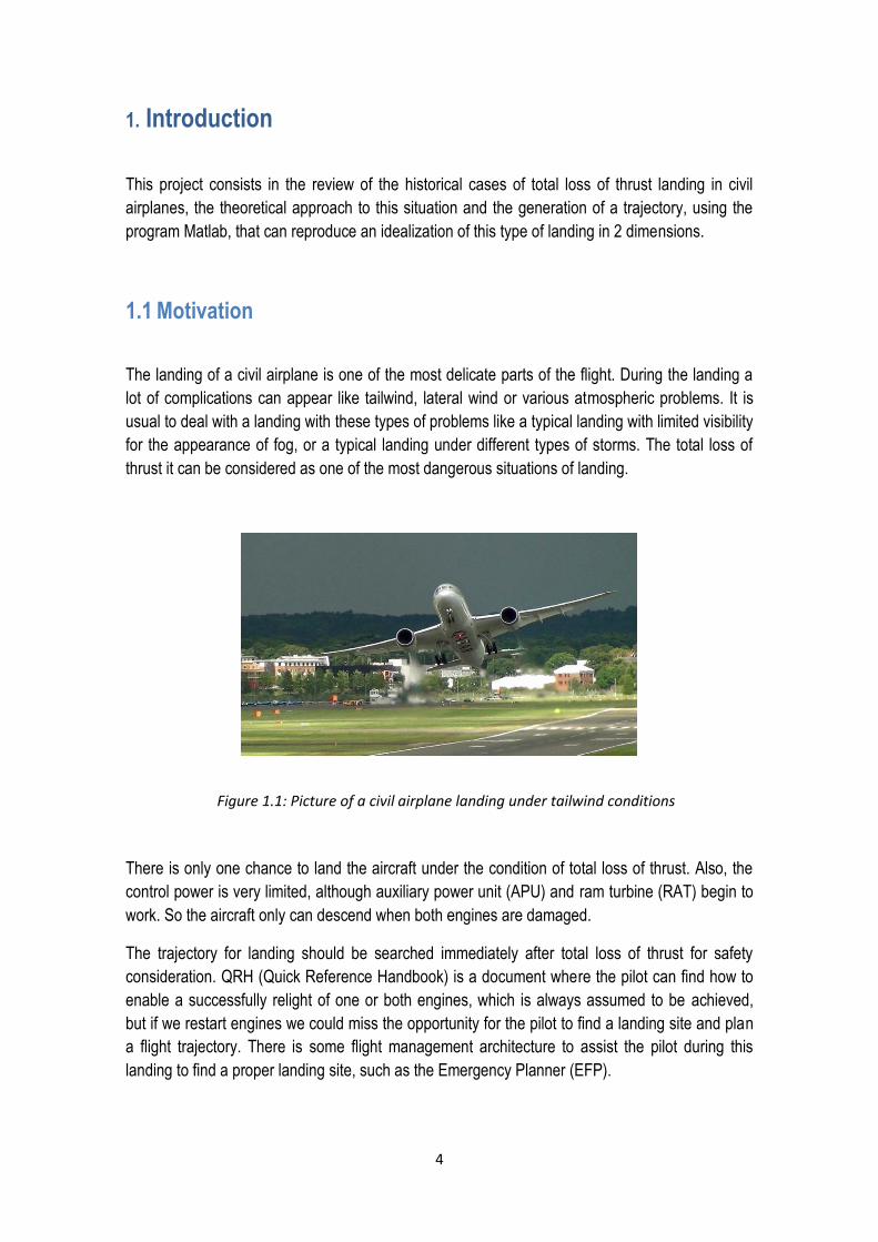
Figure 1.1: Picture of a civil airplane landing under tailwind conditions

5

1.2 Objectives

This section outlines which are the main purposes of this thesis.

The main objective of this project is to be able to generate a final approach and landing trajectory

for a civil airplane in total loss of thrust using the program Matlab. In this document there is an

implementation using Matlab that generates the trajectory described in order to achieve a correct

2 dimension idealization of the landing in total loss of thrust. Therefore the objectives of the

project are:

Making an historical overview of the total loss of thrust landings and understanding the

reasons.

Obtaining a theoretical approach of the problem in order to understand correctly what is

the landing under conditions of total loss of thrust.

Implementing a Matlab program to generate the landing trajectory.

Understanding the main safety implications as a result of this type of landing.

6

2. Historical Overview

In this section we focus on some historical cases of total loss of thrust that have required gliding

landing.

2.1 The Gimli Glider

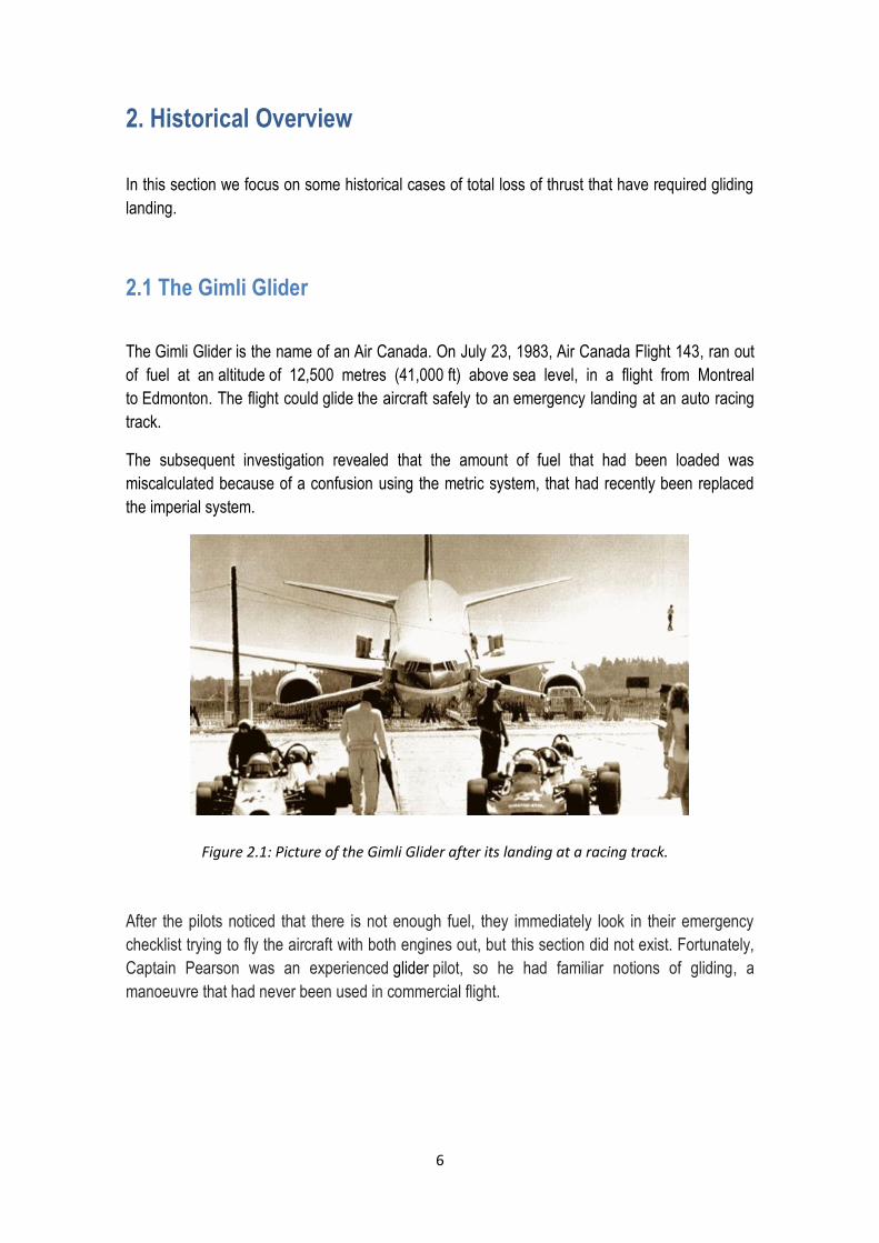
The Gimli Glider is the name of an Air Canada. On July 23, 1983, Air Canada Flight 143, ran out

of fuel at an altitude of 12,500 metres (41,000 ft) above sea level, in a flight from Montreal

to Edmonton. The flight could glide the aircraft safely to an emergency landing at an auto racing

track.

The subsequent investigation revealed that the amount of fuel that had been loaded was

miscalculated because of a confusion using the metric system, that had recently been replaced

the imperial system.

After the pilots noticed that there is not enough fuel, they immediately look in their emergency

checklist trying to fly the aircraft with both engines out, but this section did not exist. Fortunately,

Captain Pearson was an experienced glider pilot, so he had familiar notions of gliding, a

manoeuvre that had never been used in commercial flight.

Figure 2.1: Picture of the Gimli Glider after its landing at a racing track.

7

2.2 TACA Flight 110

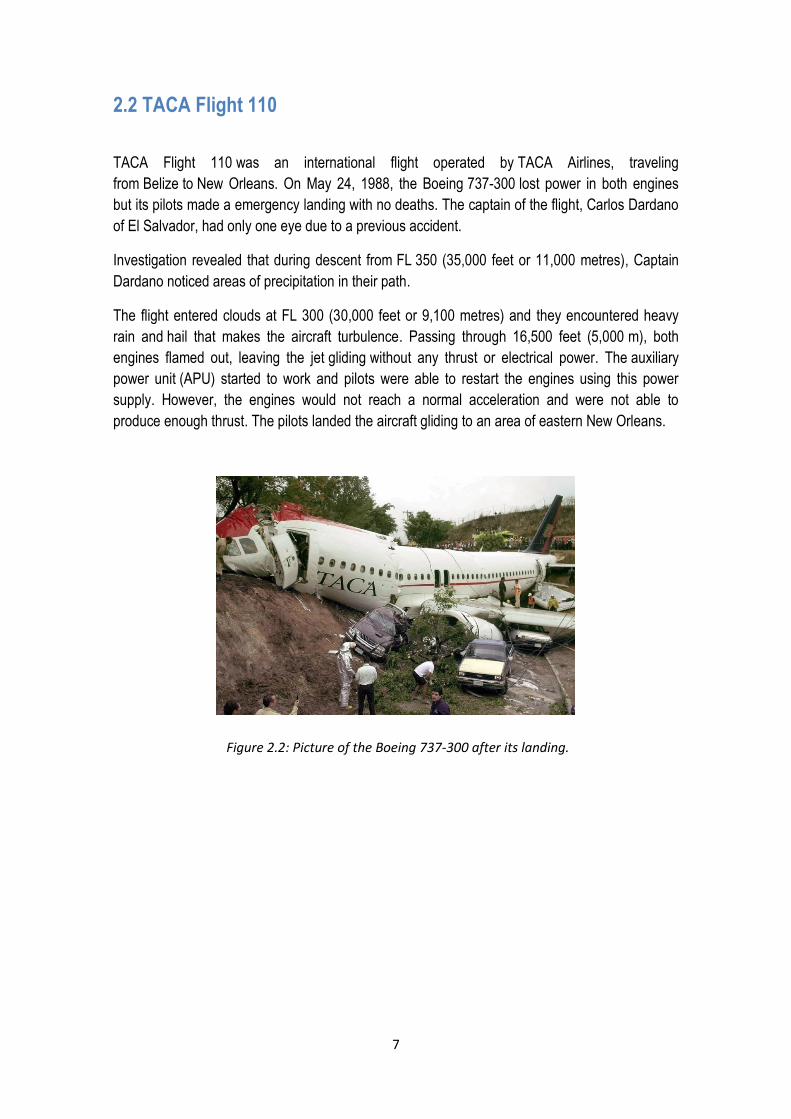
TACA Flight 110 was an international flight operated by TACA Airlines, traveling

from Belize to New Orleans. On May 24, 1988, the Boeing 737-300 lost power in both engines

but its pilots made a emergency landing with no deaths. The captain of the flight, Carlos Dardano

of El Salvador, had only one eye due to a previous accident.

Investigation revealed that during descent from FL 350 (35,000 feet or 11,000 metres), Captain

Dardano noticed areas of precipitation in their path.

The flight entered clouds at FL 300 (30,000 feet or 9,100 metres) and they encountered heavy

rain and hail that makes the aircraft turbulence. Passing through 16,500 feet (5,000 m), both

engines flamed out, leaving the jet gliding without any thrust or electrical power. The auxiliary

power unit (APU) started to work and pilots were able to restart the engines using this power

supply. However, the engines would not reach a normal acceleration and were not able to

produce enough thrust. The pilots landed the aircraft gliding to an area of eastern New Orleans.

Figure 2.2: Picture of the Boeing 737-300 after its landing.

8

2.3 Tuninter Flight 1153

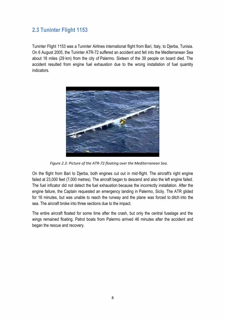
Tuninter Flight 1153 was a Tuninter Airlines international flight from Bari, Italy, to Djerba, Tunisia.

On 6 August 2005, the Tuninter ATR-72 suffered an accident and fell into the Mediterranean Sea

about 18 miles (29 km) from the city of Palermo. Sixteen of the 39 people on board died. The

accident resulted from engine fuel exhaustion due to the wrong installation of fuel quantity

indicators.

On the flight from Bari to Djerba, both engines cut out in mid-flight. The aircraft's right engine

failed at 23,000 feet (7,000 metres). The aircraft began to descend and also the left engine failed.

The fuel inficator did not detect the fuel exhaustion because the incorrectly installation. After the

engine failure, the Captain requested an emergency landing in Palermo, Sicily. The ATR glided

for 16 minutes, but was unable to reach the runway and the plane was forced to ditch into the

sea. The aircraft broke into three sections due to the impact.

The entire aircraft floated for some time after the crash, but only the central fuselage and the

wings remained floating. Patrol boats from Palermo arrived 46 minutes after the accident and

began the rescue and recovery.

Figure 2.3: Picture of the ATR-72 floating over the Mediterranean Sea.

9

2.4 US Airways Flight 1549

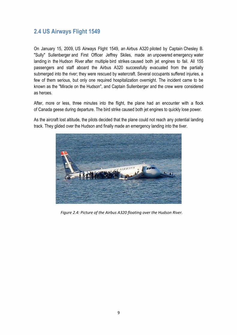
On January 15, 2009, US Airways Flight 1549, an Airbus A320 piloted by Captain Chesley B.

"Sully" Sullenberger and First Officer Jeffrey Skiles, made an unpowered emergency water

landing in the Hudson River after multiple bird strikes caused both jet engines to fail. All 155

passengers and staff aboard the Airbus A320 successfully evacuated from the partially

submerged into the river; they were rescued by watercraft. Several occupants suffered injuries, a

few of them serious, but only one required hospitalization overnight. The incident came to be

known as the "Miracle on the Hudson", and Captain Sullenberger and the crew were considered

as heroes.

After, more or less, three minutes into the flight, the plane had an encounter with a flock

of Canada geese during departure. The bird strike caused both jet engines to quickly lose power.

As the aircraft lost altitude, the pilots decided that the plane could not reach any potential landing

track. They glided over the Hudson and finally made an emergency landing into the tiver.

Figure 2.4: Picture of the Airbus A320 floating over the Hudson River.

10

3. Theoretical Approach and Main Concepts

This section describes the theoretical approach that we have used to study this problem.

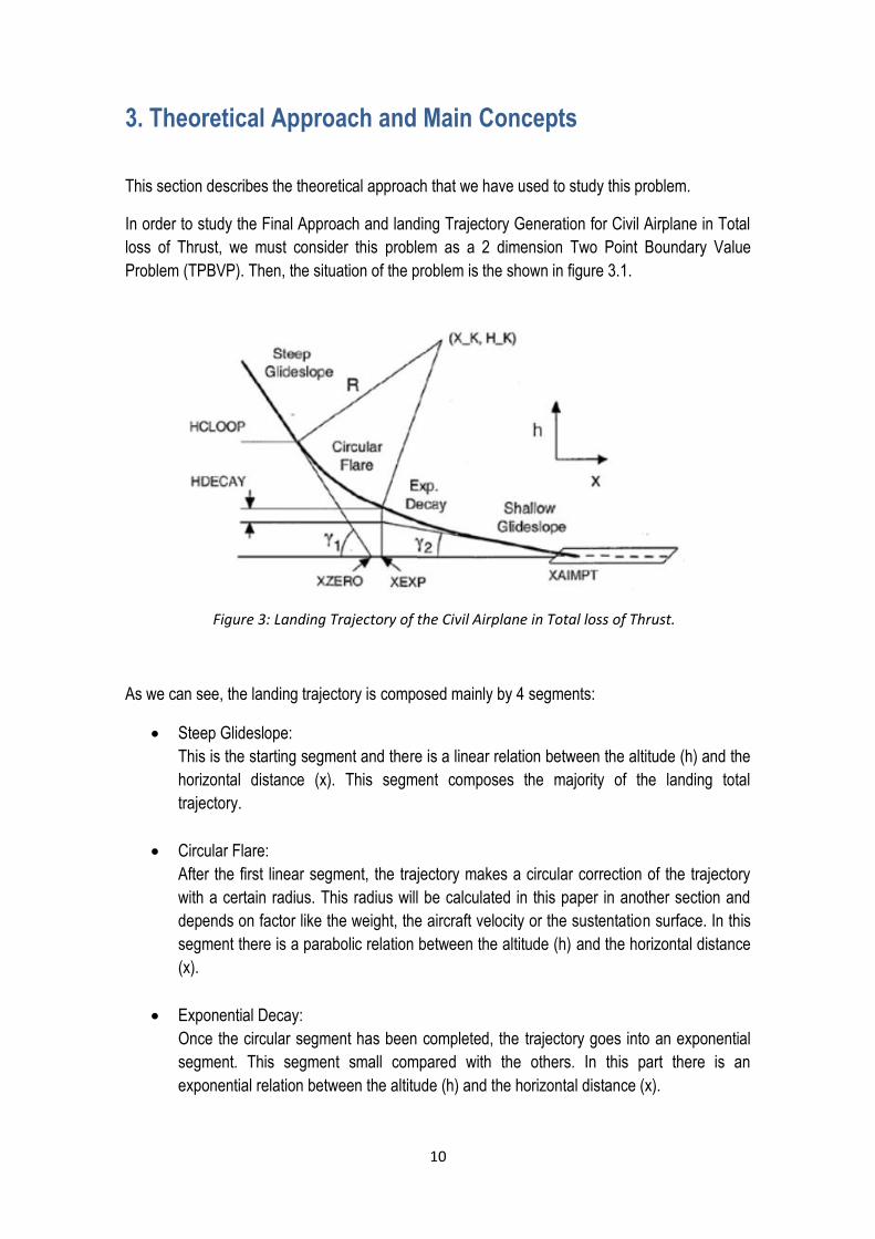
In order to study the Final Approach and landing Trajectory Generation for Civil Airplane in Total

loss of Thrust, we must consider this problem as a 2 dimension Two Point Boundary Value

Problem (TPBVP). Then, the situation of the problem is the shown in figure 3.1.

As we can see, the landing trajectory is composed mainly by 4 segments:

Steep Glideslope:

This is the starting segment and there is a linear relation between the altitude (h) and the

horizontal distance (x). This segment composes the majority of the landing total

trajectory.

Circular Flare:

After the first linear segment, the trajectory makes a circular correction of the trajectory

with a certain radius. This radius will be calculated in this paper in another section and

depends on factor like the weight, the aircraft velocity or the sustentation surface. In this

segment there is a parabolic relation between the altitude (h) and the horizontal distance

(x).

Exponential Decay:

Once the circular segment has been completed, the trajectory goes into an exponential

segment. This segment small compared with the others. In this part there is an

exponential relation between the altitude (h) and the horizontal distance (x).

Figure 3: Landing Trajectory of the Civil Airplane in Total loss of Thrust.

11

Shadow Glideslope:

After the exponential segment, the trajectory finally ends in a linear segment until the

aircraft touch down. In this segment, also there is a linear relation between the altitude

(h) and the horizontal distance (x).

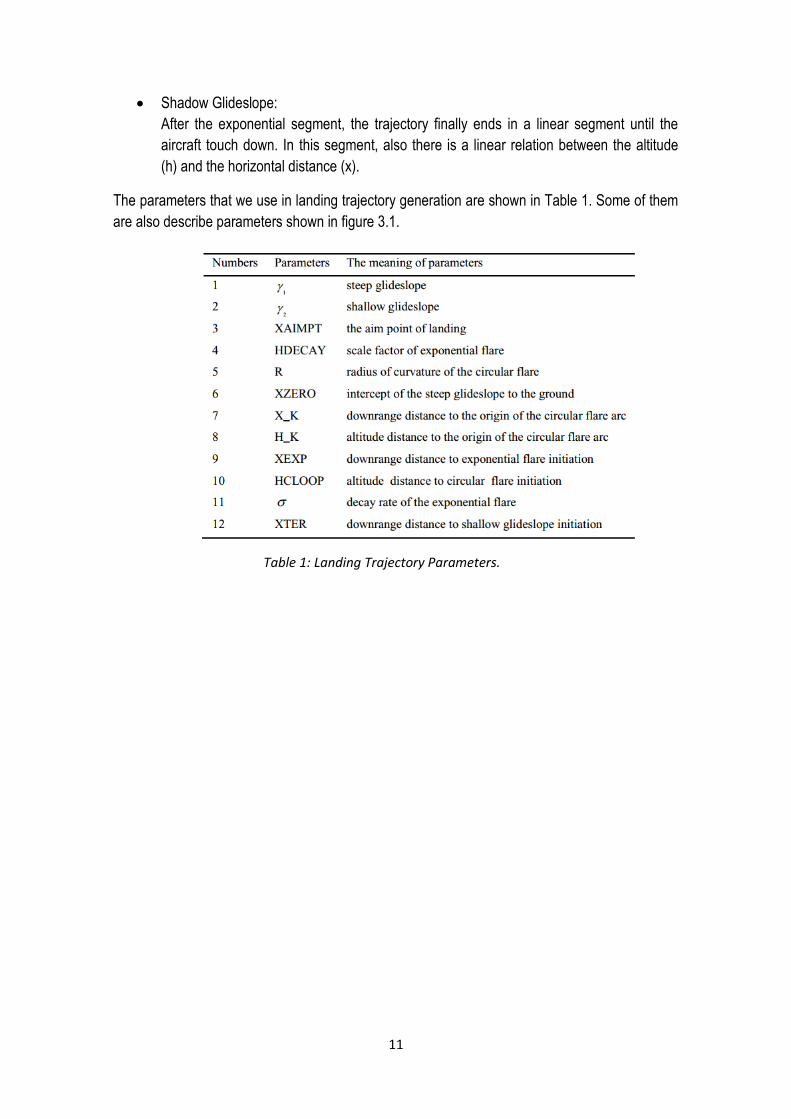
The parameters that we use in landing trajectory generation are shown in Table 1. Some of them

are also describe parameters shown in figure 3.1.

Table 1: Landing Trajectory Parameters.

12

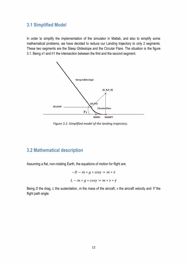
3.1 Simplified Model

In order to simplify the implementation of the simulator in Matlab, and also to simplify some

mathematical problems, we have decided to reduce our Landing trajectory to only 2 segments.

These two segments are the Steep Glideslope and the Circular Flare. The situation is the figure

3.1. Being x1 and h1 the intersection between the first and the second segment.

3.2 Mathematical description

Assuming a flat, non-rotating Earth, the equations of motion for flight are:

−𝐷 −𝑚 ∗ 𝑔 ∗ 𝑠𝑖𝑛𝛾 = 𝑚 ∗ �̇�

𝐿 − 𝑚 ∗ 𝑔 ∗ 𝑐𝑜𝑠𝛾 = 𝑚 ∗ 𝑣 ∗ �̇�

Being D the drag, L the sustentation, m the mass of the aircraft, v the aircraft velocity and ϒ the

flight path angle.

𝜸𝟏

Figure 3.1: Simplified model of the landing trajectory.

13

3.2.1 Altitude

We start this mathematical description showing the equations that define the altitude of the

trajectory as a function of the horizontal distance (x):

ℎ𝑆𝑇𝐸𝐸𝑃 = (𝑋 − 𝑋𝑍𝐸𝑅𝑂) ∗ 𝑡𝑎𝑛𝛾1 Steep Glideslope.

ℎ𝐶𝐼𝑅𝐶 = 𝐻_𝐾 − √𝑅2 − (𝑋 − 𝑋_𝐾2) Circular Flare.

We can rewrite the previous equation in their differential form:

𝑑ℎ𝑆𝑇𝐸𝐸𝑃

𝑑𝑥= 𝑡𝑎𝑛𝛾1 Steep Glideslope.

𝑑ℎ𝐶𝐼𝑅𝐶

𝑑𝑥=

𝑋−𝑋_𝐾

𝐻_𝐾−ℎ Circular Flare.

In order to ensure the continuity between segments, the trajectory parameter and derivative

between two segments should be continuous:

𝑑ℎ

𝑑𝑥‖𝑥=𝑥1

= −𝑥1 − 𝑋_𝐾

ℎ1 − 𝐻_𝐾= 𝑡𝑎𝑛𝛾1

ℎ1

𝑥1 − 𝑋𝑍𝐸𝑅𝑂= 𝑡𝑎𝑛𝛾1

Also, we need to define the parameter HCLOOP:

𝐻𝐶𝐿𝑂𝑂𝑃 = 𝐻_𝐾 − 𝑅 ∗ 𝑐𝑜𝑠𝛾1

3.2.2 Flight Path angle

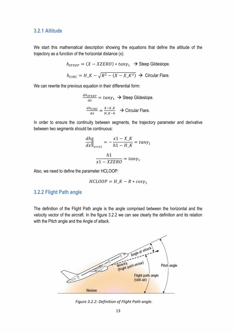
The definition of the Flight Path angle is the angle comprised between the horizontal and the

velocity vector of the aircraft. In the figure 3.2.2 we can see clearly the definition and its relation

with the Pitch angle and the Angle of attack.

Figure 3.2.2: Definition of Flight Path angle.

14

According to the definition of flight path angle:

𝛾 = 𝑎𝑟𝑐𝑡𝑎𝑛𝑑ℎ

𝑑𝑥

We look for a differential equation of the flight path angle for each segment of the trajectory:

𝑑𝛾

𝑑ℎ𝑆𝑇𝐸𝐸𝑃= 0 Steep Glideslope.

𝑑𝛾

𝑑ℎ𝐶𝐼𝑅𝐶=

1

(𝐻_𝐾−ℎ)∗𝑡𝑎𝑛𝛾 Circular Flare.

In the first segment of the trajectory, the flight path angle does not change, but during the second

segment there is an evolution of this angle that depends on the altitude. To see clearly this

relation we can integrate the differential equation and get:

𝛾𝐶𝐼𝑅𝐶 = acos(𝑐𝑜𝑛𝑠𝑡𝑎𝑛𝑡 ∗ (𝐻_𝐾 − 𝐻𝐶𝐼𝑅𝐶))

The constant in the equation depends on the initial conditions. For example, if our flight path

angle is -4 degrees in the Steep Glideslope segment, the constant is 7.7*10-4.

3.2.3 Aircraft velocity

This section outlines the different considerations about the aircraft velocity.

In order to describe correctly the evolution of the aircraft velocity during the landing trajectory, it is

important to define the stall speed:

𝑉𝑆 = √2 ∗𝑊

𝜌 ∗ 𝑆 ∗ 𝐶𝐿𝑀𝐴𝑋

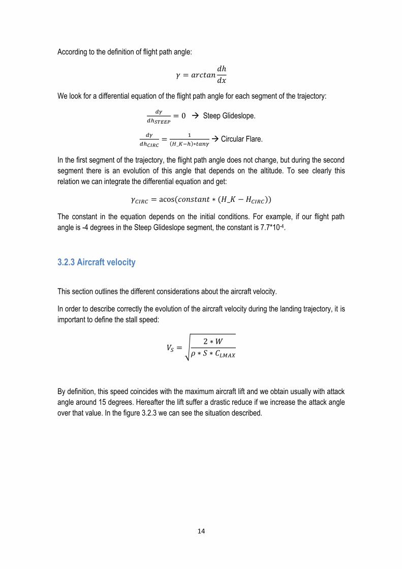
By definition, this speed coincides with the maximum aircraft lift and we obtain usually with attack

angle around 15 degrees. Hereafter the lift suffer a drastic reduce if we increase the attack angle

over that value. In the figure 3.2.3 we can see the situation described.

15

According to the velocity described previously, the landing regulations set that at the beginning of

the landing linear segment, the speed must be:

𝑉𝐴 = 1.3 ∗ 𝑉𝑆

And the speed touch down after finishing the circular segment must be:

𝑉𝑇𝐷 = 1.15 ∗ 𝑉𝑆

After this deceleration during the air landing trajectory, the aircraft reduce its velocity quickly in

the landing track. The differential equations that describe the motion and the deceleration time

are:

𝑑𝑥

𝑑𝑉=𝑊

𝑔

𝑉

𝑇 − 𝐷 − 𝜇𝑓 ∗ (𝑊 − 𝐿)

𝑑𝑡

𝑑𝑉=𝑊

𝑔

𝑉

𝑇 − 𝐷 − 𝜇𝑓 ∗ (𝑊 − 𝐿)

Where 𝜇𝑓 is the stop coefficient, x is the horizontal distance, V the aircraft velocity, t the time

spent, T the thrust, D the drag and L the lift.

We can make some consideration about these previous parameters. The stop coefficient is

always between 0.3-0.4 and the thrust is zero if we are considering that there is no reverse flow

during the aircraft stop.

Figure 3.2.3: Definition of the Stall condition.

16

3.2.4 Dynamic Pressure

The dynamic pressure is defined in a physical sense, as the kinetic energy per unit volume of a

fluid particle. This parameter helps us to study the aerodynamic stress experienced by our civil

airplane travelling at a certain velocity. Assuming that flight altitude monotonically decreases, the

equation that define the dynamic pressure is:

𝑄 =𝑊 ∗ 𝑐𝑜𝑠𝛾

𝑆 ∗ 𝐶𝐿 −2 ∗𝑊 ∗ 𝑠𝑖𝑛𝛾

𝜌 ∗ 𝑔∗ (𝑑𝛾𝑑ℎ)

Where ϒ represents the flight path angle. The differential form of the previous equation is:

𝑑𝑄

𝑑ℎ= (

1

𝜌

𝑑𝜌

𝑑ℎ−𝜌 ∗ 𝑔 ∗ 𝑆 ∗ 𝐶𝐷𝑊 ∗ 𝑠𝑖𝑛𝜌

) ∗ 𝑄 − 𝜌 ∗ 𝑔

We must noticed that the lift and drag coefficients depends on the match number and on the

attack angle.

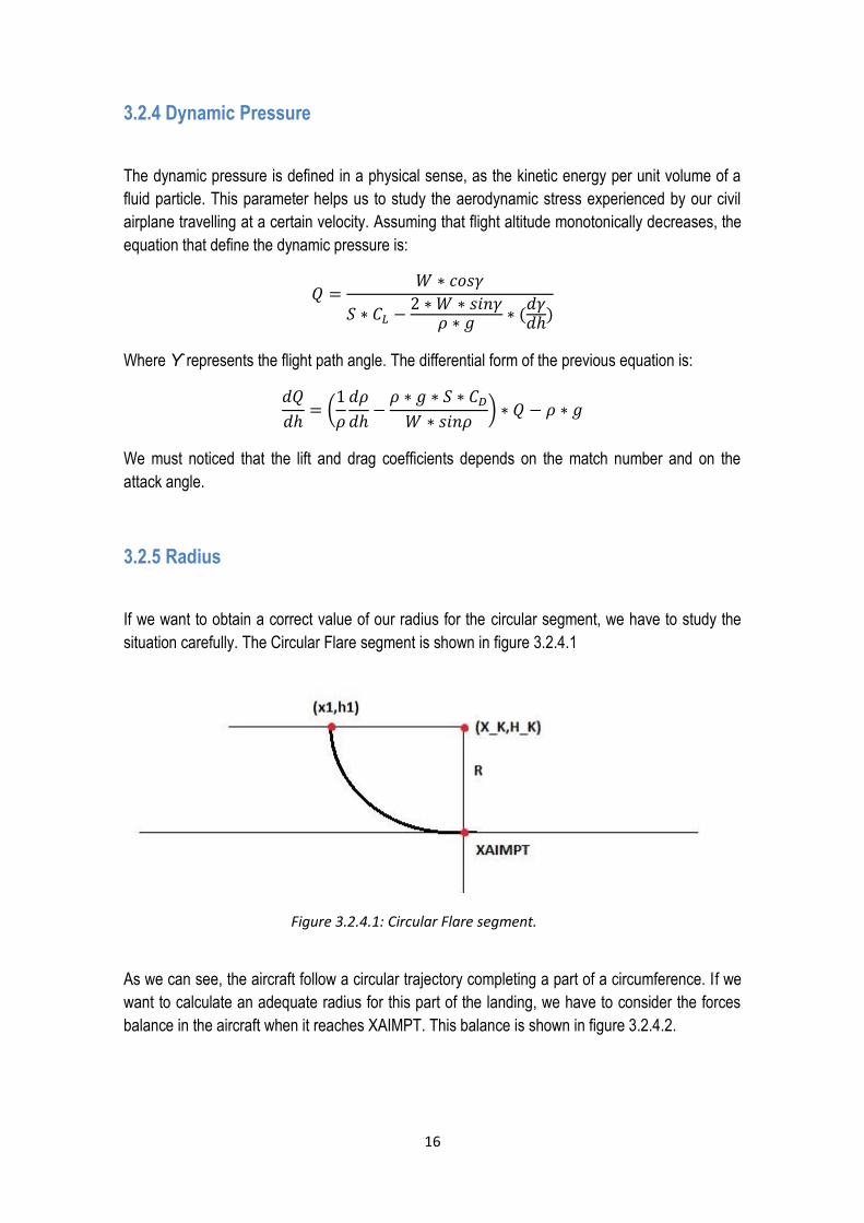
3.2.5 Radius

If we want to obtain a correct value of our radius for the circular segment, we have to study the

situation carefully. The Circular Flare segment is shown in figure 3.2.4.1

As we can see, the aircraft follow a circular trajectory completing a part of a circumference. If we

want to calculate an adequate radius for this part of the landing, we have to consider the forces

balance in the aircraft when it reaches XAIMPT. This balance is shown in figure 3.2.4.2.

Figure 3.2.4.1: Circular Flare segment.

17

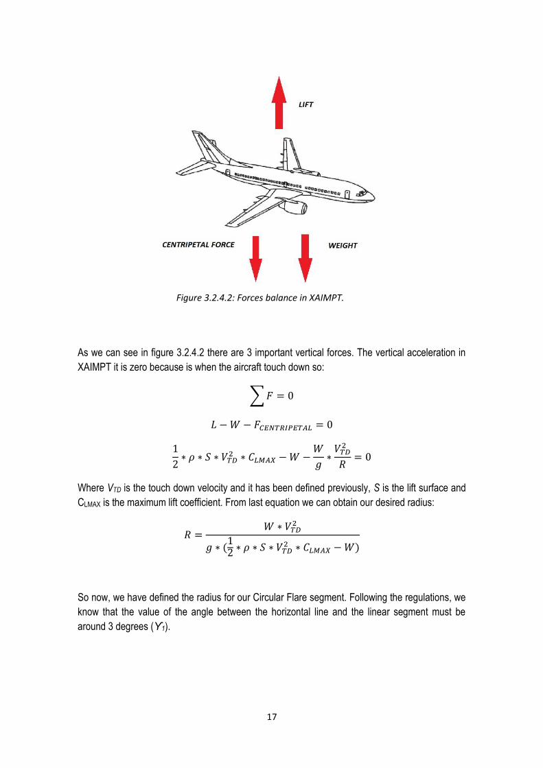
As we can see in figure 3.2.4.2 there are 3 important vertical forces. The vertical acceleration in

XAIMPT it is zero because is when the aircraft touch down so:

∑𝐹 = 0

𝐿 −𝑊 − 𝐹𝐶𝐸𝑁𝑇𝑅𝐼𝑃𝐸𝑇𝐴𝐿 = 0

1

2∗ 𝜌 ∗ 𝑆 ∗ 𝑉𝑇𝐷

2 ∗ 𝐶𝐿𝑀𝐴𝑋 −𝑊 −𝑊

𝑔∗𝑉𝑇𝐷2

𝑅= 0

Where VTD is the touch down velocity and it has been defined previously, S is the lift surface and

CLMAX is the maximum lift coefficient. From last equation we can obtain our desired radius:

𝑅 =𝑊 ∗ 𝑉𝑇𝐷

2

𝑔 ∗ (12 ∗ 𝜌 ∗ 𝑆 ∗ 𝑉𝑇𝐷

2 ∗ 𝐶𝐿𝑀𝐴𝑋 −𝑊)

So now, we have defined the radius for our Circular Flare segment. Following the regulations, we

know that the value of the angle between the horizontal line and the linear segment must be

around 3 degrees (ϒ1).

Figure 3.2.4.2: Forces balance in XAIMPT.

18

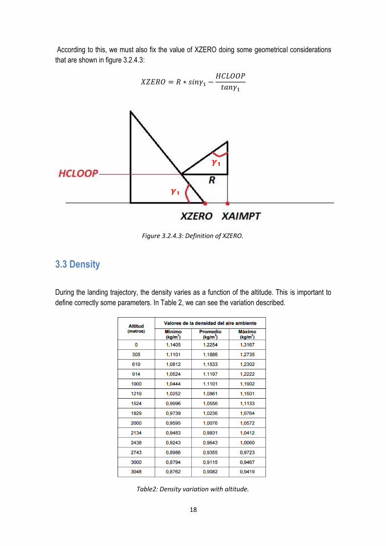
According to this, we must also fix the value of XZERO doing some geometrical considerations

that are shown in figure 3.2.4.3:

𝑋𝑍𝐸𝑅𝑂 = 𝑅 ∗ 𝑠𝑖𝑛𝛾1 −𝐻𝐶𝐿𝑂𝑂𝑃

𝑡𝑎𝑛𝛾1

3.3 Density

During the landing trajectory, the density varies as a function of the altitude. This is important to

define correctly some parameters. In Table 2, we can see the variation described.

Figure 3.2.4.3: Definition of XZERO.

𝜸𝟏

𝜸𝟏

Table2: Density variation with altitude.

19

4. Matlab implementation

This section explains the Matlab implementation of the program that simulates the Landing of a

Civil Airplane in total Loss of Thrust.

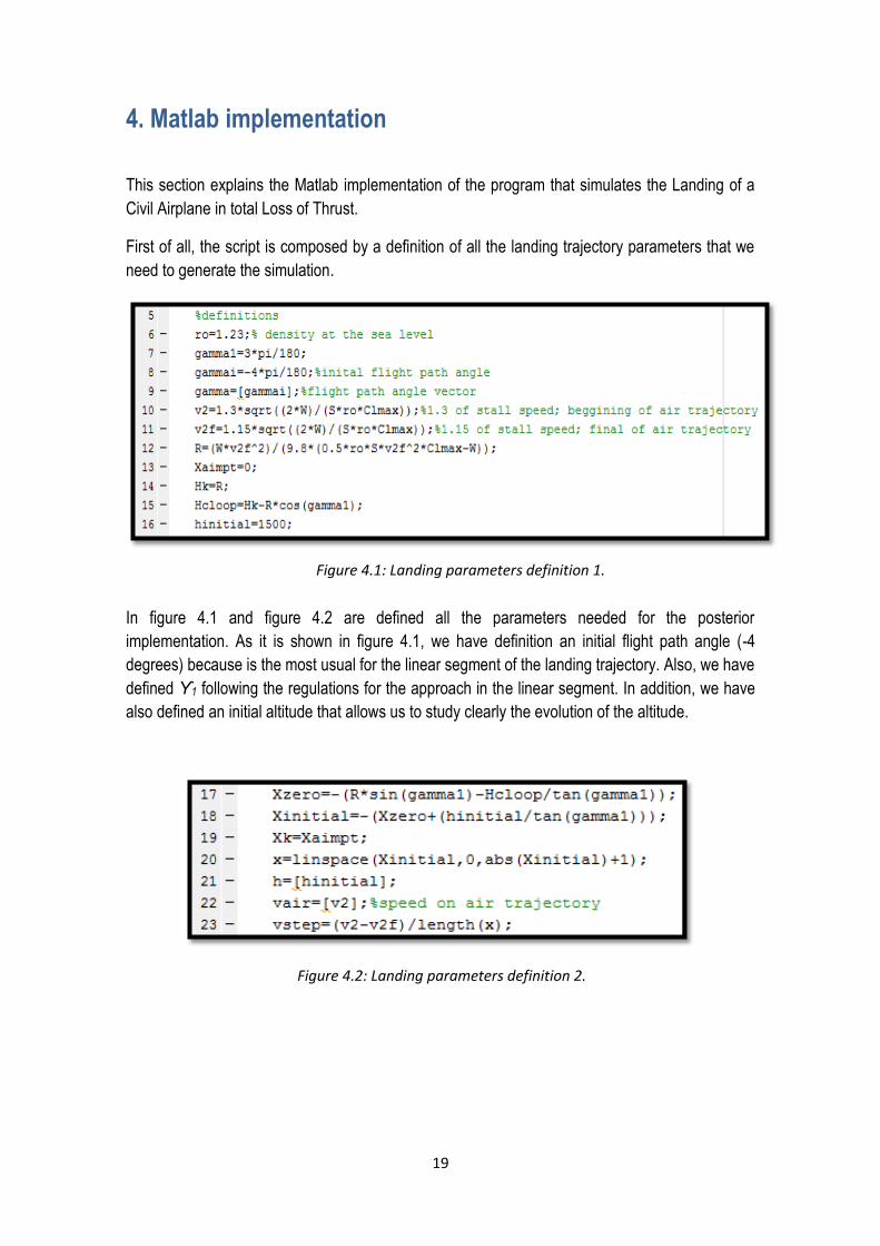
First of all, the script is composed by a definition of all the landing trajectory parameters that we

need to generate the simulation.

In figure 4.1 and figure 4.2 are defined all the parameters needed for the posterior

implementation. As it is shown in figure 4.1, we have definition an initial flight path angle (-4

degrees) because is the most usual for the linear segment of the landing trajectory. Also, we have

defined ϒ1 following the regulations for the approach in the linear segment. In addition, we have

also defined an initial altitude that allows us to study clearly the evolution of the altitude.

Figure 4.1: Landing parameters definition 1.

Figure 4.2: Landing parameters definition 2.

20

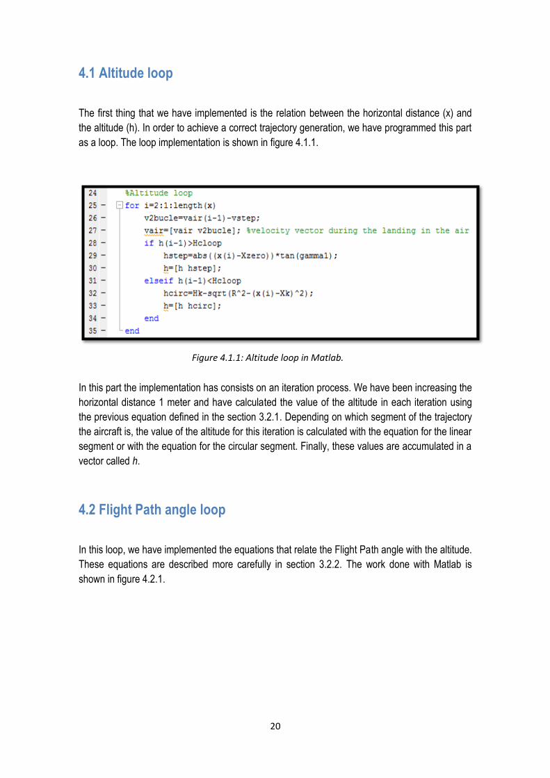
4.1 Altitude loop

The first thing that we have implemented is the relation between the horizontal distance (x) and

the altitude (h). In order to achieve a correct trajectory generation, we have programmed this part

as a loop. The loop implementation is shown in figure 4.1.1.

In this part the implementation has consists on an iteration process. We have been increasing the

horizontal distance 1 meter and have calculated the value of the altitude in each iteration using

the previous equation defined in the section 3.2.1. Depending on which segment of the trajectory

the aircraft is, the value of the altitude for this iteration is calculated with the equation for the linear

segment or with the equation for the circular segment. Finally, these values are accumulated in a

vector called h.

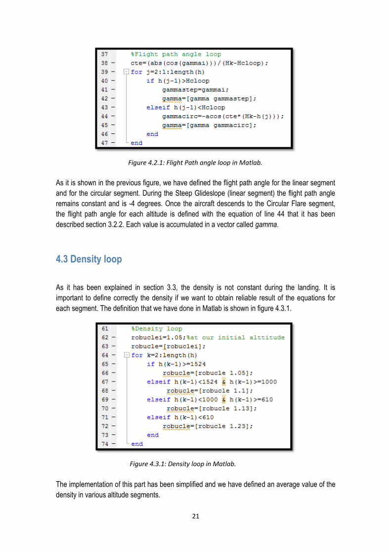
4.2 Flight Path angle loop

In this loop, we have implemented the equations that relate the Flight Path angle with the altitude.

These equations are described more carefully in section 3.2.2. The work done with Matlab is

shown in figure 4.2.1.

Figure 4.1.1: Altitude loop in Matlab.

21

As it is shown in the previous figure, we have defined the flight path angle for the linear segment

and for the circular segment. During the Steep Glideslope (linear segment) the flight path angle

remains constant and is -4 degrees. Once the aircraft descends to the Circular Flare segment,

the flight path angle for each altitude is defined with the equation of line 44 that it has been

described section 3.2.2. Each value is accumulated in a vector called gamma.

4.3 Density loop

As it has been explained in section 3.3, the density is not constant during the landing. It is

important to define correctly the density if we want to obtain reliable result of the equations for

each segment. The definition that we have done in Matlab is shown in figure 4.3.1.

The implementation of this part has been simplified and we have defined an average value of the

density in various altitude segments.

Figure 4.2.1: Flight Path angle loop in Matlab.

Figure 4.3.1: Density loop in Matlab.

22

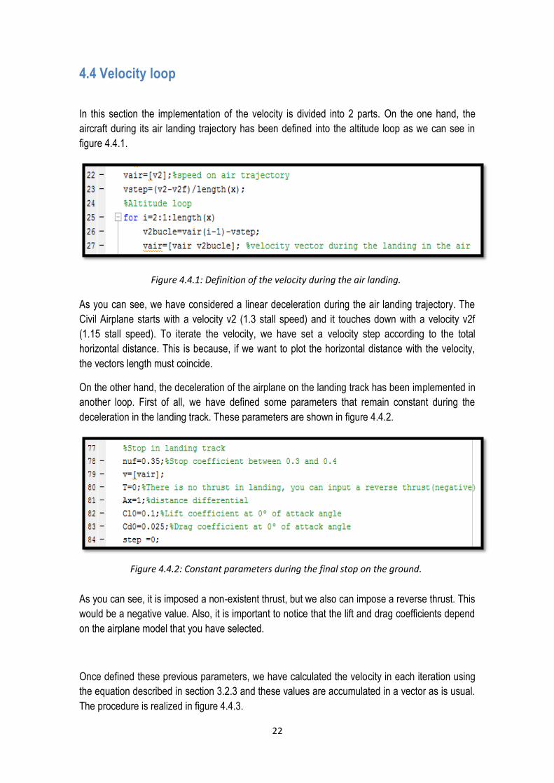
4.4 Velocity loop

In this section the implementation of the velocity is divided into 2 parts. On the one hand, the

aircraft during its air landing trajectory has been defined into the altitude loop as we can see in

figure 4.4.1.

As you can see, we have considered a linear deceleration during the air landing trajectory. The

Civil Airplane starts with a velocity v2 (1.3 stall speed) and it touches down with a velocity v2f

(1.15 stall speed). To iterate the velocity, we have set a velocity step according to the total

horizontal distance. This is because, if we want to plot the horizontal distance with the velocity,

the vectors length must coincide.

On the other hand, the deceleration of the airplane on the landing track has been implemented in

another loop. First of all, we have defined some parameters that remain constant during the

deceleration in the landing track. These parameters are shown in figure 4.4.2.

As you can see, it is imposed a non-existent thrust, but we also can impose a reverse thrust. This

would be a negative value. Also, it is important to notice that the lift and drag coefficients depend

on the airplane model that you have selected.

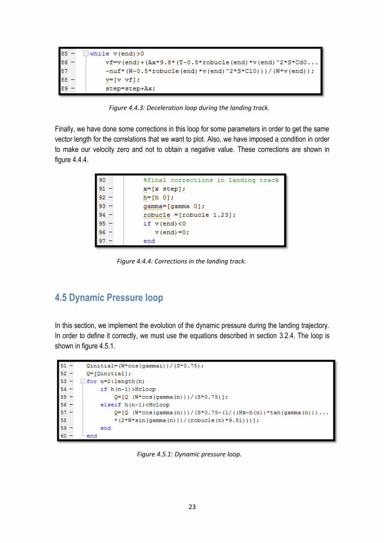
Once defined these previous parameters, we have calculated the velocity in each iteration using

the equation described in section 3.2.3 and these values are accumulated in a vector as is usual.

The procedure is realized in figure 4.4.3.

Figure 4.4.1: Definition of the velocity during the air landing.

Figure 4.4.2: Constant parameters during the final stop on the ground.

23

Finally, we have done some corrections in this loop for some parameters in order to get the same

vector length for the correlations that we want to plot. Also, we have imposed a condition in order

to make our velocity zero and not to obtain a negative value. These corrections are shown in

figure 4.4.4.

4.5 Dynamic Pressure loop

In this section, we implement the evolution of the dynamic pressure during the landing trajectory.

In order to define it correctly, we must use the equations described in section 3.2.4. The loop is

shown in figure 4.5.1.

Figure 4.4.3: Deceleration loop during the landing track.

Figure 4.4.4: Corrections in the landing track.

Figure 4.5.1: Dynamic pressure loop.

24

As it is shown, we have defined the dynamic pressure for the linear segment, where the flight

path angle does not change with the altitude, and for the circular segment, where there is a

change in flight path angle with the altitude.

Nevertheless the result of this loop is not reliable. The changes in flight path angle and in altitude

are really small. For these reason, the loop gives us an asymptotic result that does not coincide

with the real value of the dynamic pressure during the landing. For this reason, we have decided

to maintain constant the dynamic pressure assigning it a typical value for landings. This value is

approximately 2600 N per each m2.

25

5. Simulation results

This section focus on the study of the simulation result of the program implemented in Matlab.

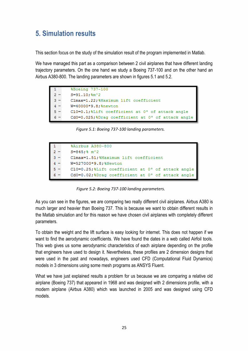
We have managed this part as a comparison between 2 civil airplanes that have different landing

trajectory parameters. On the one hand we study a Boeing 737-100 and on the other hand an

Airbus A380-800. The landing parameters are shown in figures 5.1 and 5.2.

As you can see in the figures, we are comparing two really different civil airplanes. Airbus A380 is

much larger and heavier than Boeing 737. This is because we want to obtain different results in

the Matlab simulation and for this reason we have chosen civil airplanes with completely different

parameters.

To obtain the weight and the lift surface is easy looking for internet. This does not happen if we

want to find the aerodynamic coefficients. We have found the dates in a web called Airfoil tools.

This web gives us some aerodynamic characteristics of each airplane depending on the profile

that engineers have used to design it. Nevertheless, these profiles are 2 dimension designs that

were used in the past and nowadays, engineers used CFD (Computational Fluid Dynamics)

models in 3 dimensions using some mesh programs as ANSYS Fluent.

What we have just explained results a problem for us because we are comparing a relative old

airplane (Boeing 737) that appeared in 1968 and was designed with 2 dimensions profile, with a

modern airplane (Airbus A380) which was launched in 2005 and was designed using CFD

models.

Figure 5.1: Boeing 737-100 landing parameters.

Figure 5.2: Boeing 737-100 landing parameters.

26

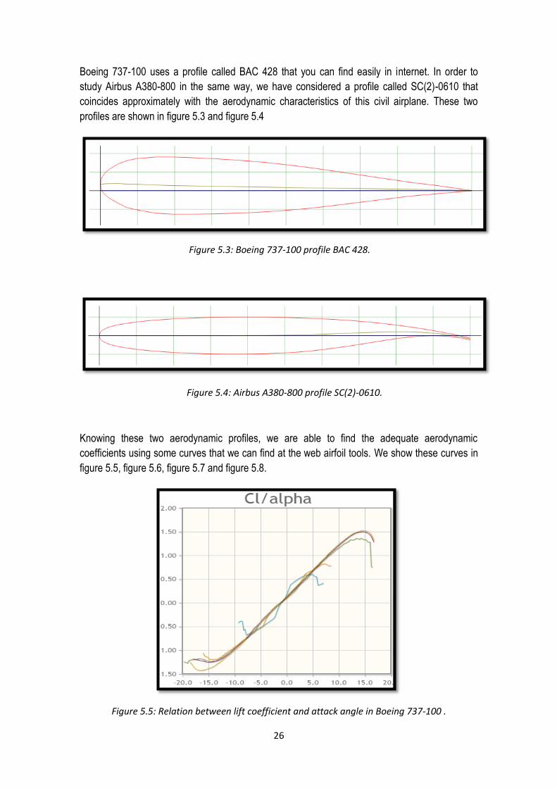
Boeing 737-100 uses a profile called BAC 428 that you can find easily in internet. In order to

study Airbus A380-800 in the same way, we have considered a profile called SC(2)-0610 that

coincides approximately with the aerodynamic characteristics of this civil airplane. These two

profiles are shown in figure 5.3 and figure 5.4

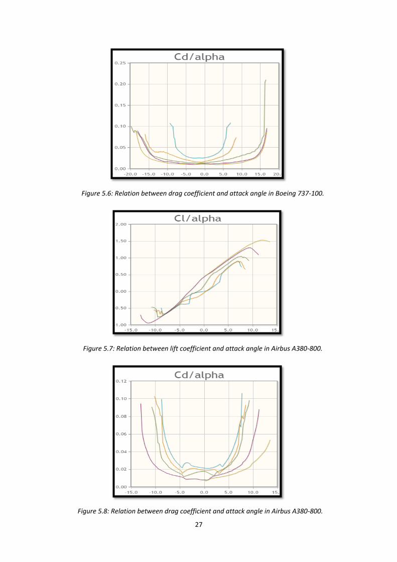
Knowing these two aerodynamic profiles, we are able to find the adequate aerodynamic

coefficients using some curves that we can find at the web airfoil tools. We show these curves in

figure 5.5, figure 5.6, figure 5.7 and figure 5.8.

Figure 5.3: Boeing 737-100 profile BAC 428.

Figure 5.4: Airbus A380-800 profile SC(2)-0610.

Figure 5.5: Relation between lift coefficient and attack angle in Boeing 737-100 .

27

Figure 5.6: Relation between drag coefficient and attack angle in Boeing 737-100.

Figure 5.7: Relation between lift coefficient and attack angle in Airbus A380-800.

Figure 5.8: Relation between drag coefficient and attack angle in Airbus A380-800.

28

5.1 Altitude results

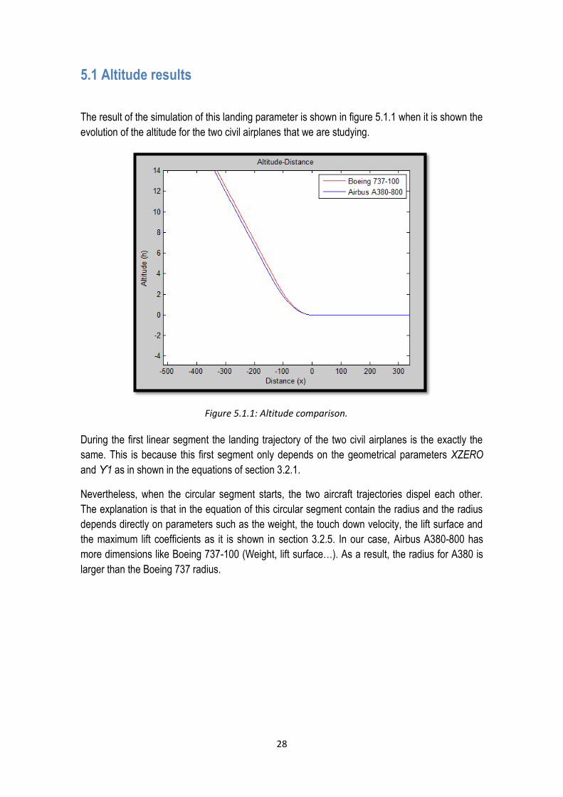
The result of the simulation of this landing parameter is shown in figure 5.1.1 when it is shown the

evolution of the altitude for the two civil airplanes that we are studying.

During the first linear segment the landing trajectory of the two civil airplanes is the exactly the

same. This is because this first segment only depends on the geometrical parameters XZERO

and ϒ1 as in shown in the equations of section 3.2.1.

Nevertheless, when the circular segment starts, the two aircraft trajectories dispel each other.

The explanation is that in the equation of this circular segment contain the radius and the radius

depends directly on parameters such as the weight, the touch down velocity, the lift surface and

the maximum lift coefficients as it is shown in section 3.2.5. In our case, Airbus A380-800 has

more dimensions like Boeing 737-100 (Weight, lift surface…). As a result, the radius for A380 is

larger than the Boeing 737 radius.

Figure 5.1.1: Altitude comparison.

29

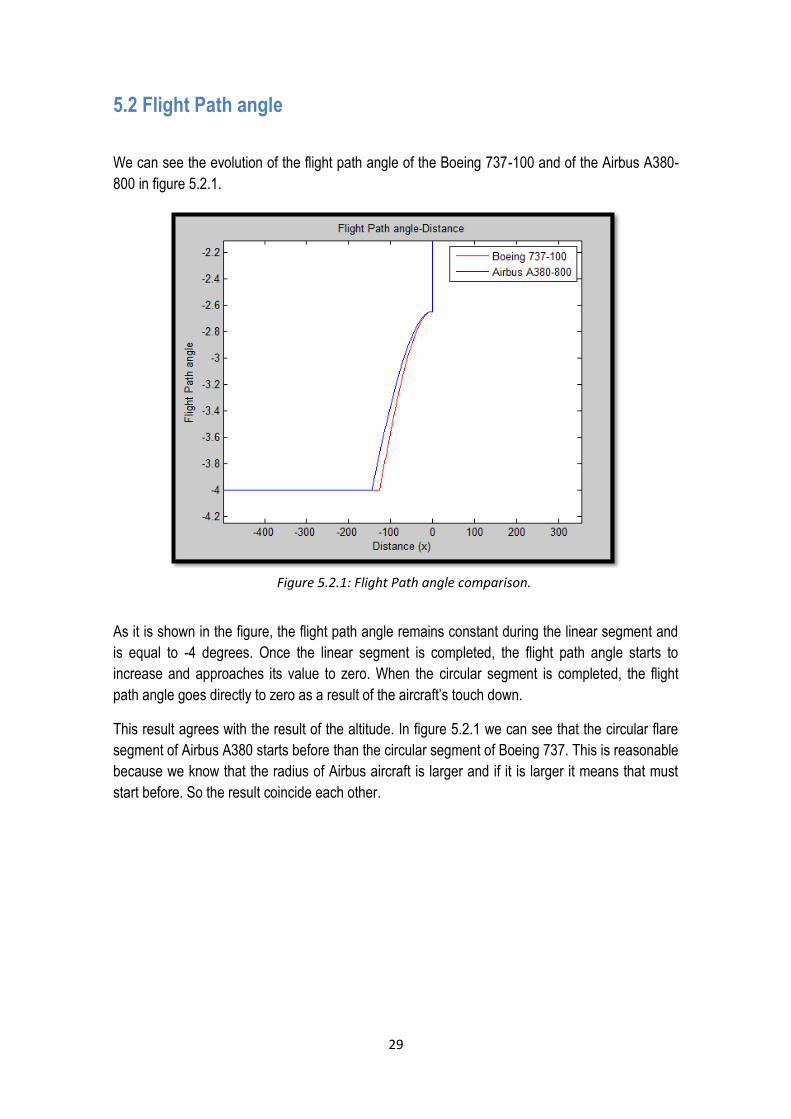
5.2 Flight Path angle

We can see the evolution of the flight path angle of the Boeing 737-100 and of the Airbus A380-

800 in figure 5.2.1.

As it is shown in the figure, the flight path angle remains constant during the linear segment and

is equal to -4 degrees. Once the linear segment is completed, the flight path angle starts to

increase and approaches its value to zero. When the circular segment is completed, the flight

path angle goes directly to zero as a result of the aircraft’s touch down.

This result agrees with the result of the altitude. In figure 5.2.1 we can see that the circular flare

segment of Airbus A380 starts before than the circular segment of Boeing 737. This is reasonable

because we know that the radius of Airbus aircraft is larger and if it is larger it means that must

start before. So the result coincide each other.

Figure 5.2.1: Flight Path angle comparison.

.

.

30

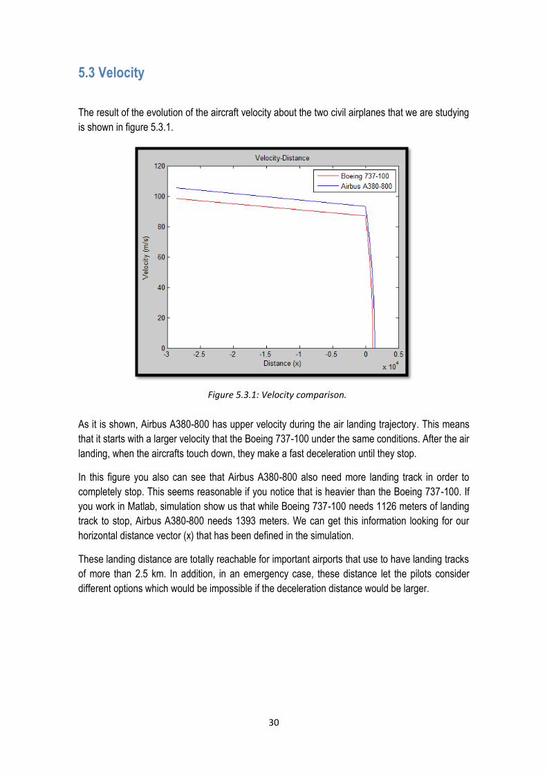
5.3 Velocity

The result of the evolution of the aircraft velocity about the two civil airplanes that we are studying

is shown in figure 5.3.1.

As it is shown, Airbus A380-800 has upper velocity during the air landing trajectory. This means

that it starts with a larger velocity that the Boeing 737-100 under the same conditions. After the air

landing, when the aircrafts touch down, they make a fast deceleration until they stop.

In this figure you also can see that Airbus A380-800 also need more landing track in order to

completely stop. This seems reasonable if you notice that is heavier than the Boeing 737-100. If

you work in Matlab, simulation show us that while Boeing 737-100 needs 1126 meters of landing

track to stop, Airbus A380-800 needs 1393 meters. We can get this information looking for our

horizontal distance vector (x) that has been defined in the simulation.

These landing distance are totally reachable for important airports that use to have landing tracks

of more than 2.5 km. In addition, in an emergency case, these distance let the pilots consider

different options which would be impossible if the deceleration distance would be larger.

Figure 5.3.1: Velocity comparison.

.

.

31

5.4 Emergency Landing

In this section, we want to make a comparison of two types of landing. On the one hand we

simulate a Boeing 737-100 landing under normal conditions. On the other hand we want to

simulate a Boeing 737-100 landing under emergency conditions.

The normal conditions that we are going to impose to the first type of landing are the initial

condition shown in the previous sections: the starting velocity is 1.3 times the stall speed. The

emergency condition is that, at the beginning of the linear segment, the aircraft velocity is the

triple of the normal case.

The simulation results comparing these two cases are identical. There is one special

consideration that will limit our chances if we want to get the landing in an emergency case. This

consideration is the landing track. In Matlab, the landing track that we need under normal

conditions is 1126 meters, while in emergency conditions we will need 1343 meters. This means

that if the velocity at the beginning of the linear segment is larger, you need more landing track to

stop the aircraft on the track. So, in an emergency case, the deceleration during the air trajectory

is one of the most important factors. Pilots have to decelerate the aircraft during the air in order to

reduce the landing track needed, because, under an emergency, is not always possible to reach

an ‘’official’’ landing track with the desirable length.

32

6. Conclusion

After the historical overview done in this document, the theoretical and mathematical concepts

revised and the Matlab simulations, we can conclude that this type of final approach and landing

trajectory can solve an emergency landing situation and improve the safety in this unusual

situations.

What we have done in Matlab is only a 2 dimension model in order to get some approximated

results of the real situation. Nevertheless, this simulation help us a lot in order to get an idea of

which are the most important factors in an emergency landing and get us a reliable

approximation. The landing altitude during the approach trajectory, the flight path angle during all

the landing and the increase of the density as a result of the descent are the main factors that we

must consider if we want to generate a landing trajectory under the condition of total loss of

thrust. After considering these parameters, there are also some important features as the radius

during the circular segment or the selection of the landing place that are determined by the

aircraft’s performance and passenger’s comfort.

To sum up, I can affirm that this thesis has help me to revise some theoretical and mathematical

aerodynamic concepts, to understand and implement a correct landing simulation using Matlab

and also to understand under what conditions an emergency landing occurs.

33

7. Bibliography

http://airfoiltools.com/airfoil/details?airfoil=b737a-il

http://it.mathworks.com/help/matlab/ref/plot.html

http://m-selig.ae.illinois.edu/ads/aircraft.html

http://airfoiltools.com/airfoil/details?airfoil=sc20610-il

http://www.engineeringtoolbox.com/air-altitude-density-volume-d_195.html

https://en.wikipedia.org/wiki/V_speeds

http://www.skybrary.aero/index.php/Unstabilised_Approach:_Landing_Distance_and_Final_Spee

d_Calculations

http://www.manualedivolo.it/index.php?option=com_content&view=article&id=1119:stallo&catid=6

6:qrs&Itemid=64

http://www.princeton.edu/~stengel/MAE331Lectures.html

http://hyperphysics.phy-astr.gsu.edu/hbase/cf.html

https://www.grc.nasa.gov/www/k-12/airplane/dynpress.html

http://www.airbus.com/aircraftfamilies/passengeraircraft/a380family/

file:///C:/Users/usuario/Downloads/Takeoff_Landing.pdf

http://www.icao.int/safety/implementation/library/manual%20aerodrome%20stds.pdf

http://www.historynet.com/the-10-greatest-emergency-landings.htm

https://en.wikipedia.org/wiki/Gimli_Glider

https://en.wikipedia.org/wiki/TACA_Flight_110

https://en.wikipedia.org/wiki/Tuninter_Flight_1153

https://en.wikipedia.org/wiki/US_Airways_Flight_1549

http://www.sciencedirect.com/science/article/pii/S1877705814012028

http://www.aero.us.es/mv/files/MV_Tema6.pdf