FWS/OBS-83/33 DECEMBER 1983

FIELD METHODS AND STATISTICAL ANALYSES FOR MONITORING SMALL SALMONID STREAMS

19970319 140 Fish and Wildlife Service U.S. Department of the Interior

DTIC QUALITY IM^SjSFiffii £

For sale by the Superintendent ot Document», U.8. Government Printing Office. Washington. D.C. 20402

FWS/OBS-83/33 December 1983

FIELD METHODS AND STATISTICAL ANALYSES FOR STORING SMALL SALMONID STREAMS

by

Carl L. Armour Kenneth P. Burnham

Western Energy and Land Use Team U.S. Fish and Wildlife Service Drake Creekside Building One

2627 Redwing Road Fort Collins, CO 80526

and

William S. Platts U.S. Forest Service

Intermountain Forest and Range Experiment Station

316 East Myrtle Boise, ID 83702

Western Energy and Land Use Team Division of Biological Services

Research and Development Fish and Wildlife Service

U.S. Department of the Interior Washington, DC 20240

DISCLAIMER

Mention of trade names or commercial products does not constitute endorse-

ment or recommendation for use by the Division of Biological Services, Fish

and Wildlife Service, U.S. Department of the Interior.

This report should be cited as:

Armour, C. L., K. P. Burnham, and W. S. Platts. 1983. Field methods and statistical analyses for monitoring small salmonid streams. U.S. Fish Wild!. Serv. FWS/OBS-83/33. 200 pp.

PREFACE

This document is written primarily for field workers responsible for

designing and conducting monitoring programs in small western salmonid streams

affected by various land uses, including grazing and timber harvest practices.

Variables to measure and types of statistical tests used to evaluate responses

of salmonids and habitat to land use practices are presented. Users of this

document will need to be familiar with statistical concepts, including sampling

variance, confidence intervals, probability distributions, and hypothesis

testing. Statistical tests presented in this document can be performed on a

hand-held calculator with log, antilog, mean, variance, standard deviation,

regression, and correlation functions. A statistician should be consulted

prior to designing and conducting any monitoring program. Monitoring programs

should be coordinated with the appropriate State fish and game agency prior to

their initiation. The authors recommend that users obtain a copy of Methods

for Evaluating Stream, Riparian, and Biotic Conditions (Platts et al. 1983,

U.S.D.A. Forest Service, Intermountain Forest and Range Experiment Station,

507 25th Street, Ogden, UT 84401) for use in combination with this document.

m

CONTENTS Page

PREFACE "] FIGURES V. TABLES V.] ACKNOWLEDGMENTS V111

CHAPTER I: INTRODUCTION l

References ' CHAPTER II. LAND USE IMPACTS AND VARIABLES TO MEASURE 8

Adverse Impacts of Land Uses 8 Selection of Variables to Measure 10 Other Measurements j- References Vl

CHAPTER III. MEASUREMENT TECHNIQUES 1/ Key Habitat Variables 19

Key Fish Variables 42 Secondary Variables °° References zl

CHAPTER IV. BASIC STATISTICAL AND STUDY DESIGN CONCEPTS 77 Basic Terms '' Descriptive Features ^° Frequency Distributions °4 Statistical Testing ^2 Parametric and Nonparametric Tests ?' Study Design ]^ Confounding Factors j^ References 1"

CHAPTER V. STATISTICAL TESTS FOR EVALUATING RESPONSES IN MANAGEMENT ACTIVITIES 128

Determination of the Data Distribution Pattern 128 Test for Homogeneity of Variance 132 Statistical Tests for Comparing Differences between Data Sets ... 138 References lyiD

APPENDICES ••;••• A. Common conversions of English units of measurement to their

metric equivalents 1=6 B. Critical values for the Wilcoxon signed rank test 197 C. Tukey's test for additivity 198

FIGURES

Number Page

1 Steps in a stream monitoring program 2

2 Potential impacts of diverse land uses on salmonids 9

3 Spacing of transects along the thalweg of a stream 20

4 Stream width (W), depth (d), and velocity (V) measurement locations on a transect 21

5 Variation of stream velocity with depth 23

6 Three common length measurements 49

7 A frequency distribution (skewed to the left) indicating the location of the mean, median, and mode 80

8 Types of frequency distributions and their plots on normal probability paper 85

9 A normal distribution ..

10 A lognormal distribution

12 Graphic demonstration of homogeneity of variance

13 General screening process to choose appropriate statistical tests for comparing single variables, such as means for different data sets

14

87

88

11 Rejection and acceptance regions for comparing a null versus an alternative hypothesis 94

99

101

Confidence limits for values of Y given values of X (the curved lines) 293

VI

Number

TABLES

Page

1 Key variables for which measurement methods are presented in Chapter III of this manual H

2 Classification of stream substrate channel materials by particle size from Lane (1947), based on sediment term- inology of the American Geophysical Union 27

3 Embeddedness rating for channel materials 28

4 Streambank soil alteration rating 35

5 Streambank vegetative stability rating 36

6 Streamside cover rating system 38

7 Ratinq of pool quality in streams between 20 and 60 feet • j 40 wide

8 Polynomial coefficients, a.., for computing the estimate

of capture probability from removal data for t = 3, 4, and 5 removal occasions 5°

9 Marking and tagging techniques 65

10 Parameters and their statistical estimators 77

11 Data transformations used for various probability distribu- tions or when the population mean y and standard deviation ö have a given relationship

12 Types of distributions appropriate for sample data in monitoring studies ■

13 Counterparts for parametric and nonparametric statistical

tests

102

104

105

vn

ACKNOWLEDGMENTS

The Dynamac Corporation, Enviro Control Division, 2548 West Orchard Place,

Ft. Collins, Colorado, assisted with work on this project by conducting a

literature review and assembling technical information for use in writing the

manual. Work by Dynamac was performed through Work Order No. 8, U.S. Fish and

Wildlife Service, Contract No. 14-16-0009-79-106. Most of Dynamac's contribu-

tion was by Elizabeth W. Cline, under the direction of Gerald C. Horak. Cathy

Short performed final editing of the manuscript. Kathleen Twomey assisted

with finalizing the manuscript and Jennifer Shoemaker was responsible for the

graphics. A special acknowledgment is given to Carolyn Gulzow and Dora Ibarra

who performed the difficult job of typing the document.

vm

CHAPTER I. INTRODUCTION

The western United States is influenced by many land management practices

that can affect fish, including energy development, livestock grazing, timber

harvest, reclamation of desert land for agriculture, and use of water for

irrigation. This document is intended to aid field personnel in designing

monitoring programs to evaluate the effects of land management practices on

aquatic resources, especially on small salmonid streams in the West. Sampling

techniques and statistical tests for analyzing data are emphasized.

The scope of a monitoring program depends on its purpose and available

human resources and funds. Monitoring programs may be initiated for several

reasons; e.g., to provide the data for use in court to substantiate an agency's

position on management approaches, to justify implementing a management program

elsewhere, or to evaluate the general condition of an area following a land

use change. If data are to be used in court, Guidelines for Preparing Expert

Testimony in Water Management Decisions Related to Instream Flow Issues, by

Lamb and Sweetman (1979), should be consulted.

Steps for planning a successful stream monitoring program are outlined in

Figure 1. Step 1 (Baseline Evaluation) is critically important. Documentation

of baseline conditions and factors affecting aquatic resources is a necessary

basis for a sound management program.

_£

Obtain baseline data; determine present con- dition of fish and habitat; determine management potential and factors preventing potential from being met.

2) Develop realistic management objectives for fish and habitat that are quantifiable and for which results are measurable.

3) Design site-specific management plan for achieving objectives.

Develop monitoring program to determine through hypotheses testing if objectives are met.

5) Conduct monitoring program; perform analyses to test hypotheses.

6A) Determine that management objectives are met.

1 6B) Determine that management

objectives are not met.

£ 7A) Modify objectives;

repeat process. 7B) Modify management to

meet original objec- tives; repeat process.

Figure 1. Steps in a stream monitoring program.

When baseline conditions are measured in order to evaluate the status of

habitat and fish communities, a preliminary pilot survey is essential in

determining if planned sampling approaches and methods are feasible (Green

1979). Advantages and disadvantages of a given method, time and financial

constraints, and personnel availability and their expertise should be consid-

ered on a site-specific basis in determining the best method. The practicality

of the sampling technique also needs to be considered; e.g., sampling equipment

must be portable if a study site is not easily accessible. It is advisable to

use the same methods in areas where sampling has previously occurred if data

comparability is desired. If satisfactory sampling methods have not been

developed for a variable, it might be necessary to select another variable for

measurement or to develop new sampling methods.. Selection of a substitute

variable with established sampling methods may be preferable to trying to

develop a new, untested sampling method.

Criteria for use in selecting the variables to measure include:

1. Expected responsiveness of variables to habitat management actions

and measurability of the responsiveness;

2. Feasibility of precise sampling (Green 1979);

3. Feasibility of sampling at reasonable costs (Green 1979; Hirsch

1980);

4. Legal status of the variables; e.g., endangered species; and

5. Level of the variables in the trophic structure, such as top preda-

tors or organisms that can serve as integrators of habitat quality

(Hirsch 1980).

Variables chosen must be closely related to the cause and effect relation-

ship to be effective in the evaluation. For example, if the program objectives

are to determine the effects of grazing on trout biomass, changes in the

habitat resulting from grazing and changes in the trout biomass should be

measured. A more comprehensive process for selecting measurement variables is

described by Fritz et al. (1980).

The cost of the monitoring program will affect its design. If the planned

cost is not within the financial means of the involved agencies, the monitoring

program may not be implemented. Green (1979:180) advises:

The best rule to follow for both the number of biotic variables

and the number of environmental variables is the fewer the

better, consistent with adequate description of the impact

effects and any natural background variation.

Management objectives (Step 2) should be stated clearly and precisely.

For example, the objective might be to narrow the stream width by 50% in a

badly degraded area or to establish enough streamside vegetation to lower the

water temperature by 3° C during the hottest periods of the summer. A fish-

eries management objective might be to improve habitat to such a degree that

mean length of fish would increase by 25%.

The site-specific management plan (Step 3) for meeting the objective is

best developed through an interdisciplinary approach. For example, if the

study site is on a rangeland, the plan should be developed with participation

of specialists in range conservation, as well as watershed management, soils,

hydrology, and aquatic biology. This interdisciplinary approach helps ensure

that the management plan will be practical, technically feasible, and compat-

ible with objectives for fish and aquatic habitat. Management plans should be

designed to solve and prevent problems affecting the resources, not to provide

temporary stop-gap improvements with no lasting impact.

Considerations for designing a successful monitoring program (Step 4) are

discussed in Chapters IV and V. Above all, the purpose of the program should

be to determine if management objectives for fish and aquatic habitat are met,

not merely to collect data. When the program is designed, the appropriate

sampling frequency and dates, the number of replicates, and the stratification

of sampling, if necessary, need to be included. Green (1979:70) lists the

following prerequisites for optimal program design:

... at least one time of sampling before and at least one after

the impact [or management program] begins, at least two loca-

tions differing in degree of impact [or management], and

measurements on an environmental as well as a biological

variable set in association with each other.

A control is needed in both time and space whenever circumstances permit

this type of design. Also, it is advisable to take a series of photographs at

permanent locations before, during, and after management to visually document

changes.

The sampling design must be suitable for testing hypotheses related to

responses of the site to change. Therefore, the statistical design of the

program must be appropriate for the statistical tests to be performed, the

sampling strategy, and the properties of the data that will be collected.

After the monitoring program is designed, data are collected (Step 5).

It is important to emphasize that even a correctly designed monitoring program

will fail if poor data collection occurs in the field. Hunter (1980) empha-

sized the need for obtaining high quality data with dependable measuring

techniques. The use of trained, experienced, and reliable field personnel is

necessary to obtain dependable results. Factors other than poor data collec-

tion techniques (Chaper IV) can adversely affect monitoring programs if precau-

tionary measures are not taken. Unusual field conditions that could affect

the results of a program in progress should be documented. If these conditions

are detected early enough, corrective measures to prevent the program from

failing may be possible.

The collected data should be analyzed to evaluate the statistical signif-

icance of any differences between managed sites and control sites. As pointed

out by Green (1979:63-64):

Having chosen the best statistical method to test your hypo-

thesis, stick with the result. An unexpected or undesired

result is not a valid reason for rejecting the method and

hunting for a "better" one.

If an unexpected result is obtained, an explanation should be attempted.

The lack of a significant difference between pre- and postmanagement values

does not necessarily mean that a change has not occurred. Failure to detect a

change may be due to several reasons, including poor program design, extreme

variability in the data, insufficient sample size, and statistical tests that

are not sufficiently sensitive.

Holling (1978) lists four types of environmental assessment information

that should be considered in data interpretation: (1) the data base, both

actual measurements and assumptions; (2) the technical methods used in the

analysis and their assumptions; (3) the results of the analyses; and (4) the

conclusions derived from the results. Holling further states that the last

two types of information have the highest priority; both of these types have

two facets, the literal meaning of the results and the degree of professional

confidence in the results. Information obtained from the monitoring program

should be assembled into a format that is understandable by resource spe-

cialists and decisionmakers (States et al. 1978).

After Step 5 (Fig. 1) is completed, a field specialist can conclude, with

an established degree of statistical confidence, whether or not management

objectives are met (Step 6A or Step 6B). If objectives are not met, assuming

adequate time has lapsed for the site to respond to management, the original

objectives can be modified (Step 7A) or different management actions can be

taken to meet the original objectives. Management practices can be advanced

when unsuccessful practices documented during a monitoring program are avoided

at other sites.

REFERENCES

Fritz, E. S., P. J. Rago, and I. P. Murarka. 1980. Strategy for assessing

impacts of power plants on fish and shellfish populations. U.S. Fish

Wildl. Serv. FWS/OBS-80/34. 68 pp.

Green, R. H. 1979. Sampling design and statistical methods for environmental

biologists. John Wiley & Sons, New York. 257 pp.

Hirsch, A. 1980. The baseline study as a tool in environmental impact assess-

ment. Pages 84-93 jn Biological evaluation of environmental impacts.

The proceedings of a symposium. Ecol. Soc. Am., Cpunc. Environ. Quality

and U.S. Fish Wildl. Serv., cosponsors, 1976, Washington, DC. U.S. Fish

Wildl. Serv. FWS/OBS-80/26. 237 pp.

Hoi ling, C. S. 1978. Adaptive environmental assessment and management. John

Wiley & Sons, Chischester, England. 377 pp.

Hunter, J. S. 1980. The National system of scientific measurement. Science

210:869-874.

Lamb, B. L. , and D. A. Sweetman. 1979, Guidelines for preparing expert

testimony in water management decisions related to instream flow issues.

Instream Flow Information Paper 1 revised. U.S. Fish Wildl. Serv.

FWS/OBS-79/37. 32 pp.

States, J. B., P. T. Haug, T. G. Shoemaker, L. W. Reed, and E. B Reed. 1978.

A systems approach to ecological baseline studies. U.S. Fish Wildl.

Serv. FWS/OBS-78/21. 406 pp.

CHAPTER II. LAND USE IMPACTS AND VARIABLES TO MEASURE

ADVERSE IMPACTS OF LAND USES

Management programs can be undertaken to improve stream conditions

adversely impacted by various land uses. Therefore, it is necessary to under-

stand how land use practices can impact streams (Fig. 2). Impacts are not

always detrimental, and the importance of individual impacts will vary among

streams. For instance, an increase in water temperature due to removal of

riparian vegetation can be beneficial in areas where the waters are too cold

for good salmonid growth. However, only potential adverse impacts are

discussed in this document. In the West, overgrazing and improper timber

harvesting and mining practices are among the several factors that can damage

aquatic habitats and salmonid populations.

Overgrazing by livestock has a variety of potential adverse impacts

(Lusby 1970; Armour 1977; Behnke and Raleigh 1978; Bowers et al. 1979; Cope

1979; Platts 1979). Livestock can compact the soil, reduce ground cover, and

trample stream banks, which can result in increased erosion and sedimentation

in the stream. Salmonid spawning and rearing habitat may be lost, in addition

to reductions in macroinvertebrate populations, which are important salmonid

food. Overgrazing can affect stream depth, pool and rubble relationships,

water temperature, and protective cover to the detriment of salmonids.

Timber harvest and associated activities (e.g., road construction) can

impact streams in similar ways to overgrazing, including compacting soil and

decreasing ground cover, resulting in increased surface runoff, erosion, and

sedimentation in the stream (Brown and Krygier 1970, 1971; Burns 1970; Gibbons

and Salo 1973; Brna 1977; Harr et al. 1979; Yee and Roelofs 1980).

Adverse land use practice

stream diversion

trampling of banks

loss of ground cover

I

compaction of soil

y\

bank sloughing and caving

reduced infiltration; increased runoff

increased stream width; decreased

depth

loss of cover • and shading

altered -v hydrograph; ~~P *" greater

fluctuations

intermittent or ' low water flows "

higher •*- ""*" temperature "*~

sedimentation

_/'V

loss of habitat

elimination of_ spawning sites"

exceed tolerance lower reproductive

success

• roads

S\

reduced riparian vegetation

physical barrier to

passage

increased salt, heavy metal, or

acid concentrations

* decreased macro-

invertebrate production

decreased terrestrial food input

decreased food supply

Net result

lower population numbers poorer condition

elimination of salmonids

sublethal effects

fish kills

Figure 2. Potential impacts of diverse land uses on salmonids. The impacts can result from several factors, including improperly managed grazing, mining, timber harvesting, and recreation uses.

Impacts due to mining vary depending on the proximity of the mine to the

stream, mining methods, and the ore being mined. Surface mining disturbance

can increase runoff by decreasing the infiltration rate and reducing the

hydraulic resistance of the surface (U.S. Forest Service 1980). A major

potential impact of surface mining is the concentration of salts and heavy

metals in the runoff water. Overland flow water and seepage from the spoil

materials may be contaminated with materials that are toxic to aquatic

organisms. Runoff and surface drainage flowing over and through copper spoil

tends to contain heavy metals and be slightly acidic, while waters flowing

over and through coal, bentonite, oil shale, phosphate, uranium, and gypsum

may contain substances that adversely impact salmonids (Moore and Mills 1977).

Roads associated with a mine may have a greater impact on the surface water

flow and water pollution than impacts directly associated with a disturbed

mine site (U.S. Forest Service 1980).

SELECTION OF VARIABLES TO MEASURE

Variables to be monitored (Table 1) should be selected carefully for the

most direct cause and effect relationships. For example, symptoms of over-

grazing are bank sloughing, increases in stream width, and decreases in stream

depth. Improved management should result in the reestablishment of a deeper,

narrower stream channel that supports more salmonids. Key variables to measure

in this situation would be stream width and depth, streambank stability,

amount of riparian vegetation, and salmonid population size.

Key Habitat Variables

Width and depth. The width and depth of streams (Fig. 2) can change with

different land uses, due to changes in stream bank stability. The recovery of

a degraded stream is accompanied by changes in stream width, depth, substrate,

cover for fish, and bank and channel stability. Stream width and depth are

especially important because several types of improper land use practices may

result in instability and sloughing of stream banks.

10

Table 1. Key variables for which measurement methods are presented in Chapter III of this manual.

Variables

Habitat Fisheries

Stream width Species composition

Stream depth Relative abundance

Discharge Lengths

Water velocity Weights

Bottom surface substrate Population numbers

Embeddedness Biomass

Streambank stability rating

Cover

Pools and riffles

Temperature

Stream discharge and velocity. Stream discharge can be affected by

timber harvesting, overgrazing, and mining when vegetation on lands adjacent

to the stream is removed or damaged. Generally, when vegetation is adversely

affected, the result is greater fluctuations in discharge on an annual basis

with a greater peak runoff and'reduced low flows. Intermittent stream condi-

tions also may develop. Streams with unstable discharge regimes are poor

habitats for fish (Hynes 1970). Hynes considers the rate of flow and fluctua-

tion in discharge to be two of the most important abiotic factors affecting

fish in running waters. Velocity is, by itself, an important attribute,

especially as it relates to substrate.

11

Bottom substrates. Substrate is an important aspect of the fish habitat

and is affected by sedimentation. Where sediment influx to the stream exceeds

the capacity of the stream to transport the sediment or flush it out, deposi-

tion occurs. Sedimentation can be harmful to salmonid reproductive success.

Salmonids spawn in gravel relatively free of sediments; otherwise eggs and

larval fish may suffocate (Bell 1973; Armour 1977). Suffocation occurs because

sediment fills intergravel spaces which reduces percolation, lessening oxygena-

tion and the flushing of embryonic waters. The "smothering" of eggs by sedi-

ment also can promote the growth of fungi, which may spread from dead eggs

throughout the entire redd. Additionally, hatched fish can be trapped by

sediment during emergence from the gravel. Embeddedness pertains to the

degree that the larger particles (boulder, rubble, or gravel) are surrounded

or covered by fine sediment (Platts et al. 1983). As the percent of substrate

embeddedness decreases, the biotic productivity increases.

Bank and channel stability and cover. When the banks and channel are

unstable, the resulting erosion can decrease fish cover and increase sedimenta-

tion downstream. Cover for salmonids consists of sheltered areas in a stream

channel where fish can rest and hide from predators. Thus, cover is a primary

requirement of suitable habitat. In small streams, important sources of cover

are streambank (riparian) vegetation and overhanging banks, both of which can

be adversely affected by several land uses, including overgrazing.

Pools and riffles. Although pools are important to fish as resting areas

and cover, food production by benthic macroinvertebrates is often greatest in

the riffle areas (Usinger 1974). To sustain good fish populations, there

should be a balance between the amount of pools and riffles.

Water temperature. Water temperature elevations can affect salmonid

growth, larvae and egg development, feeding, swimming endurance, and reproduc-

tion. Temperatures that are too warm also can result in direct mortality and

increased disease problems. Hynes (1970) considers water temperature one of

12

the most important abiotic factors in the habitat of fish in lotic waters.

Water temperatures are particularly critical in small streams with limited

volumes of water where even small changes in the amount of shading can result

in drastic temperature fluctuations.

Key Salmonid Variables

The key variables for salmonids include species composition, relative

abundance, length-weight relationships, population numbers, and biomass.

Improvements of these variables should be the objective of a salmonid manage-

ment plan. For example, a management objective may be to produce longer,

heavier fish. After management has been implemented long enough to affect

fish growth, fish lengths and weights can be monitored to determine if the

management objective was met.

OTHER MEASUREMENTS

There are stream features, other than the key variables discussed in this

document, that may be of interest from a management standpoint. These

variables can be measured if sufficient time and money are available. For

example, if the response of the ecosystem as a whole is of concern, units of

the aquatic community (including benthic macroinvertebrates) can be studied.

Macroinvertebrate variables that might be measured include biomass, species

composition, and drift or emergence. Other salmonid variables that might be

of interest under some circumstances include net production, age and growth

estimates, fecundity, parasitism, and disease incidence.

13

REFERENCES

Armour, C. L. 1977. Effects of deteriorated range streams on trout. U.S.

Bur. Land Manage., Idaho State Office, Boise, ID. 7 pp.

Behnke, R. J., and R. F. Raleigh. 1978. Grazing and the riparian zone:

impact and management perspectives. Pages 263-267 in R. R. Johnson and

J. F. McCormick, tech. coords. Strategies for protection and management

of floodplain wetlands and other riparian ecosystems: proceedings of the

symposium. U.S. For. Serv. Gen. Tech. Rep. WO-12.

Bell, M. C. 1973. Fisheries handbook of enginering requirements and biolog-

ical criteria. U.S. Army Corps of Engineers, North Pacific Division,

Portland, OR. 498 pp.

Bowers, W., B. Hosford, A. Oakley, and C. Bond. 1979. Wildlife habitats in

managed rangelands—the Great Basin of southwestern Oregon: Native

trout. U.S. For. Serv. Pacific Northwest For. Range Exp. Stn. Gen.

Tech. Rep. PNW-84. 16 pp.

Brna, P. 1977. Forest management effects on the environment: a bibliography.

U.S. Bur. Land Manage. Tech. Note 303. 23 pp.

Brown, G. W., and J. J. Krygier. 1970. Effects of clear-cutting on stream

temperature. Water Resour. Res. 6(4):1133-1139.

— • 1971. Clear-cut logging and sediment produc-

tion in the Oregon Coast Range. Water Resour. Res. 7(5):1189-1198.

Burns, J. W. 1970. Spawning bed sedimentation studies in northern California

streams. California Fish Game 56(4):253-270.

14

Cope, 0. B., ed. 1979. Grazing and riparian/stream ecosystems: proceedings

of the forum. Trout Unlimited, Inc., Colorado Council, 1740 High, Denver,

Colorado. 94 pp.

Gibbons, D. R., and E. 0. Salo. 1973. An annotated bibliography of the

effects of logging on fish of the western United States and Canada. U.S.

For. Serv. Pacific Northwest For. Range Exp. Stn. Gen. Tech. Rep. PNW-10.

145 pp.

Harr, R. D., R. L. Fredriksen, andJ. Rothacher. 1979. Changes in streamflow

following timber harvest in southwestern Oregon. U.S. For. Serv. Pacific

Northwest For. Range Exp. Stn. Res. Pap. PNW-249. 22 pp.

Hynes, H. B. N. 1970. Ecology of running waters. Univ. of Toronto Press,

Toronto. 555 pp.

Lusby, G. C. 1970. Hydrologie and biotic effects of grazing versus non-

grazing near Grand Junction, Colorado. U.S. Geol. Surv. Pap.

700-B:232-236.

Moore, R., and T. Mills. 1977. An environmental guide to western surface

mining. Part two: Impacts, mitigation, and monitoring. U.S. Fish

Wildl. Serv. FWS/OBS-78/04. 384 pp.

Platts, W. S. 1979. Livestock grazing and riparian/stream ecosystems—an

overview. Pages 39-45 jn 0. B. Cope, ed. Grazing and riparian/stream

ecosystems: proceedings of the forum. Trout Unlimited, Inc., Colorado

Council, 1740 High, Denver, Colorado. 94 pp.

Platts, W. S., W. F. Megahan, and G. W. Minshall. 1983. Methods for evaluat-

ing stream riparian and biotic conditions. U.S. For. Serv. Intermountain

For. Range Exp. Stn. Gen. Tech. Rep. INT-138. 98 pp.

15

U.S. Forest Service. 1980. User guide to hydrology: mining and reclamation

in the West. U.S. For. Serv. Intermountain For. Range Exp. Stn. Gen.

Tech. Rep. INT-74. 59 pp.

Usinger, R. L., editor. 1974. Aquatic insects of California. University of

California Press, Berkeley. 508 pp.

Yee, C. S., and T. D. Roelofs. 1980. Influence of forest and rangeland

management on anadromous fish habitat in Western North America: 4.

Planning forest roads to protect salmonid habitat. U.S. For. Serv.

Pacific Northwest For. Range Exp. Stn. Gen. Tech. Pap. PNW-109. 26 pp.

16

CHAPTER III. MEASUREMENT TECHNIQUES

Sampling and measurement techniques for the variables to be monitored are

presented in this chapter. Techniques discussed do not include all those

currently used. Procedures selected for inclusion are relatively easy to

apply, can be analyzed statistically, and are applicable to small western

streams. Additional techniques that may be needed are referenced.

The following general sampling procedures should be followed in any

monitoring program:

1. Before going into the field:

a. Compile a checklist of necessary equipment;

b. Check equipment to make certain it is operating correctly;

c. Inform personnel of their program responsibilities and train

them as needed to perform the necessary field work; and

d. Document selected sampling procedures.

2. A complete description of the sampling sites should be made during

the first sampling trip so that the sites can be easily relocated by

new personnel.

3. Photograph the sites before, during, and after treatment from

permanent photo points.

17

4. Take careful field notes on each sampling trip, including information

on the sampling site, time of sampling, weather conditions, and any

unusual habitat conditions (e.g., especially turbid water).

5. When sampling, do not disturb the site to such a degree that measure-

ments of other attributes are affected.

Both control and sample sites should be at least 100 m in length, if

possible, and should be permanently marked with stakes or flags. Control

sites should be both physically and biologically similar to the site that will

be managed. If only one control site is used, it should be upstream from the

treatment site. If the control site must be in another stream, the streams

should be similar or the differences should be well documented in advance of

any management changes or monitoring activities. The control and treatment

sites should be the same size and have the same stream gradient. Walkotten

and Bryant (1980) describe a simple instrument that does not require line of

sight that can be used to measure stream channel gradient and profiles.

Topographic maps produced by the U.S. Geological Survey can be used to estimate

gradient.

Sampling should be conducted at similar times for each site and year.

High and low water conditions have profound impacts on the physical and biolog-

ical environment of the stream so these conditions must be considered when

sampling programs are designed and conducted.

It is recommended that metric units be used in all sampling measurements.

If English units are used, they can later be converted to metric units (see

Appendix A for common conversions).

18

KEY HABITAT VARIABLES

Width

Stream width measurements, at the water surface level, should be made at

several equally spaced transects along both the control and managed sites

(Fig. 3). The number of transects depends on the variability in width in the

sample sites. Minimally, 10 permanently marked transects should be measured.

Measurements should be taken perpendicular to the flow of the water with a

tape measure stretched across the stream from one bank to the other (Fig. 4).

If the stream is divided into two channels, each channel should be measured

separately. If the stream is too wide to use a tape measure, a survey instru-

ment should be used to determine width. Stream width can be computed as the

average of the "n" measured widths:

W = n (W1+ W2 +....+ Wn )

where W. = individual width measurements

n = number of transects in the sample

The channel width can be measured as an alternative to stream width.

This type of measurement may be more useful if large fluctuations in discharge

are expected. The width of the channel should be measured at maximum bankful

water levels.

19

Figure 3. Spacing of transects along the thalweg of a stream should be equidistant; e.g., each length indicated by an Vl-1fn 1S t'ie same throughout.

20

Figure 4. Stream width (W), depth (d), and velocity (V) measurement locations on a transect. Stream width usually is measured as the distance of the observable water surface between banks. Depth is calculated as the average of several values across a transect. Distances between sampling points (e.g., X]_ and X2) are equal. Widths of sampling cells "(e.g., W]_ and w2) are also equal.

21

Depth

Stream depth should be measured along the permanent transects established

for measuring stream width (Fig. 4). For each transect, the average depth is:

d = kd. + d9 + ... + d ) nv 1 2 n'

where d. = an individual depth measurement on the transect

n = number of measurements taken on the transect. The average depth of the site is the average of the depths for all the transects if the transects are equally spaced.

Velocity and Discharge

The procedure used to measure velocity and discharge depends on the

purpose of the monitoring program and the precision required. Mean channel

velocity or discharge are measured along a transect perpendicular to the

stream flow. Alternatively, the velocity of salmonid microhabitat (e.g.,

velocity of water through spawning gravel) may be measured.

Velocity. Current meters are commonly used to determine velocity (m/sec

or ft/sec). Some current meters register revolutions per minute, from which

the velocity is calculated; other current meters measure velocity directly.

The meter must be facing directly into the stream flow and sampling should not

be done in turbulent areas because inaccurate readings will result. Current

meters need to be carefully used and calibrated.

Velocity varies with stream depth (Fig. 5) and width. The velocity

approximates zero at the channel bed and increases toward the water surface.

The velocity measured at 0.6' of total depth from the surface of the water is

approximately the mean velocity for the vertical section. The average of the

velocity taken at 0.2 and 0.8 of total depth is a close approximation of the

22

O.Od

0.2d

+-> Q.. CD -a

s- 0.6d

0.8d

mean velocity

Velocity

Figure 5. Variation of stream velocity with depth.

23

mean velocity value (Leopold et al. 1964). The shape of the velocity distribu-

tion curve depends on the roughness of the stream bed. For a given depth of

flow, the rougher the stream bed, the greater the loss of turbulent energy at

the bed, which results in a steeper gradient of velocity toward the bed

(Leopold et al. 1964). Velocity measurements should be taken at equally

spaced locations along the transect so that an average velocity can be easily

calculated. The mean velocity of the channel varies along the stream section,

depending on cross sectional area. It is recommended by the authors that the

velocity measurements be taken at 0.6 of the total depth from the surface of

the water at the same locations that depths are measured (Fig. 4).

It is possible to approximate water velocity by placing an object of

neutral buoyancy in the main current and timing how long it takes the object

to reach a predetermined place in the stream. Leopold et al. (1964) state

that an estimate of mean velocity in a given vertical position can be obtained

by timing the rate of travel of an upright float and multiplying this rate by

0.8. Fluorescent dyes and salt solutions can also be used to determine the

flow rate (Stalnaker and Arnette 1976a). The advantage of these methods is

that they do not require a current meter; however, the estimate of velocity is

only for the path the float takes, not the entire channel.

Microhabitat velocities can be monitored with a current meter at specific

areas in the stream, depending on the microhabitat of interest (e.g., spawning

areas or adult resting areas). Bottom channel velocities are probably of

greater significance to fish than average velocities. Bottom channel veloc-

ities are a better indication of the velocity the fish are experiencing and

are probably more sensitive to velocity changes than are mean channel

velocities. Spawning velocity criteria for various species of salmonids are

listed in Stalnaker and Arnette (1976b).

24

Discharge.* Stream discharge can be determined at a single transect

along the reach because it does not change significantly along the length of

the reach (provided water input is constant). The transect where discharge is

measured should be where the channel is relatively straight and the channel

bottom is as stable and smooth as possible. Sections with backwater areas and

turbulence should be avoided.

Basically, the procedure for calculating discharge (Q) requires the

measurement of velocity, depth, and width for a number of cells (Fig. 4). The

total discharge at the transect is calculated by summing values for all cells

as follows:

Q = l w.d.V. i=l

The number and location of measurements needed to calculate discharge varies.

The U.S. Geological Survey (Corbett et al . 1945; U.S. Geological Survey 1977)

recommends that velocity be measured at the 0.6 depth for stream depths between

0.5 ft (0.15 m) and 1.5 ft (0.46 m). This sampling approach may need to be

modified for other stream depths and conditions.

Stage-discharge curves can be developed if discharge measurements are

important in the monitoring program. A discussion of these curves is in U.S.

Geological Survey (1977). Other methods for estimating annual and monthly

discharge are in Stalnaker and Arnette (1976a). Additional information on the

principles involved in these measurements can be found in Corbett et al.

(1945), Leopold et al. (1964), U.S. Geological Survey (1977), and standard

texts on hydrology. Discharge data may be obtained from the U.S. Geological

Survey if they have a gaging station on the stream.

xThe discussion in this section relies heavily on information in Corbett et al (1945) and U.S. Geological Survey (1977).

25

Substrate and Sedimentation

Substrate composition can vary in a stream reach, especially between slow

and fast water areas. Slow velocity areas generally have more small particles

than do fast water areas. The location of the samples taken depends on the

purpose of the measurement. If- a representative composition measurement is

desired, several samples should be taken and divided proportionately between

slow and fast water areas. If excessive sedimentation of spawning sites is of

concern, as is most often the case, substrate samples from potential or

documented spawning sites should be collected.

Surface visual analysis.2 The composition of the channel substrate

(Table 2) is determined along the transect line from streamside to streamside.

A measuring tape is stretched between the end points of each transect, and

each 1 ft (0.3 m) division of the measuring tape is vertically projected by

eye to the stream bottom. The predominant sediment class is recorded for each

1-ft division of the bottom. For example, 1 ft of stream bottom that contains

4 inches of small cobble, 6 inches of coarse gravel, and 2 inches of fine sand

would be classified as 1 ft of coarse gravel (if a user elects not to use the

predominant sediment class approach, information for all sediment classes can

be documented). The individual 1-ft classifications across the transect are

totaled to obtain the amount of bottom in each of the size classifications.

Reference sediment samples for the smaller classes can be embedded in plastic

cubes that can be placed on the bottom during analysis. The classification in

Table 2 presents the accepted terminology and size classes for stream sedi-

ments.

A rating for embeddedness is given in Table 3. The rating is a measure-

ment of how much of the surface area of the larger sized particles is covered

by fine sediment.

JThis section is based on Platts et al. (1983)

26

r>» «=t- • fTi --—-. i— oo *.—<- oo

CTl a; T—

E re ■

_J 1—

r0 t- o 4-> s_ Cl)

H- CO

CD ■!->

NJ +-> •r— r0 CO r—

D- a>

i— E o o

•i—

+-> -a i. <u to CO O- ra

-O. >) *—"

-Q E

to o r— • f— fO E

•r— ZD S- cu i—

4-> ITS rrt O E •i—

CO i— >> cu -E E Q- E O (13 CD .E CJ3 o

E a; ro

+-> O ro •r— S- S-

+-> 0) co !- -a <C ^ CO CU

c-

F +J

ro CD M- S- O

+-> CO >> TO

M- O O i—

o E E o •p—

•r— (- +J S- ro cu O 4->

• r— M- 4-> • 1— E co cu CO S- rd •r—

r— -a O CD

co

CM O

0) -O r— CU -Q CO rö rO

I— -Q

CD Er

ü CO c > — CO — c 10 CO

Q CO 4J CO ro a E C

X C o 0 t- a Q.O a <

(0 CO ■PT5 ro *- ■p ro — cox; r-

c — T3 ro

CO -P +J 10

to !. C — CO CO VO — CO — >>s- h- O

10

oo VOO

m MlOtOr- . CO oooo . . . .o CO — co J-CM r- m CM i- O OO 1 .c m i i i i i i 1 1 1 1 MO o — ooooom inrOMOro i- c MO 00 -3" CM r-

tO c O " S-.S- o —

CM i- COOO

oo d- .3-CM OOWIOCO

■* «.r- in CM J" CM i- in CM r-M0

I I I I I I >O00 J3- CMVOOO ON.* CM i- mcM ooomcM i- J- CM i-

CMMO Mr- 00 -=f CM

I I I I I J-OOVOOO j- voco I—

tfl i_ CO

■o — (A 3 CO i- 10 O *- 0 *- 10 10 -Q CD -a CO CO cu

■a — -a CO co — 3 — X3 .a E 013 o 3 n.a ro 1- O.Q o o o c ron not!

— E w —~ 0 3—0 — W t- >, ai a>— ro — *- t- "D ro <- ro — co to co E ro E O >_1 S CO-ICO

0 > ro i_ oi

CO CO CO > > to ro ro c c c ro u) C7i o ü co E

to 3 >>c._ *- ro •o co o co

0 > ro t_

— Di CO > CO ro C £. — aift-

co >> c <-

— a)

oomooo >— rOMO CM ro

r- CM

MOCM omo o T— ro vo r- in r--

r- CM CM

o o •d- oooin mtM

-O mcM CM i-vo i-in CM r-MO ro i- 00-* CM i- OO

oo oom CM r-\OCO d-CM r- m oo orntNj \OtOr- • oointM r- O

ooomcM oomcMvo omcM i- o

r-VOCOJ- ro T— o O OOOO

i- OOOO oooo oo oom oo oinoo oo mtM r-

CM r- \0 00 VOMr-O oooo

Rlr-OOO * *

CMd-CO.-

I I I I I OJT- CM Sf CO

00 \o CM J-CM in r0<0 i- CM

\OCMd-00 r- ro VO CM

it omcM

OT- oo NOOO OOOO O • • •

• ooo Olli i oom

d-CM i- O OOOO OOOO

OOOO

J-C0VO CM J- ON

CM OOO

M0 CM .3- 00 lAr- CMit- CM moo

T3 c ro to c

ro 0TOT3 to z c s- ro ro T3 0 ro to to c c o ro — OIlEut-

to 3 >> <- — 0 >> s- ton c i- 0 o 0 — 0 >ü2U->

4J 0 CO (/) — C

0 E </> '*- to 3 C- 0 >> ro TO c t- O 0— 0 ÜSU->

ro >>>> ü ro ro >>0 ü ü ro c

0 E ü <t- U) 3 S-— 0 >j OTJ C t- O 0— 0 ÜSCi->

0 •p to

c ro >> n

■D 0

•D c

0 > 0

■D 0

T3 C 0 E E O Ü 0

27

Table 3. Embeddedness rating for channel materials (gravel, rubble, and boulder) (based on Platts et al. 1983).

Rating Rating description

5 Gravel, rubble, and boulder particles have less than 5% of their surface covered by fine sediment.

4 Gravel, rubble, and boulder particles have between 5 to 25% of their surface covered by fine sediment.

3 Gravel, rubble, and boulder particles have between 25 and 50% of their surface covered by fine sediment.

2 Gravel, rubble, and boulder particles have between 50 and 75% of their>surface covered by fine sediment.

1 Gravel, rubble, and boulder particles have over 75% of their surface covered by fine sediment.

Subsurface analysis.3 Methods of sampling and analyzing the particle

size distribution of gravels used by spawning salmonids have evolved slowly

during the past 20 years. The first quantitative samplers to receive general

use were metal tubes, open at both ends, that were forced into the substrate.

Sediments encased by the tubes were removed by hand for analysis. A variety

of samplers using this principle have been developed, but one described by

McNeil (1964) and McNeil and Ahnell (1964) has become widely accepted for

sampling streambed sediments.

The McNeil core sampler is usually constructed out of stainless steel and

can be modified to fit most sampling situations. The sampler is worked into

the channel substrate; the encased sediment core is dug out by hand and

deposited in a built-in basin. When all sediments have been removed to the

level of the lip of the core tube, a cap is placed over the tube to prevent

3This section is based on Platts et al. 1983.

28

water and the collected sediments from escaping when the tube is lifted out of

the water. Suspended sediments in the tube below the cap are lost, but this

loss is generally considered a statistically insignificant percentage of the

total sample.

The sediments and water collected are strained through a series of sieves

to determine the particle size distribution, percent fines, or geometric mean

diameter of the sediment size distribution. The sediments collected can be

analyzed in the laboratory using the "dry" method or in the field using the

"wet" method.

Disadvantages in using the McNeil sampler are that: (1) particle size

diameter that can be measured is limited to the size of the coring tube;

(2) core materials are mixed and no interpretation of vertical and horizontal

differences in particle size distribution can be made; (3) the locations at

which sediments can be measured is limited by where the core sampler can enter

the channel substrate, a factor controlled by the water depth, length of the

collector's arm, and the depth the core sampler can be pushed into the channel;

(4) the sample will be biased if the core tube pushes larger particle sizes

out of the collecting area; (5) suspended sediments in the core sampler are

lost; and (6) the core sampler cannot be used if the particle sizes are so big

or the channel substrate so hard that the core sampler cannot be pushed into

the required depth.

Even though there are limitations to this method, it is probably the most

economical method available in terms of time and money to obtain estimates of

channel substrate particle size distributions in channel depths up to 12 inches

(305 mm). The diameter of the McNeil tube should be at least 12 inches

(305 mm).

More recently, scientists have experimented with cryogenic devices to

obtain sediment samples. These devices, generally referred to as "freeze-core"

samplers, consist of a hollow probe driven into the streambed and cooled with

a cryogenic medium. After a prescribed time of cooling, the probe and a

29

frozen core of surrounding sediment are extracted. Liquid nitrogen; liquid

oxygen; solidified carbon dioxide ("dry ice"); liquid carbon dioxide (CCL);

and a mixture of acetone, dry ice, and alcohol have been used experimentally

as freezing media. Several years of development have produced a sampler

(Walkotten 1976) that uses liquid CCL. The freeze-core sampler, like the

McNeil core sampler, has become widely accepted for sampling stream substrates.

All of the freeze-core equipment presently available utilize the same

principles, although one to many probes may be used. The size of sample

collected is directly related to the number of probes and the amount of

cryogenic medium used per probe. Walkotten (1976), Everest et al. (1980),

Lotspeich and Reid (1980), and Platts and Penton (1980) discuss the construc-

tion, parts, and operation of freeze-core samplers and the analysis of samples

collected by the freeze-core method. Platts and Penton (1980) and Ringler

(1970) believe that the single probe freeze-core sampler may be biased toward

the selection of larger sized sediment particles.

The accuracy and precision of sample results with the freeze-core and

McNeil samplers have been compared in laboratory experiments. Samples

collected by both devices were representative of a known sediment mixture, but

results with the freeze-core sampler were more accurate (Walkotten 1976). It

is also more versatile and functions under a wider variety of weather and

water conditions. However, the freeze-core sampler has several disadvantages.

It is difficult to drive probes into substrates that contain many particles

over 10 inches (25 cm) in diameter, and the freeze-core technique is equipment-

intensive, requiring C02 bottles, hoses, manifolds, probes, and sample

extractors. It is also necessary to subsample cores by depth for accurate

interpretation of gravel quality (Everest et al. 1980). Therefore, it is

often necessary to collect larger cores with freeze-core equipment than can be

easily obtained by the single-core technique.

A major advantage of the freeze-core sampler is that it allows for verti-

cal stratification of substrate cores. Everest et al. (1980) have developed a

subsampler that consists of a series of open-topped boxes made of 26-gage

30

galvanized sheet metal. The core is laid horizontally across the boxes of the

subsampler and thawed with a blowtorch. Sediments freed from the core drop

directly into the boxes below.

Sample analysis. Sediment samples can be analyzed either in the field or

in the laboratory. The "wet method" can be done onsite and is the least

expensive, but also the least accurate, method. The "wet method" usually uses

a water-flushing technique with some hand shaking to sort sediments through a

series of sieves. The trapped sediment on each sieve is allowed to drain and

then poured into a water-filled graduated container. The amount of water dis-

placed determines the volume of the sediment plus the volume of any water

retained in pore spaces in the sediment. When the wet method is used, water

retained in the sediment must be accounted for, because water retention per

unit volume of fine sediments is higher than for coarse sediments. A conver-

sion factor based on particle size and specific gravity can be used to convert

wet volume to dry volume.

For more accurate results, sediment samples can be placed in containers

and transported to the laboratory for analysis. Laboratory analysis of dry

weights is the most accurate way to measure sediments because all of the water

in the sample can be evaporated, thus eliminating the need for the conversion

factors associated with the wet method. In the laboratory method, the sediment

sample is oven-dried [24 hours at 221° F (105° C)] or air-dried, passed through

a series of sieves, and the portion caught by each sieve is weighed. The

Wentworth sieve series can be adapted for sampling size classes (Table 2)

ranging from 0.002 inch to 3.94 inches (0.062 to 100 mm). The upper size

limit approximates the largest size particles in which most salmonids will

spawn. Consequently, few grains larger than 5 inches (128 mm) are present in

preferred spawning areas. The size class [10.1 to 20.2 inches (256 to 512 mm)]

is difficult for salmonids to move to deposit and cover their eggs.

Quality indices. The quality of gravels for salmonid reproduction has

traditionally been estimated by determining the percentage of fine sediments

(less than some specified diameter) in samples collected from spawning areas.

31

The field data can be compared (Hall and Lantz 1969) to results of several

laboratory studies (for example, Phillips et al. 1975) to estimate survival to

emergence of various species of salmonids. An inverse relationship between

percent fines and survival of salmonid fry has been demonstrated by several

researchers, beginning with Harrison (1923). Use of percent fines alone to

estimate gravel quality has a major disadvantage; it ignores the textural

composition of the remaining particles, which can have a mitigating effect on

survival. For example, two samples may each contain 20% by weight of fine

sediment less than 1 mm in diameter, while the average diameter of larger

particles is 10 mnv in one sample and 25 mm in the other. Interstitial voids

in the smaller diameter material would be more completely filled by a given

quantity of fine sediment than would voids in the larger material, and the

subsequent effect on survival of salmonid fry would be very different.

Other gravel quality indexes have been developed recently in an attempt

to improve on the percent fines method. Platts et al. (1979) used the geo-

metric mean diameter (d ) method for evaluating sediment effects on salmonid

incubation success. This method has three advantages over the commonly used

percent fines method: (1) it is a conventional statistical measure used by

several disciplines to represent sediment composition; (2) it relates quality

to the permeability and porosity of channel sediments and to embryo survival

as well or better than does percent fines; and (3) it is estimated from the

total sediment composition. Despite these advantages, d was shown by Beschta

(1982) to be rather insensitive to changes in stream substrate composition in

a Washington watershed. Lotspeich and Everest (1981) have shown that the use

of d alone can lead to erroneous conclusions concerning gravel quality because

d alone does not give a true analysis of the particle size distribution.

Because of these problems, Beschta (1982) raised serious questions regarding

the utility of geometric mean diameter as a quality index.

Tappel (1981) developed a modification of the d method that uses a

linear curve to depict particle size distribution. The points 0.03 inch

(0.8 mm) and 0.37 inch (9.5 mm) are used to determine the line. According to

Tappel, the slope of this line gives a truer representation of fine sediment

32

classes detrimental to incubation. A major drawback of this procedure, as

with percent fines, is that it ignores the characteristics of the larger

particles in the sample.

A recent spawning substrate quality index that appears to overcome the

limitations of percent fines measurements and geometric means has been reported

by Lotspeich and Everest (1981). Their procedure uses measures of the central

tendency of the distribution (refer to Chapter IV) of sediment particle sizes

in a sample and the dispersion of particles in relation to the central value

to characterize the suitability of gravels for salmonid incubation and

emergence. These two parameters are combined to derive a quality index called

the "fredle index", which indicates both sediment permeability and pore size.

The measure of central tendency used is the geometric mean (dg). Pore size is

directly proportional to mean grain size, regulates intragravel water velocity

and oxygen transport to incubating salmonid embryos, and controls intragravel

movement of alevins. These two substrate parameters are the primary determi-

nants of salmonid embryo survival to emergence (Platts et al. 1983).

Bank and Channel Stability

Well vegetated banks are usually stable, even if there is bank under-

cutting, which provides excellent cover for fish. Valuable fish cover is

ultimately lost when bank vegetation decreases, banks erode too much, or banks

undercut too quickly and slough off onto the stream bottom.

Streambank soil alteration.* Certain land uses, especially livestock

grazing, can reduce the stability of a streambank, resulting in the modifica-

tion of the stream. The streambank alteration rating may well provide an

early warning of changes that will eventually affect fish populations in the

stream.

"This section is from Platts et al. (1983)

33

The streambank alteration rating reflects the changes taking place in the

bank from any force (Table 4). The rating is separated into five classes.

Each class, except the one where no streambank alteration has occurred, has an

evaluation spread of 25 percentage points. Once the class is determined, the

observer must decide the actual percent of instability within that 25 point

spread. Streambanks are evaluated on the basis of how far they have moved

away from optimum conditions for the respective stream habitat type being

measured. Therefore, the observer must be able to visualize the streambank as

it would appear under optimum conditions. This visualization requirement

makes uniformity in rating alterations difficult. Any natural or artificial

deviation from this optimum condition is included in the evaluation. Natural

alteration is any change in the bank resulting from natural events. Artificial

alteration is any change not related to natural events, such as trampling by

humans or livestock, disturbance by bulldozers, or vegetation removal. Natural

and artificial alterations are reported individually, but together cannot

exceed 100%. It is often difficult to distinguish artificial from natural

alterations; if there is any doubt, the alteration is classified as natural.

It is possible to have artificial alterations masking already existing natural

alterations and vice versa. Only the major type of alteration on a unit area

is entered into the rating system in this case.

Streambank vegetative stability. The ability of vegetation and other

materials on the streambank to resist erosion from flowing water is also rated

(Table 5). The rating relates primarily to the stability that results from

vegetative cover, except in those cases where bedrock, boulder, or rubble

stabilizes the streambanks. The rating takes all protective coverings into

account. The rated portion of the bank or flood plain includes only that area

intercepted by the transect line from the water surface shoreline to 5 ft back

from the shoreline or to the top of the bank, whichever is greatest. Precision

and accuracy for this rating system are only fair so care has to be taken when

ratings are performed.

34

Table 4. Streambank soil alteration rating based on

Platts et al. (1983).

Rating Description

0 Streambanks are stable and are not being altered by water

flows or animals.

1 to 25 Streambanks are stable, but are lightly altered (less than 25%) along the transect line. Less than 25% of the stream- bank is false, broken down, or eroding.

26 to 50 Streambanks moderately altered along the transect line. At least 50% of the streambank is in a natural, stable condition. Less than 50% of the streambank is false, broken down, or

eroding. False banks3 are rated as altered. Alteration is rated as natural, artificial, or a combination of the two.

51 to 75 Streambanks have major alteration along the transect line. Less than 50% of the streambank is in a stable condition. Over 50% of the streambank is false, broken down, or eroding. A false bank with some stability and cover is still rated as altered. Alteration is rated as natural, artificial, or a combination of the two.

76 to 100 Streambanks along the transect line are severely altered. Less than 25% of the streambank is in a stable condition. Over 75% of the streambank is false, broken down, or eroding. A bank damaged in the past that has gained some stability and cover and is now classified as a false bank is still rated as altered. Alteration is rated as natural, artifi- cial, or a combination of the two.

aFalse stream banks are banks that have been eroded away and have receded back from the edge of the water. They can become stabilized by vegetation, but the edges do not hang over the water to provide cover for fish.

35

Table 5. Streambank vegetative stability rating based on Platts et al. (1983).

Rat1n9 Description

4 (Excellent) Over 80% of the streambank surfaces are covered by vegeta- tion in vigorous condition. If the streambanK is not covered by vegetation, it is protected by materials that do not allow bank erosion, such as boulders and rubble.

3 (Good) Fifty to seventy-nine percent of the streambank surfaces are covered by vegetation. Areas not covered by vegetation are protected by materials that allow only minor erosion, such as gravel or larger material.

2 (Fair) Twenty-five to forty-nine percent of the streambank surfaces are covered by vegetation. Areas not covered by vegetation are covered by materials that give limited protection, including gravel or larger material.

1 (Poor) Less than 25% of the streambank surfaces are covered by vegetation or by gravel or larger material. Areas not covered by vegetation have little or no protection from erosion, and the banks are usually eroded some each year by high water flows.

Cover

Cover is variously defined and not easily quantified. No completely

acceptable method to rate cover was identified. Arnette (1976:10) defines

instream cover as "... areas of shelter in a stream channel that provide

aquatic organisms protection from predators and/or a place in which to rest

and conserve energy due to a reduction in the force of the current" and

riparian cover as (page 10) "... areas associated with or adjacent to a stream

or cover that provide resting, shelter and protection from predators." Cover

can be furnished by water depth, surface turbulence, undercut banks, large

rocks and other submerged obstructions, instream vegetation, overhanging

vegetation, plant roots, and debris (Binns 1979).

36

Wesche (1973, 1974) developed a trout cover rating system that can be

used to compare cover ratings of the same stream section at different levels

of flow or different stream sections at the same level of flow. The equation

used is:

CR =k_obc (pF obc) + A_ (pF a)

where CR = cover rating of stream section for trout

L obc = length (ft or m) of overhead bank cover in the stream section having a water depth of at least 0.5 feet (0.1524 m) and a width of at least 0.3 feet (0.0914 m)

T = length (ft or m) of thalweg5 line through the stream section

A = surface area (ft2 or m2) of the stream section having a water depth of at least 0.5 feet (0.1524 m) and a substrate size of at least 3 inches (7.6 cm) in diameter

SA = total surface area (ft2 or m2) of the stream section at the _ average daily flow (equals 0.75 for trout at least 6 inches in length; 0.5 for trout less than 6 inches in length)

PF obc = preference factor of trout for overhead bank cover

PF a = preference factor of trout for instream rubble-boulder areas (0.25 for catachable trout and 0.5 for subcatchables)

When different stream reaches are being sampled and compared and the

average daily flow cannot be determined, measurements should be taken when

both stream sections are at the same percentage of the average daily flow.

Measurements should be taken at the highest flow for which a cover rating is

being made when the same stream section is being compared at different flow

levels (Wesche 1974). This method does quantify cover to some degree. How-

ever, Stalnaker and Arnette (1976b) point out that this technique appears to

be valid for cover-oriented salmonids.

5The down-channel course of greatest cross sectional depths (Eiserman et al

1975).

37

To evaluate instream cover, Eiserman et al. (1975) recommend counting the

number of submerged rocks that are at least 2 feet (0.61 m) in diameter and

project at least 1 foot (0.3 m) above the stream bed. Patches of aquatic

vegetation or other cover material that are at least 2 feet in diameter and

that provide cover are also included in the evaluation.

The rating system for streambank cover described in Platts et al.

(1983:24) "... considers all material (organic and inorganic) on or above the

streambank that offers streambank protection from erosion and stream shading

and provides escape cover or nesting security for fish" (Table 6). The area

of streambank to be rated is defined by a transect line covering the exposed

stream bottom, bank, and top of bank.

Table 6. Streamside cover rating system (based on Platts et al . 1983).

Rating Description

4 The dominant vegetation influencing the streamside and/or water environment consists of shrubs.

3 The dominant vegetation consists of trees.

2 The dominant vegetation consists of grass and/or forbs.

1 Over 50% of the streambank transect line intercepts have no vegetation, and the dominant material is soil, rock, bridge materials, road materials, culverts, and mine tailings.

Instream vegetative cover is measured along each 1-ft (0.3 m) division of

the measuring tape across the transect (Platts et al. 1983). If more than 50%

of the 1-ft distance contains cover, the entire 1-ft division is classified by

38

the type of cover present; if less than 50% of the 1-ft distance contains

cover, the division is not included in the measurement. Cover includes several

forms (e.g., algal mats, mosses, rooted aquatic plants, organic debris, downed

timber, and brush capable of providing protection for young-of-the-year fish);

however, it excludes thin films of algae on the channel substrate.

Pools and Riffles

Pools and riffles are commonly evaluated by determining the percentage of

the stream consisting of each category and expressing these percentages as a

ratio. The resulting ratio is compared to the assumed optimum ratio of 1:1

(based on surface area). Pools are portions of the stream that are deeper and

of lower velocity than the main current (Arnette 1976). Riffles are faster,

shallower areas with the water surface broken into waves by wholly or partly

submerged obstructions. Glides and runs, sections where the water surface is

not broken but is shallow and has a fast velocity (Duff and Cooper 1976), also

may be present in a stream.

Pool quality6 (Table 7) is an estimate of the ability of a pool to promote

fish survival and meet fish growth requirements. Platts (1974) found it is a

significant relationship between high quality pools and high fish standing

crops. Small, shallow pools, needed by young-of-the-year fish for survival,

rate low in quality, even though they are essential to fish survival. The

rating system in Table 7 was based mainly on the habitat needs of fish of

catchable size. In actuality, a combination of pool classes are required to

maintain a productive fishery.

The pool quality rating (Table 7) combines direct measurements of the

greatest pool diameter and depth with a cover analysis. Pool cover is any

material or condition that provides protection to fish, such as logs, other

organic debris, overhanging vegetation within 1 ft (0.3 m) of the water

surface, rubble, boulders, undercut banks, or water depth.

EThis section on pool quality is based on Platts et al. (1983)

39

Table 7. Rating of pool quality in streams between 20 and 60 feet wide (Platts et al. 1983).a

2A

2B

3A

3B

4B

4C

5A

Description pool rating

1A If the maximum pool diameter is within 10% of the average stream width of the study site Go to 2A, 2B

IB If the maximum pool diameter exceeds the average stream width of the study site by at least 10% Go to 3A, 3B

1C If the maximum pool diameter is less than the average stream width of the study site by 10% or more Go to 4A, 4B, 4C

If the pool is less than 2 ft in depth ... Go to 5A, 5B

If the pool is more than 2 ft in depth ... Go to 3A, 3B

If the pool is over 3 ft in depth or the pool is over

2 ft in depth and has abundant fish cover Rate 5

If the pool is less than 2 ft in depth or if the pool is between 2 and 3 ft deep and lacks fish cover Rate 4

4A If the pool is over 2 ft deep with intermediate0 or better cover Rate 3

If the pool is less than 2 ft in depth but pool cover for fish is intermediate or better Rate 2

If the pool is less than 2 ft in depth and pool

cover is classified as exposedd Rate i

If the pool has intermediate to abundant cover Rate 3

5B If the pool has exposed cover conditions Rate 2

For streams less than 20 ft wide, deduct 1 ft from all entries with foot values and add 1 ft to the values for streams wider than 60 ft.

If cover is abundant, the pool has excellent instream cover and most of the perimeter of the pool has a fish cover.

If cover is intermediate, the pool has moderate instream cover and one-half of the pool perimeter has fish cover.

If cover is exposed, the pool has poor instream cover and less than one-fourth of the pool perimeter has any fish cover.

40

As the transect line crosses the water column surface, it can intercept

any combination of pools and riffles. If more than one pool is intercepted by

the transect line, then the width of each pool is multiplied by its quality

rating and the products for all pools intercepted are summed. This total,

divided by the total pool width, is the weighted average pool rating.

As an alternative, reaches can be divided into three categories: pools;

riffles; and glides or runs. The ratio among these three categories is deter-

mined. Eiserman et al. (1975) consider an optimum condition to be 35% pools,

35% riffle, and 30% glides. This method has the advantage of classifying

glides, as well as pools and riffles.

The location and size of pools and riffles can change with changes in

discharge. Therefore, determinations of pool-riffle relationships need to be

made during the same discharge so they can be directly compared.

Temperature

The type of instrument selected to measure water temperature depends on

the kind and frequency of data needed. A hand-held mercury thermometer used

during routine sampling trips is adequate if only general temperature data is

needed. However, if more detailed or exact information is needed, at least a

maximum-minimum thermometer should be used and, ideally, a recording thermo-

meter (thermograph).

A maximum-minimum thermometer is a U-shaped liquid-in-glass thermometer

that records the maximum and minimum temperatures during the period that it is

in water (Stevens et al. 1975). Neither the time of occurrence nor the duration

of the maximum or minimum temperature are recorded. The thermometer needs to

be quickly replaced in the water when reset to avoid affecting the temperatures

recorded by exposing the thermometer to air.

41

Recording thermometers provide a continuous pen trace of temperature data

on a strip or circular chart (Stevens et al. 1975). These thermometers are

useful if information about temperature fluctuations is important to the study

or if sampling trips are fairly infrequent because of the inaccessibility of

the sample site or for other reasons.

Thermometers should be calibrated before their first use and periodically

during the field season. Two water baths, 5° C and 20° C, are used to cali-

brate the thermometer; accuracy should be within 0.5 ° C at both temperatures

(Stevens et al. 1975). Maximum-minimum thermometers should be put in a pipe

for protection, and the encased thermometer placed where water is flowing but

where the thermometer is somewhat protected. The thermometer should be placed

where it will not be exposed to the air during low flow periods or exposed to

high flows that could damage it.

Temperatures should be taken in the shade in the main flow of the stream

because these conditions are usually representative of the entire water mass.

To prevent wetbulb cooling, read the temperature without removing the thermom-

eter from the water or while the thermometer is submerged in a container

filled with water. If a recording thermometer is used, the water temperature

should be checked near the sensor with a calibrated thermometer. Stevens et

al. (1975) explain how to correct any instrument error. Mean temperatures can

be calculated several ways if the temperature does not vary across the stream

channel (e.g., arithmetic mean, area-weighted average, or discharge-weighted

average). Temperatures are usually most critical during low flow periods, and

temperature measurements should be concentrated at these times.

KEY FISH VARIABLES

A variety of techniques are available to sample fish populations in

streams and to analyze the resulting data. Each technique has different

assumptions, advantages, and disadvantages. It is important to understand the

42

characteristics of the technique used so that valid conclusions can be drawn

from the data. The most commonly used sampling technique is electrofishing,

primarily because it does not result in fish mortality if done properly and it

can be very effective in small streams.

Fish distribution is usually "clumped" in response to the nonrandom

distribution of many habitat variables (Hendricks et al. 1980), and all samp-

ling gear is selective to some degree (Weber 1973; Lagler 1978; Gulland 1980;

Henderson 1980). Selectivity causes the probability of capture to vary in

relation to some characteristic of the fish (Backiel 1980), such as species,

sex, size, or life stage. Therefore, the sample obtained usually is not

totally representative of the population. Selectivity results from extrinisic

factors (e.g., construction of the gear), intrinisic factors (e.g., behavioral

differences among or within species), or the interaction of both types of

factors (Lagler 1978). Bias may also be introduced by the sampling design,

particularly sampling time and place (Gulland 1980). Practical considerations

often make it easier to sample at certain places or times of the year (e.g.,

shallow water areas or during low flow). Gulland (1980) advises that the

amount of bias introduced by sample design and equipment be examined, if

possible, by taking at least a few samples at less convenient times and places.

This bias can be more serious than a large variance because a large variance

soon becomes apparent in the data from different samples. . Samples with a

large bias, however, may give consistent results that are incorrect.

Procedures to reduce sampling bias through sampling design are discussed in

Chapter IV.

Electrofishing.7 Electrofishing is an efficient capture method that can

be used to obtain reliable information on fish population abundance, length-

weight relationships, and age and growth for most streams of order 6 or less.

Electrofishing devices tend to have higher capture probabilities for larger

fish than for smaller fish, although the newer electrical transformers have

7The first two paragraphs of this section are based on Platts et al. (1983)

43

adjustable voltage, pulse, and frequency, which can be used to reduce size

selectivity. Electrofishing efficiency is also affected by stream conductiv-

ity, temperature, depth, and water clarity. The effects of each condition

need to be considered to obtain a reliable population estimate. Electrofishing

can be more efficient than other methods to evaluate populations, such as

seining and underwater observation, which can be biased by boulder-rubble

substrate, turbidity, aquatic vegetation, and undercut banks.

During electrofishing, fish tend to swim or drift downstream, and a

downstream blocking net needs to be in place. Sometimes the upstream end of

the sample area can be located at a fish passage restriction area. If a

restriction area is not available, a blocking net is also needed at the up-

stream area. Platts et al. (1983) found that salmonids less than 6 inches

(152.4 mm) in length seldotn tried to leave the electrofished area, while large

salmonids attempted to escape. Also, a constant capture probability is diffi-

cult to obtain when sampling sculpin populations because of their tendency to

remain in the substrate.

Electrofishing is potentially dangerous to operators; therefore, precau-

tions should be taken. Persons involved in electrofishing should have water-

proof hip boots or waders and rubber gloves. Hand-held electrodes should be

equipped with a "dead-man" automatic shut-off switch. Operators should wear

protective gloves if they will be placing their hands in the water. Electrodes

should be turned off immediately if anyone falls in the water.

Electrofishing has the following advantages over other fish sampling

techniques:

1. Preliminary preparation of the site, with consequent delay and

disturbance of the fish, is not needed (Hartley 1980).

2. Sampling can be performed with a limited number of people within a

short period of time (Hartley 1980).

44

3. It is more efficient than most other techniques (e.g., seining) when

sampling over irregular substrates and in areas with a strong current

(Dauble and Gray 1980).

4. The fish are not killed or damaged when electrofishing is done

correctly.

Other fish sampling techniques. Although electrofishing is probably the

most commonly used method of sampling fish in small streams, other methods are

available that are applicable under certain circumstances. These methods

include chemical ichthyocides, traps, seines, gill nets, explosives, and

direct observation (see Platts et al. 1983).

Chemical ichthyocides include poisons, such as rotenone, antimycin, copper

sulfate, cresol, and sodium cyanide (Weber 1973). The ideal ichythocide is:

(1) nonselective; (2) easily, rapidly, and safely used; (3) readily detoxified;

and (4) not detected and avoided by fish (Hendricks et al. 1980). Prior to

use of an ichthyocide, care must be taken to ensure that it will be used

correctly, and approval for use should be obtained from proper authorities.

The most commonly used poison is rotenone, obtained from the derris root.

It is effective in a short time period, has low toxicity to birds and mammals

(Hendricks et al. 1980), and is quickly dispersed in streams (Weber 1973).

Some fish may become trapped under rocks or other obstacles, so the entire

treated reach should be carefully examined for any dead fish. Detoxification

of rotenone can be achieved with potassium permanganate (Lawrence 1956).

Sensitivity to rotenone varies appreciably among species and among life stages

within a species (Holden 1980). The toxicity is affected by temperature, pH,

oxygen concentration, and light (Weber 1973; Hendricks et al. 1980; Holden

1980). Weber (1973) suggests that a concentration of 0.5 mg/1 be applied in

acidic or slightly alkaline waters. A concentration of 0.7 mg/1 is recommended

if bullheads and carp are present. Tracor Jitco, Inc. (1978) recommends a

concentration of 0.1 mg/1 for sensitive species. Improper application of

rotenone can have disastrous effects downstream (Hendricks et al. 1980).

45

Passive traps, made of wood, metal, netting, or plastic, are static and

rely on the movement of fish (Craig 1980). Traps are highly selective for

species and size of fish. Swift currents and debris may complicate use of

traps (Hendricks et al. 1980). Traps have the advantage of collecting fish

alive, although some predation may occur in the trap.

Species Identification

Lowe-McConnell (1978) suggests the following procedure for fish

identification:

1. Assemble the best available keys, checklists, and descriptions of

the fishes of the region.

2. Key the fish to its proper species identification.

3. Verify identification by comparing fish with:

a. pictures;

b. detailed published descriptions;

c. known geographic range of the species; and

d. identified materials in museum collections or specimens identi-

fied by a specialist.

4. Confirm identifications with a specialist.

It may not be necessary to go through this entire procedure for species

that are readily identified; however, identification of difficult species

should be confirmed by a specialist. Correct identification of species is

especially important if several species are present and one objective of the

study is to monitor changes in species composition.

46

Preservation of Samples

Fish specimens may be preserved during the monitoring study for species

identification; taxonomic studies; or studies of parasites, disease, or food

habits. Fish should be preserved in 10% formalin. Specimens larger than

7.5 cm that will be used for taxonomic or food habit studies should be slit

along the right side (the left side is usually used for measurements) so that

the formaldehyde can penetrate the body cavity. Colors will fade when the

fish are placed in preservatives, so the various markings and colors of the

fish should be documented before preservation if the specimens will be identi-

fied later.

Each specimen should be carefully labelled with the following information

(Traco Jitco, Inc. 1978):

1. Date;

2. Name of the study area;

3. Site of sampling station;

4. Type of sample (qualitative or quantitative);

5. Name of collector; and

6. Method of sample collection.

Standard Measurements

For some variables, standard measurements, such as length and weight,

will be taken. Live fish should be handled with care because they are easily

stressed by handling.

47

Length. Lagler (1978) describes three length measurements that can be

taken: standard length; fork length; and total length (Fig. 6). Standard

length is the length of a fish from its most anterior extremity (mouth closed)

to the hidden base of the median tail fin rays, where these rays articulate on

the caudal skeleton. This spot can be located by flexing the tail; a crease

will be evident at the point of articulation. Fork length is measured from

most anterior extremity of the fish to the tip of the median rays of the tail.

In species where the tail fin is not forked, fork length is the same as total

length. Total length is the greatest length of a fish from its anteriormost

extremity to the end of the tail fin. For fish with forked tail fins, the two

lobes are squeezed together to give a maximum length. If the lobes are un-

equal, the longer lobe is used. Any of these lengths can be used in monitor-

ing studies; however, total length is used most often.

A measuring board, commonly used to measure length, is efficient and

sufficiently precise for most studies. These boards contain a graduated scale

and can be made of wood, plastic, stainless steel, or aluminum. Herke (1977)

describes a basic measuring board that can be constructed out of acrylic

plastic. The boards can be made more useful by constructing them in a V-shape

and at an angle so the fish are held in place to measure. Lagler (1978)

identifies the following possible contributors to error or inconsistency in

measurements:

1. Muscular tension while fish are alive, with muscle relaxation after

death;

2. Shrinkage of fish following preservation;

3. Variation in the pressure used to put the jaws into a normal closed

position;

4. Inconsistency in squeezing the tail together to get the maximum

total length; and

5. Operator skill and consistency.

48

Figure 6. Three common length measurements,

49

"Numeral bias" may also be introduced; i.e., a tendency to record the "even"

divisions of a scale or to prefer scale divisions to interpolated length

estimates (Lagler 1978).

Weight. Measurements of weight should be taken with an accurate scale

that is sturdy enough to be used in the field. Extreme precision in weight

measurements is not possible because of variation in the amount of stomach

contents and the amount of water engulfed at capture (Lagler 1978). Because

weighing problems can be caused by fish flopping around, anesthetizing the

fish with MS222 during weighing is recommended. Weights of live fish and

preserved specimens are not comparable unless percentage of shrinkage is

known. If the fish being weighed are very small, groups of fish (e.g., five

fish per group) can be weighed and an average weight obtained. If too many

fish are captured to be weighed separately, weigh 10 in each size class (10 cm

intervals), using the first 10 encountered (Keller and Burnham 1982).

Species Composition

Data used to compile a species list can be collected with any technique,

or combination of techniques, that does not completely select against one or

more species. Sampling should be thorough enough to include species that are

in low numbers or that are small in size. Sampling should be conducted several

times during the year so that seasonal residents will also be identified.

Relative Abundance

Relative abundance data are used to determine the quantitative composition

of the community and can be calculated using fish biomass or population

numbers. Data are given as percentages of occurrence. Species must be

collected proportionately to their occurrence to obtain accurate composition

data. Therefore, sampling techniques that are species selective should not be

used. All sampling gear is selective to some degree; consequently, relative

abundance data should be analyzed with the selectivity of the gear used in

mind.

50

Length-Weight Relationships

In fish, the length-weight relationship can be expressed by the following

equation (Ricker 1975; Bagenal and Tesch 1978):

W= aLb

where W = weight

L = length

Generally, the equation is transformed to:

log(W) = log(a) + b[log(L)],

and the data are then analyzed by simple regression methods.

When the logarithm of the weight is plotted against the logarithm of the

length, the antilog of the Y-intercept is equal to "a" and the slope of the

fitted line is equal to "b" (b typically is "near" 3.0). These coefficients

vary among species and sometimes within the same species. Fish typically pass

through several stages of growth between which rather abrupt changes in struc-

ture or physiology may occur. Each growth stage may have its own length-weight

relationship (Ricker 1975) and, therefore, need to be analyzed separately.

The length-weight relationship varies during different times of the year,

primarily because fish typically lose weight during the winter and gain weight

during the summer. Weights are also affected by spawning condition and amount

of stomach contents. The length-weight relationship may also vary between

sexes.

51

Population Estimation

The only population estimation method recommended for small streams is

the removal method based on electrofishing because this method is very

efficient. In a 100 m stream section (one study site), two to four removal

passes are adequate and can be made in less than one-half day.

Field methods and considerations for electrofishing were discussed

previously in this chapter. Obtaining reliable data requires three criteria:

(1) fish cannot be lost from the study site while sampling (block-off the site

with nets if necessary); (2) all stunned fish must be captured; and (3) equal

effort must be used on all removal passes. The equal effort requirement is

especially important because estimates of population size can be badly biased

with unequal sampling effort.

One removal pass in a study area usually consists of going first upstream

and then downstream. At least two passes need to be made for an adequate

sample and three or more passes may be needed unless the efficiency of the

sampling gear is very high (i.e., a capture probability of 0.8 or more on each

pass). The optimal sampling situation is when 100% of the fish are removed in

the first pass; then the purpose of the second pass is to verify that all the

fish have been counted. In practice, capture probabilities as high as 0.8 are

uncommon, although this may be a reflection of the efficiency of the electro-

fishing gear in use, and significant numbers of fish are usually caught on the

second and subsequent passes.

If all of the fish are caught by the last removal pass, the population

estimate is the total number of fish captured. This estimate does not rely on

any assumptions about capture probabilities. For example, if the removal

counts (data) for four passes were 157, 15, 1, and 0, it is reasonable to

assume that all of the fish were caught and to use 173 (157 + 15 + l + o) as

the population estimate for that site. However, if the capture data for the

four passes was 35, 25, 20, and 18, the population size is not obvious. In

this case, it is necessary to use the removal data to estimate the population

52

size for the site. In that case, the estimate may not be very precise because

the sampling was inefficient. Statistical analysis can partially solve the

problem. However, the real "solution" is to obtain more reliable data through

the use of better equipment and field procedures, with an increased capture

probability (Capture probability in the first example above is 0.90; in the

second example, capture probability is 0.20. The population size is the same

in both cases.)

For comparative purposes, abundance data should be expressed as a consis-

tent density measure; for example, fish per linear mile of stream or fish per

surface area (see, e.g., Keller and Burnham 1982).

Computations for two removal passes. Let Uj = the number of fish removed

(captured) on the first pass and U2 = the number removed on the second pass.

An estimate of population size is:

Ul N = i-u2/u1

Estimated capture probability is:

A - 1 2

This quantity is the estimated probability of capture of a fish on one removal

pass. If the two capture probability on each pass is at least 0.80, this is a

reliable estimate of population size, without requiring exactly equal capture

probabilities on each pass.

53

Computational examples for N and p are given below for two sets of data:

Example 1 (l^ = 157, U2 = 15)

^ = 71L = öii5 = 173-6 = 174 fish 1 157

* , 15 p = 1- ||y = 0.9045

Example 2 (Uj = 35, U2 = 25)

N = F25 = dl57=122-5=123 fish

35

A ?5 p = 1- || = 0.2857

For the lower estimated p (0.2857) in example 2, the estimate of N is

unreliable in two ways: (1) it has a large within-site sampling variance; and

(2) N may be badly biased if the assumption of equal capture probability on

each removal pass is invalid. The solution to the problem is to make more

removal passes. With three or more removal passes, the assumption of equal

capture probability on every pass can be tested. However, if enough removal

passes are made so that all of the fish are caught, no assumptions or sophis-

ticated analyses are needed to estimate the population size.

The formula to determine the sampling variance of N when two passes are

made i s:

54

* _ M (1-M/N) var(N) - —^g

where M = U1 + U2

A = (M/N)2

B = (2 9)2(U2/U1) E (2 p)2(l-p)

The square root of the variance is the standard error of N, denoted by

se(N). It measures how reliable N is as an estimate of the fish population

size in the sampled site at the time of sampling.

A computational example of var(N) and se(N) when U1 - 157, U2 - 15,

M = U, + U2 = 172, N = 174, and p = 0.90 follows:

A MX- 0.9771

B = [(2) (0.9)]2 ^^f

= (3.24) (0.09554)

= 0.3096

and

fCw 172(1-172/174) _ 9 Q(. var(N> = 0.9771-0.3096 " 2"%

or se(N) = v/2~7% = 1.72

55

An approximate 95% confidence interval for N (true population size) is:

N ± 2 x se(N) = 174 ± (2 x 1.72) or 171 to 177.

Because 172 fish were actually removed, the lower bound of 171 should be

changed to 172. The narrow interval (172 to 177) indicates that N = 174 is a

precise estimate of the population size at the time of sampling [see informa- A

tion below for more on the meaning of se(N)].

Computations for the example where U, = 35, IL = 25, M = U, + U? = 60,

N = 123, and p = 0.2857 are:

A = 0.23795

B = 0.23323

var(N) = 60(0.51219) vdn.ni; 0.23795-0.23323

_ 30.7317 0.00471

= 6519.4

or

se(N) = / 6519.4 = 80.7

Such a large standard error for an estimate of 123 indicates that this N is an

unreliable estimate. The approximate 95% confidence interval is 123 ±

(2 x 80.7) or -38 to 284. The lower bound of -38 is replaced with 60 because

60 fish were actually known to be in the site, and the range becomes 60 to

284, an unacceptably large interval.

56

A problem would have been identified in the field when counts of Uj = 35

and U? = 25 were obtained. The recourse in this situation is to do more

sampling. This can be accomplished with more passes under the same conditions

as the first pass (although this will not help much when the true capture

probability, p, is only 0.2) or with increased efficiency of electrofishing.

Additional possibilities that should be looked at include equipment failure,

very low stream conductivity, and insufficient sampling effort during the

pass.

Computations for more than two removal passes. There are no simple

estimation formulas when three or more removal passes are made, except to use

the total of all fish removed as N when that appears justified (see example 1,

above). One possible estimation approach relies on a regression analysis of

the data, although this approach is not recommended (see Otis et al. 1978;

White et al. 1982).8 A maximum likelihood estimator of N (there are several

slightly different versions available) has good properties, but exact computa-

tion requires iterative numerical techniques. A very useful compromise is to

use the method developed by Zippin (1958), which relies on his published

graphs. Zippin1s method was modified slightly and the graphs were replaced

with simple polynomial functions, in order to provide a method easily applied

by field users. Thus, the method of estimating N, given below, is essentially

that developed by Zippin (1958).

Equations for three, four, and five removal passes only are presented.

The upper limit of five was selected because more than five passes would not

be required with good equipment and technique. First, two calculations are

made from the removal data:

8This free publication is available from Dr. Gary C. White, Los Alamos National Laboratory, Section LS-6, Mail Stop 495, P.O. Box 1663, Los Alamos, NM 87545.

57

M = sum of all removals = U, + IL + ... + (I

where t = the number of removal occasions

U. = number of fish in i removal pass

C = (1)U2 + (2)U2 + (3)U3 + ... + (t)Ut

C is just a weighted sum. Now form the ratio

C-M R = M

A This ratio is the basis for the estimate of capture probability (p),

except that the relationship between R and p is complicated. Excellent

approximations (one for each t = 3, 4, and 5) to this relationship were

obtained by using a polynomial in R. That is, for known coefficients given in

Table 8:

p = (a0)l + (aj)R + (a2)R2 + (a3)R

3 + (a4)R*

Table 8. Polynomial coefficients, a., for computing the estimate of capture

probability from removal data for t = 3, 4, and 5 removal occasions (assum- ing a constant capture probability on each occassion).

Coe fficient term

of

1

R

R2

R3

R4

0.996784

-0.924031

0.319563

-0.390202

0.000000

0.984082

-0.820445

0.320498

-0.141133

0.000000

0.987419

-0.861918

0.507360

-0.239719

0.039395

58

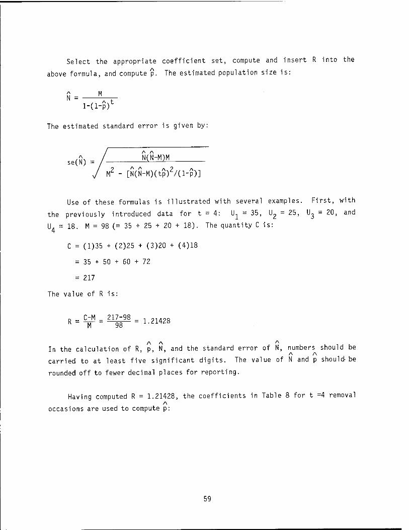
Select the appropriate coefficient set, compute and insert R into the

abo\ ̂e formula, and compute p. The estimated population size is:

A M Kl —

N ■ 1-d-p)1

The estimated standard error is given by:

,(\ / M-M)M se^iNj — /

y M2 - [N(N-M)(tp)2/(l-p)]

Use of these formulas is illustrated with severa exam pies. First, with

the previously introduced data for t = 4: U^ = 35 u2 = =25, U3 = 20, and

V =18. M = 98 (= 35 + 25 + 20 + 18). The quantity C

C = (1)35 + (2)25 + (3)20 + (4)18

=35+50+60+72

= 217

is:

The value of R is:

R = C"M = 21^-98 = 1.21428

In A A

the calculation of R, p, N, and the standard error of N, numbers A A

shou Id be

carried to at least five significant digits. The va lue of N and P shou Id- be

rounded off to fewer decimal places for reporting.

Having computed R = 1.21428, the coefficients in Table 8 for t = =4 removal

occasions are used to compute p:

59

p = 0.984082 - 0.820445 (1.21428) + 0.320498 (1.21428)2

- 0.141133 (1.21428)3

= 0.984082 - 0.996249 + 0.472566 - 0.252688

= 0.207710

A U

Using this estimate of capture probability, N = -~ can be computed: i-a-pr

A

N = 98

1-(1-0.207710)4

98

l-(0.792289)4

98 0.065964

= 161.7

Finally, the estimated standard error (the square root of the variance) A '

of N is computed. The numerator of the sampling variance is:

N(N-M)M = (161.7) (161.7 - 98) (98) = 1,009,428.42

The denominator is:

M2 - [N(N-M) (tp)2/(l-p)] =

982 - [161.7(161.7 - 98) (4(0.20771)) 2]/(l-0.20771)

= 9604 - [(161.7) (63.7) (0.83084)2]/0.792290

= 9604 - 8974.28943

= 629.71057

60

The estimated standard error of N in this example is:

ru\ / 1,009,428.42 seW V 629.71057

= / 1603.00378

= 40.0

An approximate 95% confidence interval on the unknown population size in

the study site is:

N ± 2 se(N)

For this example, the interval is 161.7 ± 2 (40.0) or 81.7 to 244.7. At this

point, it is acceptable to round off N and the interval limits to integers:

N = 162 and the approximately 95% confidence limits are 82 to 245 fish.

A

This example illustrates that the estimate of N is imprecise when the

capture probability is low (p of 0.20 is definitely low). The standard error

of 40, with N = 162, demonstrates that these electrofishing data are very

imprecise. So poor, in fact, that the lower confidence bound is less than the

98 fish actually removed. When this kind of discrepancy occurs, the lower

bound should be replaced by the number of fish actually removed, 98 in this

case.

A more abbreviated example is given below using better data: U1 = 157,

U? = 15, U3 = 1, and U4 = 0. The values of M and C are M = 173 and C = 190.

R = (190-173)/173 = 0.09826; p is computed from the polynomial specified by

the coefficients for t = 4:

p = 0.984082 - 0.820445(R) + 0.320498(R2) - 0.141133(R3)

= 0.90642

61

The estimate of population size is:

A 173 N = ^ = 173

l-(0.093578)4

with a standard error of, essentially, 0.0.

When p is at least 0.9, it is unnecessary to compute a standard error

because it would be essentially zero. The value of computing the standard

error is in representing the precision of the estimate N (see the section in

Chapter IV on interpreting sampling variation). To some extent, the reliabil- A A A

lty of N can be judged by the value of p. If p > 0.8, results are reliable A A

For 0.5 < p < 0.8, N is probably a good population estimate, although some

uncertainty remains about the actual number of fish in the sampled stream

segment. If 0.25 < p < 0.5, the results may not be very reliable, although

the estimate of N may be acceptable if three (or four, if p is near 0 25) A A '

removal passes were done. For p < 0.25, N can be very unreliable; it will not

only lack precision, but it can be severely biased by problems of unequal

capture probabilities that do not have much effect when p is large. If p <

0.10, the estimate of N is worthless. Note that, in the example above where

p = 0.20 and t = 4, N was imprecise; with such poor population estimates,

monitoring for management effects on fish abundance is a waste of time and

other resources.

Assessing the Fit of the Model

Given three or more removal passes, a chi-square goodness-of-fit test can

be used to test the assumption of equal probability (see White et al. 1982:

Chapter IV for details). As mentioned above, the assumption of equal probabil-

ity of capture between passes is only critical when p ranges from 0.2 to 0.5

for three or four removal occasions. It is unnecessary to apply the test if

most of the fish were caught during sampling.

62

A When capture probabilities are low and variable, N will be biased low

(see, e.g., Mahon 1980). Stratification by fish size and species helps to

overcome the problem of heterogeneous capture probabilities. If the data

still do not fit the model, the estimate can be accepted anyway or the

generalized removal estimator used (White et al. 1982: Chapter IV), which

sometimes helps improve the accuracy of the estimate. This approach is

complex, difficult to compute, and probably will not be very useful. There-

fore, it is not included here. Use of a computer program, especially CAPTURE

(White et al. 1982) or CMLE (Platts et al. 1983), is recommended in this

analysis.

Stratifying Data by Fish Size or Species

The estimator of population size previously presented is based on an

assumption of equal capture probability for all fish on each removal occasion.

This assumption is not critical if all of the fish of interest are caught.

However, if substantial numbers of fish are uncaught after the final pass,

model assumptions may not be met. Stratifying the removal data by fish size

classes or by species (or both) greatly helps to meet the assumptions for a

valid population estimate. Stratification based on size is especially

important in estimating biomass.

When stratifying data by size, two or three sizes classes are usually

enough. Data can be stratified on fish length because of the strong correla-

tion of length with weight and body surface area. Two size classes for rainbow

trout, for example, could be fish < 12 cm and fish > 12 cm.

If estimates are obtained by fish size class, their sum becomes the

estimate of the total number of fish of that species. The sampling variance

of that total is the sum of the sampling variances of the individual estimates.

For example:

63

Size class N se(N) var(N)

1 86 5.1 26.0 2 107 8.7 75.7 3 _43 3.2 10,2

Totals 236 m.g

The standard error of N = 236 is /ill.9 = 10.6, not the sum of the three

standard errors. Therefore, N = 236 is a reasonably good population estimate

for this species. If estimates of fish numbers are by species, simply add the

separate N values and their variances for the species involved to obtain an

estimate of the total population size and its variance.

Other population estimation methods. Capture-mark-recapture methods may

be desirable when survival rates and/or fish movements are being measured.

This method can also be used to estimate population size: For larger bodies

of water, other methods, such as capture-recapture or catch-effort may be

needed. However, these procedures are complex (see Seber 1973, 1982; Ricker

1975; Brownie et al. 1978; Otis et al. 1978; White et al. 1982). (Note that

the catch-effort method is primarily useful in commercial fisheries.)

The above methods generally require marking or tagging fish. An ideal

marking or tagging method would have the following characteristics (Laird and

Stott 1978):

1. Fish are permanently and unmistakably recognizable to anyone examin-

ing them;

2. The method is inexpensive;

3. The method is easy to apply under field conditions; and

4. The marking or tagging has no effect on fish growth, mortality,

behavior, susceptability to predation, or commercial value.

64

Unfortunately, no currently available technique has all of these criteria.

Various marking and tagging techniques are listed in Table 9. For further

discussion of these methods, see Laird and Stott (1978).

Table 9. Marking and tagging techniques (compiled from Laird and Stott 1978).

Marking techniques Tagging techniques

Fin clipping Opercular and fin punches Branding Tattooing Subcutaneous injection

dyes liquid latex vital stains fluorescent dyes

Subcutaneous tags External tags - wired on wire and plate tags hydrostatic tag (Lea tag) Petersen tag double attachment tag

External tags with an internal anchor spaghetti tag strap tag opercular tag jaw tag

Biomass

A_ — Biomass of fish within a site is estimated as NW, where W estimates the

A

average weight of all fish of the species or size class that N relates to.

Also, let se(W) represent the standard error of W. In the simplest case, a A

total of M fish are caught (= l^ + U2 + ...+ Ut); N is based on the successive

removals, and W is the average weight of the M fish caught. The standard

error of W is computed from the M individual values of fish weights, as per

the "usually" formula presented in Chapter IV. The standard error of total A _

biomass in the site, B(= NW), is approximately:

65

se(B) = B *P& + varlW) 1/2

(N)2 (W)

If it is necessary to stratify the data for a species in order to esti-

mate the population, then the total biomass in the site must also be computed

on this stratified basis. N and W are first computed for each strata.

If the removal data are stratified into two size classes, two pairs of A — A - ) r

values Np Wj and N2, W2 are calculated. Total biomass is:

A A _ A _ A A

B = NJWJ + N2W£ = ^+ Bz

A A A var(B) = var(Bp + var(B„)

Average fish weight in the site is B divided by N = N, + N?.

These formulae are valid regardless of the way W is computed. If many

fish are caught, they do not all have to be weighed. Average weight can be

estimated from a random subsample of fish caught. A more complex procedure is

to take the length of all fish, but weigh only a small number; e.g., the first 10 in each length class.

Length and weight must be recorded for each fish weighed, in addition to

the lengths of all fish caught but not weighed. The log of weight vs. log of

length (see Chapter V) is used to establish the relationship between length

and weight. The length-weight equation can then be used to predict the weight of the unweighed fish.

A less accurate but simpler approach to analyzing stratified data is

possible. Assume there are "r" 1-cm length intervals encountered and the

first 10 fish encountered in each length interval are weighed (or all are

weighed if less than 10 fish in a length interval are captured). The average

66

weight in each length interval is calculated, and the total number of fish in

successive 1-cm length intervals is tabulated. A table can then be developed

from these data:

Length class Av =rage wei ght Number caught

by length class

1 si nl

2 w2 n2

3 W3 n3

W n r r

The sum of the number of fish caught by length class (M) equals the total

number of fish removed. The averages W. are not generally based on all n.

fish in that 1-cm length interval because not all of the fish are weighed.

The estimator of the average weight of fish for the site is:

"A + n2W2 + n3W3+ ...+ nrWr W = R

Variance estimates for either the regression or weighed size class methods

can be derived. However, the procedure for the deviations is complex and is

not included in this manual.

67

SECONDARY VARIABLES

Variables other than those already discussed may be important in some

monitoring programs. These secondary variables may be habitat, fishery, or

biotic related.

Other Habitat Variables

Abiotic attributes that may be monitored under certain circumstances

include bedload, detritus, suspended solids, dissolved oxygen, pH, conduc-

tivity, alkalinity, hardness, nutrients, pesticides, metals, and salinity.

Literature is available on measurement techniques for all of these variables.

Two general references that may be useful are American Public Health

Association et al. (1971) and U.S. Geological Survey (1977).

Other Fishery Variables

Other fishery variables that can be monitored include age and growth,

food habits, production, survival or mortality, fucundity, parasitism, disease,

and net production. Measurement of many of these variables is discussed in

Ricker (1975) and Bagenal (1978).

Other Biotic Variables

If changes in the stream ecosystem are monitored hoiistically, organisms

besides fish (e.g., bacteria, periphyton, macrophytes, and macroinvertebrates)

can be sampled. There are various sampling techniques available for a number

of attributes that can be measured for each group of organisms. For example,

variables that may be of interest for macroinvertebrates include species

composition, biomass, relative abundance, emergence, and drift. General

sampling techniques for nonfish species are discussed in Cummins (1962),

Edmondson and Winberg (1971), Mason et al. (1973), Weber (1973), Benfield et

al. (1974), Greeson et al. (1977), Mason (1978), Resh (1979), and Platts et al.

68

(1983). References discussing other biotic variables that could be measured

include Edmondson and Winberg (1971), Langford and Daffern (1975), and Greeson

et al. (1977).

Identification of organisms requires someone knowledgeable about the taxa

sampled. For general information, see Usinger (1974) or Pennak (1978).

REFERENCES

American Public Health Association, American Water Works Association, and

Water Pollution Control Federation. 1971. Standard methods for the

examination of water and wastewater, 13th ed. 874 pp.

Arnette, J. L. 1976. Nomenclature for instream assessments. Pages 9-15 in

C. B. Stalnaker and J. L. Arnette, eds. Methodologies for the determina-

tion of stream resource flow requirements: an assessment. U.S. Fish

Wildl. Serv., Logan, UT.

Backiel, T. 1980. Introduction. Pages 1-5 in T. Backiel and R. L. Welcome,

eds. Guidelines for sampling fish in inland waters. European Inland

Fish. Advisory Comm. Tech. Pap. 33.

Bagenal, T., ed. 1978. Methods for assessment of fish production in fresh

waters. 3rd ed. Blackwell Scientific Publ., Oxford. IBP Handb. 3.

358 pp.

Bagenal, T. B, and F. W. Tesch. 1978. Age and growth. Pages 101-136 vn T.

Bagenal, ed. Methods for assessment of fish production in fresh waters.

3rd ed. Blackwell Scientific Publ., Oxford. IBP Handb. 3.

Benfield, E. F., A. C. Hendricks, and J. Cairns, Jr. 1974. Preferences of

two artificial substrates in collecting stream macroinvertebrates.

Hydrobiologia 45:431-440.

69

Beschta, R. L. 1982. Comment on "Stream system evaluation with emphasis on

spawning habitat for salmonids" by M. A. Shirazi and W. K. Seim. Water

Resources Research 18(4):1292-1295.

Binns, N. A. 1979. A habitat quality index for Wyoming trout streams.

Wyoming Game Fish Dept., Cheyenne. Fish. Res. Rep. 2. 75 pp.

Brownie, C, D. R. Anderson, K. P.'Burnham, and D. S. Robson. 1978. Statis-

tical inference from band recovery data - a handbook. U.S. Fish Wild!.

Serv. Resour. Publ. 131. 212 pp.

Corbett, D. M., N'. C. Grover, C. J. Paulsen, E. D. Burchard, M. H. Carson,

J. J. Dirzulaitis, H. E. Grosbach, A. B. Purton, M. R. Stackpole, C. H.

Pierce, G. C. Stevens, M. C. Boyer, and A. H. Frazier. 1945. Stream-

gaging procedure. A manual describing methods and practices of the

Geological Survey. U.S. Geol. Surv., Water Supply Pap. 888. 245 pp.

Craig, J. F. 1980. Sampling with traps. Pages 55-70 In T. Backiel and R. L.

Welcomme, eds. Guidelines for sampling fish in inland waters. European

Inland Advisory Comm. Tech. Pap. 33.

Cummins, K. W. 1962. An evaluation of some techniques for the collection and

analysis of benthic samples with special emphasis on lotic waters. Am.

Midi. Nat. 67:477-512.

Dauble, D. D., and R. H. Gray. 1980. Comparison of a small seine and a

backpack electroshocker to evaluate near shore fish populations in rivers.

Prog. Fish-Cult. 42:93-95.

earn Duff, D. A., and J. L. Cooper. 1976. Techniques for conducting a str

habitat survey on National Resource Land. U.S. Bur. Land Manage. Tech

Note 283. 72 pp.

70

Edmondson, W. T., and G. G. Winberg, eds. 1971. A manual on methods for the

assessment of secondary productivity in fresh water. Blackwell Scientific

Publ., Oxford. IBP Handb. 17. 358 pp.

Eiserman, F., G. Dern, and J. Doyle. 1975. Cold water stream handbook for

Wyoming. U.S. Soil Conserv. Serv. and Wyoming Game Fish Dept. 38 pp.

Everest, F. H., C. E. McLemore, and J. F. Ward. 1980. An improved tri-tube

cryogenic gravel sampler. U.S. For. Serv., Pacific Northwest For. Range

Exp. Stn., Res. Note PNW-350. 8 pp.

Greeson, P. E., T. A. Ehlke, G. A. Irwin, B. W. Lium, and K. V. Slack, eds.

1977. Methods for collection and analysis of aquatic biological or

microbiological samples. Techniques for water-resources investigations

of the United States Geological Survey. Book 5, Chapter 4A. U.S. Geol.

Surv. 332 pp.

Gulland, J. A. 1980. General concepts of sampling fish. Pages 7-12 HI T.

Backiel and R. L. Welcomme, eds. Guidelines for sampling fish in inland

waters. European Inland Fisheries Advisory Comm. Tech. Pap. 33.

Hall, J. D., and R. L. Lantz. 1969. Effects of logging on the habitat of

coho salmon and cutthroat trout in coastal streams. Pages 191-200 in T.

G. Northcote, ed. Symposium on salmon and trout in streams. Univ.

British Columbia, Vancouver, BC.

Harrison, C. W. 1923. Planting eyed salmon and trout eggs. Trans. Am. Fish.

Soc. 53:191-200.

Hartley, W. G. 1980. The use of electrical fishing for estimating stocks of

freshwater fish. Pages 91-95 jn T. Backiel and R. L. Welcomme, eds.

Guidelines for sampling fish in inland waters. European Inland Fish.

Advisory Comm. Tech. Pap. 33.

71

Henderson, H. F. 1980. Some statistical considerations in relation to

sampling populations of fishes. Pages 167-176 Jji T. Backiel and R. L.

Welcomme, eds. Guidelines for sampling fish in inland waters. European

Inland Fish. Advisory Comm. Tech. Pap. 33.

Hendricks, M. L., C. H. Hocutt, Jr., and J. R. Stauffer, Jr. 1980. Monitoring

of fish in lotic habitats. Pages 205-231 _in C. H. Hocutt, Jr., and

J. R. Stauffer, Jr., eds. 1980. Biological monitoring of fish.

Lexington Books, Lexington, MA.

Herke, W. H. 1977. An easily made, durable fish-measuring board. Prog.

Fish-Cult. 39:47-48.

Holden, A. V. 1980. Chemical methods. Pages 97-104 jn T. Backiel and R. L.

Welcomme, eds. Guidelines for sampling fish in inland waters. European

Inland Fish. Advisory Comm. Tech. Pap. 33.

Keller, C. R., and K. P. Burnham. 1982. Riparian fencing, grazing, and trout

habitat preference on Summit Creek, Idaho. N. Am. J. of Fish. Manage.

2:53-59.

Lagler, K. F. 1978. Capture, sampling and examination of fishes. Pages 7-47

j_n T. Bagenal, ed. Methods for assessment of fish production in fresh

waters. 3rd ed. Blackwell Scientific Publ., Oxford. IBP Handb. 3.

Laird, L. M., and B. Stott. 1978. Marketing and tagging. Pages 84-100 jn T.

Bagenal, ed. Methods for assessment of fish production in fresh water.

3rd ed. Blackwell Scientific Publ., Oxford. IBP Handb. 3.

Lane, E. W. 1947. Report of the subcommittee on sediment terminology.

Trans. Am. Geophysical Union 28(6):936-938.

72

Langford, T. E., and J. R. Daffern. 1975. The emergence of insects from a

British River warmed by power station cooling-water. Part I. Hydro-

biologia 46:71-114.

Lawrence, J. M. 1956. Preliminary results of the use of KMN04 to counteract

the effects of rotenone. Proj. Fish-Cult. 10(1):15-21.

Leopold, L. B., M. G. Wolman, and J. P. Miller. 1964. Fluvial processes in

geomorphology. W. H. Freeman and Co., San Francisco. 522 pp.

Lotspeich, F. B., and F. H. Everest. 1981. A new method for reporting and

interpreting textural composition of spawning gravel. U.S. For. Serv.,

Pacific Northwest For. Range Exp. Stn., Res. Note PNW-369. 11 pp.

Lotspeich, F., and B. Reid. 1980. A tri-tube freeze core procedure for

sampling stream-gravel. Prog. Fish-Cult. 42:96-99.

Lowe-McConnell, R. H. 1978. Identification of freshwater fishes. Pages 48-83

in T. Bagenal, ed. Methods for assessment of fish production in fresh

waters. Blackwell Scientific Publ., Oxford.

Mahon, R. 1980. Accuracy of catch-effort methods for estimating fish density

and biomass in streams. Environmental Biology of Fishes 5(4):343-360.

Mason, W. T., Jr. 1978. Methods for the assessment and prediction of mineral

mining impacts on aquatic communities: a review and analysis. Workshop

proceedings. U.S. FishWildl. Serv. FWS/OBS-78/30. 157 pp.

Mason, W. T., C. I. Weber, P. A. Lewis, and E. C. Julian. 1973. Factors

affecting the performance of basket and multiple macroinvertebrate

samples. Freshwater Biol. 3:409-436.

McNeil, W. J. 1964. A method of measuring mortality of pink salmon eggs and

larvae. U.S. Fish Wild!. Serv. Fish. Bull. 63(3):575-588.

73

McNeil, W. J., and W. H. Ahnell. 1964. Success of pink salmon spawning

relative to size of spawning bed materials. U.S. Fish Wildl. Serv.

Special Sei. Rep. 469. 15 pp.

Otis, D. L, K. P. Burnham, G. C. White, and D. R. Anderson. 1978. Statis-

tical inference from capture data on closed animal populations. Wildlife

Monograph 62:1-135.

Pennak, R. W. 1978. Freshwater invertebrates of the United States. John

Wiley & Sons, NY. 803 pp.

Phillips, R. W., L. L. Lantz, E. W. Claire, andJ. R. Moring. 1975. Some

effects of gravel mixtures on emergence of coho salmon and steelhead

trout fry. Trans. Am. Fish. Soc. 105(3):461-465.

Platts, W. S. 1974. Geomorphic and aquatic conditions influencing salmonids

and stream classification-with application to ecosystem management. U.S.

For. Serv., SEAM Program. 199 pp.

Platts, W. S., and V. E. Penton. 1980. A new freezing technique for sampling

salmonid redds. U.S. For. Serv. Intermountain For. Range Exp. Stn. Res.

Pap. INT-248. 22 pp.

Platts, W. S., W. F. Megahan, and G. W. Minshall. 1983. Methods for evaluat-

ing stream riparian and biotic conditions, U.S. For. Serv. For. Range

Exp. Stn., Gen. Tech. Rep. INT-138. 70 pp.

Platts, W. S., M. A. Shirazi, and D. H. Lewis. 1979. Sediment particle sizes

used by salmon for spawning with methods for evaluation. U.S. Environ.

Protection Agency, Corvallis, OR. 32 pp.

Resh, V. H. 1979. Sampling variability and life history features: basic

considerations in the design of aquatic insect studies. J. Fish. Res.

Board Can. 36:290-311.

74

Ricker, W. E. 1975. Computation and interpretation of biological statistics

of fish populations. Bull. Fish. Res. Board Can. 191. 382 pp.

Ringler, N. H. 1970. Effects of logging on the spawning bed environment in

two Oregon coastal streams. Oregon State Univ., Corvallis. 96 pp.

Seber, G. A. F. 1973. The estimation of animal abundance. Charles Griffin &

Co. Ltd., London. 506 pp.

Seber, G. A. F. 1982. The estimation of animal abundance (second edition).

MacMillan, New York. 665 pp.

Stalnaker, C. B., and J. L. Arnette. 1976a. Basic stream flow measurements

and relationships. Pages 16-34 i_n C. G. Stalnaker and J. L. Arnette,

eds. Methodologies for the determination of stream resource flow require-

ments: an assessment. U.S. FishWildl. Serv., Logan, UT.

. 1976b. Methodologies for determining instream flows for fish

and other aquatic life. Pages 89-138 in C. B. Stalnaker and J. L.

Arnette, eds. Methodologies for the determination of stream resource

flow requirements: an assessment. U.S. FishWildl. Serv., Logan, UT.

Stevens, H. H., Jr., J. F. Ficke, and G. F. Smoot. 1975. Water temperature-

influential factors, field measurement, and data reduction. Techniques

of water-resources investigations of the United States Geological Survey.

Book 1, Chapter Dl. U.S. Geol. Surv. 65 pp.

Tappel, P. D. 1981. A new method of relating spawning gravel composition to

salmonid embryo survival. M.S. Thesis, Univ. Idaho, Moscow. 53 pp.

Traco Jitco, Inc. 1978. Quality assurance guidelines for biological testing.

U.S. Environ. Protection Agency, Environ. Monitoring and Support Lab.,

Las Vegas, NV. EPA-600/4-78-043. 600 pp.

75

U.S. Geological Survey. 1977. National handbook of recommended methods for

water-data acquisition. U.S. Geol. Surv. v. p.

Usinger, R. L., ed. 1974. Aquatic insects of California. Univ. California

Press, Berkeley. 508 pp.

Walkotten, W. J. 1976. An improved technique for freeze sampling streambed

sediments. U.S. For. Serv., Pacific Northwest For. Range Exp. Stn., Res.

Note PNW-281. 11 pp.

Walkotten, W. J., and M. D. Bryant. 1980. An instrument to measure stream

channel gradient and profiles. Pacific Northwest For. Range Exp. Stn.,

Res. Note PNW-345. 5 pp.

Weber, C. I., ed. 1973. Biological field and laboratory methods for measuring

the quality of surface waters and effluents. U.S. Environ. Protection

Agency, Natl. Environ. Research Center. EPA-670/4-73-001. 190 pp.

Wesche, T. A. 1973. Parametric determination of minimum streamflow for

trout. Univ. Wyoming, Water Resour. Res. Inst., Laramie. Water Resour.

Ser. 37. 102 pp.

• 1974. Relationship of discharge reductions to available trout

habitat for recommending suitable streamflows. Univ. of Wyoming, Water

Resour. Res. Inst., Laramie. Water Resour. Ser. 53. 71 pp.

White, G. C, D. R. Anderson, K. P. Burnham, and D. L. Otis. 1982. Capture-

recapture and removal methods for sampling closed populations. Los

Alamos Natl. Lab. Rep. LA-8787-NERP. 235 pp.

Zippin, C. 1958. The removal method of population estimation. J. Wild!.

Manage. 22(l):82-90.

76

CHAPTER IV. BASIC STATISTICAL AND STUDY DESIGN CONCEPTS

BASIC TERMS

Statistics refers to the science of organizing and summarizing sample

data from a population to develop inferences. A population, in the biological

context, is the total number of a species in a specific area; e.g., total

number of rainbow trout in a given watershed. For most practical purposes, it

is impossible to measure all individuals in a population to calculate descrip-

tive features or parameters. Estimates of the parameters (Table 10) can be

derived, however, by sampling the population and applying statistical

procedures to the data.

Table 10. Parameters and their statistical estimators.

Parameter Statistical estimator

v mean y A

2 variance a

standard deviation o s

2 s

77

Measurement variables for a statistical population can be either contin-

uous or discrete. Continuous variables are usually measurements; e.g., stream

width or water temperature, which can be any value within a range. Discrete

variables have a limited number of possible values; e.g., count data (such as

numbers of fish in a gill net) or classification values (such as stable or

unstable stream banks).

A statistic computed to estimate a population parameter generally differs

from sample to sample because of natural variability. However, statistical

methods can be used to make inferences about parameters from sample data with

defined levels of statistical confidence. Confidence is discussed later in

this chapter.

DESCRIPTIVE FEATURES

Summary statistics are used to describe properties of sample data. The

sample mean is one of several statistics used to describe central tendency.

The equation for the mean is:

X, + X? + ... + X EX. X = -J 2 n = _JI

n n

where IX. = the sum of all the sample values

n - the number of observations or sample size

As an example, let a sample of size 15 (e.g., fish lengths rounded to centi-

meters), recorded in ascending order, be 6, 8, 9, 10, 11, 11, 11, 12, 12, 13,

13, 14, 16, 20, and 22. The mean of these values is:

x - 6 + 8 + ... +21 _ 186 .- . x 15 " TT = UA

78

This same sample of 15 values is used below to illustrate other statistical

procedures.

The sample median is the value that divides arranged data (values arranged

from the lowest to the highest) into two equal parts. That is, half of the

values in the array exceed the median, and half are less than the median.

When there are an odd number of observations (n) in an array, the median is

simply the mth value in the sequence, where m = (n+l)/2. When the sample size

is even, the median is the average of the two central most values: Xm

X +1, where m = n/2.

and

In the above example, n = 15, m = 16/2 = 8, and Xg = 12 is the median,

If n = 14 because X,c = 22 was not recorded, the median would be computed as: lb

X7 + X8 = 11 + 12 = n 5

The sample mode is the value represented by the greatest number of indi-

vidual observations in a sample. On a frequency curve, it is the value of the

variable where the peak of the curve occurs. In the above sample, the value

11 occurs most frequently (Xg = Xg = X? = 11) and is the sample mode. In this

example, the mean, median, and mode are close to each other, but not identical.

This is often the case. The mean, median, and mode of a hypothetical set of

data are illustrated in Figure 7.

For some types of data; e.g., lognormal (a skewed distribution) or annual

survival rates over a period of years, the geometric mean is more appropriate

for describing the central tendency than is the arithmetic mean. The geometric

mean of n numbers is defined by:

79

>» o c cu =3 cr CD s-

Figure 7. A frequency distribution (skewed to the right) indicating the location of the mean, median, and mode. These values relate to the central tendency for a data set.

80

X = (X, x X9 ... XJ1/n g v 1 2 n'

which is the product of the numbers raised to the power 1/n. The recommended

calculation to obtain a geometric mean is to take the log of each sample

value, compute the arithmetic mean of these logs, and then take the antilog of

this arithmetic mean:

I log X.' X = antilog 1 — 9 \ n

The logs, to base 10, for the above 15 sample values are 0.7782, 0.9031,

0.9542, 1.0, 1.0414, 1.0414, 1.0414, 1.0792, 1.0792, 1.1139, 1.1139, 1.1461,

1.2041, 1.3010, and 1.3424. The mean of these logs is X = 1.0760. The

geometric mean of the original sample is:

X = antilog (X) = 10X = lo1-0760 = 11.9 g

(Note: The geometric mean can only be computed if all sample values are

greater than zero).

Just as the mean, median, and geometric mean are used to describe the

central tendency for a set of data, other statistics can be used to describe

the variation or scatter in the sample values. The range, which is simply the

difference between the highest and lowest sample values, is an estimate of the

variation of values in a sample. (In the above example, the range is

22 - 6 = 16.0.) Because it is based only on the two most extreme values, the

range does not indicate the average variation among the sample values.

81

The sample standard deviation (s) is the statistic typically used to

describe the average variation among the sample values:

I (X.- X)2

n-1

Except for the divisor being n-1 rather than n, s is the square root of the

average squared deviation of each value from the sample mean. Computation of

the sample standard deviation by application of the above equation is tedious

even for a moderate number of observations. Use of an alternative formula

requires computation of only the sum of the sample values (IX) and the sum of

the squared sample values (EX ):

9 IX.2 - - (EX.)2 2 _ i n v -r

n-1

In the example being used here, EX. = nX = 186 and E(X.)2 = 62 + 82 + ... +

222 = 36 + 64 + ... + 484 = 2606. Hence, for this sample:

2 = 2606 - (186)2/15 _ 299.6 _ 01 ,n

S 14 " 14 " li-W

s = 4.63

When the sample mean is used to estimate the population mean (y), the precision

of this estimate depends on both the sample size and the innate sampling

variation in the population, as estimated by the standard deviation, s. The

sampling variance of X is estimated as:

82

2 var(X) = ^

The square root of this variance is an often needed quantity in statistical

inference. It is called the standard error of the mean to distinguish it from

the standard deviation; i.e., se(X) = s//n~ (see, e.g., Tacha et al. 1982).

For the current example, se(X) = 4.63//15 = 1.20.

The relative variation among the sample values is often described by the

sample coefficient of variation, cv, which is the sample standard deviation

expressed as a percentage of the sample mean:

s cv = -

The coefficient of variation is usually reported on a percent basis; i.e.,

percent cv = 100s/X. In the example, cv = 4.63/12.4 = 0.3734 or, as a percent,

37.3%.

The sample mean and standard deviation provide "point" estimates of the

corresponding population parameters. In addition to such point estimates, it

is useful to have "interval" estimates; i.e., an interval such that the true

parameter falls inside the interval with a known probability. One easily

computed type of interval is confidence intervals. A confidence interval can

be calculated for most population parameters estimated by a statistic. For

example, the interval for a population mean (y) for normally distributed data

is expressed as:

* - Vn-l5600 < » K * + Vn-l^*)

83

where t 1 = the tabular value for the t statistic a, n-l

a = 1 - the confidence level; e.g., 1 - 0.95 = 0.05

n = number of observations in the sample (the sample size)

n-l = degrees of freedom for the t statistic

se(X) = standard error of the mean, X

By selecting a 95% confidence level, a user can conclude, with 95% confidence,

that the unknown value of y is between the lower [X - t ,se(X)l and the _ _ a,n-l v /J

upper [X + t n_iSe(X)] computed confidence limits.

Methods for computing confidence intervals are included in most statis-

tical texts, including Sncdecor and Cochran (1967).

Computational methods for descriptive statistics discussed in this section

are demonstrated in Example 1 later in this chapter.

FREQUENCY DISTRIBUTIONS

The basic paradigm of statistics is that sample data can be described

(modeled) by probability (frequency) distributions. Most data analysis methods

make some assumptions about the type, or properties, of the probability model

that describes (fits) the data. If these assumptions are wrong, the results

of the analysis may be misleading. Consequently, it is important to know what

distribution describes the data. The distribution can be determined on three

types of information: (1) theoretical considerations (not usually very applic-

able in environmental work); (2) past experience; and (3) empirical examination

of the present data, especially plotting it.

When samples are obtained from a population, the data should be summarized

graphically to determine the applicable type of probability distribution

(Fig. 8). Commonly used models for discrete or count data are the positive

84

>> (J E <D 13 cr O)

4-

0) >

*r—

+■> n3

3 fc: 3 O

99. 99

50 00

0 01

99.99

50.00

0.01 Normal distribution

-s

c

n <<

skewed to left negative binomial, Poisson distribution

skewed to right Lognormal distribution

Figure 8. Types of frequency distributions and their plots on normal probability paper. The continuous curves under the upper plots for each example represent a distribution before plotting on normal probability paper (after Sokal and Rohlf 1969). A positive binomial distribution with a large sample size (n) would resemble a normal distribution.

85

binomial, the negative binomial, and the Poisson distributions. Explanations

of these distributions and statistical applications are contained in many

basic statistics texts; e.g., Snedecor and Cochran (1967) and Elliot (1977).

The normal distribution is probably the most widely used (and, unfor-

tunately, the most widely abused) model for continuous measurement variables.

The normal distribution, colloquially described as the bell-curve, is com-

pletely determined by the mean (y) and standard deviation (o) of the popula-

tion. Figure 9 illustrates a normal frequency curve. As indicated in

Figure 9, on the average, 68.3% of the sample values will be within ± la of

the mean, and 99.7% will be within ± 3a of the mean. For sample data from a

normally distributed population, X is substituted for y, and s is substituted

for o. Several nonnormal frequency distributions have been postulated for

application to continuous data (Johnson and Kotz 1970a,b). The lognormal

distribution (Fig. 10) has applicability to parametric tests because, when the

data are transformed by logarithms, they have a normal distribution. For many

variables, such as fish weight or length, the lognormal distribution may be a

more reasonable model than the normal distribution. The lognormal distribution

has also been used to model discrete variables, such as counts of fish or

species abundance (Pielou 1975). Some examples of statistical computations

are as follows.

Example 1

Problem: In a stream monitoring study, the following 10 temperatures (°C)

were taken in the managed site.

8.0 10.0 8.0 10.5 8.5 11.0

10.0 11.5 10.0 12.0

Give the descriptive statistics for these data, assuming no data trans-

formation is necessary or desired.

86

-3or -2cr -lcr -+—

0

8.3%

lcr 2cr 3o-

Z= X-u

95.5%

99.7%

Figure 9. A normal distribution.

87

Figure 10. A lognormal distribution,

88

Solution:

IX. 1. The mean, X = ——

y = 99.5 _ Q gc * 10.5

2. The median is the average of the (^ and (j + l) (fifth and

sixth, in this example) ordered values because there is an even number of temperature values:

Median = ~ 10

3. The mode is the most common value:

Mode = 10

4. The range is 12.0 - 8.0 = 4.0°C.

5. The sample standard deviation s is computed as:

IX2 - I (IX)2 s= Fl

£X2 = 64 + 64 + ... + 144 = 1007.75

1007.75 - jfj (99.5)2

= ±u = 1.403 n - 1

6. Percent coefficient of variation, cv = - x 100

cv = Y^ x 100 = 14.1%

89

7. The standard error of the mean is:

se(X) = i- = LiM = 0.444 /n~ /TO

8. Confidence limits for the true population mean, y (L = lower limit, U = upper limit):

L = X - t .seCX) ct,n-l v '

Let a = 0.05, which corresponds to a 95% confidence level Thus, tQ 05 g = 2.262, and

L = 9.95 - (2.262)(0.444) = 8.95

U = X + t n .se(X) a,n-1 v '

U = 9.95 + (2.262)(0.444) = 10.95

Therefore, 8.95 < y < 10.95 is the 95% confidence interval.

Example 2

Problem: The same data are used as in example 1, but a lognormal distribution

is assumed. The appropriate analysis in this case is to transform

each datum X to log(X) (base 10 will suffice), do the same statis-

tical analyses, and back-transform appropriate estimates (it is not

appropriate to back-transform variances, standard deviations, or standard errors).

The log(X) data are

0.9031 1.0 0.9031 1.0212 0.9294 1.0414 1.0 1.0607 1.0 1.0792

90

Solution:

1. The mean of these logs is:

log(X) = ^|JP = 0.9938

The antilog of this value is the geometric mean X :

X = antilog (0.9938) = 9.86

Compare this value to the arithmetic mean of 9.95.

Note that the geometric mean is less than the arithmetic mean. This will always be true.

2. The median is:

log(X5) + log(X6) _ 2 1

Back-transforming, 10 = antilog (1). In general, the median computed this way does not necessarily equal the median of the untransformed data.

3. The mode is:

10 = antilog(l)

Transformations do not change the estimate of the mode.

4. The range of the transformed data (1.0792 - 0.9031 = 0.1761) can be computed, but should not be back-transformed because it does not produce a valid estimate of range for the untransformed data.

5. The standard deviation of the log(X) data is needed to compute a confidence interval on y:

2 9.912 - |Q(9.9381)2

s = ä

91

s2 = 0.003944 or

s = 0.06280

6. The standard error of the mean of the log(X) values is:

0.06280 se(log(X)) =

u-u^ou = 0.01986 /1Ö

7. To obtain a 95% confidence limit on the true population mean, y, first compute the mean from the transformed data, then back transform the resultant lower and upper limits. Using a = 0.05, hence t0 05 9 = 2-262> comPute upper and lower limits with the

transformed data:

L = log(X) - 2.262 se(log(X))

L = 0.9938 - 2.262(0.01986) = 0.9489

Similarly,

U = 0.9938 + 2.262(0.01986) = 1.0387

Now back transform both limits by the antilog:

Lg = antilog(L) = icr9489 = 8.89

U = antilog(U) = lo1'0387 = 10.93 y

Therefore, 8.89 < y < 10.93 is the 95% confidence interval when proper analysis requires a log transformation.

STATISTICAL TESTING

Hypothesis testing is an important facet of statistical analysis. A

hypothesis is generally a statement about one or more parameters that needs to

be tested. For example, a field biologist might hypothesize that fish under

92

particular environmental conditions are not affected by a new management

practice. Statistical tests could be based on mean weights (X) of samples

from the population. The hypothesis could be that the mean weight of fish in

a managed area is equal to the mean weight in a control area; symbolically,

the null hypothesis is H :yj = vz- The symbol ^ represents the true popula-

tion mean for the managed area; y2 corresponds to^the true mean for the control

area. These means are estimated by Xj and X2, respectively. The null

hypothesis is either rejected or fails to be rejected (in which case it is

tentatively accepted), depending on the results of the appropriate statistical

test.

The alternative hypothesis, denoted by Ha, should be either y1 i y2> v1 >

y„, or y, < y2. The three alternative hypotheses represent situations where

the mean weights for the two zones are different, the mean weight is greater

in the managed zone, and the mean weight is less in the managed zone, respec-

tively. To test the null hypothesis, a significance level is designated;

e.g., 0.05. Significance refers to the probability of rejecting the null

hypothesis, H , when it is true. A significance level of 0.05 means that, if

H is rejected, there is a 95% confidence that the rejection is correct. An

appropriate statistical analysis for testing the null hypothesis against the

alternative hypothesis must be selected, along with the significance level.

Acceptance or rejection of the null hypothesis is determined by comparing the

computed test value, e.g., a t-value, against a critical value (Fig. 11)

determined by the theoretical sampling distribution of the test statistics

(see White et al. 1982:Chapter 2).

For example, suppose the null hypothesis HQ: ]X^ = y2 versus hM yj t y2

is to be tested using a t-test, and the designated significance level is 0.05

(denoted as a). This would be a "two-tailed" test and a statistical table

would be used to find the critical (i.e., rejection-level) t-value for the

appropriate degrees of freedom (df). Suppose this tabular value is ± 2.07 for

t ,„ J£ and the computed test statistic value is 2.78. Because the test a/2,df . statistic is greater than 2.07, the null hypothesis is rejected with 95^

confidence that the true population means are unequal.

93

«/2,df +t a/2,df

A. Acceptance and rejection regions for a computed t-value for H

versus H »1 = v2

Vj * v2> "two-tailed" test.

a,df

Acceptance and rejection regions for a t-test for H c Ha: Vl > vz„ tailed" test.

Vi = v? versus

one-

a,df

Acceptance and rejection regions for a t-test for H c Ha: Vl < y2,

tailed" test.

y-, = ]ip versus

one-

Figure 11. Rejection and acceptance regions for comparing a null versus an alternative hypothesis. Critical rejection regions (the tails" of the distribution curve) contain slash marks. Computed

values for data are compared to table values.

94

Two types of errors are possible when a hypothesis is tested. The first

type (Type I) is rejecting the null hypothesis when it is true; the second

type (Type II) is failing to reject the null hypothesis when it is false.

When a 0.05 o-level is stipulated and the null hypothesis is rejected, an

asterisk (*) is often used to denote this significance level. The computed

statistic can usually be compared against tabular values for a = 0.01(**) and

a = 0.001(***), as well as for a = 0.05. The probability of a Type I error is

always a, the level of significance. An a of 0.05 represents one chance in 20

that failure to reject the null hypothesis is wrong. The chances of making a

Type I error increases as the a value increases.

The probability of a Type II error, often denoted by ß, is a function of:

(1) the choice of a; (2) the statistical test used (given the choice of a);

(3) the difference between the true parameter value and the hypothesized

parameter value; and (4) the number of observations (sample size). The power

(or sensitivity) of a statistical test is the probability of rejecting the

null hypothesis when it is, in fact, false; thus, power is 1-ß; i.e., unity

minus the probability of a Type II error. When the true parameter value is

greatly different than the hypothesized value, the test chosen should have a

very high probability of detecting this difference; i.e., have a high power.

The "standard" statistical tests (e.g., t-test and F-test) have this property

when certain assumptions, such as normality, are met. The power of a statis-

tical test decreases drastically when parameter values for the null and the

alternative hypothesis are close together because of the difficulty in

differentiating between the hypotheses with a statistical test (Sokal and

Rohlf 1969). The sample size must be increased to increase the power of a

given test (or decrease ß) while keeping a constant for a stated null

hypothesis. However, with respect to sample size, a bigger sample does not

necessarily mean a substantially "better" test because the power of most

statistical tests is a complex function of several factors, including sample

size. Power can also be increased by changing the nature of the test, usually

through better study design. In fact, use of a good study design is the most

efficient way to increase the power of these statistical tests.

95

In summary, the ideal statistical test has a small probability of reject-

ing the null hypothesis when it is true and a large probability of rejecting

it when it is false (Elliot 1977). Hypotheses are tested to determine if the

values obtained from two or more sites (control and managed) are from the same

statistical population or from different statistical populations. Two types

of errors can be made, Type I and Type II. Because it is always possible

(though highly improbable) that a highly deviant test value could be obtained

by chance even when HQ is true, a statistical test never proves that a partic-

ular null hypothesis is false (Elliot 1977). Similarly, rejection of the null

hypothesis does not prove that the alternative hypothesis is true; it only

provides good evidence that it is true. Finally, failure to reject H does

not prove that H is true.

The process of hypothesis testing is basic to all areas of science and

can be summarized as follows:

1. Formulate the null and alternative hypotheses, H and H . 0 3

2. Specify the significance level a9.

3. Determine the statistical test to be used.

4. Determine the "rejection region" for the test.

5. Calculate the test statistic.

6. Reject or accept the null hypothesis depending on the numerical

value of the computed test statistic relative to the theoretical

rejection region.

9Most a values used for computations in this manual are a= 0.05. However, other a values can be selected for these tests.

96

This general procedure is followed in the examples given in Chapter V.

(For more explanation of parametric testing in a biological context, see White

et al. 1982:Chapter 2.)

PARAMETRIC AND NONPARAMETRIC TESTS

Two types of statistical tests are discussed in this manual: parametric

and nonparametric (discussed briefly). Parametric tests, as the name implies,

require certain assumptions about population parameters. Conversely, nonpara-

metric tests are not dependent on a given parametric distribution and, thus,

are distribution-free tests (Sokal and Rohlf 1969). Nonparametric tests are

often easier to compute than parametric tests but generally have less power.

Parametric tests make maximum use of all the information that is inherent in

the data when the necessary assumptions are met.

Nonparametric procedures are appropriate in the'following situations:

1. The hypothesis to be tested does not involve a population parameter.

2. The data have been measured in some way other than that required for

the parametric procedure that would otherwise be appropriate. For

example, count or rank data may be available, precluding the use of

an otherwise appropriate parametric procedure that requires contin-

uous data.

3. The assumptions necessary for the valid use of a parametric procedure

are not met. In many instances, the design of a research project

may suggest a certain parametric procedure. Examination of the

data, however, may reveal that one or more assumptions underlying

the test are not met. In this situation, a nonparametric procedure

is frequently the best alternative.

97

4. Results are needed in a hurry and calculations must be done by hand,

so tests that are easily calculated are necessary.

The assumptions that need to be met for classical parametric tests (such

as the t-test and various analyses of variance; i.e., the F-test) are (Siegel

1956):

1. The observations must be independent; i.e., randomly obtained;

2. The observations must be drawn from normally distributed popula-

tions; and

3. These populations must have the same variances: homogeneity of

variances (see Fig. 12) or homoscedasticity (or, in special cases,

they must have a known ratio of variances).

The basic assumption of all parametric tests is that sampling of individ-

uals is random (this does not mean haphazard). Nonrandomness of sample

selection may be reflected in lack of independence of the sample items, in

heterogeneity of variances (i.e., different variances for control vs. treatment

sites), or nonnormal distribution of the data.

Before proceeding with a parametric test, it should be determined if the

assumptions are reasonable, and verification tests should be conducted (Sokal

and Rohlf 1969). Several methods are available to test these assumptions; the

less complex tests are presented in this manual. Although many parametric

statistical methods are not greatly affected by small departures from

normality, a major violation of the required assumption of normality may

render any statistical inference based on the sample data almost meaningless.

98

Figure 12. Graphic demonstration of homogeneity of variance. Means are different but shapes of distri- bution are similar (Huntsberger 1967).

99

Four common methods for testing the assumption of normality are:

1. The graphic method;

2. The chi-square goodness-of-fit test;

3. The Wilk-Shapiro test (sample size n < 50); and

4. The Kolmogorv-Smirnov test (n > 50).

The graphic method, which involves plotting the data on normal probability

paper, is used for demonstration purposes in this text. When there are indica-

tions that the data are not normally distributed, e.g., a straight line is not

appropriate for the data points, a transformation of the data should be

attempted (Table 11). For example, if the data are plotted in a histogram and

the distribution appears to be lognormal (Fig. 10), then the individual values

in the data set should be converted to logarithms and replotted on normal

probability paper. This transformation usually results in normality, which

permits application of parametric tests.

Another approach to testing the appropriateness of a log transformation

is to plot the data on lognormal probability paper. If a straight line can be

plotted through the data points, the log-transformation is appropriate, and

the normal probability plot test is unnecessary. Methods of testing for

normality that are more quantitative are described in standard statistical

references, including Snedecor and Cochran (1967) and Sokal and Rohlf (1969).

The assumption for homogeneity of variance (Fig. 12), often necessary

when multiple data sets are being compared, can be preliminarily tested by the

normal probability plot approach. If the lines for the different data sets

are parallel, the variances are homogeneous. If the lognormal probability

plot approach is used and the lines are parallel, it is a positive test for

homogeneity of variance for lognormal data.

100

Table 11. Data transformations used for various probability distributions or when the population mean y and standard deviation a have a given relationship.

Population Relationship Transformation distribution of o to ya

Poisson a • y /T /~x~ or /"x" + 0.5

Binomial c / y(l-y) sin" (/x)

Negative binomial6 f / y(l + gv) sinh(/~x) or

sinh(/ x + 1)

Lognormal or Empirical by 1og(x) or log(x + 1)

Empirical dy(l-y) MFX")

Empirical e(l-y) log(^-^)

aa, b, c, d, e, f, and g are constants that may be known or unknown.

bThe transformation is the hyperbolic sine function, sinh(y) = (ey-e y)/2.

101

The F-test can be used to quantitatively test for homogeneity of variance

for two sample sets (e.g., control vs. treatment data) for the hypothesis H :

2 _ 2 2 2 °1 ~ °2 versus H

a: ai * °2 • Homogeneity for more than two sets of data

can be tested with Bartlett's test (Sokal and Rohlf 1969).

If the assumptions for parametric tests are not reasonably met, then two

basic choices remain: transform the data as previously discussed or use a

nonparametric test. Fortunately, a single transformation will often simulta-

neously solve several departures from the assumptions (Table 11 and see Sokal

and Rohlf 1969). For the logarithmic transformation, if the data set contains

zeros, use log(x + 1). When a transformation is done, tests of significance

are performed on the transformed data, although estimates of means (and confi-

dence intervals) are usually back-transformed in order to be presented in the

untransformed scale (Sokal and Rohlf 1969).

The statistical tests selected for use in a monitoring program depend on

the experimental design and the characteristics of the data. The first con-

sideration in choosing the statistical test to be used is the type of data

obtained for the variable. If the data are continuous (Table 12), i.e., when

values can assume any value within a given range, the choice of the test

depends on the study design, including the number of factors and the number of

replicates. If the data are discrete, but can be considered continuous because

of the wide range of values that can be assumed, the data are treated as if

they were continous (Table 12).

In situations where a percentage is used that can range from 0 to 100%,

the data can be treated as if they are continuous measurement data. Discrete

data that cannot be considered continuous, such as ranks on a small scale

(e.g., 0, 1, 2, or 3) or count data (e.g., fish relative abundance), are

analyzed using a contingency table. When the objective of the study is to

find the relationship between variables, regression or correlation analysis is

needed. Guidance for determining whether to use a parametric or a nonpara-

metric test is presented in Figure 13. Parametric and nonparametric test

counterparts are listed in Table 13.

102

Table 12. Types of distributions appropriate for sample data in monitoring studies.

Continuous

Stream width

Stream depth

Water velocity

Discharge

Water temperature

Length/weight relation- ships

Fish biomass

Distribution discrete Summary variables

Stream bank and channel

stability

Fish population estimates

Percent cover

Percent pools and riffles

Relative abundance

Relative ranks

Substrate composition

aIf there is a wide range of values, the data can be considered continuous (Pfankuch1s method).

bIf the values can take on any percentage from 0 to 100, the data can be treated as continuous measurement data.

cTreat the same as relative abundance.

103

03 p <o -o

co P CO s- o 10

• CVJ CD

CO to

• n CU 10 3 E i— O (O •i- > -P •r- <P ■o o E O <1J O CD

E E <TS •r- S- 03 p <u S- 13 <D •!- u 3 i- « 0) -o to E 03

«3

T3

l/J

O 3 E

•r— •P E o o

I to

>> = i— <ö i— S- 03 P

5- O

t/> -p CD to

(O

T3 CO O- P E

03 3 O +J _0 .|- r0 -r- 4->

"O S- 03 P E

(U in C S- T- O <xm-

I o- S- T3 O CU E +->

3 t0 .O P -p- co s- to -i->

03 T- P T3 03

■o >,

CO r— S- lö <: e

4-> to CO

co +-> +-> 03 o

•r— »r- o S- S-

O.P *ü O CU S- E Q. ro Q. S- (0 03

Q. CU E to O

=3 E

.E P

to

to - CO >-

to ■>- cu

>-

CU 0- E r— CU 03 CD 3 o cr E cu o to

CU cj—- E 03 to

•r- P S- CU 03 to >

03 CU P S-fflU- <-o o

CD o E m

•r™ s- lö >

•r- +->

CU 4-> +-> to 03 CU

•r- 4-> s- Q- O o S- S- 3 CL-P fö CL CU O rtJ E

<T3 -E CU i- -P l/) 03 -r-

=3 Q- 2

-P to

3 C tO 03 E O O O 03

P ■ 03

cu -P -o +J CU

u E •r- S- 03 S_ CU T- •P P O cu ■(-> T- E C0 4-> 03 Cü to S- T- 03 +-> Q. • (0 E E P O O to E T-

P -E C0 3 -P 10 03 T-

=3 U S

o 4-

-o C0

s- o

s- o

to _ U 4->

M- T- tO to S- CO E -l-> +-> 03 CO S- E«C

+-> 03 =» s- o

co 03 z:

>>"0 T3 r— S- C0 .Q n3 P •r- "O .E tO E tO 03 O P Q. tO

CD

CO

IX) tr>

V A p p

to CO s o

£

CM to

P to CO

JE P cr> co

•r- to -E

03 CU 4->

T3 03 •r- T3 > •■- ECVJ ÜT M

3

C0

3 to co cc

to Cl p

,_ IC • CJ to

•r— P P co to to

• r— P ra ta -p p 03 to T3

CO P P E 03 CD

'r— S- s- Cl) OL«P o <+- %- •r— CL-a Q. 03 S-

o CU tf- to O to o E -E o3 o tu

F o p to

10 to to x: CO o o 3 o to s~ Q. *(

to DI CO E r—

•p— J3 E lO CU co S_ s- 03 u > to

CO r— 03 CD s- E CU i— E to CO

13 CD E r- • s-

CO 03 1— O.

F co O i- o 3 CD S-

'p- o

104

Table 13. Counterparts for parametric and nonparametric statistical tests.

Parametric Nonparametric

Two-sample t-test

Paired t-test

One-way ANOVA

Two-way ANOVA without replicates

Two-way ANOVA with replicates

(None)

Regression

Mann-Whitney U-test, t'-test

Wilcoxon Signed-Rank

Kruskall-Wallis

Friedman1s Test

None

Chi-square contingency table

(None)

If sample sizes differ among samples, two analysis options are available:

(1) decrease the sample size by random elimination of data (results in data

loss); or (2) use a weighted analysis of variance. Sometimes data may be

missing because samples are lost or were not taken. Sokal and Rohlf (1969)

discuss methods for coping with these problems.

STUDY DESIGN

Introduction

No amount of sophisticated statistical analysis can compensate for a poor

study design. Conversely, if study design was good and the data were carefully

collected, it is always possible to do a good analysis of the results (i.e.,

an improper, or poor, analysis of the data can be validly replaced by a better

analysis). There is a large literature on study design, and yet, designing a

105

good study remains at least partially an art, based on professional judgement

and experience. Some basic principles and guidelines for environmental studies

are presented below. However, it is impossible to develop a set formula for

designing a study; whereas, it is possible to present specific formulae for

data analysis. Because of this difficulty, many books (including this manual)

may seem to underemphasize the importance of the design phase of a study.

Designing a good study requires knowledge of statistical design princi-

ples, as well as appropriate subject-matter knowledge (e.g., fisheries manage-

ment, range science, wildlife management, ecology, and related fields). If

possible, obtain help from a statistician with the study design before any

data collection occurs. For small-scale studies with limited funding, access-

ing a statistician may be difficult or impossible. Fortunately, when the

study involves one simple objective, a short time frame, and measurement of

only a few variables, the biologist in charge can often develop a good design

without statistical help.

Large scale, long term studies are a different matter, and statistical

assistance at the beginning of such studies is recommended. Because there is

no after-the-fact remedy for a poorly planned study, it is cost-effective to

spend the necessary time and money in planning all phases of the study. It is

suggested that at least 5 to 10% of the total study costs be applied to plan-

ning. If necessary, statistical help can be contracted. (A good quantitative

biologist, especially one that is interested and experienced in field applica-

tions, can also be very helpful in designing monitoring studies.) Work closely

with the statistician and get them into the field with you. Do not expect

immediate answers to design problems. A good study design requires, and is

well worth, the effort and expense.

Most books on study design assume a laboratory or agricultural setting,

where a high degree of control can be exerted over the system. To a large

extent, a high degree of control over relevant variables is not possible in

environmental studies. In particular, changes that occur over time periods of

months or years (due, for example, to weather) cannot be controlled. Because

106

of this lack of control, the optimal design for environmental studies differs

from that in laboratory and other similar settings, and the analysis of data

to test for treatment effects differs from that used in classical analyses of

variance. A useful reference on the principles of study design in environ-

mental work is the book by Green (1979) Sampling Design and Statistical Methods

for Environmental Biologists. This book begins with the statement (1): "The

purpose of this book is to provide biologists with a compact guide to the

principles and options for sampling and statistical analysis methods in envi-

ronmental studies." Ward (1978) is another useful reference in this field.

Considerable evaluation of environmental impact and monitoring methodol-

ogies has been done by the U.S. Department of Energy. Their literature is a

good source of information on the design and analysis of environmental studies.

See, for example, Eberhardt (1976), Thomas (1977), and Eberhardt (1978).

Validity in Study Design

Valid methods are necessary in any monitoring study in order to answer

the pertinent question or questions. The question that prompted the study is

often general in nature, such as "What are the effects of grazing practices on

trout?" In practice, more specific versions of this question need to be formu-

lated in order to provide the basis for the study. For the general question

above, there is no reference to a particular time period or to a particular

place. The answer should pertain to the entire area for previous years, the

year or years of the study and, especially, for future years. If the results

apply only to the time period and place of the study, they are of limited use

in a monitoring study. However, data cannot be collected for every square

foot of ground or from an entire stream. The study must rely on sampling over

space; therefore, the answer to the general question requires an extension of

the study results (an inference) beyond the spatial-temporal scope of the

study. The study design must allow such an inference to be made.

Conclusions (inferences) are valid only if the study design and analysis

methodology are valid. Valid methods are those which will, on the average,

produce the correct answer as more and more data are collected. Whether or

107

not the given design and/or analysis methods produce the correct answers is

determined by the scientific characteristics of the methods. Much of the

construction of study designs and analysis methods falls in the area of

statistics. Because of its mathematical and abstract nature, statistics often

tend to be confusing. This is unfortunate because statistics need to be used

by persons conducting field studies to define valid methods for the design and

analysis of inferential studies.

Designing a study involves the allocation of sampling effort over space

and time. This allocation is necessary because there is natural variation in

biological populations over both space and time. It is the existence of

sampling variation that causes the difficulties in design of studies and

analysis of the data. Data collected, even by standardized methods, can vary

as the result of several factors, including sampling site, year, season, time

of day, and impacts on the area sampled. Data can also vary significantly due

to the sampling method, plot size, equipment used, the persons taking the

sample, and other similar factors. The reality of sampling variation and the

need to draw conclusions broader than the specific circumstances of the study

motivate most of the principles of valid study design.

Two General Design Principles

Two types of variation in a sampled variable can be recognized: explained

and unexplained. Often the source of variation (such as habitat type, eleva-

tion, or sampling method) can be identified and the variation in a sampled

variable at least partially explained. This type of variable needs to be

recognized and incorporated into the study design; e.g., by standardizing the

sampling methods and stratifying the sampling by habitat type. Unexplained

variation is referred to as sampling variation. For example, replicate samples

may vary even when sampling occurs within an apparently uniform habitat, at

virtually the same time, using the same sampling methods. This unexplained

variation necessitates within treatment replicate sampling. If variability

were not a fact of life, there would be little need for statistics or designed

studies.

108

Any deliberate treatment, or management action, is only one possible

source of variation in the environment. Studies must be designed so that the

effects of the treatment, if any, can be separated, in the statistical

analysis, from the effects of all other possible sources of variation affecting

the response variable(s). Failure to do so violates the most important

principle of valid study design:

1. The study design must allow treatment effects (an "explained" source

of variation) to be distinguished from all other sources of varia-

tion.

In order to achieve this avoidance of confounding the treatment effect with

other sources of variation, all important sources of variation need to be

identified and allowed for through design concepts such as fixed plots over

time, stratification by habitat type, matched treatment control areas, stan-

dardized methodology, and pre- and postimpact sampling.

The second principle of valid study design is:

2. Replicate samples should be taken over space and time.

Replicate sampling must be used to validly judge the significance of differ-

ences between "treatment" and "control" conditions because of natural sampling

variation over space and time. The determination of how large a sample to

take relates, in large part, to how many replicate samples are needed to

compensate for this natural within-site sampling variation.

Study Design Guidelines

Green (1979) lists four prerequisites for optimal study design:

1. The impact (management action) must not have occurred yet, so that

baseline data can serve as a temporal control.

109

2. The type of impact and place of occurrence must be known, so that a

sampling design appropriate to tests of the hypotheses can be

formulated.

3. It must be possible to measure all of the relevant biological and

environmental variables for which statistical tests will be

conducted.

4. A comparable area that will not be impacted must be available to

serve as a control.

Stream monitoring studies should include at least one preimpact (baseline)

data set for both the control site(s) and the treatment site(s). The manage-

ment effect is estimated by comparing the two differences: the difference in

the control sites before and after management and the before and after differ-

ence in the treatment sites. It is the comparison of these two differences

that is the basis for determining the effect of any management action.

Control sites can be either upstream or downstream from the area of the

stream where the management action occurs, depending on the type of management

and the area of its impact. In some cases, a downstream control area could be

considered a "lesser-affected" study site. In other instances, the control

sites may need to be in a different, but similar stream. Similarity (at least

with respect to the variables of interest) of control and affected sites prior

to the impact is essential to the valid interpretation of postimpact sampling.

Therefore, control sites should be very carefully selected, including a statis-

tical review of any available historical data and on-site visits to the

affected area and potential control sites.

Even when the baseline sample values are very similar for each affected

site and its corresponding control site, there is no way to be certain that

differences observed between treatment and control sites at postimpact sampling

times are due only to management activities because confounding factors may

also be affecting the changes.

110

It is not always possible to include control sites, and appropriate

statistical tests for application in this situation are presented in Chapter V.

Preimpact sampling is extremely important in the absence of control sites

because baseline data becomes the only means to evaluate the effects of manage-

ment activities.

Green (1979) developed the following criteria for sampling design and

selection of statistical methods for data analysis (adapted for management

programs):

1. It must be possible to test the null hypothesis that any change in

the managed area, over a time period that includes the management

action, does not differ significantly from the change in the control

area over the same time period.

2. It must be possible to relate a demonstrated change to the management

action and to identify any effects resulting from natural environ-

mental variation rather than from the management program.

3. The analysis method must lead to an effective visual display of:

(1) change due to management, as opposed to other sources of varia-

tion; and (2) the relationship between changes due to management in

biological variables and in environmental variables.

4. It must be possible to use the study results to design subsequent

monitoring studies in order to detect future impacts of management

activities of the same type.

5. The test of the null hypothesis of no change due to management must

be as conservative, powerful, and robust as possible.

Ill

The basic questions that need to be answered are:

What do I sample?

How do I sample?

When do I sample?

Where do I sample?

How many samples do I need?

Which statistical tests do I use?

What is sampled and how it is sampled depend on the objectives of the

study and are discussed in the second and third chapters of this manual. When

to sample depends on the natural variation in the variable(s) and on the

presence of confounding factors (discussed in a subsequent section). For

example, there may be practical limitations to the time when sampling can

occur, such as ice cover, fishing pressure, or level of stream flow.

Sample sites are selected on the basis of a variety of criteria. The

site to be managed is often chosen because it has a high potential of being

managed successfully. If the managed site(s) [and the control site(s)] is not

selected at random, the statistical inferences that can be developed from the

data are quite restricted. The success of the management program at future

sites cannot be inferred when the managed site is deliberately chosen and,

therefore, not necessarily representative of other sites subjected to the same

management action in the future.

Sampling is discussed by Greeson et al. (1977) and in other available

statistical references. The four basic types of sampling are:

112

1. Simple random sampling;

2. Stratified random sampling;

3. Systematic sampling; and

4. Two-stage sampling (often called double sampling).

Simple random sampling occurs when every potential sampling unit in the

population has an equal chance of selection, and each sample unit is repre-

sentative of the entire population (Elliot 1977). Random sampling is most

reliably designed when a random numbers table is used.

Stratified random sampling increases sampling efficiency because the

population is divided into several subpopulations or strata (Elliot 1977).

These strata should be internally more homogeneous than the population as a

whole and should be well defined. Stratified sampling is most useful when the

study area contains a variety of different environments; e.g., pools and

riffles. The data from the various strata can be analyzed using a one-way

analysis of variance (see Chapter V).

Systematic sampling occurs when the first sample site is selected at

random, and the other sample sites are spaced at some fixed interval; e.g.,

every 10 m. Although this technique is easy, Elliot (1977) gives two

disadvantages of systematic sampling: (1) the sample may be very biased when

the interval between units in the sample coincides with a periodic variation

in the population; and (2) there is no valid way to estimate the standard

error of the sample mean.

Two-stage sampling is useful when there is a variable that is very diffi-

cult or expensive to measure precisely, but there exists an imprecise, quick

nondestructive way to measure that variable. The quick method is applied to a

large sample of sites and then a more precise method applied to a subset of

these sites (second stage sample). Based on the second stage sample, the

113

imprecise measurement method is calibrated by a ratio or regression method.

This method has been used to estimate biomass in terrestrial applications.

The expensive, precise method is vegetation clipping; ocular estimation is the

quick, imprecise method (see, e.g., Ahmed et al. 1983). A potential applica-

tion area in stream sampling is the estimation of macroinvertebrate abundance

and relative abundance by taxonomic groups, where the weight of samples can be

calibrated to the total sample count.

Agricultural and laboratory studies can often start, in essence, from

time "zero" (e.g., plowed fields in agriculture). However, this is not the

case in environmental studies; where control and treatment plots may differ

from each other prior to the treatment (i.e., management activities). Because

of this potential difference, optimal study design includes both control and

treatment plots, which are sampled both before and after treatment. There

should be sampling replicates for these plots; e.g., over habitat types on a

given stream, over different streams, or both. Optimal study design goes a

step further and "pairs" the control and treatment plots, then replicates

these pairs (study designs are illustrated in Chapter V, along with actual

analyses).

For example, the effect of grazing in a specific area could be evaluated

by randomly selecting a sample of 20 streams in that area. Possible control-

treatment sample site pairs are identified on each stream. Then one pair of

sites is randomly selected on each stream, and one member of each pair is

randomly selected as the treatment plot. Grazing is assumed to have occurred

on all plots, hence the "treatment" is the elimination of grazing by fenc-ing

(see, e.g., Keller and Burnham 1982). The primary plots should be large, up

to 0.5 linear mile or more of stream plus the adjacent habitat. Subsampling

is required to measure the response variables on each plot. This combination

of primary and secondary levels of sampling is common in environmental work

(see, e.g., Eberhardt 1978). The within primary-plot sampling should be based

on fixed sampling locations (fixed subplots or transects); these fixed

locations are sampled over time.

114

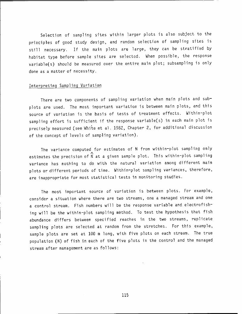
Selection of sampling sites within larger plots is also subject to the

principles of good study design, and random selection of sampling sites is

still necessary. If the main plots are large, they can be stratified by

habitat type before sample sites are selected. When possible, the response

variable(s) should be measured over the entire main plot; subsampling is only

done as a matter of necessity.

Interpreting Sampling Variation

There are two components of sampling variation when main plots and sub-

plots are used. The most important variation is between main plots, and this

source of variation is the basis of tests of treatment effects. Within-plot

sampling effort is sufficient if the response variable(s) in each main plot is

precisely measured (see White et al. 1982, Chapter 2, for additional discussion

of the concept of levels of sampling variation).

The variance computed for estimates of N from within-plot sampling only A

estimates the precision of N at a given sample plot. This within-plot sampling

variance has nothing to do with the natural variation among different main

plots or different periods of time. Within-plot sampling variances, therefore,

are inappropriate for most statistical tests in monitoring studies.

The most important source of variation is between plots. For example,

consider a situation where there are two streams, one a managed stream and one

a control stream. Fish numbers will be the response variable and electrofish-

ing will be the within-plot sampling method. To test the hypothesis that fish

abundance differs between specified reaches in the two streams, replicate

sampling plots are selected at random from the stretches. For this example,

sample plots are set at 100 m long, with five plots on each stream. The true

population (N) of fish in each of the five plots in the control and the managed

stream after management are as follows:

115

Control stream Managed stream Site N N

1 90 175

2 155 211

3 110 160

4 120 190

5 165 258

The correct test to use in this case is an unpaired t-test with 8 df.

The t-value is 3.21, which is significant at the a = 0.01 level, meaning that

the null hypothesis of no difference in fish abundance for the two streams can

be rejected at the 99% confidence level. (The reader is encouraged to compute

this test as an exercise.) The variation between plots within a stream is

natural variation; this between-plots variation is the basis for determining

differences between streams.

Within-plot sampling is necessary in order to estimate the unknown fish

abundance in each plot. As a result, there is uncertainty associated with the

subsequent estimates of fish abundance at each plot. Assume that electro-

fishing is done and that good point estimates of N are produced and standard A

errors of N are calculated:

Control stream Managed stream

SUe N Nfse(N)1 N Nfse(N)1

1 90 87(1.5)

2 155 160(4.0)

3 110 108(2.2)

4 120 126(4.8)

5 165 155(7.0)

175 168(6.2)

211 222(8.1)

160 158(4.0)

190 197(5.3)

258 245(11.7)

116

A The difference between the true N and the estimate N within each plot is

due to within-plot sampling variation; it is the average value of this squared A

difference that is estimated by the formula for var(N). For the above example,

based on the values of N, t = 3.45. There are still 8 df, and there is still

a significant difference at the a = 0.01 level.

The reason for computing se(N) = / var(N) is to determine the reliability

of the individual estimates. When there are small standard errors, the esti-

mates are reliable, and the t-test comparing fish abundance for the control A

vs. the managed stream, based on the values of N, can be computed with

confidence that the results are essentially the same as if the true N were

known; i.e., the electrofishing part of the study has been successful. (The A .

values of se(N) play no role in computing that t-test.)

A For larger values of se(N), the t-test is less reliable. If the

estimates are very inaccurate, it may be impossible to tell if there is a

difference in control and managed streams. For example, suppose that the

point estimates and standard errors for each plot are:

Control stream Managed stream

Site N Nfse(N)] N NfseCN)]

1 90 40(23.1)

2 155 230(70.5)

3 110 180(57.0)

4 120 60(28.7)

5 165 185(68.8)

A By looking at the sampling standard errors of N, it is obvious that the

study has failed because these values are too large. The estimates of N are,

therefore, too inaccurate to reliably detect any difference between streams.

The computed t-test from the above values of N is 0.49 (8 df). The result is

175 250(107.9)

211 130(61.1)

160 80(37.1)

190 201(74.0)

258 150(43.4)

117

not significant, but it would be erroneous to conclude that the populations of

the two streams are not different, meaning that management had no effect,

because the within-plot estimates of N are poor.

The important two points here are that replicate main plots are generally

needed in both control and managed areas to test for impacts and any

subsampling of main plots must produce reasonably precise results for each

main plot. It is not valid to select one plot in each stream and base the

test on the within-plot sampling variance of N. For example, if control plot

5 (true N = 165; N = 155) and managed plot 3 (true N = 160; N = 158) in the

first case above were selected'as the only study plots, an apparent test

statistic would be:

158 - 155 _ 3 = 0_372

/ 4.02 + 7.02 .06

This would approximate a standard normal variable (a t-test with many

degrees of freedom), and the results would not be significant. The test is

also invalid because the standard error of the difference in the estimates is

based, incorrectly, on within-plot variances (= 4.02 + 7.02).

Sample Size Guidelines

Sample size (i.e., sampling effort) needs to be considered at both the

main plot and within-plot levels. Unfortunately, standard formulae to deter-

mine sample size are often not useful in environmental studies, especially

when the main plots are large. When plots are very large, it is difficult to

sample enough plots, and the rule of thumb becomes to sample as many as

possible. There is a trade-off between the number of main plots and the

amount of within-plot sampling that is done, unless the study is such that the

response variables can be measured directly for the entire main plot. It is

generally better to have more main plots at the expense of less within-plot

sampling, at least up to the limit of getting reliable within-plot estimates.

118

In order to make an inference about some management action for a large area,

there should be at least 10 pairs of control-treatment main plots and at least

two within-plot sampling sites in each main plot. No inference to a larger

area is possible with only one control-treatment pair, even if the pair is

randomly selected. No amount of within-plot sampling can compensate for

having too few main plots.

Eberhardt (1978) and Green (1979) provide useful guidelines on sample

size. The following formula (modified after Calhoun 1966) is sometimes useful;

e.g., in determining the sample size needed to estimate the average macro-

invertebrate density in a stream section:

" = <%f = <V f

n = the desired sample size to achieve a 95% confidence interval on the true

mean y with a relative confidence interval width of 26. The unknown average

value of the response variable is y; the sample-to-sample standard deviation

is o. The ratio ö/y = cv is the per sample coefficient of variation, which

must be known or estimated (e.g., from a pilot study or from existing data).

It is often possible, for planning purposes, to let cv = 1.0 (100%). With

this value, n=4/62. Thus, to estimate y with "good" precision, i.e., to

obtain a 95% confidence interval with a relative half-width of 6 = 0.1, may

sometimes require a sample size of:

n = 4/(0.I)2 = 400

If 5 = 0.25, n = 4/(0.25)2 = 64, which is still very large. Useful values of

6 are < 0.25, with 5 = 0.1 representing good precision.

119

The above example illustrates the fact that when optimal target sample

sizes are computed, the result often is larger samples than can be taken

because of study constraints. Consequently, a common approach is to determine

the sample size that can be taken, given time, personnel, and budget resources,

and then find out what level of precision can be obtained with this level of

sampling. The level of precision that can be obtained will determine whether

or not the study can be expected to detect a treatment effect of practical

significance. Procedures for determining expected precision given a level of

sampling effort are beyond the scope of this document, and statistical

assistance may be needed to answer such questions.

There is a complex interplay between sample size and study design. The

role of study design is two fold: (1) to produce valid results; and (2) to

reduce the level of sampling effort needed through practices such as control-

treatment pairing, stratification, use of prior information, before/after

measurements, fixed plots, two-stage sampling, and other techniques.

Consequently, the question of sample size can only be answered with respect to

a given study design.

CONFOUNDING FACTORS

Confounding factors are factors that, if not adequately considered,

confuse conclusions regarding the success of a management program. Many

confounding factors that may be encountered in a monitoring study are listed

below under five basic categories: institutional; equipment; personnel;

biological; and statistical.

Institutional Factors

1. There must be a commitment (and, if possible, a guarantee) that the

study will be continued until it is finished.

120

2. Commitments of time, personnel, and money should be enough for the

entire study.

3. Communication lines should be kept open between the people respon-

sible for the study and land use managers. If unplanned activities

begin at the study site that may interfere with the success of the

study (e.g., construction activity), the involved personnel need to

be notified and attempts made to halt or modify the activity until

the study is completed. There also needs to be continued communica-

tion and cooperation with State agencies that have species management

responsibilites in the area.

4. Management programs should not be changed during the study.

5. Institutional constraints that may restrict sampling to certain

times should be considered when the study is designed.

Equipment

1. Biases in the results due to the sampling procedure used need to be

considered so that they do not have an undue affect on the study

conclusions. Fish sampling results, in particular, can tie differen-

tially biased by the choice of sampling gear.

2. The effect of different water conditions (e.g., turbidity, hardness,

and discharge) on the precision and efficiency of the equipment used

in the study needs to be understood and accounted for in study

results.

3. Equipment should be calibrated, as appropriate and needed.

4. Methods should remain the same throughout the study because results

are generally not comparable between methods.

121

5. Values obtained may be affected if equipment is replaced or modified

during the study. For example, the efficiency of electrofishing

units may vary with time as the battery loses its charge or if one

brand of equipment is replaced with another brand.

Personnel Factors

1. Trial runs should be conducted before study sampling begins to

familiarize personnel with equipment and to standardize methods.

2. The number of persons available must meet the requirements for the

method chosen. The same number of people should be available each

time a method is used that is affected by the number of participants

(e.g., electrofishing).

3. The amount of previous training and experience may vary among

personnel and can affect the precision of sampling. If differences

in sampling efficiency are suspected, personnel should be rotated

systematically among sites in order to avoid confounding differences

resulting from personnel involved in the sampling with treatment

effects.

4. Personnel changes during the study may introduce error if sampling

precision or bias varies among the persons involved in the sampling.

5. Sampling by personnel may vary over time; e.g., they may become more

efficient with added experience or be affected by certain times of

the day or year.

122

Biological Factors

1. Biological variables may not be independent of one another.

2. Fishing pressure affects fish population estimates and size distri-

bution and, therefore, should be considered when selecting sampling

times.

3. There is considerable natural variation in population numbers in

both time and space that can mask management effects (see Hall and

Knight 1981).

4. Biological populations may not respond immediately to changes in

their environment; i.e., there may be a lag time between the manage-

ment action and the population response. Studies may have to extend

for a number of years after treatment initiation in order to

accurately determine responses.

5. Biological populations may adapt or acclimate to conditions and,

therefore, not change. However, this phenomenon is rare.

6. Biological populations often have response thresholds, rather than

reacting linearly.

7. Factors other than those being monitored may affect populations, and

population changes may occur for reasons that are unconnected with

the management program.

8. Habitat changes unrelated to management actions may result in a

reallocation of fish in the study area, thereby increasing the

difference in population numbers between the control and managed

areas. In this case, there are the same number of fish but in

different places.

123

Statistical Factors

1. If the assumptions for the parametric tests used are only approx-

imated rather than fully meet, these assumption violations may have

serious affects on the study results.

2. Controls in time and space are necessary for valid comparisons;

however, they are far from foolproof (Eberhardt 1978).

3. The time of sampling can bias results when changes in the values of

the variable being monitored are related to time of day or year.

4. When an insufficient sample size is used, a significant difference

may exist but not be apparent. Conclusions drawn from an analysis

with an insufficient sample size may, therefore, be invalid. Green

(1979:40) advises "If it was not possible to conduct preliminary

sampling and a number must be pulled out of a hat, three replicates

per treatment combination is a good .round number. [However], it is

the overall error degrees of freedom that are important."

5. Lack of enough replication makes estimation of natural variability

impossible. Replicate samples should be taken (Green 1979:27) ". ..

within each combination of time, location and any other controlled

variable. Differences among can only be demonstrated by comparisons

within".

6. Considerable error can be introduced when the assumptions of popula-

tion estimates are not met completely.

7. Unforeseen events (e.g., a 100-year flood) can affect the study

site(s) to the extent that comparisons of differences are invalid.

8. A statistically significant relationship is not always proof of

causality because many variables are interrelated (Green 1979).

124

9. Rounding of numbers with several decimal places can cause consider-

able variation in calculations. It is advisable to retain four

digits to the right of the decimal point for computational steps.

An example of the error that can result from rounding is demonstrated

in the following example of computing a variance estimate:

2 _ I(X)2 - n(X)2 s " n-1

If n = 20, I(X)2 = 478.0499, and X = 4.8555, then s2 = 0.3438. But

if X is rounded to 4.9 and E(X)2 is rounded to 478.0, the result is

s2 = -0.1158, which is impossible for a variance. This illustrates

that, in general, if intermediate quantities in a series of calcula-

tions are rounded off, the end result of a calculation can be

seriously in error.

10. Tabular values can be selected or recorded incorrectly, which can

result in incorrect calculations or conclusions.

REFERENCES

Ahmed, J., C. D. Bonham, and W. A. Laycock. 1983. Comparison of techniques

used for adjusting biomass estimates by double sampling. J. Range Manage.

36(2):217-221.

Calhoun, A., ed. 1966. Inland fisheries management. California Dept. Fish

and Game, Sacramento. 536 pp.

Eberhardt, L. L. 1976. Quantitative ecology and impact assessment. J.

Environ. Manage. 4:27-70.

125

• 1978. Appraising variability in population studies. J.

Wildl. Manage. 42:207-238.

Elliott, J. M. 1977. Statistical analysis of samples of benthic inverte-

brates. Second edition. Freshwater Biol. Assoc. Sei. Publ. 25. Titus,

Wilson & Son, Ltd. 160 pp.

Green, R. H. 1979. Sampling design and statistical methods for environmental

biologists. John Wiley & Sons, New York. 257pp.

Greeson, P. E., T. A. Ehlke, G. A. Irwin, B. W. Lium, and K. V. Slack, eds.

1977. Methods for collection and analysis of aquatic biological or

microbiological samples. U.S. Geological Survey, Techniques of Water

Resources Investigations of the United States Geological Survey, Book 5,

Chapter 4A. Washington, DC. 332 pp.

Hall, J. D., and N. J. Knight. 1981. Natural variation in abundance of

salmonid populations in streams and its implications for design of impact

studies: A review. U.S. Environ. Protection Agency. Corvallis, OR.

EPA 600/3-81-021. 95 pp.

Huntsberger, D. V. 1967. Elements of statistical inference. Second edition.

Allyn and Bacon, Boston. 398 pp.

Johnson, N. L., and S. Kotz. 1970a. Continuous univariate distributions -1.

John Wiley & Sons, Inc., New York. 306 pp.

• 1970b. Continuous univariate distributions -2. John Wiley &

Sons, Inc., New York. 306 pp.

Keller, C. R., and K. P. Burnham. 1982. Riparian fencing, grazing, and trout

habitat preference on Summit Creek, Idaho. North Am. J. Fish. Manage.

2(l):53-59.

126

Pielou, E. C. 1975. Ecological diversity. John Wiley & Sons, Inc., New

York. 165 pp.

Siegel, S. 1956. Non-parametric statistics for the behavioral sciences.

McGraw-Hill Book Co., New York. 312 pp.

Snedecor, G. W., and W. G. Cochran. 1967. Statistical methods. Sixth

edition. Iowa State Univ. Press, Ames. 593 pp.

Sokal, R. R., and F. J. Rohlf. 1969. Biometry. W. H. Freeman and Company,

San Francisco. 776 pp.

Tacha, T. C, W. D. Warde, and K. P. Burnham. 1982. Use and interpretation

of statistics in wildlife journals. Wildl. Soc. Bull. 10:355-362.

Thomas, J. M. 1977. Factors to consider in monitoring programs suggested by

statistical analysis of available data. Pages 243-255 in W. VanWinkle,

ed. Proceedings of the conference on assessing the effects of power-

plant-induced mortality on fish populations. Pergamon Press, New York.

Ward, D. V. 1978. Biological environmental impact studies: theory and

methods. Academic Press, New York. 157 pp.

White, G. C, D. R. Anderson, K. P. Burnham, and D. L. Otis. 1982. Capture-

recapture and removal methods for sampling closed populations. Los

Alamos Natl. Lab. LA-8787-NERP. 235pp.

127

CHAPTER V. STATISTICAL TESTS FOR EVALUATING

RESPONSES TO MANAGEMENT ACTIVITIES

The following stepwise examples are for the statistical procedures

mentioned in Chapter IV. For demonstration purposes, the assumptions necessary

for parametric tests are tested for one example. The necessary assumptions

are given for the remaining examples. A statistics text by Sokal and Rohlf

(1969) and their statistical tables (Rohlf and Sokal 1969) are the primary

reference sources for the tests.

DETERMINATION OF THE DATA DISTRIBUTION PATTERN

The following total lengths (mm) of 64 adult trout are used to determine

the data distribution pattern:

162 166 148 110 109 164 148 162 219 175 87 135 121 114 115 150 94 140 199 215 150 160 142 202 214 95 282 123 146 313 264 208 127 114 161 81 163 115 155 199 172 175 97 136 173 174 113 138 111 207 136 125 160 79 171 122 93 195 121 122 102 138 110 161

128

Step 1

Prepare a frequency distribution table.

Step 2

Fish length No. of % of Cumulative

(mm) observations

3

total

4.7

% of total

70 - 89 4.7 90 - 109 6 9.4 14.1

110 - 129 15 23.4 37.5

130 - 149 10 15.5 53.0

150 - 169 12 18.7 71.7

170 - 189 6 9.4 81.1

190 - 209 6 9.4 90.5

210 - 229 3 4.7 95.2

230 - 249 0 0.0 95.2

250 - 269 1 1.6 96.8

270 - 289 1 1.6 98.4

290 - 309 0 0.0 98.4

310 - 329 1 64

1.6 100.0

Plot the data in a histogram, and draw a curve to approximate the

distribution pattern.

80 100 120 140 160 180 200 220 240 260 280 300 320

Fish length (mm)

129

Step 3

Plot the data on normal probability paper and fit a line to the data

points by visual observation. Data points are midpoints for each fish

length class.

99.99 -j

99.9 -

99

95 CD 90 cn re 80 c CD

60 Ol Q.. 40 CD >

+J 20 re 13 10 E 3 5 o

1 -

0.1 -

0.01

60 —I | | | | | | 1 1 1 1 1 j

80 100 120 140 160 180 200 220 240 260 280 300 320

Fish length (mm)

130

Step 4

The pattern appears to be lognormal. To confirm this assumption, plot

the data points on lognormal probability paper and visually fit a curve

to the points.

99.99

99.9

99-1

CD MS CD re 90 E CD O 80 s_ CD Q. 60 CD > 40

+-> rö

3 20 F 3 II) o

b

1-

0.1

0.01- -I—I—I I I

100

-I—I—I—I I I I

1000

Fish length (mm)

A straight line pattern of the data points strongly supports lognormality.

131

Step 5

Transform the data by logarithms. If parametric tests will be used,

distributions other than lognormal can often be normalized by the

appropriate transformations (Sokal and Rohlf 1969). Nonparametric tests

should be used when normalization is unsuccessful.

TEST FOR HOMOGENEITY OF VARIANCE

The following water depth data will be used to test for homogeneity of

variance:

Site 1 Site 2 Site 3

xi X.2 X. X.2 X. X.2 1 l i l l l

1.5 2.25 3.5 12.25 4.1 16.81 3.0 9.00 4.6 21.16 3.6 12.96 4.5 20.25 5.2 27.04 1.5 3.25 6.0 36.00 3.2 10.24 3.2 10.24 1.6 2.56 4.1 16.81 1.7 2.89 5.0 25.00 2.0 4.00 6.2 38.44 3.2 10.24 1.6 2.56 2.8 7.84 4.5 20.25 5.0 25.00 1.9 3.61 2.3 5.29 2.3 5.29 3.1 9.61 4.1 16.81 2.5 6.25 2.7 7.29

IX. = 1

35.7 34.0 30.8

3.57 3.40 3.08

IX.2

Sl =

147.65 130.6 111.94

147.65 - (35.7)2

10

2 130 £ _ (34)

„ 2 _ I-iU-b 10 2 S3 =

111 94 - <30-8) in. w 10

9 "2 9 9 2

= 2.24 = 1.67 = 1.90

132

Step 1

Determine the frequency distributions. The frequency distribution of the

data for Site 1 is:

Site 1

Percent % cumulative Class

Class Frequency Frequency frequency midpoint

1.5-2.6 3 30.00 30.00 2.02

2.7-3.8 2 20.00 50.00 3.22

3.9-5.0 4 40.00 90.00 4.42

5.1-6.2

10

10.00

100.00

100.00 5.62

133

Step 2

Graph data on normal probability paper (Sokal and Rohlf 1969)

CL> CD (O

•M C cu o S- 0) CL

>

E O

99.99-1

99.9-

99-

95 90 80-

60 40'

20 10 ■ 5-

1-

0.1-

0.01-

• = Site 1 o = Site 2 X = Site 3

■ = Same data point for all three sites

1 1 1 1 1—

0.0 1.0 2.0 3.0 4.0 5.0

Water depth (ft)

6.0 7.0

The slopes of the three lines are very similar, indicating that the

variances are probably homogeneous. Additional tests can be used for confirma-

tion. The lines for sites 2 and 3 overlap too much to distinguish them.

134

Step 3a

The F-test is used to test for homogeneity of variance when there are

only two data sets:

u 2 2 H : 0, = ö0 o 1 2

u 2,2 a 1 2

Select a level of confidence; e.g., a = 0.05.

Calculate the F-value = F :

2 c = _J = 2-24 , 0413

s 2 1.67 1-J'ti-3

s2

Look up the F-value for Fa ,_^ , ^ in the appropriate statistical

table where n = number of observations in each sample (10 in this

example).

The calculated F value of 1.3413 is less than the table F-value of 3.18.

Therefore, the null hypothesis cannot be rejected, and the conclusion

(with a 95% confidence level) is that the variances are equal (homogeneity

of variance).

Step 3b

Bartlett's test (Sokal and Rohlf 1969) is used to test for homogeneity of

variance when there are more than two data sets:

Sample df = n-1 s2 1og(s )

1 9 2.24 0.35024 2 9 1.67 0.22271 3 9 1.90 0.27875

135

Compute the weighted average variance:11

2 _ sum of [(variance values) times (their respective degrees of freedom)] sum of df

= (2.24) (9) + (1.67) (9) + (1.90) (9) _ 20.16 + 15.03 + 17.10 27 " 27

52.29 27

= 1.9367

Find the logarithm of 1.9367, which is 0.28706.

Sum the logs of each variance multiplied by its respective degrees of freedom:

= (0.35024) (9) + (0.22271) (9) + (0.2875) (9)

= 3.1522 + 2.0044 + 2.5875

= 7.7441

2 Compute x = 2.3026 (sum of the degrees of freedom multiplied by the log of the weighted average variance) - (sum of the logs of each variance multiplied by its respective degrees of freedom):

= (2.3026) [(27) (0.28706) - 7.7441]

= 2.3026 [7.75062 - 7.7441]

= (2.3026) (0.00652) = 0.015

Compute correction factor C:

1 1 + sum of reciprocal of individual df 3(a-l)

a = number of sample sets (a = 3 in this example)

sum of df

1 + 1 3(2)

I + I + I)_ _L 9 9 9/ 27

= 1 + (0.1667) (0.3333 - 0.037)

= 1 + (0.1667) (0.2963) = 1.0494

10If any of the s2 values are less than 1, all of the s2 values are multiplied by the same multiple of 10 so that there is at least one number to the left of the decimal in each s2 value. For example, if the smallest s2 value is 0.224, all s2 values would be multiplied by 10. This multiplication is necessary to prevent negative logs.

136

2 Compute the adjusted x :

= 2L = °-015 = o 014 C 1.0494 U,U^

2 2 2 Ho: °1 = °2 = °3

? ? 2 Ha: «^ / a/ * o3

a-1 = 2 df

Because x2 nC M^ = 5.991 and the adjusted test statistic x of 0.014 is . (Jb, \c )

lower, the null hypothesis is not rejected and we are reasonably safe to

assume that the variances are equal.

Step 4

F - test (Sokal and Rohlf 1969) max v

When Bartlett's test indicates that there is no homogeneity of variance,

the F - test can be used to determine if parametric methods are still max

acceptable; e.g.:

^ J. ..u s maximum „,<.,•„. Compute the -^ ratio: s minimum

= 2^i = ! 34 1.67 1'**

Select the tabulated Fm3v statistic: m oL x

F = F = 5 34 hmax o,(a),(n-l) rmax0.05,3,9 3-

where a = 0.05

a = number of data sets = 3

n = samples per set = 10

137

The calculated value does not exceed the tabular value, hence the null

hypothesis of equal variance is not rejected; therefore, the assumption

can be made that the variances are equal because the computed value

(1.34) is less than the tabulated F statistic (5.34) at the 5% level.

When homogeneity of variance is lacking, parametric tests can still be

used with caution if the calculated F value is less than or equal to 5. If max N

a parametric test cannot be used on the data as is, an appropriate nonpara-

metric test can be selected or attempts made to transform the data so that a

parametric test can be used (see Sokal and Rohlf 1969).

STATISTICAL TESTS FOR COMPARING DIFFERENCES BETWEEN DATA SETS

Two-sample t-test

Problem: In an area where grazing occurred, the temperature of a small

stream was determined by sampling with a hand-held thermometer to determine

the effects of grazing on stream temperature. Temperature measurements were

taken at site 1 on the stream within an area where grazing was restricted and

at site 2 on the stream where grazing was not restricted. The two-sample

t-test is used to test for differences when the samples are independent, the

data are assumed to be normally distributed, and the variances are assumed to

be homogeneous.

138

Site 1 Site 2

X. 1

X.2 h X.2 i

10.5 10.3 10.7 10.9 10.7

110.25 106.09 114.49 118.81 114.49

11.0 11.2 10.9 10.8 11.1

121.00 125.44 118.81 116.64 123.21

53.1 55.0

10.62 11.0

IX.2 = 1

2 _ IX.2 - (iX^/n

sl " frl

564.13 - 563.92

564.13 605.10

605.1 - 605

0.208 = 0.052 = 0^ = 0.025

Solution:

1. Ho: Vl = u2

Ha: Vl * y2

2. Select a; e.g. , a = 0.05.

3. Calculate the standard error (se) of the difference in the means,

*1 " *2

139

ni + n9\/(ni_1)si2 + (n2-1) sz '1 "2 Wv"l xja\

nln2 n1 + n2 - 2

5 + 5W(4) (0.0520) + (4) (0.025)

0.208 + 0.100

= 7(0.4) (0.0385) =y0.0154 = 0.124

Calculate t = *±lll = (10.62^ 11.0) = ^B_ _3_Q6 se 124 0.124

5. Look up the tabular t value for n, + n?-2 =5+5-2=8 df:

t0.05,(n1 + n2-2) = 2'306-

The null hypothesis is rejected because the test statistic t =

-3.06, which is less than the tabular critical value of t = -2.306

(for a two-tailed test, the tabular value is ±). The conclusion,

with a 95% confidence level, is that the stream temperatures are

significantly different at the site where grazing was restricted

compared to the site where grazing was not restricted.

Assume that the management objective was to lower the stream tempera-

ture by 2° C at the restricted grazing site and that temperatures

over the past several seasons (without any restricted grazing)

averaged 11.5° C. y becomes 11.5° C - 2° C = 9.5° C, and a one-

tailed t-test can be used to test H : y = 9.5 versus H : u > 9.5. oo a

140

4. - " yo - 10-62 - 9.5 _ 1.12 = ?1 CA 1 ~ ~T Ö7Ö52Ö 0.0520 Ci-°

tn nc , = 2.132 (Rohlf and Sokal 1979:Table Q). u .Ub,n,-1

The calculated t of 21.54 is greater than the tabular value of

t = 2.132. Therefore, the null hypothesis is rejected with 95%

confidence that stream temperatures in the area with restricted

grazing were not lowered by 2° C. Note that the a level in Table Q

is divided by 2 for a one-tailed test; e.g., if a = 0.05 in a one-

tailed test, select a value in the column —^- = 0.05. 2

The t'-test (Sokal and Rohlf 1969)

Problem: Stream temperatures (°C) were taken (15 readings) at a stream

site before a management program was initiated to increase bank cover. Tem-

perature readings (10 readings at the same time of the year) were also taken

after the management program was initiated. The data are:

141

Before management

X. l

15.0

X.2

l

225.00 15.0 225.00 14.5 210.25 14.0 196.00 14.5 210.25 13.5 182.25 15.0 225.00 14.5 210.25 15.0 225.00 13.5 182.25

14.5 210.25

15.0 225.00 14.5 210.25 14.0 196.00 14.0 196.00

EX. = l

216.5 EX. 2 = 3,128.75

*1 = 14.43

Solution:

After management

X. X.2 1

10.0

i

100.00 10.5 110.25 9.5 90.25

10.0 100.00 14.5 210.25 13.0 169.00 14.0 196.00 12.5 156.25 10.5 110.25 14.5 210.25

EX. = i

119 EX.2 = = 1452.5

x2 = 11.9

1. HQ: Temperatures were the same before and after the management

action or y^ = y„ versus H : y. t y„.

2. The level of significance chosen is a = 0.01.

3. The assumptions for a parametric test are not all met. In parti-

cular, the sample sizes and the variances are not equal. Therefore,

the t'-statistic is used to test for differences:

142

2 ICX^2 - UX.)2/n sl = Fl

3,128.75 - ^P2 2 1452.5 - ^

19 S2 9

3,128.75 - 46'^2-25 _ 1,452.5 - 14161

10 14

_ 3,128.75 - 3,124.817 = 1,452.5 - 1,416.1 " 14 9

= 14p =0.2810 = 36^ = 4.0444 14 y

fL (*!,.> + fL (t2>B) nl n2

4. Compute the critical level, t - ~ 0

ill + fi_ nl n2

where t. has n,-l df = 14 df and t9 has n?-l df = 9 df. 1 ,a 1 £,a c.

tl,a = ^.Ol.H = 2'977

^..^o.oi.g*3-250

0^810 (2-g77) + 4^0444 (3-250)

= 0.2810 4.0444 15 10 '

0.8365 . 13.1443 - 15 10 = 0.0558 + 1.3144 ~ 0.0187 + 0.4044 0.4231

1.3702 0.4231

= 3.238

143

Calculate the t'-statistic:

t' _ Xl " X2 _ 14.43 - 11.9

0.2810 4.0444 15 10

2.53 _ 2.53 _ 2.53

/0.0187 + 0.4044 /0.4231 0-6505

= 3.89

6. The computed test statistic t1 = 3.89 is greater than the critical

value of 3.238. Therefore, the null hypothesis is rejected, and the

conclusion, with 99% confidence, is that the mean temperatures are

different.

7. Use the same computational procedure if n, = n?.

Paired t-test

Problem: Ten transects were sampled in order to estimate the width of a

stream along the 100 m length of a managed site. The following width measure-

ments (meters), taken perpendicular to the flow of the water, were obtained

prior to the management activity:

7.1, 6.3, 7.6, 5.2, 4.3, 4.0, 5.6, 5.2, 4.9, and 6.1

The following measurements were taken at the same 10 transects after the

management action was implemented:

6.3, 5.9, 5.2, 3.7, 4.2, 3.1, 5.6, 3.8, 4.2, and 4.9

144

The paired t-test is used to determine if the stream width changed

significantly after the management activity.

Solution:

1. The null hypothesis is that there is no difference in stream width

before and after management: H : Uj = v^ versus W^\ v-^ * V^-

2. The level of significance chosen is a - 0.05.

3. The assumptions for parametric tests are met and the data are paired;

therefore, a paired t-test (Snedecor and Cochran 1968) is used.

4. The pairs are established:

Transect Before After Di fference Deviation

i Xl h d. i = Xj- x2

0.8

di -5

-0.14

(di - d)2

1 7.1 7.3 0.0196

2 6.3 5.9 0.4 -0.54 0.2916

3 7.6 5.2 2.4 1.46 2.1316

4 5.2 3.7 1.5 0.56 0.3136

5 4.3 4.2 0.1 -0.84 0.7056

6 4.0 3.1 0.9 -0.04 0.0016

7 5.6 5.6 0.0 -0.94 0.8836

8 5.2 3.8 1.4 0.46 0.2116

9 4.9 4.2 0.7 -0.24 0.0576

10 6.1 4.9 1.2 0.26 0.0676 Total 56.3 46.9 9.4 0.00 4.6840

X _ 5.63 4.69 d = 0.94 s2 = 0.5204

s_ = 0.5204/10 = 0.0520, s_ = 0.2280 d d

145

where g _ 9.4 _. Idi 10 n

VM 2

s2 = 4.684 ^ 4.684 _ i

2 0.5204 s_ V 10

n-1 n-1

2

s_ = / 0.0520 = 0.2280 d

5. t is computed as:

z s 0.228 *'1"

6. From the t table, tQ Q5 g is 2.26. n-1 = nine degrees of freedom.

7. The computed t of 4.123 is greater than the critical value. There-

fore, the null hypothesis is rejected, and the conclusion, with a

95% confidence level, is that the means are different and that the

management actions decreased the stream width.

Wilcoxon Signed-Rank Test

The Wilcoxon signed-rank test is the nonparametric analog of the paired

t-test.

Problem: Average depth measurements in tenths of meters were taken in a

stream, at the same sites, before and after management to determine the effect

of the management action on the stream depths:

146

Average depth Sample After Before

1 2.0 2 1.2 3 0.5 4 1.9 5 2.1 6 4.0 7 4.5

ZX. = i

16.2

X = 2.31

s2 = 2.08

1 3 1 1 0 9 0 8 1 2 1 0 1 0 7 3

1 04

0 03

Signed Difference rank

0.7 3 0.1 1

-0.4 -2 1.1 5 0.9 4 3.0 6 3.5 7

Solution:

1. The null hypothesis is that the median (M) of the differences between

before and after depth measurements equals zero; the alternative

hypothesis is that this median is greater than zero. Thus, this is

a one-sided test:

H : M = 0 o

H : M > 0

2. The level of significance chosen is a = 0.05.

3. Three of the assumptions for parametric tests have been met; however,

a nonparametric test will, be used because the variances of the

before and after measurements are significantly different. The

measurements are paired, so the Wilcoxon signed-rank test is used to

calculate the test statistic (T).

4. The differences between paired samples are ranked from smallest to

largest, without regard to sign.

5. Sum the positive and negative ranks separately and determine their

absolute values:

147

T+ = 26

T- = 2

6. Look up the tabular value for a one-tailed test in Appendix B of

this manual. This value is obtained by letting n equal the number

of pairs with nonzero differences (Wilcoxon and Wilcox 1964).J1 In

this case, n = 7 and a = 0.05. The smaller T value (2) is less than

the tabular value of 4; therefore, the null hypothesis is rejected.

The conclusion with a 95% confidence level is that stream depths

were greater after the management practices occurred. Another

approach for using the Wilcoxon signed-rank test is discussed in

Sokal and Rohlf (1969).

Mann-Whitney U-test

The Mann-Whitney U-test is the nonparametric analog of the unpaired

t-test.

Problem: In a stream that was greatly affected by logging activity, a

management objective was to improve the spawning habitat by increasing the

substrate size. Average spawning gravel size was chosen as the variable to

measure before and after management actions were initiated.

Before After improvement improvement

11 mm 12 mm 6 13 1 10 4 11

10 12 X = 6.4 11.6

s2 = 17.3 1.3

lThis reference can be obtained from Lederle Laboratories, Pearl River, NY.

148

Solution

1. The null hypothesis for the one-tailed test is that the average

spawning gravel diameters before management are equal to or greater

than the diameters after management has occurred; the alternative

hypothesis is that diameters after management has occurred are

greater than the diameters before management.

2. The level of significance selected is a = 0.05.

3. In testing the data for meeting parametric assumptions, it was found

that the variances were not homogeneous. The most commonly used

nonparametric test for comparing two independent (unpaired) samples

is the Mann-Whitney test. For this test, it is assumed that the

data consist of two independent random samples of continuous

variables. If n > 20, refer to Sokal and Rohlf (1969) for the

proper procedure.

4. Rearrange the data by ranking each sample separately:

Number of observa- vations in A less

Rank improvement) improvement) than each B value

1 2 3 4 5

A (before improvement)

B imp

(after rovement)

1 4 6

10 11

10 11 12 12 13

3.5 4.5

5 5 5

C = 23

The last column is calculated as follows, starting with the first

value:

A. There are three values in A less than 10 (the first value in B)

and one value in A that equals 10; therefore, the first number

in the last column is 3.5.

149

There are four values in A less than 11 and one value in A that

equals 11; therefore, the second value in the column is 4.5.

There are five values in A less than 12 and five values in A

less than 13; therefore, the last three numbers in the last

column are 5.

5. The Mann-Whitney statistic U is the greater of C or n,n,,-C. For

this example, n1n2-C = (5)(5)-23 = 2. Therefore, U =23.

6. Locate U , » for a one-tailed test in Rohlf and Sokal (1979:

table cc): UQ Q5 „ „ = 21. Us of 23 exceeds the tabular value of

21. Therefore, the null hypothesis is rejected and the conclusion,

with a 95% confidence level, is that average substrate diameter

increased as a result of management actions.

One-way Anlysis of Variance

Problem: The velocity of a stream was determined to be too low for good

fish spawning habitat. Stream improvement devices were installed on a section

of the stream in an attempt to increase velocity. Velocity measurements were

taken at one site within the stream improvement area before the management

actions occurred and at two different sites within the area after sufficient

time lapsed for management actions to be effective.

150

Replica

i

tes Before management

Site 1

Aft er management

Site 2 Site 3

1 0.4 (m/sec) 0.6 (m/ sec 0 0.7 (m/sec) 2 0.3 0.7 0.5 3 0.2 0.5 0.6 4 0.3 0.9 0.9 5 0.1 1.0 0.9 6 0.5 0.8 0.6 7 0.4 0.7 0.8

IX. 2.2 5.2 5.0

X 0.314 0.743 0.714

s2 0.0181 0.0295 0.0248

The grand total of al.l observations is 12.4; the grand mean = 0.590.

Solution:

1. The null hypothesis (H ) is that the means at all sites are equal:

H „ = y = v The alternative hypothesis (H ) is that the mean

of at least one site is different from the means of the other sites;

in particular, y„ = y-, ^ Vh •

2. The level of significance chosen is a = 0.05.

3. All of the assumptions for parametric tests have been met, and the

parametric anlysis of variance ANOVA test will be used to test for

differences.

4. Calculate the grand total for all of the observations squared:

(0.4)2 + (0.3)2 + ... + (0.6)2 + (0.8)2 = 8.56

151

5. Divide the sum of the squared site totals by the number of replicate

samples:

= (2.2)2 + (5.2)2 + (5.0)2 _ 4.84 + 27.04 + 25.0 7 7

= 5^88 = 8AZ&

6. Calculate correction term CT = grand total squared and divided by

the total sample size:

CT = ^§^ = ±%^ = 7.322

7. $S-|-tal = quantity from Step 4 - CT

= 8.56 - 7.322 = 1.238

8. SSp = quantity from Step 5 - CT

= 8.126 - 7.322 = 0.804

Within Total Groups

= 1.238 - 0.804 = 0.434

10. Prepare the ANOVA Table:

152

Variation df SS MS F-value

Between sites a-1 = 2 SSQroups = 0.804 Sh^s = QAQZ (L402 = ^^

Within sites a(n-l) = 18 SSy. Mn = Qm SSWith1n = QQH

(error) a(n-lj

where a = number of sites n = number of samples within each site

Tabular FQ>05,(2,18) = 3-55 F0.01,(2,18) " 6-01

11. The null hypothesis is rejected because the computed F test statistic

of 16.75 is greater than the tabular F value of 3.55. The conclu-

sion, with at least a 95% confidence level, is that the mean veloci-

ties for the three sites are unequal. (In this example, this test

is significant at a greater than 1% confidence level).

12. The next step is to determine which sites differ from which other

sites. It was assumed that Site 1 would be different from Sites 2

and 3 and that Sites 2 and 3 would be the same; therefore, an a

priori comparison is used.

13. The level of significance chosen is a = 0.05.

14. Determine the specific pair-wise comparisons. In this case, there

are three comparisons: Site 1 vs. 2; Site 1 vs. 3; and Site 2 vs.

3.

153

15. Calculate the Least Significant Different Term (any pair-wise

difference in means that exceeds this term is considered

significant):

LSD = t , .,. /- MS ... . OjCdfjy n within

where a = 0.05

df = a(n-l) = 18

LSD = 2.101 / | (0.024)

= 0.174

16. Calculate the differences between means and compare these differences

to the LSD value:

X2 - Xj = 0.429

X3 - Xj = 0.400

X2 - X3 = 0.029

In this example, the first two sets of means are significantly

different because the differences exceed the LSD value of 0.174.

The conclusion is that, for both sites, the means are significantly

different than the mean for the "before" management condition.

Means for the two sites after management actions occurred were not

significantly different from each other. The Student-Newman-Keuls

test (Sokal and Rohlf 1969) can also be used for multiple compar-

isons of means.

154

17. More complex comparisons are also possible; in this example, the

average of Site 2 and 3 means are compared to the mean of Site 1:

diff = (X2 + X3)/2 - Xj_

= (\) x2 + (|) x3 - Xj

This is a linear combination of means, as are the pairwise compar-

isons. The variance of each mean is s2 = (MS^..^. )/n. The variance

of a linear combination is the sum of the squared coefficient multi-

plying each mean times the variance of that mean. In this example:

var(diff) = {\)Z var(X2) + (\)Z var(X3) + (-1)2 var^)

t n\ MSWithin . f 9,s MSWithin . ,n

MSWithin (.25) + (.25) + (1)

MS = [(.25) + (.25) + 1] Within

n

1.5

= 1.5

MS,,... . Within n

0.024 = 0.005143

The test statistic [it has a t-distribution with a(n-l)df; this is

the df of the MSWithin] is:

155

t = diff

/ var(diff)

(0.743 + 0.714) - 0.314

/ 0.005143

0.729 - 0.314 0.0717

5.788

The critical level (two-tailed) is tQ Qr /■,«>> = 2.101. The computed

test value of 5.788 exceeds 2.101; therefore, the conclusion is that

the average of Sites 2 and 3 differs from the average for Site 1.

Because the averages for Sites 2 and 3 do not differ significantly

from each other, the assumption can be made that all the significant

difference suggested by the F-test represents before vs. after

management conditions. Note that, in the absence of a control site,

the conclusion that management caused the increased velocity cannot

be made on the basis of statistics alone.

Kruskal-Wallace Nonparametric Test for One-Way ANOVA (Sokal and Rohlf 1969).

Problem: The problem is the same one used to illustrate the one-way

analysis for variance but it is assumed that requirements for a parametric

test are not met. Assemble the data from all three sites in one array,

starting with the lowest value and ending with the highest:

Ve" ocity Veit Deity Ve ocity measurement Rank measurement Rar k measurement Rank

0.1 1 0.6 11 0.9 19 0.2 2 3 0.6 11 3 0.9 19

2|0.3 -^0.3

3.5 3.5

0.6 0.7

11 14

0.9 1.0

19 21

_2_ 0.4 0.4

5.5 5.5

_3_ 0.7 0.7

14 14

0.5 8 3_ 0.5

0.5 8 8 4 0.8 0.8

16. 16.

5 5

156

Ranks for equal data values are determined by averaging the positions

of the equal values; e.g., the ranks for the third and fourth values

are:

3rd + 4th = 3.5

The Xl values indicate the number of tied observations. These are

denoted as t. in the following equations. Prepare a table with <J

ranks replacing the original observations in each data set:

1 2 3 4 5 6 7

IX.

Before management

Site 1

5.5 3.5 2.0 3.5 1.0 8.0 5.5 29

4.143

After management Site 2 Site 3

11.0 14.0 8.0 19.0 21.0 16.5 14.0

103.5

14.786

14.0 8.0 11.0 19.0 19.0 11.0 16.5 98.5

14.029

Solution

1. H : The expected means for the three sites are the same. o

H : The expected means for the three sites are different. a r

2. Select a = 0.05.

157

3. Compute H

where N

12 (N) (N+l)

Sum of squared column totals

- 3(N+1)

total number of observations for all data sets

number of observations per sample site

12 (21) (22)

0.0260

(0.0260)

552.64

(29)2 + (103.5)2 + (98.5)2

7

841.00 + 10,712.25 + 9702.25" 7

3(22)

66

(21,255.50 7 66

66 = 12.949

4. Compute correction term for H to compensate for tied values:

D = 1 -

Sum of (t.-l) t.(t. +1) 0 J J

for each set of tied values (N-l) (N) (N+l)

where t. = number in each set of tied values, shown as, e.g. 2 . In this example, there are seven sets of tied values.

(1)(2)(3) + (1)(2)(3) + (2)(3)(4) + (2)(3)(4) + = 1 (2)(3)(4) + (1K2K3) + (2H3H4)

= 1

(21-1)(21)(21+1)

6+6+24+24+24+6+24

= i _ 114 9240

9240

= 1 - 0.01233 = 0.9877

H _ 12.949 5. Adjusted H = g = jj^gff = 13.11

158

6. Because H is approximately distributed as a chi-square variable, the

table value of x2n nc i is obtained where a = number of columns or U. Ub, a-i

data sets x n 05 2 = ^-^l-

7. Because the computed value of H = 13.11 is greater than XQ_Q5 2 =

5.991, the null hypothesis is rejected, and the conclusion, with at

least a 95% confidence level, is that the velocity increased after

management actions occurred. Again, without a control site, the

conclusion that the increased velocity resulted from the management

action cannot be reached on a purely statistical basis. This

conclusion may be, however, quite reasonable from a biological

viewpoint.

Parametric Two-way ANOVA Without Replication

Problem: Pool-riffle ratios were measured in three locations in a stream.

Two sites were spatial controls and the third site received special management

designed to increase the number of pools. The sample data taken after manage-

ment occurred are summarized below:

15 May 16 Jun 14 Jul 17 Aug 13 Sep 15 Oct

Site X. l

X.2 l

X. l

X.2 l

X. l

X.2 l

X. X.2 X. X.2 X. l

X.2 IX.

l(Control) 15 225 20 400 20 400 25 625 30 900 30 900 140

2(Managed) 35 1225 35 1225 40 1600 40 1600 45 2025 55 3025 250

3(Control) 15 225 15 225 20 400 25 625 _2_5 625 30 900 130

Totals 65 1675 70 1850 80 2400 90 2850 100 3550 115 4825

IX, = 520

IX. = 17150

159

Row means:

Control 1 = ~ = 23.333 6

Management = ~ = 41.667

1 30. Control 2 = ~ = 21.667

b

Mean of Control Means = 22.5

Solution:

1. HQ: Sampling periods and treatments have no affect on pool-riffle

ratios.

Ha: Sampling periods or treatments or both affect pool-riffle

ratios.

2. The level of significance is a = 0.05. All assumptions for a para-

metric test are met and the two-way ANOVA test is selected.

3. Sum the values for all measurements; i.e., 15 + 20 + 20 + . . . +

25 + 30 = 520.

4. Sum all the squared measurements; i.e., 225 + 400 + . . . + 625 +

900 = 17,150.

5. Sum the squared column totals, and divide the sum by the sample size

for the columns (i.e., the number of "treatments"):

160

_ (65)2 + (70)2 + (80)2 + (90)2 + (lOO)2 + (115)2

3

_ 4225 + 4900 + 6400 + 8100 + 10,000 + 13,225 46,850 _ - 3

= 15,616.667

6. Sum the squared row totals and divide by the sample size for the row

(i.e., the number of sampling times):

- (140)2 + (250)2 + (130)2

6

- 19,600 + 62,500 + 16,900 _ 99,000 6 6

= 16,500

7. Compute the correction term, CT, by squaring the grand total and

dividing the square by total sample size:

- (520) _ 270,400 _ 15 022 222 " (6)(3) 18 " i5'u^-^

8. Compute SSj . , = Quantity 4 - CT

= 17,150 - 15,022.222 = 2,127.778

9. Compute $SColumns = Quantity 5 - CT

= 15,616.667 - 15,022.222 = 594.445

10. Compute SSR = Quantity 6 - CT

= 16,500 - 15,022.222 = 1,477.778

11. Compute SSr- = SSX J. n ~ SS« n - SSn F Error Total Columns Rows

= 2,127.778 - 594.455 - 1,477.778 = 55.545

161

12. Prepare ANOVA Table

Source of variation df SS MS F-value

Days (Column SS) c-1 = 5 594.44 118.89 21.38***

Treatments (Row SS) r-1 = 2 1,477.78 738.89 132.89***

SS error (c-l)(r-l) = 10 55.56 5.56

SS non- 3

additivity 1 6.50 6.50 1.19b

Residual SS 9 49.06c 5.45

F0.05,(2,10) = 4"10 F0.05,(1 9)=5.12 for Nonadd and SSn . , ,

Residual

The F-value for nonadditivity is insignificant when compared to Fg gr ,, gx = 5.12. This test confirms that the effects of time

and treatments are additive, which is a prerequisite for the ANOVA test. If significance is detected, it may mean that a data trans- formation is necessary (Snedecor and Cochran 1968). Computations for the SS., ,,... .. are in Appendix C.

Nonadditivity KK

b1.19 = 6.50/5.45.

C49.06 = 55.56 -6.50.

13. The null hypothesis is rejected, and the conclusion, with a 99.9%

confidence level, is that sampling periods and treatments both

affect pool-riffle ratios. Therefore, the management actions

increased the pool-riffle ratios, and the improvement in the ratio

persisted over time.

162

14. Calculate the management effect by subtracting the mean of the

control means from the management mean; i.e., 41.667 - 22.500 =

19.167. This represents the magnitude by which management actions

increased the pool-riffle ratio (approximately doubled in this

example).

15. A t-test can be applied to confirm the conclusion that management

affected the pool-riffle ratio.

A. Calculate the variance of the management effect:

= l- f U A MS n I m s J

where n = number of observations at each sampling site

m = number of treatment ("managed") sites

s = number of control sites

MS = Error MS from the ANOVA table

=\ (l+|) 5.56

I (1.5X5.56)

= 1.390

B. Standard error of the management effect = / 1.390 = 1.179.

_ r , , .Management effect L. calculate t Standard error 0f management effect

_ 19.167 _ .fi 91

~ T7l78~ ~ 16-27

The degrees of freedom of this, or any, t-test are the same as

the degrees of freedom associated with the estimate of the

standard error used in the denominator. Degrees of freedom are

163

given in the ANOVA table for this test; in this example, there

are 10 df. From a t-distribution table, the 5% critical value

for 10 df is. tQ 05 10 = 2.288. Because 16.25 exceeds 2.228, it

is confirmed, with at least 95% confidence, that the management

actions improved pool conditions (actual significance level of

this test is much better than 5%).

Nonparametric Two-Way ANOVA Without Replication

Problem: The problem is the same as the above example which used the

parametric two-way ANOVA without replication.

The summarized data and their ranks within each period are:

Site 1 Site 2 Site 3 Period Control Rank Management Rank

15 May 15 1.5 35 3

16 Jun 20 2.0 35 3

14 Jul 20 1.5 40 3

17 Aug 25 1.5 40 3

13 Sep 30 2.0 45 3

15 Oct 30 1.5 55 _3

Rank sums over peri od s 10.0 18

Control Rank

15 1.5

15 1.0

20 1.5

25 1.5

25 1.0

30 1.5

8.0

The data are presented by period and by treatment (sample site),

exactly as in the parametric analysis. Each value is ranked across

treatments within periods ("blocks", in statistical terminology).

In this example, there are three sample sites, and ranking is easy.

These ranks replace the original data. When ties occur within

164

periods, the ranks are averaged. For example, in the period 15 May

the two controls are tied for ranks 1 and 2. Therefore, both ranks

equal 1.5.

Next, sum the ranks within each sample site. For example, the sum

of the ranks for the management site is 18.

Solution:

1 H • Pool-riffle ratios for the three sites are the same. o

H • Pool-riffle ratios for the three sites are not the same. a'

2. Let a = 0.05. Friedman's method (Sokal and Rohlf 1969), which

employs a chi-square (x2) test statistic, will be used.

3. Compute x as:

12 Total of the squared rank sums

- 3b(a+l) _(a)(b)(a+l)_

where a = number of treatments (sample sites = 3)

b = number of sample sites (i.e., blocks)

In this example, this test statistic is:

12 (3)(6)(4)

[(10)2 + (18)2 + (8)2] - 3(6)(4)

I? 72

(100 + 324 + 64) - 72

= 0.1667 (488) - 72

= 9.35

165

4. This test statistic has a chi-squared distribution with a-1 df under

the null hypothesis. In this example, using a = 0.05, the critical

level is x20.05,a-l = *20.05 2

= 5'99- Because the calculated value

of x2 = 9.35 is greater than the critical value, the null hypothesis

is rejected, and the conclusion, with a 95% confidence level, is

that there is a difference in the pool-riffle ratios among the three

sites. The assumption is made, based on the study design and an

inspection of the means, that the change in ratios resulted from the

management actions.

Parametric Two-Way ANQVA with Replication

Management

Before

19

15

14

After

44

40

39

Totals

Control

48

25

21

23

123

36

30

33

Totals 69

Grand totals 117

99

222

1. H : Management had no effect on biomass changes.

H : Management affected biomass changes.

166

2. The level of significance is a = 0.05.

3. Sum all the data values; e.g., 19 + 15 + 14 + . . . + 33 = 339.

2 2 2 4. Sum the squares of all of the data values;(e.g., 19 +15 +14 + .

. . + 332 = 10,719.

5. Square and add the sums of all of the values in each data set and

divide the square of the sums by n, where n = the number of observa-

tions per cell.

(48)2 + (123)2 + (69)2 + (99)2

_ 2304 + 15,129 + 4761 + 9801 3

31,723 _ 10,665

6. Compute the correction term, CT:

CT = (Grand totalY

rcn

where r = number of rows

c = number of columns

n = number of observations per cell

(339T 12

114,921 12

9,576.75

SS Total Quantity from Step 4

10,719 - 9,576.75

1,142.25

- CT

167

8- SSSubgroup = Sum from SteP 5 " CT

= 10,665 - 9,576.75

= 1,088.25

9 SS = SS - SS 3- °°Within ^Total ^Subgroup

= 1,142.25 - 1,088.25

= 54

10. Prepare preliminary ANOVA table:

Variation df SS MS F-ratio

SSSubgroup rc_1 = 3 1,088.25 362.75 53.74

SSWithin rc(n-l) = 8 54.00 6.75

rcn-1 = 11 1,142.25

The tabular FQ Q5 ,3 g. = 4.07. Because 53.74 > 4.07, it is very

reasonable to assume that some effect is influencing subgroup means

and that additional testing is necessary.

11. Square the row totals for the treatments and controls, sum these

squares, and divide this sum by en

where c = columns

n = observations per cell

= (171)2 + (168)2

6

_ 29,241 + 28,224

57 475 _ 3/.H/3 _ 9j5775

168

12. Square the column totals for before and after periods and divide the

square by nr

where r = number of rows = 2

(117)2 + (222)2

6

13,689 + 49,284 6

= 10,495.5

13. SSn (SS due to treatment vs. control) Rows v

= Quantity 11 - CT

= 9,577.5 - 9,576.75

= 0.75

14. SS~ , (SS due to time) Columns v

= Quantity for Step 12 - CT

= m AQI; R _ q C.-1C 7c

= 918.75

15. SST ^ ,. [SS due to time X (treatment + control)] Interaction L

= SSSubgroup " SSRows " SSColumns

= 1,088.25 - 0.75 - 918.75

= 168.75

169

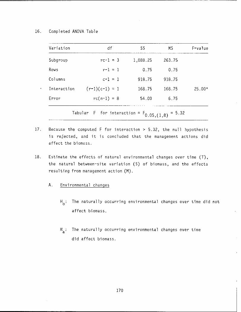
16. Completed ANOVA Table

Variation df SS MS F-value

Subgroup rc-1 = 3 1,088.25 263.75

Rows r-1 = 1 0.75 0.75

Columns c-1 = 1 918.75 918.75

Interaction (r -D( c-1) = 1 168.75 168.75

Error rc( n-1) = 8 54.00 6.75

25.00*

Tabular F for interaction = Fn nc. ,, ft\ = 5.32

17. Because the computed F for interaction > 5.32, the null hypothesis

is rejected, and it is concluded that the management actions did

affect the biomass.

18. Estimate the effects of natural environmental changes over time (T),

the natural between-site variation (S) of biomass, and the effects

resulting from management action (M).

Environmental changes

H : The naturally occurring environmental changes over time did not

affect biomass.

H : The naturally occurring environmental changes over time

did affect biomass.

170

Test at « = 0.5; t005)8df = 2.306.

where there are 8 df for the error in the ANOVA Table (Step 16).

The environmental effect = E = XCA - XCß = 33 - 23 = 10

where XrA = the mean for the control site after management

XrD = the mean for the control site before management CB

Therefore, the biomass was changed by 10 units as a result of

environmental effects.

i, • * c 2 EMS _ 2(6.75) _ , , _ w.„m Variance for E = —-— = -^-3—L - 4.b - var(,hj

where EMS = MS for the error in the ANOVA Table (Step 16)

2 = number of means considered

Standard error for E is se(E) = / var(E) = / 4.5 = 2.12

Compute t statistic for test: se(n = 2TT2 = 4'72

Because the computed t of 4.72 > 2.306, the null hypothesis is

rejected, and the conclusion is that environmental changes over

time, unrelated to the management actions, did affect biomass.

B. Natural between-site variation

H : Site differences did not affect biomass. 0

H : Site differences did affect biomass. a

171

Test at a = 0.05; tQ Q5 gdf = 2.306

Site effect = S = X^r, - X~n MB CB

where X^g = the mean for the treatment site before management

X~n = the mean for the control site before management

= 16 - 23 = -7

Variance for s = ^p = 2(6-75) = 4.5

Standard error for S = / 4.5 = 2.12

S -7 Compute t statistic for test: —j-^r = ? ' = -3.30

Because the computed t statistic of -3.30 < -2.306, the null

hypothesis is rejected, and it is concluded that natural site

variation did affect biomass.

C. Management effects

H : Management actions did not affect biomass over time.

H : Management actions did affect biomass over time. a

Use the same a and tabular t as for the previous tests; i.e.,

2.306.

Management effect = M = (XMA - XMß) - (XCA - XCß).

172

In this example, M = (41-16) - (33-23) = 25-10 = 15. M can

also be computed as:

<*MA-*MB>-E °raS (XMA-W"S-

where XMA = the mean for the management site after management

Therefore, there was a 15 unit increase in biomass due to

management actions.

... , M _ 4 (EMS) _ 4(6.75) _ Q Variance for M = —* L - —^—L - 9 n 6

where 4 is a factor indicating that four means are being compared

the standard error for M = se(M) = v9 = 3.

4. 4. 4- *• 4.' M _ 15 _ r " Compute t statistic: ,.,, - -~ - 5.

The null hypothesis is rejected, and the conclusion is that

management actions did result in an increase in biomass.

Because there are control samples, it is valid to conclude that

management had a causal effect on biomass changes.

For this test, the effects of management, environment, and site

variation were evaluated. The following three study designs

can be used to estimate effects, as indicated below:

2 12Note that this t = the F-value for interaction.

173

Estimatable effects

Premanagement Postmanagement

Management site Yes Yes

Control site Yes Yes

Management, environ- ment, and site.

Premanagement Postmanagement

Management site No Yes The sum of manage-

ment and site Control site No Yes effects (no premanagement

sampling done).

Premanagement Postmanagement

Management site Yes Yes The sum of manage-

ment and environ- Control site No No mental effects , (no control sites

sampled)

Fixed-site, Pre-, and Postevaluation of Management Actions

This is a very useful type of study design. Assume eight stream sites

are evaluated. The eight sites should be selected randomly from a larger "set

of possible sites in the area of interest so that valid inferences can be made

for this larger area. The sites can be on eight different streams of the same

type in the same general area, on one stream, or as sets of control and

treatment sites on four streams. Management (treatment) activities should be

applied to four randomly selected sites out of the eight sites.

174

Assume that the study objective is to increase the population of catchable

sport fish. Therefore, a premanagement estimate of population size must be

made at each site before management actions occur. Control sites are estab-

lished so that any natural changes in fish numbers can be documented. After

sufficient time has passed for management effects to occur, the eight sites

are resampled.

Accurate population estimates are assumed. Acceptance of this assumption

means that the within-site sampling variances of these estimates are not

considered relevant.

(The data is arranged by sample site order):

Site Premanagement

1 100

Control

Treatment

Postmanagement Di ffe rence

132 32

140 8

185 28

230 25

123 43

186 65

203 38

277 52

2 132

3 157

4 205

5 80

6 121

7 165

8 225

Compute the difference for each pair as the post- minus the premanagement

abundance. These differences reflect time plus management effects for

treatment sites. For the control sites, the differences reflect only

time effects. Compute the means and standard deviations for these two

sets of values:

Mean s^ s

Control, X 23.25 111.58 10.56 c

Treatment, XT 49.50 140.33 11.84

175

2. The null hupothesis, H : there was no treatment effect, is tested against

the one-sided alternative H : treatment resulted a

number of catchable fish. A one-sided t-test is used

the one-sided alternative H : treatment resulted in an increase in the a

The treatment effect = XT - X = 49.50 - 23.25 = 26.35

The standard error of this treatment effect is:

where n = number of control sites

nT = number of treated sites (n =nT=4). c T

In this example:

se =/ i 3(111-58) + 3(140.331/1 , 1

= / 62.97 = 7.93

3. The t-test statistic is:

+ = XT " Xc _ 26.25 _ , ,. se 7.93 " ä-6i-

The df - nc + nT - 2 = 6 in this example. The critical level for an

a = 0.05 level one-tailed t-test is:

^.05,6 = i-943

The computed value of 3.31 exceeds the tabular value of 1.943. Therefore,

HQ is rejected, and the conclusion is that management actions resulted in

an increase in the catchable fish population. (The actual significance

level of this test is much better than a = 0.05).

176

4. The test for a time effect is also a t-test (two-sided) with nc + nT - 1

df: (recall that X is the mean of the differences in fish abundance in v c the control sites before and after management actions):

*-{| (yi)sc

2 + (nT-i)sT2 L_

S6=/ nc + nT"2 \V

t = Tt61 = 4-14

The critical level is tQ Q5 ß = 2.447. Therefore, the conclusion is that

there were significant time effects on the size of the catchable fish

population.

Even if the management treatment had no effect on fish populations, the

pre- and postcomparison of responses of the four treated sites would have

shown a significant increase in catchable fish due to time effects. This

example illustrates the need for controls in long term environmental

studies.

5. Given random assignment of treatments, there should be no difference

between the expected abundance in the premanagement control sites and in

the treated sites. This is tested with an unpaired, two-sided t-test,

computed the same as was the test in Steps 2 and 3, above. Relevant

summary statistics use only premanagement data:

177

Mean s2 s

148.5 1963.0 44.30

147.8 3856.9 62.10

Control (n=4)

Treatment (n=4)

pooled (n=8) 148.1 2494.4 49.94

It is clear there is no difference in means between the two groups of

sites (the actual t value is 0.02; 6 df).

Given that the control and treated sites are, on the average, identical

with respect to the abundance of catchable fish, prior to management

activities, it is valid to just compare the postmanagement measurements

to estimate, and test for, treatment effects. The problem with this

approach is that it lacks sensitivity because the benefits of using fixed

sites (i.e., the pairing of the pre- and postmanagement measurements) are

lost. The large, natural, site-to-site variation obscures the signif-

icance of any management effect.

From the above, the pooled estimate of the standard deviation of the pre-

and postmanagement differences is:

/3(111.58) + 3(140.33) = n 2

The standard deviation in premanagement measurements across all eight

sites is 49.94. The "pairing" effect of pre- and postmeasurements on the

same site greatly reduces the variation in the experiment results.

The unpaired t-test, which does not involve the use of the pretreatment

data, uses the following statistics (based on postmanagement data only):

178

Mean s 2

Control (X ) 171.8 2052.3 45.3 c

Treatment (Xy) 197.3 4010.9 63.3

The valid, but very inefficient, t-test for a treatment effect is:

197.3 - 171.8 _ 25.5 38.9 38.9

= 0.66

This calculation has 6 df and is one-sided, but it is not significant.

Even though management significantly increased the abundance of catchable

fish, this fact would-not be proven without the inclusion of pretreatment

data.

In this example, the estimated treatment effect is 26.25 more catchable

fish. This relative increase may not be applicable to other areas because

the management effect often depends on the initial size of the population.

A better way to express the treatment effect may be as the percent change

relative to "baseline" conditions. Baseline condition is the average

number of fish in the treatment site prior to treatment (147.8 in this

example). If it is known, or assumed, that there is no difference between

control and treatment sites prior to treatment, the estimate of relative

treatment effect is based on the average pretreatment value (148.1 in

this example).

The estimated percent relative increase in catchable fish in this example

is:

-JH^ (100%) = (0.177)100% = 17.7%

179

Point 8 below further illustrates the benefits of fixed sites (i.e., pre-

and post- "pairing"); this material requires use of a more complex

statistical concept.

First, consider what results from analyzing all of the data with a two-way

ANOVA with replication. This analysis (illustrated earlier in this

chapter) is appropriate when there are no fixed sites. In this case, a

different set of sites would have been sampled after management in both

the control and management areas. This is an inefficient study design.

However, the reader may want to try computing the two-way ANOVA for these

data. Results are:

Interaction SS = 689.063 (1 df)

Error SS = 35649.3 (12 df)

F-ratio testing management effect _ Interaction MS n 9, (1,12 df) Error MS ~ U^6

In such a study design, the management effect is measured by the classical

interaction term, expressed here as:

(xTA - xTB) - (xCA - xCB) = (197.30 - 147.80) - (171.75 - 148.50)

= 49.50 - 23.25

= 26.25

This is the same as the treatment effect previously computed. But, in a

completely random two-way design (no fixed sites over time), the variance

of this effect is based on the average within-site error mean square:

4 se(treatment effect) = / (Error MS) -

180

where r = the number of replicate samples at each time, within each area

(control or treatment). For this example, r = 4, and the t-test for a

treatment effect is:

t = fffff = 0.4816 (12 df)

It is an algebraic identity that the square of this t-test value equals

the F-test value for testing interaction (i.e., in this case, 0.48162 =

0.23).

Fixed Sites Combined with Paired Control-Managed Sites

The previous study design can be improved by pairing data for control and

treatment sites. This type of pairing was not done in the above example,

where pre- and postmanagement measurements on the same site were paired,

because the sites were fixed over time. Pairs of fixed sites are selected to

implement the more efficient study design. Paired sites should be in the same

habitat type and near each other. Assume that there are n such pairs. The

power of this study design is that each control-management pair results in a

direct estimate of the management effect. If the previous example had been

designed and tested this way, the data might look like (Note: to illustrate a

point, these values are not the same as those used in the above example):

181

Premanagement Postmanagement

Site pair

1

2

3

4

Means

standard deviations

Control Managed Contrc )1 Managed

100 80 111 133

132 121 162 176

157 165 217 244

205 225 194 245

148.5 147.8 171. 0 199.5

44.30 49.94 45. 92 54.85

Each treatment effect is computed as:

managed \ _ / control after / V after

/ control \ _ / V after / \

managed \ before /

/ control \ \ before /

Management

effect

42

25

19

31

29. 25

9. 81

For example, the calculation for the first pair is:

(133-111) - (80-100) = 22 - (-20) = 22 + 20 = 42

1. H : the average management effect = 0.

H : the average management effect > 0.

Sometimes the alternative hypothesis is 2-sided, but it is usually one-

sided when the treatment is a deliberate management action to achieve

some goal.

A t-test (n-1 df) is used to test the H :

182

average treatment effect t ~ se(average treatment effect)

v _ standard deviation of the treatment effect se(average treatment effect) - ~ZZ

/ n

= i^ = 4.905

df = 3

t = ^i= 5.963.

For a one-sided test and an a-level of 0.01, t0_01>3 = 4.541. Therefore,

the H is rejected, and the conclusion is that the management actions o

increased the number of catchable fish.

This result can be compared to the result obtained when the same data are

analyzed as if the sites were fixed, but where no pairing of control and

treatment sites was done. A t-test [2(n-l) = 6 df] is used, based on the

sets of before and after differences (as explained in the preceding

example):

Managed differences

53

55

79

20

site d- Control fferences

1 11

2 30

3 60

4

X =

-11

22.5

standard de via tion = 30.09

51.75

24.24

183

The t-test statistic is:

51.75 - 22.5 se

se 3(30.09)2 + 3(24.24)2

t =

19.32

29.25 19.32

= 1.514.

! + A 4 4

For a = 0.05, the one-sided critical value of tQ Q5 g = 1.943. Therefore,

the null hypothesis is not rejected. The failure to reject the null

hypothesis is due to the inefficient study design. When possible, fixed

sites with paired control-managed sites and before and after management

measurements is the best study design (there should be at least four

replicate pairs).

Regression Analysis13

The most common use of regression analysis in the context of fisheries

studies is to relate fish weight to length. The relationship of weight to

length is E(W) = yL , where L = fish length, W = fish weight, and E(W) =

expected, or average, weight for the given length. Transforming the data to

logs produces a linear regression problem:

log(W) = a + b(log L) + z

where (a = log y)

b = the slope of the line

£ = the uncertainty about the line

1 3 When regression analysis is used to compare data, X values are for the

independent variable and values of Y are random variables (dependent variables).

184

The average value of (s)2 is the "residual mean square error;" it is analogous

to the error mean square in analysis of variance methods. Note that given

estimates of the parameters a and b, the weight can be predicted given the

length by the equation W = yl_ , where y = e .

The use of linear regression analysis can be illustrated with data from

the study of Keller and Burnham (1982). In their sampling site "3U", 19 brook

trout were captured by electrofishing, using two passes. Virtually all of the

brook trout present were caught. The fish weights in grams and lengths in

millimeters, the logs of these values, and the products of Y times X are

presented below:

i

1 2 3 4 5 6 7 8 9

10 11 12 13 14 15 16 17 18 19

W

10 7

10 10 9

10 18 15 17 18 15 13 58 58 49 72 83 94

86 97 90 95 91

102 102 116 117 119 116 114 110 171 171 170 190 206 210

totals means

c2

Y = log(W)

2. 0794 2. 3026 1. 9459 2 3026 2 3026 2 1972 2 3026 2 8904 2 7081 2 8332 2 8904 2 7081 2 5649 4 0604 4 0604 3 .8918 4 .2767 4 .4188 4 .5433

57 .2794 3 .0147 0 .7792

X = 1og(D

4. 4543 4. 5747 4. 4998 4. 5539 4 5109 4 6250 4 6250 4 7536 4 7622 4 7791 4 7536 4 7362 4 7005 5 1417 5 1417 5 .1358 5 .2470 5 .3279 5 .3471

91 .6700 4 .8247 0 .0888

YX

9.2623 10.5337 8.7562 10.4858 10.3868 10.1621 10.6500 13.7398 12.8965 13.5401 13.7398 12.8261 12.0563 20.8774 20.8774 19.9875 22.4398 23.5429 24.2935

281.0540

To compute a simple linear regression, tabulate Y, X, and YX and then

compute the sum of the products YX; the means of Y and X; and the standard

deviation s2 and sx2 of the Y and X variables. Most recently developed

scientific calculators compute regression slopes and correlations automat-

ically, once the basic X,Y data are entered.

185

Five basic items are required to compute linear regressions. The items

needed in addition to the means X, Y, are:

SP - I (X..-X)(Y..-Y) (a sum of products)

n = I X.Y. - nXY

1=1 n 1

n - 2 _ 2 SSX ~ .l (Xi~X) = (n_1)sx (a sum of squares)

SS = I (Y -Y)2 E (n-l)s2

T 1=1 n Y

The only new quantity needed is the sum of the cross products, SP. It is

computed by first summing all XY terms; 281.0540 in this example. Then

subtract nXY:

SP = 281.0540 - 19(3.0147)(4.8247)

= 281.0540 - 276.3554

= 4.6986

SSy = (n-l)sy2 = 18(0.7792) = 14.0256

SSX = 18(0.0888) = 1.5984

Given these statistics, the regression results can be computed.

186

A

1. Compute the regression coefficient, b:

A b

SP -ssx

4.6986 1.5984

= 2.9396

2. Compute A

the Y-intercept, a:

A a

A _ = Y - b X

= 3.0147 -

= -11.1686

(2.9396)(4.8247)

In this example, the equation for the regression line is:

log(W) = -11.168 + 2.9396[log(L)]

To compute a pred icted weight, insert log(L).

For example, if L = 120,

log(W) = -11.168

= -11.168

= 2.9053

+ 2.9396(4.7875)

+ 14.0733

A 2 9053 Taking the antilog, W = e ' = 18.3 grams.

This calculation can be very useful when not all the fish at a site

are both weighed and measured for length, because fish weights can

be reliably predicted from length measurements.

187

Compute the correlation coefficient, r:

SP

/ (ssx)(ssY)

4.6986

/ (1.5984)(14.0256)

4.6986 4.7348

= 0.9924

The value of r is always between ±1. The closer r is to either of

the extremes (+1 or -1), the better the linear relationship of the

variables. In this example, r = 0.9924, indicating a nearly perfect

linear relationship of log(W) and log(L). An r value of 0 indicates

that no correlation exists; therefore, Y cannot be predicted from X.

A The slope estimate, b, and r are closely related:

b = r

4.

Because the standard deviations sy and s„ are not zero, testing the

null hypothesis that the true b = 0 is equivalent to testing

H : E(r) = 0 (i.e., the true correlation of Y and X is zero).

A A Compute the standard error of b. The variance of b is:

2/i 2s A °Y

var(b) = 55

In this example, sy = 0.7792, r = 0.9924, and SSX = 1.5984. Therefore:

188

varfft - (0.7792)(l-(0.9924)2) var^D; - 1.5984

= 0.007381

se(b) = / var(b) = / 0.007381

= 0.0859

The degrees of freedom associated with the standard error are n-2

because two parameters are estimated from the data (the intercept A 2 2

and slope). The numerator of var(b), i.e., Sy (1-r ), is the

residual variance about the line. It can also be computed as:

n-2 SY u r ;

A A A where Y. = a + b X.. This equation is not as convenient a computa-

tion, but more clearly shows the nature of the residual variance and

the fact that computing the residual variance first requires the

estimation of the two parameters.

5. Test H : b = 0 vs. H : b t 0. A t-test is used; it has n-2 df: o a

A

t = -V. se(b)

In this example, assume an a = 0.01. The critical level of the test

is ( a two-sided test):

^,11-2 ~ t0.01,17 2-567

189

The computed t-value is:

2 9396 0.0859

H is rejected, and the conclusion is that there is a highly signif-

icant relationship between X (length) and Y (weight).

A 6. A confidence interval on b is more appropriate than a test of H for

fish length-weight data. The 1-a confidence interval is:

b - t 0 se(b) = lower limit a,n-<£

A A b + t 0 se(b) = upper limit a,n-2 v ' vv

Assume a = 0.05. The n of tn «r ,7 = 2.110. The lower limit is:

2.9396 - 2.110 (0.0859) = 2.758

The 95% confidence interval on b is thus 2.758 < b < 3.121.

A 7. The confidence limits for a predicted (estimated) value of Y for a

given X value can also be calculated. The standard error, sv,v, of A T j A

Y, given X, is needed:

_ / 2,, 2x / 1 x (X - X) SYIX - 7SY ^ ) J n + SST^ 2

In the above formula, all calculations are based on the sampled

data, except X, which is specified.

190

Predict average fish weight at length L = 200 mm:

X = ln(200) = 5.298

Y = -11.168 + 2.9396(5.298)

= 4.406

VI = e4-406 = 81#94 grams,

A The standard error of Y is:

,n mo^ / 1 * (X ~ 4.8247V sY|x = (0.1086) J yg + i.5984

In this example,' X = 5.298. Therefore:

sY|x = (0.1086) / j| + 0.140148

= 0.04768

2 2 The standard error has n-2 df [it basically depends on sy (l~r ),

which has n-2 df]. For a 95% confidence interval on the true

expected value of Y at X = 5.298, use:

Y * t0.05,n-2 (SY|x)-

In this example, the calculation is:

4.406 ± (2.110)(0.04768) = 4.3054 to 4.5066.

Taking antilogs, the 95% confidence interval on average fish weight

at a length of 200 mm is 74.1 to 90.6 gm.

191

When confidence limits are calculated for the dependent variable

(Y), the estimates are more accurate for X values that are close to

the sample mean X (Figure 14).

8. When there is more than one sample site, such as control and treat-

ment sites or different habitat types, the correct analysis is an

analysis of covariance. This method allows testing equality of

regression lines for several sites (Sokal and Rohlf 1969). A simple

approach for visually comparing results is to plot actual length-

weight data on log-log paper. Plots of each data set will be

patterned in a straight line. Plotting is also useful when there is

just one data set in order to determine if there are any nonconform-

ing data points.

9. Nonparametric tests for the association of continuous variables are

also available; e.g., Spearman's or Kendall's coefficient of rank

correlation tests and Olmstead and Tukey's corner test for associa-

tion. These methods are discussed in Sokal and Rohlf (1969).

Contingency Table

Problem: The following relative abundance of trout and nontrout fish was

found after management activities (pre-management data showed no differences

in control and to-be-managed sites) in a stream monitoring study:

Site Trout Nontrout

Control 34 65

Managed 41 59

The chi-square (x ) nonparametric test (Sokal and Rohlf 1969) is

used to test if the relative abundance of trout and nontrout fish is

related to management activities.

192

Figure 14. Confidence limits for values of Y given values of X (the curved lines). The interval widens as values of X deviate from the sample mean, X.

193

Solution:

1. Null hypothesis: the relative abundance of trout and nontrout fish

is unrelated to management activities.

2. Arrange the data for a two-way contingency test:

a

c

b

d

a + b

c + d

a + c b + d

In this example:

34 65 100

41 59 100

75 125 200

Calculate x

2 x =

(ad - bcT n (a + b)(c + d)(a + c)(b + d)

x = (34 x 59 - 65 x 41T 200

(100)(100)(75)(125)

x = 0.926

From a chi-square distribution table, the critical value for

chi-square with one degree of freedom [df = (r-l)(c-l); r = rows and

c = columns] and a = 0.05 is 3.84.

2 9 Because the value of the x test statistic (0.926) < critical x

(3.84), the null hypothesis is not rejected. The conclusion is that

management did not increase the relative abundance of trout.

194

REFERENCES

Keller, C. R., and K. P. Burnham. 1982. Riparian fencing, grazing, and trout

habitat preference on Summit Creek, ID. N. American Journal of Fish.

Manage. 2:53-59.

Rohlf, F. J., and R. R. Sokal. 1969. Statistical tables. W. H. Freeman and

Co., San Francisco. 253 pp.

Snedecor, G. W., and W. G. Cochran. 1968. Statistical methods. Sixth Ed.

Iowa State University Press., Ames. 593 pp.

Sokal, R. R., and F. J. Rohlf. 1969. Biometry. W. H. Freeman and Co., San

Francisco. 776 pp.

Wilcoxon, F., and R. A. Wilcox. 1964. Some rapid approximate statistical

procedures. Lederle Laboratories, Pearl River, NY. 60 pp.

195

APPENDIX A. COMMON CONVERSIONS OF ENGLISH UNITS OF MEASUREMENT TO THEIR METRIC EQUIVALENTS

English units Metric units

1 inch

1 foot

2.54 cm

30.48 cm

1 cfs

°F = (C° x 1.7985) + 32°

1 lb

1 gal

1 acre-foot

1 acre-foot

0.028 m /sec

°C = (°F - 32°) x 0.556

453.592 g

3.785 1

1233.49 m3

1,233,342.25 1

196

so co

"" iOOJtft

C\l 0 1s- CM CM —

II ro ro 00 i— ll ro i— O 0\ c_ ro

z z CD

lA r- os O u> C\l ro LA CD

©IAOVO O Is- roa r- 03 00 soa 00 ro — II ro C\J CM i- ll CM O OS 00

i— i— II r- LACM o

CM CM CM CM II ^oroosr-

a a ro ro o z. z z z

CO

o

a MD 00 0s X3 i— CM ro .3- CO

SO r- so ro o oo LASO SO LA f- LA SO lAOsO _l

II CM CM r- r- II i- osoor- i—

II LA ro T- OS CM CM CM T-

II a-r- oo lA aa roro CD

z Z Z z c_

CD T0

ro LA Is- C0 CD

""" r-NfOO

00 r- or-oo

ro CM CM 00 ro

-3- r-r-cM os

-J

II Wr-T-T- II oosr-so II a CM OS 00 CM CM >- i-

II CM OS SO ro a ro ro ro

z z Z z CD !_

CÜ 3 4->

CM a SO r- X> (/) 1— CM ro 3 CD (V r-aor- ü

+-> II T- r- i- II CM r- CM- OS 00 SO so

II 00 00 SO *— CM o oor-

ll 00 OsiAcO or-acM

O

-ü z Z Z CM CM t- r- z a ro ro ro Q.

c: rö £-

1— co lA SO co ü ,— CM ro a- —

"O a1- r-LA ro ro CM LfS JUSJO Ost- osr- ■P 0) II II oo r- so in II i- osr-so n 00 so CSJ o (/> c CM r- i- r- ro ro ro ro •— oi z Z Z z •P

•I— CO

to ■p

c o CM a lA 1— CM ro 3 CD o r- co LACO lASOSO OS r- ro CM OS r-aroCM •p

X II i— II r—so Lna II O 00 SO a II r-a i- os co o CM i- i- t- ro ro co CM e o Z Z Z Z •—

X o

5 i— ro a- !_ OS CM ro a O-

Q. <1J II COSO ro C\J II oo Ososro II 00 r- r- C0 n ro h- r- Is- CO -C o soinaa 00 r— LAro LACM osr- +-> in z Z z r— t— r- T— z ro roCM CM T0

*—» — S- i— D.

o o CM ro CO

M- Lf> 00 CM ro a f_

i/i ii II SO3O0 O II ocM tor- II mosr- oo ll SO r- r- CM CD so ^i* ro r— LA a CM ro T— 00 SO e

CD z z Z *— i— »— i— z ro ro CM CM o ZJ z: co

i—

rö os t— CM > r- 1— ro a

a- li JWO II J-so 00 CM II ro CO O 00 n OS LA r— 00 SO ' LA3 co co SO-3" ro i- i- os so a OS z z Z r- r- r- ■- z co CM CM CM •~

+-> co o r— • •1— SO 1— ro a X s_ o

o II C\J r- II r- O ro 00 II CM r-oos II roOsCMa ü J-d- roCM lAro CM O O r— LAro —

z z Z 1— T— i— t— z ro CM CM CM 5 CO r- OS o .

lA *— CM a < X .,__ II \— ll T- LACO co II r- Is- r- O n r-aoo i- • -o 3COCM CM 3- CM <- O C0 CO ro CM rr

Z z z ,- T- i- r- z CM CM CM CM TO a cu c a.

Q- CO O- ■o ■a TO n O

<c CD CD CD CD -so TO OLACM r- TO OlACM r- TO O lACM »- TO O LA CM i-

T- O -O — t- o o o — ■- OOO — r- OOO Li_

1 . -o •

1 . . . . c/> . > . . Ü5

1 . . . •

-J£ o II II II II o II II II II O II II II II o II II II II C t- rs > > > o o t- Q. a. 0. 0- I- a.ü.a.0. r- D- D- 0- 0- r- Q. o. a. a. x> c

o > ü CD

TO T0 ■o TJ — Z 0) in LA CD LA LA CD lA LA CD LA LA —

TO IACM <- o •D LACM <- O TO lACM r- O ■o LACM i- O 5 - oooo — OOOO — OOOO •— OOOO £-

1 . . . .

1 * ■ . . (/) . . . >

1 • . . • E CD

O > CD li n ll ll CD II II II II CD II II II II CD II II II II !_ — C c C C ü- 0£ o o. a. a. a. o 0. a. a. 0. O CL fi. Q. Q.

197

o Q. 0. 0. 0. CO

APPENDIX C. TUKEY'S TEST FOR ADDITIVITY

(SOKAL AND ROHLF 1969)

Data from the example for the ANOVA test on Page 159 (refer also to page

162).

Row Row dr. Site i 1 2 3 4 5 6 sums

140

means

23.333 1 15 20 20 25 30 30 -5.566 2 35 35 40 40 45 55 250 41.667 12.778 3 15 15 20 25 25 30 130 21.667 -7.222

Column sums 65 70 80 90 100 115 520

Column means 21.667 23.333 26.667 30 33 .333 38.333 GM = 28 .889

dc J

-7.222 -5.566 -2.222 1.111 4 .444 9.444

In the example, GM = the grand mean; i.e., the average of all observa-

tions (3 • 6 = 18, in this example). A set of differences is computed next:

dc. = column mean j - GM

dr. = row mean i - GM.

For example,

dc1 = 21.667 - 28.889 = -7.222

dc6 = 38.333 - 28.889 = 9.444

dr2 = 41.667 - 28.889 = 12.778

198

Another table is prepared as an intermediate step to computing the sum of

squares (1 df) for nonadditivity. In the above table, let X^. be the response

value at site (row) i and period (column) j; e.g., X^ = 15 and X25 = 45. The

main entries in the intermediate table are the products Yi . = Xi . d^. dc^. It

2 2 is useful to also tabulate (dr..) and (dc.) :

Site i

Period j , , x2

1 2 3 4 5 6 (dr.)"

1 601.88 617.38 246.91 -154.32 -740.73 -1574.13 30.869

2 -3229.90 -2484.81 -1135.71 567.85 2555.34 6637.15 163.277

3 782.36 601.88 320.95 -200.59 -802.36 -2046.14 52.157

(dc) 52.157 30.869 4.937 1.234 19.749 89.189

Element Y. ,, which is 601.88 in the above table, is computed as:

Y2 j = 601.88 = 15(-5.556)(-7.222)

Similarily, element Y2 g (i = 2, j = 6) is:

Y0 , = 6637.15 = 55(9.444)(12.778)

Compute three sums from the above table:

Q = ZIY.. = the sum of all main elements in the table

9 R = I(dr.) = the sum of the squared values of the dr. values

C = I(dc.) = the sum of the squared values of the dc, values

199

Many calculators can accumulate these sums directly from the original

table, without recording the intermediate values. However, producing the

intermediate table is a useful check for errors.

In the above example:

Q = 601.88 + 617.38 + ... - 802.36 - 2046.14

= 563.01

R = 30.869 + 163.277 + 52.157 = 246.303

C = 52.157 + 30.869 + ... + 89.189 = 198.135

The sum of squares for nonadditivity is:

SS nonadditivity Q /(RC)

(563.01)

(246.303)(198.135)

6.4953

6.5

200

502 72-101 REPORT DOCUMENTATION

PAGE

1. REPORT NO.

: " FWS/OBS-83/33

l. Title and Subtitle

Field methods and statistical analyses for monitoring small salmonid streams

3. Recipient's Accession No.

5. Report Oat« Becember 1983

Authors) Carl L. Armour, Kenneth P. Burnham, William S. Platts

9. Performing Organization Nama and Address Western Energy and Land Use Team U.S. Fish and Wildlife Service Creekside One Building 2627 Redwing Road Fort Collins, CO 80526-2899

U.S. Forest Service Intermountain Forest and Range Experiment Station

316 East Myrtle Boise, ID 83702

3. Performing Organization Rapt. No.

10. Project/Task/WorK Unit No.

U. Contract(C) or Grant(G) No.

(O

12. Sponsoring Organization Nama and Addrass Western Energy and Land Use Team Division of Biological Services Research and Development Fish and Wildlife Service Washington, DC 20240

13. Typa of Report & Period Covered

14,

IS. Suoolamantary Notes

IS. Abstract (Limit: 200 words)

This publication contains information pertaining to monitoring programs which may be used to evaluate the effects of land use practices on small salmonid streams in the Western United States. Information includes an approach for designing a monitoring program, variables which may be used with field measurement techniques, and statistical tests for evaluating data.

17. Oocumant Analysis a. Descriptors

Streams Statistical tests Field tests

3. Identifiera/Ooen-Endad Terms

Field techniques Salmonid streams Salmonid habitat Monitoring

c. COSATI Field/Group

IS. Availability Statament

Release unlimited 19. Security Class (This Reoort)

Nnr1ac,cifipH

21. No. of Pages

2Ü0 20. Security Class (This Page)

Unclassified (See ANSI-Ö9.13) See Instructions on Reverse OPTIONAL FORM 272 (4^

(Formerly NTIS-35) Oeoartmem of Commerce

rn

•• -"

"fa Headquarters. Division of Biological Services, Washington, DC

X Eastern Energy and Land Use Team Leetown, WV

# National Coastal Ecosystems Team Slidetl. LA

# Western Energy and Land Use Team Ft. Collins, CO

# Locations of Regional Offices

Puerto Rico and

Virgin Islands

REGION 1 Regional Director U.S. Fish and Wildlife Service Lloyd Five Hundred Building, Suite 500 N.E. Multnomah Street Portland, Oregon 97232

692

REGION 2 Regional Director U.S. Fish and Wildlife Service P.O.Box 1306 Albuquerque, New Mexico 87103

REGION 3 Regional Director U.S. Fish and Wildlife Service Federal Building, Fort Snelling Twin Cities, Minnesota 55111

REGION 4 Regional Director U.S. Fish and Wildlife Service Richard B. Russell Building 75 Spring Street, S.W. Atlanta, Georgia 30303

REGION 5 Regional Director U.S. Fish and Wildlife Service One Gateway Center Newton Corner, Massachusetts 02158

REGION 6 Regional Director U.S. Fish and Wildlife Service P.O. Box 25486 Denver Federal Center Denver, Colorado 80225

REGION 7 Regional Director U.S. Fish and Wildlife Service 1011 H.Tudor Road Anchorage, Alaska 99503

DEPARTMENT OF THE INTERIOR U.S. FISH AND WILDLIFE SERVICE

As the Nation's principal conservation agency, the Department of the Interior has respon- sibility for most of our nationally owned public lands and natural resources. This includes fostering the wisest use of our land and water resources, protecting our fish and wildlife, preserving the*environmental and cultural values of our national parks and historical places, and providing for the enjoyment of life through outdoor recreation. The Department as- sesses our energy and mineral resources and works to assure that their development is in the best interests of all our people. The Department also has a major responsibility for American Indian reservation communities and for people who live in island territories under U.S. administration.

■it U.S. GOVERNMENT PRINTING OFFICE: 1984—777-778/9151 REGION NO. 8