feature extraction from parametric time–frequency representations for heart murmur detection

Feature Extraction From Parametric Time–Frequency Representations

for Heart Murmur Detection

L. D. AVENDANO-VALENCIA,1 J. I. GODINO-LLORENTE,2 M. BLANCO-VELASCO,3,4

and G. CASTELLANOS-DOMINGUEZ1

1Departamento de Ingenierıa Electrica, Electronica y Computacion, Universidad Nacional de Colombia, Km. 9, Vıa alaeropuerto, Campus la Nubia, Caldas, Manizales, Colombia; 2Departamento de Ingenierıa de Circuitos y Sistemas, Universidad

Politecnica de Madrid, Ctra. de Valencia, km. 7, 28031 Madrid, Spain; 3Universidad de Alcala, Campus Universitario,28871 Alcala de Henares, Madrid, Spain; and 4Departamento Teorıa de la Senal y Comunicaciones, Ctra. Madrid-Barcelona,

km 33.628805, Alcala de Henares, Madrid, Spain

(Received 13 August 2009; accepted 17 March 2010; published online 2 June 2010)

Associate Editor Ioannis A. Kakadiaris oversaw the review of this article.

Abstract—The detection of murmurs from phonocardio-graphic recordings is an interesting problem that has beenaddressed before using a wide variety of techniques. In thiscontext, this article explores the capabilities of an enhancedtime–frequency representation (TFR) based on a time-varyingautoregressive model. The parametric technique is used tocompute the TFR of the signal, which serves as a completecharacterization of the process. Parametric TFRs contain alarge quantity of data, including redundant and irrelevantinformation. In order to extract the most relevant featuresfrom TFRs, two specific approaches for dimensionalityreduction are presented: feature extraction by linear decom-position, and tiling partition of the t–f plane. In the firstapproach, the feature extraction was carried out by means ofeigenplane-based PCA and PLS techniques. Likewise, aregular partition and a refined Quadtree partition of the t–fplane were tested for the tiled-TFR approach. As a result, thefeature extraction methodology presented, which searchesfor the most relevant information immersed on the TFR, hasdemonstrated to be very effective. The features extractedwere used to feed a simple k-nn classifier. The experimentswere carried out using 45 phonocardiographic recordings(26 normal and 19 records with murmurs), segmented toextract 548 representative individual beats. The results usingthese methods point out that better accuracy and flexibilitycan be accomplished to represent non-stationary PCG signals,showing evidences of improvement with respect to otherapproaches found in the literature. The best accuracy obtainedwas 99.06 ± 0.06%, evidencing high performance and stabil-ity. Because of its effectiveness and simplicity of implemen-tation, the proposed methodology can be used as a simplediagnostic tool for primary health-care purposes.

Keywords—Heart sounds, Feature extraction, Time–frequency

representation, Time-varying autoregressive model, Murmur

detection.

ABBREVIATIONS

2D-PCA Two-dimensional PCAAR AutoregressiveBIC Bayesian information criterionCWT Continuous wavelet transformECG ElectrocardiogramHS Heart soundk-nn k-nearest neighborsLS-TVAR Least-squares TVARPCA Principal component analysisPCG PhonocardiogramPLS Partial least squaresSNR Signal-to-noise ratiot–f Time–frequencyTFR Time–frequency representationTVAR Time-varying autoregressiveWVD Wigner–Ville distribution

INTRODUCTION

Cardiac mechanical activity is appraised by auscul-tation and processing of heart sound (HS) records(known as phonocardiographic signals—PCG), whichis an inexpensive and non-invasive procedure. Sincecomputer-based analysis of HS may contribute toimprove diagnosis of cardiac malfunctions, PCG haspreserved its importance in many medical fields of

Address correspondence to L. D. Avendano-Valencia, Departa-

mento de Ingenierıa Electrica, Electronica y Computacion, Universi-

dad Nacional de Colombia, Km. 9, Vıa al aeropuerto, Campus la

Nubia, Caldas,Manizales, Colombia. Electronicmail: ldavendanov@

unal.edu.co, [email protected], [email protected],

[email protected], [email protected]

Annals of Biomedical Engineering, Vol. 38, No. 8, August 2010 (� 2010) pp. 2716–2732

DOI: 10.1007/s10439-010-0077-4

0090-6964/10/0800-2716/0 � 2010 Biomedical Engineering Society

2716

clinical practice.2,10,19 Specifically, murmurs, which aresorted into systolic or diastolic, are some of the basicsigns of pathological changes to be identified, but theyoverlap with the cardiac beat, and these HS cannot beeasily separated by the human ear, since a largeamount of information in the frequency domain isbelow the audibility thresholds. Moreover, cardiacmurmurs are non-stationary signals that exhibitsudden frequency changes and transients. Therefore,the time–frequency representations (TFRs) havebeen proposed before to investigate the correlationbetween the time–frequency (t–f) characteristics ofmurmurs and the underlying cardiac pathologies.19

For that matter, in the literature, both non-parametricand parametric estimations of TFR are generallyemployed.7,15,17 Non-parametric methods (e.g., Wigner–Villle distribution—WVD, continuous wavelet trans-form—CWT, etc.) are based on non-parameterizedrepresentations of the signals as a simultaneous func-tion of time and frequency, whereas parametricmethods are based on parameterized expressions of atime-dependent autoregressive modeling (or relatedtypes) and their extensions. In biomedical applications,the non-parametric methods of estimation that arecommonly implemented by means of wavelet trans-form suffer of a trade-off between time and frequencyresolution.21

Since there are large differences in the transitionpatterns among the individual sets of multi-frame sig-nals, a stable estimation of the transition patternsshould be carried out. In this line, and due to itsintrinsic generality and its capacity to detect formantfrequencies, the time-varying autoregressive (TVAR)models, in which the auto-regressive coefficients areallowed to vary with time, have provided usefulempirical representations of non-stationary time seriesfor biomedical signal analysis.6 The frequency resolu-tion of the parametric methods is superior because ofthe implicit extrapolation of the autocorrelationsequence.21 Furthermore, the TVAR technique canprovide a higher resolution with respect to the non-parametric estimations, and without the complicationof the quadratic terms regarded to the quadratic TFR,or the need to generate a high time-resolution waveletanalysis. Despite these advantages, the selection of themodel order and the methods of estimation for theparameters are the two main problems, which haddiscouraged the use of TVAR models to estimate theTFR.6 Explicitly, the selection of the model order has alarge effect on the quality of the signal representa-tion,15 and for pathological PCG signals it is oftendifficult to select a unique value correctly.12,14,16 As aresult, the TVAR model may not resolve well enoughthe fine structure in the data. However, the methods ofestimation of the TVAR parameters can help with this

issue. In general, these methods should be directlycoupled with the time-varying dynamics of the PCGsignal. Assuming that the signal is stationary withinshort segments, and under the assumption that theparameters and innovations variance are independentof time,17 AR estimators can be used in short timewindows. Because of the lack of resolution, thismethod is basically suitable for cases where the evo-lution in the dynamics is slow. This is the case of thePCG signals. It must be quoted that regardless of theimprovement of the TVAR models for the represen-tation of non-stationary signals, the modeling of thePCG signal to automatically detect murmurs remainsstill an open issue.

For the automatic detection of murmurs, theTFR-based classification methods are preferred withrespect to other techniques because t–f planes haveclear discriminant capabilities to separate signalsbelonging to different classes. In addition, even that theflexibility to form the feature vector in 2D representa-tions is considered the main advantage of a t–f domain-based classification, this enhanced representation alsotends to contain a large amount of redundant data, andhence a dimensionality reduction is required. Thus,there is a growing need for new data reduction methodsthat can accurately parameterize the activity in TFR ofbiosignals, particularly those with higher resolution, asstated in Bernat et al.5 for the case of electroencepha-lographic signals. A direct approach is the use ofprincipal component analysis (PCA) to reduce thedimensionality of the feature space resulting from thet–f plane, assuming that the information is equallydistributed along with the TFR. As concluded inEnglehart et al.,11 a PCA-reduced t–f representationhas shown to effectively accommodate the looselystructured waveforms of some transient biological sig-nals, when quantitative and decision-based analysis isrequired. PCA models each TFR as the weighted sumof base functions obtained as the components, whichmaximize the variability on the dataset. Nevertheless,for classification purposes, the components obtainedare not always related with the most discriminativeinformation. Thus, similar decomposition approaches,such as partial least squares (PLS), can be used as asupervised dimensionality reduction approach thatyields components maximally related with labels.4

Nonetheless, as commonly known in the state-of-the-art, the methods, which classify the TFRs based onthe local regions of the t–f plane, have achieved highersuccess rates than those based on the entire image22;and for PCG signals this supposition is more adequate,since most of the information is concentrated whereverthe heart murmurs are present. But there is a note-worthy unsolved issue associated with local-basedanalysis, namely, the selection of the size of local

Feature Extraction for Heart Murmur Detection 2717

relevant regions. As a result, the choice of featureextractors in the t–f domain, and the classifier, is highlydependent on the final application.19

A major motivation in this study is to generate aset of parametric TFR-based features extracted fromPCG recordings, capable of detecting murmurs withhigher accuracy than using static features. So, the aimsof this study are (a) the calculation of TFRs using aTVAR model, taking directly into account the vari-ability of the PCG induced by the murmurs originatedby valve pathologies; (b) the evaluation of the best setof dynamic features, estimated from parametric-basedTFR, and suitable for the classification of heartmurmurs.

Throughout this article, the criterion followed tocompare the different approaches is the classifieraccuracy, obtained using the well-known k-nnapproach. For the sake of comparison and for thedifferent feature extraction techniques described, theresults—in terms of accuracy—of the proposed para-metric approach were compared with those obtainedusing two non-parametric methods, namely, WVD andCWT (estimated as explained in Quiceno-Manriqueet al.18). Moreover, the results were compared withother assumed baseline methods in the literature.8,23

The rest of this article is organized as follows: first,the time-varying representation implemented is intro-duced, followed by a brief description of the TVARparameter estimation method used, computed by min-imizing the mean-square error. Then, the methodologyfor feature extraction is described in detail (based onlinear decomposition and partition schemes). Lastly,the effectiveness of a feature set based on parametricTFR representing the dynamics of the HS is applied tothe detection of murmurs, comparing the results withother methods in the literature. Finally, there is a briefdiscussion of the results obtained.

BACKGROUND

The stochastic parameters that define the TVARmodel, and that are used to generate the TFRs, arebriefly described in this section. Moreover, the featureextraction techniques from TFRs considered in thisarticle are presented.

TVAR Models with Locally Stationary Assumptions

A time-variant autoregressive model of pth order,shortly TVAR(p), is described as follows

x½t� ¼ hT½t�h½t� 1� þ e½t�; e½t� � Nð0; r2e ½t�Þ ð1Þ

where h½t� ¼ fx½t� i� : i ¼ 1; . . . ; pg; h � Rp is anon-stationary (real-valued vector) processes to be

modeled, e[t] is an unobservable and uncorre-lated Gaussian sequence with zero mean and time-dependent variance re

2[t] (or innovations variance) andh½t� ¼ fhi½t�g; h � Rp are the parameters of theTVAR model. The order of a stationary model can beused as starting point to set the TVAR model order,1

but a more accurate estimation can be achieved bytrial-and-error procedures using a fitting function suchas Bayesian information criterion (BIC).17

The vector of parameters, h[t], and the innovationsvariance, re

2[t], for a given value of the samplingfrequency, fs is related to the spectral content of x[t]by21:

Sxðt; f Þ ¼r2e ½t�

1þPp

i¼1 hi½t�e�jxit=fs��

��2; Sxðt; f Þ � RT�F

ð2Þ

that can be assumed as the time-varying power spectraldensity (i.e., the TFR) of the signal if the system werestationary at the time instant t. The dimension of theTFR is given by the time and frequency resolution (Tfor time, and F for frequency).

TVAR representations differ from their conven-tional stationary counterparts in that they are time-dependent. The methods upon them provide a setof potential advantages listed in Poulimenos andFassois,17 namely, (a) its simplicity of representation,since these models may be potentially specified by alimited number of parameters; (b) improved accuracy;(c) better resolution; (d) better tracking of the time-varying dynamics; (e) flexibility of analysis, since theparametric methods are capable of directly capturingthe underlying structural dynamics regarded to thenon-stationary behavior.

The TVAR model of Eq. (1) is completed specify-ing the evolution of {hi[t]} and re

2[t]. These twoparameters will take a value at the time instant t foreach window of analysis. Nonetheless, if the coeffi-cients at each time are assumed to be independent,then the number of parameters needed becomes usu-ally greater that the amount of data. In the context ofbiological signal processing and to overcome thisproblem, the stochastic regression approach is likelymore suitable.6 Specifically, in a locally stationarymethod for TVAR model estimation (referred asLS-TVAR), the parameters, h[t], are commonly com-puted by minimizing the mean-square error within awindow of size M:

bh½t� ¼ argminh

Xt

s¼t�Mx½t� � hT½t�h½t� 1�� 2 ð3Þ

leading to the Yule-Walker equations that can besolved by any of the standard algorithms such as

AVENDANO-VALENCIA et al.2718

Burg’s one.21 The tracking ability of the LS-TVARalgorithm is prescribed by either the size of a windowor the value of a fading rate, but conditioning thelimitation of this approach: if the process evolves tooquickly, the algorithm will not properly track theevolution of the coefficients, unless the windowbecomes very short which in turn degrades the spec-tral resolution.7 Consequently, for the LS-TVARapproach (Eq. 3), only a coarse adjustment of thetracking properties can be carried out,13 which isenough for the slowly changing dynamics of the PCGsignals.

In order to complete the LS-TVAR model, thevariance of the observation noise re

2[t] must be esti-mated. A sliding window on the square of estimationerror21 can be used:

r2e ½t� ¼

1

M

Xt

s¼t�Mw½s; a�e2½t� ð4Þ

where w[s, a] is a smoothing Gaussian window withaperture of value a and length M which determines thequantity of data considered in the window.

Feature Extraction From the Enhanced t–f Planes

The TFR can be represented as a matrix,Sxðt; fÞ � RT�F; with T time and F frequency points.This matrix can be used to characterize the dynamicsof the PCG signals, but contain a large amount ofinformation difficulting further processing. Thus, theproblem stands on how to reduce the large amount ofinformation and redundancies of the TFRs, butkeeping most of the relevant information. The goal isto reduce the original TFR, Sx(t, f ), into a set of fea-tures, n � Rn; with a smaller dimension but containingthe most important information available in the formerdataset. The main drawback is that TFRs lie on abidimensional space, RT�F; while a set of featuresamenable for a simple classifier should reside on anunidimensional space Rn:

A simple approach for manipulating the TFRmatrix is reducing its dimension by downsampling oreven decimating the time and frequency resolution.However, this method has not been considered, since itremoves some important information from the TFR.An alternative approach to reduce the dimensionalitywould be to divide the two-dimensional TFR intwo-dimensional bins with similar characteristics,characterizing each bin with an average of the energycontained within it. The bigger the area of these bins,the smaller the final feature space, but the lower theresolution. These bins could be equally distributed ordefined according to the amount of information pres-ent in each part of the TFR. On the other hand, as

quoted before, another direct approach for featureextraction would be the use of a linear decompositionmethod (e.g., PCA, 2D-PCA, PLS) to decrease thedimensionality projecting the whole TFR into asmaller subspace but keeping the most relevant infor-mation. The feature extraction approaches usedthroughout this study have been grouped into twosubsections: (a) tiled-TFR approaches; and (b) lineardecomposition-based approaches.

Tiled-TFR Approaches

A straightforward approach for 2D featureextraction is to divide a given t–f plane into tilesevaluating their informativity (the lower the proba-bility of the dynamic occurrence, the higher the tileinformativity). The informativity can be carried outcomputing a statistic operator, Lf�g; over a deter-mined tile of the t–f plane Sx(Dt, Df ) such as thevariance var{Æ}:

n ¼ varfSxðDti;DfjÞg; i ¼ 1; . . . ; NDt; j ¼ 1; . . . ;NDf

ð5Þ

where Dti stands for the ith time segment; Dfj is forthe jth frequency bin; NDf stands for the number offrequency bins; and NDt is the number of time seg-ments. Therefore, it is expected that the feature setextracted from Eq. (5), n, holds enough informationrelated to the non-stationary properties of the signal.

In the beginning, the t–f tiles can be made upof fixed size frameworks, so that the feature vector canbe described as n ¼ ni : i ¼ 1; . . . ; Nb; ni 2 R1

� �;

n 2 RNb ; where Nb ¼ NDf �NDt is the number of tiles.Both, NDf and NDt can be determined empirically.9,22

Time and frequency partitions are defined as:

Dti ¼ ti�1 ti½ �; where ti ¼i � TNDt

; 8i ¼ 1; . . . ;NDt

Dfj ¼ fj�1 fj½ �; where fj ¼j � FNDf

; 8j ¼ 1; . . . ;NDf

ð6Þ

This regular configuration of time windows andfrequency bins assumes that the information content isequally distributed along the t–f plane. However, forPCG signals, this assumption might be inadequate,since most of the information is concentrated aroundthe HS,1 S1, and S2, and eventually between them, inthe systole and diastole, wherever the heart murmursare present.

1S1 implies the closing of the tricuspid and mitral valves immediately

preceding the systole, whereas S2 corresponds to the closing of the

aortic and pulmonary valves at the end of systole.


Thus, a more efficient representation might bereached using unfixed and adaptive size frameworks:for instance, using adaptive multiscale representationsvia the Quadtree decomposition that splits the t–fdomain into four equally sized tiles, where each tile canbe successively decomposed into four new tiles.20 Theroot of the tree is the initial TFR.

Linear Decomposition-Based Approaches

The PCA and the PLS methods were usedthroughout this article as unsupervised and supervisedmethods, respectively, to perform dimensionalityreduction in the TFRs. Moreover, a two-dimensionalextension of PCA was used to represent the reducedfeature space.

PCA DecompositionLet X = {vi: i = 1,…,Nr} be a set of Nr objectsgenerated by m random variables. Thus, for the ithobject, the respective data set vi ¼ v1i ; v

2i ; . . . ; vmi

� �is

given, and from which the centralized data matrix isbuilt as:

X0 ¼ ðv1 � lvÞT; ðv2 � lvÞ

T; . . . ; ðvNr� lvÞ

Th iT

;

lv ¼1

Nr

X

i2Nr

vj; X0 2 RNr�m ð7Þ

The conventional PCA looks for an orthogonaltransformation matrix W, (being WTW ¼ I; I 2 Rn�n;W 2 Rm�nÞ; to project the data onto a smaller set ofvariables with the maximum variance, by means of thelinear transformation Y = X0W, where:

W ¼ argmax trW

ðWTXT0X0WÞ ð8Þ

In practice, the solution is found by setting thecolumns of W to the n leading eigenvectors of thecovariance matrix X0

TX0.Now consider the case when each object is not

defined as a vector but as a matrix, such as TFRmatrices. Then, each object is described by a dataset

Sxiðt; fÞ � RT�F; which from now on will be denoted bySi for shorter notation. Every variable of each set Si

is time-dependent and has been measured upon a set ofT instants of time. Thus, for each object the following

dataset is given Sðj;kÞi : i ¼ 1; . . . ; Nr; j ¼ 1; . . . ; T;

n

k ¼ 1; . . . ; Fo; where notation Si

(j,k) stands for the kth

point, measured for the ith object, at the instant oftime j.

PCA can be carried out on these data performingthe same singular value decomposition but on a datamatrix of vectorized t–f domains, thus dealing with thestochastic nature of the variables by assuming that

each instant of time and frequency point Si( j,k), "j,

constitutes a new random variable. Therefore, eachobject can be described by

vi ¼ Sð1; 1Þi ; . . . ;S

ð1;FÞi ; � � � ;SðT; 1Þi ; . . . ;S

ðT;FÞi

h i;

vi 2 RT�F ð9Þ

and a linear component decomposition can be carriedout over the rewritten centralized data matrix inEq. (7). Lastly, it must be quoted that the PCAtransformation provides a means of unsuperviseddimensionality reduction, as no class membershipqualifies the data when specifying the eigenvectors ofmaximum variance.

2D-PCA DecompositionAnother approach of bi-dimensional componentanalysis (known as 2D-PCA) is discussed in Yanget al.24 and Avendano-Valencia et al.3 Further refine-ment of the object description represented in Eq. (9)can be achieved if the vector used to represent anobject, vj 2 X; is represented by the following matrix,taking into account the variability of the whole vari-able set:

vi ¼

Sð1;1Þi S

ð1;2Þi � � � S

ð1;FÞi

Sð2;1Þi S

ð2;2Þi � � � S

ð2;FÞi

..

. ... . .

. ...

SðT;1Þi S

ðT;2Þi � � � S

ðT;FÞi

2

66664

3

77775; vi 2 RT�F ð10Þ

In this case, the matrix of the data projected,Y ¼ ½wT

1 ; . . . ;wTNr�T; is described by the elementary

matrices wi ¼ viV; wi 2 RT�nF : The reduction of themodel in Eq. (8) is carried out over the column of theobjects, which implies that the variables projected arecapturing the variability of each object in time.

Also, the description of the object in Eq. (11) can betransposed to compute a transformation matrixW 2 RF�nT : Such matrix can reduce the dimensionalityof the vi rows, by means of the operation wi = WTvi,where the matrix W is calculated from the matrixset {ui = vi

T:i = 1,…,Nr}. After the calculation ofthe arrangements, VT�nf ; WF�nT ; a column–row-baseddimensionality reduction is carried out for each vj, i.e.,wi ¼WTviV; wi 2 RnT�nF : As a result, the dimen-sionality reduction takes into account not only theinstant-by-instant variability of each random variable,given by the model represented in Eq. (9), but alsochecks for information variability through the fre-quency spectrum.

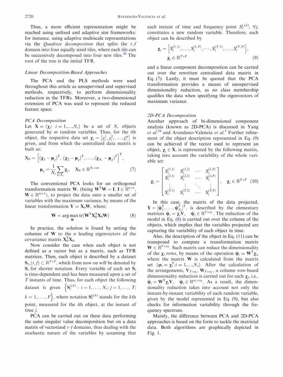
Mainly, the difference between PCA and 2D-PCAapproaches is based on the form to tackle the matricialdata. Both algorithms are graphically depicted inFig. 1.


PLS DecompositionThis regression is a recent technique that somehowgeneralizes features from PCA, by projecting a setof dependent variables from a set of independent

variables, but preserving the asymmetry of therelationship between independent variables, repre-sented by a (very) large set, and dependent variables,whereas PCA treats them symmetrically. Specifically,

FIGURE 1. Dimensionality reduction procedure for TFR matrices; (a) PCA and vectorization; (b) 2D-PCA approach.


a multidimensional input TFR space X0, can beprojected onto the basis vectors (planes), {ki: i =

1,…,m}, through the following transformation:

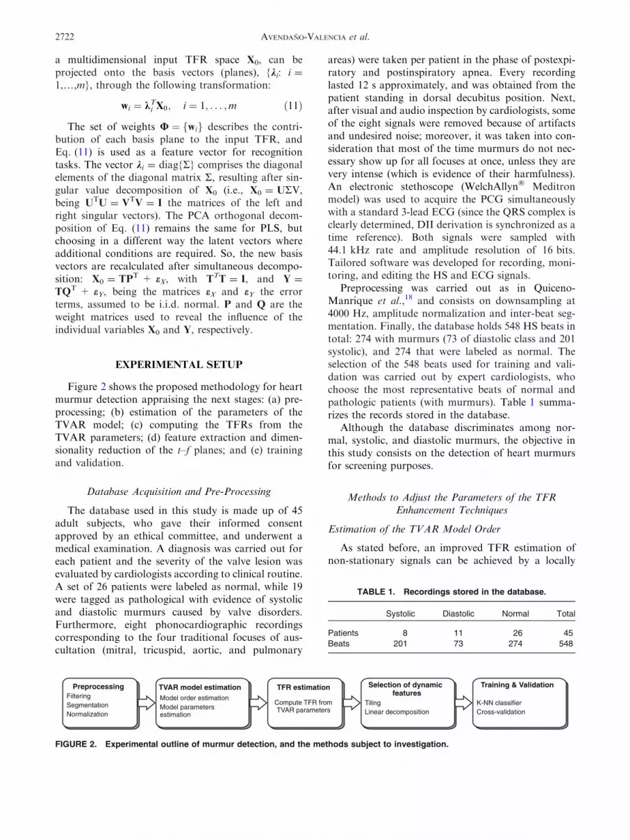
wi ¼ kTi X0; i ¼ 1; . . . ;m ð11Þ

The set of weights U ¼ fwig describes the contri-bution of each basis plane to the input TFR, andEq. (11) is used as a feature vector for recognitiontasks. The vector ki = diag{R} comprises the diagonalelements of the diagonal matrix R, resulting after sin-gular value decomposition of X0 (i.e., X0 = URV,being UTU = VTV = I the matrices of the left andright singular vectors). The PCA orthogonal decom-position of Eq. (11) remains the same for PLS, butchoosing in a different way the latent vectors whereadditional conditions are required. So, the new basisvectors are recalculated after simultaneous decompo-sition: X0 = TPT + eX, with TTT = I, and Y =

TQT + eY, being the matrices eX and eY the errorterms, assumed to be i.i.d. normal. P and Q are theweight matrices used to reveal the influence of theindividual variables X0 and Y, respectively.

EXPERIMENTAL SETUP

Figure 2 shows the proposed methodology for heartmurmur detection appraising the next stages: (a) pre-processing; (b) estimation of the parameters of theTVAR model; (c) computing the TFRs from theTVAR parameters; (d) feature extraction and dimen-sionality reduction of the t–f planes; and (e) trainingand validation.

Database Acquisition and Pre-Processing

The database used in this study is made up of 45adult subjects, who gave their informed consentapproved by an ethical committee, and underwent amedical examination. A diagnosis was carried out foreach patient and the severity of the valve lesion wasevaluated by cardiologists according to clinical routine.A set of 26 patients were labeled as normal, while 19were tagged as pathological with evidence of systolicand diastolic murmurs caused by valve disorders.Furthermore, eight phonocardiographic recordingscorresponding to the four traditional focuses of aus-cultation (mitral, tricuspid, aortic, and pulmonary

areas) were taken per patient in the phase of postexpi-ratory and postinspiratory apnea. Every recordinglasted 12 s approximately, and was obtained from thepatient standing in dorsal decubitus position. Next,after visual and audio inspection by cardiologists, someof the eight signals were removed because of artifactsand undesired noise; moreover, it was taken into con-sideration that most of the time murmurs do not nec-essary show up for all focuses at once, unless they arevery intense (which is evidence of their harmfulness).An electronic stethoscope (WelchAllyn� Meditronmodel) was used to acquire the PCG simultaneouslywith a standard 3-lead ECG (since the QRS complex isclearly determined, DII derivation is synchronized as atime reference). Both signals were sampled with44.1 kHz rate and amplitude resolution of 16 bits.Tailored software was developed for recording, moni-toring, and editing the HS and ECG signals.

Preprocessing was carried out as in Quiceno-Manrique et al.,18 and consists on downsampling at4000 Hz, amplitude normalization and inter-beat seg-mentation. Finally, the database holds 548 HS beats intotal: 274 with murmurs (73 of diastolic class and 201systolic), and 274 that were labeled as normal. Theselection of the 548 beats used for training and vali-dation was carried out by expert cardiologists, whochoose the most representative beats of normal andpathologic patients (with murmurs). Table 1 summa-rizes the records stored in the database.

Although the database discriminates among nor-mal, systolic, and diastolic murmurs, the objective inthis study consists on the detection of heart murmursfor screening purposes.

Methods to Adjust the Parameters of the TFREnhancement Techniques

Estimation of the TVAR Model Order

As stated before, an improved TFR estimation ofnon-stationary signals can be achieved by a locally

PreprocessingFilteringSegmentationNormalization

TVAR model estimationModel order estimationModel parametersestimation

TFR estimation

Compute TFR fromTVAR parameters

Selection of dynamicfeatures

TilingLinear decomposition

Training & Validation

K-NN classifierCross-validation

FIGURE 2. Experimental outline of murmur detection, and the methods subject to investigation.

TABLE 1. Recordings stored in the database.

Systolic Diastolic Normal Total

Patients 8 11 26 45

Beats 201 73 274 548


stationary TVAR model (LS-TVAR), defined by themodel order p. The literature reports that a largeorder of the linear predictor (e.g., 28) is necessary tomodel the PCG signal over its full frequency range.16

Nevertheless, the use of parametric TVAR modelingallows representing the process with a lower quantityof components.17 But, as explained in Poulimenos A,Fassois,17 a more accurate selection of the model ordercan be achieved based on the minimization of a fitnessfunction. Specifically, the fitness function is estimatedfor each HS (i.e., heart beat) by means of the BIC. Assuggested in Poulimenos A, Fassois,17 the approachconsists on evaluating BIC for every family ofparameters, e[t] and re[t], obtained for a given order ofthe model p:

BICðpÞ ¼ �XN

t¼1ln r2

e ½t� þe2½t�r2e ½t�

ð12Þ

where N is the number of signal samples. The BICcurves were computed for different cut-off frequencies(raw signal, 500 and 1000 Hz), and ranging the modelorder from 1 to 15 (Fig. 3a). Likewise, the respectivehistograms are depicted in Fig. 3b for all the records inthe database. The optimum model order is the one thatminimizes the mean BIC function (i.e., the elbow of thecurve). The figure shows that the lower the cut-offfrequency signal the smaller the order selected for themodel. Initially, the model order selected is p = 6, inline with the order reported in Guler et al.12 and Kanaiet al.14 for time-varying AR modeling of HS.

Later, in the ‘‘Results’’ section, a finer empiricaladjustment is presented ranging p from 1 to 15 andtrying to maximize the classifier accuracy.

Estimation of the Parameters of the TVAR Model

The parameters of the autoregressive model withsmoothness priors were estimated by means of theaforementioned LS-TVAR approach (Eq. 3). Underthe assumption that the AR parameters do not changequickly, the PCG recordings were divided initially intowindows of short duration (100 samples). The coeffi-cients of the LS-TVAR model were found using theBurg Algorithm.

Once the parameters of the TVAR model wereestimated, the TFRs were computed by means ofEq. (2). Figure 4 illustrates an enhanced TFR fornormal and pathologic HS, estimated using non-parametric methods (WVD and CWT which wereestimated as explained in Quiceno-Manrique et al.18),and the LS-TVAR parametric method used in thisstudy. The TFRs shown in Fig. 4 are the matrices ofdimension T 9 F, where F is the number of spectralcomponents of the PCG signal, f = [0, 400] Hz; andT is the number of discrete-time samples of eachrecording. This arrangement is intended to cover thefull-time range and a broad range of frequencies.

Methods to Adjust the Feature Extraction Algorithms

The next three sections describe the criteria andmethods followed to adjust the aforementioned featureextraction and dimensionality reduction algorithms:(a) First of all, it is described the procedure to removethe area of the spectral surface that does not containrelevant information; (b) Secondly, and regarding thefeature extraction for the tiled-based approach, it isdefined empirically the size and distribution of the t–f

2 4 6 8 10 12 14Model order

Nor

mal

ized

BIC

Raw signalFrame blocking 500HzFrame blocking 1000Hz

1 2 3 4 5 6 7 8 9 10 11 12 13 14 15

0

0.2

0.4

0.6

0.8

1

Model order

Fre

quen

cy

Raw signalFrame blocking 500HzFrame blocking 1000Hz

(a) (b)

FIGURE 3. Estimation of model order for parametric TVAR model; (a) mean BIC curves; (b) histogram of minimum BIC values.


bins that divide the TFR; (c) Third, the methods toadjust empirically the size of the projected spacewith the linear decomposition methods (e.g., PCA,2D-PCA, PLS) are described. The criterion used toadjust the feature extraction algorithms was the max-imization of the classifier performance. A simple k-nnclassifier was used in order to assess the goodness ofthe feature extraction methods.

Estimation of the Relevant Area of the TFRs

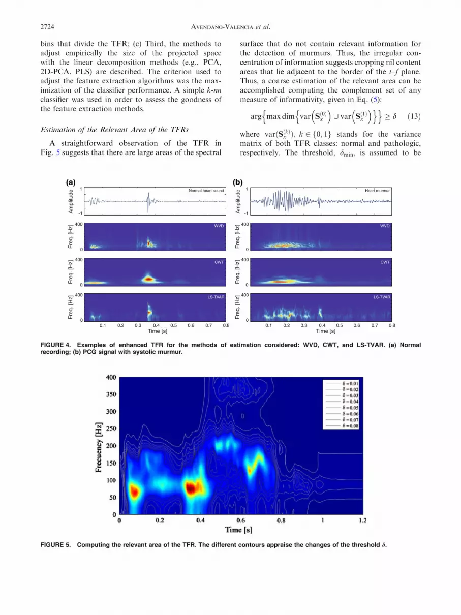
A straightforward observation of the TFR inFig. 5 suggests that there are large areas of the spectral

surface that do not contain relevant information forthe detection of murmurs. Thus, the irregular con-centration of information suggests cropping nil contentareas that lie adjacent to the border of the t–f plane.Thus, a coarse estimation of the relevant area can beaccomplished computing the complement set of anymeasure of informativity, given in Eq. (5):

arg max dim var Sð0Þx

� �[ var Sð1Þx

� �n on o� d ð13Þ

where varðSðkÞx Þ; k 2 f0; 1g stands for the variancematrix of both TFR classes: normal and pathologic,respectively. The threshold, dmin, is assumed to be

]zH[ .qer

F 0

400

]zH[ .qer

F 0

400

]zH[ .qer

F 0

400

Normal heart sound

WVD

CWT

LS-TVAR

Time [s]0.1 0.2 0.3 0.4 0.5 0.6 0.7 0.8

]zH[ .qer

F 0

400

]zH[ .qer

F 0

400

]zH[ .qer

F 0

400

Time [s]0.1 0.2 0.3 0.4 0.5 0.6 0.7 0.8

Heart murmur

WVD

CWT

LS-TVAR

(a) (b)

FIGURE 4. Examples of enhanced TFR for the methods of estimation considered: WVD, CWT, and LS-TVAR. (a) Normalrecording; (b) PCG signal with systolic murmur.

FIGURE 5. Computing the relevant area of the TFR. The different contours appraise the changes of the threshold d.


the minimum value of the relevant variability. Figure 5depicts different complement sets of variancesdepending on the value d; the lower the threshold, thewider the relevant area.

The relevant area was empirically calculated evalu-ating the average variability of the classifier perfor-mance within the interval d = [0.01, 0.08]. In thisarticle, the relevant surface of the TFR was allocatedwithin the framework described by the time interval0 £ t £ 0.8 s and the frequency band 0 £ f £ 400 Hz.

Tuning of the Tile-Based Dimensionality Reduction

On the other hand, the tiled-based approachdescribed in the ‘‘Tiled-TFR approaches’’ section wascarried out extracting several features from the TFRthat estimates the normalized energy on each specifict–f framework. These features were used only forpartitioning the TFR, but were not used for theposterior classification. For this purpose, two parti-tion schemes were tested in the time and frequencydomains: (a) First, dividing the time and frequencyaxes into equally spaced intervals, as suggested inTzallas et al.22; (b) Second, performing a Quadtreepartition scheme upon the TFR surface based on thepixel variance estimates, thus making smaller those t–ftiles with more information.

The Quadtree algorithm for computing the t–fframework (shown in Fig. 6a) is summarized next.

1. Using all the signals in the dataset used fortraining the system, compute the pixel vari-ance matrix of every TFR surface, S0

(i,j) =

var{Sx(Dti, Dfj)}, which is defined as the root ofthe tree decomposition.

2. Define an information threshold 1min and amaximum number of quad decompositioniterations Nd. Otherwise, it leads to intractablecomputational load.

3. Divide S0(i,j) into four equally sized submatrixes

Sði; jÞ1¼ varfS0ðDti; DfjÞg partitioning time and

frequency axes in equal segments.4. Compute the pixel variance in each submatrix

S1(i,j). If varfSði; jÞ

1g>1min; 8i; j; then repeat steps

3 and 4 for further splitting of quad subma-trixes, but not exceeding the number of itera-tions Nd. Otherwise, the values of Dti and Dfjare retrieved.

The tuning of the tile size for each one of the con-figurations considered was carried out by estimatingthe average variability of the classifier performancewhile changing the information threshold 1min, whichranges within the interval 1min = [0.01, 0.1]. Specifi-cally, Fig. 6b shows the outcomes with respect to thetile size, evidencing that a low value of 1min improvesthe accuracy of the classifier but increases the com-putational load.

Tuning of the Linear Decomposition Methods

The normalized matrix assessing the relevant area ofthe TFR is the basis for the following feature extrac-tion. An obvious question is how to find the number oflatent variables needed to obtain the best generaliza-tion for the prediction of new observations. Theamount of relevant latent components, n, was chosenas follows: for PCA, this value is based on the numberof breaks in the plot of the singular values, whereas forPLS, the same value is achieved by cross-validationtechniques.

The n latent variables are often interpreted byplotting them in a TFR plane (as shown in Fig. 7 withn = 4), for systolic and diastolic murmurs, and forboth decompositions considered: PCA and PLS. ForPCA, considering just the first principal component itcan be noticed the strong influence of the S1 event; theS2 event showed less variability. A more detailed

10 20 30 40 50 60 70 80 90 1000

0.05

0.1

0.15

0.2

Number of partitions

Ave

rage

var

ianc

e

Frequency

Time

(a) (b)

FIGURE 6. Computation of the Quadtree algorithm. (a) partition of the TFR information matrix; (b) number of partitions vs.framework variability.


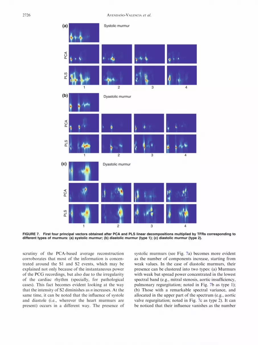
scrutiny of the PCA-based average reconstructioncorroborates that most of the information is concen-trated around the S1 and S2 events, which may beexplained not only because of the instantaneous powerof the PCG recordings, but also due to the irregularityof the cardiac rhythm (specially, for pathologicalcases). This fact becomes evident looking at the waythat the intensity of S2 diminishes as n increases. At thesame time, it can be noted that the influence of systoleand diastole (i.e., wherever the heart murmurs arepresent) occurs in a different way. The presence of

systolic murmurs (see Fig. 7a) becomes more evidentas the number of components increase, starting fromweak values. In the case of diastolic murmurs, theirpresence can be clustered into two types: (a) Murmurswith weak but spread power concentrated in the lowestspectral band (e.g., mitral stenosis, aortic insufficiency,pulmonary regurgitation; noted in Fig. 7b as type 1);(b) Those with a remarkable spectral variance, andallocated in the upper part of the spectrum (e.g., aorticvalve regurgitation; noted in Fig. 7c as type 2). It canbe noticed that their influence vanishes as the number

Systolic murmur

PC

AP

LS

1 2 3 4

(a)

PC

AP

LS

Dyastolic murmur

1 2 3 4

(b)

PC

AP

LS

Dyastolic murmur

1 2 3 4

(c)

FIGURE 7. First four principal vectors obtained after PCA and PLS linear decompositions multiplied by TFRs corresponding todifferent types of murmurs: (a) systolic murmur; (b) diastolic murmur (type 1); (c) diastolic murmur (type 2).


of components increases. A different situation isobserved for the PLS decomposition: if n = 1, there isa great influence of S1 and S2 events, but at the sametime the presence of systolic and diastolic murmursbecome quite evident.

RESULTS

In order to illustrate the problem addressed, and itsdifficultness, Fig. 8 shows several PCG waveformsbelonging to normal and pathological states alongwith their respective TFR estimated by means of theLS-TVAR algorithm. Figure 8 shows that there aresome normal signals whose waveform looks likepathological: waveforms x1 and x5 in Fig. 8a are verysimilar to murmurs, whereas x1, x3, and x5 in Fig. 8b,at first sight, resemble normal signals.

For the sake of comparison, the feature extractionalgorithms proposed were also applied to two non-parametric TFR estimations: CWT and WVD.

As commented before, the criterion used to adjustthe aforementioned procedures was the maximizationof the average accuracy for the detection of murmurs,given by the following definition:

Accuracy ð%Þ ¼ NC

NT� 100 ð14Þ

where NC is the number of correctly classified patterns,and NT is the total number of feeding patterns to theclassifier. Moreover, the sensitivity and specificity

measures are defined to assess the performance of thedetector:

Sensitivity ð%Þ ¼ NTP

NTP þNFN� 100;

Specificity ð%Þ ¼ NTN

NTN þNFP� 100

ð15Þ

where NTP is the number of true positives (murmursaccurately classified as murmur), NFN is the number offalse negatives (murmurs classified as normal signals),NTN is the number of true negatives (normal signalsaccurately classified as normal signals), and NFP is thenumber of false positives (normal signals classified asmurmurs). The accuracy was evaluated with a simplek-nn classifier using a cross-validation strategy. Thecross-validation was carried out generating 11 inde-pendent sets (i.e., folds) from the database with recordsrandomly selected. Each fold contains the same num-ber of records from both classes (i.e., normal andpathological). Ten sets were used for training while theremaining one was used for validation. The perfor-mance was calculated averaging the results for eachfold. Moreover, the standard deviation was calculated.

After filtering and length normalization of the heartbeat sounds the classification was carried out inaccordance to the following training stages:

Tuning of the k-nn classifier: By stepwiseincreasing of neighbor number, the optimalvalue of k is determined for the best classifieraccuracy. Figure 9 illustrates the outcomes for

FIGURE 8. Examples of enhanced TFR for several PCG recordings. (a) normal; (b) heart murmurs.


each one of feature sets used. The figure showsthat the classifier performance decreases as thenumber of neighbors increases. Therefore, andin order to ensure the computational stability, avalue of k = 3 was selected. Tuning of the linear decomposition methods to

reduce the dimensionality. For PCA, the infor-mation threshold and the number of compo-nents (base vectors) were the first parameters toadjust. Once again, a stepwise calculation ofthese parameters allowed selecting the optimumvalues. Figure 10a depicts the estimation of

the parameter dmin (see Eq. 13) using PCA,evidencing a large fluctuation of the estimates.For the PLS classifier the performance wasbetter and more stable. Nevertheless, the valueof the threshold was chosen to be dmin = 0.07.Figure 10b illustrates the classifier accuracy vs.the number of relevant components selected forthe different schemes tested. The performanceshows an asymptotic behavior starting from8 to 10 components for both PCA and PLStechniques. However, the PLS componentsachieved a better performance faster than forthe PCA technique. In addition, the tuning ofthe 2D-PCA approach was assessed by com-puting the accuracy for a different number ofcomponents (see Fig. 10c), which was evaluatedseparately for rows and columns. In the firstapproach, a high performance can be achievedfor a low number of components (n = 6–8),while for the column-based approach a steadyvalue of performance was reached just around(n = 10–14). During the dimensionality reduc-tion stage, the performance was recomputed totune the parameters of the model. Figure 10dshows that PLS and 2D-PCA provided betteraccuracies. Tuning the tiled-based feature extraction methods.

For a regular tiling partition, the parameter toFIGURE 9. Number of neighbors vs. accuracy for the differ-ent feature extraction approaches used.

FIGURE 10. Performance of the linear decomposition approaches tested; (a) performance vs. variance threshold for PCA andPLS; (b) performance vs. number of components of PCA and PLS; (c) performance vs. number of rows and columns for the 2D-PCAapproach; (d) performance of the classifier for PCA, PLS and 2D-PCA after tuning.


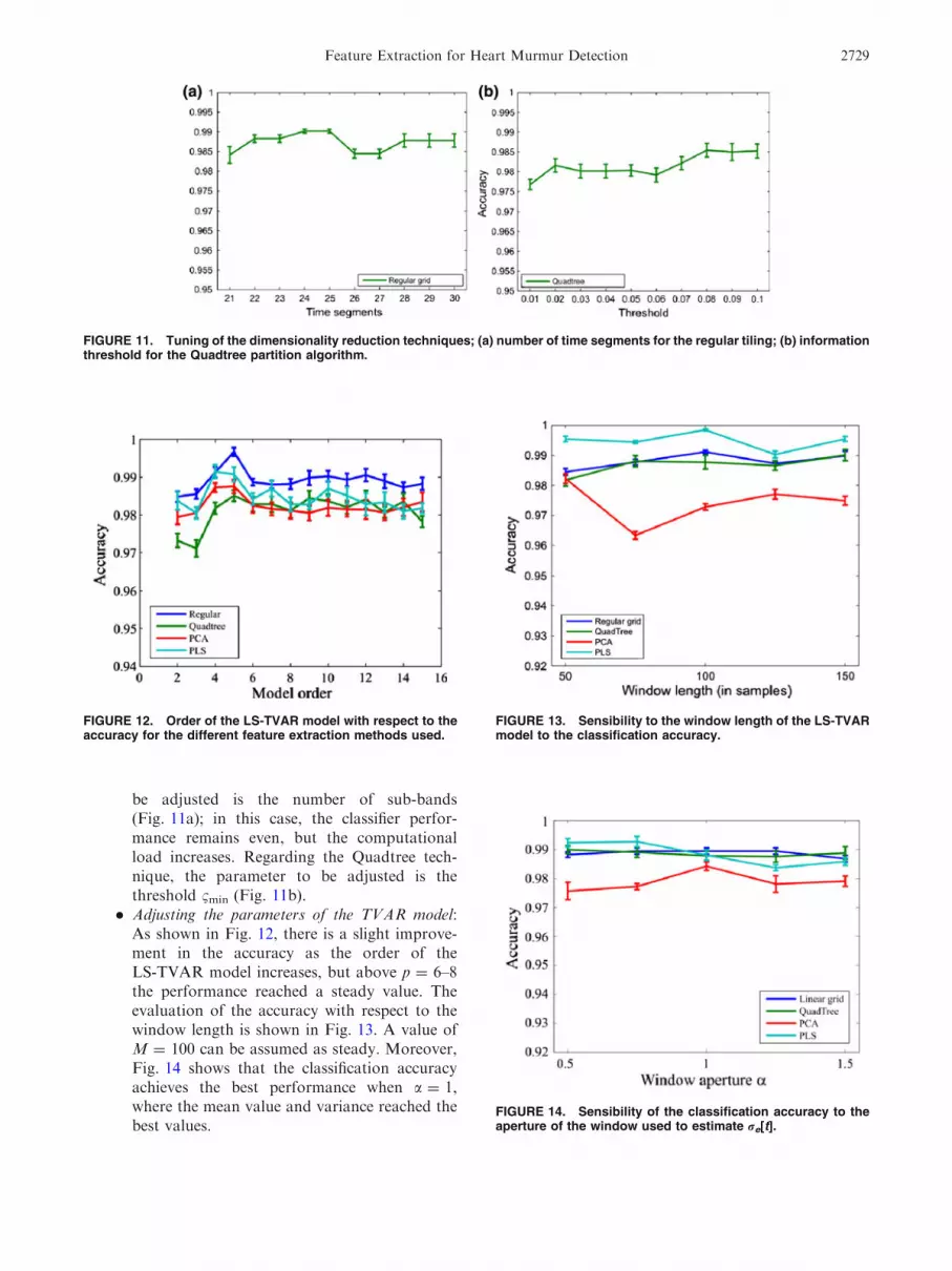
be adjusted is the number of sub-bands(Fig. 11a); in this case, the classifier perfor-mance remains even, but the computationalload increases. Regarding the Quadtree tech-nique, the parameter to be adjusted is thethreshold 1min (Fig. 11b). Adjusting the parameters of the TVAR model:

As shown in Fig. 12, there is a slight improve-ment in the accuracy as the order of theLS-TVAR model increases, but above p = 6–8the performance reached a steady value. Theevaluation of the accuracy with respect to thewindow length is shown in Fig. 13. A value ofM = 100 can be assumed as steady. Moreover,Fig. 14 shows that the classification accuracyachieves the best performance when a = 1,where the mean value and variance reached thebest values.

FIGURE 11. Tuning of the dimensionality reduction techniques; (a) number of time segments for the regular tiling; (b) informationthreshold for the Quadtree partition algorithm.

FIGURE 12. Order of the LS-TVAR model with respect to theaccuracy for the different feature extraction methods used.

FIGURE 13. Sensibility to the window length of the LS-TVARmodel to the classification accuracy.

FIGURE 14. Sensibility of the classification accuracy to theaperture of the window used to estimate re[t].


In summary, the number of neighbors of the k-nnclassifier was set to 3, and the parameters of the TVARmodel were fixed to:

The order of the TVAR model was fixed to 6. The window length of the LS-TVAR model was

fixed to M = 100. The value of the window aperture used to

calculate the variance estimator was fixed toa = 1.

Once the dimensionality reduction was accom-plished, the assemble of features used to train thesystem is summarized in Table 2.

These sets of features were used to train differentk-nn classifiers with three neighbors. Table 3 summa-rizes the classifier performance for the differentapproaches tested. The accuracies were calculatedaveraging for each fold of the cross-validation strategy.The proposed methodology evidences a high accuracy(ranging from 97 to 99%), but with no remarkabledifferences among all the configurations considered.This fact is also supported in view of the estimates forsensitivity, and specificity.

The results evidence the effectiveness, stability, anddimensionality reduction capabilities of the proposeddimensionality reduction approach based on PLSapplied to LS-TVAR TFR. In order to evaluate therobustness of this methodology against noise, it wastested under different conditions, adding artificialwhite Gaussian noise with signal-to-noise ratios(SNR) ranging from 0 to 30 dBs, with steps of 5 dBs.The results are shown in Fig. 15, where SNR = Inf,represents clean signals. The figure evidences a goodstability of this methodology with respect to the pres-ence of an additive white Gaussian noise: in the worstcase, with SNR = 0 dB, the accuracy decreased onlyfive absolute points.

Finally, Table 4 shows a comparison of the resultsachieved with the proposed methodology and otherresults reported in literature. The accuracy obtainedwith the methods described in Wang et al.23 wasobtained with the same database used in this study.

The results obtained using the methods in Delgado-Trejos et al.8 and Quiceno-Manrique et al.18 werecarried out using a subset of the database used in thisstudy that did not contain diastolic murmurs.

TABLE 2. Summary of the features extracted for each scheme proposed.

Dimensionality reduction

approach Parameters adjusted Value # features (n)

Linear grid Time partitions NDt 25 400

Frequency partitions NDf 16

Quadtree Information threshold 1min 0.06 355

PCA Information threshold dmin 0.07 16

PLS Information threshold dmin 0.07 20

2D-PCA Information threshold dmin 0.07 60

Number of time components 10

Number of frequency components 6

TABLE 3. Summary of the classification performance usingthe proposed methodology.

Feature

extraction

method Accuracy (%) Sensitivity (%) Specificity (%)

WVD

Regular 98.44 ± 0.14 99.05 ± 0.08 97.84 ± 0.23

Quadtree 98.23 ± 0.07 98.55 ± 0.12 97.91 ± 0.16

PCA 97.67 ± 0.21 98.70 ± 0.11 96.66 ± 0.39

2D-PCA 98.27 ± 0.15 99.66 ± 0.19 96.91 ± 0.27

PLS 98.76 ± 0.15 99.51 ± 0.12 98.03 ± 0.20

CWT

Regular 96.71 ± 0.36 96.80 ± 0.37 96.61 ± 0.36

Quadtree 97.04 ± 0.31 97.19 ± 0.27 96.90 ± 0.40

PCA 96.57 ± 0.28 96.46 ± 0.26 96.67 ± 0.34

2D-PCA 97.35 ± 0.32 98.39 ± 0.35 96.32 ± 0.34

PLS 97.45 ± 0.32 98.56 ± 0.44 96.38 ± 0.29

LS-TVAR

Regular 99.00 ± 0.06 99.56 ± 0.13 98.45 ± 0.14

Quadtree 98.24 ± 0.12 98.74 ± 0.28 97.76 ± 0.13

PCA 98.17 ± 0.11 97.91 ± 0.16 98.42 ± 0.14

2D-PCA 97.56 ± 0.08 98.31 ± 0.07 96.83 ± 0.17

PLS 98.40 ± 0.19 98.31 ± 0.25 98.49 ± 0.20

FIGURE 15. Accuracy of the PLS dimensionality reductionapproach for different values of SNR.


DISCUSSION

The classification accuracy remains stable as theorder of the TVAR model changes. This means thatthe model order can take values lower than thosesuggested in the literature. This fact lead us to thinkthat most PCG signals from the database are mono-component, which are successfully represented with aTVAR(2) model. Anyway, increasing the order com-plements the information given by the first twoparameters modeling the noise components present inthe PCG signal.

Regarding the linear decomposition, an eigenplane-based PCA technique (as simplest implementation)and a PLS technique (as more sophisticated) wereconsidered. Likewise, the regular partition and arefined Quadtree partition were examined for the tiled-TFR approach. As shown in Table 3, the accuracy ofthe regular tiling outperforms the rest of techniques.However, this brute-strength approach has a highercomputational load, exceeding that of the methodsbased on linear decomposition. Concerning to theimproved object representation with PCA, 2D-PCAshows a light improvement, and reached a similaraccuracy than for PLS, but with a significant reductionof the computational load. The PLS technique alsoevidenced a good behavior against additive whiteGaussian noise.

Regarding the tuning of the feature extrac-tion procedures it must be quoted that the compu-tational stability of the tiled TFR-based techniques ismostly guaranteed for actual matrix sizes of HS. Butfor linear decomposition-based techniques, it isstrongly convenient to choose a confined area ofrelevance on the t–f plane to achieve a stabledimension reduction, and anyhow diminishing reso-lution of the TFR.

For the sake of comparison, the feature extrac-tion methodology discussed in this article was alsoextended to two non-parametric TFRs: WVD andCWT. A slight degradation is observed using CWT,whereas WVD shows an equivalent performance to theproposed TVAR estimation techniques (Table 3).

Furthermore, in terms of computational load and tun-ing of working parameters can be stated that para-metric and non-parametric TFR are alike to enhancethe resolution of non-stationary PCG signals.

CONCLUSIONS

In this article, the ability of an enhanced TFR andtwo approaches for dimensionality reduction areexplored for the detection of murmurs. The enhance-ment of the TFR resolution is carried out by means ofa parametric TVAR model-based estimation tech-nique, allowing an improvement of the representationcapabilities of the HS, and hence to a better detectionof murmurs. The parametric TFR are more suitablefor capturing the time-varying dynamics of the PCGsignals than the common non-parametric approaches,because the resolution and distortion issues are workedout. Nonetheless, the emergent problems of thisparametric approach (i.e., the selection of the modelorder and the estimation of the parameters) are effec-tively solved using locally stationary assumptions.

For the PCG signals, since the enhanced TFR tendsto hold a lot of redundant data, a considerabledimensionality reduction was required. Specifically,two methods of feature extraction were analyzed: lin-ear decomposition and tiling partition of t–f plane. Theresults indicate that a similar accuracy can be accom-plished with both methodologies. The main differencelies on the effectiveness of the dimensionality reductionand the interpretability of the components obtainedusing the linear decomposition methods.

Because of the simplicity of implementation andworthy improvement of the representation capabilitiesdetermining the details of the pathological changes toidentify, the suggested TFR-based feature extractionmethodology appears to be very effective providing ahigh accuracy for the detection of murmurs. Therefore,in future studies, this framework could be applied tothe recognition among different kinds of murmurs, andto the detection of pathologies for different types ofnon-stationary biomedical signals.

In contrast, a serious drawback of the proposedmethodology is that these TFR-based feature extrac-tion techniques require fixed length recordings (i.e.,duration), so the HS must be chopped to a predeter-mined duration. This fact could limit the possibility toextrapolate the results to other databases, leading us tobe cautious, although optimistic with the resultsobtained. A possibility to overcome this problemwas suggested in Quiceno-Manrique et al.,18 wheredynamic time warping techniques were used to nor-malize the duration of each HS.

TABLE 4. Comparison with other works in the literature.

Method

Accuracy

(%)

Sensitivity

(%)

Specificity

(%)

This study 99.00 99.56 98.45

Perceptual features23 88.90 93.03 85.81

Time, frequency, fractal,

and perceptual features896.39 95.40 95.00

Dynamic contours18 98.00 96.90 97.20


ACKNOWLEDGMENTS

The authors would like to acknowledge Dr. AnaMaria Matijasevic and Dr. Guillermo Agudelo whoare working with Universidad de Caldas for organizingthe acquisition of the PCG data. This research wascarried out under grants: ‘‘Centro de Investigacion eInnovacion de Excelencia ARTICA,’’ funded byCOLCIENCIAS; and TEC2006-12887-C02 from theMinistry of Science and Technology of Spain.

REFERENCES

1Abramovich, Y., N. Spencer, and M. Turley. Orderestimation and discrimination between stationary andtime-varying (TVAR) autoregressive models. IEEE Trans.Signal Process. 55(6):2861–2876, 2007.2Ahlstrom, C., P. Hult, P. Rask, J. Karlsson, E. Nylander,U. Dahlstrom, and P. Ask. Feature extraction for systolicheart murmur classification. Ann. Biomed. Eng. 34:1666–1677, 2006.3Avendano-Valencia, D., F. Martinez-Tabares, D. Acosta-Medina, I. Godino-Llorente, and G. Castellanos-Dominguez. TFR-based feature extraction using PCAApproaches for discrimination of heart murmurs. Pro-ceedings of the 31th IEEE EMBS Annual InternationalConference (EMBC’09), 2009.4Barker, M., and W. Rayens. Partial least squares for dis-crimination. J. Chemomet. 17(3):166–173, 2003.5Bernat, E., W. Williams, and W. Gehring. DecomposingERP time–frequency energy using PCA.Clin. Neurophysiol.116:1314–1334, 2005.6Cassidy, M., and W. Penny. Bayesian nonstationaryautoregressive models for biomedical signal analysis. IEEETrans. Biomed. Eng. 49(10):1142–1152, 2002.7Cerutti, S., A. Bianchi, and L. Mainardi. Advanced spec-tral methods for detecting dynamic behaviour. Auton.Neurosci.: Basic Clin. 90(1):3–12, 2001.8Delgado-Trejos, E., A. Quiceno-Manrique, J. Godino-Llorente, M. Blanco-Velasco, and G. Castellanos-Dominguez. Digital auscultation analysis for heartmurmur detection. Ann. Biomed. Eng. 37(2):337–353, 2009.9Deng, J., J. Yao, J. Dewald, and P. Julius. Classification ofthe intention to generate a shoulder versus elbow torque bymeans of a time frequency synthesized spatial patterns BCIalgorithm. J. Neural Eng. 2(4):131–138, 2005.

10El-Segaier, M., O. Lilja, O. Lukkarinen, L. Sornmo,R. Sepponen, and E. Pesonen. Computer-based detectionand analysis of heart sound and murmur. Ann. Biomed.Eng. 33(7):937–942, 2005.

11Englehart, K., B. Hudgins, P. Parker, and M. Stevenson.Classification of the myoelectric signal using time-frequency based representations. Med. Eng. Phys. 21(6):431–438, 1999.

12Guler, I., M. Kiymik, and F. Guler. Order determination inautoregressive modeling of diastolic heart sounds. J. Med.Syst. 20(1):11–17, 1995.

13Kaipio, J., and M. Juntunen. Deterministic regressionsmoothness priors TVAR modelling. Proc. IEEE ICASSP99, 1999, 1693–1696.

14Kanai, H., N. Chubachi, and Y. Koiwa. A time-varyingAR modeling of heart wall vibration. In: Proceedings onInternational Conference of the Acoustics, Speech, and Sig-nal Processing, ICASSP 95, edited by EEE ComputerSociety, 1995, pp. 941–944.

15Marchant, B. Time-frequency analysis for biosystemsengineering. Biosyst. Eng. 85(3):261–281, 2003.

16Nandagopal, D., J. Mazumbar, and R. Bogner. Spectralanalysis of second heart sound in children by selective lin-ear prediction coding.Med. Biol. Eng. Comput. 22:229–239,1985.

17Poulimenos, A., and S. Fassois. Parametric time-domainmethods for non-stationary random vibration modellingand analysis—a critical survey and comparison. Mech.Syst. Signal Process. 20(4):763–816, 2006.

18Quiceno-Manrique, A. F., J. I. Godino-Llorente, M.Blanco-Velasco, and G. Castellanos-Domınguez. Selectionof dynamic features based on time-frequency representa-tions for heart murmur detection from phonocardiographicsignals. Ann. Biomed. Eng. 38(1):118–137, 2009.

19Sejdic, E., I. Djurovic, and J. Jiang. Time–frequencyfeature representation using energy concentration: anoverview of recent advances. Digital Signal Process. 19(1):153–183, 2009.

20Sullivan, G., and R. Baker. Efficient quadtree coding ofimages and video. IEEE Trans. Image. Process. 3(3):327–331, 1994.

21Tarvainen, M., J. Hiltunen, P. Ranta-aho, and P.Karjalainen. Estimation of nonstationary EEG with Kal-man smoother approach: an application to event-relatedsynchronization. IEEE Trans. Biomed. Eng. 51(3):516–524,2004.

22Tzallas, A., M. Tsipouras, and D. Fotiadis. Automaticseizure detection based on time-frequency analysis andartificial neural networks. Comput. Intell. Neurosci. 2007:1–13, 2007.

23Wang, P., C. S. Lim, S. Chauhan, J. Yong, A. Foo, and V.Anantharaman. Phonocardiographic signal analysis meth-od using a modified hidden Markov model. Ann. Biomed.Eng. 35(3):367–374, 2006.

24Yang, J., D. Zhang, A. Frangi, and J. Yang. Two-dimen-sional PCA: a new approach to appearance-based facerepresentation and recognition. IEEE Trans. Pattern Anal.Mach. Intell. 26(1):131–137, 2004.


feature extraction from parametric time–frequency representations for heart murmur detection

Documents