arX

iv:c

ond-

mat

/980

5214

v1 [

cond

-mat

.sta

t-m

ech]

18

May

199

8

Fast spin dynamics algorithms for classical spin systems

M. Krech, Alex Bunker, and D.P. LandauCenter for Simulational Physics, University of Georgia, Athens, Georgia 30602

We have proposed new algorithms for the numerical integration of the equations of motionfor classical spin systems. In close analogy to symplectic integrators for Hamiltonian equations ofmotion used in Molecular Dynamics these algorithms are based on the Suzuki-Trotter decompositionof exponential operators and unlike more commonly used algorithms exactly conserve spin lengthand, in special cases, energy. Using higher order decompositions we investigate integration schemesof up to fourth order and compare them to a well established fourth order predictor-correctormethod. We demonstrate that these methods can be used with much larger time steps than thepredictor-corrector method and thus may lead to a substantial speedup of computer simulations ofthe dynamical behavior of magnetic materials.Keywords: Heisenberg systems, Suzuki - Trotter decomposition, symplectic integrators, predictor- corrector methods, dynamic structure factor

PACS: 75.40.Mg, 75.40.Gb, 75.30.Ds, 75.40.-s

I. INTRODUCTION

Collective phenomena in many materials can be traced back to the presence of interacting magnetic moments onthe atomic level. The exploration of magnetic systems therefore plays a key role in both physics and materials science.The understanding of phase transitions, critical phenomena, and scaling has in part been founded on the investigationof simple model spin systems such as the Ising, the XY, and the Heisenberg model (see below). These spin systemscontinue to be of high relevance for the investigation of dynamic critical behavior and dynamic scaling. On the otherhand realistic models of magnetic materials can be constructed from these simple spin models, if the interactionparameters and the underlying lattice structure are taken as an input from experiments. However, in such casesthe theoretical analysis of experimentally accessible quantities, such as the dynamic structure factor, is usually toodemanding for analytical methods. Computer simulations of the dynamical behavior of spin systems have, therefore,become a very important tool for the theoretical understanding of dynamic critical behavior and material propertiesof magnetic systems, as the following examples may show.

Large scale computer simulations have been performed in recent years in order to explore the dynamical behavior ofclassical XY [1] and Heisenberg models [2] in d = 2 dimensions and of classical Heisenberg ferro- and antiferromagnetsin d = 3 [3,4]. The simulations are based on model Hamiltonians for continuous degrees of freedom represented by athree-component spin Sk with fixed length |Sk| = 1 for each lattice site k. A typical model Hamiltonian is then givenby

H = −J∑

<k,l>

(SxkSx

l + SykSy

l + λSzkSz

l ) − D∑

k

(Szk)2 , (1.1)

where J is the exchange integral, < k, l > denotes a nearest-neighbor pair of spins Sk, λ is an exchange anisotropyparameter, and D determines the strength of a single-site or crystal field anisotropy. For λ = 1 and D = 0 Eq.(1.1)represents the classical isotropic Heisenberg ferromagnet or the corresponding antiferromagnet for J > 0 or J < 0,respectively. In the case λ = D = 0 Eq.(1.1) reduces to the XY model.

Realistic descriptions of specific magnetic materials may require additional interactions in the Hamiltonian, likean additional two-spin exchange interaction between next nearest neighbors, third nearest neighbors, etc. (see, e.g.,Ref. [5]). Two spin interactions do not always provide a sufficient representation of the interactions in a magneticsystem. A more accurate description of the isotropic ferromagnet EuS for example also requires a three spin exchangeinteraction [6] of the type

H3 = −J3

∑

<k,l,m>

(Sk · Sl) (Sk · Sm) , (1.2)

where < k, l, m > denotes a triple of nearest neighbor spins. Four spin exchange coupling constants are often negligible,but the biquadratic interaction given by

1

H4 = −J4

∑

<k,l>

(Sk · Sl)2, (1.3)

which is well known from the Blume - Emery - Griffith (BEG) model [7], needs to be considered in certain cases [8].The thermodynamic properties of the model can be obtained from a Monte-Carlo simulation of the Hamiltonian

Htot = H+H3 +H4 given by Eqs.(1.1), (1.2), and (1.3). In order to study the dynamic properties of the spin systemthe equations of motion given by [1–4]

d

dtSk =

∂Htot

∂Sk× Sk (1.4)

must be integrated numerically, where a Monte-Carlo simulation of the model provides equilibrium configurations asinitial conditions for Eq.(1.4). Note that frequencies will be measured in energy units so that h = 1 in Eq.(1.4). Atypical quantity to be determined from the dynamics of the model is the dynamic structure factor S(q, ω), which isgiven by the space-time Fourier transform of the spin-spin correlation function

Gα,β(rk − rl, t − t′) ≡ 〈Sαk (t)Sβ

l (t′)〉, (1.5)

where α, β = x, y, z denote the spin component, rk and rl are lattice vectors, and the average 〈. . .〉 must be taken over asufficiently large number of independent initial equilibrium configurations. The effect of collective thermal excitationsof the system (e.g., phonons) is not included in the above approach. However, in magnetic systems the typical timescale on which Eq.(1.4) has to be integrated is much shorter than typical time scales set by these excitations, so thatthe above procedure can be justified. In general one has to resort to the solution of Langevin equations rather thanEq.(1.4) in order to obtain the correct dynamics, but this is beyond the scope of this article.

From the above outline of a typical Monte-Carlo spin dynamics study it is evident, that at least in d = 3 themajor part of the CPU time needed for a spin dynamics simulation is consumed by the numerical integration ofEq.(1.4). It is therefore desirable to do the integration with the biggest possible time step. However, using standardmethods a severe restriction on the size of the time step is posed by the accuracy within which the numerical methodobserves the conservation laws of the dynamics. It is evident from Eq.(1.4) that |Sk| for each lattice site k and thetotal energy are conserved. Symmetries of the Hamiltonian impose additional conservation laws. If, for example,Htot = H according to Eq.(1.1) for D = 0 and λ = 1 (isotropic Heisenberg model) the magnetization M =

∑k Sk is

a conserved quantity. For the anisotropic Heisenberg model, i.e., λ 6= 1 and/or D 6= 0 only the z-component Mz ofthe magnetization is conserved. Conservation of spin length and energy is particularly crucial, because the condition|Sk| = 1 is a major part of the definition of the model and the energy of a configuration determines its statisticalweight. It would therefore also be desirable to devise an algorithm which conserves these two quantities exactly.

The outline for the remainder of this investigation is as follows. In Sec.II we describe the properties of the currentlyused fourth-order predictor-corrector method [1–4]. Sec.III is devoted to the presentation of our new integrationprocedure, based on Trotter-Suzuki decompositions of exponential operators, which conserve spin length and, for theisotropic case only, energy exactly. In Sec.IV we compare both schemes with special regard to the accuracy withinwhich the conservation laws hold and their speed for a given demand on accuracy. A comparison within the fullframework of a spin dynamics simulation for a Heisenberg ferromagnet is also presented. We finally discuss theprospects of both algorithms in view of large scale spin dynamics simulations in Sec.V.

II. PREDICTOR-CORRECTOR METHODS

Predictor-corrector methods provide a very general tool for the numerical integration of initial value problemslike Eq.(1.4) with an equilibrium configuration as the initial value. The demand for very good spin length andenergy conservation, however, requires methods with small truncation errors in the time step δt. Further stabilityrequirements for long times have led to the implementation of a fourth-order scheme, which we briefly reproduce herefor the convenience of the reader.

In a more symbolic form Eq.(1.4) can be written as y = f(y) with the initial condition y(0) = y0, where y is ashort-hand notation of a complete spin configuration written, e.g., as a 3N dimensional vector for a lattice with Nsites. The initial equilibrium configuration is simply denoted by y0. The predictor step of the scheme is then given,e.g., by the explicit Adams-Bashforth four-step method [9]

y(t + δt) = y(t) +δt

24[55f(y(t)) − 59f(y(t− δt)) + 37f(y(t − 2δt)) − 9f(y(t − 3δt))] (2.1)

2

which has a local truncation error of the order (δt)5. The corrector step consists of typically one iteration of theimplicit Adams-Moulton three-step method [9]

y(t + δt) = y(t) +δt

24[9f(y(t + δt)) + 19f(y(t)) − 5f(y(t − δt)) + f(y(t − 2δt))] (2.2)

which also has a local truncation error of the order (δt)5. The first application of Eq.(2.1) obviously requires theknowledge of y(δt), y(2δt), and y(3δt) apart from y(0) = y0. These can be provided by three successive integrationsof y = f(y) (see Eq.(1.4)) by the fourth-order Runge-Kutta method [9] which cannot be used for the entire timeintegration, because truncation errors accumulate too fast during typical integration times required for high frequencyresolution. In order to apply Eqs.(2.1) and (2.2) repeatedly the spin configuration at the last four time steps must bekept in memory.

It is interesting to note that the predictor-corrector method according to Eqs.(2.1) and (2.2) observes the conserva-tion laws for the magnetization according to the symmetry of the Hamiltonian to within machine accuracy if periodicboundary conditions are employed. The reason is that all spins are updated simultaneously by Eqs.(2.1) and Eq.(2.2)and that the driving forces (torques) are evaluated precisely according to the exact equation of motion (see Eq.(1.4))for every time step. The periodic boundary conditions restore the discrete translational invariance of the infinitelattice in the finite sample needed for the simulation.

The predictor-corrector method is very general and, therefore, its implementation is independent of the specialstructure of the right-hand side of the equation of motion. Apart from the conservation of the magnetization theother conservation laws discussed in Sec.I will therefore only be observed within the accuracy set by the truncationerror of the method. In practice, this limits the time step to typically δt = 0.01/J in d = 3 [4] for the isotropic modelHamiltonian given by Eq.(1.1) (D = 0), where the total integration time is of the order 200/J . The same methodhas also been used in d = 2 with a time step δt = 0.025/J [2], but in this case the total integration time did notexceed 60/J . In view of the fact that a time resolution of typically 0.1/J − 0.2/J is desired for the evaluation of thetime displaced correlation function given by Eq.(1.5), it is clear that the total CPU time required for a spin dynamicssimulation in d = 3 is dominated by the numerical integration of the equations of motion. A quantitative analysis ispresented in Sec.IV.

III. SUZUKI-TROTTER DECOMPOSITION METHODS

The motion of a spin according to Eq.(1.4) may be visualized as a Larmor precession of the spin S around aneffective axis Ω which is itself time dependent. In order to illustrate our reasoning we restrict ourselves again to theHamiltonian Htot = H given by Eq.(1.1) for the simple case D = 0 but for arbitrary values of λ. The evaluation ofthe right-hand side of Eq.(1.4) then shows that the lattice can be decomposed into two sublattices such that a spinon one sublattice performs a Larmor precession in a local field Ω of neighbor spins which are all located on the othersublattice. For the Hamiltonian given by Eq.(1.1) there are only two such sublattices if the underlying lattice is, e.g.,simple cubic or bcc.

The first basic idea of the algorithm to be described below is to actually perform a rotation of a spin about itslocal field Ω by an angle α = |Ω|δt, rather than integrating Eq.(1.4) by some standard method. This procedureguarantees the conservation of the spin length |S| to within machine accuracy. (A procedure like this has already beenimplemented in a numerical study of spin motions in a classical ferromagnet [10]). The second basic idea is to exploitthe sublattice decomposition of Eq.(1.4) to also ensure energy conservation to within machine accuracy. Denoting thetwo sublattices by A and B, respectively, we can write Eq.(1.4) in the form

d

dtSk∈A = ΩB[S] × Sk∈A ,

d

dtSk∈B = ΩA[S]× Sk∈B, (3.1)

where ΩA[S] and ΩB[S] denote the local fields produced by the spins on sublattice A and B, respectively. Eitherof the equations in Eq.(3.1) reduces to a linear system of differential equations if the spins on the other sublattice arekept fixed. This suggests an alternating update scheme, i.e., the spins Sk∈A are rotated for the given values of Sk∈B

and vice versa. This implies that the scalar products Sk∈A ·ΩB[S] remain constant during the update of Sk∈A andthe scalar products Sk∈B ·ΩA[S] remain constant during the update of Sk∈B. From Eq.(1.1) for D = 0 and Eq.(1.4)we therefore find that the energy is exactly conserved during this alternating update scheme (see also Eq.(3.4)). Note,that each sublattice rotation is performed with the actual values of the spins on the other sublattice, so that only asingle copy of the spin configuration is kept in memory at any time. However, the magnetization will not be conservedduring the above rotation operations. Moreover, the two alternating rotation operations do not commute, so that acloser examination of the sublattice decomposition of the spin rotation is required.

3

In order to obtain a simple description of the operations performed on the spin configuration during the integrationof the equations of motion we again represent a full configuration by a vector y which is decomposed into two sublatticecomponents yA and yB according to y = (yA, yB). The cross products in Eq.(3.1) can be expressed by matrices A andB which are the infinitesimal generators of the rotation of the spin configuration yA on sublattice A at fixed yB andof the spin configuration yB on sublattice B at fixed yA, respectively. The exact update of the configuration y fromtime t to t + δt can then be expressed by an exponential (matrix) operator according to

y(t + δt) = e(A+B)δty(t). (3.2)

Although the exponential operator in Eq.(3.2) rotates each spin of the configuration it has no simple explicit form,because the rotation axis for each spin depends on the configuration itself (see Eq.(3.1)) and is therefore not knowna priori. However, the operators eAδt and eBδt which rotate yA at fixed yB and yB at fixed yA, respectively, do havea simple explicit form. We demonstrate this for the case λ = 1 and D = 0 in Eq.(1.1). For each k ∈ A we find

ΩA[S] = −J∑

l=NN(k)

Sl ≡ Ωk, (3.3)

where NN(k) denotes the nearest neighbors of k (which belong to yB). Eq.(3.3) can be readily generalized for λ 6= 1,the case D 6= 0 will be discussed below. From Eqs.(3.1) and (3.3) we obtain (see also Ref. [10])

Sk(t + δt) =Ωk(Ωk · Sk(t))

Ω2k

+

[Sk(t) −

Ωk(Ωk · Sk(t))

Ω2k

]cos(|Ωk|δt) +

Ωk × Sk(t)

|Ωk|sin(|Ωk|δt). (3.4)

Note, that according to Eq.(3.4) Ωk · Sk(t + δt) = Ωk · Sk(t) which explicitly confirms energy conservation. Fork ∈ B Eq.(3.4) also holds in exactly the same form. The alternating update scheme for the integration of Eq.(3.1),i.e., Eq.(1.4) now amounts to the replacement e(A+B)δt → eAδteBδt in Eq.(3.2), which is only correct up to termsof the order (δt)2 [11]. The magnetization will therefore only be conserved up to terms of the order δt (globaltruncation error), which is insufficient for practical purposes. The remedy for this shortcoming, which constitutesthe third basic idea of the algorithm, is now obvious. We simply employ higher order Suzuki-Trotter decompositionsof the exponential operator in Eq.(3.2) to increase the order of the local truncation error of the algorithm and thusimprove the magnetization conservation. The simplest possible improvement is given by the well known second orderdecomposition [11]

e(A+B)δt = eAδt/2eBδteAδt/2 + O(δt3), (3.5)

which will be used for comparison with the predictor-corrector method outlined in Sec.II. Note, that Eq.(3.5) isequivalent to the midpoint integration method applied to Eq.(3.1) (see also Ref. [10]). We furthermore use the fourthorder decomposition [11]

e(A+B)δt =5∏

i=1

epiAδt/2epiBδtepiAδt/2 + O(δt5) (3.6)

with the parameters

p1 = p2 = p4 = p5 ≡ p = 1/(4 − 41/3) and p3 = 1 − 4p. (3.7)

It is also possible to construct a decomposition like Eq.(3.6) with only three factors, but then |pi| > 1 for i =1, 2, 3 which is numerically unfavorable [11]. From Eqs.(3.5) and (3.6) the close analogy to symplectic integratorsobtained from the Liouville operator formalism for Molecular Dynamics simulations is obvious [12]. The sublatticedecomposition of the spin degrees of freedom in spin dynamics corresponds to the natural decomposition of the degreesof freedom in Hamiltonian dynamics into positions and momenta. Especially the second order decomposition givenby Eq.(3.5) is equivalent to the velocity Verlet algorithm for Molecular Dynamics simulations [13] (see also Ref. [12]for recent developments in this field) which itself is equivalent to the well-known leapfrog algorithm [12].

As will be shown in Sec.IV, the additional computational effort to be invested in the evaluation of Eq.(3.6) ascompared to Eq.(3.5) or Eqs.(2.1) and (2.2) can be compensated by using larger time steps. The evaluation of thetrigonometric functions in Eq.(3.4) can also be avoided by observing that the above decompositions are only correct towithin a certain order in δt. It is therefore sufficient to replace sin x by its Taylor polynomial T (x), where T (x) = x if

Eq.(3.5) is used and T (x) = x−x3/6 if Eq.(3.6) is used. The cosine in Eq.(3.4) then has to be replaced by√

1 − T 2(x)

4

in order to maintain conservation of spin length. It is also worth noting that the above decompositions maintain thetime inversion property of e(A+B)δt, i.e., their inverse is obtained by the replacement δt → −δt. A Hamiltonian withboth nearest and next-nearest neighbor two-spin interactions on, e.g., simple cubic or bcc lattices, can be treatedwithin the above framework if the lattice is decomposed into four sublattices. In contrast to the predictor - correctormethod conservation of magnetization according to the symmetry of the Hamiltonian is only observed within thetruncation error of the decomposition method, because according to Eqs.(3.5) and (3.6) the sublattices A and B areno longer strictly equivalent.

We now generalize the above considerations to the case D 6= 0 in Eq.(1.1). For a spin in sublattice A the equationof motion reads

d

dtSk∈A = ΩB[S] × Sk∈A − 2DSz

k∈Aez × Sk∈A, (3.8)

where ez denotes the unit vector pointing along the z-axis, and spins in sublattice B obey an equation of the same form.In contrast to the isotropic case (see Eq.(3.1)) the equation of motion for each individual spin on each sublattice isnonlinear. It is possible to obtain an analytic solution of this equation, in the spirit of Eq.(3.4), where the trigonometricfunctions are basically replaced by Jacobian elliptic functions, and to implement this solution as a rotation operationin one of the above decomposition schemes. This approach, however, involves very precision sensitive operations whichgreatly limit speed and therefore the overall efficiency of such an algorithm. In practice, it is much more convenientto include the effects of the nonlinearity in Eq.(3.8) by an iterative method, as described in the following paragraph.

For the sublattice decomposition of the spin rotation in the isotropic case discussed above the requirement forenergy conservation in the presence of a single site anisotropy reads

Ωk · Sk(t + δt) − D [Szk(t + δt)]2 = Ωk · Sk(t) − D [Sz

k(t)]2 (3.9)

for k ∈ A and k ∈ B, where Ωk is given by Eq.(3.3). In order to perform a rotation operation in analogy toEq.(3.4) we have to identify an effective rotation axis. This can be achieved by rewriting Eq.(3.9) in the form

Ωk · (Sk(t + δt) − Sk(t)) = 0, where Ωk is given by

Ωk = Ωk − D (0, 0, Szk(t) + Sz

k(t + δt)) , (3.10)

i.e., in order to perform the rotation Szk at the future time t + δt must be known in advance. This problem can only

be solved iteratively starting from the initial value Szk(t + δt) = Sz

k(t) in Eq.(3.10) and performing several updatesaccording to the decompositions given by Eqs.(3.5) or (3.6), respectively, in order to improve energy conservationaccording to Eq.(3.9). Naturally, this procedure leads to a substantial slowdown of the integration algorithm, wherethe energy is no longer exactly conserved. Details are discussed in Sec.IV. The biquadratic interaction given byEq.(1.3) can be treated by the same iterative scheme. The three-spin interaction given by Eq.(1.2), however, requiresa reconsideration of the sublattice decomposition. Specific numerical examples in comparison with those obtainedfrom the predictor-corrector method are presented in the following section.

IV. THE METHODS IN COMPARISON

For a quantitative analysis of the integration methods outlined above we restrict ourselves to the HamiltonianHtot = H given by Eq.(1.1) for λ = 1 in d = 3. The underlying lattice is simple cubic with L = 10 lattice sites ineach direction and periodic boundary conditions are imposed in all cases discussed below. The simulations have beenperformed on IBM RS/6000 workstations at the Center for Simulational Physics and a Cray C90 at the PittsburghSupercomputer Center.

In order to compare the different integration methods we first investigate the accuracy within which the conservationlaws are fulfilled. As a standard initial configuration we choose a well equilibrated configuration from a Monte-Carlosimulation of the model defined by Eq.(1.1) for λ = 1 at a temperature T = 0.8Tc for D = 0 and D = J , whereTc refers to the critical temperature of the isotropic model (D = 0) and is given by Kc = J/(kBTc) = 0.693035[14]. The magnetization of such a configuration differs from zero and provides an indicator for the numerical qualityof the magnetization conservation. We integrate the equations of motion to t = 800/J and monitor the energye(t) ≡ E(t)/(JL3) of the configuration per spin and in units of the exchange coupling constant J and the modulusm(t) ≡ |M(t)|/L3 of the magnetization per spin for the isotropic case D = 0 and its z-component mz(t) ≡ Mz(t)/L3

for the stongly anisotropic case D = J as functions of time. Note, that for these tests both integration methods arestarted from identical initial configurations. The time step for the predictor-corrector method is chosen as δt = 0.01/Jin all cases.

5

We first consider the case of D = 0 for which the implementation of Eqs.(3.5) and (3.6) using Eq.(3.4) is straight-forward. The Taylor polynomial T (x) is chosen as T (x) = x − x3/6 for Eq.(3.5) and T (x) = x − x3/6 + x5/120 forEq.(3.6) in order to reduce the amplitude of the magnetization fluctuations. Fig.1 shows that e(t) for the predictor-corrector method increases linearly with time whereas the decomposition methods both yield a constant value for e(t)as shown in Fig.1. Fig.2 displays the magnetization conservation for the predictor-corrector method (δt = 0.01/J)and the second order decomposition method according to Eq.(3.5) for δt = 0.04/J . The predictor-corrector methodconserves m(t) exactly, whereas the second order decomposition causes fluctuations of m(t) on all time scales. Theapparent deviation of the temporal average of the magnetization from the exact value is due to the finite sampletime; for times greater than 2000/J the deviation changes sign and fluctuations on time scales larger than 800/Jbecome visible. The temporal structure of m(t) for the decomposition methods given by Eq.(3.5) for δt = 0.04/J andEq.(3.6) for δt = 0.2/J is displayed in Fig.3. It is remarkable that the fourth order decomposition gives a substantiallybetter magnetization conservation than the second order decomposition despite the very large time step. In order toachieve the same overall accuracy of the magnetization conservation with the second order decomposition a time stepδt < 0.02/J is neccessary. A single integration of the equations of motion using Eq.(3.5) (second order decomposition)is about twice as fast as the predictor-corrector method used here. The more complex fourth order decomposition (seeEq.(3.6)), however, is about 2.5 times slower than the predictor corrector method. Taking the increase in time step byfactors of 4 and 20, respectively, into account, we find that both decomposition methods yield an eightfold speedupof the integration of the equation of motion. If the overall quality of the magnetization conservation is also takeninto account, there is a clear advantage for the fourth order decomposition according to Eq.(3.6) for the isotropic caseD = 0.

We now turn to the strongly anisotropic case D = J . The predictor-corrector method can be applied as before,but the decomposition scheme needs a major modification because the spin rotation axis depends on the spin valueSz

k at the future time t + δt (see Eq.(3.10)). As already pointed out in Sec.III this gives rise to a self consistencyproblem which can be solved iteratively, where the quality of the energy conservation depends on the number ofiterations performed. For the second order decomposition (see Eq.(3.5)) and the time step δt = 0.04/J two iterationsare sufficient to obtain a better energy conservation than the predictor-corrector method. This means that a singleintegration of the equations of motion using the second order decomposition takes twice as long as for D = 0, so thatits advantage in speed only comes from the increase in the time step, which is still a factor of four. For the fourthorder decomposition according to Eq.(3.6) with δt = 0.2/J six iterations are needed to obtain energy conservation towithin six significant digits, which makes one integration with the fourth order decomposition 15 times slower thanone integration with the predictor-corrector method. From the increase of δt by a factor 20 only a 30% gain in speedremains for Eq.(3.6). The number of iterations needed decreases with δt, but this decrease does not compensatethe loss in speed due to the smaller time step. However, one still obtains a greatly improved energy conservation.The direct comparison of the energy conservation is shown in Fig.4. All three methods behave in a similar way,the change in energy is basically linear with time. The reason for this is the iterative nature of all three methodsin the case D 6= 0. The magnetization fluctuations shown in Fig.5 for the predictor-corrector and the second orderdecomposition method (δt = 0.04/J) reveal the same behavior of both methods as shown in Fig.2 for D = 0. Thedirect comparison between the second and fourth order decomposition for δt = 0.04/J and δt = 0.2/J , respectively,is displayed in Fig.6. The overall accuracy of the magnetization conservation appears to be independent of D forboth decomposition methods. If the emphasis is put on overall energy conservation and speed, the second orderdecomposition given by Eq.(3.5) has some advantages over the predictor-corrector method. If the emphasis is put onenergy conservation alone, the fourth order decomposition given by Eq.(3.6) shows the best performance, but it isonly slightly faster than the predictor-corrector method.

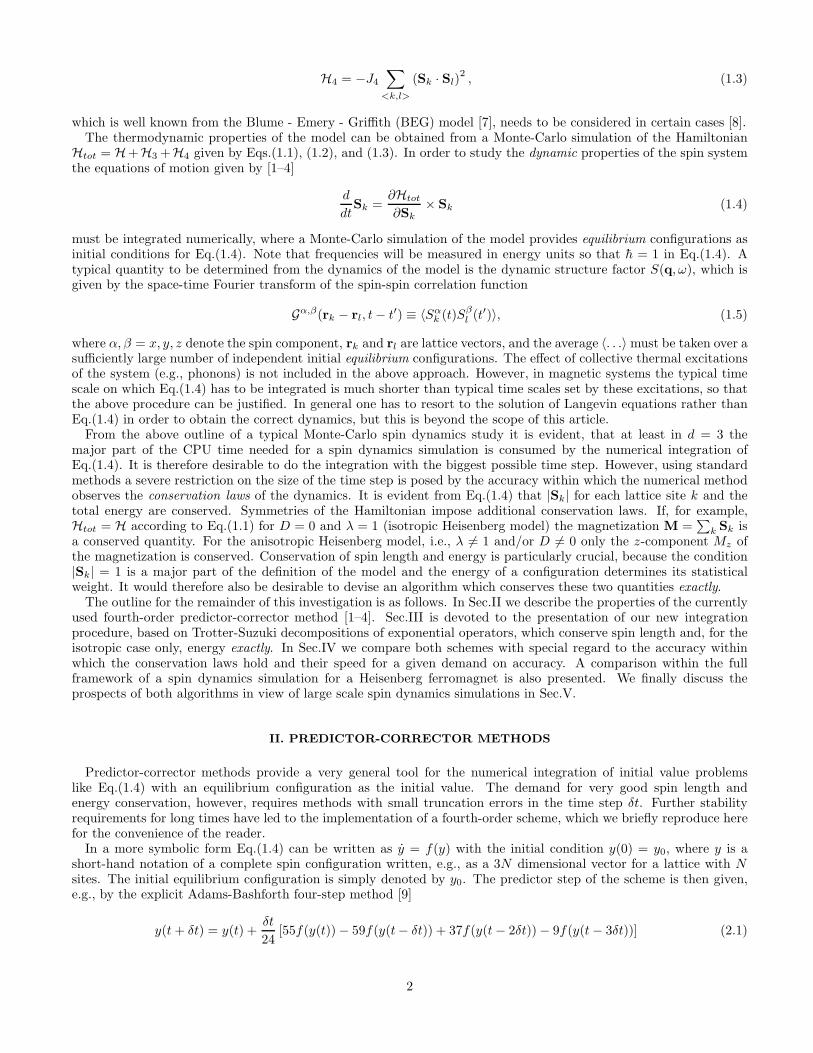
We close this section with a direct comparison of the longitudinal (Sl(q, ω)) and transverse (St(q, ω)) componentsof the dynamic structure factor for the isotropic Heisenberg ferromagnet (see Eq.(1.1) for D = 0) on a simple cubiclattice (L = 10, periodic boundary conditions) at the temperature T = 0.8Tc in the (100) direction. In order tomeasure Sl(q, ω) one has to consider the projections of all spins onto the direction of the magnetization M of theinitial configuration. Note that in general M for a given initial (equilibrium) spin configuration will be nonzero evenin a finite system. Only the average 〈M〉 of the magnetization over sufficiently many equilibrium configurations yields〈M〉 = 0 within the statistical errors. The spin components transverse to M then give access to St(q, ω). The resultsare shown in Figs.7 and 8 for q = (π/5, 0, 0), where Sl(q, ω) and St(q, ω) have been normalized to the static structurefactor Sl,t(q) ≡

∫ ∞

0Sl,t(q, ω)dω. The diamonds represent the result for the predictor-corrector method (δt = 0.01/J)

and the triangles show the result for the second order decomposition method (see Eq.(3.5), δt = 0.04/J). For bothmethods the equations of motion have been integrated to 800/J and averages have been taken over 1000 initialconfigurations, where the time displaced correlation functions have been measured to 400/J . The statistical errorindicated by the error bar represents one standard deviation. For the longitudinal structure factor shown in Fig.7the statistical error is smaller than the symbol size. The overall agreement of the data is very good. The mainmaximum corresponds to the spin wave peak and is located at ω0 = 0.25J in all cases. The frequency resolution is

6

δω = 2πJ/400 ≃ 0.016J . The shoulder like feature at ω ≃ 0.5J in Sl(q, ω) (see Fig.7) is due to many-spin waveprocesses, the description of which is beyond the scope of this article. Both methods have spent about the same CPUtime on generating the initial configurations, but with the time steps given above, the integration of the equationsof motion with the second order decomposition method is about eight times faster than with the predictor-correctormethod. The discrepancy between the errorbars shown in Fig.8 is of statistical origin and indicates the statisticaluncertainty of the errorbars themselves. Note, however, that the discrepancy only occurs in a frequency region welloutside the spin wave peak, where the signal level is almost three orders of magnitude below its peak value.

V. SUMMARY

Starting from a well developed and established predictor-corrector method for the numerical integration of theequations of motion of a classical spin system as a timing and precision standard we devised and tested an alternativeclass of algorithms which is based on Suzuki-Trotter decompositions of exponential operators. Our findings can besummarized as follows.

1. Advantages of the predictor-corrector method

The greatest advantage of the predictor-corrector method is its versatility and its capability to conserve themagnetization exactly. Isotropic and anisotropic spins systems with nearest and next-nearest neighbor inter-actions can be treated within one and the same numerical approach. The decomposition of the lattice intosublattices, which is the basis for the decomposition method, depends on the range of the interactions, so thatthis numerical approach is far less general than the predictor-corrector method. Crystal field anisotropies leavethe performance of the predictor-corrector method almost unaffected, whereas the decomposition method suffersfrom a drastic reduction in speed.

2. Advantages of the decomposition method

The greatest advantage of the decomposition method is its capability for handling large time steps and the exactconservation of spin length. In the absence of anisotropies it also conserves the energy exactly and it maintainsreversibility. For anisotropic Hamiltonians energy conservation and reversibility can be obtained to a highaccuracy using iterative schemes; exact magnetization conservation, however, is lost. The time steps typicallyused are unaccessible by the predictor-corrector method due to the lack of exact energy conservation withinthe algorithm. The resulting speedup of a spin dynamics simulation gives access to larger lattices, provideda second order decomposition is sufficiently accurate for the problem under investigation. In simple cases thefourth order decomposition yields very accurate results even for time steps an order of magnitude larger thantypical time steps used for the predictor-corrector method.

A general recommendation for one or the other method cannot be given. If, however, special interactions are themain objective of the investigation, one should resort to the predictor-corrector method because of its generality. If theinteractions in the system are standard two-spin exchange interactions and the objective is to study large systems, oneshould consider the decomposition method because of its speed and its built-in energy and spin length conservation.

ACKNOWLEDGMENTS

M. Krech gratefully acknowledges financial support of this work through the Heisenberg program of the DeutscheForschungsgemeinschaft. This research was supported in part by NSF grant #DMR - 9405018 and the PittsburghSupercomputer Center.

Note added in proof

While this work was in press we have learned that a method equivalent to the one presented here had been developedindependently by Frank, Huang, and Leimkuhler (J. Frank, W. Huang, and B. Leimkuhler, Journal of ComputationalPhysics 133, 160 (1997).) Frank, Huang, and Leimkuhler denote their method as Staggered Red-Black Method andemploy the same decomposition technique which is described in this work.

7

[1] H.G. Evertz and D.P. Landau, Phys. Rev. B 54, 12302 (1996).[2] B.V. Costa, J.E.R. Costa, and D.P. Landau, J. Appl. Phys. 81, 5746 (1997).[3] K. Chen and D.P. Landau, Phys. Rev. B 49, 3266 (1994).[4] A. Bunker, K. Chen, and D.P. Landau, Phys. Rev. B 54, 9259 (1996).[5] H.G. Bohm, W. Zinn, B. Dorner, and A. Kollmar, Phys. Rev. B 22, 5447 (1980).[6] E. Mueller-Hartmann, U. Koebler, L. Smardz, J. Mag. Mag. Mat. 173, 133 (1997)[7] M. Blume, V.J. Emery, and R.B. Griffith, Phys. Rev. A 4, 1071 (1971).[8] O. N. Mryasov, A. J. Freeman, and A. I. Liechtenstein, J. Appl. Phys. 79, 4805 (1996).[9] R.L. Burden, J.D. Faires, and A.C. Reynolds, Numerical Analysis (Prindle, Weber & Schmidt, Boston, 1981), p.205 and

pp.219.[10] R.E. Watson, M. Blume, and G.H. Vineyard, Phys. Rev. 181, 811 (1969).[11] H. Yoshida, Phys. Lett. A 150, 262 (1990); see also M. Suzuki and K. Umeno in Computer Simulation Studies in Condensed

Matter Physics VI, edited by D.P. Landau, K.K. Mon, and H.B. Schuttler (Springer, Berlin, 1993), pp. 74 and referencestherein.

[12] A. Kopf, W. Paul, and B. Dunweg, Comp. Phys. Comm. 101, 1 (1997) and references therein.[13] L. Verlet, Phys. Rev. 159, 98 (1967).[14] K. Chen, A. M. Ferrenberg, and D. P. Landau, Phys. Rev. B 48, 3249 (1993).

FIG. 1. Energy e(t) = E(t)/(JL3) per spin for the predictor-corrector method (see Eqs.(2.1) and (2.2)) for the time stepδt = 0.01/J and D = 0 (solid line). Both decomposition schemes (see Eqs.(3.5) and (3.6)) conserve the energy exactly (dashedline).

FIG. 2. Magnetization m(t) = |M(t)|/L3 per spin for the predictor-corrector method (see Eqs.(2.1) and (2.2)) for the timestep δt = 0.01/J (dashed line) and the second order decomposition scheme (see Eq.(3.5)) for the time step δt = 0.04/J (solidline) for D = 0. The predictor-corrector method conserves the magnetization exactly, whereas Eq.(3.5) yields fluctuations inm(t) on all time scales.

FIG. 3. Magnetization m(t) per spin for the fourth order decomposition method (see Eq.(3.6)) with δt = 0.2/J (solid line)and for the second order decomposition method (see Eq.(3.5)) with δt = 0.04/J (dashed line) for D = 0. The CPU time neededfor both methods with these time steps is almost the same. Despite the large time step the fourth order decomposition methodyields substantially smaller magnetization fluctuations than the second order decomposition.

FIG. 4. Energy e(t) per spin for the predictor-corrector method (see Eqs.(2.1) and (2.2)) for the time step δt = 0.01/J andD = J (solid line). The decomposition scheme given by Eq.(3.5) for δt = 0.04/J shows a decrease of e(t) (dashed line) andEq.(3.6)) for δt = 0.2/J also yields a decrease of e(t) (dotted line). For these parameters the decomposition methods showbetter energy conservation than the predictor-corrector method.

FIG. 5. Magnetization mz(t) per spin for the predictor-corrector method (see Eqs.(2.1) and (2.2)) for the time stepδt = 0.01/J (dashed line) and the second order decomposition scheme (see Eq.(3.5)) for the time step δt = 0.04/J (solid line)and D = J . The qualitative behavior of mz(t) closely resembles the behavior in the isotropic case shown in Fig.2.

FIG. 6. Magnetization mz(t) per spin for the fourth order decomposition method (see Eq.(3.6)) with δt = 0.2/J (solid line)and for the second order decomposition method (see Eq.(3.5)) with δt = 0.04/J (dashed line) for D = J . The typical temporalstructure of the fluctuations of mz(t) is very similar to the isotropic case shown in Fig.3.

FIG. 7. Longitudinal dynamic structure factor Sl(q, ω) of an isotropic Heisenberg ferromagnet for T = 0.8Tc and |q| = π/5in the (100) direction on a simple cubic lattice (L = 10, periodic boundary conditions) normalized to the static structure factorSl(q) ≡

∫∞

0Sl(q, ω)dω for the predictor-corrector method (diamonds) and the second order decomposition method (triangles)

for time steps δt = 0.01/J and δt = 0.04/J , respectively (see main text). The statistical error (one standard deviation) issmaller than the symbol size.

8

FIG. 8. Transverse dynamic structure factor St(q, ω) of an isotropic Heisenberg ferromagnet for T = 0.8Tc and |q| = π/5in the (100) direction on a simple cubic lattice (L = 10, periodic boundary conditions) normalized to the static structure factorSt(q) ≡

∫∞

0St(q, ω)dω for the predictor-corrector method (diamonds) and the second order decomposition method (triangles)

for time steps δt = 0.01/J and δt = 0.04/J , respectively (see main text). The error bars represent one standard deviation.

9

-1.65544

-1.65543

-1.65542

-1.65541

-1.65540

-1.65539

-1.65538

0 100 200 300 400 500 600 700 800

e(t)

t J

predictor-correctordecomposition

Fig.1

0.6343

0.6344

0.6345

0.6346

0.6347

0.6348

0 100 200 300 400 500 600 700 800

m(t)

t J

2nd order decompositionpredictor-corrector

Fig.2

0.63440

0.63445

0.63450

0.63455

0.63460

0.63465

0 50 100 150 200

m(t)

t J

4th order decomposition2nd order decomposition

Fig.3

-2.64165

-2.64160

-2.64155

-2.64150

-2.64145

-2.64140

-2.64135

0 100 200 300 400 500 600 700 800

e(t)

t J

predictor-corrector2nd order decomposition4th order decomposition

Fig.4

0.77728

0.77732

0.77736

0.77740

0.77744

0 100 200 300 400 500 600 700 800t J

2nd order decompositionpredictor-corrector

m (t)z

Fig.5

0.77728

0.77732

0.77736

0.77740

0.77744

0 50 100 150 200t J

4th order decomposition2nd order decomposition

m (t)z

Fig.6

0.0Fig.7

0.5 1.0ω/J

0.1

1.0

10.0Second Order DecompositionPredictor−corrector method

Sl(q,ω)S(q)

0.0Fig.8

0.5ω/J

0.01

1.00

100.002nd order decompositionpredictor−corrector

St(q,ω)S(q)