exploration of teacher-centered and task-centered
TRANSCRIPT
HAL Id: tel-03229727https://tel.archives-ouvertes.fr/tel-03229727v2
Submitted on 1 Jun 2021
HAL is a multi-disciplinary open accessarchive for the deposit and dissemination of sci-entific research documents, whether they are pub-lished or not. The documents may come fromteaching and research institutions in France orabroad, or from public or private research centers.
L’archive ouverte pluridisciplinaire HAL, estdestinée au dépôt et à la diffusion de documentsscientifiques de niveau recherche, publiés ou non,émanant des établissements d’enseignement et derecherche français ou étrangers, des laboratoirespublics ou privés.
Exploration of Teacher-Centered and Task-Centeredparadigms for efficient transfer of skills between
morphologically distinct robotsMehdi Mounsif
To cite this version:Mehdi Mounsif. Exploration of Teacher-Centered and Task-Centered paradigms for efficient transfer ofskills between morphologically distinct robots. Automatic. Université Clermont Auvergne [2017-2020],2020. English. �NNT : 2020CLFAC065�. �tel-03229727v2�
UNIVERSITÉ CLERMONT AUVERGNEÉCOLE DOCTORALE DES SCIENCES POUR L’INGÉNIEUR DE CLERMONT FERRAND
ThèsePrésentée par
Mehdi Mounsifpour obtenir le grade de
DOCTEUR D’UNIVERSITÉ
Spécialité
Électronique et Systèmes
Exploration of Teacher-Centered and Task-Centeredparadigms for efficient transfer of skills between
morphologically distinct robots
Soutenue publiquement le 15 Décembre 2020 devant le Jury :
David FILLIAT Professeur - ENSTA ParisTech RapporteurOlivier STASSE Directeur de Recherche - LAAS RapporteurGentiane VENTURE Professeur - TUAT (Japon) ExaminateurSébastien DRUON Maître de Conférences - LIRMM, UM ExaminateurLounis ADOUANE Professeur - Heudiasyc, UTC Directeur de thèseBenoit THUILOT Maître de Conférences - Institut Pascal, UCA Co-encadrantSébastien LENGAGNE Maître de Conférences - Institut Pascal, UCA Co-encadrant

ii
À mon père,à qui j’aurais voulu montrer
le potentiel professionnalisant des jeux vidéos.
iii
I have to finish this.
Ellie in The Last of Us, Part II - Naughty Dog, 2020

iv

Remerciements
En dépit de ma maîtrise, inédite dans mon entourage (même après trois ans de labeur), desnotions d’acteur-critique, de divergence de Kullback-Leibler et de l’architecture de ML-Agents, ilm’est difficile d’imaginer un scénario d’achèvement de ces travaux de thèse couronné de succès sansle soutien capital de toutes les personnes qui ont pris part, de près ou de loin, à cette aventure età qui je voudrais ici exprimer ma reconnaissance.
Si ces supports ont été de natures diverses, ils ont pavé la route vers l’achèvement de cettethèse d’un parterre d’herbe chatouilleuse. Sans parvenir à masquer totalement les rares, maisinévitables, aspérités du chemin, le niveau de confort que j’ai perçu excédait de très loin la rugositéet les irrégularités irritantes qu’aurait sans nul doute comporté une trajectoire isolée.
J’aimerais tout d’abord exprimer ma profonde gratitude envers mon directeur de thèse, Lou-nis ADOUANE. Dans une époque lointaine, ses réponses patientes à mes interrogations sur lessystèmes multi-agents ont eu un poids non-négligeable dans mes choix d’orientations. Plus récem-ment cependant, je voudrais lui signifier mon appréciation pour sa sage vision à long-terme, sesencouragements et ses conseils tactiques en terme de publications qui m’ont permis de valorisermes travaux. Si je regrette et te présente mes excuses pour t’avoir emprunté ton bureau, je suisprêt à te le parier sur le résultat d’un match de basket.
Premier par la chronologie, l’acuité et la pertinence de ses questions lors de la rédaction denos papiers, je tiens à remercier Benoit THUILOT, qui, après un interrogatoire inoubliable lorsde notre première rencontre, m’a permis de rentrer en M1 Robotique, m’ouvrant ainsi le véritablepoint de départ de cette odyssée. Ainsi, Benoit, si je suspecte que la quantité de sueurs froides etde palpitations que j’ai induite chez toi avec mes robots volants et autres modèles de jeux vidéodépasse de très loin le quota autorisé, je te remercie ta pédagogie, ton humour et ton bon sens quiont été salvateurs à plus d’un égard.
Finalement, une mention particulière à Sébastien LENGAGNE, troisième membre de l’équipeencadrante (la team des Boyz, comme je m’y référais dans le secret du bureau 3106). Au cours deces trois ans au front, Sébastien à vaillamment endossé le rôle d’encadrant de terrain. N’hésitantjamais à me lancer à l’assaut des territoires inexplorés et dangereux du transfert entre agentsde morphologie différentes, guidé par une connaissance intime des réflexes de la communautérobotique, il m’a permis de mettre en place des plans d’expériences ambitieux sur l’Universal NoticeNetwork qui feraient pâlir d’envie les clusters de calcul des GAFAM. Je voudrais te témoignerSébastien, ma profonde gratitude: tu as été un encadrant d’une rare gentillesse, attentif et àl’écoute. Malgré nos épisodiques divergences sur le mode de programmation des robots, dont Benoitpourra certainement attester, tu as supporté et encouragé la grande majorité de mes initiativesscientifiques en trouvant un délicat équilibre entre le pilotage et l’autonomie. Je suis tout à faitconscient de la chance que j’ai eu.
J’aimerais aussi adresser mes remerciements aux membres du jury, Gentiane VENTURE,Olivier STASSE, David FILLIAT et Sébastien DRUON dont les questions sagaces, la justesse
v
vi
scientifique, l’ouverture d’esprit et l’amabilité ont conféré une aura particulière au souvenir que jegarde du 15 décembre 2020.
Plus familièrement maintenant, je dédie mon prochain big-up aux locataires du bureau 3016avec qui j’ai partagé, somme toute, une proportion non-négligeable de mon temps éveillé de cesdernières années. Pendant ces moments, nous avons partagé les joies et les peines communes desdoctorants, l’effusion des nouvelles idées et l’émulation scientifique, des courses à la deadline, desmeetings MAACS, des pétitions contre le bruit des machines de l’étage du dessus ainsi que desdiscussions animées, parfois profondes et parfois un peu moins, mais systématiquement rythméespar le bruits de la chasse d’eau des sanitaires d’en face. Mention particulière à Nadhir et sa douceur,à Lobna, à Kamel, à Jojo la Fripouille. À Dimia aussi, sans qui je n’aurais jamais pu m’inscrire endeuxième année, faute de compétences techniques suffisantes pour le scanner du deuxième étage.
J’adresse aussi une pensée transpirante au club de boxe anglaise de Clermont Boxe St-Jacques,dont l’affiche à longtemps trôné sur la porte du bureau, indiquant aux visiteurs, grâce à uneinscription manuscrite de Dimia, ma victoire du 30 Novembre 2018. Merci à Adel et Bénédicted’avoir joué un rôle si structurant pendant ces années et de m’avoir offert un environnement danslequel j’ai pu me défouler, progresser comme boxeur et pratiquer mes talents d’orateurs en tantque coach.
Pour conclure, je destine le dernier paragraphe de ces remerciements à mon premier cercle,plus restreint, mais dont le soutient fut incontournable au cours de cette thèse. À ma mère et masoeur, inconditionnelles dans leur amour stratosphérique et leur affection et que j’espère rendreaussi fières de moi que je le suis d’elles. À Héloïse également, Capitaine de mon navire, qui attendaitla conclusion de cette thèse et notre départ vers la vie de JCD (Jeunes Cadres Dynamiques) avecencore plus d’impatience que moi.
Afin de ne pas diminuer excessivement la patience du lecteur qui doit encore traverser plusieursdizaines de pages pour arriver au bout de ce manuscrit, j’abrégerais ces remerciements en saluanttous ceux, proches, amis et famille, que je n’ai pas directement cités ici, mais dont l’affection resteraliée dans mon esprit à ces trois années inoubliables.
vii
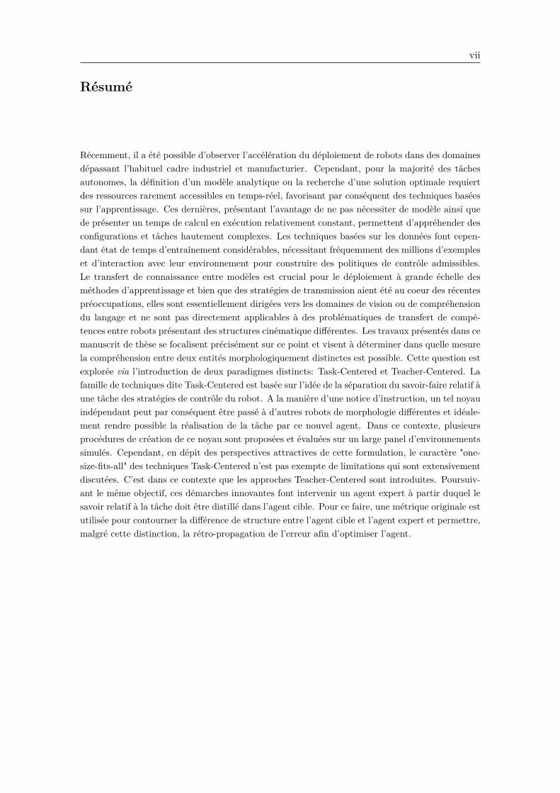
Résumé
Récemment, il a été possible d’observer l’accélération du déploiement de robots dans des domainesdépassant l’habituel cadre industriel et manufacturier. Cependant, pour la majorité des tâchesautonomes, la définition d’un modèle analytique ou la recherche d’une solution optimale requiertdes ressources rarement accessibles en temps-réel, favorisant par conséquent des techniques baséessur l’apprentissage. Ces dernières, présentant l’avantage de ne pas nécessiter de modèle ainsi quede présenter un temps de calcul en exécution relativement constant, permettent d’appréhender desconfigurations et tâches hautement complexes. Les techniques basées sur les données font cepen-dant état de temps d’entraînement considérables, nécessitant fréquemment des millions d’exempleset d’interaction avec leur environnement pour construire des politiques de contrôle admissibles.Le transfert de connaissance entre modèles est crucial pour le déploiement à grande échelle desméthodes d’apprentissage et bien que des stratégies de transmission aient été au coeur des récentespréoccupations, elles sont essentiellement dirigées vers les domaines de vision ou de compréhensiondu langage et ne sont pas directement applicables à des problématiques de transfert de compé-tences entre robots présentant des structures cinématique différentes. Les travaux présentés dans cemanuscrit de thèse se focalisent précisément sur ce point et visent à déterminer dans quelle mesurela compréhension entre deux entités morphologiquement distinctes est possible. Cette question estexplorée via l’introduction de deux paradigmes distincts: Task-Centered et Teacher-Centered. Lafamille de techniques dite Task-Centered est basée sur l’idée de la séparation du savoir-faire relatif àune tâche des stratégies de contrôle du robot. A la manière d’une notice d’instruction, un tel noyauindépendant peut par conséquent être passé à d’autres robots de morphologie différentes et idéale-ment rendre possible la réalisation de la tâche par ce nouvel agent. Dans ce contexte, plusieursprocédures de création de ce noyau sont proposées et évaluées sur un large panel d’environnementssimulés. Cependant, en dépit des perspectives attractives de cette formulation, le caractère "one-size-fits-all" des techniques Task-Centered n’est pas exempte de limitations qui sont extensivementdiscutées. C’est dans ce contexte que les approches Teacher-Centered sont introduites. Poursuiv-ant le même objectif, ces démarches innovantes font intervenir un agent expert à partir duquel lesavoir relatif à la tâche doit être distillé dans l’agent cible. Pour ce faire, une métrique originale estutilisée pour contourner la différence de structure entre l’agent cible et l’agent expert et permettre,malgré cette distinction, la rétro-propagation de l’erreur afin d’optimiser l’agent.
viii
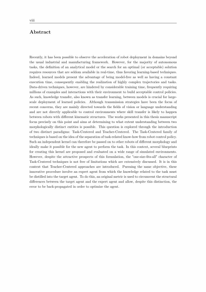
Abstract
Recently, it has been possible to observe the acceleration of robot deployment in domains beyondthe usual industrial and manufacturing framework. However, for the majority of autonomoustasks, the definition of an analytical model or the search for an optimal (or acceptable) solutionrequires resources that are seldom available in real-time, thus favoring learning-based techniques.Indeed, learned models present the advantage of being model-free as well as having a constantexecution time, consequently enabling the realization of highly complex trajectories and tasks.Data-driven techniques, however, are hindered by considerable training time, frequently requiringmillions of examples and interactions with their environment to build acceptable control policies.As such, knowledge transfer, also known as transfer learning, between models is crucial for large-scale deployment of learned policies. Although transmission strategies have been the focus ofrecent concerns, they are mainly directed towards the fields of vision or language understandingand are not directly applicable to control environments where skill transfer is likely to happenbetween robots with different kinematic structures. The works presented in this thesis manuscriptfocus precisely on this point and aims at determining to what extent understanding between twomorphologically distinct entities is possible. This question is explored through the introductionof two distinct paradigms: Task-Centered and Teacher-Centered. The Task-Centered family oftechniques is based on the idea of the separation of task-related know-how from robot control policy.Such an independent kernel can therefore be passed on to other robots of different morphology andideally make it possible for the new agent to perform the task. In this context, several blueprintsfor creating this kernel are proposed and evaluated on a wide range of simulated environments.However, despite the attractive prospects of this formulation, the "one-size-fits-all" character ofTask-Centered techniques is not free of limitations which are extensively discussed. It is in thiscontext that Teacher-Centered approaches are introduced. Pursuing the same objective, theseinnovative procedure involve an expert agent from which the knowledge related to the task mustbe distilled into the target agent. To do this, an original metric is used to circumvent the structuraldifferences between the target agent and the expert agent and allow, despite this distinction, theerror to be back-propagated in order to optimize the agent.
ix
Acronyms
• AE . . . . . . . . . . . . . . . . . . . . . . . . . . . . . . . . . . . . . . . . . . . . . . . . . . . . . . . . . . . . . . . . . AutoEncoder
• BAM . . . . . . . . . . . . . . . . . . . . . . . . . . . . . . . . . . . . . . . . . . . . . . . . Base Abstracted Modelling
• BERT . . . . . . . . . . . . . . . . . Bidirectional Encoder Representations from Transformers
• CNN . . . . . . . . . . . . . . . . . . . . . . . . . . . . . . . . . . . . . . . . . . . . . Convolutional Neural Network
• CV . . . . . . . . . . . . . . . . . . . . . . . . . . . . . . . . . . . . . . . . . . . . . . . . . . . . . . . . . . . . .Computer Vision
• DC . . . . . . . . . . . . . . . . . . . . . . . . . . . . . . . . . . . . . . . . . . . . . . . . . . . . . . . Differentiable Collision
• FFNN . . . . . . . . . . . . . . . . . . . . . . . . . . . . . . . . . . . . . . . . . . . Feed Forward Neural Network
• GAN . . . . . . . . . . . . . . . . . . . . . . . . . . . . . . . . . . . . . . . . . . . .Generative Adversarial Network
• ISV . . . . . . . . . . . . . . . . . . . . . . . . . . . . . . . . . . . . . . . . . . . . . . . . . Intermediate State Variable
• KL . . . . . . . . . . . . . . . . . . . . . . . . . . . . . . . . . . . . . . . . . . . . . . . . . . . . . . . . . . . . . .Kullback-Leibler
• LSTM . . . . . . . . . . . . . . . . . . . . . . . . . . . . . . . . . . . . . . . . . . . . . . . . Long Short-Term Memory
• MDP . . . . . . . . . . . . . . . . . . . . . . . . . . . . . . . . . . . . . . . . . . . . . . . . . .Markov Decision Process
• ML . . . . . . . . . . . . . . . . . . . . . . . . . . . . . . . . . . . . . . . . . . . . . . . . . . . . . . . . . . . .Machine Learning
• NN . . . . . . . . . . . . . . . . . . . . . . . . . . . . . . . . . . . . . . . . . . . . . . . . . . . . . . . . . . . . Neural Networks
• NLP . . . . . . . . . . . . . . . . . . . . . . . . . . . . . . . . . . . . . . . . . . . . . . Natural Language Processing
• PPO . . . . . . . . . . . . . . . . . . . . . . . . . . . . . . . . . . . . . . . . . . . . . .Proximal Policy Optimization
• RL . . . . . . . . . . . . . . . . . . . . . . . . . . . . . . . . . . . . . . . . . . . . . . . . . . . . . .Reinforcement Learning
• RNN . . . . . . . . . . . . . . . . . . . . . . . . . . . . . . . . . . . . . . . . . . . . . . . . .Recurrent Neural Network
• SAC . . . . . . . . . . . . . . . . . . . . . . . . . . . . . . . . . . . . . . . . . . . . . . . . . . . . . . . . . . . .Soft Actor-Critic
• SL . . . . . . . . . . . . . . . . . . . . . . . . . . . . . . . . . . . . . . . . . . . . . . . . . . . . . . . . . . Supervised Learning
• TAC . . . . . . . . . . . . . . . . . . . . . . . . . . . . . . . . . . . . . . . . . . . . . . . . . . . . . . . . . . . . . TAsk-Centered
• TEC . . . . . . . . . . . . . . . . . . . . . . . . . . . . . . . . . . . . . . . . . . . . . . . . . . . . . . . . . . TEacher-Centered
• TSL . . . . . . . . . . . . . . . . . . . . . . . . . . . . . . . . . . . . . . . . . . . . . . . . . . . . . . . . . . .Task-Specific Loss
• UNN . . . . . . . . . . . . . . . . . . . . . . . . . . . . . . . . . . . . . . . . . . . . . . . . . . Universal Notice Network
• VAE . . . . . . . . . . . . . . . . . . . . . . . . . . . . . . . . . . . . . . . . . . . . . . . . . . . Variational AutoEncoder
• WGAN-GP . . .Watterstein Generative Adversarial Neural with Gradient Penalty

x
Contents
1 Introduction 11.1 Opening . . . . . . . . . . . . . . . . . . . . . . . . . . . . . . . . . . . . . . 21.2 Goals . . . . . . . . . . . . . . . . . . . . . . . . . . . . . . . . . . . . . . . 41.3 Proposed Approaches . . . . . . . . . . . . . . . . . . . . . . . . . . . . . . 41.4 Contributions . . . . . . . . . . . . . . . . . . . . . . . . . . . . . . . . . . . 61.5 Manuscript outline . . . . . . . . . . . . . . . . . . . . . . . . . . . . . . . . 6
2 Neural Networks and Learning Frameworks: Theoretical Background 92.1 Machine Learning . . . . . . . . . . . . . . . . . . . . . . . . . . . . . . . . . 112.2 Neural Networks . . . . . . . . . . . . . . . . . . . . . . . . . . . . . . . . . 12
2.2.1 Neurons . . . . . . . . . . . . . . . . . . . . . . . . . . . . . . . . . . 122.2.2 Feed forward neural networks . . . . . . . . . . . . . . . . . . . . . . 13
2.2.2.1 Layers . . . . . . . . . . . . . . . . . . . . . . . . . . . . . . 142.2.2.2 Activation functions . . . . . . . . . . . . . . . . . . . . . . 15
2.2.3 Loss function and backpropagation for optimization . . . . . . . . . 172.3 Supervised Learning . . . . . . . . . . . . . . . . . . . . . . . . . . . . . . . 192.4 Reinforcement Learning . . . . . . . . . . . . . . . . . . . . . . . . . . . . . 20
2.4.1 Principle and main concepts . . . . . . . . . . . . . . . . . . . . . . . 202.4.1.1 Observations . . . . . . . . . . . . . . . . . . . . . . . . . . 212.4.1.2 Policy . . . . . . . . . . . . . . . . . . . . . . . . . . . . . . 212.4.1.3 Actions . . . . . . . . . . . . . . . . . . . . . . . . . . . . . 212.4.1.4 Trajectory and episodes . . . . . . . . . . . . . . . . . . . . 212.4.1.5 Reward Function . . . . . . . . . . . . . . . . . . . . . . . . 222.4.1.6 Reinforcement Learning Objective . . . . . . . . . . . . . . 232.4.1.7 Value functions . . . . . . . . . . . . . . . . . . . . . . . . . 232.4.1.8 Bellman Equations . . . . . . . . . . . . . . . . . . . . . . . 232.4.1.9 Advantage function . . . . . . . . . . . . . . . . . . . . . . 24
2.4.2 Practical aspects of RL . . . . . . . . . . . . . . . . . . . . . . . . . 242.4.2.1 The Exploration-Exploitation trade-off . . . . . . . . . . . 242.4.2.2 Credit assignment problem . . . . . . . . . . . . . . . . . . 25
xii CONTENTS
2.4.2.3 Sample (In)efficiency . . . . . . . . . . . . . . . . . . . . . . 252.4.3 Modern RL algorithms . . . . . . . . . . . . . . . . . . . . . . . . . . 25
2.4.3.1 Model-free and model-based RL . . . . . . . . . . . . . . . 252.4.3.2 On-Policy vs. Off-Policy . . . . . . . . . . . . . . . . . . . . 26
2.4.4 Proximal Policy Optimization . . . . . . . . . . . . . . . . . . . . . . 272.5 Generative Adversarial Learning . . . . . . . . . . . . . . . . . . . . . . . . 28
2.5.1 Principle . . . . . . . . . . . . . . . . . . . . . . . . . . . . . . . . . . 282.5.2 Reaching optimality . . . . . . . . . . . . . . . . . . . . . . . . . . . 292.5.3 Common issues and failure cases . . . . . . . . . . . . . . . . . . . . 30
2.6 Knowledge representation . . . . . . . . . . . . . . . . . . . . . . . . . . . . 312.6.1 Autoencoders . . . . . . . . . . . . . . . . . . . . . . . . . . . . . . . 312.6.2 VAE . . . . . . . . . . . . . . . . . . . . . . . . . . . . . . . . . . . . 33
2.7 Conclusion . . . . . . . . . . . . . . . . . . . . . . . . . . . . . . . . . . . . 34
3 Transfer Learning & Related works 353.1 Societal Needs for Transfer Learning . . . . . . . . . . . . . . . . . . . . . . 363.2 Transfer Learning Principles . . . . . . . . . . . . . . . . . . . . . . . . . . . 363.3 Common cases of Transfer Learning . . . . . . . . . . . . . . . . . . . . . . 383.4 Computer Vision . . . . . . . . . . . . . . . . . . . . . . . . . . . . . . . . . 403.5 Natural Language Processing . . . . . . . . . . . . . . . . . . . . . . . . . . 433.6 Transfer Learning in control tasks . . . . . . . . . . . . . . . . . . . . . . . . 45
3.6.1 Deep learning based control . . . . . . . . . . . . . . . . . . . . . . . 453.6.2 From simulation to real world . . . . . . . . . . . . . . . . . . . . . . 463.6.3 Transfer between tasks . . . . . . . . . . . . . . . . . . . . . . . . . . 47
3.6.3.1 Reward-Based Transfer . . . . . . . . . . . . . . . . . . . . 473.6.3.2 Curriculum Based Transfer . . . . . . . . . . . . . . . . . . 473.6.3.3 Intrinsically motivated Transfer . . . . . . . . . . . . . . . 483.6.3.4 Meta-Learning . . . . . . . . . . . . . . . . . . . . . . . . . 483.6.3.5 Transfer in Hierarchical Settings . . . . . . . . . . . . . . . 49
3.7 Knowledge representation in Transfer Learning . . . . . . . . . . . . . . . . 503.8 Conclusion on Transfer Learning . . . . . . . . . . . . . . . . . . . . . . . . 51
4 Task-Centered Transfer 534.1 Universal Notice Network . . . . . . . . . . . . . . . . . . . . . . . . . . . . 54
4.1.1 Principle . . . . . . . . . . . . . . . . . . . . . . . . . . . . . . . . . . 544.1.2 The UNN workflow . . . . . . . . . . . . . . . . . . . . . . . . . . . . 554.1.3 The UNN Pipeline . . . . . . . . . . . . . . . . . . . . . . . . . . . . 564.1.4 Base Abstracted Modelling . . . . . . . . . . . . . . . . . . . . . . . 574.1.5 Building and using UNN modules . . . . . . . . . . . . . . . . . . . . 58
4.2 Experiments . . . . . . . . . . . . . . . . . . . . . . . . . . . . . . . . . . . . 594.2.1 Vanilla transfer . . . . . . . . . . . . . . . . . . . . . . . . . . . . . . 604.2.2 Learning setup . . . . . . . . . . . . . . . . . . . . . . . . . . . . . . 61
CONTENTS xiii
4.2.3 Controlled Robots . . . . . . . . . . . . . . . . . . . . . . . . . . . . 624.2.4 Base Manipulation: Reacher . . . . . . . . . . . . . . . . . . . . . . . 634.2.5 A lonely manipulation: Tennis . . . . . . . . . . . . . . . . . . . . . 644.2.6 Biped walking . . . . . . . . . . . . . . . . . . . . . . . . . . . . . . . 674.2.7 Cooperative Manipulation UNN: Cooperative Move Plank . . . . . . 714.2.8 Cooperative BAM Manipulation: Dual Move Plank . . . . . . . . . . 73
4.3 Conclusion on TAsk-Centered methods . . . . . . . . . . . . . . . . . . . . . 77
5 Teacher-Centered Transfer 795.1 CoachGAN . . . . . . . . . . . . . . . . . . . . . . . . . . . . . . . . . . . . 80
5.1.1 From Task to Teacher . . . . . . . . . . . . . . . . . . . . . . . . . . 805.1.2 The CoachGAN method . . . . . . . . . . . . . . . . . . . . . . . . . 805.1.3 WGAN-GP for a suitable learning signal . . . . . . . . . . . . . . . . 835.1.4 Task and Intermediate State Variables . . . . . . . . . . . . . . . . . 845.1.5 Training the Expert . . . . . . . . . . . . . . . . . . . . . . . . . . . 865.1.6 CoachGAN Results . . . . . . . . . . . . . . . . . . . . . . . . . . . . 87
5.1.6.1 Effector Position ISV . . . . . . . . . . . . . . . . . . . . . 875.1.6.2 Approximated Kinematics ISV . . . . . . . . . . . . . . . . 895.1.6.3 Ball Rebound Speed ISV . . . . . . . . . . . . . . . . . . . 895.1.6.4 Analysis . . . . . . . . . . . . . . . . . . . . . . . . . . . . . 90
5.1.7 Conclusion on CoachGAN . . . . . . . . . . . . . . . . . . . . . . . . 925.2 Task-Specific Loss . . . . . . . . . . . . . . . . . . . . . . . . . . . . . . . . 92
5.2.1 The TSL Principle . . . . . . . . . . . . . . . . . . . . . . . . . . . . 935.2.2 Method . . . . . . . . . . . . . . . . . . . . . . . . . . . . . . . . . . 945.2.3 Transfer . . . . . . . . . . . . . . . . . . . . . . . . . . . . . . . . . . 955.2.4 Experimental setup . . . . . . . . . . . . . . . . . . . . . . . . . . . . 97
5.2.4.1 Tasks and Agents . . . . . . . . . . . . . . . . . . . . . . . 975.2.4.2 Models . . . . . . . . . . . . . . . . . . . . . . . . . . . . . 99
5.2.5 Results . . . . . . . . . . . . . . . . . . . . . . . . . . . . . . . . . . 995.2.5.1 Circle to Circle Contour Displacement . . . . . . . . . . . . 995.2.5.2 Tennis task . . . . . . . . . . . . . . . . . . . . . . . . . . . 1005.2.5.3 Autonomous TSL . . . . . . . . . . . . . . . . . . . . . . . 1035.2.5.4 Training Time & Assistive aspects . . . . . . . . . . . . . . 105
5.2.6 Conclusion on Task-Specific Loss . . . . . . . . . . . . . . . . . . . . 1055.3 Conclusion on TEacher-Centered methods . . . . . . . . . . . . . . . . . . . 106
6 General Conclusion & Prospects 109
A UNN in Mobile Manipulators settings 127

xiv CONTENTS
List of Figures
1.1 A mass directed, widely distributed, list of instructions to assemble a pieceof furniture . . . . . . . . . . . . . . . . . . . . . . . . . . . . . . . . . . . . 2
1.2 Personalized advice in a bouldering configuration: the experimented climberdistills its knowledge in the student accomplishing the task . . . . . . . . . 3
1.3 TAsk-Centered (TAC) approach with the instruction "Cross the gap" canbe answered differently given the capabilities of the current agent. . . . . . 5
1.4 TEacher-Centered approach to Kung-Fu. In this configuration, knowledgefrom the teacher agent (right) is distilled to the learner agent (left) . . . . . 5
2.1 The neuron is the basic computational unit in a neural network. . . . . . . 122.2 Feedforward neural network: vectors are sequentially processed by each
layer, first applying the layer weight parameters and then the non-linearityactivation function. The last layer returns a value that is usually used tocompute the loss. . . . . . . . . . . . . . . . . . . . . . . . . . . . . . . . . . 13
2.3 Layer connections. . . . . . . . . . . . . . . . . . . . . . . . . . . . . . . . . 142.4 The sigmoid function and its derivative. . . . . . . . . . . . . . . . . . . . . 152.5 The TanH function and its derivative. . . . . . . . . . . . . . . . . . . . . . 162.6 The ReLU function and its derivative. . . . . . . . . . . . . . . . . . . . . . 172.7 RL principle. . . . . . . . . . . . . . . . . . . . . . . . . . . . . . . . . . . . 202.8 A taxonomy of RL algorithms. . . . . . . . . . . . . . . . . . . . . . . . . . 262.9 GAN principle. . . . . . . . . . . . . . . . . . . . . . . . . . . . . . . . . . . 292.10 Mode collapse during GAN training (78). The first row shows samples of
a rather successful generator as the quality gradually increase as well asthe diversity (each MNIST class is represented). The lower row displays anexample of Mode Collapse where the generator focuses on a single point inthe target space even though various noise vectors are provided. . . . . . . . 30
2.11 An autoencoder architecture. . . . . . . . . . . . . . . . . . . . . . . . . . . 322.12 From AE to VAE: a probabilistic encoder projects the input in a Gaussian
constrained latent space. . . . . . . . . . . . . . . . . . . . . . . . . . . . . . 332.13 Code distribution for VAE on the MNIST dataset. . . . . . . . . . . . . . . 34
xvi LIST OF FIGURES
3.1 Transfer Learning principle. . . . . . . . . . . . . . . . . . . . . . . . . . . . 373.2 CNN filters detect different features based on their depth location in the
model. . . . . . . . . . . . . . . . . . . . . . . . . . . . . . . . . . . . . . . . 403.3 CNN fine-tuning/Transfer Learning process. . . . . . . . . . . . . . . . . . . 413.4 Left: Detection model based on a pretrained backbone (37). . . . . . . . . . 423.5 Segmentation results (30). . . . . . . . . . . . . . . . . . . . . . . . . . . . . 423.6 Segmentation models. Up: Fully-Connected Networks (FCN) (124). Down:
U-Nets (112). . . . . . . . . . . . . . . . . . . . . . . . . . . . . . . . . . . . 433.7 PCA representation of words (79). . . . . . . . . . . . . . . . . . . . . . . . 443.8 Language Model based Transfer Learning. . . . . . . . . . . . . . . . . . . . 453.9 CycleGAN training method. . . . . . . . . . . . . . . . . . . . . . . . . . . . 51
4.1 Knowledge location comparison. . . . . . . . . . . . . . . . . . . . . . . . . 554.2 The original UNN Pipeline staged training first creates a primitive agent
controller (in blue box) for a chosen agent configuration. The UNN forthe task relies on the generated primitive motor skills to learn a successfulpolicy (in light red box). . . . . . . . . . . . . . . . . . . . . . . . . . . . . . 56
4.3 The successive steps for deploying the transferred UNN to a new configuration. 564.4 The UNN Pipeline is composed of three stages: the input and output bases
(in green and red) are specific to the robot, while the UNN (blue) is task-related. . . . . . . . . . . . . . . . . . . . . . . . . . . . . . . . . . . . . . . 57
4.5 The BAM version of the environment prevents specific behaviour from leak-ing in the task model, leading the UNN closer to a bias-free logic. . . . . . . 58
4.6 The UNN workflow: Various solutions for creating and using modules andUNNs. Dashed violet paths are to pair the robot with its module. Dashedblue paths are to pair the task with its UNN. Black and red paths are tocreate new robot modules. Orange and blue paths are to create new taskmodule (UNN). . . . . . . . . . . . . . . . . . . . . . . . . . . . . . . . . . 59
4.7 Exchanging model layers between similar agents. . . . . . . . . . . . . . . . 604.8 Mean reward evolution on BipedalWalker-v3 environment. . . . . . . . . . . 614.9 Comparison of all configurations. Genuine configurations are able to reach
high scores while all recomposed one fail to exceed a very low threshold. . . 624.10 From left to right: Generic-3 robot, Berkeley Blue, Kuka-LWR, Leg Type
1, Leg Type 2. . . . . . . . . . . . . . . . . . . . . . . . . . . . . . . . . . . 634.11 Reacher Task. . . . . . . . . . . . . . . . . . . . . . . . . . . . . . . . . . . . 644.12 Mean reward along training on the primitive reacher task. . . . . . . . . . . 654.13 Tennis Task. . . . . . . . . . . . . . . . . . . . . . . . . . . . . . . . . . . . . 654.14 Learning performances in the Tennis environment. PPO and UNN are
performed using Kuka robot, transfer to Berkeley Blue robot. . . . . . . . . 664.15 Undesirable configurations that ultimately return positive rewards are likely
to be considered as valuable states by the agent. . . . . . . . . . . . . . . . 684.16 Dual UNN Architecture. . . . . . . . . . . . . . . . . . . . . . . . . . . . . . 68
LIST OF FIGURES xvii
4.17 Biped walk task. . . . . . . . . . . . . . . . . . . . . . . . . . . . . . . . . . 694.18 Learning performances in Biped Walk environment. PPO and UNN are
performed using 2 legs of Type1, transfer to robot composed of Leg Type1and Leg Type 2. . . . . . . . . . . . . . . . . . . . . . . . . . . . . . . . . . 70
4.19 Left: Free configurations. Right: Enforced semi-folded configurations. . . . 714.20 UNN pretraining can nudge the policy towards a more human-like gait. . . 714.21 Cooperative Move Plank Task. . . . . . . . . . . . . . . . . . . . . . . . . . 724.22 Cooperative Move Plank Task results. . . . . . . . . . . . . . . . . . . . . . 734.23 Dual-Arm Move Plank Task. . . . . . . . . . . . . . . . . . . . . . . . . . . 744.24 Dual-Arm Move Plank Task. . . . . . . . . . . . . . . . . . . . . . . . . . . 744.25 Learning performances in Dual-Arm Raise Plank environment for PPO and
UNN policies using two Kuka arms and then transferred to two BerkeleyBlue robots. . . . . . . . . . . . . . . . . . . . . . . . . . . . . . . . . . . . . 75
5.1 In its current formulation, the UNN framework is likely to find limitationsfor cases where the UNN output instruction is not directly applicable to thetransfer target. . . . . . . . . . . . . . . . . . . . . . . . . . . . . . . . . . . 81
5.2 It is possible to extend the UNN approach by implementing a less rigidinterface between the task model and the agent. . . . . . . . . . . . . . . . 82
5.3 An educated enough external observer is able to provide a feedback on theactions performed, which can be used, to some extend, to improve perfor-mance. In this stylized example, the discriminator evaluates the fighterability through the heavy bag movement. . . . . . . . . . . . . . . . . . . . 82
5.4 The CoachGAN principle. The green frame depicts the teacher discrimi-nator training process, that is then used for training the student generator(orange frame). . . . . . . . . . . . . . . . . . . . . . . . . . . . . . . . . . . 83
5.5 Student Generator (in orange) optimization in experiments Actual Kine-matics andApproximated Kinematics. Discriminator evaluation passesthrough the RISV module before reaching the generator. . . . . . . . . . . . 85
5.6 Training predictor to forsee next step ball speed. . . . . . . . . . . . . . . . 855.7 Training discriminator based on predictor outputs. . . . . . . . . . . . . . . 855.8 Student generator (in orange) training setup for experimentBall Rebound.
Discriminator evaluation goes through the predictor and RISV before mod-ifying generator parameters. . . . . . . . . . . . . . . . . . . . . . . . . . . . 86
5.9 Adversarial losses along training. . . . . . . . . . . . . . . . . . . . . . . . . 875.10 Normalized discriminator evaluation of ISV (effector positions) in the task
space for two given starting ball configurations. Higher values (yellow) arefavored. . . . . . . . . . . . . . . . . . . . . . . . . . . . . . . . . . . . . . . 88
5.11 Sampled solutions for actual and approximated ISV in green. Baseline fromuntrained generator in white. . . . . . . . . . . . . . . . . . . . . . . . . . . 88
5.12 Task-space evaluation by the discriminator based on predictor results. . . . 89
xviii LIST OF FIGURES
5.13 2D representation of the solution distribution. Successful solutions are ei-ther overlapping expert position or in the ball path. . . . . . . . . . . . . . 90
5.14 Interception performance and training time. . . . . . . . . . . . . . . . . . . 915.15 The TSL defines an Intermediate State Variable (ISV) of interest that is
responsible for sending relevant error signal to the student. In this picture,the ISV is represented by the painting. Body position having no influenceon this value, the green configuration yields a low error, while the red settingreturns a strong error value. . . . . . . . . . . . . . . . . . . . . . . . . . . . 93
5.16 TSL penalizes the student when its movement does not preserve the esti-mated metric at the previous timestep. . . . . . . . . . . . . . . . . . . . . . 94
5.17 User-assisted VAE architecture during training phase. . . . . . . . . . . . . 955.18 User-assisted VAE architecture during usage/testing phase. . . . . . . . . . 955.19 Distillation process from the teacher to the student agent via TSL. . . . . . 965.20 Various teaching cases and their corresponding losses and importance weight.
The teacher’s joints are drawn in blue, while green is used for the student. . 985.21 Reconstruction loss along training epochs and 2D code distribution on the
test set for the circle task. . . . . . . . . . . . . . . . . . . . . . . . . . . . . 1005.22 Distribution of the distance between effectors for 1000 samples after 10
successive actions using the same user input z. . . . . . . . . . . . . . . . . 1015.23 Mean Cumulative Reward Evolution and ball impact distribution for 100
shots per target point. . . . . . . . . . . . . . . . . . . . . . . . . . . . . . . 1025.24 Tennis Teacher training metrics and code distribution of a randomly sam-
pled batch of 2048 examples. . . . . . . . . . . . . . . . . . . . . . . . . . . 1035.25 Comparison of assistive performances of several players using both teacher
and student agent with baseline. . . . . . . . . . . . . . . . . . . . . . . . . 1045.26 Comparison of TSL-based controlled for autonomous agent and user-controlled
agent in a relevant environment. . . . . . . . . . . . . . . . . . . . . . . . . 1045.27 Impact distribution and action magnitude of an autonomous student along
several episodes. . . . . . . . . . . . . . . . . . . . . . . . . . . . . . . . . . 108
A.1 A subset of the possible agent configurations. From left to right: BicycleKUKA, Omnidirectional BLUE, Differential G3. Parts can be exchangedbetween agents. . . . . . . . . . . . . . . . . . . . . . . . . . . . . . . . . . . 128
A.2 Training performances on Primitive reaching task for 4 predefined configu-rations . . . . . . . . . . . . . . . . . . . . . . . . . . . . . . . . . . . . . . . 130
A.3 Comparative Pick’n Place training performances . . . . . . . . . . . . . . . 131A.4 Comparative Stacking training performances . . . . . . . . . . . . . . . . . 132A.5 Pick’n Place transfer fine-tuning performances . . . . . . . . . . . . . . . . . 132A.6 Stacking transfer fine-tuning . . . . . . . . . . . . . . . . . . . . . . . . . . . 133

List of Tables
3.1 Recent CNN architectures, performances on the ImageNet classificationtask and number of parameters (millions). . . . . . . . . . . . . . . . . . . . 38
3.2 Recent NLP architectures characteristics: Number of parameters (millions),dataset training size and evaluation score on the GLUE benchmark. . . . . 39
4.1 Tennis Summary. . . . . . . . . . . . . . . . . . . . . . . . . . . . . . . . . . 664.2 Biped Summary. . . . . . . . . . . . . . . . . . . . . . . . . . . . . . . . . . 704.3 Cooperative Move Plank. . . . . . . . . . . . . . . . . . . . . . . . . . . . . 734.4 Dual Arm Raise Plank Summary. . . . . . . . . . . . . . . . . . . . . . . . . 76
A.1 Transfer: Pick’n Place . . . . . . . . . . . . . . . . . . . . . . . . . . . . . . 133A.2 Transfer: Stacking . . . . . . . . . . . . . . . . . . . . . . . . . . . . . . . . 134

xx LIST OF TABLES
Chapter 1IntroductionContents
1.1 Opening . . . . . . . . . . . . . . . . . . . . . . . . . . . . . . . . . . . 21.2 Goals . . . . . . . . . . . . . . . . . . . . . . . . . . . . . . . . . . . . . 41.3 Proposed Approaches . . . . . . . . . . . . . . . . . . . . . . . . . . . . 41.4 Contributions . . . . . . . . . . . . . . . . . . . . . . . . . . . . . . . . 61.5 Manuscript outline . . . . . . . . . . . . . . . . . . . . . . . . . . . . . . 6
1
2 1.1. OPENING
1.1 Opening
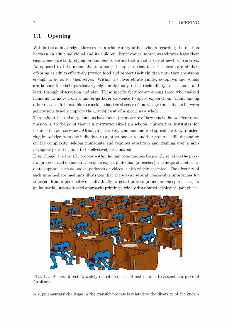
Within the animal reign, there exists a wide variety of behaviours regarding the relationbetween an adult individual and its children. For instance, most invertebrates leave theireggs alone once laid, relying on numbers to ensure that a viable size of newborn survives.As opposed to this, mammals are among the species that take the most care of theiroffspring as adults effectively provide food and protect their children until they are strongenough to do so for themselves. Within the invertebrate family, octopuses and squidsare famous for their particularly high brain/body ratio, their ability to use tools andlearn through observation and play. These specific features are among those who enabledmankind to move from a hunter-gatherer existence to space exploration. Thus, amongother reasons, it is possible to consider that the absence of knowledge transmission betweengenerations heavily impacts the development of a specie as a whole.Throughout their history, humans have taken the measure of how crucial knowledge trans-mission is, to the point that it is institutionalized (in schools, universities, institutes, forinstance) in our societies. Although it is a very common and well-spread custom, transfer-ring knowledge from one individual to another one or to another group is still, dependingon the complexity, seldom immediate and requires repetition and training over a non-negligible period of time to be effectively assimilated.Even though the transfer process within human communities frequently relies on the phys-ical presence and demonstration of an expert individual (a teacher), the usage of a interme-diate support, such as books, podcasts or videos is also widely accepted. The diversity ofsuch intermediate mediums illustrates that there exist several conceivable approaches fortransfer: from a personalized, individually-targeted process (a one-on-one sport class) toan industrial, mass-directed approach (printing a widely distributed ideological pamphlet).
FIG. 1.1. A mass directed, widely distributed, list of instructions to assemble a piece offurniture
A supplementary challenge in the transfer process is related to the diversity of the knowl-
CHAPTER 1. INTRODUCTION 3
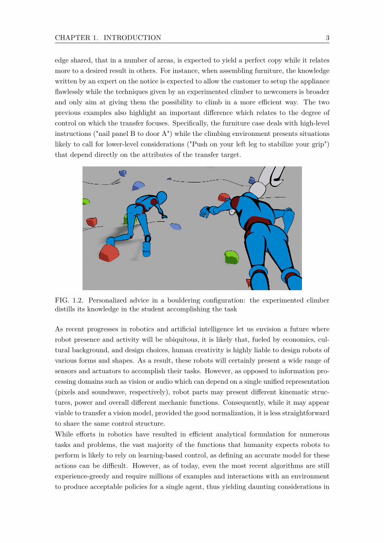
edge shared, that in a number of areas, is expected to yield a perfect copy while it relatesmore to a desired result in others. For instance, when assembling furniture, the knowledgewritten by an expert on the notice is expected to allow the customer to setup the applianceflawlessly while the techniques given by an experimented climber to newcomers is broaderand only aim at giving them the possibility to climb in a more efficient way. The twoprevious examples also highlight an important difference which relates to the degree ofcontrol on which the transfer focuses. Specifically, the furniture case deals with high-levelinstructions ("nail panel B to door A") while the climbing environment presents situationslikely to call for lower-level considerations ("Push on your left leg to stabilize your grip")that depend directly on the attributes of the transfer target.
FIG. 1.2. Personalized advice in a bouldering configuration: the experimented climberdistills its knowledge in the student accomplishing the task
As recent progresses in robotics and artificial intelligence let us envision a future whererobot presence and activity will be ubiquitous, it is likely that, fueled by economics, cul-tural background, and design choices, human creativity is highly liable to design robots ofvarious forms and shapes. As a result, these robots will certainly present a wide range ofsensors and actuators to accomplish their tasks. However, as opposed to information pro-cessing domains such as vision or audio which can depend on a single unified representation(pixels and soundwave, respectively), robot parts may present different kinematic struc-tures, power and overall different mechanic functions. Consequently, while it may appearviable to transfer a vision model, provided the good normalization, it is less straightforwardto share the same control structure.While efforts in robotics have resulted in efficient analytical formulation for numeroustasks and problems, the vast majority of the functions that humanity expects robots toperform is likely to rely on learning-based control, as defining an accurate model for theseactions can be difficult. However, as of today, even the most recent algorithms are stillexperience-greedy and require millions of examples and interactions with an environmentto produce acceptable policies for a single agent, thus yielding daunting considerations in
4 1.2. GOALS
terms of computation if this strategy was to be applied to each different robot.Consequently, the capacity to transfer skills from one agent to another, notwithstandingtheir distinct physical structure, is a crucial and essential step in the path of integratingrobots in our day-to-day lives. This work consequently proposes novel techniques to facethis issue. These approaches can be classified into two main families based on whetherthey fit in the furniture example (TAsk-Centered), displayed in Figure 1.1 or climbingconfiguration (TEacher-Centered) as shown in Figure 1.2.
1.2 Goals
This work challenges the current transfer learning paradigm and aims at showing that it ispossible to transfer knowledge from an agent to a kinematically different one. Metaphor-ically, this work can be seen as an echo to George Berkeley’s immaterialism (6) theorywhich denies the existence of material substance outside of the mind of perceiver. Themethods proposed in this work rotate this interrogation towards knowledge and investigatewhether the skills and knowledge to successfully complete a task are tied to the morphol-ogy which learned to do so. To sum up, this thesis explores the following hypothesis:is it possible to transfer knowledge, that is the expertise or control strategy in a givenenvironment, from one agent to another despite their potential morphology difference ?And, if so:
• how to cope up with the action space dimensional differences ?
• can a common state be defined ?
• to what extend can knowledge be distinct from the body ?
1.3 Proposed Approaches
This thesis focuses on two distinct ideas for transferring knowledge: TAsk-Centered (TAC)and TEacher-Centered (TEC). Fueling the TAsk-Centered approaches is the idea of no-tices, similar to the ones used by non-professional humans to quickly be able to producean object (for instance, setting up a piece of furniture) without having specifically beentrained on this type of task. In these cases, the furniture producer writes down a setof instructions that should enable another person to reach its goal, that is, assemblingthe newly acquired furniture. In this configuration, the producer does not have accessto the customers physical abilities, but makes the assumption of basic motor skills thatwould allow him to comply with the notice’s current set of instructions. In this view, theTAsk-Centered methods first aim at constructing a notice module, independent from theacting agent morphology. Once this notice module is available, it can be passed to otheragents that would then perform the task. This approach is schematised in Figure 1.3 thatdisplays an example on how two systems similarly tasked can present different strategiesto solve the given configuration.

CHAPTER 1. INTRODUCTION 5
FIG. 1.3. TAsk-Centered (TAC) approach with the instruction "Cross the gap" can beanswered differently given the capabilities of the current agent.
It is also possible to consider TEacher-Centered approaches. In this view, instead ofhaving a segmentation between the knowledge and the agent morphology as in TAsk-Centered cases, the task knowledge is tied to an agent, called the teacher or the expert.The goal of TEacher-Centered techniques, displayed in Figure 1.4, is to provide ways todistill this ability into another student agent of potentially different morphology. Thisconfiguration relates to very common settings in human civilization. Indeed, there existnumerous examples where an untrained individual can benefit from the knowledge of anexpert, thus shortening the time needed to reach mastery.
FIG. 1.4. TEacher-Centered approach to Kung-Fu. In this configuration, knowledge fromthe teacher agent (right) is distilled to the learner agent (left)

6 1.4. CONTRIBUTIONS
1.4 Contributions
As this report proposes several approaches, a novel approach classification was devised.Indeed, TAsk-Centered and TEacher-Centered techniques are two newly defined families oftransfer-learning approaches that usefully draw a line between the novel methods proposedin this work.More precisely, in the TAsk-Centered approach, we propose the Universal Notice Network(UNN) (84; 85) a stage-wise deep reinforcement learning based technique that creates atask knowledge module that can then be passed to different agents. Doing so enables tosegment the task logic, that should be common to all agents, from the control parametersinherent to each robot. This technique yields very interesting results both for the learningpart as well as the transfer, as it enables other agents to reach performances level similar tothe expert in a fraction of the training time. Besides, the segmentation pipeline involvedin this construction presents unexpected, yet highly appealing features, with respect toagent control parameters. Specifically, in the pre-training phase, it is easier to inducebiased behaviors in the agent low-level control. These behaviors can then importantlyease the learning process in the target task and also contribute to prevent undesired orunsuitable actions downstream.For the TEacher-Centered framework, this report investigates innovative unsupervisedtechniques to distill the teacher knowledge into a student agent. As opposed to TAsk-Centered techniques, where the transfer of knowledge is horizontal, these methods arebased on a clear hierarchy and the student quality is directly submitted to the teacher’s,which was less straightforward for TAsk-Centered framework. Nevertheless, TEacher-Centered methods present several strong advantages. Notably, this form of transfer isfaster, and does not require student-environment interactions, thus lessening the cost oftransfer. Furthermore, TEacher-Centered methods embed more freedom in the objectivefunction design, ultimately offering a very wide application spectrum due to their enhancedflexibility.
1.5 Manuscript outline
The remainder of the thesis is organized as follows: Chapter 2 provides an overview ofthe concepts and theoretical notions required. It introduces the recent paradigm machinelearning and quickly focuses on deep learning. After laying out the mechanisms of neuralnetworks, it goes over the most popular deep learning applications. After an outline ofsupervised learning, it examines thoroughly reinforcement learning as it is heavily reliedupon in the next chapters. Eventually, Chapter 2 looks at unsupervised learning andknowledge representation by presenting attractive frameworks: Generative AdversarialNetworks and Variational AutoEncoders that are also used in the works presented in thisreport.Chapter 3 sums up current state of the art techniques, modern trends in transfer learningand highlights their major advantages as well as their limitations, thus motivating the
CHAPTER 1. INTRODUCTION 7
proposed transfer-learning approaches.In Chapter 4, the Universal Notice Network, a TAsk-Centered transfer learning approachis introduced. This chapter details its main features and presents a series of experimentsin multiple use cases to underline the applicability of this method.TEacher-Centered methods are at the center of Chapter 5, which develops the essentialaspects of the CoachGAN and Task-Specific Loss (TSL) methods and lays down the resultsof various trials designed to underline the potentiality of these techniques.Eventually, as could be expected, Chapter 6 sets up the stage for a thorough comparisonbetween all developed methods in this works, demonstrating multiple cases of transfer be-tween a series of robots on a common task, ultimately leading to an analysis and conclusionon transfer-learning in the control-tasks paradigms.

8 1.5. MANUSCRIPT OUTLINE
Chapter 2Neural Networks and LearningFrameworks: Theoretical Background
Contents2.1 Machine Learning . . . . . . . . . . . . . . . . . . . . . . . . . . . . . . 112.2 Neural Networks . . . . . . . . . . . . . . . . . . . . . . . . . . . . . . . 12
2.2.1 Neurons . . . . . . . . . . . . . . . . . . . . . . . . . . . . . . . 122.2.2 Feed forward neural networks . . . . . . . . . . . . . . . . . . . 13
2.2.2.1 Layers . . . . . . . . . . . . . . . . . . . . . . . . . . 142.2.2.2 Activation functions . . . . . . . . . . . . . . . . . . . 15
2.2.3 Loss function and backpropagation for optimization . . . . . . . 172.3 Supervised Learning . . . . . . . . . . . . . . . . . . . . . . . . . . . . . 192.4 Reinforcement Learning . . . . . . . . . . . . . . . . . . . . . . . . . . . 20
2.4.1 Principle and main concepts . . . . . . . . . . . . . . . . . . . . 202.4.1.1 Observations . . . . . . . . . . . . . . . . . . . . . . . 212.4.1.2 Policy . . . . . . . . . . . . . . . . . . . . . . . . . . . 212.4.1.3 Actions . . . . . . . . . . . . . . . . . . . . . . . . . . 212.4.1.4 Trajectory and episodes . . . . . . . . . . . . . . . . . 212.4.1.5 Reward Function . . . . . . . . . . . . . . . . . . . . 222.4.1.6 Reinforcement Learning Objective . . . . . . . . . . . 232.4.1.7 Value functions . . . . . . . . . . . . . . . . . . . . . 232.4.1.8 Bellman Equations . . . . . . . . . . . . . . . . . . . 232.4.1.9 Advantage function . . . . . . . . . . . . . . . . . . . 24
2.4.2 Practical aspects of RL . . . . . . . . . . . . . . . . . . . . . . . 242.4.2.1 The Exploration-Exploitation trade-off . . . . . . . . 242.4.2.2 Credit assignment problem . . . . . . . . . . . . . . . 252.4.2.3 Sample (In)efficiency . . . . . . . . . . . . . . . . . . 25
2.4.3 Modern RL algorithms . . . . . . . . . . . . . . . . . . . . . . . 252.4.3.1 Model-free and model-based RL . . . . . . . . . . . . 252.4.3.2 On-Policy vs. Off-Policy . . . . . . . . . . . . . . . . 26
2.4.4 Proximal Policy Optimization . . . . . . . . . . . . . . . . . . . 272.5 Generative Adversarial Learning . . . . . . . . . . . . . . . . . . . . . . 28
9
10
2.5.1 Principle . . . . . . . . . . . . . . . . . . . . . . . . . . . . . . . 282.5.2 Reaching optimality . . . . . . . . . . . . . . . . . . . . . . . . 292.5.3 Common issues and failure cases . . . . . . . . . . . . . . . . . 30
2.6 Knowledge representation . . . . . . . . . . . . . . . . . . . . . . . . . . 312.6.1 Autoencoders . . . . . . . . . . . . . . . . . . . . . . . . . . . . 312.6.2 VAE . . . . . . . . . . . . . . . . . . . . . . . . . . . . . . . . . 33
2.7 Conclusion . . . . . . . . . . . . . . . . . . . . . . . . . . . . . . . . . . 34
CHAPTER 2. NEURAL NETWORKS AND LEARNING FRAMEWORKS:THEORETICAL BACKGROUND 11
As introduced in the previous chapter, this work aims at presenting various techniques andconcepts for the transfer of knowledge between heterogeneously shaped agents. To do so,it relies extensively on the numerical methods tied with neural networks. Consequently,this chapter presents the theoretical background required for the work addressed in thisPhD thesis. It begins by introducing the general principle and motivation of MachineLearning. Then it focuses on Neural Networks concepts and main architectures. Oncethese building blocks are in place, it goes over the principal learning paradigms, super-vised learning, reinforcement learning and finally unsupervised learning techniques andknowledge representation.
2.1 Machine Learning
The idea of intelligent machines can be found in many cultures, some of them reportingback to the antiquity, in the form of thought-capable artificial beings (113). Closer tothe modern times, various fictions explored this concept further, such as Frank Baum’sWizard of Oz, Mary Shelley’s Frankeinsten or Karel Capek’s R.U.R. (143). The field ofArtificial Intelligence draws from these ideas, but even more from the famous ComputingMachinery and Intelligence from Alan Turing (17; 138) in 1950.
Artificial Intelligence (AI) is the science that investigates the ability of a digital computeror computer-controlled robot to perform tasks commonly associated with intelligent beings(18). The beginnings of AI research are commonly associated with the Dartmouth 1956computer science conference which reunited some of the brightest minds of the era and wasexpected to lay out the main principles that would ultimately lead to reproduce the humanmind in silico. Initially, AI was dominated by rationalist ideas, which, inspired by thinkerssuch as Descartes, Spinoza or Leibniz, consider that our perceptions are fallible and thatonly reason can be a reliable guide. In practice, these ideas lead to knowledge engineeringimplementations that require formal description of a problem. Despite impressive firstsuccesses, such as the General Problem Solver or theA? algorithm (113), these approachesproved inefficient at best for many complex tasks that can be considered intuitive, suchas recognizing a face or spoken words.
Machine Learning (ML), in contrast, is inspired by empiricists such as Locke, Berkeleyor Hume, which refute the idea that only reason is reliable and would preferably usetheir perceptions to guide them in the world (23; 113). Consequently, ML can be looselydefined as gathering knowledge from experience. Specifically, the main idea fueling the MLparadigm is that, instead of hard-coding knowledge within an AI system, it is possible tofind patterns in raw data and consequently use these patterns to solve various challengingtasks that would require tedious and particularly complex algorithms otherwise. As oftoday, ML algorithms are able to segment images and generate new human faces with astrong accuracy or even predict the best moves in Go (126; 127), a high-dimensional gamethat remained out of reach for many years.
12 2.2. NEURAL NETWORKS
2.2 Neural Networks
Neural networks, also known as artificial neural networks, are the results of attemps tofind mathematical representations of how information was processed in biological systems.It is currently a highly popular technique in machine learning that is used for patternrecognition by extracting statistical features (8; 39). As hinted by their designation,neural networks can be seen as a combination of single neurons, recalling their biologicalcounterpart. The next sections present an overview of these systems, going from a singleneuron as a computational unit to more complex architectures.
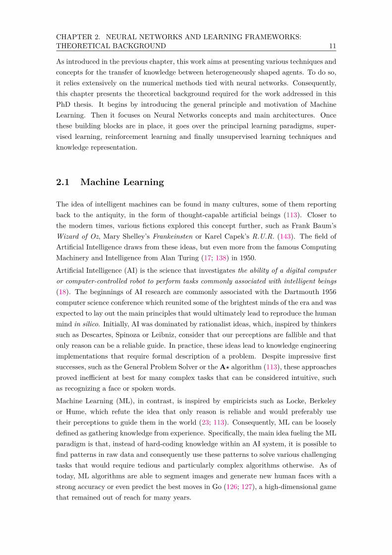
2.2.1 Neurons
In the field of deep learning, the term neuron n is commonly used to refer to a computa-tional unit that takes as input a vector X ∈ RN , with N ∈ N+, and computes an outputvalue a ∈ R given a bias b ∈ R, a vector of weights W ∈ RN and an activation functiong. More precisely, the neuron computes the pre-activation value a as the weighted sum ofthe input vector and adds a bias:
a = W TX + b =N∑i=1
wixi + b (2.1)
The result of the operation described in Equation 2.1 goes through an activation functiona that returns the final value o for this specific unit:
o = g(a) (2.2)
A neuron is considered deterministic if its output o is a function such as:
o = g(a) where g:R→ ε ⊂ R (2.3)
Similarly, a neuron is labelled stochastic if its output o is sampled from a density functiondepending on the pre-activation function
o ∼ g(a) (2.4)
Figure 2.1 shows a scheme of this computational unit and the operation it performs.
FIG. 2.1. The neuron is the basic computational unit in a neural network.

CHAPTER 2. NEURAL NETWORKS AND LEARNING FRAMEWORKS:THEORETICAL BACKGROUND 13
A neural network, also known as Multi-Layer Perceptron (MLP), is created when severallayers of multiple neuron units followed by non-linear activation functions are assembled.In general, MLPs are able to learn complex mappings and, as demonstrated by the Uni-versal Approximation Theorem, a neural network with three layers wide enough can intheory approximate any function (19; 45; 47).
2.2.2 Feed forward neural networks
Modern neural network architectures are defined as Feed Forward Neural Networks (FFNN).The word feedforward stems from the fact that information flows through the various lay-ers, producing intermediate representations to be used by the next layer of perceptrons,until the final prediction. More formally, it is possible to describe these architectures as adirected acyclic (no cycle and no self-connections) graph that composes several functions.These functions are in fact each of the network layers, usually referred to as input, hiddenand output, for the first layer, the intermediate layers and the last layer respectively, seeFigure 2.2. Beside FFNN, there exists alternative designs, such as Recurrent Neural Net-work (RNN) that prove useful when considering time-series processing. These networksusually rely on specific neurons to function, such as the Long Short Term Memory (LSTM)and will not be detailed in this report.
FIG. 2.2. Feedforward neural network: vectors are sequentially processed by each layer,first applying the layer weight parameters and then the non-linearity activation function.The last layer returns a value that is usually used to compute the loss.
Figure 2.2 represents a simple feedforward neural network architecture. Specifically, thenetwork displayed contains 3 units in its input layer (yellow), 4 in its unique hidden layer(green) and finally 1 in the output layer (red).
14 2.2. NEURAL NETWORKS
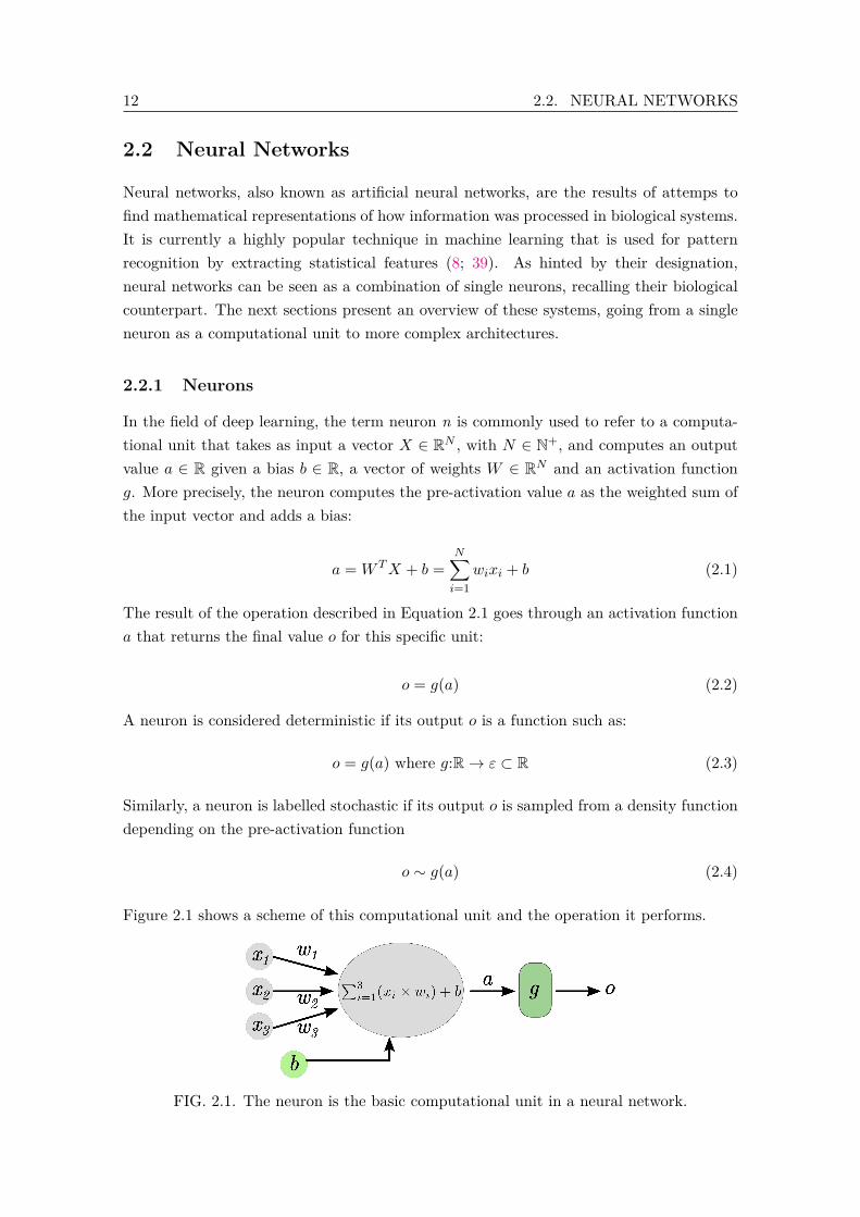
(a) Fully connected layer. (b) Partially connected layer.
FIG. 2.3. Layer connections.
2.2.2.1 Layers
The neural network displayed in Figure 2.3a has only fully-connected layers. Recently, ithas become more common to create architectures relying on partially connected layers. Inparticular, the Convolutional Neural Networks (CNN) architecture that uses convolutionalkernels as trainable weights has generated considerable interest in recent years. Differencesbetween these layers are displayed in Figure 2.3.A layer is called fully-connected if each unit of a given layer l is connected to each unit ofthe previous layer l − 1. In this case, the activations can be computed as:
∀i ∈ {1...Nl}, ali =Nl−1∑j=1
wli,jolj + bli (2.5)
and the outputs are given by:
∀i ∈ {1...Nl}, oli = gl(ali) (2.6)
where Nl is the number of units in the layer l, wli,j being the weight between the jthneuron of the layer l − 1 and the ith neuron of the layer l and bli is the bias of the ithneuron in layer l.In contrast, a layer l is considered partially connected if it contains at least one unit thatis not connected to the previous layer l − 1. It is possible to devise the activation andoutput of a partially-connected layer by setting to 0 the connection weight between twounconnected neurons. A particularly common instance of partially-connected layer is theconvolutional layer, most commonly used in image processing. Beside the obvious decreasein computational load when relying on partially connected layers, convolutional layers alsooffer, by design, a larger perception field, which allows them to detect hierarchical patterns,

CHAPTER 2. NEURAL NETWORKS AND LEARNING FRAMEWORKS:THEORETICAL BACKGROUND 15
thus justifying their usage when considering high-dimensional structured inputs.
2.2.2.2 Activation functions
The pattern recognition ability of neural networks is rooted in the presence of non-linearactivation functions. Indeed, a neural network with many layers featuring solely linearactivation functions is equivalent to a single-layer linear neural network, which limits itsexpressivity and flexibility (39). This section introduces the most common activationfunctions in recent literature.
Sigmoid
The sigmoid function was particularly popular in the early days of neural networks dueto the fact that it recalls the behaviour of a biological neuron. It outputs values rangingfrom 0 to 1 and is a monotonically increasing function. Mathematically, it can be put as:
gsigmoid(x) = σ(x) = (1 + e−x)−1 (2.7)
One of the main drawbacks of this activation function is that it saturates for considerablevalues and, as can be seen in Figure 2.4, its derivative never exceeds 0.25, which leads toshrinking gradient signals when several layers using this activation function are composed.This consequently prevents the first layers of a neural network to be efficiently modifiedand thus, to learn. This issue is common when training neural networks and is usuallyreferred to as gradient vanishing. The Sigmoid function is nevertheless still in usage,particularly at the end of neural networks with a single output, where the resulting valuecan be understood as probabilities.
FIG. 2.4. The sigmoid function and its derivative.
16 2.2. NEURAL NETWORKS
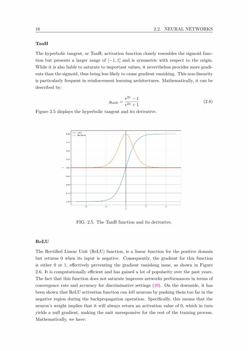
TanH
The hyperbolic tangent, or TanH, activation function closely resembles the sigmoid func-tion but presents a larger range of [−1, 1] and is symmetric with respect to the origin.While it is also liable to saturate to important values, it nevertheless provides more gradi-ents than the sigmoid, thus being less likely to cause gradient vanishing. This non-linearityis particularly frequent in reinforcement learning architectures. Mathematically, it can bedescribed by:
gtanh = e2x − 1e2x + 1 (2.8)
Figure 2.5 displays the hyperbolic tangent and its derivative.
FIG. 2.5. The TanH function and its derivative.
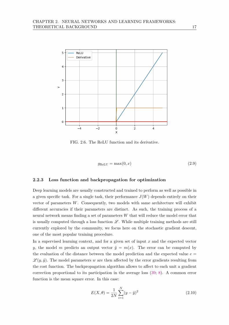
ReLU
The Rectified Linear Unit (ReLU) function, is a linear function for the positive domainbut returns 0 when its input is negative. Consequently, the gradient for this functionis either 0 or 1, effectively preventing the gradient vanishing issue, as shown in Figure2.6. It is computationally efficient and has gained a lot of popularity over the past years.The fact that this function does not saturate improves networks performances in terms ofconvergence rate and accuracy for discriminative settings (39). On the downside, it hasbeen shown that ReLU activation function can kill neurons by pushing them too far in thenegative region during the backpropagation operation. Specifically, this means that theneuron’s weight implies that it will always return an activation value of 0, which in turnyields a null gradient, making the unit unresponsive for the rest of the training process.Mathematically, we have:
CHAPTER 2. NEURAL NETWORKS AND LEARNING FRAMEWORKS:THEORETICAL BACKGROUND 17
FIG. 2.6. The ReLU function and its derivative.
gReLU = max(0, x) (2.9)
2.2.3 Loss function and backpropagation for optimization
Deep learning models are usually constructed and trained to perform as well as possible ina given specific task. For a single task, their performance J(W ) depends entirely on theirvector of parameters W . Consequently, two models with same architecture will exhibitdifferent accuracies if their parameters are distinct. As such, the training process of aneural network means finding a set of parameters W that will reduce the model error thatis usually computed through a loss function L . While multiple training methods are stillcurrently explored by the community, we focus here on the stochastic gradient descent,one of the most popular training procedure.In a supervised learning context, and for a given set of input x and the expected vectory, the model m predicts an output vector y = m(x). The error can be computed bythe evaluation of the distance between the model prediction and the expected value e =L (y, y). The model parameters w are then affected by the error gradients resulting fromthe cost function. The backpropagation algorithm allows to affect to each unit a gradientcorrection proportional to its participation in the average loss (39; 8). A common errorfunction is the mean square error. In this case:
E(X, θ) = 12N
N∑i=1
(y − y)2 (2.10)
18 2.2. NEURAL NETWORKS
where y is the target value and y is the neural network prediction. As explained above,this error should be minimized with respect to the network’s weights. For the N examples,this can be expressed as:
∂E(X, θ)∂wki,j
= 1N
N∑d=1
∂
∂wki,j
(12(yd − yd)2
)= 1N
N∑d=1
∂Ed∂wki,j
(2.11)
Using the chain rule, it is possible to write the error partial derivative:
∂E
∂wki,j= ∂E
∂akj
∂akj∂wki,j
(2.12)
where akj is the activation value of neuron j in layer k, before the activation function, asdetailled in Equation 2.1. The first term in Equation 2.12 called the error, is denoted:
δkj = ∂E
∂akj(2.13)
Using the activation value calculation, the second term in Equation 2.12 can be expressedas:
∂akj∂wki,j
= ∂
∂wki,j
(rk−1∑l=0
wkl,jok−1l
)= ok−1 (2.14)
Consequently, the partial derivative of the error function E with respect to a weight wki,jis the product between the error term of neuron j in layer k and the output of node i fromthe previous layer.
∂E
∂wki,j= δkj o
k−1i (2.15)
The error term computation depends on the neuron position in the network and startsfrom the final layer m. It can be expressed as:
E = 12(y − y)2 = 1
2(y − go(am1 ))2 (2.16)
where g0(x) is the activation function for the output layer. With the chain rule, the partialderivative is:
δm1 = (go(am1 )− y)g′o(am1 ) = (y − y)g′o(am1 ) (2.17)
Finally, the partial derivative of the error function E with respect to a weight in the finallayer wmi,j is:
∂E
∂wmi,j= δm1 o
m−1i = (y − y)g′0(am1 )om−1
i (2.18)
CHAPTER 2. NEURAL NETWORKS AND LEARNING FRAMEWORKS:THEORETICAL BACKGROUND 19
For the hidden layers, it is necessary to rely on the chain rule again:
δkj = ∂E
∂akj=
rk+1∑l=1
∂E
∂ak+1l
∂ak+1l
∂akj(2.19)
Using the error value from the next layer enables to rewrite the equation as:
δkj =rk+1∑l=1
δk+1j
∂ak+1l
∂akj(2.20)
With the activation ak+1l being ak+1
l =∑rk
j=1wk+1j,l g
(akj
), the second term in Equation
2.20 can be put as:
δkj =rk+1∑l=1
δk+1l wk+1
j,l g′(akj ) = g′(akj )rk+1∑l=1
δk+1l wk+1
j,l (2.21)
Finally, by putting it all these elements together, the partial derivative error E with respectto a weight located in the hidden layers can be expressed as:
∂E
∂wki,j= δkj o
k−1i = g′(akj )ok−1
i
rk+1∑l=1
wk+1j,l δk+1
l (2.22)
2.3 Supervised Learning
Supervised learning is the most straightforward approach when using deep learning andneural networks. This technique has been applied to a very wide range of tasks, featur-ing spam detection, image classification, video frame interpolation, system identificationand regression tasks. Despite requiring a considerable volume of examples to be success-ful, recent supervised learning algorithms have improved the state-of-the-art in numerouschallenging tasks (39).
In practice, it requires a dataset that relates input and output pairs, generally denoted(X,Y ) and consists in finding statistical relationship between these elements. Specifi-cally, with xi a given input example in the dataset, the neural network f predicts a labelyi = f(xi) which is compared to the dataset label and returns an error for this example.Mathematically:
ei = D(yi, yi) (2.23)
where D is a function that evaluates the distance between the predicted label and the realtarget. This error is then averaged with other examples from the dataset, to compute theneural network loss and thus the optimization gradients.
20 2.4. REINFORCEMENT LEARNING
2.4 Reinforcement Learning
Reinforcement Learning (RL) algorithms are a class of machine learning algorithms thatadresses the problem of optimal decisions over time (70; 125; 131). Specifically, it featuresan agent tasked to select actions in an environment in order to maximize a sum of rewardsalong the time it interacts with its world. RL is a particularly well-suited way to tacklerobotics challenges as it is able to propose successful control policies without having toanalytically define a model of the dynamics, which often proves to be challenging.
2.4.1 Principle and main concepts
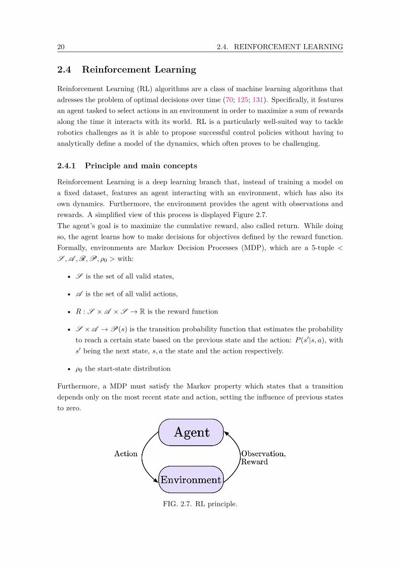
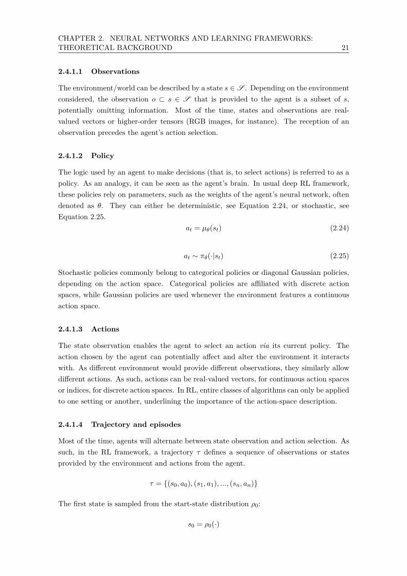
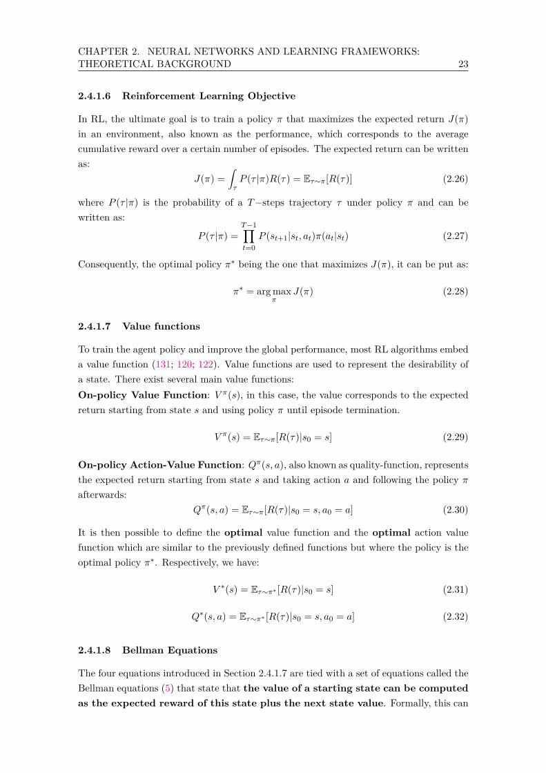
Reinforcement Learning is a deep learning branch that, instead of training a model ona fixed dataset, features an agent interacting with an environment, which has also itsown dynamics. Furthermore, the environment provides the agent with observations andrewards. A simplified view of this process is displayed Figure 2.7.The agent’s goal is to maximize the cumulative reward, also called return. While doingso, the agent learns how to make decisions for objectives defined by the reward function.Formally, environments are Markov Decision Processes (MDP), which are a 5-tuple <S ,A ,R,P, ρ0 > with:
• S is the set of all valid states,
• A is the set of all valid actions,
• R : S ×A ×S → R is the reward function
• S ×A →P(s) is the transition probability function that estimates the probabilityto reach a certain state based on the previous state and the action: P (s′|s, a), withs′ being the next state, s, a the state and the action respectively.
• ρ0 the start-state distribution
Furthermore, a MDP must satisfy the Markov property which states that a transitiondepends only on the most recent state and action, setting the influence of previous statesto zero.
FIG. 2.7. RL principle.
CHAPTER 2. NEURAL NETWORKS AND LEARNING FRAMEWORKS:THEORETICAL BACKGROUND 21
2.4.1.1 Observations
The environment/world can be described by a state s ∈ S . Depending on the environmentconsidered, the observation o ⊂ s ∈ S that is provided to the agent is a subset of s,potentially omitting information. Most of the time, states and observations are real-valued vectors or higher-order tensors (RGB images, for instance). The reception of anobservation precedes the agent’s action selection.
2.4.1.2 Policy
The logic used by an agent to make decisions (that is, to select actions) is referred to as apolicy. As an analogy, it can be seen as the agent’s brain. In usual deep RL framework,these policies rely on parameters, such as the weights of the agent’s neural network, oftendenoted as θ. They can either be deterministic, see Equation 2.24, or stochastic, seeEquation 2.25.
at = µθ(st) (2.24)
at ∼ πθ(·|st) (2.25)
Stochastic policies commonly belong to categorical policies or diagonal Gaussian policies,depending on the action space. Categorical policies are affiliated with discrete actionspaces, while Gaussian policies are used whenever the environment features a continuousaction space.
2.4.1.3 Actions
The state observation enables the agent to select an action via its current policy. Theaction chosen by the agent can potentially affect and alter the environment it interactswith. As different environment would provide different observations, they similarly allowdifferent actions. As such, actions can be real-valued vectors, for continuous action spacesor indices, for discrete action spaces. In RL, entire classes of algorithms can only be appliedto one setting or another, underlining the importance of the action-space description.
2.4.1.4 Trajectory and episodes
Most of the time, agents will alternate between state observation and action selection. Assuch, in the RL framework, a trajectory τ defines a sequence of observations or statesprovided by the environment and actions from the agent.
τ = {(s0, a0), (s1, a1), ..., (sn, an)}
The first state is sampled from the start-state distribution ρ0:
s0 = ρ0(·)
22 2.4. REINFORCEMENT LEARNING
State transition depends both on the environment, which can have a stochastic part, andthe most recent agent action, as required by MDP. Thus, for a deterministic transition,we have:
st+1 = f(st, at)
while for a stochastic, one transition can be written:
st+1 ∼ P (·|st, at)
In RL, an episode is a trajectory that ends with a termination state: a termination stateis a state that calls for a reset of the environment. It can be the goal state (reaching aspecific point in space, for instance) or an absorption state (the agent pushed the objectit was supposed to grasp out of its reach). It is also possible to consider that an episodeis over after a given number of steps.
2.4.1.5 Reward Function
The action selected by the agent after state observation is usually met by an evaluationfrom the environment: the reward. The reward function R holds a paramount importancein RL, as it is the main tool for shaping the agent behaviour. Formally, the reward functionis a real-valued function R:S × A ×S → R that evaluates an action taken in a givenstate and its effect. That is:
rt = R(st, at, st+1)
Reward functions revet various forms. Specifically, two main classes of rewards can bereferenced:
• Sparse rewards: Also known as impulse rewards, this class of functions affects areward rg to a small area of the explorable space, while most of the environmentreturns a reward rl with rg >> rl. A classic example of sparse rewards is the AtariPong environment (81) where a positive reward is only given to the agent when itscores, and inversely a negative reward is perceived when the agent lets the ball gothrough. Otherwise, the reward is null
• Shaped rewards: As opposed to a sparse reward, a shaped reward provides a learningsignal in the majority of the explorable space, offering a gradient of reward to theagent that may sometimes ease the learning phase. A reward inversely proportionalto the distance with the target point in a robotic reaching task is a common usageof shaped rewards.
Reward functions are not necessarily linear nor continue, thus giving an important flex-ibility to shape the agent behaviour. The sum of rewards over an episode is called thereturn.
CHAPTER 2. NEURAL NETWORKS AND LEARNING FRAMEWORKS:THEORETICAL BACKGROUND 23
2.4.1.6 Reinforcement Learning Objective
In RL, the ultimate goal is to train a policy π that maximizes the expected return J(π)in an environment, also known as the performance, which corresponds to the averagecumulative reward over a certain number of episodes. The expected return can be writtenas:
J(π) =∫τP (τ |π)R(τ) = Eτ∼π[R(τ)] (2.26)
where P (τ |π) is the probability of a T−steps trajectory τ under policy π and can bewritten as:
P (τ |π) =T−1∏t=0
P (st+1|st, at)π(at|st) (2.27)
Consequently, the optimal policy π∗ being the one that maximizes J(π), it can be put as:
π∗ = arg maxπ
J(π) (2.28)
2.4.1.7 Value functions
To train the agent policy and improve the global performance, most RL algorithms embeda value function (131; 120; 122). Value functions are used to represent the desirability ofa state. There exist several main value functions:On-policy Value Function: V π(s), in this case, the value corresponds to the expectedreturn starting from state s and using policy π until episode termination.
V π(s) = Eτ∼π[R(τ)|s0 = s] (2.29)
On-policy Action-Value Function: Qπ(s, a), also known as quality-function, representsthe expected return starting from state s and taking action a and following the policy πafterwards:
Qπ(s, a) = Eτ∼π[R(τ)|s0 = s, a0 = a] (2.30)
It is then possible to define the optimal value function and the optimal action valuefunction which are similar to the previously defined functions but where the policy is theoptimal policy π∗. Respectively, we have:
V ∗(s) = Eτ∼π∗ [R(τ)|s0 = s] (2.31)
Q∗(s, a) = Eτ∼π∗ [R(τ)|s0 = s, a0 = a] (2.32)
2.4.1.8 Bellman Equations
The four equations introduced in Section 2.4.1.7 are tied with a set of equations called theBellman equations (5) that state that the value of a starting state can be computedas the expected reward of this state plus the next state value. Formally, this can
24 2.4. REINFORCEMENT LEARNING
be written for both the value function as well as the action-value function as:
V π(s) = Ea∼π,s′∼P [r(s, a) + γV π(s′)] (2.33)
where the discount factor γ ∈ [0, 1] indicates weights the importance of future rewards.The closer the discount factor γ is to 1, the more significant future rewards are. (131)
Qπ(s, a) = Es′∼P [r(s, a) + γEa′∼πQπ(s′, a′)] (2.34)
where s′ ∼ P stands for s′ ∼ P (·|s, a) that indicates that the next state is sampled fromthe environment’s transition probability. Similarly, a ∼ π and a′ ∼ π mean that the actionand next actions are sampled from the policy, based on the state a ∼ π(·|s) or next states′, a′ ∼ π(·|s′), respectively.Bellman equations can be adapted for the optimal value functions as well:
V ∗(s) = maxa
Es′∼P [r(s, a) + γV ∗(s′)] (2.35)
Q∗(s, a) = Es′∼P [r(s, a) + γmaxa′
Q∗(s′, a′)] (2.36)
2.4.1.9 Advantage function
The advantage function is a way to discriminate useful actions. Mathematically, theadvantage corresponds to the subtraction of the value function V from the action-valuefunction Q.
Aπ(s, a) = Qπ(s, a)− V π(s) (2.37)
As can be deduced from this relation, an action better than the average would result in apositive advantage. This notion is at the center of various recent RL algorithms (121)
2.4.2 Practical aspects of RL
2.4.2.1 The Exploration-Exploitation trade-off
Usually, a RL agent has initially no specific knowledge about the environment it mustinteract with. In practice, this is represented by randomly initialized parameters for aneural network or a uniform state for a tabular approach. The exploration of the environ-ment, through a trial-and-error process, is a way for the agent to gather knowledge andunderstand how to reach highly valuable states. Indeed, the more the agent knows aboutthe environment, the quicker it can optimize the policy reflecting its behaviour. How-ever, due to the potentially infinite size of a wide range of environments, pure explorationcan not be considered as an efficient resources usage and is likely to confuse the agent.Similarly, systematic exploitation of available knowledge (selecting the current supposedbest action) may result in sub-optimal or poor performance overall. Consequently, a suc-cessful RL algorithm must take into account these notions and find a trade-off between
CHAPTER 2. NEURAL NETWORKS AND LEARNING FRAMEWORKS:THEORETICAL BACKGROUND 25
the two attitudes and an important quantity of works was devoted to this critical issue(4; 26; 103; 131)
2.4.2.2 Credit assignment problem
The credit-assignment problem is a frequently encountered issue in environment withsparse rewards. Specifically, as the agent seldom receives a reward signal, it is most of thetime at the end of a trajectory. Consequently, a full sequence of states and actions wasinvolved in order to get to the state that provided the reward. In these cases, it becomesdifficult to effectively discriminate between useful and detrimental actions (81; 121). Thereexist numerous examples of such environments, such as the games of Chess or Go, orsimulated environments like Pong, where the reward function sends a signal only on episodetermination. In those, as the episode trajectories can frequently exceed several dozens oftransitions, the credit assignment problem becomes obvious.
2.4.2.3 Sample (In)efficiency
While RL algorithms have drastically improved recently, training an efficient policy in theRL framework still requires a very large quantity of trajectories. In the widely recognizedDQN paper (82), the trained agent never reaches 50% of human performance even after200 million frames, which corresponds to over 900 hours of practice in real-time. Morerecently, the impressive results of OpenAI and in the Hide-and-Seek environment wereobtained after several billions of frames. However, for simpler environments, it is stillpossible to train acceptable policies within an reasonable time frame. Along with potentialcost of damaged robots during training, it is one of the main motivations for simulatedenvironments.
2.4.3 Modern RL algorithms
This section introduces practical implementations of recent RL algorithms. Starting fromthe broad perspective of model-free or model-based approaches, it progressively narrowsits focus until introducing the main RL algorithm used in this work: Proximal PolicyOptimization, see Figure 2.8.
2.4.3.1 Model-free and model-based RL
The question of using model-free or model-based algorithms can be formulated as: Doesthe agent have access to the environment model ? This has heavy implicationsas having access to the environment model implies that the agent is aware of the func-tions governing the states transitions as well as the rewards. This hypothesis has practicalupsides, as it allows the agent to plan its actions ahead, exploring various choices andweighting their consequences. A recent example of successful application of model-basedtechniques is AlphaGo(126; 127). However, in practice, a reliable environment model isseldom available, thus hindering the performances of the agent when used in the real

26 2.4. REINFORCEMENT LEARNING
FIG. 2.8. A taxonomy of RL algorithms.
settings. An alternative approach is to learn the environment dynamics. In this configu-ration, agents usually alternate between learning the environment model and improvingtheir policy. Nevertheless, this is likely to result in a biased model that is prone to be ex-ploited by the agent. Although it can lead to satisfying results in simulated environments,it is often correlated with poor behavior once deployed to the real target environments.Techniques that renounce in using the environment dynamics are classified as model-freemethods. They are currently very popular and widely used in the literature and, as therest of this report relies on this class of methods, model-based will not be detailed further.
2.4.3.2 On-Policy vs. Off-Policy
Among model-free algorithms, another crucial branching divides again the algorithmicpool into two notable groups: on-policy or off-policy algorithms. On-policy algorithmsoptimize the parameters θ of a policy πθ by performing gradient ascent on the gradient oftheir performance J(πθ) or an approximation of it. Each update (optimization) relies ondata collected by the latest policy version, which partially explains the sample inefficiencyof these techniques. On the contrary, off-policy methods learn an approximator of action-values Qθ(s, a) and their updates rely on the Bellman equation. Consequently, they donot require that the data provided for the update be generated by the latest policy. Thispresents various advantages, such as having the possibility to insert expert trajectories orhuman examples within the data used to train the policy. While this idea is appealing, asis the fact that off-policy algorithms are more sample efficient, they are also more brittle asthey do not optimize directly for the performance (given that they optimize for Qθ(s, a)).In contrast, on-policy methods are more stable and reliable (as they directly optimize forthe performance J(πθ)). The main RL algorithm used in this report is PPO and is anon-policy method.
CHAPTER 2. NEURAL NETWORKS AND LEARNING FRAMEWORKS:THEORETICAL BACKGROUND 27
2.4.4 Proximal Policy Optimization
Proximal Policy Optimization (PPO) is an on-policy, actor-critic with trust-region RLalgorithm (120) introduced in 2017 (122). Despite its relative simplicity, this method isrobust, scalable and reliable and has been at the center of various impressive RL achieve-ments in recent works (100).
On-policy updates As explained in section 2.4.3.2, the goal is to maximize the agentperformance that equates with maximizing the expected return:
J(πθ) = Eτ∼πθ [R(τ)] (2.38)
The gradient ascent update can be written:
θk+1 = θk + α∇θJ(πθ)|θk (2.39)
where ∇θJ(πθ) is the policy gradient, θk the policy parametrization at step k and α isthe learning rate. To compute the policy gradient, an analytical gradient of the policyperformance is necessary. It can be written as:
∇θJ(πθ) = Eτ∼πθ [∇θ log πθ(at|st)R(τ)] (2.40)
The updates resulting from Equation 2.40 increase the probability of an action rewardedpositively, while discouraging the agent to select actions that were met with a negativereward.
Actor-Critic As can be seen in Equation 2.40, the probability to select an action isdirectly dependent on the sum of rewards obtained in the trajectory. In practice, however,this signal may be noisy and present an important variance. Actor-critic approacheswere designed to mitigate the noise from the reward, leading to a faster and more robusttraining. Specifically, they rely on an additional network parametrized by weights φ, calledthe critic, that estimates the value Vφ(s) of each state. This scalar is then subtracted fromthe reward, allowing the action to be evaluated on whether or not it yields a superiorreturn than the expected. Consequently, Equation 2.40 becomes:
∇θJ(πθ) = Eτ∼πθ [∇θ log πθ(at|st)(R(τ)− Vφ(st))] (2.41)
In these methods, the critic is also trained and thus provides only an approximation ofthe state value. The most common loss function for the value function is:
φk = arg minφ
Est,Rt∼πk [Vφ(st)−Rt] (2.42)
where the discounted return can be expressed as Rt =∑Ni=t riγ
i−t
28 2.5. GENERATIVE ADVERSARIAL LEARNING
Proximal Policy Optimization The PPO algorithm was designed to prevent a policyfrom taking too important update steps that harm the performance, sometimes beyondrecovery, while still going as far as possible in the gradient ascent. To do so, it relies onthe notion of trust-regions. Trust-regions were introduced in (120) and rely on gradientclipping in the objective function to avoid moving the new policy too far from the previousone. The PPO objective function can be written as:
L(s, a, θold, θ) = min(rt(θ)Aπθold (s, a), clip(rt(θ), 1− ε, 1 + ε)Aπθk (s, a)) (2.43)
where rt(θ) is the ratio of the probabilities between the previous policy and the currentone for a given pair of state and action. This ratio can be expressed as:
ρt(θ) = πθ(a|s)πθold(s, a) (2.44)
and the clip function ensures that the ratio stays in the [1− ε, 1 + ε]range
2.5 Generative Adversarial Learning
RL algorithms represent the go-to approach when considering control environments andare extensively used in the Universal Notice Network method presented in Chapter 4.Nevertheless, the unsupervised learning framework offers interesting concepts and someapproaches can be repurposed in a context that is beyond their usual scope. This partintroduces the Generative Adversarial Learning (GAN) (40) framework, an unsupervisedgenerative modelling technique on which the CoachGAN transfer technique (86), one ofour main contributions, see Section 5.1, relies heavily.
2.5.1 Principle
The concept of Generative Adversarial Networks (GAN) is rooted in Information The-ory and generative modelling. In this paradigm, the goal is to estimate the underlyingdata probability Pdata of a given dataset. As opposed to discriminative modelling whichobjective is to infer labels y from data samples, the optimization of a generative modelyields a function able to generate unseen samples from a distribution matching the trainingdataset, as shown in Figure 2.9. Within the GAN framework, this process is implementedthrough a competitive setting involving two functions:
• a generator that creates samples
• a discriminator: an adversarial function that evaluates the samples
In this setting, the two networks share an objective function and are jointly trained usingthe following minimax game.
minθ
maxφ
V (Gθ, Dφ) = Ex∼Pdata [logDφ(x)] + Eθz∼Pz [log(1−Dφ(Gθ(z)))] (2.45)

CHAPTER 2. NEURAL NETWORKS AND LEARNING FRAMEWORKS:THEORETICAL BACKGROUND 29
FIG. 2.9. GAN principle.
where Gθ is the generator, using a vector of parameters θ and Dφ is the discriminator re-lying on weights φ, Pdata is the training dataset and Pz is a probability distribution for thelatent variable z used by the generator to produce samples. This latent variable is, in prac-tice, a noise vector sampled from a uniform or unit Gaussian distribution and then mappedto samples by the generator. In return, the discriminator D assigns a scalar value to thesample Gθ(z) representing how likely this sample belongs to the training distribution, thusacting as an adversarial classifier. Formally, Equation 2.45 states that the optimal dis-criminator must be able to perfectly distinguish between synthetic (generator-produced)samples and real samples from the training dataset. In practice means to respectivelyaffect a value of Dφ(Gθ(z)) = 0 to synthetic samples and a value of Dφ(x) = 1 to realsamples. On the other hand, the optimal generator should be able to confuse the dis-criminator and produce synthetic samples of high likelihood with respect to the datasetthat would systematically be classified as real by the discriminator. This adversarial setupconsequently provides a suitable way to use each model to train the other one (i.e: thediscriminator is penalized for each synthetic sample classified as real and vice-versa). Thediscriminator and generator loss function can respectively be expressed as:
LDφ = 1m
m∑i=1
[− log(Dφ(xi))− log(1−Dφ(Gθ(zi)))] (2.46)
LGθ = 1m
m∑i=1
log(1−Dφ(Gθ(zi))) (2.47)
2.5.2 Reaching optimality
As introduced in Equation 2.45, for a fixed generator Gθ, the discriminator does a binaryclassification. Practically, it should assign a value of 1 to data from the training setx ∼ Pdata and a value of 0 to samples coming from the generator x ∼ PGθ . Thus, for a
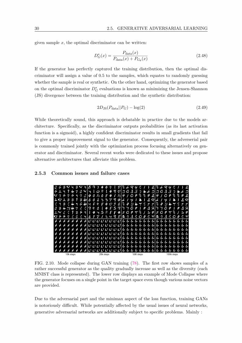
30 2.5. GENERATIVE ADVERSARIAL LEARNING
given sample x, the optimal discriminator can be written:
D∗G(x) = Pdata(x)Pdata(x) + PGθ(x) (2.48)
If the generator has perfectly captured the training distribution, then the optimal dis-criminator will assign a value of 0.5 to the samples, which equates to randomly guessingwhether the sample is real or synthetic. On the other hand, optimizing the generator basedon the optimal discriminator D∗G evaluations is known as minimizing the Jensen-Shannon(JS) divergence between the training distribution and the synthetic distribution:
2DJS(Pdata||PG)− log(2) (2.49)
While theoretically sound, this approach is debatable in practice due to the models ar-chitecture. Specifically, as the discriminator outputs probabilities (as its last activationfunction is a sigmoid), a highly confident discriminator results in small gradients that failto give a proper improvement signal to the generator. Consequently, the adverserial pairis commonly trained jointly with the optimization process focusing alternatively on gen-erator and discriminator. Several recent works were dedicated to these issues and proposealternative architectures that alleviate this problem.
2.5.3 Common issues and failure cases
FIG. 2.10. Mode collapse during GAN training (78). The first row shows samples of arather successful generator as the quality gradually increase as well as the diversity (eachMNIST class is represented). The lower row displays an example of Mode Collapse wherethe generator focuses on a single point in the target space even though various noise vectorsare provided.
Due to the adversarial part and the minimax aspect of the loss function, training GANsis notoriously difficult. While potentially affected by the usual issues of neural networks,generative adversarial networks are additionally subject to specific problems. Mainly :

CHAPTER 2. NEURAL NETWORKS AND LEARNING FRAMEWORKS:THEORETICAL BACKGROUND 31
• Unstability: As the existence of an equilibrium is not guaranteed, it is possible thatthe discriminator and the generator start a cycle of periodic domination. A symptomof this can be a sinus-like loss for both models and regular drop in generator samples.Carefully tuned hyper-parameters and model architectures can mitigate this issue.
• Mode collapse: In these cases, the generator fails to diversify its samples, basicallymapping all latent vectors to a single point or a small area of the output space,which is considered real by the discriminator. Such a phenomenon is represented inFigure 2.10.
• Discriminator domination: In some cases, the discriminator initialization allows itto detect most of synthetic samples early in training, resulting in an increase indiscriminator confidence that diminishes the gradients available for the generator.
• Overfitting: The generator is only able to generate samples that too much resemblethe training set.
Despite its extended representative and modelling power, the GAN framework offers littlestraightforward process to control the latent space. Various works have been able to iden-tify the main latent space axes by examining large quantities of samples and determiningthe transformation vector between two elements. Alternative modelling approaches, suchas the Variational AutoEncoder, the main concept of the Task-Specific Loss (TSL), seeSection 5.2, constraints the latent space to be more manageable, which in turn endowsthe user with a closer supervision on the model output.
2.6 Knowledge representation
For a large class of problems, finding the good set of features to represent the datapointconstitutes in itself an important part of the solution. However, it is most of the timeunclear how to find these features. For instance, let us consider the problem of finding ahuman face in a picture. One could consider that a face has been found if a nose and twoeyes can be detected. Nevertheless, it is not straightforward to provide the descriptionof such a feature in pixel space, as eyes and nose can have various shapes, size, andcolor. Although it is manageable to define space boundaries for these elements, it is alsonecessary to deal with various lighting setting, shadows and element occlusion (due to faceorientation, for example). A common approach in modern machine learning is to assignthe feature representation to the model as well as the discovery of the relation betweenthe input and output. Among the various architectures that implement this concept, theAutoEncoder (AE) is the most notorious instance (39; 8).
2.6.1 Autoencoders
Autoencoders are neural networks that are trained to learn to copy the input they arepresented. While this may seem like a trivial task that could be accomplished with an
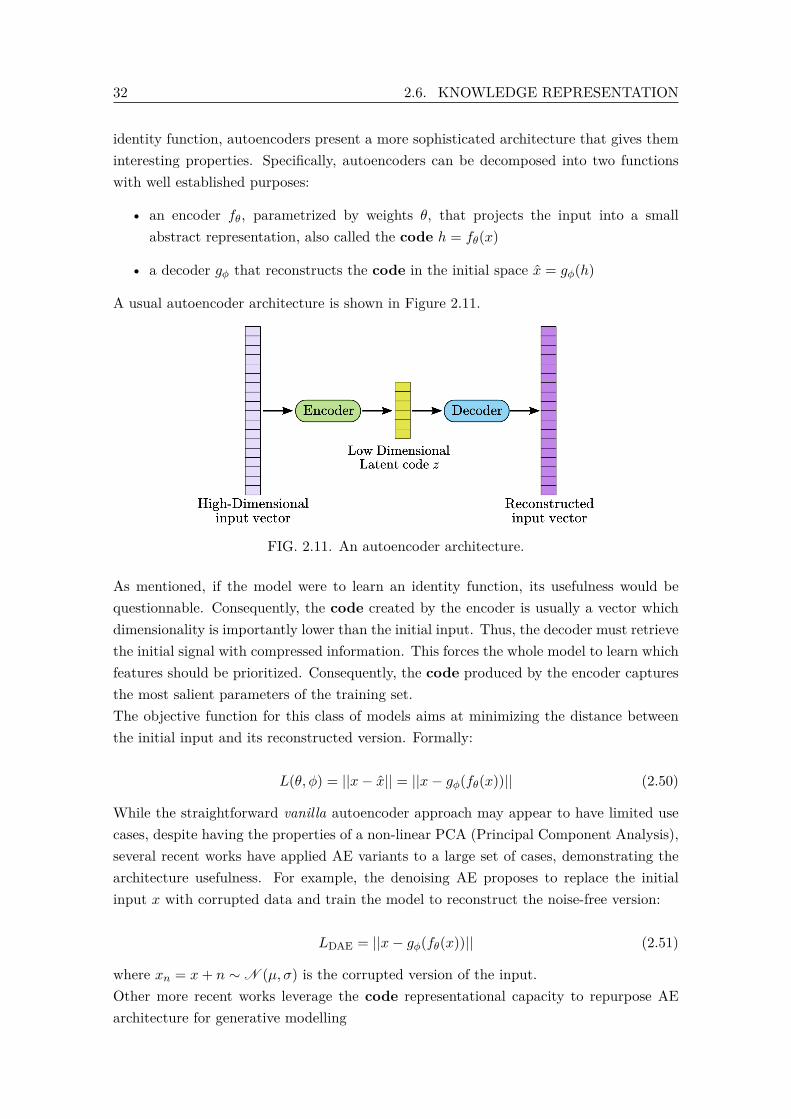
32 2.6. KNOWLEDGE REPRESENTATION
identity function, autoencoders present a more sophisticated architecture that gives theminteresting properties. Specifically, autoencoders can be decomposed into two functionswith well established purposes:
• an encoder fθ, parametrized by weights θ, that projects the input into a smallabstract representation, also called the code h = fθ(x)
• a decoder gφ that reconstructs the code in the initial space x = gφ(h)
A usual autoencoder architecture is shown in Figure 2.11.
FIG. 2.11. An autoencoder architecture.
As mentioned, if the model were to learn an identity function, its usefulness would bequestionnable. Consequently, the code created by the encoder is usually a vector whichdimensionality is importantly lower than the initial input. Thus, the decoder must retrievethe initial signal with compressed information. This forces the whole model to learn whichfeatures should be prioritized. Consequently, the code produced by the encoder capturesthe most salient parameters of the training set.The objective function for this class of models aims at minimizing the distance betweenthe initial input and its reconstructed version. Formally:
L(θ, φ) = ||x− x|| = ||x− gφ(fθ(x))|| (2.50)
While the straightforward vanilla autoencoder approach may appear to have limited usecases, despite having the properties of a non-linear PCA (Principal Component Analysis),several recent works have applied AE variants to a large set of cases, demonstrating thearchitecture usefulness. For example, the denoising AE proposes to replace the initialinput x with corrupted data and train the model to reconstruct the noise-free version:
LDAE = ||x− gφ(fθ(x))|| (2.51)
where xn = x+ n ∼ N (µ, σ) is the corrupted version of the input.Other more recent works leverage the code representational capacity to repurpose AEarchitecture for generative modelling
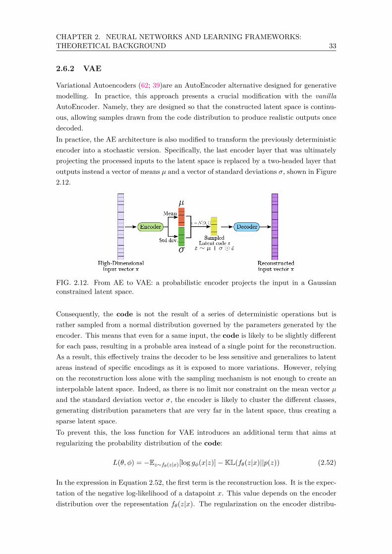
CHAPTER 2. NEURAL NETWORKS AND LEARNING FRAMEWORKS:THEORETICAL BACKGROUND 33
2.6.2 VAE
Variational Autoencoders (62; 39)are an AutoEncoder alternative designed for generativemodelling. In practice, this approach presents a crucial modification with the vanillaAutoEncoder. Namely, they are designed so that the constructed latent space is continu-ous, allowing samples drawn from the code distribution to produce realistic outputs oncedecoded.In practice, the AE architecture is also modified to transform the previously deterministicencoder into a stochastic version. Specifically, the last encoder layer that was ultimatelyprojecting the processed inputs to the latent space is replaced by a two-headed layer thatoutputs instead a vector of means µ and a vector of standard deviations σ, shown in Figure2.12.
FIG. 2.12. From AE to VAE: a probabilistic encoder projects the input in a Gaussianconstrained latent space.
Consequently, the code is not the result of a series of deterministic operations but israther sampled from a normal distribution governed by the parameters generated by theencoder. This means that even for a same input, the code is likely to be slightly differentfor each pass, resulting in a probable area instead of a single point for the reconstruction.As a result, this effectively trains the decoder to be less sensitive and generalizes to latentareas instead of specific encodings as it is exposed to more variations. However, relyingon the reconstruction loss alone with the sampling mechanism is not enough to create aninterpolable latent space. Indeed, as there is no limit nor constraint on the mean vector µand the standard deviation vector σ, the encoder is likely to cluster the different classes,generating distribution parameters that are very far in the latent space, thus creating asparse latent space.To prevent this, the loss function for VAE introduces an additional term that aims atregularizing the probability distribution of the code:
L(θ, φ) = −Ez∼fθ(z|x)[log gφ(x|z)]−KL(fθ(z|x)||p(z)) (2.52)
In the expression in Equation 2.52, the first term is the reconstruction loss. It is the expec-tation of the negative log-likelihood of a datapoint x. This value depends on the encoderdistribution over the representation fθ(z|x). The regularization on the encoder distribu-
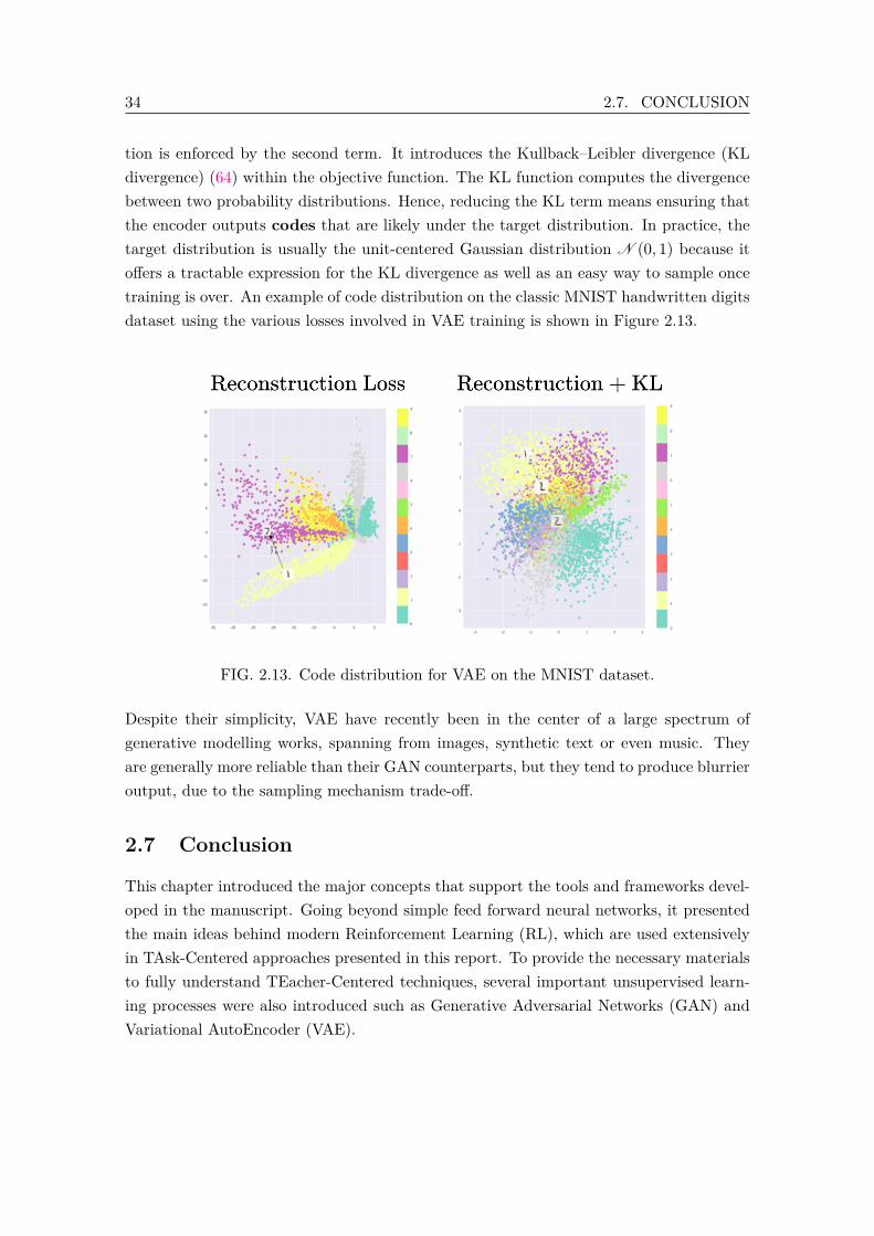
34 2.7. CONCLUSION
tion is enforced by the second term. It introduces the Kullback–Leibler divergence (KLdivergence) (64) within the objective function. The KL function computes the divergencebetween two probability distributions. Hence, reducing the KL term means ensuring thatthe encoder outputs codes that are likely under the target distribution. In practice, thetarget distribution is usually the unit-centered Gaussian distribution N (0, 1) because itoffers a tractable expression for the KL divergence as well as an easy way to sample oncetraining is over. An example of code distribution on the classic MNIST handwritten digitsdataset using the various losses involved in VAE training is shown in Figure 2.13.
FIG. 2.13. Code distribution for VAE on the MNIST dataset.
Despite their simplicity, VAE have recently been in the center of a large spectrum ofgenerative modelling works, spanning from images, synthetic text or even music. Theyare generally more reliable than their GAN counterparts, but they tend to produce blurrieroutput, due to the sampling mechanism trade-off.
2.7 Conclusion
This chapter introduced the major concepts that support the tools and frameworks devel-oped in the manuscript. Going beyond simple feed forward neural networks, it presentedthe main ideas behind modern Reinforcement Learning (RL), which are used extensivelyin TAsk-Centered approaches presented in this report. To provide the necessary materialsto fully understand TEacher-Centered techniques, several important unsupervised learn-ing processes were also introduced such as Generative Adversarial Networks (GAN) andVariational AutoEncoder (VAE).
Chapter 3Transfer Learning & Related works
Contents3.1 Societal Needs for Transfer Learning . . . . . . . . . . . . . . . . . . . . 363.2 Transfer Learning Principles . . . . . . . . . . . . . . . . . . . . . . . . 363.3 Common cases of Transfer Learning . . . . . . . . . . . . . . . . . . . . 383.4 Computer Vision . . . . . . . . . . . . . . . . . . . . . . . . . . . . . . . 403.5 Natural Language Processing . . . . . . . . . . . . . . . . . . . . . . . . 433.6 Transfer Learning in control tasks . . . . . . . . . . . . . . . . . . . . . 45
3.6.1 Deep learning based control . . . . . . . . . . . . . . . . . . . . 453.6.2 From simulation to real world . . . . . . . . . . . . . . . . . . . 463.6.3 Transfer between tasks . . . . . . . . . . . . . . . . . . . . . . . 47
3.6.3.1 Reward-Based Transfer . . . . . . . . . . . . . . . . . 473.6.3.2 Curriculum Based Transfer . . . . . . . . . . . . . . . 473.6.3.3 Intrinsically motivated Transfer . . . . . . . . . . . . 483.6.3.4 Meta-Learning . . . . . . . . . . . . . . . . . . . . . . 483.6.3.5 Transfer in Hierarchical Settings . . . . . . . . . . . . 49
3.7 Knowledge representation in Transfer Learning . . . . . . . . . . . . . . 503.8 Conclusion on Transfer Learning . . . . . . . . . . . . . . . . . . . . . . 51
35
36 3.1. SOCIETAL NEEDS FOR TRANSFER LEARNING
3.1 Societal Needs for Transfer Learning
Industry 4.0, as foreseen in (123), will correspond to an era of higher integration of cyberand physical systems. In this views, industrial actors expect a strong interconnection be-tween machines and devices, comprehensive information from the technology implementedand the ability of cyber systems to take decentralized decisions. These design principlesare driven by the need for increased flexibility in terms of tasks, short industrial prod-uct series, consequently easily reconfigurable workplaces and finally highly diverse pool ofrobots.This very dynamic industrial context introduces new and complex challenges that mayprove difficult to formalize in mathematical frameworks. Indeed, perform complex mo-tions to complete a task is still an open issue. While there exist optimization methodsbased on complete models (59; 60; 67), these are usually computationally intensive andmay not satisfy real-time constraints. To tackle this issue, the community has also beenleveraging predictive methods that are completely suitable for real-time control. However,this execution efficiency is usually achieved by sacrificing the model complexity and thusconsidering simplified versions that may not have enough degrees of freedom to expressthe full problem spectrum (22). These two methods present the strong and undeniableadvantage of allowing direct transfer of skills between different agents. However, while itis possible to conceive hybrid controllers that can mitigate each approach’s weaknesses,they nevertheless rely on an analytical model for both the task and the robot that can behard if not impossible to define. As a result, it is common to integrate various hypothesesand assumptions that highly impact the precision of the model.Recently, data-driven approaches, in particular deep learning based approaches, have beenon the rise, as they can be used to find a nearly optimal solution in order to speedup the computation time in execution, while still being able to represent highly non-linear processes. As the amount of data recorded and generated in the I4.0 processes isconsiderable, there appear to be strong incentives for learning-based approaches to becomeone of the go-to frameworks in the future.As such, this chapter introduces the main principles and ideas on which Transfer Learningrelies and proposes an overview of its applications in current literature.
3.2 Transfer Learning Principles
Transfer Learning, also sometimes referred to as domain adaptation, corresponds to con-figurations where it is desirable to exploit elements or features, that were learned in agiven domain to improve generalization in another. Transfer Learning has become a mostvaluable tool in modern deep learning due to the size of recent architectures, in particu-lar in domains such as Computer Vision (CV) and Natural Language Processing (NLP).Specifically, in such situations, the model considered must perform several tasks. In orderfor the transfer to be relevant, it is usually assumed that the distribution of tasks sharemultiple factors that can be captured by the model and increase the model performance
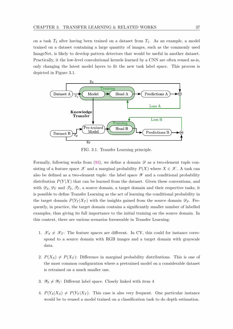
CHAPTER 3. TRANSFER LEARNING & RELATED WORKS 37
on a task T2 after having been trained on a dataset from T1. As an example, a modeltrained on a dataset containing a large quantity of images, such as the commonly usedImageNet, is likely to develop pattern detectors that would be useful in another dataset.Practically, it the low-level convolutional kernels learned by a CNN are often reused as-is,only changing the latest model layers to fit the new task label space. This process isdepicted in Figure 3.1.
FIG. 3.1. Transfer Learning principle.
Formally, following works from (93), we define a domain D as a two-element tuple con-sisting of a feature space X and a marginal probability P (X) where X ∈X . A task canalso be defined as a two-element tuple: the label space Y and a conditional probabilitydistribution P (Y |X) that can be learned from the dataset. Given these conventions, andwith DS ,DT and TS ,TT , a source domain, a target domain and their respective tasks, itis possible to define Transfer Learning as the act of learning the conditional probability inthe target domain P (YT |XT ) with the insights gained from the source domain DS . Fre-quently, in practice, the target domain contains a significantly smaller number of labelledexamples, thus giving its full importance to the initial training on the source domain. Inthis context, there are various scenarios foreseeable in Transfer Learning:
1. XS 6= XT : The feature spaces are different. In CV, this could for instance corre-spond to a source domain with RGB images and a target domain with grayscaledata.
2. P (XS) 6= P (XT ): Difference in marginal probability distributions. This is one ofthe most common configuration where a pretrained model on a considerable datasetis retrained on a much smaller one.
3. YS 6= YT : Different label space. Closely linked with item 4
4. P (YS |XS) 6= P (YT |XT ). This case is also very frequent. One particular instancewould be to reused a model trained on a classification task to do depth estimation.
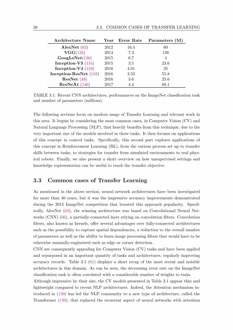
38 3.3. COMMON CASES OF TRANSFER LEARNING
Architecture Name Year Error Rate Parameters (M)AlexNet (63) 2012 16.4 60VGG(128) 2014 7.3 138
GoogLeNet(136) 2015 6.7 4Inception-V3 (134) 2015 3.5 23.6Inception-V4 (133) 2016 4.01 35
Inception-ResNet (133) 2016 3.52 55.8ResNet (48) 2016 3.6 25.6
ResNeXt (146) 2017 4.4 68.1
TABLE 3.1. Recent CNN architectures, performances on the ImageNet classification taskand number of parameters (millions).
The following sections focus on modern usage of Transfer Learning and relevant work inthis area. It begins by considering the most common cases, in Computer Vision (CV) andNatural Language Processing (NLP), that heavily benefits from this technique, due to thevery important size of the models involved in these tasks. It then focuses on applicationsof this concept in control tasks. Specifically, this second part explores applications ofthis concept in Reinforcement Learning (RL), from the various process set up to transferskills between tasks, to strategies for transfer from simulated environments to real phys-ical robots. Finally, we also present a short overview on how unsupervised settings andknowledge representation can be useful to reach the transfer objective.
3.3 Common cases of Transfer Learning
As mentioned in the above section, neural network architectures have been investigatedfor more than 40 years, but it was the impressive accuracy improvements demonstratedduring the 2012 ImageNet competition that boosted this approach popularity. Specif-ically, AlexNet (63), the winning architecture was based on Convolutional Neural Net-works (CNN) (66), a partially-connected layer relying on convolution filters. Convolutionfilters, also known as kernels, offer several advantages over fully-connected architecturessuch as the possibility to capture spatial dependencies, a reduction to the overall numberof parameters as well as the ability to learn image processing filters that would have to beotherwise manually-engineered such as edge or corner detection.CNN are consequently appealing for Computer Vision (CV) tasks and have been appliedand repurposed in an important quantity of tasks and architectures, regularly improvingaccuracy records. Table 3.1 (61) displays a short recap of the most recent and notablearchitectures in this domain. As can be seen, the decreasing error rate on the ImageNetclassification task is often correlated with a considerable number of weights to train.Although impressive by their size, the CV models presented in Table 3.1 appear thin andlightweight compared to recent NLP architectures. Indeed, the Attention mechanism in-troduced in (139) has led the NLP community to a new type of architecture, called theTransformer (139), that replaced the recurrent aspect of neural networks with attention
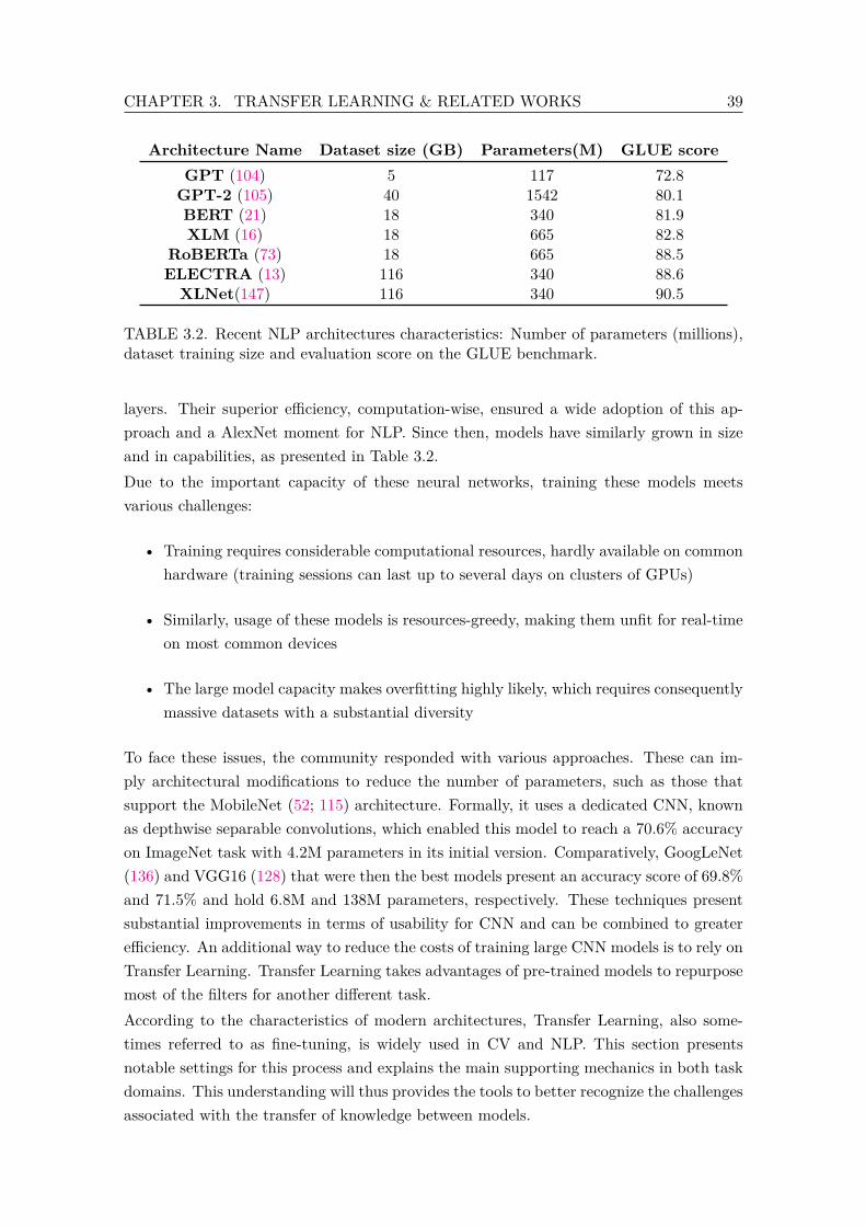
CHAPTER 3. TRANSFER LEARNING & RELATED WORKS 39
Architecture Name Dataset size (GB) Parameters(M) GLUE scoreGPT (104) 5 117 72.8GPT-2 (105) 40 1542 80.1BERT (21) 18 340 81.9XLM (16) 18 665 82.8
RoBERTa (73) 18 665 88.5ELECTRA (13) 116 340 88.6XLNet(147) 116 340 90.5
TABLE 3.2. Recent NLP architectures characteristics: Number of parameters (millions),dataset training size and evaluation score on the GLUE benchmark.
layers. Their superior efficiency, computation-wise, ensured a wide adoption of this ap-proach and a AlexNet moment for NLP. Since then, models have similarly grown in sizeand in capabilities, as presented in Table 3.2.Due to the important capacity of these neural networks, training these models meetsvarious challenges:
• Training requires considerable computational resources, hardly available on commonhardware (training sessions can last up to several days on clusters of GPUs)
• Similarly, usage of these models is resources-greedy, making them unfit for real-timeon most common devices
• The large model capacity makes overfitting highly likely, which requires consequentlymassive datasets with a substantial diversity
To face these issues, the community responded with various approaches. These can im-ply architectural modifications to reduce the number of parameters, such as those thatsupport the MobileNet (52; 115) architecture. Formally, it uses a dedicated CNN, knownas depthwise separable convolutions, which enabled this model to reach a 70.6% accuracyon ImageNet task with 4.2M parameters in its initial version. Comparatively, GoogLeNet(136) and VGG16 (128) that were then the best models present an accuracy score of 69.8%and 71.5% and hold 6.8M and 138M parameters, respectively. These techniques presentsubstantial improvements in terms of usability for CNN and can be combined to greaterefficiency. An additional way to reduce the costs of training large CNN models is to rely onTransfer Learning. Transfer Learning takes advantages of pre-trained models to repurposemost of the filters for another different task.According to the characteristics of modern architectures, Transfer Learning, also some-times referred to as fine-tuning, is widely used in CV and NLP. This section presentsnotable settings for this process and explains the main supporting mechanics in both taskdomains. This understanding will thus provides the tools to better recognize the challengesassociated with the transfer of knowledge between models.
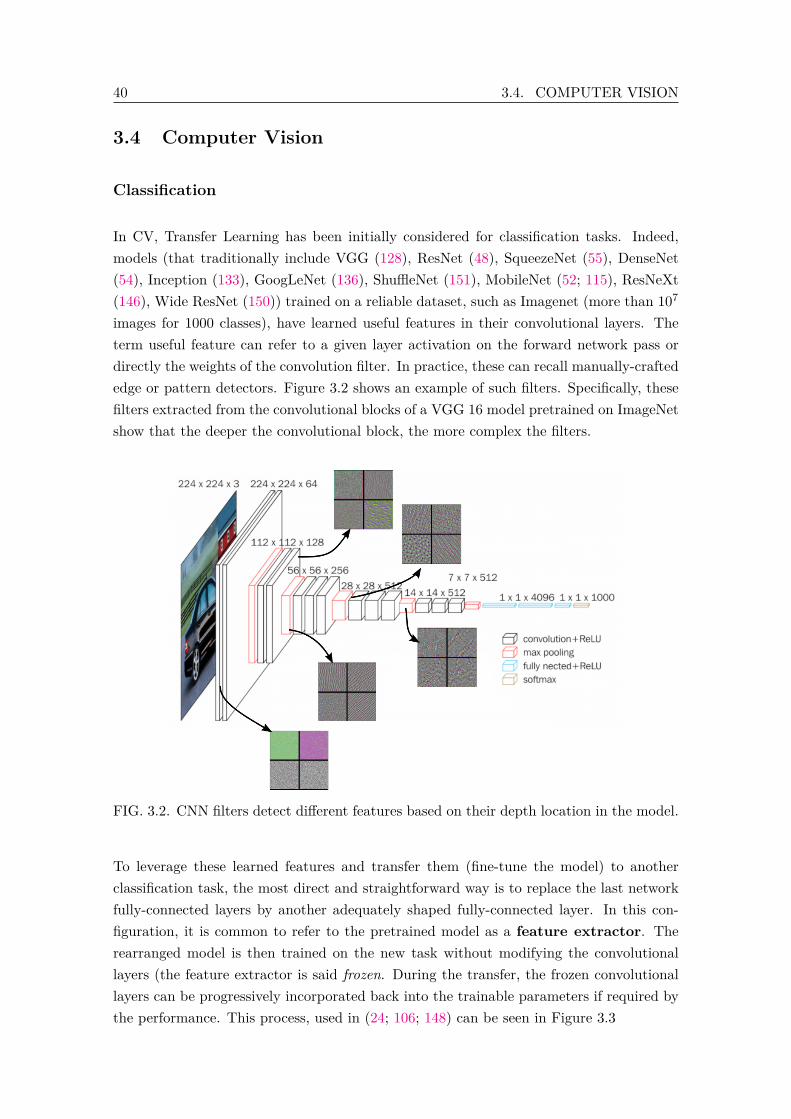
40 3.4. COMPUTER VISION
3.4 Computer Vision
Classification
In CV, Transfer Learning has been initially considered for classification tasks. Indeed,models (that traditionally include VGG (128), ResNet (48), SqueezeNet (55), DenseNet(54), Inception (133), GoogLeNet (136), ShuffleNet (151), MobileNet (52; 115), ResNeXt(146), Wide ResNet (150)) trained on a reliable dataset, such as Imagenet (more than 107
images for 1000 classes), have learned useful features in their convolutional layers. Theterm useful feature can refer to a given layer activation on the forward network pass ordirectly the weights of the convolution filter. In practice, these can recall manually-craftededge or pattern detectors. Figure 3.2 shows an example of such filters. Specifically, thesefilters extracted from the convolutional blocks of a VGG 16 model pretrained on ImageNetshow that the deeper the convolutional block, the more complex the filters.
FIG. 3.2. CNN filters detect different features based on their depth location in the model.
To leverage these learned features and transfer them (fine-tune the model) to anotherclassification task, the most direct and straightforward way is to replace the last networkfully-connected layers by another adequately shaped fully-connected layer. In this con-figuration, it is common to refer to the pretrained model as a feature extractor. Therearranged model is then trained on the new task without modifying the convolutionallayers (the feature extractor is said frozen. During the transfer, the frozen convolutionallayers can be progressively incorporated back into the trainable parameters if required bythe performance. This process, used in (24; 106; 148) can be seen in Figure 3.3
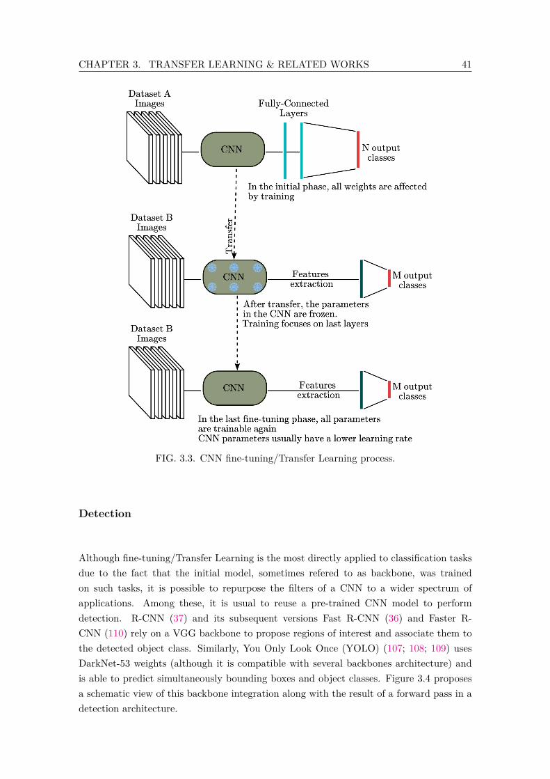
CHAPTER 3. TRANSFER LEARNING & RELATED WORKS 41
FIG. 3.3. CNN fine-tuning/Transfer Learning process.
Detection
Although fine-tuning/Transfer Learning is the most directly applied to classification tasksdue to the fact that the initial model, sometimes refered to as backbone, was trainedon such tasks, it is possible to repurpose the filters of a CNN to a wider spectrum ofapplications. Among these, it is usual to reuse a pre-trained CNN model to performdetection. R-CNN (37) and its subsequent versions Fast R-CNN (36) and Faster R-CNN (110) rely on a VGG backbone to propose regions of interest and associate them tothe detected object class. Similarly, You Only Look Once (YOLO) (107; 108; 109) usesDarkNet-53 weights (although it is compatible with several backbones architecture) andis able to predict simultaneously bounding boxes and object classes. Figure 3.4 proposesa schematic view of this backbone integration along with the result of a forward pass in adetection architecture.
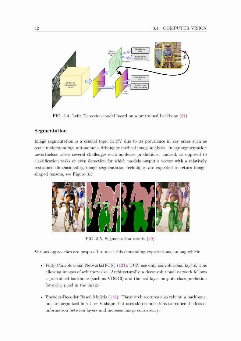
42 3.4. COMPUTER VISION
FIG. 3.4. Left: Detection model based on a pretrained backbone (37).
Segmentation
Image segmentation is a crucial topic in CV due to its prevalence in key areas such asscene understanding, autonomous driving or medical image analysis. Image segmentationnevertheless raises several challenges such as dense predictions. Indeed, as opposed toclassification tasks or even detection for which models output a vector with a relativelyrestrained dimensionality, image segmentation techniques are expected to return image-shaped tensors, see Figure 3.5.
FIG. 3.5. Segmentation results (30).
Various approaches are proposed to meet this demanding expectations, among which:
• Fully Convolutional Networks(FCN) (124): FCN use only convolutional layers, thusallowing images of arbitrary size. Architecturally, a deconvolutional network followsa pretrained backbone (such as VGG16) and the last layer outputs class predictionfor every pixel in the image
• Encoder-Decoder Based Models (112): These architectures also rely on a backbone,but are organized in a U or V shape that uses skip connections to reduce the loss ofinformation between layers and increase image consistency.

CHAPTER 3. TRANSFER LEARNING & RELATED WORKS 43
Figure 3.6 shows various architecture models. As can be seen, both construction rely ona pretrained backbone and differ mostly in the way they connect this educated part withthe new filters designed to complete the segmentation task.
FIG. 3.6. Segmentation models. Up: Fully-Connected Networks (FCN) (124). Down:U-Nets (112).
As was demonstrated in this part, Transfer Learning is largely applied in deep learning-based CV. This process is heavily supported by the fact that training a consequent modelon a large dataset results in the generation of useful detectors within the convolutionallayers. Indeed, as these architectures present a strong dimensional bottleneck, the infor-mation is mostly located outside of the fully connected layer. The convolutional layerscan then be transferred and repurposed for a wide range of tasks as was shown in recentworks. Let us now consider the application of Transfer Learning in NLP.
3.5 Natural Language Processing
Transfer Learning is a particularly common technique in the field of NLP. FromWord2Vecto current language models, Transfer Learning has been correlated with state of the artin NLP in a vast range of tasks. This section focuses on Sequential Transfer Learning, aprocess similar to those described above in Section 3.4, where the target task is consideredafter the initial model is ready.

44 3.5. NATURAL LANGUAGE PROCESSING
Word representation
As neural networks are only able to process vectors, the first step in a training processis consequently to convert the text corpuses into elements understandable by the model.It is for instance possible to create a vector representation of each unique word in thecorpus. As such, Word2Vec groups the vector of similar words in the representationspace. This model is trained through an objective function that expect the model toassign probabilities to the context (n words before and after) of a target word. Thistraining approach is called Skip-Gram (80). The resulting representation, called wordembedding, presents useful properties that go beyond the clustering of similar things andideas. Indeed, the geometry in the representation space shows that the distance betweenthe words Rome and Italy is similar to the distance between Beijing and China, see Figure3.7.
FIG. 3.7. PCA representation of words (79).
It is consequently easy to understand how these learned representations can be useful fora language model that could rely on the word embedding for a text-related task.
Language Models
The increasing popularity of the Attention mechanism (139) in neural-network has givenan important traction to the Transformer architecture, which represents now the go-to method for text-related tasks. In particular, BERT and all its subsequent variants(RoBERT (73), DistillBERT (137) showed state-of-the-art performances on GLUE, SQuADv1.1 among other tasks. Language Models (LM) are trained on immense corpuses on asimple objective: next word prediction based on all of the previous words within some text
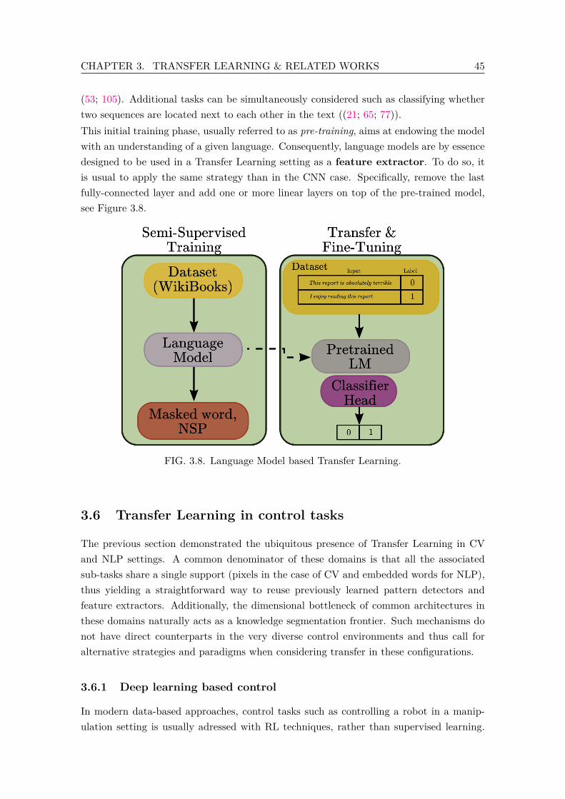
CHAPTER 3. TRANSFER LEARNING & RELATED WORKS 45
(53; 105). Additional tasks can be simultaneously considered such as classifying whethertwo sequences are located next to each other in the text ((21; 65; 77)).This initial training phase, usually referred to as pre-training, aims at endowing the modelwith an understanding of a given language. Consequently, language models are by essencedesigned to be used in a Transfer Learning setting as a feature extractor. To do so, itis usual to apply the same strategy than in the CNN case. Specifically, remove the lastfully-connected layer and add one or more linear layers on top of the pre-trained model,see Figure 3.8.
FIG. 3.8. Language Model based Transfer Learning.
3.6 Transfer Learning in control tasks
The previous section demonstrated the ubiquitous presence of Transfer Learning in CVand NLP settings. A common denominator of these domains is that all the associatedsub-tasks share a single support (pixels in the case of CV and embedded words for NLP),thus yielding a straightforward way to reuse previously learned pattern detectors andfeature extractors. Additionally, the dimensional bottleneck of common architectures inthese domains naturally acts as a knowledge segmentation frontier. Such mechanisms donot have direct counterparts in the very diverse control environments and thus call foralternative strategies and paradigms when considering transfer in these configurations.
3.6.1 Deep learning based control
In modern data-based approaches, control tasks such as controlling a robot in a manip-ulation setting is usually adressed with RL techniques, rather than supervised learning.

46 3.6. TRANSFER LEARNING IN CONTROL TASKS
Since the demonstration that it is possible for a RL agent to learn a human-level con-troller using only raw state observations (82), Deep Reinforcement Learning (DRL) hasbeen increasingly popular. Recent algorithmic advances, such as Proximal Policy Opti-mization (PPO) (122) or Soft-Actor Critic (SAC) (44) have enabled the application ofRL principle to complex environments, with non-linear dynamics and continuous actionspace, in simulation as well as in real-world (12; 20; 96; 132) conditions. For instance, theworks described in (99) demonstrate that RL is a suitable way to control high-dimensionalmorphologies to accomplish accurate locomotion tasks, such as having a simulated T-Rexshaped character that dribbles a ball with its foot toward a moving target. These impres-sive results are nevertheless particularly expensive in terms of samples collections, limitingthe direct application of such methods to real-world settings. Efforts are however deployedto tackle this issue. As such, in (44) the authors present the SAC algorithm, an off-policyRL agent, and prove that not only this approach is very efficient for the usual pool ofsimulated tasks, but also suitable for a physical task using for instance a Minotaur robot.The agent is trained from scratch, without simulations nor demonstrations, to maximizeits forward velocity. This challenging task, although brilliantly managed by the agent, isnonetheless hardly reproducible for more complex tasks. Indeed, samples collections inthe Minotaur setting are relatively unexpansive and fast, while it is likely that tasks ofenhanced sophistication may require more costly samples. Consequently, the challengesyielded by this situation invoke one of the main transfer justification for control tasks:transferring knowledge acquired in simulation to real-world settings.
3.6.2 From simulation to real world
As hinted above, despite its recent achievements, DRL is notoriously sample inefficient(7; 29; 41; 71; 81; 88; 95; 101). On-policy algorithms in particular require millions of inter-actions with an environment to learn an acceptable policy. While training in simulationoffers notable advantages, such as parallelizable policies, inexpensive samples collections,respect of safety concerns for operators as well as for the agent’s body, simulated settingsseldom offer a reliable copy of physical devices, which results in brittle and inefficientpolicies if directly deployed to a real-world setting, as the target domain differs from thetraining configuration. A possible option to mitigate these difficulties is to modify contin-uously the simulated environment to lessen the agent sensitivity to environmental changesand focus on the important features of the current task. In (97; 102), a robot is trained topush a puck to a goal position. To enhance the agent generalization capacity, the authorsintroduce the concept of dynamic randomization that modifies a physical property of theworld at each new episode, such as friction and damping of the puck or the mass of one ofthe links of the robot’s body, to develop an agent able to adapt to the unknown real worldsettings. In (91), a robotic Shadow hand is tasked with solving a Rubik’s Cube. In thiscase, the domain randomization technique is enhanced to deal with the additional image-based observations. Specifically, the agent trains in variants of the initial environment,where each variant has, in supplement to the alternative dynamic settings, different render

CHAPTER 3. TRANSFER LEARNING & RELATED WORKS 47
properties. Using a wide distribution of texture, light and ambient occlusion parametersis a crucial component to ensure that the agent will be able to transfer its behaviour fromsimulation to the real-world.
3.6.3 Transfer between tasks
3.6.3.1 Reward-Based Transfer
The significant time required to train a DRL agent on a complex task has encouragedresearchers to design strategies likely to increase the agent usability and avoid the exag-gerated expenditure of computational resources on a single simulated task. While a partof these efforts was directed towards transfer to real-world configurations, several worksset out to create agents which learned representations can be reused in another context.The works described in (3) fit in this context, as the authors demonstrate how policiestrained in a self-play setting can display subtle behavior and that it becomes possible toobserve emergent strategic behavior. Once trained, the agents are repurposed for anothertask. For instance, a humanoid agent that learned motor skills for a sumo task is thenplaced in a new environment where it must resist random wind forces and keep its bal-ance. From a computational point of view, the neural networks used by the agent arenot modified by the transfer and only the reward function will progressively affect theobserved behaviour. Similarly, (2) conducts analogous experiments but in a multi-agentsetting, namely a teamed hide-and-seek. This environment is genuinely complex as itfeatures immovable walls as well as interactable objects that can be used by the hidingagents to create seekers-safe areas. After being trained on the original task, some agentsare repurposed for alternative objectives such as simple construction tasks (which consistin putting blocks in predefined places). In the experiments described in (3), the transferproves effective as the pretrained agent requires only a short amount of time to learn effec-tive behaviour in its new environment. However, the additional tasks in (2) display a morenuanced result: the pretrained agent’s performance and learning speed barely exceeds abaseline agent trained from scratch, thus demonstrating that transfer must be carefullyplanned beforehand to be beneficial.
3.6.3.2 Curriculum Based Transfer
The strategy presented above recalls the one used in curriculum learning environments.In curriculum learning (28), the idea is to progressively increase the difficulty of an envi-ronment. Starting in a simplified version of the task allows to easily design a reward thatefficiently guide the agent towards the desired conduct. This approach has been employedin numerous recent works (15; 91; 111; 142). In (57), the authors establish that this strat-egy, which can be conceived as the transfer of previously acquired skills from one agentto a future version of itself, has numerous advantages. It simultaneously improves thegeneralization of the agent, prevents overfitting to a single and repetitive scenario (whichcan result in poor agent performance if the environment is slightly modified afterwards)
48 3.6. TRANSFER LEARNING IN CONTROL TASKS
and, in particular, allows the agent to reach a better performance level with less data,thus enhancing its efficiency.
3.6.3.3 Intrinsically motivated Transfer
Besides modifying the reward function or using a progressive curriculum to ensure agentsadapt to new but related tasks, there exist alternative approaches to broaden the agent’sstrategies and indirectly set up the transfer of skills between tasks, thanks to this enlargedparadigm. One way to reach this goal is to prevent the agent being trained to focus ona single strategy to try and solve the task. In this view, multiple works building on theidentified connection between RL and the information theory (87; 119; 153), rely on anadditional objective function that involves the maximization of the action distributionentropy to ensure the agent learns various skills (43; 44; 122). When the agent’s policiesis able to display multiple competences, it is generally able to generalize better to newenvironments. Beside entropy-based incentives, other methods have been proposed tomaximize environment exploration by the agent. (51; 83) use mutual information betweenstates and actions to intrinsically motivate the agent, a concept that recalls the curiosity-based learning (4; 74; 117; 118). For instance, in (94), the curiosity is formulated as an errorrelated to the agent’s ability to predict the consequences of its actions in a high-dimensionalobservation space. The results of this formalisation suggest that curiosity provides a moreefficient progression in an environment with sparse rewards, a better exploration that forcesthe agent to acquire new competences which in turn can be translated into generalization tounseen scenarios where the agent can reuse previously obtained knowledge and experienceto progress faster. A similar technique is implemented in (10) that furthermore tackles thenoisy-tv problem, a common issue when trying to predict observations in high-dimensionalspaces, by expressing the curiosity error as the distance between the prediction of the nextobservation by the agent and the prediction of an other randomly initialized and fixedneural network (92).The works presented in (31) take a substitute path, remarkable due to the absence ofreward provided by the environment, a configuration commonly explored in the literature(72; 90). In this framework, an entropy-maximization objective function incites the agentto generate various trajectories for an additional goal description vector. Trajectoriesrelated to different goals must be as diverse as possible to minimize the entropy loss. Inthis case as well, the authors are able to demonstrate that this approach results in theunsupervised emergence of diverse skills. In addition, the skills gained during the thoroughexploration of the environment give birth to transferable competences to slightly differenttasks.
3.6.3.4 Meta-Learning
Meta-Learning for RL recalls the language models in NLP as it is in essence designed tobe the basic understanding to a span of tasks. Specifically, this field develops techniquesthat directly optimize the adaptability of an agent. Although initially used for few shots

CHAPTER 3. TRANSFER LEARNING & RELATED WORKS 49
classifications in supervised learning settings (116), there exist several notable attemptsto apply these concepts to RL (25; 58; 141). Techniques for Meta-RL can be broadlyclassified in those classes:
• Memory-Augmented models: One of the first approaches developed consists in aug-menting neural networks with memory in the form of LSTM (Long Short TermMemory), a type Recurrent Neural Network (25)
• Meta Learning algorithms: The works relying on this strategy set out to find waysto optimize simultaneously the model on a variety of tasks
• Distributions of environments: The agent is exposed to a multitude of environmentsto enhance its capacity to generalize.
An innovative example of Meta-Learning Algorithm is the MAML (Model-Agnostic Meta-Learning) algorithm, introduced in (32). The concept of MALM is that the optimizationprocess via gradient descent should move the model in the parameters space to a saddlepoint so that task-specific fine-tuning is fast and efficient. A similar process is presentedin (89), where the model is optimized by repeatedly sampling a task, training for multiplesteps on it and updating the model parameters. This method is further improved in theCAML (Context Agnostic Meta Learning) algorithm (154) that decomposes the modelinto context parameters, intrinsic to a given task, and task-agnostic ones that are sharedparameters. Doing so provides a wider distribution of tasks as the input and outputdimensions are managed by the context parameters. Nevertheless, in practice, the taskdistributions considered in these settings are usually very narrow (149). For instance, acommon evaluation of Meta-RL algorithms involves changing the maximal joint velocitiesof a serial robot on a manipulation task, while another one consists in choosing differentrunning directions for simulated legged robots (32). These results are appealing froma theoretical point of view, but currently lack applicability as they are unlikely to besufficient to enable robots to behave realistically in human environments. Nevertheless, theparadigm that motivates the creation of a central controller that can be quickly adapted todifferent environments is highly interesting and is the main pillar of transfer in hierarchicalsettings
3.6.3.5 Transfer in Hierarchical Settings
Generally, transfer in hierarchical settings implies jointly learning a set of skills and ameta-controller, introduced as Options formulation in (131). This formulation assumesthat the Options are given, but this concept has been actively explored by the researchcommunity since then. Consequently, it is now usual to learn these options as well as thepolicy that selects them (1). Some works propose a decomposition of the considered taskinto subgoals (33; 35; 49; 140). Other techniques break the task between low-level andhigh-level control, as in (98) where the authors partition the locomotion components anduse the higher-level controller to provide goals to the lower-level controller. In this method,
50 3.7. KNOWLEDGE REPRESENTATION IN TRANSFER LEARNING
both controllers are learned simultaneously and only rely on model-free modelling, that iswithout knowledge of the equations of motion, nor character kinematics. An interestingaspect of this method is that the hierarchical structure allows interchangeability betweencomponents, thus increasing the usability of the agent.
3.7 Knowledge representation in Transfer Learning
Attempts to transfer knowledge are also represented in the unsupervised learning paradigm.In fact, the relationship between unsupervised learning and Transfer Learning might evenappear more natural as one of the main objectives in this paradigm is to be able totrain models whose optimization leads to a clear understanding of how data were gener-ated. Indeed, when the model captures efficiently the data structure, it is in particularable to provide relevant representations for subsequent usages, which proves highly usefulin neural-network based controllers (68; 69). As such, the works presented in (42) in-troduce the World Model approach where the authors leverage a three-part sequentiallytrained model that was able to overcome the previous state-of-the-art on the challengingCarRacing-V0 Gym environment (9). Most of this performance relies on the first moduleof this model: the encoding part of an AutoEncoder architecture trained on a reconstruc-tion objective, using the raw pixels from the environment. The small dimensionality of theencoder output forces the whole network to learn meaningful state representations (that is,focus on the input most salient features) that proves usable for downstream tasks. As themodel is trained in a sequential manner, it is possible to imagine that this module could bepaired to another controller to solve a different task, thus illustrating the transfer. Thereexist numerous examples of AutoEncoder architectures being successfully applied to createmeaningful representation of data. Using Variational AutoEncoder (11; 62) (VAE) is alsofrequent as the additional objective function in these architecture enables a better controlover the encoder latent representations (14; 27; 46; 76; 144). These techniques can enabletransfer beyond the usual agent-agent paradigm. In particular, the method developed in(75) takes advantage of this property to project complex multi-DoF expert, potentiallyhumans, trajectories for a given task in a small latent space. The VAE properties ensuringthat the representation is liable and consistent, the authors of this work demonstrate thatit can be used in an assistive robotics setup to ease the control of multiple DoF robots forsubsequent users, requiring only one or two DoF. The GAN framework also presents spe-cific appeals for the transfer of skills. Since the introduction of Neural Style Transfer (34),a model that transfers the painting style of a given artist to another picture, efforts wereinvested to establish the capabilities of transfer in the GAN paradigm. One of the pioneerapproach, the CycleGAN (152), demonstrates unpaired image to image translation, thatis, translate an image from domain A to domain B, was a feasible task that yielded highlyqualitative results, see Figure 3.9. Using a similar principle, the AVID (Automated VisualInstruction-following with Demonstration) method (129) replaces the human operator inthe videos of a task execution by a given robot. Then, the authors demonstrate that it
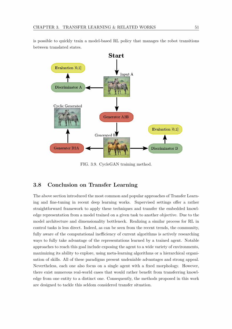
CHAPTER 3. TRANSFER LEARNING & RELATED WORKS 51
is possible to quickly train a model-based RL policy that manages the robot transitionsbetween translated states.
FIG. 3.9. CycleGAN training method.
3.8 Conclusion on Transfer Learning
The above section introduced the most common and popular approaches of Transfer Learn-ing and fine-tuning in recent deep learning works. Supervised settings offer a ratherstraightforward framework to apply these techniques and transfer the embedded knowl-edge representation from a model trained on a given task to another objective. Due to themodel architecture and dimensionality bottleneck. Realizing a similar process for RL incontrol tasks is less direct. Indeed, as can be seen from the recent trends, the community,fully aware of the computational inefficiency of current algorithms is actively researchingways to fully take advantage of the representations learned by a trained agent. Notableapproaches to reach this goal include exposing the agent to a wide variety of environments,maximizing its ability to explore, using meta-learning algorithms or a hierarchical organi-sation of skills. All of these paradigms present undeniable advantages and strong appeal.Nevertheless, each one also focus on a single agent with a fixed morphology. However,there exist numerous real-world cases that would rather benefit from transferring knowl-edge from one entity to a distinct one. Consequently, the methods proposed in this workare designed to tackle this seldom considered transfer situation.

52 3.8. CONCLUSION ON TRANSFER LEARNING

Chapter 4Task-Centered Transfer
Contents4.1 Universal Notice Network . . . . . . . . . . . . . . . . . . . . . . . . . . 54
4.1.1 Principle . . . . . . . . . . . . . . . . . . . . . . . . . . . . . . . 544.1.2 The UNN workflow . . . . . . . . . . . . . . . . . . . . . . . . . 554.1.3 The UNN Pipeline . . . . . . . . . . . . . . . . . . . . . . . . . 564.1.4 Base Abstracted Modelling . . . . . . . . . . . . . . . . . . . . 574.1.5 Building and using UNN modules . . . . . . . . . . . . . . . . . 58
4.2 Experiments . . . . . . . . . . . . . . . . . . . . . . . . . . . . . . . . . 594.2.1 Vanilla transfer . . . . . . . . . . . . . . . . . . . . . . . . . . . 604.2.2 Learning setup . . . . . . . . . . . . . . . . . . . . . . . . . . . 614.2.3 Controlled Robots . . . . . . . . . . . . . . . . . . . . . . . . . 624.2.4 Base Manipulation: Reacher . . . . . . . . . . . . . . . . . . . . 634.2.5 A lonely manipulation: Tennis . . . . . . . . . . . . . . . . . . . 644.2.6 Biped walking . . . . . . . . . . . . . . . . . . . . . . . . . . . . 674.2.7 Cooperative Manipulation UNN: Cooperative Move Plank . . . 714.2.8 Cooperative BAM Manipulation: Dual Move Plank . . . . . . . 73
4.3 Conclusion on TAsk-Centered methods . . . . . . . . . . . . . . . . . . 77
53
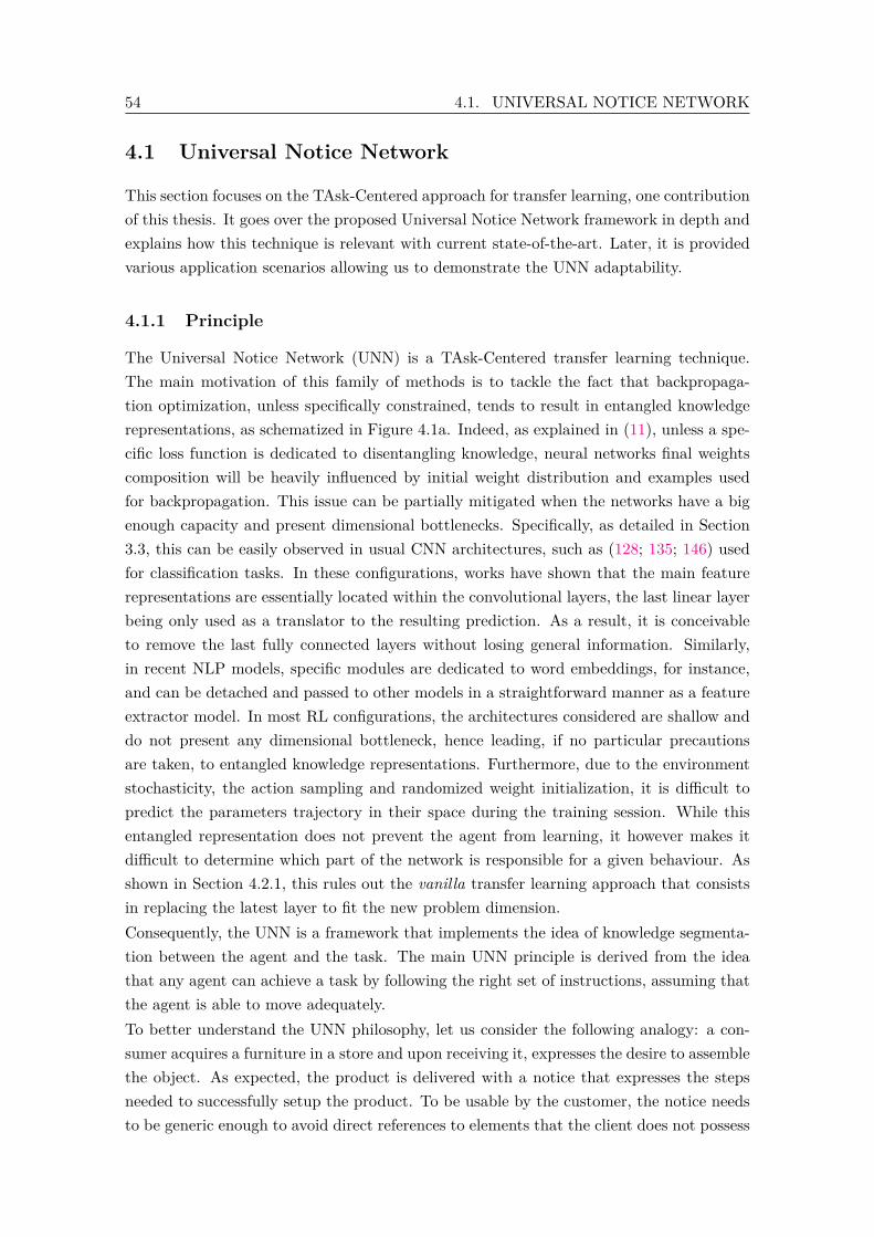
54 4.1. UNIVERSAL NOTICE NETWORK
4.1 Universal Notice Network
This section focuses on the TAsk-Centered approach for transfer learning, one contributionof this thesis. It goes over the proposed Universal Notice Network framework in depth andexplains how this technique is relevant with current state-of-the-art. Later, it is providedvarious application scenarios allowing us to demonstrate the UNN adaptability.
4.1.1 Principle
The Universal Notice Network (UNN) is a TAsk-Centered transfer learning technique.The main motivation of this family of methods is to tackle the fact that backpropaga-tion optimization, unless specifically constrained, tends to result in entangled knowledgerepresentations, as schematized in Figure 4.1a. Indeed, as explained in (11), unless a spe-cific loss function is dedicated to disentangling knowledge, neural networks final weightscomposition will be heavily influenced by initial weight distribution and examples usedfor backpropagation. This issue can be partially mitigated when the networks have a bigenough capacity and present dimensional bottlenecks. Specifically, as detailed in Section3.3, this can be easily observed in usual CNN architectures, such as (128; 135; 146) usedfor classification tasks. In these configurations, works have shown that the main featurerepresentations are essentially located within the convolutional layers, the last linear layerbeing only used as a translator to the resulting prediction. As a result, it is conceivableto remove the last fully connected layers without losing general information. Similarly,in recent NLP models, specific modules are dedicated to word embeddings, for instance,and can be detached and passed to other models in a straightforward manner as a featureextractor model. In most RL configurations, the architectures considered are shallow anddo not present any dimensional bottleneck, hence leading, if no particular precautionsare taken, to entangled knowledge representations. Furthermore, due to the environmentstochasticity, the action sampling and randomized weight initialization, it is difficult topredict the parameters trajectory in their space during the training session. While thisentangled representation does not prevent the agent from learning, it however makes itdifficult to determine which part of the network is responsible for a given behaviour. Asshown in Section 4.2.1, this rules out the vanilla transfer learning approach that consistsin replacing the latest layer to fit the new problem dimension.Consequently, the UNN is a framework that implements the idea of knowledge segmenta-tion between the agent and the task. The main UNN principle is derived from the ideathat any agent can achieve a task by following the right set of instructions, assuming thatthe agent is able to move adequately.To better understand the UNN philosophy, let us consider the following analogy: a con-sumer acquires a furniture in a store and upon receiving it, expresses the desire to assemblethe object. As expected, the product is delivered with a notice that expresses the stepsneeded to successfully setup the product. To be usable by the customer, the notice needsto be generic enough to avoid direct references to elements that the client does not possess
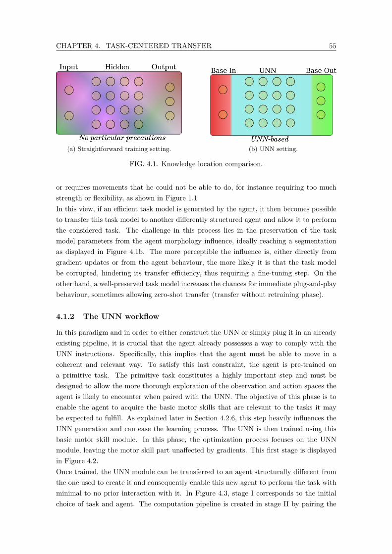
CHAPTER 4. TASK-CENTERED TRANSFER 55
(a) Straightforward training setting. (b) UNN setting.
FIG. 4.1. Knowledge location comparison.
or requires movements that he could not be able to do, for instance requiring too muchstrength or flexibility, as shown in Figure 1.1In this view, if an efficient task model is generated by the agent, it then becomes possibleto transfer this task model to another differently structured agent and allow it to performthe considered task. The challenge in this process lies in the preservation of the taskmodel parameters from the agent morphology influence, ideally reaching a segmentationas displayed in Figure 4.1b. The more perceptible the influence is, either directly fromgradient updates or from the agent behaviour, the more likely it is that the task modelbe corrupted, hindering its transfer efficiency, thus requiring a fine-tuning step. On theother hand, a well-preserved task model increases the chances for immediate plug-and-playbehaviour, sometimes allowing zero-shot transfer (transfer without retraining phase).
4.1.2 The UNN workflow
In this paradigm and in order to either construct the UNN or simply plug it in an alreadyexisting pipeline, it is crucial that the agent already possesses a way to comply with theUNN instructions. Specifically, this implies that the agent must be able to move in acoherent and relevant way. To satisfy this last constraint, the agent is pre-trained ona primitive task. The primitive task constitutes a highly important step and must bedesigned to allow the more thorough exploration of the observation and action spaces theagent is likely to encounter when paired with the UNN. The objective of this phase is toenable the agent to acquire the basic motor skills that are relevant to the tasks it maybe expected to fulfill. As explained later in Section 4.2.6, this step heavily influences theUNN generation and can ease the learning process. The UNN is then trained using thisbasic motor skill module. In this phase, the optimization process focuses on the UNNmodule, leaving the motor skill part unaffected by gradients. This first stage is displayedin Figure 4.2.Once trained, the UNN module can be transferred to an agent structurally different fromthe one used to create it and consequently enable this new agent to perform the task withminimal to no prior interaction with it. In Figure 4.3, stage I corresponds to the initialchoice of task and agent. The computation pipeline is created in stage II by pairing the
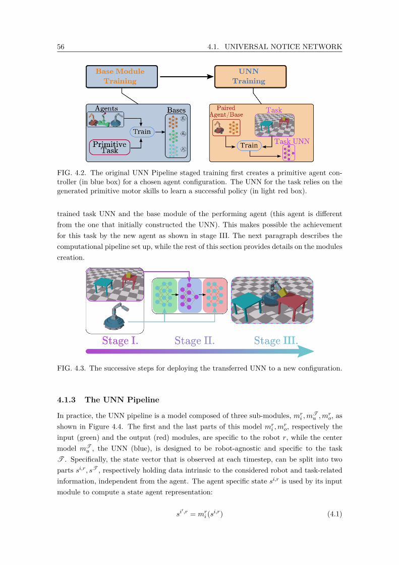
56 4.1. UNIVERSAL NOTICE NETWORK
FIG. 4.2. The original UNN Pipeline staged training first creates a primitive agent con-troller (in blue box) for a chosen agent configuration. The UNN for the task relies on thegenerated primitive motor skills to learn a successful policy (in light red box).
trained task UNN and the base module of the performing agent (this agent is differentfrom the one that initially constructed the UNN). This makes possible the achievementfor this task by the new agent as shown in stage III. The next paragraph describes thecomputational pipeline set up, while the rest of this section provides details on the modulescreation.
FIG. 4.3. The successive steps for deploying the transferred UNN to a new configuration.
4.1.3 The UNN Pipeline
In practice, the UNN pipeline is a model composed of three sub-modules, mri ,m
Tu ,m
ro, as
shown in Figure 4.4. The first and the last parts of this model mri ,m
ro, respectively the
input (green) and the output (red) modules, are specific to the robot r, while the centermodel mT
u , the UNN (blue), is designed to be robot-agnostic and specific to the taskT . Specifically, the state vector that is observed at each timestep, can be split into twoparts si,r, sT , respectively holding data intrinsic to the considered robot and task-relatedinformation, independent from the agent. The agent specific state si,r is used by its inputmodule to compute a state agent representation:
si′,r = mr
i (si,r) (4.1)
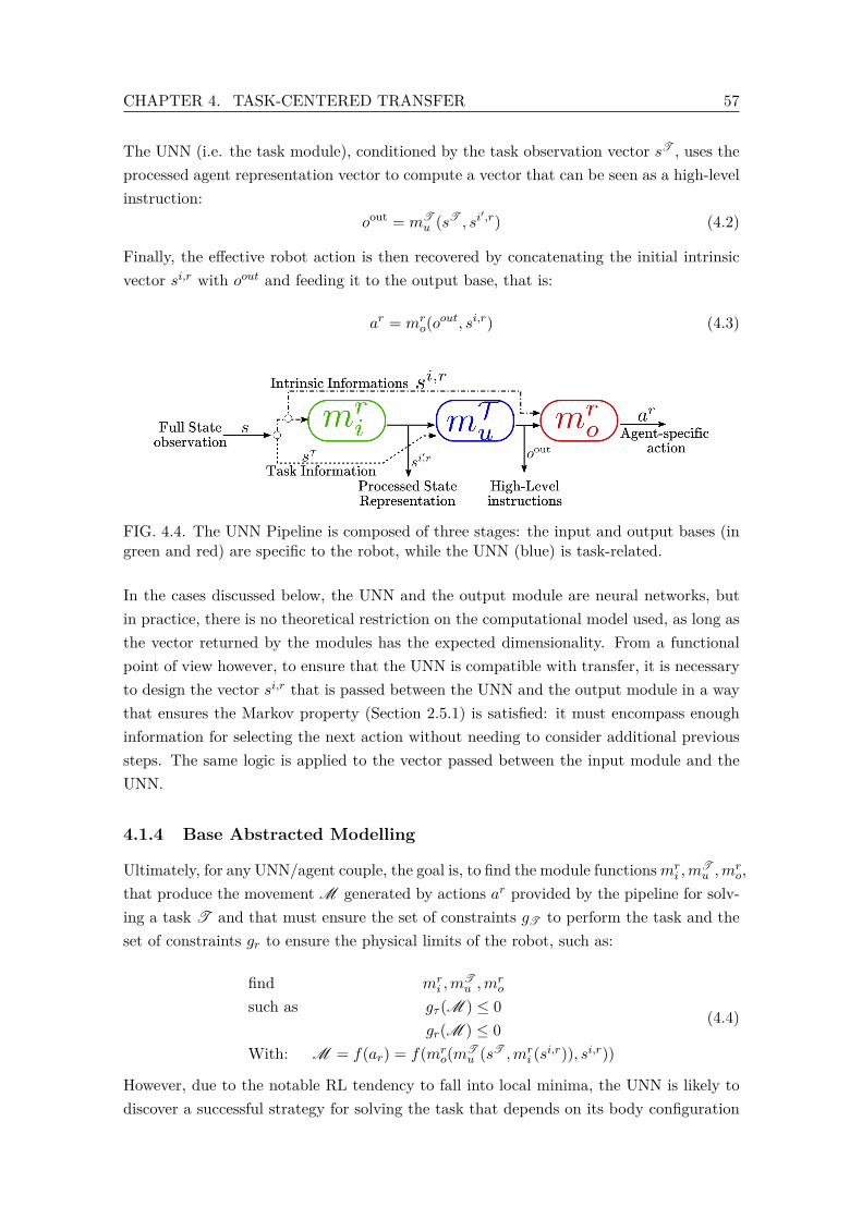
CHAPTER 4. TASK-CENTERED TRANSFER 57
The UNN (i.e. the task module), conditioned by the task observation vector sT , uses theprocessed agent representation vector to compute a vector that can be seen as a high-levelinstruction:
oout = mTu (sT , si
′,r) (4.2)
Finally, the effective robot action is then recovered by concatenating the initial intrinsicvector si,r with oout and feeding it to the output base, that is:
ar = mro(oout, si,r) (4.3)
FIG. 4.4. The UNN Pipeline is composed of three stages: the input and output bases (ingreen and red) are specific to the robot, while the UNN (blue) is task-related.
In the cases discussed below, the UNN and the output module are neural networks, butin practice, there is no theoretical restriction on the computational model used, as long asthe vector returned by the modules has the expected dimensionality. From a functionalpoint of view however, to ensure that the UNN is compatible with transfer, it is necessaryto design the vector si,r that is passed between the UNN and the output module in a waythat ensures the Markov property (Section 2.5.1) is satisfied: it must encompass enoughinformation for selecting the next action without needing to consider additional previoussteps. The same logic is applied to the vector passed between the input module and theUNN.
4.1.4 Base Abstracted Modelling
Ultimately, for any UNN/agent couple, the goal is, to find the module functionsmri ,m
Tu ,m
ro,
that produce the movement M generated by actions ar provided by the pipeline for solv-ing a task T and that must ensure the set of constraints gT to perform the task and theset of constraints gr to ensure the physical limits of the robot, such as:
find mri ,m
Tu ,m
ro
such as gτ (M ) ≤ 0gr(M ) ≤ 0
With: M = f(ar) = f(mro(mT
u (sT ,mri (si,r)), si,r))
(4.4)
However, due to the notable RL tendency to fall into local minima, the UNN is likely todiscover a successful strategy for solving the task that depends on its body configuration
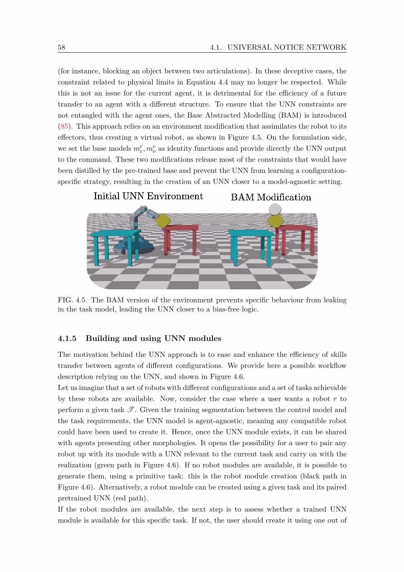
58 4.1. UNIVERSAL NOTICE NETWORK
(for instance, blocking an object between two articulations). In these deceptive cases, theconstraint related to physical limits in Equation 4.4 may no longer be respected. Whilethis is not an issue for the current agent, it is detrimental for the efficiency of a futuretransfer to an agent with a different structure. To ensure that the UNN constraints arenot entangled with the agent ones, the Base Abstracted Modelling (BAM) is introduced(85). This approach relies on an environment modification that assimilates the robot to itseffectors, thus creating a virtual robot, as shown in Figure 4.5. On the formulation side,we set the base models mr
i ,mro as identity functions and provide directly the UNN output
to the command. These two modifications release most of the constraints that would havebeen distilled by the pre-trained base and prevent the UNN from learning a configuration-specific strategy, resulting in the creation of an UNN closer to a model-agnostic setting.
FIG. 4.5. The BAM version of the environment prevents specific behaviour from leakingin the task model, leading the UNN closer to a bias-free logic.
4.1.5 Building and using UNN modules
The motivation behind the UNN approach is to ease and enhance the efficiency of skillstransfer between agents of different configurations. We provide here a possible workflowdescription relying on the UNN, and shown in Figure 4.6.Let us imagine that a set of robots with different configurations and a set of tasks achievableby these robots are available. Now, consider the case where a user wants a robot r toperform a given task T . Given the training segmentation between the control model andthe task requirements, the UNN model is agent-agnostic, meaning any compatible robotcould have been used to create it. Hence, once the UNN module exists, it can be sharedwith agents presenting other morphologies. It opens the possibility for a user to pair anyrobot up with its module with a UNN relevant to the current task and carry on with therealization (green path in Figure 4.6). If no robot modules are available, it is possible togenerate them, using a primitive task: this is the robot module creation (black path inFigure 4.6). Alternatively, a robot module can be created using a given task and its pairedpretrained UNN (red path).If the robot modules are available, the next step is to assess whether a trained UNNmodule is available for this specific task. If not, the user should create it using one out of
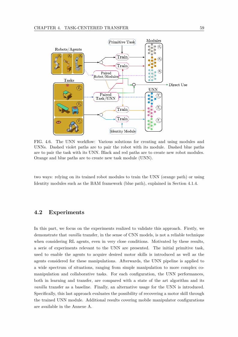
CHAPTER 4. TASK-CENTERED TRANSFER 59
FIG. 4.6. The UNN workflow: Various solutions for creating and using modules andUNNs. Dashed violet paths are to pair the robot with its module. Dashed blue pathsare to pair the task with its UNN. Black and red paths are to create new robot modules.Orange and blue paths are to create new task module (UNN).
two ways: relying on its trained robot modules to train the UNN (orange path) or usingIdentity modules such as the BAM framework (blue path), explained in Section 4.1.4.
4.2 Experiments
In this part, we focus on the experiments realized to validate this approach. Firstly, wedemonstrate that vanilla transfer, in the sense of CNN models, is not a reliable techniquewhen considering RL agents, even in very close conditions. Motivated by these results,a serie of experiments relevant to the UNN are presented. The initial primitive task,used to enable the agents to acquire desired motor skills is introduced as well as theagents considered for these manipulations. Afterwards, the UNN pipeline is applied toa wide spectrum of situations, ranging from simple manipulation to more complex co-manipulation and collaborative tasks. For each configuration, the UNN performances,both in learning and transfer, are compared with a state of the art algorithm and itsvanilla transfer as a baseline. Finally, an alternative usage for the UNN is introduced.Specifically, this last approach evaluates the possibility of recovering a motor skill throughthe trained UNN module. Additional results covering mobile manipulator configurationsare available in the Annexe A.

60 4.2. EXPERIMENTS
4.2.1 Vanilla transfer
In order to motivate further the TAsk-Centered approach, we design a toy experiment tounderline the liability of vanilla transfer in RL framework. In this view, we consider twoexactly similar agents that are trained on a unique task. Given that this experiment aimsat demonstrating that unconstrained backpropagation does not structure knowledge incommon RL architectures, the next step is to evaluate how vanilla transfer would affectthe two trained agents. Specifically, two additional configurations are created by replacingthe hidden layers of an agent in the other one, as shown in Figure 4.7. The performancesof these two are then measured on the same task.
FIG. 4.7. Exchanging model layers between similar agents.
On the realisation side, the task selected for this experiment is BipedalWalker-v3, acommon benchmark for RL. In this environment, the agent controls a biped and can applytorques to its joints. The environment provides observations to the agent in the form of a24-dimensionnal vector that describes the agent joints states and the reading from severalraycasting. Upon observation, the agent returns an action vector of 4 components, thatact as joints speeds. The goal is to prevent the biped from falling, which results in a -100reward, while bringing the agent towards the end of the path, granting a +300 reward.In order to ensure the agent has a responsible control, small negative reward proportionalto the torque magnitude are given at each time step. BipedalWalker-v3 belongs to theGym suite control tasks and even though this environment is among the most complex ofthis suite, decent policies can easily be created by a recent RL algorithm such as PPO orTD3. In this case, the policies considered are neural networks featuring one hidden layerof 64 units. Figure 4.8 displays the mean reward evolution along training. As can be seenin this Figure 4.8, the mean reward quickly hovers around 200 points, while a baselinerandom agent usually gets cumulative rewards that do not exceed -90 (9).It is then possible to apply the vanilla transfer between these two agents, for all eightpossible configurations. Figure 4.9 displays the evaluation performances of all settings.As can be observed, both genuine configurations (in blue and gray) exhibit a wide dis-tributions of results, and even though these policies have inevitable failed runs, they arealso able to reach scores above the 200 points threshold. This contrasts strongly with allrecomposed policies, for which none of the runs exceeds the -50 points threshold. In thiscase, although the Bipedal Walker presents a considerable challenge, it would have been
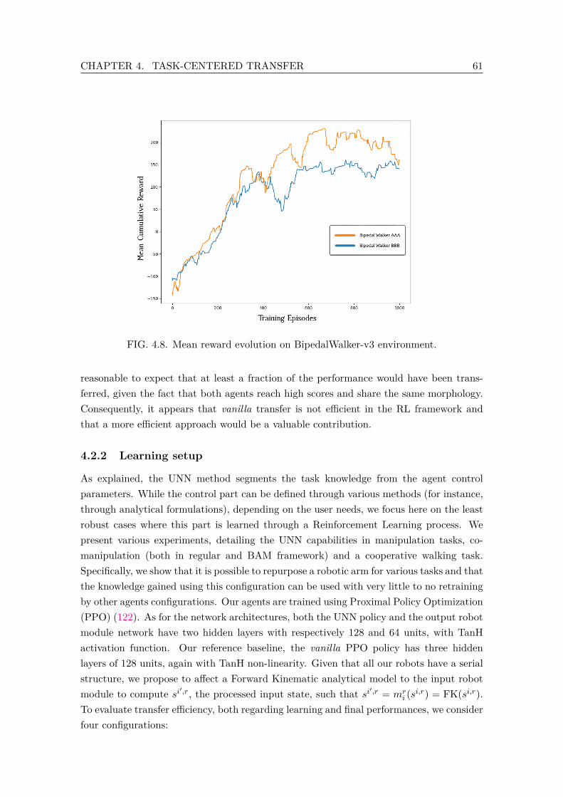
CHAPTER 4. TASK-CENTERED TRANSFER 61
FIG. 4.8. Mean reward evolution on BipedalWalker-v3 environment.
reasonable to expect that at least a fraction of the performance would have been trans-ferred, given the fact that both agents reach high scores and share the same morphology.Consequently, it appears that vanilla transfer is not efficient in the RL framework andthat a more efficient approach would be a valuable contribution.
4.2.2 Learning setup
As explained, the UNN method segments the task knowledge from the agent controlparameters. While the control part can be defined through various methods (for instance,through analytical formulations), depending on the user needs, we focus here on the leastrobust cases where this part is learned through a Reinforcement Learning process. Wepresent various experiments, detailing the UNN capabilities in manipulation tasks, co-manipulation (both in regular and BAM framework) and a cooperative walking task.Specifically, we show that it is possible to repurpose a robotic arm for various tasks and thatthe knowledge gained using this configuration can be used with very little to no retrainingby other agents configurations. Our agents are trained using Proximal Policy Optimization(PPO) (122). As for the network architectures, both the UNN policy and the output robotmodule network have two hidden layers with respectively 128 and 64 units, with TanHactivation function. Our reference baseline, the vanilla PPO policy has three hiddenlayers of 128 units, again with TanH non-linearity. Given that all our robots have a serialstructure, we propose to affect a Forward Kinematic analytical model to the input robotmodule to compute si′,r, the processed input state, such that si′,r = mr
i (si,r) = FK(si,r).To evaluate transfer efficiency, both regarding learning and final performances, we considerfour configurations:
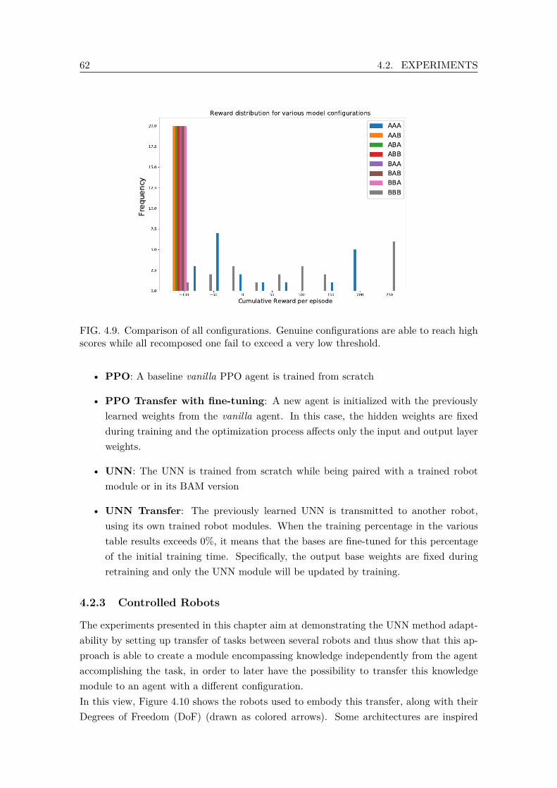
62 4.2. EXPERIMENTS
FIG. 4.9. Comparison of all configurations. Genuine configurations are able to reach highscores while all recomposed one fail to exceed a very low threshold.
• PPO: A baseline vanilla PPO agent is trained from scratch
• PPO Transfer with fine-tuning: A new agent is initialized with the previouslylearned weights from the vanilla agent. In this case, the hidden weights are fixedduring training and the optimization process affects only the input and output layerweights.
• UNN: The UNN is trained from scratch while being paired with a trained robotmodule or in its BAM version
• UNN Transfer: The previously learned UNN is transmitted to another robot,using its own trained robot modules. When the training percentage in the varioustable results exceeds 0%, it means that the bases are fine-tuned for this percentageof the initial training time. Specifically, the output base weights are fixed duringretraining and only the UNN module will be updated by training.
4.2.3 Controlled Robots
The experiments presented in this chapter aim at demonstrating the UNN method adapt-ability by setting up transfer of tasks between several robots and thus show that this ap-proach is able to create a module encompassing knowledge independently from the agentaccomplishing the task, in order to later have the possibility to transfer this knowledgemodule to an agent with a different configuration.In this view, Figure 4.10 shows the robots used to embody this transfer, along with theirDegrees of Freedom (DoF) (drawn as colored arrows). Some architectures are inspired
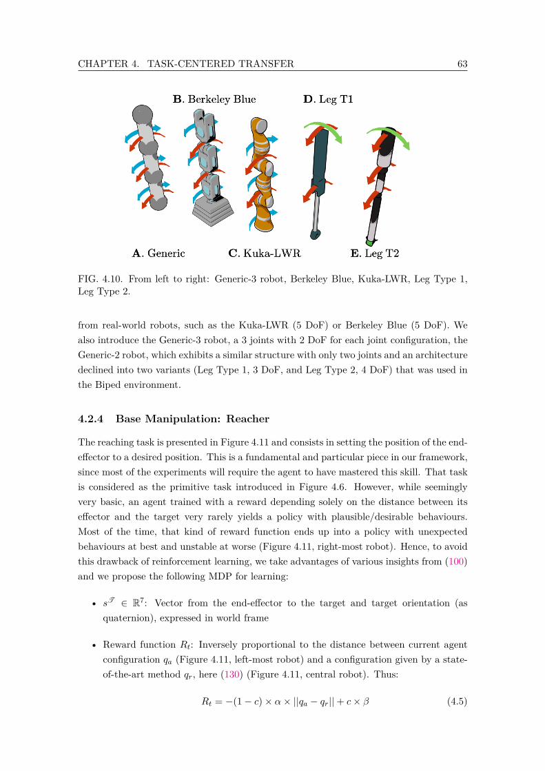
CHAPTER 4. TASK-CENTERED TRANSFER 63
FIG. 4.10. From left to right: Generic-3 robot, Berkeley Blue, Kuka-LWR, Leg Type 1,Leg Type 2.
from real-world robots, such as the Kuka-LWR (5 DoF) or Berkeley Blue (5 DoF). Wealso introduce the Generic-3 robot, a 3 joints with 2 DoF for each joint configuration, theGeneric-2 robot, which exhibits a similar structure with only two joints and an architecturedeclined into two variants (Leg Type 1, 3 DoF, and Leg Type 2, 4 DoF) that was used inthe Biped environment.
4.2.4 Base Manipulation: Reacher
The reaching task is presented in Figure 4.11 and consists in setting the position of the end-effector to a desired position. This is a fundamental and particular piece in our framework,since most of the experiments will require the agent to have mastered this skill. That taskis considered as the primitive task introduced in Figure 4.6. However, while seeminglyvery basic, an agent trained with a reward depending solely on the distance between itseffector and the target very rarely yields a policy with plausible/desirable behaviours.Most of the time, that kind of reward function ends up into a policy with unexpectedbehaviours at best and unstable at worse (Figure 4.11, right-most robot). Hence, to avoidthis drawback of reinforcement learning, we take advantages of various insights from (100)and we propose the following MDP for learning:
• sT ∈ R7: Vector from the end-effector to the target and target orientation (asquaternion), expressed in world frame
• Reward function Rt: Inversely proportional to the distance between current agentconfiguration qa (Figure 4.11, left-most robot) and a configuration given by a state-of-the-art method qr, here (130) (Figure 4.11, central robot). Thus:
Rt = −(1− c)× α× ||qa − qr||+ c× β (4.5)
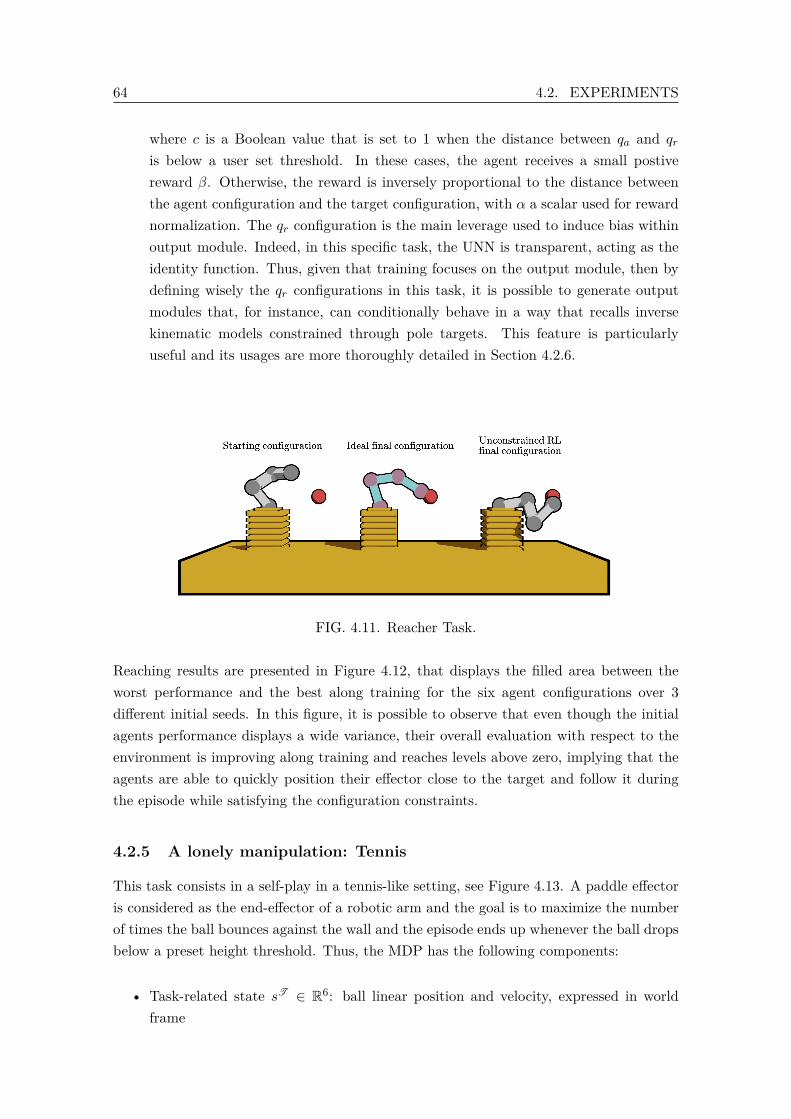
64 4.2. EXPERIMENTS
where c is a Boolean value that is set to 1 when the distance between qa and qr
is below a user set threshold. In these cases, the agent receives a small postivereward β. Otherwise, the reward is inversely proportional to the distance betweenthe agent configuration and the target configuration, with α a scalar used for rewardnormalization. The qr configuration is the main leverage used to induce bias withinoutput module. Indeed, in this specific task, the UNN is transparent, acting as theidentity function. Thus, given that training focuses on the output module, then bydefining wisely the qr configurations in this task, it is possible to generate outputmodules that, for instance, can conditionally behave in a way that recalls inversekinematic models constrained through pole targets. This feature is particularlyuseful and its usages are more thoroughly detailed in Section 4.2.6.
FIG. 4.11. Reacher Task.
Reaching results are presented in Figure 4.12, that displays the filled area between theworst performance and the best along training for the six agent configurations over 3different initial seeds. In this figure, it is possible to observe that even though the initialagents performance displays a wide variance, their overall evaluation with respect to theenvironment is improving along training and reaches levels above zero, implying that theagents are able to quickly position their effector close to the target and follow it duringthe episode while satisfying the configuration constraints.
4.2.5 A lonely manipulation: Tennis
This task consists in a self-play in a tennis-like setting, see Figure 4.13. A paddle effectoris considered as the end-effector of a robotic arm and the goal is to maximize the numberof times the ball bounces against the wall and the episode ends up whenever the ball dropsbelow a preset height threshold. Thus, the MDP has the following components:
• Task-related state sT ∈ R6: ball linear position and velocity, expressed in worldframe
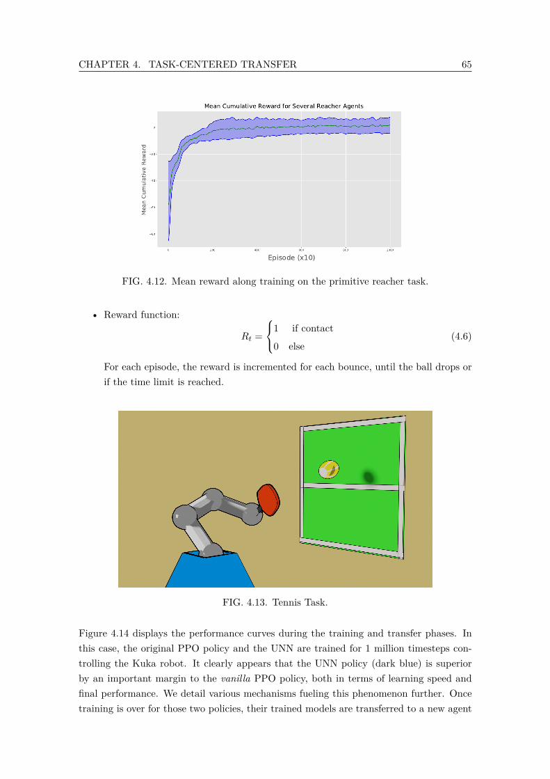
CHAPTER 4. TASK-CENTERED TRANSFER 65
FIG. 4.12. Mean reward along training on the primitive reacher task.
• Reward function:
Rt =
1 if contact
0 else(4.6)
For each episode, the reward is incremented for each bounce, until the ball drops orif the time limit is reached.
FIG. 4.13. Tennis Task.
Figure 4.14 displays the performance curves during the training and transfer phases. Inthis case, the original PPO policy and the UNN are trained for 1 million timesteps con-trolling the Kuka robot. It clearly appears that the UNN policy (dark blue) is superiorby an important margin to the vanilla PPO policy, both in terms of learning speed andfinal performance. We detail various mechanisms fueling this phenomenon further. Oncetraining is over for those two policies, their trained models are transferred to a new agent
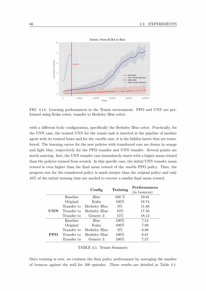
66 4.2. EXPERIMENTS
0 200000 400000 600000 800000 1000000
Steps
0
2
4
6
8
10
Cum
ula
tive r
ew
ard
10.00 %
PPO KUKA
PPO Transfer Berkeley
UNN KUKA
UNN Transfer Berkeley
Tennis: From KUKA to Blue
FIG. 4.14. Learning performances in the Tennis environment. PPO and UNN are per-formed using Kuka robot, transfer to Berkeley Blue robot.
with a different body configuration, specifically the Berkeley Blue robot. Practically, forthe UNN case, the trained UNN for the tennis task is inserted in the pipeline of anotheragent with its trained bases and for the vanilla case, it is the hidden layers that are trans-ferred. The learning curves for the new policies with transferred core are drawn in orangeand light blue, respectively for the PPO transfer and UNN transfer. Several points areworth noticing: first, the UNN transfer case immediately starts with a higher mean rewardthan the policies trained from scratch. In this specific case, the initial UNN transfer meanreward is even higher than the final mean reward of the vanilla PPO policy. Then, theprogress rate for the transferred policy is much steeper than the original policy and only10% of the initial training time are needed to recover a similar final mean reward.
Config Training Performances(in bounces)
Baseline Blue 100 % 19.01Original Kuka 100% 18.74
UNNTransfer to Berkeley Blue 0% 11.88Transfer to Berkeley Blue 10% 17.56Transfer to Generic 3 15% 18.12Baseline Blue 100% 7.54Original Kuka 100% 7.89
PPOTransfer to Berkeley Blue 0% 0.86Transfer to Berkeley Blue 100% 6.81Transfer to Generic 3 100% 7.57
TABLE 4.1. Tennis Summary.
Once training is over, we evaluate the final policy performance by averaging the numberof bounces against the wall for 100 episodes. These results are detailed in Table 4.1.
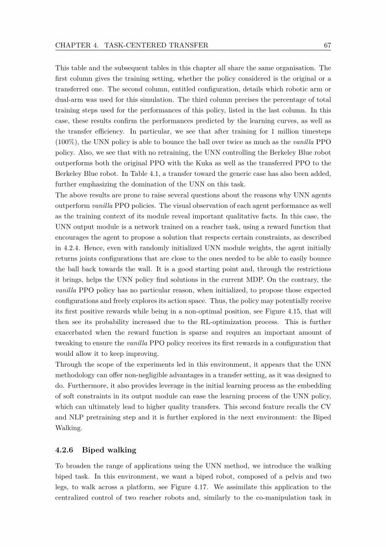
CHAPTER 4. TASK-CENTERED TRANSFER 67
This table and the subsequent tables in this chapter all share the same organisation. Thefirst column gives the training setting, whether the policy considered is the original or atransferred one. The second column, entitled configuration, details which robotic arm ordual-arm was used for this simulation. The third column precises the percentage of totaltraining steps used for the performances of this policy, listed in the last column. In thiscase, these results confirm the performances predicted by the learning curves, as well asthe transfer efficiency. In particular, we see that after training for 1 million timesteps(100%), the UNN policy is able to bounce the ball over twice as much as the vanilla PPOpolicy. Also, we see that with no retraining, the UNN controlling the Berkeley Blue robotoutperforms both the original PPO with the Kuka as well as the transferred PPO to theBerkeley Blue robot. In Table 4.1, a transfer toward the generic case has also been added,further emphasizing the domination of the UNN on this task.The above results are prone to raise several questions about the reasons why UNN agentsoutperform vanilla PPO policies. The visual observation of each agent performance as wellas the training context of its module reveal important qualitative facts. In this case, theUNN output module is a network trained on a reacher task, using a reward function thatencourages the agent to propose a solution that respects certain constraints, as describedin 4.2.4. Hence, even with randomly initialized UNN module weights, the agent initiallyreturns joints configurations that are close to the ones needed to be able to easily bouncethe ball back towards the wall. It is a good starting point and, through the restrictionsit brings, helps the UNN policy find solutions in the current MDP. On the contrary, thevanilla PPO policy has no particular reason, when initialized, to propose those expectedconfigurations and freely explores its action space. Thus, the policy may potentially receiveits first positive rewards while being in a non-optimal position, see Figure 4.15, that willthen see its probability increased due to the RL-optimization process. This is furtherexacerbated when the reward function is sparse and requires an important amount oftweaking to ensure the vanilla PPO policy receives its first rewards in a configuration thatwould allow it to keep improving.Through the scope of the experiments led in this environment, it appears that the UNNmethodology can offer non-negligible advantages in a transfer setting, as it was designed todo. Furthermore, it also provides leverage in the initial learning process as the embeddingof soft constraints in its output module can ease the learning process of the UNN policy,which can ultimately lead to higher quality transfers. This second feature recalls the CVand NLP pretraining step and it is further explored in the next environment: the BipedWalking.
4.2.6 Biped walking
To broaden the range of applications using the UNN method, we introduce the walkingbiped task. In this environment, we want a biped robot, composed of a pelvis and twolegs, to walk across a platform, see Figure 4.17. We assimilate this application to thecentralized control of two reacher robots and, similarly to the co-manipulation task in
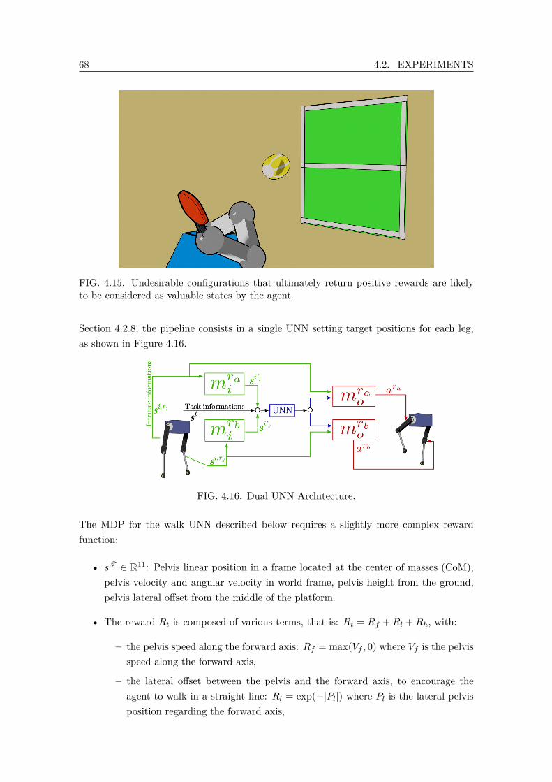
68 4.2. EXPERIMENTS
FIG. 4.15. Undesirable configurations that ultimately return positive rewards are likelyto be considered as valuable states by the agent.
Section 4.2.8, the pipeline consists in a single UNN setting target positions for each leg,as shown in Figure 4.16.
FIG. 4.16. Dual UNN Architecture.
The MDP for the walk UNN described below requires a slightly more complex rewardfunction:
• sT ∈ R11: Pelvis linear position in a frame located at the center of masses (CoM),pelvis velocity and angular velocity in world frame, pelvis height from the ground,pelvis lateral offset from the middle of the platform.
• The reward Rt is composed of various terms, that is: Rt = Rf +Rl +Rh, with:
– the pelvis speed along the forward axis: Rf = max(Vf , 0) where Vf is the pelvisspeed along the forward axis,
– the lateral offset between the pelvis and the forward axis, to encourage theagent to walk in a straight line: Rl = exp(−|Pl|) where Pl is the lateral pelvisposition regarding the forward axis,
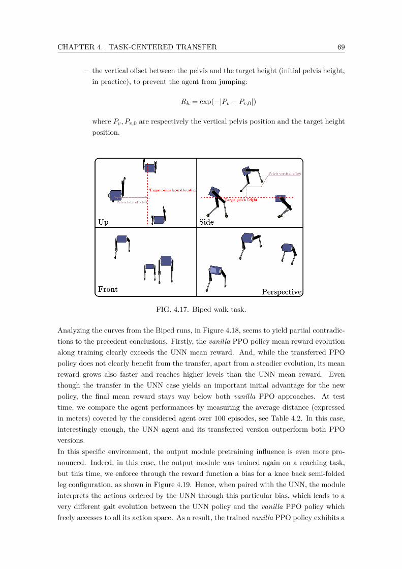
CHAPTER 4. TASK-CENTERED TRANSFER 69
– the vertical offset between the pelvis and the target height (initial pelvis height,in practice), to prevent the agent from jumping:
Rh = exp(−|Pv − Pv,0|)
where Pv, Pv,0 are respectively the vertical pelvis position and the target heightposition.
FIG. 4.17. Biped walk task.
Analyzing the curves from the Biped runs, in Figure 4.18, seems to yield partial contradic-tions to the precedent conclusions. Firstly, the vanilla PPO policy mean reward evolutionalong training clearly exceeds the UNN mean reward. And, while the transferred PPOpolicy does not clearly benefit from the transfer, apart from a steadier evolution, its meanreward grows also faster and reaches higher levels than the UNN mean reward. Eventhough the transfer in the UNN case yields an important initial advantage for the newpolicy, the final mean reward stays way below both vanilla PPO approaches. At testtime, we compare the agent performances by measuring the average distance (expressedin meters) covered by the considered agent over 100 episodes, see Table 4.2. In this case,interestingly enough, the UNN agent and its transferred version outperform both PPOversions.In this specific environment, the output module pretraining influence is even more pro-nounced. Indeed, in this case, the output module was trained again on a reaching task,but this time, we enforce through the reward function a bias for a knee back semi-foldedleg configuration, as shown in Figure 4.19. Hence, when paired with the UNN, the moduleinterprets the actions ordered by the UNN through this particular bias, which leads to avery different gait evolution between the UNN policy and the vanilla PPO policy whichfreely accesses to all its action space. As a result, the trained vanilla PPO policy exhibits a
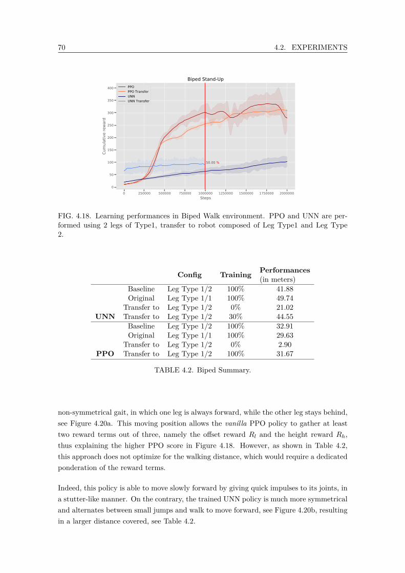
70 4.2. EXPERIMENTS
0 250000 500000 750000 1000000 1250000 1500000 1750000 2000000Steps
0
50
100
150
200
250
300
350
400
Cum
ulat
ive
rewa
rd
50.00 %
Biped Stand-UpPPOPPO TransferUNNUNN Transfer
FIG. 4.18. Learning performances in Biped Walk environment. PPO and UNN are per-formed using 2 legs of Type1, transfer to robot composed of Leg Type1 and Leg Type2.
Config Training Performances(in meters)
Baseline Leg Type 1/2 100% 41.88Original Leg Type 1/1 100% 49.74
UNNTransfer to Leg Type 1/2 0% 21.02Transfer to Leg Type 1/2 30% 44.55Baseline Leg Type 1/2 100% 32.91Original Leg Type 1/1 100% 29.63
PPOTransfer to Leg Type 1/2 0% 2.90Transfer to Leg Type 1/2 100% 31.67
TABLE 4.2. Biped Summary.
non-symmetrical gait, in which one leg is always forward, while the other leg stays behind,see Figure 4.20a. This moving position allows the vanilla PPO policy to gather at leasttwo reward terms out of three, namely the offset reward Rl and the height reward Rh,thus explaining the higher PPO score in Figure 4.18. However, as shown in Table 4.2,this approach does not optimize for the walking distance, which would require a dedicatedponderation of the reward terms.
Indeed, this policy is able to move slowly forward by giving quick impulses to its joints, ina stutter-like manner. On the contrary, the trained UNN policy is much more symmetricaland alternates between small jumps and walk to move forward, see Figure 4.20b, resultingin a larger distance covered, see Table 4.2.
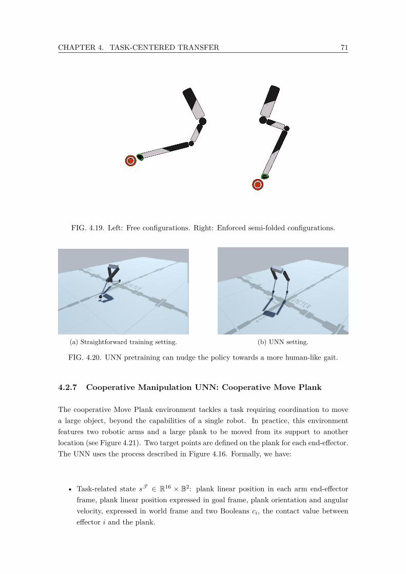
CHAPTER 4. TASK-CENTERED TRANSFER 71
FIG. 4.19. Left: Free configurations. Right: Enforced semi-folded configurations.
(a) Straightforward training setting. (b) UNN setting.
FIG. 4.20. UNN pretraining can nudge the policy towards a more human-like gait.
4.2.7 Cooperative Manipulation UNN: Cooperative Move Plank
The cooperative Move Plank environment tackles a task requiring coordination to movea large object, beyond the capabilities of a single robot. In practice, this environmentfeatures two robotic arms and a large plank to be moved from its support to anotherlocation (see Figure 4.21). Two target points are defined on the plank for each end-effector.The UNN uses the process described in Figure 4.16. Formally, we have:
• Task-related state sT ∈ R16 × B2: plank linear position in each arm end-effectorframe, plank linear position expressed in goal frame, plank orientation and angularvelocity, expressed in world frame and two Booleans ci, the contact value betweeneffector i and the plank.
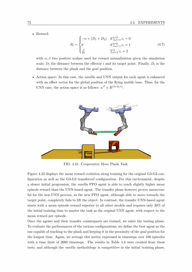
72 4.2. EXPERIMENTS
• Reward:
Rt =
−α× (D1 +D2) if
∑2i=1 ci = 0
0 if∑2i=1 ci = 1
βDt
∑2i=1 ci = 2
(4.7)
with α, β two positive scalars used for reward normalization given the simulationscale, Di the distance between the effector i and its target point. Finally, Dt is thedistance between the plank and the goal position.
• Action space: In this case, the vanilla and UNN output for each agent is enhancedwith an offset vector for the global position of the flying mobile base. Thus, for theUNN case, the action space is as follows: aT ∈ R(3+3)×2.
FIG. 4.21. Cooperative Move Plank Task.
Figure 4.22 displays the mean reward evolution along training for the original G3-G3 con-figuration as well as the G3-G2 transferred configuration. For this environment, despitea slower initial progression, the vanilla PPO agent is able to reach slightly higher meanepisode reward than the UNN-based agent. The transfer phase however proves unsuccess-ful for the non-UNN process, as the new PPO agent, although able to move towards thetarget point, completely fails to lift the object. In contrast, the transfer UNN-based agentstarts with a mean episode reward superior to all other models and requires only 30% ofthe initial training time to master the task as the original UNN agent, with respect to themean reward per episode.Once the agents and their transfer counterparts are trained, we enter the testing phase.To evaluate the performances of the various configurations, we define the best agent as theone capable of reaching to the plank and keeping it in the proximity of the goal position forthe longest time. Again, we average this metric expressed in timesteps over 100 episodeswith a time limit of 2000 timesteps. The results in Table 4.3 were created from thesetests, and although the vanilla methodology is competitive in the initial training phase,
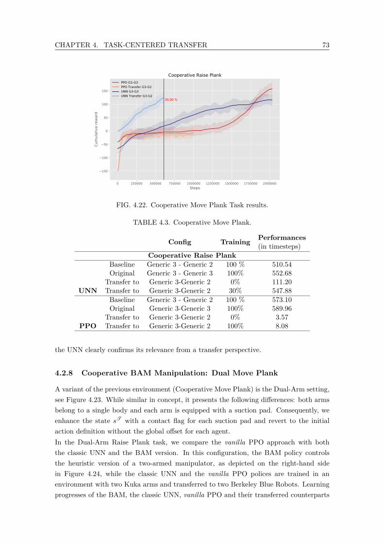
CHAPTER 4. TASK-CENTERED TRANSFER 73
0 250000 500000 750000 1000000 1250000 1500000 1750000 2000000
Steps
150
100
50
0
50
100
150
Cum
ula
tive r
ew
ard
30.00 %
Cooperative Raise Plank
PPO G3-G3
PPO Transfer G3-G2
UNN G3-G3
UNN Transfer G3-G2
FIG. 4.22. Cooperative Move Plank Task results.
TABLE 4.3. Cooperative Move Plank.
Config Training Performances(in timesteps)
Cooperative Raise PlankBaseline Generic 3 - Generic 2 100 % 510.54Original Generic 3 - Generic 3 100% 552.68
UNNTransfer to Generic 3-Generic 2 0% 111.20Transfer to Generic 3-Generic 2 30% 547.88Baseline Generic 3 - Generic 2 100 % 573.10Original Generic 3-Generic 3 100% 589.96
PPOTransfer to Generic 3-Generic 2 0% 3.57Transfer to Generic 3-Generic 2 100% 8.08
the UNN clearly confirms its relevance from a transfer perspective.
4.2.8 Cooperative BAM Manipulation: Dual Move Plank
A variant of the previous environment (Cooperative Move Plank) is the Dual-Arm setting,see Figure 4.23. While similar in concept, it presents the following differences: both armsbelong to a single body and each arm is equipped with a suction pad. Consequently, weenhance the state sT with a contact flag for each suction pad and revert to the initialaction definition without the global offset for each agent.In the Dual-Arm Raise Plank task, we compare the vanilla PPO approach with boththe classic UNN and the BAM version. In this configuration, the BAM policy controlsthe heuristic version of a two-armed manipulator, as depicted on the right-hand sidein Figure 4.24, while the classic UNN and the vanilla PPO polices are trained in anenvironment with two Kuka arms and transferred to two Berkeley Blue Robots. Learningprogresses of the BAM, the classic UNN, vanilla PPO and their transferred counterparts
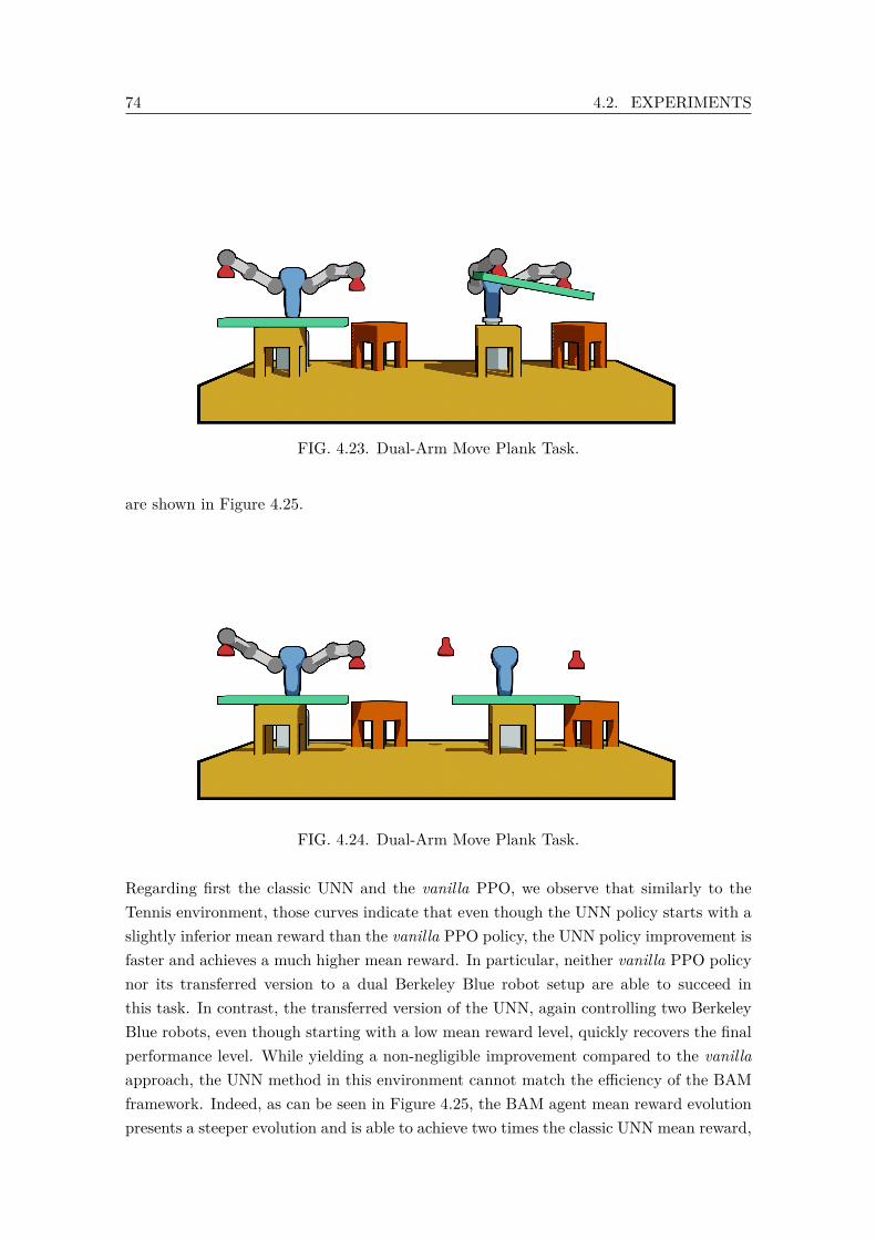
74 4.2. EXPERIMENTS
FIG. 4.23. Dual-Arm Move Plank Task.
are shown in Figure 4.25.
FIG. 4.24. Dual-Arm Move Plank Task.
Regarding first the classic UNN and the vanilla PPO, we observe that similarly to theTennis environment, those curves indicate that even though the UNN policy starts with aslightly inferior mean reward than the vanilla PPO policy, the UNN policy improvement isfaster and achieves a much higher mean reward. In particular, neither vanilla PPO policynor its transferred version to a dual Berkeley Blue robot setup are able to succeed inthis task. In contrast, the transferred version of the UNN, again controlling two BerkeleyBlue robots, even though starting with a low mean reward level, quickly recovers the finalperformance level. While yielding a non-negligible improvement compared to the vanillaapproach, the UNN method in this environment cannot match the efficiency of the BAMframework. Indeed, as can be seen in Figure 4.25, the BAM agent mean reward evolutionpresents a steeper evolution and is able to achieve two times the classic UNN mean reward,
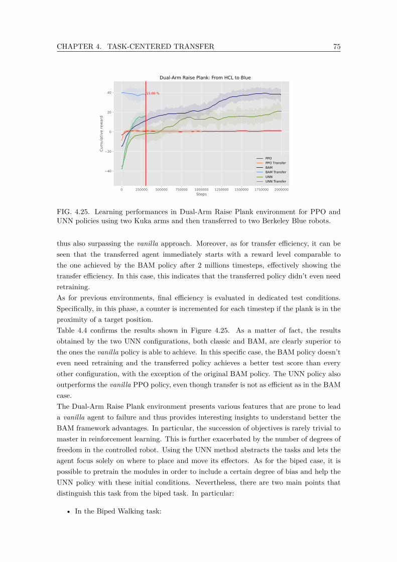
CHAPTER 4. TASK-CENTERED TRANSFER 75
0 250000 500000 750000 1000000 1250000 1500000 1750000 2000000
Steps
40
20
0
20
40
Cum
ula
tive r
ew
ard
15.00 %
Dual-Arm Raise Plank: From HCL to Blue
PPO
PPO Transfer
BAM
UNNUNN Transfer
BAM Transfer
FIG. 4.25. Learning performances in Dual-Arm Raise Plank environment for PPO andUNN policies using two Kuka arms and then transferred to two Berkeley Blue robots.
thus also surpassing the vanilla approach. Moreover, as for transfer efficiency, it can beseen that the transferred agent immediately starts with a reward level comparable tothe one achieved by the BAM policy after 2 millions timesteps, effectively showing thetransfer efficiency. In this case, this indicates that the transferred policy didn’t even needretraining.As for previous environments, final efficiency is evaluated in dedicated test conditions.Specifically, in this phase, a counter is incremented for each timestep if the plank is in theproximity of a target position.Table 4.4 confirms the results shown in Figure 4.25. As a matter of fact, the resultsobtained by the two UNN configurations, both classic and BAM, are clearly superior tothe ones the vanilla policy is able to achieve. In this specific case, the BAM policy doesn’teven need retraining and the transferred policy achieves a better test score than everyother configuration, with the exception of the original BAM policy. The UNN policy alsooutperforms the vanilla PPO policy, even though transfer is not as efficient as in the BAMcase.The Dual-Arm Raise Plank environment presents various features that are prone to leada vanilla agent to failure and thus provides interesting insights to understand better theBAM framework advantages. In particular, the succession of objectives is rarely trivial tomaster in reinforcement learning. This is further exacerbated by the number of degrees offreedom in the controlled robot. Using the UNN method abstracts the tasks and lets theagent focus solely on where to place and move its effectors. As for the biped case, it ispossible to pretrain the modules in order to include a certain degree of bias and help theUNN policy with these initial conditions. Nevertheless, there are two main points thatdistinguish this task from the biped task. In particular:
• In the Biped Walking task:

76 4.2. EXPERIMENTS
TABLE 4.4. Dual Arm Raise Plank Summary.
Config. Training Performances(in timesteps)
Original BAM 100% 1557.05
BAMTransfer to B.Blue-B.Blue 0% 1545.65Transfer to B.Blue-B.Blue 15% 1547.02Transfer to Kuka-B.Blue 0% 1451.03Original Kuka-Kuka 100% 987.11
UNNTransfer to B.Blue-B.Blue 0% 4.41Transfer to B.Blue-B.Blue 15% 926.66Transfer to Kuka-B.Blue 15% 904.31
PPO Kuka-Kuka 100% 139.40
PPOTransfer to B.Blue-B.Blue 0% 8.45Transfer to B.Blue-B.Blue 100% 152.54Transfer to Kuka-B.Blue 100% 147.78
– the qualitative appeal of the walk cycle depends on the leg configuration andnot only on foot placement,
– and from a modelling point of view, it is unclear how to design a BAM versionof the task.
• While the Cooperative Raise Plank task as designed:
– isn’t affected by the arms configuration, as long as there is no self-collision,
– but does require non-negligible coordination regarding the effectors control.Thus, unless special care is dedicated to the module training, it is likely that itmight hurt the UNN policy learning performances.
– Finally, the modelling process and constraints setup for BAM training are par-ticularly straightforward.
These points indicate that creating a BAM version of the environment is a valuable alter-native. As seen in Figure 4.25 and Table 4.4, the BAM version of the UNN behaves in amore desirable way than its counterparts, thus offering a robot-agnostic model of the taskto various robots. Then, if the modules of a particular robot are sufficiently precise, it ispossible to succeed in the task with no retraining at all and still yields higher performancesthan other policies.Obviously, it is theoretically possible to design a reward function that would lead a vanillaPPO policy to walk in a predictable manner or reach and manipulate a plank with a highaccuracy. However, this is a very complex task that requires a considerable amount offeedback, tweaking and state representation engineering in order to find the ponderationthat would, in the biped case, allow the policy to walk fast while not degrading the otherimportant components too much, namely the steering and the height control. In themanipulation task, the sequential nature of the environment would also call for carefuland thorough fine-tuning of the reward and simulations to ensure that the policy finds a
CHAPTER 4. TASK-CENTERED TRANSFER 77
reliable solution. Using the UNN method enables to greatly simplify this design process byembedding in the robot limbs a bias, that acts similarly as soft constraints. Alternatively,setting up a BAM alternative when the conditions concur to it, is highly useful to helpthe policy find a solution in highly complex and non-linear environments.
4.3 Conclusion on TAsk-Centered methods
In this section, we presented a broad range of applications for the proposed Universal No-tice Network (UNN) approach, a method that disassociates the agent control logic fromthe task it is supposed to accomplish. To motivate our approach, we began by demonstrat-ing that vanilla transfer in RL setting is detrimental to the agent by exchanging layersbetween two similar agents both trained on a unique task. This experiment enlightenedthe fact that uncontrolled backpropagation does not structure knowledge and thus makesit difficult to forsee which model part can be shared or withdrawn without hindering per-formances. Consequently, the UNN approach has been applied to various tasks. For eachdetailed environment, we compared our technique with a classical state-of-the-art algo-rithm and we demonstrated the benefits and advantages of our method, both in termsof learning speed and final performance and then tackle the issue of transfer learning.Through various examples, we show that our method enables a more efficient transferthan current methods, allowing an agent to perform as well as the original policy withlittle to no retraining, hinting toward an important training time reduction. Additionally,the experiments set up allowed us to detect that the classic UNN architecture may conveya bias from the modules pre-training which can in various situations be used as an ad-vantage. For configurations in which the bias can be detrimental or simply undesired, wealso proposed an experimental framework, the Base Abstracted Modelling, for overcomingsuch biases. Despite its numerous advantages, the UNN method is in practice hinderedby the feature that constitutes its main appeal. Indeed, the initial segmentation processrelies, in its current form, on the hand-crafted features that constitute the interface be-tween the task model and the control parameters (the output base). As a result, thisforces each agent to adopt similar conventions to use the pretrained task model. Whilethis does not necessarily harm performance, it heavily limits the method flexibility andrange of application and although there are no theoretical constraints in building anothervector interface, it has proved difficult so far to formalize the definition of such a vector.Additionally, these constraints enforce the sequential aspect of the UNN training. Whilethis feature enables a simple form of knowledge segmentation, it is also the most likelyconveyor of base biases. As a result, an alternative path worth exploring would featurea joint knowledge construction by multiple agents with different morphologies, ultimatelyyielding a consensus notice that would not necessarily rest on hand-crafted vectors. Inthe next section, we will introduced TEacher-Centered techniques that circumvent thislimitation.
78 4.3. CONCLUSION ON TASK-CENTERED METHODS
Publications
• Universal Notice Network: Transferable Knowledge Among Agents - In-ternational Conference on Control, Decision and Information Technologies (CoDIT)2019 - Paris, France
• BAM! Base Abstracted Modeling with Universal Notice Network: FastSkill Transfer Between Mobile Manipulators - International Conference onControl, Decision and Information Technologies (CoDIT) 2020 - Prague, Czech Re-public
• Universal Notice Networks: Transferring learned skills through a broadpanel of applications - Submitted to: IEEE Transactions on Systems, Man andCybernetics: Systems
Additional Material
• https://drive.google.com/drive/folders/1rhwldaISnmpmG8bksTudQnhKvgnOGy83?usp=sharing
Chapter 5Teacher-Centered Transfer
Contents5.1 CoachGAN . . . . . . . . . . . . . . . . . . . . . . . . . . . . . . . . . . 80
5.1.1 From Task to Teacher . . . . . . . . . . . . . . . . . . . . . . . 805.1.2 The CoachGAN method . . . . . . . . . . . . . . . . . . . . . . 805.1.3 WGAN-GP for a suitable learning signal . . . . . . . . . . . . . 835.1.4 Task and Intermediate State Variables . . . . . . . . . . . . . . 845.1.5 Training the Expert . . . . . . . . . . . . . . . . . . . . . . . . 865.1.6 CoachGAN Results . . . . . . . . . . . . . . . . . . . . . . . . . 87
5.1.6.1 Effector Position ISV . . . . . . . . . . . . . . . . . . 875.1.6.2 Approximated Kinematics ISV . . . . . . . . . . . . . 895.1.6.3 Ball Rebound Speed ISV . . . . . . . . . . . . . . . . 895.1.6.4 Analysis . . . . . . . . . . . . . . . . . . . . . . . . . 90
5.1.7 Conclusion on CoachGAN . . . . . . . . . . . . . . . . . . . . . 925.2 Task-Specific Loss . . . . . . . . . . . . . . . . . . . . . . . . . . . . . . 92
5.2.1 The TSL Principle . . . . . . . . . . . . . . . . . . . . . . . . . 935.2.2 Method . . . . . . . . . . . . . . . . . . . . . . . . . . . . . . . 945.2.3 Transfer . . . . . . . . . . . . . . . . . . . . . . . . . . . . . . . 955.2.4 Experimental setup . . . . . . . . . . . . . . . . . . . . . . . . . 97
5.2.4.1 Tasks and Agents . . . . . . . . . . . . . . . . . . . . 975.2.4.2 Models . . . . . . . . . . . . . . . . . . . . . . . . . . 99
5.2.5 Results . . . . . . . . . . . . . . . . . . . . . . . . . . . . . . . . 995.2.5.1 Circle to Circle Contour Displacement . . . . . . . . 995.2.5.2 Tennis task . . . . . . . . . . . . . . . . . . . . . . . . 1005.2.5.3 Autonomous TSL . . . . . . . . . . . . . . . . . . . . 1035.2.5.4 Training Time & Assistive aspects . . . . . . . . . . . 105
5.2.6 Conclusion on Task-Specific Loss . . . . . . . . . . . . . . . . . 1055.3 Conclusion on TEacher-Centered methods . . . . . . . . . . . . . . . . 106
79

80 5.1. COACHGAN
In this chapter, we present two transfer learning approaches based on TEacher-Centeredconcepts. Indeed, as opposed to Task-Centered approaches that rely on the creation ofan instance of knowledge that can be passed between agents of different morphologies,TEacher-Centered methods are designed to provide a way of distilling the knowledge ofa teacher agent within students that are potentially differently structured. Building onthis concept, these techniques are first thoroughly explained and their relevance is thenassessed on a custom environment.
5.1 CoachGAN
5.1.1 From Task to Teacher
The previous chapter introducing the UNN underlines numerous times the critical im-portance of the interface between the UNN module and the agent’s inherent bases. Dueto the restrictions brought by this bottleneck, it becomes conceivably more complex toadapt a pre-trained UNN to an agent that would not present the elements fitting withinthe interface, thus limiting the universality of this method, as shown in Figure 5.1. In aneffort to overcome this potentially hindering issue, projecting the UNN module output inan intermediate latent space appears as an interesting candidate. This idea would be ableto provide values corresponding to measurements instead of direct orders.Let us consider the experimental environment Dual-Arm Manipulation, introduced inthe previous chapter: in this case, instead of returning translation vectors and relativeeffector positions for a full episode and using the reward function to backup and evaluatethe actions, the UNN could provide a desired state measure of the manipulated objectthat should then be matched by the agent arms, as displayed in Figure 5.2. In this view,the state measure could be very diverse, as long as it can be related to the agents actionsthrough a differentiable function, to ensure that backpropagation is possible.
5.1.2 The CoachGAN method
When assisting to a sports game, even non-expert individuals are able to detect particularlyefficient players. After watching enough, observers are usually able to provide a high-leveldescription of an ideal performer and additionally may be capable to distinguish an expert’saction from a novice’s. The CoachGAN method is a loose transposition of this situtationin the GAN framework where the external observer is a discriminator and players aregenerators.Building on the concept of expert/teacher/student, where a teacher can use observationsmade during the expert class to guide its students although he was not the initial trans-fer target, CoachGAN relies on a two-step adversarial process to train a student agentby using expert knowledge via a common teacher critic. Specifically, the main idea is torepurpose a GAN discriminator (the teacher) trained on a set of expert trajectories toprovide an error signal for a student trying to accomplish the same task. As the very
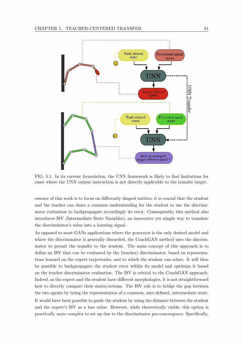
CHAPTER 5. TEACHER-CENTERED TRANSFER 81
FIG. 5.1. In its current formulation, the UNN framework is likely to find limitations forcases where the UNN output instruction is not directly applicable to the transfer target.
essence of this work is to focus on differently shaped entities, it is crucial that the studentand the teacher can share a common understanding for the student to use the discrimi-nator evaluation to backpropagate accordingly its error. Consequently, this method alsointroduces ISV (Intermediate State Variables), an innovative yet simple way to translatethe discriminator’s value into a learning signal.
As opposed to most GANs applications where the generator is the only desired model andwhere the discriminator is generally discarded, the CoachGAN method uses the discrim-inator to permit the transfer to the student. The main concept of this approach is todefine an ISV that can be evaluated by the (teacher) discriminator, based on representa-tions learned on the expert trajectories, and to which the student can relate. It will thenbe possible to backpropagate the student error within its model and optimize it basedon the teacher discriminator evaluation. The ISV is critical to the CoachGAN approach.Indeed, as the expert and the student have different morphologies, it is not straightforwardhow to directly compare their states/actions. The ISV role is to bridge the gap betweenthe two agents by being the representation of a common, user-defined, intermediate state.
It would have been possible to guide the student by using the distance between the studentand the expert’s ISV as a loss value. However, while theoretically viable, this option ispractically more complex to set up due to the discriminator pre-convergence. Specifically,
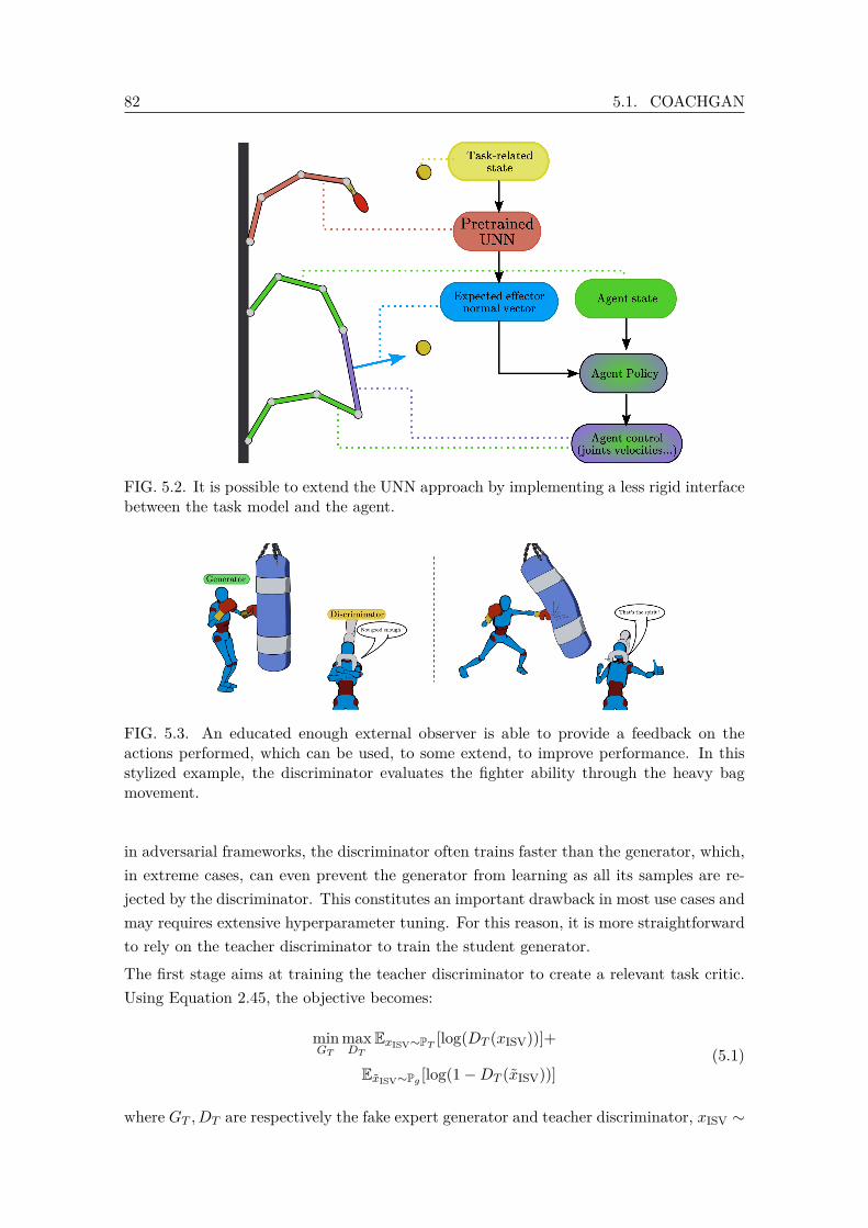
82 5.1. COACHGAN
FIG. 5.2. It is possible to extend the UNN approach by implementing a less rigid interfacebetween the task model and the agent.
FIG. 5.3. An educated enough external observer is able to provide a feedback on theactions performed, which can be used, to some extend, to improve performance. In thisstylized example, the discriminator evaluates the fighter ability through the heavy bagmovement.
in adversarial frameworks, the discriminator often trains faster than the generator, which,in extreme cases, can even prevent the generator from learning as all its samples are re-jected by the discriminator. This constitutes an important drawback in most use cases andmay requires extensive hyperparameter tuning. For this reason, it is more straightforwardto rely on the teacher discriminator to train the student generator.
The first stage aims at training the teacher discriminator to create a relevant task critic.Using Equation 2.45, the objective becomes:
minGT
maxDT
ExISV∼PT [log(DT (xISV))]+
ExISV∼Pg [log(1−DT (xISV))](5.1)
where GT , DT are respectively the fake expert generator and teacher discriminator, xISV ∼
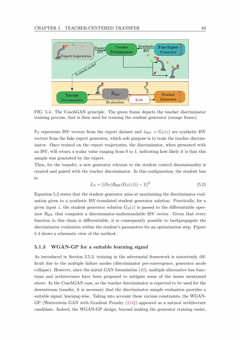
CHAPTER 5. TEACHER-CENTERED TRANSFER 83
FIG. 5.4. The CoachGAN principle. The green frame depicts the teacher discriminatortraining process, that is then used for training the student generator (orange frame).
PT represents ISV vectors from the expert dataset and xISV = GT (z) are synthetic ISVvectors from the fake expert generator, which sole purpose is to train the teacher discrim-inator. Once trained on the expert trajectories, the discriminator, when presented withan ISV, will return a scalar value ranging from 0 to 1, indicating how likely it is that thissample was generated by the expert.Then, for the transfer, a new generator relevant to the student control dimensionality iscreated and paired with the teacher discriminator. In this configuration, the student lossis:
LS = ||DT (RISV(GS(z)))− 1||2 (5.2)
Equation 5.2 states that the student generator aims at maximizing the discriminator eval-uation given to a synthetic ISV-translated student generator solution. Practically, for agiven input z, the student generator solution GS(z) is passed to the differentiable oper-ator RISV that computes a discriminator-understandable ISV vector. Given that everyfunction in this chain is differentiable, it is consequently possible to backpropagate thediscriminator evaluation within the student’s parameters for an optimization step. Figure5.4 shows a schematic view of the method.
5.1.3 WGAN-GP for a suitable learning signal
As introduced in Section 2.5.3, training in the adversarial framework is notoriously dif-ficult due to the multiple failure modes (discriminator pre-convergence, generator modecollapse). However, since the initial GAN formulation (40), multiple alternative loss func-tions and architectures have been proposed to mitigate some of the issues mentionedabove. In the CoachGAN case, as the teacher discriminator is expected to be used for thedownstream transfer, it is necessary that the discriminator sample evaluation provides asuitable signal, learning-wise. Taking into account these various constraints, the WGAN-GP (Watterstein GAN with Gradient Penalty (114)) appeared as a natural architecturecandidate. Indeed, the WGAN-GP design, beyond making the generator training easier,
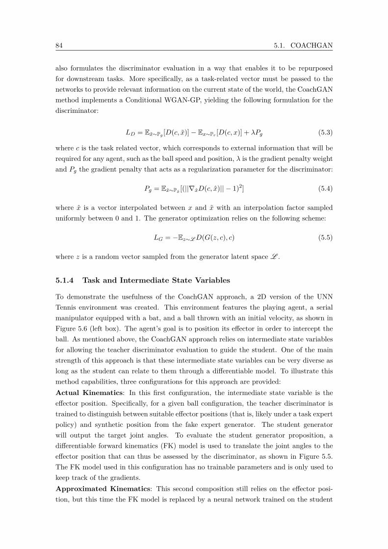
84 5.1. COACHGAN
also formulates the discriminator evaluation in a way that enables it to be repurposedfor downstream tasks. More specifically, as a task-related vector must be passed to thenetworks to provide relevant information on the current state of the world, the CoachGANmethod implements a Conditional WGAN-GP, yielding the following formulation for thediscriminator:
LD = Ex∼Pg [D(c, x)]− Ex∼Pr [D(c, x)] + λPg (5.3)
where c is the task related vector, which corresponds to external information that will berequired for any agent, such as the ball speed and position, λ is the gradient penalty weightand Pg the gradient penalty that acts as a regularization parameter for the discriminator:
Pg = Ex∼Px [(||∇xD(c, x)|| − 1)2] (5.4)
where x is a vector interpolated between x and x with an interpolation factor sampleduniformly between 0 and 1. The generator optimization relies on the following scheme:
LG = −Ez∼LD(G(z, c), c) (5.5)
where z is a random vector sampled from the generator latent space L .
5.1.4 Task and Intermediate State Variables
To demonstrate the usefulness of the CoachGAN approach, a 2D version of the UNNTennis environment was created. This environment features the playing agent, a serialmanipulator equipped with a bat, and a ball thrown with an initial velocity, as shown inFigure 5.6 (left box). The agent’s goal is to position its effector in order to intercept theball. As mentioned above, the CoachGAN approach relies on intermediate state variablesfor allowing the teacher discriminator evaluation to guide the student. One of the mainstrength of this approach is that these intermediate state variables can be very diverse aslong as the student can relate to them through a differentiable model. To illustrate thismethod capabilities, three configurations for this approach are provided:Actual Kinematics: In this first configuration, the intermediate state variable is theeffector position. Specifically, for a given ball configuration, the teacher discriminator istrained to distinguish between suitable effector positions (that is, likely under a task expertpolicy) and synthetic position from the fake expert generator. The student generatorwill output the target joint angles. To evaluate the student generator proposition, adifferentiable forward kinematics (FK) model is used to translate the joint angles to theeffector position that can thus be assessed by the discriminator, as shown in Figure 5.5.The FK model used in this configuration has no trainable parameters and is only used tokeep track of the gradients.Approximated Kinematics: This second composition still relies on the effector posi-tion, but this time the FK model is replaced by a neural network trained on the student
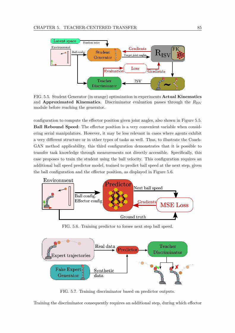
CHAPTER 5. TEACHER-CENTERED TRANSFER 85
FIG. 5.5. Student Generator (in orange) optimization in experimentsActual Kinematicsand Approximated Kinematics. Discriminator evaluation passes through the RISVmodule before reaching the generator.
configuration to compute the effector position given joint angles, also shown in Figure 5.5.Ball Rebound Speed: The effector position is a very convenient variable when consid-ering serial manipulators. However, it may be less relevant in cases where agents exhibita very different structure or in other types of tasks as well. Thus, to illustrate the Coach-GAN method applicability, this third configuration demonstrates that it is possible totransfer task knowledge through measurements not directly accessible. Specifically, thiscase proposes to train the student using the ball velocity. This configuration requires anadditional ball speed predictor model, trained to predict ball speed at the next step, giventhe ball configuration and the effector position, as displayed in Figure 5.6.
FIG. 5.6. Training predictor to forsee next step ball speed.
FIG. 5.7. Training discriminator based on predictor outputs.
Training the discriminator consequently requires an additional step, during which effector
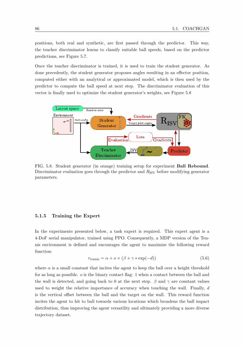
86 5.1. COACHGAN
positions, both real and synthetic, are first passed through the predictor. This way,the teacher discriminator learns to classify suitable ball speeds, based on the predictorpredictions, see Figure 5.7.
Once the teacher discriminator is trained, it is used to train the student generator. Asdone precedently, the student generator proposes angles resulting in an effector position,computed either with an analytical or approximated model, which is then used by thepredictor to compute the ball speed at next step. The discriminator evaluation of thisvector is finally used to optimize the student generator’s weights, see Figure 5.8
FIG. 5.8. Student generator (in orange) training setup for experiment Ball Rebound.Discriminator evaluation goes through the predictor and RISV before modifying generatorparameters.
5.1.5 Training the Expert
In the experiments presented below, a task expert is required. This expert agent is a4-DoF serial manipulator, trained using PPO. Consequently, a MDP version of the Ten-nis environment is defined and encourages the agent to maximize the following rewardfunction:
rtennis = α+ o× (β + γ ∗ exp(−d)) (5.6)
where α is a small constant that incites the agent to keep the ball over a height thresholdfor as long as possible. o is the binary contact flag: 1 when a contact between the ball andthe wall is detected, and going back to 0 at the next step. β and γ are constant valuesused to weight the relative importance of accuracy when touching the wall. Finally, dis the vertical offset between the ball and the target on the wall. This reward functionincites the agent to hit to ball towards various locations which broadens the ball impactdistribution, thus improving the agent versatility and ultimately providing a more diversetrajectory dataset.
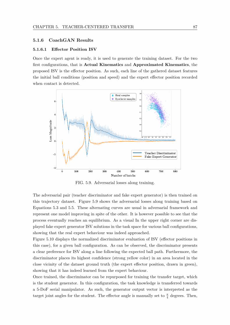
CHAPTER 5. TEACHER-CENTERED TRANSFER 87
5.1.6 CoachGAN Results
5.1.6.1 Effector Position ISV
Once the expert agent is ready, it is used to generate the training dataset. For the twofirst configurations, that is Actual Kinematics and Approximated Kinematics, theproposed ISV is the effector position. As such, each line of the gathered dataset featuresthe initial ball conditions (position and speed) and the expert effector position recordedwhen contact is detected.
FIG. 5.9. Adversarial losses along training.
The adversarial pair (teacher discriminator and fake expert generator) is then trained onthis trajectory dataset. Figure 5.9 shows the adversarial losses along training based onEquations 5.3 and 5.5. These alternating curves are usual in adversarial framework andrepresent one model improving in spite of the other. It is however possible to see that theprocess eventually reaches an equilibrium. As a visual In the upper right corner are dis-played fake expert generator ISV solutions in the task space for various ball configurations,showing that the real expert behaviour was indeed approached.Figure 5.10 displays the normalized discriminator evaluation of ISV (effector positions inthis case), for a given ball configuration. As can be observed, the discriminator presentsa clear preference for ISV along a line following the expected ball path. Furthermore, thediscriminator places its highest confidence (strong yellow color) in an area located in theclose vicinity of the dataset ground truth (the expert effector position, drawn in green),showing that it has indeed learned from the expert behaviour.Once trained, the discriminator can be repurposed for training the transfer target, whichis the student generator. In this configuration, the task knowledge is transferred towardsa 5-DoF serial manipulator. As such, the generator output vector is interpreted as thetarget joint angles for the student. The effector angle is manually set to π
4 degrees. Then,
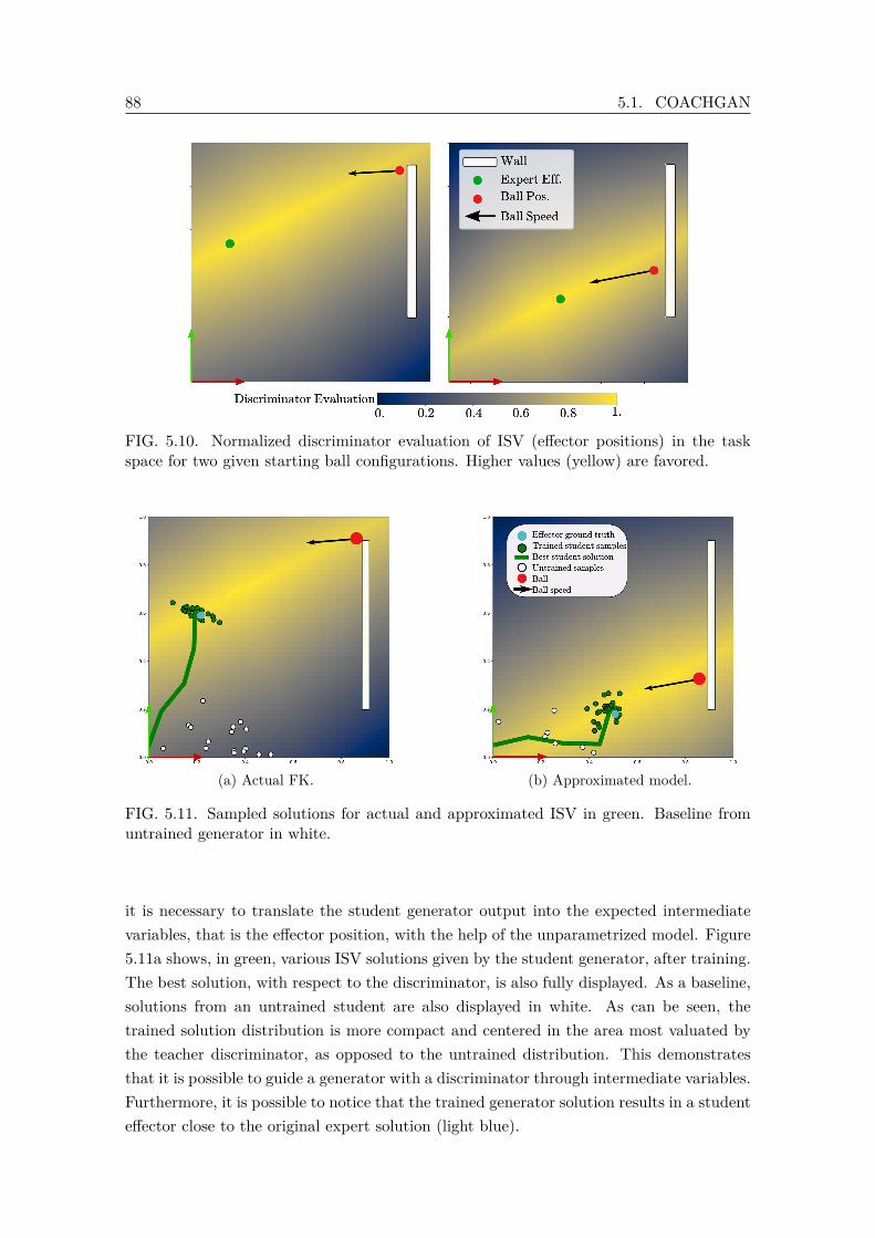
88 5.1. COACHGAN
FIG. 5.10. Normalized discriminator evaluation of ISV (effector positions) in the taskspace for two given starting ball configurations. Higher values (yellow) are favored.
(a) Actual FK. (b) Approximated model.
FIG. 5.11. Sampled solutions for actual and approximated ISV in green. Baseline fromuntrained generator in white.
it is necessary to translate the student generator output into the expected intermediatevariables, that is the effector position, with the help of the unparametrized model. Figure5.11a shows, in green, various ISV solutions given by the student generator, after training.The best solution, with respect to the discriminator, is also fully displayed. As a baseline,solutions from an untrained student are also displayed in white. As can be seen, thetrained solution distribution is more compact and centered in the area most valuated bythe teacher discriminator, as opposed to the untrained distribution. This demonstratesthat it is possible to guide a generator with a discriminator through intermediate variables.Furthermore, it is possible to notice that the trained generator solution results in a studenteffector close to the original expert solution (light blue).
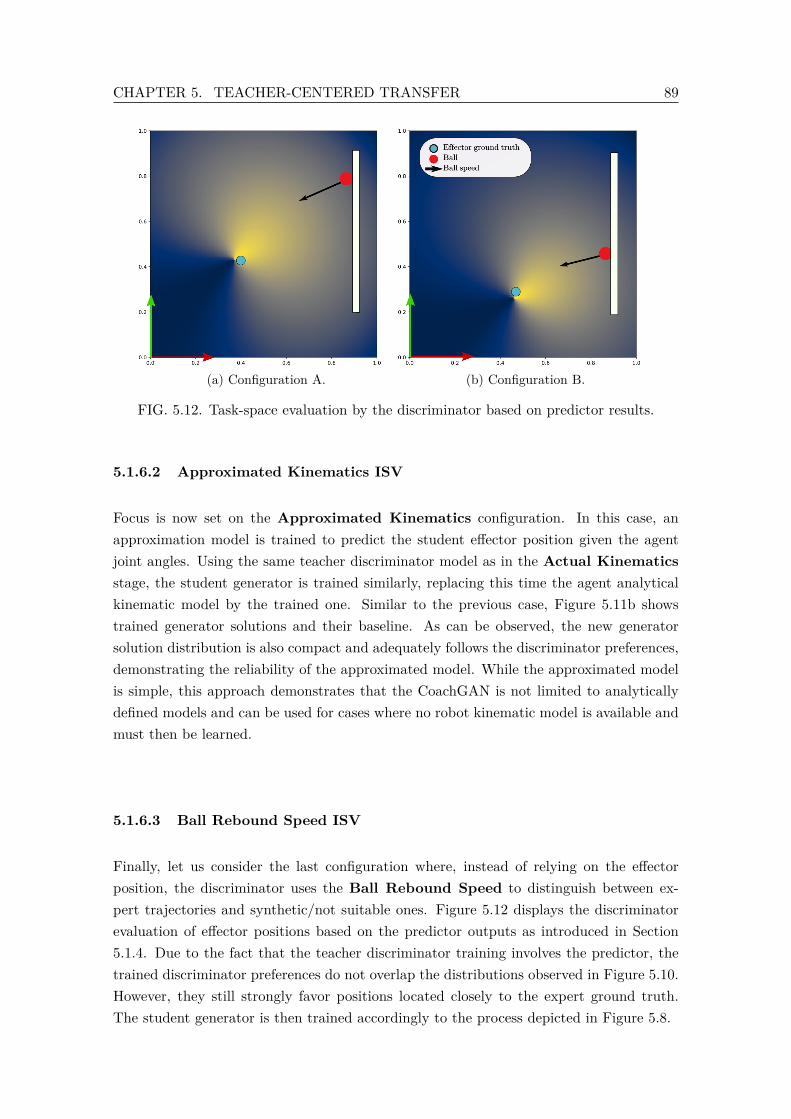
CHAPTER 5. TEACHER-CENTERED TRANSFER 89
(a) Configuration A. (b) Configuration B.
FIG. 5.12. Task-space evaluation by the discriminator based on predictor results.
5.1.6.2 Approximated Kinematics ISV
Focus is now set on the Approximated Kinematics configuration. In this case, anapproximation model is trained to predict the student effector position given the agentjoint angles. Using the same teacher discriminator model as in the Actual Kinematicsstage, the student generator is trained similarly, replacing this time the agent analyticalkinematic model by the trained one. Similar to the previous case, Figure 5.11b showstrained generator solutions and their baseline. As can be observed, the new generatorsolution distribution is also compact and adequately follows the discriminator preferences,demonstrating the reliability of the approximated model. While the approximated modelis simple, this approach demonstrates that the CoachGAN is not limited to analyticallydefined models and can be used for cases where no robot kinematic model is available andmust then be learned.
5.1.6.3 Ball Rebound Speed ISV
Finally, let us consider the last configuration where, instead of relying on the effectorposition, the discriminator uses the Ball Rebound Speed to distinguish between ex-pert trajectories and synthetic/not suitable ones. Figure 5.12 displays the discriminatorevaluation of effector positions based on the predictor outputs as introduced in Section5.1.4. Due to the fact that the teacher discriminator training involves the predictor, thetrained discriminator preferences do not overlap the distributions observed in Figure 5.10.However, they still strongly favor positions located closely to the expert ground truth.The student generator is then trained accordingly to the process depicted in Figure 5.8.

90 5.1. COACHGAN
FIG. 5.13. 2D representation of the solution distribution. Successful solutions are eitheroverlapping expert position or in the ball path.
5.1.6.4 Analysis
The performances of these models are displayed in Figure 5.13 where, for a given ballconfiguration, each model samples 2048 solutions. Sampling several predictions from themodel enables us to conduct an analysis and evaluate, for instance through the width ofthe proposed distribution of solutions, the variance of the model. Indeed, it is possible tonotice that the blue and orange distributions, corresponding respectively to the analyticalmodel and the approximated kinematics model, are very close, showing the approximatedmodel reliability for transferring the discriminator evaluation. Moreover, these distribu-tions overlap the expert effector position. The green distribution, representing solutionsfrom the generator trained with the predictor pipeline is slightly broader than the twoother distributions, as well as being located closer to the ball. As training for this modelrelied on another dataset, it consequently generated a differently inclined discriminator,leading in turn to a closer player student. Still, it appears that these distributions are di-rectly located in the ball speed direction, thus enhancing the agent chances of interceptingthe ball. Furthermore, it is possible to explain the width of the distributions by the factthat only the effector position is registered on contact and that the model is not directlyaware of the bat length. Nonetheless, as shows Figure 5.14, all generators provide educated
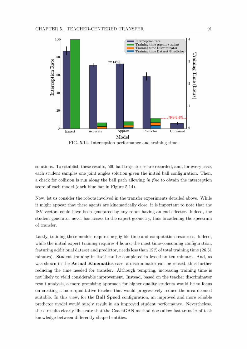
CHAPTER 5. TEACHER-CENTERED TRANSFER 91
FIG. 5.14. Interception performance and training time.
solutions. To establish these results, 500 ball trajectories are recorded, and, for every case,each student samples one joint angles solution given the initial ball configuration. Then,a check for collision is run along the ball path allowing in fine to obtain the interceptionscore of each model (dark blue bar in Figure 5.14).
Now, let us consider the robots involved in the transfer experiments detailed above. Whileit might appear that these agents are kinematically close, it is important to note that theISV vectors could have been generated by any robot having an end effector. Indeed, thestudent generator never has access to the expert geometry, thus broadening the spectrumof transfer.
Lastly, training these models requires negligible time and computation resources. Indeed,while the initial expert training requires 4 hours, the most time-consuming configuration,featuring additional dataset and predictor, needs less than 12% of total training time (26.51minutes). Student training in itself can be completed in less than ten minutes. And, aswas shown in the Actual Kinematics case, a discriminator can be reused, thus furtherreducing the time needed for transfer. Although tempting, increasing training time isnot likely to yield considerable improvement. Instead, based on the teacher discriminatorresult analysis, a more promising approach for higher quality students would be to focuson creating a more qualitative teacher that would progressively reduce the area deemedsuitable. In this view, for the Ball Speed configuration, an improved and more reliablepredictor model would surely result in an improved student performance. Nevertheless,these results clearly illustrate that the CoachGAN method does allow fast transfer of taskknowledge between differently shaped entities.
92 5.2. TASK-SPECIFIC LOSS
5.1.7 Conclusion on CoachGAN
In this section, a new step-by-step methodology for systematic and fast transfer of knowl-edge from one entity to a differently structured one has been proposed. Relying on anadversarial framework, the CoachGAN technique was evaluated using various intermediatestate variables (ISV) and shows that it is possible to transfer task knowledge to a studentagent without interaction of this agent with the task. As explained in the experimentresults, this method allows to train students within minutes, while most RL tasks requireseveral hours of training. Thus, the applications of CoachGAN are numerous, especiallygiven the increasing availability of approximation models. In its current form, this methoddoes however present some limitations. Specifically, as can be seen in the experiments,the student generator outputs correspond to final target states (for instance, the expectedconfiguration for touching the ball). This output definition can in some cases be detri-mental to the application spectrum, particularly in cases where unexpected events mustbe handled.This limitation stems directly from the learning process. Indeed, as the learning loss isestablished based on the ISV, the discriminator learns to evaluate states. As the studentgenerator is trained using the discriminator, predicting intermediate state conditioned oncurrent state makes training more difficult.Taking into account this limitation, various alternative ways could offer a way out. Astraightforward approach would be to adapt the generator to output several intermediatekey states and sum the teacher discriminator evaluations of these states to compute theerror. Although appealing, this formulation could introduce stabilization issues relatedto the number of intermediate steps and the distance between them. Another paradigmwould be to find a way to evaluate the results of a student action with respect to the actiontaken by the teacher for a similar environment configuration. The next section introducesthe Task-Specific Loss (TSL), another TEacher-Centered method that relies partly on thissecond approach to propose a reactive agent formulation.
5.2 Task-Specific Loss
As seen in the previous section, the CoachGAN methods provides a way to transfer knowl-edge from a given expert to a morphologically distinct student. However, this techniquerelies on an architecture that prevents its usage in an interactive way. Specifically, itscurrent form is geared toward the generation of intermediary states that must then bereached using other state-of-the-art methods.The Task-Specific Loss (TSL) approach, introduced in this chapter, aims at tackling thisissue by linking the student loss to its ISV variation.Building on works described in (75) that introduced a Variational Auto-Encoder (VAE)architecture suited for assistive control, the Task-Specific Loss (TSL) approach introducesan extension that improves on CoachGAN interactive limitations as well as enabling thelow-cost transfer of latent-spaces between differently shaped agents for the initial assistive
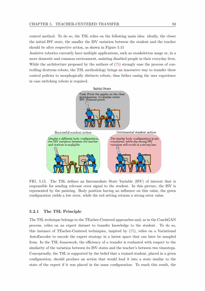
CHAPTER 5. TEACHER-CENTERED TRANSFER 93
control method. To do so, the TSL relies on the following main idea: ideally, the closerthe initial ISV state, the smaller the ISV variation between the student and the teachershould be after respective action, as shown in Figure 5.15Assistive robotics currently have multiple applications, such as exoskeletton usage or, in amore domestic and common environment, assisting disabled people in their everyday lives.While the architecture proposed by the authors of (75) strongly ease the process of con-trolling dextrous robots, the TSL methodology brings an innovative way to transfer thesecontrol policies to morphogically distincts robots, thus futher easing the user experiencein case switching robots is required.
FIG. 5.15. The TSL defines an Intermediate State Variable (ISV) of interest that isresponsible for sending relevant error signal to the student. In this picture, the ISV isrepresented by the painting. Body position having no influence on this value, the greenconfiguration yields a low error, while the red setting returns a strong error value.
5.2.1 The TSL Principle
The TSL technique belongs to the TEacher-Centered approaches and, as in the CoachGANprocess, relies on an expert dataset to transfer knowledge to the student. To do so,this instance of TEacher-Centered techniques, inspired by (75), relies on a VariationalAutoEncoder to encode the expert strategy in a latent space that can later be sampledfrom. In the TSL framework, the efficiency of a transfer is evaluated with respect to thesimilarity of the variation between its ISV states and the teacher’s between two timesteps.Conceptually, the TSL is supported by the belief that a trained student, placed in a givenconfiguration, should produce an action that would lead it into a state similar to thestate of the expert if it was placed in the same configuration. To reach this result, the
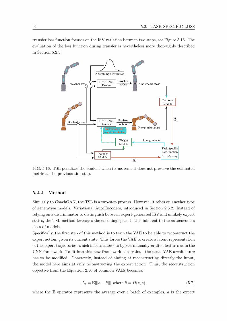
94 5.2. TASK-SPECIFIC LOSS
transfer loss function focuses on the ISV variation between two steps, see Figure 5.16. Theevaluation of the loss function during transfer is nevertheless more thoroughly describedin Section 5.2.3
FIG. 5.16. TSL penalizes the student when its movement does not preserve the estimatedmetric at the previous timestep.
5.2.2 Method
Similarly to CoachGAN, the TSL is a two-step process. However, it relies on another typeof generative models: Variational AutoEncoders, introduced in Section 2.6.2. Instead ofrelying on a discriminator to distinguish between expert-generated ISV and unlikely expertstates, the TSL method leverages the encoding space that is inherent to the autoencodersclass of models.Specifically, the first step of this method is to train the VAE to be able to reconstruct theexpert action, given its current state. This forces the VAE to create a latent representationof the expert trajectories, which in turn allows to bypass manually-crafted features as in theUNN framework. To fit into this new framework constraints, the usual VAE architecturehas to be modified. Concretely, instead of aiming at reconstructing directly the input,the model here aims at only reconstructing the expert action. Thus, the reconstructionobjective from the Equation 2.50 of common VAEs becomes:
Lr = E[||a− a||] where a = D(z, s) (5.7)
where the E operator represents the average over a batch of examples, a is the expert
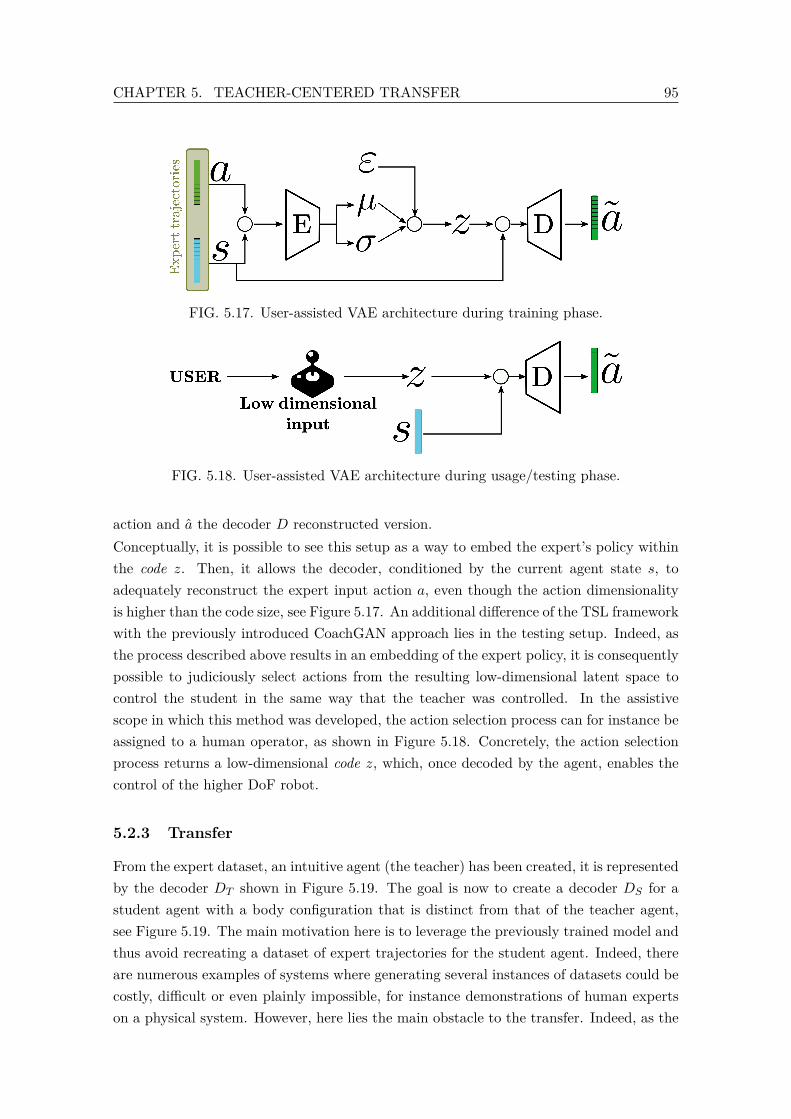
CHAPTER 5. TEACHER-CENTERED TRANSFER 95
FIG. 5.17. User-assisted VAE architecture during training phase.
FIG. 5.18. User-assisted VAE architecture during usage/testing phase.
action and a the decoder D reconstructed version.Conceptually, it is possible to see this setup as a way to embed the expert’s policy withinthe code z. Then, it allows the decoder, conditioned by the current agent state s, toadequately reconstruct the expert input action a, even though the action dimensionalityis higher than the code size, see Figure 5.17. An additional difference of the TSL frameworkwith the previously introduced CoachGAN approach lies in the testing setup. Indeed, asthe process described above results in an embedding of the expert policy, it is consequentlypossible to judiciously select actions from the resulting low-dimensional latent space tocontrol the student in the same way that the teacher was controlled. In the assistivescope in which this method was developed, the action selection process can for instance beassigned to a human operator, as shown in Figure 5.18. Concretely, the action selectionprocess returns a low-dimensional code z, which, once decoded by the agent, enables thecontrol of the higher DoF robot.
5.2.3 Transfer
From the expert dataset, an intuitive agent (the teacher) has been created, it is representedby the decoder DT shown in Figure 5.19. The goal is now to create a decoder DS for astudent agent with a body configuration that is distinct from that of the teacher agent,see Figure 5.19. The main motivation here is to leverage the previously trained model andthus avoid recreating a dataset of expert trajectories for the student agent. Indeed, thereare numerous examples of systems where generating several instances of datasets could becostly, difficult or even plainly impossible, for instance demonstrations of human expertson a physical system. However, here lies the main obstacle to the transfer. Indeed, as the
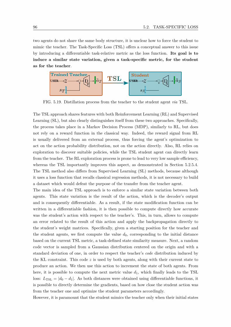
96 5.2. TASK-SPECIFIC LOSS
two agents do not share the same body structure, it is unclear how to force the student tomimic the teacher. The Task-Specific Loss (TSL) offers a conceptual answer to this issueby introducing a differentiable task-relative metric as the loss function. Its goal is toinduce a similar state variation, given a task-specific metric, for the studentas for the teacher.
FIG. 5.19. Distillation process from the teacher to the student agent via TSL.
The TSL approach shares features with both Reinforcement Learning (RL) and SupervisedLearning (SL), but also clearly distinguishes itself from these two approaches. Specifically,the process takes place in a Markov Decision Process (MDP), similarly to RL, but doesnot rely on a reward function in the classical way. Indeed, the reward signal from RLis usually delivered from an external process, thus forcing the agent’s optimization toact on the action probability distribution, not on the action directly. Also, RL relies onexploration to discover suitable policies, while the TSL student agent can directly learnfrom the teacher. The RL exploration process is prone to lead to very low sample efficiency,whereas the TSL importantly improves this aspect, as demonstrated in Section 5.2.5.4.The TSL method also differs from Supervised Learning (SL) methods, because althoughit uses a loss function that recalls classical regression methods, it is not necessary to builda dataset which would defeat the purpose of the transfer from the teacher agent.The main idea of the TSL approach is to enforce a similar state variation between bothagents. This state variation is the result of the action, which is the decoder’s outputand is consequently differentiable. As a result, if the state modification function can bewritten in a differentiable fashion, it is then possible to compute directly how accuratewas the student’s action with respect to the teacher’s. This, in turn, allows to computean error related to the result of this action and apply the backpropagation directly tothe student’s weight matrices. Specifically, given a starting position for the teacher andthe student agents, we first compute the value d0, corresponding to the initial distancebased on the current TSL metric, a task-defined state similarity measure. Next, a randomcode vector is sampled from a Gaussian distribution centered on the origin and with astandard deviation of one, in order to respect the teacher’s code distribution induced bythe KL constraint. This code z is used by both agents, along with their current state toproduce an action. We then use this action to increment the state of both agents. Fromhere, it is possible to compute the next metric value d1, which finally leads to the TSLloss: LTSL = |d0 − d1|. As both distances were obtained using differentiable functions, itis possible to directly determine the gradients, based on how close the student action wasfrom the teacher one and optimize the student parameters accordingly.However, it is paramount that the student mimics the teacher only when their initial states
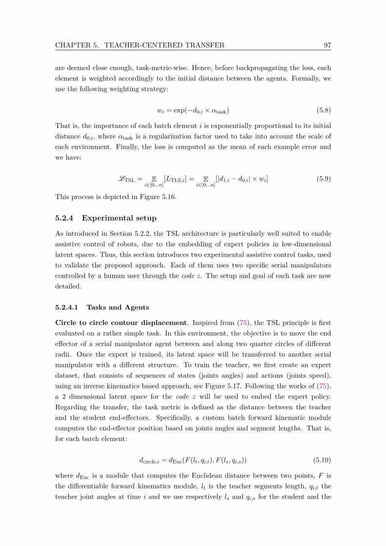
CHAPTER 5. TEACHER-CENTERED TRANSFER 97
are deemed close enough, task-metric-wise. Hence, before backpropagating the loss, eachelement is weighted accordingly to the initial distance between the agents. Formally, weuse the following weighting strategy:
wi = exp(−d0,i × αtask) (5.8)
That is, the importance of each batch element i is exponentially proportional to its initialdistance d0,i, where αtask is a regularization factor used to take into account the scale ofeach environment. Finally, the loss is computed as the mean of each example error andwe have:
LTSL = Ei∈[0...n]
[LTLS,i] = Ei∈[0...n]
[|d1,i − d0,i| × wi] (5.9)
This process is depicted in Figure 5.16.
5.2.4 Experimental setup
As introduced in Section 5.2.2, the TSL architecture is particularly well suited to enableassistive control of robots, due to the embedding of expert policies in low-dimensionallatent spaces. Thus, this section introduces two experimental assistive control tasks, usedto validate the proposed approach. Each of them uses two specific serial manipulatorscontrolled by a human user through the code z. The setup and goal of each task are nowdetailed.
5.2.4.1 Tasks and Agents
Circle to circle contour displacement. Inspired from (75), the TSL principle is firstevaluated on a rather simple task. In this environment, the objective is to move the endeffector of a serial manipulator agent between and along two quarter circles of differentradii. Once the expert is trained, its latent space will be transferred to another serialmanipulator with a different structure. To train the teacher, we first create an expertdataset, that consists of sequences of states (joints angles) and actions (joints speed),using an inverse kinematics based approach, see Figure 5.17. Following the works of (75),a 2 dimensional latent space for the code z will be used to embed the expert policy.Regarding the transfer, the task metric is defined as the distance between the teacherand the student end-effectors. Specifically, a custom batch forward kinematic modulecomputes the end-effector position based on joints angles and segment lengths. That is,for each batch element:
dcircle,i = dEuc(F (lt, qi,t), F (ls, qi,s)) (5.10)
where dEuc is a module that computes the Euclidean distance between two points, F isthe differentiable forward kinematics module, lt is the teacher segments length, qi,t theteacher joint angles at time i and we use respectively ls and qi,s for the student and the

98 5.2. TASK-SPECIFIC LOSS
weights wi are computed using Equation 5.8. Then, for a whole batch of examples, wehave:
Lcircle = Ei∈[0...n]
[wi × |dcircle,i − dcircle,i+1|] (5.11)
Initially learned by a 5 rotoid joints robot (5R), this task knowledge is then distilled withina 4R agent, which total length equate that of the 5R, through the TSL Lcircle using thisEuclidean distance between end-effectors as a metric, see Figure 5.20.
FIG. 5.20. Various teaching cases and their corresponding losses and importance weight.The teacher’s joints are drawn in blue, while green is used for the student.
Tennis Task. In this second environment, designed to evaluate our method in a morecomplex setting, the goal is to bounce a ball against a vertical wall as many times aspossible. Despite the conceptual similarities, it is distinct from the one used in Section 5.1.4where the objective was mainly to intercept the ball, while this environment emphasizesthe goal of maximizing bounces. The task is initially performed by the teacher, a 4R serialmanipulator, the last segment serving as a bat to bounce the ball. The expert dataset isgenerated by a custom RL-agent trained on this task with an additional signal to specifythe ideal impact location and a 1D latent space is used for this task. The tennis skillis then transferred to two students: a 5R and a 3R agent, with a total length equal tothe 4R’s. This time, the TSL relies on three terms: the Euclidean distance between end-effectors positions, similarly to the previous environment and referred to as Lcircle, the
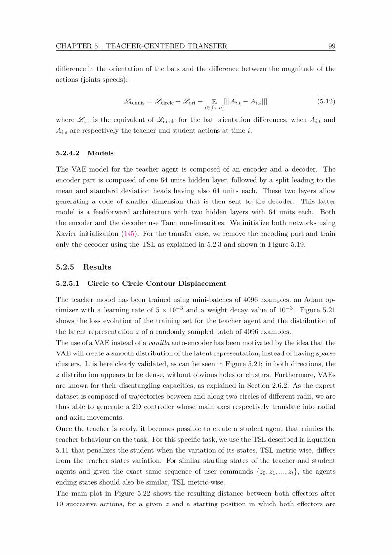
CHAPTER 5. TEACHER-CENTERED TRANSFER 99
difference in the orientation of the bats and the difference between the magnitude of theactions (joints speeds):
Ltennis = Lcircle + Lori + Ei∈[0...n]
[||Ai,t −Ai,s||] (5.12)
where Lori is the equivalent of Lcircle for the bat orientation differences, when Ai,t andAi,s are respectively the teacher and student actions at time i.
5.2.4.2 Models
The VAE model for the teacher agent is composed of an encoder and a decoder. Theencoder part is composed of one 64 units hidden layer, followed by a split leading to themean and standard deviation heads having also 64 units each. These two layers allowgenerating a code of smaller dimension that is then sent to the decoder. This lattermodel is a feedforward architecture with two hidden layers with 64 units each. Boththe encoder and the decoder use Tanh non-linearities. We initialize both networks usingXavier initialization (145). For the transfer case, we remove the encoding part and trainonly the decoder using the TSL as explained in 5.2.3 and shown in Figure 5.19.
5.2.5 Results
5.2.5.1 Circle to Circle Contour Displacement
The teacher model has been trained using mini-batches of 4096 examples, an Adam op-timizer with a learning rate of 5 × 10⁻³ and a weight decay value of 10−3. Figure 5.21shows the loss evolution of the training set for the teacher agent and the distribution ofthe latent representation z of a randomly sampled batch of 4096 examples.The use of a VAE instead of a vanilla auto-encoder has been motivated by the idea that theVAE will create a smooth distribution of the latent representation, instead of having sparseclusters. It is here clearly validated, as can be seen in Figure 5.21: in both directions, thez distribution appears to be dense, without obvious holes or clusters. Furthermore, VAEsare known for their disentangling capacities, as explained in Section 2.6.2. As the expertdataset is composed of trajectories between and along two circles of different radii, we arethus able to generate a 2D controller whose main axes respectively translate into radialand axial movements.Once the teacher is ready, it becomes possible to create a student agent that mimics theteacher behaviour on the task. For this specific task, we use the TSL described in Equation5.11 that penalizes the student when the variation of its states, TSL metric-wise, differsfrom the teacher states variation. For similar starting states of the teacher and studentagents and given the exact same sequence of user commands {z0, z1, ..., zt}, the agentsending states should also be similar, TSL metric-wise.The main plot in Figure 5.22 shows the resulting distance between both effectors after10 successive actions, for a given z and a starting position in which both effectors are
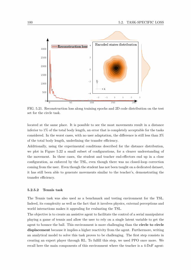
100 5.2. TASK-SPECIFIC LOSS
FIG. 5.21. Reconstruction loss along training epochs and 2D code distribution on the testset for the circle task.
located at the same place. It is possible to see the most movements result in a distanceinferior to 1% of the total body length, an error that is completely acceptable for the tasksconsidered. In the worst cases, with no user adaptation, the difference is still less than 3%of the total body length, underlining the transfer efficiency.Additionally, using the experimental conditions described for the distance distribution,we plot in Figure 5.22 a small subset of configurations, for a clearer understanding ofthe movement. In these cases, the student and teacher end-effectors end up in a closeconfiguration, as enforced by the TSL, even though there was no closed-loop correctioncoming from the user. Even though the student has not been taught on a dedicated dataset,it has still been able to generate movements similar to the teacher’s, demonstrating thetransfer efficiency.
5.2.5.2 Tennis task
The Tennis task was also used as a benchmark and testing environment for the TSL.Indeed, its complexity as well as the fact that it involves physics, external perceptions andworld interactions makes it appealing for evaluating the TSL.The objective is to create an assistive agent to facilitate the control of a serial manipulatorplaying a game of tennis and allow the user to rely on a single latent variable to get theagent to bounce the ball. This environment is more challenging than the circle to circledisplacement because it implies a higher reactivity from the agent. Furthermore, writingan analytical model to solve this task proves to be challenging. The first step consists increating an expert player through RL. To fulfill this step, we used PPO once more. Werecall here the main components of this environment where the teacher is a 4-DoF agent:
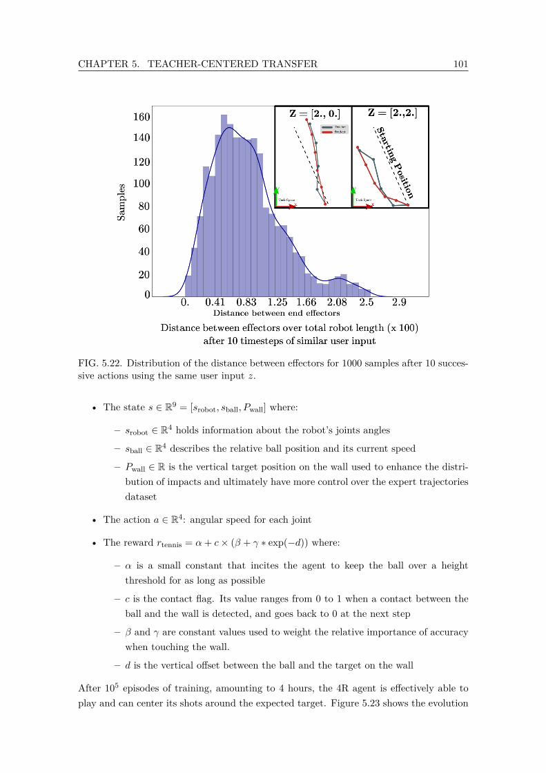
CHAPTER 5. TEACHER-CENTERED TRANSFER 101
FIG. 5.22. Distribution of the distance between effectors for 1000 samples after 10 succes-sive actions using the same user input z.
• The state s ∈ R9 = [srobot, sball, Pwall] where:
– srobot ∈ R4 holds information about the robot’s joints angles
– sball ∈ R4 describes the relative ball position and its current speed
– Pwall ∈ R is the vertical target position on the wall used to enhance the distri-bution of impacts and ultimately have more control over the expert trajectoriesdataset
• The action a ∈ R4: angular speed for each joint
• The reward rtennis = α+ c× (β + γ ∗ exp(−d)) where:
– α is a small constant that incites the agent to keep the ball over a heightthreshold for as long as possible
– c is the contact flag. Its value ranges from 0 to 1 when a contact between theball and the wall is detected, and goes back to 0 at the next step
– β and γ are constant values used to weight the relative importance of accuracywhen touching the wall.
– d is the vertical offset between the ball and the target on the wall
After 105 episodes of training, amounting to 4 hours, the 4R agent is effectively able toplay and can center its shots around the expected target. Figure 5.23 shows the evolution
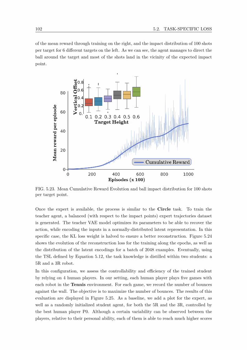
102 5.2. TASK-SPECIFIC LOSS
of the mean reward through training on the right, and the impact distribution of 100 shotsper target for 6 different targets on the left. As we can see, the agent manages to direct theball around the target and most of the shots land in the vicinity of the expected impactpoint.
FIG. 5.23. Mean Cumulative Reward Evolution and ball impact distribution for 100 shotsper target point.
Once the expert is available, the process is similar to the Circle task. To train theteacher agent, a balanced (with respect to the impact points) expert trajectories datasetis generated. The teacher VAE model optimizes its parameters to be able to recover theaction, while encoding the inputs in a normally-distributed latent representation. In thisspecific case, the KL loss weight is halved to ensure a better reconstruction. Figure 5.24shows the evolution of the reconstruction loss for the training along the epochs, as well asthe distribution of the latent encodings for a batch of 2048 examples. Eventually, usingthe TSL defined by Equation 5.12, the task knowledge is distilled within two students: a5R and a 3R robot.In this configuration, we assess the controllability and efficiency of the trained studentby relying on 4 human players. In our setting, each human player plays five games witheach robot in the Tennis environment. For each game, we record the number of bouncesagainst the wall. The objective is to maximize the number of bounces. The results of thisevaluation are displayed in Figure 5.25. As a baseline, we add a plot for the expert, aswell as a randomly initialized student agent, for both the 5R and the 3R, controlled bythe best human player P0. Although a certain variability can be observed between theplayers, relative to their personal ability, each of them is able to reach much higher scores
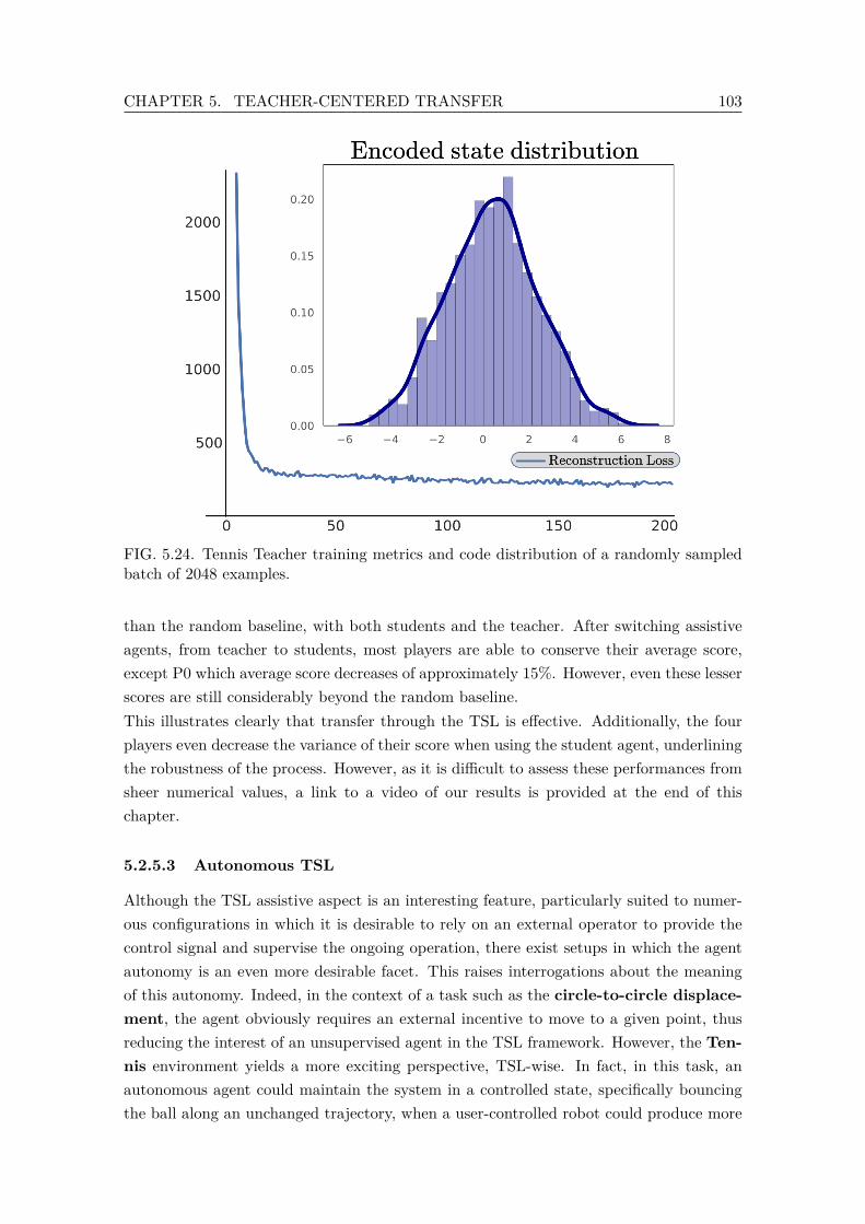
CHAPTER 5. TEACHER-CENTERED TRANSFER 103
FIG. 5.24. Tennis Teacher training metrics and code distribution of a randomly sampledbatch of 2048 examples.
than the random baseline, with both students and the teacher. After switching assistiveagents, from teacher to students, most players are able to conserve their average score,except P0 which average score decreases of approximately 15%. However, even these lesserscores are still considerably beyond the random baseline.This illustrates clearly that transfer through the TSL is effective. Additionally, the fourplayers even decrease the variance of their score when using the student agent, underliningthe robustness of the process. However, as it is difficult to assess these performances fromsheer numerical values, a link to a video of our results is provided at the end of thischapter.
5.2.5.3 Autonomous TSL
Although the TSL assistive aspect is an interesting feature, particularly suited to numer-ous configurations in which it is desirable to rely on an external operator to provide thecontrol signal and supervise the ongoing operation, there exist setups in which the agentautonomy is an even more desirable facet. This raises interrogations about the meaningof this autonomy. Indeed, in the context of a task such as the circle-to-circle displace-ment, the agent obviously requires an external incentive to move to a given point, thusreducing the interest of an unsupervised agent in the TSL framework. However, the Ten-nis environment yields a more exciting perspective, TSL-wise. In fact, in this task, anautonomous agent could maintain the system in a controlled state, specifically bouncingthe ball along an unchanged trajectory, when a user-controlled robot could produce more

104 5.2. TASK-SPECIFIC LOSS
FIG. 5.25. Comparison of assistive performances of several players using both teacher andstudent agent with baseline.
diverse movements, as schematized in Figure 5.26.
FIG. 5.26. Comparison of TSL-based controlled for autonomous agent and user-controlledagent in a relevant environment.
As was shown in the previous experiments, and particularly in the circle-to-circle dis-placement, the user input magnitude influences the output action magnitude. As such,due to the current specificities of the TSL formulation, endowing an agent with the au-tonomous characteristics, in a stabilization sense as defined above, can be done by ensuringthe user signal magnitude is null. In practice, this means that a vector of zeros z0 is con-catenated with the state s and fed in the student decoder. That is:
aAuto = D(z0, s) (5.13)
where z0 ∈ Rdim(z).To evaluate the student agent ability to stabilize the ball without user direct supervision
CHAPTER 5. TEACHER-CENTERED TRANSFER 105
and control, the impact position distribution and the action magnitude are recorded alongseveral episodes and are displayed in Figure 5.27. As can be observed, every run shown inthis figure exhibits globally the same partition: at the beginning of the episode, the agentoutputs aggressive actions to catch the ball and orient its velocity in a way that it findsfitting. Once in this configuration, the agent succeeds in maintaining the ball for a whilewith a sequence of actions of lower magnitude. Finally, a third phase can be detectedwhen the agent misses the ball and resumes to a more aggressive control to catch it back.Meanwhile, the histogram representing the distribution of impacts for each episode showsthat the agent is able to hit the ball so that most rebounds are located in a restrictedarea, thus underlining the stabilizing feature of the autonomous TSL.
5.2.5.4 Training Time & Assistive aspects
One of the principal motivation for transfer learning is to decrease the time needed toproduce a functional model. The TSL approach clearly fits within this framework, asthe effective transfer process is quite short on a regular i7 CPU with 64 Gb of RAM. Inthe Circle case, as the expert dataset relies on an inverse kinematics approach, the timeneeded for generating expert trajectories is negligible. As a result, a user could considerthe fact to create an expert with the student structure as well. However, as the teachertraining time using the expert data is close to 15 minutes, the TSL approach neverthelessyields a 66% time reduction in this environment as the transfer only requires 5 minutes.While it may appear of limited interest given the overall duration of the process, thissimple environment allowed us to illustrate the TSL capabilities. The transfer significanceis more strongly emphasized within the Tennis environment. In this configuration, theRL agent interacts during 4 hours with the environment before yielding a suitable expertpolicy, to which additional 15 minutes are necessary to train the teacher agent. In thiscase, the transfer using the TSL approach can be done in 5 minutes, that is only 7% of thetime initially needed for the teacher, and yet results in functionning assistive controllers asdemonstrated by our results. This clearly establishes the transfer value and shows that themore the expert dataset generation is costly, the more interesting the transfer of controlpolicies is.From a qualitative standpoint, this approach yields an important ease-of-use enhancement,particularly in the case of the Tennis task. Indeed, it would be highly challenging andnon-intuitive to design and use a controller to manually pilot each rotoid joint of the tennisagent. The assistive method, empowered by the TSL method, allows users to easily reacha considerable number of bounces by letting the user focus on a global plan, instead ofmanaging the low-level inputs.
5.2.6 Conclusion on Task-Specific Loss
In this section, it is proposed a new step by step methodology allowing to systematicallytransfer knowledge of task between two different structural agents. The introduced concept
106 5.3. CONCLUSION ON TEACHER-CENTERED METHODS
of Task-Specific Loss (TSL) was evaluated over various tasks, within the background ofassistive robotics. As can be seen in the results, this method offers considerable timesaving compared to state-of-the-art RL methods and can distill the task knowledge of ateacher agent within a structurally different student agent within minutes, as opposed toseveral hours of training for more complex task. Furthermore, our experiments, especiallythe Tennis task, demonstrate that the transferred knowledge is robust and that varioususers are able to generate stable performances on a task involving physics, planning andconsistency. Additionally, this TSL formulation enables in some cases an autonomoususage, in a stabilization sense. Although improvable, these results were obtained withoutdedicated architecture or agent modification or fine-tuning. The TSL application scenariosare numerous: in assistive robotics, as it can be considered to allow disabled people toseamlessly fit their new robotic platform to behave similarly to their previous one. Inother robotic domains as well, since learning-based transfer techniques for control tasksare not particularly developed.
5.3 Conclusion on TEacher-Centered methods
This chapter has presented two new approaches for transfer learning. These techniquescan be considered as TEacher-Centered because, as opposed to the UNN method, theydo not aim at embedding the task knowledge in a separate module but instead directlydistill the expert behaviour within the new agent control module. Methods belongingto this family are appealing because they do not fix a particular interface between theagents and are thus more flexible. This flexibility enables more sophisticated losses andless restrictions over the operating agents. Furthermore, unsupervised training is usuallymore reliable than RL, making the transfer more robust. The main limitation of theseapproaches in their current form is a likely accuracy loss. Indeed, the very definition ofVAE implies smooth Gaussian-like latent space, which makes it hard to have very precisevalues, a well known issue in literature. Similarly, the discriminator in the CoachGANsetting learns a probability distribution and a too sharp frontier makes it difficult for thegenerator to learn. However, these issues nevertheless allowed the transfer to occur forthe presented tasks and can be mitigated by putting more care in the loss definition ordataset
Publications
• CoachGAN: Fast Adversarial Transfer Learning between differently shapedentities - International Conference on Informatics in Control, Automation andRobotics (ICINCO) 2020 - Paris, France
• Task-Specific Loss: A TEacher-Centered Approach to Transfer Learning- Submitted to: Lecture Notes in Electrical Engineering - Springer

CHAPTER 5. TEACHER-CENTERED TRANSFER 107
Additional Material
• https://drive.google.com/drive/folders/1EZ0vSB5vzCOAbtHOPLlpOl8Megd0gm14?usp=sharing

108 5.3. CONCLUSION ON TEACHER-CENTERED METHODS
05
1015
2025
300.0
0.2
0.4
0.6
0.8
1.0
1.2
1.4
Rebounds: 20Action M
agnitudeIm
pacts distribution
05
1015
2025
30
0.0
0.2
0.4
0.6
0.8
1.0
1.2
Rebounds: 21
05
1015
2025
300.0
0.5
1.0
1.5
2.0
Rebounds: 20
05
1015
2025
300.0
0.2
0.4
0.6
0.8
1.0
1.2
Rebounds: 22
05
1015
2025
300.0
0.2
0.4
0.6
0.8
1.0
1.2Rebounds: 15
05
1015
2025
30
0.00
0.25
0.50
0.75
1.00
1.25
1.50
1.75
Rebounds: 27
05
1015
2025
300.0
0.2
0.4
0.6
0.8
1.0
1.2
Rebounds: 9
05
1015
2025
300.0
0.5
1.0
1.5
2.0
Rebounds: 16
05
1015
2025
300.0
0.2
0.4
0.6
0.8
1.0
1.2Rebounds: 23
Impact distribution and Action M
agnitude along episode
FIG.5.27.
Impact
distributionand
actionmagnitude
ofanautonom
ousstudent
alongseveralepisodes.
Chapter 6General Conclusion & Prospects
109

110
General Conclusion
As it appears reasonable to expect robots to endorse an ever more important role in thefuture human civilization, it is necessary to envision the constraints and modalities formanaging a fleet of robots. Currently, several non-negligible and systemic issues stand inthe way of the large-scale deployment of robots. In particular, the known sample ineffi-ciency of learning-based approaches, in particular for on-policy Reinforcement Learningframeworks, and the lack of structured transfer-learning strategies for these agents arerepresentative of these issues. Consequently, at the beginning of this thesis, we askedwhether the transfer of task-specific knowledge between two entities was possible, despitetheir potential morphological differences. We considered how transfer is applied in hu-man societies and were able to propose a classification of techniques: TAsk-Centered andTEacher-Centered transfer.
TAsk-Centered transfer techniques
TAsk-Centered techniques (Section 4.1) are inspired from a current common situationwhere a specialized piece of knowledge is embedded in a support without direct connectionsbetween the entity who generated the knowledge and the one receiving it. A clear humananalogy could be learning skills from a video online. This method requires nevertheless ashared interface to successfully link the piece of knowledge with the entities: for instance,it is unrealistic to consider learning to juggle with four balls if only two are available.From a practical point of view, this method was implemented in a Reinforcement RLpipeline. Having highlighted the fact that vanilla architectures and training procedureslack a clear knowledge structure, as opposed to bigger models with defined dimensionalitybottlenecks, we proposed a staged training method that decouples the control policy of agiven agent from the dedicated task skills. The numerous experiments setup to evaluatethis idea provided various insights: first, the control policy pre-training yields, on its own,several improvements over naive initialization as it is possible to embed relevant movementstrategies in the agent in a way that enables it to better tackles downstream tasks. Asexplained above, RL tends to produce agents with shaky, unstable behaviour and theintroduction of additional reward terms designed to ensure smoother actions are liable todestabilize the policy altogether, consequently making these empirical results valuable.Then, as demonstrated in the transfer between various agents (Section 4.2), the knowledgesupport module, called the Universal Notice Network (UNN), does supply the trans-fer target with appropriate information on the task. Agents with a different kinematicstructure and no previous training on the specific task are able to reach performancesclose to those of the agent that generated the knowledge, in only a fraction of the initialnumber of iterations to fine-tune their behaviours.As mentioned, the UNN method depends on a shared interface defined at the beginningof the initial training process. This interface consequently creates ties between all newagents receiving the module and the initial agent, which will prevent agents kinematically
CHAPTER 6. GENERAL CONCLUSION & PROSPECTS 111
unable to attach to this system to use the task knowledge.
TEacher-Centered Transfer Techniques
The TEacher-Centered family of techniques is the result of efforts directed towards theabstraction of the UNN interface. Indeed, instead of providing a restrictive state vector towhich all subsequent agents must conform, TEacher-Centered approaches are based on theidea that, in order to increase its usability, the task logic should rely on a kinematically-independent metric to evaluate actions. Conceptually, in a glass-of-water-fetching task,while the UNN would provide the position and orientation of both effectors holding theglass (thus making the task logic inaccessible to robots with a single effector), TEacher-Centered methods would provide a target glass state and let the agent manage its kine-matic configuration to reach such a state. To reach this objective, both TEacher-Centeredprocedures rely on a fundamental feature: the Intermediate State Variable. This vector,obtained through a differential computation, links the teacher agent with the student andenables the latter to optimize its behaviour to match the teacher’s. The IntermediateState Variable can be seen as a more flexible and customizable Universal Notice Networkinterface.The Intermediate State Variable (ISV) is central in the two TEacher-Centered tech-niques proposed. The first one, CoachGAN (Section 5.1.2), uses the Generative Adver-sarial Framework to create a discriminative model able to detect whether a given state islikely under the expert policy it has been trained on. Using the ISV permits to translatethe student states, potentially with a kinematic structure different from the expert, intoexpert states, consequently enabling the discriminative teacher to provide an evaluation ofthe movement. As the ISV computation is differentiable, it is suitable for optimizing thestudent agent. In the experiments setup to evaluate the CoachGAN technique, multipleISVs are used and we demonstrate that both analytical functions as well as approximationswith neural networks are usable, thus largely widening the applicability of this method(Section 5.1.6).The second approach, called the Task-Specific Loss (Section 5.2), addresses some ofthe CoachGAN limitations, such as the fact the latter procedure was constrained to statesprediction. This alternative formulation, based on a Variational AutoEncoder architecture,provides a framework that compares the result of student and teacher actions in an ISVdefined metric and penalizes the student agent when the result of its action results ina larger distance between its new ISV state and the teacher ISV. This procedure hasbeen evaluated on several environments and, despite the simplicity of these environments,demonstrates that task knowledge can indeed be transferred through the differentiableISV function. In addition, this approach enables the assistive control of an agent (Section5.2.5).These developments, in spite of the encouraging results obtained, are not complete andpresent undeniable limitations. First, most environments in the TEacher-Centered meth-ods are not particularly complex and include assumptions that may fail if deployed in a

112
less permissive system. While theoretically compatible with more sophisticated worlds,TEacher-Centered methods are yet to be evaluated in practical cases. Then, in both fam-ilies of approaches, very few physical constraints are taken into account for the robots.This aspect is slightly less problematic in the case of TEacher-Centered methods, Coach-GAN in particular, as it only requires looking for solutions in another area of the statespace. However, this can constitute a serious obstacle in the UNN configuration as somestates may not be reachable for another robot. Finally, an issue concerning more closelyTEacher-Centered methods is the absence of clear re-training strategy. Indeed, while theTAsk-Centered UNN was based on RL, which can in principle overcome the initial teacherby enabling backpropagation to affect all the modules, TEacher-Centered procedures aretied to the expert performance and even in the perspective of a hardly attainable perfecttransfer, current formulation simply does not conceive a way for the performance to exceedand go beyond the teacher.
Prospect
TEacher-Centered and TAsk-Centered methods convergence
The decoupling between task and policy, implemented in TAsk-Centered methods, presentsvarious advantages, in particular in the transfer from simulation to reality. As a matterof fact, training a policy in a simulated environment and releasing it in the physicalworld is not likely to result in successes, partly because of state distribution disparities.Consequently, it is conceivable to protect the task logic, learned in simulation, from thoseunexpected states by using approximators that could translate these outlying states in thestate space area in which the policy was initially trained. Furthermore, the output modulecould be trained solely in the real world to take into account the real robot properties.Doing so, in a primitive task as explained in this manuscript, is both safer and faster thantraining the entire agent on a more complex task from scratch.Furthermore, a slight paradigm change could nonetheless open new multiple and excitingperspectives for future works based on the two main ideas developed in this manuscript.For instance, the BAM approach that was designed to prevent several issues related withinterface compatibities between agents, presents, due to the model simplicity, an almosttrivial training procedure. This technique can consequently easily generate experts in agiven environment but needs to ensure continuity between the downstream sophisticatedagents and the relatively constraints-free BAM agent, which is the TAsk-Centered methodweakness. This setup present multiple opportunities for implementing TEacher-Centeredmethods where instead of managing complex interfaces and normalization parametersbetween morphological distinct agents, an ISV metric could be used to distill the BAMexpert knowledge within the student. Given the BAM expert simplicity, it would evenbe conceivable to include analytical approaches when relevant, thus vastly extending thescope of this method.
CHAPTER 6. GENERAL CONCLUSION & PROSPECTS 113
Merging TEacher-Centered and TAsk-Centered methods with externalworks
There are advantages in merging these transfer strategies with other recent works. Callingin external methods, it could be, for instance, convenient to define a UNN formulation inthe scope of Graph Neural Networks. This way, each agent joint/part would be consideredas a node graph, training could then be targeted towards a single joint and then passedto every other segment, thus extending the method flexibility.Other procedures using graphs could be foreseen as well. For instance, the UNN couldbe formulated as a GAN framework and trained to generate images based on the currentagent and world state. These images could be considered as mazes that would then besolved by a search algorithm, such as A?. A loss function would take into account whetherthe agent was able to reach its goal and penalize the UNN for inaccurate or unpracticalgraphs, in an adversarial fashion. Doing so, again using ISV, would provide reusability ofthe UNN to different agents.By stepping back and having a look at the current research landscape, recent works inOff-Policy Reinforcement Learning have highlighted goals and practical difficulties thatshare multiple features with the works described in this PhD manuscript. More precisely,considerable efforts are invested in this field toward the creation of a framework in whichan agent can efficiently reuse experiences and trajectories generated by various policies topredict an accurate value function and ultimately train a successful policy. As opposed toon-policy approaches that systematically require fresh samples, these techniques presentthe advantage of theoretically reducing the number of interactions needed between theagent and the environment.As explained, this setup conceptually mirrors the ones developed in the contributions ofthis thesis, as it expects to reuse the knowledge of other agents, experts as well as sub-optimal policies (embodied in the same agent in the case of off-policy RL) and devisethrough the trajectories present in the dataset a value function or an action value functionthat is then used to guide and fit the policy.In this view, instead of attempting to supplant these efforts to enable off-policy agents tolearn from other agents experiences, an interesting way would be to position the Teacher-Centered insights and techniques at a future convergence point. Specifically, TEC ap-proaches would allow a given agent to be trained on data generated by another policyembedded in an agent with a different structure. The implementation of this processrelies mainly on ISV and can be envisioned in one of two ways:
• Transform states from the expert trajectories into the new agent states using ISV.Learn the new agent state value function from these ISV-translated states and fitthe policy as in usual off-policy frameworks.
• Learn a relevant value function on the expert trajectories first. For the new agent,for a given state, each action taken will result in a new state that can be translatedusing ISV, and evaluated by the original expert value function.

114
While ultimately pursuing the same goal, the selection between these two options willlikely take into account the reliability and sensibility of the methods used to compute thevalue function and the ISV. For instance, an overfitted value function, displaying extremesensibility to the initial dataset may fail with given states coming from a loose ISV. Inthis case, translating the expert dataset using ISV might be more relevant. As explainedabove, despite the existence of several technical points to answer to and design choices toinfer, we are convinced that this modification to the Teacher Centered framework couldprovide an additional flexibility to the method and ultimately enhace its applicability.
Bibliography
[1] Bacon, P., Harb, J., and Precup, D. The option-critic architecture. Association forAdvancement of Articifial Intelligence (AAAI) (Feb 2016).
[2] Baker, B., Kanitscheider, I., Markov, T., Wu, Y., Powell, G., McGrew, B.,and Mordatch, I. Emergent Tool Use From Multi-Agent Autocurricula. InternationalConference on Learning Representations (ICLR) (Nov 2020).
[3] Bansal, T., Pachocki, J., Sidor, S., Sutskever, I., and Mordatch, I. Emergentcomplexity via multi-agent competition. International Conference on Learning Representa-tions (ICLR) (2018).
[4] Bellemare, M. G., Srinivasan, S., Ostrovski, G., Schaul, T., Saxton, D., andMunos, R. Unifying count-based exploration and intrinsic motivation. Advances in NeuralInformation Processing Systems (2016).
[5] Bellman, R. E. Dynamic Programming. Dover Publications, Incorporated, 2003.
[6] Berkeley, G. Three Dialogues Between Hylas and Philonous. G. James, 1713.
[7] Berkenkamp, F., and Schoell, Angela, P. Safe and robust learning control withgaussian processes. European Control Conference (EEC) (July 2015).
[8] Bishop, C. M. Pattern Recognition and Machine Learning (Information Science and Statis-tics). Springer-Verlag, Berlin, Heidelberg, 2006.
[9] Brockman, G., Cheung, V., Pettersson, L., Schneider, J., Schulman, J., Tang,J., and Zaremba, W. OpenAI Gym. CoRR abs/1606.01540 (2016).
[10] Burda, Y., Edwards, H., Storkey, A. J., and Klimov, O. Exploration by randomnetwork distillation. International Conference On Representation Learning (ICRL) (2018).
[11] Burgess, C. P., Higgins, I., Pal, A., Matthey, L., Watters, N., Desjardins, G.,and Lerchner, A. Understanding disentangling in β-VAE. International Conference onRepresentation Learning (ICLR) (Apr. 2018).
[12] Chebotar, Y., Hausman, K., Zhang, M., Sukhatme, G. S., Schaal, S., and Levine,S. Combining model-based and model-free updates for trajectory-centric reinforcement learn-ing. International Conference on Machine Learning (ICML) (2017).
115
116 BIBLIOGRAPHY
[13] Clark, K., Luong, M.-T., Le, Q. V., and Manning, C. D. ELECTRA: Pre-trainingtext encoders as discriminators rather than generators. In International Conference on Learn-ing Representations (ICLR) (2020).
[14] Co-Reyes, J. D., Liu, Y., Gupta, A., Eysenbach, B., Abbeel, P., and Levine, S.Self-consistent trajectory autoencoder: Hierarchical reinforcement learning with trajectoryembeddings. International Control on Machine Learning (ICML) (2018).
[15] Cobbe, K., Klimov, O., Hesse, C., Kim, T., and Schulman, J. Quantifying general-ization in reinforcement learning. Proceedings of Machine Learning Research (MLR) (2018).
[16] Conneau, A., and Lample, G. Cross-lingual language model pretraining. In Advances inNeural Information Processing Systems 32: Annual Conference on Neural Information Pro-cessing Systems 2019, NeurIPS 2019, 8-14 December 2019, Vancouver, BC, Canada (2019),pp. 7057–7067.
[17] Cooper, S. B., and Leeuwen, J. v. Alan Turing: His Work and Impact, 1st ed. ElsevierScience, San Diego, CA, USA, 2013.
[18] Copeland, B. J. Artificial intelligence. Encyclopædia Britannica, Mar 2020.
[19] Cybenko, G. Approximation by superpositions of a sigmoidal function. Mathematics ofControl, Signals, and Systems (MCSS) 2, 4 (Dec. 1989), 303–314.
[20] Deisenroth, M. P., and Rasmussen, C. E. Pilco: A model-based and data-efficientapproach to policy search. In Proceedings of the 28th International Conference on Interna-tional Conference on Machine Learning (Madison, WI, USA, 2011), ICML’11, Omnipress,p. 465–472.
[21] Devlin, J., Chang, M.-W., Lee, K., and Toutanova, K. BERT: Pre-training of deepbidirectional transformers for language understanding. In Proceedings of the 2019 Conferenceof the North American Chapter of the Association for Computational Linguistics: HumanLanguage Technologies, Volume 1 (Long and Short Papers) (Minneapolis, Minnesota, June2019), Association for Computational Linguistics, pp. 4171–4186.
[22] Diehl, M., Bock, H. G., Diedam, H., and Wieber, P.-B. Fast direct multiple shootingalgorithms for optimal robot control. In Fast Motions in Biomechanics and Robotics, M. Diehland K. Mombaur, Eds., vol. 340 of Lecture Notes in Control and Information Sciences.Springer Berlin / Heidelberg, 2006, pp. 65–93.
[23] Domingos, P. The Master Algorithm: How the Quest for the Ultimate Learning MachineWill Remake Our World. Basic Books, Inc., USA, 2018.
[24] Donahue, J., Jia, Y., Vinyals, O., Hoffman, J., Zhang, N., Tzeng, E., and Dar-rell, T. Decaf: A deep convolutional activation feature for generic visual recognition.Proceedings of Machine Learning Research (MLR) (2014).
[25] Duan, Y., Schulman, J., Chen, X., Bartlett, P. L., Sutskever, I., and Abbeel, P.RL2: Fast reinforcement learning via slow reinforcement learning. International Conferenceon Representation Learning (ICRL) (2017).
BIBLIOGRAPHY 117
[26] Ecoffet, A., Huizinga, J., Lehman, J., Stanley, K. O., and Clune, J. Go-explore:a new approach for hard-exploration problems. CoRR abs/1901.10995 (2019).
[27] Edwards, A. D., Sahni, H., Schroecker, Y., and Jr., C. L. I. Imitating latent policiesfrom observation. Proceedings of Machine Learning Research (MLR) (2019).
[28] Elman, J. L. Learning and development in neural networks: The importance of startingsmall. Cognition 48 (1993).
[29] Englert, P., and Toussaint, M. Combined optimization and reinforcement learning formanipulation skills. Robotics: Science and Systems (2016), 137–154.
[30] Everingham, M., Van Gool, L., Williams, C. K. I., Winn, J., and Zisserman, A.The PASCAL Visual Object Classes Challenge 2012 (VOC2012).
[31] Eysenbach, B., Gupta, A., Ibarz, J., and Levine, S. Diversity is all you need: Learn-ing skills without a reward function. International Conference on Representation Learning(ICRL) (2019).
[32] Finn, C., Abbeel, P., and Levine, S. Model-agnostic meta-learning for fast adaptationof deep networks. International Conference on Machine Learning (ICML) (2017).
[33] Frans, K., Ho, J., Chen, X., Abbeel, P., and Schulman, J. Meta-learning sharedhierarchies. International Conference On Representative Learning (ICRL) (October 2017).
[34] Gatys, L. A., Ecker, A. S., and Bethge, M. Image Style Transfer Using ConvolutionalNeural Networks. Computer Vision and Pattern Recognition (CVPR) (Aug. 2016).
[35] Ghazanfari, B., Afghah, F., and Taylor, M. E. Sequential association rule mining forautonomously extracting hierarchical task structures in reinforcement learning. IEEE Access8 (2020), 11782–11799.
[36] Girshick, R. Fast R-CNN. In Proceedings of the 2015 IEEE International Conference onComputer Vision (ICCV) (USA, 2015), IEEE Computer Society, p. 1440–1448.
[37] Girshick, R. B., Donahue, J., Darrell, T., and Malik, J. Rich feature hierarchiesfor accurate object detection and semantic segmentation. Computer Vision and PatternRecognition (CVPR) (2014).
[38] Goecks, V. G., Gremillion, G. M., Lawhern, V. J., Valasek, J., and Waytowich,N. R. Integrating behavior cloning and reinforcement learning for improved performancein sparse reward environments. International Conference on Autonomous Agents and Multi-Agent Systems (AAMAS) (2020).
[39] Goodfellow, I., Bengio, Y., and Courville, A. Deep Learning. MIT Press, 2016.http://www.deeplearningbook.org.
[40] Goodfellow, I. J., Pouget-Abadie, J., Mirza, M., Xu, B., Warde-Farley, D.,Ozair, S., Courville, A., and Bengio, Y. Generative adversarial nets. InternationalConference on Neural Information Processing Systems (NeurIPS) (2014).

118 BIBLIOGRAPHY
[41] Gu, S., Lillicrap, T., Sutskever, I., and Levine, S. Continuous deep-q learning withmodel-based acceleration. International Conference on Machine Learning (ICML) (March2016).
[42] Ha, D., and Schmidhuber, J. Recurrent world models facilitate policy evolution. InAdvances in Neural Information Processing Systems 31, S. Bengio, H. Wallach, H. Larochelle,K. Grauman, N. Cesa-Bianchi, and R. Garnett, Eds. Curran Associates, Inc., 2018, pp. 2450–2462.
[43] Haarnoja, T., Tang, H., Abbeel, P., and Levine, S. Reinforcement learning withdeep energy-based policies. International Conference on Machine Learning (ICML) (2017).
[44] Haarnoja, T., Zhou, A., Abbeel, P., and Levine, S. Soft Actor-Critic: Off-PolicyMaximum Entropy Deep Reinforcement Learning with a Stochastic Actor. InternationalConference on Machine Learning (ICML) (2018).
[45] Hassoun, M. H. Fundamentals of Artificial Neural Networks, 1st ed. MIT Press, Cambridge,MA, USA, 1995.
[46] Hausman, K., Springenberg, J. T., Wang, Z., Heess, N., and Riedmiller, M.Learning an embedding space for transferable robot skills. In International Conference onLearning Representations (2018).
[47] Haykin, S. Neural Networks: A Comprehensive Foundation. Prentice Hall, 1999.
[48] He, K., Zhang, X., Ren, S., and Sun, J. Deep residual learning for image recognition.Computer Vision and Pattern Recognition (CVPR) (2015).
[49] Heess, N., Wayne, G., Tassa, Y., Lillicrap, T. P., Riedmiller, M. A., and Silver,D. Learning and transfer of modulated locomotor controllers. CoRR abs/1610.05182 (2016).
[50] Ho, J., and Ermon, S. Generative adversarial imitation learning. International Conferenceon Neural Information Processing Systems (NeurIPS) (2016).
[51] Houthooft, R., Chen, X., Duan, Y., Schulman, J., Turck, F. D., and Abbeel,P. Curiosity-driven exploration in deep reinforcement learning via bayesian neural networks.CoRR abs/1605.09674 (2016).
[52] Howard, A. G., Zhu, M., Chen, B., Kalenichenko, D., Wang, W., Weyand, T.,Andreetto, M., and Adam, H. Mobilenets: Efficient convolutional neural networks formobile vision applications. CoRR abs/1704.04861 (2017).
[53] Howard, J., and Ruder, S. Universal Language Model Fine-tuning for Text Classification.Association for Computational Linguistics (ACL) (2018).
[54] Huang, G., Liu, Z., and Weinberger, K. Q. Densely connected convolutional networks.Computer Vision and Pattern Recognition (CVPR) (2017).
[55] Iandola, F. N., Moskewicz, M. W., Ashraf, K., Han, S., Dally, W. J., andKeutzer, K. Squeezenet: Alexnet-level accuracy with 50x fewer parameters and <1mbmodel size. International Conference on Representation Learning (ICRL) (2017).
BIBLIOGRAPHY 119
[56] Juliani, A., et al. Unity: A general platform for intelligent agents. CoRR abs/1809.02627(2018).
[57] Justesen, N., Torrado, R. R., Bontrager, P., Khalifa, A., Togelius, J., andRisi, S. Procedural level generation improves generality of deep reinforcement learning.Association for Advancement of Articifial Intelligence (AAAI) (2018).
[58] Kaiser, L., Gomez, A. N., Shazeer, N., Vaswani, A., Parmar, N., Jones, L., andUskoreit, J. One model to learn them all. arXiv:170605137v1 (June 2017).
[59] Kalawoun, R., Lengagne, S., Bouchon, F., and Mezouar, Y. Bsplines propertieswith interval analysis for constraint satisfaction problem: Application in robotics. In 15thInternational Conference on Intelligent Autonomous Systems IAS-15 (june 2018).
[60] Kalawoun, R., Lengagne, S., and Mezouar, Y. Optimal robot base placements forcoverage tasks. In 14th IEEE International Conference on Automation Science and Engi-neering (CASE 2018) (August 20-24 2018).
[61] Khan, A., Sohail, A., Zahoora, U., and Qureshi, A. S. A survey of the recentarchitectures of deep convolutional neural networks. Artificial Intelligence Review 53 (2020).
[62] Kingma, D. P., and Welling, M. Auto-encoding variational bayes. In 2nd InternationalConference on Learning Representations, ICLR Banff, AB, Canada, April 14-16, ConferenceTrack Proceedings (2014).
[63] Krizhevsky, A., Sutskever, I., and Hinton, G. E. Imagenet classification with deepconvolutional neural networks. In Proceedings of the 25th International Conference on NeuralInformation Processing Systems - Volume 1 (Red Hook, NY, USA, 2012), NIPS’12, CurranAssociates Inc., p. 1097–1105.
[64] Kullback, S., and Leibler, R. A. On information and sufficiency. Ann. Math. Statist.22, 1 (03 1951), 79–86.
[65] Lan, Z., Chen, M., Goodman, S., Gimpel, K., Sharma, P., and Soricut, R. Al-bert: A lite bert for self-supervised learning of language representations. In InternationalConference on Learning Representations (2020).
[66] Lecun, Y., Bottou, L., Bengio, Y., and Haffner, P. Gradient-based learning appliedto document recognition. In Proceedings of the IEEE (1998), pp. 2278–2324.
[67] Lengagne, S., Vaillant, J., Kheddar, A., and Yoshida, E. Generation of whole-bodyoptimal dynamic multi-contact motions. International Journal of Robotics Research (Apr2013), 17.
[68] Lesort, T., Díaz-Rodríguez, N., Goudou, J.-F., and Filliat, D. State Representa-tion Learning for Control: An Overview. Neural Networks 108 (Dec. 2018), 379–392.
[69] Lesort, T., Seurin, M., Li, X., Rodríguez, N. D., and Filliat, D. Unsupervised staterepresentation learning with robotic priors: a robustness benchmark. CoRR abs/1709.05185(2017).
[70] Levine, S. Lecture notes in CS 294-112: Deep reinforcement learning, 2016.
120 BIBLIOGRAPHY
[71] Lilicrap, T., Hunt, J., Pritzel, A., Hess, N., Erez, T., Silver, D., Tassa, Y.,and Wiestra, D. Continuous control with deep reinforcement learning. InternationalConference on Representation Learning (ICRL) (February 2016).
[72] Little, D. Y., and Sommer, F. T. Learning in embodied action-perception loops throughexploration. CoRR abs/1112.1125 (2011).
[73] Liu, Y., Ott, M., Goyal, N., Du, J., Joshi, M., Chen, D., Levy, O., Lewis, M.,Zettlemoyer, L., and Stoyanov, V. Roberta: A robustly optimized BERT pretrainingapproach. CoRR abs/1907.11692 (2019).
[74] Lopes, M., Lang, T., Toussaint, M., and yves Oudeyer, P. Exploration in model-based reinforcement learning by empirically estimating learning progress. In Advances inNeural Information Processing Systems 25, F. Pereira, C. J. C. Burges, L. Bottou, and K. Q.Weinberger, Eds. Curran Associates, Inc., 2012, pp. 206–214.
[75] Losey, D. P., Srinivasan, K., Mandlekar, A., Garg, A., and Sadigh, D. ControllingAssistive Robots with Learned Latent Actions. arXiv e-prints (Sep 2019), arXiv:1909.09674.
[76] Lynch, C., Khansari, M., Xiao, T., Kumar, V., Tompson, J., Levine, S., andSermanet, P. Learning latent plans from play. CoRR abs/1903.01973 (2019).
[77] Martin, L., Muller, B., Ortiz Suárez, P. J., Dupont, Y., Romary, L., Ville-monte de La Clergerie, É., Seddah, D., and Sagot, B. CamemBERT: a TastyFrench Language Model. Web site: https://camembert-model.fr, Oct. 2019.
[78] Metz, L., Poole, B., Pfau, D., and Sohl-Dickstein, J. Unrolled generative adversarialnetworks. CoRR abs/1611.02163 (2016).
[79] Mikolov, T., Sutskever, I., Chen, K., Corrado, G., and Dean, J. Distributedrepresentations of words and phrases and their compositionality. In Proceedings of the 26thInternational Conference on Neural Information Processing Systems - Volume 2 (Red Hook,NY, USA, 2013), NIPS’13, Curran Associates Inc., p. 3111–3119.
[80] Mikolov, T., Sutskever, I., Chen, K., Corrado, G. S., and Dean, J. Distributedrepresentations of words and phrases and their compositionality. In Advances in NeuralInformation Processing Systems 26, C. J. C. Burges, L. Bottou, M. Welling, Z. Ghahramani,and K. Q. Weinberger, Eds. Curran Associates, Inc., 2013, pp. 3111–3119.
[81] Mnih, V., Kavukcuoglu, K., Silver, D., Graves, A., Antonoglou, I., Wierstra,D., and Riedmiller, M. A. Playing Atari with Deep Reinforcement Learning. CoRRabs/1312.5602 (2013).
[82] Mnih, V., Kavukcuoglu, K., Silver, D., Rusu, A. A., Veness, J., Bellemare,M. G., Graves, A., Riedmiller, M., Fidjeland, A. K., Ostrovski, G., Petersen,S., Beattie, C., Sadik, A., Antonoglou, I., King, H., Kumaran, D., Wierstra,D., Legg, S., and Hassabis, D. Human-level control through deep reinforcement learning.Nature 518, 7540 (Feb. 2015), 529–533.
[83] Mohamed, S., and Jimenez Rezende, D. Variational information maximisation for in-trinsically motivated reinforcement learning. Advances in Neural Information ProcessingSystems (09 2015), 2772–2782.
BIBLIOGRAPHY 121
[84] Mounsif, M., Lengagne, S., Thuilot, B., and Adouane, L. Universal Notice Network:Transferable Knowledge Among Agents. 6th 2019 International Conference on Control,Decision and Information Technologies (IEEE-CoDIT) (Apr. 2019).
[85] Mounsif, M., Lengagne, S., Thuilot, B., and Adouane, L. BAM! Base AbstractedModeling with Universal Notice Network:Fast Skill Transfer Between Mobile Manipula-tors. 7th 2020 International Conference on Control, Decision and Information Technologies(IEEE-CoDIT) (July 2020).
[86] Mounsif, M., Lengagne, S., Thuilot, B., and Adouane, L. CoachGAN: Fast Adver-sarial Transfer Learning between Differently Shaped Entities. 17th International Conferenceon Informatics in Control, Automation and Robotics (ICINCO) (2020).
[87] Nachum, O., Norouzi, M., Xu, K., and Schuurmans, D. Bridging the gap betweenvalue and policy based reinforcement learning. International Conference on Neural Informa-tion Processing Systems (NeurIPS) (2017).
[88] Nagabandi, A., Kahn, G., Fearing, Ronald, S., and Levine, S. Neural network dy-namics for model-based deep reinforcement learning with model-free fine-tuning. Universityof California Berkeley Report (August 2017).
[89] Nichol, A., Achiam, J., and Schulman, J. On first-order meta-learning algorithms.International Conference on Representation Learning (ICRL) (2019).
[90] Oh, J., Guo, X., Lee, H., Lewis, R. L., and Singh, S. P. Action-conditional video pre-diction using deep networks in atari games. International Conference on Neural InformationProcessing Systems (NeurIPS) (2015).
[91] OpenAI, Akkaya, I., Andrychowicz, M., Chociej, M., Litwin, M., McGrew,B., Petron, A., Paino, A., Plappert, M., Powell, G., Ribas, R., Schneider,J., Tezak, N., Tworek, J., Welinder, P., Weng, L., Yuan, Q., Zaremba, W.,and Zhang, L. Solving Rubik’s Cube with a Robot Hand. arXiv e-prints (Oct 2019),arXiv:1910.07113.
[92] Osband, I., Aslanides, J., and Cassirer, A. Randomized prior functions for deepreinforcement learning. International Conference on Neural Information Processing Systems(NeurIPS) (2018).
[93] Pan, S. J., and Yang, Q. A survey on transfer learning. IEEE Transactions on Knowledgeand Data Engineering 22, 10 (2010), 1345–1359.
[94] Pathak, D., Agrawal, P., Efros, A. A., and Darrell, T. Curiosity-driven explorationby self-supervised prediction. International Conference on Machine Learning (ICML) (2017).
[95] Paul, C., Zain, S., Igor, M., Jonas, S., Trevor, B., Joshua, T., Pieter, A., andWojciech, Z. Transfer from simulation to real world through learning deep inverse dynamicsmodel. OpenAI - University of California - Berkeley (October 2016).
[96] Peng, B., Li, X., Gao, J., Liu, J., and Wong, K.-F. Deep Dyna-Q: Integrating planningfor task-completion dialogue policy learning. In Proceedings of the 56th Annual Meeting of theAssociation for Computational Linguistics (Volume 1: Long Papers) (Melbourne, Australia,July 2018), Association for Computational Linguistics, pp. 2182–2192.
122 BIBLIOGRAPHY
[97] Peng, X. B., Andrychowicz, M., Zaremba, W., and Abbeel, P. Sim-to-real transferof robotic control with dynamics randomization. International Conference on Robotic andAutomation (ICRA) (2018).
[98] Peng, X. B., Berseth, G., Yin, K., and van de Panne, M. Deeploco: Dynamic loco-motion skills using hierarchical deep reinforcement learning. ACM Transactions on Graphics(Proc. SIGGRAPH 2017) 36, 4 (2017).
[99] Peng, X. B., Chang, M., Zhang, G., Abbeel, P., and Levine, S. Mcp: Learn-ing composable hierarchical control with multiplicative compositional policies. In Advancesin Neural Information Processing Systems 32, H. Wallach, H. Larochelle, A. Beygelzimer,F. d'Alché-Buc, E. Fox, and R. Garnett, Eds. Curran Associates, Inc., 2019, pp. 3681–3692.
[100] Peng, X. B., Kanazawa, A., Malik, J., Abbeel, P., and Levine, S. SFV: reinforce-ment learning of physical skills from videos. ACM Trans. Graph. 37, 6 (Dec. 2018).
[101] Peng, X. B., Kumar, A., Zhang, G., and Levine, S. Advantage-weighted regression:Simple and scalable off-policy reinforcement learning. CoRR abs/1910.00177 (2019).
[102] Pinto, L., Andrychowicz, M., Welinder, P., Zaremba, W., and Abbeel, P.Asymmetric actor critic for image-based robot learning. In Robotics: Science and SystemsXIV, Carnegie Mellon University, Pittsburgh, Pennsylvania, USA, June 26-30, 2018 (2018),H. Kress-Gazit, S. S. Srinivasa, T. Howard, and N. Atanasov, Eds.
[103] Plappert, M., Houthooft, R., Dhariwal, P., Sidor, S., Chen, R. Y., Chen, X.,Asfour, T., Abbeel, P., and Andrychowicz, M. Parameter space noise for exploration.International Conference on Learning Representation (ICLR) (2018).
[104] Radford, A. Improving language understanding by generative pre-training. OpenAI Report(2018).
[105] Radford, A., Wu, J., Child, R., Luan, D., Amodei, D., and Sutskever, I. Languagemodels are unsupervised multitask learners. OpenAI Report (2019).
[106] Razavian, A. S., Azizpour, H., Sullivan, J., and Carlsson, S. CNN features off-the-shelf: an astounding baseline for recognition. Computer Vision and Pattern Recognition(CVPR) (2014).
[107] Redmon, J., Divvala, S., Girshick, R., and Farhadi, A. You only look once: Unified,real-time object detection, 2016.
[108] Redmon, J., and Farhadi, A. YOLO9000: better, faster, stronger. Computer Vision andPattern Recognition (CVPR) (2017).
[109] Redmon, J., and Farhadi, A. Yolov3: An incremental improvement. CoRRabs/1804.02767 (2018).
[110] Ren, S., He, K., Girshick, R., and Sun, J. Faster r-cnn: Towards real-time objectdetection with region proposal networks. In Advances in Neural Information ProcessingSystems 28, C. Cortes, N. D. Lawrence, D. D. Lee, M. Sugiyama, and R. Garnett, Eds.Curran Associates, Inc., 2015, pp. 91–99.
BIBLIOGRAPHY 123
[111] Riedmiller, M. A., Hafner, R., Lampe, T., Neunert, M., Degrave, J., de Wiele,T. V., Mnih, V., Heess, N., and Springenberg, J. T. Learning by playing - solvingsparse reward tasks from scratch. International Conference on Learning Representation(ICLR)International Conference on Machine Learning (ICML) (2018).
[112] Ronneberger, O., P.Fischer, and Brox, T. U-net: Convolutional networks for biomed-ical image segmentation. In Medical Image Computing and Computer-Assisted Intervention(MICCAI) (2015), vol. 9351 of LNCS, Springer, pp. 234–241. (available on arXiv:1505.04597[cs.CV]).
[113] Russell, S., and Norvig, P. Artificial Intelligence: A Modern Approach, 3rd ed. PrenticeHall Press, USA, 2009.
[114] Salimans, T., Goodfellow, I., Zaremba, W., Cheung, V., Radford, A., and Chen,X. Improved techniques for training gans. In Proceedings of the 30th International Conferenceon Neural Information Processing Systems (Red Hook, NY, USA, 2016), NIPS’16, CurranAssociates Inc., p. 2234–2242.
[115] Sandler, M., Howard, A. G., Zhu, M., Zhmoginov, A., and Chen, L. Inverted resid-uals and linear bottlenecks: Mobile networks for classification, detection and segmentation.Computer Vision and Pattern Recognition (CVPR) (2018).
[116] Schmidhuber, J. Evolutionary Principles in Self-Referential Learning. PhD thesis, Tech-nische Universitat München, 1987.
[117] Schmidhuber, J. A possibility for implementing curiosity and boredom in model-buildingneural controllers. Proceedings of the First International Conference on Simulation of Adap-tive Behavior on From Animals to Animats (1991).
[118] Schmidhuber, J. Formal theory of creativity, fun, and intrinsic motivation (1990–2010).IEEE Transactions on Autonomous Mental Development 2, 3 (2010), 230–247.
[119] Schulman, J., Abbeel, P., and Chen, X. Equivalence between policy gradients and softq-learning. CoRR abs/1704.06440 (2017).
[120] Schulman, J., Moritz, P., Levine, S., Jordan, M., and Abbeel, P. Trust regionpolicy optimization. International Conference on Machine Learning (ICML) (April 2015).
[121] Schulman, J., Moritz, P., Levine, S., Jordan, M., and Abbeel, P. High-dimensionalcontinuous control using generalized advantage estimation. International Conference onLearning Representation (September 2016).
[122] Schulman, J., Wolski, F., Dhariwal, P., Radford, A., and Klimov, O. Proximalpolicy optimization algorithms. CoRR abs/1707.06347 (2017).
[123] Schwab, K. The Fourth Industrial Revolution. Crown Publishing Group, 2017.
[124] Shelhamer, E., Long, J., and Darrell, T. Fully convolutional networks for semanticsegmentation. IEEE Trans. Pattern Anal. Mach. Intell. 39, 4 (Apr. 2017), 640–651.
[125] Silver, D. Lecture notes in reinforcement learning: Policy gradient methods, December2015.
124 BIBLIOGRAPHY
[126] Silver, D., Huang, A., Maddison, C., Guez, A., Sifre, L., van den Driessche, G.,Schrittiwiser, J., Antonoglu, I., Panneershelvam, V., Lanctot, M., Dieleman,S., Grewe, D., Nham, J., Kalchbrenner, N., Sustkever, I., Lillicrap, T., Leach,M., Kavukcuoglu, K., Graepel, T., and Hassabis, D. Mastering the game of go withdeep neural networks and tree search. The Journal of Nature (October 2015).
[127] Silver, D., Simonyan, K., Antonoglu, I., Huang, A., Guez, A., Hubert, T.,Baker, L., Lai, M., Adrian, B., Chen, Y., Sifre, L., van den Driessche, G.,Graepel, T., and Hassabis, D. Mastering the game of go without human knowledge.The Journal of Nature (April 2017).
[128] Simonyan, K., and Zisserman, A. Very deep convolutional networks for large-scale imagerecognition. In International Conference on Learning Representations (2015).
[129] Smith, L., Dhawan, N., Zhang, M., Abbeel, P., and Levine, S. AVID: LearningMulti-Stage Tasks via Pixel-Level Translation of Human Videos. International Conferenceon Robotics Science and Systems (RSS) (2020).
[130] Starke, S., et al. Evolutionary multi-objective inverse kinematics on highly articulatedand humanoid robot. 2017 IEEE/RSJ International Conference on Intelligent Robots andSystems (2017).
[131] Sutton, R., and Bardo, A. G. Reinforcement Learning: An Introduction - 3rd Edition.MIT Press, 2017.
[132] Sutton, R. S. Dyna, an integrated architecture for learning, planning, and reacting.SIGART Bull. 2, 4 (July 1991), 160–163.
[133] Szegedy, C., Ioffe, S., Vanhoucke, V., and Alemi, A. A. Inception-v4, inception-resnet and the impact of residual connections on learning. In Proceedings of the Thirty-FirstAAAI Conference on Artificial Intelligence (2017), AAAI’17, AAAI Press, p. 4278–4284.
[134] Szegedy, C., Vanhoucke, V., Ioffe, S., Shlens, J., and Wojna, Z. Rethinkingthe inception architecture for computer vision. Computer Vision and Pattern Recognition(CVPR) (2016).
[135] Szegedy, C., Vanhoucke, V., Ioffe, S., Shlens, J., and Wojna, Z. Rethinkingthe inception architecture for computer vision. Computer Vision and Pattern Recognition(CVPR) (2016).
[136] Szegedy, C., Wei Liu, Yangqing Jia, Sermanet, P., Reed, S., Anguelov, D.,Erhan, D., Vanhoucke, V., and Rabinovich, A. Going deeper with convolutions. In2015 IEEE Conference on Computer Vision and Pattern Recognition (CVPR) (June 2015),pp. 1–9.
[137] Tang, R., Lu, Y., Liu, L., Mou, L., Vechtomova, O., and Lin, J. Distilling task-specific knowledge from BERT into simple neural networks. CoRR abs/1903.12136 (2019).
[138] Turing, A. M. Computing machinery and intelligence. Mind 59, 236 (1950), 433–460.

BIBLIOGRAPHY 125
[139] Vaswani, A., Shazeer, N., Parmar, N., Uszkoreit, J., Jones, L., Gomez, A. N.,Kaiser, u., and Polosukhin, I. Attention is all you need. In Proceedings of the 31stInternational Conference on Neural Information Processing Systems (Red Hook, NY, USA,2017), NIPS’17, Curran Associates Inc., p. 6000–6010.
[140] Vezhnevets, A. S., Osindero, S., Schaul, T., Heess, N., Jaderberg, M., Silver,D., and Kavukcuoglu, K. Feudal networks for hierarchical reinforcement learning. In-ternational Conference on Machine Learning (ICML) (2017).
[141] Wang, J. X., Kurth-Nelson, Z., Tirumala, D., Soyer, H., Leibo, J. Z., Munos,R., Blundell, C., Kumaran, D., and Botvinick, M. Learning to reinforcement learn.CoRR abs/1611.05763 (2016).
[142] Wang, R., Lehman, J., Clune, J., and Stanley, K. O. Paired open-ended trailblazer(POET): endlessly generating increasingly complex and diverse learning environments andtheir solutions. CoRR abs/1901.01753 (2019).
[143] Watson, I. The aims of artificial intelligence: A science fiction view. IEEE IntelligentSystems 18, 2 (Mar. 2003), 78–80.
[144] Watter, M., Springenberg, J. T., Boedecker, J., and Riedmiller, M. A. Embedto control: A locally linear latent dynamics model for control from raw images. InternationalConference on Neural Information Processing Systems (NeurIPS) (2015).
[145] Xavier, G., and Bengio, Y. Understanding the difficulty of training deep feedforwardneural network. International Conference on Artificial Intelligence and Statistics (AISTATS)(Mar. 2010).
[146] Xie, S., Girshick, R. B., Dollár, P., Tu, Z., and He, K. Aggregated residual trans-formations for deep neural networks. Computer Vision and Pattern Recognition (CVPR)(2017).
[147] Yang, Z., Dai, Z., Yang, Y., Carbonell, J., Salakhutdinov, R. R., and Le, Q. V.Xlnet: Generalized autoregressive pretraining for language understanding. In Advancesin Neural Information Processing Systems 32, H. Wallach, H. Larochelle, A. Beygelzimer,F. d'Alché-Buc, E. Fox, and R. Garnett, Eds. Curran Associates, Inc., 2019, pp. 5753–5763.
[148] Yosinski, J., Clune, J., Bengio, Y., and Lipson, H. How transferable are features indeep neural networks? International Conference on Neural Information Processing Systems(NeurIPS) (2014).
[149] Yu, T., Quillen, D., He, Z., Julian, R., Hausman, K., Finn, C., and Levine, S.Meta-world: A benchmark and evaluation for multi-task and meta-reinforcement learning,2019.
[150] Zagoruyko, S., and Komodakis, N. Wide residual networks. British Machine VisionConference (2016).
[151] Zhang, X., Zhou, X., Lin, M., and Sun, J. Shufflenet: An extremely efficient convolu-tional neural network for mobile devices. Computer Vision and Pattern Recognition (CVPR)(2017).
126 BIBLIOGRAPHY
[152] Zhu, J.-Y., Park, T., Isola, P., and Efros, A. A. Unpaired image-to-image transla-tion using cycle-consistent adversarial networkss. In International Conference on ComputerVision (ICCV) (2017).
[153] Ziebart, B. D., Maas, A., Bagnell, J. A., and Dey, A. K. Maximum entropy in-verse reinforcement learning. Association for Advancement of Articifial Intelligence (AAAI)(2008).
[154] Zintgraf, L. M., Shiarlis, K., Kurin, V., Hofmann, K., and Whiteson, S. CAML:Fast Context Adaptation via Meta-Learning. ArXiv e-prints (Oct. 2018).
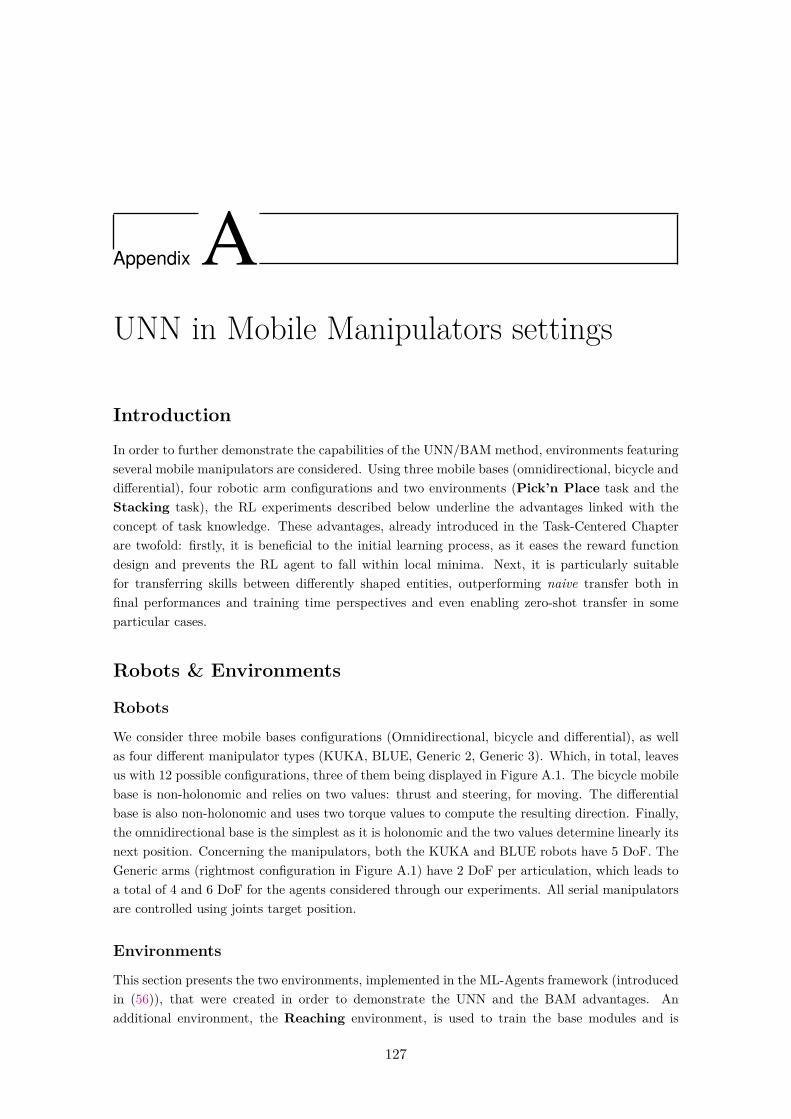
Appendix AUNN in Mobile Manipulators settings
Introduction
In order to further demonstrate the capabilities of the UNN/BAM method, environments featuringseveral mobile manipulators are considered. Using three mobile bases (omnidirectional, bicycle anddifferential), four robotic arm configurations and two environments (Pick’n Place task and theStacking task), the RL experiments described below underline the advantages linked with theconcept of task knowledge. These advantages, already introduced in the Task-Centered Chapterare twofold: firstly, it is beneficial to the initial learning process, as it eases the reward functiondesign and prevents the RL agent to fall within local minima. Next, it is particularly suitablefor transferring skills between differently shaped entities, outperforming naive transfer both infinal performances and training time perspectives and even enabling zero-shot transfer in someparticular cases.
Robots & Environments
Robots
We consider three mobile bases configurations (Omnidirectional, bicycle and differential), as wellas four different manipulator types (KUKA, BLUE, Generic 2, Generic 3). Which, in total, leavesus with 12 possible configurations, three of them being displayed in Figure A.1. The bicycle mobilebase is non-holonomic and relies on two values: thrust and steering, for moving. The differentialbase is also non-holonomic and uses two torque values to compute the resulting direction. Finally,the omnidirectional base is the simplest as it is holonomic and the two values determine linearly itsnext position. Concerning the manipulators, both the KUKA and BLUE robots have 5 DoF. TheGeneric arms (rightmost configuration in Figure A.1) have 2 DoF per articulation, which leads toa total of 4 and 6 DoF for the agents considered through our experiments. All serial manipulatorsare controlled using joints target position.
Environments
This section presents the two environments, implemented in the ML-Agents framework (introducedin (56)), that were created in order to demonstrate the UNN and the BAM advantages. Anadditional environment, the Reaching environment, is used to train the base modules and is
127
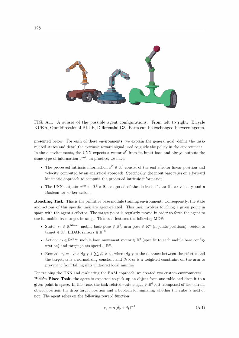
128
FIG. A.1. A subset of the possible agent configurations. From left to right: BicycleKUKA, Omnidirectional BLUE, Differential G3. Parts can be exchanged between agents.
presented below. For each of these environments, we explain the general goal, define the task-related states and detail the extrinsic reward signal used to guide the policy in the environment.In these environments, the UNN expects a vector si′ from its input base and always outputs thesame type of information oout. In practice, we have:
• The processed intrinsic information si′ ∈ R6 consist of the end effector linear position andvelocity, computed by an analytical approach. Specifically, the input base relies on a forwardkinematic approach to compute the processed intrinsic information.
• The UNN outputs oout ∈ R3 × B, composed of the desired effector linear velocity and aBoolean for sucker action.
Reaching Task: This is the primitive base module training environment. Consequently, the stateand actions of this specific task are agent-related. This task involves touching a given point inspace with the agent’s effector. The target point is regularly moved in order to force the agent touse its mobile base to get in range. This task features the following MDP:
• State: st ∈ R16+n: mobile base pose ∈ R3, arm pose ∈ Rn (n joints positions), vector totarget ∈ R3, LIDAR sensors ∈ R10
• Action: at ∈ R2+n: mobile base movement vector ∈ R2 (specific to each mobile base config-uration) and target joints speed ∈ Rn.
• Reward: rt = −α × dE,T +∑
i βi × ci, where dE,T is the distance between the effector andthe target, α is a normalizing constant and βi × ci is a weighted constraint on the arm toprevent it from falling into undesired local minima
For training the UNN and evaluating the BAM approach, we created two custom environments.Pick’n Place Task: the agent is expected to pick up an object from one table and drop it to agiven point in space. In this case, the task-related state is spap ∈ R6 ×B, composed of the currentobject position, the drop target position and a boolean for signaling whether the cube is held ornot. The agent relies on the following reward function:
rp = α(d0 + d1)−1 (A.1)
APPENDIX A. UNN IN MOBILE MANIPULATORS SETTINGS 129
where the reward rp for the Pick’n Place environment depends on α a positive scaling factor, d0
the distance from the object to the effector and d1 the distance from the object to the drop targetposition.
Stacking Task: the goal is to stack a number of cubes. The task-related state is conceptuallysimilar to the Pick’n Place, that is sstacking ∈ R3∗c × B4 where c is the number of cubes to stack,in our case c = 4. We also design a reward that penalizes the agent according to the summeddistances between each of the cube and their ideal position. That is:
rs = [4∑
i=1αi(d0,i + d1,i)]−1 (A.2)
where the Stacking task reward rs depends on αi a positive scaling factor that is adjusted ac-cording to the agent progression in the task, d0,i the distance from the cube i to the effector andd1,i the distance from the cube i to its target position.
Training setupWhile RL excels in reactive environments, it is usually less straightforward to design reward func-tions for sequential environments like those presented above. Indeed, in these cases, tuning thereward function in order to balance between a negative reward that may induce divergence in theagent’s behaviour and a positive reward that may lead the agent to accumulate rewards without aclear line of action is very subtle and requires a considerable amount of tweaking. Thus, in orderto improve the learning performances, PPO is coupled with two additional techniques:
• Pre-training with a Behavior Cloning based (38) approach
• Inverse Reinforcement Learning (50)
In practice, the agent weights go through a first training phase that consists of Behaviour-Cloningpre-training. Namely, this initial process is a supervised training setup where the agent errorcorresponds to the distance between its action prediction and the expert output. Then, during theReinforcement Learning process, the agent loss function is enhanced with the Inverse ReinforcementLearning component. Specifically, this additional loss function evaluates how likely was the latestagent trajectory to be generated by expert policy. This additional loss is minimized when theagent’s sequences of states and actions are similar to the expert’s, thus providing a pedagogicsignal to the training agent.
ResultsIn this section, the results of our method on both training and testing setup, over all environ-ments are presented. In particular, we compare our architecture, the BAM modeling, with severalbaselines, namely the naive PPO approach and the UNN segmentation. A video of our results isavailable at https://bit.ly/324Sxnz.
Training
During training, we monitor the agent’s evolution through the mean cumulative reward per episode.This metrics is common in RL and serves as a measure of how well the agent behaves within its
130
0 100000 200000 300000 400000 500000
Steps700
600
500
400
300
200
100
0
100
Cum
ulat
ive
rewa
rd
Primitives
Omni. G2Bicy. KukaDiff. BlueOmni. G3
FIG. A.2. Training performances on Primitive reaching task for 4 predefined configurations
environment.Curves in Figure A.2 are specific to our architecture and measure the output base training per-formances with respect to the reaching task. Figure A.3 and Figure A.4 respectively display theseresults for the whole architecture (bases + UNN) for the Pick’n Place and Stacking environ-ments using an Omnidirectional Generic 2 robot configuration. Due to the intermediate modeloutputs, constrained through the bases, the UNN is able to learn the task more efficiently than anaive agent. As a matter of fact, we can see that both UNN-based techniques, in red and orangerespectively representing the UNN and the BAM approaches, clearly outperform the naive PPOapproach in blue. We note that the BAM (red) and UNN (orange) curves both reach a higher finalcumulative reward than the naive PPO, while also being faster, indicating a better performanceat solving the task overall.
Transfer
UNN-based approaches aim at making the skills transfer between agents of diverse constitutionspossible. Hence, after training, we pass pre-trained models on a given configuration to anotherone with a different structure and compare their performances. In an ideal case, pairing the UNNwould not require any fine-tuning. However, in practice, most cases require additional trainingiterations for the UNN to complete the adoption by another agent configuration. We displaysome examples of this process in Figure A.5 and Figure A.6, respectively for Pick’n Place andStacking environments. These curves show for each environment how fast the performance canbe recovered for a given configuration. Specifically, the y-axis measures the relative mean rewardof the current agent projected in the lowest-to-highest interval from all initial agents. The x-axisalso indicates how much of the initial training time was necessary to reach said performance.For the Pick’n Place environment, see Figure A.5, it appears that transfer within the naiveframework is not efficient and even detrimental to the agent. The policy weights when transferredto another agent do not provide a decent initialization point and, through our experiments, theseagents systematically failed at the task. On the contrary, using the UNN-based techniques allowsto jump-start the new agent configuration with an initial level of performance that exceeds 70%of the previous agent and allows to recover almost the full performance, evaluated by the mean
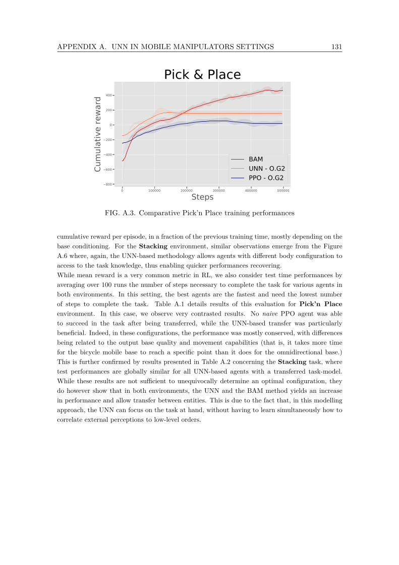
APPENDIX A. UNN IN MOBILE MANIPULATORS SETTINGS 131
0 100000 200000 300000 400000 500000
Steps800
600
400
200
0
200
400Cu
mul
ativ
e re
ward
Pick & Place
BAMUNN - O.G2PPO - O.G2
FIG. A.3. Comparative Pick’n Place training performances
cumulative reward per episode, in a fraction of the previous training time, mostly depending on thebase conditioning. For the Stacking environment, similar observations emerge from the FigureA.6 where, again, the UNN-based methodology allows agents with different body configuration toaccess to the task knowledge, thus enabling quicker performances recovering.While mean reward is a very common metric in RL, we also consider test time performances byaveraging over 100 runs the number of steps necessary to complete the task for various agents inboth environments. In this setting, the best agents are the fastest and need the lowest numberof steps to complete the task. Table A.1 details results of this evaluation for Pick’n Placeenvironment. In this case, we observe very contrasted results. No naive PPO agent was ableto succeed in the task after being transferred, while the UNN-based transfer was particularlybeneficial. Indeed, in these configurations, the performance was mostly conserved, with differencesbeing related to the output base quality and movement capabilities (that is, it takes more timefor the bicycle mobile base to reach a specific point than it does for the omnidirectional base.)This is further confirmed by results presented in Table A.2 concerning the Stacking task, wheretest performances are globally similar for all UNN-based agents with a transferred task-model.While these results are not sufficient to unequivocally determine an optimal configuration, theydo however show that in both environments, the UNN and the BAM method yields an increasein performance and allow transfer between entities. This is due to the fact that, in this modellingapproach, the UNN can focus on the task at hand, without having to learn simultaneously how tocorrelate external perceptions to low-level orders.
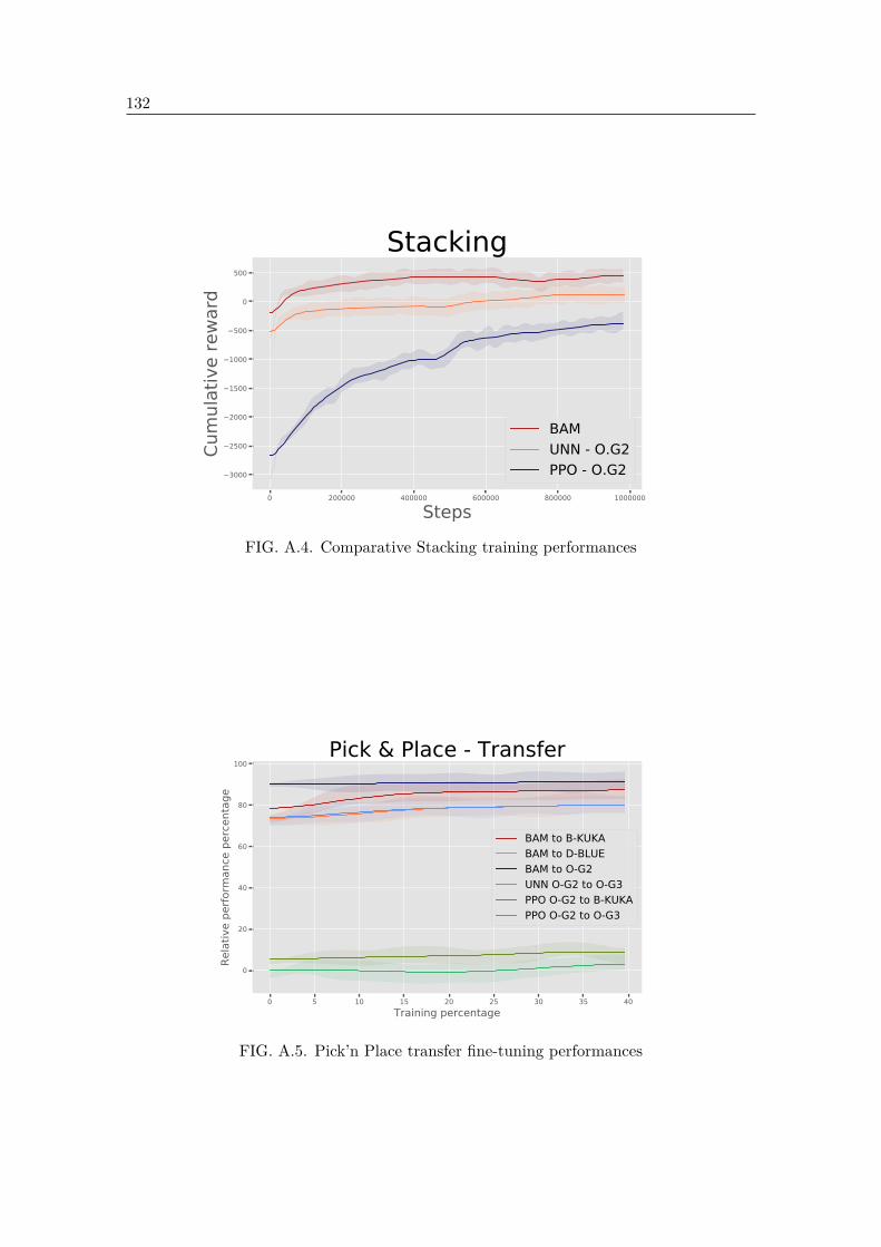
132
0 200000 400000 600000 800000 1000000
Steps
3000
2500
2000
1500
1000
500
0
500
Cum
ulat
ive
rewa
rdStacking
BAMUNN - O.G2PPO - O.G2
FIG. A.4. Comparative Stacking training performances
0 5 10 15 20 25 30 35 40Training percentage
0
20
40
60
80
100
Rela
tive
perfo
rman
ce p
erce
ntag
e
Pick & Place - Transfer
BAM to B-KUKABAM to D-BLUEBAM to O-G2UNN O-G2 to O-G3PPO O-G2 to B-KUKAPPO O-G2 to O-G3
FIG. A.5. Pick’n Place transfer fine-tuning performances

APPENDIX A. UNN IN MOBILE MANIPULATORS SETTINGS 133
0 10 20 30 40 50Training percentage
30
40
50
60
70
80
90
100
Rela
tive
perfo
rman
ce p
erce
ntag
e
Stacking - Transfer
BAM to B-KUKABAM to D-BLUEBAM to O-G2UNN O-G2 to O-G3PPO O-G2 to B-KUKAPPO O-G2 to O-G3
FIG. A.6. Stacking transfer fine-tuning
TABLE A.1. Transfer: Pick’n Place
Archi. Config. Agent Training % Perf.
PPOInitial Omni. Generic 2 100% 1355.4
TransferredOmni. Generic 3 40% FailBicy. KUKA 40% FailDiff. BLUE 40% Fail
UNNInitial Omni. Generic 2 100% 848.8
TransferredOmni. Generic 3 20% 784.8Bicy. KUKA 20% 801.7Diff. BLUE 20% 443.6
BAMInitial - 100% 412.3
TransferredOmni. Generic 2 20% 751.6Bicy. KUKA 20% 707.9Diff. BLUE 20% 747.7
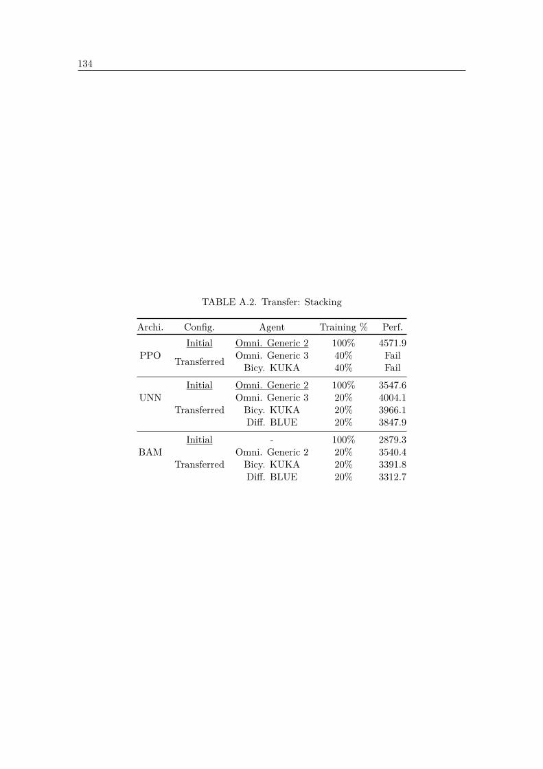
134
TABLE A.2. Transfer: Stacking
Archi. Config. Agent Training % Perf.
PPOInitial Omni. Generic 2 100% 4571.9
Transferred Omni. Generic 3 40% FailBicy. KUKA 40% Fail
UNNInitial Omni. Generic 2 100% 3547.6
TransferredOmni. Generic 3 20% 4004.1Bicy. KUKA 20% 3966.1Diff. BLUE 20% 3847.9
BAMInitial - 100% 2879.3
TransferredOmni. Generic 2 20% 3540.4Bicy. KUKA 20% 3391.8Diff. BLUE 20% 3312.7