ARTICLE IN PRESS

Neurocomputing 61 (2004) 503–512

0925-2312/$ -

doi:10.1016/j

�Correspo

116023, Chin

E-mail ad

www.elsevier.com/locate/neucom

Letters

Expectation–Maximization approaches toindependent component analysis

Mingjun Zhonga,b, Huanwen Tanga, Yiyuan Tangb,c,d,�

aInstitute of Computational Biology and Bioinformatics, Dalian University of Technology,

Dalian 116023, People’s Republic of ChinabInstitute of Neuroinformatics, Dalian University of Technology, Dalian 116023, People’s Republic of China

cLaboratory of Visual Information Processing, The Chinese Academy of Sciences, Beijing 100101,

People’s Republic of ChinadKey Lab for Mental Health, The Chinese Academy of Sciences, Beijing 100101, People’s Republic of China

Available online 20 August 2004

Abstract

Expectation–Maximization (EM) algorithms for independent component analysis are

presented in this paper. For super-Gaussian sources, a variational method is employed to

develop an EM algorithm in closed form for learning the mixing matrix and inferring the

independent components. For sub-Gaussian sources, a symmetrical form of the Pearson

mixture model (Neural Comput. 11 (2) (1999) 417–441) is used as the prior, which also enables

the development of an EM algorithm in fclosed form for parameter estimation.

r 2004 Elsevier B.V. All rights reserved.

Keywords: Independent component analysis; Overcomplete representations; EM algorithm; Variational

method

1. Introduction

Blind source separation (BSS) by independent component analysis (ICA) hasreceived great attention due to its potential signal processing applications

see front matter r 2004 Elsevier B.V. All rights reserved.

.neucom.2004.06.007

nding author. Institute of Neuroinformatics, Dalian University of Technology, Dalian

a. Tel.: +86-411-470-6039; fax: +86-411-470-9304.

dresses: sunxl_zhong@yahoo.com (M. Zhong), yy2100@163.net (Y. Tang).

ARTICLE IN PRESS

M. Zhong et al. / Neurocomputing 61 (2004) 503–512504

[1,2,4–6,8,10]. In particular, the following ICA model is considered in this paper

x ¼ As þ e; ð1Þ

where A 2 RN�M is the mixing matrix, x is an N-dimensional data vector, theelements of s which is an M-dimensional random vector define the independentcomponents, and e is the noise which is modelled as Gaussian with zero mean andcovariance matrix S: In ICA, the elements of s are assumed mutually statisticallyindependent denoting that the joint probability distribution of s is factorable, i.e.,pðsÞ ¼

QMm¼1 pðsmÞ; where p represents the probability density function (p.d.f.). The

aim of ICA is as follows: Given T observed data samples fxtgTt¼1; recover the mixing

matrix A, the original source sequences fstgTt¼1; and the noise covariance matrix S:

Several researchers have proposed various methods for estimating the mixingmatrix and the noise covariance matrix, in which the posterior moments areestimated by various approximation techniques [2,5,10,12,13]. In contrast to thesemethods, this paper presents a combined estimation method for the source signals,the mixing matrix and the noise covariance matrix based on the Expectation–Max-imization (EM) algorithm [3]. For super-Gaussian sources, a variational methodenables the posterior analytically tractable [4,7], which formulates an EM algorithmin closed form for parameter estimation. For sub-Gaussian sources, the Pearsonmixture model [8] is employed to be the source density, which naturally gives an EMalgorithm in closed form for parameter estimation.

2. Parameter estimation methods

In ICA, it has been shown that there are only two density models for the sourcepriors, i.e., the super-Gaussian density which has a positive kurtosis and the sub-Gaussian density which has a negative kurtosis.1 In this section, we will derive EMalgorithms in accordance with these two source densities, respectively.

2.1. Super-Gaussian density model

In ICA, a super-Gaussian density which has a positive kurtosis is placed on theindependent components. In particular, since the elements of s are assumed mutuallystatistically independent we employ the following factorable super-Gaussian densityas the source model [8]

pðsÞ ¼YMm¼1

1

ZðbÞGsm

ð0; 1Þcosh2=bðbsmÞ; ð2Þ

where the notation Gsmð0; 1Þ denotes a normal distribution computed at sm with zero

mean and unit variance, b is a constant and ZðbÞ is the normalizing coefficientirrelevant to s. This prior renders the posterior, i.e., pðsjx;A;SÞ; analytically

1For a scalar random variable y, kurtosis is defined in the zero-mean case by the equation kurtðyÞ ¼

Efy4g 3ðEfy2gÞ2 (For more details, see [6].)

ARTICLE IN PRESS

M. Zhong et al. / Neurocomputing 61 (2004) 503–512 505

intractable. In the following, we will derive a strict lower bound on this prior, whichgives a closed form for parameter estimation in an EM framework.

The prior density in Eq. (2) has a strict lower bound over the additionalvariational parameter x ¼ ðx1; x2; . . . ; xMÞ

T such that (see Appendix)

pðsÞXpðsjxÞ ¼YMm¼1

jðxmÞGsð0;LÞ; ð3Þ

where

L ¼ diagx1

x1 þ 2 tanhðbx1Þ; . . . ;

xM

xM þ 2 tanhðbxMÞ

� �:

Note that as b ! 1; the density in Eq. (2) becomes the following factorableLaplacian:

pðsÞ /YMm¼1

Gsmð0; 1Þ expð2jsmjÞX

YMm¼1

jðxmÞGsð0;LÞ; ð4Þ

where

L ¼ diagjx1j

jx1j þ 2; . . . ;

jxM j

jxM j þ 2

� �;

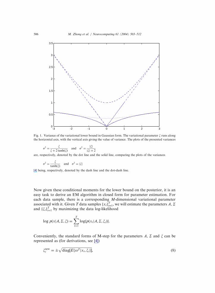
which is used as the interesting prior in learning sparse and overcompleterepresentations [10,4]. It should be noted that the variational lower bound on theprior derived in this paper is similar to the one presented by Girolami [4], whointroduced the variational method into learning sparse and overcompleterepresentations. (For a specific application of the variational method to machinelearning, see [7].) Fig. 1 shows ranges of the variances of the lower bounds in theGaussian form presented in this paper and those proposed by Girolami [4], i.e., thevariances of the lower bounds in this paper belong to ½0; 1Þ and the ones presented in[4] belong to ½0;1Þ; reflecting that the prior employed in this paper has a smallervariance than the one used in [4]. Furthermore, given the previous strict lower boundon the prior, the corresponding posterior can be represented as a strict lower boundin Gaussian form

pðsjx;A;SÞXpðsjx;A;S; xÞ ¼pðxjs;A;SÞpðsjxÞRpðxjs;A;SÞpðsjxÞds

¼GxðAs;SÞGsð0;LÞRGxðAs;SÞGsð0;LÞds

: ð5Þ

Thus, a normal form of the following variational moments can be easily obtainedbased on the posterior pðsjx;A;S; xÞ:

Efsjxt; xtg ¼ ðATS1A þ L1t Þ

1ATS1xt; ð6Þ

EfssT jxt; xtg ¼ ðATS1A þ L1t Þ

1þ Efsjxt; xtgEfsjxt; xtg

T : ð7Þ

ARTICLE IN PRESS

-3 -2 -1 0 1 2 30

0.5

1

1.5

2

2.5

3

3.5

Fig. 1. Variance of the variational lower bound in Gaussian form. The variational parameter x runs along

the horizontal axis, with the vertical axis giving the value of variance. The plots of the presented variances

s2 ¼x

xþ 2 tanhðxÞand s2 ¼

jxjjxj þ 2

are, respectively, denoted by the dot line and the solid line, comparing the plots of the variances

s2 ¼x

tanhðxÞand s2 ¼ jxj

[4] being, respectively, denoted by the dash line and the dot-dash line.

M. Zhong et al. / Neurocomputing 61 (2004) 503–512506

Now given these conditional moments for the lower bound on the posterior, it is aneasy task to derive an EM algorithm in closed form for parameter estimation. Foreach data sample, there is a corresponding M-dimensional variational parameterassociated with it. Given T data samples fxtg

Tt¼1; we will estimate the parameters A, S

and fxtgTt¼1 by maximizing the data log-likelihood

log pðxjA;S; xÞ ¼XT

t¼1

logfpðxtjA;S; xtÞg:

Conveniently, the standard forms of M-step for the parameters A, S and x can berepresented as (for derivations, see [4])

xnewt ¼ �

ffiffiffiffiffiffiffiffiffiffiffiffiffiffiffiffiffiffiffiffiffiffiffiffiffiffiffiffiffiffiffiffiffiffiffiffidiag½EfssT jxt; xtg�

p; ð8Þ

ARTICLE IN PRESS

M. Zhong et al. / Neurocomputing 61 (2004) 503–512 507

Anew ¼XT

t¼1

xtEfsjxt; xtgT

( ) XT

t¼1

EfssT jxt; xtg

( )1

; ð9Þ

Snew ¼1

T

XT

t¼1

fxtxTt AnewEfsjxt; xtgx

Tt g: ð10Þ

Note that

Mt ¼ ðATS1A þ L1t Þ

1¼ Lt LtA

T ðALtAT þ SÞ1ALt: ð11Þ

This transformation of the matrix inversion allows a really hard inverse to beconverted into an easy inverse especially when considering BSS of more sources thanmixtures, i.e., A has many columns but few rows. Inserting the terms for thevariational posterior moments into Eq. (8)–(10) gives the following updates for theparameters A, S; and x:

xnewt ¼ �

ffiffiffiffiffiffiffiffiffiffiffiffiffiffiffiffiffiffiffiffiffiffiffiffiffiffiffiffiffiffiffiffiffiffiffiffiffiffiffiffiffiffiffiffiffiffiffiffiffiffiffiffiffiffiffiffiffiffiffiffiffiffiffiffiffiffiffiffiffiffiffidiag½MtfI þ ATS1xtxT

t S1AMtg�

q; ð12Þ

Anew ¼XT

t¼1

xtxTt S

1AMTt

( ) XT

t¼1

MtfI þ ATS1xtxTt S

1AMtg

( )1

; ð13Þ

Snew ¼1

T

XT

t¼1

xtxTt Anew 1

T

XT

t¼1

MtATS1xtx

Tt : ð14Þ

Eq. (12) serves to improve the variational data likelihood pðxjA;S; xÞ to the true datalikelihood, and the convergence properties of the EM algorithm [3] ensure thatpðxjA;SÞXpðxjA;S; xnew

ÞXpðxjA;S; xoldÞ:

2.2. Sub-Gaussian density model

For sources with sub-Gaussian densities, the following Pearson mixture model inthe univariate case is employed in this paper [8]:

pðsÞ ¼ 12ðGsðm; s2Þ þ Gsðm; s2ÞÞ: ð15Þ

This mixture model is a symmetric strictly sub-Gaussian density and may serve as asuitable density for computing the score function of symmetric sub-Gaussiansources. Lee et al. [8] had derived a learning rule for complete ICA without additivenoise. Actually, this Pearson mixture model makes the posterior analyticallytractable and thus it is not required to employ various approximations for it such

ARTICLE IN PRESS

M. Zhong et al. / Neurocomputing 61 (2004) 503–512508

that

pðsjx;A;SÞ ¼pðxjs;A;SÞpðsÞRpðxjs;A;SÞpðsÞds

¼GxðAs;SÞGsðm;VÞ þ GxðAs;SÞGsðm;VÞR

GxðAs;SÞGsðm;VÞds þR

GxðAs;SÞGsðm;VÞds; ð16Þ

where V ¼ s2I: Note that W ¼ ðATS1A þ V1Þ1

¼ V VAT ðAVAT þ SÞ1AV:This posterior conveniently gives the following moments:

Efsjxtg ¼ WATS1xt; ð17Þ

EfssT jxtg ¼ W þ W ðATS1xtxTt S

1A þ V1mmT VT ÞW T : ð18Þ

Inserting these moments into Eqs. (9) and (10) gives the following updates:

Anew ¼XT

t¼1

xtxTt S

1AW T

( )

�XT

t¼1

W I þ ðATS1xtxTt S

1A þ V1mmT VT ÞW T� ( )1

; ð19Þ

Snew ¼1

T

XT

t¼1

xtxTt Anew 1

T

XT

t¼1

WATS1xtxTt : ð20Þ

3. Simulations

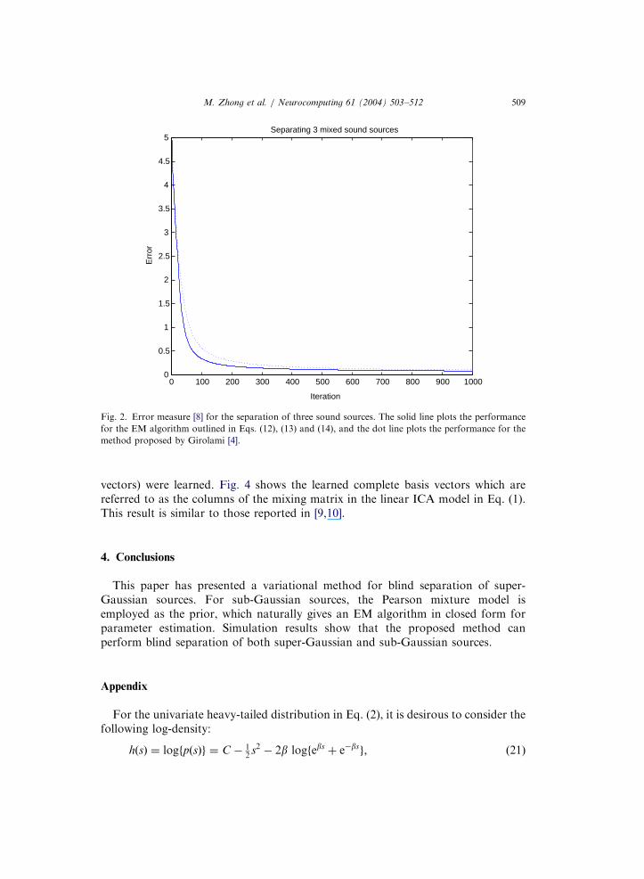
To compare this proposed method with Girolami’s EM algorithm [4], where theprior was set to be pðsÞ ¼ cosh1

ðsÞ; the error measure used in [8] was computed inthe first experiment for standard BSS with three speech sources (see Fig. 2). Theresult shows that the performance of the proposed method is similar to Girolami’sEM algorithm, though the proposed method slightly increased the convergencespeed in this experiment.

The second experiment shows the ability of the proposed EM algorithm toperform blind separation of binary sources with more sources than observations.Fig. 3 shows the result. The complexity of Pajunen’s method [11] growsexponentially with the number of the sources, whereas the complexity of this EMalgorithm scales as OðN3Þ:

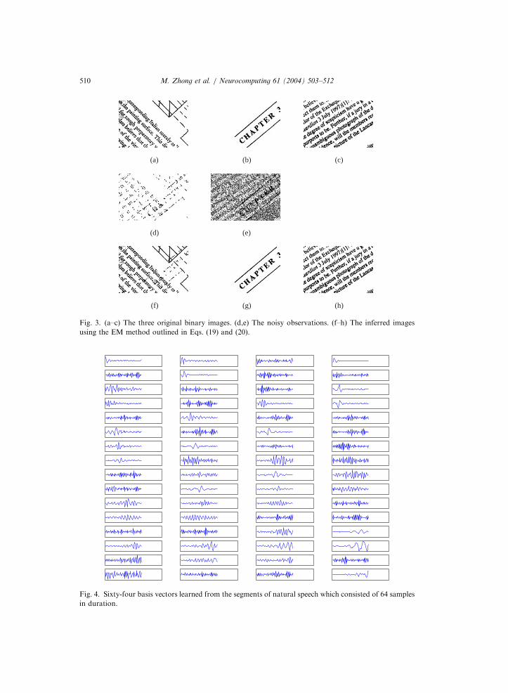
The third experiment shows the ability of the method to learn sparserepresentation for speech data which were obtained from the TIMIT database,using the speech of a single speaker, speaking 10 different example sentences. Speechsegments with 64 samples were randomly selected from the 10 speech signals, whereeach of the speech signals has 16 bits per sample at the sampling frequency of16 000 HZ. Both a complete (64 basis vectors) and an overcomplete basis (128 basis

ARTICLE IN PRESS

0 100 200 300 400 500 600 700 800 900 10000

0.5

1

1.5

2

2.5

3

3.5

4

4.5

5Separating 3 mixed sound sources

Iteration

Err

or

Fig. 2. Error measure [8] for the separation of three sound sources. The solid line plots the performance

for the EM algorithm outlined in Eqs. (12), (13) and (14), and the dot line plots the performance for the

method proposed by Girolami [4].

M. Zhong et al. / Neurocomputing 61 (2004) 503–512 509

vectors) were learned. Fig. 4 shows the learned complete basis vectors which arereferred to as the columns of the mixing matrix in the linear ICA model in Eq. (1).This result is similar to those reported in [9,10].

4. Conclusions

This paper has presented a variational method for blind separation of super-Gaussian sources. For sub-Gaussian sources, the Pearson mixture model isemployed as the prior, which naturally gives an EM algorithm in closed form forparameter estimation. Simulation results show that the proposed method canperform blind separation of both super-Gaussian and sub-Gaussian sources.

Appendix

For the univariate heavy-tailed distribution in Eq. (2), it is desirous to consider thefollowing log-density:

hðsÞ ¼ logfpðsÞg ¼ C 12

s2 2b logfebs þ ebsg; ð21Þ

ARTICLE IN PRESS

(a) (b) (c)

(d) (e)

(f) (g) (h)

Fig. 3. (a–c) The three original binary images. (d,e) The noisy observations. (f–h) The inferred images

using the EM method outlined in Eqs. (19) and (20).

Fig. 4. Sixty-four basis vectors learned from the segments of natural speech which consisted of 64 samples

in duration.

M. Zhong et al. / Neurocomputing 61 (2004) 503–512510

ARTICLE IN PRESS

M. Zhong et al. / Neurocomputing 61 (2004) 503–512 511

where C ¼ log 4ffiffiffiffi2p

p : It can be seen that this log-prior is convex in s2 due to logfebs þ

ebsg being convex in s2 [7]. Thus, the variational representation for hðsÞ has thefollowing form [7]:

hðsÞ ¼ maxx

fðs2 x2Þrx2 hðxÞ þ hðxÞg; ð22Þ

where rx2 denotes the gradient with respect to x2: It should be indicated that themaximum in the above representation is naturally attained for s2 ¼ x2: Thisconveniently gives the following expression:

pðsÞ ¼ maxx

½jðxÞGsð0; s2xÞ�; ð23Þ

where

jðxÞ ¼ pðxÞ expx2

þ 2x tanhðbxÞ2

� � ffiffiffiffiffiffiffiffiffiffi2ps2

x

qand s2

x ¼x

xþ 2 tanhðbxÞ:

Acknowledgements

We are indebted to Hongjun Chen for his helpful comments on the manuscript.The work was supported by NSFC (30170321, 90103033), MOST (2001CCA00700)and MOE (KP0302).

References

[1] A.J. Bell, T.J. Sejnowski, An information-maximization approach to blind separation and blind

deconvolution, Neural Comput. 7 (6) (1995) 1129–1159.

[2] A. Belouchrani, J.-F. Cardoso, Maximum likelihood source separation by the expectation—

maximization technique: deterministic and stochastic implementation, in: Proceedings of NOLTA,

1995, pp. 49–53.

[3] A.P. Dempster, N.M. Laird, D.B. Rubin, Maximum likelihood from incomplete data via the EM

algorithm, J. R. Stat. Soc. B 39 (1) (1977) 1–38.

[4] M. Girolami, A variational method for learning sparse and overcomplete representations, Neural

Comput. 13 (11) (2001) 2517–2532.

[5] P.A.d.E.R. Hojen-Sorensen, O. Winther, L.K. Hansen, Mean-field approaches to independent

component analysis, Neural Comput. 14 (4) (2002) 889–918.

[6] A. Hyvarinen, J. Karhunen, E. Oja, Independent Component Analysis, Wiley, New York, 2001.

[7] T.S. Jaakkola, Variational methods for inference and estimation in graphical models, Unpublished

Doctoral Dissertation, MIT, 1997.

[8] T.-W. Lee, M. Girolami, T.J. Sejnowski, Independent component analysis using an extended infomax

algorithm for mixed subgaussian and supergaussian sources, Neural Comput. 11 (2) (1999) 417–441.

[9] M.S. Lewicki, Efficient coding of natural sounds, Nat. Neurosci. 5 (4) (2002) 356–363.

[10] M.S. Lewicki, T.J. Sejnowski, Learning overcomplete representations, Neural Comput. 12 (2) (2000)

337–365.

[11] P. Pajunen, Blind separation of binary sources with less sensors than sources, in: Proceedings of 1997

International Conference on Neural Networks, vol. 3, 1997, pp. 1994–1997.

[12] Z.-W. Shi, H.-W. Tang, W.-Y. Liu, Y.-Y. Tang, Blind source separation of more sources than

mixtures using generalized exponential mixture models, Neurocomputing (2004), in press.

[13] M.-J. Zhong, H.-W. Tang, H.-J. Chen, Y.-Y. Tang, An EM algorithm for learning sparse and

overcomplete representations, Neurocomputing 57 (2004) 469–476.

ARTICLE IN PRESS

M. Zhong et al. / Neurocomputing 61 (2004) 503–512512

Mingjun Zhong studied mathematics and obtained his Ph.D. degree at the Dalian

University of Technology (China) in 2004. He was working at the Institute of

Neuroinformatics and the Institute of Computational Biology and Bioinformatics

of the Dalian University of Technology. His research interests include

independent component analysis, sparse coding, bioinformatics, and neuroinfor-

matics.

Tang Huanwen graduated from the Dalian University of Technology in 1963, and

currently a professor of mathematics and management engineering at the Dalian

University of Technology. His research interest includes computational models

and algorithm of human cognition and neural information coding, bioinformatics

and neuroinformatics. (Home page: http://brain.dlut.edu.cn)

Tang Yiyuan graduated from the Jinlin University in 1987, and currently a

professor of neuroinformatics and neuroscience at the Dalian University of

Technology. His research interest includes neuroimaging, cognition and emotion

interaction, neuroinformatics. (Home page: http://brain.dlut.edu.cn)