evaluation of serviceability of canal lining based on ahp

sustainability

Article

Evaluation of Serviceability of Canal Lining Based onAHP–Simple Correlation Function Method–Cloud Model:A Case Study in Henan Province, China

Qingfu Li 1, Huade Zhou 1,* , Qiang Ma 2 and Linfang Lu 2

��

Citation: Li, Q.; Zhou, H.; Ma, Q.; Lu,

L. Evaluation of Serviceability of

Canal Lining Based on AHP–Simple

Correlation Function Method–Cloud

Model: A Case Study in Henan

Province, China. Sustainability 2021,

13, 12314. https://doi.org/10.3390/

su132112314

Academic Editors: Mashor Housh

and Marc A. Rosen

Received: 6 August 2021

Accepted: 3 November 2021

Published: 8 November 2021

Publisher’s Note: MDPI stays neutral

with regard to jurisdictional claims in

published maps and institutional affil-

iations.

Copyright: © 2021 by the authors.

Licensee MDPI, Basel, Switzerland.

This article is an open access article

distributed under the terms and

conditions of the Creative Commons

Attribution (CC BY) license (https://

creativecommons.org/licenses/by/

4.0/).

1 School of Water Conservancy Engineering, Zhengzhou University, Zhengzhou 450001, China; [email protected] Construction Management Bureau of the Second Phase Project of Zhaokou Irrigation District of the Yellow

River, Kaifeng 475000, China; [email protected] (Q.M.); [email protected] (L.L.)* Correspondence: [email protected]

Abstract: In the process of sustainable development within modern agriculture, in order to ensurethat agricultural production has adequate water resources, canal lining (CL) is often used to transportwater in order to reduce water seepage, thus promoting the sustainable utilization of water resources.However, due to the influence of the terrain, environment, human factors and other factors, the CLoften suffers a certain degree of damage. Therefore, it is necessary to evaluate the serviceability ofthe CL, so to realize the sustainable use of the CL strategy. Aiming at the weight assignment of CLevaluation indices that are subjective and not combined with actual index data, a weight calculationmethod based on the Analytic Hierarchy Process (AHP)–simple correlation function (SCF) methodwas proposed, and game theory was used to achieve combination weighting. For the evaluationindices with the characteristics of fuzziness and randomness, the cloud model (CM) was used tocomprehensively consider these characteristics in order to realize the evaluation. Finally, a method tomeasure serviceability of CL based on AHP–SCF–CM was proposed. Taking a CL project in Chinaas an example, this method was used to evaluate the serviceability of the CL. The evaluation resultshowed that the serviceability of the CL was poor, and the qualitative evaluation result was consistentwith the actual damage condition of the project; meanwhile, a comparative study was performed incombination with the AHP–Entropy Weight (EW)–unascertained measurement theory (UMT). Thequantitative evaluation results of the two methods displayed the same grade of serviceability, whichverifies that the method proposed in this paper is more reasonable, objective and feasible from bothqualitative and quantitative perspectives. Furthermore, the evaluation results lay the foundation forsubsequent maintenance and fault prevention of the canal.

Keywords: canal lining; serviceability; AHP; simple correlation function; cloud model; game the-ory; entropy

1. Introduction

With the rapid development of China’s economy and society and the rapid increasein the population, the problem of insufficient water supply for industry, agriculture andeveryday life is becoming increasingly serious [1,2]. In order to solve this problem, Chinahas actively taken various targeted measures, such as the implementation of numerouswater storage and water diversion projects. In order to address the shortage of agriculturalwater resources in some areas along the Yellow River, China has implemented the YellowRiver irrigation area project to divert water from the river to the irrigation areas throughcanal lining. This can effectively alleviate the agricultural irrigation problem, improvethe overall grain output of the country and promote the sustainable development of theregional ecological environment.

The canal lining (CL) is an additional layer construct on the top of the existing structure,rather than a separate structure, which is composed of stone, cement slab and other

Sustainability 2021, 13, 12314. https://doi.org/10.3390/su132112314 https://www.mdpi.com/journal/sustainability

https://www.mdpi.com/journal/sustainability

https://www.mdpi.com

https://orcid.org/0000-0002-2097-1758

https://doi.org/10.3390/su132112314

https://doi.org/10.3390/su132112314

https://creativecommons.org/

https://creativecommons.org/licenses/by/4.0/

https://creativecommons.org/licenses/by/4.0/

https://doi.org/10.3390/su132112314

https://www.mdpi.com/journal/sustainability

https://www.mdpi.com/article/10.3390/su132112314?type=check_update&version=1

Sustainability 2021, 13, 12314 2 of 25

materials, implemented along the bottom and both sides of the slope of a canal. Its mainfunction is to transport water while reducing water loss, improving the effective use ofwater resources. Based on the principles of hydraulics and operational research, it is knownthat the water delivery capacity of CL depends on the shape, size and material of thewater-crossing section. If there are any defects within CL material, the water deliverycapacity of the canal will be greatly reduced [3]. The most commonly used material forCL is concrete. Although a concrete lining can effectively reduce water leakage duringwater transportation and increase the water utilization coefficient of the canal system [4],at the same time, concrete is prone to cracks due to plastic shrinkage and drying shrinkage,which seriously affects the serviceability of the CL. Operational research is an importantfoundation of modern management, which mainly includes decision theory and gametheory. Decision theory is a system analysis method, which is mainly developed to solveproblems with uncertainty, and the Analytical Hierarchy Process (AHP) is commonly usedas decision analysis method. Game theory is a decision analysis method, which is mainlyto solve the conflicts between the two parties in the game, to study a reasonable action planthat is beneficial to all parties. By using operational research to carry out weight assignmentand decision analysis on the evaluation indicators (concrete lining plate cracking, etc.) ofthe CL, and combining with evaluation methods, the evaluation of the serviceability of theCL can be realized.

Some scholars have conducted research on the frost damage in CL, Li et al. [5] con-ducted a model test on CL in the context of a freeze–thaw cycle in order to investigate themechanisms of freeze damage in canals in cold regions. Wang et al. [6] pointed out thatunder the effect of seasonal frost heave, the most basic type of failure in concrete CL iscracking, with cracks beginning to appear at the bottom and sides of the CL. Li et al. [7]proposed a new type of anti-frost heave structure for CL, which is composed of concreteslab, polystyrene insulation board, a sand gravel layer and composite geomembrane. Inaddition to frost damage in the CL, the seepage loss of water also tends to affect its ser-viceable performance. Han et al. [8] believed that the factors leading to seepage and thusaffecting the serviceability of CL include the soil hydraulic characteristics, the type of liningmaterial, the failure conditions and the time of use of the lining. Asl et al. [9] analyzedsome soil canals in the river basins of Iran and Turkey; the finite element method wasused to numerically simulate 246 trapezoidal, rectangular and triangular soil troughs withdifferent cross-sections. Eshetu et al. [10] used the inflow–outflow method to measure theleakage of the primary, secondary and tertiary canals in order to quantify the seepage of thelined and unlined irrigation canals of the Tendaho sugar plantation in Ethiopia. At present,the most commonly used methods for the comprehensive evaluation of schemes includethe grey relational analysis method [11,12], technique for order preference by similarityto ideal solution (TOPSIS) [13,14], unascertained measure theory [15] and so on. In orderto evaluate the influence of a geotextile (geosynthetic polymer material) lining on slopeinstability, Eltarabily et al. [16] selected four different lining positions in the Ismailia canalas their object of study and used the canal geometry and soil properties as variables, andafter specifying the physical properties of the soil and geotextile material, the SLOPE/Wmodule of the GeoStudio finite element software was used. The results showed that, inthe four studied sections, only two sections had normal safety factors. El-Molla et al. [17]used the SEEP/W model (which is a sub-program of GeoStudio) to study the effect ofcompacted soil lining characteristics on the seepage of trapezoidal soil canals. The hy-draulic conductivity, thickness and direction of the compacted soil lining were evaluatedin different ways. Cui et al. [18] focused on the concrete cracks that occurred during theconstruction and operation periods of the CL and classified the factors that caused thecracks based on the collected data. The 3D contact nonlinear finite element method is alsoused to evaluate the sensitivity of these factors. Moavenshahidi et al. [19] developed a newcomputer model that applied the pondage test method to automatic control data duringriver closure in order to estimate the seepage rate of different river sections. The model wasapplied to estimate the seepage rate of each depth gauge, pondage and pool, and various


effects on the selected pool were analyzed. Solomon et al. [20] studied the steady-stateseepage problem from an irrigation canal to an asymmetric trapezoidal concrete-linedcanal, and the effectiveness of clay–cement concrete lining materials was evaluated. Lundet al. [21] used a polymer sealant linear anionic polyacrylamide, as an anti-seepage materialto evaluate its effectiveness in reducing seepage losses in earthen canals. Si [22] used thewater quality comprehensive pollution index evaluation method, the fuzzy comprehensiveevaluation method and the comprehensive water quality identification index evaluationmethod to evaluate the current situation of water quality in a canal, and the results showedthat the comprehensive water quality mark index evaluation method is more applicableto the evaluation of the current water quality. Shi et al. [23] evaluated the effects of threeanti-frost heave measures for a canal in the northern alpine region from the perspectivesof fetching materials and the ease of construction, they established constitutive models ofconcrete, HAS (a new type of cementitious material composed of water-hardened slag withindustrial waste as the main raw material), curing–agent–solidified fly ash and polystyrenefoam board lining materials. Mo et al. [24] evaluated the effect of adding a compositegeomembrane on the improvement of frost heave in concrete CL, and they monitored thefrost heave of a canal with a trapezoidal concrete lining for 67 days. The results showed thatthe composite geomembrane technology can reduce the normal frost heave displacementby 14.3% and the frost heave force by 15.5%, and the improvement effect is significant.Kahlown et al. [25] constructed conventional test sections and low-cost test sections in orderto evaluate the effectiveness of various types of lining in reducing water seepage losses infield canals, and the results indicated that a low-cost lining was a better investment than aconventional lining. They recommended the use of 11 cm-thick brick conversion walls or2:1 tilt-up walls as low–cost linings.

Many scholars have carried out a great deal of work on canal evaluation and haveachieved certain results. However, with the perennial operation of the CL, the CL isaffected by various factors such as loads, environment, construction quality and otherfactors. As a result, the serviceability of the lining deteriorates from good to seriouslydamaged. Therefore, an objective methodology for the evaluation of the serviceability ofCL would be useful for the national maintenance management department in order toensure that agricultural water supplies can be maintained.

Due to the uncertainty of human factors and the ambiguity of qualitative indexdivision in CL construction, the evaluation index has the characteristics of fuzziness,randomness, etc. The cloud model (CM) can reflect the randomness of such factors in thetransformation process to achieve qualitative and quantitative mapping that is suitable forevaluating problems with the characteristics of ambiguity and uncertainty [26]. In addition,in this study, the more practical multi-scheme, multi-objective decision-making method inoperational research, the Analytical Hierarchy Process (AHP), was used to determine theobjectives of the decision, and through the construction of a hierarchical structure model,experts were invited to provide decision-making scores to achieve subjective weighting.In addition, the simple correlation function (SCF) method was used to achieve objectiveweighting, and game theory was used to combine subjective and objective weights toeffectively solve the one-sided and limited problems caused by the single weighting ofevaluation index values. Based on this, a CL serviceability evaluation method based onAHP–SCF–CM was proposed.

2. Methods2.1. Evaluation MethodCloud Model (CM)

The CM is a model for the conversion of qualitative concepts and quantitative valuesproposed on the basis of fuzzy set theory and probability, and it can reveal the inherentrelevance of the randomness and ambiguity of certain factors or concepts themselves [27].It was first proposed in 1995 by Li Deyi, an academician of the Chinese Academy ofEngineering, and has been applied in many fields, such as risk assessment [28] and engi-


neering benefit evaluation [29]. A CM can take the form of a rectangular cloud, trapezoidalcloud, normal cloud, etc. The normal CM is widely used due to its unique mathematicalcharacteristics and versatility.

(1) Definition of Normal CloudDefinition of normal cloud: Assume that U is a quantitative domain and expressed

by precise numerical values, and C is a qualitative concept of U. A normal cloud can bedefined if the quantitative value x∈U, and x is a random realization of the qualitativeconcept C, if it satisfies x~N(Ex, En

2), where En2~N(En, He

2), and the degree of membershipto C satisfies:

µ(x) = e[− (x−Ex)2

2(En)2]

(1)

where Ex is the expected value; En is the entropy value; He is the super entropy.(2) Digital Characteristics of CMThe CM includes the following three digital features: expected value Ex, entropy En,

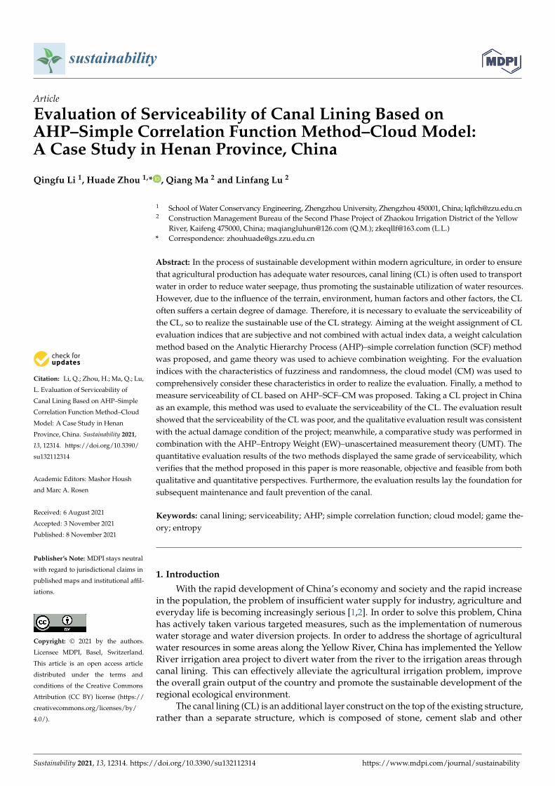
and super entropy He. Among them, Ex represents the expected value of the CM, which isa central value of the qualitative concept C in U, which is the most typical point with whichto quantify the concept; En, as a metric, is determined by both randomness and ambiguity,and the larger its value is, the more qualitative the concept is, making it difficult to quantifyits certainty; He is a metric that measures the uncertainty of entropy, which is related to thedegree of dispersion of cloud droplets, and can indirectly reflect the thickness of the cloud.A schematic diagram of the digital features of a CM is shown in Figure 1.

Sustainability 2021, 13, x FOR PEER REVIEW 4 of 26

relevance of the randomness and ambiguity of certain factors or concepts themselves [27].

It was first proposed in 1995 by Li Deyi, an academician of the Chinese Academy of Engi‐

neering, and has been applied in many fields, such as risk assessment [28] and engineering

benefit evaluation [29]. A CM can take the form of a rectangular cloud, trapezoidal cloud,

normal cloud, etc. The normal CM is widely used due to its unique mathematical charac‐

teristics and versatility.

(1) Definition of Normal Cloud

Definition of normal cloud: Assume that U is a quantitative domain and expressed

by precise numerical values, and C is a qualitative concept of U. A normal cloud can be

defined if the quantitative value xU, and x is a random realization of the qualitative concept C, if it satisfies x~N(Ex, En2), where En2~N(En,He2), and the degree of membership

to C satisfies:

2

2

( )[ ]

2( )( )x

n

x E

Ex e

(1)

where Ex is the expected value; En is the entropy value; He is the super entropy.

(2) Digital Characteristics of CM

The CM includes the following three digital features: expected value Ex, entropy En,

and super entropy He. Among them, Ex represents the expected value of the CM, which is

a central value of the qualitative concept C in U, which is the most typical point with

which to quantify the concept; En, as a metric, is determined by both randomness and

ambiguity, and the larger its value is, the more qualitative the concept is, making it diffi‐

cult to quantify its certainty; He is a metric that measures the uncertainty of entropy, which

is related to the degree of dispersion of cloud droplets, and can indirectly reflect the thick‐

ness of the cloud. A schematic diagram of the digital features of a CM is shown in Figure

1.

Figure 1. Schematic diagram of digital features of CM.

(3) Cloud Generator

The cloud generator is used to convert qualitative indicators and quantitative values

into one another. There are three types of cloud generators: (1) Forward Cloud Generator

(FCG), which converts qualitative to quantitative—the calculation flowchart of the FCG is

shown in Figure 2; (2) Backward Cloud Generator (BCG), which converts qualitative to

qualitative; (3) X cloud generator and Y cloud generator constitute a special conditional

cloud generator, in which C (Ex, En, He) is known and a specific value X or Y is used to

calculate the degree of certainty.

Figure 1. Schematic diagram of digital features of CM.

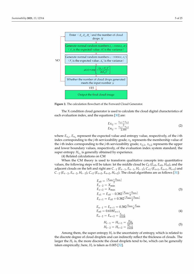
(3) Cloud GeneratorThe cloud generator is used to convert qualitative indicators and quantitative values

into one another. There are three types of cloud generators: (1) Forward Cloud Generator(FCG), which converts qualitative to quantitative—the calculation flowchart of the FCG isshown in Figure 2; (2) Backward Cloud Generator (BCG), which converts qualitative toqualitative; (3) X cloud generator and Y cloud generator constitute a special conditionalcloud generator, in which C (Ex, En, He) is known and a specific value X or Y is used tocalculate the degree of certainty.

Sustainability 2021, 13, 12314 5 of 25Sustainability 2021, 13, x FOR PEER REVIEW 5 of 26

Figure 2. The calculation flowchart of the Forward Cloud Generator.

The X condition cloud generator is used to calculate the cloud digital characteristics

of each evaluation index, and the equations [30] are:

,1 ,2

,1 ,2

2

2.355

ij ijij

ij ijij

x xEx

x xEn

(2)

where ijij

x nE E、 represent the expected value and entropy value, respectively, of the i‐th

index corresponding to the j‐th serviceability grade; xij represents the membership value

of the i‐th index corresponding to the j‐th serviceability grade; ,1 ,2ij ijx x、 represents the

upper and lower boundary values, respectively, of the evaluation index system standard;

the super entropy ijeH is generally obtained by experience.

(4) Related calculations on CM

When the CM theory is used to transform qualitative concepts into quantitative val‐

ues, the following steps will be taken: let the middle cloud be C0 (Ex0, En0, He0), and the

adjacent clouds on the left and right are C−1 (Ex−1, En−1, He−1), C+1 (Ex+1, En+1, He+1) and C−2 (Ex−2,

En−2, He−2), C+2 (Ex+2, En+2, He+2). The cloud algorithms are as follows [31]:

min max0

2 min

2 max

min max1 0

min max1 0

( )

2

( )0.382

2( )

0.3822

x

x

x

x x

x x

X XE

E X

E X

X XE E

X XE E

(3)

max min1 +1

0 +1

+12 +2

0.3826

0.618

0.618

n n

n n

nn n

X XE E

E E

EE E

(4)

Figure 2. The calculation flowchart of the Forward Cloud Generator.

The X condition cloud generator is used to calculate the cloud digital characteristics ofeach evaluation index, and the equations [30] are:

Exij =xij,1+xij,2

2Enij =

xij,1−xij,22.355

(2)

where Exij , Enij represent the expected value and entropy value, respectively, of the i-thindex corresponding to the j-th serviceability grade; xij represents the membership value ofthe i-th index corresponding to the j-th serviceability grade; xij,1, xij,2 represents the upperand lower boundary values, respectively, of the evaluation index system standard; thesuper entropy Heij is generally obtained by experience.

(4) Related calculations on CMWhen the CM theory is used to transform qualitative concepts into quantitative

values, the following steps will be taken: let the middle cloud be C0 (Ex0, En0, He0), and theadjacent clouds on the left and right are C−1 (Ex−1, En−1, He−1), C+1 (Ex+1, En+1, He+1) andC−2 (Ex−2, En−2, He−2), C+2 (Ex+2, En+2, He+2). The cloud algorithms are as follows [31]:

Ex0 = (Xmin+Xmax)2

Ex−2 = XminEx+2 = Xmax

Ex1 = Ex0 − 0.382 (Xmin+Xmax)2

Ex+1 = Ex0 + 0.382 (Xmin+Xmax)2

(3)

En−1 = En+1 = 0.382 Xmax−Xmin6

En0 = 0.618En+1

En−2 = En+2 = En+10.618

(4)

He−1 = He+1 = He00.618

He−2 = He+2 = He+10.618

(5)

Among them, the super entropy He is the uncertainty of entropy, which is related tothe discrete degree of cloud droplets and can indirectly reflect the thickness of clouds. Thelarger the He is, the more discrete the cloud droplets tend to be, which can be generallytaken empirically; here, He is taken as 0.005 [32].


When solving the digital characteristics of the CM of the evaluation target, the influ-ence of the weight values on the evaluation result is often comprehensively considered,and the following equation is used to solve the problem [33].

Ex = Ex1w1+Ex2w2+···+Exnwnw1+w2+···+wn

En =w2

1w2

1+w22+...w2

nEn1 +

w22

w21+w2

2+...w2n

En2 + . . . + w2n

w21+w2

2+...w2n

Enn

He =w2

1w2

1+w22+...w2

nHe1 +

w22

w21+w2

2+...w2n

He2 + . . . + w2n

w21+w2

2+...w2n

Hen

(6)

2.2. Weight Calculation Method2.2.1. Analytic Hierarchy Process (AHP)

The AHP is a structural weight calculation method that was proposed by the Americanoperations researcher TL Satty [34] in order to solve the problem of electricity distributionto various industrial sectors in the United States using system engineering theory andmulti-objective and multi-attribute comprehensive evaluation criteria. The main steps ofthe method are as follows:

(1) Build a hierarchical structure modelThe element at the top layer is called the target layer, which contains only one element

and plays a role of overall dominance; the element at the bottom is the index layer, whichis the basis of the entire evaluation system; the element between the top and the bottom isthe middle layer, and the middle layer can be composed of multiple layers and should beanalyzed according to specific problems.

(2) Construct a judgment matrixConstructing judgment matrix is one of the core elements of AHP. In order to deter-

mine the relationship between different layers or elements of the same layer, it is necessaryto establish a comparative judgment matrix and determine the affiliation relationshipthrough matrix analysis. AHP is a more subjective means of determining the weightof factors by expert scoring, i.e., to compare two factors in order to obtain the relativeimportance of both. For the comparison criterion of elements aij, each factor is comparedtwo by two, and the relationship between the i-th factor and the j-th factor is quantified toreflect the difference between them. The value range of aij is generally expressed by the 1–9scale method (Table 1) and the corresponding reciprocal.

Table 1. 1–9 proportional scale table.

Quantized Value Level of Importance

1 Equivalent3 Slightly important5 More important7 Very important9 Extremely important

2, 4, 6, 8 Mid-point between two importance levels

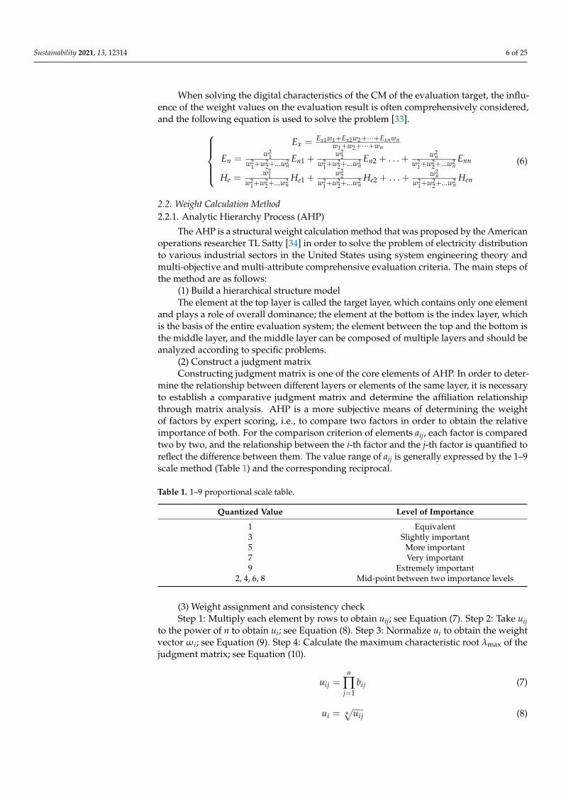
(3) Weight assignment and consistency checkStep 1: Multiply each element by rows to obtain uij; see Equation (7). Step 2: Take uij

to the power of n to obtain ui; see Equation (8). Step 3: Normalize ui to obtain the weightvector ωi; see Equation (9). Step 4: Calculate the maximum characteristic root λmax of thejudgment matrix; see Equation (10).

uij =n

∏j=1

bij (7)

ui = n√

uij (8)


ωi =ui

n∑

i=1ui

(9)

λmax =n

∑i=1

(Aω)inωi

(10)

where bij is the relatively important value of the i-th evaluation index relative to the j-thevaluation index, which is the value in the judgment matrix; A is the judgment matrix; ω isthe eigenvector; n is the number of elements.

After the weights are calculated, a consistency check is also needed. Only the cal-culated results that pass the consistency check have an acceptable degree of reliability.The consistency check usually uses the consistency ratio CR as the check standard, whichis defined as CR = CI

RI , where CI is a consistency index, and its calculation equation isCI = λmax−n

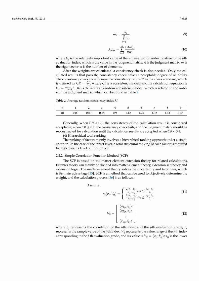
n−1 . RI is the average random consistency index, which is related to the ordern of the judgment matrix, which can be found in Table 2.

Table 2. Average random consistency index RI.

n 1 2 3 4 5 6 7 8 9

RI 0.00 0.00 0.58 0.9 1.12 1.24 1.32 1.41 1.45

Generally, when CR < 0.1, the consistency of the calculation result is consideredacceptable; when CR ≥ 0.1, the consistency check fails, and the judgment matrix should bereconstructed for calculation until the calculation results are accepted when CR < 0.1.

(4) Hierarchical total rankingThe ranking of factors mainly involves a hierarchical ranking approach under a single

criterion. In the case of the target layer, a total structural ranking of each factor is requiredto determine its level of importance.

2.2.2. Simple Correlation Function Method (SCF)

The SCF is based on the matter-element extension theory for related calculations.Extenics theory can mainly be divided into matter-element theory, extension set theory andextension logic. The matter-element theory solves the uncertainty and fuzziness, whichis its main advantage [35]. SCF is a method that can be used to objectively determine theweight, and the calculation process [36] is as follows:

Assume

rij(vi, Vij) =

2(vi−aij)

bij−aij, vi ≤

aij+bij2

2(bij−vi)

bij−aij, vi ≥

aij+bij2

(11)

Vij =

⟨

a1j, b1j⟩⟨

a2j, b2j⟩

...⟨anj, bnj

⟩ (12)

where rij represents the correlation of the i-th index and the j-th evaluation grade; virepresents the sample value of the i-th index; Vij represents the value range of the i-th indexcorresponding to the j-th evaluation grade, and its value is Vij =

⟨aij, bij

⟩; aij is the lower


limit of the value of the i-th index, and bij is the upper limit of the value of the i-th index.Moreover, i = 1, 2, · · · , n; j = 1, 2, · · · , m.

ViP =

〈a1P, b1P〉〈a2P, b2P〉

...〈anP, bnP〉

(13)

If vi ∈ ViP, (i = 1, 2, · · · , n), where ViP is the range measured by the object to beevaluated, and its value is ViP = 〈aiP, biP〉, aiP is the minimum value of the lower boundaryof the i-th index in all evaluations, biP is the maximum value of the upper boundary ofthe i-th feature in all evaluations, and Vij ⊂ ViP (i = 1, 2, · · · , n; j = 1, 2, · · · , m). Thenrijmax(vi, Vij) = max

j∈(1,2,··· , m)

{rij(vi, Vij)

}.

If the evaluation grade j of the evaluation index i of the object to be evaluated is larger,and the weight assigned by the index is greater, then take:

ri =

{jmax × (1 + rijmax(vi, Vij)), rijmax(vi, Vij) ≥ −0.5

jmax × 0.5, rijmax(vi, Vij) < −0.5(14)

Among them, jmax represents the evaluation grade into which the sample value ofindex i in the element to be evaluated falls, and the larger the value, the more restrictivethe index is to treat the matter, when rijmax = rim, jmax = max{m}.

If the evaluation grade j of the evaluation index i of the object to be evaluated is larger,the weight assigned by the index is smaller, taking:

ri =

{(m− jmax + 1)× (1 + rijmax(vi, Vij)), rijmax(vi, Vij) ≥ −0.5

(m− jmax + 1)× 0.5, rijmax(vi, Vij) < −0.5(15)

Among them, m—represents the number of categories divided for each index, whenrijmax = rim, jmax = min{m}.

Then, the weight of the index is

wi =ri

n∑

i=1ri

(16)

Among them, wi is the normalized value of the i-th evaluation index weight.

2.2.3. Game Theory Combination Weighting Method

The subjective weighting method, used to determine the weight of each indicator,is mainly based on the experience and subjective preferences of decision-makers in therelevant field of knowledge, and these methods either have a large subjective factor ordo not consider the importance of the indicators themselves to the problem. However,in practical evaluation problems, the importance of indicator factors is not affected bythe subjective factors of decision-makers and is objective, and only the combination ofsubjective and objective weights can reflect the importance of evaluation indicators. Inthe game theory combination weighting method, the participants in the game are theobjective weight coefficient and subjective weight coefficient of each evaluation index;the equilibrium condition of the game is that the deviation between the weight of eachevaluation index and the basic weight is the smallest.

The specific calculation steps [37] are as follows:


(i) Use m different weighting methods to weight the evaluation indicators, and con-struct the basic weight vector set of the evaluation indicators as wk = {wk1, wk2, · · · , wkn}(k = 1, 2, · · · , m); then, the m linear combinations are:

w =m

∑k=1

αkwTk (αk > 0,

m

∑k=1

αk = 1) (17)

In the equation, w is a possible weight vector of the evaluation index weight set; αk isthe linear combination coefficient.

(ii) Minimize the deviation between w and each wk, namely:

min

∥∥∥∥∥ m

∑j=1

αjwTj − wi

∥∥∥∥∥2

(i, j = 1, 2, · · · , n) (18)

(iii) Solve the linear combination coefficient. From the properties of matrix differ-entiation, it can be seen that the optimal first-order derivative condition equivalent toEquation (18) is:

m

∑j=1

αjwiwTj = wiwT

i (19)

Equation (19) corresponds to the following linear equations:w1·wT

1 w1·wT2 · · · w1·wT

nw2·wT

1 w2·wT2 · · · w2·wT

n· · · · · · · · · · · ·

wn·wT1 wn·wT

2 · · · wn·wTn

·

α1α2· · ·αn

=

w1·wT

1w2·wT

2· · ·

wn·wTn

(20)

(iv) The weight coefficient is normalized. According to the calculation, (α1, α2, · · · , αn)can be obtained, and then the weight coefficient can be normalized to obtain:

α∗k =αk

m∑

k=1αk

(k= 1, 2, · · · , m) (21)

(v) Solve the final combination weight. Based on game theory, the combined weightof the evaluation index is obtained as:

w∗ =m

∑k=1

α∗k wTk (22)

3. Case Study3.1. Engineering Case

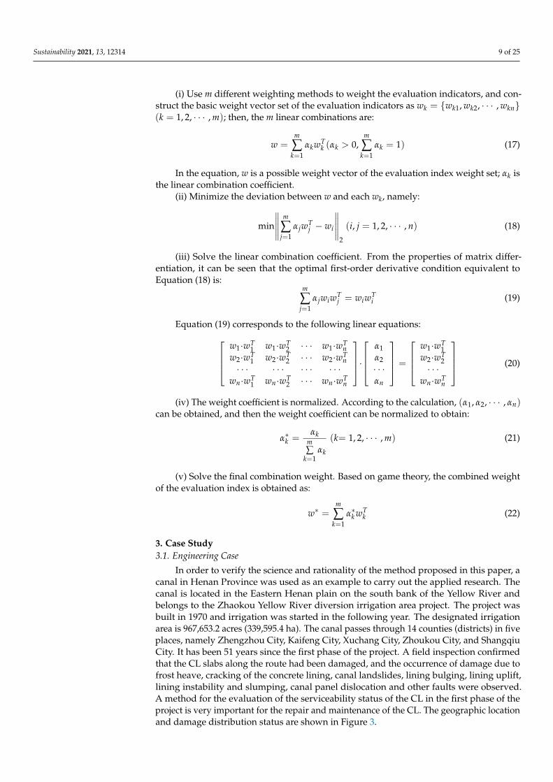
In order to verify the science and rationality of the method proposed in this paper, acanal in Henan Province was used as an example to carry out the applied research. Thecanal is located in the Eastern Henan plain on the south bank of the Yellow River andbelongs to the Zhaokou Yellow River diversion irrigation area project. The project wasbuilt in 1970 and irrigation was started in the following year. The designated irrigationarea is 967,653.2 acres (339,595.4 ha). The canal passes through 14 counties (districts) in fiveplaces, namely Zhengzhou City, Kaifeng City, Xuchang City, Zhoukou City, and ShangqiuCity. It has been 51 years since the first phase of the project. A field inspection confirmedthat the CL slabs along the route had been damaged, and the occurrence of damage due tofrost heave, cracking of the concrete lining, canal landslides, lining bulging, lining uplift,lining instability and slumping, canal panel dislocation and other faults were observed.A method for the evaluation of the serviceability status of the CL in the first phase of theproject is very important for the repair and maintenance of the CL. The geographic locationand damage distribution status are shown in Figure 3.



1

( =1,2, , )kk m

kk

k m

(21)

(v) Solve the final combination weight. Based on game theory, the combined weight

of the evaluation index is obtained as:

1k

mTk

k

w w

(22)

3. Case Study

3.1. Engineering Case

In order to verify the science and rationality of the method proposed in this paper, a

canal in Henan Province was used as an example to carry out the applied research. The

canal is located in the Eastern Henan plain on the south bank of the Yellow River and

belongs to the Zhaokou Yellow River diversion irrigation area project. The project was

built in 1970 and irrigation was started in the following year. The designated irrigation

area is 967,653.2 acres (339,595.4 ha). The canal passes through 14 counties (districts) in

five places, namely Zhengzhou City, Kaifeng City, Xuchang City, Zhoukou City, and

Shangqiu City. It has been 51 years since the first phase of the project. A field inspection

confirmed that the CL slabs along the route had been damaged, and the occurrence of

damage due to frost heave, cracking of the concrete lining, canal landslides, lining bulging,

lining uplift, lining instability and slumping, canal panel dislocation and other faults were

observed. A method for the evaluation of the serviceability status of the CL in the first

phase of the project is very important for the repair and maintenance of the CL. The geo‐

graphic location and damage distribution status are shown in Figure 3.

Figure 3. Schematic diagram of the canal’s geographic location and current status of damage distribution.

Figure 3. Schematic diagram of the canal’s geographic location and current status of damage distribution.

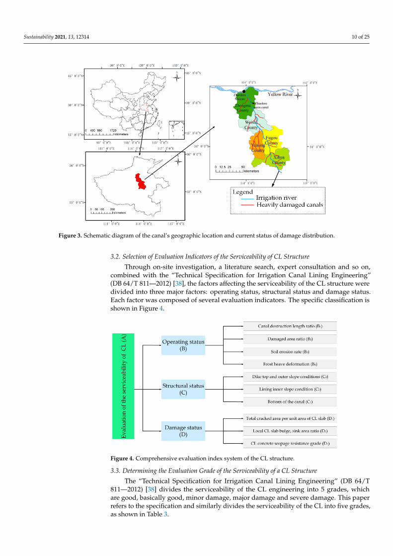
3.2. Selection of Evaluation Indicators of the Serviceability of CL Structure

Through on-site investigation, a literature search, expert consultation and so on,combined with the “Technical Specification for Irrigation Canal Lining Engineering”(DB 64/T 811—2012) [38], the factors affecting the serviceability of the CL structure weredivided into three major factors: operating status, structural status and damage status.Each factor was composed of several evaluation indicators. The specific classification isshown in Figure 4.


3.2. Selection of Evaluation Indicators of the Serviceability of CL Structure

Through on‐site investigation, a literature search, expert consultation and so on, com‐

bined with the “Technical Specification for Irrigation Canal Lining Engineering” (DB 64/T

811—2012) [38], the factors affecting the serviceability of the CL structure were divided

into three major factors: operating status, structural status and damage status. Each factor

was composed of several evaluation indicators. The specific classification is shown in Fig‐

ure 4.

Figure 4. Comprehensive evaluation index system of the CL structure.

3.3. Determining the Evaluation Grade of the Serviceability of a CL Structure

The “Technical Specification for Irrigation Canal Lining Engineering” (DB 64/T 811—

2012) [38] divides the serviceability of the CL engineering into 5 grades, which are good,

basically good, minor damage, major damage and severe damage. This paper refers to the

specification and similarly divides the serviceability of the CL into five grades, as shown

in Table 3.

Table 3. Serviceability classification of CL structure.

Evaluation Grade Serviceability of CL Structure

I Good

II Basically good

III Minor damage, needs minor repair

IV Major damage, needs major repair

V Severe damage, cannot be used

Table 3 contains qualitative descriptions; in actual engineering, some CL serviceabil‐

ity evaluation indices are characterized by fuzziness when they are divided, and it is dif‐

ficult to accurately classify which grade they belong to, while CM theory can simultane‐

ously reflect the randomness and fuzziness of describing such factors, transform the un‐

certainty relationship between qualitative and quantitative entities and form a mapping

relationship between qualitative and quantitative, which can be used to address the un‐

certainty of fuzziness factors [39]. Therefore, the CM theory method is used to devise the

serviceability evaluation indicators for the CL structure with the normal CM, and Equa‐

tions (3)–(5) are used to transform the qualitative concepts of the five grades in Table 3

into five cloud models, where the domain is [0, 1], and the results are shown in Table 4.

Figure 4. Comprehensive evaluation index system of the CL structure.

3.3. Determining the Evaluation Grade of the Serviceability of a CL Structure

The “Technical Specification for Irrigation Canal Lining Engineering” (DB 64/T811—2012) [38] divides the serviceability of the CL engineering into 5 grades, whichare good, basically good, minor damage, major damage and severe damage. This paperrefers to the specification and similarly divides the serviceability of the CL into five grades,as shown in Table 3.


Table 3. Serviceability classification of CL structure.

Evaluation Grade Serviceability of CL Structure

I GoodII Basically goodIII Minor damage, needs minor repairIV Major damage, needs major repairV Severe damage, cannot be used

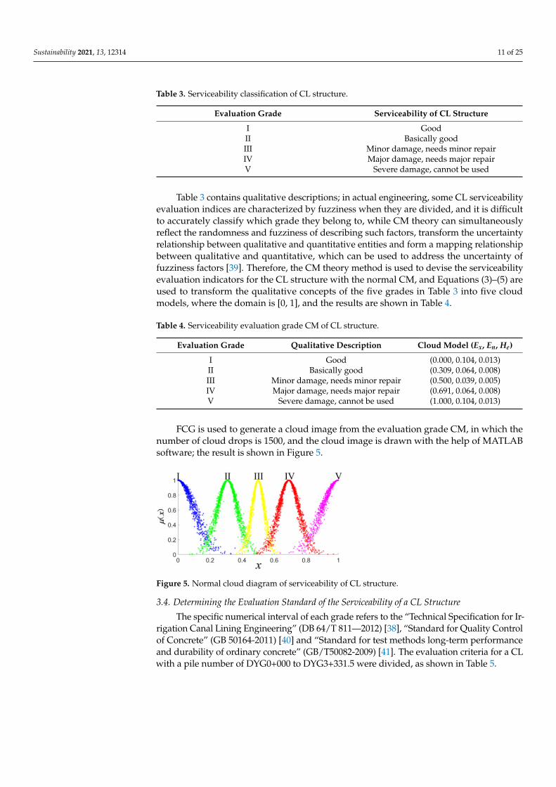
Table 3 contains qualitative descriptions; in actual engineering, some CL serviceabilityevaluation indices are characterized by fuzziness when they are divided, and it is difficultto accurately classify which grade they belong to, while CM theory can simultaneouslyreflect the randomness and fuzziness of describing such factors, transform the uncertaintyrelationship between qualitative and quantitative entities and form a mapping relationshipbetween qualitative and quantitative, which can be used to address the uncertainty offuzziness factors [39]. Therefore, the CM theory method is used to devise the serviceabilityevaluation indicators for the CL structure with the normal CM, and Equations (3)–(5) areused to transform the qualitative concepts of the five grades in Table 3 into five cloudmodels, where the domain is [0, 1], and the results are shown in Table 4.

Table 4. Serviceability evaluation grade CM of CL structure.

Evaluation Grade Qualitative Description Cloud Model (Ex, En, He)

I Good (0.000, 0.104, 0.013)II Basically good (0.309, 0.064, 0.008)III Minor damage, needs minor repair (0.500, 0.039, 0.005)IV Major damage, needs major repair (0.691, 0.064, 0.008)V Severe damage, cannot be used (1.000, 0.104, 0.013)

FCG is used to generate a cloud image from the evaluation grade CM, in which thenumber of cloud drops is 1500, and the cloud image is drawn with the help of MATLABsoftware; the result is shown in Figure 5.


Table 4. Serviceability evaluation grade CM of CL structure.

Evaluation Grade Qualitative Description Cloud Model (Ex, En, He)

I Good (0.000, 0.104, 0.013)

II Basically good (0.309, 0.064, 0.008)

III Minor damage, needs minor repair (0.500, 0.039, 0.005)

IV Major damage, needs major repair (0.691, 0.064, 0.008)

V Severe damage, cannot be used (1.000, 0.104, 0.013)

FCG is used to generate a cloud image from the evaluation grade CM, in which the

number of cloud drops is 1500, and the cloud image is drawn with the help of MATLAB

software; the result is shown in Figure 5.

Figure 5. Normal cloud diagram of serviceability of CL structure.

3.4. Determining the Evaluation Standard of the Serviceability of a CL Structure

The specific numerical interval of each grade refers to the “Technical Specification

for Irrigation Canal Lining Engineering” (DB 64/T 811—2012) [38], “Standard for Quality

Control of Concrete” (GB 50164‐2011) [40] and “Standard for test methods long‐term per‐

formance and durability of ordinary concrete” (GB/T50082‐2009) [41]. The evaluation cri‐

teria for a CL with a pile number of DYG0+000 to DYG3+331.5 were divided, as shown in

Table 5.

Table 5. Evaluation criteria for the serviceability of a CL structure.

Serial Number (SN) I II III IV V

B1 (0, 5%) [5%, 10%) [10%, 20%) [20%, 30%) [30%, 50%)

B2 (0, 5%) [5%, 10%) [10%, 20%) [20%, 30%) [30%, 40%)

B3 (0, 5%) [5%, 10%) [10%, 20%) [20%, 30%) [30%, 60%)

B4 (0, 10] (10, 20] (20, 30] (30, 40] (40, 50]

C1

The road surface of

canal is flat, and the

outer slope is

smooth

The road surface

of canal is flat on

average, and the

outer slope is

smooth

The road surface

on the top of canal

has small pits,

and the outer

slope is locally

convex

The road surface

of canal has large

pits, and the outer

slope is partially

collapsed

There are many pits

on the road surface

on the top of the ca‐

nal, and there are

many local collapses

on the outer slope

C2

Slope: smooth. The

concrete slab is

filled with joints to

keep it intact

Slope: smooth.

The concrete slab

filling is basi‐

cally intact

Slope: smooth.

There are cracks

in the partial slab

The slope surface

is flat, and there

are many cracks in

the local slab.

Slope concrete slab is

loose.

Many cracks in the

soil slab

C3

The canal bottom is

flat, and the con‐

crete lining at the

The canal bot‐

tom is flat, and

there are slight

The canal bottom

is basically kept

flat, and the canal

The canal bottom

is eroded, and the

lining concrete has

collapsed.

The scouring depth at

the bottom of the ca‐

nal is large, and the

lining concrete has

Figure 5. Normal cloud diagram of serviceability of CL structure.

3.4. Determining the Evaluation Standard of the Serviceability of a CL Structure

The specific numerical interval of each grade refers to the “Technical Specification for Ir-rigation Canal Lining Engineering” (DB 64/T 811—2012) [38], “Standard for Quality Controlof Concrete” (GB 50164-2011) [40] and “Standard for test methods long-term performanceand durability of ordinary concrete” (GB/T50082-2009) [41]. The evaluation criteria for a CLwith a pile number of DYG0+000 to DYG3+331.5 were divided, as shown in Table 5.


Table 5. Evaluation criteria for the serviceability of a CL structure.

Serial Number (SN) I II III IV V

B1 (0, 5%) [5%, 10%) [10%, 20%) [20%, 30%) [30%, 50%)B2 (0, 5%) [5%, 10%) [10%, 20%) [20%, 30%) [30%, 40%)B3 (0, 5%) [5%, 10%) [10%, 20%) [20%, 30%) [30%, 60%)B4 (0, 10] (10, 20] (20, 30] (30, 40] (40, 50]

C1

The road surfaceof canal is flat,and the outer

slope is smooth

The road surface ofcanal is flat on

average, and theouter slope is

smooth

The road surfaceon the top of canalhas small pits, andthe outer slope is

locally convex

The road surface ofcanal has large pits,and the outer slope

is partiallycollapsed

There are manypits on the road

surface on the topof the canal, andthere are many

local collapses onthe outer slope

C2

Slope: smooth.The concrete slab

is filled withjoints to keep it

intact

Slope: smooth. Theconcrete slab fillingis basically intact

Slope: smooth.There are cracks in

the partial slab

The slope surfaceis flat, and there

are many cracks inthe local slab.

Slope concrete slabis loose.

Many cracks in thesoil slab

C3

The canal bottomis flat, and the

concrete lining atthe canal bottom

has nodeformation.

The canal bottomis flat, and there

are slight cracks inthe bottom ofconcrete slab.

The canal bottomis basically kept

flat, and the canalbottom surface has

slight peeling.

The canal bottomis eroded, and thelining concrete has

collapsed.

The scouringdepth at the

bottom of the canalis large, and the

lining concrete hascollapsed and

bulges seriously.D1 (0, 100] (100, 400] (400, 700] (700, 1000] (1000, 1500]D2 (0, 5%) [5%, 10%) [10%, 20%) [20%, 30%) [30%, 45%)D3 [14, 12] (12, 10] (10, 8] (8, 6] (6, 4]

Note: For B1, B2, B3, B4, C1, C2, C3, D2 each evaluation grade or qualitative description is based on the “Technical Specification for IrrigationCanal Lining Engineering” (DB 64/T 811—2012) [38]. D1: The division of the evaluation grade of the total cracked area per unit area ofthe CL slab is based on the specification “Standard for Quality Control of Concrete” (GB 50164-2011) [40]. D3: The CL concrete seepageresistance grade is determined by taking the CL concrete after standard curing for 28 d age as the standard specimen, and the maximumwater pressure that can be withstood during the seepage resistance performance test according to the “Standard for test methods long-termperformance and durability of ordinary concrete” (GB/T50082-2009) [41]. The grade classification is based on the “Standard for QualityControl of Concrete” (GB 50164-2011) [40]. For each evaluation index, if the actual quantified value exceeds or falls below the upper andlower limit values of the interval corresponding to the evaluation grade I or V in Table 5, the value can be the upper or lower limit value ofthe interval corresponding to the evaluation grade I or V.

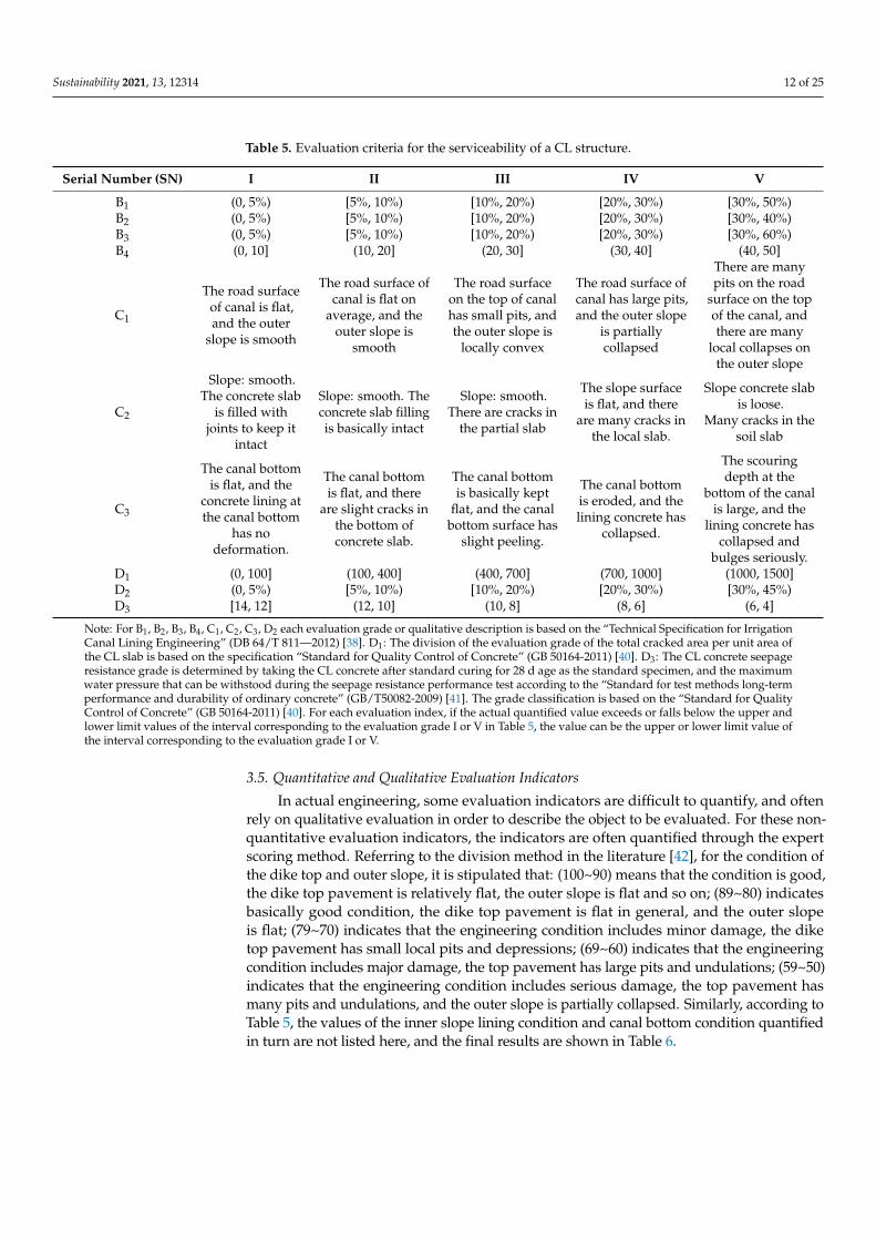
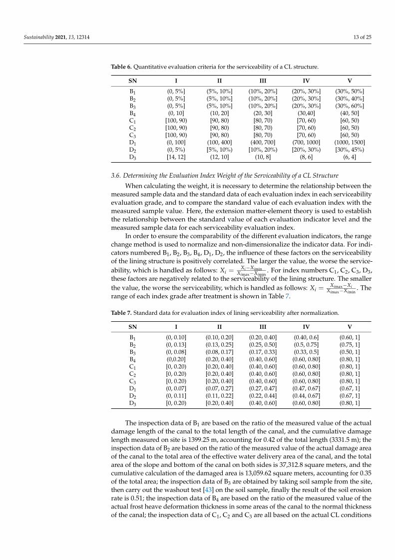
3.5. Quantitative and Qualitative Evaluation Indicators

In actual engineering, some evaluation indicators are difficult to quantify, and oftenrely on qualitative evaluation in order to describe the object to be evaluated. For these non-quantitative evaluation indicators, the indicators are often quantified through the expertscoring method. Referring to the division method in the literature [42], for the condition ofthe dike top and outer slope, it is stipulated that: (100~90) means that the condition is good,the dike top pavement is relatively flat, the outer slope is flat and so on; (89~80) indicatesbasically good condition, the dike top pavement is flat in general, and the outer slopeis flat; (79~70) indicates that the engineering condition includes minor damage, the diketop pavement has small local pits and depressions; (69~60) indicates that the engineeringcondition includes major damage, the top pavement has large pits and undulations; (59~50)indicates that the engineering condition includes serious damage, the top pavement hasmany pits and undulations, and the outer slope is partially collapsed. Similarly, according toTable 5, the values of the inner slope lining condition and canal bottom condition quantifiedin turn are not listed here, and the final results are shown in Table 6.


Table 6. Quantitative evaluation criteria for the serviceability of a CL structure.

SN I II III IV V

B1 (0, 5%] (5%, 10%] (10%, 20%] (20%, 30%] (30%, 50%]B2 (0, 5%] (5%, 10%] (10%, 20%] (20%, 30%] (30%, 40%]B3 (0, 5%] (5%, 10%] (10%, 20%] (20%, 30%] (30%, 60%]B4 (0, 10] (10, 20] (20, 30] (30,40] (40, 50]C1 [100, 90) [90, 80) [80, 70) [70, 60) [60, 50)C2 [100, 90) [90, 80) [80, 70) [70, 60) [60, 50)C3 [100, 90) [90, 80) [80, 70) [70, 60) [60, 50)D1 (0, 100] (100, 400] (400, 700] (700, 1000] (1000, 1500]D2 (0, 5%) [5%, 10%) [10%, 20%) [20%, 30%) [30%, 45%)D3 [14, 12] (12, 10] (10, 8] (8, 6] (6, 4]

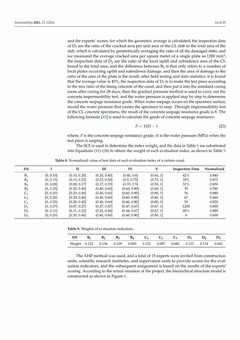
3.6. Determining the Evaluation Index Weight of the Serviceability of a CL Structure

When calculating the weight, it is necessary to determine the relationship between themeasured sample data and the standard data of each evaluation index in each serviceabilityevaluation grade, and to compare the standard value of each evaluation index with themeasured sample value. Here, the extension matter-element theory is used to establishthe relationship between the standard value of each evaluation indicator level and themeasured sample data for each serviceability evaluation index.

In order to ensure the comparability of the different evaluation indicators, the rangechange method is used to normalize and non-dimensionalize the indicator data. For indi-cators numbered B1, B2, B3, B4, D1, D2, the influence of these factors on the serviceabilityof the lining structure is positively correlated. The larger the value, the worse the service-ability, which is handled as follows: Xi =

Xi−XiminXimax−Ximin

. For index numbers C1, C2, C3, D3,these factors are negatively related to the serviceability of the lining structure. The smallerthe value, the worse the serviceability, which is handled as follows: Xi =

Ximax−XiXimax−Ximin

. Therange of each index grade after treatment is shown in Table 7.

Table 7. Standard data for evaluation index of lining serviceability after normalization.

SN I II III IV V

B1 (0, 0.10] (0.10, 0.20] (0.20, 0.40] (0.40, 0.6] (0.60, 1]B2 (0, 0.13] (0.13, 0.25] (0.25, 0.50] (0.5, 0.75] (0.75, 1]B3 (0, 0.08] (0.08, 0.17] (0.17, 0.33] (0.33, 0.5] (0.50, 1]B4 (0,0.20] (0.20, 0.40] (0.40, 0.60] (0.60, 0.80] (0.80, 1]C1 [0, 0.20) [0.20, 0.40] (0.40, 0.60] (0.60, 0.80] (0.80, 1]C2 [0, 0.20) [0.20, 0.40] (0.40, 0.60] (0.60, 0.80] (0.80, 1]C3 [0, 0.20) [0.20, 0.40] (0.40, 0.60] (0.60, 0.80] (0.80, 1]D1 (0, 0.07] (0.07, 0.27] (0.27, 0.47] (0.47, 0.67] (0.67, 1]D2 (0, 0.11] (0.11, 0.22] (0.22, 0.44] (0.44, 0.67] (0.67, 1]D3 [0, 0.20) [0.20, 0.40] (0.40, 0.60] (0.60, 0.80] (0.80, 1]

The inspection data of B1 are based on the ratio of the measured value of the actualdamage length of the canal to the total length of the canal, and the cumulative damagelength measured on site is 1399.25 m, accounting for 0.42 of the total length (3331.5 m); theinspection data of B2 are based on the ratio of the measured value of the actual damage areaof the canal to the total area of the effective water delivery area of the canal, and the totalarea of the slope and bottom of the canal on both sides is 37,312.8 square meters, and thecumulative calculation of the damaged area is 13,059.62 square meters, accounting for 0.35of the total area; the inspection data of B3 are obtained by taking soil sample from the site,then carry out the washout test [43] on the soil sample, finally the result of the soil erosionrate is 0.51; the inspection data of B4 are based on the ratio of the measured value of theactual frost heave deformation thickness in some areas of the canal to the normal thicknessof the canal; the inspection data of C1, C2 and C3 are all based on the actual CL conditions


and the experts’ scores, for which the geometric average is calculated; the inspection dataof D1 are the ratio of the cracked area per unit area of the CL slab to the total area of theslab, which is calculated by geometrically averaging the ratio of all the damaged slabs, andwe measured the average cracked area per square meter of a single plate as 1200 mm2;the inspection data of D2 are the ratio of the local uplift and subsidence area of the CLboard to the total area, and the difference between B2 is that only refers to a number oflocal plates occurring uplift and subsidence damage, and then the area of damage to theratio of the area of the plate is the result, after field testing and data statistics, it is foundthat the average value is 40%; the inspection data of D3 is to make the test piece accordingto the mix ratio of the lining concrete of the canal, and then put it into the standard curingroom after curing for 28 days, then the gradual pressure method is used to carry out theconcrete impermeability test, and the water pressure is applied step by step to determinethe concrete seepage resistance grade. When water seepage occurs on the specimen surface,record the water pressure that causes the specimen to seep. Through impermeability testof the CL concrete specimens, the result of the concrete seepage resistance grade is 8. Thefollowing formula [40] is used to calculate the grade of concrete seepage resistance:

P = 10H − 1 (23)

where, P is the concrete seepage resistance grade; H is the water pressure (MPa) when thetest piece is seeping.

The SCF is used to determine the index weight, and the data in Table 8 are substitutedinto Equations (11)–(16) to obtain the weight of each evaluation index, as shown in Table 9.

Table 8. Normalized value of test data of each evaluation index of a certain canal.

SN I II III IV V Inspection Data Normalized

B1 (0, 0.10] (0.10, 0.20] (0.20, 0.40] (0.40, 0.6] (0.60, 1] 42% 0.840B2 (0, 0.13] (0.13, 0.25] (0.25, 0.50] (0.5, 0.75] (0.75, 1] 35% 0.875B3 (0, 0.08] (0.08, 0.17] (0.17, 0.33] (0.33, 0.5] (0.50, 1] 51% 0.850B4 (0, 0.20] (0.20, 0.40] (0.40, 0.60] (0.60, 0.80] (0.80, 1] 39 0.780C1 [0, 0.20) [0.20, 0.40] (0.40, 0.60] (0.60, 0.80] (0.80, 1] 56 0.880C2 [0, 0.20) [0.20, 0.40] (0.40, 0.60] (0.60, 0.80] (0.80, 1] 67 0.660C3 [0, 0.20) [0.20, 0.40] (0.40, 0.60] (0.60, 0.80] (0.80, 1] 59 0.820D1 (0, 0.07] (0.07, 0.27] (0.27, 0.47] (0.47, 0.67] (0.67, 1] 1200 0.800D2 (0, 0.11] (0.11, 0.22] (0.22, 0.44] (0.44, 0.67] (0.67, 1] 40% 0.889D2 (0, 0.20) [0.20, 0.40] (0.40, 0.60] (0.60, 0.80] (0.80, 1] 8 0.600

Table 9. Weights of evaluation indicators.

SN B1 B2 B3 B4 C1 C2 C3 D1 D2 D3

Weight 0.122 0.136 0.109 0.065 0.122 0.087 0.082 0.122 0.114 0.041

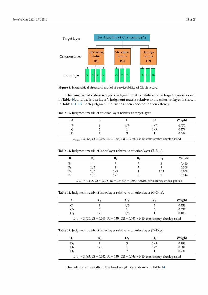
The AHP method was used, and a total of 15 experts were invited from constructionunits, scientific research institutes, and supervision units to provide scores for the eval-uation indicators, and the subsequent assignment is based on the results of the experts’scoring. According to the actual situation of the project, the hierarchical structure model isconstructed as shown in Figure 6.



10 1P H (23)

where, P is the concrete seepage resistance grade; H is the water pressure (MPa) when the

test piece is seeping.

The SCF is used to determine the index weight, and the data in Table 8 are substituted

into Equations (11)–(16) to obtain the weight of each evaluation index, as shown in Table

9.

Table 8. Normalized value of test data of each evaluation index of a certain canal.

SN I II III IV V Inspection Data Normalized

B1 (0, 0.10] (0.10, 0.20] (0.20, 0.40] (0.40, 0.6] (0.60, 1] 42% 0.840

B2 (0, 0.13] (0.13, 0.25] (0.25, 0.50] (0.5, 0.75] (0.75, 1] 35% 0.875

B3 (0, 0.08] (0.08, 0.17] (0.17, 0.33] (0.33, 0.5] (0.50, 1] 51% 0.850

B4 (0, 0.20] (0.20, 0.40] (0.40, 0.60] (0.60, 0.80] (0.80, 1] 39 0.780

C1 [0, 0.20) [0.20, 0.40] (0.40, 0.60] (0.60, 0.80] (0.80, 1] 56 0.880

C2 [0, 0.20) [0.20, 0.40] (0.40, 0.60] (0.60, 0.80] (0.80, 1] 67 0.660

C3 [0, 0.20) [0.20, 0.40] (0.40, 0.60] (0.60, 0.80] (0.80, 1] 59 0.820

D1 (0, 0.07] (0.07, 0.27] (0.27, 0.47] (0.47, 0.67] (0.67, 1] 1200 0.800

D2 (0, 0.11] (0.11, 0.22] (0.22, 0.44] (0.44, 0.67] (0.67, 1] 40% 0.889

D2 (0, 0.20) [0.20, 0.40] (0.40, 0.60] (0.60, 0.80] (0.80, 1] 8 0.600

Table 9. Weights of evaluation indicators.

SN B1 B2 B3 B4 C1 C2 C3 D1 D2 D3

Weight 0.122 0.136 0.109 0.065 0.122 0.087 0.082 0.122 0.114 0.041

The AHP method was used, and a total of 15 experts were invited from construction

units, scientific research institutes, and supervision units to provide scores for the evalu‐

ation indicators, and the subsequent assignment is based on the results of the experts’

scoring. According to the actual situation of the project, the hierarchical structure model

is constructed as shown in Figure 6.

Figure 6. Hierarchical structural model of serviceability of CL structure.

The constructed criterion layer’s judgment matrix relative to the target layer is shown

in Table 10, and the index layer’s judgment matrix relative to the criterion layer is shown

in Tables 11–13. Each judgment matrix has been checked for consistency.

Figure 6. Hierarchical structural model of serviceability of CL structure.

The constructed criterion layer’s judgment matrix relative to the target layer is shownin Table 10, and the index layer’s judgment matrix relative to the criterion layer is shownin Tables 11–13. Each judgment matrix has been checked for consistency.

Table 10. Judgment matrix of criterion layer relative to target layer.

A B C D Weight

B 1 1/5 1/7 0.072C 5 1 1/3 0.279D 7 3 1 0.649

λmax = 3.065, CI = 0.032, RI = 0.58, CR = 0.056 < 0.10, consistency check passed

Table 11. Judgment matrix of index layer relative to criterion layer (B–B1–4).

B B1 B2 B3 B4 Weight

B1 1 3 5 3 0.490B2 1/3 1 7 3 0.308B3 1/5 1/7 1 1/3 0.059B4 1/3 1/3 3 1 0.144


Table 12. Judgment matrix of index layer relative to criterion layer (C–C1–3).

C C1 C2 C3 Weight

C1 1 1/3 3 0.258C2 3 1 5 0.637C3 1/3 1/5 1 0.105


Table 13. Judgment matrix of index layer relative to criterion layer (D–D1–3).

D D1 D2 D3 Weight

D1 1 3 1/5 0.188D2 1/3 1 1/7 0.081D3 5 7 1 0.731


The calculation results of the final weights are shown in Table 14.


Table 14. Calculation results of subjective weight.

Index LayerSingle Weight

Weight ValueB C D0.072 0.279 0.649

B1 0.490 0.0353B2 0.308 0.0221B3 0.059 0.0043B4 0.144 0.0103C1 0.258 0.0721C2 0.637 0.1777C3 0.105 0.0292D1 0.188 0.1223D2 0.081 0.0525D3 0.731 0.4742

Obviously, the weights obtained by the AHP method and the SCF method show greaterdifferences in the results of the same evaluation index, such as B2, B3, C2 and D3. The gametheory combination weighting method can fully take into account the characteristics ofeach of the subjective and objective weighting methods in order to determine the levelof agreement or compromise between the subjective and objective weight values, so thatthe deviation of the subjective and objective weights is minimized. In this study, thereare two different assignment methods, so m = 2, and according to Equations (17)–(22),the integrated weight coefficient vector α1 and α2 can be determined. The α1 = 0.707 andα2 = 0.293, and the final weight calculation results are shown in Table 15.

Table 15. Final weight calculation results.

SN Weights DeterminedBased on AHP

Weights DeterminedBased on the SCF

Weights DeterminedBased on Game Theory

B1 0.0353 0.122 0.061B2 0.0221 0.136 0.055B3 0.0043 0.109 0.035B4 0.0103 0.065 0.026C1 0.0721 0.122 0.087C2 0.1777 0.087 0.151C3 0.0292 0.082 0.045D1 0.1223 0.122 0.122D2 0.0525 0.114 0.071D3 0.4742 0.041 0.347

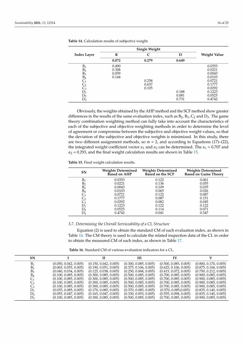
3.7. Determining the Overall Serviceability of a CL Structure

Equation (2) is used to obtain the standard CM of each evaluation index, as shown inTable 16. The CM theory is used to calculate the related inspection data of the CL in orderto obtain the measured CM of each index, as shown in Table 17.

Table 16. Standard CM of various evaluation indicators for a CL.

SN I II III IV V

B1 (0.050, 0.042, 0.005) (0.150, 0.042, 0.005) (0.300, 0.085, 0.005) (0.500, 0.085, 0.005) (0.800, 0.170, 0.005)B2 (0.065, 0.055, 0.005) (0.190, 0.051, 0.005) (0.375, 0.106, 0.005) (0.625, 0.106, 0.005) (0.875, 0.106, 0.005)B3 (0.040, 0.034, 0.005) (0.125, 0.038, 0.005) (0.250, 0.068, 0.005) (0.415, 0.072, 0.005) (0.750, 0.212, 0.005)B4 (0.100, 0.085, 0.005) (0.300, 0.085, 0.005) (0.500, 0.085, 0.005) (0.700, 0.085, 0.005) (0.900, 0.085, 0.005)C1 (0.100, 0.085, 0.005) (0.300, 0.085, 0.005) (0.500, 0.085, 0.005) (0.700, 0.085, 0.005) (0.900, 0.085, 0.005)C2 (0.100, 0.085, 0.005) (0.300, 0.085, 0.005) (0.500, 0.085, 0.005) (0.700, 0.085, 0.005) (0.900, 0.085, 0.005)C3 (0.100, 0.085, 0.005) (0.300, 0.085, 0.005) (0.500, 0.085, 0.005) (0.700, 0.085, 0.005) (0.900, 0.085, 0.005)D1 (0.035, 0.085, 0.005) (0.170, 0.085, 0.005) (0.370, 0.085, 0.005) (0.570, 0.085,0.005) (0.835, 0.140, 0.005)D2 (0.055, 0.047, 0.005) (0.165, 0.047, 0.005) (0.330, 0.093, 0.005) (0.555, 0.098, 0.005) (0.835, 0.140, 0.005)D3 (0.100, 0.085, 0.005) (0.300, 0.085, 0.005) (0.500, 0.085, 0.005) (0.700, 0.085, 0.005) (0.900, 0.085, 0.005)


Table 17. CM of each test index of a CL.

SN Cloud Model (Ex, En, Ee)

B1 (0.920, 0.068, 0.005)B2 (0.938, 0.053, 0.005)B3 (0.925, 0.064, 0.005)B4 (0.790, 0.008, 0.005)C1 (0.940, 0.051, 0.005)C2 (0.730, 0.059, 0.005)C3 (0.910, 0.076, 0.005)D1 (0.900, 0.085, 0.005)D2 (0.945, 0.047, 0.005)D3 (0.600, 0.085, 0.005)

According to the established CL structure serviceability evaluation index system, theindex CM and index weights are calculated and solved gradually from the index layer to thetarget layer until the target layer CM is solved, i.e., the comprehensive evaluation result CMis obtained. Equation (6) was used for the calculation, and the results are shown in Table 18.

Table 18. CM data for evaluation results of indicators at all layers.

Target Layer Final Cloud Model Criterion Layer Indicator Cloud Model

A (0.799, 0.077, 0.005)B (0.907, 0.057, 0.005)C (0.823, 0.058, 0.005)D (0.713, 0.084, 0.005)

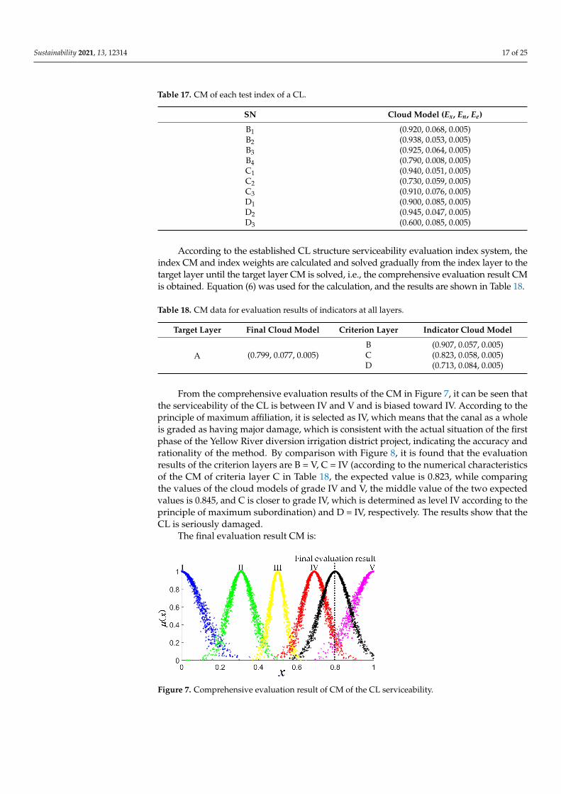
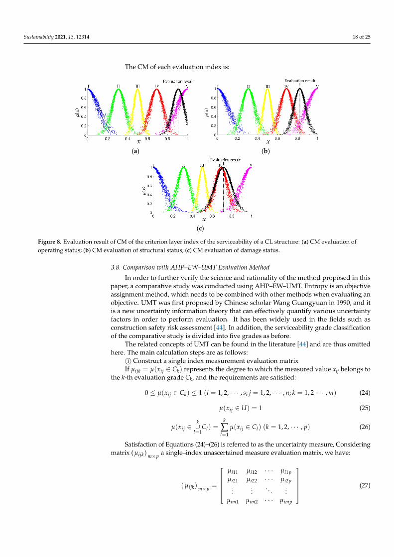
From the comprehensive evaluation results of the CM in Figure 7, it can be seen thatthe serviceability of the CL is between IV and V and is biased toward IV. According to theprinciple of maximum affiliation, it is selected as IV, which means that the canal as a wholeis graded as having major damage, which is consistent with the actual situation of the firstphase of the Yellow River diversion irrigation district project, indicating the accuracy andrationality of the method. By comparison with Figure 8, it is found that the evaluationresults of the criterion layers are B = V, C = IV (according to the numerical characteristicsof the CM of criteria layer C in Table 18, the expected value is 0.823, while comparingthe values of the cloud models of grade IV and V, the middle value of the two expectedvalues is 0.845, and C is closer to grade IV, which is determined as level IV according to theprinciple of maximum subordination) and D = IV, respectively. The results show that theCL is seriously damaged.

The final evaluation result CM is:


D1 (0.900, 0.085, 0.005)

D2 (0.945, 0.047, 0.005)

D3 (0.600, 0.085, 0.005)

According to the established CL structure serviceability evaluation index system, the

index CM and index weights are calculated and solved gradually from the index layer to

the target layer until the target layer CM is solved, i.e., the comprehensive evaluation re‐

sult CM is obtained. Equation (6) was used for the calculation, and the results are shown

in Table 18.



A (0.799, 0.077, 0.005)

B (0.907, 0.057, 0.005)

C (0.823, 0.058, 0.005)

D (0.713, 0.084, 0.005)

From the comprehensive evaluation results of the CM in Figure 7, it can be seen that

the serviceability of the CL is between IV and V and is biased toward IV. According to the

principle of maximum affiliation, it is selected as IV, which means that the canal as a whole

is graded as having major damage, which is consistent with the actual situation of the first

phase of the Yellow River diversion irrigation district project, indicating the accuracy and

rationality of the method. By comparison with Figure 8, it is found that the evaluation

results of the criterion layers are B = V, C = IV (according to the numerical characteristics

of the CM of criteria layer C in Table 18, the expected value is 0.823, while comparing the

values of the cloud models of grade IV and V, the middle value of the two expected values

is 0.845, and C is closer to grade IV, which is determined as level IV according to the prin‐

ciple of maximum subordination) and D = IV, respectively. The results show that the CL

is seriously damaged.


Figure 7. Comprehensive evaluation result of CM of the CL serviceability.

The CM of each evaluation index is:

(a) (b)





D1 (0.900, 0.085, 0.005)

D2 (0.945, 0.047, 0.005)

D3 (0.600, 0.085, 0.005)

According to the established CL structure serviceability evaluation index system, the

index CM and index weights are calculated and solved gradually from the index layer to

the target layer until the target layer CM is solved, i.e., the comprehensive evaluation re‐

sult CM is obtained. Equation (6) was used for the calculation, and the results are shown

in Table 18.



A (0.799, 0.077, 0.005)

B (0.907, 0.057, 0.005)

C (0.823, 0.058, 0.005)

D (0.713, 0.084, 0.005)

From the comprehensive evaluation results of the CM in Figure 7, it can be seen that

the serviceability of the CL is between IV and V and is biased toward IV. According to the

principle of maximum affiliation, it is selected as IV, which means that the canal as a whole

is graded as having major damage, which is consistent with the actual situation of the first

phase of the Yellow River diversion irrigation district project, indicating the accuracy and

rationality of the method. By comparison with Figure 8, it is found that the evaluation

results of the criterion layers are B = V, C = IV (according to the numerical characteristics

of the CM of criteria layer C in Table 18, the expected value is 0.823, while comparing the

values of the cloud models of grade IV and V, the middle value of the two expected values

is 0.845, and C is closer to grade IV, which is determined as level IV according to the prin‐

ciple of maximum subordination) and D = IV, respectively. The results show that the CL

is seriously damaged.




(a) (b)


(c)

Figure 8. Evaluation result of CM of the criterion layer index of the serviceability of a CL structure:

(a) CM evaluation of operating status; (b) CM evaluation of structural status; (c) CM evaluation of

damage status.

3.8. Comparison with AHP–EW–UMT Evaluation Method

In order to further verify the science and rationality of the method proposed in this

paper, a comparative study was conducted using AHP–EW–UMT. Entropy is an objective

assignment method, which needs to be combined with other methods when evaluating

an objective. UMT was first proposed by Chinese scholar Wang Guangyuan in 1990, and

it is a new uncertainty information theory that can effectively quantify various uncertainty

factors in order to perform evaluation. It has been widely used in the fields such as con‐

struction safety risk assessment [44]. In addition, the serviceability grade classification of

the comparative study is divided into five grades as before.

The related concepts of UMT can be found in the literature [44] and are thus omitted

here. The main calculation steps are as follows:

① Construct a single index measurement evaluation matrix

If ( )ijk ij kx C represents the degree to which the measured value xij belongs

to the k‐th evaluation grade Ck, and the requirements are satisfied:

0 ( ) 1 1,2, , ; 1,2, , ; 1,2 , )ij kx C i s j n k m （ (24)

( )=1ijx U (25)

1 1

( )= ( ) ( 1, 2, , )kk

ij l ij ll l

x C x C k p

(26)

Satisfaction of Equations (24)–(26) is referred to as the uncertainty measure, Consid‐

ering matrix ( )ijk m p a single–index unascertained measure evaluation matrix, we have:

11 12 1

21 22 2

1 2

( ) =

i i i p

i i i p

ijk m p

im im imp

(27)

Before establishing the single‐index unascertained measure matrix, it is necessary to

establish a single‐index unascertained measure function (UMF). At present, the construc‐

tion methods for single–index UMF mainly include linear, exponential, parabola, etc.

Among them, the linear construction method has the characteristics of simple calculation

and wide applicability, so the linear construction method is selected as the measurement

function; the corresponding function graph is shown in Figure 9.

Figure 8. Evaluation result of CM of the criterion layer index of the serviceability of a CL structure: (a) CM evaluation ofoperating status; (b) CM evaluation of structural status; (c) CM evaluation of damage status.

3.8. Comparison with AHP–EW–UMT Evaluation Method

In order to further verify the science and rationality of the method proposed in thispaper, a comparative study was conducted using AHP–EW–UMT. Entropy is an objectiveassignment method, which needs to be combined with other methods when evaluating anobjective. UMT was first proposed by Chinese scholar Wang Guangyuan in 1990, and itis a new uncertainty information theory that can effectively quantify various uncertaintyfactors in order to perform evaluation. It has been widely used in the fields such asconstruction safety risk assessment [44]. In addition, the serviceability grade classificationof the comparative study is divided into five grades as before.

The related concepts of UMT can be found in the literature [44] and are thus omittedhere. The main calculation steps are as follows:

1© Construct a single index measurement evaluation matrixIf µijk = µ(xij ∈ Ck) represents the degree to which the measured value xij belongs to

the k-th evaluation grade Ck, and the requirements are satisfied:

0 ≤ µ(xij ∈ Ck) ≤ 1 (i = 1, 2, · · · , s; j = 1, 2, · · · , n; k = 1, 2 · · · , m) (24)

µ(xij ∈ U) = 1 (25)

µ(xij ∈k∪

l=1Cl) =

k

∑l=1

µ(xij ∈ Cl) (k = 1, 2, · · · , p) (26)

Satisfaction of Equations (24)–(26) is referred to as the uncertainty measure, Consideringmatrix ( µijk)m×p a single–index unascertained measure evaluation matrix, we have:

(µijk)m×p =

µi11 µi12 · · · µi1pµi21 µi22 · · · µi2p

......

. . ....

µim1 µim2 · · · µimp

(27)


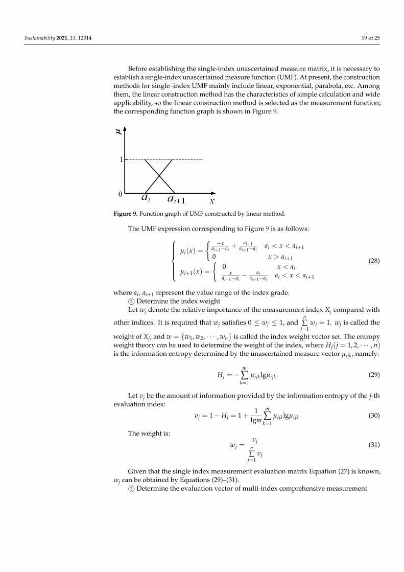
Before establishing the single-index unascertained measure matrix, it is necessary toestablish a single-index unascertained measure function (UMF). At present, the constructionmethods for single–index UMF mainly include linear, exponential, parabola, etc. Amongthem, the linear construction method has the characteristics of simple calculation and wideapplicability, so the linear construction method is selected as the measurement function;the corresponding function graph is shown in Figure 9.


Figure 9. Function graph of UMF constructed by linear method.

The UMF expression corresponding to Figure 9 is as follows:

11

1 1

1

11

1 1

( )

0

0

( )

ii i

i i i ii

i

i

i ii i

i i i i

axa x a

a a a ax

x a

x a

x axa x a

a a a a

(28)

where ia , +1ia represent the value range of the index grade.

②Determine the index weight

Let wj denote the relative importance of the measurement index Xj compared with

other indices. It is required that wj satisfies 0 1jw , and 1

1n

jj

w

. wj is called the weight

of Xj, and 1 2, , , nw w w w is called the index weight vector set. The entropy weight

theory can be used to determine the weight of the index, where ( 1, 2, , )jH j n is the

information entropy determined by the unascertained measure vector ijk , namely:

1

lgm

j ijk ijkk

H

(29)

Let jv be the amount of information provided by the information entropy of the j

‐th evaluation index:

1

11 1 lg

lg

m

j j ijk ijkk

v Hm

(30)

The weight is:

1

jj n

jj

vw

v

(31)

Given that the single index measurement evaluation matrix Equation (27) is known,

wj can be obtained by Equations (29)–(31).

③ Determine the evaluation vector of multi‐index comprehensive measurement

Let ( )ik i kP C be the degree to which the evaluation sample Pi belongs to the k‐

th evaluation category Ck, then

Figure 9. Function graph of UMF constructed by linear method.

The UMF expression corresponding to Figure 9 is as follows:µi(x) =

{−x

ai+1−ai+

ai+1ai+1−ai

ai < x < ai+1

0 x > ai+1

µi+1(x) =

{0 x < ai

xai+1−ai

− aiai+1−ai

ai < x < ai+1

(28)

where ai, ai+1 represent the value range of the index grade.2© Determine the index weight

Let wj denote the relative importance of the measurement index Xj compared with

other indices. It is required that wj satisfies 0 ≤ wj ≤ 1, andn∑

j=1wj = 1. wj is called the

weight of Xj, and w = {w1, w2, · · · , wn} is called the index weight vector set. The entropyweight theory can be used to determine the weight of the index, where Hj(j = 1, 2, · · · , n)is the information entropy determined by the unascertained measure vector µijk, namely:

Hj = −m

∑k=1

µijklgµijk (29)

Let vj be the amount of information provided by the information entropy of the j-thevaluation index:

vj = 1− Hj = 1 +1

lgm

m

∑k=1

µijklgµijk (30)

The weight is:

wj =vj

n∑

j=1vj

(31)

Given that the single index measurement evaluation matrix Equation (27) is known,wj can be obtained by Equations (29)–(31).

3© Determine the evaluation vector of multi-index comprehensive measurement


Let µik = µ(Pi ∈ Ck) be the degree to which the evaluation sample Pi belongs to thek-th evaluation category Ck, then

µik =n

∑j=1

wjµijk(i = 1, 2, · · · , s; k = 1, 2, · · · , m) (32)

Obviously 0 ≤ µik ≤ 1 andm∑

k=1µik = 1, and Equation (32) as shown is an unascertained

measure, so {µi1, µi2, · · · , µim} is called the multi-index comprehensive evaluation vector of Pi.4© Credible degree recognition

In order to obtain the final evaluation result of the evaluation object, we intro-duce the credible degree recognition criteria: let λ(λ ≥ 0.5) be the credible degree, ifC1 > C2 > · · · > Cm, and let:

k0 = min

{k :

m

∑k=1

µik ≥ λ(i = 1, 2, · · · , s)

}(33)

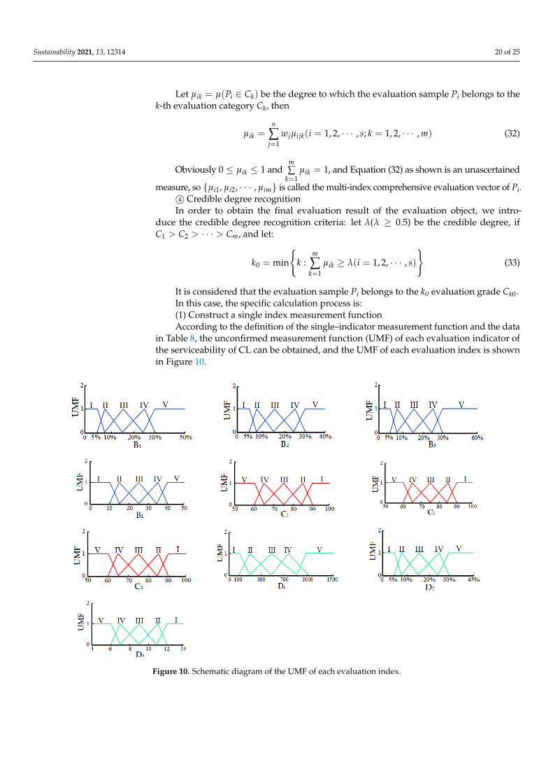
It is considered that the evaluation sample Pi belongs to the k0 evaluation grade Ck0.In this case, the specific calculation process is:(1) Construct a single index measurement functionAccording to the definition of the single–indicator measurement function and the data

in Table 8, the unconfirmed measurement function (UMF) of each evaluation indicator ofthe serviceability of CL can be obtained, and the UMF of each evaluation index is shownin Figure 10.


1

( 1, 2, , ; 1, 2, , )n

ik j ijkj

w i s k m

(32)

Obviously 1ik and 1

1m

ikk

, and Equation (32) as shown is an unascertained

measure, so 1 2, , ,i i im is called the multi‐index comprehensive evaluation vector of

Pi. ④ Credible degree recognition

In order to obtain the final evaluation result of the evaluation object, we introduce

the credible degree recognition criteria: let ( ) be the credible degree, if

1 2 mC C C , and let:

01

: ( 1,2, , )m

ikk

k min k i s

(33)

It is considered that the evaluation sample Pi belongs to the k0 evaluation grade Ck0.

In this case, the specific calculation process is:

(1) Construct a single index measurement function

According to the definition of the single–indicator measurement function and the

data in Table 8, the unconfirmed measurement function (UMF) of each evaluation indica‐

tor of the serviceability of CL can be obtained, and the UMF of each evaluation index is

shown in Figure 10.

Figure 10. Schematic diagram of the UMF of each evaluation index. Figure 10. Schematic diagram of the UMF of each evaluation index.


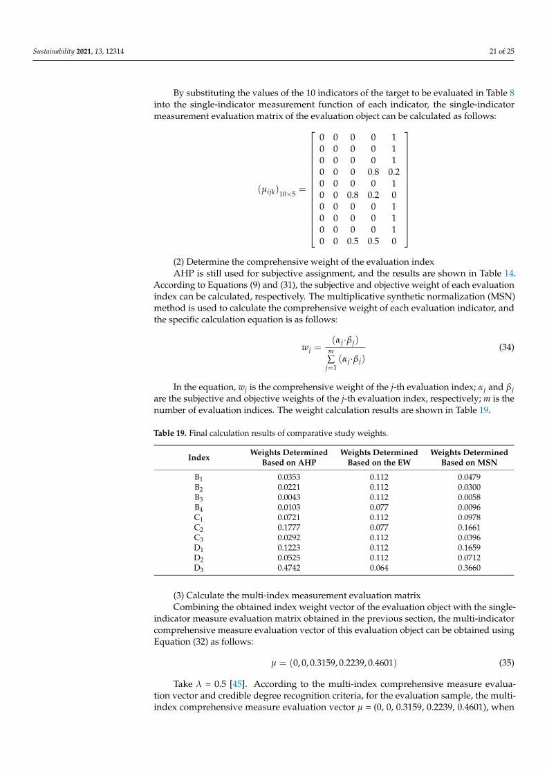
By substituting the values of the 10 indicators of the target to be evaluated in Table 8into the single-indicator measurement function of each indicator, the single-indicatormeasurement evaluation matrix of the evaluation object can be calculated as follows:

(µijk)10×5 =

0 0 0 0 10 0 0 0 10 0 0 0 10 0 0 0.8 0.20 0 0 0 10 0 0.8 0.2 00 0 0 0 10 0 0 0 10 0 0 0 10 0 0.5 0.5 0

(2) Determine the comprehensive weight of the evaluation indexAHP is still used for subjective assignment, and the results are shown in Table 14.

According to Equations (9) and (31), the subjective and objective weight of each evaluationindex can be calculated, respectively. The multiplicative synthetic normalization (MSN)method is used to calculate the comprehensive weight of each evaluation indicator, andthe specific calculation equation is as follows:

wj =(αj·β j)

m∑

j=1(αj·β j)

(34)

In the equation, wj is the comprehensive weight of the j-th evaluation index; αj and β jare the subjective and objective weights of the j-th evaluation index, respectively; m is thenumber of evaluation indices. The weight calculation results are shown in Table 19.

Table 19. Final calculation results of comparative study weights.

Index Weights DeterminedBased on AHP

Weights DeterminedBased on the EW

Weights DeterminedBased on MSN

B1 0.0353 0.112 0.0479B2 0.0221 0.112 0.0300B3 0.0043 0.112 0.0058B4 0.0103 0.077 0.0096C1 0.0721 0.112 0.0978C2 0.1777 0.077 0.1661C3 0.0292 0.112 0.0396D1 0.1223 0.112 0.1659D2 0.0525 0.112 0.0712D3 0.4742 0.064 0.3660

(3) Calculate the multi-index measurement evaluation matrixCombining the obtained index weight vector of the evaluation object with the single-

indicator measure evaluation matrix obtained in the previous section, the multi-indicatorcomprehensive measure evaluation vector of this evaluation object can be obtained usingEquation (32) as follows:

µ = (0, 0, 0.3159, 0.2239, 0.4601) (35)

Take λ = 0.5 [45]. According to the multi-index comprehensive measure evalua-tion vector and credible degree recognition criteria, for the evaluation sample, the multi-index comprehensive measure evaluation vector µ = (0, 0, 0.3159, 0.2239, 0.4601), when


µ11 + µ12 + µ13 + µ14 = 0 + 0 + 0.3159 + 0.2239 = 0.5398 > λ = 0.5, i.e., k0 = 4. The evalu-ation sample belongs to the fourth evaluation category, C4, so it can be judged that theserviceability of the CL in the case study is grade IV, which indicates major damage.

3.9. Evaluation Result Analysis

First of all, the evaluation results of the method proposed in this paper are consistentwith those of the comparative study method; however from the perspective of the calcu-lation process, the calculation complexity of the UMT is greater than that of the CM, andthe fuzziness of the evaluation index is not effectively considered, which highlights therationality and appropriateness of the method proposed in this paper. Meanwhile, from theperspective of the evaluation itself, Figure 8a shows that the CL operation status is moreseverely damaged, and the corresponding evaluation indices are the canal destructionlength, damage area ratio, soil erosion rate, etc. The damage is severe, but from Figure 8b,c,it can be seen that the canal can still be repaired and thus continue to be used. For thecollapsed area, the framework can be rebuilt for pouring, and for the area with serioussoil erosion and frost damage, the soil can be replaced or improved. Figure 8b showsthat the CL condition also displays a trend of becoming gradually unserviceable; thereare holes in the CL on both sides of the slope plate and the surface of the canal bottom,which can be filled with cement mortar. Regarding the uneven surface of the top of the dike,natural gravel can be used for paving. Figure 8c shows that the canal damage condition isrelatively serious; regarding the CL concrete slab cracking, bulging and seepage resistanceperformance, measures should be taken during canal design and management to improve thecanal’s serviceable performance. The canal design should incorporate materials with superioranti-cracking performance and anti-freezing performance, and the seepage resistance level ofthe lining structure needs to be designed in strict accordance with national specifications.

4. Conclusions

In order to understand the actual operating status and damage of the CL over time,and to overcome the shortcomings of the existing CL serviceability evaluation method, anevaluation method based on AHP–SCF–CM is proposed. The main conclusions are as follows:

(1) Ten evaluation indices were determined based on on-site investigation, a literaturesearch and expert consultation, and an evaluation index system for the serviceabilityof the CL structure was established. AHP and SCF were used to realize the subjectiveand objective assignment of indicators, which effectively utilized the rich engineeringexperience of experts and the attributes of objective data to make the calculation of weightsmore scientific and reasonable.

(2) Based on the CM theory, FCG was used to convert the measured sample datavalues of each evaluation index and the standard values and evaluation grades of eachevaluation index into a quantitative CM, and the X condition cloud generator was usedto calculate the digital features of the CM. Thus, a comprehensive evaluation CM wasobtained. The CM adequately evaluates the serviceability status of the canal lining whileaccounting for the fuzziness and randomness inherent in the evaluation indices.

(3) The case study shows that the method based on AHP–SCF–CM uses actual collecteddata to perform the evaluation, which effectively considers the actual damage state of the CL, andthe evaluation results obtained are consistent with actual engineering conditions. A comparisonwith the AHP–EW–UMT method found consistent results with the proposed method.

5. Discussion

It must also be recognized that the proposed AHP–SCF–CM method also has certainlimitations. First of all, this method needs subjective weighting. Therefore, the selection ofexperts is crucial as different experts have different engineering experience and skill levels.In the process of scoring, evaluators should be selected from design units, construction unitsand so on, combined with expert opinions. Secondly, an outstanding feature of this methodis the separation of evaluation index intervals and the acquisition of actual evaluation data.


However, the evaluation indices of different projects are complicated and not all indices willhave corresponding values in n grade intervals. Users should combine the existing lawsand regulations of the country with literature reviews and expert consultation in order todetermine the basis of division into grades. Corresponding tests should be carried out toconfirm that the indices and grading are in line with the required specifications.

In general, the nature of the CL itself is a water delivery canal whose main function isto transport water and reduce water leakage. The results of the case study in this papershow that, in addition to the measures that should be implemented during canal design,relevant management measures need to be taken. The first is to organize canal protectionteams and implement the division of labor and responsibilities, establish a system offrequent and regular inspections so that the canals can be repaired in a timely manner toensure the smooth flow of water. The second is to regularly conduct technical training forcanal protection personnel every year to strengthen their skill level.

We next plan to develop a CL serviceability evaluation system that will involveMATLAB plotting and formula calculation by writing program codes to achieve evaluation,thus simplifying the calculation process and plotting, and eventually users will only need toinput the relevant evaluation indicators and data into the system, which is also conduciveto the popularization of this evaluation method.

Author Contributions: Conceptualization, Q.L. and H.Z.; methodology, H.Z.; software, H.Z.; valida-tion, Q.L. and H.Z.; formal analysis, H.Z.; investigation, H.Z. and Q.M.; resources, Q.L. and L.L.; datacuration, H.Z.; writing—original draft preparation, H.Z.; writing—review and editing, Q.L. and H.Z.;visualization, H.Z.; supervision, Q.L.; project administration, Q.L. and L.L.; funding acquisition, Q.L.and Q.M. All authors have read and agreed to the published version of the manuscript.

Funding: This research was funded by the Key Project of Water Conservancy Science and Technologyof Henan Province (Grant No. GG202062).

Institutional Review Board Statement: Not applicable.

Informed Consent Statement: Not applicable.

Data Availability Statement: Not applicable.

Conflicts of Interest: The authors declare no conflict of interest.

References1. Qureshi, A.S.; Perry, C. Managing Water and Salt for Sustainable Agriculture in the Indus Basin of Pakistan. Sustainability 2021,

13, 5303. [CrossRef]2. Chen, H.; Gao, Z.; Zeng, W.; Liu, J.; Tan, X.; Han, S.J.; Wang, S.L.; Zhao, Y.Q.; Yu, C.K. Scale Effects of Water Saving on Irrigation

Efficiency: Case Study of a Rice-Based Groundwater Irrigation System on the Sanjiang Plain, Northeast China. Sustainability 2017,10, 47. [CrossRef]

3. Wu, C.G. Hydraulics, 4th ed.; Higher Education Press: Beijing, China, 2008.4. Zhang, F.; Guo, S.; Zhang, C.; Guo, P. An interval multiobjective approach considering irrigation canal system conditions for

managing irrigation water. J. Clean. Prod. 2019, 211, 293–302. [CrossRef]5. Li, S.; Zhang, M.; Tian, Y.; Pei, W.; Zhong, H. Experimental and numerical investigations on frost damage mechanism of a canal in

cold regions. Cold Reg. Sci. Technol. 2015, 116, 1–11. [CrossRef]6. Wang, B.; Tian, J.; Zhou, J. Effect of different concrete properties on frost heave crack in U-shaped canal lining and joint. Phys.

Chem. Earth 2021, 121, 102983. [CrossRef]7. Li, Z.; Liu, S.; Feng, Y.; Liu, K.; Zhang, C. Numerical study on the effect of frost heave prevention with different canal lining

structures in seasonally frozen ground regions. Cold Reg. Sci. Technol. 2013, 85, 242–249. [CrossRef]8. Han, X.; Wang, X.; Zhu, Y.; Huang, J. A fully coupled three-dimensional numerical model for estimating canal seepage with

cracks and holes in canal lining damage. J. Hydrol. 2021, 597, 126094. [CrossRef]9. Asl, R.H.; Salmasi, F.; Arvanaghi, H. Numerical investigation on geometric configurations affecting seepage from unlined earthen

channels and the comparison with field measurements. Eng. Appl. Comput. Fluid Mech. 2020, 14, 236–253.10. Eshetu, B.D.; Alamirew, T. Estimation of seepage loss in irrigation canals of Tendaho sugar estate, Ethiopia. Irrig. Drain. Syst. Eng.

2018, 7, 220.11. Wu, D.; Wang, N.; Yang, Z.; Li, C.; Yang, Y. Comprehensive Evaluation of Coal-Fired Power Units Using Grey Relational Analysis

and a Hybrid Entropy-Based Weighting Method. Entropy 2018, 20, 215. [CrossRef]

http://doi.org/10.3390/su13095303

http://doi.org/10.3390/su10010047

http://doi.org/10.1016/j.jclepro.2018.11.111

http://doi.org/10.1016/j.coldregions.2015.03.013

http://doi.org/10.1016/j.pce.2021.102983

http://doi.org/10.1016/j.coldregions.2012.09.011

http://doi.org/10.1016/j.jhydrol.2021.126094

http://doi.org/10.3390/e20040215


12. Wang, K.; Lu, C.; Li, Q. Study on Identifying Significant Risk Sources during Bridge Construction Based on Grey EntropyCorrelation Analysis Method. Math. Probl. Eng. 2021, 2021, 1–15.

13. Zhang, X.; Chen, M.; Guo, K.; Liu, Y.; Liu, Y.; Cai, W.; Wu, H.; Chen, Z.; Chen, Y.; Zhang, J. Regional Land Eco-Security Evaluationfor the Mining City of Daye in China Using the GIS-Based Grey TOPSIS Method. Land 2021, 10, 118.

14. Wang, Z.; Zhang, H.; Wang, Y.; Zhou, C. Integrated Evaluation of the Water Deficit Irrigation Scheme of Indigowoad Root underMulched Drip Irrigation in Arid Regions of Northwest China Based on the Improved TOPSIS Method. Water 2021, 13, 1532.

15. Li, W.; Li, Q.; Liu, Y.; Li, H.; Pei, X. Construction Safety Risk Assessment for Existing Building Renovation Project Based onEntropy-Unascertained Measure Theory. Appl. Sci. 2020, 10, 2893. [CrossRef]

16. Eltarabily, M.; Moghazy, H.E.; Negm, A.M. Assessment of slope instability of canal with standard incomat concrete-filledgeotextile mattresses lining. Alex. Eng. J. 2019, 58, 1385–1397. [CrossRef]

17. El-Molla, D.A.; El-Molla, M.A. Reducing the conveyance losses in trapezoidal canals using compacted earth lining. Ain ShamsEng. J. 2021. [CrossRef]

18. Cui, J.H.; Xie, Z.Q.; Xiao, H.J. Cause Analysis on the Cracks in Concrete Plate of Canal Lining. Appl. Mech. Mater. 2013, 405–408,2596–2599. [CrossRef]

19. Moavenshahidi, A.; Smith, R.; Gillies, M. Factors Affecting the Estimation of Seepage Rates from Channel Automation Data. J.Irrig. Drain. Eng. 2015, 141, 04014075. [CrossRef]

20. Solomon, F.; Ekolu, S. Effect of clay-concrete lining on canal seepage towards the drainage region-an analysis using Finite-Elementmethod. Constr. Mater. Struct. 2014, 344, 1331–1341.

21. Lund, A.R.; Martin, C.A.; Gates, T.K.; Scalia, J.; Babar, M.M. Field evaluation of a polymer sealant for canal seepage reduction.Agric. Water Manag. 2021, 252, 106898. [CrossRef]

22. Si, P.Y. Water Quality Evaluation and Algae Changes of the Main Canal of the Middle Route Project of South-to-North WaterTransfer Project (Hebei Section). Master’s Thesis, Hebei Agricultural University, Hebei, China, 2020.

23. Shi, J.; Zhang, X.D.; Zhen, Z.L.; Liu, Z.H. Evaluation and analysis of anti-frost heave effect of canal lining in frozen soil area basedon temperature-stress coupling. J. Yangtze River Sci. Res. Inst. 2021, 1269. Available online: https://kns.cnki.net/kcms/detail/42.1171.TV.20210611.1102.022.html (accessed on 11 June 2021).

24. Mo, T.; Lou, Z. Numerical Simulation of Frost Heave of Concrete Lining Trapezoidal Channel under an Open System. Water 2020,12, 335. [CrossRef]

25. Kahlown, M.A.; Kemper, W.D. Reducing water loses from channels using linings: Costs and benefits in Pakistan. Agric. WaterManag. 2005, 74, 57–76. [CrossRef]

26. Chen, Z.-Y.; Dai, Z.-H. Application of group decision-making AHP of confidence index and cloud model for rock slope stabilityevaluation. Comput. Geosci. 2021, 155, 104836. [CrossRef]

27. Li, D.Y.; Liu, C.Y. Study on the universality of the normal cloud mode. Strat. Study CAE 2004, 8, 28–34. (In Chinese)28. Xie, S.; Dong, S.; Chen, Y.; Peng, Y.; Li, X. A novel risk evaluation method for fire and explosion accidents in oil depots using

bow-tie analysis and risk matrix analysis method based on cloud model theory. Reliab. Eng. Syst. Saf. 2021, 215, 107791. [CrossRef]29. Yang, Z.T.; Huang, X.F.; Fang, G.H. Benefit evaluation of East Route Project of South to North Water Transfer based on trapezoid

cloud mode. Agric. Water Manag. 2021, 254, 106960. [CrossRef]30. Hou, X.; Lv, T.; Xu, J.; Deng, X.; Liu, F.; Pi, D. Energy sustainability evaluation of 30 provinces in China using the improved

entropy weight-cloud model. Ecol. Indic. 2021, 126, 107657. [CrossRef]31. Wang, J.-Q.; Peng, J.-J.; Zhang, H.-Y.; Liu, T.; Chen, X.-H. An Uncertain Linguistic Multi-criteria Group Decision-Making Method

Based on a Cloud Model. Group Decis. Negot. 2015, 24, 171–192. [CrossRef]32. Cui, Y.H.; Wu, Z.N.; Wu, L. Flood disaster risk assessment of Anying City base on cloud mode. Yangtze River 2020, 51, 7–12.

(In Chinese)33. Ren, Z.H.; Zhang, B.; Ding, Z.D. A service performance evaluation method for mountain tunnel linings based on cloud model. J.

Railw. Sci. Eng. 2020, 17, 2618–2625.34. Saaty, T.L. How to Make a Decision: The Analytic Hierarchy Process. Eur. J. Oper. Res. 1994, 48, 9–26. [CrossRef]35. Liu, S.; Li, W. Indicators sensitivity analysis for environmental engineering geological patterns caused by underground coal

mining with integrating variable weight theory and improved matter-element extension model. Sci. Total Environ. 2019, 686,606–618. [CrossRef] [PubMed]

36. Li, Q.F.; Zhou, H.D.; Zhang, H. Durability evaluation of highway tunnel lining structure based on matter element extension-simplecorrelation function method-cloud model: A case study. Math. Biosci. Eng. 2021, 18, 4027–4054. [CrossRef]

37. Sun, L.; Liu, Y.; Zhang, B.; Shang, Y.; Yuan, H.; Ma, Z. An Integrated Decision-Making Model for Transformer ConditionAssessment Using Game Theory and Modified Evidence Combination Extended by D Numbers. Energies 2016, 9, 697. [CrossRef]

38. DB 64/T 811—2012. Technical Specification for Irrigation Canal Lining Engineering; Quality and Technical Supervision Bureau ofNingxia Hui Autonomous Region: Yinchuan, China, 2012.

39. Liu, Q.Y.; Wang, M.W.; Wang, X.; Shen, F.Q.; Jin, J.L. Land Eco-Security Assessment Based on the Multi-Dimensional ConnectionCloud Model. Sustainability 2018, 10, 2096. [CrossRef]

40. Ministry of Housing and Urban-Rural Development of the People’s Republic of China. Standard for Quality Control of Concrete;China Construction Industry Press: Beijing, China, 2011.

http://doi.org/10.3390/app10082893

http://doi.org/10.1016/j.aej.2019.11.010

http://doi.org/10.1016/j.asej.2021.01.018

http://doi.org/10.4028/www.scientific.net/AMM.405-408.2596

http://doi.org/10.1061/(ASCE)IR.1943-4774.0000842

http://doi.org/10.1016/j.agwat.2021.106898

https://kns.cnki.net/kcms/detail/42.1171.TV.20210611.1102.022.html

https://kns.cnki.net/kcms/detail/42.1171.TV.20210611.1102.022.html

http://doi.org/10.3390/w12020335

http://doi.org/10.1016/j.agwat.2004.09.016

http://doi.org/10.1016/j.cageo.2021.104836

http://doi.org/10.1016/j.ress.2021.107791

http://doi.org/10.1016/j.agwat.2021.106960

http://doi.org/10.1016/j.ecolind.2021.107657

http://doi.org/10.1007/s10726-014-9385-7

http://doi.org/10.1016/0377-2217(90)90057-I

http://doi.org/10.1016/j.scitotenv.2019.04.393

http://www.ncbi.nlm.nih.gov/pubmed/31185408

http://doi.org/10.3934/mbe.2021202

http://doi.org/10.3390/en9090697

http://doi.org/10.3390/su10062096


41. Ministry of Housing and Urban-Rural Development of the People’s Republic of China. Standard for Test Methods of Long-TermPerformance and Durability of Ordinary Concrete; Construction Industry Press: Beijing, China, 2009.

42. An, Y.L.; Peng, L.M.; Wu, B. Comprehensive extension assessment on tunnel collapse risk. J. Cent. South Univ. 2011, 42, 514–520.(In Chinese)

43. Wang, X.; Li, Z.H.; Zheng, L.Y. Indoor simulation experiment on the relationship between soil denudation rate and current shearforce. J. Shenyang Agric. Univ. 2007, 4, 577–580. (In Chinese)

44. Li, W.L.; Li, H.M.; Liu, Y.J.; Wang, S.M.; Pei, X.W.; Li, Q. Fire risk assessment of high-rise buildings under construction based onunascertained measure theory. PLoS ONE 2020, 15, e0239166. [CrossRef]

45. Su, S.R.; Zhou, Y.; Zhou, Z.H. Hazard assessment of collapse using EW-AHP and unascertained measure theory. J. Eng. Geol.2019, 27, 577–584. (In Chinese)

http://doi.org/10.1371/journal.pone.0239166

evaluation of serviceability of canal lining based on ahp

Documents