Evaluating the Reverse Greedy Algorithm

Shady Coptyshady@il.ibm.com

Shmuel Urur@il.ibm.com

Elad Yom Tovyomtov@il.ibm.com

April 7, 2004

Abstract

This paper present two meta heuristics, reverse greedy andfuture aware greedy, which are variants of the greedy algo-rithm. Both are based on the observation that guessing theimpact of future selections is useful for the current selec-tion. While the greedy algorithm makes the best local se-lection given the past, future aware greedy makes the bestlocal selection given the past and the estimated future, andreverse greedy executes a number of greedy iterations andchooses the last one as the next choice. Future aware greedydepends on a future aware utility function which is problemspecific. While we have found such utility functions for theset cover problem this paper concentrate on reverse greedywhose description is truly problem independent.

Both algorithms suggested, while not quite as efficientcomputationally as the greedy algorithm, are still very effi-cient. We show interesting problems on which the greedyalgorithm has been extensively studied where the suggestedalgorithms outperform greedy. We also show a problemwith different characteristics on which the greedy algo-rithm is better and try to categorize the kind of problemsfor which future aware and reverse greedy are expected toyield good result.

1 Introduction

Many optimization problems fall under the following de-scription: the problem has a set of solutions which may

be applied in any order, together with a monotonic utilityfunction on subsets of the solutions,U . Given two subsetsof solutions A and B ifA⊃ B, U(A) ≥U(B). In addition,the utility function is usually such that for a given solutionx, U(x|A) ≤U(x|B). The optimization problem is to findthe best utility for a solution of given cardinality. Opti-mization problems that fall under this description includethe set cover problem with many of its variants [15, 7], thefacility location problems [13, 12], the maximum coverageproblem [11], and many others.

The greedy algorithm chooses solutions, one at a time,such that each solution, when chosen, gives maximum im-provement to the utility function, until the cardinality ofsolutions is reached. The types of utility functions underwhich the greedy algorithm is optimal [20, 18] has beenextensively studied. For example, if the utility function of asolution is independent of previously chosen solutions, thenthe greedy algorithm is optimal. For other problems, whilegreedy may not be optimal, it still is the algorithm of choice[9, 8, 16, 1, 17]. This is because the greedy algorithm iscomputationally efficient and tends to yield good results.There are many studies on the greedy algorithms for suchproblems that show upper and lower bounds [19, 10], aswell as other properties.

The greedy algorithm, as its name suggest, is a veryshort-sighted algorithm. It always looks for the best short-term gain. The greedy algorithm gets very good perfor-mance by ignoring global optimizations which are very ex-pensive. However, the greedy algorithm also ignores avail-

1

able relevant information that exists in the problem for-mulation, namely the cardinality of the solution set. Wepresent here a new variant on the greedy algorithm, whichwe call reverse greedy or RGreedy, which takes that car-dinality into account. We demonstrate, using experiments,that a large class of problems exists on which RGreedy out-performs the greedy algorithms. We explain our intuitionregarding the kind of problems for which it is advantageousto use RGreedy, as well as situations where it does not helpor actually hinders.

We created the RGreedy algorithm after studying a vari-ant of the set cover problem[3]. In that paper we also de-fined future aware greedy - FWGreedy. FWGreedy is char-acterized by a modified weight of the objective function ac-cording to what is likely to occur in the future. For exam-ple, in the set cover problem, we use the problem formu-lation and the knowledge of how many more sets will beselected to estimate, for each task, the probability that itwill be found in the future. We then greedily choose theset that finds the most tasks that have not been seen in theprevious sets and that are less likely to be observed in thefuture.

Both RGreedy and FWGreedy have initially smaller util-ity than the greedy algorithm. Our prediction was thatif RGreedy and FWGreedy use the knowledge of cost inan efficient way, then their utility will surpass that of thegreedy algorithm when we get close to the last set. In-deed, as Figure 1 shows for the selection of 10 solutions,RGreedy surpasses Greedy close to the end. The ini-tial experimental results have encouraged us to examineRGreedy-type of algorithms further and see how they workon other problems and how they can be improved.

Section 2 shows the intuition behind RGreedy and sam-ple problems on which it works well. We then explain sim-ple variants that may improve the result. Section 3 con-tains a number of experiments which show problems onwhich RGreedy works well. Some initial tuning work forRGreedy is also shown. Section 4 shows an experiment ona problem for which RGreedy is not suitable. It also triesto generalize the type of problems for which we do not ex-

pect this approach to work. Section 5 contains concludingremarks, as well as suggested avenues for future work.

2 Description and motivation for theRGreedy algorithm

Our original motivation for the RGreedy algorithm camewhen trying to optimize probabilistic regression suites[3, 6]. Denote byt = {t1, . . . , tn} the set of tasks to be cov-ered. Lets = {s1, . . . ,sk} be a set of heuristics for whichstatistical coverage predictors exist. The probability of cov-ering the taskt j using heuristicsi is denotedPi

j . The prob-abilistic resource constraint regression suite problem is tochoose, for any given number, a set of heuristics such thatthe number of expected distinct task seen is maximized.

The greedy algorithm for the probabilistic regressionsuite problem chooses heuristics, one at the time, such thateach heuristic when chosen increases the objective func-tion by the maximum amount. For each task the increase inthe objective function is the probability of the heuristics tocover that tasks multiplied by the probability that it was notobserved by prior heuristics.

The greedy algorithm for constructing probabilistic re-gression suites with limited resources provides efficientand high-quality regression suites, but these suites are usu-ally not optimal. One reason for the sub-optimality of thegreedy algorithm is that it does not consider future steps inthe algorithm. Specifically, the greedy algorithm ignoresthe contribution of the heuristics selected in future stepsto the overall coverage. As a result, the greedy algorithmmay select a heuristic with a high probability of coveringa given task, ignoring the fact that this task will be cov-ered with high probability in the future, even without theselected heuristic.

We define FWGreedy as an algorithm that chooses solu-tions, one at a time, such that each solution when chosengives maximum improvements to the future aware utilityfunction, which takes the future into account, as well as thepreviously used solutions.

2

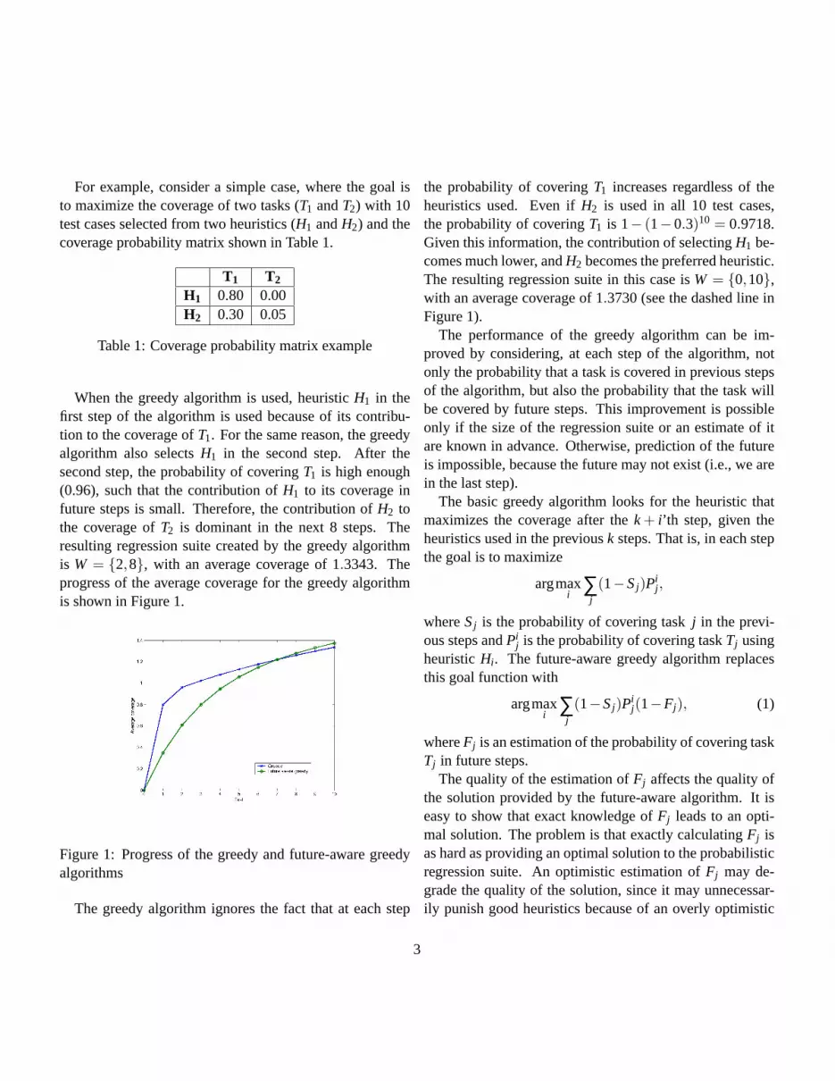
For example, consider a simple case, where the goal isto maximize the coverage of two tasks (T1 andT2) with 10test cases selected from two heuristics (H1 andH2) and thecoverage probability matrix shown in Table 1.

T1 T2

H1 0.80 0.00H2 0.30 0.05

Table 1: Coverage probability matrix example

When the greedy algorithm is used, heuristicH1 in thefirst step of the algorithm is used because of its contribu-tion to the coverage ofT1. For the same reason, the greedyalgorithm also selectsH1 in the second step. After thesecond step, the probability of coveringT1 is high enough(0.96), such that the contribution ofH1 to its coverage infuture steps is small. Therefore, the contribution ofH2 tothe coverage ofT2 is dominant in the next 8 steps. Theresulting regression suite created by the greedy algorithmis W = {2,8}, with an average coverage of 1.3343. Theprogress of the average coverage for the greedy algorithmis shown in Figure 1.

Figure 1: Progress of the greedy and future-aware greedyalgorithms

The greedy algorithm ignores the fact that at each step

the probability of coveringT1 increases regardless of theheuristics used. Even ifH2 is used in all 10 test cases,the probability of coveringT1 is 1− (1−0.3)10 = 0.9718.Given this information, the contribution of selectingH1 be-comes much lower, andH2 becomes the preferred heuristic.The resulting regression suite in this case isW = {0,10},with an average coverage of 1.3730 (see the dashed line inFigure 1).

The performance of the greedy algorithm can be im-proved by considering, at each step of the algorithm, notonly the probability that a task is covered in previous stepsof the algorithm, but also the probability that the task willbe covered by future steps. This improvement is possibleonly if the size of the regression suite or an estimate of itare known in advance. Otherwise, prediction of the futureis impossible, because the future may not exist (i.e., we arein the last step).

The basic greedy algorithm looks for the heuristic thatmaximizes the coverage after thek+ i’th step, given theheuristics used in the previousk steps. That is, in each stepthe goal is to maximize

argmaxi

∑j

(1−Sj)Pij ,

whereSj is the probability of covering taskj in the previ-ous steps andPi

j is the probability of covering taskTj usingheuristicHi . The future-aware greedy algorithm replacesthis goal function with

argmaxi

∑j

(1−Sj)Pij(1−Fj), (1)

whereFj is an estimation of the probability of covering taskTj in future steps.

The quality of the estimation ofFj affects the quality ofthe solution provided by the future-aware algorithm. It iseasy to show that exact knowledge ofFj leads to an opti-mal solution. The problem is that exactly calculatingFj isas hard as providing an optimal solution to the probabilisticregression suite. An optimistic estimation ofFj may de-grade the quality of the solution, since it may unnecessar-ily punish good heuristics because of an overly optimistic

3

future. In the extreme case, if we useFj = 1, the greedyalgorithm is reduced to a random selection of heuristics.

When a good method for estimatingFj is used, thefuture-aware algorithm should perform better than thegreedy algorithm. But if we look at coverage progress asfunction of the step in the algorithm, the greedy algorithmshould perform better than the future-aware greedy in theearly steps. This happens because the greedy algorithmtries to maximize the current gain, while the future-awarealgorithm looks at a farther horizon. Figure 1 illustratesthis. In general, we expect the future-aware algorithm fornsteps to perform better than the future-aware algorithm form steps,m> n, aftern steps.

In our experiments we examined several methods spe-cific to the set cover problem of estimating the future tobe used by FWGreedy. However, as the future aware util-ity function is problem-specific, we did not generalize thisidea to other problems.

We did create one generic algorithm – RGreedy – thattakes the estimation of the future into account. Instead ofestimating the future, RGreedy chooses in the future! Thisis accomplished by running the regular greedy algorithm tocompletion but instead of choosing the solution for the firststep, the solution that was chosen for the last step is selectedand the process is repeated. The intuition is by reversing,we choose the solution that is chosen with the most knowl-edge. We start by working on the hard parts and when weget to the easy parts we work with full knowledge of theimpact of the other solutions on the problem. RGreedy isfairly efficient, if n is the number of solutions to be chosenthen the cost of RGreedy is at mostn/2 times the cost ofthe greedy algorithm.

In this work we have evaluated the RGreedy algorithm ona number of problems in order to develop intuition on thetypes of problem on which it will work. We also checkedif RGreedy could be improved by running the algorithm afraction of the way to completion (half or three quartersfor example) and choosing there. The intuition is sim-ilar to that of classification algorithms that try to avoidover-classification that can be caused by overly training a

classifier on training data through methods such as cross-validation [5].

We denote byRGreedy(κ = 0.5), for example, an imple-mentation of the greedy algorithm in which at every stepwe execute the greedy algorithm half the way to the endand choose the last one. So if the number of heuristics tobe executed is 20 in the first step we run the greedy algo-rithm 10 times and choose the tenth while after the twelfthstep we run it four times (half way to 20) and choose thelast.

3 Description and experimental resultsfor the RGreedy algorithm

We demonstrate using two problems the advantage of theRGreedy algorithm over the greedy algorithm. For eachof the two problems, different settings are investigated. Ineach setting, a large number of random instances is gener-ated as input to the different algorithms. We evaluate theperformance of each algorithm in comparison to the oth-ers. For each setting, an algorithm’s performance is thenumber of times it achieved the best result, normalized bythe number of executions - 10000 for the first experiment,and 1000 for the second. Note that for the same instance,two algorithms could achieve the best result. We comparethe results of algorithms to each other, since we don’t knowthe optimal result, as it is computationally hard to calculate.We collected other measures such as the frequency at whichan algorithm achieved the best result exclusively, and howoften the algorithm achieved the best result divided by thenumber of other algorithms that achieved the same result inthe same experiment. These measures were omitted sincethey show the same trends as the simple measure.

3.1 Probabilistic Regression Suites with LimitedResources

Automated regression suites are essential in testing largeapplications while maintaining reasonable quality and

4

timetables. The main objection to automation of tests, inaddition to the cost of creation and maintenance, is the ob-servation that if you run the exact same test many times itbecomes a lot less likely to find bugs. To alleviate thoseproblems, a new regression suite practice, which uses ran-dom test generators to create regression suites on-the-fly,is becoming more common. In this regression practice, in-stead of maintaining tests, regression suites are generatedon-the-fly by choosing several specifications and generat-ing a number of tests from each.

Given N tasks and K test specifications, in which eachtest specification covers each task in a given probability,choose M test specifications to cover the greatest numberof tasks. This is obviously an instance of a probabilisticset cover which is an NP hard problem [7]. We discuss thevariant withK = N, were each specification was originallywritten to target a certain task, but also in some probabilityhits other tasks. This is not guaranteed in the general formof the probabilistic set cover problem. In the case that theprobability for each specification to hit tasks other than itstargeted task is zero, RGreedy and the greedy algorithmyield the same outcome. The reason for this is that oncea test specification is chosen, it no longer yields additionalbenefit, and so the only difference is the reverse order.

Copty at el. described the greedy algorithm and anRGreedy algorithm for this problem [3]. The greedy algo-rithm, chooses a test specification for each step that maxi-mizes the expected coverage, given preceding choices. TheRGreedy algorithm for the problem runs the greedy algo-rithm in each step withκ fraction of the number of testspecifications left to choose, and picks the last test speci-fication as the current chosen test specification.

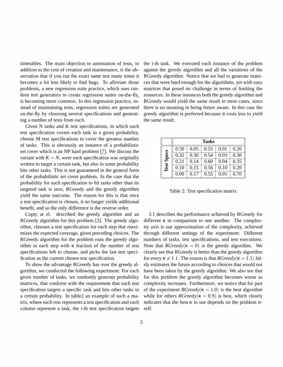
To show the advantage RGreedy has over the greedy al-gorithm, we conducted the following experiment: For eachgiven number of tasks, we randomly generate probabilitymatrices, that conform with the requirement that each testspecification targets a specific task and hits other tasks ina certain probability. In table2 an example of such a ma-trix, where each row represents a test specification and eachcolumn represent a task, the i-th test specification targets

the i-th task. We executed each instance of the problemagainst the greedy algorithm and all the variations of theRGreedy algorithm. Notice that we had to generate matri-ces that were hard enough for the algorithms, yet with easymatrices that posed no challenge in terms of limiting theresources. In these instances both the greedy algorithm andRGreedy would yield the same result in most cases, sincethere is no meaning in being future aware. In this case thegreedy algorithm is preferred because it costs less to yieldthe same result.

Tasks

Test

Spe

cs 0.50 0.05 0.55 0.01 0.200.32 0.30 0.54 0.03 0.300.21 0.14 0.60 0.04 0.350.10 0.15 0.56 0.10 0.200.00 0.17 0.55 0.01 0.70

Table 2: Test specification matrix

3.1 describes the performance achieved by RGreedy fordifferent κ in comparison to one another. The complex-ity axis is our approximation of the complexity, achievedthrough different settings of the experiment: Differentnumbers of tasks, test specifications, and test executions.Note thatRGreedy(κ = 0) is the greedy algorithm. Weclearly see that RGreedy is better than the greedy algorithmfor everyκ 6= 1.1. The reason is thatRGreedy(κ = 1.1) fal-sly estimates the future according to choices that would nothave been taken by the greedy algorithm. We also see thatfor this problem the greedy algorithm becomes worse ascomplexity increases. Furthermore, we notice that for partof the experimentRGreedy(κ = 1.0) is the best algorithmwhile for othersRGreedy(κ = 0.9) is best, which clearlyindicates that the bestκ to use depends on the problem it-self.

5

Figure 2: Comparing the performance achieved byRGreedy for differentκ for the probabilistic regressionproblem. The complexity axis is our approximation of thecomplexity, achieved by different settings of the experi-ment. Note thatRGreedy(κ = 0) is the greedy algorithm.We clearly see that RGreedy is better than the greedy al-gorithm for everyκ 6= 1.1. Note that for this problem thegreedy algorithm becomes worse as complexity increases.Finally, for some of the experimentsRGreedy(κ = 1.0) isthe best algorithm while for othersRGreedy(κ = 0.9) isbest.

3.2 Facility locating problem

Given N cities, choose M cities in which to build a facilitysuch that the sum of all minimum distances between citiesand facilities is minimized. Figure 3 shows an example ofsuch a problem with 12 cities and 4 facilities. This type offacility-locating problem is NP hard [7].

The greedy algorithm for this problem is quite trivial:Keep choosing cities to place facilities in until you reachM cities, at each step, given the preceding choices, choosethe city that minimizes the sum of all minimum distances.The RGreedy algorithm for the problem is for each step torun the greedy algorithm with the number of facilities leftto locate, and pick the greedy algorithms’ last facility loca-tion as the current chosen facility location. In the variationsthat try to overcome the over-approximation problem, werun a fraction of the way to the end, and then the last city,

Figure 3: Cities and Facilities Example. Rectangles denotecities with facilities, circles denote cities where no facilitieswere placed.

RGreedy(κ = 0.5) for example, runs the greedy algorithmhalf the way at each step and takes the last solution as thecurrent solution.

Several experiments were conducted to show the ad-vantage RGreedy has over the greedy algorithm for thisproblem. The number of cities was chosen to be 50for all the experiments. The number of facilities cho-sen was 5, 10, 15, 20, 25, 30, 35 and 45. Since choos-ing where to place M facilities is like choosing wherenot to placeN −M facilities, the problems increase incomplexity as they get closer toM = 25, and then de-crease as they climb to 50. The random maps gener-ated satisfy the triangle inequality. In this problem, weexamine a different set of RGreedy variations, withκ ∈{0,0.1,0.2,0.3,0.4,0.5,0.6,0.7,0.8,0.9,1.0,1.1}. Again,we evaluate the performance of each of our algorithms incomparison to other algorithms.

Figure 4 shows the performance of each algorithm. Sincethe performance is relative to other algorithms’ results, theyshould be examined as such. We clearly see that for thedifferent number of facilities,RGreedy(κ ≤ 1.0) is betterthan that of the greedy algorithm. We again notice thatthe best performing RGreedy is different for different set-

6

Figure 4: Comparing performance for the Facility Locat-ing Problem. Since the performance is relative to otheralgorithms’ results, they should be examined as such.We clearly see that for the different number of facilities,RGreedy(κ ≤ 1.0) is better than that of the greedy algo-rithm.

tings, for example the problem withM = 25 is best han-dled byRGreedy(κ = 0.8) while M = 15 is best handled byRGreedy(κ = 0.9) andM = 10 by RGreedy(κ = 1). Thebehaviour inM = 5 originates from the little difference be-tween the different fractions for a small horizon such as 5.As for the loss of significance for problems withM > 25,we relate it to the problem becoming easier and for the longhorizon where over-approximation is unavoidable.

4 Matching pursuit

Matching pursuit (MP) is a method for the sub-optimal ex-pansion of a signal in a redundant dictionary [4]. Thisalgorithm, combined with a dictionary of Gabor functions,defines a time-frequency transformation. Matching pursuitworks by iterative subtraction of the best matching dictio-nary functions (known as atoms) from the signal, with theappropriate amplitude and phase. Since at each iterationthe best matching function is subtracted, this is a greedyalgorithm.

Matching pursuit was used to expand a one-dimensional

chirp signal of length 64, over a dictionary that containedapproximately 21,000 Gabor functions. We ran the MP al-gorithm (Denoted by Greedy MP) for 20 iterations. At eachiteration, after finding the best fitting atom to the signal, it’sparameters were fine-tuned using 20 iterations of Nelder-Mead multidimensional unconstrained nonlinear minimiza-tion [2]. This atom was then subtracted from the remainingsignal.

The RGreedy version of MP was also used for approxi-mating the same chirp signal. The RGreedy version of MPis straightforward – Instead of using the best-fitting atomfor subtraction, the atom used by Greedy MP after, for ex-ample, 50% of iterations (In the case ofRGreedy(κ = 0.5))is used. The amplitude and phase used for subtraction arethose found for the Greedy MP.

The test was repeated with various levels of white Gaus-sian noise added to the chirp signal. Each variant of thealgorithms was run against 10 realizations of noise at eachnoise level.

Figure 5 demonstrated the average energy (over 10 real-izations) of the residual signal, when approximating a sig-nal with no noise added. As can be expected, Greedy MP(RGreedy withκ = 0) reduces the residual energy morerapidly compared to RGreedy withκ > 0, which reducesmost of the energy at latter iterations.

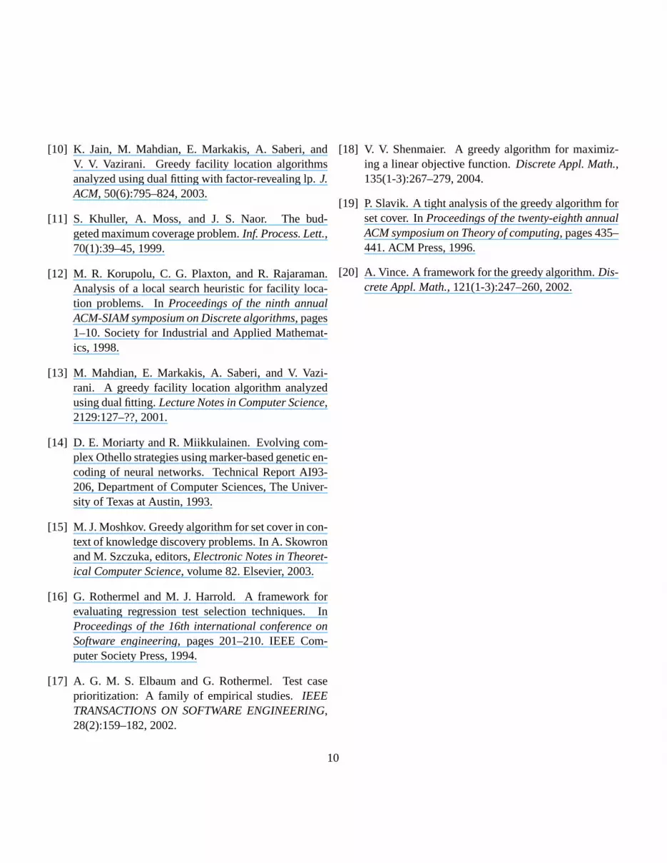
As figure 6 shows, at a given noise level Greedy MP at-tains a smaller residual energy compared to any variant ofRGreedy MP. This effect is more prominent at lower noiselevels where the difference in the residual energy of GreedyMP and RGreedy MP is larger than an order of magnitude.

This is most likely due to the fact that the dictionarycontains smooth Gabor functions. Thus, Greedy MP firstfinds a fit for the global features of the signal, and gradu-ally progresses to fitting more localized features. By usingthe atoms found in later iterations as the first atoms to be re-moved, the global features (That contain the most energy inthe signal) are removed, and thus it is difficult for RGreedyMP to remove energy as efficiently as Greedy MP. This ex-plains why, at high noise levels, where the smoothness ofthe signal is lost, the difference between Greedy MP and

7

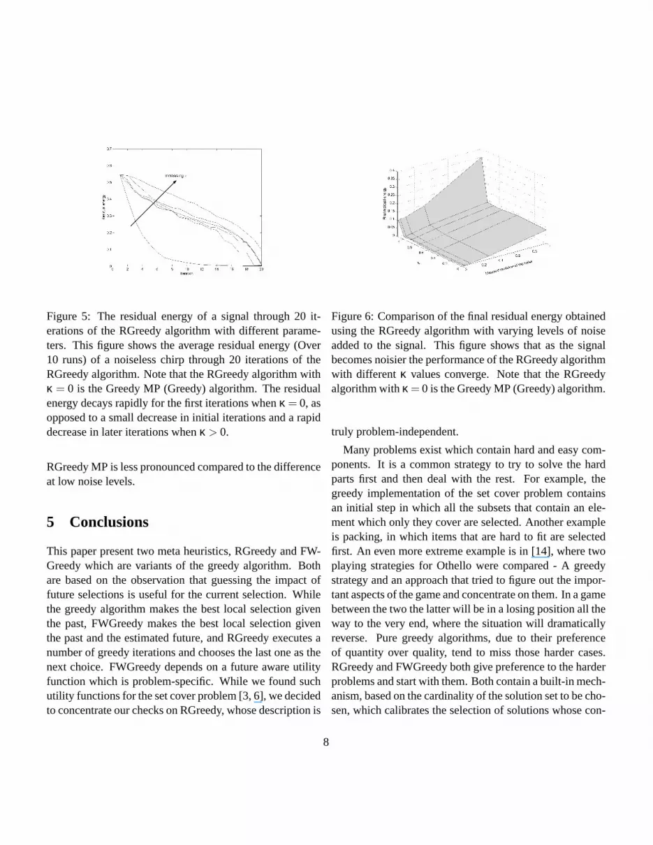
Figure 5: The residual energy of a signal through 20 it-erations of the RGreedy algorithm with different parame-ters. This figure shows the average residual energy (Over10 runs) of a noiseless chirp through 20 iterations of theRGreedy algorithm. Note that the RGreedy algorithm withκ = 0 is the Greedy MP (Greedy) algorithm. The residualenergy decays rapidly for the first iterations whenκ = 0, asopposed to a small decrease in initial iterations and a rapiddecrease in later iterations whenκ > 0.

RGreedy MP is less pronounced compared to the differenceat low noise levels.

5 Conclusions

This paper present two meta heuristics, RGreedy and FW-Greedy which are variants of the greedy algorithm. Bothare based on the observation that guessing the impact offuture selections is useful for the current selection. Whilethe greedy algorithm makes the best local selection giventhe past, FWGreedy makes the best local selection giventhe past and the estimated future, and RGreedy executes anumber of greedy iterations and chooses the last one as thenext choice. FWGreedy depends on a future aware utilityfunction which is problem-specific. While we found suchutility functions for the set cover problem [3, 6], we decidedto concentrate our checks on RGreedy, whose description is

Figure 6: Comparison of the final residual energy obtainedusing the RGreedy algorithm with varying levels of noiseadded to the signal. This figure shows that as the signalbecomes noisier the performance of the RGreedy algorithmwith different κ values converge. Note that the RGreedyalgorithm withκ = 0 is the Greedy MP (Greedy) algorithm.

truly problem-independent.

Many problems exist which contain hard and easy com-ponents. It is a common strategy to try to solve the hardparts first and then deal with the rest. For example, thegreedy implementation of the set cover problem containsan initial step in which all the subsets that contain an ele-ment which only they cover are selected. Another exampleis packing, in which items that are hard to fit are selectedfirst. An even more extreme example is in [14], where twoplaying strategies for Othello were compared - A greedystrategy and an approach that tried to figure out the impor-tant aspects of the game and concentrate on them. In a gamebetween the two the latter will be in a losing position all theway to the very end, where the situation will dramaticallyreverse. Pure greedy algorithms, due to their preferenceof quantity over quality, tend to miss those harder cases.RGreedy and FWGreedy both give preference to the harderproblems and start with them. Both contain a built-in mech-anism, based on the cardinality of the solution set to be cho-sen, which calibrates the selection of solutions whose con-

8

tribution is not too small for the selected cardinality. Thevery esthetically pleasing result is that the utility functionof the solutions suggested surpass that of the greedy algo-rithm only close to the solution cardinality, for any givencardinality.

We selected three problems, which were extensivelystudied, on which to compare RGreedy to the greedy algo-rithm. We showed that in two of these instances, set coverand facility location, RGreedy outperforms the greedy al-gorithm. But on one of them, the matching pursuit, greedyis better. We think that the difference is that the match-ing pursuit problem when solved using RGreedy has theproperty that applying small corrections first, gives it nonsmooth characteristic that detract from the first solutions.This is similar to packing first the small items and then be-ing unable to pack the hard to fit items. On the set coverproblem and the facility location problem we found thatchoosing first the harder solutions improve the final result.Our conjecture is that after choosing first the hard solutionsthe selection between the easy solutions, of which more ex-ist, is more efficient.

This paper has shown the promise inherent in the twometa heuristics. Further research is needed in order to findout the characteristic of problems on which RGreedy andFWGreedy are expected to out perform the greedy algo-rithm. We have not touched at all on lower and upperbounds. The only theoretical result we have is that if thegreedy algorithm is optimal so is RGreedy, which is not avery interesting result. It will be interesting to know if thereare problems on which RGreedy has a better theoretical up-per (and lower) bound then greedy. Many of the proofs thatshow bounds on the greedy algorithm use the fact that itsshort sighted nature to causes it to perform poorly. Suchmethods will be harder to deploy on RGreedy.

Another interesting venue of research is optimization ofRGreedy. We have found out that there is correlation be-tween the ”‘hardness”’ of the problem and the bestκ to use.Work is needed to find out if this is indeed the case and howto predict which value ofκ to use. Another, quite likely,possibility is that the optimalκ is not a constant fraction of

the number of the solutions left, but maybe just a constant,or a number that could change during the calculation, beingeither longer or shorter in the beginning.

References

[1] E. Buchnik and S. Ur. Compacting regression-suiteson-the-fly. InProceedings of the 4th Asia Pacific Soft-ware Engineering Conference, December 1997.

[2] T. Coleman, M. Branch, and A. Grace. Optimizationtoolbox for use with matlab, 1990.

[3] S. Copty, S. Fine, S. Ur, and A. Ziv. Future aware al-gorithms for probabilistic regression suites. submittedto ISSRE 2004, 2004.

[4] G. Davis, S. Mallat, and Z. Zhang. Adaptivetime-frequency approximation with matching pur-suits. Proceedings of the SPIE, (2242):402–413,1994.

[5] R. Duda, P. Hart, and D. Stork.Pattern classification.John Wiley and Sons, Inc, New-York, USA, 2001.

[6] S. Fine, S. Ur, and A. Ziv. A probabilistic regressionsuite for functional verification. DAC04, 2004.

[7] M. Garey and D. Johnson.Computers and Intractabil-ity: A Guide to the Theory of NP-Completeness. W.H.Freeman, 1979.

[8] T. L. Graves, M. J. Harrold, J.-M. Kim, A. Porter, andG. Rothermel. An empirical study of regression testselection techniques. InProceedings of the 20th inter-national conference on Software engineering, pages188–197. IEEE Computer Society, 1998.

[9] M. J. Harrold, J. A. Jones, T. Li, D. Liang, and A. Gu-jarathi. Regression test selection for java software. InProceedings of the 16th ACM SIGPLAN conferenceon Object oriented programming, systems, languages,and applications, pages 312–326. ACM Press, 2001.

9

[10] K. Jain, M. Mahdian, E. Markakis, A. Saberi, andV. V. Vazirani. Greedy facility location algorithmsanalyzed using dual fitting with factor-revealing lp.J.ACM, 50(6):795–824, 2003.

[11] S. Khuller, A. Moss, and J. S. Naor. The bud-geted maximum coverage problem.Inf. Process. Lett.,70(1):39–45, 1999.

[12] M. R. Korupolu, C. G. Plaxton, and R. Rajaraman.Analysis of a local search heuristic for facility loca-tion problems. InProceedings of the ninth annualACM-SIAM symposium on Discrete algorithms, pages1–10. Society for Industrial and Applied Mathemat-ics, 1998.

[13] M. Mahdian, E. Markakis, A. Saberi, and V. Vazi-rani. A greedy facility location algorithm analyzedusing dual fitting.Lecture Notes in Computer Science,2129:127–??, 2001.

[14] D. E. Moriarty and R. Miikkulainen. Evolving com-plex Othello strategies using marker-based genetic en-coding of neural networks. Technical Report AI93-206, Department of Computer Sciences, The Univer-sity of Texas at Austin, 1993.

[15] M. J. Moshkov. Greedy algorithm for set cover in con-text of knowledge discovery problems. In A. Skowronand M. Szczuka, editors,Electronic Notes in Theoret-ical Computer Science, volume 82. Elsevier, 2003.

[16] G. Rothermel and M. J. Harrold. A framework forevaluating regression test selection techniques. InProceedings of the 16th international conference onSoftware engineering, pages 201–210. IEEE Com-puter Society Press, 1994.

[17] A. G. M. S. Elbaum and G. Rothermel. Test caseprioritization: A family of empirical studies.IEEETRANSACTIONS ON SOFTWARE ENGINEERING,28(2):159–182, 2002.

[18] V. V. Shenmaier. A greedy algorithm for maximiz-ing a linear objective function.Discrete Appl. Math.,135(1-3):267–279, 2004.

[19] P. Slavik. A tight analysis of the greedy algorithm forset cover. InProceedings of the twenty-eighth annualACM symposium on Theory of computing, pages 435–441. ACM Press, 1996.

[20] A. Vince. A framework for the greedy algorithm.Dis-crete Appl. Math., 121(1-3):247–260, 2002.

10