For Peer Review

Analyzing scale and scope specialization efficiencies of U.S.

agricultural and non-agricultural banks using the Fourier Flexible Functional Form

Journal: Applied Economics

Manuscript ID: AFE-2010-0098.R1

Journal Selection: Applied Financial Economics

Date Submitted by the Author:

n/a

Complete List of Authors: Yu, Yingzhuo; American Express, Account Security Group Escalante, Cesar; University of Georgia, Agricultural and Applied Economics Deng, Xiaohui; American Express, Account Security Group Houston, Jack; University of Georgia, Agricultural and Applied Economics

Gunter, Lewell; University of Georgia, Agricultural and Applied Economics

JEL Code:

Q14 - Agricultural Finance < Q1 - Agriculture < Q - Agricultural and Natural Resource Economics, G21 - Banks|Other Depository Institutions|Mortgages < G2 - Financial Institutions and Services < G - Financial Economics

Keywords: Economies of scope, expansion path sub-additivity, Fourier Flexible

Editorial Office, Dept of Economics, Warwick University, Coventry CV4 7AL, UK

Submitted Manuscript

For Peer Review

Page 1 of 30

Editorial Office, Dept of Economics, Warwick University, Coventry CV4 7AL, UK

Submitted Manuscript

123456789101112131415161718192021222324252627282930313233343536373839404142434445464748495051525354555657585960

For Peer Review

1

Analyzing scale and scope specialization efficiencies of U.S. agricultural and non-

agricultural banks using the Fourier Flexible Functional Form

Yingzhuo Yua, Cesar L. Escalanteb *, Xiaohui Denga, Jack Houstonb, and Lewell F. Gunterb

a Account Security Group/Fraud Risk Management,, American Express,

20022 North 31st Avenue, Phoenix, AZ 85027 b Department of Agricultural and Applied Economics, University of Georgia, 315 Conner Hall,

Athens, GA 30602 *Corresponding Author. E-mail: cescalan@uga.edu

Running Title: Scale and Scope Efficiencies of Agricultural and Non-Agricultural Banks Abstract: This study presents results of cost estimation and efficiency analyses of various size

categories of agricultural and non-agricultural commercial banks using the Fourier flexible (FF)

function model. The traditional cost estimation model is expanded in this study with the

inclusion of loan quality and financial risk indexes often ignored in empirical efficiency models.

The FF model produced more intuitive scale efficiency results than the standard translog model

owing to its greater global approximation capability. Scale efficiency measures provide

evidence of increasing returns to scale for small and medium-size banks. Agricultural banks

demonstrated a stronger tendency to maximize the potentials of increasing returns to scale as a

result of output expansion. The translog cost model, however, remains a reliable tool in scope

efficiency analyses that, in this study, produced results suggesting that agricultural banks are

more likely to thrive more efficiently under specialized lending operations.

Page 2 of 30

Editorial Office, Dept of Economics, Warwick University, Coventry CV4 7AL, UK

Submitted Manuscript

123456789101112131415161718192021222324252627282930313233343536373839404142434445464748495051525354555657585960

For Peer Review

2

I. Background

In recent decades, rural financial markets have undergone a period of rapid transition to

adapt to structural changes in the agricultural economy and the financial services industry. The

U.S. agriculture, on one hand, has undergone massive consolidation and integration since the 20th

century, which has been driven by business decisions to take advantage of larger economies of

scale (Lamb, 1999). At the lenders’ front, on the other hand, the U.S. government began its

relaxation of laws regulating the banking sector in the 1980s by eliminating regulatory barriers to

mergers and acquisitions. In the 1990s, more deregulatory policies were passed that allowed

inter-state bank acquisitions, in addition to unrestricted merger and acquisition activities between

national banks and all types of credit institutions. The effects of deregulation in reshaping the

banking industry and increasing the level of financial innovation had substantial impacts on

competition within the industry (Northcoth, 2004).

Meanwhile, commercial banks have been increasingly involved in farm lending as

agricultural debt comprised about 33% of their total loan portfolios in the last decade (Stam et al.,

2003; Walraven et al., 1993). In the farm sector’s national balance sheets released annually by

USDA’s Economic Research Service, commercial banks continue to be the dominant provider of

agricultural loans. Their share of farm loan disbursements in the national aggregate farm loan

portfolios has steadily increased from 35.09% in 1990 to 44.47% in 2006.

As in any competitive industry, banks have always been pressured to implement

innovative business strategies that enhance operating efficiency in order to sustain their

competitiveness in the industry. These business strategies are vital to the health of the rural

economy, considering the banks’ role in influencing regional flows of funds (Samolyk, 1989).

Page 3 of 30

Editorial Office, Dept of Economics, Warwick University, Coventry CV4 7AL, UK

Submitted Manuscript

123456789101112131415161718192021222324252627282930313233343536373839404142434445464748495051525354555657585960

For Peer Review

3

Over the past several years, a number of studies have addressed the measurement of

efficiencies of financial institutions, primarily focusing on commercial banking operations

(Gilligan and Smirlock, 1984; Gropper, 1991; Berger and Humprey, 1991; McAllister and

McManus, 1993; Berger and Mester, 1997). Most of these studies reveal large cost inefficiencies

in such institutions, which have accounted for at least 20% of total banking industry costs and

have eroded about 50% of the industry’s potential profits (Berger and Mester, 1997).

In agricultural finance literature, only a few studies have explored the application of

efficiency models to agricultural lending (Ellinger and Neff, 1993; Featherstone and Moss, 1994;

Neff et al., 1994). Compared to regular commercial banks, agricultural banks1 tend to have more

liquidity concerns. Smaller banks tend to hold more farm loans in their portfolios than their

larger counterparts (Stam et al., 2003). Thus, most agricultural banks are unable to diversify

their clientele to accommodate businesses from other non-agricultural business clients possibly

due to shortage of lending funds. The specialized nature of their lending operations could result

in greater risks and uncertainty. In this regard, results of efficiency analyses based on

commercial banking operations have less relevance to agricultural banks as no parallel

conclusions can be drawn given these banks’ different styles of lending operations.

Various versions of the efficiency measurement approaches have been introduced in the

literature. The parametric approach requires strict assumptions on cost functional form and

curvature in order to obtain unbiased results. The semi-nonparametric approach relaxes such

strict functional form condition and requires only minimal a priori assumptions (Gallant, 1982).

The nonparametric method avoids the task of functional form specification, but has its own set of

limitations, such as its technological, rather than economic, optimization focus and non-

Page 4 of 30

Editorial Office, Dept of Economics, Warwick University, Coventry CV4 7AL, UK

Submitted Manuscript

123456789101112131415161718192021222324252627282930313233343536373839404142434445464748495051525354555657585960

For Peer Review

4

stochastic approach that does not allow inference formulations and statistical hypothesis testing

(Berger and Mester, 1997; Coelli et al., 2003).

Most parametric efficiency models have used either the Cobb-Douglas or translog cost

functions, which are relatively simpler and easier to estimate (Berger and Humphrey, 1991;

Gilligan and Smirlock, 1984; Gropper, 1991; Hunter et al., 1990; Noulas et al., 1990). However,

some analysts challenged the relevance and validity of certain assumptions associated with these

functions. Coelli et al.(2003) pointed out the restrictive, unrealistic assumptions in the Cobb-

Douglas framework that require all firms to have the same production elasticities and the

constraint of having substitution elasticities equal to one. McAllister and McManus (1993) raised

doubts about application of the translog cost function to different banking situations given the

poor approximation results they obtained for various banking size categories. Specifically, they

clarified that since the translog functional form represents a second-order Taylor series

approximation of an arbitrary function at a point, it forces a symmetric U-shaped average cost

curve applied to both large and small banks without differentiation. Considering the fact that

agricultural banks tend to run relatively smaller-scale operations, the translog functional form

might not be ideal for efficiency analyses in the agricultural banks category.

In this study, we employ a semi-nonparametric cost efficiency analysis using the Fourier

Flexible Functional Form (henceforth referred to as FF), which conveniently allows us to infer

relationships among variables when the true functional form of the relationships is unknown.

Moreover, this functional form includes trigonometric transformations of the variables that allow

for better, global approximation of the underlying true cost function (Gallant, 1982; Huang and

Wang, 2004; Mitchell and Onvural, 1996). This means that the FF model does not require the

restrictive conditions of functional form specificity of the parametric approach. In addition, the

Page 5 of 30

Editorial Office, Dept of Economics, Warwick University, Coventry CV4 7AL, UK

Submitted Manuscript

123456789101112131415161718192021222324252627282930313233343536373839404142434445464748495051525354555657585960

For Peer Review

5

FF model can measure any bias resulting from using the translog form since the latter is actually

a special case nested in the FF form.

To date, the FF framework has been applied only to a few commercial banking studies

(Mitchell and Onvural, 1996; Huang and Wang, 2004) and, to our knowledge, has never been

applied in the analysis of agricultural banking efficiency. The application of efficiency models to

agricultural banks has usually been complicated by the difficulty of identifying a suitable cost

functional form that can accommodate the peculiar lending patterns of these banks.2 Notably,

the FF model potentially has greater relevance in agricultural banking efficiency analyses as it

can adapt to the changing financial needs of farm businesses that emanate from the more volatile

and uncertain business environments they operate in. Moreover, as previous commercial bank

efficiency studies have claimed, the FF provides a better fit to their data due to its global

approximation capability (Bauer and Ferrier, 1996; Mitchell and Onvural, 1996).

This study introduces the application of the FF framework in banking cost efficiency

analysis, focusing specifically on scale and scope efficiencies, using a panel banking call report

dataset from the Federal Reserve Board. Specifically, scale and scope efficiency measures will

be used in this study to determine whether banks benefit through cost savings (operating

efficiency) from output expansion and product diversification, respectively. These analyses will

clarify whether the agricultural banks’ relatively smaller-scale operations and greater tendency

towards product specialization will pose as impediments to achieving cost efficiency vis-à-vis

their larger and more diversified non-agricultural banking counterparts.

This study also expands its analytical framework beyond the traditional form by

introducing loan quality and financial risk measures, which have important cost and efficiency

implications but seldom are factored into earlier efficiency models. Efficiency measures of scale

Page 6 of 30

Editorial Office, Dept of Economics, Warwick University, Coventry CV4 7AL, UK

Submitted Manuscript

123456789101112131415161718192021222324252627282930313233343536373839404142434445464748495051525354555657585960

For Peer Review

6

and scope are assessed for the FF function. In order to determine the relative strengths of the FF

framework, the results of the FF model are compared with those derived from an alternative,

competing model based on the translog cost function. The effects of bank size and specialization

on these efficiency measures are analyzed to shed light on the relative efficiencies of small,

agricultural banks vis-à-vis their larger non-agricultural counterparts.

The subsequent sections lay out the theoretical foundations of the FF cost function

framework and measures for scale and scope efficiencies considered in this study. The empirical

section describes data collection procedures, presents the empirical results, and discusses their

implications.

II. The Fourier Flexible Cost Function

The FF function is a semi-parametric approach that expands the standard translog

function by adding a linear combination of sine and cosine functions, referred to as the Fourier

series. The non-parametric Fourier series can potentially approximate any well-behaved

multivariate function since the sine and cosine terms are mutually orthogonal and function-

space-spanning (Huang and Wang, 2004). The FF function can be expressed as3:

(1) εxkxkzγxAx'xβ hh ++++++= ∑=

)]sin()cos([)21(1

0

H

hhh vuLnC β

where 0β is a constant to be estimated; ]',...,,...[ 11 qMqlNl ββββ=β is a 1)( ×+ MN vector of

coefficients to be estimated; N is the number of inputs; M is the number of outputs; ],[ q'l'x =

is a )( MNQT +× matrix of rescaled log-input prices )',...( 1 Nll=l and scaled log-output

quantities )',...( 1 Mqq=q 4; Q is the number of firms in each year and T is the number of years in

panel data; ]['ija== ββA is a )()( MNMN +×+ symmetric matrix of coefficients to be

estimated; ],...[ 1 wzz=z is a WQT × matrix of exogenous variables which capture financial risks

Page 7 of 30

Editorial Office, Dept of Economics, Warwick University, Coventry CV4 7AL, UK

Submitted Manuscript

123456789101112131415161718192021222324252627282930313233343536373839404142434445464748495051525354555657585960

For Peer Review

7

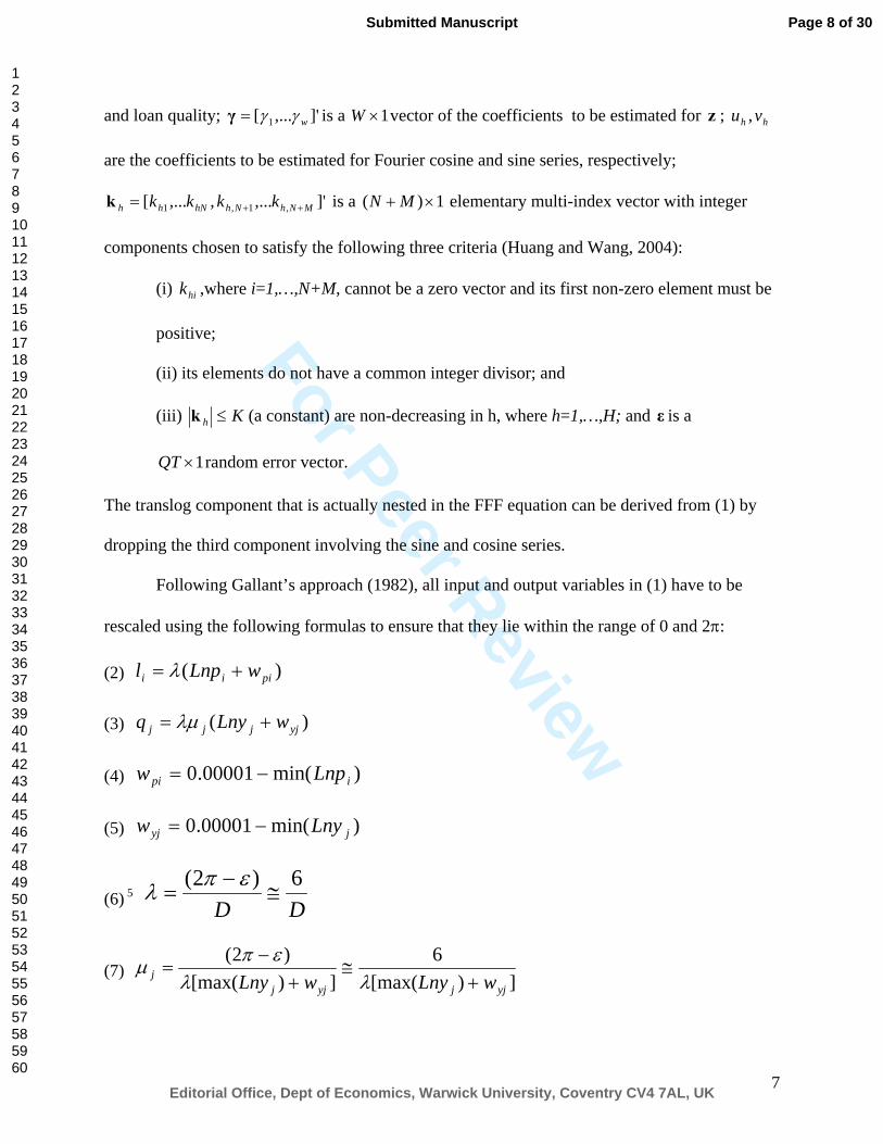
and loan quality; ]',...[ 1 wγγ=γ is a 1×W vector of the coefficients to be estimated for z ; hh vu ,

are the coefficients to be estimated for Fourier cosine and sine series, respectively;

]',...,,...[ ,1,1 MNhNhhNhh kkkk ++=k is a 1)( ×+ MN elementary multi-index vector with integer

components chosen to satisfy the following three criteria (Huang and Wang, 2004):

(i) hik ,where i=1,…,N+M, cannot be a zero vector and its first non-zero element must be

positive;

(ii) its elements do not have a common integer divisor; and

(iii) Kh ≤k (a constant) are non-decreasing in h, where h=1,…,H; and ε is a

1×QT random error vector.

The translog component that is actually nested in the FFF equation can be derived from (1) by

dropping the third component involving the sine and cosine series.

Following Gallant’s approach (1982), all input and output variables in (1) have to be

rescaled using the following formulas to ensure that they lie within the range of 0 and 2π:

(2) )( piii wLnpl += λ

(3) )( yjjjj wLnyq += λμ

(4) )min(00001.0 ipi Lnpw −=

(5) )min(00001.0 jyj Lnyw −=

(6) 5 DD6)2(

≅−

=επλ

(7) ])[max(6

])[max()2(

yjjyjjj wLnywLny +

≅+

−=

λλεπμ

Page 8 of 30

Editorial Office, Dept of Economics, Warwick University, Coventry CV4 7AL, UK

Submitted Manuscript

123456789101112131415161718192021222324252627282930313233343536373839404142434445464748495051525354555657585960

For Peer Review

8

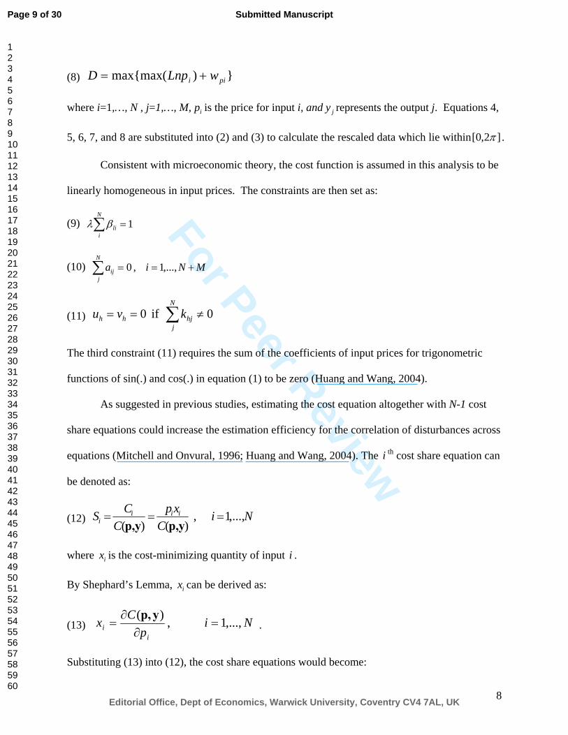
(8) })max{max( pii wLnpD +=

where i=1,…, N , j=1,…, M, ip is the price for input i, and jy represents the output j. Equations 4,

5, 6, 7, and 8 are substituted into (2) and (3) to calculate the rescaled data which lie within ]2,0[ π .

Consistent with microeconomic theory, the cost function is assumed in this analysis to be

linearly homogeneous in input prices. The constraints are then set as:

(9) ∑ =N

ili 1βλ

(10) ∑ +==N

jij MNia ,...,1 , 0

(11) ∑ ≠==N

jhjhh kvu 0 if 0

The third constraint (11) requires the sum of the coefficients of input prices for trigonometric

functions of sin(.) and cos(.) in equation (1) to be zero (Huang and Wang, 2004).

As suggested in previous studies, estimating the cost equation altogether with N-1 cost

share equations could increase the estimation efficiency for the correlation of disturbances across

equations (Mitchell and Onvural, 1996; Huang and Wang, 2004). The i th cost share equation can

be denoted as:

(12) ,...,1 , )()(

NiC

xpC

CS iiii ===

yp,yp,

where ix is the cost-minimizing quantity of input i .

By Shephard’s Lemma, ix can be derived as:

(13) ,...,1 , )( Nip

Cxi

i =∂

∂=

yp,.

Substituting (13) into (12), the cost share equations would become:

Page 9 of 30

Editorial Office, Dept of Economics, Warwick University, Coventry CV4 7AL, UK

Submitted Manuscript

123456789101112131415161718192021222324252627282930313233343536373839404142434445464748495051525354555657585960

For Peer Review

9

(14) ,...,1 , ln

)(lnln1)(

)()(ln

)(

)(

Nip

Cp

pp

CC

CC

pCp

Sii

i

i

ii

i =∂

∂=⎟⎟

⎠

⎞⎜⎜⎝

⎛∂

∂⋅

∂∂⋅

∂∂

=⎥⎦

⎤⎢⎣

⎡∂

∂

=yp,yp,

yp,yp,

yp,

yp,

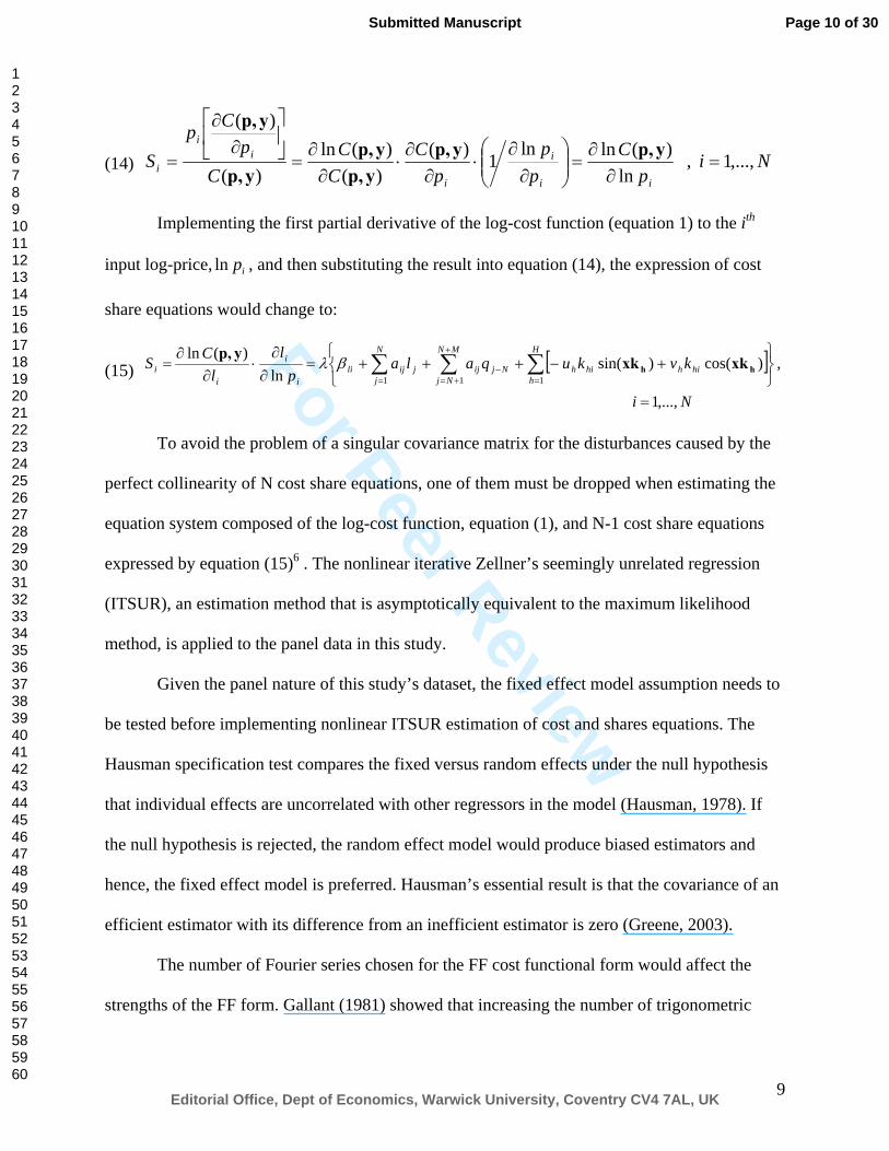
Implementing the first partial derivative of the log-cost function (equation 1) to the ith

input log-price, ipln , and then substituting the result into equation (14), the expression of cost

share equations would change to:

(15) [ ] ,...,1

, )cos()sin(ln

)(ln1 1 1

Ni

kvkuqalap

ll

CSN

j

MN

Nj

H

hhihhihNjijjijli

i

i

ii

=⎭⎬⎫

⎩⎨⎧

+−+++=∂∂

⋅∂

∂= ∑ ∑ ∑

=

+

+= =− hh xkxkyp, βλ

To avoid the problem of a singular covariance matrix for the disturbances caused by the

perfect collinearity of N cost share equations, one of them must be dropped when estimating the

equation system composed of the log-cost function, equation (1), and N-1 cost share equations

expressed by equation (15)6 . The nonlinear iterative Zellner’s seemingly unrelated regression

(ITSUR), an estimation method that is asymptotically equivalent to the maximum likelihood

method, is applied to the panel data in this study.

Given the panel nature of this study’s dataset, the fixed effect model assumption needs to

be tested before implementing nonlinear ITSUR estimation of cost and shares equations. The

Hausman specification test compares the fixed versus random effects under the null hypothesis

that individual effects are uncorrelated with other regressors in the model (Hausman, 1978). If

the null hypothesis is rejected, the random effect model would produce biased estimators and

hence, the fixed effect model is preferred. Hausman’s essential result is that the covariance of an

efficient estimator with its difference from an inefficient estimator is zero (Greene, 2003).

The number of Fourier series chosen for the FF cost functional form would affect the

strengths of the FF form. Gallant (1981) showed that increasing the number of trigonometric

Page 10 of 30

Editorial Office, Dept of Economics, Warwick University, Coventry CV4 7AL, UK

Submitted Manuscript

123456789101112131415161718192021222324252627282930313233343536373839404142434445464748495051525354555657585960

For Peer Review

10

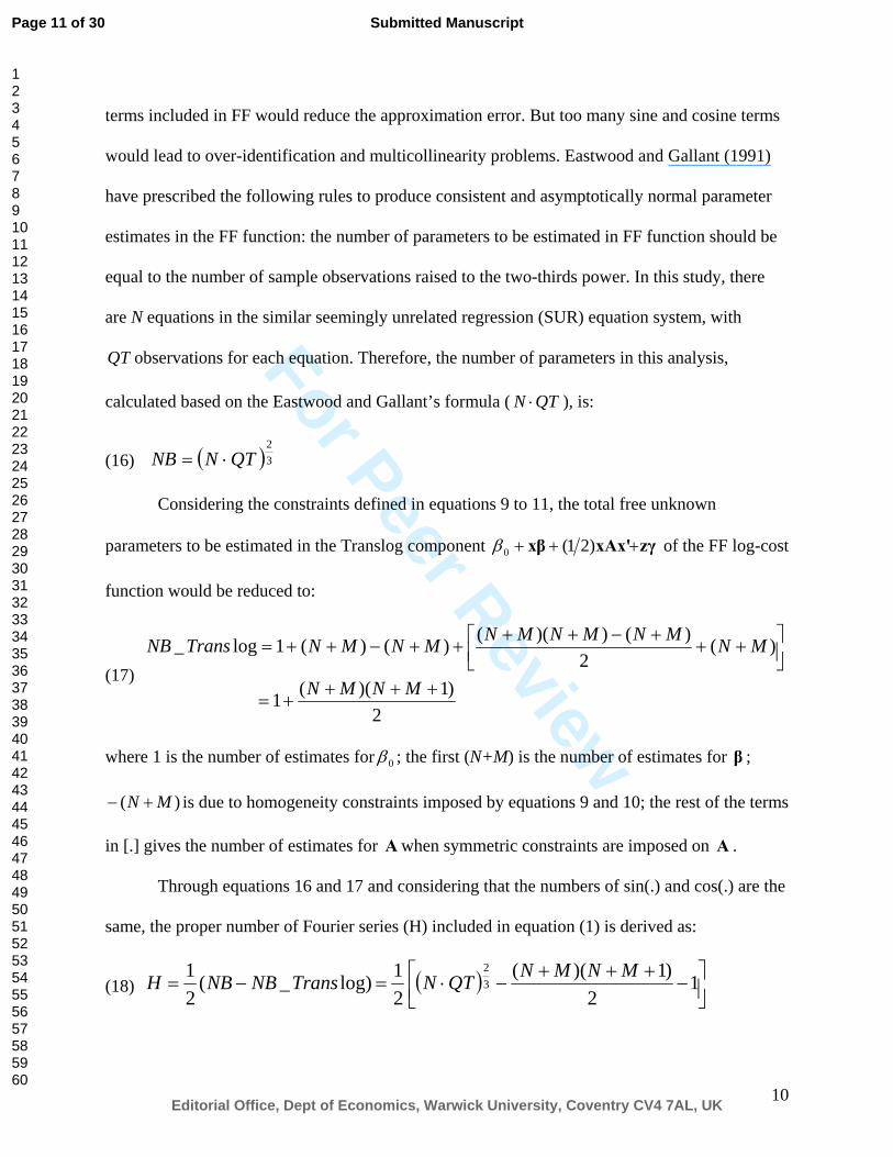
terms included in FF would reduce the approximation error. But too many sine and cosine terms

would lead to over-identification and multicollinearity problems. Eastwood and Gallant (1991)

have prescribed the following rules to produce consistent and asymptotically normal parameter

estimates in the FF function: the number of parameters to be estimated in FF function should be

equal to the number of sample observations raised to the two-thirds power. In this study, there

are N equations in the similar seemingly unrelated regression (SUR) equation system, with

QT observations for each equation. Therefore, the number of parameters in this analysis,

calculated based on the Eastwood and Gallant’s formula ( QTN ⋅ ), is:

(16) ( )32

QTNNB ⋅=

Considering the constraints defined in equations 9 to 11, the total free unknown

parameters to be estimated in the Translog component zγxAx'xβ +++ )21(0β of the FF log-cost

function would be reduced to:

(17)

2)1)((1

)(2

)())(()()(1log_

++++=

⎥⎦⎤

⎢⎣⎡ ++

+−++++−++=

MNMN

MNMNMNMNMNMNTransNB

where 1 is the number of estimates for 0β ; the first (N+M) is the number of estimates for β ;

)( MN +− is due to homogeneity constraints imposed by equations 9 and 10; the rest of the terms

in [.] gives the number of estimates for A when symmetric constraints are imposed on A .

Through equations 16 and 17 and considering that the numbers of sin(.) and cos(.) are the

same, the proper number of Fourier series (H) included in equation (1) is derived as:

(18) ( ) ⎥⎦⎤

⎢⎣⎡ −

+++−⋅=−= 1

2)1)((

21log)_(

21

32 MNMNQTNTransNBNBH

Page 11 of 30

Editorial Office, Dept of Economics, Warwick University, Coventry CV4 7AL, UK

Submitted Manuscript

123456789101112131415161718192021222324252627282930313233343536373839404142434445464748495051525354555657585960

For Peer Review

11

III. Efficiency Measures

The estimated cost function will be used to develop the following measures that capture

efficiencies realized from scale and scope of production, and variations of product specialization

strategies (Ellinger, 1994; Mitchell and Onvural, 1996).

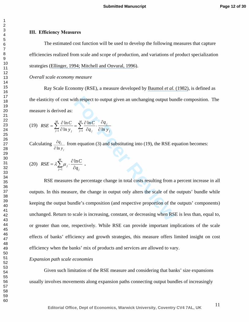
Overall scale economy measure

Ray Scale Economy (RSE), a measure developed by Baumol et al. (1982), is defined as

the elasticity of cost with respect to output given an unchanging output bundle composition. The

measure is derived as:

(19) ∑ ∑= = ∂

∂⋅

∂∂

=∂∂

=M

j

M

j j

j

jj yq

qC

yCRSE

1 1 lnln

lnln

Calculating j

j

yq

ln∂∂ from equation (3) and substituting into (19), the RSE equation becomes:

(20) ∑= ∂

∂⋅=

M

j jj q

CRSE1

lnμλ .

RSE measures the percentage change in total costs resulting from a percent increase in all

outputs. In this measure, the change in output only alters the scale of the outputs’ bundle while

keeping the output bundle’s composition (and respective proportion of the outputs’ components)

unchanged. Return to scale is increasing, constant, or decreasing when RSE is less than, equal to,

or greater than one, respectively. While RSE can provide important implications of the scale

effects of banks’ efficiency and growth strategies, this measure offers limited insight on cost

efficiency when the banks’ mix of products and services are allowed to vary.

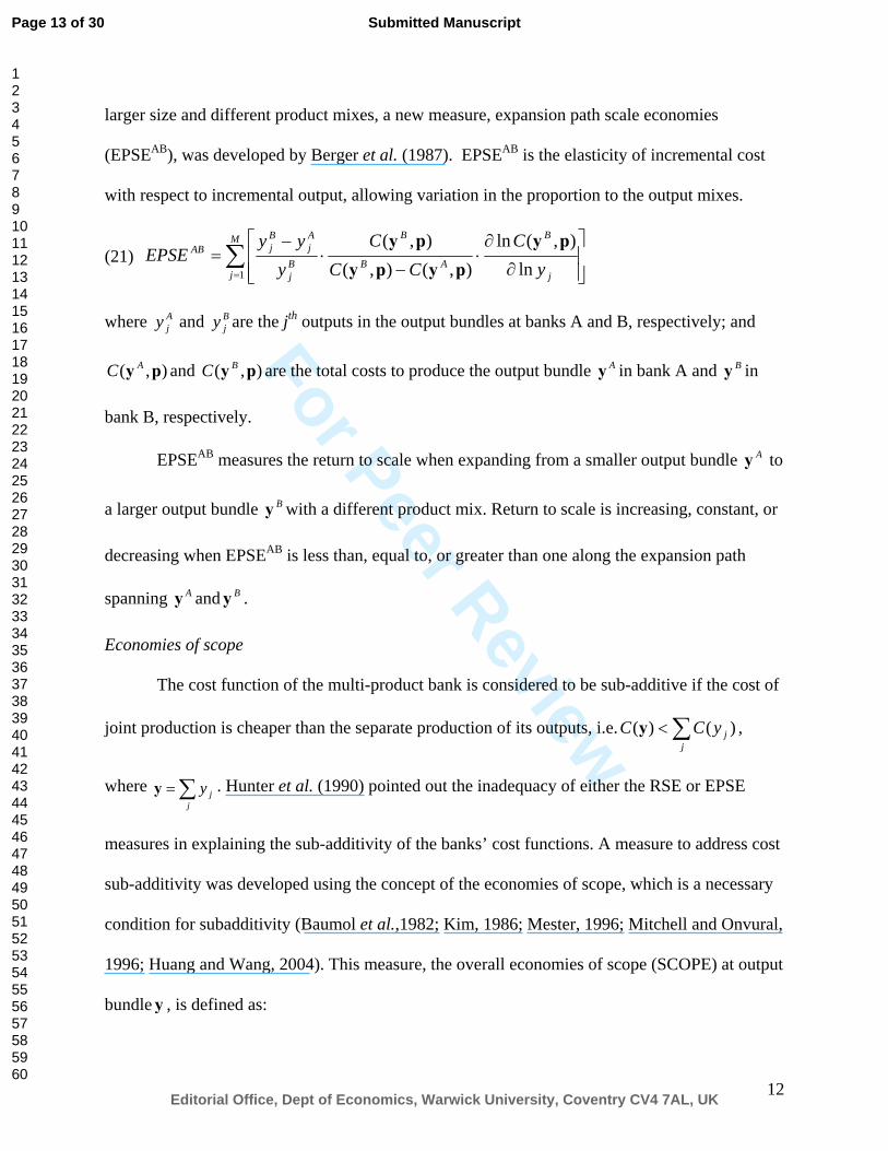
Expansion path scale economies

Given such limitation of the RSE measure and considering that banks’ size expansions

usually involves movements along expansion paths connecting output bundles of increasingly

Page 12 of 30

Editorial Office, Dept of Economics, Warwick University, Coventry CV4 7AL, UK

Submitted Manuscript

123456789101112131415161718192021222324252627282930313233343536373839404142434445464748495051525354555657585960

For Peer Review

12

larger size and different product mixes, a new measure, expansion path scale economies

(EPSEAB), was developed by Berger et al. (1987). EPSEAB is the elasticity of incremental cost

with respect to incremental output, allowing variation in the proportion to the output mixes.

(21) ∑= ⎥

⎥⎦

⎤

⎢⎢⎣

⎡

∂

∂⋅

−⋅

−=

M

j j

B

AB

B

Bj

Aj

BjAB

yC

CCC

yyy

EPSE1 ln

),(ln),(),(

),( pypypy

py

where Ajy and B

jy are the jth outputs in the output bundles at banks A and B, respectively; and

),( py AC and ),( py BC are the total costs to produce the output bundle Ay in bank A and By in

bank B, respectively.

EPSEAB measures the return to scale when expanding from a smaller output bundle Ay to

a larger output bundle By with a different product mix. Return to scale is increasing, constant, or

decreasing when EPSEAB is less than, equal to, or greater than one along the expansion path

spanning Ay and By .

Economies of scope

The cost function of the multi-product bank is considered to be sub-additive if the cost of

joint production is cheaper than the separate production of its outputs, i.e. ∑<j

jyCC )()(y ,

where ∑=j

jyy . Hunter et al. (1990) pointed out the inadequacy of either the RSE or EPSE

measures in explaining the sub-additivity of the banks’ cost functions. A measure to address cost

sub-additivity was developed using the concept of the economies of scope, which is a necessary

condition for subadditivity (Baumol et al.,1982; Kim, 1986; Mester, 1996; Mitchell and Onvural,

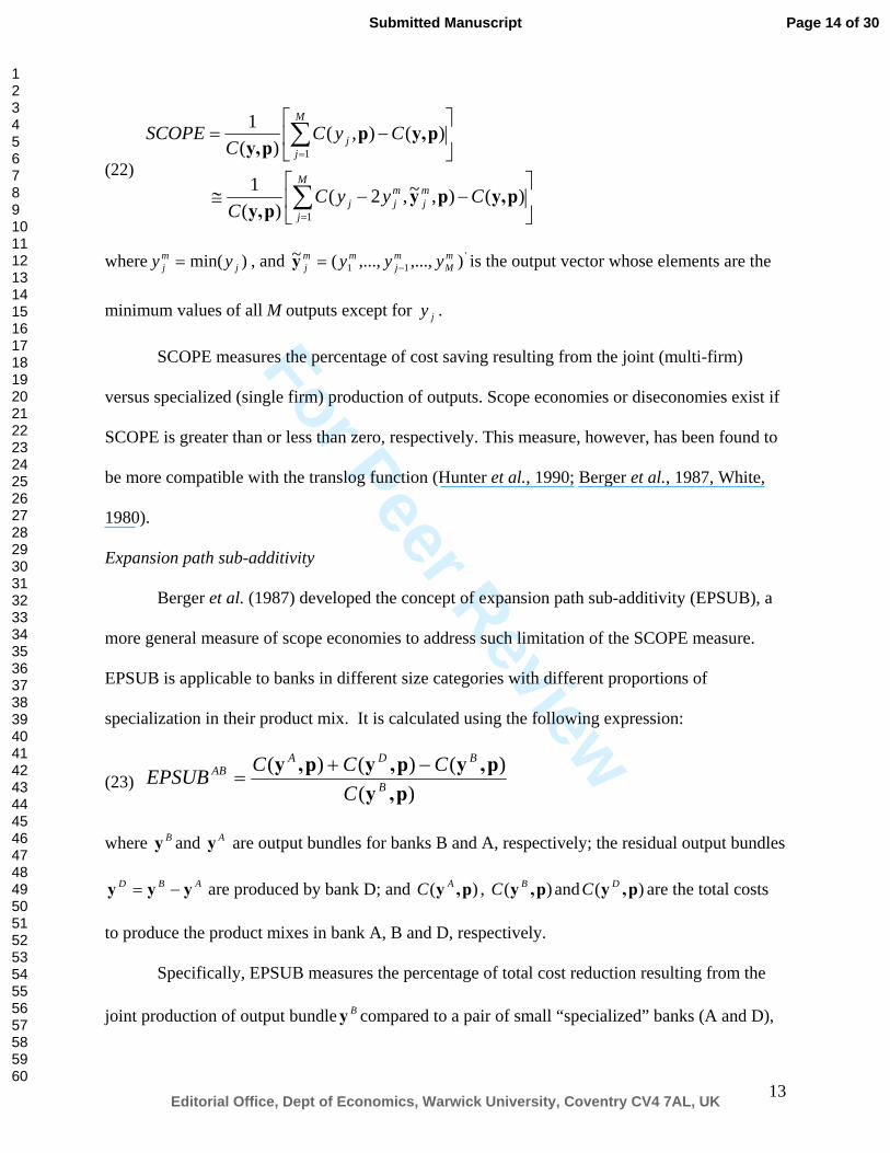
1996; Huang and Wang, 2004). This measure, the overall economies of scope (SCOPE) at output

bundle y , is defined as:

Page 13 of 30

Editorial Office, Dept of Economics, Warwick University, Coventry CV4 7AL, UK

Submitted Manuscript

123456789101112131415161718192021222324252627282930313233343536373839404142434445464748495051525354555657585960

For Peer Review

13

(22)

⎥⎦

⎤⎢⎣

⎡−−≅

⎥⎦

⎤⎢⎣

⎡−=

∑

∑

=

=

)(),~,2()(

1

)(),()(

1

1

1

py,pypy,

py,ppy,

CyyCC

CyCC

SCOPE

M

j

mj

mjj

M

jj

where )min( jmj yy = , and '

11 ),...,,...,(~ mM

mj

mmj yyy −=y is the output vector whose elements are the

minimum values of all M outputs except for jy .

SCOPE measures the percentage of cost saving resulting from the joint (multi-firm)

versus specialized (single firm) production of outputs. Scope economies or diseconomies exist if

SCOPE is greater than or less than zero, respectively. This measure, however, has been found to

be more compatible with the translog function (Hunter et al., 1990; Berger et al., 1987, White,

1980).

Expansion path sub-additivity

Berger et al. (1987) developed the concept of expansion path sub-additivity (EPSUB), a

more general measure of scope economies to address such limitation of the SCOPE measure.

EPSUB is applicable to banks in different size categories with different proportions of

specialization in their product mix. It is calculated using the following expression:

(23) )()()()(

p,yp,yp,yp,y

B

BDAAB

CCCCEPSUB −+

=

where By and Ay are output bundles for banks B and A, respectively; the residual output bundles

ABD yyy −= are produced by bank D; and )( p,y AC , )( p,y BC and )( p,y DC are the total costs

to produce the product mixes in bank A, B and D, respectively.

Specifically, EPSUB measures the percentage of total cost reduction resulting from the

joint production of output bundle By compared to a pair of small “specialized” banks (A and D),

Page 14 of 30

Editorial Office, Dept of Economics, Warwick University, Coventry CV4 7AL, UK

Submitted Manuscript

123456789101112131415161718192021222324252627282930313233343536373839404142434445464748495051525354555657585960

For Peer Review

14

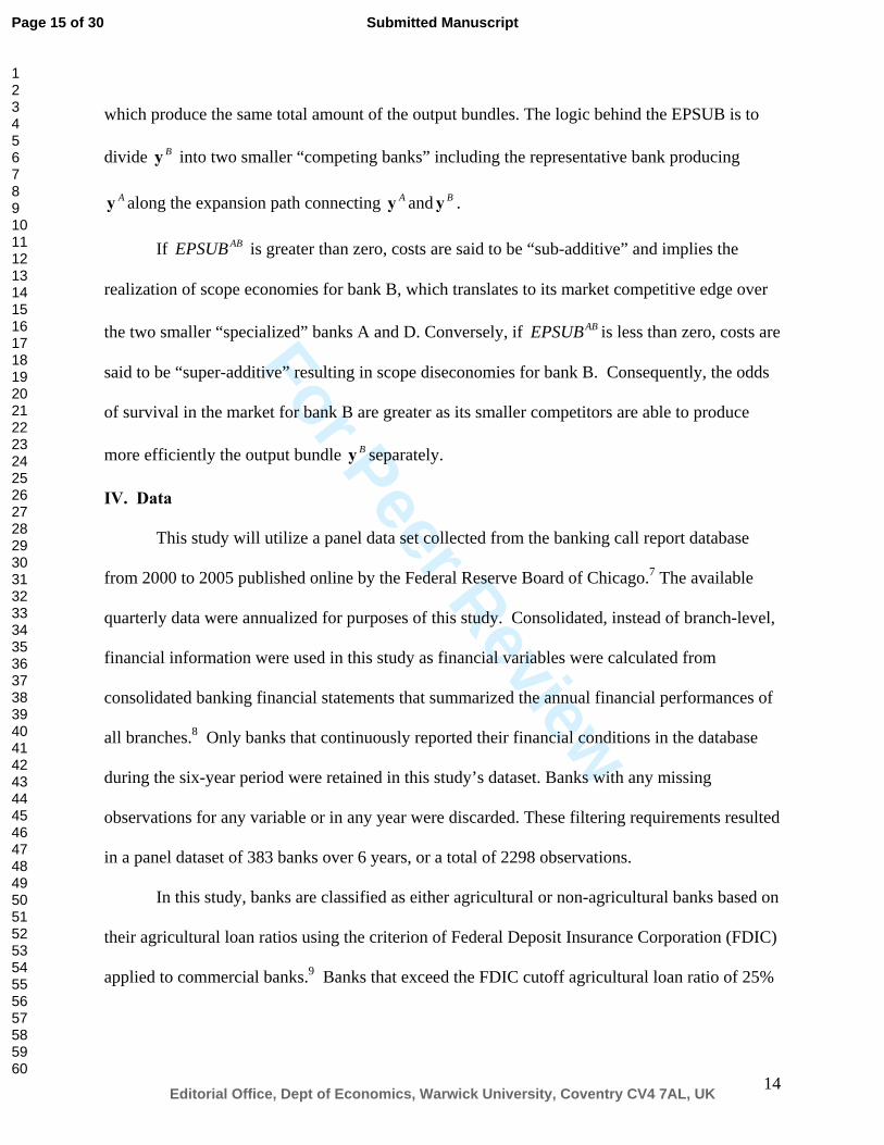
which produce the same total amount of the output bundles. The logic behind the EPSUB is to

divide By into two smaller “competing banks” including the representative bank producing

Ay along the expansion path connecting Ay and By .

If ABEPSUB is greater than zero, costs are said to be “sub-additive” and implies the

realization of scope economies for bank B, which translates to its market competitive edge over

the two smaller “specialized” banks A and D. Conversely, if ABEPSUB is less than zero, costs are

said to be “super-additive” resulting in scope diseconomies for bank B. Consequently, the odds

of survival in the market for bank B are greater as its smaller competitors are able to produce

more efficiently the output bundle By separately.

IV. Data

This study will utilize a panel data set collected from the banking call report database

from 2000 to 2005 published online by the Federal Reserve Board of Chicago.7 The available

quarterly data were annualized for purposes of this study. Consolidated, instead of branch-level,

financial information were used in this study as financial variables were calculated from

consolidated banking financial statements that summarized the annual financial performances of

all branches.8 Only banks that continuously reported their financial conditions in the database

during the six-year period were retained in this study’s dataset. Banks with any missing

observations for any variable or in any year were discarded. These filtering requirements resulted

in a panel dataset of 383 banks over 6 years, or a total of 2298 observations.

In this study, banks are classified as either agricultural or non-agricultural banks based on

their agricultural loan ratios using the criterion of Federal Deposit Insurance Corporation (FDIC)

applied to commercial banks.9 Banks that exceed the FDIC cutoff agricultural loan ratio of 25%

Page 15 of 30

Editorial Office, Dept of Economics, Warwick University, Coventry CV4 7AL, UK

Submitted Manuscript

123456789101112131415161718192021222324252627282930313233343536373839404142434445464748495051525354555657585960

For Peer Review

15

are categorized as “agricultural banks.” Using such criterion, the percentages of the agricultural

banks in this study’s dataset range from 16.2% to 17.75%.

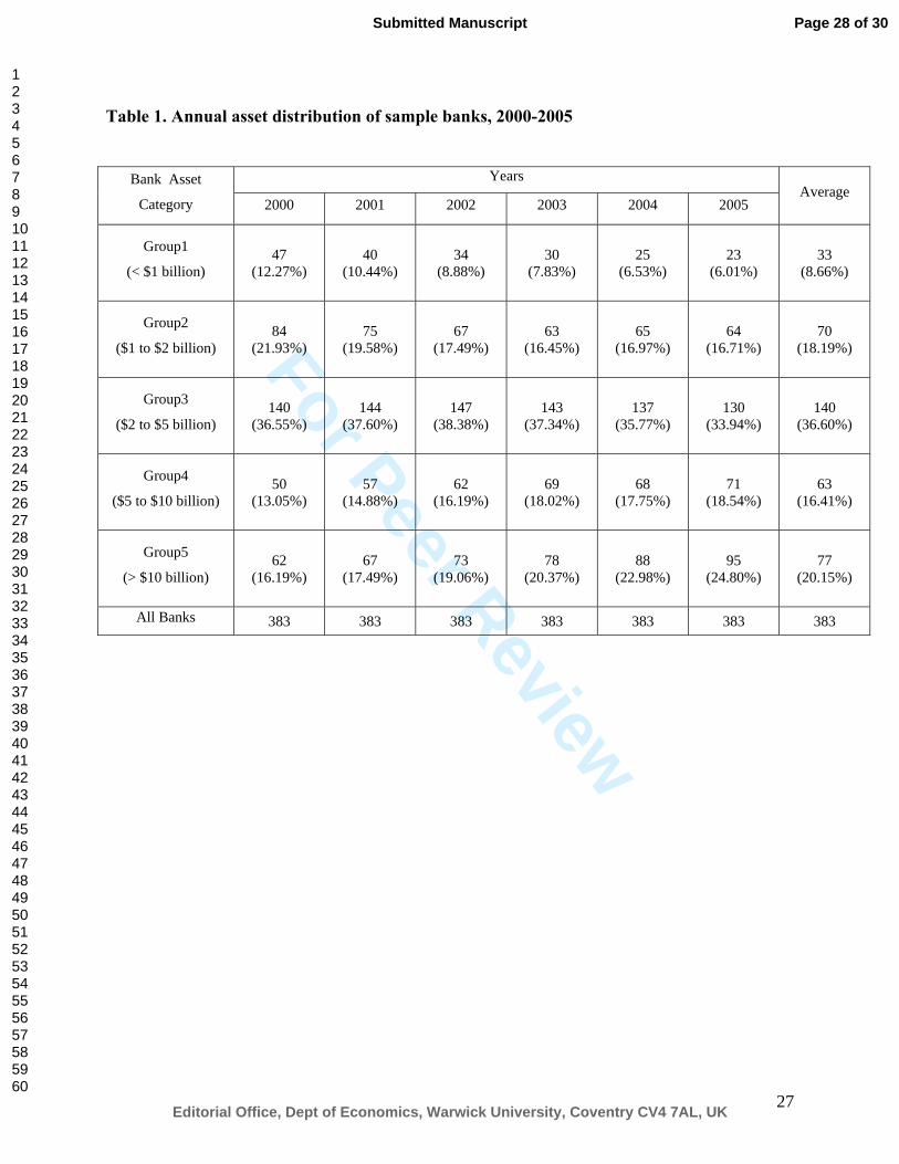
The effect of size on cost efficiencies is also factored into this analysis. This study

classifies banks under 5 size categories using total assets as the classification criterion: total

assets of less than $1 billion (Group 1); between $1 billion and $2 billion (Group 2); between $2

billion and $5 billion (Group 3); between $5 billion and $10 billion (Group 4); and over $10

billion (Group 5). Table 1 presents the distribution of sample banks across size categories.

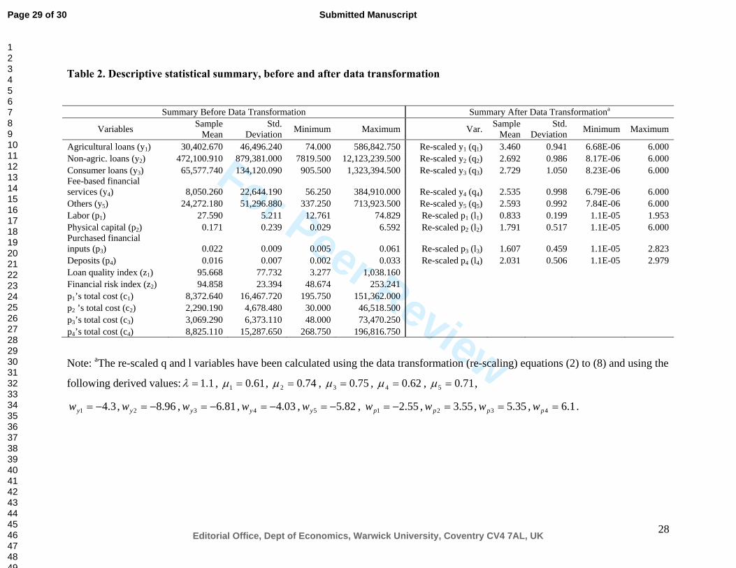
Bank output data collected include the total dollar amounts of agricultural loans ( 1y ),

non-agricultural loans ( 2y ), consumer loans ( 3y ), fee-based financial services ( 4y ), and other

assets that cannot be classified under the other asset accounts in the balance sheet ( 5y ). The

input price data categories considered in this study are labor expense per employee (salaries and

employee benefits divided by number of full-time equivalent employees, 1p ), physical capital

(occupancy and fixed asset expenditures divided by net premises and fixed assets, 2p ), purchased

financial capital inputs (expense of federal funds purchased and securities sold and interest on

time deposits of $100,000 or more divided by total dollar value of these funds, 3p ), and deposits

(interest paid on deposits divided by total dollar value of these deposits, 4p ). As earlier

described in section 2, all output variables and input price variables are rescaled within ]2,0[ π as

)',...( 51 qq=q and )',...( 41 ll=l respectively, using equations 2 to 8. In order to calculate the

inputs’ cost shares, individual input costs are also collected (denoted by 1C to 4C ). Cost

shares, iS , are then calculated as ∑=

=

=4

1

N

ii

ii

C

CS

.

Page 16 of 30

Editorial Office, Dept of Economics, Warwick University, Coventry CV4 7AL, UK

Submitted Manuscript

123456789101112131415161718192021222324252627282930313233343536373839404142434445464748495051525354555657585960

For Peer Review

16

Measures of loan quality index ( 1z ) and financial risk index ( 2z ) are also included in this

analysis to introduce a risk dimension to the efficiency models. The index 1z is calculated from

the ratio of non-performing loans to total loans (NPL) to capture the quality of the banks’ loan

portfolios10 (Stirob and Metli, 2003). The quality of a bank’s loan portfolio has important

repercussions on banking cost and efficiency. For instance, a large NPL ratio can indicate that

the bank could have realized short-run cost savings by devoting fewer resources on credit risk

assessment and loan monitoring, but eventually incurs larger expenses in resolving loan

delinquency through re-mediation, collection, litigation and/or asset liquidation procedures

(Hughes and Mester, 1993).

The index 2z is based on the banks’ capital to asset ratio11, which is used here as proxy

for financial risk. The role of equity has been understated in efficiency and risk analyses that

focus more on NPL and other liability-related measures (Hughes et al., 2000). Actually, as a

supplemental funding source to liabilities, equity capital can provide cushion to protect banks

from loan losses and financial distress. Banks with lower capital to asset ratios (CAR) would be

inclined to rely more on debt financing, which, in turn, increases the risk of insolvency.

Table 2 presents a comparison of the statistical summaries before and after data

transformation. The transformed data satisfy the data requirement to estimate the FF log-cost

function as set by equation 1. Also, the number of Fourier series in this analysis (as determined

using Equation (18) with the values N=4, M=5, Q=383, T=6) is 197≅H , where H represents the

number of elementary multi-index vectors hk to be considered in this analysis.

V. Empirical Results

The Hausman hypothesis test for random effects yielded a significant test statistic of

123.21 that indicates that the null hypothesis for random effects can be rejected. This suggests

Page 17 of 30

Editorial Office, Dept of Economics, Warwick University, Coventry CV4 7AL, UK

Submitted Manuscript

123456789101112131415161718192021222324252627282930313233343536373839404142434445464748495051525354555657585960

For Peer Review

17

that the nonlinear ITSUR can appropriately be used to estimate the coefficients in the equation

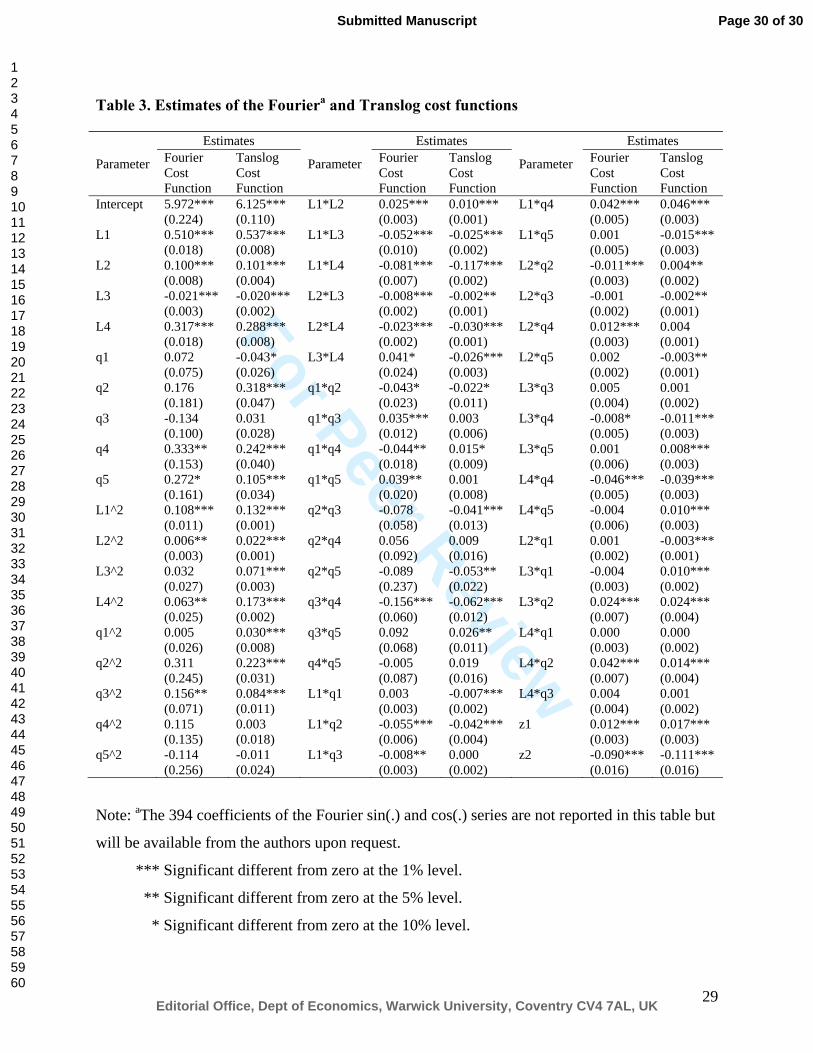
system with fixed effects. Table 3 provides a comparison of the differences between the

estimation results under the FF and translog cost models.12 The hypothesis that all coefficients of

the Fourier series are equal to zero is rejected at 0.01 significant level by an LM test (p-

value<0.0001). This, therefore, indicates that the FF is significantly different from the translog

function and that the FF cost function could be the proper functional form to estimate the cost

function.

The results in table 3 indicate that the theoretical assumptions13 for cost function are

generally true for both FF and the translog functions, with a few exceptions. First, the

coefficient sign for the purchased financial capital inputs variable (l3) is significant and negative

for both the Fourier and translog models. Both coefficients, however, are small in magnitude

and thus, would not amount to a gross violation of the cost theory’s condition of non-decreasing

in input prices. An interesting result, however, is the significantly negative coefficient for the

agricultural loans variable (q1) in the translog model. This negative coefficient result is

inconsistent with standard microeconomic theory and lends support to McAllister and McManus’

(1993) previous empirical assertion on the inadequacy of the translog cost function when applied

to banking efficiency analysis.

It is worth noting that the coefficients of loan quality index 1z and financial risk index

2z are significant for both cost models. The positive sign of 1z indicates that a deterioration in the

quality of loans will cause an increase in bank’s total operating costs. The negative sign of 2z

indicates that banks’ greater financial risk burdens are usually translated to higher operating

costs. These results emphasize the relevance of loan quality and risk measures, which have so

often been left out in most efficiency analyses.

Page 18 of 30

Editorial Office, Dept of Economics, Warwick University, Coventry CV4 7AL, UK

Submitted Manuscript

123456789101112131415161718192021222324252627282930313233343536373839404142434445464748495051525354555657585960

For Peer Review

18

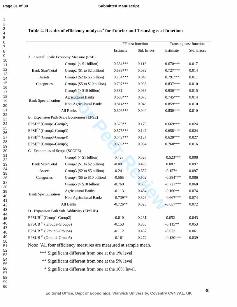
Table 4 summarizes the results for the various efficiency indicators. The RSE results

across bank size and specialization groups are all significant, except for Group 5 banks under the

FF model. This implies that almost all the sample banks are experiencing increasing returns to

scale through proportionate expansions of output bundles without altering product mixes. The

trends of the results across bank size and specialization groups are similar regardless of the cost

functional forms used. Across bank size groups, the magnitudes of the returns to scale tend to

monotonically increase with bank size. This indicates that smaller banks are able to benefit more

from increasing returns to scale than larger banks when they expand the outputs in the same

proportion. This implies that as banks grow larger, further improvements in cost efficiency may

not be realized through further output expansion. Specifically, based on the Fourier results, there

appears to be no potential benefits from production or output expansion for banks belonging to

asset group 5, such that previous trends of increasing returns to scale will collapse to constant

returns to scale. Interestingly, this result considerably extends the critical bank size limit for

exhausting economies of scale opportunities as established by Featherstone and Moss (1994) at

$60 million for banks operating in the 1990s. Apparently, more recent innovative and

technological advancements in banks’ operating structures realized since the 1990s could have

increased these institutions’ financial stamina and flexibility.

The bank specialization results provide interesting implications. Based on the absolute

values of the RSE statistics, agricultural banks in the study’s sample, relative to their non-

agricultural counterparts, have demonstrated a stronger tendency to maximize the potentials of

increasing returns to scale from output expansion. This trend is attributable to the fact that

agricultural banks generally have smaller asset base and scope of operations.

Page 19 of 30

Editorial Office, Dept of Economics, Warwick University, Coventry CV4 7AL, UK

Submitted Manuscript

123456789101112131415161718192021222324252627282930313233343536373839404142434445464748495051525354555657585960

For Peer Review

19

The differences in the RSE results in the FF and translog models reflect these differences

in these models’ capability to accurately approximate the banks’ cost function. Overall, the

magnitudes of the RSE results for the translog model are slightly larger than those obtained in

the FF model, thus suggesting the latter’s greater capability to capture tendencies to attain

increasing returns to scale.

All EPSE results in table 4 are significantly less than one, which support the earlier

results for the RSE measure. The EPSE results indicate that increasing returns to scale are

realized when banks expand from a smaller to a larger output bundle under different product

mixes. The expansion path is shown in this analysis as a transition from a smaller bank size

category to an adjacent (larger) bank size category.

The SCOPE measures derived for all banks in the sample under both cost models are

significantly negative (indicating diseconomies and scope) and different from zero. However,

the SCOPE measures calculated for the bank size groups under the FF model are not statistically

different from zero, suggesting that neither economies nor diseconomies of scope could be

verified. These FF results are consistent with those obtained by Mitchell and Onvural (1996) in

their application of the FF cost function to U.S. commercial banks.

In the translog cases, the 2nd bank size category registered the only insignificant result. In

contrast, group 1 banks exhibit tendencies to realize economies of scope while results for groups

3, 4 and 5 banks suggest the existence of diseconomies of scope. The shift from positive (group 1)

to negative (larger groups) results as well as the increasing magnitude in the absolute values of

the negative SCOPE estimates both indicate that initially realized economies of scope would

tend to diminish and revert to diseconomies of scale as banks expand their operations and

increase their asset bases.

Page 20 of 30

Editorial Office, Dept of Economics, Warwick University, Coventry CV4 7AL, UK

Submitted Manuscript

123456789101112131415161718192021222324252627282930313233343536373839404142434445464748495051525354555657585960

For Peer Review

20

Among bank specialization groups, agricultural banks realize diseconomies of scope only

under the translog model while non-agricultural banks demonstrate similar tendencies under both

the FF and translog models. These results imply the non-agricultural banks’ greater vulnerability

to realizing diseconomies of scale under expanded, more diversified operations while agricultural

banks are able to thrive more under a specialized mode of production.

The EPSUB results suggest that the costs are slightly “super-additive” along the

expansion path from group 2 to 3 and from group 4 to 5 under the translog cost approach. In

contrast, the EPSUB results are all insignificant under the FF model. This indicates that neither

scope economies nor diseconomies along the expansion path connecting a smaller and a larger

bank group are realized. These FF model results reinforce the earlier SCOPE findings.

VI. Summary and Conclusions

This study has introduced the application of the FF functional form in the estimation of

banks’ operating costs and the subsequent analyses of the effects of bank size and product

specialization on efficiency measures. Product specialization categories allow the comparative

assessments of efficiency between agricultural and non-agricultural banks.

This study’s cost estimation results lend support to previous empirical works on

commercial banks that establish the FF model’s greater capability to produce more plausible

results than the translog model. Moreover, loan quality and financial risk indexes, often ignored

in previous studies, have been found to significantly explain variations in banks’ operating costs.

Among the efficiency measures capturing economies of scale and scope, the RSE results

under the FF model suggest evidence of increasing returns to scale for small and medium-size

banks, with these economies of scale benefits reverting to constant returns to scale for larger

banks operating with more than $10 billion assets. In terms of specialization categories,

Page 21 of 30

Editorial Office, Dept of Economics, Warwick University, Coventry CV4 7AL, UK

Submitted Manuscript

123456789101112131415161718192021222324252627282930313233343536373839404142434445464748495051525354555657585960

For Peer Review

21

agricultural banks (which operate relatively smaller operations than non-agricultural banks) have

demonstrated a stronger tendency to maximize the potentials of increasing returns to scale from

output expansion. The EPSE measures obtained confirm these trends under both the FF and

translog models. The results indicate that increasing returns to scale are realized when banks

expand from a smaller to a larger output bundle under different product mixes. These trends are

evident in the proliferation of bank merger and consolidation decisions made in recent years.

Through improvements in operating structures and financial conditions realized from the

introduction of advance technology and innovations in recent years, the benchmark for realizing

favorable returns structure and financial efficiency have been raised significantly. In this study,

the critical bank size limit for exhausting economies of scale opportunities is estimated at around

$10 billion. Moreover, the smaller operations of agricultural banks offer them more opportunities

to realize increasing returns to scale than their larger banking counterparts.

Consistent with the findings of previous studies, the translog model has been shown to

produce more intuitive results than the FF model for the economies of scope analyses. The

SCOPE results indicate that economies of scope realized by smaller banks could tend to diminish

and revert to diseconomies of scale as banks expand their operations and increase their asset

bases. EPSUB results suggest that the banks’ costs are slightly “super-additive” along the

expansion path from mid- to large size categories.

The SCOPE results provide important implications for agricultural banks. The greater

risks and uncertainty usually associated with farm businesses have often raised doubts about the

viability of agricultural banks’ specialized lending operations. This study’s results actually

prove the naysayers wrong by confirming that agricultural banks are more likely to thrive more

Page 22 of 30

Editorial Office, Dept of Economics, Warwick University, Coventry CV4 7AL, UK

Submitted Manuscript

123456789101112131415161718192021222324252627282930313233343536373839404142434445464748495051525354555657585960

For Peer Review

22

efficiently under specialized lending operations while non-agricultural banks are more inclined

to realize diseconomies of scale under greater diversification of their services.

This study has shown the relative strength of the FF over the translog model in analyzing

scale efficiencies. The translog model, however, remains a relevant tool for efficiency analysis,

given its more intuitive scope efficiency results vis-à-vis the FF model results. All told, this

study’s initiation of the FF model into agricultural banking efficiency analysis paves the way for

further research efforts that might want to consider other areas of interests, such as introducing

uncertainty, transactions costs, and bank inputs shareability into the model.

Page 23 of 30

Editorial Office, Dept of Economics, Warwick University, Coventry CV4 7AL, UK

Submitted Manuscript

123456789101112131415161718192021222324252627282930313233343536373839404142434445464748495051525354555657585960

For Peer Review

23

Footnotes 1 This study refers to “agricultural banks” as deposit-taking commercial banks with agricultural loan ratios exceeding the designated cut-off ratio for categorizing agricultural and non-agricultural commercial banks. These farm lenders are therefore not to be confused with other agricultural lending institutions, such as the Farm Credit System and the federal government’s Farm Service Agency. 2 Ellinger and Neff (1994) and Neff, Dixon and Zhu both used the translog cost function; Featherstone and Moss (1994) estimated an indirect multi-product (normalized quadratic) cost function. 3 For more details on the derivation of the FF function, please see Chalfant and Gallant, 1985; Gallant and Souza, 1991. 4 Gallant (1982) claimed that rescaling the data within ]2,0[ π is important for accurate Fourier series to compensate the so-called Gibb’s phenomenon. 5 ε in equations (6) and (7) is an arbitrary infinitive small number. 6 The choice of the cost share equation to be dropped will not significantly influence the results of the estimation. 7 The period of study covered qualifies as part of the bubble period when rising land prices have driven the market to engage in significant land investment transactions and consequently pose as an impediment to implementing cost minimization strategies. Ogawa (2008) points out that since concavity condition on cost functions is based on the implicit assumption that firms are indeed minimizing costs. Thus, analyzing firm’s cost decisions during bubble periods with an imposed concavity condition will lead to model misspecification. 8 Branch banking data would ideally provide more sources of variability than consolidated banking data. However, it can be argued that consolidated banking data could have adequately captured important operating decisions on output expansion and product/service diversification as these decisions are usually made at the main headquarters. Nonetheless, the reader is cautioned to interpret this study’s results as accruing only to consolidated banking parameters . 9 The FDIC criterion for defining agricultural banks provides a compromise between the Federal Reserve System approach (periodically changing agricultural loan ratios ranging from 10% to 15% based on actual financial conditions of all commercial banks) and the methods used by the American Banking Association (based on either the absolute dollar volume of agricultural loans or an agricultural loan ratio of 50%). 10

loanstotalduepast moreor days 90 loansloans nonaccrual10000NPL100001

+×=×=z . The reason for using 1z instead

of NPL is because ln 1z is a monotonic transformation of NPL which will only change the magnitude of the NPL but

still will keep all other properties of NPL. In addition, after the transformation, ln 1z will be all positive numbers with less extreme values. 11

Assets TotalCapitalEquity 100010002 ×=×= CARz . The justification for developing 2z is the same as the rationale used for

calculating 1z . 12 For the sake of brevity, the coefficients of Fourier series are not presented in table 3. These results may be available from the authors upon request. 13 Microeconomic theory requires that the cost function should satisfy: (i) non-decreasing in input prices, (ii) homogeneity of degree one in input prices, (iii) concavity in input prices, and (iv) non-decreasing in outputs.

Page 24 of 30

Editorial Office, Dept of Economics, Warwick University, Coventry CV4 7AL, UK

Submitted Manuscript

123456789101112131415161718192021222324252627282930313233343536373839404142434445464748495051525354555657585960

For Peer Review

24

References

Bauer, P.W. and G.D. Ferrier. 1996. “Scale economies, cost efficiencies, and technological

change in Federal Reserve payments processing.” Journal of Money, Credit and Banking

28,4:1004-1039.

Baumol, W.J., J. Panzar, and R. Willig. 1982. Contestable Markets and the Theory of Industry

Structure. New York: Harcourt Brace Hovanovich.

Berger, A. N., G. Hanweck, and D. Humphrey. 1987. “Competitive Viability in banking: Scale,

Scope, and Product Mix Economies.” Journal of Monetary Economics 20: 501-520.

Berger,A. N., and D. Humphrey. 1991. “The Dominance of Inefficiencies over Scale and Product

Mix Economies in Banking.” Journal of Monetary Economics 28:117-148.

Berger, A. N., and L. Mester. 1997. “Inside the black box: What explains differences in the

efficiencies of financial institutions?” Journal of Banking & Finance 21:895-947.

Chalfant, J.A. and A.R. Gallant. 1985. “Estimating Substitution Elasticities with the Fourier Cost

Function: Some Monte Carlo Results.” Journal of Econometrics 28:205-222.

Coelli, T., A. Estache, S. Perelman, and L. Trujillo. 2003. “A Primer on Efficiency Measurement

for Utilities and Transport Regulators.” The International Bank for Reconstruction and

Development, 31.

Eastwood, B. J., and A. Gallant. 1991. “Adaptive Rules for Semi-nonparametric Estimators That

Achieve Asymptotic Normality.” Econometric Theory 7: 307-340.

Ellinger, P. N.. 1994. “Potential Gains from Efficiency Analysis of Agricultural Banks.”

American Journal of Agricultural Economics 76: 652-654.

Ellinger, P.N. and D.L. Neff. 1993. “Issues and Approaches in Efficiency Analysis of

Agricultural Banks.” Agricultural Finance Review 53:82-99.

Featherstone, A.M. and C.B. Moss. 1994. “Measuring Economies of Scale and Scope in

Agricultural Banking.” American Journal of Agricultural Economics 76:655-661.

Gallant, A.R. 1981. “On the Bias in Flexible Functional Forms and Essentially Unbiased Form.”

Journal of Econometrics 15: 211-245.

Gallant, A. R.. 1982. “Unbiased Determination of Production Technologies.” Journal of

Econometrics 20:285-323.

Gallant, A.R. and G. Souza. 1991. “On the Asymptotic Normality of Fourier Flexible Form

Estimates.” Journal of Econometrics 50:329-353.

Page 25 of 30

Editorial Office, Dept of Economics, Warwick University, Coventry CV4 7AL, UK

Submitted Manuscript

123456789101112131415161718192021222324252627282930313233343536373839404142434445464748495051525354555657585960

For Peer Review

25

Gilligan, T. W., and M. Smirlock. 1984. “An Empirical Study of Joint Production and Scale

Economies in Commercial Banking.” Journal of Banking and Finance 8:67-77.

Greene, W.H.. 2003. Econometric Analysis, 5th ed. Upper Saddle River, NJ: Prentice Hall.

Gropper, D. M. 1991. “Empirical Investigation of Changes in Scale Economies for the

Commercial Banking Firm, 1979-1986.” Journal of Money, Credit, and Banking 23:718-

727.

Hausman, J.A. 1978. “Specification Tests in Econometrics.” Econometrics 46: 1251-1271.

Huang, T.H., and M. Wang. 2004. “Estimation of scale and scope economies in multiproduct

banking: evidence from the Fourier flexible functional form with panel data.” Applied

Economics 36:1245-1253.

Hughes, J.P. and L.J. Mester. (1993), "A quality and risk-adjusted cost function for banks:

evidence on the ‘too-big-to-fail’ doctrine", Journal of Productivity Analysis, Vol. 4,

pp.292-315.

Hughes, J.P., L. Mester, and C. Moon. 2000. “Are All Scale Economies in Banking Elusive or

Illusive: Evidence Obtained by Incorporating Capital Structure and Risk Taking into

Models of Bank Production.” Wharton Center for Financial Institutions Working Paper

#00-33.

Hunter, W.C., S. Timme, and W. Yang. 1990. “An Examination of cost Subadditivity and

Multiproduct Production in Larger U.S. Banks.” Journal of Money, Credit and Banking

22:504-525.

Kim, H. Y.1986. “Economies of Scale and Economies of Scope in Multiproduct Financial

Institutions: Further Evidence from Credit Unions.” Journal of Money, Credit and

Banking 18:220-226.

Lamb, R. L. 1999. “A Market-Forces Policy for the New Farm Economy.” North Carolina State

University.

McAllister, P.H. and D. McManus. 1993. “Resolving the scale efficiency puzzle in banking.”

Journal of Banking and Finance 17:389-406.

Mester, L. J. 1996. “A Study of Bank Efficiency Taking into Account Risk-Preferences.”

Journal of Banking and Finance 20:1025-1045.

Page 26 of 30

Editorial Office, Dept of Economics, Warwick University, Coventry CV4 7AL, UK

Submitted Manuscript

123456789101112131415161718192021222324252627282930313233343536373839404142434445464748495051525354555657585960

For Peer Review

26

Mitchell, K. and N. Onvural. 1996. “Economics of scale and scope at large commercial banks:

evidence from the Fourier flexible function form.” Journal of Money, Credit and Banking

28:178-199.

Neff, D.L., B.L. Dixon, and S. Zhu. 1994. “Measuring the Efficiency of Agricultural Banks.”

American Journal of Agricultural Economics 76:662-668.

Norwood, C.A. 2004. “Competition in Banking: A Review of Literature.” Working Paper #04-

24, Bank of Canada.

Noulas, A. G., B. Ray, and S. Miller. 1990. “Returns to Scale and input Substitution for Large

Banks.” Journal of Money, Credit, and Banking 22:94-108.

Ogawa, K. 2008. “Why are concavity conditions not satisfied in the cost function?: The case of

Japanese manufacturing firms during the bubble period.” Discussion Paper No. 719. The

Institute of Social and Economic Research, Osaka University, Osaka, Japan.

Samolyk, K.A. 1989. “The Role of Banks in Influencing Regional Flows of Funds.” Federal

Reserve Bank of Cleveland, Working paper #8914.

Stam, J., D. Milkove, S. Koenig, J. Ryan, T. Covey, R. Hoppe, and P. Sundell. 2003.

Agricultural Income and Finance Annual Lender Issue. Economic Research Service, U.S.

Department of Agriculture.

Stirob, K. J., and C. Metli. 2003. “The Evolution of Loan Quality for U.S. Banks.” Current

Issues in Economics and Finance 9:1-7.

Walraven, N.A., W.Ott, and J.Rosine. 1993. Agricultural Finance Databook. Board of

Governors of the Federal Reserve System.

White, H.. 1980. “Using Least Squares to Approximate Unknown Regression Functions.”

International Economic Review 21:149-164.

Page 27 of 30

Editorial Office, Dept of Economics, Warwick University, Coventry CV4 7AL, UK

Submitted Manuscript

123456789101112131415161718192021222324252627282930313233343536373839404142434445464748495051525354555657585960

For Peer Review

27

Table 1. Annual asset distribution of sample banks, 2000-2005

Bank Asset

Category

Years Average

2000 2001 2002 2003 2004 2005

Group1

(< $1 billion) 47

(12.27%) 40

(10.44%) 34

(8.88%) 30

(7.83%) 25

(6.53%) 23

(6.01%) 33

(8.66%)

Group2

($1 to $2 billion) 84

(21.93%) 75

(19.58%) 67

(17.49%) 63

(16.45%) 65

(16.97%) 64

(16.71%) 70

(18.19%)

Group3

($2 to $5 billion) 140

(36.55%) 144

(37.60%) 147

(38.38%) 143

(37.34%) 137

(35.77%) 130

(33.94%) 140

(36.60%)

Group4

($5 to $10 billion) 50

(13.05%) 57

(14.88%) 62

(16.19%) 69

(18.02%) 68

(17.75%) 71

(18.54%) 63

(16.41%)

Group5

(> $10 billion) 62

(16.19%) 67

(17.49%) 73

(19.06%) 78

(20.37%) 88

(22.98%) 95

(24.80%) 77

(20.15%)

All Banks 383 383 383 383 383 383 383

Page 28 of 30

Editorial Office, Dept of Economics, Warwick University, Coventry CV4 7AL, UK

Submitted Manuscript

123456789101112131415161718192021222324252627282930313233343536373839404142434445464748495051525354555657585960

For Peer Review

28

Table 2. Descriptive statistical summary, before and after data transformation

Summary Before Data Transformation Summary After Data Transformationa

Variables Sample Mean

Std. Deviation Minimum Maximum Var. Sample

Mean Std.

Deviation Minimum Maximum

Agricultural loans (y1) 30,402.670 46,496.240 74.000 586,842.750 Re-scaled y1 (q1) 3.460 0.941 6.68E-06 6.000 Non-agric. loans (y2) 472,100.910 879,381.000 7819.500 12,123,239.500 Re-scaled y2 (q2) 2.692 0.986 8.17E-06 6.000 Consumer loans (y3) 65,577.740 134,120.090 905.500 1,323,394.500 Re-scaled y3 (q3) 2.729 1.050 8.23E-06 6.000 Fee-based financial services (y4) 8,050.260 22,644.190 56.250 384,910.000 Re-scaled y4 (q4) 2.535 0.998 6.79E-06 6.000 Others (y5) 24,272.180 51,296.880 337.250 713,923.500 Re-scaled y5 (q5) 2.593 0.992 7.84E-06 6.000 Labor (p1) 27.590 5.211 12.761 74.829 Re-scaled p1 (l1) 0.833 0.199 1.1E-05 1.953 Physical capital (p2) 0.171 0.239 0.029 6.592 Re-scaled p2 (l2) 1.791 0.517 1.1E-05 6.000 Purchased financial inputs (p3) 0.022 0.009 0.005 0.061 Re-scaled p3 (l3) 1.607 0.459 1.1E-05 2.823 Deposits (p4) 0.016 0.007 0.002 0.033 Re-scaled p4 (l4) 2.031 0.506 1.1E-05 2.979 Loan quality index (z1) 95.668 77.732 3.277 1,038.160 Financial risk index (z2) 94.858 23.394 48.674 253.241 p1’s total cost (c1) 8,372.640 16,467.720 195.750 151,362.000 p2 ’s total cost (c2) 2,290.190 4,678.480 30.000 46,518.500 p3’s total cost (c3) 3,069.290 6,373.110 48.000 73,470.250 p4’s total cost (c4) 8,825.110 15,287.650 268.750 196,816.750

Note: aThe re-scaled q and l variables have been calculated using the data transformation (re-scaling) equations (2) to (8) and using the

following derived values: 1.1=λ , 61.01 =μ , 74.02 =μ , 75.03 =μ , 62.04 =μ , 71.05 =μ ,

3.41 −=yw , 96.82 −=yw , 81.63 −=yw , 03.44 −=yw , 82.55 −=yw , 55.21 −=pw , 55.32 =pw , 35.53 =pw , 1.64 =pw .

Page 29 of 30

Editorial Office, Dept of Economics, Warwick University, Coventry CV4 7AL, UK

Submitted Manuscript

123456789101112131415161718192021222324252627282930313233343536373839404142434445464748495051525354555657585960

For Peer Review

29

Table 3. Estimates of the Fouriera and Translog cost functions

Note: aThe 394 coefficients of the Fourier sin(.) and cos(.) series are not reported in this table but

will be available from the authors upon request.

*** Significant different from zero at the 1% level.

** Significant different from zero at the 5% level.

* Significant different from zero at the 10% level.

Parameter

Estimates

Parameter

Estimates

Parameter

Estimates Fourier Cost Function

Tanslog Cost Function

Fourier Cost Function

Tanslog Cost Function

Fourier Cost Function

Tanslog Cost Function

Intercept 5.972*** (0.224)

6.125*** (0.110)

L1*L2 0.025*** (0.003)

0.010*** (0.001)

L1*q4 0.042*** (0.005)

0.046*** (0.003)

L1 0.510*** (0.018)

0.537*** (0.008)

L1*L3 -0.052*** (0.010)

-0.025*** (0.002)

L1*q5 0.001 (0.005)

-0.015*** (0.003)

L2 0.100*** (0.008)

0.101*** (0.004)

L1*L4 -0.081*** (0.007)

-0.117*** (0.002)

L2*q2 -0.011*** (0.003)

0.004** (0.002)

L3 -0.021*** (0.003)

-0.020*** (0.002)

L2*L3 -0.008*** (0.002)

-0.002** (0.001)

L2*q3 -0.001 (0.002)

-0.002** (0.001)

L4 0.317*** (0.018)

0.288*** (0.008)

L2*L4 -0.023*** (0.002)

-0.030*** (0.001)

L2*q4 0.012*** (0.003)

0.004 (0.001)

q1 0.072 (0.075)

-0.043*

(0.026) L3*L4 0.041*

(0.024) -0.026*** (0.003)

L2*q5 0.002 (0.002)

-0.003** (0.001)

q2 0.176 (0.181)

0.318*** (0.047)

q1*q2 -0.043* (0.023)

-0.022* (0.011)

L3*q3 0.005 (0.004)

0.001 (0.002)

q3 -0.134 (0.100)

0.031 (0.028)

q1*q3 0.035*** (0.012)

0.003 (0.006)

L3*q4 -0.008* (0.005)

-0.011*** (0.003)

q4 0.333** (0.153)

0.242*** (0.040)

q1*q4 -0.044** (0.018)

0.015* (0.009)

L3*q5 0.001 (0.006)

0.008*** (0.003)

q5 0.272* (0.161)

0.105*** (0.034)

q1*q5 0.039** (0.020)

0.001 (0.008)

L4*q4 -0.046*** (0.005)

-0.039*** (0.003)

L1^2 0.108*** (0.011)

0.132*** (0.001)

q2*q3 -0.078 (0.058)

-0.041*** (0.013)

L4*q5 -0.004 (0.006)

0.010*** (0.003)

L2^2 0.006** (0.003)

0.022*** (0.001)

q2*q4 0.056 (0.092)

0.009 (0.016)

L2*q1 0.001 (0.002)

-0.003*** (0.001)

L3^2 0.032 (0.027)

0.071*** (0.003)

q2*q5 -0.089 (0.237)

-0.053** (0.022)

L3*q1 -0.004 (0.003)

0.010*** (0.002)

L4^2 0.063** (0.025)

0.173*** (0.002)

q3*q4 -0.156*** (0.060)

-0.062*** (0.012)

L3*q2 0.024*** (0.007)

0.024*** (0.004)

q1^2 0.005 (0.026)

0.030*** (0.008)

q3*q5 0.092 (0.068)

0.026** (0.011)

L4*q1 0.000 (0.003)

0.000 (0.002)

q2^2 0.311 (0.245)

0.223*** (0.031)

q4*q5 -0.005 (0.087)

0.019 (0.016)

L4*q2 0.042*** (0.007)

0.014*** (0.004)

q3^2 0.156** (0.071)

0.084*** (0.011)

L1*q1 0.003 (0.003)

-0.007*** (0.002)

L4*q3 0.004 (0.004)

0.001 (0.002)

q4^2 0.115 (0.135)

0.003 (0.018)

L1*q2 -0.055*** (0.006)

-0.042*** (0.004)

z1 0.012*** (0.003)

0.017*** (0.003)

q5^2 -0.114 (0.256)

-0.011 (0.024)

L1*q3 -0.008** (0.003)

0.000 (0.002)

z2 -0.090*** (0.016)

-0.111*** (0.016)

Page 30 of 30

Editorial Office, Dept of Economics, Warwick University, Coventry CV4 7AL, UK

Submitted Manuscript

123456789101112131415161718192021222324252627282930313233343536373839404142434445464748495051525354555657585960

For Peer Review

30

Table 4. Results of efficiency analysesa for Fourier and Translog cost functions

FF cost function Translog cost function

Estimate Std. Errors Estimate Std. Errors

A. Overall Scale Economy Measure (RSE)

Bank Size/Total

Assets

Categories

Group1 (< $1 billion) 0.634*** 0.116 0.670*** 0.017

Group2 ($1 to $2 billion) 0.688*** 0.082 0.727*** 0.014

Group3 ($2 to $5 billion) 0.754*** 0.046 0.791*** 0.011

Group4 ($5 to $10 billion) 0.797*** 0.035 0.837*** 0.010

Group5 (> $10 billion) 0.881 0.088 0.936*** 0.015

Bank Specialization Agricultural Banks 0.680*** 0.075 0.745*** 0.014

Non-Agricultural Banks 0.814*** 0.043 0.859*** 0.010

All Banks 0.803*** 0.040 0.850*** 0.010

B. Expansion Path Scale Economies (EPSE)

EPSE12 (Group1-Group2) 0.579** 0.179 0.669*** 0.024

EPSE23 (Group2-Group3) 0.575*** 0.147 0.658*** 0.024

EPSE34 (Group3-Group4) 0.542*** 0.127 0.629*** 0.027

EPSE45 (Group4-Group5) 0.696*** 0.034 0.760*** 0.016

C. Economies of Scope (SCOPE)

Bank Size/Total

Assets

Categories

Group1 (< $1 billion) 0.428 0.326 0.523*** 0.098

Group2 ($1 to $2 billion) -0.001 0.495 0.087 0.097

Group3 ($2 to $5 billion) -0.241 0.652 -0.157* 0.097

Group4 ($5 to $10 billion) -0.565 0.502 -0.384*** 0.086

Group5 (> $10 billion) -0.769 0.503 -0.721*** 0.068

Bank Specialization Agricultural Banks -0.113 0.484 -0.160** 0.074

Non-Agricultural Banks -0.739** 0.329 -0.667*** 0.074

All Banks -0.726** 0.323 -0.657*** 0.072

D. Expansion Path Sub-Additivity (EPSUB)

EPSUB12 (Group1-Group2) -0.010 0.281 0.052 0.043

EPSUB 23 (Group2-Group3) -0.153 0.355 -0.115** 0.053

EPSUB 34 (Group3-Group4) -0.112 0.437 -0.073 0.061

EPSUB 45 (Group4-Group5) -0.161 0.272 -0.130*** 0.039

Note: aAll four efficiency measures are measured at sample mean.

*** Significant different from one at the 1% level.

** Significant different from one at the 5% level.

* Significant different from one at the 10% level.

Page 31 of 30

Editorial Office, Dept of Economics, Warwick University, Coventry CV4 7AL, UK

Submitted Manuscript

123456789101112131415161718192021222324252627282930313233343536373839404142434445464748495051525354555657585960