estudios analíticos y numéricos de un modelo de vegetación de
TRANSCRIPT
UNIVERSIDAD COMPLUTENSE DE MADRID
FACULTAD DE CIENCIAS MATEMÁTICAS DEPARTAMENTO DE MATEMÁTICA APLICADA
TESIS DOCTORAL
Estudios Analíticos y Numéricos de un Modelo de Vegetación de Tierras Secas Analytical and Numerical Studies of a Dryland Vegetation Model
MEMORIA PARA OPTAR AL GRADO DE DOCTOR
PRESENTADA POR
Paris Kyriazopoulos
Directores
Jesús Ildefonso Díaz Danielle Hilhorst
Ehud Meron
Madrid, 2014 © Paris Kyriazopoulos, 2014
Universidad Complutense deMadrid
FACULTA DE CIENCIAS MATEMATICAS
Departamento de MatematicaAplicada
Estudios Analiticos y Numericos deun modelo de vegetacion de tierras
secas
Analytical and Numerical Studies of a DrylandVegetation Model
Tesis doctoral realizada por:
Paris Kyriazopoulos
Bajo la direccnion de:
Jesus Ildefonso DıazDanielle Hilhorst
Ehud Meron
Madrid 2014


Resumen
La vegetacion en ambientes de agua muy limitada ha atrado la atencion de variosinvestigadores debido, entre otras razones, a la variedad de mosaicos de vegetacionespaciales que se producen en tales areas y los problemas ambientales que surgenen una epoca de rapidos cambios climaticos. En las ultimas dos decadas, diversosmodelos teoricos han sido formulados y usados para tratar cuestiones abiertastales como la relativas a la formacion de patrones de vegetacion, desertificacion,composicion de la comunidad vegetal y la competencia en los ecosistemas de re-cursos limitados.
En esta tesis se considera un modelo de vegetacion genrico que recoge un con-junto de relaciones esenciales entre agua y biomasa que se producen en ambientessecos. El modelo describe las interacciones entre multiples especies de plantas,el agua subterranea del suelo y las aguas superficiales, a traves de un sistema deecuaciones de reaccion-difusion, donde en particular la incognita dada por la con-centracion del agua superficial se rige por una ecuacion cuasilineal de tipo mediosporosos.
En el primer capıtulo de la tesis, nos ocupamos de un problema estacionariosimplificada para una forma unica de vida vegetal. En primer lugar, consid-eramos una ecuacion escalar para la variable biomasa y mostramos que, bajocondiciones apropiadas en los parametros fijos del problema, existen multiplessoluciones positivas para un rango del parametro precipitacion. En la segundaparte, nos ocupamos de un sistema de dos componentes de la biomasa y el suelo-agua que muestra la existencia de un continuo de soluciones fijas no uniformes queemanan de la rama de soluciones uniformes positivos utilizando la longitud delintervalo espacial como un parametro de bifurcacion. En la ultima seccion, nosocupamos del problema estacionario para la biomasa y el agua superficial y anal-izamos los frentes generados por esta incognita. En particular, suponiendo que laprecipitacion se distribuye de forma no homogenea en el espacio y se desvaneceen una subregion de un dominio dado, estudiamos la transicion de la altura delagua superficial en un entorno de la zona de cambio de precipitacion.
En el segundo capıtulo se estudia numericamente un sistema ampliado te-niendo en cuenta tambien la competencia por la luz. El sistema captura la com-petencia espacial entre dos especies de plantas distintas que hacen diferentes com-
ii
iii
promisos en la captacion de agua en el suelo y la luz solar. Identificamos un rangodel parametro de precipitacion para el que dos estados estables alternativos coex-isten. El primero de los estado describe una distribucion uniforme de una especiede planta que se especializa en la captura de agua en el suelo, mientras que elsegundo estado describe un patron peridico de una especie que se especializa en lacaptura de la luz. Se demuestra que este rango de biestabilidad generalmente sedivide en tres partes: una que corresponde a bajo rango de precipitacion, dondeel competidor superior para el agua desplaza al competidor superior para la luz,un alto rango de precipitacion donde se invierte el desplazamiento, y un rangointermedio donde ninguna de las especies desplaza a la otra. La gama intermediapermite la coexistencia de las especies en la forma de una multitud de solucioneslocalizadas estables que consisten en dominios fijos de una especie en zonas ocu-padas por las otras especies.
En el tercer capıtulo, consideramos un sistema modificado para una solaforma de vida vegetal. La difusion no lineal en la ecuacion del agua superficialcontiene ahora un trmino de absorcion fuerte que modeliza procesos peculiares deinfiltracin de aguas superficiales. Mostramos la de existencia de soluciones debilespara el problema de valor inicial en un dominio acotado y para condiciones ini-ciales acotadas: tanto para el caso del problema de condiciones de contorno detipo Dirichlet como para el caso del problema de Neumann. En el primer caso,aproximamos el problema degenerado mediante problemas regularizados conve-nientes y obtenemos adecuadas estimaciones a priori que nos permite pasar allımite. En el segundo caso, la existencia de soluciones se prueba mediante el usode un teorema de punto fijo. Por ultimo, estudiamos algunas propiedades cuali-tativas de la componente de agua superficial para perıodos secos, es decir, cuandola precipitacion es insignificante o inexistente.
Indice General
Introduccion 10.1 El modelo que se estudia en esta tesis . . . . . . . . . . . . . . . . 10
1 Sobre el sistema eliptico 171.1 Introduccion . . . . . . . . . . . . . . . . . . . . . . . . . . . . . . . 171.2 Un resultado de multiplicidad para una ecuacion escalar de biomasa 191.3 Un sistema acoplado de biomasa y concentracion de agua . . . . . 24
1.3.1 Soluciones uniformes . . . . . . . . . . . . . . . . . . . . . . 251.3.2 Soluciones no-uniformes . . . . . . . . . . . . . . . . . . . . 27
1.4 Transicion del agua superficial . . . . . . . . . . . . . . . . . . . . . 29
2 Coexistencia de especies fijando su interfase 332.1 Introduccion . . . . . . . . . . . . . . . . . . . . . . . . . . . . . . . 332.2 Modelizacion de la dinamica comun . . . . . . . . . . . . . . . . . . 35
2.2.1 Ecuaciones del modelo . . . . . . . . . . . . . . . . . . . . . 352.2.2 Competencia por el agua . . . . . . . . . . . . . . . . . . . . 362.2.3 Competencia por la luz . . . . . . . . . . . . . . . . . . . . . 372.2.4 Desarrollo de la competencia . . . . . . . . . . . . . . . . . . 382.2.5 Valores de parametros y unidades . . . . . . . . . . . . . . . 38
2.3 Soluciones estacionarias . . . . . . . . . . . . . . . . . . . . . . . . 402.3.1 Estados uniformes . . . . . . . . . . . . . . . . . . . . . . . 412.3.2 Estados espacialmente periodicos . . . . . . . . . . . . . . . 412.3.3 Estados localizados . . . . . . . . . . . . . . . . . . . . . . . 43
2.4 Coexistencia de especies y desplazamiento espacial . . . . . . . . . 432.5 Factores que controlan la coexistencia de especies . . . . . . . . . . 46
2.5.1 Competencia por la luz . . . . . . . . . . . . . . . . . . . . . 462.5.2 Conjunto de especies . . . . . . . . . . . . . . . . . . . . . . 46
2.6 Conclusion . . . . . . . . . . . . . . . . . . . . . . . . . . . . . . . . 482.7 Apendices . . . . . . . . . . . . . . . . . . . . . . . . . . . . . . . . 50
2.7.1 Estados estacionarios uniformes y sus propiedades de esta-bilidad . . . . . . . . . . . . . . . . . . . . . . . . . . . . . . 50
iv

INDICE GENERAL v
2.7.2 Analisis de la estabilidad numerica de soluciones estacionar-ias no-uniformes en un sistema finito . . . . . . . . . . . . . 56
3 Absorcion fuerte 593.1 Introduccion . . . . . . . . . . . . . . . . . . . . . . . . . . . . . . . 593.2 Existencia de soluciones . . . . . . . . . . . . . . . . . . . . . . . . 60
3.2.1 El sistema regularizado (PD) . . . . . . . . . . . . . . . . . 623.2.2 El caso de condiciones de contorno de tipo Neumann (PN ) . 70
3.3 Propiedades de la componente de agua superficial . . . . . . . . . . 743.3.1 Extincion en tiempo finito . . . . . . . . . . . . . . . . . . . 753.3.2 Estimaciones sobre el conjunto de anulacion h . . . . . . . . 76
Bibliografıa 78

Dedication
To my mom, dad and brother
vi

Acknowledgements
I owe my deepest gratitude to my advisors: Ildefonso Diaz, Danielle Hilhorst andEhud Meron, for their constant support and assistance in all the stages of thisthesis. Without their encouragement this thesis would not have been possible.
There were many other people that supported me during my doctoral studies.Starting from the beginning, I am thankful to Michael Stich for the discussionswe had in Madrid. He was the first who made me realize and appreciate thephysicists perspective about research, this helped me a lot much later when I metEhud Meron and his reasearch group in Israel. Also, I could not forget my friendsin spain Alberto, Javier, Gonzalo, my mates Alex and Tommaso who have alwaysbeen tolerant with my peculiarities.
I would like to thank the Technion in Haifa and Universite Paris Sud for thefacilities they offered to me, for my six month visit in Israel (Haifa) and one yearvisit in France (Orsay), respectively.
In Israel, I will never forget the time I spent in Sede Boker. I am grateful toEhud Meron’s research group for everything. I appreciate every group meetingI joined and every piece of knowledge they shared with me. My special thanksgo to Yonatan as his ideas were the main ingredient of the second chapter of thisthesis, to Yuval for helping me with the continuation package AUTO, to Yair andShai for the numerous discussions we had. In Haifa, I also wish to thank Elad forhis company and the things he taught me about Israel.
Finally, for the year I spent in Orsay I wish to express my appreciation toDanielle Hilhorst’s research group: Yueyuan , Cuong, Thanh Nam, who broughtme back to the mathematical way of thinking. Also, many thanks to my greekfriend Filodamos who made me feel like home during my one year stay in France.
vii
Abstract
Vegetation in water limited environments has attracted the attention of severalresearchers due to the variety of spatial vegetation mosaics that occur in suchareas and the environmental issues that arise in a time of rapid climatic changes.The last two decades various theoretical models have been formulated and used toaddress open questions concerning vegetation pattern formation, desertification,plant community composition and competition in resource limited ecosystems.
In this thesis we consider a generic vegetation model that captures a set of es-sential feedbacks between water and biomass that take place in dry environments.The model describes the interactions among multiple plant species, soil-water andsurface-water through a system of reaction-diffusion equations, where the surface-water variable, in particular, is governed by a porous medium type equation.
In the first chapter of the thesis, we are concerned with a simplified stationaryproblem for a single life form. We first consider a scalar equation for the biomassvariable and show that under appropriate conditions on fixed parameters of theproblem, multiple positive solutions exist for a range of the precipitation param-eter. In the second part, we deal with a two-component system of biomass andsoil-water showing the existence of continua of nonuniform stationary solutionswhich emanate from the branch of positive uniform solutions using the lengthof the spatial interval as a bifurcation parameter. In the last section, we dealwith the complete water-biomass stationary problem focusing on the profiles ofthe surface-water solution. In particular, assuming that precipitation is inhomo-geneously distributed in space and vanishes in a subregion of a given domain, westudy the transition of the surface-water height in a neighborhood of the vanishingregion.
In the second chapter, we study numerically an extended system taking intoaccount competition for light, too. The system captures spatial competition be-tween two distinct plant species that make different compromises in capturing soilwater and sunlight. We identify a precipitation range along the rainfall gradientwhere two alternative stable states coexist. The first state describes a uniformdistribution of a plant species that specializes in capturing soil water, whereas thesecond state describes a periodic pattern of a species that specializes in captur-ing light. We show that this bistability range generally divides into three parts:
viii
INDICE GENERAL ix
a low precipitation range where the superior competitor for water displaces thesuperior competitor for light, a high precipitation range where the displacementis reversed, and an intermediate range where neither species displaces the other.The intermediate range allows for species coexistence in the form of a multitudeof stable localized solutions consisting of fixed domains of one species in areasotherwise occupied by the other species.
In the third chapter, we consider a modified system for a single life form. Thenonlinear diffusion in the surface-water equation is combined with a strong ab-sorption term modeling the surface water infiltration process. We give existenceproofs for the initial value problem in a bounded domain for bounded initialconditions treating the case of the Dirichlet and Neumann boundary conditions,separately. In the first case, we approximate the degenerate problem by regular-ized ones and obtain some a priori estimates of the approximating solutions whichallow us to pass to the limit. In the second case, existence of solutions is provedby using a fixed point theorem. Finally, we study the qualitative properties ofthe surface-water solution for dry periods i.e when precipitation is negligible orabsent.
Contents
Introduction 10.1 The Model studied in this thesis . . . . . . . . . . . . . . . . . . . 10
1 On the elliptic system 171.1 Introduction . . . . . . . . . . . . . . . . . . . . . . . . . . . . . . . 171.2 A multiplicity result for a scalar biomass equation . . . . . . . . . 191.3 A coupled water-biomass system . . . . . . . . . . . . . . . . . . . 24
1.3.1 Uniform solutions . . . . . . . . . . . . . . . . . . . . . . . 251.3.2 Nonuniform solutions . . . . . . . . . . . . . . . . . . . . . 27
1.4 Surface water transition . . . . . . . . . . . . . . . . . . . . . . . . 29
2 Species coexistence by front pinning 332.1 Introduction . . . . . . . . . . . . . . . . . . . . . . . . . . . . . . . 332.2 Modeling community dynamics . . . . . . . . . . . . . . . . . . . . 35
2.2.1 Model equations . . . . . . . . . . . . . . . . . . . . . . . . 352.2.2 Competition for water . . . . . . . . . . . . . . . . . . . . . 362.2.3 Competition for light . . . . . . . . . . . . . . . . . . . . . . 372.2.4 Trait tradeoff . . . . . . . . . . . . . . . . . . . . . . . . . . 382.2.5 Parameter values and units . . . . . . . . . . . . . . . . . . 38
2.3 Stationary solutions . . . . . . . . . . . . . . . . . . . . . . . . . . 402.3.1 Uniform states . . . . . . . . . . . . . . . . . . . . . . . . . 412.3.2 Spatially periodic states . . . . . . . . . . . . . . . . . . . . 412.3.3 Localized states . . . . . . . . . . . . . . . . . . . . . . . . . 43
2.4 Species coexistence and spatial displacement . . . . . . . . . . . . . 432.5 Factors controlling species coexistence . . . . . . . . . . . . . . . . 46
2.5.1 Competition for light . . . . . . . . . . . . . . . . . . . . . . 462.5.2 Species pool . . . . . . . . . . . . . . . . . . . . . . . . . . . 46
2.6 Conclusion . . . . . . . . . . . . . . . . . . . . . . . . . . . . . . . 482.7 Appendices . . . . . . . . . . . . . . . . . . . . . . . . . . . . . . . 50
2.7.1 Uniform steady states and their stability properties . . . . . 502.7.2 Numerical stability analysis for nonuniform stationary so-
lutions in a finite system . . . . . . . . . . . . . . . . . . . . 56
x
CONTENTS xi
3 Strong absorption 593.1 Introduction . . . . . . . . . . . . . . . . . . . . . . . . . . . . . . . 593.2 Existence of solutions . . . . . . . . . . . . . . . . . . . . . . . . . 60
3.2.1 The regularized system to (PD) . . . . . . . . . . . . . . . . 623.2.2 The case of Neumann Boundary conditions (PN ) . . . . . . 70
3.3 Properties of the surface water component . . . . . . . . . . . . . . 743.3.1 Extinction in finite time . . . . . . . . . . . . . . . . . . . . 753.3.2 Estimates for the zeroes set of h . . . . . . . . . . . . . . . 76
Bibliography 78

Introduction
In a time of climate change and global warming the understanding of the responseof vegetation to environmental changes and the impact that this may have onecosystems has become crucial. The growth of plants as well as the distributionof vegetation depends strongly on the presence of various resources includingnutrients, water and light. Among these resources, water is commonly acceptedas a fundamental ingredient of life which is often in limited supply and depletesrapidly. As a result, dry, sub-humid, semi-arid, arid and hyper-arid regions of theplanet, collectively known as drylands, have attracted the attention of vegetationecologists and numerous other scientists. This interest is reenforced by the factthat drylands cover more than 40 percent of the earth’s land surface and arehome to more than two billion people. A common approach in the study ofdryland vegetation involves mathematical models consisting of systems of partialdifferential equations which capture an essential part of the complex processesthat take place in water limited environments. The analysis of such systems mayprovide an insight about the underlying causes of several observed phenomenasuch as spatial vegetation patterns and desertification. In addition, they can actas tools to address issues concerning species coexistence and biodiversity. Theobjective of this thesis is to study different aspects of a generic vegetation modelwhich describes interactions between biomass and water in drylands.
Empirical evidence support that vegetation in drylands forms a variety ofspatial patterns. Many of these patterns seem to be self-organized exhibitingcharacteristic length scales. Perhaps the most studied vegetation communities ofthis type are the tiger-bush patterns (TB). The TB are composed of regularlyspaced vegetation bands interspersed with bare soil that form along the contoursof gently slopped semi-arid regions and migrate uphill with constant speed thatdepends on the type of vegetation [22]. Diverse spatial vegetation patterns canalso form in the absence of any environmental anisotropy. They include almostperiodic patterns of vegetation spots, labyrinths, and vegetation gaps [20]. Suchvegetation structures are not confined to a specific type of vegetation, but ratherthe can consist of trees, shrubs and grasses. Moreover, they have been reportedworldwide at the edges of tropical deserts and they occur in a wide range ofsoils: from sandy and silty to heavy soils. This regular nonuniform character of
1
2
dryland vegetation was the motivation for the formulation of several continuumvegetation models that exhibit pattern formation properties. The first to intro-duce such a model were Lefever and Lejeune [46]. In their model, the evolutionof vegetation is governed by a fourth order partial differential equation1 whichcaptures the interactions and redistribution of plants’ biomass. Although, no wa-ter variable is present in the model, the resource scarcity can be controlled bya mortality rate parameter which may act as an aridity gradient. In particular,regular spatial patterns emerge for a subrange of this gradient: periodic pat-terns of spots, gaps and stripes are predicted for completely isotropic conditions(flat terrains), whereas moving banded structures develop when a topographicanisotropy is added (slopped terrains). After a few years, Klausmeier proposeda different vegetation model to investigate the TB phenomenon focusing on ter-rains of constant slope putting a water state variable in the picture [43]. In thismodel the biomass-water dynamics are captured by a reaction-diffusion equationfor the biomass variable and a reaction advection equation for the water variablemodeling the downhill flow of run-off water. Water supply is controlled by a pre-cipitation rate parameter which allows us to investigate the response of vegetationto rainfall fluctuations. Within a precipitation range the model predicts spatialpatterns which resemble satisfactorily the moving TB patterns [70]. Researchefforts in this direction have given numerous pattern forming models describingbiomass-water dynamics in both flat and non-flat topographies [9, 36, 60, 79].
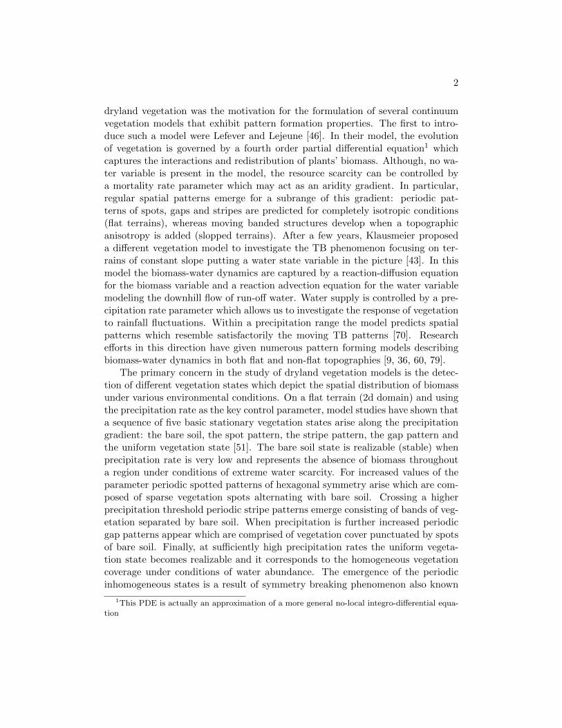
The primary concern in the study of dryland vegetation models is the detec-tion of different vegetation states which depict the spatial distribution of biomassunder various environmental conditions. On a flat terrain (2d domain) and usingthe precipitation rate as the key control parameter, model studies have shown thata sequence of five basic stationary vegetation states arise along the precipitationgradient: the bare soil, the spot pattern, the stripe pattern, the gap pattern andthe uniform vegetation state [51]. The bare soil state is realizable (stable) whenprecipitation rate is very low and represents the absence of biomass throughouta region under conditions of extreme water scarcity. For increased values of theparameter periodic spotted patterns of hexagonal symmetry arise which are com-posed of sparse vegetation spots alternating with bare soil. Crossing a higherprecipitation threshold periodic stripe patterns emerge consisting of bands of veg-etation separated by bare soil. When precipitation is further increased periodicgap patterns appear which are comprised of vegetation cover punctuated by spotsof bare soil. Finally, at sufficiently high precipitation rates the uniform vegeta-tion state becomes realizable and it corresponds to the homogeneous vegetationcoverage under conditions of water abundance. The emergence of the periodicinhomogeneous states is a result of symmetry breaking phenomenon also known
1This PDE is actually an approximation of a more general no-local integro-differential equa-tion
3
(a) Spotted patterns (b) Striped patterns (c) Gapped patterns
Figure 1: (a) Spotted vegetation patterns in Sudan (11.5331794N 27.9360008E),(b) striped patterns (labyrinths) in Niger (13.0724868N 2.2034025E), (c) gapsin vegetation cover in Senegal (15.20331N 14.8940384W). The images have beentaken from google maps.
as Turing pattern formation mechanism. These states are in conformity withthe vegetation patterns observed in fields for the corresponding rainfall values(Fig. 1). The sequence of basic states is often represented on a bifurcation dia-gram which displays branches of stationary biomass states versus the precipitationrate parameter. In such a diagram, parameter ranges can be located where twoconsecutive stable states coexist. Within these bistability ranges more spatiallyinhomogeneous solutions may emerge consisting of spatial mixtures of two basicstable states. These can be combinations of vegetation stripes and spots, or gaps.In other cases, the solutions are localized structures which consist of fronts sep-arating domains of two alternative stable states. Depending on the parametervalues, contracting or spreading fronts can generally be found. However, localizedsolutions can also be stabilized for some range of the control parameter as a resultof front pinning.
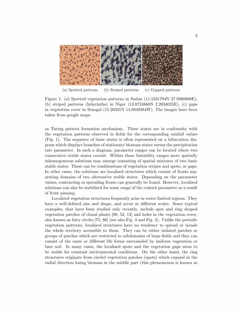
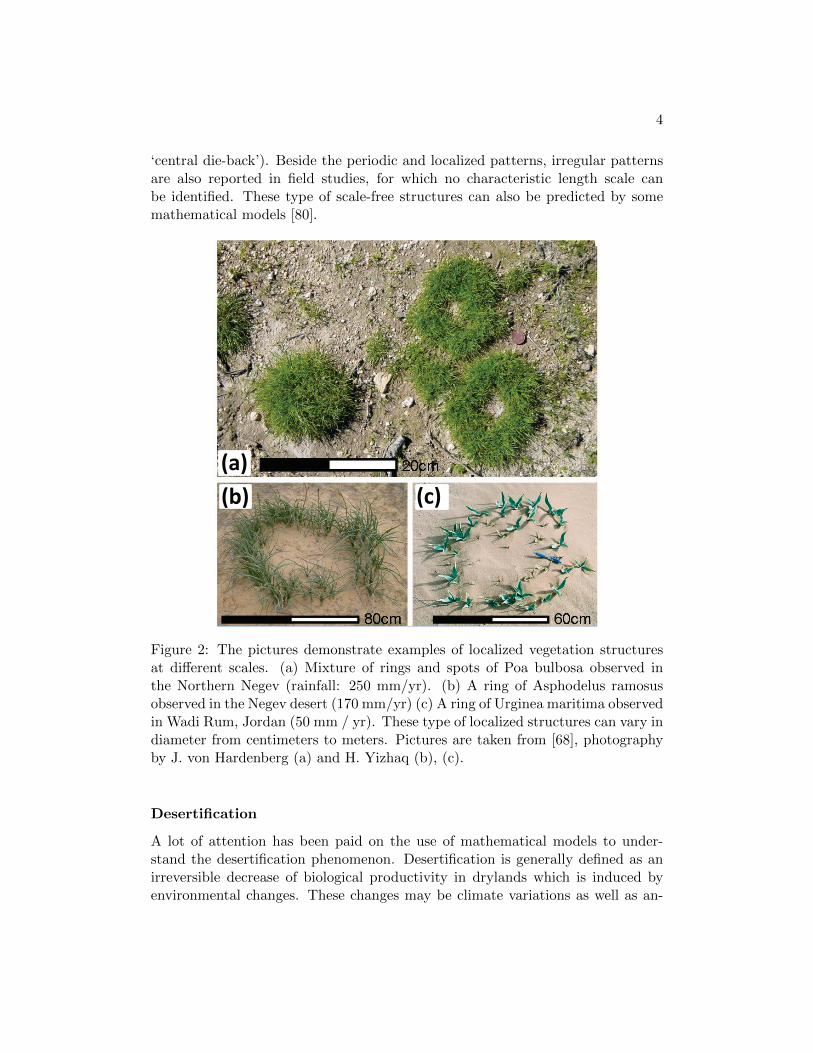
Localized vegetation structures frequently arise in water limited regions. Theyhave a well-defined size and shape, and occur at different scales. Some typicalexamples, that have been studied only recently, include spot and ring shapedvegetation patches of clonal plants [69, 52, 13] and holes in the vegetation cover,also known as fairy circles [75, 86] (see also Fig. 3 and Fig. 2). Unlike the periodicvegetation patterns, localized structures have no tendency to spread or invadethe whole territory accessible to them. They can be either isolated patches orgroups of patches which are restricted to subdomains of large fields and they canconsist of the same or different life forms surrounded by uniform vegetation orbare soil. In many cases, the localized spots and the vegetation gaps seem tobe stable for constant environmental conditions. On the other hand, the ringstructures originate from circled vegetation patches (spots) which expand in theradial direction losing biomass in the middle part (this phenomenon is known as
4
‘central die-back’). Beside the periodic and localized patterns, irregular patternsare also reported in field studies, for which no characteristic length scale canbe identified. These type of scale-free structures can also be predicted by somemathematical models [80].
(a) (b) (c)
(d)
Figure 2: The pictures demonstrate examples of localized vegetation structuresat different scales. (a) Mixture of rings and spots of Poa bulbosa observed inthe Northern Negev (rainfall: 250 mm/yr). (b) A ring of Asphodelus ramosusobserved in the Negev desert (170 mm/yr) (c) A ring of Urginea maritima observedin Wadi Rum, Jordan (50 mm / yr). These type of localized structures can vary indiameter from centimeters to meters. Pictures are taken from [68], photographyby J. von Hardenberg (a) and H. Yizhaq (b), (c).
Desertification
A lot of attention has been paid on the use of mathematical models to under-stand the desertification phenomenon. Desertification is generally defined as anirreversible decrease of biological productivity in drylands which is induced byenvironmental changes. These changes may be climate variations as well as an-
5
Figure 3: The picture depicts the so-called fairy circles which are common in thegrasslands of southern Africa, specifically in Namibia, and they can grow from 2to 15 meters in diameter.
thropogenic disturbances which in many cases accelerate the phenomenon. Thecomplex nature and multiple temporal and spatial scales of the processes thattake place in water limited ecosystems render the field and laboratory studiesinadequate to provide complete understanding of desertification. In this effortmathematical models play a crucial role as they can predict the long term spatio-temporal dynamics of vegetation and its variations with respect to environmentalparameters. In addition, they are capable to predict the various spatial vegetationpatterns observed in drylands which may act as an indicator for imminent deser-tification [42]. This is based on the perception of desertification as a catastrophicshift involving abrupt transitions from a perennial vegetated state (high produc-tivity state) to lower productivity states [64]. The critical states are vegetationpatterns which are sensitive to a decrease of an environmental parameter or adisturbance which involves removal of vegetation biomass. Consequently, slightvariations of the environmental conditions can cause a transition from one stateto another. The transition is catastrophic as recovery of previous conditions isnot enough to move the ecosystem back to high productivity levels [61]. This isusually illustrated by a hysterisis loop on a bifurcation diagram depicting the veg-etation states versus the rainfall gradient. In such a diagram and within a givenparameter range, the stable bare soil state (desert) coexists with at least one stablelow productivity vegetated state, then a shift can occur from the vegetated statetowards the bare soil state as precipitation is decreased below the left edge of thebistability range. It is notable that recent model studies have recognized patternsconsisting of vegetation spots as the lowest productivity transitional states. Fur-ther research is conducted in this direction seeking the development of preventionand restoration policies.
6
Pattern formation and localized structures
In many cases, the spatial patterns that appear in nature are a result of self-organization processes. This kind of inhomogeneous structures have been studiedin chemistry and biology using systems of reaction-diffusion equations, inspiredby the celebrated paper of Turing on morphogenesis [77]. The original work ofTuring refers to two interacting chemical substances, called morphogens, whichdiffuse throughout a given domain. The central idea behind his theory is that, un-der certain conditions, a spatially homogeneous steady state of the two substanceswhich is stable (realizable) with respect to uniform perturbations may become un-stable when the disturbances are nonuniform leading the system to some spatiallyinhomogeneous stationary state. In order for this instability to occur, the pro-ductive and degradative interactions between the two substances must be of acertain type and most importantly the two substances need to diffuse at differentrates. This diffusion driven instability, also known as symmetry-breaking instabil-ity, constitutes a first mathematically recognized pattern formation mechanism.Based on this idea, Hans Meinhardt held the research on pattern formation a stepforward by introducing a typical activator-inhibitor system, setting forth the so-called ‘short-range-activation long-range-inhibition’pattern forming principle [33].Reaction-diffusion systems inducing patterns also include the resource-consumersystems with their main representative being the Gray-Scott equations which inits original form describes simple autocatalytic reactions [38]. It is noteworthythat the Klausmeier’s vegetation model and its extensions are actually a vari-ation of the Gray-Scott model where the role of the resource is played by thesoil-water and that of the consumer by the vegetation biomass [79]. Finally,reaction-diffusion systems have been used to generate animal coats patterns ongrowing domains [4, 53], while emergence of spatial patterns is also observed infourth-order scalar evolution equations such as the extended Fisher-Kolmogorovequation [21, 55] and the Swift-Hohenberg equation [16, 72].
An important tool to study pattern formation properties of a reaction-diffusionsystem is the linear stability analysis (LSA) which we sketch below for a two-component system in a bounded domain. In particular, let F : R2 →: R2 bea continuously differentiable vector field with F (u) = (f(u), g(u)), Ω ⊂ R2 bea smooth bounded domain and consider the following reaction diffusion-system(RD)
ut −D∆u = γF (u) in R+ × Ω,
u(0, x) = u0(x) for x ∈ Ω,(1)
along with the zero Neumann boundary conditions, where
D =
(δ 00 1
),
7
δ, γ > 0 and u(t, x) = (u1(t, x), u2(t, x)). Suppose that us is a uniform steadystate of the system, that is F (us) = 0. Let J denote the linearization matrix ofF (Jacobian matrix) about the steady state and assume that all the eigenvaluesof J have negative real part, i.e
det(J) > 0 and tr (J) < 0. (2)
The latter assumption essentially implies that us is linearly stable in the absenceof diffusion. The primary aim of the LSA is to determine conditions under whichus becomes linearly unstable to spatially inhomogeneous perturbations. For thiswe let u = us + w and linearize (1) about us obtaining the following equationsupposing that |w| is small:
wt = D∆w + γJw, w(0, x) = w0(x). (3)
To solve this linear system we first consider the scalar eigenvalue problem
∆φ+ µφ = 0, ∇φ · n = 0 on ∂Ω, (4)
which admits a increasing sequence of eigenvalues, µn, and the correspondingeigenfunctions, φn, for n ∈ N, where µ0 = 0 [71]. Next we take the Fourier expan-sion of the initial distribution of the perturbation, namely w0(x) =
∑∞n=0 ψnφn,
where ψn ∈ R2 are the Fourier coefficients, and we look for solutions of the form
w(x, t) =
∞∑n=0
cn(t)φn(x),
where cn(t) ∈ R2. By substituting w(x, t) into (3) and using the fact that theeigenpair µk, φk(x) satisfies (4), we conclude that for each n, cn(t) are thesolutions of the system of ordinary differential equations
d
dtcn = γJcn − µnDcn, cn(0) = ψn.
To determine the temporal growth or decay of an eigenfunction φk(x) it sufficesto investigate the eigenvalues of the matrix
γJ − µnD,
which are given by the roots of the quadratic characteristic polynomial
det (λI − γJ + µnD) = 0, (5)
with I being the identity matrix. An instability can occur when for some nthe real part of an eigenvalue λn = λ(µn) becomes positive for given values of
8
the parameters δ and γ. Note that this cannot be the case for the zero spatialeigenvalue, µ0 = 0, as this corresponds to a uniform perturbation. Moreover, dueto the assumption (2), tr (γJ − µnD) < 0, and so the positivity of Re(λ(µn))follows only if
det (γJ − µnD) < 0.
From this, we can conclude that the following conditions are necessary in orderfor a Turing instability to occur:
fu1 + δgu2 > 0 and(fu1 + δgu2)2
4δ> fu1gu2 − fu2gu1 , (6)
where fui and gui denote partial derivatives with respect to ui of f and g, respec-tively, evaluated at the uniform steady state, us. In fact, the above conditionsalong with (2) imply that fu1 and gu2 must be of opposite signs, and that δ needsto be different than unity, which reveals that the two interacting quantities mustdiffuse at different rates. Roughly speaking, the formation of the spatially inho-mogeneous stationary solution is attributed to the exponential growth with timeof an eigenfunction cn(t)φn(x) corresponding to a temporal unstable eigenvalueλn, which is eventually bounded by the nonlinearities in the reaction-diffusionequations. The above analysis can also be carried out for other boundary condi-tions (e.g. periodic BC) and infinite domains. Finally, it worths to mention thatthe LSA is also used for fourth-order scalar equations, cross-diffusion equations,where D is not a diagonal matrix, integro-differential equations and systems ofthree or more equations. In the latter case, difficulties arise due to the higherorder polynomials that occur, examples and treatment of such systems can befound in [83].
Patterned solutions also occur in parameter regimes where a uniform steadystate remains stable. To detect such regimes bifurcation analysis is usually in-volved to investigate the likelihood and behavior of continua of nontrivial station-ary solutions (inhomogeneous solutions) lying on a space of functions versus acontrol parameter. These are branches of solutions emanating from the curve ofuniform (trivial) solutions. Bifurcation analysis can be performed using numeri-cal tools such as continuation methods [30], or analytical methods such as localand global bifurcation theory [15, 59]. In both cases, stability of some stationarysolutions is always a challenging issue that needs to be addressed. On the otherhand, spatial inhomogeneous distribution of a substance governed by a reaction-diffusion system can also be a result of interactions between different stationarystates which give rise to localized solutions. An example exhibiting such solutionsis the Swift-Hohenberg (SH) equation. A well studied form of this equation, inone spatial dimension, reads
∂tu = λu+ µu2 − u3 − (∂2x + k2
0)2u. (7)
9
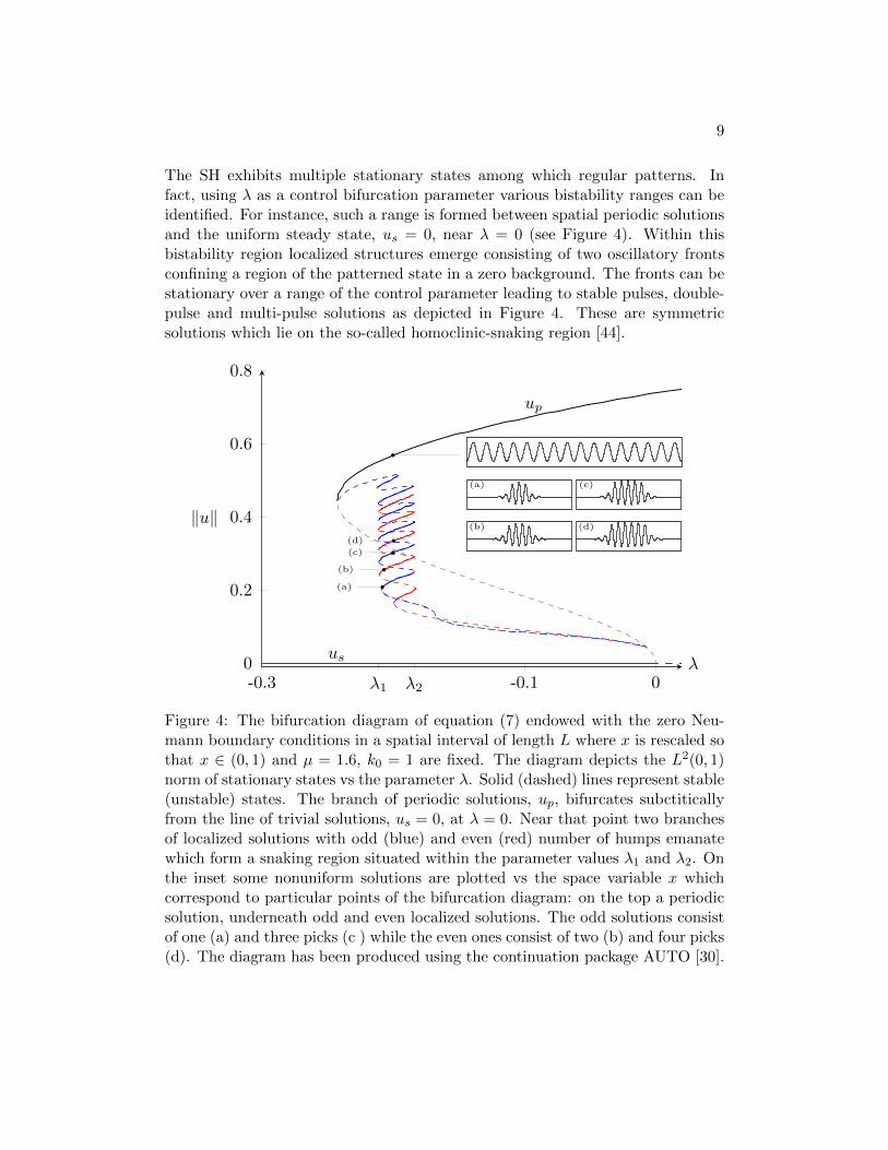
The SH exhibits multiple stationary states among which regular patterns. Infact, using λ as a control bifurcation parameter various bistability ranges can beidentified. For instance, such a range is formed between spatial periodic solutionsand the uniform steady state, us = 0, near λ = 0 (see Figure 4). Within thisbistability region localized structures emerge consisting of two oscillatory frontsconfining a region of the patterned state in a zero background. The fronts can bestationary over a range of the control parameter leading to stable pulses, double-pulse and multi-pulse solutions as depicted in Figure 4. These are symmetricsolutions which lie on the so-called homoclinic-snaking region [44].
up
us
(a)
(c)
(d)
(b)
-0.3 λ1 λ2 -0.1 00
0.2
0.4
0.6
0.8
λ
‖u‖
(a) (c)
(b) (d)
Figure 4: The bifurcation diagram of equation (7) endowed with the zero Neu-mann boundary conditions in a spatial interval of length L where x is rescaled sothat x ∈ (0, 1) and µ = 1.6, k0 = 1 are fixed. The diagram depicts the L2(0, 1)norm of stationary states vs the parameter λ. Solid (dashed) lines represent stable(unstable) states. The branch of periodic solutions, up, bifurcates subctiticallyfrom the line of trivial solutions, us = 0, at λ = 0. Near that point two branchesof localized solutions with odd (blue) and even (red) number of humps emanatewhich form a snaking region situated within the parameter values λ1 and λ2. Onthe inset some nonuniform solutions are plotted vs the space variable x whichcorrespond to particular points of the bifurcation diagram: on the top a periodicsolution, underneath odd and even localized solutions. The odd solutions consistof one (a) and three picks (c ) while the even ones consist of two (b) and four picks(d). The diagram has been produced using the continuation package AUTO [30].
10
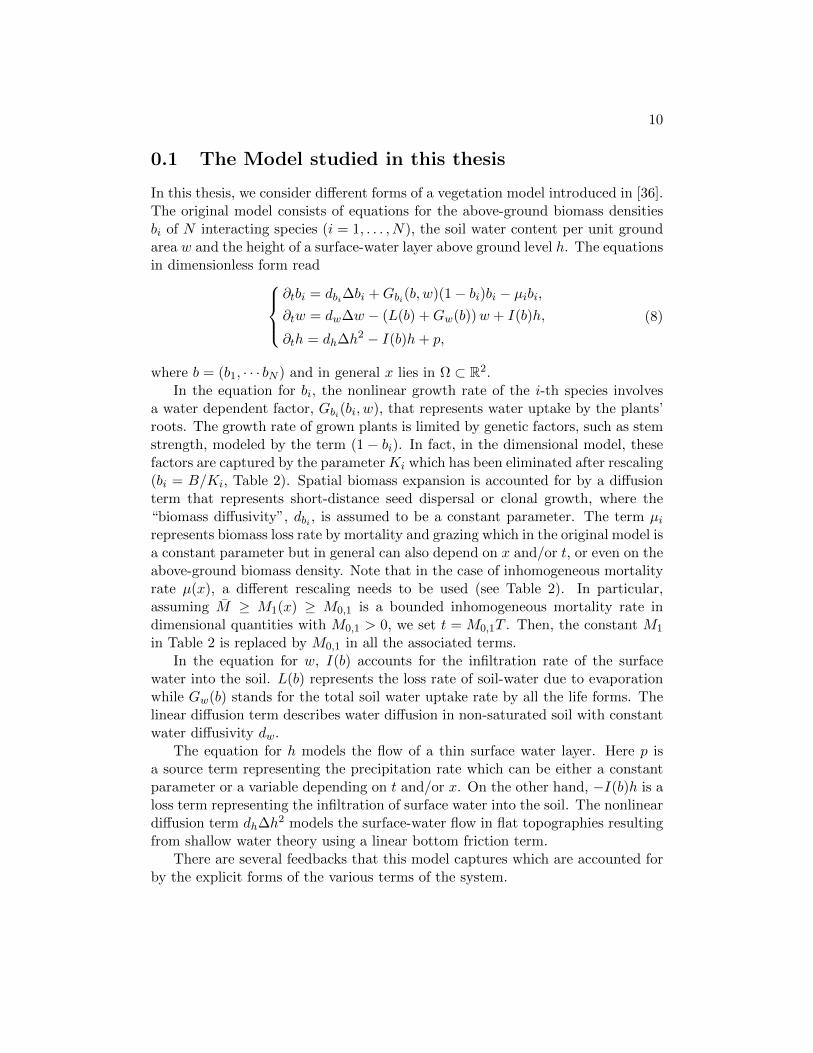
0.1 The Model studied in this thesis
In this thesis, we consider different forms of a vegetation model introduced in [36].The original model consists of equations for the above-ground biomass densitiesbi of N interacting species (i = 1, . . . , N), the soil water content per unit groundarea w and the height of a surface-water layer above ground level h. The equationsin dimensionless form read
∂tbi = dbi∆bi +Gbi(b, w)(1− bi)bi − µibi,∂tw = dw∆w − (L(b) +Gw(b))w + I(b)h,
∂th = dh∆h2 − I(b)h+ p,
(8)
where b = (b1, · · · bN ) and in general x lies in Ω ⊂ R2.In the equation for bi, the nonlinear growth rate of the i-th species involves
a water dependent factor, Gbi(bi, w), that represents water uptake by the plants’roots. The growth rate of grown plants is limited by genetic factors, such as stemstrength, modeled by the term (1 − bi). In fact, in the dimensional model, thesefactors are captured by the parameterKi which has been eliminated after rescaling(bi = B/Ki, Table 2). Spatial biomass expansion is accounted for by a diffusionterm that represents short-distance seed dispersal or clonal growth, where the“biomass diffusivity”, dbi , is assumed to be a constant parameter. The term µirepresents biomass loss rate by mortality and grazing which in the original model isa constant parameter but in general can also depend on x and/or t, or even on theabove-ground biomass density. Note that in the case of inhomogeneous mortalityrate µ(x), a different rescaling needs to be used (see Table 2). In particular,assuming M ≥ M1(x) ≥ M0,1 is a bounded inhomogeneous mortality rate indimensional quantities with M0,1 > 0, we set t = M0,1T . Then, the constant M1
in Table 2 is replaced by M0,1 in all the associated terms.In the equation for w, I(b) accounts for the infiltration rate of the surface
water into the soil. L(b) represents the loss rate of soil-water due to evaporationwhile Gw(b) stands for the total soil water uptake rate by all the life forms. Thelinear diffusion term describes water diffusion in non-saturated soil with constantwater diffusivity dw.
The equation for h models the flow of a thin surface water layer. Here p isa source term representing the precipitation rate which can be either a constantparameter or a variable depending on t and/or x. On the other hand, −I(b)h is aloss term representing the infiltration of surface water into the soil. The nonlineardiffusion term dh∆h2 models the surface-water flow in flat topographies resultingfrom shallow water theory using a linear bottom friction term.
There are several feedbacks that this model captures which are accounted forby the explicit forms of the various terms of the system.
11
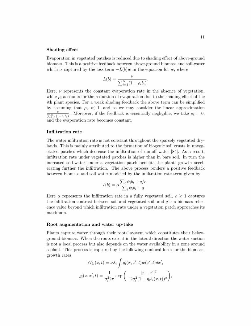
Shading effect
Evaporation in vegetated patches is reduced due to shading effect of above-groundbiomass. This is a positive feedback between above-ground biomass and soil-waterwhich is captured by the loss term −L(b)w in the equation for w, where
L(b) =ν∑N
i=1(1 + ρibi).
Here, ν represents the constant evaporation rate in the absence of vegetation,while ρi accounts for the reduction of evaporation due to the shading effect of theith plant species. For a weak shading feedback the above term can be simplifiedby assuming that ρi 1, and so we may consider the linear approximation
ν∑Ni=1(1−ρibi)
. Moreover, if the feedback is essentially negligible, we take ρi = 0,
and the evaporation rate becomes constant.
Infiltration rate
The water infiltration rate is not constant throughout the sparsely vegetated dry-lands. This is mainly attributed to the formation of biogenic soil crusts in unveg-etated patches which decrease the infiltration of run-off water [84]. As a result,infiltration rate under vegetated patches is higher than in bare soil. In turn theincreased soil-water under a vegetation patch benefits the plants growth accel-erating further the infiltration. The above process renders a positive feedbackbetween biomass and soil water modeled by the infiltration rate term given by
I(b) = α
∑i ψibi + q/c∑i ψibi + q
.
Here α represents the infiltration rate in a fully vegetated soil, c ≥ 1 capturesthe infiltration contrast between soil and vegetated soil, and q is a biomass refer-ence value beyond which infiltration rate under a vegetation patch approaches itsmaximum.
Root augmentation and water up-take
Plants capture water through their roots’ system which constitutes their below-ground biomass. When the roots extent in the lateral direction the water suctionis not a local process but also depends on the water availability in a zone arounda plant. This process is captured by the following nonlocal form for the biomass-growth rates
Gbi(x, t) = νλi
∫gi(x, x
′, t)w(x′, t)dx′,
gi(x, x′, t) =
1
σ2i 2π
exp
(− |x− x′|2
2σ2i (1 + ηibi(x, t))2
),
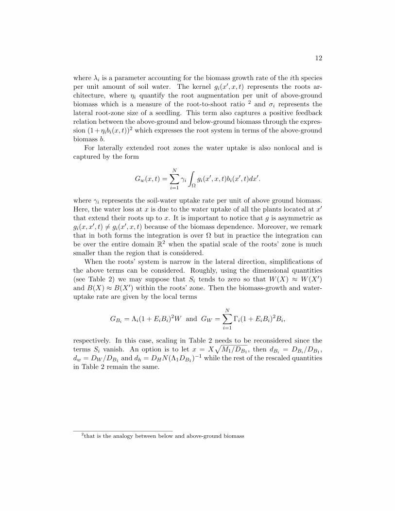
12
where λi is a parameter accounting for the biomass growth rate of the ith speciesper unit amount of soil water. The kernel gi(x
′, x, t) represents the roots ar-chitecture, where ηi quantify the root augmentation per unit of above-groundbiomass which is a measure of the root-to-shoot ratio 2 and σi represents thelateral root-zone size of a seedling. This term also captures a positive feedbackrelation between the above-ground and below-ground biomass through the expres-sion (1+ηibi(x, t))
2 which expresses the root system in terms of the above-groundbiomass b.
For laterally extended root zones the water uptake is also nonlocal and iscaptured by the form
Gw(x, t) =N∑i=1
γi
∫Ωgi(x
′, x, t)bi(x′, t)dx′.
where γi represents the soil-water uptake rate per unit of above ground biomass.Here, the water loss at x is due to the water uptake of all the plants located at x′
that extend their roots up to x. It is important to notice that g is asymmetric asgi(x, x
′, t) 6= gi(x′, x, t) because of the biomass dependence. Moreover, we remark
that in both forms the integration is over Ω but in practice the integration canbe over the entire domain R2 when the spatial scale of the roots’ zone is muchsmaller than the region that is considered.
When the roots’ system is narrow in the lateral direction, simplifications ofthe above terms can be considered. Roughly, using the dimensional quantities(see Table 2) we may suppose that Si tends to zero so that W (X) ≈ W (X ′)and B(X) ≈ B(X ′) within the roots’ zone. Then the biomass-growth and water-uptake rate are given by the local terms
GBi = Λi(1 + EiBi)2W and GW =
N∑i=1
Γi(1 + EiBi)2Bi,
respectively. In this case, scaling in Table 2 needs to be reconsidered since theterms Si vanish. An option is to let x = X
√M1/DB1 , then dBi = DBi/DB1 ,
dw = DW /DB1 and dh = DHN(Λ1DB1)−1 while the rest of the rescaled quantitiesin Table 2 remain the same.
2that is the analogy between below and above-ground biomass
13
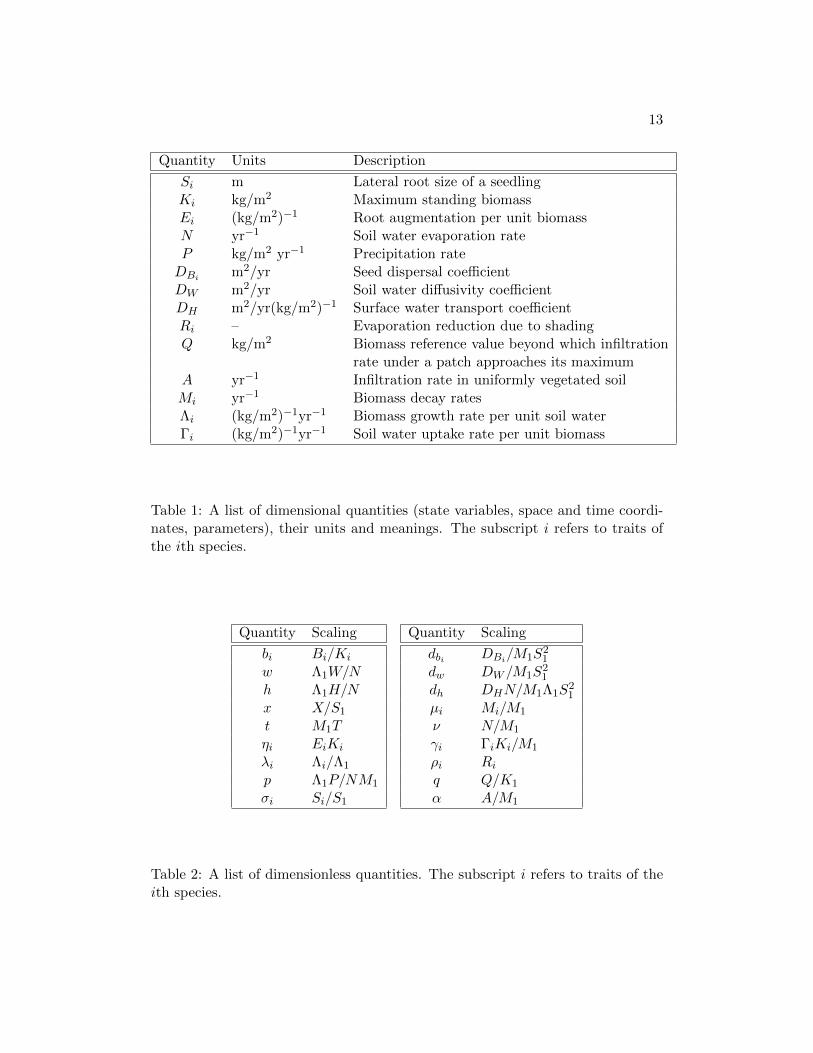
Quantity Units Description
Si m Lateral root size of a seedlingKi kg/m2 Maximum standing biomassEi (kg/m2)−1 Root augmentation per unit biomassN yr−1 Soil water evaporation rateP kg/m2 yr−1 Precipitation rateDBi m2/yr Seed dispersal coefficientDW m2/yr Soil water diffusivity coefficientDH m2/yr(kg/m2)−1 Surface water transport coefficientRi – Evaporation reduction due to shadingQ kg/m2 Biomass reference value beyond which infiltration
rate under a patch approaches its maximumA yr−1 Infiltration rate in uniformly vegetated soilMi yr−1 Biomass decay ratesΛi (kg/m2)−1yr−1 Biomass growth rate per unit soil waterΓi (kg/m2)−1yr−1 Soil water uptake rate per unit biomass
Table 1: A list of dimensional quantities (state variables, space and time coordi-nates, parameters), their units and meanings. The subscript i refers to traits ofthe ith species.
Quantity Scaling
bi Bi/Ki
w Λ1W/Nh Λ1H/Nx X/S1
t M1Tηi EiKi
λi Λi/Λ1
p Λ1P/NM1
σi Si/S1
Quantity Scaling
dbi DBi/M1S21
dw DW /M1S21
dh DHN/M1Λ1S21
µi Mi/M1
ν N/M1
γi ΓiKi/M1
ρi Riq Q/K1
α A/M1
Table 2: A list of dimensionless quantities. The subscript i refers to traits of theith species.
14
Thesis outline
In the first chapter of this thesis, we deal with the stationary problem of thevegetation model. We first examine the existence and multiplicity of biomassstationary solutions in terms of a constant precipitation rate parameter p, for alocalized simplification of the system, with non-homogeneous rate of biomass lossµ(x). In fact, we show that under appropriate conditions on fixed parametersof the problem, multiple positive solutions exist for a range of the parameter p.In the second part, we deal with a two-component system of biomass and soil-water showing the existence of continua of nonuniform stationary solutions whichemanate from the branch of positive uniform solutions using the length of thespatial interval as a bifurcation parameter. In the last part, we consider the caseof an idealized ”oasis”, ω ⊂⊂ Ω, where we study the transition of the surface-water height in a neighborhood of the set ω. Precisely, for a constant p0 > 0 weassume that p(x) = p0χω(x) on Ω, where χω denotes the characteristic functionof ω.
In the second chapter, we study the spatial competition between two plantspecies that make different compromises in capturing soil water and sunlight usinga extended model which takes into account competition for light, too. A precipi-tation range along the rainfall gradient is identified where two alternative stablestates coexist. The first state describes a uniform distribution of a plant speciesthat specializes in capturing soil water, whereas the second state describes a pe-riodic pattern of a species that specializes in capturing light. We show that thisbistability range generally divides into three parts according to the dynamics ofthe front or ecotone that separates the two plant populations: a low precipitationrange where the superior competitor for water displaces the superior competitorfor light, a high precipitation range where the displacement is reversed, and anintermediate range where neither species displaces the other. While in the lowand high precipitation ranges one species outcompetes the other, the intermediaterange allows for species coexistence in the form of a multitude of stable localizedsolutions consisting of fixed domains of one species in areas otherwise occupied bythe other species. These localized solutions can only be realized when one of thealternative stable states is spatially patterned. We further study two factors thataffect the size of the species coexistence range: the strength of the competitionfor light and the form of the tradeoff between the competitive abilities to capturewater and light.
The third chapter is devoted to the mathematical analysis of the time-dependentsystem with local biomass growth and water uptake rate terms but with a non-linear modified infiltration rate term. The existence of solutions is studied forthe case of Dirichlet (DBC) and Neumann (NBC) boundary conditions for givenessentially bounded initial data. The main difficulty in the study of the systemarises from the degeneracy in the diffusion term of the equation for the surface
15
water variable h. To overcome this difficulty, in the case of DBC, the problemis approximated by a family of regularized systems for which existence of uniquesolutions is guaranteed. Next using some a priori bounds of the approximatingsolutions we obtain a solution of the original system by passing to the limit. Forthe case of NBC, we use a different approach based on a fixed point argument.In particular, we define an operator on a convex weakly closed subset into itself.Then the weak compactness properties of a mapping defined by the solutions ofa decoupled inhomogeneous system, with fixed bounded initial data, induce thatthe operator has a weakly closed graph which ensures the existence of at least onefixed point. Finally, in the remainder of this chapter we examine the responseof the system to long dry periods, that is p(t) = 0 for t ∈ (0, T ] for T largeenough. We show that depending on the initial data and the boundary conditionsurface-water component either vanishes or forms vanishing regions which shrinkgradually.

Chapter 1
On the elliptic system
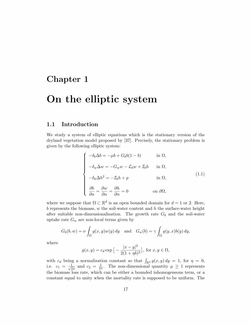
1.1 Introduction
We study a system of elliptic equations which is the stationary version of thedryland vegetation model proposed by [37]. Precisely, the stationary problem isgiven by the following elliptic system:
−δb∆b = −µb+Gbb(1− b) in Ω,
−δw∆w = −Gww − Lbw + Ibh in Ω,
−δh∆h2 = −Ibh+ p in Ω,
∂b
∂n=∂w
∂n=∂h
∂n= 0 on ∂Ω,
(1.1)
where we suppose that Ω ⊂ Rd is an open bounded domain for d = 1 or 2. Here,b represents the biomass, w the soil-water content and h the surface-water heightafter suitable non-dimensionalization. The growth rate Gb and the soil-wateruptake rate Gw are non-local terms given by
Gb(b, w) = ν
∫Ωg(x, y)w(y) dy and Gw(b) = γ
∫Ωg(y, x)b(y) dy,
where
g(x, y) = cd exp[− |x− y|2
2(1 + ηb)2
], for x, y ∈ Ω,
with cd being a normalization constant so that∫Rd g(x, y) dy = 1, for η = 0,
i.e. c1 = 1√2π
and c2 = 12π . The non-dimensional quantity µ ≥ 1 represents
the biomass loss rate, which can be either a bounded inhomogeneous term, or aconstant equal to unity when the mortality rate is supposed to be uniform. The
17
CHAPTER 1. ON THE ELLIPTIC SYSTEM 18
term Lb(b) =ν
1 + ρbstands for the evaporation rate of the soil water, and Ib(b) =
αb+ q/c
b+ qrepresents the infiltration rate of the surface-water. The third equation
of the parabolic system is a porous medium type equation that describes theoverland flow of a thin water layer and involves the precipitation rate parameterp > 0. The rest of the parameters are positive, and in fact, c > 1. As we shall see,in special cases, some of the parameters may also be taken to be equal to zero.
In section 1, we consider the case of plant species with negligible below-groundbiomass. In that case we may assume that the root extension parameter η is equalto zero. Since the minimal root size of a seedling for such plant species tends tozero, the non-local effect of the root system is insignificant. As a result, we mayreplace g(x, y) with the Dirac delta based on x. Furthermore, for suitable scalingof the dimensional quantities we may assume that δb = 1. Then we arrive at thefollowing local coupled system
−∆b = −µb+ νwb(1− b) in Ω,
−δw∆w = −γbw − Lbw + Ibh in Ω,
−δh∆h2 = −Ibh+ p in Ω,
∂b
∂n=∂w
∂n=∂h
∂n= 0 on ∂Ω.
(1.2)
Moreover, we shall limit ourselves to the case where infiltration feedback andsoil-water diffusion are not present. Roughly, this corresponds to δw = δh = 0.Finally, we consider an inhomogeneous biomass loss rate µ, which cannot exceed aminimal loss rate due to natural mortality and a maximal total loss rate. Precisely,in dimensionless quantities, we suppose that µ ∈ C1(Ω) is such that 1 ≤ µ(x) ≤ µ,for x ∈ Ω. On the basis of the considerations described above, in the first sectionwe shall investigate the existence of positive solutions in terms of the precipitationparameter p, when Ω ⊂ R2 is a bounded domain with C2 boundary.
In the second part, we study the existence of nonuniform solutions for a sim-plified coupled system of the biomass variable b and the soil-water variable w in1d. This is done by using a global bifurcation theorem and treating the length ofthe spatial interval as a bifurcation parameter. In particular, we show that con-tinua of positive nonuniform solutions emanate from points of a branch of uniform(constant) solutions, for parameter values determined by particular eigenvalues ofan associated linear problem.
In the third part, we consider system (1.1) in a bounded two dimensionaldomain assuming that the precipitation rate is inhomogeneous. Particularly, weassume that p is constant in a closed subset ω ⊂⊂ Ω and vanishes outside ω.
CHAPTER 1. ON THE ELLIPTIC SYSTEM 19
Here, one may think of p(·) as a distributed water resource which is not negligibleonly on a sub-region ω of Ω. Moreover, in contrast with section 1, in this sectionwe suppose that δw, δh > 0 and that the loss rate is a constant. In that occasion,we investigate the free boundary of the surface-water solution component h, interms of the parameters involved in the third equation of (1.1).
1.2 A multiplicity result for a scalar biomass equation
In this section, we seek non-negative solutions of (1.2), depending on the pa-rameter p, when δw = δh = 0 and µ(x) is a smooth function in Ω such that1 ≤ µ(x) ≤ µ, where Ω is two dimensional bounded domain with a C2 boundary.Thus, we study the following elliptic problem
−∆b+ µ(x)b = pf(b) in Ω,
∂b
∂n= 0 on ∂Ω,
(Pp)
for
f(b) =νb(1− b)(1 + ρb)
γb(1 + ρb) + ν.
Clearly, f(·) ∈ C2(R+),
0 ≤ f(s) ≤M for all s ∈ [0, 1],
andf(s) < 0 for s ≥ 1.
We also note, that b ≡ 0 is a solution of (Pp) for all p > 0, such a solution willbe called the trivial. We shall first consider a subclass of weak solutions, namely,the so-called variational solutions. So, let us consider the set
K = v ∈ H1(Ω) | 0 ≤ v ≤ 1 in Ω,
and let
Fp(v) = p
∫ v
0f(s) ds .
We define the variational functional
Jp(v) =1
2
∫Ω
(|∇v|2 + µ(x)v2
)dx− Φp(v),
where
Φp(v) :=
∫ΩFp(v(x)) dx.

CHAPTER 1. ON THE ELLIPTIC SYSTEM 20
Definition 1. We shall call a function v ∈ H1(Ω), a variational solution of (Pp),if v is a minimum of the functional Jp on the set K.
Remark 1. It can be easily verified that any variational solution is a weak solutionof a multivalued equation involving the subdifferential, ∂IK of the convex function
IK(x) =
0 if x ∈ K+∞ if x /∈ K
As it is proved in [23, Chapter 4] this multivalued equation satisfies the samecomparison principle with the Euler-Lagrange equation which does not involve∂IK (i.e. equation (Pp)). Thus if the solutions of (Pp) are greater than 0 or lessthan 1 in Ω the same holds for the multivalued equation.
We have:
Theorem 1. For each p > 0, there exists at least one variational solution of (Pp).
Proof. Since K is a convex closed subset of H1(Ω), in order to show that Jpattains a minimum (due to a version of the Weierstrass theorem, see [85] p.513),it suffices to show that Jp is weakly lower semicontinuous and weakly coercivedefined on K.
(i) Jp is weakly lower semicontinuous. Indeed, the norm on H1(Ω) is weaklylower semicontinuous. On the other hand, the embedding H1(Ω) → Lq(Ω) iscompact for 1 ≤ q < ∞, since N = dim(Ω) = 2. Therefore, if vn is a sequencein K that converges weakly in H1(Ω) to a function v, we know that (up to asubsequence) vn → v strongly in Lq(Ω). This actually implies that
Φp(vn)→ Φp(v)
and so the map Φp : K ⊂ H1(Ω)→ R is weakly continuous. Thus Jp(v) is weaklylower semicontinuous.
(ii) Jp is coercive. Indeed, for u ∈ K we have Φp(v) ≤ pM‖v‖L1(Ω) ≤ pM |Ω|so for some constant C(p,Ω) > 0, Jp(v) ≥ 1
2‖v‖2H1 − C(p,Ω) which implies that
J(v)→∞ as ‖v‖2H1 →∞. This ends the proof of the Theorem 1.
We now proceed to consider solutions of (Pp) which are not necessarily varia-tional solutions. Our study is inspired by a previous one arising in a completelydifferent context: some simple climate models [25].
Before stating our main result, it is useful to consider the following auxiliary al-gebraic equations which provide us with positive constant super and sub-solutionsof (Pp) for a range of the parameter p.
s = pf(s), s ∈ R, (E1)
CHAPTER 1. ON THE ELLIPTIC SYSTEM 21
µs = pf(s), s ∈ R. (E2)
So, let us make some observations and introduce notation related to the set ofnon-negative solution of (E1) and (E2). We first observe that for all p > 0, s = 0satisfies both equations and any possible positive solution of the auxiliary equa-tions has to be lower than unity. We shall denote by Γ1 and Γ2 the (bifurcation)curves of nontrivial positive solutions corresponding to the algebraic equations(E1) and (E2), respectively. Now, let
T1(p, s) = s− pf(s)
andT2(p, s) = µs− pf(s).
Clearly, if pi is such that∂
∂sTi(pi, 0) = 0, (1.3)
then Γi bifurcates from the line of trivial solutions at (pi, 0), for i = 1, 2. Onecan easily check that p1 = 1 and p2 = µ. Moreover, if the following condition issatisfied
ρ > 1 and γ < ν(ρ− 1), (C1)
then∂2
∂s2Ti(pi, 0) < 0 and the bifurcation at (pi, 0) is subrcritical. In fact, (C1)
also assures that Γi has a unique ”turning point” (p∗i , s∗) which satisfies
Ti(p∗i , s∗) = 0 =
∂
∂sTi(p
∗i , s∗) (1.4)
as well as∂2
∂s2Ti(p
∗i , s∗) > 0 and
∂
∂pTi(p
∗i , s∗) < 0,
for i = 1, 2, where
s∗ =−(γ + ν) +
√ν2 + γν + ργν
γρ> 0.
Finally, we point out that for fixed p ∈ (p∗i , pi), (Ei) has two distinct positivesolutions denoted by s1
i,p and s2i,p, which are such that
s1i,p < s∗ < s2
i,p,
while for p ≥ pi, (Ei) has a unique positive solution denoted again by s2i,p.
CHAPTER 1. ON THE ELLIPTIC SYSTEM 22
Theorem 2. Let p1, p2 be the bifurcation points of (E1), (E2) given by (1.3).Also, assume that (C1) holds true and let p∗i be the unique points that satisfy(1.4) for i = 1, 2. Then,
(i) if p ∈ (0, p∗1), the trivial solution b ≡ 0 is the only possible non-negativesolution of (Pp).
(ii) if p∗2 < p1 and p ∈ (p∗2, p1), (Pp) has at least two positive solutions, besidesthe trivial solution b ≡ 0.
(iii) if p ∈ (maxp1, p∗2,∞), then besides the trivial solution, (Pp) has at least
one positive solution. In fact, for p large enough, there exists ξ ∈ (0, 1) anda unique non-trivial positive solution of (Pp) satisfying ξ ≤ b(x) < 1 in Ω.Moreover, this unique solution is also a variational solution of (Pp).
Proof. (i) By (C1), there exists a unique pair (p∗1, s∗) ∈ Γ1 such that f ′(s∗) > 0.
In fact, we have that
f(s) ≤ sf ′(s∗) for all s ≥ 0. (1.5)
Therefore, if b ∈ H1(Ω) is a non-negative solution of (Pp), by multiplying (Pp) byb and integrating over Ω, since µ(x) ≥ 1, we have that∫
Ωb2 dx ≤
∫Ω
(|∇b|2 + b2
)dx ≤
∫Ωf(b)b dx ≤ pf ′(s∗)
∫Ωb2 dx.
So, a non-negative solution which is not the trivial may exist only for p > p∗1.In order to obtain (ii) and (iii), we now focus on positive constant super andsub-solutions of (Pp). Clearly, for p > 0 any positive solutions of the followingproblems
−∆Up + Up = pf(Up) in Ω,
∂Up∂n ≥ 0 on ∂Ω,
and −∆Vp + µVp = pf(Vp) in Ω,
∂Vp∂n ≤ 0 on ∂Ω,
are respectively, sup or sub-solutions of (Pp). So, for every p > p∗1 positive so-lutions of (E1) form a family of positive constant super-solutions and for everyp > p∗2 > 0 positive solutions of (E2) form a family of sub-solutions of (Pp).Namely, we let
U1p ≡ s1
1,p, U2p ≡ s2
1,p and V 2p ≡ s2
2,p.
(ii) If p∗2 < p1, for each p ∈ (p∗2, p1), we consider the ordered intervals [0, U1p ]
and [V 2p , U
2p ], then from [1, Theorem 15.2, p.668], (Pp) has at least three distinct
CHAPTER 1. ON THE ELLIPTIC SYSTEM 23
solutions b1, b2 and b3 such that 0 ≤ b1 < b2 < b3 < U2p . Since b1 may be
identically zero (ii) follows.(iii) For each p ∈ (maxp1, p
∗2,∞), we consider the ordered interval [V 2
p , U2p ]
where Vp and Up are such that Vp < Up. It is easy to check that the conditions ofthe results in [1] hold true and so there exist a minimal and a maximal solutionin [V 2
p , U2p ]. Moreover, for p large enough, any such positive weak solution takes
values in an interval [ξ, 1) where f(·) is decreasing which implies the uniquenessof any possible weak solution taking values in that interval. Finally, the energy ofsuch weak solution is less than zero. Therefore, we deduce that for p large enoughup is also a variational solution of (Pp).
It is actually natural to ask whether the set of positive solutions consistsof a connected closed set in R × X for some function space X. To this end,we let X = C(Ω) and recall that X possesses a positive cone P induced bythe natural ordering. In fact, since P has non-empty interior, P is total i.e.,u − v : u, v ∈ P − 0 is dense in X. We denote by K the solution operatorof −∆ + µ(x) together with the homogeneous Neumann boundary conditions,and by F : P → X the Nemiskii operator given by F (u) = f+(u(·)) wheref+ = maxf, 0. Note that f+ ∈ C0,α(R) and F is continuous and clearly, ifu ∈ P , then F (u) ∈ P . Now let us consider the following auxiliary problem.
−∆b+ µ(x)b = pf+(b) in Ω,
∂b
∂n= 0 on ∂Ω.
(P+p )
Since K is a linear positive compact operator from X to itself, we have that forp > 0 the map
pK F : P → X
is completely continuous and positive, where the latter means that pKF (P ) ⊂ P .Finally, the fixed point equation u = pK Fu for u ∈ X, is equivalent to equation(P+
p ). It can be checked that K F is right Frechet differentiable at u = 0, withK being the Frechet derivative from the right. Therefore by Theorem 18.3 in [1](see also [17]), we conclude that:
Theorem 3. The problem (P+p ) possesses an unbounded continuum of positive
solutions C+ in R+ × P , emanating from the line of trivial solutions (p, 0) at(p∗, 0), where p∗ is the unique positive eigenvalue with a positive eigenvector ofthe following eigenvalue problem:
−∆b+ µ(x)b = λb in Ω,
∂b
∂n= 0 on ∂Ω.
(1.6)
CHAPTER 1. ON THE ELLIPTIC SYSTEM 24
Remark 2. By standard regularity theory and the strong maximum principle, wehave that max
Ωb(x) < 1. Therefore, since f(s) = f+(s) for s ∈ [0, 1], we have that
(p, b) ∈ C+ also satisfies (Pp). Note that this is true for all ν, γ, ρ > 0.
1.3 A coupled water-biomass system
In this section, we study the existence of nonuniform solutions for a coupledsystem of the biomass variable b and the soil water variable w in a boundedinterval. In particular, to obtain a two-component system and we ignore theinfiltration feedback by setting δh = 0 in (1.1) (the infiltration feedback canbe neglected in sandy soils where the infiltration of surface water uniform andfast). Then we assume that the plant species with biomass b does not extend itsroots in the lateral direction. As a result, we can consider local biomass growthand water-uptake rate terms which are given by the forms Gb = νw(1 + ηb)and Gw = γb(1 + ηb), respectively. Furthermore, we assume that the biomassloss rate µ is uniform. We note that under the preceding assumptions, we maytake δb = µ = 1, by choosing appropriately the rescaled quantities in the non-dimensionalization process. Finally, we also assume that a weak shading feedbackis present in the system. In other words, ρ 1 (note that ρ represents thewater evaporation reduction due to shading of the plants) and so we can use alinear approximation of the evaporation rate term, namely, Lb ≈ ν(1 − ρb). Thesimplified coupled system then reads
− bxx = νwb(1− b)(1 + ηb)− b,− δwwxx = p− w (ν(1− ρb) + γb(1 + ηb)) ,
(1.7)
for x in Ω = (0, l)Next, in order to study the existence of spatially nonuniform solutions with
respect to the length of the spatial domain, we rescale the spatial variable xletting x = xl−1. By dropping the tilde notation and letting ξ = l2, (1.7) can betransformed into the system
− bxx = ξ (νwb(1− b)(1 + ηb)− b) ,− δwwxx = ξ (p− w (ν(1− ρb) + γb(1 + ηb))) ,
(1.8)
where x ∈ (0, 1) and ξ plays the role of a parameter in the system which carriesinformation about the size of the spatial interval. We recall that system (1.8) isconsidered together with the homogeneous NBC:
bx(0) = bx(1) = 0 = wx(0) = wx(1). (1.9)
Next we find conditions under which the above system possesses positive uniformsolutions.
CHAPTER 1. ON THE ELLIPTIC SYSTEM 25
1.3.1 Uniform solutions
It is clear, that the pair (b0, w0) = (0, p/ν) is a trivial uniform nonnegative solutionof (1.8). In addition, we can find pairs of positive uniform solutions of the systemfor specific choices of the parameters. Precisely, real pairs of constants (b±s , w
±s )
satisfying (1.8) exist when
dis(p, ν, η, γ, ρ) := (pν(η − 1)− γ + νρ)2 − 4ην(1− p)(pν + γ) ≥ 0 , (1.10)
and are given by the expressions
b±s =(η − 1)pν − γ + νρ±
√dis
2η(pν + γ),
w±s =p
b±s2γη + b±s (γ − νρ) + ν
.
We further need to determine the parameter values for which these solutions arepositive. To simplify exposition in what follows we will assume that
ρ < minγ/ν, 1. (H1)
Then it is enough to find a parameter regime where b±s is positive since this inducespositivity of w±s , too. To this end, we distinguish two cases given that (1.10) issatisfied for p, ν, η, γ, ρ > 0:
1. if pν(η − 1) − γ + νρ ≥ 0, then b+s is positive for p > 1, while b−s < 0.Note that, in this case, for p = 1, b+s coincides with the solution b0 = 0 andb±s = b0 when pν(η − 1)− γ + νρ = 0.
2. if pν(η − 1)− γ + νρ < 0, then setting
pc :=2√ην(η + ρ)(γη + γ − νρ+ ν)− γ(η + 1)− ην(ρ− 2) + νρ
(η + 1)2ν,
we have that b±s > 0 for pc < p < 1, while b+s > 0 and b−s < 0 for p > 1.Note that in this case, necessarily η > 1. Moreover, for p = 1, b−s coincideswith the solution b0 = 0.
Next we focus only on the uniform solutions (b+s , w+s ), for the parameter values
that they are positive and we drop the ”+” notation. Our aim is to examine therise of non-uniform solutions, emanating from the branch of uniform solutionsusing ξ as a bifurcation parameter. To apply a global bifurcation theorem, whichis stated in the next section, it is convenient to set u = b− bs and v = w−ws, so
CHAPTER 1. ON THE ELLIPTIC SYSTEM 26
that the constant solutions of the system are shifted to the origin. In particular,the shifted system is given by,
− uxx = ξ (J11u+ J12v + f(u, v)) ,
− δwvxx = ξ (J21u+ J22v + g(u, v)) ,(1.11)
along with the zero Neumann boundary conditions
ux(0) = ux(1) = 0 = vx(0) = vx(1), (1.12)
where
J11 :=νws(1 + 2bs(η − 1)− 3b2sη)− 1, (1.13)
J12 :=νbs(1− bs)(1 + ηbs), (1.14)
J21 :=− 2bswsγη − wsγ + wsνρ, (1.15)
J22 :=− γb2sη − bsγ + bsνρ− ν, (1.16)
are the coefficients of the linear reaction part and
f(u, v) :=uv(−3b2sην + 2bsην − 2bsν + ν
)− 3bsu
2vην
− 3bsu2wsην − u3vην − u3wsην
+ u2vην − u2vν + u2wsην − u2wsν,
g(u, v) :=− vu2γη − uv(2bsγη + γ − νρ)− u2wsγη.
are the non-linear reaction parts. It is also meaningful to consider the linearproblem associated to (1.11), (1.12), namely, the eigenvalue problem
− uxx = ξ (J11u+ J12v) ,
− δwvxx = ξ (J21u+ J22v) ,
ux(0) = ux(1) = 0 = vx(0) = vx(1).
(1.17)
Note that a necessary condition for a point ξ∗ to be a bifurcation point of (1.11),(1.12) is (1.17) to possess a non-trivial solution at ξ∗. Problem (1.17) admitsnon-nontrivial solutions for values of ξ such that
det
(J11ξ − σi J12ξJ21ξ J22ξ − δwσi
)= 0 ,
where σi are the eigenvalues of −∂xx with the zero Neumann boundary conditions.In particular, these values are given by the pairs:
ξ±i = σiδwJ11 + J22 ±
√(δwJ11 + J22)2 − 4δw(J11J22 − J12J21)
2(J11J22 − J12J21), (1.18)
CHAPTER 1. ON THE ELLIPTIC SYSTEM 27
In order for the ξ±i to be distinct real and positive numbers for each i ≥ 1, weassume that
(δwJ11 + J22)2 − 4δw(J11J22 − J12J21) > 0 (H2)
andJ11J22 − J12J21 > 0 and δwJ11 + J22 > 0, (H3)
respectively, for fixed values of the parameters p, γ, η, ν, ρ, δw. It can be checkedthat these conditions are satisfied for a range of the parameters given that δw > 1.
1.3.2 Nonuniform solutions
In order to investigate the existence of nonuniform solutions we first state anextension of the celebrated global bifurcation theorem of Rabinowitz [59], intro-duced by Blat and Brown in [8]. In this theorem the notion of the index of anisolated fixed point of a mapping is used. This can be defined in terms of theLeray-Schauder degree of the mapping in an neighborhood of the isolated fixedpoint [2, 48, 71]. In particular, let F be a continuously differentiable compactoperator defined on a Banach space to itself, and let F ′u(u0) denote the Frechetderivative of F at u0. We recall that if I − F ′u(u0) is invertible, then u0 is anisolated fixed point of F , and the index of I − F at u0 is given by
ind (I − F, u0) = (−1)β,
where β is the sum of the algebraic multiplicities of the eigenvalues of F ′u(u0)which are greater than unity.
Theorem 4. Let X be a Banach space and let F : R × X → X be a compact,continuously differentiable operator such that F (ξ, 0) = 0. Suppose that F can bewritten as,
F (ξ, u) = K(ξ)u+R(ξ, u)
where K(ξ) a linear compact operator and the Frechet derivative of Ru(ξ, 0) = 0.Let ξ∗ be such that I −K(ξ) is invertible when 0 < |ξ − ξ∗| < ε for some ε > 0.Suppose ind (I − F (ξ, ·), 0) is constant on (ξ∗ − ε, ξ∗) and (ξ∗, ξ∗ + ε) such that ifξ∗ − ε < ξ1 < ξ∗ < ξ2 < ξ∗ + ε, then ind (I − F (ξ1, ·), 0) 6= ind (I − F (ξ2, ·), 0).Then there exists a continuum, C, in the ξ − u plane of solutions of u = F (ξ, u),such that one of the following alternatives holds true
1. either C joins (ξ∗, 0) to (ξ, 0) where I −K(λ) is not invertible,
2. or C joins (ξ∗, 0) to infinity in R.
CHAPTER 1. ON THE ELLIPTIC SYSTEM 28
Let us now put our problem into the context of the preceding theorem. Thiscan be achieved by rewriting (1.11) as an integral equation. For this we introducethe following Holder spaces
Y = (f1, f2)| f1, f2 ∈ C2, α([0, 1]) and f1x(0) = f1x(1) = 0 = f2x(0) = f2x(1),
Z = (f1, f2)| f1, f2 ∈ Cα([0, 1]).First we define the operator L : Y → Z given by L(u.v) = (−∂xxu,−δw∂xxv).Next we let N : Z → Z be the operator defined by the nonlinear reaction parts,namely
N(u, v) := (f(u, v), g(u, v)),
and the operators J : Z → Z and D : Z → Z defined, respectively, by the actionof
J =
(J11 J12
J21 122
)and
D =
(1 00 δw
)on elements of Z, where we have used the same notation for the operators definedon Z and the corresponding matrices. Then, finding solutions of system (1.11),(1.12) is equivalent to finding an element of Y satisfying the equation
L(u, v) = ξJ(u, v) + ξN(u, v). (1.19)
Note that because of the zero Neumann boundary conditions, L is not invertable,so we cannot pass to the integral equation problem at this point. However, addingD in both sides the new operator defined by
L(u, v) := L(u, v) +D(u, v)
is invertible since the problem− c1yxx + c2y = z,
yx(0) = yx(1) = 0,(1.20)
with z ∈ Cα([0, 1]) has a unique solution y ∈ C2, α([0, 1]) for all c1, c2 > 0.Therefore, solving (1.11), (1.12) is finally equivalent to solving the equation
(u, v) = ξL−1J(u, v) + L−1D(u, v) + ξL−1N(u, v) =: F (ξ, u, v). (1.21)
We remark that F : R × Z → Y is continuous operator and as Y is compactedembedded into Z, in fact, F : R×Z → Z is compact (see for instance [2]). Then,
CHAPTER 1. ON THE ELLIPTIC SYSTEM 29
setting K(ξ)(u, v) := ξL−1J(u, v) + L−1D(u, v) and R(ξ, u, v) := ξL−1N(u, v),F is in the form of Theorem 4 for Z = X. In addition, F (ξ, 0, 0) = 0 for allξ, the Frechet derivative of R(ξ, u, v) at (0, 0) is zero and the linear operatorK(ξ) : Z → Z is compact. To apply Theorem 4, we need to find the critical valuesof ξ for which ind(I − K(ξ)) changes sign. To evaluate the indices we look foreigenvalues of K(ξ)(u, v), thus we search for nontrivial solutions of K(ξ)(u, v) =λ(u, v). Writing the latter problem in terms of the differential operators we see
that its nontrivial solutions occur for the pairs of eigenvalues λ±i (ξ) =1+σiξ/ξ
±i
1+σi
with i ≥ 1. Clearly, λ±i (ξ) are increasing functions of ξ and they cross 1 whenξ passes through ξ±i . Moreover, it can be shown that if ξ±i 6= ξ∓j for i 6= j (i.e.
excluding eigenvalues with algebraic multiplicity different than 1) λ±i are simpleeigenvalues (see for instance [12] and references therein). Therefore evaluating theindex of K(ξ) in the right and left neighborhood of such ξ±i , Theorem 4 can beapplied with ξ∗ = ξ±i and ε > 0 sufficiently small.
We conclude, that there exist continua C±i in R × Z which bifurcate from(ξ±i , 0, 0). Moreover, a triple (ξ, u, v) ∈ C±i satisfies (1.11), (1.12), therefore sincethe solutions of the original problem (1.8),(1.9) are given by b = u + bs andw = v+ws, the branches C±i , define continua of solutions of the original problem,bifurcating from (ξ±i , bs, ws), which we denote by C±i . Finally, the solutions lyingon C±i are positive for ξ > 0. This is a consequence of the maximum principleand the use of local bifurcation theory [59], which ensures that the solutionsare nonnegative sufficiently close to the bifurcation point. We also note that acontinuum can cross the ξ = 0 axis only at (0, bs, ws). To prove that this cannotbe the case, and so C±i are defined only for ξ > 0, a priori estimates need tobe derived for the solutions of the problem. Such estimates can also provideinformation about the global behavior of the branches of nonuniform solutions.
1.4 Surface water transition
In this section, we study the third equation of system (1.1), assuming that δw, δh >0 and that the precipitation rate is not completely constant in Ω, but vanishesoutside a closed subset ω ⊂⊂ Ω. For p0 > 0, we let p(x) = p0χω(x) on Ω, whereχω denotes the characteristic function of ω. We recall that the non-linear termof the equation involves the so-called infiltration contrast parameter c > 1. Now,supposing that b is a given non-negative solution of the corresponding equationof system (1.1) for the given boundary conditions, we set
θ(x) := αb(x) + q/c
b(x) + qin Ω.
CHAPTER 1. ON THE ELLIPTIC SYSTEM 30
Obviously, we have that αc ≤ θ(x) ≤ α on Ω. On the other hand, letting h = h2,
if h ≥ 0 and δh > 0, then the third equation can be written as−∆h+
θ(x)
δh
√h = φ(x) in Ω,
∂h
∂n= 0 on ∂Ω,
(1.22)
with φ(x) :=p0
δhχω(x).
We point out that, in general, we cannot ensure the uniqueness of functionh (in fact, in the preceding section, we exhibit a case of multiplicity of b andso of h). Nevertheless, for fixed b the non-negative solution of (1.22) is unique.Furthermore, by the maximum principle, we know that a possible solution h mustsatisfy that
‖h‖L∞(Ω) ≤(p0c
α
)2.
The following theorem provides an estimate on the location of the null set of asolution component h. This estimate depends on c, α, δh and p0.
Theorem 5. Let h be the third component of any non-negative solution of thesystem (1.1). Then, necessarily, h(x) = 0 for all x ∈ Ω− ω such that
d(x, ∂Ω ∪ ∂ω) > 4√p0c√δhα
.
In fact, at least one of those possible solutions verifies that h(x) = 0 for any
x ∈ Ω− ω such that d(x, ∂ω) > 4√p0c√δhα
.
Proof. We set m =α/c
δh. Following [23], we look for a local comparison function
hm such that h ≤ hm on the ball BR(x0) and hm(x0) = 0, where R ≥ 4√p0c√δhα
so that BR(x0) ⊂ Ω − ω. Then, since h ≥ 0 clearly h(x0) = 0 (and in a weaksense if h is not continuous). In fact, if hm ∈ H1(Ω) satisfies
−∆hm +m
√hm ≥0 in BR(x0), (1.23)
hm ≥(p0c
α
)2on ∂BR(x0), (1.24)
then, since
−∆h+m√h =
(m− θ(x)
δh
)√h ≤ 0 ≤ −∆hm +m
√hm in BR(x0),
CHAPTER 1. ON THE ELLIPTIC SYSTEM 31
by the comparison principle, we have that h ≤ hm.Now, for such x0 ∈ Ω − ω, we consider the function hm(x) = Cm|x − x0|4 where
Cm =(m16
)2. Then it is not difficult to check (see [23]) that
−∆hm +m
√hm ≥ 0 in BR(x0),
and so the first conclusion holds. The second assertion holds merely by extendingby zero some of those solutions on the set of x ∈ Ω − ω such that d(x, ∂ω) >
4√p0c√δhα
(since, obviously it also satisfies the Neumann boundary conditions).
Remark 3. In fact, it is possible to give a sharper estimate (near ∂Ω) dependingon the geometry of the domain Ω [23, ch. 2] but we shall not detail it here.
Remark 4. From the estimate of the preceding theorem we deduce that the dis-tance of the free boundary from the set ω increases when one of the parametersp0, δh or c increases or when α decreases. Moreover, the same answer remainstrue when the variation of the parameters is not necessarily monotone in each of
them but the combination of them given by the expression
√p0c√δh
αincreases.

Chapter 2
Species coexistence by frontpinning
2.1 Introduction
Water-limited vegetation is generally patchy. According to the traditional view,vegetation patchiness is a result of an underlying physical template, often formedby slow geologic and geomorphologic processes, that creates favorable vegetation-growth areas [67]. A different view of vegetation patchiness has been motivatedby recent field observations of banded vegetation and other forms of regular vege-tation patterns in nearly homogeneous landscapes [76, 19]. According to this viewvegetation patterns can result from small-scale biomass-water feedbacks that giverise to self-organization at large scales even in spatially uniform systems [62, 51].Mathematical models that capture these feedbacks have been very instrumental inunderstanding the causes of self-organized vegetation patchiness and the specificforms it takes along the rainfall gradient [9]. Studies of such models have firstidentified five basic vegetation states along the rainfall gradient [81, 60]: uniformvegetation, hexagonal gap patterns, stripes or labyrinthine patterns, hexagonalspot patterns, and bare soil, which are in good agreement with field observa-tions. They further suggest richer forms of self-organized vegetation patchiness:disordered spatial mixtures of basic states in bistability ranges, and amorphouspatches that span wide patch-size distributions under conditions of global com-petition [80, 51].
Most model studies have considered a single plant species, overlooking thelarge plant communities that generally exist in water-limited landscapes [66]. Thetendency of water-limited ecosystems to self-organize in patchy landscapes raisesthe question: what impact does vegetation pattern formation have on speciescoexistence and diversity? This is a significant question, particularly nowadays,when transitions between different vegetation states become more likely due to the
33
CHAPTER 2. SPECIES COEXISTENCE BY FRONT PINNING 34
ongoing global climate change and the environmental fluctuations associated withit [32]. Understanding the response of plant communities to such transitions isimportant for maintaining the diversity of water-limited ecosystems and securingtheir function and stability.
Very few model studies have addressed the interaction between different speciesin water-limited vegetation, taking into account mechanisms of vegetation patternformation. All of them have considered a pattern-forming species that acts as anecosystem engineer [40, 41] by concentrating the water resource, thereby facili-tating the growth of the other species understory [58, 39, 49]. One set of studieshas focused on the interplay between biomass-water feedbacks that have oppositeeffects on the soil-water distribution, and the development ecosystem engineeringunder conditions of water stress [36, 34, 51]. Two other studies focused on speciescoexistence where a pattern-forming ecosystem engineer is an inferior competitorthat survives the competition with a superior competitor because of the highlydispersive character of the latter [5, 54].
In this paper we propose a new pattern-formation mechanism of species coex-istence that is based on a generic mathematical property associated with bista-bility of a uniform state and a periodic-pattern state - the possible existence of amultitude of stable localized structures (or homoclinic orbits in an appropriatelydefined dynamical system) [44]. These structures consist of confined domains ofthe patterned state in a background of the other, spatially uniform, alternativestable state, and vice versa. Their existence is related to the dynamics of thetransition zones that separate the two alternative stable states, i.e. the frontsthat are bi-asymptotic to the two states [57]. When the two alternative stablestates are spatially uniform the fronts propagate in one direction or another, ex-cept for a particular value of the control parameter (the Maxwell point) at whichthe fronts are stationary [56]. By contrast, when one of the alternative stablestates is spatially patterned there might exist a finite range of the control param-eter within which fronts are stationary or pinned. It is within this range thatlocalized structures are found. The mathematical property described above iscommonly referred to as “homoclinic snaking”, because of the snake-like forms ofthe solution branches that describe the localized structures in the correspondingbifurcation diagrams [44]. Localized structures of this kind were found also ina vegetation model for a single plant species in a bistability range of periodicvegetation pattern and bare soil [47, 86].
To study species coexistence associated with bistability of uniform and pat-terned states we consider two plant species in water limited ecosystems that arerelated to one another by a tradeoff between investment in growing taller shootsand investment in increasing root-to-shoot ratio. Taller plants have an advan-tage in capturing light whereas plants with higher root-to-shoot ratios have anadvantage in capturing soil water. We study the interaction between these two
CHAPTER 2. SPECIES COEXISTENCE BY FRONT PINNING 35
species along a rainfall gradient using a modified version of the vegetation modelintroduced by Gilad et al. [35] that includes inter-specific competition for light.Since the proposed coexistence mechanism is based on a generic mathematicalproperty of bistable pattern-forming systems, the results presented here may beapplicable to many other contexts of ecological communities.
2.2 Modeling community dynamics
The model we study is based on the multi-species vegetation model introducedby Gilad et al. [34, 50]. The Gilad et al. model describes the evolution of a plantcommunity in a water limited system where species interact through competitionfor water. In its most general form the model consists of a system of integro-differential equations that models non-local water uptake by laterally extendedroot zones. Here we study a modified version of this model that takes into accountcompetition for light too, but simplifies it in other respects.
2.2.1 Model equations
The original model consists of equations for the above-ground biomass densitiesBi of N interacting species (i = 1, . . . , N), the soil water content per unit groundarea W and the height of a surface-water layer above ground level H. We simplifyit first by assuming that the infiltration rate of surface water into the ground isapproximately constant, independent of the plants’ biomass. Quite often theinfiltration rate in bare soil is lower than that in vegetated soil because it iscovered by physical and biogenic crust that makes the infiltration slower [31].This effect can be negligible in sandy soils which are often uncrusted. When theinfiltration rate is constant the equation for H decouples from the equations forW and the Bis and the variable H can be eliminated [86]. The model equationsin one dimension (1d) then read
∂Bi∂t
= Λi(B)GBi(Bi,W )(1−Bi/Ki)Bi −MiBi +DBi
∂2Bi∂x2
, (2.1a)
∂W
∂t= P − LW −GW (B)W +DW
∂2W
∂x2, (2.1b)
where B = (B1, . . . , BN ) and x represents a 1d lateral direction. The nonlineargrowth rate of the i-th species includes a water dependent factor, GBi(Bi,W ),that represents water uptake by the plants’ roots, and a biomass dependent factor,Λi(B), that accounts for light attenuation by competing plant species. The growthrate of grown plants is also limited by genetic factors, such as stem strength,whose effects are lumped in the parameter Ki. In the case of annuals Ki can alsorepresent the limited size a plant can develop in its life cycle. Biomass growth is
CHAPTER 2. SPECIES COEXISTENCE BY FRONT PINNING 36
also limited by mortality and grazing that are represented by the parameter Mi.Spatial biomass expansion is accounted for by a diffusion term that representsshort-distance seed dispersal or clonal growth, where the “biomass diffusivity”,DBi , is assumed to be a constant parameter. In the soil water equation (2.1b), theparameter P represents the precipitation rate while L represents the evaporationrate, which in general may also depend on the above-ground biomass to accountfor reduced evaporation by shading. The factor GW (B) is the rate of water uptakeby the plants’ roots, and its biomass dependence reflects the increase in the root-zone size as the above-ground increases, i.e. the root-to-shoot ratio. Lastly, theterm DW∂
2W/∂x2 models water transport in a non-saturated soil with DW beinga diffusivity constant.
2.2.2 Competition for water
Plants compete for water through water uptake by their roots. For laterally ex-tended root zones the uptake is nonlocal and is captured by the following form [36],
GW (x, t) =N∑i=1
Γi
∫gi(x
′, x, t)Bi(x′, t)dx′,
where the kernel gi(x′, x, t) represents the roots architecture, and the integration
is over the root zone of plants located at x. We use the form
gi(x, x′, t) =
1
σi√
2πexp
(− |x− x′|2
2σ2i (1 + EiBi(x, t))2
),
where Ei quantify the root augmentation per unit of above-ground biomass, whichis a measure of the root-to-shoot ratio. Note that gi(x, x
′, t) 6= gi(x′, x, t) because
of the biomass dependence. The biomass growth rates have nonlocal forms too
GBi(x, t) =
∫gi(x, x
′, t)W (x′, t)dx′,
since they depend on water availability at all points where the plants’ roots extendto.
Another simplification we make here is the assumption of laterally confinedroot zones. This assumption is consistent with the assumption of sandy soil (usedto eliminate the surface water variable) because its high soil-water diffusivitycombined with gravity gives an advantage to plants with roots extending verticallyto deep soil layers. To implement this simplification we take the limits σi → 0(vanishingly small lateral root sizes of seedlings) in which the biomass growthrates and the water uptake rate become
CHAPTER 2. SPECIES COEXISTENCE BY FRONT PINNING 37
GBi(Bi,W ) = (1 + EiBi)W, (2.2)
GW (B) =N∑i=1
ΓiBi(1 + EiBi) . (2.3)
Competition for water can be inter-specific, occurring between individuals thatbelong to different plant species, or intra-specific, occurring between individualsthat belong to the same plant species. Inter-specific competition is captured bythe rate forms (2.2) and (2.3), which give advantage to species with higher Eivalues, for they grow faster and leave less water for other species. Intra-specificcompetition is also captured but in a spatial context; the biomass density of agiven species, Bi, does not resolve the different individuals that contribute to thebiomass Bi(x, t)dx within a small length element (area element in 2d) around thepoint x, but does distinguish between groups of individuals that occupy differentlength elements.
An important manifestation of intra-specific competition occurring betweendistinct spatial locations is spatial instabilities leading to vegetation patterns.Intra-specific competition leading to vegetation pattern formation is captured bythe soil-water diffusion term and the water uptake term in (2.1b), which togetherwith the water-dependent biomass growth rate form a positive feedback betweenlocal vegetation growth and water transport towards the growing vegetation. Thewater uptake by a patch of growing vegetation depletes the local soil water contentand induces water diffusion from the patch surroundings. The supply of waterby diffusion accelerates the vegetation growth in the patch, but also inhibits thegrowth in the patch surroundings, thereby favoring the growth of nonuniformperturbations and the formation of vegetation patterns.
2.2.3 Competition for light
When the productivity of a system is sufficiently high, taller plants reduce theavailability of light to shorter plants by shading. The positive feedback betweenshoot growth and light availability results in an inter-specific competition forlight that can lead to the dominance of the taller plant species [74] 1. To capturecompetition for light we introduce the following form for the biomass growth rateof the i-th plant species:
1Note that the biomass variable represents the overall biomass per unit area of the i-th species,irrespective of the number of individuals contributing to it. Thus, the modeling approach usedhere does not resolve local intra-specific competition. However, it does take into account nonlocalintra-specific competition as explained in Section 2.2.
CHAPTER 2. SPECIES COEXISTENCE BY FRONT PINNING 38
Λi(B) = Ωi
(1− Σj 6=iBj
ΣBj + h
). (2.4)
Here, Ωi represents the growth rate of the i-th species in the absence of competitorsand h is a positive constant serving as a reference value for the total biomassbeyond which light becomes a limiting resource for small plants.
2.2.4 Trait tradeoff
We consider species that make different tradeoffs between investment in shootgrowth and investment in root growth. To define this tradeoff we quantify theinvestment in shoot growth by the parameter K and the investment in root growthby the parameter E, and describe them parametrically as
K = K(χ;α) =Kmin + (Kmax −Kmin)(1− χ)α,
E = E(χ;α) =Emin + (Emax − Emin)χα , (2.5)
where χ ∈ [0, 1] is a dimensionless tradeoff parameter, which describes the commu-nity of interest. The ith species is defined by the pair (Ki, Ei) or, alternatively, bythe point χi on the tradeoff axis2. The parameter α > 0 delimits tradeoff curvesin the rectangle R = [Emin, Emax] × [Kmin,Kmax] that describe different speciespools as Fig. 2.1 illustrates.
2.2.5 Parameter values and units
The model equations are presented in dimensional form. The dimensions of thestate variables, the independent space and time variables, and the model param-eters are presented in Table 1. Table 1 also displays the numerical values usedin this study for the various parameters. No attempt has been made to fit theparameter values to a specific ecosystem; the values used rather represent the cor-rect orders of magnitude for herbaceous or small woody vegetation (e.g. shrubs)in general. For simplicity, in what follows we drop the units notation from numer-ical values of parameters and variables and refer the reader to Table 1 for thatpurpose.
2More precisely, the point χi, including a small length element ∆χ around it, describes afunctional group whose species share the same values, Ki and Ei, of the functional traits K andE.
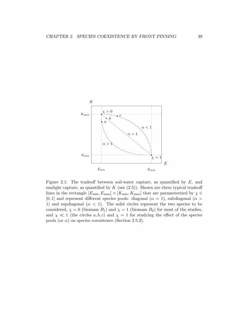
CHAPTER 2. SPECIES COEXISTENCE BY FRONT PINNING 39
α < 1
α > 1
α = 1
Emin Emax
Kmin
Kmaxχ = 0
χ = 1
c
ab
E
K
Figure 2.1: The tradeoff between soil-water capture, as quantified by E, andsunlight capture, as quantified by K (see (2.5)). Shown are three typical tradeofflines in the rectangle [Emin, Emax]× [Kmin,Kmax] that are parameterized by χ ∈[0, 1] and represent different species pools: diagonal (α = 1), subdiagonal (α >1) and supdiagonal (α < 1). The solid circles represent the two species to beconsidered, χ = 0 (biomass B1) and χ = 1 (biomass B2) for most of the studies,and χ 1 (the circles a, b, c) and χ = 1 for studying the effect of the speciespools (or α) on species coexistence (Section 2.5.2).
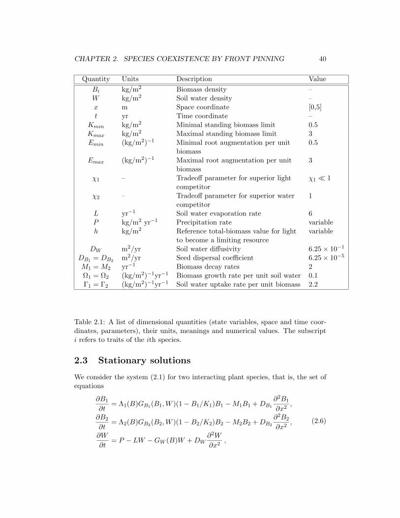
CHAPTER 2. SPECIES COEXISTENCE BY FRONT PINNING 40
Quantity Units Description Value
Bi kg/m2 Biomass density –W kg/m2 Soil water density –x m Space coordinate [0,5]t yr Time coordinate –
Kmin kg/m2 Minimal standing biomass limit 0.5Kmax kg/m2 Maximal standing biomass limit 3Emin (kg/m2)−1 Minimal root augmentation per unit 0.5
biomassEmax (kg/m2)−1 Maximal root augmentation per unit 3
biomassχ1 – Tradeoff parameter for superior light χ1 1
competitorχ2 – Tradeoff parameter for superior water 1
competitorL yr−1 Soil water evaporation rate 6P kg/m2 yr−1 Precipitation rate variableh kg/m2 Reference total-biomass value for light variable
to become a limiting resourceDW m2/yr Soil water diffusivity 6.25× 10⁻¹
DB1 = DB2 m2/yr Seed dispersal coefficient 6.25× 10⁻⁵
M1 = M2 yr−1 Biomass decay rates 2Ω1 = Ω2 (kg/m2)−1yr−1 Biomass growth rate per unit soil water 0.1Γ1 = Γ2 (kg/m2)−1yr−1 Soil water uptake rate per unit biomass 2.2
Table 2.1: A list of dimensional quantities (state variables, space and time coor-dinates, parameters), their units, meanings and numerical values. The subscripti refers to traits of the ith species.
2.3 Stationary solutions
We consider the system (2.1) for two interacting plant species, that is, the set ofequations
∂B1
∂t= Λ1(B)GB1(B1,W )(1−B1/K1)B1 −M1B1 +DB1
∂2B1
∂x2,
∂B2
∂t= Λ2(B)GB2(B2,W )(1−B2/K2)B2 −M2B2 +DB2
∂2B2
∂x2,
∂W
∂t= P − LW −GW (B)W +DW
∂2W
∂x2,
(2.6)
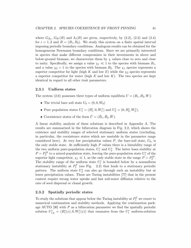
CHAPTER 2. SPECIES COEXISTENCE BY FRONT PINNING 41
where GBi , GW (B) and Λi(B) are given, respectively, by (2.2), (2.3) and (2.4)for i = 1, 2 and B = (B1, B2). We study this system on a finite spatial intervalimposing periodic boundary conditions. Analogous results can be obtained for thehomogeneous Newmann boundary conditions. Since we are primarily interestedin species that make different compromises in their investments in above andbelow-ground biomass, we characterize them by χ values close to zero and closeto unity. Specifically, we assign a value χ1 1 to the species with biomass B1,and a value χ2 = 1 to the species with biomass B2. The χ1 species represents asuperior competitor for light (high K and low E) while the χ2 species representsa superior competitor for water (high E and low K). The two species are keptidentical in regard to all other trait parameters.
2.3.1 Uniform states
The system (2.6) possesses three types of uniform equilibria U = (B1, B2,W ):
• The trivial bare soil state U0 = (0, 0,W0)
• Pure population states U∗1 = (B∗1 , 0,W∗1 ) and U∗2 = (0, B∗2 ,W
∗2 ),
• Coexistence states of the form U = (B1, B2, W ).
A linear stability analysis of these solutions is described in Appendix A. Theresults are summarized in the bifurcation diagram in Fig. 2.2, which shows theexistence and stability ranges of selected stationary uniform states (excluding,in particular, the coexistence states which are unstable in the parameter rangeconsidered here). At very low precipitation values P , the bare-soil state, U0, isthe only stable state. At sufficiently high P values there is a bistability range ofthe two uniform pure-population states, U∗1 and U∗2 . The latter loses stability atP = PM2 to a mixed-population state, leaving the pure-population state U∗1 of thesuperior light competitor, χ1 1, as the only stable state in the range P > PM2 .The stability range of the uniform state U∗1 is bounded below by a nonuniformstationary instability at P T1 (see Fig. 2.2) that leads to a stationary periodicpattern. The uniform state U∗2 can also go through such an instability but atlower precipitation values. These are Turing instabilities [77] that in the presentcontext require strong water uptake and fast soil-water diffusion relative to therate of seed dispersal or clonal growth.
2.3.2 Spatially periodic states
To study the solutions that appear below the Turing instability at P T1 we resort tonumerical continuation and stability methods. Applying the continuation pack-age AUTO [30] with P as a bifurcation parameter we find the spatially periodicsolution U∗1,p = (B∗1(x), 0,W ∗1 (x)) that emanates from the U∗1 uniform-solution
CHAPTER 2. SPECIES COEXISTENCE BY FRONT PINNING 42
U∗2
U∗1
U0
U∗1,p
110 P0 PT1
130 PM2
1500
0.1
0.2
0.3
0.4
0.5
0.6
P
Maxim
um
biomass
0
0.2
0.4
B1
A periodic state U∗1,p = (B1(x), 0,W (x))
0 0.2 0.4 0.6 0.8 1
19.3
19.4
x
W
Figure 2.2: Bifurcation diagram (top) showing biomass-precipitation solutionbranches for the bare-soil state, U0, the two pure-population uniform states, U∗1and U∗2 , and for the pure-population periodic-pattern state, U∗1,p, for which themaximum biomass is plotted. Solid (dashed) lines denote stable (unstable) states.The two uniform states bifurcate from the bare-soil state at P = P0. The periodic-pattern state bifurcates from the corresponding uniform state at P = P T1 andreconnects to it at a lower precipitation value. The spatial dependence of thebiomass B1(x) and soil-water W (x) associated with the periodic-pattern stateU∗1,p = (B1(x), 0,W (x)) are shown at the bottom part of the figure. Note theexistence of a bistability precipitation range of the uniform U∗2 solution and of theperiodic U∗1,p solution. Parameters are as in Table 1 with χ1 = 0. Note that thespatial domain is scaled down by a factor 5.
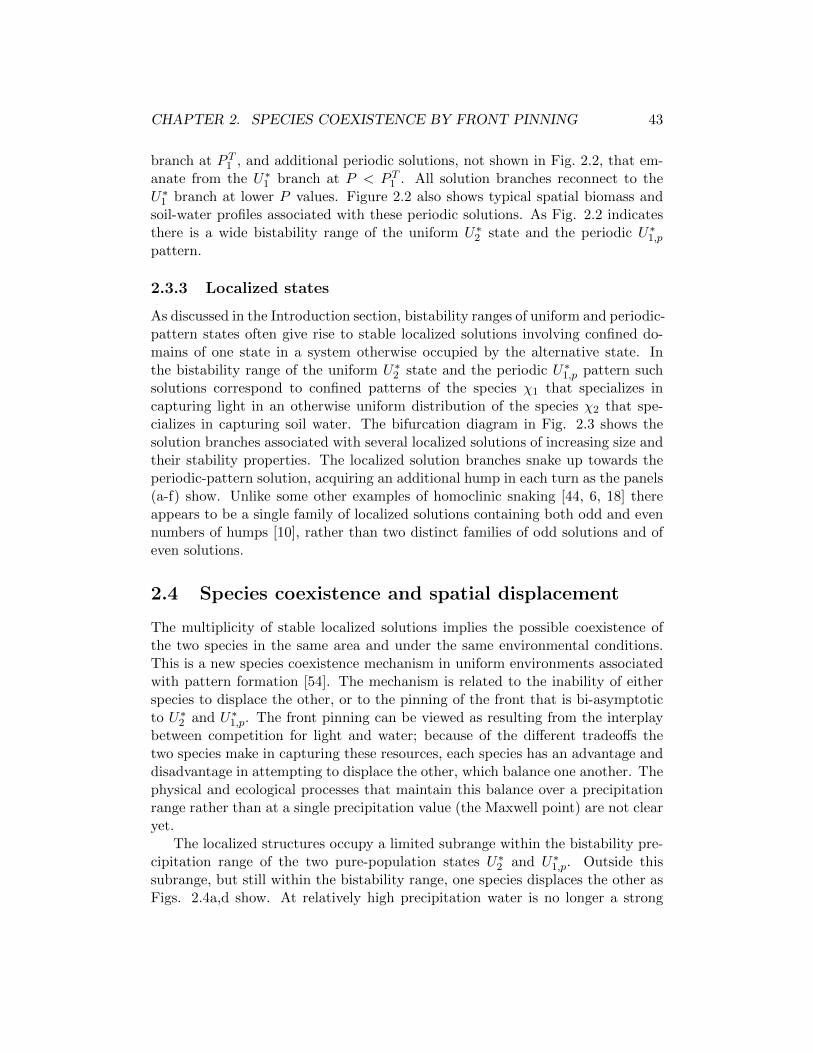
CHAPTER 2. SPECIES COEXISTENCE BY FRONT PINNING 43
branch at P T1 , and additional periodic solutions, not shown in Fig. 2.2, that em-anate from the U∗1 branch at P < P T1 . All solution branches reconnect to theU∗1 branch at lower P values. Figure 2.2 also shows typical spatial biomass andsoil-water profiles associated with these periodic solutions. As Fig. 2.2 indicatesthere is a wide bistability range of the uniform U∗2 state and the periodic U∗1,ppattern.
2.3.3 Localized states
As discussed in the Introduction section, bistability ranges of uniform and periodic-pattern states often give rise to stable localized solutions involving confined do-mains of one state in a system otherwise occupied by the alternative state. Inthe bistability range of the uniform U∗2 state and the periodic U∗1,p pattern suchsolutions correspond to confined patterns of the species χ1 that specializes incapturing light in an otherwise uniform distribution of the species χ2 that spe-cializes in capturing soil water. The bifurcation diagram in Fig. 2.3 shows thesolution branches associated with several localized solutions of increasing size andtheir stability properties. The localized solution branches snake up towards theperiodic-pattern solution, acquiring an additional hump in each turn as the panels(a-f) show. Unlike some other examples of homoclinic snaking [44, 6, 18] thereappears to be a single family of localized solutions containing both odd and evennumbers of humps [10], rather than two distinct families of odd solutions and ofeven solutions.
2.4 Species coexistence and spatial displacement
The multiplicity of stable localized solutions implies the possible coexistence ofthe two species in the same area and under the same environmental conditions.This is a new species coexistence mechanism in uniform environments associatedwith pattern formation [54]. The mechanism is related to the inability of eitherspecies to displace the other, or to the pinning of the front that is bi-asymptoticto U∗2 and U∗1,p. The front pinning can be viewed as resulting from the interplaybetween competition for light and water; because of the different tradeoffs thetwo species make in capturing these resources, each species has an advantage anddisadvantage in attempting to displace the other, which balance one another. Thephysical and ecological processes that maintain this balance over a precipitationrange rather than at a single precipitation value (the Maxwell point) are not clearyet.
The localized structures occupy a limited subrange within the bistability pre-cipitation range of the two pure-population states U∗2 and U∗1,p. Outside thissubrange, but still within the bistability range, one species displaces the other asFigs. 2.4a,d show. At relatively high precipitation water is no longer a strong
CHAPTER 2. SPECIES COEXISTENCE BY FRONT PINNING 44
U∗2
U∗1
U∗1,p
125 130 135 140
0.15
0.2
0.25
0.3
0.35
0.4
P
‖B‖
(a)
(b)
(c)
(d)
(e)
(f)
0
0.2
0.4
0.6(a)
B1,B
2
(b)
0
0.2
0.4
0.6(c)
B1,B
2
(d)
0 0.2 0.4 0.6 0.8 10
0.2
0.4
0.6(e)
x
B1,B
2
0 0.2 0.4 0.6 0.8 1
(f)
x
B1
B2
Figure 2.3: A bifurcation diagram that includes localized solution branches (top).The vertical axis is chosen here to be the L2 norm of the biomass variables definedas ‖B‖ = (
∫B2
1 + B22dx)1/2. The inset shows a blow up of the localized solution
branches labeled in ascending order of localized-solution sizes as the spatial solu-tion forms in panels (a-f) show. The blue and black graphs denote B1 and B2,respectively. Parameters are as in Table 1 except that the spatial domain is scaleddown by a factor 5.
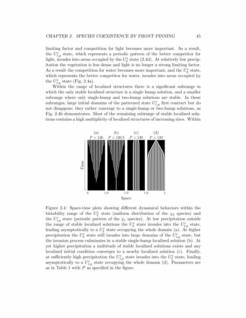
CHAPTER 2. SPECIES COEXISTENCE BY FRONT PINNING 45
limiting factor and competition for light becomes more important. As a result,the U∗1,p state, which represents a periodic pattern of the better competitor forlight, invades into areas occupied by the U∗2 state (2.4d). At relatively low precip-itation the vegetation is less dense and light is no longer a strong limiting factor.As a result the competition for water becomes more important, and the U∗2 state,which represents the better competitor for water, invades into areas occupied bythe U∗1,p state (Fig. 2.4a).
Within the range of localized structures there is a significant subrange inwhich the only stable localized structure is a single hump solution, and a smallersubrange where only single-hump and two-hump solutions are stable. In thesesubranges, large initial domains of the patterned state U∗1,p first contract but donot disappear; they rather converge to a single-hump or two-hump solutions, asFig. 2.4b demonstrates. Most of the remaining subrange of stable localized solu-tions contains a high multiplicity of localized structures of increasing sizes. Within
0 1
(a)P = 126
0 1
(b)P = 126.5
0 1
(c)P = 130
0 1
(d)P = 133
Space
Tim
e
Figure 2.4: Space-time plots showing different dynamical behaviors within thebistability range of the U∗2 state (uniform distribution of the χ2 species) andthe U∗1,p state (periodic pattern of the χ1 species). At low precipitation outsidethe range of stable localized solutions the U∗2 state invades into the U∗1,p state,leading asymptotically to a U∗2 state occupying the whole domain (a). At higherprecipitation the U∗2 state still invades into large domains of the U∗1,p state, butthe invasion process culminates in a stable single-hump localized solution (b). Atyet higher precipitation a multitude of stable localized solutions exists and anylocalized initial condition converges to a nearby localized solution (c). Finally,at sufficiently high precipitation the U∗1,p state invades into the U∗2 state, leadingasymptotically to a U∗1,p state occupying the whole domain (d). Parameters areas in Table 1 with P as specified in the figure.

CHAPTER 2. SPECIES COEXISTENCE BY FRONT PINNING 46
this subrange most initial conditions have “nearby” stable localized solutions towhich they converge on a relative short time scale without noticeable contractionor expansion, as Fig. 2.4c demonstrates.
2.5 Factors controlling species coexistence
The precipitation range of stable localized structures defines the species coex-istence range; domains of periodic distributions of the χ1 species embedded inan otherwise uniform distribution of the χ2 species or vice versa. The size ofthis range naturally depends on model parameters that affect the competition forlight and water. Two parameters of this kind are investigated below, the referencebiomass value h, which controls the intensity of the competition for light, and thespecies pool parameter α.
2.5.1 Competition for light
The strength of the competition for light can be controlled using the parameterh that appears in equation (2.4) for the biomass growth rate Λi(B). Smallervalues of h imply lower biomass growth rate for the shaded species and thus astronger competition effect. Conversely, as h is increased the competition forlight becomes weaker and completely disappears when h → ∞ as Λi approachesa constant value independent of B. Figure 2.5 shows the effect of increasing h onthe species-coexistence range as measured by the existence range of the one-humpsolution. Apart from a small range of low h values, the species-coexistence rangeis found to decrease as h is increased. The reduction in the coexistence rangeoccurs mostly through a shift of its low precipitation edge to higher precipitationvalues. As the competition for light decreases the advantage of χ1 over χ2 weakensand χ2 is able to displace χ1. The balance between the two competitive abilities(capturing light vs. capturing water) that leads to front pinning, is then regainedonly at higher precipitation values.
2.5.2 Species pool
We recall that E and K are the biotic parameters that control the competitiveabilities to capture water and light, respectively. The actual values that theseparameters can take in the rectangle R = [Emin, Emax] × [Kmin,Kmax] are deter-mined by the tradeoff curves obtained for different α values, as Fig. 2.1 illustrates.Each curve is parameterized by χ ∈ [0, 1] and represents a different species pool.
In order to study how does the species pool affect coexistence in 2-speciescommunities we fix the species with biomass density B2 at χ2 = 1 and vary thespecies with biomass density B1 from χ1 = 0 to a small positive value. In otherwords, we reduce the gap between the two species by weakening the ability to
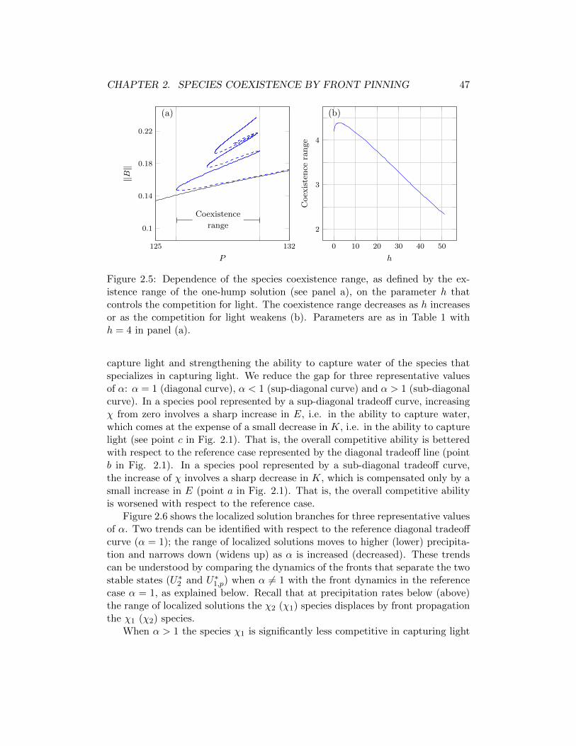
CHAPTER 2. SPECIES COEXISTENCE BY FRONT PINNING 47
125 132
0.1
0.14
0.18
0.22
Coexistence
range
(a)
P
‖B‖
0 10 20 30 40 50
2
3
4
(b)
h
Coexistence
range
Figure 2.5: Dependence of the species coexistence range, as defined by the ex-istence range of the one-hump solution (see panel a), on the parameter h thatcontrols the competition for light. The coexistence range decreases as h increasesor as the competition for light weakens (b). Parameters are as in Table 1 withh = 4 in panel (a).
capture light and strengthening the ability to capture water of the species thatspecializes in capturing light. We reduce the gap for three representative valuesof α: α = 1 (diagonal curve), α < 1 (sup-diagonal curve) and α > 1 (sub-diagonalcurve). In a species pool represented by a sup-diagonal tradeoff curve, increasingχ from zero involves a sharp increase in E, i.e. in the ability to capture water,which comes at the expense of a small decrease in K, i.e. in the ability to capturelight (see point c in Fig. 2.1). That is, the overall competitive ability is betteredwith respect to the reference case represented by the diagonal tradeoff line (pointb in Fig. 2.1). In a species pool represented by a sub-diagonal tradeoff curve,the increase of χ involves a sharp decrease in K, which is compensated only by asmall increase in E (point a in Fig. 2.1). That is, the overall competitive abilityis worsened with respect to the reference case.
Figure 2.6 shows the localized solution branches for three representative valuesof α. Two trends can be identified with respect to the reference diagonal tradeoffcurve (α = 1); the range of localized solutions moves to higher (lower) precipita-tion and narrows down (widens up) as α is increased (decreased). These trendscan be understood by comparing the dynamics of the fronts that separate the twostable states (U∗2 and U∗1,p) when α 6= 1 with the front dynamics in the referencecase α = 1, as explained below. Recall that at precipitation rates below (above)the range of localized solutions the χ2 (χ1) species displaces by front propagationthe χ1 (χ2) species.
When α > 1 the species χ1 is significantly less competitive in capturing light
CHAPTER 2. SPECIES COEXISTENCE BY FRONT PINNING 48
compared to the reference case α = 1 because of its smaller K value. It is alsoless competitive in capturing water because it is significantly less better off inwater capture compared with the reference case (see Fig. 2.1). As a result, thereexists a precipitation range (just below P = 130 in Fig. 2.6) where the species χ1
displaces χ2 when α = 1 but fails to displace χ2 and forms localized structureswhen α > 1. Likewise, there exists a precipitation range (around P = 125) whereχ2 is unable to displace χ1 when α = 1 but succeeds when α > 1. This explainsthe shift of the localized solutions range to higher P as α increases beyond unity.It also explains the narrowing down of the localized solutions range because theadvantage of χ2 over χ1 is stronger at lower P than the converse advantage athigher P and therefore the contraction of the localized solutions range at the lowerP edge is larger than the extension of the range at the upper P edge. Similararguments explain the shift of the localized solutions range to lower P and itswidening as α decreases below unity.
Finally, we note that if we reduce the gap between the two species by fixingχ1 = 0 and decreasing slightly χ2 away from unity along the different trait curves,using again the diagonal (α = 1) as a reference curve, the effect on the localizedsolutions range compared to Fig. 2.6 is qualitatively the same with respect to thewidening of the localized solutions range, while it is the inverse with respect tothe shift of the range.
2.6 Conclusion
We used a spatially explicit mathematical model to study conditions for spatialcoexistence of two plant species that make different tradeoffs in capturing twolimiting resources, soil water and sun light. We focused on a parameter regimethat gives rise to bistability of two pure-population states over a range of pre-cipitation rates: a uniform state of a species that specializes in capturing waterand a patterned state of a species that specializes in capturing light. Within thebistability range we identified a sub-range where localized solutions exist, describ-ing fixed domains of the patterned states in a system otherwise occupied by theuniform state. Stable solutions of this kind imply long-term spatial coexistenceof the two species. We found that the size of the coexistence precipitation rangesize reduces as the competition for light becomes weaker. We further found thatthe size of this range and its position along the precipitation axis vary with theform of the tradeoff curve, which defines the nature of the species pool.
Localized structures in bistability ranges of uniform and patterned states havebeen found in various physical contexts [44], and are likely to occur in ecologicalcontexts too. The context considered in this paper, i.e. a plant community dis-tributed along a tradeoff axis of above-ground vs. below-ground resource-capturecapabilities, may be applicable to herbaceous plant communities in which one or
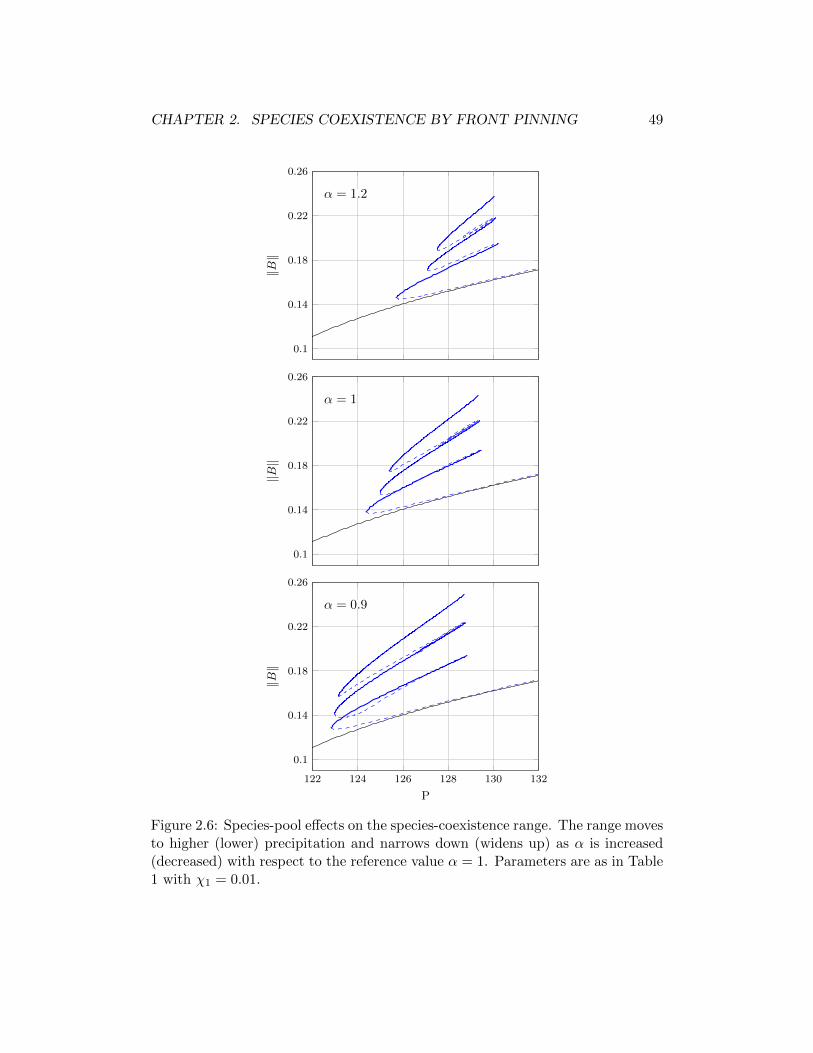
CHAPTER 2. SPECIES COEXISTENCE BY FRONT PINNING 49
0.1
0.14
0.18
0.22
0.26
α = 1
‖B‖
0.1
0.14
0.18
0.22
0.26
α = 1.2
‖B‖
122 124 126 128 130 132
0.1
0.14
0.18
0.22
0.26
α = 0.9
P
‖B‖
Figure 2.6: Species-pool effects on the species-coexistence range. The range movesto higher (lower) precipitation and narrows down (widens up) as α is increased(decreased) with respect to the reference value α = 1. Parameters are as in Table1 with χ1 = 0.01.
CHAPTER 2. SPECIES COEXISTENCE BY FRONT PINNING 50
more species are capable of forming patterns [68, 52]. Woody-herbaceous sys-tems, such as Savanna landscapes [63], provide another possible example. Here,the pattern-forming woody life form constitutes the stable periodic-pattern stateand the herbaceous vegetation forms the alternative stable uniform state - thegrassland [34]. Localized structures consisting of confined domains of the woodypattern in an otherwise uniform grassland then create savanna-like landscapes.A related problem is shrubland-grassland transitions, e.g. the displacement ofblack grama (Bouteloua eriopoda) grassland by creosotebush (Larrea tridentata)shrubland [78]. Here, the displacement process is a front propagation problem,which indicates the possible realization of pinned fronts and localized structuresunder different environmental conditions. In all these examples identifying bista-bility ranges of uniform and patterned population states may shed new light onthe possible dynamical responses of the corresponding plant communities to en-vironmental changes. We note that the assumption of sandy soil, which we usedto simplify the model equations by eliminating overland water flow, applies toseveral examples of pattern-forming herbaceous and woody-herbaceous systems,e.g. herbaceous gap patterns (fairy circles) [14] and savanna landscapes [65] insouthern Africa. We believe, however, that the coexistence mechanism is gen-eral and applies to other soil types in bistability ranges of uniform and patternedvegetation states.
A basic assumption underlying the model equations is translational invariance,that is, the absence of any external heterogeneity, such as non-uniform rainfall.Such heterogeneities can lead to front pinning and species coexistence even inthe case of bistability of uniform states; a non-uniform rainfall that shifts theprecipitation rate from one side of the Maxwell point to another can lead tofront pinning at the spatial location of the Maxwell point. The significance ofthe results reported here is that front pinning and species coexistence can occureven in uniform (translationally invariant) systems. In the current study theprecipitation range of species coexistence is pretty narrow. Further studies areneeded in order to identify biotic and abiotic circumstances that lead to widercoexistence ranges.
2.7 Appendices
2.7.1 Uniform steady states and their stability properties
Uniform steady states
We focus in this appendix on the trivial uniform state, U0 = (0, 0,W0) withW0 = P/L, and on the two pure-population uniform states U∗1 = (B∗1 , 0,W
∗1 )
and U∗2 = (0, B∗2 ,W∗2 ) for B∗1 , B
∗2 > 0. We do not study mixed states of the form
(B1, B2,W ) as they are unstable in the parameter range we consider in this study.
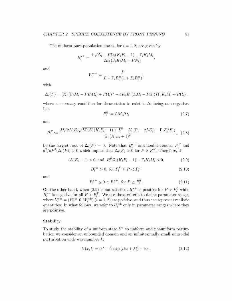
CHAPTER 2. SPECIES COEXISTENCE BY FRONT PINNING 51
The uniform pure-population states, for i = 1, 2, are given by
B∗i± =
±√∆i + PΩi(KiEi − 1)− ΓiKiMi
2Ei (ΓiKiMi + PNi),
and
W ∗i± =
P
L+ ΓiB±i (1 + EiB
±i ),
with
∆i(P ) = (Ki (ΓiMi − PEiΩi) + PΩi)2 − 4KiEi (LMi − PΩi) (ΓiKiMi + PΩi) ,
where a necessary condition for these states to exist is ∆i being non-negative.Let,
P 0i := LMi/Ωi (2.7)
and
PFi :=Mi(2KiEi
√LΓiKi(KiEi + 1) + L2 −Ki (Γi − 2LEi)− ΓiK
2i Ei)
Ωi (KiEi + 1)2 , (2.8)
be the largest root of ∆i(P ) = 0. Note that B∗i± is a double root at PFi and
d2/dP 2(∆i(P )) > 0 which implies that ∆i(P ) > 0 for P > PFi . Therefore, if
(KiEi − 1) > 0 and PFi Ωi(KiEi − 1)− ΓiKiMi > 0, (2.9)
B∗i± > 0, for PFi ≤ P < P 0
i , (2.10)
andB∗i− ≤ 0 < B∗i
+, for P ≥ P 0i . (2.11)
On the other hand, when (2.9) is not satisfied, B∗i+ is positive for P > P 0
i whileB∗i− is negative for all P > PFi . We use these criteria to define parameter ranges
where U∗i± = (B∗i
±, 0,W ∗i±) (i = 1, 2) are positive, and thus can represent realistic
quantities. In what follows, we refer to U∗i± only in parameter ranges where they
are positive.
Stability
To study the stability of a uniform state U∗ to uniform and nonuniform pertur-bation we consider an unbounded domain and an infinitesimally small sinusoidalperturbation with wavenumber k:
U(x, t) = U∗ + U exp (ikx+ λt) + c.c., (2.12)
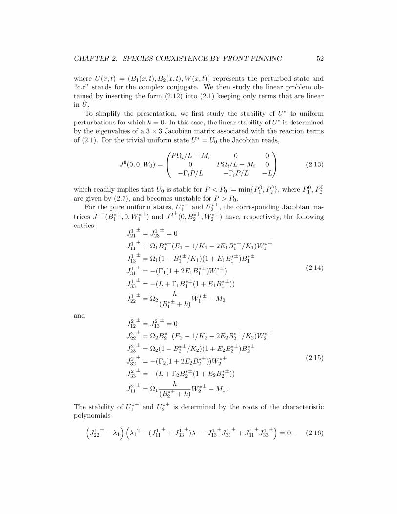
CHAPTER 2. SPECIES COEXISTENCE BY FRONT PINNING 52
where U(x, t) = (B1(x, t), B2(x, t),W (x, t)) represents the perturbed state and“c.c” stands for the complex conjugate. We then study the linear problem ob-tained by inserting the form (2.12) into (2.1) keeping only terms that are linearin U .
To simplify the presentation, we first study the stability of U∗ to uniformperturbations for which k = 0. In this case, the linear stability of U∗ is determinedby the eigenvalues of a 3× 3 Jacobian matrix associated with the reaction termsof (2.1). For the trivial uniform state U∗ = U0 the Jacobian reads,
J0(0, 0,W0) =
PΩi/L−Mi 0 00 PΩi/L−Mi 0
−ΓiP/L −ΓiP/L −L
(2.13)
which readily implies that U0 is stable for P < P0 := minP 01 , P
02 , where P 0
1 , P 02
are given by (2.7), and becomes unstable for P > P0.For the pure uniform states, U∗1
± and U∗2±, the corresponding Jacobian ma-
trices J1±(B∗1±, 0,W ∗1
±) and J2±(0, B∗2±,W ∗2
±) have, respectively, the followingentries:
J121±
= J123±
= 0
J111±
= Ω1B∗1±(E1 − 1/K1 − 2E1B
∗1±/K1)W ∗1
±
J113±
= Ω1(1−B∗1±/K1)(1 + E1B∗1±)B∗1
±
J131±
= −(Γ1(1 + 2E1B∗1±)W ∗1
±)
J133±
= −(L+ Γ1B∗1±(1 + E1B
∗1±))
J122±
= Ω2h
(B∗1± + h)
W ∗1± −M2
(2.14)
andJ2
12±
= J213±
= 0
J222±
= Ω2B∗2±(E2 − 1/K2 − 2E2B
∗2±/K2)W ∗2
±
J223±
= Ω2(1−B∗2±/K2)(1 + E2B∗2±)B∗2
±
J232±
= −(Γ2(1 + 2E2B∗2±))W ∗2
±
J233±
= −(L+ Γ2B∗2±(1 + E2B
∗2±))
J211±
= Ω1h
(B∗2± + h)
W ∗2± −M1 .
(2.15)
The stability of U∗1± and U∗2
± is determined by the roots of the characteristicpolynomials(
J122± − λ1
)(λ1
2 − (J111±
+ J133±
)λ1 − J113±J1
31±
+ J111±J1
33±)
= 0 , (2.16)
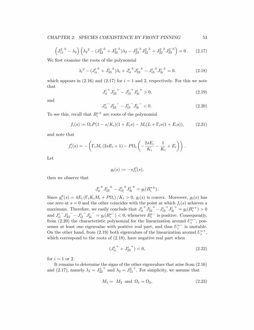
CHAPTER 2. SPECIES COEXISTENCE BY FRONT PINNING 53(J2
11± − λ2
)(λ2
2 − (J222±
+ J233±
)λ2 − J223±J2
32±
+ J222±J2
33±)
= 0 . (2.17)
We first examine the roots of the polynomial
λi2 − (J iii
±+ J i33
±)λi + J iii
±J i33± − J ii3
±J i3i±
= 0. (2.18)
which appears in (2.16) and (2.17) for i = 1 and 2, respectively. For this we notethat
J iii+J i33
+ − J ii3+J i3i
+> 0, (2.19)
andJ iii−J i33− − J ii3
−J i3i−< 0 . (2.20)
To see this, recall that B∗i± are roots of the polynomial
fi(s) := ΩiP (1− s/Ki)(1 + Eis)−Mi(L+ Γis(1 + Eis)), (2.21)
and note that
f ′i(s) = −(
ΓiMi (2sEi + 1)− PΩi
(−2sEi
Ki− 1
Ki+ Ei
)).
Let
gi(s) := −sf ′i(s),then we observe that
J iii±J i33± − J ii3
±J i3i±
= gi(B∗i±) .
Since g′′i (s) = 4Ei (ΓiKiMi + PΩi) /Ki > 0, gi(s) is convex. Moreover, gi(s) hasone zero at s = 0 and the other coincides with the point at which fi(s) achieves a
maximum. Therefore, we easily conclude that J iii+J i33
+−J ii3+J i3i
+= gi(B
∗i
+) > 0
and J iii−J i33−−J ii3
−J i3i−
= gi(B∗i−) < 0, whenever B∗i
− is positive. Consequently,from (2.20) the characteristic polynomial for the linearization around U∗i
−, pos-sesses at least one eigenvalue with positive real part, and thus U∗i
− is unstable.On the other hand, from (2.19) both eigenvalues of the linearization around U∗i
+,which correspond to the roots of (2.18), have negative real part when
(J iii+
+ J i33+
) < 0, (2.22)
for i = 1 or 2.It remains to determine the signs of the other eigenvalues that arise from (2.16)
and (2.17), namely λ1 = J122
+and λ2 = J2
11+
. For simplicity, we assume that
M1 = M2 and Ω1 = Ω2, (2.23)
CHAPTER 2. SPECIES COEXISTENCE BY FRONT PINNING 54
which is compatible with the parameter values considered in Table 1. Then,
λi(B+i ;P ) =
PΩ1h
(B+i + h)(L+ ΓiB
+i (1 + EiB
+i )−M1.
Moreover, the algebraic system
λi(s;P ) = 0, fi(s;P ) = 0, (2.24)
with fi given in (2.21), is solvable for a pair (s, P ). We consider the solution pair(si, P
Mi ) with
s∗i :=(EiKi − 1− Eih+
√(EiKi − 1− hEi)2 − 4Ei(h(1− EiKi)−Ki)
)(2Ei)
−1,
andPMi := M1(s∗i + h)(L+ Γis
∗i (1 + Eis
∗i )(Ω1h)−1 . (2.25)
Then, we have that λi(B+i ) is negative for P < PMi when
EiKi ≥ 1, (2.26)
orEiKi < 1 and h < Ki/(1− EiKi), (2.27)
while it is positive for EiKi < 1, h ≥ Ki/(1−EiKi) and P > P0, or for EiKi ≥ 1and P > PMi .
We conclude that when (2.22), (2.23) along with (2.26) or (2.27) are satisfiedfor i = 1 (respectively i = 2), U∗1
+ (respectively U∗2+) is stable, for all P < PM1
(respectively P < PM2 ). On the other hand, U∗i− is unstable for the range of P
defined in (2.10).We are now in a position to study the stability of the trivial state, U0, and
of the two pure-population states, U∗1± and U∗2
±, to the growth of nonuniformperturbations characterized by nonzero wavenumbers, i.e. k 6= 0 in (2.12). Thedynamics of such perturbation are determined by the eigenvalues of the matrix
Jk = J − k2D ,
whereD = diag(DB1 , DB2 , DW ),
and J is given by (2.13) for U0 and by the expressions in (2.14) and (2.15) for U∗1±
and U∗2±. The eigenvalues of Jk are determined by the roots of the characteristic
polynomial:
det(J − k2D − λI3) = 0, (2.28)
CHAPTER 2. SPECIES COEXISTENCE BY FRONT PINNING 55
where I3 is the 3 × 3 identity matrix. It can be easily checked that for P <P0 = minP 0
1 , P02 the trivial state U0 remains stable for all k, since the diagonal
elements of J0 in (2.13) are negative.For the pure-population state U∗1
+ (respectively U∗2+), we assume that (2.22),
(2.23) along with (2.26) or (2.27) are satisfied and that P < PM1 (respectivelyP < PM2 ), so that the state is stable for k = 0. For the sake of clarity, inwhat follows we drop superscript ′+′ in the notation of the elements (2.14), (2.15)of the Jacobian matrix. Then, the characteristic polynomial (2.28) for the twopure-population states takes the forms
(J1
22 − k2DB2 − λ1
) (λ1
2 − α1(k2)λ1 + β1(k2))
= 0 , (2.29)(J2
11 − k2DB1 − λ2
) (λ2
2 − α2(k2)λ2 + β2(k2))
= 0 , (2.30)
where
αi(k2) = (J iii + J i33)− (DBi +DW )k2 , (2.31)
βi(k2) = DBiDWk
4 − (DBiJi33 +DWJ
iii)k
2 + (J iiiJi33 − J ii3J i3i) . (2.32)
Clearly the single eigenvalues λ1(k2) = J122 − k2DB2 and λ2(k2) = J2
11 − k2DB1
are negative for all k, and the other two eigenvalues are given by
λi±(k2) =
αi(k2)±
√αi(k2)2 − 4βi(k2)
2. (2.33)
Since αi(k2) < 0, the real part of λ−i (k2) remains negative for all k, while λ+
i maybecome positive, only if
βi(k2) < 0, (2.34)
for some k 6= 0. From, (2.19), this immediately implies, that (DBiJi33 + DWJ
iii)
needs to be positive, or
T (δ) = δJ i33 + J iii > 0 , δ := DBi/DW . (2.35)
Therefore, since J i33 < 0, destabilization of S∗i+, requires
J iii = ΩiB∗i
+
(Ei − 1/Ki − 2
EiKiB∗i
+
)W ∗i
+ > 0 . (2.36)
In addition, from (2.22) (J iii+Ji33) < 0 and since T (δ) = (δJ i33+J iii) is a decreasing
function of δ, we also needδ < 1. (2.37)
CHAPTER 2. SPECIES COEXISTENCE BY FRONT PINNING 56
Moreover, (2.32) has a minimum at
ki,c2 =
(DBiJi33 +DWJ
iii)
2DBiDW, (2.38)
and so (2.34) is satisfied for some k 6= 0, when the parameter values Ki, Ei,Mi, L,Ni,Γ, P and the diffusion coefficients DBi , DW are such that the minimum valuegiven by the expression
βi(ki,c2) = 4DBiDW (J iiiJ
i33 − J ii3J i3i)− (DBiJ
i33 +DWJ
iii)
2, (2.39)
is negative. Finally, zeros of the right hand side of (2.39) with respect to P provideus the instability thresholds denoted by P Ti , while the wavenumber ki,c growingat the instability point is given by (2.38).
2.7.2 Numerical stability analysis for nonuniform stationary so-lutions in a finite system
We consider a reaction-diffusion system of the form:
∂tU = DLU + F (U),
where the spatial variable x lies in the interval [0, 1], U = (U1, U2, U3), D =diag (D1, D2, D3) for D1, D2, D3 real positive numbers, L = diag (∂xx, ∂xx, ∂xx)and
F (U) = (f1(U), f2(U), f3(U))
is a differentiable vector field. We consider the system either with periodic bound-ary conditions or homogeneous Neumann boundary conditions.
We divide the spatial interval into the uniform grid xj = j∆x, for j = 0, . . . N ,with ∆x = 1/N , and we let
Uh = (u01, . . . , u
N1 , u
02, . . . , u
N2 , u
03, . . . , u
N3 ),
represent the vector of U evaluated at the grid nodes. Then we use the standardsecond order central difference approximation of the second derivative given by a3 points stencil. This approximation can be represented by a (N + 1)× (N + 1)matrix A. Consequently, we denote by δA = diag(D1A, D2A, D3A) the 3(N +1)× 3(N + 1) matrix approximating DL, and by
Fh(Uh) = (f1(u01), . . . , f1(uN1 ), f2(u0
2), . . . , f2(uN2 ), f3(u03), . . . , f3(uN3 )) .
the vector field evaluated at the node points.We then compute the discrete Jacobian matrix of Fh, denoted by JFh around
an inhomogeneous discretized steady state U(x) ending up with a linear operator
δA+ JFh∣∣Uh.

CHAPTER 2. SPECIES COEXISTENCE BY FRONT PINNING 57
Finally, we compute the spectrum of δA + JFh∣∣Uh
using MATLAB, in order to
determine the linear stability of U(x) for the system U ′h = δAUh + Fh(Uh), withUh(t), Fh in R3(N+1).


Chapter 3
Strong absorption
3.1 Introduction
We study a system which captures the interactions between vegetation and waterin arid and semi-arid areas [37]. The system in non-dimensionalized form reads
∂tb = db∆b+ wG1(b)(1− b)b− b,∂tw = dw∆w − (L(b) +G2(b))w + I(b)hα,
∂th = dh∆hm − I(b)hα + p.
(3.1)
Here, b represents the concentration of the above ground biomass, w the soil watercontent and h the height of a thin surface water layer per unit area. The equationfor the evolution of biomass involves a water dependent growth rate G(b, w), amortality term with constant loss rate and a linear diffusion term modeling growthdue to seeds dispersal or clonal growth. In the equation for the soil water, we havea loss term which consists of the water up-take rate by the plant’s roots denoted byG2(b) and the biomass dependent evaporation rate L(b). Moreover, the equationcontains the source term I(b)hα representing the infiltrated surface water, whichis discussed in more detail below, and a linear diffusion term modeling the soilwater transport. The third equation models the surface water flow and how thisinfiltrates into the ground. The variable h corresponds to the non-dimensionlessquantity H = ρd, where d(t, x) represents the depth in meters of the surface waterwhere x ∈ Ω ⊂ R2 and ρ is the constant density of the fluid. In fact, the thirdequation in dimensional quantities (and m ≥ 2) can be derived by the continuityequation
∂H
∂t+ div (H~u) = P − IH
and the shallow water momentum equation
Du
∂t= −g∇(ζ + d) +
1
ρF,
59
CHAPTER 3. STRONG ABSORPTION 60
where ~u is the horizontal velocity of the fluid, F represents ground surface friction,P stands for the precipitation rate and IH is the infiltration rate of water throughthe soil surface. Moreover, ζ1 denotes the height of the soil surface and g stands forthe acceleration of gravity. We consider a friction term of the form F = −k~u/dl,for l ≥ 0 and k > 0, a biomass and surface water dependent infiltration rate termof the form I(B,H) = IB(B)IH(H) and we let ζ = 0 which corresponds to aregion with flat topography. Then
∂H
∂t− c∆Hm = P − I(B,H)H,
where m = l + 2 and c =g
mkρl. The biomass dependent infiltration rate IB
captures the infiltration contrast between vegetated regions and bare soil due tothe formation of biogenic crusts in unvegetated regions which reduce the infiltra-tion of surface water. Therefore, this term is monotonically increasing with Bapproaching a constant infiltration for high biomass concentrations. The coun-terpart IH of the infiltration rate is chosen to be decreasing function of H takingthe explicit form Hα−1 for α ∈ (0, 1).
This chapter is organized as follows. In Section 2 we make explicit the initialand boundary conditions as well as the expressions of the function for which exis-tence (3.1) is studied. In particular, we consider the system for two distinct casesof boundary conditions: the zero Dirichlet and Neumann boundary conditions.For the first case, we define a regularized approximating system which possessespositive bounded solutions. This allows us to pass to the limit of the approxi-mating problem proving the existence of solutions for the original problem. Forthe second case, we use a different approach, specifically, existence of solutions isgiven by a fixed point argument employing the Arino, Gautier and Penot fixedpoint theorem for sequentially weakly continuous mappings in Banach spaces [3].In Section 3 we examine the behavior of the zeroes set of the surface water com-ponent h in the absence of precipitation for sufficiently long time intervals.
3.2 Existence of solutions
In what follows, we denote by Ω a bounded domain in R2 with regular boundary∂Ω and for T > 0 we let QT = Ω× (0, T ) and ST = ∂Ω× (0, T ). Our purpose isto prove the existence of a solution U = (b, w, h) of the system
∂tb = db∆b+ wG1(b)(1− b)b− b, in QT ,
∂tw = dw∆w − (L(b) +G2(b))w + I(b)hα, in QT ,
∂th = dh∆hm − I(b)hα + p, in QT .
(3.2)
1For non-trivial land topographies ζ(x) is a nonnegative function of the space variable x andit is convenient to set Z = ρζ.

CHAPTER 3. STRONG ABSORPTION 61
together with the initial conditions,
b(x, 0) = b0(x), w(x, 0) = w0(x), h(x, 0) = h0(x) for x ∈ Ω. (3.3)
and some boundary conditions which are either of Dirichlet type
b = w = h = 0, on ∂Ω× (0, T ) (3.4)
or of Neumann type
∂b
∂n=∂w
∂n=∂hm
∂n= 0, on ∂Ω× (0, T ). (3.5)
We shall also assume two classes of conditions on the initial data: either theircontinuity
b0, w0, h0 ∈ C(Ω), (3.6)
or their possible discontinuity
b0, w0, h0 ∈ L∞(Ω), (3.7)
but in any case we shall always assume
0 ≤ b0 ≤ 1, w0 ≥ 0, h0 ≥ 0, on Ω. (3.8)
Concerning the precipitation term, we assume that p ∈ L∞(QT ) is nonnegative.Moreover, we suppose that
I(b) = θb+ r/c
b+ r, (3.9)
L(b) =ν
1 + ρb, (3.10)
G1(b) = ν(1 + ηb)2, (3.11)
G2(b) = γb(1 + ηb)2, (3.12)
where db, dw, dh, η, ρ, r, ν, θ > 0 and c ≥ 1 are given constants. For later use wealso note that for s ∈ [0, 1], I(s), G1(s), G2(s) are nondecreasing functions andL(s) is nonincreasing function, so
I(0) ≤ I(s) ≤ I(1), for s ∈ [0, 1] (3.13)
andL(1) ≤ L(s) +G2(s) ≤ L(0) +G2(1), for s ∈ [0, 1]. (3.14)
In what follows we refer to the Dirichlet problem (3.2), (3.4) and (3.3) asProblem (PD), and to the Neumann problem (3.2), (3.4) and (3.5) as Problem(PN ). To begin with we define the notions of weak solutions of both problems.
CHAPTER 3. STRONG ABSORPTION 62
Definition 2. We call (b, w, h) a weak solution of Problem (PD) on [0, T ], if itsatisfies
1. (b, w, h) ∈ C([0, T ], (L1(Ω))3∩(L∞(QT ))3) and b, w, hm ∈ L∞((0, T );H10 (Ω))
2. for all ψ ∈ C1(QT ) ∩ L2(0, T ;H10 (Ω))∫
Ωb(t)ψ(t) + db
∫ t
0
∫Ω∇b · ∇ψ − bψt dxdτ =
∫Ωb0ψ(0)+
+
∫ t
0
∫ΩG1(b)w(1− b)b− bψ,
(3.15)
∫Ωw(t)ψ(t) + dw
∫ t
0
∫Ω∇w · ∇ψ − wψtdxdτ =
∫Ωw0ψ(0)+
+
∫ t
0
∫Ω− (L(b) +G2(b))w + I(b)hαψ,
(3.16)
∫Ωh(t)ψ(t) + dh
∫ t
0
∫Ω∇hm · ∇ψ − hψtdxdτ =
∫Ωh0ψ(0)+
+
∫ t
0
∫Ωp− I(b)hαψ dxdτ.
(3.17)
Definition 3. We call (b, w, h) a weak solution of Problem (PN ) on [0, T ], if itsatisfies
1. U ∈ C([0, T ], L1(Ω)3) ∩ (L∞(QT ))3) and b, w, hκ ∈ L∞((0, T );H1(Ω))
2. for all ψ ∈ C1(QT ) ∩ L2(0, T ;H1(Ω)) b, w, h satisfies (3.15)–(3.17)
As a matter of fact, in the case of Dirichlet boundary conditions we shall beable to prove, additionally, that the weak solutions are continuous functions ifhypothesis (3.6) holds true. In the case of Neumann boundary conditions thecontinuity will only be obtained with respect to the time variable:
3.2.1 The regularized system to (PD)
The main difficulty for the study of Problem (PD) is the fact that the equation forh is degenerate parabolic. Here, we overcome this difficulty by defining a sequenceof approximating uniformly parabolic problems for which classical solutions exist.Finally, we prove existence of Problem (PD) by passing to the limit thanks tosome a priori estimates.
For ε ∈ (0, 1), κ ≥ 1 and 0 < α < 1, we let
φε(s) := (s+ ε)m − εm,
CHAPTER 3. STRONG ABSORPTION 63
andfε(s) := (s+ ε)α − εα.
We consider the regularized system
∂tbε − db∆bε + bε = G1(bε)wε(1− bε)bε, in QT ,
∂twε − dw∆wε + (L(bε) +G2(bε))wε = I(bε)fε(hε), in QT ,
∂thε − dh∆(φε(hε)) + I(bε)fε(hε) = pε, in QT ,
b = w = h = 0, on ST ,
bε(x, 0) = b0,ε(x), wε(x, 0) = w0,ε(x),
hε(x, 0) = h0,ε(x), for x ∈ Ω,
(3.18)
where pε ∈ C∞ such that0 ≤ pε ≤ ‖p‖L∞(QT ), (3.19)
‖pε − p‖L1(QT ) → 0 as ε→ 0, (3.20)
for T > 0 arbitrary and the initial conditions b0,ε, w0,ε, h0,ε, with
bε(0) = b0,ε, wε(0) = w0,ε, hε(0) = h0,ε ∈ C∞c (Ω),
such that
0 ≤ b0,ε(x) ≤ ‖b0‖L∞(Ω), 0 ≤ w0,ε(x) ≤ ‖w0‖L∞(Ω), 0 ≤ h0,ε(x) ≤ ‖h0‖L∞(Ω)
(3.21)for a.e x ∈ Ω and
(b0,ε, w0,ε, h0,ε)→ (b0, w0, h0) in (L1(Ω))3 as ε→ 0. (3.22)
We also note for later use that (3.19), (3.20) and (3.21), (3.22) imply
pε → p in Lq(QT ) as ε→ 0, (3.23)
and(b0,ε, w0,ε, h0,ε)→ (b0, w0, h0) in (Lq(Ω))3 as ε→ 0, (3.24)
for all q > 1.Under the above considerations the following result holds
Theorem 6. For every ε ∈ (0, 1), problem (3.18) possesses a unique classicalsolution (bε, wε, hε) such that
0 ≤ bε ≤ 1, in QT (3.25)
and there exists a positive constant C such that
0 ≤ wε, hε ≤ C, in QT , (3.26)
where C does not depend on ε.
CHAPTER 3. STRONG ABSORPTION 64
Proof. The existence of classical solution of (3.18) for the non-negative initial data(b0,ε, w0,ε, h0,ε) follows from [45]. Moreover, from the classical maximum principlewe have that for bε,0 ∈ [0, 1], 0 ≤ bε ≤ 1. Similarly, we can show that wε, hε ≥ 0.Next we prove that hε is bounded from above. We first recall the definitionof the negative and positive parts of a function f , namely (f)+ = maxf, 0,(f)− = max−f, 0. We set, h = hε − h, with h an arbitrary positive constantto be determined later. We multiply the equation for hε in (3.18), by h+ andintegrate over Ω to obtain∫
Ω
∂hε∂t
h+ dx− dh∫
Ω∆φε(hε)h+ dx+
∫ΩI(bε)fε(hε)h+ dx =
∫Ωpεh+ dx, (3.27)
which implies that
1
2
d
dt
∫Ω|h+|2 dx+ dh
∫Ωφ′ε(hε)|∇h+|2 dx+
∫ΩI(bε)fε(hε)h+ dx =
∫Ωpεh+ dx.
(3.28)From (3.13), (3.28) and the fact that, φ′ε(hε) > 0, 0 ≤ pε(t, x) ≤ ‖p‖L∞(QT ), wehave that
1
2
d
dt
∫Ω|h+|2 + I(0)
∫Ωfε(hε)h+ ≤ ‖p‖L∞(QT )
∫Ωh+ dx, (3.29)
from which we infer that
1
2
d
dt
∫Ω|h+|2 + I(0)
∫Ω
(fε(hε)− fε(h)
)(hε − h)+
≤ ‖p‖L∞(QT )
∫Ωh+ dx,
(3.30)
which we may write as
1
2
d
dt
∫Ω|h+|2 + I(0)
∫Ω
(fε(hε)− fε(h)
)(hε − h)+
≤(‖p‖L∞(QT ) − I(0)fε(h)
) ∫Ωh+ dx,
(3.31)
Thanks to the monotonicity of φε(·), the second term on the left hand side of theabove inequality is nonnegative. Next, we look for h > ‖h0‖L∞(Ω) such that
‖p‖L∞(QT ) − I(0)fε(h) ≤ 0. (3.32)
Since, −fε(h) ≤ (1− hα), we may choose
h := max
(‖p‖L∞(QT )
I(0)+ 1
)1/α
, ‖h0‖L∞(Ω)
, (3.33)
CHAPTER 3. STRONG ABSORPTION 65
so thatd
dt
∫Ω|h+|2(t) dx ≤ 0, (3.34)
which in turn implies that
|h+(t)|2L2(Ω) ≤ |h+(0)|2L2(Ω) = |(h0 − h)+|2L2(Ω) = 0 , (3.35)
for h given by (3.33), and so,
hε ≤ h in QT . (3.36)
To obtain an upper bound for wε we work similarly. We set w = wε−w, wherew is a positive constant to be determined later, we multiply the equation for wεin (3.18) by w+ and integrate over Ω to obtain that
1
2
d
dt
∫Ω|w+|2 dx+ δw
∫Ω|∇w+|2 dx+
+
∫Ω
(L(bε) +G2(bε))(|w+|2 + ww+) dx =
∫ΩI(bε)fε(hε)w+ dx.
(3.37)
where we have used the equality wε = (wε − w)+ − (wε − w)− + w. Then, from(3.13), (3.36) and the fact that fε(s) ≤ sα for s ≥ 0, we have that∫
ΩI(bε)fε(hε)w+ dx ≤ I(1)hα
∫Ωw+ dx. (3.38)
So, using (3.14) and dropping the appropriate non-negative terms on the left handside of (3.37), we end up with
1
2
d
dt
∫Ω|w+|2 dx+
(wL(1)− I(1)hα
) ∫Ωw+ dx ≤ 0. (3.39)
Therefore, arguing as before we may choose
w := max
I(1)hα
L(1), ‖w0‖L∞(Ω)
,
so thatwε ≤ w, in QT . (3.40)
Next we remark that bε satisfies a problem of the formbεt = db∆bε + Fε in QT
bε = 0 on ST
bε(x, 0) = b0,ε(x) in Ω
(3.41)
CHAPTER 3. STRONG ABSORPTION 66
where0 ≤ b0,ε ≤ ‖b0‖L∞(Ω) ≤ 1
andFε ∈ L∞(QT ). (3.42)
Multiplying the equation by bε and integrating by parts, we deduce that
‖bε‖L2(0,T ;H10 (Ω)) ≤ C, (3.43)
Further taking the duality product < ·, · >(H−1,H10 ) of bεt with an arbitrary test
function from L2(0, T ;H10 (Ω)), we deduce that
‖bεt‖L2(0,T ;H−1(Ω)) ≤ C, (3.44)
Then, the inequalities (3.43) and (3.44) imply that
bε is relative compact in L2(QT ). (3.45)
(cf. [73, Theorem 2.1 p. 27]. We deduce that there exist a function b ∈L2(0, T ;H1
0 (Ω)) with bt ∈ L2(0, T ;H−1(Ω)) and a subsequence bεj of bε suchthat
bεj → b strongly in L2(QT ) (3.46)
bεj t → bt weakly in L2(0, T ;H10 (Ω)) (3.47)
Moreover, it follows from [73, Lemma 1.2 p.260] that
b ∈ C([0, T ];L2(Ω)). (3.48)
Finally, it is clear that 0 ≤ b ≤ 1 for all t ∈ [0, T ] and a.e. x ∈ Ω. Since, wε satisfiesthe equation it follows in a similar way that wε converges along a subsequenceto a limit w strongly in L2(QT ) and weakly in L2(0, T ;H1
0 (Ω)) as ε → 0 wherew ∈ C([0, T ];L2(Ω)) and 0 ≤ w ≤ w for all t ∈ [0, T ] and a.e. x ∈ Ω.
Next we consider the problem for hε, namely∂thε = ∆φε(hε)− I(bε)fε(hε) + pε in QT ,
hε = 0 on ST ,
hε(x, 0) = h0,ε(x) for x ∈ Ω,
(3.49)
We first prove the following estimate
Lemma 1. We have that
1
2
∫Ω
(hε)2(t) dx+
∫ T
0
∫Ω|∇ψε(hε)|2 dx dt ≤ C(T ) (3.50)
CHAPTER 3. STRONG ABSORPTION 67
where ψε(s) =∫ s
0
√φ′ε(s) ds, which in turn implies that∫ T
0
∫Ω|(∇φε(hε(t))|2 ≤ C(T ) (3.51)
Proof. The function hε satisfies the initial value problem
hεt = dh∆φε(hε) +Gε (3.52)
together with zero Dirichlet boundary conditions where we have setGε = −I(bε)fε(hε)+pε, and so ‖Gε‖L∞(QT ) ≤ C. We multiply the equation (3.52) by hε and integrateby parts to deduce that
1
2
d
dt
∫Ω
(hε)2(t) dx+ dh
∫Ω∇φε(hε) · ∇hε dxdt =
∫ΩGεhε dx (3.53)
which implies that∫Ω
(hε)2(t) dx+ 2dh
∫ T
0
∫Ωφ′ε(hε)|∇hε|2 dxdt
≤∫
ΩG2ε dxdt+
∫ T
0
∫Ωh2ε dxdt+
∫Ωh2
0ε dx.
(3.54)
Since∫ T
0
∫Ωφ′ε(hε)|∇hε|2 dxdt =
∫ T
0
∫Ω
(√φ′ε(hε)∇hε)2 =
∫ T
0
∫Ω|∇ψε(hε)|2 dxdt,
(3.55)we deduce that∫
Ω(hε(T ))2 dx+ 2dh
∫ T
0
∫Ω|∇ψε(hε)|2 ≤
∫ T
0
∫ΩG2ε dxdt+
+
∫ T
0
∫Ωh2ε dxdt+
∫Ωh2
0ε dx,
(3.56)
which in turn yields inequality (3.50). To prove (3.51), we observe that∫ T
0
∫Ω|(∇φε(hε(t))|2 =
∫ T
0
∫Ωφ′ε(hε(t))
2|∇hε(t)|2 dxdt
≤ sup |φ′ε(hε(x, t))|∫ T
0
∫Ωφ′ε(hε(t))|∇hε(t)|2 dxdt
≤M∫ T
0
∫Ω
(√φ′ε(hε(t))∇hε(t)
)2,
(3.57)
where M is independent of ε and so (3.51) follows from (3.55) and (3.50).
CHAPTER 3. STRONG ABSORPTION 68
Next we set Uε = φε(hε) and βε(·) = φ−1ε (·), to apply the result of [29, Theorem
6.2].
Lemma 2. (i) For all τ > 0, the function Uε is equicontinuous in QτT . Pre-cisely, there exists a continuous nondecreasing function ωτ (·) with ωτ (0) = 0,such that
|Uε(x1, t1)− Uε(x2, t2)| ≤ ωτ (|x1 − x2|+ |t1 − t2|1/2) (3.58)
for all (xi, ti) ∈ QτT , i = 1, 2. The function ωτ does not depend on ε.
(ii) if in addition U(0, x) = U0(x) ∈ C(Ω), then Uε is equicontinuous on QT .
We deduce from Lemma 2(i) that for all τ > 0, Uεj is precompact in C(QτT )and thus there exists a subsequence that we denote again by Uεj and a functionζ ∈ C(QτT ) such that
Uεj → ζ,
uniformly in QτT as εj → 0. Then,
|hεj − ζ1/m| = |βε(Uεj )− ζ1/m|≤ |βεj (Uεj )− (Uεj )
1/m|+ |(Uεj )1/m − ζ1/m|,(3.59)
Therefore, since for all ε > 0, |βε(Uε) − (Uε)1/m| < 2ε, setting h = ζ1/m we have
thathεj → h, uniformly in QτT ,
φε(hεj )→ hm uniformly in QτT ,(3.60)
as εj → 0, for all τ > 0. Moreover, from Lemma 1 there exists a subsequence ofhεj which we denote again by hεj and a function χ ∈ L2((0, T );H1
0 (Ω)) suchthat
φεj (hεj ) χ weakly in L2(0, T ;H10 (Ω)), (3.61)
as εj → 0. Since, L2(Ω) ⊂ H−1(Ω) we further deduce that φεj (hεj ) χ weaklyin L2(QT ). On other hand, φεj (hεj ) ≤ (hεj )
m ≤ hm and from (3.60) we havethat φεj (hεj )→ hm a.e in QT . Then, by the dominated convergence theorem wededuce that φεj (hεj )→ φ(h) strongly in L2(QT ). Therefore, φ(hεj ) hm weaklyin L2(QT ) and uniqueness of the weak limits implies that χ = hm. Hence, weconclude that
φεj (hεj ) hm weakly in L2(0, T ;H10 (Ω)), (3.62)
as εj → 0.Next we prove that (b, w, h) is a weak solution of Problem (P ). We multiply
the three partial differential equations in (3.18) by ψ ∈ C1(QT )∩L2(0, T ;H10 (Ω))
CHAPTER 3. STRONG ABSORPTION 69
and integrate by parts to obtain (here for simplicity ε = εj)∫Ωbε(t)ψ(t) + db
∫ t
0
∫Ω∇bε · ∇ψ − bεψt dxdτ =
∫Ωb0,εψ(0)+∫ t
0
∫ΩG1(bε)wε(1− bε)bε − bεψ,
(3.63)
∫Ωwε(t)ψ(t) + dw
∫ t
0
∫Ω∇wε · ∇ψ − wεψtdxdτ =
∫Ωw0,εψ(0)+∫ t
0
∫Ω− (L(bε) +G2(bε))wε + I(bε)fε(hε)ψ,
(3.64)
∫Ωhε(t)ψ(t) + dh
∫ t
0
∫Ω∇φε(hε) · ∇ψ − hεψtdxdτ =
∫Ωh0,εψ(0)+∫ t
0
∫Ωpε − I(bε)fε(hε)ψ dxdτ.
(3.65)
To summarize we have that bε,wε, hε are positive and bounded. Moreover, thereexists and a subsequence of (bε, wε, hε), which converges strongly to (b, w, h) in(L2(QT ))3, and a.e in QT , and (bε, wε, φε(hε)) converges weakly to (b, w, φ(h)) in(L2(0, T ;H1
0 ))3. To pass to the limit in the terms involving fε(hε) we notice that
|fε(s)− sα| ≤ 2εα. (3.66)
and thus,
|I(bε)fε(hε)− I(bε)fε(hε)| ≤|I(bε)||(fε(hε)− f(hε)|+ |I(bε)− I(b)||f(hε)|+ |I(b)||f(hε)− f(h)|
≤2I(1)εα + |I(bε)− I(b)||f(h)|+ |I(1)||f(hε)− f(h)| .
(3.67)
Moreover, recalling (3.23) and (3.24), we can let ε→ 0 in (3.63)-(3.65), to obtainthe integral identities (3.15)-(3.17). Finally, if h0 ∈ C(Ω) from Lemma 2(ii)h ∈ C(QT ).
In fact, a weak solution of Problem (PD) exists even if h0 is just essentiallybounded, since working as above we know that there exists h ∈ C((0, T ], (L1(Ω)).We would also like to know is ‖h(t)‖L1(Ω) is continuous at 0. To this end let h0,n bea sequence of smooth bounded functions which converges to h0 in L1(Ω). Workingas above and using Lemma 2(ii) there exists a solution of the system, denoted byhn, obtained as a limit of the approximating system such that hn ∈ C(QT ). Nextnote that
‖h(t)− h0‖L1(Ω) ≤ ‖h(t)− hn(t)‖L1(Ω) + ‖hn(t)− h0,n‖L1(Ω) + ‖h0,n − h0‖L1(Ω)
(3.68)
CHAPTER 3. STRONG ABSORPTION 70
where the second term on the right hand side goes to zero as t tends to 0, whilethe last term becomes arbitrarily small for n large enough. On the other hand,for any ε > 0 and h1(0) and h2(0) smooth initial data, the solutions h1,ε and h2,ε
of the corresponding approximating problems satisfy
‖h1,ε(t)− h2,ε(t)‖L1(Ω) ≤ ‖h1,ε(0)− h2,ε(0)‖L1(Ω) +
∫ t
0‖b1,ε(s)− b2,ε(s)‖L1(Ω) ds
≤ ‖h1,ε(0)− h2,ε(0)‖L1(Ω) + tD.
where D is a positive constant. Letting ε→ 0, this in turn implies that
‖h1(t)− h2(t)‖L1(Ω) ≤ ‖h1(0)− h2(0)‖L1(Ω) + tD (3.69)
Finally, by (3.68) and (3.69)
‖h(t)− h0‖L1(Ω) ≤‖h(0)− hn(0)‖L1(Ω)
+ tD + ‖hn(t)− h0,n‖L1(Ω) + ‖h0,n − h0‖L1(Ω)
(3.70)
thus t 7→ ‖h(t)‖L1(Ω) is continuous at zero and so h ∈ C([0, T ];L1(Ω)). We thushave the following result
Theorem 7. If the initial condition (h0, b0, w0) satisfies (3.7) and (3.8), thenthere exists a weak solution (b, w, h) of Problem (PD) such that 0 ≤ b ≤ 1,0 ≤ w ≤ w and 0 ≤ h ≤ h. If in addition h0, b0, w0 ∈ C(Ω), then h ∈ C(QT ) andb, w ∈ C(Ω× [δ, T ]) for all δ > 0.
Proof. To complete the proof we note that from (3.42) and [45, Theorem 9.1 p.341] it follows that 2
‖bε‖W 2,1q (QδT )
≤ C(δ, T, q,Ω) (3.71)
for all δ ∈ (0, T ) and all q ∈ (1,∞), where QTδ = (δ, T )× Ω. This in turn impliesthat
‖bε‖Cα,α2 (Ω×[δ,T ])≤ C, (3.72)
for α = 2 − N+2q and q 6= N + 2 [11, Lemma 3.5]. Therefore, we can conclude
(passing if necessary to another subsequence) that bεj → b uniformly in QδT forall δ > 0 and so b ∈ C(Ω× [δ, T ]). Similarly, w ∈ C(Ω× [δ, T ]) .
3.2.2 The case of Neumann Boundary conditions (PN)
Although the above strategy can also be adapted to obtain the existence of weaksolutions in the case of the Neumann problem (PN ), in this section, we exploit adifferent approach which is based on a fixed point argument.
2Here, W 2, 1q (QTδ ) = W 1, q(δ, T ;Lq(Ω)) ∩ Lq(δ, T ;W 2, q(Ω) ∩W 1, q
0 (Ω))
CHAPTER 3. STRONG ABSORPTION 71
Theorem 8. There exists a weak solution of Problem PN .
Before, giving the proof of Theorem 8 it is useful to state a lemma related tothe problem
∂tu−∆ϕ(u) = v in QT ,∂ϕ(u)∂n = 0 on ST ,
u(x, 0) = u0(x) for x ∈ Ω.
(3.73)
where ϕ : R→ R is nondecreasing continuous function with ϕ(0) = 0, u0 ∈ L1(Ω)and v ∈ L1(0, T ;L1(Ω)). It is known that system (3.73) possesses a unique weaksolution [7]. For fixed u0, let as denote by uv the unique weak solution of (3.73)for some v ∈ L1(0, T ;L1(Ω)).
Lemma 3. Suppose that ϕ : R → R is strictly increasing continuous functionwith ϕ(0) = 0, then
(i) for each fixed u0 ∈ L1(Ω) and a weakly relatively compact set K in L1(0, T ;L1(Ω)),the set uv : v ∈ K is relatively compact in C([0, T ];L1(Ω)).
(ii) for each fixed u0 ∈ L∞(Ω) and a bounded set K in L∞(0, T ;L∞(Ω)) themapping v 7→ uv, is sequentially continuous from K endowed with the weaktopology of L1(0, T ;L1(Ω)) into C([0, T ];Lp(Ω)) endowed with the strongtopology, for all p ∈ [1,∞).
For the proof of Lemma 3 (i) we refer to the results of Diaz-Vrabie [26, 27]. Itmust be pointed out that although the compactness results of the above referencesconcern the case of Dirichlet boundary conditions, the arguments are identical forthe case of Neumann boundary conditions (see [27, Section 2] and [7]). On theother hand Lemma 3 (ii) is a consequence of the counterpart (i) thanks to theuniqueness of the weak solution (for details see [28, Corollary 1, Section 2] or [28,Corollary 3.1] for the case p = 1).
For convenience in what follows, if u = (u1, u2, u3) is a vector function withui ∈ X, where X is a Banach space, we shall make use of the notation ‖u‖X :=maxi=1,2,3‖ui‖X.
Proof of Theorem 8. Let us start with the existence of a local (in time) weaksolution of (PN ). We introduce the reaction functions R : R3 → R3 given by
R(b, w, h) = (R1(b, w, h), R2(b, w, h), R3(b, w, h))
with R1(b, w, h) = wG1(b)(1− b)b− bR2(b, w, h) = −(L(b) +G2(b))w + I(b)h|h|α−1
R3(b, w, h) = −I(b)h|h|α−1.
(3.74)
CHAPTER 3. STRONG ABSORPTION 72
where I(b) (respectively L(b)) is a truncation of I(b) (respectively L(b)) extendingit continuously by a constant equal to I(0) (respectively L(0)) for b < 0. We chooseK > 0 such that
max(‖b0‖L∞(Ω), ‖w0‖L∞(Ω), ‖h0‖L∞(Ω)) + 1 ≤ K.
Since the functions Ri : R3 → R are continuous it is possible to find M > 0, suchthat
max|R1(b, w, h)| , |R2(b, w, h)| , |R3(b, w, h)|+ ‖p‖L∞(QT ) ≤M
assumed that0 ≤ b, w, h ≤ K.
Now we define the ”solution operator” S : L1(0, T : L1(Ω))3 → C([0, T ];L2(Ω))3
by S(f, g, v) = (b, w, h) where b, w, h are the unique weak solutions of the decou-pled system
∂tb− db∆b = f in QT ,∂tw − dw∆w = g in QT ,∂th− dh∆hm = v in QT ,∂b∂n = ∂w
∂n = ∂h∂n = 0 on ST ,
b(x, 0) = b0(x), w(x, 0) = w0(x), h(x, 0) = h0(x) for x ∈ Ω.
Next to control some a priori estimates it is useful to introduce the followingconvex set (adapted to the reaction terms R(b, w, h)):
Kr,T0 = (f, g, v) : f, g, v ∈ L1(0, T0 : L1(Ω)), ‖(f, g, v)‖L∞(QT0 ) ≤ r,
where QT0 := (0, T0)× Ω, r ≥M and T0 ∈ (0, T ] is such that
S(Kr,T0) ⊂ BL∞(QT0 )(0,K)
with BL∞(QT0 )(0,K) := u ∈ L∞(QT0)3 : ‖u‖L∞(QT0 )) ≤ K. Recall that Mdepends on K through the properties of R. Moreover, it is not difficult to see thatKr,T0 is nonempty and weakly compact in (L1(0, T0 : L1(Ω)))3. Next let us definethe restriction of the solution operator on Kr,T0 :
S = S|Kr,T0 : Kr,T0 → L∞(QT0)3.
We also define the composition of the realization operator associated to R and S,namely, the operator R : Kr,T0 → C([0, T ];L2(Ω))3 defined by
R(f, g, v) = (R1(S(f, g, v)), R2(S(f, g, v)), R3(S(f, g, v)) + p)
CHAPTER 3. STRONG ABSORPTION 73
i.e. R(f, g, v) = R(b, w, h) with (b, w, h) = S(f, g, v). Then, from the choice ofthe set Kr,T0 we know that R maps Kr,T0 into Kr,T0 .
Next we prove that there exists at least one fixed point of R : Kr,T0 → Kr,T0 .This will be a consequence of a variant of the Schauder fixed point theorem givenin [82, Theorem 1.2.11 (Arino, Gautier and Penot)], which requires R to beweakly-weakly sequentially continuous. It is actually enough to show that thegraph of R, is weakly-weakly sequentially closed [82, Corollary 1.2.5]. To thisend, let (fn, gn, vn)n∈N ∈ Kr,T0 and (Fn, Gn, Vn)n∈N ∈ R(fn, gn, vn) be se-quences which converge weakly in (L1((0, T );L1(Ω)))3 to (f, g, v) and (F,G, V ),respectively. Then from Lemma 3 (ii) S is weakly-strongly sequentially contin-uous from L1(0, T0;L1(Ω)) into C([0, T0];Lp(Ω)) and so we may assume withoutloss of generality (taking a subsequence if necessary) that
S(fn, gn, vn)→ S(f, g, v) a.e in QT0 , (3.75)
which, by continuity of Ri, implies that
Ri(S(fn, gn, vn))→ Ri(S(f, g, v)) a.e in QT0 . (3.76)
Moreover, Ri(S(fn, gn, vn)) is a.e bounded in QT0 and therefore by the dom-inated convergence theorem we have that R(fn, gn, vn) → R(f, g, v) stronglyin (L1(QT0))3. Consequently, by uniqueness of weak limits we conclude that(F,G, V ) = R(f, g, v). Therefore, the graph of R is weakly-weakly sequentiallyclosed and so R has at least one fixed point (f, g, v). Since (b, w, h) = S(f, g, v)we conclude that (b, w, h) is a weak solution of the problem (PN ) on the cylinderQT0 := (0, T0)× Ω, i.e. a local (in time) solution of (PN ) on QT0 .
Now it only remains to prove that no possible blow-up of the norm inC([0, T ];L2(Ω))3 may arise to get the continuation of the local weak solution tothe whole cylinder QT . But for the reaction terms R(b, w, h) given by (3.74) andfor positive initial conditions satisfying (3.7), (3.8) this is an easy task: indeed,similar arguments to the ones of the proof of Theorem 1 show that the local weaksolution satisfies that
0 ≤ b ≤ 1, 0 ≤ w ≤ C a.e. in QT0 ,
where C > 0 is independent of T0 and, by well-known estimates for the porousmedium with monotone absorption
0 ≤ h ≤ ‖h0‖L∞(Ω) + T‖p‖L∞(QT ) a.e. in QT0
which is also independent of T0. Therefore, the local weak solution can be ex-tended, by taking T0 as initial time and the values of b, w, h, at t = T0 as new initialdata, to the complete cylinder QT producing at least one global weak solution of(PN ) in view of the fact that b, w, h are nonnegative.
CHAPTER 3. STRONG ABSORPTION 74
Remark. The above type of arguments can be applied to prove the con-vergence of some numerical algorithms that relies in suitable decoupling of thesystem and applying the Diaz-Vrabie 1989 ad hoc compactness argument. Forinstance we can consider the following iterative argument: we solve the uniformlyparabolic equations by prescribing the h-component
∂tbn = db∆bn + wnG1(bn)(1− bn)bn − bn in QT ,
∂twn = dw∆wn − (L(bn) +G2(bn))wn + I(bn)hαn−1 in QT ,(3.77)
together with the initial conditions,
bn(x, 0) = b0(x), wn(x, 0) = w0(x), for x ∈ Ω, (3.78)
and Neumann boundary conditions
∂bn∂n
=∂wn∂n
= 0, on ∂Ω× (0, T ). (3.79)
Then we solve the degenerate equation by prescribing the b-component
(Ph,n) =
∂thn = dh∆hmn − I(bn−1)hαn + p in QT ,∂hn∂n = 0 on ∂Ω× (0, T ),hn(x, 0) = h0(x) for x ∈ Ω.
Obviously the iteration starts with the initial data. The existence of weak so-lutions for the decoupled problems are easy modifications of previous results inthe literature (or they can be obtained by following some ideas of the precedingsection for the treatment of the Dirichlet case). The convergence of the algorithmis a small variant of the proof of Theorem 3.
3.3 Properties of the surface water component
In this section, we focus on the qualitative properties of the surface water com-ponent h investigating the impact of dry periods on the zeroes set of h. Precisely,we assume that precipitation is negligible, if not absent, for sufficiently long time,that is
p(t) = 0 for t ∈ (0, T ), (3.80)
with T large enough. Then, we can show that h vanishes after a finite time for theDirichlet boundary conditions. In addition, for certain range of the parametersand a compacted supported initial condition, h expands its support by forming afree boundary during the dry period.
In what follows, without loss of generality we suppose that δh = 1. We let(b, w, h) be a solution of system (3.2) for a non-negative and bounded initial datum
CHAPTER 3. STRONG ABSORPTION 75
(b0, w0, h0), with 0 ≤ b0 ≤ 1. In order to determine the properties of h it sufficesto study the following scalar equation
∂th−∆hm + I(b(t, x))hα = 0 in QT , (3.81)
which involves the bounded solution component b. We consider (3.81), subject tothe homogeneous Dirichlet boundary conditions
h(t, x) = 0, ∀(t, x) ∈ [0, T )× ∂Ω, (3.82)
and a given non-negative initial datum
h0 = h(0, x), x ∈ Ω. (3.83)
At the end of the section some remarks are given concerning the homogeneousNewmann boundary conditions as well as the non-homogeneous Dirichlet bound-ary conditions.
3.3.1 Extinction in finite time
We recall that 0 ≤ b0 ≤ 1 implies 0 ≤ b ≤ 1, and thus I(0) ≤ I(b(t, x) ≤ I(1).Therefore, if h satisfies (3.81)–(3.83) and U is such that
∂U
∂t−∆Um + I(0)Uα ≥ 0 in Ω
U(t, x) ≥ h(t, x) on (0, T )× Ω
U(0, x) ≥ h(0, x) in Ω
(3.84)
since∂h
∂t−∆hm + I(0)hα ≤ ∂h
∂t−∆hκ + I(b(t, x))hα = 0. (3.85)
by comparison we have that h ≤ U in QT [24]. This simple observation leads tothe following
Theorem 9. Let (3.80) hold true and let (b, w, h) be a solution of problem (3.2)–(3.4) in the time interval (0, T ). Then, if T > 0 is large enough, there existsT ∗ ∈ (0, T ) such that h(t, x) = 0 for all t > T ∗.
Proof. Let U be uniform in space satisfying the non-linear ODE:∂U
∂t+ λUα = 0,
U(0) = ‖h0‖L∞(Ω),(3.86)
for λ > 0. Then, for α < 1, (3.86) possesses the following explicit solution
U(t;λ) = (max0, ‖h0‖1−αL∞(Ω) − λ(1− α)t)1/(1−α) , (3.87)
CHAPTER 3. STRONG ABSORPTION 76
Obviously, U(t; I(0)) = U(t) satisfies (3.84). As a result, letting
T ∗(‖h0‖L∞(Ω), I(0), α) =(‖h0‖L∞(Ω))
(1−α)
I(0)(1− α),
by comparison 0 ≤ h(t) ≤ U(t), h(t) = 0 for all t ≥ T ∗(‖h0‖L∞(Ω), I(0), α).
3.3.2 Estimates for the zeroes set of h
First, let us introduce the following notation. If f is a real-valued function definedon Ω, we denote by supp(f) the support of f in Ω, that is
supp(f) := x ∈ Ω| f(x) 6= 0,
and by N(f) the complement of the support, namely,
N(f) := Ω− supp(f).
Next we estimate the location of the zeros of h in Ω for all t in (0, T ).
Theorem 10. Let σ = α/m < 1 and suppose that h0 ∈ L∞(Ω) is a nonnegativeand compacted supported initial datum. Then N(h(t, x) ⊂ N(h0(x)) for all t ∈
(0, T ). In particular, if we set M = ‖h0‖L∞(Ω), L∗ =
(Mm
K
) 21−σ
and K =(I(0)(1−σ)2
2(2σ+N(1−σ))
) 11−σ
, we have that
N(h(t, x)) ⊂ x ∈ (Ω− supp(h(0, x))) s.t dist(x, supp(h(0, x))) ≥ L∗.
Proof. We look for local sup-solutions which may vanish at points of the zeroset of the initial datum h0. Letting σ = α/κ, we have that for 0 < σ < 1 and
λ > 0, the function V (x) = K(λ)|x − x0|2
1−σ , with K(λ) =(
λ(1−σ)2
2(2σ+N(1−σ))
) 11−σ
satisfies the equation −∆V + λV σ = 0 (see [23]). Now, let x0 ∈ Ω − supp(h0),R := distx0, supp(h0) and Ω := (BR(x0)∩Ω). Then for u(t, x) = (V (x))1/m wehave that
∂tu−∆um + I(0)uσ = 0 in (0, T )× Ω,
u(x) ≥ 0 = h0(x) on Ω,(3.88)
andu ≥ 0 on (0, T )× (∂Ω ∩ Ω). (3.89)
By (3.85), u is a local super solution of (3.81) as long as the inequality h(t, x) ≤u(t, x) is also satisfied for all x in ∂BR(x0) ∩ int (Ω) and t ∈ (0, T ). In fact, since|x− x0| = R on ∂BR(x0), if
R ≥(
Mmh
K(I(0))
) 1−σ2
(3.90)
CHAPTER 3. STRONG ABSORPTION 77
and ‖h‖L∞(0,T ;Ω) ≤ Mh, we have that(K(I(0))R
21−σ)1/κ
≥ Mh which in turn
implies thatu ≥ h, on (0, T )× ∂Ω− ∂Ω. (3.91)
Therefore, when (3.90) holds true, u is a local sup-solution thanks to (3.85),(3.88), (3.89) and (3.91). Finally, ‖h‖L∞(0,t;Ω) ≤ ‖h0‖L∞(Ω), so we may set Mh =‖h0‖L∞(Ω) and since 0 ≤ h(x0) ≤ u(x0) = 0 the result follows.
Remark 5. In the case of homogeneous Neumann boundary conditions, a similarresult is true due to the local nature of the supersolutions. In particular, in theproof above we may take R := distx0, supp(h0)∪ ∂Ω so that the ball BR(x0) forx0 ∈ Ω − supp(h0) is entirely contained in Ω, then if (3.90) is satisfied, (3.85),along with (3.88) and (3.91) ensure that the super-solution is appropriately de-fined.
Remark 6. The same result holds true for the problem with compacted supportedinhomogeneous Dirichlet boundary conditions, i.e when h(t, x) = g(t, x) ≥ 0 on(0, T )× (∂Ω∩ Ω) with g(t, ·) > 0 on a compact subset of ∂Ω. In this case, we maytake R := distx0, supp(h0) ∪ (∪τ>0 supp (g(τ, ·))).
Bibliography
[1] H. Amann. Fixed point equations and nonlinear eigenvalue problems in or-dered Banach spaces. SIAM Review, 18(4):620–709, 1976.
[2] A. Ambrosetti and A. Malchiodi. Nonlinear Analysis and Semilinear EllipticProblems. Cambridge studies in Advanced Mathematics, 2007.
[3] O. Arino, S. Gautier, and J. P. Penot. A fixed point theorem for sequen-tially continuous mappings with application to ordinary differential equa-tions. Funkcial. Ekvac, 27(3):273–279, 1984.
[4] J. B. L. Bard. A model for generating aspects of zebra and other mammaliancoat patterns. Journal of Theoretical Biology, 93(2):363–385, 1981.
[5] M. Baudena and M. Rietkerk. Complexity and coexistence in a simple spatialmodel for arid savanna ecosystems. Theoretical Ecology, 6(2):131–141, 2013.
[6] M. Beck, J. Knobloch, D. Lloyd, B. Sandstede, and T. Wagenknecht. Snakes,ladders, and isolas of localized patterns. SIAM Journal on MathematicalAnalysis, 41(3):936–972, 2009.
[7] P. Benilan. Equations d’evolution dans un espace de Banach quelconque etapplications. PhD thesis, Universite Paris XI, 1972.
[8] J. Blat and K. Brown. Global bifurcation of positive solutions in some systemsof elliptic equations. SIAM Journal on Mathematical Analysis, 17(6):1339–1353, 1986.
[9] F. Borgogno, P. D’Odorico, F. Laio, and L. Ridolfi. Mathematical modelsof vegetation pattern formation in ecohydrology. Reviews of Geophysics,47:RG1005, 2009.
[10] U. Bortolozzo, M. G. Clerc, and S. Residori. Local theory of the slantedhomoclinic snaking bifurcation diagram. Phys. Rev. E, 78:036214, Sep 2008.
78
BIBLIOGRAPHY 79
[11] D. Brochet, D. Hilhorst, and X. Chen. Finite dimensional exponential attrac-tor for the phase field model. Applicable Analysis: An International Journal,49(3-4):197–212, 1993.
[12] K. J. Brown and F. A. Davidson. Global bifurcation in the brusselator sys-tem. Nonlinear Analysis: Theory, Methods & Applications, 24(12):1713–1725, 1995.
[13] F. Cartenı, A. Marasco, G. Bonanomi, S. Mazzoleni, M. Rietkerk, and F. Gi-annino. Negative plant soil feedback explaining ring formation in clonalplants. Journal of theoretical biology, 313:153–161, 2012.
[14] M. D. Cramer and N. N. Barger. PLoS ONE, 8:e70876, 2013.
[15] M. G. Crandall and P. H. Rabinowitz. Bifurcation from simple eigenvalues.Journal of Functional Analysis, 8(2):321–340, 1971.
[16] M. C. Cross and P. C. Hohenberg. Pattern formation outside of equilibrium.Reviews of modern physics, 65(3):851, 1993.
[17] E. Dancer. Global solution branches for positive mappings. Arch. RationalMech. Anal., 52:181–192, 1973.
[18] J. H. P. Dawes. Localized pattern formation with a large-scale mode: Slantedsnaking. SIAM J. Applied Dynamical Systems, 7:186–206, 2008.
[19] V. Deblauwe, N. Barbier, P. Couteron, O. Lejeune, and J. Bogaert. The globalbiogeography of semi-arid periodic vegetation patterns. Global Ecology andBiogeography, 17(6):715–723, Nov. 2008.
[20] V. Deblauwe and J. Bogaert. Modulation des structures de vegetation auto-organisees en milieu aride/self-organized vegetation pattern modulation inarid climates. 2010.
[21] G. T. Dee and W. van Saarloos. Bistable systems with propagating frontsleading to pattern formation. Physical review letters, 60(25):2641–2644, 1988.
[22] J. M. d’Herbes, C. Valentin, D. J. Tongway, and J. C. Leprun. Bandedvegetation patterns and related structures. In Banded vegetation patterningin arid and semiarid environments, pages 1–19. Springer, 2001.
[23] J. I. Dıaz. Nonlinear partial differential equations and free boundaries. Pit-man Advanced Publishing Program, 1985.
[24] J. I. Diaz and F. de Thelin. On a nonlinear parabolic problem arising in somemodels related to turbulent flows. SIAM J. Math. Anal., 25(4):1085–1111,1994.
BIBLIOGRAPHY 80
[25] J. I. Dıaz, J. Hernandez, and L. Tello. On the multiplicity of equilibrium so-lutions to a nonlinear diffusion equation on a manifold arising in climatology.Mathematical Analysis and Applications, 216(AY975691):593–613, 1997.
[26] J. I. Dıaz and I. I. Vrabie. Proprietes de compacite de l’operateur de greengeneralise pour l’equation des milieux poreux. Comptes rendus de l’Academiedes sciences. Serie 1, Mathematique, 309(4):221–223, 1989.
[27] J. I. Dıaz and I. I. Vrabie. Compactness of the green operator of nonlinear dif-fusion equations: application to boussinesq type systems in fluid mechanics.Topol. Methods in Nonlinear Anal, 4:399–416, 1994.
[28] J. I. Dıaz and I. I. Vrabie. Existence for reaction diffusion systems. a compact-ness method approach. Journal of mathematical analysis and applications,188(2):521–540, 1994.
[29] E. DiBenedetto. Continuity of weak solutions to a general porous mediumequation. Indiana University Journal, (32):83–118, 1983.
[30] E. Doedel, R. C. Paffenroth, A. R. Champneys, T. F. Fairgrieve, Y. A.Kuznetsov, B. E. Oldeman, B. Sandstede, and X. Wang. Auto2000. Technicalreport, Concordia University, 2002.
[31] D. J. Eldridge, E. Zaady, and S. M. Infiltration through three contrastingbiological soil crusts in patterned landscapes in the negev, israel. J Stat Phys,148:723–739, 2012.
[32] C. B. Field, V. Barros, T. F. Stocker, D. Qin, D. J. Dokken, L. L. Ebi, M. D.Mastrandrea, K. J. Mach, G.-K. Plattner, S. K. Allen, M. Tignor, and P. M.Midgley. Managing the risks of extreme events and disasters to advance cli-mate change adaptation: A special report of the intergovernmental panel onclimate change. Technical report, Cambridge University Press, Cambridge,UK, and New York, NY, USA, 2013.
[33] A. Gierer and H. Meinhardt. A theory of biological pattern formation. Ky-bernetik, 12(1):30–39, 1972.
[34] E. Gilad, M. Shachak, and E. Meron. Dynamics and spatial organization ofplant communities in water-limited systems. Theoretical Population Biology,72:214–230, 2007.
[35] E. Gilad, J. von Hardenberg, A. Provenzale, M. Shachak, and E. Meron.Ecosystem engineers: from pattern formation to habitat creation. PhysicalReview Letters, 93(9):098105–098105, 2004.
BIBLIOGRAPHY 81
[36] E. Gilad, J. von Hardenberg, A. Provenzale, M. Shachak, and E. Meron. Amathematical model of plants as ecosystem engineers. Journal of TheoreticalBiology, 244:680–691, 2007.
[37] E. Gilad, J. von Hardenberg, A. Provenzale, M. Shachak, and E. Meron. Amathematical model of plants as ecosystem engineers. Journal of TheoreticalBiology, 244:680–691, 2007.
[38] P. Gray and S. K. Scott. Autocatalytic reactions in the isothermal, continu-ous stirred tank reactor: Isolas and other forms of multistability. ChemicalEngineering Science, 38(1):29 – 43, 1983.
[39] C. Holzapfel, K. Tielborger, H. Parag, J. Kigel, and M. Sternberg. Annualplant-shrub interactions along an aridity gradient. Basic and Applied Ecology,7:268–279, 2006.
[40] C. Jones, J. Lawton, and M. Shachak. Organisms as ecosystem engineers.Oikos, 69:373–386, 1994.
[41] C. Jones, J. Lawton, and M. Shachak. Positive and negative efects of organ-isms as ecosystem engineers. Ecology, 78:1946–1957, 1997.
[42] S. Kefi, M. Rietkerk, C. L. Alados, Y. Pueyo, V. P. Papanastasis, A. Elaich,and P. C. de Ruiter. Spatial vegetation patterns and imminent desertificationin Mediterranean arid ecosystems. Nature, 449(7159):213–7, Sept. 2007.
[43] C. A. Klausmeier. Regular and irregular patterns in semiarid vegetation.Science, 284(5421):1826–1828, 1999.
[44] E. Knobloch. Spatially localized structures in dissipative systems: open prob-lems. Nonlinearity, 21(4):T45, 2008.
[45] O. A. Ladyzhenskaya, V. A. Solonnikov, and N. N. Uraltseva. Linear andquasilinear equations of parabolic type, volume 23 of Translations of Mathe-matical Monographs. American Mathematical Society, Providence, R.I., 1967.
[46] R. Lefever and O. Lejeune. On the origin of tiger bush. Bulletin of Mathe-matical Biology, 59:263–294, 1997.
[47] O. Lejeune, M. Tlidi, and P. Couteron. Localized vegetation patches: Aself-organized response to resource scarcity. Physical Review E, 66(1):10901,2002.
[48] T. Ma and S. Wang. Bifurcation theory and applications, volume 53. WorldScientific, 2005.
BIBLIOGRAPHY 82
[49] F. Maestre, F. Valladares, and J. Reynolds. Is the change of plant-plantinteractions with abiotic stress predictable? a meta-analysis of field resultsin arid environments. J. Ecol., 93:748–757, 2005.
[50] E. Meron. Modeling dryland landscapes. Math. Model. Nat. Phenom., 6:163–187, 2011.
[51] E. Meron. Pattern-formation approach to modelling spatially extendedecosystems. Ecological Modelling, 234:70–82, 2012.
[52] E. Meron, H. Yizhaq, and E. Gilad. Localized structures in dryland vegeta-tion: Forms and functions. Chaos, 17(037109), 2007.
[53] J. D. Murray. Mathematical Biology II: Spatial Models and Biomedical Appli-cations, volume 18 of Interdisciplinary Applied Mathematics. Springer NewYork, 2003.
[54] J. Nathan, J. von Hardenberg, and E. Meron. Spatial instabilities untie theexclusion-principle constraint on species coexistence. Journal of TheoreticalBiology, 335:198 – 204, 2013.
[55] L. A. Peletier and W. C. Troy. Spatial patterns described by the extendedfisher–kolmogorov equation: Periodic solutions. SIAM Journal on Mathe-matical Analysis, 28(6):1317–1353, 1997.
[56] L. Pismen. Patterns and Interfaces in Dissipative Dynamics. Springer Seriesin Synergetics. Springer, 2006.
[57] Y. Pomeau. Front motion, metastability and subcritical bifurcations in hy-drodynamics. Physica D, 23:3–11, 1986.
[58] F. I. Pugnaire and M. T. Luque. Changes in plant interactions along agradient of environmental stress. Oikos, 93:42–49, 2001.
[59] P. H. Rabinowitz. Some global results for nonlinear eigenvalue problems.Journal of functional analysis, 7(3):487–513, 1971.
[60] M. Rietkerk, M. C. Boerlijst, F. van Langevelde, R. HilleRisLambers,J. van de Koppel, L. Kumar, H. H. T. Prins, and A. M. D. Roos. Self-organization of vegetation in arid ecosystems. American Naturalist, 160:524–530, 2002.
[61] M. Rietkerk, S. C. Dekker, P. C. de Ruiter, and J. van de Koppel.Self-organized patchiness and catastrophic shifts in ecosystems. Science,305:1926–1929, 2004.
BIBLIOGRAPHY 83
[62] M. Rietkerk and J. van de Koppel. Regular pattern formation in real ecosys-tems. Trends in Ecology and evolution, 23(3):169–175, 2008.
[63] M. Sankaran, J. Ratnam, and N. P. Hanan. Tree–grass coexistence in savan-nas revisited – insights from an examination of assumptions and mechanismsinvoked in existing models. Ecology Letters, 7(6):480–490, 2004.
[64] M. Scheffer, S. R. Carpenter, J. A. Foley, C. Folke, and B. Walker. Catas-trophic shifts in ecosystems. Nature, 413:591–596, 2001.
[65] R. Scholes, P. Dowty, K. Caylor, D. Parsons, P. Frost, and H. Shugart. Trendsin savanna structure and composition along an aridity gradient in the kala-hari. Journal of Vegetation Science, 13:419–428, 2002.
[66] M. Shachak, J. R. Gosz, A. Perevolotsky, and S. T. A. Pickett. Biodiversityin Drylands: Towards a Unified Framework. Oxford University Press, 2005.
[67] E. Sheffer, J. von Hardenberg, H. Yizhaq, M. Shachak, and E. Meron.Emerged or imposed: a theory on the role of physical templates and self-organisation for vegetation patchiness. Ecology Letters, 16(2):127–139, 2013.
[68] E. Sheffer, H. Yizhaq, E. Gilad, M. Shachak, and E. Meron. Why do plantsin resource deprived environments form rings? Ecological Complexity, 4:192–200, 2007.
[69] E. Sheffer, H. Yizhaq, M. Shachak, and E. Meron. Mechanisms of vegetation-ring formation in water-limited systems. Journal of Theoretical Biology,273(1):138–146, 2011.
[70] J. A. Sherratt and G. J. Lord. Nonlinear dynamics and pattern bifurca-tions in a model for vegetation stripes in semi-arid environments. TheoriticalPopulation Biology, 71:1–11, 2007.
[71] J. Smoller. Shock waves and reaction-diffusion equations. In Research sup-ported by the US Air Force and National Science Foundation. New Yorkand Heidelberg, Springer-Verlag (Grundlehren der Mathematischen Wis-senschaften. Volume 258), 1983, 600 p., volume 258, 1983.
[72] J. Swift and P. C. Hohenberg. Hydrodynamic fluctuations at the convectiveinstability. Phys. Rev. A, 15:319–328, Jan 1977.
[73] R. Temam. Navier–Stokes Equations and Nonlinear Functional Analysis.Society for Industrial and Applied Mathematics, 1995.
[74] D. Tilman. Resource competition and community structure. Monographs inPopulation Biology. Princeton University Press, Princeton, New Jersey, USA,1982.
BIBLIOGRAPHY 84
[75] M. Tlidi, R. Lefever, and A. Vladimirov. On vegetation clustering, localizedbare soil spots and fairy circles. In Dissipative Solitons: From Optics toBiology and Medicine, pages 1–22. Springer, 2008.
[76] D. J. Tongway, C. Valentin, J. Seghieri, and J.-C. Menaut, editors. BandedVegetation Patterning in Arid and Semiarid Environments: Ecological Pro-cesses and Consequences for Management. Ecological Studies 149. Springer,2001.
[77] A. M. Turing. The chemical basis of morphogenesis. Philosophical Transac-tions of the Royal Society of London, series B, 237:37–72, 1952.
[78] L. Turnbull, J. Wainwright, and R. E. Brazier. Changes in hydrology anderosion over a transition from grassland to shrubland. Hydrological Processes,24(4):393–414, 2010.
[79] S. van der Stelt, A. Doelman, G. Hek, and J. D. M. Rademacher. Rise and fallof periodic patterns for a generalized klausmeier–gray–scott model. Journalof nonlinear science, 23(1):39–95, 2013.
[80] J. von Hardenberg, A. Y. Kletter, H. Yizhaq, J. Nathan, and E. Meron.Periodic versus scale-free patterns in dryland vegetation. Proc. Roy. Soc. B,277:1771–1776, 2010.
[81] J. von Hardenberg, E. Meron, M. Shachak, and Y. Zarmi. Diversity of veg-etation patterns and desertification. Physical Review Letters, 87:198101–1,2001.
[82] I. I. Vrabie. Compactness methods for nonlinear evolutions, volume 75. CRCPress, 1995.
[83] L. Wang and M. Y. Li. Diffusion-driven instability in reaction–diffusionsystems. Journal of mathematical analysis and applications, 254(1):138–153,2001.
[84] N. E. West. Structure and functions of microphytic soil crusts in wildlandecosystems of arid to semi-arid regions. Advances in ecological Research,20:179–223, 1990.
[85] E. Zeidler. Nonlinear Functional Analysis and Its Applications, volume II/B.Springer, 1990.
[86] Y. R. Zelnik, S. Kinast, H. Yizhaq, G. Bel, and E. Meron. Regime shiftsin models of dryland vegetation. Philosophical Transactions R. Soc. A,371:20120358, 2013.