Estimating aboveground biomass inAvicennia marina plantation inIndian Sundarbans using high-resolution satellite data

Sudip MannaSubrata NandyAbhra ChandaAnirban AkhandSugata HazraVinay Kumar Dadhwal

Estimating aboveground biomass in Avicennia marinaplantation in Indian Sundarbans using high-resolution

satellite data

Sudip Manna,a,* Subrata Nandy,b Abhra Chanda,a Anirban Akhand,a

Sugata Hazra,a and Vinay Kumar DadhwalcaJadavpur University, School of Oceanographic Studies, 188 Raja S. C. Mullick Road,

Kolkata 700032, West Bengal, IndiabIndian Space Research Organisation, Indian Institute of Remote Sensing, Dehradun 248001,

Uttarakhand, IndiacIndian Space Research Organisation, National Remote Sensing Centre, Balanagar,

Hyderabad 500625, Andhra Pradesh, India

Abstract. Mangroves are active carbon sequesters playing a crucial role in coastal ecosystems.In the present study, aboveground biomass (AGB) was estimated in a 5-year-old Avicenniamarina plantation (approximate area ≈190 ha) of Indian Sundarbans using high-resolution sat-ellite data in order to assess its carbon sequestration potential. The reflectance values of eachband of LISS IV satellite data and the vegetation indices, viz., normalized difference vegetationindex (NDVI), optimized soil adjusted vegetation index (OSAVI), and transformed differencevegetation index (TDVI), derived from the satellite data, were correlated with the AGB. OSAVIshowed the strongest positive linear relationship with the AGB and hence carbon content of thestand. OSAVI was found to predict the AGB to a great extent (r2 ¼ 0.72) as it is known to nullifythe background soil reflectance effect added to vegetation reflectance. The total AGB of theentire plantation was estimated to be 236 metric tons having a carbon stock of 54.9 metrictons, sequestered within a time span of 5 years. Integration of this technique for monitoringand management of young mangrove plantations will give time and cost effective results. ©2014 Society of Photo-Optical Instrumentation Engineers (SPIE) [DOI: 10.1117/1.JRS.8.083638]

Keywords: aboveground biomass; Avicennia marina; normalized difference vegetation index;optimized soil adjusted vegetation index; transformed difference vegetation index; Sundarbans.

Paper 13230 received Jun. 25, 2013; revised manuscript received Jan. 24, 2014; accepted forpublication Apr. 8, 2014; published online May 7, 2014.

1 Introduction

Mangrove ecosystems support the tropical coasts with their immense sturdy and adaptive capa-bilities. It is one of the highest productive ecosystems pertaining to the land–sea boundary.1 Theeffect of gradual change in the hydrologic setting of mangrove’s habitat is reflected in the man-grove stand, which in turn, is sensitive to environmental pressure on the system. These globallythreatened coastal forests2 play an inevitable role in the carbon budget, and their carbon pro-duction rates are equivalent to tropical humid forests.3 Carbon sequestered in plant body is esti-mated by means of measuring biomass of vegetation stands, which in turn, indicates local andregional carbon budget of the vegetation.4 Biomass estimates give a baseline for understandingthe rate of primary productivity and maturity, storage and cycling of carbon in the ecosystem, andstress on the forest stand.5 It is also known to reveal the dynamics of carbon cycle, which helps tounderstand the carbon budget of the system as a whole.6 Plantations are managed to rejuvenatethe sustainability of the natural system, which is under anthropogenic pressure and also to storethe carbon. Apart from that, it also provides bioenergy and biomaterials. Various studies7–9

*Address all correspondence to: Sudip Manna, E-mail: sudipmarine@gamil.com

0091-3286/2014/$25.00 © 2014 SPIE

Journal of Applied Remote Sensing 083638-1 Vol. 8, 2014

reflect the importance of carbon sequestration assessment. Additionally, such studies onmangroves give information about the carbon balance of the coastal zone. Estimation of biomassfor plantations is an efficient monitoring technique, which is needed to assess carbon budget inmangroves. Aboveground biomass (AGB) estimation of mangroves requires a number of param-eters in natural systems, especially in woody plants. In forests, nondestructive estimation of AGBrequires multiple parameters, such as height, diameter at breast height, specific density, andvarious other parameters, which are tough to estimate in natural mangroves. Allometric equa-tions developed for a particular mangrove species in a particular geomorphologic setting do notnecessarily exactly predict AGB for the same species in a different geographical area. Variousallometric equations were developed for the same species in different locations.10 Nevertheless,for a particular species at different locations, such models should be developed specifically.Litterfall along with all the living and dead finer ground components account for total AGB,which makes its estimation complex. Estimation models work well on plantations with uniformspecies patterns and unmixed distribution. However, adequate inventory in the mangrove forestis cumbersome. Only live AGB is estimated here which contributes to spectral responses.

Lately, allometric determination of biomass is the most accepted nondestructive methodwhich is being utilized for estimates of standing biomass.10 Absolute biomass estimates involvefelling of trees in sample plots and weighing them.11 However, satellite remote sensing is aproven tool for mapping land use patterns and estimating vegetation biomass/carbon.12,13

Additionally, remote sensing has proved over two decades to be a quick, synoptic, and timeand cost effective tool for discerning the facts and data about the condition and extent of threat-ened mangrove ecosystems.14 LISS IV data from Indian Remote Sensing (IRS) satellite havebeen used for biomass estimation15 by simulation of optical responses of vegetation to remotesensing data. Plant canopy reflects back the energy received on its surface as a functional recip-rocation of its chlorophyll content, cell structure, and moisture content of leaves.14,16 Theseresponses, after passing through the atmosphere, are recorded digitally by satellites. The atmos-pheric corrections are made to negate the effects of transmission through the atmosphere.Atmospherically corrected satellite imagery had many advantages over raw digital numbers(DNs)17 including an increase in the dynamic range of reflectance, which aided in better depic-tion of ground measurements in comparison to spectral response recorded by satellite sensor.Estimation of biomass using field data does not solely depict the entire scenario, as a few sam-plings cannot predict the complete biomass storage of the large heterogeneously developed veg-etation. From ground samples, after being able to develop strong correlations with satellite data,partial distribution of biomass can be estimated, and the relation can be applied to the entireextent of the study area to develop a synoptic status. Remote sensing has given AGB estimationa new perspective with precise coverage of a large extent and with cost effectiveness. Presently,satellite technology is being applied for studies and management of the mangrove communityas it is often difficult to do field sampling in mangroves. Normalized difference vegetationindex (NDVI) has been used in various studies as a proxy of productivity and biomass.18–21

Various empirical relations for biomass estimates through vegetation indices directly orindirectly have been developed in many studies.22

Few studies were conducted11,23,24 on the biomass from mixed forests of Sundarbanmangroves, but the same on single species plantations was rarely reported from this part ofthe subcontinent. Though ecologically not very significant like natural forests, most of the plan-tations throughout the globe are grown as monocultures.25 Application of satellite data for AGBestimation is done in this province for the first time, which happens to be an ecologically criticaldomain and the geo-morphological settings along with floral and faunal composition of this arearestricts ground sampling to a large extent.

Amongst the several true mangrove species thriving all over the tropics, Avicennia marina,the gray mangrove is one of the most commonly available. Survival of A. marina is controlled bythe existing physico-chemical limits in the zone of tidal influence.26 This mangrove is shadeintolerant and grows over a wide salinity range of 0 to 30 ppt.27

The present study was conducted in a mangrove plantation with an aim to assess the capabil-ity of high-resolution satellite data to estimate AGB and the carbon sequestration potential ofA. marina from juvenile stage through their growth for a period of over 5 years.

Manna et al.: Estimating aboveground biomass in Avicennia marina plantation. . .

Journal of Applied Remote Sensing 083638-2 Vol. 8, 2014

2 Methods

2.1 Study Area

Sundarban was declared a UNESCO world heritage site in the year 1987. It is principally sub-divided into a core zone of 1700 km2, manipulation zone of 2400 km2, restoration zone of230 km2, and a development zone of 5300 km2.28 Even under such conserved status, theseislands have undergone various land use and land cover changes, which are threats to this pro-tective ecosystem. Eventually, many successful attempts have been made for ecological resto-ration, mainly by the planting of mangroves. The present study was carried out in a plantation ofA. marina in the Kalisthan area (Fig. 1) of Henry Island. It is located at the south east extreme ofthe Namkhana block in the Indian part of Sundarban. Most of the landmass lying adjacent to thestudy area has been converted into aquaculture ponds. The climate in this part of the continent isgenerally subdivided into summer monsoon (June to September), postmonsoon (October toJanuary), and premonsoon (February to May) seasons. 70% to 80% of the annual rainfall occursduring the summer monsoon.24 The Kalisthan plantation [Fig. 2(a)] faces the sea without anyobstruction, but due to its geo-morphological setting it does not get regularlyinundated by the prevailing diurnal tides except for spring tides and equinox tides, thus leavingthe soil with hypersaline conditions with a hard substrata.

2.2 Field Sampling Design

In plantations, the entire community can be considered as a population of n numbers and uniformspecies composition with same age, for which “random sampling strategy”29 has been adoptedfor the present study. Extensive and precise samplings were conducted during the month ofJanuary to get cloud free clear sky. In order to correlate field data with satellite data, all theplots were aligned to the north direction. Forty-two plots of area 0.01 ha (10 × 10m2) werelaid randomly across the study area.

Fig. 1 Study area with sampling locations.

Manna et al.: Estimating aboveground biomass in Avicennia marina plantation. . .

Journal of Applied Remote Sensing 083638-3 Vol. 8, 2014

2.3 AGB Sample Collection, Processing, and Estimation

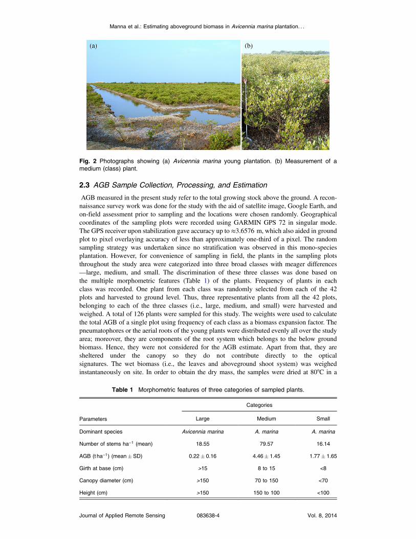
AGB measured in the present study refer to the total growing stock above the ground. A recon-naissance survey work was done for the study with the aid of satellite image, Google Earth, andon-field assessment prior to sampling and the locations were chosen randomly. Geographicalcoordinates of the sampling plots were recorded using GARMIN GPS 72 in singular mode.The GPS receiver upon stabilization gave accuracy up to ≈3.6576 m, which also aided in groundplot to pixel overlaying accuracy of less than approximately one-third of a pixel. The randomsampling strategy was undertaken since no stratification was observed in this mono-speciesplantation. However, for convenience of sampling in field, the plants in the sampling plotsthroughout the study area were categorized into three broad classes with meager differences—large, medium, and small. The discrimination of these three classes was done based onthe multiple morphometric features (Table 1) of the plants. Frequency of plants in eachclass was recorded. One plant from each class was randomly selected from each of the 42plots and harvested to ground level. Thus, three representative plants from all the 42 plots,belonging to each of the three classes (i.e., large, medium, and small) were harvested andweighed. A total of 126 plants were sampled for this study. The weights were used to calculatethe total AGB of a single plot using frequency of each class as a biomass expansion factor. Thepneumatophores or the aerial roots of the young plants were distributed evenly all over the studyarea; moreover, they are components of the root system which belongs to the below groundbiomass. Hence, they were not considered for the AGB estimate. Apart from that, they aresheltered under the canopy so they do not contribute directly to the opticalsignatures. The wet biomass (i.e., the leaves and aboveground shoot system) was weighedinstantaneously on site. In order to obtain the dry mass, the samples were dried at 80°C in a

Fig. 2 Photographs showing (a) Avicennia marina young plantation. (b) Measurement of amedium (class) plant.

Table 1 Morphometric features of three categories of sampled plants.

Parameters

Categories

Large Medium Small

Dominant species Avicennia marina A. marina A. marina

Number of stems ha−1 (mean) 18.55 79.57 16.14

AGB (t ha−1) (mean� SD) 0.22� 0.16 4.46� 1.45 1.77� 1.65

Girth at base (cm) >15 8 to 15 <8

Canopy diameter (cm) >150 70 to 150 <70

Height (cm) >150 150 to 100 <100

Manna et al.: Estimating aboveground biomass in Avicennia marina plantation. . .

Journal of Applied Remote Sensing 083638-4 Vol. 8, 2014

hot air oven until they attained constant weight and then a conversion factor was derived. Theweighing accuracy was maintained to at least 0.1 g. AGB was estimated in tons perhectare both in wet and dry forms using area and weight conversion factors. The sampleswere analyzed for carbon content by CHN analyzer (2400 Series II CHNS/O Analyzer,PerkinElmer, Waltham Massachusetts).

3 Satellite Data and Vegetation Indices

3.1 Preprocessing

GeoRPC IRS-Resourcesat 2 LISS IV data of February 2012 were used for the present study. Theimage is comprised of three spectral bands [Green: 0.52 to 0.59, Red: 0.62 to 0.68, and NearInfrared (NIR): 0.77 to 0.86 μm] with a spatial resolution of 5.8 m. The raw DNs were convertedto radiance using sensor calibration coefficients. Radiance (Li) conversion was done as follows:

Li ¼�Lmax − Lmin

Qcalmax

�Qcal þ Lmin;

where Li is spectral radiance at the sensors’ aperture W∕ðm2 sr μmÞ, Qcal is calibrated DN,Qcalmax is maximum possible DN value and Lmax and Lmin are scaled spectral radiances.

Radiance was then converted to top of atmosphere reflectance (ρ) using ERDAS IMAGINEspatial modeler as

ρ ¼ ΠLid2

E0Cos θ;

where Li is the spectral radiance, d2 is the Earth–sun distance,30 E0 is the exo-atmospheric solarirradiance for LISS IV,31 and θ is the solar zenith angle (90 deg minus the sun elevation angle).Finally, the image was corrected for atmospheric effects using ATCOR module in Geomatica2012. The image was finally geo-referenced from field ground control points (GCP)s usingUniversal Transverse Mercator (UTM) projection and World Geodetic System (WGS) 84datum with root-mean-square error of <0.5 × pixel.

3.2 Vegetation Indices

Vegetation indices are long used as a good proxy for the biomass based on the optical response ofthe plant canopies. Three spectral indices viz., NDVI,32 optimized soil adjusted vegetation index(OSAVI),33 and TDVI,34 were used to assess their correlation to AGB estimates. NDVI has beenused for biomass studies effectively,21,35 with the drawback of saturation at high-biomass con-tent. The study site is a young plantation with less biomass in comparison to mature forests, soNDVI was taken into account to assess the AGB content. It directly gives an estimate of absorp-tion by green canopy in red band and reflection by leaves as a function of their structure, which isa proxy indicator of plant health and biomass in lower ranges.21 However, OSAVI is used as itreduces the effect of background soil noise in the total spectral response of green canopy. Thespectral response of a canopy (if <100%) also includes background soil reflection. Since thecanopy is not very dense in the present study area and partial exposure of dry soil had anadded effect, OSAVI is potent in giving a proxy to biomass as a function of canopy responsenegating soil response. TDVI has been used as it is as sensitive as OSAVI but it does not saturatelike NDVI and OSAVI and provides a linear relation with higher canopy density. In a studyconducted in one of the islands of Indian Sundarbans, TDVI was found to be the best indexin delineation of vegetation cover.36

The mathematical formulations for the indices are as follows:

NDVI ¼ ðρnir − ρredÞ∕ðρnir þ ρredÞ (1)

OSAVI ¼ ðρnir − ρredÞ∕ðρnir þ ρred þ LÞ (2)

Manna et al.: Estimating aboveground biomass in Avicennia marina plantation. . .

Journal of Applied Remote Sensing 083638-5 Vol. 8, 2014

TDVI ¼ 1.5 × ½ðρnir − ρredÞ∕ffiffiffiffiffiffiffiffiffiffiffiffiffiffiffiffiffiffiffiffiffiffiffiffiffiffiffiffiffiffiffiρ2nir þ ρred þ 0.5

q�; (3)

where ρnir ¼ NIR band, ρred ¼ red band, and L ¼ soil adjustment coefficient.

3.3 AGB-Reflectance, AGB-Indices Model from Remote Sensing Data andModel Validation

The AGB values from field inventory plots were correlated with the reflectance from satellitedata and vegetation indices. The pixel size of the image was converted to 10 ×m × 10 ×m tomatch the size of field plots by averaging window. Pearson correlation analysis was conductedbetween field-derived AGB data with the reflectance and vegetation indices to develop a sig-nificant relationship, if any. Out of 42 sample plots, 70% (30 plots) were used for modeling and30% (12 plots) were used for model validation. Thirty ground plot locations were selected ran-domly and corresponding band values from three bands and their indices were extracted. Thesevalues were used to correlate AGB with spectral data, and the resulting relations were usedfurther for predictions. The predictions were validated through the remaining 12 ground datasets. Prior to the modeling, the images were masked-off the bare earthen tracks and pondsby null values for convenience.

4 Results

4.1 Field Observations

Young plants of A. marina were planted in the Kalisthan region to restore and rejuvenate thebarren land facing the sea front having tidal influence, though the inundation of the studyarea is seasonal. Inundation and exposure of intertidal wetlands due to cyclic tidal flux isconsidered favorable for mangrove plants as they bring nutrients, which was not observed inthe study site. Various factors like rainfall (200 to 300 cm), atmospheric humidity (60% to90%), and temperature (19°C to 35°C) favor their growth.37 Furthermore, this deltaic man-grove habitat37 having a high-tidal range, is very dynamic and dominated by fluvial proc-esses,38 but in certain pockets, as the study area, this effect is null due to the geomorphologicsetting. For such regions, the concept of monoculture plantations has been adopted for betterstand management with low biodiversity. Same aged juveniles of the species A. marina weresowed at a time in the plantation but they attained different levels of growth and most of theplants were thickened at the base. Despite being a mono-species plantation, some other man-grove species also flourished as cohorts, namely Excoecaria agallocha and Agialites rotun-difolia. The heterogeneity of the vegetation is introduced in the study area in due course oftime by invasion of other mangrove species from various sources (tidal, biological invasion,and natural succession). In spite of that, the plantation is not much affected by the invasion.The very few numbers of different mangrove plants other than A. marina do not contribute tothe biomass per plot significantly and are considered as a constant bias to total estimate.Overall the AGB in the studied plots ranged from 3 to 20.9 t ha−1 with a mean value of13.9� 3.9 t ha−1. The soil was very dry and hard with salty crusts formed on the surface.Maximum numbers of plants in the sampling plots, in small, medium, and large categorieswere recorded as 59, 124, and 58, respectively.

4.2 Relationship between Biomass, Reflectance, and Vegetation Indices

In this study, AGB was measured in the field for subsequent estimation of carbon sequestrationcapability of a young mangrove plantation. The regression models between field estimated AGBand reflectance (three bands) along with vegetation indices viz., NDVI, TDVI, and OSAVI, areillustrated in Figs. 3(a)–3(f) and tested for their reliability for further AGB prediction based onsatellite remote sensing. We have established an empirical relationship between biomass in sam-pling plots to the reflectance and vegetation indices. While modeling, a sound correlation of

Manna et al.: Estimating aboveground biomass in Avicennia marina plantation. . .

Journal of Applied Remote Sensing 083638-6 Vol. 8, 2014

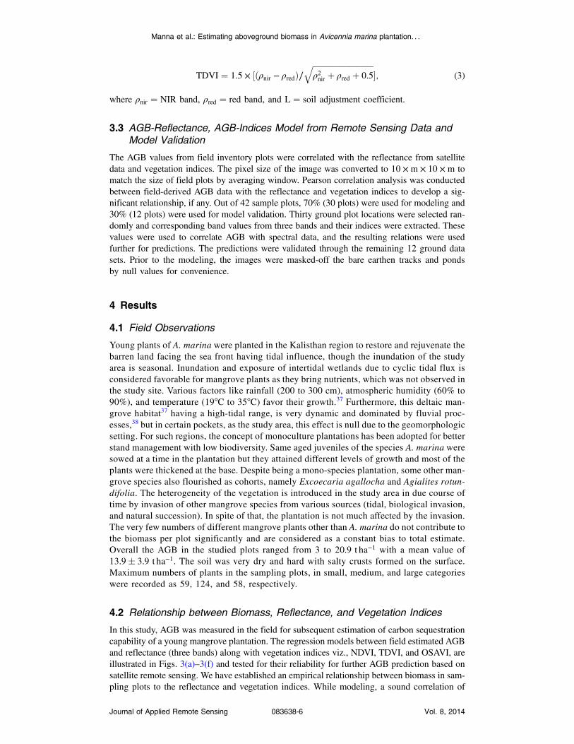
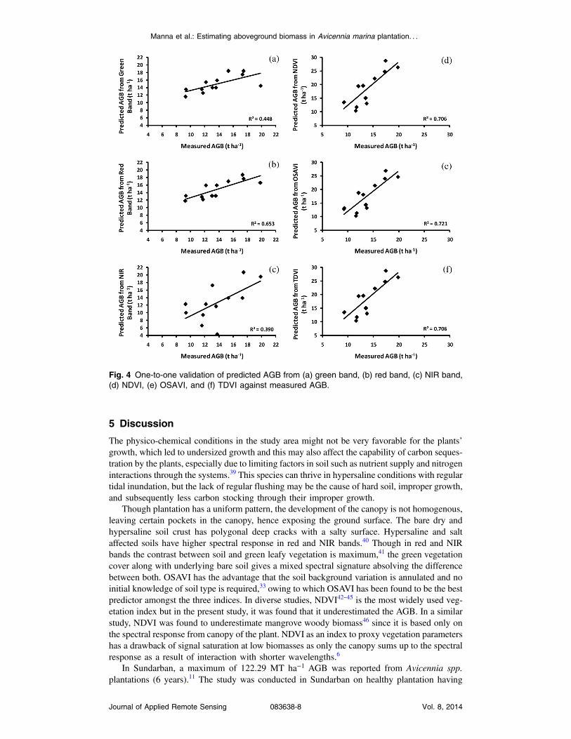
AGB with green and red band reflectance was observed (r2 ¼ 0.609, p < 0.01, and r2 ¼ 0.682,p < 0.01, respectively), but the infra-red band has shown a weak correlation (r2 ¼ 0.327,p < 0.05). Similar relations were observed with NDVI, OSAVI, and TDVI and they haveshown a good correlation (r2 ¼ 0.682, r2 ¼ 0.685, and r2 ¼ 0.683, p < 0.01, respectively).The maximum AGB predicted by NDVI model is 28 t ha−1 (r2 ¼ 0.706, p < 0.01) (Fig. 4).TDVI was used as it ensures that saturation is not reached at high-canopy density34 and a linearrelation is maintained. Results based on TDVI derived AGB showed that it overestimated, andmaximum range of predicted AGB was 38.16 t ha−1. The best predictor index for the AGB wasOSAVI-AGB model, where it showed a maximum AGB limit of 34.85 t ha−1.The maps for predicted AGB from the three indices are illustrated in Figs. 5(a)–5(c).

4.3 Carbon Stock Assessment

From the field estimated AGB, subsequent carbon conversion was done. Using the OSAVI-AGBregression model, a carbon map [Fig. 5(d)] of the study area was prepared. Carbon storage capac-ity of the plants indicated an increasing trend from leaves to branch to stems where stems seques-tered highest (≈56%). In young plants, stem and branches are not very distinct. The AGB for theplants of three categories were 3376.6� 235.7 g, 1198.1� 162.6 g, and 319.8� 82.4 g,respectively. On an average in the study area, a 5-year old A. marina plant can sequester∼49.92% of carbon to its dry biomass. As output of modeled biomass estimates, the studyarea, the plantation, has a total AGB of 236 metric tons through which 54.9 metric tons of carbonis sequestered within a time span of 5 years.

Fig. 3 The scatter diagram along with the linear trend line between aboveground biomass (AGB)and (a) green band, (b) red band, (c) near infrared (NIR) band, (d) normalized difference vegetationindex (NDVI), (e) optimized soil adjusted vegetation index (OSAVI), and (f) transformed differencevegetation index (TDVI).

Manna et al.: Estimating aboveground biomass in Avicennia marina plantation. . .

Journal of Applied Remote Sensing 083638-7 Vol. 8, 2014

5 Discussion

The physico-chemical conditions in the study area might not be very favorable for the plants’growth, which led to undersized growth and this may also affect the capability of carbon seques-tration by the plants, especially due to limiting factors in soil such as nutrient supply and nitrogeninteractions through the systems.39 This species can thrive in hypersaline conditions with regulartidal inundation, but the lack of regular flushing may be the cause of hard soil, improper growth,and subsequently less carbon stocking through their improper growth.

Though plantation has a uniform pattern, the development of the canopy is not homogenous,leaving certain pockets in the canopy, hence exposing the ground surface. The bare dry andhypersaline soil crust has polygonal deep cracks with a salty surface. Hypersaline and saltaffected soils have higher spectral response in red and NIR bands.40 Though in red and NIRbands the contrast between soil and green leafy vegetation is maximum,41 the green vegetationcover along with underlying bare soil gives a mixed spectral signature absolving the differencebetween both. OSAVI has the advantage that the soil background variation is annulated and noinitial knowledge of soil type is required,33 owing to which OSAVI has been found to be the bestpredictor amongst the three indices. In diverse studies, NDVI42–45 is the most widely used veg-etation index but in the present study, it was found that it underestimated the AGB. In a similarstudy, NDVI was found to underestimate mangrove woody biomass46 since it is based only onthe spectral response from canopy of the plant. NDVI as an index to proxy vegetation parametershas a drawback of signal saturation at low biomasses as only the canopy sums up to the spectralresponse as a result of interaction with shorter wavelengths.6

In Sundarban, a maximum of 122.29 MT ha−1 AGB was reported from Avicennia spp.plantations (6 years).11 The study was conducted in Sundarban on healthy plantation having

Fig. 4 One-to-one validation of predicted AGB from (a) green band, (b) red band, (c) NIR band,(d) NDVI, (e) OSAVI, and (f) TDVI against measured AGB.

Manna et al.: Estimating aboveground biomass in Avicennia marina plantation. . .

Journal of Applied Remote Sensing 083638-8 Vol. 8, 2014

ideal growing condition by completely harvesting the trees. In the present study, a maximum of34.85 t ha−1 of AGB was observed, which is far less than the former study and is based on anondestructive method. This difference may be supported with the assertion that the presentplantation does not have all the normal essential growth parameters required37 for mangrovegrowth. The use of high-resolution satellite data for biomass study enabled gross, quick, andefficient estimation where the sampling is less viable. The reflectance in red band predictedthe AGB with 65% accuracy. A significant empirical relation is observed between vegetationindices and AGB where OSAVI-based prediction is 72.1% accurate, whereas NDVI and TDVIpredicted the same with a little less accuracy i.e., 70.2%. In various studies,47–49 spectral datawere used as proxy to biomass estimates in all kind of terrains but, AGB estimation using opticaldata is never done in this conserved site. This study, apart from AGB estimation, also depictedthe carbon sequestration capability of A. marina for a period of 5 years. Despite a juvenilegrowth stage, the plants failed to attain the normal growth with stunted development and thick-ening of base. However, this estimate may serve as a baseline for natural mangrove forests ofSundarban, which is dominated by A. marina in the western fringes. These plants have spatialpreference and under hypersaline conditions their growth retards, which make them stunted.50,51

The results from the present study show that the plantation sequestered carbon with an upperrange of about 6.64 t ha−1 within 5 years, which indicates good potential for plantation conser-vation in this geomorphologic system. Optical remote sensing–based biomass estimates arerestricted to perform better in lower biomass ranges,52 which is significantly projected in ourstudy with a high-confidence level of 72.1%.

Fig. 5 (a) NDVI predicted AGB* map, (b) OSAVI predicted AGB* map, (c) TDVI derived AGB*map, and (d) carbon* map derived from OSAVI-based prediction. (*indicates the unit in t ha−1).

Manna et al.: Estimating aboveground biomass in Avicennia marina plantation. . .

Journal of Applied Remote Sensing 083638-9 Vol. 8, 2014

6 Conclusions

To conclude, the present study on plantation yielded more precise results. Significance of thepresent approach is to assess mangrove patches with moderate biomass values by remote sensing(high-resolution satellite data) as an alternative to extensive field inventory, as spectral signaturesare surface response only and with growth, the canopy density to biomass ratio becomes satu-rated. This type of approach is suitable to a large extent in cases of young mono-species plan-tations. The fact that a small sampling can predict the carbon sequestration in a mangroveplantation with 72% accuracy advocated its use on such site-specific restoration efforts.Monitoring and management of mangrove plantations by the method is timely as it gives asynoptic view without disturbing the ecosystem. However, this approach needs to be refinedin further studies and should be supported by specific assessment of local conditions.

Acknowledgments

Authors are grateful to National Remote Sensing Centre (NRSC), Department of Space,Government of India, for funding the research work. S. Nandy is grateful to the director,Indian Institute of Remote Sensing, Indian Space Research Organisation, for supporting thestudy, and Abhra Chanda is grateful to the Department of Science and Technology,Government of India, for providing the INSPIRE fellowship.

References

1. F. Blasco, P. Saenger, and E. Janodet, “Mangroves as indicators of coastal change,” Catena27(3–4), 67–178 (1996), http://dx.doi.org/10.1016/0341-8162(96)00013-6.

2. S. Bouillon et al., “Mangrove production and carbon sinks: a revision of global budgetestimates,” Global Biogeochem. Cycles 22(2), 1–12 (2008), http://dx.doi.org/10.1029/2007GB003052.

3. D. M. Alongi, “Carbon sequestration in mangrove forests,” Carbon Manage. 3(3), 313–322(2012), http://dx.doi.org/10.4155/cmt.12.20.

4. J. G. Kairo et al., “Structural development and productivity of replanted mangrove planta-tions in Kenya,” For. Ecol. Manage. 255(7), 2670–2677 (2008), http://dx.doi.org/10.1016/j.foreco.2008.01.031.

5. M. L. G. Soares, “Estudo da biomassa ae´rea de manguezais do sudeste do Brasil e ana´ lisede modelos,” Vol. 2. Ph.D. Thesis, Instituto Oceanogra´ fico, Universidade de Sao Paulo,Brazil (1997).

6. T. E. Fatoyinbo and A. H. Armstrong, “Remote characterization of biomass measurements: casestudy of mangrove forests,”M.Momba and F. Bux, Eds., Biomass, Sciyo, Croatia, p. 202 (2010).

7. N. H. Ravindranath and B. S. Somashekhar, “Potential and economics of forestry optionsfor carbon sequestration in India,” Biomass Bioenergy 8(5), 323–342 (1995), http://dx.doi.org/10.1016/0961-9534(95)00025-9.

8. S.Nilsson andW. Schopfhauser, “The carbon-sequestration potential of a global afforestationprogram,” Clim. Change 30(3), 267–293 (1995), http://dx.doi.org/10.1007/BF01091928.

9. D. M. Alongi, “Carbon payments for mangrove conservation: ecosystem constraints anduncertainties of sequestration potential,” Environ. Sci. Policy 14(4), 462–470 (2011),http://dx.doi.org/10.1016/j.envsci.2011.02.004.

10. A. Komiyama, J. E. Ong, and S. Poungparn, “Allometry, biomass, and productivity of man-grove forests: a review,” Aquat. Bot. 89(2), 128–137 (2008), http://dx.doi.org/10.1016/j.aquabot.2007.12.006.

11. P. K. R. Choudhuri, “Biomass production of mangrove plantation in Sunderbans, WestBengal (India)—a case study,” Indian. For. 117(1), 3–12 (1991).

12. A. Chhabra and V. K. Dadhwal, “Assessment of major pools and fluxes of carbon in Indianforests,” Clim. Change 64(3), 341–360 (2004), http://dx.doi.org/10.1023/B:CLIM.0000025740.50082.e7.

Manna et al.: Estimating aboveground biomass in Avicennia marina plantation. . .

Journal of Applied Remote Sensing 083638-10 Vol. 8, 2014

13. M. Kaul, G. M. J. Mohren, and V. K. Dadhwal, “Phytomass carbon pool of trees andforests in India,” Clim. Change 108(1–2), 243–259 (2011), http://dx.doi.org/10.1007/s10584-010-9986-3.

14. C. Kuenzer et al., “Remote sensing of mangrove ecosystems: a review,” Remote Sens. 3(5),878–928 (2011), http://dx.doi.org/10.3390/rs3050878.

15. R. Madugundu, V. Nizalapur, and C. S. Jha, “Estimation of LAI and above-ground biomassin deciduous forests: Western Ghats of Karnataka, India,” Int. J. App. Ear. Obs. Geoinf. 10(2), 211–219 (2008), http://dx.doi.org/10.1016/j.jag.2007.11.004.

16. J. Kamaruzaman and I. Kasawani, “Imaging spectrometry on mangrove species identifica-tion and mapping in Malaysia,” WSEAS Trans. Bio. Biomed. 8(4), 118–126 (2007).

17. A. R. Sharma, K. V. S. Badarinath, and P. S. Roy, “Corrections for atmospheric andadjacency effects on high resolution sensor data—a case study using IRS-P6 LISS-IVdata,” in The Int. Archives Photogramming, Remote Sensing and Spatial InformationSciences, XXXVII Part B8, pp. 497–502, Beijing (2008).

18. P. M. Mather, Computer Processing of Remotely-Sensed Images 2nd ed., John Wiley &Sons, Chichester, England (1999).

19. G. M. Foody et al., “Mapping the biomass of Bornean tropical rain forest from remotelysensed data,” Global Ecol. Biogeogr. 10(4), 379–386 (2001), http://dx.doi.org/10.1046/j.1466-822X.2001.00248.x.

20. X. Li et al., “Chen X regression and analytical models for estimating mangrove wetlandbiomass in South China using Radarsat images,” Int. J. Remote Sens. 28(24),5567–5582 (2007), http://dx.doi.org/10.1080/01431160701227638.

21. H. Santin-Janin et al., “Assessing the performance of NDVI as a proxy for plant biomassusing non-linear models: a case study on the Kerguelen archipelago,” Pol. Biol. 32(6),861–871 (2009), http://dx.doi.org/10.1007/s00300-009-0586-5.

22. C. Kalaitzidis, V. Heinzel, and D. Zianis, “A review of multispectral vegetation indices forbiomass estimation,” in Imagin[e/g] Europe, Proceedings of the 29th Symposium of theEuropean Assoc. Remote. Sens. Lab., Chania, Greece (2009).

23. A. Mitra, K. Sengupta, and K Banerjee, “Standing biomass and carbon storage of above-ground structures in dominant mangrove trees in the Sundarbans,” For. Ecol. Manage. 261(7), 1325–1335 (2011), http://dx.doi.org/10.1016/j.foreco.2011.01.012.

24. R. Ray et al., “Carbon sequestration and annual increase of carbon stock in a mangrove forest,”Atmos. Environ. 45(28), 5016–5024 (2011), http://dx.doi.org/10.1016/j.atmosenv.2011.04.074.

25. FAO, State of the World’s Forests, Rome, Italy (2001).26. P. Clarke and P. J. Myerscough, “The intertidal distribution of the grey mangrove (Avicennia

marina) in southeastern Australia: the effects of physical conditions, interspecific competi-tion, and predation on propagule establishment and survival,” Aus. J. Ecol. 18 (3), 307–315(1993), http://dx.doi.org/10.1111/aec.1993.18.issue-3.

27. A. I. Robertson and D. M. Alongi, “Coastal and Estuarine Studies,” Tropical MangroveEcosystems, A. I. Robertson and D. M. Alongi, Eds., American Geophysical Union,Washington (1992).

28. S. Nandy and S. P. S. Kushwaha, “Study on the utility of IRS 1D LISS-III data andthe classification techniques for mapping of Sunderban mangroves,” J. Coast. Conser.15(1), 123–137 (2011), http://dx.doi.org/10.1007/s11852-010-0126-z.

29. B. Husch, T. W. Beers, and J. A. J. Kershaw, “Sampling Design in Forest Inventories,”Chap. 13 in Forest Mensuration, 4th ed., pp. 299–336, John Wiley and Sons Inc.,Hoboken, New Jersey (2003).

30. G. Chander, B. L. Markham, and D. L. Helder, “Summary of current radiometric calibrationcoefficients for Landsat MSS, TM, ETM+, and EO-1 ALI sensors,” Remote Sens. Environ.113(5), 893–903 (2009), http://dx.doi.org/10.1016/j.rse.2009.01.007.

31. M. R. Pandya et al., “Spectral characteristics of sensors onboard IRS-1D and P6 satellites:estimation and their influence on surface reflectance and NDVI,” J. Indian Soc. RemoteSens. 35(4), 333–350 (2007), http://dx.doi.org/10.1007/BF02990789.

32. C. J. Tucker, “Red and photographic infrared linear combinations for monitoring vegeta-tion,” Remote Sens. Environ. 8(2), 127–150 (1979), http://dx.doi.org/10.1016/0034-4257(79)90013-0.

Manna et al.: Estimating aboveground biomass in Avicennia marina plantation. . .

Journal of Applied Remote Sensing 083638-11 Vol. 8, 2014

33. M. D. Steven, “The sensitivity of the OSAVI vegetation index to observational parameters,”Remote Sens. Environ. 63(1), 49–60 (1998), http://dx.doi.org/10.1016/S0034-4257(97)00114-4.

34. A. Bannari, H. Asalhi, and P. M. Teillet, “Transformed difference vegetation index (TDVI)for vegetation cover mapping,” in IGARSS IEEE Int. Geosci. Remote Sens. Symp., Vol. 5,pp. 3053–3055 (2002).

35. P. S. Roy and S. A. Ravan, “Biomass estimation using satellite remote sensing data—aninvestigation on possible approaches for natural forest,” J. Biosci. 21(4), 535–561 (1996),http://dx.doi.org/10.1007/BF02703218.

36. S. Manna et al., “Vegetation cover change analysis from multi-temporal satellite data inJharkhali Island, Sundarbans, India,” Indian J. Geo-Mar. Sci. 42(3), 331–342 (2013).

37. R. N. Mandal and K. R. Naskar, “Diversity and classification of Indian mangroves: areview,” Trop. Ecol. 49(2), 131–146 (2008).

38. D. Ganguly et al., “Geomorphological study of Sundarban deltaic estuary,” J. Indian Soc.Remote Sens. 34(4), 431–435 (2006), http://dx.doi.org/10.1007/BF02990928.

39. R. Oren et al., “Katul, soil fertility limits carbon sequestration by forest ecosystems in aCO2-enriched atmosphere,” Nature 411, 469–472 (2001), http://dx.doi.org/10.1038/35078064.

40. A. K. Koshal, “Spectral characteristics of soil salinity areas in parts of South—West Punjabthrough remote sensing and GIS,” Int. J. Remote Sens. GIS 1(2), 84–89 (2012).

41. Y. Y. Aldakheel, A. M. Elprince, and M. A. Aatti, “Mapping vegetation and saline soil usingNDVI in arid irrigated lands,” in ASPRS 2006 Ann. Conf., Reno, Nevada (2006).

42. F. V. D. Meer et al., “Vegetation indices, above ground biomass estimates and the red edgefrom MERIS,” Int. Arc. Photogramm. Remote. Sens. XXXIII(Part B7), 1580–1587 (2000).

43. G. Cui et al., “Vegetation classification and biomass estimation using IKONOS imagery inMt. ChangBai mountain area,” J. Korean For. Soc. 101(3), 356–364 (2012).

44. T. Borowik et al., “Normalized difference vegetation index (NDVI) as a predictor of forageavailability for ungulates in forest and field habitats,” Eur. J. Wildl. Res. 59(5), 675–682(2013), http://dx.doi.org/10.1007/s10344-013-0720-0.

45. Y. Gua et al., “NDVI saturation adjustment: a new approach for improving cropland per-formance estimates in the Greater Platte River Basin, USA,” Ecol. Indic. 30, 1–6 (2013),http://dx.doi.org/10.1016/j.ecolind.2013.01.041.

46. X. Li et al., “Inventory of mangrove wetlands in the Pearl River Estuary of China usingremote sensing,” J. Geog. Sci. 16(2), 155–164 (2006), http://dx.doi.org/10.1007/s11442-006-0203-2.

47. S. A. Sader et al., “Tropical forest biomass and successional age class relationships to avegetation index derived from Landsat TM data,” Remote Sens. Environ. 28, 143–156(1989), http://dx.doi.org/10.1016/0034-4257(89)90112-0.

48. A. Huete, H. Liu, and W. Leeuwen, “The use of vegetation indices in forested regions:issues of linearity and saturation,” in IEEE Int. Geosci. Remote. Sens. IGARSS, RemoteSensing—A Scientific Vision for Sustainable Development, Vol. 4, pp. 1966–1968 (1997).

49. A. Psomas et al., “Hyperspectral remote sensing for estimating aboveground biomass andfor exploring species richness patterns of grassland habitats,” Int. J. Remote Sens. 32(24),9007–9031 (2011), http://dx.doi.org/10.1080/01431161.2010.532172.

50. “Land cover assessment and monitoring, Pakistan,” Volume 10-A, Environment assessmenttechnical reports, Report No. UNEP/EAP.TR/95-06 (1998).

51. A. Mitra, K. Banerjee, and D. P. Bhattacharyya, The Other Face of Mangroves, Govt. ofWest Bengal, India (2004).

52. J. A. Anaya, E. Chuvieco, and A. Palacios-Orueta, “Above ground biomass assessment inColombia: a remote sensing approach,” For. Ecol. Manage. 257(4), 1237–1246 (2009),http://dx.doi.org/10.1016/j.foreco.2008.11.016.

Biographies of the authors are not available.

Manna et al.: Estimating aboveground biomass in Avicennia marina plantation. . .

Journal of Applied Remote Sensing 083638-12 Vol. 8, 2014