Essays on Labour Market inDeveloping Countries

Peng Zhang

Faculty of EconomicsUniversity of Cambridge

This dissertation is submitted for the degree ofDoctor of Philosophy

Newnham College June 2018

ii

Abstract

This PhD thesis focuses on determinants of labour market outcomes in development economicswith a special interest in South Africa and China.

After an introduction in chapter 1, the key chapter 2, Ethnic Diversity and Labour MarketOutcomes: Evidence from Post-Apartheid South Africa joint with Sara Tonini, investigates howethnic diversity amongst black South Africans affects their employment opportunities in thepost-Apartheid era. We find that ethnic diversity has a positive impact on the employment rateof the black South Africans, and it only affects ethnic groups with relatively large populationsize. To address the endogeneity of ethnic composition, we explore the location of historical“black homelands” and argue that districts more equally distant to multiple homelands are moreethnically diverse. In our instrumental variable regressions, a one standard deviation increase inethnic diversity index increases employment rate by 3 (5) percentage point in 1996 (2001), whichis around 8% (13%) of the average employment rate. We then propose a model of a coordinationgame to explain these findings. A more ethnically diverse place requires a higher rate of inter-ethnic communication to maintain social connection. As inter-ethnic communication requiresmore skills than intra-ethnic connection, people in ethnically diverse districts are motivated toinvest more in social skills to be able to communicate with those outside their own group. Theacquisition of these social skills makes them better equipped for the labour market.

The remaining two chapters look into the intergenerational transmission of socio-economicstatus in South Africa and China. Chapter 3, Returns to Education, Marital Sorting and FamilyBackground in South Africa joint with Patrizio Piraino, applies the model of Lam (1993, JPE)which combines intergenerational transmission of ability and assortative mating to investigatethe relative explanatory power of father-in-law’s and father’s background for male wages. Inthe empirical analysis, after correcting for potential measurement errors in earnings and educa-tion, we find that father-in-law’s schooling is more correlated with male workers’ labour marketearnings, employment rate and labour force participation than own father’s schooling in con-temporary South Africa. This difference is more obvious when parental educational levels arehigher.

Chapter 4, Higher Education Expansion and Intergenerational Mobility in ContemporaryChina, studies how higher education affects the upward mobility of people from relatively dis-advantaged families. Intergenerational occupational mobility is stimulated when children fromdifferent social classes end up in similar occupations. Whether or not they have similar occupa-tional status depends not only on their level of education but also the occupational returns toeducation. Given there is already a convergence in educational achievements between childrenfrom different social classes in contemporary China, in this paper, I focus on their occupationalreturns to education. Occupational status is measured by the widely-accepted ISEI scaling sys-tem ranging from 16 to 90 points with large number indicating higher occupational status. I

iii

take advantage of an exogenous college expansion policy in 1999 as a natural experiment andfind that one additional year of education increases the occupational status of their first job by2.243 (2.774) points on average along the ISEI scale in OLS (IV) regressions. And children fromupper-class families do not necessarily have higher returns to education than children from othersocial classes. The average occupational returns to education are higher for the most recent jobthan the first job, but the difference among social classes is still not significant.

iv

To my parents, my grandfather and other family members for all their support.

v

vi

Declaration

This dissertation is the result of my own work and includes nothing which is the outcome ofwork done in collaboration except as declared in the Introduction and specified in the text. Itis not substantially the same as any that I have submitted, or, is being concurrently submittedfor a degree or diploma or other qualification at the University of Cambridge or any otherUniversity or similar institution. I further state that no substantial part of my dissertation hasalready been submitted, or, is being concurrently submitted for any such degree, diploma orother qualification at the University of Cambridge or any other University or similar institution.It does not exceed the prescribed word limit of 60,000 words.

Peng ZhangJune 2018

vii

Acknowledgements

I am deeply indebted to my supervisors Pramila Krishnan and Toke Aidt for their contin-uous support and valuable suggestions throughout my PhD study. I am also very grateful toKaivan Munshi, Hamish Low, Gabriella Santangelo, Meredith Crowley, Kai Liu, Jane CooleyFruehwirth, Sriya Iyer and Julia Shvets whose comments significantly improved the thesis. Iwould also thank Murray Leibbrandt and Ingrid Woolard who offered me the opportunity tovisit the University of Cape Town and work with great people there. I learnt especially a lotfrom my talented coauthor Patrizio Piraino. Tim Brophy and Lynn Woolfrey provided superuseful guidance in helping me get familiar with data in South Africa.

I also thank my outstanding friends and colleagues in Cambridge Muhammad Farid Ahmed,Jake Bradley, Yujiang Chen, Jeroen Dalderop, Sihua Ding, Axel Gottfries, Felix Grey, BoweiGuo, Lu Han, Jiaqi Li, Simon Lloyd, Rafe Martyn, David Minarsch, Ekaterina Smetanina, JohnSpray, Chen Wang, Daniel Wales, Ruochen Wu and Jasmine Xiao for insightful discussions.Moreover, I would like to thank my friends, colleagues as well as roommates Sara Tonini andAlessandro Tondini when we were PODER fellows at the University of Cape Town. It was sucha great time both personally and academically to be with amazing people like you.

In particular I would like to thank my parents and my grandfather whose continuous supportis of fundamental importance throughout my PhD. You always mean a lot to me.

My PhD study also got the financial support from Cambridge Overseas Trust, PODERprogram (Policy Design and Evaluation Research in Developing Countries) as part of the Marie-Curie Fellowship and Luca D’ Agliano Scholarship.

Peng ZhangJune 2018

ix

Contents

1 Introduction 1

2 Ethnic Diversity and Labour Market Outcomes: Evidence from Post-ApartheidSouth Africa 32.1 Introduction . . . . . . . . . . . . . . . . . . . . . . . . . . . . . . . . . . . . . . . 32.2 Institutional Setting . . . . . . . . . . . . . . . . . . . . . . . . . . . . . . . . . . 9

2.2.1 Ethnic groups in South Africa and the formation of ethnic diversity . . . 92.2.2 The role of Apartheid in shaping inter-ethnic relations and labour market

outcomes . . . . . . . . . . . . . . . . . . . . . . . . . . . . . . . . . . . . 112.2.3 Labour market in post-Apartheid South Africa . . . . . . . . . . . . . . . 13

2.3 Data . . . . . . . . . . . . . . . . . . . . . . . . . . . . . . . . . . . . . . . . . . . 132.4 Empirical Methodology and Specification . . . . . . . . . . . . . . . . . . . . . . 17

2.4.1 Baseline model specification and potential bias . . . . . . . . . . . . . . . 172.4.2 Instrumental variable approach . . . . . . . . . . . . . . . . . . . . . . . . 192.4.3 Supplementary approach: district-level fixed effects . . . . . . . . . . . . . 26

2.5 Empirical Results . . . . . . . . . . . . . . . . . . . . . . . . . . . . . . . . . . . . 262.5.1 Ethnic diversity and labour market outcomes . . . . . . . . . . . . . . . . 262.5.2 Supplementary approach: district-level fixed effects . . . . . . . . . . . . . 292.5.3 Heterogeneous effects of ethnic diversity on employment . . . . . . . . . . 302.5.4 Robustness check . . . . . . . . . . . . . . . . . . . . . . . . . . . . . . . . 312.5.5 Decomposing ethnic diversity index . . . . . . . . . . . . . . . . . . . . . . 33

2.6 How Does Ethnic Diversity Affect Employment: A Theoretical Model and Mech-anism . . . . . . . . . . . . . . . . . . . . . . . . . . . . . . . . . . . . . . . . . . 352.6.1 A theoretical framework . . . . . . . . . . . . . . . . . . . . . . . . . . . . 352.6.2 Social interaction, skill acquisition and distribution of group size . . . . . 392.6.3 Ethnic diversity, social skill acquisition and employment: empirical evidence 442.6.4 Summary of the theoretical model and mechanism . . . . . . . . . . . . . 462.6.5 Ruling out some alternative explanations . . . . . . . . . . . . . . . . . . 47

2.7 Conclusion and Discussion . . . . . . . . . . . . . . . . . . . . . . . . . . . . . . . 49

3 Returns to Education, Marital Sorting and Family Background in SouthAfrica 713.1 Introduction . . . . . . . . . . . . . . . . . . . . . . . . . . . . . . . . . . . . . . . 713.2 Theoretical Framework . . . . . . . . . . . . . . . . . . . . . . . . . . . . . . . . . 74

3.2.1 Model . . . . . . . . . . . . . . . . . . . . . . . . . . . . . . . . . . . . . . 743.2.2 Schooling, intergenerational transmission and assortative mating . . . . . 75

xi

3.2.3 Predictions to be tested in the empirical sections . . . . . . . . . . . . . . 783.2.4 Dealing with measurement errors . . . . . . . . . . . . . . . . . . . . . . . 79

3.3 Data . . . . . . . . . . . . . . . . . . . . . . . . . . . . . . . . . . . . . . . . . . . 793.3.1 Data source . . . . . . . . . . . . . . . . . . . . . . . . . . . . . . . . . . . 793.3.2 Dealing with measurement errors and permanent income measures . . . . 813.3.3 Assortative mating and labour force participation: descriptive statistics . 81

3.4 Empirical Framework . . . . . . . . . . . . . . . . . . . . . . . . . . . . . . . . . 823.5 Empirical Results . . . . . . . . . . . . . . . . . . . . . . . . . . . . . . . . . . . . 82

3.5.1 Earnings equation: family background and assortative mating . . . . . . . 823.5.2 Heterogeneity of the effects of family background and assortative mating . 843.5.3 Robustness check . . . . . . . . . . . . . . . . . . . . . . . . . . . . . . . . 853.5.4 Other labour market outcomes: employment and labour market partici-

pation . . . . . . . . . . . . . . . . . . . . . . . . . . . . . . . . . . . . . . 863.6 Conclusion and discussion . . . . . . . . . . . . . . . . . . . . . . . . . . . . . . . 87

4 Higher Education Expansion and Intergenerational Mobility in Contempo-rary China 994.1 Introduction . . . . . . . . . . . . . . . . . . . . . . . . . . . . . . . . . . . . . . . 994.2 Conceptual Framework . . . . . . . . . . . . . . . . . . . . . . . . . . . . . . . . . 102

4.2.1 Determinants of occupational status . . . . . . . . . . . . . . . . . . . . . 1024.2.2 Social class, education and intergenerational mobility . . . . . . . . . . . 103

4.3 Intergenerational Occupational Mobility in Contemporary China . . . . . . . . . 1044.3.1 Data . . . . . . . . . . . . . . . . . . . . . . . . . . . . . . . . . . . . . . . 1044.3.2 Intergenerational occupational mobility in contemporary China . . . . . . 107

4.4 Empirical Strategies . . . . . . . . . . . . . . . . . . . . . . . . . . . . . . . . . . 1074.4.1 Baseline regressions . . . . . . . . . . . . . . . . . . . . . . . . . . . . . . 1074.4.2 Natural experiment approach . . . . . . . . . . . . . . . . . . . . . . . . . 109

4.5 Empirical Results . . . . . . . . . . . . . . . . . . . . . . . . . . . . . . . . . . . . 1114.5.1 Baseline results . . . . . . . . . . . . . . . . . . . . . . . . . . . . . . . . . 1114.5.2 Natural experiment approach and test of the IV strategy . . . . . . . . . 111

4.6 Robustness Check And Alternative Explanations . . . . . . . . . . . . . . . . . . 1144.6.1 College degree and occupational status . . . . . . . . . . . . . . . . . . . . 1144.6.2 Possible confounding policies . . . . . . . . . . . . . . . . . . . . . . . . . 1144.6.3 Family fixed effects . . . . . . . . . . . . . . . . . . . . . . . . . . . . . . . 1154.6.4 Alternative explanations . . . . . . . . . . . . . . . . . . . . . . . . . . . . 116

4.7 Conclusions . . . . . . . . . . . . . . . . . . . . . . . . . . . . . . . . . . . . . . . 117

A Appendix to Chapter 2 131A.1 Appendix. Bantu migration and the formation of ethnic diversity from historical

narratives . . . . . . . . . . . . . . . . . . . . . . . . . . . . . . . . . . . . . . . . 131A.2 Appendix. Data source and construction of district-level variables . . . . . . . . 133A.3 Appendix. Explanation on how to draw data for simulation . . . . . . . . . . . . 135

A.3.1 Hold the number of groups constant . . . . . . . . . . . . . . . . . . . . . 135A.3.2 Hold the dispersion of group size constant . . . . . . . . . . . . . . . . . . 135

A.4 Appendix. Tables and figures . . . . . . . . . . . . . . . . . . . . . . . . . . . . . 136

xii

B Appendix to Chapter 3 141B.1 Appendix. Models . . . . . . . . . . . . . . . . . . . . . . . . . . . . . . . . . . . 141

B.1.1 Proof of assortative mating and regression coefficients . . . . . . . . . . . 141

C Appendix to Chapter 4 143C.1 Appendix. Figures and tables . . . . . . . . . . . . . . . . . . . . . . . . . . . . . 143

Chapter 1

Introduction

This thesis focuses on development economics with a special interest in identifying constraintswhich prevent workers from being well equipped for labour market opportunities in South Africaand China. These constrains, such as complexity in social and ethnic interactions, not onlyrestrict contemporaneous labour market opportunities but also can have long-lasting effects overgenerations due to the intergenerational persistence in socio-economic outcomes. Furthermore,they can affect both the quantity (e.g. employment rate) and quality (e.g. occupational choiceand wage) of jobs accessible to workers.

I investigate two broad questions. Firstly, which features in developing countries affect con-temporaneous labour market outcomes? Secondly, what is the role of intergenerational trans-mission in determining children’s labour market opportunities? Chapter 2 answers the firstquestion by investigating a factor especially highlighted in African countries - ethnic relation-ships, and identifying its impact on the post-Apartheid labour market in South Africa. Althoughit has been shown that ethnic diversity, or ethnic fragmentation, is an important reason whyAfrican countries fall behind in economic growth, this chapter suggests that ethnic diversity hasa surprisingly positive effect on the employment rate among the black South Africans, whichcan be explained by a model of a coordination game.

The other two chapters answer the second question by providing theory and evidence onintergenerational transmission of socio-economic status in China and South Africa. Chapter3 compares parents and parents-in-law to see which of the two can be more correlated withchildren’s labour market outcomes in post-Apartheid South Africa. Consistent with previousevidence from Brazil, we also find the seemingly counterintuitive result that father-in-law’s ed-ucational background has a stronger explanatory power than father’s schooling for male wages,employment rate and labour force participation rate in South Africa, after correcting for poten-tial measurement errors in both earnings and education. It is because it is possible that moreinformation on children’s unobserved characteristics is captured by father-in-law’s educationthan father’s education.

In Chapter 4, I study intergenerational mobility in China’s labour market in the recentdecades after the economic reform in 1978. Instead of taking the common approach by focusingon the difference in educational levels among social classes, I investigate if occupational returnsto education are different among children from different social classes. I find that upper-classchildren do not necessarily have higher returns to education than children from other groups.Therefore, equalisation in educational opportunities is an effective way to stimulate the inter-

1

generational mobility of children from more disadvantaged classes.The methodology of the thesis lies on exogenous historical events, geographical features

and policy change to identify causal relationships, and/or use theoretical models to explainthe mechanism. Data comes from administrative censuses, large-scale household surveys andgeographical and archival sources.

Due to the word limit, some robustness checks in these chapters are not included in the thesisbut can be found in the online version of the papers, which will be specified in the correspondingparagraphs.

2

Chapter 2

Ethnic Diversity and Labour MarketOutcomes: Evidence fromPost-Apartheid South Africa

Sara Tonini and Peng Zhang

Abstract. This paper investigates how ethnic diversity amongst black South Africans affectstheir labour market outcomes in the post-Apartheid era. We find that ethnic diversity has apositive impact on the employment rate of the black South Africans, and it only affects ethnicgroups with relatively large population size. To address the endogeneity of ethnic composition,we explore the location of historical “black homelands” and argue that districts equally distantto multiple homelands are ethnically diverse. In our instrumental variable regressions, a onestandard deviation increase in ethnic diversity index increases employment rate by 3 (5) per-centage point in 1996 (2001), which is around 8% (13%) of the average employment rate. Wealso disentangle the two components in the ethnic diversity index and show that the variationin our diversity index comes from the dispersion of group size. We then propose a model of acoordination game to explain these findings. A more ethnically diverse place has less dispersionof group size, which implies a higher rate of inter-ethnic communication needed to maintainthe overall level of social connection. As inter-ethnic communication requires more skills thanintra-ethnic connection, people in ethnically diverse districts are motivated to invest more insocial skills to be able to communicate with those outside their own group. The acquisition ofthese social skills makes them better equipped for the labour market. The key mechanism ofthe model is verified by both numerical simulation and empirical evidence.

Keywords: Ethnic diversity; Employment; Social skill; South Africa; Homeland.JEL classification: O12, J40, Z13, N37.

2.1 Introduction

Many developing countries are characterised by a diverse composition of ethnic groups. A grow-ing body of literature studies the link between ethnic diversity and economic performance, whichis summarised in Alesina and La Ferrara (2005). The majority of the literature finds a negativeassociation between ethnic diversity and many socio-economic indicators. More ethnically frac-tionalised communities can experience slower economic development as measured by GDP per

3

capita (Easterly and Levine, 1997). They may also have higher social costs which are reflectedin lower levels of trust and participation in social activities (Alesina and La Ferrara, 2000, 2002),inefficient public goods provision (Alesina et al., 1997; Gomes et al., 2016) and higher inequality(Alesina et al., 2016b). The ethnic cleavage may also be detrimental to the establishment of aculture of inclusiveness and tolerance which is favorable to economic growth.

Much less is known on how ethnic diversity affects individual outcomes, especially labourmarket performance which is of great importance in driving economic development (Anand et al.,2016). This paper adds to this micro-level discussion by investigating how ethnic diversityamongst black South Africans (i.e. within-black ethnic diversity) affects their labour marketoutcomes in post-Apartheid era. We focus on the black people as the black population representsan overwhelming part of the whole South African labour force.1 Moreover, the inter-ethnicrelationship amongst the black can be more important than the black-white (or black-coloured)division in social interaction as the long-term Apartheid regime separated different racial groupsand confined their choice of residence, which persists in the post-Apartheid years. It is thereforenot common that the black and the white (or the black and the coloured) reside in the samecommunity and have close interactions. Therefore, the coexistence of the black and white (orblack and coloured) in the same district may not necessarily imply social interactions betweenthem in reality.

We focus on how the employment rate of the black South Africans responds to the compo-sition of black ethnic groups in the district of their residence.2 Post-Apartheid South Africaprovides a unique and interesting setting for the study of the diversity-labour market nexus.On the one hand, ethnic identity remains distinct even after generations of integration. Thisis because ethnicity became a salient concept during Apartheid (from 1948 to 1994) when theApartheid government deteriorated inter-ethnic relationships by reinforcing the ethnic solidarityto prevent black ethnic groups from forming a coalition to fight against the white government(Gradin, 2014). On the other hand, the Apartheid regime has largely destroyed both the regionalpath dependence in demand of black labour and the intergenerational occupational persistencein labour market outcomes by compressing the educational and job opportunities of the blackSouth Africans universally. The Apartheid government imposes strict labour regulations toprevent the black South Africans from performing semi-skilled and skilled jobs or running theirown business in “white” areas. Therefore the post-Apartheid era is the first time since the early20th century when the majority of the black South Africans could freely make decisions on oc-cupations or set up their own business. Thus contemporaneous labour market outcomes of theblack might convey less information on the persistence in regional labour demand and inherited

1For example, according to the census data, the proportion of the white over the whole South African populationdecreases from 18.2% in 1980 to 10.9% in 1996 with the coloured population staying small and stable (13.7% in1980 and 11.7% in 1996). Among the working age (15-64) population, the black South Africans make up 74.25%of the whole labour force participants. The majority of workers (i.e. those who have a job) are also black (58.81%black, 17.7% coloured and 22.7% white).

2There is literature about ethnic diversity at the workplace level, which shows the complementarities betweenworkers from different cultural backgrounds as a rationale for the existence of a global firm (Lazear, 1999b). Weargue that it is better to focus on the ethnic diversity in places of residence than places of work in our setting.Firstly, the model we propose in the paper links ethnic diversity to interactions an individual has ever had in hisdaily life, which is better captured at places of residence. Secondly, we later on show that in the data around60% of the whole black population do not have a job, which means the information on their place of work isnot available. Thirdly the overwhelming majority of black South Africans live and work in the same magisterialdistrict (i.e. the geographical unit in our analysis). For example, in 1996 census data, the correlation betweendistrict of work and district of residence among the whole black population who are employed is 0.98. Thereforeit does not make too much sense to distinguish the two concepts.

4

abilities which are the confounders in our analysis.Baseline results, based on 1996 and 2001 census data, show that black individuals are more

likely to be employed in a more ethnically diverse district. Especially they are more likely towork as an employee, as opposed to setting up their own business.

One challenge in interpreting this as a causal relationship is that the formation of ethnicdiversity in a district may not be random. For example, if a district has more job opportunitiesor higher levels of development, it will attract people from diverse ethnic backgrounds. Thesepeople will be more likely to be employed simply due to the higher labour demand in thosedistricts. Or if people with some specific characteristics (i.e. higher ability) are attracted bymore ethnically diverse districts, they might also perform better than their counterparts whereverthey go. A simple OLS regression will generate biased estimates of the effect of ethnic diversityon employment.

We therefore turn to an instrumental variable strategy, which relies on the location of his-torical black settlements (known as “homelands”). Following the standard assumption in theliterature about migration (Alesina et al., 2015), we assume that the magnitude of migrationdecreases with the distance between the original homelands and the destination districts. Inparticular, our instrument exploits the fact that a district tends to host a more diverse popu-lation if it is equally distant to multiple homelands. On the contrary, a district becomes morehomogeneous if it is relatively close to one homeland but far away from the rest. Importantly,the equidistance to multiple homelands remains a strong predictor of ethnic diversity even aftercontrolling for the proximity of the district to the closest homeland. This further confirms thatwhat can be captured by this instrument is not purely the absolute distance to these homelandsbut the equidistance to multiple homelands.

In our main IV regressions, a one standard deviation increase in ethnic diversity index in 1996(2001) increases employment rate by 2.98 (4.56) percentage points, which is 8.12% (13.04%) ofthe average employment rate in 1996 (2001). This positive effect only holds for the black ethnicgroups with relatively large population size.

We further decompose ethnic diversity index into the inverse of the number of different ethnicgroups and the dispersion of group size. A clear investigation of the mechanism through whichethnic diversity works on labour market outcomes requires disentangling these two components.This can also be solved with our instrumental variable approach. By construction, the numberof ethnic groups is fixed in our instrumental variable, which is exactly the number of historicalhomelands. Therefore the only variation in the instrumental variable comes from the differencein the distance between the destination district and different homelands, which captures thedifference in the population size among different ethnic groups in the destination. Both OLSand IV regressions based on this decomposition shows that when the number of ethnic groups isfixed, a more even distribution of group size (which leads to a higher degree of ethnic diversity)in the district of our interest can increase the employment rate of the black South Africans.

We propose a model of a coordination game in the spirit of the literature on social interactionto explain these findings. Utility comes from both intra- and inter-group communication. Weassume inter-ethnic communication is more costly than intra-ethnic connection (because oneneeds to overcome barriers such as language). Given the number of ethnic groups, a moreethnically diverse place has less dispersion of group size, which implies a higher rate of inter-ethnic communication needed to maintain the overall level of social connection. Therefore it is

5

more necessary for people in ethnically diverse districts to invest in social skills to be able tocommunicate with those outside their own groups. Their labour market outcomes will improveaccordingly as these additional social skills can help them in finding jobs, either by reducingsearch cost or by improving their productivity.

Our key mechanism can also explain why only groups with large population size respond toethnic diversity. Starting from the situation where everyone in the district invests in social skillsin order to participate in inter-ethnic communication, groups with larger size are more likely todeviate from this coordination because they can get enough social connection by intra-ethniccommunications. This is especially the case in an ethnically homogeneous place where they arethe dominant groups, but is less likely to be the case if the district is more diverse as theirpopulation share becomes smaller. For groups with smaller size who heavily rely on inter-ethnicconnection, they do not have the incentive to deviate and will always participate in inter-ethnicinteraction and invest in social skills regardless of the diversity level.

We conduct both numerical simulation and analysis based on real data to verify the keymechanism of the model. We fix the number of different ethnic groups and explore the disper-sion of group size. The results consistently show that holding other parameters constant, lessdispersion of group size (i.e. larger diversity) incentivises people to invest in social skills. Ournumerical simulation also shows that our results can be reconciled with papers finding the neg-ative correlation between ethnic diversity and economic development, as the level of investmentin social skills can potentially decrease with diversity when per unit cost of investment is toohigh. IV regressions similar to our main analysis based on 1996 census data also find that ourproxy of social skills increases with ethnic diversity and this effect only exists among groupswith large size.Contributions This paper contributes to the literature in four ways. Firstly, we find aninnovative way to capture the exogenous variation in ethnic diversity. Our instrumental variablehas advantages over instruments exploring simple geographical features. For example, distanceto certain places is commonly used as an instrument for migration but whether this is orthogonalto economic conditions has been challenged.3 By construction we control for the distance to theclosest homeland and explore the remaining variation in equidistance to multiple homelands,which could be less problematic than the simple distance measures. Alternatively, one can usethe historical ethnic diversity directly as an instrument for contemporary diversity, as explored inMiguel and Gugerty (2005) who use the historical distribution of ethnic residence in two districtsin Kenya as an instrumental variable to study ethnic diversity and public goods provision. Sucha historical distribution of ethnic settlements might also be correlated with other factors. Forexample, they find that places where several settlements intersect are in lack of sufficient publicgoods provision. This might however just be because public policies are less effective at theborder between different districts in general, whether or not these districts represent a diversecomposition of ethnic groups. Our instrument mitigates this violation of exclusion restrictionby focusing on districts outside these settlements instead of the settlements themselves. Moreimportantly, by construction we can have places relatively far from all homelands but still withreasonably high ethnic diversity level as long as they are equidistant to all homelands. Theseplaces are less likely to be affected by the initial conditions of original homelands.

3For example, a place close to an economic centre might get the positive spillover from the centre, or a placeclose to the road might perform better than others simply because the demand for road is higher in a better place.

6

Secondly, our instrumental variable also manages to disentangle the two components indiversity index: number of groups and dispersion of group size. In our instrument the numberof different groups is fixed (i.e. the number of homelands is fixed), and the variation only comesfrom the dispersion of group size. Therefore ethnic diversity has a clear interpretation in ourstory: a more diverse place means the distribution of group size is more even. Accordingly theemployment opportunity is driven by the degree of dispersion of group size, which is directlyrelated to our theoretical model.

Thirdly, we contribute theoretically to the mechanism through which ethnic diversity affectseconomic performance. Traditional network literature emphasises the importance of group size.In particular, social connection increases with the size of own group, which means the networkeffect decreases with the degree of ethnic diversity. This indicates a negative association be-tween ethnic diversity and socio-economic outcomes and contradicts our empirical findings. Wepropose that what drives our whole story is not the absolute amount of social connection but thecomposition of social interaction. A more ethnically diverse place does not necessarily have moretotal amount of social interaction, but it has more skill investment because a larger proportionof communication takes place across ethnic lines, which is more challenging than intra-ethniccommunication and therefore motivates people to invest more in skills. Furthermore, traditionalexplanations on why diversity improves labour market performance, such as knowledge spillover,skill complementarity and discrimination, are not completely compatible with our empirical ev-idence.4 Our model of coordination game provides a new perspective on how ethnic diversitypositively affects labour market outcomes.

Moreover, our mechanism expands the literature on the importance of skill composition inlabour market by linking skill mix to ethnic relations. Labour economists have highlighted theimportance of skill mix in the labour force (Acemoglu and Autor, 2011). In particular, highersocial skills in the workplace can facilitate people’s trading of tasks based on each other’s com-parative advantage, therefore increasing overall productivity (Deming, 2017). Taking a stepback, we provide some insight on how to motivate the acquisition of these social skills in prepa-ration for the labour market. Our mechanism shows that this could potentially be achieved byencouraging ethnic diversity of their communities and stimulating inter-ethnic communication.

Fourthly, we contribute to the literature on South African labour market by emphasisinganother dimension of inter-group relations in addition to black-white divisions, and showingthis also has important implications on labour market outcomes of the black. Studies on SouthAfrica have been focusing on the segregation between black and white while each group withinthe black population is implicitly seen as being homogeneous. What we show in this paper isthat each black ethnic group has distinct features and the inter-ethnic relationship amongst theblack population is important in their economic opportunities.

Focusing on the within-black ethnic diversity can also deal with the major obstacles tocontemporary unemployment amongst the black South Africans. Banerjee et al. (2008) proposethat the stagnancy of the high unemployment rate among the black in post-Apartheid SouthAfrica might be mainly due to high search cost in job hunting and little growth in the informalsectors. On the one hand, social skill acquisition in an ethnically diverse district can reduce thishigh search cost. On the other hand, as the informal sector is not powerful enough to providemore employment opportunities, black South Africans still rely heavily on jobs in formal sectors

4Detailed discussion is in the theoretical section of the paper.

7

where skill complexity is required and social skills can be very important.Related Literature This paper mainly relates to two strands of literature. The first oneis the empirical analysis on the relationship between ethnic diversity and economic develop-ment. A general perspective is that ethnic diversity is negatively associated with economicopportunities at the regional level. It is the case especially in African countries characterisedby high ethnic fragmentation (Michalopoulos, 2012; Michalopoulos and Papaioannou, 2013).5

Ethnic fragmentation harms the economic performance in these countries as it is associated withunder-investment in public goods (Michalopoulos and Papaioannou, 2013), conflict (Amodio andChiovelli, forthcoming) and collective action failures resulting from difficulties in imposing socialsanctions in diverse places (Miguel and Gugerty, 2005).

Discussions at the micro level are relatively scarce. There is some firm-level microecono-metric evidence on the direct effect of ethnic divisions on workers’ productivity in Kenya whichdocuments that upstream workers undersupply downstream workers at the sacrifice of total out-put if these people come from different ethnic groups (Hjort, 2014). Another strand of literaturelooks at how entrepreneurs from a specific ethnic group make use of their ethnic networks todevelop social capital and mobilise resources (Iyer and Shapiro, 1999), but this is not directlylinked to ethnic diversity. Thus, how the level of ethnic fractionalisation affects labour marketoutcomes remains unclear.

Some papers established a causal relationship between ethnic diversity and economic out-comes. The first approach relies on the exogenous change of ethnic diversity in the time dimen-sion, for example due to the implementation of new jurisdictions (Alesina et al., 2016a). Thesecond approach is based on natural or quasi-experiments which directly affect the level of ethnicdiversity. For example, Algan et al. (2016) explore an exogenous allocation of public housingin France at the apartment block level and Dahlberg et al. (2012) make use of a policy on thecompulsory allocation of refugees in Sweden. In South Africa, however, ethnic diversity doesnot change dramatically over time, which means there is not enough time variation to identifychanging levels of diversity. It is also hard to find proper natural or quasi-experiments due tothe political sensitivity of ethnic topics in this country. Therefore, the above two commonlyestablished identification strategies in the current literature are not feasible in our setting.

The second strand of literature concerns the theoretical models on social interaction. Thereare two key differences between our model and several models documenting social interactions inresponse to diversity in current literature. On the one hand, unlike models relying on the intrinsicethnic-specific parameters of taste, preference or discrimination (for example, Morgan and Vardy(2009) shows minority candidates produce noisier signals of their ability), we show that ethnicdiversity still affects people’s decision in investments in social skills without documenting thoseassumptions. This is in line with the recent finding that ethnic diversity can be independent ofcultural diversity (Desmet et al., 2017). On the other hand, unlike Glaeser et al. (1992) whichrequires that communication is more extensive or the amount of social connection is larger inmore diverse places (Alesina and La Ferrara, 2000), in our model the overall level of socialinteraction does not necessarily increase with ethnic diversity (overall social interaction is the

5More research in developed world finds support for the positive side of diversity (Andersson et al., 2005;Niebuhr, 2010; Ottaviano and Peri, 2006). The relationship between diversity and economic performance canalso be non-linear. For example, Nikolova et al. (2013) use data from the post-soviet states and show thatentrepreneurship is increasing in ethnic heterogeneity at low level of diversity, while it loses its positive impactwhen diversity reaches a certain threshold.

8

sum of intra- and inter-ethnic connections). Ethnic diversity results in more investments insocial skills because inter-ethnic communication is more costly (or requires more skills) thanintra-ethnic connection.

The mechanism in our paper is the closest to, yet distinct in important aspects from, twoexisting papers. In the story in Lazear (1999a), he finds that immigrants to the U.S. have higherEnglish proficiency when there are smaller proportions of people from their native country inthe communities in their destination. Our paper also documents that people are incentivisedto learn English to have access to more potential communication partners (in our story wegeneralise “language” to a broader concept of social skill). The key difference is that they focuson the assimilation of the immigrants to the U.S and therefore the majority group (i.e. theU.S. native) do not respond to the diversity level in different communities. However, both thetheoretical model and empirical findings in our paper show the opposite - only groups with largesize (analogue to the U.S. native in his paper) are affected by ethnic diversity whereas smallergroups (analogue to the minority group of immigrants in the U.S.) behave indifferently betweenethnically diverse and homogeneous places.6 What generates this difference is that his modelis featured by unilateral assimilation of the immigrants to the U.S. while in our model socialinteraction and skill investments are bilateral. This makes more sense especially in ethnicallydiverse places where no ethnic group has overwhelming group size. Also due to strong ethnicidentities, groups with smaller size will invest in a common or official language rather than thelanguage of the large group. In our modelling part, we show further that unilateral assimilationis not consistent with our empirical results.

In another model on social interactions between different groups, Alesina and La Ferrara(2000) assume that individuals prefer to communicate with people with similar income, raceor ethnicity and conclude that homogeneous communities have higher levels of social capital.Instead of making the direct assumption of group-based preference, we treat this as an implicitimplication of the model and argue that people have preference towards groups similar to thembecause the cost of intra-ethnic communication is lower.

The paper unfolds as follows. In Section 2, we provide a historical overview of the patternand formation of ethnic diversity as well as summary statistics on labour market in South Africancontext. In Section 3, we describe the data sources and how we construct the variables of ourinterest. Section 4 details the empirical methodology, focusing on the instrumental variable andits validity. In Section 5, we comment on the results about how ethnic diversity affects labourmarket outcomes in post-Apartheid South Africa and how this impact differs across sub-groups.Section 6 proposes a theoretical model with numerical simulation and empirical evidence toexplain the main empirical results and rule out some alternative explanations. Finally we drawsome conclusions and policy implications in Section 7.

2.2 Institutional Setting

2.2.1 Ethnic groups in South Africa and the formation of ethnic diversity

None of the black ethnic groups are indigenous in South Africa. All of them migrated fromeastern and central Africa to southern Africa starting from centuries ago, as part of the so-

6We control for the proportion of the black over the whole population in our analysis and focus on within-blackcommunication.

9

called “Bantu migration”.Before explaining the narratives, two concepts should be made clear. The first is “homeland”

which refers to the original settlements of those ethnic groups when they first moved to SouthAfrica. The second is “white areas” or ”white South Africa”7 which refers to places in SouthAfrica outside those homelands. Many years after arrival in South Africa, those black peoplemoved out of their original homelands and ended up in these “white areas” due to differentreasons, mainly the pressure of conflicts with the British and Dutch colonisers as well as otherethnic groups. Therefore, “white areas” are not areas where only white people reside, but placesoutside original black homelands (the proportion of the black over the whole population can stillbe large in those “white areas”).

Based on Mwakikagile (2010) and Gradin (2014), we provide historical narratives on the massmigration of ethnic groups from central Africa towards South Africa, the original settlements ofthese ethnic groups and the migration of these people out of their homelands to “white areas”in South Africa. The timeline about the history of the settlements and migration of the blackethnic groups outside their own settlements up to the time of South Africa’s independence canbe found in the upper panel of Figure 2.1.

The indigenous groups in South Africa are San and Khoikhoi (both are “coloured” groups)residing in the southwestern and southeastern coast about 2000 years ago. Around 700s A.D.,black Africans had settled in the northern part of what is South Africa today.8 They weremembers of different Bantu ethnic groups who had moved southward from East-Central Africa(the Great Lake district around Congo) and spoke related languages.

Ethnicity-specific information on the Bantu migration from eastern and central Africa to-wards South Africa and the formation of ethnic diversity in “white areas” are summarised inAppendix A.1. The table contains information on the timing of their migration into SouthAfrica, geographical location of original homelands, timing of migration outside homelands andthe Bantustans assigned to them during Apartheid (which will be explained in constructing ourinstrumental variable). For example, Zulu are believed to be descended from a leader namedZulu born in the Congo Basin area. In the 16th century, they migrated to the south and even-tually settled in the eastern part of South Africa, an area now known as Kwazulu-Natal. TheZulu empire in the 1800s witnessed their vast migration and expansion of territory.

One indication from the narratives is that the black had settled in the country long beforeEuropeans arrived. For example, the diaries of shipwrecked Portuguese sailors attest to a largeBantu-speaking population in present-day Kwazulu-Natal by 1552. In 1652 Jan van Riebeeckand about 90 other people set up a permanent European settlement as a provisioning stationfor the Dutch East India Company at Table Bay on the Cape of Good Hope, beginning the eraof European colonisation.

Due to the pressure from the potential conflicts with white colonisers and the other ethnicgroups, the nine black ethnic groups began to move out of their homelands or change theirterritories. By the early 1700s, there were already some African groups migrating into theinterior of the country to shield themselves from European domination. By 1750 some whitefarmers, known as Boers, expanded to the region where they encountered the Xhosa and Zulu.Starting from 1789, a series of wars and conflicts over land and cattle ownership broke out

7It became an official terminology during the Apartheid regime.8Some argue it is as early as the third century (Gradin, 2014).

10

between the Boers and the black ethnic groups. In early 1800s the British replaced the Dutchat the Cape as the dominant force. The Boers, defeated by the British, migrated eastwards intotoday’s Kwazulu-Natal and Free State where the conflicts between the Boers and Zulu peoplecontinued. Many other ethnic groups have encountered similar conflicts.

The destination of their migration is not well-documented. This information, however, canbe reflected from today’s distribution of ethnic groups across South Africa. This pattern ofmigration will also affect today’s distribution of ethnic diversity. For example, a place wouldbe more diverse potentially if more ethnic groups moved in. Details will be shown in the nextsection. One thing which needs to be emphasised here is that in most of the cases the keydriving force of emigration from ethnic homelands is the conflict either with the white or withother ethnic groups rather than the economic benefits in the destination.

Importantly, further evidence shows that the mass migration both from central to southernAfrica and from homelands to “white areas” within South Africa took place mainly before thespur of industrialisation and modern economy. The discovery of mineral resources is a milestonein the economic development and transformation towards modern South Africa. Diamonds werefirst discovered in 1867 along Vaal and Orange rivers, and in Kimberley in 1871. In 1886, goldwas first discovered in Witwatersrand, around today’s Johannesburg, which stimulated tradeand construction in large dimensions. All this took place after the Bantu migration. Thismeans the migration from homelands to “white” areas, although not completely random, maynot be purely driven by the economic prospects in the destination.

In 1910 the Union of South Africa was established, which declared the superior socio-economic status of the white politically and created a white-dominated society. Since thenracial discrimination has been a prominent feature of South African society even before theofficial institution of Apartheid, and the mobility of the black was largely restricted.

Summary demographic statistics about the nine ethnic groups are reported in Table 1.1 for1996 data and Table 1.2 for 2001 data. The distribution of population share among these ninegroups and their labour market outcomes are similar in these two years. In both 1996 and 2001there are three out of nine ethnic groups (Xhosa, Zulu and South Sotho) who have relativelylarge population size (i.e. their share of the whole population is over 20%). We define themas large groups. Another two ethnic groups have smaller size (Tswana and North Sotho), andare therefore defined as medium groups. The remaining four ethnic groups have much smallerpopulation share (less than 5%) and are defined as small groups.

2.2.2 The role of Apartheid in shaping inter-ethnic relations and labour mar-ket outcomes

Since mid-1900s, inter-ethnic relationships and labour market outcomes have been significantlyshaped by the Apartheid regime and related regulations. The regime reinforced the ethnicidentity and destroyed much of the path dependence in the opportunities for education andlabour market for the black. The timeline of the Apartheid regime can be found in the lowerpanel of Figure 2.1.

Starting in 1948, the ruling Afrikaner National Party (NP) implemented a program of apart-ness and formalized a racial classification system, which transformed into official Apartheid bythe 1951 Bantu Authorities Act and 1953 Bantu Self-Govern Act. Each individual living in SouthAfrica belonged to one of the four races (White, Indian, Colored, Black), which essentially de-

11

fined an individual’s social and political rights. In addition, the government over-emphasisedthe differences among the various ethnic groups, in the spirit of the “divide et impera” princi-ple. The ethnic segregation, on top of the racial separation, was to guarantee the political andeconomic supremacy of the white minority. This exacerbated division of ethnic groups servedas a tool for the white to control the black in an easier way (Gradin, 2014).

With the introduction of the Promotion of Black Self-Government Act in 1959, the gov-ernment delimited a number of scattered rural areas as “native reserves” for blacks (called“Bantustans”), one for each ethnic group. The designated areas for the reserves amounted to 13percent of the total South African territory, while the blacks accounted for more than 75 percentof the total population. Blacks’ land ownership was restricted, as well as their ability to freelymove and settle in the white South Africa. Internal migration was severely regulated until therepeal of the Pass Laws Act in 1986. With the forced removal of the blacks from the “white ar-eas” of South Africa, the Bantustans became over-densely populated territories, where land wasovergrazed and afflicted with serious soil erosion. The economic development of these reservesnever materialized, leaving their inhabitants in acute poverty (Christopher, 2001). In 1970, theregime promulgated the National States Citizenship Act, which provided citizenship to blacksin their homelands. The ultimate aim was to create a number of ethnicity-based independentstates.

In conclusion, the Apartheid regime used separation along racial lines and ethnic lines as afundamental device for the demarcation of physical and social boundaries for all interactions.

One thing which needs to be pointed out is that Apartheid did not shift the big picture of themagnitude and distribution of ethnic diversity in these “white areas”, despite the campaign offorced-removal during this time. During the Apartheid period, 3.5 million (equivalent to 1

5 of theblack South African population in 1980) were forcibly removed from their homes and dumped inareas designed for the black by the Apartheid government. However, our data shows that thisforced removal did not lead to large changes in the pattern of the distribution of black SouthAfricans across “white” districts. In 1996 census data, 79.61% of the black population in the“white areas” of our interest never moved in their life. 11.82% moved within their birth districtand only 6.63% migrated across districts. These inter-district migrants did not dramaticallychange the ethnic diversity of “white” districts, as we find the high correlation of district-levelethnic diversity between 1996 and 1985 (the correlation is 0.88, calculated from 1985 and 1996census by the authors). Therefore it is still reasonable to link contemporaneous distributionof ethnic diversity to the location of historical homelands, despite the large campaign of blackmigration during the Apartheid era.

The Apartheid regime also severely limited the job opportunities and resources among theblack (Posel, 2001). The Bantu Education Act of 1953 ensured that non-whites received a sub-standard quality of education, while access to occupation was regulated by the 1956 IndustrialConciliation Act. Whites were authorized to determine the racial allocation of jobs (Mariotti,2012) and to reserve certain professions for themselves, especially in the manufacturing sector.In particular, the black were banned from semi-skilled and skilled occupations. Similarly, blackswere not allowed to run their own businesses in white areas. In fact, only with the advent ofthe democracy, in 1993, non-whites were able to make their free occupational choices. This,together with the reallocation of industries, changed the industrial and occupational structuresin white areas, which partly weakened the path-dependence in regional demand of black labour.

12

Moreover, the intergenerational occupational persistence, which has been shown to be particu-larly relevant for employment (Sørensen, 2007; Pasquier-Doumer, 2012; Magruder, 2010), doesnot represent a very important issue in the early post-Apartheid era. In other words, blacksmay rely more on resources outside their families in overcoming the entry barriers to jobs (bar-riers such as information about trade partners and market opportunities, informal credit andinsurance arrangement).

2.2.3 Labour market in post-Apartheid South Africa

High unemployment rates and large proportion of discouraged workers remain important issuesin the South African labour market in the post-Apartheid era (Bhorat and Oosthuizen, 2005;Leibbrandt et al., 2009). Based on 1996 census data, over 60 percent of the working-age blackpopulation are either unemployed or out of labour force. A large share of the unemployed in 2005have never worked in their life. To make things worse, skill-biased technological changes lead toan increase in capital-labour ratio in late 1980s and the whole 1990s, further reducing demandfor unskilled labour. At the same time, real wage has been stable or decreasing between 1995and 2005 (Banerjee et al., 2008). The increase in the supply of unskilled labour, together withthe shrinkage in labour demand due to skill-biased technical change as well as the exodus of thewhite (who are the owners of capital and factories) largely leads to this persistent unemploymentissues in the contemporary South African labour market (Banerjee et al., 2008). Furthermore,there is a very low informal employment rate in South Africa, which is only 7.7% - 9.7% basedon various measures of informality in September 2004 Labour Force Survey (Heintz and Posel,2007), possibly because there are also entry barriers in those informal sectors (Kingdon andKnight, 2004). This means the formal wage-employed sector is still the main force in absorbingincreased labour supply.

Summary statistics on labour market outcomes based on 1996 and 2001 census data confirmthis pattern. In Table 1.1 and Table 1.2, in the overall sample, less than 40% are employed overthe whole working-age black population, among which self-employment rate is particularly low(3.2% in 1996 and 2.3% in 2001). The slight rise in unemployment rate from 1996 to 2001 isconsistent with the current finding that unemployment rate peaked between 2001 and 2003 inSouth Africa (Banerjee et al., 2008).

There is, however, large heterogeneity among different ethnic groups. In general, groups withmedium and small sizes are more active in the labour market and more likely to be employed,both in self- and wage-employed jobs. This indicates that groups with smaller size are in generalmore active in the labour market and more competitive in job search, which can be explainedby the theoretical model later on in the paper.

2.3 Data

For our empirical analysis, we make use of different data sources. We rely on census data for mainanalysis. There are three years of census data in the post-Apartheid era: 1996, 2001 and 2011,all of which are the 10% sample from the original national sample in publicly available sources.We do not use 2011 census as both the classification and boundary of magisterial districts havechanged dramatically after 2001, making it less reliable to match the new system of magisterialdistricts in 2011 to the older ones. More importantly, in publicly available 2011 census data,

13

there is no information on which magisterial district each individual resides in. As respondents in1996 and 2001 census cannot be matched, we use them as two separate cross-sectional data-sets.

The unit of analysis is the Magisterial District (MD).9 There are 354 magisterial districts inSouth Africa, with an average territory size of 3447.5 km2 and average population size of 0.1million in 1996. It is particularly convenient to use the MD as a small-scale geographical unitfor comparative analysis, given that all other administrative divisions have been revised and re-demarcated repeatedly since the first democratic election in 1994. It also provides a reasonablylarge geographical unit to define labour market. Our final sample consists of 210 districts in2001 census (205 in 1996 census), which are the “white” areas outside the historical homelands.Take 2001 census as an example. The excluded districts are either part of the homelands andthus had distinct political status and partially different laws and labour market regulations (124districts)10, or districts where the black population in 2001 accounted for less than 1% of theoverall population (11 districts11), or they cannot be matched with 1985 census data that isexplored in the instrumental variable approach (9 districts).12

Status in employment. In both 1996 and 2001 census data, we construct an individual-level binary variable for unemployment. The dummy takes value 1 if one is unemployed oreconomically inactive and 0 if one is employed (either self-employed or an employee). Amongworkers who are employed, we also consider the allocation of them between self-employment andwage-employment jobs. More in details, an individual is considered to be self-employed if s/hedeclares to be either self-employed, an employer or work in the family business. To do this, wecreate another dummy variable only for employed people. It equals 1 if one is self-employed andtakes value 0 if s/he declares to be an employee. We only consider working-age black population(15-64 years old).

Ethnicity. Following Amodio and Chiovelli (forthcoming), the ethnolinguistic group eachindividual belongs to is identified using the information on the first language they speak inthe 1996 and 2001 census. There are nine black ethnic groups in the country: Xhosa, Zulu,Swazi, Ndebele, North Sotho, South Sotho, Tswana, Tsonga, and Venda. Following Desmetet al. (2012), we rely on Lewis’ Ethnologue tree of ethnolinguistic groups (Lewis et al., 2009)to build our measures of ethnic diversity.13 For each magisterial district and census year, wecalculate the relative shares of each ethnic group within the black population and combinethem into ethnic diversity index: the fractionalisation index.14 Universally used in the empirical

9We calculate the ethnic diversity of the magisterial districts where individuals reside in. There are threereasons why we do not use district of work for the main analysis. Firstly, the mechanism we provide in thispaper regarding how ethnic diversity affects labour market outcomes is more related to the districts where oneresides (i.e. places where one has social interaction even before entering the labour force) than where one works,which we will explain in the theoretical model. Secondly, the correlation between district of work and district ofresidence is very high so that they provide similar information. Thirdly, more than half of the black populationare unemployed or out of labour force. Therefore the information on their district of work is unavailable and hasto be replaced by the information on district of residence, making the district-level information among this groupand that among the employed people less comparable.

10The boundary of the homelands does not coincide with the boundary of contemporary MD. Taking a conser-vative method, we define district with less than 10 % overlap with homelands as “white” districts.

11This figure is 16 in 1996 census data, which is why the total number of districts of our interest is 205 in 1996.12OLS regression results remain unchanged if we include the nine districts which cannot be matched with 1985

census data.13The nine black ethnolinguistic groups of South Africa belong to the Niger-Congo language family and corre-

spond to level 11 in the tree of ethnolinguistic groups.14We consider another index: polarization index in the robustness check (results are in the online version). It

has been proved that fractionalisation index performs better in explaining economic outcomes than polarisationindex (Alesina et al., 2003).

14

literature on ethnic diversity (Desmet et al., 2017; Easterly and Levine, 1997; Alesina et al., 2003;Alesina and La Ferrara, 2005), the ethno-linguistic fractionalisation index (ELF) is a decreasingtransformation of the Hirschmann-Herfindahl concentration index and is defined as

ELF = 1−m∑k=1

s2k

where sk is the population share of ethnolinguistic group k andm is the overall number of groups.Intuitively, the index measures the probability that two individuals who are randomly drawnfrom the population belong to different ethnic groups. A larger value of the fractionalisationindex indicates higher level of diversity in the magisterial district.

Figure 2.2 shows how ethnic diversity, measured by the ELF index, is distributed in thedistricts of our interest in 1980, 1985, 1996 and 2001. Districts in darker colours are those withhigher ethnic diversity. There is large variation in ethnic diversity levels across South Africa. Ingeneral, districts in the northeastern part of the country are more ethnically diverse than thosein the southwestern part. In addition, some districts in the middle part of the country are themost ethnically diverse ones. These patterns will be explained when we construct instrumentalvariables. Districts coloured in white are those inside original homelands, with less than 1% ofthe black population or that cannot be matched to 1985 census data. A cross-year comparisonshows that the degree of ethnic diversity in these districts is very stable. The patterns areextremely similar between year 1996 and 2001. The spatial distribution of ethnic diversity duringApartheid (1980 and 1985) is slightly different but places with higher (lower) degree of diversityremain ethnically diverse (homogenous) over time. This reveals that the formation of ethnicdiversity is a historical event and not largely driven by contemporary migration. A comparisonbetween 1980 and 1996 (or 2001) confirms that the Apartheid regime did not drastically shiftthe spatial distribution of ethnic diversity.

A more detailed investigation of the distribution of ethnic groups in districts with differentdegrees of ethnic diversity is in the last column of Table 1.1 and Table 1.2 for year 1996 and 2001respectively. Ethnic groups with relatively larger population size (e.g. Xhosa) are distributedin more homogeneous places while small groups (e.g. Venda) are in more diverse districts. Thisimplies that homogenous places are dominated by groups with large size over the national pop-ulation while the distribution of population size over different groups is more even in ethnicallydiverse districts.

Demographic, socio-economic and geographical controls. From the censuses, we alsoderive a number of controls, which we introduce in our regressions either at the individual levelor as aggregated information at the district level. Individual characteristics include gender, age,educational attainment, marital status and whether one’s father is alive. Among the district-level controls, we consider population density, proportion of the blacks, proportion of peopleworking in manufacturing and service sectors, whether the district is mainly rural or urban,and whether there is a river and road crossing the district. Additionally, we introduce othergeographical factors, which can potentially shape the economic activities of a region. Startingfrom the Mineral Resources Data System15, we compute the density of mine for each district.Our geographical unit here, magisterial district, is large enough to capture activities related to

15Mineral Resources Data System, MRDS, is a collection of reports describing metallic and nonmetallic mineralresources throughout the world. Spatial data is available at: https://mrdata.usgs.gov/mrds/.

15

the mining sector. Furthermore, the density of mine has two advantages over a simple dummyfor the presence of mining activities. Firstly, it takes into account the number of mineral re-sources in each district as the magnitude of the effect of mines can increase with the number ofmines available at the district level. Secondly, it captures the fact that mineral resources havelarger economic effects in more condensed districts either due to higher population density orlower travel cost to the mines. In order to account for the agricultural suitability of land, we usethe measure of terrain ruggedness from Nunn and Puga (2012).16 We also include the measureof soil quality as another proxy for agricultural suitability. Data comes from the HarmonizedWorld Soil Database from the Food and Agricultural Organization of the United Nations. Itis a discrete index ranging from 1 to 7, with a descending order of soil quality.17 As a proxyfor the economic development at the local level, we use the National Oceanic and AtmosphericAdministration night-time light satellite images data for 1996 and 2001 (Michalopoulos and Pa-paioannou, 2013).18 We also include the number of conflicts in each district as it has been provedto be correlated with ethnic diversity (Amodio and Chiovelli, forthcoming) and potentially af-fects economic prosperities. “Conflicts” here incorporate violence outside the context of a civilwar, including violence against civilians, militia interactions, communal conflict, and rioting.A detailed discussion of conflicts in post-Apartheid South Africa can be found in Amodio andChiovelli (forthcoming).

The rationale of taking into account these control variables is to control for the main driversof economic development especially employment which are correlated with ethnic diversity. Adetailed discussion is in the section about empirical model specification. Details on the sources ofdata and methods in constructing district-level control variables are presented in the AppendixC.1.

Before looking into the data, it is worthwhile to point out some differences in informationcollected in 1996 and 2001 census. Firstly, 1996 census distinguishes between those who areunemployed and out of labour force (i.e. economically inactive) while 2001 census combinesthese two categories. We thus conduct analysis separately as well as jointly for these two groupsin 1996 data, and compare the results based on the joint group with the corresponding resultsusing 2001 census.

Secondly, we also explore labour market outcomes other than employment status to enrichour analysis on South African labour market, including wage, income and working hours. infor-mation on working hours is only available in 2001 census data. We thus focus on 2001 censusin calculating hourly income. In addition, a drawback of the income information in the censusdata in both years is that it calculates income from all possible income sources, including labourmarket income, social grant and other sources like bonus, rent or interest. As a result, anotherdataset (i.e. Labour Force Survey) is required for a more precise measurement of wage, whichwill be discussed in the empirical results.

Thirdly, 1996 census data asks information on both first and second language spoken whereas2001 census only asks people about the first language they speak. Therefore, we only look at

16We also tried the measure of slope from the same data source. The results are very similar. We do not includeruggedness and slope at the same time as they are highly correlated (the correlation is larger than 0.9), whichpotentially leads to multicollinearity issues in regressions.

17In the soil quality index, 1 = No or slight limitations; 2 = Moderate limitations; 3 = Severe limitations; 4 =Very severe limitations; 5 = Mainly non-soil; 6 = Permafrost area; 7 = Water bodies.

18Night-light data is at 30-second grid level. Here we take the average night-time light density within eachmagisterial district by summing up the night-light measure over these grids and dividing it by area of the district.

16

1996 census to test our channel of social skill acquisition using proficiency of a second languageas a proxy for social skills.

Fourthly, in the robustness check, we reinforce our analysis by looking at natives and migrantsseparately to see if our results are purely driven by the selection of migrants in each district.For migrants in each district, we have full information on the exact year of their migration tothe current magisterial districts only in 1996 census. In 2001 census only migration between1996 and 2001 is recorded. Therefore, in 1996 census data non-migrants are defined as thosewho either never moved or moved within magisterial districts and migrants are defined basedon cross-district migration. In 2001 census non-migrants are those who did not migrate between1996 and 2001 or migrated within magisterial districts while migrants are people who movedacross districts between 1996 and 2001.

Table 2.1 and 2.2 compare districts whose ethnic diversity is above and below the mediumlevel of ethnic fragmentation in 1996 and 2001, respectively. The last column shows the p-valuecorresponding to the t-statistics on the difference between districts with high and low ethnicdiversity. In both years more diverse places perform significantly better in all indicators ofemployment, including employment rate, proportion of self-employed people and employees overthe whole working-age black population. Among those people who are employed, there is somedifference among sectors and occupations. In 1996 census places with higher level of diversityhave a larger proportion of people in the manufacturing sector and less in the service sectorand this pattern will change once we include our control variables in regressions. Districts withlarger ethnic diversity also have less proportion of people in the unskilled occupations among allworkers. The similar pattern holds in 2001 census.

The negative correlation between unemployment and ethnic diversity at the district level isfurther confirmed in Figure 2.3 where we plot the proportion of unemployed (including econom-ically inactive) people over the whole working-age black population against ethnic diversity ineach district. The downward-sloping line between these two variables is observed in both 1996and 2001.

2.4 Empirical Methodology and Specification

2.4.1 Baseline model specification and potential bias

We study the relationship between ethnic diversity among the black population living in “whiteareas” in South Africa and their labour market outcomes. In particular, we examine whether thewithin-black ethnic diversity affects blacks’ employment opportunities. We start by examiningthe cross-sectional evidence and investigating the relationship separately for year 1996 and 2001.For both of the years we specify our linear probability model as follows:

Emplikdp = α+ βELFdp + γXikdp + δZdp + vikdp (2.1)

where Emplikdp is a dummy variable for the labour market outcome for individual i ofethnicity k in district d in province p, taking value 1 if one is unemployed or economicallyinactive, and 0 if employed. We also report the results for wage-employment, self-employment(including self-employed, employer and working in the family business) and the substitution

17

between wage-employment and self-employment within the subsample of the employed people.ELFdp takes the value of the within-black ethnic diversity index (i.e. fractionalisation indexcomputed in Section 2.319) in district d in province p. Xikdp is a vector of individual-levelcharacteristics (age, gender, educational attainment, marital status, whether one’s father isalive which is a proxy for family financial and non-financial support). Zdp is a set of both time-varying demographic and economic controls and time-invariant geographical characteristics atthe district level, which will be explained in more detail below.

Unobservables which potentially affect employment rate are included in the term vikdp. vikdpcan therefore be decomposed into the following items:

vikdp = θp + λk + ϵikdp (2.2)

ϵikdp is the random error term. θp is province fixed effect which mainly controls for his-torical path dependence in job opportunities in each province, as well as province-level fiscalvariables including social grant provision and policies on taxation and redistribution. There isalso evidence that there is inequality between ethnic groups (Alesina et al., 2016b) and that thegaps between different ethnic groups lie in their demographic structure, location, education andlabour market outcomes (Gradin, 2014). Therefore we introduce λk, ethnic group fixed effects,which allows us to control for mechanical compositional effect and ensures we are comparingindividuals from the same ethnic group across districts exposed to different levels of diversity.

Cross-sectional estimates suffer from omitted variable bias originating from ϵikdp. For exam-ple, the existence of a local economic centre in the district could both create the demand forlabour and encourage diversity, in that job opportunities attract individuals from other districtswith different ethnic backgrounds. Or more energetic individuals with higher work spirits, whoare intrinsically more likely to be employed than the average population, may sort to morediverse districts which have more active atmosphere. In these cases, our results will suffer fromupward bias as both ethnic diversity and employment rate are positively correlated with theunobserved district and individual characteristics.

To address the concern that the results are driven by these confounding factors, we firstinclude a rich set of district controls Zdp to limit the information in unobserved items. Toaccount for market size effects, we introduce the population density and urban/rural status ofthe district. As proxies for local economic development, we use the average night-time lightdensity across 30-second grid areas within each district, and the share of blacks in the districtpopulation. For the industrial structure of the district which potentially leads to differences inlabour intensity of firms, we control for the proportion of people employed in manufacturing andservice sectors. Furthermore, to control for the direct spillover from homelands, we include thedistance to homelands. To control for the potential cost of ethnic diversity like conflicts, we addthe number of violence in each district in the corresponding years, as conflict has been provedto be associated with ethnic diversity (Amodio and Chiovelli, forthcoming) and potentially jobopportunities for the blacks (for example, there might be more closure of factories in moreturbulent districts). Finally, to control for agricultural suitability and other geographic factorsrelevant to the local economic activities we use the terrain ruggedness, the existence of a river

19We use the results about polarization index as a robustness check. Results are in the online version.

18

and a road crossing the district and the density of mineral resources.The remaining district-level omitted variables are included in ϵikdp. Our results will be biased

if they are correlated with employment rates. All this will be dealt with using the instrumentalvariable discussed later on.

Unobserved information at the individual level in ϵikdp might also bias the OLS result.We therefore cluster standard errors at the district level to allow for correlation of the errorterm across individuals in the same district. Furthermore, as a robustness check, we conductregressions only on people who are born and remain in the districts (i.e. native people) as wellas those who only migrated within districts. If the main results still hold among the native,the potential selection of people moving into places with different levels of diversity based onindividual-level criteria will not largely drive the whole story. This will be discussed in moredetail in the empirical results.

The relationship between ethnic diversity and labour market outcomes can also be investi-gated at the district level. The results are in the online version of the paper.

2.4.2 Instrumental variable approach

Our instrument for ethnic diversity exploits the historical origins of the location of blacks’homelands. As explained in the institutional setting, the nine black ethnic groups moved long agofrom the northern territories of the African continent and settled in different regions of today’sSouth Africa, with one ethnic group occupying one settlements (i.e. defined as “homelands”).Assume the magnitude of migration from the homelands to outside districts decreases with thedistance between them and distance is the only determinant in migration. When they movedout of these homelands to the outside districts (i.e. “white” districts which we are focusing onin this paper), the territories that are equally distant to multiple homelands are more likelyto be inhabited by individuals with different ethnic origins, and therefore the ethnic diversitywill be the highest. On the contrary, places close to only one homeland and far away fromthe rest become ethnically homogeneous as they have one group dominant in population sizemigrating from the closest homeland. Visually, this prediction is confirmed by the distributionof ethnic diversity in South Africa in 1996 (Figure 2.2). As shown before, places with relativelyhigher level of diversity are not necessarily places at the border or close to economic centresof the country, but are those in the middle and northeastern part of the territory surroundedby multiple homelands. Furthermore, districts on the far western part of the country presentreasonably high level of ethnic diversity although being far away from all homelands. This isbecause these districts are still equally equidistant from all the homelands.

We therefore need an instrument that captures the equidistance of each district to all theoriginal homelands. Our instrumental variable strategy proceeds in two stages. First, similarto Alesina et al. (2015), we estimate a parsimonious gravity model of migration based on 1985census data (i.e. pre-1994 distribution of ethnic groups). We aim at predicting the level ofwithin-black ethnic diversity in each white district d, solely as a function of a factor that isplausibly exogenous to labour market outcomes of the blacks: the distance of the district tothe homelands. Second, we start from the predicted stocks to construct a diversity index.Specifically, we estimate:

Ndk85 = α+ β1Disdk + γk + ϵdk85 (2.3)

19

where Ndk85 is the actual stock of individuals belonging to ethnic group k in (white) districtd in 1985; Disdk is the bilateral Euclidian distance between the centroid of district d and theclosest border of homeland for ethnic group k20; and γk is the homeland fixed effect. Thedeterminants in our model are the ones traditionally used in the related literature (Mayda,2010; Beine et al., 2013; Ortega and Peri, 2014; Dumont et al., 2010). In particular, the physicaldistance between two districts (the homelands and the white areas) accounts for the migrationcosts, while the homeland fixed effects take into account common shocks in living conditions inthe original settlement and the stock of population of each ethnic group in homelands, whichcan also influence migration decision. Following Santos Silva and Tenreyro (2006), we estimatethe model by using the pseudo poisson maximum likelihood (PPML) estimator, which bettersuits the count data in the dependent variable.21

By imposing a universal β1 to all ethnic groups, we assume that the per-unit migrationcost is the same for everyone, regardless of their ability and ethnicity. In addition, by ignoringany characteristics of the destination (e.g. population size, economic development and jobopportunities) in the gravity model, we impose the condition that the benefit of migration isthe same for everyone. Therefore by construction our predicted number of migrants from eachhomeland is only determined by the distance between homeland and destination.

In principle, the migration stocks could be predicted by 1996 and 2001 data. Nevertheless,we prefer to use the 1985 census data to rule out the selection of migration resulting from themovements of the black population after 1994 (this happened even as early as the repeal of thePass Law in 1986). In fact, as previously documented (Section 2.2), the blacks had very limitedfreedom in choosing their own residential location and were strictly regulated in inter-districtmigration before 1986. After 1986 these constraints were loosened and the blacks had somefreedom to decide where to resettle. Therefore, the distribution of ethnic groups in 1985 isless affected by the simultaneous change of labour market conditions and blacks’ selection into“white areas” in the post-Apartheid era. Another reason why we use the 1985 distribution ofthe black population is that the equidistance to different homelands is a feature which staysstable over time. By sticking to 1985 data we can construct an instrumental variable whosevalue stays the same between 1996 and 2001 to make the IV regression results in these two yearsmore comparable.22

Using the predicted stocks Ndk = α+β1Disdk+ γk, we calculate the predicted share of ethnicgroup k in the black population of district d and construct the instrument for the fractionalisationindex ELF :

20The reason why we use the centroid of the districts instead of capital city is that capital cities are not well-defined at the magisterial district level. We use the border instead of the centroid of the homeland becausethe shape of the homeland is highly irregular and scattered. Furthermore, the distribution of population withinhomeland is highly uneven, making the centroid of homeland a less reliable measure in capturing the distancebetween the destination and the location of potential migrants from homeland.

21We do not control for the population size in the destination in the gravity model as it might be endogenouslydetermined by the level of economic development in the destination which potentially affects the flow of migrantsinto the destination. Here our aim is not to get the most precise estimate of bilateral migration but to constructthe counterfactual number of migrants in each district under a hypothetical setting where bilateral migration isonly determined by distance between the original homeland and destination.

22We do not find much variation in fragmentation index between 1996 and 2001, which means ethnic diversitystays relatively stable over time.

20

ELF = 1−m∑k=1

sk2 with sk =

Ndk∑mk=1 Ndk

(2.4)

The same instrumental variable approach with the same model specification at the first stagecan be applied to district level regressions.

The remaining challenge is to find a proper measure of the original homelands for each ethnicgroups. As there is no document about the exact location and boundary of these homelands,we use the territories of Bantustans during Apartheid as proxies for these original homelands.As is discussed in the institutional setting, with the ascent of the apartheid regime, the white-dominated government of South Africa designated specific territories as pseudo-national home-lands (i.e. “native reserves”, called “Bantustans” in the official documents) for the country’sblack African population. The Bantustans were organized on the basis of ethnic and linguisticgroupings and were a major administrative device for the exclusion of blacks from the “whiteareas” of South Africa. The location of the Bantustans is based on the government’s knowledgeand documents about the historical location of homelands of each ethnic group. Ten Bantustanswere created for these nine ethnic groups (There are two Bantustans for Xhosa people - Transkeiand Ciskei. Other groups each occupies one Bantustan).23

To verify that the location and territory of Bantustans can be treated as proxies for theoriginal homelands for the black people, we compare the distribution of these Bantustans andthe “Murdock map”. This map, drawn by an anthropologist George Murdock in 195324, providesthe information on what the dominant ethnic group is in each geographical unit on the map ofthe whole African continent at the end of the 19th century. As reflected in the Murdok’s map(panel (a) in Figure 2.4) (each colour represents a certain group dominating the correspondingplace in terms of population size), up to the end of the 19th century, each of the nine groupshas occupied some specific areas of the country. The Murdock map reveals the distributionof dominant ethnic group in each geographical unit rather than the exact location of originalhomelands. And the boundary of the geographical units on this map does not coincide with theborder of magisterial districts in South Africa. Therefore, the Murdock map can only roughlyimplies the spatial distribution of each ethnic group in South Africa, which is a result of boththe distribution of original homelands and the migration of ethnic groups from these originalsettlements to other places.

Comparing Murdock’s map in panel (a) and the distribution of Bantustans under the Apartheidsystem in panel (b) in Figure 2.4, we can find large overlaps between the Bantustan and the re-gion where the same group have dominated historically in Murdock’s map. For example, placesaround the Bantustan designed for Tswana people (the dark green part in panel (b)) are also theplaces dominated by Tswana people (labeled with the same dark green colour) at the end of the19th century in Murdock’s map in panel (a). Therefore, it is reasonable to use the distributionof Bantustans as proxies for the location of original ethnic homelands.

The map in Figure 2.5 presents the value of predicted diversity index together with the

23Therefore we treat Transkei and Ciskei as one homeland in the gravity model. When we calculate the distancebetween each district and the original homeland of Xhosa people, we measure the distance between each districtand Transkei and Ciskei respectively and choose the smaller one.

24The map has been digitized by Nathan Nunn, starting from “Tribal Map of Africa” which is a fold out mapfrom the book “Africa: Its peoples and Their Culture History” by George Murdock, 1959.

21

distribution of Bantustans across the country. The white places with slashes are either placeswhich cannot be plausibly considered as “white” South Africa of our interest as they havemore than 10% overlap with Bantustans, or places which cannot be matched with 1985 censusdata. The spatial pattern of predicted value of ethnic diversity in this figure is similar to thedistribution of ethnic diversity in Figure 2.2 based on the real data. Again, places with thehighest predicted ethnic diversity are those amid multiple homelands (mainly in the middle andnortheastern part of the country). A more important feature is that the distance to the closesthomeland (proxied by Bantustans) does not completely determine the level of predicted ethnicdiversity. That is to say, places close to a specific Bantustan (and far from the other ones)may not be highly diverse. It is particularly the case for the districts around the Bantustans ofTranskei, Ciskei, Kwazulu and Bophuthatswana.

Test of validity of the instrumental variable

Identification requires the instrument to capture the ethnic diversity pattern observed in 1996and 2001 and to be uncorrelated with any other determinants of the blacks’ labour marketoutcomes. The first condition is satisfied provided that: 1) The historical distribution of ethnicgroups within the country varies with and is closely related to the distance of the destinationregion (“white” district) from multiple Bantustans, and 2) Apartheid did not overturn thehistorical pattern. As for the second condition, the non-randomness of blacks’ homelands couldcast doubts on its fulfillment. The proximity to the Bantustans might well be correlated withunobserved factors other than diversity, affecting the blacks’ labour market outcomes.

However, the instrument exploits the distance to multiple ethnic homelands as a predictor fordiversity. As mentioned above, the map in Figure 2.5 shows that districts with higher predicteddiversity are the ones that are “equally” distant to multiple homelands, and not necessarily theones that are the closest to a specific homeland. For example, although being contiguous toone of the Bantustans - Transkei (identified with the red color in Figure 2.5), districts in theSouth-East are among the most ethnically homogeneous areas because they are located at theperiphery of other homelands. To further ensure that the instrument only captures the relativedistance to multiple homelands and not the proximity to a single Bantustan, in the regressionswe control for the distance to the closest homeland. As all the homelands are located at theeastern part of the country, controlling for distance to the closest homeland can also deal withthe problem that the instrumental variable might purely capture the west-east division of thecountry.

We argue that, conditional on proximity to a single homeland, the distance to multiplehomelands is as good as random. The most direct narrative evidence is that according to thetimeline in the institutional setting, the mass migration of the black largely occurred before thediscovery of mines, rise of industrial sectors and modern development. This means the migrationfrom homelands to “white” areas is not purely driven by the higher economic prosperity in thedestination.

For a more rigorous test of the validity of our instrumental variable, we run regressionsto show that the predicted ethnic diversity index is not correlated with potential confounderswhich determine ethnic diversity and employment simultaneously, conditional on all the controlvariables in our first stage regressions. Firstly, we test the correlation between the instrumen-tal variable and potential job opportunities. According to agglomeration economics, economic

22

centres, as clusters of economic activities, business and capital inflow, may act as the hub of jobcreation. Therefore, distance to economic centres may capture the potential job opportunitiesan individual is exposed to, based on the spillover of economic prosperity from the economiccentres. There are five main economic centres in South Africa: Cape Town, Pretoria, Durban,Port Elisabeth and Johannesberg. In the validity test we calculate the distance from the cen-troid of each magisterial district to the closest economic centre and correlates it with predictedfragmentation index discussed above.

The second potential confounding factor is the economic activity of the white. On the onehand, as the Apartheid regime destroyed the self-employment opportunities, leadership and thetraining towards skilled occupations of the black in the “white” South Africa, the majority of theemployers of wage-employed black people are the whites. Although our main regressions focuson the blacks, the population size and the employment status of the whites are also importantin determining black people’s employment rate, as they might be the providers of potentialjobs to the black workers. On the other hand, the dominance and wealth of the white mightpotentially affect the migration decision of the early black migrants. Black people from differentethnic groups may move to a district where the white behave relatively better as there are moreopportunities (or poorer as there is less stress/competition from the white) and thus the ethnicdiversity of the black might be correlated with the behaviours of the white. We then calculate theemployment rate of the white among their working-age population for each magisterial districtin our sample and see if it relates to ethnic diversity of the black.

Thirdly, path dependence also matters in determining contemporary employment opportu-nities. As the distribution of black settlements is not completely random, the equidistance tomultiple original settlements might reveal some socio-economic characteristics besides the dis-tance itself (i.e. customs, early conflict or the distribution of ancient civilisations) which havelong-term impact on contemporary development. This persistence of particular socio-economicfeatures is usually a concern in literature which constructs instrumental variables with geograph-ical variables. However, in our special setting, the Apartheid regime before our sample periodcompressed the opportunities of education, job opportunities and residential choice nationwideamong the black and potentially destroyed part of such historical path dependence. If we canshow that the path dependence which potentially correlates with equidistance to homelandswas largely destroyed by the Apartheid regime due to the shift in residential patterns and there-allocation of economic activities both for the black and the white, we will be safer to claimthat the historical persistence is not likely to affect contemporary employment opportunitiesdirectly. As there is no reliable data to reveal the employment pattern of the black duringapartheid, we use the employment pattern of the white in 1980 as a proxy for the remainingpath-dependence in employment close to the end of the apartheid and see if it correlates withour instrumental variable measured with 1996 and 2001 data. For the employment status ofthe white in 1980, we do not consider self-employment as the definition of self-employment isnot quite clear under Apartheid regime and therefore has large measurement errors.25 We alsoconsider the population size of the white in 1980.

The fourth potential confounding factor is the magnitude of contemporary migration. Al-though historical migration was not mainly driven by economic prospects, it might still be the

25There are four censuses during Apartheid: 1960, 1970, 1980 and 1985 census. We only consider 1980 censusas the data quality is higher than that in 1960 and 1970 census. Publicly available 1985 census data has noinformation on employment status.

23

case that contemporary diversity results from contemporary migrants which are driven by eco-nomic opportunities. Therefore, we need to show that our predicted diversity does not relateto the magnitude of contemporary migration which refers to cross-district migration ever hap-pening in one’s life in 1996 census and cross-district migration between 1996 and 2001 in 2001census.

Table 3 shows the results on the validity of the instrumental variable based on 1996 and2001 census data. We regress a set of variables that potentially affect employment rate onpredicted fractionalisation index conditional on all the control variables in the main regressionsdiscussed above. Panel A, B, C and D present the tests on the relationship between predictedethnic diversity and job opportunities, economic activities of the white, path dependence andcontemporary migration, respectively. We obtain the coefficients of the tests by regressingthe corresponding dependent variables (as reported in the table) on predicted ethnic diversityconditional on all the control variables in the main regression. These dependent variables include:distance to the closest economic centre, proportion of white people who are self-employed overthe white population in 1996 and 2001, proportion of white people who are employees over thewhite population in 1996 and 2001, proportion of white people over the whole population in1996, 2001 and 1980, proportion of white people who are employees over the white populationin 1980 and the number of contemporary migrants in each district. We do not find systematicrelationships between these potential confounders and our instrumental variable, which meansthat the predicted ethnic diversity can be considered as a valid instrumental variable.

Other potential threats to the instrumental variable

This section discusses some remaining potential threats to the instrumental variable which arenot likely to be measured with available data.

Firstly, one may argue that the original distribution of ethnic homelands is not completelyrandom. The fact that one place is close to multiple homelands might mean that these homelandsare themselves close to each other. Similarly, one possible pre-requisite for a place to be closeto only one homeland is that those homelands might be scattered and relatively far away fromeach other. If the whole region is equipped with better endowments (geography, climate or soilquality) than the others at the time of the Bantu migration from central Africa, this place couldattract more than one ethnic groups to establish their homelands, whilst regions with only oneethnic homeland or regions where the distribution of homelands is more scattered might be lessattractive in resources and endowments. Therefore, our instrumental variable - the predicteddiversity index might just capture the distribution of homelands and the original endowmentsof the whole surrounding region.

This is not likely to be the case for the following reasons. The first reason is that our instru-mental variable captures the equidistance to different homelands conditional on the distance tothe closest homeland. By construction places far away from all homelands can still have reason-ably high predicted diversity, as long as it is of equidistance to all these homelands. These placesare less likely to be affected by the original endowments and resources of ethnic homelands. Thesecond reason is that we have already controlled for geographical endowments (ruggedness, soilquality and river) in each district which are potentially correlated with their initial developmentby affecting their agricultural production. The third reason is that if our instrumental variablemainly captures the initial economic development and the endowments or resources of the region

24

rather than ethnic diversity, the predicted diversity index should be correlated with the labourmarket outcomes among both black and white population. However, as is shown in Table 3,our instrumental variable is not systematically correlated with the employment rate of whiteworkers. Therefore, it is unlikely that the initial endowments in the regions surrounding ethnichomelands challenge the exclusion restriction of the instrumental variable.

Secondly, there is a possibility that districts close to multiple homelands might be the tradingcentres for people from those homelands whilst trade flows in districts close to only one homelandare less. This might also lead to the difference between these two types of places in the initialeconomic prosperity and the establishment of cities resulting from trade. Here we show this isunlikely to severely violate the validity of our instrumental variable. Our instrumental variableby construction allows for the case that a place far away from all homelands can be reasonablydiverse if it is equidistant to different homelands. And this place is less affected by the initialtrade flows among homelands. Furthermore, places with more initial trade flows might becomecontemporaneous economic centres due to the path dependence in city development and theaccumulation of capital and labour. In our validity test we do not find a systematic pattern ofthe distance to the closest economic centre and predicted diversity index.

Thirdly, one may worry that certain events which attract diverse migrants might happencoincidentally in places close to multiple homelands. For example, the homeland for Tswanagroup (i.e. the Bantustan of Bophuthatswana) and places in Mpumalanga and Limpopo Province(in the northeastern part of the country) are rich in mineral resources. If our instrumentalvariable mainly captures the distribution of mineral resources, and if the discovery of mines ina district motivates people of diverse backgrounds to migrate into the district and at the sametime boosts economic development, what can be reflected in the predicted ethnic diversity ismainly the effect of mineral resources. In our analysis we have controlled for the density of themines in each district. More importantly, narrative evidence reveals that the mass migrationfrom central Africa (which can be dated back to the 11th and 12th century) and the emigrationfrom homelands to “white” South Africa happened well before the discovery of mineral resources(mainly starting from the 19th century). Therefore, the discovery of mines and the related eventsare not likely to violate the validity of our instrumental variable.

First stage results

Table A0 in the Appendix reports the estimated parameters of the gravity model. It suggests thatthe distance between a white district d and an ethnic group’s homeland is strongly negativelycorrelated with the size of the same ethnic group’s population living in district d. Table 4presents the first-stage regression of the instrument at the individual level. We are interestedin both working-age population (age 15-64) and a subsample which have already finished fulleducation (age 25-64). All regressions include province fixed effects and all control variables.Columns 1 and 2 (3 and 4) report the first-stage regression results based on 1996 (2001) censusdata. In both years the predicted fragmentation index ELF is positively associated with theobserved index ELF . The F-statistics are very high in all regressions (i.e. much larger than 10),indicating that the instrument is a very strong predictor of ethnic diversity. Comparing column1 and 2 reveals that the F-statistics remain stable in both the full sample and the subsample.Comparison between columns 3 and 4 confirms the same pattern in year 2001.

25

2.4.3 Supplementary approach: district-level fixed effects

The fact that we have two-year cross-sectional census data and that the territory of magisterialdistricts stay stable between 1996 and 2001 motivate us to find a way to construct panel dataat district level as a supplementary approach to the instrumental variable specification, which isto control for district-level confounders directly by including district fixed effect. Therefore weconstruct a balanced panel by matching the magisterial districts between 1996 and 200126 andconduct the district-level model by adding magisterial district fixed effect. Any time-invariantvariables in Zdp and θp are dropped automatically. Instead we add time fixed effect ut in themodel.27

Empldt = α+ βELFdt + δZdt + σd + ut + ϵdt (2.5)

We report the results of this district-level fixed effects model right after the main analysis.

2.5 Empirical Results

2.5.1 Ethnic diversity and labour market outcomes

Ethnic diversity on employment

Table 5 summarizes the main results on the effect of ethnic diversity (measured by fractionali-sation index) on unemployment rate. The dependent variable is a dummy which equals 1 if oneis unemployed or out of labour force and 0 otherwise (including people who are self-employedand employees). In 1996 census data which distinguishes people who are unemployed and outof labour force, we create dummies for unemployment and labour force participation and lookat how they respond to ethnic diversity separately. Columns 1-6 report the results in year 1996while columns 7-8 are for year 2001 when unemployed workers and people out of labour force arecombined into one category in the original census data. Panel A in Table 5 reports the resultsbased on the cross-sectional OLS regressions at the individual level. Panel B in Table 5 providesthe corresponding estimates based on the instrumental variable regressions. We provide resultsboth for the full sample (which gives a lower bound of the effect of diversity on employment)and a subgroup of people aged from 25 to 64 who have finished their education (which gives anupper bound of the effect of diversity on employment). All regressions control for the individualand district level characteristics as well as ethnicity fixed effects discussed above.

In most of the OLS and IV regressions in Table 5 the coefficients of ethnic diversity on26Among 205 magisterial districts in 1996 and 210 districts in 2001, 205 of them can be matched, given that

we exclude districts with less than 1% of black people over the whole population.27A potential further specification is to combine the above two approaches and rely on fixed effect-IV approach.

The rationale to do this is that some district-level unobservables might change over time which cannot be capturedby time-invariant σd. In this case, we have the first difference specification:

∆Empldt = α+ β∆ELFdt + δ∆Zdt +∆fdt + ϵdt

Ideally we can find an instrumental variable for fdt. A similar case to this specification can be found in Dust-mann et al. (2017). However, this first-difference specification at district level with instrumental variable is notappropriate here because there is little variation in both the real-world ethnic diversity and the predicted ethnicdiversity (i.e. the equidistance to different homelands does not change in the time dimension) over time, which isnot sufficient for reliable statistical inference.

26

unemployment (or labour force participation or these two outcomes altogether) are significantlynegative, indicating that within-black diversity increases the rate of employment and labourforce participation. Comparing panel A and panel B, the negative and significant coefficientsof ethnic diversity remain in IV regressions in many columns. In panel B, comparing columns2, 4 and 6 reveals that ethnic diversity increases employment mainly by decreasing the numberof people who are actively looking for jobs but still unemployed, rather than bringing peopleinto the labour force. Table 5 also shows that the coefficients of ethnic diversity are larger andmore significant for the subgroup of people who have finished education than those for the fullsample, which confirms that the full-sample analysis gives a lower bound of the effect of ethnicdiversity.

We focus on the full sample (i.e. lower bound) to calculate the magnitude of the effectsof ethnic diversity on employment based on the results in columns 5 and 7. In panel A incolumn 5, a one standard deviation increase in ethnic diversity index in 1996 is associatedwith a 2.15 percentage point decrease in unemployment (including inactivity), which is 3.51%of the average unemployment (including inactivity) rate.28 Similarly, in panel A in column7, a one standard deviation increase in ethnic diversity index in 2001 is associated with a 3.88percentage point decrease in unemployment (including inactivity), which is 5.97% of the averageunemployment (including inactivity) rate.29 Correspondingly, in IV regressions, a one standarddeviation increase in ethnic diversity index in 1996 (2001) decreases unemployment (includinginactivity) by 2.61 (4.40) percentage point, which is 4.24% (6.91%) of the average unemployment(including inactivity) in 1996 (2001).

Comparing the magnitude of estimates in OLS and IV regressions in both years shows thatthe magnitude of the effects of ethnic diversity on unemployment rate increases largely between1996 and 2001 (from 3.51% of the average unemployment rate to 5.97% in OLS and from 4.24%to 6.91% in IV) and IV estimates are slightly larger than OLS estimates. This can be explainedby the fact that IV regressions capture LATE for workers at the margin of being affected byethnic diversity, who might be the most responsive to diversity levels.

We further breaks down employment status into two categories: self-employment and wage-employment. The results (in the online version of the paper) show that within-black ethnicdiversity has a positive effect on black’s labour market outcomes of the blacks mainly in wageemployment. There are two potential reasons to explain why the effect of ethnic diversity on self-employment is not obvious. Firstly, as described in summary statistics, self-employment rate isonly 2-3% among the black South Africans, which means the variation of self-employment rateacross districts might be too limited for reasonable statistical inference. In addition, measure-ment errors in self-employment might be large. If these measurement errors are not random,it will also bias our results. Secondly, it is reasonable that self-employment does not respondas much as wage-employment. Current literature relates self-employment, especially small-scale entrepreneurs, to trust, tolerance or cohesive networks (Barr, 1998) and argues that self-

28It can be calculated that the standard deviation of ethnic diversity in 1996 is 0.2659. The coefficient ofdiversity index in panel A in column 6 is -0.081. Therefore a one standard deviation in diversity index decreasesunemployment by 0.081 * 0.2659 = 0.0215. From Table 1.1 we know that the average unemployment (includinginactivity) rate among the black in “white” districts is 0.613. Therefore this point decrease is 0.0215/0.613=3.51% of the average unemployment rate.

29It can be calculated that the standard deviation of ethnic diversity in 2001 is 0.2586. Therefore in 2001 onestandard deviation in diversity index decreases unemployment by 0.146 * 0.2586 = 0.038. From Table 1.2 weknow that the average unemployment (including inactivity) rate among the black in “white” districts is 0.636.Therefore this point decrease is 0.038/0.636= 5.97% of the average unemployment rate.

27

employment increases with trust. Since ethnic diversity can potentially lower the level of trust(Alesina and La Ferrara, 2000, 2002), the overall effect of ethnic diversity on self-employmentcan be ambiguous.

Table 6 further presents how ethnic diversity affects workers’ choice between self-employmentand being an employee. As self-employment rate is between 2% - 3% of the whole working-ageblack population, we drop self-employed people from the whole sample and investigate if ethnicdiversity increases the probability of being an employee against unemployed in columns 1 and5, as most of the effects of ethnic diversity on employment takes place in wage-employed jobs.

Columns 3, 4, 7 and 8 only include employed people and look at the allocation of theseworkers between self- and wage- employment. The dependent variable equals 1 if one is self-employed and 0 if wage-employed. This is to investigate the effect of ethnic diversity on thepotential substitution between self- and wage-employment among employed black population.We replicate the results of the main analysis by restricting the sample to people who are eitherwage-employed or self-employed (i.e. excluding the unemployed and the inactive). Although theself-employment rate might be too low for enough variations to generate significant statisticalinference, we find that the coefficients of ethnic diversity are consistently negative in OLS andIV regressions in both years. That is to say, ethnic diversity helps unemployed individuals getinto employment; a large fraction of those newly employed people opt for working for others asan employee.

Focusing on the full sample (excluding self-employed people) in columns 1 and 5, we find thata one standard deviation increase in ethnic diversity index increases the rate of wage employmentamong the working-age black by 2.29 (3.76) percentage point in 1996 (2001) in OLS regressions,which is around 6.23% (10.67%) increase of the average wage-employment rate in 1996 (2001).In IV regressions, a one standard deviation increase in ethnic diversity index increases the rate ofwage employment among the working-age black by 2.98 (4.56) percentage point in 1996 (2001),which is around 8.12% (13.04%) increase of the average wage-employment rate in 1996 (2001).30

Ethnic diversity on wage, income and working hours

In this section we investigate labour market outcomes other than employment to get a morethorough picture of how labour market responds to ethnic diversity in post-Apartheid SouthAfrica. We replicate the above individual-level regressions (both OLS and IV) by replacing thedependent variables with other labour market outcomes, including working hours, hourly wageand monthly earnings. As information on working hours is only available in 2001 census data,we only conduct these analyses based on 2001 data. For data on working hours, if values ofself-reported weekly working hour are larger than 80, we treat them as outliers and exclude themfrom regressions. In addition, we trim the income data by excluding values above 5 standarddeviation of the mean income. Hourly wage is constructed by dividing monthly earnings bymonthly working hours (i.e. four times of weekly working hours).

Data on monthly income in 2001 census includes both labour market earnings and incomefrom other sources such as dividend, rent or social grant. We first report the results based onthese rough measures of monthly earnings and replicate the regressions with more precise dataon labour market earnings and working hours.

30The wage employment rate is 36.69% in 1996 and 34.97% in 2001 after excluding self-employed people.

28

Panel A in Table 7 reports the OLS and IV regression results on these labour market mea-sures based on 2001 census data. Dependent variables include: log monthly income, log hourlyearnings and weekly working hours. As self-employed workers and employees have very differentdeterminants of working hours and earnings, and that ethnic diversity mainly increases wage-employment rate, we only focus on employees in all regressions.31 Columns 3 and 6 indicatethat ethnic diversity does not affect weekly working hours among the employees. Thereforethe increase in employment in response to ethnic diversity comes from the extensive margin byincreasing employability of unemployed and inactive people, rather than the intensive margin(measured by weekly working hours). And this extension of the extensive margin of labour isnot achieved at the sacrifice of decreased intensive margin.

Columns 1, 2, 4 and 5 show some evidence on the increase in both monthly and hourlyincome among the black employees in response to ethnic diversity. As stated above, informationon income in census data incorporates all potential income sources. Therefore we need anotherdataset which asks information on labour market earnings in particular. We turn to OctoberHousehold Survey 1996 to replicate all the results in Panel A.32 We do not choose year 2001because starting from year 1998 there is no information on the magisterial districts each indi-vidual lives in. The results are in Panel B in Table 7. Columns 3 and 6 confirm that weeklyworking hours are not responsive to ethnic diversity. In columns 1, 2, 4 and 5 the effects ofethnic diversity on measures of labour market earnings are not significant, possibly because theincrease in employment can come from both the supply and demand side of the labour market,or because the measures of nominal earnings are not adjusted for price levels (as there is noprice or living cost data at the magisterial district level).

2.5.2 Supplementary approach: district-level fixed effects

As a supplementary approach to the instrumental variable approach, we provide estimationresults on district-level fixed effects models based on the model specification (2.5) in Table8. We construct a balanced panel between 1996 and 2001 (205 magisterial districts each).The measures of labour market outcomes (i.e. dependent variables) are: proportion of peoplewho are unemployed or inactive among the whole working-age black population; proportionof employed workers among the whole working-age black population (excluding self-employedpeople); ratio of the number of self-employed workers versus employees and log monthly incomeamong employees.

Similar to the main IV regression results, larger diversity is associated with more employ-ment, mainly in wage-employment, while there is no significant correlation between ethnic di-versity and monthly income. In particular, in district fixed effects regressions we find someevidence that larger diversity is associated with a higher ratio of wage-employment in relationto self-employment.

The magnitude of coefficients in Table 8 are larger than those in Table 5 and Table 6,which can be explained by two possible reasons. Firstly, district-level regressions do not includeethnicity fixed effect which is used to capture ethnicity-specific unobservables that affect the

31There are more observations in columns 3 and 6 than others because there are missing values in income andwe trim the income values above 5 standard deviation from the mean.

32It is an annual survey staring from 1993 (which was renamed as Labour Force Survey conducted twice a yearfrom 2000 and became a quarterly survey from 2008). In 1996 survey 72890 individuals are covered, among which16082 have information on work status.

29

labour market outcomes of each ethnicity such as the attitudes towards work and leisure andethnic-specific skills. It is however not appropriate to include this fixed effect in the district-levelregressions due to the potential multicollinearity problem, as the proportion of each ethnic groupin a district is already a component of the ethnic diversity index.

Secondly, the relatively larger coefficients of panel regressions might reflect some time-varyingdistrict-level unobservables. For example, people are more likely to move to ethnically diversedistricts as time goes by as a result of increased benefits in the destination (i.e. the economy ofthe districts with larger ethnic diversity might grow more rapidly than that in more homogeneousdistricts). This does not affect our IV regressions as our instrumental variable is not likely to becorrelated with the economic development in the destination. However, panel regressions withdistrict-level fixed effects may lead to upward bias of the key estimators as they do not take intoaccount these time-varying unobservables.

2.5.3 Heterogeneous effects of ethnic diversity on employment

Table 9 splits the whole sample into several sub-samples to investigate the heterogeneity inthe impact of ethnic diversity on labour market outcomes with individual-level regressions. Inparticular, we replicate the regressions in the main specification by carrying out the same analysison these sub-samples. By excluding workers who are self-employed, we use a dummy dependentvariable which takes the value 1 if one is an employee and 0 if one is unemployed or inactive.33

Panel A in Table 9 replicate the same regressions in columns 1 and 5 in Table 6 by splittingthe working-age black population into ethnic groups with different population size. Panel B andC look at the allocation of employees among different sectors and occupations in response toethnic diversity by regressing the probability of working in particular sectors or occupations ondiversity index among employees.

Panel A splits the sample by group size. As is shown in Table 1.1 and 1.2, we have three“large” groups whose population share is above 20%, two “medium” groups whose share isbetween 10% and 20% and the remaining “small” groups each making up less than 5% ofthe whole black population. We look at these three groups separately and discuss how theyare affected by ethnic diversity. The results reveal that only the group with “large” size arepositively affected by diversity. None of the columns show that ”small” groups respond toethnic diversity while evidence on the “medium” group is mixed. It is not very likely that theresults are purely driven by the lack of power of statistical inference due to smaller sample size.In all the regressions for “medium” and “small” groups, the t-statistics is far from being largeenough to generate significant inference. Furthermore, in some regressions the coefficients ofethnic diversity are negative, especially for those in the “small” group in 1996.

In panel B and C, we look at the allocation of industries and occupations among employedworkers to show that the improvement in employment rate is not accompanied by the increase inless skilled jobs or the expansion of primary sectors. Otherwise this will lead to a less favourableindustrial and occupational structure.

Both 1996 and 2001 census data provides information on the industrial sectors they work,which we classify into agriculture, manufacturing and service sectors. Panel B presents the re-sults on this allocation. There is no evidence to show that ethnic diversity affects the industrial

33We also conduct the analysis with a dummy on whether one is unemployed (including inactive people) or not.The results are quite similar.

30

structure of the districts in IV regressions. This further confirms the idea that the employ-ment opportunities generated from ethnic diversity are not purely driven by the expansion ofmanufacturing sector due to the revolutionary events like the discovery of mines, nor from theexpansion of the primary sector.

We study the allocation of employees further by looking into occupations to show if ethnicdiversity leads to a less skilled occupational structure. In both 1996 and 2001 census for eachworker there is information on the occupation classified into a detailed 3-digit code. We aggre-gate this 3-digit coding system into types of occupations based on their skill levels: manager,professional, clerk, service worker, craft worker, skilled worker in agricultural sector, machineoperator and unskilled worker. The dependent variables in Panel C are dummies on whetherone works in one of these occupations. According to the regression results, ethnic diversitydecreases people’s chance of becoming a machine operator and increases their probability of be-ing a manager, professional employee and clerk. One common feature is that occupations suchas manager, professional and clerk require more language and social skills while the demandfor social skills is the least among machine operators. This is closely linked to our mechanismthrough which ethnic diversity influences labour market outcomes, which will be discussed inthe modelling part.

2.5.4 Robustness check

We conduct a series of robustness checks in this section to consolidate the result that ethnicdiversity increases employment rate among working-age black population.

Firstly, in the main analysis we use population density and the proportion of black peopleover the whole population as our control variables. They two altogether capture the informationon the total population size of the black in the destination districts. As our census data isa 10% subsample of the original census data and the size of population is calculated withthe post-stratification weights, these two variables may suffer from measurement errors. Ourfirst robustness check is to replace these two control variables with the total distance fromthe destination district to all black homelands. The idea is that if all black people in the“white” districts come from historical homelands and the migration from those homelands tothe destination decreases with distance, total distance to all homelands will be a proxy for thepool of black population in the destination. We therefore replicate the main analysis using totaldistance to all homelands to capture population density and proportion of black people. Theresults are very similar (results are in the online version).

Secondly, we provide some further evidence on the argument that our result is not purelydriven by the sorting of migrants. We show that the positive correlation between ethnic diver-sity and labour market outcomes does not purely come from the migrants with higher abilitiesmoving to more diverse places and therefore are performing better in job searching. We dividethe whole working-age black population into three sub-samples with different levels of sorting:people who were born and stay in the district or people migrating within districts (i.e. “na-tive” people); people moving across districts (i.e. “migrants”); immigrants moving from othercountries (“immigrants”).34 In Table 10 we run the same IV regressions35 as those in the main

34Note that “migrants” and “immigrants” in 2001 census data are those who move across districts or countriesbetween 1996 and 2001, whereas in 1996 census they are the people whose last migration was across districts orcountries.

35OLS regressions have very similar results. We only show the results about IV regressions here.

31

analysis separately for these three groups in 1996 and 2001. The dependent variables include adummy on whether one is unemployed and a dummy on whether one is an employee (excludingself-employed workers).

Columns 1 and 4 show that in both years ethnic diversity positively affects the labour marketoutcomes of native people who are the least likely to sort to places with higher ethnic diversity,as they were born in these districts and remained there, or moved within districts. The positiveeffect of ethnic diversity on employment also exists among immigrants in columns 3 and 6, themostly selected sample based on ability and preference (although the number of immigrants inSouth Africa belonging to one of the nine ethnic groups is very small compared with the wholeblack population). Interestingly, there is no effect of ethnic diversity on employment amongmigrants across districts. As we discussed in the validity of the instrumental variable, there aretwo potential mechanisms of selection among migrants. Either the selection occurs in the originalplace, meaning people with higher ability choose to move out; or the selection takes place at thedestination, meaning people sort to places with higher economic prosperity or job opportunitiesor more socially active environment when they decide where to move. The result about cross-district migrants here suggest that the first selection mechanism is more important - migrantsare of higher ability and therefore behave better wherever they end up, which indicates thatthe relationship between ethnic diversity and employment is not solely driven by the selectionof destinations.

Another potential threat to the interpretation of our results as illustrating a positive impactof ethnic diversity on employment is the emigration of the white after the end of Apartheid. Ithas been observed that there has been a large emigration of the white out of South Africa after1994 and that white people moved out of the country for the fear of the worsening economicconditions, weaker government capacity, or the revenge from the black after the nightmare ofApartheid. A place having larger diversity might just indicate that the power of the white isweaker in these places (so that the black community can grow and attract people with a diversebackground). If this is the case, there would be more white people emigrating from South Africain a district with larger ethnic diversity index. The mass emigration of the white may lead tomany job vacancies to be filled by black workers, consequentially improving the job opportunitiesof the black. If this story is true, the correlation between ethnic diversity index and employmentrate in a district cannot reflect the impact of ethnic diversity as ethnic diversity index here isjust a proxy for the power of the white.

We therefore regress the number of the white in 1996 and 2001 respectively and the differencein the number of white residents between 1985 and 1996 (or 1985 and 2001) on ethnic diversityindex for each district, using the same set of control variables. We find in Table 11 that theethnic diversity index is associated with neither the absolute number of the white population northe difference in the white population before and after the end of Apartheid (which captures theemigration of the white). This confirms that ethnic diversity is positively related to employmentnot simply because these places have more job vacancies left by the white people who emigratedfrom the country.

Thirdly, related literature suggests using Conley’s standard errors in regressions to accountfor the spatial correlation in error terms (Michalopoulos and Papaioannou, 2013). Correspondingto individual-level regressions, we depend on district-level regressions and use Conley’s standarderrors to replicate the analysis. It is required to set up a cutoff distance above which there is

32

no spatial correlation. Current cross-country analysis in Africa uses 2000km as the cutoff value(Michalopoulos and Papaioannou, 2013). In our paper, we reduce the cutoff value to 1000kmfor within-country regressions. Spatially correlated error terms are both implemented in OLSand GMM (using the same IV as that is in the main analysis) regressions. Appendix Table A1reports all these results. Ethnic diversity still has a positive impact on employment opportunitiesin all columns in both OLS and IV regressions. Comparing GMM estimates with the previousmain IV analysis, we find that the magnitude of the effect of ethnic diversity is in general largerin regressions with spatially correlated errors.

Last but not least, we use non-linear econometric methods to estimate the main regressions.Given that our outcomes are measured by binary variables, we replicate our results by estimatinga logit model, a probit model and a probit model with the instrumental variable in both 1996and 2001. Results are summarized in the Appendix Table A2.1. Marginal effects at averageethnic diversity index are reported in all columns. The positive effect of ethnic diversity on bothemployment as a whole and wage-employment in particular (excluding self-employed people incolumns 4 - 6) is robust to these specifications. The magnitude of the marginal effects is verysimilar to those in Table 5 and Table 6 in baseline regressions. For example in logit regressionsin 2001, the coefficient of ethnic diversity on wage employment is 0.145, which is roughly thesame as the corresponding coefficient in OLS regressions in Table 6 (0.144 in column 5). In IVregressions the magnitude in non-linear models is smaller than that in linear IV models but thesignificance remains the same. For example, in probit regressions with our instrumental variablebased on 2001 census data, the coefficient of ethnic diversity on employment is 0.140 while inthe corresponding IV regression it is 0.176 (column 5 in Table 6).

In Appendix Table A2.2 we also implement multinomial regressions to take into account thedecisions of both self-employment and wage-employment. We construct a variable of employmentstatus which equals 0 if one is unemployed, 1 if one is self-employed and 2 if one is wageemployed. Columns in Appendix Table A2.2 captures the marginal effects of ethnic diversity onthe decision of self-employment and wage employment, relative to the outcome of unemployment.Columns 1 and 2 report the cross-sectional multinomial logit regression results while columns3 and 4 report the multinomial probit regressions with our instrumental variable. The resultsindicate that wage employment rate responds positively to ethnic diversity while there is norobust evidence on self-employment rate. The magnitude of the effect of ethnic diversity inmultinomial logit regressions is similar to that in our main analysis while the magnitude inIV regressions is much larger in multinomial models than in linear probability models. Forexample, the coefficient is 0.135 in 2001 in multinomial logit regressions and 0.125 in OLSregressions with linear probability models. The corresponding coefficient is 0.981 in multinomialprobit regressions with instrumental variable and 0.182 in IV regressions with linear probabilitymodels.

2.5.5 Decomposing ethnic diversity index

We can decompose ethnic diversity index into two components: the number of groups and thedispersion of group size. Suppose there are m ethnic groups in a district. Group k has apopulation share sk over the whole population. Our ethnic diversity index is thus decomposedin the following way:

33

ELF = 1−m∑i=1

s2k = 1−m∑k=1

((sk −1

m) +

1

m)2

It is obvious to get the following decomposition:

ELF = 1− 1

m︸︷︷︸1/No. of groups

−m∑k=1

(sk −1

m)2︸ ︷︷ ︸

Dispersion of group size

(2.6)

Leaving aside the constant term (i.e. 1), the first item in the ethnic diversity index is aninverse of number of ethnic groups and the second item captures the dispersion of group size.We therefore replicate the main analysis by using these two items to replace ethnic diversityindex for both the whole sample and the subsamples with different population size and see howthey are correlated with wage employment rate.

The corresponding results are in columns 1-4 in Table 12.1. We find that in 1996 and 2001,both of the two terms are negatively correlated with wage employment rate, which means thatemployment rate increases with the number of ethnic groups in a district and decreases if thedistribution of group size becomes more uneven (column 1). Again, a detailed investigation ofsubgroups shows that these two components only affect ethnic groups with relatively large size(column 2 - 4).

As both components are significantly correlated with wage employment rate, we need todisentangle these two factors for a further investigation of the mechanism through which ethnicdiversity improves labour market opportunities. Here our instrumental variable not only providesan exogenous variation on ethnic diversity but also helps disentangle these two components byfixing one and exploring the variation in the other. By construction the instrumental variable iscalculated based on the distance from each district to all the historical black homelands. That isto say, the number of groups in the predicted ethnic diversity index is fixed, which is the same asthe total number of homelands. Therefore the only variation in the instrumental variable comesfrom the uniformity in the distance to different homelands (which refers to the distribution ofpopulation size among all these ethnic groups). By applying this instrumental variable, ethnicdiversity has a clear meaning here: a more diverse place implies the distribution of group size ismore even, which is independent of the number of ethnic groups.

To verify this argument, we run the IV regressions similar to our main analysis in Table12.2. In Panel A, we control for the number of groups (i.e. the corresponding variable is aninverse of the number of groups) and use the predicted ethnic diversity index as an instrumentalvariable for the dispersion of group size for both 1996 and 2001. IV regressions in column 1 - 6imply that given the number of groups, a decrease in the dispersion of group size (i.e. group sizeis distributed in a more even way, which is the case in a more diverse place) will significantlyincrease the wage employment rate. Again, this only works for ethnic groups with relatively largepopulation size. Furthermore, the instrumental variable remains strong in all these columns asthe F statistics is close to or larger than 10, especially for large groups.

In Panel B we control for the dispersion of group size and instrument the number of groups(i.e. the corresponding variable is an inverse of the number of groups). In all columns theinstrumental variable is weak as F-statistics is around or below 3. This confirms that theinstrumental variable does not capture the number of different groups.

34

Summary of empirical results. The above empirical section consolidates the followingresults which are the basis for the theoretical model in the next section:

1. Ethnic diversity increases employment among the working-age black population and thismainly takes place in wage-employed jobs.

2. The positive effect of ethnic diversity on employment only works for the ethnic groupswith relatively large size.

3. Ethnic diversity affects employment opportunities through the change in the dispersion ofpopulation size among different ethnic groups.

2.6 How Does Ethnic Diversity Affect Employment: A Theo-retical Model and Mechanism

We propose a theoretical framework consistent with our empirical findings above to explain thepositive effects of ethnic diversity on employment and the heterogeneity of the effects acrosssub-groups. More specifically, we focus on social skill investment which increases with ethnicdiversity. The model can be verified by both numerical simulation and empirical evidence fromreal data.

2.6.1 A theoretical framework

The story is as follows. Assume that inter-ethnic communication requires more skills thanintra-ethnic interaction. In a more diverse place, the necessity to communicate with individualsfrom different ethnic groups motivates people to learn and practise more social skills. Theacquisition of this extra skill, which is helpful in reducing coordination costs or increasing labourproductivity (which we will discuss later on), can make them more competitive in the labourmarket and increase their chances of finding jobs.

In more detail, people obtain utility from interacting with those both inside and outsidetheir own ethnic group. Establishing a relationship with someone from a different ethnic grouprequires more skills than with those from the same ethnic group (this may be due to barrierslike language). In a more ethnically diverse place people have to communicate with a largerproportion of individuals outside their own ethnic group to maintain a certain level of socialconnection. Therefore they put in more efforts in developing social skills, as long as the benefitof interacting with a different ethnic group outweighs the cost of learning efforts. Social skillshere can be of many types, including both cognitive skills like language and non-cognitive skillslike pro-social traits. When people are in the labour force, these skills are beneficial to theirlabour market performance, in addition to their human capital investment.

What needs to be emphasised here is that more ethnically diverse places do not necessarilyhave more overall social interaction but the investment in social skills should be higher becausea larger proportion of social interaction comes from inter-group connection which requires moreskills than intra-ethnic communication.

The distinction between social connection and investment in social skills is analogue to theliterature which differentiates social connectedness and network formation (Chay and Munshi,2015). Their story implies that there exists a threshold above which social connectedness and

35

network-based outcomes are positively correlated. Similarly, in our story, the level of socialconnection can be high in both ethnically homogeneous and diverse places, but investment insocial skills is only high when a large proportion of this social connection takes place betweenethnic groups as intra-ethnic communication is relatively costless.

Model setup

We provide a model of a coordination game to explain the mechanism. We assume that indi-viduals gain utility from social interaction at the cost of investing in social skills. As the cost ofcommunicating with a different ethnic group is larger than that with the same group, we assumecommunication within each ethnic group is costless. The cost of investment in social skills forinter-ethnic interaction is c per unit. We also assume that the amount of investment in socialskills xik equals the output of the investment (i.e. the amount of skills acquired) for individuali in ethnic group k. We have the following setup of a coordination game:

Players. Each group only differs in terms of their population size. Suppose there are m

ethnic groups in total. We denote these different groups as m different sets N1, N2, . . . Nm, eachwith a group size nk and k = 1, 2, . . .m. The overall population in each district is N , so that∑m

k=1 nk = N . Each ethnic group then has the share sk and k = 1, 2, . . .m over the wholepopulation in the district. Here sk = nk

N .Strategies. Each individual i in group k invests xik in social skills. For simplicity we

assume xik is a binary variable which equals 1 (0) if i invests (does not invest).36 One can onlyparticipate in inter-ethnic social interaction if he invests in social skills. The total amount ofpeople each individual i in ethnic group Nk with a group size nk has access to in the inter-ethniccommunication is calculated as xik

∑j =k

∑q∈Nj

xjq. There is complementarity between i’s owninvestment in social skills and the overall investment level of people outside group k. Thereforethe total number of people interacting with i (both inside and outside his own group) can becalculated as nk + xik

∑j =k

∑q∈Nj

xjq.One important feature of the strategy is that by construction we assume skill investment

is bilateral. If xik = 0, i cannot benefit from social interaction even if everyone outside hisgroup invests in social skills. As is discussed in the literature review part, papers discussing thesocial behaviour of ethnic minorities in the American society argues that investment in socialskills is unilateral as ethnic minorities try to assimilate to the American society by learningthe language spoken by the American majority while the Americans do not put in any effortsin learning additional language. However, in our case, if we assume that skill investment isunilateral such that the “small” ethnic group assimilates to the “large” group by learning theirlanguage while the “large” group does not need to make any investment, we should observethe pattern that only the “small” ethnic group responds to ethnic diversity, which directlycontradicts our empirical finding (where we find only “large” ethnic group responds to ethnicdiversity). Therefore, a more reliable assumption in our setting is that both groups make effortsin learning additional social skills. A reasonable example is that both groups learn a commonlanguage. This is also consistent with our proxy of social skill later on, which is the proficiency

36One can potentially treat xik as a continuous variable or make xik heterogeneous in communicating withdifferent ethnic groups. For example, similar to Akerlof (1997), we can introduce the investment of xikj ifindividual i is interacting with group j, and xikj is a decreasing function of social distance between groups kand j. However, this binary setting of xik is already enough to explain the key empirical findings about ethnicdiversity discussed above.

36

of English/Afrikaans as the second language. In this case one can communicate with peoplefrom another ethnic group only if both learn a second official language.

Utility. Individual i belonging to group k obtains utility from social interaction whichdepends on the size of his own group nk and the number of people he can reach in otherethnic groups, the latter relying on both his own investment in social skills and the effortsfrom other ethnic groups. The utility from overall social interaction is written as f(nk +

xik∑

j =k

∑q∈Nj

xjq), which is assumed to be increasing at a diminishing rate. That is, f ′ > 0

and f ′′ < 0. The implication is that utility from social interaction increases as more peopleparticipate in communication, but this has a diminishing return as people get tired from sociallife when the number of contacts increases. We can thus write the net utility Uik from overallsocial interaction for individual i in group k as follows:

Uik = f(nk + xik ·∑j =k

∑q∈Nj

xjq)− cxik

We then normalise the amount of social interaction by the overall population size N in thecorresponding district. By doing this we control for the whole population size and what mattersin social interaction is the share of each group over the whole population rather than the absolutelevel of group size. There are three reasons to do this normalisation. Firstly, each group’s shareof population size, instead of the absolute level of group size, is directly linked to our measureof ethnic diversity index. Secondly, controlling for the magnitude of overall population sizein each district is consistent with our empirical analysis where we control for the populationdensity in each district and investigate the remaining variation in ethnic diversity. Thirdly, theinterpretation of the utility function becomes more intuitive. As the total amount of time forsocial interaction is limited for each individual, what matters more in social connection is notthe total amount of people one has access to, but the probability of establishing connection toa person one randomly meets in the district per unit time. After this normalisation, the utilityfunction becomes:

Uik = f(sk +xik ·

∑j =k

∑q∈Nj

xjq

N)− cxik (2.7)

Here we also assume that the per unit cost of social interaction is the same in differentdistricts. In principle one can extend the model by allowing the cost c to vary across districts.If this is the case, how the investment in social skills responds to ethnic diversity might beambiguous. On the one hand, it can increase with the level of ethnic diversity, which will beexplained by our mechanism. On the other hand, it may decrease with ethnic diversity asmore ethnically diverse districts might have more conflicts, which discourage people from socialinteraction. However, as we find the positive effect of ethnic diversity on employment in theempirical part, we argue that the positive side of ethnic diversity is more important than itsnegative side. Furthermore, how conflict responds to ethnic diversity has been discussed inother literature already and is not the central focus of this paper. Therefore, we only focuson explaining the positive effect of ethnic diversity by simplifying other potential factors at thenegative side. In our numerical simulation we also set different values for c to see how this affectsour results.

Equilibrium. In this paper we focus on pure strategy Nash equilibrium. In this game,

37

player i from group k chooses either xik = 1 or xik = 0 to maximise his total utility from socialinteraction. In the pure strategy Nash equilibrium, no one has the incentive to deviate from hiscurrent decision.

Clearly the coordination game has multiple equilibria. For example, xik = 0, ∀i, k is a Nashequilibrium. This is because starting with this initial condition, no one has the incentive todeviate. In more detail, for an individual i in group k, his utility from social interaction is:

Uik =

f(sk)− c, if xik = 1

f(sk), if xik = 0

Therefore individual i always gets higher utility by not investing in social skills. That is tosay, in order for the social interaction to happen, there might be some initial efforts to stimulatecommunication.

Key features of the Nash equilibrium with the maximal level of skill investment

Each Nash equilibrium is characterised by its own level of skill investment so that it doesnot make sense to conduct comparative statics across different Nash equilibria in this setting.Moreover, the ultimate Nash equilibrium in a given district with a given distribution of groupsize purely depends on its initial condition (i.e. how many groups choose x = 1 and howmany choose x = 0 in this district originally). As there is no particular selection criterion ofthe initial condition in each district, it is reasonable to assume that the initial conditions areassigned randomly to each district. In this case, each district falls in any of its own possibleNash equilibria with equal probability. Therefore, the expected level of skill investment in eachdistrict at the equilibrium is determined by the range of its possible Nash equilibria (i.e. theNash equilibria with the maximal and minimal level of investment in social skills). That is tosay, to capture the expected level of skill investment in each district, we can just focus on therange of possible Nash equilibria in each district instead of discussing each Nash equilibriumindividually.

As discussed before, the Nash equilibrium with the minimal level of skill investment is thesame for all districts (i.e. everyone chooses x = 0). In this case, the range of possible Nashequilibria in each district is only determined by the Nash equilibrium with the maximal level ofskill investment. Therefore in the following discussion we only focus on the equilibrium where thenumber of individuals investing in social skills is as large as possible, and see how this equilibriumstate changes in response to group size. By doing this, we can indirectly demonstrate how theexpected level of skill investment changes with ethnic diversity in each district.

One important feature of this particular equilibrium is that to guarantee the maximumparticipation in inter-ethnic communication, individuals always choose to invest in social skillsunless the net utility from doing so is strictly smaller than that from deviating. In other words,even if the individual is indifferent between investing and not investing, he will always chooseto invest in social skills.

In addition, we derive the following two lemmas which capture the key characteristics of theNash equilibrium in this coordination game with the maximal level of skill investment.

Lemma 2.6.1. In each district, people from the same ethnic group choose the same amount ofinvestment.

38

Proof. Suppose player 1 and player 2 both come from ethnic group k with group size nk. Withoutloss of generality we assume x1k = 1 and x2k = 0. We focus on the pure strategy equilibriumwith the maximum number of skill investment. As both 1 and 2 maximise their utility fromsocial interaction, we have:f(sk +

∑j =k

∑q∈Nj

xjq

N )− c ≥ f(sk), for player 1

f(sk +

∑j =k

∑q∈Nj

xjq

N )− c < f(sk), for player 2

Clearly these two inequalities contradict each other. Therefore we must have x1k = x2k = 1

or x1k = x2k = 0.

Based on this, we have lemma 2.6.2:

Lemma 2.6.2. In each district, people from different groups choose the same amount of invest-ment as long as the population size of these groups is the same.

Proof. Suppose player i and player j come from ethnic group k and l, and sk = sl. Without lossof generality we assume xik = 1 and xjl = 0. According to lemma 2.6.1, everyone from group k

(l) chooses xik = 1 (xjl = 0). As both i and j maximise their utility from social interaction, wehave: f(sk + sl · 0 +

∑p=k,p=l

∑q∈Np

xpq

N )− c ≥ f(sk), for player i

f(sl + sk · 1 +∑

p=k,p=l

∑q∈Np

xpq

N )− c < f(sl), for player j

When sk = sl, these two inequalities hold altogether if and only if f(sk+∑

p=k,p =l

∑q∈Np

xpq

N )−

c > f(sk + sk +

∑p=k,p =l

∑q∈Np

xpq

N ) for each possible xpq in group p. As f ′ > 0, sk ≥ 0, c > 0,this inequality cannot hold.

Therefore we must have xik = xjl = 1 or xik = xjl = 0.

2.6.2 Social interaction, skill acquisition and distribution of group size

Analytical predictions: staring from a symmetric case

Combining lemma 2.6.1 and lemma 2.6.2, we can link the size distribution of ethnic groups tosocial skill investments. To guarantee the maximal level of skill investment in equilibrium, westart with the initial condition where xik = 1, ∀i, k and study people’s incentive to deviate fromthis condition.

We derive an analytical proposition based on a symmetric case where all groups in a districthave the same population size (i.e. group size is distributed evenly). We later on show thatit is not feasible to prove the proposition with an arbitrary distribution of group share. So wewill provide a numerical simulation based on the generalised density function of group share toverify the proposition.

Consistent with the empirical strategy, we fix the total number of ethnic groups in a districtand see how a more even (uneven) distribution of these groups affect social skill acquisition.Suppose the number of groups m is fixed but groups are not distributed evenly. Starting fromthe point where each group has the same population size and compare it with the case ofasymmetric size distribution among all these groups, we have the following proposition:

39

Proposition 2.6.1. Suppose the total number of different groups is given. Compared with thesymmetric case where each group has the same population size in the district and everyoneinvests in social skills, social skill investment decreases when the dispersion of group size in adistrict increases (i.e. the distribution of population size among different groups becomes moreuneven).

Proof. Given the total number of different groupsm, the dispersion of group size can be capturedby

∑mk=1(sk − 1

m)2.37 Starting from the symmetric case where every group has s = 1m , when

the distribution of group size is more uneven, the gap in the population share among all thesegroups becomes larger. One implication is that if

∑mk=1(sk −

1m)2 becomes larger, either there

exists one sk which is extremely large or there exist several sk which are larger than the fixedmean value of group share 1

m (Otherwise the overall population size is smaller than N). As aresult, to show that a higher proportion of people will deviate from the initial condition whenthe distribution of group size is more dispersed, we just need to show that larger groups aremore likely to deviate.

Starting from xik = 1,∀i, k, the utility of social interaction for individual j in group k is:

Ujk =

f(sk + (1− sk))− c, if xjk = 1

f(sk), if xjk = 0

Individual j in this group will deviate if:

f(1)− c < f(sk) ⇒ sk > s∗ (2.8)

Suppose in the symmetric case no one deviates, which means f(1)− c ≥ f( 1m). When group

sizes are more unevenly distributed in a district, the population share of the largest group(s)becomes larger than 1

m . Suppose in a district, sk is the largest group in the distribution ofgroup size (sk > 1

m), it is straightforward that it is more likely to have sk > s∗ when group sizesare more unevenly distributed in the district. In this case the largest group k will deviate andchoose xjk = 0. For the remaining groups, suppose group l is the second largest group. Giventhe largest group deviates from investment, the same logic shows that for group l to deviate aswell, we must have:

f(1− sk)− c < f(sl) (2.9)

Since f ′ > 0, we find that the motivation of deviating increases with group size. In particular,when the dispersion of group size is larger in a district, more groups will have relatively largesizes so that they will deviate from investment in social skills.

37In principle the dispersion of group size can also be captured by the variance or standard deviation of groupshare. Here

∑mk=1(sk − 1

m)2 = m ∗ V ar(sk). We do not use the V ar(sk) to measure the dispersion here, because

to prove the level of investment changes with number of different groups and the dispersion of group size, wemust hold one fixed and get the other to vary. In statistics V ar(sk) decreases intrinsically with m. Therefore, itis very hard to find the same V ar(sk) for different m. It is better to scale V ar(sk) up by a scalar m. In anothercase, if we want to hold m constant and see the changes in the dispersion, it does not matter whether we use∑m

k=1(sk − 1m)2 or V ar(sk) as

∑mk=1(sk − 1

m)2 = m ∗ V ar(sk).

40

Numerical simulation with a convoluted density function of group size: algorithmand results

In this section we give a more generalised verification of proposition 2.6.1 with numerical sim-ulation by allowing for a convoluted density function of group size in a district. The logic issimilar to that behind the equation 2.8.

Suppose there are m groups in total in a district. Without loss of generality we rank themby an ascending order of group size. We have:

s1 ≤ s2 ≤ . . . ≤ sk ≤ sk+1 ≤ sm

From the starting point where everyone invests in social skills, the largest group will deviateif:

f(1)− c < f(sm)

After the largest group deviates, the second largest group will deviate if:

f(1− sm)− c < f(sm−1)

In general, suppose sk is the last group which deviates from the initial condition. We have:f(1− sm − sm−1 − . . .− sk+1 − sk)− c = f(s∗)

sk−1 ≤ s∗ < sk(2.10)

Given the population share of each group over the total population in the district, the largests∗, which gaurantees the maximal level of social interaction at the equilibrium, is unique.

The total proportion of people deviating from the initial condition is Y =∑m

sk>s∗ sk. Andthe overall level of skill investment is 1− Y = 1−

∑msk>s∗ sk.

It is not feasible to get an analytical analysis on how Y changes with m or∑m

k=1(sk −1m)2

with an arbitrary distribution of group size. This is mainly because Y depends on both thenumber of groups which deviate from the initial condition and the population share of thesegroups. These two are not easily captured simultaneously by a density function of group share.Furthermore, with different parameter values c, how Y reacts to the dispersion of group sizeis not always unambiguous. For example, in some particular distribution, we may find thatY decreases with the dispersion of group share, which we have encountered in our numericalsimulation. However, if the amount of tests in the numerical simulation is large enough, we canget overwhelming results that support our propositions.

Algorithm. We need to numerically show that for a convoluted distribution of group sharein a district, the proportion of people who deviate from investing in social skills (i.e. Y ) increaseswith the dispersion of group size

∑mk=1(sk −

1m)2 when the number of groups is fixed. Suppose

the utility function is f(x) =√x. c in principle can take any positive values. We conduct our

simulation based on three of them: c = 0.1, c = 0.2 and c = 0.5. For each c, the steps ofsimulation are as follows.

1. Draw sk, k = 1, 2, . . . ,m from a convoluted distribution of s, but make sure that∑m

k=1 sk =

1 (Appendix A.3 explains how to make the constrained draws in more detail).

41

2. Choose a particular m as we want to fix the number of groups.

3. Rank each sk in an ascending order.

4. Suppose the largest group share is sm. Y = 0 if √sm ≤√1 − c. Otherwise move to the

next step.

5. Suppose the second largest share is sm−1. Y = sm if √sm−1 ≤√1− sm − c. Otherwise

move to the next step.

6. Continue until we find s∗ which satisfies Equation 2.10. Y =∑m

sk>s∗ sk.

7. Y = 1 if we search till the smallest s1 but still could not find such s∗.

8. Operate another draw of sk. Repeat the steps 3-7 to get different Y . In our simulation weconduct 100000 tests.

9. Fix m, we calculate the standard deviation of group share in each test (i.e. SD(s)) andfinally draw a figure of mean value of Y over SD(s).

The simulation results are in Figure 2.6. Here we fixed the number of groups m and see howthe proportion of people who deviate from investment changes with the dispersion of group sizein a district. For each value labeled in the x axis, we conduct 100000 tests to get the mean valueof Y . For each test, we also do the same simulation for different c. Consistent to proposition2.6.1, the probability of deviating increases with the dispersion of group size in a district. Thisis robust to different numbers of groups we set in our simulation. The intuition is that whenthe distribution of group size becomes more uneven, there is a larger chance that we can havegroups with very large sizes and these are the groups which are the most likely to deviate.

One interesting finding is that when c is relatively large and the number of groups is small(which means each group is important), the proportion of people who deviate can decrease withthe dispersion of group size (panel a in Figure 2.6). This is reasonable because for examplewe can have two districts, one having only one very large group and the other having severallarge groups. The relative magnitude of their overall population share in the correspondingdistrict can be ambiguous. This means, if the conflict level in a district is too high (i.e. cost ofinvestment is too large), a more diverse district (i.e. less dispersion of group size) can potentiallyhave less investment in social skills, which might be harmful to economic outcomes.

Social interaction, skill acquisition and ethnic diversity

We prove from the above proposition that skill investment is higher when the group size is moreevenly distributed. And how does these relate to ethnic diversity?

Equation 2.6 indicates that ethnic diversity decreases with the dispersion of group size. Basedon proposition 2.6.1, we have the following proposition 2.6.2:

Proposition 2.6.2. Social skill investment increases with ethnic diversity (which means a moreeven distribution of group size given the number of groups).

Following proposition 2.6.2, we also have proposition 2.6.3:

Proposition 2.6.3. Ethnic groups with relatively small group size are not affected by ethnicdiversity.

42

This is because starting from xik = 1, ∀i, k, in the Nash equilibrium with the maximal level ofsocial interaction, the small group will not deviate as long as their group size is below a certainlevel (regardless of the strategies of the large group). In other words, they always choose toparticipate in inter-ethnic communication and invest in social skills regardless of ethnic diversitylevels. Therefore the small groups will in general have more social skill investment than the largegroups but their social skill investment is not affected by ethnic diversity of the district. Theintuition is that as the small groups get relatively less utility from intra-group communication,they rely more on inter-group connection and therefore are less sensitive to changes in the levelof ethnic diversity.

One thing to notice is that in our data, “large”, “medium” and “small” groups are definedby the group size in the national population while in the model “small”, “medium” and “large”groups are defined at district level. However, definitions at these two levels are compatible inour data. A detailed investigation of the population share in each district in both 1996 and2001 shows that in general groups with large population size at the national level are also thedominant group in ethnically homogeneous districts, while groups with small population shareat the national level also makes up a very small part of the population in those districts. Indiverse places the population share of these groups becomes more balanced.

Social skills and labour market outcomes

The social skills acquired through inter-group interaction in a diverse place can improve workers’employment opportunities in several ways.

Less search cost in job hunting. Social skill lowers the cost of searching for potentialjobs, therefore increasing labour supply. More social skills help individuals build closer andstronger intra-group contacts. For example, people with higher social skills are better at makinguse of networks and other methods in gaining job information or asking for referrals. Currentliterature shows that social network is an important factor in providing more job opportunitiesfor low-educated labour both in South Africa (Magruder, 2010) and in other developing countries(Munshi, 2003).

Increased productivity of certain skills. Recent literature incorporates different tasksin the production function (Acemoglu and Autor, 2011) and highlights the importance of socialskills (Deming, 2017). Under the framework that low and high-skilled workers have their owncomparative advantages in dealing with different tasks and the range of tasks performed bylow-skilled workers is determined by where their comparative advantages are, Deming (2017)explains that social skill increases the productivity of certain tasks by allowing workers withcomparative advantages to trade their tasks, which leads to more efficient production. In ourstory, acquiring additional social skills may also potentially increase the productivity of certaintasks and increase the employment chances for low-skilled workers by allowing them to performa wider range of tasks.

Overcoming skill deficit. A simple explanation on why social skill stimulates employmentis that it works as a substitute for other skills required by employers. In particular, low-educatedworkers may lack skills necessary for certain occupations, which prevents them from getting theposition. For example, if the candidate for the position of a salesman lacks necessary skillsof communication, proficiency of additional language may compensate for this communicationskills. As the substitutability between social skill and skills acquired through formal education

43

helps more people qualified for the positions they apply for in a more diverse place, the employ-ment rate will increase accordingly. Skill acquisition from inter-group interaction here functionsin a way similar to what is emphasised in related literature that community-based network canwork as a substitute for endowments by helping individuals from disadvantaged families get outof low-skill occupational traps (Munshi, 2011).

2.6.3 Ethnic diversity, social skill acquisition and employment: empirical ev-idence

In this section we provide some evidence to show that social skill acquisition increases with ethnicdiversity. There is no straightforward information in census data on social skills. The closestone we can approach is the information on second language at home, including whether or notone speaks a second language and which language they speak. A black person is considered tohave some proficiency in a second language if he speaks either one of the nine ethnic languagesor a common language (English or Afrikaans). Language is often considered as a cognitive skillwhich can be learnt from school. In this setting, however, controlling for educational backgroundand investigating into the heterogeneity in the acquisition of language skills among sub-groups,we hope the proficiency of the second language can capture some information on the skills oneacquires from inter-group interactions.

More importantly, whether one speaks a second language (and which language he speaks)reflects more of his investment in social skills than the inheritance of language skills from hisparents. This results from a series of laws and regulations during the Apartheid regime. Firstly,inter-racial marriage was prohibited during Apartheid starting from 1949 when the Prohibitionof Mixed Marriage Act came into effect. The act was repealed in 1985 by the Immorality andProhibition of Mixed Marriages Amendment Act. In 1996 and 2001 census, parents and spouseof the working-age black people of our interest either lived through Apartheid when marriagebetween black and white (or black and coloured) was abandoned, or they got married beforethe independence of South Africa from the British colonisation when there was already informalracial segregation. Thus it is not very likely that the proficiency of English or Afrikaans amongthe current generation was purely obtained from their parents in the inter-racial marriage. Evenamong the black population, inter-ethnic marriage is also rare. As discussed at the beginning ofthe paper, inter-ethnic relationship was deteriorated during Apartheid so that marrying someonefrom another ethnic group is not a common case. Appendix Table A3 shows that in 1996 census,the contemporary inter-ethnic marriage rate is less than 4%. This phenomenon is even morerare in the parental generation as their inter-ethnic marriage rate is only 1%. Although there issample selection as only spouse and parents cohabiting with the household head are included inthe census, this statistics can still reflect the low inter-ethnic marriage rate.

Furthermore, whether one speaks a second language is not very likely to capture the languageproficiency of individuals before they decided to move out of the homelands. As is discussedin the institutional setting, there were almost no indigenous black people in the “white” areasin South Africa and the contemporary population in these districts are mainly the decedentsof the migrants from different homelands before the arrival of white colonisers. Therefore it isunlikely that those ancestors learnt English or Afrikaans before migration. Furthermore, in theinstitutional setting, we have already shown that over 90% of the black population surveyed in1996 census either never moved or moved within districts up to the time when they were surveyed.

44

Even among recent migrants in 2001, intra-district migration is much larger than inter-districtmigration. This further shows that the distribution of ethnic diversity in our census data islargely inherited from the historical pattern rather than driven by contemporaneous migrationwho potentially acquired language skills before migrating.

To prove the channel in our theoretical model, we first show that ethnic diversity improvessocial skill acquisition (i.e. measured by second language proficiency) and then we demonstratethat higher social skill is correlated with higher employment rate conditional on ethnic diversity.As the information on second language proficiency is only reported in 1996 census data, we onlyshow the results in 1996 census in this section.

Appendix Table A3 also reveals that the proportion of people who speak a second languageis not too small. Among the whole black population, around 22.5% speaks a second language,8.7% (13.8%) of which speaks a common language (ethnic language). In the regression analysiswe focus on the common language (English or Afrikaans) instead of ethnic language as theformer one is more related to labour market performance in wage-employment and less likely toreflect family inheritance as the ban on inter-racial marriage was more strict than inter-ethnicmarriage within the black.38

We introduce a dummy variable on whether one can speak English or Afrikaans as a secondlanguage and regress it on ethnic diversity in 1996, conditional on the same set of controlvariables in the main analysis. Simple OLS regressions may suffer from the same problem asdiscussed before. For example, there are two potential types of selection of migrants relatedto their language proficiency. Firstly, migrants with higher ability are able to move out of thehomelands and these people might have already mastered a second language prior to migration.Secondly, migrants with better language proficiency choose to move to a more diverse areawhere there are more job opportunities. If the first type of selection is the case, people withhigher ability than their counterparts in the original homelands can potentially move to bothethnically homogenous and diverse places. Thus we should not see any correlation betweenethnic diversity and proficiency of second language if language skills are purely captured by theselection of migrants at the time of moving out of homelands. The second selection of migrationcomes from the fact that migrants with higher ability (including language efficiency) move tomore diverse places as migrants who cannot speak a common language may find it difficult tocommunicate with people outside their ethnic groups. To deal with this selection, we use thesame instrumental variable approach as implemented in the main analysis (i.e. using predictedvalue of ethnic diversity in 1996 as an instrument for real ethnic diversity).

Table 13.1 shows both OLS and IV regression results about how ethnic diversity affectsindividuals’ second language proficiency. Panel A and B investigate the results for the wholeblack population and the heterogeneity of the effects of ethnic diversity by group size. Thecoefficients in Panel A in both OLS and IV regressions are significantly positive, indicating thatethnic diversity increases the probability of learning a second language (English or Afrikaans).In Panel B, a comparison between groups with large, medium and small population size indicatesthat ethnic diversity has a strong and positive effect on language skills only among the ethnicgroups with relatively large population size, which is consistent with proposition 2.6.3 in themodel. In addition, the instrumental variable remains strong in both whole-sample and sub-

38But in regressions the proficiency of both common language and ethnic language can respond to ethnicdiversity.

45

sample regressions.One concern in interpreting the positive impacts of ethnic diversity on language proficiency as

a result of social interaction is that in a more diverse place the importance of English or Afrikaansis more highlighted. For example, firms will have a more favourable environment for employeesto learn an official language, as employees have to serve customers or talk to colleagues whosefirst language is different from these employees’ own ethnic language. In this case languageproficiency is developed after one has found a job rather than before, and the probability offinding a job is affected by other factors. To show that the improvement in language proficiencyis driven by the need for social interaction instead of a skill purely developed in the workplace, wesplit the sample into subgroups with different ages: young people below the age of 15, working-age people (15-64) and people who are retired (≥65) in Table 13.2. We find the positive andsignificant effect of ethnic diversity on language proficiency in IV regressions among all the threeage groups, which indicates that the language skill can be achieved even before people enter thelabour force, and therefore is not purely driven by the requirement from the workforce.

As a further check of our mechanism, we decompose the ethnic diversity index into theinverse of number of groups and the dispersion of group size and conduct the same OLS andIV regressions as described in Table 12.1 and 12.2 by replacing the dependent variables witha dummy on whether one can speak English or Afrikaans as the second language. The resultsare in columns 5 - 8 in Table 12.1 and 7 - 9 in Table 12.2. All the results imply that languageproficiency increases when the distribution of group size becomes more even, and this only worksfor groups with large population size.

We then look at whether acquisition of social skills improves labour market outcomes by re-gressing employment probabilities on the proficiency of a second language (English or Afrikaans)conditional on ethnic diversity, which is presented in Table 14. The dependent variable in PanelA is a dummy on whether one is employed or not (including unemployed and inactive) while inPanel B the dependent variable equals 1 if one is an employee and 0 if one is unemployed orinactive. The independent variable in all these OLS regressions is a dummy on whether one canspeak English or Afrikaans as a second language. Again we look at the whole sample and the dif-ference among groups with large, medium and small population size. In all regressions learninga second common language is positively and significantly associated with a higher employmentrate (both overall employment rate and wage-employment rate).

2.6.4 Summary of the theoretical model and mechanism

In summary, diversity along ethnic lines could provide individuals with social skills, which im-proves their employability. That is to say, even if ethnic diversity does not necessarily increasethe amount of overall social interaction within a district, it may still motivate people in morediverse areas to learn and practise more skills. This is because communication with individu-als from different ethnic groups requires more efforts and skills than intra-ethnic interaction.The acquisition of this extra skill, which is helpful in reducing coordination cost or increasingproductivity of certain skills, could increase an individual’s chances of finding a job.

The key point of the story is that it is not the overall amount of social interaction thatdrives the whole story, but the composition of the social interaction. That is to say, more diversedistricts do not necessarily have larger amount of social interaction but a larger proportion of theinteraction comes from inter-ethnic communication, which is more challenging than intra-ethnic

46

connection and therefore gives people more motivation to invest in social skills.In our model, without imposing any intrinsic difference in taste, skills or attitudes between

different ethnic groups, the tradeoff between the cost of and benefit from developing social skillsleads to the conclusion that inter-ethnic social interaction and investment in social skills arethe most likely to occur in a place where the distribution of group size is relatively even, whichimplies a larger ethnic diversity. It is because starting from an initial condition where everyoneinvests in social skills, less people deviate from this investment decision in the equilibrium statein a more ethnically diverse place. This effect occurs mainly among the ethnic groups withrelatively large group size. In the labour market, the acquisition of these extra social skills ishelpful in lowering the barrier to formal jobs by reducing coordination and search costs, byincreasing productivity of certain skills or by substituting for some necessary skills which areotherwise not available.

2.6.5 Ruling out some alternative explanations

Ethnic diversity might positively affect the labour market outcomes of the blacks through sev-eral channels. Here we rule out some alternative explanations through which ethnic diversityimproves labour market outcomes based on our data and narratives.

Labour supply: skill complementarity. There might be some skill complementaritiesamong different ethnic groups, as each may have their own comparative advantages in skills. Forexample, South Sotho are believed to have special skills as shaft-sinkers on the mines (Guy andThabane, 1988). Therefore, diversity generates creativity and innovation by combining peoplewith different skills. In this case, we can also expect diversity to affect differently individualswith different level of education. A priori, we would expect to find a stronger effect for the highereducated whose activities would benefit more from knowledge-sharing and problem solving.

In Appendix Table A4 we replicate the main results by splitting the sample into peoplewith high and low educational levels. According to the compulsory schooling law in the post-Apartheid South Africa, one has to go to school when reaching the age of seven and stays atschool until the age of fifteen or the ninth grade. We therefore use 9 years of schooling as acutting point between high and low-educated people. “High education” refers to people withmore than 9 years of schooling (i.e. high school, college and postgraduate) while “low education”means no education, primary and junior high school education. We present both OLS and IVresults in both years.39 In 1996 the positive and significant effect of ethnic diversity on wage-employment rate only exists among low-educated working-age black population. The magnitudeof the coefficients of ethnic diversity index is also larger among the low-educated group. In IVregressions in 2001 the positive effect of ethnic diversity still only holds for low-educated people.However, there is some difference in its magnitude between 1996 and 2001. From 1996 to 2001the magnitude of the coefficient of ethnic diversity index increases largely from 0.05 to 0.12 forhigh-educated people while for low-educated people the increase is smaller (from 0.14 to 0.19).A more detailed split of the sample reveals that the increase in the magnitude of the effectof ethnic diversity on wage-employment rate takes place only among college graduates whilefor high-school graduates the coefficient is insignificant and the magnitude is still around 0.05.

39The results are robust to other definitions of “high” and ”low” educational categories. For example, we alsosplit the sample into people with more and less than 7 years of schooling, and people whose years of schooling areabove and below the mean value in the district where they live.

47

All this indicates the substitutability rather than the complementarity between education andethnic diversity.

Furthermore, if ethnic diversity generates skill complementarity, it might also give birth tonew occupations as new skills can be learnt from other ethnic groups and this creates oppor-tunities for occupations which rely on otherwise infeasible tasks. Therefore, if ethnic diversitystimulates new ideas and skills, we may observe a larger range of occupations in a more diverseplace. We regress the range of occupations in each district40 on ethnic diversity. The resultsfrom 1996 and 2001 census are in Appendix Table A5.1 and Appendix Table A5.2. We do notfind any positive relationship between diversity and potential new occupations in either OLS orIV regressions.

Labour supply: social grant. Social grant, such as Old Age pension, potentially dis-incentivise labour force participation in South Africa (Banerjee et al., 2008). At the same timethere is a possibility that a more ethnically homogenous place is associated with higher level ofpublic goods provision, which might include social grants. In particular, governments in a moreethnically homogeneous place might be willing to offer more social grants due to the nepotismtowards the dominant group in that place or less coordination cost among ethnic groups. If thereceipt of social grants dis-incentivise working-age people to enter labour force, this could alsoexplain the association between higher ethnic diversity and higher employment rate. However,this is not the case in our setting for two reasons. Firstly, provision of social grants is mainlydesigned at the national level, which does not vary across magisterial districts. Secondly, weinclude province fixed effects to account for potential discrepancy of social grants at provincelevel.

Labour demand: discrimination. Discrimination in the labour market is a potentialreason why homogeneous places discourage employment, as employers deliberately prevent theminority groups from gaining job opportunities and therefore the demand for minority labouris declined (Goldberg, 1982). It has been proved that the disutility from discrimination againstminority groups in the production network harms the productivity of co-workers (Hjort, 2014;Borjas and Bronars, 1989).

A more diverse place can reduce the discrimination against minority groups by encouraginghigher level of tolerance and openness. As the chance of interacting and communicating withother ethnic groups increases in a more ethnically diverse place, discrimination in the labourmarket becomes less of an issue, either because employers have access to more information aboutthe productivity and behaviours of ethnic minorities, or because they are more open to peoplefrom different backgrounds.

If this story is the case, we would expect that ethnic groups with smaller size benefit morefrom increased ethnic diversity than those with relatively larger size, which contradicts ourempirical evidence.

Labour demand: diversity of taste. Another potential driving force of labour demandmight be the diversity of taste. As people from different ethnic groups have diversified tastesfor consumption goods, the variety of consumption increases when a place becomes more eth-nically diversified. This induces the diversity of production as well, resulting in higher varietyof labour inputs in the production process. When different labour inputs are complementary in

40We measure the range of tasks by counting the total number of different occupations observed in each district.Occupations are counted in 3-digit code level.

48

the production function, this love for variety of labour increases the total demand for labour,therefore improving workers’ chance in the labour market. However, if this is the case, we shouldsee the positive effect of ethnic diversity among both large and small ethnic groups, which alsocontradicts the empirical findings. There is also related literature about how greater diversifi-cation of sectoral demands reduces unemployment (Neumann and Topel, 1991). However thisworks under the condition that workers are mobile enough, which is not likely to be a prevalentcase in South Africa where many black people locate far away from economic centres and thetransportation cost is very high to them.

2.7 Conclusion and Discussion

This paper provides empirical support for the positive role played by within-black ethnic diversityand blacks’ labour market outcomes in post-Apartheid South Africa based on an instrumentalvariable approach. We also propose a theoretical model to explain how the need for inter-ethnicsocial interaction stimulates investment in social skills in more ethnically diverse places, makingblack workers better equipped for the labour market.

The finding reveals that ethnic identity, together with inter-ethnic relationship, is still adistinctive feature shaping people’s social life and labour market in modern South African society.The distinction between ethnic groups does not fade away after years of integration, resultingfrom the Apartheid regime which reinforced ethnic identity. In addition, although the climateof hatred and mistrust generated by the Apartheid system had substantial repercussions on thesocial fabric, inter-ethnic connections still occur within the black population.

Our result is different from, yet can be reconciled with, the association between ethnic diver-sity and inter-ethnic cleavages or the erosion of social cohesion. Firstly, most of those literaturehighlights the underprovision of public goods and social capital in ethnically fragmented com-munities in developing countries (Alesina et al., 2016a), or the conflict between different ethnicgroups (Amodio and Chiovelli, forthcoming). Our story takes a different angle by focusing onskill investment motivated by social interaction. This can just be another side of inter-personalrelations which can co-exist with conflicts or coordination problems. Secondly, in our numer-ical simulation, we show that the level of investment in social skills can decrease with ethnicdiversity (i.e. increase with the dispersion of group size) when per unit cost of investment c islarge enough. This means, if the conflict level in a district is too high (i.e. cost of investment istoo large), ethnic diversity can potentially decrease investment and the consequential economicgrowth. Thirdly, we have shown in our model that the initial condition in skill investment is im-portant in shaping the ultimate equilibrium. If the society starts from the situation where no oneactively participates in inter-ethnic communication, benefits from inter-ethnic connection willstay at the low level forever. Therefore, societies where ethnic diversity is negatively associatedwith socio-economic indicators might have worse initial conditions in inter-ethnic interaction.

We also find the heterogeneous effects of ethnic diversity on labour market outcomes fordifferent sub-groups. In particular, labour market outcomes of the ethnic groups with larger sizeare more responsive to ethnic diversity. This indicates that our story is not likely to be the casewhere the minority assimilates to the majority by integrating into their culture and language,nor is it the story that diversity alleviates discrimination against minority groups (in both casesonly the small group will respond to diversity level). Rather, in our story groups with both large

49

and small sizes participate in social interaction and invest in social skills in response to ethnicdiversity.

More importantly, what drives our story is not the number of groups but the distributionof group size. Different from many other papers, we do not impose any intrinsic difference intaste or preference among different ethnic groups. We show that people respond differently inplaces with low and high levels of ethnic diversity not because ethnically diverse districts bringabout more groups which contribute to something unique in these diverse places, but becausethe relative size of their group results in different motivations to invest in social skills.

Could any interventions be designed to increase employment opportunities for the blackSouth African? As is presented in the theoretical framework, a successful intervention mustencourage more inter-ethnic connection which can motivate people to invest in more social skills.It can be an efficient policy as we show that the initial investment in social skills is importantto the ultimate equilibrium. Therefore, an attempt at fostering inter-ethnic communication ina more diverse society will have long-lasting effects on overall skill investments. Policies whichdirectly improve black people’s social skills may also be effective in preparing them for betteremployment opportunities.

These interventions to improve people’s labour market performance have far-reaching im-plications not only in different aspects of South African society but also in dealing with ethnicissues all over the world. On the one hand, reducing unemployment can have other importantconsequences on South African society. For example, it has been estimated that in contempo-rary South Africa a 10 percentage point reduction in unemployment lowers the Gini coefficientby 3 percent (Anand et al., 2016).

On the other hand, this paper can also shed light on dealing with inter-ethnic relations inother African countries or even developed countries. In recent decades, Western societies havealso become considerably more ethnically diverse due to the net immigration flows and the grow-ing presence of ethnic communities (Putnam, 2007), which gives rise to more social problems.For example, there is some negative evidence of ethnic diversity on the support for redistribu-tion which in particular harms low-income earners (Dahlberg et al., 2012). Furthermore, currentimmigration policies in the US and the European refugee crisis also require urgent modificationin policy interventions to improve inter-ethnic relationships and explore the positive impact ofethnic diversity on economic outcomes, to which our mechanism about inter-ethnic interactionscan be generalised. Our identification strategy can also be generalised to studies on other typesof diversity or migration. For example, replacing homelands with individuals’ countries of origin,one can instrument the ethnic composition of immigrants in Europe or the U.S. with a measureof equidistance to multiple home countries (Alesina et al. (2015) implements an approach similarto this).

50

..From 700s A.D. .Bantu migrationfrom central

and eastern Africa

.1652 .First permanent

European settlement

. Before mid-1800s.Emigration fromhomelands to“white areas”

. 1867.First discovery

of mines

. 1910.Establishing theUnion of SA

(a) Timeline of Bantu migration and early development in South Africa

..1948 .Independence

.1951 .Bantu

AuthoritiesAct

.1953.Bantu

Self-GovernAct

. 1976.Transkei

Independence

. 1986.End of

Pass Law

. 1994.End of

Apartheid

(b) Timeline of modern South Africa starting from Apartheid

Notes: The figures presents the timeline of important nodes in South African history: Bantu migration fromcentral and eastern Africa, emigration of ethnic groups from original homelands, the White colonisation, thediscovery of mines and Apartheid regime. Sources of narratives: Mwakikagile (2010) and Gradin (2014).

Figure 2.1: Timeline of Bantu migration, historical development and Apartheid regime inSouth Africa

(a) ELF 1980 (b) ELF 1985

(c) ELF 1996 (d) ELF 2001

Notes: The figure presents the geographical pattern of ethnic diversity across South African districts in 1980,1985, 1996 and 2001 for the “white areas”. Within-black ethnic diversity is measured with FractionalisationIndex analogue to Herfindahl Index. The results are calculated by the authors based on the corresponding

census data.

Figure 2.2: Distribution of ethnic fractionalisation index: 1980. 1985, 1996, 2001

51

(a) Unemployment and ethnic diversity (ELF) 1996

(b) Unemployment and ethnic diversity (ELF) 2001

Notes: The figures present the results on the correlation between ethnic diversity and unemployment rate. Bothare measured at the magisterial district level (therefore unemployment rate is calculated as the proportion of

unemployed people over the whole working-age black population in a district). The results are calculated by theauthors based on 1996 and 2001 census data.

Figure 2.3: The relationship between ethnic diversity and unemployment in South Africa in1996 and 2001

52

(a) Murdock’s map

(b) Bantustan

Notes: The figures compare the distribution of ethnic groups in South Africa in Murdock map and the locationof Bantustans as proxies for ethnic homelands. Murdock map comes from George Murdock’s 1959 work whichillustrates the dominant ethnic group in each geographical unit, which is highly consistent with the Bantustans

for these ethnic groups assigned by the Apartheid government. This confirms that the location of theseBantustans can well reflect the spatial distribution of original homelands for those ethnic groups.

Figure 2.4: Comparison between the historical settlements of the black ethnic groups andBantustans

53

Notes: The figure shows the spatial distribution of our instrumental variable for ethnic diversity - the predictedethnic fractionalisation index. Following the idea that districts more (less) equidistant to multiple homelandsare more (less) diverse, we first calculate the stock of each ethnic group in each district based on the distancebetween the district and the corresponding homeland with a gravity model. The instrumental variable is a

predicted fractionalisation index calculated based on the predicted stock of black migrants.

Figure 2.5: Distribution of predicted ethnic fractionalisation index

54

(a) m = 3 (b) m = 5

(c) m = 7 (d) m = 9

Notes: The figures show the results on the numerical simulation of the proportion of people who deviate frominvesting in social skills in response to the dispersion of group size in the district. Each group has populationshare si and there are m groups in total. The dispersion of group size is measured by

∑mi=1(si −

1m)2. In each

graph we hold the number of groups m constant. We also consider different per unit cost of investment c.

Figure 2.6: Numerical simulation results on how the level of investments in social skillsresponds to dispersion of group size

55

Populationsize

Shareofthe

Selfemployed

Wage

employee

Unem

ployedInactive

Unem

ployedELF

blackpopulation

+inactive

Xhosa

22294520.252

0.0270.312

0.2730.388

0.6610.230

[0.162][0.463]

[0.445][0.487]

[0.474][0.301]

Zulu2073036

0.2340.037

0.3490.264

0.3500.614

0.521[0.189]

[0.477][0.441]

[0.477][0.487]

[0.273]South

Sotho2009582

0.2270.026

0.3490.242

0.3830.625

0.467[0.159]

[0.477][0.428]

[0.486][0.484]

[0.23]Tswana

10391380.117

0.0260.384

0.2240.367

0.5900.525

[0.158][0.486]

[0.417][0.482]

[0.492][0.243]

North

Sotho770110.7

0.0870.038

0.4120.236

0.3140.549

0.700[0.192]

[0.492][0.424]

[0.464][0.498]

[0.116]Tsonga

295688.60.033

0.0750.434

0.2470.244

0.4910.715

[0.263][0.496]

[0.431][0.430]

[0.500][0.109]

Ndebele

185065.80.021

0.0400.358

0.2270.375

0.6020.689

[0.195][0.480]

[0.419][0.484]

[0.490][0.111]

Swazi181467.1

0.0200.041

0.4050.224

0.3300.554

0.604[0.198]

[0.491][0.417]

[0.470][0.497]

[0.166]Venda

80189.340.009

0.0480.497

0.2020.252

0.4550.714

[0.214][0.500]

[0.402][0.434]

[0.498][0.113]

Overall

8863729.51.000

0.0320.355

0.2510.361

0.6130.274

[0.177][0.479]

[0.434][0.48]

[0.487][0.266]

Note:

The

number

andproportion

ofeachethnic

groupin

thewhole

blackpopulation

arecalculated

inthe

“white”

magisterialdistricts

which

canbe

matched

to1985

censusandwhose

blackpopulation

accountsformore

than1%

oftheoverallpopulation.

Populationsize

isnotalwaysaninteger

becauseit

isweighted

byeach

person’sweight

inthe

censusdata.

Employm

entoutcom

esare

calculatedfrom

individual-level1996census

dataam

ongthe

working-ageblacks.

“Self-employed”

refersto

theproportion

ofself-employed

peoplein

eachethnic

groupover

thewhole

working-agepopulation

ofthecorresponding

ethnicgroup.

Other

labourmarket

outcomes

arecalculated

insim

ilarways.

The

mean

degreeofethnic

diversityindex

iscalculated

atthe

districtlevel.

Allother

statisticsare

calculatedat

theindividuallevel.

Table1.1:

Summary

statisticsofdem

ographicsand

employm

entam

ongblack

ethnicgroups

in1996

56

Population size Share of the black population Self employed Wage employee Unemployed+inactive ELFXhosa 3105625 0.249 0.017 0.299 0.684 0.251

[0.130] [0.458] [0.465] [0.298]Zulu 2798132 0.224 0.025 0.331 0.643 0.558

[0.156] [0.471] [0.479] [0.264]South Sotho 2531013 0.203 0.020 0.324 0.657 0.500

[0.139] [0.468] [0.475] [0.221]Tswana 1373413 0.110 0.018 0.373 0.610 0.578

[0.132] [0.484] [0.488] [0.225]North Sotho 1341608 0.107 0.027 0.396 0.577 0.689

[0.163] [0.490] [0.494] [0.148]Tsonga 552403.3 0.044 0.048 0.421 0.531 0.714

[0.214] [0.494] [0.50] [0.128]Ndebele 292188.3 0.023 0.029 0.370 0.601 0.708

[0.168] [0.483] [0.490] [0.131]Swazi 324071.7 0.026 0.028 0.376 0.597 0.579

[0.164] [0.484] [0.491] [0.189]Venda 172927.4 0.014 0.034 0.457 0.509 0.724

[0.183] [0.498] [0.500] [0.119]Overall 12491382 1.000 0.023 0.341 0.636 0.302

[0.149] [0.474] [0.481] [0.259]Note: The number and proportion of each ethnic group in the whole black population are calculated in the “white” magisterial districts whichcan be matched to 1985 census and whose black population accounts for more than 1% of the overall population. Population size is not alwaysan integer because it is weighted by each person’s weight in the census data. Employment outcomes are calculated from individual-level 2001census data among the working-age blacks.“Self-employed” refers to the proportion of self-employed people in each ethnic group over the wholeworking-age population of the corresponding ethnic group. Other labour market outcomes are calculated in similar ways. The 2001 census datadoes not distinguish unemployed and economically inactive people. The mean degree of ethnic diversity index is calculated at the district level.All other statistics are calculated at the individual level.

Table 1.2: Summary statistics of demographics and employment among black ethnic groups in 2001

57

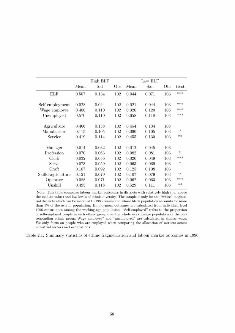
High ELF Low ELFMean S.d Obs Mean S.d. Obs ttest

ELF 0.507 0.134 102 0.044 0.071 103 ***

Self employment 0.028 0.044 102 0.021 0.044 103 ***Wage employee 0.400 0.110 102 0.320 0.120 103 ***Unemployed 0.570 0.110 102 0.658 0.118 103 ***

Agriculture 0.466 0.138 102 0.454 0.134 103Manufacture 0.115 0.105 102 0.090 0.105 103 *

Service 0.419 0.114 102 0.455 0.130 103 **

Manager 0.014 0.032 102 0.012 0.045 103Profession 0.070 0.063 102 0.082 0.081 103 *

Clerk 0.032 0.056 102 0.020 0.049 103 ***Serve 0.073 0.059 102 0.063 0.069 103 *Craft 0.107 0.092 102 0.125 0.108 103

Skilld agriculture 0.121 0.079 102 0.107 0.079 103 *Operator 0.088 0.071 102 0.062 0.063 103 ***Unskill 0.495 0.118 102 0.529 0.111 103 **

Note: This table compares labour market outcomes in districts with relatively high (i.e. abovethe median value) and low levels of ethnic diversity. The sample is only for the “white” magiste-rial districts which can be matched to 1985 census and whose black population accounts for morethan 1% of the overall population. Employment outcomes are calculated from individual-level1996 census data among the working-age population. “Self-employed” refers to the proportionof self-employed people in each ethnic group over the whole working-age population of the cor-responding ethnic group.“Wage employee” and “unemployed” are calculated in similar ways.We only focus on people who are employed when comparing the allocation of workers acrossindustrial sectors and occupations.

Table 2.1: Summary statistics of ethnic fragmentation and labour market outcomes in 1996

58

High ELF Low ELFMean S.d Obs Mean S.d. Obs ttest

ELF 0.527 0.126 105 0.077 0.084 105 ***

Self employment 0.022 0.055 105 0.019 0.045 105Wage employee 0.396 0.114 105 0.315 0.118 105 ***Unemployed 0.582 0.118 105 0.667 0.118 105 ***

Agriculture 0.338 0.155 105 0.376 0.152 105Manufacture 0.183 0.130 105 0.096 0.089 105 ***

Service 0.478 0.138 105 0.527 0.152 105 *

Manager 0.017 0.051 105 0.017 0.068 105Profession 0.082 0.075 105 0.080 0.076 105

Clerk 0.056 0.055 105 0.054 0.084 105Serve 0.081 0.071 105 0.076 0.069 105Craft 0.059 0.071 105 0.084 0.093 105 ***

Skilld agriculture 0.117 0.084 105 0.074 0.071 105 ***Operator 0.108 0.075 105 0.088 0.071 105 ***Unskill 0.480 0.120 105 0.527 0.121 105 **

Note: This table compares labour market outcomes in districts with relatively high (i.e. abovethe median value) and low levels of ethnic diversity. The sample is only for the “white” magis-terial districts which can be matched to 1985 census and whose black population accounts formore than 1% of the overall population. Employment outcomes are calculated from individual-level 2001 census data among the working-age black population. “Self-employed” refers to theproportion of self-employed people in each ethnic group over the whole working-age populationof the corresponding ethnic group.“Wage employee” and “unemployed” are calculated in similarways. We only focus on people who are employed when comparing the allocation of workersacross industrial sectors and occupations.

Table 2.2: Summary statistics of ethnic fragmentation and labour market outcomes in 2001

59

[1] [2]Dependent variable 1996 2001Panel A: Job opportunitiesDistance to the closest economic centre -274959.5 -245255.3

(301774.502) (260543.026)

Panel B: Economic activities of the whiteShare of white who are self employed contemporarily 0.230* 0.031

(0.139) (0.136)Share of white who are wage employed contemporarily 0.095 0.185

(0.170) (0.158)Proportion of white 0.335 0.149

(0.221) (0.140)

Panel C: Path dependenceShare of white who are wage employed in 1980 -0.227 -0.245

(0.217) (0.219)Proportion of white in 1980 -0.118 -0.707***

(0.255) (0.238)

Panel D: Contemporary migrationNumber of migrants -44201.67 9845.154

(37163.296) (24771.553)

District controls YES YESIndividual controls (district average) YES YESProvince fixed effect YES YESObs 205 210Note: This table conducts validity test of the instrumental variable based on 1996 and 2001 censusdata. The sample is only for the “white” magisterial districts which can be matched to 1985 censusand whose black population accounts for more than 1% of the overall population. All regressions are atthe district level. We control for district-level variables especially geographical features, individual-levelcontrols aggregated at district average and province fixed effects. *** p<0.01, ** p<0.05, * p<0.1.

Table 3: Validity of the instrumental variable

60

[1] [2] [3] [4]1996 2001

Age 15-64 Age 25-64 Age 15-64 Age 25-64Predicted ELF 1.515*** 1.488*** 1.653*** 1.623***

(0.320) (0.326) (0.292) (0.293)Edu 0.000 0.000 0.000 0.000

(0.000) (0.000) (0.000) (0.000)Male 0.000 0.000 0.001 0.001*

(0.001) (0.001) (0.001) (0.001)Age -0.000 -0.000* -0.000 -0.000**

(0.000) (0.000) (0.000) (0.000)Married 0.003* 0.002 0.004*** 0.003**

(0.002) (0.001) (0.001) (0.001)Father alive 0.000 0.001 0.002** 0.002**

(0.001) (0.001) (0.001) (0.001)Pop density 0.000*** 0.000*** 0.000** 0.000***

(0.000) (0.000) (0.000) (0.000)Urban 0.012 0.012 0.003 0.002

(0.011) (0.011) (0.010) (0.010)River 0.084*** 0.080*** 0.062** 0.060**

(0.029) (0.029) (0.027) (0.028)Density mine 0.434 0.337 0.781 0.697

(0.709) (0.698) (0.717) (0.695)Prop black -0.290*** -0.289*** -0.421*** -0.421***

(0.056) (0.056) (0.077) (0.077)Distance closest -0.000** -0.000** -0.000*** -0.000***

(0.000) (0.000) (0.000) (0.000)Ruggedness 0.005 0.006 -0.005 -0.004

(0.008) (0.008) (0.007) (0.007)Soil quality 0.051* 0.052* 0.054** 0.053*

(0.029) (0.029) (0.027) (0.027)Per capita light 0.340 0.353 0.583 0.562

(0.232) (0.231) (0.369) (0.361)Road 0.009 0.013 0.011 0.015

(0.030) (0.030) (0.029) (0.028)Conflict 0.018* 0.017* -0.004** -0.004**

(0.009) (0.009) (0.002) (0.002)Proportion manu 0.305** 0.313*** 0.261*** 0.272***

(0.118) (0.117) (0.076) (0.074)Proportion service 0.377*** 0.373*** 0.198** 0.191**

(0.129) (0.129) (0.086) (0.084)Ethnicity fixed effect YES YES YES YESProvince fixed effect YES YES YES YESF-statistics of the instrument 22.36 20.87 32.04 30.60R-squared 0.875 0.879 0.887 0.890Observations 464,130 318,610 697,369 484,639Note: This table reports the first-stage results of the instrumental variable based on 1996 and2001 census data and report the F-statistics of the instrumental variable. The sample is only forthe “white” magisterial districts which can be matched to 1985 census and whose black populationaccounts for more than 1% of the overall population. All regressions are at the individual level.We report all the control variables, both district-level variables especially geographical featuresand individual-level controls for socio-economic status. We control for ethnicity and provincefixed effects. *** p<0.01, ** p<0.05, * p<0.1.

Table 4: First-stage regression results: individual level regressions

61

[1] [2] [3] [4] [5] [6] [7] [8]Unemployed Inactive Unemployed + inactive Unemployed + inactive

1996 1996 1996 2001Age 15-64 Age 25-64 Age 15-64 Age 25-64 Age 15-64 Age 25-64 Age 15-64 Age 25-64

Panel A: OLS estimatesEthnic fractionalisation ELF -0.024 -0.031 -0.057** -0.051** -0.081** -0.082** -0.146*** -0.148***

(0.018) (0.027) (0.023) (0.022) (0.032) (0.039) (0.037) (0.042)Individual controls YES YES YES YES YES YES YES YESDistrict controls YES YES YES YES YES YES YES YESProvince FE YES YES YES YES YES YES YES YESR-squared 0.033 0.075 0.153 0.094 0.195 0.123 0.175 0.107Observations 464,130 318,610 464,130 318,610 464,130 318,610 697,368 484,639

Panel B: IV estimatesEthnic fractionalisation ELF -0.142*** -0.126** 0.043 -0.036 -0.098 -0.163* -0.170* -0.206**

(0.046) (0.064) (0.061) (0.061) (0.076) (0.087) (0.088) (0.098)Individual controls YES YES YES YES YES YES YES YESDistrict controls YES YES YES YES YES YES YES YESProvince FE YES YES YES YES YES YES YES YESF statistics of the instrument 22.36 20.87 22.36 20.87 22.36 20.87 32.04 30.60R-squared 0.032 0.074 0.153 0.094 0.195 0.123 0.175 0.106Observations 464,130 318,610 464,130 318,610 464,130 318,610 697,369 484,639Note: This table reports results about the effect of ethnic diversity on unemployment rate at individual-level regressions based on 1996 and 2001 census data.The sample is only for the “white” magisterial districts which can be matched to 1985 census and whose black population accounts for more than 1% of theoverall population. We control for district-level variables especially geographical features, individual-level controls aggregated at district average and ethnicityfixed effects. We also control for province fixed effects. Ethnic diversity is measured with fractionalisation index. We separate unemployed and economicallyinactive groups only for 1996 results as these two categories are combined in 2001 census. “Unemployed + inactive” is a dummy variable which equals 1 if oneis unemployed or inactive and 0 if one is employed. *** p<0.01, ** p<0.05, * p<0.1.

Table 5: Ethnic diversity, unemployment and labour force participation: individual level regressions

[1] [2] [3] [4] [5] [6] [7] [8]Wage employment Self/wage Wage employment Self/wage

1996 1996 2001 2001Age 15-64 Age 25-64 Age 15-64 Age 25-64 Age 15-64 Age 25-64 Age 15-64 Age 25-64

Panel A: OLS estimatesEthnic fractionalisation ELF 0.086*** 0.087** -0.024 -0.020 0.144*** 0.147*** 0.013 0.012

(0.033) (0.041) (0.017) (0.017) (0.037) (0.043) (0.013) (0.013)Individual controls YES YES YES YES YES YES YES YESDistrict controls YES YES YES YES YES YES YES YESProvince FE YES YES YES YES YES YES YES YESR-squared 0.194 0.126 0.011 0.01 0.173 0.106 0.008 0.008Observations 449,200 305,099 180,535 162,333 681,529 470,552 253,809 228,519

Panel B: IV estimatesEthnic fractionalisation ELF 0.112 0.173* -0.055 -0.030 0.176** 0.215** -0.043 -0.041

(0.077) (0.091) (0.043) (0.040) (0.087) (0.098) (0.037) (0.034)Individual controls YES YES YES YES YES YES YES YESDistrict controls YES YES YES YES YES YES YES YESProvince FE YES YES YES YES YES YES YES YESF statistics of the instrument 22.46 21 20.24 20.31 32.33 30.88 27.93 28.61R-squared 0.194 0.126 0.011 0.01 0.173 0.106 0.008 0.007Observations 449,200 305,099 180,535 162,333 681,529 470,552 253,809 228,519Note: This table reports results about the effect of ethnic diversity on employment and the allocation between self- and wage-employment at individual-levelregressions based on 1996 and 2001 census data. The sample is only for the “white” magisterial districts which can be matched to 1985 census and whoseblack population accounts for more than 1% of the overall population. We control for district-level variables especially geographical features, individual-levelcontrols aggregated at district average and ethnicity fixed effects. We also control for province fixed effects. Ethnic diversity is measured with fractionalisationindex. In column 1, 2, 5, 6 we drop self-employed people as they are a very small proportion of the whole working-age population. Column 3, 4, 7, 8 arebased only on the employed black people. *** p<0.01, ** p<0.05, * p<0.1.

Table 6: Ethnic diversity and employment status: individual level regresions

62

[1] [2] [3] [4] [5] [6]OLS OLS OLS IV IV IV

Log monthly Log hourly Hour Log monthly Log hourly Hourincome wage income wage

Panel A: Individual level, census dataEthnic fractionalisation ELF 0.326*** 0.362*** -1.279 0.497*** 0.414 2.482

(0.071) (0.090) (1.286) (0.190) (0.268) (3.809)Individual controls YES YES YES YES YES YESDistrict controls YES YES YES YES YES YESProvince FE YES YES YES YES YES YESF statistics of the instrument 28.28 28.28 28.12R-squared 0.345 0.314 0.053 0.345 0.314 0.052Observations 228,256 228,256 232,533 228,256 228,256 232,533

Panel B: Individual level, LFS dataEthnic fractionalisation ELF -0.0772 -0.0286 0.107 0.439 0.0361 23.23

(0.253) (0.246) (2.943) (0.996) (0.870) (16.51)Individual controls YES YES YES YES YES YESDistrict controls YES YES YES YES YES YESProvince FE YES YES YES YES YES YESF statistics of the instrument 5.497 5.322 5.591R-squared 0.482 0.474 0.054 0.480 0.474 0.018Observations 3,478 3,615 3,660 3,478 3,615 3,660Note: This table reports results about the effect of ethnic diversity on other labour market outcomes at individual-level regressions,including working hour, hourly wage and monthly earnings. We only report the result in 2001 as there is no information on hoursof working in 1996 census. The sample is only for the “white” magisterial districts which can be matched to 1985 census andwhose black population accounts for more than 1% of the overall population. We control for district-level variables especiallygeographical features, individual-level controls aggregated at district average and ethnicity fixed effects. We control for provincefixed effects. Ethnic diversity is measured with fractionalisation index. All the columns only focus on employees. *** p<0.01, **p<0.05, * p<0.1.

Table 7: Ethnic diversity, intensive margin and wage: individual level regressions

[1] [2] [3] [4]Dependent variable unemploy + inactive wage employ self/wage log monthly incomeEthnic fractionalisation ELF -0.291*** 0.341*** -0.133* -0.382

(0.0709) (0.072) (0.0696) (0.365)Individual controls (district average) YES YES YES YESDistrict controls YES YES YES YESR-squared 0.493 0.488 0.244 0.730Observations 410 410 410 410Note: This table reports results about the effect of ethnic diversity on employment based on the district-level balanced panel. Thesample is only for the “white” magisterial districts which can be matched to 1985 census and whose black population accounts formore than 1% of the overall population. We control for district-level variables which vary over time and individual-level controlsaggregated at district level and province fixed effects. Ethnic diversity is measured with fractionalisation index. The dependentvariable in column 1 is the proportion of unemployed over the whole working-age black population. Column 2 is defined in a similarway but we exclude those who are self-employed. Column 3 has the dependent variable which is the ratio of the number of self-employed to that of employees at district level. Column 4 only focuses on back people who are employed. *** p<0.01, ** p<0.05, *p<0.1.

Table 8: Ethnic diversity and employment: district fixed effects models

63

Table 9: Heterogeneous effects of ethnic diversity on wage-employment: individual level regressions

[1] [2] [3] [4]OLS IV OLS IV

Dependent variable 1996 1996 2001 2001

Panel A: By ethnicityLarge 0.111*** 0.125 0.148*** 0.182**

(0.035) (0.081) (0.032) (0.086)Obs 320,901 320,901 459,108 459,108Medium 0.018 -0.150 0.203*** -0.029

(0.075) (0.210) (0.061) (0.207)Obs 91,373 91,373 149,632 149,632Small -0.016 -0.606* 0.035 0.210

(0.104) (0.326) (0.083) (0.415)Obs 36,926 36,926 72,789 72,789

Panel B: By industrial sectorAgriculture 0.068** 0.034 0.016 0.067

(0.033) (0.070) (0.031) (0.073)Obs 165,605 165,605 180,227 180,227Manufacturing -0.024*** -0.008 -0.008 -0.012

(0.009) (0.019) (0.010) (0.020)Obs 165,605 165,605 180,227 180,227Service -0.044 -0.026 -0.008 -0.055

(0.027) (0.061) (0.028) (0.073)Obs 165,605 165,605 180,227 180,227

Panel C: By occupationManager 0.004 0.016 0.006* 0.023***

(0.004) (0.010) (0.003) (0.008)Obs 153,294 153,294 224,942 224,942Profession -0.016 0.107** -0.011 0.092*

(0.016) (0.046) (0.013) (0.052)Obs 153,294 153,294 224,942 224,942Clerk 0.015** -0.004 0.022** 0.033

(0.006) (0.014) (0.010) (0.024)Obs 153,294 153,294 224,942 224,942Serve -0.022* 0.037 0.015 -0.044

(0.011) (0.033) (0.016) (0.038)Obs 153,294 153,294 224,942 224,942Craft -0.015 -0.033 -0.043 0.024

(0.029) (0.067) (0.027) (0.048)

Continued on next page

64

Table 9 – continued from previous page

[1] [2] [3] [4]OLS IV OLS IV

Dependent variable 1996 1996 2001 2001

Obs 153,294 153,294 224,942 224,942Skilled agriculture 0.002 -0.073 0.014 -0.059*

(0.021) (0.046) (0.015) (0.033)Obs 153,294 153,294 224,942 224,942Operator -0.036** -0.143*** -0.038** -0.058

(0.016) (0.047) (0.018) (0.038)Obs 153,294 153,294 224,942 224,942Unskilled 0.068* 0.094 0.035 -0.010

(0.035) (0.072) (0.035) (0.064)Obs 153,294 153,294 224,942 224,942Individual controls YES YES YES YESDistrict controls YES YES YES YESProvince FE YES YES YES YES

Note: This table reports the main results about the heterogeneous effects of ethnicdiversity on the probability of being an employee at individual-level regressions bysub-groups in both 1996 and 2001 census. The sample is only for the “white” mag-isterial districts which can be matched to 1985 census and whose black populationaccounts for more than 1% of the overall population. We control for district-levelvariables especially geographical features, individual-level controls aggregated at dis-trict average and ethnicity fixed effects. We also control for province fixed effects.Ethnic diversity is measured with fractionalisation index. All the columns in Panel Band Panel C only focus on employees to illustrate the allocation of employed workersacross different industrial sectors and occupations. *** p<0.01, ** p<0.05, * p<0.1.

65

[1] [2] [3] [4] [5] [6]Unemployed + inactive Wage employment

Native Migrants Immigrants Native Migrants ImmigrantsPanel A: IV estimates, 1996 censusEthnic fractionalisation ELF -0.161** 0.142 -0.506 0.171** -0.131 0.530*

(0.079) (0.133) (0.321) (0.081) (0.134) (0.316)Individual controls YES YES YES YES YES YESDistrict controls YES YES YES YES YES YESProvince FE YES YES YES YES YES YESF statistics of the instrument 24.05 15.52 8.432 24.12 15.51 8.826R-squared 0.191 0.193 0.299 0.188 0.196 0.330Observations 305,458 128,215 4,657 296,864 122,956 4,283

Panel B: IV estimates, 2001 censusEthnic fractionalisation ELF -0.153* -0.247 -0.991* 0.158** 1.048* 0.252

(0.080) (0.211) (0.592) (0.080) (0.624) (0.209)Individual controls YES YES YES YES YES YESDistrict controls YES YES YES YES YES YESProvince FE YES YES YES YES YES YESF statistics of the instrument 33.73 16.65 6.618 33.90 17.14 6.666R-squared 0.171 0.196 0.289 0.168 0.198 0.312Observations 568,260 119,696 20,390 556,296 116,089 19,250Note: This table reports results about the effect of ethnic diversity on employment separately for native, migrants andimmigrants at individual-level regressions based on 1996 and 2001 census data. “Native” is defined as people who were bornin the district and never move out or within-district migrants. ”Migrants” are cross-district migrants while “immigrants” arethose who migrated from another country. The sample is only for the “white” magisterial districts which can be matched to1985 census and whose black population accounts for more than 1% of the overall population. We control for district-levelvariables especially geographical features, individual-level controls aggregated at district average and ethnicity fixed effects.We also control for province fixed effects. Ethnic diversity is measured with fractionalisation index. In columns 4-6 we dropself-employed people as they are a very small proportion of the whole working-age population. *** p<0.01, ** p<0.05, *p<0.1.

Table 10: Ethnic diversity and employment: separating native, migrants and immigrants

[1] [2] [3] [4] [5] [6]1996 2001

Number of white in 1996 Number of white in 1985 Diffrence: 96 - 85 Number of white in 2001 Number of white in 1985 Diffrence: 01 - 85Panel A: OLS estimatesEthnic fractionalisation ELF 12758.975 765.232 11993.742 -9966.072 4529.285 -14495.357

(25151.926) (31380.028) (13971.953) (29215.642) (25530.141) (15013.818)R-squared 0.766 0.781 0.452 0.767 0.895 0.782Observations 205 205 205 210 210 210

Panel B: IV estimatesEthnic fractionalisation ELF 145935.526 226342.130 -80406.604 33390.776 15067.044 18323.731

(185457.367) (204618.284) (59332.187) (106236.562) (84187.211) (33223.976)F statistics of instruments 10.19 10.19 10.19 29.85 29.85 29.85R-squared 0.735 0.720 0.349 0.765 0.894 0.776Observations 205 205 205 210 210 210Individual controls YES YES YES YES YES YESDistrict controls YES YES YES YES YES YESProvince FE YES YES YES YES YES YESNote: This table looks at whether ethnic diversity is correlated with the number of white population in 1996 and 2001 and the emigration of the white from the district after the end of Apartheid at district-levelregressions. The sample is only for the “white” magisterial districts which can be matched to 1985 census and whose black population accounts for more than 1% of the overall population. We control for district-levelvariables especially geographical features and individual-level controls aggregated at district average. We also control for province fixed effects. Ethnic diversity is measured with fractionalisation index. *** p<0.01,** p<0.05, * p<0.1.

Table 11: Ethnic diversity and the emigration of the white

66

[1] [2] [3] [4] [5] [6] [7] [8]Wage employee Common language (only 1996)

Whole sample Large Medium Small Whole sample Large Medium SmallPanel A: 1996 censusDispersion of size -0.087*** -0.110*** -0.015 0.014 -0.035* -0.028 -0.054 0.015

(0.033) (0.034) (0.073) (0.102) (0.018) (0.020) (0.033) (0.032)1/No. of groups -0.170*** -0.194*** -0.207 0.405 0.016 0.020 0.127 -0.097

(0.044) (0.045) (0.311) (0.555) (0.028) (0.031) (0.366) (0.177)R-squared 0.194 0.187 0.201 0.230 0.068 0.068 0.072 0.061Observations 449,200 320,901 91,373 36,926 654,116 469,737 131,601 52,778

Panel B: 2001 censusDispersion of size -0.148*** -0.152*** -0.207*** -0.033

(0.037) (0.031) (0.057) (0.083)1/No. of groups -0.284*** -0.266*** 0.419 -0.555

(0.065) (0.057) (0.777) (1.126)R-squared 0.173 0.164 0.177 0.200Observations 681,529 459,108 149,632 72,789Individual controls YES YES YES YES YES YES YES YESDistrict controls YES YES YES YES YES YES YES YESProvince FE YES YES YES YES YES YES YES YESNote: This table reports results based on the decomposition of ethnic diversity index into items relating to number of ethnic groups andgroup share, and how these two items are associated with employment rate at individual-level OLS regressions with 1996 and 2001 censusdata. The sample is only for the “white” magisterial districts which can be matched to 1985 census and whose black population accountsfor more than 1% of the overall population. We control for district-level variables especially geographical features, individual-level controlsaggregated at district average and ethnicity fixed effects. We also control for province fixed effects. Ethnic diversity is measured withfractionalisation index. We look at both the whole sample and sub-samples split by sample size. *** p<0.01, ** p<0.05, * p<0.1.

Table 12.1: Decomposing ethnic diversity into number of groups and dispersion of population share

[1] [2] [3] [4] [5] [6] [7] [8] [9]Wage employee 1996 Wage employee 2001 Common language 1996

Large Medium Small Large Medium Small Large Medium SmallPanel A: Instrument dispersion of sizeDispersion of size -0.166** 0.166 0.570* -0.213** 0.030 -0.202 -0.136* 0.068 -0.012

(0.077) (0.197) (0.319) (0.084) (0.203) (0.429) (0.073) (0.168) (0.097)1/No. of groups -0.249*** -0.073 0.864 -0.335*** 0.531 -0.603 -0.086 0.224 -0.116

(0.080) (0.374) (0.604) (0.107) (0.721) (1.059) (0.079) (0.434) (0.190)F statistics of the instrument 17.98 7.662 9.421 23.68 12.11 4.009 18.31 8.424 10.03R-squared 0.187 0.200 0.223 0.164 0.175 0.199 0.066 0.070 0.061Observations 320,901 91,373 36,926 459,108 149,632 72,789 469,737 131,601 52,778

Panel B: Instrument number of groupsDispersion of size -0.270 0.057 0.113 -0.505 0.065 -0.044 -0.313 -0.006 0.011

(0.248) (0.156) (0.135) (0.751) (1.802) (0.101) (0.322) (0.060) (0.036)1/No. of groups -0.566 1.514 4.145 -1.781 56.536 -8.462 -0.619 1.256 -0.289

(0.573) (2.867) (2.830) (3.415) (377.818) (26.742) (0.716) (1.169) (0.630)F statistics of the instrument 0.897 1.128 3.477 0.204 0.0212 0.331 1.112 1.393 3.392R-squared 0.184 0.196 0.220 0.142 -0.825 0.193 0.038 0.066 0.061Observations 320,901 91,373 36,926 459,108 149,632 72,789 469,737 131,601 52,778Individual controls YES YES YES YES YES YES YES YES YESDistrict controls YES YES YES YES YES YES YES YES YESProvince FE YES YES YES YES YES YES YES YES YESNote: This table reports results based on the decomposition of ethnic diversity index into items relating to number of ethnic groups and group share, and howthese two items are associated with employment rate at individual-level IV regressions with 1996 and 2001 census data. The sample is only for the “white”magisterial districts which can be matched to 1985 census and whose black population accounts for more than 1% of the overall population. We control fordistrict-level variables especially geographical features, individual-level controls aggregated at district average and ethnicity fixed effects. We also control forprovince fixed effects. Ethnic diversity is measured with fractionalisation index. We look at the sub-samples split by group size. *** p<0.01, ** p<0.05, *p<0.1.

Table 12.2: Verifying that the instrument variable captures the dispersion of group size

67

[1] [2]OLS IV

Panel A: Whole sampleOverall 0.036** 0.109*

(0.018) (0.065)F statistics of the instrument 23.07Obs 654,116 654,116

Panel B: By ethnicityLarge 0.028 0.161**

(0.020) (0.078)F statistics of the instrument 17.30Obs 469,737 469,737

Medium 0.052 -0.078(0.034) (0.188)

F statistics of the instrument 9.052Obs 131,601 131,601

Small -0.014 0.024(0.031) (0.093)

F statistics of the instrument 10.76Obs 52,778 52,778Individual controls YES YESDistrict controls YES YESProvince FE YES YES

Note: This table reports results about the effect of ethnic diversity on the acquisition of social skills (proficiency of secondlanguage as a proxy) at individual-level regressions based on 1996 census data (as there is no information on the second languagein 2001 census). The sample is only for the “white” magisterial districts which can be matched to 1985 census and whose blackpopulation accounts for more than 1% of the overall population. We control for district-level variables especially geographicalfeatures, individual-level controls aggregated at district average and ethnicity fixed effects. We also control for province fixedeffects. Ethnic diversity is measured with fractionalisation index. We look at both the whole sample and sub-samples split bygroup size. *** p<0.01, ** p<0.05, * p<0.1.

Table 13.1: Ethnic diversity and skill acquisition: second language

68

[1] [2] [3]<15 15-64 >=65

Panel A: Large groupELF 0.121** 0.174** 0.236**

(0.057) (0.088) (0.110)F statistics of the instrument 17.34 17.22 14.89Obs 108,939 342,890 17,908

Panel B: Medium groupELF -0.079 -0.064 -0.458

(0.115) (0.209) (0.350)F statistics of the instrument 11.10 8.097 12.96Obs 28,848 97,754 4,999

Panel C: Small groupELF 0.093 -0.005 -0.033

(0.073) (0.106) (0.122)F statistics of the instrument 11.96 9.896 15.56Obs 10,238 40,690 1,850Individual controls YES YES YESDistrict controls YES YES YESProvince FE YES YES YES

Note: This table reports results about the effect of ethnic diversity on the acquisition of social skills (proficiency of secondlanguage as a proxy) at individual-level regressions based on 1996 census data (as there is no information on the second languagein 2001 census). The sample is only for the “white” magisterial districts which can be matched to 1985 census and whose blackpopulation accounts for more than 1% of the overall population. We control for district-level variables especially geographicalfeatures, individual-level controls aggregated at district average and ethnicity fixed effects. We also control for province fixedeffects. Ethnic diversity is measured with fractionalisation index. In particular, we split the sample by age groups. *** p<0.01,** p<0.05, * p<0.1.

Table 13.2: Ethnic diversity and skill acquisition across age groups: second language

69

[1] [2] [3] [4]Overall Large Medium Small

Panel A: Unemployed as dependent variable, conditional on diversitySecond official -0.133*** -0.123*** -0.144*** -0.176***

(0.013) (0.010) (0.022) (0.036)Individual controls YES YES YES YESDistrict controls YES YES YES YESProvince FE YES YES YES YESR-squared 0.201 0.193 0.212 0.229Obs 461,942 329,416 93,673 38,853

Panel B: Wage employ as dependent variable, conditional on diversitySecond official 0.132*** 0.121*** 0.143*** 0.179***

(0.013) (0.011) (0.023) (0.036)Individual controls YES YES YES YESDistrict controls YES YES YES YESProvince FE YES YES YES YESR-squared 0.199 0.191 0.209 0.236Obs 447,103 319,580 90,817 36,706Note: This table reports results about the relationship between social skill acquisition (proficiencyof second language as a proxy) and employment at individual-level regressions based on 1996 censusdata. We control for ethnic diversity and investigate whether this language skill is positively corre-lated with employment chances. The sample is only for the “white” magisterial districts which canbe matched to 1985 census and whose black population accounts for more than 1% of the overallpopulation. We control for district-level variables especially geographical features, individual-levelcontrols aggregated at district average and ethnicity fixed effects. We also control for province fixedeffects. Ethnic diversity is measured with fractionalisation index. In Panel A we keep the wholeworking-age black sample while in Panel B we drop self-employed people as they are a very smallproportion of the whole working-age population. *** p<0.01, ** p<0.05, * p<0.1.

Table 14: Skill acquisition and labour market outcomes: second language

70

Chapter 3

Returns to Education, Marital Sortingand Family Background in South Africa

Patrizio Piraino and Peng Zhang

Abstract. This paper investigates whether father-in-law’s background has a stronger explanatory powerthan father’s background for male wages in South Africa. We also investigate the heterogeneity of the effectsof father and father-in-law’s background at different educational levels and between different populationgroups. After correcting for potential measurement errors in both earnings and education, we find that,consistent with existing studies on Brazil, father-in-law’s schooling has a larger effect on male workers’labour market earnings than own father’s schooling. The gap increases with parental educational levels.Father’s background plays a more important role in explaining labour market income of black South Africanmales compared to white males, while this does not hold for father-in-law’s background. Furthermore, wefind that family background and marital sorting are also related to other labour market outcomes, such asemployment and labour force participation.

Keywords: Intergenerational mobility; Marital sorting; Education; South Africa.JEL classification: I24, J24, J62.

3.1 Introduction

Research on intergenerational transmission of socio-economic status shows that parental education playsan important role in children’s socio-economic outcomes such as income in both developing and developedcountries (Solon, 1992; Piraino, 2015; Dahl and DeLeire, 2008; Dustmann, 2005; Bingley and Cappellari,2014; Eisenhauer and Pfeiffer, 2008; Mare, 2000). An interesting phenomenon is that in developing countrieslike Brazil, fathers-in-law’s schooling explains more of male workers’ wage than father’s schooling (Lam andSchoeni, 1993), which is however not the case in more developed countries such as the US (Lam and Schoeni,1994) and UK (Blanden, 2004). This is not likely driven by factors commonly believed to be responsiblefor the transmission of socio-economic status across generations such as family connections. For example, ifchildren from better educated parents have higher income due to the network provided by the family, it isreasonably to assume that this nepotism is larger between father and son than that between father-in-lawand son-in-law. This means the educational background of fathers-in-law should have smaller explanatorypower than that of fathers, which contradicts the above empirical finding.

In Lam and Schoeni (1993), they provide a model that links the degree of assortative mating to inter-generational inequality to explain this paradox. The mechanism is as follows. Earnings are determined byeducation and unobserved individual characteristics such as ability. Family background can be considered

71

as a signal for this unobserved ability. For male workers, own father’s education serves as proxy for only theinherited components of the ability while father-in-law’s education signals both the inherited and uninheriteddeterminants of ability. As there is more information in father-in-law’s schooling than father’s schooling,father-in-law’s background will have a relatively larger explanatory power in male workers’ earnings. InLam and Schoeni (1994), they compare the results from a series of wage equations in the United Statesand Brazil and further show that the explanatory power of father-in-law’s education is larger in countriescharacterised by a higher degree of assortative mating and lower female labour force participation.

Bringing assortative mating into research on intergenerational transmission of socio-economic statuscontinues to attract attention in more recent literature. Papers focusing on different countries may showresults different from the evidence in Brazil but most of them confirm that marital sorting is unneglectablein determining intergenerationally transmitted earnings (Holmlund, 2008). For example, Handy (2015)uses the US data and finds that assortative mating explains around one quarter of the intergenerationalcorrelation in education and income. Using data from Germany and the UK, Ermisch et al. (2006) show thatmarital sorting explains a high proportion of the covariance between offspring’s and parents’ family income inboth countries. Eika et al. (2014) focus on the contribution of gender and marital status to intergenerationalmobility in the United States and Norway. In their paper, the intergenerational earnings mobility of marriedwomen is influenced by a combination of assortative mating and labour supply responses.

It is therefore worthwhile to further investigate how assortative mating and intergenerational transmis-sion jointly determine earnings by expanding the pioneering work of Lam and Schoeni (1993, 1994). Inparticular, three questions remain to be answered: are the effects of father and father-in-law’s backgroundon male workers’ earnings nonlinear across different educational categories? Are the current results contam-inated by measurement errors and inaccurate measure of lifetime earnings (i.e. using transitory earning asa proxy for permanent earning) which are usually the challenges in research on intergenerational transmis-sion? Are the results from Brazil applicable to other developing countries with more complicated structureof labour market and more serious unemployment issues?

Based on these, in this paper we follow the framework of Lam and Schoeni (1993, 1994) and re-examinethe paradox that father-in-law’s education explains more of male workers’ income than father’s educationby looking at the intergenerational transmission and assortative mating in the South African labour market.The contributions of the paper lie in the following three aspects.

Firstly, we capture the heterogeneity of the effects of father and father-in-law’s background at differenteducational levels and document its nonlinearity. It has been noticed that returns to education can beconvex in response to educational levels in developing countries. Some studies suggest it might be simplydue to selection into higher education (Colclough et al., 2009). As educational levels increase, people whochoose to attend higher educational institutes will have higher abilities. Therefore the increase in estimatedreturns to education may only capture the increased omitted variable bias due to unobserved ability aseducational levels increase. In this paper, we show that whether this explanation is true can be partlyrevealed from parental information. We find that this convexity also exists in returns to father and father-in-law’s education. Furthermore, the magnitude and convexity of the effect of own education, althoughdeclining, do not disappear after controlling for parental background. Following the intuition that fatherand father-in-law’s education capture unobserved ability, this result indicates that the convexity in thereturns to education is not totally driven by the selection of people with higher ability to enter highereducational institutes and therefore implies that real returns to high school and college education can behigh in developing countries.

Secondly, we deal with measurement errors and the challenge of measuring permanent earnings oftenfaced by research on intergenerational transmission, based on a panel survey of households with adjusted

72

value of education and income according to updated information in each wave. In Lam’s paper linkingfamily background and assortative mating, he pointed out that even if the magnitude of measurementerrors in schooling is small, increase in measurement error bias after controlling for parental backgroundcan account for as much as 80% of the decrease in returns to schooling. Therefore, over the last decade,increased availability of longitudinal data and advances in econometric techniques have allowed economists toovercome some of the most common measurement issues and to obtain reliable estimates of intergenerationalincome mobility in a number of countries (Corak, 2006; Mazumder, 2005). Similarly, we use panel data tocorrect for errors from transitory income data by averaging income across waves. Furthermore, as the dataalso reports the “best” estimate of education and income which corrects for measurement errors in any singlewave, we can further deal with measurement errors by using “best” estimates rather than original values.

Thirdly, we conduct analysis similar to Lam and Schoeni (1993, 1994) with the above two improvementsin the setting of South Africa to see whether their results can be generalised to other developing countriesbesides Brazil and how their conclusions might differ when we turn to a country with more complicatedstructure of labour market and more serious unemployment issues. South Africa has two features that lead toits distinguished labour market structure. On the one hand, South Africa is characterised by segmented buthighly linked labour market, which can be revealed by the diverse response to intergenerational transmissionbetween black and white. The forced racial segregation of the past has a legacy in the highly segmentedsociety of the present. Income inequality is among the highest in the world, and vast differences remainacross racial groups in a variety of socioeconomic outcomes (Leibbrandt et al., 2009).

As the degree of intergenerational transmission can be different across groups within the same country(Mazumder, 2011), especially between different races (Hertz, 2008), it is worthwhile to investigate the racialdifference in assortative mating and intergenerational correlation between the black and white in SouthAfrica. Specifically, given the fragmented labour market and high inequality between black and white inSouth Africa, it is reasonable to assume that the degree of assortative mating and the rate of female labourforce participation, the two most important factors determining the effects of father-in-law’s background, canbe quite different between the black and the white. It also makes sense to focus on the assortative matingwithin race as inter-racial marriages are still uncommon. Furthermore, unlike the case in Brazil, labourforce participation rate is very low in South Africa. As a result, it would also be valuable to look at howparental background and assortative mating determine other labour market outcomes such as probabilityof employment and labour force participation besides earnings.

In our paper, after controlling for measurement errors in education and income, the earnings equations ofSouth African male workers show that parental background variables have significant explanatory power. Wefind that father-in-law’s schooling has a larger effect on labour market earnings than own father’s schooling,consistent with the result from Brazil. To further confirm the relatively larger effect of father-in-law’sbackground, we find that the drop in the coefficients on father’s schooling is larger than that on father-in-law’s schooling when own schooling is included in the earnings equation, indicating that the informationcontained in father’s schooling and own education is highly overlapped so that the marginal contribution offather’s education to information on unobserved ability is relatively limited. Following the same reasoning,the drop in the coefficients on own schooling is smaller when father’s schooling is included than when father-in-law’s schooling is included. Furthermore, parental background and martial sorting not only explain labourmarket earnings but also relate to other labour market outcomes such as probability of employment andlabour force participation.

In terms of the heterogeneity of the effects of parental background, first, we find that there is convexity inthe structure of returns to education. In particular, the patterns we observed for the average schooling effectare mostly displayed at the higher level of education categories. This convexity declines after controlling for

73

parental background but does not disappear. This implies that there is an endogenous selection of peoplewith high ability into higher education but this selection does not fully capture the pattern of convex returnsto education. Second, there is heterogeneity between the black and the white in response to intergenerationaltransmission and assortative mating. Parental background plays a more important role in labour marketincome for the black while this pattern does not exist for father-in-law’s education. The reason why the roleof father-in-law’s education does not differ between the black and white might be that assortative mating islower and the male-female ratio of the variance in income is larger among the white than that among theblack (both are verified by data). The former leads to a smaller effect of father-in-law’s education relativeto father’s education while the latter indicates a larger relatively effect of father-in-law’s schooling.

The rest of the paper is structured as follows. The next section offers a theoretical discussion of the linksbetween marital sorting and intergenerational mobility. Section 3 describes the data used for the empiricalanalysis. Section 4 provides empirical framework. The results are presented and discussed in Section 5.Section 6 concludes.

3.2 Theoretical Framework

3.2.1 Model

We use the notation m for men (i.e. husband) and w for women (i.e. wife). Suppose ym, Sm and Am arehusband’s labour market income, schooling and ability, respectively. We do not consider inherited wealth(like bequest) here as we only focus on labour market outcome for empirical study1. Fm is father’s schooling,which captures inherited part of schooling and ability. Su

m and Aum are uninherited parts which determine

schooling and ability. Labour market income is determined by observed schooling and unobserved overallability. Here we have:

ym = β0m + βsmSm + βamAm + um (3.1)

Sm = αsm + γsmFm + Sum (3.2)

Am = αam + γamFm +Aum (3.3)

If we regress husband’s labour market income on father’s education, we have:

ym = δ0m + δfmFm + vm (3.4)

Here:δfm = βsmγsm + βamγam (3.5)

δ0m = β0m + βsmαsm + βamαam

Similarly,yw = δ0w + δfwFw + vw, δfw = βswγsw + βawγaw (3.6)

Based on Lam’s model, we make the following three assumptions.

1Following Lam and Schoeni (1993) which treats inherited wealth and labour market earnings separately.

74

1. The degree of assortative mating is captured by the correlation of lifetime income between husbandand wife, proxied by ρymyw .

2. There is no additional assortative mating other than income. This means that given the income ofboth husband and wife, the degree of assortative mating does not depend on other socio-economicfactors such as education. The intuition of this assumption is that the husband with higher incomeprefers a spouse with higher income. But he does not care whether this high income is from herhigh educational level or good luck in the labour market. Mathematically, the correlation betweenhusband’s income and wife’s other socio-economic factors should be zero conditional on wife’s income,meaning: ρymsw·yw = 0, ρywsm·ym = 0, ρymaw·yw = 0, ρywam·ym = 0, ρymfw·yw = 0, ρywfm·ym = 0.

3. Uninherited components of ability and schooling are not correlated.

According to Lam and Schoeni (1993), from the second assumption above, we can get the followingequation.

ρymfw = ρywym · ρywfw (3.7)

With the above three assumptions, we consider the following regressions.First, directly from equation 3.4 and 3.5, if we regress husband’s labour market income on his father’s

education and define the coefficient of father’s education as βymfm , we have:

plimβymfm = ρymfm · σymσfm

(3.8)

Second, we regress husband’s labour market income on his father’s schooling, conditional on its ownschooling. Suppose the coefficient of father’s education in this regression is βymfm·sm . We have:

plimβymfm·sm = ρymfm · σymσfm

[1− ρsmfm ·ρsmym

ρymfm

1− ρ2smfm

] (3.9)

Third, when we regress income on father-in-law’s schooling, we get the coefficient of father-in-law, definedas βymfm . We have:

plimβymfw = δfw · ρymyw · σymσyw

(3.10)

Fourth, we regress income on father-in-law’s schooling conditional on own schooling, get the coefficientof father-in-law’s schooling, defined as βymfw·sm . We have:

plimβymfw·sm = δfw · ρymyw · σymσyw

[1− ρ2ymsm

1− ρ2ymsmρ2ymywR

2ywfw

] (3.11)

Here R2ywfw

is the R2 from a regression of yw on fw. The proofs of equation 3.7 - 3.11 are in the Appendix.

3.2.2 Schooling, intergenerational transmission and assortative mating

From the above four formulas, we can make the following propositions which shed light on schooling,intergenerational transmission and assortative mating. The first three propositions are explain in Lam andSchoeni (1993) with intuitions and we provide rigorous proof here.

Proposition 3.2.1. Father-in-law’s schooling can have a more explanatory power on labour market earningsthan own father’s schooling. And the explanatory power depends on the degree of assortative mating and the

75

variance in male income relative to that in female income. That is: it is possible to have βymfw > βymfm

when ρymyw is not too small and σym > σyw (or equivalently: σum > σuw).

Proof. When equation 3.7 holds, we have:

ρymfw

ρywfm

=ρymywρywfw

ρymywρymfm

=ρywfw

ρymfm

Therefore:

ρymfw − ρymfm =ρywfw · ρywfm − ρ2ymfm

ρymfm

When ρywfw > ρymfm , it is possible to have: ρymfw > ρymfm

Since:

ρymfm =Cov(YmFm)

σymσfm, ρywfw =

Cov(YwFw)

σywσfw

When other parts are equal, ρywfw > ρymfm implies σym > σyw (or equivalently: σum > σuw).Furthermore, given equation 3.10, as ρymyw or σym

σywincreases, the explanatory power of father-in-law will

also increase.

Proposition 3.2.2. The relative drop in the coefficients on father’s schooling can be larger than thaton father-in-law’s schooling when own schooling is included in the earnings equation. That is to say:βymfm−βymfm·sm

βymfm>

βymfw−βymfw·smβymfw

. It is especially true when ρymyw or σymσyw

is large.

Proof. Based on equations 3.8 - 3.11, we have:

βymfm − βymfm·smβymfm

= 1−1− ρsmfm ·ρsmym

ρymfm

1− ρ2smfm

βymfw − βymfw·smβymfw

= 1−1− ρ2ymsm

1− ρ2ymsmρ2ymywR

2ywfw

For proposition 3.2.2 to hold, we must have:

1−1− ρsmfm ·ρsmym

ρymfm

1− ρ2smfm

> 1−1− ρ2ymsm

1− ρ2ymsmρ2ymywR

2ywfw

This is the condition which has to be satisfied. It is easy to get:

∂[1−ρ2ymsm

1−ρ2ymsmρ2ymyw

R2ywfw

]

∂ρymyw

> 0

And:

∂[1−ρ2ymsm

1−ρ2ymsmρ2ymyw

R2ywfw

]

∂R2ywfw

> 0

That is, when ρymyw or σymσyw

is large, the righthand side of the above inequality is smaller, meaning thecondition is easier to satisfy.

76

Proposition 3.2.3. The coefficients on own schooling can decline more when father-in-law’s schooling isincluded, than when father’s schooling is included. That is, βymsm·fm < βymsm, βymsm·fw < βymsm, andβymsm−βymsm·fm

βymsm<

βymsm−βymsm·fwβymsm

.

Proof. This can be proved from the perspective of omitted variable bias. When investigating returns to owneducation, the true regression function is the equation 3.1. However, we rely on the following regressioninstead:

ym = β0m + βsmSm + um

The estimated value is:

ˆβymsm =Cov(β0m + βsmSm + βamAm + um)Sm)

V ar(Sm)= βsm + βam

Cov(SmAm)

V ar(Sm)(3.12)

When adding Fm into the regression, the omitted variable bias (i.e. βamCov(SmAm)V ar(Sm) ) is reduced as Fm

captures some information on the unobserved ability in um.Taking father’s education as an example. When adding father’s education, the new estimated coefficient

is:

ˆβymsm·fm =V ar(Fm)Cov(YmSm)− Cov(FmSm)Cov(YmFm)

V ar(Sm)V ar(Fm)− Cov2(FmSm)

ym = ˜β0m + βsmSm + βamγamFm + βamAum + um

With some algebra we can prove:

ˆβymsm·fm = βsm + βamCov(SmAu

m)

V ar(Sm)(1− ρ2AuFm·S) (3.13)

ρ2AuFm·S is the partial correlation of uninherited ability and father’s education with control of own edu-cation. As father-in-law’s education captures both inherited and uninherited ability while father’s educationonly captures inherited ability, this partial correlation can be larger when father-in-law’s education is addedthan when father’s education is controlled. Thus the omitted variable bias βam

Cov(Sm,Aum)

V ar(Sm) (1 − ρ2AuFm·S) issmaller when we add father-in-law’s education rather than father’s education, meaning the coefficient ofown education will decreases more towards the true value.

Proposition 3.2.4. Whether the returns to own education are convex simply due to endogenous selectioninto higher education can be partly revealed from father and father-in-law’s education.

Proof. According to the equation 3.12, βamCov(SmAm)V ar(Sm) is the omitted variable bias. If there is more selection

into education when educational levels become higher, it means Cov(SmAm) increases with educationallevels, leading to more severely overestimated returns to own education.

According to the equation 3.13, if father’s education and father-in-law’s education altogether capturesinherited and uninherited abilities perfectly, this convex pattern will disappear once we control for father orfather-in-law’s background. And the convex pattern will be less obvious when father-in-law’s education isincluded (when ρAuFm·S < ρAuFw·S).

77

Proposition 3.2.5. If the degree of assortative mating is lower and the gender gap in labour force participa-tion is higher among the white than the black, father’s education is relatively more important in determiningmale workers’ income for the black than the white but the racial difference in the effects of father-in-law’sbackground is ambiguous.

Proof. We will show in the descriptive statistics that the degree of assortative mating is larger and the malelabour force participation is lower among the black than the white. Lower male labour force participationrate indicates that uninherited ability is less important in determining the black’s job market outcome andρsmym (and therefore ρfmym) will be larger among the black. From equation 3.8 and 3.10, it is obvious tofind that the effect of father’s education on male workers’ earnings is larger among the black than the white.

Furthermore, from equation 3.9, we notice that the relative decrease in omitted variable bias resulting

from unobserved ability after controlling own education is 1 −1−

ρsmfm·ρsmym

ρymfm

1−ρ2smfm

. This decrease is larger ifρsmym is higher. This implies the decrease in the coefficient of parental background is larger among theblack than the white after controlling for own education.

Comparing between equations 3.10 and 3.11, the relative decrease in omitted variable bias resulting fromunobserved ability after controlling own education is 1− 1−ρ2ymsm

1−ρ2ymsmρ2ymyw

R2ywfw

. It can be shown that:

∂1−ρ2ymsm

1−ρ2ymsmρ2ymywR2ywfw

∂ρsmym

< 0

∂1−ρ2ymsm

1−ρ2ymsmρ2ymywR2ywfw

∂ρymyw

> 0

It is obvious that if the uninherited ability is more important (ρsmym is smaller) and the degree ofassortative mating is lower ρymyw among the white than the black, the effect of controlling for own educationon father-in-law’s coefficient will be ambiguous, as these two forces drive the change in the coefficients offather-in-law’s education in the opposite directions.

3.2.3 Predictions to be tested in the empirical sections

There are five predictions derived from theoretical framework which will be tested in the empirical analysis.

1. Father-in-law’s schooling can have a higher effect on labour market earnings than own father’s school-ing.

2. The drop in the coefficients on father’s schooling is larger than that on father-in-law’s schooling whenown schooling is included in the earnings equation.

3. The drop in the coefficients on own schooling is smaller when father’s schooling is included than whenfather-in-law’s schooling is included.

4. If the returns to own education are convex due to endogenous selection into higher education, thisconvexity will be reduced after including father’s education and father-in-law’s education and morereduction takes place after father-in-law’s education is included.

5. Parental background plays a more important role in labour market income among the black than thewhite while the racial difference in the effect of father-in-law’s education is ambiguous. Moreover,the coefficient of parental education decreases more among the black than the white after controlling

78

for own education but the racial difference in the change of coefficients of father-in-law’s education isambiguous.

3.2.4 Dealing with measurement errors

Measurement errors and inaccurate estimates of permanent income are challenging to research on intergener-ational transmission (Nybom and Stuhler, 2016). Accordingly, these measurement errors might contaminatethe explanations on our results if they differ between variables of father and father-in-law. With measure-ment errors, the coefficients of own education or parental background are smaller than the true ones andthe bias from the measurement errors in own education will be larger if additional variables such as parentalbackground are added into regressions. Therefore, we may still observe the decline in the magnitude of owneducation after controlling for father or father-in-law’s education but here the results are simply driven bythe amplified measurement errors after controlling for more variables, not based on any relation betweenintergenerational transmission, assortative mating and income.

As is pointed out in Lam and Schoeni (1993), when we regress labour market income on own education,suppose education Sm is measured with bias: S∗

m = Sm + wm. Define λ = V ar(w)V ar(S∗) . The estimated returns

to education is:

βys = βs ·σ2s

σ∗2s

= βs(1− λ) (3.14)

When we add parental background Fm or Fw into the regression, the new estimated coefficient becomes:

ˆβys·f = βs(1−λ

1−R2s∗·F

) (3.15)

R2s∗·F is the R2 from a regression of S∗

m on F 2.Comparing equation 3.14 and 3.15, after controlling for parental education, as R2

s∗·F < 1, the mea-surement error in own education will become larger and as a result the coefficient of own education willdecrease. If R2

s∗·F is larger when father-in-law’s education is included, which is very likely as father-in-law’sbackground captures uninherited components in addition to inherited parts of ability, the measurement errorwill increase more after adding father-in-law’s education than adding father’s education. In this case, thecoefficient of own education will also decrease more when father-in-law’s education is controlled, comparedwith when father’s education is included.

Measurement errors lead to the same pattern as the predictions in the theoretical framework. It istherefore necessary to deal with measurement errors before staring main empirical analysis. Methods to dealwith measurement errors in both dependent and independent variables will be addressed in the followingsection.

3.3 Data

3.3.1 Data source

Our data is based upon the National Income Dynamics Study (NIDS) wave 1 to wave 4 (year 2008, 2010,2012 and 2014), the first national longitudinal household survey in South Africa. It is a biannual nationwidehousehold survey from 2008 which consisted of a nationally representative sample of approximately 7,300households. The most recent wave was conducted in 2014 with 11895 households.

2See Lam’s paper for details about measurement error.

79

NIDS used a combination of household and individual level questionnaires to obtain information on awide selection of human capital variables, labour force experiences and demographic characteristics suchas education, family relationships and household composition. The present study mainly uses informationfrom the adult questionnaire, which includes the wages and other incomes of the adults in the household,as well as their level of education and employment status. Each household member is assigned a personalidentification code. For those who co-reside with their parents, NIDS also provides information on theirfather, mother and spouse’s identification code in order to link between parents and children and husbandand wife in the same household. Therefore, for people co-residing with their parents, we can obtain theinformation on their fathers (i.e. by linking respondent with his father via identification code) and fathers-in-law (i.e. by linking respondent with his spouse via identification code and looking at spouse’s father)from this linked data. In addition, all adults are asked to complete a section on parental background, whereinformation on the educational qualification, living status and occupation of both parents is recalled byrespondents even if they do not co-reside with their parents. Therefore, for respondents living separatelywith parents, parental information is obtained from this section on parental background. Key informationregarding non-resident and deceased parents is obtained in this retrospective section.

Individual monthly income, which is used to capture labour market outcomes, is derived from variablesin the Adult and Proxy datasets. We only consider labour market income, which is the sum of wage fromthe main job, wage from the second job, casual wage, self-employment income, 13th cheque, bonus payment,profit share, income from helping friends and extra piece-rate income3.

Employment status follows the International Labour Organization’s definitions. Each respondent isassigned to one of the following groups: employed, unemployed (strict definition), unemployed (broad def-inition) and not economically active. Being employed includes having primary jobs, secondary jobs, self-employment, causal work, agricultural work and helping others with business. We consider both the strictand broad definitions of unemployment when determining respondents’ employment status.

We restrict our sample to working age males (i.e. 25 - 64 years old) who are either married or livingwith their partner4. From this sample of married individuals, we limit our analysis to those couples whohave non-missing information on the earnings of the husbands and parental education.

For the purposes of identifying measurement errors and capturing permanent income rather than tran-sitory income, we make use of the panel feature of the NIDS data. Detailed methods of dealing with thesetwo problems are described in the following section. To construct our whole sample, we first pool the datain all the four waves and only keep those observations where information on labour market income (incomeis treated as missing in the year of unemployment or being outside labour force5), education and parentaleducation is not missing in at least one of the four waves. That means, we only include people who areemployed at least in one of the four waves and whose information on education and parental background isnot missing in at least one wave. This results in an unbalanced panel with a subsample of 1447 differentrespondents.

3For some of the non-respondents of individual surveys, there is a proxy dataset which contains information provided by aproxy. Information on income in the Proxy dataset is shown via a series of unfolding brackets, rather than a point estimateof the income. We choose the mid-point of the interval the respondents’ income falls in. For those whose income is above thevalue of the highest bracket we assign the value of the upper bound of the top bracket plus the gap between the lower boundof the highest bracket and the mid-point of the second highest bracket.

4We also conduct analysis for female to further verify our mechanism, which will be discussed in the empirical results. We donot present the results explicitly as the sample of working women is more selective due to lower female labour force participationrate. The results are provided upon request.

5Being outside labour force is defined as “economically inactive” in the NIDS data.

80

3.3.2 Dealing with measurement errors and permanent income measures

To deal with measurement errors in education, parental education and earnings, we use the “best” variablesin the NIDS data. In wave 2-4, the NIDS team reports data containing “best” variables which indicate thebest estimate of the variables like education and income given the updated information in each consecutivewave. For example, according to the Wave 4 User Manual, the “best” variable of education is created basedon the following two principles. First, it compares information on education across all the waves and selectsthe value of education which appears the most frequently as the best estimate of education. Second, in wave4 in particular, a subsample of individuals whose educational progression is not consistent across waveswere asked an additional set of questions to make sure there is no impossible progression between grades(for example, downgrade educational levels). Therefore, for education, we use the wave 4 data as the bestestimate and replace the corresponding values in education in the preceding waves with wave 4 data. Thesame process of reducing inconsistencies also applies to the parental information. In each wave, incomemeasure is also replaced by the “best” estimate in the corresponding time period6.

Estimating permanent income is based on the panel feature of the data. We replace the transitory incomewith the average of all non-missing income values across the four waves. The income during unemployedand economically inactive period is treated as missing. Therefore, if one only works in year 2010 and 2012,the measure of income is the average of his labour market income in these two years. This sample includespeople who work in at least one of the waves, which allows us to correct for some bias from self-selectioninto employment in each period as we do not require that people included in the sample must work in all thefour waves. We construct similar measures for employment rate and labour force participation rate. If oneis employed (participate in the labour force) at least half of the time between 2008 and 2014, the dummyon employment or participation will be one7.

3.3.3 Assortative mating and labour force participation: descriptive statistics

Patterns of assortative mating and labour force participation are in table 1, for black and white separately.The “all” category also includes the coloured and Indian population. Results are both unweighted andweighted with post-stratification weights.

Degree of assortative mating is measured with the correlation of education and income (after correctionfor measurement errors and transitory shocks) across all waves between husband and wife. Note thataccording to Lam, the most proper measurement of assortative mating based on economic status is thecorrelation of spouses’ lifetime overall income (i.e. including labour market income and other sources ofincome such as bequest). As there is no data on lifetime overall income for either husband and wife, wehave to investigate labour market income and education as proxies for overall income instead. According toLam and Schoeni (1993), the correlation between husband and wife’s labour market income or education issmaller than the real correlation based on their overall income, and education is a better proxy than labourmarket income. Although our measure might lead to the potential underestimate of the effect of assortativemating, they are still indicative of level of assortative mating and the difference between black and white inSouth Africa.

In the weighted data, the degree of assortative mating measured by the correlation of years of educationbetween husband and wife is 0.603 for the black and 0.525 for the white. The degree of assortative mating isless in both groups if measured by average income across waves. The correlation of income between husband

6We choose the “best variable” for income in each wave although if measurement errors in the dependent variables arerandom, they should not affect the coefficients of regressors.

7This, together with the fact that we focus on the married sample, the employment rate will be higher in our sample thanin other analysis.

81

and wife is 0.4854 for the black and -0.0028 for the white. According to Lam and Schoeni (1993), the mostindicative measure of assortative mating based on lifetime earnings is actually the correlation of educationallevel, which is high in our sample. In all the measures, assortative mating remains higher among the blackthan the white. Results with unweighted data differ in magnitude but the differential pattern between theblack and the white remains the same. All the above evidence shows that the degree of assortative matingbetween spouse is reasonably high in South Africa and is higher for the black than the white.

In table 1, neither employment rate nor labour force participation is very high in general but both arehigher among the white than the black. In the weighted sample, among the black, labour force participationis 78.7% for male but only 63.2% for female. The corresponding figure for the white is 90.6% for maleand 69.6% for female. Among those who participate in the labour force, 85.6% of black male are employedwhile the employment rate for black female is only 69%. The employment rate is 98.1% for white male and84.5% for white female. The same pattern of labour force participation and employment can be found inthe unweighted sample.

In total, there is some degree of assortative mating in South African in both racial groups but it is higheramong the black than the white. Labour force participation in South African labour market is not verylarge in general but it is larger among the white than the black and larger for male than female. Therefore,based on our theoretical framework, we should observe that the education of fathers-in-law can explain moreof respondents’ income than that of fathers.

3.4 Empirical Framework

After correcting for measurement errors, our test of intergenerational transmission and assortative matingis based on the following basic earnings equation:

Yit = βEdui + f(Ageit) + γWhitei + δt + α+ ϵit (3.16)

where Yit is the log transform of average income of individual i entering the data in wave t. f(Ageit)

includes both linear and quadratic form of age. Age is measured at the first year when individual i appearedin the survey. Whitei equals 1 if one’s population group is white and 0 if he is black, coloured or Indian.To account for the calendar effect arising from the year of survey, we also control for the survey year t whenindividual i first appeared in the data.

The key variable is Edui. It refers to a set of educational variables, including respondent’s own educationin the baseline regression, his father’s education in the regression about intergenerational transmission andfather-in-law’s education in the regression about assortative mating. Then we regress the log transform ofincome on both own education and father’s (father-in-law’s) education to test how much father’s (father-in-law’s) background can explain earnings. All regressions are weighted with post-stratification weights in thedata.

3.5 Empirical Results

3.5.1 Earnings equation: family background and assortative mating

We first estimate the earnings equation by regressing log earnings on own education, father’s education andfather-in-law’s education. We are primarily interested in the magnitude of these three variables. Controlvariables include age, age square, a dummy on whether one belongs to the white population group and avariable indicating the year when the respondent first appeared in the data. Educational level is measured

82

by a continuous variable of years of education.Table 2 presents the main results 8. Column 1 reveals a standard Mincer regression to estimate the returns

to own schooling when no family background variables are included. In columns 2 and 3, own father’s andfather-in-law’s schooling are included as the explanatory variables, respectively. In columns 4 and 5 we addfather’s and father-in-law’s schooling to the Mincer equation in column 1. We add father’s education andfather-in-law’s education altogether in column 6. All models have log earnings as the dependent variablesand include controls for age, age squared and a race dummy (i.e. white).

The results show that average returns to schooling in South Africa are significant. One additional yearof schooling increases labour market income by 19.7% (column 1). Incidentally, this value is very close tothe estimated returns in Lam and Schoeni (1994) for Brazil.

In column 2, the coefficient of father’s schooling reveals that individuals with better educated fathershave an earnings advantage. An additional year of father’s schooling is associated to a 10.7% increasein earnings. When comparing this coefficient to that from column 3, we observe that the magnitude ofthe coefficient on father-in-law’s schooling is higher. The log earnings advantage associated to a one-yearincrease in father-in-law schooling is 13.2%. Note also that column 3 has a larger explanatory power asindicated by the value of R-square.

When we add father’s schooling to the equation in column 1, we observe a decline in the effect of ownschooling from 0.197 to 0.177. As expected, the apparent effect of own schooling decreases when a familybackground variable is added as a regressor. When we focus our attention on the magnitude of the coefficienton father’s schooling, we see that it is less than half of the corresponding coefficient in column 1. That is,much of the parental advantage picked up by the father’s schooling variable seems to operate through thechannel of own education.

Moving to model 5, we can compare the changes in the estimated coefficients of interest when father-in-law’s schooling is included in the equation. Again, the effect of own schooling is mitigated by the inclusionof a family background variable. More importantly, the fall in the coefficient on own schooling is largerin model 5 than model 4. Also, if we look at the table horizontally and compare the two coefficients onfather-in-law’s schooling (columns 3 and 5), we see that the drop in the apparent effect of father-in-law’sschooling is smaller than the drop we observe in the coefficient on father’s schooling from columns 2 to 49.

The difference between father and father-in-law’s education is further confirmed in column 6 when we addboth of them at the same time. Father-in-law;s education has a larger explanatory power and the coefficientof father’s education is even not significant. Moreover, the decline in the coefficient of father’s educationafter adding own education (from 0.107 to 0.011) is still larger than that of father-in-law’s education (from0.132 to 0.0718).

The above results can be interpreted in light of the theoretical discussion in Section 2 of this paper.First, earnings equations for South African men show that parental background variables have significantexplanatory power. Father-in-law’s schooling has larger effects on earnings compared to own father’s school-ing. That husband’s earnings may be more highly correlated with their wives’ family background than withtheir own family background was one of the implications of the theoretical model we discussed above. Ifwe consider family background as a signal for unobserved individual characteristics, the results confirmthat own father’s education serves as proxy for just the inherited components of earnings. Father-in-law’seducation signals both the inherited and uninherited determinants of earnings due to high degree of assor-

8We also have results based on the original values of education with the one-shot observation of income, the original valuesof education with average income and education corrected for measurement error with the one-shot observation of income,respectively. These tables are available in the online version of the paper.

9The change in coefficients of father-in-law’s schooling is 0.132−0.0760.132

= 0.424 and the change in father’s schooling is0.107−0.0409

0.107= 0.62.

83

tative mating and larger variance in male income relative to female income. The fact that returns to ownschooling drop more after controlling for father-in-law’s education than father’s education further confirmsthat father-in-law’s education captures more information on ability than father’s schooling.

The second main result is the differential drop in the coefficients on father’s schooling and father-in-law’s schooling when own schooling is included in the earnings equation. The theoretical model presentedabove allows a revealing interpretation of this finding. After controlling for schooling, we expect to see alarge decline in the apparent effect of own father’s education on earnings when parental advantage operatesmostly through the offspring’s education. On the contrary, we expect a smaller decline in the apparenteffect of father-in-law’s education on husband’s earnings as information on uninherited ability contained infather-in-law’s schooling cannot be captured by own schooling10.

3.5.2 Heterogeneity of the effects of family background and assortative mating

Convexity of returns to education and family background: categorical educational levels

The effects of parental background and assortative mating might be nonlinear as educational levels increase.Table 3 replaces the year of schooling variable with education categories. South Africa is characterised bya strong convex relationship between education and earnings (Keswell and Poswell, 2004). Much of theestimated average returns to schooling derive from superior returns at higher education levels. In particular,a spike in the estimated returns to schooling is typically observed for individuals who have at least obtaineda high school degree (the matric).

As year 7 is the final year of primary school and year 12 is the last year of secondary school (i.e.completing matriculation), we define categorical educational levels as follows: educational level = 1 if noeducation, = 2 if 1-6 years of schooling, = 3 if 7-11 years of schooling, = 4 if finishing matriculation, = 5if college or postgraduate. Using the first category (i.e. no education) as the base group, we find that theresults in table 3 confirm the convexity of the return structure in South Africa. In columns 1 - 3, returns toall schooling measures increase sharply with the progression of education at the categories of middle schooland college. For example, in column 1, receiving a junior high school degree, compared with no education,increases labour market income by 104.2%, while a college degree leads to over 250% increase. The samepattern is also shown in father’s education and father-in-law’s education.

Most importantly, we note that the apparent effects of the schooling of fathers and fathers-in-law areconsistent with the results shown in the previous tables. Comparing column 2 and 3, we find that the mag-nitude of coefficients is larger in father-in-law’s education than father’s education in almost all educationallevels, especially at the matric level. Again, this is further confirmed in column 6 where we add both ofthem altogether.

Furthermore, the changing patterns in returns to parental schooling after adding one’s own schoolingare now mostly displayed in all education categories. For example, comparing the gap in the magnitudeof father’s education before and after controlling for own education (column 2 and 4) with the gap in themagnitude of father-in-law’s education (column 3 and 5) reveals that coefficients of father-in-law’s educationdecrease less than father’s education in almost every educational level.

10To further verify the mechanism, we conduct the same analysis on the female sample and all the findings are the oppositeto those based on the male sample, as expected. For example, father’s education has more explanatory power than father-in-law’s education (the return to father’s education is 0.138 and it is 0.095 for father-in-law’s education). This also confirms theintergenerational transmission between father and daughter is larger than that between father and son (0.138 versus 0.107).Returns to own education decreases more when father’s education is included compared with when father-in-law’s education isconsidered (it decreases from 0.213 to 0.2 when adding father-in-law’s education and from 0.213 to 0.18 when adding father’seducation). Returns to father-in-law’s education decline more when own education is included (returns to father’s educationbecome half of the original value when adding own education but father-in-law’s education drop to only one third of the originalvalue).

84

Another important result is that the convexity in returns to education drops obviously after controllingfor parental background especially at the higher education categories but do not disappear completely.This implies that selection into higher education based on both inherited and uninherited ability is one ofthe reasons explaining the convex returns to education but may not be the only determinant. In currentliterature it can also be explained by the falling demand for and the increased supply of low-skilled workers,as well as the weakening quality of schooling at lower educational levels (Colclough et al., 2009).

Differences in black and white population

Differences among population groups are prominent in South African economy, especially between the blackand white people. Therefore, the effects of parental background and assortative mating might also differbetween the black and the white. In this section, we only focus on black and white population (i.e. excludingcoloured) and interact the white dummy with categorical levels of own education, father’s education andfather-in-law’s education. All the interaction terms reveal the differential pattern of schooling, intergenera-tional transmission and assortative mating between the black and the white. As there is no observation ofthe white people who only obtain grade 1-7 in our sample and there are only 3 observations with grade 8,we aggregate educational levels into three categories: below matriculation, matriculation and college (andabove). Categorisation of parental education is also adjusted according to the sample definition. The newcategories are: below 10 years of schooling, 10 -11 years, matriculation and college. The results are in table4.1.

In table 4.1, the interaction terms between the white dummy and own education (i.e. matriculationand college) are negatively significant, indicating that the returns to own schooling are larger among theblack than the white, as is shown in column 1. This might indicate that the unobserved part of the earningsequation explains a larger part of the income of the white than that of the black. In column 2, the interactionterms between the white dummy and father’s education are negative when year of father’s schooling is 10-11or matriculation, meaning father’s education explains less of the returns to own education for the white.Comparing the gap in parental background between column 2 and 4, we find that the coefficient of father’seducation decreases more among the black after including own education in the regression, further confirmingthat parental background is less orthogonal to own education among the black than the white.

At the same time, column 3 shows that the role of fathers-in-law is not significantly different between theblack and the white, as the interaction terms between the white dummy and father-in-law’s education are notsignificant. Although the pattern gets a bit more clear in column 6, it is still consistent with the theoreticalprediction that the racial difference in the effect of father-in-law’s background is ambiguous because thedegree of assortative mating is lower and the gender gap in labour force participation is higher among thewhite than the black, which drives the importance of father-in-law’s education in opposite directions. Thefact that the male-female ratio of the variance in income is larger among the white than that among theblack is reflected in table 4.2, which presents the male-female ratio of standard deviation in labour marketearnings among the overall population, black and white.

3.5.3 Robustness check

Given the possible racial difference in education, intergenerational transmission and assortative mating, asrobustness checks, we first add more race dummies to see if the regression results are still robust.

As there are four population groups in total, we add dummies on whether one is coloured, Indian orwhite, respectively, to the main regressions. The results are in table 5.1 for continuous level of educationand 5.2 for categorical eduction. In both tables, the coefficients of education are slightly smaller than the

85

corresponding coefficients in tables 2 and 3. However, the patterns of intergenerational transmission andassortative mating remain the same. Comparing columns 2 and 3, we find that the coefficients of fathers-in-law are larger than those of fathers, not only in continuous educational levels but also in all educationalcategories. Columns 4 and 5 show that after controlling for own education, the coefficients of father’seducation decrease more than those of father-in-law’s. There is also convexity in the returns to educationin these regressions.

In table 6.1 and 6.2 we also add two variables on location and replicate the regression results in table2 and 3. We first introduce a variable “district” to capture the district council of one’s current residence(53 district councils in total). “Urban” is a dummy variable on whether one lives in urban or rural area.Comparing table 6.1 and 2, we find that the returns to both own education and family background aresmaller when we control for location and urban/rural division. For example, in column 1 in both tables,the returns to own education decrease from 0.197 in table 2 to 0.189 in table 6.1. However, the two keyconclusions remain the same: father-in-law’s education has more explanatory power than father’s educationand the information captured by father’s education has more overlap with own education.

3.5.4 Other labour market outcomes: employment and labour market participation

South African labour market is characterised by high unemployment rate and large temporary transitioninto and out of employment. Therefore, parental background may affect not only labour market incomebut also employment rate and participation rate. Furthermore, as the estimates of the intergenerationalcorrelation of earnings can be sensitive to sample selection rules (Couch and Lillard, 1998), it would beindicative to include unemployed or inactive people in our sample to see how parental background affectstheir labour market outcomes.

Table 7 replicates regressions in table 3 but expands the sample to all people who are active in thelabour market, whether employed or not. In these regressions, we replace the labour market income withthe probability of being employed as the dependent variable. We use Probit models instead of linearregression models and report marginal effects in all columns.

The result shows that having a college education increases the chance of being employed by 10.8%compared with being illiterate, as is presented in column 1. In consistent with the previous results, father-in-law’s background has more explanatory power than father’s education at the high school and collegelevel. According to the comparison of column 2 and 3, father-in-law’s education is significantly relatedto employment probability only when father-in-law finishes high school or has a college degree. However,in column 4 and 5, all the effects of parental background is absorbed by the inclusion of own education,indicating that father’s and father-in-law’s education affects employment probability almost completelythrough the channel of own education.

In table 8 we replace probability of employment with labour force participation and include all the malerespondents in our sample. We create a dummy variable which equals one if one is economically active inthe labour market, whether employed or not. The rest of the regressions and datasets remains the same.Table 8 indicates that both father’s and father-in-law’s education has explanatory power in the decision oflabour force participation, and the comparison between column 2 and 3, and column 4 and 5 indicates thatfather-in-law’s education plays a more important role in determining male labour force participation thanfather’s background, especially at high school and college level.

In total, parental background and martial sorting not only explain labour market earnings but also relateto other labour market outcomes such as probability of employment and labour force participation. Thesetwo measures might be more indicative in reflecting South African labour market than earnings, becauselabour force participation is very low in our sample and many potential workers will be excluded from our

86

analysis if we only focus on people with positive labour market earnings.

3.6 Conclusion and discussion

Following Lam and Schoeni (1993), this paper further investigates the seemingly counterintuitive phe-nomenon that father-in-law’s background has a stronger explanatory power than father’s background formale wages by focusing on South African labour market. We extend Lam’s paper in the following threeways. Firstly, we capture the heterogeneity of the effects of father and father-in-law’s background at dif-ferent educational levels and document its nonlinearity to explain where the convexity in returns to owneducation comes from. Secondly, we deal with measurement errors in education and the challenge of mea-suring permanent earnings which might lead to biased estimate of the importance of the parental educationin the estimates of returns to own schooling. Thirdly, we extend Lam’s conclusions to other developingcountries such as South Africa, a country with more complicated structure of labour market and moreserious unemployment issues.

After correcting for measurement errors in education and income, consistent with the current literatureon South African labour market (Finn and Leibbrandt, 2016), we find high intergenerational transmissionin socio-economic status in South Africa. More importantly, father-in-law’s schooling has a higher effecton labour market earnings than own father’s schooling, consistent with the result from Brazil. In addition,the drop in the coefficients on father’s schooling is larger than that on father-in-law’s schooling when ownschooling is included in the earnings equation, and the drop in the coefficients on own schooling is smallerwhen father’s schooling is included than when father-in-law’s schooling is included. Both of these furtherconfirm the larger importance of father-in-law’s education relative to father’s background.

We also find the convexity in the returns to own education declines after controlling for parental back-ground but does not disappear. This implies that there is an endogenous selection of people with highability into higher education but this selection does not fully account for the high returns to own educationin South Africa.

We also notice the heterogeneity between the black and the white in response to intergenerationaltransmission and assortative mating in this segmented labour market. Our data suggests that assortativemating is lower and the male-female ratio of the variance in income is larger among the white than theblack, which leads to the fact that parental background plays a more important role in labour marketincome among the black while this pattern does not exist for father-in-law’s education.

87

Assortative

mating

Employm

entrate

Participationrate

EducationAverage

income

Male

Female

Male

Female

Unw

eightedAll

0.720.1681

0.8710.727

0.7790.579

Black0.682

0.48220.844

0.6970.748

0.567W

hite0.566

-0.00620.983

0.8870.887

0.668

Weighted

All

0.6850.1113

0.8990.748

0.8280.649

Black0.603

0.48540.856

0.690.787

0.632W

hite0.525

-0.00280.981

0.8450.906

0.696

Obs

676676

18411424

23642461

Note:

This

tableshow

spatterns

ofassortative

mating

andlabour

forceparticipation.

The

degreeof

assortativemating

ismeasured

bythe

correlationbetween

husbandand

wife

ineducation

andincom

eacrosswaves.

The

“Employed”

columnsshow

theprobability

ofbeingem

ployedgiven

participationin

thelabourm

arket.The

“Participation”colum

nsreporttheprobability

oflabourforce

participationfor

allrespondentsbetween

age25

and65.

Aswe

focuson

themarried

sample

andpeople

who

areem

ployedor

participatein

thelabour

forcein

atleast

oneofthe

waves,theem

ployment

andlabour

forceparticipation

ratemight

behigher

thanthe

calculationin

otherpapers.

Table1:

Assortative

mating

andlabour

forceparticipation

inSouth

Africa

88

[1] [2] [3] [4] [5] [6]VARIABLES Income Income Income Income Income Income

Edu 0.197*** 0.177*** 0.158*** 0.155***(0.0116) (0.0122) (0.0138) (0.0127)

Father edu 0.107*** 0.0409*** 0.0111(0.0121) (0.0102) (0.0157)

In-law edu 0.132*** 0.0760*** 0.0718***(0.0193) (0.0217) (0.0259)

Age -0.00786 0.0317 0.0625 0.00946 0.0355 0.0379(0.0422) (0.0469) (0.0421) (0.0428) (0.0368) (0.0376)

Age sq 0.000301 -0.000289 -0.000640 0.000129 -0.000168 -0.000189(0.000493) (0.000548) (0.000487) (0.000498) (0.000424) (0.000432)

White 0.494*** 0.326 0.212 0.241 0.0797 0.0337(0.185) (0.205) (0.275) (0.183) (0.269) (0.231)

Svy_year 0.0475** 0.0903*** 0.0872*** 0.0494** 0.0510** 0.0513**(0.0220) (0.0260) (0.0240) (0.0219) (0.0219) (0.0217)

Constant -89.28** -174.5*** -169.1*** -93.53** -97.21** -97.93**(43.85) (51.97) (48.01) (43.63) (43.82) (43.36)

Observations 1,447 1,447 1,447 1,447 1,447 1,447R-squared 0.410 0.250 0.319 0.422 0.455 0.456Note: This table shows regression results of average income across waves on own education, father’seducation and father-in-law’s education for all respondents aged 25 to 65 in South Africa. Data comesfrom National Income Dynamics Study wave 1 - 4 (year 2008, 2010, 2012 and 2014). Variables ofeducation are corrected for measurement errors. Observations for regressions are weighted using post-stratification weights. *** p<0.01, ** p<0.05, * p<0.1.

Table 2: Earnings equation with continuous level of education

89

[1] [2] [3] [4] [5] [6]VARIABLES Income Income Income Income Income IncomeOwnYear 1-6 0.168 0.143 0.109 0.118

(0.149) (0.152) (0.152) (0.152)Year 7-11 1.042*** 0.931*** 0.812*** 0.809***

(0.133) (0.133) (0.141) (0.137)Matric 1.465*** 1.287*** 1.160*** 1.145***

(0.209) (0.199) (0.244) (0.222)College 2.536*** 2.280*** 2.054*** 2.030***

(0.171) (0.174) (0.177) (0.171)FatherYear 1-6 0.249* -0.0346 -0.166

(0.137) (0.111) (0.111)Year 7-11 1.100*** 0.514*** 0.201

(0.159) (0.111) (0.134)Matric 1.128*** 0.421 0.0628

(0.275) (0.267) (0.345)College 1.398*** 0.532** 0.123

(0.224) (0.224) (0.239)Father-in-lawYear 1-6 0.545*** 0.348*** 0.370***

(0.157) (0.131) (0.139)Year 7-11 1.053*** 0.638*** 0.575***

(0.166) (0.178) (0.212)Matric 1.819*** 1.079*** 1.002***

(0.278) (0.261) (0.323)College 1.620*** 0.766** 0.686*

(0.304) (0.338) (0.387)Age -0.00990 0.0236 0.0426 0.00474 0.0151 0.0146

(0.0434) (0.0469) (0.0418) (0.0435) (0.0380) (0.0393)Age sq 0.000321 -0.000224 -0.000406 0.000166 6.30e-05 6.47e-05

(0.000499) (0.000545) (0.000491) (0.000495) (0.000437) (0.000449)White 0.404** 0.392** 0.246 0.159 0.0396 0.00111

(0.193) (0.188) (0.273) (0.179) (0.251) (0.207)Svy_year 0.0500** 0.0818*** 0.0824*** 0.0443** 0.0486** 0.0434**

(0.0226) (0.0260) (0.0240) (0.0221) (0.0219) (0.0216)Constant -93.53** -157.1*** -158.8*** -82.57* -91.35** -80.86*

(45.04) (51.84) (48.12) (43.87) (43.69) (43.02)

Observations 1,447 1,447 1,447 1,447 1,447 1,447R-squared 0.419 0.252 0.318 0.437 0.467 0.471Note: This table shows regression results of average income across waves on own education, father’seducation and father-in-law’s education for all respondents aged 25 to 65 in South Africa. Data comesfrom National Income Dynamics Study wave 1 - 4 (year 2008, 2010, 2012 and 2014). Variables of educationare corrected for measurement errors. Observations for regressions are weighted using post-stratificationweights. *** p<0.01, ** p<0.05, * p<0.1.

Table 3: Earnings equation with categorical levels of education

90

[1] [2] [3] [4] [5] [6]VARIABLES Income Income Income Income Income IncomeOwnWhite * matric -1.382** -1.419** -1.313*** -1.321***

(0.588) (0.571) (0.479) (0.460)White * college -0.906*** -0.842** -0.871*** -0.796**

(0.342) (0.331) (0.317) (0.310)Matric 0.794*** 0.765*** 0.806*** 0.775***

(0.112) (0.112) (0.109) (0.110)College 1.609*** 1.575*** 1.562*** 1.548***

(0.110) (0.106) (0.110) (0.109)FatherWhite * 10-11 -0.795** -0.878** -0.921*

(0.400) (0.401) (0.479)White * matric -0.941* -0.797 -0.575

(0.504) (0.494) (0.562)White * college -0.546 0.154 -0.0209

(0.392) (0.376) (0.490)Year 10-11 0.750*** 0.390 0.378

(0.286) (0.241) (0.246)Matric 0.799*** 0.408*** 0.216

(0.237) (0.132) (0.160)College 0.849*** -0.0929 -0.156

(0.280) (0.254) (0.231)Father-in-lawWhite * 10-11 0.959 1.173 1.147*

(0.799) (0.734) (0.686)White * matric 0.388 0.369 0.356

(0.803) (0.673) (0.682)White * college 0.483 0.699 0.684

(0.828) (0.682) (0.688)Year 10-11 0.420** 0.0724 0.0886

(0.205) (0.207) (0.200)Matric 1.009*** 0.669*** 0.613**

(0.225) (0.230) (0.271)College 0.801** -0.0286 -0.00886

(0.323) (0.296) (0.273)Age 0.00490 0.0247 0.0523 0.0182 0.0197 0.0306

(0.0449) (0.0535) (0.0473) (0.0427) (0.0415) (0.0419)Age sq 0.000103 -0.000269 -0.000563 -3.88e-05 -5.19e-05 -0.000178

(0.000521) (0.000620) (0.000549) (0.000495) (0.000478) (0.000482)White 1.529*** 1.414*** 0.316 1.818*** 0.755 1.100**

(0.285) (0.176) (0.746) (0.333) (0.533) (0.427)Svy_year 0.0661** 0.0961*** 0.101*** 0.0664*** 0.0660*** 0.0674***

(0.0258) (0.0280) (0.0280) (0.0250) (0.0252) (0.0249)Constant -125.6** -185.8*** -196.7*** -126.5** -125.8** -128.8***

(51.51) (55.77) (56.11) (49.84) (50.62) (49.89)

Observations 1,156 1,156 1,156 1,156 1,156 1,156R-squared 0.387 0.237 0.268 0.398 0.418 0.424

Note: This table shows regression results of average income across waves on own education, father’seducation and father-in-law’s education for all respondents aged 25 to 65 in South Africa. Data comesfrom National Income Dynamics Study wave 1 - 4 (year 2008, 2010, 2012 and 2014). Variables of educationare corrected for measurement errors. Observations for regressions are weighted using post-stratificationweights. *** p<0.01, ** p<0.05, * p<0.1.

Table 4.1: Earnings equation with heterogeneous effects of parental background between black and white

91

Male Female Male/female ratio

All 28942.42 10846.5 2.6683649Black 8605.476 6025.592 1.4281544White 45439.42 25388.78 1.7897441Note: This table shows standard deviation of income inblack and white population. Male and femalegroups are estimated separately. Data comes from NIDSwave 1 - 4.

Table 4.2: Standard deviation of income in black and white population

[1] [2] [3] [4] [5] [6]VARIABLES Income Income Income Income Income Income

Edu 0.185*** 0.173*** 0.156*** 0.154***(0.0103) (0.0116) (0.0134) (0.0125)

Father edu 0.0890*** 0.0290*** 0.00635(0.0110) (0.0104) (0.0152)

In-law edu 0.119*** 0.0682*** 0.0662**(0.0214) (0.0243) (0.0275)

Age -0.00211 0.0335 0.0618 0.00937 0.0341 0.0356(0.0422) (0.0466) (0.0413) (0.0428) (0.0365) (0.0374)

Age sq 0.000242 -0.000305 -0.000626 0.000128 -0.000151 -0.000165(0.000491) (0.000543) (0.000478) (0.000498) (0.000421) (0.000430)

Coloured 0.312** 0.114 0.0565 0.240** 0.154 0.143(0.121) (0.172) (0.161) (0.116) (0.118) (0.112)

Indian 0.756*** 0.954*** 0.649** 0.632*** 0.396** 0.380**(0.170) (0.280) (0.261) (0.181) (0.198) (0.188)

White 0.634*** 0.557*** 0.363 0.429** 0.195 0.163(0.185) (0.197) (0.307) (0.182) (0.306) (0.265)

Svy_year 0.0460** 0.0874*** 0.0855*** 0.0477** 0.0499** 0.0502**(0.0221) (0.0263) (0.0244) (0.0220) (0.0223) (0.0220)

Constant -86.33* -168.6*** -165.5*** -90.05** -94.94** -95.50**(44.01) (52.49) (48.82) (43.84) (44.52) (43.90)

Observations 1,447 1,447 1,447 1,447 1,447 1,447R-squared 0.427 0.272 0.329 0.432 0.460 0.460Note: This table shows regression results of average income across waves on own education, father’seducation and father-in-law’s education for all respondents aged 25 to 65 in South Africa, with racedummies. Data comes from National Income Dynamics Study wave 1 - 4 (year 2008, 2010, 2012 and2014). Variables of education are corrected for measurement errors. Observations for regressions areweighted using post-stratification weights. *** p<0.01, ** p<0.05, * p<0.1.

Table 5.1: Robustness check: earnings equation with more race

92

[1] [2] [3] [4] [5] [6]VARIABLES Income Income Income Income Income IncomeOwnYear 1-6 0.188 0.167 0.121 0.132

(0.163) (0.159) (0.157) (0.155)Year 7-11 1.022*** 0.954*** 0.815*** 0.824***

(0.146) (0.140) (0.146) (0.140)Matric 1.381*** 1.280*** 1.133*** 1.138***

(0.212) (0.201) (0.245) (0.222)College 2.417*** 2.267*** 2.044*** 2.041***

(0.172) (0.178) (0.180) (0.173)FatherYear 1-6 0.243* -0.0455 -0.175

(0.139) (0.115) (0.113)Year 7-11 0.881*** 0.343*** 0.113

(0.138) (0.109) (0.123)Matric 0.980*** 0.300 0.0208

(0.269) (0.264) (0.337)College 1.225*** 0.405* 0.0838

(0.210) (0.217) (0.230)Father-in-lawYear 1-6 0.549*** 0.352*** 0.386***

(0.158) (0.132) (0.137)Year 7-11 0.986*** 0.579*** 0.553**

(0.181) (0.194) (0.219)Matric 1.627*** 0.923*** 0.895**

(0.302) (0.297) (0.350)College 1.439*** 0.621* 0.592

(0.332) (0.350) (0.399)Age -0.00176 0.0275 0.0431 0.00715 0.0153 0.0145

(0.0423) (0.0462) (0.0414) (0.0430) (0.0378) (0.0391)Age sq 0.000238 -0.000257 -0.000410 0.000144 5.89e-05 6.54e-05

(0.000485) (0.000535) (0.000485) (0.000489) (0.000434) (0.000446)Coloured 0.298** 0.0865 0.0502 0.207* 0.133 0.119

(0.122) (0.171) (0.158) (0.115) (0.121) (0.110)Indian 0.871*** 0.912*** 0.653*** 0.675*** 0.520** 0.452**

(0.178) (0.267) (0.250) (0.187) (0.214) (0.219)White 0.562*** 0.592*** 0.407 0.345** 0.191 0.145

(0.189) (0.181) (0.309) (0.176) (0.283) (0.231)Svy_year 0.0479** 0.0822*** 0.0807*** 0.0447** 0.0474** 0.0434**

(0.0227) (0.0262) (0.0243) (0.0221) (0.0221) (0.0215)Constant -89.64** -158.1*** -155.5*** -83.39* -89.11** -80.90*

(45.06) (52.31) (48.78) (43.89) (44.10) (42.88)

Observations 1,447 1,447 1,447 1,447 1,447 1,447R-squared 0.440 0.271 0.327 0.448 0.473 0.475Note: This table shows regression results of average income across waves on own education, father’seducation and father-in-law’s education for all respondents aged 25 to 65 in South Africa, with racedummies. Data comes from National Income Dynamics Study wave 1 - 4 (year 2008, 2010, 2012 and2014). Variables of education are corrected for measurement errors. Observations for regressions areweighted using post-stratification weights. *** p<0.01, ** p<0.05, * p<0.1.

Table 5.2: Robustness check: earnings equation with categorical education and more race

93

[1] [2] [3] [4] [5] [6]VARIABLES Income Income Income Income Income Income

Edu 0.189*** 0.172*** 0.154*** 0.151***(0.0117) (0.0123) (0.0133) (0.0122)

Father edu 0.0937*** 0.0384*** 0.00992(0.0122) (0.0105) (0.0158)

In-law edu 0.123*** 0.0751*** 0.0715***(0.0203) (0.0222) (0.0263)

Age -0.00511 0.0279 0.0534 0.0102 0.0330 0.0351(0.0432) (0.0467) (0.0418) (0.0436) (0.0378) (0.0386)

Age sq 0.000264 -0.000249 -0.000536 0.000114 -0.000144 -0.000163(0.000502) (0.000543) (0.000483) (0.000505) (0.000436) (0.000445)

White 0.468** 0.291 0.154 0.235 0.0640 0.0234(0.187) (0.202) (0.278) (0.180) (0.270) (0.232)

District 0.000117 0.000113 -6.92e-05 8.18e-05 -4.12e-05 -4.26e-05(0.000155) (0.000177) (0.000174) (0.000147) (0.000141) (0.000140)

Urban 0.182* 0.480*** 0.450*** 0.148 0.139 0.132(0.101) (0.109) (0.125) (0.0954) (0.102) (0.101)

Svy_year 0.0481** 0.0876*** 0.0847*** 0.0498** 0.0512** 0.0515**(0.0221) (0.0257) (0.0238) (0.0220) (0.0219) (0.0217)

Constant -90.67** -169.2*** -163.9*** -94.35** -97.60** -98.21**(44.00) (51.26) (47.55) (43.75) (43.70) (43.28)

Observations 1,446 1,446 1,446 1,446 1,446 1,446R-squared 0.414 0.273 0.337 0.424 0.457 0.458Note: This table shows regression results of average income across waves on own education, father’seducation and father-in-law’s education for all respondents aged 25 to 65 in South Africa, with controlson district council and urban/rural division. Data comes from National Income Dynamics Study wave1 - 4 (year 2008, 2010, 2012 and 2014). Variables of education are corrected for measurement errors.Observations for regressions are weighted using post-stratification weights. *** p<0.01, ** p<0.05, *p<0.1.

Table 6.1: Robustness check: earnings equation with regional variables

94

[1] [2] [3] [4] [5] [6]VARIABLES Income Income Income Income Income IncomeOwnYear 1-6 0.0981 0.0931 0.0654 0.0791

(0.164) (0.164) (0.163) (0.163)Year 7-11 0.908*** 0.839*** 0.727*** 0.734***

(0.151) (0.150) (0.152) (0.150)Matric 1.291*** 1.170*** 1.052*** 1.051***

(0.218) (0.211) (0.242) (0.226)College 2.352*** 2.161*** 1.945*** 1.935***

(0.186) (0.187) (0.185) (0.180)FatherYear 1-6 0.144 -0.0728 -0.193*

(0.132) (0.108) (0.109)Year 7-11 0.959*** 0.463*** 0.169

(0.149) (0.105) (0.132)Matric 0.956*** 0.357 0.0159

(0.273) (0.270) (0.343)College 1.247*** 0.481** 0.0856

(0.247) (0.237) (0.243)Father-in-lawYear 1-6 0.469*** 0.321** 0.354**

(0.156) (0.131) (0.138)Year 7-11 0.960*** 0.610*** 0.561***

(0.176) (0.182) (0.214)Matric 1.715*** 1.048*** 0.989***

(0.286) (0.266) (0.325)College 1.474*** 0.713** 0.651*

(0.318) (0.339) (0.387)Age -0.00719 0.0201 0.0339 0.00434 0.0119 0.0106

(0.0432) (0.0470) (0.0417) (0.0437) (0.0384) (0.0397)Age sq 0.000281 -0.000187 -0.000308 0.000161 9.07e-05 0.000101

(0.000494) (0.000543) (0.000488) (0.000495) (0.000442) (0.000454)White 0.360* 0.346* 0.180 0.145 0.0168 -0.0109

(0.195) (0.192) (0.274) (0.184) (0.250) (0.208)District 0.000124 0.000106 -3.72e-05 7.65e-05 -1.30e-06 -9.56e-06

(0.000181) (0.000180) (0.000169) (0.000168) (0.000151) (0.000151)Urban 0.290*** 0.485*** 0.469*** 0.248*** 0.237*** 0.236***

(0.0932) (0.115) (0.118) (0.0884) (0.0902) (0.0858)Svy_year 0.0509** 0.0791*** 0.0800*** 0.0449** 0.0490** 0.0436**

(0.0228) (0.0257) (0.0236) (0.0222) (0.0218) (0.0216)Constant -95.64** -151.9*** -154.1*** -83.75* -92.28** -81.26*

(45.44) (51.30) (47.36) (44.16) (43.66) (43.01)

Observations 1,446 1,446 1,446 1,446 1,446 1,446R-squared 0.428 0.275 0.337 0.443 0.472 0.476Note: This table shows regression results of average income across waves on own education, father’seducation and father-in-law’s education for all respondents aged 25 to 65 in South Africa, with controlson district council and urban/rural division. Data comes from National Income Dynamics Study wave1 - 4 (year 2008, 2010, 2012 and 2014). Variables of education are corrected for measurement errors.Observations for regressions are weighted using post-stratification weights. *** p<0.01, ** p<0.05, *p<0.1.

Table 6.2: Robustness check: earnings equation with categorical education and regional variables

95

[1] [2] [3] [4] [5] [6]VARIABLES Employ Employ Employ Employ Employ EmployOwnYear 1-6 -0.0101 -0.00677 -0.00799 -0.00553

(0.0383) (0.0382) (0.0378) (0.0378)Year 7-11 -0.0364 -0.0367 -0.0334 -0.0339

(0.0380) (0.0376) (0.0377) (0.0375)Matric 0.0282 0.0313 0.0362 0.0392

(0.0347) (0.0356) (0.0353) (0.0359)College 0.108*** 0.110*** 0.108** 0.113***

(0.0388) (0.0425) (0.0421) (0.0435)FatherYear 1-6 -0.0204 -0.0363 -0.0320

(0.0335) (0.0345) (0.0343)Year 7-11 0.0429 0.0202 0.0205

(0.0293) (0.0296) (0.0300)Matric 0.0328 -0.0153 -0.0199

(0.0367) (0.0342) (0.0344)College 0.0466 -0.000568 -0.0187

(0.0369) (0.0420) (0.0377)Father-in-lawYear 1-6 -0.0108 -0.0151 -0.0103

(0.0294) (0.0288) (0.0297)Year 7-11 -0.0139 -0.0431 -0.0429

(0.0266) (0.0269) (0.0265)Matric 0.0789* 0.0451 0.0460

(0.0412) (0.0397) (0.0384)College 0.0884** 0.0516 0.0554

(0.0383) (0.0420) (0.0373)Age 0.00886 0.00828 0.00935 0.00896 0.0103 0.0103

(0.00875) (0.00927) (0.00926) (0.00882) (0.00880) (0.00885)Age sq -0.000106 -0.000115 -0.000128 -0.000107 -0.000120 -0.000120

(0.000102) (0.000103) (0.000104) (0.000102) (0.000102) (0.000102)White 0.123* 0.142*** 0.115** 0.125** 0.0884* 0.0992**

(0.0632) (0.0545) (0.0519) (0.0529) (0.0515) (0.0482)Svy_year 0.00362 0.00606 0.00570 0.00357 0.00307 0.00316

(0.00503) (0.00547) (0.00515) (0.00502) (0.00487) (0.00489)Observations 1,739 1,739 1,739 1,739 1,739 1,739Note: This table shows regression results of the probability of being employed across waves on owneducation, father’s education and father-in-law’s education for all respondents aged 25 to 65 in SouthAfrica. Marginal effects in Probit models are reported. Data comes from National Income DynamicsStudy wave 1 - 4 (year 2008, 2010, 2012 and 2014). Variables of education are corrected for measurementerrors. Observations for regressions are weighted using post-stratification weights. *** p<0.01, ** p<0.05,* p<0.1.

Table 7: Probability of employment with categorical level of education

96

[1] [2] [3] [4] [5] [6]VARIABLES Patricipate Patricipate Patricipate Patricipate Patricipate PatricipateOwnYear 1-6 0.0217 0.0160 0.0163 0.0142

(0.0311) (0.0309) (0.0310) (0.0307)Year 7-11 0.0108 0.00126 0.000141 -0.00339

(0.0295) (0.0294) (0.0293) (0.0293)Matric 0.0594** 0.0442 0.0428 0.0374

(0.0290) (0.0298) (0.0294) (0.0299)College 0.139*** 0.102*** 0.0958*** 0.0794**

(0.0353) (0.0362) (0.0348) (0.0350)FatherYear 1-6 0.0966*** 0.0811** 0.0716*

(0.0357) (0.0357) (0.0367)Year 7-11 0.0436 0.0216 -0.00574

(0.0291) (0.0305) (0.0306)Matric 0.113* 0.0779 0.0579

(0.0637) (0.0647) (0.0634)College 0.174*** 0.130** 0.0908

(0.0492) (0.0519) (0.0599)Father-in-lawYear 1-6 0.0352 0.0168 -0.000838

(0.0413) (0.0425) (0.0421)Year 7-11 0.0763*** 0.0550* 0.0536**

(0.0272) (0.0284) (0.0266)Matric 0.123*** 0.0903** 0.0783*

(0.0418) (0.0417) (0.0436)College 0.190*** 0.154*** 0.133***

(0.0444) (0.0445) (0.0498)Age 0.0422*** 0.0441*** 0.0440*** 0.0437*** 0.0440*** 0.0442***

(0.00725) (0.00697) (0.00722) (0.00703) (0.00729) (0.00704)Age sq -0.000594*** -0.000622*** -0.000622*** -0.000605*** -0.000609*** -0.000608***

(7.87e-05) (7.49e-05) (7.77e-05) (7.64e-05) (7.89e-05) (7.65e-05)White 0.0377 0.00619 -0.00117 -0.0235 -0.0332 -0.0692

(0.0350) (0.0446) (0.0363) (0.0461) (0.0364) (0.0441)Svy_year 0.0133*** 0.0156*** 0.0144*** 0.0135*** 0.0126*** 0.0128***

(0.00437) (0.00428) (0.00411) (0.00440) (0.00421) (0.00419)Observations 2,364 2,364 2,364 2,364 2,364 2,364Note: This table shows regression results of the labour force participation across waves on own education, father’seducation and father-in-law’s education for all respondents aged 25 to 65 in South Africa. Marginal effects in Probitmodels are reported. Data comes from National Income Dynamics Study wave 1 - 4 (year 2008, 2010, 2012 and 2014).Variables of education are corrected for measurement errors. Observations for regressions are weighted using post-stratification weights. *** p<0.01, ** p<0.05, * p<0.1.

Table 8: Labour market participation with categorical level of education

97

Chapter 4

Higher Education Expansion andIntergenerational Mobility inContemporary China

Peng ZhangAbstract. Intergenerational occupational mobility is stimulated when children from different social classesend up in similar occupations. Whether or not they have similar occupational status depends not onlyon their level of education but also the occupational returns to education among these groups. Giventhere is already a convergence in educational achievements between children from different social classes incontemporary China, in this paper, I focus on their occupational returns to education. Occupational statusis measured by the widely-accepted ISEI scaling system ranging from 16 to 90 points with large numberindicating higher occupational status. I take advantage of an exogenous college expansion policy in 1999as a natural experiment and find that one additional year of education increases the occupational status oftheir first job by 2.243 (2.774) points on average along the ISEI scale in OLS (IV) regressions. And childrenfrom upper-class families do not necessarily have higher returns to education than children from other socialclasses. The average occupational returns to education are higher for the most recent job than the first job,but the difference among social classes is still not significant.

Keywords: Intergenerational mobility; Occupational choice; Education; Contemporary China.JEL classification: I24, J24, J62.

4.1 Introduction

Occupation is a robust and thorough indicator of individuals’ socio-economic status. It has two advantagescompared with income as a measurement. First, occupation is regarded as the most important indica-tor of overall socio-economic status in most sociology literature, which better captures not only economicachievements but also social status than pure economic measurements such as income (Ganzeboom, 1996).Second, measurement error in income data is a big problem and may result in severe bias. Furthermore,many income measures capture transitory income data which is highly affected by temporary fluctuations(Solon, 1992). The problem of measurement error is more severe in developing countries where income datafrom cross-sectional household surveys or short panels are not sufficient to support estimates of permanentincome.

Research on intergenerational mobility has come a long way since the review in the Handbook of LaborEconomics by Solon (1999), but as Black and Devereux (2011) state, there is little literature on occupational

99

mobility. Intergenerational occupational mobility has important implications. A high intergenerational per-sistence rate indicates that upper-class families can maintain their privilege by increasing children’s chancesof succeeding in the job market even if children from middle-class and working-class families have higherabilities (Banerjee and Newman, 1993), which leads to the mismatches in the labour market (Magruder,2010) and the persistence in inequality over time. But evidence on intergenerational occupational mobilityin developing countries is especially scarce. Current studies show that intergenerational occupational per-sistence is as high as 43% in India, due to the caste system (Hnatkovska et al., 2013). Similar persistencerates are also found in Indonesia, Nepal and Vietnam (Pakpahan et al., 2009).

China has a higher rate of intergenerational occupational mobility than most developing countries(Takenoshita, 2007; Chen, 2012). This has been partly attributable to its merit-based educational sys-tem. Particularly, the college entrance exam system provided equality of opportunity in tertiary education.China’s job market has also become more merit-based since the 1978 reform as the role of human capi-tal became more crucial in recent years. For example, a college education is a necessary criterion for alladministrative positions (Bian, 2002).

Whether or not this educational system can be viewed as playing a key role in improving intergenerationalmobility depends on two aspects: accessibility to education and returns to education. Following Kreidlet al. (2014), I use the term “occupational returns to education” to study the effects of education onoccupational attainments. Occupational returns to education indicate the average additional occupationalstatus one can achieve in response to an additional year of schooling. Therefore, if both accessibility toeducation and occupational returns to given education levels do not differ among children from differentfamily backgrounds, this educational system can provide a meritocratic route for best children to becomeoccupational elites.

Most of the existing studies pay attention to the first aspect to investigate whether access to education isrelated to family background. In this paper I focus on the second aspect and compare occupational returnsto education across different socio-economic groups. My empirical analysis is based on the theoretical modeldeveloped by Becker (1981) and individual-level repeated cross-sectional data (waves 2003, 2005, 2008, 2010,2012, 2013 and 2015) from the China General Social Survey (CGSS).

There are a number of difficulties in establishing causal links between education and occupational status.In this paper I follow the natural experiment approach. In particular, I take advantage of an unexpectedpolicy change in China’s higher education in 1999 as a natural experiment, which increased the collegeenrolment rate from 34% in 1998 to 48% in 1999. This empirical strategy has some similarities to severalstudies on intergenerational transmission using exogenous changes in educational policies which affectedparticular birth cohorts (Black et al., 2005; Carneiro et al., 2013; Oreopoulos et al., 2006; Currie andMoretti, 2003; Maurin and McNally, 2008; Chevalier, 2004). Unlike most of these papers which focus oncompulsory schooling laws, the natural experiment in this paper is an exogenous change in higher educationand is an intervention occurring at a later stage in education, which can play a more important role thanprimary education in determining people’s chance of obtaining a privileged occupation.

I find that occupational returns to education are high in contemporary China. Occupational status ismeasured by the widely-accepted ISEI scaling system ranging from 16 to 90 points. Occupations of higherstatuses receive higher scores. One additional year of education increases the occupational status of thefirst job by 2.243 (2.774) points on average along the ISEI scale in OLS (IV) regressions. However, childrenfrom upper-class families do not necessarily have higher returns to education than children from other socialclasses. The average occupational returns to education are even higher for the most recent job compared withthe first job, but the difference among social classes is still not significant. Given that upper-class childrenhave slightly higher educational levels than middle-class children and occupational returns to education are

100

concave, my result indicates that increasing educational levels can potentially stimulate the intergenerationalmobility of middle-class children.

This paper mainly contributes to literature on intergenerational mobility in developing countries byproviding an indirect way to capture intergenerational mobility and focusing on an aspect less extensivelystudied: occupational returns to education which can have indirect implications on intergenerational mobil-ity. If occupational returns to education are the same regardless of family background, policies aiming atequalising educational attainments among different social classes (such as lowering the financial burden ofdisadvantaged families) can stimulate intergenerational mobility.

My second contribution lies in the identification of cross-partial effects of children’s education and familybackground to see whether educational attainments and family resources are complements or substitutesin determining children’s socio-economic status. This is particularly important given China’s merit-basededucational system because children who reach the minimum requirements in entrance exams can get pro-moted to higher education regardless of their family background. As a result, the comparison of childrenfrom different family backgrounds with similar levels of education helps us better understand the relativeroles of family resources and own human capital.

Related literature The paper follows research on intergenerational occupational mobility and is the-oretically inspired by Gary Becker’s framework which explains the intergenerational transmission througheducation (Becker and Tomes, 1979; Becker, 1981). In his model, parents maximize their utility by choosingbetween their own consumption and investments in their offspring. He predicted that intergenerationalmobility is affected by the propensity to invest in children, the degree of endowment transmission (family’scaste, religion, race, culture, genes or reputation) and the ability to finance this investment (Becker, 1981).

Empirically, this paper relates to the literature studying how much educational attainments can explainintergenerational mobility (Bowles and Gintis, 2002; Botticini and Eckstein, 2006; Di Pietro and Urwin,2003). Testing the causal impact of education on intergenerational transmission is the focus of recentliterature1. The first approach takes advantage of unique datasets to compare biological and adoptiveparents or identical and fraternal twins. It is shown that both pre- and post-birth factors contributeto intergenerational education transmission but post-birth factors are more important for sons’ income(Bjorklund et al., 2006). This approach has the advantage that it disentangles the effects between geneticinheritance and parental socio-economic statuses. However, the observed correlation between twins shouldstill be driven by parental characteristics which are not genetically transmitted and are potentially correlatedto both education and job market performance.

Another approach in causal identification, which is more widely used and is followed by this paper, isbased on exogenous shocks in the educational level as natural experiments (Black et al., 2005). Shocks orinstrument variables include: changes in compulsory schooling laws (Carneiro et al., 2013; Oreopoulos et al.,2006), variation in schooling costs (Carneiro et al., 2013) and the availability of college in ones’s community(Currie and Moretti, 2003).

The specific identification strategy in this paper is closest to those used by Maurin and McNally (2008)and Chevalier (2004). Maurin and McNally (2008) look at an exogenous change in college admission rate inFrance to identify parents’ years of schooling. France was thrown into a state of turmoil in 1968 when normalexamination procedures were abandoned and the pass rate for different qualifications increased enormously.As a result, a larger proportion of students were able to pursue more years of higher education than wouldotherwise have been possible. The instrumental variable in my paper is also based on an exogenous changein college admission rate. The major difference is that college expansion was a temporary shock which onlyhappened in 1968 in France while the college expansion process has been continuously taking place in China

1A detailed discussion is in Black and Devereux (2011).

101

since 1999.This expansion of higher education in China has brought about additional difficulties in identification

strategies because it is hard to disentangle college expansion effects from cohort effects as the expansionhas continued since 1999. Moreover, treatment effects of this natural experiment may be heterogenous indifferent cohorts. As a result, I follow Chevalier (2004) in constructing a group of instrumental variablesby interacting the policy dummy with cohort trend.

The next section presents a conceptual framework explaining the role of education in intergenerationalmobility. Section 3 discusses data and descriptive statistics of China’s intergenerational occupational mobil-ity and education expansion. Details of the empirical strategy and results are reported in sections 4 and 5.I will also discuss robustness checks, further checks which control for household fixed effects and alternativeexplanations in sections 6 before conclusions.

4.2 Conceptual Framework

Research on intergenerational transmission places education as the central mechanism through which ad-vantages in human capital are passed from one generation to the next. The conceptual framework of thisstudy follows this approach and modifies it by focusing on the cross-partial effects between education andparents’ social classes. The framework is based on a simplified version of Becker and Tomes (1979) andBecker (1981).

4.2.1 Determinants of occupational status

Parents are classified into three social classes: upper class (h), middle class (m) and working class (l).The classification is based on their occupational status. Y k

i indicates children’s occupational status if theirparents are from social class k, k ∈ {h,m, l}.

Following Becker and Tomes (1979) and Becker (1981), parents allocate resources between their ownconsumption and children’s human capital investment Ei based on their social class k. Children get humancapital investments (i.e. education) and gain their own occupational statuses. Li refers to other determinantsof children’s occupational statuses including child’s ability and family endowments. Becker (1981) stated thatfamily endowments are “determined by the reputation and the connections of families, the contribution tothe ability, race and other characteristics of children, or the learning, skills and other commodities acquiredthrough belonging to a certain family”. For example, parents can provide networks for job market candidatesor impose their preference of certain jobs. Furthermore, children’s labour market outcomes also depend onrandom factors. Based on the theory and the corresponding model specification in (Solon, 1999), a child i

from social class k gains occupational status Y ki written as:

Y ki = αi + ϕkEi + Li = αi + ϕkEi + δk + βXi + ui, with k ∈ {h,m, l}. (4.1)

The key parameter here is ϕk, the occupational returns to education. The relative magnitude of ϕk amongdifferent social classes determine whether education and family background are substitutable, complementaryor separable. ui is a random factor such as luck during job applications. Determinants of occupational statusbesides education (Li) are decomposed into a social class fixed effect δk and some proxies for the strengthof family endowments and individual characteristics which are included in Xi

2. Variables in Li serve as

2β is assumed to be constant among children from different social classes for simplicity. I also run regressions where β differsamong different social groups but the magnitude and significance of core coefficients are quite similar.

102

control variables. A more rigorous control for Li will be performed in robustness check where Li is treatedas a household fixed effect.

4.2.2 Social class, education and intergenerational mobility

Based on equation 4.1, a comprehensive framework which links social class, education and intergenerationalmobility is provided in this section. Similar to the potential outcome framework, it estimates and com-pares ϕk among individuals from three discretised social classes. The dependent variable Yi refers to theoccupational status of individual i, which can be written as:

Yi = Y hi D1i + Y l

i D2i + Y mi (1−D1i −D2i) (4.2)

D1i is a dummy variable which indicates whether an individual is from an upper-class family. D2i isa dummy variable which indicates a working-class background. Middle class is the reference group. Y k

i isrepresented explicitly by Y h

i , Y mi and Y l

i . Their corresponding functions are as follows:

Y hi = αi + (ϕ1 + ξ)Ei + δ1 + βXi + ui. (4.3)

Y mi = αi + ξEi + βXi + ϵi. (4.4)

Y li = αi + (ϕ2 + ξ)Ei + δ2 + βXi + vi. (4.5)

ϕ1 (ϕ2) is the difference in occupational returns to education between individuals from upper-class(working-class) and middle-class families. Class fixed effects δk equal to δ1 and δ2 for individuals withupper-class and working-class origins, respectively. As the reference group, middle class has δm = 0.

We can link social class and education to occupational status by combining equations 4.2, 4.3, 4.4 and4.5. The cross-partial effects of parents’ social class and children’s education on children’s occupationalstatus can be modeled as:

Yi = αi + ϕ1Ei ×D1i + ϕ2Ei ×D2i + ξEi + δ1D1i + δ2D2i + βXi + ui. (4.6)

This model specification has direct implications on intergenerational occupational mobility. Especiallywhen educational achievements of children from middle-class and working-class families have increased,differences in occupational returns to education among individuals from different social class origins mattermore than the level of education in determining intergenerational occupational mobility. If ϕ is higher amongupper-class children, the reduction in educational inequality will make a less difference in intergenerationalmobility.

Both ϕ1 and ϕ2 matter in intergenerational mobility but I focus on ϕ1. The reason is that children fromupper-class and middle-class families have had similar levels of education in recent years. However, thereis still a large gap in educational achievement between them and working-class children, making ϕ2 lessindicative for intergenerational mobility. We therefore have the following predictions:

• If ϕ1 ≤ 0 then ϕh ≤ ϕm: increases in educational achievements among students from middle-classfamily could stimulate their intergenerational upward mobility.

• If ϕ1 > 0 then ϕh > ϕm; increases in educational achievements makes less difference in their intergen-erational upward mobility.

103

4.3 Intergenerational Occupational Mobility in Contemporary China

4.3.1 Data

The primary source of data in this paper is individual-level data from the nationwide China General SocialSurvey (CGSS). This is a biannual (annual in 2005 and 2006) repeated cross-sectional database compiledby the Survey Research Center of the Hong Kong University of Science and Technology. The CGSS projecttargets civilian adults aged 18 and older. In accordance with the sampling process in China’s fifth census in2000, a national sample of 5,900 urban households was interviewed in the 2003-2006 phase, with modificationsin the 2008-2015 wave due to changes in community development (Bian and Li, 2012). We use data in 2003,2005, 2008, 2010, 2012, 2013 and 2015. Data in 2006 is omitted as the coding for occupational status isnot consistent with the others and we do not use data in 2011 as the year of entrance to the labour marketis missing. To rule out the confounders from the systematic rural-urban division in occupational structureand educational achievement, I focus only on urban samples in the following analysis. To further controlfor the influences of social chaos during the Cultural Revolution, I restrict the sample to adults born after1969. Their educational achievements were not likely to be affected by the Cultural Revolution during 1966-1976. Furthermore, they all entered the job market after 1985 (at the age of 16) after the reform towards amarketised economy was launched. To make sure individuals in our sample finish their whole education, werestrict the sample to people aged above 25.

CGSS data has three advantages in capturing individuals’ and parental occupational status. First, itpartly deals with potential bias resulting from labour force participation because it collects informationon the last job for currently unemployed respondents. As a result, I can approximate the occupationalstatus of currently unemployed respondents by coding their last existing jobs, which makes my results lesssensitive to selection into the labour market. Second, it provides retrospective information on the overallemployment history of each individual, which makes it possible to separate their first jobs and current jobsas individuals may experience job mobility in their life. Third, the CGSS survey also contains detailedinformation on parents’ occupation when each individual was 18 years old 3, which is just the time whenparents and children make decisions on whether to pursue higher education or enter the job market.

This study focuses on the influence of fathers’ occupational status on children’s occupational choice inthe empirical analysis. As is mentioned by Lin and Bian (1991), fathers’ occupational status, compared withmothers’ resources, is more crucial in determining children’s job market performance in urban China wheremale-superior social norm still dominates. I ran similar regressions by including both parents’ occupationalstatus and found that the coefficients of mothers’ background are not significant. I also use the highestoccupational standing of either the father or the mother to impute the occupational status of the family toreplace father’s occupational status and found that the magnitude and significance of core variables do notchange too much.

I use a pooled sample of both men and women to study children’s occupational status. Although in somestudies the samples were restricted to men because the status attainment process may be different acrossgenders, it has also been proved in some studies that the analysis might be biased by restricting the sampleto men because changes in the supply of and demand for female labor over time will also affect men’s choicein the job market (Kreidl et al., 2014). This distortion is larger in China’s context because male and femalelabor forces can be more competing in China than in other countries. For example, the manual sector ishighly sex-segregated in the US, but female participation in this sector is not highly restricted in Chinapartly because of the state protection in the pre-reform era where women even got involved in militaryproduction and manual work in heavy industries (Chen, 2012). The proportion of females who stay at home

3The 2005 wave asked questions on parents’ occupation when the respondents were 14 years old.

104

for housework instead of participating in the labour force is less than 2% among Chinese women under 30years old. Also I ran regressions by splitting sample into men and women and found that although themagnitude of core variables differ between men and women, the sign of these coefficients remain the sameacross genders.

Summary statistics of the national sample are presented in table A1. The gender ratio is more or lessbalanced. The average age is 35.33 years in 2015 wave, which is the age when respondents finish theireducation and are at an early stage of their occupation. In general there is a decline in the proportionof employments in state sectors across the four waves, which reflects the privatisation taking place from1992. Years of education, especially the proportion of college graduates is increasing with time. Variationsof these socio-economic variables across wave indicate that the province fixed effect and survey year fixedeffects should be controlled in the empirical analysis.

Occupations in CGSS are classified based on ISCO-88 (International Standard Classification of Occupa-tions 1988) from the year 2008 and CSCO (Chinese Standard Classification of Occupations) in the 2003 and2005 waves. I convert CSCO to ISCO-88 classifications to make the measurements in each wave comparable4. ISCO-88 is a hierarchical four-digit system of nested classification of occupations based on skill require-ments (Ganzeboom, 1996). For example, 1120 stands for “Senior government officials”, 2110 for “Physicist,chemist and related professionals” and 8111 for “Mining plant operators” 5.

I then convert ISCO-88 codes to the Socio-Economic Index of Occupational Status (ISEI) to map eachoccupation into its occupational standing 6. ISEI is an optimal scaling of occupations which ranks occupa-tions according to their skill levels and income status. More precisely, it is a ranking of attributes of differentoccupations based on their potential of converting individuals’ educational attainment to expected earnings(Ganzeboom, 1996). ISEI scores are continuous measurements of occupational status under occupationaltitles.

One advantage of ISEI scaling is that ISEI was developed without interference from any criterion whichis external to the process of stratification itself. As a result, although ISEI was first created to studyoccupational stratification in the US, it can also be applied to China’s context even if occupational prestigemight be different between these two countries. Thus it is arguably the best available international standardranking of occupations.

As is pointed out in current literature (Kreidl et al., 2014), another advantage of ISEI ranking systemis that it has a relatively stable distribution across contexts and is robust to changes in the distributionof occupations as long as the underlying stratification principles remain the same. As a result, differencesin occupational returns to education are less likely to be associated with differences in the distribution ofoccupations among different social classes. Thus the potential changes in occupational structure since 1978

4The code is provided by China Family Panel Studies. The codebook is available athttp://www.isss.edu.cn/cfps/sj/data2010/2013-07-11/180.html. One potential problem with ISCO-88 is that there might havebeen changes in occupations since 1978. For example, new occupations have emerged after the process of marketisation andglobalisation. To prove that this does not severely affect my results, I suppose that the emerging occupations which are notincluded or cannot be integrated into the existing categories are classified as the category “hard to classify” in ISCO-88. In theonline version of the paper I show that the proportion of respondents whose occupations are “hard to classify” in each year isnot increasing over time. I also control for year of entrance in the labour market in regressions to compare cohorts looking forjobs at the same year.

5According to the ISCO88 manual by International Labour Organisation in 1990, virtually every occupation can be defined asa self-employed or salaried position. Thus, ISCO-88 does not acknowledge self-employment, ownership, and supervising status.Self-employers and small shop owners are classified with workers managing establishments on someone else’s behalf. Membersof the Armed Forces are excluded from the sample as working in the army is a temporary job.

6There are two additional scales used to measure socio-economic status of different occupations in sociology (Xie, 2012).Treiman’s Standard International Occupational Prestige Scale (SIOPS) is largely based on prestige measures and reputation.This is not applicable in China’s context as prestige of different occupations has changed a lot after the economic reform. Forexample, manufacturing workers were once highly respected but they lost this privilege after 1978. Erikson and Goldthorpe’sclass categories (EGP) map the ISCO-88 occupation categories into a discontinuous 10-category classification, which loses muchinformation on the relative status of different occupations.

105

become less of an issue when ISCO-88 codes are converted to hierarchical ISEI scores.Operational procedures for coding can be found in Ganzeboom (1996) and detailed comparisons of ISEI

and ISCO-88 are in its appendix. ISEI scores are created by computing a weighted sum of socioeconomiccharacteristics of each occupation. The code of converting ISCO-88 to ISEI with some adaption to China’scontext is provided by the China Family Panel Studies7. The resulting set of scores ranges from 16 to90, with Judges (ISCO-88 is 2422) gaining the highest score. The lowest score is jointly held by two unitgroups: Agricultural, Fishery and Related Laborers (ISCO-88 is 9200) and Domestic Helpers and Cleaners(ISCO-88 is 9130). A higher ISEI score represents a higher occupational status8. The ISCO-88 and ISEIwere applied to occupations in China by Deng and Treiman (1997) using 1982 Census data and the resultswere reasonable. They also made slight changes in CSCO before matching it with ISCO and ISEI, whichare also adapted here.

However, a single continuous measurement of fathers’ occupational status is not enough to generatea complete pattern of the effects of family background due to two reasons. First, the effects of fathers’occupational status may not change in a monotonic way with the increase of fathers’ ISEI scores. For exam-ple, children from middle-class families are proved to be the most motivative in current literature (Maurinand McNally, 2008). Thus middle-class children might have higher occupational returns to education thanchildren from both upper-class and working-class families. If this is true, occupational returns to educationdo not change monotonically along the ISEI scale. Second, the effects of an increase in fathers’ occupa-tional status may be heterogenous even if the effects of fathers’ occupational status change in a generallymonotonic way. Sometimes a slight increase in ISEI score may lead to fundamentally different effects butsometimes not. For example, although production clerks (ISEI is 43) and paper-products machine operator(IESI is 38) differ little in ISEI scores, they represent two fundamentally different occupations (i.e. white-collar and blue-collar jobs, respectively). Thus they may influence children’s occupational achievements tovery different degrees. On the contrary, senior government officials (ISEI is 68) and corporate managersin large enterprises (ISEI is 70) are similar both in ISEI scores and occupation categories. As a result, anadequate study of family background requires that fathers’ occupational status should also be treated as aset of discrete categories.

Although research can benefit from a discretised measure of occupational status, the discretisation pro-cess requires careful consideration. In this paper I compared EGP scheme and ISEI to determine thethreshold in ISEI scale for each social class. Details are in the online version of the paper. I define peoplewith ISEI scores larger than 60 to be the upper class. People scoring between 40 and 60 in their ISEI are themiddle class while the rest belong to the working class. This definition also has economic intuitions because40 is the mean value of ISEI scores of service workers who are considered to be on the boundary betweenmiddle-class and working-class people while 60 is the mean value of ISEI scores of upper-level and middle-level professional workers who are regarded to be the watershed between upper class and middle class. Inempirical analysis I will run regressions with both continuous measurements of father’s occupational status(as robustness check) and their discretised social classes (as main analysis).

Summary statistics of continuous occupational status and discrete social classes based on ISEI scores arein table 1. The sample consists of 16% upper-class, 41% middle-class and 44% working-class people. ISEIscores of first occupations of the respondents range from 16 to 90. People from upper-class families havealmost double the chance of getting an upper-class job than people from middle-class background. Gaps

7The codebook is available at http://www.isss.edu.cn/cfps/sj/data2010/2013-07-11/180.html.8The skill-level distinctions embedded in the logic of ISCO88 are also reflected in the ISEI scale. For example, associate

professionals average 16 points less (5 points more) than professionals (clerical workers). The manual/nonmanual divide (betweenclerical and skilled-crafts occupations) is 11 points. In the manual ranks, craft workers are only 3 points higher than machineoperators, which lead elementary occupations by 11 points, according to Ganzeboom (1996).

106

in ISEI scores exist among people with different educational achievements. College graduates (includingpostgraduates) achieve 13 points more than senior school graduates and 18 points higher than people withjunior degree. They are also the most likely to get upper-class occupations (31%). I also list the occupationalstatus of people entering the job market in different years. ISEI scores increase with entrance years, from38.4 points in the 1978-1986 cohort to 45.5 points in the post-1998 cohort, indicating that the economicdevelopment since 1978 has resulted in more opportunities for occupations of higher socio-economic status.ISEI scores of current occupations are higher than those of first occupations, on average.

4.3.2 Intergenerational occupational mobility in contemporary China

The time trend of intergenerational mobility in contemporary China can be obtained from figure 4.1 whichpresents the occupational status of the first job among individuals coming from different family backgroundseach year. As the year of entrance to the labour market goes by, the society has become more mobile as theaverage ISEI scores among children from both middle-class and working-class families have increased. Andthe gap in occupational status among respondents from upper and middle classes has been narrowing since1985, especially after 2010 when the average ISEI scores are almost the same among children from thesetwo social groups. This might be because after the marketisation since 1978, social hierarchy and networkresources, which largely constrained intergenerational upward mobility of the middle-class and working-classpeople, have given way to credentials and ability (Yang, 2006; Bian, 2002).

There is also a convergence in educational achievements among children from different social backgrounds.Figure 4.2 reports the educational achievements of each cohort who enter the labour market after 1985 fromdifferent social backgrounds in the CGSS sample. To achieve universal compulsory primary education,China launched its Compulsory Education Law on July 1, 1986, which made 9 years of education (6 years ofprimary school plus 3 years of junior high school) compulsory for students in the entire country. Accordingto the law, all the children at age six (or seven in some cases) should have the right and obligation to finishat least junior schooling regardless of gender, ethnicity and family background (Fang et al., 2012). Figure4.2 reveals that years of schooling of students from all three social classes are above 10 among all cohorts,indicating that China has achieved the national goal of extending universal compulsory education amongall the school-aged population.

4.4 Empirical Strategies

The empirical model directly follows equation 4.6 in the conceptual framework. Main regressions are basedon a discretised measurement of fathers’ occupational status.

4.4.1 Baseline regressions

Baseline analysis is the OLS regression of children’s ISEI scores on family background and its interactionwith educational attainment. One concern is that the time trend in China’s economy may directly affectpeople’s opportunities of being employed in upper-class occupations, regardless of the development of highereducation. China has been growing rapidly since 1978, transforming from a planned economy to a market-oriented one after the enforcement of the reform and opening-up policy in 1978. Great changes took placein this post-reform period, resulting in a continuous decline in employment in manufacturing industriesand a rise of tertiary industries. This means job opportunities increased continuously in upper-class andmiddle-class occupations (especially professional and service jobs) after the 1978 reform. Although all birthcohorts in my sample went to the job market after 1985, this time trend in the economy can still affect

107

individuals’ occupational choices because it is possible that cohorts born later on had better chances to getupper-class jobs. Furthermore, job opportunities may also differ across regions. Metropolitan cities such asBeijing and Shanghai and economically advanced cities in East China may have encountered larger economicdevelopment.

To address these issues, I further consider cohort and spatial effects. Respondents enter the job market atthe same year should experience the same occupational opportunities. As in the current literature (Chevalier,2004), I include a quadratic function of year of entrance of each individual in all regressions to allow forthe curvilinear relationship between year of entrance and occupational status. Each measurement of yearof entrance is subtracted by 1985 in regression models. I also add dummies on province of residence tocontrol for spatial patterns in the changing economy. Additionally, I control for calendar effects and trendsin reported education and occupation, by controlling for the year each wave of the survey was conducted.

Furthermore, more socio-economically advanced parents tend to have children at an older age. Someaspects of parents’ socio-economic status, which cannot be completely captured by fathers’ occupations,can also directly affect children’s job market performance. In the existing literature, fathers’ years of birthmatter as fathers born in more recent years tend to have higher socio-economic status as a result of theeconomic development. Fathers’ party membership is also important in determining children’s job huntingin China’s context (Bian, 1997). To account for this, I also control for father’s birth year and father’s partymembership in some of the regression models9.

Fathers’ occupational statuses are discretised into three social classes. As is suggested in Section 3, Ialso present models where father’s occupational statuses are represented by a continuous measurement ofISEI scores in the Appendix. The baseline regression model is as follows10:

Occupationi = (schooli × downfatheri)θ + (schooli × upfatheri)β

+ downfatheriλ+ upfatheriδ + schooliγ + entrancei + entrance2i +Xiω + α+ ϵi.(4.7)

where downfatheri and upfatheri are dummies on fathers’ occupations (working-class and upper-classoccupations, respectively). Respondents from middle-class families are treated as the reference group.Occupationi refers to individuals’ occupational status (can be both first and most recent jobs). schooli

is a continuous variable of years of schooling for each respondent. entrancei and entrance2i includes en-trance cohort trend and forms a quadratic form of entrance year to control for the time trend. Xi includesgender, ethnicity, father’s birth year and father’s party membership. ϵi is the random error term for un-observable individual characteristics. I also include dummies of province of residence and survey year tofurther control for variations across regions and years of survey. The model predicts that if β is negativeor zero, increase in educational achievements of middle class children can stimulate their intergenerationalupward mobility.

9Other potential confounders such as father’s education can be captured by father’s occupational status.10The baseline OLS regression with continuous measurements of father’s occupational status is:

Occupationi = (schooli × father′s ISEIi)β + father′s ISEIiλ+ schooliγ

+ entrancei + entrance2i +Xiω + α+ ϵi.

where father′s ISEIi represents father’s occupational status measured by continuous ISEI scores. I include dummies of provinceof residence and dummies of the survey year to further control for variations across regions and years of survey. The modelpredicts that if β is negative or zero, then increase in educational achievements of children from relatively disadvantaged familiescan stimulate their intergenerational upward mobility.

108

4.4.2 Natural experiment approach

Three conditions must be satisfied to get consistent estimates of occupational returns to schooling amongindividuals from different social classes:

Cov(ui, Ei) = 0; Cov(ui, Ei ×D1i) = 0; Cov(ui, Ei ×D2i) = 0. (4.8)

These conditions, however, may not be satisfied in simple cross-sectional analysis. Confounding factorscome from the unobservables in the error term which may be correlated with education and occupationalstatus at the same time. For example, the variable of years of schooling may suffer from endogeneity whenunobservable individual characteristics such as ability can affect both education and occupational choicepositively, as individuals with higher abilities tend to obtain more education and are more likely to havehigher occupational status. It is thus unable to disentangle the effect of education from that of underlyingabilities. The above OLS estimation may overestimate the effect of schooling and its interaction terms.

Natural experiments can help identify causal relationship. Instrumental variables based on naturalexperiments can deal with the remaining variations in Li resulting from the unobserved confounders whichcannot be controlled by D1i, D2i and Xi and potentially affect children’s occupation and education at thesame time11. In this part, I take advantage of an exogenous change in college admission rate to address theissue of endogeneity by using it’s functional form as instrumental variables for the endogenous variable ofeducation and its interaction terms with 2SLS estimates. I also calculated LIML estimates which are morerobust to weak instruments in instrumental variable regressions.

The natural experiment comes from an unexpected increase in the college admission rate in 1999. InJune 1999, the central government and the Ministry of Education increased the number of students admittedto tertiary education by 0.55 million. As a result, the number of new college students increased by 48%compared with that in 1998, which is the largest increase since 1978. In addition, the admission rate increasedfrom 34% in 1998 to 48% in 1999 (Yeung, 2013). This made year 1999 a milestone in the history of China’shigher education. More importantly, this expansion in 1999 was unexpected for high school graduates andtheir families as the announcements were made less than one month before the college entrance exams whichwere held in early July. The expansion policy can thus be regarded as an exogenous experiment becauseit did not have enough time to dramatically change the behavior of high school graduates. The number ofnew college students continued to increase in the following years, as is reflected in figure 4.3 in the CGSSsample.

The expansion in 1999 lowered the thresholds (minimum requirement of exam scores) for college ad-mission, which enabled a proportion of students on the margin of the higher education system to pursuemore years of higher education than would otherwise have been possible. However, access to higher edu-cation is still a competitive process after 1999 because all students still need to take the National CollegeEntrance Examination, which is described as “thousands of troops crossing a single-log bridge” in the publicmedia (Yeung, 2013). This means there is still a large variation in years of schooling among cohorts whoparticipated in college entrance exams after 1999, which makes the instrumental variable analysis plausible.

I estimate the effect of an increase in opportunities of tertiary education by exploiting this variation inyears of schooling caused by the college expansion policy. I construct a dummy variable posti on this policychange as the instrumental variable for years of schooling. That is to say, posti = 1 if individual i wasaffected by this policy change. Consistent with Maurin and McNally (2008), the effect of college expansionpolicy on any given birth cohort is important if it is mainly made up of students at relevant stages of tertiary

11I do not use other identification strategies such as difference-in-difference or regression discontinuity design as it is impossibleto identify treatment and control group for the former one in my data and there are no enough observations for the latter one.

109

education12. According to the compulsory schooling law in 1986, students are required to go to primaryschools at 6 or 7 years old. After 6 years of primary education, 3 years of junior schooling and 3 years ofsenior school education, they are generally 18 or 19 years old when making the decisions on whether or notto attend college (Fang et al., 2012). It is plausible to assume that the expansion policy in 1999 primarilyaffected students born at or after 1979 who were at an early stage of higher education in 1999 (around 19years old in 1999) while individuals were not potentially affected by the expansion policy if they were above20 years old in 1999.

Thus posti = 1 if a respondent i was less than 20 years old on the policy’s effective date (i.e. i was bornat or after 1979) and equals 0 otherwise. I rely on this binary variable to determine whether each individualwas affected by the 1999 reform.

This binary variable captures the difference in educational achievements for cohorts before and after the1999 reform. However, it cannot distinguish the variation in the time trend that is driven just by differencesacross birth cohorts - for example, the fraction of people who can achieve college degrees is increasing eachyear (cohort effect). As a result, a cohort trend should also be included in the first stage regressions.

Furthermore, this simple binary variable does not take into account the fact that the effect of the 1999policy may be heterogeneous for post-reform cohorts. As is shown in figure 4.3, college admission rate keptincreasing over time after 1999. As a result, cohorts who took college entrance exams later can benefitmore from the expansion policy, which suggests that the treatment effect of this natural experiment isnot homogenous for all post-reform cohorts. Variations in the probability of attending college after 1999indicate that this reform shifted the educational attainment of all post-reform cohorts in a non-uniform wayeven after controlling for trends in education. To account for the heterogeneous treatment effects, I followChevalier (2004) and include both the binary variable posti and the interactions between posti and a trendof cohort of birth as instruments for each individual’s education. The predicted educational attainment ofeach individual, rather than the observed one, is used to estimate occupational returns to education.

Both year of schooling and its interaction terms with parental social classes are potentially endogenous sothat both should be instrumented to avoid the problem of “forbidden regressions”. I also include interactionterms between the above two instrumental variables (i.e. posti and its interaction with a trend of the cohortof birth) and parental social classes in the whole set of instrumental variables. This idea comes from Bunand Harrison (2014) who proved that if z is a valid instrument for x and there is a dummy w, z × w isbetter than z as an instrument for x × w. This is mainly because using only z is likely to suffer fromunderidentification problems.

In first-stage regressions, the instruments for the endogenous variables (schooli, schooli × downfatheri,schooli × upfatheri) are posti, posti × cohorti, posti × upfatheri, posti × cohorti × upfatheri, posti ×downfatheri, posti × cohorti × downfatheri. The exogenous variables included are entrancei, entrance2i ,upfather, downfather and Xi

13. First-stage regressions are run separately for each of these three endoge-nous variables.

Concerns of the exogeneity of this IV approach arise from the following aspects. First, some high schoolgraduates who were expected to take college entrance exams in 1998 may have been able to anticipate theexpansion policy in the next year and thus postponed their exams to 1999. This is not very likely thoughdue to the fact that the expansion policy was largely unanticipated. Second, students who failed the exams

12Variations in enrolment rates across province and time may be another potential IV. However, as is pointed out in Currie andMoretti (2003), enrolment reflects both the supply of college places and the demand for these places, which can be endogenousas well.

13Xi is a vector variable including gender, father’s party membership and father’s year of birth. In regressions where acontinuous measurement of fathers’ occupational status is used, the instruments for the endogenous variables (schooli andschooli × father′s ISEIi) are posti, posti × cohorti, posti × father′s ISEIi, posti × cohorti × father′s ISEIi. The exogenousvariables included are entrancei, entrance2i , father′s ISEIi, Xi.

110

in 1998 may retake the exams in 1999, which lowers the average ability of candidates in 1999. However, itdoes not affect the results because re-examination happens every year after 1978, which cannot explain thesharp gap in educational achievements between cohorts born before and after 1980.

4.5 Empirical Results

4.5.1 Baseline results

I consider two dependent variables in regression analysis: the ISEI scores of individuals’ first occupations(first ISEI) and current occupations (ISEI)14. Both dependent variables are important. On the onehand, it is not common for children to get elite occupations (such as managers, senior government officersor professors) in their first job even if they get the best education or come from families at the top ofthe occupational status. However, they may obtain elite positions at a later stage of their careers. Thus,looking at first occupations may underestimate their potentials in upward mobility. On the other hand,those who have the motivation to change their jobs may systematically differ from those who stick to theirfirst occupations. Focusing only on current jobs may suffer from potential selection bias. As a result, Iconsider both the first occupation and the current occupation in empirical analysis.

In the existing literature where wages are used as dependent variables, it is common that the percentagechanges in wages rather than the absolute levels of earnings are computed to estimate economic returns toeducation. It is however not permitted in studies of occupational status because ISEI is an interval scalewith no naturally occurring zero point Kreidl et al. (2014). Thus I interpret the occupational returns toeducation as changes in average occupational status caused by an additional year of education.

Table 2 reports the baseline models. β is the estimate of interest. The base model (column 1 and 3) do notinclude parental characteristics. Column 2 and 4 add father’s year of birth and father’s party membership.The significance of coefficients between these two models is similar while the effect of education is slightlysmaller in magnitude when fathers’ background information is controlled for. The full model indicates thathaving one additional year of schooling provides an advantage of 2.243 points in ISEI scores in the firstoccupation and 2.292 in most recent occupation. However, the interaction terms are not significant in allregressions and even negative in regressions regarding current occupations. This indicates that there is nostrong evidence to show that occupational returns to education are different among upper-class and middle-class children in either first occupation or most recent occupation. In the robustness check, I will furtherconsider two possible policies on labour market to show that structural changes in China’s economy afterthe economic reform does not affect this result.

4.5.2 Natural experiment approach and test of the IV strategy

The models accounting for the endogeneity of children’s education are identified by the 1999 college expansionpolicy as a natural experiment. A quadratic form of year-of-entrance cohort trend, province fixed effect,survey year fixed effect and all other exogenous variables which appear in OLS regressions are controlled inall first-stage regressions.

Table 3 presents first-stage results based on discrete measurements of fathers’ social classes. As there aretwo dummies on social classes in the regressions (upper class and working class), there are six instrumentalvariables in total (i.e. the reform dummy, its interaction with a birth cohort trend and all interactions

14The chance of upward mobility in people’s career history, which might be determined by family background, is also aninteresting topic regarding occupational status attainment. Thus I also used a binary variable on whether one has ever switchedoccupational status as a dependent variable. I do not present the results here because there is too little variation to add anyinformation in the current data set. This issue will be investigated more carefully in future studies.

111

between these two variables and two dummies on social classes). Compared with the first three columnswith the last three ones, I find the inclusion of father’s party membership and years of birth again lowersthe value of F statistic of IV from 23.03 to 12.51). But the F statistics is still large. P-values of Hansen Jstatistics further confirms that the IV passes the overidentification test.

Table 4 reports two stage least square (2SLS) and limited-information maximum likelihood (LIML) re-gressions (to account for possible weak IV problem). An additional year of schooling increases the averageISEI scores of first occupations by 2.774 in LIML estimation for the first occupation (2.243 for the corre-sponding OLS regression) and 3.338 for the current occupation (2.292 for the corresponding OLS regression).It also suggests there is no significant evidence to show that people from upper-class families have higheroccupational returns than people from other social classes. The interaction term between schooling andupper-class dummy is even negative in these IV regressions for both first and current occupations.

Table A2 shows the results where fathers’ occupational statuses are measured by a continuous scale. Thedependent variable is the ISEI score of the first occupation in columns 1 and 2 while columns 3 and 4 reportregression results of current occupations. Father’s characteristics are controlled for in all regressions. Theestimates of years of schooling are still significantly positive and slightly larger than those in OLS regressions(2.502 versus 2.272 for the first occupation, and 3.348 versus 2.295 for the current occupation). In accordancewith the results in OLS regressions, the interaction term between years of schooling and fathers’ occupationalstatus measured by ISEI scores is not significant and even negative for current occupation. The magnitudeand significance of core coefficients are very similar between 2SLS and LIML estimators, which furtherconfirms the instrumental variables are strong.

Comparing coefficients in table 4 between OLS and IV regressions indicates that the magnitudes aregenerally larger in IV regressions. As is indicated by Angrist and Imbens (1995) and Card (2001), a highervalue in the IV specification is a typical finding in the literature estimating the returns to education. Card(2001) provides some explanations. Firstly, upward bias due to unobserved abilities in OLS estimates mightbe relatively small compared with their downward bias due to measurement errors. Thus IV estimatescan be larger than OLS estimates if instrumental variables can correct for the measurement errors in OLSregressions. Secondly, 2SLS estimators based on quasi-experimental comparisons rely on grouped databecause it can only identify two groups: the treatment group and the compare group. This grouping mayamplify any inherent bias in OLS regressions by reducing the variance in the endogenous variable by morethan it reduces the covariance of the endogenous variable with the bias terms. In this study I introduce notonly a policy dummy but also the interaction terms between the policy dummy and a cohort trend to reducethis bias in IV estimates resulting from quasi-experimental comparisons. The third reason is that the effectof education varies across individuals and IV and OLS estimates capture different aspects of the distributionof this effect. IV estimates here mainly identify marginal children who would not have attended collegehad there not been the expansion policy. These students typically have higher marginal effects of schoolingthan the average as they treasure the chance of going to universities and are more motivated in findingupper-class jobs. The fact that IV estimates are generally larger than those coming from OLS regressionsis consistent with a LATE interpretation.

This gives rise to a potential challenge in interpreting the results based on IV regressions. If IV regressionsprovide an estimate of the average effect on occupational choice of changes in years of schooling encounteredby affected students in the after-1979 cohorts and the composition of marginal people who are affected bythe IV is different among social classes, the significance and magnitude of the interaction terms betweenschooling and social classes may just capture different LATE based on different marginal population whoare affected by the IV, instead of real difference in occupational returns to education among different socialclasses. Figure A1 shows this might not be a serious problem. It is very likely that the marginal children

112

who are affected by the college expansion policy are those high-school graduates who would otherwise nothave been able to go to college had it been no college expansion. Therefore, I compare the proportionof people who have high school degree (on the left hand side) and above (on the right hand side) amongdifferent social classes. I find that especially in the years right before the college expansion policy (year ofbirth from 1976 to 1978), the proportion of high school graduates is quite similar between children fromupper-class and middle-class families. This indicates that the composition of marginal children affected bythe policy may not be largely different among social classes.

Furthermore, as the college expansion policy was implemented in a period when the One Child Policywas introduced, it is necessary to show that the increase in educational level after the college expansionis due to this change in education policy rather than the One Child Policy. The One Child Policy tooklegal effect in 1979 (Qian, 2008), resulting in a sharp decline in the number of children born after 1979 whoreached the college attending age in 1998. This policy may be related to education and labour market intwo ways. First, the number of participants in college entrance exams and job markets may largely declineafter 1998 because of the One Child Policy, which can relax the competition in college entrance exams andin job hunting when they graduate; this can increase their chances of being admitted by universities as wellas finding a good job. Second, as children have less siblings in their households, family resources can bemore concentrated and they can be taken better care of by their parents, which increases their academic andjob market performance at the same time. As the One Child Policy may affect children’s schooling togetherwith their occupational status, the instrumental variables will also suffer from the problem of endogeneity ifthe dummy posti mainly captures the effect of the One Child Policy rather than the 1999 college expansionpolicy.

I show the instrumental variable captures college expansion policy instead of One Child Policy in twoways. Firstly, according to Qian (2008), before 1979 when the One Child Policy was officially launched,family planning policies in China had already begun with a four-year birth spacing law in the early 1970s,which, together with the One Child Policy, affected cohorts born in and after 1976. Thus, the effective dateof the One Child Policy does not coincide with the birth of the 1979 cohort who reached age 19 or 20 in1999 when the college expansion policy was implemented.

Based on this evidence, I regress years of schooling on birth year dummy variables for all birth cohortsfrom 1970 to see if the One Child Policy can solely explain the increase in educational achievements of laterbirth cohorts in the sample. The corresponding regression is as follows:

schooli =

1990∑l=1970

dlζl +Xiω + α+ ϵi. (4.9)

where the dl variables represent cohort dummies from 1970 to 1990, which are variables of interest.A quadratic function of entrance year is still controlled and father’s characteristics, children’s gender andchildren’s ethnicity are included in Xi.

The results are in table 5.1. Columns 1 and 3 have no father’s characteristics while columns 2 and4 include all control variables. Both years of schooling and the probability of getting college educationare regressed. The coefficients or marginal effects of the birth cohort between 1976 and 1978 are eithersignificantly negative or not significant, which reveals that One Child Policy does not solely explain theincrease in educational levels. The significant increase in educational levels starts from the 1979 birthcohort.

Secondly, as the minority group is not affected by the One Child Policy, if the increase in educationallevel for people born after 1979 is only due to the One Child Policy, we would expect that the increase inschooling is smaller among the minority group than the Han group. Therefore, I interact the instrumental

113

variable with a dummy on minority group and focus on the interaction term. I run regressions for bothyears of schooling and the probability of getting a college degree. In table 5.2, both of the interaction termsare far from being significant, which indicates that there is no significant evidence to prove that the OneChild Policy is mainly responsible for the change in educational levels.

4.6 Robustness Check And Alternative Explanations

4.6.1 College degree and occupational status

Robustness checks are divided into three parts. In the first robustness check the variable of year of schoolingis replaced by a dummy on whether one has a college degree.

The 1999 expansion policy directly changes the admission rate in higher education and as a result mainlyaffects students with college degrees. Thus, I conduct a robustness check by replacing the variable of years ofschooling with a dummy variable on whether one has a college degree. The results are in table 6. Columns1 and 2 show results for OLS regressions and 3-6 are results based on the natural experiment with thesame set of instrumental variables as above. I only report the results based on the discrete measurementof fathers’ occupational status but the results based on the continuous ISEI scale are also robust. Hereboth occupational statuses in first occupations and current occupations are regressed against interactionterms of a dummy on whether one has a college degree with dummies on working-class and upper-classfamily backgrounds. Instrumental variables also pass the weak IV test and overidentification test. In OLSregressions in column 1, having a college degree provides an advantage of 12.37 points in the ISEI scaleof the first occupation (which becomes 22.87 in IV regressions in column 4). Again, there is no significantevidence to show that upper-class children have higher occupational returns to education and the interactionterm between schooling and upper-class dummy is even negative. The results are similar regarding the mostrecent occupation rather than the first occupation.

4.6.2 Possible confounding policies

Although individuals in the sample were born in a short span of time, they may still encounter structuralchanges in the economy, which will also affect their opportunities in job hunting.

As a result, I conduct some robustness checks by adding dummies on policy changes which can accountfor possible structural changes in the economy. When looking at each policy change, a dummy on whethereach individual was influenced by this policy is added into regression models. This policy dummy will alsobe interacted with all key variables (education and interaction terms between education and fathers’ socialclasses) in regression analysis. Thus the interaction among education, upper-class family background andpolicy dummy (school × upfather × policy) should be the core variable in this robustness check. Policychange does not significantly affect the results if the coefficient of this variable is insignificant.

I consider two policies which took place in China after 1978. The first reform in the 1990s is theaccelerated process of marketisation after 1992. The year 1993 is important in China’s economic developmentas China has sped up the process of reform and opening-up since then. In March 1992, the authoritiesdeclared an end to the 1988 “rectification program” of centrally imposed price controls. In October 1992,the Communist Party formally endorsed Deng Xiaoping’s view that the market system is compatible withsocialism and called for the establishment of a “socialist market economy”. Exchange rates were unified,a labor law was issued and reforms of state-owned enterprises were announced for 18 cities in 1993 (Jaggiet al., 1996). All this may have created new job opportunities for children who entered the job market after1993, affecting their occupational choice.

114

The second reform in the 1990s relates to the urban job allocation system. From the mid-1950s to the late1980s, a government program of job assignments was the core of the job allocation system in urban Chinawhere the central government controlled the size, growth and allocation of urban jobs mainly for collegegraduates. After graduating from college, youths waited for state job assignments and were restricted fromswitching between places of employment once assigned. Potential candidates for state job assignments werescreened by authorities from residences, schools and recruiting organizations. The screening process wasbased on each applicant’s demographic information, political and academic performance. Youths who gotthe job through state assignments were notified only of their place of employment and did not know theirparticular occupations until they checked in at the assigned work place (Bian, 1997). As a result, cohorts whocame to the job market before the termination of this policy had little freedom in choosing their occupationsand can thus be systematically different from those who looked for jobs after that. Reforms of this urbanjob allocation system began in 1992 when the central government encouraged more freedom in job huntingfor college graduates. This planning system was cancelled in 1996 and was completely terminated in allprovinces in 1998.

I consider these two policies one by one in table 7. Dummy variables market and urban refer to themrespectively. These dummy variables equal 1 if individuals were affected by the policy change. I only reportthe interaction terms between the policy dummies and key variables related to occupational returns toeducation. OLS and IV regressions are conducted in terms of both first and current occupations. Althoughinterpretations of the results of IV regressions should be cautious because F statistics of IVs are not veryhigh, the general pattern remains quite consistent and the results are similar between 2SLS and LIMLestimators. The coefficients of interaction terms between policy dummies, schooling and fathers’ socialclasses are insignificant in all the six columns. This indicates that individuals do not behave fundamentallydifferent after the accelerated process of marketisation and the abolishment of the urban job allocationsystem.

4.6.3 Family fixed effects

Another way to deal with the unobservables in Li is to treat Li as a household fixed effect and control itdirectly using sibling data. Here Li can be assumed to be family-specific because genetic makeup, parents’attitudes towards occupation and their child-rearing practices differ across families 15.

As there is no sibling data in CGSS, we use an alternative data set, RUMiC 2008 (Rural Urban Migrationin China, 2008). RUMiC 2008 sibling data provides information on education and occupational choices ofsiblings originating from the same household. However, occupations in RUMiC are roughly classified into 7large categories instead of being coded into ISCO-88 system. I therefore replace the continuous measure ofISEI status with a dummy on whether one has an upper-class job and regress equation 4.1 for each socialclass separately with household fixed effects to get direct estimates of ϕ. The logit regression thus becomes16:

Pr(upih = 1) = f(αk + ϕkEih + Li

h)

= f(αk + ϕkEih + µh +Xi

hβ + T ihη + ϵih), with k ∈ {h,m, l}

(4.10)

15These factors have been the focus of literature in intergenerational mobility. A detailed discussion is in Black and Devereux(2011).

16One problem with the sibling data is that individuals with siblings may have family characteristics which are fundamentallydifferent from those of families with only one child after the implementation of the One Child Policy. Thus focusing only onsibling data will lead to selection bias by cropping individuals in one-child families out of the whole sample. To deal with thepotential selection bias, I first match between families with only one child and those with multiple children based on individuals’years of schooling, gender, age and fathers’ characteristics. Then I run both linear probability and logit models with householdfixed effects on the matched sample.

115

upih is a binary variable on whether or not individual i from household h is employed in an upper-class job, instead of a continuous variable on ISEI scores. µh is the time-invariant unobservable familycharacteristics which can be controlled by household fixed effect. T i

h indicates a quadratic form of age(to replace year of entrance). ϵih is an individual-specific random variable which captures the remainingvariation in unmeasured determinants of occupational choice among siblings.

Table 8 presents the results of occupational returns to education in the corresponding linear probabilityand logit models with household fixed effects. Coefficients of years of schooling are all positive and significantat the 1% level among all three social classes. Although the magnitude of coefficients here is not comparablewith that in the previous regressions where the dependent variable is a continuous measurement of occu-pational status, we find that the estimated occupational returns to education are even larger in magnitudeamong children from middle-class families compared with children whose fathers have upper-class jobs. Forexample, in logit models, children in middle-class families get a 10.5% advantage in obtaining an upper-classjob from one additional year of schooling, which is only 6.82% for children from upper-class families. Thenumber of observations varies with family background but is generally small in all these regressions, whichmeans cohorts born recently (after 1970) are largely exposed to the One Child Policy so that they are lesslikely to have siblings17.

I also did other robustness checks. For example, replacing year of entrance with year of birth in theregressions as well as using more detailed discretisation to take into account the discrepancy in classifyingfather’s occupations. The results are both robust and can be found in the online version of the paper.

4.6.4 Alternative explanations

1. Educational levels are different.

One possible explanation for the different returns to education among different social classes mightbe that if the returns to education are not linear with the increase in educational levels, differentschooling among social classes leads to different returns to education directly. In particular, if returnsto education are concave and children from middle-class families have lower educational levels thanupper-class children, it is natural that middle-class children will have relatively higher returns toeducation. Figure A2 shows that this is not the case. I draw the returns to education for childrenfrom all three social classes and find that the occupational returns to education are always convex.When middle-class children have slightly lower educational levels than upper-class ones, as indicatedby data, they will have lower returns to education if the curve of human capital production function isthe same between these two groups. But in reality the returns to education are not necessarily higheramong upper-class than middle-class children.

2. Compositional change in the ability distribution.

The education expansion policy allowed more high school graduates to go to college by lowering thethresholds of scores in college entrance exams, leading to a compositional change in the distribution ofability among higher education candidates. As the college entrance exam system selects students withthe top scores, a higher admission rate may lead to a lower average ability of the college graduates,which means students who attended exams after 1999 may have lower abilities in general. As a result,

17Unobserved individual characteristics may still affect education as well as chances of intergenerational occupational mobility,despite controlling for family fixed effects. For example, individuals with higher ability may get both higher educationalachievement and better occupations than their siblings. Thus, it is still useful to instrument for unobserved individual factorswith the college expansion policy. However, the coefficient of the dummy variable in first-stage regressions is not significant formiddle-class families (not reported here). Hence, these are not a valid group of instruments for education among middle-classchildren and I do not report IV regressions here. Possible reasons may be that the sample size is not large enough for birthcohorts after 1979 and the variations in their year of birth and educational attainment may not be large enough.

116

the observed decrease in the chance of attaining an upper-class job for some students may only resultfrom the fact that candidates who attended college after 1999 had lower abilities on average. Thus, theywere less likely to find an upper-class job, even if they finished college education. Using RUMiC2008data on college entrance examination scores, I find this is not very likely (results are in the onlineversion).

3. Increase in tuition fees.

Under the central planning regime, higher education was heavily subsidized. These subsidies have beenlowered by the Chinese government since 1993 when higher education institutions became increasinglydecentralized both financially and administratively. From 1995 to 2004, tuition fees increased from 800RMB per person per year to 5000 RMB per person per year, on average. Expenditures on educationranked first in total household expenditures in the early 2000s. Increasing tuition fees resulted infinancial constraints for some families, which might be the reason why poor families had to give upcollege opportunities and might have benefited less from the expansion policy (Yeung, 2013).

However, family’s ability to finance college tuition may not contribute too much to the difference ineducational achievements and occupational choice for students in this paper. First, my major focusis middle-class families which might be less likely to suffer from this financial burden, compared withworking-class or lower-income families. Second, a comparison of educational achievements of childrenfrom upper-class and middle-class families reveals that the proportions of students who have collegedegrees are quite similar across these two groups after 1980. This indicates that children from middle-class families are not severely affected by the financial burden from the increase in tuition fees. Thus,the influence of tuition fees on college admission is limited when the question of interest in the aboveanalysis is how occupational choice responds to an additional year of schooling.

4.7 Conclusions

Education plays a key role in intergenerational transmission (Bowles and Gintis, 2002). Models by Beckerand Tomes (1979) and Becker (1981) place education as the central mechanism through which advantages arepassed from one generation to the next. Following this approach, most of the current studies on education andintergenerational transmission do not explicitly study the occupational returns to education among differentsocial groups. The past decades have witnessed a convergence in educational levels between children fromupper-class and middle-class families in China. However, this convergence in education may not lead toa convergence in occupational status if occupational returns to given educational levels are higher amongupper-class children.

Motivated by this argument, I examine whether the occupational returns to education are different amongsocial groups. Based on a college expansion policy in 1999, empirical results show that one additional yearof education increases the occupational status of their first job by 2.243 (2.774) points on average along theISEI scale in OLS (IV) regressions. And children from upper-class families do not necessarily have higherreturns to education than children from other social classes. The average occupational returns to educationare even higher for the most recent job compared with the first job, but the difference among social classesis still not significant.

Why don’t children from upper-class families necessarily have higher returns to education? Normallythere are higher possibilities of getting better jobs when children go to better schools (like the “Key” highschool and “leading” universities in China’s educational system). However, using data on school quality inCGSS, I find that the quality of education does not differ between these two groups, which might be one of

117

the answers to this question (results are in the online version).This is consistent with the most recent evidence in China which shows that education and family re-

sources might not be complements (Emran and Sun, 2014). However, this is different from findings in otherdeveloping countries (Behrman et al., 2001), or evidence from developed countries such as Italy which pointsout that children’s achievements still largely depend on parents’ social status despite the establishment ofan egalitarian education system (Di Pietro and Urwin, 2003).

This paper also sheds light on policies aiming at increasing intergenerational mobility by equalising ed-ucational attainment. It verifies the long-term belief that higher education is “a golden ticket” for peoplefrom less advantaged family background in China. As the occupational returns to education are not nec-essarily larger among upper-class children, policies aiming at equalising education, such as the 1999 collegeexpansion policy, can not only increase the educational achievements among children from all different socialgroups, but also potentially motivate intergenerational occupational mobility.

118

Notes: The figure plots the ISEI scores for children who enter the labour market after 1985. Children from upper-class, middle-class and working-class families are dealt with separately. Data source: CGSS 2003, 2005, 2008, 2010,2012, 2013, 2015.

Figure 4.1: Occupational status among children from different family backgrounds over time

Notes: The picture captures years of schooling over years of entrance to the labour market. Children from upper-class, middle-class and working-class families are studied separately. Data source: CGSS 2003, 2005, 2008, 2010,2012, 2013, 2015.

Figure 4.2: Years of schooling for each birth cohort

119

Notes: The picture captures the probability of getting a college degree for each birth cohort. Data source: CGSS2003, 2005, 2008, 2010, 2012, 2013, 2015.

Figure 4.3: Probability of obtaining a college degree for each birth cohort

120

Occu First occu First First FirstISEI ISEI Upper Middle Down

Mean SD Mean SD Mean SD Mean SD Mean SDOverall 45.22 15.12 44.56 14.95 0.16 0.36 0.41 0.49 0.44 0.5

Father ISEIupper 51.21 16.07 50.24 16.34 0.27 0.44 0.45 0.5 0.29 0.45middle 47.97 14.35 47.1 13.97 0.16 0.37 0.52 0.5 0.31 0.46down 43 14.62 42.48 14.45 0.13 0.33 0.36 0.48 0.51 0.5

Educationilliteratre 31.09 10.62 30.94 10.68 0.04 0.2 0.11 0.31 0.85 0.36primary 33.47 9.92 32.63 8.57 0 0.05 0.16 0.37 0.84 0.37junior 36.8 11.34 36.13 10.43 0.03 0.18 0.25 0.44 0.71 0.45senior 41.83 12.86 40.79 12.24 0.06 0.25 0.41 0.49 0.53 0.5college 54.04 14.15 53.71 14.33 0.31 0.46 0.53 0.5 0.16 0.37

Entrance year78-86 39.95 12.77 38.35 13.19 0.09 0.29 0.25 0.44 0.65 0.4886-92 43.61 15.1 41.3 14.06 0.12 0.32 0.34 0.47 0.55 0.592-98 46.08 15.54 45 15.26 0.17 0.37 0.4 0.49 0.43 0.49>98 45.62 14.91 45.46 14.92 0.17 0.37 0.42 0.49 0.42 0.49

Note: The table presents summary statistics of occupational status both for current occupations andfirst occupations in CGSS data 2003, 2005, 2008, 2010, 2012, 2013 and 2015. First occu ISEI refers tothe ISEI scores for the first job. First upper, first middle, first down are dummies on whether one’s firstoccupation is an upper-class, middle-class and working-class job.

Table 1: Summary statistics of occupational status

121

[1] [2] [3] [4]VARIABLES First ISEI First ISEI ISEI ISEI

school*upper class 0.142 0.152 -0.0418 -0.0385(0.203) (0.204) (0.208) (0.209)

school*working class 0.110 0.114 0.0548 0.0569(0.133) (0.133) (0.136) (0.137)

schoolyear 2.259*** 2.243*** 2.297*** 2.292***(0.120) (0.121) (0.124) (0.125)

upper class -0.00862 -0.131 2.735 2.688(2.749) (2.755) (2.850) (2.858)

working class -2.745 -2.707 -1.822 -1.808(1.705) (1.706) (1.786) (1.787)

female 1.704*** 1.718*** 1.723*** 1.725***(0.323) (0.322) (0.328) (0.328)

entrance year 0.236** 0.221** -0.107 -0.109(0.0988) (0.101) (0.104) (0.106)

entrance year2 -0.00897*** -0.00890*** 0.000997 0.00101(0.00339) (0.00340) (0.00351) (0.00352)

minority -0.233 -0.223 -0.0839 -0.0827(0.709) (0.709) (0.714) (0.714)

father party member 0.348 0.146(0.411) (0.424)

father birthyear 0.0214 0.00410(0.0209) (0.0214)

Province FE YES YES YES YESYear FE YES YES YES YESConstant 14.19*** -27.24 18.87*** 10.90

(1.840) (40.44) (1.994) (41.47)Observations 8,481 8,481 8,481 8,481R-squared 0.303 0.303 0.289 0.289Note: The dependent variables include individuals’ ISEI scores of both first occu-pations (columns 1 and 2) and current occupations (columns 3 and 4). Fathers’occupational status is measure by two dummies of their social classes (upper classand working class). The base model (columns 1 and 3) only includes province fixedeffects and survey year fixed effects. The second model (columns 2 and 4) addsparental characteristics as additional determinants, including father’s year of birthand father’s party membership. Robust standard errors are calculated. *** p<0.01,** p<0.05, * p<0.1.

Table 2: OLS regressions: father’s social classes

122

[1] [2] [3] [4] [5] [6]No father’s characteristics Father’s characteristics

VARIABLES school school*upper class school*working class school school*upper class school*working classCoefficientspost -0.874 -0.201** -0.188 -0.554 -0.237*** 0.094

(0.796) (0.081) (0.244) (0.769) (0.086) (0.254)post*upper -3.774*** -4.207*** -0.127 -3.708*** -4.197*** -0.105

(1.152) (0.843) (0.304) (1.129) (0.842) (0.321)post*working 0.532 0.008 0.066 0.474 0.013 0.019

(0.860) (0.059) (0.423) (0.829) (0.061) (0.424)post*cohort 0.138** 0.009 0.004 0.105* 0.015** -0.028

(0.055) (0.006) (0.018) (0.054) (0.007) (0.020)post*cohort*upper 0.266*** 0.400*** 0.005 0.253*** 0.399*** -0.002

(0.076) (0.055) (0.020) (0.075) (0.054) (0.021)post*cohort*working -0.035 -0.001 0.096*** -0.038 -0.001 0.096***

(0.058) (0.004) (0.028) (0.055) (0.004) (0.028)upper class 0.523*** 12.959*** -0.001 0.527*** 12.958*** 0.005

(0.145) (0.111) (0.036) (0.145) (0.111) (0.039)working class -1.336*** 0.004 11.092*** -1.025*** 0.020 11.260***

(0.116) (0.011) (0.066) (0.117) (0.017) (0.071)female -0.443*** -0.025 -0.385*** -0.431*** -0.026 -0.377***

(0.076) (0.027) (0.065) (0.076) (0.027) (0.065)entrance year 0.198*** 0.055*** 0.120*** 0.173*** 0.058*** 0.096***

(0.026) (0.010) (0.023) (0.027) (0.010) (0.024)entrance year2 -0.006*** -0.002*** -0.004*** -0.005*** -0.002*** -0.003***

(0.001) (0.000) (0.001) (0.001) (0.000) (0.001)minority -0.179 -0.024 -0.044 -0.166 -0.026 -0.031

(0.182) (0.061) (0.153) (0.177) (0.061) (0.152)father party member 0.897*** 0.039 0.497***

(0.090) (0.040) (0.067)father birthyear 0.028*** -0.004* 0.026***

(0.006) (0.002) (0.005)Province FE YES YES YES YES YES YESYear FE YES YES YES YES YES YESConstant 13.468*** -0.018 0.803*** -42.022*** 7.336* -50.398***

(0.255) (0.077) (0.212) (12.017) (3.926) (9.804)Observations 8,481 8,481 8,481 8,481 8,481 8,481R-squared 0.0262 0.0262 0.0262 0.0139 0.0139 0.0139IV testsF statistics of IV 23.03 23.03 23.03 12.51 12.51 12.51Hansen J statistics 1.303 1.303 1.303 1.326 1.326 1.326Hansen J p-value 0.7283 0.7283 0.7283 0.7229 0.7229 0.7229Note: The dependent variables are three endogenous variables: years of schooling and its interaction with fathers’ occupational statuses which aremeasured by dummies of their social classes (upper class and working class). The base model (columns 1, 2 and 3) only includes province fixed effectsand survey year fixed effects. The second model (columns 4, 5 and 6) adds parental characteristics as additional determinants, including father’syear of birth and father’s party membership. Instrumental variables include: policy dummy, its interactions with cohort trend and the interactions ofthe above two variables with dummies on fathers’ social classes. Overidentification test is based on Hansen J statistics. Robust standard errors arecalculated. *** p<0.01, ** p<0.05, * p<0.1.

Table 3: First-stage regressions: father’s social classes

123

[1] [2] [3] [4] [5] [6] [7] [8]First ISEI ISEI

VARIABLES 2SLS LIML 2SLS LIML 2SLS LIML 2SLS LIML

schoolyear 2.772*** 2.776*** 2.767*** 2.774*** 2.985*** 3.001*** 3.293*** 3.338***(0.557) (0.560) (0.645) (0.654) (0.569) (0.578) (0.672) (0.695)

school*upper class -0.560 -0.563 -0.564 -0.568 -0.661 -0.671 -0.708 -0.727(0.676) (0.678) (0.671) (0.673) (0.680) (0.685) (0.680) (0.687)

school*working class -0.056 -0.057 -0.058 -0.058 -0.042 -0.044 0.020 0.021(0.532) (0.534) (0.526) (0.527) (0.542) (0.547) (0.543) (0.548)

upper class 9.212 9.249 9.266 9.313 10.746 10.863 11.220 11.447(8.924) (8.948) (8.839) (8.868) (8.975) (9.040) (8.950) (9.036)

working class -0.128 -0.112 -0.108 -0.096 0.228 0.276 -0.279 -0.246(6.808) (6.831) (6.659) (6.682) (6.961) (7.025) (6.899) (6.970)

female 1.863*** 1.865*** 1.862*** 1.865*** 2.009*** 2.016*** 2.151*** 2.172***(0.358) (0.359) (0.390) (0.393) (0.366) (0.368) (0.407) (0.415)

entrance year 0.185 0.185 0.185 0.184 -0.201 -0.203 -0.227* -0.233*(0.119) (0.119) (0.124) (0.125) (0.125) (0.126) (0.132) (0.134)

entrance year2 -0.008** -0.008** -0.008** -0.008** 0.003 0.003 0.003 0.004(0.004) (0.004) (0.004) (0.004) (0.004) (0.004) (0.004) (0.004)

minority -0.165 -0.164 -0.165 -0.164 0.023 0.025 0.055 0.062(0.719) (0.719) (0.720) (0.721) (0.730) (0.731) (0.744) (0.747)

father party member 0.012 0.006 -0.691 -0.732(0.603) (0.610) (0.630) (0.648)

father birthyear 0.002 0.002 -0.047 -0.049(0.035) (0.035) (0.036) (0.038)

Province FE YES YES YES YES YES YES YES YESYear FE YES YES YES YES YES YES YES YESConstant 7.344 7.289 3.303 3.920 9.624 9.406 96.099 100.283

(7.393) (7.438) (62.762) (63.446) (7.568) (7.689) (65.816) (67.737)Observations 8,481 8,481 8,481 8,481 8,481 8,481 8,481 8,481R-squared 0.297 0.297 0.297 0.297 0.276 0.276 0.257 0.254Note: The dependent variables include both first occupations and current occupations. Fathers’ occupational statuses aremeasured by dummies on fathers’ social classes. The base model (columns 1, 2, 5 and 6) only includes province fixed effects andsurvey year fixed effects. The second model (columns 3, 4, 7 and 8) adds parental characteristics as additional determinants,including father’s year of birth and father’s party membership. Instrumental variables include: policy dummy, its interactionswith a cohort trend and the interactions of the above three variables with dummies on fathers’ social classes. Both 2SLS andLIML are used. Robust standard errors are calculated. *** p<0.01, ** p<0.05, * p<0.1.

Table 4: IV regressions: father’s social classes

124

[1] [2] [3] [4]VARIABLES schoolyear schoolyear college college

1970 -0.431** -0.383* -0.0663** -0.0620**(0.202) (0.201) (0.0310) (0.0307)

1971 -0.616*** -0.552*** -0.0868*** -0.0799**(0.201) (0.200) (0.0322) (0.0321)

1972 -0.167 -0.0279 -0.0196 -0.00380(0.209) (0.207) (0.0315) (0.0313)

1973 -0.404* -0.280 -0.0450 -0.0321(0.223) (0.218) (0.0325) (0.0321)

1974 -0.107 0.0657 -0.0289 -0.0108(0.218) (0.215) (0.0335) (0.0331)

1975 -0.459** -0.277 -0.0814** -0.0637*(0.220) (0.213) (0.0335) (0.0327)

1976 -0.559** -0.344 -0.0682* -0.0466(0.242) (0.236) (0.0364) (0.0353)

1977 -0.154 0.138 -0.0179 0.0147(0.250) (0.245) (0.0365) (0.0354)

1978 0.0489 0.361 -0.0164 0.0171(0.251) (0.242) (0.0369) (0.0357)

1979 0.255 0.561** 0.0197 0.0516(0.258) (0.249) (0.0387) (0.0373)

1980 0.288 0.619** 0.0107 0.0444(0.261) (0.245) (0.0378) (0.0356)

1981 0.649** 1.014*** 0.0774* 0.114***(0.279) (0.262) (0.0407) (0.0382)

1982 0.515* 0.888*** 0.0358 0.0734**(0.265) (0.248) (0.0392) (0.0367)

1983 0.738** 1.163*** 0.0682* 0.111***(0.296) (0.275) (0.0414) (0.0383)

1984 1.068*** 1.530*** 0.139*** 0.186***(0.312) (0.291) (0.0441) (0.0405)

1985 0.810*** 1.336*** 0.0521 0.107***(0.309) (0.284) (0.0443) (0.0403)

1986 1.055*** 1.549*** 0.128** 0.178***(0.370) (0.345) (0.0515) (0.0476)

1987 0.670* 1.231*** 0.0468 0.105**(0.361) (0.335) (0.0533) (0.0489)

1988 1.025** 1.615*** 0.0699 0.131**(0.438) (0.409) (0.0578) (0.0540)

1989 1.913*** 2.527*** 0.153** 0.216***(0.466) (0.444) (0.0763) (0.0737)

1990 1.723*** 2.369*** 0.149** 0.214***(0.491) (0.465) (0.0727) (0.0682)

Father control NO YES NO YESObservations 8,481 8,481 8,478 8,478R-squared 0.224 0.210Note: I regress years of schooling on birth year dummy variables for allbirth cohorts from 1970 to 1990, including the cohorts between the imple-mentations of the One Child Policy and the college expansion policy, tosee if the One Child Policy can solely explain the increase in educationalachievements of later birth cohorts in the sample. Robust standard errorsare calculated. *** p<0.01, ** p<0.05, * p<0.1.

Table 5.1: Test on the identification strategy: cohort effect125

[1] [2]VARIABLES schoolyear college

college expansion * minority -0.181 -0.0292(0.356) (0.0472)

college expansion 0.810*** 0.0915***(0.120) (0.0167)

upper class 0.550*** 0.0694***(0.122) (0.0199)

working class -1.073*** -0.131***(0.0956) (0.0156)

female -0.452*** -0.0480***(0.0758) (0.0114)

entrance year 0.130*** 0.0168***(0.0252) (0.00356)

entrance year2 -0.00329*** -0.000353***(0.000869) (0.000116)

minority -0.0950 0.00285(0.210) (0.0315)

father party member 0.910*** 0.125***(0.0901) (0.0136)

father birthyear 0.0358*** 0.00367***(0.00584) (0.000899)

Province FE YES YESYear FE YES YESObservations 8,481 8,478R-squared 0.218Note: I interact years of schooling with minority dummy. As theminority are not affected by the One Child Policy, if the One ChildPolicy can solely explain the increase in educational achievementsof later birth cohorts in the sample, we should expect the interac-tion term to be negatively significant. Robust standard errors arecalculated. *** p<0.01, ** p<0.05, * p<0.1.

Table 5.2: Test on the identification strategy: minority

126

[1] [2] [3] [4] [5] [6]First ISEI ISEI First ISEI ISEI

VARIABLES OLS OLS 2SLS LIML 2SLS LIML

college *upper class 1.498 -0.227 -2.168 -2.333 -2.576 -2.961(1.164) (1.172) (4.883) (4.946) (5.048) (5.205)

college *working class 3.178*** 2.596*** 1.732 1.814 2.759 3.012(0.814) (0.830) (3.867) (3.943) (4.120) (4.310)

college 12.37*** 12.79*** 22.183*** 22.869*** 26.511*** 28.268***(0.699) (0.714) (4.877) (5.210) (5.221) (5.884)

upper class 1.408* 2.653*** 2.890 2.941 3.120 3.228(0.855) (0.883) (2.708) (2.737) (2.800) (2.876)

working class -3.322*** -2.876*** -1.479 -1.417 -1.102 -0.961(0.531) (0.568) (1.817) (1.851) (1.958) (2.042)

female 1.388*** 1.394*** 1.828*** 1.867*** 2.115*** 2.217***(0.325) (0.331) (0.413) (0.428) (0.446) (0.480)

entrance year 0.316*** -0.0128 0.182 0.170 -0.231 -0.261*(0.102) (0.107) (0.130) (0.134) (0.142) (0.152)

entrance year2 -0.0122*** -0.00236 -0.010*** -0.010*** 0.001 0.001(0.00348) (0.00360) (0.004) (0.004) (0.004) (0.004)

minority -0.546 -0.393 -0.462 -0.458 -0.305 -0.295(0.693) (0.697) (0.714) (0.720) (0.764) (0.787)

father party member 0.647 0.452 -0.449 -0.540 -1.262* -1.496*(0.418) (0.431) (0.687) (0.728) (0.735) (0.818)

father birthyear 0.0609*** 0.0444** 0.012 0.008 -0.034 -0.045(0.0207) (0.0213) (0.034) (0.036) (0.036) (0.040)

Province FE YES YES YES YES YES YESYear FE YES YES YES YES YES YESConstant -80.56** -43.44 8.709 16.552 102.069 122.508

(40.14) (41.13) (64.054) (67.638) (69.206) (76.556)Observations 8,481 8,481 8,481 8,481 8,481 8,481R-squared 0.288 0.272 0.224 0.213 0.109 0.061

IV testsF statistics of IV 9.316 9.316 9.316 9.316Hansen J statistics 2.787 2.787 2.787 2.787Hansen J p-value 0.4256 0.4256 0.4256 0.4256Note: Dependent variables include both first and current occupations. Fathers’ occupational statuses aremeasured by dummies on fathers’ social classes. Both OLS and IV regression results are presented. Year ofschooling is replaced by a dummy on whether one has a college degree. Instrumental variables include: policydummy, its interactions with a cohort trend and the interactions of the above two variables with dummieson fathers’ social classes. Robust standard errors are calculated. *** p<0.01, ** p<0.05, * p<0.1.

Table 6: Robustness check: using a dummy on college degree instead of years of schooling

127

[1] [2] [3] [4] [5] [6]First ISEI ISEI First ISEI ISEI

VARIABLES OLS OLS 2SLS LIML 2SLS LIMLReform 1: accelerated marketisationschool*upper*market -0.0815 0.0171 0.555 0.559 1.073 1.076

(0.105) (0.105) (0.736) (0.740) (0.805) (0.808)school*working*market 0.148* 0.268*** 0.960 0.965 1.321 1.325

(0.0806) (0.0841) (0.812) (0.817) (0.886) (0.891)school*market 0.317** 0.291** 1.372 1.373 1.637 1.637

(0.143) (0.143) (1.210) (1.215) (1.267) (1.271)

IV testsF statistics of IV 4.008 4.008 4.008 4.008Hansen J statistics 0.841 0.841 0.841 0.841Hansen J p-value 0.8396 0.8396 0.8396 0.8396

Reform 2: urban job allocationschool*upper*urban -0.0729 -0.107 0.278 0.291 0.438 0.468

(0.0867) (0.0853) (0.354) (0.367) (0.373) (0.399)school*working*urban -0.0193 0.0138 0.372 0.388 0.401 0.430

(0.0667) (0.0680) (0.393) (0.412) (0.405) (0.444)school*urban 0.105 0.0789 0.259 0.253 0.613 0.618

(0.116) (0.117) (0.807) (0.829) (0.826) (0.870)

IV testsF statistics of IV 3.506 3.506 3.506 3.506Hansen J statistics 2.681 2.681 2.681 2.681Hansen J p-value 0.8477 0.8477 0.8477 0.8477

Control YES YES YES YES YES YESProvince FE YES YES YES YES YES YESYear FE YES YES YES YES YES YESNote: Dependent variables include both first occupations and current occupations. Fathers’ occupational statusesare measured by dummies on fathers’ social classes (upper class and working class). Policy 1 refers to the acceler-ated marketization process after 1992. Policy 2 refers to the abolishment of urban job allocation system in 1996.Only interaction terms are reported. All the models include province fixed effects, survey year fixed effects andparental characteristics, including father’s year of birth and father’s party membership. Results of Weak IV andOveridentification test are also presented. Robust standard errors are calculated. *** p<0.01, ** p<0.05, * p<0.1.

Table 7: Robustness check: possible confounding policies

128

[1] [2] [3] [4] [5] [6]LPM LPM LPM Logit Logit Logit

VARIABLES Upper Middle Working Upper Middle Working

schoolyear 0.0369*** 0.0449*** 0.0397*** 0.0682*** 0.105*** 0.0781***(0.0132) (0.0104) (0.00606) (0.0226) (0.0172) (0.00793)

age -0.130 0.0669 0.935*** -0.305 0.0412 2.367***(0.145) (0.163) (0.0957) (0.498) (0.3923) (0.117)

age_square 4.27e-05 -0.00261 -0.000259 -0.000442 -0.0101** 0.000893(0.00208) (0.00218) (0.00123) (0.00545) (0.00395) (0.00196)

female 0.056 0.09* -0.0686** 0.128 0.318*** -0.164***(0.0575) (0.05) (0.0318) (0.0928) (0.0702) (0.0499)

Observations 134 131 437 134 131 437Note: Regressions with household fixed effect are presented. The dependent variable is a dummyon upper-class job. Standard errors are in parentheses. Columns 1, 2 and 3 (or 4, 5, and 6) refer toindividuals from upper-class, middle-class and working-class families. Data source: RUMiC 2008.*** p<0.01, ** p<0.05, * p<0.1.

Table 8: Regressions with household fixed effect on the matched sample

129

Appendix A

Appendix to Chapter 2

A.1 Appendix. Bantu migration and the formation of ethnic diversityfrom historical narratives

Below we provide a summary of the history of the Bantu migration from central and eastern Africa andthe settlement of these groups in South Africa for each ethnic groups in details. Narrative evidence issummarised from Mwakikagile (2010) and Gradin (2014).

131

Ethnicity Time of migrationinto SA

Homelands Time of movinginto white areas

Bantustan

Xhosa Before 1400s Today’s EasternCape

After conflicts withthe native Khoisan

Ciskei and Transkei

Zulu 16th century Eastern part,today’s Kwazulu-Natal

Early 1800s KwaZulu

Swazi 15th and 16th cen-turies

Southern part ofTongaland in whatis now Mozambique

17th and 18th cen-turies into the Pon-gola River

KaNgwane

Ndebele Before 1835 Today’s North-ern Province,Mpumalanga andGauteng

By 1835 towardsSwaziland andNorthern Transvaal

KwaNdebele,Lebowa

North Sotho 1500s Today’s Limpopoand Northwest

After the war withBoers and Ndebele

Qwawa

South Sotho 1500s Today’s Limpopoand Northwest

After the war withBoers and Ndebele

Qwawa

Tswana 1500s Today’s Limpopoand Northwest

After the war withBoers and Ndebele

Bophuthatswana

Tsonga Before the early1500s

Close to today’sMozambique

After conflicts withZulu

Gazankulu

Venda Before 800s A.D. A mountainous areain the northern partclose to LimpopoRiver

800s A.D. to MatopoHills

Venda

132

A.2 Appendix. Data source and construction of district-level variables

In this section we present data sources and the construction of our district-level control variables in detail.Emphasis has been given on those geographical measures.

Variable Data source Construction of variable

Panel A: From censusArea of the district Census 1996 and 2001 district-level

shape file.Calculated from the shape file di-rectly in ArcGIS.

Population density Census 1996 and 2001. Calcualte the total number of blackin each district in census data anddivide it by area.

Proportion of the black Census 1996 and 2001. Calculate the number of black overthe whole population.

Proportion of manufacturing Census 1996 and 2001. Calculate the number of peopleworking in manufacturing sectorover the whole employed black peo-ple.

Proportion of service Census 1996 and 2001. Calculate the number of peopleworking in service sector over thewhole employed black people.

Urban/rural Census 1996 and 2001. Information on whether one lives inan urban or rural settlement is ex-plicit in census data.

133

Variable Data source Construction of variable

Panel B: Sources on geographyOverlap of district and homeland A map (shape file) of homeland

provided by Tim Brophy andAdrian Frith.

Intersecting the boundary ofdistricts with that of homelandsand seeing the overlap in Ar-cGIS.

River Census 2001 river shape file. Overlapping shape file of dis-tricts and river and directly cal-culating in ArcGIS.

Road Census 2001 major road shapefile.

Overlapping shape file of dis-tricts and road and directly cal-culating in ArcGIS.

Ruggedness From Nunn and Puga (2012).We also tried the measure ofslope from the same data sourcewith similar results.

Same as Nunn and Puga (2012).

Soil quality Harmonized WorldSoil Database.http://www.fao.org/soils-portal/soil-survey/soil-maps-and-databases/harmonized-world-soil-database-v12/en/.

Calculating average soil qualitymeasures in a district (averageof the index over grids in a dis-trict).

Density of mine Mineral ResourcesData System (MRDS)https://mrdata.usgs.gov/mrds/.

Overlapping shape file of dis-tricts and mines. Calculatingnumber of mines in each districtand dividing it by area.

Nighlight per capita The National Oceanicand Atmospheric Ad-ministration night-timelight satellite images.www.noaa.gov/stories/our-earth-at-night.

Calculating nightlight measuresin a district (summation of theindex over grids). Dividing itby the whole population in thedistrict obtained from censusdata.

Distance from district to homeland A map (shape file) of homelandprovided by Tim Brophy andAdrian Frith.

Calculating Euclidean betweencentroid of districts and theborder of homelands.

Distance to closest homeland A map (shape file) of homelandprovided by Tim Brophy andAdrian Frith.

Choosing the mininum value ofthe distance to all homelands.

Conflict The Geo-referenced EventDataset of the Uppsala Con-flict Data Program (UCDP-GED v1.5) for 1996. TheArmed Conflict Location andEvent Data Project (ACLED)database for 2001.

Same as Amodio and Chiovelli(forthcoming).

134

A.3 Appendix. Explanation on how to draw data for simulation

In this Appendix we explain in more detail how to draw a series of sk, k = 1, 2, . . . ,m from a convoluteddistribution of s under certain constraints in our simulation.

A.3.1 Hold the number of groups constant

Given a particular value of m, we just need to make sure∑m

k=1 sk = 1 when we draw these m differentvalues of sk.

Choose a particular value of m and hold it as a constant, we start by drawing dk, k = 1, 2, . . . ,m froma uniform distribution at any positive interval (here we use the interval [0,1]). Set sk = dk∑m

k=1 dk. It is

straightforward to prove that by this definition∑m

k=1 sk = 1. Also by this transformation sk no longerfollows uniform distribution, which satisfies our requirement that in the numerical simulation we need aconvoluted density function of s. Therefore sk, k = 1, 2, . . . ,m is the series of our simulated data whichrepresents each group’s share over the whole population in the real data.

A.3.2 Hold the dispersion of group size constant

In this cases the value of∑m

k=1(sk −1m)2 has to be fixed. That is to say, we need to make sure

∑mk=1 sk = 1

and∑m

k=1(sk −1m)2 = T (T is a constant) when we draw these m different values of sk.

Similarly, we start by drawing dk, k = 1, 2, . . . ,m from a uniform distribution at any positive interval(here we use the interval [0,1] again). Set yk = yk∑m

k=1 yk.

Choose a particular value of∑m

k=1(sk −1m)2 (suppose it equals T ) and hold it as a constant, we define

sk = 1m +

yk− 1m√∑m

k=1(yk− 1

m )2

T

. We can prove that sk, k = 1, 2, . . . ,m is the series of our simulated data which

represents each group’s share over the whole population in the real data.1

This is because:

m∑k=1

sk =

m∑k=1

1

m+

m∑k=1

(yk −1

m)

1√∑mk=1(yk−

1m)2

T

= 1

m∑k=1

(sk −1

m)2 =

m∑k=1

(yk −1

m)2

1∑mk=1(yk−

1m)2

T

= T

Again, although we start from the uniform distribution, after the transformation, the distribution of skbecomes convoluted.

After making the draws, we conduct 100000 tests for each possible value of m and calculate the meanvalue of Y for each m (following the institutional setting, we choose m = 2, 3, . . . , 9). Then we draw a figureof the mean value of Y over the corresponding m.

1One potential problem is that by this transformation yk might be negative. In our simulation, with relatively large numbersof T this can occur in few occasions. As the number of tests is large enough, we just drop those test with at least one negativeyk in our simulated sample.

135

A.4 Appendix. Tables and figures

Dependent variable: ethnic population Nkd

Coef. Std. Err. t-statDistance Diskd -.0039 ( .0007) -5.17Ethnic group fixed effects:Group 1 .9750 ( .2139) 4.56Group 2 .6133 (.1769 ) 3.47Group 3 .1778 (.2248 ) 0.79Group 4 -.4604 (.2311 ) -1.99Group 5 .2220 (.2259) 0.98Group 6 .8940 (.1803) 4.96Group 8 .0469 (.1833) 0.26Group 9 -.8184 (.2776) -2.95Constant 9.157 ( .2176) 42.08R-squared .092Observations 1989

Note: This table reports results about the gravity model which helps estimate the stockof each ethnic group in each ”white” district based on 1985 census data. The sample isfor all the ”white” magisterial districts which can be matched to 1996 and 2001 census.We control for homeland fixed effects and run a regression of the stock of ethnic groupson the distance between their corresponding homelands and each district using PPMLmodels. *** p<0.01, ** p<0.05, * p<0.1.

Table A0: Gravity model predicting the stock of black population in white districts: PPML estimator

136

[1] [2] [3] [4] [5] [6]1996 2001

Uunemployed + inactive Wage employee Self/wage Unemployed + inactive Wage employee Self/wagePanel A: OLS estimatesEthnic fractionalisation ELF -0.072*** 0.073*** -0.002 -0.125*** 0.127*** 0.004

(0.018) (0.018) (0.020) (0.037) (0.035) (0.023)Individual controls YES YES YES YES YES YESDistrict controls YES YES YES YES YES YESProvince FE YES YES YES YES YES YES

Panel B: IV (GMM) estimatesEthnic fractionalisation ELF -0.385** 0.378** 0.024 -0.193* 0.220* -0.147

(0.156) (0.159) (0.076) (0.114) (0.122) (0.076)Individual controls YES YES YES YES YES YESDistrict controls YES YES YES YES YES YESProvince FE YES YES YES YES YES YESNote: This table reports results about the effect of ethnic diversity on employment and the allocation between self- and wage-employment at district-level regressions basedon 1996 and 2001 census data. The sample is only for the ”white” magisterial districts which can be matched to 1985 census and whose black population accounts for morethan 1% of the overall population. We control for district-level variables especially geographical features and individual-level controls. We also control for province fixedeffects. Ethnic diversity is measured with fractionalisation index. Dependent variables are the proportion of people in each employment status over the whole working-ageblack population. We use Conley’s standard errors with spatial correlations for both OLS and GMM analysis. We use 1000km as the cutoff value above which there is nospatial correlation. *** p<0.01, ** p<0.05, * p<0.1.

Table A1: Ethnic diversity and employment: district level regressions using spatially correlated standarderrors

[1] [2] [3] [4] [5] [6]Unemployed + inactive Wage employment

Logit Probit IV Probit Logit Probit IV ProbitPanel A: 1996 censusEthnic fractionalisation ELF -0.080** -0.078** -0.078 0.085** 0.083** 0.082

(0.033) (0.033) (0.080) (0.034) (0.034) (0.081)Observations 464,130 464,130 464,130 449,200 449,200 449, 200

Panel B: 2001 censusEthnic fractionalisation ELF -0.148*** -0.145*** -0.144 0.145*** 0.143*** 0.140

(0.038) (0.038) (0.091) (0.039) (0.038) (0.089)Observations 697,369 697,369 697,369 681,529 681,529 681,529

Individual controls YES YES YES YES YES YESDistrict controls YES YES YES YES YES YESProvince FE YES YES YES YES YES YESNote: This table reports results about the effect of ethnic diversity on employment based on non-linear econometricmodels in 1996 and 2001. The sample is only for the ”white” magisterial districts which can be matched to 1985 censusand whose black population accounts for more than 1% of the overall population. We control for district-level variablesespecially geographical features, individual-level controls aggregated at district average and ethnicity fixed effects. Wealso control for province fixed effects. Ethnic diversity is measured with fractionalisation index. In column 4, 5 and 6we drop self-employed people as they are a very small proportion of the whole working-age population. *** p<0.01, **p<0.05, * p<0.1.

Table A2.1: Estimations based on non-linear econometric models

137

[1] [2] [3] [4]Mlogit IV Mprobit

Self employment Wage employee Self employment Wage employeePanel A: 1996 censusEthnic fractionalisation ELF -0.008 0.086** 0.106 0.586

(0.007) (0.034) (0.381) (0.418)Observations 464,130 464,130 464,130 464,130

Panel B: 2001 censusEthnic fractionalisation ELF 0.012** 0.135*** 0.408 0.981***

(0.005) (0.038) (0.427) (0.369)Observations 697,369 697,369 697,369 697,369

Individual controls YES YES YES YESDistrict controls YES YES YES YESProvince FE YES YES YES YESNote: This table reports results about the effect of ethnic diversity on employment based on multinomial econometric models(both with and without instrumental variables) in 1996 and 2001. The sample is only for the ”white” magisterial districtswhich can be matched to 1985 census and whose black population accounts for more than 1% of the overall population. Wecontrol for district-level variables especially geographical features, individual-level controls aggregated at district average andethnicity fixed effects. We also control for province fixed effects. Ethnic diversity is measured with fractionalisation index.*** p<0.01, ** p<0.05, * p<0.1.

Table A2.2: Estimations based on multinomial econometric models

Mean Std. Dev. ObsInter-ethnic marriage

Own generation 0.966 0.18 96,031Parental generation 0.99 0.0966 532

Second language among married peopleAny second language 0.2356 0.424 95,580

Second English/Afrikaans 0.0888 0.284 95,580Second ethnic language 0.147 0.354 95,580

Second language among whole sampleAny second language 0.225 0.418 203,327

Second English/Afrikaans 0.087 0.283 203,327Second ethnic language 0.138 0.345 203,327

Note: This table reports inter-ethnic marriage rate (i.e. marriage betweendifferent ethnic groups within the black population). Ethnicity is identi-fied from the first language spoken by both household head and spousefor the current generation, and household head’s parents for the parentalgeneration. We also report the proportion of the black population whocan speak a second language.

Table A3: Inter-ethnic marriage rate and ethnic diversity: 1996 census

138

[1] [2] [3] [4]Low edu High edu

OLS IV OLS IVPanel A: 1996 censusEthnic fragmentation index 0.100*** 0.142* 0.037 0.051

(0.035) (0.078) (0.029) (0.089)F statistics of the instrument 23.89 14.69R-squared 0.184 0.184 0.275 0.275Obs 297,206 297,206 151,994 151,994

Panel B: 2001 censusEthnic fragmentation index 0.136*** 0.191** 0.154*** 0.115

(0.041) (0.090) (0.029) (0,101)F statistics of the instrument 33.91 25.78R-squared 0.172 0.171 0.221 0.221Obs 390,222 390,222 291,307 291,307Individual controls YES YES YES YESDistrict controls YES YES YES YESProvince FE YES YES YES YESNote: This table reports the main results about the heterogeneous effects of ethnic diver-sity on the probability of being an employee at individual-level regressions by educationallevels in both 1996 and 2001 census. The sample is only for the ”white” magisterial dis-tricts which can be matched to 1985 census and whose black population accounts formore than 1% of the overall population. We control for district-level variables especiallygeographical features, individual-level controls aggregated at district average and ethnic-ity fixed effects. We also control for province fixed effects. Ethnic diversity is measuredwith fractionalisation index. ”High” (”Low”) education is defined as years of schoolingabove (below) 9. *** p<0.01, ** p<0.05, * p<0.1.

Table A4: Ethnic diversity and wage employment rate: by education level

[1] [2] [3] [4] [5] [6] [7] [8]Var manager Var profession Var clerk Var serve Var craft Var skill agri Var operator Var unskill

Panel A: OLS estimatesEthnic fragmentation index 0.611 0.361 -1.323 -1.228 -0.320 -1.499 -2.040 -3.813***

(0.965) (3.601) (0.911) (1.119) (0.589) (1.807) (1.704) (1.223)R-squared 0.793 0.865 0.825 0.762 0.538 0.818 0.827 0.803Obs 205 205 205 205 205 205 205 205

Panel B: IV estimatesEthnic fragmentation index -4.534 -10.272 -8.039*** -10.269* -4.614* -22.605** -23.246*** -9.949*

(4.595) (15.507) (3.034) (5.651) (2.405) (9.911) (7.629) (5.247)F statistics of the instrument 10.19 10.19 10.19 10.19 10.19 10.19 10.19 10.19R-squared 0.761 0.856 0.760 0.653 0.363 0.660 0.612 0.769Obs 205 205 205 205 205 205 205 205Individual controls YES YES YES YES YES YES YES YESDistrict controls YES YES YES YES YES YES YES YESProvince FE YES YES YES YES YES YES YES YESNote: This table reports results about the effect of ethnic diversity on the variety of occupations among employees in 1996. The sample is only for the ”white” magisterialdistricts which can be matched to 1985 census and whose black population accounts for more than 1% of the overall population. We control for district-level variablesespecially geographical features and individual-level controls aggregated at district average. We also control for province fixed effects. Ethnic diversity is measured withfractionalisation index. *** p<0.01, ** p<0.05, * p<0.1.

Table A5.1: Ethnic diversity and the range of occupations: 1996

139

[1] [2] [3] [4] [5] [6] [7] [8]Var manager Var profession Var clerk Var serve Var craft Var skill agri Var operator Var unskill

Panel A: OLS estimatesEthnic fragmentation index 0.319 -0.960 -1.252** 0.459 -0.982* -0.898 -0.713 -1.494

(1.081) (3.594) (0.619) (0.583) (0.570) (1.679) (1.744) (0.924)R-squared 0.843 0.888 0.829 0.824 0.571 0.870 0.860 0.809Obs 210 210 210 210 210 210 210 210

Panel B: IV estimatesEthnic fragmentation index -0.589 -4.808 -5.316*** 0.432 -3.628*** -11.541*** -6.318 -4.933*

(2.093) (10.362) (1.856) (1.600) (1.349) (3.753) (5.270) (2.554)F statistics of the instrument 29.85 29.85 29.85 29.85 29.85 29.85 29.85 29.85R-squared 0.842 0.887 0.787 0.824 0.515 0.825 0.849 0.791Obs 210 210 210 210 210 210 210 210Individual controls YES YES YES YES YES YES YES YESDistrict controls YES YES YES YES YES YES YES YESProvince FE YES YES YES YES YES YES YES YESNote: This table reports results about the effect of ethnic diversity on the variety of occupations among employees in 2001. The sample is only for the ”white” magisterialdistricts which can be matched to 1985 census and whose black population accounts for more than 1% of the overall population. We control for district-level variablesespecially geographical features and individual-level controls aggregated at district average. We also control for province fixed effects. Ethnic diversity is measured withfractionalisation index. *** p<0.01, ** p<0.05, * p<0.1.

Table A5.2: Ethnic diversity and the range of occupations: 2001

140

Appendix B

Appendix to Chapter 3

B.1 Appendix. Models

B.1.1 Proof of assortative mating and regression coefficients

We first prove equation 3.7.

Proof. From the formula of partial correlation, we have:

ρymfw·yw =ρymfw − ρymywρfwyw√1− ρ2ymyw

√1− ρ2fwyw

Since we assume ρymfw·yw = 0, we have:

ρymfw = ρywym · ρywfw

Proof of equation 3.8 is as follows.

Proof.plimβymfm =

Cov(YmFm)

V ar(Fm)=

ρymfm

σ2fm

· σym · σfm = ρymfm · σymσfm

We then prove equation 3.9.

Proof.

βymfm·sm =V ar(Sm)Cov(YmFm)− Cov(SmFm)Cov(YmSm)

V ar(Fm)V ar(Sm)− Cov(SmFm)2

=σ2smρymfm · σymσfm − ρsmfm · σsm · σfm · ρymsm · σsm · σym

σ2fm

σ2sm − ρ2smfm

· σ2smσ

2fm

=

ρymfm ·σym

σfm− ρsmfm ·σym ·ρymsm

σfm

1− ρ2smfm

= ρymfm · σymσfm

[1− ρsmfm ·ρsmym

ρymfm

1− ρ2smfm

]

141

For equation 3.10:

Proof.βymfw =

Cov(ymFw)

V ar(Fw)=

ρymfw · σymσfwσ2fw

ρywfw =Cov(ywFw)

σywσfw=

Cov(ywFw)

σ2fw

·σfwσyw

= δfw ·σfwσyw

Given equation 3.7, we have:

βymfw =σymσfwσ2fw

· ρywym · ρywfw = δfw · ρymyw · σymσyw

Based on this, we prove equation 3.11:

Proof.

βymfw·sm =V ar(Sm)Cov(YmFw)− Cov(SmFw)Cov(YmSm)

V ar(Fw)V ar(Sm)− Cov(SmFw)2

=σ2smρymfw · σymσfw − ρsmfw · σsm · σfw · ρymsm · σsm · σym

σ2fwσ2sm − ρ2smfw

· σ2smσ

2fw

Given the second assumption, we have:

ρsmfw = ρsmym · ρymyw · ρywfw

Then:

βymfw·sm =

ρymfw ·σym

σfw− ρywfw ·ρ2ymsm

·σym ·ρywym

σfw

1− ρ2smym · ρ2ymyw ·R2ywfw

=

ρymyw ·σymρywfwσfw

− ρymyw ·ρ2ymsm·σym ·ρywfw

σfw

1− ρ2smym · ρ2ymyw ·R2ywfw

Since ρywfw = δfw · σfwσyw

, we have:

βymfw·sm =δfw · ρymyw

σyw· σym − δfw · σym

σyw· ρymyw · ρ2ymsm

1− ρ2smym · ρ2ymyw ·R2ywfw

142

Appendix C

Appendix to Chapter 4

C.1 Appendix. Figures and tables

(a) Senior

(b) Senior + college

Notes: The figures capture the composition of children having high school degree (or above) among different social classes overbirth cohort. The left hand side shows the proportion of people having high-school degree while the right hand side shows

high-school and college degree. Data source: CGSS 2003, 2005, 2008, 2010, 2012, 2013, 2015.

Figure A1: Proportion of people having high school degree or above over birth cohort

143

Notes: The picture captures the occupational returns to schooling among people from different social classes. Datasource: CGSS 2003, 2005, 2008, 2010, 2012, 2013, 2015.

Figure A2: Occupational returns to schooling among social classes

144

2003

2005

2008

2010

2012

2013

2015

Dem

ogra

phic

sAge

Mean

33.56

30.07

30.89

32.2

34.43

34.64

35.33

SD5.39

2.82

3.53

4.45

5.46

5.6

6.31

Female

Mean

0.51

0.54

0.51

0.49

0.49

0.49

0.54

SD0.5

0.5

0.5

0.5

0.5

0.5

0.5

Soci

o-ec

onom

icst

atus

State

Mean

0.38

0.58

0.52

0.42

0.29

0.39

0.35

SD0.48

0.49

0.5

0.49

0.45

0.49

0.48

Income

Mean

3576

0.39

1177

8.6

1645

3.9

2647

9.14

3896

5.12

4296

1.41

5526

4.15

SD87

024.17

1238

3.03

2259

4.41

2531

2.2

5099

3.07

4832

2.97

1619

82.66

Scho

olyear

Mean

12.18

12.15

12.15

12.59

12.31

12.47

12.07

SD3.26

2.84

2.84

3.02

3.27

3.23

3.48

Junior

Mean

0.23

0.23

0.22

0.18

0.22

0.21

0.26

SD0.42

0.42

0.41

0.38

0.42

0.41

0.44

Senior

Mean

0.29

0.38

0.41

0.36

0.25

0.27

0.25

SD0.45

0.48

0.49

0.48

0.44

0.44

0.43

College

Mean

0.42

0.36

0.35

0.41

0.46

0.47

0.41

SD0.49

0.48

0.48

0.49

0.5

0.5

0.49

Partymem

ber

Mean

0.14

0.12

0.09

0.13

0.14

0.14

0.13

SD0.34

0.33

0.29

0.33

0.35

0.35

0.33

Note:

The

tablep

resentss

ummarystatist

icso

fCGSS

data

2003

,200

5,20

08,2

010,

2012

,201

3an

d20

15.S

ocio-econo

micss

tatus

ofindividu

alsinclud

e:ifthey

work

inthestate-ow

nedsectors,

income,

yearsof

scho

olingan

dcommun

istpa

rtymem

bership.

TableA1:

Summarystatist

icsof

CGSS

data

145

[1] [2] [3] [4]First ISEI ISEI

VARIABLES 2SLS LIML 2SLS LIML

schoolyear 2.498*** 2.502*** 3.324*** 3.348***(0.792) (0.800) (0.820) (0.833)

schoolyear *father ISEI 0.002 0.002 -0.003 -0.003(0.014) (0.014) (0.014) (0.014)

father ISEI 0.030 0.030 0.065 0.067(0.176) (0.176) (0.179) (0.180)

female 1.828*** 1.830*** 2.157*** 2.165***(0.397) (0.399) (0.415) (0.418)

entrance year 0.191 0.190 -0.233* -0.235*(0.125) (0.126) (0.134) (0.135)

entrance year2 -0.008** -0.008** 0.004 0.004(0.004) (0.004) (0.004) (0.004)

minority -0.163 -0.163 0.066 0.069(0.715) (0.715) (0.740) (0.741)

father party member 0.004 0.001 -0.696 -0.710(0.556) (0.559) (0.583) (0.589)

father birthyear 0.008 0.007 -0.046 -0.047(0.036) (0.036) (0.038) (0.038)

Province FE YES YES YES YESYear FE YES YES YES YESConstant -6.710 -6.416 93.900 95.574

(63.371) (63.838) (66.565) (67.375)Observations 8,481 8,481 8,481 8,481R-squared 0.301 0.301 0.258 0.257Note: The dependent variables include both first occupations and currentoccupations. Fathers’ occupational status is measured by a continuous ISEIscale. Instrumental variables include: policy dummy, its interactions witha cohort trend and the interactions of the above two variables with fathers’ISEI scores. Robust standard errors are calculated. *** p<0.01, ** p<0.05, *p<0.1.

Table A2: IV regressions: father’s ISEI scores

146

Bibliography

Aakvik, A., J. J. Heckman, and E. J. Vytlacil (2005): “Estimating treatment effects for discreteoutcomes when responses to treatment vary: an application to Norwegian vocational rehabilitation pro-grams,” Journal of Econometrics, 125, 15–51.

Acemoglu, D. and D. Autor (2011): Skills, tasks and technologies: Implications for employment andearnings, vol. 4, Elsevier Inc.

Akerlof, G. A. (1997): “Social distance and social decisions,” Econometrica, 65, 1005–1027.

Akguc, M., G. Giulietti, and K. F. Zimmermann (2013): “The RUMiC Longitudinal Survey : fosteringresearch on labor markets in China. IZA working paper,” .

Alesina, A., R. Baqir, and W. Easterly (1997): “Public goods and ethnic divisions,” The QuarterlyJournal of Economics, 114, 1243–1284.

Alesina, A., A. Devleeschauwer, S. Kurlat, and R. Wacziarg (2003): “Fractionalization,” Journalof Economic Growth, 8, 155–194.

Alesina, A., C. Gennaioli, and S. Lovo (2016a): “Public goods and ethnic diversity: evidence fromdeforestation in Indonesia,” .

Alesina, A., J. Harnoss, and H. Rapoport (2015): “Birthplace diversity and economic prosperity,” .

Alesina, A. and E. La Ferrara (2000): “Participation in heterogeneous communities,” The QuarterlyJournal of Economics, 115, 847–904.

——— (2002): “Who trusts others?” Journal of Public Economics, 85, 207–234.

Alesina, A. and E. La Ferrara (2005): “Ethnic diversity and economic performance,” Journal ofEconomic Literature, XLIII, 762–800.

Alesina, A., S. Michalopoulos, and E. Papaioannou (2016b): “Ethnic inequality,” Journal of PoliticalEconomy, 124, 428–488.

Algan, Y., C. Hemet, and D. D. Laitin (2016): “The social effects of ethnic diversity at the local level:a natural experiment with exogenous residential allocation,” Journal of Political Economy, 124, 696–732.

Altonji, J. G. and T. A. Dunn (2000): “An intergenerational model of wages , hours , and earnings,”The Journal of Human Resources, 35, 221–258.

Amodio, F. and G. Chiovelli (forthcoming): “Ethnicity and violence during democratic transitions:evidence from South Africa,” Journal of the European Economic Association.

147

Anand, R., S. Kothari, and N. Kumar (2016): “South Africa: labor market dynamics and inequality,”.

Andersson, R., J. M. Quigley, and M. Wilhelmsson (2005): “Agglomeration and the spatial distri-bution of creativity,” Papers in Regional Science, 84, 445–464.

Anger, S. and G. Heineck (2009): “Do smart parents raise smart children? The intergenerationaltransmission of cognitive abilities,” Journal of Population Economics, 23, 1105–1132.

Angrist, J. D. (2001): “Estimation of limited dependent variable models with dummy endogenous regres-sors: simple strategies for empirical practice,” Journal of Business and Economic Statistics, 19, 2–28.

Angrist, J. D. and G. W. Imbens (1995): “Two-stage least squares estimation of average causal effectsin models with variable treatment intensity,” American Statistical Association, 90, 431–442.

Arrow, K. (1971): “The theory of discrimination,” Discrimination in Labor Markets, 3.

Atkin, D. (2015): “Endogenous skill acquisition and export manufacturing in Mexico,” Working Paper,1–66.

Auten, B. G., G. Gee, and N. Turner (2013): “Income inequality, mobility, and turnover at the top inthe US, 1987-2010,” The American Economic Review: Papers and proceedings, 103, 168–172.

Awaworyi Churchill, S. (2015): “Fractionalization and entrepreneurial activities,” .

Aydemir, A., W.-h. Chen, and M. Corak (2009): “Intergenerational earnings mobility among thechildren of Canadian immigrants,” The Review of Economics and Statistics, 91, 377–397.

Bai, C.-E., J. Lu, and Z. Tao (2006): “The multitask theory of state enterprise reform: empirical evidencefrom China,” The American Economic Review, 96, 353–357.

Bandiera, O., I. Barankay, and I. Rasul (2005): “Social preferences and the response to incentives:evidence from personnel data,” The Quarterly Journal of Economics, 120, 917–962.

——— (2009): “Social connections and incentives in the workplace: evidence from personnel data,” Econo-metrica, 77, 1047–1094.

——— (2010): “Social incentives in the workplace,” Review of Economic Studies, 77, 417–458.

Banerjee, A., S. Galiani, J. Levinsohn, Z. McLaren, and I. Woolard (2008): “Why has unem-ployment risen in the New South Africa?” Economics of Transition, 16, 715–740.

Banerjee, A. V. and A. F. Newman (1993): “Occupational choice and the processof development,”Journal of Political Economy, 101, 274–298.

Barr, A. (1998): “Enterprise performance and the functional diversity of social capital,” Tech. rep., Centrefor the Study of African Economies, University of Oxford.

Bayer, P., S. L. Ross, and G. Topa (2008): “Place of work and place of residence: informal hiringnetworks and labor market outcomes,” Journal of Political Economy, 116, 1150–1196.

Beaman, L. A. (2012): “Social networks and the dynamics of labour market outcomes: evidence fromrefugees resettled in the US,” The Review of Economic Studies, 79, 128–161.

148

Becker, G. (1981): A treatise on the family, Chicago: University of Chicago Press.

Becker, G. S. and N. Tomes (1979): “An equilibrium theory of the distribution of income and intergen-erational mobility,” Journal of Political Economy, 87, 1153–1189.

Behrman, J. and P. Taubman (1985): “Intergenerational earnings mobility in the United States: someestimates and a test of Becker’s intergenerational endowments model,” The Review of Economics andStatistics, 67, 144–151.

Behrman, J. R., A. Gaviria, and M. Szekely (2001): “Intergenerational mobility in Latin America,”Economía, 2, 1–31.

Beine, M., F. Docquier, and M. Schiff (2013): “International migration, transfer of norms and homecountry fertility,” Canadian Journal of Economics/Revue canadienne d’économique, 46, 1406–1430.

Bennedsen, M., K. M. Nielsen, F. Perez-Gonzalez, and D. Wolfenzon (2007): “Inside the familyfirm: the role of families in succession decisions and performance,” The Quarterly Journal of Economics,122, 647–691.

Bertrand, M., E. Duflo, and S. Mullainathan (2004): “How much should we trust difference-in-difference estimates?” The Quarterly Journal of Economics, 119, 249–275.

Bhorat, H. and M. Oosthuizen (2005): “The post-Apartheid South African labour market,” .

Bian, Y. (1994): “Guanxi and the allocation of urban jobs in China,” The Quarterly Journal of Economics,140, 971–999.

——— (1997): “Bringing strong ties back in: indirect ties, network bridges, and job searches in China,”American Sociological Review, 62, 366–385.

——— (2002): “Chinese social stratification and social mobility,” Annual Review of Sociology, 28, 91–116.

Bian, Y., R. Breiger, D. Davis, and J. Galaskiewicz (2005): “Occupation, class, and social networksin urban China,” Social Forces, 83, 1443–1468.

Bian, Y. and L. Li (2012): “The Chinese General Social Survey (2003-8): sample designs and dataevaluation,” Chinese Sociological Review, 45, 70–97.

Bingley, P. and L. Cappellari (2014): “Correlations of brothers’ earnings and intergenerational trans-mission,” .

Bjorklund, A. and M. Jantti (1997): “Intergenerational income mobility in Sweden compared to theUnited States,” The American Economic Review, 87, 1009–1018.

Bjorklund, A., M. Lindahl, and E. Plug (2006): “The origins of intergenerational associations: lessonsfrom Swedish adoption data,” The Quarterly Journal of Economics, 121, 999–1028.

Black, S. E. and P. Devereux (2011): “Recent developments in intergenerational mobility,” Handbookof Labor Economics, 4, 1487–1541.

Black, S. E., P. J. Devereux, and K. G. Salvanes (2005): “Why the apple doesn’t fall far: under-standing intergenerational transmission of human capital,” The American Economic Review, 95, 437–449.

149

——— (2009): “Like father, like son? a note on the intergenerational transmission of IQ scores,” EconomicsLetters, 105, 138–140.

Blanden, J. (2004): “Intergenerational mobility and assortative mating in the UK,” .

Blau, P. M. and O. D. Duncan (1967): The American occupational structure, New York: John Wileyand Sons.

Borjas, G. J. (1992): “Ethic capital and intergenerational mobility,” The Quarterly Journal of Economics,107, 123–150.

Borjas, G. J. and S. G. Bronars (1989): “Consumer discrimination and self-employment,” Journal ofPolitical Economy, 97, 581–605.

Botticini, M. and Z. Eckstein (2006): “Path dependence and occupations,” New Palgrave Dictionaryof Economics.

Bowles, S. and H. Gintis (2002): “The inheritance of inequality,” The Journal of Economic Perspectives,16, 3–30.

Brugiavini, A., D. Cavapozzi, G. Pasini, and E. Trevisan (2013): “Working life histories fromSHARELIFE: a retrospective panel,” .

Bun, M. J. and T. D. Harrison (2014): “OLS and IV estimation of regression medoels includingendogenous interactin terms,” .

Burchardi, K. B. and T. A. Hassan (2013): “The economic impact of social ties: evidence from Germanreunification,” The Quarterly Journal of Economics, 128, 1219–1271.

Calvó-armengol, A. and M. O. Jackson (2004): “The effects of social networks on employment andinequality,” The American Economic Review, 94, 426–454.

Cameron, A. C. and P. K. Trivedi (2005): Microeconometrics: methods and applications, Cambridge,UK: Cambridge University Press.

Card, D. (2001): “Estimating the return to schooling: progress on some persistent econometric problems,”Econometrica, 69, 1127–1160.

Carmichael, F. (2000): “Intergenerational mobility and occupational status in Britain,” Applied Eco-nomics Letters, 7, 391–396.

Carneiro, P., C. Meghir, and M. Parey (2013): “Maternal education, home environments, and thedevelopment of children and adolescents,” Journal of the European Economic Association, 11, 123–160.

Chadwick, L. and G. Solon (2002): “Intergenerational income mobility among daughters,” The AmericanEconomic Review, 92, 335–344.

Chay, K. and K. Munshi (2015): “Black networks after emancipation: evidence from reconstruction andthe Great Migration,” .

Chen, M. (2012): “Intergenerational mobility in contemporary China : 1996-2006,” Phd thesis, Universityof Manchester.

150

Cheng, Y. and J. Dai (1995): “Intergenerational mobility in modern China,” European SociologicalReview, 11, 17–35.

Chevalier, A. (2004): “Parental education and child’s education: a natural experiment,” .

Christopher, A. J. (2001): The atlas of changing South Africa, London and New York: Routledge.

Cichello, P. L., C. Almeleh, L. Mncube, and M. Oosthuizen (2011): “Perceived barriers to entryinto self-employment in Khayelitsha, South Africa: crime, risk, start-up capital dominate profit concerns,”.

Colclough, C., G. Kingdon, and H. A. Patrinos (2009): “The pattern of returns to education andits implications,” Research Consortium on Educational Outcomes & Poverty, 1–5.

Conley, T. G. and G. Topa (2002): “Socio-economic distance and spatial patterns in unemployment,”Journal of Applied Econometrics, 17, 303–327.

Corak, M. (2006): “Do poor children become poor adults? lessons from a cross-country comparison ofgenerational earnings mobility,” .

——— (2013): “Income inequality, equality of opportunity and intergenerational mobility,” The Journal ofEconomic Perspectives, 27, 79–102.

Couch, K. a. and D. R. Lillard (1998): “Sample selection rules and the intergenerational correlationof earnings,” Labour Economics, 5, 313–329.

Cui, Y., D. Nahm, and M. Tani (2013): “Earnings differentials and returns to education in China,1995-2008. IZA working paper,” .

Currie, J. and E. Moretti (2003): “Mother’s education and the intergenerational transmission of humancapital: evidence from college openings,” The Quarterly Journal of Economics, 118, 1495–1532.

Dahl, M. and T. DeLeire (2008): “The association between children’s earnings and fathers’ lifetimeearnings: estimates using administrative data,” Institute for Research on Poverty.

Dahlberg, M., K. Edmark, and H. Lundqvist (2012): “Ethnic diversity and preferences for redistri-bution,” Journal of Political Economy, 120, 41–76.

Dávila, B. A., M. T. Mora, and S. K. Stockly (2011): “Does Mestizaje matter in the US ? economicstratification of Mexican immigrants,” The American Economic Review: Papers and proceedings, 101,593–597.

de Parros, R. P., F. H. G. Ferreira, J. R. M. Vega, and J. S. Chanduvi (2009): Measuringinequality of opportunities in Latin America and the Caribbean, Washington, D.C.: The World Bank.

Deaton, A. (1985): “Panel data from time series of cross-sections,” Journal of Econometrics, 30, 109–126.

Deming, D. (2017): “The growing importance of social skills in the labor market,” The Quarterly Journalof Economics, 1593–1640.

Démurger, S., S. Li, and J. Yang (2012): “Earnings differentials between the public and private sectorsin China: Exploring changes for urban local residents in the 2000s,” China Economic Review, 23, 138–153.

151

Deng, Z. and D. J. Treiman (1997): “The impact of the Cultural Revolution on trends in educationalattainment in the People’s Republic of China,” American Journal of Sociology, 103, 391–428.

Desmet, K., I. Ortuño-Ortín, and R. Wacziarg (2012): “The political economy of linguistic cleav-ages,” Journal of Development Economics, 97, 322–338.

Desmet, K., I. Ortuno-Ortin, and R. Wacziarg (2017): “Culture, ethnicity, and diversity,” AmericanEconomic Review, 107, 2479–2513.

Di Pietro, G. and P. Urwin (2003): “Intergenerational mobility and occupational status in Italy,”Applied Economics Letters, 10, 793–797.

Dumont, J.-C., G. Spielvogel, and S. Widmaier (2010): “International migrants in developed, emerg-ing and developing countries,” OECD Social, Employment and Migration Working Paper No.114.

Duranton, G. and D. Puga (2001): “Nursery cities: urban diversity, process innovation, and the lifecycle of products,” The American Economic ReviewAmerican Economic Review, 91, 1545–1477.

Dustmann, C. (2005): “Intergenerational mobility and return migration: comparing the sons of foreignand native born fathers,” Centre for Research and Analysis of Migration.

Dustmann, C., T. Frattini, and I. P. Preston (2013): “The effect of immigration along the distributionof wages,” The Review of Economic Studies, 80, 145–173.

Dustmann, C., U. Schoenberg, and J. Stuhler (2017): “Labor supply shocks, native wages, and theadjustment of local employment,” The Quarterly Journal of Economics, 132, 435–483.

Easterly, W. and R. Levine (1997): “Africa’s growth tragedy: policies and ethnic divisions,” TheQuarterly Journal of Economics, 112, 1203–1250.

Eika, L., M. Magne, and Z. Basit (2014): “Educational assortative mating and household incomeinequality,” NBER Working Papers.

Eisenhauer, P. and F. Pfeiffer (2008): “Assessing intergenerational earnings persistence among Ger-man workers,” .

Emran, M. S. and Z. Hou (2013): “Access to markets and rural poverty: evidence from householdconsumption in China,” The Review of Economics and Statistics, 95, 682–697.

Emran, M. S. and F. Shilpi (2010): “Intergenerational occupational mobility in rural economy: evidencefrom Nepal and Vietnam,” The Journal of Human Resources, 46, 429–458.

——— (2011): “Intergenerational occupational mobility in rural economy: evidence from Nepal and Viet-nam,” The Journal of Human Resources, 46, 427–458.

Emran, M. S. and Y. Sun (2011): “Magical transition? intergenerational educational and occupationalmobility in rural China: 1988-2002,” .

——— (2014): “Are the children of uneducated farmers doubly doomed? farm, nonfarm and intergenera-tional educational mobility in rural China,” .

Eraydin, A., T. Tasan-Kok, and J. Vranken (2010): “Diversity matters: immigrant entrepreneurshipand contribution of different forms of social integration in economic performance of cities,” EuropeanPlanning Studies, 18, 521–543.

152

Erikson, R. and J. H. Goldthorpe (2002): “Intergenerational inequality: a sociological perspective,”Journal of Economic Perspectives, 16, 31–44.

Ermisch, J. and M. Francesconi (2002): “Intergenerational mobility in Britain: new evidence from theBHPS. Institute for Social and Economic Research working paper,” .

Ermisch, J., M. Francesconi, and T. Siedler (2006): “Intergenerational mobility and marital sorting,”The Economic Journal, 116, 659–679.

Fainstein, S. S. (2005): “Cities and diversity: should we want it? Can we plan for it?” Urban AffairsReview, 41, 3–19.

Fairlie, R. W. (1999): “The absence of the African-American owned business: an analysis of the dynamicsof self-employment,” Journal of Labor Economics, 17, 80–108.

Fan, C. (2002): “The elite, the natives, and the outsiders: migration and labor market segmentation inurban China,” Annals of the Association of American Geographers, 92, 103–124.

Fang, H., K. N. Eggleston, J. A. Rizzo, S. Rozelle, and R. J. Zeckhauser (2012): “The returnsto education in China: evidence from the 1986 compulsory education law. NBER Working Paper,” .

Fedderke, J. (2012): “The cost of rigidity: the case of the South African labor market,” .

Finn, A. and M. Leibbrandt (2016): “Patterns of persistence: Intergenerational mobility and Educationin South Africa,” South Africa Labour and Development Research Unit.

Ganzeboom, H. B. (1996): “Internationally comparable measures of occupational status for the 1988International Standard Classification of Occupations,” Social Science Research, 239, 201–239.

Giuntella, O., G. L. Mattina, and C. Quintana-Domeque (2017): “Assortative mating, intergenera-tional transmission and inequality: evidence from birth weight using parental grandmother fixed effects,”.

Glaeser, E. L., H. D. Kallal, J. A. Scheinkman, and A. Shleifer (1992): “Growth in cities,”Journal of Political Economy, 100, 1126–1152.

Glaeser, E. L., J. Scheinkman, and A. Shleifer (1995): “Economic growth in a cross-section ofcities,” Journal of Monetary Economics, 36, 117–143.

Goldberg, M. S. (1982): “Discrimination, nepotism, and long-run wage differentials,” The QuarterlyJournal of Economics, 307–319.

Gomes, J., K. Desmet, and O.-O. Ignacio (2016): “The geography of linguistic diversity and theprovision of public goods,” .

Gong, H., A. Leigh, and X. Meng (2012): “Intergenerational income mobility in urban China,” Reviewof Income and Wealth, 58, 481–503.

Gradin, C. (2014): “Poverty and ethnicity among black South Africans,” .

Granovetter, M. (1983): “The strength of weak ties: a network theory revisited,” Sociological Theory,1, 201–233.

153

——— (2000): “The economic sociology of firms and entrepreneurs,” in Entrepreneurship: The SocialScience View, ed. by R. Swedberg, Oxford University Press, 244–280.

Grimm, M., J. Krüger, and J. Lay (2011): “Barriers to entry and returns to capital in informal activities:evidence from Sub-Saharan Africa,” Review of Income and Wealth, 57.

Guy, J. and M. Thabane (1988): “Technology, ethnicity and ideology: basotho miners and shaft-sinkingon the South African gold mines,” Journal of Southern African Studies, 14, 257–278.

Haihui, Z., X. Zhaohui, S. Jiang, and G. L. Lugar (2013): A scholarly review of Chinese studies inNorth America (in Chinese), Ann Arbor: Association for Asian Studies.

Handy, C. (2015): “Assortative mating and intergenerational persistence of schooling and earnings,” MPRAPaper.

Hanson, G. H. and C. Mcintosh (2010): “The great Mexican emigration,” The Review of Economicsand Statistics, 92, 798–810.

Harper, D. A. (2003): Foundations of entrepreneurship and economic development, London, UK: Rout-ledge.

Heintz, J. and D. Posel (2007): “Revisiting informal employment and segmentation in the South Africanlabor market,” .

Hertz, T. (2008): “A group-specific measure of intergenerational persistence,” Economics Letters, 100,415–417.

Hjort, J. (2014): “Ethnic divisions and production in firms,” The Quarterly Journal of Economics,1899–1946.

Hnatkovska, V., A. Lahiri, and S. B. Paul (2013): “Breaking the caste barrier: intergenerationalmobility in India,” The Journal of Human Resources, 48, 435–473.

Holmlund, H. (2008): “Intergenerational mobility and assortative mating: effects of an educational re-form,” Centre for the Economics of Education.

Huang, Y. (2001): “Gender, hukou, and the occupational attainment of female migrants in China (1985 -1990),” Environment and Planning A, 33, 257–279.

Ioannides, Y. M. and L. D. Loury (2004): “Job information networks, neighborhood effects and in-equality,” Journal of Economic Literature, 42, 1056–1093.

Iyer, G. R. and J. M. Shapiro (1999): “Ethnic entrepreneurial and marketing systems: Implications forthe global economy,” Journal of International Marketing, 83–110.

Jaggi, G., M. Rundle, D. Rosen, and Y. Takahashi (1996): “China’s economic reforms: chronologyand statistics,” .

Jr., R. G. F. and G. C. Loury (2013): “Valuing diversity,” Journal of Political Economy, 121, 747–774.

Kahn, C. and D. Mookherjee (1988): “A competitive efficiency wage model with Keynesian features,”The Quarterly Journal of Economics, CIII, 609–645.

154

Keswell, M. and L. Poswell (2004): “Returns to education in South Africa: a retrospective sensitivityanalysis of the available evidence,” South African Journal of Economics, 72, 834–860.

Khor, N. and J. Pencavel (2006): “Income mobility of individuals in China and the United States,” .

Khunou, S. (2009): “Traditional leadership and independent Bantustans of South Africa: some milestonesof transformative constitutionalism beyond Apartheid,” PER: Potchefstroomse Elektroniese Regsblad, 12,81–122.

Kim, S. (1989): “Labor specialization and the extent of the market,” Journal of Political Economy, 97,692–705.

King, G. and L. Zeng (2001): “Logistic regression in rare events data,” Political analysis, 9, 137–163.

Kingdon, G. G. and J. Knight (2004): “Unemployment in South Africa: the nature of the beast,” WorldDevelopment, 32, 391–408.

Kramarz, F. and O. N. Skans (2014): “When strong ties are strong: Networks and youth labour marketentry,” The Review of Economic Studies, 0, 1–37.

Kreidl, M., H. B. Ganzeboom, and D. J. Treiman (2014): “How did occupational returns to educationchange over time?” .

La Ferrara, E. (2002): “Inequality and group participation: theory and evidence from rural Tanzania,”Journal of Public Economics, 85, 235–273.

Labar, K. (2007): “Intergenerational mobility in China. CERDI working paper,” .

Lam, D. and R. F. Schoeni (1993): “Effects of family background on earnings and returns to schooling :Evidence from Brazil,” Journal of Political Economy, 101, 710–740.

——— (1994): “Family ties and labor markets in the United States and Brazil,” Journal of Human Re-sources, 29, 1235–1258.

Lazear, E. P. (1999a): “Culture and language,” Journal of Political Economy, 107, 95–124.

——— (1999b): “Globalisation and the market for team-mates,” Economic Journal, 109, 15–40.

Lee, C.-i. and G. Solon (2009): “Trends in intergenerational income mobility,” The Review of Economicsand Statistics, 91, 766–772.

Leibbrandt, M., I. Woolard, H. McEwen, and C. Koep (2009): “Employment and inequality out-comes in South Africa,” .

Lewis, M. P., G. F. Simons, and C. D. Fennig (2009): Ethnologue: languages of the world, vol. 16, SILinternational Dallas, TX.

Li, S., J. Whalley, and C. Xing (2013): “China’s higher education expansion and unemployment ofcollege graduates,” China Economic Review.

Li, S. and C. Xing (2010): “China’s higher education expansion and its labor market consequences,” .

Lin, N. and Y. Bian (1991): “Getting ahead in urban China,” American Journal of Sociology, 97, 657–688.

Lindbeck, A. and D. Snower (2002): “The insider-outsider theory: a survey,” .

155

Long, J. and J. Ferrie (2013): “Intergenerational occupational mobility in Great Britain and the UnitedStates since 1850,” The American Economic Review, 103, 1109–1137.

Loury, G. C. (1981): “Intergenerational transfers and the distribution of earnings,” Econometrica, 49,843–867.

Loury, L. D. (2006): “Some contacts are more equal than others: informal networks, job tenure andwages,” Journal of Labor Economics, 24, 299–318.

Luke, N. and K. Munshi (2006): “New roles for marriage in urban Africa: kinship networks and the labormarket in Kenya,” Review of Economics and Statistics, 88, 264–282.

Luke, N., K. Munshi, and M. Rosenzweig (2004): “Marriage, neworks, and jobs in third world cities,”Journal of the European Economic Association, 2, 437–446.

Magruder, J. R. (2010): “Intergenerational networks, unemployment, and persistent inequality in SouthAfrica,” American Economic Journal: Applied Economics, 2, 62–85.

——— (2012): “High unemployment yet few small firms: the role of centralized bargaining in South Africa,”American Economic Journal: Applied Economics, 4, 138–166.

Majumder, R. (2010): “Intergenerational mobility in educational and occupational attainment: a com-parative study of social class in India,” The Journal of Applied Economic Research, 4, 463–494.

Maoz, Y. D. and O. Moav (1999): “Intergenerational mobility and process of development,” The Eco-nomic Journal, 109, 677–697.

Mare, R. D. (2000): “Assortative mating, intergenerational mobility, and educational inequality,” Cali-fornia Center for Population Research.

Mariotti, M. (2012): “Labour markets during apartheid in South Africa,” The Economic History Review,65, 1100–1122.

Maurin, E. and S. McNally (2008): “Vive la revolution! long-term educational returns of 1968 to theangry students,” Journal of Labor Economics, 26, 1–33.

Mayda, A. M. (2010): “International migration: a panel data analysis of the determinants of bilateralflows,” Journal of Population Economics, 23, 1249–1274.

Mazumder, B. (2005): “Fortunate sons: new estimates of intergenerational mobility in the United Statesusing social security earnings data,” Review of Economics and Statistics, 87, 235–255.

——— (2011): “Black-white differences in intergenerational economic mobility in the US,” Federal ReserveBank of Chicago, 1–28.

McCrary, J. and H. Royer (2011): “The effect of female education on fertility and infant health: evidencefrom school entry policies using exact data of birth,” The American economic review, 101, 158–195.

Mckenzie, D. and H. Rapoport (2007): “Network effects and the dynamics of migration and inequality:theory and evidence from Mexico,” Journal of Development Economics, 84, 1–24.

McKenzie, D. J. and C. Woodruff (2006): “Do entry costs provide an empirical basis for povertytraps? Evidence from Mexican microenterprises,” Economic development and cultural change, 55, 3–42.

156

Michalopoulos, S. (2012): “The origins of ethnolinguistic diversity,” American Economic Review, 102,1508–1539.

Michalopoulos, S. and E. Papaioannou (2013): “Pre-Colonial ethnic institutions and contemporaryAfrican development,” Econometrica, 81, 113–152.

Miguel, E. and M. K. Gugerty (2005): “Ethnic diversity, social sanctions, and public goods in Kenya,”Journal of Public Economics, 89, 2325–2368.

Miller, R. A. (1984): “Job matching and occupational choice,” Journal of Political Economy, 92,1086–1120.

Montalvo, J. G. and M. Reynal-Querol (2005): “Ethnic polarization, potential conflict, and civilwars,” The American Economic Review, 95, 796–816.

Montgomery, B. J. D. (1991): “Social networks and labor-market outcomes: toward an economic anal-ysis,” The American Economic Review, 81, 1408–1418.

Montgomery, J. D. (1992): “Job search and network composition: implications of the strength-of-weak-ties hypothesis,” American Sociological Review, 57, 586–596.

Mookherjee, D. and D. Ray (2003): “Persistent inequality,” Review of Economic Studies, 70, 369–393.

Morgan, J. and F. Vardy (2009): “Diversity in the workplace,” American Economic Review, 99, 472–485.

Munshi, K. (2003): “Networks in the modern economy: Mexican migrants in the U.S. labor market,” TheQuarterly Journal of Economics, 118, 549–599.

——— (2011): “Strength in numbers: networks as a solution to occupational traps,” Review of EconomicStudies, 78, 1069–1101.

Munshi, K. and M. Rosenzweig (2006): “Traditional institutions meet the modern world: caste, genderand schooling choices in a globalizing economy,” American Economic Review, 96, 1225–1252.

Murdock, G. P. (1959): Africa: its peoples and their culture history, McGraw-Hill.

Mwakikagile, G. (2010): South Africa as a multi-ethnic society, Dar es Salaam, Tanzania: ContinentalPress.

Neumann, G. and R. Topel (1991): “Employment risk, diversification, and unemployment,” The Quar-terly Journal of Economics, 1341–1365.

Newey, W. K. (1987): “Efficient estimation of limited dependent variable models with endogenous ex-planatory variables,” Journal of Econometrics, 36, 231–250.

Ng, I. Y., X. Shen, and K. W. Ho (2009): “Intergenerational earnings mobility in Singapore and theUnited States,” Journal of Asian Economics, 20, 110–119.

Niebuhr, A. (2010): “Migration and innovation: Does cultural diversity matter for regional R&D activity?”Papers in Regional Science, 89, 563–585.

Nikolova, E., D. Simroth, et al. (2013): “Does cultural diversity help or hinder entrepreneurs? Evi-dence from eastern Europe and central Asia,” Tech. rep., European Bank for Reconstruction and Devel-opment.

157

Nunn, N. and D. Puga (2012): “Ruggedness: the blessing of bad geography in Africa,” Review ofEconomics and Statistics, 94, 20–36.

Nybom, M. and J. Stuhler (2016): “Heterogeneous income profiles and lifecycle bias in intergenerationalmobility estimation,” Journal of Human Resources, 51, 239–268.

Obukhova, E. (2012): “Motivation vs. relevance: using strong ties to find a job in Urban China,” Socialscience research, 41, 570–80.

Oreopoulos, P. (2003): “The long-Run consequences of living in a poor neighborhood,” The QuarterlyJournal of Economics, 118, 1533–1575.

Oreopoulos, P., M. Page, and A. H. Stevens (2008): “The intergenerational effects of worker dis-placement,” Journal of Labor Economics, 26, 455–000.

Oreopoulos, P., M. E. Page, and A. H. Stevens (2006): “The intergenerational effects of compulsoryschooling,” Journal of Labor Economics, 24, 729–760.

Ortega, F. and G. Peri (2014): “Openness and income: The roles of trade and migration,” Journal ofInternational Economics, 92, 231–251.

Ottaviano, G. I. and G. Peri (2006): “The economic value of cultural diversity: evidence from UScities,” Journal of Economic geography, 6, 9–44.

Page, M. E. (2006): “Father’s education and children’s human capital: evidence from the World War IIG. I. Bill,” .

Pakpahan, Y. M., D. Suryadarma, and A. Suryahadi (2009): “Destined for destitution: intergenera-tional poverty persistence in Indonesia. SMERU Research Institute working paper,” .

Pasquier-Doumer, L. (2012): “Intergenerational transmission of self-employed status in the informalsector: a constrained choice or better income prospects? Evidence from seven West African countries,”Journal of African Economies, 22, 73–111.

Patel, K. and F. Vella (2013): “Immigrant networks and their implicaitons for occupational choice andwages,” The Review of Economics and Statistics, 95, 1249–1277.

Perez-Gonzalez, F. (2006): “Inherited control and firm performance,” The American Economic Review,96, 1559–1588.

Peri, G. and C. Sparber (2009): “Task specialization, immigration and wages,” American EconomicJournal: Applied Economics, 1, 135–169.

Peters, H. E. (1992): “Patterns of intergenerational mobility in income and earnings,” The Review ofEconomics and Statistics, 74, 456–466.

Piraino, P. (2015): “Intergenerational earnings mobility and equality of opportunity in South Africa,”World Development, 67, 396–405.

Posel, D. (2001): “What’s in a name? Racial categorisations under apartheid and their afterlife,” Trans-formation 47, 50–74.

Putnam, R. D. (2007): “E pluribus unum: diversity and community in the twenty-first century the 2006Johan Skytte Prize Lecture,” Scandinavian Political Studies, 30, 137–174.

158

Qian, N. (2008): “Missing women and the price of tea in China: the effect of sex-specific earnings on seximbalance,” The Quarterly Journal of Economics, 123, 1251–1285.

Quheng, D., B. Gustafsson, and L. Shi (2012): “Intergenerational income persistency in urban China.IZA working paper,” .

Raftery, A. E. and M. Hout (1993): “Maximally maintained inequality: expansion, reform, and oppor-tunity in Irish education, 1921-75,” Sociology of Education, 66, 41–62.

Rees, A. (1966): “Information networks in labor markets,” The American Economic Review, 56, 559–566.

Rosenzweig, M. R. and J. Zhang (2013): “Economic growth, comparative advantage, and genderdifferences in schooling outcomes: Evidence from the birthweight differences of Chinese twins,” Journalof Development Economics, 104, 245–260.

Santos Silva, J. and S. Tenreyro (2006): “The log of gravity,” The Review of Economics and statistics,88, 641–658.

Sicherman, N. and O. Galor (1990): “A theory of career mobility,” Journal of Political Economy, 98,169–192.

Simon, C. J. and J. T. Warner (1992): “Matchmaker, matchmaker: the effect of old boy networks onjob match quality, earnings, and tenure,” Journal of Labor Economics, 10, 306–330.

Sobel, R. S., N. Dutta, and S. Roy (2010): “Does cultural diversity increase the rate of entrepreneur-ship?” The Review of Austrian Economics, 23, 269–286.

Solon, G. (1992): “Intergenerational income mobility in the United States,” The American EconomicReview, 82, 393–408.

——— (1999): “Intergenerational mobility in the labor market,” Handbook of Labor Economics, 3,1761–1800.

——— (2002): “Cross-country differences in intergenerational earnings mobility,” Journal of EconomicPerspectives, 16, 59–66.

Sørensen, J. B. (2007): “Closure and exposure: Mechanisms in the intergenerational transmission ofself-employment,” in The Sociology of Entrepreneurship, Emerald Group Publishing Limited, 83–124.

Sun, Y. (2013): “Fate or opportunity? impact of family background on household welfare in rural China,”Ph.D. thesis, The George Washington University.

Takenoshita, H. (2007): “Intergenerational mobility in East Asian countries: a comparative study ofJapan, Korea and China,” International Journal of Japanese Sociology, 16, 64–79.

Topa, G. (2001): “Social interactions, local spillovers and unemployment,” The Review of Economic Studies,68, 261–295.

Train, K. (2003): Dicrete choice methods with simulation, Cambridge: Cambridge University Press.

Treiman, D. J., M. Mckeever, and E. Fodor (1996): “Racial differences in occupational status andincome in South Africa, 1980 and 1991,” Demography, 33, 111–132.

159

von Fintel, D. (2016): “Institutional wage-setting, labour demand and labour supply: causal estimatesfrom a South African pseudo-panel,” .

Wahba, J. and Y. Zenou (2005): “Density, social networks and job search methods: theory and applicationto Egypt,” Journal of Development Economics, 78, 443–473.

Walder, A. G. (1995): “Career mobility and the communist political order,” American Sociological Review,60, 309–328.

Wang, S.-Y. (2012): “Credit constraints, job mobility and entrepreneurship: evidence from a propertyreform in China,” The Review of Economics and Statistics, 94, 532–551.

——— (2013): “Marriage networks, nepotism and labor market outcomes in China,” American EconomicJournal: Applied Economics, 5, 91–112.

Whyte, M. K. (1996): “The Chinese family and economic development: obstacle or engine?” EconomicDevelopment and Cultural Change, 45, 1–30.

Wittenberg, M. (2002): “Job search in South Africa: a nonparametric analysis,” South African Journalof Economics, 70, 1163–1197.

Wong, R. S.-K. (1990): “Understanding cross-national variation in occupational mobility,” AmericanSociological Review, 55, 560–573.

Wu, X. (2010): “Voluntary and involuntary job mobility and earnings inequality in urban China,1993−2000,” Social Science Research, 39, 382–395.

——— (2014): School choice in China: a different tale?, Abingdon, Oxon: Routledge.

Wu, X. and D. J. Treiman (2007): “Inequality and equality under Chinese socialism: the Hukou systemand intergenerational occupational mobility,” American Journal of Sociology, 113, 415–445.

Xie, Y. (2012): “China Family Panel Studies (2010) User’s Mannual,” .

Yang, J. (2006): Analysis of social structure in contemporary China (in Chinese), Lanzhou: Gansu RenminPress.

Yeung, W.-J. J. (2013): “China’s higher education expansion and social stratification. ASIA RESEARCHInstitute working paper,” .

Zhang, X. and G. Li (2003): “Does guanxi matter to nonfarm employment?” Journal of ComparativeEconomics, 31, 315–331.

Zhigang, Y. and C. Lin (2013): “The trend and mechanism of intergenerational income mobility in China:an analysis from the perspective of human capital, social capital and wealth,” The World Economy, 36,880–898.

160