essays on capital flows, crises and economic performance
TRANSCRIPT
Essays on Capital Flows, Crises andEconomic Performance
A thesis submitted to The University of Manchester for the degree of
Doctor of Philosophy
in the Faculty of Humanities
2012
Abdilahi Ali
School of Social ScienceEconomics
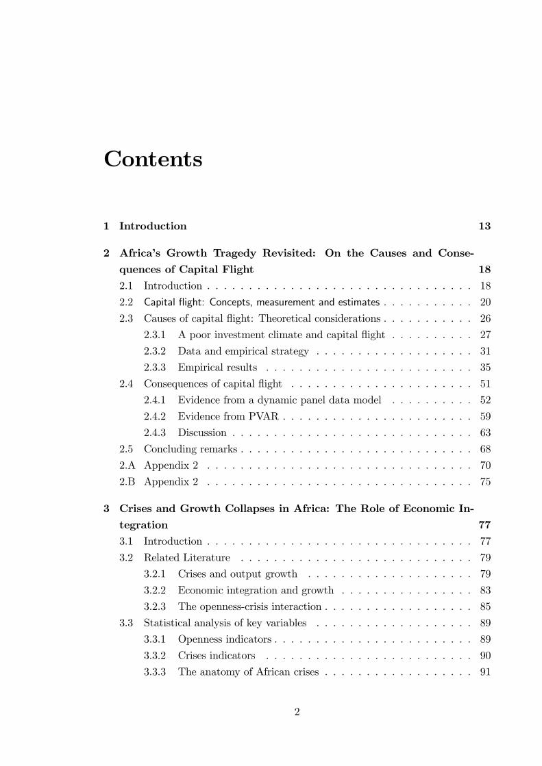
Contents
1 Introduction 13
2 Africa�s Growth Tragedy Revisited: On the Causes and Conse-quences of Capital Flight 182.1 Introduction . . . . . . . . . . . . . . . . . . . . . . . . . . . . . . . . 18
2.2 Capital �ight: Concepts, measurement and estimates . . . . . . . . . . . 20
2.3 Causes of capital �ight: Theoretical considerations . . . . . . . . . . . 26
2.3.1 A poor investment climate and capital �ight . . . . . . . . . . 27
2.3.2 Data and empirical strategy . . . . . . . . . . . . . . . . . . . 31
2.3.3 Empirical results . . . . . . . . . . . . . . . . . . . . . . . . . 35
2.4 Consequences of capital �ight . . . . . . . . . . . . . . . . . . . . . . 51
2.4.1 Evidence from a dynamic panel data model . . . . . . . . . . 52
2.4.2 Evidence from PVAR . . . . . . . . . . . . . . . . . . . . . . . 59
2.4.3 Discussion . . . . . . . . . . . . . . . . . . . . . . . . . . . . . 63
2.5 Concluding remarks . . . . . . . . . . . . . . . . . . . . . . . . . . . . 68
2.A Appendix 2 . . . . . . . . . . . . . . . . . . . . . . . . . . . . . . . . 70
2.B Appendix 2 . . . . . . . . . . . . . . . . . . . . . . . . . . . . . . . . 75
3 Crises and Growth Collapses in Africa: The Role of Economic In-tegration 773.1 Introduction . . . . . . . . . . . . . . . . . . . . . . . . . . . . . . . . 77
3.2 Related Literature . . . . . . . . . . . . . . . . . . . . . . . . . . . . 79
3.2.1 Crises and output growth . . . . . . . . . . . . . . . . . . . . 79
3.2.2 Economic integration and growth . . . . . . . . . . . . . . . . 83
3.2.3 The openness-crisis interaction . . . . . . . . . . . . . . . . . . 85
3.3 Statistical analysis of key variables . . . . . . . . . . . . . . . . . . . 89
3.3.1 Openness indicators . . . . . . . . . . . . . . . . . . . . . . . . 89
3.3.2 Crises indicators . . . . . . . . . . . . . . . . . . . . . . . . . 90
3.3.3 The anatomy of African crises . . . . . . . . . . . . . . . . . . 91
2
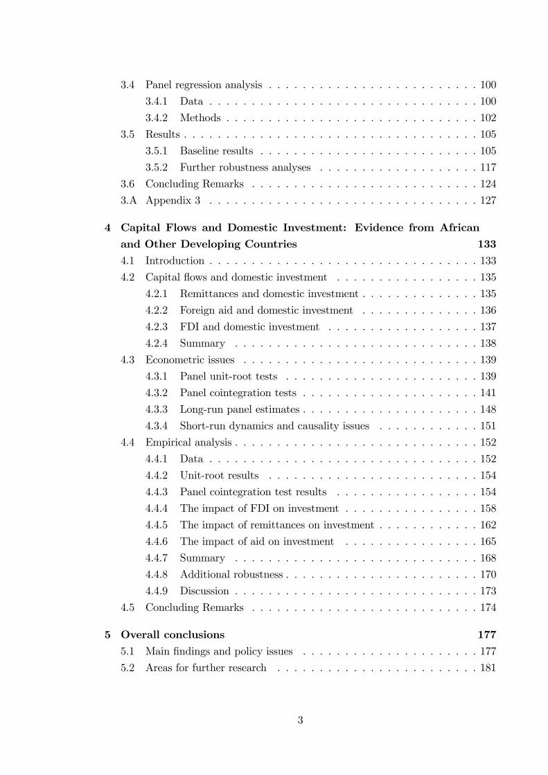
3.4 Panel regression analysis . . . . . . . . . . . . . . . . . . . . . . . . . 100
3.4.1 Data . . . . . . . . . . . . . . . . . . . . . . . . . . . . . . . . 100
3.4.2 Methods . . . . . . . . . . . . . . . . . . . . . . . . . . . . . . 102
3.5 Results . . . . . . . . . . . . . . . . . . . . . . . . . . . . . . . . . . . 105
3.5.1 Baseline results . . . . . . . . . . . . . . . . . . . . . . . . . . 105
3.5.2 Further robustness analyses . . . . . . . . . . . . . . . . . . . 117
3.6 Concluding Remarks . . . . . . . . . . . . . . . . . . . . . . . . . . . 124
3.A Appendix 3 . . . . . . . . . . . . . . . . . . . . . . . . . . . . . . . . 127
4 Capital Flows and Domestic Investment: Evidence from Africanand Other Developing Countries 1334.1 Introduction . . . . . . . . . . . . . . . . . . . . . . . . . . . . . . . . 133
4.2 Capital �ows and domestic investment . . . . . . . . . . . . . . . . . 135
4.2.1 Remittances and domestic investment . . . . . . . . . . . . . . 135
4.2.2 Foreign aid and domestic investment . . . . . . . . . . . . . . 136
4.2.3 FDI and domestic investment . . . . . . . . . . . . . . . . . . 137
4.2.4 Summary . . . . . . . . . . . . . . . . . . . . . . . . . . . . . 138
4.3 Econometric issues . . . . . . . . . . . . . . . . . . . . . . . . . . . . 139
4.3.1 Panel unit-root tests . . . . . . . . . . . . . . . . . . . . . . . 139
4.3.2 Panel cointegration tests . . . . . . . . . . . . . . . . . . . . . 141
4.3.3 Long-run panel estimates . . . . . . . . . . . . . . . . . . . . . 148
4.3.4 Short-run dynamics and causality issues . . . . . . . . . . . . 151
4.4 Empirical analysis . . . . . . . . . . . . . . . . . . . . . . . . . . . . . 152
4.4.1 Data . . . . . . . . . . . . . . . . . . . . . . . . . . . . . . . . 152
4.4.2 Unit-root results . . . . . . . . . . . . . . . . . . . . . . . . . 154
4.4.3 Panel cointegration test results . . . . . . . . . . . . . . . . . 154
4.4.4 The impact of FDI on investment . . . . . . . . . . . . . . . . 158
4.4.5 The impact of remittances on investment . . . . . . . . . . . . 162
4.4.6 The impact of aid on investment . . . . . . . . . . . . . . . . 165
4.4.7 Summary . . . . . . . . . . . . . . . . . . . . . . . . . . . . . 168
4.4.8 Additional robustness . . . . . . . . . . . . . . . . . . . . . . . 170
4.4.9 Discussion . . . . . . . . . . . . . . . . . . . . . . . . . . . . . 173
4.5 Concluding Remarks . . . . . . . . . . . . . . . . . . . . . . . . . . . 174
5 Overall conclusions 1775.1 Main �ndings and policy issues . . . . . . . . . . . . . . . . . . . . . 177
5.2 Areas for further research . . . . . . . . . . . . . . . . . . . . . . . . 181
3

Bibliography 183
Final Word Count: 41995
4
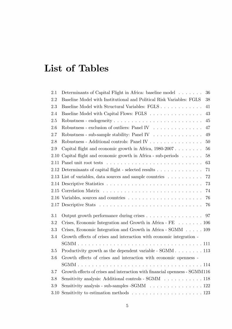
List of Tables
2.1 Determinants of Capital Flight in Africa: baseline model . . . . . . . 36
2.2 Baseline Model with Institutional and Political Risk Variables: FGLS 38
2.3 Baseline Model with Structural Variables: FGLS . . . . . . . . . . . . 41
2.4 Baseline Model with Capital Flows: FGLS . . . . . . . . . . . . . . . 43
2.5 Robustness - endogeneity . . . . . . . . . . . . . . . . . . . . . . . . . 45
2.6 Robustness - exclusion of outliers: Panel IV . . . . . . . . . . . . . . 47
2.7 Robustness - sub-sample stability: Panel IV . . . . . . . . . . . . . . 49
2.8 Robustness - Additional controls: Panel IV . . . . . . . . . . . . . . . 50
2.9 Capital �ight and economic growth in Africa, 1980-2007 . . . . . . . . 56
2.10 Capital �ight and economic growth in Africa - sub-periods . . . . . . 58
2.11 Panel unit root tests . . . . . . . . . . . . . . . . . . . . . . . . . . . 63
2.12 Determinants of capital �ight - selected results . . . . . . . . . . . . . 71
2.13 List of variables, data sources and sample countries . . . . . . . . . . 72
2.14 Descriptive Statistics . . . . . . . . . . . . . . . . . . . . . . . . . . . 73
2.15 Correlation Matrix . . . . . . . . . . . . . . . . . . . . . . . . . . . . 74
2.16 Variables, sources and countries . . . . . . . . . . . . . . . . . . . . . 76
2.17 Descriptive Stats . . . . . . . . . . . . . . . . . . . . . . . . . . . . . 76
3.1 Output growth performance during crises . . . . . . . . . . . . . . . . 97
3.2 Crises, Economic Integration and Growth in Africa - FE . . . . . . . 106
3.3 Crises, Economic Integration and Growth in Africa - SGMM . . . . . 109
3.4 Growth e¤ects of crises and interaction with economic integration -
SGMM . . . . . . . . . . . . . . . . . . . . . . . . . . . . . . . . . . . 111
3.5 Productivity growth as the dependent variable - SGMM . . . . . . . . 113
3.6 Growth e¤ects of crises and interaction with economic openness -
SGMM . . . . . . . . . . . . . . . . . . . . . . . . . . . . . . . . . . . 114
3.7 Growth e¤ects of crises and interaction with �nancial openness - SGMM116
3.8 Sensitivity analysis: Additional controls - SGMM . . . . . . . . . . . 118
3.9 Sensitivity analysis - sub-samples -SGMM . . . . . . . . . . . . . . . 122
3.10 Sensitivity to estimation methods . . . . . . . . . . . . . . . . . . . . 123
5
3.11 Descriptive statistics . . . . . . . . . . . . . . . . . . . . . . . . . . . 130
3.12 Correlations between crises and growth . . . . . . . . . . . . . . . . . 130
3.13 Correlations between openness and growth . . . . . . . . . . . . . . . 131
3.14 Correlations between crisis and openness . . . . . . . . . . . . . . . . 131
3.15 Data sources . . . . . . . . . . . . . . . . . . . . . . . . . . . . . . . . 132
4.1 Panel unit root test results . . . . . . . . . . . . . . . . . . . . . . . . 155
4.2 Panel cointegration test results: Full sample . . . . . . . . . . . . . . 156
4.3 Panel cointegration test results: Sub-samples . . . . . . . . . . . . . . 157
4.4 Panel cointegration with cross-sectional dependence . . . . . . . . . . 159
4.5 Cross-sectional independence tests . . . . . . . . . . . . . . . . . . . . 159
4.6 Panel cointegration with structural breaks and cross-sectional depen-
dence . . . . . . . . . . . . . . . . . . . . . . . . . . . . . . . . . . . . 160
4.7 The impact of FDI on investment . . . . . . . . . . . . . . . . . . . . 162
4.8 DOLS country estimates for FDI . . . . . . . . . . . . . . . . . . . . 163
4.9 Short-run dynamics and causality for FDI . . . . . . . . . . . . . . . 164
4.10 The impact of REM on investment . . . . . . . . . . . . . . . . . . . 165
4.11 DOLS country estimates for REM . . . . . . . . . . . . . . . . . . . . 166
4.12 Short-run dynamics and causality for REM . . . . . . . . . . . . . . . 167
4.13 The impact of AID on investment . . . . . . . . . . . . . . . . . . . . 168
4.14 Short-run dynamics and causality for AID . . . . . . . . . . . . . . . 169
4.15 The e¤ects of capital �ows on investment . . . . . . . . . . . . . . . . 172
6
List of Figures
2.1 Average CF (% GDP) from Africa . . . . . . . . . . . . . . . . . . . . 25
2.2 Impulse-responses for 1-4 lag bivariate VAR of CF and INV . . . . . 64
2.3 Impulse-responses for 1-4 lag bivariate VAR of CF and output . . . . 65
3.1 Average growth performance around crisis episodes in Africa . . . . . 93
3.2 Growth performance around a sudden stop crisis (Guinea-Bissau) . . 94
3.3 Growth performance around a sovereign debt crisis (Niger) . . . . . . 94
3.4 Growth performance around a currency crisis (Ethiopia) . . . . . . . 95
3.5 Growth performance around a twin crisis (Mozambique) . . . . . . . 95
3.6 Output growth and economic integration during debt crises . . . . . . 98
3.7 Output growth and �nancial openness during debt crises . . . . . . . 98
3.8 Output growth and short-term debt during debt crises . . . . . . . . 99
3.9 Output growth and international reserves during debt crises . . . . . 99
3.10 Currency crises in Africa . . . . . . . . . . . . . . . . . . . . . . . . . 128
3.11 Sovereign debt crises in Africa . . . . . . . . . . . . . . . . . . . . . . 128
3.12 Sudden stop episodes in Africa . . . . . . . . . . . . . . . . . . . . . . 129
3.13 Twin crises in Africa . . . . . . . . . . . . . . . . . . . . . . . . . . . 129
4.1 Outlier removals: WD-DOLS estimates . . . . . . . . . . . . . . . . . 170
7
Abstract
This thesis explores three important factors that have been central to the pursuitof economic development in developing countries, particularly those in Africa. Theseare capital �ows, economic integration and �nancial crises.
Chapter 1 examines the causes and consequences of capital �ight in Africancountries. Building on standard portfolio choice model, the study links the phe-nomenon of capital �ight to the domestic investment climate (broadly de�ned) andshows that African agents move their portfolios abroad as a result of a deterioratingdomestic investment climate where the risk-adjusted rate of return is unfavourable.The results presented suggest that economic risk, policy distortions and the poorpro�tability of African investments explain the variation in capital �ight. In addi-tion, employing a PVAR and its corresponding impulse responses, the chapter showsthat capital �ight shocks worsen economic performance.
Chapter 2 explores the (independent) e¤ects of crises and openness on a largesample of African countries using dynamic panel techniques. Focusing on suddenstops, currency, twin and sovereign debt crises, the chapter shows that economiccrises are associated with growth collapses in Africa. In contrast, economic opennessis found to be bene�cial to growth. More importantly, we �nd that, consistent withstandard Mundell-Flemming type models and sticky-price open economy models,greater openness to trade and �nancial �ows mitigates the adverse e¤ects of crises.
In the �nal chapter, we examine whether capital �ows such as FDI, foreign aidand migrant remittances crowd-in or crowd-out domestic investment in developingcountries. Applying recently developed panel cointegration techniques which canhandle cross-sectional heterogeneity, serial correlation and endogeneity, we �nd thatFDI and remittances have a positive and signi�cant e¤ect on domestic investment inthe long-run while aid tends to act as a substitute for investment. We also conductpanel Granger causality analysis and �nd that the e¤ect of FDI on investmentis both transitory as well as permanent. That is, it tends to crowd-in domesticinvestment both in the short-run and in the long-run. We do not �nd any causallinks between foreign aid and investment. The results show that, while remittancesdo not have causal e¤ects on investment in the short-run, there is a bidirectional(causal) relationship between the two in the long-run.
8

DeclarationI declare that no portion of the work referred to in the thesis has been submitted
in support of an application for another degree or quali�cation of this or any otheruniversity or other institute of learning.
9
Copyright Statementi. The author of this thesis (including any appendices and/or schedules to thisthesis) owns certain copyright or related rights in it (the �Copyright�) and hehas given The University of Manchester certain rights to use such Copyright,including for administrative purposes.
ii. Copies of this thesis, either in full or in extracts and whether in hard orelectronic copy, may be made only in accordance with the Copyright, Designsand Patents Act 1988 (as amended) and regulations issued under it or, whereappropriate, in accordance with licensing agreements which the University hasfrom time to time. This page must form part of any such copies made.
iii. The ownership of certain Copyright, patents, designs, trade marks and otherintellectual property (the �Intellectual Property�) and any reproductions ofcopyright works in the thesis, for example graphs and tables (�Reproduc-tions�), which may be described in this thesis, may not be owned by theauthor and may be owned by third parties. Such Intellectual Property andReproductions cannot and must not be made available for use without theprior written permission of the owner(s) of the relevant Intellectual Propertyand/or Reproductions.
iv. Further information on the conditions under which disclosure, publication andcommercialisation of this thesis, the Copyright and any Intellectual Propertyand/or Reproductions described in it may take place is available in the Uni-versity IP Policy
see http://www.campus.manchester.ac.uk/medialibrary/policies/intellectualproperty.pdf,
in any relevant Thesis restriction declarations deposited in the University Li-brary, The University Library�s regulations
see http://www.manchester.ac.uk/library/aboutus/regulations
and in The University�s policy on presentation of Theses.
10

Dedication
To my dear mother [Allaha daayo]&
To the loving memory of my father [Allaha u naxariisto]
11
Acknowledgement
Pursuing a doctoral degree in economics is a long and sometimes tough journey. Iwould like to thank all those who made my journey a joyful one. In particular, Iam greatly indebted to my supervisors, Dr Bernard Walters and Dr Katsushi Imai,for their support and guidance throughout my research. I wish also to thank theSchool of Social Sciences and the Economics Department for funding my PhD.
I must also express my profound gratitude to my friends at the Economics Depart-ment for all the insightful discussions we shared. Special thanks go to Dr Sha�ulAzam, Dr. Laurence Roope, Zeeshan Atiq and Natina Yaduma for their invaluableinput and comments on the �nal draft of the thesis. I especially want to thankObbey Elamin, Adams Adama and Dr Maria Quattri for always being there for mewhenever I needed them.
During my PhD studies, I had the opportunity to present my research (including twoof the chapters in this thesis) at international conferences including the InternationalEconomic Association 16th World Congress (Beijing, China) and the CSAE 25thConference on Economic Development in Africa (University of Oxford) as well as ata number of seminars at the University of Manchester. I wish to acknowledge thesuggestions, critics and comments I received from the participants.
I am also thankful to Prof. Joakim Westerlund and Prof. Jörg Breitung for allowingme to use their GAUSS codes.
I wish to pay tribute to my dear mother and late father for being a great sourceof inspiration to me. This thesis is dedicated to them. My heartfelt thanks andappreciation goes to my adoptive mother, Zainab, without whom I would not bewhere I am today.
Last but not least, I would like to thank my wife, Rahma and children Adnan, Nadia,Amina and Hannah for their love and sacri�ces. Without the care and dedicationof my wife, my life would truly have been tough.
12
Chapter 1
Introduction
�Despite a lower level of wealth per worker than any other region, Africanwealth owners have chosen to locate 39% of their portfolios outsideAfrica�.
- Collier and Gunning (1999; pp 92-93)
The role and movement of capital �ows has, for a long time, been a hotly contested
issue among economists and policymakers. During the Bretton Wood conference
of 1944, for example, the principal architects of the global �nancial order, John
Maynard Keynes and Harry Dexter White, were extremely concerned with the mo-
bility of capital across borders. In their view, �capital �ight from poorer countries
needed to be regulated in order to reduce the scale of international �nancial crises,
enhance the policy autonomy of poorer countries and preserve a stable exchange
rate�(Helleiner, 2005: 289-90).
Almost 70 years on, developing countries, particularly those in Sub-Saharan
Africa (SSA), are experiencing a substantial out�ow of domestic private capital.
Evidence shows that SSA has the highest incidence of capital out�ows relative to
both GDP and overall private wealth as close to half of all private portfolios are
held outside the region (Collier et al. 2001; Collier and Gunning, 1999). A recent
study suggests that around $700 billion has left the region between 1970 and 2008
(Ndikumana and Boyce, 2011). This is in spite of the fact that the continent suf-
fers from chronic internal and external imbalances, compelling it to rely heavily on
foreign savings. In particular, it is highly dependent on aid to �nance a consider-
13
able portion of its investment and import demand. Similarly, most countries in the
region have accumulated a substantial amount of foreign borrowing to cover their
domestic imbalances.
In order to reduce the overreliance on foreign savings and at the same time to
contain capital �ight, virtually all African countries have put in place policies that
entail trade and �nancial liberalisation. The basic premise of these reforms was
that increased international trade and �nancial integration could propel African
economies to a high-growth trajectory. At the same time, many developing countries,
including most African economies, have implemented policies and measures aimed
at attracting foreign direct investment (FDI) into their economies while remittance
�ows have become an indispensable source of development �nance in the developing
world.
Nonetheless, like other developing countries in other regions, African economies
have also encountered their share of economic and �nancial crises. As recent global
events illustrate, crises can have devastating e¤ects on economic activity and can
hit countries with strong, as well as those with weak, macroeconomic fundamentals.
Thus, economists and policymakers are increasingly concerned with understanding
the genesis, evolution and consequences of economic crises.
In light of these preliminary observations, this thesis is broadly concerned with
capital �ows, openness, crises and economic performance. It consists of three inde-
pendent essays with particular reference to African countries. In what follows, we
summarise the content of each of the three substantive chapters.
Chapter 2: Africa�s Growth Tragedy Revisited: On the Causes and Consequencesof Capital Flight
If basic economic theory is anything to go by, then capital-scarce less developed
countries (LDCs) should be able to retain own domestic capital since the marginal
returns are higher there. Capital �ight, the out�ow of foreign exchange from poorer
countries, seems to defy that logic. The objective of this essay is to examine the
14
determinants and output costs of these out�ows in the case of SSA.
In the �rst part of the essay, we provide a systematic account of why African
agents engage in capital �ight by adopting a portfolio-choice framework. In partic-
ular, we link African capital out�ows to the attractiveness of the domestic invest-
ment climate and postulate that African agents consider all available information
to make optimal choices regarding whether to shift their wealth abroad or not. For
the purpose of our empirical analysis, we identify four dimensions of the domestic
investment climate at the macroeconomic level, which we argue are important deter-
minants of private capital out�ows. The impact of each dimension on capital �ight
is empirically tested using annual panel data for 37 SSA countries over the 1980-
2000 period. The results suggest that an improved investment climate in the form of
more pro�table opportunities, a sound macroeconomic environment, less economic
risk and good institutions are associated with lower capital �ight in Africa.
In the second part of the essay, we estimate a dynamic growth model using the
bias corrected least-squares dummy variable estimator developed by Kiviet (1995;
1999), Bun and Kiviet (2003) and extended by Bruno (2005) on a panel dataset
for 37 SSA economies over the 1980-2007 period, and show that capital �ight is
associated with a poor growth performance. To capture the dynamic response of
domestic investment and economic growth to capital �ight episodes, we estimate
a bivariate panel vector autoregression (PVAR) model and its associated impulse
response functions which con�rm that capital �ight is harmful to both domestic
capital formation and growth.
Chapter 3: Crises and Growth Collapses in Africa: The Role of Economic Inte-gration
In the past few decades, many African countries have implemented policies of trade
and �nancial liberalisation. At same time, many of them have encountered economic
and �nancial crises. This chapter explores the (independent) e¤ects of crises and
openness on a large sample of African countries using dynamic panel techniques.
15
More speci�cally, it explores whether greater openness to trade and �nancial �ows
exacerbates or lessens the adverse e¤ects of crises. The chapter is particularly in-
terested in four di¤erent types of crises, namely, sudden stops, currency, twin and
sovereign debt crises. To our knowledge, this is the �rst attempt in understanding
the e¤ects of these types of crises in the context of African countries. Most of the
existing literature focuses on mainly emerging markets, even though many African
countries have also been subject to these types of crises.
The study shows that crises are associated with growth collapses in Africa. In
contrast, economic openness is found to be bene�cial to growth. More importantly,
we �nd that, consistent with standardMundell-Flemming type models, greater open-
ness to trade and �nancial �ows mitigate the adverse e¤ects of crises. We identify
three important channels through which this can occur. First, openness (particularly
to trade but also to �nancial �ows) tends to lessen the adjustment costs associated
with external crises. This suggests that it is associated with quicker recoveries facil-
itated by higher output in the tradable sector which would keep the fall in domestic
demand in check. Second, at times of crises, open economies tend to enjoy more
room for manoeuvre (e.g. trade credits) than closed ones. Finally, openness is asso-
ciated with higher solvency through greater willingness to meet outstanding external
liabilities for fear of sanctions in case of default.
Chapter 4: Capital Flows and Domestic Investment: Evidence from Panel Coin-tegration
Capital �ows, both o¢ cial and private, play a pivotal role in �nancing development
in poorer countries. The three most important types are o¢ cial aid, FDI and remit-
tances. The objective of this chapter is to examine whether these �ows �crowd-in�
or �crowd-out� domestic investment in developing countries. The study uses re-
cently developed panel cointegration techniques on a balanced panel of 47 countries,
including 21 African economies. More speci�cally, we pay a particular attention to
the time series properties of the variables under study. At the same time, we take
16
into account issues such as cross-sectional dependence, structural breaks and regime
shifts.
We begin by assessing whether capital �ows and domestic investment form a
stable long-run relationship. We show that this is in fact the case. We then estimate
the nature of this relationship using a range of estimators and �nd that FDI and
remittances have a robust crowding-in e¤ect on domestic investment in the long-
run. On the contrary, foreign aid has a crowding-out e¤ect on investment. We then
conduct panel Granger causality analysis and �nd that foreign aid does not have a
causal e¤ect on investment and vice versa.
On the other hand, we show that there is a two-way causality between remit-
tances and investment in the long-run but no causal link in the short-run. That
is to say, increases in investment are a result of as well as a cause of increases in
remittances in the long-run. Two mechanisms are highlighted: remittances could
be used to enhance human capital (e.g. education and health), this in turn could
improve the (rate and/or productivity of) domestic investment in the long-run. In
turn, increases in the accumulation of capital investments by remittance-receiving
households may cause more remittances in the long-run (assuming that self-interest
dominates altruistic motives).
With respect to FDI, the study �nds that there is a bi-directional relationship
between FDI and investment in the short-run. This suggests that, on the one hand,
the FDI activity may crowd-in domestic �rms by, for example, demanding more of
their products. On the other hand, the FDI activity may itself take place as a result
of increased domestic investment which the multinational corporation may interpret
as a re�ection of the soundness of the economy. In the long-run, however, we �nd
that there is a unidirectional causal link between FDI and domestic investment,
running from FDI to investment. Overall, we interpret these �ndings as evidence
that FDI has both transitory positive e¤ects as well as permanent bene�cial e¤ects
on investment.
17
Chapter 2
Africa�s Growth TragedyRevisited: On the Causes andConsequences of Capital Flight
2.1 Introduction
Sub-Saharan Africa�s (SSA) economic performance for the past four decades has
been characterised by economic stagnation. As a result, the region has consistently
su¤ered from balance of payment disequilibria, dwindling government �nances, in-
creasing macroeconomic and political instability and, as a consequence, a higher
incidence of poverty (Artadi and Sala-i-Martin, 2003; Collier, 2006). These per-
sistent economic di¢ culties have meant that Africa has become heavily reliant on
external �nancing. More speci�cally, the region is highly dependent on aid for a con-
siderable portion of its investments and imports. Similarly, most of the countries in
the region have been identi�ed by the Highly Indebted Poor Countries Initiative as
having unsustainably high levels of debt.
However, paradoxically, the signi�cant in�ow of o¢ cial capital (debt and aid)
to SSA has been accompanied by a substantial out�ow of domestic private capital.
Compared to other developing regions, it has been shown that SSA has the highest
incidence of capital �ight relative to both GDP and overall private wealth; close
to 40 percent of all private portfolios are held outside the region (Collier et al.
2001; Collier and Gunning, 1999). A recent study by Ndikumana and Boyce (2008)
18
shows that the magnitude of SSA portfolios held abroad surpasses its total liabilities,
making it a net creditor to the rest of the world.
A natural question that arises is: what factors are driving private capital out of
Africa? This question has attracted a large body of research which, broadly speak-
ing, identi�es macroeconomic and political conditions as the main cause of African
capital �ight (see for example, Lensink et al. 1998; Collier et al. 2001; Ndiku-
mana and Boyce, 2003; Ndiaye 2009). While these contributions have enhanced
our understanding of this phenomenon, they mostly fail to consider non-traditional
determinants such as governance and the structural features of the African countries.
We attempt to remedy this shortcoming by providing a systematic account of
why African agents engage in capital �ight. We adopt a portfolio-choice frame-
work and link African capital �ight to the attractiveness of the domestic investment
climate. The importance of the domestic investment climate in attracting foreign
investment has long been recognised in the literature. This chapter addresses the
related but neglected issue, namely the role the domestic investment climate can
play in determining whether local entrepreneurs retain their portfolios domestically.
The investment climate is de�ned as the structural, institutional, and overall
macroeconomic environments which confront economic agents, whether they be
�rms, entrepreneurs or individuals. We argue that these location-speci�c factors
determine not only the incentive structures facing agents, but also the (pro�table)
opportunities available within the domestic economy (World Bank, 2005). For the
purpose of our empirical analysis, we identify four dimensions of the domestic in-
vestment climate at the macroeconomic level. The impact of each dimension on
capital �ight is empirically tested using annual panel data for 37 SSA countries over
the 1980-2000 period. The empirical analysis suggests that an improved investment
climate in the form of more pro�table opportunities, a sound macroeconomic envi-
ronment, less economic risk and good institutions are associated with lower capital
�ight in Africa. This �nding is robust to the exclusion of outliers, sub-samples, and
19
to endogeneity concerns.
We also explore the macroeconomic consequences of capital �ight. To this end,
we conduct two types of analyses. First, we augment a fairly standard growth
regression with our measure of capital �ight using recently developed dynamic panel
techniques on a sample of 37 SSA countries over the period 1980-2007. Second, we
estimate a panel vector autoregression (PVAR) model and generate its corresponding
impulse response functions in order to unravel how economic growth and domestic
investment react to capital �ight shocks. The results suggest that capital �ight is
associated with poorer economic performance.
The chapter is organised as follows. Section 2 sets out the concept and mea-
surement of capital �ight. Section 3 examines the drivers of capital �ight and con-
tains the analytical framework, presenting the data, econometric model and results.
Section 4 examines the consequences of capital �ight, describing the methods and
discussing the results. Finally, Section 5 concludes.
2.2 Capital �ight: Concepts, measurement and esti-mates
"Capital �ight is -like the proverbial elephant- easier to identify than to de-�ne". Lessard and Williamson, 1987. p.1
There is a vast and growing theoretical and empirical literature on capital �ight.
However, providing a rigorous de�nition of this concept has proven a di¢ cult task
even though the late economic historian Charles Kindleberger traces it back to the
Revocation of the Edict of Nantes in 1685 (Kindleberger, 1987). Essentially, two
strategies have been adopted when trying to de�ne capital �ight; one strand of the
literature attempts to distinguish it from �normal�capital out�ows in terms of mo-
tive. This �motivational�de�nition was �rst used by Kindleberger in his well-known
work on the nature of short-term capital movements where he viewed capital �ight
20
as �abnormal�out�ows �propelled from a country...by ...any one or more of a com-
plex list of fears and suspicions�(Kindleberger, 1937, p. 158 quoted in Lessard and
Williamson, 1987 p. 202). This implies that capital �ight, unlike normal portfolio
adjustments, is driven by �a signi�cant perceived deterioration in risk-return pro-
�les associated with assets located in a particular country�(Walter, 1987 p. 105).
Policy induced distortions such as anticipated tax hikes, expected devaluation and
expropriation of assets have been identi�ed as some of the factors that propel capital
to ��ee�.
According to Lessard and Williamson (1987, p. 203) capital �ight is �that which
�ees from the perception of abnormal risks at home�. Some researchers within this
strand further argue that the di¤erence between normal capital out�ows and capital
�ight lies in the fact that the latter is in con�ict with the interests of the country
in question by imposing an economic cost on the whole economy and violating the
�social contract� (Walter, 1987). Hence, the �motivational�de�nition implies that
investors from capital-scarce LDCs move their capital abroad not in pursuit of better
oppurtunities elswhere but rather in fear of higher perceived risks at home. As a
result, the action of an American acquiring assets abroad would be termed �normal�
capital out�ows whereas a Kenyan purchasing those same assets would be regarded
as engaging in �capital �ight�.
A formidable weakness with the above de�nition, however, is that it is impossible
to empirically isolate �normal�capital out�ows from capital �ight in terms ofmotives.
In fact, the above literature has so far failed to device a measure of capital �ight
that is able to successfully distinguish �distortion-induced abnormal out�ows�from
ordinary portfolio diversi�cations (see also Gordon and Levine, 1989).
Cuddington (1986) on the other hand con�nes capital �ight to only short term,
speculative or �hot money��ows that leave a given economy in response to either
risks or deterioration of expected returns to investment. According to Cuddington
(1986), hot money �ows tend to respond swiftly to �political and �nancial crises,
21
heavier taxes .. tightning of capital controls, or major devaluation[s] .. or actual or
incipient hyperin�ation�(p. 2). In addition, he postulates that short-term �ows are
more sensative to adverse shocks since they can easily be moved to other favourable
destinations especially given the nature of modern capital markets. But what Cud-
dington seems to ignore is the fact that investors who are scaping adverse domestic
shocks may also acquire real assets abroad (eg. land, equipments etc) or purchase
longer-term stocks, government bonds and deposits that have maturities greater
than 1 year (Chang et al. 1997). Furthermore, long-term capital may also react
swiftly to macroeconomic changes since the modern global �nancial markets elimi-
nate to a greater extent any lequidity loss associated with acquiring long-term bonds
or equities (ibid). In particular, long-term securities such as bonds and stocks can
increasingly be traded in secondary markets almost as easily as short-term instru-
ments such as T-Bills and commertial papers.
The second strand of the literature avoids the distinction between �normal�cap-
ital out�ows and capital �ight and de�nes all build up of foreign assets from capital
scarce countries as capital �ight. This �contextual�de�nition, �rst proposed by the
World Bank (1985), argues that capital �ight is inherently related to the notion
of national welfare loss. In particular, it is stressed that for a country - unable to
cover its investment, import and government budgetary requirements or service its
liabilities �any systematic capital out�ows represent a great constraint on its eco-
nomic development potential. This �contextual�de�nition makes the measurement
of capital �ight more tractable and �ts well with our view that capital �ight diverts
resources away from domestic real investment in capital-starved economies such as
those in SSA. In their seminal paper on the consquences of capital �ight, Deppler
and Williamson (1987) essert the following:
"the fundamental economic concern about capital �ight ... is that it
reduces welfare in the sense that it leads to a net loss in the total real
resources available to an economy for investment and growth. That is,
capital �ight is viewed as a diversion of domestic savings away from �-
22
nancing domestic real investment and in favor of foreign �nancial invest-
ment. As a result, the pace of growth and development of the economy
is retarded from what it otherwise would have been" (p. 52).
The above is quoted at length because it captures one of the main motivations
behind the present research. But of course a critical reader may question the valid-
ity of the assumption that capital moved from an LDC economy diverts resources
away from domestic investment. Gordon and Levine (1989) for example argue that
domestic savings could be used for consumption instead of investment or alterna-
tively it could be used to purchase in�ation �hedges�(e.g. real estate) with little
impact on overall economic growth. Even if this was the case, however, the pro-
found detrimental e¤ects of �capital �ight�go beyond reductions in domestic savings
and include less government revenues, increased macroeconomic instability through
herding behaviour, and widened macroeconomic imbalances.
Thus, we de�ne capital �ight as the out�ow of foreign exchange from poorer
countries so our aim is to attempt to explain why any resident capital (be it reported
or unreported, long or short-term) would be moved from African economies with
limited capital and where presumably the marginal product is higher.
Since the accumulation of foreign assets by agents in LDCs may not be (properly)
captured in o¢ cial statistics, one can residually derive the net increases in the ex-
ternal assets by turning to the well-known fundamental balance of payments (BOP)
identity for an open economy. This states that changes in o¢ cial reserves (RES)
must be equal to the sum of the current account (CA), capital account (KA), net
errors and omissions (EO):
�RES = CA+KA+ EO (2.1)
For ease of exposition, the capital account, KA1, can be split into o¢ cial capital
1The �ows can be divided into those that are destined for the o¢ cial sector and those of theprivate sector. In the �rst case, we are essentially concerned with increases in external indebtedness(�DEBT ), while in the latter we are concerned with net equity �ows of the private sector (NFI).
23
in�ows (�DEBT ) plus private in�ows (NFI), minus out�ows or capital �ight (CF ):
KA = �DEBT +NFI � CF (2.2)
Substituting KA from (2.2) into (2.1) and rearranging yields (with EO = 0 since it
is a balancing item):
CF = �DEBT +NFI + CA��RES (2.3)
This is the most widely used approach when estimating the phenomenon of capital
�ight. It was pioneered by the World Bank (1985) and is the broadest and most
reliable measure available. It indicates that any increase in private external assets
(capital �ight) must be o¤set by increases in o¢ cial �ows (debt), by net capital �ows
from foreign investment, by a current account surplus, or by reductions in reserves.
This relationship holds since it is directly based on the BOP accounting identity.
When expression (2.3) > 0, we have capital �ight and when it is < 0 we have a
reversal of previous out�ows2.
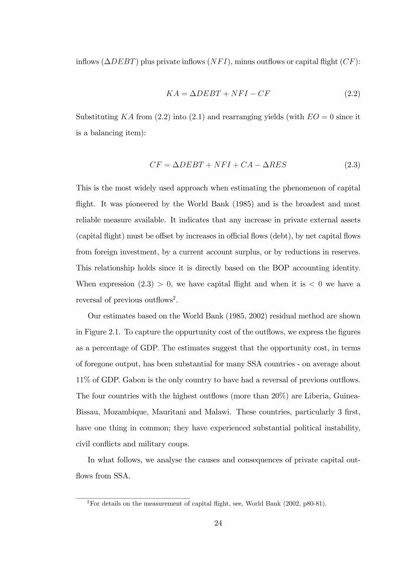
Our estimates based on the World Bank (1985, 2002) residual method are shown
in Figure 2.1. To capture the oppurtunity cost of the out�ows, we express the �gures
as a percentage of GDP. The estimates suggest that the opportunity cost, in terms
of foregone output, has been substantial for many SSA countries - on average about
11% of GDP. Gabon is the only country to have had a reversal of previous out�ows.
The four countries with the highest out�ows (more than 20%) are Liberia, Guinea-
Bissau, Mozambique, Mauritani and Malawi. These countries, particularly 3 �rst,
have one thing in common; they have experienced substantial political instability,
civil con�icts and military coups.
In what follows, we analyse the causes and consequences of private capital out-
�ows from SSA.
2For details on the measurement of capital �ight, see, World Bank (2002, p80-81).
24
GabonSouth Africa
SwazilandAngola
MauritiusEthiopiaKenya
CameroonBurkina FasoCote d'Ivoire
Congo, Dem. Rep.ZimbabweRwandaCentral African Republic
BurundibeninUganda
MadagascarTanzaniaGhana
NigerSenegalTogo
Congo, Rep.Gambia, The
Cape VerdeMaliSudanSeychellesChadComoros
ZambiaMalawi
MauritaniaMozambique
GuineaBissauLiberia
10 0 10 20 30mean of cf
Figure 2.1: Average CF (% GDP) from Africa
25
2.3 Causes of capital �ight: Theoretical consider-ations
The standard portfolio choice model, in which rational agents consider available
information to make optimal portfolio decisions, provides the analytical framework
for this chapter. Hence, it is assumed that wealth holders diversify their portfolio
holdings by acquiring a range of assets whose demand is in�uenced by relative risk-
return considerations.
Drawing on the theoretical contributions by Sheets (1995), Collier et al. (2001)
and Le and Zak (2006), we link the acquisition of foreign assets (i.e. capital �ight
episodes) to the risk-return features prevailing in African countries. Sheets (1995)
is one of the �rst to explicitly apply a portfolio choice framework in the context
of capital �ight. His model suggests that capital �ight is determined by the usual
risk diversi�cation motive along with two important incentives, namely relative risk
and return di¤erentials. The �rst incentive implies that capital �ight arises due
to factors that raise the relative riskiness of the domestic economy. The second
incentive highlights factors that a¤ect the macroeconomic environment adversely
and thus reduce the risk-adjusted returns to domestic assets.
Along these lines, Le and Zak (2006) show that the decision to invest domestically
is a function of the risk-return features prevailing in a given country relative to
world markets. More speci�cally, agents will retain their portfolio holdings within
their own country when domestic pro�tability improves relative to abroad and when
economic risk decreases.
In this study, we generalise the risk-return characteristics to include the whole
domestic investment climate. In particular, we postulate that capital �ight simply
takes place in response to deteriorating domestic economic conditions where the risk-
adjusted rate of return to investments is unfavourable. In the following subsection,
we identify four factors that in�uence the domestic investment climate, and hence
the decision of agents whether to engage in capital �ight.
26
2.3.1 A poor investment climate and capital �ight
Our central hypothesis is that a poor domestic investment climate changes the rel-
ative risk and returns of domestically held assets in such a way that, following the
implications of portfolio choice theory, incentives for capital �ight are created. We
distinguish four factors that, at the macroeconomic level, in�uence the investment
climate and hence the likelihood of capital �ight: risk-return features; institutions
and political risk; structural features; and the composition of capital �ows.
Risk and return features
We posit that the relative riskiness and pro�tability of domestic investments deter-
mines whether or not capital �ight takes place. An important contributor to the
relative riskiness of LDCs is indebtedness. It is generally accepted that a high debt
burden increases insecurity as to future tax and public investment levels, through its
e¤ects on the debt service capacity of the government. This, in turn, may translate
into a greater likelihood of budget de�cits, possible in�ationary �nancing, and ex-
change rate volatility - all of which disadvantage domestic assets relative to foreign
assets. Similarly, a high level of indebtedness increases the country�s vulnerabil-
ity to external shocks, which heightens uncertainty over expected future returns to
investments. There is overwhelming evidence in support of the hypothesis that in-
debtedness increases risk and thus causes capital �ight in LDCs (see for example,
Cerra et al. 2008; Ndikumana and Boyce, 2003; Collier et al. 2001; Lensink et al.
2000).
Another source of increased riskiness in developing countries is the likelihood of
economic crises. In particular, low levels of international reserves, which imply a
higher probability of a balance of payment crisis, can adversely a¤ect the domestic
investment climate. Similarly, unsustainable budget de�cits, which may cause agents
to lose con�dence in the ability of the government to manage the economy, have
27
been identi�ed as important sources of uncertainty. A number of studies provide
empirical evidence that risk indicators such as low levels of o¢ cial reserves and
weak government budget positions are associated with increased capital �ight (see
for example, Hermes and Lensink, 2001; Cerra at al. 2008).
Furthermore, the speci�c macroeconomic policies pursued by the government
directly in�uence the riskiness of the domestic economy and hence the investment
climate. For instance, macroeconomic instability in the form of high and volatile
in�ation erodes the real value of domestic assets. Similarly, poor exchange rate
management, such as an overvalued currency or a black market premium, may
contribute to economic uncertainty, as they generate incorrect signals to economic
agents (Edwards, 1989). The existing evidence suggests that currency overvaluation,
in particular, can be harmful since it may result in lower economic growth, a higher
probability of speculative attacks, shortages of foreign exchange and balance of pay-
ments crises (Rodrik, 2008). These distortionary macroeconomic policies have (at
least historically) been the norm rather than the exception in most African countries
(Collier and Gunning, 1999). The literature on the determinants of capital �ight
identi�es macroeconomic instability and currency overvaluation as important fac-
tors that explain cross-country variation in capital �ight (see for example, Lensink
et al. 1998; Le and Zak, 2006; Ndiaye, 2009).
An important factor that may prompt domestic capital to �ee is low domestic
returns to investments. A standard proxy for the relative pro�tability of domestic
investments is the interest rate di¤erential between the domestic and world markets
(proxied by the US Treasury Bill rate). A large di¤erential implies that domestic
agents, in an attempt to maximise their portfolios, substitute into foreign assets if
the yield on short-term instruments is higher. That capital �ight may take place in
response to poor returns to domestic investments is supported by numerous studies.
For example, Collier et al. (2004) report that in their sample of countries returns
to capital abroad and domestic economic as well as political conditions determine
28
capital �ight. Fedderke and Liu (2002) �nd that domestic and foreign rates of return
play a crucial role in explaining capital out�ows from South Africa.
Institutions and political risk
It is largely accepted that good quality institutions are essential for the domestic
investment climate. As emphasised by North (1990), institutions, both formal and
informal, arise as a result of agents�attempts to reduce transaction costs and uncer-
tainties. Hence, �high quality�institutions are associated with higher rates of return
since they lower transaction costs.
Recent contributions (Acemoglu and Johnson, 2005; Acemoglu et al. 2001) show
that institutions directly in�uence whether economic agents engage in productive
investments or not. The decision to invest domestically, for example, depends on
whether property rights and other investment-promoting institutions are in place
(North, 1990). In the absence of these, agents must internalise additional costs (for
example, protection of own capital investments) or other payments in the case of
corruption. In addition, uncertainty about property rights causes a wedge between
the marginal product of capital and its rate of return (Svensson, 1998).
Moreover, an increasing body of evidence shows that improvements in the insti-
tutional framework are associated with productivity gains (Hall and Jones, 1999).
It has been established that countries with weak institutions tend to pursue dis-
tortionary macroeconomic policies (e.g. high and variable in�ation, large budget
de�cits and misaligned exchange rates) which worsen the domestic investment cli-
mate (Acemoglu et al. 2003).
The existing empirical evidence supports the view that a �good� institutional
development is associated with a lower incidence of capital �ight (see for example,
Lensink et al. 2000; Collier et al. 2004; Le and Zak, 2006; Cerra et al. 2008).
29
Structural features
In this study, we argue that the structural features of SSA economies may make
them susceptible to particular shocks, which may adversely a¤ect their economic
performance. For example, low export diversi�cation and high primary commodity
dependence have been found to increase African economies�vulnerability to terms
of trade shocks (Collier and Dollar, 2004). Similarly, as emphasised by the �resource
curse�literature, natural resource abundance and the rents it generates may have
contributed to Africa�s corruption, political instability and civil con�icts (Collier
and Hoe er, 1998; Sachs and Warner, 2001). However, if the rents are used for
productive investments (e.g. Botswana), the �curse�should disappear and resources
would then be associated with better domestic investment environments.
A profound change to the structures of African countries in the past two decades
is the increased liberalisation of trade. However, the impact of trade openness on
the domestic investment climate is ambiguous a priori. To the extent that increased
integration imports external volatility, the e¤ects would be negative. If, however,
trade openness results in static and/or dynamic gains in the form of better allocation
of resources, then improved productivity and more pro�table investment opportu-
nities would follow. A contribution of this study is that it attempts to investigate
how African countries�structural features may relate to the phenomenon of capital
�ight from the region.
The composition of capital �ows
The type and composition of capital �ows to SSA may have consequences for the
domestic investment climate. For most African countries, foreign aid is still one of
the most important sources of �nance. However, the e¤ects of aid on the investment
climate are highly controversial. Some argue (for example, Knack, 2001) that aid
may be detrimental to the investment climate of recipient countries as it tends to
30
encourage corruption and rent-seeking, while others (for example, Hansen and Tarp,
2001) suggest that it improves the economic performance of recipient economies.
Empirically, the literature on capital �ight has produced mixed results; for example,
Lensink et al. (2000), Hermes and Lensink (2001) and Collier et al. (2004) identify
development aid as a signi�cant determinant of capital �ight, whereas Cerra et al.
(2008) �nd the opposite. Some types of capital �ows, such as short-term borrowing,
are known to weaken the investment climate, since they encourage economic risk
(Rodrik and Velasco, 1999). Ndiaye (2009) �nds evidence that short-term debt
fuels capital �ight in his sample of African countries. The impact of other types of
private capital �ows such as FDI, on capital �ight is ambiguous. Some studies (for
example, Kant, 1996) suggest that FDI reduces capital �ight through its bene�cial
e¤ect on the domestic investment climate, which gains empirical support in the work
of Harrigan et al. (2002) and Cerra et al. (2008).
In summary, we hypothesise that capital �ight from Africa is linked to the re-
gion�s poor domestic investment climate. In what follows, we test this empirically.
2.3.2 Data and empirical strategy
The empirical strategy we adopt consists of �rst estimating a baseline model and
then augmenting it with indicators that capture the di¤erent dimensions of the
domestic investment climate. In doing so, we adopt an incremental approach ex-
amining one dimension at a time. The baseline model consists of a set of variables
that capture the policy environment and the risk-return features of the countries in
the sample. Unless otherwise stated, all the data are drawn from the World Bank�s
World Development Indicators (2009) and the baseline model is given by:
CFit = �0 + riskit�0 + returnit +$Yit + �i + �t + "it (2.4)
where CFit denotes capital �ight as a percentage of GDP, �i is time invariant
31
country-speci�c �xed e¤ect, �t is a time speci�c e¤ect, "it is the error term and
i and t represent country and time period, respectively. The vector, riskit, contains
distortionary policy indicators such as macroeconomic instability (proxied by the log
of CPI in�ation), exchange rate overvaluation (measured by the degree to which the
domestic currency deviates from Purchasing Power Parity), and the black market
premium - a symptom of a tightly controlled foreign exchange market (measured by
the ratio of the parallel exchange rate to the o¢ cial rate), the latter two variables
are sourced from the Global Development Network Growth database (2009). As
additional indicators of economic risk, we use the level of foreign reserves (measured
as months of imports) and indebtedness (measured by net �ows of long-term debt
as a percentage of GDP). We use this particular indebtedness indicator since it cap-
tures new borrowing (including IMF purchases), debt service and interest payments.
Hence it is closely linked with changes in domestic economic conditions and provides
a good re�ection of the extent to which domestic assets are viewed �risky�.
To capture the rate of return on investment in each African country (returnit),
we use the deposit rate di¤erential between that country and that of world markets
(proxied by the US T-bill rate), adjusted for exchange rate changes. We also control
for the overall level of economic development using the logarithm of real per capita
income denoted by Yit.
Our dataset covers 37 SSA economies over the period 1980-2000 as consistent
data on our proxies for macroeconomic distortions are only available till 2000. The
de�nitions and sources for all the variables, along with a list of the countries are
provided in Table 2.13 in Appendix 2A.
To investigate the role institutions play in explaining capital �ight from Africa,
we add to the baseline speci�cation a set of institutional and political risk vari-
ables, namely property rights, institutional quality, political stability, governance,
and ethnic fractionalisation. Following Acemoglu et al. (2003), we use Polity IV�s
constraint on the executive as a measure of property rights protection. This variable
32
captures procedural rules which constrain political leaders and other powerful elites
and thus is closely linked with the security of private property rights (Acemoglu et
al. 2003).
To capture the quality of African political institutions, we use �institutional qual-
ity�which is a summary index based on three International Country Risk Guide
(ICRG) institutional sub-components, namely: corruption; rule of law; and bureau-
cratic quality, scaled 0-1. �Political stability� is proxied by the average Freedom
House political rights and civil liberty scores (both variables are drawn from Hade-
nius and Teorell, 2007). �Governance�is measured by the Polity2 score, which cap-
tures the constraints placed on the chief executive, the competitiveness of political
participation, and the openness of executive recruitment. A higher value of any of
the institutional measures implies a better quality of institutions, meaning stronger
property rights, less likelihood for political instability etc. Finally, we also control for
ethnic fractionalisation since Easterly and Levine (1997) link it to Africa�s �growth
tragedy�.
To examine how the structural features of African countries relate to the phenom-
enon of capital �ight, the baseline speci�cation is augmented with a set of structural
variables: the terms of trade; primary export dependence (constructed by Sachs and
Warner, 2000 and drawn from Azam and Hoe er, 2002); government size (captured
by government expenditure as a percentage of GDP); trade openness (imports plus
exports as percent of GDP); and resource abundance (measured by mineral exports
as a percentage of total exports: from IMF DOTS, 2009).
Finally, to examine how the composition of in�ows impacts on the extent of
capital �ight, we add three capital �ow variables to the baseline speci�cation: foreign
aid (measured in terms of a percentage of GNI); FDI (expressed in percentage of
GNP); and short term debt (measured as a percentage of long term debt, the World
Bank�s Global Development Finance database, 2009).
We �rst estimate equation (2.4) using the pooled ordinary least squares estima-
33
tor (POLS) with robust standard errors. However, since the POLS estimator yields
biased results in the presence of unobserved country-speci�c e¤ects, we also apply
conventional static panel models such as random (RE) and �xed e¤ects (FE). The
RE estimator requires that the country-speci�c e¤ect is uncorrelated with the inde-
pendent variables while the FE is consistent irrespective of whether this is true or
not.
Since standard macroeconomic datasets are prone to panel heteroscedasticity
and serial correlation, we test for group-wise heteroscedasticity and serial correla-
tion using the modi�ed Wald test (Greene, 2000) and the Wooldridge (2002) test,
respectively. While both FE and RE can handle panel heteroscedasticity, neither
overcomes serial correlation, which, if not properly addressed, leads to consistent
but ine¢ cient results (Baltagi, 2006). Throughout, (see Tables 2.1-2.4 below), we
�nd that the within country residuals are serially correlated and the null hypothesis
of homoscedasticity is strongly rejected. To take account of these potential biases,
we use Feasible Generalised Least Squares (FGLS), which allows estimation in the
presence of autocorrelation within panels and heteroskedasticity and cross-sectional
correlation across panels.
Tables 2.14 and 2.15 report respectively the summary statistics and pair wise
correlations of the variables. The mean of capital �ight for the sample is 13.3
percent of GDP and ranges in value between -95.4 and 128.4 percent, both for
Liberia. Table 2.14 also shows that, on average, international reserves in Africa are
below the recommended level of 3 - 4 months of import cover while in�ation amounts
to 6 percent.
The correlation matrix shows that capital �ight has the expected association with
all the baseline variables except return di¤erential. As expected, capital �ight is in-
versely correlated with the measures of institutional development. At the same time,
it is positively associated with government size, trade openness, primary commodity
dependence and terms of trade, and negatively correlated with natural resources.
34
Moreover, the correlation between capital �ight and all the measures of capital �ows
is positive, somewhat consistent with previous results.
2.3.3 Empirical results
Baseline model
Table 2.1 presents our baseline model which controls for the level of economic devel-
opment (log per capita income), economic risk (level of foreign reserves and indebt-
edness) and macroeconomic distortionary policies (black market premium, macro-
economic instability [log CPI in�ation] and currency overvaluation) and pro�tability
(return di¤erential). In all speci�cations, the results indicate that the higher the
level of economic development in the form of increased per capita incomes, the lower
the incentives for capital �ight. The regressions also show that reserve holdings have
a negative and signi�cant association with capital �ight, presumably because they
help bu¤er the economy from balance of payments crises. As in Ndikumana and
Boyce (2008) and Collier et al. (2001), we �nd that higher levels of indebtedness
are associated with increased capital �ight; this may re�ect the relative riskiness of
African countries.
As expected, we �nd that currency overvaluation helps to explain the occurrence
of capital �ight in Africa. The coe¢ cient of this variable is positive and highly signif-
icant, implying that, on average, African economies with misaligned exchange rates
tend to experience more capital �ight, perhaps re�ecting expectations about future
depreciation of the currency. This is in line with the previous �ndings reported
by Collier et al. (2001) for their African sample. Not surprisingly, macroeconomic
instability is positively related to capital �ight. This implies that the acquisition
of foreign assets may act as a hedge against losses due to a poor domestic macro-
economic environment. However, this variable is insigni�cant at conventional levels.
The black market premium, which has been extensively used as a proxy for trade
distortions, enters with an unexpected negative but signi�cant sign. A plausible
35
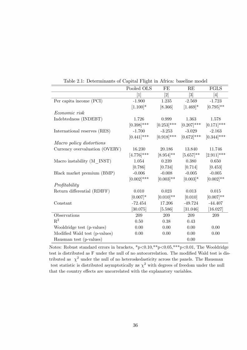
Table 2.1: Determinants of Capital Flight in Africa: baseline model
Pooled OLS FE RE FGLS[1] [2] [3] [4]
Per capita income (PCI) -1.900 1.235 -2.569 -1.723[1.100]* [8.366] [1.469]* [0.795]**
Economic riskIndebtedness (INDEBT) 1.726 0.999 1.363 1.578
[0.398]*** [0.253]*** [0.207]*** [0.171]***International reserves (RES) -1.700 -3.253 -3.029 -2.163
[0.441]*** [0.918]*** [0.672]*** [0.344]***Macro policy distortionsCurrency overvaluation (OVERV) 16.230 20.186 13.840 11.746
[4.776]*** [8.954]** [5.657]** [2.911]***Macro instability (M_INST) 1.054 0.239 0.380 0.650
[0.786] [0.734] [0.714] [0.453]Black market premium (BMP) -0.006 -0.008 -0.005 -0.005
[0.002]*** [0.003]** [0.003]* [0.002]**Pro�tabilityReturn di¤erential (RDIFF) 0.010 0.023 0.013 0.015
[0.007]* [0.010]** [0.010] [0.007]**Constant -72.454 17.206 -49.724 -44.407
[30.075] [5.586] [31.046] [16.027]Observations 209 209 209 209R2 0.50 0.38 0.43Wooldridge test (p-values) 0.00 0.00 0.00 0.00Modi�ed Wald test (p-values) 0.00 0.00 0.00 0.00Hausman test (p-values) 0.00
Notes: Robust standard errors in brackets, *p<0.10,**p<0.05,***p<0.01, The Wooldridgetest is distributed as F under the null of no autocorrelation. The modi�ed Wald test is dis-tributed as �2 under the null of no heteroskedasticity across the panels. The Hausmantest statistic is distributed asymptotically as �2 with degrees of freedom under the nullthat the country e¤ects are uncorrelated with the explanatory variables.
36
explanation for this could be that when the spread between the o¢ cial and parallel
market exchange rate is high, domestic agents can sell their foreign exchange holdings
at a premium, which implies a substitution away from foreign assets. Alternatively,
it could be that the legal restrictions on domestic residents taking funds outside
the country may have been e¤ective. Finally, we include the �return di¤erential�
between each country and that of world markets and �nd a positive and signi�cant
e¤ect. This supports Sheets�(1995) �return di¤erential incentive�, suggesting that
when the yield on domestic instruments is low relative to overseas, foreign assets
become attractive.
In summary, the preceding results con�rm that capital �ight from Africa is sig-
ni�cantly linked to the region�s poor pro�tability, economic risk and macroeconomic
policy distortions.
Institutional and political risk variables
We now consider the role institutional and political risk indicators play in explaining
capital �ight from Africa. Each institutional measure is �rstly added to the baseline
model separately in order to examine its direct association with capital �ight. We
report only the estimates based on the FGLS for the following main reasons: 1) Even
though both the FE and RE can overcome heteroscedasticity, neither can handle
serial correlation, which, if not properly taken into account, leads to consistent but
ine¢ cient estimates (Baltagi, 2006), and 2) when there is an AR(1) error structure
within the cross-sections and heteroscedasticity across the groups, neither estimates
of the FE nor that of the RE is optimal under both the null and alternative of the
standard Hausman test. In particular, the standard formulae for the their variances
are invalid (for a discussion see Yu, 2009). Hence, we only report the results based
on the more e¢ cient estimator of FGLS.
Table 2.2 contains the results. In column [1], we augment the baseline speci�-
cation with our measure of �political stability�and �nd that it is inversely related
to the phenomenon of capital �ight, suggesting that countries with stable political
37
Table 2.2: Baseline Model with Institutional and Political Risk Variables: FGLS
[1] [2] [3] [4] [5] [6]BMP -0.004 -0.005 -0.021 -0.032 -0.019 -0.051
[0.002]** [0.002]** [0.008]** [0.011]*** [0.009]** [0.010]***OVERV 8.459 10.788 14.927 17.744 14.098 20.898
[2.965]*** [3.009]*** [2.678]*** [3.807]*** [3.075]*** [4.241]***M_INST 0.709 0.814 1.639 1.368 1.326 2.582
[0.449] [0.491]* [0.549]*** [0.543]** [0.526]** [0.503]***RES -1.959 -2.252 -2.249 -2.857 -2.290 -2.047
[0.342]*** [0.383]*** [0.396]*** [0.413]*** [0.382]*** [0.511]***PCI 0.358 -1.925 -2.441 -3.447 -1.946 -0.348
[1.002] [0.794]** [0.812]*** [1.346]** [0.792]** [1.293]RDIFF 0.011 0.015 0.014 0.034 0.010 0.030
[0.007] [0.007]** [0.015] [0.018]* [0.017] [0.022]INDEBT 1.598 1.558 1.665 0.727 1.620 0.967
[0.166]*** [0.173]*** [0.179]*** [0.279]*** [0.181]*** [0.237]***POL_STAB -1.102 -0.975
[0.409]*** [0.565]*ETHNIC -6.378 -14.218
[2.713]** [4.802]***PRR -1.302 -3.685
[0.474]*** [0.889]***IQ -17.633 -40.987
[5.936]*** [6.495]***GOV -0.263
[0.189]N 209 203 186 110 186 90Tests (p-values)Wooldridge 0.00 0.00 0.00 0.00 0.00 0.00WALD 0.00 0.00 0.00 0.00 0.00 0.00
Notes: Robust standard errors in brackets, *p<0.10,**p<0.05,***p<0.01, the Wooldridgetest is distributed as F under the null of no autocorrelation. The modi�ed Wald test is dis-tributed as �2 under the null of no heteroskedasticity across the panels.
38
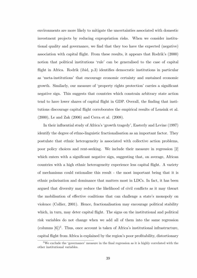
environments are more likely to mitigate the uncertainties associated with domestic
investment projects by reducing expropriation risks. When we consider institu-
tional quality and governance, we �nd that they too have the expected (negative)
association with capital �ight. From these results, it appears that Rodrik�s (2000)
notion that political institutions �rule� can be generalised to the case of capital
�ight in Africa. Rodrik (ibid, p.3) identi�es democratic institutions in particular
as �meta-institutions� that encourage economic certainty and sustained economic
growth. Similarly, our measure of �property rights protection�carries a signi�cant
negative sign. This suggests that countries which constrain arbitrary state action
tend to have lower shares of capital �ight in GDP. Overall, the �nding that insti-
tutions discourage capital �ight corroborates the empirical results of Lensink et al.
(2000), Le and Zak (2006) and Cerra et al. (2008).
In their in�uential study of Africa�s �growth tragedy�, Easterly and Levine (1997)
identify the degree of ethno-linguistic fractionalisation as an important factor. They
postulate that ethnic heterogeneity is associated with collective action problems,
poor policy choices and rent-seeking. We include their measure in regression [2]
which enters with a signi�cant negative sign, suggesting that, on average, African
countries with a high ethnic heterogeneity experience less capital �ight. A variety
of mechanisms could rationalise this result - the most important being that it is
ethnic polarisation and dominance that matters most in LDCs. In fact, it has been
argued that diversity may reduce the likelihood of civil con�icts as it may thwart
the mobilisation of e¤ective coalitions that can challenge a state�s monopoly on
violence (Collier, 2001). Hence, fractionalisation may encourage political stability
which, in turn, may deter capital �ight. The signs on the institutional and political
risk variables do not change when we add all of them into the same regression
(columns [6])3. Thus, once account is taken of Africa�s institutional infrastructure,
capital �ight from Africa is explained by the region�s poor pro�tability, distortionary
3We exclude the �governance�measure in the �nal regression as it is highly correlated with theother institutional variables.
39
macroeconomic policies and high risk.
Structural Variables
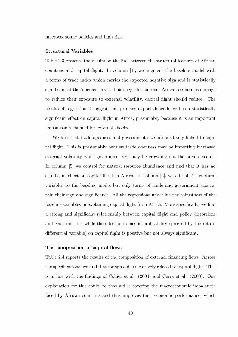
Table 2.3 presents the results on the link between the structural features of African
countries and capital �ight. In column [1], we augment the baseline model with
a terms of trade index which carries the expected negative sign and is statistically
signi�cant at the 5 percent level. This suggests that once African economies manage
to reduce their exposure to external volatility, capital �ight should reduce. The
results of regression 2 suggest that primary export dependence has a statistically
signi�cant e¤ect on capital �ight in Africa, presumably because it is an important
transmission channel for external shocks.
We �nd that trade openness and government size are positively linked to capi-
tal �ight. This is presumably because trade openness may be importing increased
external volatility while government size may be crowding out the private sector.
In column [5] we control for natural resource abundance and �nd that it has no
signi�cant e¤ect on capital �ight in Africa. In column [6], we add all 5 structural
variables to the baseline model but only terms of trade and government size re-
tain their sign and signi�cance. All the regressions underline the robustness of the
baseline variables in explaining capital �ight from Africa. More speci�cally, we �nd
a strong and signi�cant relationship between capital �ight and policy distortions
and economic risk while the e¤ect of domestic pro�tability (proxied by the return
di¤erential variable) on capital �ight is positive but not always signi�cant.
The composition of capital �ows
Table 2.4 reports the results of the composition of external �nancing �ows. Across
the speci�cations, we �nd that foreign aid is negatively related to capital �ight. This
is in line with the �ndings of Collier et al. (2004) and Cerra et al. (2008). One
explanation for this could be that aid is covering the macroeconomic imbalances
faced by African countries and thus improves their economic performance, which
40
Table 2.3: Baseline Model with Structural Variables: FGLS
[1] [2] [3] [4] [5] [6]BMP -0.006 -0.004 -0.004 -0.004 -0.006 -0.004
[0.002]*** [0.002]** [0.002]** [0.002]* [0.002]** [0.002]*OVERV 13.826 11.181 11.598 10.746 15.905 15.220
[2.932]*** [2.955]*** [3.004]*** [2.948]*** [3.032]*** [4.517]***M_INST 1.374 0.785 1.032 0.422 0.760 1.560
[0.513]*** [0.530] [0.513]** [0.454] [0.533] [0.650]**RES -2.123 -2.298 -1.835 -2.352 -1.907 -0.942
[0.391]*** [0.366]*** [0.418]*** [0.363]*** [0.422]*** [0.570]*PCI -1.578 -2.341 -2.018 -3.363 -1.615 -3.782
[0.848]* [0.863]*** [0.785]** [1.024]*** [0.972]* [1.656]**RDIFF 0.017 0.011 0.013 0.011 0.015 0.009
[0.007]** [0.007] [0.007]* [0.007] [0.008]* [0.008]INDEBT 1.538 1.659 1.584 1.482 1.491 1.316
[0.169]*** [0.186]*** [0.180]*** [0.170]*** [0.205]*** [0.267]***TOTR -0.038 -0.063
[0.014]*** [0.026]**PRI_COMM 10.127 -3.265
[5.691]* [10.332]GOV_SIZE 0.243 0.761
[0.118]** [0.222]***OPENNESS 0.080 0.078
[0.031]** [0.051]RESOURCES -0.036 0.011
[0.036] [0.032]Observations 196 190 194 207 174 140Tests (p-values)Wooldridge 0.00 0.00 0.00 0.00 0.00 0.00Wald 0.00 0.00 0.00 0.00 0.00 0.00
Notes: Robust standard errors in brackets, *p<0.10,**p<0.05,***p<0.01,the Wooldridge test is distributed as F under the null of no autocorrelation.The modi�ed Wald test is distributed as �2 under the null of noheteroskedasticity across the panels.
41
then translates into less capital �ight. Alternatively, the tendency for aid in�ows
to reduce capital �ight be linked to debt cancellations which tend to improve the
domestic investment climate. Regression [2], by contrast, suggests that FDI is as-
sociated with higher out�ows of endogenous capital - a result which is statistically
signi�cant at the 1 percent level. Provided that this is a causal link, the estimated
coe¢ cient would suggest that a one percentage point increase in the share of FDI
to GNP will produce a 1.9 percentage point rise in the ratio of capital �ight to
GDP. This can be interpreted in two ways. It could be that this �nding is related to
the nature of FDI to most African countries, which is mostly connected to natural
resource exploitation with little or no forward and backward linkages with the wider
economy. Alternatively, this result could be linked to crisis conditions within the
host economy which prevent pro�t repatriation.
We �nd, supporting Ndiaye (2009), a signi�cant positive e¤ect of short term
borrowing on capital �ight in Africa. This is in line with the results of a broader
research agenda on the role of short term liabilities in fostering �nancial instability
in LDCs (see for example, Radelet and Sachs, 1998; Rodrik and Velasco, 1999).
Regression [4] estimates an extended speci�cation which includes all of our capital
�ow variables. As can be seen, our results remain largely unchanged.
Based on our results so far, we can state that economic risk, policy distortions
and poor pro�tability of African investments help to explain the variation in capital
�ight from the region. In addition, we account for the role structural, institutional
and external resource �ows play in shaping agents�portfolio choice in Africa. The
estimated results show that these factors, to the extent that they a¤ect the domestic
investment climate, are positively related to capital �ight.
Robustness checks: Endogeneity
Our preceding results, which indicated that there is a robust relationship between the
domestic investment climate and capital �ight, may be subject to endogeneity and
reverse causality. There is some evidence (see for example, Ndikumana and Boyce,
42
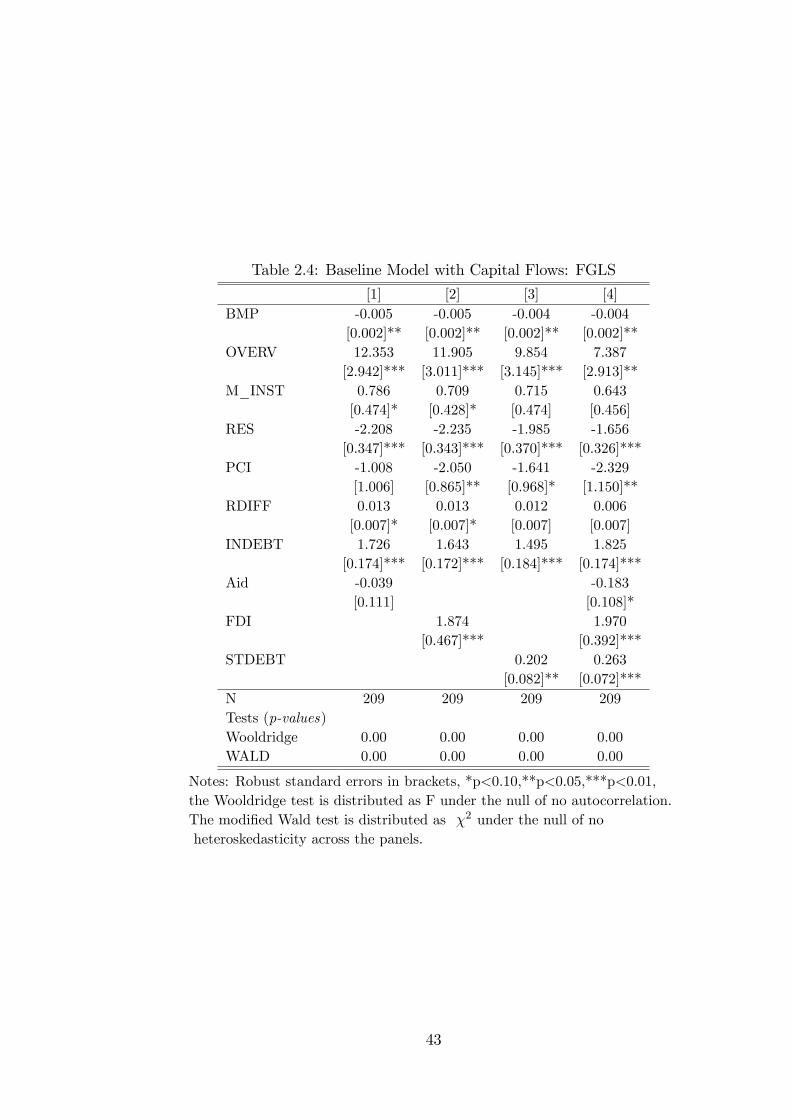
Table 2.4: Baseline Model with Capital Flows: FGLS
[1] [2] [3] [4]BMP -0.005 -0.005 -0.004 -0.004
[0.002]** [0.002]** [0.002]** [0.002]**OVERV 12.353 11.905 9.854 7.387
[2.942]*** [3.011]*** [3.145]*** [2.913]**M_INST 0.786 0.709 0.715 0.643
[0.474]* [0.428]* [0.474] [0.456]RES -2.208 -2.235 -1.985 -1.656
[0.347]*** [0.343]*** [0.370]*** [0.326]***PCI -1.008 -2.050 -1.641 -2.329
[1.006] [0.865]** [0.968]* [1.150]**RDIFF 0.013 0.013 0.012 0.006
[0.007]* [0.007]* [0.007] [0.007]INDEBT 1.726 1.643 1.495 1.825
[0.174]*** [0.172]*** [0.184]*** [0.174]***Aid -0.039 -0.183
[0.111] [0.108]*FDI 1.874 1.970
[0.467]*** [0.392]***STDEBT 0.202 0.263
[0.082]** [0.072]***N 209 209 209 209Tests (p-values)Wooldridge 0.00 0.00 0.00 0.00WALD 0.00 0.00 0.00 0.00
Notes: Robust standard errors in brackets, *p<0.10,**p<0.05,***p<0.01,the Wooldridge test is distributed as F under the null of no autocorrelation.The modi�ed Wald test is distributed as �2 under the null of noheteroskedasticity across the panels.
43
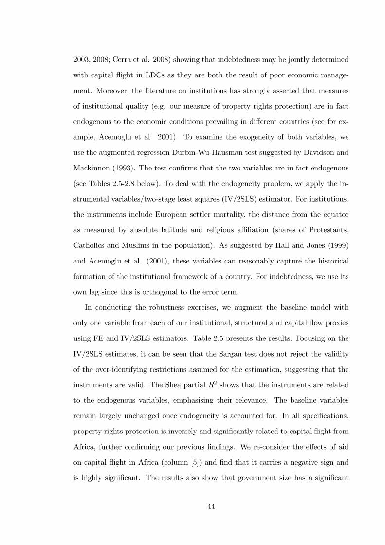
2003, 2008; Cerra et al. 2008) showing that indebtedness may be jointly determined
with capital �ight in LDCs as they are both the result of poor economic manage-
ment. Moreover, the literature on institutions has strongly asserted that measures
of institutional quality (e.g. our measure of property rights protection) are in fact
endogenous to the economic conditions prevailing in di¤erent countries (see for ex-
ample, Acemoglu et al. 2001). To examine the exogeneity of both variables, we
use the augmented regression Durbin-Wu-Hausman test suggested by Davidson and
Mackinnon (1993). The test con�rms that the two variables are in fact endogenous
(see Tables 2.5-2.8 below). To deal with the endogeneity problem, we apply the in-
strumental variables/two-stage least squares (IV/2SLS) estimator. For institutions,
the instruments include European settler mortality, the distance from the equator
as measured by absolute latitude and religious a¢ liation (shares of Protestants,
Catholics and Muslims in the population). As suggested by Hall and Jones (1999)
and Acemoglu et al. (2001), these variables can reasonably capture the historical
formation of the institutional framework of a country. For indebtedness, we use its
own lag since this is orthogonal to the error term.
In conducting the robustness exercises, we augment the baseline model with
only one variable from each of our institutional, structural and capital �ow proxies
using FE and IV/2SLS estimators. Table 2.5 presents the results. Focusing on the
IV/2SLS estimates, it can be seen that the Sargan test does not reject the validity
of the over-identifying restrictions assumed for the estimation, suggesting that the
instruments are valid. The Shea partial R2 shows that the instruments are related
to the endogenous variables, emphasising their relevance. The baseline variables
remain largely unchanged once endogeneity is accounted for. In all speci�cations,
property rights protection is inversely and signi�cantly related to capital �ight from
Africa, further con�rming our previous �ndings. We re-consider the e¤ects of aid
on capital �ight in Africa (column [5]) and �nd that it carries a negative sign and
is highly signi�cant. The results also show that government size has a signi�cant
44
Table 2.5: Robustness - endogeneity
Fixed e¤ects Panel IV[1] [2] [3] [4] [5] [6]
INDEBT 1.934 2.02 2.022 2.041 2.811 2.955[0.225]*** [0.237]*** [0.256]*** [0.311]*** [0.306]*** [0.321]***
BMP -0.043 -0.046 -0.047 -0.016 -0.014 -0.021[0.014]*** [0.014]*** [0.014]*** [0.014] [0.014] [0.014]
OVERV 23.416 20.155 21.614 9.246 10.63 10.064[7.802]*** [8.291]** [8.789]** [5.135]* [4.967]** [5.152]*
PCI 7.171 3.278 4.61 -2.995 -3.616 -4.578[9.476] [10.049] [11.477] [1.081]*** [1.083]*** [1.115]***
M_INSTAB 0.991 1.074 1.222 1.352 1.433 2.196[0.871] [0.873] [0.917] [0.830] [0.799]* [0.866]**
RES -2.159 -1.903 -1.52 -2.3 -1.664 -1.355[0.862]** [0.889]** [0.975] [0.573]*** [0.569]*** [0.573]**
RDIFF 0.075 0.077 0.077 0.058 0.058 0.058[0.027]*** [0.027]*** [0.027]*** [0.028]** [0.027]** [0.027]**
PRR -1.145 -1.221 -2.596 -3.788 -2.47 -3.017[1.003] [1.004] [1.269]** [0.913]*** [1.031]** [1.013]***
Aid -0.225 -0.248 -0.431 -0.615[0.196] [0.203] [0.141]*** [0.143]***
GOV_SIZE 0.387 0.429[0.203]* [0.155]***
N 187 187 173 145 145 133Test of exogeneity 0.05 0.04 0.03Sargan test 0.26 0.48 0.27Shea partial R-squared from �rst stage
Indebtedness 0.58 0.68 0.67Property rights 0.53 0.47 0.56
Notes: Robust standard errors in brackets, *p<0.10,**p<0.05,***p<0.01,the Davidson-MacKinnon test of exogeneity tests the null that an OLS-typeestimator would yield consistent estimates. The null of the Sargan test is that theover-identifying restrictions are valid. The Shea partial R-squared is atest of instrument relevancy.
45
positive relationship with capital �ight (column [6]).
Robustness checks: Outliers
To investigate further the robustness of the baseline results, we take into account
the possible presence of outliers which may distort the estimates. In line with East-
erly et al. (2004), we use Hadi�s (1994) method for detecting in�uential outliers in
multivariate regressions, removing distant data points that fall in the 5 percent crit-
ical level. The results, shown in Table 2.6, highlight that our fundamental �ndings
are robust to the exclusion of outliers. However, while the e¤ects of risk and macro
distortionary indicators are signi�cant, the impact of the pro�tability of investments
in Africa (proxied by the return di¤erential variable) is insigni�cant. In columns ([2
�4]), we reconsider the e¤ects of property rights protection on capital �ight. The
results suggest that this variable, perhaps by facilitating transactions and reducing
risks, expands domestic investment opportunities and thus curtails capital �ight in
our African sample. In line with our previous �ndings, we �nd that countries with
a higher government expenditures in GDP experience higher incidence of capital
�ight, a result which is statistically signi�cant. Finally, once outliers are removed
the coe¢ cient of the aid variable retains its sign but is marginally insigni�cant.
Robustness checks: Sub-sample stability
In Table 2.7, we evaluate the stability of the estimates across sub-periods, focusing
on the 1980-89 sub-period. We are particularly interested in this period because
macroeconomic mismanagement and crises were rife in most African countries dur-
ing this �lost decade�. The results show that our risk and policy distortion indicators
retain their sign and signi�cance unlike our measures of pro�tability. Also, property
rights, government size and foreign aid are still robustly related to capital �ight
from Africa. Hence, our results point to the importance of the domestic investment
climate for economic agents�portfolio-choice. In particular, weak institutions, poor
policy choices and increased economic riskiness, insofar as they in�uence the domes-
46
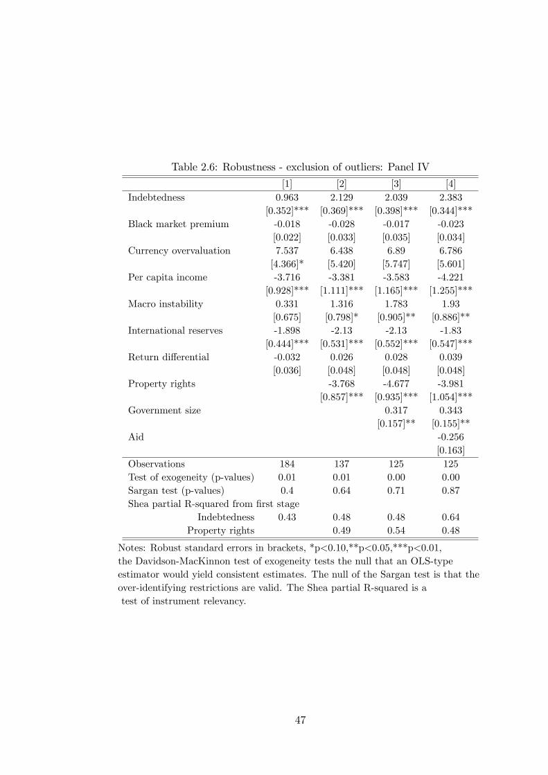
Table 2.6: Robustness - exclusion of outliers: Panel IV
[1] [2] [3] [4]Indebtedness 0.963 2.129 2.039 2.383
[0.352]*** [0.369]*** [0.398]*** [0.344]***Black market premium -0.018 -0.028 -0.017 -0.023
[0.022] [0.033] [0.035] [0.034]Currency overvaluation 7.537 6.438 6.89 6.786
[4.366]* [5.420] [5.747] [5.601]Per capita income -3.716 -3.381 -3.583 -4.221
[0.928]*** [1.111]*** [1.165]*** [1.255]***Macro instability 0.331 1.316 1.783 1.93
[0.675] [0.798]* [0.905]** [0.886]**International reserves -1.898 -2.13 -2.13 -1.83
[0.444]*** [0.531]*** [0.552]*** [0.547]***Return di¤erential -0.032 0.026 0.028 0.039
[0.036] [0.048] [0.048] [0.048]Property rights -3.768 -4.677 -3.981
[0.857]*** [0.935]*** [1.054]***Government size 0.317 0.343
[0.157]** [0.155]**Aid -0.256
[0.163]Observations 184 137 125 125Test of exogeneity (p-values) 0.01 0.01 0.00 0.00Sargan test (p-values) 0.4 0.64 0.71 0.87Shea partial R-squared from �rst stage
Indebtedness 0.43 0.48 0.48 0.64Property rights 0.49 0.54 0.48
Notes: Robust standard errors in brackets, *p<0.10,**p<0.05,***p<0.01,the Davidson-MacKinnon test of exogeneity tests the null that an OLS-typeestimator would yield consistent estimates. The null of the Sargan test is that theover-identifying restrictions are valid. The Shea partial R-squared is atest of instrument relevancy.
47
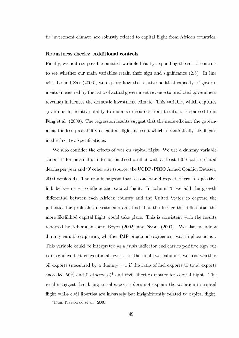
tic investment climate, are robustly related to capital �ight from African countries.
Robustness checks: Additional controls
Finally, we address possible omitted variable bias by expanding the set of controls
to see whether our main variables retain their sign and signi�cance (2.8). In line
with Le and Zak (2006), we explore how the relative political capacity of govern-
ments (measured by the ratio of actual government revenue to predicted government
revenue) in�uences the domestic investment climate. This variable, which captures
governments� relative ability to mobilise resources from taxation, is sourced from
Feng et al. (2000). The regression results suggest that the more e¢ cient the govern-
ment the less probability of capital �ight, a result which is statistically signi�cant
in the �rst two speci�cations.
We also consider the e¤ects of war on capital �ight. We use a dummy variable
coded �1�for internal or internationalised con�ict with at least 1000 battle related
deaths per year and �0�otherwise (source, the UCDP/PRIO Armed Con�ict Dataset,
2009 version 4). The results suggest that, as one would expect, there is a positive
link between civil con�icts and capital �ight. In column 3, we add the growth
di¤erential between each African country and the United States to capture the
potential for pro�table investments and �nd that the higher the di¤erential the
more likelihhod capital �ight would take place. This is consistent with the results
reported by Ndikumana and Boyce (2002) and Nyoni (2000). We also include a
dummy variable capturing whether IMF progamme agreement was in place or not.
This variable could be interpreted as a crisis indicator and carries positive sign but
is insigni�cant at conventional levels. In the �nal two columns, we test whether
oil exports (measured by a dummy = 1 if the ratio of fuel exports to total exports
exceeded 50% and 0 otherwise)4 and civil liberties matter for capital �ight. The
results suggest that being an oil exporter does not explain the variation in capital
�ight while civil liberties are inverserly but insigni�cantly related to capital �ight.4From Przeworski et al. (2000)
48
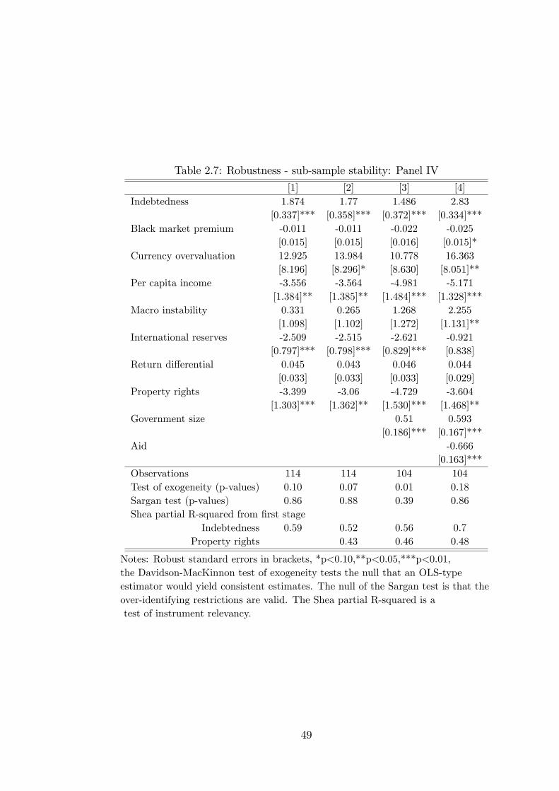
Table 2.7: Robustness - sub-sample stability: Panel IV
[1] [2] [3] [4]Indebtedness 1.874 1.77 1.486 2.83
[0.337]*** [0.358]*** [0.372]*** [0.334]***Black market premium -0.011 -0.011 -0.022 -0.025
[0.015] [0.015] [0.016] [0.015]*Currency overvaluation 12.925 13.984 10.778 16.363
[8.196] [8.296]* [8.630] [8.051]**Per capita income -3.556 -3.564 -4.981 -5.171
[1.384]** [1.385]** [1.484]*** [1.328]***Macro instability 0.331 0.265 1.268 2.255
[1.098] [1.102] [1.272] [1.131]**International reserves -2.509 -2.515 -2.621 -0.921
[0.797]*** [0.798]*** [0.829]*** [0.838]Return di¤erential 0.045 0.043 0.046 0.044
[0.033] [0.033] [0.033] [0.029]Property rights -3.399 -3.06 -4.729 -3.604
[1.303]*** [1.362]** [1.530]*** [1.468]**Government size 0.51 0.593
[0.186]*** [0.167]***Aid -0.666
[0.163]***Observations 114 114 104 104Test of exogeneity (p-values) 0.10 0.07 0.01 0.18Sargan test (p-values) 0.86 0.88 0.39 0.86Shea partial R-squared from �rst stage
Indebtedness 0.59 0.52 0.56 0.7Property rights 0.43 0.46 0.48
Notes: Robust standard errors in brackets, *p<0.10,**p<0.05,***p<0.01,the Davidson-MacKinnon test of exogeneity tests the null that an OLS-typeestimator would yield consistent estimates. The null of the Sargan test is that theover-identifying restrictions are valid. The Shea partial R-squared is atest of instrument relevancy.
49
Table 2.8: Robustness - Additional controls: Panel IV
[1] [2] [3] [4] [5] [6]PRR -2.437 -2.833 -2.475 -2.499 -2.422 -3.422
[1.034]** [1.058]*** [1.070]** [1.070]** [1.131]** [1.337]**INDEBTH 2.695 2.764 2.846 2.897 2.904 2.957
[0.307]*** [0.369]*** [0.365]*** [0.364]*** [0.365]*** [0.363]***BMP -0.028 -0.03 -0.023 -0.022 -0.022 -0.027
[0.013]** [0.012]** [0.012]* [0.013]* [0.013]* [0.013]**OVERV 12.851 8.55 9.721 10.891 11.23 11.279
[5.171]** [5.261] [5.168]* [5.515]** [5.977]* [5.815]*PCI -4.038 -2.361 -2.555 -2.471 -2.761 -2.356
[1.099]*** [1.351]* [1.314]* [1.318]* [2.747] [2.731]M_INST 2.035 0.957 0.95 1.001 1.002 1.128
[0.841]** [0.877] [0.856] [0.856] [0.857] [0.855]RES -1.449 -1.516 -1.345 -1.21 -1.228 -1.092
[0.554]*** [0.715]** [0.706]* [0.734]* [0.768] [0.759]RDIFF 0.061 0.068 0.069 0.071 0.071 0.075
[0.026]** [0.024]*** [0.024]*** [0.024]*** [0.024]*** [0.024]***Aid -0.565 -0.498 -0.58 -0.592 -0.601 -0.619
[0.138]*** [0.149]*** [0.151]*** [0.152]*** [0.161]*** [0.155]***GOV_SIZE 0.508 0.484 0.475 0.458 0.455 0.468
[0.150]*** [0.144]*** [0.141]*** [0.143]*** [0.144]*** [0.143]***GOV_EFFECT -4.383 -4.24 -3.144 -3.244 -3.226 -3.161
[2.005]** [1.911]** [1.967] [1.985] [2.000] [1.976]War 4.445 3.895 4.009 3.948 4.734
[2.449]* [2.416] [2.420]* [2.483] [2.533]*GRDIFF 0.474 0.502 0.505 0.532
[0.176]*** [0.180]*** [0.181]*** [0.180]***IMF 1.372 1.405 0.831
[2.007] [2.018] [2.050]OIL 0.874 -0.286
[7.144] [7.087]C_LIB -1.588
[1.222]Observations 136 116 115 115 115 115Test of exogeneity 0.15 0.09 0.04 0.08 0.16 0.13Sargan test 0.30 0.12 0.20 0.18 0.18 0.30Shea partial R-squared from �rst stage
Indebtedness 0.67 0.59 0.60 0.61 0.60 0.61Property rights 0.52 0.57 0.57 0.57 0.55 0.55
Notes: Robust standard errors in brackets, *p<0.10,**p<0.05,***p<0.01,the Davidson-MacKinnon test of exogeneity tests the null that an OLS-typeestimator would yield consistent estimates. The null of the Sargan test is that theover-identifying restrictions are valid. The Shea partial R-squared is atest of instrument relevancy.
50
Throughout, our central results retain their sign and signi�cance, suggesting that
omitted variable bias in not a concern.
2.4 Consequences of capital �ight
There are various channels through which capital �ight may in�uence the growth
performance of African countries. The most obvious is the investment channel as
capital �ight involves the transfer of scarce �nancial resources (domestic savings)
that could otherwise be used to augment domestic capital formation. For a typical
African economy already su¤ering from chronic internal and external imbalances,
any systematic capital out�ows would require either a reduction in the amount of
foreign exchange reserves available or an increase in external �nancing. Since there
is a limit to both, the economy would eventually need to make BOP corrections
by initiating expenditure-switching policies that boost the current account balance
and thus o¤set the initial out�ow. Alternatively, expenditure-reducing policies (e.g.
contractive monetary policy) would be needed to bring about the required adjust-
ment. Whatever measure undertaken, it is clear that resident capital out�ows would
lower savings and thus investment and economic growth at least in the short run
especially in small open economies (Deppler and Williamson, 1987, p. 224).
Furthermore, capital �ight undermines SSA governments�attempts to generate
domestic resources by eroding their already thin tax base and thus increases their
dependence on external �nancing. This may exercibate the �scal position of the
government and, in that case, the consequences might be more capital �ight. This
can be illustrated if one uses an intertemporal framework where the expectations
of economic agents become an important driver of their decisions. In particular,
provided that agents use all available information, they would expect increased
future tax liabilities as a result of the de�cit and thus may engage in future capital
51
�ight5.
Capital �ight may also impede the current and future growth potential indirectly
through its impacts on the stability of the economy. More speci�cally, it can be a
great source of macroeconomic instability since investors may interpret substantial
capital �ight as a sign of deeper economic di¢ culties and this may fuel further
�ight through herding behaviour. In addition, it has considerable social costs and
has consequences for both poverty and income inequality as the poor tend to su¤er
higher taxation or cuts in social services as a result of the decision of wealthier
segments of society to transfer their assets abroad.
Finally, capital �ight has an important political economy dimension since �it can
be a powerful political weapon against government policies that threaten the wealth
or the prerogatives of the rich� (Epstein, 2005 p. 6). In other words, the fear is
that certain government policies (e.g. higher taxes at times of crisis) which may be
bene�cial to society as a whole may alienate the rich in such a way that they decide
to take their wealth abroad. To the extent that the government does not implement
its desired policy in fear of capital �ight, its sovereignty, autonomy and credibility
are undermined. Hence, capital �ight has the potential to a¤ect income distribution,
capital formation, government �nances and the macroeconomic environment of SSA
countries adversely.
2.4.1 Evidence from a dynamic panel data model
To test the hypothesis that capital �ight hinders economic growth in Africa, we
augment a fairly standard growth model with our measure of capital �ight using the
following dynamic model speci�cation:
yit = �yi;t�1 + �CFit +Xit� + "it (2.5)
5This argument can be contrasted to the central proposition of the Ricardian equivalence whereagents are assumed to internalise the government�s budget contraint and therefore de�cits andtheir �nancing does not in�uence their decisions.
52
where for i = 1; :::N; and t = 2; :::T , yit is the growth rate of per capita income,
CFit is the share of capital �ight in GDP, "it = �it + �i with E(�it) = E(�i) =
E(�it�i) = 0, and the transient errors are assumed to serially independent, i.e.
E(�it�is) = 0 8s 6= t. Further, it assumed that E(yit�it) = 0 8 t.
The vector Xit corresponds to a set of standard growth determinants, including
domestic investment, in�ation, trade openness, �nancial deepening (captured by the
share of M2 in GDP), government expenditure and institutional quality (measured
by the �Polity2 score�from PolityIV dataset). The Polity2 score captures the con-
straints placed on the chief executive, the competitiveness of political participation,
and the openness and competitiveness of executive recruitment. It ranges from -10
to +10, with higher values implying stronger democratic institutions. A list of the
countries as well as the sources of the variables are reported in Tables 2.16 while
summary statistics are reported in Table 2.17 in Appendix 2.B.
Given the presence of the lagged dependent variable yi;t�1 which is positively
correlated with the time invariant �xed e¤ect (�i), the OLS estimator is inconsistent.
The �xed e¤ect or Least-Squares Dummy Variable (LSDV) estimator which wipes
out �i through �within�transformation does not entirely solve the problem. To show
this, take the �rst lag of (2.5):
yit�1 = �yi;t�2 + �CFit�1 +Xit�1� + "it�1; where "it�1 = �it�1 + �i (2.6)
Substituting (2.6) into (2.5), one can see that �i is now a function of yit�1 as it is in
"it�1, violating the assumption of independence between "it and yit,i.e. E(yit; "it) 6=
0. Hence, the correlation between the autoregressive variable and the transformed
error term remains, making the LSDV estimator also bias especially in short panels
(Judson and Owen, 1999).
A popular method to address the above bias has been to take the �rst di¤erence
53
of equation (2.5) to eliminate �i via either an instrumental variable appraoch (e.g.
Andersen and Hsiao,1982) or a generalized method of moments (GMM) estimator
(e.g. Arellano and Bond, 1991; Arellano and Bover, 1995; Blundell and Bond, 1998).
However, Monte Carlo studies (e.g. Kiviet, 1995; Judson and Owen, 1999; Bun and
Carree, 2006; Bun and Kiviet, 2006) show that an alternative estimator, which
directly corrects for the bias, may perform better in typical macro panels - giving
more accurate coe¢ cients and lower standard errors. Known as the bias-corrected
LSDV (LSDVC), this estimator was �rst developed by Kiviet (1995), Bun and Kiviet
(2003) and extended to cases of unbalanced panels (such as ours) by Bruno (2005).
The LSDVC estimator considers the following matrix version of equation (2.5):
y = D�+W� + " (2.7)
where y and " are (NT x 1) vectors of the dependent variable and the error term,
D is the matrix of individual dummy variables, W = [yi;t�1...X] a (NT x k) is the
matrix of observations, � = [�; �] a (k x 1) vector of coe¢ cients; � is a vector of
individual �xed e¤ects and N; T; k denote the number of observations, periods and
coe¢ cients, respectively. To allow for the unbalanced nature of our dataset and
following Bruno (2005), one can rewrite equation (2.7) as:
Cy = CD�+ CW� + C" (2.8)
where C is a (NT x NT ) block-diagonal matrix with the dynamic selection rule
cit on the diagonal. De�ne a selection indicator as pit = 1 if (yit; xit) = 1 and 0
otherwise and the rule cit = 1 if (pit; pit�1) = (1; 1) and 0 otherwise. Hence, the
selection rule allows the use of observations for which current and one-period lagged
values are available. The LSDV estimator for model (2.7) becomes:
�LSDV = (W0McW )
�1W 0Mcy (2.9)
54
whereMc = CfI�D(D0CD)�1D0gC denotes the symmetric and indempotent (NT x
NT ) matrix that removes the individual �xed e¤ects. Kiviet (1995), Bun and Kiviet
(2003) and Bruno (2005) derive bias approximation terms which can be subtracted
from the standard LSDV estimator as follows:
BCLSDV = LSDV �Bi (2.10)
where Bi is three di¤erent bias approximations given by B1 = d1(T�1); B2 = B1 +
d2(N�1T�1); B3 = B2 + d3(N
�1T�2). According to evidence presented by Bun and
Kiviet (2003), the bias approximation of B3 is very close to the true bias. Since
the bias approximation depends on the unknown population parameters (�2",�); a
consistant estimator is needed to obtain these before the bias correction can be
conducted6. The standard errors are bootstrapped with 1000 replications.
Estimates of the dynamic growth model (2.5) are shown in Table 2.9. In the �rst
speci�cation, the rate of growth of GDP per capita is regressed on capital �ight, in-
vestment, in�ation, trade openness and �nancial deepening. As a robustness check,
we augment this speci�cation with government expenditure and institutional qual-
ity, respectively. In the �nal speci�cation, we include all the variables. With the
exception of �nancial deepening, which carries an unexpected signi�cant negative
coe¢ cient, all the other conditioning variables are consistent with our a priori expec-
tations. More speci�cally, domestic investment and trade openness are found to have
a signi�cant positive e¤ect on growth while macroeconomic instability measured by
in�ation restrains growth. Consistent with the �ndings of Misati and Nyamongo
(2011), we �nd that government expenditure is negatively related to growth. Also,
we �nd that political institutions are bene�cial to growth.
Turning to our variable of interest, we �nd evidence suggesting that capital �ight,
6Simulations conducted by Bruno (2005) suggest that the di¤erence GMM estimator of Arellanoand Bond (1991) is superior to the system GMM estimator of Blundell and Bond (1998) and theIV estimator of Anderson and Hsiao (1982) when initialising the bias correction. Hence, we usethe �rst.
55
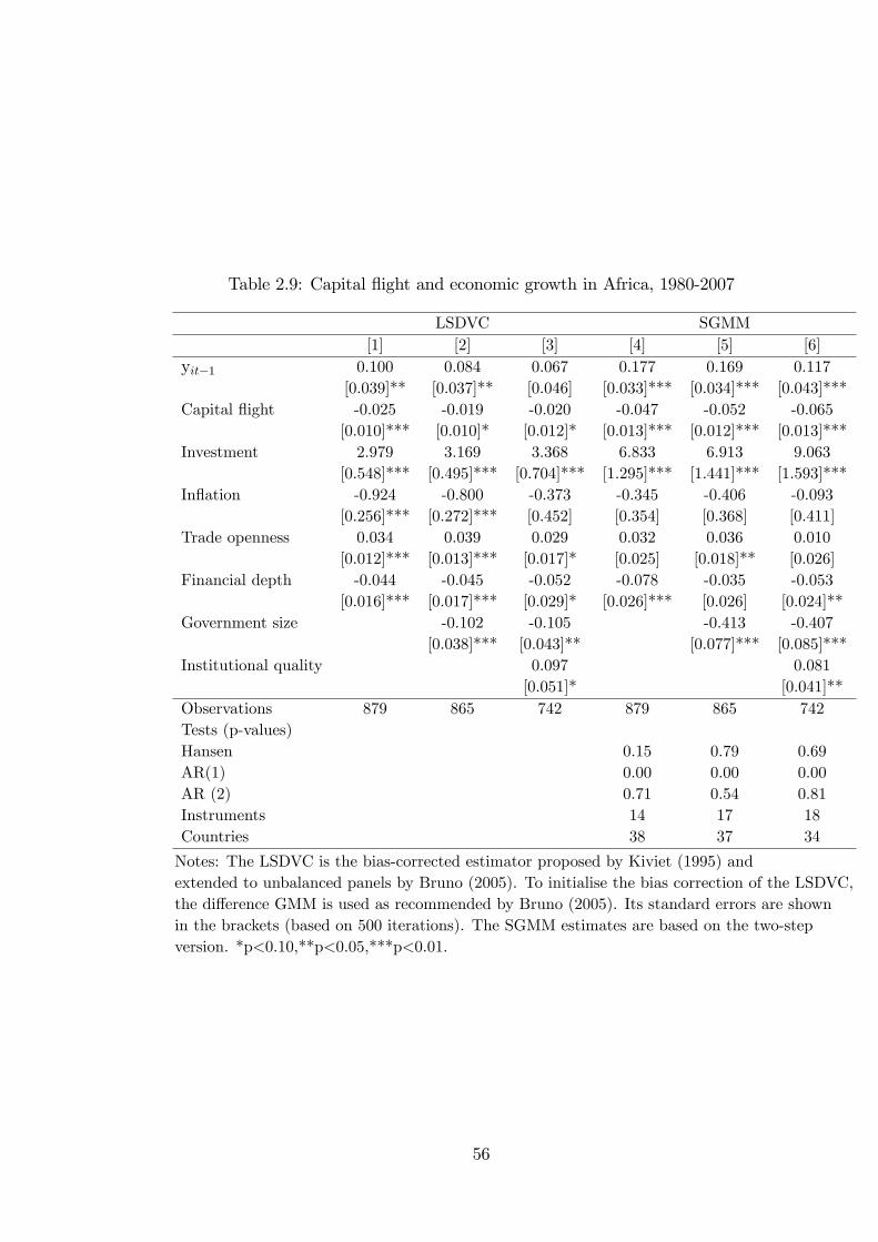
Table 2.9: Capital �ight and economic growth in Africa, 1980-2007
LSDVC SGMM[1] [2] [3] [4] [5] [6]
yit�1 0.100 0.084 0.067 0.177 0.169 0.117[0.039]** [0.037]** [0.046] [0.033]*** [0.034]*** [0.043]***
Capital �ight -0.025 -0.019 -0.020 -0.047 -0.052 -0.065[0.010]*** [0.010]* [0.012]* [0.013]*** [0.012]*** [0.013]***
Investment 2.979 3.169 3.368 6.833 6.913 9.063[0.548]*** [0.495]*** [0.704]*** [1.295]*** [1.441]*** [1.593]***
In�ation -0.924 -0.800 -0.373 -0.345 -0.406 -0.093[0.256]*** [0.272]*** [0.452] [0.354] [0.368] [0.411]
Trade openness 0.034 0.039 0.029 0.032 0.036 0.010[0.012]*** [0.013]*** [0.017]* [0.025] [0.018]** [0.026]
Financial depth -0.044 -0.045 -0.052 -0.078 -0.035 -0.053[0.016]*** [0.017]*** [0.029]* [0.026]*** [0.026] [0.024]**
Government size -0.102 -0.105 -0.413 -0.407[0.038]*** [0.043]** [0.077]*** [0.085]***
Institutional quality 0.097 0.081[0.051]* [0.041]**
Observations 879 865 742 879 865 742Tests (p-values)Hansen 0.15 0.79 0.69AR(1) 0.00 0.00 0.00AR (2) 0.71 0.54 0.81Instruments 14 17 18Countries 38 37 34
Notes: The LSDVC is the bias-corrected estimator proposed by Kiviet (1995) andextended to unbalanced panels by Bruno (2005). To initialise the bias correction of the LSDVC,the di¤erence GMM is used as recommended by Bruno (2005). Its standard errors are shownin the brackets (based on 500 iterations). The SGMM estimates are based on the two-stepversion. *p<0.10,**p<0.05,***p<0.01.
56
as expected, is harmful to economic growth. This supports the notion that capital
�ight, by eroding domestic �nancial resources, is associated with poor economic
performance. This is consistant with the �ndings reported by Ndiaye (2009) and
Fofack and Ndikumana (2009).
The underlying assumption of the LSDVC estimator is that all the right hand
side variables are exogenous, except the autoregressive term. However, this may not
be the case as there may be various sources of endogeneity with respect to equation
(2.5). For instance, there could be a measurement error concerning our indicator of
capital �ight given the nature of BOP data. In addition, there could be simultaneity
and reverse causality as most of the growth determinants we use are known to have
a feedback relationship with economic growth. Hence, we relax the assumption of
exogeneity of the explanatory variables by applying the system GMMwhich controls
for these issues7. The results are presented in the �nal 3 speci�cations.
The SGMM results are generally in line with the LSDVC estimates as far as
the sign and signi�cance is concerned. More speci�cally, they provide strong evi-
dence that capital �ight signi�cantly retards growth. Across all speci�cations, the
autoregressive parameter is positive and mostly signi�cant implying that growth is
relatively persistent over time. This supports the dynamic speci�cation adopted
here. The validity of the instruments is not rejected in the SGMM regressions.
In particular, the speci�cations pass the Hansen J test for over-identifying restric-
tions. They also pass the Arellano-Bond tests for serial correlation, con�rming that
our models are not misspeci�ed. Finally, all the models pass the F-test for overall
signicance of the regressions.
As a robustness test, we re-run the full speci�cation above for sub-periods (1980-
89, 1990-99, and 2000-07). The results are summarised in Table 2.10. It seems that
7It should be emphasised that the SGMM is appropriate in the context of large N and smallT given that its asymptotic prosperities are based on this assumption. Hence, our results shouldbe treated with caution as they do not ful�l this requirement. However, the fact that the resultsbased on LSDVC, SGMM and PVAR (discussed below) all point to the same direction imply thatwe are able to sidestep any limitation each technique might have separately. The SGMM is fullyexplained in Chapter 3.
57
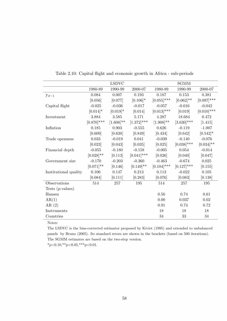
Table 2.10: Capital �ight and economic growth in Africa - sub-periods
LSDVC SGMM1980-89 1990-99 2000-07 1980-89 1990-99 2000-07
yit�1 0.084 0.007 0.193 0.187 0.153 0.381[0.056] [0.077] [0.106]* [0.055]*** [0.062]** [0.097]***
Capital �ight -0.025 -0.036 -0.017 -0.057 -0.016 -0.042[0.014]* [0.019]* [0.014] [0.013]*** [0.019] [0.010]***
Investment 3.884 3.585 5.171 4.287 18.684 0.472[0.870]*** [1.608]** [1.372]*** [1.908]** [3.630]*** [1.415]
In�ation 0.185 0.903 -0.555 0.626 -0.119 -1.007[0.609] [0.638] [0.849] [0.434] [0.642] [0.542]*
Trade openness 0.033 -0.019 0.041 -0.039 -0.140 -0.076[0.023] [0.043] [0.035] [0.025] [0.038]*** [0.034]**
Financial depth -0.055 -0.180 -0.158 -0.005 0.054 -0.014[0.028]** [0.113] [0.041]*** [0.026] [0.040] [0.047]
Government size -0.170 -0.203 -0.360 -0.463 -0.674 0.025[0.071]** [0.146] [0.149]** [0.104]*** [0.127]*** [0.155]
Institutional quality 0.106 0.147 0.213 0.113 -0.022 0.105[0.084] [0.111] [0.283] [0.076] [0.083] [0.138]
Observations 514 257 195 514 257 195Tests (p-values)Hansen 0.56 0.74 0.61AR(1) 0.00 0.037 0.02AR (2) 0.91 0.74 0.72Instruments 18 18 18Countries 34 33 34
Notes:
The LSDVC is the bias-corrected estimator proposed by Kiviet (1995) and extended to unbalanced
panels by Bruno (2005). Its standard errors are shown in the brackets (based on 500 iterations).
The SGMM estimates are based on the two-step version.
*p<0.10,**p<0.05,***p<0.01.
58
our results are stable across the sub-periods and the coe¢ cient of capital �ight
remains negative and generally signi�cant at conventional levels. Hence, capital
�ight is associated with lower economic growth in our sample of African countries.
2.4.2 Evidence from PVAR
PVAR approach
While the above �ndings give us an insight into the relationship between capital �ight
and growth, it is much more useful to explore the dynamic responses of domestic
investment and economic growth to capital �ight episodes. To this end, we apply a
PVAR approach in the vein of Love and Zicchino (2006) and estimate the following
�rst-order VAR model:
Yit = 0 +
jXj=1
jYi;t�j + �i + %t + "it (2.11)
where for country i at time t, Yit is a two-variable vector [either capital �ight and
investment both expressed as shares of GDP or capital �ight and per capita income],
�i represents a vector of country-speci�c �xed e¤ects, %t is a vector of period-e¤ects,
"it is a vector of the error disturbances, and j is the lag length. As in Love and
Zacchino (2006), the variables are time-demeaned prior to estimation8.
Since by construction the lagged dependent variables are correlated with the un-
observed country-level �xed e¤ect, �i, we use forward mean-di¤erencing or �Herlmert
procedure�. This procedure transforms the variables into deviations from forward
means. For example, y�pit =PTi
s=t+1 ypis=(Ti � t); where y
�pit are future observations
of ypit; and "�pit =
PTis=t+1 "
pis=(Ti � t)9; where "
�pit are future observations of "
pit, and
Ti is the last observation for each i. This transfomation ensures the orthogonality
between the transformed and lagged variables and thus validates the use of lagged
8The properties of time demeaning is explained in Chapter 3.9ypit and "
pit are components of the vectors Yit = (y
1it; y
2it; ::; y
FMit )0 and "it = ("1it; "
2it; ::; "
FMit )0,
respectively.
59
right hand side variables as instruments for the endogenous variables via system
GMM procedure (Love and Zicchino, 2006).
Following Koutsomanoli-Filippaki and Mamatzakis (2009) and Koetter and Po-
rath (2007), we wish to estimate equation (2.11) primarily because we are interested
in generating impulse response functions (IRF) which depict the reaction of one vari-
able in the system to innovations in another variable while keeping all other shocks
at zero. For this purpose, it is useful to rewrite equation (2.11) into a standard
�rst-order bivariate VAR of the form:
CFit = �1i0 + �10t +
jXj=1
�11jCFit�j +
jXj=1
�12jV Iit�j + "1it (2.12)
V Iit = �2i0 + �20t +
jXj=1
�21jV Iit�j +
jXj=1
�22jV Iit�j + "2it (2.13)
where for country i at time t, CFit is the share of capital �ight in GDP, V Iit denotes
a variable of interest (i.e. either investment over GDP or per capita income), �i0 and
�0t represent country-speci�c and year e¤ects, respectively and "it are uncorrelated
white-noise errors with zero means and constant variences. The model captured by
equations (2.12) and (2.13) is the so-called structural VAR, which cannot be esti-
mated due to the correlation between CFit with "2it and of V Iit with "1it. Provided
that the endogenous variables are stationary, the estimated model can be solved and
a moving average (MA) representation can be set up as follows10:
CFit = �10 +
1Xj=1
b11j"1it�j +
1Xj=1
b12j"2t�j (2.14)
V Iit = �20 +1Xj=1
b21j"1it�j +1Xj=1
b22j"2t�j (2.15)
10In the MA representation, each variable in the system is a function of current and past errors"1 and "2:
60
Since the error terms in the above representation are correlated and they tend to
move together, they must be made orthogonal (i.e. uncorrelated). One method is to
multiply the MA representation with the Cholesky decomposition of the variance-
covariance matrix of the errors. The orthogonalised MA representation becomes:
CFit = '10 +
1Xj=1
�11je1it�j +
1Xj=1
�12je2t�j (2.16)
V Iit = '20 +1Xj=1
�21je1it�j +
1Xj=1
�22je2t�j (2.17)
which is multiplied with:
0B@ �11j �12j
�21j �22j
1CA =
0B@ b11j b12j
b21j b22j
1CA � C;0B@ e1it
e2it
1CA = C�1 �
0B@ "1it
"2it
1CA (2.18)
where C is the Cholesky decomposition of the covariance matrix of the error terms:
0B@ Cov ("1it; "2it)
Cov ("1it; "2it)
Cov ("1it; "2it)
Cov ("1it; "2it)
1CA = C � C 0 (2.19)
The orthogonalised MA representation depicts the IRF, where e1it and e2it can
be interpreted as a shock in CF and V I, respectively, and the parameter estimates
in (2.16) and (2.17) capture the response of the dependent variable to shocks that
took place j periods before. Our main coe¢ cient of interest is �21j which captures
the response of either domestic investment or per capita income to a shock in CF
over periods j. The ordering of the variables in the VAR system is crucial for
the Cholesky decomposition. Based on our a priori expectations, we assume that
innovations in CF in�uence our variables of interest contemporaneously and also
with a lag, hence CF appears �rst in the ordering. This implies that investment
and income shocks do not have instantenous impact on CF episodes and that they
61
in�uence CF only with a lag. The standard errors are produced with Monte Carlo
simulations in order to calculate the 10th and 90th percentiles of the distribution
which are then used as con�dence intervals of the IRF. The Monte Carlo simulations
are based on 1000 repetitions.
PVAR results
Given the underlying assumptions of the PVAR, we �rst test whether our vari-
ables are stationary using the augmented Dickey-Fuller and Phillips-Perron tests
suggested by Maddala and Wu (1999). The results, which are summarised in Table
1.11, suggest that the variables are indeed stationary. Hence, we proceed with our
estimation of the PVAR. To avoid over-parametrisation and at the same time ensure
that our �ndings are not sensitive to the choice of lags, we report lag lengths 1-411.
Figure 2.2 summarises some selected results based on a bivariate VAR of CF and
INV. Our objective is to explore the dynamic response of INV to a one standard
deviation shock in CF. The results indicate, as expected, that INV su¤ers following
a CF episode. More speci�cally, it falls on impact and rapidly declines the �rst
3 years. Considering a horizon of 6 years, our results show that INV does not
recover in the short to medium term. Consequently, capital �ight shocks seem
to have a sizeable e¤ect on domestic capital formation in African countries. It
could be that CF is magnifying the credit constraints which are, in most African
countries, binding. It could also be that, once a proportion of domestic savings
shift abroad, African economies are less likely to get access to alternative sources of
funds for domestic investment. It is reasonable to assume that international markets
may view African agents� acquisition of foreign asset as a sign that the African
country concerned is �risky�. Figure 2.3 shows the response of domestic output to one
standard deviation shock in CF. On impact, output response is negative. However,
this does not last throughout the 6-year period even though it does not reverse
11Based on Schwartz Information Criterion, which we run for each cross-section, the optimallag is 2. However, our results do not change even when we consider higher order lags.
62
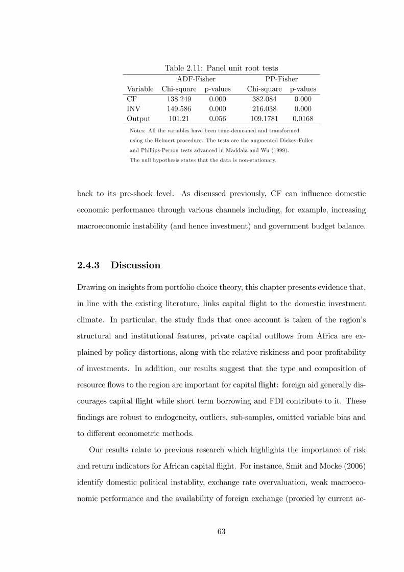
Table 2.11: Panel unit root testsADF-Fisher PP-Fisher
Variable Chi-square p-values Chi-square p-valuesCF 138.249 0.000 382.084 0.000INV 149.586 0.000 216.038 0.000Output 101.21 0.056 109.1781 0.0168
Notes: All the variables have been time-demeaned and transformed
using the Helmert procedure. The tests are the augmented Dickey-Fuller
and Phillips-Perron tests advanced in Maddala and Wu (1999).
The null hypothesis states that the data is non-stationary.
back to its pre-shock level. As discussed previously, CF can in�uence domestic
economic performance through various channels including, for example, increasing
macroeconomic instability (and hence investment) and government budget balance.
2.4.3 Discussion
Drawing on insights from portfolio choice theory, this chapter presents evidence that,
in line with the existing literature, links capital �ight to the domestic investment
climate. In particular, the study �nds that once account is taken of the region�s
structural and institutional features, private capital out�ows from Africa are ex-
plained by policy distortions, along with the relative riskiness and poor pro�tability
of investments. In addition, our results suggest that the type and composition of
resource �ows to the region are important for capital �ight: foreign aid generally dis-
courages capital �ight while short term borrowing and FDI contribute to it. These
�ndings are robust to endogeneity, outliers, sub-samples, omitted variable bias and
to di¤erent econometric methods.
Our results relate to previous research which highlights the importance of risk
and return indicators for African capital �ight. For instance, Smit and Mocke (2006)
identify domestic political instablity, exchange rate overvaluation, weak macroeco-
nomic performance and the availability of foreign exchange (proxied by current ac-
63
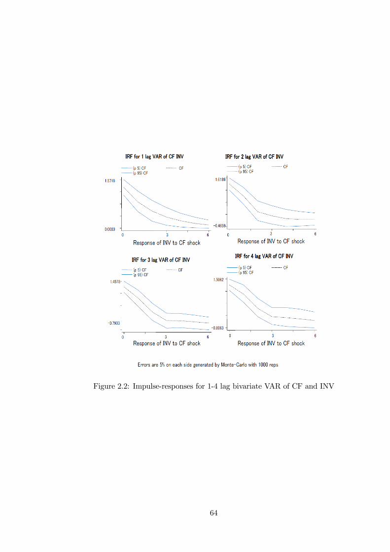
Figure 2.2: Impulse-responses for 1-4 lag bivariate VAR of CF and INV
64
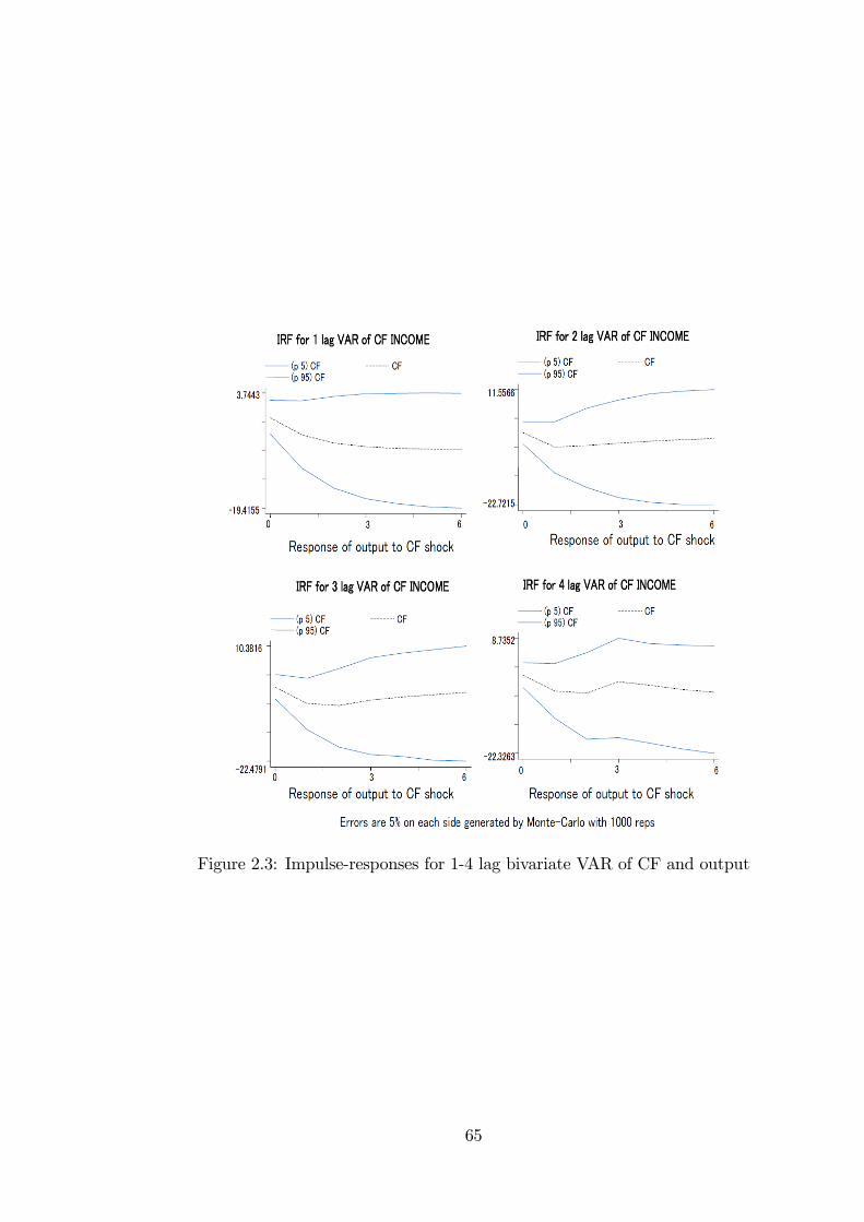
Figure 2.3: Impulse-responses for 1-4 lag bivariate VAR of CF and output
65
count surpluses and increases in foreign debt) as the most important drivers of
capital �ight from South Africa. Similarly, Ajayi (1992) reports that capital �ight
from Nigeria is explained by the rate of growth of the economy, real interest rate
di¤erential between Nigeria and the United States, �nancial repression, degree of
currency misalignment, variation in in�ation and the �scal de�cit.
Nyoni (2000) attempts to explain the causes of capital �ight from Tanzania. His
results show that growth di¤erentials between Tanzania and the UK are positively
and signi�cantly related to capital �ight from Tanzania. Ng�eno (2000) speci�es a
portfolio adjustment model in which domestic agents allocate their wealth among
di¤erent �nancial instruments based on their relative risk and return features using
Kenya as a case study. His results indicate that an overvalued exchange rate tends
to stimulate capital �ight as it signals possible devaluation. The return di¤erential
is also found to be negatively and signi�cantly related to capital �ight episodes from
Kenya.
Fedderke and Liu (2002) test the proposition that capital out�ows relate pos-
itively to expropriation risk and the foreign rate of return and negatively to the
domestic rate of return using South Africa as a case study. Their long-run esti-
mates suggest that the domestic and foreign rates of the return (proxied by the rate
of growth of GDP and interest rate di¤erentials) play a crucial role in explaining
capital out�ows. Similarly, risk indicators, especially political instability, seem to
stimulate capital out�ows in South Africa.
Lawanson (2007) attempts to capture the portfolio behaviour of private wealth
holders in Nigeria and �nds that poor economic performance, real interest rate dif-
ferentials, parallel market exchange rate premium, increased domestic and external
debt overhang, �scal de�cits and macroeconomic instability (proxied by changes in
in�ation rate) are closely related to capital �ight episodes. Forgha (2008) �nds ev-
idence suggesting that capital �ight is determined by political instability and poor
macroeconomic performance in the form of high in�ation, interest rate di¤erential,
66
excessive �scal de�cits and high external debt servicing in the case of Cameroon.
Ndikumana and Boyce (2003) analyse the causes of capital �ight for a sample
of 30 SSA economies, including 24 countries classi�ed as severely indebted low-
income countries. They identify external borrowing and the growth di¤erential
(between SSA and OECD trading partners as well as the United States) as signi�cant
drivers of capital �ight from Africa. These �ndings are reinforced in Ndikumana and
Boyce (2008) who, in addition, �nd that economic growth discourages capital �ight
instances while macroeconomic instability is found to stimulate it by eroding the
con�dence of investors. Ndiaye (2009) examines the determinants of capital �ight
in the case of 15 SSA countries from Franc Zone. Summarily, he �nds that short-
and long-term borrowing, macroeconomic instability, exchange rate overvaluation,
governance and institutional indicators are signi�cant correlates of capital �ight
episodes.
Tables 2.12 in appendix 2A summarises the core determinants of capital �ight
previously identi�ed. These determinants may be grouped into �pull� factors in
developed countries and �push�factors within LDCs. The main pull factors include
more developed �nancial sectors and less risks while the push factors include poor
macroeconomic environments, political uncertainty, less developed �nancial sectors
and distortionary policies.
Our �ndings that capital �ight tends to deteriorate domestic economic perfor-
mance is closely related to the results of Ndiaye (2009) and Fofack and Ndikumana
(2009). These authors �nd that capital �ight signi�cantly reduces domestic capi-
tal formation. In particular, their results indicate that the adverse e¤ects of capital
�ight on domestic investment mainly operates through private investment more than
public investment.
67
2.5 Concluding remarks
Many African countries have received signi�cant levels of o¢ cial capital in the form
of debt and foreign aid whilst experiencing substantial out�ows of private wealth.
Against this backdrop, this study has attempted to unravel the causes and macro-
economic consequences of these out�ows.
Building upon the work by Le and Zak (2006), Collier et al. (2001) and Sheets
(1995), we link the phenomenon of capital �ight to the domestic investment climate
(broadly de�ned) and contend that African agents move their portfolios as a result
of a deteriorating domestic investment climate where the risk-adjusted rate of return
is unfavourable. The results suggest that economic risk, policy distortions and the
poor pro�tability of African investments can explain the variation in capital �ight
from SSA. Moreover, the �nding that measures of institutional quality are inversely
related to capital �ight are in line with the theoretical view that institutions reduce
transaction costs, improve the pro�tability of the domestic economy and, hence,
encourage entrepreneurs to invest within the economy. Also, these results add to
the growing empirical evidence (Lensink et al. 2000; Le and Zak, 2006; Cerra et al.
2008) that institutions, insofar as they in�uence the domestic investment climate,
discourage capital �ight. We also �nd that resource in�ows as well as the structural
features of African economies are important in�uences on capital �ight. The �ndings
of this study are robust to outliers, endogeneity and sub-samples. On the basis of
these �ndings, we conclude that improved macroeconomic and institutional environ-
ments would help African economies, not only to attract more foreign investments,
but also to retain their local capital.
The study also con�rms that capital �ight is indeed harmful to economic growth.
The �ndings based on the dynamic panel model shows that capital �ight carries a
negative and signi�cant coe¢ cient. This indicates that the loss of domestic savings
associated with capital �ight episodes are harmful to economic performance.
In an attempt to explore the dynamic responses of investment and domestic out-
68

put, we �nd that one standard error shock in capital �ight reduces both investment
and income. In particular, investment falls on impact following capital �ight and
does not recover in the short to medium term horizon. Overall, the �ndings of this
study emphasise the detrimental e¤ects of capital �ight in the African context where
credit is scarce.
69
2.A Appendix 2
This section contains additional information regarding the dataset used to investigate
the determinants of capital �ight from SSA.
Data and sources used to calculate capital �ight
To calculate CF, equation (2.3) on page 24 was used. The current account de�cit
and the increases in external debt and o¢ cial reserves are from Global Development
Finance database (World Bank, June 2009); net foreign investments are the sum of
the following lines from the International Financial Statistics database (IMF, Sept.
2009): IFS lines78bdd, 78bed, 78bhd, 78bid, 78bkd, 78bmd, 78bwd, and 78bxd. For
the speci�c de�nitions, please consult the IMF BOP Manual (5th edition). Some of
the missing data are �lled from IMF country reports.
70
Table 2.12: Determinants of capital �ight - selected resultsStudy Sample and period Signi�cant Variables
Henry (1996) 3 Caribbean countries, 1971-87: In�ation (-/0); Growth (-/0)
Time series Budget de�cit (+/0)
Pol instability (+); debt (+)
interest rate di¤ (+)
Exchange rate (-/0)
Lensink et al. (1998) 9 SSA countries, 1970-91: pooled OLS In�ation (+); demand deposit (-)
Capital stock (-); deposit rate (-)
Exchange rate (+); debt (+)
Hermes and Lensink (2001) 84 developing countries Government consumption (+)
1971�91: Cross-section taxation (+); budget de�cit (+)
interest rate (+); Aid (+)
political instability (+)
Bank lending (+/0)
Collier et al. (2001) 50 LDC countries, 1980�90; Capital stock (+/0)
Cross-section analysis Dollar distortion index(+)
Square of debt stock (+)
Harrigan et al. (2002) Malaysia, 1970-96; time series GDP growth (-); debt (+) ; FDI (-)
in�ation (-/+); interest di¤ (+/0)
Exchange rate depreciation (+)
Le and Zak (2006) 45 developing countries, Variance of in�ation (+)
1976-91: Panel data methods Macro policy uncertainty (+)
Political instability (+)
Var [interest rate] (+)
Cerra at al. (2008) 100 developing countries, GDP growth (-)
1970�2001; Panel data analysis Budget de�cit (+)
Domestic credit growth (+)
Institutional quality (-)
Currency crises (+)
Debt (+)
Ndikumana and Boyce 40 SSA countries, 1970-04: Lagged cap �ight (+); Debt (+)
(2008) Panel data methods Stock of debt (+)
GDP growth lagged (-)
Ndiaye (2009) 15 Franc Zone SSA countries, Lagged capital �ight (+)
1970-05: panel methods FDI (-); Aid (+); In�ation (+)
Short-term debt (+)
Long-term debt (+)
Exchange rate overvaluation (+)
Good governance (-)
Institutional quality (-)
Notes: signs in parentheses denote a statistically signi�cant e¤ect (+, - and 0 signify positive, negative and no
signi�cant relation, respectively); more than one sign in a bracket implies mixed results.
71
Table 2.13: List of variables, data sources and sample countriesVariable Source
Capital �ight (% GDP) Estimated using the World Bank residual method, see main text
Black market premium Global Development Network Growth Database (GDNGD, 2009)
Macroeconomic instability Measured by the logarithm of CPI (annual change). World Bank (2009): WDI
Real overvaluation index Expressed in logarithm form. (GDNGD, 2009)
Indebtedness Net �ows on long term debt as a % GDP. World Bank (2009): GDF
International reserves Expressed in months of imports. World Bank (2009): WDI
Real per capita income Expressed in logarithm form. World Bank (2009): WDI
Return di¤erential (Domestic real deposit rate - US T-Bill rate - % change in the exchange rate),
where the exchange rate = LCU per US$. World Bank (2009): WDI, IMF (2009): IFS
Property rights �Constraint on the executive�, ranges between 1 (weak) and 7 (strong). PolityIV (2009)
Institutional quality The mean value of ICRG subcomponents: �Corruption�, �Law and Order�, and
�Bureaucratic Quality�, scaled 0 -1, such that higher values indicate higher
quality of institutions (Teorell and Hadenius, 2007)
Governance Captured by �Polity2�score, indicating a country�s governance status on a 0-10 scale,
where 10 means strong. Polity IV (2009)
Political stability Measured by the average Freedom House �political rights and civil liberty�scores�,
scaled 1-10, where 10 means strong. Teorell and Hadenius (2007)
Ethnic fractionalisation Easterly and Levine dataset (1997)
Terms of trade World Bank (2009): WDI
Trade openness Captured by the ratio of exports plus imports as a % GDP. WDI (2009)
Government size Measured by total government expenditure as a % of GDP. WDI (2009)
Primary commodity dep. Sachs and Warner (2000) - obtained from Azam and Hoe er (2002)
Aid Development aid as a % of GNI. World Bank (2009): WDI
FDI Foreign Direct Investment as a % GNP. World Bank (2009): WDI
Short term debt Expressed as a % of total external debt. World Bank (2009): WDI
War A dummy variable. PRIO/Uppsala Armed Con�ict Dataset, (2009)
Gov e¤ectiveness The relative political capacity measure created by Feng et al. (2000)
Resource abundance Share of mineral exports in total exports. IMF (2009): DOTS
BOP crisis Likelihood of balance of payment crisis captured by a dummy variable coded 1 if
reserves are than 30 days worth of imports, 0 otherwise. World Bank (2009): WDI
List of countries: Angola; Benin; Burkina Faso; Burundi; Cameroon; Cape Verde; Central African Rep.; Chad;Comoros; Congo, Dem. Rep.; Congo, Rep.; Cote d�Ivoire; Ethiopia; Gabon; Gambia; Ghana; Guinea-Bissau;
Kenya; Liberia; Madagascar; Malawi; Mali; Mauritania; Mauritius; Mozambique; Niger; Rwanda; Senegal;
Seychelles; South Africa; Sudan; Swaziland; Tanzania; Togo; Uganda; Zambia; Zimbabwe.
72
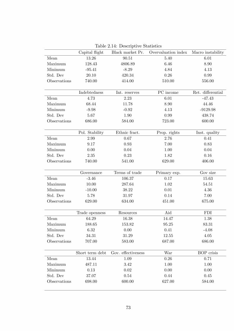
Table 2.14: Descriptive StatisticsCapital �ight Black market Pr. Overvaluation index Macro instability
Mean 13.26 90.51 5.40 6.01Maximum 128.43 4806.89 6.46 8.90Minimum -95.41 -8.29 4.84 4.13Std. Dev 20.10 420.34 0.26 0.99Observations 740.00 414.00 510.00 556.00
Indebtedness Int. reserves PC income Ret. di¤erentialMean 4.73 2.23 6.01 -47.43Maximum 68.44 11.78 8.90 44.46Minimum -9.98 -0.92 4.13 -9129.98Std. Dev 5.67 1.90 0.99 438.74Observations 686.00 584.00 723.00 600.00
Pol. Stability Ethnic fract. Prop. rights Inst. qualityMean 2.99 0.67 2.76 0.41Maximum 9.17 0.93 7.00 0.83Minimum 0.00 0.04 1.00 0.04Std. Dev 2.35 0.23 1.82 0.16Observations 740.00 541.00 629.00 406.00
Governance Terms of trade Primary exp. Gov sizeMean -3.46 106.37 0.17 15.63Maximum 10.00 287.64 1.02 54.51Minimum -10.00 38.22 0.01 4.36Std. Dev 5.78 31.97 0.14 7.00Observations 629.00 634.00 451.00 675.00
Trade openness Resources Aid FDIMean 64.29 16.38 14.47 1.38Maximum 188.65 153.82 95.25 83.31Minimum 6.32 0.00 0.41 -4.08Std. Dev 34.31 31.29 12.55 4.05Observations 707.00 583.00 687.00 686.00
Short term debt Gov. e¤ectiveness War BOP crisisMean 13.44 1.09 0.26 0.71Maximum 487.11 3.42 1.00 1.00Minimum 0.13 0.02 0.00 0.00Std. Dev 37.07 0.54 0.44 0.45Observations 698.00 600.00 627.00 584.00
73

Table 2.15: Correlation MatrixCapital Flight and Baseline Variablesi ii iii iv v vi vii viii
Capital �ight 1.00Black market premium 0.03 1.00Overvaluation index 0.10* 0.26* 1.00Macro instability 0.04 0.17* -0.11* 1.00Log per capita income -0.12* -0.14* 0.11* -0.26* 1.00Return di¤erential -0.01 -0.07 0.06 -0.40* 0.08 1.00International reserves -0.20* -0.04 -0.24* -0.13* -0.25* 0.05 1.00Indebtedness 0.51* 0.08 0.02 0.06 -0.16* 0.04 -0.11* 1.00
Capital Flight and Institutional Variablesi ii iii iv v vi
Capital �ight 1.00Property rights -0.08* 1.00Institutional quality -0.20* 0.14* 1.00Political stability -0.08* 0.47* 0.20* 1.00Ethnic fractionalisation -0.02 0.03 -0.24* 0.00 1.00Governance -0.10* 0.90* -0.30 0.59* 0.00 1.00
Capital Flight and Structural Variablesi ii iii iv v vi
Capital �ight 1.00Trade openness 0.04 1.00Government size 0.16* 0.49* 1.00Primary commodity exports 0.10* 0.45* 0.30* 1.00Terms of trade 0.13* 0.02 0.02 0.20* 1.00Natural resources -0.05 0.30* 0.17* 0.45* 0.15* 1.00
Capital Flight and Capital Flow Variablesi ii iii iv
Capital �ight 1.00FDI 0.05 1.00Aid 0.30* -0.05 1.00Short term debt 0.11* 0.11* -0.08* 1.00
Capital Flight and Additional Variablesi ii iii iv
Capital �ight 1.00Government e¤ectiveness 0.04 1.00Civil war -0.04 -0.12* 1.00Balance of payments crisis 0.20* 0.00 0.00 1.00
Notes: * indicates signi�cance at the 5 percent level.
74
2.B Appendix 2
This section contains additional information regarding the dataset used to investigate
the consequences of capital �ight from SSA.
75
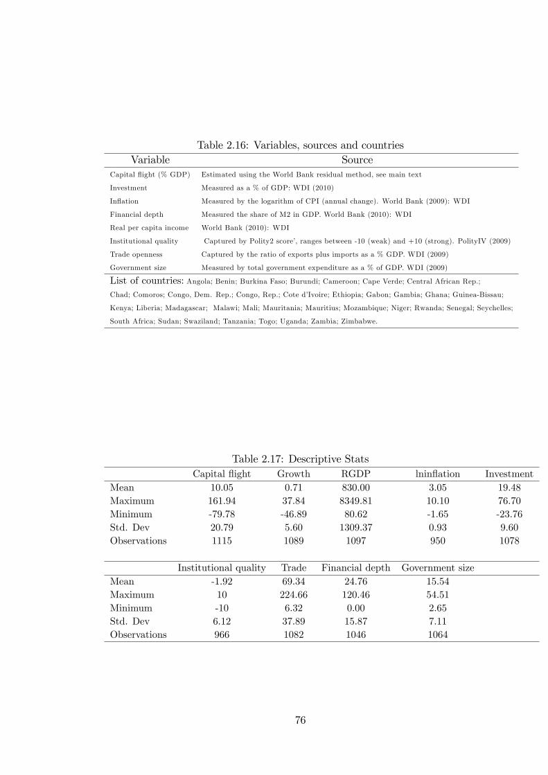
Table 2.16: Variables, sources and countriesVariable Source
Capital �ight (% GDP) Estimated using the World Bank residual method, see main text
Investment Measured as a % of GDP: WDI (2010)
In�ation Measured by the logarithm of CPI (annual change). World Bank (2009): WDI
Financial depth Measured the share of M2 in GDP. World Bank (2010): WDI
Real per capita income World Bank (2010): WDI
Institutional quality Captured by Polity2 score�, ranges between -10 (weak) and +10 (strong). PolityIV (2009)
Trade openness Captured by the ratio of exports plus imports as a % GDP. WDI (2009)
Government size Measured by total government expenditure as a % of GDP. WDI (2009)
List of countries: Angola; Benin; Burkina Faso; Burundi; Cameroon; Cape Verde; Central African Rep.;Chad; Comoros; Congo, Dem. Rep.; Congo, Rep.; Cote d�Ivoire; Ethiopia; Gabon; Gambia; Ghana; Guinea-Bissau;
Kenya; Liberia; Madagascar; Malawi; Mali; Mauritania; Mauritius; Mozambique; Niger; Rwanda; Senegal; Seychelles;
South Africa; Sudan; Swaziland; Tanzania; Togo; Uganda; Zambia; Zimbabwe.
Table 2.17: Descriptive StatsCapital �ight Growth RGDP lnin�ation Investment
Mean 10.05 0.71 830.00 3.05 19.48Maximum 161.94 37.84 8349.81 10.10 76.70Minimum -79.78 -46.89 80.62 -1.65 -23.76Std. Dev 20.79 5.60 1309.37 0.93 9.60Observations 1115 1089 1097 950 1078
Institutional quality Trade Financial depth Government sizeMean -1.92 69.34 24.76 15.54Maximum 10 224.66 120.46 54.51Minimum -10 6.32 0.00 2.65Std. Dev 6.12 37.89 15.87 7.11Observations 966 1082 1046 1064
76
Chapter 3
Crises and Growth Collapses inAfrica: The Role of EconomicIntegration
3.1 Introduction
It is largely accepted that trade and �nancial openness can promote the transmis-
sion of business cycle �uctuations among countries, making them more vulnerable
to contagion (Frankel, 2000). However, notwithstanding the potential risks associ-
ated with globalisation, an increasing number of African countries have embarked
on policies of trade and �nancial liberalisation. As a result, Africa is today more
integrated into the global economic system than it was few decades ago. Yet, like
developing countries in other regions, African economies have also encountered their
share of economic and �nancial crises. As recent global events illustrate, crises can
have devastating e¤ects on economic activity and can hit countries with strong,
as well as, those with weak macroeconomic fundamentals. Thus, economists and
policy-makers are increasingly concerned with understanding the genesis, evolution
and consequences of economic crises.
The objective of this study is to explore how crises and openness a¤ect economic
growth in Africa. More speci�cally, we examine whether greater openness to trade
and �nancial �ows exacerbates or lessens the adverse e¤ects of �nancial crises. We
distinguish between four di¤erent types of crises, namely, sudden stops, currency,
77
twin and sovereign debt crises. To our knowledge, this is the �rst study to examine
the e¤ects of these types of crises in the context of African economies. Most of the
existing literature focuses onmainly emerging markets, even though many African
countries have also been subject to these types of crises.
A �sudden stop�in capital in�ows is a type of crisis in which access to foreign
capital is abruptly and severely curtailed, precipitating large swings in the capital
account of the balance of payments1. It is closely associated with current account
reversals (from large de�cits to smaller de�cits/ surpluses), reserve depletion, growth
collapses as well as currency and sovereign debt crises (Calvo, 1998)2. Sudden stops
can be caused by the behaviour of global investors (i.e. a sudden decline in gross
in�ows to a particular country due to a sharp fall in the demand for that country�s
assets). They can also be driven by domestic economic agents (i.e. a sharp increase in
gross out�ows or capital �ight as a result of a sudden shift towards foreign securities).
A currency crisis, on the other hand, occurs when investors substitute away
from a particular country�s assets in anticipation of a potential depreciation of the
currency, while a sovereign debt crisis involves a default or restructuring of debt
obligations. Twin crises, �rst coined by Kaminsky and Reinhart (1999), arise when
currency crises are followed by banking crises. As shown by, among others, Kaufman
(2000) and Bordo et al. (2001), twins tend to have much more harmful e¤ects on the
economy relative to either currency or banking crises on their own. The di¤erent
types of crises may hit simultaneously, as they may be triggered o¤ by common
underlying factors, and one crisis may also help precipitate another.
Guidotti et al. (2004) �nd that sudden stops have been a common occurrence
in developing countries since the late 1970s, and Deb (2005) asserts that capital
1This capital account adjustment is usually termed �capital reversal�in the existing literature.2Sudden stops and the accompanying liquidity constraints imply that the current account must
be abruptly adjusted (i.e. reduced). This can be avoided by depleting the reserve holdings of thecentral bank, provided there are enough reserves and the central bank is willing to do so (however,reserve depletion may initiate currency crises) or, alternatively, by seeking emergency funding frominternational �nancial institutions. In any case, a current account reversal can be very painful aslabour and goods markets tend to be in�exible in the short-run.
78
reversals and sudden stops are developing country phenomena. Edwards (2004)
shows that, in his sample of 157 economies, African countries have encountered
more sudden stops simultaneously with current account reversals than has any other
region. Glick et al. (2006) document that currency crises were more frequent in
Africa than in any other developing region. Andersson and Karpestam (2011) show
that, of all the types of crises that have hit African countries, debt crises have been
the most harmful to both output growth and total factor productivity.
The results of this study, as expected, show that �nancial crises are associ-
ated with growth collapses in Africa. In contrast, economic openness is found to
be bene�cial to growth. More speci�cally, we �nd that, consistent with standard
Mundell-Flemming type models, greater openness to trade and �nancial �ows tends
to mitigate the adverse e¤ects of crises.
The chapter is organised as follows. Section 2 reviews the existing literature.
Section 3 contains some preliminary analysis and presents our crises and openness
measures. Section 4 presents the econometric techniques used, while Section 5 dis-
cusses the results. Finally, Section 6 concludes.
3.2 Related Literature
In this section, we �rstly provide a brief overview of the ways in which economic
and �nancial crises relate to output collapses. Subsequent to this, we revisit the
openness-growth relationship with a view to summarising the �ndings of the ex-
isting literature. Finally, we present an analytical discussion of the role economic
integration can play in the relationship between crises and output growth.
3.2.1 Crises and output growth
An increasing body of evidence links economic and �nancial crises to output col-
lapses. The existing literature, both theoretical and empirical, emphasises that crises
79
are associated with output losses due to their adverse e¤ects on domestic capital for-
mation, labour market, exchange rates, asset prices, aggregate demand, and total
factor productivity.
Korinek (2011) postulates that crises cause self-reinforcing ��nancial ampli�ca-
tion� e¤ects in which countries can be caught in a vicious circle of falling prices
(exchange rates and asset prices), deteriorating balance sheets and decreasing ag-
gregate demand. More speci�cally, crises, particularly those that come in the form
of capital reversals, sudden stops and currency crises, are associated with sharp falls
in the exchange rate and asset prices. This, in turn, deteriorates domestic �rms�
balance sheets by undermining their collateral value and net worth, further reduc-
ing their ability to borrow and invest owing to reduced access to credit. These
e¤ects tend to be ampli�ed in environments where there is credit scarcity, high li-
ability dollarization and �nancial market imperfections. In crisis-hit countries, lack
of credit availability reduces aggregate demand by tightening the budget constraints
of agents, so decreasing their consumption and investment levels.
The tendency of crises to undermine investor con�dence can arise, not only from
lack of credit availability, but also from increased risk and uncertainty. In addition,
in Keynesian settings where prices/wages are downward sticky, depressed aggregate
demand is associated with higher unemployment and output losses (Reinhart and
Calvo, 2000). Furceri and Mourougane (2012) contend that crises may either in-
crease or decrease total factor productivity. On the one hand, crises may reduce
total factor productivity through their negative impact on innovation and research
and development as these tend to be higher in good times. On the other hand,
total factor productivity may increase in crisis situations if �rms, in an attempt
to minimise losses and retain competitiveness, restructure and/or improve their X-
e¢ ciency.
There is a vast literature on the macroeconomic consequences of crises. For
example, Dornbusch et al. (1995) show that sudden stop episodes played a crucial
80
role in triggering and aggravating the Mexican tequila crisis of 1994/1995. Guidotti
et al. (2004) �nd that sudden stops are associated with output contractions across
a range of developed and developing countries. More importantly, they �nd that
government policy stance plays a role in the aftermath of a sudden stop crisis.
In particular, countries with open trade regimes and �oating exchange rates tend
to have a better growth performance than those with closed economies and �xed
exchange rates. In addition, they �nd that liability dollarization tends to hurt
economic growth in the aftermath of a sudden stop. The contractionary e¤ect
of capital �ow reversals and sudden stop crises is also con�rmed by Deb (2005).
However, his results suggest that the negative e¤ects of these types of crises on
growth is conditional on the level of economic development so that output losses are
more likely to be felt in developing and emerging economies than in industrialised
countries.
Edwards (2004) �nds that current account reversals associated with sudden stops
are inversely related to real GDP growth but that trade openness tends to lessen
the negative e¤ects of reversals. In contrast, he �nds that �nancial openness tends
not to in�uence the extent to which reversals a¤ect growth. Similar to the �ndings
reported by Guidotti et al. (2004), Edwards (2004) �nds that �exible exchange rates
tend to mitigate the adverse e¤ects of reversals.
Other studies highlight the importance of institutions in in�uencing the out-
comes of crises. For example, Cavallo and Cavallo (2010) show that better quality
institutions tend to mitigate the adverse e¤ects of banking, debt and sudden stop
crises since good institutions tend to promote better policy responses following ad-
verse shocks. On the other hand, Joyce and Nabar (2009) demonstrate that the
adverse impacts of crises on domestic investment is conditional on the presence of
other types of shocks. More speci�cally, they �nd that sudden stops are harmful to
investment only if they coincide with banking crises. In a similar vein, Cowan and
Raddatz (2012) and Gallego and Tessada (2012) postulate that the negative output
81
e¤ect of sudden stops arises because these types of crises tend to aggravate �nancial
frictions prevailing in the domestic economy. For example, industries that rely more
on external �nancing and those with higher liquidity constraints tend to experience
a fall in their activity during a sudden stop, especially when the domestic �nancial
system is weak.
Gupta et al. (2003) explore the behaviour of output during currency crises for
a sample of 91 developing countries. They �nd that currency crises are in most
cases contractionary, particularly in countries that are less open to trade, in large
developing countries, in countries with open capital accounts and when crises are
preceded by large capital in�ows. In a series of studies, Hutchison and Noy (2002;
2005; 2006) examine the output costs of various types of crises in emerging markets.
Their �ndings con�rm that currency, banking and sudden stop crises cause substan-
tial output losses, with sudden stops having the most adverse (albeit short-lived)
e¤ects on growth.
Focusing on sovereign debt crises, Rose (2005), De Paoli and Hoggarth (2006)
and Borensztein and Panizza (2010) emphasise that defaults can impose severe costs
on developing countries including loss of trade partners and credit as well as higher
costs of future �nance. The costs can be particularly high if the developing country
defaults on o¢ cial Paris Club debt. A number of studies con�rm that sovereign debt
crises are associated with output falls. For example, Sturzenegger (2004) reports that
countries that have defaulted grow about 0.6% less than those that have not and
that defaults which trigger banking crises and macroeconomic instability are much
more harmful to output performance than those that do not. This is con�rmed by
De Paoli and Hoggarth (2006), who �nd the negative e¤ect of default on output
to be larger when defaults coincide with banking and/or currency crises and when
it takes countries longer to clear their arrears or restructure their debts. Similar
results are also reported by Borensztein and Panizza (2009).
In sum, the existing studies surveyed above provide ample evidence that �nancial
82
crises are associated with output losses, particularly in emerging markets. In this
study, we argue that there is scope for additional work to establish the growth
outcomes of crises in African countries. Hence, we attempt to �ll this gap in the
literature.
3.2.2 Economic integration and growth
Economists have long held the view that increased international trade can propel
countries to a high-growth trajectory. Standard trade theory, for example, postulates
that trade openness is associated with static gains as it provides greater scope for the
accumulation of human and physical capital. In particular, openness can facilitate
economies to allocate their resources more e¢ ciently by providing market platforms
which allow economies of scale and division of labour to take place � increasing
total factor productivity. Moreover, endogenous growth theories (e.g. Romer, 1994;
Rivera-Batiz and Romer, 1991) predict that opening up trade enables countries to
acquire new technologies, skills, knowledge and various other positive externalities
which can bring about dynamic gains resulting in higher economic growth.
Similarly, an extensive theoretical literature identi�es various direct and indirect
channels through which �nancial openness can foster higher productivity and im-
prove economic performance. Kose et al. (2009) contend that �nancial integration
can increase capital accumulation by relaxing credit constraints and augmenting do-
mestic resources. In addition, openness to �nancial �ows can promote more e¢ cient
capital allocation as a result of increased risk-sharing opportunities which enables
�rms to undertake more risky but high-return investments (Obstfeld, 1994). As the
volume of capital increases, the cost of capital should fall since the domestic economy
becomes more liquid (Prasad et al. 2003). Other strands of the literature postulate
that �nancial globalisation helps improve the domestic �nancial sector, market dis-
cipline, government policies and corporate governance (Rajan and Zingales, 2003;
Klein and Olivei, 2008; Bon�glioli, 2008; Kose et al. 2009).
83
An extensive survey of the literature by Williamson and Maher (1998) concludes
that, while �nancial liberalisation can result in higher e¢ ciency in terms of invest-
ments and greater �nancial development, it can coincide with severe banking and
other crises. Hence, one particular line of enquiry pursued by many researchers is
whether economic integration, especially �nancial openness, is closely linked with
crises. On the one hand, economists such as Stiglitz (2000) argue that capital ac-
count openness may increase the likelihood of encountering �nancial crises. On the
other hand, Edwards (2007) and Glick et al. (2006) fail to �nd evidence that coun-
tries with high capital mobility su¤er disproportionately more crises than those with
lower capital mobility.
Ranciere et al. (2006) decompose the growth outcome of international �nancial
liberalisation into two e¤ects: a positive direct e¤ect and a negative indirect e¤ect
due to higher propensity to crisis. Their empirical estimates suggest that the direct
positive e¤ect of �nancial openness on growth signi�cantly outweighs the growth
loss associated with more frequent �nancial crises. Employing probit and panel
regressions, Lee and Shin (2007) report similar results, that is, the positive �nancial
liberalisation e¤ect on growth dominates the indirect negative e¤ect due to crises.
The empirical literature focusing on African countries has approached the in-
vestigation of the growth-openness relationship in two main ways: (i) by directly
testing the growth e¤ects of measures of trade and/or �nancial openness, and (ii) by
identifying the channels through which economic integration in�uences growth. For
example, using instrumental variable estimations, Bruckner and Lederman (2012)
�nd a robust positive link between trade openness and growth in Sub-Saharan Africa.
Similar results have been reported by Changa and Mendy (2012). Baliamoune-Lutz
and Ndikumana (2007) �nd results suggesting that institutional quality play an
important role in the openness-growth nexus in Africa.
Focusing on �nancial openness, Fowowe (2008) shows that there is a signi�cant
and robust positive relationship between economic growth and �nancial liberali-
84
sation policies in his sample of Sub-Saharan African countries. Similarly, Ahmed
(2011) provides evidence that �nancial integration has had a positive (albeit not sta-
tistically signi�cant) direct impact on output growth in Africa. However, he �nds
that �nancial openness in Africa has had a positive and robust e¤ect on African
�nancial markets and thereby indirectly bene�tted their growth performance.
The foregoing review of the existing literature suggests that trade openness can
improve economic performance. Similarly, �nancial openness can improve the e¢ -
ciency and depth of �nancial sectors. However, embedded in �nancial liberalisation
is the risk of crises which disrupt economic activity.
3.2.3 The openness-crisis interaction
One can identify two opposing hypotheses as to whether economic and �nancial
integration mitigate or exacerbate the adverse e¤ects of �nancial crises. On the one
hand, some have argued that openness can be an important crisis ampli�er, in that
it can expose countries to external shocks, while others suggest that it can act as a
crisis bu¤er insofar as it can help accommodate external shocks.
Openness as a crisis ampli�er
As summarised by Cavallo and Frankel (2008), a number of arguments have been
put forward in support of the view that openness to trade can trigger or exacerbate
crises. In particular, countries that are more integrated into the global economy are
more likely to be subject to external shocks emanating from, for example, trading
partners. As a result, the argument goes, these economies are more prone to export
collapses and/or diminishing trade credits which in turn can trigger sudden stops
and other types of crises. Empirical �ndings by Ramey and Ramey (1995), Milesi-
Ferretti and Razin (2000) and Easterly et al. (2001) suggest that openness to trade
is closely linked to output volatility and a higher likelihood of external crises.
With respect to capital account openness, economists such as Stiglitz (2000) ar-
gue that it can aggravate pre-existing market distortions caused by informational
85
asymmetries, credit market imperfections, poor institutions and moral hazards, in-
creasing the likelihood of crises (Stiglitz, 2000). While the overwhelming majority of
economists, including Stiglitz, remain in favour of long-term private capital in�ows
(e.g. foreign direct investment), many point to the destabilising e¤ects of volatile and
pro-cyclical surges in in�ows. Hence, it has been argued that capital account open-
ness may lead to increased in�ows of short term capital and a higher risk of abrupt
reversals (Agenor, 2004; Singh, 2003). Others assert that capital movements, as a
result of �nancial openness, may increase macroeconomic instability (e.g. upward
pressures on the exchange rates, asset price bubbles, credit booms, higher in�ation,
consumption growth volatility etc.) and lead to the presence of more short-term,
high risk speculative capital in the economy (Arestis, 2005).
Openness as a crisis bu¤er
The idea that openness to trade can lower the probability of crises or, alternatively,
lessen the adverse e¤ects of external crises is not new in economics. For instance,
a number of studies have postulated that there is an inverse relationship between
trade openness and default probabilities. More precisely, countries with higher trade
activities are less likely to default on their international obligations since their trad-
ing partners could impose harsh sanctions on them in the event of a default (Rose,
2005).
An alternative argument suggests that trade openness lessens the adjustment
costs associated with external crises. In particular, it has been suggested that open
economies are more likely to �export their way out of a crisis�. This was �rst noted
by Sachs (1985), who observed that in the early 1980s Latin American countries
were subject to numerous debt crises, in spite of having similar levels of debt to
GDP ratios as Asian countries, precisely because of their lower trade openness and
hence their inability to generate foreign exchange to service their debt. Recently,
Guidotti et al. (2004) have shown that countries with open trade regimes tend to
have better growth performances and quicker recoveries in the face of sudden stop
86
crises than those with closed economies.
How trade openness reduces the adjustment costs of external shocks has been
elaborated on by, among others, Edwards (2004), Cavallo and Frankel (2008), Calvo
et al. (2003) and Ripoll-i-Alcon (2010). Suppose that an economy has to abruptly
adjust to a shock (e.g. a sudden stop episode). In the �rst instance, assume that
expenditure-switching policies are not possible (i.e. the exchange rate is �xed). In
this case, the country must implement spending cuts to satisfy its intertemporal re-
source constraint and thus run a current account surplus. In the standard Keynesian
and Mundell-Flemming type of models, the severity of the adjustment is negatively
related to the marginal propensity to import, with a higher propensity implying
lower adjustment costs. Thus, more open economies would, ceteris paribus, su¤er
less contraction3.
Similar conclusions can be reached if one uses traditional tradable/nontradable
models. To illustrate this, assume that it is now possible for the country to im-
plement expenditure-switching policies. In this case, to improve the trade balance,
the relative price of non-tradables must fall. Hence, the needed adjustment can, at
least in part, be achieved through a nominal and real depreciation of the exchange
rate. This would in turn, following sticky-price open economy models and conven-
tional Mundell-Fleming type models, improve the recovery of the economy through
increased competitiveness4.
Recent experiences from emerging markets, however, show that the e¤ect of
depreciation on output can in fact be contractionary particularly when there is
a currency mismatch brought about by the so-called �original sin�5. As shown
by a number of theoretical (see for example, Aghion et al. 2001; Choi and Cook,
3Output losses would be inevitable if wages and prices are rigid. This is more likely to be thecase in the short-run.
4For a survey, see Lane (2001). The bene�cial e¤ects of the depreciation would depend on anumber of factors, including whether the Marshall-Lerner condition holds.
5This refers to the situation where developing countries cannot get loans denominated in theirown currencies from international �nancial markets. Thus, a depreciation/ devaluation of theircurrencies would make the value of their liabilities rise. These balance sheet e¤ects would reducethe net worth of �rms.
87
2004) and empirical contributions (see for example, Aguiar, 2005), the balance sheet
e¤ects of a depreciation can cause output contraction as a result of dwindling �rm
net worth. However, as emphasised by Cavallo and Frankel (2008), the required
devaluation may not be large for countries with higher trade to GDP ratios and, in
turn, the balance sheet e¤ects need not be large. Consequently, the prediction is
that more open countries can mitigate the adverse e¤ects of external shocks better
than closed economies, which are more likely to end up in a recession due to the
need implement more severe adjustments.
Using a simple theoretical model, Ripoll-i-Alcon (2010) shows that trade inte-
gration can not only mitigate crises, but can also reduce the frequency of external
�nancial crises. The model highlights three distinct mechanisms all of which are
related to the macroeconomic e¤ects of trade growth. The �rst channel is the stan-
dard pro-competitive e¤ect which arises from a depreciation of the exchange rate.
The second relates to how trade integration can improve the economy�s solvency
through, for example, greater willingness to meet outstanding external liabilities
for fear of sanctions in case of default. Finally, the model predicts that more open
economies would experience a quicker recovery, facilitated by higher output in the
tradable goods sector which would keep the fall in domestic demand in check.
Do these e¤ects also apply to �nancial integration? Edwards (2004) and ref-
erences cited therein seem to suggest so. That is, similarly to trade integration,
�nancial openness tends to reduce the adjustment costs of external shocks and thus
enables the economy to recover more quickly6.
The African context
As our discussion regarding the two competing hypotheses indicates, the openness-
crisis interaction can only be settled empirically. In this study, we argue that a
necessary condition for �nancial openness to amplify crises is the existence of a
6A careful examination of the existing literature, however, indicates that, under fairly standardassumptions, �nancial openness may in fact result in greater instability (see for example Kim etal. 2012 for a review).
88
highly liquid and well-developed �nancial system, which is absent in most African
countries. In the African context, as is largely accepted, �nancial crises tend to be
transmitted via the real sector (e.g. trade collapses). So the question of whether
openness lessens the impact of crises can be approached in two di¤erent ways. One
way is to examine whether open countries are more prone to crises (i.e. whether they
have a higher probability of encountering an external shock). An alternative way,
which is perhaps more useful, is to explore whether countries that are more open
to trade and �nancial �ows su¤er smaller reductions in output following external
shocks relative to more closed economies. In other words, are open economies more
likely to accommodate external shocks? In what follows, we attempt to answer this
latter question.
3.3 Statistical analysis of key variables
3.3.1 Openness indicators
We utilise several measures of economic and �nancial openness. We use the eco-
nomic dimension of the KOF index of globalisation (Dreher, 2006). It is a weighted
index of actual economic �ows (trade, foreign direct investment, portfolio investment
and income payments to foreign nationals each measured as a percentage of GDP)
and their restrictions (hidden import barriers, mean tari¤ rate, taxes on interna-
tional trade and capital account restrictions). This is our preferred indicator since
it captures the degree to which economies are connected to the rest of the world. As
sensitivity tests, we also employ the actual economic �ows sub-index from the same
dataset and the share of trade (sum of exports and imports) in GDP, each capturing
di¤erent aspects of cross border transactions.
To measure �nancial openness, we use the de facto indicator constructed by
Lane and Milesi-Ferretti (2006). This variable measures the external assets and
89
liabilities of economies (as a share of GDP) and thus provides a useful overview of
a country�s �nancial linkages to the rest of the world. As a robustness check, we
disaggregate the gross external liabilities and use the sub-component of FDI as an
additional measure of �nancial integration7. Finally, we use the de jure index of
capital account openness proposed by Chinn and Ito (2006). This measure is the
�rst principal component of four binary dummy variables related to restrictions on
cross-border �nancial transactions.
3.3.2 Crises indicators
To identify episodes of sudden stop crises, we closely follow the work of Guidotti et
al. (2004) and Calvo et al. (2004) to de�ne a sudden stop as a fall in the �nancial
account that is at least one standard deviation below the sample mean and more
than 5 percent of the country�s GDP. However, we impose an additional requirement
in that we require the episode to be disruptive. One way to do this is to follow the
procedure by Hutchison and Noy (2006). They focus on episodes that coincide with
other types of crises. Our approach is broader and requires the episode to coincide
with, or be followed by, other forms of �nancial crises, namely, currency and debt
crises. In this way, our measure of a sudden stop re�ects not only changes in the
mood of global capital markets, but also how harmful the episode might be. Hence,
we use a dummy variable that takes on a value 1 if there is a sudden stop in a
country during a particular year and 0 otherwise.
We also make use of similar dummy variables capturing the incidence of currency
and sovereign debt crises. Our currency crisis measure is based on that of Reinhart
and Rogo¤ (2009), who de�ne it as an annual depreciation (local currency vs US
dollar) of 15 percent or more. Our sovereign debt crisis measure comes from the
same source and is de�ned as a failure to meet a principal or interest payment on
7Kose et al. (2008) do a similar disaggregation of stocks of liabilities into debt, FDI and equitycomponents (from Lane and Milesi-Ferretti, 2006), arguing that the bene�ts of �nancial opennessare closely linked with the e¤ects of these in�ows.
90
the due date (or speci�ed grace period) including rescheduling of debt agreements
irrespective of the nature of any new terms.
Following Kaminsky and Reinhart (1999) and Bordo et al. (2001), we also con-
sider the e¤ects of the joint (�twin�) occurrence of banking and currency crises on
output growth in Africa. The data on banking crises comes from the dataset by
Laeven and Valencia (2008). Finally, to capture the severity and intensity of �nan-
cial crises, we construct a composite crisis index, which can take on a value between
0 and 4, depending on the number of types of crises encountered by a country in a
particular year. For example, in 1992 Nigeria simultaneously experienced a sudden
stop episode with currency, twin, and sovereign debt crises. Hence, we award Nigeria
an index score of 4 for that particular year. We then weigh the index by the share
of each country�s GDP in world output. A similar procedure has been adopted by
Reinhart and Reinhart (2010). The composite measure has a number of attractive
features relative to the crisis dummies, which we discuss later.
3.3.3 The anatomy of African crises
Using the de�nitions and sources detailed above, we identify a total of 202 currency
crises, 172 sovereign debt crises, 249 sudden stop episodes and 56 twin crises (banking
and currency). Figure 3.10 shows the distribution of currency crises over time. It
seems that the highest number of currency crises were recorded in 1994, when the
CFA franc was devalued by 50%. The occurrence of sovereign debt crises peaked
during the mid to late 1980s (Figure 3.11), while a signi�cant number of countries
experience sudden stop episodes from the late 1970s onwards (Figure 3.12). Twin
crises were the least frequent type of crisis during the sample period, occurring
mostly in the 1990s (Figure 3.13).
We now turn our attention to the behaviour of output growth during crisis
episodes. To this end, we conduct a basic event analysis where we examine whether
91
a crisis event is accompanied by an output loss or growth collapse8. The existing
literature de�nes an output loss or growth collapse as the deviation of actual output
(growth) from its potential trend9 (see, for example, Bordo et al. 2001; Boyd et al.
2005 and Gupta et al. 2007). As is standard in the literature, we estimate the out-
put trend based on a 5-year pre-crisis period ending 3 years prior to each crisis event
using Hodrick-Prescott smoothed output series. However, in the majority of cases,
we end up with negative growth trends10. Similar problems have been encountered
by Abiad et al. (2009) and Angkinand (2008). To get round this, the �rst authors
extend the pre-crisis period back until a positive trend is achieved (10 to 20 years
back) while the latter author sets all the negative 3-year pre-crisis growth rates to
zero.
In this study, we opt for an alternative strategy which imposes as few restrictive
assumptions as possible. In particular, we ask the following question. How does
output growth behave before, during and after �nancial crises? A simple way to do
this is to compare the actual growth rates in period T (onset of a crisis) to those
in T�1; ::T�5 (pre-crisis window) and in T+1; ::T+5 (post crisis period)11. Figure
3.1 shows that debt crises tend to be associated with greater output collapses in
Africa. This is in line with the �ndings of Andersson and Karpestam (2011) that
debt crises have been the most harmful to type of crisis output growth in Africa.
The �gure suggests that sudden stop episodes tend to be preceded by a boom and
that output tends to su¤er a small contraction. The idea that sudden stops occur on
the back of boom times is consistent with the notion that developing countries tend
to experience capital in�ow bonanzas during good times (procyclicality), perhaps
8Event studies have become standard in the crises literature following the seminal work byEichengreen et al. (1995) and Frankel and Rose (1996).
9The potential output (growth) trend is usually estimated from the average of 3-5 year pre-crises output (growth).
10Negative trends would suggest that output falls inde�nitely, even in the absence of a shock(see Abiad et al. 2009).
11Any crisis episodes occuring within a window of 4 years are grouped as 1 and their average isused. Where 5-year averages are not available, shorter windows are used instead. Countries withepisodes lasting 10 or more consecutive years are omitted.
92
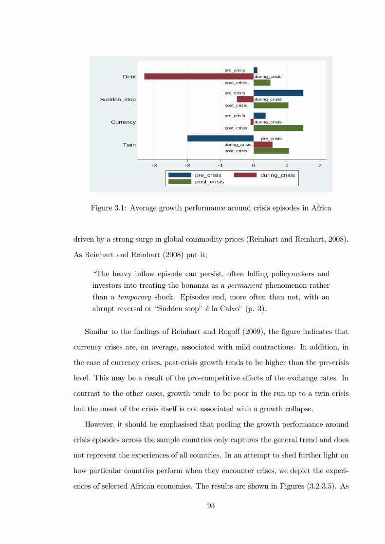
post_crisis
during_crisispre_crisis
post_crisisduring_crisis
pre_crisis
post_crisis
during_crisispre_crisis
post_crisisduring_crisis
pre_crisis
3 2 1 0 1 2
Twin
Currency
Sudden_stop
Debt
pre_crisis during_crisispost_crisis
Figure 3.1: Average growth performance around crisis episodes in Africa
driven by a strong surge in global commodity prices (Reinhart and Reinhart, 2008).
As Reinhart and Reinhart (2008) put it;
�The heavy in�ow episode can persist, often lulling policymakers and
investors into treating the bonanza as a permanent phenomenon rather
than a temporary shock. Episodes end, more often than not, with an
abrupt reversal or �Sudden stop�á la Calvo�(p. 3).
Similar to the �ndings of Reinhart and Rogo¤ (2009), the �gure indicates that
currency crises are, on average, associated with mild contractions. In addition, in
the case of currency crises, post-crisis growth tends to be higher than the pre-crisis
level. This may be a result of the pro-competitive e¤ects of the exchange rates. In
contrast to the other cases, growth tends to be poor in the run-up to a twin crisis
but the onset of the crisis itself is not associated with a growth collapse.
However, it should be emphasised that pooling the growth performance around
crisis episodes across the sample countries only captures the general trend and does
not represent the experiences of all countries. In an attempt to shed further light on
how particular countries perform when they encounter crises, we depict the experi-
ences of selected African economies. The results are shown in Figures (3.2-3.5). As
93
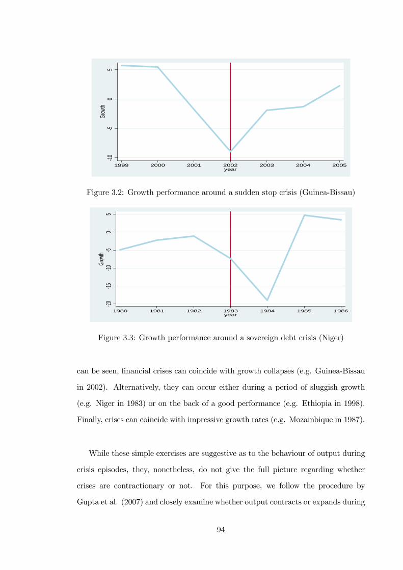
105
05
Grow
th
1999 2000 2001 2002 2003 2004 2005year
Figure 3.2: Growth performance around a sudden stop crisis (Guinea-Bissau)
2015
105
05
Grow
th
1980 1981 1982 1983 1984 1985 1986year
Figure 3.3: Growth performance around a sovereign debt crisis (Niger)
can be seen, �nancial crises can coincide with growth collapses (e.g. Guinea-Bissau
in 2002). Alternatively, they can occur either during a period of sluggish growth
(e.g. Niger in 1983) or on the back of a good performance (e.g. Ethiopia in 1998).
Finally, crises can coincide with impressive growth rates (e.g. Mozambique in 1987).
While these simple exercises are suggestive as to the behaviour of output during
crisis episodes, they, nonetheless, do not give the full picture regarding whether
crises are contractionary or not. For this purpose, we follow the procedure by
Gupta et al. (2007) and closely examine whether output contracts or expands during
94
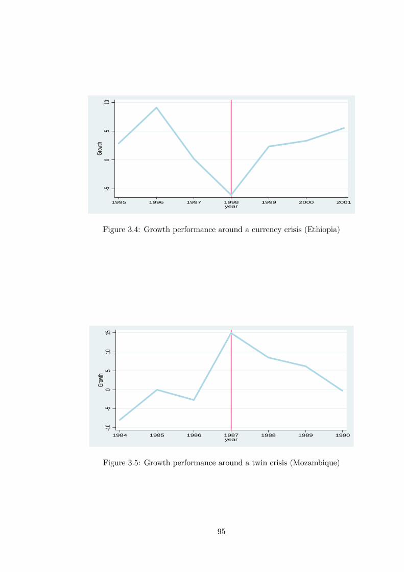
50
510
Grow
th
1995 1996 1997 1998 1999 2000 2001year
Figure 3.4: Growth performance around a currency crisis (Ethiopia)
105
05
1015
Grow
th
1984 1985 1986 1987 1988 1989 1990year
Figure 3.5: Growth performance around a twin crisis (Mozambique)
95
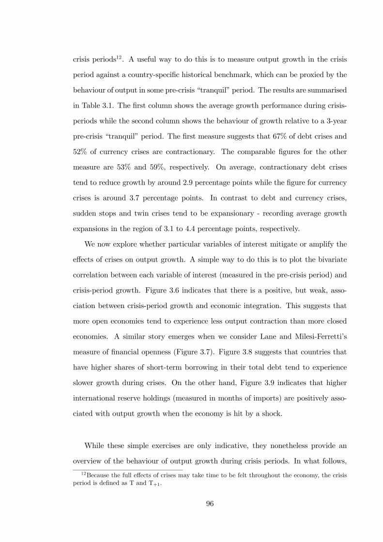
crisis periods12. A useful way to do this is to measure output growth in the crisis
period against a country-speci�c historical benchmark, which can be proxied by the
behaviour of output in some pre-crisis �tranquil�period. The results are summarised
in Table 3.1. The �rst column shows the average growth performance during crisis-
periods while the second column shows the behaviour of growth relative to a 3-year
pre-crisis �tranquil�period. The �rst measure suggests that 67% of debt crises and
52% of currency crises are contractionary. The comparable �gures for the other
measure are 53% and 59%, respectively. On average, contractionary debt crises
tend to reduce growth by around 2.9 percentage points while the �gure for currency
crises is around 3.7 percentage points. In contrast to debt and currency crises,
sudden stops and twin crises tend to be expansionary - recording average growth
expansions in the region of 3.1 to 4.4 percentage points, respectively.
We now explore whether particular variables of interest mitigate or amplify the
e¤ects of crises on output growth. A simple way to do this is to plot the bivariate
correlation between each variable of interest (measured in the pre-crisis period) and
crisis-period growth. Figure 3.6 indicates that there is a positive, but weak, asso-
ciation between crisis-period growth and economic integration. This suggests that
more open economies tend to experience less output contraction than more closed
economies. A similar story emerges when we consider Lane and Milesi-Ferretti�s
measure of �nancial openness (Figure 3.7). Figure 3.8 suggests that countries that
have higher shares of short-term borrowing in their total debt tend to experience
slower growth during crises. On the other hand, Figure 3.9 indicates that higher
international reserve holdings (measured in months of imports) are positively asso-
ciated with output growth when the economy is hit by a shock.
While these simple exercises are only indicative, they nonetheless provide an
overview of the behaviour of output growth during crisis periods. In what follows,
12Because the full e¤ects of crises may take time to be felt throughout the economy, the crisisperiod is de�ned as T and T+1:
96
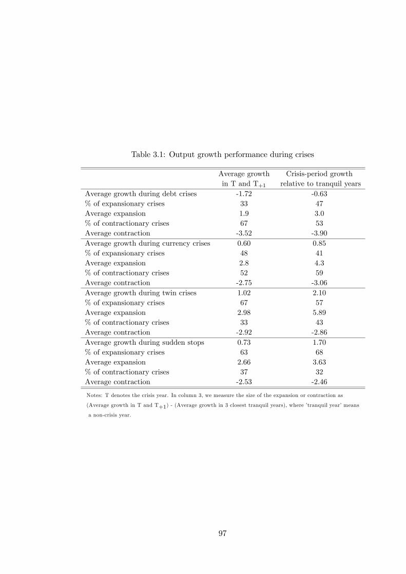
Table 3.1: Output growth performance during crises
Average growth Crisis-period growthin T and T+1 relative to tranquil years
Average growth during debt crises -1.72 -0.63% of expansionary crises 33 47Average expansion 1.9 3.0% of contractionary crises 67 53Average contraction -3.52 -3.90Average growth during currency crises 0.60 0.85% of expansionary crises 48 41Average expansion 2.8 4.3% of contractionary crises 52 59Average contraction -2.75 -3.06Average growth during twin crises 1.02 2.10% of expansionary crises 67 57Average expansion 2.98 5.89% of contractionary crises 33 43Average contraction -2.92 -2.86Average growth during sudden stops 0.73 1.70% of expansionary crises 63 68Average expansion 2.66 3.63% of contractionary crises 37 32Average contraction -2.53 -2.46
Notes: T denotes the crisis year. In column 3, we measure the size of the expansion or contraction as
(Average growth in T and T+1) - (Average growth in 3 closest tranquil years), where �tranquil year�means
a non-crisis year.
97
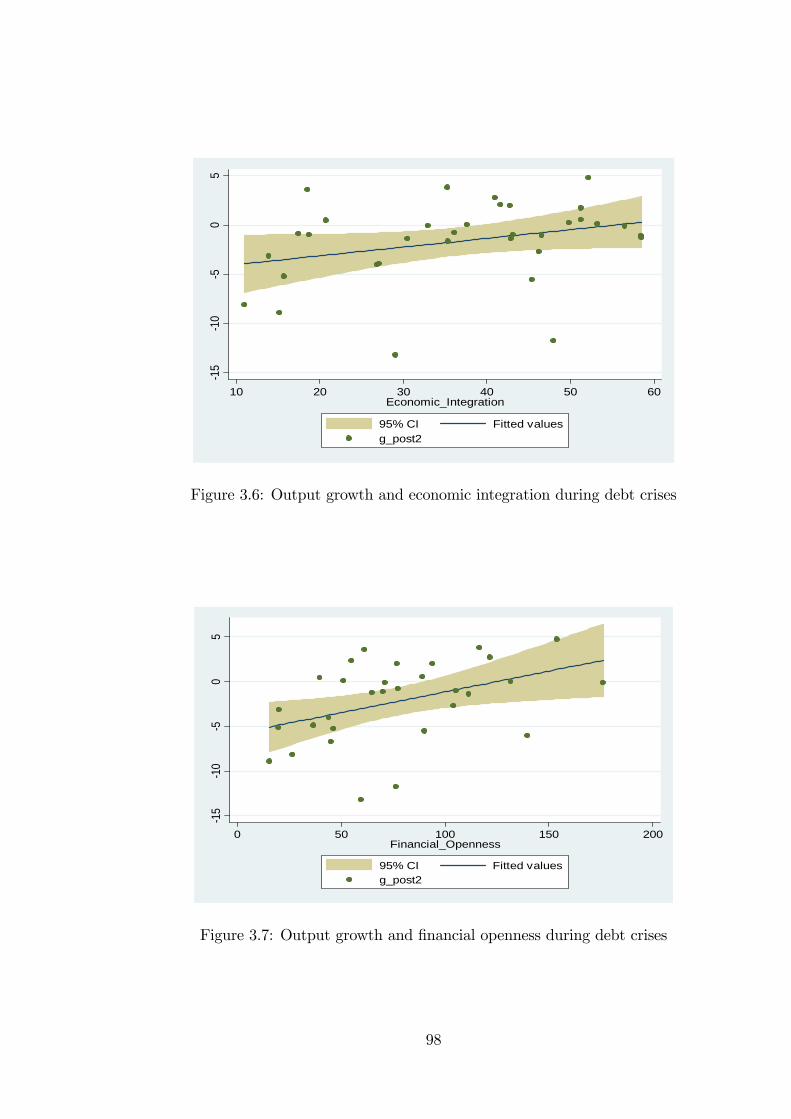
15
10
50
5
10 20 30 40 50 60Economic_Integration
95% CI Fitted valuesg_post2
Figure 3.6: Output growth and economic integration during debt crises
15
10
50
5
0 50 100 150 200Financial_Openness
95% CI Fitted valuesg_post2
Figure 3.7: Output growth and �nancial openness during debt crises
98
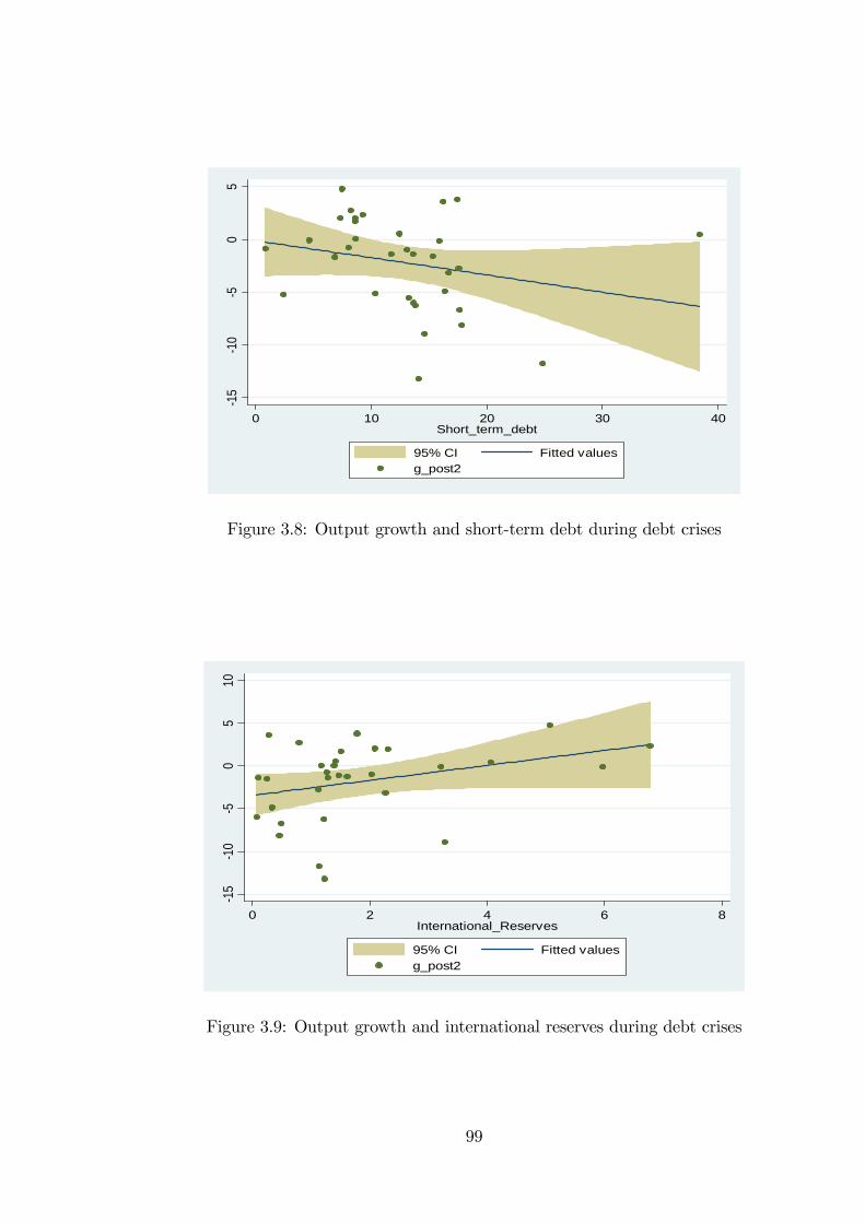
15
10
50
5
0 10 20 30 40Short_term_debt
95% CI Fitted valuesg_post2
Figure 3.8: Output growth and short-term debt during debt crises
15
10
50
510
0 2 4 6 8International_Reserves
95% CI Fitted valuesg_post2
Figure 3.9: Output growth and international reserves during debt crises
99
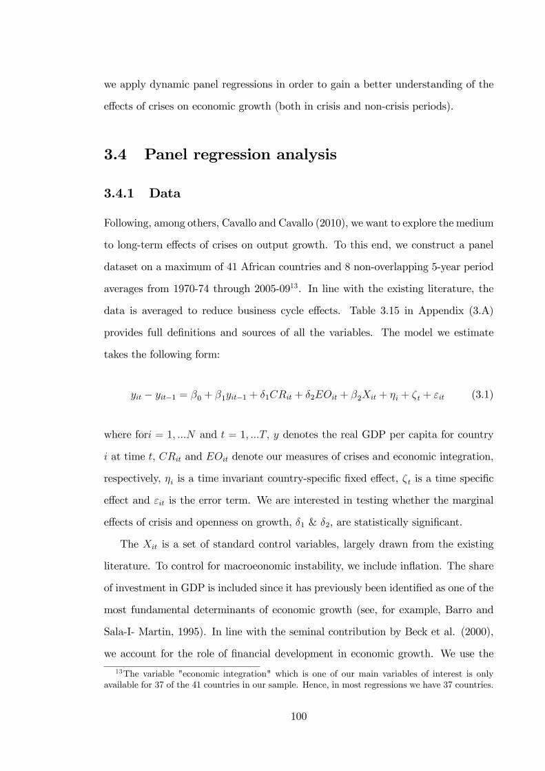
we apply dynamic panel regressions in order to gain a better understanding of the
e¤ects of crises on economic growth (both in crisis and non-crisis periods).
3.4 Panel regression analysis
3.4.1 Data
Following, among others, Cavallo and Cavallo (2010), we want to explore the medium
to long-term e¤ects of crises on output growth. To this end, we construct a panel
dataset on a maximum of 41 African countries and 8 non-overlapping 5-year period
averages from 1970-74 through 2005-0913. In line with the existing literature, the
data is averaged to reduce business cycle e¤ects. Table 3.15 in Appendix (3.A)
provides full de�nitions and sources of all the variables. The model we estimate
takes the following form:
yit � yit�1 = �0 + �1yit�1 + �1CRit + �2EOit + �2Xit + �i + �t + "it (3.1)
where fori = 1; :::N and t = 1; :::T; y denotes the real GDP per capita for country
i at time t, CRit and EOit denote our measures of crises and economic integration,
respectively, �i is a time invariant country-speci�c �xed e¤ect, �t is a time speci�c
e¤ect and "it is the error term. We are interested in testing whether the marginal
e¤ects of crisis and openness on growth, �1 & �2, are statistically signi�cant.
The Xit is a set of standard control variables, largely drawn from the existing
literature. To control for macroeonomic instability, we include in�ation. The share
of investment in GDP is included since it has previously been identi�ed as one of the
most fundamental determinants of economic growth (see, for example, Barro and
Sala-I- Martin, 1995). In line with the seminal contribution by Beck et al. (2000),
we account for the role of �nancial development in economic growth. We use the
13The variable "economic integration" which is one of our main variables of interest is onlyavailable for 37 of the 41 countries in our sample. Hence, in most regressions we have 37 countries.
100
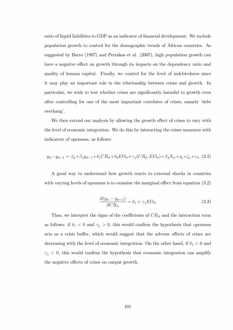
ratio of liquid liabilities to GDP as an indicator of �nancial development. We include
population growth to control for the demographic trends of African countries. As
suggested by Barro (1997) and Petrakos et al. (2007), high population growth can
have a negative e¤ect on growth through its impacts on the dependency ratio and
quality of human capital. Finally, we control for the level of indebtedness since
it may play an important role in the relationship between crises and growth. In
particular, we wish to test whether crises are signi�cantly harmful to growth even
after controlling for one of the most important correlates of crises, namely �debt
overhang�.
We then extend our analysis by allowing the growth e¤ect of crises to vary with
the level of economic integration. We do this by interacting the crises measures with
indicators of openness, as follows:
yit�yit�1 = �0+�1yit�1+�1CRit+�2EOit+ 1(CRit�EOit)+�2Xit+�i+�t+"it (3.2)
A good way to understand how growth reacts to external shocks in countries
with varying levels of openness is to examine the marginal e¤ect from equation (3.2)
@(yit � yit�1)@CRit
= �1 + 1EOit (3.3)
Thus, we interpret the signs of the coe¢ cients of CRit and the interaction term
as follows: if �1 < 0 and 1 > 0, this would con�rm the hypothesis that openness
acts as a crisis bu¤er, which would suggest that the adverse e¤ects of crises are
decreasing with the level of economic integration. On the other hand, if �1 < 0 and
1 < 0, this would con�rm the hypothesis that economic integration can amplify
the negative e¤ects of crises on output growth.
101
3.4.2 Methods
A particular issue of concern in estimating our model (equation 3.1 or 3.2) is en-
dogeneity bias. The endogeneity may arise from omitted variables, simultaneity or
reverse causality. Another concern is the presence of the autoregressive term, which
invalidates the ordinary least squares estimator along with conventional static panel
�xed e¤ects and random e¤ects. Thus, we use the generalised method of moments
(GMM) estimators proposed by Holtz-Eakin et al. (1988) and Arellano and Bond
(1991) and further developed by Arellano and Bover (1995) and Blundell and Bond
(1998). These estimators address the likely source of endogeneity, �i, by di¤erencing
and then using �internal�instruments for the right hand side variables. Controlling
for time-speci�c e¤ects, equations (3.1) or (3.2) can be written more concisely as:
yit = �yit�1 + �0Xit + �i + "it (3.4)
Given that yit and xit may be correlated with �i and that yit�1 and Xit are not
strictly exogenous (i.e. they are not uncorrelated to past, present and future error
terms), one can use the di¤erenced GMM estimator suggested by Arellano and Bond
(1991) which allows for the elimination of the possible source of omitted variable
bias, namely �i, by di¤erencing both sides of equation (3.4):
yit � yit�1 = �(yit�1 � yit�2) + �0(xit � xit�1) + ("it � "it�1)
or (3.5)
�yit = ��yit�1 + �0�xit +�"it
However, by construction, the lagged dependent variable is correlated with the
di¤erenced error term (E[�yit�1;�"it] 6= 0). In addition, the endogeneity of the
regressors remains. Arellano and Bond (1991) show that if one assumes the transient
102
errors to be uncorrelated (E["it; "it�s] = 0 for all s � t) and the explanatory variables
to be weakly exogenous (i.e. they are uncorrelated with future realisations of the
error term), one can use lagged values as instruments. Hence, the moment conditions
de�ning the di¤erenced GMM is given by:
E[yi;t�s("it � "it�1)] = 0; (3.6)
E[Xi;t�s("it � "it�1)] = 0; for s � 2; t = 3; :::T (3.7)
Hence, we can use �deeper�internal instruments dated t� 2 or earlier as instru-
ments. However, as shown by Arellano and Bover (1995) and Blundell and Bond
(1998), in cases where the data series displays persistence, the lagged levels of the
variables could be weak instruments, resulting in downward biased estimates, es-
pecially in short panels. In recognition of this, we use the system GMM (SGMM)
dynamic panel estimator advanced in Arellano and Bover (1995) and Blundell and
Bond (1998), which has been shown to have superior �nite sample properties. Re-
taining the weak exogeneity assumption, the SGMM applies a system of equations,
one in levels (equation 3.4) and one in di¤erences (equation 3.5), and uses lagged
�rst di¤erences of the regressors as instruments in the �rst case and lagged levels
of the dependent and explanatory variables as instruments in the latter case. The
validity of the additional instruments requires, however, that the �rst di¤erences of
the regressors in equation (3.5) are uncorrelated with the country speci�c e¤ects, �i;
across all periods. That is,
E[yi;t+p � �i] = E[yi;t+q � �i] (3.8)
E[Xi;t+p � �i] = E[Xi;t+q � �i] for all p and q (3.9)
Based on this and on the previous assumption of weak exogeneity, the moment
103
conditions for the regression in levels become:
E[(yi;t�s � yi;t�s�1) � (�i + "it)] = 0 (3.10)
E[(Xi;t�s �Xi;t�s�1) � (�i + "it)] = 0 for s = 1; t = 3; :::T (3.11)
Whether the lagged values of the variables in the growth model are valid instru-
ments can be examined by a test on the appropriateness of the moment restrictions.
We use three speci�cation tests suggested by Blundell and Bond (1998): 1) a Hansen
J test for over-identifying restrictions, which evaluates the joint validity of the in-
strument matrix by testing the null hypothesis that they are uncorrelated with the
residuals, 2) a di¤erence-in-Hansen J test for the validity of the additional moment
restrictions required for the 2-step SGMM (i.e. the additional instruments for the
levels equation), and 3) the Arellano-Bond test of second-order serial correlation
examining the hypothesis that the error term, "it, is not serially correlated.
The SGMM has both a one-step and a two-step version. The one-step GMM
estimator is built on the assumption that "it is i:i:d (i.e homoskedastic across i and
t) while the two-step estimator allows "it to be heteroskedastic. Even though the
two-step estimator is asymptotically more e¢ cient, its standard errors are downward
biased making inference problematic (Blundell and Bond, 1998; Roodman, 2006).
We solve this by implementing Windmeijer�s (2005) �nite sample correction, which
makes the two-step GMM e¢ cient asymptotically. As shown by, among others,
Windmeijer (2005) and Roodman (2009), a large number of instruments can have
serious consequences in �nite samples because they over�t the endogenous variables
and also weaken the Hansen J test. To avoid this, we follow the procedure suggested
by Roodman (2009), collapsing the instrument matrix and restricting the instrument
set to the closest possible lags of all non strictly exogenous variables.
Table 3.11 reports the summary statistics of all the variables used in the esti-
104
mations14. As can be seen, economic growth and our measures of openness display
considerable heterogeneity among the sample countries. As a starting point, Table
3.12 depicts the pairwise correlation coe¢ cients between each of our crisis indicator
and the dependent variable. As expected, we observe a negative relationship - that
is, �nancial crises are associated with a poor economic performance. The table also
shows that, even though the crisis variables capture di¤erent dimensions of shocks,
they are related to one another. As Table 3.13 indicates, growth is signi�cantly and
positively correlated with economic integration, cross border transactions and trade
openness. Finally, Table 3.14 indicates that there is a negative correlation between
crises and openness.
3.5 Results
3.5.1 Baseline results
In Table 3.2, we explore the (independent) e¤ects of crises and openness on economic
growth (i.e. without interaction terms). Across the 5 regressions, we augment our
growth model with the �ve di¤erent indicators of crises described above, along with
our preferred measure of economic integration. These regressions are based on the
standard �xed e¤ects panel estimator. The estimated coe¢ cients of economic inte-
gration are all positive and generally signi�cant at conventional levels, suggesting
that openness is associated with a better growth performance. Consistent with the
existing literature, a sudden stop crisis is harmful to output growth. Similarly, the
rest of the �nancial crisis indicators are inversely related to growth, the coe¢ cients
of these variables being statistically signi�cant at the 1% level. Hence, these pre-
liminary �ndings support the notion that crises tend to disrupt economic activity
while openness, perhaps by relaxing credit constraints and thus improving capital
accumulation, is bene�cial to economic performance.
14Tables 3.11 through 3.14 are displayed in Appendix 3A.
105
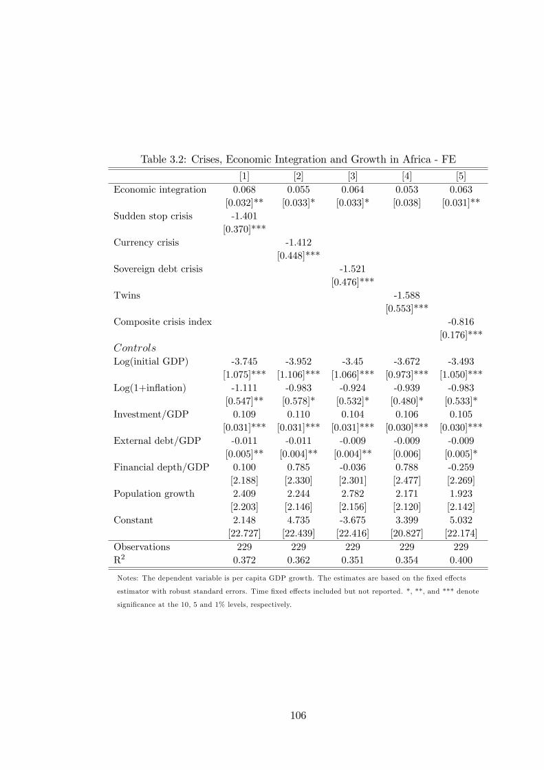
Table 3.2: Crises, Economic Integration and Growth in Africa - FE
[1] [2] [3] [4] [5]Economic integration 0.068 0.055 0.064 0.053 0.063
[0.032]** [0.033]* [0.033]* [0.038] [0.031]**Sudden stop crisis -1.401
[0.370]***Currency crisis -1.412
[0.448]***Sovereign debt crisis -1.521
[0.476]***Twins -1.588
[0.553]***Composite crisis index -0.816
[0.176]***ControlsLog(initial GDP) -3.745 -3.952 -3.45 -3.672 -3.493
[1.075]*** [1.106]*** [1.066]*** [0.973]*** [1.050]***Log(1+in�ation) -1.111 -0.983 -0.924 -0.939 -0.983
[0.547]** [0.578]* [0.532]* [0.480]* [0.533]*Investment/GDP 0.109 0.110 0.104 0.106 0.105
[0.031]*** [0.031]*** [0.031]*** [0.030]*** [0.030]***External debt/GDP -0.011 -0.011 -0.009 -0.009 -0.009
[0.005]** [0.004]** [0.004]** [0.006] [0.005]*Financial depth/GDP 0.100 0.785 -0.036 0.788 -0.259
[2.188] [2.330] [2.301] [2.477] [2.269]Population growth 2.409 2.244 2.782 2.171 1.923
[2.203] [2.146] [2.156] [2.120] [2.142]Constant 2.148 4.735 -3.675 3.399 5.032
[22.727] [22.439] [22.416] [20.827] [22.174]Observations 229 229 229 229 229R2 0.372 0.362 0.351 0.354 0.400
Notes: The dependent variable is per capita GDP growth. The estimates are based on the �xed e¤ects
estimator with robust standard errors. Time �xed e¤ects included but not reported. *, **, and *** denote
signi�cance at the 10, 5 and 1% levels, respectively.
106
In general terms, all the conditioning variables are consistent with our prior
expectations. More speci�cally, initial income carries a signi�cant negative sign,
con�rming the conditional convergence hypothesis. The estimated coe¢ cients of
in�ation are signi�cantly negative, implying that macroeconomic instability is linked
to low growth rates. In line with the so-called �debt overhang�hypothesis, we obtain
negative and generally signi�cant coe¢ cients of external debt. There is no evidence
to support the idea that population growth or �nancial depth have a signi�cant
in�uence on growth. Investment, on the other hand, helps to explain the variation
in growth, further underlying the importance of capital accumulation for economic
development.
However, a legitimate concern with these results is that some of the right hand
side variables may be endogenously related to growth. A particular source of en-
dogeneity which may plague our baseline model is reverse causality. For example,
it is likely that the level of economic integration may change with the growth per-
formance of the economy, so that countries may open up their current and capital
accounts precisely because of improved domestic growth performance. To overcome
these concerns, we re-estimate the baseline regressions in Table 3.2 using the two-
step SGMM. The results are reported in Table 3.3.
Once endogeneity concerns are addressed, economic integration retains its posi-
tive and signi�cant e¤ect on growth. Across all speci�cations, the coe¢ cients of this
variable are signi�cant at the 1% level, emphasising that openness does matter for
growth in Africa. Focusing on regression [1], the results imply that a 1% increase
in the economic openness to GDP ratio is accompanied by a rise in income of 0.25
percentage points. We �nd robust evidence that crises are detrimental to economic
performance. The results suggest that currency crises have a marginally stronger
depressing impact on output growth than the other types of crises, closely followed
by twin crises, sovereign debt and sudden stops. Interestingly, the coe¢ cient of our
composite measure, which captures the intensity with which countries encounter
107
multiple crises, is somewhat lower than the other crisis indicators but, nonetheless,
negative and highly signi�cant. Accordingly, crisis-hit African economies are ex-
pected, on average, to grow between 1:68 and 1 percentage points less than those
that do not su¤er from any crises.
The three speci�cation tests are all well-behaved; the Hansen test of over-identifying
restrictions fails to reject the null that the instruments are valid. Similarly, the
di¤erence-in-Hansen test fails to reject the null that the orthogonality conditions
derived from the levels equation are appropriate. Finally, the regressions pass the
second order serial correlation test, con�rming that there is no second-order serial
correlation in the error term of the �rst-di¤erenced equation. Hence, these tests
support the validity and consistency of the SGMM estimator.
Varying the impact of crises across levels of openness
In order to investigate whether the level of economic integration in�uences the re-
lationship between crises and growth, we interact the openness variable with our
crises indicators. The results are summarised in Table 3.4.
Regression [1] shows that sudden stop episodes have a highly signi�cant negative
association with economic growth: an African country which experiences a sudden
stop episode in a given period is expected to grow 4 percentage points less than a
country without such an episode. On the other hand, openness has a signi�cant
bene�cial e¤ect on economic performance. The coe¢ cient of the interaction term
carries a signi�cant positive sign, suggesting that economic integration mitigates
the adverse e¤ects of a sudden stop crisis. So a highly open economy such as South
Africa with an average openness to GDP ratio of 0.60, would be able to avoid any
output losses around sudden stops15. On the other hand, in a period of crisis, the
output growth of the least open economy (i.e. Rwanda with an average openness to
15The overall growth e¤ect following a sudden stop for South Africa would be given by thefollowing equation; �4:191 + (0:07 � 0:60) � 100 = 0:009
108
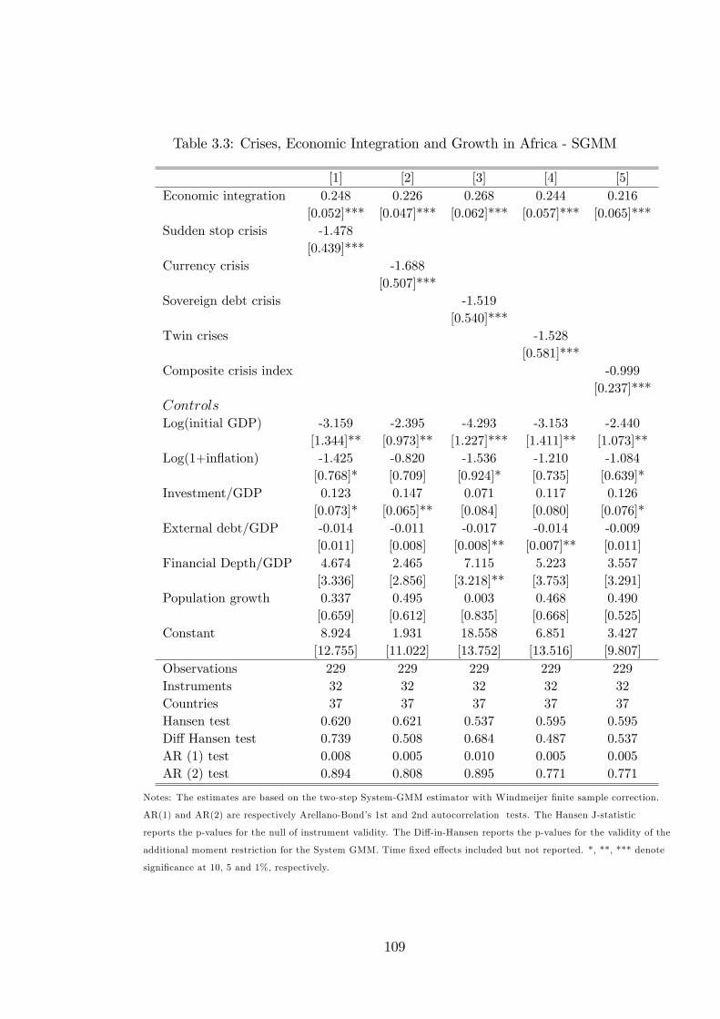
Table 3.3: Crises, Economic Integration and Growth in Africa - SGMM
[1] [2] [3] [4] [5]Economic integration 0.248 0.226 0.268 0.244 0.216
[0.052]*** [0.047]*** [0.062]*** [0.057]*** [0.065]***Sudden stop crisis -1.478
[0.439]***Currency crisis -1.688
[0.507]***Sovereign debt crisis -1.519
[0.540]***Twin crises -1.528
[0.581]***Composite crisis index -0.999
[0.237]***ControlsLog(initial GDP) -3.159 -2.395 -4.293 -3.153 -2.440
[1.344]** [0.973]** [1.227]*** [1.411]** [1.073]**Log(1+in�ation) -1.425 -0.820 -1.536 -1.210 -1.084
[0.768]* [0.709] [0.924]* [0.735] [0.639]*Investment/GDP 0.123 0.147 0.071 0.117 0.126
[0.073]* [0.065]** [0.084] [0.080] [0.076]*External debt/GDP -0.014 -0.011 -0.017 -0.014 -0.009
[0.011] [0.008] [0.008]** [0.007]** [0.011]Financial Depth/GDP 4.674 2.465 7.115 5.223 3.557
[3.336] [2.856] [3.218]** [3.753] [3.291]Population growth 0.337 0.495 0.003 0.468 0.490
[0.659] [0.612] [0.835] [0.668] [0.525]Constant 8.924 1.931 18.558 6.851 3.427
[12.755] [11.022] [13.752] [13.516] [9.807]Observations 229 229 229 229 229Instruments 32 32 32 32 32Countries 37 37 37 37 37Hansen test 0.620 0.621 0.537 0.595 0.595Di¤ Hansen test 0.739 0.508 0.684 0.487 0.537AR (1) test 0.008 0.005 0.010 0.005 0.005AR (2) test 0.894 0.808 0.895 0.771 0.771
Notes: The estimates are based on the two-step System-GMM estimator with Windmeijer �nite sample correction.
AR(1) and AR(2) are respectively Arellano-Bond�s 1st and 2nd autocorrelation tests. The Hansen J-statistic
reports the p-values for the null of instrument validity. The Di¤-in-Hansen reports the p-values for the validity of the
additional moment restriction for the System GMM. Time �xed e¤ects included but not reported. *, **, *** denote
signi�cance at 10, 5 and 1%, respectively.
109
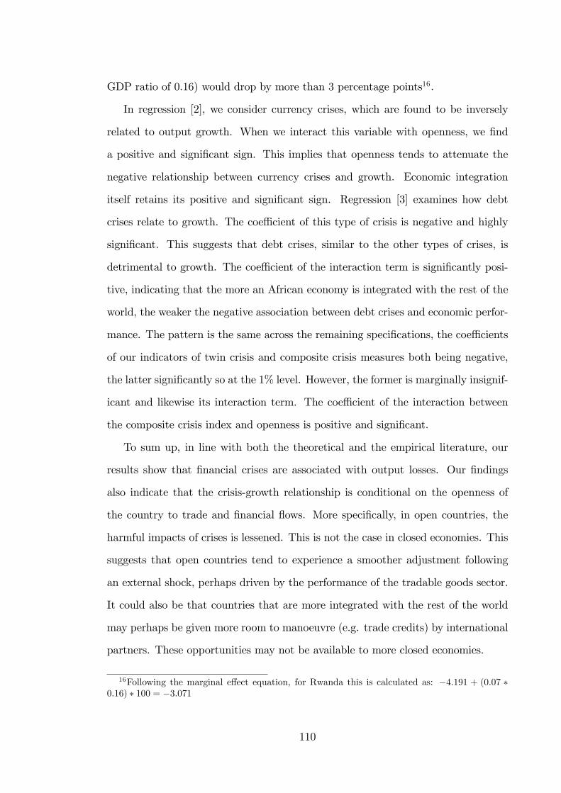
GDP ratio of 0.16) would drop by more than 3 percentage points16.
In regression [2], we consider currency crises, which are found to be inversely
related to output growth. When we interact this variable with openness, we �nd
a positive and signi�cant sign. This implies that openness tends to attenuate the
negative relationship between currency crises and growth. Economic integration
itself retains its positive and signi�cant sign. Regression [3] examines how debt
crises relate to growth. The coe¢ cient of this type of crisis is negative and highly
signi�cant. This suggests that debt crises, similar to the other types of crises, is
detrimental to growth. The coe¢ cient of the interaction term is signi�cantly posi-
tive, indicating that the more an African economy is integrated with the rest of the
world, the weaker the negative association between debt crises and economic perfor-
mance. The pattern is the same across the remaining speci�cations, the coe¢ cients
of our indicators of twin crisis and composite crisis measures both being negative,
the latter signi�cantly so at the 1% level. However, the former is marginally insignif-
icant and likewise its interaction term. The coe¢ cient of the interaction between
the composite crisis index and openness is positive and signi�cant.
To sum up, in line with both the theoretical and the empirical literature, our
results show that �nancial crises are associated with output losses. Our �ndings
also indicate that the crisis-growth relationship is conditional on the openness of
the country to trade and �nancial �ows. More speci�cally, in open countries, the
harmful impacts of crises is lessened. This is not the case in closed economies. This
suggests that open countries tend to experience a smoother adjustment following
an external shock, perhaps driven by the performance of the tradable goods sector.
It could also be that countries that are more integrated with the rest of the world
may perhaps be given more room to manoeuvre (e.g. trade credits) by international
partners. These opportunities may not be available to more closed economies.
16Following the marginal e¤ect equation, for Rwanda this is calculated as: �4:191 + (0:07 �0:16) � 100 = �3:071
110
Table 3.4: Growth e¤ects of crises and interaction with economic integration -SGMM
[1] [2] [3] [4] [5]Sudden stops Currency Debt Twins Composite
Economic integration 0.215 0.202 0.256 0.228 0.188[0.061]*** [0.050]*** [0.067]*** [0.058]*** [0.058]***
Sudden stops -4.191[1.600]***
Currency crises -3.434[1.425]**
Sovereign debt crises -5.638[1.613]***
Twin crises -2.970[1.981]
Composite crises index -1.899[0.669]***
Integration*crisis 0.070 0.054 0.111 0.041 0.028[0.033]** [0.031]* [0.049]** [0.044] [0.016]*
ControlsLog(initial GDP) -3.714 -2.814 -4.848 -3.585 -3.633
[1.212]*** [1.018]*** [1.379]*** [1.340]*** [1.303]***Log(1+in�ation) -1.390 -0.531 -1.884 -1.176 -1.304
[0.778]* [0.852] [0.774]** [0.579]** [0.681]*Investment/GDP 0.131 0.130 0.081 0.118 0.082
[0.077]* [0.071]* [0.081] [0.084] [0.074]External debt/GDP -0.017 -0.012 -0.018 -0.018 -0.013
[0.008]** [0.007]* [0.008]** [0.007]*** [0.009]Financial Depth/GDP 5.734 4.348 7.461 5.699 6.973
[2.622]** [2.741] [4.878] [3.511] [3.105]**Population growth 0.174 0.366 -0.555 0.101 0.086
[0.658] [0.664] [1.074] [0.744] [0.724]Constant 14.737 5.688 28.379 13.604 16.556
[11.456] [11.411] [16.608]* [13.450] [13.753]Observations 229 229 229 229 229Instruments 34 34 34 34 34Countries 37 37 37 37 37Hansen test 0.719 0.569 0.477 0.426 0.702Di¤ Hansen test 0.801 0.752 0.536 0.488 0.680AR (1) test 0.005 0.003 0.011 0.004 0.004AR (2) test 0.893 0.790 0.876 0.497 0.826
Notes: The estimates are based on the two-step System-GMM estimator with Windmeijer �nite sample correction.
AR(1) and AR(2) are respectively Arellano-Bond�s 1st and 2nd autocorrelation tests. The Hansen J-statistic
reports the p-values for the null of instrument validity. The Di¤-in-Hansen reports the p-values for the validity of the
additional moment restriction for the System GMM. Time �xed e¤ects included but not reported. *, **, *** denote
signi�cance at 10, 5 and 1% levels, respectively.
111
Productivity growth as the dependent variable
We have so far been using the growth rate of real per capita GDP as the dependent
variable. However, it could be that, for example, economic integration in�uences
growth through its bene�cial e¤ects on productivity. Hence, we are interested to
see whether our results can be generalised to productivity growth (i.e. output per
worker)17. Table 3.5 presents the e¤ects of economic integration and crises on pro-
ductivity growth. Across the di¤erent regressions, our measures of crises enter with
the expected (negative) signs and are all statistically signi�cant. Similarly, openness
retains its sign and signi�cance - reinforcing our previous �ndings. The coe¢ cients
of the interaction terms remain positive and marginally signi�cant in most cases.
Hence, the results corroborate the hypothesis that openness can act as a crisis bu¤er.
Alternative measures of economic integration
To ensure that our results are not sensitive to the choice of openness indicator, we use
various other measures that capture the degree to which economies are integrated
with the rest of the world. For the sake of brevity, Tables 3.6 and 3.7 contain
only the results for our variables of interest (i.e. measures of openness, crises and
their interaction terms)18. As can be seen in Panel A of Table 3.6, our previous
�ndings remain largely robust when we use �cross border transactions�as a measure
of openness. However, while the coe¢ cient of this variable is positive, it is only
signi�cant in 2 out of the 5 regressions. Nonetheless, our measures of crises retain
their expected (negative) signs and are statistically signi�cant at conventional levels.
More importantly, the interaction e¤ects remain positive and generally statistically
signi�cant.
In panel B of Table 3.6, we apply trade openness as an indicator of economic
17Hall and Jones (1999) show that output per worker is strongly correlated with productivityor the Solow residual (r = 0:89). Strictly speaking, however, this may not be a good indicator ofproductivity but we follow Joyce and Nabar (2009) who do a similar robustness check.
18The regressions include the set of control variables employed so far.
112
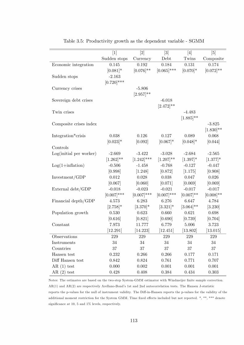
Table 3.5: Productivity growth as the dependent variable - SGMM
[1] [2] [3] [4] [5]Sudden stops Currency Debt Twins Composite
Economic integration 0.145 0.192 0.184 0.131 0.174[0.081]* [0.076]** [0.065]*** [0.070]* [0.072]**
Sudden stops -2.163[0.720]***
Currency crises -5.806[2.957]**
Sovereign debt crises -6.018[2.472]**
Twin crises -4.483[1.885]**
Composite crises index -3.825[1.830]**
Integration*crisis 0.038 0.126 0.127 0.089 0.068[0.023]* [0.092] [0.067]* [0.048]* [0.044]
ControlsLog(initial per worker) -2.669 -3.422 -3.028 -2.684 -2.565
[1.262]** [1.242]*** [1.207]** [1.397]* [1.377]*Log(1+in�ation) -0.506 -1.458 -0.768 -0.127 -0.447
[0.998] [1.248] [0.872] [1.175] [0.908]Investment/GDP 0.012 0.028 0.038 0.047 0.026
[0.067] [0.060] [0.071] [0.069] [0.069]External debt/GDP -0.018 -0.023 -0.021 -0.017 -0.017
[0.007]*** [0.007]*** [0.007]*** [0.007]** [0.008]**Financial depth/GDP 4.573 6.283 6.276 6.647 4.784
[2.758]* [3.370]* [3.321]* [3.064]** [3.230]Population growth 0.530 0.623 0.660 0.621 0.698
[0.616] [0.821] [0.690] [0.739] [0.704]Constant 7.973 11.777 6.779 5.006 3.723
[12.291] [14.223] [12.451] [13.802] [13.015]Observations 229 229 229 229 229Instruments 34 34 34 34 34Countries 37 37 37 37 37Hansen test 0.232 0.266 0.266 0.177 0.171Di¤ Hansen test 0.842 0.824 0.761 0.771 0.707AR (1) test 0.000 0.002 0.001 0.001 0.001AR (2) test 0.428 0.408 0.384 0.434 0.303
Notes: The estimates are based on the two-step System-GMM estimator with Windmeijer �nite sample correction.
AR(1) and AR(2) are respectively Arellano-Bond�s 1st and 2nd autocorrelation tests. The Hansen J-statistic
reports the p-values for the null of instrument validity. The Di¤-in-Hansen reports the p-values for the validity of the
additional moment restriction for the System GMM. Time �xed e¤ects included but not reported. *, **, *** denote
signi�cance at 10, 5 and 1% levels, respectively.
113
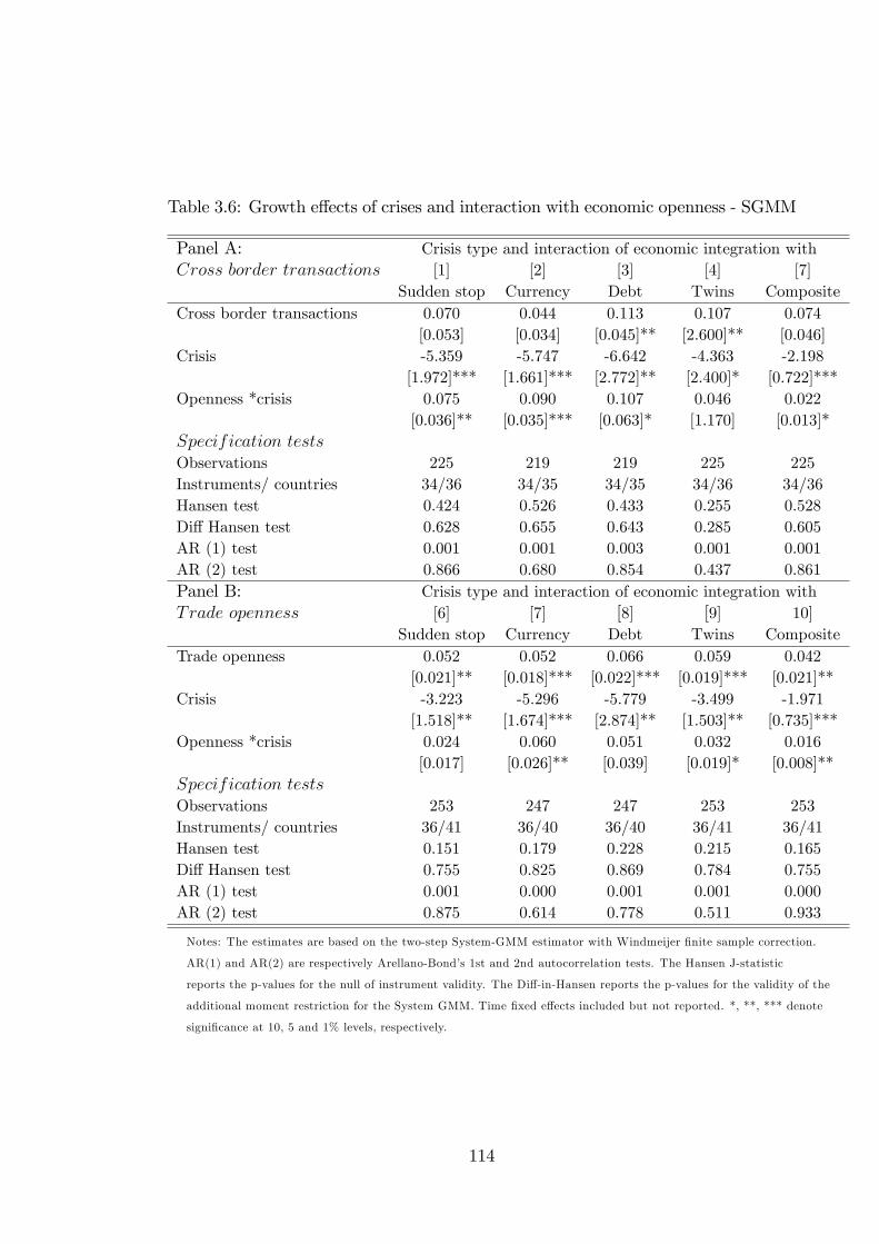
Table 3.6: Growth e¤ects of crises and interaction with economic openness - SGMM
Panel A: Crisis type and interaction of economic integration withCross border transactions [1] [2] [3] [4] [7]
Sudden stop Currency Debt Twins CompositeCross border transactions 0.070 0.044 0.113 0.107 0.074
[0.053] [0.034] [0.045]** [2.600]** [0.046]Crisis -5.359 -5.747 -6.642 -4.363 -2.198
[1.972]*** [1.661]*** [2.772]** [2.400]* [0.722]***Openness *crisis 0.075 0.090 0.107 0.046 0.022
[0.036]** [0.035]*** [0.063]* [1.170] [0.013]*Specification testsObservations 225 219 219 225 225Instruments/ countries 34/36 34/35 34/35 34/36 34/36Hansen test 0.424 0.526 0.433 0.255 0.528Di¤ Hansen test 0.628 0.655 0.643 0.285 0.605AR (1) test 0.001 0.001 0.003 0.001 0.001AR (2) test 0.866 0.680 0.854 0.437 0.861Panel B: Crisis type and interaction of economic integration withTrade openness [6] [7] [8] [9] 10]
Sudden stop Currency Debt Twins CompositeTrade openness 0.052 0.052 0.066 0.059 0.042
[0.021]** [0.018]*** [0.022]*** [0.019]*** [0.021]**Crisis -3.223 -5.296 -5.779 -3.499 -1.971
[1.518]** [1.674]*** [2.874]** [1.503]** [0.735]***Openness *crisis 0.024 0.060 0.051 0.032 0.016
[0.017] [0.026]** [0.039] [0.019]* [0.008]**Specification testsObservations 253 247 247 253 253Instruments/ countries 36/41 36/40 36/40 36/41 36/41Hansen test 0.151 0.179 0.228 0.215 0.165Di¤ Hansen test 0.755 0.825 0.869 0.784 0.755AR (1) test 0.001 0.000 0.001 0.001 0.000AR (2) test 0.875 0.614 0.778 0.511 0.933
Notes: The estimates are based on the two-step System-GMM estimator with Windmeijer �nite sample correction.
AR(1) and AR(2) are respectively Arellano-Bond�s 1st and 2nd autocorrelation tests. The Hansen J-statistic
reports the p-values for the null of instrument validity. The Di¤-in-Hansen reports the p-values for the validity of the
additional moment restriction for the System GMM. Time �xed e¤ects included but not reported. *, **, *** denote
signi�cance at 10, 5 and 1% levels, respectively.
114
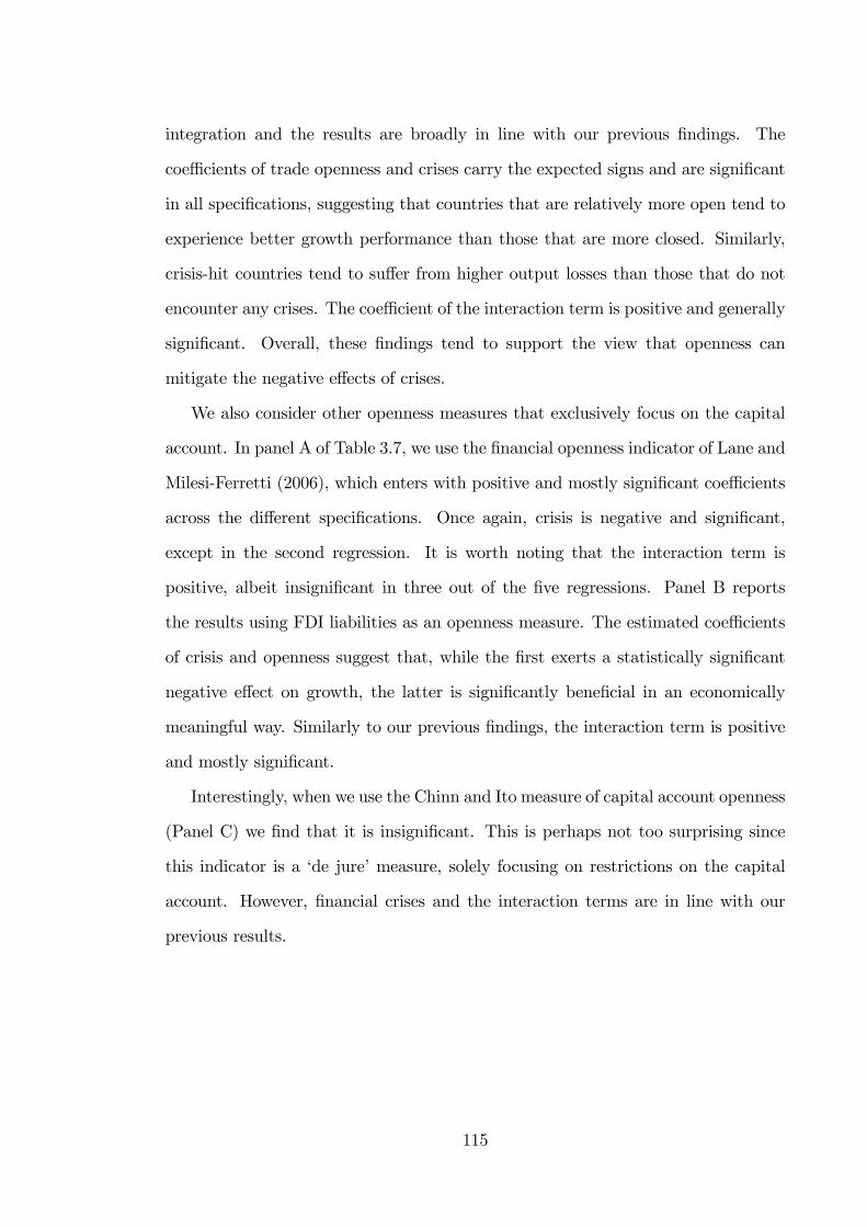
integration and the results are broadly in line with our previous �ndings. The
coe¢ cients of trade openness and crises carry the expected signs and are signi�cant
in all speci�cations, suggesting that countries that are relatively more open tend to
experience better growth performance than those that are more closed. Similarly,
crisis-hit countries tend to su¤er from higher output losses than those that do not
encounter any crises. The coe¢ cient of the interaction term is positive and generally
signi�cant. Overall, these �ndings tend to support the view that openness can
mitigate the negative e¤ects of crises.
We also consider other openness measures that exclusively focus on the capital
account. In panel A of Table 3.7, we use the �nancial openness indicator of Lane and
Milesi-Ferretti (2006), which enters with positive and mostly signi�cant coe¢ cients
across the di¤erent speci�cations. Once again, crisis is negative and signi�cant,
except in the second regression. It is worth noting that the interaction term is
positive, albeit insigni�cant in three out of the �ve regressions. Panel B reports
the results using FDI liabilities as an openness measure. The estimated coe¢ cients
of crisis and openness suggest that, while the �rst exerts a statistically signi�cant
negative e¤ect on growth, the latter is signi�cantly bene�cial in an economically
meaningful way. Similarly to our previous �ndings, the interaction term is positive
and mostly signi�cant.
Interestingly, when we use the Chinn and Ito measure of capital account openness
(Panel C) we �nd that it is insigni�cant. This is perhaps not too surprising since
this indicator is a �de jure�measure, solely focusing on restrictions on the capital
account. However, �nancial crises and the interaction terms are in line with our
previous results.
115
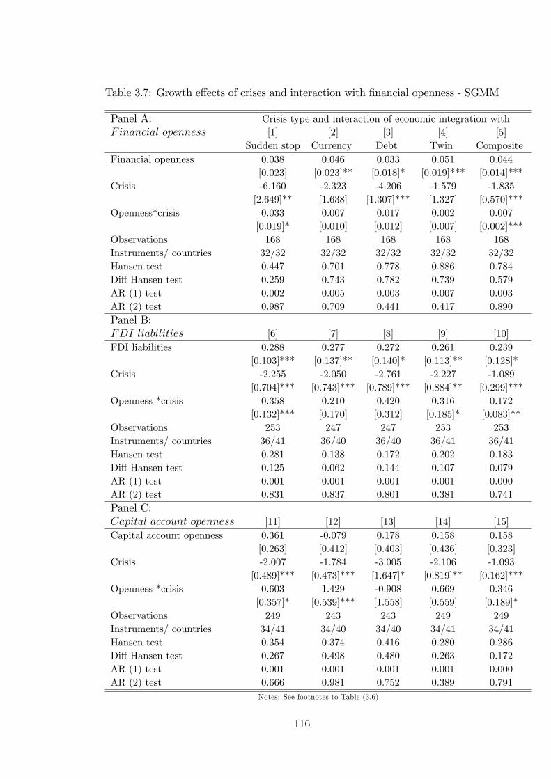
Table 3.7: Growth e¤ects of crises and interaction with �nancial openness - SGMM
Panel A: Crisis type and interaction of economic integration withFinancial openness [1] [2] [3] [4] [5]
Sudden stop Currency Debt Twin CompositeFinancial openness 0.038 0.046 0.033 0.051 0.044
[0.023] [0.023]** [0.018]* [0.019]*** [0.014]***Crisis -6.160 -2.323 -4.206 -1.579 -1.835
[2.649]** [1.638] [1.307]*** [1.327] [0.570]***Openness*crisis 0.033 0.007 0.017 0.002 0.007
[0.019]* [0.010] [0.012] [0.007] [0.002]***Observations 168 168 168 168 168Instruments/ countries 32/32 32/32 32/32 32/32 32/32Hansen test 0.447 0.701 0.778 0.886 0.784Di¤ Hansen test 0.259 0.743 0.782 0.739 0.579AR (1) test 0.002 0.005 0.003 0.007 0.003AR (2) test 0.987 0.709 0.441 0.417 0.890Panel B:FDI liabilities [6] [7] [8] [9] [10]FDI liabilities 0.288 0.277 0.272 0.261 0.239
[0.103]*** [0.137]** [0.140]* [0.113]** [0.128]*Crisis -2.255 -2.050 -2.761 -2.227 -1.089
[0.704]*** [0.743]*** [0.789]*** [0.884]** [0.299]***Openness *crisis 0.358 0.210 0.420 0.316 0.172
[0.132]*** [0.170] [0.312] [0.185]* [0.083]**Observations 253 247 247 253 253Instruments/ countries 36/41 36/40 36/40 36/41 36/41Hansen test 0.281 0.138 0.172 0.202 0.183Di¤ Hansen test 0.125 0.062 0.144 0.107 0.079AR (1) test 0.001 0.001 0.001 0.001 0.000AR (2) test 0.831 0.837 0.801 0.381 0.741Panel C:Capital account openness [11] [12] [13] [14] [15]Capital account openness 0.361 -0.079 0.178 0.158 0.158
[0.263] [0.412] [0.403] [0.436] [0.323]Crisis -2.007 -1.784 -3.005 -2.106 -1.093
[0.489]*** [0.473]*** [1.647]* [0.819]** [0.162]***Openness *crisis 0.603 1.429 -0.908 0.669 0.346
[0.357]* [0.539]*** [1.558] [0.559] [0.189]*Observations 249 243 243 249 249Instruments/ countries 34/41 34/40 34/40 34/41 34/41Hansen test 0.354 0.374 0.416 0.280 0.286Di¤ Hansen test 0.267 0.498 0.480 0.263 0.172AR (1) test 0.001 0.001 0.001 0.001 0.000AR (2) test 0.666 0.981 0.752 0.389 0.791
Notes: See footnotes to Table (3.6)
116
3.5.2 Further robustness analyses
Additional controls
To ensure that our crises indicators do not merely proxy for other events that may
in�uence growth, we control for a number of additional variables. In the following
sensitivity analyses, we report only the results for our preferred measures of open-
ness and crisis, namely, economic integration (proxied by the economic dimension
of the KOF index) and the composite crisis indicator. Our composite measure has a
number of attractive features. Firstly, it captures whether simultaneously encoun-
tering di¤erent types of crises has an additional adverse e¤ect on growth, above and
beyond the adverse e¤ect of each crisis individually. Secondly, and perhaps more im-
portantly, it is more suitable in the context of the system GMM where lags are used
as instruments to overcome issues of endogeneity19. The results are summarised in
Table 3.8. In the �rst sets of regressions, we account for the roles political and insti-
tutional variables play in determining output growth (e.g. Acemoglu et al. 2003).
Recent evidence also suggests that political variables can have a signi�cant in�uence
on the growth outcomes of �nancial crises (Cavallo and Cavallo, 2010). Hence, we
add indicators such as regime type, polity, civil unrest and political rights to the
baseline speci�cation. These variables are not signi�cantly related to output growth
in our sample countries, of more interest in the present context, our central �ndings
remain robust.
We need to rule out the possibility that crisis incidence and the extent to which
it in�uences growth may depend on the availability of su¢ cient reserves or changes
in the terms of trade (see for example, Li and Ouyang, 2011). Thus, we explore the
in�uence of reserve holdings and terms of trade on growth and �nd that the �rst
carries a signi�cant and positive sign while the latter is insigni�cant (regressions [5]
and [6]). This implies that a high level of reserves may be interpreted as a signi�cant
19Using the lag of a dummy variable to account for endogeneity may not be appropriate (see,Cavallo and Cavallo, 2010).
117
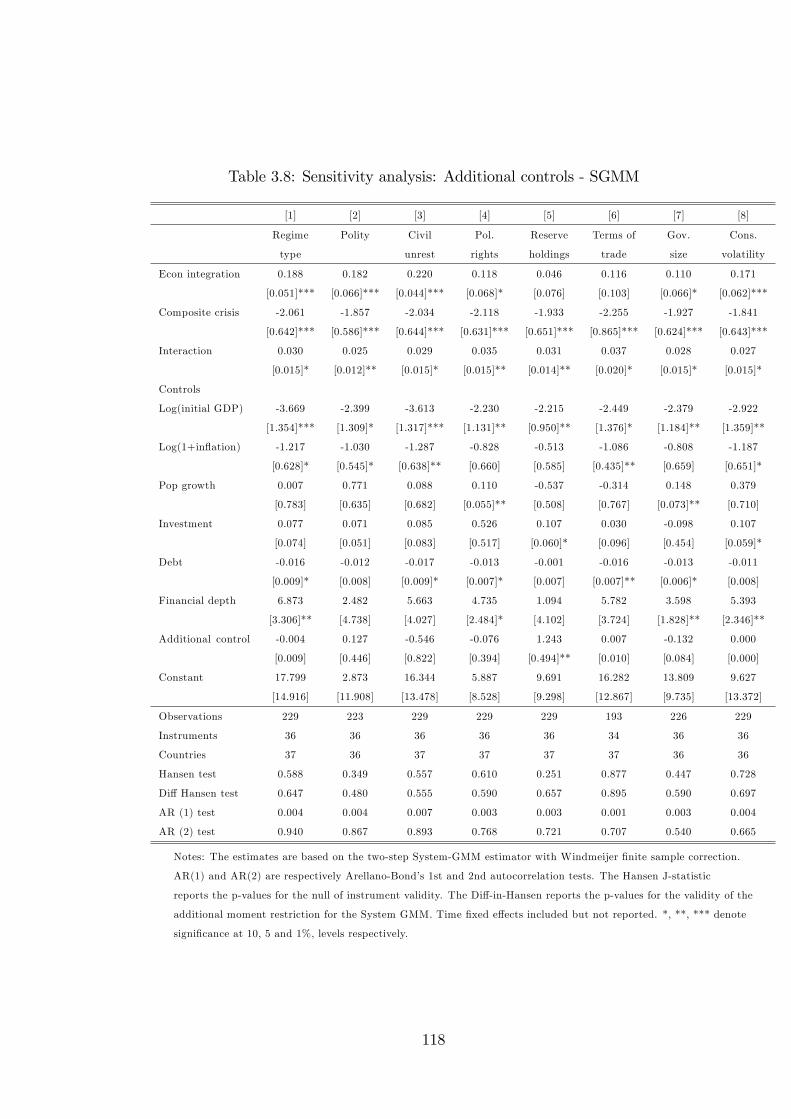
Table 3.8: Sensitivity analysis: Additional controls - SGMM
[1] [2] [3] [4] [5] [6] [7] [8]
Regime Polity Civil Pol. Reserve Terms of Gov. Cons.
type unrest rights holdings trade size volatility
Econ integration 0.188 0.182 0.220 0.118 0.046 0.116 0.110 0.171
[0.051]*** [0.066]*** [0.044]*** [0.068]* [0.076] [0.103] [0.066]* [0.062]***
Composite crisis -2.061 -1.857 -2.034 -2.118 -1.933 -2.255 -1.927 -1.841
[0.642]*** [0.586]*** [0.644]*** [0.631]*** [0.651]*** [0.865]*** [0.624]*** [0.643]***
Interaction 0.030 0.025 0.029 0.035 0.031 0.037 0.028 0.027
[0.015]* [0.012]** [0.015]* [0.015]** [0.014]** [0.020]* [0.015]* [0.015]*
Controls
Log(initial GDP) -3.669 -2.399 -3.613 -2.230 -2.215 -2.449 -2.379 -2.922
[1.354]*** [1.309]* [1.317]*** [1.131]** [0.950]** [1.376]* [1.184]** [1.359]**
Log(1+in�ation) -1.217 -1.030 -1.287 -0.828 -0.513 -1.086 -0.808 -1.187
[0.628]* [0.545]* [0.638]** [0.660] [0.585] [0.435]** [0.659] [0.651]*
Pop growth 0.007 0.771 0.088 0.110 -0.537 -0.314 0.148 0.379
[0.783] [0.635] [0.682] [0.055]** [0.508] [0.767] [0.073]** [0.710]
Investment 0.077 0.071 0.085 0.526 0.107 0.030 -0.098 0.107
[0.074] [0.051] [0.083] [0.517] [0.060]* [0.096] [0.454] [0.059]*
Debt -0.016 -0.012 -0.017 -0.013 -0.001 -0.016 -0.013 -0.011
[0.009]* [0.008] [0.009]* [0.007]* [0.007] [0.007]** [0.006]* [0.008]
Financial depth 6.873 2.482 5.663 4.735 1.094 5.782 3.598 5.393
[3.306]** [4.738] [4.027] [2.484]* [4.102] [3.724] [1.828]** [2.346]**
Additional control -0.004 0.127 -0.546 -0.076 1.243 0.007 -0.132 0.000
[0.009] [0.446] [0.822] [0.394] [0.494]** [0.010] [0.084] [0.000]
Constant 17.799 2.873 16.344 5.887 9.691 16.282 13.809 9.627
[14.916] [11.908] [13.478] [8.528] [9.298] [12.867] [9.735] [13.372]
Observations 229 223 229 229 229 193 226 229
Instruments 36 36 36 36 36 34 36 36
Countries 37 36 37 37 37 37 36 36
Hansen test 0.588 0.349 0.557 0.610 0.251 0.877 0.447 0.728
Di¤ Hansen test 0.647 0.480 0.555 0.590 0.657 0.895 0.590 0.697
AR (1) test 0.004 0.004 0.007 0.003 0.003 0.001 0.003 0.004
AR (2) test 0.940 0.867 0.893 0.768 0.721 0.707 0.540 0.665
Notes: The estimates are based on the two-step System-GMM estimator with Windmeijer �nite sample correction.
AR(1) and AR(2) are respectively Arellano-Bond�s 1st and 2nd autocorrelation tests. The Hansen J-statistic
reports the p-values for the null of instrument validity. The Di¤-in-Hansen reports the p-values for the validity of the
additional moment restriction for the System GMM. Time �xed e¤ects included but not reported. *, **, *** denote
signi�cance at 10, 5 and 1%, levels respectively.
118
deterrent of potential economic di¢ culties. As expected, the coe¢ cient of crisis
exhibits a negative and statistically signi�cant e¤ect on growth. The coe¢ cient of
the interaction between crisis and openness is positive and signi�cant (with a p-
value of 0.022) in column [5] but the signi�cance level drops to 10 percent in column
[6]. Based on this, we can posit that the (negative) relationship between crises
and growth gets weaker the more integrated an economy becomes. In other words,
economic integration acts as a crisis bu¤er by mitigating the adverse e¤ects of crises
on output growth.
We also examine how growth relates to consumption volatility and government
size. We �nd that, while both of these variables carry the expected signs, neither
of them are signi�cant at conventional levels and their inclusion does not alter our
basic �ndings. Hence, we can state that our results remain robust when we account
for other important correlates of growth. Moreover, the validity of the instruments
is not rejected in any of the SGMM regressions. In particular, the speci�cations pass
the Hansen J test for over-identifying restrictions. They also pass the Arellano-Bond
tests for serial correlation, con�rming that our models are not misspeci�ed.
Sub-samples
As an additional robustness check, we re-estimate our baseline results for various
sub-samples to test their stability. Firstly, there could be parameter heterogeneity
across the conditional growth distribution, so that countries in the higher growth
quantiles may respond di¤erently to both crises and economic integration than do
countries whose growth rates are in the lower quantiles. To explore this, the �rst
two columns of Table 3.9 are based on quantile regressions where we report both
the 25th quantile (low growth) and the 75th quantile of the growth distribution
(high growth). Interestingly, we �nd that high growth performers tend to bene�t
signi�cantly from openness while poor performers do not as much. In addition,
the coe¢ cient of openness for the high growth group is more than twice as large
119
as that for the low growth group. The results suggest that the adverse impact of
crises on output growth is signi�cantly di¤erent from zero for both groups, but the
magnitude is slightly larger in the higher growth distribution. More importantly,
the coe¢ cient of the interaction term is positive and signi�cant for both groups,
albeit only marginally so for the high growth group. Hence, our baseline results
remain unchanged.
In a similar vein, we test whether higher income African countries are driving
the results, since they generally tend to be more integrated with the rest of the
world. To confront this, we split the sample according to the level of economic
development and de�ne those economies with a level of per capita income equal to
or below the sample median as �low income�. The results for this group are reported
in column 3 and continue to point to the importance of crises in undermining growth
in low income African countries. While there is no signi�cant link between economic
integration and growth, the results suggest that the adverse e¤ect of crises on growth
is lower the more open the economy is.
The negative link between crises and growth that we have found so far could be
due to the presence of resource-rich countries since these may be more prone to crises
but also more integrated with the rest of the world. Hence, we examine whether our
central �ndings survive if we focus on resource-poor economies only. As a proxy for
resources, we use the share of oil rents in GDP. The estimated regression (column
[4]) is largely in line with our previous �ndings insofar as it points to the tendency
of openness to lessen the adverse e¤ects of crises.
As previously emphasised by a number of studies (see, for example, Loayza and
Ranciere, 2005), one of the most important transmission channels between crises
and output growth is the �nancial system. Accordingly, it could be that our results
are driven by countries with more developed �nancial systems. The regression re-
sults reported in column [5] are based on a sub-sample of countries with relatively
poor �nancial systems. Again, the interaction term between crises and openness is
120
positive and signi�cant, implying that openness tends to lessen the disruptive e¤ects
of crisis on output growth, even in the absence of sophisticated �nancial systems.
We also examine whether our �ndings are true for those countries with greater re-
strictions on trade. This sample of �closed�economies is selected based on levels of
tari¤s (column[6]). As the results show, the baseline results remain unchanged.
As a number of studies indicate (see, for example, Esaka, 2010), the exchange rate
regime of a country may in�uence the relationship between crises and output. As a
�nal exercise, therefore, we divide our sample countries into two groups, based on
the prevailing exchange rate regime. In column [7], we show the results for countries
with �semi �exible�regimes (i.e. those with either crawling/managed �oated or pure
�oated) and �nd that this does not alter our baseline results signi�cantly. When we
conduct similar exercise for those with ��xed/pegged�exchange rates, we �nd that,
while crisis is negative and signi�cant, both openness and the interaction term lose
their signi�cance.
To sum up, our sub-sample analysis indicates that crises are signi�cantly associ-
ated with poorer economic performance. However, this negative e¤ect decreases with
the level of openness. Lastly, the SGMM diagnostics are satisfactory throughout the
sensitivity analysis.
Alternative estimators
Finally, we check whether our results remain robust to alternative estimators. Table
3.10 shows the results. The �rst column reports results based on simple pooled
OLS. Even though this estimator does not account for unobserved heterogeneity
or endogeneity, it can nonetheless shed some light on the links between crises and
growth. The signi�cant negative sign of the coe¢ cient of the crisis variable con�rms
the detrimental e¤ect of crises on output growth. The sign and signi�cance of the
interaction term is in line with our baseline regression.
To ensure that our results are not sensitive to the presence of outliers, we re-run
121
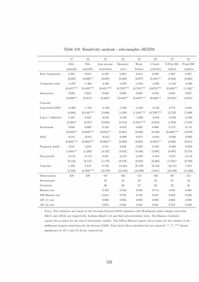
Table 3.9: Sensitivity analysis - sub-samples -SGMM
[1] [2] [3] [4] [5] [6] [7] [8]
25th 75th Low income Resource Weak Closed S-Flex ER Fixed ER
quantile quantile economies poor �nance countries regime regimes
Econ integration 0.024 0.054 0.130 0.064 0.044 0.093 0.067 0.087
[0.022] [0.026]** [0.087] [0.048] [0.077] [0.041]** [0.044] [0.065]
Composite crisis -1.278 -1.464 -2.401 -2.637 -2.953 -2.982 -2.150 -2.029
[0.347]*** [0.423]*** [0.851]*** [0.722]*** [0.745]*** [0.675]*** [0.930]** [1.156]*
Interaction 0.020 0.021 0.040 0.038 0.056 0.046 0.034 0.027
[0.009]** [0.011]* [0.023]* [0.016]** [0.019]*** [0.020]** [0.018]* [0.031]
Controls
Log(initial GDP) -0.406 -1.194 -2.446 -1.688 -3.349 -2.139 2.774 0.016
[0.264] [0.218]*** [2.028] [1.338] [1.216]*** [0.730]*** [2.725] [1.809]
Log(1+ in�ation) 0.481 0.025 -0.831 -0.456 -1.660 -0.424 -0.376 -0.580
[0.288]* [0.327] [0.633] [0.412] [0.351]*** [0.653] [1.650] [1.078]
Investment 0.045 0.098 0.135 0.076 0.092 0.080 0.172 0.118
[0.023]** [0.023]*** [0.058]** [0.087] [0.092] [0.049] [0.049]*** [0.079]
Debt -0.011 -0.015 -0.012 -0.009 -0.011 -0.018 -0.003 -0.005
[0.002]*** [0.003]*** [0.005]** [0.009] [0.007] [0.007]** [0.008] [0.017]
Financial depth 2.541 2.233 3.741 3.028 -5.027 0.458 -9.426 -9.805
[1.054]** [1.229]* [3.127] [4.825] [6.550] [5.097] [8.387] [9.714]
Pop growth -0.152 -0.172 0.201 -0.473 -0.307 -0.164 2.522 -0.118
[0.142] [0.157] [1.179] [0.723] [0.597] [0.363] [1.531]* [0.786]
Constant 1.485 8.215 8.759 13.564 27.579 13.412 -40.174 1.813
[2.338] [2.562]*** [19.750] [12.670] [10.209] [4.851] [32.280] [14.330]
Observations 229 229 187 162 113 136 90 124
Instruments 24 24 24 34 24 24
Countries 30 30 27 33 22 28
Hansen test 0.462 0.532 0.850 0.714 0.625 0.304
Di¤ Hansen test 0.614 0.795 0.734 0.647 0.625 0.328
AR (1) test 0.006 0.004 0.009 0.005 0.025 0.029
AR (2) test 0.653 0.302 0.585 0.861 0.727 0.429
Notes: The estimates are based on the two-step System-GMM estimator with Windmeijer �nite sample correction.
AR(1) and AR(2) are respectively Arellano-Bond�s 1st and 2nd autocorrelation tests. The Hansen J-statistic
reports the p-values for the null of instrument validity. The Di¤-in-Hansen reports the p-values for the validity of the
additional moment restriction for the System GMM. Time �xed e¤ects included but not reported. *, **, *** denote
signi�cance at 10, 5 and 1% levels, respectively.
122
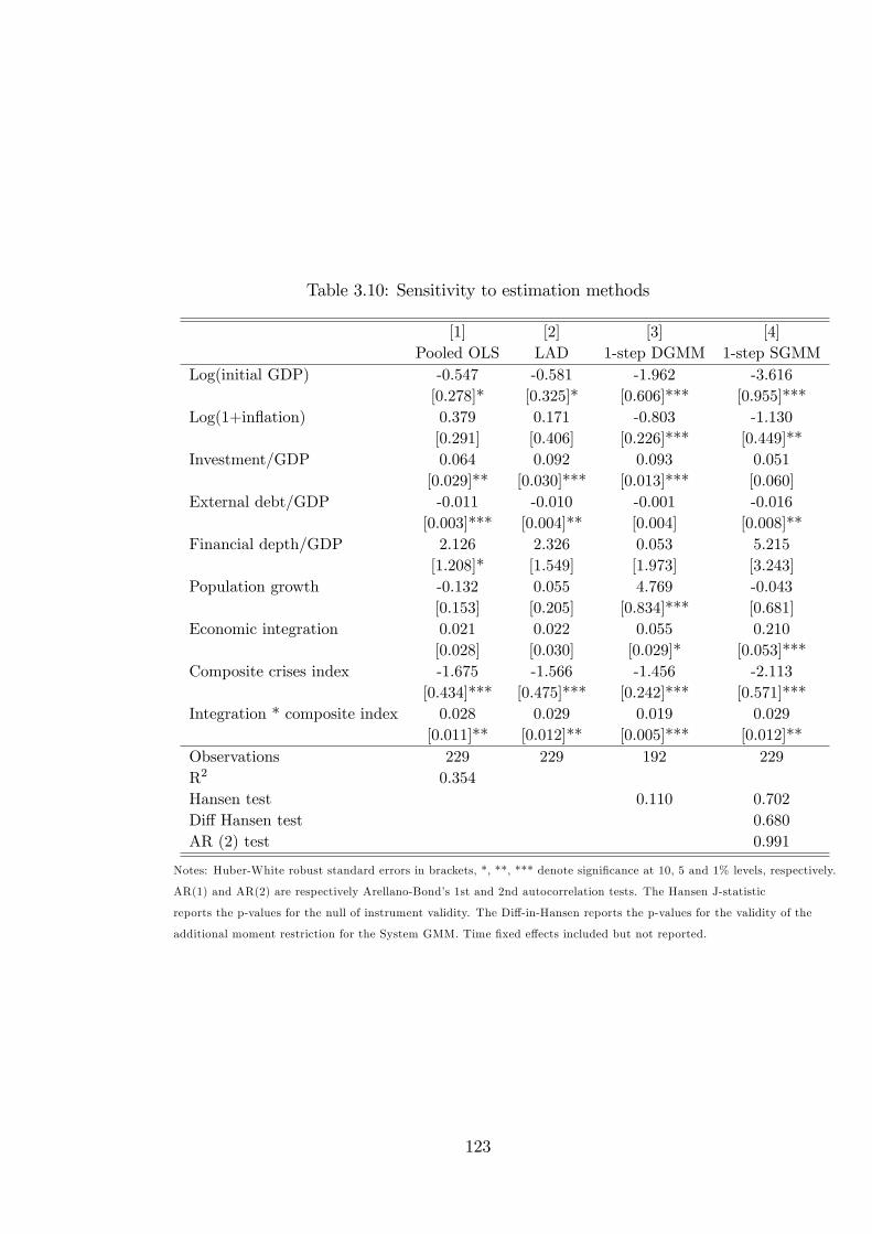
Table 3.10: Sensitivity to estimation methods
[1] [2] [3] [4]Pooled OLS LAD 1-step DGMM 1-step SGMM
Log(initial GDP) -0.547 -0.581 -1.962 -3.616[0.278]* [0.325]* [0.606]*** [0.955]***
Log(1+in�ation) 0.379 0.171 -0.803 -1.130[0.291] [0.406] [0.226]*** [0.449]**
Investment/GDP 0.064 0.092 0.093 0.051[0.029]** [0.030]*** [0.013]*** [0.060]
External debt/GDP -0.011 -0.010 -0.001 -0.016[0.003]*** [0.004]** [0.004] [0.008]**
Financial depth/GDP 2.126 2.326 0.053 5.215[1.208]* [1.549] [1.973] [3.243]
Population growth -0.132 0.055 4.769 -0.043[0.153] [0.205] [0.834]*** [0.681]
Economic integration 0.021 0.022 0.055 0.210[0.028] [0.030] [0.029]* [0.053]***
Composite crises index -1.675 -1.566 -1.456 -2.113[0.434]*** [0.475]*** [0.242]*** [0.571]***
Integration * composite index 0.028 0.029 0.019 0.029[0.011]** [0.012]** [0.005]*** [0.012]**
Observations 229 229 192 229R2 0.354Hansen test 0.110 0.702Di¤ Hansen test 0.680AR (2) test 0.991
Notes: Huber-White robust standard errors in brackets, *, **, *** denote signi�cance at 10, 5 and 1% levels, respectively.
AR(1) and AR(2) are respectively Arellano-Bond�s 1st and 2nd autocorrelation tests. The Hansen J-statistic
reports the p-values for the null of instrument validity. The Di¤-in-Hansen reports the p-values for the validity of the
additional moment restriction for the System GMM. Time �xed e¤ects included but not reported.
123
the baseline speci�cation using the Least Absolute Deviation (LAD) estimator. By
using the median (instead of the mean) of the dependent variable (conditional on
the values of the explanatory variables), this estimator tends to generate results
that are less a¤ected by distant data points. As can be seen in the second column of
Table 3.10, the results support our previous �nding that openness tends to dampen
the negative in�uence of crises on growth.
Our main results so far have been based on the two-step system GMM. As a
robustness check, in the last two columns we report results based on 1-step DGMM
and SGMM, respectively. The estimates suggest that openness is positively and
signi�cantly associated with higher growth rates. They also indicate that there is a
signi�cant negative relationship between growth and crises. Finally, the coe¢ cient
of the interaction term is consistent with our previous results.
In sum, we �nd that �nancial crises are associated with output losses in our
sample of countries. Our results also suggest that economic integration, perhaps
by relaxing credit constraints, helps economies to overcome the adverse e¤ects of
�nancial crises on economic performance.
3.6 Concluding Remarks
In this study, we use a large African sample to analyse comprehensively the relation-
ship between crises and growth. Focusing on four di¤erent types of �nancial crises,
we provide evidence showing that external shocks can account for a large fraction
of the cross-country variation in output growth over the sample period. The central
�ndings of this study are in line with the theoretical view that crises disrupt eco-
nomic activity. Our empirical results add to the growing empirical evidence (Cavallo
and Cavallo, 2010; Joyce and Nabar, 2009) that crises undermine economic growth.
In contrast to the existing literature, our study solely focuses on African coun-
tries. In addition, our main results are obtained using the two-step system GMM
124
developed by Arellano and Bover (1995) and Blundell and Bond (1998), which con-
trols for endogeneity, measurement error and omitted variable biases. Also, our
results remain robust to a battery of sensitivity analyses where we consider addi-
tional control variables, various econometric methods, outliers and sub-samples.
In line with the existing literature (e.g. Bruckner and Lederman, 2012; Changa
and Mendy, 2012), we �nd a robust positive link between economic openness and
growth performance in Africa. Our results can be generalised to measures of �nancial
openness. A variety of mechanisms could rationalise this result - the most plausible
being that �nancial openness may have had a robust bene�cial e¤ect on African
�nancial markets and thus indirectly promoted growth (see, Ahmed, 2011).
In an attempt to identify the speci�c channels through which crises a¤act output
growth, we test the hypothesis that the level of economic integration in the crisis-hit
country might be important. We �nd that crises have had a more disruptive e¤ect
on growth in countries with lower levels of openness. For instance, it could be that
openness lessens the adjustment costs associated with external crises, as suggested
by sticky price open economy models as well as conventional Mundell-Flemming type
models. This implies that once an economy reaches a certain level of �nancial and
economic openness, the negative e¤ects of crises would be minimised, presumably
because the country would be in a position to keep the fall in aggregate demand in
check.
However, an important caveat remains; most of the hypothesized bene�cial ef-
fects of openness (e.g. more e¢ cient capital allocation) highlighted in the theoretical
literature cannot be empirically tested due to lack of appropriate proxies. Never-
theless, in tandem with both the theoretical and empirical literature, our results
strongly indicate that economic openness is associated with higher growth rates in
Africa. But at the same time, as our previous results with respect to capital �ight
show, openness may exacerbate the domestic investment climate through its ten-
dency to import volatility. Moreover, it may create avenues for capital �ight to take
125

place (e.g. under-invoicing of exports and over-invoicing of imports etc.). Thus,
openness would be more bene�cial in an environment where the other dimensions of
the domestic investment climate are strong - good institutions and macroeconomic
stability, among others.
126

3.A Appendix 3
127
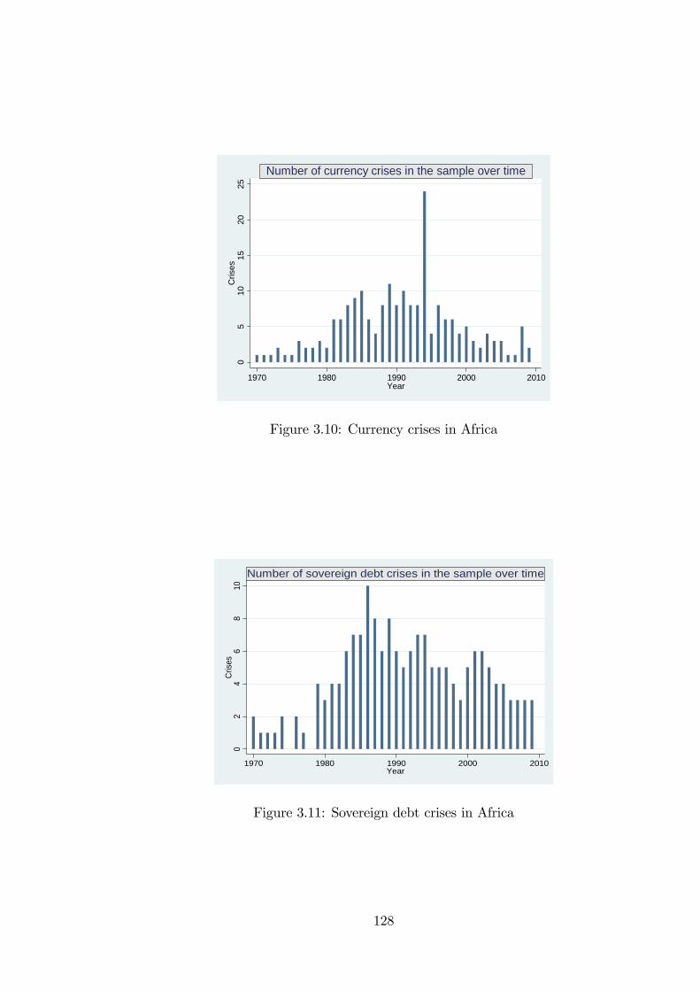
05
1015
2025
Cris
es
1970 1980 1990 2000 2010Year
Number of currency crises in the sample over time
Figure 3.10: Currency crises in Africa
02
46
810
Crise
s
1970 1980 1990 2000 2010Year
Number of sovereign debt crises in the sample over time
Figure 3.11: Sovereign debt crises in Africa
128
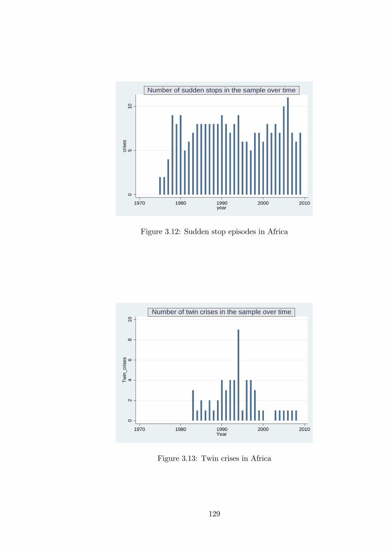
05
10cr
ises
1970 1980 1990 2000 2010year
Number of sudden stops in the sample over time
Figure 3.12: Sudden stop episodes in Africa
02
46
810
Twin
_cris
es
1970 1980 1990 2000 2010Year
Number of twin crises in the sample over time
Figure 3.13: Twin crises in Africa
129
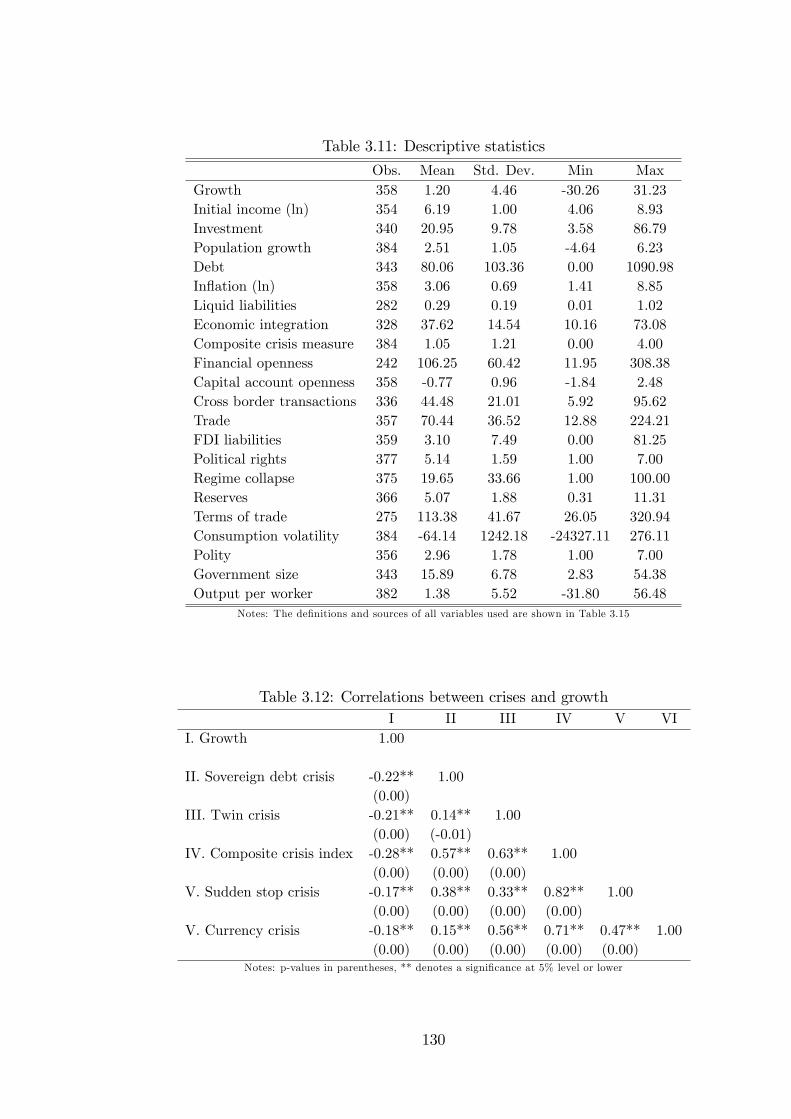
Table 3.11: Descriptive statistics
Obs. Mean Std. Dev. Min MaxGrowth 358 1.20 4.46 -30.26 31.23Initial income (ln) 354 6.19 1.00 4.06 8.93Investment 340 20.95 9.78 3.58 86.79Population growth 384 2.51 1.05 -4.64 6.23Debt 343 80.06 103.36 0.00 1090.98In�ation (ln) 358 3.06 0.69 1.41 8.85Liquid liabilities 282 0.29 0.19 0.01 1.02Economic integration 328 37.62 14.54 10.16 73.08Composite crisis measure 384 1.05 1.21 0.00 4.00Financial openness 242 106.25 60.42 11.95 308.38Capital account openness 358 -0.77 0.96 -1.84 2.48Cross border transactions 336 44.48 21.01 5.92 95.62Trade 357 70.44 36.52 12.88 224.21FDI liabilities 359 3.10 7.49 0.00 81.25Political rights 377 5.14 1.59 1.00 7.00Regime collapse 375 19.65 33.66 1.00 100.00Reserves 366 5.07 1.88 0.31 11.31Terms of trade 275 113.38 41.67 26.05 320.94Consumption volatility 384 -64.14 1242.18 -24327.11 276.11Polity 356 2.96 1.78 1.00 7.00Government size 343 15.89 6.78 2.83 54.38Output per worker 382 1.38 5.52 -31.80 56.48
Notes: The de�nitions and sources of all variables used are shown in Table 3.15
Table 3.12: Correlations between crises and growthI II III IV V VI
I. Growth 1.00
II. Sovereign debt crisis -0.22** 1.00(0.00)
III. Twin crisis -0.21** 0.14** 1.00(0.00) (-0.01)
IV. Composite crisis index -0.28** 0.57** 0.63** 1.00(0.00) (0.00) (0.00)
V. Sudden stop crisis -0.17** 0.38** 0.33** 0.82** 1.00(0.00) (0.00) (0.00) (0.00)
V. Currency crisis -0.18** 0.15** 0.56** 0.71** 0.47** 1.00(0.00) (0.00) (0.00) (0.00) (0.00)
Notes: p-values in parentheses, ** denotes a signi�cance at 5% level or lower
130
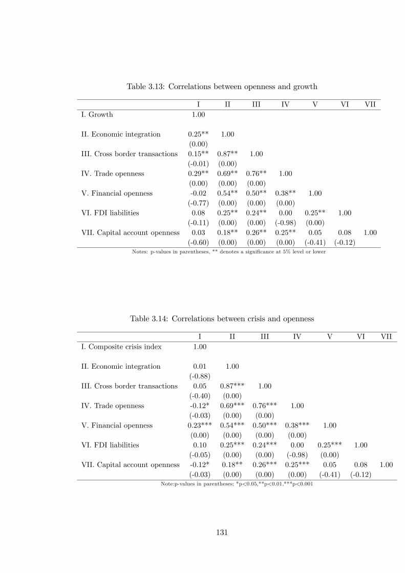
Table 3.13: Correlations between openness and growth
I II III IV V VI VIII. Growth 1.00
II. Economic integration 0.25** 1.00(0.00)
III. Cross border transactions 0.15** 0.87** 1.00(-0.01) (0.00)
IV. Trade openness 0.29** 0.69** 0.76** 1.00(0.00) (0.00) (0.00)
V. Financial openness -0.02 0.54** 0.50** 0.38** 1.00(-0.77) (0.00) (0.00) (0.00)
VI. FDI liabilities 0.08 0.25** 0.24** 0.00 0.25** 1.00(-0.11) (0.00) (0.00) (-0.98) (0.00)
VII. Capital account openness 0.03 0.18** 0.26** 0.25** 0.05 0.08 1.00(-0.60) (0.00) (0.00) (0.00) (-0.41) (-0.12)
Notes: p-values in parentheses, ** denotes a signi�cance at 5% level or lower
Table 3.14: Correlations between crisis and openness
I II III IV V VI VIII. Composite crisis index 1.00
II. Economic integration 0.01 1.00(-0.88)
III. Cross border transactions 0.05 0.87*** 1.00(-0.40) (0.00)
IV. Trade openness -0.12* 0.69*** 0.76*** 1.00(-0.03) (0.00) (0.00)
V. Financial openness 0.23*** 0.54*** 0.50*** 0.38*** 1.00(0.00) (0.00) (0.00) (0.00)
VI. FDI liabilities 0.10 0.25*** 0.24*** 0.00 0.25*** 1.00(-0.05) (0.00) (0.00) (-0.98) (0.00)
VII. Capital account openness -0.12* 0.18** 0.26*** 0.25*** 0.05 0.08 1.00(-0.03) (0.00) (0.00) (0.00) (-0.41) (-0.12)
Note:p-values in parentheses; *p<0.05,**p<0.01,***p<0.001
131
Table 3.15: Data sources
Variable De�nition and SourceGrowth Real per capita GDP growth rate. World Bank (2011): WDI
Initial income First value of real per capita income for each 5-year period. World Bank (2011): WDI
Sudden stop crisis Own calculation based on a modi�ed version of Calvo et al. (2004). See text for description
Currency crisis Reinhart and Rogo¤ (2009). See text for description
Sovereign debt crisis Reinhart and Rogo¤ (2009). See text for description
Twin crisis Joint occurrence of banking and currency crises. The data on banking crises is from
Laeven and Valencia (2008)
Composite crisis index Own calculation based on types of crises encountered in a particular year, weighted by each
country�s share in world output.
Investment Gross capital formation as a % of GDP. World Bank (2011): WDI
Debt External borrowing as a % of GDP. World Bank (2011): WDI
Financial depth Captured by Liquid liabilities as a % of GDP. World Bank (2011): WDI
In�ation Change in CPI. World Bank (2011): WDI
Trade openness Imports + exports as a % of GDP. World Bank (2011): WDI
Economic integration Measured by actual �ows of trade and investment and their restrictions,
expressed as a % of GDP. Dreher (2006, revised 2011)
Cross border transaction De-facto measure of openness (measured by actual �ows of
trade, FDI +portfolio + payments to foreigners) as a % of GDP. Dreher (2006, revised 2011)
Capital acc. openness Chinn-Ito�s de jure index (revised 2011)
Financial openness De facto �n openness sum of total cross-border assets and liablities over GDP.
FDI liabilities Share of FDI liabilities in GDP. Lane and Milesi-Ferretti (2006, revised 2011)
Productivity Output per worker. PWT 7.0 (2011)
Government size Government expenditure as % of GDP. World Bank (2011): WDI
Political rights The extent of political rights in a country as calculated by Freedom
House. Coded from 1-7 (7 being the worst). FH surveys (2011)
Regime type Ranges from Monarchy, Military, One-party, Multi-party system to full Democracy (higher value),
Teorell and Hadenius (2007).
Reserves FX Reserves minus gold (% GDP). Lane and Milesi-Ferretti (2006)
Civil unrest Dummy taking the value 1 if country has a military con�ict in current year. PRIO/UCDP (2011)
Terms of trade Net barter terms of trade index. World Bank (2011): WDI
Consumption volality Standard deviation of consumption. Underlying data from PWT 7.0 (2011)
Polity Executive Constraints (Decision Rules): from (1) Unlimited Authority to (7) Limited Authority.
PolityIV dataset (2011)
132
Chapter 4
Capital Flows and DomesticInvestment: Evidence fromAfrican and Other DevelopingCountries
4.1 Introduction
Foreign capital in�ows are viewed by many economists as means of accelerating the
rates of growth of developing countries. The three most important external sources
of capital are o¢ cial aid, foreign direct investment (FDI) and migrant remittances.
Historically, foreign aid has been the dominant, but in the last two decades, FDI
and remittances have taken a more prominent role in developing countries.
An important issue, however, is whether these types of in�ows act as comple-
ments or substitutes for domestic investment and thus economic growth. Theoret-
ically, capital in�ows can facilitate economic development by enhancing the avail-
ability of funds for productive investments and thereby ease the resource constraints
faced by recipient countries. In addition, some of these �ows, particularly FDI, can
have embedded in them knowledge, technology and management skills, which can
have positive externalities on the host economy.
On the other hand, as has been suggested by many, these types of external �nance
may in fact have adverse e¤ects on the recipient economy. For example, foreign
133
aid, or at least certain types of it, can displace domestic savings and thus erode the
ability of the recipient countries to generate own resources for investment and growth
(Ouattara, 2009). Similarly, FDI may have negative e¤ects on the performance of
domestic �rms by outcompeting them in, for example, product markets. Some of
the activities of multinational companies (e.g. transfer pricing, dividend and royalty
repatriation, high import-propensity) can have adverse e¤ects on the host countries�
tax revenues and balance of payments (Apergis et al. 2006). Remittances too may
not contribute to economic growth as it may act as a compensatory transfer, which
tend to be used for consumption rather than productive investment (Chami et al.
2005).
The empirical evidence on the relationship between capital in�ows and domestic
investment has been mixed. Some studies �nd that capital in�ows exert a positive
e¤ect on domestic investment, while others either report a negative association or
fail to �nd any signi�cant link.
The objective of this study is to contribute to this literature but we depart from
the existing literature in a number of ways. Firstly, we use recently developed panel
cointegration tests that can handle a number of econometric issues, including cross-
sectional heterogeneity, structural breaks and endogeneity concerns. Secondly, we
examine the long-run relationship between these in�ows and domestic investment for
the panel as a whole as well as for individual countries. Thirdly, we apply panel error
correction methods to uncover the short-run dynamics in the relationship between
capital �ows and domestic investment. Finally, we conduct a panel Granger causality
analysis in order to establish whether the long and short-run e¤ects are indeed of a
causal nature.
The chapter is organised as follows. Section 2 provides a brief overview of the
existing literature on the relationship between capital �ows and domestic investment.
Section 3 sets out the econometric model, presenting the data and the techniques
used. Section 4 discusses the results while Section 5 concludes.
134
4.2 Capital �ows and domestic investment
The literature on the e¤ects of capital in�ows on domestic investment is vast with
varying results. In what follows, we summarise the ways in which these in�ows can
in�uence domestic investment. In doing so, we highlight the contributions of the
present study.
4.2.1 Remittances and domestic investment
The macroeconomic e¤ects of remittances largely depend on whether they act as
pure compensatory transfers or capital �ows (Chami et al. 2005). In the �rst case,
altruistic motives dominate in the sense that the migrant is concerned with the
well-being of his/her relatives. In the latter case, though, self-interest dominates,
suggesting that the migrant retains some sort of ownership over the assets. In both
cases, however, the response of the economy to increases in remittances could be
either negative or positive.
On the one hand, remittance �ows can have negative e¤ects on the recipient
economy through their adverse in�uences on income distributions (Orrenius et al.
2010), household�s labour supply and savings rates (Chami et al. 2005). In addi-
tion, similar to any other resource in�ow, sustained levels of remittances tend to be
associated with �Dutch disease�e¤ects (Amuedo-Dorantes et al. 2004) as well as
increases in conspicuous consumption rather than productive investments (Chami
et al. 2005).
On the other hand, there is considerable evidence showing that, although remit-
tances may mainly go to consumption, a substantial portion of it goes to human
capital formation in the form of better nutrition, schooling and health (Gupta et
al. 2009). Moreover, increased consumption and even �unproductive�investments
(e.g. real estate) can have signi�cant multiplier e¤ects, encouraging more capital
accumulation and growth through spillover e¤ects (Ratha, 2003; Gupta et al. 2009).
135
Evidence also suggests that remittances tend to reduce households�credit constraints
and thus boost the depth of the �nancial sector (Guilamo and Ruiz-Arranz, 2009;
Aggarwal et al. 2011). Furthermore, it has been shown that remittance receiving
households, on average, tend to save and invest more than other comparable house-
holds (Adams, 2007). Other studies show remittances are associated with poverty
reductions (Adams and Page, 2005) and higher educational attainments (Rapoport
and Docquier, 2005). Finally, remittance �ows have been found to act more counter-
cyclically than other types of in�ows and thus are a more stable source of foreign
exchange at times of economic di¢ culties (Combes and Ebeke, 2011; Chami et al.
2009).
4.2.2 Foreign aid and domestic investment
Foreign aid di¤ers from the two other �ows in two distinct ways. Firstly, it goes
to the public sector. Secondly, and perhaps more importantly, its relationship with
domestic investment is much more straightforward, particularly in low income coun-
tries. This is because, in such countries, foreign aid can directly augment the level
of public investment as it relaxes the government budget constraint. However, this
argument assumes the absence of the so-called �fungibility proposition�in which aid
may not enhance public investments as it tends to go to government consumption
instead (see for example, Boone, 1996; Swaroop et al. 2000).
However, as shown by Herzer and Morrissey (2009), the general validity of the
�fungibility proposition� can be questioned on the grounds that government con-
sumption and investment are not easily distinguishable. For example, government
consumption may include expenditures that cover the social sector (e.g. human
capital investments). Evidence suggests that aid is signi�cantly associated with in-
creases in public investment, including expenditures on health and education as well
as reductions in public sector borrowing (Ouattara, 2006). In an earlier contribution,
Hansen and Tarp (2001) �nd that, in most countries, there is a one-to-one relation
136
between aid �ows and investment. Focusing on an African sample, Levy (1988)
�nds that foreign aid has a signi�cant positive association with both investment
and economic growth. Also, examing this issue for a sample of African countries,
Hadjimichael et al. (1995) suggest that the e¤ect of aid on investment is at best
mixed. However, when they divide the countries into good performers vs poor per-
formers, their results indicate that aid crowds-in domestic investment in countries
with good macroeconomic conditions.
Besides public investments, foreign aid can stimulate overall domestic investment
through its bene�cial e¤ects on private investments. According to Herzer and Grimm
(2012) and Herzer and Morrissey (2009), under certain conditions, increased aid
in�ows may reduce the level of tax-�nanced public investments which implies less
resource transfer from the private sector.
Besides the level of public and private investments, one can identify various other
indirect ways through which foreign aid can either stimulate or discourage, not just
the level of domestic investment, but its productivity. As the literature on aid-
e¤ectiveness suggests, to the extent that aid improves the overall investment climate
of the recipient country (e.g. enhanced infrastructure, institutional environment,
human capital etc.), other things being equal, it should increase the productivity of
domestic investment projects (Herzer and Morrissey, 2009).
On the other hand, foreign aid may discourage domestic investment if, for in-
stance, it aggravates the institutional environment of the recipient country by pro-
moting rent-seeking activities or if the in�ows are not properly managed by the
government or the central bank (for example, Dutch disease e¤ects).
4.2.3 FDI and domestic investment
Most developing countries have implemented policies to attract FDI into their
economies. This move has been justi�ed on the grounds that multinational com-
panies possess some intangible assets including technological capabilities and man-
137
agerial skills, creating linkages with domestic �rms (Agosin and Machado, 2005).
However, the impact of FDI on domestic investment can be very complicated. On
the one hand, FDI can crowd-out domestic investment by squeezing endogenous
�rms in both product and �nancial markets (Borenszten et al. 1998). In particular,
it can put pressure on wages and other input prices as well as deteriorate the bal-
ance of payments of the host economy through higher import propensity (Apergis
et al. 2006). Even in the absence of these negative e¤ects, FDI may not create
the needed backward and forward linkages with the wider economy (Agosin and
Machado, 2005).
On the other hand, FDI can crowd-in domestic investment by creating com-
plementarities with domestic �rms, encouraging them to adopt new technologies
(Apergis et al. 2006). Similarly, FDI, particularly in the form of Green�eld invest-
ment, can increase the demand for domestic input products and employment and
through spillover e¤ects increase the productivity of domestic �rms (Borensztein et
al. 1998; Apergis et al. 2006).
However, the existing evidence suggests that the bene�cial e¤ects of FDI on
domestic investment are conditional on a number of factors. It has been found that
FDI tends to crowd-in domestic investment if the degree of technological spillover
is high (Sanna-Randacio, 2002), if the technology gap between the foreign �rm and
the domestic one is not that big (Kokko, 1994) and if there is a minimum level of
human capital in the host country (Borensztein et al. 1998).
4.2.4 Summary
As the above review suggests, the impact of capital �ows on domestic invesment can
either be positive or negative. In addition, the relationship can be dynamic in nature
in the sense that some of the �ows may undermine domestic investment in the short-
run while this may not be the case in the long-run. Also, their e¤ects on investment
may be conditional on a number of country-speci�c factors. Moreover, at least in
138
the case of FDI and less so in the case of remittances, domestic investment may
itself be responsible for the capital in�ow. For example, in an environment where
information is costly or incomplete, multinational �rms may view the investments
made by domestic �rms as a re�ection of the soundness of the domestic economy
(Apergis et al. 2006). Hence, it is important to take these points into account,
which we try to do in our empirical exercises.
4.3 Econometric issues
To examine the relationship between capital �ows and domestic investment, we use
recently developed panel cointegration techniques. An attractive feature of these
methods is that they are able to overcome a number of econometric issues such as
omitted variable bias, endogeneity concerns and measurement errors (Baltagi and
Kao, 2001; Phillips and Moon, 2000). Moreover, they can be applied on shorter
data series since they utilise both the time and cross-sectional dimensions.
Before we begin our analysis, we �rst examine the time series properties of the
variables. We then perform panel cointegration tests to establish whether there is a
long-run equilibrium relationship between our variables of interest. This is followed
by an estimation of the long-run estimates. Finally, we estimate the short-run
relationship as well as the direction of any causality.
4.3.1 Panel unit-root tests
To test the time series properties of the variables, we apply the panel unit root
test developed by Levin, Lin and Chu (2002) (LLC). This test can be viewed as an
extension of the standard (Augmented) Dickey�Fuller test and takes the following
form:
139
�yit = x0it� + yit�1 +
kXj=1
�ij�yit�j + "it (4.1)
where i = 1; 2; :::N , t = 1; 2; :::T , yit denotes each variable under consideration
in our model, k denotes the lag length, the vector x0it includes panel-speci�c �xed
e¤ects or panel-speci�c �xed and time e¤ects, and � is the corresponding vector of
coe¢ cients. Hence, the test assumes that the coe¢ cient of the autoregresssive term
to be homogeneous across all i (i.e. i = ) and examines the null hypothesis of
H0: = 0, against the alternative H1: i < 0. However, the restriction of to be the
same for all countries may be problematic. Thus, we also report the Im, Pesaran
and Shin (2003) (IPS) test, which allows for heterogeneity across i but also for serial
correlation in the error term. The IPS is based on the following model:
�yit = x0it�i + iyit�1 +
kXj=1
�ij�yit�j + "it (4.2)
where the null hypothesis is that all the series are non-stationary, H0: i = 0, against
the alternative of stationarity in some of the series, H1: i < 0 for i = 1; ::N1; i = 0
for i = N1+1; ::N: This test applies a standardised t-bar statistic which is based on
estimating separate unit root tests and averaging their ADF t-statistic:
�t =
pN(tiT �N�1
NXi=1
E(tiT )vuutN�1NXi=1
V ar(tiT )
(4.3)
where tiT is the individual ADF t-statistic for the N cross-section units, E(tiT ) and
V ar(tiT ) are respectively the mean and variance of tiT computed via Monte Carlo
simulations by Im et al. (2003).
However, both the LLC and IPS unit root tests may lead to erroneous results if
there is cross-sectional dependence among the N units emanating from, for example,
140
common e¤ects. In other words, if the assumption of uncorrelated error terms among
the countries is violated so that E["it"js] 6= 0 8 t; s and i 6= j: Hence, we also report
the cross-sectionally augmented ADF test statistic developed by Pesaran (2007),
which takes the following model as its point of departure:
�yit = x0it� + iyit�1 +
kXj=1
�j�yit�j + �i�yit�1 +
kXj=0
�ij��yit�j + "it (4.4)
where cross-sectional dependence is addressed by including the cross-sectional mean
of the lagged values of yit and its di¤erences. The cross-sectionally augmented IPS
(CIPS) is then de�ned as the simple average of the individual cross-section ADF
regressions and is given by:
CIPS =1
N
NXi=1
ti (4.5)
where ti is the t-statistic of the OLS estimate of i in Equation (4.4). The critical
values are tabulated by Pesaran (2007).
4.3.2 Panel cointegration tests
Our primary objective is to test whether there is a long-run cointegration between
domestic investment and each of our variables of interest. To this end, we implement
the residual based panel cointegration test developed by Kao (1999) which can be
formulated as follows:
yit = �i + �xit + "it (4.6)
where i = 1; 2; :::N , t = 1; 2; :::T , yit denotes our dependent variable, xit is, respec-
tively, each of our explanatory variables. The residual from Equation (4.6) can be
applied to an ADF-type test as follows:
141
"it = �"it�1 +
nXj=1
�j�"it�j + �it (4.7)
The null hypothesis tested is that there is no panel cointegration, H0:� = 0, against
the alternative of cointegration,H1:� < 0; based on the assumption that � is common
across the N cross-sectional units implying that there is homogenous cointegrating
vectors.
Since the assumption of homogeneity among the cross-sectional units may be too
strong, we also report the Pedroni (1999, 2004) panel cointegration test which o¤ers
considerable �exibility as it allows for heterogeneity in the long-run cointegrating
vectors. This test considers the following model for each cross-section:
yit = �i + �it + xit�i + "it (4.8)
where yit and xit are assumed to be integrated of order one, I(1), �i and �it are
respectively country-speci�c time and �xed e¤ects, and "it denote the generated
residuals, capturing deviations from the long-run relationship. The test can handle
multiple explanatory variables (if needed) and allows the parameter � to be di¤erent
across i. More speci�cally, it is based on establishing whether the residuals from
Equation (4.8) are I(1) by estimating the following auxiliary regression:
"it = �i"it�1 + �it (4.9)
Pedroni (1999, 2004) constructs seven test statistics which capture both the within-
and between-dimensions of the panel. The within-dimension tests consist of four
di¤erent test statistics which pool � across i for the unit root tests on "it. The null
hypothesis of these four statistics is that there is no cointegration, H0:�i = 1, against
the alternative that there is a common � in the countries, i.e. (�i = �) < 1 for all i.
The between-dimension tests which consist of three di¤erent test statistics also test
the null hypothesis of no cointegration, H0:�i = 1 but the alternative states that
142
each cross-section has a di¤erent �, such that �i < 1 for all i. The between-dimension
tests are based on averages of � across i for the unit root tests on "it. As shown by
Pedroni (1999, 2004), these seven test statistics are distributed asymptotically as
standard normal, N(0; 1).
Considering cross-sectional dependence
An important shortcoming with the above panel cointegration tests is that they im-
pose a common factor restriction - that is, they assume that the long-run parameters
for the level variables are equal to the short-run parameters of the variables in their
�rst di¤erences. As shown by Westerlund (2007), when this assumption does not
hold, the above cointegration methods su¤er from a signi�cant loss of power. Thus,
a failure to account for cross-sectional dependence may lead to biased estimates.
Therefore, in addition to the above methods, we also report more appropriate panel
cointegration tests proposed byWesterlund (2007) to explore whether there is a long-
run relationship between capital �ows and domestic investment. Westerlund (2007)
sidesteps the assumption of a common factor restriction by utilising the structural
(rather than residual) dynamics. In particular, he tests the null hypothesis of no
cointegration by examining whether the error-correction term in a conditional panel
error-correction is equal to zero. Thus, a rejection of the null can be interpreted
as a rejection of the null of no cointegration. The error-correction tests assume the
following data-generating process:
�yit = �0idt + �i(yit�1 � �0ixit�1) +
piXj=1
�ij�yit�j +
piXj=�qi
ij�xit�j + "it (4.10)
where i = 1; 2; :::N , t = 1; 2; :::T , dt contains the deterministic components, pi and
qi are, respectively, lag and lead orders (to account for weakly exogenous variables)
while yit and xit denote our dependent and each of our explanatory variables. The
above speci�cation can handle serially correlated residuals, country-speci�c intercept
143
and slope parameters along with trend terms. Equation (4.10) can be rewritten as:
�yit = �0idt + �iyit�1 � �0ixit�1 +
piXj=1
�ij�yit�j +
piXj=�qi
ij�xit�j + "it (4.11)
where �0i = (��i�0i), �i is the error correction term, capturing the speed at which
the system reverts back to equilibrium after a shock. If �i < 0, then there is an error
correction, suggesting that yit and xit are cointegrated. On the other hand, if �i = 0,
then there is no cointegration since the model would not be error-correcting. Thus,
the null hypothesis is H0: �i = 0 for all i. Westerlund (2007) develops four di¤erent
statistics which can be used to establish the existance of a panel cointegration. Two
of them are panel tests (denoted P� and P�), testing the alternative hypothesis that
the panel is cointegrated as a whole (Hp1: �i = � < 0 for all i). On the other
hand, the other two are group-mean statistics, (denoted G� and G�), which test the
alternative that at least one element in the panel is cointegrated (Hg1: �i < 0 for at
least one i). Thus, the panel tests assume that �i is homogenous for all i while the
group-mean tests do not require this.
Cross-sectional dependency
To formally examine whether the panel members are indeed independent, we apply
the CD test proposed by Pesaran (2004). This test is normally distributed under
the null of cross-sectional independence and is based on an average of all pair-wise
correlations of the OLS residuals from the individual regressions in the panel model:
yit = �i + �ixit + �it; (4.12)
where i = 1; 2; :::N , t = 1; 2; :::T . Allowing �i and �i to vary across the panel
members, the residuals from (4.12) can be written as:
�it = yit � ai � �ixit (4.13)
144
The CD test statistic is then given by:
CD =
p2T
N(N � 1)
N�1Xi=1
NXj=i+1
!ij
!(4.14)
where !ij is the sample estimate of the pair-wise correlation of the OLS residuals,
�it, based on equation (4.12):
!ij =
PTt=1 �it�jt�PT
t=1 �2it
�1=2 �PTt=1 �
2jt
�1=2 (4.15)
where �i and �j are the (T x 1) vector of estimated residuals from each panel member.
Pesaran (2004) shows that the CD test is robust to a single or multiple breaks in
the slope parameters and/or in the residual variances of the individual regressions.
Structural breaks and regime shifts
Given the length of the time period we cover and the heterogeneity of the countries
under study, it is highly likely that our variables of interest may have been in�uenced
by various shocks emanating from, for example, regime and policy changes. As is
well-known, most developing countries have implemented economic reforms which
may have had a direct impact on investment rates but also on capital �ows. Similarly,
our variables of interest may have been in�uenced by exogenous shocks given the
nature of the global economy. International capital �ows, for example, tend to
coincide with global economic trends, increasing in boom times and declining in bad
ones. Thus, to fully understand the relationship between investment and capital
�ows, structural breaks and regime shifts need to be accounted for.
In this study, as an additional robustness, we implement the panel cointegra-
tion test proposed by Westerlund and Edgerton (2008), which accounts for both
structural breaks and cross-sectional dependence. Westerlund and Edgerton (2008)
develop two di¤erent tests that allow for unknown structural breaks in both inter-
cept and slope of the cointegrating model, heteroskedastic and serially correlated
145
errors as well as time trends. The location of the structural breaks may be at di¤er-
ent dates for the cross-sectional units. The two versions are derived from Lagrange
Multiplier-based (LM) unit-root tests based on the model
yit = ai + �it+ �iDit + x0it�i + (Ditxit)
0 + i + zit (4.16)
where xit = xit�1 + wit is a k-dimensional vector containing the regressors which
follows a random walk (wit is an error term with a mean zero and assumed to be
independent across i), and Dit is a scaler break dummy such that Dit = 1 if t > Ti
and zero otherwise. The intercept and slope (ai and �i) are country-speci�c while
�i and i are their parameter values after the break or shift. To allow for cross-
sectional dependence, the disturbance term zit is assumed to depend on unobserved
common factors as follows:
zit = �0Ft + �it, (4.17)
Fjt = �jFjt�1 + ujt, (4.18)
�(L)��it = ��it�1 + eit, (4.19)
where Ft is a r-dimensional vector of unobserved common factors Fjt for j = 1; 2; :::r,
�(L) := 1 �Ppi
j=1 �ijLj is a scaler polynomial in the lag operator L and �i is a
comformable vector of loading parameters. Ft is stationary assuming that �j < 1
for all j. Therefore, the relationship in equation (4.16) is cointegrated if �i < 0
and it is spurious if �i = 0. The null hypothesis to be performed states that all N
cross-sections are spurious against the alternative that the �rst N1 are cointegrated
while the rest (N0 = N �N1) are spurious. Westerlund and Edgerton (2008) utilise
the LM principle in which the parameters de�ned by the hypotheses can be tested
in a likelihood framework. In particular, they test whether the score vector (or �rst
derivative vector) has a zero mean when evaluated at the vector of true parameters
146
under the H0. For this purpose, they consider the following log-likelihood function:
Log(L) = cons tan t� 12
NXi=1
T log(�2i )�
1
�2i
TXt=1
e2it
!: (4.20)
To derive the test, Westerlund and Edgerton (2008) focus on the log-likelihood
with respect to �2i which they then use to evaluate the resulting score. De�ning
�2i := 1=TPT
t=1 e2it, the score for each i becomes:
@ logL
@�it=1
�2i
TXt=2
(�Sit ��Si)(Sit � Si) (4.21)
where Sit is a residual (see below) and�Si and Si are, respectively, the mean of �Sit
and Sit. Westerlund and Edgerton (2008) show that the score vector is proportional
to the numerator of the OLS estimate of �i in the model
�Sit = cons tan t+ �iSit�1 + error (4.22)
Thus, the null of no cointegration vs. H1 for each i can be setup as a zero-slope
restriction in (4.22) using, for example, the t-ratio associated with �i. For the panel
as a whole, then, the sum of these can be used. The variable Sit is given by (to
allow for cross-sectional dependence):
Sit := yit � �it � �it+ �iDit � x0it�i � (Ditxit)0 i � �
0iFt; (4.23)
where Ft are based on the sum of the �rst principal component of the common factor
estimates (�F ;�F ). To allow for serial correlation equation (4.22) becomes
�Sit = cons tan t+ �iSit�1 +pXj=1
�ij�Sit�j + error (4.24)
Given these, Westerlund and Edgerton (2008) develop two LM-based tests to
examine H0 vs. H1. First, they de�ne the �rst test statistic as follows:
147
LM�(i) := T �i
�!i�i
�(4.25)
where �i is the OLS estimate in equation (4.24), �i are the estimated standard error
!i are the long-run variance of the error terms all from regression (4.24). The second
test statistic is given by:
LM� (i) :=�i
SE(�i); (4.26)
where SE(�i) are the standard errors of �i. They show that the two LM-based tests
for the panel are simply:
LM��(N) :=
1
N
NXi=1
LM�(i), LM�� (N) :=
1
N
NXi=1
LM� (i) (4.27)
where LM��(N) and LM
�� (N) are respectively the means. Westerlund and Edgerton
(2008) show the corresponding normalised test statistics are given by1:
z�(N) =pN(LM�
�(N)� E(B�)), (4.28)
z� (N) =pN(LM�
� (N)� E(B� )) (4.29)
Thus, the above two panel cointegration tests account for cross-sectional depen-
dence as well as unknown structural breaks in both slope and intercept.
4.3.3 Long-run panel estimates
Once we con�rm the presence of a cointegration among the variables, we apply
the within-dimension-based dynamic OLS (WD-DOLS) estimator developed by Kao
and Chiang (2000) to uncover the e¤ects of each type of in�ow on domestic capital
1For a proof of the asymptotic properties of the two LM tests as well as their detailed deriva-tions, see Westerlund and Edgerton (2008).
148
formation. To implement the WD-DOLS estimator, we consider the following panel
model:
INVit = �i + �1CFit + "it (4.30)
where CFit is, respectively, each of our endogenous regressors. Provided that our
data is non-stationary, the WD-DOLS estimator addresses issues of serial correlation
and endogeneity concerns by augmenting equation (4.30) with leads and lags of the
�rst di¤erences of each right hand side (endogenous) variable as follows:
INVit = �i + �CFit +
qXj=�q
ij�CFit+j + �it (4.31)
whereij are the leads and lags. TheWD-DOLS estimator is superconsistent, under
cointegration, producing unbiased estimates of the long-run cointegrating relation-
ship.
Nevertheless, a particular weakness with the WD-DOLS estimator is that it
assumes that the slope coe¢ cients are homogenous across the cross-sectional units.
However, this pooling assumption, if not true, can result in a serious bias in both
static and dynamic panels (Asteriou and Hall, 2007). Thus, as a robustness check,
we also estimate our model (equation 4.30) using the between-dimension mean-
group DOLS (MG-DOLS) estimator for heterogeneous cointegrated panels suggested
by Pedroni (2001). This estimator allows the long-run slope coe¢ cients to vary
across countries by running seperate regressions for each cross-section and then
averaging them, � = N�1PNi=1 �i. Thus, the estimates can be viewed as the mean
value of the individual cointegrating vectors. As emphasised by Pesaran and Smith
(1995), group-mean estimators generate more consistent estimates, in the presence
of heterogeneous cointegrating vectors, than do within-dimension estimators. In
addition, the MG-DOLS estimator has better small sample properties (Pedroni,
2001).
149
As highlighted previously, we need to consider the possible issue of cross-sectional
dependency. For example, investment rates and capital �ows in our sample of coun-
tries may respond to (unobserved) common external shocks (e.g. global business
cycles), meaning that they may become correlated across i. Ignoring this interde-
pendence may result in erroneous estimates. A simple way to deal with this type
of error dependence is to demean the data over the cross-sectional units so that the
cross-section averages of the variables, say �xt = N�1PNi=1 xit are subtraced from the
observations, say xit. This procedure can mitigate the e¤ects of error dependence
(Pedroni, 2001; Levin et al. 2002). Thus, we re-estimate the WD-DOLS regres-
sions using demeaned data. This simple strategy, while e¤ective, implies that the
unobserved external factors are the same across countries. To the extent that coun-
tries have di¤erent macroeconomic and institutional environments, for example, it
is highly likely that their responses and behaviour towards capital �ows would be
di¤erent. To this end, we also apply the Common Correlated E¤ects Mean Group
estimator (CCEMG) developed by Pesaran (2006). Applying this estimator, one
can rewrite the error term in Eq (4.30) as having a multifactor structure as follows:
"it = !0if t + �it (4.32)
where f t is k x 1 vector of unobserved common factors, which may a¤ect the countries
with di¤erent intensities, and �it is country-speci�c error term, assumed to be weakly
dependent across the cross-sectional units. The common factors f t are allowed to
be correlated with the regressors in Eq (4.30):
xit = �i + �0if t + �it (4.33)
where xit is each of our regressors, �i is k x 1 vector of factor loadings, and �it is the
error term assumed to be independently distributed of f t and �it.
To take into account the presence of common e¤ects, Pesaran (2006) suggests
150
that one can approximate f t by cross-section averages of the dependent and ex-
planatory variables and then run standard panel regressions augmented with these
averages. As shown by a number of studies (e.g. Pesaran, 2006; Pesaran and Tosetti,
2011), this CCEMG performs well in small samples and can handle the presence of
autocorrelation in the residuals and unit roots in the common factors.
As a �nal robustness check, we apply Breitung�s (2005) two-step estimator which,
unlike the above methods, can handle dynamic e¤ects. Following Breitung (2005),
it can be shown that a cointegrated model has the following Vector Error Correction
Model (VECM) representation (in the case of a VAR[1]):
�yit = ai�0yit�1 + "it (4.34)
where "it is a white noise error with E("it) = 0 and positive de�nite covariance
matrixP
i = E("it"jt). The matrix �0 captures the long-run relationship among
the variables and is assumed to be the same across i while ai andP
i are short-run
parameters which vary across i. In the �rst step, the country-speci�c short-run pa-
rameters are generated from separate models for each cross-section unit resulting in
country-speci�c cointegration vectors. In the second step, the long-run cointegration
matrix �0 is estimated using the pooled regression:
qit = �0yit�1 + �it (4.35)
where qit and �it are based on the generated short-run parameters ai andP
i. Bre-
itung (2005) and Breitung and Pesaran (2008) show that this estimator has a normal
distribution and corrects for endogeneity in the second step.
151
4.3.4 Short-run dynamics and causality issues
Provided that the variables are cointegrated, a panel VEC can be utilised to test
the causality between capital �ows and domestic investment. Based on the Engle
and Granger (1987) representation theorem, a two-step procedure can be performed.
First, the long-run model speci�ed in equation (4.30) can be estimated using any
e¢ cient estimator in order to obtain its residuals. Second, de�ning the lagged resid-
uals from equation (4.30) as the error correction term, the following error correction
model can be estimated:
�INV it= �1j+X
pk=1 11ik�INV it�k+
Xpk=1 12ik�CF it�k+�1i"it�1+u1it; (a)
�CF it= �2j+X
pk=1 21ik�CF it�k+
Xpk=1 22ik�INV it�k+�2i"it�1+u2it; (b)
where � is the �rst-di¤erence operator; p is the optimal lag length determined by
standard information criterion. The null hypothesis of no short-run causality can be
examined, respectively, based on H0: 12ik = 0 and H0: 22ik = 0 for all ik. In other
words, short-run causality can be tested evaluating the statistical signi�cance of the
partial F -statistic associated with the corresponding regressor. On the other hand,
long-run causality can be tested by the statistical signi�cance of, respectively, �1i
and �2i (the error correction terms) using t-statistics.
4.4 Empirical analysis
4.4.1 Data
In this study, we apply a balanced panel of 47 developing and emerging economies
over the period 1980-2006. The sample selection is based on the availability of
152
consistent data on all the relevant variables2. To examine the relationship between
capital �ows and domestic investment, we estimate the following version of model
(4.30):
INVit = �i + it + �CFit + "it (4.36)
where INVit is the share of investment in GDP for countries i = 1; ::::N and time
periods t = 1; ::::T , �i and it are, respectively, country speci�c �xed and time
e¤ects, capturing any country-speci�c unobservables that are relatively stable over
time and "it is the error term, CFit denotes, respectively, FDI, remittances and
foreign aid, all expressed as a share of GDP and sourced from World Development
Indicators (2011).
As is the standard norm in panel cointegration studies (see for example, Crowder
and de Jong, 2011; Herzer and Grimm, 2012), equation (4.36) is a very parsimonious
speci�cation that soley focuses on the bivariate long-run link between each type of
in�ow and domestic investment. The validity of this speci�cation, however, requires
that the variables in (4.36) are nonstationary or, more precisely, integrated of the
same order. In that case, the variables would have a stationary error term, implying
that they constitute a cointegrating vector (Asteriou and Hall, 2007). Following
from the well-known cointegration proposition, then, provided there is cointegration
between investment and each type of in�ow, such (long-run) relationship should
exist even if more variables are added to the speci�cation (see for example, Herzer
and Grimm, 2012).
In estimating equation (4.36), we �rst need to consider the properties of the
variables and then whether they form a cointegrating relationship. Moreover, we
need to control for any cross-sectional dependence that may be present (e.g. common
shocks such as global business cycle e¤ects or other spillover e¤ects). In addition, we
2The techniques we apply require a balanced panel so we restrict our sample to developingcountries with consistent data.
153
have to make explicit assumptions regarding whether the slope coe¢ cients (the �s
in eq(4.36)) are indeed the same across the panel or whether they are heterogenous.
Also, we need to control for the possibility that the variables and countries under
study go through structural breaks and regime shifts.
While our primary objective is to understand the long-run relationship between
capital �ows and domestic invesment, we also explore two additional questions: 1)
How does domestic investment repond to capital �ows in the short-run? and 2) Are
the long and short-run e¤ects of a causal nature? Finally, besides establishing the
e¤ects of capital �ows on domestic investment for the sample as a whole, we also
attempt to capture the relationship between the variables in individual countries.
4.4.2 Unit-root results
Table 4.1 reports the results of the LLC, IPS and CIPS panel unit root tests which
include a constant and trend term. In general terms, the tests indicate that we
cannot reject the null hypothesis of a unit root in levels, suggesting that the vari-
ables are non-stationary. However, the four series are stationary in �rst-di¤erences,
implying that they are integrated of order one, I(1)3. This is generally true when we
divide the sample into regional categories. Hence, we can now proceed with panel
cointegration tests to explore whether there is a long-run equilibrium relationship
between capital �ows and domestic investment.
4.4.3 Panel cointegration test results
Table 4.2 shows the results of the residual-based panel cointegration tests. In the top
panel, we report the results of the Kao (1999) test, which strongly rejects the null
3The IPS statistic suggests that aid is stationary in levels for the sample as a whole butsince we �nd evidence of cross-sectional dependence (see below) the results of this test are notreliable anyway. The CIPS is our preferred test statistic as it overcomes the issue of cross-sectionaldependence.
154
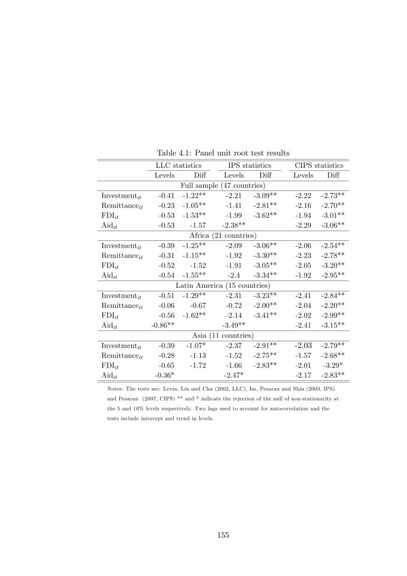
Table 4.1: Panel unit root test results
LLC statistics IPS statistics CIPS statisticsLevels Di¤ Levels Di¤ Levels Di¤
Full sample (47 countries)Investmentit -0.41 -1.22** -2.21 -3.09** -2.22 -2.73**Remittanceit -0.23 -1.05** -1.41 -2.81** -2.16 -2.70**FDIit -0.53 -1.53** -1.99 -3.62** -1.94 -3.01**Aidit -0.53 -1.57 -2.38** -2.29 -3.06**
Africa (21 countries)Investmentit -0.39 -1.25** -2.09 -3.06** -2.06 -2.54**Remittanceit -0.31 -1.15** -1.92 -3.30** -2.23 -2.78**FDIit -0.52 -1.52 -1.91 -3.05** -2.05 -3.20**Aidit -0.54 -1.55** -2.4 -3.34** -1.92 -2.95**
Latin America (15 countries)Investmentit -0.51 -1.29** -2.31 -3.23** -2.41 -2.84**Remittanceit -0.06 -0.67 -0.72 -2.00** -2.04 -2.20**FDIit -0.56 -1.62** -2.14 -3.41** -2.02 -2.99**Aidit -0.86** -3.49** -2.41 -3.15**
Asia (11 countries)Investmentit -0.39 -1.07* -2.37 -2.91** -2.03 -2.79**Remittanceit -0.28 -1.13 -1.52 -2.75** -1.57 -2.68**FDIit -0.65 -1.72 -1.66 -2.83** -2.01 -3.29*Aidit -0.36* -2.47* -2.17 -2.83**
Notes: The tests are: Levin, Lin and Chu (2002, LLC), Im, Pesaran and Shin (2003, IPS)
and Pesaran (2007, CIPS) ** and * indicate the rejection of the null of non-stationarity at
the 5 and 10% levels respectively. Two lags used to account for autocorrelation and the
tests include intercept and trend in levels.
155
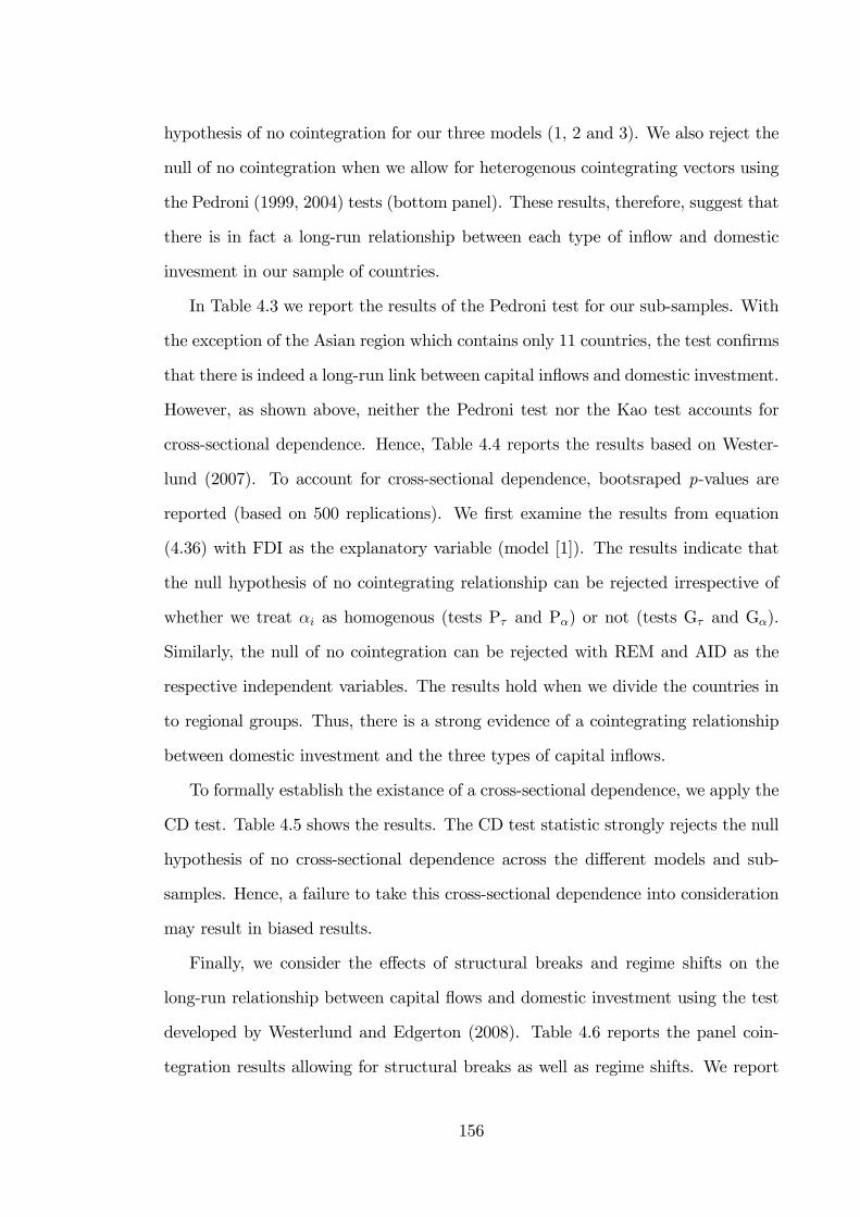
hypothesis of no cointegration for our three models (1, 2 and 3). We also reject the
null of no cointegration when we allow for heterogenous cointegrating vectors using
the Pedroni (1999, 2004) tests (bottom panel). These results, therefore, suggest that
there is in fact a long-run relationship between each type of in�ow and domestic
invesment in our sample of countries.
In Table 4.3 we report the results of the Pedroni test for our sub-samples. With
the exception of the Asian region which contains only 11 countries, the test con�rms
that there is indeed a long-run link between capital in�ows and domestic investment.
However, as shown above, neither the Pedroni test nor the Kao test accounts for
cross-sectional dependence. Hence, Table 4.4 reports the results based on Wester-
lund (2007). To account for cross-sectional dependence, bootsraped p-values are
reported (based on 500 replications). We �rst examine the results from equation
(4.36) with FDI as the explanatory variable (model [1]). The results indicate that
the null hypothesis of no cointegrating relationship can be rejected irrespective of
whether we treat �i as homogenous (tests P� and P�) or not (tests G� and G�).
Similarly, the null of no cointegration can be rejected with REM and AID as the
respective independent variables. The results hold when we divide the countries in
to regional groups. Thus, there is a strong evidence of a cointegrating relationship
between domestic investment and the three types of capital in�ows.
To formally establish the existance of a cross-sectional dependence, we apply the
CD test. Table 4.5 shows the results. The CD test statistic strongly rejects the null
hypothesis of no cross-sectional dependence across the di¤erent models and sub-
samples. Hence, a failure to take this cross-sectional dependence into consideration
may result in biased results.
Finally, we consider the e¤ects of structural breaks and regime shifts on the
long-run relationship between capital �ows and domestic investment using the test
developed by Westerlund and Edgerton (2008). Table 4.6 reports the panel coin-
tegration results allowing for structural breaks as well as regime shifts. We report
156
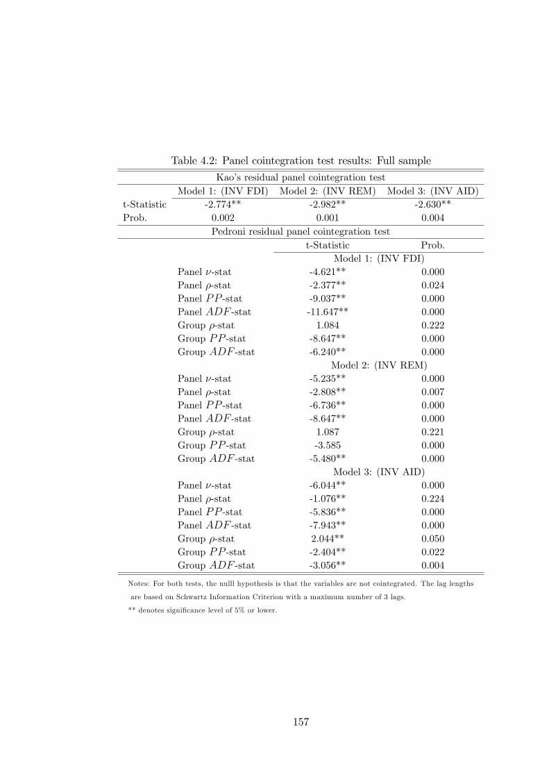
Table 4.2: Panel cointegration test results: Full sample
Kao�s residual panel cointegration testModel 1: (INV FDI) Model 2: (INV REM) Model 3: (INV AID)
t-Statistic -2.774** -2.982** -2.630**Prob. 0.002 0.001 0.004
Pedroni residual panel cointegration testt-Statistic Prob.
Model 1: (INV FDI)Panel �-stat -4.621** 0.000Panel �-stat -2.377** 0.024Panel PP -stat -9.037** 0.000Panel ADF -stat -11.647** 0.000Group �-stat 1.084 0.222Group PP -stat -8.647** 0.000Group ADF -stat -6.240** 0.000
Model 2: (INV REM)Panel �-stat -5.235** 0.000Panel �-stat -2.808** 0.007Panel PP -stat -6.736** 0.000Panel ADF -stat -8.647** 0.000Group �-stat 1.087 0.221Group PP -stat -3.585 0.000Group ADF -stat -5.480** 0.000
Model 3: (INV AID)Panel �-stat -6.044** 0.000Panel �-stat -1.076** 0.224Panel PP -stat -5.836** 0.000Panel ADF -stat -7.943** 0.000Group �-stat 2.044** 0.050Group PP -stat -2.404** 0.022Group ADF -stat -3.056** 0.004
Notes: For both tests, the nulll hypothesis is that the variables are not cointegrated. The lag lengths
are based on Schwartz Information Criterion with a maximum number of 3 lags.
** denotes signi�cance level of 5% or lower.
157
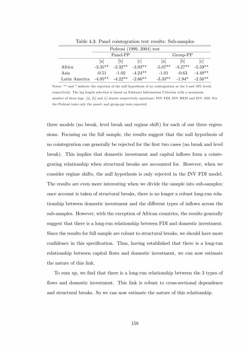
Table 4.3: Panel cointegration test results: Sub-samples
Pedroni (1999, 2004) testPanel-PP Group-PP
[a] [b] [c] [a] [b] [c]Africa -3.35** -2.32** -3.93** -5.87** -3.27** -5.59**Asia -0.51 -1.02 -4.24** -1.01 -0.63 -4.49**Latin America -4.95** -4.22** -2.66** -3.33** -1.94* -2.56**
Notes: ** and * indicate the rejection of the null hypothesis of no cointegration at the 5 and 10% levels
respectively. The lag length selection is based on Schwartz Information Criterion with a maximum
number of three lags. [a], [b] and [c] denote respectively equations: INV FDI, INV REM and INV AID. For
the Pedroni tests only the panel- and group-pp tests reported.
three models (no break, level break and regime shift) for each of our three regres-
sions. Focusing on the full sample, the results suggest that the null hypothesis of
no cointegration can generally be rejected for the �rst two cases (no break and level
break). This implies that domestic investment and capital in�ows form a cointe-
grating relationship when structural breaks are accounted for. However, when we
consider regime shifts, the null hypothesis is only rejected in the INV FDI model.
The results are even more interesting when we divide the sample into sub-samples;
once account is taken of structural breaks, there is no longer a robust long-run rela-
tionship between domestic investment and the di¤erent types of in�ows across the
sub-samples. However, with the exception of African countries, the results generally
suggest that there is a long-run relationship between FDI and domestic investment.
Since the results for full sample are robust to structural breaks, we should have more
con�dence in this speci�cation. Thus, having established that there is a long-run
relationship between capital �ows and domestic investment, we can now estimate
the nature of this link.
To sum up, we �nd that there is a long-run relationship between the 3 types of
�ows and domestic investment. This link is robust to cross-sectional dependence
and structural breaks. So we can now estimate the nature of this relationship.
158
Table 4.4: Panel cointegration with cross-sectional dependence
Sample Statistic [a] [b] [c]Full sample Gt -2.267** -2.314** -2.084**
Ga -7.581*** -7.765*** -7.441***Pt -13.741*** -14.221*** -12.550***Pa -6.669*** -6.588*** -6.151***
Africa Gt -2.181** -2.036** -1.834Ga -7.409*** -6.884*** -6.580***Pt -7.989*** -8.317*** -7.053***Pa -5.786*** -5.511*** -5.028***
Latin America Gt -2.703*** -2.948** -2.363**Ga -8.963*** -10.029*** -8.939***Pt -9.069*** -9.179*** -8.644***Pa -8.289*** -8.197*** -8.002***
Asia Gt -1.839 -1.979 -2.179*Ga -6.024*** -6.358*** -7.044***Pt -7.424*** -8.250*** -7.319***Pa -6.929*** -8.131*** -7.444***
Notes: The optimal lag length is based on the Akaike Information Criterion
with a maximum lag and lead lengths of 2 and the width of the Bertlett-kernel
window is set to 3. The two types of statistics are respectively the group-mean
and the panel tests. To control for cross-sectional dependencies, bootsrapped
p-values are reported (based on 500 replications) for a one-sided test. The null is
no panel cointegration. [a], [b] and [c] denote respectively equations: INV FDI,
INV REM and INV AID. ***, ** and * denote signi�cance at 1, 5 and 10% levels
respectively.
Table 4.5: Cross-sectional independence tests
Sample Statistic [a] [b] [c]Full sample CD without a linear trend 12.16*** 12.66*** 12.40***Africa 2.36** 3.09*** 3.11***Latin America 3.45*** 3.47*** 3.62***Asia 7.03*** 9.47*** 7.83***Sample Statistic [a] [b] [c]Full sample CD with a linear trend 9.38*** 12.01*** 12.19***Africa 0.76 3.05*** 2.90***Latin America 6.60*** 8.50*** 7.85***Asia 3.30*** 3.41*** 3.32***
Notes: The CD test is due to Pesaran (2004) and takes the null of cross-sectional
independence. [a], [b] and [c] denote respectively equations: INV FDI, INV REM
and INV AID. *** and ** denote signi�cance at 1 and 5 % levels respectively.
159
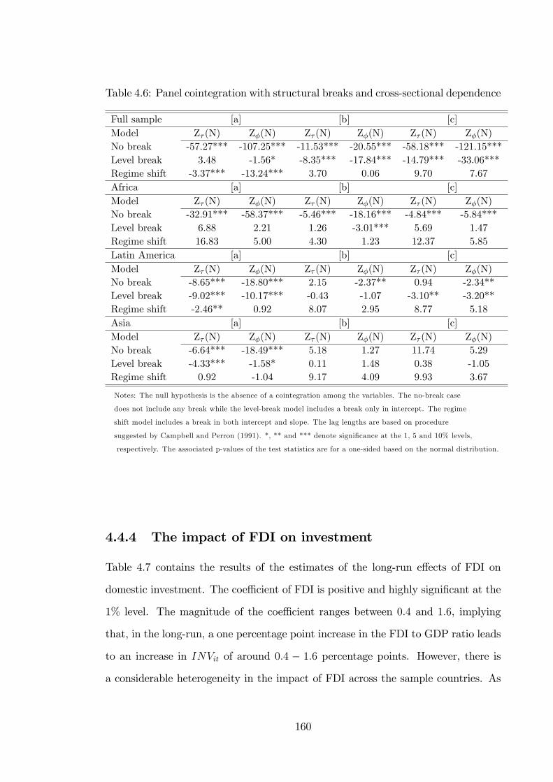
Table 4.6: Panel cointegration with structural breaks and cross-sectional dependence
Full sample [a] [b] [c]Model Z� (N) Z�(N) Z� (N) Z�(N) Z� (N) Z�(N)No break -57.27*** -107.25*** -11.53*** -20.55*** -58.18*** -121.15***Level break 3.48 -1.56* -8.35*** -17.84*** -14.79*** -33.06***Regime shift -3.37*** -13.24*** 3.70 0.06 9.70 7.67Africa [a] [b] [c]Model Z� (N) Z�(N) Z� (N) Z�(N) Z� (N) Z�(N)No break -32.91*** -58.37*** -5.46*** -18.16*** -4.84*** -5.84***Level break 6.88 2.21 1.26 -3.01*** 5.69 1.47Regime shift 16.83 5.00 4.30 1.23 12.37 5.85Latin America [a] [b] [c]Model Z� (N) Z�(N) Z� (N) Z�(N) Z� (N) Z�(N)No break -8.65*** -18.80*** 2.15 -2.37** 0.94 -2.34**Level break -9.02*** -10.17*** -0.43 -1.07 -3.10** -3.20**Regime shift -2.46** 0.92 8.07 2.95 8.77 5.18Asia [a] [b] [c]Model Z� (N) Z�(N) Z� (N) Z�(N) Z� (N) Z�(N)No break -6.64*** -18.49*** 5.18 1.27 11.74 5.29Level break -4.33*** -1.58* 0.11 1.48 0.38 -1.05Regime shift 0.92 -1.04 9.17 4.09 9.93 3.67
Notes: The null hypothesis is the absence of a cointegration among the variables. The no-break case
does not include any break while the level-break model includes a break only in intercept. The regime
shift model includes a break in both intercept and slope. The lag lengths are based on procedure
suggested by Campbell and Perron (1991). *, ** and *** denote signi�cance at the 1, 5 and 10% levels,
respectively. The associated p-values of the test statistics are for a one-sided based on the normal distribution.
4.4.4 The impact of FDI on investment
Table 4.7 contains the results of the estimates of the long-run e¤ects of FDI on
domestic investment. The coe¢ cient of FDI is positive and highly signi�cant at the
1% level. The magnitude of the coe¢ cient ranges between 0:4 and 1:6, implying
that, in the long-run, a one percentage point increase in the FDI to GDP ratio leads
to an increase in INVit of around 0:4 � 1:6 percentage points. However, there is
a considerable heterogeneity in the impact of FDI across the sample countries. As
160
Table 4.7: The impact of FDI on investment
Full sampleFDIit N Obs
WD-DOLS (Kao and Chiang, 2000) 0.998 [13.46]*** 47 1269
WD-DOLS (Demeaned data) 0.404 [6.31]*** 47 1269
MG-DOLS (Pedroni (2001) 1.603 [14.05]*** 47 1269
CCEMG estimator ((Pesaran, 2006) 0.604 [3.83]*** 47 1269
2-step estimator (Breitung, 2005) 0.459 [7.53]*** 47 1269Sub-samples#
Africa 1.737 [13.88]*** 21 567LA 0.456 [5.36]*** 15 405Asia 0.03 [0.15] 11 297
Notes: The DOLS regressions are estimated with two leads and two lags.
T-statistics in brackets. *** indicate singi�cance at the 1% level.#These estimates are based on the WD-OLS estimator.
shown in Table 4.8, for 10 out of the 47 countries (or 21% of the sample countries)
FDI �ows are associated with a decrease in domestic investment, while in 37 out of
the 47 countries (or 79% of the countries) the e¤ect of FDI on investment is positive.
Signi�cant large negative e¤ects are observed in countries such as Mozambique and
Sudan, closely followed by Jordan while signi�cant positive e¤ects are recorded in
Algeria, Niger and Bangladesh.
When we consider the e¤ects of FDI on investment for the 3 regional sub-samples,
it seems that the positive long-run assocation between the two variables is only
signi�cant for the African and Latin American regions while it is not statistically
signi�cant for the Asian group. The coe¢ cient of FDI is highest for the African
sub-sample, suggesting that FDI has a stronger crowding-in e¤ect in in this region.
Again, the insigni�cance of the coe¢ cient of FDI for the Asian sub-sample may be
due to the low number of countries in the sample.
The long and short-run Granger causality tests are reported in Table 4.9. The
161
results suggest that, for the sample as a whole, there is a bidirectional causal link
between FDI and domestic investment in the short-run as both respective (lagged)
regressors are signi�cantly di¤erent from zero at standard con�dence levels. This
indicates that, in the short-run, increased investment is both the result of as well
as the driver of increased FDI. The error correction term is statistically signi�cant
in equation (a), with a moderate speed of adjustment to the long-run equilibrium.
On the other hand, the error correction term in equation (b) is insigni�cant. From
this, we can deduce that, in the long-run, the relationship between the two vari-
ables is unidirectional from FDI to domestic investment. With the exception of
the Asian sub-sample where the long-run relationship is bidirectional, we observe a
unidirectional link (from FDI to investment) in both the African and Latin Amer-
ican regions. For the Asian group, both of the lagged regressors are insigni�cant,
meaning there is no causal link between FDI and Investment in the short-run.
4.4.5 The impact of remittances on investment
The long-run e¤ects of remittances on investment are summarised in Table 4.10.
Similar to the FDI case, our estimates suggest that remittances are positively asso-
ciated with domestic investment. The coe¢ cient of this variable is signi�cant in all
but one estimator (CCEMG estimator). The point estimates suggest a bene�cial
e¤ect in the region of 0:2 to 0:6 percentage points in the long-run. As can be seen in
Table 4.11, there is a considerable heterogeneity with respect to the long-run e¤ects
of remittances on investment. In roughly 1=3 of the countries, remittances carry a
negative coe¢ cient while there is a positive e¤ect in 2=3 of the countries.
We observe similar results when we disaggregate the sample into 3 regional
groups. In particular, the coe¢ cient of the remittance variable is positive for all
regions, albeit insigni�cant for the Asian countries. Again, we suspect that the low
number of Asian countries in the sample may be the cause of the insigni�cance of
this variable.
162
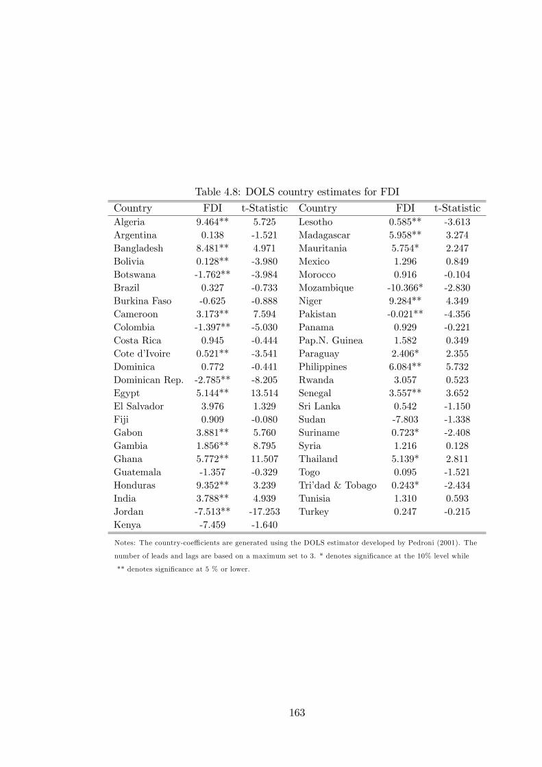
Table 4.8: DOLS country estimates for FDI
Country FDI t-Statistic Country FDI t-StatisticAlgeria 9.464** 5.725 Lesotho 0.585** -3.613Argentina 0.138 -1.521 Madagascar 5.958** 3.274Bangladesh 8.481** 4.971 Mauritania 5.754* 2.247Bolivia 0.128** -3.980 Mexico 1.296 0.849Botswana -1.762** -3.984 Morocco 0.916 -0.104Brazil 0.327 -0.733 Mozambique -10.366* -2.830Burkina Faso -0.625 -0.888 Niger 9.284** 4.349Cameroon 3.173** 7.594 Pakistan -0.021** -4.356Colombia -1.397** -5.030 Panama 0.929 -0.221Costa Rica 0.945 -0.444 Pap.N. Guinea 1.582 0.349Cote d�Ivoire 0.521** -3.541 Paraguay 2.406* 2.355Dominica 0.772 -0.441 Philippines 6.084** 5.732Dominican Rep. -2.785** -8.205 Rwanda 3.057 0.523Egypt 5.144** 13.514 Senegal 3.557** 3.652El Salvador 3.976 1.329 Sri Lanka 0.542 -1.150Fiji 0.909 -0.080 Sudan -7.803 -1.338Gabon 3.881** 5.760 Suriname 0.723* -2.408Gambia 1.856** 8.795 Syria 1.216 0.128Ghana 5.772** 11.507 Thailand 5.139* 2.811Guatemala -1.357 -0.329 Togo 0.095 -1.521Honduras 9.352** 3.239 Tri�dad & Tobago 0.243* -2.434India 3.788** 4.939 Tunisia 1.310 0.593Jordan -7.513** -17.253 Turkey 0.247 -0.215Kenya -7.459 -1.640
Notes: The country-coe¢ cients are generated using the DOLS estimator developed by Pedroni (2001). The
number of leads and lags are based on a maximum set to 3. * denotes signi�cance at the 10% level while
** denotes signi�cance at 5 % or lower.
163
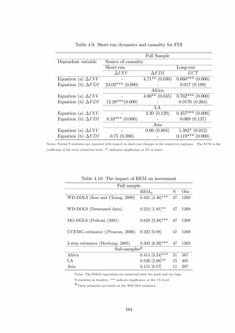
Table 4.9: Short-run dynamics and causality for FDI
Full SampleDependent variable Source of causality
Short-run Long-run�INV �FDI ECT
Equation (a) �INV - 4.71** (0.030) 0.660*** (0.000)Equation (b) �FDI 24.02*** (0.000) - 0.017 (0.199)
AfricaEquation (a) �INV - 4.00** (0.045) 0.762*** (0.000)Equation (b) �FDI 12.28***(0.000) - 0.0170 (0.264)
LAEquation (a) �INV - 2.30 (0.129) 0.457*** (0.000)Equation (b) �FDI 8.33*** (0.000) - 0.069 (0.137)
AsiaEquation (a) �INV - 0.06 (0.804) 1.383* (0.012)Equation (b) �FDI 0.75 (0.390) - 0.119*** (0.000)
Notes: Partial F-statistics are reported with respect to short-run changes in the respective regressor. The ECM is the
coe¢ cient of the error correction term. ** indicates singi�cance at 5% or lower.
Table 4.10: The impact of REM on investment
Full sampleREMit N Obs
WD-DOLS (Kao and Chiang, 2000) 0.431 [4.46]*** 47 1269
WD-DOLS (Demeaned data) 0.222 [1.91]** 47 1269
MG-DOLS (Pedroni (2001) 0.628 [9.38]*** 47 1269
CCEMG estimator ((Pesaran, 2006) 0.222 [0.98] 47 1269
2-step estimator (Breitung, 2005) 0.302 [6.29]*** 47 1269Sub-samples#
Africa 0.414 [3.24]*** 21 567LA 0.526 [2.66]** 15 405Asia 0.151 [0.57] 11 297
Notes: The DOLS regressions are estimated with two leads and two lags.
T-statistics in brackets. *** indicate singi�cance at the 1% level.#These estimates are based on the WD-OLS estimator.
164
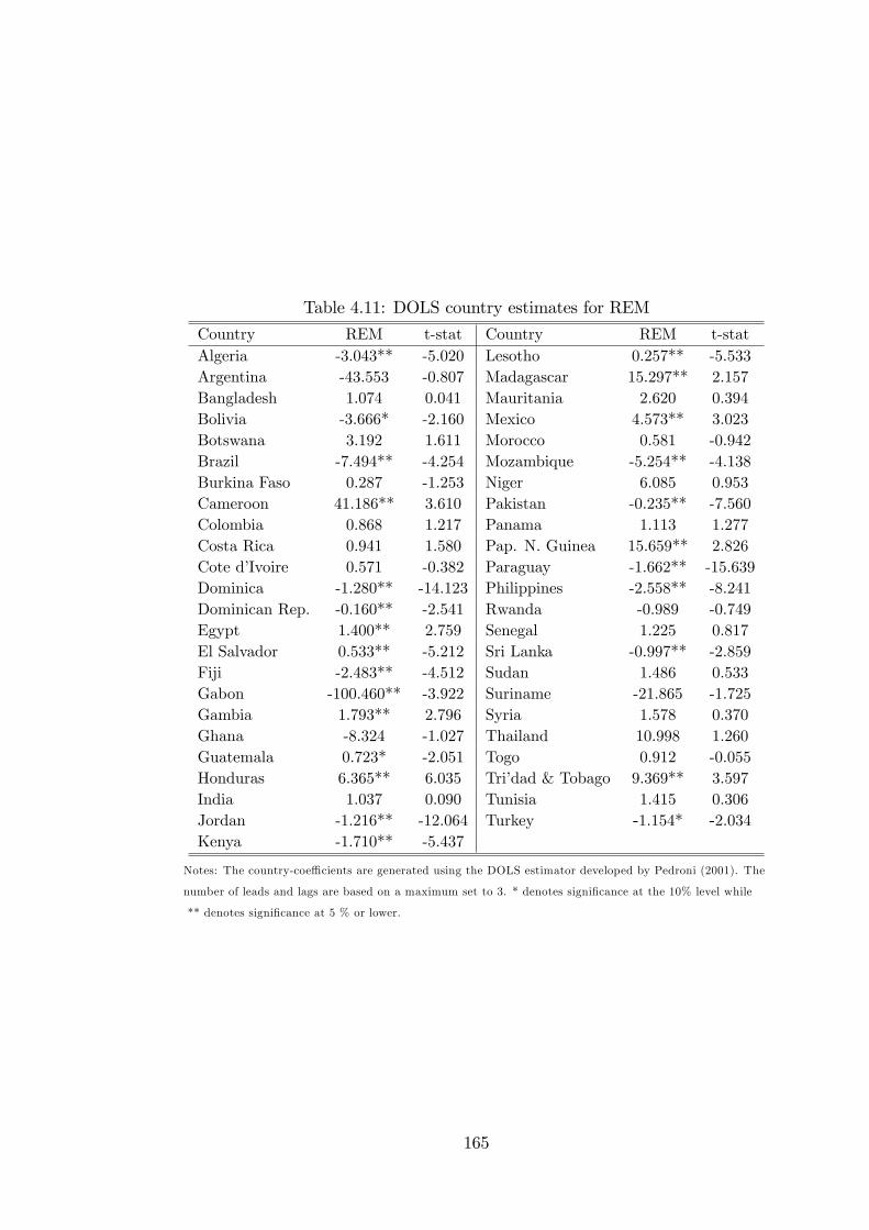
Table 4.11: DOLS country estimates for REM
Country REM t-stat Country REM t-statAlgeria -3.043** -5.020 Lesotho 0.257** -5.533Argentina -43.553 -0.807 Madagascar 15.297** 2.157Bangladesh 1.074 0.041 Mauritania 2.620 0.394Bolivia -3.666* -2.160 Mexico 4.573** 3.023Botswana 3.192 1.611 Morocco 0.581 -0.942Brazil -7.494** -4.254 Mozambique -5.254** -4.138Burkina Faso 0.287 -1.253 Niger 6.085 0.953Cameroon 41.186** 3.610 Pakistan -0.235** -7.560Colombia 0.868 1.217 Panama 1.113 1.277Costa Rica 0.941 1.580 Pap. N. Guinea 15.659** 2.826Cote d�Ivoire 0.571 -0.382 Paraguay -1.662** -15.639Dominica -1.280** -14.123 Philippines -2.558** -8.241Dominican Rep. -0.160** -2.541 Rwanda -0.989 -0.749Egypt 1.400** 2.759 Senegal 1.225 0.817El Salvador 0.533** -5.212 Sri Lanka -0.997** -2.859Fiji -2.483** -4.512 Sudan 1.486 0.533Gabon -100.460** -3.922 Suriname -21.865 -1.725Gambia 1.793** 2.796 Syria 1.578 0.370Ghana -8.324 -1.027 Thailand 10.998 1.260Guatemala 0.723* -2.051 Togo 0.912 -0.055Honduras 6.365** 6.035 Tri�dad & Tobago 9.369** 3.597India 1.037 0.090 Tunisia 1.415 0.306Jordan -1.216** -12.064 Turkey -1.154* -2.034Kenya -1.710** -5.437
Notes: The country-coe¢ cients are generated using the DOLS estimator developed by Pedroni (2001). The
number of leads and lags are based on a maximum set to 3. * denotes signi�cance at the 10% level while
** denotes signi�cance at 5 % or lower.
165
The question is then: Are these e¤ects of a causal nature? Table 4.12 shows
that, in general, there is no causal relationship between remittances and investment
in the short-run for the sample as a whole or for the regional groups. However, in
the long-run, we �nd a signi�cant two-way causal relationship for the full sample
as well as for the African and Latin American sub-sample. That is, increases in
investment is both a result of as well as a cause of increases in remittances. This
could suggest that remittance �ows are being used in improvement of human capital
(e.g. education and health). These would have bene�cial e¤ects on investment in
the long-run. Alternatively, the multiplier e¤ects generated by the expenditures of
remittance-receiving households may be encouraging more investment or the house-
holds may themselves be making small capital investments. In the latter case, this
could generate more remittance �ows if we assume that the migrant is not just al-
truistic but also self-interested. In other words, if remittance-receiving households
engage in successful business ventures, the migrants may send more remittances in
order to enhance their own wealth4. Results by Alleyne et al. (2008) seem to con-
�rm that remittances are not only driven by altruistic motives but also investment
motives. Thus, remittances may drive investment while investment itself may cause
more remittances.
4.4.6 The impact of aid on investment
Table 4.13 contains the results on the link between foreign aid and investment. The
coe¢ cient of aid carries a signi�cant negative sign, suggesting that aid has a discour-
aging e¤ect on domestic investment in the long-run. There is a great variation in the
magnitude reported by the di¤erent estimators. The MG-DOLS and the CCEMG
estimators, which allow the slope coe¢ cients to vary across the sample countries,
indicate a much larger negative association between aid and investment. As for
4This assumes that the migrant and the remittance-receiving household can overcome issuesof adverse selection and moral hazard and that they can trust each other.
166
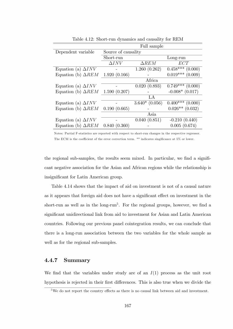
Table 4.12: Short-run dynamics and causality for REM
Full sampleDependent variable Source of causality
Short-run Long-run�INV �REM ECT
Equation (a) �INV - 1.260 (0.262) 0.458*** (0.000)Equation (b) �REM 1.920 (0.166) - 0.019*** (0.009)
AfricaEquation (a) �INV - 0.020 (0.893) 0.749*** (0.000)Equation (b) �REM 1.590 (0.207) - -0.008* (0.017)
LAEquation (a) �INV - 3.640* (0.056) 0.400*** (0.000)Equation (b) �REM 0.190 (0.665) - 0.026** (0.032)
AsiaEquation (a) �INV - 0.040 (0.851) -0.210 (0.440)Equation (b) �REM 0.840 (0.360) - 0.005 (0.674)
Notes: Partial F-statistics are reported with respect to short-run changes in the respective regressor.
The ECM is the coe¢ cient of the error correction term. ** indicates singi�cance at 5% or lower.
the regional sub-samples, the results seem mixed. In particular, we �nd a signi�-
cant negative association for the Asian and African regions while the relationship is
insigni�cant for Latin American group.
Table 4.14 shows that the impact of aid on investment is not of a causal nature
as it appears that foreign aid does not have a signi�cant e¤ect on investment in the
short-run as well as in the long-run5. For the regional groups, however, we �nd a
signi�cant unidirectional link from aid to investment for Asian and Latin American
countries. Following our previous panel cointegration results, we can conclude that
there is a long-run association between the two variables for the whole sample as
well as for the regional sub-samples.
4.4.7 Summary
We �nd that the variables under study are of an I(1) process as the unit root
hypothesis is rejected in their �rst di¤erences. This is also true when we divide the
5We do not report the country e¤ects as there is no causal link between aid and investment.
167
Table 4.13: The impact of AID on investment
AIDit N ObsWD-DOLS (Kao and Chiang, 2000) -6.694 [-1.73]** 47 1269
WD-DOLS (Demeaned data) -4.577 [-1.37]* 47 1269
MG-DOLS (Pedroni (2001) -46.023 [-5.60]*** 47 1269
CCEMG estimator (Pesaran, 2006) -135.404 [-1.77]* 47 1269
2-step estimator (Breitung, 2005) 2.298 [1.06] 47 1269Sub-samples#
Africa -9.961 [-1.88]** 21 567Asia -12.732 [-1.62]* 11 297LA 10.462 [0.85] 15 405
Notes: The DOLS regressions are estimated with two leads and two lags.
T-statistics in brackets. *** indicate singi�cance at the 1% level. #These estimates
are based on the WD-OLS estimator.
countries into 3 regional groups, namely, Africa, Asia and Latin America. We also
conduct panel cointegration analysis which con�rm that the models we consider are
error-correcting. That is to say, we can reject the null hypothesis of no cointegration
for the sample as a whole and also for the regional groups. We also con�rm the
presence of cross-sectional dependence also for the regional sub-samples.
Because the variables are stationary and form a cointegrating relationship, we
estimate the nature of this link. The long-run estimates show that FDI and remit-
tances are positively related to domestic investment in the sample as a whole while
aid is negatively associated with it. These results generally hold for the regions
under consideration. In particular, the long-run e¤ects of remittances and FDI on
investment are positive in all three regions, albeit insigni�cant in the Asian group.
The coe¢ cient of aid is negative and signi�cant in Africa and Asia while it is positive
and insigni�cant in Latin America. The insigni�cance of remittances and FDI in
the Asian sub-sample may be due to the small number of countries we have.
Our causality analysis provides additional insight into the e¤ects of capital �ows
168
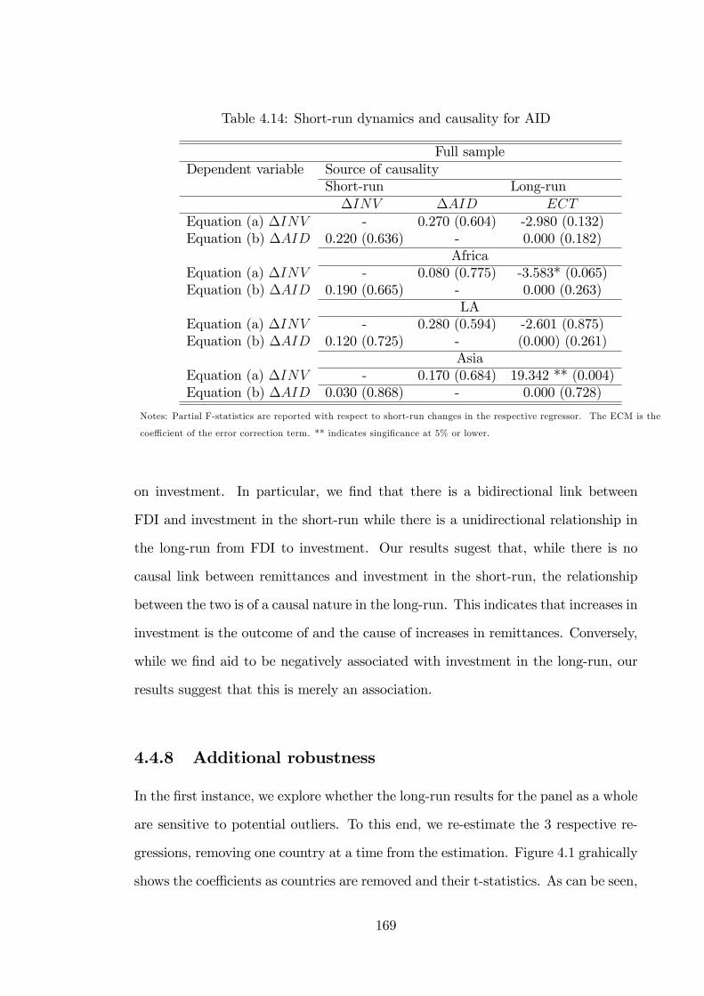
Table 4.14: Short-run dynamics and causality for AID
Full sampleDependent variable Source of causality
Short-run Long-run�INV �AID ECT
Equation (a) �INV - 0.270 (0.604) -2.980 (0.132)Equation (b) �AID 0.220 (0.636) - 0.000 (0.182)
AfricaEquation (a) �INV - 0.080 (0.775) -3.583* (0.065)Equation (b) �AID 0.190 (0.665) - 0.000 (0.263)
LAEquation (a) �INV - 0.280 (0.594) -2.601 (0.875)Equation (b) �AID 0.120 (0.725) - (0.000) (0.261)
AsiaEquation (a) �INV - 0.170 (0.684) 19.342 ** (0.004)Equation (b) �AID 0.030 (0.868) - 0.000 (0.728)
Notes: Partial F-statistics are reported with respect to short-run changes in the respective regressor. The ECM is the
coe¢ cient of the error correction term. ** indicates singi�cance at 5% or lower.
on investment. In particular, we �nd that there is a bidirectional link between
FDI and investment in the short-run while there is a unidirectional relationship in
the long-run from FDI to investment. Our results sugest that, while there is no
causal link between remittances and investment in the short-run, the relationship
between the two is of a causal nature in the long-run. This indicates that increases in
investment is the outcome of and the cause of increases in remittances. Conversely,
while we �nd aid to be negatively associated with investment in the long-run, our
results suggest that this is merely an association.
4.4.8 Additional robustness
In the �rst instance, we explore whether the long-run results for the panel as a whole
are sensitive to potential outliers. To this end, we re-estimate the 3 respective re-
gressions, removing one country at a time from the estimation. Figure 4.1 grahically
shows the coe¢ cients as countries are removed and their t-statistics. As can be seen,
169
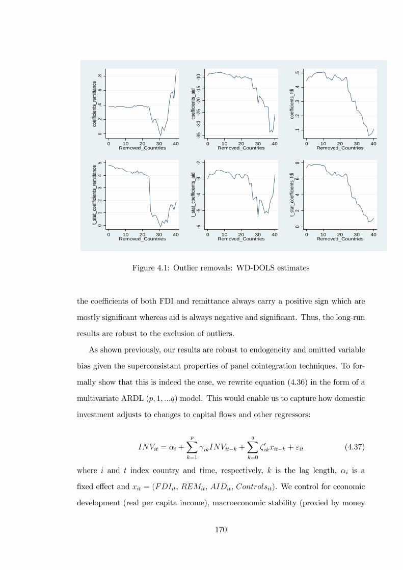
0.2
.4.6
.8co
effic
ients
_rem
ittan
ce
0 10 20 30 40Removed_Countries
35
30
25
20
15
10
coef
ficien
ts_a
id
0 10 20 30 40Removed_Countries
.1.2
.3.4
.5co
effic
ients
_fdi
0 10 20 30 40Removed_Countries
01
23
45
t_st
at_c
oeffi
cient
s_re
mitt
ance
0 10 20 30 40Removed_Countries
65
43
2t_
stat
_coe
fficie
nts_
aid
0 10 20 30 40Removed_Countries
02
46
8t_
stat
_coe
fficie
nts_
fdi
0 10 20 30 40Removed_Countries
Figure 4.1: Outlier removals: WD-DOLS estimates
the coe¢ cients of both FDI and remittance always carry a positive sign which are
mostly signi�cant whereas aid is always negative and signi�cant. Thus, the long-run
results are robust to the exclusion of outliers.
As shown previously, our results are robust to endogeneity and omitted variable
bias given the superconsistant properties of panel cointegration techniques. To for-
mally show that this is indeed the case, we rewrite equation (4.36) in the form of a
multivariate ARDL (p; 1; :::q) model. This would enable us to capture how domestic
investment adjusts to changes to capital �ows and other regressors:
INVit = �i +
pXk=1
ikINVit�k +
qXk=0
� 0ikxit�k + "it (4.37)
where i and t index country and time, respectively, k is the lag length, �i is a
�xed e¤ect and xit = (FDIit, REMit, AIDit, Controlsit). We control for economic
development (real per capita income), macroeconomic stability (proxied by money
170
growth), openness (trade/GDP) and government size (proxied by government ex-
penditure/GDP). All the variables are drawn from WDI (2011).
Following Pesaran and Smith (1995), equation (4.37) can be re-parameterised
as:
�INVit = �i + �iINVit�1 + �0ixit +
p�1Xk=1
�ik�INVit�k +
q�1Xk=0
��0ik�xit�k + "it; (4.38)
where
�i = �(1�Pp
k=1 ik); �i =Pq
k=0 � ik;
�ik = �Pp
m=k+1 im; k = 1; 2; :::p� 1; and
��ik = �Pq
m=k+1 � im; k = 1; 2; :::q � 1;
To estimate the short-run dynamics as well as the long-run e¤ects, equation
(4.38) can be expressed as an error-correction model as follows:
�INVit = �i+�i(INVit�1�'0ixit)+p�1Xk=1
�ik�INVit�k+
q�1Xk=0
��0ik�xit�k+ "it; (4.39)
where 'i = (�i=�i) captures the long-run relationship between investment and the
regressors while �ik and ��0ik capture the short-run dynamics linking investment to
both its past values and the other variables in the model. The error-correction
parameter, �i, measures the speed of adjustment of investment to its long-run equi-
librium following a change in the regressors. Provided that �i is signi�cant and
negative, one can deduce that the variables exhibit a return to long-run equilibrium
(i.e. there is a long-run relationship between them).
The above ARDL speci�cation overcomes issues of endogeneity since all the
regressors enter the model with lags. In addition, it allows the parameters to be
di¤erent for each country. To estimate equation (4.39), we use the Pooled Mean
Group estimator developed by Pesaran and Smith (1995). This estimator allows
171
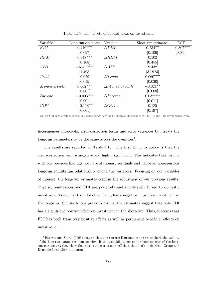
Table 4.15: The e¤ects of capital �ows on investment
Variable Long-run estimates Variable Short-run estimates ECTFDI 0:410*** �FDI 0:234** �0:307***
[0:097] [0:109] [0:034]REM 0:348*** �REM 0:502
[0:108] [0:455]AID �6:417*** �AID 9:432
[1:495] [31:923]Trade 0:029 �Trade 0:060***
[0:019] [0:020]Money growth 0:002*** �Money growth �0:021**
[0:001] [0:008]Income �0:003*** �Income 0:032***
[0:001] [0:011]GOV �0:118** �GOV 0:185
[0:001] [0:197]Notes: Standard errors reported in parentheses,***, ** and * indicate singi�cance at the 1, 5 and 10% levels respectively.
heteregenous intercepts, error-correction terms and error variances but treats the
long-run parameters to be the same across the countries6.
The results are reported in Table 4.15. The �rst thing to notice is that the
error-correction term is negative and highly signi�cant. This indicates that, in line
with our previous �ndings, we have stationary residuals and hence an non-spurious
long-run equilibrium relationship among the variables. Focusing on our variables
of interest, the long-run estimates con�rm the robustness of our previous results.
That is, remittances and FDI are positively and signi�cantly linked to domestic
investment. Foreign aid, on the other hand, has a negative impact on investment in
the long-run. Similar to our previous results, the estimates suggest that only FDI
has a signi�cant positive e¤ect on investment in the short-run. Thus, it seems that
FDI has both transitory positive e¤ects as well as permanent bene�cial e¤ects on
investment.
6Pesaran and Smith (1995) suggest that one can use Hausman type test to check the validityof the long-run parameter homogeneity. If the test fails to reject the homogeneity of the long-run parameters, they show that this estimator is more e¢ cient than both their Mean Group andDynamic �xed e¤ect estimators.
172
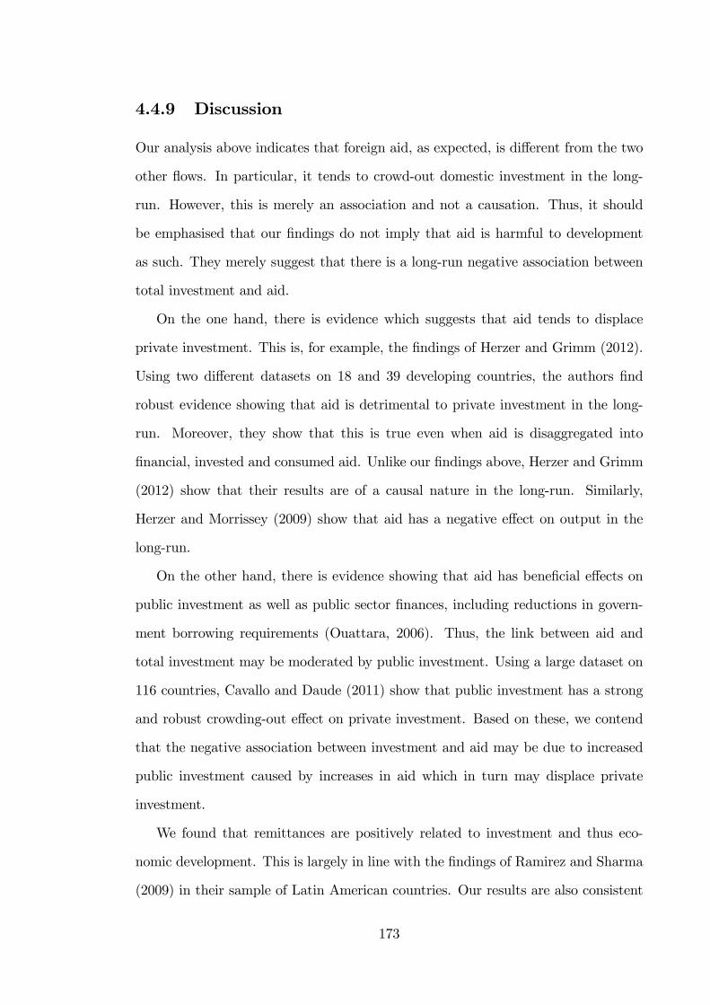
4.4.9 Discussion
Our analysis above indicates that foreign aid, as expected, is di¤erent from the two
other �ows. In particular, it tends to crowd-out domestic investment in the long-
run. However, this is merely an association and not a causation. Thus, it should
be emphasised that our �ndings do not imply that aid is harmful to development
as such. They merely suggest that there is a long-run negative association between
total investment and aid.
On the one hand, there is evidence which suggests that aid tends to displace
private investment. This is, for example, the �ndings of Herzer and Grimm (2012).
Using two di¤erent datasets on 18 and 39 developing countries, the authors �nd
robust evidence showing that aid is detrimental to private investment in the long-
run. Moreover, they show that this is true even when aid is disaggregated into
�nancial, invested and consumed aid. Unlike our �ndings above, Herzer and Grimm
(2012) show that their results are of a causal nature in the long-run. Similarly,
Herzer and Morrissey (2009) show that aid has a negative e¤ect on output in the
long-run.
On the other hand, there is evidence showing that aid has bene�cial e¤ects on
public investment as well as public sector �nances, including reductions in govern-
ment borrowing requirements (Ouattara, 2006). Thus, the link between aid and
total investment may be moderated by public investment. Using a large dataset on
116 countries, Cavallo and Daude (2011) show that public investment has a strong
and robust crowding-out e¤ect on private investment. Based on these, we contend
that the negative association between investment and aid may be due to increased
public investment caused by increases in aid which in turn may displace private
investment.
We found that remittances are positively related to investment and thus eco-
nomic development. This is largely in line with the �ndings of Ramirez and Sharma
(2009) in their sample of Latin American countries. Our results are also consistent
173
with the �ndings of Nsiah and Fayissa (2011) who found that remittances are posi-
tively related to economic development in developing countries. Similar to us, these
authors found that the positive impact is signi�cant in Latin America and Africa
while this is not the case in Asian countries.
Finally, our results indicate that, of the 3 �ows, FDI has been most bene�cial to
the countries in our sample. We �nd that there is a bidirectional (causal) linkage
between domestic investment and FDI in the short-run. This is consistent with the
idea that increased FDI results in an increase in the demand for, for example, do-
mestically produced inputs while at the same time the operations of domestic �rms
may induce more FDI (Apergis et al. 2006). In the long-run, however, our results
show that there is a unidirectional causal link - from FDI to investment. The chan-
nels through which this crowding-in may take are many and include technological
spillover and various other complementarities with domestic �rms.
Overall, our results point to the bene�cial e¤ects of FDI and remittances.
4.5 Concluding Remarks
The objective of this study was to establish whether there is a long-run stable re-
lationship between domestic investment and the 3 main types of capital �ows that
developing countries receive. Using recently developed panel cointegration tech-
niques, the study utilises a balanced panel of 47 developing countries.
The results show there is a long-run relationship between investment and each
of the in�ows. This result is robust to cross-sectional dependency as well as struc-
tural and regime changes. Upon estimating the nature of the long-run equilibrium
relationship, the study �nds that remittances and FDI have statistically signi�cant
positive e¤ects on investment in the long-run. On the contrary, the results suggest
that aid is inversely associated with investment.
While the role of aid in economic development is by no means a trivial one,
174
this study shows that private sources of development �nance can play a pivotal
role in developing countries. This is particularly relevant now given the heated
debate aid tends to generate in both the economics literature and in policy circles.
An important contribution of this study is that it pays particular attention to the
properties of the variables under study as well the underlying assumptions of the
econometric techniques. Given that we employ more superior estimation methods,
our results should be more reliable.
The overall �ndings suggest a number of important policy implications. In the
case of remittances, developing countries can improve the e¤ectiveness of these �ows.
A particular channel is the �nancial system. Thus, developing countries should
develop their �nancial sectors in order to allow remittance-receiving households to
have the facilities needed for productive investments. Given that remittances tend
to boost the level of deposits and credit in banking system (Aggarwal et al. 2011), a
well-developed �nancial system would generate even more bene�ts. In the same vein,
they should adopt policies that reduce the transaction costs attached to receiving
the funds so that households can get their remittances as smoothly as possible. One
way to do this is to reduce redtape, but perhaps, more importantly, competition
should be encouraged among money transfer companies.
With respect to FDI, as is largely accepted, developing countries should improve
the human capital of their citizens. Similarly, given the experiences of East Asian
countries, governments should have clear policies in regards to FDI with the aim
of maximising the bene�ts domestic �rms get from multinational companies. Even
though our results are strongly in favour of FDI, we emphasise that, unless the
particular country formulates cohesive policies, the bene�cial e¤ects of FDI would
be minimal. The actual experience of many African countries is a case in point;
many multinational companies in a number of African countries have not created
forward and backward linkages with the wider economy.
While we do not �nd a positive link between domestic investment and foreign
175
aid, we argue that this does not necessarily imply that aid is bad for developing
countries. We should remember an important point which is; it is highly unlikely
that remittances and FDI would reach the poorest households. Thus, aid tends to
�ll a crucial gap in the �nances of developing countries, particularly development
projects. It can also have other bene�ts; as the �rst chapter indicated, it tends to
reduce capital �ight, perhaps, through its bene�cial e¤ects on the public sector.
Overall, the important role these resource �ows can play in economic develop-
ment is not a trivial matter. As this study has shown, capital �ows can propel
developing economies to a high-growth trajectory by augmenting the rate of capital
accumulation.
176
Chapter 5
Overall conclusions
This thesis deals with the broad issues of capital �ows, openness and crises and how
these in turn a¤ect the economic performance of developing countries particularly
those in Africa. Throughout the various parts of the thesis, we have attempted
to make signi�cant contributions to the existing literature. In what follows, we
highlight these. Subsequent to this, we identify possible avenues for further research.
5.1 Main �ndings and policy issues
The existing literature on why African agents move their portfolios abroad tends
to be somewhat fragmented and insu¢ cient, identifying mainly macroeconomic and
political conditions as the cause (Lensink et al. 1998; Collier et al. 2001; Ndiku-
mana and Boyce, 2003; Ndiaye, 2009). To mitigate these shortcomings, Chapter
2 adopts a more systematic approach to �nding the causes of capital �ight. To
this end, it emphasises the importance of the investment climate - de�ned as the
structural, institutional and overall macroeconomic environments which confront
economic agents, whether they be �rms, entrepreneurs or private individuals. The
chapter then speci�es four factors that, at the macroeconomic level, in�uence the
investment climate and hence the likelihood of capital �ight: risk-return features;
177
institutions and political risk, structural features and the composition of capital
�ows.
The results indicate that good institutions are robustly associated with lower
capital �ight in SSA. This is a crucial (and robust) �nding, particularly given the
range of indicators we use. This result is in line with the central tenets of insti-
tutional economics. Institutional economics de�nes institutions as both formal and
informal rules that agents devise in order to reduce transaction costs and uncertain-
ties (Menard and Shirley, 2005). Thus, institutions provide incentive structures and
determine agents�behaviour. Within this perspective, markets as well as the over-
all economy can be viewed as organisational arrangements that support production
and exchange. However, in SSA, markets are characterised by imperfect informa-
tion, poor enforcement mechanisms and high levels of transaction costs. This is
due to extensive uncertainties and risks. In such environment, private agents tend
to engage in demonetisation, currency substitution (dollarisation) and capital �ight
(Nissanke and Aryeetey, 2003). Furthermore, African economies tend to be dualis-
tic and segmented in nature with a large informal sector governed by "indigenous
social norms and codes" and a small formal sector governed by weak "third-party
enforcement and other elaborate institutional structures" (Ibid, p. 38 & 58). Thus,
improvements in the institutional environment are expected to positively in�uence
the domestic investment climate and hence discourage capital �ight.
The chapter postulates that capital �ight, like any other decision reached by
rational economic agents, depends largely on their expectations about their future
situation which makes their perception of the macroeconomic environment a sig-
ni�cant factor. Thus, as the results show, capital �ight from Africa is signi�cantly
linked to the region�s poor pro�tability, economic risk and macroeconomic distor-
tions. Thus, there are crucial gains to be had by reducing macroeconomic risk and
initiating structural transformation of African economies.
The empirical results also show that capital �ight undermines economic perfor-
178
mance. The growth regressions suggest that capital �ight robustly retards growth.
With respect to domestic investment, the impulse response functions show that
investment falls in response to capital �ight episodes. We show that it does not
recover to its pre-episode level in the short to medium term horizon. We contend
that capital �ight episodes may be magnifying the credit constraint which are, in
most African countries, binding.
It should be emphasised that the dynamic response of invesment and output to
capital �ight has never been captured in the context of African countries. This is
an important gap the present research addresses. Overall, we conclude that capital
�ight is a pressing policy concern in SSA since it adversely a¤ects domestic capital
formation, government �nances and the general economic performance.
The second chapter contributes to the literature on the output costs of �nan-
cial crises in African economies. To the best of my knowledge, this has so far
been neglected in the context of African countries. The chapter shows that crises
are detrimental to growth in African countries. This suggests that crises impede
economic activity. This is undoubtedly true in the African context where many
countries depend on few commodities and where the public �nances are already
under pressure.
One of the main aims of the chapter was to explore whether openness modarates
the relationship between crises and output growth. After controlling for a range
of growth determinants, the interactive model shows that openness tends to miti-
gate the adverse e¤ects of crises on growth. This is robust to various measures of
openness. Economic integration itself is robustly related to growth. An important
conclusion is that African countries should adopt policies that maximise the bene�ts
of economic integration. In particular, international trade should be diversi�ed and
should be the corner stone of the structural transformation needed in most African
countries. As the study shows, openness to �nancial �ows (mainly long-term) has
been good to African economic performance. This is not to say that �nancial �ows
179
are without risks but rather - that African countries should harness their full po-
tential. An important factor in this context is the need for African countries to
develop their �nancial sectors. A widely held view, however, is that the shallow
and underdeveloped �nancial systems of Africa are a blessing in disguise since the
�nancial sector is an important channel through which crises transmit into coun-
tries. However, if this was true emerging and developed countries would not have
been hit by crises. Overall, our view is that, while trade and �nancial openness can
amplify the transmission of business cycle �uctuations among countries, they can,
nonetheless, act as an engine of growth.
The �nal chapter revisits the old debate of whether capital �ows encourage do-
mestic investment. This is an important policy issue. The chapter attempts to
explore the short-run as well as the long-run dynamics of these �ows. In addition,
since the e¤ects of capital �ows could be di¤erent across countries, the experiences
of individual countries is also considered. A signi�cant contribution of the study
is that it utilises recently developed panel cointegration techniques which have a
number of advantages over existing static and panel methods. For example, the
need for �nding instruments for the variables is sidestepped. Moreover, rich dy-
namic speci�cations are adopted. We �nd that FDI and remittances have robust
positive e¤ects on domestic investment. An important implication emenating from
this study is that policies should be adopted that promote the use of remittances for
the acquisition of human capital as well as physical capital. The same can be said
about FDI, that is, unless African countries devise proper policies so as to herness
the full bene�ts of foreign direct investment, the e¤ects would be minimum. An
important �nding is that aid seems to be negatively associated with investment in
the long-run. As we emphasise below, this �nding needs more scrutiny.
180
5.2 Areas for further research
While the current study improves our understanding of the causes of capital �ight
from SSA, the possible linkages between private out�ows and the government �scal
stance has not been addressed due to data constraints. However, we know from
a number of public �nance models that there may be an important relationship
between the two. For example, Ize and Ortiz (1987) present a theoretical model in
which an LDC government fails to adjust swiftly to sudden adverse shocks due to
�scal rigidities. As a result, the rigidities increase the probability of the government
defaulting on its liabilities since they weaken its debt-servicing capacity. The model
shows that, in such economic environments, capital �ight would be stimulated for
two reasons. First, domestic investors would increase their acquisition of foreign
assets expecting higher government taxation in the future. Second, it is postulated
that in case of acute debt-servicing di¢ culties the government would give priority to
its foreign debt obligations (since they attract harsher penalties e.g. less trade credits
etc) as compared to its domestic debt obligations. This discriminatory treatment
of domestic asset holders leads to increased instances of capital �ight. Given the
potential importance of this relationship particularly in poor African countries where
�scal rigidities are prevalent, country case studies could potentially be used in future
studies so as to overcome the issue of data availability.
Another avenue for future research and one which the current literature has so
far failed to take note o¤ relates to the phenomenon of sudden stops. As is largely
known, this phenomenon can be driven by both global and local economic agents.
Nonetheless, the existing literature de�nes sudden stops as episodes that involve
sudden net reversals. This may not be that helpful from the point of few of policy
makers. More speci�cally, without knowing whether the sudden stop originates from
the domestic economy or from the outside, it may not be easy to do something about
it. Whether this can be done in the future largely depends on data availability.
Finally, the �nding that aid crowds out domestic investment is an important
181

avenue for further research for the following reasons. First, private in�ows such
as FDI or remittances will not cover basic development projects or other public
goods. Second, strictly speaking, these �ows are not meant for poverty reduction
(i.e. not all poor households can count on them). Hence, the importance of aid for
poverty alleviation cannot be overemphasised. Thus, the conditions under which aid
�ows crowd-out investment need to be investigated. Along these lines, the e¤ects of
di¤erent types of aid �ows on investment should also be explored.
182
Bibliography
[1] Abiad, A. Balakrishnan, R. Koeva Brooks, P. Leigh, D. & Tytell, I. (2009).
What�s the Damage? Medium-Term Output Dynamics After Banking Crises.
IMF working papers, 1-37.
[2] Acemoglu, D. and S. Johnson (2005). Unbundling Institutions. Journal of Po-
litical Economy, 113 (5): 949-995.
[3] Acemoglu, D. Johnson, S. and J. Robinson (2001). The Colonial Origins of
Comparative Development: An Empirical Investigation. American Economic
Review, 91(5): 1369-401.
[4] Acemoglu, D. Johnson, S. Robinson, J. and Y. Thaicharoen (2003). Insti-
tutional Causes, Macroeconomic Symptoms: Volatility, Crises and Growth.
Journal of Monetary Economics, 50(1): 49-123.
[5] Adams Jr, R. H. & Page, J. (2005). Do international migration and remittances
reduce poverty in developing countries? World Development, 33(10), 1645-
1669.
[6] Adams R. H. Jr. (2007). International Remittances and the Household: Analy-
sis and Review of Global Evidence. World Bank Policy Research Working
Paper 4116.
[7] Agénor, P. R. (2004). Does globalization hurt the poor? International Eco-
nomics and Economic Policy, 1(1), 21-51.
183
[8] Aggarwal, R. Demirgüç-Kunt, A. & Pería, M. S. M. (2011). Do remittances
promote �nancial development? Journal of Development Economics, 96(2),
255-264.
[9] Aghion, P. Bacchetta, P. & Banerjee, A. (2001). Currency crises and mone-
tary policy in an economy with credit constraints. European economic review,
45(7), 1121-1150.
[10] Agosin, M. R. & Machado, R. (2005). Foreign investment in developing coun-
tries: Does it crowd in domestic investment? Oxford Development Studies,
33(2), 149-162.
[11] Aguiar, M. (2005). Investment, devaluation, and foreign currency exposure:
The case of Mexico. Journal of Development Economics, 78(1), 95-113.
[12] Ahmed, A. D. (2011). International Financial Integration, Investment and
Economic Performance in Sub-Saharan African Countries, Global Economy
Journal, 11 (4) 1-26.
[13] Ajayi, S. I. (1992). An economic analysis of capital �ight from Nigeria. World
Bank, Working Paper 993.
[14] Alleyne, D. Kirton, C. & Figueroa, M. (2008). Macroeconomic Determinants
of Migrant remittances to Caribbean Countries: Panel unit roots and cointe-
gration. The Journal of Developing Areas, 41(2), 137-153.
[15] Amuedo-Dorantes, C. Bansak, C. & Pozo, S. (2005). On the remitting patterns
of immigrants: Evidence from Mexican survey data. Economic Review, 90(1),
37-58.
[16] Anderson, T. W. & Hsiao, C. (1982). Formulation and estimation of dynamic
models using panel data. Journal of econometrics, 18(1), 47-82.
184
[17] Andersson, F. N. & Karpestam, P. (2011). Short and Long Run Growth E¤ects
of Financial Crises in Developing Countries. Unpublished manuscript
[18] Angkinand Prabha, A. (2008). Output Loss and Recovery from Banking
and Currency Crises: Estimation Issues. Available at SSRN 1320730. [On-
line:(http://papers.ssrn.com/sol3/papers.cfm?abstract_id=1320730)]
[19] Apergis, N. Katrakilidis, C. P. & Tabakis, N. M. (2006). Dynamic linkages
between FDI in�ows and domestic investment: a panel cointegration approach.
Atlantic Economic Journal, 34(4), 385-394.
[20] Arellano, M. & Bond, S. (1991). Some tests of speci�cation for panel data:
Monte Carlo evidence and an application to employment equations. The Re-
view of Economic Studies, 58(2), 277-297.
[21] Arellano, M. & Bover, O. (1995). Another look at the instrumental variable
estimation of error-components models. Journal of econometrics, 68(1), 29-51.
[22] Arestis, P. (2005). Financial liberalization and the relationship
between �nance and growth. Unpublished manuscript [Online:
(http://www.landecon.cam.ac.uk/research/reuag/ccepp/publications/WP05-
05.pdf)]
[23] Artadi, E. V. and X. Sala-I-Martin (2003). The Economic Tragedy of the XXth
Century: Growth in Africa. NBER Working Paper Series, Nr. 9865.
[24] Asteriou, D. & Hall, S. G. (2007). Applied econometrics: a modern approach
using EViews and micro�t. Palgrave Macmillan.
[25] Azam, J. P. and A. Hoe er (2002). Violence against Civilians in Civil Wars:
Looting or Terror? Journal of Peace Research 39 (4): 461-485.
185
[26] Baliamoune-Lutz, M. & Ndikumana, L. (2007). The growth e¤ects of openness
to trade and the role of institutions: New evidence from African countries.
UMASS-Amherst Economics Department Working Paper No. 1-1-2007
[27] Baltagi, B. H. & Kao, C. (2001). Nonstationary panels, cointegration in panels
and dynamic panels: A survey (Vol. 15, pp. 7-51). Emerald Group Publishing
Limited.
[28] Barro, R. (1997). Determinants of Economic Growth: A Cross-Country Study.
NBER Working Paper, (5698).
[29] Barro, R. J. & Sala-I-Martin, X. (1995). Economic Growth. McGraw Hill, New
York.
[30] Beck, T. Levine, R. & Loayza, N. (2000). Finance and the Sources of Growth.
Journal of �nancial economics, 58(1), 261-300.
[31] Blundell, R. & Bond, S. (1998). Initial conditions and moment restrictions in
dynamic panel data models. Journal of econometrics, 87(1), 115-143.
[32] Bon�glioli, A. (2008). Financial integration, productivity and capital accumu-
lation. Journal of International Economics, 76(2), 337-355.
[33] Boone, P. (1996). Politics and the e¤ectiveness of foreign aid. European Eco-
nomic Review, 40(2), 289-329.
[34] Bordo, M. Eichengreen, B. Klingebiel, D. & Martinez-Peria, M. S. (2001). Is
the crisis problem growing more severe? Economic policy, 16(32), 51-82.
[35] Borensztein, E. & Panizza, U. (2009). The costs of sovereign default. IMF
Sta¤ Papers, 56(4), 683-741.
[36] Borensztein, E. & Panizza, U. (2010). Do Sovereign Defaults Hurt Exporters?.
Open Economies Review, 21(3), 393-412.
186
[37] Borensztein, E. De Gregorio, J. & Lee, J. W. (1998). How does foreign direct
investment a¤ect economic growth? Journal of international Economics, 45(1),
115-135.
[38] Boyd, J. H. Kwak, S. & Smith, B. (2005). The real output losses associated
with modern banking crises. Journal of Money, Credit and Banking, 977-999.
[39] Breitung, J. (2005). A parametric approach to the estimation of cointegration
vectors in panel data. Econometric Reviews, 24(2), 151-173.
[40] Breitung, J. & Pesaran, M. H. (2008). Unit roots and cointegration in panels.
The Econometrics of Panel Data, 279-322.
[41] Brückner, M. & Lederman, D. (2012). Trade causes growth in Sub-Saharan
Africa. World Bank Policy Research Working Paper, (6007).
[42] Bruno, G. S. (2005). Estimation and inference in dynamic unbalanced panel-
data models with a small number of individuals. Stata Journal, 5(4), 473.
[43] Bun, M. J. & Carree, M. A. (2006). Bias-corrected estimation in dynamic
panel data models with heteroscedasticity. Economics letters, 92(2), 220-227.
[44] Bun, M. J. & Kiviet, J. F. (2003). On the diminishing returns of higher-order
terms in asymptotic expansions of bias. Economics Letters, 79(2), 145-152.
[45] Bun, M. J. & Kiviet, J. F. (2006). The e¤ects of dynamic feedbacks on LS
and MM estimator accuracy in panel data models. Journal of Econometrics,
132(2), 409-444.
[46] Calvo, G. A. (1998). Capital Flows and Capital-Market Crises: The Simple
Economics Of Sudden Stops. Journal of Applied Economics, 1(1), 35-54.
[47] Calvo, G. A. Izquierdo, A. & Talvi, E. (2003). Sudden stops, the real exchange
rate, and �scal sustainability: Argentina�s lessons (No. w9828). National Bu-
reau of Economic Research.
187
[48] Calvo, G. Izquierdo, A. & Mejia, L. F. (2004). On the Empirics of Sud-
den Stops: The Relevance of Balance-Sheet E¤ects. NBER Working Paper,
(w10520).
[49] Cavallo, A. F. & Cavallo, E. A. (2010). Are crises good for long-term growth?
The role of political institutions. Journal of Macroeconomics, 32(3), 838-857.
[50] Cavallo, E. A. & Frankel, J. A. (2008). Does openness to trade make countries
more vulnerable to sudden stops, or less? Using gravity to establish causality.
Journal of International Money and Finance, 27(8), 1430-1452.
[51] Cavallo, E. & Daude, C. (2011). Public investment in developing countries: A
blessing or a curse? Journal of Comparative Economics, 39(1), 65-81.
[52] Cerra, V. Rishi, M. and S. Saxena (2008). Robbing the Riches: Capital �ight,
Institutions and Debt. Journal of Development Studies, 44(8): 1190-1213.
[53] Chami, R. Fullenkamp, C. & Jahjah, S. (2005). Are Immigrant Remittance
Flows a Source of Capital for Development? IMF Sta¤ Papers, 52(1).
[54] Chami, R. Hakura, D. & Montiel, P. (2009). Remittances: an automatic out-
put stabilizer? IMF Working Papers, 1-31.
[55] Chang, C. C. & Mendy, M. (2012). Economic growth and openness in Africa:
What is the empirical relationship? Applied Economics Letters, 19(18), 1903-
1907.
[56] Chang, P. H. Claessens, S. & Cumby, R. E. (1997). Conceptual and method-
ological issues in the measurement of capital �ight. International Journal of
Finance & Economics, 2(2), 101-119.
[57] Chinn, M. D. & Ito, H. (2008). A new measure of �nancial openness. Journal
of Comparative Policy Analysis, 10(3), 309-322.
188
[58] Choi, W. G. & Cook, D. (2004). Liability dollarization and the bank balance
sheet channel. Journal of International Economics, 64(2), 247-275.
[59] Collier, P. (2006). African Growth: Why A �Big Push�? Journal of African
Economies, (15), Supplement 2, 188-211.
[60] Collier, P. and A. Hoe er (1998). On Economic Causes of Civil War. Oxford
Economic Papers, 50(4), 563-73.
[61] Collier, P. and D. Dollar (2004). Development E¤ectiveness: What Have We
Learnt? Economic Journal, 114 (496), F244-F271.
[62] Collier, P. and J. W. Gunning (1999). Explaining African Economic Perfor-
mance. Journal of Economic Literature, 37 (1): 64-111.
[63] Collier, P. Hoe er, H. and C. Pattillo (2001). Flight Capital as a Portfolio
Choice. The World Bank Economic Review, 15 (1): 55-80.
[64] Collier, P. Hoe er, H. and C. Pattillo (2004). Aid and Capital Flight, Mimeo,
Centre for the Study of African Economies, Oxford University.
[65] Combes, J. L. & Ebeke, C. (2011). Remittances and household consumption
instability in developing countries. World Development, 39(7), 1076-1089.
[66] Cowan, K. & Raddatz, C. (2012). Sudden stops and �nancial frictions: Evi-
dence from industry-level data. Journal of International Money and Finance.
[67] Crowder, W. J. & de Jong, P. J. (2011). Does investment lead to greater
output? A panel error-correction model analysis. Applied Economics, 43(7),
773-785.
[68] Cuddington, J. T. (1986). Capital �ight: issues, estimates and explanations.
Princeton Studies in International Finance, 58.
189
[69] De Paoli, B. & Hoggarth, G. (2006). Costs of sovereign default. Bank of Eng-
land Quarterly Bulletin, Fall.
[70] Deb, S. (2005). Output growth, capital �ow reversals and sudden stop crises
(No. 2006, 06). Working papers//Department of Economics, Rutgers, the
State University of New Jersey.
[71] Deppler, M. & Williamson, M. (1987). Capital �ight: concepts, measurement,
and issues. Sta¤ Studies for the World Economic Outlook, 39-58.
[72] Dornbusch, R. I. Goldfajn, and R.O. Valdés (1995), Currency Crises and Col-
lapses, Brookings Papers on Economic Activity, 2, pp. 219-293.
[73] Dreher, A. (2006). Does globalization a¤ect growth? Evidence from a new
index of globalization. Applied Economics, 38(10), 1091-1110.
[74] Easterly, W. and R. Levine (1997). Africa�s Growth Tragedy: Policies and
Ethnic Divisions. The Quarterly Journal of Economics, 112(4), 1203-50.
[75] Easterly, W. Islam, R. & Stiglitz, J. E. (2001). Shaken and stirred: explaining
growth volatility. In Annual World Bank Conference on Development Eco-
nomics, Vol. (191).
[76] Easterly, W. Levine, R. and D. Roodman (2004). Aid, Policies and Growth,
American Economic Review, 94, (3): 774-780.
[77] Edwards, S. (1989). Exchange Rate Misalignment in Developing Countries.
The World Bank Research Observer, 4 (1): 3-21.
[78] Edwards, S. (2004). Financial openness, sudden stops and current account
reversals. National Bureau of Economic Research, Working Paper 10277.
[79] Edwards, S. (2007). Capital controls, capital �ow contractions, and macro-
economic vulnerability. Journal of International Money and Finance, 26(5),
814-840.
190
[80] Eichengreen, B. Rose, A. K. Wyplosz, C. Dumas, B. & Weber, A. (1995). Ex-
change market mayhem: the antecedents and aftermath of speculative attacks.
Economic policy, 249-312.
[81] Engle, R. F. & Granger, C. W. (1987). Co-integration and error correction:
representation, estimation, and testing. Econometrica: journal of the Econo-
metric Society, 251-276.
[82] Epstein, G. A. (2005). Capital �ight and capital controls in developing coun-
tries. Edward Elgar Publishing.
[83] Esaka, T. (2010). Exchange rate regimes, capital controls, and currency crises:
Does the bipolar view hold? Journal of international �nancial markets, insti-
tutions and money, 20(1), 91-108.
[84] Fedderke, J. W. & Liu, W. H. (2002). Modelling the determinants of capital
�ows and capital �ight: with an application to South African data from 1960
to 1995. Economic Modelling, 19(3), 419-444.
[85] Feng, Y, Kugler J, and P. Zak (2000). The Politics of Fertility and Economic
Development. International Studies Quarterly, 44 (3): 667-693.
[86] Ferretti, G. M. M. & Razin, A. (2000). Current account reversals and currency
crises, empirical regularities. In Currency crises (pp. 285-326). University of
Chicago Press.
[87] Fofack, H. & Ndikumana, L. (2009). Potential gains from capital �ight repatri-
ation for Sub-Saharan African countries. World Bank Policy ResearchWorking
Paper Series, No. 5024
[88] Forgha, Njimanted (2008): Capital Flight, Measurability and Economic
Growth in Cameroun: An Economic Investigation. International Review of
Business Research Papers, 4:pp. 74-90
191
[89] Fowowe, B. (2008), Financial Liberalization Policies and Economic Growth:
Panel Data Evidence from Sub-Saharan Africa. African Development Review,
20: 549�574.
[90] Frankel, J. A. (2000). Globalization of the Economy. National Bureau of Eco-
nomic Research, Working Paper 7858.
[91] Frankel, J. A. & Rose, A. K. (1996). Currency crashes in emerging markets:
An empirical treatment. Journal of international Economics, 41(3), 351-366.
[92] Furceri, D. & Mourougane, A. (2012). The e¤ect of �nancial crises on potential
output: new empirical evidence from OECD countries. Journal of Macroeco-
nomics, 34 (3), 822-832).
[93] Gallego, F. A. & Tessada, J. A. (2012). Sudden stops, �nancial frictions, and
labor market �ows: Evidence from Latin America. Journal of Development
Economics, 97(2), 257-268.
[94] Giuliano, P. & Ruiz-Arranz, M. (2009). Remittances, �nancial development,
and growth. Journal of Development Economics, 90(1), 144-152.
[95] Glick, R. Guo, X. & Hutchison, M. (2006). Currency crises, capital-account
liberalization, and selection bias. The Review of Economics and Statistics,
88(4), 698-714.
[96] Gordon, D. B. & Levine, R. (1989). The �Problem�of Capital Flight� a Cau-
tionary Note. The World Economy, 12(2), 237-252.
[97] Greene,W. (2000). Econometric Analysis. Prentice-Hall, Upper Saddle River,
New Jersey .
[98] Guidotti, P. E. Sturzenegger, F. Villar, A. de Gregorio, J. & Goldfajn, I.
(2004). On the Consequences of Sudden Stops. Economia, 171-214.
192
[99] Gupta, P. Mishra, D. & Sahay, R. (2003). Output response to currency crises.
IMF Working Paper No. WP/03/230, International Monetary Fund, Wash-
ington, DC.
[100] Gupta, P. Mishra, D. & Sahay, R. (2007). Behavior of output during currency
crises. Journal of International Economics, 72(2), 428-450.
[101] Gupta, S. Pattillo, C. A. & Wagh, S. (2009). E¤ect of remittances on poverty
and �nancial development in Sub-Saharan Africa. World Development, 37(1),
104-115.
[102] Hadenius, A. and J. Teorell (2007). Pathways from Authoritarianism. Journal
of Democracy, 18(1): 143-156.
[103] Hadi, A.S. (1994). A Modifcation of a Method for the Detection of Outliers in
Multivariate Samples. Journal of the Royal Statistical Society, Series B (56):
393-396.
[104] Hadjimichael, M. T., D. Ghura, M. Muhleisen, R. Nord, and E. M. Ucer (1995).
Sub-Saharan Africa: Growth, savings, and investment, 1986-93. Occasional
Paper 118, International Monetary Fund.
[105] Hall, R. and C. Jones (1999). Why Do Some Countries Produce So Much More
Output Per Worker Than Others? Quarterly Journal of Economics, 114(1):
83-116.
[106] Hansen, H. and F. Tarp (2001). Aid and Growth Regressions. Journal of De-
velopment Economics, 64, 547-70.
[107] Harrigan, J. Mavrotas, G. and Z. Yusop (2002). On the Determinants of Cap-
ital Flight: a New Approach. Journal of the Asia Paci�c Economy, 7 (2)
203-241.
193
[108] Helleiner, E. (2005). Regulating capital �ight. In Epstein, G. A. (2005). Capital
�ight and capital controls in developing countries. Edward Elgar Publishing.
[109] Henry, L. (1996). Capital �ight from beautiful places: the case of three
Caribbean countries. International Review of Applied Economics, 10(2), 263-
272.
[110] Hermes, N. And R. Lensink (2001). Capital Flight and the Uncertainty of
Government Policies. Economics Letters, 71 (3): 377-381.
[111] Herzer, D. & Morrissey, O. (2009). The long-run e¤ect of aid on domestic
output, CREDIT Research Paper No. 09, 01, Centre for Research in Economic
Development and International Trade, Nottingham.
[112] Herzer, D. & Grimm, M. (2012). Does foreign aid increase private investment?
Evidence from panel cointegration. Applied Economics, 44(20), 2537-2550.
[113] Holtz-Eakin, D. Newey, W. & Rosen, H. S. (1988). Estimating vector autore-
gressions with panel data. Econometrica: Journal of the Econometric Society,
1371-1395.
[114] Hutchison, M. M. & Noy, I. (2002). Output Costs of Currency and Balance of
Payments Crises in Emerging Markets. Comparative Economic Studies, 44(2-
3), 27-44.
[115] Hutchison, M. M. & Noy, I. (2005). How bad are twins? Output costs of
currency and banking crises. Journal of Money, Credit, and Banking, 37(4),
725-752.
[116] Hutchison, M. M. & Noy, I. (2006). Sudden stops and the Mexican wave:
Currency crises, capital �ow reversals and output loss in emerging markets.
Journal of Development Economics, 79(1), 225-248.
194
[117] Im, K. S. Pesaran, M. H. & Shin, Y. (2003). Testing for unit roots in hetero-
geneous panels. Journal of econometrics, 115(1), 53-74.
[118] International Monetary Fund. (1994). World Economic Outlook, May.
[119] Ize, A., & Ortiz, G. (1987). Fiscal rigidities, public debt, and capital �ight.
Sta¤ Papers-International Monetary Fund, 311-332.
[120] Joyce, J. P. & Nabar, M. (2009). Sudden stops, banking crises and investment
collapses in emerging markets. Journal of Development Economics, 90(2), 314-
322.
[121] Judson, R. A. & Owen, A. L. (1999). Estimating dynamic panel data models:
a guide for macroeconomists. Economics letters, 65(1), 9-15.
[122] Kaminsky, G. L. & Reinhart, C. M. (1999). The twin crises: the causes of
banking and balance-of-payments problems. American economic review, 473-
500.
[123] Kant, C. (1996). Foreign Direct Investment and Capital Flight. Princeton
Studies in International Finance, No. 80. Princeton, NJ: Princeton University.
[124] Kao, C. (1999). Spurious regression and residual-based tests for cointegration
in panel data. Journal of Econometrics, 90(1), 1-44.
[125] Kao, C. & Chiang, M. H. (2000). On the estimation and inference of a coin-
tegrated regression in panel data. Nonstationary Panels, Panel Cointegration,
And Dynamic Panels, 15, 179.
[126] Kaufman, G. G. (2000). Banking and Currency Crisis and Systemic Risk: A
Taxonomy and Review. Financial Markets, Institutions & Instruments, 9(2),
69-131.
195
[127] Kim, D. H. Lin, S. C. & Suen, Y. B. (2012). Dynamic E¤ects of Financial
Openness on Economic Growth and Macroeconomic Uncertainty. Emerging
Markets Finance and Trade, 48(1), 25-54.
[128] Kindleberger, C. P. (1987). Capital Flight� A Historical Perspective. Capital
Flight and Third World Debt. Washington, DC: Institute for International
Economics.
[129] Kiviet, J. F. (1995). On bias, inconsistency, and e¢ ciency of various estimators
in dynamic panel data models. Journal of econometrics, 68(1), 53-78.
[130] Klein, M. W. & Olivei, G. P. (2008). Capital account liberalization, �nancial
depth, and economic growth. Journal of International Money and Finance,
27(6), 861-875.
[131] Knack, S. (2001). Aid Dependence and the Quality of Governance: Cross-
Country Empirical Tests. Southern Economic Journal, 68 (2): 310-329.
[132] Koetter, M. & Porath, D. (2007). E¢ cient, pro�table and safe banking: an
oxymoron? Evidence from a panel VAR approach. Deutsche Bundesbank,
Discussion Paper, 2007, 02.
[133] Kokko, A. (1994). Technology, market characteristics, and spillovers. Journal
of development economics, 43(2), 279-293.
[134] Korinek, A. (2011). The new economics of prudential capital controls: A re-
search agenda. IMF Economic Review, 59(3), 523-561.
[135] Kose, A. M. Prasad, E. S. & Terrones, M. E. (2009). Does openness to in-
ternational �nancial �ows raise productivity growth?. Journal of International
Money and Finance, 28(4), 554-580.
196
[136] Koutsomanoli-Filippaki, A. & Mamatzakis, E. (2009). Performance and
Merton-type default risk of listed banks in the EU: A panel VAR approach.
Journal of Banking & Finance, 33(11), 2050-2061.
[137] Laeven, L. & Valencia, F. (2008). Systemic banking crises: a new database.
IMF Working Papers, 1-78.
[138] Lane, P. R. (2001). The new open economy macroeconomics: a survey. Journal
of International Economics, 54(2), 235-266.
[139] Lane, P. R. & Milesi-Ferretti, G. M. (2007). The external wealth of nations
mark II: Revised and extended estimates of foreign assets and liabilities, 1970�
2004. Journal of International Economics, 73(2), 223-250.
[140] Lawanson, A. O. (2007). An econometric analysis of capital �ight from Nigeria:
a portfolio approach (Vol. 166). African Economic Research Consortium.
[141] Le, Q. V. and P. J. Zak (2006). Political Risk and Capital Flight. Journal of
International Money and Finance, 25 (2): 308-329.
[142] Lee, I. & Shin, J. H. (2008). Financial Liberalization, Crises, and Economic
Growth. Asian Economic Papers, 7(1), 106-115.
[143] Lensink, R. Hermes, N. and V. Murinde (1998). The E¤ect of Financial Liber-
alisation on Capital Flight in African Economies. World Development 26(7),
1349-1368.
[144] Lensink, R. Hermes, N. and V. Murinde (2000). Capital Flight and Political
Risk. Journal of International Money and Finance, 19 (1): 73-92.
[145] Lessard, D. R. & Williamson, J. (1987). Capital �ight and third world debt.
Inst for Intl Economics, Washington DC.
[146] Levin, A. Lin, C. F. & James Chu, C. S. (2002). Unit root tests in panel data:
asymptotic and �nite-sample properties. Journal of econometrics, 108(1), 1-24.
197
[147] Levy, V. (1988). Aid and growth in Sub-Saharan Africa: The recent experi-
ence. European Economic Review, 32(9), 1777-1795.
[148] Li, J. & Ouyang, A. Y. (2011). Currency crises: can high reserves o¤set vul-
nerable fundamentals? Applied Economics, 43(16), 2055-2069.
[149] Loayza, N. V. & Ranciere, R. (2006). Financial development, �nancial fragility,
and growth. Journal of Money, Credit and Banking, 1051-1076.
[150] Love, I. & Zicchino, L. (2006). Financial development and dynamic investment
behavior: Evidence from panel VAR. The Quarterly Review of Economics and
Finance, 46(2), 190-210.
[151] Maddala, G. S. & Wu, S. (1999). A comparative study of unit root tests with
panel data and a new simple test. Oxford Bulletin of Economics and statistics,
61(S1), 631-652.
[152] Maher, M. & Williamson, J. (1998). A Survey of Financial Liberalization.
Princeton, NJ: Department of Economics, Princeton University. Essays in In-
ternational Finance No. 211.
[153] Misati, R. N. & Nyamongo, E. M. (2011). Financial liberalization, �nancial
fragility and economic growth in Sub-Saharan Africa. Journal of Financial
Stability.
[154] Ndiaye, A. S. (2009) Capital �ight and its determinants in the Franc Zone,
African Journal of Economic Policy, 16(1), 65-104.
[155] Ndikumana, L. and J. K Boyce (2003). Public Debts and Private Assets: Ex-
plaining Capital Flight from Sub-Saharan African Countries. World Develop-
ment, 31 (1) 107-130.
[156] Ndikumana, L. and J. K. Boyce (2008): New Estimates of Capital Flight from
Sub-Saharan African Countries: Linkages with External Borrowing and Policy
198
Options. Department of Economics and PERI, University Of Massachusetts,
Amherst. Working Paper Series Number 166.
[157] Ndikumana, L. & Boyce, J. K. (2011). Capital �ight from sub-Saharan Africa:
linkages with external borrowing and policy options. International Review of
Applied Economics, 25(2), 149-170.
[158] Ng�eno, N. K. (2000). Capital Flight in Kenya. in I. Ajayi and M. S. Khan
(eds), External Debt and Capital Flight in Sub-Saharan Africa. Washington,
DC: The IMF Institute, 300-21.
[159] Nissanke, M. and E. Aryeetey (Eds) (2003). Comparative Development Ex-
periences of Sub-Saharan Africa and East Asia; An Institutional Approach.
Aldershot: Ashgate.
[160] North, D. (1990). Institutions, Institutional Change, and Economic Perfor-
mance. New York: Cambridge University Press.
[161] Nsiah, C. & Fayissa, B. (2011). Remittances and economic growth in Africa,
Asia, and Latin American-Caribbean countries: a panel unit root and panel
cointegration analysis. Journal of Economics and Finance, 1-18.
[162] Nyoni, T., (2000): Capital Flight from Tanzania. in I. Ajayi and M. S. Khan
(eds), External Debt and Capital Flight in Sub-Saharan Africa. Washington,
DC: The IMF Institute, 265-99.
[163] Obstfeld, M. (1994). Risk-Taking, Global Diversi�cation, and Growth, Amer-
ican Economic Review, 85, 1310-29.
[164] Orrenius, P. M. Zavodny, M. Cañas, J. & Coronado, R. (2010). Do Remittances
Boost Economic Development-Evidence from Mexican States? Law & Bus.
Rev. Am. 16, 803.
199
[165] Ouattara, B. (2006). Foreign aid and government �scal behaviour in developing
countries: panel data evidence. Economic Modelling, 23(3), 506-514.
[166] Ouattara, B. (2009). A re-examination of the savings displacement hypothesis.
Empirical Economics, 36(3), 671-683.
[167] Pedroni, P. (1999). Critical values for cointegration tests in heterogeneous
panels with multiple regressors. Oxford Bulletin of Economics and statistics,
61(S1), 653-670.
[168] Pedroni, P. (2001). Purchasing power parity tests in cointegrated panels. Re-
view of Economics and Statistics, 83(4), 727-731.
[169] Pedroni, P. (2004). Panel cointegration: asymptotic and �nite sample prop-
erties of pooled time series tests with an application to the PPP hypothesis.
Econometric theory, 597-625.
[170] Pesaran, M. H. (2004). General Diagnostic Tests for Cross Section Dependence
in Panels. Cambridge Working Papers in Economics.
[171] Pesaran, M. H. (2006). Estimation and inference in large heterogeneous panels
with a multifactor error structure. Econometrica, 74(4), 967-1012.
[172] Pesaran, M. H. (2007). A simple panel unit root test in the presence of cross-
section dependence. Journal of Applied Econometrics, 22(2), 265-312.
[173] Pesaran, M. H. & Smith, R. (1995). Estimating long-run relationships from
dynamic heterogeneous panels. Journal of econometrics, 68(1), 79-113.
[174] Pesaran, M. H. & Tosetti, E. (2011). Large panels with common factors and
spatial correlation. Journal of Econometrics, 161(2), 182-202.
[175] Petrakos, G. Arvanitidis, P. & Pavleas, S. (2007). Determinants of economic
growth: the experts�view. DynReg report no 20.
200
[176] Phillips, P. C. & Moon, H. R. (2000). Nonstationary panel data analysis: An
overview of some recent developments. Econometric Reviews, 19(3), 263-286.
[177] Prasad, E. Rogo¤, K. Wei, S. J. & Kose, M. A. (2003). E¤ects of �nancial
globalisation on developing countries: Some empirical evidence. Economic and
Political Weekly, 4319-4330.
[178] Przeworski, A. Alvarez, M. E. Cheibub, J. A. & Limongi, F. (2000). Democracy
and development: political institutions and well-being in the world, 1950-1990
(Vol. 3). Cambridge University Press.
[179] Radelet, S. And J. D. Sachs (1998). The East Asian Financial Crisis: Diagno-
sis, Remedies, Prospects. Brookings Papers on Economic Activity, 1, 1-74.
[180] Rajan, R. G. & Zingales, L. (2003). The great reversals: the politics of �nancial
development in the twentieth century. Journal of �nancial economics, 69(1),
5-50.
[181] Ramey, G. and Ramey, V.A. 1995. Cross-country evidence on the link between
volatility and growth. American Economic Review 85, 1138�1151.
[182] Ramirez, M. D. & Sharma, H. (2009). Remittances and Growth in Latin Amer-
ica: A Panel Unit Root and Panel Cointegration Analysis. Estudios Economi-
cos de Desarrollo Internacional, 9(1).
[183] Ranciere, R. Tornell, A. & Westermann, F. (2006). Decomposing the e¤ects
of �nancial liberalization: Crises vs. growth. Journal of Banking & Finance,
30(12), 3331-3348.
[184] Rapoport, H. & Docquier, F. (2006). The economics of migrants�remittances.
Handbook on the Economics of Giving, Reciprocity and Altruism, 2, 1135-
1198.
201
[185] Ratha, D. (2003). Worker�s remittances: An important and stable source of
external development �nance. Washington, DC: Global Development Finance.
[186] Reinhart, C. M. and Reinhart, V. R. (2010). After the Fall,
Federal Reserve Bank of Kansas City Economic Symposium,
Macroeconomic Challenges: The Decade Ahead, manuscript,
http://www.kansascityfed.org/publicat/sympos/2010/reinhart-paper.pdf
[187] Reinhart, C. M. & Reinhart, V. R. (2008). Capital �ow bonanzas: An encom-
passing view of the past and present. National Bureau of Economic Research,
Working Paper 14321.
[188] Reinhart, C. M. & Rogo¤, K. S. (2009). This time is di¤erent: Eight centuries
of �nancial folly. Princeton University Press.
[189] Reinhart, C. & Calvo, G. (2000). When capital in�ows come to a sudden
stop: Consequences and policy options. In P.B. Kenen, A.K. Swoboda (Eds.),
Key Issues in Reform of the International Monetary and Financial System,
International Monetary Fund (2000)
[190] Ripoll-i-Alcón, J. (2010). Trade Integration as a Mechanism of Financial Crisis
Prevention. International Advances in Economic Research, 16(2), 149-164.
[191] Rivera-Batiz, L. A. & Romer, P. M. (1991). International trade with endoge-
nous technological change. European Economic Review, 35(4), 971-1001.
[192] Rodrik, D. (2000). Institutions for High-Quality Growth: What They Are and
How to Acquire Them. Studies in Comparative International Development,
35(3), 3-31.
[193] Rodrik, D. (2008). The Real Exchange Rate and Economic Growth. Brookings
Papers on Economic Activity, 2, 365.412.
202
[194] Rodrik, D. and A. Velasco (1999). Short-Term Capital Flows. NBER Working
Paper 7364.
[195] Romer, P. M. (1994). The origins of endogenous growth. The Journal of Eco-
nomic Perspectives, 8(1), 3-22.
[196] Roodman, D. (2006). How to do xtabond2: An introduction to di¤erence and
system GMM in Stata. Center for Global Development working paper, (103).
[197] Roodman, D. (2007). The Anarchy of Numbers: Aid, Development, and Cross-
country Empirics, World Bank Economic Review, 21(2), 255-277.
[198] Roodman, D. (2009). A note on the theme of too many instruments. Oxford
Bulletin of Economics and Statistics, 71(1), 135-158.
[199] Rose, A. K. (2005). One reason countries pay their debts: renegotiation and
international trade. Journal of development economics, 77(1), 189-206.
[200] Sachs, J. (1985). External debt and macroeconomic performance in Latin
America and East Asia, Brookings Papers on Economic Activity 2, 523-573.
[201] Sachs, J. D. and A. M. Warner (2000). Natural Resource Abundance and Eco-
nomic Growth, In Gerald M. Meier and James E. Rauch, (Eds), Leading Issues
in Economic Development, 7th Edition. Oxford: Oxford University Press.
[202] Sachs, J. D. and A. M. Warner (2001). The Curse of Natural Resources. Eu-
ropean Economic Review, 45(4-6), 827-838.
[203] Sanna-Randaccio, F. (2002). The impact of foreign direct investment on home
and host countries with endogenous R&D. Review of International Economics,
10(2), 278-298.
[204] Sheets, N. (1995). Capital Flight from the Countries in Transition: Some
Theory and Empirical Evidence. International Finance Discussion Paper No.
514. Board of Governors of the Federal Reserve System, Washington, DC.
203
[205] Singh, A. (2003). Capital account liberalization, free long-term capital �ows,
�nancial crises and economic development. Eastern Economic Journal, 29(2),
191-216.
[206] Smit, B. W. & Mocke, B. A. (2006). Capital �ight from South Africa: Magni-
tude and causes. South African Journal of Economics, 59(2), 60-77.
[207] Stiglitz, J. E. (2000). Capital market liberalization, economic growth, and
instability. World development, 28(6), 1075-1086.
[208] Sturzenegger, F. (2004). Tools for the analysis of debt problems. Journal of
Restructuring Finance, 1(01), 201-223.
[209] Svensson, J. (1998). Investment, Property Rights and Political Instability:
Theory and Evidence. European Economic Review, 42 (7): 1317-1341.
[210] Swaroop, V. Jha, S. & Sunil Rajkumar, A. (2000). Fiscal e¤ects of foreign
aid in a federal system of governance: the case of India. Journal of Public
Economics, 77(3), 307-330.
[211] Walter, I. (1987). The mechanisms of capital �ight. Donald R. Lessard and J.
Williamson, Capital Flight and Third World Debt. Washington, DC: Institute
for International Economics.
[212] Westerlund, J. (2007). Testing for Error Correction in Panel Data*. Oxford
Bulletin of Economics and Statistics, 69(6), 709-748.
[213] Westerlund, J. & Edgerton, D. L. (2008). A Simple Test for Cointegration in
Dependent Panels with Structural Breaks. Oxford Bulletin of Economics and
Statistics, 70(5), 665-704.
[214] Windmeijer, F. (2005). A �nite sample correction for the variance of linear
e¢ cient two-step GMM estimators. Journal of econometrics, 126(1), 25-51.
204
[215] Wooldridge, J. M. (2002). Econometric Analysis of Cross Section and Panel
Data. Cambridge, MA: MIT Press.
[216] World Bank (2010). HIPC at-a-Glance Guide, Fall 2010.
http://worldbank.org/intdebtdept/resources/468980256580106544/Hipcfall2010_eng.pdf
[217] World Bank (2002). Global Development Finance: Financing the Poorest
Countries. World Bank Publications.
[218] World Bank. (1985). International Capital and Economic Development: World
Development Report 1985. Washington, DC: World Bank.
[219] World Bank. (2005). A Better Investment Climate for Everyone: World De-
velopment Report 2005. Washington D.C: World Bank.
[220] Yu, Y. (2009). Determinants of variations in state per capita personal income:
a panel data approach. Applied Economics Letters, 17(3), 235-239.
205