Essays in Educational Economics and Industry Structure

Mark A. McLeod

Dissertation submitted to the faculty of Virginia Polytechnic Institute and State University

In partial fulfillment of the requirements for the degree of

Doctor of Philosophy In

Economics

Catherine Eckel (Co-chair) Nancy Lutz (Co-chair)

Rick Ashley Sheryl Ball Aris Spanos

July 14th 2003

Blacksburg Virginia

Keywords: instructional technology, teaching, principles, advertiser supported markets, radio, program choice

Copyright 2003 Mark McLeod

Essays in Educational Economics and Industry Structure

Mark A. McLeod

Abstract My dissertation contains two separate components. One part is a theoretical examination

of the effect of ownership structure on format choice in the radio industry. I use a

Hotelling type location model to study the effects of mergers in the radio industry. I find

that common ownership of two radio stations results in format choices that are more

similar than under competitive ownership, and also that the stations will advertise more if

they are operated under common ownership. Welfare results are ambiguous, but there is

evidence that total welfare might decrease as the result of a merger, with obvious policy

implications for the Federal Trade Commission and the Antitrust Division of the

Department of Justice who evaluate and regulate mergers in all industries.

The second component is an empirical study designed to assess the effectiveness of a

mathematical tutorial that I authored in conjunction with colleagues in the Math

department here at Virginia Tech. I taught four large sections of Principles of

Macroeconomics in the spring and fall of 2001. Each class met on MWF; two sections at

8 AM, one at 10:10 AM, and one at 1:25 PM. I required one of the sections (8 AM

Spring) to review the module and take a proficiency quiz to demonstrate their skill level

in basic math that is used in the Economics Principles course. Final average in the course

is the dependant variable in a regression designed to discover which variables have

explanatory power in determining performance in introductory economics. Besides

exposure to the math module, I include other independent variables describing class time,

semester, demographics and effort. In addition, I collected qualitative information about

the students' perceptions of the module's effectiveness and administration.

I find that exposure to the Math module does not have a significant effect on performance

in the course. However, within the treatment group, there is a positive significant effect

of time spent using the module on performance. Also, being registered for an 8 AM

section has a significant negative effect. Overall, student comments indicate a dislike for

the module. Students report that they prefer learning math skills through lectures by the

professor and use of textbooks.

Acknowledgements

First I would like to thank the members of my committee who provided invaluable

assistance and advice in the completion of this dissertation. In particular, I would like to

thank Catherine Eckel who convinced me to return to the economics department after my

hiatus spent as a professional musician, and Nancy Lutz whose patience, persistence, and

stellar example of a professional economist drove me to be successful in this field. Third,

I would like to thank the Center for Excellence in Undergraduate Teaching for funding

which allowed me to help design, write, and implement the instructional technology used

in this research. Fourth, I would like to thank Jim Washenberger, Margaret McQuain,

and Chris Beattie from the department of Mathematics at Virginia Tech for their

assistance in the development of the instructional math module. I would also like to

thank Djavad Salehi-Isfahani for his role in initiating and supervising the development of

the math module. Fifth, I thank my fellow musicians and friends, in particularJohn

Fogle, Tom Lehman, Tom Snediker, and Tim Taylor who always stood behind me and

taught me how to be successful as a musician and a person. The skills I acquired from

the time spent working with them in various bands allowed me to become a better teacher

and professional person. Sixth, I thank my mother, father, and sisters who provided me

with a loving environment from which to go forth. Finally, I would like to thank my

wife, Katie Allen, without whose persistence, determination, and shining example I might

never have finished my degree.

iv

Table of Contents

Acknowledgements______________________________________________________ iv

Table of Contents ________________________________________________________v

Introduction to Educational Economics _____________________________________ 1 The Use of Technology and other Tools in the Teaching of Principles of Economics ____ 4

Procedure _____________________________________________________________ 8 Data and Analysis___________________________________________________________ 9

Interpretation _________________________________________________________ 10

Data and Analysis from the Treatment Class ________________________________ 13

TABLES _____________________________________________________________ 14 Table 1 (Procedure) ________________________________________________________ 14 Table 2 (Descriptive Data)___________________________________________________ 15 Table 3 (Regression Results) _________________________________________________ 16 Table 4 (Survey Results) ____________________________________________________ 17 Table 5 (Effectiveness in the Treatment Class) __________________________________ 18 Table 6 (Use of the Module) _________________________________________________ 19

Introduction to Radio Mergers ___________________________________________ 21 Previous Research _________________________________________________________ 22

The Competition Model _________________________________________________ 28

Merger ______________________________________________________________ 34 Operating Costs ___________________________________________________________ 36

Welfare ______________________________________________________________ 37

Conclusion ___________________________________________________________ 39

References ___________________________________________________________ 40

v

Introduction to Educational Economics

Many studies have sought to determine which student characteristics are determinants of

success in college courses. Explanatory variables typically found in the literature include

various demographic, effort, and background data. In this paper, I include measures of

many of these factors in an attempt to demonstrate the robustness of these results. This

paper differs from previous research, however, in two important ways.

First, I test the effect of exposure to a Mathematics/Economics module on students'

performance in introductory economics. This module was co-authored with two

members of the Mathematics faculty at Virginia Tech. It is described in more detail

below. An idea central to this project is that if math skills are an important determinant

of success in an introductory economics course, then perhaps there are ways to improve

those skills during the course, and therefore improve economic learning. Clearly nothing

can be done ex post about a student's SAT score or the number of math classes taken

prior to the beginning of the course. However, a review module might be an effective

way to improve math skills. The module might accomplish this without demanding a lot

of class time. Most professors agree that they would rather teach economics in their

classes than review high school mathematics, and this approach allows the use of

technology to reduce the amount of class time spent on such review, while still

accomplishing the goal of enhanced performance.

Second, I test the effect on student performance of taking the class at 8 am. My

experience with teaching 8 am classes suggests that students perform more poorly at that

early hour. One obvious reason is that the tendency to miss class is much greater at that

time, but even after controlling for attendance, I find some evidence that students are

more likely to be unsuccessful when taking a class at 8 am.

1

Previous Research

Many authors have studied the effects of different factors on performance in an

introductory economics class. Much of the research has documented the importance of

math skills on student performance in introductory economics. Durden and Ellis (1995)

found that the Math SAT score was positively and significantly related to success in

economics. They collected survey data from 3 classes of Principles of economics totaling

364 students, and found that every 100 points obtained on the Math Sat score increased

the average in Principles of Economics by an estimated 1.1 points. This finding was

significant at the 1-percent level. In addition, they found that having taken a course in

calculus increased a student's average in Principles of Economics by an estimated 3.3

points. This finding was significant at the 5-percent level.

Williams, Waulder, and Duggal (1992) found Math SAT score to be a major determinant

of success in Principles of Economics on multiple choice and numerical/spatial exams,

but not essay exams. Their data were collected from a sample of 150 students at Widener

University, and while their study was initially intended to ascertain whether or not gender

makes a difference in performance in Principles of Economics, they discovered that a 100

point increase in Math SAT score translated into an estimated 2-percentage point increase

in their score on multiple choice exams, and a 4-percentage point increase in their score

on numerical/spatial exams. Both of these estimates were significant at the 1-percent

level. They did not, however, find that having taken calculus had a significant effect on

performance. This latter finding is in contrast with results from Anderson, Benjamin, and

Fuss (1994), who used a sample of 3898 students at the University of Toronto, and found

that having taken calculus had a positive and significant effect on student grades in

introductory economics. This result must be interpreted with care, since their study only

included persons whose calculus grade was among their top six reported grades from that

year, and therefore excluded persons who did poorly in calculus.

Lumsden and Scott (1987) found that achieving an A level in Mathematics contributed

positively and significantly to student success on multiple-choice economics exams.

2

Their study included 1240 students from 17 different universities in the United Kingdom,

and their estimates, which are significant at the 5-percent level indicated that achieving

an A in high school mathematics increased performance on a standard economics

multiple choice exam by .61 correct questions out of twenty.

Much of the literature is also concerned with the impact of class attendance on

performance. Durden and Ellis (1995), Park and Kerr (1990), Romer (1993), Akpom and

Huller (1994), and Schmidt (1983) all found a positive relationship between attendance

and course grade. The results of Durden and Ellis (1995) suggested that only excessive

absenteeism (more than four absences during a semester) was costly to a student's

performance. They estimated that missing 5 or 6 classes caused a reduction in overall

average of 3.228 points; that missing 7 or 8 classes cost a student 3.475 points, and that

missing more than 8 classes cost a student 3.521 points.

Using a sample of 97 students, Park and Kerr used an OLS regression and estimated that

each missed class caused a reduction of .0622 in the students grade point average for the

class, where an A was assigned a value of 3, a B was assigned a value of 2, a C was

assigned a value of 1, and a D or an F was assigned a value of 0. In other words, a

student who missed 8 classes was likely to receive a grade which was half a letter grade

lower than a student who missed no classes. This finding was significant at the 5-percent

level.

Romer, using a sample of 195 students from three different sized universities, reported

that each 10-percent increase in number of classes attended resulted in a .219 increase in

the grade point average for the course, where grade point average was measured in the

standard A=4, B=3, C=2, D=1 manner. So a student who attended all classes on average

obtained a grade over two letter grades higher than a student who attended none of the

lectures. Akpom and Huller also found a statistically significant positive effect of

attendance on performance in introductory economics, although the functional form used

in their regression make the magnitude of this result difficult to interpret. Schmidt finds

3

that an increase in the number of hours spent in lecture of 1-percent translated into an

increase in the percentage correct of .215-percent.

Very little work has been done on the effect of the scheduled class meeting time on

academic performance. Ford (1972) and Akpom and Huller (1994) found no significant

effect of class time on academic performance. However, their studies were each limited

to describing class time as either an evening class or a day class. This classification was

intended in both studies to account for part-time and professional students who typically

take classes at night. In a related article, Henebry (1997) reported that students had a

better chance to pass a class when they chose a class that met three times a week, instead

of twice a week, and she also reported that meeting twice a week was better than meeting

only once a week

.

Anderson, Benjamin, and Fuss (1994), and Lumsden and Scott (1987) found evidence

that men perform better on multiple-choice examinations than women. This seems to be

a general result that applies to other fields besides economics. Brasfield, Harrison, and

McCoy (1993) find that having taken economics courses in high school contributed

positively to students' grades.

The Use of Technology and other Tools in the Teaching of Principles of

Economics

Becker and Watts (1996 and 2001) assert that despite an interest and emphasis on the use

of technology in the teaching of introductory economics, the majority of economics

teachers at the university level still resort to the traditional “chalk and talk” method of

teaching. While journals, instructor’s manuals for principles courses and other

publications often suggest other teaching techniques, the literature reveals a small amount

of evidence concerning the use of technology in the economics classroom.

A notable exception is a study by Agarwal and Day (1999) which assess the impact of the

use of the internet in enhancing economic learning. They supplemented their standard

4

lecture with email and a discussion list to facilitate student-teacher communication, and

the use of the World Wide Web to disseminate information to students. They test three

separate hypotheses that the use of the internet affects learning and retention; that it

affects student evaluations of instructors; and that it affects student attitudes toward

economics. They collected data from two sections of graduate microeconomics and two

sections of undergraduate macroeconomics. They find that, using the scores on the Test

of Understanding College Economics III (TUCE) as the independent variable, internet

enhancement in the classroom positively and significantly affected learning and retention.

Also, internet use positively and significantly affected student evaluations of instructors.

Finally, internet use positively affected students’ attitude toward economics in the

graduate class, but had no significant impact in the undergraduate class.

Brown and Liedholm (2002) discovered that using an online method of instruction had a

negative impact on student learning. They taught three different types of courses. The

first was a traditional lecture class which met for three hours per week, the second a

hybrid class which met two hours per week and was supplemented with online materials,

and the third was a virtual class which had no lectures and was conducted entirely online.

Their findings indicate that learning was worse in the virtual class, especially with regard

to questions which required a more sophisticated application of economic techniques.

Cohn, et al (2001) used an experimental design which included four sections of Principles

taught at the University of South Carolina and concluded that using graphs in the

Principles course had no significant impact on learning.

Simkins (1999) provides two examples of implementing the Internet into the economics

classroom. He required students to form groups and access the internet to find relevant

information about a particular Federal Reserve District. After summarizing the relevant

economic conditions, each group provided a policy recommendation in a simulated

Federal Open Market Committee meeting. To finalize the project, all of the groups were

required to reach a consensus concerning a hypothetical interest rate change, and then

they each wrote a summary report. Also, Simkins suggested using the Iowa Electronic

5

Markets to give students a hands-on introduction to the workings of economic markets.

He does not, however, provide any evidence of the effectiveness of these pedagogical

techniques.

Stone (1999) integrated what he called “computer-based lecture (CBL)” into his

classroom. Using an interactive commercial software package called Toolbook, he

incorporates sound, video, and computer graphics into his lectures. He asserts that this

enhances learning by maintaining student attention and increasing the clarity and

accuracy of lectures material such as graphs and charts. He uses an example of price

floors and ceilings which comes from his lecture. He discusses four applications of this

technology, including improved classroom discussion, incorporating writing exercises

and cases, economic experiments, and student presentations. While his exposition is

compelling, his evidence that these techniques are effective at improving student learning

is anecdotal at best.

Similarly, Greenlaw (1999) provides subjective evidence that using a commercial form of

groupware called Forum provides students with a learning forum superior to the

traditional lecture setting. Forum allows the instructor to create a “common, hypertext

workspace” in which students can communicate with the instructor and each other.

Forum allows the use of both text and graphics tailored to the particular subject matter.

He suggests that the benefits of using Forum come from stretching the time frame for

learning. That is, because concepts and remarks can be revisited and reviewed at any

time after they are posted, students have more time to think about ideas and responses to

discussion questions, and therefore might give more sophisticated responses. Also, the

responsibility for learning is shifted away from the instructor and toward the student.

While a typical lecture might be more carefully thought out, the process of “digging”

through materials might improve learning retention. Again, it is important to note that

the author’s conclusions are subjective, and the need for a more formal evaluation of this

technique is in order.

6

Other articles provide resources to interested instructors. Daniel (1999) presents the

reader with techniques of using Java in their websites and potential applications. Java

allows the instructor to program interactive features into their webpages, including

graphical calculators and spreadsheets. Websites are provided to get help in

implementing these applications. McCain (1999) has written and made available an

online economics textbook. Parks (1999) gives suggestions on effective use of email and

other web applications. Kaufman and Kaufman (2002) describe an interactive graphing

tool used in their Principles classes. Vachris (1999) is one of many authors who provide

outlines for a distance learning economics course.

Finally, there are a number of references which can be found illustrating experiments

which can be used by instructors in their classes (see Dickinson (2002) for conducting the

Ultimatum game; Oxoby (2001) for an experiment on Monopoly; Garrett (2000) for an

Entry and Exit game). Proponents of the use of experiments in the classroom suggest that

they are effective learning tools because of their ability to heighten attention and

participation in class, and because the student is required to actively learn a particular

concept rather than simply having it explained to them. While the articles concerning

experiments typically include the results of the experiments which were run, only two

provide objective analysis of the effectiveness of these tools. Gremmons and Potters

(1997) test the effectiveness of supplementing standard lectures in macroeconomics with

a SIER (simulating international economic relations) game. They test for learning

achievement and retention, and they find that students who were exposed to the SIER

game performed better on a multiple choice exam on the topic covered than those who

only received a lecture covering the same topic. Furthermore, they find that retention of

the knowledge on a surprise test administered several weeks later was greater in the

gaming group. Frank (1997) Discovered that students exposed to an experiment designed

to illustrate the “tragedy of the commons” performed significantly better on a multiple

choice exam than those who merely received a lecture on the topic. These studies

combined with the wealth of anecdotal evidence about the effectiveness of using in-class

experiments to enhance learning suggest a bright future for their incorporation in

Principles of Economics classes.

7

The Instructional Module

In conjunction with the Math Department at Virginia Tech, I authored a Math/Economics

module designed to sharpen the math skills typically used in introductory economics.

Components of the Module include graphing and algebra skills. The module is

interactive, with practice questions as well as step-by-step coverage of these basic

concepts. The module can be viewed at

http://course-delivery.emporium.math.vt.edu/econ/Tutorial/Econ.html

The contents of the module include calculating the slope of a line, determining the

equation of a line, graphing lines, shifting the graphs of lines, solving single variable

equations, solving systems of two equations with two unknowns, and working with

percentages and inverse functions. The module contains detailed explanations of the

concepts, examples with economic content, and a practice quiz with which the student

can test his or her ability. For example, the subsection on the slope of a line contains

elements about the definition of a line; the definition of the slope of a line; lines with

positive, negative, zero and undefined slopes; finding the point slope and slope-intercept

equations of a line; practice problems requiring the user to calculate the slope of a line or

find the equation of a line; and several economic applications illustrating the use of slope.

Procedure

Four sections of Principles of Macroeconomics at Virginia Tech were used in this

analysis as shown in Table 1. In the spring of 2001 one class, consisting of 172 students

met at 8am. This class was given an in-class demonstration of the Instructional Module,

and the students were required to take a proficiency quiz at a separate testing center. The

proficiency quiz consisted of 12 questions involving basic math concepts typically used

in introductory economics. The other class consisting of 542 students met at 10:10am,

and this class was not exposed to the Instructional Module. In the fall of 2001, another

class consisting of 363 students met at 8am. Finally, a fourth class consisting of 213

8

students met at 1:25pm. Neither of these classes was exposed to the module. All

sections met three times a week for 50 minutes each. This is summarized in Table 1.

The measure of student performance in my study is the students' final average in

Economics 2006, Introduction to Macroeconomics. There were four midterm

examinations in the class, and the best three scores were used to determine the students'

midterm average. The midterm average was then averaged with the final grade, with the

midterm average counting 67.5%, and the final counting 32.5%. The data for the control

variables were collected from a survey given in the four sections of Principles of

Macroeconomics during the spring and fall Semesters 2001 at Virginia Tech. The sample

population consisted of 740 students who completed the entire survey. In addition, the

survey included qualitative questions designed to measure students' perception of the

usefulness of the module. These responses are summarized in Table 4.

Data and Analysis

The independent variables in the regression include academic year, grade point average,

the square of the grade point average, gender, age, race, number of math classes taken at

the calculus level or above, the number of those math classes in which the student

received a B or better, Math SAT score, the student's grade in Principles of

Microeconomics (a prerequisite for Principles of Macroeconomics), the type of class

(required for major, required for core curriculum, or elective), number of hours spent

studying outside of class, number of hours working at a paying job per week, number of

classes missed, major, whether the class was taken at 8 AM, whether the class was taken

in the spring or the fall, and whether or not the class was exposed to the Instructional

Module. All of the variable names, descriptions, means and standard deviations are given

in Table 2.

9

The variable Performance was regressed on all other variables. The results of this

regression are given in Table 3.1

Interpretation

The coefficient of the treatment variable, Math Module, is negative but statistically

insignificant. Thus there is no evidence that the module was effective in improving

performance when implemented in the manner described earlier. By no means should we

conclude from this that the module is of no value. It may indeed be useful when

implemented in an alternative manner. One suggestion is to first identify students who

have weak math skills, possibly by giving the class an initial math assessment test. The

module might be effective when it is targeted to those students who fail to achieve a

certain threshold on the assessment exam. In attempting to evaluate the differential effect

of exposure to the module by students with weaker math skills, I conducted the analysis

on sub-samples of the population. Using students who achieved a Math SAT score of

below 500, I find that exposure to the module still has an insignificant effect on

performance (t = -0.49). Alternative models truncated the population by including only

those students who had two or fewer math classes in which they made a B or better, and

by including only students who had a GPA of less than 2.5. In none of these scenarios

was there a positive significant effect of the math module.

1 The results were corrected for heteroskedasticity by using a feasible generalized least squares regression (Econometric Analysis, Greene, 2001). These results are the ones given. After the corrected regression was run, the Ramsey Reset test for linearity generated a p-value of .5775, so I do not reject the null hypothesis of linearity of the model. Seven outliers were dropped from the analysis. After this adjustment of the sample, the resulting p-value generated by a skewness-kurtosis test for normality is .1434, and the p-value for the Shapiro-Wilk test for normal data is .0995, so I fail to reject the null hypothesis that the residuals in this regression are distributed normally. Finally, the p-value generated by the Cook-Weisburg test for heteroskedasticity is .0771, indicating that the problem of heteroskedasticity was corrected in a satisfactory manner.

10

The coefficient of the Eightam variable is negative and significant at the 10% level (5%

level for a one-tailed test), providing some evidence that students perform more poorly at

that early hour, even after controlling for attendance. The results suggest that taking the

class at eight o'clock in the morning decreases the student's average by 1.66 points. It

should be pointed out that students might self-select into different classes, which may

confound this result. For example, less motivated students may register for classes later

and therefore be forced to take the class at 8:00.

In order to properly specify the model, it was necessary to include the GPA Squared

variable. This coefficient is positive and significant, while the coefficient of GPA is

negative and significant. A quick calculation reveals that when grade point average is

below 1.6831, Performance decreases as GPA increases. At grade point average levels

higher than 1. 6831, the opposite is true. The latter result is intuitively clear. A possible

explanation for the former result is that students with very low grade point averages,

possibly on or facing academic probation, work harder to succeed.

Results that are consistent with prior expectations include the positive and significant

coefficients of Male, SAT, Attendance, MathB, and Sci/Eng and Grade2005. Earlier

studies have found that men tend to perform better on multiple choice examinations than

women, and performance in this study was indeed measured by results of multiple-choice

exams. In this study, men on average score 1.44 percentage points higher than women.

SAT and MathB are both measures of mastery of mathematical concepts typically used

in economics courses. Every 100 points higher that a student scores on their Math SAT

test yields an increase of .96 percentage points in their final score. Every additional math

class at the calculus level or beyond in which a student makes a B grade or better means

an estimated 0.7 points higher on their final average. Also, Science and Engineering

majors tend to need good math skills for success in those curriculums, and therefore

receive more intensive math training. I find that Science and Engineering majors score

an estimated 2.99 points higher on their final average than do the other students. The

positive effect of attendance on academic performance has been documented by other

studies. I find that each additional class a student attends increases their final average by

11

an estimated .54 points. It seems obvious that students who do well in the first semester

of economics would tend to perform better in the second semester, and this is indeed the

case. I find that an increase of one level in the grade earned in Principles of

Microeconomics (e.g., from a B to a B+) translates into an estimated increase of .32

points in the student's final average. Finally, the negative and significant coefficient on

Age is consistent with the notion that, other things constant, older students would reveal a

tendency to stay in an academic class for longer than usual, suggesting retarded progress.

In this study, a one-year increase in student age means an estimated decrease of .52

points in their final average.

In order to obtain a more detailed analysis, the Class and Work variables were divided

into separate categories and modeled as separate dummy variables in the regression. The

regression suggests that freshman do worse than other classes, and that achieving the

status of being a senior is significantly and positively related to performance in the class.

This result may be due to differences in the sample over class rank. Achieving a higher

class level might "weed out" those students who have demonstrated sub-par academic

achievement, and seniors in particular, who have extra motivation to do well in order to

graduate, may put more effort into the course. This also might occur because seniors

have developed social capital and have friends who have taken the course, have access to

old exams, and have other advantages that freshman might not. Anderson, Benjamin, and

Fuss obtained a similar result and offered an explanation consistent with this idea.

This study suggests that working does not have a significant effect on a student's

academic performance until the students starts working over 20 hours per week. It is

interesting that students who work 30-40 hours per week are also not negatively affected.

This might be due to better time management skills or a greater commitment to doing

well both academically and financially. Also, students who must work a substantial

number of hours might appreciate the value of their education more than students who

work little or not at all. The results of the Work6 coefficient must be interpreted with

caution, because there were only two students who reported that they worked more than

40 hours per week.

12

Survey Results

Results of a survey given only to the students who were exposed to the module are

summarized in Table 4. It is clear from this data that students do not like learning math

skills from a computerized module. This in large part might help to explain the

insignificant effect the module had on class performance.

Data and Analysis from the Treatment Class

In order to further the analysis, I ran a regression using only the data from the treatment

class. The dependent variable Average was regressed on some of the independent

variables, and the results are given in Table 5. From this regression, several things stand

out. First, the amount of time spent using the module (HOURS) positively and

significantly affected the performance of the student in the class. Second, those with

lower SAT scores benefited more from using the module. These results suggest that

there is an effective way to use the module. Specifically, targeting those with low SAT

scores and implementing methods to increase the time spent using the module should

enhance the module’s effectiveness.

Given these results, it is interesting to find out who actually used the module. To do this,

I regressed the number of hours spent using the module (HOURS) on several of the

student characteristic variables. These results are given in Table 6. This information

reveals that students with low SAT scores are more likely to use the module. Also, there

is some evidence that females use the module more than males, but that coefficient is not

statistically significant.

Combining the information from these two regressions, there is evidence that the module

did serve a useful purpose. Specifically, it enhanced performance by those with low

Math SAT scores, and in fact those students were more likely to use the module.

13

TABLES

Table 1 (Procedure)

Semester Number of Students Class Time Exposed to Module

Spring 2001 172 8:00 am Yes

Spring 2001 542 10:10 am No

Fall 2001 363 8:00 am No

Fall 2001 213 1:25 PM No

14

Table 2 (Descriptive Data) Variable Explanation Mean

S D

Performance The student's final average in the class, calculated by averaging the three highest midterms, each counting 22.5%, and the final exam, counting 32.5%

76.73 9.96

AY The student's academic year (1=Freshman; 2=Sophmore; 3=Junior; 4=Senior; 5=Other

2.22 .63

GPA The student's self reported grade point average 2.82 .67

GPA Square The square of GPA 8.41 3.32

Math Module A dummy variable which takes a value of 0 if the student was not exposed to the math module, and 1 if the student was exposed to the math module

.11 .31

Male A dummy variable which takes a value of 1if the student is a male, and 0 if the student is a female

.59 .49

Age The student's age in years 19.73 .99

Black/Hispanic A dummy variable which takes on the value 1 if the student is black or Hispanic, and 0 otherwise

.05 .23

Other A dummy variable which takes on the value 0 if the student is white, black or Hispanic, and 1 otherwise

.13 .33

Work The number of self reported hours that the student worked per week for pay during the semester. Hours worked were broken into categories as follows: 1) 0 2) 1-10 3) 11-20 4) 21-30 5) 31-40 6) over 40

1.57 1.02

Math The number of math classes taken at the calculus level or beyond, including high school

3.94 1.84

Math B+ The number of math classes taken at the calculus level or beyond in which the student received at least a B

2.79 1.77

SAT The student's score on their math SAT divided by 10 59.94 8.56

Grade 2005 The student's grade in Econ 2005--Principles of Microeconomics. Grades were reported as follows: 1= D or D-; 2 = D+; 3 = C-; 4 = C; 5 = C+; 6 = B-; 7 = B; 8 = B+; 9 = A-10 = A

4.80 2.20

Study The number of self reported hours that the student spent studying for Econ 2006 outside of class

2.17 1.99

Attendance 9 minus the number of classes missed during the semester (students who missed more than 9 classes received a zero for this variable)

4.66 2.85

Elective A dummy variable which takes a value of 1 if the class was a free elective for the student, and 0 otherwise

.16 .37

Sci/Eng A dummy variable which takes a value of 1 if the student was a science or engineering major, and 0 otherwise

.13 .34

Econ Major A dummy variable which takes a value of 1 if the student was an economics major, and a value of 0 otherwise

.11 .31

Eightam A dummy variable which has a value of 0 if the student was not in an 8 am section, and a value of 1 if the student was in an 8 am section

.42 .49

Fall A dummy variable that has a value of 0 if the student was enrolled in the class during the spring semester and a value of 1 if the student was enrolled during the fall semester.

.46 .50

15

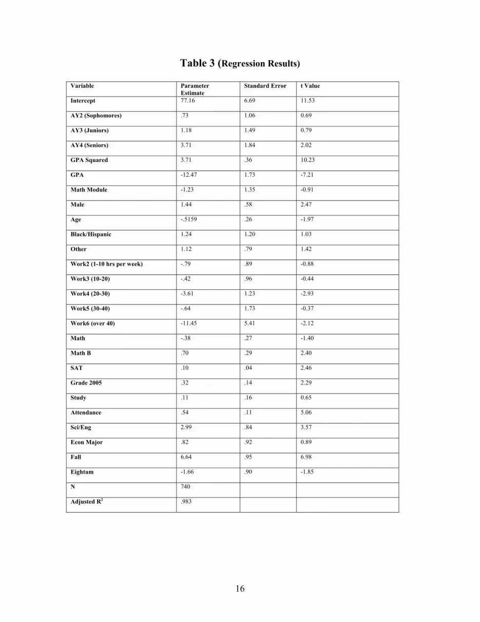
Table 3 (Regression Results)

Variable Parameter Estimate

Standard Error t Value

Intercept 77.16 6.69 11.53

AY2 (Sophomores) .73 1.06 0.69

AY3 (Juniors) 1.18 1.49 0.79

AY4 (Seniors) 3.71 1.84 2.02

GPA Squared 3.71 .36 10.23

GPA -12.47 1.73 -7.21

Math Module -1.23 1.35 -0.91

Male 1.44 .58 2.47

Age -.5159 .26 -1.97

Black/Hispanic 1.24 1.20 1.03

Other 1.12 .79 1.42

Work2 (1-10 hrs per week) -.79 .89 -0.88

Work3 (10-20) -.42 .96 -0.44

Work4 (20-30) -3.61 1.23 -2.93

Work5 (30-40) -.64 1.73 -0.37

Work6 (over 40) -11.45 5.41 -2.12

Math -.38 .27 -1.40

Math B .70 .29 2.40

SAT .10 .04 2.46

Grade 2005 .32 .14 2.29

Study .11 .16 0.65

Attendance .54 .11 5.06

Sci/Eng 2.99 .84 3.57

Econ Major .82 .92 0.89

Fall 6.64 .95 6.98

Eightam -1.66 .90 -1.85

N 740

Adjusted R2 .983

16

Table 4 (Survey Results)

Number of Hours Spent Using the Module

Number of Times Accessing the Module

Preferred Method of Learning Mathematical Material

Useful Parts of the Module

Useful Material Covered in the Module

One: 53.8% One: 23.7% Book: 18.3% Examples: 40.9% Slope: 20.4% Two: 19.4% Two: 31.2% Lecture: 44.1% Practice Problems:

50.5% Graphing: 16.1%

Three: 9.7% Three: 19.4% Tutor: 16.1% Explanations: 19.4%

Solving single variable equation: 16.1%

Four: 3.2% Four: 7.5% Fellow Student: 18.3% Econ Applications: 8.6%

Solving system of two equations: 28%

Five: 1% Five: 5.4% Module: 3.2% Graphics: 8.6% Percentages: 23.7% Zero: 12.9% Zero: 12.9% None: 29% None: 45.2% There were 93 respondents. Percentages in columns 4 and 5 add up to over 100% because students were allowed to choose more than one choice for those questions.

17

Table 5 (Effectiveness in the Treatment Class)

Dependent Variable is AVERAGE Variable Parameter Estimate Standard Error t Value Hours 15.54 5.56 2.8 Hours*SAT -0.26 0.10 -2.69 Math 1.21 0.86 1.4 MathB -1.04 0.94 -1.1 SAT 0.50 0.21 2.33 GPA 3.82 2.07 1.85 Grade2005 2.47 0.57 4.33 Blackhis 2.67 7.56 0.35 Other 7.64 4.27 1.79 Othermajor 8.46 3.86 2.19 Scieng 5.67 4.47 1.27 Male 2.10 1.99 1.06 Constant 8.39 13.77 0.61

18

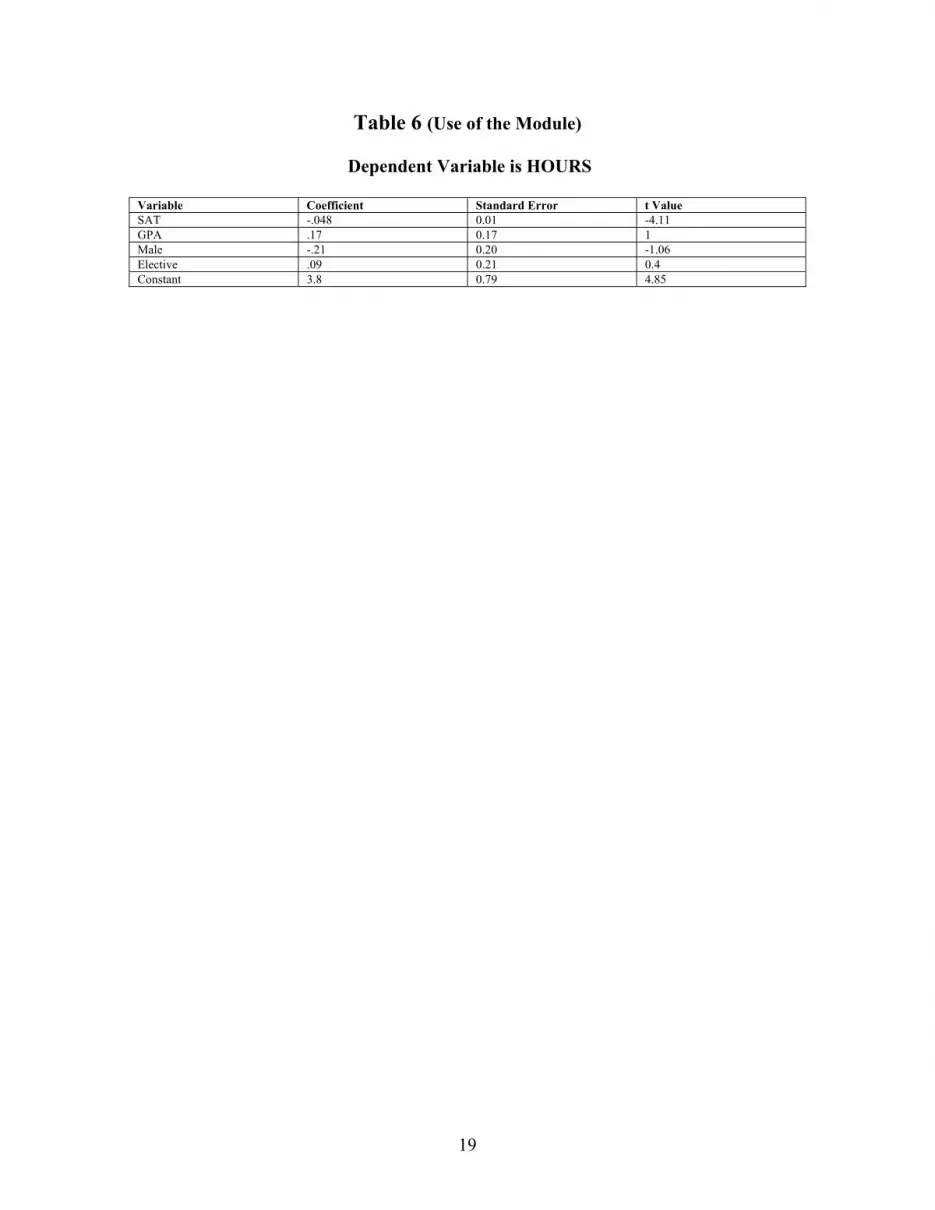
Table 6 (Use of the Module)

Dependent Variable is HOURS Variable Coefficient Standard Error t Value SAT -.048 0.01 -4.11 GPA .17 0.17 1 Male -.21 0.20 -1.06 Elective .09 0.21 0.4 Constant 3.8 0.79 4.85

19

Conclusion

In this article I have studied the characteristics that determine a student's success in

introductory economics. Unlike previous research, I have included in my analysis

exposure to an online tutorial and class meeting time as explanatory characteristics.

While the online tutorial appears to have done little to enhance student performance,

there is evidence that taking the class at 8 AM is detrimental to student's learning. Since

there is very little research on this, more work should be done to determine, if possible,

which class meeting times are most conducive to performance in economics and other

subjects. Another idea for future research is to implement the online tutorial in a

different manner; in particular to first screen students, and target the tutorial toward those

who do not perform as well on a pre-test of basic math ability. It would be useful to learn

which students (if any) benefit from such a tutorial.

The effects of other explanatory characteristics included in the model are generally

consistent with previous research. Those with significant positive effects include being

male, higher attendance, higher math SAT score, being a science or engineering major,

higher grades in the previous economics course, a greater number of math classes

receiving a B or better, obtaining a higher academic status (especially for seniors), and

higher GPA. Those with significant negative effects on performance include a greater

number of hours worked and older ages.

20

Introduction to Radio Mergers

Since the Telecommunications Act of 1996 relaxed radio ownership restrictions2, there

has been an explosion of radio mergers. In the first year following the passage of the

Telecom Act there were over 1000 radio mergers, about 140 of which automatically came

before the Department of Justice for review under the requirements of the Hart-Scott-

Rodino Act. Only three resulted in action by the Department of Justice, and those

mergers were allowed under the provision of divestiture of one or more of the stations.

Here I explore the implications of radio mergers using a variation of the standard

Hotelling location model. The key feature that distinguishes radio and media in general

from other firms is the nature of obtaining revenue. Radio stations typically give their

product away "for free" and collect revenue through advertising sales. Consumers must

choose which station, if any, to listen to based on the format of the radio stations and the

level of advertising. The stations attempt to maximize profits by selling audiences to

advertisers. A lower level of advertising will attract a larger audience, ceteris paribus.

The level of advertising is analogous to the price paid by consumers in "conventional"

markets, but differs in that consumers who pay a monetary price still receive the

complete product, while advertising actually reduces the quantity of the product supplied.

While this is not true in certain forms of media such as newspapers and magazines, an

advertisement during a radio broadcast lowers the amount of time available for regular

programming.

In this paper, I find that in a duopoly, competing firms offer more diversified formats and

lower advertising levels, while two stations that merge will offer more similar formats

with higher

advertising levels. This is in direct contrast to the results of many previous studies.

Welfare implications of mergers are ambiguous. My model shows that mergers may

increase or decrease social welfare as measured by total economic surplus. Mergers 2For a synopsis of the main provisions of the Telecommunications Act of 1996, see Ekeuland, Ford, and Koutsky, Market Power In Radio Markets: An Empirical Analysis of Local and National Concentration, 43 Journal of Law and Economics 157-84 (2000).

21

increase total economic surplus if the price at which firms can sell their advertising space

is sufficiently high or if the loss of utility incurred by consumers from having to listen to

lesser preferred programming is sufficiently low.

Previous Research

A substantial amount of literature exists addressing the question of programming format

in the television and radio industries. The major issues include welfare comparisons

between different types of industry structures, comparisons between advertiser based

revenue versus consumer based revenue, and the issue of whether or not there exists a

bias toward popular programming and away from minority-tastes programming. Many of

the models are based on the television industry, but can readily be applied to radio as

well.

The literature on the effect of ownership structure on format choice begins with an

important article by Steiner (1952). He compares the outcome of a monopolistic

television industry with a triopoly. The results obtained are driven by several strong

assumptions. First, he constructs viewer preferences among three alternative programs.

Viewers are divided into groups of different sizes, with members of each group all having

the same first choice among the alternatives. Specifically, it is assumed that there are

8750 viewers and 3 programs such that 5000 viewers rank program 1 as their first choice,

2500 rank program 2 as their first choice, and the remaining 1250 rank program 3 as their

first choice. Furthermore, viewers are assumed to watch either their first choice or not

watch at all. Channel capacity in the industry is set at 3.

Under one market structure, separate audience-maximizing agents individually own each

station. All viewers are assumed to be of equal value to the stations, and in the event that

two or more stations show the same program, the audience for that program is divided

equally among those stations. Under the monopolistic market structure, one agent

operates all three stations, with the goal to maximize total audience among all three

22

stations. Costs of programming are normalized to zero, so each station has an incentive

to broadcast something as long as there is an audience greater than zero.

Under the separate ownership market structure, given the preferences above, 2 stations

will show program 1, with each getting an audience of 2500, and the third station will

show program 2, also getting an audience of 2500. Program 3 will not be shown. Under

the common ownership structure, the monopolist will show all three programs, and

thereby capture the entire audience.

Using this ad hoc example, Steiner first identified a bias against minority-taste

programming that can result from the individually owned market structure. Minority-

taste programming is loosely defined as programming which appeals to audiences of

relatively small cardinality. Although the assumptions needed to obtain this result are

extremely strong, the literature shows that this bias remains through many alterations of

the model.

Rothenburg (1962) relaxes the assumption that viewers will only watch their first choice.

Instead, he posits that there is a “common-denominator” program that all viewers will

watch. Viewer preferences are as follows: 5000 viewers will watch only program 1, 2500

prefer program 2, but will watch program 1 if program 2 is not shown, and 1250 prefer

program 3, but will watch program 1 if program 3 is not available. Not surprisingly,

program duplication is even more pronounced in the individually owned setting, with all

three stations showing program 1. Both the Rothenburg paper and the Steiner paper

explore only certain audience distributions, and their results are limited in generality.

Rothenburg also explores the effect of allowing more stations. In this case, as the

number of stations increases, it becomes optimal at some point for the stations to show

different programs, as the audience for the “common-denominator” program is divided

into smaller and smaller parts. Thus, the bias against minority programming might well

disappear with an unlimited number of stations.

23

By varying patterns of viewer choice, audience preference distributions, cost structures of

the firms, and channel capacities, Beebe (1977) generalizes Steiner’s model, analyzing 36

different situations. The resulting program patterns for each situation under a monopoly

setting are compared to those resulting from individual station ownership. The

comparisons include which setting provides more choices, which setting obtains the

greater audience, and which setting would win a vote among viewers where viewers vote

for the structure which gives them their highest choice.

Among the important findings, Beebe discovers situations where the Steiner result—that

a monopoly structure provides more viewer choices than the individually owned

structure—does not hold. If the viewer groups are fairly close in size, competitors will no

longer engage in program duplication. Not only is Steiner’s result sensitive to his highly

skewed preference distribution, but also to the assumption that viewers will only watch

their most preferred program. If viewers are assumed to be willing to watch a “common

denominator” program, the monopolist will quite likely show only this program. Thus,

the individually owned setting will likely produce more first (or preferred) choices than a

monopoly structure.

Welfare comparisons are not always straightforward, as there exist cases where one

structure satisfies more first choices, but the other structure attracts a larger total

audience. Also, even a structure that satisfies more first choices and attracts a larger total

audience might not be Pareto superior to its counterpart since there might exist at least

one individual (or group of homogeneous individuals) who receives a higher choice

under the latter structure than the former. More specific structure on viewer choices,

such as a cardinal ranking of programs instead of an ordinal one, is necessary to compare

many of the outcomes.

Beebe's analysis allows for the fact that listening to a program has an opportunity cost for

the listener. This opportunity cost determines a reservation utility—a level of listening

satisfaction which the viewer must obtain in order to be willing to watch any program at

all. The analysis indicates that viewers who have such reservation utility and thus might

24

not attend any station's programming are more likely to be shown their preferred choices

in a monopoly setting. Beebe cites adequate channel capacity as a necessary condition

for minority programs to be shown given profit maximization and advertiser-generated

revenues. A sufficient condition for minority programming to be shown in a competitive

setting is the above combined with the existence of a group of viewers which ranks that

program highest and is greater in number than the break-even constraint. In a monopoly

setting, a sufficient condition for a minority program to be shown are both of the above

combined with the viewer group’s refusal to watch an alternative program. In either

situation, the break-even constraint is determined by the firms' cost structure, and it is

entirely possible that for sufficiently high costs, some channels will go unused.

Spence and Owen (1977) include a “willingness-to-pay” factor in their analysis of market

structure and its effect on performance. Their analysis takes aim at pay TV, where

revenue is generated directly from the viewers as well as or instead of from advertisers.

This aspect is not readily applicable to the radio industry, where all revenue is generated

from advertisers, but they do also consider the behavior of a TV structure where

advertisers are the sole source of funds.

Spence and Owen also discover a bias against minority-taste programming. Indeed, they

find it to be greater in an advertiser paid setting than when the stations receive money

directly from viewers. The reasoning is straightforward. It is assumed that advertising

revenue is a direct function of the number of viewers, and so if advertisers are the sole

source of revenue, then the only thing that matters to the advertisers is the number of

persons in the audience. Because intensity of preferences and audience demographics are

not considered, it is readily apparent that a program offered at a zero price which gains an

audience of size n will be shown over a program which gains an audience of size n-1,

even though the program which the n-1 group prefers might be extremely valuable to that

group whereas the program preferred by the group of n viewers might be just barely

preferred to not viewing. When the viewers actually pay to see the program, their

willingness-to-pay somewhat alleviates this problem, but a bias still exists toward mass

appeal programming and away from minority-taste programming. Spence and Owen also

25

find a related bias against expensive programs. That is, stations might choose to show a

less expensive program even though a more expensive one might generate greater overall

benefits.

Wildman and Owen (1985) extend the analysis of the Spence/Owen model to include

advertising time as a choice variable. A fundamental assumption in this model is that the

market for advertising is perfectly competitive, and therefore the price of advertising is

constant. Also, viewers are assumed to dislike advertising. In this context, advertising is

viewed as a cost to watching a program and the station attempts to maximize the number

of “audience-minutes”—the number of advertising minutes multiplied by the total

number of viewers. The solution to the profit-maximizing problem of the station is

exactly analogous to the solution of the traditional profit-maximizing behavior of a firm

facing a downward sloping demand curve. The number of viewers for a particular

program is a function of the amount of advertising which that program has. As with any

maximization done by a firm facing a downward sloping demand curve, there is a

deadweight loss with price (the amount of advertising) being too high, and quantity

(number of viewers) being too low for social efficiency.

Noam explores the role of the government in providing public service programs and

concludes that such programming becomes less and less attractive as the number of

channels becomes greater. This is consistent with the deregulation result mentioned

earlier, and is fairly obvious. Noam does conclude that the presence of a public station

which broadcasts a minority-taste program will give private stations incentive to produce

programs which appeal to mass audiences.

It is worth mentioning at this point that one way for a government to reduce the bias

against minority-taste programming is to subsidize public stations that broadcast

programs that are preferred by smaller audiences. This has been undertaken in both TV

and radio. However, the deregulation of the cable TV industry in the late 1970’s and

early 1980’s, which effectively allowed for the expansion of the number of channels

available, greatly lessened support for publicly funded programming. Since the

26

expansion of the number of channels encourages stations to creep into the realm of

minority-taste programming, this is not surprising.

Kehoe (1989), following de Palma, Ginsburgh, Papageorgiou, and Thisse, develops a

model of radio formatting which shows that social welfare can be increased from that of

the equilibrium outcome if firms located on the outside of a product space move even

further outside. The model is set within the Hotelling framework. The dispersed

equilibrium is generated by the assumption that there exists a degree of heterogeneity

among listeners. Thus, a random variable, assumed to be iid, is added to each agent’s

utility function.

The results of the model include a theorem which states that in equilibrium, the stations

located on the outside of the product space would increase total surplus if they were to

move even farther to the outside. This is interpreted to mean that there is a bias against

minority-taste programming. Kehoe is able to obtain this result within a spatial

competition framework without having to include intensity (cardinal utility) of

preferences as Spence and Owen do.

An empirical study by Berry and Waldfogel (2001) provides some evidence that radio

mergers result in more diversified programming formats being offered relative to the

number of stations in the market. They also find however that radio station consolidation

reduces entry into the market, and so the number of stations operating in a market might

also be reduced. Their conclusions suggest that a common ownership group might

choose formats for their stations strategically in order to lower entry into a market. They

take advantage of the natural experiment occurring because of the Telecommunications

Act, analyzing market structure and performance before and after the implementation of

that legislation.

27

The Competition Model

In this model, I assume that consumers are differentiated by their preferences for different

radio formats. I also assume that consumers dislike advertisements. Thus, I think of

radio format as a horizontal characteristic, while the advertising level of the stations is a

vertical characteristic.

Consider 2 firms that compete for advertising revenue in the following 2-stage game.

First, each firm simultaneously chooses a format, which I model a la Hotelling as a

choice ∈ [0,1], i={1,2}. Without loss of generality, let ix 1x ≤ . In the second stage,

each firm simultaneously chooses an advertising level, a ∈[0,1], i={1,2}. It is

reasonable to think that format would be chosen first. Formats require a large repertoire

of CDs, tapes, etc to adequately provide a particular genre of music. In the case of news,

sports or talk radio, a consistent set of personalities is necessary to maintain audience

loyalty. Advertising contracts, on the other hand, are typically short lived and can thus be

altered more easily. The firms' choice of and a determines a location in the two-

dimensional space [0,1]X[0,1].

2x

i

ix i

A consumer located at c∈[0,1] gains utility from listening to station located at (i ix , ia ) at

the constant rate of U i = - tu *( d ), where is a utility parameter which represents the

rate of utility gained from listening to a consumer’s ideal station with no commercials,

is a disutility parameter, and d is distance from a consumer’s location in the unit

interval, [0,1], to station i ’s location in the 2-dimensional space, [0,1]x[0,1]. Thus,

=

i

i

u

t

di ( ) 22ii axc +− . In this utility specification, ads on preferred stations are preferable

to ads on less preferred stations. This utility specification also has the appealing property

that the cross partial derivative of utility with respect to distance and advertising is

negative. Advertisements on preferred stations, while preferable to ads on less preferred

stations, still cut into the more valued programming time of the preferred station.

Therefore, additional ads on stations located close to the consumer on the horizontal axis

28

reduce utility at a greater rate than additional ads on stations located farther away. This

seems intuitively plausible. A consumer listening to a program that she really enjoys will

suffer more when a commercial comes on than a consumer listening to a program that she

doesn't really like that much, even though the former commercial is more enjoyable than

the latter.

I assume that all consumers have the same opportunity cost of listening to the radio,

which I normalize to zero. Thus, consumers are differentiated only by their location in

the horizontal format space. This allows me to focus on the effects of merger between

the two stations.

I assume that programming is divided into program periods of a given length. During a

program period, a consumer has three options. She can listen to station 1 for the program

period, listen to station 2 for the program period, or not listen. Since the opportunity cost

of listening is 0, consumers will listen as long as U i ≥ 0, for some i. A consumer who is

just indifferent to listening to either station for the entire program period is located at

c*( ,1x 2x

1d

, 1a

=

, ), the implicit function which solves U2a

2d

1 = . Clearly U if and

only if .

2U 21 U=

Firms generate revenue based on the amount of advertising time, ia , times the amount of

consumers who listen to the ads. I assume that the market for advertising is perfectly

competitive, so that firms can sell all the advertising they want at a constant price, A . I

normalize production costs to zero, so that profit for firm i is given by:

iΠ = A * *ia iD , = {1,2}, i

where is the demand captured by Firm i . Firm i will capture all of the consumers for

whom > 0 and U > U , ,j∈{1,2},

iD

iU i j i i ≠ j. Given the utility specification above,

there will be two locations where a consumer listening to a firm gains exactly 0 utility--

one to the right of the firm, and one to the left. Therefore the demand faced by station 1

29

is equal to min{c*, } - max{0, }, where c is the location of the consumer to the

right of Firm 1 who gains exactly 0 utility by listening to Firm 1, and is the location of

the consumer to the left of Firm 1 who gains exactly 0 utility by listening to Firm 1.

Similarly, Firm 2's demand will be min{1, c } - max{c*, } where is the location

of the consumer to the right of Firm 2 who gains exactly 0 utility by listening to Firm 2,

and is the location of the consumer to the left of Firm 2 who gains exactly 0 utility by

listening to Firm 2.

Rc1

≥

Lc1R1

Lc1

cR2

Lc2R2

Lc2

2

The following proposition demonstrates that when consumers have significant distaste for

station formats that are less than ideal, then two independently operated stations will

diversify so that they each capture a disjoint set of consumers, and effectively operate as

independent monopolies.

Proposition 1: If t 2u , then the firms will diversify to the point that each has a

separate monopoly.

Proof: I will show that given these parameter values, a profit maximizing monopolist

will generate demand of no more than half of the consumers. Therefore, there is "room"

for two firms to act as individual monopolists, which is an equilibrium.

The maximum profit a firm can make is the profit obtained as a monopolist. If

the market is not "covered" by a monopolist located at x∈[0,1], meaning that some

consumers would receive utility less than 0 and therefore not listen, and the monopolist

locates close enough to x = 21 so that consumers located at c = 0 and c = 1 receive utility

less than or equal to 0, then the demand facing a monopolist can be found by determining

the locations of the consumers who gain exactly zero utility. Given the utility

specification I am using, there are two locations where the consumer gains exactly 0

utility, one to the right of x and one to the left. Call these locations c and c ,

respectively. Since utility is strictly decreasing in distance, all consumers to the left of

R L

30

Rc

Rc

and to the right of Lc will listen, and all other consumers will not listen. These

locations are:

Lc

L

Π

a∂Π∂

a

2

2u

= x + t

tau 222 − and

= x - t

tau 222 − .

Demand is given by c R - c = 2

ttau 222 − .

The monopolist's profit is then given by

= A * a * 2t

tau 222 − .

The first order condition for profit maximization is

= 2242

222 24utta

uta+−

+− = 0.

Solving for , I obtain a

* = 2t

u .

Demand for the monopolist when * =a2t

u is:

D = t

u*2 . Solving D = 21 , I obtain = t 22u . Since D is strictly decreasing in t , I

conclude that if t ≥ , then the maximum demand that a single firm can have at the

profit maximizing level of advertising equals 21 . Therefore with 2 firms, as long as t ≥

2 , there exist locations (in particular = 1x41 and = 2x

43 ) such that each gains

monopoly profit. Since this maximizes profit for each firm, this is an equilibrium

2u

31

outcome. All other equilibria involve variations of location which allow each firm to

gain monopoly profit. QED

Proposition 2: If t ≤2

3u then the firms locate at ( , ) = (1/6, 5/6), with ( a , a ) =

(

1x 2x 1 2

31 ,

31 ).

Proof: This is verified by solving the two firms' optimization problems using backward

induction. The consumer who is indifferent between listening to station 1 and station 2 is

located at

c* = ( )21

22

21

22

21

2 xxxxaa

−−+− . Taking locations as given, the first order conditions for profit

maximization in the advertising subgame are:

1

1

a∂Π∂ =

21

21

xxa−

+ ( )21

22

21

22

21

2 xxxxaa

−−+− = 0

2

2

a∂Π∂ = 1 +

21

22

xxa−

- ( )21

22

21

22

21

2 xxxxaa

−−+− = 0.

Solving these equations simultaneously, I obtain

1a * = 2

222

211 xxxx ++−−

and

2a * = 2

33 222

211 xxxx −++−

. The second order conditions for profit maximization

hold:

21

12

a∂Π∂ =

21

13xx

a−

0 (since ); ≤ 1x ≤ 2x

22

22

a∂Π∂ =

21

23xx

a−

0 (since ≤ ). ≤ 1x 2x

As can be easily seen by inspection, the closer the firms are together, the lower the levels

of advertising in equilibrium.

32

Substituting these values into the firms' profit functions, I get

1Π = ( )

81 2

2221121 xxxxxx ++−−++

and

2Π = ( )

8333 2

2221121 xxxxxx −++−++−−

The first order conditions for profit maximization with respect to locations are

1

1

x∂Π∂ =

( )222

211

21222

21

16

25241

xxxx

xxxxx

++−−

+−++−− = 0 and

2

2

x∂Π∂ =

( )( )22

211

21222

21

3316

2341529

xxxx

xxxxx

+−−+−

+++−− = 0.

Solving these first order conditions simultaneously for and , I obtain 1x 2x

*1x =

61

*2x =

65 .

Again, the second order conditions hold:

21

12

x∂Π∂ =

43

− .

22

22

x∂Π∂ =

43

−

The complete solution to the model is

*1x =

61

*2x =

65

*1a = = *

2a3

1

*1Π =

*2Π =

32A

33

Finally, I note that the utility level of the consumer located at c* is 0, provided that t

≥

≤2

3u . This last step is necessary to ensure that demand for Firm 1 is equal to c*,

demand for Firm 2 is equal to (1-c*), and thus the profit functions used in the analysis are

correct. If t >2

3u , then the consumer located at c* will receive utility less than 0. In this

case, the firms could increase profit by moving closer to the center because demand for

Firm 1 would be strictly increasing in location, and demand for Firm 2 would be strictly

decreasing in location. This is because the market is not "covered". Since the profit

functions are concave in both advertising and location, the equilibrium is unique.

QED

Merger

Here I analyze the advertising and location choices of the firms if they were to merge

under common ownership. I assume that a merger results in a single decision maker who

operates both stations and maximizes total (joint) profits. In order to make meaningful

comparisons to the competition model, I restrict my analysis to the case where t ≤2

3u .

As shown in Proposition 2, this means that, in the competitive case, the firms do not act

as separate monopolists, and that the entire market is covered.

Proposition 3 shows that if consumers do not really mind what they are listening to, then

the firms will advertise all of the time. The parameter assumptions in this proposition are

close to the spirit of earlier models where audiences are assumed to listen to one program

or another, but never choose to not listen. Such a consumer would either have a very low

opportunity cost of listening, or a great tolerance for almost any type of programming.

One might consider a person driving in a car or working out--situations where listening to

a radio program does not preclude other activity.

34

Proposition 3: If t ≤174u , then two stations operating under common ownership will

each advertise all of the time ( = 1, i=1,2). ia

Proof: For this very low level of , advertising all of the time still captures the entire

market between the two firms. If =

t

t174u , then the firms will locate at = 1x

41 , = 2x

43 . If < t

174u , then there are an infinite number of location choices that allow the firms

to capture the entire market together while advertising all of the time. Clearly this will

maximize the joint profits of the firm. QED

The parameter restrictions in the following proposition allow for a meaningful

comparison to the competitive case described by Proposition 2:

Proposition 4: If 174u < t <

23u , then the firms will locate at = 1x

41 , = 2x

43 . The

advertising levels are = =*1a *

2at

tu4

16 22 − .

Proof: This advertising level allows the firms to capture the entire market between them.

Suppose by construction that Firm 1 locates at = 1x41 . Given the parameter restrictions

stated above, if Firm 1 advertises at the level of = 1at

tu4

16 22 − , then the consumers

located at c = 0 and c = 21 gain exactly 0 utility by listening to Firm 1. All consumers

located at c∈(0, 21 ) gain positive utility listening to Firm 1. Similarly, if Firm 2 located

at x = 43 and advertised at the level of = 2a

tu4

2 t 2−16 , then consumers located at c =

35

21 and c = 1 gain exactly 0 utility by listening to station 2. All consumers located at

c∈(21 ,1) gain positive utility from listening to station 2. Thus, consumers located at

c∈(0, 21 ) listen to Firm 1, and consumers located at c∈(

21 ,1) listen to Firm 2. (Whether

the consumers located at c = 0, c = 21 and c = 1 listen or not is immaterial to the

optimization since they each occupy a space of measure 0.) In this situation, advertising

less would not increase profits since the firms are already capturing the entire market

between them. Advertising more by either station would decrease profit, since at that

level of advertising the derivative of profit with respect to advertising for each station is

negative:

i

i

a∂Π∂

= 2

22 )8(t

utA − , i= 1,2 when =iat

tu4

16 22 − . It is easily verified that this is

negative as long as t falls within the range specified in Proposition 4. QED

Operating Costs

The previous analysis was done having normalized the cost of operating a station to 0.

However, in the merger case, this assumption loses generality. Specifically, if the cost of

operating a station is greater than t

tutuA 2222 4216( −−− , then the profit-

maximizing common ownership will shut down one station and operate as a single firm

monopolist. It should be noted that if 2

32 utu << , then the single-firm monopolist will

no longer "cover" the market. The single-firm monopolist will set an advertising level of

tua2

* = . If 2ut < then the market will be covered. Otherwise, there will be some

consumers who do not listen to the programming. In this situation, the single-firm

monopolist will have some leeway as to format selection and will not necessarily choose

the middle of the location space.

36

Welfare

Total welfare in each scenario is the sum of profits by the firms plus utility by all

consumers. If the market is covered, this is given by:

21

1

20

1*

*

Π+Π++= ∫∫c

c

dcudcuW

Total welfare in equilibrium in the competitive case is equal to

tuAArcArctuAW C 600415.057735.0]3

1sinh[12]32

1sinh[12138363

−+≅

+++−+=

and total welfare in equilibrium in the merger case is

+−

−++

−=

uttLog

ttuu

ttuAM

421

1616

2416 222

W .

The difference is a decreasing function of . Depending upon the

parameter values, it is possible for either the merger case or the competitive case to yield

greater welfare. For example, if

)( MC WW − A

1== tU , then if 968.<A , the difference between

welfare in the competitive case and welfare in the merger case is positive, so welfare is

greater in the competitive case. If then the opposite is true. The interpretation

is clear: when firms can sell their advertising units at a high price, the increase in firms'

profits resulting from merger outweighs the decrease in consumer utility.

969.>A

I can also say that in the competition model the firms are too far apart for social

efficiency.

2

2222222

1 )21(2)21(12()21()11)

211(1(2

xxxxaaAaaxaxat

xW C

−−+−−

++−−+=∂∂

37

Substituting the equilibrium values of , , and a , 1x 2x 1a 2 txW 0657415.0

1

=∂∂ which is

greater than 0 as long as t is greater than 0. Therefore, total welfare would increase if

Firm 1 moved closer to the center. Similarly, in equilibrium, the derivative of total

welfare with respect to is , indicating that total welfare would increase if

Firm 2 moved closer to the center.

2x t657415.0−

In equilibrium,i

C

aW∂∂

≅ tA 481577.2/ − , i = 1,2. Therefore if A < then there is

too much advertising, and if > there is too little advertising.

t963153.0

A 963153.0 t

In the merger model, 0=∂∂

i

M

xW in equilibrium, i=1,2, indicating that the firms are

located at the welfare maximizing locations. This is a standard result, and follows from

the fact that ( , ) = (1x 2x41 ,

43 ) will minimize total "transportation" costs of consumers.

Finally,

4

)11611161(162

26

246223

1

++−

−+−−+

=∂∂ ut

uttLOGtutA

aW M

.

Since this is increasing in , if A

11611161[)16(

21

246

246223

++−

−+−+−−>

uttuttLOGUttA ,

then there is too little advertising in the merger model, and if

38

11611161[)16(

21

246

246223

++−

−+−+−−<

uttuttLOGuttA , then there is too much advertising

for social optimality.

For example, if , this threshold is 1== tu 98921.0≅ .

Conclusion

In contrast to earlier papers, I have found that a switch from competitive ownership to

common ownership of radio stations might result in format choices which are more

similar under the common ownership scheme. While welfare implications are

ambiguous, there is some evidence that competitive ownership might be more efficient

than monopoly. The results are driven by the utility specification which includes a

measure of viewers' intensity of preferences as well as the possibility that consumers

might choose not to listen at all. This utility specification assumes that consumers are

affected by both advertising time and format choice, which seems to accurately capture

the flavor of advertiser supported markets.

I also find that the principle of maximum differentiation found by d'Aspremont,

Gabsxewicz and Thisse (1979) does not hold under the preference assumptions of this

paper. In their paper, the cost of consuming a product equals the transportation cost

associated with the purchase of a product plus the monetary price of the product. Here

the "price" of the product can be thought of as the level of advertising time, but this price

is not separable from the utility diminution resulting from listening to a less than ideal

station format.

The results of this paper suggest that radio mergers may lessen economic

efficiency through their effect on total advertising time. A weakness here, however, is

that the benefits to the advertisers are not considered. One might reasonably think that a

monopolistic radio industry would create higher prices for advertisers, leading to welfare

reductions. A more robust model which explores this is in order.

39

References

Agarwal, R., and A. E. Day. 1998. The Impact of the Internet on Economic Education.

Journal of Economic Education 29 99-110.

Akpom, U.N., and Huller, I.S. 1994. Class Attendance and Student Performance in

Principles of Economics Course. Midsouth Academy of Economics and Finance Papers

and Proceedings: 319-328.

Alexander, P. J., Entry Barriers, Release Behavior, and Multi-product Firms in the Music

Recording Industry, 9 (1994) Review of Industrial Organization 85-98.

Anderson, G., D. Benjamin, and M. Fuss. 1994. The Determinants of Success in

University Economics Courses. Journal of Economic Education 25 (Spring): 99-119.

Becker, W. E., and M. Watts. 1996. Chalk and Talk: A National Survey on Teaching

Undergraduate Economics. American Economic Review v86 448-53.

Becker, W. E., and M. Watts. 2001. Teaching Economics at the Start of the 21st Century:

Still Chalk-and-Talk. American Economic Review, v91, n2 (May 2001): 446-51.

Beebe, J., Institutional Structure and Program Choices in Television Markets, 91 (1977)

Quarterly Journal of Economics 15-38

Berry, S. and J. Waldfogel, Do Mergers Increase Product Variety? Evidence from Radio

Broadcasting 116 (3) (2001) Quarterly Journal of Economics 1009-1025.

Besen, S.M., The Value of Television Time, 42 (1976) Southern Economic Journal 435-

41.

40

Blair, R.D and R.E. Romano, Pricing Decisions of the Newspaper Monopolist, 59 (1993)

Southern Economic Journal 721-32.

Brasfield, D., D. Harrison, and J. McCoy. 1993. The Impact of High School Economics

on the College Principles of Economics Course. Journal of Economic Education 24

(Spring): 99-111.

Brown, B., Liedholm, C., 2002. Can Web Courses Replace the Classroom in Principles of

Microeconomics? American Economic Review, v92, n2 444-48.

Coase, R. H., Monopoly Pricing with Interrelated Costs and Demands, 13 (1946)

Economica 278-94.

Cohn, E. et al (2001). Do Graphs Promote Learning in Principles of Economics? The

Journal of Economic Education, v32 n4 p160.

Daniel, J. 1999. Using the Web to Improve Computer-Aided Instruction in Economics.

The Journal of Economic Education, v30 n3 p225.

Dickinson, David L., 2002. A Bargaining Experiment to Motivate Discussion on

Fairness. The Journal of Economic Education, v33 n2 p136.

Durden, G.C., and Ellis, L.V. 1995 The Effect of Attendance on Student Learning in

Principles of Economics. American Economic Review (May): 343-346.

Ely, D., and L. Hittle. 1990. The Impact of Math Background on Performance in

Managerial Economics and Basic Finance Courses. Journal of Financial Education

(Fall): 59-61

Frank, B. 1997. The Impact of Classroom Experiments on the Learning of Economics:

an Empirical Investigation. Economic Inquiry Oct 1997 v35 n4 p763(7) p 1.

41

Ford, B. 1972. The Effect of Peer Editing/Grading on the Grammar-Usage and Theme-

Composition Ability of College Freshmen. Dissertation, University of Oklahoma.

Garratt, Rod, 2000. A Free Entry and Exit Experiment, The Journal of Economic

Education, v31 n3 p237.

Greenlaw, S. 1999. Using Groupware to Enhance Teaching and Learning in

Undergraduate Economics. Journal of Economic Education, v30, n1 33-42. Gremmen, H., & Potters, J. 1997. Assessing the Efficacy of Gaming in Economic

Education. Journal of Economic Education, Fall. V28 n4 291-303.

Henebry, K. 1997. The Impact of Class Schedule on Student Performance in a

Financial Management Course. Journal of Education for Business

(November/December): 114-120.

Hotelling, H., Stability in Competition 39 (1929) Economic Journal 41-57.

Katz, A., and Becker, W. 1999. Technology and the Teaching of Economics to

Undergraduates. The Journal of Economic Education, v30 n3 p194.

Kaufman, D., 2002. Interactive Web Graphs for Economic Principles. The Journal of

Economic Education, v33 n3 p296.

Kehoe, M., The Choice of Format and Advertising Time in Radio Broadcasting, Ph.D.

Dissertation, (1989) University of Virginia.

Lancaster, K., The Economics of Product Variety: A Survey, 9 (1990) Marketing

Science 189-206.

42

Lumsden, K., and A. Scott. 1987. The Economics Student Reexamined: Male-Female

Differences in Comprehension. Journal of Economic Education 18 (Fall): 365-375.

McCain, R., 2000. Essential Principles of Economics: A Hypermedia Textbook. The

Journal of Economic Education, v31 n1 p9.

Noam, E. M., A public and Private Choice Model of Broadcasting, 55 (1987) Public

Choice 163-187

Owen, B. and Wildman, S., Video Economics (1992) Cambridge Massachusetts: Harvard

University Press

Oxoby, Robert J., A Monopoly Classroom Experiment. The Journal of Economic

Education Spring 2001 v32 n2 p160.

Park, K., and P. Kerr. 1990. Determinants of Academic Performance: A Multinomial

Logit Approach. Journal of Economic Education 21 (Spring): 101-111.

Parks, R. 1999. Macro Principles, PowerPoint, and the Internet: Four Years of the Good,

the Bad, and the Ugly. The Journal of Economic Education v30 n3 p200.

Romer, D. 1993. Do Students Go To Class? Should They? Journal of Economic

Perspectives 7 (Summer): 167-174.

Rothenburg, J., Consumer Sovereignty and the Economics of TV Programming, 4 (1962)

Studies in Public Communication 45-54

Schmidt, R. 1983. Who Maximizes What? A Study in Student Time Allocation.

American Economic Review (May): 23-28.

43

44

Siegfried, J. 1979. Male-Female Differences in Economic Education: A Survey. Journal

of Economic Education 10 (Spring): 1-11.

Simkins, S. 1999. Promoting Active-Student Learning Using the World Wide Web in

Economics Courses. Journal of Economic Education v30, n3 278-87.

Spence, A.M. and Owen, B., Television Programming, Monopolistic Competition and

Welfare, 91 (1977) Quarterly Journal of Economics 103-126

Steiner, P., Programming Patterns and the Workability of Competition in Radio

Broadcasting, 66 (1952) Quarterly Journal of Economics 194-223

Stone, L., 1999. Multimedia Instruction Methods. The Journal of Economic Education

v30 i3 p265

Tirole, J. 1993. The Theory of Industrial Organization. Cambridge, Mass.: The MIT

Press.

Vachris, M. 1999. Teaching Principles of Economics without "Chalk and Talk": The

Experience of CNU Online. The Journal of Economic Education v30 n3 p292

Varian, H. 1984. Microeconomic Analysis. New York: W.W.Norton

Veljanovski, C, ed. 1989. Freedom in Broadcasting. Hobart Paperback series, no. 29

London: Institute of Economic Affairs 262.

Williams, M., C. Waldauer, and V. Duggal. 1992. Gender Differences in Economic

Knowledge: An Extension of the Analysis. Journal of Economic Education 23

(Summer): 219-231.