EPR OFEXCHANGE

COUPLEDSYSTEMS

ALESSANDRO BENCINIAND DANTE GATTESCHI

DOVER PUBLICATIONS, INC.MINEOLA, NEW YORK

2

CopyrightCopyright © 1990, 2012 by Dante Gatteschi

All rights reserved.

Bibliographical Note

This Dover edition, first published in 2012, is an unabridged republication of the work originally published bySpringer-Verlag, Heidelberg, in 1990. Dr. D. Gatteschi has prepared a new Foreword specially for this Doveredition.

Library of Congress Cataloging-in-Publication Data

Bencini, Alessandro, 1951–EPR of exchange coupled systems / Alessandro Bencini and Dante Gatteschi. p. cm.Originally published: Heidelberg : Springer, 1990 under the title: Electron paramagnetic resonance of

exchange coupled systems.Includes bibliographical references and index.eISBN-13: 978-0-486-31032-91. Electron paramagnetic resonance spectroscopy. I. Gatteschi, D. (Dante). II. Bencini, Alessandro, 1951–

Electron paramagnetic resonance of exchange coupled systems. III. Title.

QC763.B46 2012538'.364—dc23

2012012107

Manufactured in the United States by Courier Corporation48854301

www.doverpublications.com

3

Foreword to the Dover Edition

Twenty years is a long time for a book, even more so for a specialist book like EPRof Exchange Coupled Systems. Unfortunately during this time my friendAlessandro, who co-authored the book with me, passed away in an unexpected anduntimely way. In the words of Takeji Takui who, during a symposium in Japan saidDr. Alessandro Bencini was “… a great scientist … who had made invaluablecontribution in the field of ESR spectroscopy relevant to molecule basedmagnetism.”

In my opinion, the book stands the impact of time, despite being completeddirectly before the explosion of single molecule magnetism. In fact, the discoverythat some molecules containing a few magnetic ions behaving as tiny magnetsactually expanded the relevance of EPR of Exchange Coupled Systems. It was toobad that the “single molecule magnets,” as they are usually called, are not present,but it is good that the theory which allows the analysis of their properties is workedout here in detail.

The other field which developed after the publication of this book is that of thetheoretical calculation of the exchange interaction, a field to which Alessandromade important contributions. Alessandro was not scared by mathematics, and allthe parts of the book where complex formulas are competently used were his effort.Having here described the parts of the book which would be different if the bookwere written in the present day, the rest continues to provide a very useful tool in astill expanding interdisciplinary research area.

It is to Alessandro’s daughter Victoria that I dedicate this reprint. It may berewarding to see your father’s book used all over the world, dear Vic; and maybeyou will appreciate your name printed so close to his. Later, I hope it will help youto realize what a great scientist your father was.

D. GATTESCHI

4

Preface

This book is intended to collect in one place as much information as possible on theuse of EPR spectroscopy in the analysis of systems in which two or more spins aremagnetically coupled. This is a field where research is very active and chemistsare elbow-to-elbow with physicists and biologists in the forefront. Here, as inmany other fields, the contributions coming from different disciplines are veryimportant, but for active researchers it is sometimes difficult to follow theliterature, due to differences in languages, and sources which are familiar to, e.g., aphysicist, are exotic to a chemist. Therefore, an effort is needed in order to providea unitary description of the many different phenomena which are collected under thetitle. In order to define the arguments which are treated, it is useful to state clearlywhat is not contained here. So we do not treat magnetic phenomena in conductorsand we neglect ferro- and antiferromagnetic resonance. The basic foundations ofEPR spectroscopy are supposed to be known by the reader, while we introduce thebasis of magnetic interactions between spins.

In the first two chapters we review the foundations of exchange interactions,trying to show how the magnetic parameters are bound to the electronic structure ofthe interacting centers. Chapter 3 is about the spectra of pairs, and Chapter 4 givesa brief introduction to the spectra of systems containing more than two, but less thaninfinite, centers. Chapter 5 is about relaxation, while Chapter 6 shows how thecomplicated cases of infinite lattices can be tackled, and how EPR can providefirst-hand information on spin dynamics.

The following chapters report a survey of experimental data which hopefullywill be of some help as general reference to the field: Chapter 7 is about spectra ofpairs, Chapter 8 about systems in which transition metal ions are coupled to stableorganic radicals, Chapter 9 reports some examples of magnetically coupledsystems found in biological materials, a fascinating and fast expanding area,Chapter 10 surveys low dimensional materials, and Chapter 11 finally reports theuse of EPR to characterize excitons and exciton motion. The survey is far fromcomplete, but hopefully it will be a useful introduction to the area.

At the end of a preface it is mandatory to express sincere thanks to all the peoplewho made the authors feel less desperate in their struggle with the literature tofollow and the pages to write. So first of all we would like to dedicate the book toNinetta, Silvia, Alessandra, and Mariella who did not oppose to the frequentretreats from family life.

Many people read in advance some chapters and gave us useful suggestions,

5

which certainly improved the manuscript. The flaws, of course, remain ourresponsibility. We heartily thank E.I. Solomon, O. Kahn, G.R. Eaton, S.S. Eaton, S.Clement, J.P. Renard, R.D. Willett, and J. Drumheller. All the people in our groupin Florence, C. Benelli, A. Dei, C. Zanchini, A. Caneschi, L. Pardi, O. Gouillou,and R. Sessoli must be particularly thanked for acting as guinea pigs reading themanuscript from the first stages.

Finally, it is a tradition to thank the people who typed the manuscript.Unfortunately in this technological era we had to type the manuscript ourselves, sothat we can only thank our personal computers which made the burden bearable.

Alessandro BenciniDante Gatteschi

6

Table of Contents

1 Exchange and Superexchange

1.1 The Exchange Interaction1.2 Anderson’s Theory1.3 Molecular Orbital Exchange Models1.4 Quantitative MO Calculations of Singlet-Triplet Splitting

2 Spin Hamiltonians

2.1 The Spin Hamiltonian Approach2.2 The Magnetic Spin-Spin Interaction2.3 The Exchange Contribution2.4 Biquadratic Terms2.5 Justification of the Spin Hamiltonian Formalism2.6 Exchange Involving Degenerate States2.7 Exchange in Mixed Valence Species

3 Spectra of Pairs

3.1 The Spin Hamiltonian for Interacting Pairs3.2 Spin Levels in the Strong Exchange Limit3.3 Spectra of Pairs in the Strong Exchange Limit3.4 Spin Levels in the Weak Exchange Limit3.5 Spectra of Pairs in the Weak Exchange Limit3.6 Intermediate Exchange

4 Spectra of Clusters

4.1 The Spin Hamiltonian for Oligonuclear Systems of Interacting Spins4.2 Spin Levels of Exchange Coupled Clusters in the Strong Exchange Limit4.2.1 Spin Levels of Trinuclear Clusters4.2.2 Spin Levels of Tetranuclear Clusters4.2.3 Spin Levels of Linear Clusters4.3 EPR Spectra of Exchange Coupled Clusters in the Strong Exchange Limit4.3.1 EPR Spectra of Trinuclear Clusters4.3.2 EPR Spectra of Tetranuclear Clusters

7

5 Relaxation in Oligonuclear Species

5.1 Introduction5.2 Theoretical Basis of Spin Relaxation in Pairs5.3 Iridium(IV) Pairs5.4 Copper Pairs5.5 Two-Iron-Two-Sulfur Ferredoxins5.6 Relaxation in Larger Clusters

6 Spectra in Extended Lattices

6.1 Exchange and Dipolar Interactions in Solids6.2 Exchange Narrowing6.3 Additional Broadening Mechanisms6.4 Exchange Narrowing in Lower Dimensional Systems6.4.1 The Effect of Weak Interchain Coupling6.4.2 Half-Field Transitions6.4.3 Temperature Dependence of the Spectra6.4.4 Frequency Dependence of the Line Widths

7 Selected Examples of Spectra of Pairs

7.1 Early Transition Metal Ion Pairs7.2 Copper Pairs7.3 Heterometallic Pairs7.4 Organic Biradicals

8 Coupled Transition-Metal Ions-Organic Radicals

8.1 Introduction8.2 Nitroxides Directly Bound to Metal Ions8.3 Weak Exchange with Nitroxides8.4 Semiquinones

9 Biological Systems

9.1 Introduction9.2 Copper Proteins9.3 Iron Proteins9.3.1 Iron Porphyrins and Heme Proteins9.3.2 Iron-Sulfur Proteins9.3.3 Sulfite Reductase9.3.4 Nitrogenase9.3.5 Iron-Binding Proteins Without Cofactors or Sulfur Clusters

8

9.4 Exchange-Coupled Species in the Photosynthetic O2-Evolving Complexes

10 Low Dimensional Materials

10.1 Linear Chain Manganese(II)10.2 Linear Chain Copper(II)10.3 Two-Dimensional Manganese(II)10.4 Two-Dimensional Copper(II)

11 Excitons

11.1 Introduction11.2 Excitons11.3 EPR of Triplet Excitons in Linear Organic Radical Systems

Appendix A. Second Quantization

Appendix B. Properties of Angular Momentum Operators and Elements ofIrreducible Tensor Algebra.

B.1 Properties of Angular Momentum OperatorsB.2 Addition of Two Angular Momenta. Clebsch-Gordon Coefficients and “3j”

SymbolsB.2.1 DefinitionsB.2.1.1 Equivalent DefinitionsB.2.1.2 Phase Convention and PropertiesB.2.1.3 The “3J” SymbolsB.2.2 Methods of CalculationsB.2.2.1 Special FormulaeB.3 The “6j” Symbols and the Racah W CoefficientsB.3.1 DefinitionsB.3.2 PropertiesB.3.3 Methods of CalculationB.3.3.1 Special FormulaeB.4 The “9j” SymbolsB.4.1 DefinitionB.4.2 PropertiesB.4.3 Special FormulaeB.5. Irreducible Tensor OperatorsB.5.1 DefinitionsB.5.1.1 Compound Irreducible Tensor OperatorsB.5.1.2 Tensor Product of Two First-Rank Irreducible Tensor Operators

9

B.5.2 Properties of Irreducible Tensor OperatorsB.5.3 Reduced Matrix Elements of Special Operators

Subject Index

10

1 Exchange and Superexchange

1.1 The Exchange Interaction

The essential fundament of the exchange (or the superexchange) interaction is theformation of a weak bond. It is well known that spin pairing characterizes bondformation: two isolated hydrogen atoms have a spin S = 1/2 each, but when theycouple to form a molecule, H2, the result is a spin singlet state, because the twoelectrons must pair their spins to obey the Pauli principle. If the bond is strongenough, the possibility of having the two electrons with parallel spins is very low,and the triplet state has a much higher energy than the singlet ( , the singlet-triplet separation, is much larger than kT at room temperature). However, if thebonding interaction is weak, the singlet-triplet energy separation becomes smaller,and eventually of the same order of magnitude as kT. It must be recalled here thatalthough the exchange interaction is a bond interaction, therefore, acting only on theorbital coordinates of the electrons, the spin coordinates are extremely useful forthe characterization of the wave functions of the pair. In fact, the Pauli principleimposes that the complete wave function of a system is antisymmetric with respectto the exchange of electrons: in the above example of the hydrogen molecule thesymmetric orbital function must be coupled to the antisymmetric spin singletfunction, and the antisymmetric orbital function is coupled to the symmetric spintriplet. Therefore, spins act as indicators of the nature of the orbital states.

When the two centers in the pair have individual spins Si different from , as canoccur when the number of unpaired electrons is larger than one, the states of thepair are classified by the total spin quantum number S defined by the angularmomentum addition rules:

The exchange regime occurs when the interaction between two species,characterized by individual spins S1 and S2 before turning on the coupling, yields anumber of levels characterized by different total spins, neglecting relativisticeffects, which are thermally populated within the normal range of temperatures.

With regards to the intuitively simple example of two identical species with Si =1/2 (one unpaired electron on each noninteracting species), three cases can occur inthe limit of weak interaction. When the interaction is vanishingly small, the two

11

spins are completely uncorrected and the two centers can be described by theirindividual spin quantum numbers. A simple way of determining whether thissituation holds is through measurements of the magnetic susceptibility which mustbe the sum of the individual susceptibilities. In principle, EPR as well can be usedto this purpose, and one should observe the spectra of the individual spins.However, EPR is a much more sensitive technique than static magneticsusceptibility measurements, and even residual interactions, including magneticdipolar interactions, as small as a fraction of wave number, can be enough to yieldspectra very different from the spectra of the individual spins. In other words, EPRmoves the limit for vanishingly small interaction to much lower energy than in thecase of magnetic susceptibility. Indeed, for the latter the limit is always of the orderof kT, and unless extremely low temperatures are reached, it cannot become muchsmaller than 1 cm−1. EPR can easily detect interactions of 10−2–10−3 cm−1 even atroom temperature. Even two spins as far apart as 1000 pm can be found to beinteracting by the EPR technique.

The second limiting case occurs when the two spins are coupled in such a waythat the singlet is the ground state and the triplet is thermally populated. In this casethe coupling is said to be antiferromagnetic.

The third limiting case occurs when the triplet is the ground state and the singletis thermally populated. In this case the coupling is said to be ferromagnetic.

When the two individual spins have Si 1/2, the situation is similar: theantiferromagnetic case is obtained when S = |S1 — S2| is the ground state, and theferromagnetic case is obtained when S = S1 + S2 has the lowest energy. A simplepicture of the three limiting cases for S1 = S2 = 1/2 is shown in Fig. 1.1.

The exchange regime can be rarely obtained when two paramagnetic atoms aredirectly bound, but generally this situation is found in more complex molecules. Arather common case is that of two paramagnetic metal ions which are bridged bysome intervening, formally diamagnetic, atoms. A relevant example is shown inFig. 1.2. The two copper(II) ions, which have a ground d9 configuration, and oneunpaired electron each, are bridged by one oxalato ion. It has been foundexperimentally [1.1] that the Cu(ox)Cu moiety has a ground singlet and an excitedtriplet at ≈ 385 cm−1. Since the copper-copper distance, > 500 pm, is too long tojustify any direct overlap between the two metal ions, it must be concluded that thediamagnetic oxalato ion is effectively transmitting the exchange interaction. Thissituation, in which the paramagnetic centers are coupled through interveningdiamagnetic atoms, or groups of atoms, is referred to as superexchange.

In order to put all the above qualitative conclusions on a more quantitative basisit is necessary to resort to some model for the description of the chemical bondintervening between the two individual species. The first successful attempt in thisdirection was made by Anderson [1.2], who used a Valence Bond approach andclarified which terms are responsible for the coupling. Much effort has been made

12

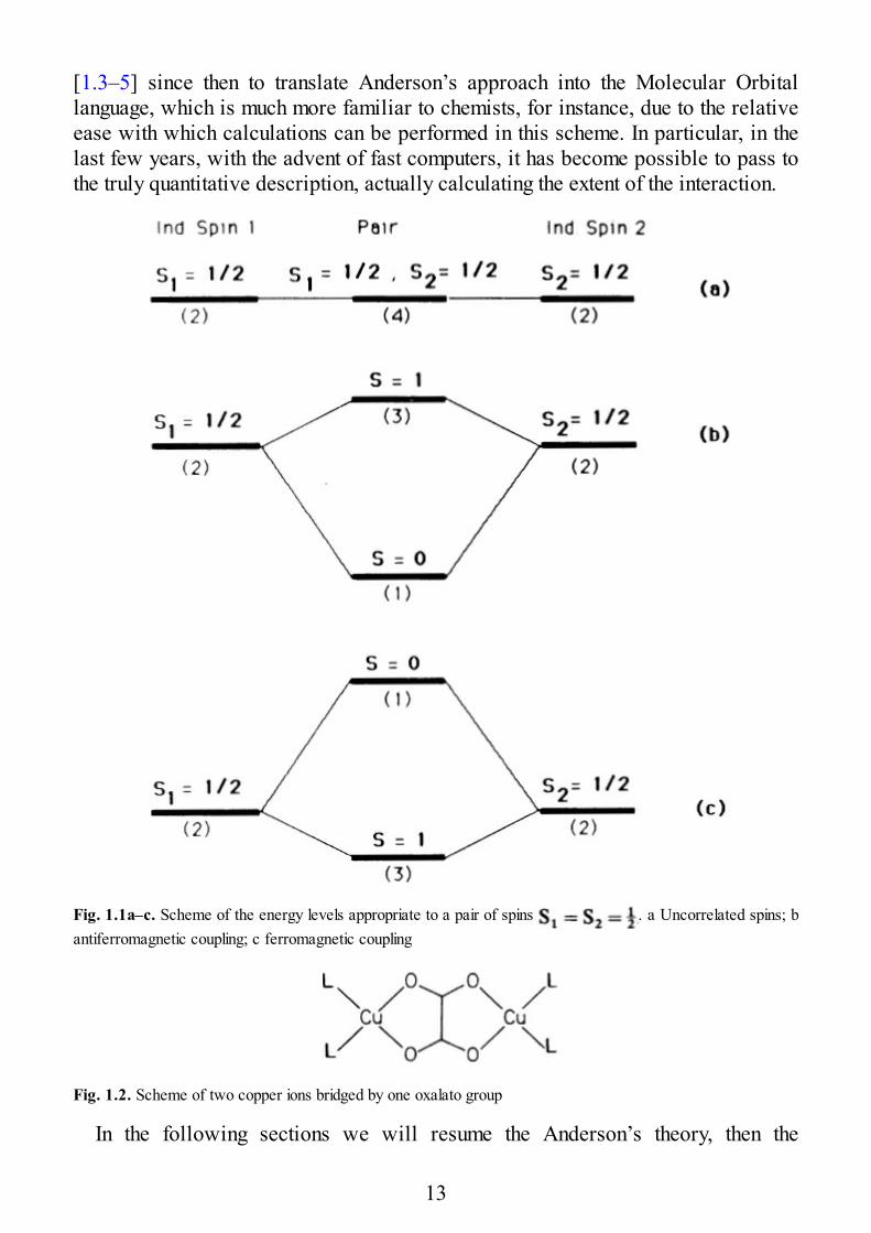
[1.3–5] since then to translate Anderson’s approach into the Molecular Orbitallanguage, which is much more familiar to chemists, for instance, due to the relativeease with which calculations can be performed in this scheme. In particular, in thelast few years, with the advent of fast computers, it has become possible to pass tothe truly quantitative description, actually calculating the extent of the interaction.

Fig. 1.1a–c. Scheme of the energy levels appropriate to a pair of spins . a Uncorrelated spins; bantiferromagnetic coupling; c ferromagnetic coupling

Fig. 1.2. Scheme of two copper ions bridged by one oxalato group

In the following sections we will resume the Anderson’s theory, then the

13

qualitative MO models, and finally we will give a description of the quantitativeMO calculations.

1.2 Anderson’s Theory

Anderson’s theory [1.2] takes a firm standpoint in the theory of magneticinteractions. Before that many important contributions were provided byHeisenberg [1.6,7], Dirac [1.8], van Vleck [1.9], and many others [1.10,11], but theliterature was full of confusion regarding the use of orthogonal or non-orthogonalbasis functions.

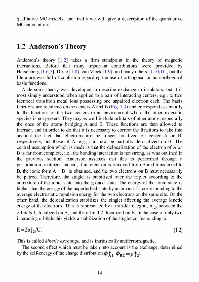
Anderson’s theory was developed to describe exchange in insulators, but it ismost simply understood when applied to a pair of interacting centers, e.g., to twoidentical transition metal ions possessing one unpaired electron each. The basisfunctions are localized on the centers A and B (Fig. 1.3) and correspond essentiallyto the functions of the two centers in an environment where the other magneticspecies is not present. They may as well include orbitals of other atoms, especiallythe ones of the atoms bridging A and B. These functions are then allowed tointeract, and in order to do that it is necessary to correct the functions to take intoaccount the fact that electrons are no longer localized on center A or B,respectively, but those of A, e.g., can now be partially delocalized on B. Thecentral assumption which is made is that the delocalization of the electron of A onB is far from complete, i.e., the bonding interaction is not strong, as was outlined inthe previous section. Anderson assumes that this is performed through aperturbation treatment. Indeed, if an electron is removed from A and transferred toB, the ionic form A + B− is obtained, and the two electrons on B must necessarilybe paired. Therefore, the singlet is stabilized over the triplet according to theadmixture of the ionic state into the ground state. The energy of the ionic state ishigher than the energy of the unperturbed state by an amount U, corresponding to theaverage electrostatic repulsion energy for the two electrons on the same site. On theother hand, the delocalization stabilizes the singlet affecting the average kineticenergy of the electrons. This is represented by a transfer integral, b12, between theorbitals 1, localized on A, and the orbital 2, localized on B. In the case of only twointeracting orbitals this yields a stabilization of the singlet corresponding to:

This is called kinetic exchange, and is intrinsically antiferromagnetic.The second effect which must be taken into account is the exchange, determined

by the self-energy of the charge distribution :

14

This term was called potential exchange, and it stabilizes the triplet over thesinglet according to Hund’s rule. Anderson uses also the term superexchange for thekinetic exchange, but we prefer to avoid it, because it can generate confusion withthe current meaning of interaction propagated by intervening atoms. He also usesthe term direct for potential exchange, but again we prefer the term used in the text,because generally with direct exchange one understands an interaction notpropagated by intervening atoms.

Fig. 1.3. Scheme of two paramagnetic centers, A and B, bridged by a diamagnetic group C

In the case of one unpaired electron on each center, the singlet-triplet separationcan be written as:

When there is more than one unpaired electron per center, the energies of thevarious spin multiplets can still be expressed by one parameter:

The formalism which allows us to do that will be developed in Chap. 2.Finally, a third term was taken into consideration. This is due to polarization

effects which are determined by the presence of magnetic electrons. In fact, foropen shell systems the energy of the spin-up orbitals must be different from theenergy of the spin-down ones, because of the exchange terms in the Hartree-Fockequations, which are nonzero for electrons with the same spin. This effect, forinstance, is capable of inducing unpaired spin density on a formally diamagneticligand, by favoring one spin state over the other. The total effect of this term can beeither ferro- or antiferromagnetic, depending on the nature of the interactingorbitals. This is much more difficult to appreciate qualitatively, and it has beengenerally neglected.

This model developed by Anderson has had the great merit of putting on a firmtheoretical basis the exchange interactions, clarifying all the points which hadbecome inextricably entangled in the previous literature. The main drawback of thetheory has been that passing to the true quantitative approach has proved to bepractically impossible, after some initial attempts [1.12–17]. As Anderson states

15

[1.2]: “it seems wise not to claim more than about 100% accuracy for the theory inview of the uncertainties”.

However, this rationalization allowed Goodenough [1.18, 19] and Kanamori [1.20]to express some rules, which for quite some time now have been the bible forexperimentalists wishing to understand the magnetic properties of transition metalcompounds. They can be expressed as follows:

1. When the two ions have lobes of magnetic orbitals (the orbitals containing theunpaired electrons) pointing toward each other in such a way that the orbitalswould have a reasonably large overlap integral, the exchange isantiferromagnetic;

2. When the orbitals are arranged in such a way that they are expected to be incontact but have no overlap integral, the interaction is ferromagnetic;

3. If a magnetic orbital overlaps an empty orbital, the interaction between the twoions is ferromagnetic.

The most thorough and detailed exploitation of these rules has been made in areview article by Ginsberg [1.21], to which the interested reader is referred.

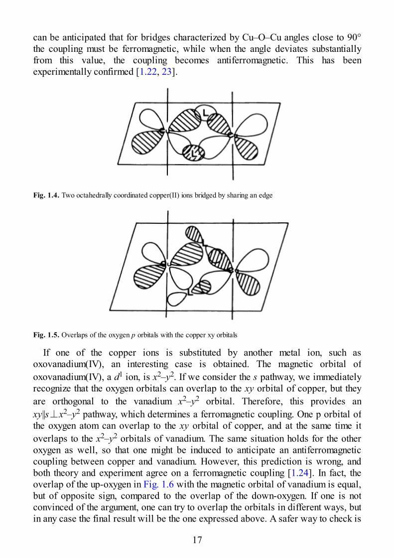
It is perhaps useful at this point to work out an example in order to familiarizethe techniques which allow one to understand, in a qualitative way, how exchangeoperates between magnetic orbitals. Let us focus on one of the possible geometriesof pairs, such as that depicted in Fig. 1.4, which corresponds to two octahedrajoined thorough one side. If the two metal ions are copper(II), with a d9

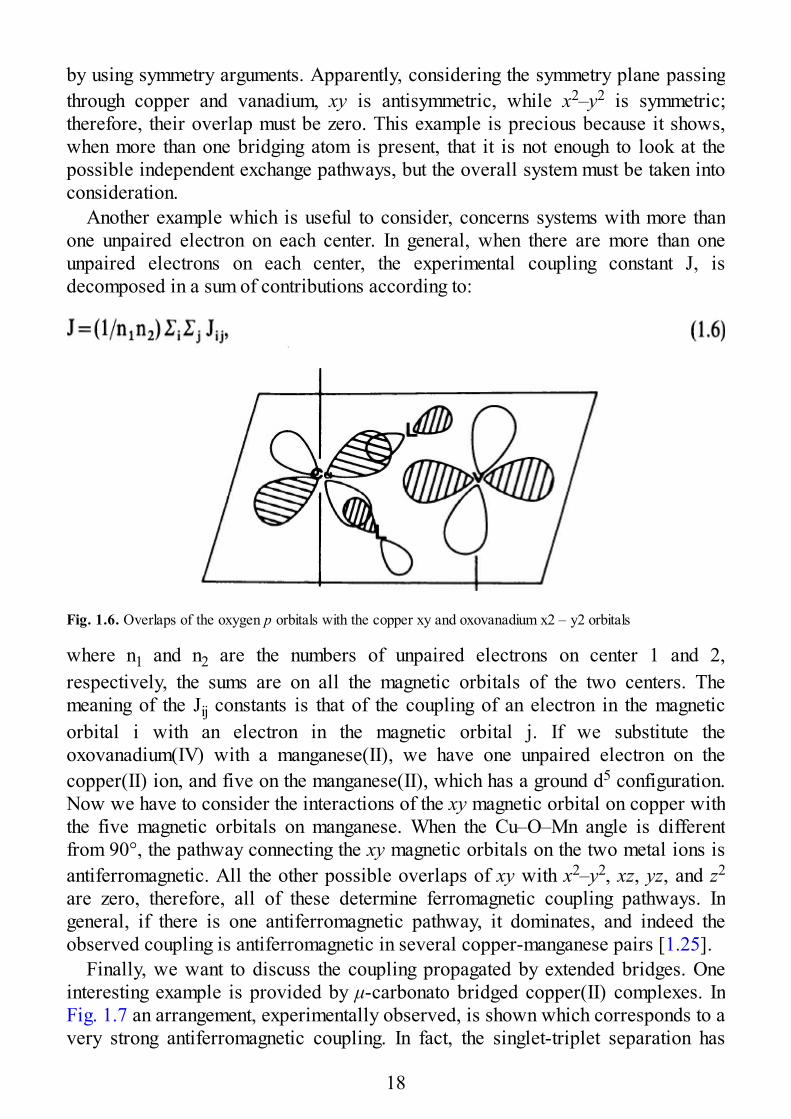
configuration, the magnetic orbitals are of the xy type, in an appropriate referenceframe. The bridge atom, which might be an oxygen atom, has both s and p orbitalscompletely filled. The xy orbital of the left atom overlaps the s orbitals of theoxygens, which in turn overlap the xy orbital of the right copper. According to rule(1) of Goodenough and Kanamori, this corresponds to an antiferromagneticpathway, which can be symbolically written as: xy||s||xy. Since the oxygen orbital isspheric, the extent of the coupling does not depend on the copper-oxygen-copperangle, but only on the copper-oxygen distance. Matters are different when weconsider the overlap with a p orbital. The overlap with, e.g., the right copper ioncan be maximized (Fig. 1.5), but then the overlap with the left xy orbital isdetermined by the geometry of the bridge. If the O–Cu–O angle, ϕ, is 90°, theoverlap of the latter with the p orbital is zero, but a variation in the value of theangle can restore an overlap different from zero. In the case of ϕ = 90° the exchangepathway can be written as: xy||p⊥xy, which according to Goodenough-Kanamorirules, corresponds to a ferromagnetic coupling, while in case of ϕ 90° thepathway can be written as: xy||p||xy, which gives antiferromagnetic coupling. Sincethe oxygen atoms have both s and p orbitals, both exchange mechanisms must beoperative. However, the p orbitals must interact more strongly, because theirenergies are closer to those of the d orbitals than that of the s orbitals. Therefore, it

16

can be anticipated that for bridges characterized by Cu–O–Cu angles close to 90°the coupling must be ferromagnetic, while when the angle deviates substantiallyfrom this value, the coupling becomes antiferromagnetic. This has beenexperimentally confirmed [1.22, 23].

Fig. 1.4. Two octahedrally coordinated copper(II) ions bridged by sharing an edge

Fig. 1.5. Overlaps of the oxygen p orbitals with the copper xy orbitals

If one of the copper ions is substituted by another metal ion, such asoxovanadium(IV), an interesting case is obtained. The magnetic orbital ofoxovanadium(IV), a d1 ion, is x2–y2. If we consider the s pathway, we immediatelyrecognize that the oxygen orbitals can overlap to the xy orbital of copper, but theyare orthogonal to the vanadium x2–y2 orbital. Therefore, this provides anxy||s⊥x2–y2 pathway, which determines a ferromagnetic coupling. One p orbital ofthe oxygen atom can overlap to the xy orbital of copper, and at the same time itoverlaps to the x2–y2 orbitals of vanadium. The same situation holds for the otheroxygen as well, so that one might be induced to anticipate an antiferromagneticcoupling between copper and vanadium. However, this prediction is wrong, andboth theory and experiment agree on a ferromagnetic coupling [1.24]. In fact, theoverlap of the up-oxygen in Fig. 1.6 with the magnetic orbital of vanadium is equal,but of opposite sign, compared to the overlap of the down-oxygen. If one is notconvinced of the argument, one can try to overlap the orbitals in different ways, butin any case the final result will be the one expressed above. A safer way to check is

17

by using symmetry arguments. Apparently, considering the symmetry plane passingthrough copper and vanadium, xy is antisymmetric, while x2–y2 is symmetric;therefore, their overlap must be zero. This example is precious because it shows,when more than one bridging atom is present, that it is not enough to look at thepossible independent exchange pathways, but the overall system must be taken intoconsideration.

Another example which is useful to consider, concerns systems with more thanone unpaired electron on each center. In general, when there are more than oneunpaired electrons on each center, the experimental coupling constant J, isdecomposed in a sum of contributions according to:

Fig. 1.6. Overlaps of the oxygen p orbitals with the copper xy and oxovanadium x2 – y2 orbitals

where n1 and n2 are the numbers of unpaired electrons on center 1 and 2,respectively, the sums are on all the magnetic orbitals of the two centers. Themeaning of the Jij constants is that of the coupling of an electron in the magneticorbital i with an electron in the magnetic orbital j. If we substitute theoxovanadium(IV) with a manganese(II), we have one unpaired electron on thecopper(II) ion, and five on the manganese(II), which has a ground d5 configuration.Now we have to consider the interactions of the xy magnetic orbital on copper withthe five magnetic orbitals on manganese. When the Cu–O–Mn angle is differentfrom 90°, the pathway connecting the xy magnetic orbitals on the two metal ions isantiferromagnetic. All the other possible overlaps of xy with x2–y2, xz, yz, and z2

are zero, therefore, all of these determine ferromagnetic coupling pathways. Ingeneral, if there is one antiferromagnetic pathway, it dominates, and indeed theobserved coupling is antiferromagnetic in several copper-manganese pairs [1.25].

Finally, we want to discuss the coupling propagated by extended bridges. Oneinteresting example is provided by μ-carbonato bridged copper(II) complexes. InFig. 1.7 an arrangement, experimentally observed, is shown which corresponds to avery strong antiferromagnetic coupling. In fact, the singlet-triplet separation has

18

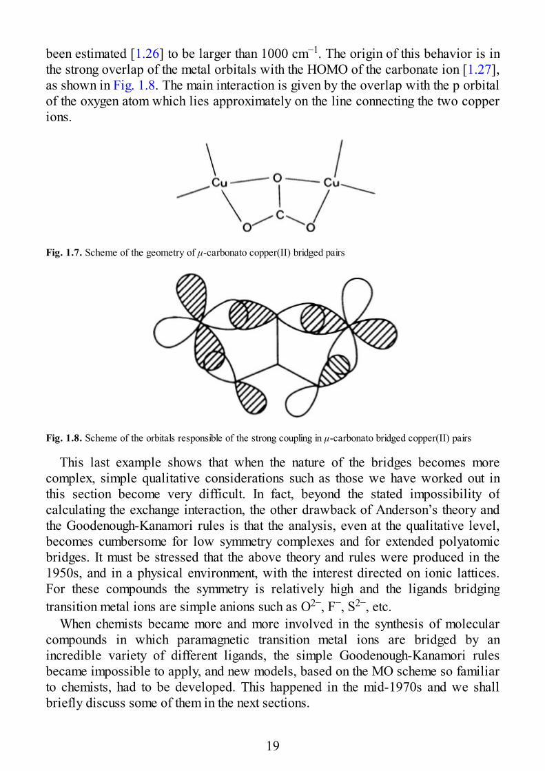
been estimated [1.26] to be larger than 1000 cm−1. The origin of this behavior is inthe strong overlap of the metal orbitals with the HOMO of the carbonate ion [1.27],as shown in Fig. 1.8. The main interaction is given by the overlap with the p orbitalof the oxygen atom which lies approximately on the line connecting the two copperions.

Fig. 1.7. Scheme of the geometry of μ-carbonato copper(II) bridged pairs

Fig. 1.8. Scheme of the orbitals responsible of the strong coupling in μ-carbonato bridged copper(II) pairs

This last example shows that when the nature of the bridges becomes morecomplex, simple qualitative considerations such as those we have worked out inthis section become very difficult. In fact, beyond the stated impossibility ofcalculating the exchange interaction, the other drawback of Anderson’s theory andthe Goodenough-Kanamori rules is that the analysis, even at the qualitative level,becomes cumbersome for low symmetry complexes and for extended polyatomicbridges. It must be stressed that the above theory and rules were produced in the1950s, and in a physical environment, with the interest directed on ionic lattices.For these compounds the symmetry is relatively high and the ligands bridgingtransition metal ions are simple anions such as O2−, F−, S2−, etc.

When chemists became more and more involved in the synthesis of molecularcompounds in which paramagnetic transition metal ions are bridged by anincredible variety of different ligands, the simple Goodenough-Kanamori rulesbecame impossible to apply, and new models, based on the MO scheme so familiarto chemists, had to be developed. This happened in the mid-1970s and we shallbriefly discuss some of them in the next sections.

19

1.3 Molecular Orbital Exchange Models

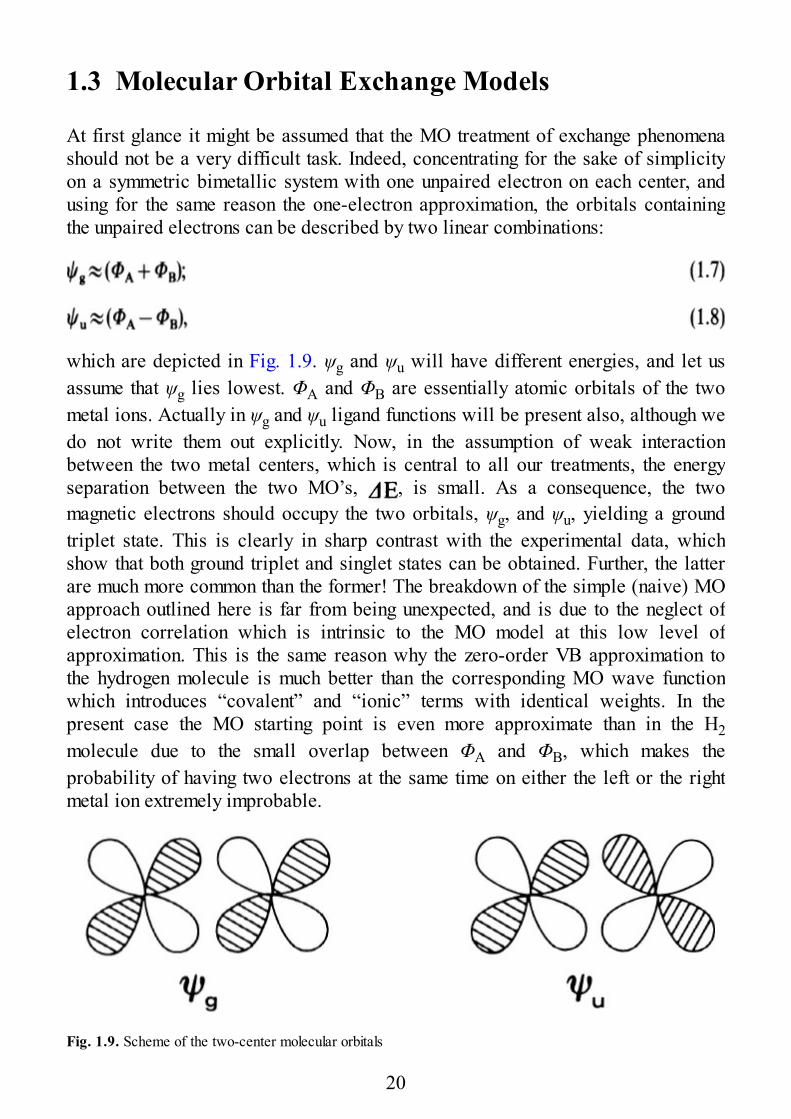
At first glance it might be assumed that the MO treatment of exchange phenomenashould not be a very difficult task. Indeed, concentrating for the sake of simplicityon a symmetric bimetallic system with one unpaired electron on each center, andusing for the same reason the one-electron approximation, the orbitals containingthe unpaired electrons can be described by two linear combinations:

which are depicted in Fig. 1.9. ψg and ψu will have different energies, and let usassume that ψg lies lowest. ΦA and ΦB are essentially atomic orbitals of the twometal ions. Actually in ψg and ψu ligand functions will be present also, although wedo not write them out explicitly. Now, in the assumption of weak interactionbetween the two metal centers, which is central to all our treatments, the energyseparation between the two MO’s, , is small. As a consequence, the twomagnetic electrons should occupy the two orbitals, ψg, and ψu, yielding a groundtriplet state. This is clearly in sharp contrast with the experimental data, whichshow that both ground triplet and singlet states can be obtained. Further, the latterare much more common than the former! The breakdown of the simple (naive) MOapproach outlined here is far from being unexpected, and is due to the neglect ofelectron correlation which is intrinsic to the MO model at this low level ofapproximation. This is the same reason why the zero-order VB approximation tothe hydrogen molecule is much better than the corresponding MO wave functionwhich introduces “covalent” and “ionic” terms with identical weights. In thepresent case the MO starting point is even more approximate than in the H2molecule due to the small overlap between ΦA and ΦB, which makes theprobability of having two electrons at the same time on either the left or the rightmetal ion extremely improbable.

Fig. 1.9. Scheme of the two-center molecular orbitals

20

Several corrections to this extremely simple scheme have been suggested, eitherperforming configuration interaction calculations, at various degrees ofsophistication, or using a modified model, which makes the MO model closer to theVB.

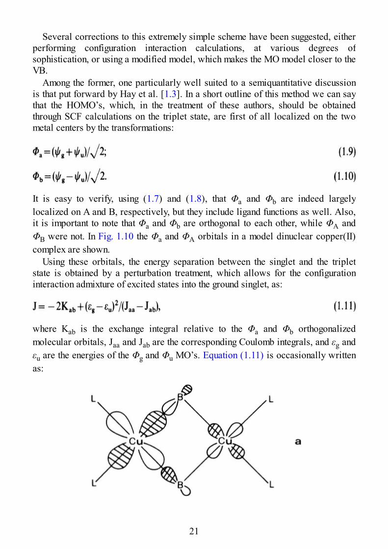
Among the former, one particularly well suited to a semiquantitative discussionis that put forward by Hay et al. [1.3]. In a short outline of this method we can saythat the HOMO’s, which, in the treatment of these authors, should be obtainedthrough SCF calculations on the triplet state, are first of all localized on the twometal centers by the transformations:

It is easy to verify, using (1.7) and (1.8), that Φa and Φb are indeed largelylocalized on A and B, respectively, but they include ligand functions as well. Also,it is important to note that Φa and Φb are orthogonal to each other, while ΦA andΦB were not. In Fig. 1.10 the Φa and ΦA orbitals in a model dinuclear copper(II)complex are shown.

Using these orbitals, the energy separation between the singlet and the tripletstate is obtained by a perturbation treatment, which allows for the configurationinteraction admixture of excited states into the ground singlet, as:

where Kab is the exchange integral relative to the Φa and Φb orthogonalizedmolecular orbitals, Jaa and Jab are the corresponding Coulomb integrals, and εg andεu are the energies of the Φg and Φu MO’s. Equation (1.11) is occasionally writtenas:

21

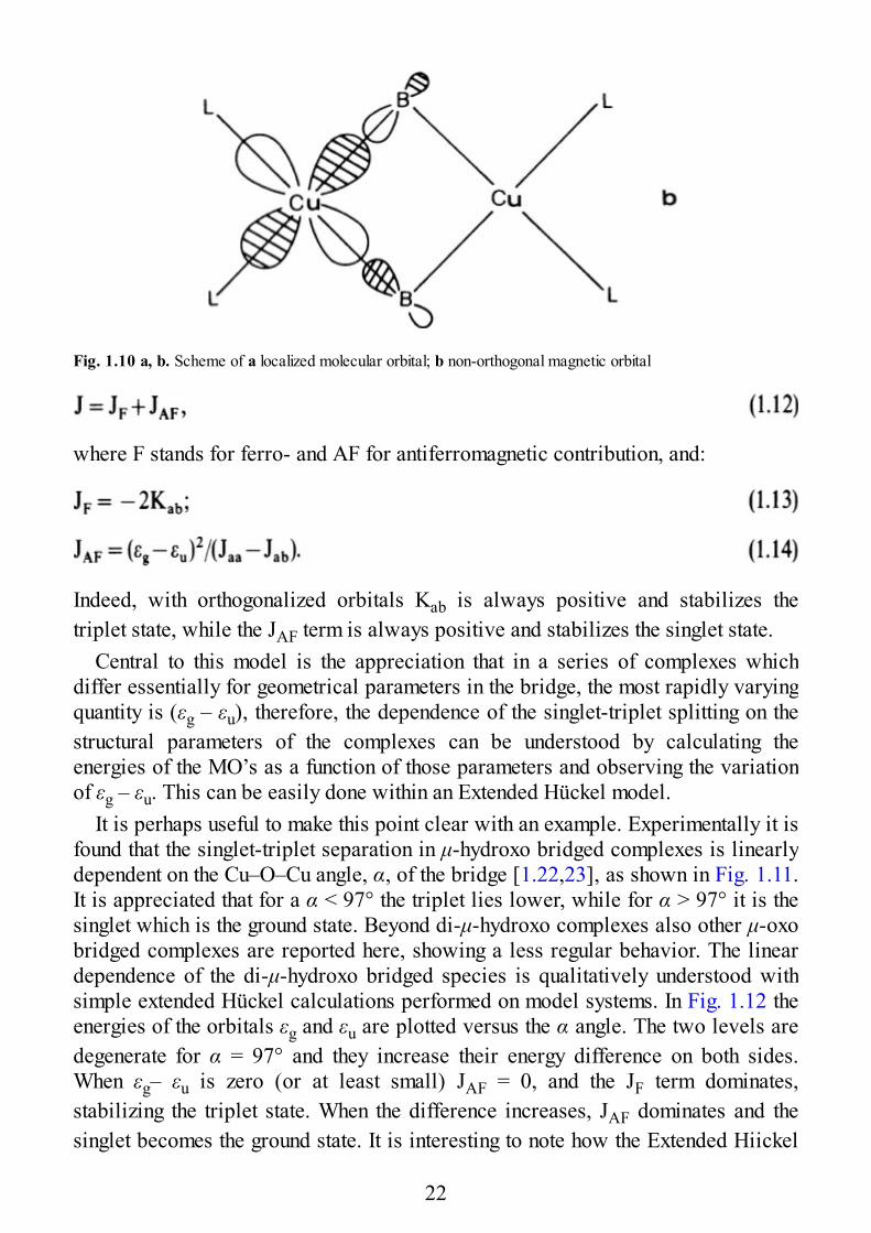
Fig. 1.10 a, b. Scheme of a localized molecular orbital; b non-orthogonal magnetic orbital

where F stands for ferro- and AF for antiferromagnetic contribution, and:

Indeed, with orthogonalized orbitals Kab is always positive and stabilizes thetriplet state, while the JAF term is always positive and stabilizes the singlet state.

Central to this model is the appreciation that in a series of complexes whichdiffer essentially for geometrical parameters in the bridge, the most rapidly varyingquantity is (εg – εu), therefore, the dependence of the singlet-triplet splitting on thestructural parameters of the complexes can be understood by calculating theenergies of the MO’s as a function of those parameters and observing the variationof εg – εu. This can be easily done within an Extended Hückel model.

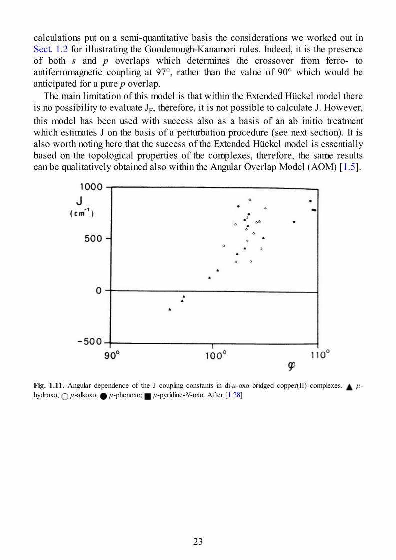
It is perhaps useful to make this point clear with an example. Experimentally it isfound that the singlet-triplet separation in μ-hydroxo bridged complexes is linearlydependent on the Cu–O–Cu angle, α, of the bridge [1.22,23], as shown in Fig. 1.11.It is appreciated that for a α < 97° the triplet lies lower, while for α > 97° it is thesinglet which is the ground state. Beyond di-μ-hydroxo complexes also other μ-oxobridged complexes are reported here, showing a less regular behavior. The lineardependence of the di-μ-hydroxo bridged species is qualitatively understood withsimple extended Hückel calculations performed on model systems. In Fig. 1.12 theenergies of the orbitals εg and εu are plotted versus the α angle. The two levels aredegenerate for α = 97° and they increase their energy difference on both sides.When εg– εu is zero (or at least small) JAF = 0, and the JF term dominates,stabilizing the triplet state. When the difference increases, JAF dominates and thesinglet becomes the ground state. It is interesting to note how the Extended Hiickel

22

calculations put on a semi-quantitative basis the considerations we worked out inSect. 1.2 for illustrating the Goodenough-Kanamori rules. Indeed, it is the presenceof both s and p overlaps which determines the crossover from ferro- toantiferromagnetic coupling at 97°, rather than the value of 90° which would beanticipated for a pure p overlap.

The main limitation of this model is that within the Extended Hückel model thereis no possibility to evaluate JF, therefore, it is not possible to calculate J. However,this model has been used with success also as a basis of an ab initio treatmentwhich estimates J on the basis of a perturbation procedure (see next section). It isalso worth noting here that the success of the Extended Hückel model is essentiallybased on the topological properties of the complexes, therefore, the same resultscan be qualitatively obtained also within the Angular Overlap Model (AOM) [1.5].

Fig. 1.11. Angular dependence of the J coupling constants in di-μ-oxo bridged copper(II) complexes. μ-hydroxo; μ-alkoxo; μ-phenoxo; μ-pyridine-N-oxo. After [1.28]

23

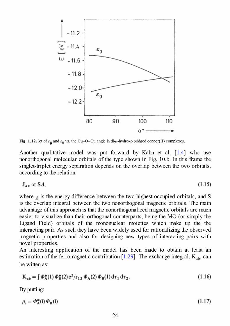
Fig. 1.12. lot of εg and εu vs. the Cu–O–Cu angle in di-μ-hydroxo bridged copper(II) complexes.

Another qualitative model was put forward by Kahn et al. [1.4] who usenonorthogonal molecular orbitals of the type shown in Fig. 10.b. In this frame thesinglet-triplet energy separation depends on the overlap between the two orbitals,according to the relation:

where is the energy difference between the two highest occupied orbitals, and Sis the overlap integral between the two nonorthogonal magnetic orbitals. The mainadvantage of this approach is that the nonorthogonalized magnetic orbitals are mucheasier to visualize than their orthogonal counterparts, being the MO (or simply theLigand Field) orbitals of the mononuclear moieties which make up the theinteracting pair. As such they have been widely used for rationalizing the observedmagnetic properties and also for designing new types of interacting pairs withnovel properties.An interesting application of the model has been made to obtain at least anestimation of the ferromagnetic contribution [1.29]. The exchange integral, Kab, canbe witten as:

By putting:

24

with i = 1, 2, Eq. (1.16), can be rewriten as:

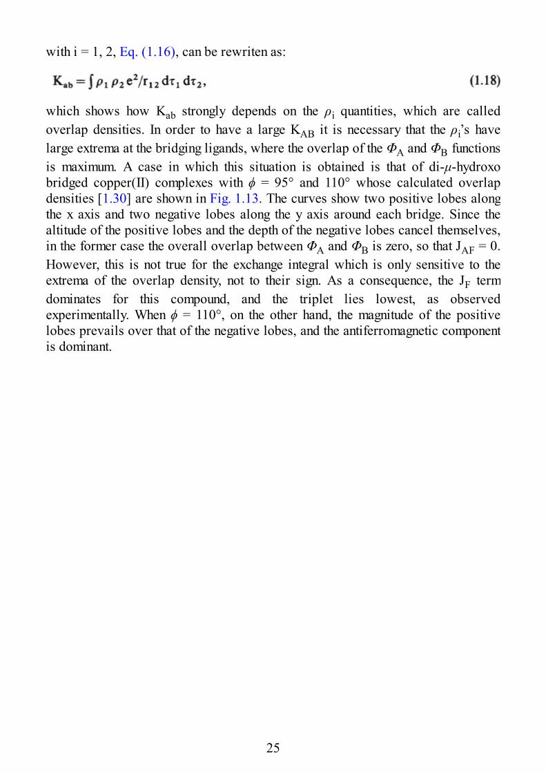
which shows how Kab strongly depends on the ρi quantities, which are calledoverlap densities. In order to have a large KAB it is necessary that the ρi’s havelarge extrema at the bridging ligands, where the overlap of the ΦA and ΦB functionsis maximum. A case in which this situation is obtained is that of di-μ-hydroxobridged copper(II) complexes with ϕ = 95° and 110° whose calculated overlapdensities [1.30] are shown in Fig. 1.13. The curves show two positive lobes alongthe x axis and two negative lobes along the y axis around each bridge. Since thealtitude of the positive lobes and the depth of the negative lobes cancel themselves,in the former case the overall overlap between ΦA and ΦB is zero, so that JAF = 0.However, this is not true for the exchange integral which is only sensitive to theextrema of the overlap density, not to their sign. As a consequence, the JF termdominates for this compound, and the triplet lies lowest, as observedexperimentally. When ϕ = 110°, on the other hand, the magnitude of the positivelobes prevails over that of the negative lobes, and the antiferromagnetic componentis dominant.

25

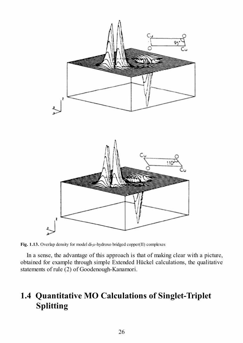
Fig. 1.13. Overlap density for model di-μ-hydroxo bridged copper(II) complexes

In a sense, the advantage of this approach is that of making clear with a picture,obtained for example through simple Extended Hückel calculations, the qualitativestatements of rule (2) of Goodenough-Kanamori.

1.4 Quantitative MO Calculations of Singlet-TripletSplitting

26

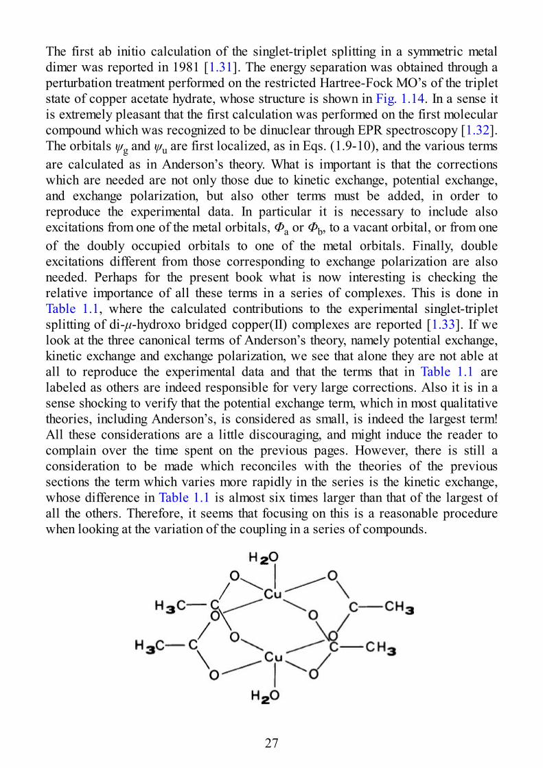
The first ab initio calculation of the singlet-triplet splitting in a symmetric metaldimer was reported in 1981 [1.31]. The energy separation was obtained through aperturbation treatment performed on the restricted Hartree-Fock MO’s of the tripletstate of copper acetate hydrate, whose structure is shown in Fig. 1.14. In a sense itis extremely pleasant that the first calculation was performed on the first molecularcompound which was recognized to be dinuclear through EPR spectroscopy [1.32].The orbitals ψg and ψu are first localized, as in Eqs. (1.9-10), and the various termsare calculated as in Anderson’s theory. What is important is that the correctionswhich are needed are not only those due to kinetic exchange, potential exchange,and exchange polarization, but also other terms must be added, in order toreproduce the experimental data. In particular it is necessary to include alsoexcitations from one of the metal orbitals, Φa or Φb, to a vacant orbital, or from oneof the doubly occupied orbitals to one of the metal orbitals. Finally, doubleexcitations different from those corresponding to exchange polarization are alsoneeded. Perhaps for the present book what is now interesting is checking therelative importance of all these terms in a series of complexes. This is done inTable 1.1, where the calculated contributions to the experimental singlet-tripletsplitting of di-μ-hydroxo bridged copper(II) complexes are reported [1.33]. If welook at the three canonical terms of Anderson’s theory, namely potential exchange,kinetic exchange and exchange polarization, we see that alone they are not able atall to reproduce the experimental data and that the terms that in Table 1.1 arelabeled as others are indeed responsible for very large corrections. Also it is in asense shocking to verify that the potential exchange term, which in most qualitativetheories, including Anderson’s, is considered as small, is indeed the largest term!All these considerations are a little discouraging, and might induce the reader tocomplain over the time spent on the previous pages. However, there is still aconsideration to be made which reconciles with the theories of the previoussections the term which varies more rapidly in the series is the kinetic exchange,whose difference in Table 1.1 is almost six times larger than that of the largest ofall the others. Therefore, it seems that focusing on this is a reasonable procedurewhen looking at the variation of the coupling in a series of compounds.

27

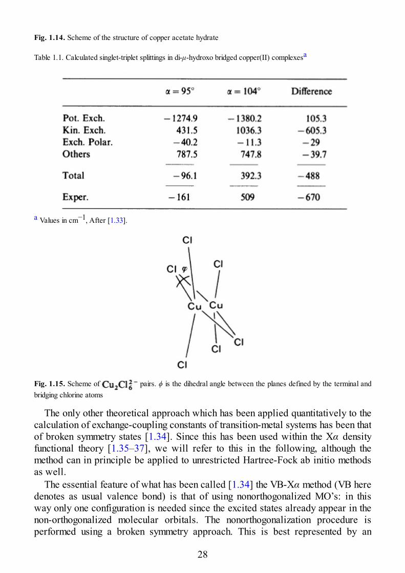
Fig. 1.14. Scheme of the structure of copper acetate hydrate

Table 1.1. Calculated singlet-triplet splittings in di-μ-hydroxo bridged copper(II) complexesa

a Values in cm−1, After [1.33].

Fig. 1.15. Scheme of pairs. ϕ is the dihedral angle between the planes defined by the terminal andbridging chlorine atoms

The only other theoretical approach which has been applied quantitatively to thecalculation of exchange-coupling constants of transition-metal systems has been thatof broken symmetry states [1.34]. Since this has been used within the Xα densityfunctional theory [1.35–37], we will refer to this in the following, although themethod can in principle be applied to unrestricted Hartree-Fock ab initio methodsas well.

The essential feature of what has been called [1.34] the VB-Xα method (VB heredenotes as usual valence bond) is that of using nonorthogonalized MO’s: in thisway only one configuration is needed since the excited states already appear in thenon-orthogonalized molecular orbitals. The nonorthogonalization procedure isperformed using a broken symmetry approach. This is best represented by an

28

example. Let us consider a dimer as shown in Fig. 1.15. The molecularsymmetry is D2d and the calculation can be performed for the triplet state in thislimit. Using a spin-unrestricted approach (different orbitals for different spins), it ispossible to define a state in which the magnetic orbital on the left copper atom isoccupied by an electron with spin-up and that of the right copper by an electronwith spin-down, by removing the symmetry elements which transform the twocopper atoms one into the other and by imposing a mirror symmetry to the spindensities. In the case this can be done by performing the calculationimposing C2v instead of D2d symmetry. The resulting state, named broken symmetrystate, is not a pure spin state (it will be an admixture of singlet and triplet) but itsenergy can be related to that of the pure spin states through standard spin projectiontechniques. In Fig. 1.16 contour maps of the magnetic orbitals are plotted [1.38] inthe xy plane for various values of ϕ. It is apparent that for both ϕ = 0° and 70° theorbitals are largely delocalized, while for ϕ = 45° they are strongly localized on theleft and right copper atoms, respectively. The ϕ = 0° and 70° correspond toantiferromagnetic coupling (relatively large covalency determines largedelocalization), while ϕ = 45° corresponds to ferromagnetic coupling (relativelyweak covalency favors the localized picture). The broken symmetry state isequivalent to a state constructed using nonorthogonal orbitals:

29

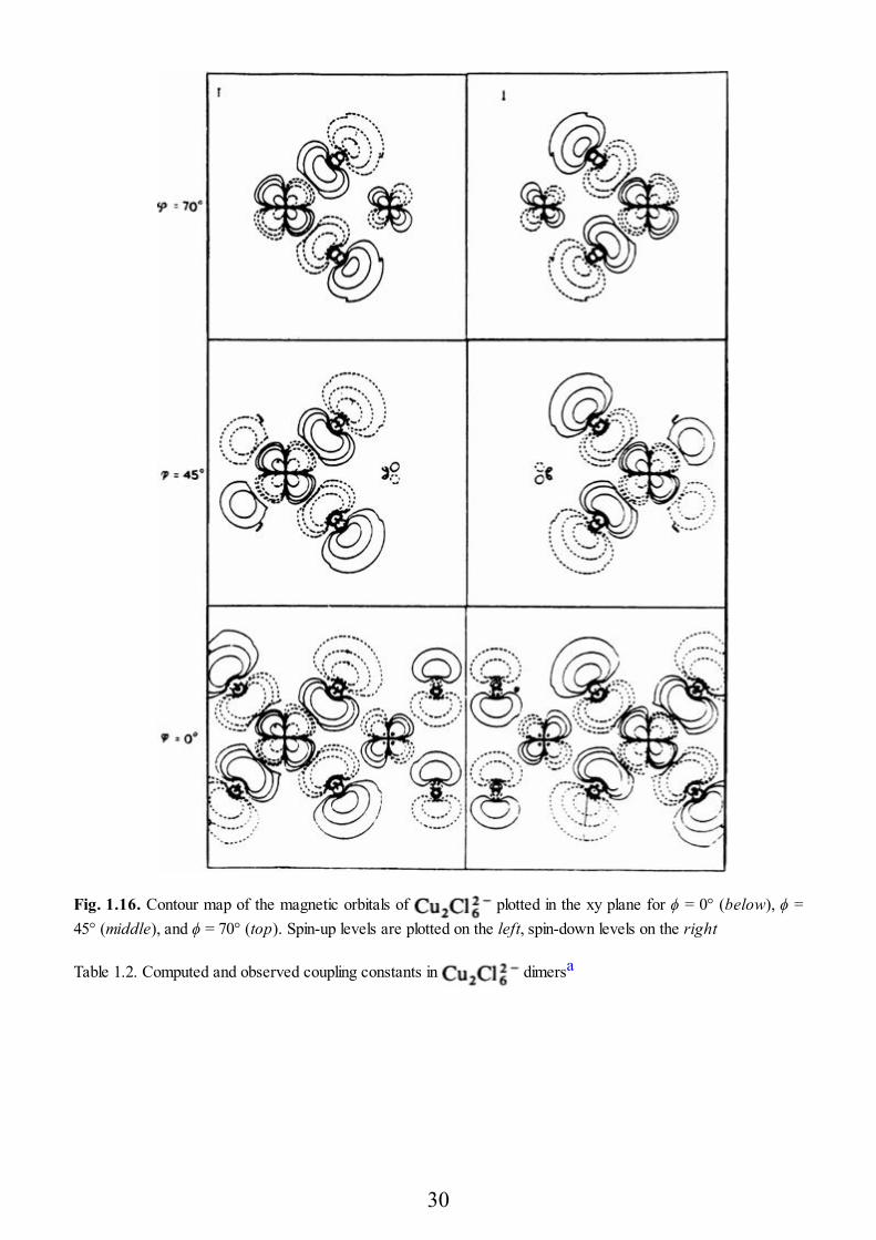
Fig. 1.16. Contour map of the magnetic orbitals of plotted in the xy plane for ϕ = 0° (below), ϕ =45° (middle), and ϕ = 70° (top). Spin-up levels are plotted on the left, spin-down levels on the right

Table 1.2. Computed and observed coupling constants in dimersa

30

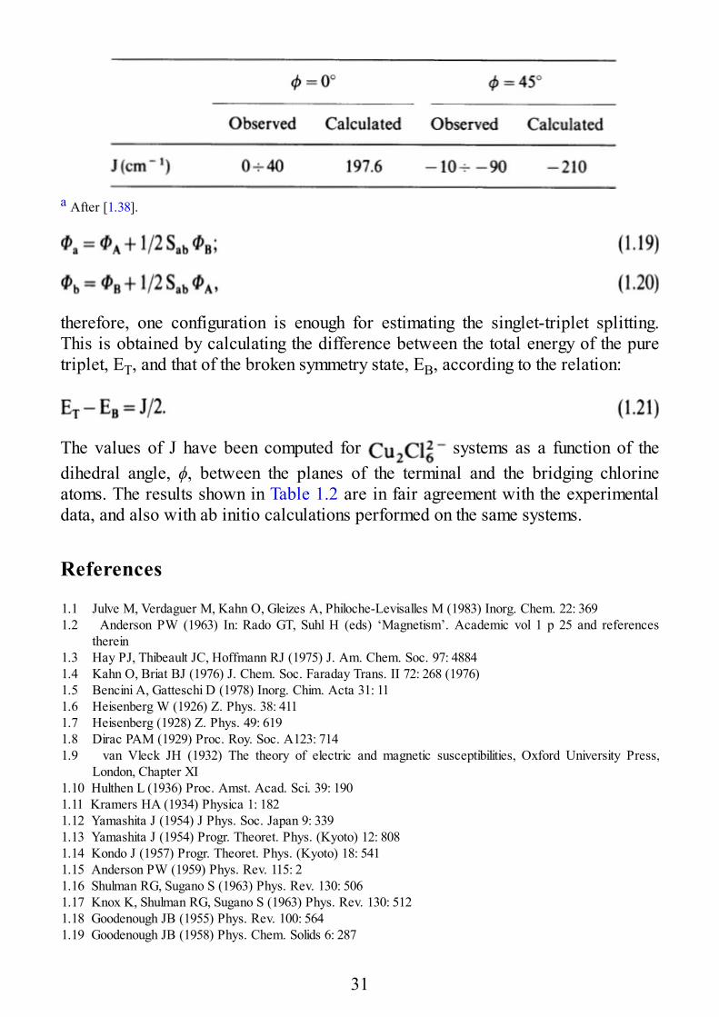
a After [1.38].

therefore, one configuration is enough for estimating the singlet-triplet splitting.This is obtained by calculating the difference between the total energy of the puretriplet, ET, and that of the broken symmetry state, EB, according to the relation:

The values of J have been computed for systems as a function of thedihedral angle, ϕ, between the planes of the terminal and the bridging chlorineatoms. The results shown in Table 1.2 are in fair agreement with the experimentaldata, and also with ab initio calculations performed on the same systems.

References

1.1 Julve M, Verdaguer M, Kahn O, Gleizes A, Philoche-Levisalles M (1983) Inorg. Chem. 22: 3691.2 Anderson PW (1963) In: Rado GT, Suhl H (eds) ‘Magnetism’. Academic vol 1 p 25 and references

therein1.3 Hay PJ, Thibeault JC, Hoffmann RJ (1975) J. Am. Chem. Soc. 97: 48841.4 Kahn O, Briat BJ (1976) J. Chem. Soc. Faraday Trans. II 72: 268 (1976)1.5 Bencini A, Gatteschi D (1978) Inorg. Chim. Acta 31: 111.6 Heisenberg W (1926) Z. Phys. 38: 4111.7 Heisenberg (1928) Z. Phys. 49: 6191.8 Dirac PAM (1929) Proc. Roy. Soc. A123: 7141.9 van Vleck JH (1932) The theory of electric and magnetic susceptibilities, Oxford University Press,

London, Chapter XI1.10 Hulthen L (1936) Proc. Amst. Acad. Sci. 39: 1901.11 Kramers HA (1934) Physica 1: 1821.12 Yamashita J (1954) J Phys. Soc. Japan 9: 3391.13 Yamashita J (1954) Progr. Theoret. Phys. (Kyoto) 12: 8081.14 Kondo J (1957) Progr. Theoret. Phys. (Kyoto) 18: 5411.15 Anderson PW (1959) Phys. Rev. 115: 21.16 Shulman RG, Sugano S (1963) Phys. Rev. 130: 5061.17 Knox K, Shulman RG, Sugano S (1963) Phys. Rev. 130: 5121.18 Goodenough JB (1955) Phys. Rev. 100: 5641.19 Goodenough JB (1958) Phys. Chem. Solids 6: 287

31

1.20 Kanamori J (1959) Phys. Chem. Solids 10: 871.21 Ginsberg A (1971) Inorg. Chim. Acta Rev. 5: 451.22 Hatfield WE (1974) Am. Chem. Soc. Symp. Ser. No 5: 1081.23 Hodgson DJ (1975) Progr. Inorg. Chem. 19: 1731.24 Kahn O, Galy J, Journaux Y, Jaud J, Morgenstern-Badarau I (1982) J. Am. Chem. Soc. 104: 21651.25 Kahn O (1987) Structure and Bonding (Berlin) 68: 911.26 Churchill MR, Davies G, El-Sayed MA, El-Shazly MF, Hutchinson JP, Rupich MW, Watkins KO (1979)

Inorg. Chem 18: 22961.27 Albonico C, Bencini A (1988) Inorg. Chem. 27: 19341.28 Gatteschi D, Bencini A (1985) In Willett RD, Gatteschi D, Kahn O (eds) Magneto-structural correlations in

exchange coupled systems. Reidel, Dordrecht, p 2411.29 Kahn O, Charlot MF (1980) Nouv. J. Chim. 4: 5671.30 Chariot MF, Journaux Y, Kahn O, Bencini A, Gatteschi D, Zanchini C (1986) Inorg. Chem. 25: 10601.31 de Loth P, Cassoux P, Daudey JP, Malrieu JP (1981) J. Am. Chem. Soc. 103: 40071.32 Bleaney B, Bowers KD. Proc. R. Soc. A214, 451 (1952)1.33 Daudey JP, de Loth P, Malrieu JP (1985) In: Willett RD, Gatteschi D, Kahn O (eds) ‘Magneto-structural

correlations in exchange coupled systems’. Reidel, Dordrecht p 871.34 Noodlemann L (1981) J. Chem. Phys. 74: 57371.35 Herman F, McLean AD, Nesbet RK (eds) (1979) Computational methods for large molecules and

localized states in solids. Plenum, New York1.36 Johnson KH (1973) Adv. Quantum Chem. 7: 1431.37 Slater JC (1974) Quantum theory of molecules and solids McGraw Hill, New York1.38 Bencini A, Gatteschi D (1986) J. Am. Chem. Soc. 108: 5763

32

2 Spin Hamiltonians

2.1 The Spin Hamiltonian Approach

The replacement of the true hamiltonian of a system with an effective one whichoperates only on the spin variables is commonplace in all areas of magneticresonance spectroscopy. This is a parametric approach, which is helpful for theinterpretation of sets of experimental data. The parameters which are obtained haveno particular meaning per se, but they must be compared with more fundamentaltheory. When one finds, for example, that the EPR spectra of a copper(II) complexcan be interpreted within the spin hamiltonian formalism to yield g|| = 2.20, g⊥ =2.06, it is only recurring to ligand field theory that the conclusion can be made thatthe unpaired electron is located in either a x2 – y2 or a xy orbital.

It is therefore the great simplicity of the spin hamiltonian approach which makesit so well suited for the analysis of complex systems, allowing at least a first-orderrationalization of their properties. For example in Fig. 2.1 the temperaturedependence of the magnetic susceptibility of copper acetate hydrate [2.1] is shownwhose structure was shown in Fig. 1.14. The experimental points show that thesusceptibility increases on decreasing temperature in the range 300–280 K, while itdecreases on decreasing further the temperature below 280 K. This behavior iseasily interpreted within a simple spin hamiltonian formalism to yield a parameterJ = 280 cm−1, which is a measure of the energy separation of the singlet and tripletstates orginating from the interaction of the two unpaired electrons localized on thetwo copper ions. The sign of J indicates that the singlet lies lower, i.e., the couplingis antiferromagnetic. Explaining both the sign and the intensity of the interaction canbe done only within the theories developed in the previous sections, but someimportant results have already been achieved with the much simpler spinhamiltonian model.

The main difficulty related to the spin hamiltonian model is the justification ofthe model itself. Therefore, in order not to complicate the situation too much at thisstage, we defer this discussion to Sect. 2.5 and develop the spin hamiltonianformalism first.

Let us assume two centers, A and B, whose individual magnetic properties,before allowing them to interact, can be described by the effective spin operatorsSA and SB, respectively. The spin quantum numbers SA and SB, may, or may not,correspond to the true spin of the system. In general, we may say that the value of

33

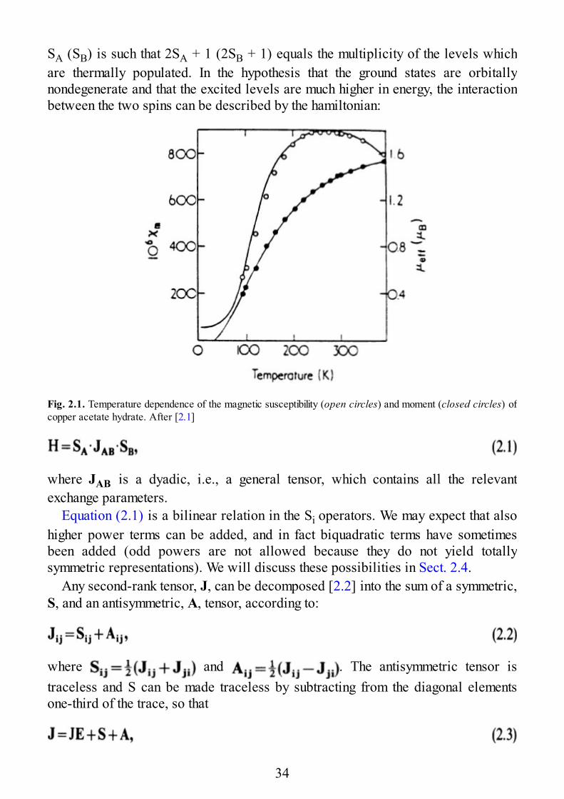
SA (SB) is such that 2SA + 1 (2SB + 1) equals the multiplicity of the levels whichare thermally populated. In the hypothesis that the ground states are orbitallynondegenerate and that the excited levels are much higher in energy, the interactionbetween the two spins can be described by the hamiltonian:

Fig. 2.1. Temperature dependence of the magnetic susceptibility (open circles) and moment (closed circles) ofcopper acetate hydrate. After [2.1]

where JAB is a dyadic, i.e., a general tensor, which contains all the relevantexchange parameters.

Equation (2.1) is a bilinear relation in the Si operators. We may expect that alsohigher power terms can be added, and in fact biquadratic terms have sometimesbeen added (odd powers are not allowed because they do not yield totallysymmetric representations). We will discuss these possibilities in Sect. 2.4.

Any second-rank tensor, J, can be decomposed [2.2] into the sum of a symmetric,S, and an antisymmetric, A, tensor, according to:

where and . The antisymmetric tensor istraceless and S can be made traceless by subtracting from the diagonal elementsone-third of the trace, so that

34

where E is the identity matrix and J= 1/3 Tr(J). Using this decomposition Eq. (2.1)can be rewritten as:

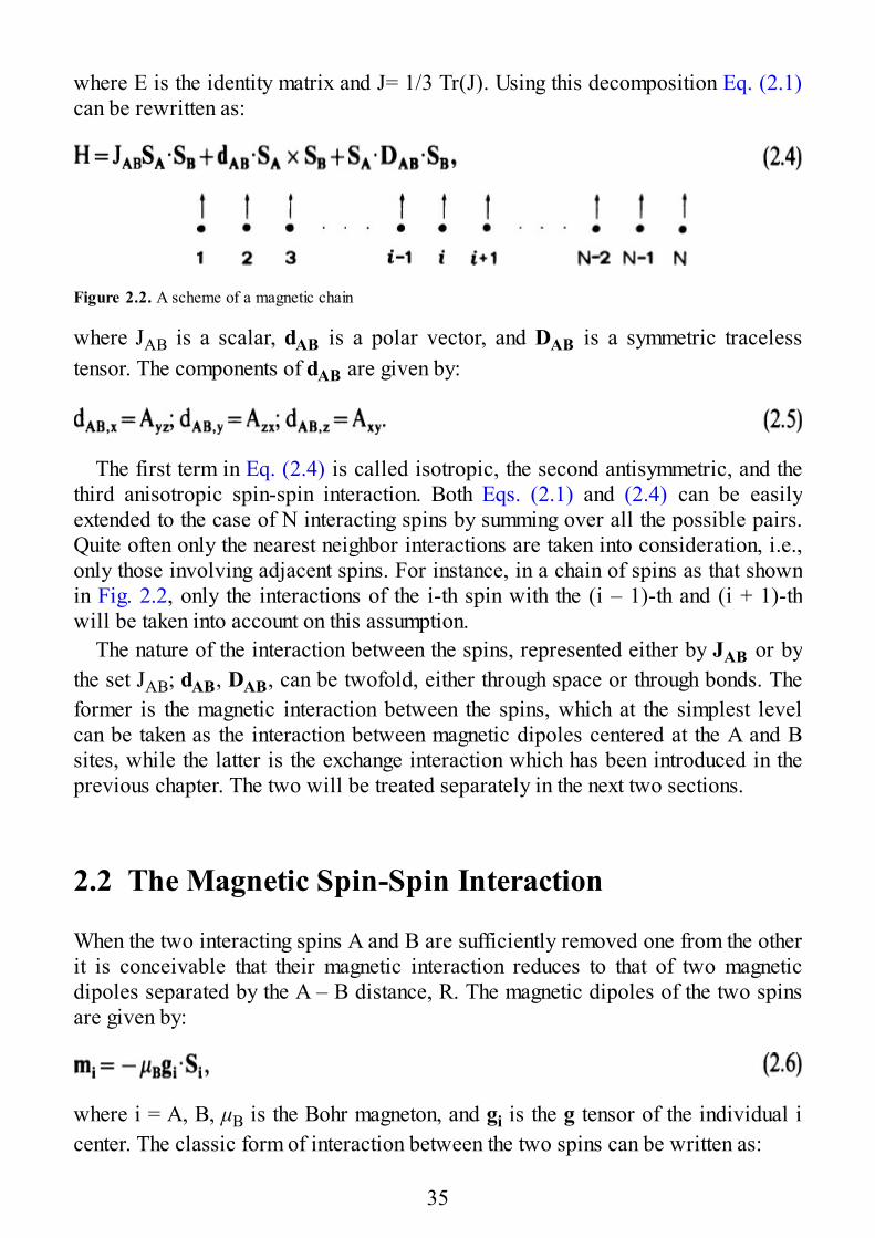
Figure 2.2. A scheme of a magnetic chain

where JAB is a scalar, dAB is a polar vector, and DAB is a symmetric tracelesstensor. The components of dAB are given by:

The first term in Eq. (2.4) is called isotropic, the second antisymmetric, and thethird anisotropic spin-spin interaction. Both Eqs. (2.1) and (2.4) can be easilyextended to the case of N interacting spins by summing over all the possible pairs.Quite often only the nearest neighbor interactions are taken into consideration, i.e.,only those involving adjacent spins. For instance, in a chain of spins as that shownin Fig. 2.2, only the interactions of the i-th spin with the (i – 1)-th and (i + 1)-thwill be taken into account on this assumption.

The nature of the interaction between the spins, represented either by JAB or bythe set JAB; dAB, DAB, can be twofold, either through space or through bonds. Theformer is the magnetic interaction between the spins, which at the simplest levelcan be taken as the interaction between magnetic dipoles centered at the A and Bsites, while the latter is the exchange interaction which has been introduced in theprevious chapter. The two will be treated separately in the next two sections.

2.2 The Magnetic Spin-Spin Interaction

When the two interacting spins A and B are sufficiently removed one from the otherit is conceivable that their magnetic interaction reduces to that of two magneticdipoles separated by the A – B distance, R. The magnetic dipoles of the two spinsare given by:

where i = A, B, μB is the Bohr magneton, and gi is the g tensor of the individual icenter. The classic form of interaction between the two spins can be written as:

35

where

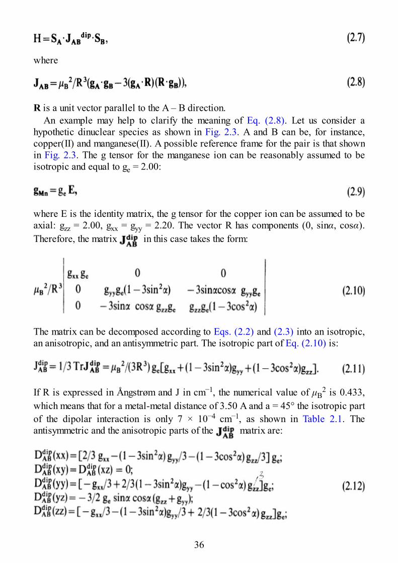
R is a unit vector parallel to the A – B direction.An example may help to clarify the meaning of Eq. (2.8). Let us consider a

hypothetic dinuclear species as shown in Fig. 2.3. A and B can be, for instance,copper(II) and manganese(II). A possible reference frame for the pair is that shownin Fig. 2.3. The g tensor for the manganese ion can be reasonably assumed to beisotropic and equal to ge = 2.00:

where E is the identity matrix, the g tensor for the copper ion can be assumed to beaxial: gzz = 2.00, gxx = gyy = 2.20. The vector R has components (0, sinα, cosα).Therefore, the matrix in this case takes the form:

The matrix can be decomposed according to Eqs. (2.2) and (2.3) into an isotropic,an anisotropic, and an antisymmetric part. The isotropic part of Eq. (2.10) is:

If R is expressed in Ångstrøm and J in cm−1, the numerical value of μB2 is 0.433,

which means that for a metal-metal distance of 3.50 A and a = 45° the isotropic partof the dipolar interaction is only 7 × 10−4 cm−1, as shown in Table 2.1. Theantisymmetric and the anisotropic parts of the matrix are:

36

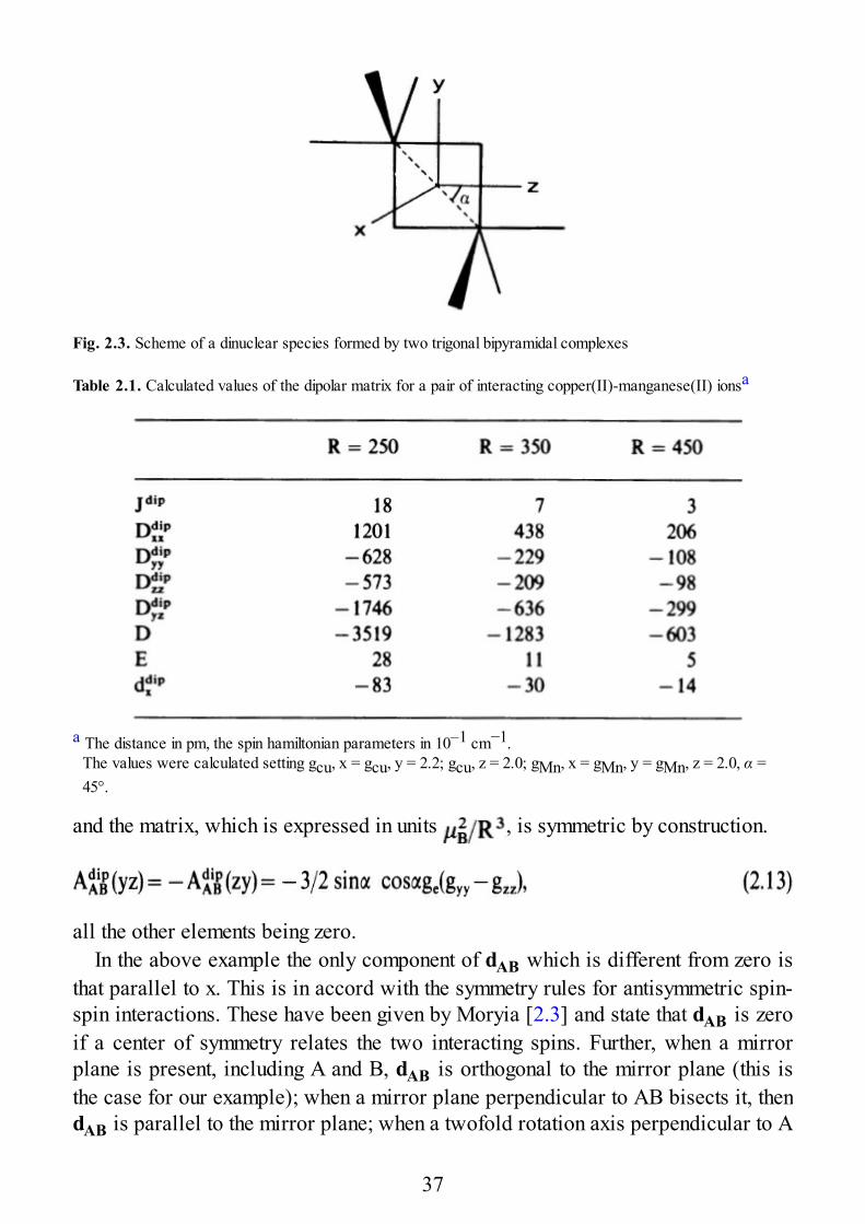
Fig. 2.3. Scheme of a dinuclear species formed by two trigonal bipyramidal complexes

Table 2.1. Calculated values of the dipolar matrix for a pair of interacting copper(II)-manganese(II) ionsa

a The distance in pm, the spin hamiltonian parameters in 10–1 cm−1.The values were calculated setting gcu, x = gcu, y = 2.2; gcu, z = 2.0; gMn, x = gMn, y = gMn, z = 2.0, α =45°.

and the matrix, which is expressed in units , is symmetric by construction.

all the other elements being zero.In the above example the only component of dAB which is different from zero is

that parallel to x. This is in accord with the symmetry rules for antisymmetric spin-spin interactions. These have been given by Moryia [2.3] and state that dAB is zeroif a center of symmetry relates the two interacting spins. Further, when a mirrorplane is present, including A and B, dAB is orthogonal to the mirror plane (this isthe case for our example); when a mirror plane perpendicular to AB bisects it, thendAB is parallel to the mirror plane; when a twofold rotation axis perpendicular to A

37

–B passes through the midpoint of A –B, then dAB is orthogonal to the twofold axis;when there is an n-fold axis (n > 2) along A – B, then dAB is parallel to A – B.

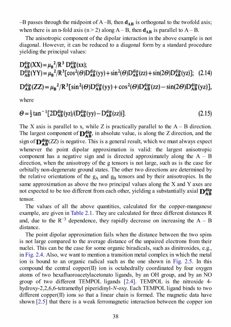
The anisotropic component of the dipolar interaction in the above example is notdiagonal. However, it can be reduced to a diagonal form by a standard procedureyielding the principal values:

where

The X axis is parallel to x, while Z is practically parallel to the A – B direction.The largest component of , in absolute value, is along the Z direction, and thesign of (ZZ) is negative. This is a general result, which we must always expectwhenever the point dipolar approximation is valid: the largest anisotropiccomponent has a negative sign and is directed approximately along the A – Bdirection, when the anisotropy of the g tensors is not large, such as is the case fororbitally non-degenerate ground states. The other two directions are determined bythe relative orientations of the gA and gB tensors and by their anisotropies. In thesame approximation as above the two principal values along the X and Y axes arenot expected to be too different from each other, yielding a substantially axial tensor.

The values of all the above quantities, calculated for the copper-manganeseexample, are given in Table 2.1. They are calculated for three different distances Rand, due to the R−3 dependence, they rapidly decrease on increasing the A – Bdistance.

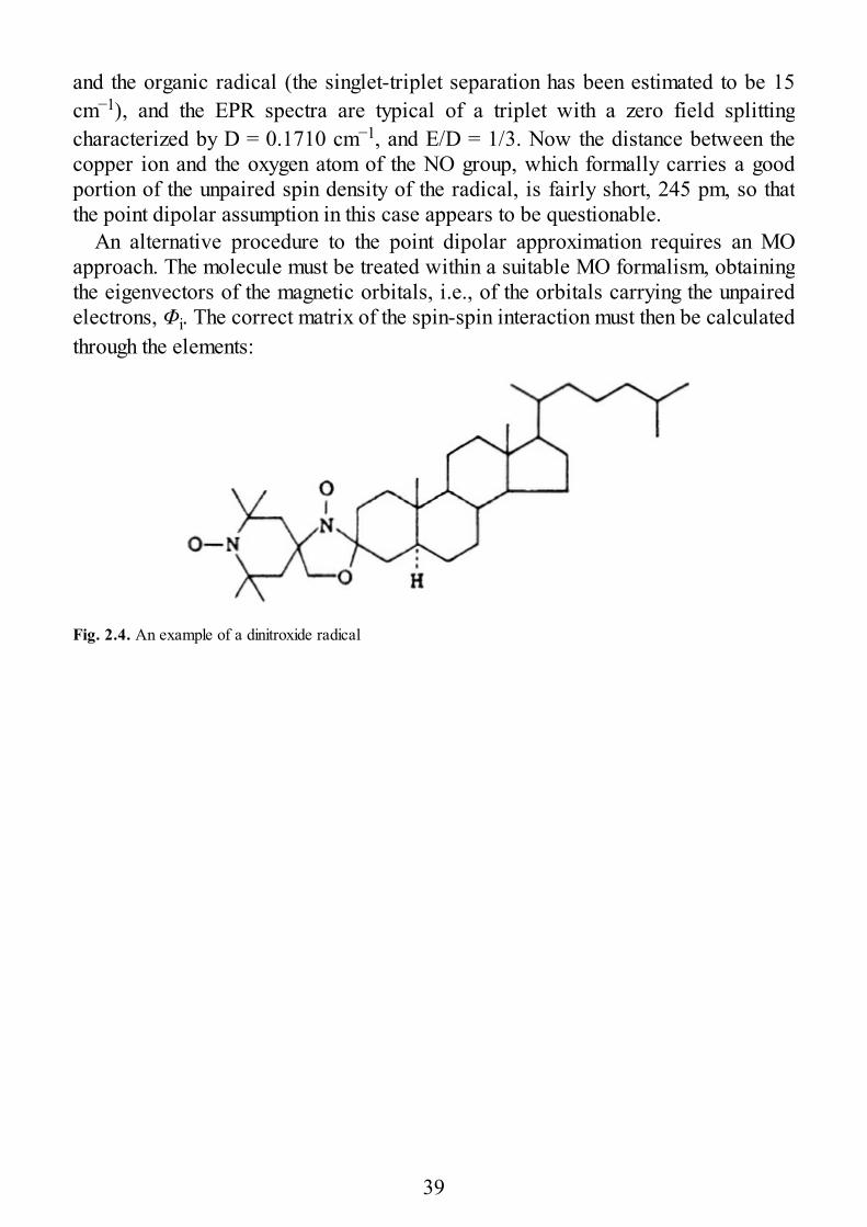
The point dipolar approximation fails when the distance between the two spinsis not large compared to the average distance of the unpaired electrons from theirnuclei. This can be the case for some organic biradicals, such as dinitroxides, e.g.,in Fig. 2.4. Also, we want to mention a transition metal complex in which the metalion is bound to an organic radical such as the one shown in Fig. 2.5. In thiscompound the central copper(II) ion is octahedrally coordinated by four oxygenatoms of two hexafluoroacetylacetonato ligands, by an OH group, and by an NOgroup of two different TEMPOL ligands [2.4]. TEMPOL is the nitroxide 4-hydroxy-2,2,6,6-tetramethyl piperidinyl-N-oxy. Each TEMPOL ligand binds to twodifferent copper(II) ions so that a linear chain is formed. The magnetic data haveshown [2.5] that there is a weak ferromagnetic interaction between the copper ion

38

and the organic radical (the singlet-triplet separation has been estimated to be 15cm−1), and the EPR spectra are typical of a triplet with a zero field splittingcharacterized by D = 0.1710 cm−1, and E/D = 1/3. Now the distance between thecopper ion and the oxygen atom of the NO group, which formally carries a goodportion of the unpaired spin density of the radical, is fairly short, 245 pm, so thatthe point dipolar assumption in this case appears to be questionable.

An alternative procedure to the point dipolar approximation requires an MOapproach. The molecule must be treated within a suitable MO formalism, obtainingthe eigenvectors of the magnetic orbitals, i.e., of the orbitals carrying the unpairedelectrons, Φi. The correct matrix of the spin-spin interaction must then be calculatedthrough the elements:

Fig. 2.4. An example of a dinitroxide radical

39

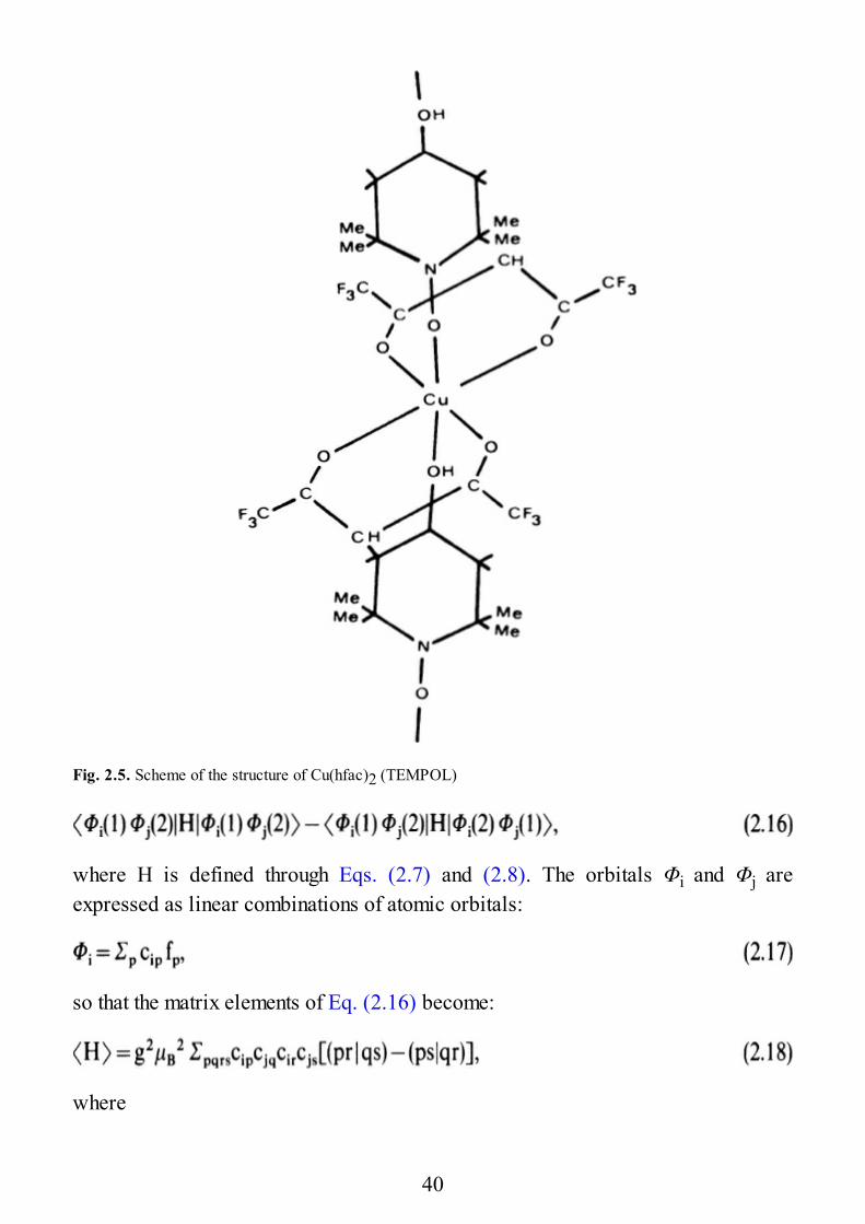
Fig. 2.5. Scheme of the structure of Cu(hfac)2 (TEMPOL)

where H is defined through Eqs. (2.7) and (2.8). The orbitals Φi and Φj areexpressed as linear combinations of atomic orbitals:

so that the matrix elements of Eq. (2.16) become:

where

40

In the literature several methods have been reported to calculate these integrals [2.6– 8] and the methods applied to several aromatic hydrocarbons [2.9, 10], and othersystems [2.11, 12]. However, for systems characterized by relatively weakexchange, like the ones in which we are interested, the main difficulty is that ofobtaining reliable molecular orbitals, as discussed in Chap. 1. Therefore, themethod has been relatively seldom used, and empirical methods have beenemployed.

Attempts have been made of taking into account the fact that the dipoles cannotbe regarded as point dipoles by introducing two [2.13] (or four in the case oftransition metal ions [2.14]) negative charges delocalized along the lobes of thep(d) orbitals which formally carry the unpaired electrons. The charge localizedalong the lobes of the orbital is 1/2(1/4) the overall charge assumed to be presentin the orbital. The distance of the negative charge from the nucleus has beenassumed to be 35 pm for p and 50 pm for d orbitals, considering that for purelyatomic orbitals the p(d) electron density maximizes at that distance.

Finally, another complication must be mentioned here with regards to the use ofempirical methods. So far it has been assumed that the magnetic dipoles areessentially localized on two centers. Now let us take into consideration two metalions bridged by some intervening ligand: it is apparent that the unpaired electrons,although mainly localized on the metal ions, will have a finite probability also onthe bridging and the remaining ligands. Although the fraction of electronstransferred to the ligand may be small, the distance of the ligand from the metal ismuch smaller than that of the other metal so that a relevant contribution can alsoresult. It is worth mentioning here that this is a general problem in magneticresonance spectroscopy which has been discussed at length also in theparamagnetic NMR literature [2.15]. However, this problem is, alas, difficult tosolve. In fact, in order to calculate the ligand contribution to the magnetic spin-spininteraction fairly accurate functions are needed and, as outlined in the previouschapter, the era of MO calculations on actual dinuclear species has just started.Recently Extended Hückel calculations have been applied to fluoro-bridgedcopper(II) dimers, but the values did not deviate significantly from those expectedfor the point-dipolar approximation [2.16].

2.3 The Exchange Contribution

The isotropic part of the exchange-determined component of JAB, is mainlydetermined by the weak bonding interaction described in the previous chapter, and

41

we will not expand on it further. The anisotropic and the antisymmetric parts of , on the other hand, are determined by relativistic effects, i.e., by the admixture ofexcited states into the ground state by spin-orbit coupling. The rigorous inclusion ofspin-orbit coupling effects in exchange-coupled systems is very difficult, and nocompletely rigorous attempt to do this has been made. In the following we willreport the essential lines of a treatment suggested by Kanamori [2.17], whichalthough simplified, has been used with some success in the interpretation of theEPR spectra of transition metal compounds.

From the elementary theory of EPR it is well known that excited states can beadmixed into the orbitally non-degenerate ground state by spin-orbit coupling,yielding g values different from the free electron value ge. Spin-orbit coupling ismore important for transition metal ions than for organic radicals, as shown by the gvalues which for the latter are generally quasi-isotropic and close to ge. Thesituation is much more complicated in the case of lanthanides and actinides andwill not be considered here.

For transition metal ions and for organic radicals spin-orbit coupling can betreated as a perturbation. Therefore, in the lowest state (i denotes the spincenter) the excited states will be admixed through the spin-orbit hamiltonian, Hso,for which a convenient form is:

where the sum is over all the unpaired electrons of the configuration, li and Si arethe orbital and spin angular momentum operators, respectively, and ξ(ri) is a radialfunction. The perturbed functions can be written as:

where the sum is over all the excited states, and is the energy differencebetween the excited and the ground state.

If the exchange interaction is introduced as a perturbation, leaving the relativehamiltonian Hex unexplicit, the first terms which are relevant to the anisotropiccontribution to appear in third order and are given by:

where the suffix of Hso indicates that it operates on the coordinates of the electroncentered on A. Of course, analogous terms for B will also be found, and a sum mustbe performed on all the excited states.

The final result is that it is possible to rewrite the sum of terms similar to Eq.

42

(2.22) by separating the spin and orbital variables according to the effective spinhamiltonian:

where

where the α sum is over the two centers (α = A, B; β indicates the center differentfrom α); the i and j sums are over all the excited states; k and 1 are cartesiancomponents. This matrix is not traceless nor symmetric, when the A and B centersare different, therefore, it must be reduced according to the procedure outlined inthe previous section. Equation (2.24) has been obtained in the simplifyingassumption that the excited states mixed into the ground state by spin-orbit couplingbelong to the same ground spectral term, so that the relative hamiltonian can bewritten as:

is identical to . It is not a simple exchangeintegral, but rather the exchange interaction with an excited state. We will comeback to this below.

Equation (2.24) can take a more appealing form when the symmetry of the systemis at least orthorhombic and only one excited state is admixed intothe ground state by each La,k component. In this case (2.24) reduces to:

Comparing the expression which gives the g tensors for the individual centers a:

we see that finally Eq. (2.26) can be written as:

43

which shows that the elements of the matrix are of the order of , whichmeans that for orbitally nondegenerate ground states the matrix elements are verysmall. For example for organic radicals, manganese(II), or gadolinium(III) ions, forwhich , the elements of the matrix are practically zero. Equation (2.28)also shows that the principal axes of the exchange contribution to JAB are parallelto the principal axes of g, provided that the two g tensors of the A and B centers areparallel to each other.

In the decomposition of the scalar component adds to the scalar componentoriginating from the exchange interaction between the ground, , states. Whenthe latter is of the order of at least 10° cm−1, then the additional component broughtabout by spin-orbit coupling can be safely neglected. However, this cannot be thecase when the ground state exchange interaction is smaller.

A caveat must be clearly stressed at this point, and it pertains to the J(eαgβeαgβ)parameter. According to its definition it describes the exchange interaction betweenthe ground, , orbital on center β, with the excited, , orbital on center α.This interaction can be completely different from the interaction between theground states gα and gβ, i.e., it can have different sign and different intensity. Thispoint can be made clear with one example. Let us take into consideration adinuclear copper(II) complex like the one described in Sect. 1.2 and in Fig. 1.4. Wesaw that the ground orbital can be described to a satisfactory approximation as xyand that the exchange interaction between the two magnetic orbitals can be eitherferro- or antiferro-magnetic, depending on the Cu–L–Cu angle. The excited state x2

– y2 is mixed into the ground state through spin-orbit coupling by the z componentof L and . The exchange interaction between these twoorbitals is dominated by the fact that they are orthogonal: according to theGoodenough-Kanamori rules, this means that the coupling between the two must beferromagnetic. Indeed, we already considered this case in Sect. 1.2, for acopper(II)-oxovanadium (IV) pair. Therefore, when the Cu–L–Cu angle is largeenough, J(xy, xy, xy, xy) is antiferromagnetic and J(x2 – y2, xy, x2 – y2, xy) isferromagnetic. It is apparent that any attempt to estimate Jcucu

ex(ZZ) by replacingthe unknown value of J(x2 – y2, xy, x2 –y2, xy) in (2.28) by the value of J(xy, xy, xy,xy), determined for instance through magnetic susceptibility measurements, isdestined to fail.

Since for orbitally nondegenerate ground states the main contribution of is tothe zero field splitting tensor, it has been customary to have an order of magnitudeestimate of the D tensor, using for instance the D parameter, according to:

where J is J(gAgBgAgB). From the considerations above it is apparent that this

44

estimation can be completely wrong and must be used, faut de mieux, with extremecircumspection.

Indeed, the EPR spectra of a few copper(II) complexes possessing the geometryof Fig. 1.4 have been studied [2.18,19]. In all cases the largest zero field splittingcomponent has been observed to be orthogonal to the coordination plane, inagreement with a dominant exchange contribution to the zero field splitting, and notalong the copper-copper direction, as would be required by dominant dipolarinteraction. The results are summarized in Fig. 2.6, where the experimental Dzzvalues are plotted vs the copper-copper distance. The dotted area corresponds tothe calculated dipolar interaction: it is apparent that all the experimental points arewell above that, even at the largest distances [2.20]. The experimental exchangecontributions can be fitted with an exponential regression [2.18], but it is safer touse this result as indicative that Dzz decreases on increasing the metal-metaldistance.

A corollary to the use of (2.29) has been that when J is small, the exchangecontribution to D can be neglected, and the experimental value can be safelyassumed to be due to the dipolar component, thus allowing one to determine themetal-metal distance through the R−3 dependence of D. For instance, it has beencommon practice to neglect the exchange contribution to the zero field splittingwhen J < 30 cm−1 [2.21]. Although it may work sometimes, there are severalexamples in the literature which show how dangerous it can be to rely on it in orderto obtain structural information.

45

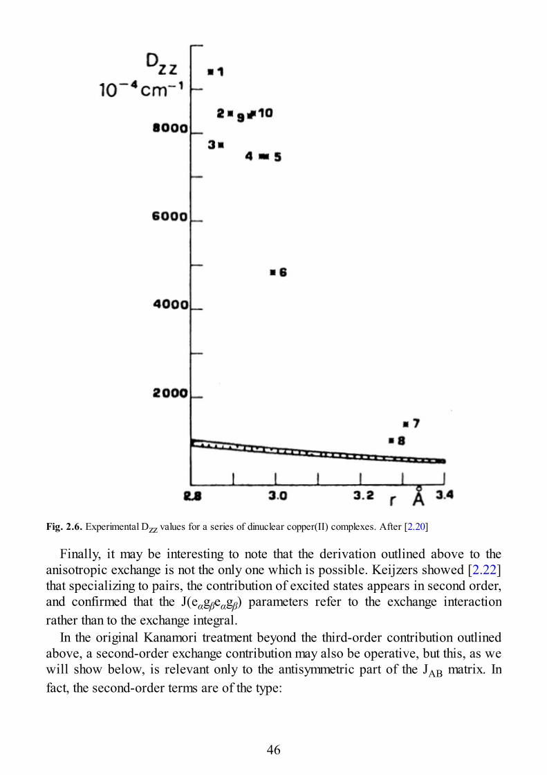
Fig. 2.6. Experimental Dzz values for a series of dinuclear copper(II) complexes. After [2.20]

Finally, it may be interesting to note that the derivation outlined above to theanisotropic exchange is not the only one which is possible. Keijzers showed [2.22]that specializing to pairs, the contribution of excited states appears in second order,and confirmed that the J(eαgβeαgβ) parameters refer to the exchange interactionrather than to the exchange integral.

In the original Kanamori treatment beyond the third-order contribution outlinedabove, a second-order exchange contribution may also be operative, but this, as wewill show below, is relevant only to the antisymmetric part of the JAB matrix. Infact, the second-order terms are of the type:

46

If we assume that the relevant excited states which can be admixed into the groundstate belong to the same spectroscopic term as the ground state, then (2.30) can berewritten as:

where use has been made of the fact that:

for real orbitals. The hamiltonian then takes the form:

By setting:

(2.33) finally becomes:

which yields the second-order contribution of the exchange interactions to theantisymmetric spin-spin interactions. From (2.35) we learn that is identical tozero when the two ions are related by an inversion center, and more generally thatthe symmetry rules for are the same as outlined above for the magneticcontribution.

These rules have been expressed in a more general way by Bencini andGatteschi [2.23]. Two cases can be distinguished: one in which the twoparamagnetic centers are related by a symmetry element and the other where theyare not. In the former the symmetry of the pair is higher than the symmetry of theindividual centers, while in the latter the symmetry of the pair is identical to that ofthe single centers. In this case the orientation of d is determined recurring to thecharacter table of the symmetry point group of the pair. In fact, d may be differentfrom zero only if some of the individual di’s are different from zero. In order tohave this it is necessary that |ei > and |gi > span the same irreducible representation

47

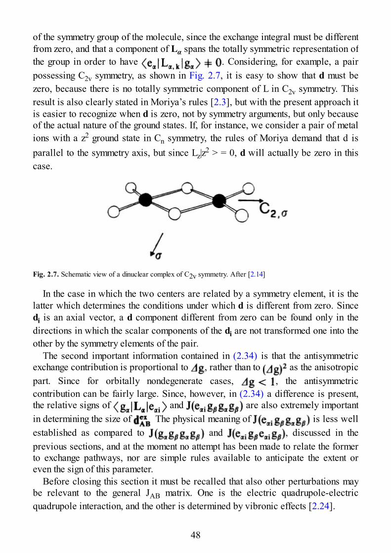
of the symmetry group of the molecule, since the exchange integral must be differentfrom zero, and that a component of Lα spans the totally symmetric representation ofthe group in order to have . Considering, for example, a pairpossessing C2v symmetry, as shown in Fig. 2.7, it is easy to show that d must bezero, because there is no totally symmetric component of L in C2v symmetry. Thisresult is also clearly stated in Moriya’s rules [2.3], but with the present approach itis easier to recognize when d is zero, not by symmetry arguments, but only becauseof the actual nature of the ground states. If, for instance, we consider a pair of metalions with a z2 ground state in Cn symmetry, the rules of Moriya demand that d isparallel to the symmetry axis, but since Lz|z2 > = 0, d will actually be zero in thiscase.

Fig. 2.7. Schematic view of a dinuclear complex of C2v symmetry. After [2.14]

In the case in which the two centers are related by a symmetry element, it is thelatter which determines the conditions under which d is different from zero. Sincedi is an axial vector, a d component different from zero can be found only in thedirections in which the scalar components of the di are not transformed one into theother by the symmetry elements of the pair.

The second important information contained in (2.34) is that the antisymmetricexchange contribution is proportional to , rather than to as the anisotropicpart. Since for orbitally nondegenerate cases, , the antisymmetriccontribution can be fairly large. Since, however, in (2.34) a difference is present,the relative signs of and are also extremely importantin determining the size of The physical meaning of is less wellestablished as compared to and , discussed in theprevious sections, and at the moment no attempt has been made to relate the formerto exchange pathways, nor are simple rules available to anticipate the extent oreven the sign of this parameter.

Before closing this section it must be recalled that also other perturbations maybe relevant to the general JAB matrix. One is the electric quadrupole-electricquadrupole interaction, and the other is determined by vibronic effects [2.24].

48

The electronic quadrupole interaction is bound to the electrostatic interactionresulting from the charge distribution on one ion of the pair contributing to theelectric field gradient at the other. It has an R−5 dependence and it increases withthe increase of the orbital contribution to the ground state. Therefore, it proved tobe of some importance in the analysis of the EPR spectra of lanthanide ions.

The vibronic-determined interaction has its origin in the modulation of thecrystal field at one spin center A induced by phonons. In a pair the modulation atthe two centers is correlated in such a way that a phonon emitted, e.g., by A, isimmediately absorbed by center B. This yields a component depending on R−3,which in the case of nickel(II) Tutton salt has been calculated to be of the sameorder as the magnetic dipolar interaction.

2.4 Biquadratic Terms

Beyond the bilinear terms it is possible to introduce also higher-order terms in thespin hamiltonian, among which biquadratic terms are the most important. Also inthis case there are several different possible origins, but the most relevant are thehigher order intrinsic exchange and the exchange striction effects.

The former enters naturally Anderson’s theory [2.25] when it is extended to thefourth order in perturbation and physically represents the admixture into the groundstate of excited states corresponding to a double excitation in the superexchangeprocess. This process can be represented by a spin hamiltonian:

Several attempts to estimate j for different cases have been made and, althoughthere are large discrepancies in the calculated values, there seems to be a fairlygeneral agreement that the j/J ratio is of the order of 10−2 at best [2.26]. Although itis a small effect, it can be observed in the analysis of the EPR spectra of systemswith large S values since the inclusion of (2.36) in the total spin hamiltonianinduces variations in the S manifold splitting pattern.

The other important physical phenomenon which can give rise to a term like(2.36) is exchange striction [2.27], i.e., the change in the R distance between thetwo spin centers due to the exchange stabilization. In general, |J| increases ondecreasing the R distance: therefore, exchange tends to bring the two spins closerbut the process is not indefinite because the restoring forces oppose that. Assuminga simple Hooke’s law for the restoring force yields a biquadratic form of theeffective hamiltonian identical to (2.36).

49

2.5 Justification of the Spin Hamiltonian Formalism

The most elegant justification of the spin hamiltonian formalism has been providedby Stevens using a second quantization perturbational approach [2.28, 29]. We willtry to provide here a concise illustration of the method, using the mathematicalformalism as little as possible. We provide in Appendix A a short resume of thefoundations of the second quantization formalism in order to provide the readerswho are not familiar with it the possibility of following the line of reasoning,although at the expenses of some rigour.

Central to Stevens treatment is a reformulation of the perturbation problem forthe case of two interacting ions. Throughout the treatment the orbitals on the twospin centers are assumed to be orthogonal. The true hamiltonian appropriate to thesystem is denoted H, and is not further specified, except to say that it is as completeas possible. In order to perform a perturbation treatment a suitable unperturbedhamiltonian H0 is defined, such that

H0 is not, as often assumed, simply the sum of the hamiltonians appropriate to the Aand B species separately, because, if this intuitively simple procedure is followed,the unusual result is obtained that the perturbed hamiltonian has higher symmetrythan the unperturbed one! One can be easily convinced that this would be the caseconsidering that the HA + HB hamiltonian is not invariant to the exchange ofelectrons between A and B, while the hamiltonian including the perturbation mustnecessarily be invariant to electron exchange. Therefore, H0 is chosen according todifferent criteria: it must be invariant to electron exchange and it must be suitablefor a perturbation treatment. These two conditions are met by the hamiltonian:

where |n > is an eigenstate of H and the sum extends over all the states. The quantityΩn is defined as:

and it is the n-th eigenvalue of H or the mean of the eigenvalues taken over a groupof guasi-degenerate levels. The energy of the unperturbed state does not need to beknown: the only relevant information is that all the |n > functions have the sameenergy with the hamiltonian H0. It should be noted that this procedure applies tosymmetric as well as to nonsymmetric A–B species. The perturbation hamiltonianis:

50

Defining the projection operators:

where the sums are over the ground and the excited states specified by the 0 and iindexes, respectively, it is possible to express the correction to energy up to secondorder by an effective hamiltonian defined as:

where is the energy difference between the ground and the excited manifold:

Using (2.43) it is possible to arrive at the required spin hamiltonian. It is at thispoint that second quantized operators are needed. For the reader who is notfamiliar with them it can be stated that second quantized operators provide aformalism for handling Slater determinants, which, as is well known, become arather cumbersome tool for providing antisymmetrization when numerous orbitalsare involved.

Let us suppose to have defined the Slater determinant appropriate to a system,for instance of three electrons, and then we wish to pass to a four-electron system:formally this can be easily done by defining an operator , called creationoperator, which simply performs what we wish. This means that operating with , on the system of three electrons a new Slater determinant, 4 × 4, is obtained whichdiffers from the previous one due to the addition of one electron in the ασ (α orbitalσ spin part) orbital. Conversely, if we wish to go back to the system of threeelectrons we have just to define an annihilation operator, aaασ, which performsexactly what we want. If we define a vacuum state (a state with no electrons) wemay construct from that all the Slater determinants we want by simply using all theelectron creation operators we need. So, for instance, applying the operator:

on the vacuum state we obtain a 5 × 5 Slater determinant in which the five dorbitals are singly occupied with spin-up.

Using the appropriate theory, one- and two-electron operators can be expressedin second quantization as:

51

where H1 is a one-electron and H12 is a two-electron operator.A general hamiltonian for a pair contains both one- and two-electron operators:

some of them involve orbitals localized on the same center, while some involveorbitals belonging to both centers.

Considering the perturbation hamiltonian (2.43) the first-order contribution,given by PoH′Po, contains many terms, which, however, keep the number ofelectrons on center A and B respectively fixed. This means that if an electron isannihilated by, e.g., ai, another one must be created at the same site by, e.g. .Pairs of operators do not necessarily commute. Among two-electronoperators sets of the type , where k and 1 are localized on B while j andi are located on A, are present. It is easy to prove that pairs of operators ondifferent sites necessarily commute. It is this property which can be used for thecomparison of the spin hamiltonian formalism. Indeed, in the latter case thehamiltonian is expressed as a sum of terms, some of which include couples of spinoperators on the same center, which do not necessarily commute, and couples ofspin operators on different centers, which do necessarily commute. Thesecommutation rules are analogous to those of angular momentum operators, andindeed a general expression is available which relates angular momentum andsecond quantized operators. This is given in Appendix A. Through this approach itis possible to substitute to the true hamiltonian, expressed by the second quantizedoperators, a spin hamiltonian, expressed through angular momentum operators.The first-order perturbation hamiltonian is:

This can be split into two components, one collecting the parts of the hamiltonianwhich operate on the electrons of the same center, either A and B, and the otherwhich contains operators which mix the functions of the two centers. In the secondquantized form these components are given by:

52

where HL contains all of the ligand field interaction and single ion electronrepulsion which is contained in H0. Aδδ′. and Bδδ′ δ″ δ′″ are defined as matrixelements of one- and two-electron operators, respectively, according to (2.46) and(2.47), respectively. The indices α refer to the spin coordinates and α and β to theorbitals centered on A and B, respectively.

The second-order term in (2.43) can be rewritten as:

Retaining only the terms in which one electron is transferred from A to B orvice-versa, the spin hamiltonian becomes:

where U has exactly the same meaning as in Anderson’s theory.Using the relation between angular momentum and second quantized operators

given in Appendix A, Heff reduces to:

Neglecting the scalar terms, and passing from one-electron to all-electron spinoperators, one finally finds:

with

where f is a positive proportionality factor dependent on the electron configuration.It can be simply expressed as:

and the term in parenthesis in (2.55) can be indicated as Jαββα, i.e., as the exchangeinteraction involving the α orbital on A and the β orbital on B. corresponds to Anderson’s kinetic exchange and Bαββα corresponds to potentialexchange. Therefore, (2.54) corresponds exactly to the Heisenberg exchangehamiltonian. No anisotropy is present in (2.53) because in the true hamiltonian wedid not include either spin-orbit or magnetic terms.

53

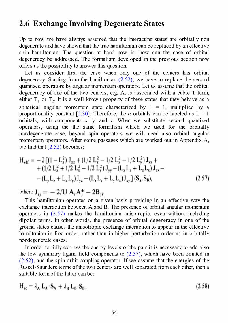
2.6 Exchange Involving Degenerate States

Up to now we have always assumed that the interacting states are orbitally nondegenerate and have shown that the true hamiltonian can be replaced by an effectivespin hamiltonian. The question at hand now is: how can the case of orbitaldegeneracy be addressed. The formalism developed in the previous section nowoffers us the possibility to answer this question.

Let us consider first the case when only one of the centers has orbitaldegeneracy. Starting from the hamiltonian (2.52), we have to replace the secondquantized operators by angular momentum operators. Let us assume that the orbitaldegeneracy of one of the two centers, e.g. A, is associated with a cubic T term,either T1 or T2. It is a well-known property of these states that they behave as aspherical angular momentum state characterized by L = 1, multiplied by aproportionality constant [2.30]. Therefore, the α orbitals can be labeled as L = 1orbitals, with components x, y, and z. When we substitute second quantizedoperators, using the the same formalism which we used for the orbitallynondegenerate case, beyond spin operators we will need also orbital angularmomentum operators. After some passages which are worked out in Appendix A,we find that (2.52) becomes:

where .This hamiltonian operates on a given basis providing in an effective way the

exchange interaction between A and B. The presence of orbital angular momentumoperators in (2.57) makes the hamiltonian anisotropic, even without includingdipolar terms. In other words, the presence of orbital degeneracy in one of theground states causes the anisotropic exchange interaction to appear in the effectivehamiltonian in first order, rather than in higher perturbation order as in orbitallynondegenerate cases.

In order to fully express the energy levels of the pair it is necessary to add alsothe low symmetry ligand field components to (2.57), which have been omitted in(2.52), and the spin-orbit coupling operator. If we assume that the energies of theRussel-Saunders terms of the two centers are well separated from each other, then asuitable form of the latter can be:

54

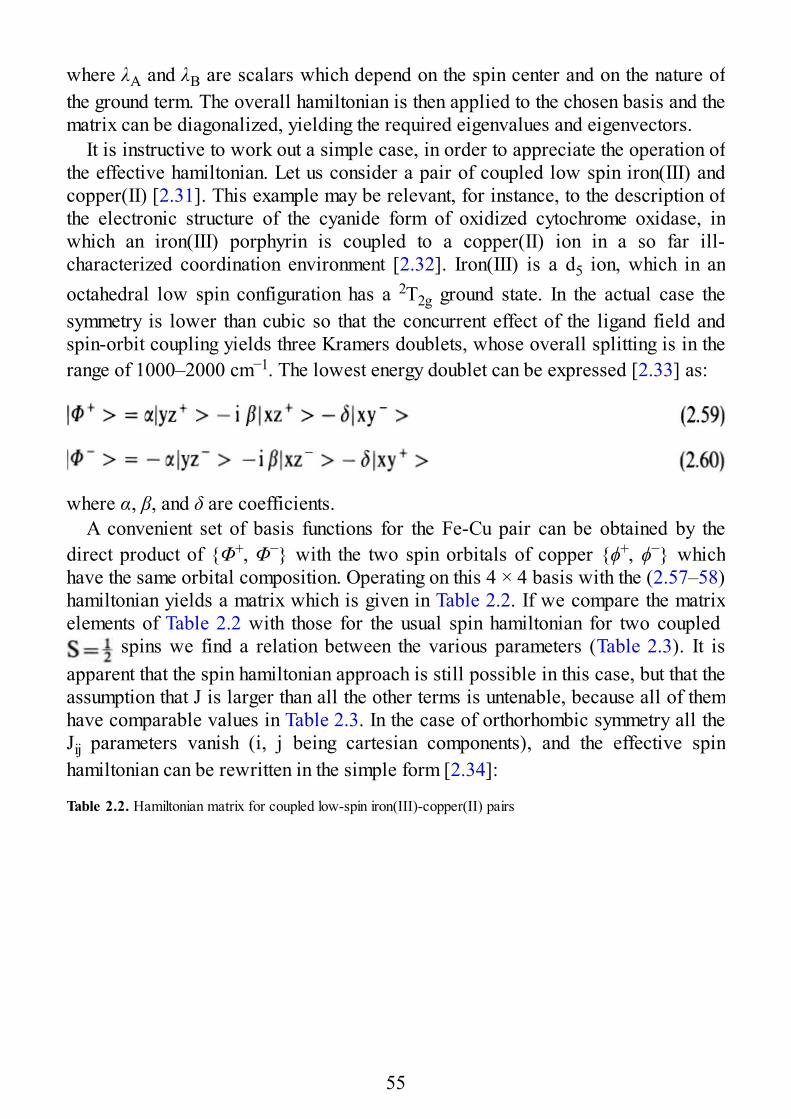
where λA and λB are scalars which depend on the spin center and on the nature ofthe ground term. The overall hamiltonian is then applied to the chosen basis and thematrix can be diagonalized, yielding the required eigenvalues and eigenvectors.

It is instructive to work out a simple case, in order to appreciate the operation ofthe effective hamiltonian. Let us consider a pair of coupled low spin iron(III) andcopper(II) [2.31]. This example may be relevant, for instance, to the description ofthe electronic structure of the cyanide form of oxidized cytochrome oxidase, inwhich an iron(III) porphyrin is coupled to a copper(II) ion in a so far ill-characterized coordination environment [2.32]. Iron(III) is a d5 ion, which in anoctahedral low spin configuration has a 2T2g ground state. In the actual case thesymmetry is lower than cubic so that the concurrent effect of the ligand field andspin-orbit coupling yields three Kramers doublets, whose overall splitting is in therange of 1000–2000 cm−1. The lowest energy doublet can be expressed [2.33] as:

where α, β, and δ are coefficients.A convenient set of basis functions for the Fe-Cu pair can be obtained by the

direct product of {Φ+, Φ−} with the two spin orbitals of copper {ϕ+, ϕ−} whichhave the same orbital composition. Operating on this 4 × 4 basis with the (2.57–58)hamiltonian yields a matrix which is given in Table 2.2. If we compare the matrixelements of Table 2.2 with those for the usual spin hamiltonian for two coupled

spins we find a relation between the various parameters (Table 2.3). It isapparent that the spin hamiltonian approach is still possible in this case, but that theassumption that J is larger than all the other terms is untenable, because all of themhave comparable values in Table 2.3. In the case of orthorhombic symmetry all theJij parameters vanish (i, j being cartesian components), and the effective spinhamiltonian can be rewritten in the simple form [2.34]:

Table 2.2. Hamiltonian matrix for coupled low-spin iron(III)-copper(II) pairs

55

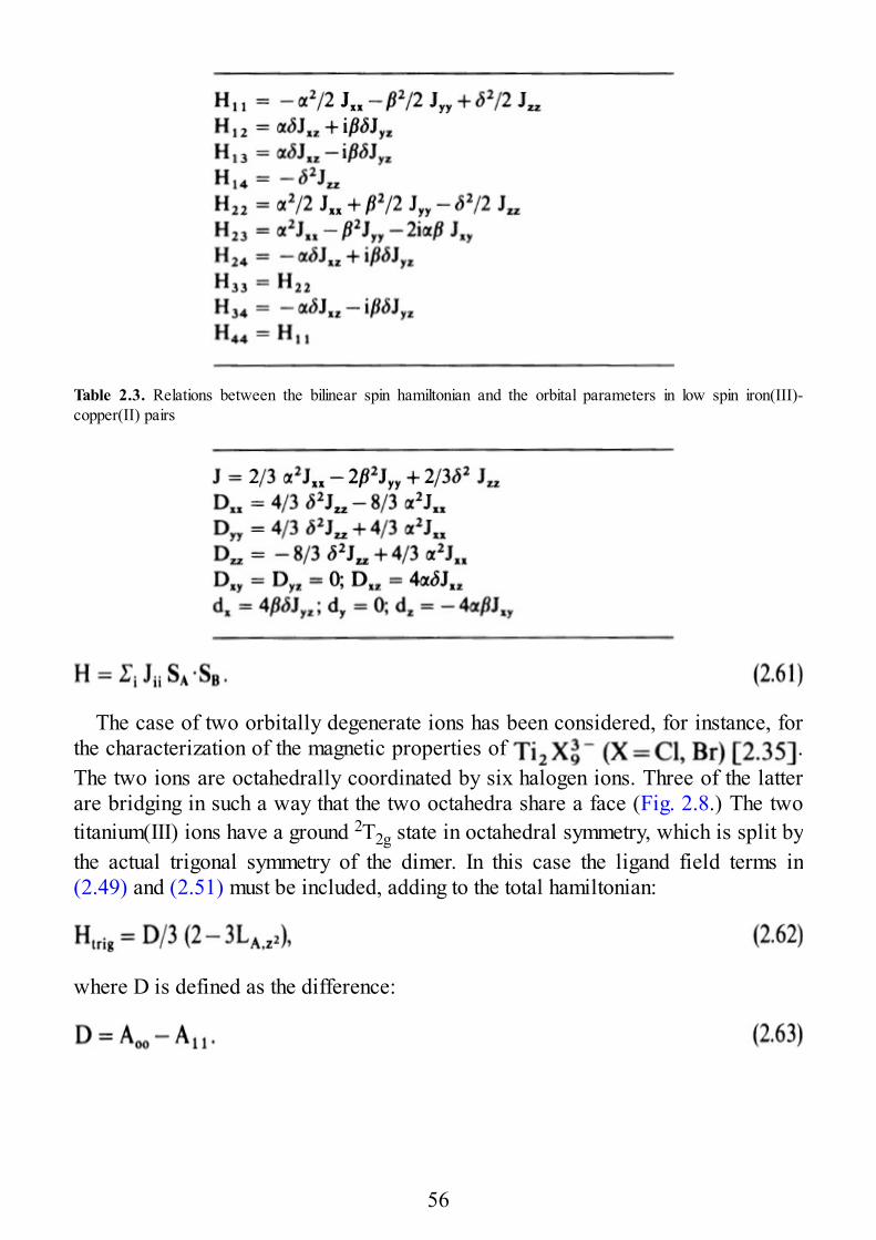
Table 2.3. Relations between the bilinear spin hamiltonian and the orbital parameters in low spin iron(III)-copper(II) pairs

The case of two orbitally degenerate ions has been considered, for instance, forthe characterization of the magnetic properties of .The two ions are octahedrally coordinated by six halogen ions. Three of the latterare bridging in such a way that the two octahedra share a face (Fig. 2.8.) The twotitanium(III) ions have a ground 2T2g state in octahedral symmetry, which is split bythe actual trigonal symmetry of the dimer. In this case the ligand field terms in(2.49) and (2.51) must be included, adding to the total hamiltonian:

where D is defined as the difference:

56

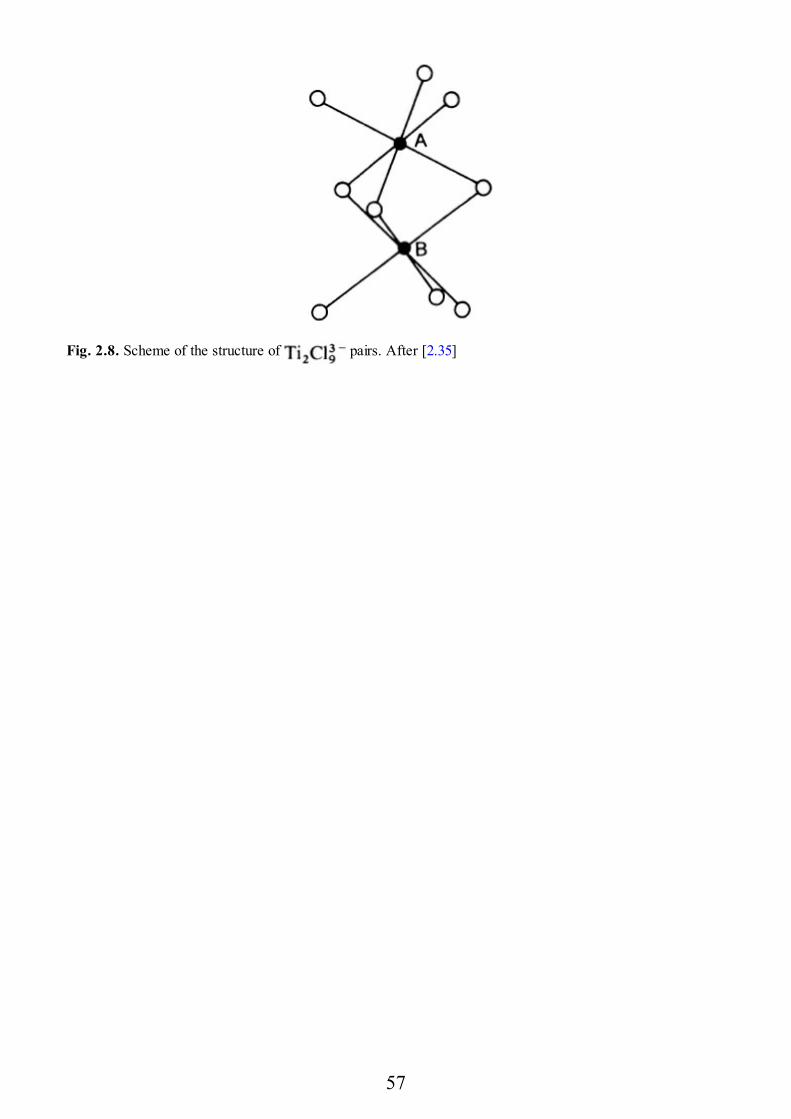
Fig. 2.8. Scheme of the structure of pairs. After [2.35]

57

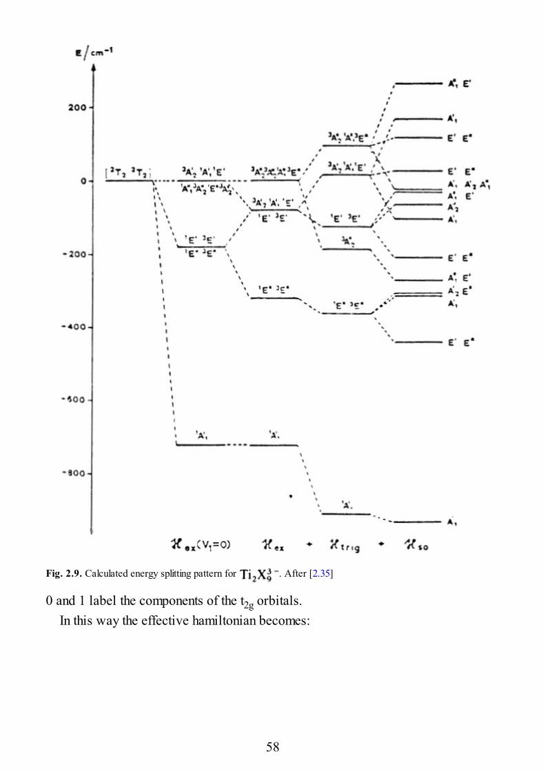
Fig. 2.9. Calculated energy splitting pattern for . After [2.35]

0 and 1 label the components of the t2g orbitals.In this way the effective hamiltonian becomes:

58

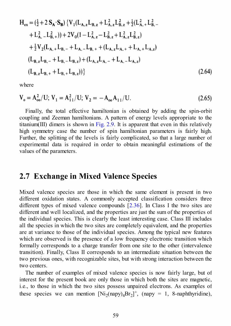
where

Finally, the total effective hamiltonian is obtained by adding the spin-orbitcoupling and Zeeman hamiltonians. A pattern of energy levels appropriate to thetitanium(III) dimers is shown in Fig. 2.9. It is apparent that even in this relativelyhigh symmetry case the number of spin hamiltonian parameters is fairly high.Further, the splitting of the levels is fairly complicated, so that a large number ofexperimental data is required in order to obtain meaningful estimations of thevalues of the parameters.

2.7 Exchange in Mixed Valence Species

Mixed valence species are those in which the same element is present in twodifferent oxidation states. A commonly accepted classification considers threedifferent types of mixed valence compounds [2.36]. In Class I the two sites aredifferent and well localized, and the properties are just the sum of the properties ofthe individual species. This is clearly the least interesting case. Class III includesall the species in which the two sites are completely equivalent, and the propertiesare at variance to those of the individual species. Among the typical new featureswhich are observed is the presence of a low frequency electronic transition whichformally corresponds to a charge transfer from one site to the other (intervalencetransition). Finally, Class II corresponds to an intermediate situation between thetwo previous ones, with recognizable sites, but with strong interaction between thetwo centers.

The number of examples of mixed valence species is now fairly large, but ofinterest for the present book are only those in which both the sites are magnetic,i.e., to those in which the two sites possess unpaired electrons. As examples ofthese species we can mention [Ni2(napy)4Br2]+, (napy = 1, 8-naphthyridine),

59

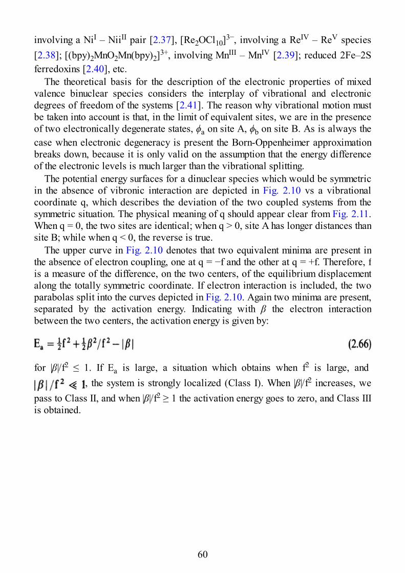
involving a NiI – NiiII pair [2.37], [Re2OCl10]3−, involving a ReIV – ReV species[2.38]; [(bpy)2MnO2Mn(bpy)2]3+, involving MnIII – MnIV [2.39]; reduced 2Fe–2Sferredoxins [2.40], etc.

The theoretical basis for the description of the electronic properties of mixedvalence binuclear species considers the interplay of vibrational and electronicdegrees of freedom of the systems [2.41]. The reason why vibrational motion mustbe taken into account is that, in the limit of equivalent sites, we are in the presenceof two electronically degenerate states, ϕa on site A, ϕb on site B. As is always thecase when electronic degeneracy is present the Born-Oppenheimer approximationbreaks down, because it is only valid on the assumption that the energy differenceof the electronic levels is much larger than the vibrational splitting.

The potential energy surfaces for a dinuclear species which would be symmetricin the absence of vibronic interaction are depicted in Fig. 2.10 vs a vibrationalcoordinate q, which describes the deviation of the two coupled systems from thesymmetric situation. The physical meaning of q should appear clear from Fig. 2.11.When q = 0, the two sites are identical; when q > 0, site A has longer distances thansite B; while when q < 0, the reverse is true.

The upper curve in Fig. 2.10 denotes that two equivalent minima are present inthe absence of electron coupling, one at q = −f and the other at q = +f. Therefore, fis a measure of the difference, on the two centers, of the equilibrium displacementalong the totally symmetric coordinate. If electron interaction is included, the twoparabolas split into the curves depicted in Fig. 2.10. Again two minima are present,separated by the activation energy. Indicating with β the electron interactionbetween the two centers, the activation energy is given by:

for |β|/f2 ≤ 1. If Ea is large, a situation which obtains when f2 is large, and , the system is strongly localized (Class I). When |β|/f2 increases, we

pass to Class II, and when |β|/f2 ≥ 1 the activation energy goes to zero, and Class IIIis obtained.

60

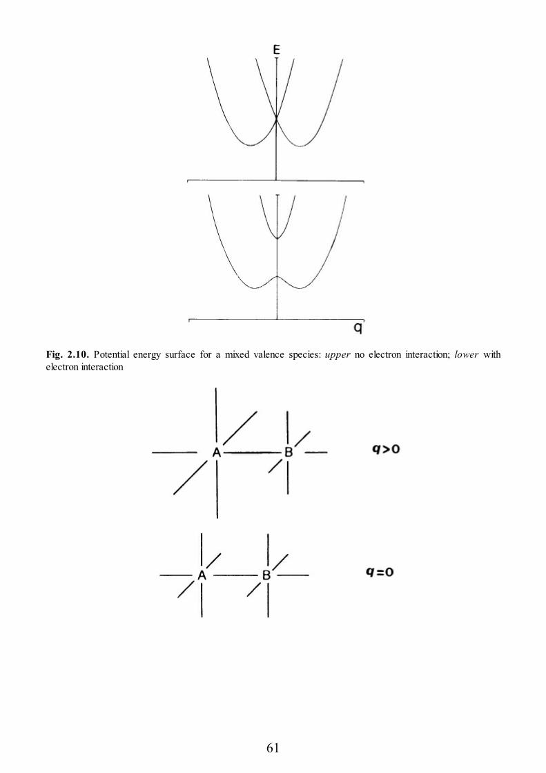
Fig. 2.10. Potential energy surface for a mixed valence species: upper no electron interaction; lower withelectron interaction

61

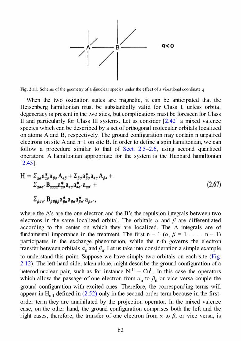
Fig. 2.11. Scheme of the geometry of a dinuclear species under the effect of a vibrational coordinate q

When the two oxidation states are magnetic, it can be anticipated that theHeisenberg hamiltonian must be substantially valid for Class I, unless orbitaldegeneracy is present in the two sites, but complications must be foreseen for ClassII and particularly for Class III systems. Let us consider [2.42] a mixed valencespecies which can be described by a set of orthogonal molecular orbitals localizedon atoms A and B, respectively. The ground configuration may contain n unpairedelectrons on site A and n−1 on site B. In order to define a spin hamiltonian, we canfollow a procedure similar to that of Sect. 2.5–2.6, using second quantizedoperators. A hamiltonian appropriate for the system is the Hubbard hamiltonian[2.43]:

where the A’s are the one electron and the B’s the repulsion integrals between twoelectrons in the same localized orbital. The orbitals α and β are differentiatedaccording to the center on which they are localized. The A integrals are offundamental importance in the treatment. The first n – 1 (α, β = 1 . . . . n – 1)participates in the exchange phenomenon, while the n-th governs the electrontransfer between orbitals αn and βn. Let us take into consideration a simple exampleto understand this point. Suppose we have simply two orbitals on each site (Fig.2.12). The left-hand side, taken alone, might describe the ground configuration of aheterodinuclear pair, such as for instance NiII − CuII. In this case the operatorswhich allow the passage of one electron from αn to βn or vice versa couple theground configuration with excited ones. Therefore, the corresponding terms willappear in Heff defined in (2.52) only in the second-order term because in the first-order term they are annihilated by the projection operator. In the mixed valencecase, on the other hand, the ground configuration comprises both the left and theright cases, therefore, the transfer of one electron from α to β, or vice versa, is

62

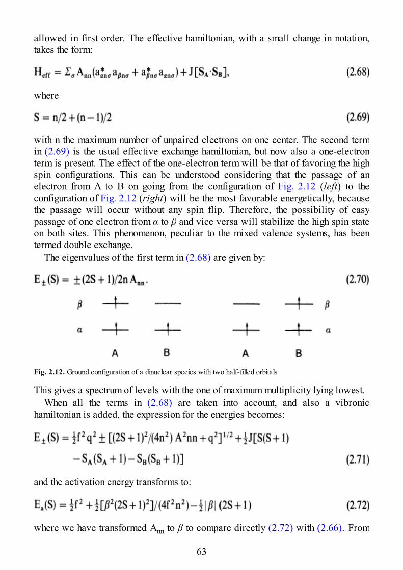
allowed in first order. The effective hamiltonian, with a small change in notation,takes the form:

where

with n the maximum number of unpaired electrons on one center. The second termin (2.69) is the usual effective exchange hamiltonian, but now also a one-electronterm is present. The effect of the one-electron term will be that of favoring the highspin configurations. This can be understood considering that the passage of anelectron from A to B on going from the configuration of Fig. 2.12 (left) to theconfiguration of Fig. 2.12 (right) will be the most favorable energetically, becausethe passage will occur without any spin flip. Therefore, the possibility of easypassage of one electron from α to β and vice versa will stabilize the high spin stateon both sites. This phenomenon, peculiar to the mixed valence systems, has beentermed double exchange.

The eigenvalues of the first term in (2.68) are given by:

Fig. 2.12. Ground configuration of a dinuclear species with two half-filled orbitals

This gives a spectrum of levels with the one of maximum multiplicity lying lowest.When all the terms in (2.68) are taken into account, and also a vibronic

hamiltonian is added, the expression for the energies becomes:

and the activation energy transforms to:

where we have transformed Ann to β to compare directly (2.72) with (2.66). From

63

this comparison we learn that in the case of antiferromagnetic exchange there is acompetition between double exchange, which favors the high spin state andexchange, and the activation energy is increased compared to the case of noexchange. In other terms the antiferromagnetic interaction slows down the transferrate.

The energy of the minima can be expressed as:

which shows that vibronic coupling adds a negative contribution to the exchangeconstant.

References

2.1 Martin R L (1968) In: Ebsworth EAV, Maddock AG, Sharpe AG (eds) New pathways in inorganicchemistry., Cambridge University Press, London, p 175

2.2 Silver BL (1976) Irreducible tensor methods Academic, New York2.3 Moriya (1963) In: Rado GT, Suhl H (eds) Magnetism, Academic New York, Vol 1 p 852.4 Anderson OP, Kuechler T S (1980) Inorg. Chem. 19: 14172.5 Bencini A, Benelli C, Gatteschi D, Zanchini C (1984) J. Am. Chem. Soc. 106: 58132.6 Geller M (1963) J. Chem. Phys. 39: 842.7 Matcha RL, Kern CW, Schrader DM (1969) J. Chem. Phys. 51: 21522.8 Matcha RL, Kern CW (1970) Phys. Rev. Lett. 25: 9812.9 Van der Waals JH, ter Maten G (1964) Mol. Phys 8: 3012.10 Boorstein SA, Goutermann M (1965) J. Chem. Phys. 42: 30702.11 McWeeny R (1961) J. Chem. Phys. 34: 3992.12 de Jager G, de Jong J, Mac Lean C, Ros P (1977) Theoret. Chim. Acta 20: 572.13 Brustolon M, Pasimeni L, Corvaja C (1973) Chem. Phys. Letters 21: 1942.14 Belford RL, Chasteen ND, So H, Tapscott RE (1969) J. Am. Chem. Soc. 91: 46752.15 Bertini I, Luchinat C (1986) NMR of paramagnetic molecules in biological systems Benjamin/Cummings:

Menlo Park, CA2.16 Gribnau M (1988) Ph.D. Thesis, Nijmegen2.17 Kanamori J (1963) In: Rado TG, Suhl H (eds) Magnetism. Academic, New York, vol 1 p 1612.18 Bencini A, Gatteschi D, Zanchini C, Haase W (1985) Inorg. Chem. 24: 34852.19 Charlot MF, Journaux Y, Kahn O, Bencini A, Gatteschi D, Zanchini C (1985) Inorg. Chem. 25: 10602.20 Bencini A, Gatteschi D, Zanchini C (1985) Inorg. Chem. 24: 7002.21 Smith TD, Pilbrow JR (1974) Coord. Chem. Rev. 13: 1732.22 Keijzers CP (1986) In: Electron spin resonance The Royal Society of Chemistry, London, vol 10B p 12.23 Bencini A, Gatteschi D (1982) Mol. Phys. 47: 1612.24 Owen J, Harris EA (1972) In: Geschwind S (ed.) Electron paramagnetic resonance. Plenum, New York, p

4272.25 Anderson PW (1963) In: Seitz F, Turnbull (eds) Solid state physics. New York, vol 14 p 992.26 Huang NL, Orbach R (1964) Phys. Rev. Letters 12: 2752.27 Kanamori J (1957) Progr. Theor. Phys. (Japan) 17: 1972.28 Stevens KWH (1976) Phys. Rep. 24c, 12.29 Stevens KWH (1985) In: Willett RD, Gatteschi D, Kahn O (eds.), Magneto-structural correlations in

exchange coupled systems. Reidel, Dordrecht p 1052.30 Griffith JS (1961) The theory of transition metal ions Cambridge University Press2.31 Bencini A, Gatteschi D, Zanchini C (1985) Mol. Phys. 56: 972.32 Malmstrom BG (1980) In: (1980) In: Spiro TG (ed) Metal ion activation of dioxygen., Ed; Wiley, New York

64

p 1812.33 Palmer G (1979) In: Dolphin D (ed) The Porphyrins; Academic press, New York, p 3132.34 Kahn O, Toller P, Coudanne H. (1979) Chem. Phys. 42: 3552.35 Leuenberger B, Güdel HU (1984) Mol. Phys. 51: 12.36 Robin MB, Day P (1967) Adv. Inorg. Chem. Radiochem. 10: 2482.37 Sacconi L, Mealli C, Gatteschi D. (1974) Inorg. Chem. 13: 1852.38 Campbell RJ, Clark R J M (1978) Mol. Phys. 36: 11332.39 Cooper SR, Calvin M (1977) J. Am. Chem. Soc. 99: 66232.40 Mascharak PK, Papaefthymiou GC, Frankel RB, Holm RH (1981) J. Am. Chem. Soc. 103:61102.41 Wong KY, Schatz PN (1981) Progr. Inorg. Chem. 28: 3692.42 Girerd J-J (1983) J. Chem. Phys. 79: 17662.43 Hubbard J (1963) Proc. R. Soc. London Ser. A 276: 238

65

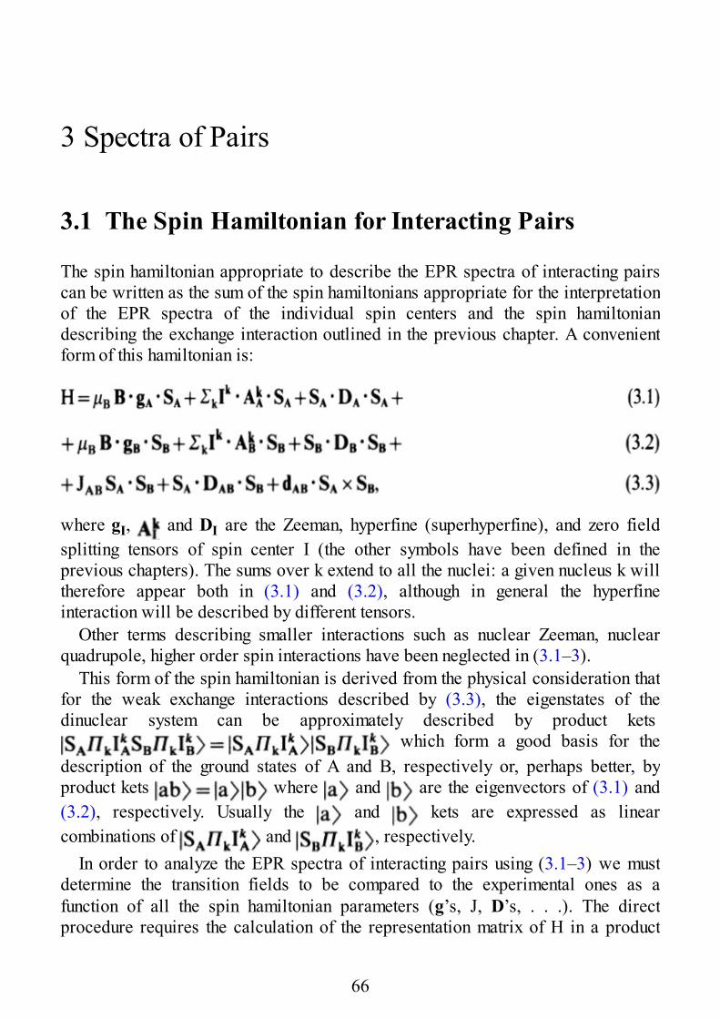
3 Spectra of Pairs

3.1 The Spin Hamiltonian for Interacting Pairs

The spin hamiltonian appropriate to describe the EPR spectra of interacting pairscan be written as the sum of the spin hamiltonians appropriate for the interpretationof the EPR spectra of the individual spin centers and the spin hamiltoniandescribing the exchange interaction outlined in the previous chapter. A convenientform of this hamiltonian is:

where gI, and DI are the Zeeman, hyperfine (superhyperfine), and zero fieldsplitting tensors of spin center I (the other symbols have been defined in theprevious chapters). The sums over k extend to all the nuclei: a given nucleus k willtherefore appear both in (3.1) and (3.2), although in general the hyperfineinteraction will be described by different tensors.

Other terms describing smaller interactions such as nuclear Zeeman, nuclearquadrupole, higher order spin interactions have been neglected in (3.1–3).

This form of the spin hamiltonian is derived from the physical consideration thatfor the weak exchange interactions described by (3.3), the eigenstates of thedinuclear system can be approximately described by product kets

which form a good basis for thedescription of the ground states of A and B, respectively or, perhaps better, byproduct kets where and are the eigenvectors of (3.1) and(3.2), respectively. Usually the and kets are expressed as linearcombinations of and , respectively.

In order to analyze the EPR spectra of interacting pairs using (3.1–3) we mustdetermine the transition fields to be compared to the experimental ones as afunction of all the spin hamiltonian parameters (g’s, J, D’s, . . .). The directprocedure requires the calculation of the representation matrix of H in a product

66

basis . By direct diagonalization of this matrix weobtain the eigenvalues and eigenvectors corresponding to a given set of spinhamiltonian parameters and for a fixed value of the magnetic field from which it ispossible to compute the transition frequencies and intensities. The whole proceduremust then be repeated by varying the spin hamiltonian parameters until a reasonableagreement is obtained between the computed and observed transition frequencies. Itis apparent that even neglecting hyperfine coupling this procedure requires longcomputer time.

Another possible approach is the so-called eigenfield method [3.1–2], whichgives the resonance fields for each setting of the spin hamiltonian parameters assolutions of a generalized eigenvalue equation. The solution of this equationrequires the diagonalization of an N2 matrix. Since the computer time needed formatrix diagonalization increases roughly as (N2)3, the eigenfield method becomesunworkable as N increases. It seems therefore appropriate to look for approximatesolutions which are valid in some limit cases and to reserve the accuratecalculations only for desperate situations in which the approximate methods cannotbe applied. Furthermore, the approximate methods often allow one to obtainanalytical solutions which greatly help experimentalists in rationalizing the EPRspectra.

The most common approximation is to consider the isotropic exchange as theleading term in (3.1–3). JAB can actually take any value usually ranging from a fewwave numbers to hundreds of wave numbers both in transition metal complexes orin radical ion pairs. For normal operating frequencies the Zeeman energy is in therange 0.3–1.2 cm−1, hyperfine interactions are normally much smaller than this, andanisotropic exchange for orbitally nondegenerate states hardly exceeds 1 cm−1,usually being much smaller. The single ion zero field splitting can be fairly large incouples involving transition metal ions even in the case of orbitally nondegenerateground states. For instance, the zero field splitting measured in octahedral high spinnickel(II) or tetrahedral high spin cobalt(II) complexes is in the range 100−101 cm−1

[3.3].In the following we will solve first the hamiltonian (3.1–3) assuming that JAB is

larger than all the other terms in the spin hamiltonian (strong exchange limit). Laterwe will show how to extend the formalism in the case of small JAB values (weakexchange limit) and in the last section of this chapter we will present solutions insome limiting cases in which anisotropic interactions, including single ion zerofield splitting, are considerably larger than the other terms in the spin hamiltonian.

3.2 Spin Levels in the Strong Exchange Limit

67

In the strong exchange limit we consider the effect of the other operators in (3.1–3)as a perturbation on the eigenvalues of JABSA · SB. Since the z component, Sz, ofthe total spin operator S = SA + SB and S2 = S · S commute with JABSA · SB, theeigenstates of S2, with eigenvalues S(S + 1), and of Sz, with eigenvalues – S ≤ M ≤S, are also eigenstates of JABSA · SB. The total spin quantum numbers, S, whichfollow the vector addition relation

and the M values can be used to label the energy levels of JABSA · SB. Theisotropic exchange interaction removes the degeneracy of the eigenvalues of S2 andoriginates a number of states whose energies are given by

each state being (2S+ 1)-fold degenerate. The energy differences between adjacentstates are:

The energy levels arising from the exchange interaction between two differentpairs, one with SA = SB = 1/2 and the other with SA = SB = 5/2, are shown in Fig.3.1.

Sz and S2 do not form a complete set of commuting observables and and must be added to complete the set. Any eigenvalue of JABSA · SB should thus bewritten as . In the following we will generally omit the SA and SBlabels when there is no ambiguity on the spin states SA and SB. The statescan be easily built in the product space according to

68

Fig. 3.1. Energy levels arising from the exchange interaction between two spins 1/2 (left) and 5/2 (right). Thelevels are labeled according to the total spin quantum number S

where are the vector coupling or Clebsch–Gordancoefficients relative to the coupling of the S1 and S2 vector operators. They aredefined in Appendix B.

In the strong isotropic exchange limit the energy separation between adjacentlevels given by (3.6) will be assumed to be much larger than hν and no directtransition between states of different S will be observable. The EPR spectra arejust the superposition of the spectra observed for the different total spin stateswhich are thermally populated at the temperature of the experiment. The spectra canthus be phenomenologically described by one or more S spin hamiltonians of theform

instead of (3.1–3). It is now our purpose to show how gs, Ds, and can be

69

expressed as linear combinations of the individual spin centers and exchange spinhamiltonian parameters appearing in (3.1–3). The reader who is not interested inthe derivation can skip the next pages and pass directly to the results which aregiven in (3.20–23).

It is convenient to transform the spin hamiltonian (3.1–3) by substituting

for SA and SB in (3.1–3). This procedure [3.4] gives:

where (3.11) and (3.12) are the Zeeman, individual spin center zero field splittingand hyperfine terms, (3.13) contains the isotropic and anisotropic terms, and (3.14)contains the antisymmetric terms. In (3.11) g± = gA±gB and D± = DA±DB. In thefollowing we will not explicitly consider the antisymmetric term whose effect onthe energy levels will be discussed at the end of the section.

In order to set up the matrix representation of (3.11–14) on the basiswe note that all the operators containing S have nonzero matrix elements onlywithin an S manifold, or , where f(S)is any operator containing S, while matrix elements of operators containing V obeythe selection rules ∆S = 0,±1,±2. Instead of using the cartesian components, Tij(i, j= x, y, z), of the various tensors and tensor operators appearing in (3.11–14), wewill adopt in the following their irreducible tensor components, Tkq(k = 0, 1, 2; – k≤ q ≤ k), i.e., those components which span the irreducible representations of thereal orthogonal rotation group SO(3) [3.5]. Tensors (tensor operators) expressed inthis form are called irreducible tensors (tensor operators) and their components areeasily expressed as linear combinations of cartesian components as shown in Table3.1 for zero-, first-, and second-rank tensors (tensor operators). Since irreducibletensor operators can be defined on different operator variables, it is necessary tospecify the type of variable, and this is done by including it in parentheses.

The irreducible tensor operators have the following properties:

70

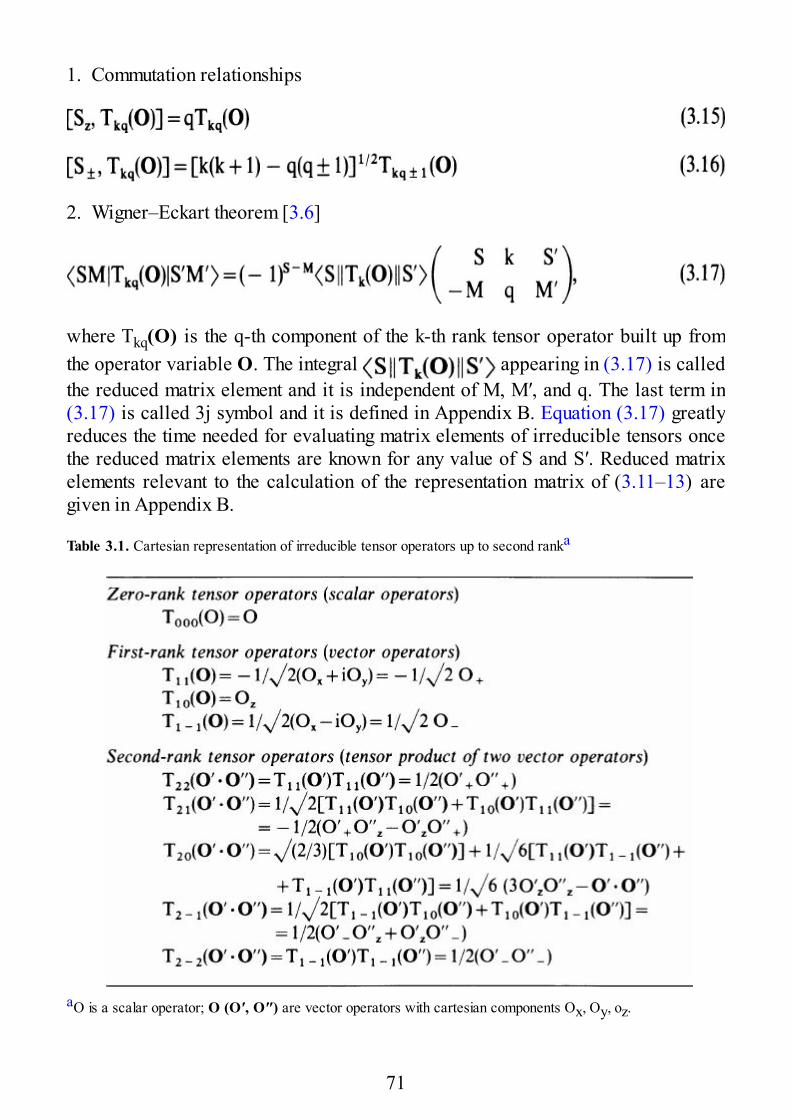
1. Commutation relationships

2. Wigner–Eckart theorem [3.6]

where Tkq(O) is the q-th component of the k-th rank tensor operator built up fromthe operator variable O. The integral appearing in (3.17) is calledthe reduced matrix element and it is independent of M, M′, and q. The last term in(3.17) is called 3j symbol and it is defined in Appendix B. Equation (3.17) greatlyreduces the time needed for evaluating matrix elements of irreducible tensors oncethe reduced matrix elements are known for any value of S and S′. Reduced matrixelements relevant to the calculation of the representation matrix of (3.11–13) aregiven in Appendix B.

Table 3.1. Cartesian representation of irreducible tensor operators up to second ranka

aO is a scalar operator; O (O′, O″) are vector operators with cartesian components Ox, Oy, oz.

71

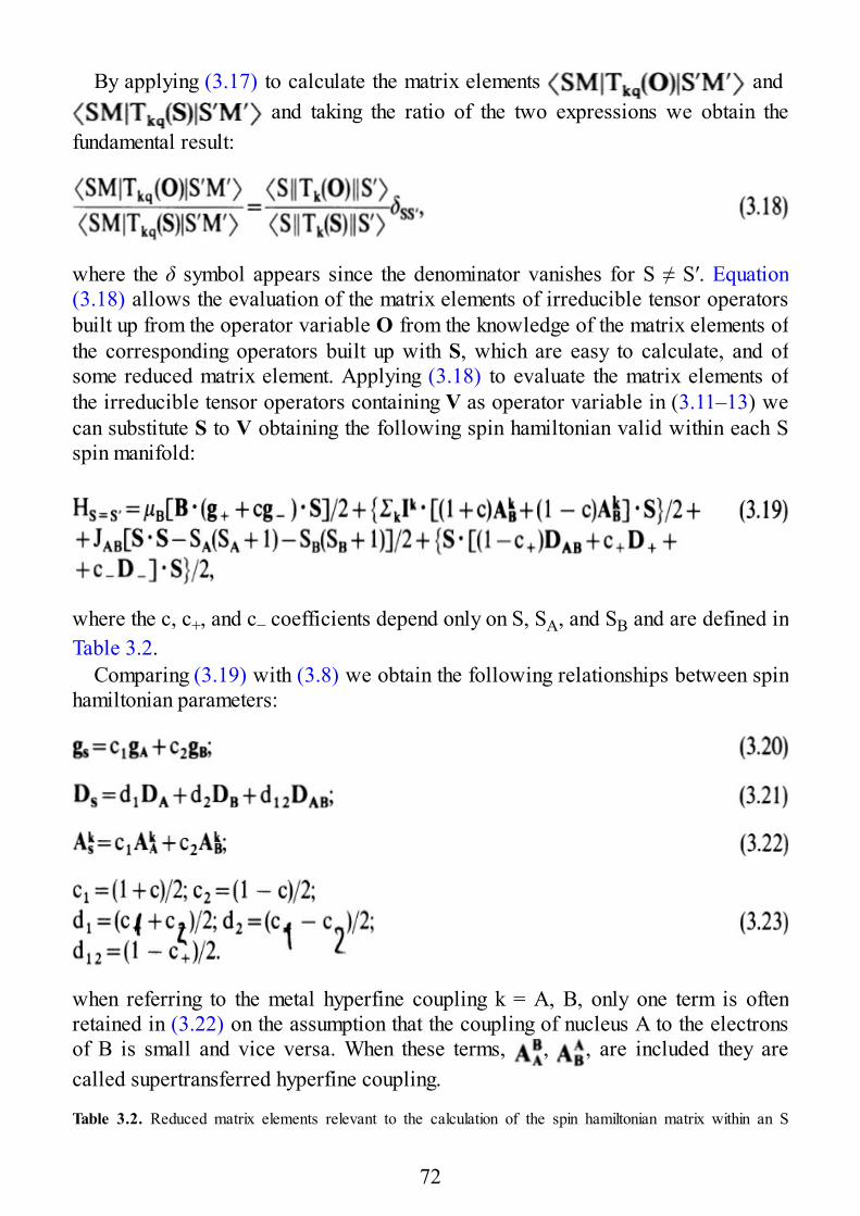
By applying (3.17) to calculate the matrix elements and and taking the ratio of the two expressions we obtain the

fundamental result:

where the δ symbol appears since the denominator vanishes for S ≠ S′. Equation(3.18) allows the evaluation of the matrix elements of irreducible tensor operatorsbuilt up from the operator variable O from the knowledge of the matrix elements ofthe corresponding operators built up with S, which are easy to calculate, and ofsome reduced matrix element. Applying (3.18) to evaluate the matrix elements ofthe irreducible tensor operators containing V as operator variable in (3.11–13) wecan substitute S to V obtaining the following spin hamiltonian valid within each Sspin manifold:

where the c, c+, and c− coefficients depend only on S, SA, and SB and are defined inTable 3.2.

Comparing (3.19) with (3.8) we obtain the following relationships between spinhamiltonian parameters:

when referring to the metal hyperfine coupling k = A, B, only one term is oftenretained in (3.22) on the assumption that the coupling of nucleus A to the electronsof B is small and vice versa. When these terms, , , are included they arecalled supertransferred hyperfine coupling.

Table 3.2. Reduced matrix elements relevant to the calculation of the spin hamiltonian matrix within an S

72

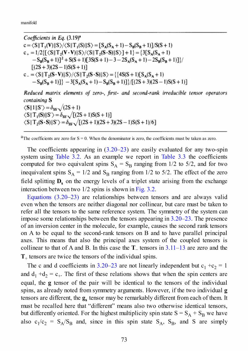
manifold

aThe coefficients are zero for S = 0. When the denominator is zero, the coefficients must be taken as zero.

The coefficients appearing in (3.20–23) are easily evaluated for any two-spinsystem using Table 3.2. As an example we report in Table 3.3 the coefficientscomputed for two equivalent spins SA = SB ranging from 1/2 to 5/2, and for twoinequivalent spins SA = 1/2 and SB ranging from 1/2 to 5/2. The effect of the zerofield splitting Ds on the energy levels of a triplet state arising from the exchangeinteraction between two 1/2 spins is shown in Fig. 3.2.

Equations (3.20–23) are relationships between tensors and are always valideven when the tensors are neither diagonal nor collinear, but care must be taken torefer all the tensors to the same reference system. The symmetry of the system canimpose some relationships between the tensors appearing in 3.20–23. The presenceof an inversion center in the molecule, for example, causes the second rank tensorson A to be equal to the second-rank tensors on B and to have parallel principalaxes. This means that also the principal axes system of the coupled tensors iscollinear to that of A and B. In this case the T− tensors in 3.11–13 are zero and theT+ tensors are twice the tensors of the individual spins.

The c and d coefficients in 3.20–23 are not linearly independent but c1 +c2 = 1and d1 +d2 = c+. The first of these relations shows that when the spin centers areequal, the g tensor of the pair will be identical to the tensors of the individualspins, as already noted from symmetry arguments. However, if the two individual gtensors are different, the gs tensor may be remarkably different from each of them. Itmust be recalled here that “different” means also two otherwise identical tensors,but differently oriented. For the highest multiplicity spin state S = SA + SB we havealso c1/c2 = SA/SB and, since in this spin state SA, SB, and S are simply

73

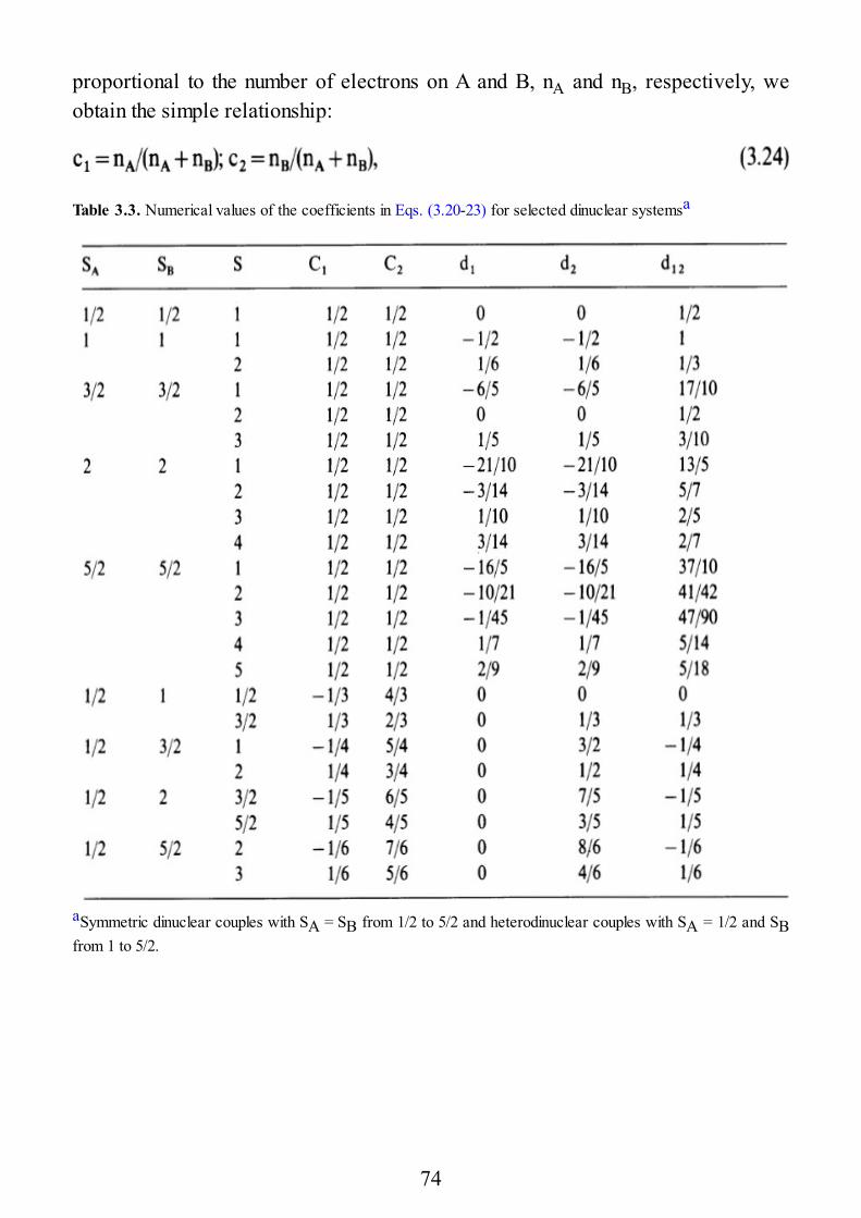
proportional to the number of electrons on A and B, nA and nB, respectively, weobtain the simple relationship:

Table 3.3. Numerical values of the coefficients in Eqs. (3.20-23) for selected dinuclear systemsa

aSymmetric dinuclear couples with SA = SB from 1/2 to 5/2 and heterodinuclear couples with SA = 1/2 and SBfrom 1 to 5/2.

74

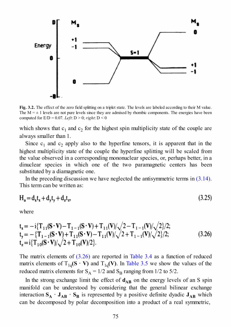
Fig. 3.2. The effect of the zero field splitting on a triplet state. The levels are labeled according to their M value.The M = ± 1 levels are not pure levels since they are admixed by rhombic components. The energies have beencomputed for E/D = 0.07. Left: D > 0; right: D < 0

which shows that c1 and c2 for the highest spin multiplicity state of the couple arealways smaller than 1.

Since c1 and c2 apply also to the hyperfine tensors, it is apparent that in thehighest multiplicity state of the couple the hyperfine splitting will be scaled fromthe value observed in a corresponding mononuclear species, or, perhaps better, in adinuclear species in which one of the two paramagnetic centers has beensubstituted by a diamagnetic one.

In the preceding discussion we have neglected the antisymmetric terms in (3.14).This term can be written as:

where

The matrix elements of (3.26) are reported in Table 3.4 as a function of reducedmatrix elements of T1q(S · V) and T1q(V). In Table 3.5 we show the values of thereduced matrix elements for SA = 1/2 and SB ranging from 1/2 to 5/2.

In the strong exchange limit the effect of dAB on the energy levels of an S spinmanifold can be understood by considering that the general bilinear exchangeinteraction SA · JAB · SB is represented by a positive definite dyadic JAB whichcan be decomposed by polar decomposition into a product of a real symmetric,

75

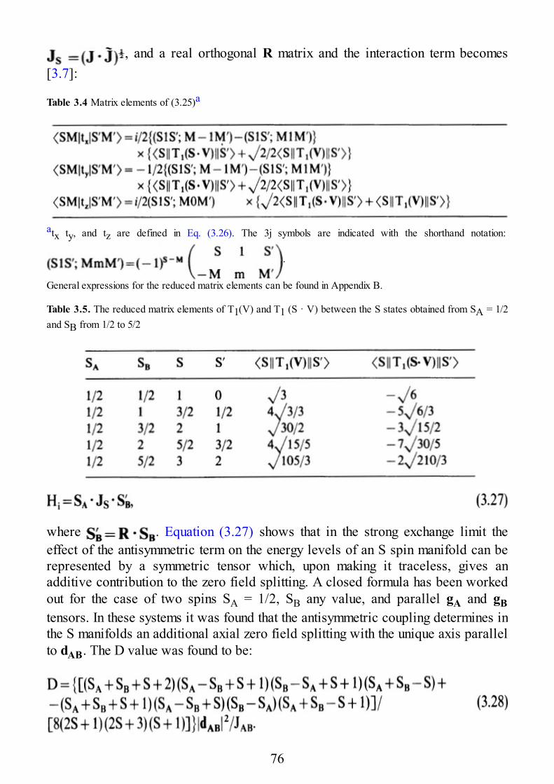
, and a real orthogonal R matrix and the interaction term becomes[3.7]:

Table 3.4 Matrix elements of (3.25)a

atx ty, and tz are defined in Eq. (3.26). The 3j symbols are indicated with the shorthand notation:

.

General expressions for the reduced matrix elements can be found in Appendix B.

Table 3.5. The reduced matrix elements of T1(V) and T1 (S · V) between the S states obtained from SA = 1/2and SB from 1/2 to 5/2

where . Equation (3.27) shows that in the strong exchange limit theeffect of the antisymmetric term on the energy levels of an S spin manifold can berepresented by a symmetric tensor which, upon making it traceless, gives anadditive contribution to the zero field splitting. A closed formula has been workedout for the case of two spins SA = 1/2, SB any value, and parallel gA and gBtensors. In these systems it was found that the antisymmetric coupling determines inthe S manifolds an additional axial zero field splitting with the unique axis parallelto dAB. The D value was found to be:

76

It must be remembered now that this is the effect on the energy levels only. Infact, since (3.25) admixes states with it affects the transition intensitiesof the EPR spectra as well as the angular variation of the line widths. In general, itwill be difficult to recognize these effects on the EPR spectra and then it will bepossible to measure the antisymmetric dAB vector from (3.28) only if we can safelyestimate all the other contributions to the zero field splitting both in value and inspace orientation. The symmetry of the molecule imposes severe conditions on theantisymmetric exchange term as already elucidated in Chap. 2 and can be of help insolving this problem.

3.3 Spectra of Pairs in the Strong Exchange Limit

Spectra of pairs in the strong exchange limit are generally formed by one or morespectra arising by the spin multiplets which are thermally populated at thetemperature of the experiment [3.8]. The theory which is therefore needed tointerpret the spectra of pairs in the strong exchange limit is essentially the theoryused to interpret the EPR spectra of S ≥ l/2 spin systems [3.3]. It must be mentionedthat often spin states as rare as S = 3 or higher can arise from the exchangeinteraction, which are not commonly observed in simple systems.

Some further complications must, however, be expected since: (1) the spectra ata given temperature can be a superposition of spectra arising from differentmultiplets; (2) the g and D tensors will in general be diagonal in different referenceframes. The first point generally requires that the EPR spectra are recorded atdifferent temperatures, in order to individuate which signal belongs to which spinstate. The total intensity of the signals arising from a given multiplet is temperature-dependent according to the Boltzmann law:

where Z is the partition function

and k is the Boltzmann constant. The temperature dependence of Is for the statesarising from the coupling between two SA = SB = 5/2 spins is shown in Fig. 3.3. Bymeasuring the dependence of the signal intensity of the EPR spectra it is inprinciple possible to determine the relative energies of the thermally populatedlevels. This procedure has been used several times in the literature, but the resultsare generally less accurate than those obtained from the measurement of thetemperature variation of the bulk magnetic susceptibility, mainly due to

77

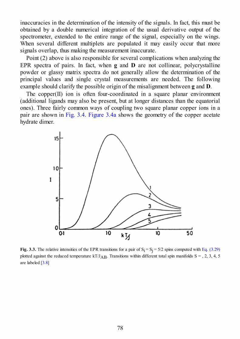
inaccuracies in the determination of the intensity of the signals. In fact, this must beobtained by a double numerical integration of the usual derivative output of thespectrometer, extended to the entire range of the signal, especially on the wings.When several different multiplets are populated it may easily occur that moresignals overlap, thus making the measurement inaccurate.

Point (2) above is also responsible for several complications when analyzing theEPR spectra of pairs. In fact, when g and D are not collinear, polycrystallinepowder or glassy matrix spectra do not generally allow the determination of theprincipal values and single crystal measurements are needed. The followingexample should clarify the possible origin of the misalignment between g and D.

The copper(II) ion is often four-coordinated in a square planar environment(additional ligands may also be present, but at longer distances than the equatorialones). Three fairly common ways of coupling two square planar copper ions in apair are shown in Fig. 3.4. Figure 3.4a shows the geometry of the copper acetatehydrate dimer.

Fig. 3.3. The relative intensities of the EPR transitions for a pair of Si = Sj = 5/2 spins computed with Eq. (3.29)plotted against the reduced temperature kT/JAB. Transitions within different total spin manifolds S = , 2, 3, 4, 5are labeled [3.8]

78

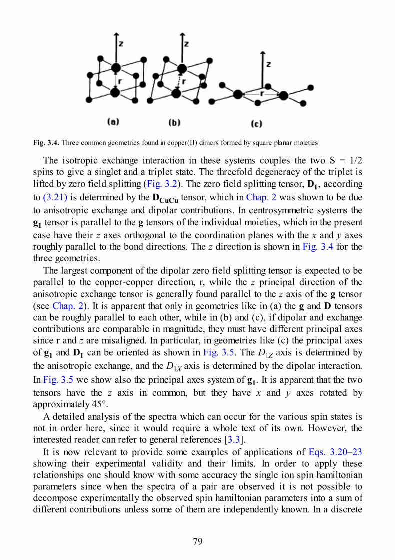
Fig. 3.4. Three common geometries found in copper(II) dimers formed by square planar moieties

The isotropic exchange interaction in these systems couples the two S = 1/2spins to give a singlet and a triplet state. The threefold degeneracy of the triplet islifted by zero field splitting (Fig. 3.2). The zero field splitting tensor, D1, accordingto (3.21) is determined by the DCuCu tensor, which in Chap. 2 was shown to be dueto anisotropic exchange and dipolar contributions. In centrosymmetric systems theg1 tensor is parallel to the g tensors of the individual moieties, which in the presentcase have their z axes orthogonal to the coordination planes with the x and y axesroughly parallel to the bond directions. The z direction is shown in Fig. 3.4 for thethree geometries.

The largest component of the dipolar zero field splitting tensor is expected to beparallel to the copper-copper direction, r, while the z principal direction of theanisotropic exchange tensor is generally found parallel to the z axis of the g tensor(see Chap. 2). It is apparent that only in geometries like in (a) the g and D tensorscan be roughly parallel to each other, while in (b) and (c), if dipolar and exchangecontributions are comparable in magnitude, they must have different principal axessince r and z are misaligned. In particular, in geometries like (c) the principal axesof g1 and D1 can be oriented as shown in Fig. 3.5. The D1Z axis is determined bythe anisotropic exchange, and the D1X axis is determined by the dipolar interaction.In Fig. 3.5 we show also the principal axes system of g1. It is apparent that the twotensors have the z axis in common, but they have x and y axes rotated byapproximately 45°.

A detailed analysis of the spectra which can occur for the various spin states isnot in order here, since it would require a whole text of its own. However, theinterested reader can refer to general references [3.3].

It is now relevant to provide some examples of applications of Eqs. 3.20–23showing their experimental validity and their limits. In order to apply theserelationships one should know with some accuracy the single ion spin hamiltonianparameters since when the spectra of a pair are observed it is not possible todecompose experimentally the observed spin hamiltonian parameters into a sum ofdifferent contributions unless some of them are independently known. In a discrete

79

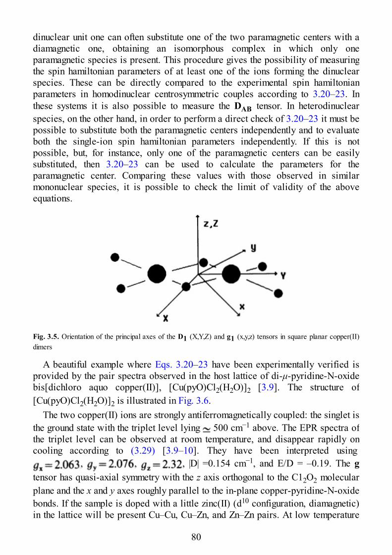
dinuclear unit one can often substitute one of the two paramagnetic centers with adiamagnetic one, obtaining an isomorphous complex in which only oneparamagnetic species is present. This procedure gives the possibility of measuringthe spin hamiltonian parameters of at least one of the ions forming the dinuclearspecies. These can be directly compared to the experimental spin hamiltonianparameters in homodinuclear centrosymmetric couples according to 3.20–23. Inthese systems it is also possible to measure the DAB tensor. In heterodinuclearspecies, on the other hand, in order to perform a direct check of 3.20–23 it must bepossible to substitute both the paramagnetic centers independently and to evaluateboth the single-ion spin hamiltonian parameters independently. If this is notpossible, but, for instance, only one of the paramagnetic centers can be easilysubstituted, then 3.20–23 can be used to calculate the parameters for theparamagnetic center. Comparing these values with those observed in similarmononuclear species, it is possible to check the limit of validity of the aboveequations.

Fig. 3.5. Orientation of the principal axes of the D1 (X,Y,Z) and g1 (x,y,z) tensors in square planar copper(II)dimers

A beautiful example where Eqs. 3.20–23 have been experimentally verified isprovided by the pair spectra observed in the host lattice of di-μ-pyridine-N-oxidebis[dichloro aquo copper(II)], [Cu(pyO)Cl2(H2O)]2 [3.9]. The structure of[Cu(pyO)Cl2(H2O)]2 is illustrated in Fig. 3.6.

The two copper(II) ions are strongly antiferromagnetically coupled: the singlet isthe ground state with the triplet level lying 500 cm−1 above. The EPR spectra ofthe triplet level can be observed at room temperature, and disappear rapidly oncooling according to (3.29) [3.9–10]. They have been interpreted using

, , , |D| =0.154 cm−1, and E/D = –0.19. The gtensor has quasi-axial symmetry with the z axis orthogonal to the C12O2 molecularplane and the x and y axes roughly parallel to the in-plane copper-pyridine-N-oxidebonds. If the sample is doped with a little zinc(II) (d10 configuration, diamagnetic)in the lattice will be present Cu–Cu, Cu–Zn, and Zn–Zn pairs. At low temperature

80

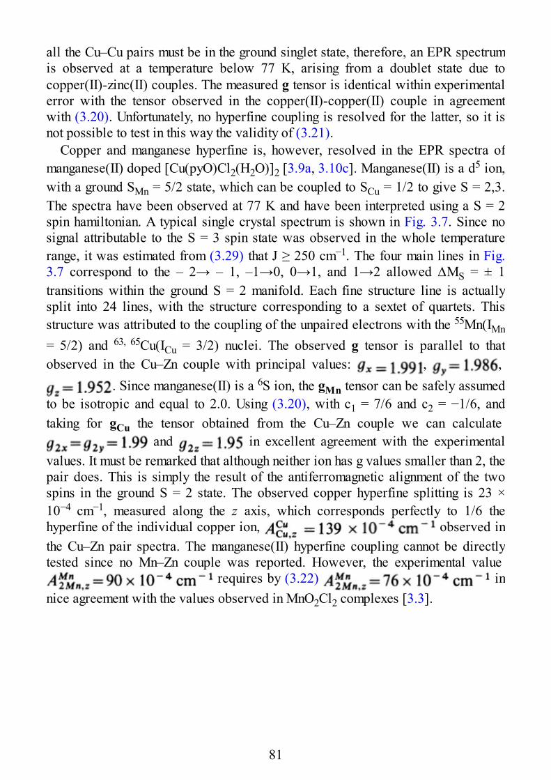
all the Cu–Cu pairs must be in the ground singlet state, therefore, an EPR spectrumis observed at a temperature below 77 K, arising from a doublet state due tocopper(II)-zinc(II) couples. The measured g tensor is identical within experimentalerror with the tensor observed in the copper(II)-copper(II) couple in agreementwith (3.20). Unfortunately, no hyperfine coupling is resolved for the latter, so it isnot possible to test in this way the validity of (3.21).

Copper and manganese hyperfine is, however, resolved in the EPR spectra ofmanganese(II) doped [Cu(pyO)Cl2(H2O)]2 [3.9a, 3.10c]. Manganese(II) is a d5 ion,with a ground SMn = 5/2 state, which can be coupled to SCu = 1/2 to give S = 2,3.The spectra have been observed at 77 K and have been interpreted using a S = 2spin hamiltonian. A typical single crystal spectrum is shown in Fig. 3.7. Since nosignal attributable to the S = 3 spin state was observed in the whole temperaturerange, it was estimated from (3.29) that J ≥ 250 cm−1. The four main lines in Fig.3.7 correspond to the – 2→ – 1, –1→0, 0→1, and 1→2 allowed ∆MS = ± 1transitions within the ground S = 2 manifold. Each fine structure line is actuallysplit into 24 lines, with the structure corresponding to a sextet of quartets. Thisstructure was attributed to the coupling of the unpaired electrons with the 55Mn(IMn

= 5/2) and 63, 65Cu(ICu = 3/2) nuclei. The observed g tensor is parallel to thatobserved in the Cu–Zn couple with principal values: , ,

. Since manganese(II) is a 6S ion, the gMn tensor can be safely assumedto be isotropic and equal to 2.0. Using (3.20), with c1 = 7/6 and c2 = −1/6, andtaking for gCu the tensor obtained from the Cu–Zn couple we can calculate

and in excellent agreement with the experimentalvalues. It must be remarked that although neither ion has g values smaller than 2, thepair does. This is simply the result of the antiferromagnetic alignment of the twospins in the ground S = 2 state. The observed copper hyperfine splitting is 23 ×10−4 cm−1, measured along the z axis, which corresponds perfectly to 1/6 thehyperfine of the individual copper ion, observed inthe Cu–Zn pair spectra. The manganese(II) hyperfine coupling cannot be directlytested since no Mn–Zn couple was reported. However, the experimental value

requires by (3.22) innice agreement with the values observed in MnO2Cl2 complexes [3.3].

81

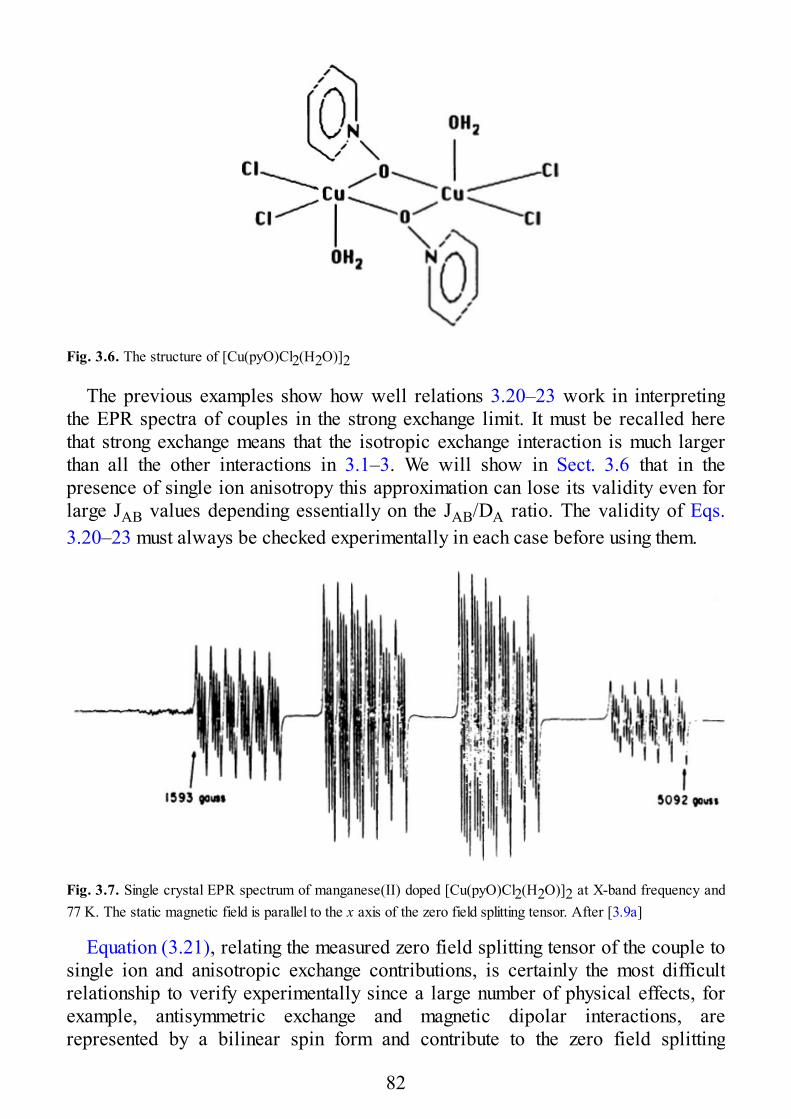
Fig. 3.6. The structure of [Cu(pyO)Cl2(H2O)]2

The previous examples show how well relations 3.20–23 work in interpretingthe EPR spectra of couples in the strong exchange limit. It must be recalled herethat strong exchange means that the isotropic exchange interaction is much largerthan all the other interactions in 3.1–3. We will show in Sect. 3.6 that in thepresence of single ion anisotropy this approximation can lose its validity even forlarge JAB values depending essentially on the JAB/DA ratio. The validity of Eqs.3.20–23 must always be checked experimentally in each case before using them.

Fig. 3.7. Single crystal EPR spectrum of manganese(II) doped [Cu(pyO)Cl2(H2O)]2 at X-band frequency and77 K. The static magnetic field is parallel to the x axis of the zero field splitting tensor. After [3.9a]

Equation (3.21), relating the measured zero field splitting tensor of the couple tosingle ion and anisotropic exchange contributions, is certainly the most difficultrelationship to verify experimentally since a large number of physical effects, forexample, antisymmetric exchange and magnetic dipolar interactions, arerepresented by a bilinear spin form and contribute to the zero field splitting

82

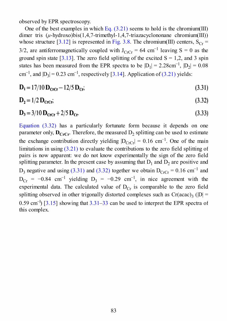
observed by EPR spectroscopy.One of the best examples in which Eq. (3.21) seems to hold is the chromium(III)

dimer tris (μ-hydroxo)bis(1,4,7-trimethyl-1,4,7-triazacyclononane chromium(III))whose structure [3.12] is represented in Fig. 3.8. The chromium(III) centers, SCr =3/2, are antiferromagnetically coupled with JCrCr = 64 cm−1 leaving S = 0 as theground spin state [3.13]. The zero field splitting of the excited S = 1,2, and 3 spinstates has been measured from the EPR spectra to be |D1| = 2.28cm−1, |D2| = 0.08cm−1, and |D3| = 0.23 cm−1, respectively [3.14]. Application of (3.21) yields:

Equation (3.32) has a particularly fortunate form because it depends on oneparameter only, DCrCr. Therefore, the measured D2 splitting can be used to estimatethe exchange contribution directly yielding |DCrCr| = 0.16 cm−1. One of the mainlimitations in using (3.21) to evaluate the contributions to the zero field splitting ofpairs is now apparent: we do not know experimentally the sign of the zero fieldsplitting parameter. In the present case by assuming that D1 and D2 are positive andD3 negative and using (3.31) and (3.32) together we obtain DCrCr = 0.16 cm−1 andDCr = −0.84 cm−1 yielding D3 = −0.29 cm−1, in nice agreement with theexperimental data. The calculated value of DCr is comparable to the zero fieldsplitting observed in other trigonally distorted complexes such as Cr(acac)3 (|D| =0.59 cm−l) [3.15] showing that 3.31–33 can be used to interpret the EPR spectra ofthis complex.

83

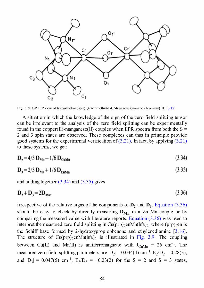
Fig. 3.8. ORTEP view of tris(μ-hydroxo)bis(1,4,7-trimethyl-1,4,7-triazacyclononane chromium(III) [3.12]

A situation in which the knowledge of the sign of the zero field splitting tensorcan be irrelevant to the analysis of the zero field splitting can be experimentallyfound in the copper(II)-manganese(II) couples when EPR spectra from both the S =2 and 3 spin states are observed. These complexes can thus in principle providegood systems for the experimental verification of (3.21). In fact, by applying (3.21)to these systems, we get:

and adding together (3.34) and (3.35) gives

irrespective of the relative signs of the components of D2 and D3. Equation (3.36)should be easy to check by directly measuring DMn in a Zn–Mn couple or bycomparing the measured value with literature reports. Equation (3.36) was used tointerpret the measured zero field splitting in Cu(prp)2enMn(hfa)2, where (prp)2en isthe Schiff base formed by 2-hydroxypropiophenone and ethylenediamine [3.16].The structure of Cu(prp)2enMn(hfa)2 is illustrated in Fig. 3.9. The couplingbetween Cu(II) and Mn(II) is antiferromagnetic with JCuMn = 26 cm−1. Themeasured zero field splitting parameters are |D2| = 0.034(4) cm−1, E2/D2 = 0.28(3),and |D3| = 0.047(5) cm−1, E3/D3 = −0.23(2) for the S = 2 and S = 3 states,

84

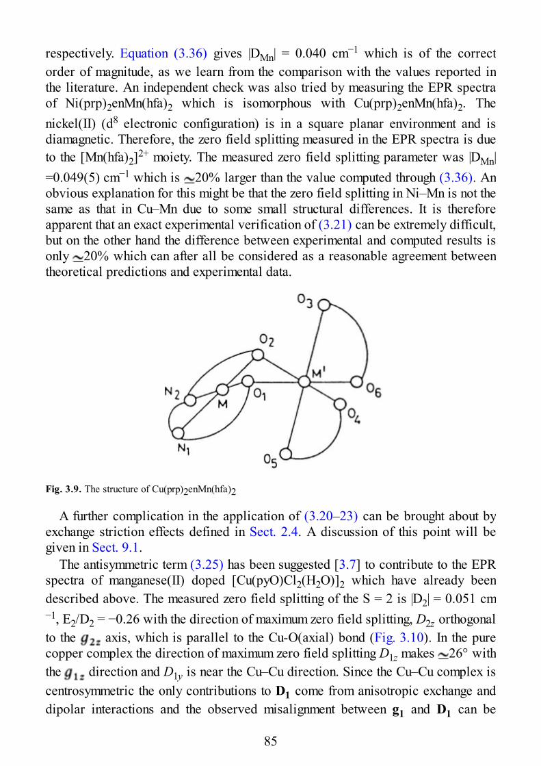
respectively. Equation (3.36) gives |DMn| = 0.040 cm−1 which is of the correctorder of magnitude, as we learn from the comparison with the values reported inthe literature. An independent check was also tried by measuring the EPR spectraof Ni(prp)2enMn(hfa)2 which is isomorphous with Cu(prp)2enMn(hfa)2. Thenickel(II) (d8 electronic configuration) is in a square planar environment and isdiamagnetic. Therefore, the zero field splitting measured in the EPR spectra is dueto the [Mn(hfa)2]2+ moiety. The measured zero field splitting parameter was |DMn|=0.049(5) cm−1 which is 20% larger than the value computed through (3.36). Anobvious explanation for this might be that the zero field splitting in Ni–Mn is not thesame as that in Cu–Mn due to some small structural differences. It is thereforeapparent that an exact experimental verification of (3.21) can be extremely difficult,but on the other hand the difference between experimental and computed results isonly 20% which can after all be considered as a reasonable agreement betweentheoretical predictions and experimental data.

Fig. 3.9. The structure of Cu(prp)2enMn(hfa)2

A further complication in the application of (3.20–23) can be brought about byexchange striction effects defined in Sect. 2.4. A discussion of this point will begiven in Sect. 9.1.

The antisymmetric term (3.25) has been suggested [3.7] to contribute to the EPRspectra of manganese(II) doped [Cu(pyO)Cl2(H2O)]2 which have already beendescribed above. The measured zero field splitting of the S = 2 is |D2| = 0.051 cm−1, E2/D2 = −0.26 with the direction of maximum zero field splitting, D2z orthogonalto the axis, which is parallel to the Cu-O(axial) bond (Fig. 3.10). In the purecopper complex the direction of maximum zero field splitting D1z makes 26° withthe direction and D1y is near the Cu–Cu direction. Since the Cu–Cu complex iscentrosymmetric the only contributions to D1 come from anisotropic exchange anddipolar interactions and the observed misalignment between g1 and D1 can be

85

rationalized by a nondiagonal DCuCu tensor due to the low symmetry of thecomplex. It is apparent that the same explanation does not hold for the Cu–Mncouple. In fact, purely anisotropic exchange interactions would require D2z parallelto , or slightly misaligned from it like in the Cu–Cu couple, while purelydipolar interactions would put D2z parallel to the Cu–Mn direction. Both of theseinteractions cause the D2z to be nearly orthogonal to the observed one. Furthermore,since the exchange contributions to DAB are proportional to and (seeChap. 2), they are expected to be smaller in the Cu–Mn than in the Cu–Cu pairbecause of gMn ge [3.3]. It must be noted that the Cu–Mn couple isnoncentrosymmetric and antisymmetric exchange interactions can be operative.Since the overall symmetry of the complex is not far from Cs, the σ plane includingthe copper(II) and manganese(II) ions and the oxygens of the water molecules, weexpect a dCuMn vector perpendicular to σ. The gMn tensor can be assumed asisotropic so that gCu and gMn are collinear and Eq. (3.28), which expresses theeffect of d on the S = 2 state, can be applied. Using (3.21), (3.28) and the values ofthe coefficients reported in Table 3.3 we can decompose the D2 tensor according to

86

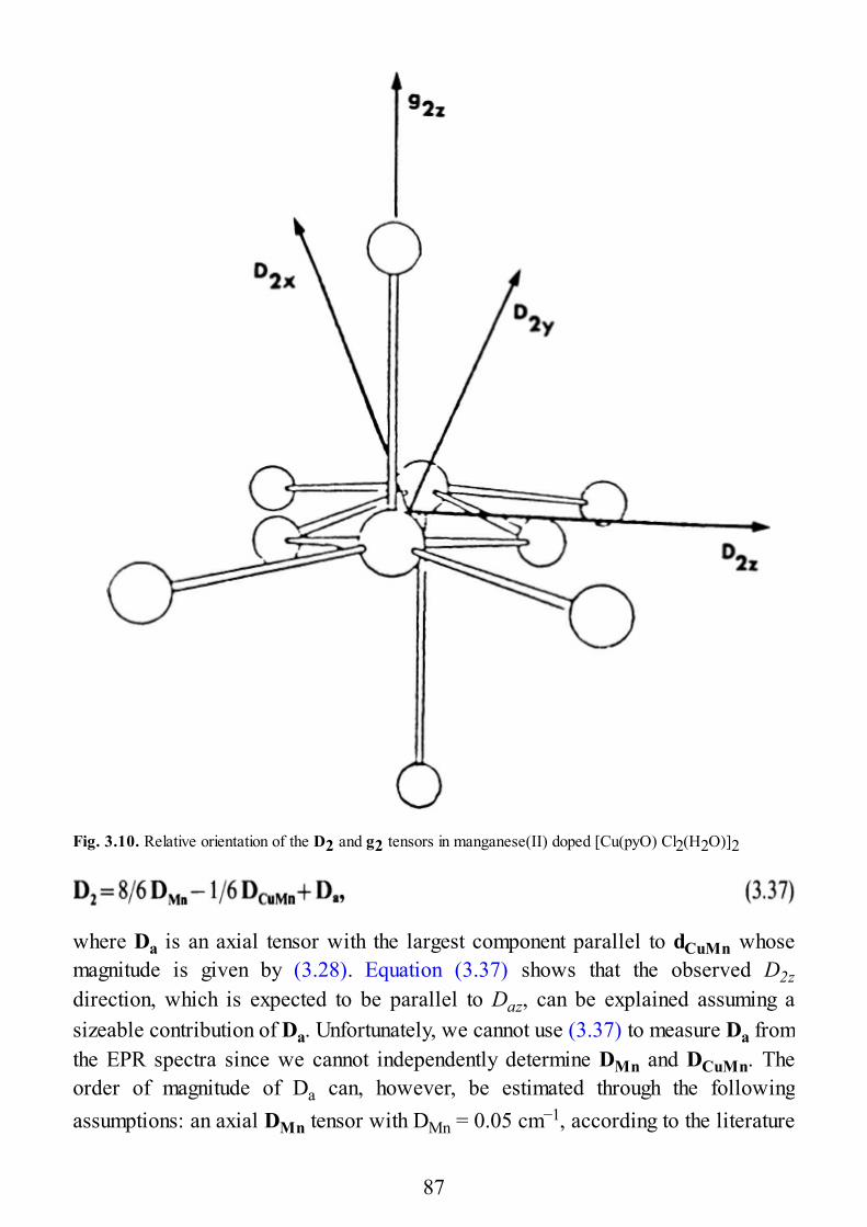
Fig. 3.10. Relative orientation of the D2 and g2 tensors in manganese(II) doped [Cu(pyO) Cl2(H2O)]2

where Da is an axial tensor with the largest component parallel to dCuMn whosemagnitude is given by (3.28). Equation (3.37) shows that the observed D2zdirection, which is expected to be parallel to Daz, can be explained assuming asizeable contribution of Da. Unfortunately, we cannot use (3.37) to measure Da fromthe EPR spectra since we cannot independently determine DMn and DCuMn. Theorder of magnitude of Da can, however, be estimated through the followingassumptions: an axial DMn tensor with DMn = 0.05 cm−1, according to the literature

87

reports; the exchange contribution to DCuMn taken to be the same as in the Cu–Cucouple, which overestimates it; computing the dipolar contribution to DCuMn usingthe Cu–Cu direction seen in the crystal structure. With the above assumptions. Eq.(3.37) gives Da = –0.03 cm−1, Ea/Da = 0, using for Da the sign anticipated from Eq.(3.28), which corresponds to ||dCuMn|2/JcuMn| = 0.48 cm−1.

3.4 Spin Levels in the Weak Exchange Limit

When the assumptions made in Sect 3.2 are no longer valid, the eigenvectors of S2

and Sz do not give a good description of the spin states and correct eigenvalues andeigenvectors must be obtained by diagonalization of the full hamiltonian matrix.The formalism developed in the previous sections can, however, be retained. It issufficient to add to the spin hamiltonian (3.19), which has no nonzero matrixelements within states with different S, the additional terms:

In (3.38–39) we have neglected the antisymmetric term (3.25) for the sake ofsimplicity. By application of the Wigner–Eckart theorem (3.17) one can easilyrecognize the S states which are connected by (3.38–39). In fact, due to thetriangular relationships of the 3j symbols, the first-rank irreducible tensor operatorsin (3.38) and the second-rank irreducible tensor operators in (3.39) can connectonly states with . For couples in which SA = SB a furtherrestriction applies to the matrix elements of the operator S · D _ · V which arenonzero only when . It must be also remembered that when an inversioncenter connects A and B, D _ = 0. General expressions for the matrix elements of(3.38–39) are reported in Appendix B. Some matrix elements of operatorscontaining V have been analytically expressed as a function of SA, SB, S, and S′[3.4] and are reported in Table 3.6.

Perturbation expressions [3.17] have been derived for the eigenvalues and theeigenvectors of a two S = 1/2 spin system when the Zeeman effect is dominant overthe anisotropic terms appearing in (3.19, 3.38–39). This situation has beenexperimentally encountered in a wide variety of spin-labeled transition metalcomplexes containing copper(II), silver(II), and oxovanadium(IV), in titanium(III),copper(II), and oxovanadium(IV) dinuclear complexes in which the metal centersare more than 8 Å apart, as well as in many systems of biological interest like B12-dependent enzyme reactions. In these systems, moreover, anisotropic exchange

88

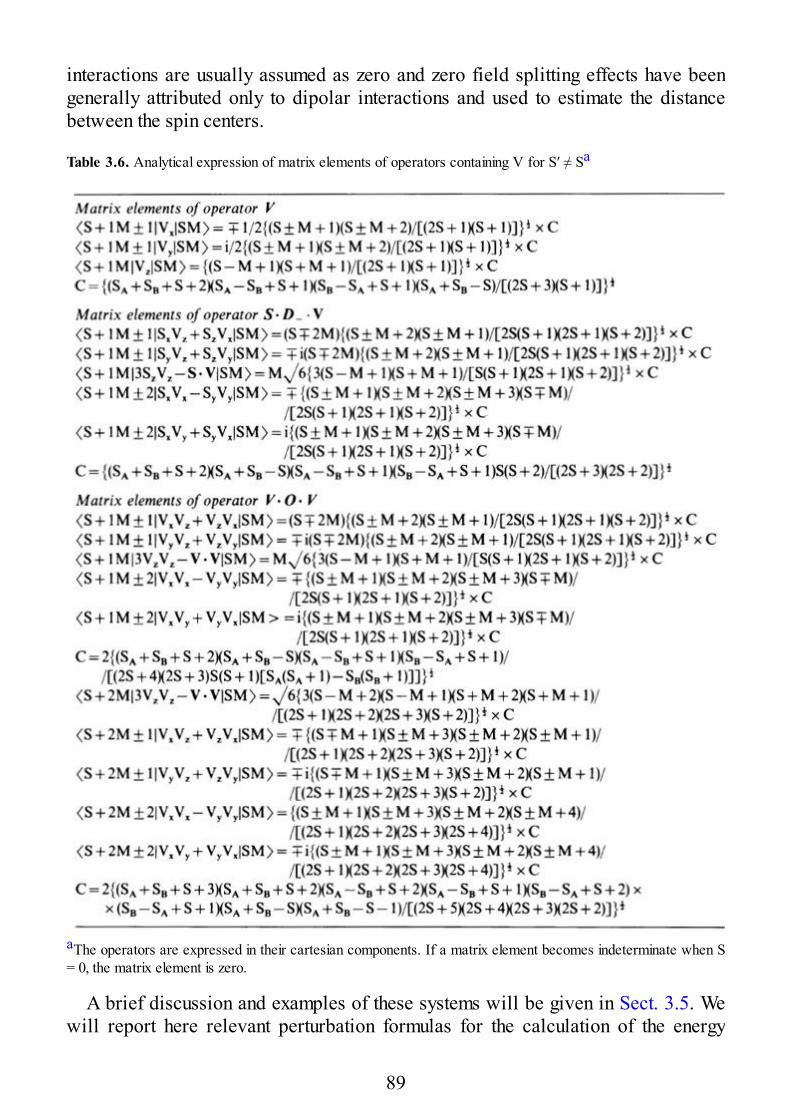
interactions are usually assumed as zero and zero field splitting effects have beengenerally attributed only to dipolar interactions and used to estimate the distancebetween the spin centers.

Table 3.6. Analytical expression of matrix elements of operators containing V for S′ ≠ Sa

aThe operators are expressed in their cartesian components. If a matrix element becomes indeterminate when S= 0, the matrix element is zero.

A brief discussion and examples of these systems will be given in Sect. 3.5. Wewill report here relevant perturbation formulas for the calculation of the energy

89

levels and EPR spectra of a couple of dissimilar centers SA = 1/2 and SB = 1/2. Acomplete treatment of the perturbation procedure can be found in Ref. [3.17a].

The hamiltonian we consider here has the form

In the single ion terms HA and HB we have considered only the hyperfinecoupling with one nucleus. The HAB term has been assumed to contain onlyisotropic exchange and anisotropic effects. These latter effects have been generallyconsidered to be due to the magnetic dipolar interaction between the SA and SBspins. In order to work out a perturbation procedure all the spin hamiltonians mustbe referred to the same axes. It is generally used to refer (3.40–43) to the gAprincipal axes system, (xA, yA, zA). The general orientation of spin B with respectto spin A is shown in Fig. 3.11. In addition to the definition of the A – B distance,rAB, and to the polar angles, ε and η, of the rAB vector one needs to specify thethree Euler angles, α, β, and γ, defining the orientation of the gB principal axes, (xB,yB, zB), with respect to (xA, yA, zA). In general, the gB tensor will not be diagonalin the (xA, yA, zA) reference system. Explicit expressions for the dipolar part of theDAB term , have been given as a function of the principal values of gA and gB,the spin-spin distance rAB, and the angular variables ε, η, α, β, γ. A simpleexpression was derived by Pilbrow using the principal values of the g tensors andthe direction cosines of (xB, yB, zB) and rAB with respect to the (xA, yA, zA) axes:

90

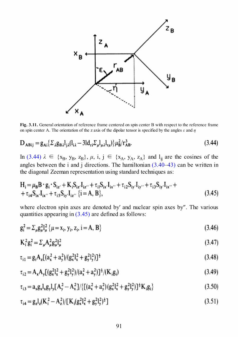
Fig. 3.11. General orientation of reference frame centered on spin center B with respect to the reference frameon spin center A. The orientation of the z axis of the dipolar tensor is specified by the angles ε and η

In (3.44) λ ∈ {xB, yB, zB}, μ, i, j ∈ {xA, yA, zA} and lij are the cosines of theangles between the i and j directions. The hamiltonian (3.40–43) can be written inthe diagonal Zeeman representation using standard techniques as:

where electron spin axes are denoted by′ and nuclear spin axes by″. The variousquantities appearing in (3.45) are defined as follows:

91

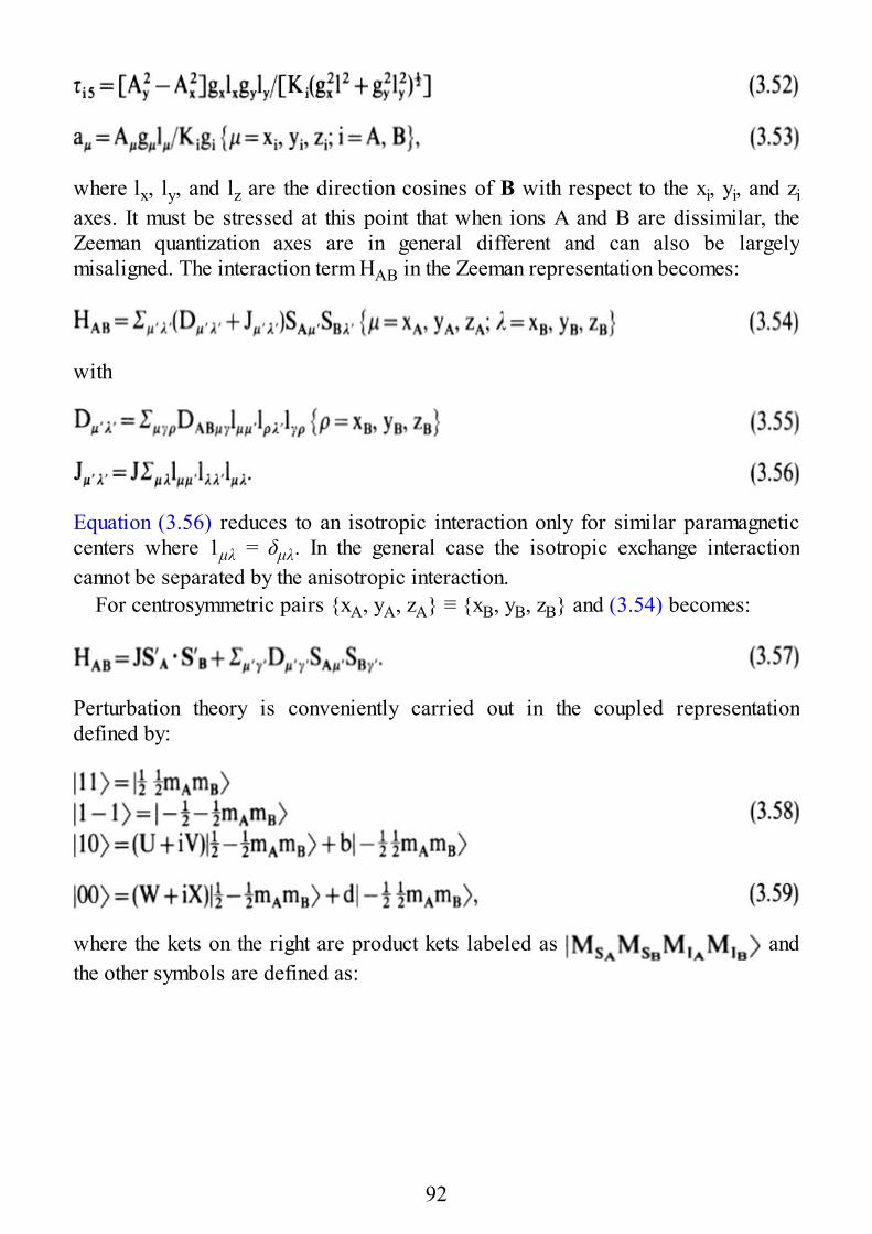
where lx, ly, and lz are the direction cosines of B with respect to the xi, yi, and ziaxes. It must be stressed at this point that when ions A and B are dissimilar, theZeeman quantization axes are in general different and can also be largelymisaligned. The interaction term HAB in the Zeeman representation becomes:

with

Equation (3.56) reduces to an isotropic interaction only for similar paramagneticcenters where 1μλ = δμλ. In the general case the isotropic exchange interactioncannot be separated by the anisotropic interaction.

For centrosymmetric pairs {xA, yA, zA} ≡ {xB, yB, zB} and (3.54) becomes:

Perturbation theory is conveniently carried out in the coupled representationdefined by:

where the kets on the right are product kets labeled as andthe other symbols are defined as:

92

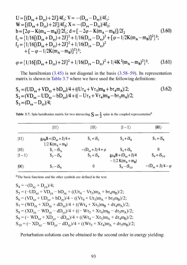
The hamiltonian (3.45) is not diagonal in the basis (3.58–59). Its representationmatrix is shown in Table 3.7 where we have used the following definitions:

Table 3.7. Spin hamiltonian matrix for two interacting spins in the coupled representationa

aThe basis functions and the other symbols are defined in the text.

S4 = −(Dxy + Dyx)/4;S5 = (−UDxz + VDyz − bDzx + ((Uτ4 − Vτ5)mA + bτ4mB)/2;S6 = (VDxz + UDyz + bDzy)/4 − ((Vτ4 + Uτ5)mA + bτ5mB)/2;S7 = (WDzx + XDzy + dDxz)/4 + ((Wτ4 + Xτ5)mB + dτ4mA)/2;S8 = (XDzx − WDzy − dDyz)/4 + ((− Wτ5 + Xτ4)mB − dτ5mA)/2;S9 = (− WDxz + XDyz − dDzx)/4 + ((Wτ4 − Xτ5)mA + dτ4mB)/2;S10 = (− XDxz − WDyz − dDzy)/4 + ((Wτ5 + Xτ4)mA + dτ5mB)/2;

Perturbation solutions can be obtained to the second order in energy yielding:

93

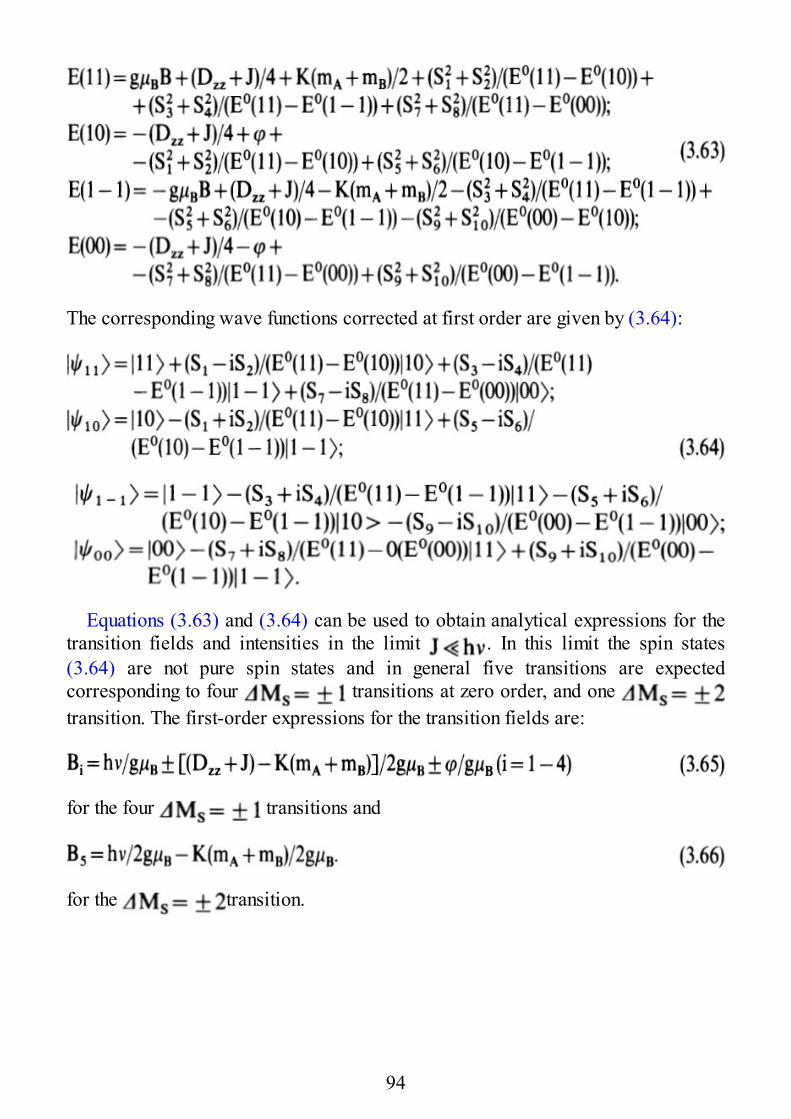
The corresponding wave functions corrected at first order are given by (3.64):

Equations (3.63) and (3.64) can be used to obtain analytical expressions for thetransition fields and intensities in the limit . In this limit the spin states(3.64) are not pure spin states and in general five transitions are expectedcorresponding to four transitions at zero order, and one transition. The first-order expressions for the transition fields are:

for the four transitions and

for the transition.

94

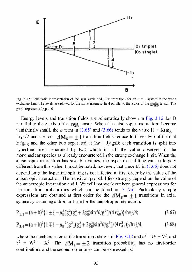
Fig. 3.12. Schematic representation of the spin levels and EPR transitions for an S = 1 system in the weakexchange limit. The levels are plotted for the static magnetic field parallel to the z axis of the tensor. Thegraph represents JAB > 0

Energy levels and transition fields are schematically shown in Fig. 3.12 for Bparallel to the z axis of the tensor. When the anisotropic interactions becomevanishingly small, the φ term in (3.65) and (3.66) tends to the value [J + K(mA −mB)]/2 and the four transition fields reduce to three: two of them athν/gμB and the other two separated at (hν ± J)/gμB; each transition is split intohyperfine lines separated by K/2 which is half the value observed in themononuclear species as already encountered in the strong exchange limit. When theanisotropic interaction has sizeable values, the hyperfine splitting can be largelydifferent from this value. It must be noted, however, that since B5 in (3.66) does notdepend on φ the hyperfine splitting is not affected at first order by the value of theanisotropic interaction. The transition probabilities strongly depend on the value ofthe anisotropic interaction and J. We will not work out here general expressions forthe transition probabilities which can be found in [3.17a]. Particularly simpleexpressions are obtained at first order for the transitions in axialsymmetry assuming a dipolar form for the anisotropic interaction:

where the numbers refer to the transitions shown in Fig. 3.12 and a2 = U2 + V2, andb2 = W2 + X2. The transition probability has no first-ordercontributions and the second-order ones can be expressed as:

95

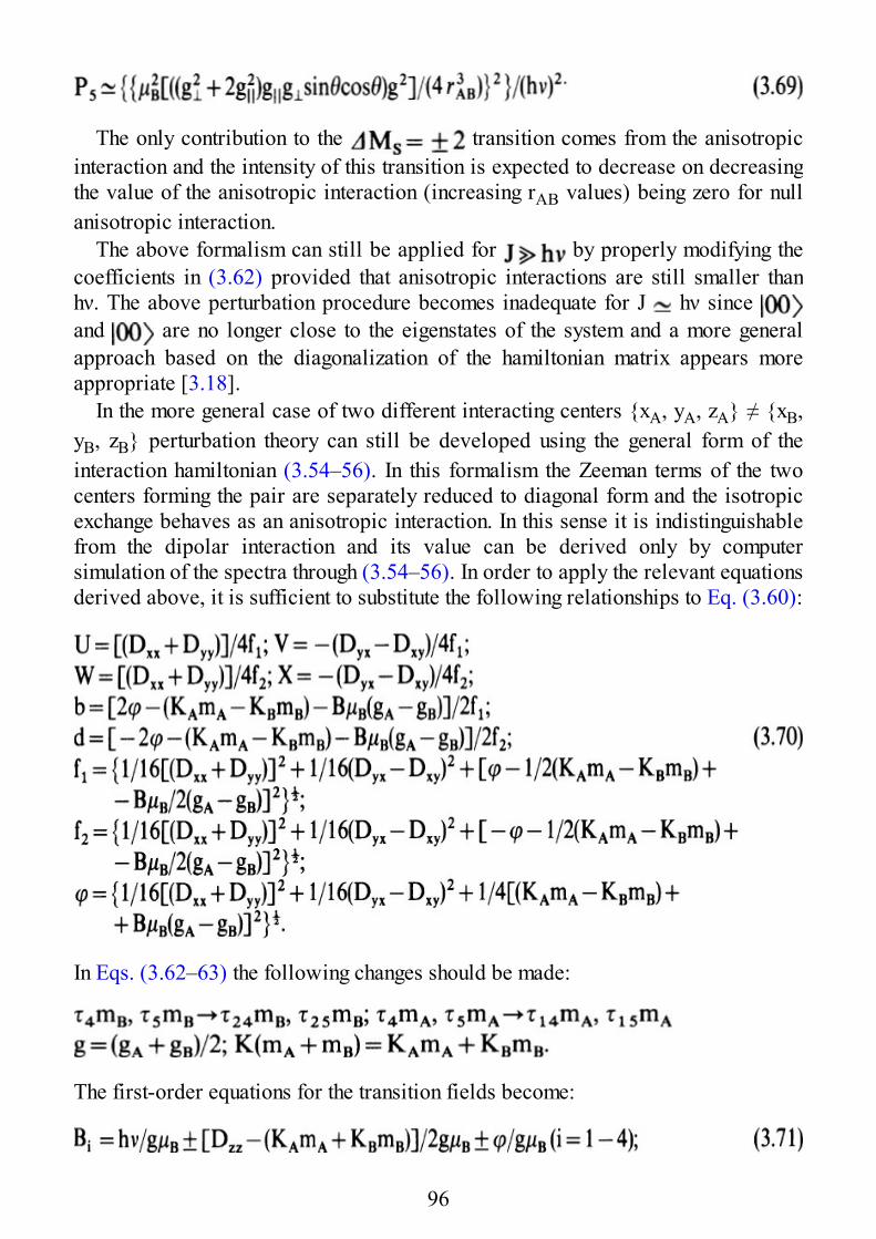
The only contribution to the transition comes from the anisotropicinteraction and the intensity of this transition is expected to decrease on decreasingthe value of the anisotropic interaction (increasing rAB values) being zero for nullanisotropic interaction.

The above formalism can still be applied for by properly modifying thecoefficients in (3.62) provided that anisotropic interactions are still smaller thanhν. The above perturbation procedure becomes inadequate for J hν since and are no longer close to the eigenstates of the system and a more generalapproach based on the diagonalization of the hamiltonian matrix appears moreappropriate [3.18].

In the more general case of two different interacting centers {xA, yA, zA} ≠ {xB,yB, zB} perturbation theory can still be developed using the general form of theinteraction hamiltonian (3.54–56). In this formalism the Zeeman terms of the twocenters forming the pair are separately reduced to diagonal form and the isotropicexchange behaves as an anisotropic interaction. In this sense it is indistinguishablefrom the dipolar interaction and its value can be derived only by computersimulation of the spectra through (3.54–56). In order to apply the relevant equationsderived above, it is sufficient to substitute the following relationships to Eq. (3.60):

In Eqs. (3.62–63) the following changes should be made:

The first-order equations for the transition fields become:

96

In the limit situation of zero exchange and dipolar interactions φ is 1/2[(KAmA −KBmB) + BμB(gA − gB)] and the EPR spectrum consists of two separate resonancesat gA and gB with hyperfine splittings KA and KB, respectively.

3.5 Spectra of Pairs in the Weak Exchange Limit

In the weak exchange limit, and more generally when isotropic and anisotropicinteractions have comparable magnitude, the singlet and triplet states are no longerpure spin states and the EPR spectra depend on both JAB and DAB. Weakanisotropic interactions between inequivalent centers result in EPR spectra whichshow separate resonances near the g values of the individual ions. These spectrahave been referred to as AB patterns, in analogy with high resolution NMR spectra.

Following the angular dependence of the transition fields on single crystals, it ispossible to measure isotropic and anisotropic contributions as well as hyperfineinteractions. An example of the relative influence of isotropic, anisotropic, andhyperfine interactions on the appearance of single crystal EPR spectra is shown inFig. 3.13. The combined isotropic and anisotropic interactions result in a furthersplitting of the hyperfine lines, which in the case of two S = 1/2 interacting spinsare split into doublets.

In the literature only a few examples of single crystal spectra have been reportedand much effort has been exerted to measure the spin hamiltonian parameters bycomputer simulation of polycrystalline powder or frozen solution spectra and anumber of simulation procedures have been suggested [3.17–18]. In fluid solutionthe anisotropic interactions, which are represented by a traceless second-ranktensor, are averaged to zero by the tumbling motion of the molecule. Provided thatthe dinuclear structure is retained in the fluid solution, the EPR spectra can be usedto estimate the JAB value. This procedure has been applied to obtain the JAB valuesof a wide variety of spin-labeled transition metal complexes of copper(II),silver(II), and oxovanadium(IV). The spectra generally show AB patterns, whoselines can be referred to as metal or radical according to the nature of the transition(g value) as JAB → 0. For JAB values smaller than the g-value difference betweenthe metal and radical resonances both the metal and radical resonances are splitinto doublets. On increasing the value of JAB the intensity of the outer lines of theAB spectrum decreases and the positions of the inner metal and radical resonancestend to their average value. With this technique JAB values in the range 10−4 – 10−1

cm−1 have been measured [3.17c].The analysis of polycrystalline powder or frozen solution spectra is generally

97

complicated by the fact that not all the transitions can be observedsince they merge into a central broad line, because of the low value of DAB, or canbe obscured by the presence of monomeric impurities. Some information can,however, be extracted from the observation of the transition. Thetransition field in the polycrystalline powder spectrum is at

where and α2 = cos−1 {[9 − 4(DAB/hν)2]/[27 −

36 (DAB/hν)2]}. In axial symmetry (EAB = 0) it is possible to measure DAB directlyfrom the position of the transition once one has measuredindependently the g values. Equation (3.72) can be applied only when singlet andtriplet states are well separated in energy with respect to hv and for . In this case the g values can be expressed to a goodapproximation through Eq. (3.20). In the hypothesis that all of the anisotropicinteractions come from dipolar interaction, the measured DAB values can be used toestimate the distance between the spin centers, rAB, using the relationship:

98

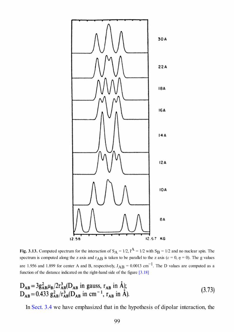
Fig. 3.13. Computed spectrum for the interaction of SA = 1/2, IA = 1/2 with SB = 1/2 and no nuclear spin. Thespectrum is computed along the z axis and rAB is taken to be parallel to the z axis (ε = 0, η = 0). The g values

are 1.956 and 1.899 for center A and B, respectively, JAB = 0.0013 cm−1. The D values are computed as afunction of the distance indicated on the right-hand side of the figure [3.18]

In Sect. 3.4 we have emphasized that in the hypothesis of dipolar interaction, the

99

intensity of the transition in single crystals depends on [see e.g.(3.69)]. The intensity of the signal in a polycrystalline sample or a frozen solutionresults from the spherical average of the single crystal intensities and it is thereforeexpected to depend also on . Furthermore, the intensity of the transitions is enhanced when the three spin levels are equally separated in energyso it is greater when the magnetic field is at about 54.7°, the magic angle withrespect to rAB, i.e., the value of the angle at which the dipolar fine structurecollapses. The actual value of the magic angle is, however, dependent on theanisotropies of the spin system and can significantly deviate from the 54.7° value[3.18]. At the magic angle the shape of the resonance line is greatly influenced bythe nuclear hyperfine interaction and could be used to monitor the relativeorientation of the dipolar and hyperfine axes. By computer simulation it has beenshown that the relative intensity of the transition, defined as the ratiobetween the intensity of transition 5 with respect to the total intensity of transitions1–4 (see Fig. 3.12), is a monotonic function of rAB. A plot of the logarithm of therelative intensity versus rAB, computed for gA gB = 2, is shown in Fig. 3.14. Ithas been found that in any case the relative intensity of the transitionfollows the general relationship [3.20]:

where A is a constant depending on the g values of the two spin centers and on thefrequency of the experiment. The value of the constant A at a given frequency andfor given gA and gB can be determined by a least squares fit of the computedrelative intensity of the transition with (3.74). This procedure can be followed forany value of hν and g and allows one to determine the A value appropriate to thesystem under examination. In the case of only one anisotropic gi tensor the Aconstant takes the form:

100

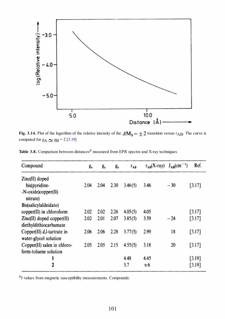
Fig. 3.14. Plot of the logarithm of the relative intensity of the transition versus rAB. The curve iscomputed for gA gB = 2 [3.19]

Table 3.8. Comparison between distancesa measured from EPR spectra and X-ray techniques

aJ values from magnetic susceptibility measurements. Compounds:

101

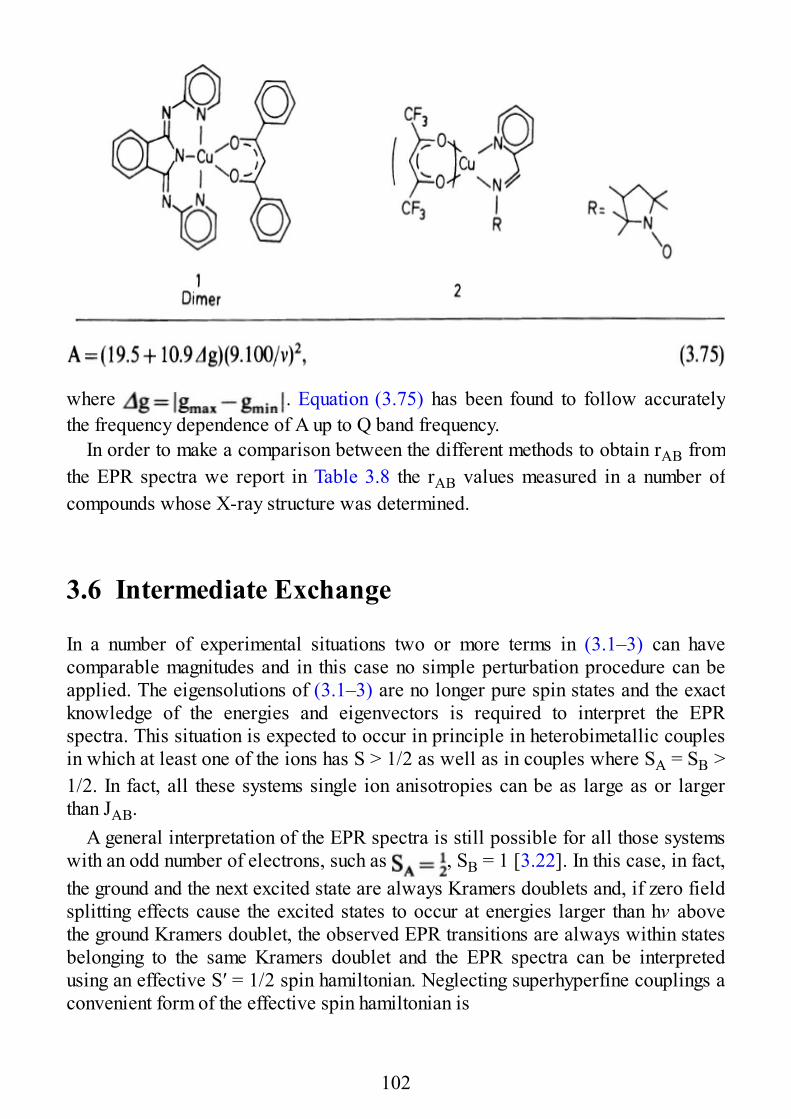
where . Equation (3.75) has been found to follow accuratelythe frequency dependence of A up to Q band frequency.

In order to make a comparison between the different methods to obtain rAB fromthe EPR spectra we report in Table 3.8 the rAB values measured in a number ofcompounds whose X-ray structure was determined.

3.6 Intermediate Exchange

In a number of experimental situations two or more terms in (3.1–3) can havecomparable magnitudes and in this case no simple perturbation procedure can beapplied. The eigensolutions of (3.1–3) are no longer pure spin states and the exactknowledge of the energies and eigenvectors is required to interpret the EPRspectra. This situation is expected to occur in principle in heterobimetallic couplesin which at least one of the ions has S > 1/2 as well as in couples where SA = SB >1/2. In fact, all these systems single ion anisotropies can be as large as or largerthan JAB.

A general interpretation of the EPR spectra is still possible for all those systemswith an odd number of electrons, such as , SB = 1 [3.22]. In this case, in fact,the ground and the next excited state are always Kramers doublets and, if zero fieldsplitting effects cause the excited states to occur at energies larger than hν abovethe ground Kramers doublet, the observed EPR transitions are always within statesbelonging to the same Kramers doublet and the EPR spectra can be interpretedusing an effective S′ = 1/2 spin hamiltonian. Neglecting superhyperfine couplings aconvenient form of the effective spin hamiltonian is

102

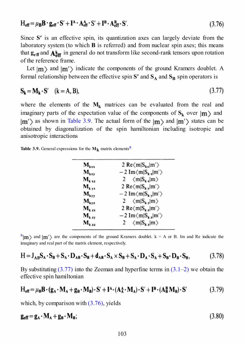
Since S′ is an effective spin, its quantization axes can largely deviate from thelaboratory system (to which B is referred) and from nuclear spin axes; this meansthat geff and in general do not transform like second-rank tensors upon rotationof the reference frame.

Let and indicate the components of the ground Kramers doublet. Aformal relationship between the effective spin S′ and SA and SB spin operators is

where the elements of the Mk matrices can be evaluated from the real andimaginary parts of the expectation value of the components of Sk over and

as shown in Table 3.9. The actual form of the and states can beobtained by diagonalization of the spin hamiltonian including isotropic andanisotropic interactions

Table 3.9. General expressions for the Mk matrix elementsa

a and are the components of the ground Kramers doublet. k = A or B. Im and Re indicate theimaginary and real part of the matrix element, respectively.

By substituting (3.77) into the Zeeman and hyperfine terms in (3.1–2) we obtain theeffective spin hamiltonian

which, by comparison with (3.76), yields

103

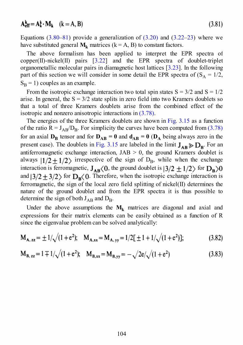
Equations (3.80–81) provide a generalization of (3.20) and (3.22–23) where wehave substituted general Mk matrices (k = A, B) to constant factors.

The above formalism has been applied to interpret the EPR spectra ofcopper(II)-nickel(II) pairs [3.22] and the EPR spectra of doublet-tripletorganometallic molecular pairs in diamagnetic host lattices [3.23]. In the followingpart of this section we will consider in some detail the EPR spectra of (SA = 1/2,SB = 1) couples as an example.

From the isotropic exchange interaction two total spin states S = 3/2 and S = 1/2arise. In general, the S = 3/2 state splits in zero field into two Kramers doublets sothat a total of three Kramers doublets arise from the combined effect of theisotropic and nonzero anisotropic interactions in (3.78).

The energies of the three Kramers doublets are shown in Fig. 3.15 as a functionof the ratio R = JAB/DB. For simplicity the curves have been computed from (3.78)for an axial DB tensor and for DAB = 0 and dAB = 0 (DA being always zero in thepresent case). The doublets in Fig. 3.15 are labeled in the limit . For anantiferromagnetic exchange interaction, JAB > 0, the ground Kramers doublet isalways irrespective of the sign of DB, while when the exchangeinteraction is ferromagnetic, , the ground doublet is for and for . Therefore, when the isotropic exchange interaction isferromagnetic, the sign of the local zero field splitting of nickel(II) determines thenature of the ground doublet and from the EPR spectra it is thus possible todetermine the sign of both JAB and DB.

Under the above assumptions the Mk matrices are diagonal and axial andexpressions for their matrix elements can be easily obtained as a function of Rsince the eigenvalue problem can be solved analytically:

104

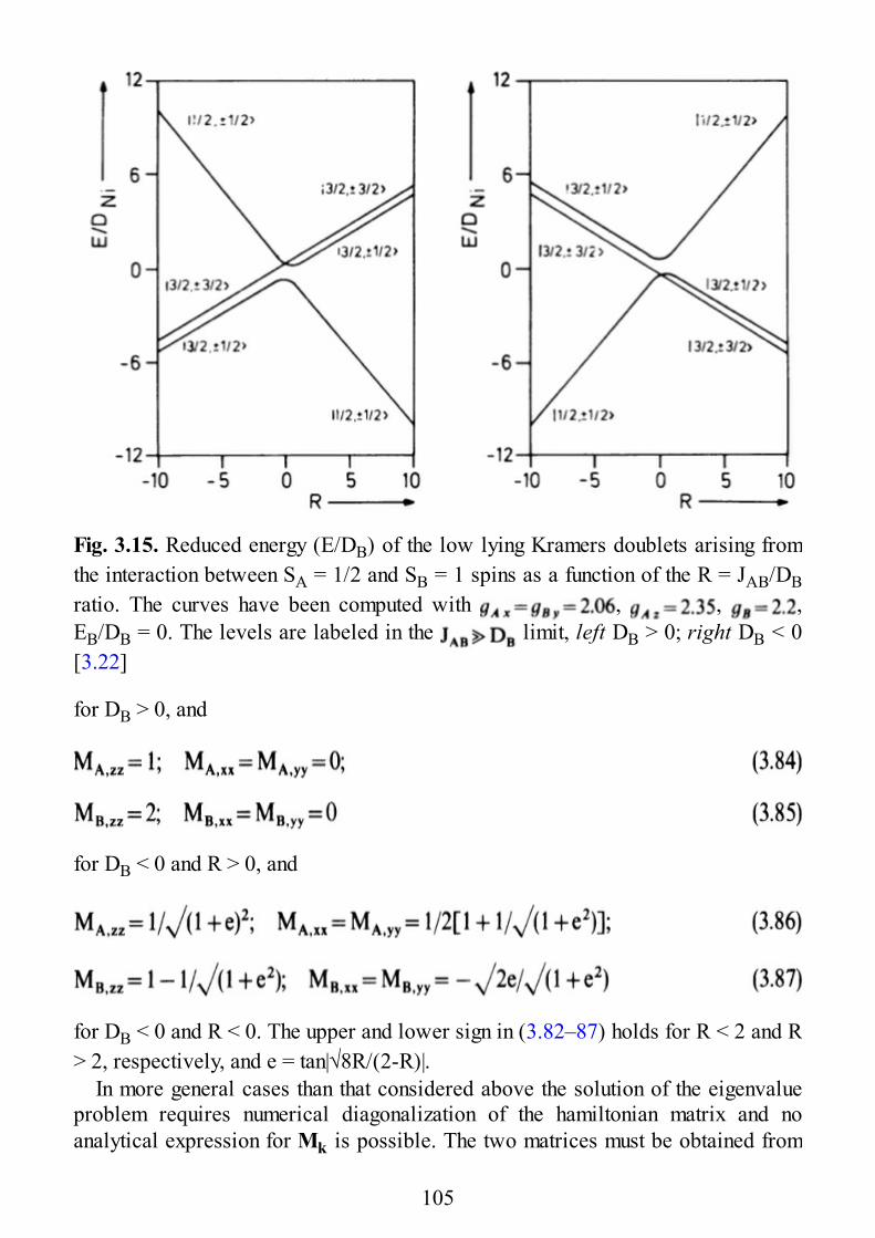
Fig. 3.15. Reduced energy (E/DB) of the low lying Kramers doublets arising fromthe interaction between SA = 1/2 and SB = 1 spins as a function of the R = JAB/DBratio. The curves have been computed with , , ,EB/DB = 0. The levels are labeled in the limit, left DB > 0; right DB < 0[3.22]

for DB > 0, and

for DB < 0 and R > 0, and

for DB < 0 and R < 0. The upper and lower sign in (3.82–87) holds for R < 2 and R> 2, respectively, and e = tan|√8R/(2-R)|.

In more general cases than that considered above the solution of the eigenvalueproblem requires numerical diagonalization of the hamiltonian matrix and noanalytical expression for Mk is possible. The two matrices must be obtained from

105

Table 3.9 using the eigenvectors obtained from the diagonalization of (3.78).As an example we show in Figs. 3.16 and 3.17 the effective g and A tensors

computed including only the B single ion anisotropy, in the axial case, and for λB =EB/DB = 0.13, for DB positive and DB negative, respectively. It is apparent that thelargest deviations from the limiting values computed using (3.20–22) are computedon the A values. In fact, the computed g values closely approach the limiting valuesfor R > 3, while the A values are still significantly different from the limitingvalues at R = 5. This is clearly a consequence of eqs (3.80) and (3.81) since the

tensor depends on the Mk matrix only and even a small deviation of Mk fromthe constant value required by (3.23) is important. These calculations suggest theuse of the deviation of from the limiting value of as a sensitive probefor the estimation of the R ratio.

106

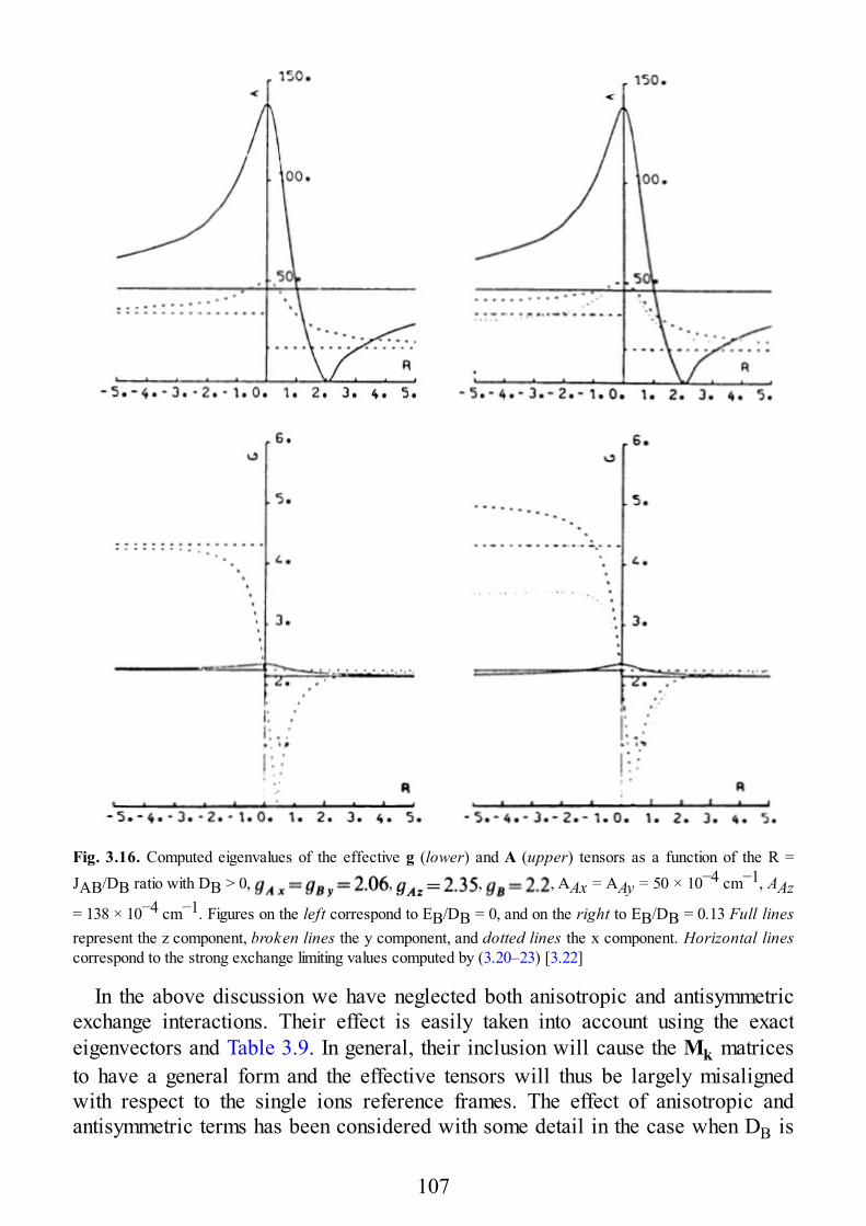
Fig. 3.16. Computed eigenvalues of the effective g (lower) and A (upper) tensors as a function of the R =JAB/DB ratio with DB > 0, , , , AAx = AAy = 50 × 10−4 cm−1, AAz= 138 × 10−4 cm−1. Figures on the left correspond to EB/DB = 0, and on the right to EB/DB = 0.13 Full linesrepresent the z component, broken lines the y component, and dotted lines the x component. Horizontal linescorrespond to the strong exchange limiting values computed by (3.20–23) [3.22]

In the above discussion we have neglected both anisotropic and antisymmetricexchange interactions. Their effect is easily taken into account using the exacteigenvectors and Table 3.9. In general, their inclusion will cause the Mk matricesto have a general form and the effective tensors will thus be largely misalignedwith respect to the single ions reference frames. The effect of anisotropic andantisymmetric terms has been considered with some detail in the case when DB is

107

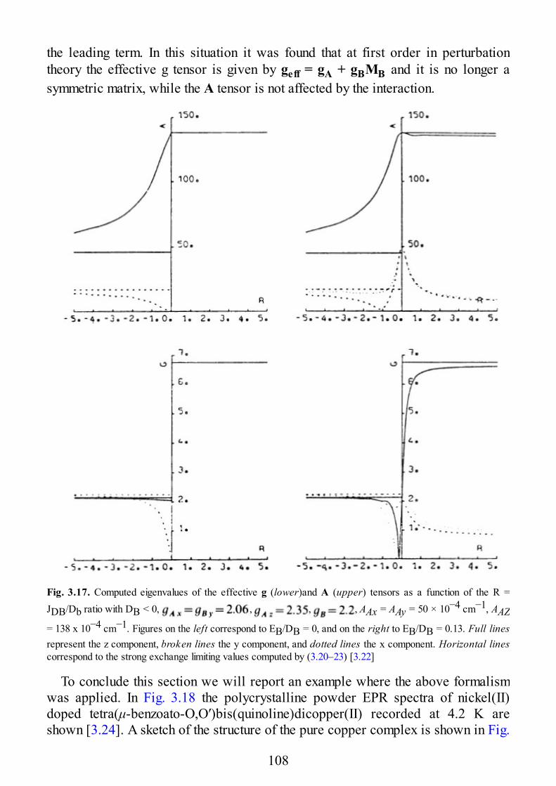
the leading term. In this situation it was found that at first order in perturbationtheory the effective g tensor is given by geff = gA + gBMB and it is no longer asymmetric matrix, while the A tensor is not affected by the interaction.

Fig. 3.17. Computed eigenvalues of the effective g (lower)and A (upper) tensors as a function of the R =JDB/Db ratio with DB < 0, , , , AAx = AAy = 50 × 10−4 cm−1, AAZ= 138 x 10−4 cm−1. Figures on the left correspond to EB/DB = 0, and on the right to EB/DB = 0.13. Full linesrepresent the z component, broken lines the y component, and dotted lines the x component. Horizontal linescorrespond to the strong exchange limiting values computed by (3.20–23) [3.22]

To conclude this section we will report an example where the above formalismwas applied. In Fig. 3.18 the polycrystalline powder EPR spectra of nickel(II)doped tetra(μ-benzoato-O,O′)bis(quinoline)dicopper(II) recorded at 4.2 K areshown [3.24]. A sketch of the structure of the pure copper complex is shown in Fig.

108

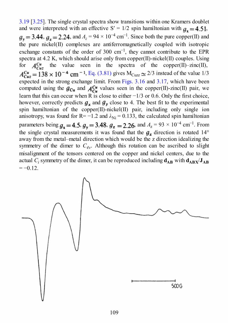
3.19 [3.25]. The single crystal spectra show transitions within one Kramers doubletand were interpreted with an effective S′ = 1/2 spin hamiltonian with ,

, , and Az = 94 × 10−4 cm−1. Since both the pure copper(II) andthe pure nickel(II) complexes are antiferromagnetically coupled with isotropicexchange constants of the order of 300 cm−1, they cannot contribute to the EPRspectra at 4.2 K, which should arise only from copper(II)-nickel(II) couples. Usingfor the value seen in the spectra of the copper(II)–zinc(II),

, Eq. (3.81) gives MCuzz 2/3 instead of the value 1/3expected in the strong exchange limit. From Figs. 3.16 and 3.17, which have beencomputed using the and values seen in the copper(II)-zinc(II) pair, welearn that this can occur when R is close to either −1/3 or 0.6. Only the first choice,however, correctly predicts and close to 4. The best fit to the experimentalspin hamiltonian of the copper(II)-nickel(II) pair, including only single ionanisotropy, was found for R= −1.2 and λNi = 0.133, the calculated spin hamiltonianparameters being , , , and Az = 93 × 10−4 cm−1. Fromthe single crystal measurements it was found that the direction is rotated 14°away from the metal–metal direction which would be the z direction idealizing thesymmetry of the dimer to C4ν. Although this rotation can be ascribed to slightmisalignment of the tensors centered on the copper and nickel centers, due to theactual Ci symmetry of the dimer, it can be reproduced including dAB with dABX/JAB= −0.12.

109

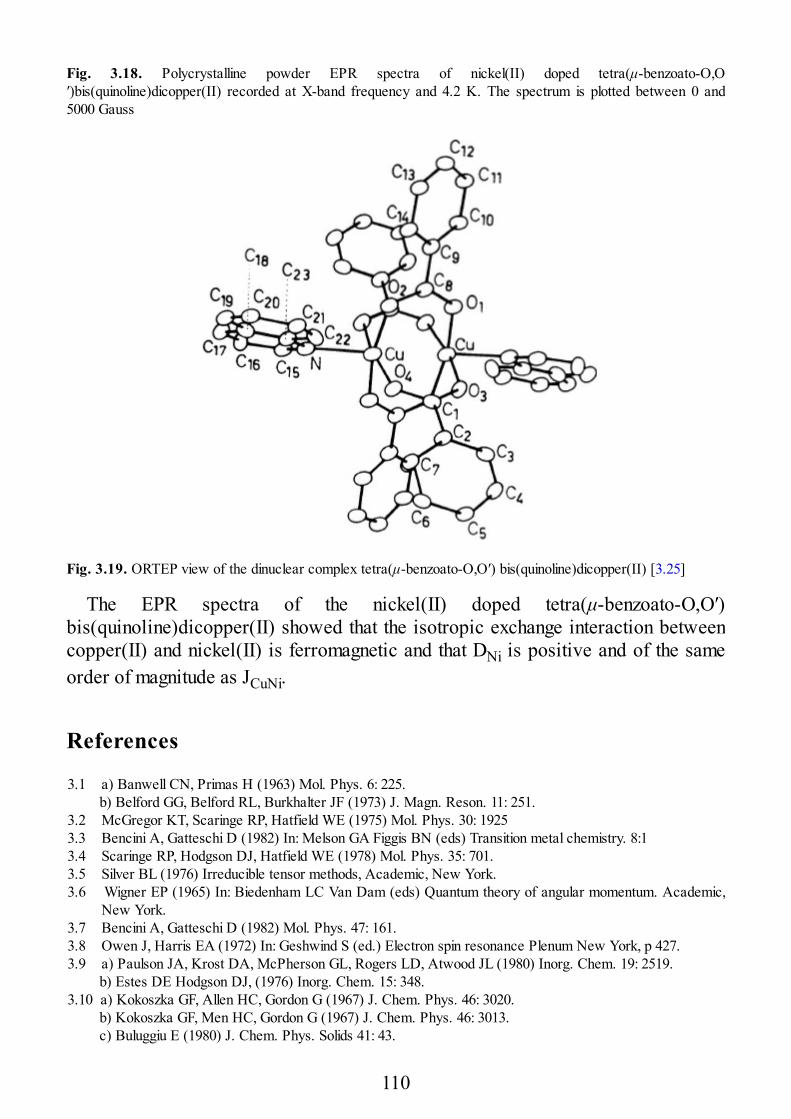
Fig. 3.18. Polycrystalline powder EPR spectra of nickel(II) doped tetra(μ-benzoato-O,O′)bis(quinoline)dicopper(II) recorded at X-band frequency and 4.2 K. The spectrum is plotted between 0 and5000 Gauss

Fig. 3.19. ORTEP view of the dinuclear complex tetra(μ-benzoato-O,O′) bis(quinoline)dicopper(II) [3.25]

The EPR spectra of the nickel(II) doped tetra(μ-benzoato-O,O′)bis(quinoline)dicopper(II) showed that the isotropic exchange interaction betweencopper(II) and nickel(II) is ferromagnetic and that DNi is positive and of the sameorder of magnitude as JCuNi.

References

3.1 a) Banwell CN, Primas H (1963) Mol. Phys. 6: 225.b) Belford GG, Belford RL, Burkhalter JF (1973) J. Magn. Reson. 11: 251.

3.2 McGregor KT, Scaringe RP, Hatfield WE (1975) Mol. Phys. 30: 19253.3 Bencini A, Gatteschi D (1982) In: Melson GA Figgis BN (eds) Transition metal chemistry. 8:13.4 Scaringe RP, Hodgson DJ, Hatfield WE (1978) Mol. Phys. 35: 701.3.5 Silver BL (1976) Irreducible tensor methods, Academic, New York.3.6 Wigner EP (1965) In: Biedenham LC Van Dam (eds) Quantum theory of angular momentum. Academic,

New York.3.7 Bencini A, Gatteschi D (1982) Mol. Phys. 47: 161.3.8 Owen J, Harris EA (1972) In: Geshwind S (ed.) Electron spin resonance Plenum New York, p 427.3.9 a) Paulson JA, Krost DA, McPherson GL, Rogers LD, Atwood JL (1980) Inorg. Chem. 19: 2519.

b) Estes DE Hodgson DJ, (1976) Inorg. Chem. 15: 348.3.10 a) Kokoszka GF, Allen HC, Gordon G (1967) J. Chem. Phys. 46: 3020.

b) Kokoszka GF, Men HC, Gordon G (1967) J. Chem. Phys. 46: 3013.c) Buluggiu E (1980) J. Chem. Phys. Solids 41: 43.

110

3.11 Krost DA, McPherson GL (1978) J. Am. Chem. Soc. 100: 987.3.12 Wieghardt K, Chauduri P, Nuber B, Weis J (1982) Inorg. Chem., 21: 3086.3.13 Bolster DE, Gütlich P, Hatfield WE, Kremer S, Müller EW, Wieghardt K (1983) Inorg. Chem. 22: 1725.3.14 Kremer S (1985) Inorg. Chem. 24: 8873.15 Al’tshuler SA, Kozyrev BM (1974) Electron paramagentic resonance in compounds of transition elements,

Wiley, New York.3.16 Banci L, Bencini A, Gatteschi D (1981) Inorg. Chem. 20: 2734.3.17 a) Smith TD, Pilbrow JR (1974) Coord. Chem. Rev. 13: 173.

b) Carr SG, Smith TD, Pilbrow JR (1974) J. Chem. Soc. Faraday Trans. 2: 497c) Eaton SS, More KM, Sawant BM, Boymel PM, Eaton GR (1983) J. Magn. Reson. 52: 435.

3.18 Coffman RE, Buettner GR (1979) J. Chem. Phys. 83: 2392.3.19 Eaton SS, More KM, Sawant BM, Eaton G R (1983) J. Am. Chem. Soc. 105: 6560.3.20 Coffman RE, Pezeshk A (1986) J. Magn. Reson. 70: 21.3.21 Boyd PWD, Toy AD, Smith TD, Pilbrow JR (1973) J. Chem. Soc. Dalton Trans., 1549.3.22 Bencini A Gatteschi D (1985) Mol. Phys. 54: 969.3.23 a) Hulliger J (1984) Ph.D. Thesis, University of Zürich, Zürich.

b) Hulliger J (1987) Mol. Phys. 60: 973.24 Bencini A, Benelli C, Gatteschi D, Zanchini C (1980) J. Am. Chem. Soc. 102: 5820.3.25 Bencini A, Gatteschi D, Mealli C (1979) Cryst. Struct. Commun. 8: 305.

111

4 Spectra of Clusters

4.1 The Spin Hamiltonian for Oligonuclear Systems ofInteracting Spins

The spin hamiltonian appropriate to describe the EPR spectra of clusters of three ormore weakly interacting paramagnetic centers can be written as an obviousextension of (3.1–3) and takes the form

In (4.1) Hi is the spin hamiltonian (3.1) of the individual spin center i and Hij isthe interaction hamiltonian (3.3) between couples of spins assumed to be symmetricwith respect to the i and j indices. The sums in (4.1) extend over all theparamagnetic centers forming the cluster. It must be stressed here that (4.1) is notthe most general hamiltonian to describe the magnetic and exchange interactions ina cluster. Such a hamiltonian, in fact, has the only requisite to be invariant withrespect to the symmetry operations of the cluster and should include n-centerinteractions as well as spin operators of the form jij(Si • Sj)2. Hamiltonian (4.1) is,however, the most widely used to interpret the EPR spectra and we will use thisoperator in the following. A number of general equations, which we will report inthis chapter, can be, however, easily modified to include the jij terms.

The most commonly investigated clusters are the ones in which the isotropicexchange interaction is the dominant term in (4.1). In this case the eigenstates of(4.1) are most conveniently found among the eigenstates of Sz and S2 where S =∑iSi is the total spin operator. This situation is completely analogous to that foundfor the dinuclear case and we will call this the strong exchange limit. In thissituation the EPR transitions occur within a given S manifold or within statesarising from a given S manifold and the EPR spectra can be interpreted using spinhamiltonians containing parameters which can be expressed as linear combinationsof terms including single ion spin hamiltonian parameters and interaction terms.

When the above assumptions are no longer valid, the interpretation of the EPRspectra requires the knowledge of the eigenstates of (4.1), which must be obtainedthrough matrix diagonalization. These eigenstates can then be used as zero-orderfunctions to which one can apply the Zeeman perturbation. This approach, which

112

we already noted to be hardly applicable to the dinuclear case, becomes practicallyunworkable when applied to higher nuclearity clusters.

In the literature a number of trinuclear clusters have been carefully investigatedthrough EPR spectroscopy, only a few tetranuclear clusters have been studied, andvery little has been done on larger clusters. In almost all the cases the strongexchange limit was applied. Thus, in the following we will develop the necessaryformalism to compute the energy levels of trinuclear clusters in the strong exchangelimit and we will give the necessary information to extend the formalism to largerclusters. Later we will derive the equations for interpreting the EPR spectra oftrinuclear systems in the strong exchange limit.

4.2 Spin Levels of Exchange Coupled Clusters in theStrong Exchange Limit

In the strong exchange limit we can label the spin levels of the cluster according tothe eigenvalues of S2 and Sz. These operators, in fact, commute with the isotropicpart of (4.1). Since we are dealing with more than two spins, the eigenstates of Szand S2 are not uniquely determined by the spin quantum numbers S and Ms, but anumber of additional quantum numbers are required according to the different“coupling schemes” of the interacting spins. Consider, for example, the simplestcase of the coupling of three spins Si(i = A, B, C). The total spin can be obtained bycoupling spins SA and SB first to give SAB = SA + SB and then SAB and Sc to give S= SAB + Sc. The resulting states will be conveniently labeled using the eigenvaluesof the commuting observables as . In the case of three spins the allowed spin states are:

corresponding to one quartet, S = 3/2, and two doublet, S = 1/2, states. We might aswell couple SB and Sc first to give SBC = SB + Sc and then SA and SBC to give S =SA + SBC. With this coupling scheme we obtain states like ,corresponding to the same eigenvalues of S2 and Sz as the states

. From the coupling of three spins we can obtain a maximumof eight spin functions orthogonal to each other which span the space;therefore the two eightfold orthonormal sets and

113

are not linearly independent and must be transformed one intothe other by a unitary transformation. In general, this means that any

ket can be expressed as a linear combination of kets according to:

where the sum is over all the allowed values of the intermediate spin couplingquantum number SBC. The expansion coefficients in (4.3) are just the scalarproducts between kets taken from the two coupling schemes and are independent ofM (scalar products do not depend on the orientation of the coordinate system).These coefficients, which are also called recoupling coefficients, are mostcommonly written using a 6-j symbol, so called for obvious reasons, to which theyare related by a phase factor according to

The above arguments can be extended to the coupling of four spins to give statesof the form . All these kets are related by unitarytransformations using 9-j symbols

The most relevant properties of the 6-j and 9-j symbols are given in Appendix B.Numerical tables of 6-j and 9-j symbols are given in Refs. [4.1–3].

Recoupling of five, six, and seven spins are possible through 12-, 15-, and 18-jsymbols [4.4] which will not be used in this book.

In the most general case the isotropic exchange hamiltonian for a rn-nuclearcluster

commutes with S2 and Sz, but does not commute with all of the intermediate spincoupling operators. Since we use a representation whose states are eigenstates ofthe squares of the intermediate spin coupling operators and of S2 and Sz, the

114

representation matrix of (4.6) will be block diagonal, each block corresponding tostates with the same value of S independent of the eigenvalues of the otheroperators forming the commuting set of observables of our representation. The fullrepresentation matrix of (4.6) can be built up by recurrence starting from one pairof spins and adding one spin at a time, thus reducing the problem always to thecoupling of two spins, or using the general vector coupling scheme. The firstapproach is slowly convergent especially when dealing with , due to thelarge number of spin states to be considered, while the second method becomesunworkable for clusters with more than four atoms, since it requires the use of 12-jand higher multiplicity symbols which are difficult to handle without the help of afast computer. Vector coupling techniques are, however, very helpful in dealingwith trinuclear systems and coupling this technique with the recurrence method forlarger clusters is probably the best way to operate.

Let us first examine the case of three interacting spins. It is convenient to rewritethe interaction hamiltonian in (4.1) in a generalized form as

where Tk(Si) is a k-rank irreducible tensor operator of the operator variable Si[4.5] and the spin centers are labeled with numbers instead of letters for the sake ofclarity. We will adopt this notation in the rest of the chapter. Ok is a k-rankirreducible tensor operator which contains the spin hamiltonian parameters.Operator (4.7) is equivalent to the interaction spin hamiltonian Hij in (4.1). Let usconsider, for example, the J12S1 · S2 part of the isotropic exchange interaction. In(4.7) it is obtained by putting Tk3(S3) = 1, which implies k3 = 0 since the identityoperator is zero rank, k = 0, and k12 = 0 as

Since

we get

where we have defined

115

In a similar way we can define the Ok tensors to express the interaction hamiltonianin the usual way. It must be noted that in (4.7) we included also terms of the form

as well as terms with higher spin powers and multicenter interactions.The matrix elements of Xk can be efficiently computed using the Wigner-Eckart

theorem [4.6]:

where the reduced matrix element is given by the general equation

General expressions for the reduced matrix elements of zero-, first-, and second-rank tensor operators appearing in the right-hand side of (4.13) are given in Table3.2.

One of the possible forms of the generalized interaction spin hamiltonian for atetranuclear cluster is:

where we have coupled a tensor operator of rank k1 to a tensor operator of rank k2to give a tensor operator of rank k12 (|k1 − k2| ≤ k12 ≤ k1 + k2); then we coupled thisoperator to a tensor operator of rank k3 to get a tensor operator of rank k123 (|k12 −k3| ≤ k123 ≤ k12 + k3) which finally couples with a fourth tensor operator of rank k4to give a total tensor operator of rank k (0 ≤|k123 − k4| ≤ k ≤ k123 + k3 ≤ 2). Since thetensor operator of rank k12, Tk12(S12) = {Tk1(S1) ⊗ Tk2(S2)}k12, is always obtained,in this coupling scheme, by coupling the same two tensor operators Tk1(S1) andTk2(S2) we can rewrite (4.14) in a way formally similar to (4.7) as

116

The matrix elements of (4.15) can be computed through (4.12) and (4.13). Thereduced matrix element of Tk12(S12) needed in (4.13) can be computed as

Repeated applications of (4.12), (4.13), and (4.15) allow one to compute thematrix elements of any interaction operator for clusters containing more than fourspin centers.

It must be noted here that although the above equations seem rather complicatedto be handled, they offer the great advantage to be close equations which can beeasily included in a general computer program which deals with any spin system.

4.2.1 Spin Levels of Trinuclear Clusters

The most general arrangement of three centers is on the vertex of a general triangle(Fig. 4.1).

Each spin interacts with the adjacent ones and the strength of these interactionsdetermines the magnetic geometry of the triad. When the three coupling constantsare equal, we have a regular triad (represented by an equilateral triangle). Whentwo of them, e.g. J13 and J23, are equal but different from the other, J12, we have asymmetric triad (represented by an isosceles triangle) and when all the couplingconstants are different we have a general triad (represented by a scalene triangle).A limiting situation can occur when one of the coupling constants, e.g. J13, is zero.This corresponds to a linear arrangement of the three spin centers (linear triad)when only nearest neighbor interactions are considered. This approximation is themost widely used in the treatment of spin clusters and most often only interactionsbetween adjacent spins are included in (4.6). The linear triad is symmetric whenthe two coupling constants J12 and J23 have the same value.

The spin hamiltonian (4.6) describing the isotropic exchange interaction betweenthree paramagnetic centers in a general triad takes the form:

117

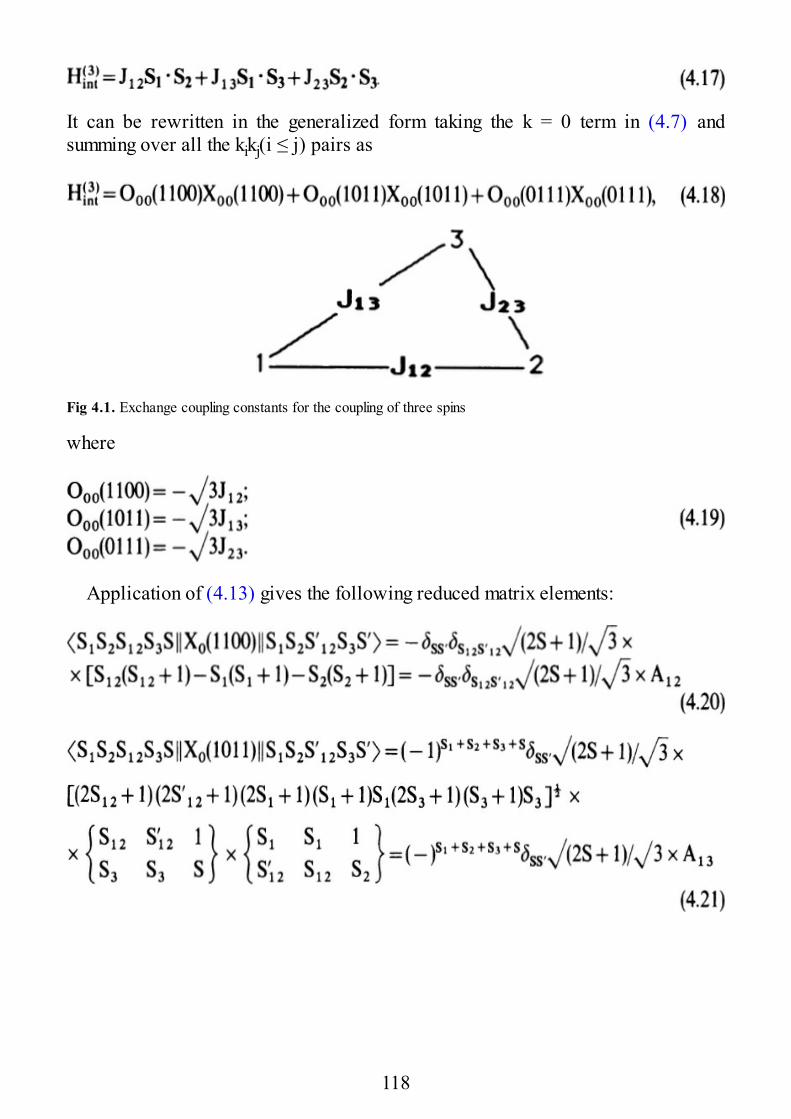
It can be rewritten in the generalized form taking the k = 0 term in (4.7) andsumming over all the kikj(i ≤ j) pairs as

Fig 4.1. Exchange coupling constants for the coupling of three spins

where

Application of (4.13) gives the following reduced matrix elements:

118

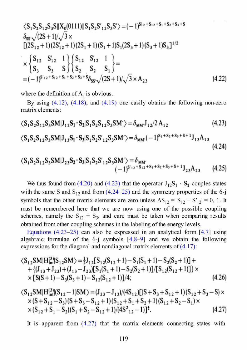
where the definition of Aij is obvious.By using (4.12), (4.18), and (4.19) one easily obtains the following non-zero

matrix elements:

We thus found from (4.20) and (4.23) that the operator J12S1 · S2 couples stateswith the same S and S12 and from (4.24–25) and the symmetry properties of the 6-jsymbols that the other matrix elements are zero unless ΔS12 = |S12 − S′12| = 0, 1. Itmust be remembered here that we are now using one of the possible couplingschemes, namely the S12 + S3, and care must be taken when comparing resultsobtained from other coupling schemes in the labeling of the energy levels.

Equations (4.23–25) can also be expressed in an analytical form [4.7] usingalgebraic formulae of the 6-j symbols [4.8–9] and we obtain the followingexpressions for the diagonal and nondiagonal matrix elements of (4.17):

It is apparent from (4.27) that the matrix elements connecting states with

119

are zero when J13 = J23 and the hamiltonian matrix is diagonal. This isthe case of a symmetric triad. For a regular triad all the coupling constants areequal and spin states with the same S are at the same energy:

For a symmetric linear triad the hamiltonian matrix is diagonal and the diagonalelements have the form:

Explicit expressions for the hamiltonian matrix of a number of general triples aregiven in Table 4.1.

The reduced energies of the spin levels for trinuclear systems with 1/2 spins arereported in Fig. 4.2 as a function of the r = J13/J23 and R = J12/J23 ratios. From thecoupling the following spin states arise: , , and . Figure4.2a shows the energy levels for a symmetric triple (r = 1). In this case thehamiltonian matrix is always diagonal independently of the R value. When R = 1we have a regular triad and the S = 1/2 states are degenerate. The energy levels fora linear triad are shown in Fig. 4.2b. When R = 1 we have a symmetric linear triad.In Fig. 4.2c and d the energy levels for general triads with r = 0.5 and − 0.5,respectively, are shown. The ground state of the triad is always a doublet statewhen r is negative and smaller than − 0.5 independently of the sign of J23. Thequartet state is the ground state only for R > 0 and J23 < 0, i.e., when all thepairwise interactions are ferromagnetic.

4.2.2 Spin Levels of Tetranuclear Clusters

On increasing the number of interacting nuclei the topology of the magneticinteraction becomes more complicate since the number of possible geometricalarrangements of the spin centers is larger. For clusters with more than three spins,in fact, we pass from a plane topology to a space topology. Fortunately not all thepossible topological structures for an n-vertex cluster can be found in nature andwe can thus avoid the complication of a general treatment of the exchangeinteraction in tetranuclear clusters to a few cases which have been studied. Anyinterested reader can of course perform the calculation of the spin levels of anycluster following the equations of Sect. 4.1.

Table 4.1. Explicit expression of the nonzero matrix elementsa of the isotropic exchange operator for generaltriads with

120

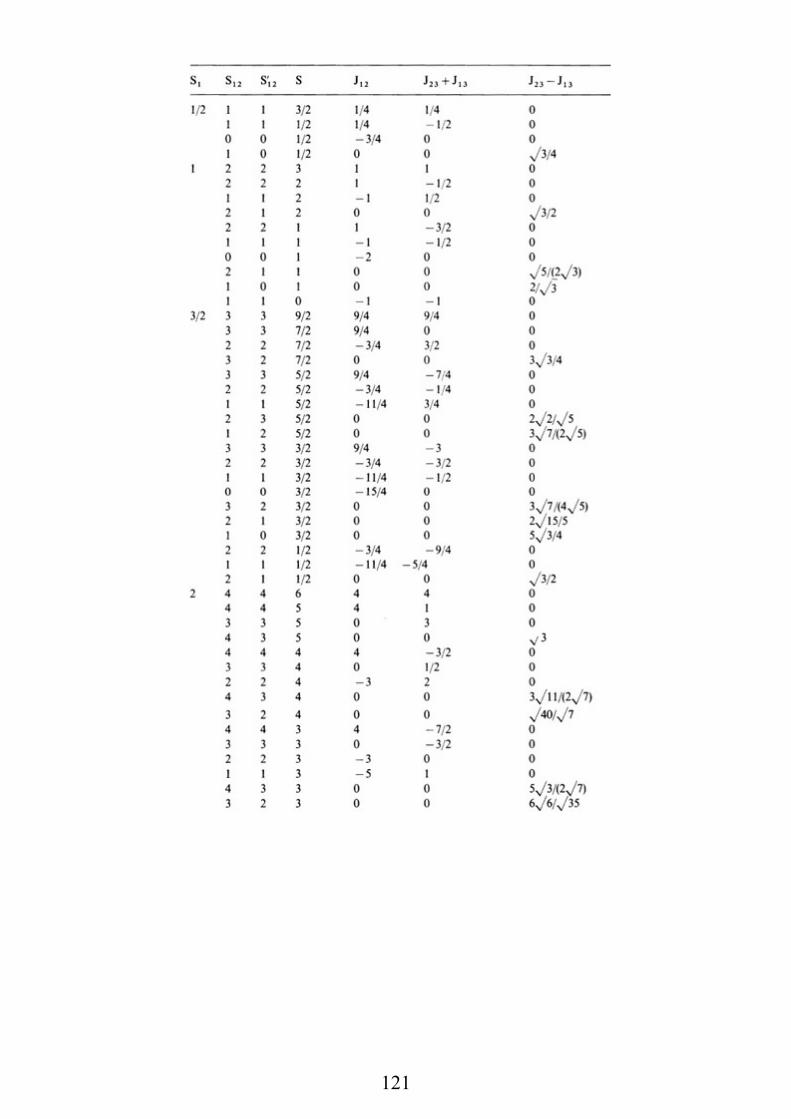
121

122

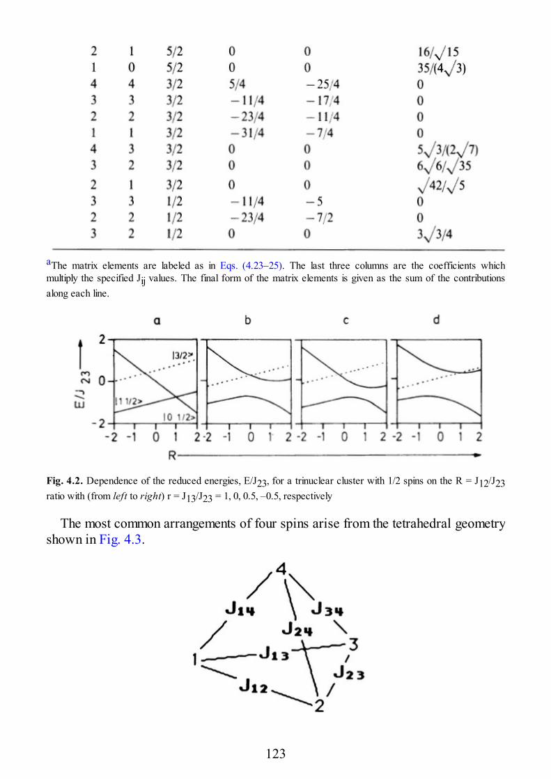
aThe matrix elements are labeled as in Eqs. (4.23–25). The last three columns are the coefficients whichmultiply the specified Jij values. The final form of the matrix elements is given as the sum of the contributionsalong each line.

Fig. 4.2. Dependence of the reduced energies, E/J23, for a trinuclear cluster with 1/2 spins on the R = J12/J23ratio with (from left to right) r = J13/J23 = 1, 0, 0.5, –0.5, respectively

The most common arrangements of four spins arise from the tetrahedral geometryshown in Fig. 4.3.

123

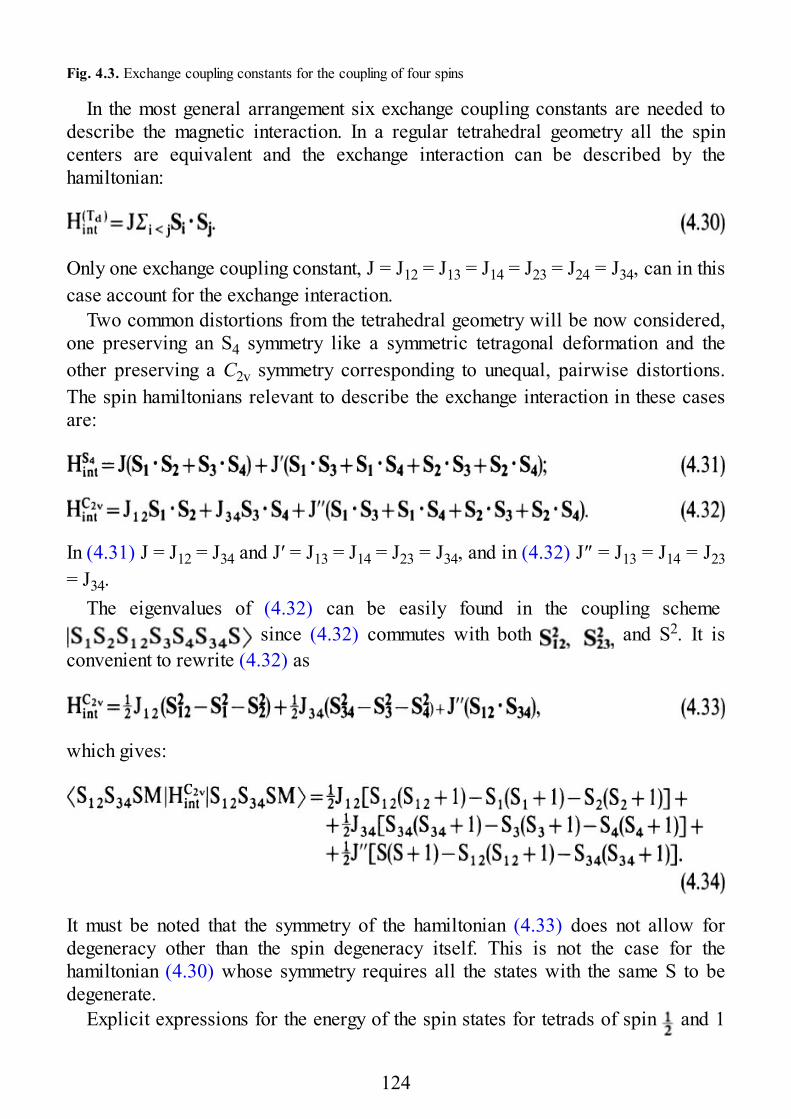
Fig. 4.3. Exchange coupling constants for the coupling of four spins

In the most general arrangement six exchange coupling constants are needed todescribe the magnetic interaction. In a regular tetrahedral geometry all the spincenters are equivalent and the exchange interaction can be described by thehamiltonian:

Only one exchange coupling constant, J = J12 = J13 = J14 = J23 = J24 = J34, can in thiscase account for the exchange interaction.

Two common distortions from the tetrahedral geometry will be now considered,one preserving an S4 symmetry like a symmetric tetragonal deformation and theother preserving a C2v symmetry corresponding to unequal, pairwise distortions.The spin hamiltonians relevant to describe the exchange interaction in these casesare:

In (4.31) J = J12 = J34 and J′ = J13 = J14 = J23 = J34, and in (4.32) J″ = J13 = J14 = J23= J34.

The eigenvalues of (4.32) can be easily found in the coupling scheme since (4.32) commutes with both and S2. It is

convenient to rewrite (4.32) as

which gives:

It must be noted that the symmetry of the hamiltonian (4.33) does not allow fordegeneracy other than the spin degeneracy itself. This is not the case for thehamiltonian (4.30) whose symmetry requires all the states with the same S to bedegenerate.

Explicit expressions for the energy of the spin states for tetrads of spin and 1

124

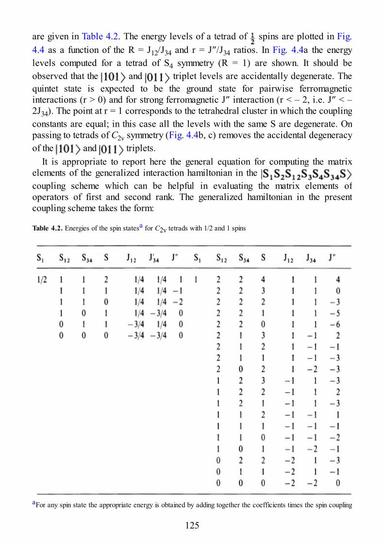
are given in Table 4.2. The energy levels of a tetrad of spins are plotted in Fig.4.4 as a function of the R = J12/J34 and r = J″/J34 ratios. In Fig. 4.4a the energylevels computed for a tetrad of S4 symmetry (R = 1) are shown. It should beobserved that the and triplet levels are accidentally degenerate. Thequintet state is expected to be the ground state for pairwise ferromagneticinteractions (r > 0) and for strong ferromagnetic J″ interaction (r < – 2, i.e. J″ < –2J34). The point at r = 1 corresponds to the tetrahedral cluster in which the couplingconstants are equal; in this case all the levels with the same S are degenerate. Onpassing to tetrads of C2v symmetry (Fig. 4.4b, c) removes the accidental degeneracyof the and triplets.

It is appropriate to report here the general equation for computing the matrixelements of the generalized interaction hamiltonian in the coupling scheme which can be helpful in evaluating the matrix elements ofoperators of first and second rank. The generalized hamiltonian in the presentcoupling scheme takes the form:

Table 4.2. Energies of the spin statesa for C2v tetrads with 1/2 and 1 spins

aFor any spin state the appropriate energy is obtained by adding together the coefficients times the spin coupling

125

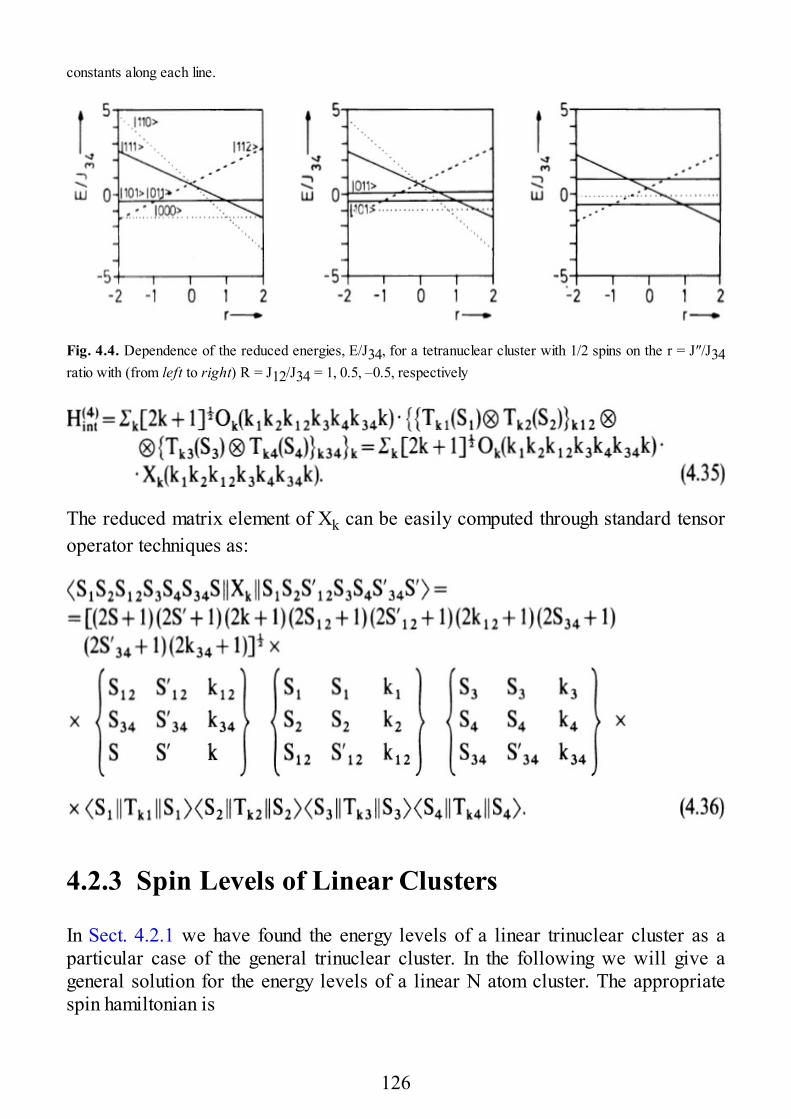
constants along each line.

Fig. 4.4. Dependence of the reduced energies, E/J34, for a tetranuclear cluster with 1/2 spins on the r = J″/J34ratio with (from left to right) R = J12/J34 = 1, 0.5, –0.5, respectively

The reduced matrix element of Xk can be easily computed through standard tensoroperator techniques as:

4.2.3 Spin Levels of Linear Clusters

In Sect. 4.2.1 we have found the energy levels of a linear trinuclear cluster as aparticular case of the general trinuclear cluster. In the following we will give ageneral solution for the energy levels of a linear N atom cluster. The appropriatespin hamiltonian is

126

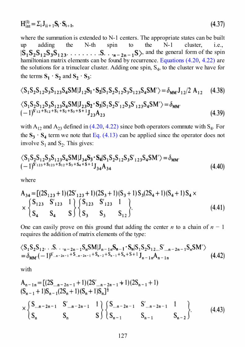
where the summation is extended to N-1 centers. The appropriate states can be builtup adding the N-th spin to the N-1 cluster, i.e.,

, and the general form of the spinhamiltonian matrix elements can be found by recurrence. Equations (4.20, 4.22) arethe solutions for a trinuclear cluster. Adding one spin, S4, to the cluster we have forthe terms S1 · S2 and S2 · S3:

with A12 and A23 defined in (4.20, 4.22) since both operators commute with S4. Forthe S3 · S4 term we note that Eq. (4.13) can be applied since the operator does notinvolve S1 and S2. This gives:

where

One can easily prove on this ground that adding the center n to a chain of n − 1requires the addition of matrix elements of the type:

with

127

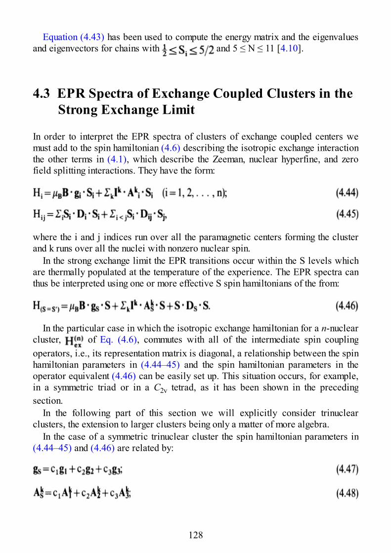
Equation (4.43) has been used to compute the energy matrix and the eigenvaluesand eigenvectors for chains with and 5 ≤ N ≤ 11 [4.10].

4.3 EPR Spectra of Exchange Coupled Clusters in theStrong Exchange Limit

In order to interpret the EPR spectra of clusters of exchange coupled centers wemust add to the spin hamiltonian (4.6) describing the isotropic exchange interactionthe other terms in (4.1), which describe the Zeeman, nuclear hyperfine, and zerofield splitting interactions. They have the form:

where the i and j indices run over all the paramagnetic centers forming the clusterand k runs over all the nuclei with nonzero nuclear spin.

In the strong exchange limit the EPR transitions occur within the S levels whichare thermally populated at the temperature of the experience. The EPR spectra canthus be interpreted using one or more effective S spin hamiltonians of the from:

In the particular case in which the isotropic exchange hamiltonian for a n-nuclearcluster, of Eq. (4.6), commutes with all of the intermediate spin couplingoperators, i.e., its representation matrix is diagonal, a relationship between the spinhamiltonian parameters in (4.44–45) and the spin hamiltonian parameters in theoperator equivalent (4.46) can be easily set up. This situation occurs, for example,in a symmetric triad or in a C2v tetrad, as it has been shown in the precedingsection.

In the following part of this section we will explicitly consider trinuclearclusters, the extension to larger clusters being only a matter of more algebra.

In the case of a symmetric trinuclear cluster the spin hamiltonian parameters in(4.44–45) and (4.46) are related by:

128

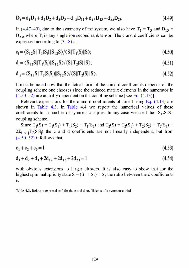
In (4.47–49), due to the symmetry of the system, we also have T2 = T3 and D13 =D23, where Ti is any single ion second rank tensor. The c and d coefficients can beexpressed according to (3.18) as

It must be noted now that the actual form of the c and d coefficients depends on thecoupling scheme one chooses since the reduced matrix elements in the numerator in(4.50–52) are actually dependent on the coupling scheme [see Eq. (4.13)].

Relevant expressions for the c and d coefficients obtained using Eq. (4.13) areshown in Table 4.3. In Table 4.4 we report the numerical values of thesecoefficients for a number of symmetric triples. In any case we used the {S12S3S}coupling scheme.

Since T1(S) = T1(S1) + T1(S2) + T1(S3) and T2(S) = T2(S1) + T2(S2) + T2(S3) +2Σi < jT2(SiSj) the c and d coefficients are not linearly independent, but from(4.50–52) it follows that

with obvious extensions to larger clusters. It is also easy to show that for thehighest spin multiplicity state S = (S1 + S2) + S3 the ratio between the c coefficientsis

Table 4.3. Relevant expressionsa for the c and d coefficients of a symmetric triad

129

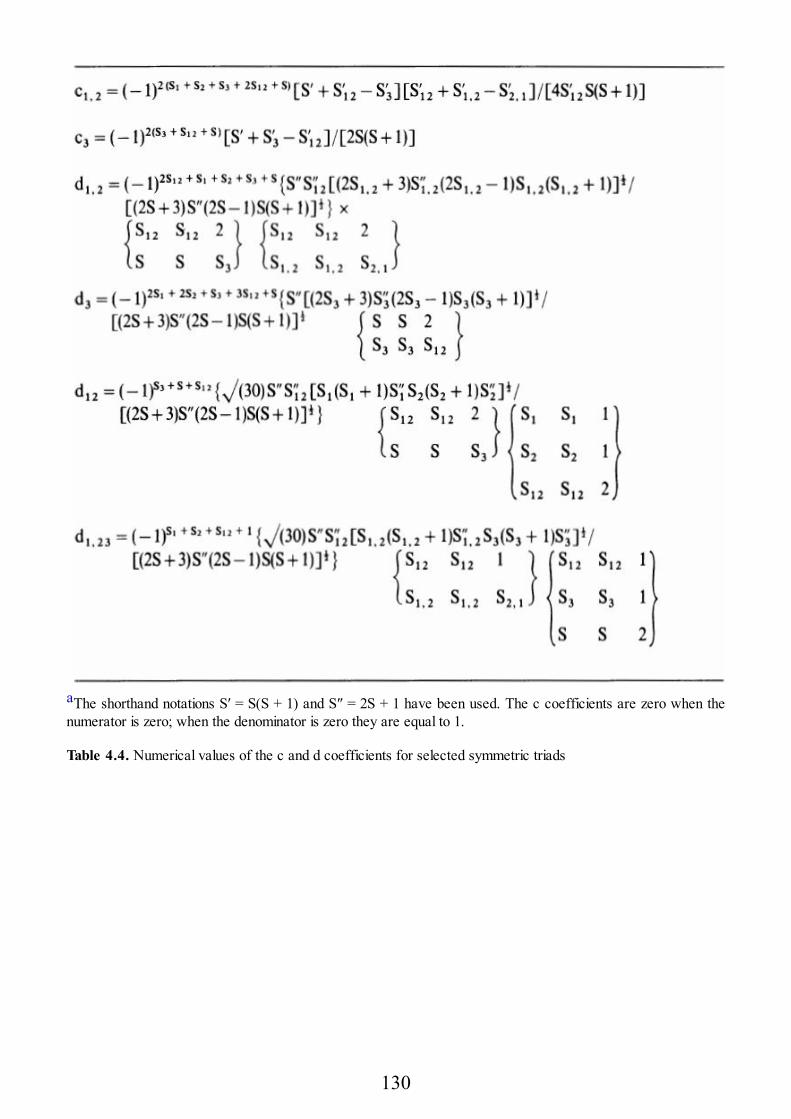
aThe shorthand notations S′ = S(S + 1) and S″ = 2S + 1 have been used. The c coefficients are zero when thenumerator is zero; when the denominator is zero they are equal to 1.

Table 4.4. Numerical values of the c and d coefficients for selected symmetric triads

130

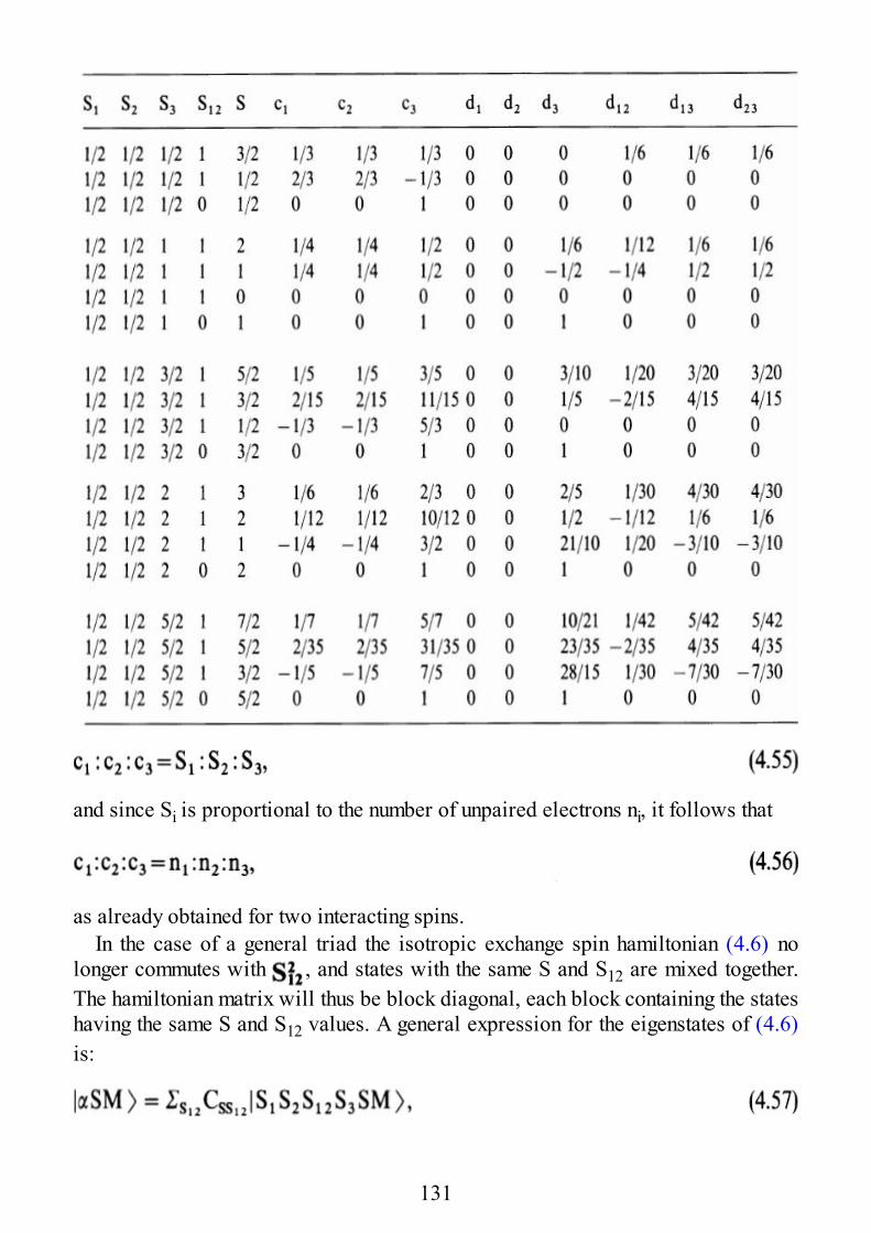
and since Si is proportional to the number of unpaired electrons ni, it follows that

as already obtained for two interacting spins.In the case of a general triad the isotropic exchange spin hamiltonian (4.6) no

longer commutes with , and states with the same S and S12 are mixed together.The hamiltonian matrix will thus be block diagonal, each block containing the stateshaving the same S and S12 values. A general expression for the eigenstates of (4.6)is:

131

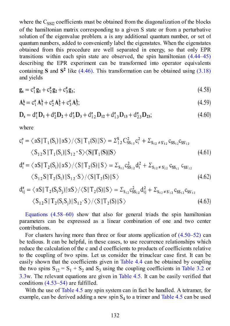
where the CSSl2 coefficients must be obtained from the diagonalization of the blocksof the hamiltonian matrix corresponding to a given S state or from a perturbativesolution of the eigenvalue problem. a is any additional quantum number, or set ofquantum numbers, added to conveniently label the eigenstates. When the eigenstatesobtained from this procedure are well separated in energy, so that only EPRtransitions within each spin state are observed, the spin hamiltonian (4.44–45)describing the EPR experiment can be transformed into operator equivalentscontaining S and S2 like (4.46). This transformation can be obtained using (3.18)and yields

where

Equations (4.58–60) show that also for general triads the spin hamiltonianparameters can be expressed as a linear combination of one and two centercontributions.

For clusters having more than three or four atoms application of (4.50–52) canbe tedious. It can be helpful, in these cases, to use recurrence relationships whichreduce the calculation of the c and d coefficients to products of coefficients relativeto the coupling of two spins. Let us consider the trinuclear case first. It can beeasily shown that the coefficients given in Table 4.4 can be obtained by couplingthe two spins S12 = S1 + S2 and S3 using the coupling coefficients in Table 3.2 or3.3w. The relevant equations are given in Table 4.5. It can be easily verified thatconditions (4.53–54) are fulfilled.

With the use of Table 4.5 any spin system can in fact be handled. A tetramer, forexample, can be derived adding a new spin S4 to a trimer and Table 4.5 can be used

132

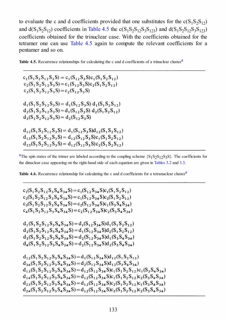
to evaluate the c and d coefficients provided that one substitutes for the c(S1S2S12)and d(S1S2S12) coefficients in Table 4.5 the c(S1S2S12S3S123) and d(S1S2S12S3S123)coefficients obtained for the trinuclear case. With the coefficients obtained for thetetramer one can use Table 4.5 again to compute the relevant coefficients for apentamer and so on.

Table 4.5. Recurrence relationships for calculating the c and d coefficients of a trinuclear clustera

aThe spin states of the trimer are labeled according to the coupling scheme {S1S2S12S3S}. The coefficients forthe dinuclear case appearing on the right-hand side of each equation are given in Tables 3.2 and 3.3.

Table 4.6. Recurrence relationship for calculating the c and d coefficients for a tetranuclear clustera

133

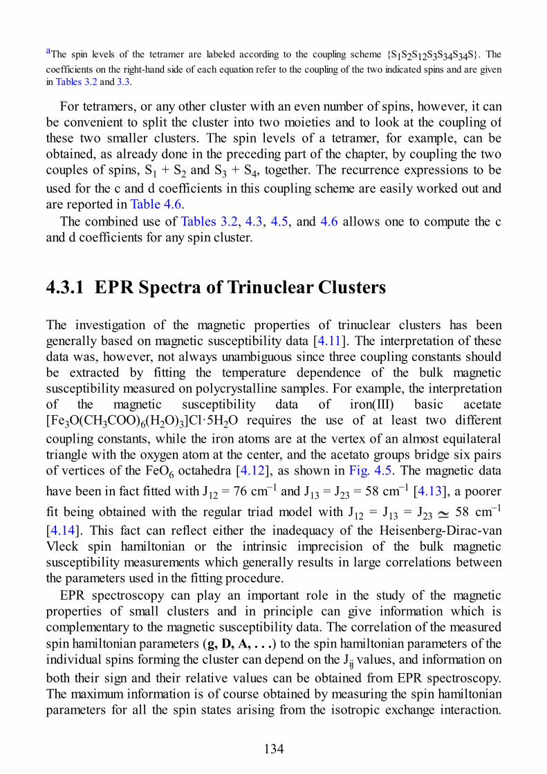
aThe spin levels of the tetramer are labeled according to the coupling scheme {S1S2S12S3S34S34S}. Thecoefficients on the right-hand side of each equation refer to the coupling of the two indicated spins and are givenin Tables 3.2 and 3.3.

For tetramers, or any other cluster with an even number of spins, however, it canbe convenient to split the cluster into two moieties and to look at the coupling ofthese two smaller clusters. The spin levels of a tetramer, for example, can beobtained, as already done in the preceding part of the chapter, by coupling the twocouples of spins, S1 + S2 and S3 + S4, together. The recurrence expressions to beused for the c and d coefficients in this coupling scheme are easily worked out andare reported in Table 4.6.

The combined use of Tables 3.2, 4.3, 4.5, and 4.6 allows one to compute the cand d coefficients for any spin cluster.

4.3.1 EPR Spectra of Trinuclear Clusters

The investigation of the magnetic properties of trinuclear clusters has beengenerally based on magnetic susceptibility data [4.11]. The interpretation of thesedata was, however, not always unambiguous since three coupling constants shouldbe extracted by fitting the temperature dependence of the bulk magneticsusceptibility measured on polycrystalline samples. For example, the interpretationof the magnetic susceptibility data of iron(III) basic acetate[Fe3O(CH3COO)6(H2O)3]Cl·5H2O requires the use of at least two differentcoupling constants, while the iron atoms are at the vertex of an almost equilateraltriangle with the oxygen atom at the center, and the acetato groups bridge six pairsof vertices of the FeO6 octahedra [4.12], as shown in Fig. 4.5. The magnetic datahave been in fact fitted with J12 = 76 cm−1 and J13 = J23 = 58 cm−1 [4.13], a poorerfit being obtained with the regular triad model with J12 = J13 = J23 58 cm−1

[4.14]. This fact can reflect either the inadequacy of the Heisenberg-Dirac-vanVleck spin hamiltonian or the intrinsic imprecision of the bulk magneticsusceptibility measurements which generally results in large correlations betweenthe parameters used in the fitting procedure.

EPR spectroscopy can play an important role in the study of the magneticproperties of small clusters and in principle can give information which iscomplementary to the magnetic susceptibility data. The correlation of the measuredspin hamiltonian parameters (g, D, A, . . .) to the spin hamiltonian parameters of theindividual spins forming the cluster can depend on the Jij values, and information onboth their sign and their relative values can be obtained from EPR spectroscopy.The maximum information is of course obtained by measuring the spin hamiltonianparameters for all the spin states arising from the isotropic exchange interaction.

134

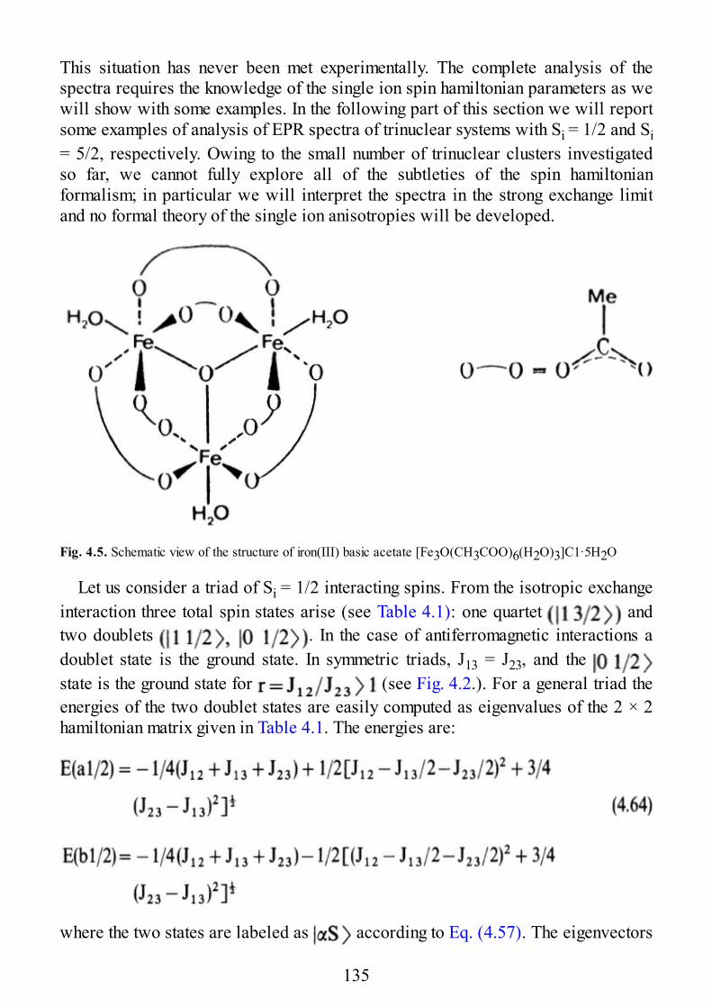
This situation has never been met experimentally. The complete analysis of thespectra requires the knowledge of the single ion spin hamiltonian parameters as wewill show with some examples. In the following part of this section we will reportsome examples of analysis of EPR spectra of trinuclear systems with Si = 1/2 and Si= 5/2, respectively. Owing to the small number of trinuclear clusters investigatedso far, we cannot fully explore all of the subtleties of the spin hamiltonianformalism; in particular we will interpret the spectra in the strong exchange limitand no formal theory of the single ion anisotropies will be developed.

Fig. 4.5. Schematic view of the structure of iron(III) basic acetate [Fe3O(CH3COO)6(H2O)3]C1·5H2O

Let us consider a triad of Si = 1/2 interacting spins. From the isotropic exchangeinteraction three total spin states arise (see Table 4.1): one quartet andtwo doublets . In the case of antiferromagnetic interactions adoublet state is the ground state. In symmetric triads, J13 = J23, and the state is the ground state for (see Fig. 4.2.). For a general triad theenergies of the two doublet states are easily computed as eigenvalues of the 2 × 2hamiltonian matrix given in Table 4.1. The energies are:

where the two states are labeled as according to Eq. (4.57). The eigenvectors

135

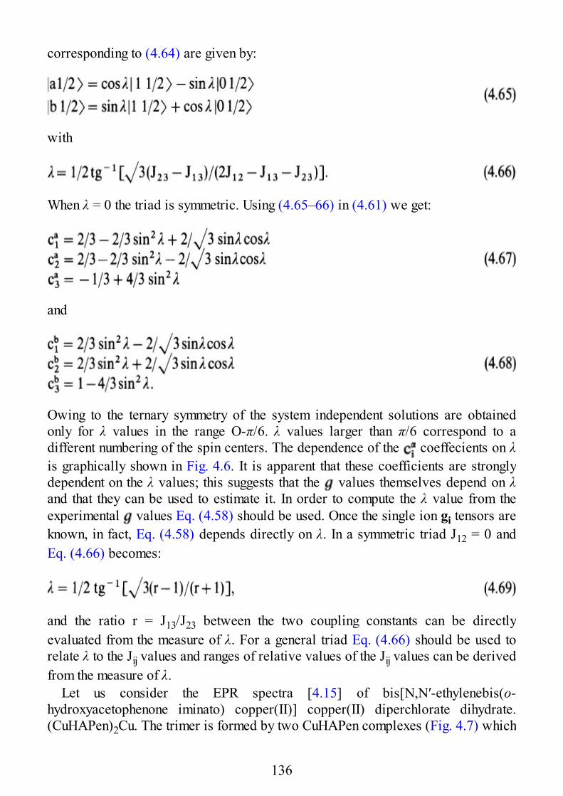
corresponding to (4.64) are given by:

with

When λ = 0 the triad is symmetric. Using (4.65–66) in (4.61) we get:

and

Owing to the ternary symmetry of the system independent solutions are obtainedonly for λ values in the range O-π/6. λ values larger than π/6 correspond to adifferent numbering of the spin centers. The dependence of the coeffecients on λis graphically shown in Fig. 4.6. It is apparent that these coefficients are stronglydependent on the λ values; this suggests that the values themselves depend on λand that they can be used to estimate it. In order to compute the λ value from theexperimental values Eq. (4.58) should be used. Once the single ion gi tensors areknown, in fact, Eq. (4.58) depends directly on λ. In a symmetric triad J12 = 0 andEq. (4.66) becomes:

and the ratio r = J13/J23 between the two coupling constants can be directlyevaluated from the measure of λ. For a general triad Eq. (4.66) should be used torelate λ to the Jij values and ranges of relative values of the Jij values can be derivedfrom the measure of λ.

Let us consider the EPR spectra [4.15] of bis[N,N′-ethylenebis(o-hydroxyacetophenone iminato) copper(II)] copper(II) diperchlorate dihydrate.(CuHAPen)2Cu. The trimer is formed by two CuHAPen complexes (Fig. 4.7) which

136

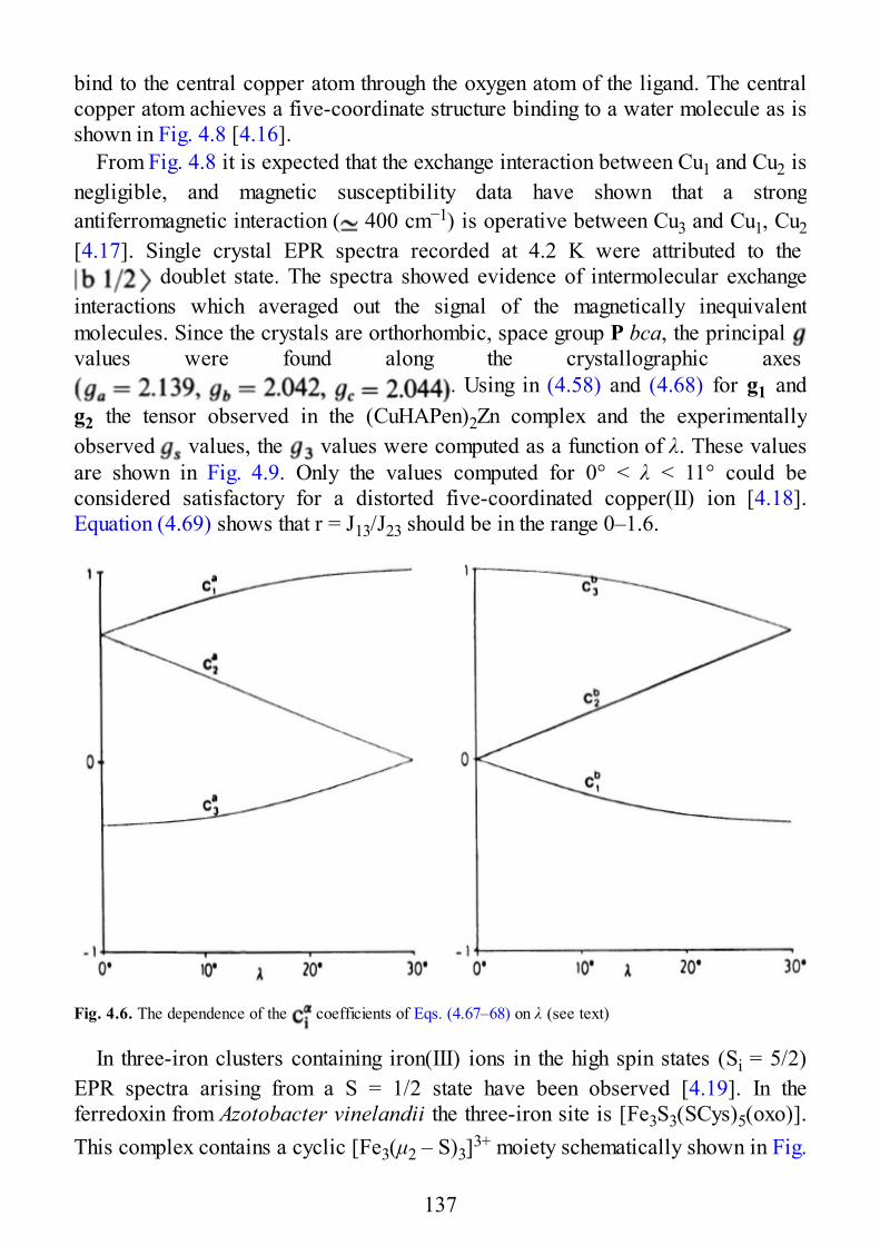
bind to the central copper atom through the oxygen atom of the ligand. The centralcopper atom achieves a five-coordinate structure binding to a water molecule as isshown in Fig. 4.8 [4.16].

From Fig. 4.8 it is expected that the exchange interaction between Cu1 and Cu2 isnegligible, and magnetic susceptibility data have shown that a strongantiferromagnetic interaction ( 400 cm−1) is operative between Cu3 and Cu1, Cu2[4.17]. Single crystal EPR spectra recorded at 4.2 K were attributed to the

doublet state. The spectra showed evidence of intermolecular exchangeinteractions which averaged out the signal of the magnetically inequivalentmolecules. Since the crystals are orthorhombic, space group P bca, the principal values were found along the crystallographic axes

. Using in (4.58) and (4.68) for g1 andg2 the tensor observed in the (CuHAPen)2Zn complex and the experimentallyobserved values, the values were computed as a function of λ. These valuesare shown in Fig. 4.9. Only the values computed for 0° < λ < 11° could beconsidered satisfactory for a distorted five-coordinated copper(II) ion [4.18].Equation (4.69) shows that r = J13/J23 should be in the range 0–1.6.

Fig. 4.6. The dependence of the coefficients of Eqs. (4.67–68) on λ (see text)

In three-iron clusters containing iron(III) ions in the high spin states (Si = 5/2)EPR spectra arising from a S = 1/2 state have been observed [4.19]. In theferredoxin from Azotobacter vinelandii the three-iron site is [Fe3S3(SCys)5(oxo)].This complex contains a cyclic [Fe3(μ2 – S)3]3+ moiety schematically shown in Fig.

137

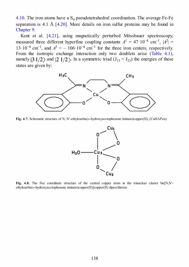
4.10. The iron atoms have a S4 pseudotetrahedral coordination. The average Fe-Feseparation is 4.1 Å [4.20]. More details on iron sulfur proteins may be found inChapter 9.

Kent et al. [4.21], using magnetically perturbed Mössbauer spectroscopy,measured three different hyperfine coupling constants A1 = 47·10−4 cm−1, |A2| =13·10−4 cm−1, and A3 = – 106·10−4 cm−1 for the three iron centers, respectively.From the isotropic exchange interaction only two doublets arise (Table 4.1),namely and . In a symmetric triad (J13 = J23) the energies of thesestates are given by:

Fig. 4.7. Schematic structure of N, N′-ethylenebis(o-hydroxyacetophenone iminato)copper(II), (CuHAPen)

Fig. 4.8. The five coordinate structure of the central copper atom in the trinuclear cluster bis[N,N′-ethylenebis(o-hydroxyacetophenone iminato)copper(II)]copper(II) diperchlorate

138

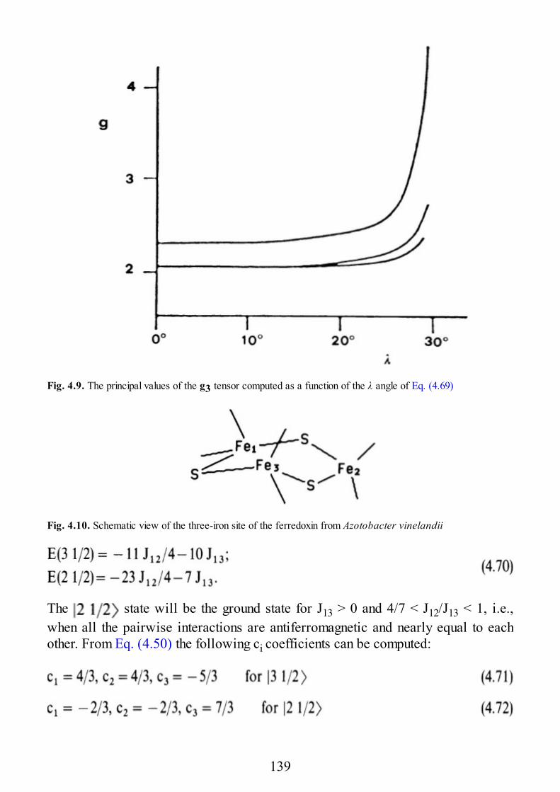
Fig. 4.9. The principal values of the g3 tensor computed as a function of the λ angle of Eq. (4.69)

Fig. 4.10. Schematic view of the three-iron site of the ferredoxin from Azotobacter vinelandii

The state will be the ground state for J13 > 0 and 4/7 < J12/J13 < 1, i.e.,when all the pairwise interactions are antiferromagnetic and nearly equal to eachother. From Eq. (4.50) the following ci coefficients can be computed:

139

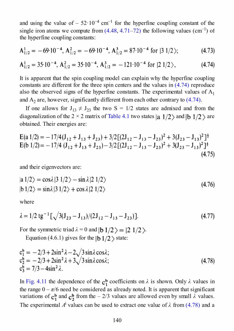
and using the value of – 52·10−4 cm−1 for the hyperfine coupling constant of thesingle iron atoms we compute from (4.48, 4.71–72) the following values (cm−1) ofthe hyperfine coupling constants:

It is apparent that the spin coupling model can explain why the hyperfine couplingconstants are different for the three spin centers and the values in (4.74) reproducealso the observed signs of the hyperfine constants. The experimental values of A1and A2 are, however, significantly different from each other contrary to (4.74).

If one allows for J13 ≠ J23 the two S = 1/2 states are admixed and from thediagonalization of the 2 × 2 matrix of Table 4.1 two states and areobtained. Their energies are:

and their eigenvectors are:

where

For the symmetric triad λ = 0 and .Equation (4.6.1) gives for the state:

In Fig. 4.11 the dependence of the coefficients on λ is shown. Only λ values inthe range 0 – π/6 need be considered as already noted. It is apparent that significantvariations of and from the – 2/3 values are allowed even by small λ values.The experimental Ai values can be used to extract one value of λ from (4.78) and a

140

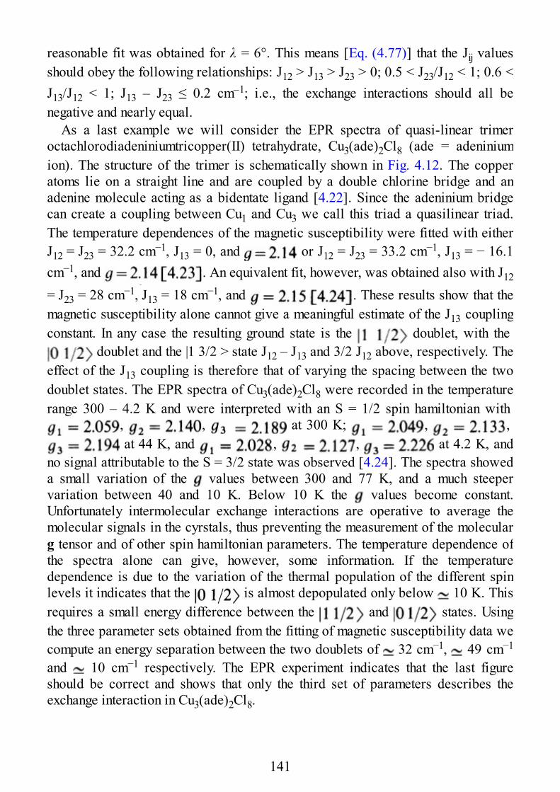
reasonable fit was obtained for λ = 6°. This means [Eq. (4.77)] that the Jij valuesshould obey the following relationships: J12 > J13 > J23 > 0; 0.5 < J23/J12 < 1; 0.6 <J13/J12 < 1; J13 – J23 ≤ 0.2 cm–1; i.e., the exchange interactions should all benegative and nearly equal.

As a last example we will consider the EPR spectra of quasi-linear trimeroctachlorodiadeniniumtricopper(II) tetrahydrate, Cu3(ade)2Cl8 (ade = adeniniumion). The structure of the trimer is schematically shown in Fig. 4.12. The copperatoms lie on a straight line and are coupled by a double chlorine bridge and anadenine molecule acting as a bidentate ligand [4.22]. Since the adeninium bridgecan create a coupling between Cu1 and Cu3 we call this triad a quasilinear triad.The temperature dependences of the magnetic susceptibility were fitted with eitherJ12 = J23 = 32.2 cm−1, J13 = 0, and or J12 = J23 = 33.2 cm−1, J13 = − 16.1cm−1, and . An equivalent fit, however, was obtained also with J12

= J23 = 28 cm−1, J13 = 18 cm−1, and . These results show that themagnetic susceptibility alone cannot give a meaningful estimate of the J13 couplingconstant. In any case the resulting ground state is the doublet, with the

doublet and the |1 3/2 > state J12 – J13 and 3/2 J12 above, respectively. Theeffect of the J13 coupling is therefore that of varying the spacing between the twodoublet states. The EPR spectra of Cu3(ade)2Cl8 were recorded in the temperaturerange 300 – 4.2 K and were interpreted with an S = 1/2 spin hamiltonian with

, , at 300 K; , , at 44 K, and , , at 4.2 K, and

no signal attributable to the S = 3/2 state was observed [4.24]. The spectra showeda small variation of the values between 300 and 77 K, and a much steepervariation between 40 and 10 K. Below 10 K the values become constant.Unfortunately intermolecular exchange interactions are operative to average themolecular signals in the cyrstals, thus preventing the measurement of the molecularg tensor and of other spin hamiltonian parameters. The temperature dependence ofthe spectra alone can give, however, some information. If the temperaturedependence is due to the variation of the thermal population of the different spinlevels it indicates that the is almost depopulated only below 10 K. Thisrequires a small energy difference between the and states. Usingthe three parameter sets obtained from the fitting of magnetic susceptibility data wecompute an energy separation between the two doublets of 32 cm−1, 49 cm−1

and 10 cm−1 respectively. The EPR experiment indicates that the last figureshould be correct and shows that only the third set of parameters describes theexchange interaction in Cu3(ade)2Cl8.

141

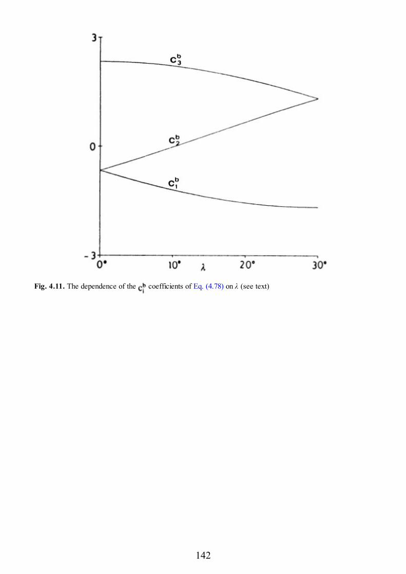
Fig. 4.11. The dependence of the coefficients of Eq. (4.78) on λ (see text)

142

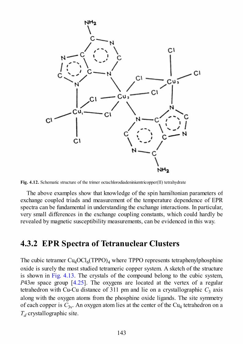
Fig. 4.12. Schematic structure of the trimer octachlorodiadeniniumtricopper(II) tetrahydrate

The above examples show that knowledge of the spin hamiltonian parameters ofexchange coupled triads and measurement of the temperature dependence of EPRspectra can be fundamental in understanding the exchange interactions. In particular,very small differences in the exchange coupling constants, which could hardly berevealed by magnetic susceptibility measurements, can be evidenced in this way.

4.3.2 EPR Spectra of Tetranuclear Clusters

The cubic tetramer Cu4OCl6(TPPO)4 where TPPO represents tetraphenylphosphineoxide is surely the most studied tetrameric copper system. A sketch of the structureis shown in Fig. 4.13. The crystals of the compound belong to the cubic system,P43m space group [4.25]. The oxygens are located at the vertex of a regulartetrahedron with Cu-Cu distance of 311 pm and lie on a crystallographic C3 axisalong with the oxygen atoms from the phosphine oxide ligands. The site symmetryof each copper is C3v. An oxygen atom lies at the center of the Cu4 tetrahedron on aTd crystallographic site.

143

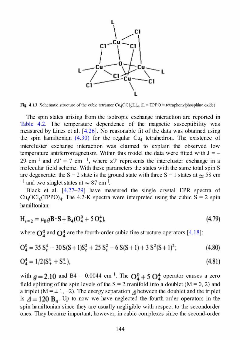
Fig. 4.13. Schematic structure of the cubic tetramer Cu4OCl6(L)4 (L = TPPO = tetraphenylphosphine oxide)

The spin states arising from the isotropic exchange interaction are reported inTable 4.2. The temperature dependence of the magnetic susceptibility wasmeasured by Lines et al. [4.26]. No reasonable fit of the data was obtained usingthe spin hamiltonian (4.30) for the regular Cu4 tetrahedron. The existence ofintercluster exchange interaction was claimed to explain the observed lowtemperature antiferromagnetism. Within this model the data were fitted with J = –29 cm−1 and z′J′ = 7 cm −1, where z′J′ represents the intercluster exchange in amolecular field scheme. With these parameters the states with the same total spin Sare degenerate: the S = 2 state is the ground state with three S = 1 states at 58 cm−1 and two singlet states at 87 cm−l.

Black et al. [4.27–29] have measured the single crystal EPR spectra ofCu4OCl6(TPPO)4. The 4.2-K spectra were interpreted using the cubic S = 2 spinhamiltonian:

where and are the fourth-order cubic fine structure operators [4.18]:

with and B4 = 0.0044 cm−1. The operator causes a zerofield splitting of the spin levels of the S = 2 manifold into a doublet (M = 0, 2) anda triplet (M = ± 1, −2). The energy separation between the doublet and the tripletis . Up to now we have neglected the fourth-order operators in thespin hamiltonian since they are usually negligible with respect to the secondorderones. They became important, however, in cubic complexes since the second-order

144

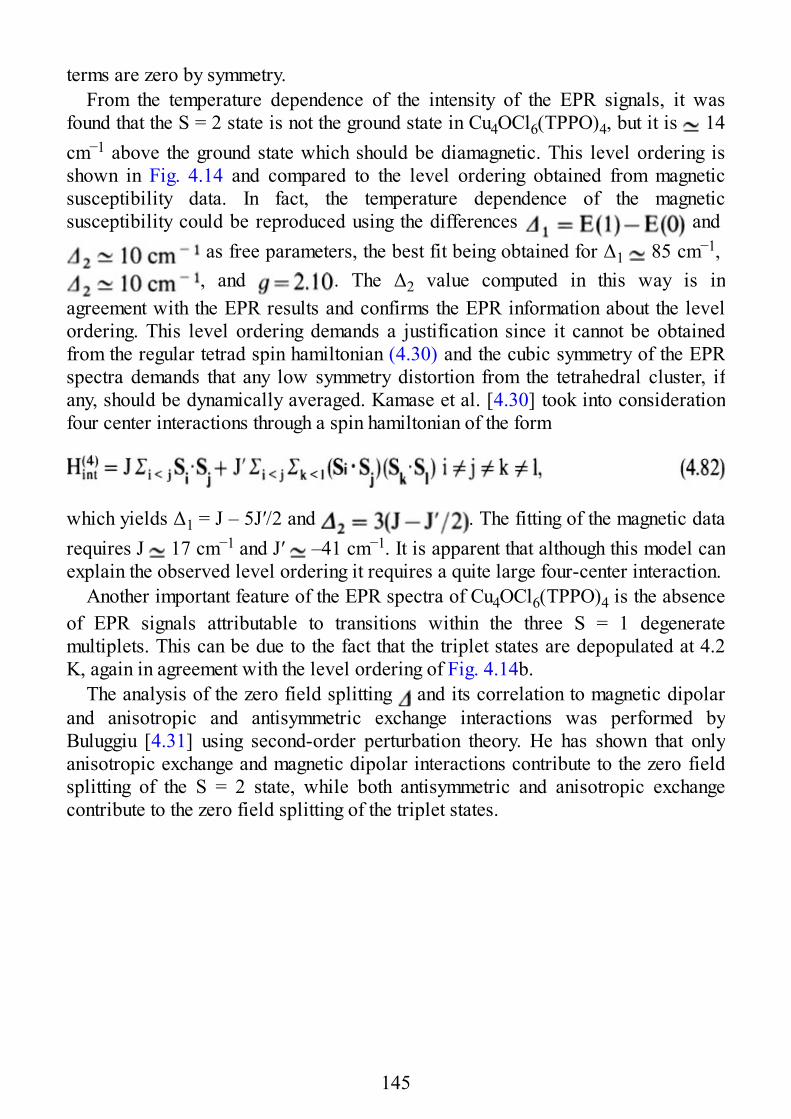
terms are zero by symmetry.From the temperature dependence of the intensity of the EPR signals, it was

found that the S = 2 state is not the ground state in Cu4OCl6(TPPO)4, but it is 14cm−1 above the ground state which should be diamagnetic. This level ordering isshown in Fig. 4.14 and compared to the level ordering obtained from magneticsusceptibility data. In fact, the temperature dependence of the magneticsusceptibility could be reproduced using the differences and

as free parameters, the best fit being obtained for Δ1 85 cm−1, , and . The Δ2 value computed in this way is in

agreement with the EPR results and confirms the EPR information about the levelordering. This level ordering demands a justification since it cannot be obtainedfrom the regular tetrad spin hamiltonian (4.30) and the cubic symmetry of the EPRspectra demands that any low symmetry distortion from the tetrahedral cluster, ifany, should be dynamically averaged. Kamase et al. [4.30] took into considerationfour center interactions through a spin hamiltonian of the form

which yields Δ1 = J – 5J′/2 and . The fitting of the magnetic datarequires J 17 cm−1 and J′ –41 cm−1. It is apparent that although this model canexplain the observed level ordering it requires a quite large four-center interaction.

Another important feature of the EPR spectra of Cu4OCl6(TPPO)4 is the absenceof EPR signals attributable to transitions within the three S = 1 degeneratemultiplets. This can be due to the fact that the triplet states are depopulated at 4.2K, again in agreement with the level ordering of Fig. 4.14b.

The analysis of the zero field splitting and its correlation to magnetic dipolarand anisotropic and antisymmetric exchange interactions was performed byBuluggiu [4.31] using second-order perturbation theory. He has shown that onlyanisotropic exchange and magnetic dipolar interactions contribute to the zero fieldsplitting of the S = 2 state, while both antisymmetric and anisotropic exchangecontribute to the zero field splitting of the triplet states.

145

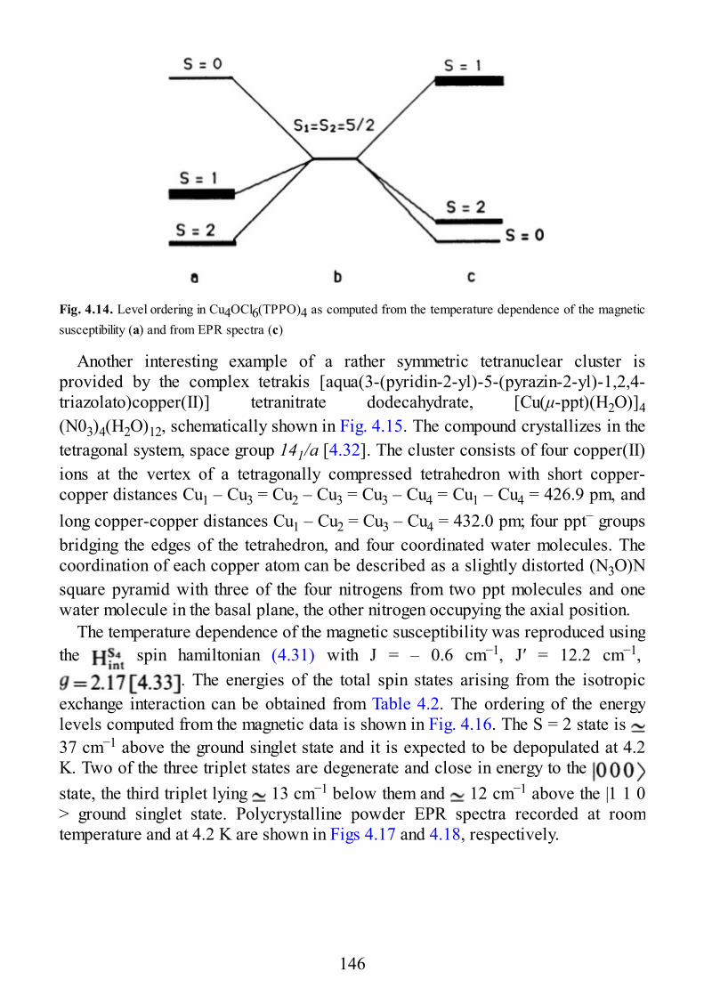
Fig. 4.14. Level ordering in Cu4OCl6(TPPO)4 as computed from the temperature dependence of the magneticsusceptibility (a) and from EPR spectra (c)

Another interesting example of a rather symmetric tetranuclear cluster isprovided by the complex tetrakis [aqua(3-(pyridin-2-yl)-5-(pyrazin-2-yl)-1,2,4-triazolato)copper(II)] tetranitrate dodecahydrate, [Cu(μ-ppt)(H2O)]4(N03)4(H2O)12, schematically shown in Fig. 4.15. The compound crystallizes in thetetragonal system, space group 141/a [4.32]. The cluster consists of four copper(II)ions at the vertex of a tetragonally compressed tetrahedron with short copper-copper distances Cu1 – Cu3 = Cu2 – Cu3 = Cu3 – Cu4 = Cu1 – Cu4 = 426.9 pm, andlong copper-copper distances Cu1 – Cu2 = Cu3 – Cu4 = 432.0 pm; four ppt− groupsbridging the edges of the tetrahedron, and four coordinated water molecules. Thecoordination of each copper atom can be described as a slightly distorted (N3O)Nsquare pyramid with three of the four nitrogens from two ppt molecules and onewater molecule in the basal plane, the other nitrogen occupying the axial position.

The temperature dependence of the magnetic susceptibility was reproduced usingthe spin hamiltonian (4.31) with J = – 0.6 cm−1, J′ = 12.2 cm−1,

. The energies of the total spin states arising from the isotropicexchange interaction can be obtained from Table 4.2. The ordering of the energylevels computed from the magnetic data is shown in Fig. 4.16. The S = 2 state is 37 cm−1 above the ground singlet state and it is expected to be depopulated at 4.2K. Two of the three triplet states are degenerate and close in energy to the state, the third triplet lying 13 cm−1 below them and 12 cm−1 above the |1 1 0> ground singlet state. Polycrystalline powder EPR spectra recorded at roomtemperature and at 4.2 K are shown in Figs 4.17 and 4.18, respectively.

146

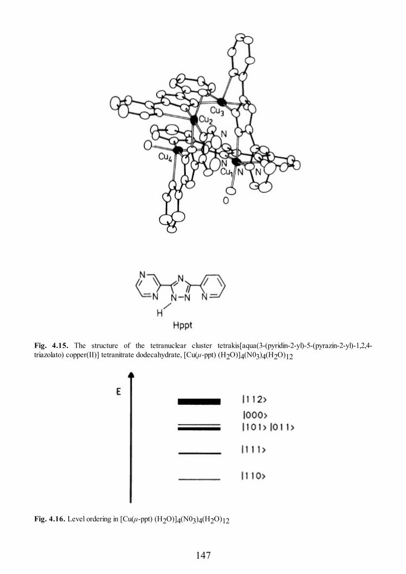
Fig. 4.15. The structure of the tetranuclear cluster tetrakis[aqua(3-(pyridin-2-yl)-5-(pyrazin-2-yl)-1,2,4-triazolato) copper(II)] tetranitrate dodecahydrate, [Cu(μ-ppt) (H2O)]4(N03)4(H2O)12

Fig. 4.16. Level ordering in [Cu(μ-ppt) (H2O)]4(N03)4(H2O)12

147

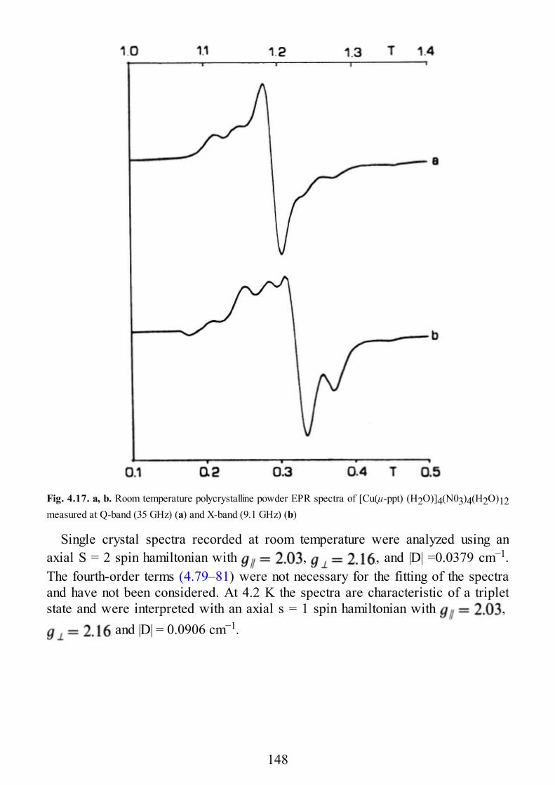
Fig. 4.17. a, b. Room temperature polycrystalline powder EPR spectra of [Cu(μ-ppt) (H2O)]4(N03)4(H2O)12measured at Q-band (35 GHz) (a) and X-band (9.1 GHz) (b)

Single crystal spectra recorded at room temperature were analyzed using anaxial S = 2 spin hamiltonian with , , and |D| =0.0379 cm−1.The fourth-order terms (4.79–81) were not necessary for the fitting of the spectraand have not been considered. At 4.2 K the spectra are characteristic of a tripletstate and were interpreted with an axial s = 1 spin hamiltonian with ,

and |D| = 0.0906 cm−1.

148

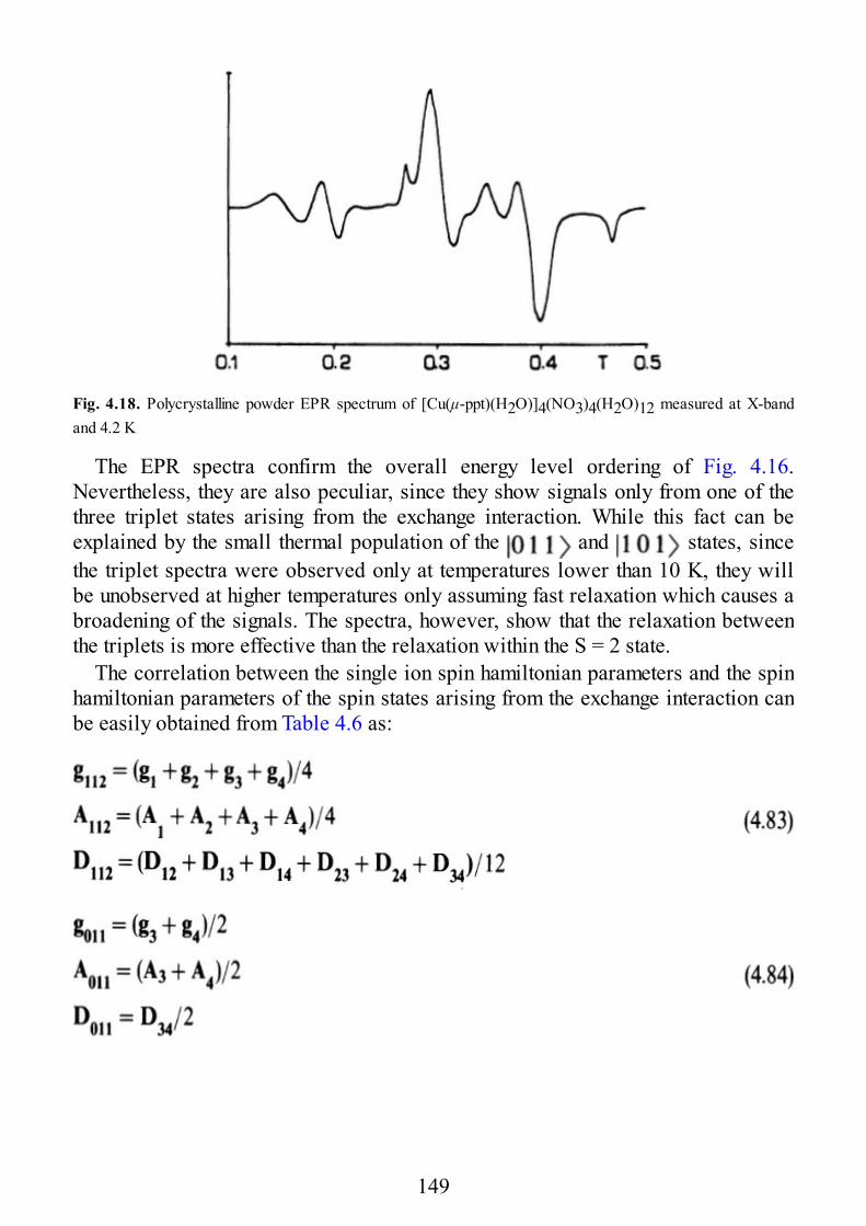
Fig. 4.18. Polycrystalline powder EPR spectrum of [Cu(μ-ppt)(H2O)]4(NO3)4(H2O)12 measured at X-bandand 4.2 K

The EPR spectra confirm the overall energy level ordering of Fig. 4.16.Nevertheless, they are also peculiar, since they show signals only from one of thethree triplet states arising from the exchange interaction. While this fact can beexplained by the small thermal population of the and states, sincethe triplet spectra were observed only at temperatures lower than 10 K, they willbe unobserved at higher temperatures only assuming fast relaxation which causes abroadening of the signals. The spectra, however, show that the relaxation betweenthe triplets is more effective than the relaxation within the S = 2 state.

The correlation between the single ion spin hamiltonian parameters and the spinhamiltonian parameters of the spin states arising from the exchange interaction canbe easily obtained from Table 4.6 as:

149

After referring all of the tensors in (4.83–4.86) to the tetragonal x, y, z axes andapplying the S4 symmetry relationships between the tensors, we obtain the relevantequations to interpret the EPR spectra:

where D and E are the usual zero field splitting parameters. Equations (4.83, 4.86)show that the g tensors of the and states should be equal, inexcellent agreement with the experimental results. Assuming a regular C4vsymmetry around each copper ion, nice agreement with the observed g tensors isobtained using and in (4.87, 4.88), which are in fairagreement with the values expected for a monomeric square pyramidal copper(II)complex. From (4.88, 4.90) the following zero field splitting parameters wereobtained: D13, zz = 0.0681 cm−1and D12, zz = 0.0153 cm−1.

The spectra at 4.2 K show a resolved copper hyperfine structure in the planeperpendicular to the crystallographic c axis. The observed maximum splitting intoseven line components is . This splitting isobserved when the static magnetic field is parallel to the z molecular axes of twocopper ions. In the same crystal orientation the other two copper ions forming thetetramer have their x molecular axes, parallel to the field, therefore, the expectedsplitting is very small. The observed value of requires

for the individual copper ion, in agreement with

150

the value expected for a square pyramidal complex [4.18].

References

4.1 Rotenberg M, Bivens R, Metropolis N, Wooten JK Jr (1959) The 3-j and 6-j symbols, Technology, MIT,Cambridge, Massachussets

4.2 Smith K (1958) Table of Wigner 9-j symbols for integral and half-integral values of the parameters, ANL-5860, Argonne National Lab., Chicago

4.3 Howell KM (1959) Revised tables of 6-j symbols, Res. Rep. 59-1, Univ. of Southampton Maths. Dept.,Southampton, England

4.4 Yutsis AP, Levinson IB, Vanagas VV (1962) Mathematical apparatus of the theory of angular momentum,Israel Program for Scientific Translations, Jerusalem

4.5 Silver BL (1976) Irreducible Tensor Methods, Academic, New York4.6 Wigner EP (1965) In. Biedenham LC, VanDam H(eds) Quantum theory of angular momentum. Academic,

New York4.7 Griffith JS (1972) Structure and Bonding, 10: 874.8 Edmonds AR, (1968) Angular momentum in quantum mechanics, Princeton University Press, Princeton,

New Jersey4.9 Viehland LA, Curtis CF (1974) J. Chem. Phys., 60: 4924.10 Rakitin YuV, Kalinnikov VT, Hatfield WE (1977) Phys. Stat. Sol. b 81: 3794.11 O’Connor CJ (1982) Progr. Inorg. Chem, 29: 2034.12 Figgis BN, Robertson GB (1965) Nature 205: 6944.13 Blake AB, Yavari A, Hatfield WE, Sethulekshmi CN (1985) J. Chem. Soc. Dalton Trans., 25094.14 Earnshaw A, Figgis BN, Lewis J (1966) J. Chem. Soc. A, 16564.15 Banci L, Bencini A, Dei A, Gatteschi D (1983) Inorg. Chem. 22: 40184.16 Epstein JM, Figgis BN, White A, Willis AC (1974) J. Chem. Soc. Dalton Trans., 19544.17 Gruber SJ, Harris CM, Sinn E (1968) J. Chem. Phys., 49: 21834.18 Bencini A, Gatteschi D In. Melson GA, Figgis BN (eds) Transitional metal chemistry, Marcel Dekker, New

York, 8: 1 (1982)4.19 Guigliarelli B, Gayda JP, Bertrand P, More C (1986) Biochim. Biophys. Acta 871: 1494.20 Beinert H, Emptage MH, Dreyer J-L, Scott RA, Hahn JE, Hodgson KA, Thompson AJ (1983) Proc Natl.

Acad. Sci. USA, 80: 3934.21 Kent TA, Huynh BH, Münck E (1980) Proc. Natl. Acad. Sci. USA, 77: 65744.22 De Meester P, Skapski AC (1972) J. Chem. Soc. Dalton Trans, 24004.23 Brown DB, Wasson JR, Hall JW, Hatfield WE (1977) Inorg. Chem. 16: 25264.24 Banci L, Bencini A, Gatteschi D (1983) Inorg. Chem. 22: 26814.25 Bertrand JA, (1967) Inorg. Chem 6: 4954.26 Lines ME, Ginsberg AP, Martin RL, Sherwood RC (1972) J. Chem. Phys. 57: 14.27 Rubins RS, Black TD, Barak J (1986) J. Chem. Phys. 85: 37704.28 Dickinson RC, Baker WA, Jr, Black TD, Rubins RS (1983) J. Chem. Phys. 79: 26094.29 Black TD, Rubins RS, De DK, Dickinson RC, Baker WA, Jr (1984) J. Chem. Phys. 80: 46204.30 Kamase K, Osaki K, Uryu N, (1979) Phys. Letters A73: 2414.31 Buluggiu E, (1986) J. Chem. Phys., 84: 12434.32 Prins R, de Graaf RAG, Haasnoot J G, Vaden C, Reedijk J (1986) J. Chem. Soc. Chem. Commun. 14304.33 Bencini A, Gatteschi D, Zanchini C, Haasnoot JG, Prins R Reedijk (1987) J. Am. Chem. Soc. 109: 2926

151

5 Relaxation in Oligonuclear Species

5.1 Introduction

Relaxation is extremely important in the EPR of magnetically coupled systems,exactly as it is important for the spectra of isolated spins. However, the study ofrelaxation properties of exchange coupled systems has not yet had the sameattention which has been devoted to the other parameters in the EPR spectra ofthese compounds. Some work has been performed on pairs, much less is availablefor oligonuclear species, a little more has been worked out for extended systems, aswill be shown in Chap. 6.

The main limitation in the study of EPR relaxation is the experimental difficultyin the determination of either T1 and T2, which are very short at high temperature.Under this respect also the spectra of isolated spins have not been fullyinvestigated, suffering the same limitations. Therefore, only a few studies at verylow temperature are available, while the high temperature range has been hardlyinvestigated at all, except for some indirect investigations through NMRmeasurements [5.1].

In the following we will briefly outline the theoretical basis of electron spin-lattice relaxation in pairs, resuming in short the general theories and specializingthem to couples. We will work out in detail some examples and then we willmention some results in clusters containing more than two electron spins.

5.2 Theoretical Basis of Spin Relaxation in Pairs

The theoretical model currently used to describe spin-lattice relaxation in pairs isanalogous to that of mononuclear species [5.2–4]. This treatment is now wellestablished and we refer to the quoted texts, also for the necessary references.

For pairs, like for mononuclear species, several different processes can beoperative, namely the direct, the Raman, and the Orbach processes. The spin systemis assumed to be immersed in a thermal bath, to which it can dissipatenonradiatively energy. Since the theory was first developed for solids, theenvironment in which the spin is immersed is called lattice, and the latticevibrations, phonons, are responsible for the relaxation.

152

A spin system is characterized by a set of eigenvalues of the hamiltonian whichdescribes it in the absence of dynamic phenomena. Turning on the interaction withthe lattice determines a fluctuation of all the terms of the hamiltonian, which arethen modulated by the phonon bath. All the components can be modulated, but themost important for relaxation in single spin systems are crystal field and zero fieldsplitting modulation. In coupled spin systems also modulation of the exchangehamiltonian becomes important, as will be shown later. The modulatedhamiltonians have the same form as the static ones, but the relative parametersreflect the strain dependence of the static parameters and the symmetry of thedynamic hamiltonian can be reduced compared to the static one. For instance, thehamiltonian appropriate to the modulation of the isotropic exchange can take theform:

where J′ = ro δJ/δrAB. rAB is the distance between the two coupled centers, and ro istheir equilibrium distance. The matrix elements of the dynamic hamiltonians,therefore, follow the same selection rules as the corresponding static ones. Aphonon can be either absorbed or emitted when two levels have matrix elementsdifferent from zero with the dynamic hamiltonian.

Considering two levels and , a possible relaxation mechanism isoperative when the lattice can induce a transition between the two, with theabsorption of one phonon, whose energy corresponds to the energy differencebetween the two levels, as shown in Fig. 5.1. This is the so-called direct process,which, in order to be efficient requires that an elevated number of phonons ofenergy ωmn is present in the lattice. Since ωmn is small for an ordinary EPRexperiment, only at very low temperature is this condition fulfilled. In fact, theenergy density of phonons as a function of x = hωmn/kT is shown in Fig. 5.2. Athigh temperature (x ≈ O) the number of phonons available is very small, but ondecreasing T (increasing x), the number of phonons increases sharply. For instance,for a frequency of 9 GHz, the ratio of the energy densities of phonons at T = 1 Kand T = 10 K is ≈ 82.

153

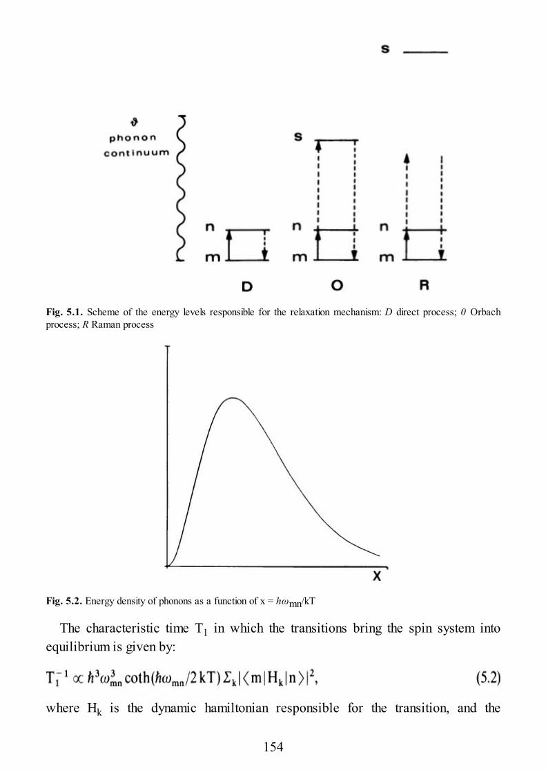
Fig. 5.1. Scheme of the energy levels responsible for the relaxation mechanism: D direct process; 0 Orbachprocess; R Raman process

Fig. 5.2. Energy density of phonons as a function of x = hωmn/kT

The characteristic time T1 in which the transitions bring the spin system intoequilibrium is given by:

where Hk is the dynamic hamiltonian responsible for the transition, and the

154

summation is over the various modes of vibration. If , (5.2) shows that is directly proportional to T.

The above expression has been obtained on the assumption that the transfer ofenergy of phonons to the bath is instantaneous. However, since the number ofphonons available is much smaller than that of the spins in an undiluted material,each phonon must experience a very high number of collisions for every collisionexperienced by a spin. This has the effect of considerably reducing the meanlifetime for the phonon, and consequently to reduce the mean free path of phonons.At low temperature this may become shorter than the crystal size, thus making theprocess of exchange with the bath much longer. This situation is referred to as“phonon bottleneck”, and it alters considerably the relaxation mechanism. It hasbeen established that under these conditions is proportional to:

If , is proportional to T2 rather than to T, as required by (5.2).Beyond the direct one-phonon process, there are several two-phonon processes,

which are more effective at high temperatures, of which the most relevant arenamed after Orbach and Raman, respectively. The former consists in the absorptionof a phonon ω1 exciting the spin into the level, which lies in the phononcontinuum, and the emission of a second phonon ω2 from to , asschematized in Fig. 5.1. In this way the phonons which are responsible for therelaxation have energies and , much larger than that of the direct processand are therefore much more numerous than those which allow the direct process(Fig. 5.2).

The Raman relaxation must be distinguished in a first- and a second-orderprocess. The former occurs when the dynamic hamiltonian has matrix elementsdifferent from zero between the two levels and involved in the relaxation.The transition between the two can occur via absorption of one phonon ω1 andemission of a phonon ω2 with the condition that ħωmn = ħω2−ħω1 Phonons ofenergy close to the maximum in the diagram of Fig. 5.2 can contribute in this case,thus making this process much more effective than the direct one at hightemperatures. In the second-order Raman process the two states and areboth coupled to an excited state and a transition between them can be induced bythe absorption and emission of two virtual phonons outside the phonon continuum.

Each of these processes has different temperature dependences. The Orbachprocess is characterized by:

which becomes simply proportional to exp if exp .

155

The temperature dependence of the Raman process is different for Kramers andnon-Kramers states. For the latter it is found that

while for the former

under the condition that T < Θ. Θ is the maximum phonon frequency available in themedium, expressed as temperature. In a lattice this corresponds to the Debyetemperature. When T > Θ both for Kramers and non-Kramers ions in the Ramanprocess, becomes proportional to T2.

Finally, when the ground state is a multiplet, then the and levels in theEPR transition can be coupled to the other states of the multiplet. In this case therelaxation process is named after Blume and Orbach. It leads at low temperaturesto a dependence of the type:

In an exchange-coupled pair, by definition, there are a number of electroniclevels with energies comparable to kT. Therefore, these can provide effectiverelaxation pathways, which make in general larger for pairs than for isolatedions, through two phonon relaxation processes. In fact, the modulation processes,which are already present for single spins, may become more efficient due to thepresence of new, low lying levels which are generated by the exchange interaction.

The modulation processes of the exchange interaction can be split as usual intoisotropic, anisotropic, and antisymmetric components. Modulation of isotropicexchange can yield relaxation only to the second order for pairs, but it can beeffective also to the first order for larger clusters. In fact, the selection rules forisotropic exchange require and , but for couples only one totalspin state with a given value of S is possible. This condition is no longer met forlarger clusters, where more total spin states with the same value of S can exist.Anisotropic and antisymmetric exchange, on the other hand, can couple states withdifferent S and M, therefore, although they are generally much smaller than theisotropic one, they can produce sizeable effects to the first order in pairs.

With this background we may now examine some examples. The experimentalstudies of spin-lattice relaxation have focused essentially on either simple dopedlattices, such as Ir4+ pairs in (NH4)2PtCl6, or materials of biological interest,among which we choose iron-ferredoxins as interesting examples.

156

5.3 Iridium(IV) Pairs

The studies of iridium(IV) pairs constitute a classic in relaxation of exchange-coupled systems, and we will work them out in detail, following the originalpapers by Owens and Yngvesson [5.5, 6]. The temperature dependence of therelaxation rate for iridium(IV) doped (NH4)2PtCl6 is shown in Fig. 5.3. Theexperiments were performed on single crystals, at various doping levels. At lowdoping levels does not depend markedly on concentration, while thedependence is much more dramatic when the concentration increases. This has beentaken as evidence of an intrinsic relaxation of pairs to the lattice, not involvingcross-relaxation to higher nuclearity intermediates.

The procedure for a theoretical estimation of requires knowledge of theground state and of the excited states which can be admixed into it and of thenormal modes of vibration of the pair. Ir4+ has a ground 2T2g state in octahedralsymmetry, which is split by spin-orbit coupling and low symmetry effects to give aground doublet and an excited quartet. These two states can be described byeffective spins S = 1/2 and S = 3/2, respectively. The ligand field states are givenin Table 5.1. Coupling the two doublets yields a singlet and a triplet, correspondingto the ground manifold of a pair. Excited manifolds correspond to one ion in the

state and the other in the excited S = 3/2 state, yielding two S = 2 and two S= 1 states. At higher energy we find the states generated by the interaction of thetwo ions in the excited S = 3/2 states, yielding S = 3, 2, 1, and 0. In order todetermine the relaxation process we must calculate the admixture of the excitedstates into the low lying singlet and triplet states via the exchange and the Zeemanhamiltonian and then evaluate the matrix elements of the dynamic hamiltonianincluding the vibrations. Since the energy separation between the total spin states islarge compared to the anisotropic exchange and Zeeman interaction, the correctfunctions can be obtained through a perturbation treatment.

157

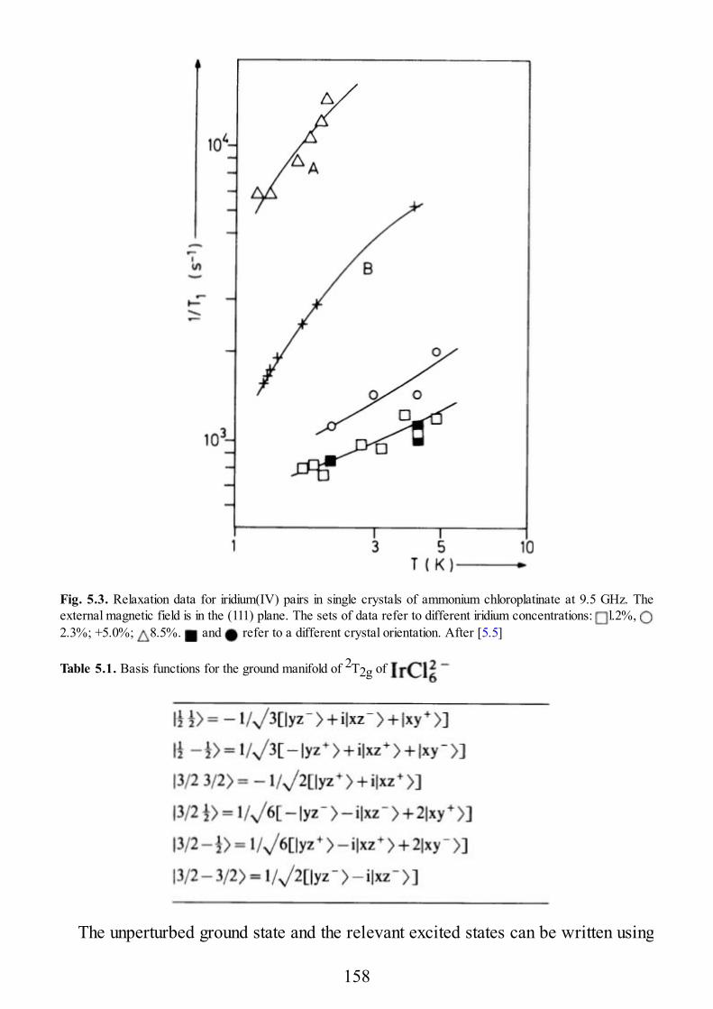
Fig. 5.3. Relaxation data for iridium(IV) pairs in single crystals of ammonium chloroplatinate at 9.5 GHz. Theexternal magnetic field is in the (111) plane. The sets of data refer to different iridium concentrations: l.2%, 2.3%; +5.0%; 8.5%. and refer to a different crystal orientation. After [5.5]

Table 5.1. Basis functions for the ground manifold of 2T2g of

The unperturbed ground state and the relevant excited states can be written using

158

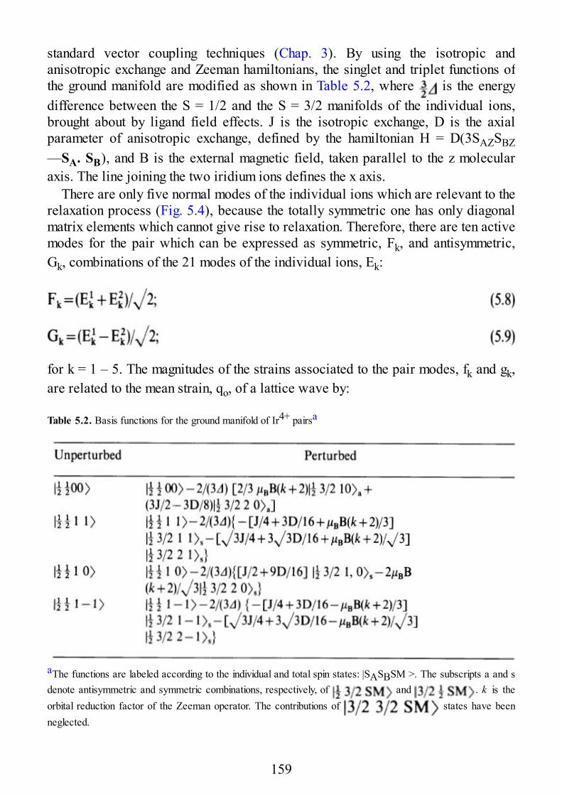
standard vector coupling techniques (Chap. 3). By using the isotropic andanisotropic exchange and Zeeman hamiltonians, the singlet and triplet functions ofthe ground manifold are modified as shown in Table 5.2, where is the energydifference between the S = 1/2 and the S = 3/2 manifolds of the individual ions,brought about by ligand field effects. J is the isotropic exchange, D is the axialparameter of anisotropic exchange, defined by the hamiltonian H = D(3SAZSBZ—SA. SB), and B is the external magnetic field, taken parallel to the z molecularaxis. The line joining the two iridium ions defines the x axis.

There are only five normal modes of the individual ions which are relevant to therelaxation process (Fig. 5.4), because the totally symmetric one has only diagonalmatrix elements which cannot give rise to relaxation. Therefore, there are ten activemodes for the pair which can be expressed as symmetric, Fk, and antisymmetric,Gk, combinations of the 21 modes of the individual ions, Ek:

for k = 1 – 5. The magnitudes of the strains associated to the pair modes, fk and gk,are related to the mean strain, qo, of a lattice wave by:

Table 5.2. Basis functions for the ground manifold of Ir4+ pairsa

aThe functions are labeled according to the individual and total spin states: |SASBSM >. The subscripts a and sdenote antisymmetric and symmetric combinations, respectively, of and . k is theorbital reduction factor of the Zeeman operator. The contributions of states have beenneglected.

159

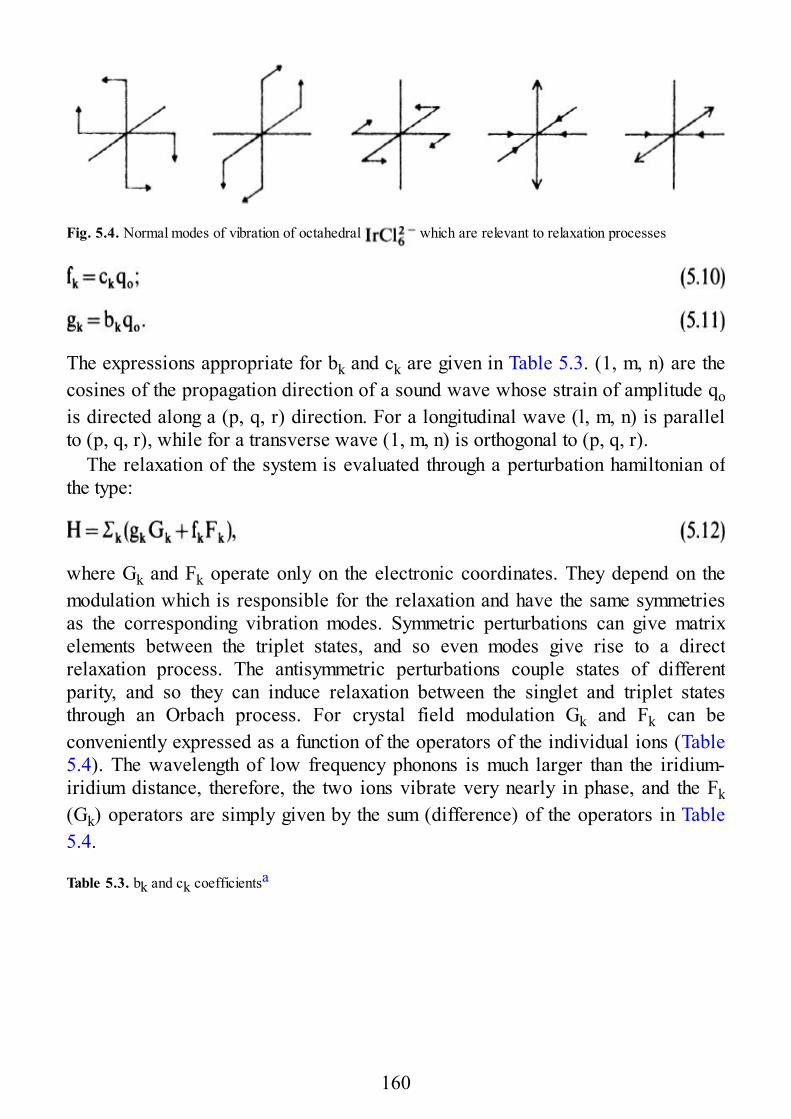
Fig. 5.4. Normal modes of vibration of octahedral which are relevant to relaxation processes

The expressions appropriate for bk and ck are given in Table 5.3. (1, m, n) are thecosines of the propagation direction of a sound wave whose strain of amplitude qois directed along a (p, q, r) direction. For a longitudinal wave (l, m, n) is parallelto (p, q, r), while for a transverse wave (1, m, n) is orthogonal to (p, q, r).

The relaxation of the system is evaluated through a perturbation hamiltonian ofthe type:

where Gk and Fk operate only on the electronic coordinates. They depend on themodulation which is responsible for the relaxation and have the same symmetriesas the corresponding vibration modes. Symmetric perturbations can give matrixelements between the triplet states, and so even modes give rise to a directrelaxation process. The antisymmetric perturbations couple states of differentparity, and so they can induce relaxation between the singlet and triplet statesthrough an Orbach process. For crystal field modulation Gk and Fk can beconveniently expressed as a function of the operators of the individual ions (Table5.4). The wavelength of low frequency phonons is much larger than the iridium-iridium distance, therefore, the two ions vibrate very nearly in phase, and the Fk(Gk) operators are simply given by the sum (difference) of the operators in Table5.4.

Table 5.3. bk and ck coefficientsa

160

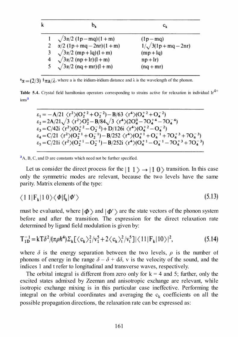
, where a is the iridium-iridium distance and λ is the wavelength of the phonon.

Table 5.4. Crystal field hamiltonian operators corresponding to strains active for relaxation in individual Ir4+

ionsa

aA, B, C, and D are constants which need not be further specified.

Let us consider the direct process for the transition. In this caseonly the symmetric modes are relevant, because the two levels have the sameparity. Matrix elements of the type:

must be evaluated, where and are the state vectors of the phonon systembefore and after the transition. The expression for the direct relaxation ratedetermined by ligand field modulation is given by:

where δ is the energy separation between the two levels, ρ is the number ofphonons of energy in the range δ – δ + dδ, v is the velocity of the sound, and theindices 1 and t refer to longitudinal and transverse waves, respectively.

The orbital integral is different from zero only for k = 4 and 5; further, only theexcited states admixed by Zeeman and anisotropic exchange are relevant, whileisotropic exchange mixing is in this particular case ineffective. Performing theintegral on the orbital coordinates and averaging the ck coefficients on all thepossible propagation directions, the relaxation rate can be expressed as:

161

where P is a constant. If we compare (5.15) with the analogous expression for thesingle ion:

we see that neglecting D,

Therefore, as far as the direct process is concerned, the relaxation rate of the pairinduced by crystal field modulation can be slower than that of the single ion.

Modulation of the anisotropic exchange is also symmetric in the spincoordinates, therefore, it can induce direct relaxation processes between the tripletstates. Since this term is not operative for single ions, its inclusion determines afaster relaxation for the pair. The hamiltonian can be expressed as:

with D′ = ro δD/δrAB. The contribution of this term to the direct process is similarto (5.14). The matrix element of the electronic hamiltonian has been estimatednumerically to correspond to ≈ 7 cm−1, in such a way that the contribution of theanisotropic exchange to the direct relaxation rate is

The triplet state functions can relax also by an Orbach process involving thesinglet level. In this case it is the antisymmetric modes Gk which are relevant,because they can couple the two spin multiplets of opposite parity. The calculatedrelaxation rate is of the type:

The temperature dependence in (5.20) is different from that in (5.4), because in thiscase the states involved in relaxation are higher in energy than the state of theOrbach process. This is a process which has no counterpart in the single ion. Theexperimental data of Fig. 5.3 were fitted with this dependence, using the J value 5.2cm−1. However, the predicted rate is within a factor of 3 of the observed rate, sothat it was concluded only that it is probable that (5.20) is a major contribution tothe relaxation process.

162

5.4 Copper Pairs

Another simple system which has been investigated is that of copper pairs inzinc(II) bis(diethyl-dithiocarbamato), Zn(dtc)2, single crystals [5.7]. A typicalspectrum of a single crystal containing 5% copper(II) is shown in Fig. 5.5. Inaddition to the four intense lines in the center of the spectrum, which arise fromisolated copper(II) ions, two well-resolved groups of septets, arising from copperpairs, are resolved. The relaxation rate was measured using pulse and spin-echotechniques. At T < 4K the experimental data were found to follow the temperaturedependence expected for a direct process, with at 28.8 GHz and

at 9.0 GHz, while in the range 4 < T < 12 K the data could be fitted byan Orbach process: with δ = 13±1 cm−1. δwas considered to correspond to the singlet-triplet splitting, the triplet lying lower.

The calculated relaxation rate for the direct process is 2.5 times faster than thatfor the single ion, however, the experimental result is that relaxation in thedinuclear species is 16 times faster than in the single ion. A possible explanationfor this difference lies in the fact that single ions and pairs have different structures.

Another important feature of the relaxation rate of the direct process is itsfrequency dependence. In fact, (5.14) requires a direct linear dependence of on , while the experimental data on Cu : Zn(dtc)2 rather suggest an inverselinear dependence. This anomaly has been explained on the basis of the dominantrole of isotropic exchange modulation in weak fields.

163

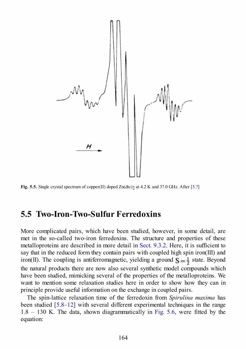
Fig. 5.5. Single crystal spectrum of copper(II) doped Zn(dtc)2 at 4.2 K and 37.0 GHz. After [5.7]

5.5 Two-Iron-Two-Sulfur Ferredoxins

More complicated pairs, which have been studied, however, in some detail, aremet in the so-called two-iron ferredoxins. The structure and properties of thesemetalloproteins are described in more detail in Sect. 9.3.2. Here, it is sufficient tosay that in the reduced form they contain pairs with coupled high spin iron(III) andiron(II). The coupling is antiferromagnetic, yielding a ground state. Beyondthe natural products there are now also several synthetic model compounds whichhave been studied, mimicking several of the properties of the metalloproteins. Wewant to mention some relaxation studies here in order to show how they can inprinciple provide useful information on the exchange in coupled pairs.

The spin-lattice relaxation time of the ferredoxin from Spirulina maxima hasbeen studied [5.8–12] with several different experimental techniques in the range1.8 – 130 K. The data, shown diagrammatically in Fig. 5.6, were fitted by theequation:

164

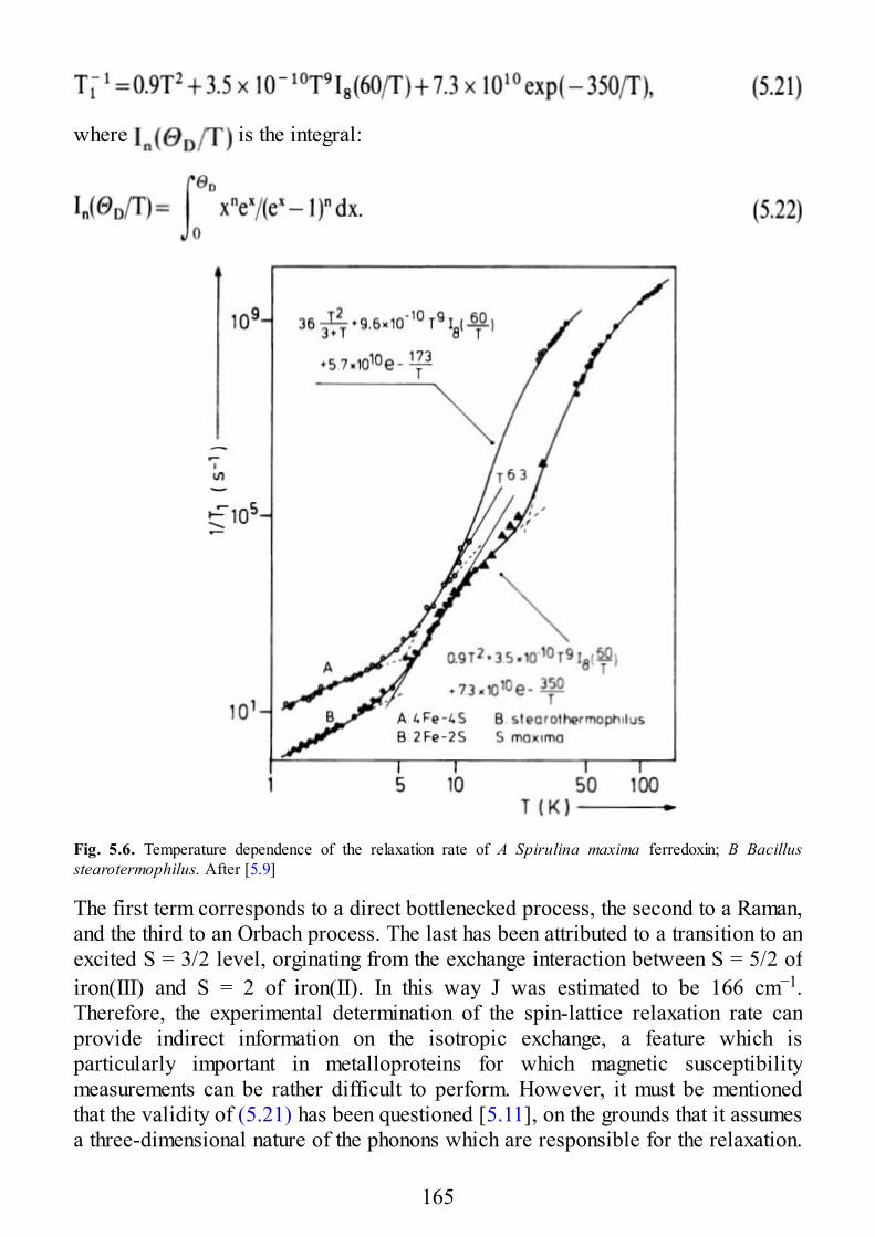
where is the integral:

Fig. 5.6. Temperature dependence of the relaxation rate of A Spirulina maxima ferredoxin; B Bacillusstearotermophilus. After [5.9]

The first term corresponds to a direct bottlenecked process, the second to a Raman,and the third to an Orbach process. The last has been attributed to a transition to anexcited S = 3/2 level, orginating from the exchange interaction between S = 5/2 ofiron(III) and S = 2 of iron(II). In this way J was estimated to be 166 cm−1.Therefore, the experimental determination of the spin-lattice relaxation rate canprovide indirect information on the isotropic exchange, a feature which isparticularly important in metalloproteins for which magnetic susceptibilitymeasurements can be rather difficult to perform. However, it must be mentionedthat the validity of (5.21) has been questioned [5.11], on the grounds that it assumesa three-dimensional nature of the phonons which are responsible for the relaxation.

165

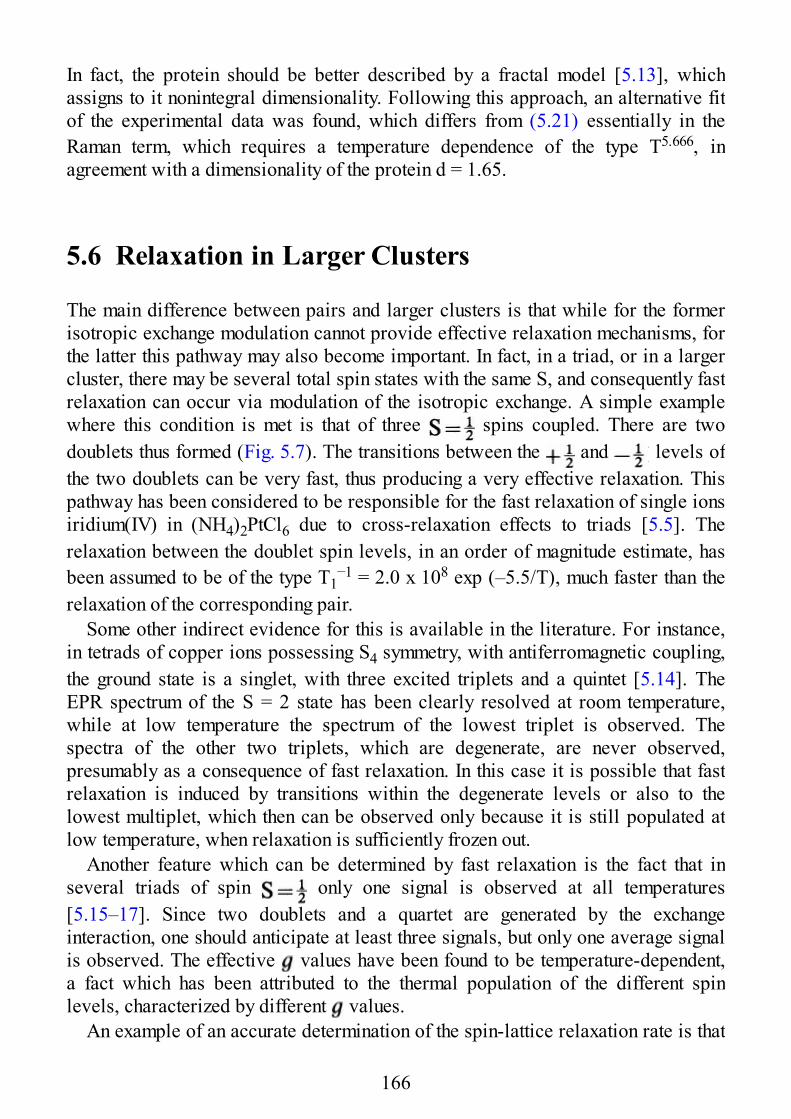
In fact, the protein should be better described by a fractal model [5.13], whichassigns to it nonintegral dimensionality. Following this approach, an alternative fitof the experimental data was found, which differs from (5.21) essentially in theRaman term, which requires a temperature dependence of the type T5.666, inagreement with a dimensionality of the protein d = 1.65.

5.6 Relaxation in Larger Clusters

The main difference between pairs and larger clusters is that while for the formerisotropic exchange modulation cannot provide effective relaxation mechanisms, forthe latter this pathway may also become important. In fact, in a triad, or in a largercluster, there may be several total spin states with the same S, and consequently fastrelaxation can occur via modulation of the isotropic exchange. A simple examplewhere this condition is met is that of three spins coupled. There are twodoublets thus formed (Fig. 5.7). The transitions between the and levels ofthe two doublets can be very fast, thus producing a very effective relaxation. Thispathway has been considered to be responsible for the fast relaxation of single ionsiridium(IV) in (NH4)2PtCl6 due to cross-relaxation effects to triads [5.5]. Therelaxation between the doublet spin levels, in an order of magnitude estimate, hasbeen assumed to be of the type T1

−1 = 2.0 x 108 exp (–5.5/T), much faster than therelaxation of the corresponding pair.

Some other indirect evidence for this is available in the literature. For instance,in tetrads of copper ions possessing S4 symmetry, with antiferromagnetic coupling,the ground state is a singlet, with three excited triplets and a quintet [5.14]. TheEPR spectrum of the S = 2 state has been clearly resolved at room temperature,while at low temperature the spectrum of the lowest triplet is observed. Thespectra of the other two triplets, which are degenerate, are never observed,presumably as a consequence of fast relaxation. In this case it is possible that fastrelaxation is induced by transitions within the degenerate levels or also to thelowest multiplet, which then can be observed only because it is still populated atlow temperature, when relaxation is sufficiently frozen out.

Another feature which can be determined by fast relaxation is the fact that inseveral triads of spin only one signal is observed at all temperatures[5.15–17]. Since two doublets and a quartet are generated by the exchangeinteraction, one should anticipate at least three signals, but only one average signalis observed. The effective values have been found to be temperature-dependent,a fact which has been attributed to the thermal population of the different spinlevels, characterized by different values.

An example of an accurate determination of the spin-lattice relaxation rate is that

166

of four iron-four sulfur ferredoxins from Bacillus Stearothermophilus [5.9]. In Fig.5.6B the temperature dependence of T1

−1 is shown, which was fitted according to:

Fig. 5.7. Scheme of the energy levels of three coupled spins

This shows that below 4 K the condition is that of a phonon bottleneck, for4<T<10K a Raman process is dominant, with a Debye temperature Θ = 60K, like inthe 2Fe-2S protein, while for T > 10K an Orbach process becomes dominant withan excited level at 173 K. In all the temperature ranges the relaxation rate for the 4Fe protein is at least an order of magnitude faster than that of the 2Fe protein,except that in the range where the Raman process is dominant, where there is only afactor of 3 between the two.

References

5.1 Bertini I, Luchinat C (1985) NMR of Paramagnetic Molecules in Biological Systems, Benjamin/Cummings:Menlo Park

5.2 Abragam A, Bleaney B (1970) Electron Paramagnetic Resonance of Transition Ions, Clarendon Press,Oxford

5.3 Stevens, KWH (1967) Rep. Progr Phys 30, 1895.4 Owen J, Harris E A (1972) in Electron Paramagnetic Resonance; Geschwind, S., Ed.; Plenum Press, New

York London5.5 Harris EA, Yngvesson KS (1968) J. Phys. Cl, 9905.6 Harris EA, Yngvesson KS (1968) J. Phys. Cl, 10115.7 Al’tshuler SA, Kirmse R, Solovev BV (1975) J. Phys. C, 8, 19075.8 Gayda JP, Gibson JF Cammack R, Hall DO, Mullinger R (1976) Biochim. Biophys. Acta 434, 1545.9 Bertrand P, Gayda JP, Rao KK (1982) J. Chem. Phys. 76, 47155.10 Gayda JP, Bertrand P, Deville A, More C, Roger G, Gibson JF, Cammack R (1979) Biochim. Biophys.

Acta, 581, 155.11 Stapleton HJ, Allen JP, Flynn CP, Stinson DG, Kurtz SR (1985) Phys. Rev. Letters 45, 14565.12 Bertrand P, Roger G, Gayda JP (1980) J. Magn. Reson. 40, 5395.13 Tarasov VV (1958) J. Am. Chem. Soc. 80, 50525.14 Bencini A, Gatteschi D, Zanchini C, Haasnot JG, Prins R, Reedijk J (1987) J Am. Chem. Soc. 109, 29265.15 Benelli C, Gatteschi D, Zanchini C, Latour JM, Rey P (1986) Inorg. Chem. 25, 42425.16 Banci L, Bencini A, Dei A, Gatteschi D (1983) Inorg. Chem. 22, 40185.17 Banci L, Bencini A, Gatteschi D (1983) Inorg. Chem. 22, 2681

167

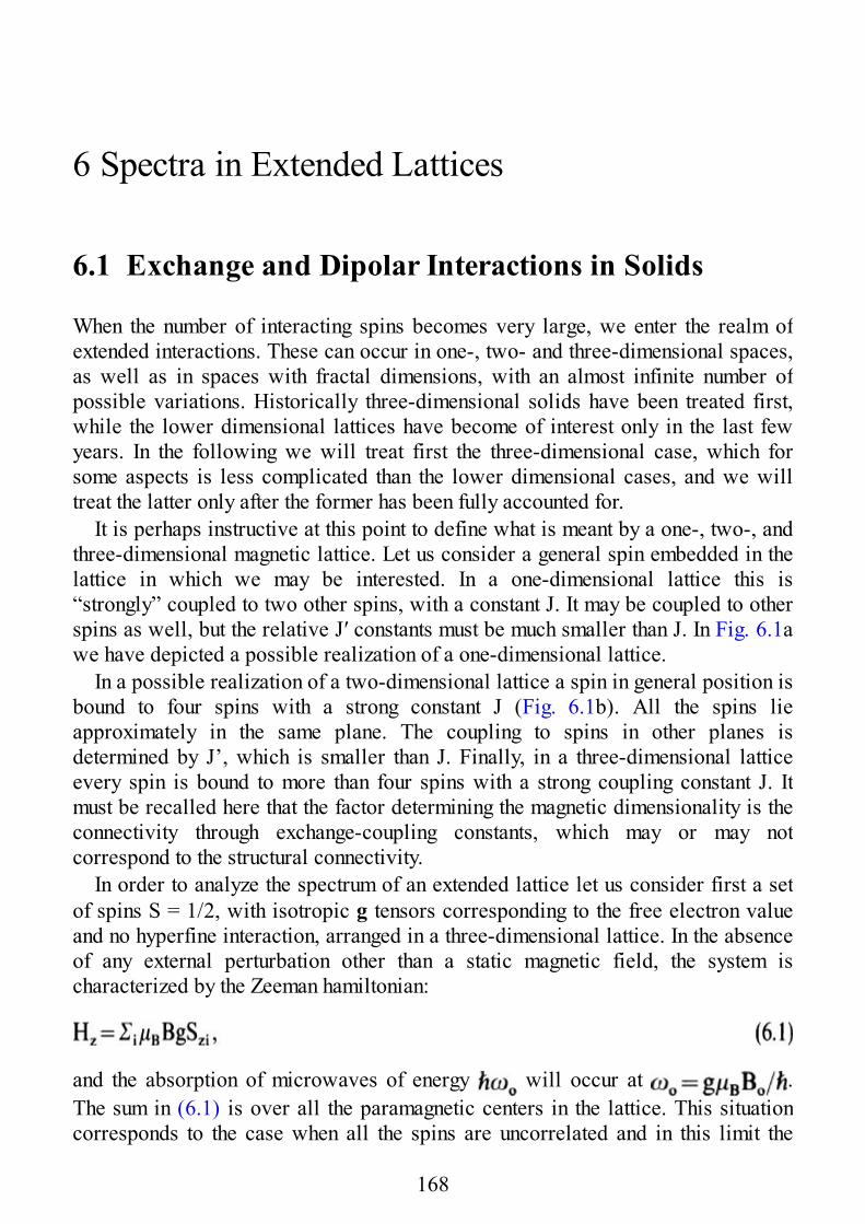
6 Spectra in Extended Lattices

6.1 Exchange and Dipolar Interactions in Solids

When the number of interacting spins becomes very large, we enter the realm ofextended interactions. These can occur in one-, two- and three-dimensional spaces,as well as in spaces with fractal dimensions, with an almost infinite number ofpossible variations. Historically three-dimensional solids have been treated first,while the lower dimensional lattices have become of interest only in the last fewyears. In the following we will treat first the three-dimensional case, which forsome aspects is less complicated than the lower dimensional cases, and we willtreat the latter only after the former has been fully accounted for.

It is perhaps instructive at this point to define what is meant by a one-, two-, andthree-dimensional magnetic lattice. Let us consider a general spin embedded in thelattice in which we may be interested. In a one-dimensional lattice this is“strongly” coupled to two other spins, with a constant J. It may be coupled to otherspins as well, but the relative J′ constants must be much smaller than J. In Fig. 6.1awe have depicted a possible realization of a one-dimensional lattice.

In a possible realization of a two-dimensional lattice a spin in general position isbound to four spins with a strong constant J (Fig. 6.1b). All the spins lieapproximately in the same plane. The coupling to spins in other planes isdetermined by J’, which is smaller than J. Finally, in a three-dimensional latticeevery spin is bound to more than four spins with a strong coupling constant J. Itmust be recalled here that the factor determining the magnetic dimensionality is theconnectivity through exchange-coupling constants, which may or may notcorrespond to the structural connectivity.

In order to analyze the spectrum of an extended lattice let us consider first a setof spins S = 1/2, with isotropic g tensors corresponding to the free electron valueand no hyperfine interaction, arranged in a three-dimensional lattice. In the absenceof any external perturbation other than a static magnetic field, the system ischaracterized by the Zeeman hamiltonian:

and the absorption of microwaves of energy will occur at .The sum in (6.1) is over all the paramagnetic centers in the lattice. This situationcorresponds to the case when all the spins are uncorrelated and in this limit the

168

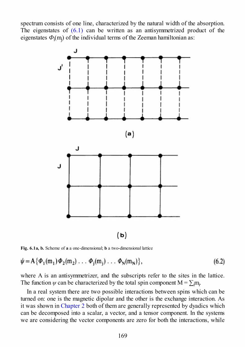
spectrum consists of one line, characterized by the natural width of the absorption.The eigenstates of (6.1) can be written as an antisymmetrized product of theeigenstates Фi(mj) of the individual terms of the Zeeman hamiltonian as:

Fig. 6.1a, b. Scheme of a a one-dimensional; b a two-dimensional lattice

where A is an antisymmetrizer, and the subscripts refer to the sites in the lattice.The function ψ can be characterized by the total spin component M = ∑imi.

In a real system there are two possible interactions between spins which can beturned on: one is the magnetic dipolar and the other is the exchange interaction. Asit was shown in Chapter 2 both of them are generally represented by dyadics whichcan be decomposed into a scalar, a vector, and a tensor component. In the systemswe are considering the vector components are zero for both the interactions, while

169

the scalar is zero for the magnetic dipolar and the tensor is zero for the exchangeinteraction. The hamiltonian for the latter can be written as:

and if the distance between paramagnetic centers is large for any couple of spinsthe hamiltonian for the former is given by:

where rjk is the vector connecting the sites of the j and k spins and the sums areextended to the entire lattice.

Hdip can be rewritten according to the relation:

The first term in the parentheses couples states with , the second and thethird states with , and the fourth states with . The effect ofHdip therefore is that of modifying the eigenstates of Hz, which are given by (6.2),admixing into them states differing in M by 0, ± 1, and ± 2, respectively. A simpleperturbation treatment, which is valid in the assumption that , gives themixing coefficients . Transitions between the total spin states canbe induced by the transverse magnetization operator, Sx = ∑iSix, connecting statesdiffering in mi by ±1. Therefore, the transitions between the perturbed states willbe, at the c2 order of magnitude, between states with δM = 0, ±1, ±2, and ±3. As aconsequence, transitions centered at ω = 0, 2ωo, and 3ωo, with an intensityproportional to c2, will add to the main absorption at ω = ωo

The second effect of the dipolar interaction is that of broadening the main linecentered at ω = ωo The reason for this broadening can become intuitively clear ifwe build up the infinite lattice by starting from two, three. . . interacting spins. Inthe limit of weak exchange two spins yield a singlet and a triplet, for which twoallowed transitions will be observed between the states described by M = + 1 andM = 0, and M = − 1 and M = 0, respectively. The separation between the two lines,which are symmetrically spaced around ωo, depends on the direction of the external

170

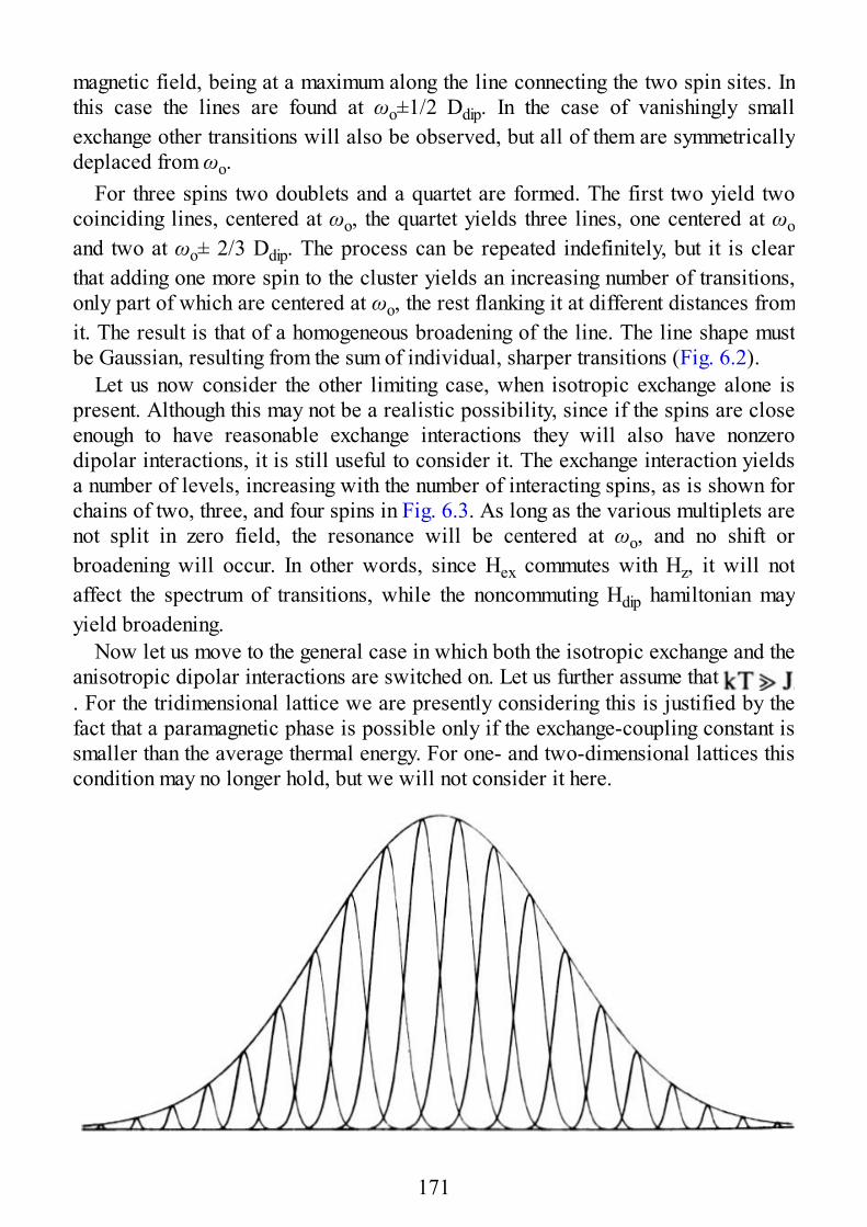
magnetic field, being at a maximum along the line connecting the two spin sites. Inthis case the lines are found at ωo±1/2 Ddip. In the case of vanishingly smallexchange other transitions will also be observed, but all of them are symmetricallydeplaced from ωo.

For three spins two doublets and a quartet are formed. The first two yield twocoinciding lines, centered at ωo, the quartet yields three lines, one centered at ωoand two at ωo± 2/3 Ddip. The process can be repeated indefinitely, but it is clearthat adding one more spin to the cluster yields an increasing number of transitions,only part of which are centered at ωo, the rest flanking it at different distances fromit. The result is that of a homogeneous broadening of the line. The line shape mustbe Gaussian, resulting from the sum of individual, sharper transitions (Fig. 6.2).

Let us now consider the other limiting case, when isotropic exchange alone ispresent. Although this may not be a realistic possibility, since if the spins are closeenough to have reasonable exchange interactions they will also have nonzerodipolar interactions, it is still useful to consider it. The exchange interaction yieldsa number of levels, increasing with the number of interacting spins, as is shown forchains of two, three, and four spins in Fig. 6.3. As long as the various multiplets arenot split in zero field, the resonance will be centered at ωo, and no shift orbroadening will occur. In other words, since Hex commutes with Hz, it will notaffect the spectrum of transitions, while the noncommuting Hdip hamiltonian mayyield broadening.

Now let us move to the general case in which both the isotropic exchange and theanisotropic dipolar interactions are switched on. Let us further assume that . For the tridimensional lattice we are presently considering this is justified by thefact that a paramagnetic phase is possible only if the exchange-coupling constant issmaller than the average thermal energy. For one- and two-dimensional lattices thiscondition may no longer hold, but we will not consider it here.

171

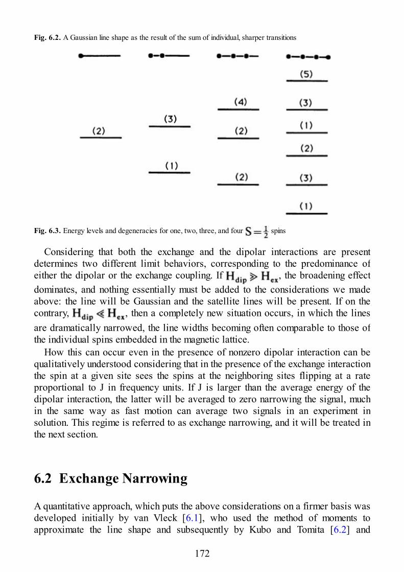
Fig. 6.2. A Gaussian line shape as the result of the sum of individual, sharper transitions

Fig. 6.3. Energy levels and degeneracies for one, two, three, and four spins

Considering that both the exchange and the dipolar interactions are presentdetermines two different limit behaviors, corresponding to the predominance ofeither the dipolar or the exchange coupling. If , the broadening effectdominates, and nothing essentially must be added to the considerations we madeabove: the line will be Gaussian and the satellite lines will be present. If on thecontrary, , then a completely new situation occurs, in which the linesare dramatically narrowed, the line widths becoming often comparable to those ofthe individual spins embedded in the magnetic lattice.

How this can occur even in the presence of nonzero dipolar interaction can bequalitatively understood considering that in the presence of the exchange interactionthe spin at a given site sees the spins at the neighboring sites flipping at a rateproportional to J in frequency units. If J is larger than the average energy of thedipolar interaction, the latter will be averaged to zero narrowing the signal, muchin the same way as fast motion can average two signals in an experiment insolution. This regime is referred to as exchange narrowing, and it will be treated inthe next section.

6.2 Exchange Narrowing

A quantitative approach, which puts the above considerations on a firmer basis wasdeveloped initially by van Vleck [6.1], who used the method of moments toapproximate the line shape and subsequently by Kubo and Tomita [6.2] and

172

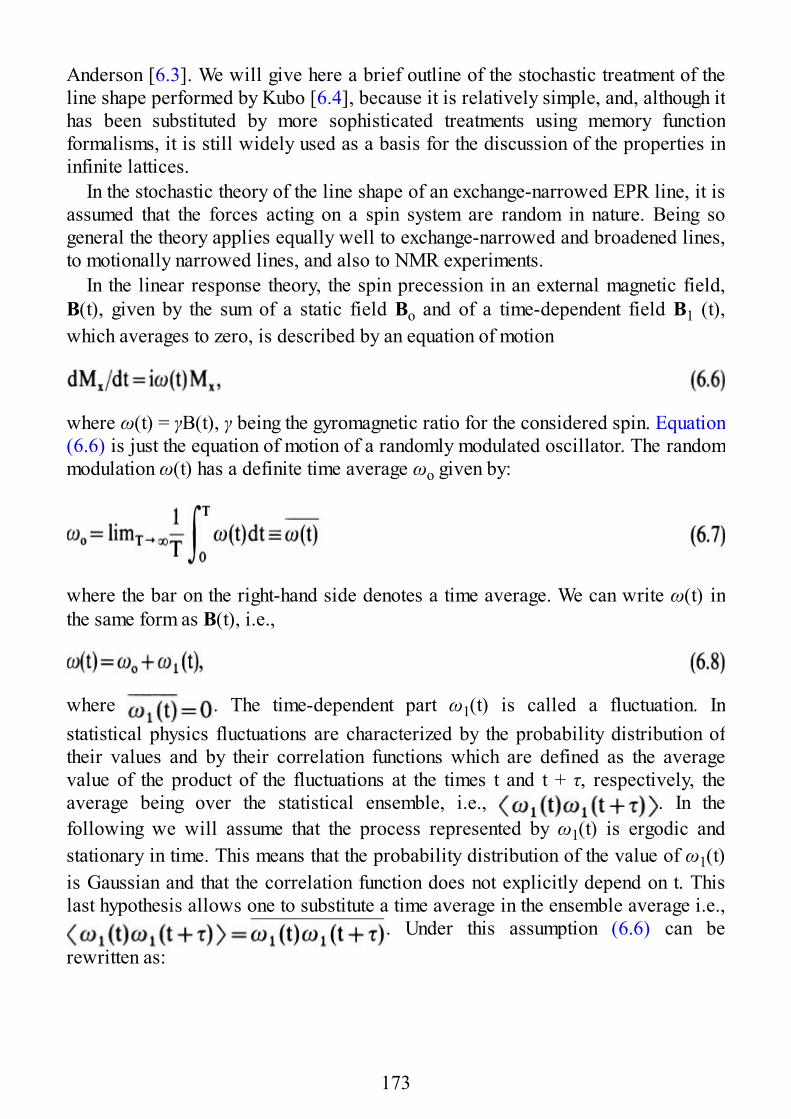
Anderson [6.3]. We will give here a brief outline of the stochastic treatment of theline shape performed by Kubo [6.4], because it is relatively simple, and, although ithas been substituted by more sophisticated treatments using memory functionformalisms, it is still widely used as a basis for the discussion of the properties ininfinite lattices.

In the stochastic theory of the line shape of an exchange-narrowed EPR line, it isassumed that the forces acting on a spin system are random in nature. Being sogeneral the theory applies equally well to exchange-narrowed and broadened lines,to motionally narrowed lines, and also to NMR experiments.

In the linear response theory, the spin precession in an external magnetic field,B(t), given by the sum of a static field Bo and of a time-dependent field B1 (t),which averages to zero, is described by an equation of motion

where ω(t) = γB(t), γ being the gyromagnetic ratio for the considered spin. Equation(6.6) is just the equation of motion of a randomly modulated oscillator. The randommodulation ω(t) has a definite time average ωo given by:

where the bar on the right-hand side denotes a time average. We can write ω(t) inthe same form as B(t), i.e.,

where . The time-dependent part ω1(t) is called a fluctuation. Instatistical physics fluctuations are characterized by the probability distribution oftheir values and by their correlation functions which are defined as the averagevalue of the product of the fluctuations at the times t and t + τ, respectively, theaverage being over the statistical ensemble, i.e., . In thefollowing we will assume that the process represented by ω1(t) is ergodic andstationary in time. This means that the probability distribution of the value of ω1(t)is Gaussian and that the correlation function does not explicitly depend on t. Thislast hypothesis allows one to substitute a time average in the ensemble average i.e.,

. Under this assumption (6.6) can berewritten as:

173

decomposing ω(t) into its time-independent, ωo, and its time-dependent, ω1(t),parts.

The assembly of spins in the lattice can be considered to form a statisticalensemble, so that the expectation value of Mx(t) can be evaluated by performing anensemble average of the random process ω(t):

where Mx(0) is the initial value of Mx at t = 0. defines

a function Φ′(t), which is called the relaxation function of the oscillator. Itdescribes the decay of the transverse magnetization in a frame rotating at theresonance angular frequency ωo. Equation (6.10) can be rewritten as:

where * indicates complex conjugation.The fluctuation-dissipation theorem for a linear response system shows that the

resonance absorption spectrum at the angular frequency ω is given by the Fouriertransform of Φ′(t):

where I(ω — ω0) is normalized to unit. The absorption line is centered at ω0 and isbroadened by ω1(t). In other words, the resonance at ω0 is modulated by the time-dependent perturbation ω1(t).

In order to characterize the modulation process two parameters are used, namelyits amplitude and its correlation time. The former, which measures the magnitude ofthe modulation, is defined by:

174

is the average of the square of the modulation process. If we refer to Fig.6.2, is the average of the square of the width of each of the individualresonances which are contained under the envelope of the line. In the hypothesis ofGaussian modulation of ω1(t) this quantity is equivalent to the second moment of theresonance, which is defined by:

Clearly, the larger M2, the broader is the overall resonance.The correlation time of the modulation is defined by:

where ψ(t), the correlation function of the modulation:

ψ(τ) is normalized to M2 for τ = 0. ψ(τ) shows how much the modulation at time t +τ is influenced, i.e., correlated, by the value of the modulation at time t. In fact, ifψ(τ) is close to 1, it means that ω1(t + τ) ≈ ω1(t) ≈ ω1(0), while if ψ(τ) is close to 0,it means that there is no correlation between the two values. In Fig. 6.4 a typicalbehavior of the correlation function is plotted. It is seen to decrease rapidly at thebeginning, and then more slowly for the long times. The characteristic time τccorresponds to the time after which the correlation function is reduced to less thanone-half the initial value. τc is a measure of the speed of the modulation and it tellsus how fast the modulation vanishes. The exchange interaction determines a timevariation of the spin states of the system which is inversely proportional to thevalue of the coupling constant in frequency units. Therefore, τc is often taken as:

175

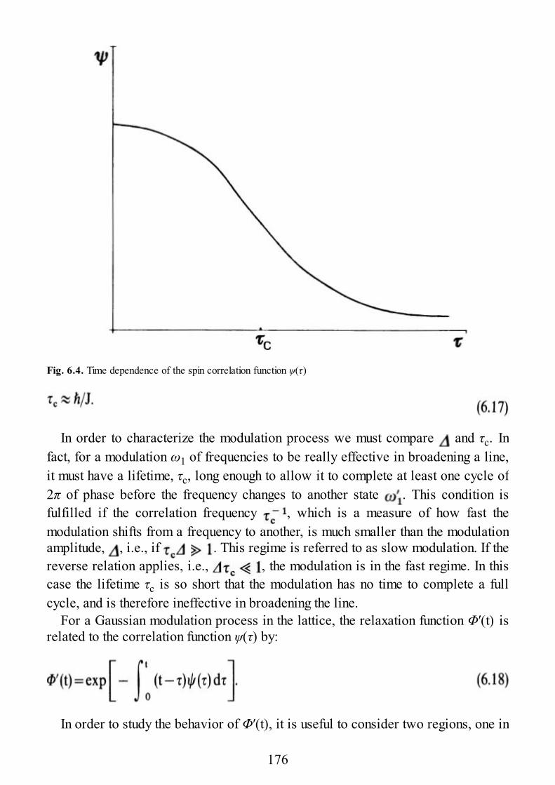
Fig. 6.4. Time dependence of the spin correlation function ψ(τ)

In order to characterize the modulation process we must compare and τc. Infact, for a modulation ω1 of frequencies to be really effective in broadening a line,it must have a lifetime, τc, long enough to allow it to complete at least one cycle of2π of phase before the frequency changes to another state . This condition isfulfilled if the correlation frequency , which is a measure of how fast themodulation shifts from a frequency to another, is much smaller than the modulationamplitude, , i.e., if . This regime is referred to as slow modulation. If thereverse relation applies, i.e., , the modulation is in the fast regime. In thiscase the lifetime τc is so short that the modulation has no time to complete a fullcycle, and is therefore ineffective in broadening the line.

For a Gaussian modulation process in the lattice, the relaxation function Φ′(t) isrelated to the correlation function ψ(τ) by:

In order to study the behavior of Φ′(t), it is useful to consider two regions, one in

176

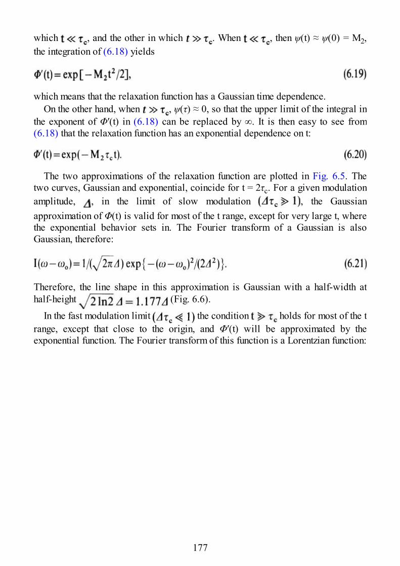
which , and the other in which . When , then ψ(t) ≈ ψ(0) = M2,the integration of (6.18) yields

which means that the relaxation function has a Gaussian time dependence.On the other hand, when , ψ(τ) ≈ 0, so that the upper limit of the integral in

the exponent of Φ′(t) in (6.18) can be replaced by ∞. It is then easy to see from(6.18) that the relaxation function has an exponential dependence on t:

The two approximations of the relaxation function are plotted in Fig. 6.5. Thetwo curves, Gaussian and exponential, coincide for t = 2τc. For a given modulationamplitude, , in the limit of slow modulation , the Gaussianapproximation of Φ(t) is valid for most of the t range, except for very large t, wherethe exponential behavior sets in. The Fourier transform of a Gaussian is alsoGaussian, therefore:

Therefore, the line shape in this approximation is Gaussian with a half-width athalf-height (Fig. 6.6).

In the fast modulation limit the condition holds for most of the trange, except that close to the origin, and Φ′(t) will be approximated by theexponential function. The Fourier transform of this function is a Lorentzian function:

177

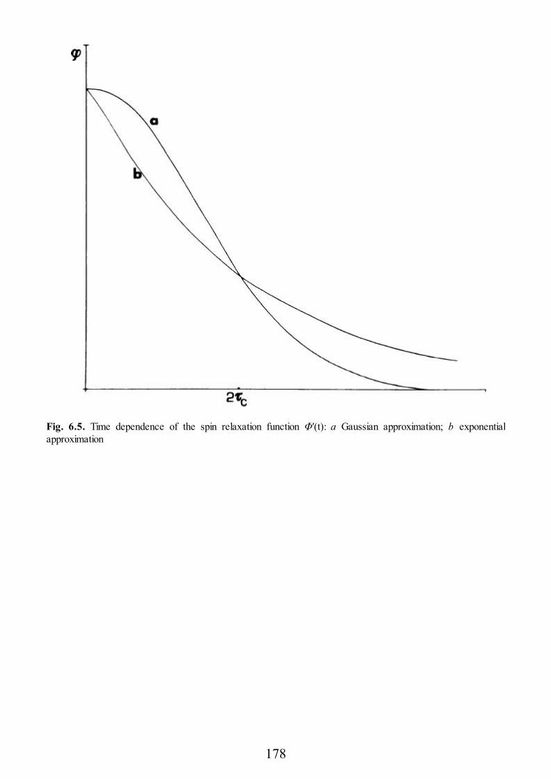
Fig. 6.5. Time dependence of the spin relaxation function Φ′(t): a Gaussian approximation; b exponentialapproximation

178

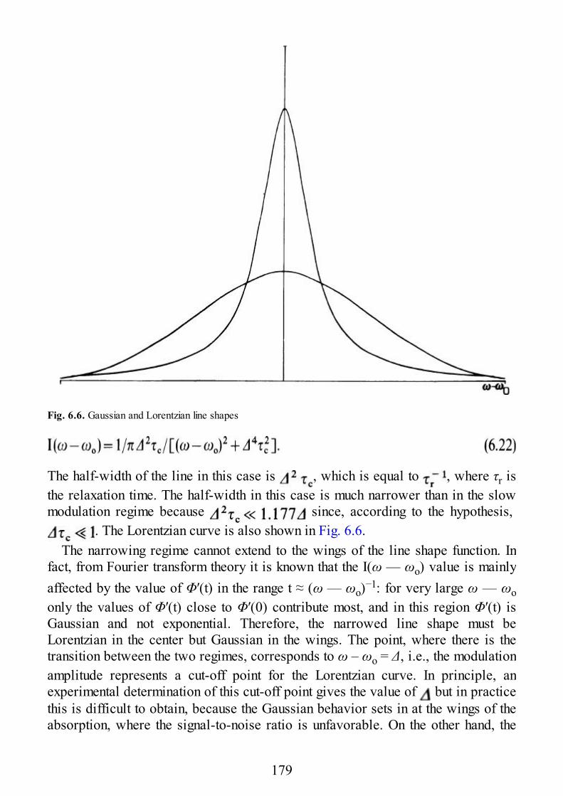
Fig. 6.6. Gaussian and Lorentzian line shapes

The half-width of the line in this case is , which is equal to , where τr isthe relaxation time. The half-width in this case is much narrower than in the slowmodulation regime because since, according to the hypothesis,

. The Lorentzian curve is also shown in Fig. 6.6.The narrowing regime cannot extend to the wings of the line shape function. In

fact, from Fourier transform theory it is known that the I(ω — ωo) value is mainlyaffected by the value of Φ′(t) in the range t ≈ (ω — ωo)−1: for very large ω — ωoonly the values of Φ′(t) close to Φ′(0) contribute most, and in this region Φ′(t) isGaussian and not exponential. Therefore, the narrowed line shape must beLorentzian in the center but Gaussian in the wings. The point, where there is thetransition between the two regimes, corresponds to ω – ωo = Δ, i.e., the modulationamplitude represents a cut-off point for the Lorentzian curve. In principle, anexperimental determination of this cut-off point gives the value of but in practicethis is difficult to obtain, because the Gaussian behavior sets in at the wings of theabsorption, where the signal-to-noise ratio is unfavorable. On the other hand, the

179

broadening regime cannot apply at ω ≈ ωo, because in this case it is the exponentialpart of Φ′(t) which determines the line shape, and the curve must be Lorentzian.However, in slow modulation this condition is limited to a very narrow rangearound the center, so that the Lorentzian section is totally undetectable.

The above treatment is very general in nature, and can be applied to anymagnetic resonance experiment, ESR, NMR. . . , with either motional or exchangemodulation.

In the EPR spectra of a magnetic solid the slow dipolar interaction broadens thelines yielding a Gaussian shape, while the exchange interactions can be fast enoughto bring the system in the exchange-narrowing regime. The speed of the modulationcan be estimated from the frequency of the interaction: in Chap. 2 we have seen thatthe dipolar interactions for paramagnetic centers, separated by at least 300 pm, aretypically of the order of 10−1 – 10−2 cm−1, which on a frequency scale correspondsto 108–109 Hz, while exchange interactions can be at least one order of magnitudelarger than the upper limit of the former. Therefore, the narrowing condition isfulfilled in many cases, and, since it is exchange-determined, it is called exchangenarrowing. In the following we will focus on this scheme, and will try to expressthe ψ(τ) and Φ′(t) functions using the hamiltonians appropriate to the system,relating the calculated absorption curves to parameters which depend on the natureof the interaction between the paramagnetic centers.

The exchange-narrowing condition is fulfilled if . In this case wecan split the total hamiltonian, H, into an unperturbed and a perturbed component:

where Ho comprises the Zeeman and exchange hamiltonians, and H′ includes thedipolar term. Since the two hamiltonians describe largely different frequencies, Hobeing much faster than H′, it is convenient to redefine Φ′(t) in such a way to removethe fast Zeeman and exchange frequencies and focus on the slow perturbingfrequencies. We will not develop the treatment in detail, but rather will touch uponthe relevant points, trying to underline what is relevant to the physics of theproblem, without entering the mathematics, which is rather involved.

The relaxation function of the system defined by (6.10) can be rewritten usingtime-dependent perturbation theory as:

where is in the interaction representation with respect to the unperturbedhamiltonian:

180

and M + (t) is in the Heisenberg representation with respect to the total hamiltonian,i.e., M + (t) = exp(iHt/ћ)M + exp(– iHt/ћ). Heisenberg and representationinteraction are the two different schemes for expressing the time dependence ofoperators and wave-functions. It is easy to verify that according to (6.25) the timeevolution of is only determined by the slow, dipolar perturbation. Φ(t) in(6.24) is related to Φ′(t) by the relation Φ(t) = eiωot Φ′(t).

In order to evaluate Φ(t) two thermal averages must be performed according to(6.24). The thermal average of the transverse magnetization relates itto the intensity of the EPR signal or the static susceptibility via:

where χc is the static magnetic susceptibility for a system with the same individualspin and the same g tensor of the system under investigation, but following theCurie law:

χ(T)/χc is a measure of the spin correlations at any temperature: if the ratio is equalto 1 the susceptibility of the system is that of a Curie paramagnet, and the spins aretotally uncorrelated, while deviations from this value express larger spin-spininteractions.

The thermal average of the numerator of (6.26) is more difficult to evaluatedirectly, therefore, in order to obtain Φ(t) it is necessary to use (6.18), and thecorrelation function ψ(τ) defined by (6.16) must be explicitly rewritten expressingthe time dependence of the transverse magnetization through commutators requiredby time-dependent perturbation theory as:

where H′(τ) is in the interaction representation:

In the evaluation of ψ(τ) the perturbing dipolar hamiltonian H′(τ) can bereexpressed in an equivalent way, by considering the fact that Hex commutes withthe Zeeman hamiltonian. The time dependence relative to the latter, for a pair (ij) inthe lattice, is given by:

181

with mi = – 1, 1 or 0 for , , and , respectively. If we define M = mi + mj,we see that M can be 0, ±1, ±2 and the H′(τ) hamiltonian can be rewritten as:

where GM(τ) shows time dependence on the exchange hamiltonian:

GM(0) is that part of the dipolar hamiltonian which induces a change M in the totalspin. Using (6.29 – 32) ψ(τ) becomes:

where gM(τ) is a time correlation function defined as:

which is related to that part of the perturbing hamiltonian which induces a changeM in the total Zeeman quantum number. The sum extends from M = 0 to M = 2, dueto the fact that only bilinear spin-spin terms are taken into account. Historically theterms with M = 0 are called secular, while the others are collectively callednonsecular. The total time dependence associated with the Zeeman hamiltonian iscontained in cos(Mωo τ), while the time variation associated with the exchangeinteraction is contained in .In the case of dipolar interactions the functions are of the type:

where is a dipolar factor as shown in Table 6.1 and is a timecorrelation function involving four spin operators which are obtained by combiningthe spin operators of Table 6.1 for the (ij) and (kl) pairs.

The physical meaning of a spin correlation function isthat its value is a statement of a probability that at time τ a spin deviation α is onsite i, while at the same time on sites j, k, and 1 the spin values are β, γ, and δ,respectively. In the Gaussian modulation limit these can be decoupled into productsof two spin correlation functions, allowing for relatively simple calculations. Thedecoupling leads to:

Table 6.1. Dipolar factors and relative spin operatorsa

182

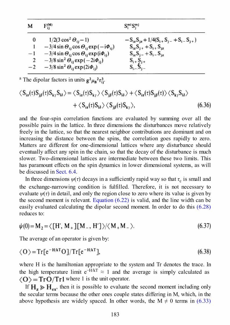
a The dipolar factors in units .

and the four-spin correlation functions are evaluated by summing over all thepossible pairs in the lattice. In three dimensions the disturbances move relativelyfreely in the lattice, so that the nearest neighbor contributions are dominant and onincreasing the distance between the spins, the correlation goes rapidly to zero.Matters are different for one-dimensional lattices where any disturbance shouldeventually affect any spin in the chain, so that the decay of the disturbance is muchslower. Two-dimensional lattices are intermediate between these two limits. Thishas paramount effects on the spin dynamics in lower dimensional systems, as willbe discussed in Sect. 6.4.

In three dimensions ψ(τ) decays in a sufficiently rapid way so that τc is small andthe exchange-narrowing condition is fulfilled. Therefore, it is not necessary toevaluate ψ(τ) in detail, and only the region close to zero where its value is given bythe second moment is relevant. Equation (6.22) is valid, and the line width can beeasily evaluated calculating the dipolar second moment. In order to do this (6.28)reduces to:

The average of an operator is given by:

where H is the hamiltonian appropriate to the system and Tr denotes the trace. Inthe high temperature limit e−H/kT ≈ 1 and the average is simply calculated as

where 1 is the unit operator.If , then it is possible to evaluate the second moment including only

the secular terms because the other ones couple states differing in M, which, in theabove hypothesis are widely spaced. In other words, the M ≠ 0 terms in (6.33)

183

determine a very fast decay of the ψ(τ) function in this limit. Within thisapproximation, for a single spin characterized by the quantum number S, we find

where we have used the definition of shift operators. This can be rewritten as:

The indicated sum yields:

Therefore, for a single spin we find

Finally passing to N spins:

In the same way for the numerator of (6.37) we find:

Therefore, (6.37) becomes:

where the sum is performed by choosing one paramagnetic center in the lattice andincluding all the other centers in the sum. Due to the dependence the number ofsites to be included in the sum is relatively small. In (6.39) we used the relationbetween the second moments in a field, M2(B), and in a frequency, M2(ω), sweptexperiment:

If M2 must be expressed in Gauss and rjk in Å, then (6.39) can be written as:

If, on the other hand, the condition is relaxed, then the nonsecular

184

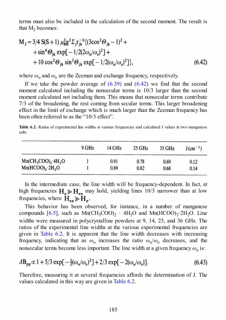
terms must also be included in the calculation of the second moment. The result isthat M2 becomes:

where ωo and ωe are the Zeeman and exchange frequency, respectively.If we take the powder average of (6.39) and (6.42) we find that the second

moment calculated including the nonsecular terms is 10/3 larger than the secondmoment calculated not including them. This means that nonsecular terms contribute7/3 of the broadening, the rest coming from secular terms. This larger broadeningeffect in the limit of exchange which is much larger than the Zeeman frequency hasbeen often referred to as the “10/3 effect”.

Table 6.2. Ratios of experimental line widths at various frequencies and calculated J values in two manganesesalts

In the intermediate case, the line width will be frequency-dependent. In fact, athigh frequencies may hold, yielding lines 10/3 narrower than at lowfrequencies, where .

This behavior has been observed, for instance, in a number of manganesecompounds [6.5], such as Mn(CH3COO)2 · 4H2O and Mn(HCOO)2·2H2O. Linewidths were measured in polycrystalline powders at 9, 14, 25, and 36 GHz. Theratios of the experimental line widths at the various experimental frequencies aregiven in Table 6.2. It is apparent that the line width decreases with increasingfrequency, indicating that as ωo increases the ratio ωo/ωe decreases, and thenonsecular terms become less important. The line width at a given frequency ωo is:

Therefore, measuring it at several frequencies affords the determination of J. Thevalues calculated in this way are given in Table 6.2.

185

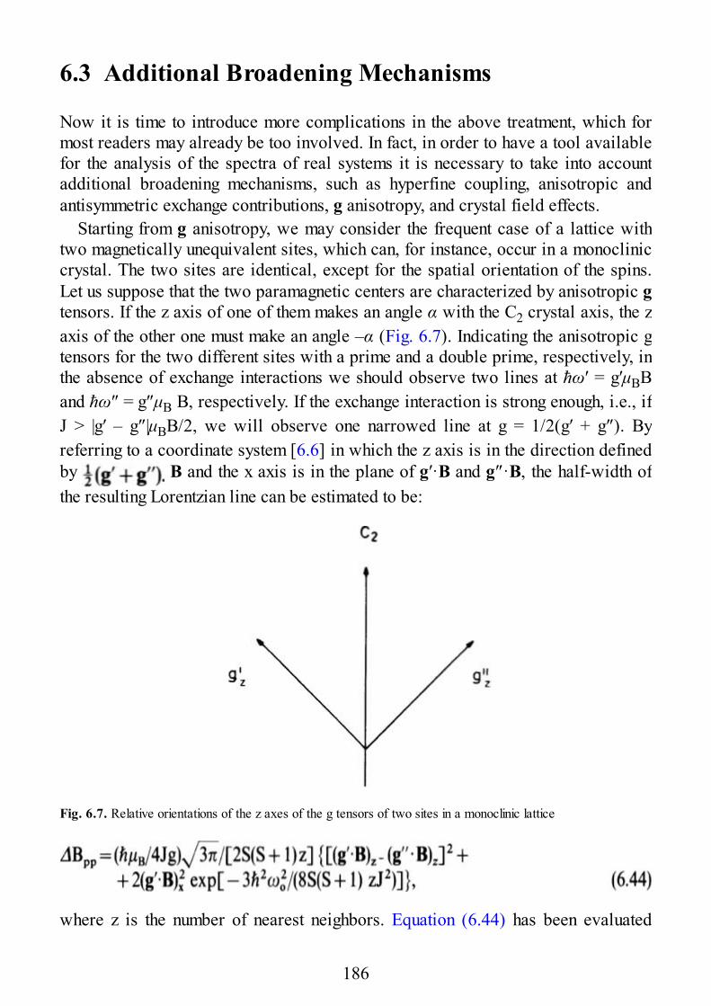
6.3 Additional Broadening Mechanisms

Now it is time to introduce more complications in the above treatment, which formost readers may already be too involved. In fact, in order to have a tool availablefor the analysis of the spectra of real systems it is necessary to take into accountadditional broadening mechanisms, such as hyperfine coupling, anisotropic andantisymmetric exchange contributions, g anisotropy, and crystal field effects.

Starting from g anisotropy, we may consider the frequent case of a lattice withtwo magnetically unequivalent sites, which can, for instance, occur in a monocliniccrystal. The two sites are identical, except for the spatial orientation of the spins.Let us suppose that the two paramagnetic centers are characterized by anisotropic gtensors. If the z axis of one of them makes an angle α with the C2 crystal axis, the zaxis of the other one must make an angle –α (Fig. 6.7). Indicating the anisotropic gtensors for the two different sites with a prime and a double prime, respectively, inthe absence of exchange interactions we should observe two lines at ħω′ = g′μBBand ħω″ = g″μB B, respectively. If the exchange interaction is strong enough, i.e., ifJ > |g′ – g″|μBB/2, we will observe one narrowed line at g = 1/2(g′ + g″). Byreferring to a coordinate system [6.6] in which the z axis is in the direction definedby B and the x axis is in the plane of g′·B and g″·B, the half-width ofthe resulting Lorentzian line can be estimated to be:

Fig. 6.7. Relative orientations of the z axes of the g tensors of two sites in a monoclinic lattice

where z is the number of nearest neighbors. Equation (6.44) has been evaluated

186

assuming that the anisotropy effects for the magnetic moment associated with theoscillating field applied parallel to x can be neglected. The first term in squarebrackets is the secular one, and gives a contribution which increases with theZeeman frequency ωo because it depends on the external field. The broadeningprocess is not an indefinite one, however, because when the difference in thesquare brackets becomes too large two lines will be observed. This case will bebriefly treated below. The second term is the nonsecular one, which gives broaderlines at low frequencies. Often this term is small, and it can be usually neglected.As a result the line width is generally estimated to be simply given by:

As expected (6.45) does not give any broadening effect when the two g tensors aremagnetically equivalent.

In the opposite limit of the strong field two lines are observed which showbroadening and shift effects when the exchange frequency becomes comparable tothe difference in the Zeeman frequencies of the two lines. The calculation using theKubo-Tomita approach provides the shifts of the two sets of lines:

The coordinate axes in this case are chosen in such a way that z′ and z″ areparallel to g′·B and g″·B, respectively, and x′ and x″ are parallel to each other andperpendicular to the z′ – z″ plane. With this choice Θ is the angle between z′ and z″and the l′s, m′s, and n′s are defined by:

where M is the operating dipole moment.In the case of two spins , the derivative absorption shape can be expressed

as:

187

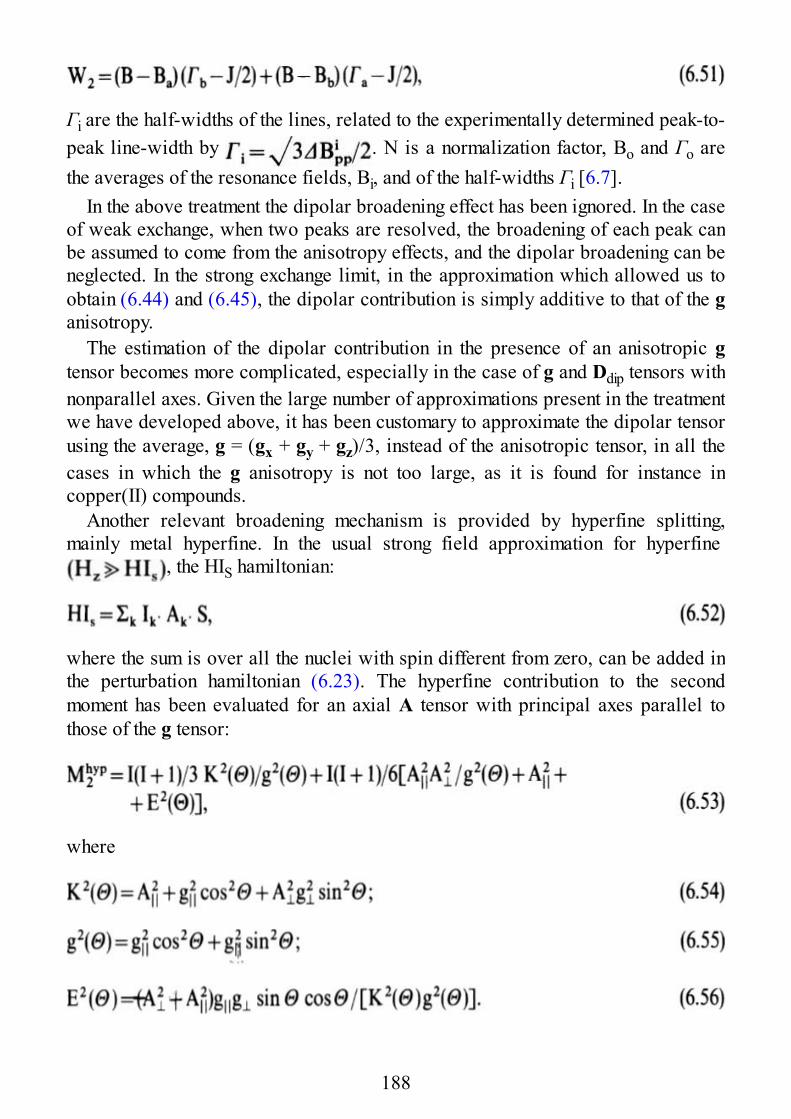
Γi are the half-widths of the lines, related to the experimentally determined peak-to-peak line-width by . N is a normalization factor, Bo and Γo arethe averages of the resonance fields, Bi, and of the half-widths Γi [6.7].

In the above treatment the dipolar broadening effect has been ignored. In the caseof weak exchange, when two peaks are resolved, the broadening of each peak canbe assumed to come from the anisotropy effects, and the dipolar broadening can beneglected. In the strong exchange limit, in the approximation which allowed us toobtain (6.44) and (6.45), the dipolar contribution is simply additive to that of the ganisotropy.

The estimation of the dipolar contribution in the presence of an anisotropic gtensor becomes more complicated, especially in the case of g and Ddip tensors withnonparallel axes. Given the large number of approximations present in the treatmentwe have developed above, it has been customary to approximate the dipolar tensorusing the average, g = (gx + gy + gz)/3, instead of the anisotropic tensor, in all thecases in which the g anisotropy is not too large, as it is found for instance incopper(II) compounds.

Another relevant broadening mechanism is provided by hyperfine splitting,mainly metal hyperfine. In the usual strong field approximation for hyperfine

, the HIS hamiltonian:

where the sum is over all the nuclei with spin different from zero, can be added inthe perturbation hamiltonian (6.23). The hyperfine contribution to the secondmoment has been evaluated for an axial A tensor with principal axes parallel tothose of the g tensor:

where

188

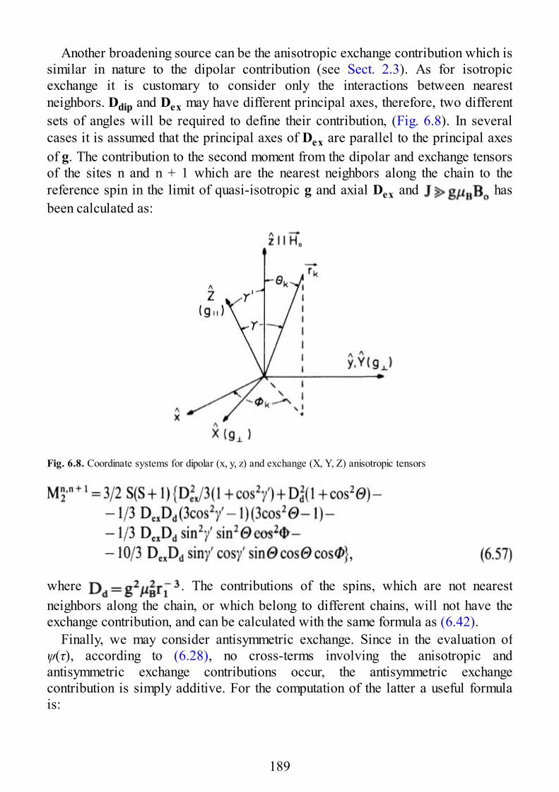
Another broadening source can be the anisotropic exchange contribution which issimilar in nature to the dipolar contribution (see Sect. 2.3). As for isotropicexchange it is customary to consider only the interactions between nearestneighbors. Ddip and Dex may have different principal axes, therefore, two differentsets of angles will be required to define their contribution, (Fig. 6.8). In severalcases it is assumed that the principal axes of Dex are parallel to the principal axesof g. The contribution to the second moment from the dipolar and exchange tensorsof the sites n and n + 1 which are the nearest neighbors along the chain to thereference spin in the limit of quasi-isotropic g and axial Dex and hasbeen calculated as:

Fig. 6.8. Coordinate systems for dipolar (x, y, z) and exchange (X, Y, Z) anisotropic tensors

where . The contributions of the spins, which are not nearestneighbors along the chain, or which belong to different chains, will not have theexchange contribution, and can be calculated with the same formula as (6.42).

Finally, we may consider antisymmetric exchange. Since in the evaluation ofψ(τ), according to (6.28), no cross-terms involving the anisotropic andantisymmetric exchange contributions occur, the antisymmetric exchangecontribution is simply additive. For the computation of the latter a useful formulais:

189

where and are the secular and nonsecular parts, respectively, and FAis the static spin correlation which depends on the number of nearest neighbors.The secular and nonsecular contributions can be calculated as:

The Ω’s are given in Table 6.3. The polar angles Θ and Φ are defined in such a waythat the polar axis is parallel to the static magnetic field.

For individual spins another possible broadening mechanism isdetermined by single ion zero field splitting effects. The second moment for anaxial zero field splitting

is given by

where Θ is the angle of the static magnetic field with the unique axis of the zerofield splitting tensor.

Table 6.3. Coefficients for antisymmetric exchange

6.4 Exchange Narrowing in Lower DimensionalSystems

The reason why the structural and magnetic dimensionality can affect the exchange-narrowing mechanism is easily understood by recalling that the spin correlationfunction is a measure of the probability that a disturbance (a spindeviation) is localized on site i for a time τ. This probability is bound to themechanism according to which the disturbance can move in the lattice, and it is

190

clear that the movement will be much more difficult in one-dimensional than inthree-dimensional exchange-coupled systems, since the number of alternative pathsfor a disturbance to move from one site to another is much more limited in theformer. We have already seen that in three dimensions the characteristic time for thedecay of the correlation functions, τc, can be estimated to be inversely proportionalto J, the exchange frequency. In one dimension, however, this time is too short, andwe must explore the behavior of ψ(τ) also beyond this limit, ψ(τ) for a one-dimensional system is shown in Fig. 6.9. For low τ, ψ(τ) is approximated by aGaussian function, like in the three-dimensional case, but beyond τ1 the decay ofψ(τ) is best approximated by τ−1/2 [6.8]. In a three-dimensional system thecorresponding curve follows a τ− 3/2 dependence, and in general for a d-dimensional lattice ψ(τ) ∞ τ− d/2 beyond τ1. The origin of the d dependence lies inthe spin diffusion mechanism which is responsible for the decay. An importantconsequence of this behavior is that for one- and two-dimensional materials theintegral (6.15) shows divergence for t → ∞, a fact which does not hold for threedimensions where the decay as τ− 3/2 is fast enough to ensure convergence. Thedivergence is more pronounced for one dimension, where it has a t1/2 dependence,than for two dimensions, where it has a dependence In (t). This means that thepresence of the diffusive tail makes (6.15) and (6.18) invalid for low dimensionalsystems.

191

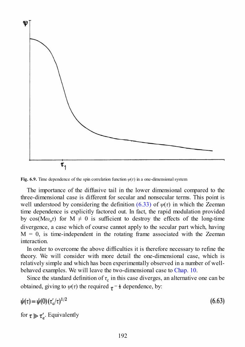
Fig. 6.9. Time dependence of the spin correlation function ψ(τ) in a one-dimensional system

The importance of the diffusive tail in the lower dimensional compared to thethree-dimensional case is different for secular and nonsecular terms. This point iswell understood by considering the definition (6.33) of ψ(τ) in which the Zeemantime dependence is explicitly factored out. In fact, the rapid modulation providedby cos(Mωoτ) for M ≠ 0 is sufficient to destroy the effects of the long-timedivergence, a case which of course cannot apply to the secular part which, havingM = 0, is time-independent in the rotating frame associated with the Zeemaninteraction.

In order to overcome the above difficulties it is therefore necessary to refine thetheory. We will consider with more detail the one-dimensional case, which isrelatively simple and which has been experimentally observed in a number of well-behaved examples. We will leave the two-dimensional case to Chap. 10.

Since the standard definition of τc in this case diverges, an alternative one can beobtained, giving to ψ(τ) the required dependence, by:

for . Equivalently

192

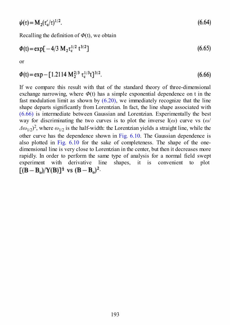
Recalling the definition of Φ(t), we obtain

or

If we compare this result with that of the standard theory of three-dimensionalexchange narrowing, where Φ(t) has a simple exponential dependence on t in thefast modulation limit as shown by (6.20), we immediately recognize that the lineshape departs significantly from Lorentzian. In fact, the line shape associated with(6.66) is intermediate between Gaussian and Lorentzian. Experimentally the bestway for discriminating the two curves is to plot the inverse I(ω) curve vs (ω/Δω1/2)2, where ω1/2 is the half-width: the Lorentzian yields a straight line, while theother curve has the dependence shown in Fig. 6.10. The Gaussian dependence isalso plotted in Fig. 6.10 for the sake of completeness. The shape of the one-dimensional line is very close to Lorentzian in the center, but then it decreases morerapidly. In order to perform the same type of analysis for a normal field sweptexperiment with derivative line shapes, it is convenient to plot

.

193

Fig. 6.10. Plot of the inverse I(ω) versus (ω/Δω1/2)2 curve for a Lorentzian and a Gaussian, and the line shapeappropriate to a one-dimensional system

Since a Lorentzian line shape is characteristic of fast exchange and a Gaussian ofslow exchange, we can state that the slow decay of the correlation in one dimensiondoes not allow the system to reach the fast exchange regime, but leaves it in anintermediate situation. As a consequence lines will be broader in one-dimensionalcompounds compared to three-dimensional systems. In fact, for the latter ΔBpp =M2/J, while for the former .

If we use (6.39) for the second moment in (6.65) and (6.66) and if we assumethat only dipolar contributions along the chain are relevant, we see that the angulardependence of the secular term in the linear chain case reduces to (3cos2 Θ – 1)4/3.Θ is the angle between the chain direction and the external magnetic field.

Since the fast Zeeman modulation washes out the anomalous contributions fromthe long-time diffusive tail for the nonsecular terms, the corresponding componentof Φ(t) has the usual simple exponential dependence on t. Therefore, the explicit

194

form of Φ(t), taking into account the angular dependence and the frequencydependence, will be:

where A1, A2, and A3 are numerical constants. A2 and A3 depend on the ωo/ωeratio, as in (6.42).

The long-time part of Φ(t) mainly affects the center of the absorption, where ω –ωo ≈ 0, therefore, this part of the line will be dominated by the secular terms atmost angles. Whenever this occurs the absorption line is intermediate between aGaussian and a Lorentzian curve. The main exception to this behavior is observedfor the magic angle, Θ = 54.74°, when the secular term goes to zero, and Lorentzianbehavior is anticipated.

The best practical realization, up to the moment, of one-dimensional behavior,has been observed [6.9] in [N(CH3)4]MnCl3, tetramethylammonium manganesetrichloride (or TMMC). The crystal structure of TMMC [6.10] is illustrated in Fig.6.11. Each manganese(II) ion is octahedrally coordinated to six chloride ions. Theoctahedra share a face to form a chain. The manganese-manganese distance withinthe chain (324.5 pm) is much shorter than the interchain distance (915.1 pm). Theintrachain coupling constant has been found [6.11] to be 9.3 cm−1. The angulardependence of ΔBpp is shown in Fig. 6.12. The line is broadest parallel to the chainaxis, is at a minimum at the magic angle, and then it increases again to reach asecondary maximum for Θ = 90°. The experimental points are satisfactorily fit forΔBpp = A + B(3cos2 Θ – 1)4/3, in good agreement with theory.

6.4.1 The Effect of Weak Interchain Coupling

In all the above treatments we have neglected the exchange interactions betweenchains. In fact, however, neglecting this may induce serious errors and it is nowtime to consider its effect. We consider it in the linear chain, but the results can beextended to the two-dimensional case as well.

195

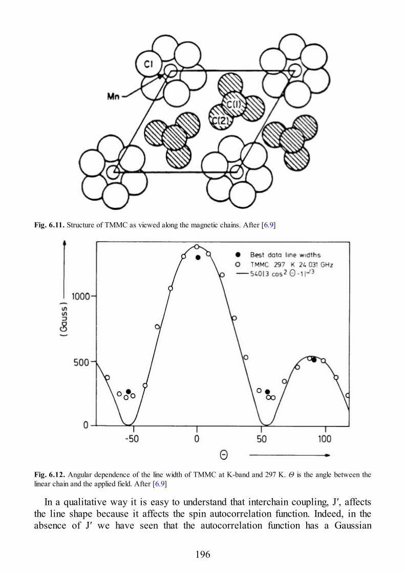
Fig. 6.11. Structure of TMMC as viewed along the magnetic chains. After [6.9]

Fig. 6.12. Angular dependence of the line width of TMMC at K-band and 297 K. Θ is the angle between thelinear chain and the applied field. After [6.9]

In a qualitative way it is easy to understand that interchain coupling, J′, affectsthe line shape because it affects the spin autocorrelation function. Indeed, in theabsence of J′ we have seen that the autocorrelation function has a Gaussian

196

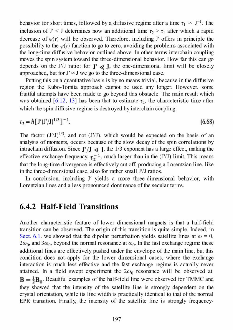
behavior for short times, followed by a diffusive regime after a time τ1 ∝ J−1. Theinclusion of J′ < J determines now an additional time τ2 > τ1 after which a rapiddecrease of ψ(τ) will be observed. Therefore, including J′ offers in principle thepossibility to the ψ(τ) function to go to zero, avoiding the problems associated withthe long-time diffusive behavior outlined above. In other terms interchain couplingmoves the spin system toward the three-dimensional behavior. How far this can godepends on the J′/J ratio: for , the one-dimensional limit will be closelyapproached, but for J′ ≈ J we go to the three-dimensional case.

Putting this on a quantitative basis is by no means trivial, because in the diffusiveregion the Kubo-Tomita approach cannot be used any longer. However, somefruitful attempts have been made to go beyond this obstacle. The main result whichwas obtained [6.12, 13] has been that to estimate τ2, the characteristic time afterwhich the spin diffusive regime is destroyed by interchain coupling:

The factor (J′/J)1/3, and not (J′/J), which would be expected on the basis of ananalysis of moments, occurs because of the slow decay of the spin correlations byintrachain diffusion. Since , the 1/3 exponent has a large effect, making theeffective exchange frequency, , much larger than in the (J′/J) limit. This meansthat the long-time divergence is effectively cut off, producing a Lorentzian line, likein the three-dimensional case, also for rather small J′/J ratios.

In conclusion, including J′ yields a more three-dimensional behavior, withLorentzian lines and a less pronounced dominance of the secular terms.

6.4.2 Half-Field Transitions

Another characteristic feature of lower dimensional magnets is that a half-fieldtransition can be observed. The origin of this transition is quite simple. Indeed, inSect. 6.1. we showed that the dipolar perturbation yields satellite lines at ω = 0,2ω0, and 3ω0, beyond the normal resonance at ω0. In the fast exchange regime theseadditional lines are effectively pushed under the envelope of the main line, but thiscondition does not apply for the lower dimensional cases, where the exchangeinteraction is much less effective and the fast exchange regime is actually neverattained. In a field swept experiment the 2ω0 resonance will be observed at

. Beautiful examples of the half-field line were observed for TMMC andthey showed that the intensity of the satellite line is strongly dependent on thecrystal orientation, while its line width is practically identical to that of the normalEPR transition. Finally, the intensity of the satellite line is strongly frequency-

197

dependent, becoming roughly as expected.The angular dependence of the intensity for the usual transversal experimental

setup, i.e., for spectra recorded with the oscillating microwave field orthogonal tothe static magnetic field, in the case of a one-dimensional magnet is of the type[6.14]:

where Θ is as usual the angle between the magnetic axis and the external magneticfield and Γ+ (Θ) is the angular-dependent width of the main line. The overallangular dependence of the intensity of the half-field line in a transverse fieldexperiment is shown in Fig. 6.13. In practice the intensity shows a sharp maximumat the magic angle, due to the 3 cos2 Θ – 1 dependence of the denominator, and goesto zero at both Θ = 0° and 90°, due to the sin2 Θ cos2 Θ dependence of thenumerator.

Another important feature of the half-field transition is that its intensity can begreatly enhanced compared to the intensity of the main EPR line if a longitudinalfield experiment is performed, i.e., if the oscillating microwave field is parallel tothe static magnetic field. In Fig. 6.14 such an effect is clearly shown: indeed, theintensity of the half-field line is larger than that of the main line. In this case theangular dependence of the line intensity is of the type:

and so the maximum intensity must be expected orthogonal to the chain axis, asexperimentally observed.

198

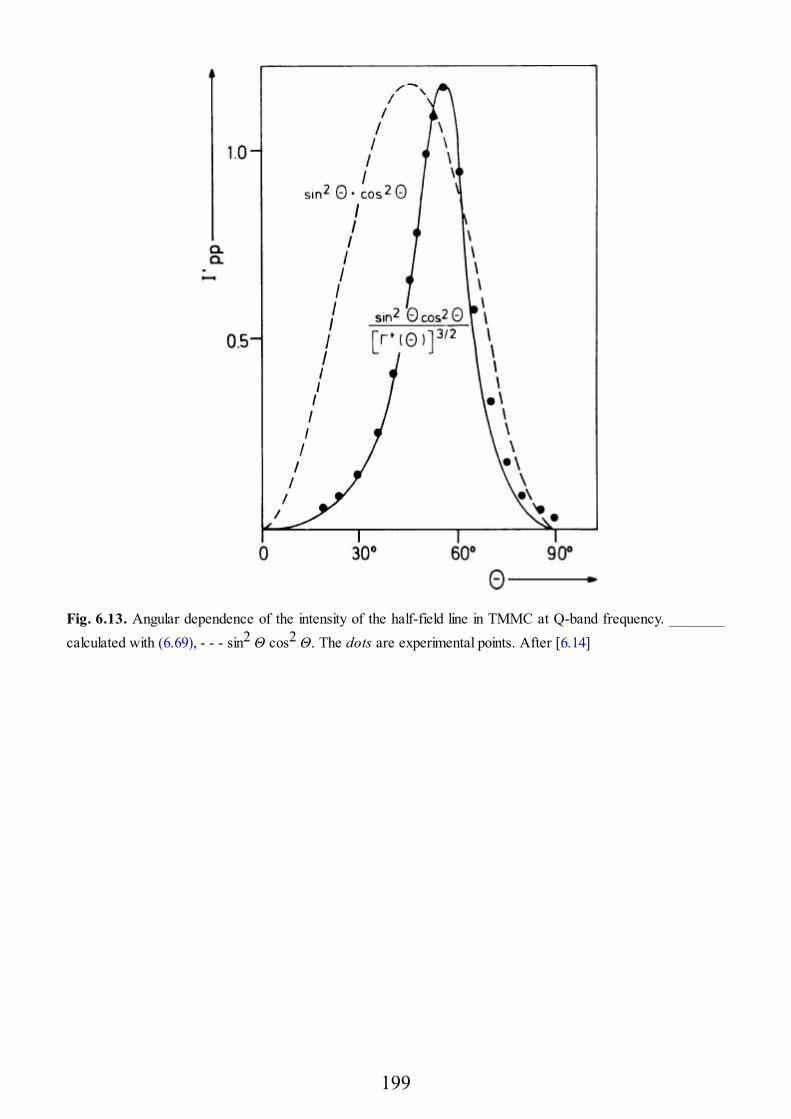
Fig. 6.13. Angular dependence of the intensity of the half-field line in TMMC at Q-band frequency. _______calculated with (6.69), - - - sin2 Θ cos2 Θ. The dots are experimental points. After [6.14]

199

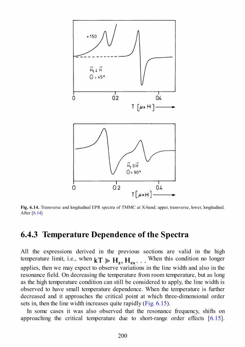
Fig. 6.14. Transverse and longitudinal EPR spectra of TMMC at X-band; upper, transverse, lower, longitudinal.After [6.14]

6.4.3 Temperature Dependence of the Spectra

All the expressions derived in the previous sections are valid in the hightemperature limit, i.e., when When this condition no longerapplies, then we may expect to observe variations in the line width and also in theresonance field. On decreasing the temperature from room temperature, but as longas the high temperature condition can still be considered to apply, the line width isobserved to have small temperature dependence. When the temperature is furtherdecreased and it approaches the critical point at which three-dimensional ordersets in, then the line width increases quite rapidly (Fig. 6.15).

In some cases it was also observed that the resonance frequency, shifts onapproaching the critical temperature due to short-range order effects [6.15].

200

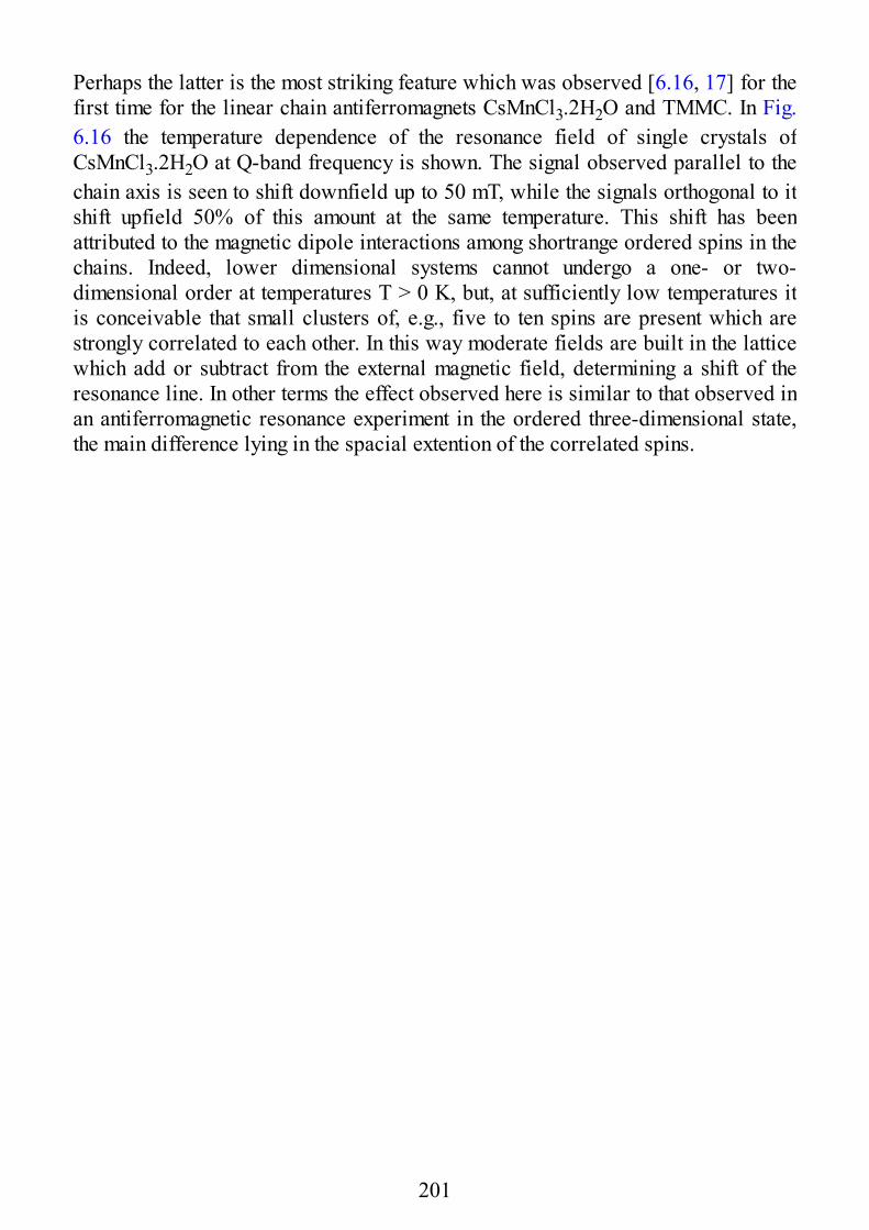
Perhaps the latter is the most striking feature which was observed [6.16, 17] for thefirst time for the linear chain antiferromagnets CsMnCl3.2H2O and TMMC. In Fig.6.16 the temperature dependence of the resonance field of single crystals ofCsMnCl3.2H2O at Q-band frequency is shown. The signal observed parallel to thechain axis is seen to shift downfield up to 50 mT, while the signals orthogonal to itshift upfield 50% of this amount at the same temperature. This shift has beenattributed to the magnetic dipole interactions among shortrange ordered spins in thechains. Indeed, lower dimensional systems cannot undergo a one- or two-dimensional order at temperatures T > 0 K, but, at sufficiently low temperatures itis conceivable that small clusters of, e.g., five to ten spins are present which arestrongly correlated to each other. In this way moderate fields are built in the latticewhich add or subtract from the external magnetic field, determining a shift of theresonance line. In other terms the effect observed here is similar to that observed inan antiferromagnetic resonance experiment in the ordered three-dimensional state,the main difference lying in the spacial extention of the correlated spins.

201

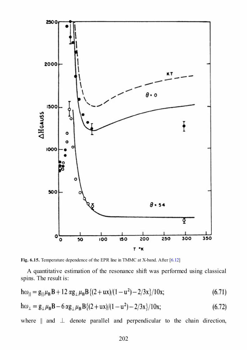
Fig. 6.15. Temperature dependence of the EPR line in TMMC at X-band. After [6.12]

A quantitative estimation of the resonance shift was performed using classicalspins. The result is:

where || and ⊥ denote parallel and perpendicular to the chain direction,

202

respectively,

Fig. 6.16. Temperature dependence of the resonance field for CsMnCl3·2H2O at 34.4 GHz. The field isparallel to a (+), the chain direction, , and . The curves are calculated. After [6.16]

and

where r is the nearest-neighbor spin-spin distance. Equations (6.71–75) have beenobtained for one-dimensional manganese salts, and indeed the use of classical spinsseems to be more appropriate for S = 5/2 than for S = 1/2. However, they havebeen used also for ferromagnetic copper salts, as we will see in Chap. 10.

The relations (6.71–75) can be generalized in the form [6.18]:

where is the resonance field along the i direction, χi, χj and χk are the one-dimensional susceptibilities parallel to the i, j, and k directions, and gi is the

203

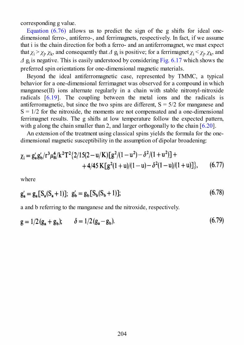
corresponding g value.Equation (6.76) allows us to predict the sign of the g shifts for ideal one-

dimensional ferro-, antiferro-, and ferrimagnets, respectively. In fact, if we assumethat i is the chain direction for both a ferro- and an antiferromagnet, we must expectthat χi > χj, χk, and consequently that Δ gi is positive; for a ferrimagnet χi < χj, χk, andΔ gi is negative. This is easily understood by considering Fig. 6.17 which shows thepreferred spin orientations for one-dimensional magnetic materials.

Beyond the ideal antiferromagnetic case, represented by TMMC, a typicalbehavior for a one-dimensional ferrimagnet was observed for a compound in whichmanganese(II) ions alternate regularly in a chain with stable nitronyl-nitroxideradicals [6.19]. The coupling between the metal ions and the radicals isantiferromagnetic, but since the two spins are different, S = 5/2 for manganese andS = 1/2 for the nitroxide, the moments are not compensated and a one-dimensionalferrimagnet results. The g shifts at low temperature follow the expected pattern,with g along the chain smaller than 2, and larger orthogonally to the chain [6.20].

An extension of the treatment using classical spins yields the formula for the one-dimensional magnetic susceptibility in the assumption of dipolar broadening:

where

a and b referring to the manganese and the nitroxide, respectively.

204

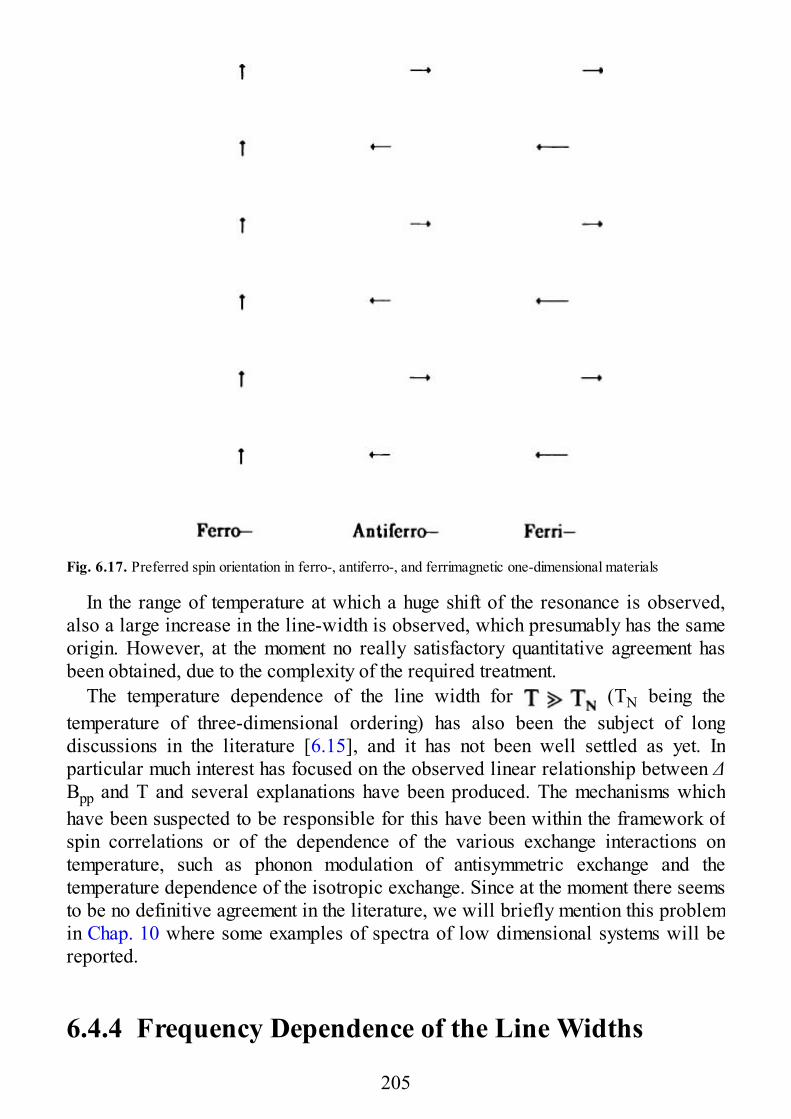
Fig. 6.17. Preferred spin orientation in ferro-, antiferro-, and ferrimagnetic one-dimensional materials

In the range of temperature at which a huge shift of the resonance is observed,also a large increase in the line-width is observed, which presumably has the sameorigin. However, at the moment no really satisfactory quantitative agreement hasbeen obtained, due to the complexity of the required treatment.

The temperature dependence of the line width for (TN being thetemperature of three-dimensional ordering) has also been the subject of longdiscussions in the literature [6.15], and it has not been well settled as yet. Inparticular much interest has focused on the observed linear relationship between ΔBpp and T and several explanations have been produced. The mechanisms whichhave been suspected to be responsible for this have been within the framework ofspin correlations or of the dependence of the various exchange interactions ontemperature, such as phonon modulation of antisymmetric exchange and thetemperature dependence of the isotropic exchange. Since at the moment there seemsto be no definitive agreement in the literature, we will briefly mention this problemin Chap. 10 where some examples of spectra of low dimensional systems will bereported.

6.4.4 Frequency Dependence of the Line Widths

205

The frequency dependence of the line widths has been studied for linear chaincompounds, at some particular angular setting. Of great interest is the behavior atthe magic angle [6.21], where it has been found that:

In fact, at the magic angle the secular components vanish, and the simple motionalnarrowing theory can be used to calculate the line width. The difference withnormal three-dimensional behavior lies essentially in the intensity of the effect,which is much more pronounced in the low dimensional systems. The experimentalfrequency dependence of the line widths of TMMC was fitted with the expression:

with A = 28 ± 3 G, and S = 406 ± 8 G GHz1/2 at 295 K. Attempts were also madeto calculate these two quantities using various decoupling techniques of thecorrelation function, with moderate success [6.22–24].

The behavior is completely different for Θ = 90°, i.e., when the static magneticfield is orthogonal to the chain axis.

References

6.1 van Vleck JH (1948) Phys. Rev. 74:11686.2 Anderson PW, Weiss PR (1953) Rev. Mod. Phys. 25:2696.3 Kubo R, Tomita K (1954) J. Phys. Soc. Jpn. 9:8886.4 Kubo R (1961) In ter Haar D (ed) Fluctuation, relaxation and resonance in magnetic systems. Oliver and

Boyd, Edinburgh p 236.5 Pleau E, Kokoszka G (1973) J. Chem. Soc. Faraday Trans. II 69:3556.6 Anderson PWJ (1954) J. Phys. Soc. Jpn 9:3166.7 Hoffmann SK (1983) Chem. Phys. Letters 98:3296.8 Richards PM (1975) In: Local properties at phase transitions. Editrice Compositori Bologna, p 5396.9 Dietz RE, Merritt FR, Dingle R, Hone D, Silbernagel BG, Richards PM (1971) Phys. Rev. Letters 26:11866.10 Morosin B, Graeber (1967) J. Acta Cryst. 23:7666.11 Hone DW, Richards PM (1974) Annu. Rev. Meter. Sci. 4:3376.12 Cheung TTP, Soos ZG, Dietz RE, Merritt FR (1978) Phys. Rev. B 17: 12666.13 Hennessy MJ, McElwee CD, Richards PM (1975) Phys. Rev. B 7:9306.14 Benner H, Weise J (1979) Physica 96B:2166.15 Drumheller (1982) J. Magnetic Res. Rev. 7:1236.16 Nagata K, Tazuke Y (1972) J. Phys. Soc. Jpn. 32:3376.17 Tazuke Y, Nagata KJ (1971) J Phys. Soc. Jpn. 30:2856.18 Karasudani T, Okamoto H (1977) J. Phys. Soc. Jpn. 43:11316.19 Caneschi A, Gatteschi D, Rey P, Sessoli R (1988) Inorg. Chem. 27:17566.20 Caneschi A, Gatteschi D, Renard, J-P, Rey P, Sessoli R (1989) Inorg. Chem. 28:19766.21 Siegel E, Lagendijk A (1979) Solid State Commun. 32:5616.22 Lagendijk A (1976) Physica 83B:2836.23 Lagendijk A, Siegel E (1976) Solid State Commun. 20:7096.24 Siegel E, Mosebach H, Pauli N, Lagendijk A (1982) Phys. Lett. 90A:309

206

7 Selected Examples of Spectra of Pairs

7.1 Early Transition Metal Ion Pairs

Very detailed EPR spectra have been recorded for manganese(II) pairs in MgO andCaO. Manganese(II) enters substitutionally the host crystals: at concentrations ofabout 1 % appreciable numbers of isolated pairs are found which werecharacterized at three frequencies (15.5, 24.5, and 35.5 GHz) over the temperaturerange 1.2 to 300 K [7.1].

A typical spectrum of Mn2 +: CaO at 35.5 GHz is shown in Fig. 7.1. Signals areobserved from all the five total spin states: it is apparent that on loweringtemperature the low spin states increase the intensity relative to the high spin states.The signals shown in Fig. 7.1 are only part of the spectrum, the scheme of which isgiven in Fig. 7.2. The temperature dependence of the signal intensity of Mn:MgOwas found to conform to the curves of Fig. 3.3, and the order of the levels is shownin Fig. 7.3. The levels deviate considerably from a Landé interval rule (Table 7.1),a result which was explained by including biquadratic terms. The levels on the leftin Fig. 7.3 are calculated only with bilinear exchange, while those on the right,which correspond to a good approximation of the experimental data, are obtainedincluding a biquadratic exchange constant j, such that j/J = 0.05. The effect ofbiquadratic exchange on the energy separations is quite dramatic, according to therelation:

The biquadratic term may have its origin from both an intrinsic higher orderexchange and by exchange striction as discussed in Section 2.4. Beyond thedeparture from Lande interval rule biquadratic exchange has been considered to beresponsible also for the departure of the anisotropic exchange parameters from thesimple behavior expected using Eq. (3.21). The experimental D and E parametersfor the various spin states are given in Table 7.1. According to Table 3.3, the Diparameters should be given by:

207

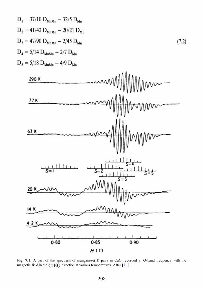
Fig. 7.1. A part of the spectrum of manganese(II) pairs in CaO recorded at Q-band frequency with themagnetic field in the direction at various temperatures. After [7.1]

208

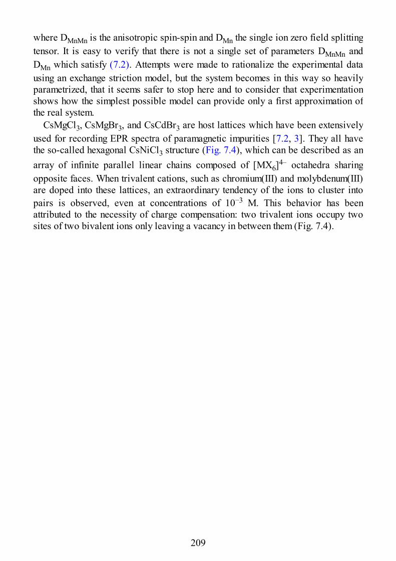
where DMnMn is the anisotropic spin-spin and DMn the single ion zero field splittingtensor. It is easy to verify that there is not a single set of parameters DMnMn andDMn which satisfy (7.2). Attempts were made to rationalize the experimental datausing an exchange striction model, but the system becomes in this way so heavilyparametrized, that it seems safer to stop here and to consider that experimentationshows how the simplest possible model can provide only a first approximation ofthe real system.

CsMgCl3, CsMgBr3, and CsCdBr3 are host lattices which have been extensivelyused for recording EPR spectra of paramagnetic impurities [7.2, 3]. They all havethe so-called hexagonal CsNiCl3 structure (Fig. 7.4), which can be described as anarray of infinite parallel linear chains composed of [MX6]4– octahedra sharingopposite faces. When trivalent cations, such as chromium(III) and molybdenum(III)are doped into these lattices, an extraordinary tendency of the ions to cluster intopairs is observed, even at concentrations of 10−3 M. This behavior has beenattributed to the necessity of charge compensation: two trivalent ions occupy twosites of two bivalent ions only leaving a vacancy in between them (Fig. 7.4).

209

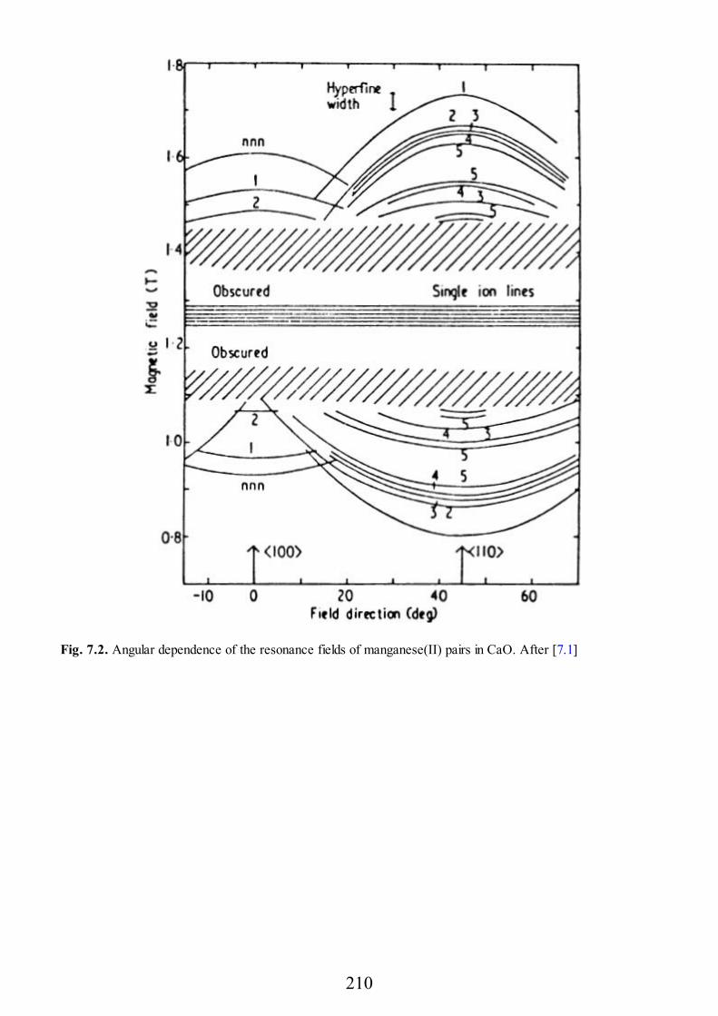
Fig. 7.2. Angular dependence of the resonance fields of manganese(II) pairs in CaO. After [7.1]

210

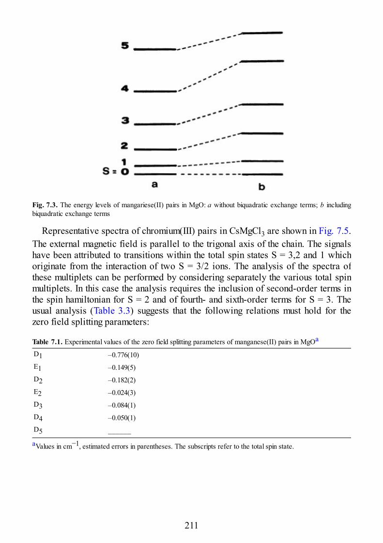
Fig. 7.3. The energy levels of mangariese(II) pairs in MgO: a without biquadratic exchange terms; b includingbiquadratic exchange terms

Representative spectra of chromium(III) pairs in CsMgCl3 are shown in Fig. 7.5.The external magnetic field is parallel to the trigonal axis of the chain. The signalshave been attributed to transitions within the total spin states S = 3,2 and 1 whichoriginate from the interaction of two S = 3/2 ions. The analysis of the spectra ofthese multiplets can be performed by considering separately the various total spinmultiplets. In this case the analysis requires the inclusion of second-order terms inthe spin hamiltonian for S = 2 and of fourth- and sixth-order terms for S = 3. Theusual analysis (Table 3.3) suggests that the following relations must hold for thezero field splitting parameters:

Table 7.1. Experimental values of the zero field splitting parameters of manganese(II) pairs in MgOa

D1 –0.776(10)E1 –0.149(5)D2 –0.182(2)E2 –0.024(3)D3 –0.084(1)D4 –0.050(1)D5 ______

aValues in cm−1, estimated errors in parentheses. The subscripts refer to the total spin state.

211

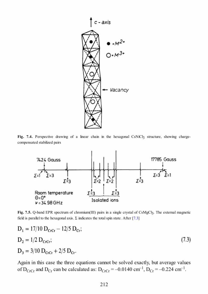
Fig. 7.4. Perspective drawing of a linear chain in the hexagonal CsNiCl3 structure, showing charge-compensated stabilized pairs

Fig. 7.5. Q-band EPR spectrum of chromium(III) pairs in a single crystal of CsMgCl3. The external magneticfield is parallel to the hexagonal axis. Σ indicates the total spin state. After [7.3]

Again in this case the three equations cannot be solved exactly, but average valuesof DCrCr and DCr can be calculated as: DCrCr = –0.0140 cm–1, DCr = –0.224 cm–1.

212

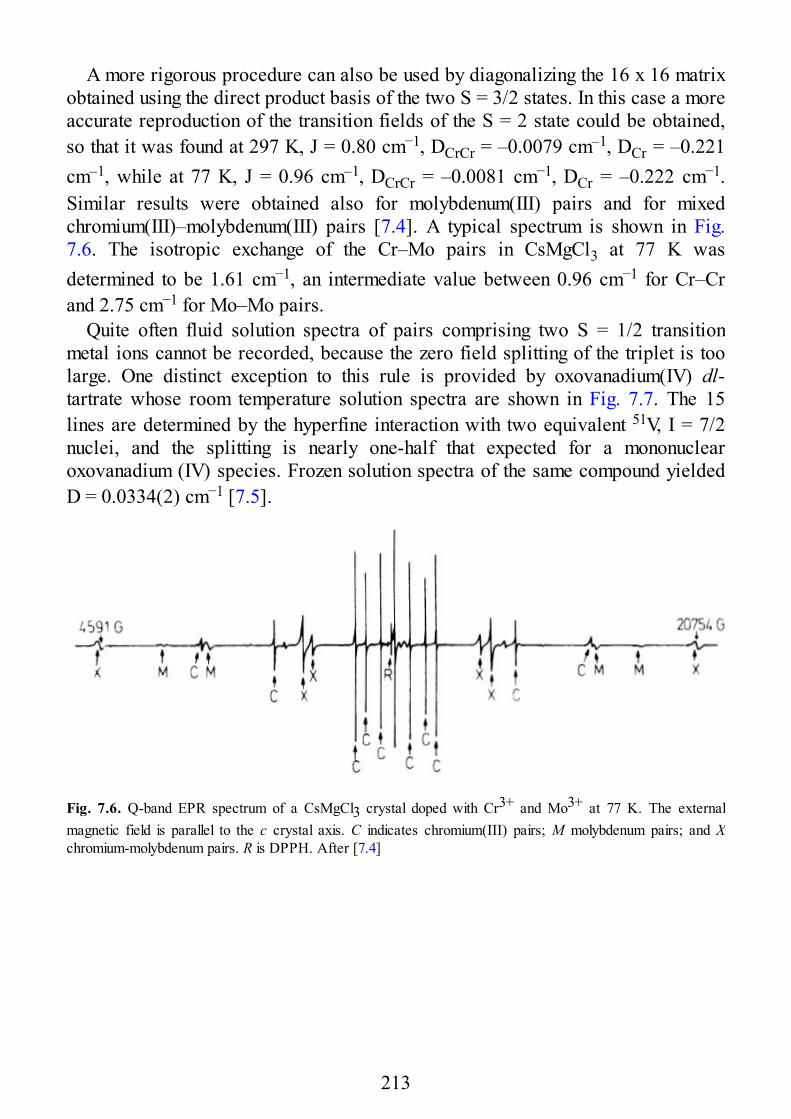
A more rigorous procedure can also be used by diagonalizing the 16 x 16 matrixobtained using the direct product basis of the two S = 3/2 states. In this case a moreaccurate reproduction of the transition fields of the S = 2 state could be obtained,so that it was found at 297 K, J = 0.80 cm−1, DCrCr = –0.0079 cm–1, DCr = –0.221cm–1, while at 77 K, J = 0.96 cm–1, DCrCr = –0.0081 cm−1, DCr = –0.222 cm−1.Similar results were obtained also for molybdenum(III) pairs and for mixedchromium(III)–molybdenum(III) pairs [7.4]. A typical spectrum is shown in Fig.7.6. The isotropic exchange of the Cr–Mo pairs in CsMgCl3 at 77 K wasdetermined to be 1.61 cm−1, an intermediate value between 0.96 cm−1 for Cr–Crand 2.75 cm−1 for Mo–Mo pairs.

Quite often fluid solution spectra of pairs comprising two S = 1/2 transitionmetal ions cannot be recorded, because the zero field splitting of the triplet is toolarge. One distinct exception to this rule is provided by oxovanadium(IV) dl-tartrate whose room temperature solution spectra are shown in Fig. 7.7. The 15lines are determined by the hyperfine interaction with two equivalent 51V, I = 7/2nuclei, and the splitting is nearly one-half that expected for a mononuclearoxovanadium (IV) species. Frozen solution spectra of the same compound yieldedD = 0.0334(2) cm−1 [7.5].

Fig. 7.6. Q-band EPR spectrum of a CsMgCl3 crystal doped with Cr3+ and Mo3+ at 77 K. The externalmagnetic field is parallel to the c crystal axis. C indicates chromium(III) pairs; M molybdenum pairs; and Xchromium-molybdenum pairs. R is DPPH. After [7.4]

213

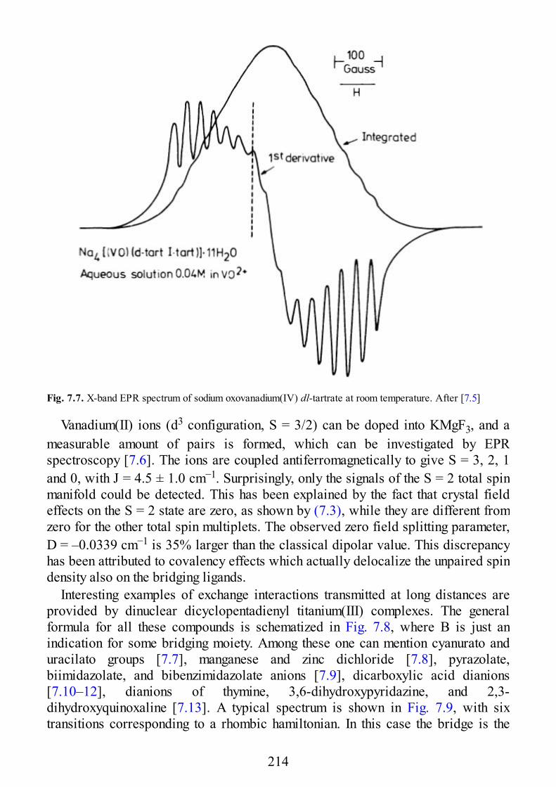
Fig. 7.7. X-band EPR spectrum of sodium oxovanadium(IV) dl-tartrate at room temperature. After [7.5]

Vanadium(II) ions (d3 configuration, S = 3/2) can be doped into KMgF3, and ameasurable amount of pairs is formed, which can be investigated by EPRspectroscopy [7.6]. The ions are coupled antiferromagnetically to give S = 3, 2, 1and 0, with J = 4.5 ± 1.0 cm−1. Surprisingly, only the signals of the S = 2 total spinmanifold could be detected. This has been explained by the fact that crystal fieldeffects on the S = 2 state are zero, as shown by (7.3), while they are different fromzero for the other total spin multiplets. The observed zero field splitting parameter,D = –0.0339 cm−1 is 35% larger than the classical dipolar value. This discrepancyhas been attributed to covalency effects which actually delocalize the unpaired spindensity also on the bridging ligands.

Interesting examples of exchange interactions transmitted at long distances areprovided by dinuclear dicyclopentadienyl titanium(III) complexes. The generalformula for all these compounds is schematized in Fig. 7.8, where B is just anindication for some bridging moiety. Among these one can mention cyanurato anduracilato groups [7.7], manganese and zinc dichloride [7.8], pyrazolate,biimidazolate, and bibenzimidazolate anions [7.9], dicarboxylic acid dianions[7.10–12], dianions of thymine, 3,6-dihydroxypyridazine, and 2,3-dihydroxyquinoxaline [7.13]. A typical spectrum is shown in Fig. 7.9, with sixtransitions corresponding to a rhombic hamiltonian. In this case the bridge is the

214

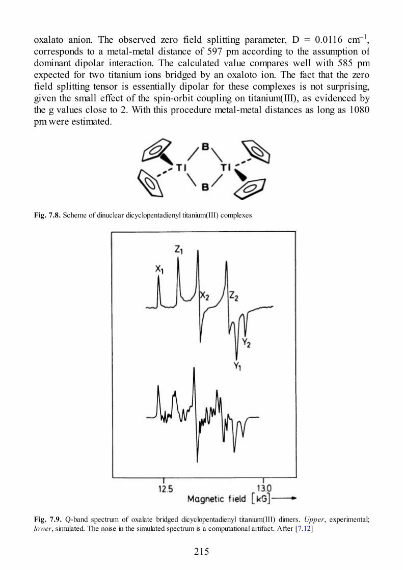
oxalato anion. The observed zero field splitting parameter, D = 0.0116 cm–1,corresponds to a metal-metal distance of 597 pm according to the assumption ofdominant dipolar interaction. The calculated value compares well with 585 pmexpected for two titanium ions bridged by an oxaloto ion. The fact that the zerofield splitting tensor is essentially dipolar for these complexes is not surprising,given the small effect of the spin-orbit coupling on titanium(III), as evidenced bythe g values close to 2. With this procedure metal-metal distances as long as 1080pm were estimated.

Fig. 7.8. Scheme of dinuclear dicyclopentadienyl titanium(III) complexes

Fig. 7.9. Q-band spectrum of oxalate bridged dicyclopentadienyl titanium(III) dimers. Upper, experimental;lower, simulated. The noise in the simulated spectrum is a computational artifact. After [7.12]

215

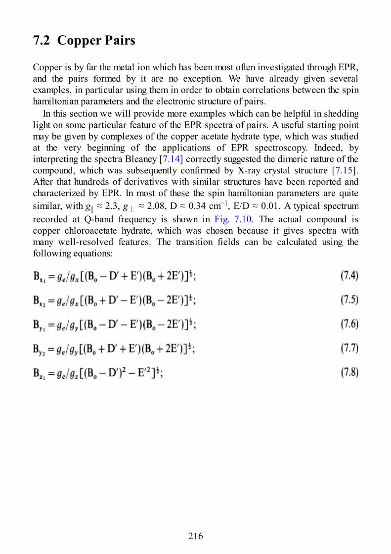
7.2 Copper Pairs

Copper is by far the metal ion which has been most often investigated through EPR,and the pairs formed by it are no exception. We have already given severalexamples, in particular using them in order to obtain correlations between the spinhamiltonian parameters and the electronic structure of pairs.

In this section we will provide more examples which can be helpful in sheddinglight on some particular feature of the EPR spectra of pairs. A useful starting pointmay be given by complexes of the copper acetate hydrate type, which was studiedat the very beginning of the applications of EPR spectroscopy. Indeed, byinterpreting the spectra Bleaney [7.14] correctly suggested the dimeric nature of thecompound, which was subsequently confirmed by X-ray crystal structure [7.15].After that hundreds of derivatives with similar structures have been reported andcharacterized by EPR. In most of these the spin hamiltonian parameters are quitesimilar, with g|| ≈ 2.3, g⊥ ≈ 2.08, D ≈ 0.34 cm−1, E/D ≈ 0.01. A typical spectrumrecorded at Q-band frequency is shown in Fig. 7.10. The actual compound iscopper chloroacetate hydrate, which was chosen because it gives spectra withmany well-resolved features. The transition fields can be calculated using thefollowing equations:

216

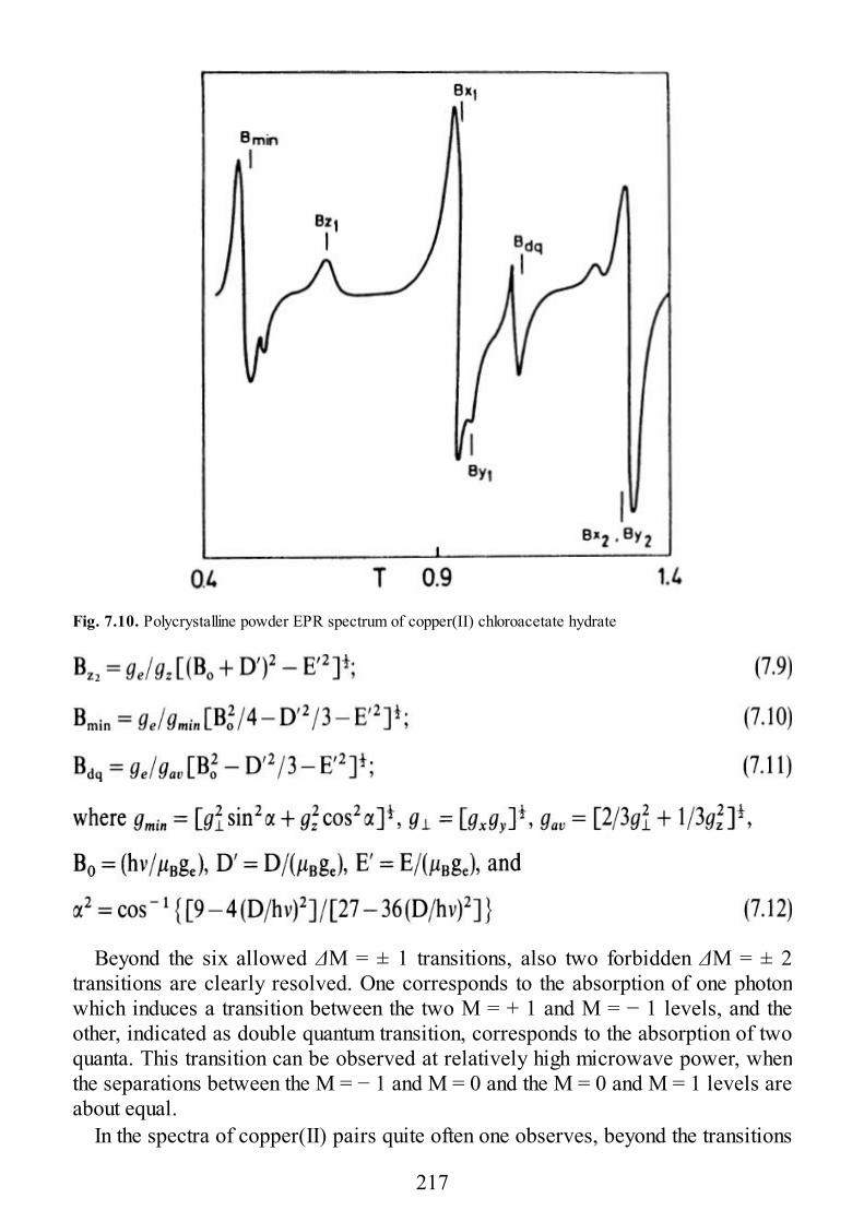
Fig. 7.10. Polycrystalline powder EPR spectrum of copper(II) chloroacetate hydrate

Beyond the six allowed ΔM = ± 1 transitions, also two forbidden ΔM = ± 2transitions are clearly resolved. One corresponds to the absorption of one photonwhich induces a transition between the two M = + 1 and M = − 1 levels, and theother, indicated as double quantum transition, corresponds to the absorption of twoquanta. This transition can be observed at relatively high microwave power, whenthe separations between the M = − 1 and M = 0 and the M = 0 and M = 1 levels areabout equal.

In the spectra of copper(II) pairs quite often one observes, beyond the transitions

217

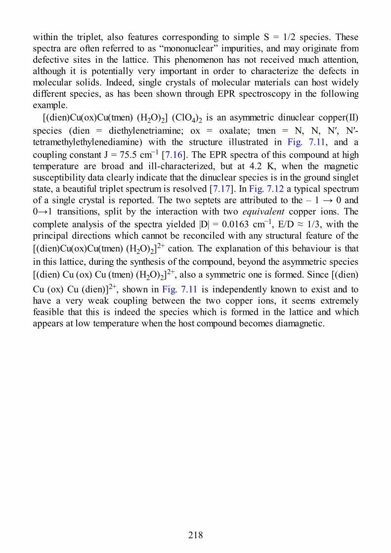
within the triplet, also features corresponding to simple S = 1/2 species. Thesespectra are often referred to as “mononuclear” impurities, and may originate fromdefective sites in the lattice. This phenomenon has not received much attention,although it is potentially very important in order to characterize the defects inmolecular solids. Indeed, single crystals of molecular materials can host widelydifferent species, as has been shown through EPR spectroscopy in the followingexample.

[(dien)Cu(ox)Cu(tmen) (H2O)2] (ClO4)2 is an asymmetric dinuclear copper(II)species (dien = diethylenetriamine; ox = oxalate; tmen = N, N, N′, N′-tetramethylethylenediamine) with the structure illustrated in Fig. 7.11, and acoupling constant J = 75.5 cm−1 [7.16]. The EPR spectra of this compound at hightemperature are broad and ill-characterized, but at 4.2 K, when the magneticsusceptibility data clearly indicate that the dinuclear species is in the ground singletstate, a beautiful triplet spectrum is resolved [7.17]. In Fig. 7.12 a typical spectrumof a single crystal is reported. The two septets are attributed to the – 1 → 0 and0→1 transitions, split by the interaction with two equivalent copper ions. Thecomplete analysis of the spectra yielded |D| = 0.0163 cm−1, E/D ≈ 1/3, with theprincipal directions which cannot be reconciled with any structural feature of the[(dien)Cu(ox)Cu(tmen) (H2O)2]2+ cation. The explanation of this behaviour is thatin this lattice, during the synthesis of the compound, beyond the asymmetric species[(dien) Cu (ox) Cu (tmen) (H2O)2]2+, also a symmetric one is formed. Since [(dien)Cu (ox) Cu (dien)]2+, shown in Fig. 7.11 is independently known to exist and tohave a very weak coupling between the two copper ions, it seems extremelyfeasible that this is indeed the species which is formed in the lattice and whichappears at low temperature when the host compound becomes diamagnetic.

218

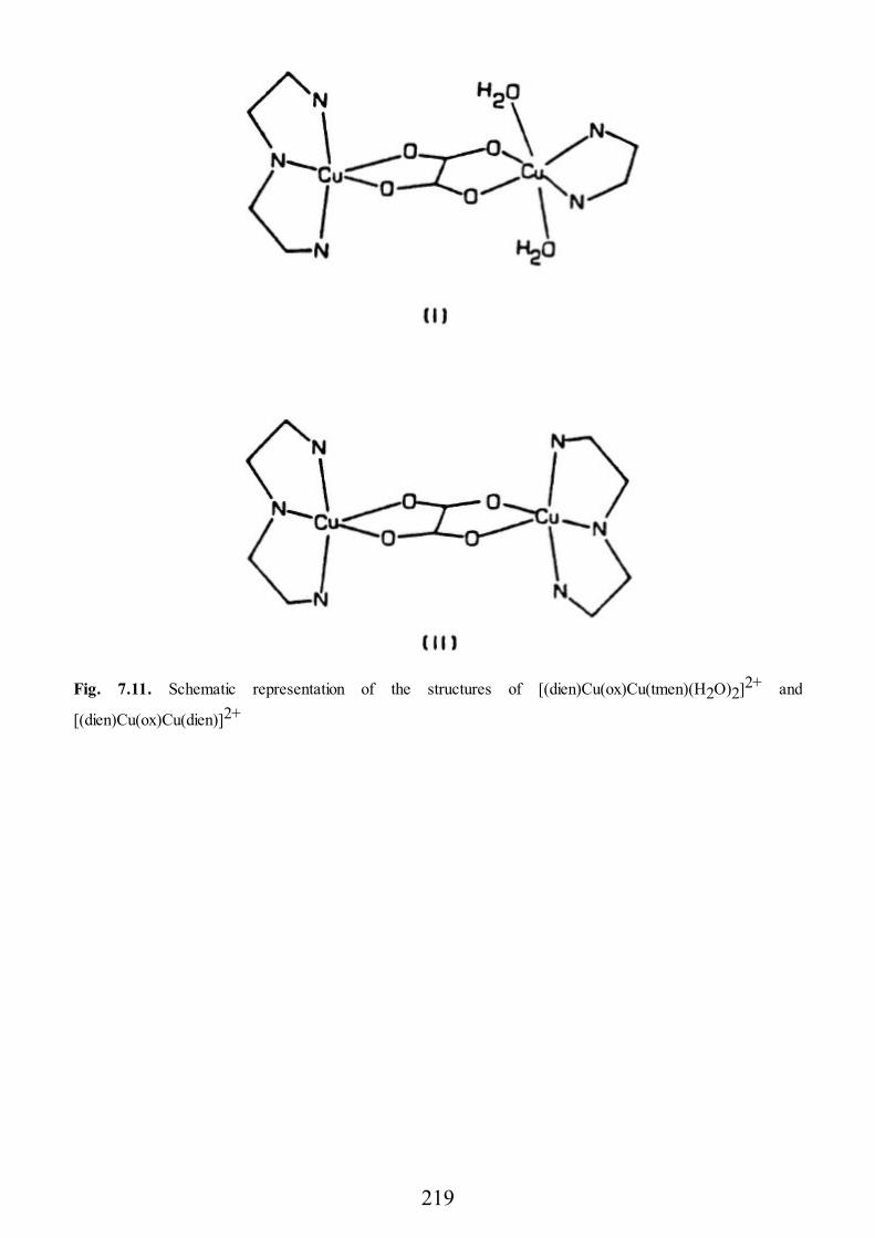
Fig. 7.11. Schematic representation of the structures of [(dien)Cu(ox)Cu(tmen)(H2O)2]2+ and

[(dien)Cu(ox)Cu(dien)]2+

219

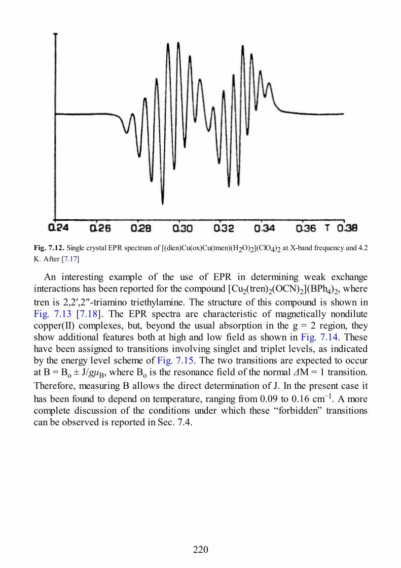
Fig. 7.12. Single crystal EPR spectrum of [(dien)Cu(ox)Cu(tmen)(H2O)2](ClO4)2 at X-band frequency and 4.2K. After [7.17]

An interesting example of the use of EPR in determining weak exchangeinteractions has been reported for the compound [Cu2(tren)2(OCN)2](BPh4)2, wheretren is 2,2′,2″-triamino triethylamine. The structure of this compound is shown inFig. 7.13 [7.18]. The EPR spectra are characteristic of magnetically nondilutecopper(II) complexes, but, beyond the usual absorption in the g = 2 region, theyshow additional features both at high and low field as shown in Fig. 7.14. Thesehave been assigned to transitions involving singlet and triplet levels, as indicatedby the energy level scheme of Fig. 7.15. The two transitions are expected to occurat B = Bo ± J/gμB, where Bo is the resonance field of the normal ΔM = 1 transition.Therefore, measuring B allows the direct determination of J. In the present case ithas been found to depend on temperature, ranging from 0.09 to 0.16 cm−1. A morecomplete discussion of the conditions under which these “forbidden” transitionscan be observed is reported in Sec. 7.4.

220

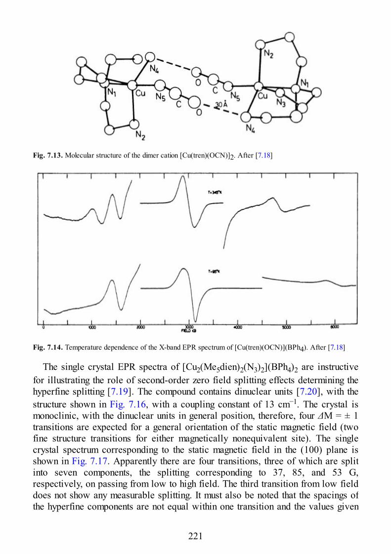
Fig. 7.13. Molecular structure of the dimer cation [Cu(tren)(OCN)]2. After [7.18]

Fig. 7.14. Temperature dependence of the X-band EPR spectrum of [Cu(tren)(OCN)](BPh4). After [7.18]

The single crystal EPR spectra of [Cu2(Me5dien)2(N3)2](BPh4)2 are instructivefor illustrating the role of second-order zero field splitting effects determining thehyperfine splitting [7.19]. The compound contains dinuclear units [7.20], with thestructure shown in Fig. 7.16, with a coupling constant of 13 cm−1. The crystal ismonoclinic, with the dinuclear units in general position, therefore, four ΔM = ± 1transitions are expected for a general orientation of the static magnetic field (twofine structure transitions for either magnetically nonequivalent site). The singlecrystal spectrum corresponding to the static magnetic field in the (100) plane isshown in Fig. 7.17. Apparently there are four transitions, three of which are splitinto seven components, the splitting corresponding to 37, 85, and 53 G,respectively, on passing from low to high field. The third transition from low fielddoes not show any measurable splitting. It must also be noted that the spacings ofthe hyperfine components are not equal within one transition and the values given

221

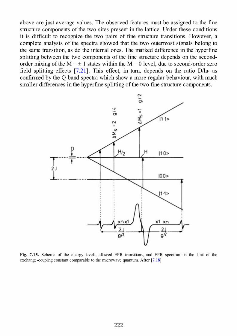
above are just average values. The observed features must be assigned to the finestructure components of the two sites present in the lattice. Under these conditionsit is difficult to recognize the two pairs of fine structure transitions. However, acomplete analysis of the spectra showed that the two outermost signals belong tothe same transition, as do the internal ones. The marked difference in the hyperfinesplitting between the two components of the fine structure depends on the second-order mixing of the M = ± 1 states within the M = 0 level, due to second-order zerofield splitting effects [7.21]. This effect, in turn, depends on the ratio D/hν asconfirmed by the Q-band spectra which show a more regular behaviour, with muchsmaller differences in the hyperfine splitting of the two fine structure components.

Fig. 7.15. Scheme of the energy levels, allowed EPR transitions, and EPR spectrum in the limit of theexchange-coupling constant comparable to the microwave quantum. After [7.18]

222

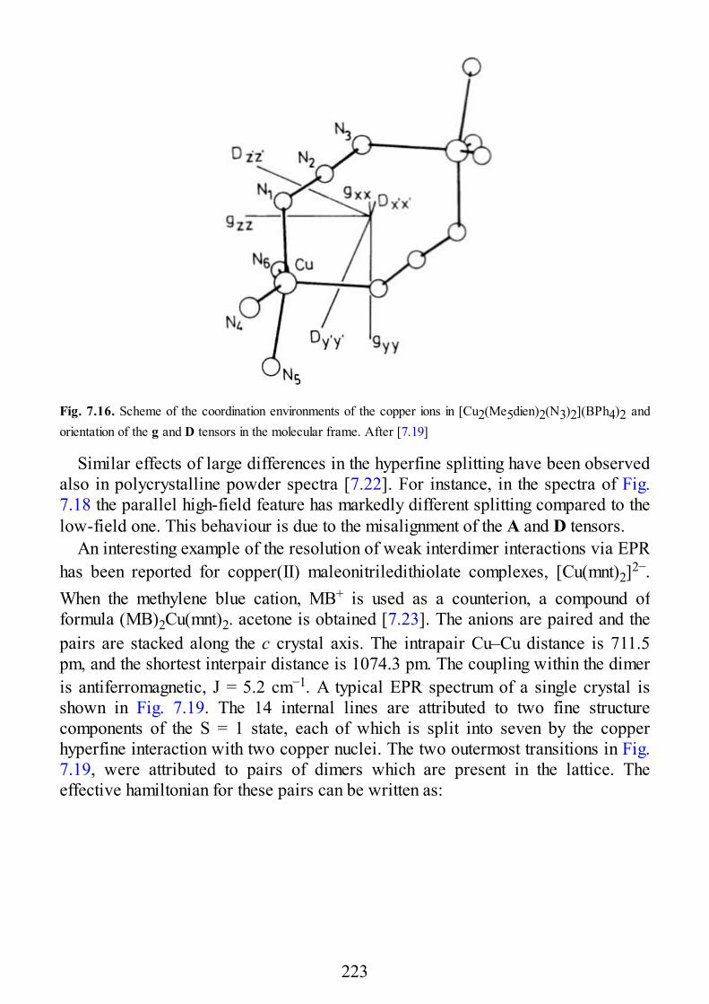
Fig. 7.16. Scheme of the coordination environments of the copper ions in [Cu2(Me5dien)2(N3)2](BPh4)2 andorientation of the g and D tensors in the molecular frame. After [7.19]

Similar effects of large differences in the hyperfine splitting have been observedalso in polycrystalline powder spectra [7.22]. For instance, in the spectra of Fig.7.18 the parallel high-field feature has markedly different splitting compared to thelow-field one. This behaviour is due to the misalignment of the A and D tensors.

An interesting example of the resolution of weak interdimer interactions via EPRhas been reported for copper(II) maleonitriledithiolate complexes, [Cu(mnt)2]2−.When the methylene blue cation, MB+ is used as a counterion, a compound offormula (MB)2Cu(mnt)2. acetone is obtained [7.23]. The anions are paired and thepairs are stacked along the c crystal axis. The intrapair Cu–Cu distance is 711.5pm, and the shortest interpair distance is 1074.3 pm. The coupling within the dimeris antiferromagnetic, J = 5.2 cm−1. A typical EPR spectrum of a single crystal isshown in Fig. 7.19. The 14 internal lines are attributed to two fine structurecomponents of the S = 1 state, each of which is split into seven by the copperhyperfine interaction with two copper nuclei. The two outermost transitions in Fig.7.19, were attributed to pairs of dimers which are present in the lattice. Theeffective hamiltonian for these pairs can be written as:

223

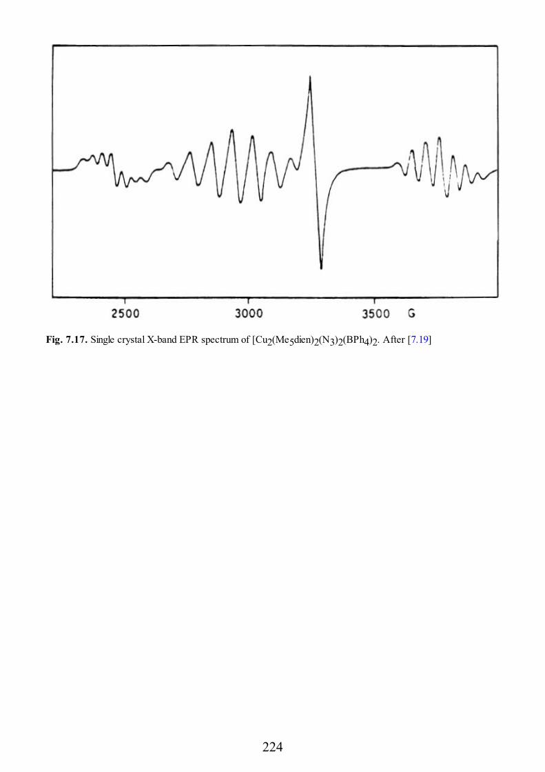
Fig. 7.17. Single crystal X-band EPR spectrum of [Cu2(Me5dien)2(N3)2(BPh4)2. After [7.19]

224

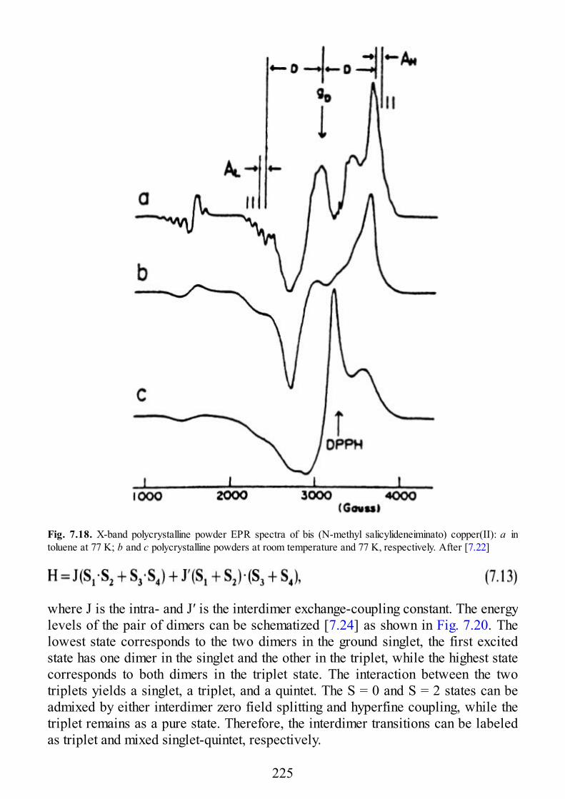
Fig. 7.18. X-band polycrystalline powder EPR spectra of bis (N-methyl salicylideneiminato) copper(II): a intoluene at 77 K; b and c polycrystalline powders at room temperature and 77 K, respectively. After [7.22]

where J is the intra- and J′ is the interdimer exchange-coupling constant. The energylevels of the pair of dimers can be schematized [7.24] as shown in Fig. 7.20. Thelowest state corresponds to the two dimers in the ground singlet, the first excitedstate has one dimer in the singlet and the other in the triplet, while the highest statecorresponds to both dimers in the triplet state. The interaction between the twotriplets yields a singlet, a triplet, and a quintet. The S = 0 and S = 2 states can beadmixed by either interdimer zero field splitting and hyperfine coupling, while thetriplet remains as a pure state. Therefore, the interdimer transitions can be labeledas triplet and mixed singlet-quintet, respectively.

225

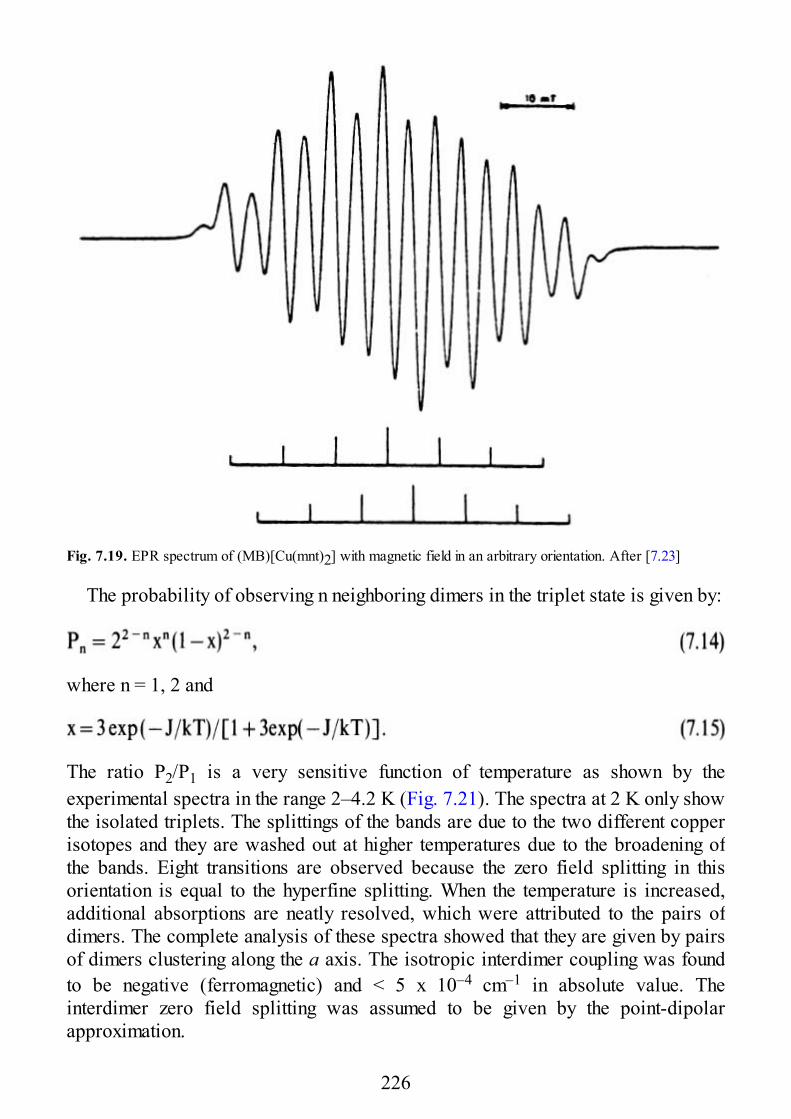
Fig. 7.19. EPR spectrum of (MB)[Cu(mnt)2] with magnetic field in an arbitrary orientation. After [7.23]

The probability of observing n neighboring dimers in the triplet state is given by:

where n = 1, 2 and

The ratio P2/P1 is a very sensitive function of temperature as shown by theexperimental spectra in the range 2–4.2 K (Fig. 7.21). The spectra at 2 K only showthe isolated triplets. The splittings of the bands are due to the two different copperisotopes and they are washed out at higher temperatures due to the broadening ofthe bands. Eight transitions are observed because the zero field splitting in thisorientation is equal to the hyperfine splitting. When the temperature is increased,additional absorptions are neatly resolved, which were attributed to the pairs ofdimers. The complete analysis of these spectra showed that they are given by pairsof dimers clustering along the a axis. The isotropic interdimer coupling was foundto be negative (ferromagnetic) and < 5 x 10–4 cm–1 in absolute value. Theinterdimer zero field splitting was assumed to be given by the point-dipolarapproximation.

226

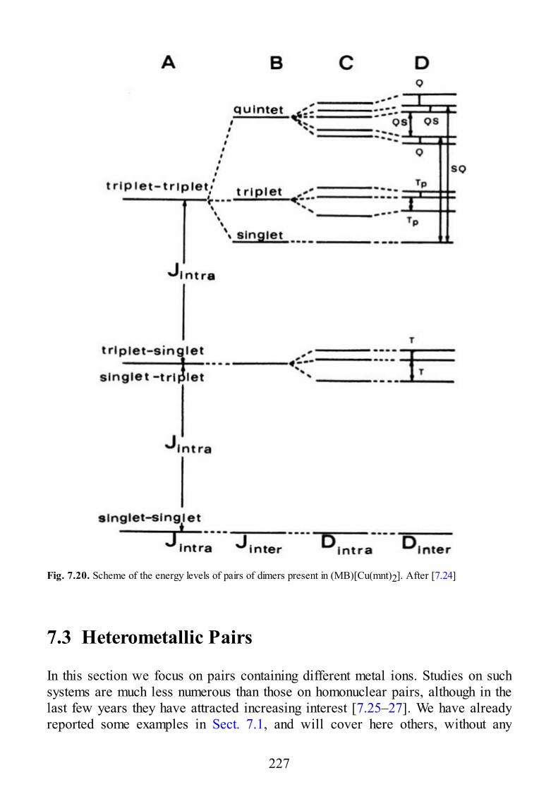
Fig. 7.20. Scheme of the energy levels of pairs of dimers present in (MB)[Cu(mnt)2]. After [7.24]

7.3 Heterometallic Pairs

In this section we focus on pairs containing different metal ions. Studies on suchsystems are much less numerous than those on homonuclear pairs, although in thelast few years they have attracted increasing interest [7.25–27]. We have alreadyreported some examples in Sect. 7.1, and will cover here others, without any

227

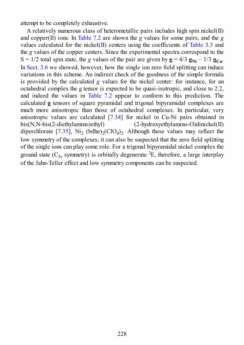
attempt to be completely exhaustive.A relatively numerous class of heterometallic pairs includes high spin nickel(II)

and copper(II) ions. In Table 7.2 are shown the g values for some pairs, and the gvalues calculated for the nickel(II) centers using the coefficients of Table 3.3 andthe g values of the copper centers. Since the experimental spectra correspond to theS = 1/2 total spin state, the g values of the pair are given by g = 4/3 gNi – 1/3 gCu.In Sect. 3.6 we showed, however, how the single ion zero field splitting can inducevariations in this scheme. An indirect check of the goodness of the simple formulais provided by the calculated g values for the nickel center: for instance, for anoctahedral complex the g tensor is expected to be quasi-isotropic, and close to 2.2,and indeed the values in Table 7.2 appear to conform to this prediction. Thecalculated g tensors of square pyramidal and trigonal bipyramidal complexes aremuch more anisotropic than those of octahedral complexes. In particular, veryanisotropic values are calculated [7.34] for nickel in Cu-Ni pairs obtained inbis(N,N-bis(2-diethylamino)ethyl) (2-hydroxyethylamino-O)dinickel(II)diperchlorate [7.35], Ni2 (bdhe)2(ClO4)2. Although these values may reflect thelow symmetry of the complexes, it can also be suspected that the zero field splittingof the single ions can play some role. For a trigonal bipyramidal nickel complex theground state (C3v symmetry) is orbitally degenerate 3E, therefore, a large interplayof the Jahn-Teller effect and low symmetry components can be suspected.

228

Fig. 7.21. Experimental single crystal EPR spectra of (MB)[Cu(mnt)2] in the range 2–4.2 K, with the staticmagnetic field parallel to a. After [7.24]

Table 7.2. g values for nickel(II) complexes calculated from the spectra of Cu-Ni pairs

229

That this can be the case is confirmed by the spectra of the analogous cobalt(II)-nickel(II) pairs which correspond to transitions within one Kramers doublet, with gvalues g1 = 3.4, g2 = 0.8, g3 = 0.6. These values cannot be reproduced with anysimple formula of the type (3.34), and must reflect a much more complicatedsituation.

More tractable spectra were recorded [7.28, 29] for Co–Ni pairs in bis(1, 5-dipheny1-1,3,5-pentanetrionato) tetrakis (pyridine) dimetal(II), M2trik(py)4, anddiaquo (1,4-dihydrazionphthalazine) metal(II), M2(dhph) (H2O)4, whose structureis schematized in Fig. 7.22. The EPR spectra recorded at 4.2 K show transitionswithin one Kramers doublet with gz = 2.1, gx = 1.2, gy = 0.3 and gz = 0.6, gx = 0.9,gy = 2.1, respectively. The x, y, and z directions for the two complexes are shownin Fig. 7.23. In octahedral symmetry cobalt(II) has an orbitally degenerate 4T1gstate, which is split by spin-orbit coupling and low symmetry components to yield aground Kramers doublet. The simplest approach to rationalize the observed gvalues is to consider the ground Kramers doublet as an effective S = 1/2 spin andcouple it with S = 1 for nickel. In this frame the g values of the pair might beassociated with the total spin S = 1/2. However, use of the coefficients of Table 3.3fails to give reasonable values, when the g values of the nickel and cobalt center,obtained from the spectra of the Cu-Ni and Co-Zn pairs, respectively, are used. Amore sophisticated approach takes into account the orbital degeneration of thecobalt(II) ion, through a hamiltonian

230

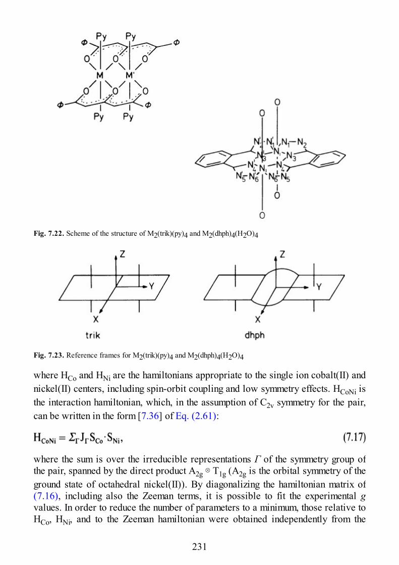
Fig. 7.22. Scheme of the structure of M2(trik)(py)4 and M2(dhph)4(H2O)4

Fig. 7.23. Reference frames for M2(trik)(py)4 and M2(dhph)4(H2O)4

where HCo and HNi are the hamiltonians appropriate to the single ion cobalt(II) andnickel(II) centers, including spin-orbit coupling and low symmetry effects. HCoNi isthe interaction hamiltonian, which, in the assumption of C2v symmetry for the pair,can be written in the form [7.36] of Eq. (2.61):

where the sum is over the irreducible representations Γ of the symmetry group ofthe pair, spanned by the direct product A2g ⊗ T1g (A2g is the orbital symmetry of theground state of octahedral nickel(II)). By diagonalizing the hamiltonian matrix of(7.16), including also the Zeeman terms, it is possible to fit the experimental gvalues. In order to reduce the number of parameters to a minimum, those relative toHCo, HNi, and to the Zeeman hamiltonian were obtained independently from the

231

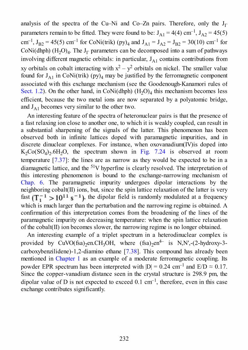
analysis of the spectra of the Cu–Ni and Co–Zn pairs. Therefore, only the JΓ

parameters remain to be fitted. They were found to be: JA1 = 4(4) cm–1, JA2 = 45(5)cm–1, JB2 = 45(5) cm–1 for CoNi(trik) (py)4 and JA1 = JA2 = JB2 = 30(10) cm–1 forCoNi(dhph) (H2O)4. The JΓ parameters can be decomposed into a sum of pathwaysinvolving different magnetic orbitals: in particular, JA1 contains contributions fromxy orbitals on cobalt interacting with x2 – y2 orbitals on nickel. The smaller valuefound for JA1 in CoNi(trik) (py)4 may be justified by the ferromagnetic componentassociated with this exchange mechanism (see the Goodenough-Kanamori rules ofSect. 1.2). On the other hand, in CoNi(dhph) (H2O)4 this mechanism becomes lessefficient, because the two metal ions are now separated by a polyatomic bridge,and JA1 becomes very similar to the other two.

An interesting feature of the spectra of heteronuclear pairs is that the presence ofa fast relaxing ion close to another one, to which it is weakly coupled, can result ina substantial sharpening of the signals of the latter. This phenomenon has beenobserved both in infinite lattices doped with paramagnetic impurities, and indiscrete dinuclear complexes. For instance, when oxovanadium(IV)is doped intoK2Co(SO4)2.6H2O, the spectrum shown in Fig. 7.24 is observed at roomtemperature [7.37]: the lines are as narrow as they would be expected to be in adiamagnetic lattice, and the 51V hyperfine is clearly resolved. The interpretation ofthis interesting phenomenon is bound to the exchange-narrowing mechanism ofChap. 6. The paramagnetic impurity undergoes dipolar interactions by theneighboring cobalt(II) ions, but, since the spin lattice relaxation of the latter is veryfast , the dipolar field is randomly modulated at a frequencywhich is much larger than the perturbation and the narrowing regime is obtained. Aconfirmation of this interpretation comes from the broadening of the lines of theparamagnetic impurity on decreasing temperature: when the spin lattice relaxationof the cobalt(II) ion becomes slower, the narrowing regime is no longer obtained.

An interesting example of a triplet spectrum in a heterodinuclear complex isprovided by CuVO(fsa)2en.CH3OH, where (fsa)2en4– is N,N′,-(2-hydroxy-3-carboxybenzilidene)-1,2-diamino ethane [7.38]. This compound has already beenmentioned in Chapter 1 as an example of a moderate ferromagnetic coupling. Itspowder EPR spectrum has been interpreted with |D| = 0.24 cm–1 and E/D ≈ 0.17.Since the copper-vanadium distance seen in the crystal structure is 298.9 pm, thedipolar value of D is not expected to exceed 0.1 cm–1, therefore, even in this caseexchange contributes significantly.

232

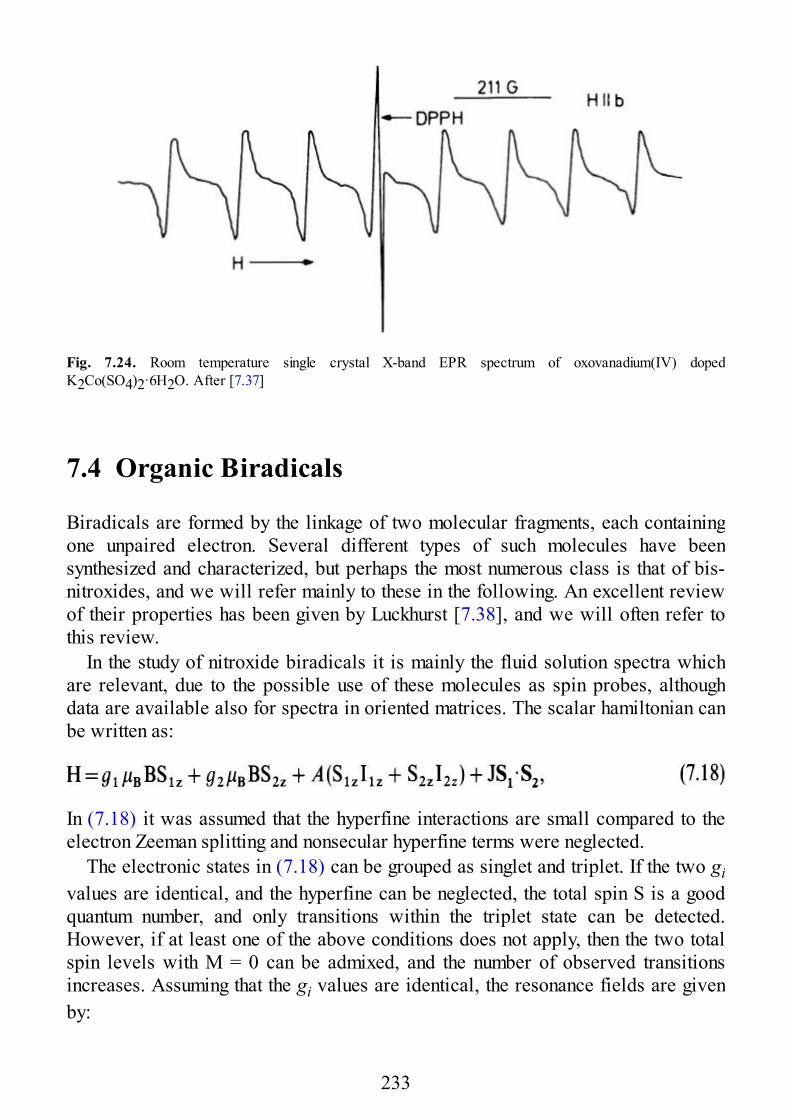
Fig. 7.24. Room temperature single crystal X-band EPR spectrum of oxovanadium(IV) dopedK2Co(SO4)2·6H2O. After [7.37]

7.4 Organic Biradicals

Biradicals are formed by the linkage of two molecular fragments, each containingone unpaired electron. Several different types of such molecules have beensynthesized and characterized, but perhaps the most numerous class is that of bis-nitroxides, and we will refer mainly to these in the following. An excellent reviewof their properties has been given by Luckhurst [7.38], and we will often refer tothis review.

In the study of nitroxide biradicals it is mainly the fluid solution spectra whichare relevant, due to the possible use of these molecules as spin probes, althoughdata are available also for spectra in oriented matrices. The scalar hamiltonian canbe written as:

In (7.18) it was assumed that the hyperfine interactions are small compared to theelectron Zeeman splitting and nonsecular hyperfine terms were neglected.

The electronic states in (7.18) can be grouped as singlet and triplet. If the two givalues are identical, and the hyperfine can be neglected, the total spin S is a goodquantum number, and only transitions within the triplet state can be detected.However, if at least one of the above conditions does not apply, then the two totalspin levels with M = 0 can be admixed, and the number of observed transitionsincreases. Assuming that the gi values are identical, the resonance fields are givenby:

233

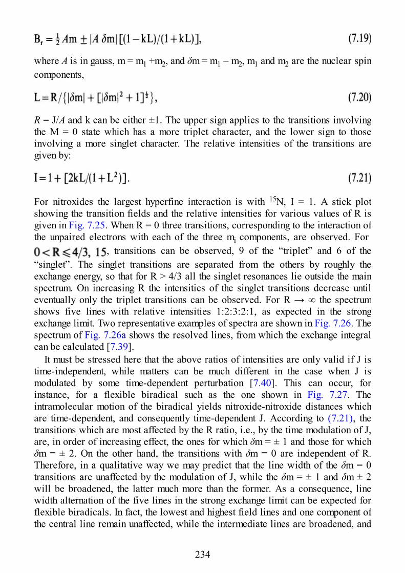
where A is in gauss, m = m1 +m2, and δm = m1 – m2, m1 and m2 are the nuclear spincomponents,

R = J/A and k can be either ±1. The upper sign applies to the transitions involvingthe M = 0 state which has a more triplet character, and the lower sign to thoseinvolving a more singlet character. The relative intensities of the transitions aregiven by:

For nitroxides the largest hyperfine interaction is with 15N, I = 1. A stick plotshowing the transition fields and the relative intensities for various values of R isgiven in Fig. 7.25. When R = 0 three transitions, corresponding to the interaction ofthe unpaired electrons with each of the three mi components, are observed. For

, transitions can be observed, 9 of the “triplet” and 6 of the“singlet”. The singlet transitions are separated from the others by roughly theexchange energy, so that for R > 4/3 all the singlet resonances lie outside the mainspectrum. On increasing R the intensities of the singlet transitions decrease untileventually only the triplet transitions can be observed. For R → ∞ the spectrumshows five lines with relative intensities 1:2:3:2:1, as expected in the strongexchange limit. Two representative examples of spectra are shown in Fig. 7.26. Thespectrum of Fig. 7.26a shows the resolved lines, from which the exchange integralcan be calculated [7.39].

It must be stressed here that the above ratios of intensities are only valid if J istime-independent, while matters can be much different in the case when J ismodulated by some time-dependent perturbation [7.40]. This can occur, forinstance, for a flexible biradical such as the one shown in Fig. 7.27. Theintramolecular motion of the biradical yields nitroxide-nitroxide distances whichare time-dependent, and consequently time-dependent J. According to (7.21), thetransitions which are most affected by the R ratio, i.e., by the time modulation of J,are, in order of increasing effect, the ones for which δm = ± 1 and those for whichδm = ± 2. On the other hand, the transitions with δm = 0 are independent of R.Therefore, in a qualitative way we may predict that the line width of the δm = 0transitions are unaffected by the modulation of J, while the δm = ± 1 and δm ± 2will be broadened, the latter much more than the former. As a consequence, linewidth alternation of the five lines in the strong exchange limit can be expected forflexible biradicals. In fact, the lowest and highest field lines and one component ofthe central line remain unaffected, while the intermediate lines are broadened, and

234

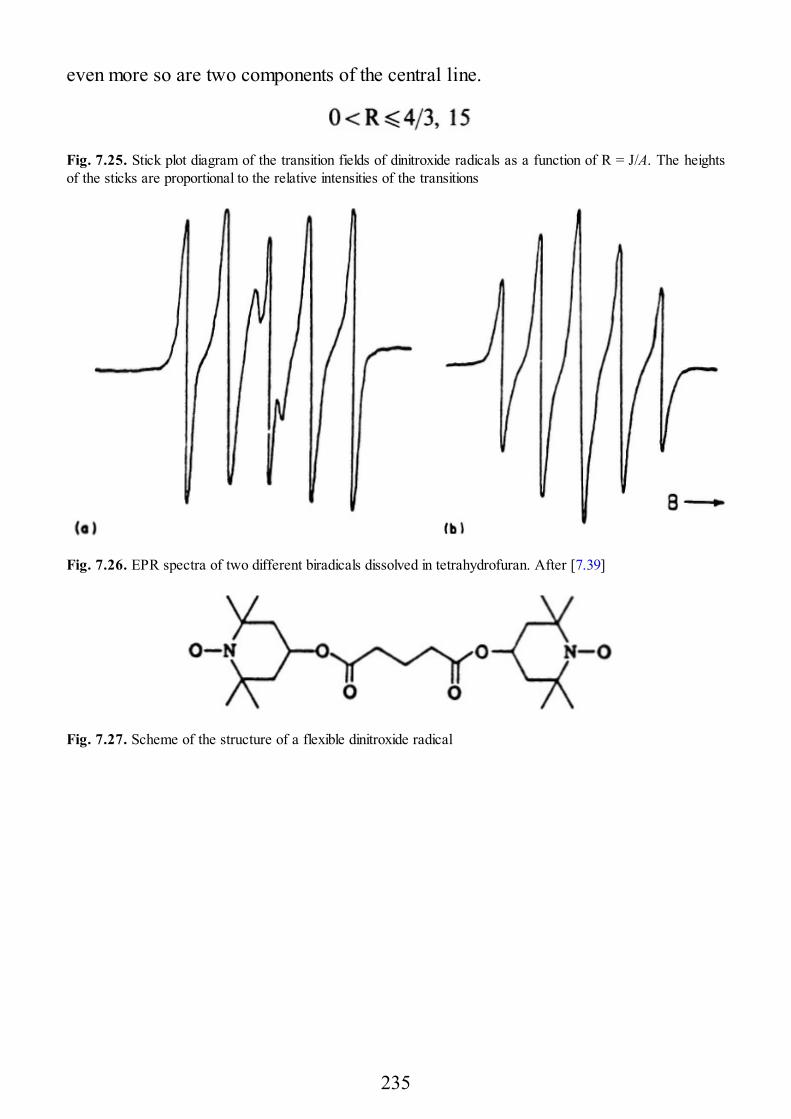
even more so are two components of the central line.

Fig. 7.25. Stick plot diagram of the transition fields of dinitroxide radicals as a function of R = J/A. The heightsof the sticks are proportional to the relative intensities of the transitions

Fig. 7.26. EPR spectra of two different biradicals dissolved in tetrahydrofuran. After [7.39]

Fig. 7.27. Scheme of the structure of a flexible dinitroxide radical

235

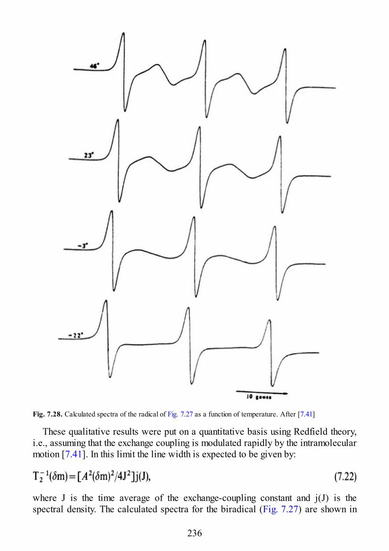
Fig. 7.28. Calculated spectra of the radical of Fig. 7.27 as a function of temperature. After [7.41]

These qualitative results were put on a quantitative basis using Redfield theory,i.e., assuming that the exchange coupling is modulated rapidly by the intramolecularmotion [7.41]. In this limit the line width is expected to be given by:

where J is the time average of the exchange-coupling constant and j(J) is thespectral density. The calculated spectra for the biradical (Fig. 7.27) are shown in

236

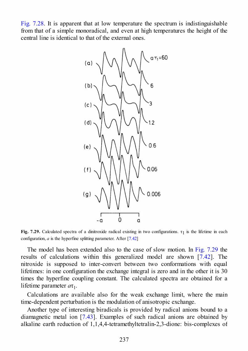
Fig. 7.28. It is apparent that at low temperature the spectrum is indistinguishablefrom that of a simple monoradical, and even at high temperatures the height of thecentral line is identical to that of the external ones.

Fig. 7.29. Calculated spectra of a dinitroxide radical existing in two configurations. τ1 is the lifetime in eachconfiguration, a is the hyperfine splitting parameter. After [7.42]

The model has been extended also to the case of slow motion. In Fig. 7.29 theresults of calculations within this generalized model are shown [7.42]. Thenitroxide is supposed to inter-convert between two conformations with equallifetimes: in one configuration the exchange integral is zero and in the other it is 30times the hyperfine coupling constant. The calculated spectra are obtained for alifetime parameter aτ1.

Calculations are available also for the weak exchange limit, where the maintime-dependent perturbation is the modulation of anisotropic exchange.

Another type of interesting biradicals is provided by radical anions bound to adiamagnetic metal ion [7.43]. Examples of such radical anions are obtained byalkaline earth reduction of 1,1,4,4-tetramethyltetralin-2,3-dione: bis-complexes of

237

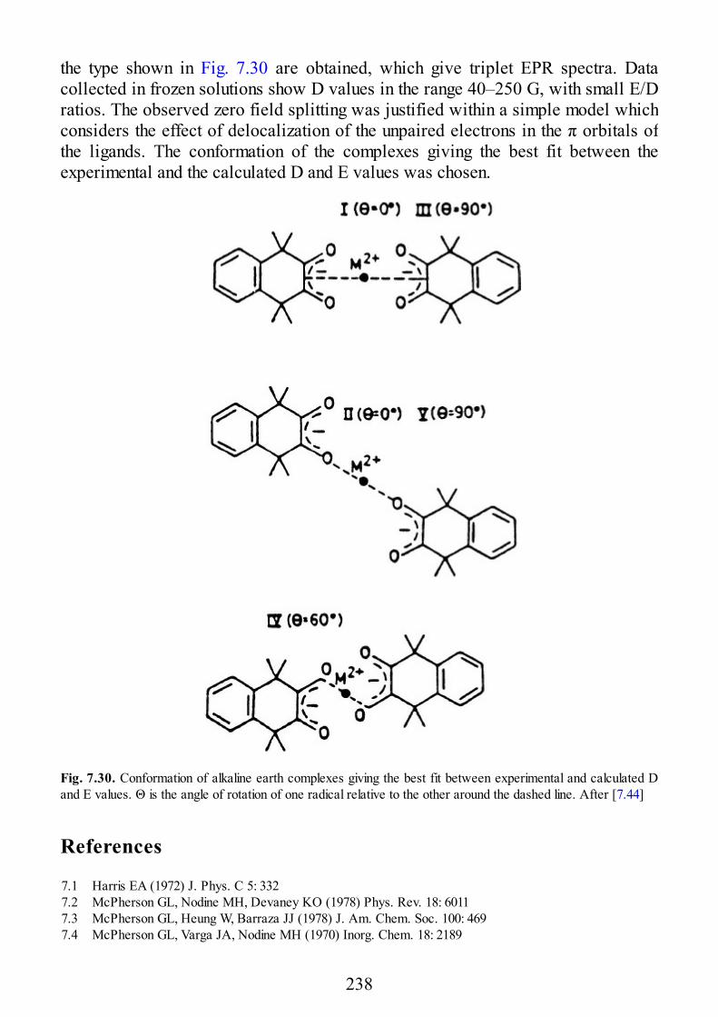
the type shown in Fig. 7.30 are obtained, which give triplet EPR spectra. Datacollected in frozen solutions show D values in the range 40–250 G, with small E/Dratios. The observed zero field splitting was justified within a simple model whichconsiders the effect of delocalization of the unpaired electrons in the π orbitals ofthe ligands. The conformation of the complexes giving the best fit between theexperimental and the calculated D and E values was chosen.

Fig. 7.30. Conformation of alkaline earth complexes giving the best fit between experimental and calculated Dand E values. Θ is the angle of rotation of one radical relative to the other around the dashed line. After [7.44]

References

7.1 Harris EA (1972) J. Phys. C 5: 3327.2 McPherson GL, Nodine MH, Devaney KO (1978) Phys. Rev. 18: 60117.3 McPherson GL, Heung W, Barraza JJ (1978) J. Am. Chem. Soc. 100: 4697.4 McPherson GL, Varga JA, Nodine MH (1970) Inorg. Chem. 18: 2189

238

7.5 Belford RL, Chasteen ND, So H, Tapscott RE (1969) J. Am. Chem. Soc. 91: 46757.6 Smith SRP, Owen J (1971) J. Phys. C 4: 13997.7 Fieselmann BM, McPherson AM, McPherson GL (1978) Inorg. Chem. 17: 18417.8 Setukowski D, Jungst R, Stucky GD (1978) Inorg. Chem. 17: 18487.9 Fieselmann BF, Hendrickson DN, Stucky GD (1978) Inorg. Chem. 17: 20787.10 Kramer LS, Clauss AW, Francesconi LC, Corbin DR, Hendrickson DN, Stucky GD (1981) Inorg. Chem.

20: 20707.11 Francesconi LC, Corbin DR, Clauss AW, Hendrickson DN, Stucky GD (1981) Inorg. Chem. 20: 20787.12 Francesconi LC, Corbin DR, Clauss AW, Hendrickson DN, Stucky GD (1981) Inorg. Chem. 20: 20597.13 Corbin DR, Francesconi LC, Hendrickson DN, Stucky GD (1981) Inorg. Chem. 20: 20847.14 Bleaney B, Bowers KD (1952) Proc. R. Soc. A214: 4517.15 van Niekerk, Schoening FRL (1953) Acta Cryst. 6: 2277.16 Julve M, Verdaguer M, Gleizes A, Philoche-Levisalles M, Kahn O (1984) Inorg. Chem. 23: 38087.17 Bencini A, Gatteschi D, Zanchini C, Kahn O, Verdaguer M, Julve M (1986) Inorg. Chem. 25: 31817.18 Duggan DM, Hendrickson DN (1974) Inorg. Chem. 13: 29297.19 Banci L, Bencini A, Gatteschi D (1984) Inorg. Chem. 23: 21387.20 Felthouse TR, Hendrickson DN (1978) Inorg. Chem. 17: 4447.21 Iwasaki M (1974) J. Magn. Reson. 16: 4177.22 Yokoi H, Chikira M (1975) J. Am. Chem. Soc. 97: 39757.23 Snaathorst D, Doesburg HM, Perenboom JA, Keijzers CP (1981) Inorg. Chem. 20: 25267.24 Snaathorst D, Keijzers C P (1984) Mol. Phys. S1: 5097.25 Gatteschi D, Bencini A (1985) In: Willett RD, Gatteschi D, Kahn O (eds) Magneto-Structural correlations

in exchange coupled systems. Willett RD, Reidel, Dordrecht, p 2417.26 Gatteschi D (1983) In: Bertini, I, Drago RS, Luchinat C (Eds) The coordination chemistry of

metalloenzymes. Reidel, Dordrecht, p 2157.27 Kahn O (1987) Structure and bonding (Berlin) 68: 897.28 Banci L, Bencini A, Benelli C, Dei A, Gatteschi D (1981) Inorg. Chem. 20: 13997.29 Banci L, Bencini A, Benelli C, Gatteschi D (1982) Inorg. Chem. 21: 38687.30 Morgenstern-Badarau I, Rerat M, Kahn O, Jaud K, Galy (1982) J. Inorg. Chem. 21: 30507.31 Journaux Y, Kahn O, Morgenstern-Badarau I, Galy J, Jaud J, Bencini A, Gatteschi D (1985) J. Am. Chem.

Soc. 107: 63057.32 Banci L, Bencini A, Gatteschi D, Dei A (1979) Inorg. Chim. Acta 36, L4197.33 Kokoszka GF, Allen HC, Gordon G (1967) J. Chem. Phys. 46: 30207.34 Banci L, Bencini A, Dei A, Gatteschi D (1981) Inorg. Chem. 20: 3937.35 Dapporto P, Sacconi L (1970) J. Chem. Soc. A 6817.36 Kahn O, Tola P, Coudanne H (1979) Chem. Phys. 42: 3557.37 Saraswat RS, Upreti GC (1978) J. Phys. Soc. Jpn. 44: 11427.38 Kahn O, Galy J, Journaux Y, Jaud J, Morgenstern-Badarau (1982) J. Am. Chem. Soc. 104:21657.39 Luckhurst GR (1976) In: Berliner LJ (ed) Spin labeling. Academic, New York, p 1337.40 Nakajima A, Ohya-Nishiguchi H, Deguchi Y (1973) Bull. Chem. Soc. Jpn. 45: 7137.41 Luckhurst GR (1966) Mol. Phys. 10: 5437.42 Luckhurst GR, Pedulli GF (1970) J. Am. Chem. Soc. 92: 47387.43 Parmon VN, Zhidomirov GM (1974) Mol. Phys. 27: 3677.44 Brustolon M, Pasimeni L, Corvaja C (1981) JCS Dalton 604

239

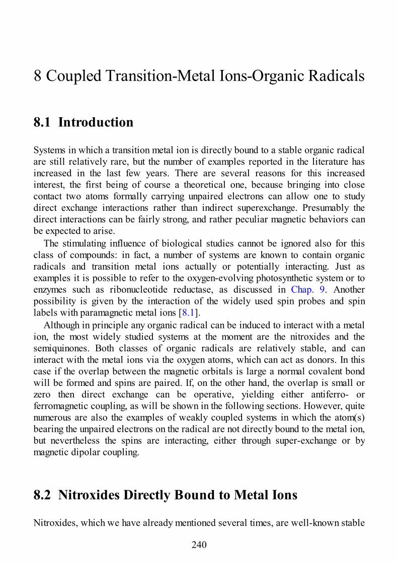
8 Coupled Transition-Metal Ions-Organic Radicals

8.1 Introduction

Systems in which a transition metal ion is directly bound to a stable organic radicalare still relatively rare, but the number of examples reported in the literature hasincreased in the last few years. There are several reasons for this increasedinterest, the first being of course a theoretical one, because bringing into closecontact two atoms formally carrying unpaired electrons can allow one to studydirect exchange interactions rather than indirect superexchange. Presumably thedirect interactions can be fairly strong, and rather peculiar magnetic behaviors canbe expected to arise.

The stimulating influence of biological studies cannot be ignored also for thisclass of compounds: in fact, a number of systems are known to contain organicradicals and transition metal ions actually or potentially interacting. Just asexamples it is possible to refer to the oxygen-evolving photosynthetic system or toenzymes such as ribonucleotide reductase, as discussed in Chap. 9. Anotherpossibility is given by the interaction of the widely used spin probes and spinlabels with paramagnetic metal ions [8.1].

Although in principle any organic radical can be induced to interact with a metalion, the most widely studied systems at the moment are the nitroxides and thesemiquinones. Both classes of organic radicals are relatively stable, and caninteract with the metal ions via the oxygen atoms, which can act as donors. In thiscase if the overlap between the magnetic orbitals is large a normal covalent bondwill be formed and spins are paired. If, on the other hand, the overlap is small orzero then direct exchange can be operative, yielding either antiferro- orferromagnetic coupling, as will be shown in the following sections. However, quitenumerous are also the examples of weakly coupled systems in which the atom(s)bearing the unpaired electrons on the radical are not directly bound to the metal ion,but nevertheless the spins are interacting, either through super-exchange or bymagnetic dipolar coupling.

8.2 Nitroxides Directly Bound to Metal Ions

Nitroxides, which we have already mentioned several times, are well-known stable

240

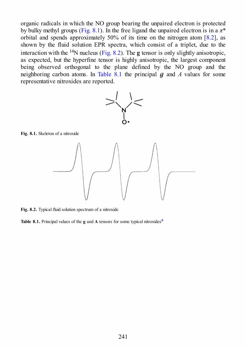
organic radicals in which the NO group bearing the unpaired electron is protectedby bulky methyl groups (Fig. 8.1). In the free ligand the unpaired electron is in a π*orbital and spends approximately 50% of its time on the nitrogen atom [8.2], asshown by the fluid solution EPR spectra, which consist of a triplet, due to theinteraction with the 14N nucleus (Fig. 8.2). The g tensor is only slightly anisotropic,as expected, but the hyperfine tensor is highly anisotropic, the largest componentbeing observed orthogonal to the plane defined by the NO group and theneighboring carbon atoms. In Table 8.1 the principal and A values for somerepresentative nitroxides are reported.

Fig. 8.1. Skeleton of a nitroxide

Fig. 8.2. Typical fluid solution spectrum of a nitroxide

Table 8.1. Principal values of the g and A tensors for some typical nitroxidesa

241

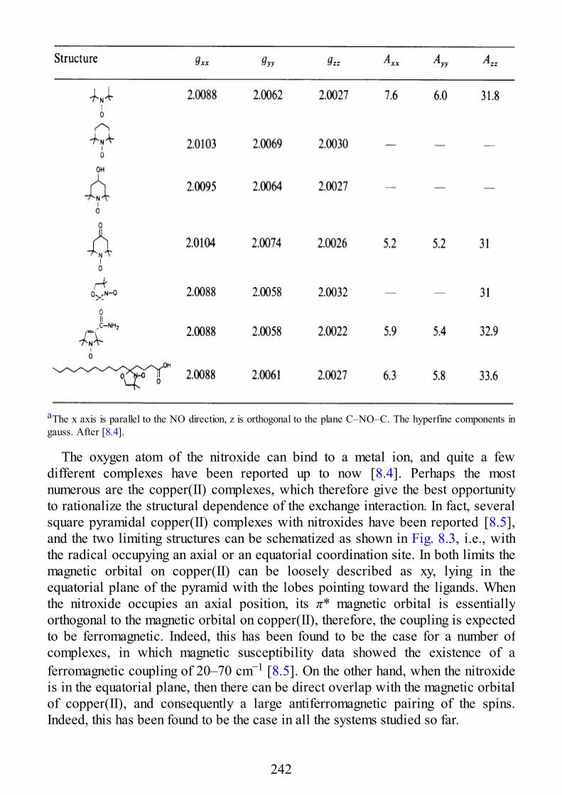
aThe x axis is parallel to the NO direction, z is orthogonal to the plane C–NO–C. The hyperfine components ingauss. After [8.4].

The oxygen atom of the nitroxide can bind to a metal ion, and quite a fewdifferent complexes have been reported up to now [8.4]. Perhaps the mostnumerous are the copper(II) complexes, which therefore give the best opportunityto rationalize the structural dependence of the exchange interaction. In fact, severalsquare pyramidal copper(II) complexes with nitroxides have been reported [8.5],and the two limiting structures can be schematized as shown in Fig. 8.3, i.e., withthe radical occupying an axial or an equatorial coordination site. In both limits themagnetic orbital on copper(II) can be loosely described as xy, lying in theequatorial plane of the pyramid with the lobes pointing toward the ligands. Whenthe nitroxide occupies an axial position, its π* magnetic orbital is essentiallyorthogonal to the magnetic orbital on copper(II), therefore, the coupling is expectedto be ferromagnetic. Indeed, this has been found to be the case for a number ofcomplexes, in which magnetic susceptibility data showed the existence of aferromagnetic coupling of 20–70 cm−1 [8.5]. On the other hand, when the nitroxideis in the equatorial plane, then there can be direct overlap with the magnetic orbitalof copper(II), and consequently a large antiferromagnetic pairing of the spins.Indeed, this has been found to be the case in all the systems studied so far.

242

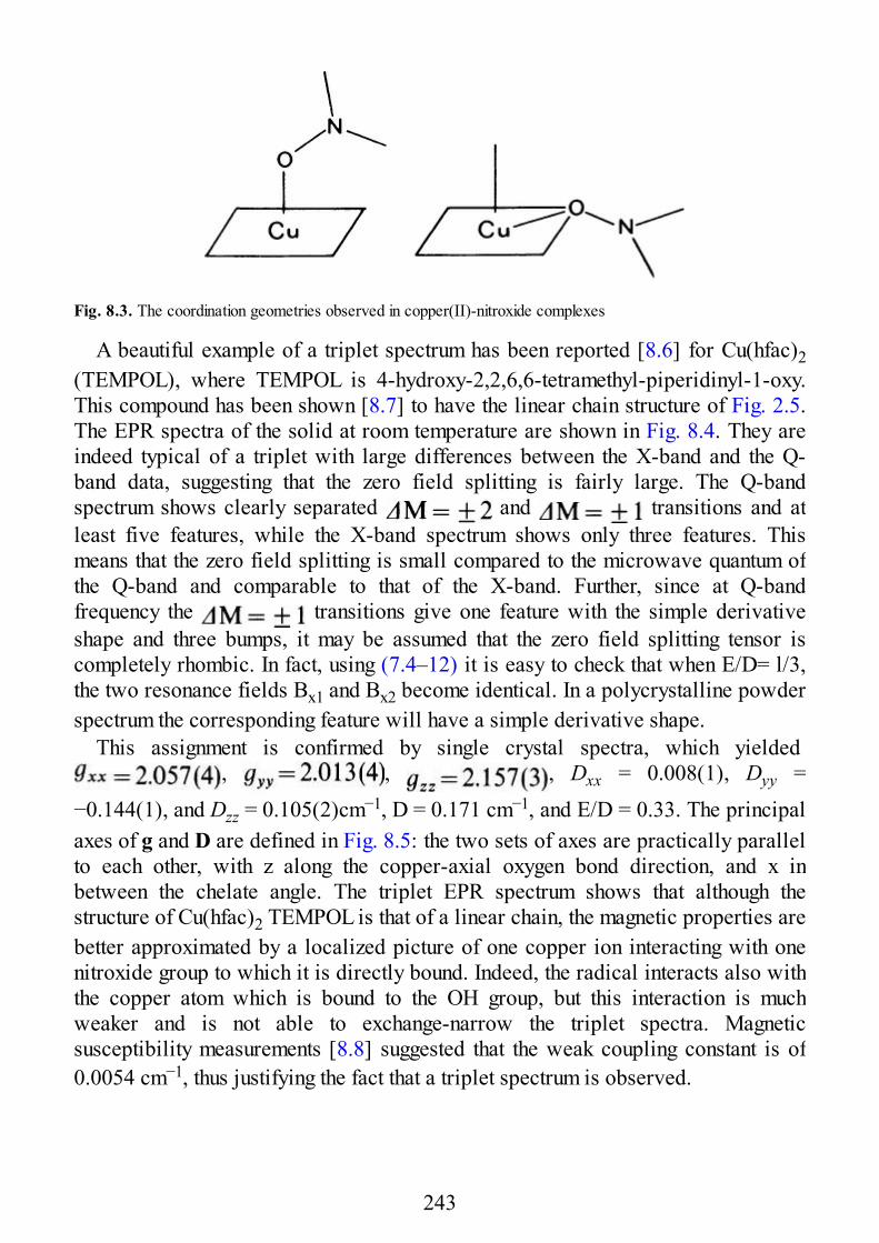
Fig. 8.3. The coordination geometries observed in copper(II)-nitroxide complexes

A beautiful example of a triplet spectrum has been reported [8.6] for Cu(hfac)2(TEMPOL), where TEMPOL is 4-hydroxy-2,2,6,6-tetramethyl-piperidinyl-1-oxy.This compound has been shown [8.7] to have the linear chain structure of Fig. 2.5.The EPR spectra of the solid at room temperature are shown in Fig. 8.4. They areindeed typical of a triplet with large differences between the X-band and the Q-band data, suggesting that the zero field splitting is fairly large. The Q-bandspectrum shows clearly separated and transitions and atleast five features, while the X-band spectrum shows only three features. Thismeans that the zero field splitting is small compared to the microwave quantum ofthe Q-band and comparable to that of the X-band. Further, since at Q-bandfrequency the transitions give one feature with the simple derivativeshape and three bumps, it may be assumed that the zero field splitting tensor iscompletely rhombic. In fact, using (7.4–12) it is easy to check that when E/D= l/3,the two resonance fields Bx1 and Bx2 become identical. In a polycrystalline powderspectrum the corresponding feature will have a simple derivative shape.

This assignment is confirmed by single crystal spectra, which yielded , , , Dxx = 0.008(1), Dyy =

−0.144(1), and Dzz = 0.105(2)cm−1, D = 0.171 cm−1, and E/D = 0.33. The principalaxes of g and D are defined in Fig. 8.5: the two sets of axes are practically parallelto each other, with z along the copper-axial oxygen bond direction, and x inbetween the chelate angle. The triplet EPR spectrum shows that although thestructure of Cu(hfac)2 TEMPOL is that of a linear chain, the magnetic properties arebetter approximated by a localized picture of one copper ion interacting with onenitroxide group to which it is directly bound. Indeed, the radical interacts also withthe copper atom which is bound to the OH group, but this interaction is muchweaker and is not able to exchange-narrow the triplet spectra. Magneticsusceptibility measurements [8.8] suggested that the weak coupling constant is of0.0054 cm−1, thus justifying the fact that a triplet spectrum is observed.

243

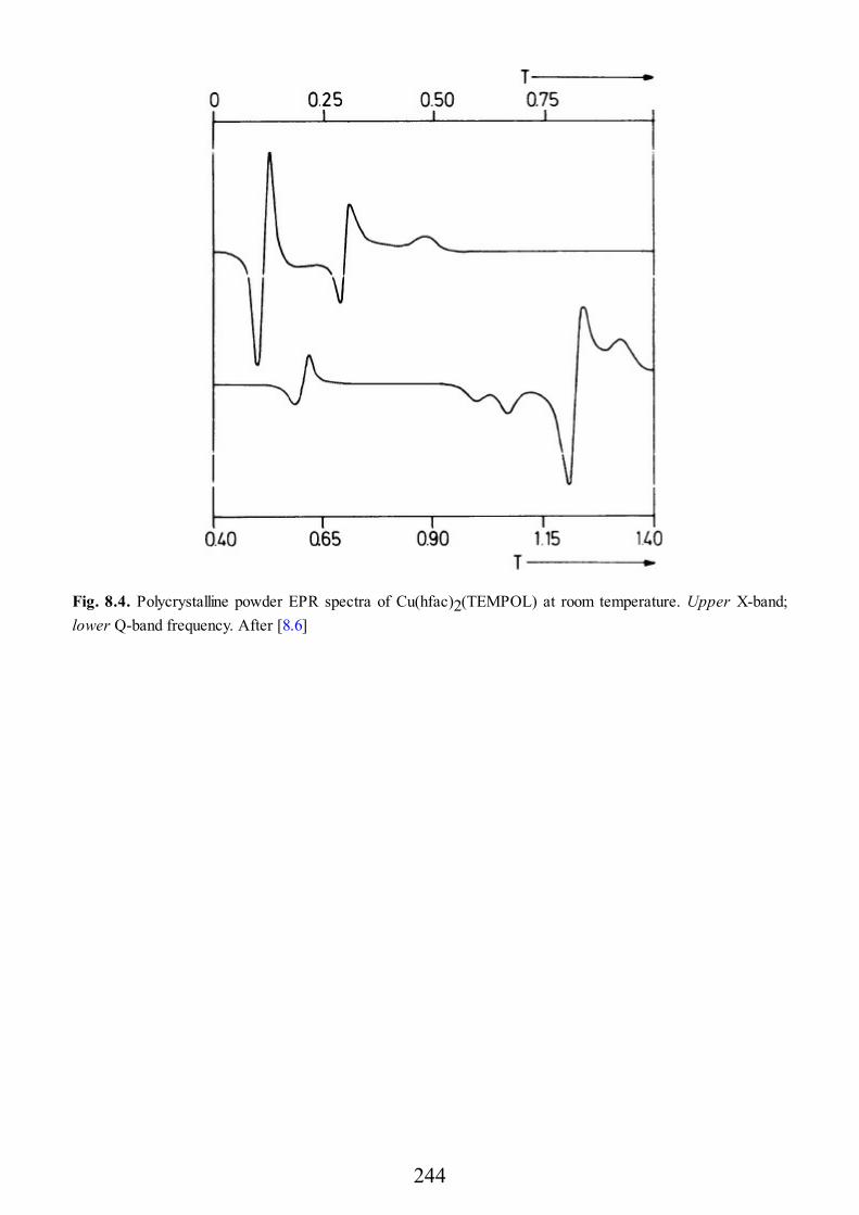
Fig. 8.4. Polycrystalline powder EPR spectra of Cu(hfac)2(TEMPOL) at room temperature. Upper X-band;lower Q-band frequency. After [8.6]

244

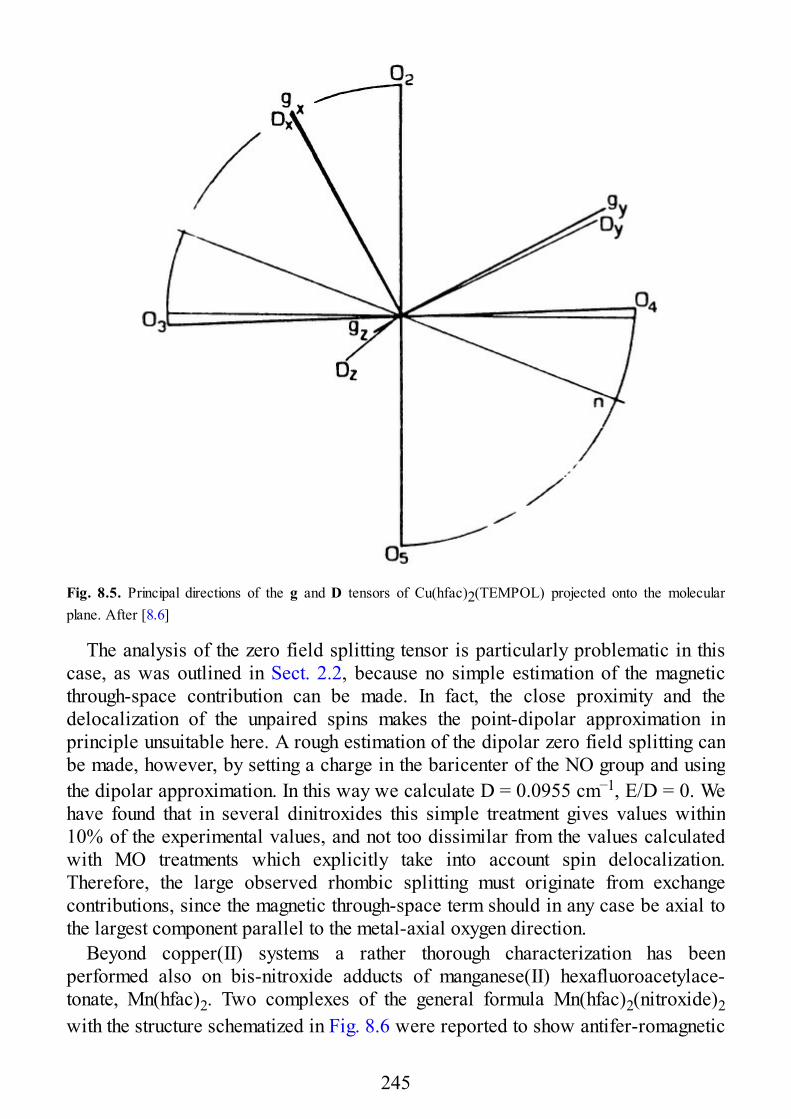
Fig. 8.5. Principal directions of the g and D tensors of Cu(hfac)2(TEMPOL) projected onto the molecularplane. After [8.6]

The analysis of the zero field splitting tensor is particularly problematic in thiscase, as was outlined in Sect. 2.2, because no simple estimation of the magneticthrough-space contribution can be made. In fact, the close proximity and thedelocalization of the unpaired spins makes the point-dipolar approximation inprinciple unsuitable here. A rough estimation of the dipolar zero field splitting canbe made, however, by setting a charge in the baricenter of the NO group and usingthe dipolar approximation. In this way we calculate D = 0.0955 cm−1, E/D = 0. Wehave found that in several dinitroxides this simple treatment gives values within10% of the experimental values, and not too dissimilar from the values calculatedwith MO treatments which explicitly take into account spin delocalization.Therefore, the large observed rhombic splitting must originate from exchangecontributions, since the magnetic through-space term should in any case be axial tothe largest component parallel to the metal-axial oxygen direction.

Beyond copper(II) systems a rather thorough characterization has beenperformed also on bis-nitroxide adducts of manganese(II) hexafluoroacetylace-tonate, Mn(hfac)2. Two complexes of the general formula Mn(hfac)2(nitroxide)2with the structure schematized in Fig. 8.6 were reported to show antifer-romagnetic

245

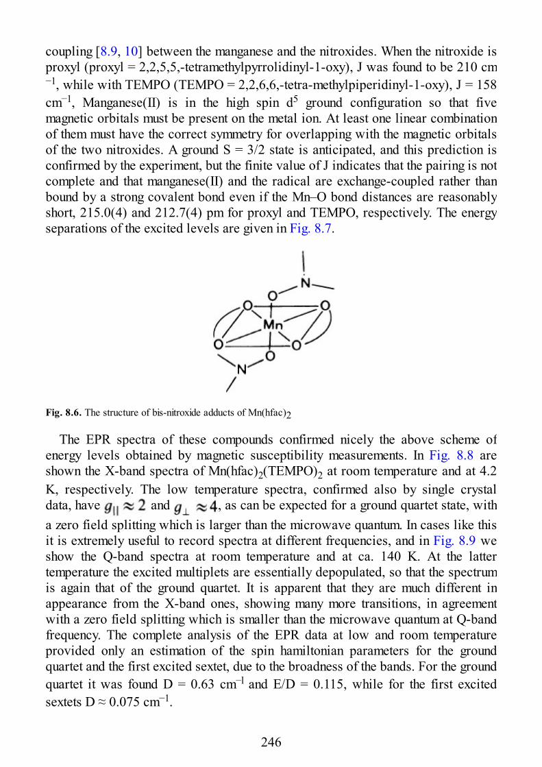
coupling [8.9, 10] between the manganese and the nitroxides. When the nitroxide isproxyl (proxyl = 2,2,5,5,-tetramethylpyrrolidinyl-1-oxy), J was found to be 210 cm−1, while with TEMPO (TEMPO = 2,2,6,6,-tetra-methylpiperidinyl-1-oxy), J = 158cm−1, Manganese(II) is in the high spin d5 ground configuration so that fivemagnetic orbitals must be present on the metal ion. At least one linear combinationof them must have the correct symmetry for overlapping with the magnetic orbitalsof the two nitroxides. A ground S = 3/2 state is anticipated, and this prediction isconfirmed by the experiment, but the finite value of J indicates that the pairing is notcomplete and that manganese(II) and the radical are exchange-coupled rather thanbound by a strong covalent bond even if the Mn–O bond distances are reasonablyshort, 215.0(4) and 212.7(4) pm for proxyl and TEMPO, respectively. The energyseparations of the excited levels are given in Fig. 8.7.

Fig. 8.6. The structure of bis-nitroxide adducts of Mn(hfac)2

The EPR spectra of these compounds confirmed nicely the above scheme ofenergy levels obtained by magnetic susceptibility measurements. In Fig. 8.8 areshown the X-band spectra of Mn(hfac)2(TEMPO)2 at room temperature and at 4.2K, respectively. The low temperature spectra, confirmed also by single crystaldata, have and , as can be expected for a ground quartet state, witha zero field splitting which is larger than the microwave quantum. In cases like thisit is extremely useful to record spectra at different frequencies, and in Fig. 8.9 weshow the Q-band spectra at room temperature and at ca. 140 K. At the lattertemperature the excited multiplets are essentially depopulated, so that the spectrumis again that of the ground quartet. It is apparent that they are much different inappearance from the X-band ones, showing many more transitions, in agreementwith a zero field splitting which is smaller than the microwave quantum at Q-bandfrequency. The complete analysis of the EPR data at low and room temperatureprovided only an estimation of the spin hamiltonian parameters for the groundquartet and the first excited sextet, due to the broadness of the bands. For the groundquartet it was found D = 0.63 cm−l and E/D = 0.115, while for the first excitedsextets D ≈ 0.075 cm−1.

246

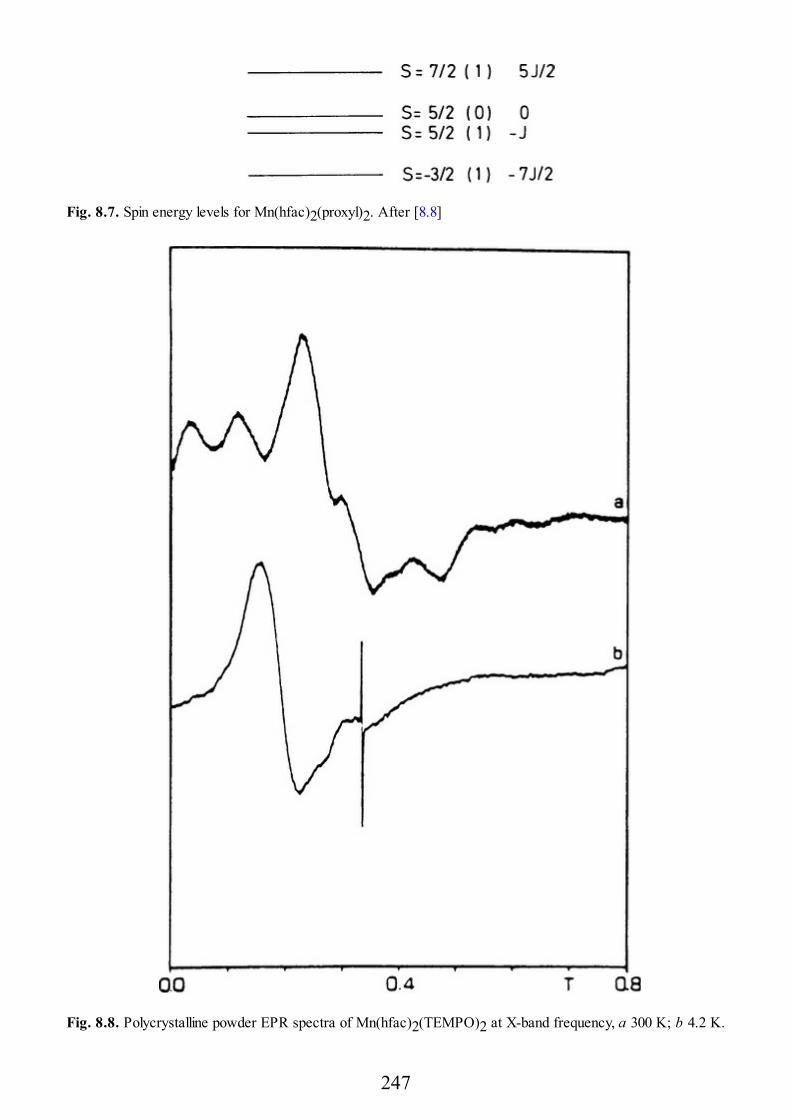
Fig. 8.7. Spin energy levels for Mn(hfac)2(proxyl)2. After [8.8]

Fig. 8.8. Polycrystalline powder EPR spectra of Mn(hfac)2(TEMPO)2 at X-band frequency, a 300 K; b 4.2 K.

247

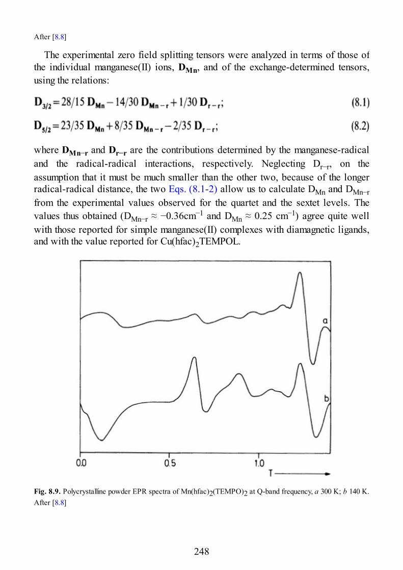
After [8.8]

The experimental zero field splitting tensors were analyzed in terms of those ofthe individual manganese(II) ions, DMn, and of the exchange-determined tensors,using the relations:

where DMn−r and Dr−r are the contributions determined by the manganese-radicaland the radical-radical interactions, respectively. Neglecting Dr−r, on theassumption that it must be much smaller than the other two, because of the longerradical-radical distance, the two Eqs. (8.1-2) allow us to calculate DMn and DMn−rfrom the experimental values observed for the quartet and the sextet levels. Thevalues thus obtained (DMn−r ≈ −0.36cm−1 and DMn ≈ 0.25 cm−1) agree quite wellwith those reported for simple manganese(II) complexes with diamagnetic ligands,and with the value reported for Cu(hfac)2TEMPOL.

Fig. 8.9. Polycrystalline powder EPR spectra of Mn(hfac)2(TEMPO)2 at Q-band frequency, a 300 K; b 140 K.After [8.8]

248

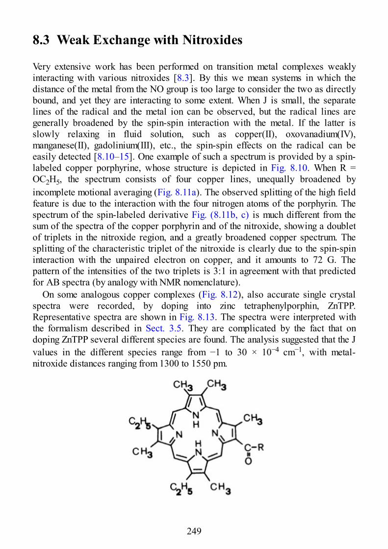
8.3 Weak Exchange with Nitroxides

Very extensive work has been performed on transition metal complexes weaklyinteracting with various nitroxides [8.3]. By this we mean systems in which thedistance of the metal from the NO group is too large to consider the two as directlybound, and yet they are interacting to some extent. When J is small, the separatelines of the radical and the metal ion can be observed, but the radical lines aregenerally broadened by the spin-spin interaction with the metal. If the latter isslowly relaxing in fluid solution, such as copper(II), oxovanadium(IV),manganese(II), gadolinium(III), etc., the spin-spin effects on the radical can beeasily detected [8.10–15]. One example of such a spectrum is provided by a spin-labeled copper porphyrine, whose structure is depicted in Fig. 8.10. When R =OC2H5, the spectrum consists of four copper lines, unequally broadened byincomplete motional averaging (Fig. 8.11a). The observed splitting of the high fieldfeature is due to the interaction with the four nitrogen atoms of the porphyrin. Thespectrum of the spin-labeled derivative Fig. (8.11b, c) is much different from thesum of the spectra of the copper porphyrin and of the nitroxide, showing a doubletof triplets in the nitroxide region, and a greatly broadened copper spectrum. Thesplitting of the characteristic triplet of the nitroxide is clearly due to the spin-spininteraction with the unpaired electron on copper, and it amounts to 72 G. Thepattern of the intensities of the two triplets is 3:1 in agreement with that predictedfor AB spectra (by analogy with NMR nomenclature).

On some analogous copper complexes (Fig. 8.12), also accurate single crystalspectra were recorded, by doping into zinc tetraphenylporphin, ZnTPP.Representative spectra are shown in Fig. 8.13. The spectra were interpreted withthe formalism described in Sect. 3.5. They are complicated by the fact that ondoping ZnTPP several different species are found. The analysis suggested that the Jvalues in the different species range from −1 to 30 × 10−4 cm−1, with metal-nitroxide distances ranging from 1300 to 1550 pm.

249

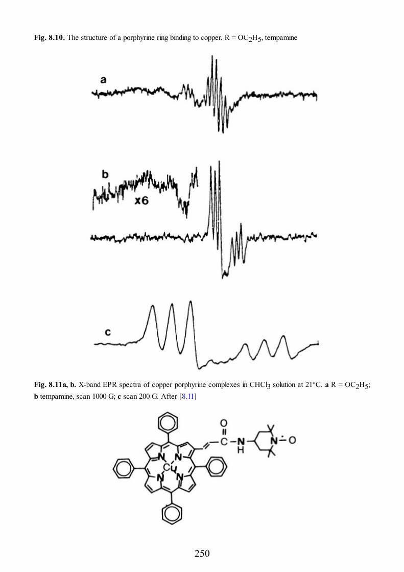
Fig. 8.10. The structure of a porphyrine ring binding to copper. R = OC2H5, tempamine

Fig. 8.11a, b. X-band EPR spectra of copper porphyrine complexes in CHCl3 solution at 21°C. a R = OC2H5;b tempamine, scan 1000 G; c scan 200 G. After [8.11]

250

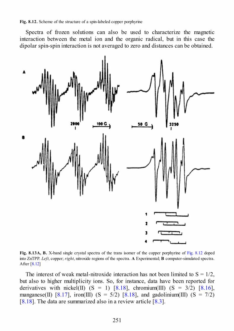
Fig. 8.12. Scheme of the structure of a spin-labeled copper porphyrine

Spectra of frozen solutions can also be used to characterize the magneticinteraction between the metal ion and the organic radical, but in this case thedipolar spin-spin interaction is not averaged to zero and distances can be obtained.

Fig. 8.13A, B. X-band single crystal spectra of the trans isomer of the copper porphyrine of Fig. 8.12 dopedinto ZnTPP. Left, copper; right, nitroxide regions of the spectra. A Experimental; B computer-simulated spectra.After [8.12]

The interest of weak metal-nitroxide interaction has not been limited to S = 1/2,but also to higher multiplicity ions. So, for instance, data have been reported forderivatives with nickel(II) (S = 1) [8.18], chromium(III) (S = 3/2) [8.16],manganese(II) [8.17], iron(III) (S = 5/2) [8.18], and gadolinium(III) (S = 7/2)[8.18]. The data are summarized also in a review article [8.3].

251

Spin labeling has been extensively used to investigate biological molecules, forinstance, cytochrome P450. Simple model compounds have also been studied, inorder to provide a firm basis for the interpretation of the spectra observed in morecomplicated systems [8.19]. Figure 8.14 illustrates one of these models. When twomolecules of imidazole are bound, the iron(III) is in the low spin form (S = 1/2).The EPR spectra of FeTPP(Im)2 and of one spin-labeled derivative are shown inFig. 8.15. Spectrum A is that of the native porphyrin and is typical of low spiniron(III), with , and 2.91. The two spin-labeled derivatives yieldfairly similar spectra markedly different from those of the native species. The sharpsignal at in both B and C is due to free nitroxide, which is present as animpurity, the remaining four features being due to the iron(III) spin-labeledcomplex. Two signals at and 2.14, respectively, correspond to theaverage between the of the radical and and 2.27 of the ironporphyrin, respectively. The other two signals at and 2.32 correspond tothe partial average of the signal of FeTPP with of the radical. Thisindicates that the exchange interaction is much larger than the g anisotropy for theformer signals, but not large enough to average the latter. The spectra weresimulated according to the procedure outlined in [8.13]. The best fit yielded J =0.28 cm−1 and a distance between iron(III) and the radical of 700 pm.

252

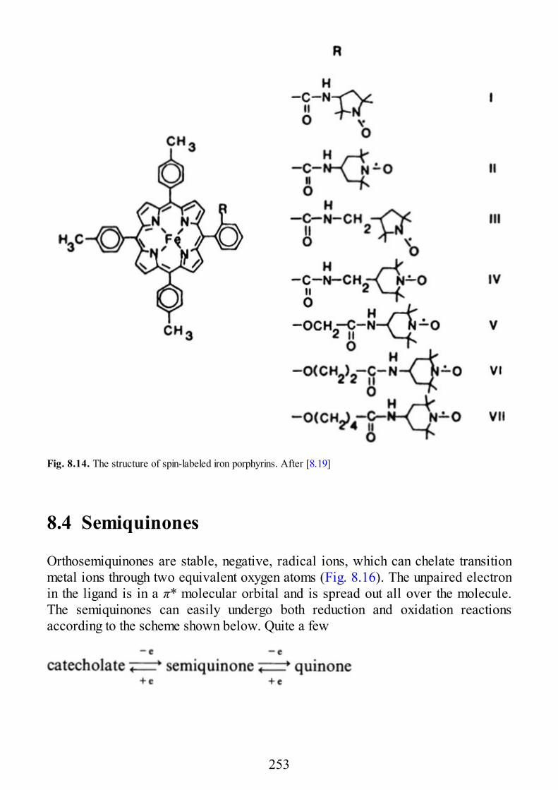
Fig. 8.14. The structure of spin-labeled iron porphyrins. After [8.19]

8.4 Semiquinones

Orthosemiquinones are stable, negative, radical ions, which can chelate transitionmetal ions through two equivalent oxygen atoms (Fig. 8.16). The unpaired electronin the ligand is in a π* molecular orbital and is spread out all over the molecule.The semiquinones can easily undergo both reduction and oxidation reactionsaccording to the scheme shown below. Quite a few

253

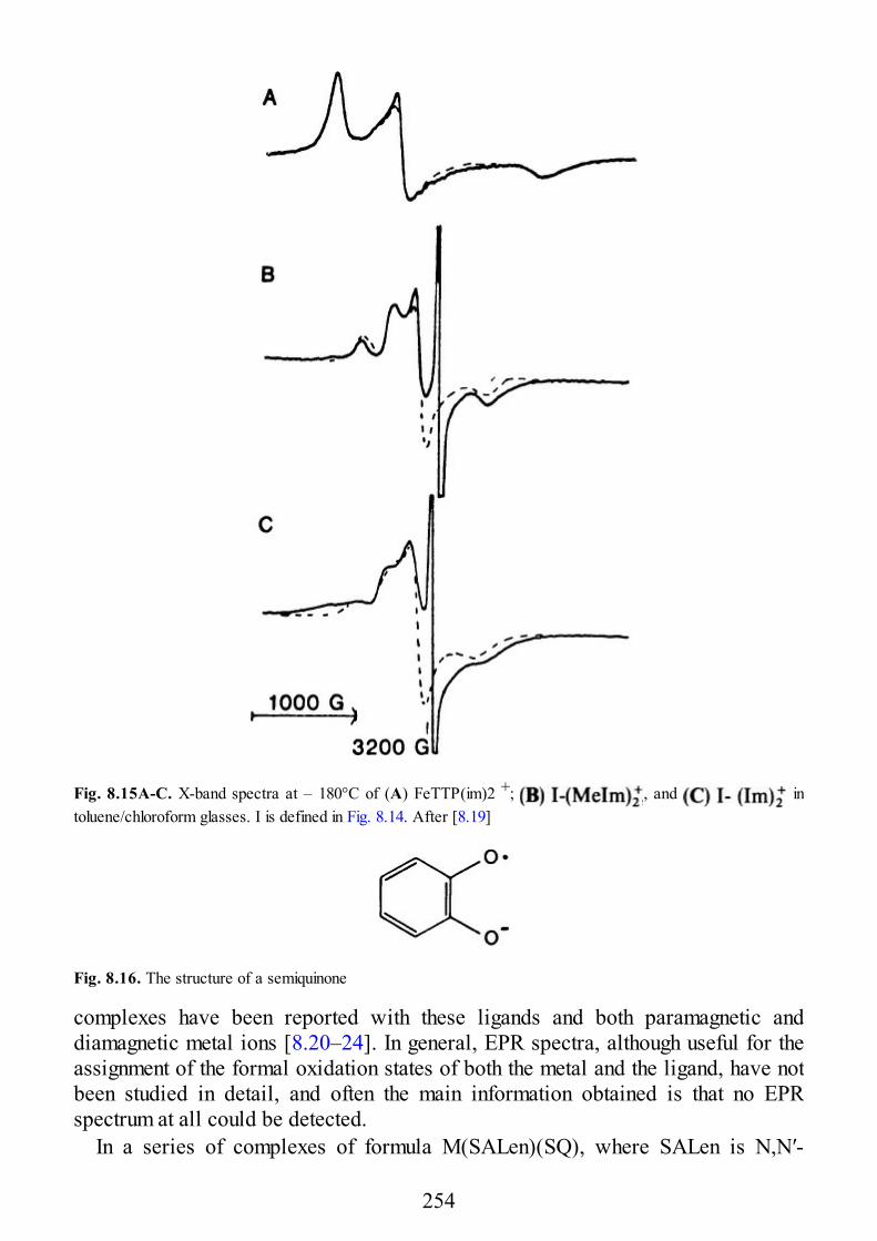
Fig. 8.15A-C. X-band spectra at – 180°C of (A) FeTTP(im)2 +; , and intoluene/chloroform glasses. I is defined in Fig. 8.14. After [8.19]

Fig. 8.16. The structure of a semiquinone

complexes have been reported with these ligands and both paramagnetic anddiamagnetic metal ions [8.20–24]. In general, EPR spectra, although useful for theassignment of the formal oxidation states of both the metal and the ligand, have notbeen studied in detail, and often the main information obtained is that no EPRspectrum at all could be detected.

In a series of complexes of formula M(SALen)(SQ), where SALen is N,N′-

254

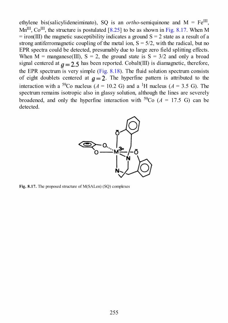
ethylene bis(salicylideneiminato), SQ is an ortho-semiquinone and M = FeIII,MnIII, CoIII, the structure is postulated [8.25] to be as shown in Fig. 8.17. When M= iron(III) the magnetic susceptibility indicates a ground S = 2 state as a result of astrong antiferromagnetic coupling of the metal ion, S = 5/2, with the radical, but noEPR spectra could be detected, presumably due to large zero field splitting effects.When M = manganese(III), S = 2, the ground state is S = 3/2 and only a broadsignal centered at has been reported. Cobalt(III) is diamagnetic, therefore,the EPR spectrum is very simple (Fig. 8.18). The fluid solution spectrum consistsof eight doublets centered at . The hyperfine pattern is attributed to theinteraction with a 59Co nucleus (A = 10.2 G) and a 1H nucleus (A = 3.5 G). Thespectrum remains isotropic also in glassy solution, although the lines are severelybroadened, and only the hyperfine interaction with 59Co (A = 17.5 G) can bedetected.

Fig. 8.17. The proposed structure of M(SALen) (SQ) complexes

255

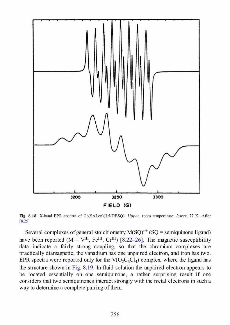
Fig. 8.18. X-band EPR spectra of Co(SALen)(3,5-DBSQ). Upper, room temperature; lower, 77 K. After[8.25]

Several complexes of general stoichiometry M(SQ)n+ (SQ = semiquinone ligand)have been reported (M = VIII, FeIII, CrIII) [8.22–26]. The magnetic susceptibilitydata indicate a fairly strong coupling, so that the chromium complexes arepractically diamagnetic, the vanadium has one unpaired electron, and iron has two.EPR spectra were reported only for the V(O2C6Cl4) complex, where the ligand hasthe structure shown in Fig. 8.19. In fluid solution the unpaired electron appears tobe located essentially on one semiquinone, a rather surprising result if oneconsiders that two semiquinones interact strongly with the metal electrons in such away to determine a complete pairing of them.

256

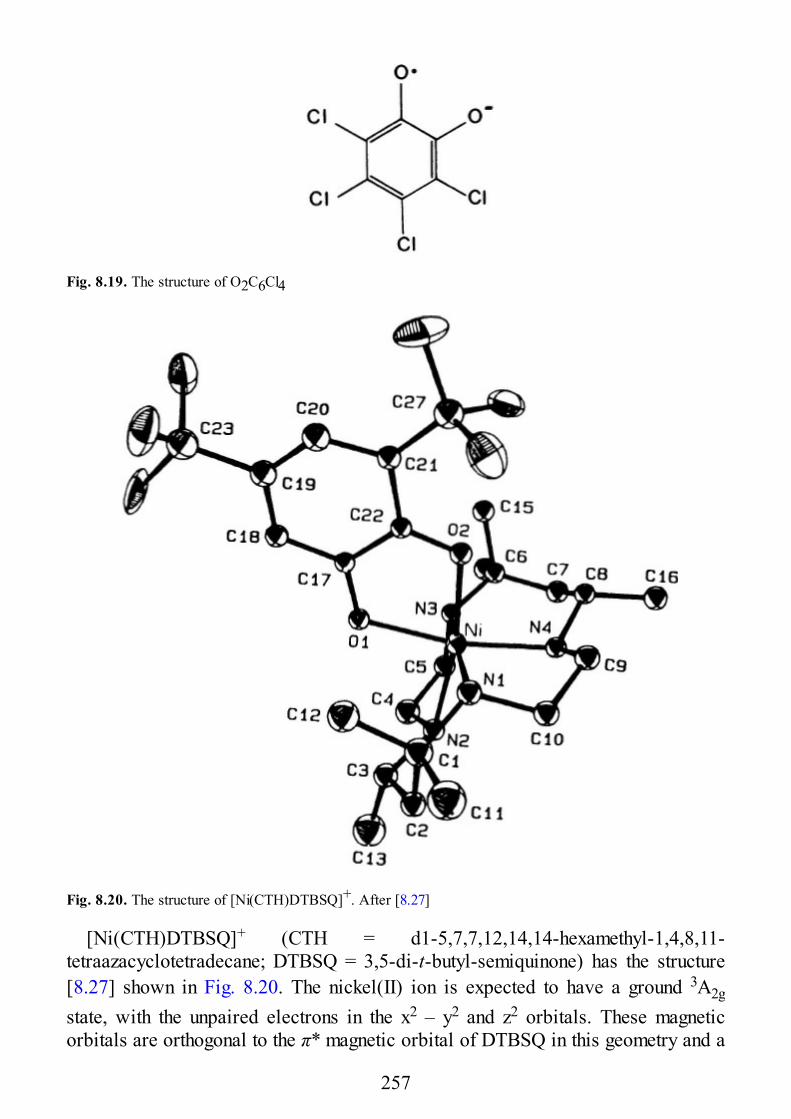
Fig. 8.19. The structure of O2C6Cl4

Fig. 8.20. The structure of [Ni(CTH)DTBSQ]+. After [8.27]

[Ni(CTH)DTBSQ]+ (CTH = d1-5,7,7,12,14,14-hexamethyl-1,4,8,11-tetraazacyclotetradecane; DTBSQ = 3,5-di-t-butyl-semiquinone) has the structure[8.27] shown in Fig. 8.20. The nickel(II) ion is expected to have a ground 3A2g

state, with the unpaired electrons in the x2 – y2 and z2 orbitals. These magneticorbitals are orthogonal to the π* magnetic orbital of DTBSQ in this geometry and a

257

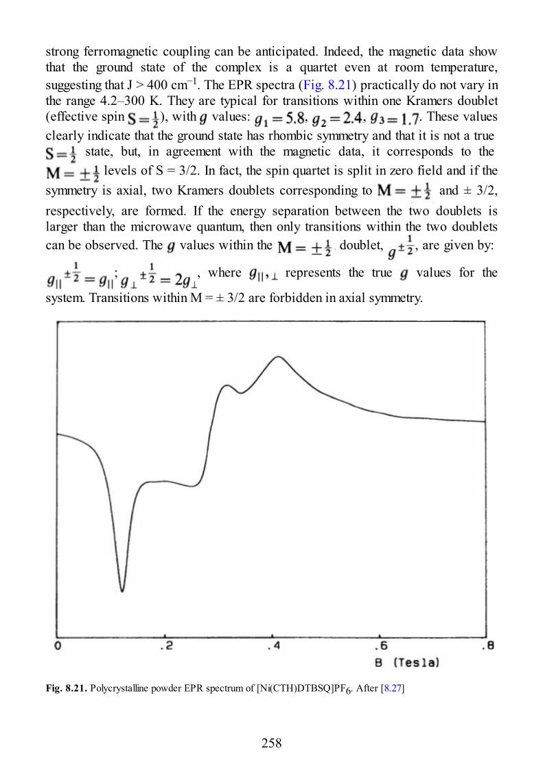
strong ferromagnetic coupling can be anticipated. Indeed, the magnetic data showthat the ground state of the complex is a quartet even at room temperature,suggesting that J > 400 cm−1. The EPR spectra (Fig. 8.21) practically do not vary inthe range 4.2–300 K. They are typical for transitions within one Kramers doublet(effective spin ), with values: , , . These valuesclearly indicate that the ground state has rhombic symmetry and that it is not a true

state, but, in agreement with the magnetic data, it corresponds to the levels of S = 3/2. In fact, the spin quartet is split in zero field and if the

symmetry is axial, two Kramers doublets corresponding to and ± 3/2,respectively, are formed. If the energy separation between the two doublets islarger than the microwave quantum, then only transitions within the two doubletscan be observed. The values within the doublet, , are given by:

; , where represents the true values for the

system. Transitions within M = ± 3/2 are forbidden in axial symmetry.

Fig. 8.21. Polycrystalline powder EPR spectrum of [Ni(CTH)DTBSQ]PF6. After [8.27]

258

If the symmetry is lower than axial, then the values in the two Kramersdoublets are given [8.28] by:

where t = E/D.If we assume that then from (8.3) and the experimental

values we can calculate , , and t. Thus, we find , , E/D =0.293. In the present case the values are the average of the values of the nickelion and of the semiquinone. Using Eq. (3.20) and Table 3.3, assuming that for theradical is 2.00, we finally calculate , in excellent agreement with thevalue expected for nickel(II) in octahedral symmetry.

More examples of simple model systems in which a metal ion interacts withsemiquinones are given in Sect. 9.4.

References

8.1 Hyde JS, Swartz HM, Antholine WE (1979) In Berliner LJ (ed) Spin labeling II. Academic, New York, p71.

8.2 Janzen EG (1971) Top. Stereochem. 6: 1178.3 Eaton SS Eaton GR (1978) Coord. Chem. Rev. 26: 207, Eaton SS, Eaton GR (1988) Coord. Chem. Rev.

88: 238.4 Berliner LJ (ed) (1976) ’Spin labeling’, Academic, New York, p 5658.5 Caneschi A, Gatteschi D, Grand A, Laugier J, Pardi L, Rey P (1988) Inorg. Chem. 27:1031 and references

therein.8.6 Bencini A, Benelli C, Gatteschi D, Zanchini C (1984) J. Am. Chem. Soc. 106, 58138.7 Anderson OP, Kuechler TS (1980) Inorg. Chem. 19: 14178.8 Benelli C, Gatteschi D, Zanchini C, Doedens RJ, Dickman MH, Porter LC (1986) Inorg. Chem. 25: 34538.9 Dickman MH, Porter LC, Doedens RJ (1986) Inorg. Chem. 25: 25958.10 Eaton SS, Dubois DL, Eaton GR (1978) J. Mag. Res. 32: 2518.11 Braden GA, Trevor KT, Neri JM, Greenslade DJ, Eaton GR (1977) J. Am. Chem. Soc. 99:48548.12 Damoder R, More KM, Eaton GR, Eaton SS (1983) J. Am. Chem. Soc. 105: 21478.13 Eaton SS, More KM, Sawant BM, Eaton GR (1983) J. Am. Chem. Soc. 105: 65608.14 Eaton SS, More KM, Sawant BM, Boymel PM, Eaton GR (1983) J. Magn. Res. 52: 4358.15 Hafid S, Eaton GR, Eaton SS (1983) J. Mag. Res. 51: 4708.16 More KM, Eaton GR, Eaton SS, Hideg K (1986) Inorg. Chem. 25: 38658.17 More JK, More KM, Eaton GR, Eaton SS (1984) J. Am. Chem. Soc. 106: 53958.18 More KM, Eaton GR, Eaton SS (1986) Inorg. Chem. 25: 26388.19 Fielding L, More KM, Eaton GR, Eaton SS (1986) J. Am. Chem. Soc. 108: 618 and references therein.8.20 Kahn O, Prins R, Reedijk J, Thompson JS (1987) Inorg. Chem. 26: 35578.21 Lynch MW, Buchanan RM, Pierpont CG, Hendrickson DN (1981) Inorg. Chem. 20: 1038

259

8.22 Cass ME, Gordon NR, Pierpont CG (1986) Inorg. Chem. 25: 39628.23 Brown DG, Hemphill WD (1979) Inorg. Chem. 18: 20398.24 Buchanan RM, Fitzgerald BJ, Pierpont CG (1979) Inorg. Chem. 18: 34398.25 Kessel SL, Emerson RM, Debrunner PG, Hendrickson DN (1980) Inorg. Chem. 19: 11708.26 Buchanan RM, Kessel SL, Downs HH, Pierpont CG, Hendrickson DN (1978) J. Am. Chem. Soc. 100:

78948.27 Benelli C, Dei A, Gatteschi D, Pardi L (1988) Inorg. Chem. 27: 28318.28 Pilbrow JR (1978) J. Magn. Reson. 31: 479

260

9 Biological Systems

9.1 Introduction

The application of EPR to the study of magnetically coupled species in biologicalsystems is one of the most intensively exploited fields at the moment, and almostevery day new exciting examples are reported. Therefore, here more than in anyother section, we will not be able to give exhaustive coverage of the area, butsimply will report those examples which seem to us to be more appropriate,interesting, and worthy of attention. The whole field has already been covered by anumber of review articles [9.1–4], to which the interested reader is invited to refer.Also, given the necessity of using a number of related techniques in order to obtaina good understanding of the complex matter, it may prove useful to consider otherrelated magnetic techniques, such as nuclear magnetic resonance [9.5–7], ENDOR[9.8], magnetically perturbed Mössbauer spectroscopy [9.9–10], etc. Indeed, in thefollowing sections we will frequently refer to the last mentioned technique, whichhas proved to be extremely useful for the characterization of iron proteins.

We will briefly review copper proteins, then iron proteins, and finally thephotosynthetic oxygen-evolving processes, both in higher plants and bacteria.

9.2 Copper Proteins

A number of important proteins and enzymes contain copper ions at the active site[9.11–14]. The principal biological role known up to now for proteins whichcontain copper include oxygen transport and activation, electron transfer, ironmetabolism, and superoxide dismutation. For this book the most interesting coppersystems are superoxide dismutase (SOD) and the coupled dinuclear copperproteins such as hemocyanin, the oxygen-binding protein of mollusks andarthropods, and tyrosinase, an enzyme with both monooxygenase and oxidaseactivity.

SOD is an enzyme which is present in the erythrocytes of mammalians whichcatalyzes the dismutation of the toxic superoxide ions [9.15]. The enzyme frombovine erythrocytes is composed of two identical subunits, each of which containsone copper(II) and one zinc(II) ion. Frequently, it is indicated as Cu2Zn2SOD. The

261

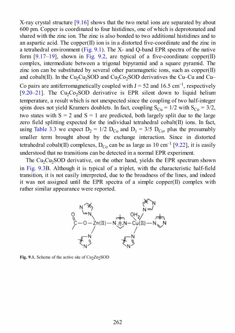
X-ray crystal structure [9.16] shows that the two metal ions are separated by about600 pm. Copper is coordinated to four histidines, one of which is deprotonated andshared with the zinc ion. The zinc is also bonded to two additional histidines and toan aspartic acid. The copper(II) ion is in a distorted five-coordinate and the zinc ina tetrahedral environment (Fig. 9.1). The X- and Q-band EPR spectra of the nativeform [9.17–19], shown in Fig. 9.2, are typical of a five-coordinate copper(II)complex, intermediate between a trigonal bipyramid and a square pyramid. Thezinc ion can be substituted by several other paramagnetic ions, such as copper(II)and cobalt(II). In the Cu2Cu2SOD and Cu2Co2SOD derivatives the Cu–Cu and Cu–Co pairs are antiferromagnetically coupled with J = 52 and 16.5 cm−1, respectively[9.20–21]. The Cu2Co2SOD derivative is EPR silent down to liquid heliumtemperature, a result which is not unexpected since the coupling of two half-integerspins does not yield Kramers doublets. In fact, coupling SCu = 1/2 with SCo = 3/2,two states with S = 2 and S = 1 are predicted, both largely split due to the largezero field splitting expected for the individual tetrahedral cobalt(II) ions. In fact,using Table 3.3 we expect D2 = 1/2 DCo and D1 = 3/5 DCo, plus the presumablysmaller term brought about by the exchange interaction. Since in distortedtetrahedral cobalt(II) complexes, DCo can be as large as 10 cm−1 [9.22], it is easilyunderstood that no transitions can be detected in a normal EPR experiment.

The Cu2Cu2SOD derivative, on the other hand, yields the EPR spectrum shownin Fig. 9.3B. Although it is typical of a triplet, with the characteristic half-fieldtransition, it is not easily interpreted, due to the broadness of the lines, and indeedit was not assigned until the EPR spectra of a simple copper(II) complex withrather similar appearance were reported.

Fig. 9.1. Scheme of the active site of Cu2Zn2SOD

262

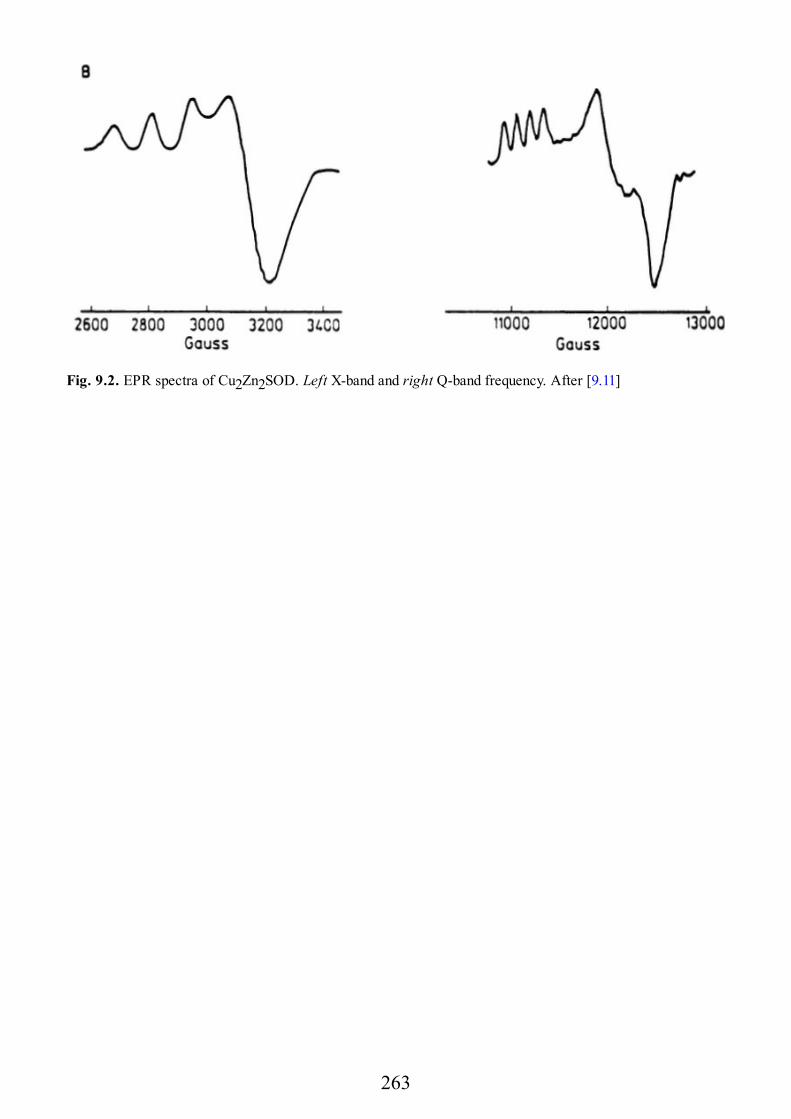
Fig. 9.2. EPR spectra of Cu2Zn2SOD. Left X-band and right Q-band frequency. After [9.11]

263

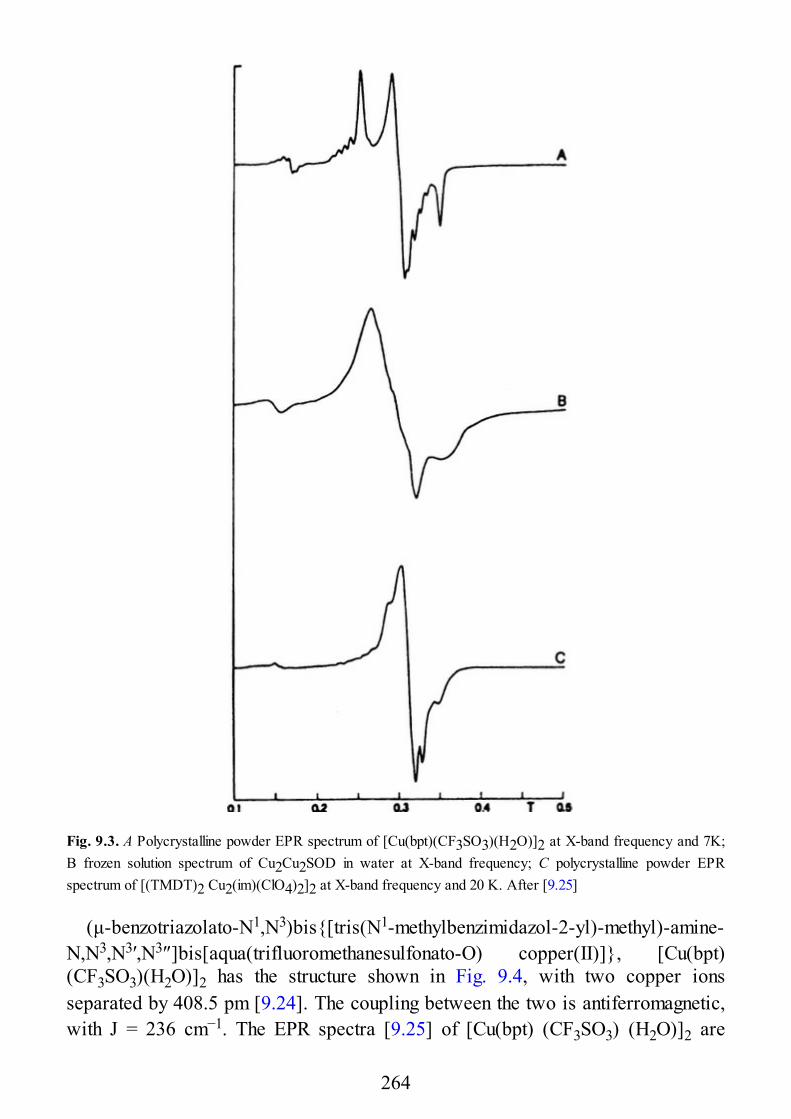
Fig. 9.3. A Polycrystalline powder EPR spectrum of [Cu(bpt)(CF3SO3)(H2O)]2 at X-band frequency and 7K;B frozen solution spectrum of Cu2Cu2SOD in water at X-band frequency; C polycrystalline powder EPRspectrum of [(TMDT)2 Cu2(im)(ClO4)2]2 at X-band frequency and 20 K. After [9.25]

(μ-benzotriazolato-N1,N3)bis{[tris(N1-methylbenzimidazol-2-yl)-methyl)-amine-N,N3,N3′,N3″]bis[aqua(trifluoromethanesulfonato-O) copper(II)]}, [Cu(bpt)(CF3SO3)(H2O)]2 has the structure shown in Fig. 9.4, with two copper ionsseparated by 408.5 pm [9.24]. The coupling between the two is antiferromagnetic,with J = 236 cm−1. The EPR spectra [9.25] of [Cu(bpt) (CF3SO3) (H2O)]2 are

264

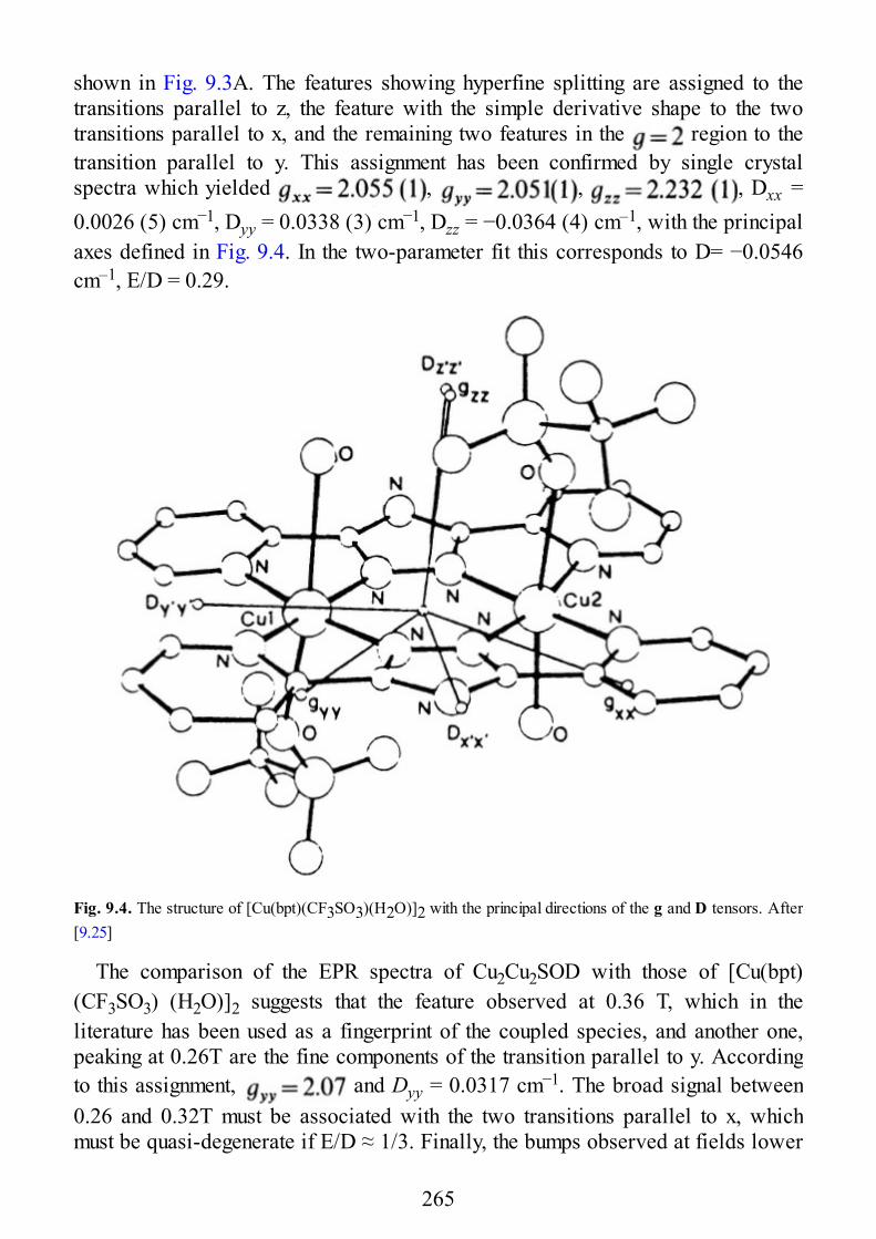
shown in Fig. 9.3A. The features showing hyperfine splitting are assigned to thetransitions parallel to z, the feature with the simple derivative shape to the twotransitions parallel to x, and the remaining two features in the region to thetransition parallel to y. This assignment has been confirmed by single crystalspectra which yielded , , , Dxx =0.0026 (5) cm−1, Dyy = 0.0338 (3) cm−1, Dzz = −0.0364 (4) cm–1, with the principalaxes defined in Fig. 9.4. In the two-parameter fit this corresponds to D= −0.0546cm–1, E/D = 0.29.

Fig. 9.4. The structure of [Cu(bpt)(CF3SO3)(H2O)]2 with the principal directions of the g and D tensors. After[9.25]

The comparison of the EPR spectra of Cu2Cu2SOD with those of [Cu(bpt)(CF3SO3) (H2O)]2 suggests that the feature observed at 0.36 T, which in theliterature has been used as a fingerprint of the coupled species, and another one,peaking at 0.26T are the fine components of the transition parallel to y. Accordingto this assignment, and Dyy = 0.0317 cm−1. The broad signal between0.26 and 0.32T must be associated with the two transitions parallel to x, whichmust be quasi-degenerate if E/D ≈ 1/3. Finally, the bumps observed at fields lower

265

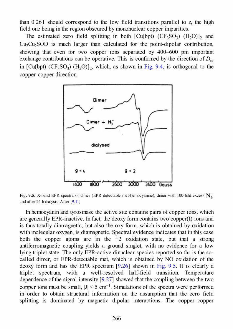
than 0.26T should correspond to the low field transitions parallel to z, the highfield one being in the region obscured by mononuclear copper impurities.

The estimated zero field splitting in both [Cu(bpt) (CF3SO3) (H2O)]2 andCu2Cu2SOD is much larger than calculated for the point-dipolar contribution,showing that even for two copper ions separated by 400–600 pm importantexchange contributions can be operative. This is confirmed by the direction of Dzzin [Cu(bpt) (CF3SO3) (H2O)]2, which, as shown in Fig. 9.4, is orthogonal to thecopper-copper direction.

Fig. 9.5. X-band EPR spectra of dimer (EPR detectable met-hemocyanine), dimer with 100-fold excess and after 24-h dialysis. After [9.11]

In hemocyanin and tyrosinase the active site contains pairs of copper ions, whichare generally EPR-inactive. In fact, the deoxy form contains two copper(I) ions andis thus totally diamagnetic, but also the oxy form, which is obtained by oxidationwith molecular oxygen, is diamagnetic. Spectral evidence indicates that in this caseboth the copper atoms are in the +2 oxidation state, but that a strongantiferromagnetic coupling yields a ground singlet, with no evidence for a lowlying triplet state. The only EPR-active dinuclear species reported so far is the so-called dimer, or EPR-detectable met, which is obtained by NO oxidation of thedeoxy form and has the EPR spectrum [9.26] shown in Fig. 9.5. It is clearly atriplet spectrum, with a well-resolved half-field transition. Temperaturedependence of the signal intensity [9.27] showed that the coupling between the twocopper ions must be small, |J| < 5 cm−1. Simulations of the spectra were performedin order to obtain structural information on the assumption that the zero fieldsplitting is dominated by magnetic dipolar interactions. The copper–copper

266

distance was thus estimated to be ≈ 600 pm. Addition of excess azide results in theformation of dimer , in which the copper–copper distance was estimated to be≈ 500 pm [9.28]. In these EPR-active, largely uncoupled derivatives, it is currentlybelieved that the endogenous bridge responsible for the large coupling in the metform is detached. The weak EPR signal observed in met hemocyanin has beenattributed to a small fraction of the sites where the endogenous bridge has a lowerstability constant [9.29].

9.3 Iron Proteins

Iron proteins form a very large group, which is usually split into three classes, (1)hemoglobin and myoglobin, which are responsible for the transport and storage ofoxygen; (2) iron-sulfur proteins, which are responsible for electron transport andare widely distributed in plants, animals, and microorganisms; and (3) that whichcontains oxo-bridged iron(III) ions, which perform a variety of biologicalfunctions, including oxygen transport, the reduction of ribo- and deoxyribo-nucleotides, phosphate ester hydrolysis, and iron storage. It is especially in the lasttwo classes that proteins relevant to this book are to be found, although well-documented cases of exchange-coupled species are found also in iron porphyrins,which are structurally related to the hemoglobin class of iron proteins.

9.3.1 Iron Porphyrins and Heme Proteins

Heme is a porphinato iron complex in which the common oxidation states for themetal atom are +2 and +3, each of which can have several different spin states.Indeed, iron(II), which has a d6 configuration, can have a ground S = 0, 1, and 2state, while iron(III), which is a d5 ion, can have S = 1/2, 3/2, and 5/2. All thesedifferent spin states have been observed [9.30]. From the EPR point of view theimportant hemes are the iron(III) derivatives, because this ion has an odd number ofelectrons, and in all the possible geometries and spin states it has a ground Kramersdoublet which always yields a spectrum, provided that the temperature issufficiently low to yield a long enough relaxation time. Matters are different for theparamagnetic states of iron(II), which is an even electron ion. In this case, in fact,zero field splitting removes the spin degeneracy of the ground multiplet to such anextent that transitions between the states can often be induced only at fields muchhigher than those usually available.

Particularly interesting appear to be the so-called high-valent iron porphyrins[9.31, 32]. This expression is used to refer to iron porphyrin complexes more

267

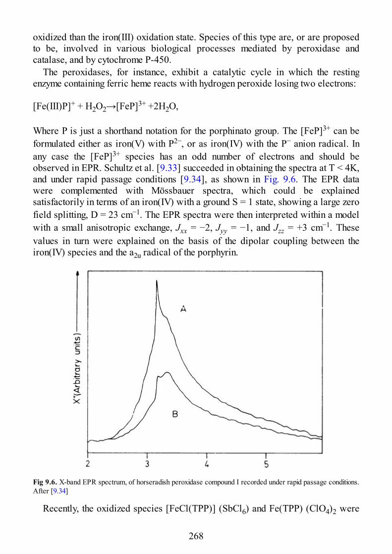
oxidized than the iron(III) oxidation state. Species of this type are, or are proposedto be, involved in various biological processes mediated by peroxidase andcatalase, and by cytochrome P-450.

The peroxidases, for instance, exhibit a catalytic cycle in which the restingenzyme containing ferric heme reacts with hydrogen peroxide losing two electrons:

[Fe(III)P]+ + H2O2→[FeP]3+ +2H2O,

Where P is just a shorthand notation for the porphinato group. The [FeP]3+ can beformulated either as iron(V) with P2−, or as iron(IV) with the P− anion radical. Inany case the [FeP]3+ species has an odd number of electrons and should beobserved in EPR. Schultz et al. [9.33] succeeded in obtaining the spectra at T < 4K,and under rapid passage conditions [9.34], as shown in Fig. 9.6. The EPR datawere complemented with Mössbauer spectra, which could be explainedsatisfactorily in terms of an iron(IV) with a ground S = 1 state, showing a large zerofield splitting, D = 23 cm−1. The EPR spectra were then interpreted within a modelwith a small anisotropic exchange, Jxx = −2, Jyy = −1, and Jzz = +3 cm−1. Thesevalues in turn were explained on the basis of the dipolar coupling between theiron(IV) species and the a2u radical of the porphyrin.

Fig 9.6. X-band EPR spectrum, of horseradish peroxidase compound I recorded under rapid passage conditions.After [9.34]

Recently, the oxidized species [FeCl(TPP)] (SbCl6) and Fe(TPP) (ClO4)2 were

268

also characterized [9.35] (TPP = tetraphenylporphinato). In this case the Fe(TPP)moiety has only two positive charges, one electron less than [FeP]3+, and no EPRspectra could be observed. However, the Mössbauer spectra showed the presenceof high spin iron(III), and the magnetic data showed that a strong antiferromagneticcoupling is operative in [FeCl(TPP)] (SbCl6), J > 500 cm−1, while the coupling isferromagnetic in [Fe (TPP) (ClO4)2, J ≈ − 80 cm−l. For the former the ground stateis S = 2, and for the latter it is S = 3, both originating from the interaction of SFe =5/2 and Sr = 1/2. It is interesting also to note that NMR spectra of the twocompounds showed opposite shifts of the phenyl protons: for instance, the ortho-and para protons are shifted downfield (42 and 35 ppm, respectively) in [FeCl(TPP)] (SbCl6) and upfield (−19 and −13 ppm) in Fe(TPP) (ClO4)2. This is abeautiful example of the alternation in sign of the hyperfine coupling constant (theEPR eq.uivalent of the NMR isotropic shift) in the high and low total spin statesobtained by coupling a spin S with another with . Indeed, the use of Table 3.3yields A = + 1/6 Ar for S = 3 and A = −1/6 Ar for S = 2.

Another system which is very interesting from the EPR point of view iscytochrome-c-oxidase [9.36]. Although very active research is being done on thisenzyme at the present time not very much is known about its structure. It is knownthat it is the respiratory enzyme that catalytically reduces 1 mol dioxygen to 2 molwater with the concomitant release of energy which is stored in the ADP-ATPcycle. The enzyme contains four metal centers (two irons and two coppers) perfunctioning unit. In the oxidized (resting) form of the enzyme one iron is in a hemeunit, and one copper is isolated and EPR-detectable, while at the active site there isa high spin iron(III) which is strongly coupled to a copper(II) ion to give a ground S= 2 state. The S = 3 state has been estimated to be at least 1200 cm−1 above theground state. The system is EPR-silent, presumably due to large zero field splitting.

If the native enzyme is treated with cyanide, the FeIII-CuII moiety remains EPR-silent, although there is no doubt that the iron(III) ion is forced into the low spinform. There are conflicting reports in the literature, but it seems now that thecoupling between low spin iron(III) and copper(II) is in this case ferromagnetic,yielding a ground triplet state [9.37]. Some model compounds were alsosynthesized containing low spin iron(III) porphinato and a square planar copper(II)ion bridged by a cyanide ion which occupies axial positions for both the metal ions[9.38]. These species yielded EPR spectra at low temperatures with manyresonances in the range 0−0.5 T. They were attributed to transitions between thelevels of what was substantially described as S′ = 1 level. The point we want tomake here is that a low spin iron(III)-copper(II) pair is complicated by the fact thatthe iron has a quasi-degenerate orbital ground state, making the analysis of theenergy levels, and of the EPR transitions, of the pair rather difficult. Indeed, if wetake into account the orbital degeneracy we see that the energy levels must beexpressed through a spin hamiltonian which includes the isotropic, anisotropic, and

269

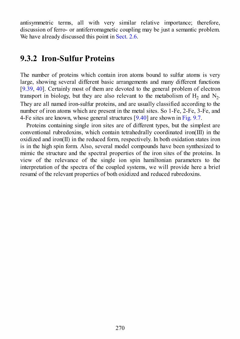
antisymmetric terms, all with very similar relative importance; therefore,discussion of ferro- or antiferromagnetic coupling may be just a semantic problem.We have already discussed this point in Sect. 2.6.

9.3.2 Iron-Sulfur Proteins

The number of proteins which contain iron atoms bound to sulfur atoms is verylarge, showing several different basic arrangements and many different functions[9.39, 40]. Certainly most of them are devoted to the general problem of electrontransport in biology, but they are also relevant to the metabolism of H2 and N2.They are all named iron-sulfur proteins, and are usually classified according to thenumber of iron atoms which are present in the metal sites. So 1-Fe, 2-Fe, 3-Fe, and4-Fe sites are known, whose general structures [9.40] are shown in Fig. 9.7.

Proteins containing single iron sites are of different types, but the simplest areconventional rubredoxins, which contain tetrahedrally coordinated iron(III) in theoxidized and iron(II) in the reduced form, respectively. In both oxidation states ironis in the high spin form. Also, several model compounds have been synthesized tomimic the structure and the spectral properties of the iron sites of the proteins. Inview of the relevance of the single ion spin hamiltonian parameters to theinterpretation of the spectra of the coupled systems, we will provide here a briefresumé of the relevant properties of both oxidized and reduced rubredoxins.

270

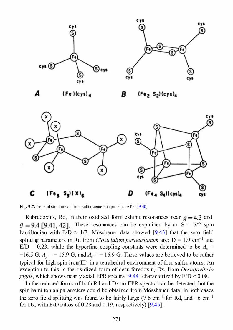
Fig. 9.7. General structures of iron-sulfur centers in proteins. After [9.40]

Rubredoxins, Rd, in their oxidized form exhibit resonances near and . These resonances can be explained by an S = 5/2 spin

hamiltonian with E/D ≈ 1/3. Mössbauer data showed [9.43] that the zero fieldsplitting parameters in Rd from Clostridium pasteurianum are: D = 1.9 cm−1 andE/D = 0.23, while the hyperfine coupling constants were determined to be Ax =−16.5 G, Ay = − 15.9 G, and Az = − 16.9 G. These values are believed to be rathertypical for high spin iron(III) in a tetrahedral environment of four sulfur atoms. Anexception to this is the oxidized form of desulforedoxin, Dx, from Desulfovibriogigas, which shows nearly axial EPR spectra [9.44] characterized by E/D ≈ 0.08.

In the reduced forms of both Rd and Dx no EPR spectra can be detected, but thespin hamiltonian parameters could be obtained from Mössbauer data. In both casesthe zero field splitting was found to be fairly large (7.6 cm−1 for Rd, and −6 cm−1

for Dx, with E/D ratios of 0.28 and 0.19, respectively) [9.45].

271

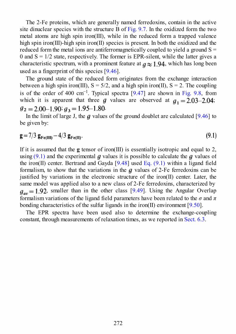
The 2-Fe proteins, which are generally named ferredoxins, contain in the activesite dinuclear species with the structure B of Fig. 9.7. In the oxidized form the twometal atoms are high spin iron(III), while in the reduced form a trapped valencehigh spin iron(III)-high spin iron(II) species is present. In both the oxidized and thereduced form the metal ions are antiferromagnetically coupled to yield a ground S =0 and S = 1/2 state, respectively. The former is EPR-silent, while the latter gives acharacteristic spectrum, with a prominent feature at , which has long beenused as a fingerprint of this species [9.46].

The ground state of the reduced form originates from the exchange interactionbetween a high spin iron(III), S = 5/2, and a high spin iron(II), S = 2. The couplingis of the order of 400 cm−1. Typical spectra [9.47] are shown in Fig. 9.8, fromwhich it is apparent that three values are observed at ;

; .In the limit of large J, the values of the ground doublet are calculated [9.46] to

be given by:

If it is assumed that the g tensor of iron(III) is essentially isotropic and equal to 2,using (9.1) and the experimental values it is possible to calculate the values ofthe iron(II) center. Bertrand and Gayda [9.48] used Eq. (9.1) within a ligand fieldformalism, to show that the variations in the values of 2-Fe ferredoxins can bejustified by variations in the electronic structure of the iron(II) center. Later, thesame model was applied also to a new class of 2-Fe ferredoxins, characterized by

, smaller than in the other class [9.49]. Using the Angular Overlapformalism variations of the ligand field parameters have been related to the σ and πbonding characteristics of the sulfur ligands in the iron(II) environment [9.50].

The EPR spectra have been used also to determine the exchange-couplingconstant, through measurements of relaxation times, as we reported in Sect. 6.3.

272

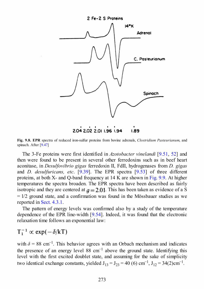
Fig. 9.8. EPR spectra of reduced iron-sulfur proteins from bovine adrenals, Clostridium Pasteurianum, andspinach. After [9.47]

The 3-Fe proteins were first identified in Azotobacter vinelandi [9.51, 52] andthen were found to be present in several other ferredoxins such as in beef heartaconitase, in Desulfovibrio gigas ferredoxin II, FdII, hydrogenases from D. gigasand D. desulfuricans, etc. [9.39]. The EPR spectra [9.53] of three differentproteins, at both X- and Q-band frequency at 14 K are shown in Fig. 9.9. At highertemperatures the spectra broaden. The EPR spectra have been described as fairlyisotropic and they are centered at . This has been taken as evidence of a S= l/2 ground state, and a confirmation was found in the Mössbauer studies as wereported in Sect. 4.3.1.

The pattern of energy levels was confirmed also by a study of the temperaturedependence of the EPR line-width [9.54]. Indeed, it was found that the electronicrelaxation time follows an exponential law:

with δ = 88 cm−1. This behavior agrees with an Orbach mechanism and indicatesthe presence of an energy level 88 cm−1 above the ground state. Identifying thislevel with the first excited doublet state, and assuming for the sake of simplicitytwo identical exchange constants, yielded J13 = J23 = 40 (6) cm−1, J12 = 34(2)cm−1.

273

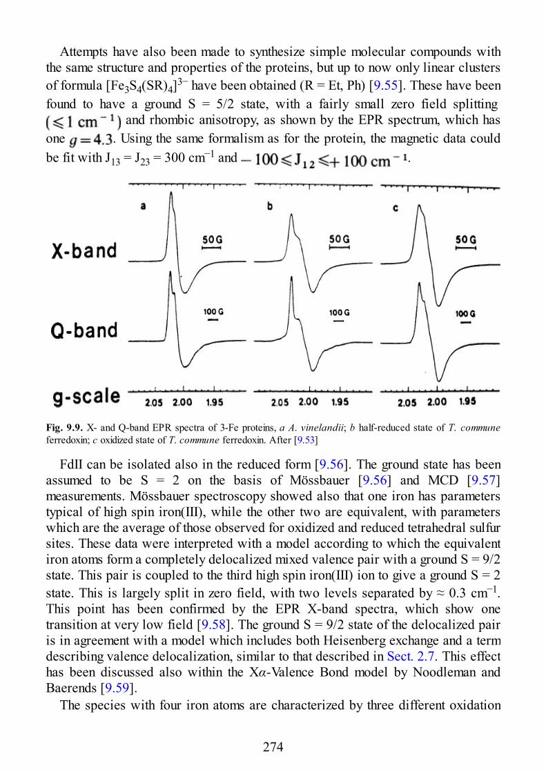
Attempts have also been made to synthesize simple molecular compounds withthe same structure and properties of the proteins, but up to now only linear clustersof formula [Fe3S4(SR)4]3− have been obtained (R = Et, Ph) [9.55]. These have beenfound to have a ground S = 5/2 state, with a fairly small zero field splitting

and rhombic anisotropy, as shown by the EPR spectrum, which hasone . Using the same formalism as for the protein, the magnetic data couldbe fit with J13 = J23 = 300 cm−1 and .

Fig. 9.9. X- and Q-band EPR spectra of 3-Fe proteins, a A. vinelandii; b half-reduced state of T. communeferredoxin; c oxidized state of T. commune ferredoxin. After [9.53]

FdII can be isolated also in the reduced form [9.56]. The ground state has beenassumed to be S = 2 on the basis of Mössbauer [9.56] and MCD [9.57]measurements. Mössbauer spectroscopy showed also that one iron has parameterstypical of high spin iron(III), while the other two are equivalent, with parameterswhich are the average of those observed for oxidized and reduced tetrahedral sulfursites. These data were interpreted with a model according to which the equivalentiron atoms form a completely delocalized mixed valence pair with a ground S = 9/2state. This pair is coupled to the third high spin iron(III) ion to give a ground S = 2state. This is largely split in zero field, with two levels separated by ≈ 0.3 cm−1.This point has been confirmed by the EPR X-band spectra, which show onetransition at very low field [9.58]. The ground S = 9/2 state of the delocalized pairis in agreement with a model which includes both Heisenberg exchange and a termdescribing valence delocalization, similar to that described in Sect. 2.7. This effecthas been discussed also within the Xα-Valence Bond model by Noodleman andBaerends [9.59].

The species with four iron atoms are characterized by three different oxidation

274

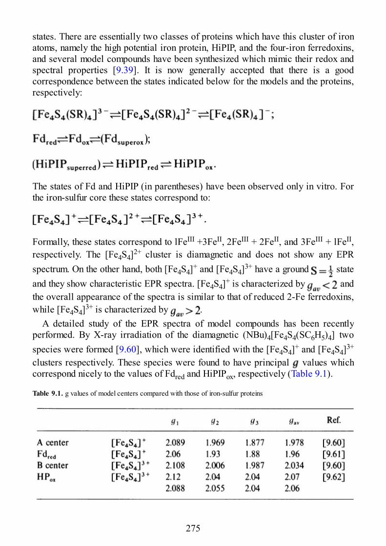
states. There are essentially two classes of proteins which have this cluster of ironatoms, namely the high potential iron protein, HiPIP, and the four-iron ferredoxins,and several model compounds have been synthesized which mimic their redox andspectral properties [9.39]. It is now generally accepted that there is a goodcorrespondence between the states indicated below for the models and the proteins,respectively:

The states of Fd and HiPIP (in parentheses) have been observed only in vitro. Forthe iron-sulfur core these states correspond to:

Formally, these states correspond to lFeIII +3FeII, 2FeIII + 2FeII, and 3FeIII + lFeII,respectively. The [Fe4S4]2+ cluster is diamagnetic and does not show any EPRspectrum. On the other hand, both [Fe4S4]+ and [Fe4S4]3+ have a ground stateand they show characteristic EPR spectra. [Fe4S4]+ is characterized by andthe overall appearance of the spectra is similar to that of reduced 2-Fe ferredoxins,while [Fe4S4]3+ is characterized by .

A detailed study of the EPR spectra of model compounds has been recentlyperformed. By X-ray irradiation of the diamagnetic (NBu)4[Fe4S4(SC6H5)4] twospecies were formed [9.60], which were identified with the [Fe4S4]+ and [Fe4S4]3+

clusters respectively. These species were found to have principal values whichcorrespond nicely to the values of Fdred and HiPIPox, respectively (Table 9.1).

Table 9.1. g values of model centers compared with those of iron-sulfur proteins

275

The diamagnetism in [Fe4S4]2+ can be rationalized assuming antiferromagneticcoupling between two pairs of mixed valence iron(II)-iron(III) couples [9.59].[Fe4S4]+ is similar to the reduced form of 2-Fe ferredoxin, because two iron(III)ions are strongly coupled to give an S = 0 ground state, and what is left is aniron(III)-iron(II) couple practically identical to that of the 2-Fe species.

Recently also some clusters of the type MFe3S4 have been isolated and studied.For instance, model compounds of formula [MFe3S4(SPhCl)3((C3H5)2Cat)CN]3−,with M = Mo, W, (SPhCl = p-chloro-thiophenol; Cat = catecholate) give spectracharacteristic of a ground S = 3/2 subject to a large zero field splitting [9.63].

CoFe3S4 clusters were obtained [9.64] by incubation of Desulfovibrio gigasferredoxin, which contains Fe3S4 clusters, with Co2+. The EPR spectrum revealsthe hyperfine splitting into eight components expected for 59Co, and the values,corresponding to an effective state, are , , .This cluster is described as [CoFe3S4]2+, isoelectronic to the [Fe4S4]+ cluster.

9.3.3 Sulfite Reductase

The sulfite reductase isolated from Escherichia coli is a complexhemoflavoprotein of molecular weight 685 000 containing four sirohemes and fourFe4S4 clusters [9.65]. It catalyzes the six-electron reductions of to S2− andof to NH3. The protein can be split and a subunit containing one sirohemeand one Fe4S4 cluster can be isolated. This subunit is indicated as SiR. Fullreduction of this unit is accomplished by two electrons. The oxidized form of theenzyme yields an EPR spectrum characteristic of a high spin iron(III) heme [9.66].No other signal attributable to the Fe4S4 cluster is observed, suggesting that it is inthe diamagnetic +2 oxidation state. Mössbauer data have confirmed that the heme isin the high spin +3 oxidation state, but have also shown that the iron ions of theFe4S4 cluster experience a magnetic hyperfine interaction, i.e., that the spin state ofthe cluster is S = 5/2 as well [9.67, 68]. This can only occur if the two moieties,heme and 4Fe-4S, are coupled. No detailed analysis of the data has been attempted,but a model has been suggested according to which the four iron atoms of Fe4S4 arestrongly coupled to yield the usual S = 0 ground state, but they are also coupled tothe heme iron with smaller coupling constants.

One electron reduction of SiR causes loss of the ferriheme signals, thus showingthat the iron(III) of the heme is reduced. Addition of a second electron results in theappearance of a novel EPR signal, with , 2.29, and 2.07.

276

9.3.4 Nitrogenase

Nitrogenase comprises two extremely air-sensitive metalloproteins (Fe protein)and one molybdenum iron protein (MoFe protein) [9.69]. The Fe protein acceptselectrons from oxidative processes operating at or below −0.4 V and thenspecifically passes them on to the MoFe protein for use in the reduction ofdinitrogen and other substrates. The MoFe protein is a tetramer of molecular weight220 000–240 000, containing 2 mol molybdenum, approximately 30 mol iron, andapproximately 30 mol acid-labile sulfur per mol peptide component.

One of the most prominent features of the MoFe protein is its EPR spectrum[9.70, 71], shown in Fig. 9.10. The spectrum is typical of an S = 3/2 largely split inzero field, with effective values 4.3, 3.6, and 2. There is now evidence that thisspectrum is due to a multimetal cluster which is present in the active site of theenzyme. Model compounds of formula [Fe(MS4)2]3− (M = Mo, W) were found[9.72] to yield EPR spectra very similar to those of the enzyme.

Fig. 9.10. EPR spectra of A. vinelandii MoFe protein of nitrogenase at 2 K. A absorption derivative; B rapid

277

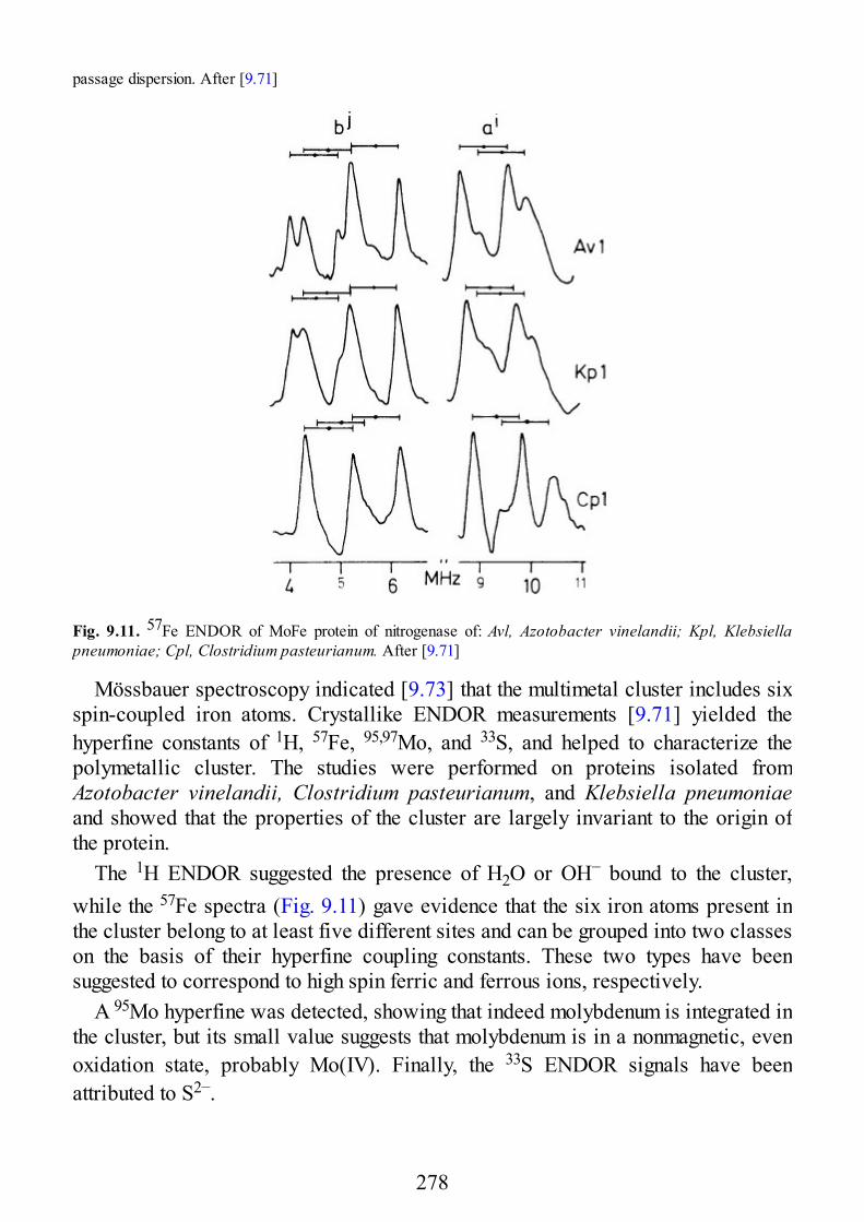
passage dispersion. After [9.71]

Fig. 9.11. 57Fe ENDOR of MoFe protein of nitrogenase of: Avl, Azotobacter vinelandii; Kpl, Klebsiellapneumoniae; Cpl, Clostridium pasteurianum. After [9.71]

Mössbauer spectroscopy indicated [9.73] that the multimetal cluster includes sixspin-coupled iron atoms. Crystallike ENDOR measurements [9.71] yielded thehyperfine constants of 1H, 57Fe, 95,97Mo, and 33S, and helped to characterize thepolymetallic cluster. The studies were performed on proteins isolated fromAzotobacter vinelandii, Clostridium pasteurianum, and Klebsiella pneumoniaeand showed that the properties of the cluster are largely invariant to the origin ofthe protein.

The 1H ENDOR suggested the presence of H2O or OH− bound to the cluster,while the 57Fe spectra (Fig. 9.11) gave evidence that the six iron atoms present inthe cluster belong to at least five different sites and can be grouped into two classeson the basis of their hyperfine coupling constants. These two types have beensuggested to correspond to high spin ferric and ferrous ions, respectively.

A 95Mo hyperfine was detected, showing that indeed molybdenum is integrated inthe cluster, but its small value suggests that molybdenum is in a nonmagnetic, evenoxidation state, probably Mo(IV). Finally, the 33S ENDOR signals have beenattributed to S2−.

278

9.3.5 Iron-Binding Proteins Without Cofactors orSulfur Clusters

In this category are included all the iron proteins which, having different functions,have in common the negative structural property that they do not have either a hemegroup or a sulfur cluster. They include ferritins, which are widespread in plants,animals, and protista as iron storage proteins; ribonucleotide reductase, which hasa central role in DNA synthesis; hemerythrin, which is the oxygen transport proteinin some invertebrates; uteroferrin, and the purple acid phosphatases, which catalizephosphoester hydrolysis. All these proteins contain μ-oxo bridged iron atoms,although additional bridging ligands may be present. For most of these enzymesEPR has provided extremely important information.

Ferritin. Ferritin consists of a multisubunit protein shell, apoferritin, surrounding acore of hydrous ferric oxide [9.74]. The core is variable in size, and may consist ofas many as 4500 atoms. The average composition of the core is(FeOOH)8.FeO.OPO3H2. It has crystalline behavior, and its size has been estimatedto be 6400 ± 2000 pm.

There are still many problems related to the structure and to the way in which theiron core is formed and depleted, and indeed ferritin is the most inorganic of themetal proteins, with a chemistry which has been related to the chemistry of rust[9.75]. Its magnetic properties are those of a superparamagnet. This means that theiron centers are strongly coupled yielding a bulk ferromagnet. However, since thedomains are limited (the protein size is large but finite), the overall magneticbehavior is that of a paramagnet, in which the individual magnets are indeed theprotein molecules.

Hemerythrin. Hemerythrin is an oxygen carrier protein which occurs in severalphyla of marine invertebrates. It occurs as either an octamer, a trimer, or a dimer ofalmost identical subunits of molecular weight close to 14 000 [9.76]. The activesite contains two bridged iron atoms. The iron atoms are octahedrally co-ordinatedand they share three bridging ligands, namely an oxo group and two carboxylatesbelonging to aspartate and glutamate residues. The structure of the binuclear ironsite in methemerythrin azide of Themiste discretum is shown in Fig. 9.12 [9.77](methemerythrin is the artificially oxidized form of hemerythrin). The two ironatoms both have the oxidation number +3. The nonoxygenated form,deoxohemerythrin, contains two iron(II) ions, while the oxygenated form containstwo iron(III) and a peroxide group. There is also a half-oxidized form ofdeoxyhemerythrin, semi-met-hemerythrin, which has an iron(III) and an iron(II).

Apparently, the only EPR spectra which can be readily obtained are those of thesemi-met forms [9.78]. The so-called (semi-met)2 is obtained by one-electron

279

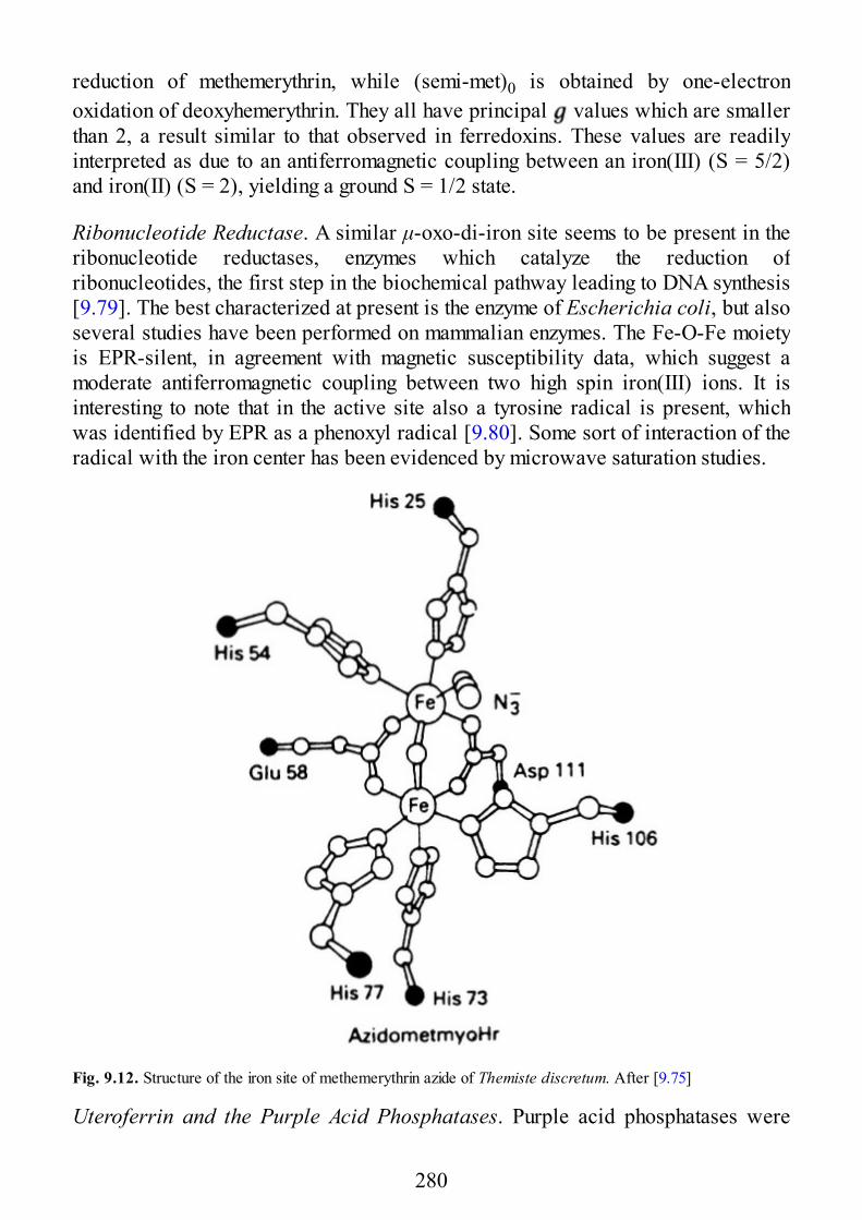
reduction of methemerythrin, while (semi-met)0 is obtained by one-electronoxidation of deoxyhemerythrin. They all have principal values which are smallerthan 2, a result similar to that observed in ferredoxins. These values are readilyinterpreted as due to an antiferromagnetic coupling between an iron(III) (S = 5/2)and iron(II) (S = 2), yielding a ground S = 1/2 state.

Ribonucleotide Reductase. A similar μ-oxo-di-iron site seems to be present in theribonucleotide reductases, enzymes which catalyze the reduction ofribonucleotides, the first step in the biochemical pathway leading to DNA synthesis[9.79]. The best characterized at present is the enzyme of Escherichia coli, but alsoseveral studies have been performed on mammalian enzymes. The Fe-O-Fe moietyis EPR-silent, in agreement with magnetic susceptibility data, which suggest amoderate antiferromagnetic coupling between two high spin iron(III) ions. It isinteresting to note that in the active site also a tyrosine radical is present, whichwas identified by EPR as a phenoxyl radical [9.80]. Some sort of interaction of theradical with the iron center has been evidenced by microwave saturation studies.

Fig. 9.12. Structure of the iron site of methemerythrin azide of Themiste discretum. After [9.75]

Uteroferrin and the Purple Acid Phosphatases. Purple acid phosphatases were

280

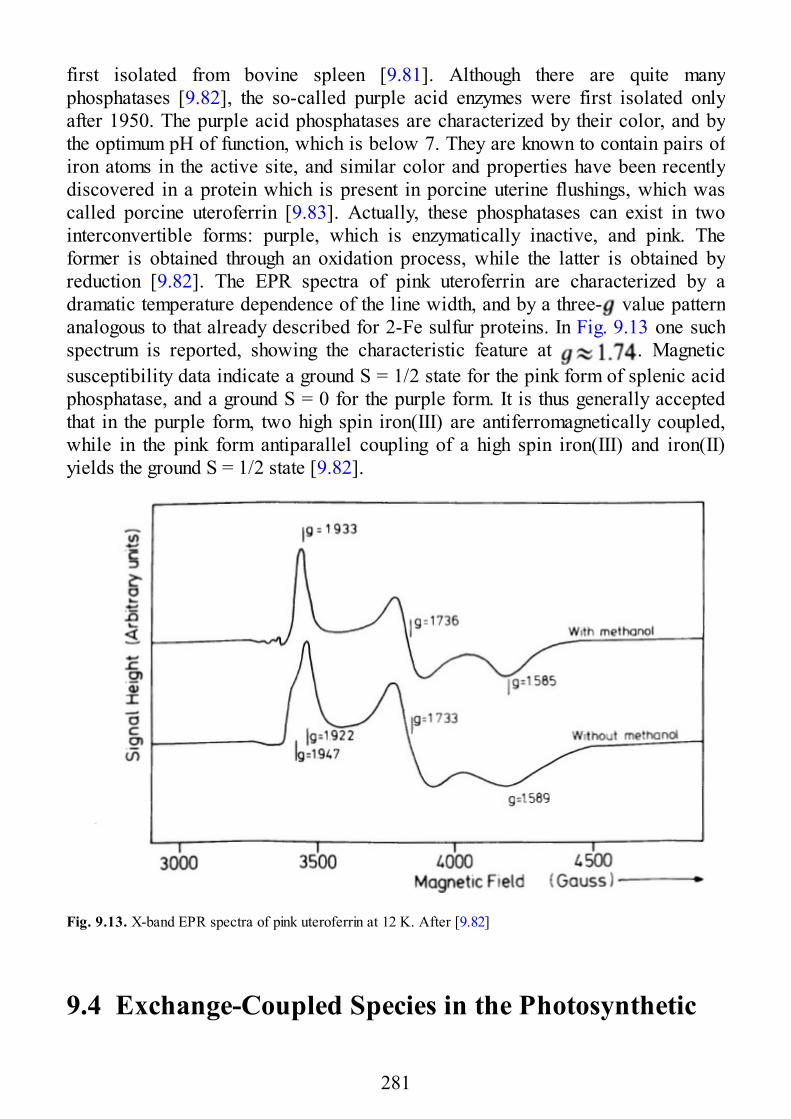
first isolated from bovine spleen [9.81]. Although there are quite manyphosphatases [9.82], the so-called purple acid enzymes were first isolated onlyafter 1950. The purple acid phosphatases are characterized by their color, and bythe optimum pH of function, which is below 7. They are known to contain pairs ofiron atoms in the active site, and similar color and properties have been recentlydiscovered in a protein which is present in porcine uterine flushings, which wascalled porcine uteroferrin [9.83]. Actually, these phosphatases can exist in twointerconvertible forms: purple, which is enzymatically inactive, and pink. Theformer is obtained through an oxidation process, while the latter is obtained byreduction [9.82]. The EPR spectra of pink uteroferrin are characterized by adramatic temperature dependence of the line width, and by a three- value patternanalogous to that already described for 2-Fe sulfur proteins. In Fig. 9.13 one suchspectrum is reported, showing the characteristic feature at . Magneticsusceptibility data indicate a ground S = 1/2 state for the pink form of splenic acidphosphatase, and a ground S = 0 for the purple form. It is thus generally acceptedthat in the purple form, two high spin iron(III) are antiferromagnetically coupled,while in the pink form antiparallel coupling of a high spin iron(III) and iron(II)yields the ground S = 1/2 state [9.82].

Fig. 9.13. X-band EPR spectra of pink uteroferrin at 12 K. After [9.82]

9.4 Exchange-Coupled Species in the Photosynthetic

281

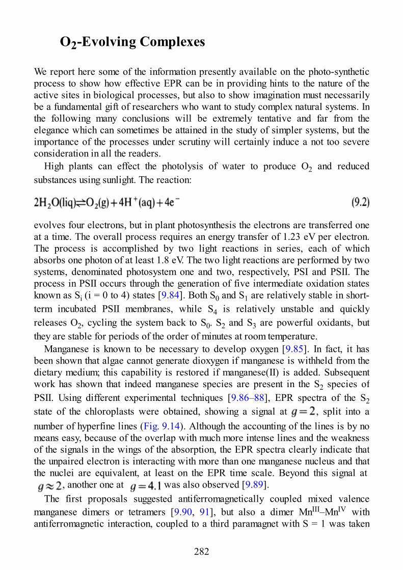
O2-Evolving Complexes

We report here some of the information presently available on the photo-syntheticprocess to show how effective EPR can be in providing hints to the nature of theactive sites in biological processes, but also to show imagination must necessarilybe a fundamental gift of researchers who want to study complex natural systems. Inthe following many conclusions will be extremely tentative and far from theelegance which can sometimes be attained in the study of simpler systems, but theimportance of the processes under scrutiny will certainly induce a not too severeconsideration in all the readers.

High plants can effect the photolysis of water to produce O2 and reducedsubstances using sunlight. The reaction:

evolves four electrons, but in plant photosynthesis the electrons are transferred oneat a time. The overall process requires an energy transfer of 1.23 eV per electron.The process is accomplished by two light reactions in series, each of whichabsorbs one photon of at least 1.8 eV. The two light reactions are performed by twosystems, denominated photosystem one and two, respectively, PSI and PSII. Theprocess in PSII occurs through the generation of five intermediate oxidation statesknown as Si (i = 0 to 4) states [9.84]. Both S0 and S1 are relatively stable in short-term incubated PSII membranes, while S4 is relatively unstable and quicklyreleases O2, cycling the system back to S0. S2 and S3 are powerful oxidants, butthey are stable for periods of the order of minutes at room temperature.

Manganese is known to be necessary to develop oxygen [9.85]. In fact, it hasbeen shown that algae cannot generate dioxygen if manganese is withheld from thedietary medium; this capability is restored if manganese(II) is added. Subsequentwork has shown that indeed manganese species are present in the S2 species ofPSII. Using different experimental techniques [9.86–88], EPR spectra of the S2state of the chloroplasts were obtained, showing a signal at , split into anumber of hyperfine lines (Fig. 9.14). Although the accounting of the lines is by nomeans easy, because of the overlap with much more intense lines and the weaknessof the signals in the wings of the absorption, the EPR spectra clearly indicate thatthe unpaired electron is interacting with more than one manganese nucleus and thatthe nuclei are equivalent, at least on the EPR time scale. Beyond this signal at

, another one at was also observed [9.89].The first proposals suggested antiferromagnetically coupled mixed valence

manganese dimers or tetramers [9.90, 91], but also a dimer MnIII–MnIV withantiferromagnetic interaction, coupled to a third paramagnet with S = 1 was taken

282

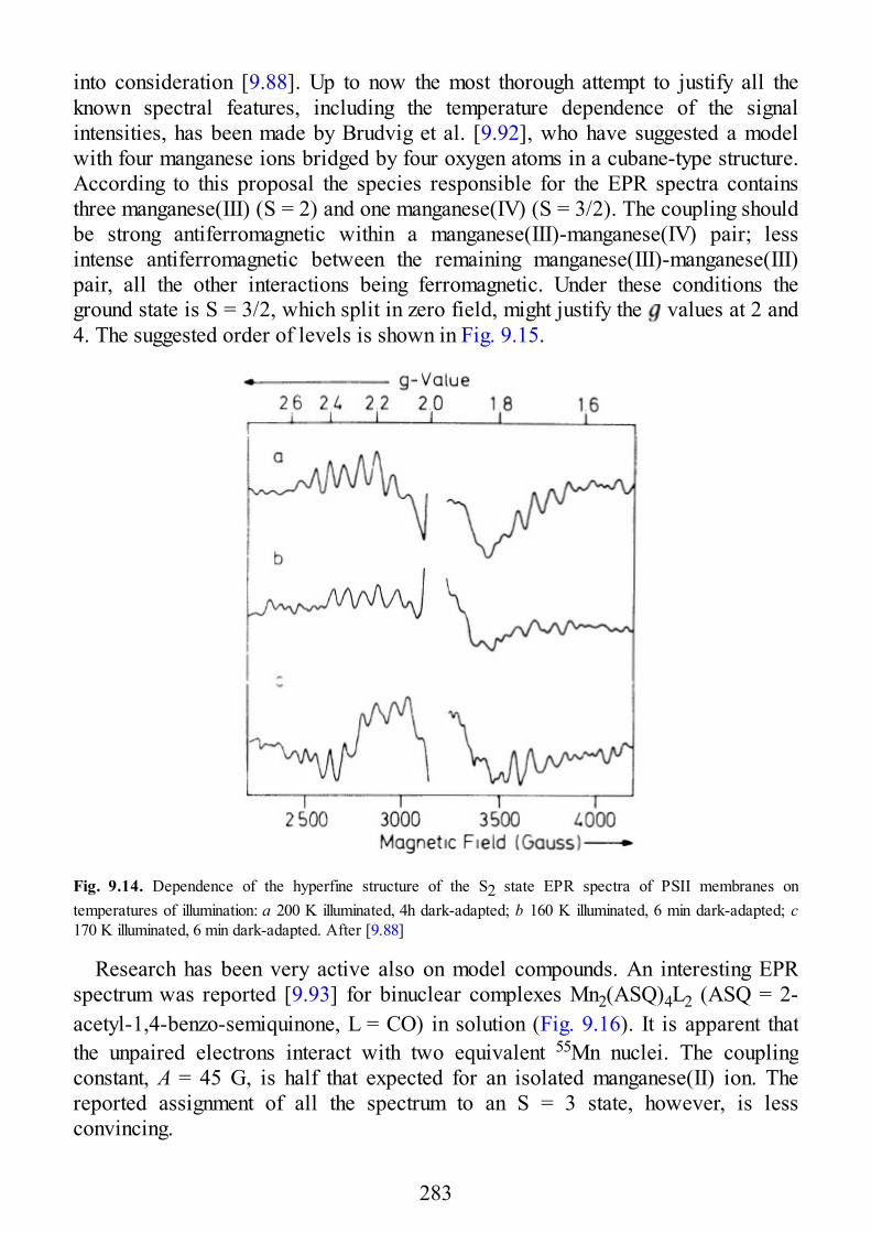
into consideration [9.88]. Up to now the most thorough attempt to justify all theknown spectral features, including the temperature dependence of the signalintensities, has been made by Brudvig et al. [9.92], who have suggested a modelwith four manganese ions bridged by four oxygen atoms in a cubane-type structure.According to this proposal the species responsible for the EPR spectra containsthree manganese(III) (S = 2) and one manganese(IV) (S = 3/2). The coupling shouldbe strong antiferromagnetic within a manganese(III)-manganese(IV) pair; lessintense antiferromagnetic between the remaining manganese(III)-manganese(III)pair, all the other interactions being ferromagnetic. Under these conditions theground state is S = 3/2, which split in zero field, might justify the values at 2 and4. The suggested order of levels is shown in Fig. 9.15.

Fig. 9.14. Dependence of the hyperfine structure of the S2 state EPR spectra of PSII membranes ontemperatures of illumination: a 200 K illuminated, 4h dark-adapted; b 160 K illuminated, 6 min dark-adapted; c170 K illuminated, 6 min dark-adapted. After [9.88]

Research has been very active also on model compounds. An interesting EPRspectrum was reported [9.93] for binuclear complexes Mn2(ASQ)4L2 (ASQ = 2-acetyl-1,4-benzo-semiquinone, L = CO) in solution (Fig. 9.16). It is apparent thatthe unpaired electrons interact with two equivalent 55Mn nuclei. The couplingconstant, A = 45 G, is half that expected for an isolated manganese(II) ion. Thereported assignment of all the spectrum to an S = 3 state, however, is lessconvincing.

283

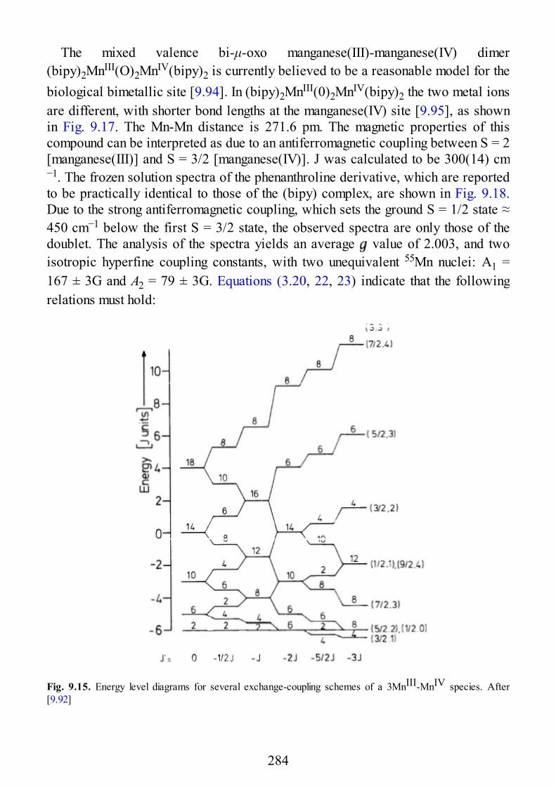
The mixed valence bi-μ-oxo manganese(III)-manganese(IV) dimer(bipy)2MnIII(O)2MnIV(bipy)2 is currently believed to be a reasonable model for thebiological bimetallic site [9.94]. In (bipy)2MnIII(0)2MnIV(bipy)2 the two metal ionsare different, with shorter bond lengths at the manganese(IV) site [9.95], as shownin Fig. 9.17. The Mn-Mn distance is 271.6 pm. The magnetic properties of thiscompound can be interpreted as due to an antiferromagnetic coupling between S = 2[manganese(III)] and S = 3/2 [manganese(IV)]. J was calculated to be 300(14) cm−1. The frozen solution spectra of the phenanthroline derivative, which are reportedto be practically identical to those of the (bipy) complex, are shown in Fig. 9.18.Due to the strong antiferromagnetic coupling, which sets the ground S = 1/2 state ≈450 cm−1 below the first S = 3/2 state, the observed spectra are only those of thedoublet. The analysis of the spectra yields an average value of 2.003, and twoisotropic hyperfine coupling constants, with two unequivalent 55Mn nuclei: A1 =167 ± 3G and A2 = 79 ± 3G. Equations (3.20, 22, 23) indicate that the followingrelations must hold:

Fig. 9.15. Energy level diagrams for several exchange-coupling schemes of a 3MnIII-MnIV species. After[9.92]

284

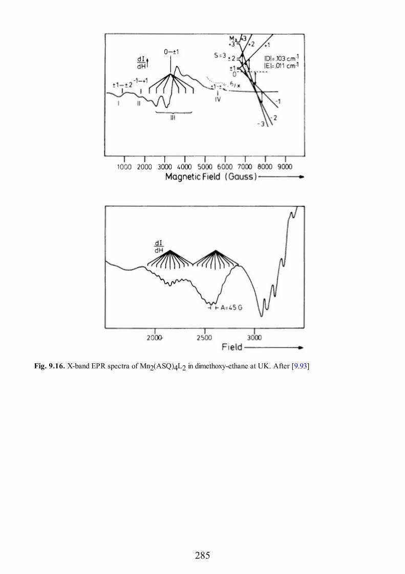
Fig. 9.16. X-band EPR spectra of Mn2(ASQ)4L2 in dimethoxy-ethane at UK. After [9.93]

285

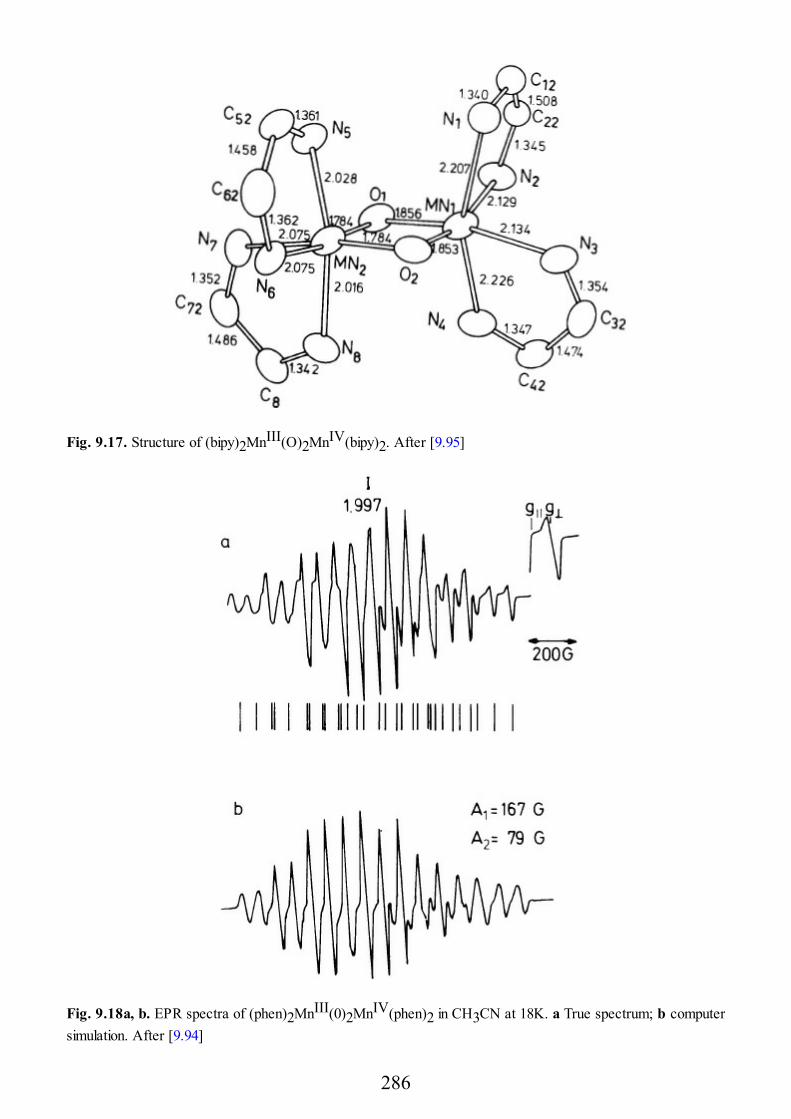
Fig. 9.17. Structure of (bipy)2MnIII(O)2MnIV(bipy)2. After [9.95]

Fig. 9.18a, b. EPR spectra of (phen)2MnIII(0)2MnIV(phen)2 in CH3CN at 18K. a True spectrum; b computersimulation. After [9.94]

286

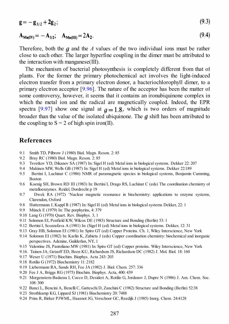
Therefore, both the and the A values of the two individual ions must be ratherclose to each other. The larger hyperfine coupling in the dimer must be attributed tothe interaction with manganese(III).

The mechanism of bacterial photosynthesis is completely different from that ofplants. For the former the primary photochemical act involves the light-inducedelectron transfer from a primary electron donor, a bacteriochlorophyll dimer, to aprimary electron acceptor [9.96]. The nature of the acceptor has been the matter ofsome controversy, however, it seems that it contains an ironubiquinone complex inwhich the metal ion and the radical are magnetically coupled. Indeed, the EPRspectra [9.97] show one signal at , which is two orders of magnitudebroader than the value of the isolated ubiquinone. The shift has been attributed tothe coupling to S = 2 of high spin iron(II).

References

9.1 Smith TD, Pilbrow J (1980) Biol. Magn. Reson. 2: 859.2 Bray RC (1980) Biol. Magn. Reson. 2: 859.3 Tsvetkov YD, Dikanov SA (1987) In: Sigel H (ed) Metal ions in biological systems. Dekker 22: 2079.4 Makinen MW, Wells GB (1987) In: Sigel H (ed) Metal ions in biological systems. Dekker 22:1899.5 Bertini I, Luchinat C (1986) NMR of paramagnetic species in biological systems, Benjamin Cumming,

Boston9.6 Koenig SH, Brown RD III (1983) In: Bertini I, Drago RS, Luchinat C (eds) The coordination chemistry of

metalloenzymes. Reidel, Dordrecht p 199.7 Dwek RA (1972) ‘Nuclear magnetic resonance in biochemistry: applications to enzyme systems,

Clarendon, Oxford9.8 Huttermann J, Kappl R (1987) In: Sigel H (ed) Metal ions in biological systems Dekker, 22: 19.9 Münck E (1979) In: The porphyrins, 4: 3799.10 Lang G (1970) Quart. Rev. Biophys. 3, 19.11 Solomon EI, Penfield KW, Wilcox DE (1983) Structure and Bonding (Berlin) 53: 19.12 Bertini I, Scozzafava A (1981) In: (Sigel H (ed) Metal ions in biological systems. Dekker, 12: 319.13 Gray HB, Solomon EI (1981) In: Spiro GT (ed) Copper Proteins. Ch. 1, Wiley Interscience, New York9.14 Solomon EI (1982) In: Karlin K, Zubieta J (eds) Copper coordination chemistry: biochemical and inorganic

perspectives. Adenine, Guilderlan, NY, 19.15 Valentine JS, Pantoliano MW (1981) In: Spiro GT (ed) Copper proteins. Wiley Interscience, New York9.16. Tainen JA, Getzoff ED, Been KU, Richardson JS, Richardson DC (1982) J. Mol. Biol. 18: 1609.17 Weser U (1971) Biochim. Biophys. Acta 243: 2039.18 Rotilio G (1972) Biochemistry 11: 21829.19 Liebermann RA, Sands RH, Fee JA (1982) J. Biol. Chem. 257: 3369.20 Fee J A, Briggs RG (1975) Biochim. Biophys. Acta, 400: 4399.21 Morgenstern-Badarau I, Cocco D, Desideri A, Rotilio G, Jordanov J, Dupre N (1986) J. Am. Chem. Soc.

108: 3009.22 Banci L, Bencini A, Benelli C, Gatteschi D, Zanchini C (1982) Structure and Bonding (Berlin) 52:389.23 Strothkamp KG, Lippard SJ (1981) Biochemistry 20: 74889.24 Prins R, Birker PJWML, Haasnot JG, Verschoor GC, Reedijk J (1985) Inorg. Chem. 24:4128

287

9.25 Bencini A, Gatteschi D, Zanchini C, Haasnot JG, Prins R, Reedijk J (1985) Inorg. Chem. 24: 28129.26 Himmelwright R S, Eickman NC, Lu Bien CD, Solomon EI (1980) J. Am. Chem. Soc. 102: 53789.27 Schoot Uiterkamp AJM, van der Deen H, Berendsen HCJ, Boas JF (1974) Biochim. Biophys. Acta, 372:

4079.28 Himmelwright RS, Eickman NC, Solomon EI (1979) Biochim. Biophys. Res. Commun. 86: 6289.29 Wilcox DE, Long JR, Solomon EI (1984) J. Am. Chem. Soc. 106: 21869.30 Gray HB, Schugar HJ (1973) In: Eichhorn GL (ed) Inorganic biochemistry. Elsevier, Amsterdam 1: 1029.31 Dunford HB, Stillmann JS (1976) Coord. Chem. Rev. 19: 1879.32 Dunford HB (1982) Adv. Inorg. Biochem. 4, 419.33 Schulz CE, Devaney PW, Winkler H, Debrunner PG, Doan N, Chiang R, Rutter R, Hager LP (1979) FEBS

Lett. 103: 1029.34 Schulz CE, Rutter R, Sage JT, Debrunner PG, Hager LP (1984) Biochemistry 23: 47439.35 Gans P, Buisson G, Duee E, Marchon JC, Erler BS, Scolz WF, Reed CA (1986) J. Am. Chem. Soc. 108:

12239.36 Caughey WS, Wallace WJ, Volpe JA, Yoshikawa S (1976) In: Boyer PD (ed) The Enzymes 13: 2999.37 Thomson AJ, Johnson MK, Greenwood C, Gooding PE, (1981) Biochem. J. 193: 6879.38 Gunter MJ, Berry KJ, Murray KS (1984) J. Am. Chem. Soc. 106: 42279.39 Berg JM, Holm RH (1982) In: Spiro TG (ed) Iron sulfur proteins. Vol. 4; Ch. 1 Wiley, New York9.40 Orme-Johnson WH, Orme-Johnson NR (1982) In: Spiro TG (ed) Iron Sulfur Proteins. Vol. 4, Ch. 2 Wiley,

New York9.41 Peisach J, Blumberg WE, Lode ET, Coon MJ (1971) J. Biol. Chem. 246: 58779.42 Rao KK, Evans MCW, Cammack R, Hall AO, Thompson CL, Jackson PJ, Johnson CE (1972) Biochem. J.

129: 10639.43 Debrunner PG, Münck E, Que L, Schulz CE (1977) In: Lovenberg W (ed) Iron sulfur proteins Vol. III.

Academic, New York, 3819.44 Moura I, Huynh BH, Hansinger RP, Le Gall J, Xavier AV, Münck EJ (1980) Biol. Chem. 225: 24939.45. Huynh BH, Kent JA (1984) Adv. Inorg. Biochem. 6: 1939.46 Gibson JF, Hall DO, Thornley JHM, Whatley FR (1966) Proc. Natl. Acad. Sci. US 56: 9879.47 Orme-Johnson WH, Sands RH (1972) in: Lovenberg W (ed) Iron Sulfur Proteins II, Ch. 5 Academic, New

York9.48 Bertrand P, Gayda JP (1979) Biochim. Biophys. Acta 579: 1079.49 Bertrand P, Guigliarelli B, Gayda JP, Beardwood P, Gibson JF (1985) Biochim. Biophys. Acta 831: 2619.50 Benelli C, Gatteschi D, Zanchini C (1987) Biochim. Biophys. Acta 1893: 3659.51 Stout CD, Ghoshi D, Pattabhi K, Robbins AH (1980) J. Biol. Chem. 255: 17979.52 Emptage MH, Kent TA, Huynh BH, Rawlings J, Orme-Johnson WH, Münck E (1980) J. Biol. Chem. 255,

17939.53 Guigliarelli B, Gayda JP, Bertrand P, More C (1986) Biochim. Biophys. Acta 871: 1499.54 Gayda JP, Bertrand P, Theodule FX, Moura JJG (1982) J. Chem. Phys. 77, 33879.55 Girerd J-J, Papaefthymiou GC, Watson AD, Gamp E, Hagen KS, Edelstein N, Frankel RB, Holm RH

(1984) J. Am. Chem. Soc. 106: 59419.56 Huynh BH, Moura JJG, Moura I, Kent TA, Le Gall J, Xavier AV, Münck E (1980) J. Biol. Chem. 255:

32429.57 Thomson AJ, Robinson AE, Johnson MK, Moura JJG, Moura I, Xavier AV, Le Gall (1981) J. Biochim.

Biophys. Acta 670, 939.58 Papaefthymiou GC, Girerd J-J, Moura I, Moura JJG, Münck E (1987) J. Am. Chem. Soc. 109: 47039.59 Noodleman L, Baerends EJ (1984) J. Am. Chem. Soc. 106: 11429.60 Gloux J, Gloux P, Lamotte B, Rins G (1985) Phys. Rev. Lett 54: 5999.61 Stombaugh NA, Burris RH, Orme-Johnson WH (1975) J. Biol. Chem. 248: 79519.62 Antanaitis BC, Moss TH (1975) Biochim. Biophys. Acta 405: 2629.63 Masharak PK, Papaefthymiou GC, Armstrong WH, Foner S, Frankel RB, Holm RH (1983) Inorg. Chem.

22: 28519.64 Gloux J, Gloux P, Rius G (1986) J. Am. Chem. Soc. 108: 35419.65 Siegel LM (1978) In: Singer JP, Ondarza RN (eds) Mechanism of oxidizing enzymes. Elsevier, North-

Holland, 2019.66 Jannick PA, Siegel LM (1982) Biochemistry 21: 3538

288

9.67 Christner JA, Münck E, Janick PA, Siegel LM (1983) J. Biol. Chem. 258: 111479.68 Christner JA, Janick PA, Siegel LM, Münck E (1983) J. Biol. Chem. 258: 111579.69 Nelson MJ, Lindahl PA, Orme-Johnson WH (1981) In: Eichhorn GL, Marzilli LG (eds) Advances in

inorganic biochemistry. Elsevier, New York9.70 Davis LC, Shah VK, Brill WJ, Orme-Johnson WH (1972) Biochim. Biophys. Acta 256: 5129.71 Venters RA, Nelson MJ, McLean PA, True AE, Levy MA, Hoffman BM, Orme-Johnson WH (1986) J.

Am. Chem. Soc. 108: 34879.72 Friesen GD, McDonald JW, Newton WE, Euler WB, Hoffman BM (1983) Inorg. Chem. 22: 22029.73 Huynh BH, Münck E, Orme-Johnson WH, (1979) Biochim. Biophys. Acta 576: 19299.74 Gabrio BW, Shoden A, Finch CA (1953) J. Biol. Chem. 204, 8159.75 Lippard SJ (1986) Chem. Brit. 22, 2229.76 Klotz IM, Keresztes-Nagy S (1961) Biochemistry 2: 4459.77 Stenkamp RE, Sieker LC, Jensen LH (1984) J. Am. Chem. Soc. 106: 6189.78 Wilking RG, Harrington PC (1983) Adv. Inorg. Biochem. 5: 519.79 Sjöberg BM, Gräslund A (1983) Adv. Inorg. Biochem. 5: 879.80 Ehrenberg A, Reichard P (1972) J. Biol. Chem. 247: 34859.81 Sundarajan TA, Sarma PS (1954) Biochem. J. 56: 1259.82 Atanaitis BC, Aisen P (1983) Adv. Inorg. Biochem. 5: 1119.83 Schlosnagle DC, Bazer FW, Tsibris JCM, Roberts RM (1974) J. Biol. Chem. 249: 75749.84 Kok B, Forbush B, McGloin M (1970) Photochem. Photobiol. 11: 4579.85 Sauer K (1980) Acc. Chem. Res. 13: 2499.86 Dismukes GC, Siderer Y (1981) Proc. Natl. Acad. Sci. US 78: 2749.87 Brudvig J, Casey J, Sauer K (1983) Biochim. Biophys. Acta 723: 3619.88 de Paula JC, Brudvig GW (1985) J. Am. Chem. Soc. 107: 26439.89 Casy JL, Sauer K (1984) Biochim. Biophys. Acta 767: 219.90 Hansson O, Andreasson LE (1982) Biochim. Biophys. Acta 679: 6219.91 Dismukes GC, Ferris K, Watnick P (1982) Photobiochem. Photobiophys. 3: 2439.92 de Paula JC, Beck WF, Brudvig GW (1986) J. Am. Chem. Soc. 108: 40029.93 Mathur P, Dismukes GC (1983) J. Am. Chem. Soc. 105: 70939.94 Cooper SR, Dismukes GC, Klein MP, Calvin M (1978) J. Am. Chem. Soc. 100: 72489.95 Plaksin PM, Stoufer RC, Mathew M, Palenick GJ (1972) J. Am. Chem. Soc. 94: 21219.96 Parson WW, Cogdell R (1975) J. Biochim. Biophys. Acta, 416: 1059.97 Okamura MY, Isaacson RA, Feher, G (1975) Proc. Natl. Acad. Sci. US 72: 3491

289

10 Low Dimensional Materials

10.1 Linear Chain Manganese(II)

Any review of the EPR spectra of linear chain compounds must necessarily startfrom [(CH3)4N]MnCl3 or, in a form more familiar in the physical literature,TMMC. Indeed, this is the first compound on which the one-dimensional propertieswere studied [10.1] and even after about 20 years it is still an excellent testingground for all the refinements that new sophisticated theories are able to introduce[10.2-4]. We have already used many of the TMMC data in Chap. 6, so that we willadd here only some more details.

Since manganese(II) is a 6S ion many of its magnetic properties are particularlysimple (isotropic g tensor, small single ion zero-field splitting, absence ofanisotropic and antisymmetric exchange contributions). A number of manganese(II)compounds have been studied, including CsMnCl3.2H2O (CMC) and CsMnBr3. It isimportant to recall here that ideal one-dimensional behavior is determined by aone-dimensional structure and one-dimensional exchange pathways. In TMMC bothconditions are met, while in CMC the difference between the intra- and interchainmanganese-manganese contacts is much smaller, so that a less ideal behavior canbe anticipated. Some relevant structural and magnetic properties of these threecompounds are reported in Table 10.1. Since the ideal linear chain behavior willbe attained by a given compound when the ratio of the inter- and intra-chaincoupling constants J′/J tends to zero, it is apparent that TMMC is much better thanthe other two in this respect.

It is perhaps useful to recall here the characteristics of a well-behaved linearchain Heisenberg antiferromagnet: (1) the EPR spectrum consists of a singleexchange-narrowed line with angular dependence of |3 cos2Θ −1|4/3, where Θ is theangle of the external magnetic field with the chain axis; (2) the line shape can bedescribed by the Fourier transform of exp(−t3/2) at Θ = 0° and by a Lorentzianfunction at the magic angle Θ = 54.7°; (3) the magic angle line-width isproportional to the inverse square root of the microwave frequency; (4) at Θ = 90°the line width increases with increasing frequency (inverse 10/3 effect); (5) inaddition to the main line, a half-field transition can be observed. All theseproperties together are rarely met, and practically only TMMC behaves in thismanner.

Beyond those already reported, of interest are the studies of TMMC and CMC

290

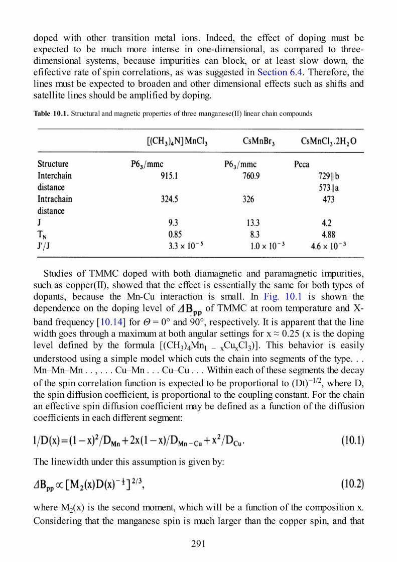
doped with other transition metal ions. Indeed, the effect of doping must beexpected to be much more intense in one-dimensional, as compared to three-dimensional systems, because impurities can block, or at least slow down, theefifective rate of spin correlations, as was suggested in Section 6.4. Therefore, thelines must be expected to broaden and other dimensional effects such as shifts andsatellite lines should be amplified by doping.

Table 10.1. Structural and magnetic properties of three manganese(II) linear chain compounds

Studies of TMMC doped with both diamagnetic and paramagnetic impurities,such as copper(II), showed that the effect is essentially the same for both types ofdopants, because the Mn-Cu interaction is small. In Fig. 10.1 is shown thedependence on the doping level of of TMMC at room temperature and X-band frequency [10.14] for Θ = 0° and 90°, respectively. It is apparent that the linewidth goes through a maximum at both angular settings for x ≈ 0.25 (x is the dopinglevel defined by the formula [(CH3)4Mn1 − xCuxCl3)]. This behavior is easilyunderstood using a simple model which cuts the chain into segments of the type. . .Mn–Mn–Mn . . , . . . Cu–Mn . . . Cu–Cu . . . Within each of these segments the decayof the spin correlation function is expected to be proportional to (Dt)−1/2, where D,the spin diffusion coefficient, is proportional to the coupling constant. For the chainan effective spin diffusion coefficient may be defined as a function of the diffusioncoefficients in each different segment:

The linewidth under this assumption is given by:

where M2(x) is the second moment, which will be a function of the composition x.Considering that the manganese spin is much larger than the copper spin, and that

291

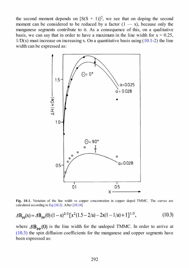
the second moment depends on [S(S + 1)]2, we see that on doping the secondmoment can be considered to be reduced by a factor (1 — x), because only themanganese segments contribute to it. As a consequence of this, on a qualitativebasis, we can say that in order to have a maximum in the line width for x = 0.25,1/D(x) must increase on increasing x. On a quantitative basis using (10.1-2) the linewidth can be expressed as:

Fig. 10.1. Variation of the line width vs copper concentration in copper doped TMMC. The curves arecalculated according to Eq (10.2). After [10.14]

where is the line width for the undoped TMMC. In order to arrive at(10.3) the spin diffusion coefficients for the manganese and copper segments havebeen expressed as:

292

where the exchange-coupling constant is in Kelvin. DMn–Cu is taken as DMn–Cu =aDMn, where a is an adjustable parameter. In (10.4) and (10.5) JMn and JCu are thecoupling constants for the pure manganese and copper salts, respectively, whoseexperimental values are 9.3 and 63 cm−1. Using (10.3–5) and the experimental linewidths, the diffusion factor in the Mn–Cu segments has been estimated to be: DMn–

Cu = 1.48 K. If the simplest possible relation is assumed for JMn–Cu:

then we obtain JMn–Cu = 0.6 cm−1 which is smaller than the value obtained frommagnetic susceptibility and Neel temperature measurements (1.95 cm−1).

This simple model, however, breaks down for measurements at the magic angle,because in this case the linewidth keeps increasing with x up to the largestavailable value (x ≈ 0.5).

Doping TMMC with 20% Cd2+ the spectrum with the static magnetic fieldrecorded parallel to the chain axis shows (Fig. 10.2) a central line attributed[10.15] to single ion resonances and to short chains of Mn2+ ions. The symmetricalstructure of ten lines which is superimposed on it is attributed to ion pairs whichhave total spin states S = 5, 4, 3, 2, 1, and 0. The d and b lines are attributed to S =5, c to S = 4 and S = 2, a and e to S = 3. The spectra yielded the single ion zerofield splitting, D = 0.007(2) cm−1 and the dipolar term, Ddip = 0.0566(9) cm−1

which agree well with the values obtained by doping [(CH3)4N]CdCl3 with Mn2+

[10.16, 17].CsMnBr3 is a good example of a less ideal manganese(II) linear chain

compound. It shows [10.12] the angular dependence of the line width featured inFig. 10.3. The experimental points were recorded at three different frequencies. Atlow frequency, 8.82 GHz, the line width has a minimum at 90°, contrary to theexpected one-dimensional behavior with a minimum at the magic angle. Thisminimum is reestablished at higher frequencies (35.52 and 72.15 GHz), but theangular dependence can be described by the function:

293

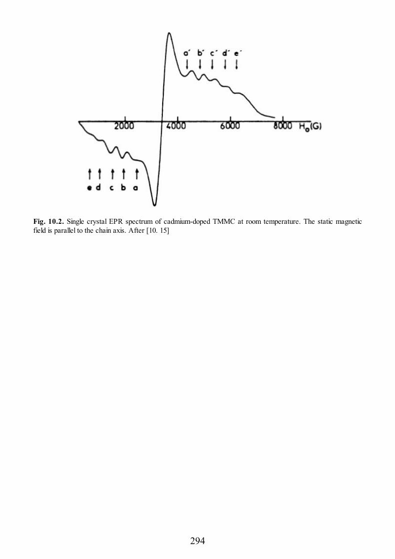
Fig. 10.2. Single crystal EPR spectrum of cadmium-doped TMMC at room temperature. The static magneticfield is parallel to the chain axis. After [10. 15]

294

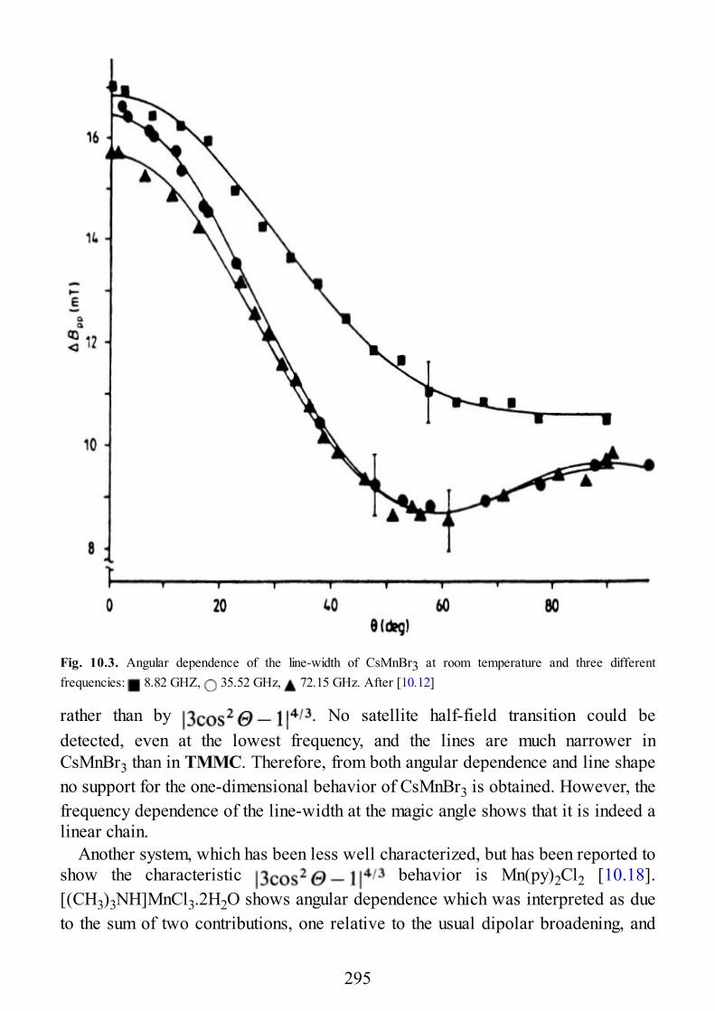
Fig. 10.3. Angular dependence of the line-width of CsMnBr3 at room temperature and three differentfrequencies: 8.82 GHZ, 35.52 GHz, 72.15 GHz. After [10.12]

rather than by . No satellite half-field transition could bedetected, even at the lowest frequency, and the lines are much narrower inCsMnBr3 than in TMMC. Therefore, from both angular dependence and line shapeno support for the one-dimensional behavior of CsMnBr3 is obtained. However, thefrequency dependence of the line-width at the magic angle shows that it is indeed alinear chain.

Another system, which has been less well characterized, but has been reported toshow the characteristic behavior is Mn(py)2Cl2 [10.18].[(CH3)3NH]MnCl3.2H2O shows angular dependence which was interpreted as dueto the sum of two contributions, one relative to the usual dipolar broadening, and

295

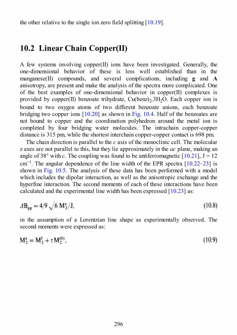
the other relative to the single ion zero field splitting [10.19].

10.2 Linear Chain Copper(II)

A few systems involving copper(II) ions have been investigated. Generally, theone-dimensional behavior of these is less well established than in themanganese(II) compounds, and several complications, including g and Aanisotropy, are present and make the analysis of the spectra more complicated. Oneof the best examples of one-dimensional behavior in copper(II) complexes isprovided by copper(II) benzoate trihydrate, Cu(benz)2.3H2O. Each copper ion isbound to two oxygen atoms of two different benzoate anions, each benzoatebridging two copper ions [10.20] as shown in Fig. 10.4. Half of the benzoates arenot bound to copper and the coordination polyhedron around the metal ion iscompleted by four bridging water molecules. The intrachain copper-copperdistance is 315 pm, while the shortest interchain copper-copper contact is 698 pm.

The chain direction is parallel to the c axis of the monoclinic cell. The molecularz axes are not parallel to this, but they lie approximately in the ac plane, making anangle of 38° with c. The coupling was found to be antiferromagnetic [10.21], J = 12cm−1. The angular dependence of the line width of the EPR spectra [10.22–23] isshown in Fig. 10.5. The analysis of these data has been performed with a modelwhich includes the dipolar interaction, as well as the anisotropic exchange and thehyperfine interaction. The second moments of each of these interactions have beencalculated and the experimental line width has been expressed [10.23] as:

in the assumption of a Lorentzian line shape as experimentally observed. Thesecond moments were expressed as:

296

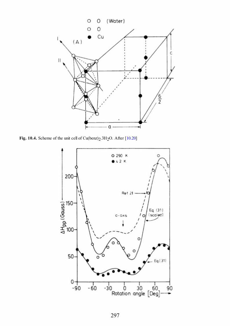
Fig. 10.4. Scheme of the unit cell of Cu(benz)2.3H2O. After [10.20]

297

Fig. 10.5. The experimental and theoretical line width data for Cu(benz)2.3H2O. The rotation angle is from a inthe ac plane. After [10.23]

where and are the calculated full and secular second moments,respectively, τ is a parameter, which accounts for the increased role of secularterms in one dimension. For τ = 0, Eq. (10.9) yields the usual three-dimensionalbehavior, while when τ is large, the angular dependence is dominated by thesecular components, τ values of order of unity are consistent with Lorentzian lines,and slightly enhanced secular components.

The expressions for the various components of M2 were given in Chap. 6. Caremust be taken to consider the different principal directions of the various termsresponsible for the broadening of the lines. For Cu(benz)2. 3H2O the angulardependence of the experimental line width was reproduced using the parameters,Dex = 0.125(15)cm−1 and τ = 1.0(2), where Dex is the zero field splitting parameterassociated with anisotropic exchange. The other parameters (Ax, Ay, Az, Dd for thedipolar interaction, J) were fixed at the values experimentally observed.

An interesting observation to be made here is that since Ddip and Dex arediagonal in different reference frames, the presence of anisotropic exchange limitsthe one-dimensional behavior. In fact, the largest deviations from Lorentzian lineshapes are expected parallel to the chain direction, where the intrachain dipolarinteraction reduces to the purely secular component. However, in general, Dex willnot have its z axis parallel to this, and nonsecular components are thusreintroduced. The only case in which the two contributions add up positively toyield one-dimensional behavior is when the two tensors are parallel to each other.An example is provided by CuSALMe, where SALMe is the Schiff base formed bymethylamine and salicylaldehyde [10.24]. In this case the planar CuSALMemolecules are stacked on top of an other [10.25] so that the z molecular axes andthe chain axis are practically coincident. The copper-copper distance along thechain is 333 pm, while the shortest interchain copper-copper separation is 919 pm.The line width at 76 K was found to follow a behavior, and theline shape along the chain was found to correspond nicely to the Fourier transformof .

Copper pyrazine nitrate, Cu(pyz) (NO3)2, is a one-dimensional antiferromagnet[10.26], but the EPR spectra do not show the classic one-dimensional dependenceof the line width [10.23]. Indeed, as shown in Fig. 10.6, the line width does notshow magic angle behaviour in any of the three principal planes. The unit cell isorthorhombic [10.27] and each copper ion is coordinated by two nitrogen atoms oftwo pyrazines and two oxygen atoms of two nitrate ions on the vertices of a squareplane. Two additional axial sites are occupied by two other nitrate oxygens at alonger distance (Fig. 10.7). In principle there are two possibilities for the magneticexchange pathway defining the chain direction: one is through the pyrazine bridge

298

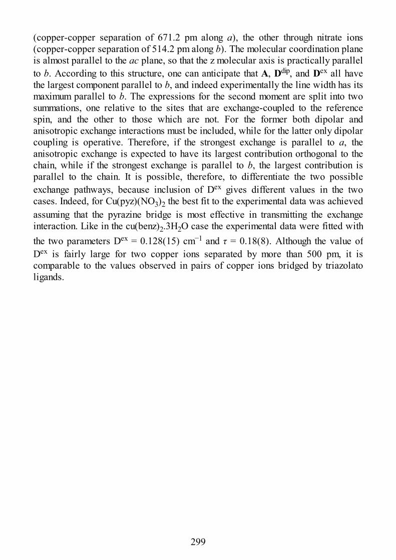
(copper-copper separation of 671.2 pm along a), the other through nitrate ions(copper-copper separation of 514.2 pm along b). The molecular coordination planeis almost parallel to the ac plane, so that the z molecular axis is practically parallelto b. According to this structure, one can anticipate that A, Ddip, and Dex all havethe largest component parallel to b, and indeed experimentally the line width has itsmaximum parallel to b. The expressions for the second moment are split into twosummations, one relative to the sites that are exchange-coupled to the referencespin, and the other to those which are not. For the former both dipolar andanisotropic exchange interactions must be included, while for the latter only dipolarcoupling is operative. Therefore, if the strongest exchange is parallel to a, theanisotropic exchange is expected to have its largest contribution orthogonal to thechain, while if the strongest exchange is parallel to b, the largest contribution isparallel to the chain. It is possible, therefore, to differentiate the two possibleexchange pathways, because inclusion of Dex gives different values in the twocases. Indeed, for Cu(pyz)(NO3)2 the best fit to the experimental data was achievedassuming that the pyrazine bridge is most effective in transmitting the exchangeinteraction. Like in the cu(benz)2.3H2O case the experimental data were fitted withthe two parameters Dex = 0.128(15) cm−1 and τ = 0.18(8). Although the value ofDex is fairly large for two copper ions separated by more than 500 pm, it iscomparable to the values observed in pairs of copper ions bridged by triazolatoligands.

299

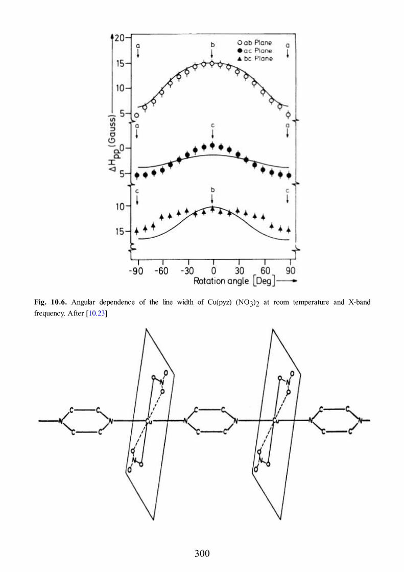
Fig. 10.6. Angular dependence of the line width of Cu(pyz) (NO3)2 at room temperature and X-bandfrequency. After [10.23]

300

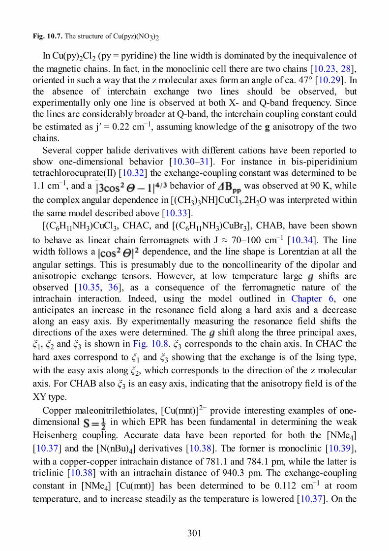
Fig. 10.7. The structure of Cu(pyz)(NO3)2

In Cu(py)2Cl2 (py = pyridine) the line width is dominated by the inequivalence ofthe magnetic chains. In fact, in the monoclinic cell there are two chains [10.23, 28],oriented in such a way that the z molecular axes form an angle of ca. 47° [10.29]. Inthe absence of interchain exchange two lines should be observed, butexperimentally only one line is observed at both X- and Q-band frequency. Sincethe lines are considerably broader at Q-band, the interchain coupling constant couldbe estimated as j′ = 0.22 cm−1, assuming knowledge of the g anisotropy of the twochains.

Several copper halide derivatives with different cations have been reported toshow one-dimensional behavior [10.30–31]. For instance in bis-piperidiniumtetrachlorocuprate(II) [10.32] the exchange-coupling constant was determined to be1.1 cm−1, and a behavior of was observed at 90 K, whilethe complex angular dependence in [(CH3)3NH]CuCl3.2H2O was interpreted withinthe same model described above [10.33].

[(C6H11NH3)CuCl3, CHAC, and [(C6H11NH3)CuBr3], CHAB, have been shownto behave as linear chain ferromagnets with J ≈ 70–100 cm−1 [10.34]. The linewidth follows a dependence, and the line shape is Lorentzian at all theangular settings. This is presumably due to the noncollinearity of the dipolar andanisotropic exchange tensors. However, at low temperature large shifts areobserved [10.35, 36], as a consequence of the ferromagnetic nature of theintrachain interaction. Indeed, using the model outlined in Chapter 6, oneanticipates an increase in the resonance field along a hard axis and a decreasealong an easy axis. By experimentally measuring the resonance field shifts thedirections of the axes were determined. The shift along the three principal axes,ξ1, ξ2 and ξ3 is shown in Fig. 10.8. ξ3 corresponds to the chain axis. In CHAC thehard axes correspond to ξ1 and ξ3 showing that the exchange is of the Ising type,with the easy axis along ξ2, which corresponds to the direction of the z molecularaxis. For CHAB also ξ3 is an easy axis, indicating that the anisotropy field is of theXY type.

Copper maleonitrilethiolates, [Cu(mnt)]2− provide interesting examples of one-dimensional in which EPR has been fundamental in determining the weakHeisenberg coupling. Accurate data have been reported for both the [NMe4][10.37] and the [N(nBu)4] derivatives [10.38]. The former is monoclinic [10.39],with a copper-copper intrachain distance of 781.1 and 784.1 pm, while the latter istriclinic [10.38] with an intrachain distance of 940.3 pm. The exchange-couplingconstant in [NMe4] [Cu(mnt)] has been determined to be 0.112 cm−1 at roomtemperature, and to increase steadily as the temperature is lowered [10.37]. On the

301

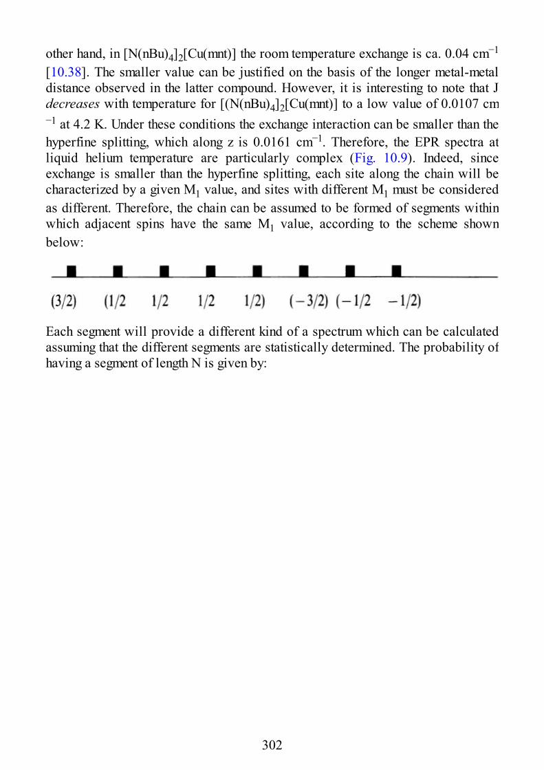
other hand, in [N(nBu)4]2[Cu(mnt)] the room temperature exchange is ca. 0.04 cm−1

[10.38]. The smaller value can be justified on the basis of the longer metal-metaldistance observed in the latter compound. However, it is interesting to note that Jdecreases with temperature for [(N(nBu)4]2[Cu(mnt)] to a low value of 0.0107 cm−1 at 4.2 K. Under these conditions the exchange interaction can be smaller than thehyperfine splitting, which along z is 0.0161 cm−1. Therefore, the EPR spectra atliquid helium temperature are particularly complex (Fig. 10.9). Indeed, sinceexchange is smaller than the hyperfine splitting, each site along the chain will becharacterized by a given M1 value, and sites with different M1 must be consideredas different. Therefore, the chain can be assumed to be formed of segments withinwhich adjacent spins have the same M1 value, according to the scheme shownbelow:

Each segment will provide a different kind of a spectrum which can be calculatedassuming that the different segments are statistically determined. The probability ofhaving a segment of length N is given by:

302

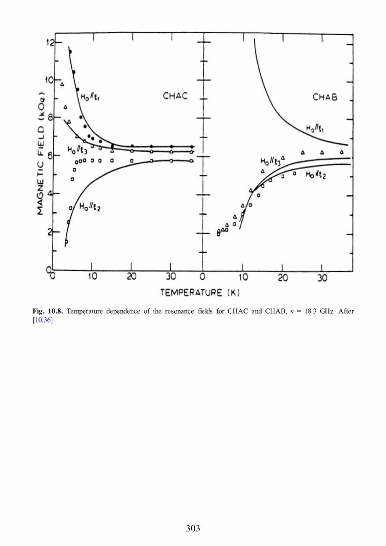
Fig. 10.8. Temperature dependence of the resonance fields for CHAC and CHAB, v = 18.3 GHz. After[10.36]

303

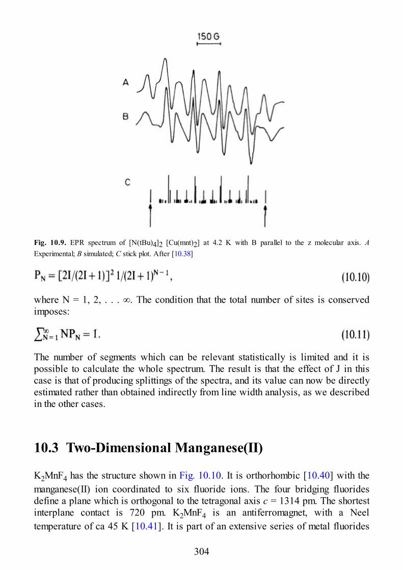
Fig. 10.9. EPR spectrum of [N(tBu)4]2 [Cu(mnt)2] at 4.2 K with B parallel to the z molecular axis. AExperimental; B simulated; C stick plot. After [10.38]

where N = 1, 2, . . . ∞. The condition that the total number of sites is conservedimposes:

The number of segments which can be relevant statistically is limited and it ispossible to calculate the whole spectrum. The result is that the effect of J in thiscase is that of producing splittings of the spectra, and its value can now be directlyestimated rather than obtained indirectly from line width analysis, as we describedin the other cases.

10.3 Two-Dimensional Manganese(II)

K2MnF4 has the structure shown in Fig. 10.10. It is orthorhombic [10.40] with themanganese(II) ion coordinated to six fluoride ions. The four bridging fluoridesdefine a plane which is orthogonal to the tetragonal axis c = 1314 pm. The shortestinterplane contact is 720 pm. K2MnF4 is an antiferromagnet, with a Neeltemperature of ca 45 K [10.41]. It is part of an extensive series of metal fluorides

304

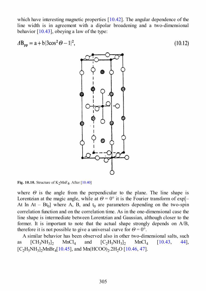
which have interesting magnetic properties [10.42]. The angular dependence of theline width is in agreement with a dipolar broadening and a two-dimensionalbehavior [10.43], obeying a law of the type:

Fig. 10.10. Structure of K2MnF4. After [10.40]

where Θ is the angle from the perpendicular to the plane. The line shape isLorentzian at the magic angle, while at Θ = 0° it is the Fourier transform of exp[–At In At – Bt0] where A, B, and t0 are parameters depending on the two-spincorrelation function and on the correlation time. As in the one-dimensional case theline shape is intermediate between Lorentzian and Gaussian, although closer to theformer. It is important to note that the actual shape strongly depends on A/B,therefore it is not possible to give a universal curve for Θ = 0°.

A similar behavior has been observed also in other two-dimensional salts, suchas [CH3NH3]2 MnCl4 and [C2H5NH3]2 MnCl4 [10.43, 44],[C2H5NH3]2MnBr4[10.45], and Mn(HCOO)2.2H2O [10.46, 47].

305

10.4 Two-Dimensional Copper(II)

There are quite a number of two-dimensional copper(II) magnets because manycopper halides, with different cations [Cat]2[CuX4], (X = Cl, Br), possess layeredstructures [10.48]. In general, in all the systems studied the angular dependence ofthe line width does not show any particular effect which can be attributed to anincreased role of the secular terms, and the lines are within error lorentzians.

The most obvious reason for this is that in two-dimensional magnets it iscomparatively more difficult than in one-dimensional magnets to havesimplification in the expressions of, e.g. the dipolar second moment analogous tothe one for which all the Θij’s are identical (Θij = Θ) for one dimension. Thus, thereare different angular contributions which quench the secular components.

Lacking any particular interest in this respect on the spin dynamics in thesecompounds, the major interest has focused on the temperature dependence of theline width. In fact, for most of these compounds, was found to decreaselinearly with temperature in the range above the transition to the ordered state. Sucha behavior has been found, for instance, in K2CuCl4.2H2O [10.49, 50],Cu(HCOO)2.4H2O [10.51], Cu(HCOO)2.2(NH2)2CO.2H2O [10.52], and in many ofthe layered tetrahalides [10.48],

In Cu(HCOO)2.4H2O each copper is coordinated to four oxygen atoms of fourdifferent formiate anions, which bridge two different copper ions [10.53]. Thesemolecular planes define a layer parallel to the ab crystallographic plane of amonoclinic cell. The coordination around copper is completed by two watermolecules, which are connected to other water molecules in a layer which isinterposed between the copper layers. The line width decreases linearly withtemperature in the range 50–300 K. This behavior has been attributed [10.50] tophonon modulation of the antisymmetric exchange, which can occur between pairsof copper ions not related by an inversion center. A quantitative analysis yieldedd/J ≈ 0.005, which is roughly 20 times smaller than one would obtain fromMoryia’s estimate . A similar behavior was observed in the analogousCu(HCOO)2.2(NH2)CO.2H2O.

Layered [Cat]2[CuX4] salts are the most numerous group of two-dimensionalcopper(II) magnets. They all have a structure formed of layers such as thosedepicted [10.48, 54] in Fig. 10.11. Each copper is coordinated to 4 + 2 chlorides,the long bonds lying in the plane of the layer. The isotropic coupling isferromagnetic. A detailed analysis of the EPR spectra was performed by Soos et al.[10.54] for [Pt(NH3)4]CuCl4 and [H3N(CH2)3NH3] [CuCl4]. They included dipolar,anisotropic, and antisymmetric exchange interactions to analyze the line widths.Using the formulae of Sect. 6.3 they could show that dipolar, hyperfine, and gtensor contributions to the second moment are negligible, and included only the

306

anisotropic and antisymmetric exchange:

where A and S refer to antisymmetric and symmetric, respectively, J is the isotropicexchange constant, χc is the Curie susceptibility, and χ(T) is the true susceptibilityat the temperature T, FA and Fs are factors describing the static spin correlation dueto the isotropic exchange, related to the two-spin correlation functions

where cn indicates

Fig. 10.11. Schematic representation of the layer and the polar coordinates of the magnetic field.After [10.54]

The temperature dependence of F1(kT/J)χc/χ(T), I = A, S is shown in Fig. 10.12 fora square planar ferromagnet. Since for kT > J the dependence is linear, theobserved temperature dependence of is justified.

307

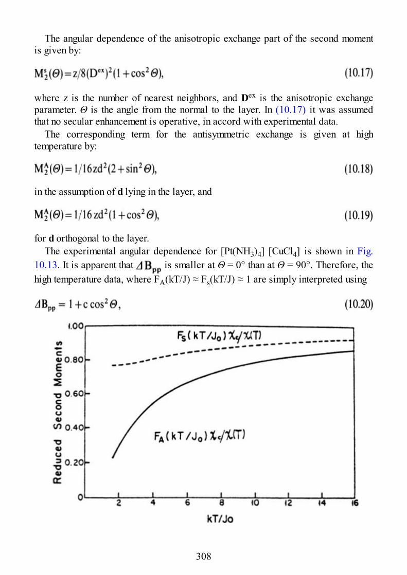
The angular dependence of the anisotropic exchange part of the second momentis given by:

where z is the number of nearest neighbors, and Dex is the anisotropic exchangeparameter. Θ is the angle from the normal to the layer. In (10.17) it was assumedthat no secular enhancement is operative, in accord with experimental data.

The corresponding term for the antisymmetric exchange is given at hightemperature by:

in the assumption of d lying in the layer, and

for d orthogonal to the layer.The experimental angular dependence for [Pt(NH3)4] [CuCl4] is shown in Fig.

10.13. It is apparent that is smaller at Θ = 0° than at Θ = 90°. Therefore, thehigh temperature data, where FA(kT/J) ≈ Fs(kT/J) ≈ 1 are simply interpreted using

308

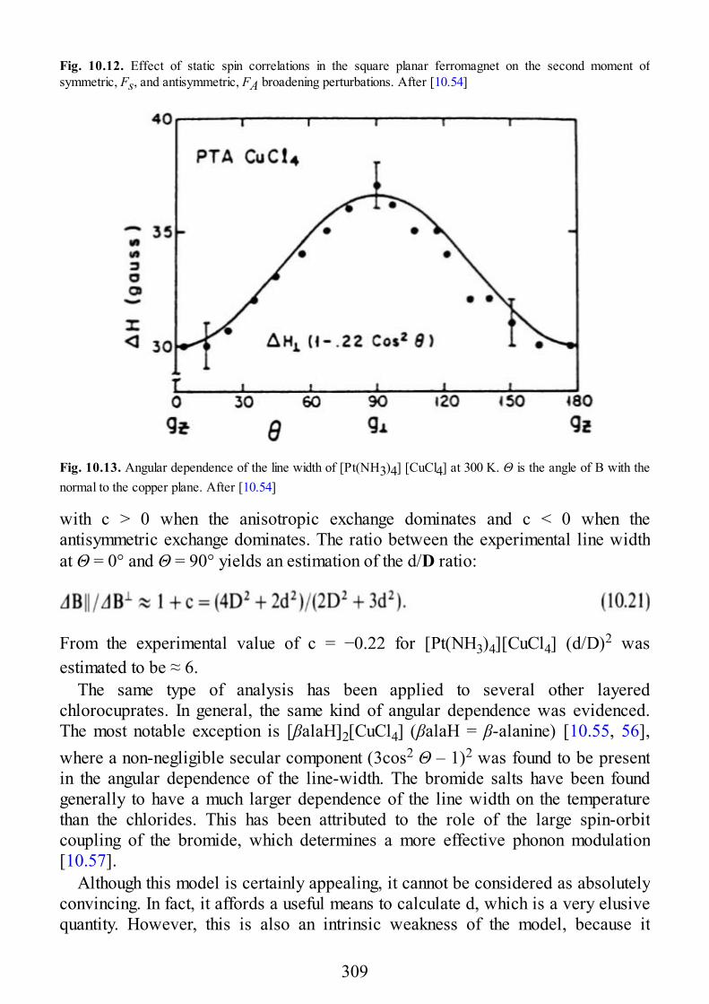
Fig. 10.12. Effect of static spin correlations in the square planar ferromagnet on the second moment ofsymmetric, Fs, and antisymmetric, FA broadening perturbations. After [10.54]

Fig. 10.13. Angular dependence of the line width of [Pt(NH3)4] [CuCl4] at 300 K. Θ is the angle of B with thenormal to the copper plane. After [10.54]

with c > 0 when the anisotropic exchange dominates and c < 0 when theantisymmetric exchange dominates. The ratio between the experimental line widthat Θ = 0° and Θ = 90° yields an estimation of the d/D ratio:

From the experimental value of c = −0.22 for [Pt(NH3)4][CuCl4] (d/D)2 wasestimated to be ≈ 6.

The same type of analysis has been applied to several other layeredchlorocuprates. In general, the same kind of angular dependence was evidenced.The most notable exception is [βalaH]2[CuCl4] (βalaH = β-alanine) [10.55, 56],where a non-negligible secular component (3cos2 Θ – 1)2 was found to be presentin the angular dependence of the line-width. The bromide salts have been foundgenerally to have a much larger dependence of the line width on the temperaturethan the chlorides. This has been attributed to the role of the large spin-orbitcoupling of the bromide, which determines a more effective phonon modulation[10.57].

Although this model is certainly appealing, it cannot be considered as absolutelyconvincing. In fact, it affords a useful means to calculate d, which is a very elusivequantity. However, this is also an intrinsic weakness of the model, because it

309

cannot have independent checks, either experimental, because no other technique iseasily available to measure d, or theoretical, because at present, and perhaps formany years to come, there is no way of calculating d.

As a confirmation of these doubts we must recall here that other justificationshave been put forward to justify the linear dependence of on temperature.Among these, one which has been worked out in some detail, is the temperaturedependence of the isotropic exchange. Indeed, there is evidence in the literature thatthe interchain and the interlayer interaction may be temperature-dependent. Onesuch example is K2CuCl4.2H2O, which contains two magnetically non-equivalentchains, which can be characterized by two values, and . For exchangeenergies less than , two resonances are observed. Bymeasuring the magnetic field at which the two lines coalesce, it is possible toobtain J. For this particular compound J was found to decrease with increasingtemperature in the range 77–300 K. The ratio J(300)/J(77) is ≈ 1/5. This is not theonly data of this kind, because similar results have been observed for othertransition metal complexes. On this basis it was concluded that also phononmodulation of the isotropic exchange can be responsible for the temperaturedependence of the line width. The effect of phonon modulation was estimatedthrough a simplified model, which assumes an exponential dependence of J on thedistance between the paramagnetic centers. The model has been applied with somesuccess to some layered copper(II) compounds [10.58].

References

10.1 Dietz, RE, Merritt FR, Dingle R, Hone D, Silbernagel, BG, Richards PM (1971) Phys. Rev. Lett. 26: 118610.2 Lagendijk A (1978) Phys. Rev. B 18: 132210.3 Benner H, Broedehl M, Seitz W, Wiese J (1983) J. Phys. C 16: 601110.4 Siegel E, Mosebach H, Pauli N, Lagendijk A (1982) Phys. Lett. 90A: 30910.5 Morosin B, Graeber EJ Acta Cryst. 23: 76610.6 Dupas C, Renard JP (1976) Solid state commun. 20: 58110.7 Goodyear J, Kennedy D (1972) Acta Cryst. B28: 164010.8 Jensen SJ, Andersen P, Rasmussen SE (1962) Acta Chem. Scand. 16: 189010.9 de Jonge WJM, Swuste CHW, Kopinga K, Takeda K (1975) Phys. Rev. B 12: 585810.10 Eibschutz M, Sherwood RC, Hsu FSL, Cox DE 1972 AIP Conf. Proc. N10 PI, Graham CD, Rhyme JR,

Rhyme IJ, eds. p 68410.11 de Jonge WJM, Hijmans JPAM, Boersma F, Schouten JC, Kopinga K (1978) Phys. Rev. B17: 292210.12 Kalt H, Siegel E, Pauli N, Mosebach H, Wiese J, Edgar A (1983) J. Phys. C 16: 642710.13 Allroth E (1980) J Phys. C13: 383.10.14 Clement S, Dupas C, Renard JP, Cheikh-Rouhou A (1983) J. Physique 43: 76710.15 Clement S, Renard JP, Ablart G (1984) J. Magn. Reson. 60: 4610.16 McPherson GL, Henling LM, Koch RE, Quarls HF. (1977) Phys. Rev. B16: 198310.17 Tazuke Y (1977) J. Phys. Soc. Jpn.42: 161710.18 Richards PM, Quinn RK, Morosin B (1973) J. Chem. Phys. 59: 447410.19 Iio K, Isobe M, Nagata K (1975) J. Phys. Soc. Jpn. 38: 121210.20 Koizumi H, Osaki K, Watanabe T (1963) J. Phys. Soc. Jpn. 18: 11710.21 Date M, Yamazaki H, Motokawa M, Tazawa S (1974) Progr. Theor. Phys. Suppl. No 405, 194

310

10.22 Okuda K, Hata H, Date M (1972) J. Phys. Soc. Jpn. 33: 157410.23 McGregor KT, Soos ZG (1976) J. Chem. Phys. 64: 250610.24 Bartkowski RR, Morosin B (1972) Phys. Rev. B, 420910.25 Lingafelter EC, Simmons GL, Morosin B, Scheringer S, Freinburg C (1961) Acta Cryst. 14: 122210.26 Losee DB, Richardson HW, Hatfield WE, (1973) J. Chem. Phys. 59: 360010.27 Santoro A, Mighell AD, Reimann CW (1970) Acta Cryst. 26: 97910.28 Hughes RC, Morosin B, Richards PM (1975) Phys. Rev. B11: 179510.29 Morosin B (1975) Acta Cryst. 31: 36210.30 Karra JS, Kemmerer G E (1979) Phys. Lett 73A: 6310.31 Ikeke M, Date M (1971) J. Phys. Soc. Jpn 30: 9310.32 Drumheller JE, Seifert PL, Zaspel CE, Snively LO (1980) J. Chem. Phys. 73: 583010.33 Ritter MB, Drumheller JE, Kite TM, Snively LO (1983) Phys. Rev. B28: 494910.34 Groenedijk HA, Blote HWJ, van Duyneveldt AJ, Gaura RM, Landee CP, Willett RD (1981) Physica

106B: 4710.35 Poertadji S, Ablart G, Pescia J, Clement S, Cheikh-Rouhou AJ (1983) J. Physique Lett 44: L56110.36 Hoogerbeets R, van Duyneveldt AJ (1983) Physica 121B: 23310.37 Kuppusamy P, Manoharan PT (1985) Inorg. Chem. 24: 305310.38 Plumlee KW, Hoffmann BM, Ibers JA (1975) J. Chem. Phys. 63: 192610.39 Mahadevan C, Seshasayee M (1984) J. Crystallogr. Spectrosc. Res. 14: 21310.40 Richards PM In. Local Properties at Phase Transitions, Editrice Compositori, Bologna, 1975 p 53910.41 Breed DJ (1967) Physica 37, 3510.42 De Jongh LJ, Block R (1975) Physica 79: 56810.43 Richards PM, Salamon MB (1974) Phys. Rev. B9, 3210.44 Boesch HP, Schmocker U, Waldner F, Emerson K, Drumheller JE (1971) Phys. Lett. A36: 46110.45 Riedel EF, Willett RD (1975) Solid State Commun. 16: 41310.46 Lynch M, Kokoszka G, Szydlik P (1979) J. Phys. Chem. Solids 40: 7910.47 Shia L, Kokoszka G (1974) J. Chem. Phys. 60: 110110.48 Willett RD In. Magneto Structural Correlations in Exchange Coupled Systems, Willett RD, Gatteschi D,

Kahn O. (eds) Dordrecht, 1985 p 26910.49 Zaspel CE, Drumheller JE (1977) Phys. Rev. B16: 177110.50 Okuda T, Date M (1970) J. Phys. Soc. Jpn. 28: 30810.51 Castner TG, Jr, Seehra MS (1971) Phys Rev B4: 3810.52 Shimizu M, Ajiro Y (1980) J. Phys. Soc. Jpn. 48: 41410.53 Kiriyama R, Ibamoto H, Matsuo K (1954) Acta Cryst 7: 48210.54 Soos ZG, McGregor KT, Cheung TTP, Silverstein AJ (1977) Phys. Rev. B16: 303610.55 Willett RD, Jardine FH, Rouse I, Wong RJ, Landee CP, Numata M (1981) Phys. Rev. B 24: 537210.56 Kite TM, Drumheller JE, Emerson K (1982) J. Magn. Res. 48: 2010.57 Willett RD, Extine M (1981) Phys. Letters 81A: 53610.58 Kite TM, Drumheller JE (1983) J. Magn. Reson. 54: 253

311

11 Excitons

11.1 Introduction

In the previous chapters we have taken into consideration magnetic interactions ininsulators. The EPR spectra of conductors are much different, often correspondingto Pauli paramagnetism, and they cannot be interpreted within the scheme of weakmagnetic interactions. Between insulators and conductors there are, of course,semiconductors. They often show EPR spectra which are not too dissimilar fromthose of insulators, although their detailed interpretation shows the role of electrondelocalization. In particular, many organic molecular semiconductors at sufficientlylow temperatures show triplet spectra, which in a first approximation can beconsidered as arising from the exchange interaction between neighboring centers[11.1–3]. These interactions, however, are not always localized between adjacentcenters and their accurate description requires the use of a number of concepts onthe band theory of solids. In the language of the band theory of solids thesephenomena take the collective name of excitons, and they are not restricted tosemiconductors but can be found also in insulators [11.4–5]. In the next section wewill briefly introduce the concept of exciton using elementary band theory concepts,and in the following part of the chapter we will work out some examples where theclose similarity of the spectra of some excitonic systems to the spectra of extendedlattices reported in Chaps. 6 and 10 will be apparent.

11.2 Excitons

Among the elementary excitations in semiconducting solids, the one which involvesthe transition of an electron from the filled valence band to the empty conductionband requires the creation of an electron-hole pair. The electron is in theconduction band and the hole is left in the valence band. When the electron-holeinteraction is taken into account, a number of energy levels in the energy gapbetween the valence and the conduction band are generated. These levels are calledexciton states, and the interacting electron-hole pair is called an exciton.

In a number of cases the electron and the hole are separated by several latticeconstants and their interaction is conveniently represented as a purely electrostaticinteraction between particles with opposite charges. These types of excitons are

312

called Wannier-Mott excitons and their motion is well represented as the motion ofa quasi-particle of effective mass μ* moving in a homogeneous dielectric[11.6–18].

In the case where the electron and the hole are localized on the same or on anadjacent lattice position we have a strong electron-hole interaction and excitons ofthis type are called Frenkel excitons. The most important property that Frenkel andWannier excitons have in common is the possibility of successive transfer of energyfrom one lattice site to another, as a consequence of the translational symmetry ofthe wave function. We can say that the excitons move through the solid.

Excitons are a collective excited state of a solid and, in principle, one can expectan excitonic system when in the solid molecules are present with available excitedstates which can also interact with each other and transmit the excitation through theentire crystal. Common examples of excitonic systems are given by organic crystalsand the excitons in these systems take the name of molecular excitons [11.4].Examples of molecular organic crystals are the crystal of benzene or naphtalene orother aromatic systems. These are insulating solids in which the organic moleculesweakly interact with each other through van der Waals forces. If one can excite in amolecule an electron from the ground into an excited state, this excitation is notlocalized on one particular site of the crystal, but due to the interaction betweenmolecules in the crystal, it is delocalized over the entire crystal. In other words, ifN is the number of molecules forming the crystals with one molecule in the unit celland we have the possibility of forming only one excited state per molecule, wehave N excited crystal states. These states form a band of states and the width ofthis exciton band depends on the strength of the intermolecular interactions. Whenmore than one molecule is present in the unit cell, it has been shown that more thanone band corresponds to any excited molecular state. In the particular case of twoindependent molecules per unit cell, the exciton bands are split into two bandsseparated in energy. This energy separation is known as Davidov splitting [11.8]. Inbenzene crystals the Davidov splitting of the singlet excitons was found to be ≈ 40cm−1.

Up to this point we have never explicitly considered the spin of the excitons. Inmolecular crystals one can have both singlet and triplet excited states. For examplein benzene or other aromatic molecules, transitions between the ground singlet stateand excited triplet states are allowed by spin-orbit coupling and, therefore, tripletstates can be populated via photoexcitation. Since direct transitions toward theground singlet states are spin-forbidden, these triplet states can have a lifetimelonger than that of the singlet-singlet excitations. The decay of the molecule fromone triplet excited state into the singlet ground state can occur radiatively byemission of radiation. This phenomenon is known as phosphorescence. The lifetimeof phosphorescent organic crystals can range from 10 to 10−3 s. EPR spectra fromthe triplet states of photoexcited organic systems have been measured since 1959and are still being extensively studied [11.9–12].

313

Other systems in which triplet excitons have been investigated through EPRspectroscopy are the segregated stack charge transfer (CT), organic solids and theorganic free radical systems. Organic CT solids which present exciton states aregenerally formed by π molecular organic acceptors like tetracyanoquinodimethane(TCNQ), chloranil, tetracyanobenzene (TCNB), and donors like tetrathiafulvalene(TTF) or N, N, N′, N′-tetramethyl-p-phenylenediamine (TMPD). The acceptors (A)and donors (D) in the crystals, which give rise to triplet exciton spectra, aredisposed into alternating (dimerized, trimerized, tetramerized) segregated stackscontaining all A′s or D′s. In these systems triplet exciton spectra have beenobserved both from free excitons [11.1] and from excitons trapped in impuritycenters (exciton traps) [11.13].

It is apparent from the above introduction that a detailed description of theexciton nature and dynamics is beyond the scope of the present book. In thefollowing we will limit ourselves to a qualitative description of the effect of theexciton motion on the EPR spectra of triplet excitons in those systems where thetriplets can be viewed as generated by exchange interaction between neighboringcenters.

11.3 EPR of Triplet Excitons in Linear OrganicRadical Systems

A number of solids containing linear chains of planar organic radicals stacked faceto face have been synthesized from the beginning of 1960 up to now. Thesecompounds range from insulators to magnetic semiconductors and spin correlationin these systems has been extensively studied. Some review articles dealing withthe structure and properties of linear organic radical solids can be found in Refs.[11.1, 11.14–17].

One of the most thoroughly studied systems is that formed by the TCNQmolecules, whose structure is illustrated in Fig. 11.1. The π molecular electronicsystem can easily accept one electron to form the stable radical anion TCNQ−.These anions tend to stack one over an other to form segregated stacks of planarmolecules. The negative charge is stabilized by either simple M+ cations (M = Na,Cs, Rb, NH4) or more complex molecular systems like cationic complexes.

The TCNQ-containing compounds show a large variety of structural motifs andexhibit a number of different magnetic and electrical properties. They range frommetallike substances with temperature independent paramagnetism to essentiallydiamagnetic materials of low electrical conductivity. In a number of thesecompounds a paramagnetism attributable to thermally accessible triplet states wasobserved and EPR spectra characteristic of mobile S = 1 spin excitations have

314

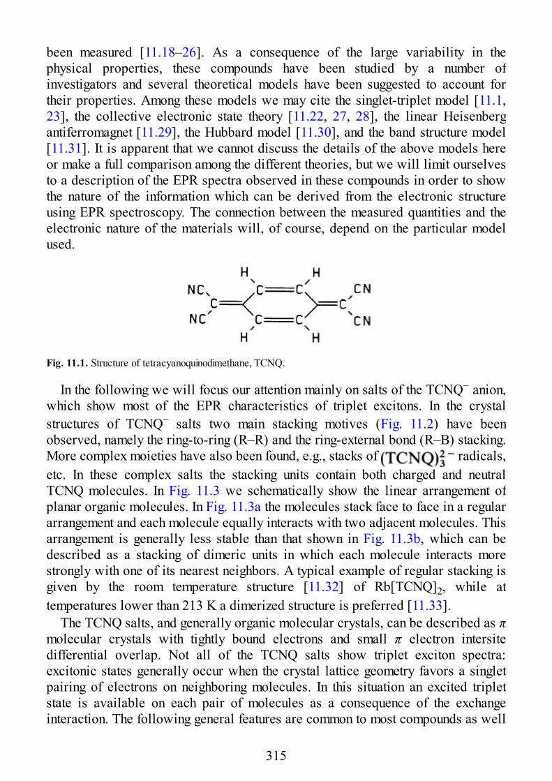
been measured [11.18–26]. As a consequence of the large variability in thephysical properties, these compounds have been studied by a number ofinvestigators and several theoretical models have been suggested to account fortheir properties. Among these models we may cite the singlet-triplet model [11.1,23], the collective electronic state theory [11.22, 27, 28], the linear Heisenbergantiferromagnet [11.29], the Hubbard model [11.30], and the band structure model[11.31]. It is apparent that we cannot discuss the details of the above models hereor make a full comparison among the different theories, but we will limit ourselvesto a description of the EPR spectra observed in these compounds in order to showthe nature of the information which can be derived from the electronic structureusing EPR spectroscopy. The connection between the measured quantities and theelectronic nature of the materials will, of course, depend on the particular modelused.

Fig. 11.1. Structure of tetracyanoquinodimethane, TCNQ.

In the following we will focus our attention mainly on salts of the TCNQ− anion,which show most of the EPR characteristics of triplet excitons. In the crystalstructures of TCNQ− salts two main stacking motives (Fig. 11.2) have beenobserved, namely the ring-to-ring (R–R) and the ring-external bond (R–B) stacking.More complex moieties have also been found, e.g., stacks of radicals,etc. In these complex salts the stacking units contain both charged and neutralTCNQ molecules. In Fig. 11.3 we schematically show the linear arrangement ofplanar organic molecules. In Fig. 11.3a the molecules stack face to face in a regulararrangement and each molecule equally interacts with two adjacent molecules. Thisarrangement is generally less stable than that shown in Fig. 11.3b, which can bedescribed as a stacking of dimeric units in which each molecule interacts morestrongly with one of its nearest neighbors. A typical example of regular stacking isgiven by the room temperature structure [11.32] of Rb[TCNQ]2, while attemperatures lower than 213 K a dimerized structure is preferred [11.33].

The TCNQ salts, and generally organic molecular crystals, can be described as πmolecular crystals with tightly bound electrons and small π electron intersitedifferential overlap. Not all of the TCNQ salts show triplet exciton spectra:excitonic states generally occur when the crystal lattice geometry favors a singletpairing of electrons on neighboring molecules. In this situation an excited tripletstate is available on each pair of molecules as a consequence of the exchangeinteraction. The following general features are common to most compounds as well

315

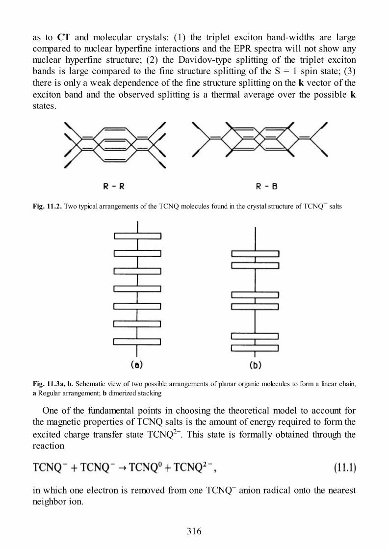
as to CT and molecular crystals: (1) the triplet exciton band-widths are largecompared to nuclear hyperfine interactions and the EPR spectra will not show anynuclear hyperfine structure; (2) the Davidov-type splitting of the triplet excitonbands is large compared to the fine structure splitting of the S = 1 spin state; (3)there is only a weak dependence of the fine structure splitting on the k vector of theexciton band and the observed splitting is a thermal average over the possible kstates.

Fig. 11.2. Two typical arrangements of the TCNQ molecules found in the crystal structure of TCNQ− salts

Fig. 11.3a, b. Schematic view of two possible arrangements of planar organic molecules to form a linear chain,a Regular arrangement; b dimerized stacking

One of the fundamental points in choosing the theoretical model to account forthe magnetic properties of TCNQ salts is the amount of energy required to form theexcited charge transfer state TCNQ2−. This state is formally obtained through thereaction

in which one electron is removed from one TCNQ− anion radical onto the nearestneighbor ion.

316

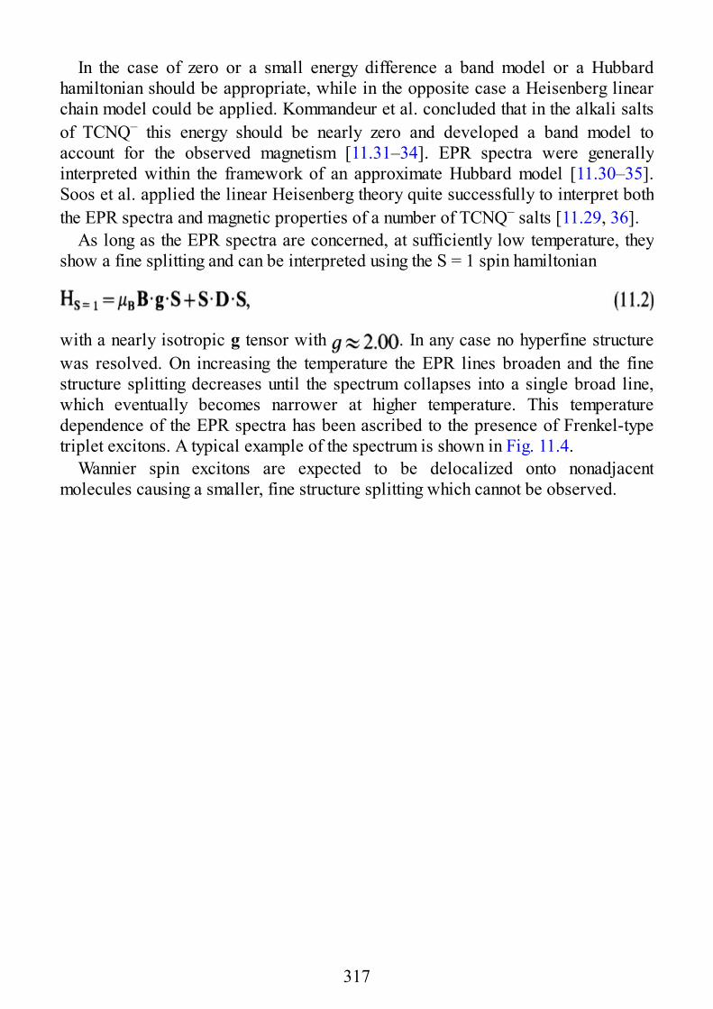
In the case of zero or a small energy difference a band model or a Hubbardhamiltonian should be appropriate, while in the opposite case a Heisenberg linearchain model could be applied. Kommandeur et al. concluded that in the alkali saltsof TCNQ− this energy should be nearly zero and developed a band model toaccount for the observed magnetism [11.31–34]. EPR spectra were generallyinterpreted within the framework of an approximate Hubbard model [11.30–35].Soos et al. applied the linear Heisenberg theory quite successfully to interpret boththe EPR spectra and magnetic properties of a number of TCNQ− salts [11.29, 36].

As long as the EPR spectra are concerned, at sufficiently low temperature, theyshow a fine splitting and can be interpreted using the S = 1 spin hamiltonian

with a nearly isotropic g tensor with . In any case no hyperfine structurewas resolved. On increasing the temperature the EPR lines broaden and the finestructure splitting decreases until the spectrum collapses into a single broad line,which eventually becomes narrower at higher temperature. This temperaturedependence of the EPR spectra has been ascribed to the presence of Frenkel-typetriplet excitons. A typical example of the spectrum is shown in Fig. 11.4.

Wannier spin excitons are expected to be delocalized onto nonadjacentmolecules causing a smaller, fine structure splitting which cannot be observed.

317

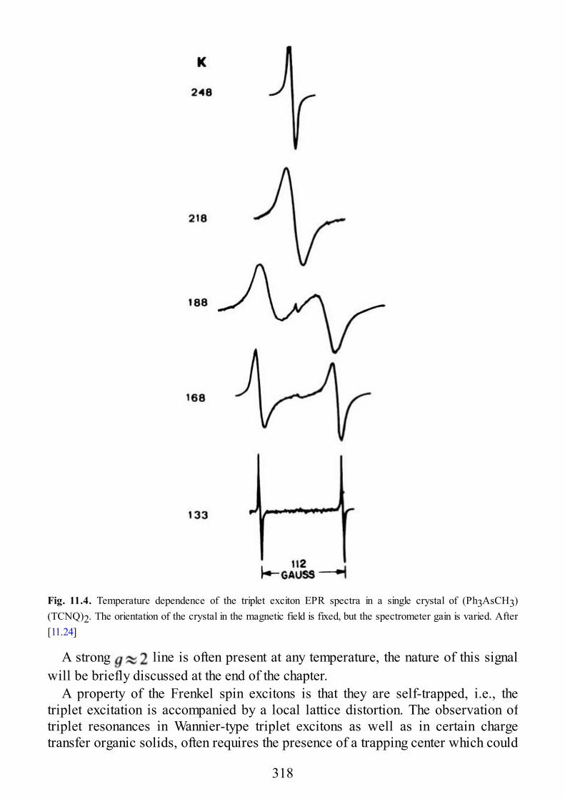
Fig. 11.4. Temperature dependence of the triplet exciton EPR spectra in a single crystal of (Ph3AsCH3)(TCNQ)2. The orientation of the crystal in the magnetic field is fixed, but the spectrometer gain is varied. After[11.24]

A strong line is often present at any temperature, the nature of this signalwill be briefly discussed at the end of the chapter.

A property of the Frenkel spin excitons is that they are self-trapped, i.e., thetriplet excitation is accompanied by a local lattice distortion. The observation oftriplet resonances in Wannier-type triplet excitons as well as in certain chargetransfer organic solids, often requires the presence of a trapping center which could

318

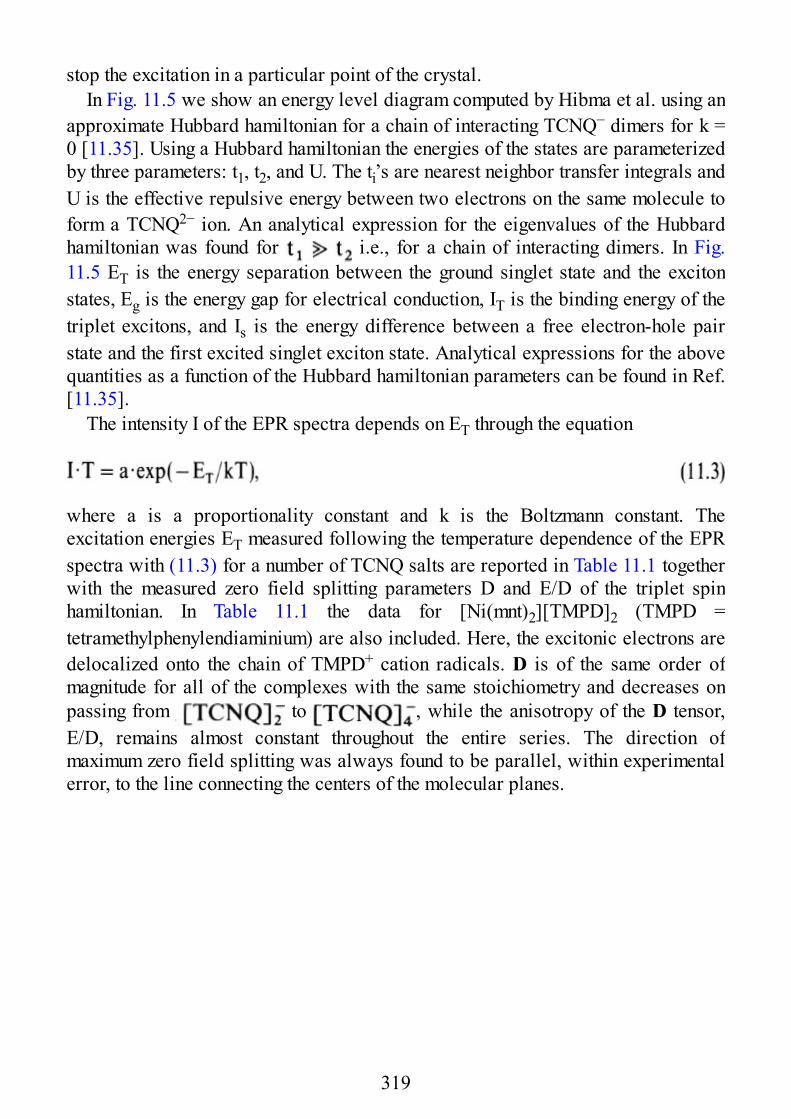
stop the excitation in a particular point of the crystal.In Fig. 11.5 we show an energy level diagram computed by Hibma et al. using an

approximate Hubbard hamiltonian for a chain of interacting TCNQ− dimers for k =0 [11.35]. Using a Hubbard hamiltonian the energies of the states are parameterizedby three parameters: t1, t2, and U. The ti’s are nearest neighbor transfer integrals andU is the effective repulsive energy between two electrons on the same molecule toform a TCNQ2− ion. An analytical expression for the eigenvalues of the Hubbardhamiltonian was found for i.e., for a chain of interacting dimers. In Fig.11.5 ET is the energy separation between the ground singlet state and the excitonstates, Eg is the energy gap for electrical conduction, IT is the binding energy of thetriplet excitons, and Is is the energy difference between a free electron-hole pairstate and the first excited singlet exciton state. Analytical expressions for the abovequantities as a function of the Hubbard hamiltonian parameters can be found in Ref.[11.35].

The intensity I of the EPR spectra depends on ET through the equation

where a is a proportionality constant and k is the Boltzmann constant. Theexcitation energies ET measured following the temperature dependence of the EPRspectra with (11.3) for a number of TCNQ salts are reported in Table 11.1 togetherwith the measured zero field splitting parameters D and E/D of the triplet spinhamiltonian. In Table 11.1 the data for [Ni(mnt)2][TMPD]2 (TMPD =tetramethylphenylendiaminium) are also included. Here, the excitonic electrons aredelocalized onto the chain of TMPD+ cation radicals. D is of the same order ofmagnitude for all of the complexes with the same stoichiometry and decreases onpassing from to , while the anisotropy of the D tensor,E/D, remains almost constant throughout the entire series. The direction ofmaximum zero field splitting was always found to be parallel, within experimentalerror, to the line connecting the centers of the molecular planes.

319

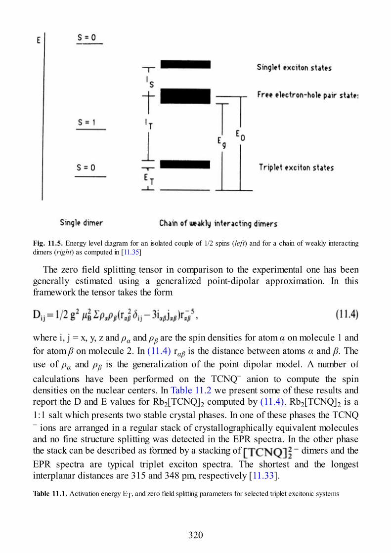
Fig. 11.5. Energy level diagram for an isolated couple of 1/2 spins (left) and for a chain of weakly interactingdimers (right) as computed in [11.35]

The zero field splitting tensor in comparison to the experimental one has beengenerally estimated using a generalized point-dipolar approximation. In thisframework the tensor takes the form

where i, j = x, y, z and ρα and ρβ are the spin densities for atom α on molecule 1 andfor atom β on molecule 2. In (11.4) rαβ is the distance between atoms α and β. Theuse of ρα and ρβ is the generalization of the point dipolar model. A number ofcalculations have been performed on the TCNQ− anion to compute the spindensities on the nuclear centers. In Table 11.2 we present some of these results andreport the D and E values for Rb2[TCNQ]2 computed by (11.4). Rb2[TCNQ]2 is a1:1 salt which presents two stable crystal phases. In one of these phases the TCNQ− ions are arranged in a regular stack of crystallographically equivalent moleculesand no fine structure splitting was detected in the EPR spectra. In the other phasethe stack can be described as formed by a stacking of dimers and theEPR spectra are typical triplet exciton spectra. The shortest and the longestinterplanar distances are 315 and 348 pm, respectively [11.33].

Table 11.1. Activation energy ET, and zero field splitting parameters for selected triplet excitonic systems

320

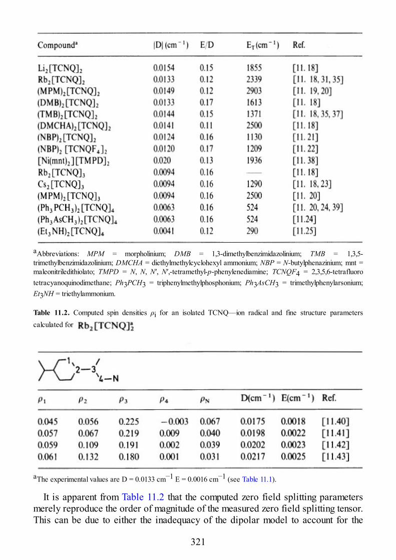
aAbbreviations: MPM = morpholinium; DMB = 1,3-dimethylbenzimidazolinium; TMB = 1,3,5-trimethylbenzimidazolinium; DMCHA = diethylmethylcyclohexyl ammonium; NBP = N-butylphenazinium; mnt =maleonitriledithiolato; TMPD = N, N, N′, N′,-tetramethyl-p-phenylenediamine; TCNQF4 = 2,3,5,6-tetrafluorotetracyanoquinodimethane; Ph3PCH3 = triphenylmethylphosphonium; Ph3AsCH3 = trimethylphenylarsonium;Et3NH = triethylammonium.

Table 11.2. Computed spin densities ρi for an isolated TCNQ—ion radical and fine structure parameterscalculated for

aThe experimental values are D = 0.0133 cm−1 E = 0.0016 cm−1 (see Table 11.1).

It is apparent from Table 11.2 that the computed zero field splitting parametersmerely reproduce the order of magnitude of the measured zero field splitting tensor.This can be due to either the inadequacy of the dipolar model to account for the

321

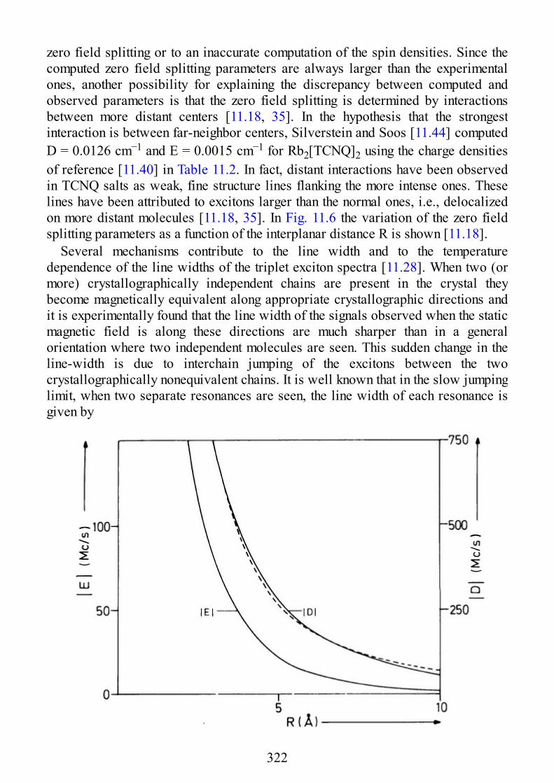
zero field splitting or to an inaccurate computation of the spin densities. Since thecomputed zero field splitting parameters are always larger than the experimentalones, another possibility for explaining the discrepancy between computed andobserved parameters is that the zero field splitting is determined by interactionsbetween more distant centers [11.18, 35]. In the hypothesis that the strongestinteraction is between far-neighbor centers, Silverstein and Soos [11.44] computedD = 0.0126 cm−1 and E = 0.0015 cm−1 for Rb2[TCNQ]2 using the charge densitiesof reference [11.40] in Table 11.2. In fact, distant interactions have been observedin TCNQ salts as weak, fine structure lines flanking the more intense ones. Theselines have been attributed to excitons larger than the normal ones, i.e., delocalizedon more distant molecules [11.18, 35]. In Fig. 11.6 the variation of the zero fieldsplitting parameters as a function of the interplanar distance R is shown [11.18].

Several mechanisms contribute to the line width and to the temperaturedependence of the line widths of the triplet exciton spectra [11.28]. When two (ormore) crystallographically independent chains are present in the crystal theybecome magnetically equivalent along appropriate crystallographic directions andit is experimentally found that the line width of the signals observed when the staticmagnetic field is along these directions are much sharper than in a generalorientation where two independent molecules are seen. This sudden change in theline-width is due to interchain jumping of the excitons between the twocrystallographically nonequivalent chains. It is well known that in the slow jumpinglimit, when two separate resonances are seen, the line width of each resonance isgiven by

322

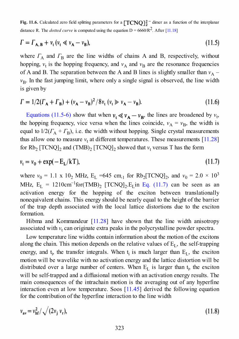
Fig. 11.6. Calculated zero field splitting parameters for a dimer as a function of the interplanar

distance R. The dotted curve is computed using the equation D = 6660/R2. After [11.18]

where ГA and ГB are the line widths of chains A and B, respectively, withouthopping, νt is the hopping frequency, and νA and νB are the resonance frequenciesof A and B. The separation between the A and B lines is slightly smaller than νA –νB. In the fast jumping limit, where only a single signal is observed, the line widthis given by

Equations (11.5-6) show that when , the lines are broadened by νt,the hopping frequency, vice versa when the lines coincide, νA = νB, the width isequal to l/2(ГA + ГB), i.e. the width without hopping. Single crystal measurementsthus allow one to measure νt at different temperatures. These measurements [11.28]for Rb2 [TCNQ]2 and (TMB)2 [TCNQ]2 showed that νt versus T has the form

where ν0 = 1.1 x 102 MHz, EL =645 cm-1 for Rb2[TCNQ]2, and ν0 = 2.0 × 103

MHz, EL = 1210cm−1for(TMB)2 [TCNQ]2.ELin Eq. (11.7) can be seen as anactivation energy for the hopping of the exciton between translationallynonequivalent chains. This energy should be nearly equal to the height of the barrierof the trap depth associated with the local lattice distortions due to the excitonformation.

Hibma and Kommandeur [11.28] have shown that the line width anisotropyassociated with νt can originate extra peaks in the polycrystalline powder spectra.

Low temperature line widths contain information about the motion of the excitonsalong the chain. This motion depends on the relative values of EL, the self-trappingenergy, and ti, the transfer integrals. When ti is much larger than EL, the excitonmotion will be wavelike with no activation energy and the lattice distortion will bedistributed over a large number of centers. When EL is larger than ti, the excitonwill be self-trapped and a diffusional motion with an activation energy results. Themain consequences of the intrachain motion is the averaging out of any hyperfineinteraction even at low temperature. Soos [11.45] derived the following equationfor the contribution of the hyperfine interaction to the line width

323

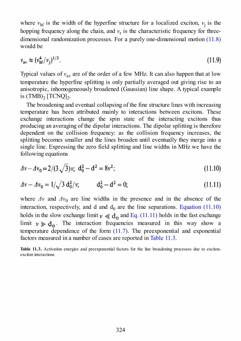
where νhf is the width of the hyperfine structure for a localized exciton, νj is thehopping frequency along the chain, and νr is the characteristic frequency for three-dimensional randomization processes. For a purely one-dimensional motion (11.8)would be

Typical values of νav are of the order of a few MHz. It can also happen that at lowtemperature the hyperfine splitting is only partially averaged out giving rise to ananisotropic, inhomogeneously broadened (Gaussian) line shape. A typical exampleis (TMB)2 [TCNQ]2.

The broadening and eventual collapsing of the fine structure lines with increasingtemperature has been attributed mainly to interactions between excitons. Theseexchange interactions change the spin state of the interacting excitons thusproducing an averaging of the dipolar interactions. The dipolar splitting is thereforedependent on the collision frequency: as the collision frequency increases, thesplitting becomes smaller and the lines broaden until eventually they merge into asingle line. Expressing the zero field splitting and line widths in MHz we have thefollowing equations

where Δν and Δν0 are line widths in the presence and in the absence of theinteraction, respectively, and d and d0 are the line separations. Equation (11.10)holds in the slow exchange limit and Eq. (11.11) holds in the fast exchangelimit . The interaction frequencies measured in this way show atemperature dependence of the form (11.7). The preexponential and exponentialfactors measured in a number of cases are reported in Table 11.3.

Table 11.3. Activation energies and preexponential factors for the line broadening processes due to exciton-exciton interactions

324

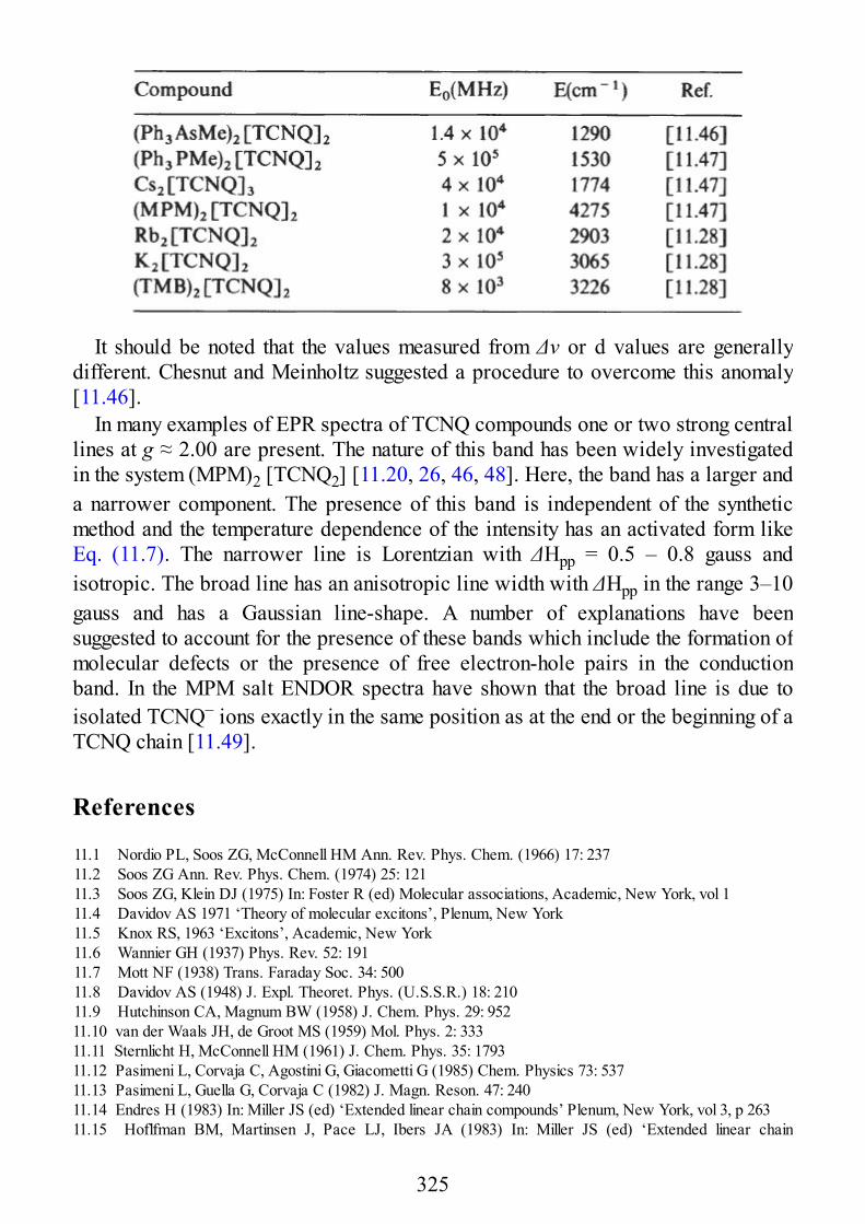
It should be noted that the values measured from Δν or d values are generallydifferent. Chesnut and Meinholtz suggested a procedure to overcome this anomaly[11.46].

In many examples of EPR spectra of TCNQ compounds one or two strong centrallines at g ≈ 2.00 are present. The nature of this band has been widely investigatedin the system (MPM)2 [TCNQ2] [11.20, 26, 46, 48]. Here, the band has a larger anda narrower component. The presence of this band is independent of the syntheticmethod and the temperature dependence of the intensity has an activated form likeEq. (11.7). The narrower line is Lorentzian with ΔHpp = 0.5 – 0.8 gauss andisotropic. The broad line has an anisotropic line width with ΔHpp in the range 3–10gauss and has a Gaussian line-shape. A number of explanations have beensuggested to account for the presence of these bands which include the formation ofmolecular defects or the presence of free electron-hole pairs in the conductionband. In the MPM salt ENDOR spectra have shown that the broad line is due toisolated TCNQ− ions exactly in the same position as at the end or the beginning of aTCNQ chain [11.49].

References

11.1 Nordio PL, Soos ZG, McConnell HM Ann. Rev. Phys. Chem. (1966) 17: 23711.2 Soos ZG Ann. Rev. Phys. Chem. (1974) 25: 12111.3 Soos ZG, Klein DJ (1975) In: Foster R (ed) Molecular associations, Academic, New York, vol 111.4 Davidov AS 1971 ‘Theory of molecular excitons’, Plenum, New York11.5 Knox RS, 1963 ‘Excitons’, Academic, New York11.6 Wannier GH (1937) Phys. Rev. 52: 19111.7 Mott NF (1938) Trans. Faraday Soc. 34: 50011.8 Davidov AS (1948) J. Expl. Theoret. Phys. (U.S.S.R.) 18: 21011.9 Hutchinson CA, Magnum BW (1958) J. Chem. Phys. 29: 95211.10 van der Waals JH, de Groot MS (1959) Mol. Phys. 2: 33311.11 Sternlicht H, McConnell HM (1961) J. Chem. Phys. 35: 179311.12 Pasimeni L, Corvaja C, Agostini G, Giacometti G (1985) Chem. Physics 73: 53711.13 Pasimeni L, Guella G, Corvaja C (1982) J. Magn. Reson. 47: 24011.14 Endres H (1983) In: Miller JS (ed) ‘Extended linear chain compounds’ Plenum, New York, vol 3, p 26311.15 Hoflfman BM, Martinsen J, Pace LJ, Ibers JA (1983) In: Miller JS (ed) ‘Extended linear chain

325

compounds’ Plenum, New York, vol 3, p 45911.16 Zeller HR (1973) Adv. Solid State Phys. 13: 3111.17 Garito AF, Heeger A J (1974) Acc. Chem. Res. 7: 23211.18 Hibma T, Dupuis P, Kommandeur J (1972) Chem. Phys. Letters 15: 1711.19 Marechal MA, McConnell HM (1965) J. Chem. Phys. 43: 49711.20 Bailey JC, Chestnut DB (1969) J. Chem. Phys. 51: 511811.21 Harms RH, Keller HJ, Nothe D, Wehe D, Heimer NE, Metzger RM, Gundel D, Sixl H (1982) Mol. Cryst.

Liq. Cryst. 85: 24911.22 Metzger RM, Heimer NE, Gundel D, Sixl H, Harms RH, Keller HJ, Nothe D, Wehe D (1982) J. Chem.

Phys. 77: 620311.23 Chestunt DB, Arthur P (1962) J. Chem. Phys. 36: 296911.24 Chestnut DB, Phillips WD (1961) J. Chem. Phys. 35: 100211.25 Flandrois S, Amiell J, Carmona F, Delhaes P (1975) Solid State Commun. 17: 28711.26 Hoffmann SK, Corvan PJ, Singh P, Sethulekshmi CN, Metzger RM, Hatfield WE (1983) J. Am. Chem.

Soc., 105: 460811.27 Winkler RG, Reineker P (1987) Mol. Phys. 60: 128311.28 Hibma T, Kommandeur J (1975) Phys. Rev. B 12: 260811.29 Soos ZG (1965) J. Chem. Phys. 43: 112111.30 Soos ZG, Klein DJ (1971) J. Chem. Phys. 55: 328411.31 Vegter JG, Kommandeur J (1975) J. Mol. Cryst. Liq. Cryst., 30: 1111.32 Shirotani I, Kobayashi H (1973) Bull. Chem. Soc. Jpn. 46: 259511.33 Hoekstra A, Spoelder T, Vos A (1972) Acta Cryst. B28: 1411.34 Vegter JG, Kommandeur J, Fedders PA (1973) Phys. Rev. B 7: 292911.35 Hibma T, Sawatzky GA, Kommandeur J (1977) Phys. Rev. B 15: 395911.36 Soos ZG, Hughes RCJ. (1967) Chem. Phys. 46: 25311.37 Dupuis P, Flandrois S, Neel J (1969) C.R. Acad Sci. (Paris) C269: 109111.38 Hove MJ, Hoffman BM, Ibers JA (1972) J. Chem. Phys. 56: 349011.39 Thomas DD, Merkl AW, Hildebrandt AF, McConnell HM (1964) J. Chem. Phys. 40: 258811.40 Lowitz DA (1967) J. Chem. Phys. 46: 469811.41 Bieber A, Andre JJ, (1974) Chem. Phys. 5: 16611.42 Jonkman HT, van der Velde GA, Nieuwpoort WC (1974) Chem. Phys. Letters 25: 6211.43 Johansen H (1975) Int. J. Quantum Chem., 9: 45911.44 Silverstein AJ, Soos ZG (1976) Chem. Phys. Letters, 39: 52511.45 Soos ZG (1965) J. Chem. Phys. 44: 172911.46 Chestnut DB, Meinholtz DC (1984) J. Chem. Phys. 80: 354011.47 Jones MT, Chestnut DB (1963) J. Chem. Phys., 38: 131111.48 Kepler RG (1963) J. Chem. Phys. 39: 352811.49 Maniero AL, Priolisi O, Corvaja CJ. Chem. Soc. Faraday Trans. (in press)

326

Appendix A. Second Quantization

The formalism of second quantization, or the occupation number representation forfermions, allows one to write multi electron wave functions and operators moresimply than using the Slater antisymmetrized product of one-electron functions[2.1]. The main advantage of this method compared to that of Slater determinants isthat it leads to a compact notation, while the latter is rather cumbersome even forsmall numbers of electrons. However, there is really no result which can be provedwithin the second quantization formalism which cannot be obtained using the Slaterformalism.

In the one-electron approximation a quantum state of a system is defined by anantisymmetrized product of the occupied one-electron spin orbitals. A typical formof an N electron system is:

where A is an antisymmetrizer, ri represents space and spin variables of electron i,and ki is a set of quantum numbers defining the state of the electron i.

When we have chosen a complete orthonormal set of one-electron spin orbitalswe can associate to each state (A.1) a vector formed by the occupation number ofeach spin orbital of the complete set. This number, due to the antisymmetryrequirement of the wave function, can be either 0 or 1. Equation (A.1) gives theoccupation number representation of the system.

Let us consider a three-electron state as an example. In second quantization it isrepresented by:

which indicates that one electron is present in Φk, one in Φ1, and one in Φm, whileall the others are vacant. ψklm is equivalent to the Slater determinant:

327

It should be noted that while in the Slater representation ψklm is given by a 3 x 3determinant, (A.2) is a vector in an infinite dimensional space.

A general state vector can be written as:

with nk = 0, 1. The state vector for which nk = 0, for all k, is a vacuum state. Thestate (A.4) is orthonormalized by the conditions:

and it forms a vector of a Hilbert space.All the possible state vectors can be constructed starting from the vacuum state

using creation operators, , i.e., an operator which creates an electron in the stateΦk. In the Slater formalism a creation operator transforms an N x N Slaterdeterminant into an (N + 1) x (N + 1) one. Of course, this (N + 1) (N + 1)determinant will be nonzero if Φk is different from any other state already present,otherwise the determinant will have two equal rows, i.e., creates a particle inthe k-th orbital provided it is initially vacant

If nk in the initial state is equal to 1, the result of the creation operator is zero:

Conversely, an annihilation operator ak removes an electron in the k-th orbitalprovided that the orbital in question initially contained an electron:

If it operates on a vacant orbital, the result is zero:

In order to pass from the second quantization to the Slater formalism it is importantto arrange the one-electron orbitals in a given order and then to employ the sameorder in the Slater determinant.

The creation and annihilation operators have several interesting properties:

328

This is obvious if initially nk = 1. On the other hand, the first operator creates anelectron in k, if it is initially vacant, and the second will find nk = 1. Analogouslyone has:

In fact, if nk and nj are zero in , . Condition 3 indicates that

anti-commute. This can be symbolically written as:

It also follows from above:

In fact, let , then

. For and , so that , or equivalently . The eigenvalue of

is the occupation number of the k-th orbital. defines a number operatorfor the k-th orbital:

One- and two-electron operators can be expanded in terms of the creation andannihilation operators. Let us start from one-electron operators, which we indicateas Σifi. The matrix element of this operator between two states and is zero,if the two vectors differ in more than one component orbital. If they differ in justone orbital, e.g., k1 in and k2 in , then:

In the right term we have omitted the subscript indicating the electron, because the

329

matrix element is taken between one-electron states.If the states are identical, then

If we define an operator:

then it is easy to show that this operator leads to the same matrix elements betweenthe and states as the Σifi operator.

The procedure can be extended to two-electron operators, yielding for a generaloperator Σi ≠ jgij to the identity:

Among one-electron operators an interesting special case is that in which each fi= 1, so that the total operator, N, represents the total number of electrons and iscalled the number operator:

For our purposes it is important to establish the relations between secondquantized operators and angular momentum operators. Let us start from anintuitively clear example and then obtain general formulae. Let us consider ,and suppose that m and m′ are two orbitals on the same center, both with spin up.Let us further assume that both orbitals belong to the same configuration, forinstance of d orbitals, and are characterized by two different values of the magneticquantum number, m and m′, respectively. The operator removes an electron from m′and creates another one in m, keeping the spin up. The effect of the operator hasbeen that of changing the overall M = Σimi value by m′ – m. This is the same effectof angular momentum operators, therefore, it can be hoped to relate toangular momentum operators. This indeed has been done. For orbitals belonging tothe same 1 manifold, the following relations must hold [A.2]:

where

330

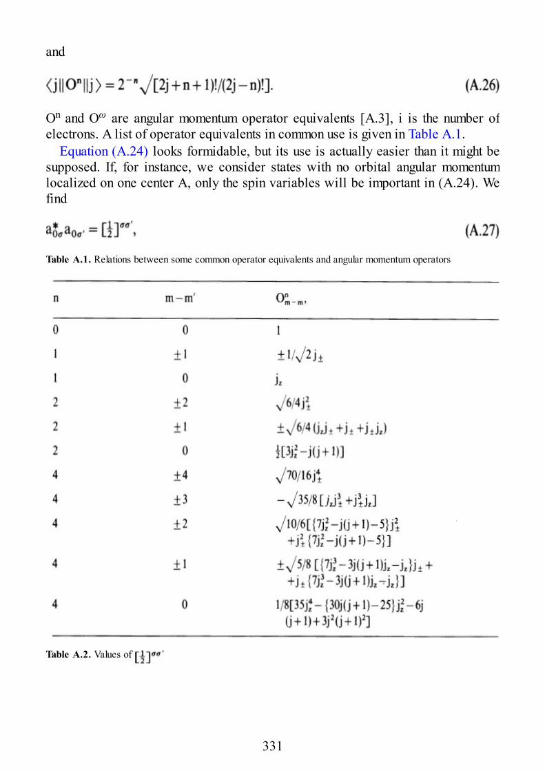
and

On and Oω are angular momentum operator equivalents [A.3], i is the number ofelectrons. A list of operator equivalents in common use is given in Table A.1.

Equation (A.24) looks formidable, but its use is actually easier than it might besupposed. If, for instance, we consider states with no orbital angular momentumlocalized on one center A, only the spin variables will be important in (A.24). Wefind

Table A.1. Relations between some common operator equivalents and angular momentum operators

Table A.2. Values of

331

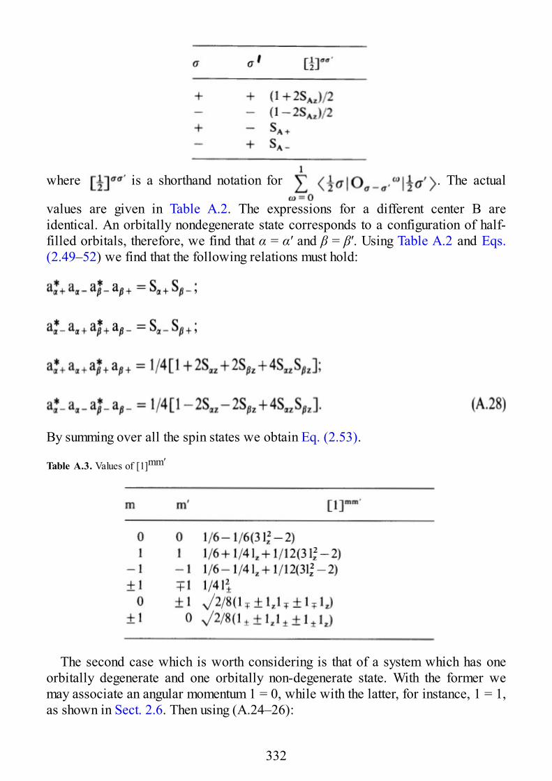
where is a shorthand notation for . The actual

values are given in Table A.2. The expressions for a different center B areidentical. An orbitally nondegenerate state corresponds to a configuration of half-filled orbitals, therefore, we find that α = α′ and β = β′. Using Table A.2 and Eqs.(2.49–52) we find that the following relations must hold:

By summing over all the spin states we obtain Eq. (2.53).

Table A.3. Values of [1]mm′

The second case which is worth considering is that of a system which has oneorbitally degenerate and one orbitally non-degenerate state. With the former wemay associate an angular momentum 1 = 0, while with the latter, for instance, 1 = 1,as shown in Sect. 2.6. Then using (A.24–26):

332

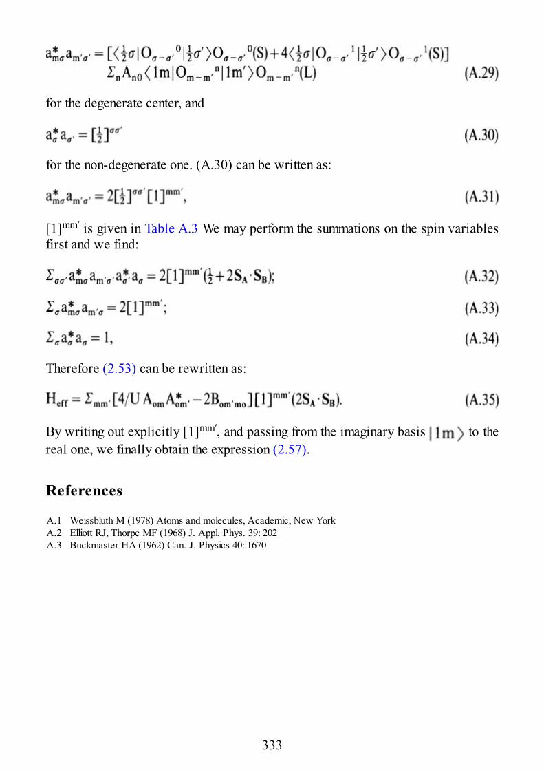
for the degenerate center, and

for the non-degenerate one. (A.30) can be written as:

[1]mm′ is given in Table A.3 We may perform the summations on the spin variablesfirst and we find:

Therefore (2.53) can be rewritten as:

By writing out explicitly [1]mm′, and passing from the imaginary basis to thereal one, we finally obtain the expression (2.57).

References

A.1 Weissbluth M (1978) Atoms and molecules, Academic, New YorkA.2 Elliott RJ, Thorpe MF (1968) J. Appl. Phys. 39: 202A.3 Buckmaster HA (1962) Can. J. Physics 40: 1670

333

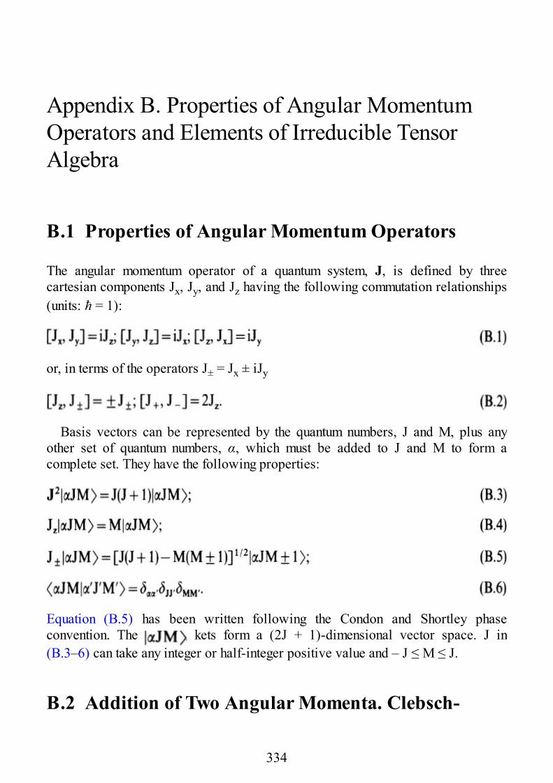
Appendix B. Properties of Angular MomentumOperators and Elements of Irreducible TensorAlgebra

B.1 Properties of Angular Momentum Operators

The angular momentum operator of a quantum system, J, is defined by threecartesian components Jx, Jy, and Jz having the following commutation relationships(units: ħ = 1):

or, in terms of the operators J± = Jx ± iJy

Basis vectors can be represented by the quantum numbers, J and M, plus anyother set of quantum numbers, α, which must be added to J and M to form acomplete set. They have the following properties:

Equation (B.5) has been written following the Condon and Shortley phaseconvention. The kets form a (2J + 1)-dimensional vector space. J in(B.3–6) can take any integer or half-integer positive value and – J ≤ M ≤ J.

B.2 Addition of Two Angular Momenta. Clebsch-

334

Gordon Coefficients and “3j” Symbols

B.2.1 Definitions

Let jA and jB be angular momenta of quantum systems A and B, respectively. Thetotal angular momentum of quantum systems A and B together is

The tensor product of the (2jA + 1) kets of A and (2jB + 1) kets of B gives aspace of (2jA + 1) (2jB + 1) kets which are simultaneous eigenvectors of , , jAz,and jBz:

The basis vectors of (B.7) can be obtained from (B.8) by a unitarytransformation as simultaneous eigenvectors of , , J2, Jz, which are allcommuting operators, as

The coefficients of the unitary transformation are calledClebsch-Gordon coefficients.

B.2.1.1 Equivalent Definitions

1 In: Condon EU, Shortley GH (1935) The theory ofatomic spectra, Cambridge University Press, New York

2. In: Biedenharn LC (1952) Tables of the Racah coefficients, OakRidge National Lab., Physics Division, ORNL-1098

3. where it has been considered that M = mA + mB; In: RoseME Elementary theory of angular momentum, (1957) Wiley, New York

4. In: Wigner EP (1958) Group theory and its application to the quantummechanics of atomic spectra, Academic, New York

B.2.1.2 Phase Convention and Properties

A commonly used convention to fix the relative phase of kets (B.9) is

335

1 is real and positive.2 follows Eq. (B.5).

The Clebsch-Gordon coefficients have the following main properties:

1. They are real and form an orthogonal matrix;2. The coefficients are different from zero, if mA + mB = M and |jA – jB | ≤ J ≤ jA +

jB;3. .

B.2.1.3 The “3j” Symbols

Wigner defined the following quantities which are proportional to the Clebsch-Gordon coefficients in order to better exploit the symmetry properties:

The 3j symbols have the following properties:1. Even permutations of the columns leave the numerical value unchanged:

2. Odd permutations of the columns multiply the value by (-1)jA + jB + J:

3. When the signs of mA, mB, and M are simultaneously changed, the value ismultiplied by (-1)jA + JB + J:

4. Regge symmetry: a 3j symbol can be transformed in the square matrix:

336

If this matrix is reflected through its diagonals or the rows or columns arecyclically permuted, the 3j symbol which is associated with the resultant matrix hasthe same value as the original one. These rules add 72 new symmetries to thesymmetries in 1, 2, and 3.

B.2.2 Methods of Calculations

A general formula for the calculation of the 3j symbols has been developed byRacah:

with α + β + δ = 0 and |a – b| ≤ d ≤ (a+b) andΓ(abd) = (a + b – d)!(b + d – a)!(d + a – b)!/(a + b + d + 1)!

In (B.11) Σt extends over all integral values of t for which the factorials are ≥ 0.The number of terms in the summation is μ + 1, where μ is the smallest of the ninenumbers:

a ± α; b ± β; d ± δ; a + b – d; b + d – a; d + a – b.

B.2.2.1 Special Formulae

337

where J = j1 + j2 + j3.

B.3 The “6j” Symbols and the Racah W Coefficients

B.3.1 Definitions

The 6j symbols appear in the case of the coupling of three angular momenta j1, j2,and j3 as the coefficients of the unitary transformation which connects two differentcoupling schemes. From the direct product of the vector spaces of the three angularmomenta j1, j2, and j3 we get a (2j1 + 1)(2j2 + 1)(2j3 + 1)-dimensional spacespanned by the kets . Defining atotal angular momentum of the system as J = j1 + j2 + j3, the subspace of angularmomentum (JM) can be defined according to:

min∣j1 ± j2 ± j3∣ ≤ J ≤ (j1 + j2 + j3); – J ≤ M ≤ J.

In general, different systems of basis vectors can be defined according to thecoupling scheme of the angular momenta:

1. Coupling scheme j1 + j2 = j12; j12 + j3 = J: vectors

2. Coupling scheme j2 + j3 = j23; ji + j23 = J: vectors

Since the kets in (B.12) and (B.13) span the same vector space as those in (B.8)and (B.9), they are related by a unitary transformation

338

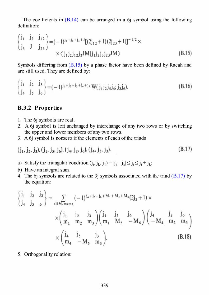
The coefficients in (B.14) can be arranged in a 6j symbol using the followingdefinition:

Symbols differing from (B.15) by a phase factor have been defined by Racah andare still used. They are defined by:

B.3.2 Properties

1. The 6j symbols are real.2. A 6j symbol is left unchanged by interchange of any two rows or by switching

the upper and lower members of any two rows.3. A 6j symbol is nonzero if the elements of each of the triads

a) Satisfy the triangular condition (ji, jk, j1) = |ji – jk| ≤ ji ≤ ji + jk;b) Have an integral sum.4. The 6j symbols are related to the 3j symbols associated with the triad (B.17) by

the equation:

5. Orthogonality relation:

339

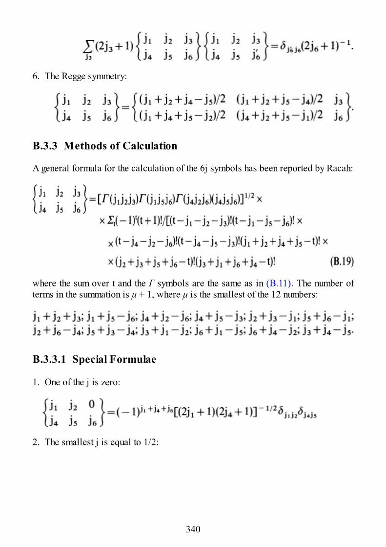
6. The Regge symmetry:

B.3.3 Methods of Calculation

A general formula for the calculation of the 6j symbols has been reported by Racah:

where the sum over t and the Γ symbols are the same as in (B.11). The number ofterms in the summation is μ + 1, where μ is the smallest of the 12 numbers:

B.3.3.1 Special Formulae

1. One of the j is zero:

2. The smallest j is equal to 1/2:

340

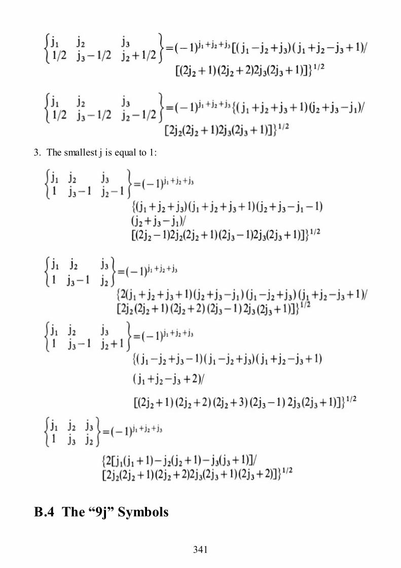
3. The smallest j is equal to 1:

B.4 The “9j” Symbols

341

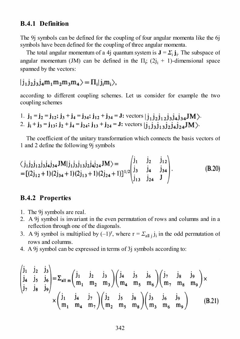
B.4.1 Definition

The 9j symbols can be defined for the coupling of four angular momenta like the 6jsymbols have been defined for the coupling of three angular momenta.

The total angular momentum of a 4j quantum system is J = Σi ji. The subspace ofangular momentum (JM) can be defined in the Πi; (2ji + 1)-dimensional spacespanned by the vectors:

according to different coupling schemes. Let us consider for example the twocoupling schemes

1. j1 = j2 = j12; j3 + j4 = j34; j12 + j34 = J: vectors .2. ji + j3 = j13; j2 + j4 = j24; j13 + j24 = J: vectors .

The coefficient of the unitary transformation which connects the basis vectors of1 and 2 define the following 9j symbols

B.4.2 Properties

1. The 9j symbols are real.2. A 9j symbol is invariant in the even permutation of rows and columns and in a

reflection through one of the diagonals.3. A 9j symbol is multiplied by (–1)r, where r = Σall j ji in the odd permutation of

rows and columns.4. A 9j symbol can be expressed in terms of 3j symbols according to:

342

5. Orthogonality relation:

B.4.3 Special Formulae

1. One of the j is zero: the 9j symbol collapses to a 6j symbol:

B.5 Irreducible Tensor Operators

B.5.1 Definitions

A tensor operator can be defined as a set of operators that transform linearly oneinto another under rotation of the coordinate system. A set of (2k + 1) operatorswhich transform linearly one into the other is called a kth-rank tensor operator or atensor operator of order k. A scalar operator, O, is a zero-rank tensor operator, avector operator, O, is a first-rank tensor operator having cartesian components Ox,Oy, and Oz. A tensor operator is generally indicated by the symbol Tkq(O), where kis the rank, q is in the range ± k, and O indicates the type of quantum mechanicaloperator used. Unless it is explicitly necessary we will omit in the following the Osymbol, meaning any tensor operator of rank k.

A tensor operator Tkq(q = – k, . . . , k) is called irreducible tensor operator if its(2k + 1) components transform under a rotation R of the coordinate systemaccording to:

343

where Rk is the Wigner rotation matrix and spans the k-th irreducible representationof the real orthogonal rotation group SO(3). Through (B.22) the components of anirreducible tensor operator can be expressed as a linear combination of the morecommon cartesian components. Some examples are shown in Table 3.1.

B.5.1.1 Compound Irreducible Tensor Operators

The tensor product of two irreducible tensor operators of rank k1 and k2, Tk1 andTk2, can be defined as the set of (2k1 + 1) (2k2 + 1) operators:

The set of operators (B.23) is in general reducible and we can construct from itan irreducible tensor operator of order k called the tensor product of Tk1 and Tk2of order k according to:

When not explicitly stated, Tk1 and Tk2 are commuting tensor operators such asoperators acting on two vector spaces 1 and 2 separately, like SA and SB in Chap.3, or operators acting separately on spin and space coordinates, like the spin-orbitcoupling operator of one particle ŀs.

According to (B.10) we can rewrite (B.24) as

where one necessarily has |k1 – k2| ≤ k ≤ (k1 + k2).It is an obvious extension of the above definition to construct tensor operators as

products of more than two irreducible tensor operators and the relative formulaewill not be explicitly given here.

B.5.1.2 Tensor Product of Two First-rank Irreducible TensorOperators

From the tensor product of two irreducible tensor operators with k1 = k2 = 1 we getthree sets of irreducible tensor operators corresponding to k = 0, 1, and 2. For k = 0from (B.25) one has

344

The usual scalar product of two vector operators (T·T) = TxTx + TyTy + TzTz isrelated to (B.26) by

or more generally

For k = 1 one has

For k = 2 one has

It is interesting to note that (B.30) applied to two tensor operators acting on thesame set of coordinates, such as two spin operators, gives identically zero, as aconsequence of the commutation relations. This can be easily verified by thereader.

B.5.2 Properties of Irreducible Tensor Operators

1. Commutation relations with the total angular momentum operator J (Racah’scommutation relations):

345

2. Adjoint tensor operators.The adjoint or Hermitean conjugate, , of a tensor operator Tkq is definedby:

where + denotes the Hermitean conjugate. Using (B.31) the spherical harmonicsY1m form an Hermitean tensor operator. Definitions equivalent to (B.31) are:

With respect to (B.32) the spherical harmonics of odd order are anti-Hermitean.3. Wigner-Eckart theorem:

where is called reduced matrix element. τ indicates any set ofquantum numbers required to completely specify the quantum system. The followingform of the theorem is sometimes used:

The conjugate of a reduced matrix element is (k integral)

Equation (B.33) or (B.34) can be used to compute the matrix element of anytensor operator provided the reduced matrix elements are known.

B.5.3 Reduced Matrix Elements of Special Operators

1. Identity operator:

2. Total angular momentum:

346

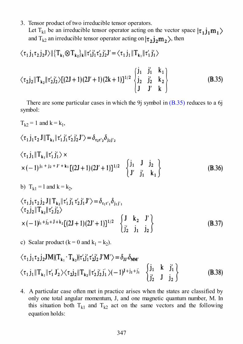
3. Tensor product of two irreducible tensor operators.Let Tk1 be an irreducible tensor operator acting on the vector space and Tk2 an irreducible tensor operator acting on , then

There are some particular cases in which the 9j symbol in (B.35) reduces to a 6jsymbol:

Tk2 = 1 and k = k1,

b) Tk1 = l and k = k2,

c) Scalar product (k = 0 and k1 = k2).

4. A particular case often met in practice arises when the states are classified byonly one total angular momentum, J, and one magnetic quantum number, M. Inthis situation both Tk1 and Tk2 act on the same vectors and the followingequation holds:

347

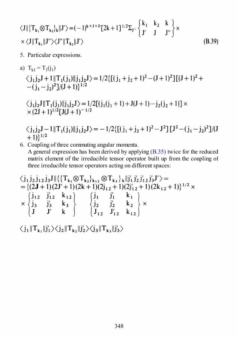
5. Particular expressions.

a) Tk1 = T1(j1)

6. Coupling of three commuting angular momenta.A general expression has been derived by applying (B.35) twice for the reducedmatrix element of the irreducible tensor operator built up from the coupling ofthree irreducible tensor operators acting on different spaces:

348

Subject Index

ab initio 12, 15, 18activation energy 43, 44Anderson 2, 3–9, 15, 34, 38, 139angular momentum operator 37, 38Angular Overlap Model 12annihilation operator 36antiferromagnet 164antiferromagnetic coupling 2, 4–6, 8, 10, 14, 18, 20, 30, 46, 62, 63, 79, 81, 107, 108, 114, 130, 133, 179Azotobacter vinelandii 109

Bacillus Stearothermophilus 133Bleaney 174Blume–Orbach relaxation 124Born–Oppenheimer 43broken symmetry 16, 18

ci coefficients 101, 102, 104, 105, 107, 108, 110, 111chromium(III) 62, 63, 168–171classical spins 163, 164Clebsch–Gordon 51cluster 86, 100, 101, 132, 133, 163–, linear 99–100–, pentanuclear 104–, tetranuclear 90, 93–99, 104, 105, 113–119–, trinuclear 91–93, 101, 104, 105, 106–113cobalt(II) 49, 184, 185, 186copper(II) 2, 6, 8, 14–16, 20, 23, 25, 27, 30, 39, 45, 58, 60, 61, 63–67, 74, 79, 82–84, 108, 109, 111–116, 119, 130,

133, 152, 164, 173, 175–177, 179–182, 184–187copper acetate hydrate 15, 20, 174correlation function 140–142, 147, 148, 155, 156, 159, 165, 166– time 141, 155, 156, 159Coulomb integral 10coupling scheme 87, 102creation operator 36cross relaxation 125, 133crystal field 33, 122, 128, 129, 15063, 65Cu 61Curie 146cut–off 144, 159cytochrome oxidase 39

di coefficients 101, 102, 104, 105dij coefficients 101, 102, 104, 105Debye temperature 124, 134

349

density functional 16diffusive tail 157dipolar interaction 2, 30, 33, 39, 64, 67, 68, 115, 136–138, 145, 146, 153, 173Dirac 3, 106direct relaxation 121, 122, 128–130double exchange 45, 46– excitation 34– quantum transition 175doublet 107–109, 114, 125, 133, 137, 139dynamic hamiltonian 122–125

effective hamiltonian 35eigenfield method 49energy density 122Euler angles 68exchange, anisotropic 22, 27, 31, 33, 39, 49, 51, 59, 62, 64, 67, 68, 70–75, 81, 115, 116, 125–127, 129, 130, 150,

167, 168, 191–, antisymmetric 22, 24, 27, 31–33, 51, 56, 57, 62, 64, 66, 82, 115, 116, 125, 150, 165–, bilinear 56, 62, 147, 167–, biquadratic 167–, direct 5–, integral 10, 13, 14, 29, 31–, isotropic 22, 27, 49–51, 59, 61, 68, 70, 73, 74, 81, 88, 89, 91, 100, 107, 109, 122, 125, 126, 129, 130, 132, 133,

139, 165– kinetic 4, 15, 16, 38– narrowing 139, 145, 148, 156, 186–, potential 4, 15, 38– striction 34, 64, 168Extended Huckel 11, 12, 15, 27extended interactions 135

fast modulation 142, 143ferredoxins 42, 109, 125, 131, 133ferrimagnet 164ferromagnet 164ferromagnetic coupling 2, 4–8, 10, 13, 18, 30, 79, 98, 181, 186fine structure 179fluctuation–dissipation theorem 141forbidden transition 175, 177Fourier transform 141, 143, 144fourth order operators 114, 118fractal 132

gadolinium(III) 29g anisotropy 150gaussian distribution 140– lineshape 137, 139, 143, 145, 157, 158– modulation 141, 142, 147Goodenough 5, 6, 9, 12, 15, 30, 186g shift 163, 165

half field transitions 160Heisenberg 3, 38, 44, 106– representation 145heterodinuclear species 60

350

homodinuclear species 60homogeneous broadening 137Hubbard 44hydrogen molecule 1hyperfine 48, 49, 55, 68, 72–74, 76, 78, 79, 101, 109–111, 119, 135, 150, 153, 177, 179, 180, 187

interaction representation 145interchain coupling 158, 159intercluster exchange 114intermediate exchange 77–84, 87intermolecular exchange 112iridium(IV) 124, 129, 133iron(II) 106, 131, 132iron(III), high spin 109, 111, 131, 132–, low spin 39

Jahn–Teller 184

Kahn 13Kanamori 5, 6, 9, 12, 15, 27, 30, 31, 186Kramers 78, 79, 81, 124, 184Kubo–Tomita theory 139, 152, 159

lanthanide ions 33lattice wave 128ligand field 20, 39, 129linear response 141linewidth alternation 191longitudinal wave 128, 129lorentzian lineshape 144, 151, 155, 157, 158low dimensional lineshape 156–158

magic angle 158magnetic dimensionality 135– dipoles 22– orbital 5, 13, 17, 18, 26, 35, 186– susceptibility 2, 20, 106, 112, 113, 116, 132, 146, 175manganese(II) 8, 23, 25, 29, 60, 61, 63, 64, 65, 150, 158, 163, 164, 167manganese(III) 42manganese(IV) 42memory function 139mixed valence 42, 44, 45modulation amplitude 141, 142molecular orbital 2, 3, 9–11, 13, 16, 25, 27molybdenum(III) 168, 170monomeric impurity 74Moryia 24, 32, 33Mossbauer 10955Mn 61

14N 187nearest-neighbor interaction 148, 153nickel(II) 33, 42, 45, 49, 64, 79, 82–84, 182–185nitronyl nitroxide 164nitroxide 25, 187, 189

351

NMR 27, 121, 139, 145nonorthogonalized orbitals 16, 18non-secular 147, 150, 151, 154, 187

one-dimensional 135, 139, 148, 155, 158, 160one-phonon process 123operator equivalent 101, 102Orbach relaxation 121–124, 128, 130. 132, 134orbitally degenerate 38, 44organic biradical 25, 187, 190, 191– radical 28, 29orthogonalized orbitals 11, 44overlap density 14oxovanadium(IV) 7, 30, 66, 67, 74, 171, 172, 186

phonon 33, 121, 123, 124, 132phonon bottle-neck 123, 132, 134Pilbrow 68point dipolar approximation 25, 27, 181polarization 5, 15porphyrin 39potential energy surface 43projection operator 35

quadrupole, electric 33–, nuclear 48quartet 125, 133, 137, 139quintet 98, 133, 180, 181

radical ion 49, 191Raman relaxation 121–124, 132, 134recoupling coefficient 88recurrence relationship 102Redfield theory 190reduced matrix element 52, 53, 56, 90, 102relaxation 121– function 142, 143, 145, 156rhenium 42

second moment 148, 149, 154– quantization 34, 36, 37, 38secular 147, 148, 150, 151, 154, 158, 166septet 175short range order effects 162silver(II) 66, 74singlet 1, 2, 4, 5, 10–12, 18, 20, 60, 117, 125, 127, 128, 130, 137, 175, 177, 180, 181, 189Slater 36slow modulation 142, 143, 144SO(3) group 52spin degeneracy 98– diffusion 155– hamiltonian 20, 34–36, 48, 51, 66, 79, 81, 86, 89, 90, 100, 102, 114–116, 118– labeling 66– lattice relaxation 131, 132, 186– orbit coupling 27–29, 38, 39, 125

352

– probe 187Spirulina maxima 131statistical ensemble 140Stevens 34strain 128strong exchange limit 49–66, 86–91, 100, 152, 157, 190superexchange 1, 2, 4superhyperfine 48supertransferred hyperfine 53symbol 3–j 52, 66– 6–j 88, 92– 9–j 88– 12–j 88– 15–j 88– 18–j 88

T1 121, 123–125, 129–131, 133T2 121TEMPOL 25tensor, antisymmetric 21– operator 52, 90, 99– operator irreducible 52, 53, 66, 89–, symmetric 21tetrad 98, 115, 133three-dimensional 135, 139, 148, 155, 157, 163titanium(III) 40, 42, 67, 172, 173TMMC 158, 160, 163, 166transfer integral 4transition intensity 48, 76– metal ion 28, 49– probability 72transverse wave 128, 129triad, general 91, 107, 108–, linear 91–, regular 91, 93–, symmetric 91, 93, 102, 107, 108, 110triplet 1, 2, 4, 5, 10–12, 14, 15, 17, 18, 20, 25, 54, 60, 98, 114, 116–118, 125, 127–130, 133, 137, 175, 177, 180, 181,

189two-dimensional 135, 139, 148, 155, 163two-phonon process 123, 124

unitary transformation 87

51V 186vacuum state 36Valence Bond 2, 10vanadium(II) 172van Vleck 3, 106, 139vector coupling 88, 126vibronic effects 33, 43, 46vitamin B12 67

weak exchange limit 66–77, 137, 152, 157, 191Wigner–Eckart theorem 52, 66, 89

353

Xα 16

Zeeman 42, 48, 51, 69, 79, 86, 101, 125–127, 129, 135, 136, 145–147, 149, 151, 185, 187zero field splitting 25, 30, 48, 49, 51, 54, 57, 59, 62, 64, 67, 79, 101, 116, 119, 122, 154, 168, 172, 173, 177, 179, 181,

183, 184, 191zinc(II) 60, 61, 83, 84, 109, 130, 184, 185

354

www.doverpublications.com

355