Full Terms & Conditions of access and use can be found athttp://www.tandfonline.com/action/journalInformation?journalCode=tenh20

Download by: [89.101.199.114] Date: 01 July 2016, At: 02:08

Environmental Hazards

ISSN: 1747-7891 (Print) 1878-0059 (Online) Journal homepage: http://www.tandfonline.com/loi/tenh20

Exploring the spatial dimension of community-level flood risk perception: a cognitive mappingapproach

Michael Brennan, Eoin O’Neill, Finbarr Brereton, Ilda Dreoni & HarutyunShahumyan

To cite this article: Michael Brennan, Eoin O’Neill, Finbarr Brereton, Ilda Dreoni & HarutyunShahumyan (2016): Exploring the spatial dimension of community-level flood risk perception: acognitive mapping approach, Environmental Hazards, DOI: 10.1080/17477891.2016.1202807

To link to this article: http://dx.doi.org/10.1080/17477891.2016.1202807

Published online: 30 Jun 2016.

Submit your article to this journal

View related articles

View Crossmark data

Exploring the spatial dimension of community-level flood riskperception: a cognitive mapping approachMichael Brennana , Eoin O’Neilla,b , Finbarr Breretona,b , Ilda Dreonia andHarutyun Shahumyanc

aUCD Planning and Environmental Policy, University College Dublin, Belfield, Dublin 4, Ireland; bUCD EarthInstitute, University College Dublin, Belfield, Dublin 4, Ireland; cNational Center for Smart Growth Researchand Education, University of Maryland, College Park, MD, USA

ABSTRACTEnvironmental perceptions are central to individuals’ behaviouralinteractions with the environment. Cognitive maps, portraying aspatial representation of an individual’s environmental perception,can be aggregated to gain insight into the collectiveenvironmental perception of groups and populations. This paperuses cognitive mapping techniques to examine one aspect ofenvironmental perception, flood risk perception, within aresidential population (n = 305). Flood risk perception wasexamined for the whole sample and six subgroup pairs. Usingsubgroups allowed examination of how factors previously shownto influence flood risk perception influence the cognitive mapproduction in this population. We use a novel technique (slopeanalysis) to examine how the population’s perception of flood riskcompares with expert assessments of flood risk, and compare theresults of this novel technique with a commonly used cognitivemap analysis technique (majority threshold method). Bothmethods identify areas where there is consensus within thepopulation as to which areas are at risk of flooding. However,slope analysis usefully identifies areas where the population’sperception of flood risk lacks consensus, and is at odds withexpert assessments of flood risk, without the loss of informationinherent in the majority threshold method. Thus, this techniqueprovides a novel approach to studies of environmental perceptionthat can be widely applied within many fields.

ARTICLE HISTORYReceived 31 August 2015Accepted 13 June 2016

KEYWORDSCognitive maps; riskperception; boundaryanalysis; flooding

1. Introduction

Environmental perception is central to the behavioural interactions of individuals andgroups with their surrounding environment. Such interactions have been muchresearched in various disciplines, including neuroscience (Devlin, 2012), psychology(Cassidy, 2013), sociology (Hamilton, Hartter, Safford, & Stevens, 2014) and hazard man-agement (Bubeck, Botzen, & Aerts, 2012). It is also examined at various scales for manyreasons, with the most important being that perception of a place can influence thebehaviour of an individual or groups within and around that place (Curtis et al., 2014).

© 2016 Informa UK Limited, trading as Taylor & Francis Group

CONTACT Eoin O’Neill eoin.oneill@ucd.ie UCD Planning and Environmental Policy, Richview, Belfield, Dublin 4

ENVIRONMENTAL HAZARDS, 2016http://dx.doi.org/10.1080/17477891.2016.1202807

Dow

nloa

ded

by [

89.1

01.1

99.1

14]

at 0

2:08

01

July

201

6

By studying how individuals and groups perceive their environment, a better understand-ing of why certain actions have been taken in the past and an indication of what futureactions may be expected can be established (Curtis, 2012; Curtis et al., 2014; Kellens, Terp-stra, & De Maeyer, 2013). Within the field of environmental perception, the topic of riskperception of natural hazards has become a focus of intense study, and has been recog-nised as key to effective hazard management strategies (Bubeck et al., 2012; O’Neill,Brennan, Brereton, & Shahumyan, 2015; Spoel & Den Hoed, 2014). This has arisen as theperception of a hazard can influence how individuals and groups prepare (or not) forthese hazards, and how they respond to information or hazard warnings (Kellens et al.,2013), with personal and local knowledge heavily informing risk perception in a place(Adger et al., 2009).

1.1. Risk and risk perception

Before exploring the factors that influence how people perceive risk, it is important toconsider the construct of the concept of risk itself. This is complex as there is no uni-versally agreed definition of risk (Aven, 2012a) with different interpretations emergingfrom various disciplines, and also between ‘expert’ professionals and lay people(Althaus, 2005; Aven, 2012b; Aven & Kristensen, 2005). A principal construct sees riskcomprising the product of probability and consequences measures (Lindell & Hwang,2008). It is this conceptualisation of risk, comprising probability and consequence,which we employ for this paper. An individual’s perception of risk, arising from the sub-jective judgements that people make about the characteristics and significance of risk(Slovic, 1987), builds upon people’s understanding of risk. It incorporates emotionsand feelings (Griffin et al., 2008; Slovic, Finucane, Peters, & MacGregor, 2004), butpeople’s risk interpretation and actions are also influenced by other factors (Eiseret al., 2012). Just as geographic factors such as proximity to a hazard source is important(Zhang, Hwang, & Lindell, 2010), personal factors also play a role informing perceptions,for example: past experience of a hazard (Keller, Siegrist, & Gutscher, 2006), income andeducation (Botzen, Aerts, & Van Den Bergh, 2009), emotions (e.g. fear) (Grothmann &Reusswig, 2006), social interactions (Hamilton et al., 2014) and trust (Terpstra, 2011).These factors, amongst other, interact to influence an individual’s perception of risk(for detailed review with a more complete range of factors, see Bubeck et al., 2012;Eiser et al., 2012; Kellens et al., 2013; Sjöberg, 2000). Hazard management strategieswhich do not take cognisance of the divergent interactions between these factorsand risk perception – for example, relying on raising awareness through warnings –have been known to have limited effectiveness (Baan & Klijn, 2004; Buchecker, Ogasa,& Maidl, 2016; McEwen & Jones, 2012). It is thus prudent to examine hazard risk percep-tion within any community where hazard risk management is deemed necessary. Fur-thermore, many factors influencing risk perception are by their nature subjective,requiring researchers to use methodologies that attempt to translate these subjectivefactors into data that would facilitate comparison between individuals, or be aggregatedin community studies. One method which seeks to integrate the diverse factors whichinfluence environmental perception, including risk perception, into a single output iscognitive mapping.

2 M. BRENNAN ET AL.

Dow

nloa

ded

by [

89.1

01.1

99.1

14]

at 0

2:08

01

July

201

6

1.2. Cognitive mapping

1.2.1. OverviewIn this paper, a cognitive map is taken to be a spatial representation of an individual’senvironmental perception as portrayed on a sketch map (Kim, Mutter, & Westphal,1988). Cognitive maps are created by drawing a sketch outline, on a basemap, of placesthat are perceived as fitting certain criteria, for example, are at risk of flooding (Ruin, Gail-lard, & Lutoff, 2007). In relation to risk perception, cognitive maps are useful as they graphi-cally represent the spatial extent of a person’s risk perception (O’Neill et al., 2015).However, one caveat is that cognitive maps are not perfect representations of spatial per-ceptions, as there can be an inconsistency between an individual’s knowledge of an areaand their ability to represent that knowledge on a map (Didelon, Ruffray, Boquet, &Lambert, 2011). Nevertheless, the utility of cognitive maps for the identification of individ-uals whose perceptions of the spatial extent of risk are markedly at odds with expertassessments of risk has been demonstrated previously (O’Neill et al., 2015).

Cognitive mapping has been employed in diverse environmental perception studies,examining how individuals and groups perceive factors such as neighbourhood bound-aries (Coulton, Jennings, & Chan, 2013; Lohmann & McMurran, 2009; Minnery, Knight,Byrne, & Spencer, 2009) boundaries of geographic regions (Didelon et al., 2011), andalso in studies focusing on the perception of risk by individuals and groups from ahazard. These hazards can be anthropogenic in nature, such as crime (Curtis, 2012;Curtis et al., 2014; Matei, Ball-Rokeach, & Qiu, 2001) and pollution (Brody, Peck, & Highfield,2004; Stone, 2001), or naturally occurring hazards such as volcanos (Gaillard, 2008; Gaillard,D’Ercole, & Leone, 2001; Leone & Lesales, 2009) and flooding (Brilly & Polic, 2005; Pagneux,Gísladóttir, & Jónsdóttir, 2011; Ruin et al., 2007).

1.2.2. Analysis of cognitive mapsGiven the breath of topics examined, it is perhaps unsurprising that the method of analysisused in such studies varies widely. The methods used range from basic methods such assimple overlaying of respondent maps and subsequent visual interpretation of the imageby the researchers (Brilly & Polic, 2005; Campbell, Henly, Elliott, & Irwin, 2009; Ceccato &Snickars, 2000), progressing to aggregation of maps (Coulton, Korbin, Chan, & Su, 2001;Gaillard et al., 2001) and culminating in the application of sophisticated spatial statisticalmethods (Curtis et al., 2014; O’Neill et al., 2015; Ratcliffe, 2010). However, more commonly,individual-level cognitive map data are aggregated together to generate a type of ‘densitymap’, where the ‘density’ at any one point on the density map represents the number ofrespondents who include this area in their individual map. Thus, these density maps canillustrate where a group of respondents’ perception of an environmental attribute hasachieved consensus (high density) and where consensus is lacking (low density) on thetopic under study (Coulton et al., 2001).

1.2.3. Density map creation, display and analysisThe aggregation process is usually accomplished through a stepwise process: firstly, indi-vidual maps are digitised into GIS vector polygons,1 these polygons are converted tocoincident rasters2 of identical cell-size, then the rasters are combined using an aggrega-tion tool such as the raster calculator function in ArcGIS (www.esri.com) to generate the

ENVIRONMENTAL HAZARDS 3

Dow

nloa

ded

by [

89.1

01.1

99.1

14]

at 0

2:08

01

July

201

6

density map. Once a density map is created, a common next step is to generate a boundedarea which defines the limits of the topic being studied.

In terms of analysis, advanced analytical techniques can be found in density mapstudies exploring perception of topics such as neighbourhood boundaries and human per-ceptions such as fear (Curtis et al., 2014) but such advanced techniques do not seem tohave been employed in studies of risk perception concerning natural hazards. Thesestudies tend to produce density maps which aggregate individual cognitive maps withthe resultant density map capturing a single quality (areas at risk from the hazardsunder research), categorised into arbitrary zones based on percentage of respondentswho include a given area as being at risk in their maps and analysed by visual inspectionof the resultant maps (Leone & Lesales, 2009; Pagneux et al., 2011; Salazar & D’Ercole,2009).

1.3. Aims and objectives

In this paper, we seek to examine the spatial extent of flood risk perception of a residentialpopulation through the creation of a series of density maps, generated by the aggregationof cognitive maps, from members of that population as a whole and several subgroupsand examine how lay perceptions of flood risk compare with an expert assessment offlood risk. This paper seeks to contribute to the flood risk perception literature throughits novel application of a spatial analytical tool (slope analysis) to identify boundaries ofrisk perception before comparing it with the more commonly used majority thresholdmethod (i.e. creation of a core area). The results of both this novel method and the majoritythreshold method are then compared. The paper now proceeds with a description of thestudy area and the study area context. This is followed by the methodological processused to construct respondent cognitive maps, details of the spatial analytical methodsemployed and the identification of the geographical areas where large disparitiesbetween lay and expert assessments of flood risk exist. The article concludes by discussingthe use of cognitive mapping approaches in the context of flood risk management, and itsapplication to environmental perception generally.

2. Study area description and context

2.1. Case study area and context

The town of Bray, situated on the banks of the River Dargle, 22 km south of Dublin city wasused as the case study area (Figure 1). Bray has a long history of flooding, with multiplemajor flood events occurring in the past 100 years (1905, 1931, 1965 and 1986) as wellas some less significant events. The 1986 event is of particular significance, beingcaused by exceptionally heavy rainfall produced by the extratropical ‘HurricaneCharlie’,3 and resulting in widespread flooding in Bray and to a lesser extent nationally(Irish Meteorological Service 1986). The Hurricane Charlie event was estimated to be a1-in-100 year event and the most severe impacts were felt in low elevation areas ofBray located alongside the river Dargle (Bray Town Council, Mitchell and Associates, &McGill Planning, 2007).

4 M. BRENNAN ET AL.

Dow

nloa

ded

by [

89.1

01.1

99.1

14]

at 0

2:08

01

July

201

6

Figure 1. Case study area boundaries and residential buildings in Bray.

ENVIRO

NMEN

TALHAZARD

S5

Dow

nloa

ded

by [

89.1

01.1

99.1

14]

at 0

2:08

01

July

201

6

Following the 1986 flood event, there have been a number of significant events interms of the planning and design of a flood relief scheme over recent years:

. Public consultation on the design of a flood relief scheme began in 2006;

. The national planning board (An Bord Pleanála) approved the scheme in August 2008;and

. Funding for construction was allocated in January 2011 by the Office of Public Works(OPW), the state agency responsible for flood risk management.

The global financial crisis, coupled with a change of government, led to the suspensionof funding pending the completion of a review of all capital expenditure by the new gov-ernment during 2011. This review created large uncertainties concerning both the sche-dule and very viability of the scheme, leading to intense local media speculation duringthe period of the review (Fogarty, 2011). In addition to providing background context,moreover, fieldwork for this study was undertaken during this latter period of uncertainty.4

2.2. Case study and fieldwork parameters

The boundary of the case study area is defined by a 500 m buffer surrounding the 1986flood extent in Bray, with a GIS layer of the flood extent supplied by the OPW. Whilesuch modelled flood extents do not purport to be 100% accurate, they represent thebest available assessments of risk extent (Siegrist & Gutscher, 2006). Thus, the 1986flood represents the expert assessment of flood risk against which density maps offlood risk perception were compared. The case study area represents a diverse popu-lation in terms of tenure type, socio-economic and demographic groups. To capturethis range of characteristics located differentially across the case study area, inter-viewers were each assigned locations across one of three neighbourhood strata(Chuang, Cubbin, Ahn, & Winkleby, 2005) within the buffer, with each strata comprisingabout one-third of the household population. Fieldwork was carried out by trainedinterviewers at the respondents’ front doors and consisted of face-to-face interviewsusing the paper-and-pencil interviewing method and taking approximately 30minutes to complete. The interview consisted of questions relating to respondents’ pre-paredness for and knowledge of flooding, past flood-related experience and emotions,and included a cognitive mapping exercise. For each neighbourhood strata, 100 respon-dents were sought to capture the full range of individual and community variation, andto sample households located inside and outside of the 1986 modelled flood extent.This study targeted respondents from residential households rather than businessesor institutions. During the five-week fieldwork period between September andOctober 2011, 60% of all dwellings across the three strata were approached by an inter-viewer. Upon face-to-face contact being achieved, a total of 305 face-to-face interviewswere undertaken, a 59% participation rate. Comparison of the study sample with theBray population census data (CSO, 2011) showed the study sample to be broadly repre-sentative of the case study area.

6 M. BRENNAN ET AL.

Dow

nloa

ded

by [

89.1

01.1

99.1

14]

at 0

2:08

01

July

201

6

3. Methods

3.1. Creating respondent cognitive maps

Each respondent was asked to delineate the area they believed would be threatened by asevere flood event. Therefore, each respondent produced a cognitive map of areas at riskof flooding within the study area (Figure 2). Given the challenges associated with commu-nicating flood probabilities to the public (O’Sullivan et al., 2012), it was decided not to referto flood probability in the question, or to ask respondents to include degrees of risk in theircognitive maps, rather they were asked to simply delineate the area at risk from an eventcomparable in scale to Hurricane Charlie, an event known by flood-managers as a 1-in-100year event. The use of a previous event in the framing of the question benefits by enga-ging local knowledge and local flood memory of that event (McEwen & Jones, 2012;Twigger-Ross et al., 2014). The exact question wording was as follows:

Thinking about the Dargle River here in Bray, could you outline as accurately as possible onthis map, the likely extent of the area you believe would be affected by a severe flood, forexample, a flood similar in scale to that of Hurricane Charlie in 1986.

The respondents were given a 1:20,000 scale map of the Bray area and a felt-tip pen andinterviewers were instructed to assist them in orientating themselves by identifying thelocation of the respondent’s home and key landmarks on the map, if assistance wassought. To mitigate the potential issues concerning map comprehension (Haynes,Barclay, & Pidgeon, 2007), a north arrow, a heavy line to delineate the course of theriver Dargle, the inclusion of roads and road names, a scale bar, key landmarks andlight shading to indicate contour changes were included in the map. Additionally,

Figure 2. Example of a cognitive map generated by a respondent. The shaded portion denotes areasthe respondent perceives as at risk of flooding. Interviewer notation in top left corner.

ENVIRONMENTAL HAZARDS 7

Dow

nloa

ded

by [

89.1

01.1

99.1

14]

at 0

2:08

01

July

201

6

although there is no consensus on the appropriate size and scale to be used in a base map(Curtis et al., 2014), the extent of the Bray area base map was chosen so as to: display anarea large enough to encompass the study area from which the respondents wereselected, include the residences of respondents both inside and outside the 1986 floodextent, display the area on a scale that facilitated respondent comprehension, be practicalto implement at all respondents’ front doors and so comprised an A4 page.

The cognitive maps were scanned, georeferenced5 with a reference layer provided bythe local street network, and then digitised into a GIS vector polygon representing thespatial extent of perceived flood risk as graphically illustrated by each respondent.These polygons were rasterised (Figure 3) in preparation for the creation of densitymaps, the creation of the latter being described below. A 20 m cell size was chosen forthe raster format. At this scale (1 cm = 200 m), a distance of 1 mm on the map is rep-resented by 20 m in reality; since positional inconsistencies of this and greater magnitude(Kelly, 2000) have been observed in other studies on respondent generated maps, theresearchers determined a 20 m cell size to be appropriate for this study.

3.2. Creation and analysis of risk density maps

The respondents’ cognitive maps were combined using the raster calculator function inArcGIS (www.esri.com), with each cell (pixel) in the resultant density map having an unam-biguous value, equating to the number of respondents that identified this specific area asat risk of flooding. Thus, the higher the cell value, the greater the number of respondentswho perceive flood risk in the area.

Visual analysis involved inspection of the density maps, while quantitative analysisnecessitated defining a boundary for these maps. Boundaries are frequently used instudies seeking to compare subjective or perception-informed boundaries, such as neigh-bourhood extent or unsafe areas, against official data such as census tracts or policereports (Coulton, Chan, & Mikelbank, 2011; Coulton et al., 2001; Minnery et al., 2009).When generating these bounded areas, many studies use a threshold method (e.g. percen-tage of respondents) to generate a bounded ‘core area’ within which it is stated that themajority of respondents agree. The threshold used to define a majority of respondentsvarying in the literature; examples range from 51% (Minnery et al., 2009) to 70%(Coulton et al., 2001); some studies merely state that a core exists, presenting a supportingimage, but do not detail a threshold percentage of respondents that agree (Matei & Ball-Rokeach, 2005).

To properly assess areas which the sampled population perceives to be at flood risk,and areas where there is little or no agreement, we employed two methods. Firstly, thisinvolves defining a boundary in terms of majority respondent agreement, and secondlyby detecting areas of the density map where there is a rapid drop-off in agreement. Ina manner analogous to Minnery et al. (2009), majority agreement was defined as thosedensity map cells which had values greater than 50% of the total respondents used tocreate the density map. Although this generated a sharp boundary which could be com-pared to the 1986 flood extent, it necessitates a loss of information concerning thechanges in the spatial extent of risk perception both inside and outside this boundary.Nevertheless, the bounded shapes generated by the majority approach are useful for com-parative analysis, for example, between different population subgroups (Section 3.3). To

8 M. BRENNAN ET AL.

Dow

nloa

ded

by [

89.1

01.1

99.1

14]

at 0

2:08

01

July

201

6

Figure 3. Conversion steps from respondent cognitive map to vector polygon and raster formats. ENVIRO

NMEN

TALHAZARD

S9

Dow

nloa

ded

by [

89.1

01.1

99.1

14]

at 0

2:08

01

July

201

6

assess the similarity between the majority agreement shape of each subgroup componentand the 1986 flood extent, a spatial statistical tool (Fuzzy Kappa comparison) was used.Fuzzy Kappa comparison is a GIS tool which gives a measure of spatial fit betweenshapes, and is often a part of the calibration and validation of land-cover/land-usechange models (Ding, Wang, Wu, & Liu, 2013; Kumar, Arya, & Vojinovic, 2013; Shahumyanet al., 2009). However, more recently Fuzzy Kappa comparison has been applied in cogni-tive map studies, for example, in the examination of neighbourhood perceptions in atransport study (Macharis et al., 2006), and assessment of individual cognitive maps offlood risk perception (O’Neill et al., 2015).

Detecting areas of the density maps where there is a rapid drop-off in agreementwas accomplished using the slope function in ArcGIS. Density maps are analogous totopographic maps; in topographic maps each cell has a value representing heightabove sea-level, whereas in density maps the cell values represent number of respon-dents who perceive this area to be at risk of flooding. Given their analogous formats,tools commonly used in topographic analysis, for example, slope and aspect functions,can be applied to the analysis of density maps. In topographic analysis, slope breaks,that is, a significant change in slope between cells, have been used to detect bound-aries between distinct areas within maps (Dymond, Derose, & Harmsworth, 1995). Simi-larly, in this study, slope breaks were used with density maps to detect sharp changesin respondent agreement. This provided a useful complementary tool to the majorityagreement approach as sharp changes in agreement were detectable in all areas ofthe density map, not just those areas identified as at-risk by the majority ofrespondents.

3.3. Creating population subgroups

Several subgroups were created from the sampled population. To create subgroups, thesample was divided into pairs of subgroup components, with each subgroup com-ponent defined in opposition to its partner (Table 1). Six subgroups were chosenbased on a review of the literature which identified a sample of factors that havebeen included in a large body of research on risk perception. These factors were: proxi-mity to hazard zone – in this case whether or not a respondent was living within the1986 flood extent (Hung, 2009), flood experience (Keller et al., 2006), housing tenure

Table 1. Subgroup types and description of subgroup components.

Subgroup typeDescription of subgroup

components Source

Proximity to hazardsource

Residence inside flood extent Botzen et al., 2009; Hung, 2009Residence outside flood extent

Flood experience Been flooded Burningham et al., 2008; Keller et al., 2006Not been flooded

Housing tenure Home owner Kellens et al., 2011; Kreibich, Thieken, Grunenberg, Ullrich, &Sommer, 2009Not home owner

Age Over 35 years old Botzen et al., 2009; Knocke & Kolivras, 200735 years old and under

Self-reportedpreparedness

Prepared Miceli et al., 2008Non prepared

Education level College educated Botzen et al., 2009; Knocke & Kolivras, 2007Not college educated

10 M. BRENNAN ET AL.

Dow

nloa

ded

by [

89.1

01.1

99.1

14]

at 0

2:08

01

July

201

6

(Kellens, Zaalberg, Neutens, Vanneuville, & De Maeyer, 2011), age (Knocke & Kolivras,2007), self-reported preparedness – in this case respondents stating they had takenpreparative action (Miceli, Sotgiu, & Settanni, 2008), and education (Botzen et al.,2009). However, the magnitude and direction of each factor’s influence is somewhatcontested in the literature (Botzen et al., 2009; Kellens et al., 2013; Siegrist & Gutscher,2006; Wachinger, Renn, Begg, & Kuhlicke, 2013). Given the varied findings on the natureof the influence of these factors, differences between components in each subgroupcan contribute to the debate concerning each factor’s importance to flood riskperception.

4. Results

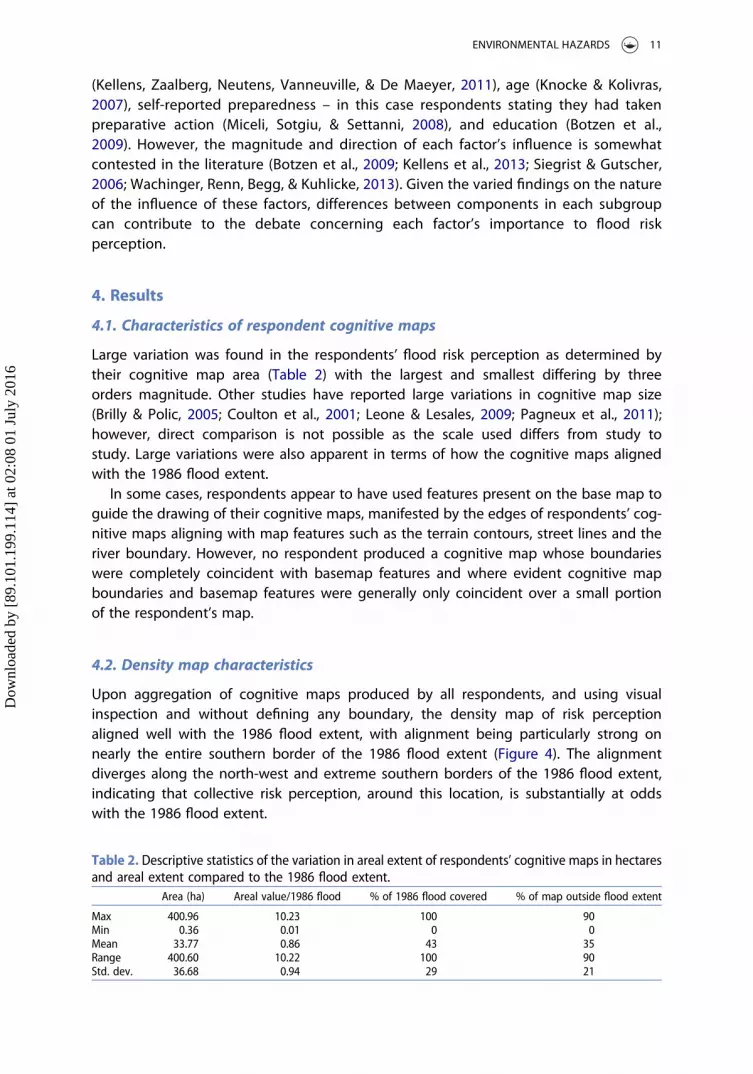
4.1. Characteristics of respondent cognitive maps

Large variation was found in the respondents’ flood risk perception as determined bytheir cognitive map area (Table 2) with the largest and smallest differing by threeorders magnitude. Other studies have reported large variations in cognitive map size(Brilly & Polic, 2005; Coulton et al., 2001; Leone & Lesales, 2009; Pagneux et al., 2011);however, direct comparison is not possible as the scale used differs from study tostudy. Large variations were also apparent in terms of how the cognitive maps alignedwith the 1986 flood extent.

In some cases, respondents appear to have used features present on the base map toguide the drawing of their cognitive maps, manifested by the edges of respondents’ cog-nitive maps aligning with map features such as the terrain contours, street lines and theriver boundary. However, no respondent produced a cognitive map whose boundarieswere completely coincident with basemap features and where evident cognitive mapboundaries and basemap features were generally only coincident over a small portionof the respondent’s map.

4.2. Density map characteristics

Upon aggregation of cognitive maps produced by all respondents, and using visualinspection and without defining any boundary, the density map of risk perceptionaligned well with the 1986 flood extent, with alignment being particularly strong onnearly the entire southern border of the 1986 flood extent (Figure 4). The alignmentdiverges along the north-west and extreme southern borders of the 1986 flood extent,indicating that collective risk perception, around this location, is substantially at oddswith the 1986 flood extent.

Table 2. Descriptive statistics of the variation in areal extent of respondents’ cognitive maps in hectaresand areal extent compared to the 1986 flood extent.

Area (ha) Areal value/1986 flood % of 1986 flood covered % of map outside flood extent

Max 400.96 10.23 100 90Min 0.36 0.01 0 0Mean 33.77 0.86 43 35Range 400.60 10.22 100 90Std. dev. 36.68 0.94 29 21

ENVIRONMENTAL HAZARDS 11

Dow

nloa

ded

by [

89.1

01.1

99.1

14]

at 0

2:08

01

July

201

6

4.2.1. Majority agreementThe majority agreement approach produced a core area of high overlap between res-pondents’ maps, which is coincident with the central region of the 1986 flood extent(Figure 5). This indicates that between 50.1% and 72% of respondents (153/305–222/305) perceive at least this area to be at risk of flooding. This core area (13.88 ha)covered approximately 36% of the 1986 flood extent. In terms of the similarity betweenthe majority agreement shape and the 1986 flood extent, Fuzzy Kappa comparison indi-cates a similarity of 0.53, where a Kappa score of 0.41–0.60 indicates moderate spatialfit (Landis & Koch, 1977). The majority agreement shape acts as a measure of consensus,clearly identifying an area widely agreed to be at risk of flooding. However, the weaknessof this method is that much information is lost in the conversion from density map tomajority threshold shape.

4.2.2. Slope-defined boundariesApplying the slope tool enabled the visualisation of slope breaks within the density map(Figure 6). These slope breaks can be considered as boundaries, in that they denote asharp change in the level of agreement between respondents. As with the densitymap, these boundaries aligned well with the southern border of the 1986 flood extentbut also showed alignment along much of the northern border. The slope-defined

Figure 4. Density map produced from the whole sample of respondents compared to the 1986 floodextent.

12 M. BRENNAN ET AL.

Dow

nloa

ded

by [

89.1

01.1

99.1

14]

at 0

2:08

01

July

201

6

boundaries were not continuous, with alignment between slope-defined boundaries andthe borders of the 1986 flood extent diverging in the north-east and south-west (positionsdenoted as 1, Figure 6). This implies that this is an area where agreement betweenrespondents declines more smoothly with distance from the border of the 1986 floodextent, indicating that there is large variation within the sample population as to wherethey perceive the border of the flood risk zone in the north of the study area. Also, anadditional weaker slope-defined boundary juts into the centre of 1986 flood extent(position 2, Figure 6). This signifies an area where agreement between respondents isdeclining, indicating that there is consensus, erroneously, between some of thesampled population that this area represents an edge to the flood zone. Interestingly, aroad present on the base map is co-located with this erroneous edge, suggestingthat this base map feature may have guided cognitive map construction in some respon-dents. The influence of this map feature was not apparent in the individual cognitivemaps nor the density map, and only became so when the slope-defined boundarieswere created.

As with the density map, the alignment of the southern edges of both the 1986flood extent and the slope-defined boundary may be the result of terrain contoursin this area guiding the respondents’ perception of flood risk. However, as these con-tours form the boundary of the 1986 flood extent, it can be argued that respondentscorrectly aligned their risk perception with these flood-limiting features. Additionally,

Figure 5. Majority agreement area produced from the whole sample of respondents compared to the1986 flood extent.

ENVIRONMENTAL HAZARDS 13

Dow

nloa

ded

by [

89.1

01.1

99.1

14]

at 0

2:08

01

July

201

6

there is good alignment between the slope-defined boundaries and the 1986 floodextent in areas of high population, that is, the centre and south of the study area.In contrast, the areas of least consensus between slope-defined boundary and1986 flood extent (Figure 6, positions 1) are also the least populated areas.

4.3. Population subgroups

4.3.1. Areal comparison and majority agreement shapesThe subgroup analysis results are more difficult to interpret. Visually, it is difficult toidentify significant differences between the density maps generated for subgroup com-ponents. As with the whole sample density map, all subgroup density maps aligned wellwith the southern border of the 1986 flood extent, with alignment tending to be lessstrong with the north, north-west and extreme southern borders of the 1986 floodextent. However, differences between subgroup component majority agreementshapes were immediately apparent (see Table 3, Figures 7–12). Those respondentswho had previous flood experience, in line with the general risk perception literature(Burningham, Fielding, & Thrush, 2008), could be expected to have a better understand-ing of the spatial extent of flood risk compared to those without this experience. Equally,it is unsurprising to find greater appreciation of the spatial extent of flood risk in respon-dents who report being prepared for flooding (Miceli et al., 2008). Although there is

Figure 6. Visualisation of the slope-defined boundaries for the whole sample density map. Alignment isparticularly strong on the southern and north-western boundaries.

14 M. BRENNAN ET AL.

Dow

nloa

ded

by [

89.1

01.1

99.1

14]

at 0

2:08

01

July

201

6

mixed evidence for proximity to hazard influencing risk perception (Hung, 2009; Siegrist& Gutscher, 2006), in this study the majority agreement shape produced by those livingin the flood extent performed far better compared to those living outside both in termsof covering more of the 1986 flood extent and Fuzzy Kappa comparison (Table 1). Therewas only a small difference in performance between the majority agreement shapesproduced by home owners and other tenure types, with home owners producingmajority agreement shapes that performed slightly better, in line with other studies(Burningham et al., 2008; Pelling, 1997). The influence of age was detectable, with themajority agreement shape produced by those over 35 years of age outperformingthat produced by those under 35. Level of education did not produce consistentresults, with the majority agreement shape for the non-college educated coveredslightly more of the 1986 flood extent than their counterparts, although the collegeeducated majority agreement shape was more similar in shape to the 1986 floodextent (Table 3).

4.3.2. Slope-defined boundariesThe slope-defined boundaries highlighted similarities and differences between subgrouppair components. Respondents whose residence was located within the 1986 flood extentproduced slope-defined boundaries that showed stronger alignment with the northernborder of the flood extent compared to respondents living outside the flood extent,suggesting that this collection of respondents had a clearer understanding of the floodzone’s spatial extent. A similar situation was found for respondents who own their resi-dences, those with a third-level education, and those over 35 years of age comparedtheir alternate subgroup components. Uniquely among the subgroup components,those with flood experience did not produce an erroneous slope-defined boundaryjutting into the centre of 1986 flood extent.

While the factors used to define the subgroups are known to influence flood riskperception, generating sloped-defined boundaries for these subgroups provides anovel approach to allow the differences in spatial extent of risk perception to bevisualised.

Table 3. Descriptive statistics of the majority agreement for the subgroup pairs.Respondents (n) Cells (n) Area (ha) % flood extent Fuzzy Kappa value

Residence inside flood extent 116 494 19.76 50.67 0.443Residence outside flood extent 189 257 10.28 26.36 0.220Previously flooded 86 452 18.08 46.36 0.411Not previously flooded 218 299 11.96 30.67 0.269Home owner 227 353 14.12 36.21 0.333Not home owner 71 328 13.12 33.64 0.292Over 35 years old 235 367 14.68 37.64 0.33735 years old and under 67 228 9.12 23.38 0.208Prepared 33 596 23.84 61.13 0.546Non prepared 271 329 13.16 33.74 0.297College educated 141 345 13.80 35.38 0.350Not college educated 163 358 14.32 36.72 0.318Whole sample 305 347 13.88 35.59 0.530

ENVIRONMENTAL HAZARDS 15

Dow

nloa

ded

by [

89.1

01.1

99.1

14]

at 0

2:08

01

July

201

6

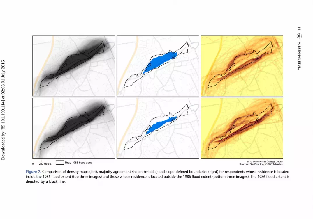
Figure 7. Comparison of density maps (left), majority agreement shapes (middle) and slope-defined boundaries (right) for respondents whose residence is locatedinside the 1986 flood extent (top three images) and those whose residence is located outside the 1986 flood extent (bottom three images). The 1986 flood extent isdenoted by a black line.

16M.BREN

NANET

AL.

Dow

nloa

ded

by [

89.1

01.1

99.1

14]

at 0

2:08

01

July

201

6

Figure 8. Comparison of density maps (left), majority agreement shapes (middle) and slope-defined boundaries (right) for respondents who have experiencedflooding (top three images) and those who have not experienced flooding (bottom three images). The 1986 flood extent is denoted by a black line.

ENVIRO

NMEN

TALHAZARD

S17

Dow

nloa

ded

by [

89.1

01.1

99.1

14]

at 0

2:08

01

July

201

6

Figure 9. Comparison of density maps (left), majority agreement shapes (middle) and slope-defined boundaries (right) for respondents who own their residence(top three images) and those who do not own their residence (bottom three images). The 1986 flood extent is denoted by a black line.

18M.BREN

NANET

AL.

Dow

nloa

ded

by [

89.1

01.1

99.1

14]

at 0

2:08

01

July

201

6

Figure 10. Comparison of density maps (left), majority agreement shapes (middle) and slope-defined boundaries (right) for respondents aged over 35 years old forflooding (top three images) and those aged 35 and under (bottom three images). The 1986 flood extent is denoted by a black line.

ENVIRO

NMEN

TALHAZARD

S19

Dow

nloa

ded

by [

89.1

01.1

99.1

14]

at 0

2:08

01

July

201

6

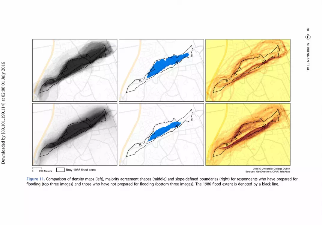
Figure 11. Comparison of density maps (left), majority agreement shapes (middle) and slope-defined boundaries (right) for respondents who have prepared forflooding (top three images) and those who have not prepared for flooding (bottom three images). The 1986 flood extent is denoted by a black line.

20M.BREN

NANET

AL.

Dow

nloa

ded

by [

89.1

01.1

99.1

14]

at 0

2:08

01

July

201

6

Figure 12. Comparison of density maps (left), majority agreement shapes (middle) and slope-defined boundaries (right) for respondents with a third-level edu-cation (top three images) and those without a third-level education (bottom three images). The 1986 flood extent is denoted by a black line.

ENVIRO

NMEN

TALHAZARD

S21

Dow

nloa

ded

by [

89.1

01.1

99.1

14]

at 0

2:08

01

July

201

6

5. Discussion

5.1. Overview

This paper sought to examine the spatial extent of flood risk perception of a residentialpopulation through the creation of a series of density maps, generated by the aggregationof cognitive maps from members of that population as a whole, and several subgroups.Using these subgroups allowed some exploratory analysis of how factors previouslyshown to affect flood risk perception affect the production of density maps in this residen-tial population. This study advanced the analysis of density maps by utilising a novelspatial analytical method (slope analysis) which usefully identifies areas where the respon-dents’ perception of flood risk lacks consensus, and is at odds with expert assessments offlood risk, without the loss of information inherent in a commonly used density map analy-sis technique (majority threshold method).

5.2. Whole sample maps

Individual cognitive maps were aggregated into density maps to produce a visualisation ofthe populations’ spatial extent of risk perception. When this aggregation takes place aninteresting phenomenon occurs. Despite large variation in size, position and shape of indi-vidual cognitive maps, the aggregate risk perception of the sampled population as rep-resented by the density map broadly aligns with the 1986 flood extent. This suggeststhat when the individual cognitive maps are aggregated together, this collection of layknowledge is converging toward the expert assessment of flood risk extent.

Analogous phenomena have been described in other studies and have found that theaggregation of knowledge from a group can be the basis for potentially superior knowl-edge generation, relative to any one individual of that group. The explanation thesestudies provide is that there is error, or ‘noise’, associated with each individual contributionand that when all knowledge/judgements from the group are aggregated then the noise isreduced or eliminated (Yi, Steyvers, Lee, & Dry, 2012). This phenomenon is reported instudies exploring problems concerning ranking, that is, listing entities or events in thecorrect order (Steyvers, Lee, Miller, & Hemmer, 2009), computation, for example, findingthe shortest possible route that visits multiple locations (the travelling salesmanproblem (Yi et al., 2012) and eyewitness reconstruction (Hemmer, Steyvers, & Miller, 2010)).

A comparable process appears to be occurring when individual cognitive maps areaggregated to form density maps. The noise associated with any one individual’s cognitivemap, that is, those areas of the cognitive map outside the 1986 flood extent, is reducedwhen the maps are aggregated – that is, these areas record lower cell values comparedto areas within the 1986 flood extent. Similar effects are evident when the majority agree-ment shapes and slope-defined boundaries are examined. In the majority agreementshapes, areas with low agreement (i.e. ‘noisy’ areas) are simply eliminated from theseshapes. For the slope-defined boundaries, the transition areas from ‘non-noisy’ to ‘noisy’that form boundaries are identified as locations of rapidly changing agreement. Theslope-defined boundaries can be described as ‘fuzzy’ and ‘open’, compared to the ‘crisp’and ‘closed’ boundaries of the majority agreement shape method (Jacquez, Maruca, &Fortin, 2000). While the meaning of ‘open’ and ‘closed’ are self-explanatory (i.e. boundariesthat do not and do enclose an area respectively), ‘fuzzy’ and ‘crisp’ warrant further

22 M. BRENNAN ET AL.

Dow

nloa

ded

by [

89.1

01.1

99.1

14]

at 0

2:08

01

July

201

6

explanation. Here ‘crisp’ boundaries are zero-thickness lines, such as are present at theborders of the majority agreement shapes, whereas ‘fuzzy’ boundaries represent anarea in space. While other studies have noted the disparity between density mapscreated from lay knowledge and expert-generated risk zones (Leone & Lesales, 2009),the use of a slope-defined boundary to identify areas where group-level risk perceptionis unclear and at odds with experts’ assessment represents an advance within cognitivemap literature as we have found no evidence of its use in any other studies.

The density map of the entire sample, coupled with the information from the slope-defined boundary, suggests that, as a group, the sampled respondents have a clear under-standing of the location of almost the entire southern border of the flood extent, as well asthe north-west border. However, both the density map and slope-defined boundarysuggest that the respondents are unclear as to the location of the north-east borderand extreme southern border. Additionally, the presence of a, albeit weaker, slope-defined boundary that juts into the 1986 flood extent (position 2, Figure 6) indicatesthat some of the respondents erroneously consider this area to be an edge to the floodzone.

5.3. Subgroup maps

The combination of methods, density map, majority agreement shape and slope-definedboundary usefully differentiates the subgroup pairs. Respondents who live inside the floodzone (Figure 7) have been flooded before (Figure 8), own their homes (Figure 9), are older(Figure 10), and self-report being prepared for flooding (Figure 11) all produce majorityagreement shapes covering more of the 1986 flood extent and better conforming tothe flood extent compared to their counterparts, as measured by Fuzzy Kappa comparison.Despite the mixed evidence of these factors’ influence on risk perception, our resultssuggest that the above-mentioned groups appear to have higher accuracy in terms ofthe spatial extent of risk perception, though caution should be applied before generalisingthe differences between subgroups results beyond this study.

Comparing the slope-defined boundaries of subgroup pairs gave more nuanced results.As with the whole sample, all subgroup components generated a slope-defined boundarystrongly aligning with the southern border of the 1986 flood extent, with poorer alignmentalong the northern boundaries of the 1986 flood extent. Subgroup components whichproduced higher performing majority agreement shapes also tended to produce slope-defined boundaries which better aligned with the northern borders, whereas the othersubgroup components tended to produce a fuzzy northern boundary throughout the1986 flood extent (see Figures 7–9 and 11). Finally, the presence of a slope-defined bound-ary jutting into the 1986 flood extent is present in most subgroup components (exempli-fied in position 2, Figure 6 for the whole sample), though it is notably absent for thoserespondents who previously experienced flooding (Figure 8, and close up in Figure 13).

5.4. Implications for the use of slope-defined boundaries

In terms of flood risk management in this area, the results described represent a usefulpoint from which awareness-raising interventions may begin. The use of all these tech-niques together allows an assessment of the state of local knowledge, with the results

ENVIRONMENTAL HAZARDS 23

Dow

nloa

ded

by [

89.1

01.1

99.1

14]

at 0

2:08

01

July

201

6

suggesting that the collective lay assessment of flood risk in the study area is broadly (butnot entirely) in line with the expert assessment of flood risk. To maximise the usefulness ofthis collective knowledge, it would be desirable to promote the free flow of this knowl-edge throughout the population (Olsson, Folke, & Berkes, 2004). The subgroup analysissuggests that there are particular groups (e.g. those with flood experience) whosepooled flood knowledge could be usefully mobilised.

The use of slope-defined boundaries is a novel approach in the analysis of densitymaps, and it is argued that this represents an advance compared to the use of the majorityagreement method. While a loss of information occurs when generating either majorityagreement shapes or slope-defined boundaries from density maps (i.e. the numbers ofrespondents agreeing in each cell), more information is retained in the slope-definedboundaries. For example, slope-defined boundaries retain the same areal extent of theoriginal density map, in contrast to the majority agreement shapes which exclude areasof low agreement. Additionally, while both methods identify areas of agreementbetween respondents, slope-defined boundaries allow nuances of agreement (e.g. rapidversus gradual changes in agreement) to be visualised throughout the study site. Considerthe slope-defined boundary map for the whole sample (Figure 6). As noted above, theslope-defined boundaries are well aligned with southern border of the 1986 floodextent, while alignment breaks down in the north-east border, suggesting the

Figure 13. Slope-defined boundaries as displayed in Figure 8 (left) and with magnified sections (right).The top images display slope-defined boundaries generated for respondents who have experiencedflooding, the bottom images display slope-defined boundaries generated for who have not experi-enced flooding.

24 M. BRENNAN ET AL.

Dow

nloa

ded

by [

89.1

01.1

99.1

14]

at 0

2:08

01

July

201

6

respondents are unclear as to the location of the flood extent in this area. This prompts thequestion of why this is the case. One explanation is that this area contains a golf courseand it could be speculated that a lack of access and familiarity with this site results in alack of consensus between respondents as to where in this area would be affected by aflood event. The same factors pertaining to access and/or familiarity may also accountfor the breakdown between slope-defined boundaries and the 1986 flood extent borderin other areas.

5.5. Limitations of the study

Several limitations of this study relating to the interpretation of survey questions,approach to sampling and also data capture and analysis methods must also be noted.

5.5.1. Survey questionThe survey question asked respondents to ‘outline… the likely extent of the area youbelieve would be affected by a severe flood’; it is possible some respondents interpretedthis to include areas indirectly affected by flooding (e.g. a respondent could considerthemselves affected if their own area wasn’t flooded but they could not access servicesin a flooded area) as well as directly affected areas. Additionally, the question makes noreference to numerical probabilities, which, as can be argued, fails to consider thatverbal statements can be more ambiguous than numerical statements (Budescu, Wein-berg, & Wallsten, 1988). However, the increased ambiguity, or not, of verbal over numericalstatements is currently contested in the literature with evidence for (Budescu et al., 1988;Wallsten, Budescu, & Zwick, 1993) and against (Bradford et al., 2012; Ludy & Kondolf, 2012;O’Sullivan et al., 2012). Though initial survey design considered question phrasings usingrisk numerical probabilities, this was not pursued. Instead, the question was framedaround a previous event due to the finding that many respondents preferred risk to beexpressed in terms of previous flood events (O’Sullivan et al., 2012) and framing questionsaround the recollection of previous events benefits from utilisation of flood memory andsharing of local knowledge concerning experience of that event (McEwen & Jones, 2012).Finally, in an Irish context, the Hurricane Charlie event, in addition to being a 1-in-100 yearevent, is seen as a significant flood event, with the national broadcaster in 2013 referringto it as ‘one of the worst hurricanes in Living Memory’.6

5.5.2. SamplingAs respondent distribution was not uniform throughout the study area (Figure 1), this non-uniform distribution could potentially influence respondent risk perception in differentparts of the study area. While this influence may be present, there is evidence against itbeing a predominant factor. All density maps appear to indicate lower consensusbetween respondents as to the northern boundary of the flood extent compared to thesouthern boundary, despite over one-third of the sampled population (n = 139) beinglocated either on the northern border of the flood extent or north of the flood extent. Ifrespondent distribution was a predominant factor, one might expect that the northernboundary would display greater consensus, and this was not found. The non-equalsample sizes of the subgroup components is potentially a cause for concern, as it is con-ceivable that subgroup components with low sample sizes may have insufficient data to

ENVIRONMENTAL HAZARDS 25

Dow

nloa

ded

by [

89.1

01.1

99.1

14]

at 0

2:08

01

July

201

6

cancel out the ‘noise’ associated with each individual’s cognitive map. The average sub-group sample size is 155, with the minimum of 33 and maximum of 271 (Table 3). It is gen-erally accepted that for sample sizes of 30 or more the normality assumptions of meansapproximately holds due to the Central Limit Theorem (Field, 2013). Moreover, statisticaltests usually do not make assumptions about the equality of sample sizes. And in thisstudy, despite the sometimes large differences in subgroup component sample size,there is no obvious effect of sample size. When subgroup pairs are compared, it is oftenthe subgroup component with the lower sample size that produces slope-defined bound-aries which most closely align with the borders of the 1986 flood extent (e.g. see Figures 7,8 and 11).

5.5.3. Data captureThe point can bemade that the respondents were only asked to draw the area they think isat risk of flooding (a specific cognitive mapping task). A question then arises to whetherthis captures risk perceptions more generally, or only perceived exposure or vulnerability.However, it may be overly simplistic to interpret cognitive maps as only portraying per-ceived exposure or perceived vulnerability, as people are influenced affectively whenthey draw their maps (Curtis et al., 2014; Golledge, 2007) and cognitive maps include affec-tive elements of perception (Downs & Stea, 1973; Gould & White, 1973; Lynch, 1960).Additionally, it must be noted that base map features may have influenced the construc-tion of respondent cognitive maps, and hence had an influence on the resulting densityand slope-defined boundary maps. The literature notes that respondent estimations ofenvironmental quality can be influenced by local topography and other physical features(Bonnes, Uzzell, Carrus, & Kelay, 2007) and it appears that a similar effect occurred in somecases here.

5.5.4. Data analysisOne other limitation that arises in this paper relates to the determination of the statisticalsignificance. For each subgroup component, we assess the similarity between its majorityagreement shape and the 1986 flood extent using Fuzzy Kappa comparison. Thus, for eachsubgroup pair, only two Fuzzy Kappa values are being compared. In this context, the tra-ditional measures of statistical significance (e.g. t-test) are not applicable. Although aweakness of this approach, we do not feel that this invalidates its usefulness. Similarly,it is apparent that the use of slope-defined boundaries is not without its limitations.While the slope-defined boundaries allow visualisation and interpretation of patternsinherent in the raw data, the edges of these boundaries must themselves be defined bythe researcher so as to enable future quantitative analysis.

6. Conclusion

The use of slope-defined boundaries represents an advance in the environmental risk per-ception literature, arising from the application of a novel analytical technique to cognitivemaps. The key contribution of slope-defined boundaries is that they allow changes ofrespondent environmental risk perception inherent in the raw data to be visualised andinterpreted, without the loss of nuance and spatial extent inherent in the majority agree-ment method. Despite the limitations noted above, using slope-defined boundaries in

26 M. BRENNAN ET AL.

Dow

nloa

ded

by [

89.1

01.1

99.1

14]

at 0

2:08

01

July

201

6

conjunction with other methods (e.g. density maps) has the potential to contribute toassessments of the spatial extent of risk perception, concerning the state of local knowl-edge and identifying geographic areas where flood risk perception of the populationdiverges from expert assessments of risk. Targeted communication and informationsharing can then take place, so that lay perceptions are informed by expert risk assess-ments and, importantly, local knowledge can be fed back into these expert assessments.

In situations of limited resources, an approach analogous to the one described herecould be of use to give initial indications of flood extent in hydrologically un-surveyedareas. Accounts exist of similar exercises being conducted in developing countries(Hamdi, 2010), though they do not describe if areas are identified where community-level risk perception is lacking in clarity. More generally, this methodology could beapplied to topics which have previously employed cognitive maps to study other elementsof environmental perception. Slope-defined boundaries would add information to suchstudies by visualising boundaries of perception throughout the source density mapextent, locating areas where respondent consensus aligns or diverges with objectivemeasures (e.g. crime figures) and illustrating areas which lack respondent consensusand how these relate to physical features. Additionally, the ‘fuzziness’ inherent in slope-defined boundaries could be considered a truer reflection environmental perception com-pared to the ‘crisp’ boundaries of the majority agreement method. Employing thesemethods with the use of subgroups can usefully identify where variations in environ-mental perception are present (or not) between different sections of a given population,allowing appropriate management responses studies to be undertaken. Finally, whereslope-defined boundaries of environmental perception diverge from objective measures,this could potentially allow cognitive maps to be used to identify areas where a group ofrespondents lack access or familiarity which they might otherwise be expected to have.

Notes

1. Vector data are representations of the world using points, lines, and polygons. They are usefulfor storing data that have discrete boundaries, such as country borders, land parcels andstreets.

2. Rasters consist of matrices of pixels (called cells) arranged in a grid where each cell contains avalue representing information, for example, elevation. Examples include digital photographs,satellite imagery or scanned maps (www.esri.com).

3. Hurricane Charley is the official designation assigned by the World Meteorological Organis-ation. However, it is referenced locally as Hurricane Charlie.

4. The scheme construction is expected to be completed during 2016.5. Georeferening an image means to establish its location in terms of map projections or coor-

dinate systems (Hackeloeer et al., 2014).6. http://www.rte.ie/archives/2013/0826/470307-one-of-the-worst-hurricanes-in-living-memory/

Acknowledgements

This work could not have been accomplished without the extensive manual and digital proces-sing input of Richard Geoghegan and Sean Judge. The authors are very grateful for their assist-ance. Additionally, the authors would very much like to thank Dr Alex Hagen-Zanker of theUniversity of Surrey for his expertise on the use of Fuzzy Kappa statistics. His input is greatlyappreciated.

ENVIRONMENTAL HAZARDS 27

Dow

nloa

ded

by [

89.1

01.1

99.1

14]

at 0

2:08

01

July

201

6

Disclosure statement

No potential conflict of interest was reported by the authors.

Funding

This work formed part of the FLOODPAP project and was supported by UCD Planning & Environ-mental Policy.

ORCiD

Michael Brennan http://orcid.org/0000-0002-5646-028XEoin O’Neill http://orcid.org/0000-0003-3476-161XFinbarr Brereton http://orcid.org/0000-0002-7040-0128Ilda Dreoni http://orcid.org/0000-0001-8420-522XHarutyun Shahumyan http://orcid.org/0000-0001-6247-0954

References

Adger, W. N., Dessai, S., Goulden, M., Hulme, M., Lorenzoni, I., Nelson, D.,…Wreford, A. (2009). Arethere social limits to adaptation to climate change? Climatic Change, 93(3–4), 335–354. doi:10.1007/s10584-008-9520-z

Althaus, C. E. (2005). A disciplinary perspective on the epistemological status of risk. Risk Analysis, 25,567–588.

Aven, T. (2012a). The risk concept – Historical and recent development trends. Reliability Engineeringand System Safety, 99, 33–44.

Aven, T. (2012b). Foundations issues in risk assessment and risk management. Risk Analysis, 32, 1647–1656.

Aven, T., & Kristensen, V. (2005). Perspectives on risk: Review and discussion of the basis for establish-ing a unified and holistic approach. Reliability Engineering and System Safety, 90, 1–14.

Baan, P. J., & Klijn, F. (2004). Flood risk perception and implications for flood risk management in theNetherlands. International Journal of River Basin Management, 2(2), 113–122.

Bonnes, M., Uzzell, D., Carrus, G., & Kelay, T. (2007). Inhabitants’ and experts’ assessments of environ-mental quality for urban sustainability. Journal of Social Issues, 63(1), 59–78. doi:10.1111/j.1540-4560.2007.00496.x

Botzen, W., Aerts, J., & Van Den Bergh, J. (2009). Dependence of flood risk perceptions on socioeco-nomic and objective risk factors. Water Resources Research, 45(10), 1–15.

Bradford, R., O’Sullivan, J., van der Craats, I., Krywkow, J., Rotko, P., Aaltonen, J.,… Schelfaut, K. (2012).Risk perception – Issues for flood management in Europe. Natural Hazards & Earth System Sciences,12(7), 2299–2309.

Bray Town Council, Mitchell and Associates, & McGill Planning. (2007). River Dargle (Bray) flooddefense scheme environmental impact statement. Bray Co. Wicklow: Author.

Brilly, M., & Polic, M. (2005). Public perception of flood risks, flood forecasting and mitigation. NaturalHazards and Earth System Science, 5(3), 345–355.

Brody, S. D., Peck, B. M., & Highfield, W. E. (2004). Examining localized patterns of air quality percep-tion in Texas: A spatial and statistical analysis. Risk Analysis, 24(6), 1561–1574. doi:10.1111/j.0272-4332.2004.00550.x

Bubeck, P., Botzen, W. J. W., & Aerts, J. C. J. H. (2012). A review of risk perceptions and other factorsthat influence flood mitigation behavior. Risk Analysis, 32(9), 1481–1495. doi:10.1111/j.1539-6924.2011.01783.x

Buchecker, M., Ogasa, D. M., & Maidl, E. (2016). How well do the wider public accept integrated floodrisk management? An empirical study in two Swiss alpine valleys. Environmental Science & Policy,55(Part 2), 309–317. doi:10.1016/j.envsci.2015.07.021

28 M. BRENNAN ET AL.

Dow

nloa

ded

by [

89.1

01.1

99.1

14]

at 0

2:08

01

July

201

6

Budescu, D. V., Weinberg, S., & Wallsten, T. S. (1988). Decisions based on numerically and verballyexpressed uncertainties. Journal of Experimental Psychology: Human Perception and Performance,14(2), 281–294. doi:10.1037/0096-1523.14.2.281

Burningham, K., Fielding, J., & Thrush, D. (2008). ‘It’ll never happen to me’: Understanding publicawareness of local flood risk. Disasters, 32(2), 216–238. doi:10.1111/j.1467-7717.2007.01036.x

Campbell, E., Henly, J. R., Elliott, D. S., & Irwin, K. (2009). Subjective constructions of neighborhoodboundaries: Lessons from a qualitative study of four neighborhoods. Journal of Urban Affairs,31, 461–490.

Cassidy, T. (2013). Environmental psychology: Behaviour and experience in context. East Sussex:Psychology Press.

Ceccato, V. A., & Snickars, F. (2000). Adapting GIS technology to the needs of local planning.Environment and Planning B: Planning and Design, 27(6), 923–937.

Chuang, Y. C., Cubbin, C., Ahn, D., & Winkleby, M. A. (2005). Effects of neighbourhood socioeconomicstatus and convenience store concentration on individual level smoking. Journal of Epidemiologyand Community Health, 59(7), 568–573.

Coulton, C., Chan, T., & Mikelbank, K. (2011). Finding place in community change initiatives: Using GISto uncover resident perceptions of their neighborhoods. Journal of Community Practice, 19(1), 10–28. doi:10.1080/10705422.2011.550258

Coulton, C., Jennings, M. Z., & Chan, T. (2013). How big is my neighbourhood? Individual and contex-tual effects on perception of neighbourhood scale. American Journal of Community Psychology, 51,140–150.

Coulton, C., Korbin, J., Chan, T., & Su, M. (2001). Mapping residents’ perceptions of neighborhoodboundaries: A methodological note. American Journal of Community Psychology, 29(2), 371–383.

CSO. (2011). Area profile for town: Bray Egal town and its environs Co. Wicklow. Swords, Co. Dublin:Author.

Curtis, J. W. (2012). Integrating sketch maps with GIS to explore fear of crime in the urban environ-ment: A review of the past and prospects for the future. Cartography and Geographic InformationScience, 39(4), 175–186.

Curtis, J. W., Shiau, E., Lowery, B., Sloane, D., Hennigan, K., & Curtis, A. (2014). The prospects and pro-blems of integrating sketch maps with geographic information systems to understand environ-mental perception: A case study of mapping youth fear in Los Angeles gang neighborhoods.Environment and Planning B: Planning and Design, 41(2), 251–271.

Devlin, A. S. (2012). Environmental perception: 3 wayfinding and spatial cognition. In S. D. Clayton(Ed.), The Oxford handbook of environmental and conservation psychology (p. 41–64). New York:Oxford University Press.

Didelon, C., Ruffray, S. D., Boquet, M., & Lambert, N. (2011). A world of interstices: A fuzzy logicapproach to the analysis of interpretative maps. The Cartographic Journal, 48(2), 100–107.

Ding, W.-J., Wang, R.-Q., Wu, D.-Q., & Liu, J. (2013). Cellular automata model as an intuitive approachto simulate complex land-use changes: An evaluation of two multi-state land-use models in theYellow River Delta. Stochastic Environmental Research and Risk Assessment, 27(4), 899–907.

Downs, R., & Stea, D. (1973). Image and environment. Chicago, IL: Aldine Publishing Company.Dymond, J. R., Derose, R. C., & Harmsworth, G. R. (1995). Automated mapping of land components

from digital elevation data. Earth Surface Processes and Landforms, 20(2), 131–137. doi:10.1002/esp.3290200204

Eiser, J. R., Bostrom, A., Burton, I., Johnston, D. M., McClure, J., Paton, D.,…White, M. P. (2012). Riskinterpretation and action: A conceptual framework for responses to natural hazards.International Journal of Disaster Risk Reduction, 1, 5–16.

Fogarty, M. (2011). 25 years on, Hurricane Charley is remembered. Wicklow People Newspaper.Field, A. (2013). Discovering statistics using IBM SPSS statistics (4th ed.). London: Sage.Gaillard, J.-C. (2008). Alternative paradigms of volcanic risk perception: The case of Mt. Pinatubo in

the Philippines. Journal of Volcanology and Geothermal Research, 172(3), 315–328.Gaillard, J.-C., D’Ercole, R., & Leone, F. (2001). Cartography of population vulnerability to volcanic

hazards and lahars of Mount Pinatubo (Philippines): A case study in Pasig-Potrero River basin (pro-vince of Pampanga) / Cartographie de la vulnérabilité des populations face aux phénomènes

ENVIRONMENTAL HAZARDS 29

Dow

nloa

ded

by [

89.1

01.1

99.1

14]

at 0

2:08

01

July

201

6

volcaniques et aux lahars du Mont Pinatubo (Philippines): cas du bassin de la rivière Pasig-Potrero(province de Pampanga). Géomorphologie: relief, processus, environnement, 7, 209–221.

Golledge, R. G. (2007). Behavioral geography and the theoretical/quantitative revolution.Geographical Analysis, 40, 239–257.

Gould, P., & White, R. (1973). Mental maps. Harmondsworth: Penguin Books.Griffin, R. J., Yang, Z., ter Huurne, E., Boerner, F., Ortiz, S., & Dunwoody, S. (2008). After the flood: Anger,

attribution, and the seeking of information. Science Communication, 29(3), 285–315.Grothmann, T., & Reusswig, F. (2006). People at risk of flooding: Why some residents take precaution-

ary action while others do not. Natural Hazards, 38(1–2), 101–120.Hamdi, N. (2010). The Placemaker’s guide to building community. London: Earthscan.Hamilton, L. C., Hartter, J., Safford, T. G., & Stevens, F. R. (2014). Rural environmental concern: Effects of

position, partisanship, and place. Rural Sociology, 79(2), 257–281.Haynes, K., Barclay, J., & Pidgeon, N. (2007). Volcanic hazard communication using maps: An evalu-

ation of their effectiveness. Bulletin of Volcanology, 70, 123–138.Hemmer, P., Steyvers, M., & Miller, B. (2010). The wisdom of crowds with informative priors. Proceedings

of the 32nd Annual Conference of the Cognitive Science Society, University of California, Irvine, CA.Hung, H. C. (2009). The attitude towards flood insurance purchase when respondents’ preferences

are uncertain: A fuzzy approach. Journal of Risk Research, 12(2), 239–258.Irish Meteorological Service. (1986). August 1986 monthly weather bulletin. Retrieved from. http://

www.met.ieJacquez, G. M., Maruca, S., & Fortin, M. J. (2000). From fields to objects: A review of geographic bound-

ary analysis. Journal of Geographical Systems, 2(3), 221–241. doi:10.1007/pl00011456Kellens, W., Terpstra, T., & De Maeyer, P. (2013). Perception and communication of flood risks: A sys-

tematic review of empirical research. Risk Analysis, 33(1), 24–49. doi:10.1111/j.1539-6924.2012.01844.x

Kellens, W., Zaalberg, R., Neutens, T., Vanneuville, W., & De Maeyer, P. (2011). An analysis of the publicperception of flood risk on the Belgian Coast. Risk Analysis, 31(7), 1055–1068. doi:10.1111/j.1539-6924.2010.01571.x

Keller, C., Siegrist, M., & Gutscher, H. (2006). The role of the affect and availability heuristics in riskcommunication. Risk Analysis, 26(3), 631–639.

Kelly, N. M. (2000). Spatial accuracy assessment of wetland permit data. Cartography and GeographicInformation Science, 27(2), 117–127.

Kim, S.-I., Mutter, L. R., & Westphal, J. M. (1988). Development of a computerized cognitive mappingtechnique for establishing the service area of neighborhood parks. Journal of Park and RecreationAdministration, 6(3), 29–45.

Knocke, E. T., & Kolivras, K. N. (2007). Flash flood awareness in southwest Virginia. Risk Analysis, 27(1),155–169.

Kreibich, H., Thieken, A. H., Grunenberg, H., Ullrich, K., & Sommer, T. (2009). Extent, perception andmitigation of damage due to high groundwater levels in the city of Dresden, Germany. NaturalHazards and Earth System Science, 9(4), 1247–1258. doi:10.5194/nhess-9-1247-2009

Kumar, D. S., Arya, D. S., & Vojinovic, Z. (2013). Modeling of urban growth dynamics and its impact onsurface runoff characteristics. Computers, Environment and Urban Systems, 41, 124–135.

Landis, J. R., & Koch, G. G. (1977). The measurement of observer agreement for categorical data.Biometrics, 33, 159–174.

Leone, F., & Lesales, T. (2009). The interest of cartography for a better perception and management ofvolcanic risk: From scientific to social representations: The case of Mt. Pelée volcano, Martinique(Lesser Antilles). Journal of Volcanology and Geothermal Research, 186(3), 186–194.

Lindell, M. K., & Hwang, S. N. (2008). Households’ perceived personal risk and responses in a multi-hazard environment. Risk Analysis, 28(2), 539–556.

Lohmann, A., & McMurran, G. (2009). Resident-defined neighborhood mapping: Using GIS to analyzephenomenological neighborhoods. Journal of Prevention & Intervention in the Community, 37(1),66–81.

Ludy, J., & Kondolf, G. M. (2012). Flood risk perception in lands ‘protected’ by 100-year levees. NaturalHazards, 61(2), 829–842.

30 M. BRENNAN ET AL.

Dow

nloa

ded

by [

89.1

01.1

99.1

14]

at 0

2:08

01

July

201

6

Lynch, K. (1960). The image of the city. Cambridge: MIT Press.Macharis, C., Witte, A. D., Steenberghen, T., Walle, S. V. D., Lannoy, P., & Polain, C. (2006). Impact and

effectivity of “Free” public transport measures: Lessons from the case study of Brussels. EuropeanTransport / Trasporti Europei, 32, 26–48.

Matei, S., Ball-Rokeach, S. J., & Qiu, J. L. (2001). Fear and misperception of Los Angeles Urban space: Aspatial-statistical study of communication-shaped mental maps. Communication Research, 28,429–463.

Matei, S. A., & Ball-Rokeach, S. (2005). Watts, the 1965 Los Angeles riots, and the communicative con-struction of the fear epicenter of Los Angeles. Communication Monographs, 72(3), 301–323.

McEwen, L., & Jones, O. (2012). Building local/lay flood knowledges into community flood resilienceplanning after the July 2007 floods, Gloucestershire, UK. Hydrology Research, 43(5), 675–688.doi:10.2166/nh.2012.022

Miceli, R., Sotgiu, I., & Settanni, M. (2008). Disaster preparedness and perception of flood risk: A studyin an alpine valley in Italy. Journal of Environmental Psychology, 28(2), 164–173.

Minnery, J., Knight, J., Byrne, J., & Spencer, J. (2009). Bounding neighbourhoods: How do residents doit? Planning Practice & Research, 24(4), 471–493. doi:10.1080/02697450903327170

Olsson, P., Folke, C., & Berkes, F. (2004). Adaptive comanagement for building resilience in social–eco-logical systems. Environmental Management, 34(1), 75–90. doi:10.1007/s00267-003-0101-7

O’Neill, E., Brennan, M., Brereton, F., & Shahumyan, H. (2015). Exploring a spatial statistical approachto quantify flood risk perception using cognitive maps. Natural Hazards, 76(3), 1573–1601.

O’Sullivan, J., Bradford, R., Bonaiuto, M., De Dominicis, S., Rotko, P., Aaltonen, J.,… Langan, S. (2012).Enhancing flood resilience through improved risk communications. Natural Hazards and EarthSystem Science, 12(7), 2271–2282.

Pagneux, E., Gísladóttir, G., & Jónsdóttir, S. (2011). Public perception of flood hazard and flood risk inIceland: A case study in a watershed prone to ice-jam floods. Natural Hazards, 58(1), 269–287.doi:10.1007/s11069-010-9665-8

Pelling, M. (1997). What determines vulnerability to floods: A case study in Georgetown, Guyana.Environment and Urbanization, 9(1), 203–226.

Ratcliffe, J. (2010). Crime mapping: Spatial and temporal challenges. In A. R. Piquero & D. Weisburd(Eds.), Handbook of quantitative criminology (pp. 5–24). New York, NY: Springer.

Ruin, I., Gaillard, J.-C., & Lutoff, C. (2007). How to get there? Assessing motorists’ flash flood risk per-ception on daily itineraries. Environmental Hazards, 7(3), 235–244. doi:10.1016/j.envhaz.2007.07.005

Salazar, D., & D’Ercole, R. (2009). Percepción del riesgo asociado al volcán Cotopaxi y vulnerabilidaden el Valle de Los Chillos (Ecuador). Boletín del Instituto Francés de Estudios Andinos, 38(3), 849–871.

Shahumyan, H., Twumasi, B. O., Convery, S., Foley, R., Vaughan, E., Casey, E.,… Brennan, M. (2009).Data preparation for the MOLAND model application for the greater Dublin region. UrbanInstitute Ireland Working Paper Series, 09/04, 39 p.

Siegrist, M., & Gutscher, H. (2006). Flooding risks: A comparison of lay people’s perceptions andexpert’s assessments in Switzerland. Risk Analysis, 26(4), 971–979. doi:10.1111/j.1539-6924.2006.00792.x

Sjöberg, L. (2000). Factors in Risk Perception. Risk Analysis, 20(1), 1–12. doi:10.1111/0272-4332.00001.Slovic, P. (1987). Perception of risk. Science, 236(4799), 280–285.Slovic, P., Finucane, M. L., Peters, E., & MacGregor, D. G. (2004). Risk as analysis and risk as feelings:

Some thoughts about affect, reason, risk, and rationality. Risk Analysis, 24(2), 311–322.Spoel, P., & Den Hoed, R. C. (2014). Places and people: Rhetorical constructions of ‘community’ in a

Canadian environmental risk assessment. Environmental Communication, 8(3), 267–285. doi:10.1080/17524032.2013.850108

Steyvers, M., Lee, M. D., Miller, B., & Hemmer, P. (2009). The wisdom of crowds in the recollection oforder information. Paper presented at the Advances in Neural Information Processing Systems22 (NIPS 2009), University of California, Irvine, CA.

Stone, J. V. (2001). Risk perception mapping and the Fermi II nuclear power plant: Toward an ethno-graphy of social access to public participation in Great Lakes environmental management.Environmental Science & Policy, 4(4–5), 205–217. doi:10.1016/S1462-9011(01)00029-6

ENVIRONMENTAL HAZARDS 31

Dow

nloa

ded

by [

89.1

01.1

99.1

14]

at 0

2:08

01

July

201

6

Terpstra, T. (2011). Emotions, trust, and perceived risk: Affective and cognitive routes to flood prepa-redness behavior. Risk Analysis, 31(10), 1658–1675.

Twigger-Ross, C., Kashefi, E., Weldon, S., Brooks, K., Deeming, H., Forrest, S.,… Tapsell, S. (2014). Floodresilience community pathfinder evaluation: Rapid evidence assessment. London: Defra.

Wachinger, G., Renn, O., Begg, C., & Kuhlicke, C. (2013). The risk perception paradox—Implications forgovernance and communication of natural hazards. Risk Analysis, 33(6), 1049–1065. doi:10.1111/j.1539-6924.2012.01942.x

Wallsten, T. S., Budescu, D. V., & Zwick, R. (1993). Comparing the calibration and coherence of numeri-cal and verbal probability judgments. Management Science, 39(2), 176–190.

Yi, S. K. M., Steyvers, M., Lee, M. D., & Dry, M. J. (2012). The wisdom of the crowd in combinatorialproblems. Cognitive Science, 36(3), 452–470. doi:10.1111/j.1551-6709.2011.01223.x

Zhang, Y., Hwang, S. N., & Lindell, M. K. (2010). Hazard proximity or risk perception? Evaluating effectsof natural and technological hazards on housing values. Environment and Behavior, 42(5), 597–624.

32 M. BRENNAN ET AL.

Dow

nloa

ded

by [

89.1

01.1

99.1

14]

at 0

2:08

01

July

201

6