endangered butterflies as a model system for managing source
TRANSCRIPT

1.
FINAL REPORT
Endangered Butterflies as a Model System for Managing Source-Sink Dynamics on Department of Defense Lands
SERDP Project RC-2119
NOVEMBER 2017
Elizabeth Crone Tufts University Christine Damiani Institute for Wildlife Studies Nick Haddad WK Kellogg Biological Station- Michigan State University Brian Hudgens Institute for Wildlife Studies William F Morris Duke University Cheryl Schultz Washington State University Vancouver
Distribution Statement A

Page Intentionally Left Blank

This report was prepared under contract to the Department of Defense Strategic Environmental Research and Development Program (SERDP). The publication of this report does not indicate endorsement by the Department of Defense, nor should the contents be construed as reflecting the official policy or position of the Department of Defense. Reference herein to any specific commercial product, process, or service by trade name, trademark, manufacturer, or otherwise, does not necessarily constitute or imply its endorsement, recommendation, or favoring by the Department of Defense.

Page Intentionally Left Blank

REPORT DOCUMENTATION PAGE Form Approved
0MB No. 0704-0188
The public reporting burden for this collection or Information iJ estimated to average 1 hour per response, Including the time for reviewing Instructions. sean:~lng existing data 1011n:es, gathering and maintaining the data needed, and completing and revrewing the colleciion of Information. Send comments regard ng this burden estimate or any other aspect of this collection of Information, Including suggestions for redueing the burden, to Oepartment of Oefense. washlngton Headquarters Services. Directorate for Information Operations and Reports (0704.0188), 1215 Jelferson Oavis Highway, Suite 1204, Arlington, VA 22202-4302, Respondents should be aware that notwithstanding any other provision of law, no person shall be subject to any penalty far failing to comply with a collection of Information ii it does not display a currenUy valid 0MB control number, PLEASE DO NOT RETURN YOUR FORM TO THE ABOVE ADDRESS.
1. REPORT DATE (DD•MM-YYYY) 12. REPORT TYPE 3. DATES COVERED (From - To)
11/30/2017 SERDP Final Report 7/31/2014 -1/30/2018 4. TITLE AND SUBTITLE Sa. CONTRACT NUMBER
Endangered Butterflies as a Model System for Managing Source-Sink Contract 14-C-0044 Dynamics on Department of Defense Lands
Sb. GRANT NUMBER
Sc. PROGRAM ELEMENT NUMBER
6. AUTHOR(S) Sd. PROJECT NUMBER Elizabeth Crone RC-2119
Se. TASK NUMBER
Sf. WORK UNIT NUMBER
7. PERFORMING ORGANIZATION NAME(S) AND ADDRESS(ES) 8. PERFORMING ORGANIZATION Tufts Universtiy REPORT NUMBER
163 Packard Ave., Barnum 016 RC-2119 Medford, MA 02155
9. SPONSORING/MONITORING AGENCY NAME(S) AND ADDRESS(ES) 10. SPONSOR/MONITOR'S ACRONYM(S) Strategic Environmental Research and Development Program SERDP 4800 Mark Center Drive, Suite 17003 Alexandria, VA 22350-3605 11. SPONSOR/MONITOR'S REPORT
NUMBER(S)
RC-2119 12. DISTRIBUTION/AVAILABILITY STATEMENT
Distribution A; unlimited public release
13. SUPPLEMENTARY NOTES
14. ABSTRACT
Through a combination of field studies and state-of-the-art quantitative models, we used three species of endangered butterflies as a model system to rigorously investigate the source-sink dynamics of species being managed on military lands. Butterflies have numerous advantages as models for source-sink dynamics, including rapid generation times and relatively limited dispersal, but they are subject to the same processes that determine source-sink dynamics of longer-lived, more vagile taxa.
15. SUBJECTTERMS
Appalachian brown, Baltimore checkerspot, correlated random walk, Fender's blue, fire, floods, habitat restoration, hardwood removal, herbicide, host plant, life cycle, models, population dynamics, source sink dynamics, spatially explicit individual based model (SEIBM), St. Francis satyr, Taylor's checkerspot
16. SECURITY CLASSIFICATION OF: 17. LIMITATION OF 18. NUMBER
a. REPORT b.ABSTRACT c. THIS PAGE ABSTRACT OF PAGES
UNCLASS UNCLASS UNCLASS UNCLASS 299
19a. NAME OF RESPONSIBLE PERSON
Elizabeth Crone 19b. TELEPHONE NUMBER (Include area code)
617-627-0847
Standard Form 298 (Rev. 8198) Prescribed by ANSI Sid. Z39.18

Page Intentionally Left Blank

1
TABLE OF CONTENTS
List of Figures and Tables......................................................................................................... 4
List of Acronyms............................................................................................................ ……… 9
Keywords.................................................................................................................................... 10
Acknowledgements ................................................................................................................... 10
1 Abstract .................................................................................................................................. 11
1.1 Objective .............................................................................................................................. 11
1.2 Technical Approach ............................................................................................................ 11
1.3 Results ................................................................................................................................. 11
1.4 Benefits ............................................................................................................................... 11
2 Objective................................................................................................................................ 12
2.1 Background.......................................................................................................................... 12
2.1.1 Consequences of Source Sink Dynamics......................................................................... 12
2.1.2 Relevance to DoD............................................................................................................ 16
2.2 Study Species........................................................................................................................ 17
2.2.1 Fender’s Blue Butterfly.................................................................................................... 17
2.2.2 St. Francis’ Satyr/Appalachian Brown Butterfly.............................................................. 18
2.2.3 Taylor’s/ Baltimore Checkerspot...................................................................................... 19
3 Materials and Methods ......................................................................................................... 20
3.1 Fender’s Blue Butterfly......................................................................................................... 20
3.1.1 Statistical Analysis direct planting.................................................................................... 20
3.1.2 Implementation of SEIBMs direct planting…………………………………………….. 23
3.1.3 Model validation and simplification direct planting…………………………………….. 28
3.1.4 Field Data monitoring movement and demography fire management………………….. 28
3.1.5 Statistical analysis fire management…………………………………………………….. 32
3.1.6 Implementation of SEIBMS fire management………………………………………….. 35
3.1.7 Model validation and simplification fire management…………………………………. 54
3.2 Saint Francis’ Satyr/ Appalachian Brown........................................................................... 66
3.2.1 Field Data Hardwood removal/inundation...………………............................................. 66
3.2.2 Monitor movement and demography ……………............................................................ 66
3.2.3 Statistical analysis hardwood removal/inundation............................................................. 69
3.2.4 Documenting predator community...……………………………………………………. 70
2
3.2.5 Refine measurements of vital rates, trends and abundance………………...…………… 71
3.2.6 Implementation of SEIBMS hardwood removal/ inundation............................................ 76
3.2.7 Model validation and simplification hardwood removal/inundation……………………. 77
3.2.8 Scenario Analysis hardwood removal/ inundation……………………………………… 79
3.3 Taylor’s Checkerspot/ Baltimore Checkerspot hostplants & herbicides............................. 81
3.3.1 Monitoring movement and demography: hostplants.............................................. …….. 81
3.3.2 Experimental tests & analysis: herbicides………………………………………………. 93
3.3.3 Minimum patch size and connectivity…………………………………………………… 100
3.3.4 Implementation of SEIBMs.............................................................................................. 115
3.4 Transition Activities............................................................................................................. 128
3.4.1 Review of management actions for TERS......................................................................... 128
3.4.2 Develop user guide to SEIBMs.......................................................................................... 129
3.4.3 Apply tools to additional case studies................................................................................ 130
3.4.4 End User Work Shop.......................................................................................................... 149
4 Results and Discussion........................................................................................................... 150
4.1 Fender’s Blue Butterfly ....................................................................................................... 150
4.1.1 SEIBMs direct planting…………………………………………………………………. 150
4.1.2 Demographic influences of fire…………......................................................................... 161
4.1.3 Time series demographic model of fire effects................................................................. 168
4.1.4 SEIMBs fire management………………………………………………………………. 172
4.2 St Francis’ Satyr/ Appalachian brown.................................................................................. 186
4.2.1 Demographic impacts of inundation and clearing………………………………………. 186
4.2.2 Movement in response to inundation and clearing……………………………………… 190
4.2.3 Predator communities…………………………………………………………………… 192
4.2.4 SEIBMs: Scenario analysis on real landscapes…………………………………………. 195
4.2.5 Refine measurements of vital rates, trends and abundance……………………………… 198
4.3 Taylor’s/ Baltimore Checkerspot......................................................................................... 202
4.3.1 Effects of hostplants…………………………………………………………………….. 202
4.3.2 Effects of herbicide……………………………………………………………………… 211
4.3.3 Minimum patch size and connectivity………………………………………………….. 216
4.3.4 SEIBMs: Scenario analysis on real landscapes………………………………………… 218
4.4 Transition Activities............................................................................................................. 231
4.4.1 Review of management actions for TERS........................................................................ 231
3
4.4.2 User guide to SEIBMs...................................................................................................... 245
4.4.3 Apply tools to additional case studies............................................................................... 253
4.4.5 End User Work Shop........................................................................................................ 275
5 General lessons and tools…………………………………………………………………. 279
5.1 Modeling approaches and statistical tools………………………………………………… 279
5.1.1 GLMMs and parameter estimation……………………………………………………… 279
5.1.2 Analytical tractable source-sink models………………………………………………… 279
5.1.3 Spatially explicit individual based models (SEIBMs)………………………………….. 280
5.2 Cross-species patterns…………………………………………………………………….. 281
4
List of Figures and Tables
Figure 2.1.1-1. The importance of spatial and temporal variation for source-sink-trap dynamics.
Table 2.1.2-1. Representative butterfly species managed on military lands (focal species in the present
study are in bold)
Table 3.1.1-1. AICc model comparison of three population models.
Figure 3.1.1-1. Population dynamics of Fender's blue butterfly at three sites at the Willow Creek preserve.
Table 3.1.2.1. Details of lupine planting scenarios.
Figure 3.1.2.1. Maps of lupine planting scenarios.
Table 3.1.6-1. Kincaid's lupine areas and Fender's blue population sizes at Fern Ridge.
Figure 3.1.6-1. Map of the Fern Ridge metapopulation
Figure 3.1.6-2. Logical flowchart of the adult flight period as a model process.
Table 3.1.6-2. Summary of parameter values.
Figure 3.1.6-3. Logical flowchart of adult-to-adult transitions between flight periods.
Table 3.1.7.1. Summary of logistic and exponential growth models.
Table 3.1.7-2. Summary of logistic and exponential growth models with adjustment term.
Table 3.1.7-3. Summary of residence times and adjusted per-step probabilities of an adult next year for
both growth models.
Table 3.1.7-4. Summary of simulation model predictions with new estimated parameters.
Table 3.1.7-5. Summary of mark-recapture study.
Table 3.1.7-6. Summary of observed connectivity.
Table 3.1.7-7. Summary of mark-recapture analysis.
Figure 3.2.5-1 Second flight period Pollard-Yates counts for Appalachian Brown butterflies from 2014-17
Table 3.2.8-1. Scenarios explored in the SFS SEIBM.
Figure 3.3.1.1-1. Map of site and areas covered by C. glabra and P. lanceolata.
Figure 3.3.1.2-1. Life cycle of E. phaeton, showing parameters used to estimate population growth rates.
Table 3.3.1.2-1. Parameters used to calculate habitat-specific growth rates, and models for estimating
parameters from data collected between 2012 and 2014.
Figure 3.3.3-1. Landscape for Baltimore checkerspot movement models.
Table 3.3.3-1. Estimated parameters and derived variables used to evaluate critical minimum patch size
for Baltimore checkerspot butterfly persistence.
Figure 3.3.4.1-1 Taylor's checkerspot spatially explicit individual-based model diagrams for A) the
endogenous model and B) the exogenous model.
Table 3.3.4.1-1 Parameter values used in the Taylor's checkerspot SEIBM.

5
Figure 3.3.4.1-2 The South Puget Trough study area of western Washington, including the Mima Mounds
Natural Area Preserve and Glacial Heritage Preserve.
Figure 3.3.4.2-1 Estimated Taylor's checkerspot butterfly abundance at a single site in Washington state.
Table 3.3.4-2. Checkerspot movement parameters estimated using generalized linear mixed-effects
models in R.
Table 3.4.3.1-1 Comparison of coefficients of phylogeny model, model with species as a random effect
and species + family as a random effect.
Figure 3.4.3.1-1: Location of field sites for diffusion and density experiment.
Figure 3.4.3.1-2: diffusion and density sampling transect protocol (example) and example of flight paths.
Figure 3.4.3.1-3. Phylogenetic tree of species included in the statistical analyses.
Table 3.4.3.2-1. Edge types studied for each butterfly species
Figure 3.4.3.4-1. Representative examples of simulated landscapes used to study the consequences of
habitat loss, habitat fragmentation, and dispersal ability on source-sink population dynamics.
Figure 4.1.1-1. Population trajectories of scenarios, environmental stochasticity uncorrelated among
patches.
Figure 4.1.1-2. Demographic responses of Fender's blue
Figure 4.1.1-2. Population trajectories of scenarios, environmental stochasticity correlated among patches.
Figure 4.1.1-3. Mean residence time per butterfly for each scenario.
Figure 4.1.1-4. Estimated intrinsic rate of increase values for each scenario with 95% CIs.
Table 4.1.2-1. Models of comparing model structure with effect of prescribed fire to null model with no
effect of fire for eggs, and larvae.
Table 4.1.2-2. Demographic parameters for Fender's blue in relation to time since fire
Table 4.1.2-3. Analyses of FBB movement parameters.
Table 4.1.2-4. Dispersal parameters from burn experiment.
Table 4.1.2-5. Boundary behavior, estimated from GLMMs including random effects of experimental
blocks ('fingers') and fixed effects of lupine patches.
Figure 4.1.3-1. Targeted vs Non-targeted burns as a function of percent habitat burned.
Figure 4.1.3-2. Results of the life table response experiment analysis (LTRE
Figure 4.1.4-1 Metapopulation growth rate response to each fire strategy.
Table 4.1.4-1. Site-level extirpation frequency and extirpation risk.
Figure 4.1.4-2. Site-level population growth rate response to each fire strategy.
Figure 4.1.4-3. Proportion of immigrant eggs in the year after fire.
Figure 4.1.4-4. Site-level proportion of immigrant eggs in the year after fire.
Figure 4.1.4-5. Metapopulation growth rate response to each fire strategy without immigrant eggs.

6
Figure 4.1.4-6. Site-level population growth rate response to each fire strategy without immigrant eggs.
Figure 4.2.1-1. Proportional survival of Satyrodes appalachia eggs and juveniles when protected from
predation or accessible to predators in different restoration treatment types.
Figure 4.2.2-1 Differences in Rn2/n (mean squared displacement per move) between restoration
treatments for our target species, St. Francis' satyr, and our surrogate species, Appalachian Brown.
Figure 4.2.3-1. Average number of dragonfly species observed per day.
Figure 4.2.3-2. Average number of individual dragonflies observed per day.
Figure 4.2.4-1. Mean annual growth rate for each source population scenario and for the three sink
scenarios.
Table 4.2.4-1. Results of the ANOVA analyses for population growth and mean abundance for each of
the Source scenarios.
Figure 4.2.4-2. Mean maximum dispersal distances in each of the source population scenarios for control
and sink simulations.
Figure 4.2.5-1. Means and standard error of St. Francis satyr and Appalachian brown caterpillar survival.
Table 4.2.5-1. Population growth rates for Appalachian browns in all treatment types.
Figure 4.3.1-1. Larval survival rates and number of larvae per nest on C. glabra and P. lanceolate.
Table 4.3.1-1. Most suitable host plant inferred from parameter estimates, i.e., the host plant conferring
higher values of the specified parameter.
Figure 4.3.1-2. Nests in C. glabra and P. lanceolata
Figure 4.3.1-3. Female adult daily survival, and body mass on C. glabra and P. lanceolata, and total
female adult population size from 2012-2014.
Figure 4.3.1-5. Population growth rates with and without adult survival correction, followed by LTRE
analysis with growth rates for C. glabra where each vital rate was replaced with the P. lanceolata value.
Table 4.3.2- 2 Analysis of Species × Hostplant experiment
Figure 4.3.2-1 Results from Graminicide experiment.
Table 4.3.2-1 Results from Species × Hostplant experiment
Figure 4.3.2-2. Results from Species × Hostplant Experiment for gregariousness of larvae as measured by
group size given that they were grouped.
Figure 4.3.2-3. Average number of ants observed per sample.
Figure 4.3.3-1. Baltimore checkerspot butterfly habitat patch size versus population growth rate and 95%
CIs calculated by parametric bootstrapping over all flight and demographic parameters
Figure 4.3.4-1 Mean intrinsic growth rate under the endogenous model with no environmental
stochasticity and the exogenous model with high environmental stochasticity as a function of distance
between patches and number of patches.

7
Figure 4.3.4-3 Coefficient of variation (CV) of total population size as a function of the number of
patches, and distance between patches under the exogenous and endogenous models with correlated or no
environmental stochasticity, or uncorrelated stochasticity.
Figure 4.3.4-4. Individual patch population trajectories for the 2-patch scenario and all inter-patch
distances under the endogenous model with no environmental stochasticity.
Figure 4.4.1-1. Types of habitat management conducted by the 27 managers surveyed, and the types of
management questions they need to address.
Table 4.4.1-1. List of the 26 participating installations, and the species for which managers provided
information on monitoring data.
Table 4.4.1-2. Types of monitoring data collected on DoD installations.
Figure 4.4.1-2. Types and amounts of monitoring data collected on DoD-managed species.
Figure 4.4.1-3. DoD managers' experience and perception of SEIBMs.
Figure 4.4.1-4. Factors that would prevent managers from considering using SEIBMs.
Table 4.4.2-1. Availability of habitat and population size data for the species of interest for 9 SEIBMs
developed to guide habitat management.
Table 4.4.2-2. Survival data available for the species of interest for 9 SEIBMs developed to guide habitat
management.
Table 4.4.2-3. Fecundity data available for the species of interest for 9 SEIBMs developed to guide
habitat management.
Table 4.4.2-4. Movement data available for the species of interest for 9 SEIBMs used for habitat
management.
Figure 4.4.3.1-1. Sample sizes of 25 species included in analyses. Included are those species × land cover
class combinations with at least four complete moves.
Table 4.4.3.1-1. Models testing relationship of diffusion or component parameters (move length, turning
angle or move time) with density.
Figure 4.4.3.1-2. Relationship between diffusion and butterfly density.
Table 4.4.3.1-2. Models testing relationship of diffusion or component parameters (length, turning angle
or time) with density.
Table 4.4.3.1-3: Table of diffusion rates by species.
Figure 4.4.3.2-1 Edge crossing behavior at vegetation edges.
Figure 4.4.3.3-1. Taxonomic distribution of Phyla, Classes, and Orders across species-study
combinations used in our analysis.
Table 4.4.3.3-1. Statistical summary of GLMMs with taxonomic random effects
8
Figure 4.4.3.3-2. Number of studies showing faster movement in lower quality habitat (LQ > HQ), higher
quality habitat (HQ > LQ), or no pattern.
Figure 4.4.3.4-1. Long-term population growth rate of bumble bees under different proportions of natural
landscape and levels of habitat aggregation.
Figure 4.4.3.4-2. Relative population density of bumble bees in natural and agricultural habitats under
different proportions of natural landscape and levels of habitat aggregation.
Figure 4.4.3.4-3. Transient dynamics following immediate conversion of natural habitat to agriculture
assuming landscape was initially completely natural.
Figure 4.4.3.4-4. Transient dynamics following immediate conversion agricultural habitat to natural
habitat assuming landscape was initially completely agricultural.
Table 4.4.3.5-1. Estimated Karner blue dispersal parameters.
Table 4.4.3.5-2. Un-normalized coefficients and standard errors (SE) of multi-state mark-recapture model
for Karner Blue movement across a heterogeneous landscape.
Table 4.4.4-1 Attendees at End-user workshop

9
List of Acronyms
ABB Appalachian Brown Butterfly AFB Air Force Base AIC Akaike Information Criterion ANOVA Analysis of Variance BACI Before After Control Impact BCa Bias-Corrected and Accelerated CI Confidence Interval CJS Cormack-Jolly-Seber Model CV Coefficient of Variation dAIC Difference in Akaike Information Criterion GIS Geographic Information System GLM Generalized Linear Model GLMM Generalized Linear Mixed Models GPS Global Positioning System GR Growth Rate INCA INsect Count Analyzer JAGS Just Another Gibbs Sampler KSS Kierstead, Slobodkin and Skellam LM Linear Model LMM Linear Mixed Model LTRE Life Table Response Experiments MLE Maximum Likelihood Estimate MSARNG Mississippi Army National Guard NAD North American Datum NAS Naval Air Station ODD Overview, Design concepts, Details PMJM Preble's Meadow Jumping Mouse POPAN Population Analysis PVC Polyvinyl chloride PY Pollard-Yates SD Standard Deviation SE Standard Error SEIBM Spatially Explicit Individual-Based Model SELES Spatially-Explicit Landscape Event Simulator SERDP Strategic Environmental Research and Development Program SFS Saint Francis Satyr TERS Threatened, Endangered, or Rare Species USACE United States Army Corps of Engineers USAF United States Air Force USFWS United States Fish and Wildlife Service UTM Universal Trans Mercator

10
Keywords : Appalachian brown, Baltimore checkerspot, correlated random walk, Fender's blue, fire,
floods, habitat restoration, hardwood removal, herbicide, host plant, life cycle, models, population
dynamics, source sink dynamics, spatially explicit individual based model (SEIBM), St. Francis satyr,
Taylor's checkerspot.
11
Abstract
1.1 Background and Objective Background: Department of Defense (DoD) lands provide the best available habitat for numerous threatened, endangered and at-risk species (TER-S), and many of these species are currently managed on military lands by controlled disturbances (e.g. fires) or by de novo restoration of habitat. However, these management strategies run the risk of converting sources (where births exceed deaths) into sinks (where deaths exceed births) or of creating ecological traps - low-quality but attractive restored habitat that bleeds animals from nearby sources, threatening metapopulation viability. In addition, disturbance during and successional changes in habitat quality following management or restoration may lead local habitat patches to cycle from sink to source status and back. Objective: Through a combination of field studies and state-of-the-art quantitative models, we used three species of endangered butterflies as a model system to rigorously investigate the source-sink dynamics of species being managed on military lands. Butterflies have numerous advantages as models for source-sink dynamics, including rapid generation times and relatively limited dispersal, but they are subject to the same processes that determine source-sink dynamics of longer-lived, more vagile taxa. 1.2 Technical Approach: For two of our focal species, we used previous restorations and ongoing management to study temporal source-sink dynamics. For the third, initiated new restoration, allowing us to examine management effects in a controlled experiment. We measured demography and movement at all phases of the disturbance cycle following management or restoration. We used these data to parameterize detailed spatially explicit individual-based simulation models (SEIBMs) linked to real landscapes with dynamic changes in habitat quality due to management. We also validated our general approach by comparing patterns in our focal species to general, cross-taxa, patterns. To further generalize our results, we extended our approach to other TER-S insect populations to inform additional management questions. 1.3 Results: For our focal species work, we found that, in most cases, habitat restoration was creating “source” habitat. In all cases, restoration had both positive and negative effects on individual vital rates, and it was necessary to integrate these effects across the life cycle to calculate the net effects of restoration. Our cross-species analysis broadly validated use of correlated random walk models with edge behavior as a basis for prediction spatial population dynamics, and revealed an important empirical pattern, specifically that animals tend to have faster movement in lower-quality habitat. This pattern means that matrix and sink habitat may increase connectivity in mixed-used landscapes, even when it does not enhance population viability. 1.4 Benefits: Using these field-measured vital rates, we developed system specific simulation models to evaluate different management scenarios. These were presented to local managers at a capstone workshop. Our work also revealed some previously unknown aspects of species biology, including the importance of species interactions (mutualism, competition, and predation) in determining the source-sink status of restoration. In some cases, this understanding immediately redirected management efforts. In others (usually, cases in which our detailed mechanistic studies differed from managers a priori opinions), we hope that this will cause managers to think more carefully about assumptions and perhaps prioritize research to evaluate their expectations, if not immediately changing management. More generally, our case studies demonstrate (1) the importance of measuring vital rates throughout a species life cycle, in the field, in order to assess the impacts of land management, (2) a range of simple to detail-rich modeling approaches for making these assessments, and examples of when such approaches are most useful, and (3) assessment of the main impacts of widely-used restoration tools, including herbicides, fire, artificial dams, and hardwood removal.

12
2 Objective
2.1 Background
2.1.1 Consequences of Source Sink Dynamics
Although abundance and habitat choice are often assumed to be reliable indicators of
habitat quality, ecologists have known for decades that immigration can allow populations to
persist in unsuitable sites (where deaths outnumber births) and that habitat preference does not
necessarily match habitat quality (van Horne 1983, Holt 1985, Pulliam 1988). Adding low-
quality (i.e., sink) habitat to a landscape, as may occur during restoration, may increase or
decrease metapopulation viability (reviewed by Dias 1996, Schlaepfer et al. 2002, Battin 2004,
Gilroy and Sutherland 2007). At one extreme, if animals move to low-quality habitat only when
source habitat is fully occupied, adding sink habitat to a landscape increases overall
metapopulation size and, consequently, viability (Pulliam 1988). At the other extreme, if animals
perceive sink habitat to be high quality, adding sinks to a landscape creates ecological traps that
may lead to extinction of both the source and sink populations (Donovan and Thompson 2001).
Although there is evidence of this most worrisome result - negative impacts of low-quality
habitat on populations in high quality habitat - for birds in fragmented landscapes (e.g., Weldon
and Haddad 2005), as well as from highly contrived experimental situations (e.g., Gundersen et
al. 2001), we know little about whether habitat management and restoration have the potential to
create ecological traps for any species. Furthermore, habitat quality is unlikely to be static in
time; patches that act as sinks in some circumstances may serve as sources in others (cf.
Boughton 1999, Crone et al. 2001). Therefore, improperly classifying sinks as permanent traps
and removing them from the portfolio of management options may reduce the success of
conservation efforts. The conceptual model that underpins our project is that the source-sink
status of habitat patches is dynamic in space and time, and that managers can use knowledge of
13
dynamic sources and sinks to guide habitat restoration and management (Fig. 2.1.1-1).
Our work focused on butterflies, which have proven to be key model species for
understanding spatial ecology, including metapopulations (Hanski 1999, Boggs et al. 2003),
source-sink dynamics (Boughton 1999, 2000), and climate-induced range shifts (Parmesan et al.
1999). Butterflies are an ideal model system for studying source-sink dynamics because their
short life-spans and relatively limited dispersal make it feasible to monitor their population
dynamics and movement over multiple generations within the timeframe of a single study.
Nonetheless, the basic processes of local population growth and dispersal behavior that underlie
butterfly source-sink dynamics are the same ones that govern the dynamics of other species for
which DoD has management responsibility (including amphibians, birds, and large carnivores).
These processes are far more amenable to study in butterflies, so we will develop butterflies as a
model system, then demonstrate the applicability of our approach to vertebrates (see Transition
plan, below). Moreover, as multiple butterfly species are currently targets of management and
habitat restoration efforts on military lands (Table 2.1.2-1), the question of whether such efforts
are creating sources or sinks is directly important to DoD, above and beyond the value of
butterflies as models for other TER-S species.
We investigated the source-sink status of restored and remnant habitat for three
endangered butterfly species found on military lands (Table 2.1.2-1): Fender’s blue butterfly
(FBB, Icaricia icarioides fenderi) in Oregon; the St. Francis’ satyr (SFS, Neonympha mitchellii
francisci) at Ft. Bragg, NC, and the Taylor’s checkerspot butterfly (TCB, Euphydryas editha
taylori) at Ft. Lewis, WA. We proposed to study these 3 species jointly for several reasons.
First, all are species of conservation concern: FBB is found only in remnant prairies in western
Oregon, SFS is known only from Ft. Bragg, and TCB is an endemic species of rapidly

14
disappearing prairies in the Pacific Northwest, with some of its largest populations at Ft. Lewis.
Second, all 3 species are the targets of management and/or restoration efforts that run the risk of
converting sources to sinks or creating traps, at least initially. Third, all 3 species have similar
ecologies: all are historically dependent on habitats created by disturbance (fire in the case of
FBB and TCB, and transient wetlands created by the construction and abandonment of beaver
dams in the case of SFS) and/or on host plants that are themselves disturbance-dependent. Given
this similarity, what we learn about one species may “add value” to studies of the others. Fourth,
members of our team have done extensive work on the first 2 species, but as two separate
research groups; working together will facilitate the application of field and modeling methods
that have been developed for one species to the others. Finally, the third species, on which
neither group has worked in the past, offers the opportunity to assess how well our models can be
extended to other endangered butterflies.
15
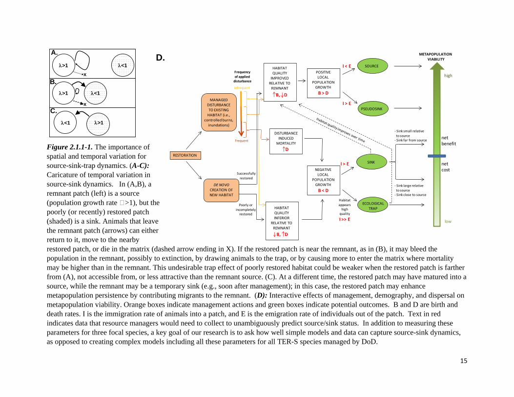
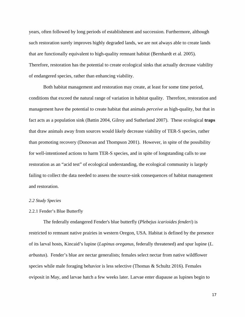
Figure 2.1.1-1. The importance of spatial and temporal variation for source-sink-trap dynamics. (A-C): Caricature of temporal variation in source-sink dynamics. In (A,B), a remnant patch (left) is a source (population growth rate >1), but the poorly (or recently) restored patch (shaded) is a sink. Animals that leave the remnant patch (arrows) can either return to it, move to the nearby restored patch, or die in the matrix (dashed arrow ending in X). If the restored patch is near the remnant, as in (B), it may bleed the population in the remnant, possibly to extinction, by drawing animals to the trap, or by causing more to enter the matrix where mortality may be higher than in the remnant. This undesirable trap effect of poorly restored habitat could be weaker when the restored patch is farther from (A), not accessible from, or less attractive than the remnant source. (C). At a different time, the restored patch may have matured into a source, while the remnant may be a temporary sink (e.g., soon after management); in this case, the restored patch may enhance metapopulation persistence by contributing migrants to the remnant. (D): Interactive effects of management, demography, and dispersal on metapopulation viability. Orange boxes indicate management actions and green boxes indicate potential outcomes. B and D are birth and death rates. I is the immigration rate of animals into a patch, and E is the emigration rate of individuals out of the patch. Text in red indicates data that resource managers would need to collect to unambiguously predict source/sink status. In addition to measuring these parameters for three focal species, a key goal of our research is to ask how well simple models and data can capture source-sink dynamics, as opposed to creating complex models including all these parameters for all TER-S species managed by DoD.
λ>1
λ>1
λ<1
λ<1
λ<1
x
x
A.
B.
C.λ>1
SINK
RESTORATION
POSITIVE LOCAL
POPULATION GROWTH
B > D
NEGATIVE LOCAL
POPULATION GROWTH
B < D
SOURCE
METAPOPULATION VIABILITY
MANAGED DISTURBANCE TO EXISTING
HABITAT (i.e., controlled burns,
inundations)
DE NOVOCREATION OF NEW HABITAT
Frequency of applied
disturbance
infrequent
frequent
HABITAT QUALITY
IMPROVED RELATIVE TO
REMNANT
DB,
DISTURBANCE INDUCED
MORTALITYD
Poorly or incompletely
restored
Successfullyrestored
HABITAT QUALITY INFERIOR
RELATIVE TO REMNANT
B, D
ECOLOGICAL TRAP
PSEUDOSINK
I < E
Habitat appears
high quality
I >> E
I > E
I > E
- Sink small relative to source
- Sink far from source
- Sink large relativeto source
- Sink close to source
high
low
netbenefit
netcost
D.
16
2.1.2 Relevance to DoD
Department of Defense (DoD) lands provide the best available habitat for numerous
threatened, endangered and at-risk (TER-S) species. Many of these species do best on DoD lands
because they require disturbance-dependent habitats such as those created by fires and localized
floods, and DoD resource managers can manage these disturbances with techniques that are
difficult or impossible to employ on private lands. Ideally, such management creates population
sources that increase metapopulation viability. However, habitat management often has both
beneficial and detrimental effects on populations of TER-S species. For example, where fires are
necessary in grasslands to control woody plants and improve habitat quality for wildlife, those
fires often kill animals, particularly less mobile juveniles. In this case, too-frequent management
runs the risk of creating sinks rather than sources.
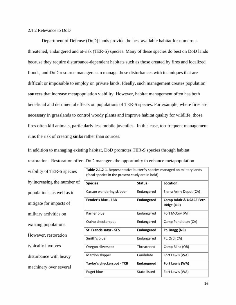
In addition to managing existing habitat, DoD promotes TER-S species through habitat
restoration. Restoration offers DoD managers the opportunity to enhance metapopulation
viability of TER-S species
by increasing the number of
populations, as well as to
mitigate for impacts of
military activities on
existing populations.
However, restoration
typically involves
disturbance with heavy
machinery over several
Table 2.1.2-1. Representative butterfly species managed on military lands (focal species in the present study are in bold)
Species Status Location
Carson wandering skipper Endangered Sierra Army Depot (CA)
Fender’s blue - FBB Endangered Camp Adair & USACE Fern Ridge (OR)
Karner blue Endangered Fort McCoy (WI)
Quino checkerspot Endangered Camp Pendleton (CA)
St. Francis satyr - SFS Endangered Ft. Bragg (NC)
Smith’s blue Endangered Ft. Ord (CA)
Oregon silverspot Threatened Camp Rilea (OR)
Mardon skipper Candidate Fort Lewis (WA)
Taylor’s checkerspot - TCB Endangered Fort Lewis (WA)
Puget blue State-listed Fort Lewis (WA)
17
years, often followed by long periods of establishment and succession. Furthermore, although
such restoration surely improves highly degraded lands, we are not always able to create lands
that are functionally equivalent to high-quality remnant habitat (Bernhardt et al. 2005).
Therefore, restoration has the potential to create ecological sinks that actually decrease viability
of endangered species, rather than enhancing viability.
Both habitat management and restoration may create, at least for some time period,
conditions that exceed the natural range of variation in habitat quality. Therefore, restoration and
management have the potential to create habitat that animals perceive as high-quality, but that in
fact acts as a population sink (Battin 2004, Gilroy and Sutherland 2007). These ecological traps
that draw animals away from sources would likely decrease viability of TER-S species, rather
than promoting recovery (Donovan and Thompson 2001). However, in spite of the possibility
for well-intentioned actions to harm TER-S species, and in spite of longstanding calls to use
restoration as an “acid test” of ecological understanding, the ecological community is largely
failing to collect the data needed to assess the source-sink consequences of habitat management
and restoration.
2.2 Study Species
2.2.1 Fender’s Blue Butterfly
The federally endangered Fender's blue butterfly (Plebejus icarioides fenderi) is
restricted to remnant native prairies in western Oregon, USA. Habitat is defined by the presence
of its larval hosts, Kincaid’s lupine (Lupinus oreganus, federally threatened) and spur lupine (L.
arbustus). Fender’s blue are nectar generalists; females select nectar from native wildflower
species while male foraging behavior is less selective (Thomas & Schultz 2016). Females
oviposit in May, and larvae hatch a few weeks later. Larvae enter diapause as lupines begin to
18
senesce. Post-diapause larvae begin feeding the following spring in March and pupate in April.
Fender’s blue movement can be described as a correlated random walk with preference at patch
boundaries (Schultz 1998, Schultz and Crone 2001), and slower diffusion in breeding habitat
than in matrix (e.g. Schultz 1998, 0.5 m2/s vs 8.6 m2/s). Lifetime displacement is on the scale of
a hundred meters to few kilometers.
2.2.2 St. Francis’ Satyr/Appalachian Brown Butterfly
The St. Francis satyr (Neonympha mitchellii francisci) is a small, brown butterfly that is a
subspecies of Neonympha mitchellii. The St. Francis’ satyr is bivoltine, with adults emerging in
late May through early June, and in late July through early August. Extensive searching has
determined that St. Francis’ satyrs occur only on Fort Bragg military base, located in central
North Carolina (Kuefler et al. 2008). Ft. Bragg is in the Sandhills region, and supports mostly
longleaf pine forest with bottomland hardwood forests along stream floodplains. These streams
dissect much of the terrain, but drainages are often interrupted by dirt roads used as fire breaks
spaced every ≈200 m. Historically, fire played a large role in suppressing woody undergrowth
along stream corridors and maintaining open herbaceous meadows. However, fire suppression is
now common throughout the region. Current management plans at Fort Bragg include burning
the pine understory approximately every three years, and largely exclude fire from riparian
zones.
This stream network is also often modified by beavers, which dam portions of a creek to
create flooded ponds that usually kill most standing hardwoods. Once these dams are abandoned
and flood waters subside, the habitat is ideal for supporting wetland plants such as sedges in the
Carex family. This includes C. mitchelliana, which is thought to be the main host plant for St.
Francis’ satyr larvae based its successful use in captive rearing and its ubiquity in sites where St.
19
Francis’ satyrs are found. Other potential host plants that could support St. Francis’ satyr larvae
include C. lurida and C. atlantica, which larvae will eat in captivity, and C. turgenscens, which
is widespread throughout the wetlands in artillery ranges.
Due to the rarity of St. Francis’ satyrs, a similar species, the Appalachian Brown
(Satyrodes appalachia) is often used in research as a surrogate species. The Appalachian Brown
is a bivoltine butterfly that is dependent on the same wetland habitats as St. Francis’ satyrs and is
locally abundant. The host plants of S. appalachia are thought to be primarily sedge (e.g.,
Carex) species (Kuefler et al. 2008). Previous research has shown the Appalachian Brown to be
an appropriate surrogate to use in place of the St. Francis’ satyr (Hudgens et al. 2012) for which
ethical concerns preclude most experimental manipulation.
2.2.3 Taylor’s/ Baltimore Checkerspot
Text borrowed from Brown & Crone 2016a, 2016b
The Baltimore checkerspot butterfly is the state insect of Maryland (U.S.A.), where
populations are in decline (Frye et al. 2013). It is also ecologically and morphologically similar
to several at-risk checkerspot subspecies, including the federally listed Taylor’s checkerspot
(Euphydryas editha taylori; Bennett et al. 2013, Severns and Breed 2014a), Bay checkerspot (E.
editha bayensis; Wahlberg et al. 2004), and Quino checkerspot (E. editha quino; Mattoni et al.
1997). The Baltimore checkerspot is a univoltine butterfly species occurring in colonies of tens
to thousands of adults in the eastern United States (Scott 1986, Scholtens 1991). Females mate
once and lay clutches of tens to hundreds of eggs on the underside of leaves of one of two host
plant species: the native white turtlehead (Chelone glabra L., Plantaginacae) used throughout the
range, and the introduced English plantain (Plantago lanceolata L., Plantaginaceae) used in parts
20
of the range (Bowers et al. 1992). Gregarious early instar larvae coinhabit silken nests and drop
to the ground in late autumn to overwinter (Bowers et al. 1992). In spring, postdiapause larvae
emerge to feed on nearby host plants and species with similar chemical compounds, pupate, and
emerge as adults in late spring to early summer (Stamp 1982).
3 Materials and Methods
3.1 Fender’s Blue Butterfly
3.1.1 Statistical Analysis direct planting
We used monitoring data from Willow Corner to evaluate whether the 2003 restoration
project caused that population to decline. We hypothesized that planting a strip of native plants
around existing lupine patches created a population sink, because butterflies spent time foraging
in this “nectar buffer”, which lacked larval host plants for oviposition. These behavioral
observations were accompanied by a noticeable decline in butterfly abundance. However, that
decline could have been due to other factors, such as poor weather conditions site-wide, and
cumulative impacts of research on individuals and habitat. To evaluate this hypothesis, we
compared population dynamics at Willow Corner, the restoration site, to two other sites at
Willow Creek, which experienced similar weather conditions but did not have the same kind of
restoration treatment.
We fit three competing models of density independent population growth. First, we
evaluated simple population growth with no systematic changes in growth rate:
Nt = λtN0 eq(1)
Second, if populations crashed in year x, but population growth rate was constant before and
after the crash, then, for t > x, populations should grow (or decline) as follows:
21
Nt = λt-x Nx Ps = λt-x Ps [λxN0] eq(2)
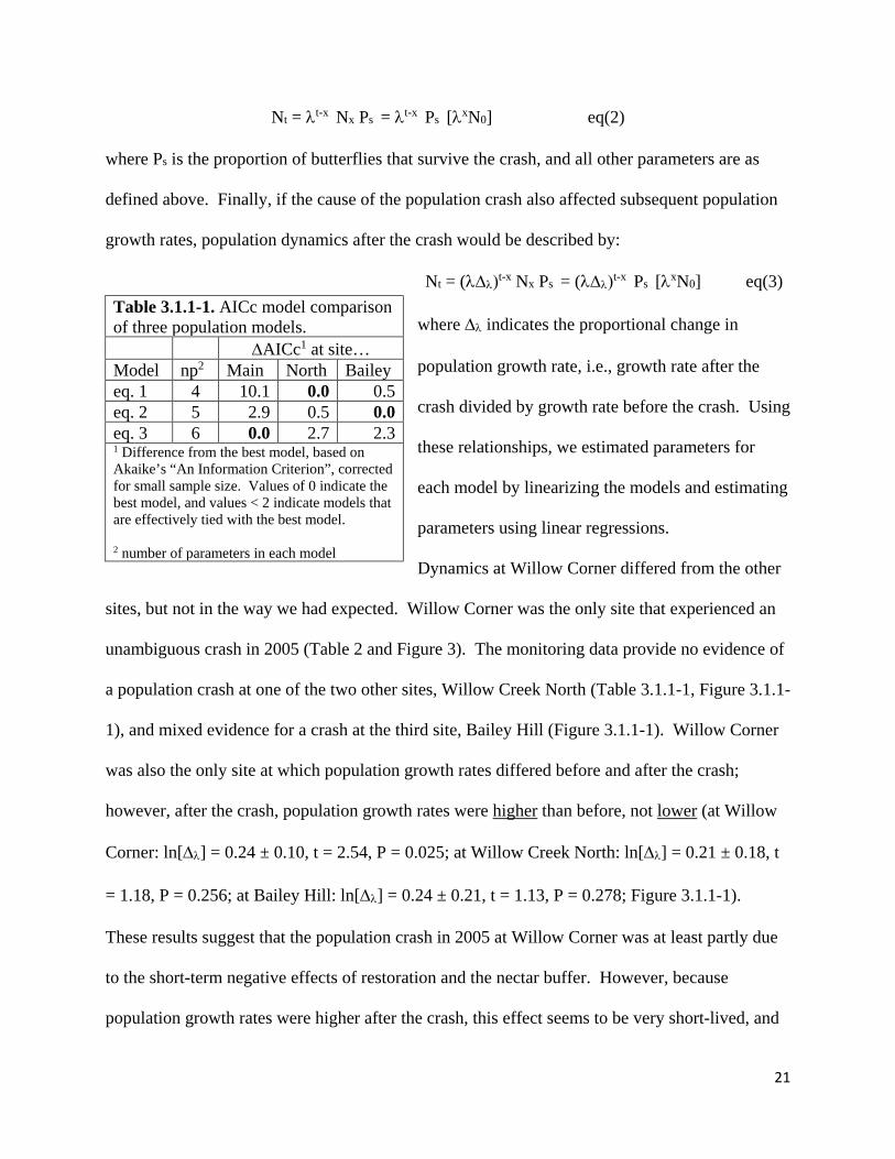
where Ps is the proportion of butterflies that survive the crash, and all other parameters are as
defined above. Finally, if the cause of the population crash also affected subsequent population
growth rates, population dynamics after the crash would be described by:
Nt = (λ∆λ)t-x Nx Ps = (λ∆λ)t-x Ps [λxN0] eq(3)
where ∆λ indicates the proportional change in
population growth rate, i.e., growth rate after the
crash divided by growth rate before the crash. Using
these relationships, we estimated parameters for
each model by linearizing the models and estimating
parameters using linear regressions.
Dynamics at Willow Corner differed from the other
sites, but not in the way we had expected. Willow Corner was the only site that experienced an
unambiguous crash in 2005 (Table 2 and Figure 3). The monitoring data provide no evidence of
a population crash at one of the two other sites, Willow Creek North (Table 3.1.1-1, Figure 3.1.1-
1), and mixed evidence for a crash at the third site, Bailey Hill (Figure 3.1.1-1). Willow Corner
was also the only site at which population growth rates differed before and after the crash;
however, after the crash, population growth rates were higher than before, not lower (at Willow
Corner: ln[∆λ] = 0.24 ± 0.10, t = 2.54, P = 0.025; at Willow Creek North: ln[∆λ] = 0.21 ± 0.18, t
= 1.18, P = 0.256; at Bailey Hill: ln[∆λ] = 0.24 ± 0.21, t = 1.13, P = 0.278; Figure 3.1.1-1).
These results suggest that the population crash in 2005 at Willow Corner was at least partly due
to the short-term negative effects of restoration and the nectar buffer. However, because
population growth rates were higher after the crash, this effect seems to be very short-lived, and
Table 3.1.1-1. AICc model comparison of three population models. ∆AICc1 at site… Model np2 Main North Bailey eq. 1 4 10.1 0.0 0.5 eq. 2 5 2.9 0.5 0.0 eq. 3 6 0.0 2.7 2.3 1 Difference from the best model, based on Akaike’s “An Information Criterion”, corrected for small sample size. Values of 0 indicate the best model, and values < 2 indicate models that are effectively tied with the best model. 2 number of parameters in each model
22
effectively moderated by lupine planting in later years that prevented ecological trap effects of
restoration. In addition, there were management burns at Willow Corner in 2005 and 2007.
Burning would be a plausible alternative hypothesis for a crash in 2005. These fires may be
improving habitat quality and may be partly responsible for faster population growth after the
crash. A final caveat is that patterns are not that different across the three sites. The main
contribution to differences in statistical significance is the size of the error bars, not the values of
the coefficients. In addition, these analyses rule out a hypothesis that had been of concern to
managers, specifically, the idea that research is negatively affecting the Willow Creek
population, since recent population growth rates have been significantly higher than past growth
rates.
Based on this analysis, we explored effects of direct planting, using previously-published
population parameters (Schultz 1998, Schultz & Crone 2001, McIntire et al. 2007), as opposed to
including additional potential effects of ecological traps created by the patterning of Fender’s
blue hostplants in relation to surrounding habitat.
1995 2000 2005 2010
050
010
0015
0
year
est #
but
terfl
ies
1995 2000 2005 2010
050
010
0015
0
year
est #
but
terfl
ies
1995 2000 2005 2010
050
010
0015
0
year
est #
but
terfl
ies
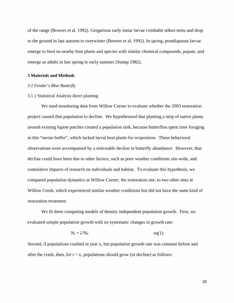
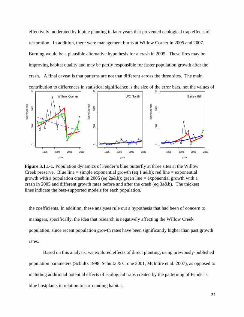
Figure 3.1.1-1. Population dynamics of Fender’s blue butterfly at three sites at the Willow Creek preserve. Blue line = simple exponential growth (eq 1 a&b); red line = exponential growth with a population crash in 2005 (eq 2a&b); green line = exponential growth with a crash in 2005 and different growth rates before and after the crash (eq 3a&b). The thickest lines indicate the best-supported models for each population.
Willow Corner WC North Bailey Hill

23
3.1.2 Implementation of SEIBMs direct planting
3.1.2.1: Model Description
To explore the effects of different planting strategies on Fender’s blue population
dynamics, we developed theoretical landscapes that only contain lupine and prairie habitat. Our
model simulates how a butterfly’s population dynamics respond to four different spatial
scenarios of planting lupine habitat, compares how the responses change with landscape scale,
and further compares how responses change with varying edge behavior and environmental
stochasticity. We used an existing spatially-explicit agent-based model built for Fender’s blue
butterfly (FendNet; McIntire et al. 2007), using the Spatially-Explicit Landscape Event
Simulator (SELES; Fall and Fall 2001) to build and run model simulations. Simulation output
was analyzed using R (R Core Team 2013).
In our model, we track individual butterflies and residence time in lupine. We include
habitat-specific movement modeled as a bias-correlated random walk (Schultz and Crone 2001).
Male behavior differs from female behavior, and because colonization depends only on females,
our model is female-only as in other simulation models with this species (McIntire et al. 2007,
Severns et al. 2013). We incorporate environmental stochasticity estimated from annual
fluctuations in observed population growth rate to account for stochastic population changes
between years (McIntire et al. 2007; Schultz and Hammond 2003). The dimension of time is
tracked as steps (ticks), where one day is equivalent to 140 steps, based on time budget analysis
(Schultz and Crone 2001). Thus, an average flight season of 42 days becomes 5880 steps, and an
average adult lifespan of 15 days becomes 2100 steps. Because most butterflies live an average
of 15 days with a few living much longer, lifespan is drawn from a truncated negative
exponential distribution of 2100 steps at the beginning of each flight period (McIntire et al. 2007;

24
Crone and Schultz 2003). A successful oviposition event is a constant per-step probability of
laying an egg that survives to adult, if a butterfly is in lupine habitat. During model simulation,
butterflies emerge at once and move until either the end of their lifespan, or the end of the flight
season. Butterfly population dynamics and residence time (in steps) in lupine are emergent
properties of habitat-specific behavior.
3.1.2.2: Management Scenarios and Analysis
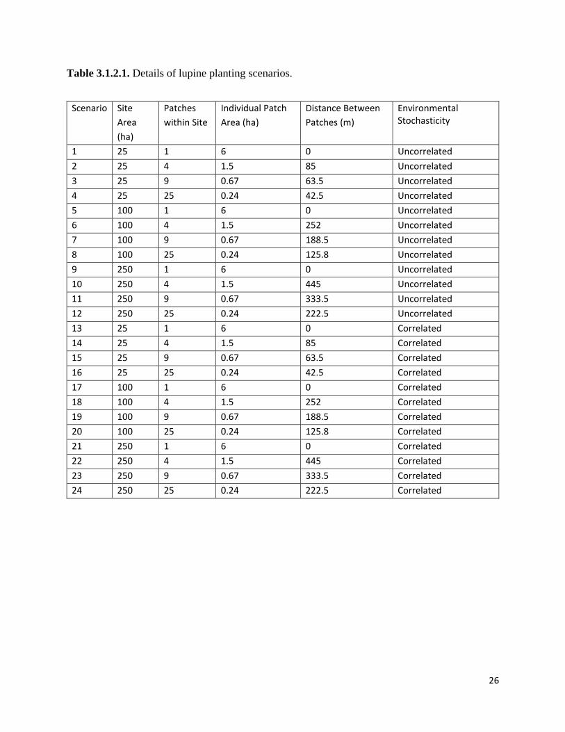
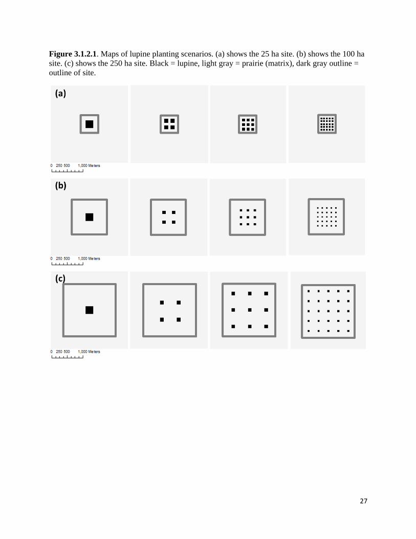
We developed four spatial scenarios of planting lupine habitat within a given landscape,
and designed three landscapes of different scales for each planting scenario (Table 3.1.2.1). Each
planting scenario contained a constant total area of six hectares of lupine, with the degree of
fragmentation (e.g., number of lupine patches) differing among scenarios. In the first scenario,
all six hectares of lupine are planted into a single patch. For the second scenario, four lupine
patches are planted, each with an area of 1.5 hectares. Nine lupine patches are planted in the third
scenario, each with an area of 0.67 hectares. In the fourth scenario, 25 lupine patches are planted,
with each patch having an area of 0.24 hectares. The three landscapes for each scenario are 25
hectares, 100 hectares, and 250 hectares, with lupine patches evenly spread across the landscape.
Thus, in total, we designed a suite of twelve management scenarios (Figure 3.1.2.1).
Each management scenario was repeated twice with differing parameters. In the first
case, environmental stochasticity independently varies for each lupine patch each year. In the
second case, we changed environmental stochasticity to be the same across all lupine patches,
only varying each year. For the third case, environmental stochasticity varies independently for
each patch each year, but we excluded edge behavior at lupine/prairie boundaries. Simulations
were run for 50 years with an initial population of 500 butterflies spread evenly across lupine

25
patches at the beginning of each simulation. We ran 500 replicates of each management scenario
and parameter set.
We analyzed population dynamics over time for each management scenario by
calculating the mean and standard deviation of population size each year over all replicates. To
assess how residence time changes under each scenario, we used a zero-intercept regression to
calculate the mean number of days in lupine per butterfly over all years and all replicates.
Finally, we used a nonlinear least squares approach in R to estimate the intrinsic rate of increase
and 95% confidence intervals for each scenario using a density-dependent population growth
model.
26
Table 3.1.2.1. Details of lupine planting scenarios.
Scenario Site Area (ha)
Patches within Site
Individual Patch Area (ha)
Distance Between Patches (m)
Environmental Stochasticity
1 25 1 6 0 Uncorrelated 2 25 4 1.5 85 Uncorrelated 3 25 9 0.67 63.5 Uncorrelated 4 25 25 0.24 42.5 Uncorrelated 5 100 1 6 0 Uncorrelated 6 100 4 1.5 252 Uncorrelated 7 100 9 0.67 188.5 Uncorrelated 8 100 25 0.24 125.8 Uncorrelated 9 250 1 6 0 Uncorrelated 10 250 4 1.5 445 Uncorrelated 11 250 9 0.67 333.5 Uncorrelated 12 250 25 0.24 222.5 Uncorrelated 13 25 1 6 0 Correlated 14 25 4 1.5 85 Correlated 15 25 9 0.67 63.5 Correlated 16 25 25 0.24 42.5 Correlated 17 100 1 6 0 Correlated 18 100 4 1.5 252 Correlated 19 100 9 0.67 188.5 Correlated 20 100 25 0.24 125.8 Correlated 21 250 1 6 0 Correlated 22 250 4 1.5 445 Correlated 23 250 9 0.67 333.5 Correlated 24 250 25 0.24 222.5 Correlated
27
Figure 3.1.2.1. Maps of lupine planting scenarios. (a) shows the 25 ha site. (b) shows the 100 ha site. (c) shows the 250 ha site. Black = lupine, light gray = prairie (matrix), dark gray outline = outline of site.
28
3.1.3 Model validation and simplification direct planting
3.1.3.1: Model Validation
Our model is calibrated by Fender’s blue biology using parameters estimated in the field
and an existing model framework (Schultz and Crone 2001; McIntire et al. 2007). Because of the
hypothetical nature of the model landscape, we do not have observed field data to compare to
simulation output. However, we were able to use our control scenario, a single six-hectare lupine
patch, to verify simulation output. Specifically, we used residence time predictions of previous
spatial models used to estimate minimum patch size for the species (Crone and Schultz 2003).
Output from simulation matched residence time predictions for a six-hectare patch. Thus, our
model captures the necessary biology to test the effects of different planting scenarios on
butterfly population dynamics.
3.1.4 Field Data monitoring movement and demography fire management
Our study was conducted at Baskett Slough National Wildlife Refuge in Oregon, USA
(44⁰57’N, 123⁰15’W). We located experimental plots in the upland area known as Baskett Butte
where hostplant lupine is comprised of a hybrid population of Kincaid’s and spur lupine (Figure
1, Severns, Meyers & Tran 2012). Baskett Butte encompasses one of few remaining remnants of
Willamette Valley prairie with a Fender’s blue population (USFWS 2010). For the years of our
experiment, 2011-2014, Baskett Butte was estimated to support 700-1900 Fender’s blue
butterflies (Fitzpatrick 2014).
We initiated the experiment in Spring 2011. Pretreatment data were collected in June
2011, prescribed burns were lit in October 2011, and post-treatment data were collected in
Spring 2012, 2013 and 2014. The experiment followed a blocked design with burning assigned
randomly to half of each of four replicate fingers of prairie vegetation located on the west-facing
29
slope of Baskett Butte. Areal extent of burns varied from 0.07 to 0.42 ha based on area within
each prairie finger. Strips of oak woodland separated these blocks. Each replicate contained 20
1m x 1m plots with at least 30% cover of hostplant lupine (total of 2 x 20 x 4 = 160 m2 plots).
One objective of this experiment was to quantify the effects of a cool-season (fall) burn, for
comparison with past analyses based on a hot-season (summer) burn (Schultz & Crone 1998).
Demographic response
Each season, we monitored demographic response by counting eggs in each lupine plot in
June and damaged lupine leaves (an index of post-diapause larvae; Warchola et al. 2015) in each
lupine plot in April. Fender’s blue larvae leave characteristic foraging signs in which they
completely consume emerging lupine leaves before the leaflets expand, leaving short stems with
small remnants of the leaflets. Since larvae are cryptic and difficult to detect, we used
characteristic feeding damage as a measure of larval presence. Larval foraging is an index of
Fender’s blue larva abundance, with an average of 22 damaged leaves per larva (Warchola et al.
2015).
Behavioral response to disturbance
We assessed behavioral response to fire by quantifying adult movement paths in relation
to fire treatments. We released 20 females at random points along each of four burn boundaries
in May-June 2012 and mapped their flight paths (following methods in Schultz 1998). Briefly,
we searched our research area at Baskett Slough, netted butterflies, cooled them and moved them
to the release location, generally moving them less than 50m from the point of capture. Upon
release, we followed butterflies and flagged each location at which the butterfly landed or every
20 seconds while in flight for up to 15 flags. We noted time at each flagged point. We used a
30
Magellan Promark III GPS to locate the position of each flag to the nearest 10 cm. In addition to
flagging each flight path, we created a map of the burn boundary and lupine boundaries with 1 m
accuracy. We calculated length and time of each move step, and turning angle relative to flying
in a straight line as well as habitat burn status and lupine presence at each flag. We used these
flight paths to quantify edge behavior (similar to edge releases in Schultz 1998). Specifically, we
created circles in ArcGIS at 1, 2 and 5 m radius from each release point along the boundary. We
recorded whether the butterfly crossed each circle perimeter into the burned or unburned side.
Analysis of Experimental Data
Demography
We analyzed effects of fire on butterfly demography and movement behavior using
generalized linear mixed models (GLMMs; lme4 package in R, Bates, Maechler & Walker
2015). This analysis breaks the life cycle into two stages: eggs and post-diapause larvae
(estimated from leaf damage, see “Experiment” above). Vital rates are therefore the number of
eggs produced per post-diapause larva, and survival of eggs through diapause to the post-
diapause larval stage. We did not explicitly measure vital rates of the adult life stage because the
scale of adult movement does not correspond to the scale of experimental treatments; these vital
rates are implicitly included by estimating fecundity as the number of eggs in June per post-
diapause larva in April.
We analyzed the number of eggs in June per larva in April (i.e., per capita reproduction)
using Poisson family, log-link GLMMs. Because larvae grow into adults that fly at a larger scale
than the plots, the analysis included larvae from all plots, and egg counts from plots in each
treatment. We included counts at all three time periods (April larvae, June eggs in burned plots,

31
and June larvae in unburned plots) as fixed effects, and manipulated the design matrix of the
GLMM to obtain the ratio of eggs in burned and unburned plots to larvae across both treatment
plots. All models also included random effects of block and an observation-level random effect
to account for overdispersion (Elston et al. 2001). Sample sizes in each year differed slightly:
320 plots (summed across life stages) in 2012, 298 plots in 2013, and 316 in 2014. Differences
were driven by the fact that lupines in individual plots may not re-emerge from roots in all years,
or lupine may be temporarily absent in some plots due to herbivory from voles. In addition to
testing differences among treatments, we used a GLMM to estimate average eggs per larva in
control plots across all years, for use in models for years when we did not collect larval data,
e.g., 2011, the year before the burn. This model included a random effect of year, and an
interaction of stage × year to account for among-year variation in the ratio of eggs per larva.
Following Warchola et al. (2015), we estimated overwinter survival from the ratio of
damaged leaves in April to eggs in the previous June. We estimated this ratio using Poisson
family, log-link GLMMs, with damaged leaves in April as the dependent variable, and ln-
transformed eggs in June as an offset. Models also included burn treatment as a fixed effect, and
effects of burn × block and plot within block as random effects. To scale damaged leaves to the
actual number of larvae, we used the estimated ratio of larvae per damaged leaf in each year
reported by Warchola et al. (2015, their Table S2).
Dispersal behavior
We used Gaussian (normal) family GLMMs with random effects of Path ID (“Butterfly”)
and block (“Finger”) to test whether flight path parameters differed among burned and unburned
areas, lupine and non-lupine patches, and their interactions. Move length, turning angle and
move time were dependent variables. Models also included burn treatment and habitat

32
(lupine/non-lupine) as fixed effects, and random effects of individual butterfly, block and plot
within block as random effects. We tested these effects using marginal (Type II) hypothesis tests
(Anova function in the car package in R, Fox & Weisberg 2011). Move lengths and move times
were log-transformed prior to analysis, and cosines of turning angles were, first, scaled to be
from 0 (180° reversals) to 1 (straight lines), then logit-transformed to approximate normality. We
analyzed the proportion of butterflies that moved to the burned side (relative to 50:50 null
hypothesis), and tested whether this proportion differed between lupine and non-lupine release
points. Analyses were conducted using binomial family, logit link GLMMs, with burn finger as a
random effect (lupine (finger) effects did not improve models, dAIC > 3 for all distances (where
dAIC is the difference in Akaike Information Criterion).
3.1.5 Statistical analysis fire management
Matrix model with succession:
We used our experimental data to construct a model of butterfly population dynamics
with fire and post-fire succession, with demographic differences between habitat stages in the
year of the burn, 1 year post-fire, 2 years post-fire and 3+ years post-fire. We chose this time
scale based on our demographic data. We did not include directed movement toward higher-
quality post-disturbance habitat because we did not observe this behavior. We chose a
deterministic model rather than a stochastic one because we only conducted experimental
burning in one year and cannot estimate year-to-year variability in demographic rates. This
model can be written in a general sense in terms of three processes.
Fire and habitat succession are described by the following transition matrix:

33
𝐵𝐵𝑚𝑚𝑚𝑚 =
⎣⎢⎢⎡
𝑏𝑏0 𝑏𝑏1 𝑏𝑏2 𝑏𝑏3(1 − 𝑏𝑏0) 0 0 0
0 (1 − 𝑏𝑏1) 0 00 0 (1 − 𝑏𝑏2) (1 − 𝑏𝑏3)⎦
⎥⎥⎤
Where bi is the probability of fire i years after a burn, starting with 0 in the year of the burn, and
fire effects last for two years. For most management scenarios, we expect that bi = 0 for all i
except b3 (Scenario 1, below). We also consider cases where b0 = b1 = b2 = b3, i.e., burning
without respect to recent fire history (Scenario 2, below).
The next matrix describes survival of butterflies, as a function of time since fire:
𝑆𝑆𝑚𝑚𝑚𝑚 = �
𝑠𝑠0 0 0 00 𝑠𝑠1 0 00 0 𝑠𝑠2 00 0 0 𝑠𝑠3
�
where si is the survival through diapause of butterflies i years after fire.
The third matrix describes reproduction, and includes transitions from each habitat to
each habitat type, based on movement of adults. In this matrix fi refers to the total fecundity of
individuals who spend time in habitat i. In the absence of local dispersal (an assumption that will
be explored below) and assuming no attraction toward higher-quality habitat, fecundity is
divided among successional stages in proportion to their abundance on the landscape, pi. In a
steady-state system, pi is defined by the leading eigenvector of Bmx, normalized to one:
𝐹𝐹𝑚𝑚𝑚𝑚 = �
𝑓𝑓0𝑝𝑝0 𝑓𝑓0𝑝𝑝0 𝑓𝑓0𝑝𝑝0 𝑓𝑓0𝑝𝑝0𝑓𝑓1𝑝𝑝1 𝑓𝑓1𝑝𝑝1 𝑓𝑓1𝑝𝑝1 𝑓𝑓1𝑝𝑝1𝑓𝑓2𝑝𝑝2 𝑓𝑓2𝑝𝑝2 𝑓𝑓2𝑝𝑝2 𝑓𝑓2𝑝𝑝2𝑓𝑓3𝑝𝑝3 𝑓𝑓3𝑝𝑝3 𝑓𝑓3𝑝𝑝3 𝑓𝑓3𝑝𝑝3
�
Note that an individual’s reproduction depends only on the habitat composition of the landscape,
not on the habitat type where it eclosed. We adjust this model to allow for local dispersal by
34
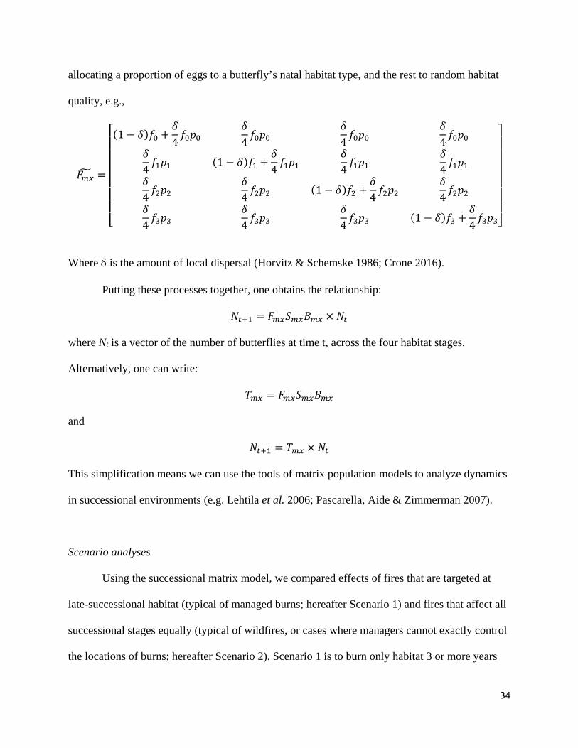
allocating a proportion of eggs to a butterfly’s natal habitat type, and the rest to random habitat
quality, e.g.,
𝐹𝐹𝑚𝑚𝑚𝑚� =
⎣⎢⎢⎢⎢⎢⎢⎡(1 − 𝛿𝛿)𝑓𝑓0 +
𝛿𝛿4𝑓𝑓0𝑝𝑝0
𝛿𝛿4𝑓𝑓0𝑝𝑝0
𝛿𝛿4𝑓𝑓0𝑝𝑝0
𝛿𝛿4𝑓𝑓0𝑝𝑝0
𝛿𝛿4𝑓𝑓1𝑝𝑝1 (1 − 𝛿𝛿)𝑓𝑓1 +
𝛿𝛿4𝑓𝑓1𝑝𝑝1
𝛿𝛿4𝑓𝑓1𝑝𝑝1
𝛿𝛿4𝑓𝑓1𝑝𝑝1
𝛿𝛿4𝑓𝑓2𝑝𝑝2
𝛿𝛿4𝑓𝑓2𝑝𝑝2 (1 − 𝛿𝛿)𝑓𝑓2 +
𝛿𝛿4𝑓𝑓2𝑝𝑝2
𝛿𝛿4𝑓𝑓2𝑝𝑝2
𝛿𝛿4𝑓𝑓3𝑝𝑝3
𝛿𝛿4𝑓𝑓3𝑝𝑝3
𝛿𝛿4𝑓𝑓3𝑝𝑝3 (1 − 𝛿𝛿)𝑓𝑓3 +
𝛿𝛿4𝑓𝑓3𝑝𝑝3⎦
⎥⎥⎥⎥⎥⎥⎤
Where δ is the amount of local dispersal (Horvitz & Schemske 1986; Crone 2016).
Putting these processes together, one obtains the relationship:
𝑁𝑁𝑡𝑡+1 = 𝐹𝐹𝑚𝑚𝑚𝑚𝑆𝑆𝑚𝑚𝑚𝑚𝐵𝐵𝑚𝑚𝑚𝑚 × 𝑁𝑁𝑡𝑡
where Nt is a vector of the number of butterflies at time t, across the four habitat stages.
Alternatively, one can write:
𝑇𝑇𝑚𝑚𝑚𝑚 = 𝐹𝐹𝑚𝑚𝑚𝑚𝑆𝑆𝑚𝑚𝑚𝑚𝐵𝐵𝑚𝑚𝑚𝑚
and
𝑁𝑁𝑡𝑡+1 = 𝑇𝑇𝑚𝑚𝑚𝑚 × 𝑁𝑁𝑡𝑡
This simplification means we can use the tools of matrix population models to analyze dynamics
in successional environments (e.g. Lehtila et al. 2006; Pascarella, Aide & Zimmerman 2007).
Scenario analyses
Using the successional matrix model, we compared effects of fires that are targeted at
late-successional habitat (typical of managed burns; hereafter Scenario 1) and fires that affect all
successional stages equally (typical of wildfires, or cases where managers cannot exactly control
the locations of burns; hereafter Scenario 2). Scenario 1 is to burn only habitat 3 or more years
35
since fire, using bi = 0 for i < 3. Scenario 2 is to burn the same proportion of all habitat types (as
defined by time since burning) in each burn. We compare population growth rate (λ, the long-
term per capita growth rate across all habitat types) across the potential range of habitat burned
(0 to 100% each year) for each strategy. We evaluated the effects of different values of bi (the
proportion of habitat burned) and 𝛿𝛿 (local dispersal) for each scenario. All of the above analyses
are prospective (sensu Caswell 2000) in the sense that they compare the effects of possible future
management when each system is at equilibrium. We also conducted retrospective (sensu
Caswell 2000) analysis of how variation in vital rates affected population viability (life table
response experiments, LTRE, Caswell 1989), modified to our successional model). In the LTRE,
we compare population growth rate with no effects of fire to population growth rates with each
demographic response added individually to the model. For example, in assessing the importance
of fire effects on larval survivorship in the year after the fire, we compared population growth
rate in the model with parameters set at baseline levels without fire to population growth rate in
the model with demographic effect of fire only on larval survivorship in the year after fire. We
evaluated the LTRE using Scenario 1 (late-successional burning only) with b3 set to the optimal
portion of stage 3 successional habitat burned and with Scenario 2 (fire across all habitat,
regardless of time since fire).
3.1.6 Implementation of SEIBMS fire management
3.1.6.1: Study Area
Some of the fastest-growing Fender’s blue populations inhabit four sites surrounding Fern Ridge
Reservoir in Eugene, OR, with metapopulation size reaching approximately 5,810 individuals in
2015 (Fitzpatrick 2015; Table 3.1.6-1). Managers with the U.S. Army Corps of Engineers
36
implement mowing and herbicide application to control invasive grasses and woody species and
are restoring Fender’s blue host plant and nectar species within the sites. Controlled burns are
sometimes applied in the sites, and managers seek to structure burn plans to maximize
metapopulation growth rate (W. Messinger, pers. comm.). Thus, our model landscape includes
the four primary Fender’s blue populations in the Fern Ridge Reservoir metapopulation (Figure
3.1.6-1). We use a 2-meter pixel resolution of the Fern Ridge landscape, mapped using a spatial
reference of NAD 1983 UTM Zone 10N. The landscape is composed of lupine patches, prairie,
open woods, and reservoir. Kincaid’s lupine patches total 1.6 ha in area, ranging from the largest
site containing 0.85 ha to the smallest site containing 0.12 ha (Table 3.1.6-1).
The prairie matrix is characterized by a mosaic of native and invasive prairie grasses and
encroaching woody vegetation. The structure of the forested areas is open, similar to other sites
in the species’ range. Because butterflies behave similarly at the edge of reservoir and at the edge
of wooded areas (Smokey 2016, unpubl. data), for the purposes of our model, we classify the
Fern Ridge Reservoir as open woods. In total, the three habitat types in our landscape are lupine
habitat, prairie matrix, and open woods matrix.
3.1.6.2: Model Description
We follow the ODD (overview, design concepts, details) protocol (Grimm et al. 2006, 2010) to
describe our model and include exhaustive in section 3.1.6.4. Our model simulates how a
butterfly metapopulation’s growth rate responds to three different spatial configurations of fire
disturbance in the landscape, and compares how responses change with intensity of disturbance.
The model distinguishes egg contributions between natal and immigrant butterflies at each site to
test the role of immigrants on population recovery post-fire under each management scenario.
We used NetLogo (Wilensky 1999) to build and run model simulations and R (R Core Team
2013) to analyze simulation output.
37
Male behavior differs from female behavior, and because colonization depends only on
females, our model is female-only as in other simulation models with this species (McIntire et al.
2007, Severns et al. 2013). Controlled burns in the Fender’s blue range occur during autumn,
which is also the timing of historic Native American fires (Hamman et al. 2011). We track
individual butterflies and eggs, fire disturbance on the landscape, residence time for each habitat
type, and connectivity patterns between sites in our model. We distinguish individuals as either
immigrant or natal butterflies, where immigrants are individuals that did not eclose in a given
site, but rather dispersed to it. It follows that natal butterflies are individuals that eclosed in a
given site. Our model includes habitat-specific movement, with boundary crossing behavior at
open woods and reservoir (water) edge (Schultz and Crone 2001; Schultz et al. 2012). Fire
disturbance has a dynamic effect on habitat quality, and impacts growth rate depending on time
since fire. We model this dynamic by incorporating the effects of burning on larval survival and
fecundity into a disturbance multiplier that depends on time since fire. Using vital rate estimates
from experimental burns (Schultz and Crone 1998; Warchola et al., in press), we calculate
population growth rate in treatment i in years since fire b as the product of larval survival
multiplied by fecundity:
𝜆𝜆𝑖𝑖,𝑏𝑏 = 𝑠𝑠𝑖𝑖,𝑏𝑏 × 𝑓𝑓𝑖𝑖,𝑏𝑏 (1)
where λi,b is population growth rate, si,b is larval survival, and fi,b is fecundity. Specifically, b
ranges from 0 to 3, where 0 is the burn year, 1 is one year since fire, 2 is two years since fire, and
3 is three or more years since fire. The disturbance multiplier in year since fire b is then
calculated as the ratio of population growth rate in burn treatments to unburn treatments:
𝐷𝐷𝑏𝑏 = 𝜆𝜆𝐵𝐵,𝑏𝑏𝜆𝜆𝑈𝑈,𝑏𝑏
(2)
38
where Db is the disturbance multiplier, λB,b is the population growth rate in burned areas, and λU,b
is the population growth rate in unburned areas.
We incorporate environmental stochasticity estimated from annual fluctuations in observed
population growth rate to account for stochastic population changes between years (McIntire et
al. 2007; Schultz and Hammond 2003). The dimension of time is tracked as steps (ticks), where
one day is equivalent to 140 steps, based on time budget analysis (Schultz and Crone 2001).
Thus, an average flight season of 42 days becomes 5880 steps, and an average adult lifespan of
15 days becomes 2100 steps. Because most butterflies live an average of 15 days with a few
living much longer, lifespan is drawn from a truncated negative exponential distribution of 2100
steps at the beginning of each flight period (McIntire et al. 2007; Crone and Schultz 2003). A
successful oviposition event is a constant per-step probability of laying an egg that survives to
adult, if a butterfly is in lupine habitat. During model simulation, butterflies emerge at once and
move until either the end of their lifespan, or the end of the flight season. Residence time (in
steps) in lupine of natal and immigrant butterflies are emergent properties of habitat-specific
behavior. Thus, population size in year t+1 becomes:
𝑁𝑁𝑡𝑡+1 = �𝑝𝑝 × 𝑅𝑅𝑁𝑁,𝑡𝑡 + 𝑝𝑝 × 𝑅𝑅𝐼𝐼,𝑡𝑡� × 𝐸𝐸𝑡𝑡 × 𝐷𝐷𝑏𝑏
(3)
where p is per-step probability of successful oviposition, RN,t is the residence time of natal
butterflies, RI,t is the residence time of immigrant butterflies, and Et is environmental
stochasticity.
3.1.6.3: Management Scenarios and Analysis
We developed three spatial scenarios of partitioning lupine habitat for fire disturbance
across the landscape, and chose four years as a constant fire return interval following

39
management suggestions of previous studies (Pickens and Root 2009; Schultz and Crone 1998;
Warchola et al., in press). The first scenario burns all lupine habitat at a site (“whole” scenario)
once every four years. Here, one site is burned every year. The second scenario partitions sites
into halves (“half” scenario), such that half of the lupine habitat is burned within a site once
every other year. In this case, two sites are burned every year. The third scenario partitions sites
into quarters (“quarter” scenario), such that a quarter of the lupine habitat is burned within a site
each year with each quarter being burned every four years. Under this scenario, each site is
burned each year. Burning always occurs in the first year of simulation, and simulations run for
20 years to iterate through five fire return intervals in the landscape. Our model was not sensitive
to initial burning conditions, and model output was similar between the first ten and last ten
years of simulation (unpubl. analysis).
Each scenario was modeled twice, once for early-season burns and once for late-season
burns. Early-season burns in August scorch more of the landscape, and hereafter will be referred
to as “hot” burns. Late-season burns in October are cooler and disturb less of the landscape, and
hereafter will be referred to as “cool” burns. Cool burns are less expensive for managers, and
may be more appealing in conservation plans (M. McKinley, pers. comm.). Thus, we developed
cool burns and hot burns for each of our scenarios. Demographic parameters for fire intensity
come from experimental hot and cool burns (Schultz and Crone 1998; Warchola et al., in press)
in a major Fender’s blue population at Baskett Slough National Wildlife Refuge in Dallas, OR.
In total, we have six fire management scenarios for our model, plus a status quo scenario without
fire disturbance. For each of the seven scenarios, we ran 500 replicates. We then repeated all
seven scenarios using a life-table response experiment approach by removing egg contributions

40
of immigrant butterflies, such that the only contributions to population size in year t+1 are from
natal butterflies.
We analyzed population growth rate response to fire at the metapopulation and site level
for each scenario. Because Fender’s blue is univoltine, we calculated annual geometric growth
rate λ as the ratio of population size in year t+1 to year t. Values were transformed to a log-scale
and we estimated mean yearly geometric growth rate over all years and all simulations for each
scenario. We used standard errors to estimate 95% confidence intervals for these means, and
back-transformed parameter estimates.
To assess the relative contribution of immigrant eggs in the year after fire, we estimated the
proportion ρ of eggs laid by immigrants to all eggs:
𝜌𝜌𝑗𝑗 = 𝑅𝑅𝐼𝐼,𝑗𝑗
𝑅𝑅𝑁𝑁,𝑗𝑗+𝑅𝑅𝐼𝐼,𝑗𝑗 (4)
where ρj is the proportion of immigrant eggs the year after fire in site j, RI,j is the residence time
of immigrants, and RN,j is the residence time of natal butterflies. In this case, natal butterflies are
individuals that survived fire the previous year. To estimate the proportion for the
metapopulation, we added all steps made by immigrant butterflies in sites one year post-fire,
divided by all steps made in those sites one year post-fire, over each fire return interval:
𝜌𝜌𝑚𝑚 = 𝑅𝑅𝐼𝐼,𝑓𝑓+𝑅𝑅𝐼𝐼,𝑓𝑓+1+𝑅𝑅𝐼𝐼,𝑓𝑓+2+𝑅𝑅𝐼𝐼,𝑓𝑓+3(𝑅𝑅𝑁𝑁,𝑓𝑓+𝑅𝑅𝐼𝐼,𝑓𝑓)+(𝑅𝑅𝑁𝑁,𝑓𝑓+1+𝑅𝑅𝐼𝐼,𝑓𝑓+1)+(𝑅𝑅𝑁𝑁,𝑓𝑓+2+𝑅𝑅𝐼𝐼,𝑓𝑓+2)+(𝑅𝑅𝑁𝑁,𝑓𝑓+3+𝑅𝑅𝐼𝐼,𝑓𝑓+3)
(5)
where ρm is the proportion of immigrant eggs the year after fire over the fire return interval, RI,f is
the residence time of immigrants in sites one year post-fire in year f, and RN,f is the residence
time of natal butterflies in sites one year post-fire in year f. Specifically, f is the first year of the
fire return interval, and ranges from 1 to 4. Thus, we accounted for the landscape-scale process
over a full disturbance period.

41
Because the number of eggs is directly proportional to number of moves in habitat, we
translate proportion of steps to proportion of eggs. We assumed a normal distribution for
calculating mean proportions given sufficient replication, and estimated mean proportions for
each site and for the metapopulation over the first three fire return intervals of each scenario.
Given the skew of proportions toward zero, we used bootstrapping to estimate 95% bias-
corrected and accelerated (BCa) confidence intervals using the package simpleboot in R (R Core
Team 2013).
To estimate extirpation risk for each of the four populations for each scenario, we
constructed binomial extirpation probabilities and confidence intervals. Given a sample size of
500 replicates for each scenario, we assumed a successful trial to be at least one extirpation
during a 20-year simulation. Thus, we could estimate the probability of an extinction event in 20
years for each of the four populations and each scenario. In addition, we totaled the number of
times each population was extirpated in each scenario over all 20-year simulations to calculate
extirpation frequency.
3.1.6.4: Detailed Model Protocol
Purpose: Fire disturbance is a powerful tool to maintain early-successional landscapes
for many species. Controlled burns help to maximize the quality of habitat throughout a
landscape. Subdividing a landscape into multiple burn units allows for recolonization after fire,
buffering potential negative mortality impacts across a population. Managers with the U.S. Army
Corps of Engineers are implementing burn plans across four major populations of the
endangered Fender’s blue butterfly. Our model explores how a metapopulation’s growth rate
response to fire disturbance changes between three different spatial configurations of burn units
42
in the landscape. We compare how these responses change between two intensities of fire
disturbance using empirical field data. Finally, we quantify the role of contributions of eggs from
immigrant butterflies on site population recovery post-fire.
State variables and scales: The model comprises four hierarchical levels: individual
butterflies, habitat, management sites, and management subsites. Individuals are given state
variables for identity, lifespan, and identity of the site where the butterfly eclosed. The landscape
is composed of four major sites with independent populations, and it is broken into three major
habitat types. Each site is given state variables for identity, spatial orientation, fire management,
burn year, number of years since a fire event, and environmental stochasticity. Depending on the
fire management variable, sites may remain whole, or be divided into two or four subsites. If a
site is divided into subsites, each subsite is given state variables for identity, burn year, number
of years since a fire event, and environmental stochasticity. The three major habitat types are
lupine, prairie, and open woods. Each habitat is given state variables for step length, turning
angle, and residence time of individuals in the habitat. Lupine is given an additional state
variable for per-step probability of oviposition.
Fire disturbance introduces a dynamic effect of habitat quality, which is implemented in
the model as growth rate multipliers. Depending on a site’s or subsite’s number of years since a
fire event, the population next year is affected by a growth rate multiplier. Four growth rate
multipliers are used: burn year, 1 year post-fire, 2 years post-fire, and 3+ years post-fire.
Multipliers are estimated from butterfly vital rates using empirical field data from an
experimental burn (Schultz and Crone 1998; Warchola et al., in press). Detailed explanations of
these vital rates and calculations for growth rate multipliers can be found in Warchola et al. (in
press).

43
The model depicts the Fern Ridge landscape in Eugene, OR. Four major Fender’s blue
butterfly populations are present in the landscape, and each population is considered one
management unit. The left, top, right, and bottom extents of the model world are 477329,
4884321, 481218, and 4880955, respectively, in units of meters and spatial reference of NAD
1983 UTM Zone 10N. The world grid is 1944 by 1682 boxes mapped at a 2-meter pixel
resolution, with each pixel representing one of three habitat types. Previous agent-based models
with the Fender’s blue butterfly have used both 1-meter and 2-meter pixel resolutions, which
correspond to the resolution of both host plant mapping in the landscape and the scale of
butterfly movement when tracked in the field. Length of time in the model is tracked as steps
(ticks), where 140 steps is equivalent to one day. A flight season is defined as 5880 steps, or ~39
days. This temporal resolution is retained from previous agent-based models with the butterfly
(McIntire et al. 2007).
Process overview and scheduling: Each simulation year is broken into 5880 time steps
(ticks) that represent an average flight season of ~39 days. A site’s fire management, burn year,
and initial population size is chosen at the beginning of each simulation, and each site or subsite
updates its years since fire disturbance at the end of each flight period. At the beginning of each
flight season, all butterflies emerge at once. During each time step, butterflies move, oviposit if
on lupine patch, or die if at the end of their lifespan. Habitats update residence times and
butterflies update the identity of their last site of residence. At the end of the flight season, any
remaining butterflies still alive are killed. Environmental stochasticity is drawn for each site at
the end of each flight period and, if applicable to the scenario, applied to subsites. The model
counts all eggs laid at each site or subsite, adjusts the count depending on the site or subsite’s
environmental stochasticity for that year, and then adjusts the count depending on the site or

44
subsite’s time since fire disturbance. The adjusted counts become the next year’s population.
Thus, population dynamics in the model use annual adult-to-adult transitions. The model iterates
in this fashion for a total of 20 simulation years.
Design concepts: The basic principles of the model are that individuals move through the
landscape with habitat-specific parameters, have some per-step probability of laying an egg that
produces an adult next year if on lupine habitat, and die at the end of their lifespan. Management
scenarios divide sites in the landscape into respective burn units with corresponding timings of
fire disturbance. The effects of fire on larval mortality and fecundity are incorporated into
growth rate multipliers based on time since fire, such that the model applies the necessary
demographic effects of fire depending on the timing and location of a population in the
landscape.
Population dynamics, movement, and metapopulation processes emerge as a result of the
adaptive modeling process. Specific emergent dynamics include growth rate and spatial
distribution of the total population in each simulation year.
Individuals are not given adaptive traits and do not make decisions that either directly or
indirectly improve their fitness, nor do individuals estimate consequences of their decisions.
Thus, the model does not attempt to quantify the fitness consequences of individual behaviors or
assume that those behaviors affect individual fitness.
Individuals are able to sense the type of habitat they are on, and if they draw a move that
crosses a boundary. Thus, individual butterflies move and oviposit according to the habitat in the
landscape. Individuals sense the identity of the site or subsite they are on, thus quantifying where
butterflies disperse in the landscape.

45
There is no interaction between individuals and individuals do not form social groups.
The model is female-only and does not implement any interaction among individuals.
Demographic and movement parameters are represented as probabilities or drawn from
empirical probability distributions. Movement processes are drawn from exponential and
wrapped normal empirical probability distributions for step lengths and turning angles,
respectively (McIntire et al. 2007; Schultz and Crone 2001). Crossing into open woods habitat is
a probabilistic event (Schultz et al. 2012). Movement in lupine edge is modeled as a bias-
correlated random walk (Schultz and Crone 2001). When a butterfly is on a lupine patch,
oviposition is probabilistic. Negative exponential and log-normal empirical probability
distributions are used when drawing lifespan and environmental stochasticity, respectively
(McIntire et al. 2007). For probabilistic events, the model compares input probabilities with
output from a randomly generated number between 0-1. If the random number is less than the
input probability, the event occurs.
At the end of each simulation year, the model records counts of eggs laid by site and
subsite. The counts are adjusted for environmental stochasticity, followed by a growth rate
multiplier for years since fire disturbance. This allows us to observe adult-to-adult transitions and
extinction/colonization events in each year across the various locations of the landscape. From
this, we can calculate mean geometric growth rate and tally extinction events. Through a
simulation year, the model updates the number of moves made by butterflies in habitat by site.
These moves are counted both for immigrant butterflies (butterflies that did not eclose,
but rather flew to the site) and natal butterflies (butterflies that did eclose in the site), and sums
reported at the end of each simulation year. This allows us to calculate mean proportion of eggs
laid by immigrant butterflies in all years of simulation. In addition, the model updates the

46
number of moves made by immigrant butterflies to a site during each step of a simulation year,
allowing us to observe dispersal events through the landscape.
Initialization: During model initialization, the landscape is loaded, the fire regime is set,
and butterflies are added to the landscape. Habitat types in the landscape are constant for each
scenario. Depending on the scenario, the fire regime will differ, and partition sites into subsites
appropriately. Individual butterflies are added to each site at given starting populations,
randomly moving to lupine patches within the site and drawing unique lifespans from a truncated
negative exponential distribution with a mean of 2100 time steps. The identity of the site where a
butterfly lives updates at the beginning of the simulation and for each time step, such that
movement between sites can be quantified during simulation.
Input: Major inputs for the model include the Fern Ridge landscape, starting population
sizes from 2009 survey data, and movement parameters and demographic vital rates. The model
depicts the Fern Ridge landscape in Eugene, OR with left, top, right, and bottom extents of the
model world 477329, 4884321, 481218, and 4880955, respectively, in units of meters and spatial
reference of NAD 1983 UTM Zone 10N. Starting population sizes are 242 for Shore Lane, 188
for Spires Lane, 210 for Eaton Lane, and 580 for Green Oaks; these numbers are constant at the
beginning of each simulation regardless of fire scenario and come directly from population
surveys (Fitzpatrick 2015). Parameter estimation for movement rules is found in McIntire et al.
(2007), Schultz and Crone (2001), and Schultz et al. (2012). See Table 3.1.6-2 for a complete list
of input variables.
Submodels: The model reads in the raster landscape and assigns color-coding and patch-
only variables: a patch’s site number, subsite number, habitat type, direction (in degrees) to the
closest lupine patch, residence time, natal residence time, immigrant residence time, and

47
connectivity tracking variable. The site number identifies a lupine patch as belonging to one of
four major sites. The subsite number identifies a lupine patch as belonging to one of four
quadrants of a major site. The habitat type identifies a pixel as prairie matrix, open woods
matrix, lupine edge, or lupine. Direction identifies a patch’s direction to the closest lupine pixel,
a value used in movement rules. Residence time tracks the total number of butterfly steps spent
in a patch. Natal residence time tracks the total number of butterfly steps spent in a patch where
the patch’s site and the butterfly’s site of eclosure are the same. Immigrant residence time tracks
the total number of butterfly steps spent in a patch where the patch’s site and the butterfly’s site
of eclosure are different. The connectivity tracking variable is a unique number given to
individuals, updated at every tick such that the model tallies when a butterfly has moved to a
different site (e.g., a dispersal event). Finally, each patch within a site or subsite is given a time
since fire variable.
At the beginning of each simulation, butterflies are given turtle-only variables: lifespan,
natal site, and recent site. Lifespan is based off of a truncated negative exponential probability
distribution with a mean of 2100 steps, and butterflies die when at the end of their lifespan or
when the simulation year is over at 5880 steps. Butterflies are given identities for the site in
which they eclosed, and during each step, the variable identifying their most recent site is
updated for use in tracking dispersal events.
Depending on the fire scenario, the fire regime will partition sites into subsites. In the
case of a whole fire scenario, sites are not partitioned and subsite-level tracking is not used. In
the case of a half fire scenario, sites are partitioned into halves using numerical identifiers in the
raster map such that approximately 50% of each site’s lupine habitat is in each subsite. In the
case of the quarter fire scenario, sites are partitioned into quarters using numerical identifiers in

48
the raster map such that approximately 25% of each site’s lupine habitat is in each subsite. The
timing for each initial burn in the landscape is dependent on the fire scenario. The time since fire
disturbance is set at the beginning of simulation (depending on fire scenario) and updated at the
end of each year of simulation. If the time since fire variable equals zero, a patch is burned in
that year.
Movement processes are drawn from exponential and wrapped normal empirical
probability distributions for step lengths and turning angles, respectively (McIntire et al. 2007;
Schultz and Crone 2001). Crossing into open woods habitat is a probabilistic event (Schultz et al.
2012). Movement in lupine edge is modeled as a bias-correlated random walk (Schultz and
Crone 2001). When a butterfly is on a lupine patch, oviposition is probabilistic. During each
dispersal step, butterflies update their variable for most recent site and update the residence time
for the habitat patch they are on. If the butterfly moves to a different site in a given step, it
updates a global list for tracking dispersal events between sites. See Figure 3.1.6-2 for a visual.
The model tracks population-level changes between each flight season of 5880 steps. At the end
of the flight season, the model draws environmental stochasticity for each site based on a log-
normal distribution with a mean of 0 and variance of 0.6 (McIntire et al. 2007). Counts of eggs
occur by site or subsite depending on the fire regime, and the value for environmental
stochasticity is multiplied to the count. Depending on the fire regime and time since fire, a
disturbance growth rate multiplier is applied to the counts which become the starting population
for the next year of simulation. During this submodel, the model resets global lists used in
tracking, updates time since fire for each site/subsite, and records output. See Figure 3.1.6-3 for a
visual.
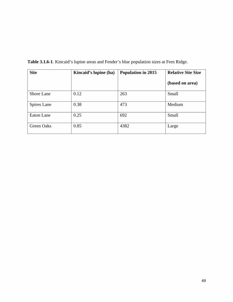
49
Table 3.1.6-1. Kincaid’s lupine areas and Fender’s blue population sizes at Fern Ridge.
Site Kincaid’s lupine (ha) Population in 2015 Relative Site Size
(based on area)
Shore Lane 0.12 263 Small
Spires Lane 0.38 473 Medium
Eaton Lane 0.25 692 Small
Green Oaks 0.85 4382 Large
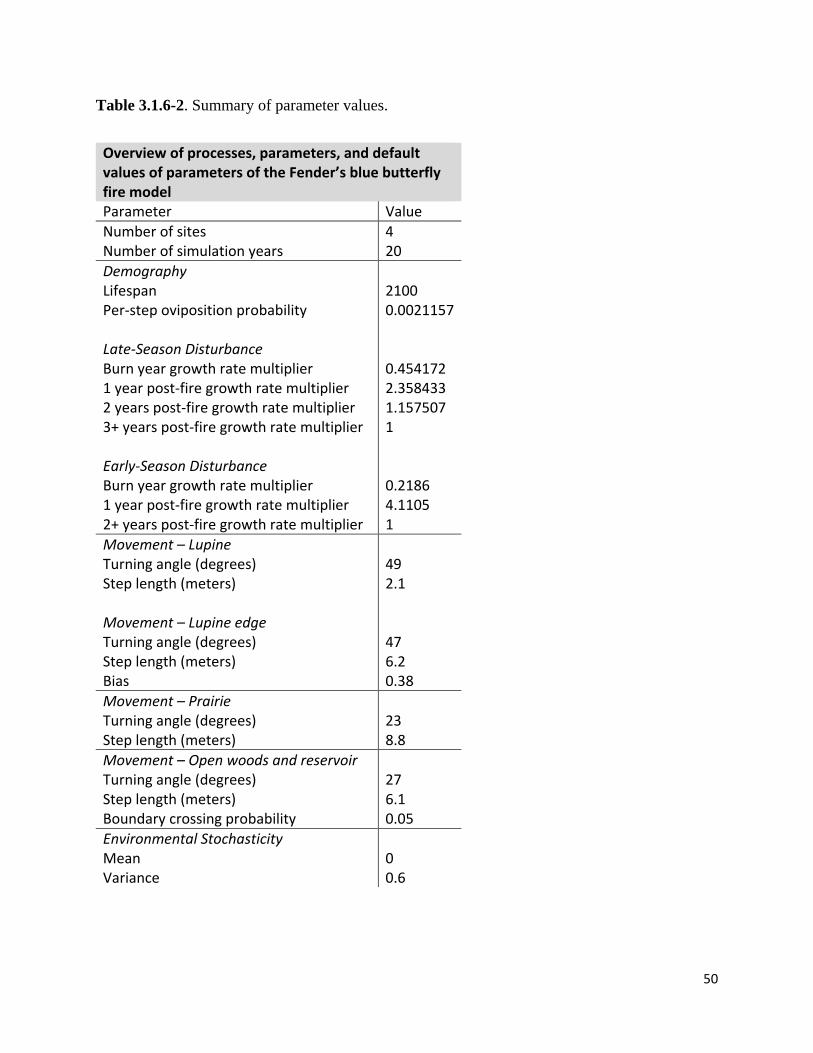
50
Table 3.1.6-2. Summary of parameter values.
Overview of processes, parameters, and default values of parameters of the Fender’s blue butterfly fire model Parameter Value Number of sites Number of simulation years
4 20
Demography Lifespan Per-step oviposition probability Late-Season Disturbance Burn year growth rate multiplier 1 year post-fire growth rate multiplier 2 years post-fire growth rate multiplier 3+ years post-fire growth rate multiplier Early-Season Disturbance Burn year growth rate multiplier 1 year post-fire growth rate multiplier 2+ years post-fire growth rate multiplier
2100 0.0021157 0.454172 2.358433 1.157507 1 0.2186 4.1105 1
Movement – Lupine Turning angle (degrees) Step length (meters) Movement – Lupine edge Turning angle (degrees) Step length (meters) Bias
49 2.1 47 6.2 0.38
Movement – Prairie Turning angle (degrees) Step length (meters)
23 8.8
Movement – Open woods and reservoir Turning angle (degrees) Step length (meters) Boundary crossing probability
27 6.1 0.05
Environmental Stochasticity Mean Variance
0 0.6
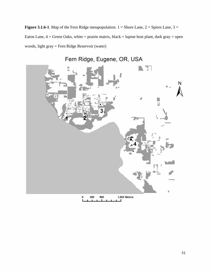
51
Figure 3.1.6-1. Map of the Fern Ridge metapopulation. 1 = Shore Lane, 2 = Spires Lane, 3 =
Eaton Lane, 4 = Green Oaks, white = prairie matrix, black = lupine host plant, dark gray = open
woods, light gray = Fern Ridge Reservoir (water)
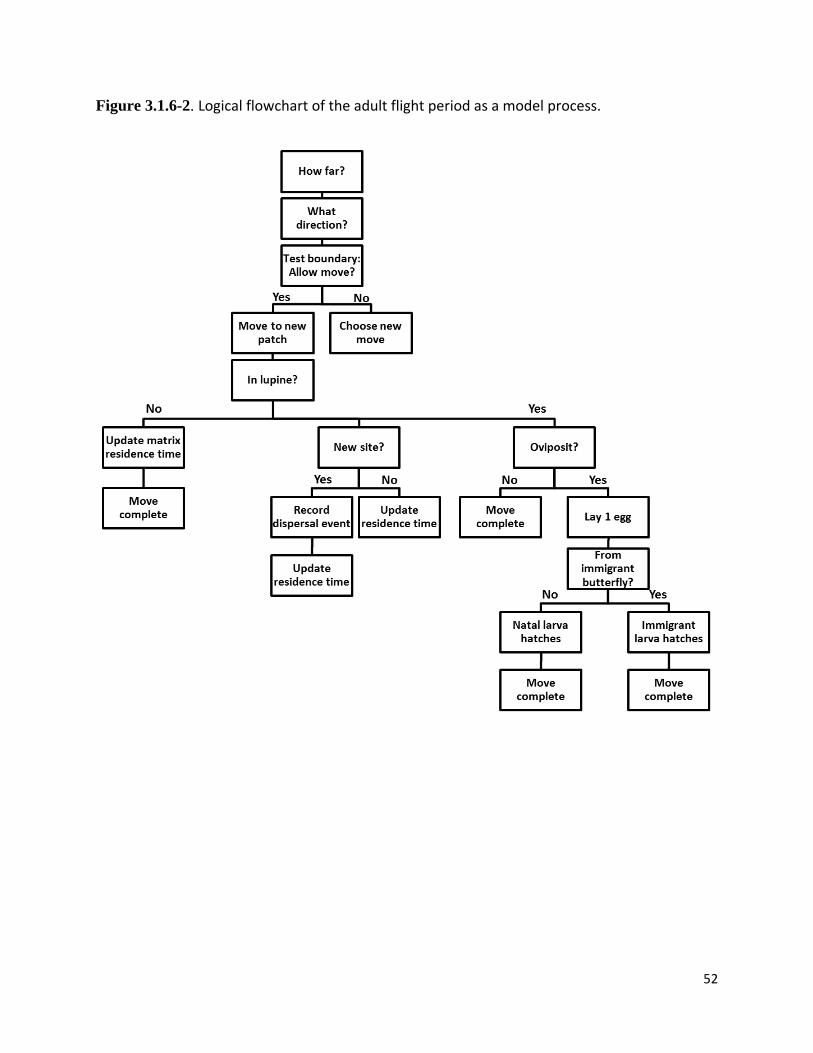
52
Figure 3.1.6-2. Logical flowchart of the adult flight period as a model process.
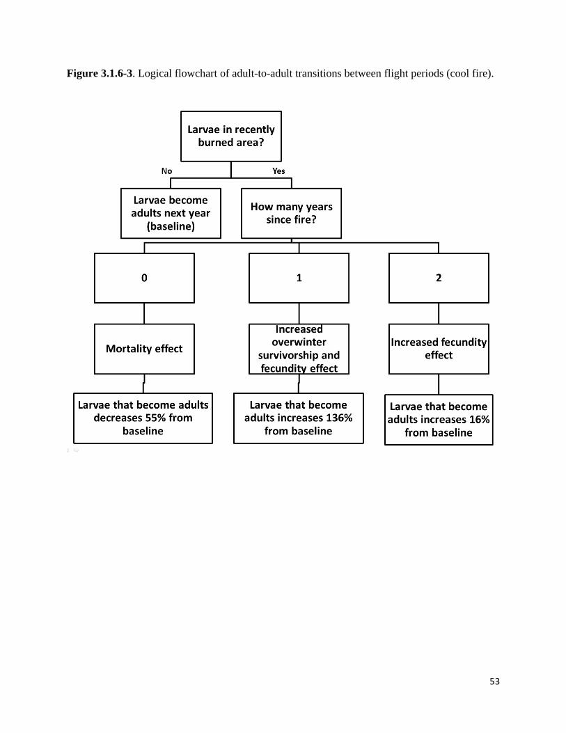
53
Figure 3.1.6-3. Logical flowchart of adult-to-adult transitions between flight periods (cool fire).
54
3.1.7 Model validation and simplification fire management
3.1.7.1: Model Calibration
Previous simulation models with the butterfly accurately captured status quo population and
movement dynamics across the majority of the range, but underestimate population growth at
Fern Ridge (McIntire et al. 2007; Severns et al. 2013). To account for this difference, we
modeled the per-step probability of successful oviposition p as the ratio of population growth
rate to residence time in lupine (sensu Crone and Schultz 2003):
𝑝𝑝 = 𝜆𝜆𝑜𝑜𝑏𝑏𝑜𝑜𝑅𝑅
(1)
where R is residence time, in steps, and λobs is observed population growth rate. We estimated
λobs using a nonlinear least squares approach with the SSlogis function in R and observed
Fender’s blue populations from 1993 – 2015. Then, we estimated R as the average residence time
per butterfly using our simulation model, and validated the simulation estimate matched
observed residence times from a mark-recapture study in the landscape. Thus, we solved for the
per-step probability of successful oviposition at Fern Ridge, and simulation output of yearly
metapopulation growth rates under status quo management was consistent with observed
metapopulation dynamics in the landscape.
3.1.7.2: Model Validation Process
Summary: We fit logistic and exponential population growth models using a nonlinear
least squares approach in R to observed Fender’s blue butterfly counts from 1993 – 2015 at four
sites in the Fern Ridge landscape in Eugene, Oregon (Table 3.1.7-1). We found a signal of
carrying capacity at three sites and described intrinsic rate of increase (r) and population growth
rate (λ) for all sites. To account for potential biases in model fit given the change of sampling

55
methods in 2010, we fit additional models with an adjustment parameter (β) and found two sites
could potentially be influenced by the change in methods (Table 3.1.7-2). Using spatially-
explicit individual-based simulation with environmental stochasticity and open woods in the
Fern Ridge landscape, we quantified average residence time (steps) per butterfly in each site.
When a butterfly is assumed to spend its entire life (2100 steps) in habitat with a per-tick
probability of an adult next year equivalent to 1/933 (0.0010718), expected population growth
rate is 2.25. Using this mathematical approach with exponential population growth rates at Fern
Ridge sites coupled with site-specific mean residence times per butterfly from simulation, we
calculated an adjusted per-tick probability of an adult next year (Table 3.1.7-3). With this
adjusted probability (0.0021157) and new estimate of carrying capacity at 10,000 butterflies per
hectare, we simulated 100 20-year replicates and quantified site-specific geometric growth rates
and found simulation predictions were slightly less than observed population growth rates, but
with some variance (Table 3.1.7-4).
Methods: We used a nonlinear approach using the nls() and SSlogis() functions in R to
estimate carrying capacity and intrinsic rate of increase parameters for the Fender’s Blue
butterfly. Using Greg Fitzpatrick’s report, “2015 Status of the Fender’s Blue Butterfly in the
Willamette Valley, Oregon” containing population sampling estimates at Fern Ridge, data were
separated into four sites (Shore Lane, Spires Lane, Eaton Lane, and Green Oaks), and the total
sum of these sites, all by year. Data were assigned an arbitrary number 0 from 1993-2009 and 1
from 2010-2015 to account for possible differences when sampling methods changed in 2010 for
use in estimating an adjustment parameter, described below.
We reported parameter estimates of carrying capacity and intrinsic rate of increase along
with 95% confidence intervals for growth rate for the logistic model, and reported parameter
56
estimates of intrinsic rate of increase and 95% confidence intervals for growth rate for the
exponential model. We used anova methods to test whether the logistic model fit observed data
significantly better than the exponential model. We plotted model fit versus observed data for
each site and for all of Fern Ridge from 1993-2015, and then projected model fit an additional 25
years into the future. Given the slight difficulty in fitting the logistic model to the observed data
for Eaton Lane, we created a log-likelihood profile varying K from 5,000 to 100,000 in
increments of 1,000 and discovered a negligible increase in model fit with increasing carrying
capacity. So, we assumed an arbitrary K of 10,000 for the site in order for the nonlinear least
squares function to converge in R and provide an estimate of intrinsic rate of increase for the site.
To explore potential influence of the change of sampling methods in 2010, we adapted both the
logistic and exponential models to estimate an adjustment parameter β using the term (1 +
β*yD), where yD is the arbitrary number 0 for years 1993 to 2009, and 1 for years 2010 to 2015.
If the change in methods significantly changes the data, we expect model estimates of β will be
significantly different from 0. In other words, if the change in methods at Green Oaks results in
observed population estimates being 1.5 times higher, the β parameter will approximately equal
to 0.5 and significantly different from 0. We used anova methods to test whether the models with
the adjustment term fit the observed data significantly better than the models without the
adjustment term.
Using spatially-explicit individual-based simulation, we ran 100 20-year replicates
without fire, with environmental stochasticity, with open woods at a 0.05 per-step boundary
crossing probability, and carrying capacity of 3930 butterflies per hectare in the Fern Ridge
landscape, and quantified average residence time (steps) per butterfly in each site. Starting
numbers of butterflies for simulation were at carrying capacity to give a high sample size for

57
residence time. From the intrinsic rate of increase parameters from the logistic and exponential
growth models without the adjustment term, we calculated population growth rate for each site.
We used the relationship between population growth rate and residence time to establish adjusted
per-step probabilities of an adult next year (λ = per-step probability adult next year * steps in
lupine). Specifically, we divided population growth rate by residence time in steps to give the
values for per-step probability of an adult next year. As an example, if we assume a butterfly
spends its entire life in lupine (2100 steps) with a per-step probability of an adult next year of
1/933, the corresponding population growth rate is 2.25.
We assumed that Fern Ridge has been experiencing an intrinsic rate of increase most
similar to an exponential population model, meaning that the most plausible population growth
rates and adjusted per-step probabilities of an adult next year would be from estimates and
calculations with the exponential growth model. We assumed that the estimated carrying
capacity of ~15,000 butterflies for all of Fern Ridge would serve as a reasonable ceiling for use
in simulation, so taking this number with the ~1.5 hectares of lupine habitat present in the
landscape yields a new estimate of carrying capacity of ~10,000 butterflies per hectare for
simulation. Using the adjusted per-step probability of 0.0021157 from the exponential model and
estimated carrying capacity of ~10,000 butterflies per hectare from the logistic model along with
environmental stochasticity and 0.05 per-step probability of crossing into open woods, we
repeated 100 20-year simulations without fire to evaluate new model predictions of population
growth rate. Further, to test whether these parameter estimates result in growing populations, we
started simulations with 100 butterflies in each site.
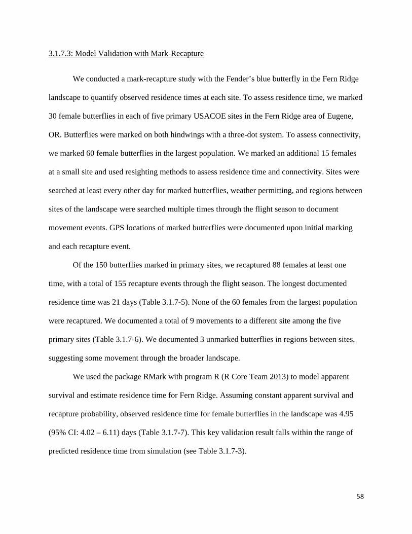
58
3.1.7.3: Model Validation with Mark-Recapture
We conducted a mark-recapture study with the Fender’s blue butterfly in the Fern Ridge
landscape to quantify observed residence times at each site. To assess residence time, we marked
30 female butterflies in each of five primary USACOE sites in the Fern Ridge area of Eugene,
OR. Butterflies were marked on both hindwings with a three-dot system. To assess connectivity,
we marked 60 female butterflies in the largest population. We marked an additional 15 females
at a small site and used resighting methods to assess residence time and connectivity. Sites were
searched at least every other day for marked butterflies, weather permitting, and regions between
sites of the landscape were searched multiple times through the flight season to document
movement events. GPS locations of marked butterflies were documented upon initial marking
and each recapture event.
Of the 150 butterflies marked in primary sites, we recaptured 88 females at least one
time, with a total of 155 recapture events through the flight season. The longest documented
residence time was 21 days (Table 3.1.7-5). None of the 60 females from the largest population
were recaptured. We documented a total of 9 movements to a different site among the five
primary sites (Table 3.1.7-6). We documented 3 unmarked butterflies in regions between sites,
suggesting some movement through the broader landscape.
We used the package RMark with program R (R Core Team 2013) to model apparent
survival and estimate residence time for Fern Ridge. Assuming constant apparent survival and
recapture probability, observed residence time for female butterflies in the landscape was 4.95
(95% CI: 4.02 – 6.11) days (Table 3.1.7-7). This key validation result falls within the range of
predicted residence time from simulation (see Table 3.1.7-3).
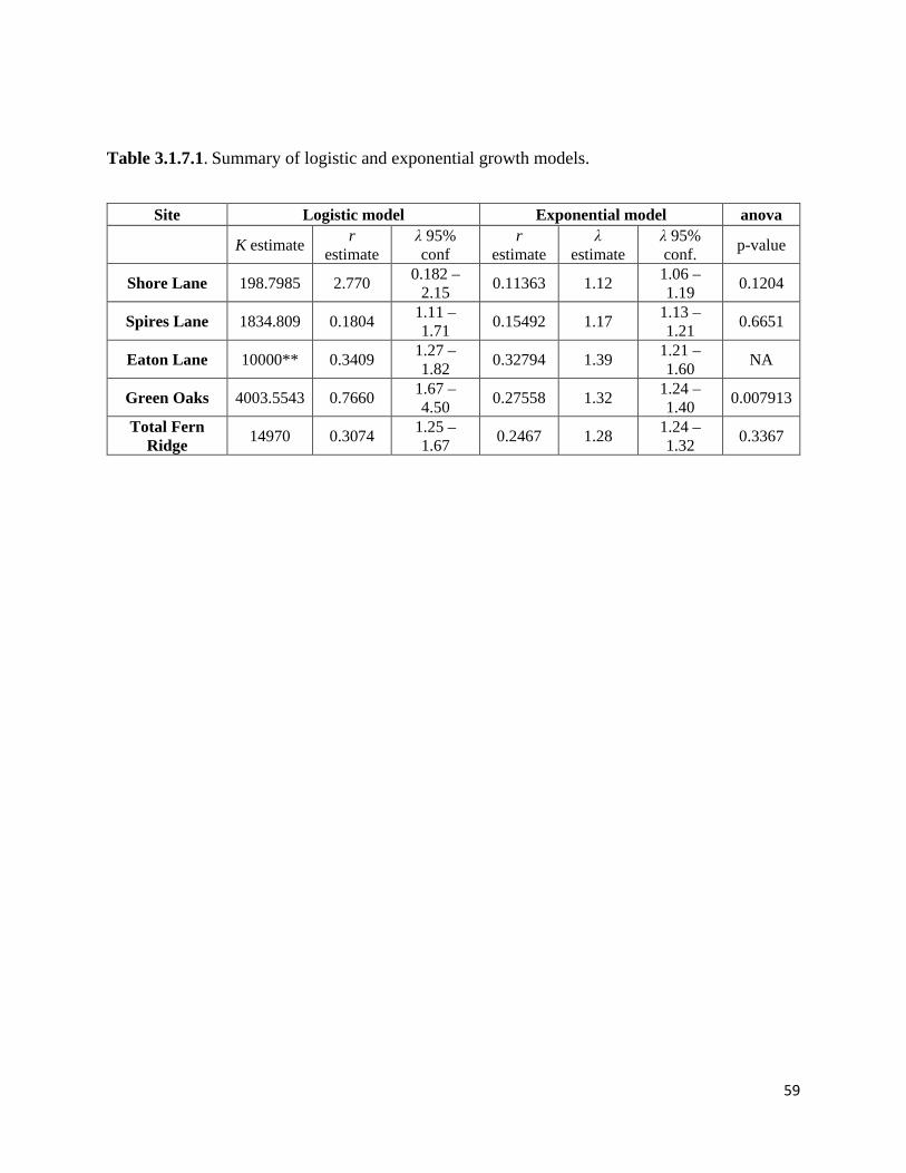
59
Table 3.1.7.1. Summary of logistic and exponential growth models.
Site Logistic model Exponential model anova
K estimate r estimate
λ 95% conf
r estimate
λ estimate
λ 95% conf. p-value
Shore Lane 198.7985 2.770 0.182 – 2.15 0.11363 1.12 1.06 –
1.19 0.1204
Spires Lane 1834.809 0.1804 1.11 – 1.71 0.15492 1.17 1.13 –
1.21 0.6651
Eaton Lane 10000** 0.3409 1.27 – 1.82 0.32794 1.39 1.21 –
1.60 NA
Green Oaks 4003.5543 0.7660 1.67 – 4.50 0.27558 1.32 1.24 –
1.40 0.007913
Total Fern Ridge 14970 0.3074 1.25 –
1.67 0.2467 1.28 1.24 – 1.32 0.3367
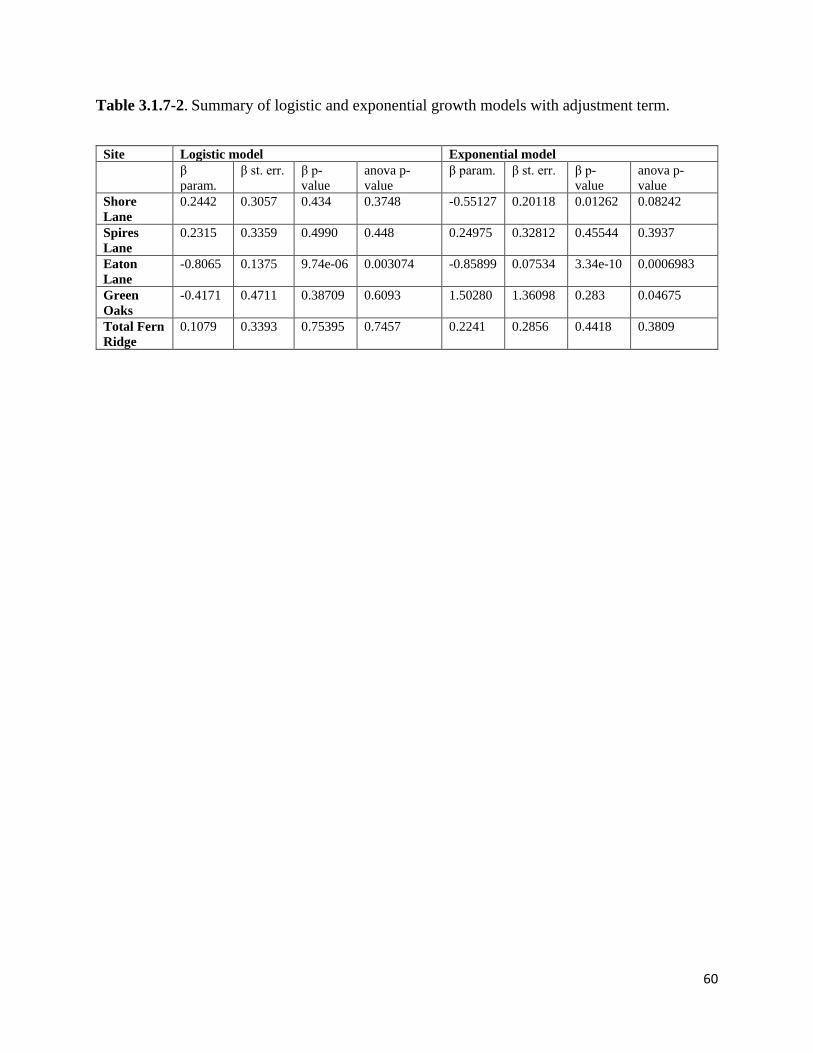
60
Table 3.1.7-2. Summary of logistic and exponential growth models with adjustment term.
Site Logistic model Exponential model β
param. β st. err. β p-
value anova p-value
β param. β st. err. β p-value
anova p-value
Shore Lane
0.2442 0.3057 0.434 0.3748 -0.55127 0.20118 0.01262 0.08242
Spires Lane
0.2315 0.3359 0.4990 0.448 0.24975 0.32812 0.45544 0.3937
Eaton Lane
-0.8065 0.1375 9.74e-06 0.003074 -0.85899 0.07534 3.34e-10 0.0006983
Green Oaks
-0.4171 0.4711 0.38709 0.6093 1.50280 1.36098 0.283 0.04675
Total Fern Ridge
0.1079 0.3393 0.75395 0.7457 0.2241 0.2856 0.4418 0.3809
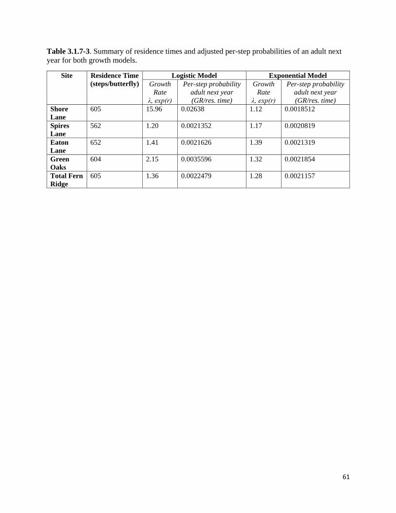
61
Table 3.1.7-3. Summary of residence times and adjusted per-step probabilities of an adult next year for both growth models.
Site Residence Time (steps/butterfly)
Logistic Model Exponential Model Growth
Rate λ, exp(r)
Per-step probability adult next year (GR/res. time)
Growth Rate
λ, exp(r)
Per-step probability adult next year (GR/res. time)
Shore Lane
605 15.96 0.02638 1.12 0.0018512
Spires Lane
562 1.20 0.0021352 1.17 0.0020819
Eaton Lane
652 1.41 0.0021626 1.39 0.0021319
Green Oaks
604 2.15 0.0035596 1.32 0.0021854
Total Fern Ridge
605 1.36 0.0022479 1.28 0.0021157
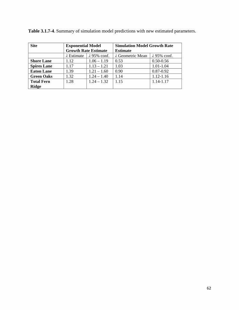
62
Table 3.1.7-4. Summary of simulation model predictions with new estimated parameters.
Site Exponential Model Growth Rate Estimate
Simulation Model Growth Rate Estimate
λ Estimate λ 95% conf. λ Geometric Mean λ 95% conf. Shore Lane 1.12 1.06 – 1.19 0.53 0.50-0.56 Spires Lane 1.17 1.13 – 1.21 1.03 1.01-1.04 Eaton Lane 1.39 1.21 – 1.60 0.90 0.87-0.92 Green Oaks 1.32 1.24 – 1.40 1.14 1.12-1.16 Total Fern Ridge
1.28 1.24 – 1.32 1.15 1.14-1.17

63
Table 3.1.7-5. Summary of mark-recapture study.
Site # Marked # Unique Recaps # Total Recaps Longest Residence Time
West Shore 30 11 17 11 days West Spires 30 21 41 11 days East Spires 30 23 31 12 days North Eaton 30 16 24 20 days South Eaton 30 17 42 21 days

64
Table 3.1.7-6. Summary of observed connectivity.
Connectivity To West Shore
To West Spires
To East Spires
To North Eaton
To South Eaton
From West Shore
0 0 0 0
From West Spires
0 6 0 0
From East Spires
0 2 0 0
From North Eaton
0 0 0 1
From South Eaton
0 0 0 0
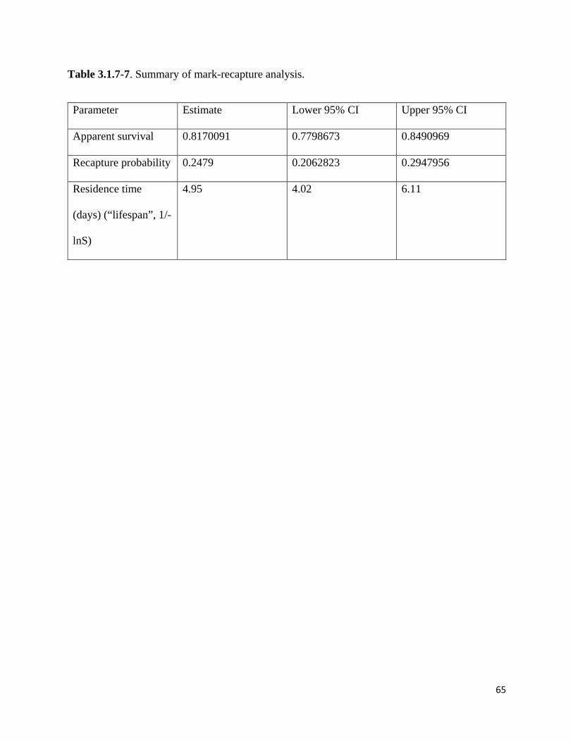
65
Table 3.1.7-7. Summary of mark-recapture analysis.
Parameter Estimate Lower 95% CI Upper 95% CI
Apparent survival 0.8170091 0.7798673 0.8490969
Recapture probability 0.2479 0.2062823 0.2947956
Residence time
(days) (“lifespan”, 1/-
lnS)
4.95 4.02 6.11
66
3.2 Saint Francis’ Satyr/ Appalachian Brown
3.2.1 Field Data Hardwood removal/inundation
To create restoration sites, in the spring of 2011 we established four restoration areas,
each containing four 30m x 30m experimental plots. In each area, plots were randomly assigned
to one of four treatments in a factorial design: 1) manual removal of most trees; 2) installation of
temporary dams; 3) both tree removal and installation of dams; and 4) no manipulation. Tree
removal was intended to increase light availability within wetlands to encourage herbaceous
plant growth. We intentionally left ≈10% of the trees in order to mimic the canopy structure
found in beaver-created wetlands in our area. We maintained tree removal treatments by cutting
back the re-sprout of trees and shrubs in 2012 and 2013 to suppress hardwood canopy
regeneration. Damming was intended to increase soil moisture and the amount of standing
water, a key requirement for sedges. In dammed plots, we installed 0.5 m high and 1 m wide
water-filled temporary coffer dams (Aquadam Inc., Scotia, CA, USA) across the length of the
downstream edge of the plot, which inundated ≈10 m of the downstream portion of the plot.
Within each plot we established 27 uniformly distributed 1.5 × 1.5 m vegetation subplots that were
surveyed for percent cover of all sedge species and the major vegetation types (e.g. grasses,
forbs, and shrubs) prior to restoration in Spring 2011, as well as in Fall 2011, Spring 2012, and
Spring 2013.
3.2.2 Monitor movement and demography
Movement
We observed both Appalachian Browns and St. Francis’ satyrs at all treatment plots in all
four experimental blocks. Two observers controlled digital compasses (KVH Datascopes)
67
mounted on PVC poles inside the plots. Butterflies were either released from the center of the
30m x 30m plot or observed in natural flight. The pair of observers recorded synchronous
bearings of the target butterfly every 5 seconds while it was moving. Observations stopped when
butterflies stopped moving for more than 30 minutes or left the plot (Kuefler et al. 2010).
Using trigonometry and the observer bearings, the length of each 5-second move and turn
angle between consecutive moves were calculated for all butterflies with 3 or more recorded
moves. From the move lengths and turn angles, we calculated the mean squared displacement per
move (hereafter Rn2/n), which measures the spread of a population over space (Turchin 1998). A
larger Rn2/n indicates that the butterflies are moving more quickly (longer move lengths) and
more directly (smaller turn angles). We compared the distributions of move lengths, turn angles,
and Rn2/n from different species and treatment sites using the Kolmogorov-Smirnoff test.
Confidence intervals were measured by creating bootstrapped datasets (10000 repetitions) and
taking the middle 95% of results.
Demography
To estimate the direct and indirect effects of restoration treatments on Appalachian brown
demography, we estimated egg survival and larval to adult survival independently. To estimate
egg survival, we placed greenhouse raised, potted C. mitchelliana plants with a known number
of eggs into our established experimental restoration plots and counted the number of eggs that
remained after 48 hours. We first caged wild-caught Appalachian brown females on potted sedge
plants in a greenhouse at Ft. Bragg, and counted the number of eggs laid. Each restoration plot
received one pair of potted sedges, one randomly assigned to a predator exclusion treatment and
a second that was accessible to all predators. Plants in the predator exclusion treatment were
68
enclosed in a cage constructed from a 20L fine mesh fabric paint strainer and bent wire. A 15-
cm band of Tanglefoot® insect barrier was applied to pots to exclude crawling predators. Paired
plants were placed in the center of each restoration plot on dry ground within five meters of each
other. All plants were removed from the field after 48 hours and we counted the number of eggs
remaining.
To estimate survival over the larval and pupal stages, we deployed a known number of
larvae into experimental arenas created in each plot and counted the number of butterflies that
emerged. We constructed larval arenas by removing the ends of a standard 55 gallon
polyethylene food grade drum and cutting the remainder into thirds, resulting in an
approximately 57 cm diameter x 35 cm tall ring. At six randomly chosen locations in each plot,
rings were buried approximately 10 cm into the ground surrounding naturally occurring, mature
C. mitchelliana. In one block with low sedge abundance, field cages were placed around
greenhouse raised and transplanted C. mitchelliana plants. We randomly assigned each arena to a
predator-free or predator-accessible treatment. Predator-free arenas were enclosed with tulle
netting that was secured to the outside of the rings using nylon straps and tied at the top of a
vertical support structure to hold the fabric off the plants. All potential predators were manually
removed from predator-free arenas prior to addition of larvae. Arenas accessible to predators
remained open during larval development, but once pupae were observed, arenas were enclosed
with tulle netting to facilitate capture of emerging adults. Five larvae varying in age from first to
third instars (most commonly second instars) were placed into each arena in a block on the same
day. Larvae were left to develop in the field. After the observation of pupae, arenas were
checked daily for newly emerged adults until no butterflies were found for five consecutive days.

69
3.2.3 Statistical analysis hardwood removal/inundation
To assess changes in the plant community resulting from restoration treatments, we
performed a Before After Control Impact (BACI) linear mixed effects analysis using the lmer
function in the lme4 package (Bates et al. 2013) and the ANOVA function in the car package
(Fox and Weisberg 2011) in the statistical platform R 3.0.2 (R Development Core Team 2013).
Our model contained fixed effects of tree removal, damming, and year, all interaction terms, and
a random effect of plot. We used a Type II Wald chi-square test to evaluate the effect of
restoration on: (1) percent cover of Carex mitchelliana (the most likely host plant species in our
plots); (2) percent cover of all sedges; and (3) percent cover of all understory vegetation.
We assessed whether restoration treatment had direct and indirect effects on egg and
juvenile survival using generalized linear mixed models (GLMMs) with the function glmer from
the lme4 package. The numbers of eggs or juveniles that survived to the end of the experiment
were treated as binomial responses. In all analyses, tree removal, damming, predation treatment,
and their interactions, as well as flight period for egg survival, were treated as fixed effects;
block and plot were treated as crossed random effects. We used Wald Z tests to assess the
statistical significance of the fixed effects.
To assess direct effects, we tested for effects of restoration treatments and their
interaction on survival using only the predator-free treatments. For egg survival, we began with a
model that included the three-way interaction between tree removal, damming, and flight period
(plus all lower-order terms) to test whether the main and interactive effects of the restoration
treatments differed between flight periods. Because this three-way interaction was not significant
(P = 0.14), we fit a model with all two-way interactions between tree removal, damming, and
flight period. We used the same model (without flight period) to assess the direct effect of
restoration treatments on juvenile survival. To assess the net effect of restoration treatments (i.e.,

70
direct and indirect effects combined), we used the same models as for direct effects, but only
used data from the predator-accessible treatment.
Indirect effects of restoration mediated through predation were investigated by comparing
the survival in predator-free and predator-accessible treatments as a function of restoration
treatment. An effect of restoration treatment on predation intensity would be indicated by a
significant tree removal × predation treatment, damming × predation treatment, or tree removal ×
damming × predation treatment interaction. For egg survival, the four-way interaction between
tree removal, damming, predation treatment, and flight period was not significant (P = 0.57);
therefore we dropped the four-way interaction from the model but included all three-way
interactions. For juvenile survival, the three-way interaction between the tree removal, damming,
and predation treatments was not significant (P = 0.76), so we fit a model with all two-way
interactions. To estimate the mortality of eggs and juveniles due to predation, we calculated a
mortality response ratio by dividing the survival rate in the predator accessible treatment by the
survival rate in the predator-free treatment and subtracting this value from 1.
3.2.4 Documenting predator community
During different stages of their life cycles, St. Francis’ satyrs are subject to predation by a
host of predators including spiders, dragonflies, ants and birds. Thus, the abundance and
distribution of predators is a significant determinant of habitat quality for St. Francis’ satyrs. In
2013, we measured the species richness and abundance of dragonflies and ants in each of our
restoration plots as part of our ongoing research comparing the quality of different restoration
treatments.
To survey dragonflies, we walked through all restoration sites for 15 minutes noting
abundance and species of all dragonflies observed. When possible, we recorded dragonfly sex
71
and distance observed from transects. We surveyed on a total of seven days between June 5 –
August 12.
To survey ants, we placed nine ant traps at locations spaced out within each plot at the
same sites. For each plot, traps were set out on each of two mornings (June 26 and 27) and two
afternoons (July 11, 15 and 16). Traps consisted of a 3x5 index card with approximately 50 g of
tuna and honey placed in its center. The traps were left in the plots for two hours, after which all
ants attracted to the traps were collected. Ants were organized into vials of ethanol for further
identification and numeration in the laboratory.
3.2.5 Refine measurements of vital rates, trends and abundance
ABB and SFS caterpillar behavior and survival methods
Caterpillar host use and survival
We measured St. Francis’ satyr caterpillar survival in the field by releasing a known
number of first instar caterpillars into experimental arenas, allowing them to develop in the
arenas, and then counting the adult butterflies that emerged from arenas. We used experimental
arenas composed of a 57cm tall X 37cm diameter ring of a polyethylene food grade drum buried
approximately 10 cm into the ground (Aschehoug et al. 2015). These arenas were installed in
2012 around naturally occurring C. mitchelliana. When preparing arenas in 2016, we chose
existing arenas that already contained C. mitchelliana so we would not need to supplement larval
diets. Because we were limited in our study by our federal permit to using a small number of
endangered caterpillars, we only measured caterpillar survival in the control and tree
removal/dam implementation treatments in two blocks of the original restoration experiment,
releasing caterpillars into two arenas per plot for a total of 8 arenas. We released 7 first instar
72
caterpillars into each arena over two days. Two arenas, one in each treatment, were invaded by
ants after the first day of releases, so no additional caterpillars were released into them and they
were dropped from the experiment. We left arenas open to predation and counted caterpillars
daily. Once we observed pupae, we enclosed the arenas with mosquito netting. We continued to
visit arenas daily, recording and releasing all adults that emerged. By releasing St. Francis’ satyr
caterpillars into arenas, we were able to observe larval feeding and host choice in the wild for the
first time. In addition to simply counting caterpillars daily, we recorded the species of sedge on
which each caterpillar was feeding.
We tested whether larval survival differed among treatments between St. Francis’ satyr
and Appalachian Brown (data from Aschehoug et al. 2015). To do this, we used a general linear
model with a binomial response variable, including a species*treatment interaction main effect.
We conducted this analysis using the glm function of the lme4 package, and Anova function of
the car package in R.
Caterpillar behavior
We measured Appalachian brown and St. Francis’ satyr caterpillar behavior using captive
individuals. These originated from wild-caught females brought into the greenhouse to lay eggs
and then released back into the wild as adults. When the eggs hatched, we allowed first instar
caterpillars to crawl onto potted C. mitchelliana plants in screened captive rearing enclosures.
We measured the height above soil level for 20 caterpillars of each species twice a week for four
weeks. To test for differences in foraging behavior height, we used a two-way ANOVA with a
species*date interaction term to account for differences in foraging behavior as caterpillars
develop. Caterpillar heights were square-root transformed to meet ANOVA assumptions. These
73
experiments were done in the greenhouse at Ft. Bragg which is programed to replicate outside
environmental conditions.
Caterpillar microhabitat
We measured the sedge canopy above captive St. Francis’ satyr and Appalachian brown
caterpillars in arenas as a measure of how likely a caterpillar is to be shaded by sedges. We did
this by dropping a pin through the sedges to the location of each caterpillar and counting the
number of sedge blades that contacted the pin above the caterpillar’s location. As with height
data, we collected sedge canopy on 20 caterpillars of each species twice a week for four weeks.
To compare sedge canopy above the two species, we totaled the number of individuals counted
with zero, one, two, three, and four hits above them on the pin for each species across all eight
surveys. We used a chi-square test to test for differences between sedge canopy cover
experienced by St. Francis’ satyrs and Appalachian browns.
Appalachian Brown Population Surveys
We began counting Appalachian Brown butterflies mid-summer 2014. Appalachian
Brown counts were recorded alongside Saint Francis Satyr counts during daily surveys in the
second flight period. Surveys occurred at both historic and restoration sites for Saint Francis
Satyr and consisted of transect walks through each 30x30m plot of each site. The daily counts
were converted into Pollard-Yates counts by summing the weekly average of the daily counts.
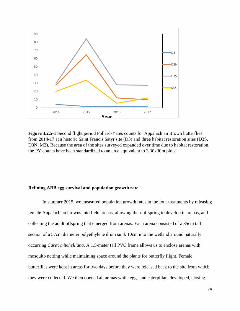
74
Figure 3.2.5-1 Second flight period Pollard-Yates counts for Appalachian Brown butterflies from 2014-17 at a historic Saint Francis Satyr site (D3) and three habitat restoration sites (D3S, D3N, M2). Because the area of the sites surveyed expanded over time due to habitat restoration, the PY counts have been standardized to an area equivalent to 3 30x30m plots.
Refining ABB egg survival and population growth rate
In summer 2015, we measured population growth rates in the four treatments by releasing
female Appalachian browns into field arenas, allowing their offspring to develop in arenas, and
collecting the adult offspring that emerged from arenas. Each arena consisted of a 35cm tall
section of a 57cm diameter polyethylene drum sunk 10cm into the wetland around naturally
occurring Carex mitchelliana. A 1.5-meter tall PVC frame allows us to enclose arenas with
mosquito netting while maintaining space around the plants for butterfly flight. Female
butterflies were kept in areas for two days before they were released back to the site from which
they were collected. We then opened all arenas while eggs and caterpillars developed, closing
0
10
20
30
40
50
60
70
80
90
2014 2015 2016 2017
D3
D3N
D3S
M2
Year
75
them again once pupae were observed. We then visited arenas daily, recording and releasing all
adults that emerged. In each experimental treatment, we deployed four arenas for a total of 16
per site. We did this at both M2 and D3S.
To estimate egg survival, we followed the fate of individual eggs laid by female
butterflies in the field arenas. To do this, we searched for eggs at the time of the female’s release,
inspecting the plants without moving the vegetation and making detailed notes on the position of
each egg we could find. We then re-visited arenas daily, recording the status of each of these
eggs until they had all hatched, disappeared, or it was obvious they would never hatch. This
strategy allowed us to estimate egg survival in-situ without having to transport eggs from the
greenhouse to the field. It also had the advantage of allowing females to choose egg locations,
although this was somewhat constrained by the enclosure and the vegetation contained within.
To analyze egg survival, we used generalized linear mixed models with binomially
distributed errors. We included site (2 levels), the two restoration treatments, and flight period as
fixed effects and considered plot and corral as random factors, to account for the repeated
measures across flight periods for the same plots and corrals (nested within plot). A model with
site and a three-way interaction between flight period, cut treatment, and dam treatment and both
random factors failed to converge, so we next tried a model with site plus all two-way
interactions between flight period and cut and dam treatment; none of the two-way interactions
were significant, and the variance among plots was close to zero. Hence our final model
contained main effects of site, flight period, cut treatment, and dam treatment, and a random
effect of corral.
76
3.2.6 Implementation of SEIBMS hardwood removal/ inundation
For the rare and federally endangered Saint Francis satyr (Neonympha mitchellii
francisci) butterfly, sedge-dominated wetlands at intermediate successional stages are known
source habitat that support robust growing populations (Kuefler et al. 2008, Cayton et al. 2015).
These wetlands typically occur within riparian forest corridors, which contain some of the same
sedge species found in source wetland habitat, and upon which St. Francis satyrs rely for
oviposition and larval food sources. But these sedge species occur at lower densities in riparian
forest corridors than in source wetland habitat. While butterflies may oviposit eggs on the sedges
within riparian forest, our observations indicate that these forest habitats are unable to sustain
populations. Thus, if oviposition does occur within riparian forests, it would be considered sink
habitat for St. Francis satyrs. Since the primary management strategy for recovering St. Francis
satyr populations is to use tree removal and stream damming within the riparian corridor to
restore or create new wetland habitat (Cayton et al. 2015), understanding how riparian habitats
might impact populations occupying adjacent wetland habitat, whether they act as sinks or not, is
important for the success of restoration efforts. In addition, since riparian corridors often connect
wetland habitats to each other, understanding the role they play in facilitating connectivity and
contributing to range expansion, will be critical to the effort to rebuild a viable interconnected
SFS metapopulation that is resilient to disturbance and changing climatic conditions.
Much theoretical work has been done to assess the role sink habitat plays in population
dynamics, but the findings indicate divergent roles depending on a wide variety of factors,
demonstrating the context-specific effects of sink habitat (Himes Boor et al. in prep). To explore
the specific role of sink habitat for St. Francis satyrs on Fort Bragg, we developed a spatially
explicit individual-based model (SEIBM) using Netlogo v.5.2.1 (Wilensky 1999) and
77
parameterized it using a combination of empirical data movement and demographic data and
pattern-oriented modeling (see section 3.2.7 below). The SEIBM simulates movement and
demography of individual SFS over multiple generations within a landscape representative of the
areas on Ft. Bragg occupied by two sub-populations of SFS.
The simulated landscape in the SEIBM is composed of 30m x 30m grid cells
characterized as one of the following habitat types: wetland, riparian forest, upland forest, and
open areas (including grasslands and developed areas). Open and upland forest are matrix habitat
through which butterflies move but do not reproduce (i.e., do not oviposit eggs) due to the
absence of sedges. Wetland patches serve as source habitat in which reproduction occurs and
populations are generally stable or growing. Riparian forest is, depending on the simulation,
either matrix habitat with no reproduction, or sink habitat in which reproduction can occur but at
non-self-sustaining levels.
3.2.7 Model validation and simplification hardwood removal/inundation
The SFS SEIBM is parameterized using empirical demographic and movement data
gathered from SFS, and a surrogate species. Because of St. Francis satyr’s endangered status and
rarity, direct handling and experimental manipulations are generally precluded. Therefore, when
no SFS data were available to parameterize the model, we used data from the Appalachian brown
butterfly (ABB), which occupies similar habitats, has a similar life history, and has been shown
to be a suitable surrogate species for St. Francis satyr movement (Hudgens et al. 2012). Details
on parameter values used in the model and their empirical source can be found in Hudgens et al.
2012 and Himes Boor et al. (in prep).
78
To parameterize the butterfly movement portion of the SFS SEIBM we used data from
multiple empirical studies that estimated flight distances, turn angles, and resting frequency and
duration primarily from ABB. As simulated butterflies move around the landscape, they
encounter habitat boundaries where they must choose to cross out of one habitat into another.
Inclusion of boundary crossing behavior has previously been found to be an important element in
the accuracy of SFS SEIBMs (Hudgens et al. 2012). To parameterize the habitat boundary
crossing probabilities, we used a combination of empirical data from one study of St. Francis
satyr movement that measured the likelihood of butterflies crossing from wetland habitat into
forest habitat (Hudgens et al. 2012 Appendix), and another study of Appalachian brown butterfly
(Kuefler et al. 2008) for all other boundary crossing probabilities. Similarly, empirical
oviposition rates were not available for SFS or ABB, so we adjusted the oviposition rates used in
the model until we achieved growth rates in each colony that matched empirical growth rates. In
this way, our model is able to emulate empirical individual behavioral patterns (e.g., colony
wetland residence times) and empirical population-level patterns (e.g., growth over time).
Previously conducted model simplification exercises revealed that models that included detailed
movement behavior (e.g., turning angles and move distance) and boundary crossing behavior
performed better than simpler models parameterized solely with mean dispersal distances
(Hudgens et al. 2012). The benefit of the increased complexity was especially pronounced when
simulations were conducted over broader spatial extent that included more varied habitat. As a
result, our final model included the full complexity of fine-scaled movement behavior and
boundary-crossing behavior.

79
3.2.8 Scenario Analysis hardwood removal/ inundation
We used the model to compare five primary metrics with and without the possibility of
butterfly reproduction in riparian forests (i.e., presence and absence of sink habitat) in two areas
of Fort Bragg that currently support SFS populations. The metrics included total population
abundance and variability, population growth rate, mean and maximum dispersal distances. In
those scenarios with sink habitat, oviposition occurred in extant colony wetland habitat at
empirically based rates, and at lower levels within riparian forest habitat. We tested two levels of
oviposition rate in riparian habitat, one based on an assumption of 10% sedge cover in riparian
habitats and the other on an assumption of 5% sedge cover. We determined the oviposition rate
at these sedge cover levels by fitting a second-degree polynomial function to the oviposition
rates at the eastern and western colonies, which have 30$ and 15% sedge cover respectively, and
assuming zero oviposition probability at 0% sedge cover. We confirmed via simulation that the
estimated oviposition rates in riparian habitat produced declining populations in the absence of
source (wetland) habitat. In those simulations in which no sink habitat was present, riparian
forests acted as matrix habitat and oviposition was only allowed within extant colony wetland
habitat.
In addition to presence and absence of sink habitat, we also varied the total amount of
wetland to the landscape by adding restored habitat in two sizes and at two distance from extant
colony wetland habitat. At each extant colony on Fort Bragg we ran simulations with no
additional restored wetland, and additional restored habitat at 60% and 100% of extant habitat.
The restored wetlands were placed within the riparian corridor adjacent to or at 600m away from
extant wetland colony habitat. Empirical growth rates at the two extant colonies (East and West)
are markedly different; thus by conducting simulations at the two colony sites, we were also able
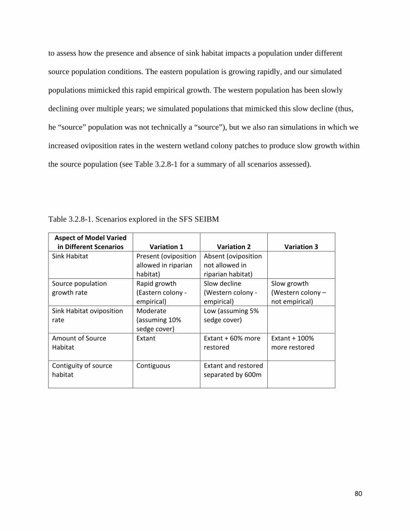
80
to assess how the presence and absence of sink habitat impacts a population under different
source population conditions. The eastern population is growing rapidly, and our simulated
populations mimicked this rapid empirical growth. The western population has been slowly
declining over multiple years; we simulated populations that mimicked this slow decline (thus,
he “source” population was not technically a “source”), but we also ran simulations in which we
increased oviposition rates in the western wetland colony patches to produce slow growth within
the source population (see Table 3.2.8-1 for a summary of all scenarios assessed).
Table 3.2.8-1. Scenarios explored in the SFS SEIBM
Aspect of Model Varied in Different Scenarios Variation 1 Variation 2 Variation 3
Sink Habitat Present (oviposition allowed in riparian habitat)
Absent (oviposition not allowed in riparian habitat)
Source population growth rate
Rapid growth (Eastern colony - empirical)
Slow decline (Western colony - empirical)
Slow growth (Western colony – not empirical)
Sink Habitat oviposition rate
Moderate (assuming 10% sedge cover)
Low (assuming 5% sedge cover)
Amount of Source Habitat
Extant Extant + 60% more restored
Extant + 100% more restored
Contiguity of source habitat
Contiguous Extant and restored separated by 600m
81
3.3 Taylor’s Checkerspot/ Baltimore Checkerspot hostplants & herbicides
3.3.1.1 Monitoring movement and demography: hostplants
We conducted fieldwork on the Baltimore checkerspot butterfly at an ~11.5-ha study site
of conservation land in the town of Harvard, Massachusetts, USA (Figure 3.3.1.1-1). This site
included ~2 ha of host plant habitat, and ~8 ha of open meadows with nectar plants. In our
population, butterflies regularly oviposited on both host plant species, and nectared on a variety
of wildflowers in open meadows.
Demography: Larval survival
We measured post-diapause (i.e., spring) larval survival to eclosion as adults on each host
plant by collecting individuals in the early spring 2012 and 2013 and rearing them in 60 × 60 cm
insect enclosures set-up over unoccupied C. glabra or P. lanceolata (four post-diapause larvae in
each of 10 C. glabra and 12 P. lanceolata enclosures in 2012, and five post-diapause larvae in
each of 14 C. glabra and 14 P. lanceolata enclosures in 2013). In 2012, the population was very
small and all larvae were originally found in host plant patches of C. glabra; enclosures depleted
of host plant were removed from the study. In 2013, larvae were moved to enclosures from
patches of both C. glabra and P. lanceolata in a crossed design, following Bowers et al.’s design
for estimating larval survival in the laboratory (1992). Enclosures at risk of depletion were
supplemented with the host plant over which they were placed. We estimated overwinter survival
from winter 2013 to spring 2014 on each host plant by setting up cages of wire and tulle fabric
around inactive pre-diapause nests in mid-fall 2013 (9 C. glabra cages and 10 P. lanceolata
cages). We monitored cages two-three times per week in spring 2014, counting and removing
post-diapause larvae when they were at about the same stage as the start of post-diapause larval
82
monitoring the previous years. All cages contained sufficient host plant growth so no
supplementation was necessary.
Demography: Female daily adult survival, population size, and individual mass
We used a capture-mark-recapture study of adult butterflies to estimate daily survival of
females eclosed from C. glabra or P. lanceolata insect enclosures in 2012 and 2013, and to
estimate population size of wild-caught adult females in 2012, 2013, and 2014. We marked the
wings of adults with a unique color combination of 3–5 dots using metallic gel pens, and
surveyed the entire site for new individuals and recaptures several times per week from the late
June until no more butterflies were observed in the field (mid-July to early August depending on
the population size). As a proxy for fecundity, we used a digital scale to measure body mass of
all adult females upon removal from insect enclosures in 2012 and 2013.
Demography: Number of nests, nest size
In the late summer/early fall of 2013 and 2014, we estimated the number of nests laid by
adult females on C. glabra and P. lanceolata using a mark-resight study. We searched for nests
on both host plants across the entire site on five occasions, marking newly sighted nests close to
the ground with an inconspicuous tag, and recording resights of already marked nests. We
estimated the number of prediapause larvae per nest in the late summer/early fall 2013 and 2014
by making a small opening in a portion of nests (63 in 2013, 92 in 2014) and counting the
number of individuals in each nest to the nearest ten from 2 to 5 times (to minimize nest
disturbance) over 5–10 occasions.
Movement
We quantified movement behavior by mapping individual flight paths in low and high
quality habitat cover classes and in open and forest matrix, and by releasing butterflies at forest
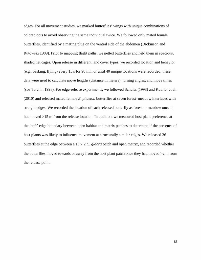
83
edges. For all movement studies, we marked butterflies’ wings with unique combinations of
colored dots to avoid observing the same individual twice. We followed only mated female
butterflies, identified by a mating plug on the ventral side of the abdomen (Dickinson and
Rutowski 1989). Prior to mapping flight paths, we netted butterflies and held them in spacious,
shaded net cages. Upon release in different land cover types, we recorded location and behavior
(e.g., basking, flying) every 15 s for 90 min or until 40 unique locations were recorded; these
data were used to calculate move lengths (distance in meters), turning angles, and move times
(see Turchin 1998). For edge-release experiments, we followed Schultz (1998) and Kuefler et al.
(2010) and released mated female E. phaeton butterflies at seven forest–meadow interfaces with
straight edges. We recorded the location of each released butterfly as forest or meadow once it
had moved >15 m from the release location. In addition, we measured host plant preference at
the ‘soft’ edge boundary between open habitat and matrix patches to determine if the presence of
host plants was likely to influence movement at structurally similar edges. We released 26
butterflies at the edge between a 10 × 2 C. glabra patch and open matrix, and recorded whether
the butterflies moved towards or away from the host plant patch once they had moved >2 m from
the release point.
84
Figure 3.3.1.1-1. Map of site and areas covered by C. glabra and P. lanceolata.
3.3.1.2 Statistical analysis: hostplants
We conducted all statistical analyses using in R (R Core Team 2015), JAGS (Plummer
2003), and Program MARK (White and Burnham 1999), and using the R packages ‘lme4’ (Bates
et al. 2015), R2jags (Su and Yajima 2015), and unmarked (Fiske and Chandler 2011).
Hostplant-specific demography
We estimated demographic parameters for calculating host plant-specific population
growth rates using generalized linear models and mixed effects models (GLMs and GLMMs;
including a random effect of enclosure to account for variation in microsite or other effects that

85
might influence larval survival estimates), and using methods for analyzing capture-mark-
recapture/resight and unmarked population data (Table 3.3.1.2-1). From these models we
obtained the host plant-specific values for post-diapause survival, φ1, overwinter survival, φ2,
larvae per nest, l, female adult mass, m, and female daily adult survival, φ3, and population-level
values for the number of nests, n, and number of adult females, N (Figure 3.3.1.2-1). We inferred
population-level oviposition preference for C. glabra or P. lanceolata by testing whether the
proportion of nests found on each type of host plant differed from the proportion of area
occupied by a given host at our site, i.e., ~0.3 for ~30% host plant cover of C. glabra (C.g.) and
~0.7 for ~70% of host plant cover of P. lanceolata (P.l.). We used the upper and lower
confidence intervals (CIs) of the number of nests estimated to estimate upper and lower
confidence intervals of the proportions (e.g., C.g.uppCI=C.g.uppCI/(C.g.uppCI+P.l.lowCI) and
C.g.lowCI=C.g.lowCI/(C. glabralowCI+P.l.uppCI).
We used parametric bootstrapping of parameter values obtained as shown in Table
3.3.1.2-1 to estimate host plant-specific population growth rates as 𝜆𝜆 = 𝜙𝜙1 × 𝜙𝜙2 × 𝑛𝑛𝑁𝑁 × 𝑙𝑙 × 𝑚𝑚∗.
Here, a value of λ = 1 indicates an annually stable (not growing or declining) population, λ = 2
indicates a population doubling annually, and λ = 0.9 indicates a population declining by 10%
annually (see Gotelli 2001). In our formula, m* is a body mass correction for n/N, assuming
fecundity is proportional to body mass to allocate the proportion of total nests per adult relative
to the body mass of adults reared on C. glabra (C.g.) versus P. lanceolata (P.l.), where 𝑚𝑚𝐶𝐶.𝑔𝑔.∗ =
2×𝑚𝑚𝐶𝐶.𝑔𝑔.
𝑚𝑚𝐶𝐶.𝑔𝑔.+𝑚𝑚𝑃𝑃.𝑙𝑙. and 𝑚𝑚𝑃𝑃.𝑙𝑙.
∗ = 2×𝑚𝑚𝑃𝑃.𝑙𝑙.𝑚𝑚𝐶𝐶.𝑔𝑔.+𝑚𝑚𝑃𝑃.𝑙𝑙.
. Given that post-diapause larval survival and the number of
nests per adult varied across years, we estimated host plant-specific population growth rates (λhp,
corresponding to parameters for C. glabra or P. lanceolata) as:
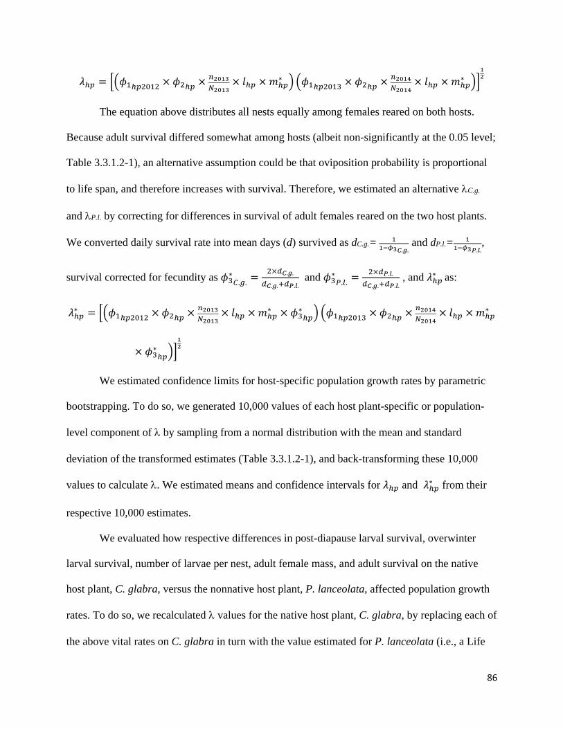
86
𝜆𝜆ℎ𝑝𝑝 = ��𝜙𝜙1ℎ𝑝𝑝2012 × 𝜙𝜙2ℎ𝑝𝑝 × 𝑛𝑛2013𝑁𝑁2013
× 𝑙𝑙ℎ𝑝𝑝 × 𝑚𝑚ℎ𝑝𝑝∗ � �𝜙𝜙1ℎ𝑝𝑝2013 × 𝜙𝜙2ℎ𝑝𝑝 × 𝑛𝑛2014
𝑁𝑁2014× 𝑙𝑙ℎ𝑝𝑝 × 𝑚𝑚ℎ𝑝𝑝
∗ ��12
The equation above distributes all nests equally among females reared on both hosts.
Because adult survival differed somewhat among hosts (albeit non-significantly at the 0.05 level;
Table 3.3.1.2-1), an alternative assumption could be that oviposition probability is proportional
to life span, and therefore increases with survival. Therefore, we estimated an alternative λC.g.
and λP.l. by correcting for differences in survival of adult females reared on the two host plants.
We converted daily survival rate into mean days (d) survived as dC.g.= 11−𝜙𝜙3𝐶𝐶.𝑔𝑔.
and dP.l.= 11−𝜙𝜙3𝑃𝑃.𝑙𝑙.
,
survival corrected for fecundity as 𝜙𝜙3∗𝐶𝐶.𝑔𝑔. = 2×𝑑𝑑𝐶𝐶.𝑔𝑔.
𝑑𝑑𝐶𝐶.𝑔𝑔.+𝑑𝑑𝑃𝑃.𝑙𝑙. and 𝜙𝜙3∗𝑃𝑃.𝑙𝑙. = 2×𝑑𝑑𝑃𝑃.𝑙𝑙.
𝑑𝑑𝐶𝐶.𝑔𝑔.+𝑑𝑑𝑃𝑃.𝑙𝑙. , and 𝜆𝜆ℎ𝑝𝑝∗ as:
𝜆𝜆ℎ𝑝𝑝∗ = ��𝜙𝜙1ℎ𝑝𝑝2012 × 𝜙𝜙2ℎ𝑝𝑝 × 𝑛𝑛2013𝑁𝑁2013
× 𝑙𝑙ℎ𝑝𝑝 × 𝑚𝑚ℎ𝑝𝑝∗ × 𝜙𝜙3∗ℎ𝑝𝑝� �𝜙𝜙1ℎ𝑝𝑝2013 × 𝜙𝜙2ℎ𝑝𝑝 × 𝑛𝑛2014
𝑁𝑁2014× 𝑙𝑙ℎ𝑝𝑝 × 𝑚𝑚ℎ𝑝𝑝
∗
× 𝜙𝜙3∗ℎ𝑝𝑝��12
We estimated confidence limits for host-specific population growth rates by parametric
bootstrapping. To do so, we generated 10,000 values of each host plant-specific or population-
level component of λ by sampling from a normal distribution with the mean and standard
deviation of the transformed estimates (Table 3.3.1.2-1), and back-transforming these 10,000
values to calculate λ. We estimated means and confidence intervals for 𝜆𝜆ℎ𝑝𝑝 and 𝜆𝜆ℎ𝑝𝑝∗ from their
respective 10,000 estimates.
We evaluated how respective differences in post-diapause larval survival, overwinter
larval survival, number of larvae per nest, adult female mass, and adult survival on the native
host plant, C. glabra, versus the nonnative host plant, P. lanceolata, affected population growth
rates. To do so, we recalculated λ values for the native host plant, C. glabra, by replacing each of
the above vital rates on C. glabra in turn with the value estimated for P. lanceolata (i.e., a Life
87
Table Response Analysis, LTRE; Caswell 2001). We did not do this for number of nests on C.
glabra versus P. lanceolata per adult since the total number of nests per adult was combined in
our formula. For consistency, we evaluated the results of these substitutions for values of both λ
(without including differences in adult survival) and λ* (including differences in adult survival).
Movement: Parameter estimation for minimum patch size model
To estimate movement parameters for our analytical calculation of minimum patch size,
we bootstrapped over individual flight paths with at least 4 moves (Npaths=22, mean moves=28,
max. moves=39) to calculate the average move length, squared move length, cosine of turning
angle, and time per move, following Turchin (1998). We calculated the asymptotic per-move
increase in squared displacement, 𝑅𝑅�𝑛𝑛2, and the diffusion coefficient, 𝐷𝐷, using the standard
correlated random walk approach (Kareiva and Shigesada 1983, Schultz 1998, Turchin 1998).
We calculated confidence limits for 𝑅𝑅�𝑛𝑛2 and D by sampling entire paths with replacement for
1000 iterations. We sampled paths rather than moves to account for variation among individuals
while maintaining correlation among parameters within individuals. We compared predicted 𝑅𝑅�𝑛𝑛2
to observed displacements by calculating the mean squared displacement for all pairs of steps
within each path, back-transforming to net displacement and taking the mean and standard
deviation across individual butterflies (Turchin 1998).
We evaluated the assumption that movement followed a correlated random walk in our
population with our capture-mark-recapture data. We compared the distance and time between
relocations of marked adult females, with the expectation that squared distance should increase
linearly with time (Turchin 1998; 𝑑𝑑2=4𝐷𝐷t), where 𝑑𝑑2 is the squared distance between sequential
capture locations and t is the time interval between captures (in days). We regressed 𝑑𝑑2 against t
88
to test the expectation that the intercept of this relationship did not differ from 0 and used the
slope coefficient of a 0-intercept model as an estimate of 4D. We used flight time per day to
convert D in square meters per day to square meters per second. Our observations indicated that
butterflies flew mostly from the hours of 1000-1500, as these were the earliest and latest times
we could collect flight path data. About 80% of days had suitable conditions for flight—others
were too rainy or very hot and humid—yielding an estimated 4 flight hours/day. We used 5 flight
hours/day as an upper limit (i.e., movement on all days including rainy ones) and 2 flight
hours/day as a lower limit (i.e., the time needed to make observations from flight paths and
mark-recapture match exactly).
Host-plant specific movement: Parameter estimation for SEIBMs
To estimate movement parameters for SEIBMs, we estimated mean move length, m,
cosine of the turning angle, ρ, probability of resting, P, and time spent resting, τ (e.g., if a
transition between two points took more than 15 seconds, the interval at which the movement
data were collected, any additional time beyond the 15 seconds is time that was spent resting at
the first of the two points), using GLMMs. We included individual butterfly ID as a random
effect in all models. For models estimating the time spent resting, we also included a unique
identifier for each move (pooled across all butterflies) as a random effect to account for
overdispersion (Elston et al. 2001); this model fit the data better than a model with butterfly ID
alone as a random effect (χ2=7576, df=1, p<0.001).
In mixed-effects models, the back-transformed fixed effect coefficients are a biased
estimate of the true population means (Jensen's inequality; Ruel and Ayres 1999, Bolnick et al.
2011, Crone 2013). We estimated ‘unbiased’ means of back-transformed parameters by sampling
89
from a normal distribution with the link-function scale MLE coefficient and among-individual
standard deviation from GLMMs (described in Crone 2013). We back-transformed the samples
and calculated means, variances, and coefficients of variation of the back-transformed values.
We estimated preference at forest edges initially by fitting GLMMs with open habitat or matrix
land cover type as a fixed effect, final location (open vs. forest) as the dependent variable, and
release location as a random effect. Given non-significant effects of the different open cover
types, we tested whether the overall proportion of butterflies entering the forest versus meadow
differed from 50% using an intercept-only binomial GLMM (i.e., to compare the mean
proportion with 0.50, or 0 on a logit scale). We tested for host plant preference at ‘soft’ edges
between host plants and open matrix and using a binomial GLM.
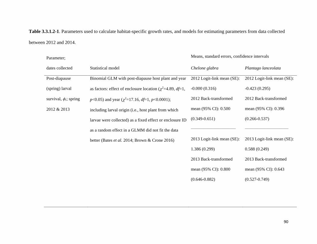
90
Table 3.3.1.2-1. Parameters used to calculate habitat-specific growth rates, and models for estimating parameters from data collected
between 2012 and 2014.
Parameter;
dates collected Statistical model
Means, standard errors, confidence intervals
Chelone glabra Plantago lanceolata
Post-diapause
(spring) larval
survival, φ1; spring
2012 & 2013
Binomial GLM with post-diapause host plant and year
as factors: effect of enclosure location (χ2=4.89, df=1,
p<0.05) and year (χ2=17.16, df=1, p<0.0001);
including larval origin (i.e., host plant from which
larvae were collected) as a fixed effect or enclosure ID
as a random effect in a GLMM did not fit the data
better (Bates et al. 2014; Brown & Crone 2016)
2012 Logit-link mean (SE):
-0.000 (0.316)
2012 Back-transformed
mean (95% CI): 0.500
(0.349-0.651)
________________________________
2013 Logit-link mean (SE):
1.386 (0.299)
2013 Back-transformed
mean (95% CI): 0.800
(0.646-0.882)
2012 Logit-link mean (SE):
-0.423 (0.295)
2012 Back-transformed
mean (95% CI): 0.396
(0.266-0.537)
_______________________________
2013 Logit-link mean (SE):
0.588 (0.249)
2013 Back-transformed
mean (95% CI): 0.643
(0.527-0.749)
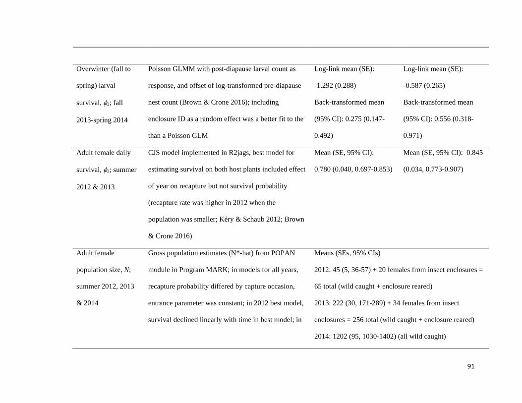
91
Overwinter (fall to
spring) larval
survival, φ2; fall
2013-spring 2014
Poisson GLMM with post-diapause larval count as
response, and offset of log-transformed pre-diapause
nest count (Brown & Crone 2016); including
enclosure ID as a random effect was a better fit to the
than a Poisson GLM
Log-link mean (SE):
-1.292 (0.288)
Back-transformed mean
(95% CI): 0.275 (0.147-
0.492)
Log-link mean (SE):
-0.587 (0.265)
Back-transformed mean
(95% CI): 0.556 (0.318-
0.971)
Adult female daily
survival, φ3; summer
2012 & 2013
CJS model implemented in R2jags, best model for
estimating survival on both host plants included effect
of year on recapture but not survival probability
(recapture rate was higher in 2012 when the
population was smaller; Kéry & Schaub 2012; Brown
& Crone 2016)
Mean (SE, 95% CI):
0.780 (0.040, 0.697-0.853)
Mean (SE, 95% CI): 0.845
(0.034, 0.773-0.907)
Adult female
population size, N;
summer 2012, 2013
& 2014
Gross population estimates (N*-hat) from POPAN
module in Program MARK; in models for all years,
recapture probability differed by capture occasion,
entrance parameter was constant; in 2012 best model,
survival declined linearly with time in best model; in
Means (SEs, 95% CIs)
2012: 45 (5, 36-57) + 20 females from insect enclosures =
65 total (wild caught + enclosure reared)
2013: 222 (30, 171-289) + 34 females from insect
enclosures = 256 total (wild caught + enclosure reared)
2014: 1202 (95, 1030-1402) (all wild caught)
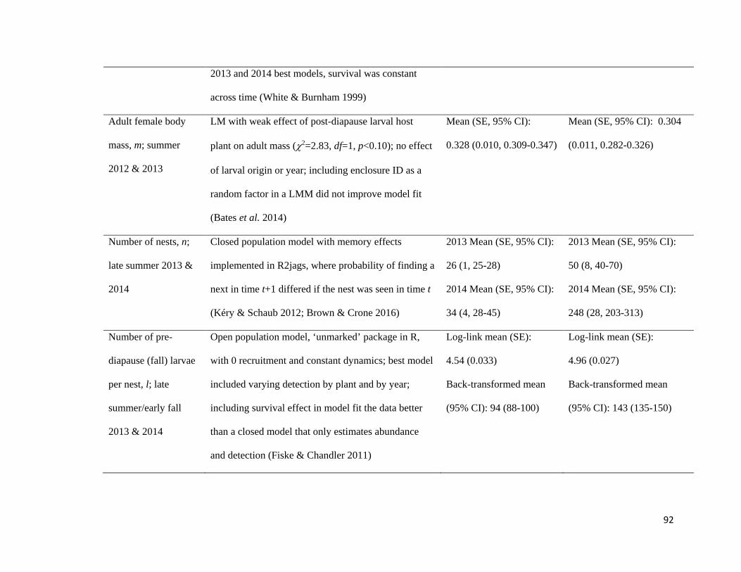
92
2013 and 2014 best models, survival was constant
across time (White & Burnham 1999)
Adult female body
mass, m; summer
2012 & 2013
LM with weak effect of post-diapause larval host
plant on adult mass (χ2=2.83, df=1, p<0.10); no effect
of larval origin or year; including enclosure ID as a
random factor in a LMM did not improve model fit
(Bates et al. 2014)
Mean (SE, 95% CI):
0.328 (0.010, 0.309-0.347)
Mean (SE, 95% CI): 0.304
(0.011, 0.282-0.326)
Number of nests, n;
late summer 2013 &
2014
Closed population model with memory effects
implemented in R2jags, where probability of finding a
next in time t+1 differed if the nest was seen in time t
(Kéry & Schaub 2012; Brown & Crone 2016)
2013 Mean (SE, 95% CI):
26 (1, 25-28)
2014 Mean (SE, 95% CI):
34 (4, 28-45)
2013 Mean (SE, 95% CI):
50 (8, 40-70)
2014 Mean (SE, 95% CI):
248 (28, 203-313)
Number of pre-
diapause (fall) larvae
per nest, l; late
summer/early fall
2013 & 2014
Open population model, ‘unmarked’ package in R,
with 0 recruitment and constant dynamics; best model
included varying detection by plant and by year;
including survival effect in model fit the data better
than a closed model that only estimates abundance
and detection (Fiske & Chandler 2011)
Log-link mean (SE):
4.54 (0.033)
Back-transformed mean
(95% CI): 94 (88-100)
Log-link mean (SE):
4.96 (0.027)
Back-transformed mean
(95% CI): 143 (135-150)
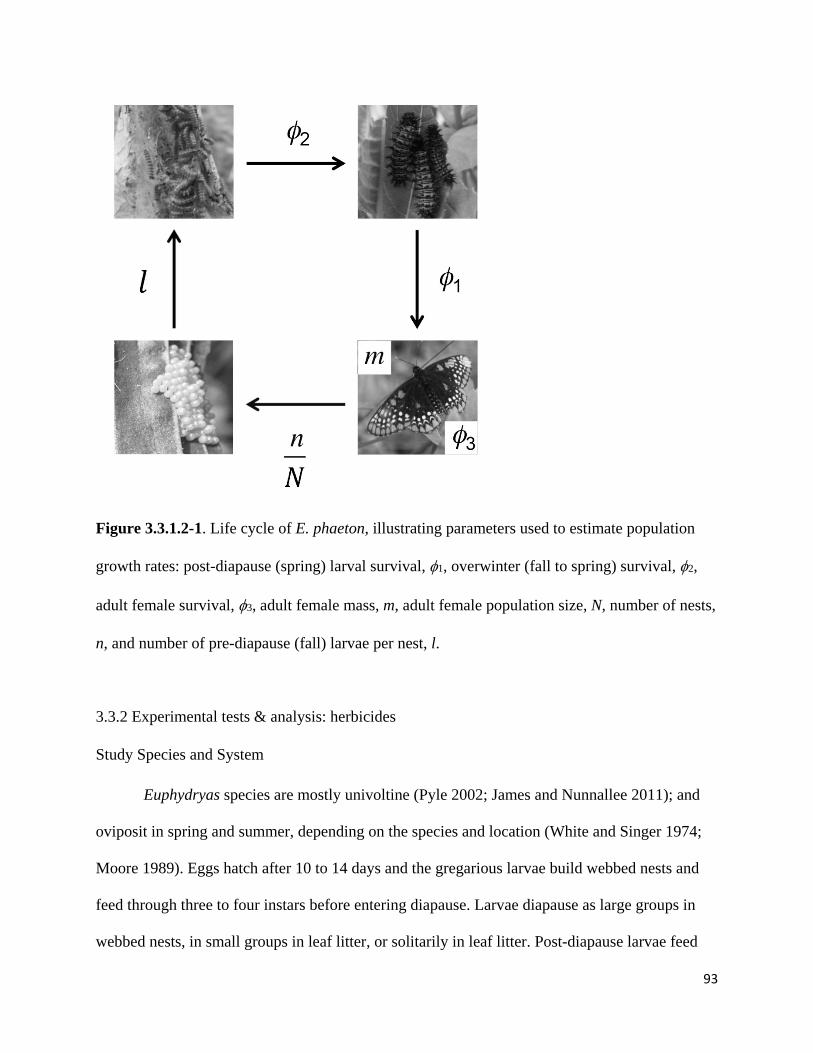
93
Figure 3.3.1.2-1. Life cycle of E. phaeton, illustrating parameters used to estimate population
growth rates: post-diapause (spring) larval survival, φ1, overwinter (fall to spring) survival, φ2,
adult female survival, φ3, adult female mass, m, adult female population size, N, number of nests,
n, and number of pre-diapause (fall) larvae per nest, l.
3.3.2 Experimental tests & analysis: herbicides
Study Species and System
Euphydryas species are mostly univoltine (Pyle 2002; James and Nunnallee 2011); and
oviposit in spring and summer, depending on the species and location (White and Singer 1974;
Moore 1989). Eggs hatch after 10 to 14 days and the gregarious larvae build webbed nests and
feed through three to four instars before entering diapause. Larvae diapause as large groups in
webbed nests, in small groups in leaf litter, or solitarily in leaf litter. Post-diapause larvae feed

94
through additional instars in small groups or solitarily, after which they pupate briefly and eclose
(Bowers et al. 1992; Singer and McBride 2010; James and Nunnallee 2011).
We used E. phaeton, E. colon and E. editha colonia to investigate consequences of
graminicide-based management. We chose these species to represent a range within the genus,
and as surrogates to advise habitat management of federally-listed Euphydryas species in North
America. Both E. e. colonia and E. colon reside in the same region as endangered E. e. taylori
and use the same native larval hostplants as other E. editha, as well as other Euphydryas in
western North America (Pyle 2002; James and Nunnallee 2011). Our third proxy, E. phaeton, is
a well-studied species from eastern North America (e.g. Stamp 1981; Bowers et al. 1992; Brown
and Crone 2016). Like the three western at-risk species, E. e. bayensis, E. e. quino and E. e.
taylori (Severns and Warren 2008) some populations of E. phaeton have switched from a native
pre-diapause hostplant to non-native Plantago lanceolata (Bowers et al. 1992; Severns and
Warren 2008).
Euphydryas larvae use hostplants from several families within the superorder Lamianae,
all of which synthesize iridoid glycosides (Bowers 1991; Rimpler 1991). These include plant
families in the order Lamiales (Families: Boraginaceae, Buddlejaceae, Orobanchaceae,
Plantaginaceae, Scrophulariaceae) and Dipsacales (Families: Caprifoliaceae, Dipsacaceae,
Valerianaceae). North American hostplants include non-native species in these plant families
including the genera Lonicera and Plantago, in which P. lanceolata, P. major and L. japonica
are hosts for larval Euphydryas (White and Singer 1974; Singer et al. 2008; MDNR 2014;
Robinson et al. 2016). Iridoid glycosides are secondary plant compounds that often reduce
herbivory in non-adapted insects (Bowers 1991); however, these compounds serve as feeding
95
stimulants in some specialists, such as Euphydryas, and, when sequestered, may deter predators
(Bowers 1983; Bowers 1991; Wahlberg 2001).
Graminicides
Three post-emergent graminicides are used regularly by land managers for prairie
restoration in the Pacific Northwest; fluazifop-p-butyl, clethodim and sethoxydim. These
chemicals systemically target active meristematic sites by inhibiting acetyl coenzyme A
carboxylase and thus constrain lipid synthesis (Walker et al. 1988). Larval stages of the butterfly
life cycle may be most susceptible to direct and indirect non-target herbicide effects through
dermal contact, ingestion of herbicide, or reduction in hostplant nutritional quality. For
experiments, we used the herbicide formulations most commonly chosen by land managers in
Pacific Northwest prairies: fluazifop-p-butyl as Fusilade DX® (24.5% fluazifop-p-butyl,
Syngenta Crop Protection LLC, Greensboro, North Carolina), sethoxydim as Poast® (18%
sethoxydim, BASF Corporation, Research Triangle Park, NC) and clethodim as Envoy Plus®
(12.6% clethodim, Valent Corporation, Walnut Creek, CA). These chemicals are applied in
combination with a “sticker-spreader” to increase efficacy. In all graminicide treatments, we use
adjuvant NuFilm IR ® (96% poly-1-p- menthene, Miller Chemical and Fertilizer Corporation,
Hanover, PA).
Experiments
To test for the effects of graminicides on Euphydryas larvae, we conducted two
investigations in the Washington State University Vancouver greenhouse. In the first experiment
(the “Graminicide” experiment), we examine effects of different graminicides on larval survival
and chemistry of E. colon reared on Plantago lanceolata. Although P. lanceolata is a non-native
hostplant, it is the lone hostplant species used by all three Euphydryas species. In the “Species x
96
Hostplant” experiment, we measured a number of demographic and behavioral responses to a
single graminicide for three Euphydryas species reared on different host plants. In this second
experiment, we used microcosms constructed of 37.8 litre nursery containers potted with either
native hostplants (Chelone glabra for E. phaeton, Castilleja hispida for E. e. colonia and E.
colon) or novel hostplant P. lanceolata. We used Eriophyllum lanatum [Compositae] as a host
for hemiparasitic C. hispida and therefore we included it in novel host (P. lanceolata)
microcosms for E. colon and E. editha to control for its presence.
For both experiments, we collected eggs from females caught in the wild from montane
areas of Washington State for E. colon and E. editha (Yakima County, WA, 46.71 N, -121.11
W), and from egg clusters collected in the wild in Massachusetts (Worcester County, MA, 42.48
N, -71.57 W) for E. phaeton. In both experiments, we reared caterpillars to second instar on P.
lanceolata to ensure all larvae received the same nutritional opportunity prior to treatment. On
treatment day, we weighed each larva and randomly assigned to a treatment. Given that colonies
often merge in the wild, and benefits of gregariousness seem based primarily on group size rather
than relatedness (Moore 1989; Costa and Ross 2003; Ehrlich and Hanski 2004), mixing families
is unlikely to influence experimental outcome. We sprayed plants and larvae using a Precision
backpack sprayer (RandD Sprayers, Opelousas, Louisiana) with a flat fan 8002VS nozzle and
CO2 propellant (276kPa) at the manufacturer’s recommended field rates. Larvae were given
unlimited food until they entered diapause, which was determined by absence of feeding for two
days.
Graminicide Experiment
In the Graminicide experiment, we applied five treatments to 200 2nd instar E. colon
larvae (40 individual larvae per treatment) on August 12, 2014. Treatments included three
97
graminicides each combined with NuFilm adjuvant: fluazifop-p-butyl, sethoxydim and
clethodim. In addition, we conducted a water treatment and a treatment with just NuFilm.
Graminicides were applied per manufacturer recommended rates: 7.5 mL fluazifop-p-butyl with
3.9 mL NuFilm per 1000 mL distilled water; 15.0mL sethoxydim with 3.1mL Nufilm per 1000
mL distilled water; and 5.04 mL clethodim with 2.25mL Nufilm per 1000 mL distilled water. In
the NuFilm only treatment, we mixed 3.9 mL of NuFilm per 1000 ml distilled water. Larvae
were exposed individually and separately from the hostplant, with the same equipment and rate.
Larvae were weighed prior to experimental treatment, and then placed in individual 60 ml
rearing containers for the duration of the experiment. Larvae were fed fresh Plantago from the
appropriate treatment until they stopped feeding and entered diapause, at which time the date of
diapause initiation was recorded and larvae were weighed. Larvae were placed in diapause
containers in September following protocols with related diapausing species (Linders, E. e.
taylori, pers. comm. and Saastomoinen, M. cinxia, pers. comm). Five individuals from each
treatment were sent to University of Colorado for quantification of iridoid glycosides in
December 2014.
Aucubin and catalpol (the iridoid glycosides found in P. lanceolata (Bowers and Stamp
1992) are known to be sequestered by Euphydryas (Bowers et al. 1992). These were extracted
from freshly frozen caterpillars (methods in Bowers et al. 1992) and quantified by gas
chromatography (methods in Gardner and Stermitz 1988; Bowers et al. 1992). Quantification
was based on calibration with pure aucubin and catalpol coupled with the internal standard
phenyl-β-D-glucopyranoside (PBG, Sigma Aldrich) (0.500 mg/sample), that was added to each
sample. Wet weights of frozen larvae were converted to dry weights using a separate set of
caterpillars that were weighed wet and then dried at 50oC for 48 hours and re-weighed.
98
Species x Hostplant Experiment
In the second experiment, we applied fluazifop-p-butyl mixed with NuFilm (at the same
rates as the Graminicide Experiment) to larval three Euphydryas species and their hostplant
species. All treatments were initiated in August and September 2013, when sufficient numbers of
larvae reached 2nd instar to conduct a trial, such that E. colon were treated on August 26th, E.
editha were treated on August 1st and 5th, and E. phaeton were treated on August 10th, 31st, Sept
1st and 3rd. Larvae were placed in groups of 20 in each experimental microcosm. We allowed
larvae to feed gregariously as they do in the wild; each microcosm contained ample plant
biomass to support a cohort of 20 larvae. We replicated the four treatments (graminicide vs
control by native vs novel hostplant) six times (except for E. colon, which had five replicates)
with a 20-larva cohort per treatment group (microcosm). We positioned microcosms randomly in
the greenhouse to mitigate unintended biases. We noted survival and made the following
behavioral observations daily: (1) how many larvae were solitary or group size if not solitary, (2)
whether each larva was actively feeding or not. Larvae were considered part of a group if they
were in, on, or within one nest-width from the webbed nest. Because nest sizes were never > 20,
we could visually inspect all individuals without damaging webbing. Larvae that stopped feeding
and remained within the webbing for more than 48 hours were noted as ‘in diapause.’ We
weighed larvae to determine final (diapause) mass.
Statistical Analysis
We used generalized linear models with mixed effects where appropriate to analyze
experimental data. Data were analyzed using ‘lme4’ package (Bates et al. 2015) in R using
99
(g)lm and (g)lmer functions for models without and with random effects, respectively (R Core
Team 2015).
In the Graminicide experiment, we assessed survivorship to diapause using a general
linear model with a binomial distribution, logit link and a single fixed effect of Treatment (one of
three graminicides, NuFilm, or control). We analyzed development time from treatment date to
diapause with a Poisson distribution, a log link and a fixed effect of Treatment. Survivorship and
development time did not show evidence of overdispersion in this experiment. We analyzed
change in mass from initial to final using a linear model with fixed effects of initial vs final size.
We analyzed percent dry weight of aucubin and catalpol using linear models with Treatment as a
fixed effect. For analyses in the Graminicide experiment, we report χ2 from Likelihood Ratio
Tests for type II χ2 tests from analysis of deviance. In addition, to test if each treatment was
different from the control, we report P-values from Dunnett contrasts for multiple comparisons
using R package ‘multcomp’ (Hothorn et al. 2008).
For the Species x Hostplant experiment, Exposure (i.e., use of graminicide or not),
Species (Euphydryas species) and Host (host plant species) and their interactions were included
as fixed effects. Treatment date, observation date and microcosm were included as random
effects. Microcosm, as a random effect, takes repeated observations of larvae per microcosm into
account (experimental block) and observation date, when applicable, accounts for repeated
measures (in time). We analyzed survivorship to diapause using a linear model with a binomial
distribution and logit link. We analyzed development time from treatment date to diapause with a
Poisson distribution and log link; this model included an observation-level random effect to
account for possible overdispersion (Elston et al. 2001). For effects of herbicides on change in
mass, we used a Gaussian family, identity link effect model with an additional fixed effect of
100
observation date (initial vs. final size). We analyzed gregariousness and feeding behavior using
a binomial distribution and logit link. We analyzed the number of larvae per group using a
Poisson distribution and log link; we used the total number of grouped larvae as the response
variable and the log- transformed number of groups as an offset to estimate the model ratio. This
model included an observation-level random effect to account for overdispersion.
3.3.3 Minimum patch size and connectivity
Minimum patch size estimation
The idea of minimum patch area, first proposed by Skellam (1951) and Kierstead and
Slobodkin (1953) (collectively KSS’s model) provides a mechanistic framework for estimating
MAR as a function of movement and demography. In KSS’s framework, minimum patch area is
modeled using reaction-diffusion equations that describe the change in population density over
time and movement is modeled according to a random walk (Cosner 2008). Individuals diffuse
out of patches and if a patch is too small, they will leave before reproducing. Accordingly, there
is a threshold critical minimum patch size, below which a population cannot persist (Crone &
Schultz 2003). Because large patches have lower emigration rates than small patches as a
function of size and edge-to-area ratio, patch size predicts residence time (days spent in the
patch, sensu Schultz & Crone 2001) and subsequent population growth (Fahrig 2007). We
combined KSS’s theoretical notion of minimum patch area with field-collected movement and
demographic data to analytically estimate the minimum patch size for the Baltimore checkerspot
butterfly (Euphydryas phaeton, Nymphalidae).
We modified KSS’s model to reflect the temporal dynamics of butterfly life histories.
Specifically, butterflies move, die, and lay eggs throughout their lives as they encounter host

101
plants, and eggs hatch into relatively immobile larvae that mature over the course of a year
(Crone & Schultz 2003). Movement and survival can be modeled with an equation identical to
KSS’s model, where r is the distance of individuals from the patch center, D is the diffusion
coefficient, and the instantaneous population growth rate is replaced with the instantaneous rate
of mortality, µ:
𝜕𝜕𝑛𝑛𝜕𝜕𝑡𝑡
= −𝜇𝜇𝜇𝜇 + 𝐷𝐷 1𝑟𝑟𝜕𝜕𝜕𝜕𝑟𝑟�𝑟𝑟 𝜕𝜕𝑛𝑛
𝜕𝜕𝑟𝑟�. [1]
The solution for Eq. 1 becomes
𝑛𝑛(𝑟𝑟,𝑡𝑡)𝑛𝑛(𝑟𝑟,0)
= exp �− �𝜇𝜇 + 𝐷𝐷 �𝛽𝛽1𝑅𝑅�2� 𝑡𝑡�, [2]
where R is the patch radius, β1≈2.41 (the first 0 of a Bessel function; see derivation in Kot 2001),
and n(r,t) describes the population size at time t and location r (cf. Kot’s [2001] Eqs. 16.69-
16.70). Equation 2 represents the proportion of animals left in a patch of radius R at time, as a
function of loss from mortality (m) and movement (𝐷𝐷 �𝛽𝛽1𝑅𝑅�2). The expected residence time as a
function of patch radius is
1
�𝜇𝜇+𝐷𝐷�𝛽𝛽1𝑅𝑅 �2� [3]
(i.e., the reciprocal of the rate of loss). The ratio of expected residence time in a patch of radius R
to the organism’s lifespan in an infinitely large patch is
𝜇𝜇
�𝜇𝜇+𝐷𝐷�𝛽𝛽1𝑅𝑅 �2�. [4]
Reproduction is proportional to the amount of time spent in the patch, so the realized annual
population growth rate becomes
𝜆𝜆 = 𝑏𝑏max �𝜇𝜇
�𝜇𝜇+𝐷𝐷�𝛽𝛽1𝑅𝑅 �2��, [5]
102
where bmax is the per capita number of offspring that survive to reproduce in unlimited habitat.
The population persists in isolation if l≥1, and the radius (in meters), Rc, of the CMP is
𝑅𝑅𝑐𝑐 = 𝛽𝛽1�𝐷𝐷
𝜇𝜇(𝑏𝑏max−1) [6]
(Kot’s [2001] Eq. 16.75).
As in KSS’s continuous-reproduction model, Rc increases with D and declines with bmax.
In our model, Rc also declines as mortality, m increases because we assumed maximum
reproductive output is independent of adult mortality. Hence, a species with a shorter lifespan
and the same reproductive output reproduces more quickly, allowing it to persist in smaller
patches. The model is a conservative assessment of CMP because individuals do not return to a
patch after leaving (see mathematical explorations of effects of edge behavior in Ovaskainen
2004, Schultz and Crone 2001 and Xiao et al. 2013). From Eq. 6 the CMP in hectares is
𝜋𝜋10,000
𝑅𝑅𝐶𝐶2 = 𝜋𝜋𝛽𝛽12𝐷𝐷
(10,000)𝜇𝜇(𝑏𝑏max−1).
We estimated vital rates and population size estimates from data collected 2013-2014 as
described in Section 3.3.2, but estimated across values for both host plants rather than separately.
These values were post-diapause larval survival, φ1 population size, 𝑁𝑁�, and survival rate, φ3, of
adult females; number of larval nests, 𝜇𝜇�; larvae per nest, 𝑙𝑙; and overwinter survival, φ2 (Table
3.3.4-1). We calculated the observed maximum population growth rate as the product of post-
diapause survival × overwinter survival × nests per adult × larvae per nest:
𝑏𝑏max = ∅1∅20.5𝑛𝑛�𝑙𝑙𝑁𝑁�
, [7]
where the 0.5 accounts for an approximately even sex ratio (female offspring per adult female).
We calculated confidence limits for bmax with parametric bootstrapping (i.e., sampling over
normal distributions defined by the means and standard errors of each model parameter).

103
Equation 7 is a conservative estimate of bmax because we estimated nests per female in a
finite patch. Alternatively, we could assume that the probability of reproduction is proportional
to the amount of time spent in a patch; in this case, the observed number of nests, 𝜇𝜇�, would be
the actual maximum lifetime number of nests, 𝜇𝜇�∗, multiplied by the proportion of an individual’s
lifespan spent in the patch (from Eq. 4):
𝜇𝜇� = 𝜇𝜇�∗ � 𝜇𝜇
�𝜇𝜇+𝐷𝐷�𝛽𝛽1𝑅𝑅 �2��. [8]
Here, m is the instantaneous (per second) mortality rate of adult females calculated from flight
time per day and the daily survival rate, φ3, D is the diffusion coefficient, and R is the patch
radius. We used R=183 m for our ~10.5-ha study site and all other parameters as estimated
above. We solved for 𝜇𝜇�∗ with Eq. 8 and calculated bmax and all other derived variables twice,
once using 𝜇𝜇� as our estimate of nests produced and once using 𝜇𝜇�∗. Parametric bootstrap
confidence limits of variables calculated using 𝜇𝜇�∗ included sampling distributions for D and φ3
(Table 3.3.3-1).
We evaluated the estimated growth rate by comparing predicted population growth rates
(Eq. 5) with changes in abundance at our study site (2012-2014). We calculated the expected
population growth rate as bmax (Eq. 7) multiplied by the proportion of time spent in the patch
(Eq. 4).
SEIBM implementation
We calculated landscape-scale metrics, specifically residence time of Baltimore
checkerspot butterflies in their natal patch and dispersal to [i.e., connectivity] and time spent in a

104
new patch using a spatially-explicit individual-based simulation model built in Netlogo
(Wilensky 1999). To do so, we first created a habitat-nonhabitat only simulation model to
estimate growth rates, mean residence time (days in patch) and mean dispersal distance. For this
habitat-nonhabitat model, we used parameter estimates from GLMMs for demography averaged
across host plants as shown in Table 3.3.3-1. In addition to these values, we also estimated the
probability of oviposition, o, as 𝜇𝜇�/(𝑁𝑁�×L), where L is the expected lifetime in days. The logit-
transformed survival on any given day, d, starting at d = 0, is β0 + β1 × d. We defined the
expected lifetime, L, as the number of days for the inverse-logit transformed daily survival,
exp (𝛽𝛽0+𝛽𝛽1 × 𝑑𝑑)exp(𝛽𝛽0+𝛽𝛽1 × 𝑑𝑑)+1, to decline to 0.5, i.e., solving for L such that ∏ exp (𝛽𝛽0+𝛽𝛽1 × 𝑑𝑑)
exp(𝛽𝛽0+𝛽𝛽1 × 𝑑𝑑)+1𝐿𝐿𝑑𝑑=0 = 0.5. We re-
estimated movement parameters across host plants using GLMMs as described in Section 3.2.2;
Table 3.3.3-2).
For our habitat-nonhabitat SEIBM, we ran 1000 5-year simulations for circular habitat
patches of 0.1, 0.2, 0.5, 1, 2, 4, 8, 12, 16, 20, 24, 28, 32, 36, and 40 hectares, each with a starting
population size of 50; within 5 years, populations either went extinct or grew exponentially. We
assumed a season of 28 days based on the earliest to the latest days butterflies were seen at our
site in 2012 and 2013, and assumed that individuals were active ~4-flight-hours/day (see Section
3.3.2). At each time step, individuals in the model lived or died, layed eggs or did not, and
moved or rested. The only difference in this model between habitat and nonhabitat was that
oviposition occured only in habitat. The logit-transformed survival on any given day and the
probability of oviposition were converted to 15-s intervals, the time step at which the model
proceeded. Nest size was chosen from a Poisson distribution with a mean of 𝑙𝑙, the number of
larvae per nest estimated from the field, and multiplied by overwinter survival, post-diapause
survival, and 0.5 to model only adult females.
105
For each individual that lived and was not already resting at a particular time step, we
used the per-move probability of resting to determine if it moved or rested. If it rested, the time
spent resting was drawn from a Poisson distribution at the beginning of each resting bout, and
the individual returned to the “not resting” pool at the end of that bout. For individuals that
moved, we modeled movement as a correlated random walk (i.e., the direction, θ, of a move at
time t is correlated with the direction at time t–1). We simulated movement direction from a
wrapped Cauchy distribution defined as 𝜃𝜃𝑡𝑡 = 𝜃𝜃𝑡𝑡−1 + 2arctan �1−𝜌𝜌1+𝜌𝜌
𝑡𝑡𝑡𝑡𝜇𝜇{𝜋𝜋[𝑈𝑈(−0.5,0.5)]}�,
where the initial direction is randomly chosen from 0 – 2π, and ρ is the mean cosine of the
turning angle (Barton et al. 2009). We simulated move lengths from a gamma distribution with
parameters α (scale) = µ2/σ and λ (shape) = µ/σ, where µ and σ are the back-transformed mean
and variance of move length (everywhere else in this paper, λ refers to the population growth
rate, not the shape parameter).
We calculated statistics based on years 2-5 of simulations because the first year (and
resulting population growth rate) was affected by the initial random placement of adults on the
landscape. We estimated the annual population growth rate, λ, for each patch size by regressing
the population size, N, across model iterations for a particular patch size at time t+1 against the
intercept, with an offset of the population size at time t, using a Poisson GLM. We obtained
dispersal distances in two ways. First, we recorded the mean dispersal distance across individuals
in each of the 1000 simulations per patch size to estimate the distribution of average distances
moved across replicate simulations. Second, we quantified the net distance dispersed in a single
year by 5000 homogeneous individuals and 5000 individuals with heterogeneity in movement in
a 2-Ha patch to describe variation across individuals within a single population.
106
To add landscape-specific metrics to our habitat-nonhabitat model, we created base maps
of structural variation in land cover across our study site from aerial photographs available in
ArcMap (2013–2014 orthoimagery from MassGIS 2014). We used aerial photographs to separate
forest and open areas on the landscape and manually traced and digitized these areas in ArcMap.
We ground-truthed maps by walking the perimeters of open areas on the landscape, and checked
that the recorded areas of GPS points based on ground observations matched those of the
digitized landscape. We divided open land cover types into habitat and open matrix by
estimating the relative density of native and non-native host plants across our site. We surveyed
all non-forested land in a regular 50 × 50 m grid, using a compass to follow straight lines. We
stopped every ~10 m, and chose a sampling location offset from the main grid by walking a
randomly chosen 0–5 paces in a randomly chosen direction (following Holl and Crone 2004).
We recorded the distance of the three closest individuals of C. glabra up to five meters from the
sampling location, and the three closest individuals of P. lanceolata up to one meter from the
sampling location. The search area for C. glabra was larger than for P. lanceolata because C.
glabra are less dense and more conspicuous, so we would not have obtained reasonable
estimates of the relative density of C. glabra had we restricted the search area to one meter. It
would not, however, have been feasible to search for P. lanceolata within a five-meter radius
from each point in tall grass without trampling butterfly habitat. We estimated relative host plant
density ad hoc by converting the distance, d, of each individual from each sampling location into
the area of a circle with radius d, taking the reciprocal of the area (defined as zero for cases
where there were no additional plants within the search area), and averaging the three numbers
for the three individuals of each host plant species. We used spatial interpolation (kriging) of ln-
107
transformed density indices to create a map of plant densities (Figure 3.3.3-1; Kriging tool,
ArcMap 10.3, ESRI 2015).
We divided the study area into discrete patches based on estimated host plant densities,
and classified these into five land cover classes: (1) high quality C. glabra habitat [mean (SD) =
0.03 (0.09) plants/m2], (2) high quality P. lanceolata habitat [mean (SD) = 76.3 (211.1)
plants/m2], (3) low quality habitat, typically areas with at least ~1/10 of the P. lanceolata density
found in high quality habitat [mean (SD) = 4.9 (32.8) plants/m2; note there was no low quality C.
glabra habitat in our study area], (4) open matrix, i.e., non-forested areas lacking host plants, and
(5) forest matrix. We created an ~1 km buffer from the central-most point of our ~11.5 hectare
study region, and classified most areas outside of our study site as open or forest matrix using
aerial imagery as described above. The only exception was a wetland separated by forest ~0.2
km from our study site containing C. glabra, that we classified as low quality habitat because
preliminary observations suggest that C. glabra density in this patch is noticeably lower than in
our main study site. This patch has not recently been occupied by Baltimore checkerspots (E.
Crone, pers. obs) and is the only wetland in the area with C. glabra according to our
observations and those of local naturalists (members of the Massachusetts Butterfly Club, see
Breed et al. 2013, and the local town conservation committee).
We programmed movement parameters in SEIBMs to differ among specified land cover
classifications across a landscape representing our study area. Although there was no low quality
C. glabra habitat within our study area from which to estimate movement in the new patch, we
programmed movement in this patch as low quality based on our measurements from low quality
P. lanceolata habitat, which is reasonable given the similarity in movement parameters between
the two host plants in high quality habitat. We included edge behavior at forest boundaries by
108
programming individual butterflies predicted to cross from open to forest areas in simulations to
instead randomly turn back with probability 1 – (z/0.5), where z is the observed proportion
crossing the edge (following Hudgens et al. 2012). Note that this relationship defines the
proportion of simulated crossing events that are not allowed, not the proportion of crossing
events, i.e., the proportion is 0 when z = 0.5. We assigned new moves to butterflies that turned
back at edges until a move was generated in which the individual remained in the meadow.
There was no preference for the host plant at ‘soft’ boundaries between patches with host plants
versus open matrix—the observed preference was exactly even—so we did not include edge
behavior at non-forest edges in our simulations. To simplify this SEIBM, and because we were
not using it to estimate population growth rates, we excluded demography. All other model
assumptions were identical to the simpler habitat-nonhabitat model described above.
We evaluated the consequences of different land cover classification decisions for
residence time of Baltimore checkerspot butterflies in their natal patch and dispersal to [i.e.,
connectivity] and time spent in a new patch by simulating movement based on combinations of
four decisions: (1) combined or separate estimates for move lengths and turning angles in high
and low quality habitat; (2) combined or separate estimates for move lengths and turning angles
in open and forest matrix; (3) combined or separate estimates for resting parameters across
habitat/non-habitat types, and (4) inclusion or not of edge behavior. In other words, we
separately evaluated the effects of (A) separating movement and resting parameters for all land
cover classes versus separating them only when parameters differ significantly, (B) dividing
landscapes into only habitat and matrix versus finer categorization within each category, and (C)
including preference at patch edges. We based these decisions on several factors. First, we
combined or separated movement and resting parameters based on the results of our statistical
109
analysis of movement across land cover classes. Second, classic movement studies often
consider only differences among move lengths and turning angles, and assume resting behavior
is constant across land cover types (e.g., Kindvall 1999; Schultz and Crone 2001). Finally, edge
behavior is not straightforward to estimate from many common kinds of movement data such as
GPS tracking and capture-recapture data, so its consequences are not always considered.
For each of 16 movement scenarios, we recorded residence time in the natal patch, the
proportion of butterflies that entered the new patch, and residence time in the new patch. For
each scenario, we simulated movement in 10,000 adult butterflies randomly placed across the
study site within high quality C. glabra habitat, high quality P. lanceolata habitat, and low
quality habitat; 100% of nests in which the gregarious larvae reside occurred in these areas.
Preliminary simulations in which adults only emerged from high-quality patches led to
qualitatively similar results (unpubl. data). We chose 10,000 as a population size large enough to
capture the expected range of expected dispersal distances. We treated simulation edges as
‘absorbing,’ whereby individuals cannot return once they reach the simulation edge (e.g., Reeve
et al. 2008) because we observed that fewer than ten percent of simulated butterflies reached the
edge of our simulated landscape, and those that approached the edge did not return to our focal
study site or the unoccupied patch within the simulation period.
We summarized simulation results using Gamma family inverse-link GLMs for residence
times and binomial family logit-link GLMs for the probability of finding the new patch.
Individual butterfly was the unit of replication in all models. We summarized data by (1)
comparing models in which only one of each of four modeling decisions were altered to results
from a ‘reference’ model based on statistical analysis, and (2) calculating the average value of
response variables across all simulation scenarios with or without each of the four decisions.
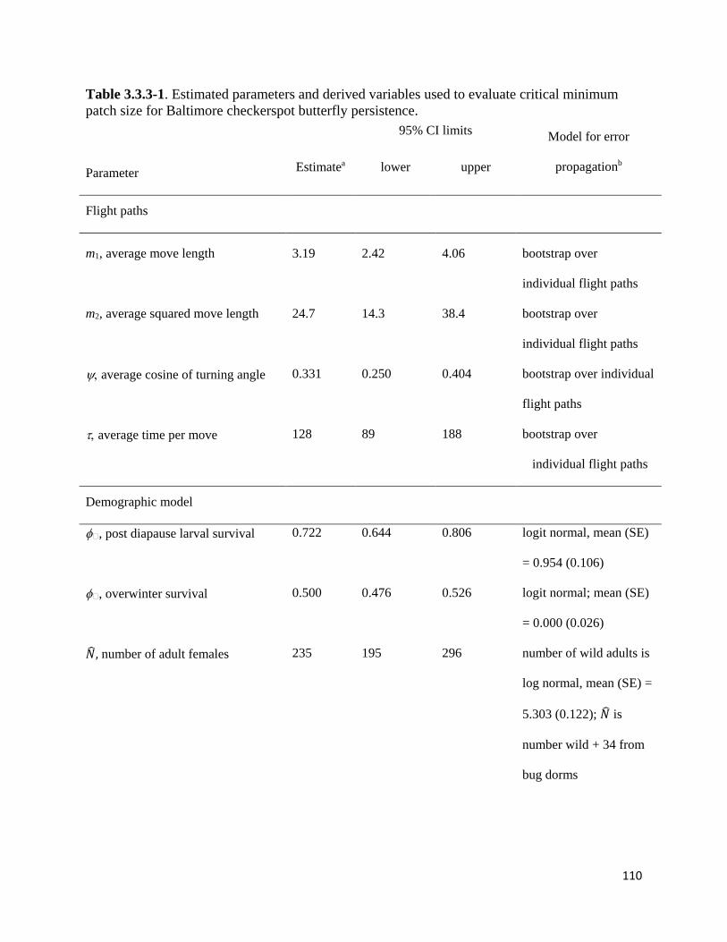
110
Table 3.3.3-1. Estimated parameters and derived variables used to evaluate critical minimum patch size for Baltimore checkerspot butterfly persistence. 95% CI limits Model for error
propagationb Parameter Estimatea lower upper
Flight paths
m1, average move length 3.19 2.42 4.06 bootstrap over
individual flight paths
m2, average squared move length 24.7 14.3 38.4 bootstrap over
individual flight paths
ψ, average cosine of turning angle 0.331 0.250 0.404 bootstrap over individual
flight paths
τ, average time per move 128 89 188 bootstrap over
individual flight paths
Demographic model
φ, post diapause larval survival 0.722 0.644 0.806 logit normal, mean (SE)
= 0.954 (0.106)
φ, overwinter survival 0.500 0.476 0.526 logit normal; mean (SE)
= 0.000 (0.026)
𝑁𝑁�, number of adult females 235 195 296 number of wild adults is
log normal, mean (SE) =
5.303 (0.122); 𝑁𝑁� is
number wild + 34 from
bug dorms
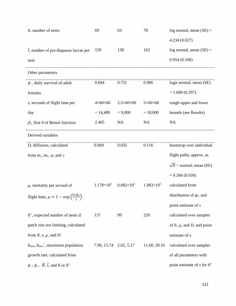
111
𝜇𝜇�, number of nests 69 63 78 log normal, mean (SE) =
4.234 (0.027)
𝑙𝑙, number of pre-diapause larvae per
nest
150 138 162 log normal, mean (SE) =
0.954 (0.106)
Other parameters
φ, daily survival of adult
females
0.844 0.751 0.906 logit normal, mean (SE)
= 1.689 (0.297)
s, seconds of flight time per
day
4×60×60
= 14,400
2.5×60×60
= 9,000
5×60×60
= 18,000
rough upper and lower
bounds (see Results)
β1, first 0 of Bessel function 2.405 NA NA NA
Derived variables
D, diffusion, calculated
from m1, m2, ψ, and τ
0.069 0.035 0.116 bootstrap over individual
flight paths; approx. as
√𝐷𝐷 ~ normal; mean (SE)
= 0.266 (0.039)
µ, mortality per second of
flight time, 𝜇𝜇 = 1 − exp �ln𝜙𝜙3𝑠𝑠�
1.178×10⁵ 0.682×10⁵ 1.983×10⁵ calculated from
distribution of φ3, and
point estimate of s
𝜇𝜇�∗, expected number of nests if
patch size not limiting, calculated
from 𝜇𝜇�, s, µ, and D.
137 99 220 calculated over samples
of 𝜇𝜇�, µ, and D, and point
estimate of s.
bmax, bmax*, maximum population
growth rate, calculated from
φ, φ, 𝑁𝑁�, 𝑙𝑙, and 𝜇𝜇� or 𝜇𝜇�∗
7.96, 15.74 2.65, 5.17 11.60, 29.16 calculated over samples
of all parameters with
point estimate of s for 𝜇𝜇�∗
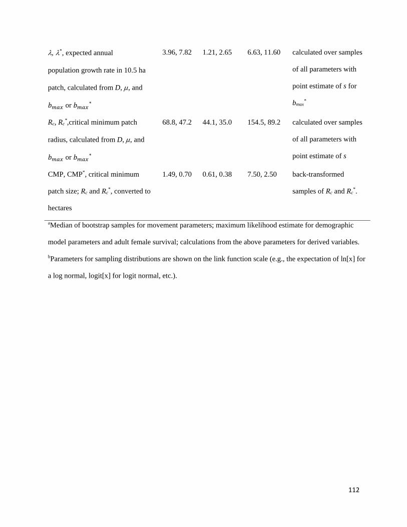
112
λ, λ*, expected annual
population growth rate in 10.5 ha
patch, calculated from D, µ, and
𝑏𝑏𝑚𝑚𝑚𝑚𝑚𝑚 or 𝑏𝑏𝑚𝑚𝑚𝑚𝑚𝑚∗
3.96, 7.82 1.21, 2.65 6.63, 11.60 calculated over samples
of all parameters with
point estimate of s for
bmax*
Rc, Rc*,critical minimum patch
radius, calculated from D, µ, and
𝑏𝑏𝑚𝑚𝑚𝑚𝑚𝑚 or 𝑏𝑏𝑚𝑚𝑚𝑚𝑚𝑚∗
68.8, 47.2 44.1, 35.0 154.5, 89.2 calculated over samples
of all parameters with
point estimate of s
CMP, CMP*, critical minimum
patch size; Rc and Rc*, converted to
hectares
1.49, 0.70 0.61, 0.38 7.50, 2.50 back-transformed
samples of Rc and Rc*.
aMedian of bootstrap samples for movement parameters; maximum likelihood estimate for demographic
model parameters and adult female survival; calculations from the above parameters for derived variables.
bParameters for sampling distributions are shown on the link function scale (e.g., the expectation of ln[x] for
a log normal, logit[x] for logit normal, etc.).
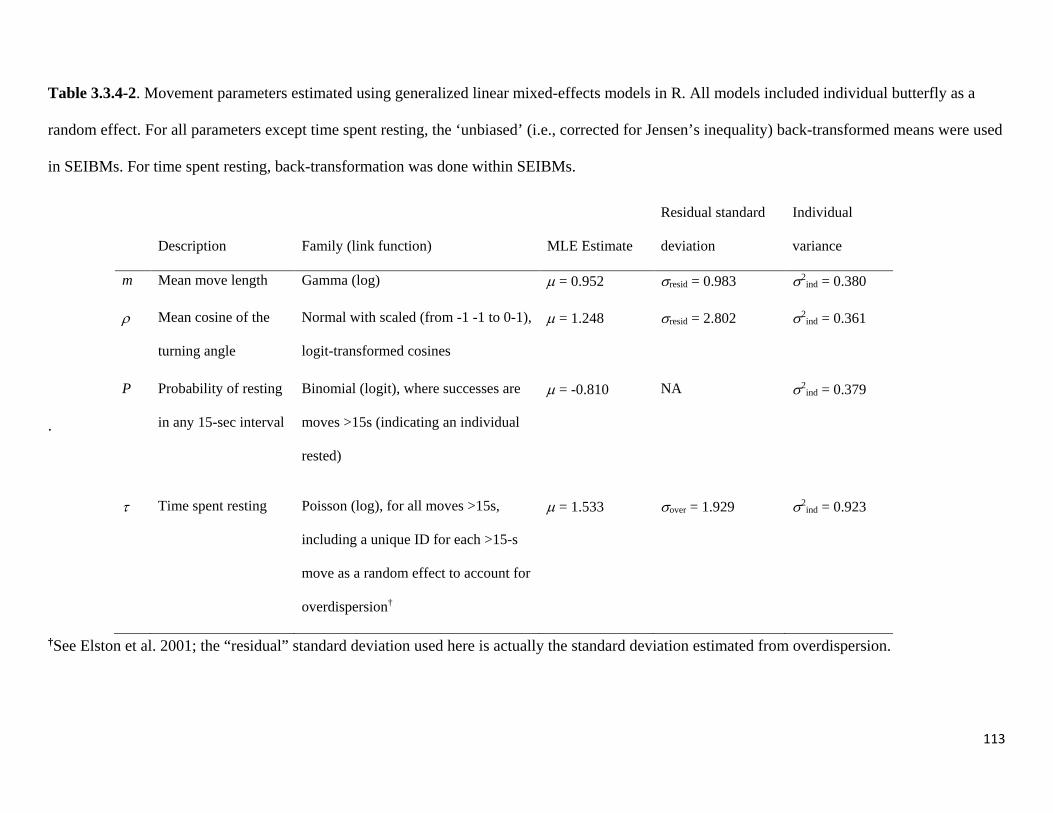
113
Table 3.3.4-2. Movement parameters estimated using generalized linear mixed-effects models in R. All models included individual butterfly as a
random effect. For all parameters except time spent resting, the ‘unbiased’ (i.e., corrected for Jensen’s inequality) back-transformed means were used
in SEIBMs. For time spent resting, back-transformation was done within SEIBMs.
.
†See Elston et al. 2001; the “residual” standard deviation used here is actually the standard deviation estimated from overdispersion.
Description Family (link function) MLE Estimate
Residual standard
deviation
Individual
variance
m Mean move length Gamma (log) µ = 0.952 σresid = 0.983 σ2ind = 0.380
ρ Mean cosine of the
turning angle
Normal with scaled (from -1 -1 to 0-1),
logit-transformed cosines
µ = 1.248 σresid = 2.802 σ2ind = 0.361
P Probability of resting
in any 15-sec interval
Binomial (logit), where successes are
moves >15s (indicating an individual
rested)
µ = -0.810
NA σ2ind = 0.379
τ Time spent resting Poisson (log), for all moves >15s,
including a unique ID for each >15-s
move as a random effect to account for
overdispersion†
µ = 1.533 σover = 1.929 σ2ind = 0.923
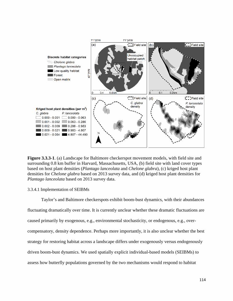
114
Figure 3.3.3-1. (a) Landscape for Baltimore checkerspot movement models, with field site and surrounding 0.8 km buffer in Harvard, Massachusetts, USA, (b) field site with land cover types based on host plant densities (Plantago lanceolata and Chelone glabra), (c) kriged host plant densities for Chelone glabra based on 2013 survey data, and (d) kriged host plant densities for Plantago lanceolata based on 2013 survey data. 3.3.4.1 Implementation of SEIBMs
Taylor’s and Baltimore checkerspots exhibit boom-bust dynamics, with their abundances
fluctuating dramatically over time. It is currently unclear whether these dramatic fluctuations are
caused primarily by exogenous, e.g., environmental stochasticity, or endogenous, e.g., over-
compensatory, density dependence. Perhaps more importantly, it is also unclear whether the best
strategy for restoring habitat across a landscape differs under exogenously versus endogenously
driven boom-bust dynamics. We used spatially explicit individual-based models (SEIBMs) to
assess how butterfly populations governed by the two mechanisms would respond to habitat
115
restoration strategies that varied in the level of resource patchiness – from a single large patch to
multiple patches spaced at different distances.
We developed two SEIBMs that reflected the Taylor’s checkerspot life cycle, one
simulating exogenously driven dynamics and the other emulating one type of endogenously
governed dynamics. In both cases, populations have the capacity for rapid growth and decline
(i.e., boom-bust dynamics) and are limited by some form of density dependence. In the
exogenous model, we assume the population is regulated by abrupt density dependence (via a
population ceiling) and that environmental stochasticity is responsible for inter-annual
fluctuations in population size. In the endogenous model, we simulate a resource-consumer
dynamic that results in over-compensatory density dependence producing large fluctuations in
population size even in the absence of environmental stochasticity.
Both SEIBMs were built using Netlogo software (Wilensky 1999), and simulated the
movement of adult female butterflies in the same way. Parameter values and sources are
provided in Table 3.3.4-1. Many of these are taken from field research with Baltimore
checkerspot, and details regarding data collection and parameter estimation can be found in
Brown and Crone (2016) and Brown et al. (in review).
We simulated female movement and demography in 15-second time steps to match
empirical movement data. Every 15 seconds, a female could move or rest (according to an
empirically estimated binomial probability of initiating a rest or move). The duration of rests (in
number of time steps) was drawn from a Poisson distribution with log normal mean. If the
female moved, we modeled her movement as a correlated random walk, drawing the move
length from a gamma distribution, and the turn angle (relative to the current heading) from a
wrapped Cauchy distribution. At each time step, whether resting or moving, females could
116
oviposit a clutch of eggs with a per-time-step probability converted from lifetime fecundity, and
with clutch size drawn from a Poisson distribution. Individuals also had a chance of dying at
each time step, based on empirically estimated daily survival probabilities scaled to the 15-
second time-step, but maximum possible lifespans were limited to four weeks. Once all adult
butterflies had died, an empirically estimated combined egg and larval survival probability
dictated how many of the eggs and subsequent pre-diapause larvae survived the summer and
early winter to become post-diapause larvae the following year. We assumed a 50% sex ratio,
only retaining females for subsequent years.
Demographic stochasticity is an emergent property of the models as a result of the above
stochastic demographic and movement parameters and finite population size. While movement,
adult longevity, and egg and larval survival were the same in the two models, the relationship
between oviposition and host plant biomass differed, as follows.
Endogenous model: The endogenous model was designed to emulate negative density
dependent feedback by linking the total number of eggs that could be oviposited to the available
biomass of the principal host plants (Castilleja and Plantago spp.) in a given year, which was
affected by the amount consumed by post-diapause larvae (Fig. 3.3.4-1A). Each post-diapause
larva consumed one host plant (if available), based on laboratory estimates of feeding rates (M.
Linders pers. comm.; Barclay et al. 2009). If insufficient biomass of the principal host plants was
present to feed all post-diapause larvae, we assumed that they were able to exploit alternative
food sources (Dunwiddie et al. 2016) and that their survival was not adversely affected by the
available biomass. Those that survived (based on empirical post-diapause survival probability)
metamorphosed into adult butterflies. During the adult life stage, oviposition was restricted to the
principal host plants since oviposition on other plants (even those that can support post-diapause

117
larvae) has been found to be lethal to newly hatched larvae (Bowers and Schmitt 2013), and was
limited to a maximum of 130 eggs per 10 plants. Thus, consumption of host plants in late
winter/spring by post-diapause larvae had the potential to negatively impact the number of eggs
that could be oviposited by those same individuals once they became adults. Once the total
number of eggs in a patch exceeded the maximum capacity (maximum per plant multiplied by
the number of plants remaining per patch), the probability of oviposition was set to zero for all
adults in the patch. If no host plant biomass remained after the post-diapause larval stage, no
oviposition was allowed during the adult phase; if this occurred in every patch, the population
went extinct. We made the simplifying assumption that consumption of host biomass by
(successively) post- and pre-diapause larvae in one year did not affect plant biomass in the
following year (and therefore we did not explicitly track consumption by pre-diapause larvae).
Given that the host plants are short-lived perennials that are capable of rapid compensation for
herbivory, the assumption that plant biomass at the start of each growing season is independent
of the amount of feeding in the previous year is reasonable. Simulations ended after 30 years or
when the population went extinct, whichever came first. Extinction occurred if no eggs were
oviposited in a given year or if no adults emerged in the spring because all individuals failed to
survive the egg and larval stages.
Exogenous model: The exogenous model was designed to simulate a population with
abrupt density dependence imposed at a population ceiling, with the primary driver of population
fluctuations being random environmental variation in the height of the ceiling. In the exogenous
model, we did not consider the interaction between Taylor’s checkerspot and its host plants.
When post-diapause larvae metamorphosed into adults, if the resulting adult count exceeded the
ceiling, the adult population was reduced to the ceiling; otherwise, it remained unchanged (Fig.
118
3.3.4.1-1B). Adults behaved as in the endogenous model, except that no limits on oviposition
were imposed. In the absence of environmental stochasticity, populations grew to the ceiling and
remained at that level indefinitely. To achieve population fluctuations similar in magnitude to
those in the endogenous model, in each year we multiplied the per-patch ceiling value by a
lognormal random deviate (log μ = 0, log σ = 0.5), such that the ceiling value fluctuated annually
and these fluctuations were perfectly correlated among patches. The mean total population
ceiling was 31,000 adult females (to match the expected number of individuals that would be
supported by the available plant biomass in the endogenous model), and the mean per-patch
ceiling was the total population divided evenly among the patches.
Landscape:
The landscape used in the SEIBMs represents an area within the Puget Trough prairies in
WA that includes Glacial Heritage Preserve, where restoration efforts have been underway for
Taylor’s checkerspot for more than a decade, and Mima Mounds Natural Area Preserve, where
future restoration efforts have been proposed (Fig. 3.3.4.1-2). We ran simulations at both the
Glacial Heritage and Mima Mounds sites, but given their similarity, no significant differences
were found between the two sites, so we only present results from the Mima Mounds site. The
simulated landscape consisted of four habitat types among which butterfly demography or
movement differed: restored prairie, harboring a concentration of Taylor’s checkerspot host
plants; nectar prairie, representing areas with nectar food sources for adult butterflies but no host
plants (high quality matrix); fields and exurban areas, with no host or nectar plants for butterflies
(low quality matrix); and forest, representing a partial barrier to butterfly travel. Oviposition only
occurred within restored host prairie habitat, and thus larvae were restricted to this habitat type.
Adult movement characteristics, including step length and turning angle distributions, differed
119
among the four habitat types, but resting characteristics, including resting probability and rest
duration distributions, were the same in all habitats. We did not model movement of the
relatively immobile larvae.
In our simulated landscape, distinct boundaries existed between each habitat type, but,
with the exception of the forest boundary, our simulated butterflies did not respond directly to
habitat boundaries. At forest edges, butterflies crossed into forest habitat with binomial
probability 0.3 which is somewhat more often than observed for upland prairie butterflies
(Schultz et al. 2012, Brown et al. in review), but is less than wet meadow butterflies at forest
edges (Kuefler et al. 2010). They crossed all other boundaries without restriction or modification
of their flight trajectory. Butterflies may exhibit some level of attraction to areas of concentrated
host or nectar plants or repulsion from non-preferred habitat (Schultz and Crone 2001), but we
have not observed attraction to host plants in Baltimore checkerspots (Brown et al. in review).
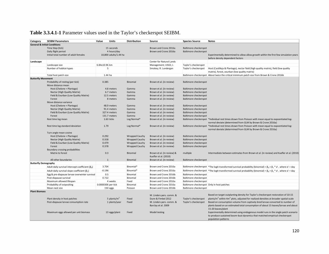
120
Table 3.3.4.1-1 Parameter values used in the Taylor’s checkerspot SEIBM. Category SEIBM Parameters Value Units Distribution Source Species Source NotesGeneral & Initial Conditions
Time Step (tick) 15 seconds Brown and Crone 2016a Baltimore checkerspotDaily flight period 4 hours/day Brown and Crone 2016a Baltimore checkerspotInitial total number of adult females 10,800 adults/1.44 ha Experimentally determined to allow allow growth within the first few simulation years
before density dependent factorsLandscape
Landscape size 6.84x10.96 km Taylor's checkerspotNumber of habitat-types 5 Taylor's checkerspot Host (Castilleja & Plantago), nectar field (high quality matrix), field (low quality
matrix), forest, exurban (low quality matrix)Total host patch size 1.44 ha Baltimore checkerspot About twice the critical minimum patch size from Brown & Crone 2016b
Butterfly MovementProbability of resting (per tick) 0.385 Binomial Brown et al. (in review) Baltimore checkerspotMove distance mean
Host (Chelone + Plantago) 4.8 meters Gamma Brown et al. (in review) Baltimore checkerspotNectar (High Quality Matrix) 6.7 meters Gamma Brown et al. (in review) Baltimore checkerspotField & Exurban (Low Quality Matrix) 12.5 meters Gamma Brown et al. (in review) Baltimore checkerspotForest 8 meters Gamma Brown et al. (in review) Baltimore checkerspot
Move distance varianceHost (Chelone + Plantago) 48.9 meters Gamma Brown et al. (in review) Baltimore checkerspotNectar (High Quality Matrix) 91.4 meters Gamma Brown et al. (in review) Baltimore checkerspotField & Exurban (Low Quality Matrix) 327.4 meters Gamma Brown et al. (in review) Baltimore checkerspotForest 131.7 meters Gamma Brown et al. (in review) Baltimore checkerspot
Rest time log mean 1.63 ticks Log Normal* Brown et al. (in review) Baltimore checkerspot *Individual rest times drawn from Poisson with mean equal to expoentiated log-normal deviate (determined from GLM by Brown & Crone 2016a)
Rest time log standard deviation 1.79 Log Normal* Brown et al. (in review) Baltimore checkerspot *Individual rest times drawn from Poisson with mean equal to expoentiated log-normal deviate (determined from GLM by Brown & Crone 2016a)
Turn angle mean cosineHost (Chelone + Plantago) 0.292 Wrapped Cauchy Brown et al. (in review) Baltimore checkerspotNectar (High Quality Matrix) 0.318 Wrapped Cauchy Brown et al. (in review) Baltimore checkerspotField & Exurban (Low Quality Matrix) 0.479 Wrapped Cauchy Brown et al. (in review) Baltimore checkerspotForest 0.378 Wrapped Cauchy Brown et al. (in review) Baltimore checkerspot
Boundary crossing probabilitiesMatrix to forest 0.3 Binomial Brown et al. (in review) &
Kuefler et al. (2010)multiple Intermediate between estimates from Brown et al. (in review) and Kuefler et al. (2010)
All other boundaries 1 Binomial Brown et al. (in review) Baltimore checkerspotButterfly Demography
Adult daily survival intercept coefficient (β0) 3.704 Binomial* Brown and Crone 2016a Baltimore checkerspot *The logit-transformed survival probability (binomial) = β0 + β1 * d , where d = dayAdult daily survival slope coefficient (β1) -0.196 Binomial* Brown and Crone 2016a Baltimore checkerspot *The logit-transformed survival probability (binomial) = β0 + β1 * d , where d = dayEgg & pre-diapause larvae overwinter survival 0.5 Binomial Brown and Crone 2016b Baltimore checkerspotPost-diapause survival 0.722 Binomial Brown and Crone 2016b Baltimore checkerspotMaximum allowed lifespan 4 weeks Fixed Brown and Crone 2016a Baltimore checkerspotProbability of ovipositing 0.0000306 per tick Binomial Brown and Crone 2016a Baltimore checkerspot Only in host patchesMean nest size 150 eggs Poisson Brown and Crone 2016b Baltimore checkerspot
Plant Biomass
Plant density in host patches 5 plants/m2 FixedM. Linders pers. comm. & Dunn & Fimbel 2012 Taylor's checkerspot
Based on target outplanting density for Taylor's checkerspot restoration of 10-15 plants/m2 within 4m2 plots, adjusted for realized densities at broader spatial scale
Post-diapause larvae consumption rate 1 plants/year Fixed M. Linders pers. comm. & Barclay et al. 2009
Taylor's checkerspot Based on consumption volume from captively bred larvae converted to number of plants based on an estimated total conusmption of about 15 leaves/larvae and about 15-20 leaves/plant
Maximum eggs allowed per unit biomass 13 eggs/plant Fixed Model testing Experimentally determined using endogenous model runs in the single patch scenario to produce sustained boom-bust dynamics that matched empirical checkerspot population patterns
Center for Natural Lands Management; USGS; J. Smokey; R. Lundergan
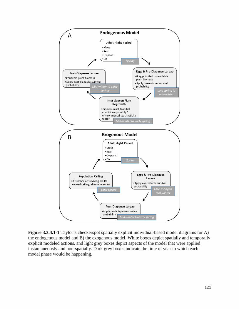
121
Figure 3.3.4.1-1 Taylor’s checkerspot spatially explicit individual-based model diagrams for A) the endogenous model and B) the exogenous model. White boxes depict spatially and temporally explicit modeled actions, and light grey boxes depict aspects of the model that were applied instantaneously and non-spatially. Dark grey boxes indicate the time of year in which each model phase would be happening.
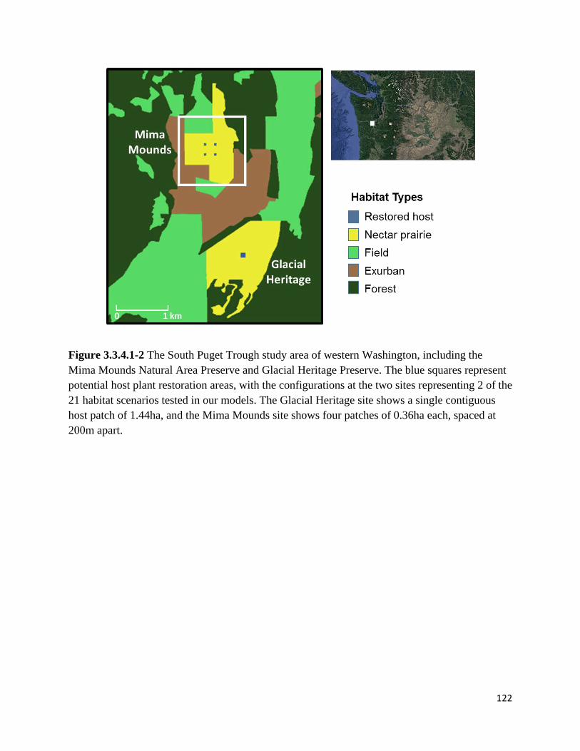
122
Figure 3.3.4.1-2 The South Puget Trough study area of western Washington, including the Mima Mounds Natural Area Preserve and Glacial Heritage Preserve. The blue squares represent potential host plant restoration areas, with the configurations at the two sites representing 2 of the 21 habitat scenarios tested in our models. The Glacial Heritage site shows a single contiguous host patch of 1.44ha, and the Mima Mounds site shows four patches of 0.36ha each, spaced at 200m apart.
123
3.3.4.2 Model validation and simplification
While population estimates for Taylor’s checkerspots are relatively sparse, like other
checkerspot butterflies (e.g., Hellmann et al. 2004), Taylor’s checkerspots appear to exhibit
boom-bust cycles within the few remaining extant populations (Fig. 3.3.4-1). Given the paucity
of long-term abundance data for Taylor’s checkerspot, in our model, we did not try to emulate
observed population trajectories precisely, but instead, compared our model population
trajectories with natural populations to ensure that the general magnitude and pattern of
fluctuations was similar.
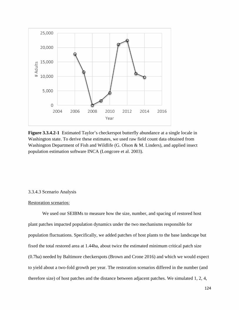
124
Figure 3.3.4.2-1 Estimated Taylor’s checkerspot butterfly abundance at a single locale in Washington state. To derive these estimates, we used raw field count data obtained from Washington Department of Fish and Wildlife (G. Olson & M. Linders), and applied insect population estimation software INCA (Longcore et al. 2003).
3.3.4.3 Scenario Analysis
Restoration scenarios:
We used our SEIBMs to measure how the size, number, and spacing of restored host
plant patches impacted population dynamics under the two mechanisms responsible for
population fluctuations. Specifically, we added patches of host plants to the base landscape but
fixed the total restored area at 1.44ha, about twice the estimated minimum critical patch size
(0.7ha) needed by Baltimore checkerspots (Brown and Crone 2016) and which we would expect
to yield about a two-fold growth per year. The restoration scenarios differed in the number (and
therefore size) of host patches and the distance between adjacent patches. We simulated 1, 2, 4,
125
6, and 8 patches, varying from 1.44 to 0.18ha per patch, and for scenarios with 2 or more
patches, we varied the distance between patches (20, 50, 100, 200, 400m), for a total of twenty-
one unique restoration scenarios (e.g., Fig. 3.3.4-2).
Environmental Stochasticity
Correlated. We compared output from the exogenous model (marked by high
stochasticity correlated among patches) with output from the endogenous model with no
environmental stochasticity. In addition, because environmental stochasticity may also have
some impact on endogenously governed populations (Stamp 1984), we also compared the
exogenous model output with endogenous output impacted by two levels of stochasticity
(moderate and high). With no environmental stochasticity, in the endogenous model, the plant
biomass in each patch was reset to the same base level at the start of each year. Under moderate
and high stochasticity, the level of biomass in each patch was reset to the base level multiplied
by a lognormal random deviate (log μ = 0; log σ = 0.25 or log σ = 0.5 respectively), such that, as
in the exogenous model, annual environmental variation was perfectly correlated among patches.
Uncorrelated. As has been shown with Bay checkerspots, micro-climatic differences can
cause demography to differ even at relatively small distances (Ehrlich and Hanski 2004). To
assess the potential impact of variation in habitat quality and micro-climate among patches, we
also applied environmental stochasticity to patches in an uncorrelated fashion in both models. To
do so, we generated a different lognormal deviate for each patch each year, multiplying the
deviate by the per-patch ceiling value (in the exogenous model) or by the per-patch base biomass
level (in the endogenous model). We did not include any between-year auto-correlation in the
environmental stochasticity.
126
Simulations and Output
We ran each simulation for 30 years and produced 100 simulations for each combination
of model, restoration scenario, and environmental stochasticity (i.e., 2 models, 21 scenarios, and
5 possible environmental stochasticity combinations). For each simulation, we tracked total
population size through time starting at 10,800 individuals, which was chosen to generally allow
populations to grow for 2-3 years before density dependence was invoked. We compared model
output using the following metrics: extinction risk, mean population size, intrinsic growth rate,
and temporal coefficient of variation of population size. We calculated extinction risk as the
proportion of simulations that ended in extinction (total population size of zero) within the 30-
year time horizon for each model-restoration-stochasticity scenario. We calculated the mean
population size as the average number of adults produced each year over all years and all
simulations (𝑁𝑁�). For the mean intrinsic growth rate (�̅�𝑟), we averaged over all simulations the
natural log of the annual growth over the first two years:
�̅�𝑟 =∑ ln �
𝑁𝑁𝑖𝑖,2𝑁𝑁𝑖𝑖,0
�𝑛𝑛𝑖𝑖=1
2𝜇𝜇
where Ni,0 is the starting adult population size in simulation i, Ni,2 is the adult population size in
the second year of simulation i, and n is the number of simulations (100). We calculated the
population size coefficient of variation (CV) as the standard deviation of adult population size
over all years and all simulations divided by the mean population size (𝑁𝑁�).
To understand the role that metapopulation dynamics (e.g., extinction-recolonization and
the rescue effect) plays in creating the population-level patterns in our two models, we also
assessed the following patch-level dynamics: extinction rates, patch population variability, patch
recolonization rate, and the level of dispersal among patches. We calculated mean per-patch
extinction rates as the total number of patch extinctions (defined as zero adults present in a patch

127
at the beginning of a year) over all patches, years, and simulations in a given scenario divided by
the number of patch-years (i.e., number of patches multiplied by number of years and number of
simulations). For patch population variability, we calculated the CV as above using the standard
deviation and the mean patch population size across all patches and simulations. We calculated
the mean recolonization rate as the total number of patch recolonizations (adults present at the
beginning of an annual cycle following an extinction in that patch in a previous year) divided by
the total number of patch extinctions over all patches, all years, and all simulations. To minimize
model run time, we did not record individual dispersal events between patches, but instead
recorded the proportion of time individuals spent in all host patches relative to their lifespan, and
the time spent in their non-natal host patch relative to time spent in all host patches. The latter
metric provided an indirect measure of dispersal among patches.
3.4 Transition Activities
3.4.1 Review of management actions for TERS
SEIBMs are potentially useful tools for guiding resource management decisions.
However, they are complex models with heavy data requirements, and not appropriate for all
management scenarios. To better understand the types of habitat management and restoration
being conducted on Department of Defense (DoD) installations and the capability of managers to
build SEIBMs using available monitoring data, we conducted an informal survey of DoD natural
resource managers. This information helps us to assess the practical applicability of SEIBMs for
guiding habitat management on DoD lands, and to better understand managers’ perceptions and
needs, so we can provide them with useful information and tools.

128
Contact information for 90 DoD installations potentially conducting habitat management
or restoration for threatened, endangered, or rare species (TERS) were identified using the
National Military Fish & Wildlife Association website (www.nmfwa.net), Breuer (2016), reports
(Rubinoff et al. 2006, Balbach et al. 2010), and word of mouth. We sent e-mails to 115 natural
resource managers at these installations, inviting them to participate in a survey on the utility of
SEIBMs for managing habitat for wildlife. Those who agreed were asked to read a paragraph on
SEIBMs and complete a three part, multiple choice questionnaire. In the first part, managers
were asked questions about how habitat management is conducted on their installation. They
were also asked whether the questions commonly addressed by SEIBMs would be important for
managing their species. In the second part, managers were asked to provide information on the
types of monitoring data collected for at least one species whose habitat is being restored or
managed on the installation. They were asked whether they collect the types of data required to
build an SEIBM, namely habitat, survival, fecundity, movement, and population size data. In the
third part, managers were asked about whether they felt SEIBMs would enhance their ability to
manage species on their installation, and what factors would limit them from using SEIBMs.
3.4.2 Develop user guide to SEIBMs
Based on results of the informal survey of DoD natural resource managers (see section
4.4.1), we found that SEIBMs could address questions relevant to the management of habitat for
TERS on military installations, and that managers are open to using them. However, if these
models are to be more generally applied, managers need a better understanding of how SEIBMs
are constructed and what they can do. When asked what information would help them evaluate
whether SEIBMs would be a practical tool for management, 26% of the managers surveyed
stated that they would like to see examples of SEIBMs that were used successfully to guide

129
habitat management. They also wanted to know what types of survey work are needed to collect
the appropriate data, what information SEIBMs could provide that habitat assessments don’t, and
whether SEIBM results would be accepted by federal regulatory agencies like the U.S. Fish and
Wildlife Service and U.S. Forest Service. Guided by these requests, we wrote a user guide that
covers SEIBM construction, data collection, limitations, and how SEIBMs perform relative to
simpler habitat and demographic analyses. We used examples from the scientific literature to
illustrate how SEIBMs have performed in various contexts.
To provide managers with a more concrete example of the amount and types of data
required to build an SEIBM, and to assess the extent of DoD managers’ limitations in building
SEIBMs with current data sets, we also reviewed the data sets for 9 working SEIBMs used to
guide habitat management. This set of studies was compiled by searching Google Scholar for
papers published between 2000-2015 using the terms “spatially explicit individual based model”
or “spatially explicit population model”. In addition, we included unpublished data sets for the
Fender’s blue butterfly and St. Francis’ satyr SEIBMs developed for this SERDP project.
Criteria for selection of studies were that SEIBMs were applied to decision-making for an actual
habitat restoration project, and that the authors provide documentation or references for the data
used to parameterize the model. We summarized the amount and types of data collected on
habitat, population size, survival, fecundity, and movement behavior.
3.4.3 Apply tools to additional case studies
3.4.3.1 Diffusion and Density
Study Area and Environments
We conducted our study at 19 field sites in Israel along a climatic gradient from the arid
Negev desert to Mediterranean regions of northern Galilee (Fig. 3.4.3.1-1a). Each site was
130
located at the intersection of an agricultural field and a semi-natural area. Butterfly densities and
movement behaviours were recorded in four land cover classes: wheat fields, olive groves, semi-
natural grasslands or scrublands, and field margins.
The first two land cover classes, wheat fields and olive groves, were common agricultural
crop field types that differ greatly in their structure. Wheat fields (Fig. 3.4.3.1-1b) were open
monocultures, most of which were intensively managed with agrochemicals and mechanical
disturbance. Olive groves (Fig. 3.4.3.1-1c) were structurally heterogeneous environments, with
rows of mature trees (> 4m height) separated by areas of open habitat, and typically less
intensively managed than wheat fields. Butterfly host and nectar plants were patchily found in
the open microhabitats of olive groves, and butterflies used the trees for shade, perching or
roosting.
The third and fourth land cover classes were the semi-natural grasslands and scrublands
outside the agricultural fields (Fig. 3.4.3.1-1d), and the margins of the fields themselves. The
grassland/scrubland areas were open areas containing a diversity of plants not occurring in other
areas. Although grazed by goats and cattle, these sites were otherwise undisturbed. The “field
margin” land cover class (Fig. 3.4.3.1-1e) included linear elements such as unpaved roads,
fences, or paths that separated agricultural fields from the surrounding semi-natural environment.
Field margins were characterized by a heterogeneous mix of vegetation that resulted from
elevated nutrient levels, agrochemical use and mechanical disturbances. Ruderal species were
often abundant, offering resources including nectar and host plants. The field margin also
attracted perching or “ravining” species that establish territories along linear features (Tennent
1995). Field margins ranged in width from 1.5-21 m (average 9.6 m) between sites (for further
details see Pe'er et al. 2011b).
131
Butterfly surveys and movement data
We conducted surveys along transects established in sites containing one of the two
agricultural field types (olive or wheat), field margin, and the surrounding semi-natural
grassland/scrubland area. Each transect consisted of three lines perpendicular to the field margin,
starting 50 m within the semi-natural area, traversing the width of the field margin, and
extending 100 m into the agricultural field. Transect lines were connected by two 50 m lines
parallel to the field margin, one in the semi-natural area and one in the field margin (Fig. 3.4.3.1-
2a, see also Pe’er et al. 2011b). Additionally, a 100 m transect was sampled along the length of
the field margin. Semi-natural areas were only sampled to a depth of 50 m because the
topography in most sites tended to change beyond this depth, rendering the environment no
longer homogeneous.
We completed 2-3 surveys along transects at each site from March to May 2006, the peak
of butterfly activity in Israel, and the period in which wheat fields and olive groves received
minimal treatment. We used standard Pollard Walk methods to conduct surveys between 09:00
and 16:00, under conditions of <50% cloud cover, temperatures of 18-33˚C, and wind speeds
<10 km/hr. Pollard-Yates indices correlate well with population size in many studies (Thomas
2005; Collier, Mackay & Benkendorff 2008). For each survey, two observers walked at a
constant pace of 1 km/hr, searching for butterflies within 5 m of the transect line (i.e., a 10 m
wide survey width), and recorded a GPS location for each individual butterfly observed. In
addition, we recorded short movement paths for as many butterflies as possible during the
surveys. Observer pairs recorded butterfly movement paths from when an individual butterfly
was first located, following the butterfly at > 1.5 m distance and registering locations at which
the individual landed or changed direction until one of the following conditions was met: 20
132
seconds, 6 turns, 40 m distance, or the butterfly disappeared from view. Observer pairs recorded
total observation time and resting time of each followed individual. After completion of the
observation, one of the two observers recorded the GPS location of each stopping or turning
location. We noted land cover class (semi-natural area, field margin, and wheat field or olive
grove) for each marked point. When we encountered two butterflies simultaneously, we followed
the path of the less common species. For common species, we recorded up to 20 observations per
site on a given sampling day. Examples of movement paths are provided in Fig. 2. We conducted
our study within a single season because observed differences in diffusion rates between land
cover classes are generally much larger than differences between years (e.g. Schultz, Franco &
Crone 2012).
Diffusion Rates
We calculated diffusion coefficients (D) for each species × land cover class combination
using the equation 𝐷𝐷 = 𝑀𝑀+2𝜓𝜓𝜇𝜇2
4𝜏𝜏(1−𝜓𝜓), where μ is average move length, M is average squared move
length, ψ is mean cosine of the turning angle, and τ is the average duration per move or move
time (Turchin 1998, page Box 5.3 and page 102). For each individual, we partitioned the
movement path into moves made in each land cover class. Each move consisted of a move
length, measured as the distance between turning or stopping points i and i+1, and a turning
angle θi , measured as the angle between move i-1 and i. If the movement path contained only
two points (i.e., a straight line with no landing behaviours observed), we assigned a very small
angle (<1 degree) for the turning angle. This non-zero value was introduced to prevent the
calculated diffusion rate from being estimated as infinity (i.e., because a mean turning angle, ψ,
of 0 has a mean cosine of 1, reducing the denominator in the above equation for D to 0, and any
fraction with a denominator of 0 = infinity). Because flight time was measured for the entire path
133
rather than for each move, we estimated the average speed [meters per second] as �̅�𝑠 =
𝑡𝑡𝑡𝑡𝑡𝑡𝑚𝑚𝑙𝑙 𝑝𝑝𝑚𝑚𝑡𝑡ℎ 𝑙𝑙𝑙𝑙𝑛𝑛𝑔𝑔𝑡𝑡ℎ𝑡𝑡𝑡𝑡𝑡𝑡𝑚𝑚𝑙𝑙 𝑡𝑡𝑖𝑖𝑚𝑚𝑙𝑙 𝑖𝑖𝑛𝑛 𝑓𝑓𝑙𝑙𝑖𝑖𝑔𝑔ℎ𝑡𝑡
, and the duration for each move as 𝑡𝑡𝑖𝑖 = 𝑙𝑙𝑖𝑖𝑠𝑠̅
+ 𝑟𝑟𝑖𝑖, where li is the move length
preceding stop i and ri is the resting time at stop i. We averaged move lengths, move durations,
and turn angles over the pooled moves in each species × land cover class combination (following
Schultz and Crone 2001). We estimated diffusion coefficients for combinations for which at least
5 complete moves were recorded, i.e., 5 move lengths, 5 move times, and 4 turn angles. To
separate between edge-mediated behaviour and movement behaviour within semi-natural areas,
olives groves and wheat fields, we used only data that were collected at least 10 m away from the
field margin, i.e., far enough from boundary within semi-natural areas, olives or wheat. The 10 m
buffer was based on various studies demonstrating a shift in movement behaviour close to
structural habitat boundaries (Haddad 1999; Schultz & Crone 2001; Ovaskainen & Cornell 2003;
Ovaskainen 2004; Schultz, Franco & Crone 2012; Zurita et al. 2012). We also visually inspected
the data to corroborate that this buffer width was consistent with our data. We used all movement
behaviour within field margins as this area is, by definition, a boundary-influenced habitat type.
For each move within each species × land cover class combination, we used bootstrapping to
create 1000 sample sets of the 4 movement parameters μ, M, τ and ψ. From these we calculated
expected net squared displacement, 𝐸𝐸(𝑅𝑅2) = 𝑀𝑀+2𝜓𝜓𝜇𝜇2
(1−𝜓𝜓) for a single move, and diffusion rate, D, for
each species × land cover class across these 1000 sample sets. We based analyses below on the
median of bootstrapped estimates of D, 𝐸𝐸(𝑅𝑅2), μ, τ and ψ.
Density
We used survey data to estimate the density (abundance divided by area) of each species
in each land cover class. We estimated abundance for each species at each site using the survey
date with the highest count for that species at that site. We calculated the sampling area as the

134
length of the survey transect × transect width (10 m). We only used density data from each of the
four primary land cover classes (semi-natural areas, field margin, olive groves and wheat fields)
and excluded all observations within the 10 m boundary zone for olive groves, wheat fields and
semi-natural areas for consistency with the treatment of movement data above.
Statistical Analysis
We determined the relationship between density and diffusion using linear mixed models
(lme4 package in R, Bates, Maechler & Walker 2015) with diffusion, wingspan, and diffusion ×
wingspan as fixed effects, and butterfly species as a random effect (to account for repeated
measures of species, and supported by an initial test of the best model for the random effects
structure, Zuur et al. 2009). We did not detect phylogenetic signal in our data (Table 3.4.3.1-1
and Figure 3.4.3.1-3), so we did not use phylogenetic regressions because the lme4 package
allows greater model flexibility, including the ability to weight models by confidence in the data.
We included wingspan estimated to the nearest 0.5 cm using published keys and field guides
(Table 3.4.3.1-1) as an index of body size because it is a potential correlate of density (e.g.,
Gaston & Lawton 1988) that could influence the relationship between density and diffusion.
Because densities may differ among species and among land cover classes, e.g., species for
which semi-natural areas whereas versus olive groves are higher quality habitat, we ran an
additional analysis with land cover class as a fixed effect in addition to diffusion, wingspan, and
diffusion × wingspan. We used models with land cover as a fixed effect to evaluate the
importance of land cover class relative to diffusion for predicting density, and to estimate
densities in each habitat type evaluated at median values of wingspan and diffusion. We
calculated 95% confidence limits of expected densities by parametric bootstrapping, i.e., taking
0.025 and 0.975 quantiles of 1000 sampled values sampled from a multivariate normal
135
distribution defined by model coefficients and sampling error variance-covariance matrix of
fixed estimates (vcov() function in R).
In all models, we log+0.5-transformed diffusion rate and density for each species × land
cover class combination to improve normality in the residuals. Because sample sizes were highly
variable, with common species having many more movement paths than rare species (Fig.
4.4.3.1-1), we weighted models by the inverse of the 95% bootstrap confidence interval
standardized to a mean of one (to keep the total error degrees of freedom constant). For
standardization, we used the confidence interval of the diffusion rate, expected net square
displacement, or flight path parameter (μ, ψ, and τ) estimate, as appropriate for the predictor
variable in each model.
In addition to testing diffusion as a predictor of density, we tested whether parameters
measured directly from flight paths were sufficient predictors of density. For example, does
move length sufficiently predict variation in density? We repeated the analyses above with move
length, cosine of turning angle and time per move (μ, ψ, and τ, 𝐸𝐸(𝑅𝑅2), above), in turn, as fixed
effects (again with wing span and land cover class as covariates). We log+0.5-transformed move
lengths and times per move and logit-transformed cosines of turning angles that were scaled to
range from 0 to 1. As a second test of possible independent drivers of density, we quantified the
relationships between body size and diffusion, and body size and density, for all species in our
data set. Specifically, we calculated median diffusion rate and density for each species. We used
linear models to test whether body size was a significant predictor of either diffusion rate or
density. This analysis differs from the models above in that we evaluated the relationship among
species, averaged across land cover classes, rather than within species, among land cover classes.
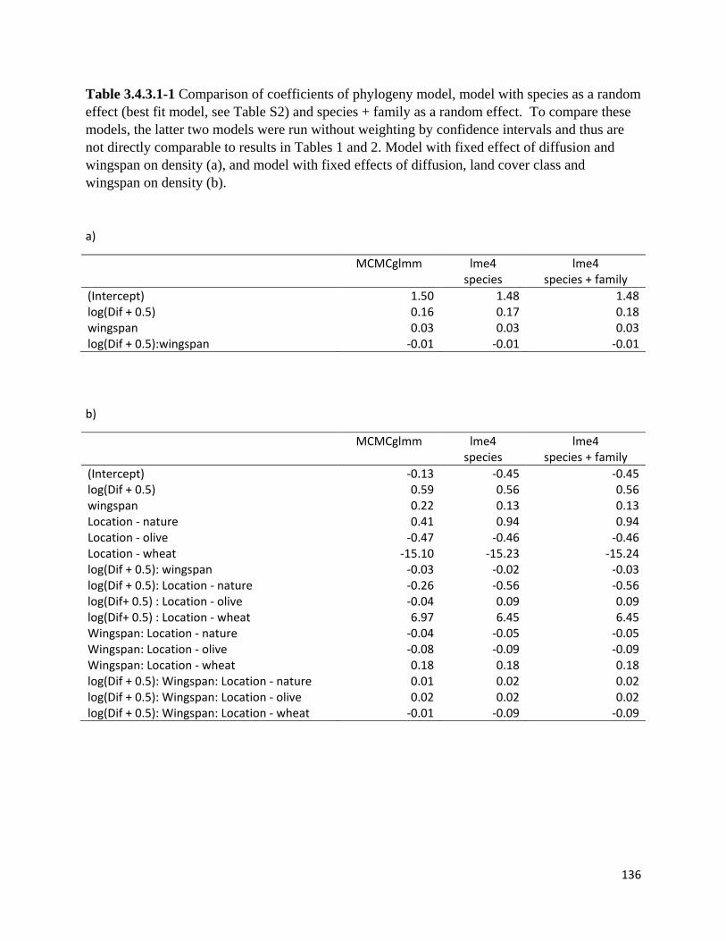
136
Table 3.4.3.1-1 Comparison of coefficients of phylogeny model, model with species as a random effect (best fit model, see Table S2) and species + family as a random effect. To compare these models, the latter two models were run without weighting by confidence intervals and thus are not directly comparable to results in Tables 1 and 2. Model with fixed effect of diffusion and wingspan on density (a), and model with fixed effects of diffusion, land cover class and wingspan on density (b).
a)
MCMCglmm lme4 species
lme4 species + family
(Intercept) 1.50 1.48 1.48 log(Dif + 0.5) 0.16 0.17 0.18 wingspan 0.03 0.03 0.03 log(Dif + 0.5):wingspan -0.01 -0.01 -0.01
b)
MCMCglmm lme4 species
lme4 species + family
(Intercept) -0.13 -0.45 -0.45 log(Dif + 0.5) 0.59 0.56 0.56 wingspan 0.22 0.13 0.13 Location - nature 0.41 0.94 0.94 Location - olive -0.47 -0.46 -0.46 Location - wheat -15.10 -15.23 -15.24 log(Dif + 0.5): wingspan -0.03 -0.02 -0.03 log(Dif + 0.5): Location - nature -0.26 -0.56 -0.56 log(Dif+ 0.5) : Location - olive -0.04 0.09 0.09 log(Dif+ 0.5) : Location - wheat 6.97 6.45 6.45 Wingspan: Location - nature -0.04 -0.05 -0.05 Wingspan: Location - olive -0.08 -0.09 -0.09 Wingspan: Location - wheat 0.18 0.18 0.18 log(Dif + 0.5): Wingspan: Location - nature 0.01 0.02 0.02 log(Dif + 0.5): Wingspan: Location - olive 0.02 0.02 0.02 log(Dif + 0.5): Wingspan: Location - wheat -0.01 -0.09 -0.09
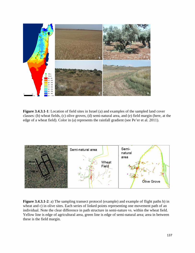
137
Figure 3.4.3.1-1: Location of field sites in Israel (a) and examples of the sampled land cover classes: (b) wheat fields, (c) olive groves, (d) semi-natural area, and (e) field margin (here, at the edge of a wheat field). Color in (a) represents the rainfall gradient (see Pe’er et al. 2011).
Figure 3.4.3.1-2: a) The sampling transect protocol (example) and example of flight paths b) in wheat and c) in olive sites. Each series of linked points representing one movement path of an individual. Note the clear difference in path structure in semi-nature vs. within the wheat field. Yellow line is edge of agricultural area, green line is edge of semi-natural area; area in between these is the field margin.
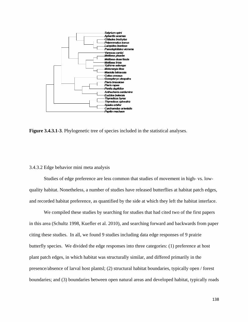
138
Figure 3.4.3.1-3. Phylogenetic tree of species included in the statistical analyses.
3.4.3.2 Edge behavior mini meta analysis
Studies of edge preference are less common that studies of movement in high- vs. low-
quality habitat. Nonetheless, a number of studies have released butterflies at habitat patch edges,
and recorded habitat preference, as quantified by the side at which they left the habitat interface.
We compiled these studies by searching for studies that had cited two of the first papers
in this area (Schultz 1998, Kuefler et al. 2010), and searching forward and backwards from paper
citing these studies. In all, we found 9 studies including data edge responses of 9 prairie
butterfly species. We divided the edge responses into three categories: (1) preference at host
plant patch edges, in which habitat was structurally similar, and differed primarily in the
presence/absence of larval host plantsl; (2) structural habitat boundaries, typically open / forest
boundaries; and (3) boundaries between open natural areas and developed habitat, typically roads

139
or parking lots, but sometimes including developed suburban areas. Not all studies included all
interfaces (Table 3.4.3.2-1).
We used binomial family, logit link
generalized linear mixed models (GLMMs)
to evaluate edge preference. For each study,
the number of trials (butterflies released at
each edge type) and the number choosing
habitat vs. matrix were extracted from the
original raw data. We included the logit-
transformed expected proportion of
butterflies choosing matrix habitat as an
offset. Thus, the test of whether there is a
significant cross-study preference for habitat
over matrix is the p-value testing whether the intercept coefficient for each model differs from 0.
Species was included in each model as a random effect, which makes the standard deviation of
that random effect the expected among-species standard deviation in edge preference.
3.4.3.3 Movement in high quality vs low quality habitat meta analysis
We compiled a long list of 267 studies related to movement in heterogeneous
environments by searching forward for papers that cited several classic studies of movement in
heterogeneous environments. We then screened these papers for studies that included both
estimates of the rate of net displacement (net distance moved per time) in at least two habitat
types, and independent estimates of habitat quality (indicated by demographic rates such birth or
Table 3.4.3.2-1. Edge types studied for each butterfly species
Butterfly species Edge type
Host Forest Pavement
Appalachian Brown
1
Baltimore Checkerspot 1 1
Crystal Skipper
1 1
Fenders Blue 1 1
Monarch
1 1
Pearl Crescent
1
Regal Fritillary 1 1 1
Scarce Large Blue 1 1 1
Taylors Checkerspot
1 1
140
death rates, food density, and/or population growth rates) for these habitat types. Hereafter, we
refer to “net displacement per time” as “movement”. Studies were excluded if they did not have
both movement and habitat quality measurements in at least two environment types, if habitat
quality was assumed but not documented (e.g., assuming suburban vs. natural areas represent
“high” and “low” quality), or habitat quality was inferred from movement behavior (e.g.,
foraging behavior of pelagic birds as an indicator of prey density). Studies were also excluded if
the measure of movement confounded net displacement with other aspects of behavior, such as
preference at patch boundaries, e.g., studies of residence time in patches were not used because
longer residence times could reflect slower movement or higher preference at patch boundaries.
Studies were retained in the data base if they included a response variable that related in a
monotonic way to movement, even if they were not sufficient to predict net displacement, e.g.,
studies were retained if they included measures of speed or tortuosity but not both.
Of the original set of studies, 64 included clear, independent measures of habitat quality
and the rate of net displacement. 14 studies were ambiguous, and their inclusion was decided by
consultation among three co-authors (Schultz, Hodgson, and Crone when needed as a tie-
breaker). This led to a final set of 78 studies. For analysis, we used each species within each
study as the unit of observation. Of 78 studies, 71 included one species, four included two
species, two included three species, and one included four species. Conclusions changed only
slightly if we randomly chose one species from each study for inclusion in the analysis.
We used a simple vote-counting meta-analysis, because studies included several different
metrics of movement in different units (e.g., speed, tortuosity, diffusion coefficients), and
because we were primarily interested in the qualitative direction, not the magnitude of the
response. We divided studies into three categories: studies in which movement (net

141
displacement per time) was faster in lower-quality habitat, studies in which movement was
slower in lower-quality habitat, and studies in which the pattern was unclear. Unclear patterns
could reflect statistically nonsignificant relationships, or studies in which multiple measures of
movement led to different conclusions (i.e., different sets of habitat conditions, or different
metrics, such as speed and tortuosity, that had relationships in different directions and were not
combined into a net metric of movement). We also compiled taxonomic data (Phylum, Class,
Order, Family, Genus, Species).
We analyzed the relationship between habitat quality and movement using binomial
family, logit link, generalized linear mixed models (GLMMs) with various metrics of taxonomy
as random effects. In general, these were nonsignificant, so final conclusions were based on a
GLM (generalized linear model with no random effects). We used intercept-only models to
compare the proportion of studies with faster vs. slower movement in lower quality habitat. We
tested whether the proportion of “faster” studies differed significantly from 0.5 (note that 0.5
equals 0 on a logit scale, so this is the default p-value included in the summary() function). We
repeated analyses using ordinal multinomial logistical regression (polr function in R; with no
random effects but including the 10 ambiguous studies) to obtain confidence limits for the
proportion of all studies in each category, after accounting for ambiguous studies. Confidence
limits were obtained by parametric bootstrapping, i.e., 95% quantiles of 1000 simulated data sets
obtained with the sim() function, and re-analyzed with the polr() function.
3.4.3.4 Applications of source sink dynamics to bumblebees
Rationale: During the course of this award, the rusty-patched bumble bee (Bombus affinis)
became the first federally-listed bee species in the continental US. We used available data for
common bumble bee species, and the conceptual framework developed for source-sink dynamics
142
of Fenders’ blue butterflies, to develop a preliminary model of bumble bee dynamics in
heterogeneous source-sink landscapes.
Model Overview
Bumble bees are social insects that live in annual colonies, each founded in the spring by
a single reproductive queen. Within each colony, sterile workers collect resources and tend to
larvae while the queen produces multiple cohorts of workers throughout the season and new
reproductive queens at the end of each season (as well as short-lived reproductive males). Newly
produced, mated queens that survive the winter and establish new colonies form the basis for
populations in the following year. Because we are interested in predicting long-term population
dynamics over several years, we model population dynamics as the number of queens
establishing nests in year t per nesting queen in year t-1. This relationship implicitly includes
within-season colony dynamics (cf. Crone and Williams 2016, and see Demographic and
Dispersal Data, below).
At the landscape level, population dynamics are described by the population projection
matrix:
𝐀𝐀 = �𝐹𝐹𝑛𝑛𝑚𝑚𝑡𝑡𝛿𝛿𝑛𝑛𝑚𝑚𝑡𝑡 𝐹𝐹𝑚𝑚𝑔𝑔𝑟𝑟(1 − 𝛿𝛿𝑚𝑚𝑔𝑔𝑟𝑟)
𝐹𝐹𝑛𝑛𝑚𝑚𝑡𝑡(1 − 𝛿𝛿𝑛𝑛𝑚𝑚𝑡𝑡) 𝐹𝐹𝑚𝑚𝑔𝑔𝑟𝑟𝛿𝛿𝑚𝑚𝑔𝑔𝑟𝑟�, (1)
where 𝐹𝐹𝑖𝑖 is the per-capita rate of increase in habitat 𝑖𝑖. In our model of bumble bees, this
represents the rate at which queens in habitat 𝑖𝑖 produce new queens that establish colonies the
following year, and is the product of multiple processes: survival of new queens over the winter,
colony establishment probability the following spring, the probability that an established colony
produces any new queens, and the average number of queens produced per successful colony
(Crone & Williams, 2016). Queens that successfully establish new colonies remain in the habitat
143
type in which they were produced with probability 𝛿𝛿𝑖𝑖, or emigrate from their natal habitat into
the alternative habitat type with probability 1- 𝛿𝛿𝑖𝑖.
Demographic and Dispersal Data
We used the values for demographic parameters reported in Crone and Williams (2016),
as a basis for exploring the population-dynamic consequences of habitat change. These
parameters were estimated from data collected by Williams, Regetz, and Kremen (2012), who
experimentally placed bumble bee colonies in different landscape types. Crone and Williams
(2016) partitioned colony dynamics into effects of local land cover type, floral resources during
colony growth, and within-colony demographic parameters, such as initial colony size and
growth rate per floral resource unit (cf. Williams and Crone 2016). Annual population growth
rate (queens per queen) was higher in natural landscapes than in conventional agricultural
landscapes, even after accounting for ambient floral densities (𝐹𝐹𝑛𝑛𝑚𝑚𝑡𝑡 = 1.64, 𝐹𝐹𝑚𝑚𝑔𝑔𝑟𝑟 = 0.56). We
explore these discrete effects of local habitat type in our models to illustrate the general effects of
source-sink dynamics in the familiar matrix model framework. Preliminary exploration of
continuous spatial variation led to qualitatively similar dynamics as the discrete model (E. Crone,
unpubl. analyses).
To model the dispersal of bumble bee queens from their natal colonies, we derived
dispersal kernels using published data for queen dispersal distances in two bumble bee species:
B. flavifrons (Fig. 4 in Bowers, 1985) and B. pascuorum (Fig. 2B in Lepais et al., 2010).
Hereafter, we label the best-supported dispersal kernals for the two species 𝑘𝑘𝑙𝑙𝑡𝑡𝑛𝑛𝑔𝑔 and 𝑘𝑘𝑠𝑠ℎ𝑡𝑡𝑟𝑟𝑡𝑡 to
distinguish bumble bees capable of relatively long distance queen dispersal (based on the
dispersal data for B. pascuorum) from those with limited dispersal (B. flavifrons).
Landscape Configuration and Movement between Habitat Types
144
We used a series of landscape simulations to examine the effects of landscape structure
and bumble bee dispersal ability on source-sink dynamics. We used Saura and Martínez-Millán’s
(2000) modified random cluster algorithm to generate a series of heterogeneous landscapes,
while independently controlling the amount of remaining natural habitat, denoted by η, and the
degree of habitat aggregation, denoted by α (where larger values of α result in less habitat
fragmentation; Fig. 3.4.3.4-1). We constructed a range of landscapes from highly agricultural (η
= 0.05) to moderately natural (η = 0.50; more than enough natural landscape to facilitate rapidly
increasing populations), and from highly fragmented (α = 0.05) to highly aggregated landscapes
(α = 0.30).
We estimated 𝛿𝛿𝑛𝑛𝑚𝑚𝑡𝑡 and 𝛿𝛿𝑚𝑚𝑔𝑔𝑟𝑟 in each simulated landscape under each of the two species’
dispersal kernels (𝑘𝑘𝑠𝑠ℎ𝑡𝑡𝑟𝑟𝑡𝑡 and 𝑘𝑘𝑙𝑙𝑡𝑡𝑛𝑛𝑔𝑔; see results in 4.4.3.4), by repeatedly placing “newly
emerged” queens randomly in each habitat and drawing random dispersal distances from the
empirical dispersal kernels. From these simulations, we calculated the probability that
individuals remained in their natal habitat (𝛿𝛿𝑖𝑖) or moved into the alternative habitat (1 − 𝛿𝛿𝑖𝑖).
Measurement of Long-Term (Asymptotic) Population Dynamics across Landscape Scenarios
For landscapes under each combination of η and α, we used the corresponding estimates
of 𝛿𝛿𝑛𝑛𝑚𝑚𝑡𝑡 and 𝛿𝛿𝑚𝑚𝑔𝑔𝑟𝑟 to generate a population matrix model using equation 1. We used standard
methods to describe landscape-wide asymptotic population dynamics:
For each population matrix, we calculated the long-term population growth rate (denoted
λ) as the dominant eigenvalue of the matrix (Caswell, 2001). For conventional stage-structured
populations, λ describes the per-capita rate at which the population (and each life cycle stage)
multiplies after the population has converged on its stable structure in the long-term. For our
spatially structured model, λ describes the per-capita annual rate at which the entire source-sink
145
population (and populations in each habitat) grows or declines in the long-term. In this way, λ
describes the suitability of the landscape for long-term bumble bee persistence; λ > 1 implies
long-term population growth, λ = 1 implies population stability, and 0 < λ < 1 implies long-term
exponential decline.
The corresponding right eigenvector of each population matrix describes the stable
population structure. In our spatially-structured matrix models, population structure represents
the relative abundance of bumble bee colonies in natural and agricultural habitats in the long-
term, analogous to the stable stage distribution in stage-structured matrix models.
Measurement of Short-Term (Transient) Population Dynamics Following Landscape Change
Sudden environmental perturbations (e.g., conversion of natural habitat to agriculture)
can generate short-term “transient” population dynamics that differ from asymptotic dynamics
(Stott, Townley & Hodgson, 2011). In our source-sink models, transient dynamics are generated
when the distribution of colonies among natural and agricultural habitats immediately following
a landscape change differs from the eventual stable distribution at equilibrium. Transient
population dynamics will occur until the new stable population structure is attained, at which
point the population will grow or decline at a constant annual rate (λ) with a constant relative
proportion of bumble bee colonies in each habitat type (Caswell, 2001).
We explored transient dynamics for two contrasting and ecologically relevant scenarios.
To study the effects of an abrupt loss of natural habitat, we assume a fraction of a completely
natural landscape was abruptly converted to agriculture such that λ in the modified landscape
was 0.8 (leading to a 20% decrease per year in the long-term). To study the effects of an abrupt
restoration of natural habitat, we assume a fraction of a completely agricultural landscape was
immediately restored to natural habitat such that λ in the restored landscape was equal to 1.2

146
(leading to a 20% increase per year in the long-term). These are extreme cases along a potential
continuum of disturbance scenarios, but are nevertheless of heuristic value for understanding
transient dynamics in source-sink systems and of applied relevance (e.g., the rapid conversion of
over 530,000 ha of formerly protected grassland habitat to agricultural land in the midwestern
United States from 2010 to 2013; Morefield et al., 2016).
We assumed that initial habitat loss or restoration initially removed all bumble bees from
the altered habitat patches; thus, initial abundance in the newly created habitat was set to 0. This
assumption is plausible for ground-nesting bumble bees, where soil preparation (either for
agricultural land conversion or seeding of native species during restoration) is likely to impose
significant disturbance to underground colonies and diapausing queens. For each scenario, we
use numerical simulations to plot the resulting transient dynamics and calculate the time required
for the population to converge on its new long-term growth rate.
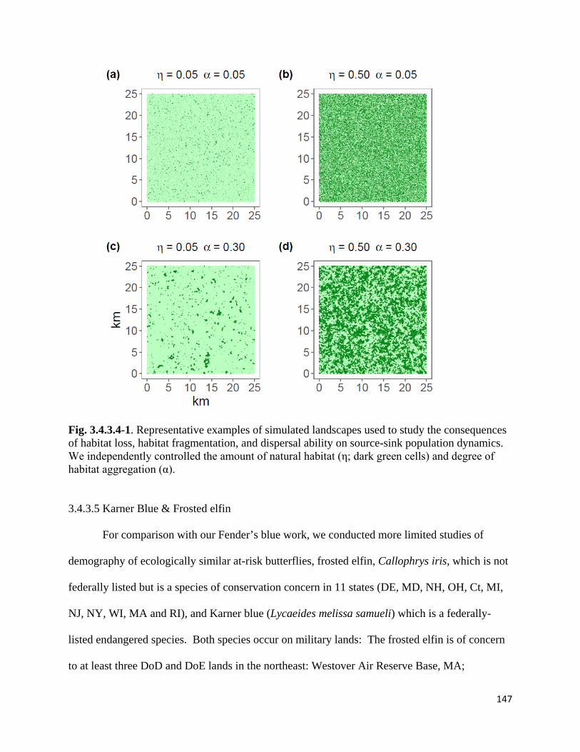
147
Fig. 3.4.3.4-1. Representative examples of simulated landscapes used to study the consequences of habitat loss, habitat fragmentation, and dispersal ability on source-sink population dynamics. We independently controlled the amount of natural habitat (η; dark green cells) and degree of habitat aggregation (α).
3.4.3.5 Karner Blue & Frosted elfin
For comparison with our Fender’s blue work, we conducted more limited studies of
demography of ecologically similar at-risk butterflies, frosted elfin, Callophrys iris, which is not
federally listed but is a species of conservation concern in 11 states (DE, MD, NH, OH, Ct, MI,
NJ, NY, WI, MA and RI), and Karner blue (Lycaeides melissa samueli) which is a federally-
listed endangered species. Both species occur on military lands: The frosted elfin is of concern
to at least three DoD and DoE lands in the northeast: Westover Air Reserve Base, MA;

148
Brookhaven National Laboratory, NY (historic), and the NH State Military Reserve. The Karner
blue occurs at Ft. McCoy, WI, and the NH State Military Reserve.
For the frosted elfin, we monitored adult butterfly populations for three summers, 2015-
2017, in relation to a management burn that was conducted in 2015 (after the adult flight period)
on a private conservation lands. We expected that, if the effects of this particular management
burn were similar to the effects of fires used to improve Fender’s blue habitat, we might see a
drop in population size in 2016 (due to direct effects of fire) but recovery and a possible in 2017
(due to increased habitat quality). We tested this by conducting a mark-recapture study in three
years, and estimating the three population sizes using the POPAN module in Program MARK.
For the Karner blue, we worked with NH Fish and Game to estimate dispersal kernels
from a mark-recapture program they conducted at the Concord Airfield (adjacent to the NH State
Military Reserve) from 2007-2015. We analyzed movement using multi-state mark-recapture
models with states defined as sites on the airfield and adjacent lands, and distance-dependent
transition probabilities. We also estimated the “resistance” (sensu Ricketts 2001) of different
habitat types (open, forest, and pavement) using multistate models with different coefficients for
the effect of distance through different habitat types.
3.4.4 End User Work Shop
In May 2016, we convened a workshop with project scientists and DoD Natural Resource
specialists to discuss project findings, demonstrate project tools and gain insights into how
project tools might be fine-tuned to address resource management needs. The workshop was
held at Washington State University’s Vancouver campus, within proximity of two of our three
focal species, Fender’s blue and Taylor’s checkerspot.

149
In the invitation, we described the overall SERDP project goals, including developing
Spatially Explicit Individual Based Management Models to guide management on DoD land
when concerns about status of habitat as source vs sink may influences natural resource decisions
for at-risk species. The goals of the workshop were
• to demonstrate the Spatially Explicit Individual Based Models (SEIBMs) to the managers
working most closely with these species, and with related species on Department of
Defense Lands,
• to create a venue to demonstrate the value of the approach to managers needing to make
short and long-term decisions about how to allocate and manage land for these at-risk
species,
• to spark discussions about how biologists and managers from across these systems can
learn from each other’s work to enhance the work in their own region, and
• to provide us with feedback about how we can direct future research to promote recovery
of endangered species in concert with Department of Defense activities as well as other
uses of these lands
4 Results and Discussion
4.1 Fender’s Blue Butterfly
4.1.1 SEIBMs direct planting
4.1.1.1: Population Responses
We found stable population dynamics among the scenarios with environmental
stochasticity independent among patches (uncorrelated; Scenarios 1-12), with only one scenario

150
resulting in population declines (Figure 4.1.1-1). Increasing the number of patches decreased the
variability of the population around carrying capacity, but also resulted in slower population
growth to carrying capacity. With 25 patches spread through the 100 ha site, population growth
was slower. In the 250 ha site with 25 patches, populations generally declined to extinction
(Figure 4.1.1-1).
Population dynamics were more variable among the scenarios with environmental
stochasticity constant among patches (correlated; Scenarios 13-24). Standard deviation of the
mean population size each year was greater when compared with the uncorrelated scenarios
(Figure 4.1.1-2). Variability of the population around carrying capacity remained high across all
scenarios except for those that tended toward extinction. Increasing the number of patches
generally decreased population growth to carrying capacity compared to the uncorrelated
scenarios, and the 25 patch planting strategy resulted in population declines in both the 100 ha
and 250 ha sites (Figure 4.1.1-2).
4.1.1.2: Residence Time Responses
Residence time per butterfly decreased as the number of patches increased among
scenarios (Figure 4.1.1-3a; 4.1.1-3b). In a single six hectare patch, residence time per butterfly
was 13 days in both correlated and uncorrelated scenarios. Among the uncorrelated scenarios,
increasing the number of patches to 9 dropped residence time to 9.5 days and 7.9 days at the 25
ha and 250 ha sites, respectively. Further increasing the number of patches to 25 resulted in a
residence time of 8 days at the 25 ha site and 5.5 days at the 250 ha site (Figure 4.1.1-3a).
Residence times did not differ when compared to the correlated scenarios (Figure 4.1.1-3b).
When edge behavior was removed from the model, residence time per butterfly dropped to 2.9

151
days in a single six hectare patch and to 0.6 days in the 250 ha site with 25 patches (Figure 4.1.1-
3c).
4.1.1.3: Intrinsic Rate of Increase among Scenarios
Increasing the number of patches generally decreased the intrinsic rate of increase (r)
among all scenarios (Figure 4.1.1-4a; 4.1.1-4b). Populations grew fastest within a single six-
hectare lupine patch, up to r = 1.21 (95% CI: 1.05 – 1.40) with correlated environmental
stochasticity and up to r = 1.18 (95% CI: 1.02 – 1.37) with uncorrelated environmental
stochasticity. Among the uncorrelated scenarios, increasing both the number of patches and the
size of the site resulted in lower estimates of r (Figure 4.1.1-4a). The 9-patch scenario within the
25 ha site produced r = 0.96 (95% CI: 0.92 – 1.00) compared to r = 0.53 (95% CI: 0.52 – 0.55) at
the 250 ha site. This contrasts with the 25-patch scenarios, with an intrinsic rate of increase of r =
0.70 (95% CI: 0.68 – 0.71) at the 25 ha site and r = 0.01 (95% CI: -0.03 – 0.04) at the 250 ha
site.
We found a similar trend of increasing the number of patches and the size of the site on
estimates of r among the correlated scenarios (Figure 4.1.1-4b). Compared to the uncorrelated
scenarios, the intrinsic rate of increase was routinely lower as patch fragmentation and site size
increase. With the 4-patch scenarios, r = 0.98 (95% CI: 0.92 – 1.04) at the 25 ha site for the
uncorrelated scenario, and r = 0.71 (95% CI: 0.63 – 0.81) for the same site size in the correlated
scenario. The correlated 9-patch scenarios resulted in r = 0.57 (95% CI: 0.50 – 0.65) at the 25 ha
site and r = 0.34 (95% CI: 0.29 – 0.39) at the 250 ha site.
4.1.1.4: Discussion
152
Our study indicates that there is substantial flexibility in planning restoration plantings
for Fender’s blue. A large range of lupine patch sizes spread across small to medium size sites
does well at balancing sufficient habitat area that is close enough for butterflies moving
throughout the site to readily locate lupine. However, when sites grow too large (e.g. 250 ha), the
patches are too isolated, and butterflies that fly into the matrix do not locate sufficient lupine
habitat to have adequate fecundity.
Coupled with these findings, is the overwhelming importance of understanding the
behavior of the focal species in relation to habitat structure. The population dynamics in our
restoration scenarios would be fundamentally altered if our focal species lacked edge behavior.
In this case, instead of having a great deal of flexibility in planning for restoration, the population
is likely to decline rapidly to extinction unless significant additional resources are restored.
Many species exhibit attraction behavior towards critical resources or structures (Kalarus et al.
2013, Skorka et al. 2013). For example, experimental work by Crammer et al. (2012) in the
United Kingdom indicates that bumblebees follow hedgerows as well as artificial linear
structures and butterflies also respond to these structures (see also Dover and Sparks 2000).
Spatial planning of these elements influences connectivity for these bees and reproductive
success of plants which the bees pollinate.
We note that in some species attraction to conspecifics drives behavioral decisions and
may be more important than habitat structure or quality, per se (e.g. O'Neil et al. 2014). In
butterflies, as well as many other taxa, some species show positive density dependent emigration
and immigration (e.g Nowicki and Vrabec 2011) and other species show negative density
dependent migration (Roland et al. 2000). We do not know the effect of density on Fender’s blue
migration and these factors are not considered within our modeling efforts here.
153
We note that it is also the case that for many foraging insects, a correlated random walk
without a bias captures the movement behavior and population dynamics of the populations
(Kareiva and Shigesada 1983, Brouwers and Newton 2010), and that movement behaviors can
lead to persistent populations over the site if the sites are highly heterogeneous with sufficient
coverage of key hostplants. For Fender’s blue, a correlated random walk without bias would be
insufficient to support the population, as evidenced by the rapid decline to extinction in
simulation runs with no edge behavior.
Questions we raise are parallel to questions often considered in the context of restoring
pollinators to augment ecosystem services. Surprisingly landscape context is rarely considered
in the context of pollination services. Hadley and Betts (2012) were stunned to find that only 6
of 303 studies investigating pollinator services considered effects of landscape context and
structure as separate from effects of habitat loss. This finding indicates a lack of awareness in
considering pollinator behavior in the context of this ecosystem service. In contrast, studies
focused on plant insect interactions are increasingly aware of the role of plant spacing in the
population dynamics of the herbivores
Integrating behavior into site-based restoration planning leads to scale-sensitive decisions
for recreation of habitat structure. For example, Conlisk et al. (2014) find that if habitat
restoration for the San Diego cactus wren, Campylorhynchus brunneicapillus sandiegensis, is
limited to a 20 ha area, restoration efforts should focus on enhancing patch size. In contrast, if
restoration efforts include a 200 ha restoration, then connectivity becomes a key consideration.
Rarely is behavior considered as an active component in spatial planning of restoration
efforts. A notable exception to this is restoration of tropical forests. In tropical dry forests,
Lindell and others (2008, 2013) note that placement of trees as bird-perches influences behavior
154
of avian seed predators, key species to facilitate seed dispersal of tropical trees. Advantageous
placement of focal trees results in more rapid and complete restoration of tropical dry forests.
Similarly, clusters of restored trees substantially increased recruitment of animal-dispersed tree
species in tropical premontane forests (Zahawi et al 2013). For Fender’s blue, spatial planning
will be important resulting dynamics at sites that are large for the Willamette Valley (250 Ha)
but, due to edge behavior, the system is robust to a large variety of planting configurations at
smaller sites as long as sufficient resources are restored across the site.
Our approach lends itself to address questions raised by numerous authors on the
challenge of defining a “patch.” As the field of landscape ecology and conservation planning has
exploded over the last two decades, the need to specify patches on a map which have ecological
significance has similarly mushroomed. In fields such as conservation planning for rare species,
state level conservation plans, or plans which respond to emerging threats from climate change,
use of maps with discrete patch boundaries are central. But, often when planners need to
demarcate the maps, questions arise about the complexity or lack of ecological understanding
and limit our ability to draw lines on maps. In our case, great discussion surrounds the question
of boundaries for Fender’s blue habitat. Is it the boundary of lupine? Or nectar? Of the meadow?
The property line? In addition, when species use multiple resources that do not directly co-occur
(e.g. hostplants and nectar resources), demarcating maps is more challenging. Finally, lines
might be drawn on maps for multiple purposes. So, for example, one map might include lupine
habitat which drives attraction to habitat and thus residence time, and other map might include
nectar habitat as areas that include key resources to be managed or conserved to maintain a
population. Decisions about where to draw these lines, to create a single map vs. multiple maps
for different purposes, or which maps to use for what purpose, are critical to conservation and
155
restoration planning, as well as region-wide conservation initiatives. Our study for Fender’s blue
supports flexible planning in which there is a minimum coverage of a key resource, hostplant
lupine, across a spatial area of a “patch.” This approach may help with planning for other taxa in
which decisions about resource abundance and distribution are critical to restoration success.
We conclude with a few thoughts for advancing restoration work for at-risk species. First,
models and approaches such as this are possible because the models are carefully parameterized
based on demography and dispersal behavior of the focal species. While less depth may be
necessary in some cases, it would be short-sighted to ignore the importance of key behavioral
traits, in this case edge behavior, when planning for restoration. In several cases, underestimating
the importance of behavioral traits has resulted in ecological traps in which individuals are
attracted to sub-optimal habitat. Second, models provide a way to conduct “virtual experiments,”
which can save thousands of dollars and decades of time, depending on the type and extent of
habitat. Even limited data can be used in a modeling context to construct “what if” scenarios that
can help guide on-the-ground efforts. Finally, a combination of data and models can be used to
construct “rules of thumb” which can help biologists and planners take next steps in pivotal
conservation decisions. In this case, our models help inform DoD, USFWS and other agencies
that we have great flexibility in the arrangement of reproductive resources as long as there are
sufficient resources and spread within a site of ~ 50-100 Ha. For many planning efforts, this is
sufficient precision for planners to take next steps in prioritizing land and selecting areas for
purchase.
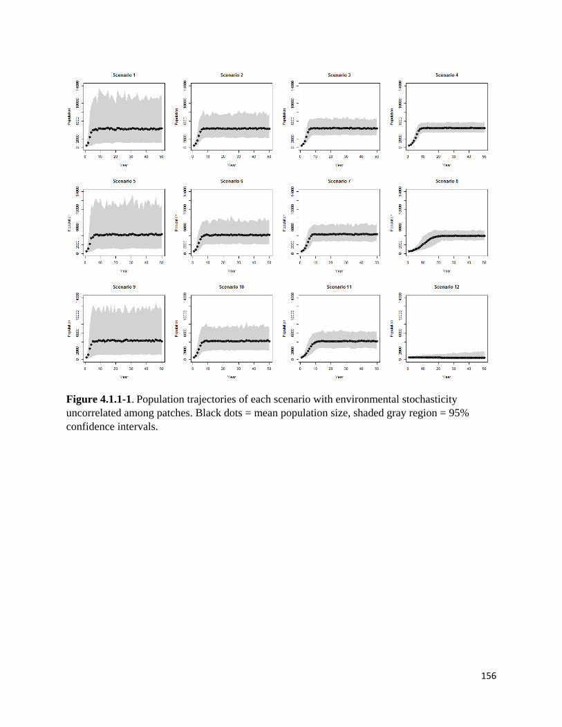
156
Figure 4.1.1-1. Population trajectories of each scenario with environmental stochasticity uncorrelated among patches. Black dots = mean population size, shaded gray region = 95% confidence intervals.
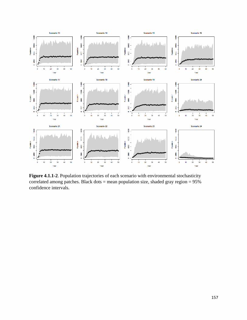
157
Figure 4.1.1-2. Population trajectories of each scenario with environmental stochasticity correlated among patches. Black dots = mean population size, shaded gray region = 95% confidence intervals.
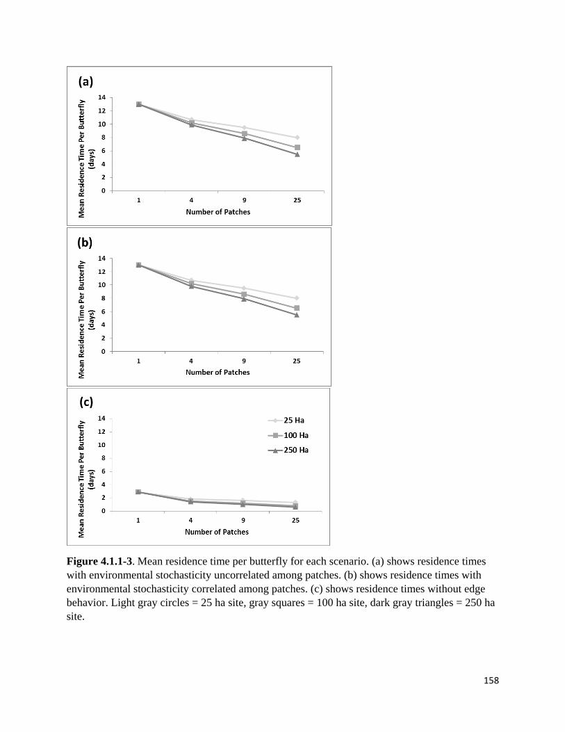
158
Figure 4.1.1-3. Mean residence time per butterfly for each scenario. (a) shows residence times with environmental stochasticity uncorrelated among patches. (b) shows residence times with environmental stochasticity correlated among patches. (c) shows residence times without edge behavior. Light gray circles = 25 ha site, gray squares = 100 ha site, dark gray triangles = 250 ha site.
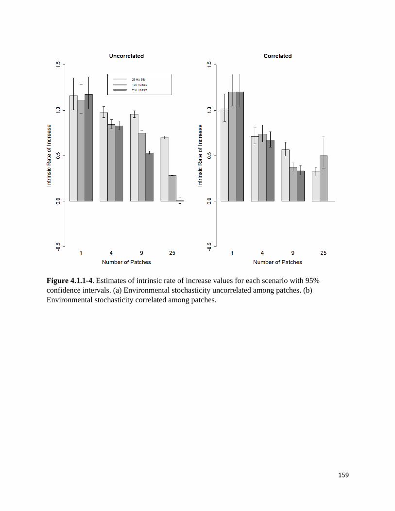
159
Figure 4.1.1-4. Estimates of intrinsic rate of increase values for each scenario with 95% confidence intervals. (a) Environmental stochasticity uncorrelated among patches. (b) Environmental stochasticity correlated among patches.
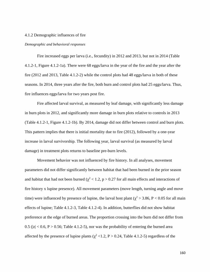
160
4.1.2 Demographic influences of fire
Demographic and behavioral responses
Fire increased eggs per larva (i.e., fecundity) in 2012 and 2013, but not in 2014 (Table
4.1.2-1, Figure 4.1.2-1a). There were 68 eggs/larva in the year of the fire and the year after the
fire (2012 and 2013, Table 4.1.2-2) while the control plots had 48 eggs/larva in both of these
seasons. In 2014, three years after the fire, both burn and control plots had 25 eggs/larva. Thus,
fire influences eggs/larva for two years post fire.
Fire affected larval survival, as measured by leaf damage, with significantly less damage
in burn plots in 2012, and significantly more damage in burn plots relative to controls in 2013
(Table 4.1.2-1, Figure 4.1.2-1b). By 2014, damage did not differ between control and burn plots.
This pattern implies that there is initial mortality due to fire (2012), followed by a one-year
increase in larval survivorship. The following year, larval survival (as measured by larval
damage) in treatment plots returns to baseline pre-burn levels.
Movement behavior was not influenced by fire history. In all analyses, movement
parameters did not differ significantly between habitat that had been burned in the prior season
and habitat that had not been burned (χ2 < 1.2, p > 0.27 for all main effects and interactions of
fire history x lupine presence). All movement parameters (move length, turning angle and move
time) were influenced by presence of lupine, the larval host plant (χ2 > 3.86, P < 0.05 for all main
effects of lupine; Table 4.1.2-3, Table 4.1.2-4). In addition, butterflies did not show habitat
preference at the edge of burned areas. The proportion crossing into the burn did not differ from
0.5 (|z| < 0.6, P > 0.56; Table 4.1.2-5), nor was the probability of entering the burned area
affected by the presence of lupine plants (χ2 <1.2, P > 0.24, Table 4.1.2-5) regardless of the
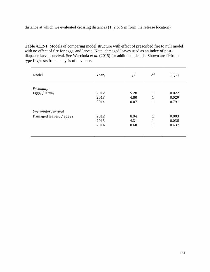
161
distance at which we evaluated crossing distances (1, 2 or 5 m from the release location).
Table 4.1.2-1. Models of comparing model structure with effect of prescribed fire to null model with no effect of fire for eggs, and larvae. Note, damaged leaves used as an index of post-diapause larval survival. See Warchola et al. (2015) for additional details. Shown are 2from type II χ2tests from analysis of deviance.
Model Yeart χ2 df P(χ2) Fecundity Eggst / larvat 2012 5.28 1 0.022 2013 4.80 1 0.029 2014 0.07 1 0.791 Overwinter survival Damaged leaves t / egg t-1 2012 8.94 1 0.003 2013 4.31 1 0.038 2014 0.60 1 0.437
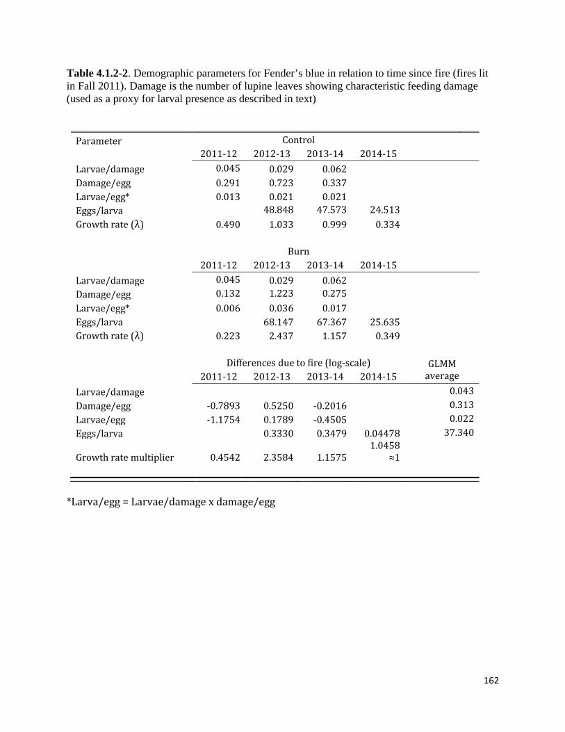
162
Table 4.1.2-2. Demographic parameters for Fender’s blue in relation to time since fire (fires lit in Fall 2011). Damage is the number of lupine leaves showing characteristic feeding damage (used as a proxy for larval presence as described in text)
Parameter Control 2011-12 2012-13 2013-14 2014-15 Larvae/damage 0.045 0.029 0.062 Damage/egg 0.291 0.723 0.337 Larvae/egg* 0.013 0.021 0.021 Eggs/larva 48.848 47.573 24.513 Growth rate (λ) 0.490 1.033 0.999 0.334 Burn 2011-12 2012-13 2013-14 2014-15 Larvae/damage 0.045 0.029 0.062 Damage/egg 0.132 1.223 0.275 Larvae/egg* 0.006 0.036 0.017 Eggs/larva 68.147 67.367 25.635 Growth rate (λ) 0.223 2.437 1.157 0.349 Differences due to fire (log-scale) GLMM
average 2011-12 2012-13 2013-14 2014-15 Larvae/damage 0.043 Damage/egg -0.7893 0.5250 -0.2016 0.313 Larvae/egg -1.1754 0.1789 -0.4505 0.022 Eggs/larva 0.3330 0.3479 0.04478 37.340
Growth rate multiplier 0.4542 2.3584 1.1575 1.0458
≈1
*Larva/egg = Larvae/damage x damage/egg
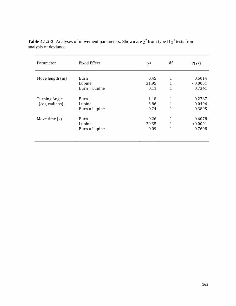
163
Table 4.1.2-3. Analyses of movement parameters. Shown are χ2 from type II χ2 tests from analysis of deviance.
Parameter Fixed Effect χ2 df P(χ2) Move length (m) Burn 0.45 1 0.5014 Lupine 31.95 1 <0.0001 Burn × Lupine 0.11 1 0.7341 Turning Angle Burn 1.18 1 0.2767 (cos, radians) Lupine 3.86 1 0.0496 Burn × Lupine 0.74 1 0.3895 Move time (s) Burn 0.26 1 0.6078 Lupine 29.35 1 <0.0001 Burn × Lupine 0.09 1 0.7608
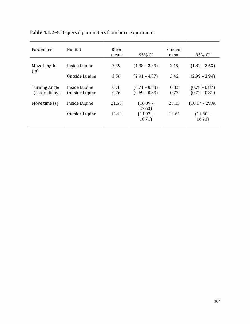
164
Table 4.1.2-4. Dispersal parameters from burn experiment.
Parameter Habitat Burn Control mean 95% CI mean 95% CI Move length (m)
Inside Lupine 2.39 (1.98 – 2.89) 2.19 (1.82 – 2.63)
Outside Lupine 3.56 (2.91 – 4.37) 3.45 (2.99 – 3.94) Turning Angle Inside Lupine 0.78 (0.71 – 0.84) 0.82 (0.78 – 0.87) (cos, radians) Outside Lupine 0.76 (0.69 – 0.83) 0.77 (0.72 – 0.81) Move time (s) Inside Lupine 21.55 (16.89 –
27.63) 23.13 (18.17 – 29.48
Outside Lupine 14.64 (11.07 – 18.71)
14.64 (11.80 – 18.21)
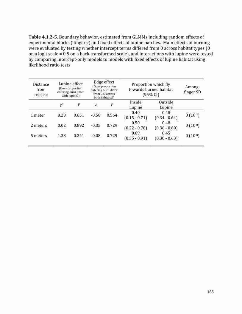
165
Table 4.1.2-5. Boundary behavior, estimated from GLMMs including random effects of experimental blocks (‘fingers’) and fixed effects of lupine patches. Main effects of burning were evaluated by testing whether intercept terms differed from 0 across habitat types (0 on a logit scale = 0.5 on a back transformed scale), and interactions with lupine were tested by comparing intercept-only models to models with fixed effects of lupine habitat using likelihood ratio tests
Distance from
release
Lupine effect (Does proportion
entering burn differ with lupine?)
Edge effect (Does proportion
entering burn differ from 0.5, across both habitats?)
Proportion which fly towards burned habitat
(95% CI)
Among-finger SD
χ2 P z P Inside Lupine
Outside Lupine
1 meter 0.20 0.651 -0.58 0.564 0.40 (0.15 - 0.71)
0.48 (0.34 - 0.64) 0 (10-7)
2 meters 0.02 0.892 -0.35 0.729 0.50 (0.22 - 0.78)
0.48 (0.36 - 0.60) 0 (10-8)
5 meters 1.38 0.241 -0.08 0.729 0.69 (0.35 - 0.91)
0.45 (0.30 - 0.63) 0 (10-8)
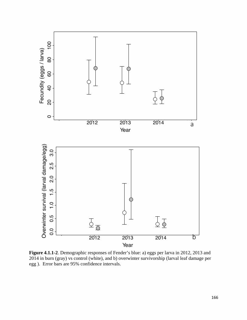
166
Figure 4.1.1-2. Demographic responses of Fender’s blue: a) eggs per larva in 2012, 2013 and 2014 in burn (gray) vs control (white), and b) overwinter survivorship (larval leaf damage per egg ). Error bars are 95% confidence intervals.
a
b

167
4.1.3 Time series demographic model of fire effects
Population model
For Scenario 1, i.e., targeted burning of habitat ≥3 years post-burn, the best strategy is to
burn as much of this habitat stage as possible, with the optimum at burning 100% of this habitat
stage each year, which is 27.03% of the landscape (Figure 4.1.3-1). Directed fire (Scenario 1) is
always better than randomly burning without respect to fire history (Scenario 2). However, if
targeted fire is not feasible or if a wildfire starts, the best strategy (e.g., the context in which
managers might not want to control wildfires) is to burn 19% of the habitat (Figure 4.1.3-1b,
max λ = 1.085 at 19% of the habitat burned when 𝛿𝛿 = 0, max λ = 1.012 at 0 of the habitat burned
when 𝛿𝛿 = 1). If more than 42% of the landscape burns in an undirected manner and dispersal is
random (𝛿𝛿 = 0), then λ < 1 and fire quickly shifts from a beneficial management strategy to
disturbance purely detrimental event. With all local dispersal (𝛿𝛿 = 1), population growth rate (λ)
drops below 1 with 8% of the habitat burning.
In our models, local dispersal, i.e., reproducing within the same successional stage, is
always worse than dispersing throughout the site. With targeted fire management (Scenario 1), λ
= 1.2, with global dispersal (δ = 0) but less than 1.01 with 100% local dispersal (Figure 4.1.3-
1a). With undirected fire (Scenario 2), the effect of dispersal strategy on population growth is
smaller, especially when a large fraction of the habitat burns (Figure 4.1.3-1b). In addition, local
dispersal reduces the optimal proportion of the landscape burned under Scenario 2 (untargeted
burning), but not Scenario 1 (targeted burning; Figure 4.1.3-1a & b)
Life table response experiments (LTRE) indicated that the three demographic effects of
fire have similar magnitude impacts on population growth rates. In Scenario 1, reduced larval
survival through the fire leads to an 18.1% decrease in growth rate, increased fecundity for two

168
years after the burn leads to a 20.5% increase in growth rate, and increased larval survival in the
year after the fire, leads to an 18.0% increase in growth rate. Together, these effects result in a
20.5% increase in growth rate, i.e., λ = 1.22 with targeted burning of 100% of habitat that was
burned at least 3 years ago (Figure 4.1.3-2a). In Scenario 2, reduced larval survival through the
fire leads to a 13.7% decrease in growth rate, increased larval survival in the year after the fire
leads to an increase in 11.1% increase in population growth rate, and increased fecundity for two
years after the fire leads to an 11.4% increase in population growth rate. Together, these effects
result in a 7.2% increase in growth rate, ie. λ = 1.08 assuming the optimum proportion of habitat
burned with unplanned fire, 19% (Figure 4.1.3-2b).
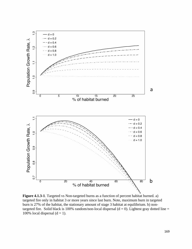
169
Figure 4.1.3-1. Targeted vs Non-targeted burns as a function of percent habitat burned. a) targeted fire only in habitat 3 or more years since last burn. Note, maximum burn in targeted burn is 27% of the habitat, the stationary amount of stage 3 habitat at equilibrium. b) non-targeted fire. Solid black is 100% random/non-local dispersal (d = 0). Lightest gray dotted line = 100% local dispersal (d = 1).
a
b
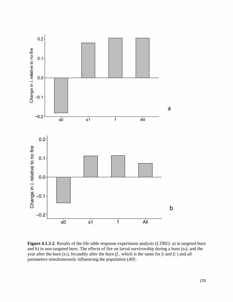
170
Figure 4.1.3-2. Results of the life table response experiment analysis (LTRE): a) in targeted burn and b) in non-targeted burn. The effects of fire on larval survivorship during a burn (s0), and the year after the burn (s1), fecundity after the burn (f , which is the same for f1 and f2 ) and all parameters simultaneously influencing the population (All) .
a
b

171
4.1.4 SEIMBs fire management
4.1.4.1: Population Response to Fire
The observed metapopulation growth rate from census data from 1993 – 2015 is λ = 1.28
(95% CI: 1.24 – 1.32), and the metapopulation growth rate from the no fire scenario simulation
is λ = 1.15 (95% CI: 1.14 – 1.17). Cool fire under the “whole” scenario reduces metapopulation
growth rate to λ = 1.23 (95% CI: 1.21 – 1.25), and hot fire further reduces growth rate to λ = 1.17
(95% CI: 1.15 – 1.19). The “half” scenarios with both hot and cool fire result in metapopulation
growth rates similar to the observed growth rate (Figure 4.1.4-1). We found significant increases
in metapopulation growth rate relative to the observed growth rate with the “quarter” scenario.
Cool fire increases metapopulation growth rate to λ = 1.36 (95% CI: 1.34 – 1.37), and hot fire
increases growth rate to λ = 1.55 (95% CI: 1.52 – 1.57). Hot fire under the “quarter” scenario
brings metapopulation growth rate to conservation target levels set by population viability
analyses (Figure 4.1.4-1).
We found differences between sites in population growth rate response to fire (Figure
4.1.4-2). Fire always decreased growth rates below observed growth rate at the small sites (Shore
Lane and Eaton Lane), even with fine-scale burn plans. Under the “whole” scenario, hot fire
decreased population growth rate at Shore Lane to λ = 0.68 (95% CI: 0.65 – 0.72), and to λ =
1.10 (95% CI: 1.07 – 1.13) at the largest site, Green Oaks. The “quarter” scenario with hot fire
decreased population growth rate to λ = 0.99 (95% CI: 0.97 – 1.01) at Shore Lane, but increased
growth rate to λ = 1.51 (95% CI: 1.48 – 1.54) at Green Oaks. Only the “quarter” scenario with
hot fire raised population growth rate at the largest site to conservation target levels set by
population viability analyses (Figure 4.1.4-2).

172
4.1.4.2: Proportion of Eggs from Immigrant Butterflies
Under the no fire scenario, 5% (95% CI: 4.98 – 5.13%) of eggs in the landscape are laid
by immigrant butterflies. This proportion is not different under the “quarter” scenario in the year
after fire (Figure 4.1.4-3). The “whole” scenario with cool fire increases the proportion in the
year after fire to 10.2% (95% CI: 9.8 – 10.6%), and nearly doubles the proportion to 18.9% (95%
CI: 18.3 – 19.5%) with hot fire. We found the “half” scenario slightly increases the proportion of
eggs laid the year after fire by immigrant butterflies compared to no fire (Figure 4.1.4-3).
We found stark differences of post-fire proportions between sites (Figure 4.1.4-4). Under
no fire, the proportion of eggs laid by immigrant butterflies at Shore Lane was 66%, but only 1%
at Green Oaks. The “quarter” scenario did not significantly change proportions of eggs laid by
immigrant butterflies in the year after fire, and tended to slightly reduce proportions compared to
no fire. Proportions were significantly higher with hot fire under the “whole” scenario, ranging
from 86% (95% CI: 85 - 86%) at Shore Lane to 44% (95% CI: 43 - 45%) at Spires Lane. The
“half” scenario slightly increased the proportion of eggs laid the year after fire at each site except
for Green Oaks (Figure 4.1.4-4).
4.1.4.3: Extirpation Risk from Management Strategies
Fire management that does not partition sites into burn units tends to increase the
frequency of extirpations and increase extirpation risk for small populations (Table 4.1.4-1).
Under the “whole” scenario, Shore Lane had an extirpation probability of 20% (95% CI: 17 –
24%) with hot fire. For the same scenario, the largest population had an extirpation probability of
1% (95% CI: 0 – 2%). Both frequency of extirpation and extirpation risk noticeably decrease
with the “half” and “quarter” scenarios. We found 0% extirpation risk under the “quarter”
173
scenario with hot fire for all populations except Shore Lane, which showed extirpation under
every scenario (Table 4.1.4-1).
4.1.4.4: Life-table Response Experiment without Immigrant Eggs
Metapopulation growth rate with no fire and no immigrant eggs is λ = 1.08 (95% CI: 1.05
– 1.12; Figure 4.1.4-5). Cool fire under the “whole” scenario slightly increases metapopulation
growth rate to λ = 1.17 (95% CI: 1.15 – 1.19), while hot fire reduces growth rate to λ = 1.03
(95% CI: 1.00 – 1.06). The “half” scenarios result in increases up to λ = 1.21 (95% CI: 1.19 –
1.23) with cool fire, and the “quarter” scenarios substantially increase metapopulation growth
rate up to λ = 1.47 (95% CI: 1.44 – 1.49) with hot fire when compared to no fire (Figure 4.1.4-5).
The small populations of Shore Lane and Eaton Lane are routinely extirpated under all scenarios
without immigrant eggs, resulting in population growth rates of λ = 0 (Figure 4.1.4-6). For Spires
Lane under the “whole” scenario, both cool and hot fire decreased population growth rates to λ =
0.09 (95% CI: 0.08 – 0.10) and λ = 0.02 (95% CI: 0.02 – 0.03), respectively, when compared to
no fire. Only the “quarter” scenario with hot fire was able to substantially boost Spires Lane
growth rate to λ = 0.73 (95% CI: 0.70 – 0.77). The largest population, Green Oaks, showed
increases in population growth rate to λ = 1.26 (95% CI: 1.23 – 1.29) and λ = 1.43 (95% CI: 1.40
– 1.46) for cool and hot fire, respectively, when compared to no fire with the “quarter” scenario.
Under the “whole” scenario, cool fire slightly increased Green Oaks’ population growth rate to λ
= 1.14 (95% CI: 1.11 – 1.17), while hot fire reduced growth rate to λ = 1.01 (95% CI: 0.98 –
1.05; Figure 4.1.4-6).
4.1.4.5: Discussion
We find that fine-scale fire disturbance is better for this Fender’s blue metapopulation.
Fine-scale fire disturbance increases population growth rates in the landscape relative to no fire
174
simulation, regardless of burn intensity. Hot burns cause greater extremes in population
dynamics, and hot burns in combination with fine-scale approaches generate higher population
growth rates than cool burns. Extirpation risk is minimized by fine-scale disturbance, similar to
results by earlier studies with non-spatial models (Schultz and Crone 1998). Consistent with
optimal strategies suggested by demographic matrix modeling approaches (Warchola et al., in
press), only about a quarter of habitat should be disturbed each year in order to achieve the
greatest population boosts.
While many studies infer the importance of dispersing individuals in population recovery
after disturbance (e.g., Banks et al. 2011; Harper et al. 2000; Lindenmayer et al. 2009; Panzer
2003), our results clearly illustrate how immigrants are key drivers of population recovery after
fire by using a life-table response experiment approach. Through directly removing contributions
of immigrant eggs on population growth, we showed decreases in metapopulation growth rate
under all management scenarios when compared to simulation including immigrant eggs (Figure
4.1.4-5). Small populations rely on recolonization via immigrant egg contributions for population
persistence, and larger populations suffer decreases in growth rate from lack of immigrant eggs
even with fine-scale burning (Figure 4.1.4-6). This key result of our modeling is further clarified
by our analysis of the proportion of eggs laid by immigrants compared to natal butterflies
(survivors) in the year after fire. Large-scale fire leads to higher proportions of eggs from
immigrant individuals relative to survivors after disturbance when compared to no fire, with the
greatest proportions seen in small populations (Figure 4.1.4-4). By contrast, fine-scale
disturbance does not change the proportion relative to no fire.
Thus, when disturbance affects most of a population, the magnitude of population growth
rate after fire is largely driven by immigrant eggs. However, this is not uniformly the case across
175
our metapopulation, as demonstrated by the minimal influence of immigrants on population
growth at the largest site. Banks et al. (2011) studied response of small mammals to fire, and
found that in-situ survival from refugia in large habitat patches was responsible for driving
population recovery after fire. Their conclusion explains patterns seen in our largest population,
where the proportion of immigrant eggs is a negligible driver of population growth rate under all
management scenarios. Even with the “whole” fire scenario, enough individuals within the
relatively greater lupine extent at Green Oaks are able to survive fire and drive population
recovery after disturbance. Because dynamics at our largest population are predominantly driven
by residents, it is a reasonable hypothesis that refugia within large habitat patches facilitate
population recovery even after large-scale disturbance.
Differences in fire intensity may affect the role of immigrant individuals in shaping
population recovery after disturbance. Under our “whole” management scenario, the proportion
of immigrant eggs relative to survivors after fire is nearly double with hot burns (Figure 4.1.4-3).
This effect can be explained by differences in larval mortality with fire intensity. Butterfly larvae
are thought to be able to evade fire mortality by finding refuge at the base of host plants, in leaf
litter, and in soil (Thom et al. 2015). For Fender’s blue, hot fire kills more overwintering larvae
than cool fire, presumably because hot fire penetrates deeper into soil while cool fire leaves
refugia in the burn mosaic (Schultz and Crone 1998; Warchola et al., in press). Thom et al.
(2015) studied the mortality response of the atala hairstreak (Eumaeus atala Poey), another fire-
adapted butterfly, at different depths of burial. They found that larvae at deeper depths could
evade fire mortality, and survival of larvae was correlated with peak fire temperature. Thus, the
difference we found in the proportion of immigrant eggs after hot fire compared to cool fire can
be attributed to the difference in mortality between fire intensity. Managers sensitive to

176
population losses may find cool burns to be more appealing, since cool burns lessen larval
mortality and allow for population recovery to be driven by in-situ survivors.
Extinction risk in our model was greatest in large-scale, hot burns with extirpation events
driven by small populations (Table 4.1.4-1). Studies investigating population recovery after fire
in other systems found similar risk of disturbance on extirpation of small populations of birds
and butterflies (van Mantgem et al. 2015). Hermes copper (Lycaena hermes), a rare butterfly
near San Diego, CA, exists in a historically well-linked metapopulation that is now highly
fragmented. Small populations of the butterfly were extirpated after wildfire, leading Marschalek
and Klein (2010) to emphasize post-fire recolonization as critical to population recovery. Both
Hermes copper and Fender’s blue have adequate dispersal capability to move within in their
respective metapopulations. Yet, fire-extirpated Hermes copper populations have rarely
recolonized, and Marschalek and Klein (2010) cautioned that more frequent fire might reduce the
species’ ability to recover. Because habitat fragmentation and loss of connectivity generally
increase extirpation risk, fine-scale burning can alleviate added risk from disturbance, especially
if there is concern whether recolonization will occur in highly fragmented metapopulations.
We were surprised to find hot burns in combination with fine-scale disturbance yielded
the highest population growth rates. Fire of higher intensity eliminates more thatch and woody
vegetation compared to cool burns, resulting in more nutrient release and better habitat quality
for plants after fire (Reinhart et al. 2016). From our experimental burns, fire leads to greater host
plant biomass and higher fecundity after disturbance (Schultz and Crone 1998; Warchola et al.
2015; Warchola et al., in press). In these studies, we found hot burns result in higher fecundity
than cool burns. In our present model, we minimize mortality from disturbance with the
“quarter” fire scenarios which generate a higher proportion of surviving butterflies contributing

177
eggs relative to immigrants in years after fire (Figure 4.1.4-3). Because of higher fecundity after
hot fire, these surviving individuals and immigrants lay more eggs in areas burned with hot fire
than in areas burned with cool fire. Thus, because of higher fecundity, population growth rates in
our “quarter” scenarios are highest with hot fire. These growth rate predictions are near
downlisting target levels set by population viability analyses with the Fender’s blue (Schultz and
Hammond 2003). This strongly suggests hot burns, when applied at finer scales in the landscape,
might be the ideal management strategy across the species’ range; but, it is worth emphasizing
the option of late-season burns during the cool months, which is cheaper for managers and still
gives population boosts at fine scales.
Management Conclusions: In synthesizing our findings, we offer some key points for
managers to consider when developing burn regimes to manage fire-sensitive animal
populations. If fire is to be used sparingly to minimize impact to the population, cool burns are
better, and fine-scale disturbance lowers extinction risk. If fire is to be used to maximize
population growth rates, hot burns in combination with fine-scale disturbances are optimal. If
constraints limit the frequency of burning, cool burns are cheaper and can be applied at larger
scales with less negative impact to populations. The role of immigrants in driving post-fire
population recovery can be important, especially for small populations. Since extinction risk is
generally driven by small populations, connectivity to larger populations may ensure adequate
population recovery after fire and minimize extirpation. In general, connectivity between
populations in the landscape could be a critical component to enable post-fire population
recovery of many taxa.
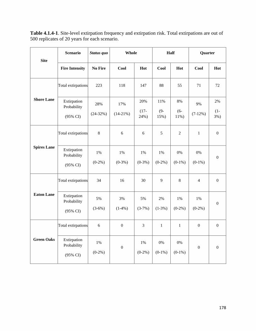
178
Table 4.1.4-1. Site-level extirpation frequency and extirpation risk. Total extirpations are out of 500 replicates of 20 years for each scenario.
Site
Scenario Status quo Whole Half Quarter
Fire Intensity No Fire Cool Hot Cool Hot Cool Hot
Shore Lane
Total extirpations 223 118 147 88 55 71 72
Extirpation Probability
(95% CI)
28%
(24-32%)
17%
(14-21%)
20%
(17-24%)
11%
(9-15%)
8%
(6-11%)
9%
(7-12%)
2%
(1-3%)
Spires Lane
Total extirpations 8 6 6 5 2 1 0
Extirpation Probability
(95% CI)
1%
(0-2%)
1%
(0-3%)
1%
(0-3%)
1%
(0-2%)
0%
(0-1%)
0%
(0-1%) 0
Eaton Lane
Total extirpations 34 16 30 9 8 4 0
Extirpation Probability
(95% CI)
5%
(3-6%)
3%
(1-4%)
5%
(3-7%)
2%
(1-3%)
1%
(0-2%)
1%
(0-2%) 0
Green Oaks
Total extirpations 6 0 3 1 1 0 0
Extirpation Probability
(95% CI)
1%
(0-2%) 0
1%
(0-2%)
0%
(0-1%)
0%
(0-1%) 0 0
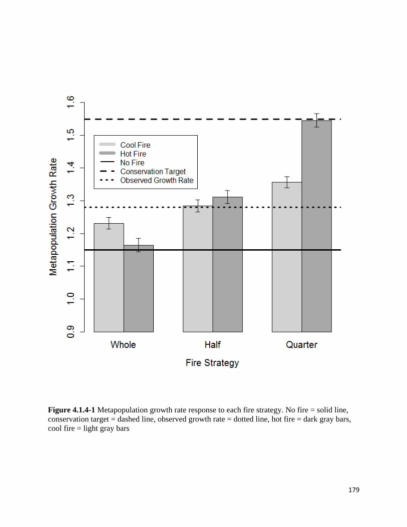
179
Figure 4.1.4-1 Metapopulation growth rate response to each fire strategy. No fire = solid line, conservation target = dashed line, observed growth rate = dotted line, hot fire = dark gray bars, cool fire = light gray bars
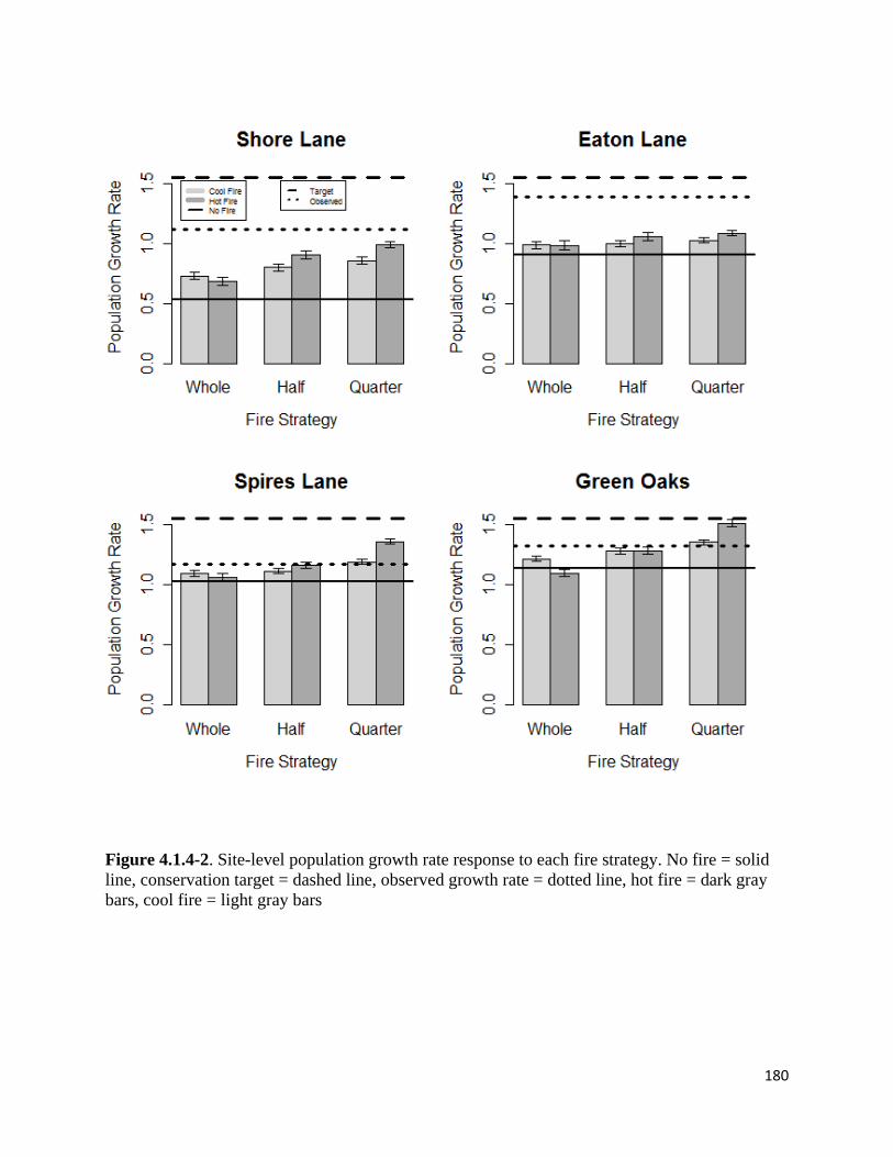
180
Figure 4.1.4-2. Site-level population growth rate response to each fire strategy. No fire = solid line, conservation target = dashed line, observed growth rate = dotted line, hot fire = dark gray bars, cool fire = light gray bars
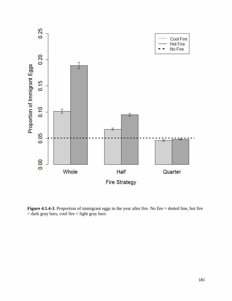
181
Figure 4.1.4-3. Proportion of immigrant eggs in the year after fire. No fire = dotted line, hot fire = dark gray bars, cool fire = light gray bars
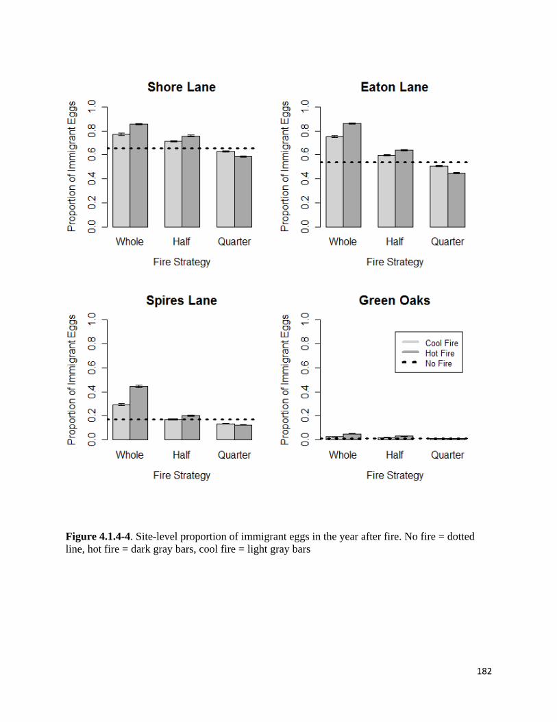
182
Figure 4.1.4-4. Site-level proportion of immigrant eggs in the year after fire. No fire = dotted line, hot fire = dark gray bars, cool fire = light gray bars
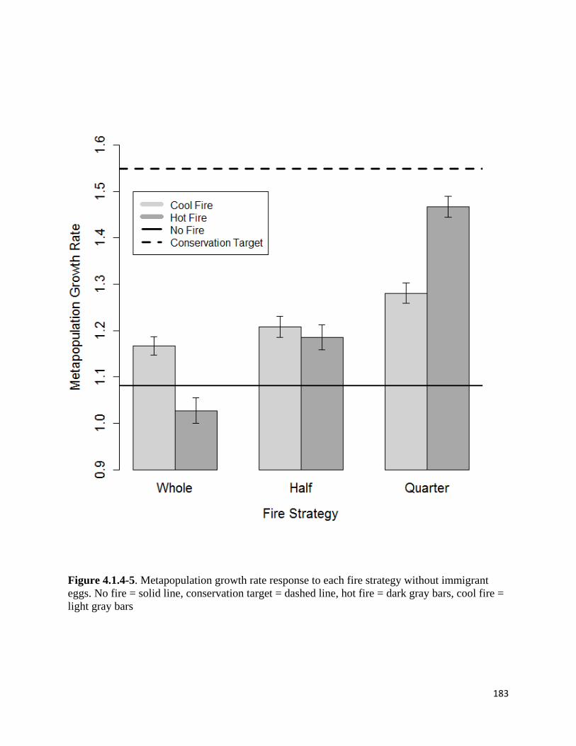
183
Figure 4.1.4-5. Metapopulation growth rate response to each fire strategy without immigrant eggs. No fire = solid line, conservation target = dashed line, hot fire = dark gray bars, cool fire = light gray bars
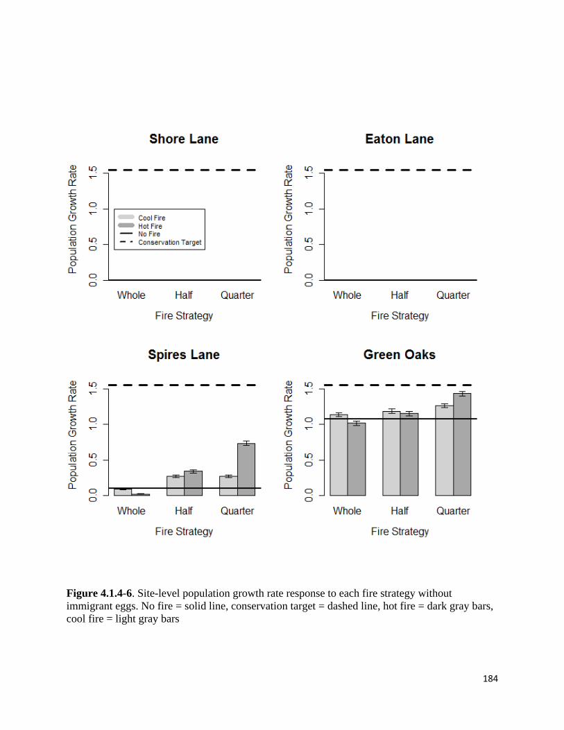
184
Figure 4.1.4-6. Site-level population growth rate response to each fire strategy without immigrant eggs. No fire = solid line, conservation target = dashed line, hot fire = dark gray bars, cool fire = light gray bars

185
4.2 St Francis’ Satyr/ Appalachian brown
4.2.1 Demographic impacts of inundation and clearing
Despite the lack of strong direct effects, restoration treatments had strong predator-
mediated indirect effects on the survival of Appalachian brown eggs and juveniles. When
Appalachian brown eggs were exposed to predation, survival in the three types of restored plots
was about one third of the survival in control plots (Fig. 4.2.1-1C). This suggests that our
manipulation of tree cover and standing water substantially increased predation of butterfly eggs.
Interestingly, we found that predation of eggs in plots with both tree removal and damming was
less than would be expected if the effects of tree removal and damming were additive (Fig. 4.2.1-
1B). While we do not know the mechanism behind this interaction, it reduces the strong negative
indirect effect of both tree removal and damming on egg survival when applied alone. In
contrast, when Appalachian brown juveniles were exposed to predation, survival rates differed
among types of restoration. Survival of juveniles in dammed plots was two times higher than in
control or tree removal and dammed plots, and five times higher than in tree removal plots (Fig.
4.2.1-1C). The differences in predation among restoration treatment types (Fig. 4.2.1-1B) are
likely driven by changes in access to juveniles by ground predators. Dams increased the amount
of standing water within our plots, and this likely reduced the ability of ground predators, such as
ants and some spiders, to gain access to juveniles.
While the work presented here demonstrates the effects of restoration treatments on
immature stages of S. appalacia, it does not assess these effects on the adult stage of S.
appalachia. Positive responses of adult vital rates to restoration, such as increased recruitment
due to higher oviposition rates where host plants are more abundant or higher adult survivorship
due to lower adult predation, could ameliorate the strong negative effects we document in this
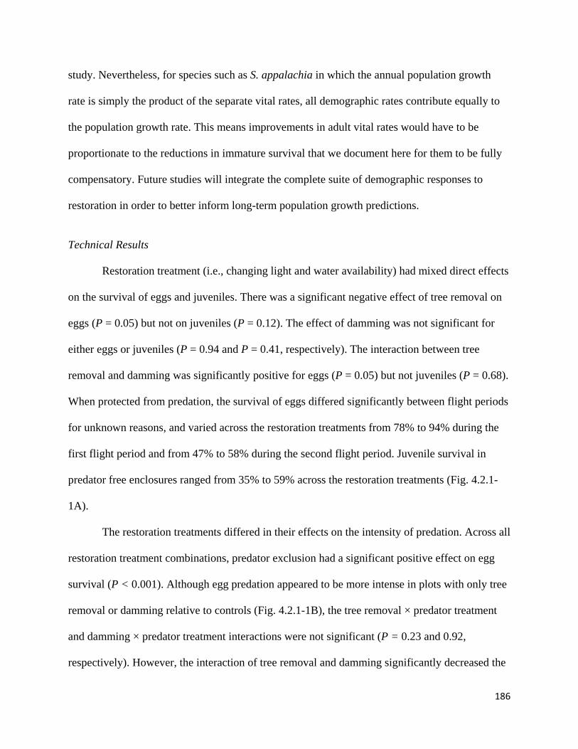
186
study. Nevertheless, for species such as S. appalachia in which the annual population growth
rate is simply the product of the separate vital rates, all demographic rates contribute equally to
the population growth rate. This means improvements in adult vital rates would have to be
proportionate to the reductions in immature survival that we document here for them to be fully
compensatory. Future studies will integrate the complete suite of demographic responses to
restoration in order to better inform long-term population growth predictions.
Technical Results
Restoration treatment (i.e., changing light and water availability) had mixed direct effects
on the survival of eggs and juveniles. There was a significant negative effect of tree removal on
eggs (P = 0.05) but not on juveniles (P = 0.12). The effect of damming was not significant for
either eggs or juveniles (P = 0.94 and P = 0.41, respectively). The interaction between tree
removal and damming was significantly positive for eggs (P = 0.05) but not juveniles (P = 0.68).
When protected from predation, the survival of eggs differed significantly between flight periods
for unknown reasons, and varied across the restoration treatments from 78% to 94% during the
first flight period and from 47% to 58% during the second flight period. Juvenile survival in
predator free enclosures ranged from 35% to 59% across the restoration treatments (Fig. 4.2.1-
1A).
The restoration treatments differed in their effects on the intensity of predation. Across all
restoration treatment combinations, predator exclusion had a significant positive effect on egg
survival (P < 0.001). Although egg predation appeared to be more intense in plots with only tree
removal or damming relative to controls (Fig. 4.2.1-1B), the tree removal × predator treatment
and damming × predator treatment interactions were not significant (P = 0.23 and 0.92,
respectively). However, the interaction of tree removal and damming significantly decreased the
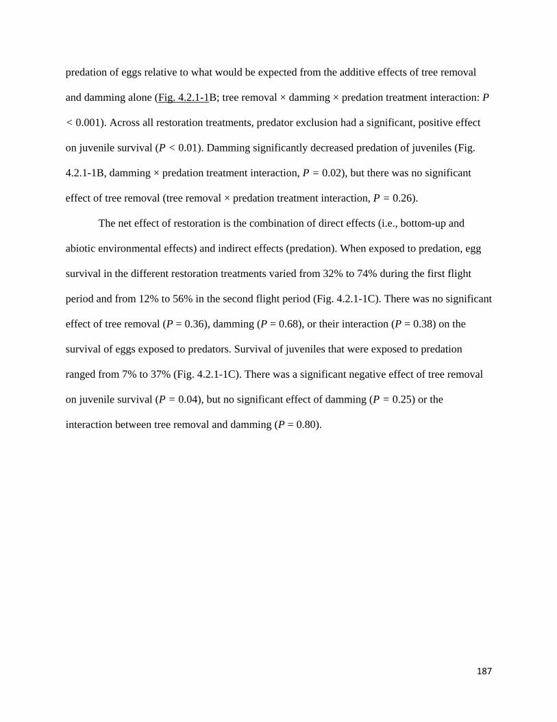
187
predation of eggs relative to what would be expected from the additive effects of tree removal
and damming alone (Fig. 4.2.1-1B; tree removal × damming × predation treatment interaction: P
< 0.001). Across all restoration treatments, predator exclusion had a significant, positive effect
on juvenile survival (P < 0.01). Damming significantly decreased predation of juveniles (Fig.
4.2.1-1B, damming × predation treatment interaction, P = 0.02), but there was no significant
effect of tree removal (tree removal × predation treatment interaction, P = 0.26).
The net effect of restoration is the combination of direct effects (i.e., bottom-up and
abiotic environmental effects) and indirect effects (predation). When exposed to predation, egg
survival in the different restoration treatments varied from 32% to 74% during the first flight
period and from 12% to 56% in the second flight period (Fig. 4.2.1-1C). There was no significant
effect of tree removal (P = 0.36), damming (P = 0.68), or their interaction (P = 0.38) on the
survival of eggs exposed to predators. Survival of juveniles that were exposed to predation
ranged from 7% to 37% (Fig. 4.2.1-1C). There was a significant negative effect of tree removal
on juvenile survival (P = 0.04), but no significant effect of damming (P = 0.25) or the
interaction between tree removal and damming (P = 0.80).
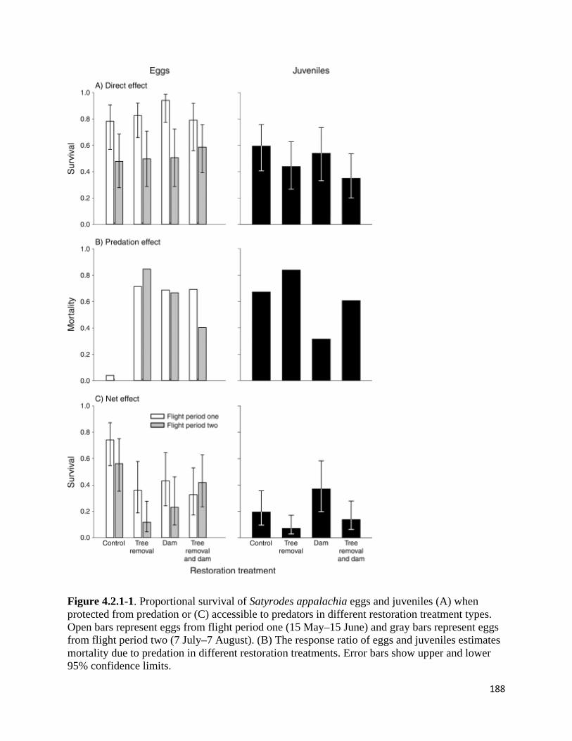
188
Figure 4.2.1-1. Proportional survival of Satyrodes appalachia eggs and juveniles (A) when protected from predation or (C) accessible to predators in different restoration treatment types. Open bars represent eggs from flight period one (15 May–15 June) and gray bars represent eggs from flight period two (7 July–7 August). (B) The response ratio of eggs and juveniles estimates mortality due to predation in different restoration treatments. Error bars show upper and lower 95% confidence limits.
189
4.2.2 Movement in response to inundation and clearing
We tracked 121 Appalachian Brown and 22 St. Francis’ satyr butterflies for movement
behavior over the two flight periods. There was no significant difference, for either species, of
the distributions of move lengths, turn angles, or Rn2/n in our four different restoration
treatments. However, Appalachian Brown butterflies had significantly larger move lengths and
Rn2/n compared to our target species, St. Francis satyr (Figure 4.2.2-1).
Movement behavior under different restoration treatments was similar one year after
restoration treatments. However, anecdotally, butterflies seemed more active in the sunnier sites
that received the hardwood removal treatment. Cut sites were also the only restoration plots
where St. Francis’ satyr colonized naturally. Compared to the Kuefler et al. (2010) study of
movement behavior in continuous riparian forest and wetland habitat, the move lengths and Rn2/n
were smaller in the 30m x 30m restoration plots, possibly due to the abrupt forest edges at the
boundaries.
In the future, we will use demographic information to test whether our restored habitat
serves as population sources or sinks for the larger meta-population of butterflies. One danger
that must be tested is whether restoration creates an ecological trap, in which butterflies falsely
sense that poor habitat is suitable. Combining our movement behavior study with demographic
information will allow us to determine whether butterflies appropriately assess restored habitat
quality. If they move more slowly in restored sites that have low resources or high predation risk,
we would be concerned about restoration creating an ecological trap.
190
Figure 4.2.2-1 Differences in Rn2/n (mean squared displacement per move) between restoration
treatments for our target species, St. Francis’ satyr, and our surrogate species, Appalachian
Brown. The 95% confidence intervals are from a bootstrapped dataset.
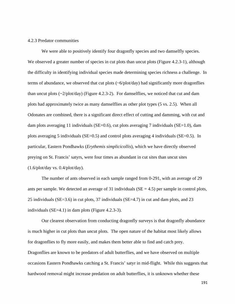
191
4.2.3 Predator communities
We were able to positively identify four dragonfly species and two damselfly species.
We observed a greater number of species in cut plots than uncut plots (Figure 4.2.3-1), although
the difficulty in identifying individual species made determining species richness a challenge. In
terms of abundance, we observed that cut plots (~6/plot/day) had significantly more dragonflies
than uncut plots (~2/plot/day) (Figure 4.2.3-2). For damselflies, we noticed that cut and dam
plots had approximately twice as many damselflies as other plot types (5 vs. 2.5). When all
Odonates are combined, there is a significant direct effect of cutting and damming, with cut and
dam plots averaging 11 individuals (SE=0.6), cut plots averaging 7 individuals (SE=1.0), dam
plots averaging 5 individuals (SE=0.5) and control plots averaging 4 individuals (SE=0.5). In
particular, Eastern Pondhawks (Erythemis simplicicollis), which we have directly observed
preying on St. Francis’ satyrs, were four times as abundant in cut sites than uncut sites
(1.6/plot/day vs. 0.4/plot/day).
The number of ants observed in each sample ranged from 0-291, with an average of 29
ants per sample. We detected an average of 31 individuals (SE = 4.5) per sample in control plots,
25 individuals (SE=3.6) in cut plots, 37 individuals (SE=4.7) in cut and dam plots, and 23
individuals (SE=4.1) in dam plots (Figure 4.2.3-3).
Our clearest observation from conducting dragonfly surveys is that dragonfly abundance
is much higher in cut plots than uncut plots. The open nature of the habitat most likely allows
for dragonflies to fly more easily, and makes them better able to find and catch prey.
Dragonflies are known to be predators of adult butterflies, and we have observed on multiple
occasions Eastern Pondhawks catching a St. Francis’ satyr in mid-flight. While this suggests that
hardwood removal might increase predation on adult butterflies, it is unknown whether these
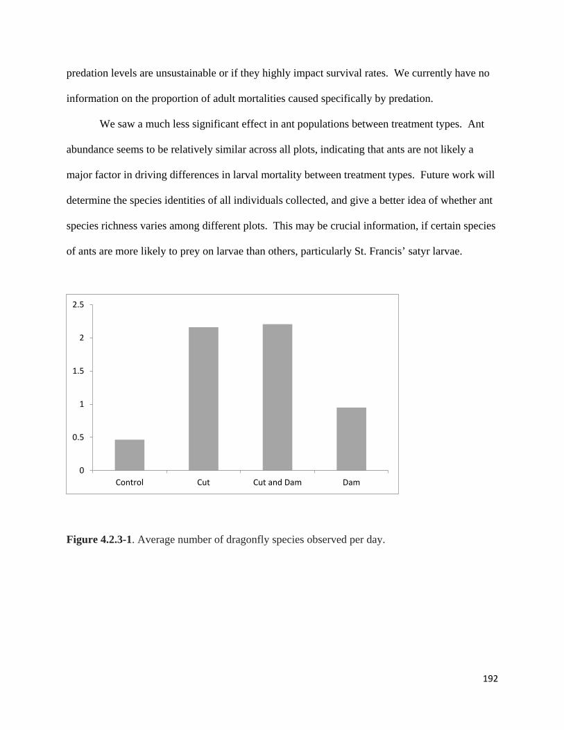
192
predation levels are unsustainable or if they highly impact survival rates. We currently have no
information on the proportion of adult mortalities caused specifically by predation.
We saw a much less significant effect in ant populations between treatment types. Ant
abundance seems to be relatively similar across all plots, indicating that ants are not likely a
major factor in driving differences in larval mortality between treatment types. Future work will
determine the species identities of all individuals collected, and give a better idea of whether ant
species richness varies among different plots. This may be crucial information, if certain species
of ants are more likely to prey on larvae than others, particularly St. Francis’ satyr larvae.
Figure 4.2.3-1. Average number of dragonfly species observed per day.
0
0.5
1
1.5
2
2.5
Control Cut Cut and Dam Dam
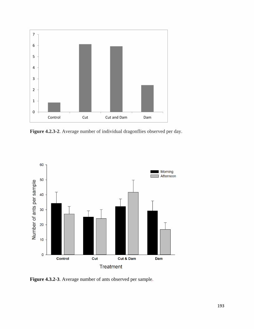
193
Figure 4.2.3-2. Average number of individual dragonflies observed per day.
Figure 4.3.2-3. Average number of ants observed per sample.
0
1
2
3
4
5
6
7
Control Cut Cut and Dam Dam
194
4.2.4 SEIBMs: Scenario analysis on real landscapes
The results of our SEIBM source-sink simulations showed that in all three source
scenarios (Eastern rapidly growing, Western slowly declining, and hypothetical Western slowly
growing), the presence of sink habitat increased population growth rates (Fig. 4.2.4-1) and
population abundance (Table 4.2.4-1). Similarly, increasing quality of sink habitat (from 5% to
10% sedge cover) also increased population growth rates and mean population abundance (Table
4.2.4-1). In all cases the effect sizes were small, but in the case of population growth in the
Western population, the relative effect of the small increase was substantial, given that for the
empirical slowly declining simulated population, the population growth rate increased enough
when butterflies used the sink habitat to allow the population to grow rather than decline. The
growth rate for the hypothetical slow growing Western population more than doubled when
butterflies had access to low quality (5% sedge cover) habitat, and the rate quadrupled when
butterflies used the sink habitat with 10% sedge cover.
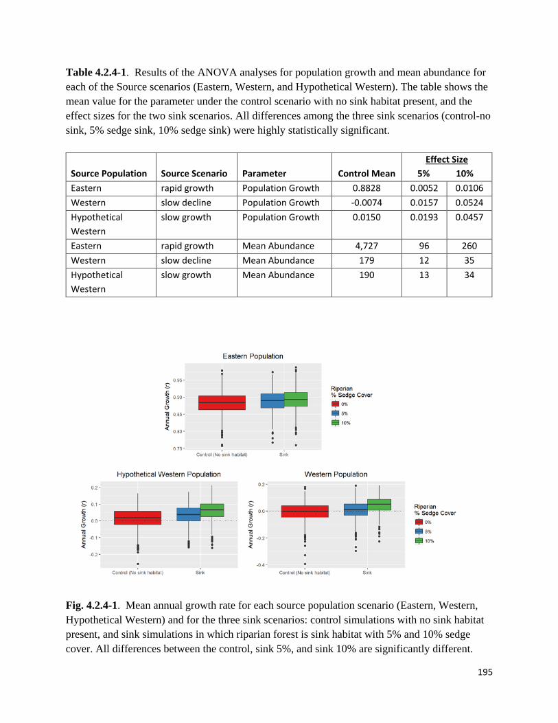
195
Table 4.2.4-1. Results of the ANOVA analyses for population growth and mean abundance for each of the Source scenarios (Eastern, Western, and Hypothetical Western). The table shows the mean value for the parameter under the control scenario with no sink habitat present, and the effect sizes for the two sink scenarios. All differences among the three sink scenarios (control-no sink, 5% sedge sink, 10% sedge sink) were highly statistically significant.
Source Population Source Scenario Parameter Control Mean Effect Size
5% 10% Eastern rapid growth Population Growth 0.8828 0.0052 0.0106 Western slow decline Population Growth -0.0074 0.0157 0.0524 Hypothetical Western
slow growth Population Growth 0.0150 0.0193 0.0457
Eastern rapid growth Mean Abundance 4,727 96 260 Western slow decline Mean Abundance 179 12 35 Hypothetical Western
slow growth Mean Abundance 190 13 34
Fig. 4.2.4-1. Mean annual growth rate for each source population scenario (Eastern, Western, Hypothetical Western) and for the three sink scenarios: control simulations with no sink habitat present, and sink simulations in which riparian forest is sink habitat with 5% and 10% sedge cover. All differences between the control, sink 5%, and sink 10% are significantly different.
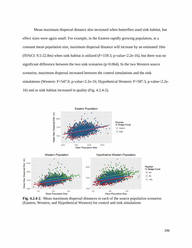
196
Mean maximum dispersal distance also increased when butterflies used sink habitat, but
effect sizes were again small. For example, in the Eastern rapidly growing population, at a
constant mean population size, maximum dispersal distance will increase by an estimated 16m
(95%CI: 9.5-22.8m) when sink habitat is utilized (F=159.3, p-value<2.2e-16), but there was no
significant difference between the two sink scenarios (p=0.064). In the two Western source
scenarios, maximum dispersal increased between the control simulations and the sink
simulations (Western: F=547.9, p-value<2.2e-16; Hypothetical Western: F=587.3, p-value<2.2e-
16) and as sink habitat increased in quality (Fig. 4.2.4-2).
Fig. 4.2.4-2. Mean maximum dispersal distances in each of the source population scenarios (Eastern, Western, and Hypothetical Western) for control and sink simulations

197
Theoretical models have shown a wide variety of population responses to the presence of
sink habitat from positive to negative depending on a wide range of factors. For one endangered
butterfly species, our model demonstrates that sink habitat can provide small but significant
benefits by increasing its growth rate and population size, and facilitating dispersal. While the
impact of such sink habitat may be small, for small populations with negative or slow growth
such as the Western St. Francis satyr population, these increases may make the difference
between continued existence and extirpation. While more research will be necessary to
understand if St. Francis satyrs are indeed using riparian forests as sink habitat, our models
provide insight into the value of any type of sink habitat, whether it be riparian forest or
degraded wetland, to the species. This may be particularly helpful for this species which relies on
ephemeral sedge wetlands that degrade over time in the absence of disturbance. Degraded
wetland habitat can itself be a sink if it fails to maintain stable or growing population (as
illustrated by our Western St. Francis satyr population), but our study indicates that restoration of
adjacent habitat may benefit the population more than restoring the existing degraded wetland
since it could serve as sink habitat that contributes to the overall growth and health of the
population. More broadly, our empirically based SEIBM model demonstrates how SEIBMs can
be used to bridge the gap between theoretical models and empirical studies to better understand
the ecological role of sink habitats for a given species.
4.2.5 Refine measurements of vital rates, trends and abundance
ABB and SFS caterpillar behavior and survival results Caterpillar host use and survival
We released a total of 37 St. Francis’ satyr caterpillars into field arenas, 10 of which
successfully survived to become adult butterflies (21% survival). Based on our estimates of egg
198
laying rates and egg survival from the greenhouse, we expect each St. Francis’ satyr female to
produce, on average, 60 eggs, 48 of which hatch, and to replace herself, we expect two
caterpillars to survive to adult (4.2% survival), assuming a stable population. The overall
survival we measured was considerably higher than this expectation.
Small, green caterpillars are difficult to find within arenas supporting dense growth of
sedges. However we were able to find some caterpillars each day we checked arenas. In the four
arenas that contained multiple sedges, 67 ± 27% of the St. Francis’ satyr caterpillars we found
were feeding on C. atlantica, until they were fourth instars, at which point 100% of our
observations were on C. mitchelliana. The remaining 33% of the St. Francis’ satyr caterpillars
were found feeding on C. mitchelliana as early instars. We did not release Appalachian brown
caterpillars into arenas as part of this project so we do not have data on their host preferences.
However, we released Appalachian browns into arenas in 2012 and have conducted subsequent
arena work with them as part of other experiments. In prior experiments in these same arenas
(Aschehoug, et al. 2015), we have never observed Appalachian browns feeding on C. atlantica.
Occasionally they will feed on grass species when grass is abundant within arenas, but C.
mitchelliana is by far the preferred host of Appalachian browns.
Caterpillar survival did not differ between species (p=0.42) or treatments (p=0.58). The
interaction term is marginally significant (p=0.10) and in the context of small sample sizes for St.
Francis’ satyr indicates a trend toward differential survival between Appalachian browns and St.
Francis’ satyrs across treatments (Figure 4.2.5-1).
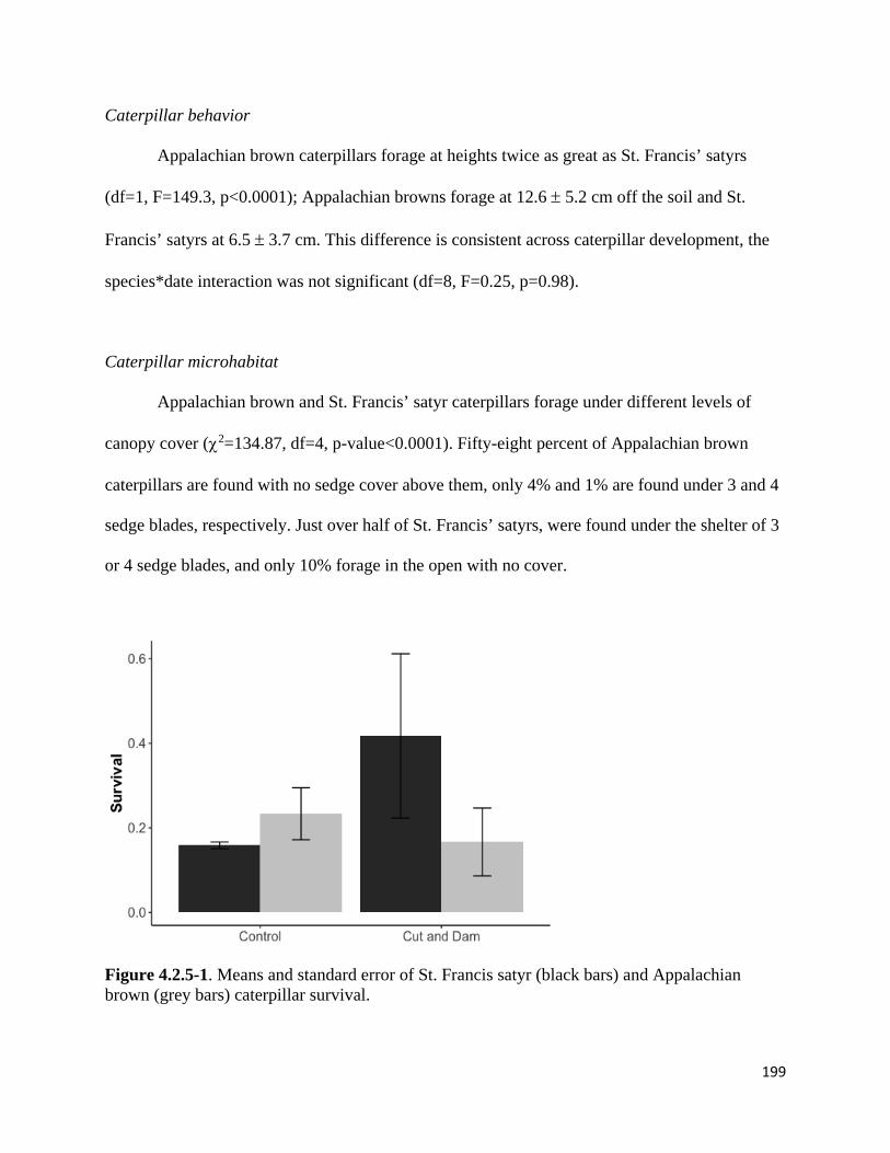
199
Caterpillar behavior
Appalachian brown caterpillars forage at heights twice as great as St. Francis’ satyrs
(df=1, F=149.3, p<0.0001); Appalachian browns forage at 12.6 ± 5.2 cm off the soil and St.
Francis’ satyrs at 6.5 ± 3.7 cm. This difference is consistent across caterpillar development, the
species*date interaction was not significant (df=8, F=0.25, p=0.98).
Caterpillar microhabitat
Appalachian brown and St. Francis’ satyr caterpillars forage under different levels of
canopy cover (χ2=134.87, df=4, p-value<0.0001). Fifty-eight percent of Appalachian brown
caterpillars are found with no sedge cover above them, only 4% and 1% are found under 3 and 4
sedge blades, respectively. Just over half of St. Francis’ satyrs, were found under the shelter of 3
or 4 sedge blades, and only 10% forage in the open with no cover.
Figure 4.2.5-1. Means and standard error of St. Francis satyr (black bars) and Appalachian brown (grey bars) caterpillar survival.
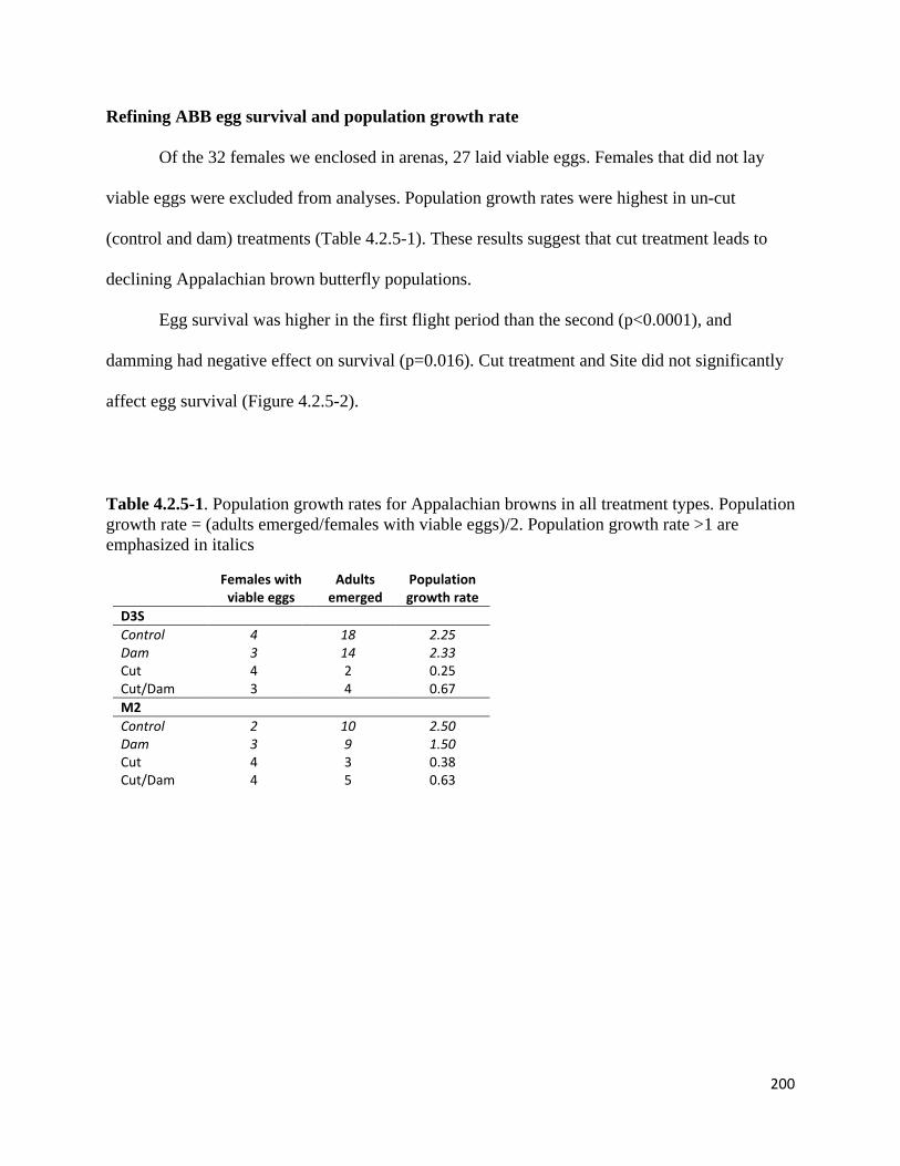
200
Refining ABB egg survival and population growth rate
Of the 32 females we enclosed in arenas, 27 laid viable eggs. Females that did not lay
viable eggs were excluded from analyses. Population growth rates were highest in un-cut
(control and dam) treatments (Table 4.2.5-1). These results suggest that cut treatment leads to
declining Appalachian brown butterfly populations.
Egg survival was higher in the first flight period than the second (p<0.0001), and
damming had negative effect on survival (p=0.016). Cut treatment and Site did not significantly
affect egg survival (Figure 4.2.5-2).
Table 4.2.5-1. Population growth rates for Appalachian browns in all treatment types. Population growth rate = (adults emerged/females with viable eggs)/2. Population growth rate >1 are emphasized in italics
Females with
viable eggs Adults
emerged Population growth rate
D3S Control 4 18 2.25 Dam 3 14 2.33 Cut 4 2 0.25 Cut/Dam 3 4 0.67 M2 Control 2 10 2.50 Dam 3 9 1.50 Cut 4 3 0.38 Cut/Dam 4 5 0.63
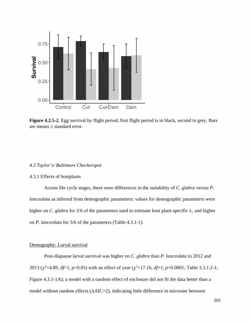
201
Figure 4.2.5-2. Egg survival by flight period, first flight period is in black, second in grey. Bars are means ± standard error.
4.3 Taylor’s/ Baltimore Checkerspot
4.3.1 Effects of hostplants
Across life cycle stages, there were differences in the suitability of C. glabra versus P.
lanceolata as inferred from demographic parameters: values for demographic parameters were
higher on C. glabra for 2/6 of the parameters used to estimate host plant-specific λ, and higher
on P. lanceolata for 3/6 of the parameters (Table 4.3.1-1).
Demography: Larval survival
Post-diapause larval survival was higher on C. glabra than P. lanceolata in 2012 and
2013 (χ2=4.89, df=1, p<0.05) with an effect of year (χ2=17.16, df=1, p<0.0001; Table 3.3.1.2-1;
Figure 4.3.1-1A); a model with a random effect of enclosure did not fit the data better than a
model without random effects (∆AIC=2), indicating little difference in microsite between
202
enclosures. Overwinter survival, on the other hand, was higher on P. lanceolata than on C.
glabra (χ2=3.25, df=2, p<0.10; Table 3.3.1.2-1; Figure 4.3.1-1B); a model with a random effect
of enclosure was a better fit to the data than a model without the random effect (∆AIC=344),
indicating variation among microsites in estimates of overwinter survival beyond that attributed
to host plant alone (among-site variance = 0.69).
Demography: Number of nests, nest size, and population-level oviposition preference
More nests were laid on P. lanceolata than C. glabra in both 2013 and 2014 (Table
3.3.1.2-1; Figure 4.3.1-2A), and P. lanceolata nests contained more larvae than C. glabra nests
(Table 3.3.1.2-1; Figure 4.3.1-1C). In 2013, the proportion of nests in P. lanceolata versus C.
glabra did not differ from the proportion of area covered by P. lanceolata and C. glabra, but in
2014 the proportion of nests on P. lanceolata was higher than its proportion of land cover
(Figure 4.3.1-2B).
Demography: Female daily adult survival, population size, and individual mass
Daily survival of adult females did not differ based on their post-diapause host (P.
lanceolata versus C. glabra; Table 3.3.1.2-1; Figure 4.3.1-3A). Females that were reared during
the post-diapause period in enclosures with C. glabra were larger in mass than females reared in
enclosures with P. lanceolata (χ2=2.83, df=1, p<0.10; Table 3.3.1.2-1; Figure 4.3.1-3B). The
population size of adult females increased from 2012 to 2014 (Figure 4.3.1-3C).
Demography: Host plant-specific population growth rates
Habitat-specific population growth rates, with and without adjusting for survival
differences in fecundity, were higher on P. lanceolata than C. glabra (Figure 4.3.1-4). The
survival-fecundity adjustment exaggerated this difference, but did not qualitatively affect our
203
conclusions about host-plant specific population growth rates (Figure 4.3.1-4). Estimated annual
population growth rates were high, but broadly consistent with observed increases in population
size during the study period (Figure 4.3.1-3C). Replacing the value for overwinter survival on C.
glabra with the value for overwinter survival on P. lanceolata, assuming all other parameter
values were those of C. glabra, led to the greatest change in population growth rates relative the
same replacement for other vital rates for C. glabra; all other means fell within the confidence
limits of the original population growth rate estimates for C. glabra (Figure 4.3.1-5).
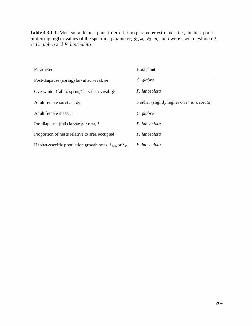
204
Table 4.3.1-1. Most suitable host plant inferred from parameter estimates, i.e., the host plant conferring higher values of the specified parameter; φ1, φ2, φ3, m, and l were used to estimate λ
on C. glabra and P. lanceolata.
Parameter Host plant
Post-diapause (spring) larval survival, φ1 C. glabra
Overwinter (fall to spring) larval survival, φ2 P. lanceolata
Adult female survival, φ3 Neither (slightly higher on P. lanceolata)
Adult female mass, m C. glabra
Pre-diapause (fall) larvae per nest, l P. lanceolata
Proportion of nests relative to area occupied P. lanceolata
Habitat-specific population growth rates, λC.g. or λP.l P. lanceolata
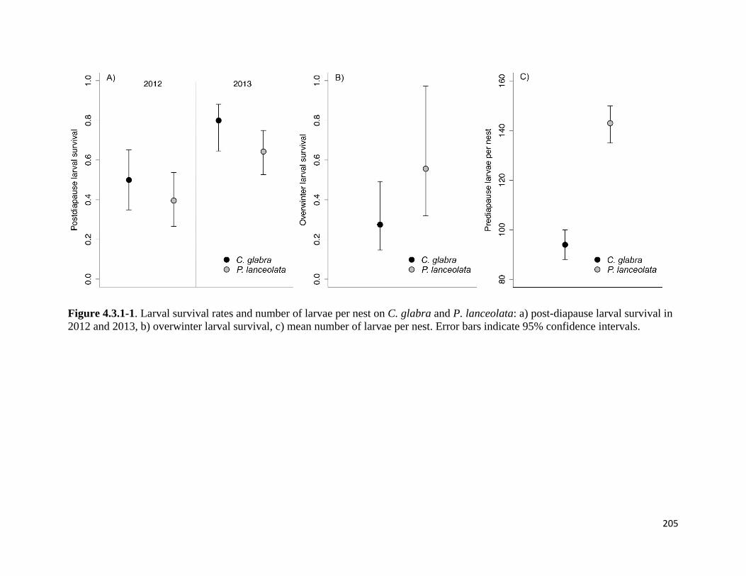
205
Figure 4.3.1-1. Larval survival rates and number of larvae per nest on C. glabra and P. lanceolata: a) post-diapause larval survival in 2012 and 2013, b) overwinter larval survival, c) mean number of larvae per nest. Error bars indicate 95% confidence intervals.
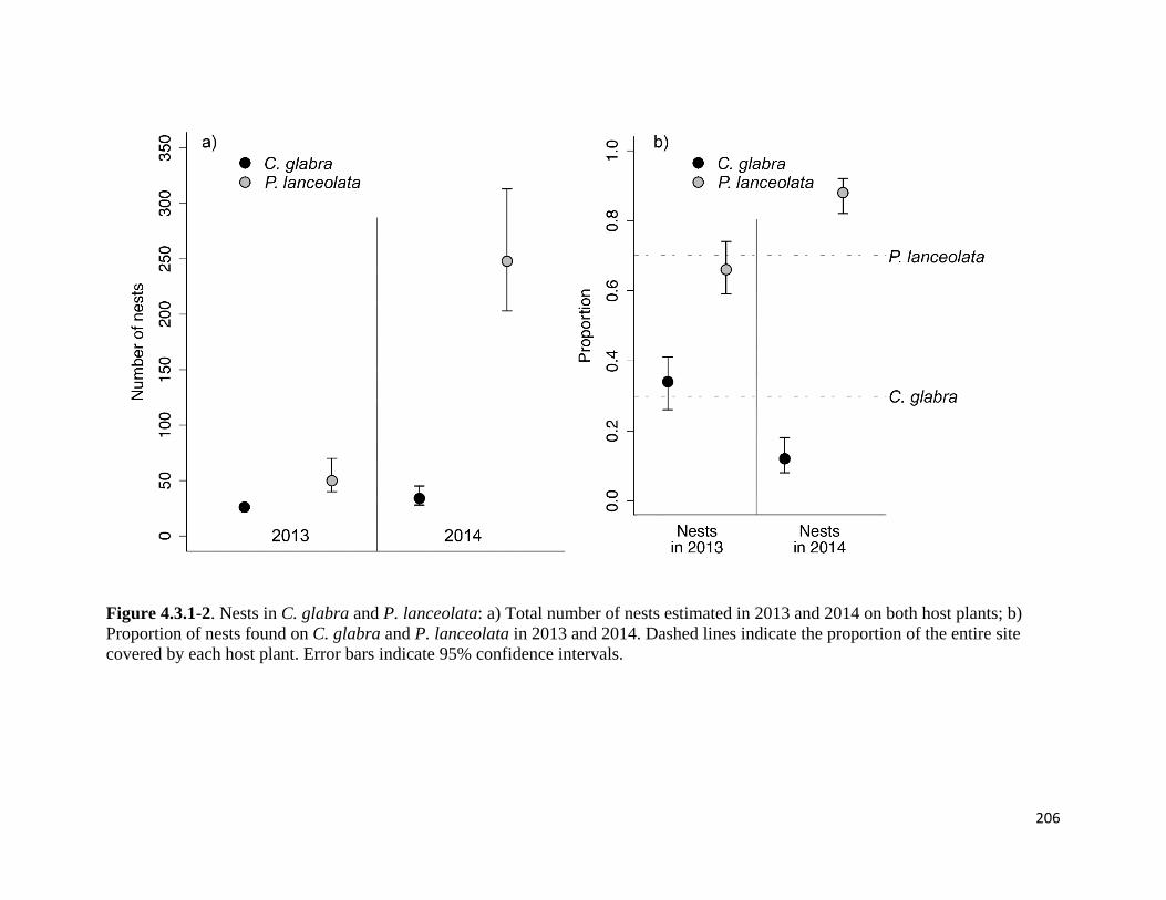
206
Figure 4.3.1-2. Nests in C. glabra and P. lanceolata: a) Total number of nests estimated in 2013 and 2014 on both host plants; b) Proportion of nests found on C. glabra and P. lanceolata in 2013 and 2014. Dashed lines indicate the proportion of the entire site covered by each host plant. Error bars indicate 95% confidence intervals.
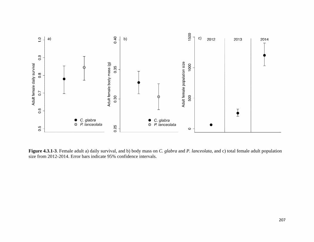
207
Figure 4.3.1-3. Female adult a) daily survival, and b) body mass on C. glabra and P. lanceolata, and c) total female adult population size from 2012-2014. Error bars indicate 95% confidence intervals.
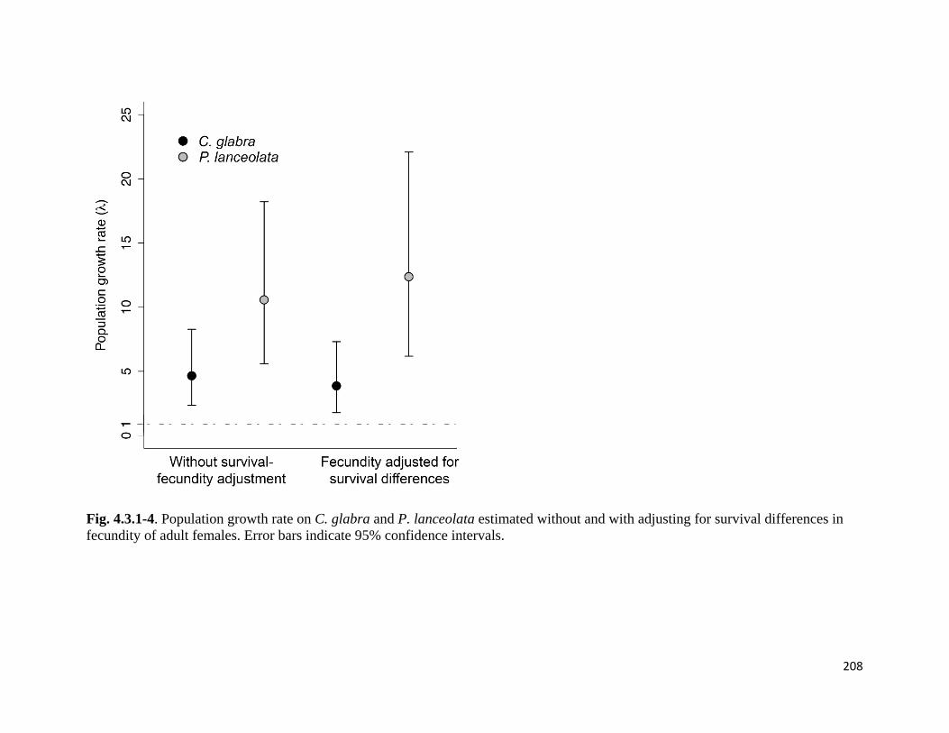
208
Fig. 4.3.1-4. Population growth rate on C. glabra and P. lanceolata estimated without and with adjusting for survival differences in fecundity of adult females. Error bars indicate 95% confidence intervals.

209
Fig 4.3.1-5. Population growth rates a) with and b) without adult survival correction, followed by LTRE analysis with growth rates for C. glabra where each vital rate was replaced in turn with the P. lanceolata value for a = post-diapause survival, b = overwinter survival, c = number of larvae per nest, d = female adult body mass, and e = female adult survival.
210
4.3.2 Effects of herbicide
Graminicide Experiment
Survivorship of Euphydryas colon to diapause was influenced by graminicide application
(Figure 4.3.2-1a, χ2 = 9.49, df = 4, P = 0.049). Sethoxydim reduced survivorship to diapause
from 98% in control treatment to 78% in treated groups (P = 0.029). Effects of clethodim on
survivorship to diapause, 85%, were not significantly different from the control group (P =
0.085). Neither fluazifop-p-butyl nor NuFilm influenced survival to diapause. Development
time did not differ significantly among treatment groups (χ2 = 0.62, df = 4, P = 0.960) nor did
mass at diapause (F = 0.24, df = 4, P = 0.912).
Iridoid glycoside profiles differed among treatments. Iridoid glycosides were about a
quarter of the dry weight of larvae in all treatment groups, including the control (Figure 4.3.2-
1b). Total amount (in mg per larva) of iridoid glycosides did not vary among treatments (χ2 =
6.69, df = 4, P = 0.153). However, graminicide treated larvae had substantially higher aucubin
and lower catalpol than control larvae (χ2 = 15.31, df = 4, P = 0.004). Percent dry weight of
aucubin was almost double that of the controls in all three graminicide treatments while NuFilm
treated larvae were not affected (Figure 4.3.2-1b). Fluazifop-p-butyl, sethoxydim and clethodim
treated larvae all had significantly higher dry weight of aucubin relative to the control (P< 0.05
for all pairwise comparisons between graminicides and controls). In contrast, catalpol varied
among groups (χ2 = 10.19, df = 4, P = 0.037), but was only significantly lower than the control
in clethodim-sprayed larvae (P = 0.018 for clethodim, P>0.50 for other comparisons).
211
Species x Hostplant Experiment
Herbicide treatment did not influence survival or development time of any of the
Euphydryas species (Tables 4.3.2-1 and 4.3.2-2). Survival differed among Euphydryas and
hostplant species (Table 2, Species, Host and Species x Host terms). Survival was >90% for all
species and hostplant combinations except E. colon foraging on Castilleja. Euphydryas editha
and E. phaeton took longer to reach diapause on the novel host (13.5 vs. 16.4 days by E. editha;
11.1 vs. 12.4 days by E. phaeton; Table 4.3.2-1). Growth (i.e., change in mass during the
experiment) was not consistently affected by treatment (Table 4.3.2-2, main effect of Treatment).
However, there was a marginally significant (P = 0.057) of Treatment x Host interaction (Table
4.3.2-2). In general, herbicide consistently reduced growth on P. lanceolata but had no
consistent effect on larvae reared on their native hosts (C. glabra or C. hispida).
Graminicide only influenced the foraging frequency of one species on one hostplant
(Table 4.3.2-2, 3-way interaction). Euphydryas phaeton was less likely to be observed foraging
on treated than control C. glabra plants, but this effect was not present when foraging on P.
lanceolata (Table 4.3.2-1). In general, the likelihood of observing active feeding was higher for
E. editha and E. phaeton when feeding on P. lanceolata (Tables 4.3.2-1 and 4.3.2-2).
Graminicide influenced group size in pre-diapause larva (Table 4.3.2-2, Treatment effect). Group
sizes were smaller in graminicide cohorts for E. colon and E. phaeton (Figure 4.3.2-2). Group
size also differed among Euphydryas and host plant species (Table 4.3.2-2, Species, Host, and
Host x Species effects). Group sizes were larger in E. colon and E. editha cohorts on P.
Lanceolata (relative to their native host C. hispida), and larger in E. phaeton on its native host,
C. glabra.
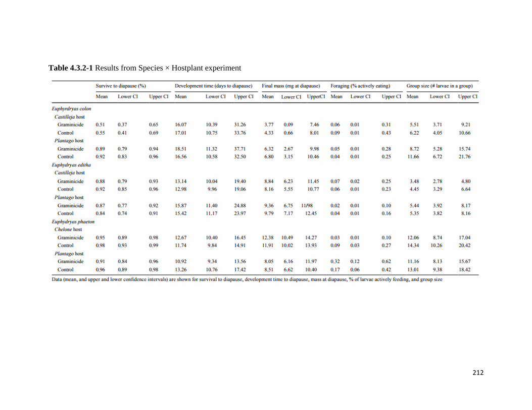
212
Table 4.3.2-1 Results from Species × Hostplant experiment
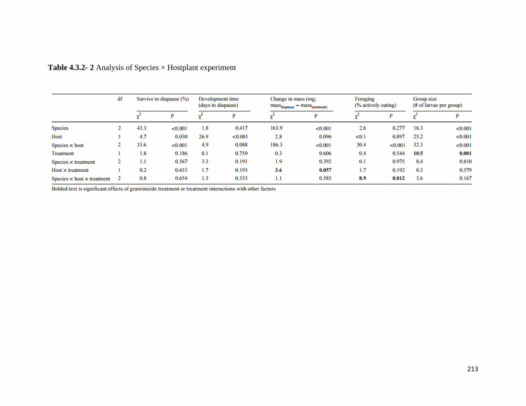
213
Table 4.3.2- 2 Analysis of Species × Hostplant experiment
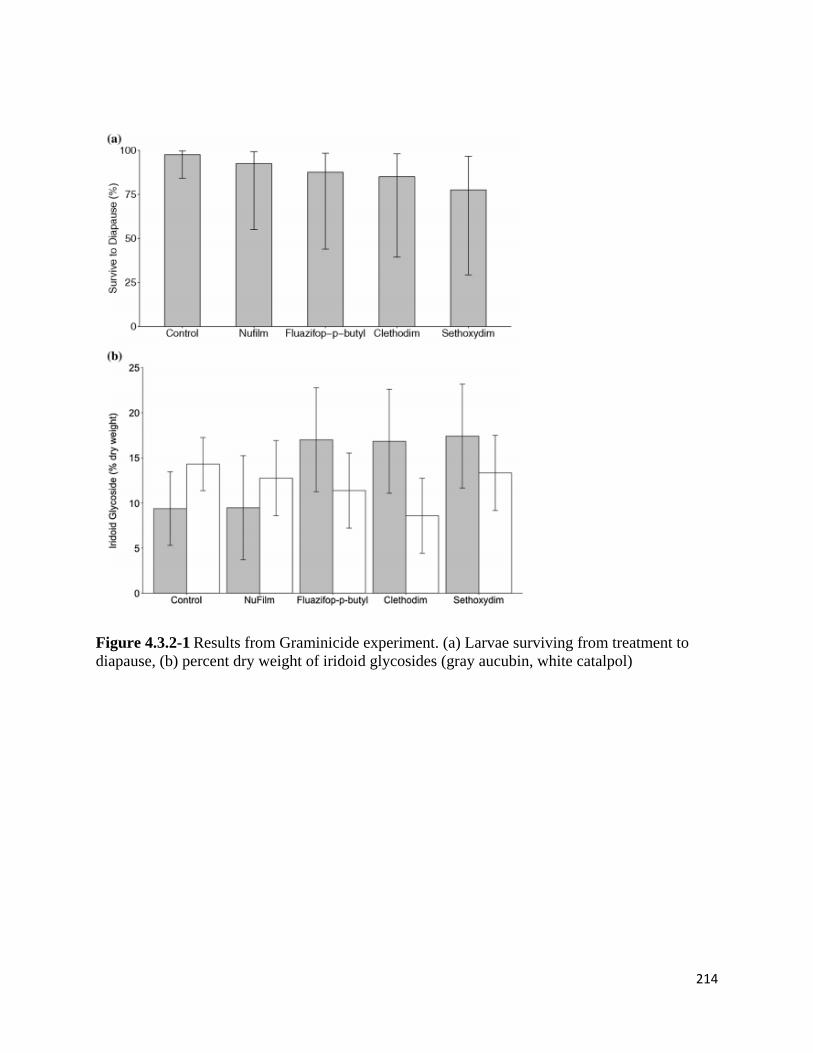
214
Figure 4.3.2-1 Results from Graminicide experiment. (a) Larvae surviving from treatment to diapause, (b) percent dry weight of iridoid glycosides (gray aucubin, white catalpol)
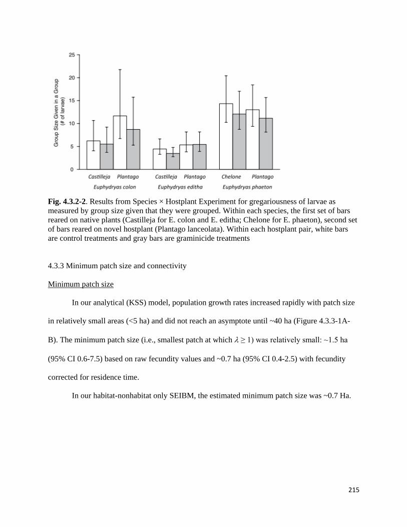
215
Fig. 4.3.2-2. Results from Species × Hostplant Experiment for gregariousness of larvae as measured by group size given that they were grouped. Within each species, the first set of bars reared on native plants (Castilleja for E. colon and E. editha; Chelone for E. phaeton), second set of bars reared on novel hostplant (Plantago lanceolata). Within each hostplant pair, white bars are control treatments and gray bars are graminicide treatments
4.3.3 Minimum patch size and connectivity
Minimum patch size
In our analytical (KSS) model, population growth rates increased rapidly with patch size
in relatively small areas (<5 ha) and did not reach an asymptote until ~40 ha (Figure 4.3.3-1A-
B). The minimum patch size (i.e., smallest patch at which λ ≥ 1) was relatively small: ~1.5 ha
(95% CI 0.6-7.5) based on raw fecundity values and ~0.7 ha (95% CI 0.4-2.5) with fecundity
corrected for residence time.
In our habitat-nonhabitat only SEIBM, the estimated minimum patch size was ~0.7 Ha.
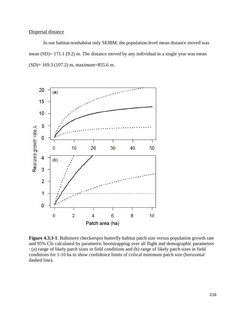
216
Dispersal distance
In our habitat-nonhabitat only SEIBM, the population-level mean distance moved was
mean (SD)= 171.1 (9.2) m. The distance moved by any individual in a single year was mean
(SD)= 169.3 (107.2) m, maximum=855.6 m.
Figure 4.3.3-1. Baltimore checkerspot butterfly habitat patch size versus population growth rate and 95% CIs calculated by parametric bootstrapping over all flight and demographic parameters : (a) range of likely patch sizes in field conditions and (b) range of likely patch sizes in field conditions for 1-10 ha to show confidence limits of critical minimum patch size (horizontal dashed line).
217
4.3.4 SEIBMs: Scenario analysis on real landscapes
Population-Level Dynamics:
With a single restored host patch, populations under both the endogenous (with no
stochasticity) and exogenous (with correlated high stochasticity) models exhibit boom-bust
dynamics, as designed. Although both models produce high inter-annual variability in population
size (CV=0.62 and 0.56, respectively), only under the endogenous model is extinction risk also
high, with 62% of simulated populations going extinct before 30 years, compared to no
extinction at the level of stochasticity we used in the exogenous model.
Regardless of the model used, dividing the habitat into an increasing number of patches
(and thus decreasing the size of each patch) or moving the patches farther apart decreases the
intrinsic growth rate, eventually leading to negative growth (Fig. 4.3.4-1). Despite this
commonality between the models, the consequences of patchiness for boom-bust dynamics are
very different under the two models.
Under the exogenous model, as the number of patches increases, boom-bust dynamics
continue unabated at the whole population level (Fig. 4.3.4-2 A), with population variability
increasing due to an increase in demographic stochasticity (Fig. 4.3.4-3 A) as mean population
size decreases. Thus, under the exogenous model, splitting the habitat does not dampen boom-
bust dynamics but rather leads to less population stability and a smaller population. Extinction
risk remains low, however, for all scenarios with a positive intrinsic growth rate. In the
endogenous model, splitting the restored area into multiple patches generally decreases
population variability, with the amplitude of boom-bust fluctuations decreasing with an
increasing number of patches (Fig. 4.3.4-2B & 4.3.4-3A). Under this model, extinction risk
declines from 0.62 in the single patch scenario to 0 when the habitat is divided into 2 or more
218
patches (at 20m spacing). Mean population size is generally larger in multiple patch scenarios
with positive intrinsic growth rates relative to the single-patch scenario, and mean population
size increases with an increasing number of patches (at 20m spacing).
Increasing patch spacing yields the same general pattern. Under the exogenous model, as
distance between patches increases (and thus as intrinsic growth rate declines; Fig. 4.3.4-1),
population variability increases (Fig. 4.3.4-2A & 4.3.4-3B) and mean population size decreases
(Appendix S3: Table S1). Again, for all scenarios with a positive intrinsic growth rate, 30-year
extinction risk remains at or near zero under the exogenous model. Under the endogenous model,
for all multi-patch scenarios that yield a positive intrinsic growth rate (e.g., 2 patches at any
spacing, 4 patches at 20 or 50m spacing, etc.), as patches get farther apart, population variability
declines (Fig. 4.3.4-2B & 4.3.4-3B) and extinction risk remains at zero (Fig. 4.3.4-2B). Mean
population size increases with increasing distance under the two-patch scenario up to 100m
spacing, but decreases in all other scenarios. Regardless of the model, in scenarios in which the
patches were too small and/or too far apart to maintain a positive intrinsic growth rate (see Fig.
4.3.4-1), extinction risk was high, or in a few cases, extinction risk was low but a slowly
declining trajectory guaranteed extinction within a few years beyond the 30-year simulation
window (e.g., see the 4-patch/100m scenario in Fig. 4.3.4-2B).
Patch-Level Dynamics:
Since movement parameters do not differ between models, as expected, all metrics
related to dispersal and host patch residence time are the same in both models, exhibiting the
following patterns. Time spent in host patches declines with decreasing patch size and increasing
inter-patch distance. Similarly, dispersal among patches as measured by the proportion of time
spent in non-natal patches declines with patch size and interpatch distance, with butterflies
219
spending almost no time in non-natal patches when patches are spaced at 400m, regardless of
patch size. As a result, patch recolonizations decrease with increasing distance and number of
patches, and is near zero for patches at 400m spacing.
Individual patch populations generally mirror total population patterns under their
respective models with correlated stochasticity. For example, under the exogenous model, patch
population variability and patch extinctions generally increase with increasing number (and
decreasing size) of patches and with increasing distance between patches. In the endogenous
model, for scenarios in which the intrinsic growth rate is positive, as the patches get smaller and
farther apart, individual patch population variability is dampened and patch extinctions decline.
Effects of Environmental Stochasticity Type and Level
Not surprisingly, when correlated environmental stochasticity is added to the endogenous
model, in the single-patch scenario, population variability increases (Fig. 4.3.4-3A), and
extinction occurs in all simulations for both levels of stochasticity. However, as the number of
patches or inter-patch distance increases, boom-bust dynamics are dampened (Fig. 4.3.4-3A &
B), and extinction risk declines up to the point at which the intrinsic growth rate drops below
zero.
Relative to the correlated stochasticity versions, uncorrelated stochasticity results in
dampened boom-bust dynamics in both models (cf. Fig. 4.3.4-3A, C & Fig. 4.3.4-3B, D) and
lower extinction risk. In addition, under the exogenous model, multiple patches with
uncorrelated stochasticity produce less variation in total population size relative to the single
patch scenario (Fig. 4.3.4-3C) in contrast to the correlated case in which variability only
increases with patch number (Fig. 4.3.4-3A). Increasing the distance between patches in the
220
uncorrelated exogenous model, however, did not further dampen boom-bust dynamics (Fig.
4.3.4-3D). All other patterns associated with decreasing patch size and increasing inter-patch
distance in the exogenous model are the same with uncorrelated as with correlated stochasticity
(Fig. 4.3.4-3). Similarly, for the endogenous model with uncorrelated stochasticity, total
population variability is lower relative to correlated stochasticity model output, but the general
patterns resulting from decreasing patch size and increasing inter-patch distance are unchanged
(Fig. 4.3.4-3C & 4.3.4-3D).
Patch extinctions decrease and recolonization increases under both models with
uncorrelated stochasticity compared to correlated stochasticity. Temporal variability in patch
populations (patch CV) is lower under uncorrelated stochasticity in both models but
demonstrates the same overall patterns relative to correlated stochasticity (e.g., increasing with
number of patches under the exogenous model).
Discussion
Our models illustrate that the mechanism driving fluctuations can dictate how boom-bust
populations respond to patchy environments, and thus, how best to manage such populations. We
found that when boom-bust dynamics are driven exclusively by exogenous factors such as
climatic variability, patchy environments generally increase inter-annual variability and put
populations at greater risk of extinction due to an increase in demographic stochasticity.
Although our 30-year extinction risk metric did not indicate that a low to moderate number of
patches spaced relatively closely would result in higher extinction risk under the exogenous
model, these populations were slower growing, more variable, and smaller relative to the single-
patch populations. Thus, we expect their longer-term extinction risk would be elevated (Inchausti
and Halley 2003), and that intentionally creating resource patchiness offered only disadvantages
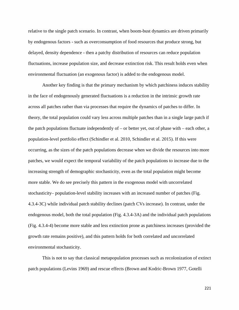
221
relative to the single patch scenario. In contrast, when boom-bust dynamics are driven primarily
by endogenous factors - such as overconsumption of food resources that produce strong, but
delayed, density dependence - then a patchy distribution of resources can reduce population
fluctuations, increase population size, and decrease extinction risk. This result holds even when
environmental fluctuation (an exogenous factor) is added to the endogenous model.
Another key finding is that the primary mechanism by which patchiness induces stability
in the face of endogenously generated fluctuations is a reduction in the intrinsic growth rate
across all patches rather than via processes that require the dynamics of patches to differ. In
theory, the total population could vary less across multiple patches than in a single large patch if
the patch populations fluctuate independently of – or better yet, out of phase with – each other, a
population-level portfolio effect (Schindler et al. 2010, Schindler et al. 2015). If this were
occurring, as the sizes of the patch populations decrease when we divide the resources into more
patches, we would expect the temporal variability of the patch populations to increase due to the
increasing strength of demographic stochasticity, even as the total population might become
more stable. We do see precisely this pattern in the exogenous model with uncorrelated
stochasticity– population-level stability increases with an increased number of patches (Fig.
4.3.4-3C) while individual patch stability declines (patch CVs increase). In contrast, under the
endogenous model, both the total population (Fig. 4.3.4-3A) and the individual patch populations
(Fig. 4.3.4-4) become more stable and less extinction prone as patchiness increases (provided the
growth rate remains positive), and this pattern holds for both correlated and uncorrelated
environmental stochasticity.
This is not to say that classical metapopulation processes such as recolonization of extinct
patch populations (Levins 1969) and rescue effects (Brown and Kodric-Brown 1977, Gotelli
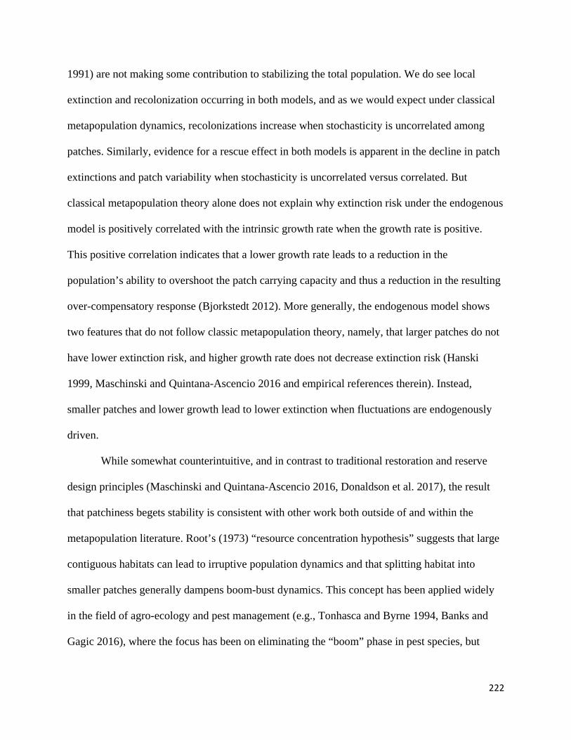
222
1991) are not making some contribution to stabilizing the total population. We do see local
extinction and recolonization occurring in both models, and as we would expect under classical
metapopulation dynamics, recolonizations increase when stochasticity is uncorrelated among
patches. Similarly, evidence for a rescue effect in both models is apparent in the decline in patch
extinctions and patch variability when stochasticity is uncorrelated versus correlated. But
classical metapopulation theory alone does not explain why extinction risk under the endogenous
model is positively correlated with the intrinsic growth rate when the growth rate is positive.
This positive correlation indicates that a lower growth rate leads to a reduction in the
population’s ability to overshoot the patch carrying capacity and thus a reduction in the resulting
over-compensatory response (Bjorkstedt 2012). More generally, the endogenous model shows
two features that do not follow classic metapopulation theory, namely, that larger patches do not
have lower extinction risk, and higher growth rate does not decrease extinction risk (Hanski
1999, Maschinski and Quintana-Ascencio 2016 and empirical references therein). Instead,
smaller patches and lower growth lead to lower extinction when fluctuations are endogenously
driven.
While somewhat counterintuitive, and in contrast to traditional restoration and reserve
design principles (Maschinski and Quintana-Ascencio 2016, Donaldson et al. 2017), the result
that patchiness begets stability is consistent with other work both outside of and within the
metapopulation literature. Root’s (1973) “resource concentration hypothesis” suggests that large
contiguous habitats can lead to irruptive population dynamics and that splitting habitat into
smaller patches generally dampens boom-bust dynamics. This concept has been applied widely
in the field of agro-ecology and pest management (e.g., Tonhasca and Byrne 1994, Banks and
Gagic 2016), where the focus has been on eliminating the “boom” phase in pest species, but

223
rarely, if ever, has it been considered in conjunction with species of conservation concern, where
the “bust” phases are more problematic. Previous metapopulation theory has shown that
dispersal among two or more populations exhibiting chaotic fluctuations (one form of boom-bust
dynamics) can be stabilizing (Gonzalez-Andujar and Perry 1993, Hastings 1993, Doebeli 1995,
Gyllenberg et al. 1996, Doebeli and Ruxton 1997). While not all dispersal-induced stability
derives from the mechanism of dampened growth rates (Doebeli 1995, Abbott 2011), many of
the theoretical models implicitly (e.g.,Gonzalez-Andujar and Perry 1993, Hastings 1993) or
explicitly (e.g., Doebeli 1995) demonstrate this stability mechanism. Our endogenous model not
only confirms the stabilizing effect of a dampened growth rate for boom-bust populations using
empirically estimated demographic and movement parameters, but also demonstrates that these
theoretical patterns can have important implications in the applied context of species
management and habitat restoration. Below we discuss implications of our results for our
understanding of the biology and management of checkerspots and other boom-bust populations.
Our results have several important implications for managing fluctuating populations
including Taylor’s checkerspot specifically. First, when fluctuations are endogenously driven, it
may in fact make sense to “manage the fluctuations”, rather than seeking to increase intrinsic
growth, maximize population size, or enhance dispersal and connectivity, which are most often
the focus in conservation and recovery efforts (Gerber and Hatch 2002, Donaldson et al. 2017).
While a clear positive relationship has been established between population variability and
extinction risk (Goodman 1987, Fagan et al. 2001, Inchausti and Halley 2003), management
often focuses on mitigating for variability rather than managing it directly. For example, in
classic metapopulations, local extinction or low sizes of local populations may not be considered
problematic as long as dispersal among populations is sufficient to allow for recolonization or
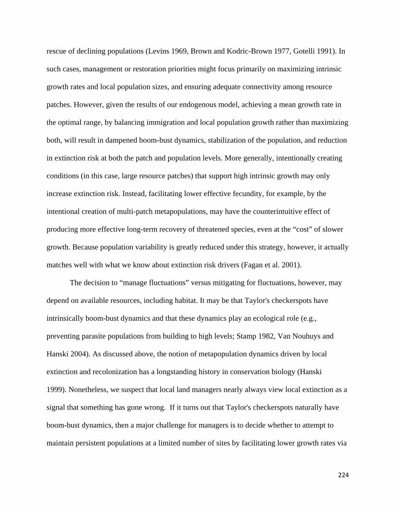
224
rescue of declining populations (Levins 1969, Brown and Kodric-Brown 1977, Gotelli 1991). In
such cases, management or restoration priorities might focus primarily on maximizing intrinsic
growth rates and local population sizes, and ensuring adequate connectivity among resource
patches. However, given the results of our endogenous model, achieving a mean growth rate in
the optimal range, by balancing immigration and local population growth rather than maximizing
both, will result in dampened boom-bust dynamics, stabilization of the population, and reduction
in extinction risk at both the patch and population levels. More generally, intentionally creating
conditions (in this case, large resource patches) that support high intrinsic growth may only
increase extinction risk. Instead, facilitating lower effective fecundity, for example, by the
intentional creation of multi-patch metapopulations, may have the counterintuitive effect of
producing more effective long-term recovery of threatened species, even at the “cost” of slower
growth. Because population variability is greatly reduced under this strategy, however, it actually
matches well with what we know about extinction risk drivers (Fagan et al. 2001).
The decision to “manage fluctuations” versus mitigating for fluctuations, however, may
depend on available resources, including habitat. It may be that Taylor's checkerspots have
intrinsically boom-bust dynamics and that these dynamics play an ecological role (e.g.,
preventing parasite populations from building to high levels; Stamp 1982, Van Nouhuys and
Hanski 2004). As discussed above, the notion of metapopulation dynamics driven by local
extinction and recolonization has a longstanding history in conservation biology (Hanski
1999). Nonetheless, we suspect that local land managers nearly always view local extinction as a
signal that something has gone wrong. If it turns out that Taylor's checkerspots naturally have
boom-bust dynamics, then a major challenge for managers is to decide whether to attempt to
maintain persistent populations at a limited number of sites by facilitating lower growth rates via
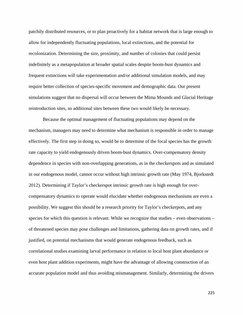
225
patchily distributed resources, or to plan proactively for a habitat network that is large enough to
allow for independently fluctuating populations, local extinctions, and the potential for
recolonization. Determining the size, proximity, and number of colonies that could persist
indefinitely as a metapopulation at broader spatial scales despite boom-bust dynamics and
frequent extinctions will take experimentation and/or additional simulation models, and may
require better collection of species-specific movement and demographic data. Our present
simulations suggest that no dispersal will occur between the Mima Mounds and Glacial Heritage
reintroduction sites, so additional sites between these two would likely be necessary.
Because the optimal management of fluctuating populations may depend on the
mechanism, managers may need to determine what mechanism is responsible in order to manage
effectively. The first step in doing so, would be to determine of the focal species has the growth
rate capacity to yield endogenously driven boom-bust dynamics. Over-compensatory density
dependence in species with non-overlapping generations, as in the checkerspots and as simulated
in our endogenous model, cannot occur without high intrinsic growth rate (May 1974, Bjorkstedt
2012). Determining if Taylor’s checkerspot intrinsic growth rate is high enough for over-
compensatory dynamics to operate would elucidate whether endogenous mechanisms are even a
possibility. We suggest this should be a research priority for Taylor’s checkerpots, and any
species for which this question is relevant. While we recognize that studies – even observations –
of threatened species may pose challenges and limitations, gathering data on growth rates, and if
justified, on potential mechanisms that would generate endogenous feedback, such as
correlational studies examining larval performance in relation to local host plant abundance or
even host plant addition experiments, might have the advantage of allowing construction of an
accurate population model and thus avoiding mismanagement. Similarly, determining the drivers
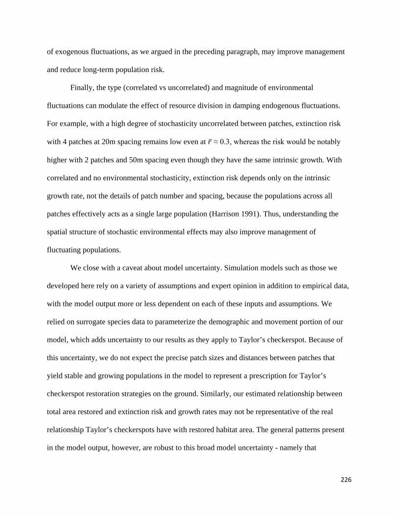
226
of exogenous fluctuations, as we argued in the preceding paragraph, may improve management
and reduce long-term population risk.
Finally, the type (correlated vs uncorrelated) and magnitude of environmental
fluctuations can modulate the effect of resource division in damping endogenous fluctuations.
For example, with a high degree of stochasticity uncorrelated between patches, extinction risk
with 4 patches at 20m spacing remains low even at �̅�𝑟 ≈ 0.3, whereas the risk would be notably
higher with 2 patches and 50m spacing even though they have the same intrinsic growth. With
correlated and no environmental stochasticity, extinction risk depends only on the intrinsic
growth rate, not the details of patch number and spacing, because the populations across all
patches effectively acts as a single large population (Harrison 1991). Thus, understanding the
spatial structure of stochastic environmental effects may also improve management of
fluctuating populations.
We close with a caveat about model uncertainty. Simulation models such as those we
developed here rely on a variety of assumptions and expert opinion in addition to empirical data,
with the model output more or less dependent on each of these inputs and assumptions. We
relied on surrogate species data to parameterize the demographic and movement portion of our
model, which adds uncertainty to our results as they apply to Taylor’s checkerspot. Because of
this uncertainty, we do not expect the precise patch sizes and distances between patches that
yield stable and growing populations in the model to represent a prescription for Taylor’s
checkerspot restoration strategies on the ground. Similarly, our estimated relationship between
total area restored and extinction risk and growth rates may not be representative of the real
relationship Taylor’s checkerspots have with restored habitat area. The general patterns present
in the model output, however, are robust to this broad model uncertainty - namely that
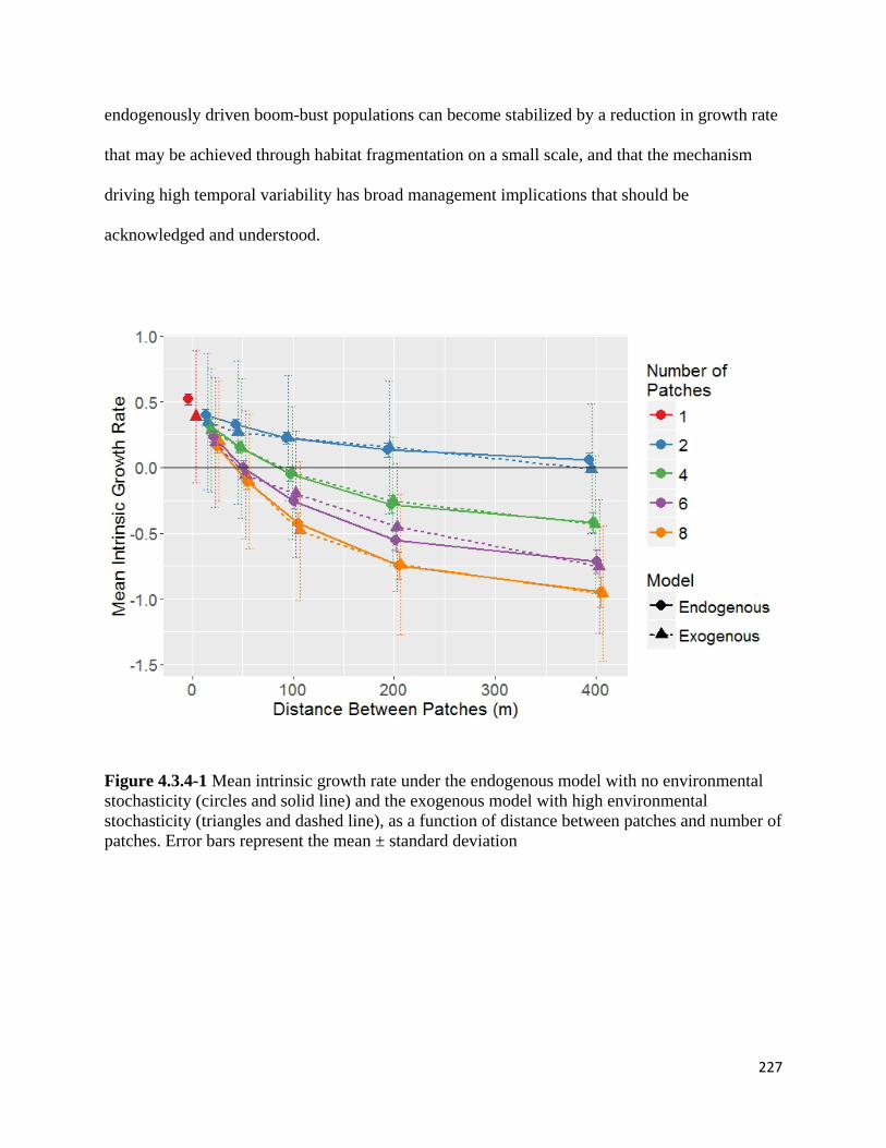
227
endogenously driven boom-bust populations can become stabilized by a reduction in growth rate
that may be achieved through habitat fragmentation on a small scale, and that the mechanism
driving high temporal variability has broad management implications that should be
acknowledged and understood.
Figure 4.3.4-1 Mean intrinsic growth rate under the endogenous model with no environmental stochasticity (circles and solid line) and the exogenous model with high environmental stochasticity (triangles and dashed line), as a function of distance between patches and number of patches. Error bars represent the mean ± standard deviation
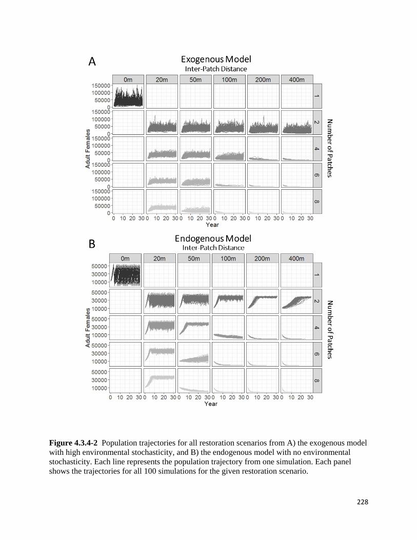
228
Figure 4.3.4-2 Population trajectories for all restoration scenarios from A) the exogenous model with high environmental stochasticity, and B) the endogenous model with no environmental stochasticity. Each line represents the population trajectory from one simulation. Each panel shows the trajectories for all 100 simulations for the given restoration scenario.
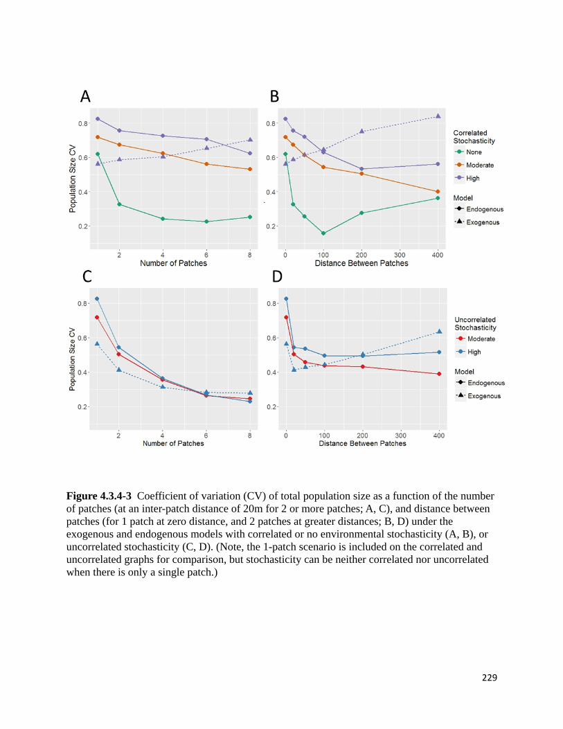
229
Figure 4.3.4-3 Coefficient of variation (CV) of total population size as a function of the number of patches (at an inter-patch distance of 20m for 2 or more patches; A, C), and distance between patches (for 1 patch at zero distance, and 2 patches at greater distances; B, D) under the exogenous and endogenous models with correlated or no environmental stochasticity (A, B), or uncorrelated stochasticity (C, D). (Note, the 1-patch scenario is included on the correlated and uncorrelated graphs for comparison, but stochasticity can be neither correlated nor uncorrelated when there is only a single patch.)
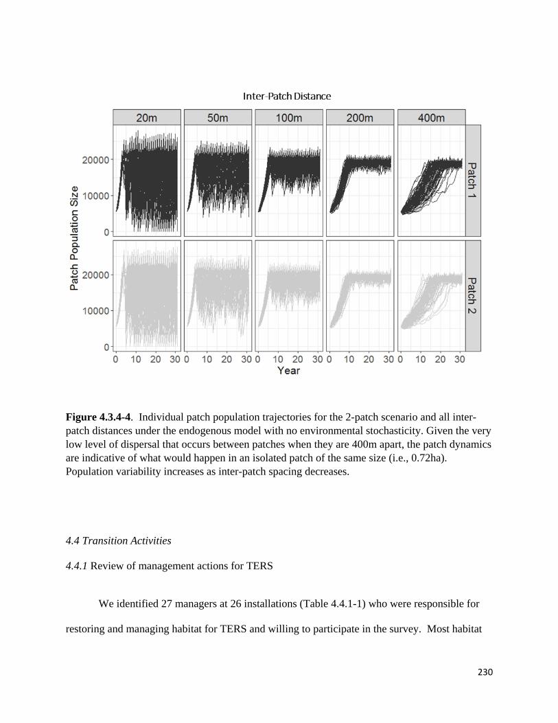
230
Figure 4.3.4-4. Individual patch population trajectories for the 2-patch scenario and all inter-patch distances under the endogenous model with no environmental stochasticity. Given the very low level of dispersal that occurs between patches when they are 400m apart, the patch dynamics are indicative of what would happen in an isolated patch of the same size (i.e., 0.72ha). Population variability increases as inter-patch spacing decreases.
4.4 Transition Activities
4.4.1 Review of management actions for TERS
We identified 27 managers at 26 installations (Table 4.4.1-1) who were responsible for
restoring and managing habitat for TERS and willing to participate in the survey. Most habitat

231
management conducted on participating installations involves restoring existing degraded habitat
using prescribed burns, herbicides, and mechanical treatments (Figure 4.4.1-1a). Fewer
installations attempt to create new habitat or acquire land to preserve habitat. Only a few attempt
to create dispersal corridors. About a third of the installations reintroduce animals into habitat
that has been created or restored.
When asked about management questions that need to be addressed, most managers
indicated a need to know which habitat patches should be restored or managed to have the
greatest impact on viability, and whether restoring all available habitat will improve viability
(Figure 4.4.1-1b). Over half the managers also wanted to know where to locate new areas of
habitat to ensure connectivity, whether restoration or creation of habitat would mitigate for the
loss of suitable habitat, and whether viability is affected by the timing and frequency of
disturbances used to manage habitat. Although only 7% of managers create corridors on their
installations, 44% wanted to know if adding corridors would improve population viability.
About a third of the managers wanted to know where animals should be reintroduced. Only 37%
of managers indicated they were in a position where they needed to choose between alternative
restoration strategies to meet management objectives. In addition, 3 managers who are trying to
deter wildlife from entering airfields or firing ranges, asked if SEIBMs could predict whether
restoring or creating habitat would draw animals away from areas of military use. One manager
also wanted to know whether animals would use new habitat after it had been created.
Managers provided information on 25 monitoring data sets for wildlife species whose
habitats were being restored or managed on 23 installations (Fort Bragg and Vandenberg AFB
each provided information for 2 species, Table 4.4.1-2). Of these data sets, 12 were birds, 6
were insects, 5 were reptiles, and 2 were mammals. Nearly all installations (96%) collected data
232
on population size, and 88% had habitat data in a GIS database (Figure 4.4.1-2a). Over half also
collected demographic and movement data, and 48% had behavioral information on individual
movement paths. Of the 12 bird data sets, 7 were red-cockaded woodpecker (Picoides borealis),
a species whose recovery efforts have been guided by SEIBMs since the late 1990s (USFWS
2003). Therefore, installations managing red-cockaded woodpeckers likely already collect the
types of data necessary to parameterize an SEIBM. Likewise, since our research group is
building SEIBMs for Fender’s blue butterfly (Icaricia icarioides fenderi) and St. Francis’ satyr
(Neonympha mitchellii francisci), data sets for these species are also adequate for building
SEIBMs. If we omit the red-cockaded woodpecker, Fender’s blue butterfly, and St. Francis’
satyr data sets to better reflect the typical amount of data a DoD manager is likely to possess, a
slightly smaller proportion of the remaining 16 data sets on 15 installations possess the necessary
data to parameterize an SEIBM (Figure 4.4.1-2a), and the amount of population size data shifts
downward, with the percentage of data sets with greater than 10 years of data decreasing from
52% to 25% (Figure 4.4.1-2b). However, most installations (81%) still had GIS databases of
environmental variables that could be used to construct habitat maps (Figure 4.4.1-2a), and most
data sets (69%) had more than 5 years of population size data. Approximately half of the
installations collected multiple years of data on survival and reproductive success, and 44%
possessed radio telemetry or satellite tag data that could be used to estimate movement
parameters.
Only 6 (22%) of the 27 managers surveyed had previous experience with SEIBMs and
only one (Eglin AFB) was currently using an SEIBM to manage species on the installation
(Figure 4.4.1-3). Nevertheless, 89% were open to the idea of using an SEIBM, with 33%
responding that they definitely thought using an SEIBM would enhance their ability to manage

233
habitat and 56% undecided. (Figure 4.4.1-3). The main factors that managers felt would prevent
them from using SEIBMs (Figure 4.4.1-4) were lack of modeling experience (74%), lack of data
(52%), and lack of resources to collect necessary data (52%). 30% of managers had doubts
about the reliability of predictions, and 26% felt that the simpler decision-making methods they
currently use were adequate. In these cases, methods were generally habitat-based and decisions
depended more on practicality or needs of the military that were not related to viability of the
species being managed. Only 7% of managers felt the types of questions that SEIBMs address
were not relevant to management on DoD installations.
After reviewing the questionnaires, we believe SEIBMs have potential for general
application on military installations. Most questions typically addressed by SEIBMs are the
same questions that the surveyed DoD managers take into consideration when making habitat
management decisions; in particular, what is the impact of restoring habitat on population
viability, and which patches have the greatest impact on viability? In addition, SEIBMs are
capable of addressing two other questions brought up by military managers: whether animals
will actually use habitat that has been newly created, and whether habitat can be created or
restored in such a way to draw animals away from an area of military use. In fact, SEIBMs have
previously been applied to similar questions. Kanagaraj et al. (2013) used an SEIBM to predict
whether tigers will find and use corridors connecting habitat patches in India and Nepal, based
on landscape context and individual movement behavior. In Japan, an SEIBM has been used to
design a strategy of establishing “alternate feeding areas” to alleviate damage to wheat crops by
white-fronted geese (Amano et al. 2007). Therefore, the types of questions that SEIBMs address
have great applicability to management of TERS habitat on military installations. Only 7% of
surveyed managers felt the types of questions that SEIBMs address were not relevant to

234
management on their installations. Ironically, one of the reasons given was that SEIBMs are
unnecessary because red-cockaded woodpeckers have been increasing under the current
management practice of placing recruitment clusters in suitable habitat next to existing clusters.
In fact, this practice was developed using insights from an SEIBM (Letcher et al. 1998, Crowder
et al. 1998, Walters et al. 2002, USFWS 2003).
In general, the DoD managers surveyed were open to using SEIBMs, but their main
limitations were insufficient data and lack of modeling experience. Although most installations
collect habitat and population size data, only about half collect the demographic or movement
data required to build an SEIBM. The DoD-managed species for which SEIBMs have already
been built (red-cockaded woodpecker, Fender’s blue butterfly, St. Francis’ satyr) have been the
subjects of detailed research and data collection for decades. However, not all SEIBMs start off
being built with such extensive data sets. If only one or two parameters are unknown, a method
called “pattern-oriented modeling” can be used to estimate parameter values whose simulated
population dynamics most closely match observed data (Rushton et al. 1997, Stephens et al.
2002). Parameters may also be derived from literature or surrogate species. Predictions from
initial models built with short-term or incomplete data sets should be used with caution to guide
management decisions. However, even preliminary models built with sparse data can generate
insights and testable hypotheses, and are useful for pinpointing what data need to be collected to
improve future predictions.
Besides the installations that manage for red-cockaded woodpecker, St. Francis’ satyr,
and Fender’s blue butterfly, four installations (Camp Shelby, U.S. Air Force Academy, Camp
Grayling, and Fort Riley) currently seem to have sufficient data to consider building an SEIBM.
Because military training at Camp Shelby occurs in the DeSoto National Forest, management of
235
the gopher tortoise is shared by the Mississippi Army National Guard, U.S. Fish and Wildlife
Service, U.S. Forest Service, and the Nature Conservancy. To manage gopher tortoise
(Gopherus Polyphemus), Camp Shelby surrounds each tortoise colony with a 200’ buffer zone,
and has established a 2200-acre refuge that is managed to achieve optimal habitat conditions
using prescribed burns (MSARNG 2014). A major objective is to keep tortoises off the artillery
firing ranges, where exposure to vehicle activity poses a significant mortality risk. As described
above, an SEIBM might be able to predict whether providing desirable habitat elsewhere is
likely to result in the desired redistribution of tortoises away from the firing ranges. The U.S.
Air Force Academy currently protects riparian habitat on its base along Monument Creek for the
Preble’s meadow jumping mouse (Zapus hudsonius preblei). As a result, the base contains one
of the largest PMJM populations documented within the range of the subspecies (Grunau et al.
1999). However, species viability is still threatened by habitat fragmentation and degradation
that has isolated sub-populations along the tributaries from the main stem sub-population, and
the Monument Creek population from other populations outside the base. An SEIBM could be
used to evaluate connectivity among habitat patches and determine where habitat might be
restored or corridors created to facilitate movement among sub-populations. Camp Grayling has
used clear cuts and fire to open tree canopy and create habitat for massasauga rattlesnakes
(Sistrurus catenatus). An SEIBM could answer questions about whether snakes can access and
benefit from these new habitat patches. Fort Riley uses prescribed burns and herbicides to
restore tallgrass prairie habitat for the greater prairie chicken (Tympanuchus cupido). An SEIBM
could inform managers about when, where, and how often to burn in order to achieve goals of
species persistence.

236
The other major limitation preventing managers from using SEIBMs is lack of modeling
experience. SEIBMs have the potential to capture the dynamics of complex systems, but coding
that complexity into a model is beyond the abilities of the typical manager. However, limited
modeling experience can be overcome by reaching out to researchers who specialize in
ecological modeling. Some modelers are consultants who contract their services (e.g.,
www.langrailsback.com, https://www.fws.gov/rcwrecovery/rcw_model.html). Others are
academics who may have access to funding and graduate students who are looking for applied
projects on which to develop their skills. Thus, collaboration with academic institutions may
enable managers to collect data and build SEIBMs with fewer resources than might be imagined.
The most successful collaborations require close communication between manager and modeler,
so the modeler has the appropriate biological information and understanding of the system, and
the manager understands how to interpret model outputs.
Based on our informal survey, most DoD managers viewed SEIBMs as potentially useful
for addressing many of the questions they face when managing wildlife habitat. The main
factors limiting their use are lack of data and modeling experience. Only a few of the
installations are capable of building an SEIBM with the data on hand, and the majority of
managers have no experience with modeling. However, if DoD managers were to collaborate
with civilians specializing in ecological modeling, these obstacles are not insurmountable.
Because of their complexity and high data requirements, SEIBMs are not practical for single
decisions that need to be made immediately, or decisions that are dictated primarily by logistical
feasibility or military needs. However, when integrated into the long term management of a
TERS, SEIBMs provide insights into complex population dynamics and offer a science-based
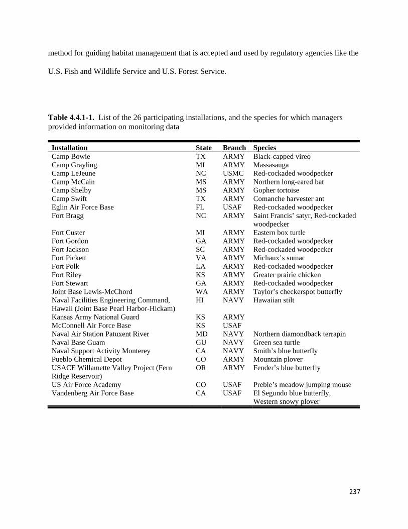
237
method for guiding habitat management that is accepted and used by regulatory agencies like the
U.S. Fish and Wildlife Service and U.S. Forest Service.
Table 4.4.1-1. List of the 26 participating installations, and the species for which managers provided information on monitoring data Installation State Branch Species Camp Bowie TX ARMY Black-capped vireo Camp Grayling MI ARMY Massasauga Camp LeJeune NC USMC Red-cockaded woodpecker Camp McCain MS ARMY Northern long-eared bat Camp Shelby MS ARMY Gopher tortoise Camp Swift TX ARMY Comanche harvester ant Eglin Air Force Base FL USAF Red-cockaded woodpecker Fort Bragg NC ARMY Saint Francis’ satyr, Red-cockaded
woodpecker Fort Custer MI ARMY Eastern box turtle Fort Gordon GA ARMY Red-cockaded woodpecker Fort Jackson SC ARMY Red-cockaded woodpecker Fort Pickett VA ARMY Michaux’s sumac Fort Polk LA ARMY Red-cockaded woodpecker Fort Riley KS ARMY Greater prairie chicken Fort Stewart GA ARMY Red-cockaded woodpecker Joint Base Lewis-McChord WA ARMY Taylor’s checkerspot butterfly Naval Facilities Engineering Command, Hawaii (Joint Base Pearl Harbor-Hickam)
HI NAVY Hawaiian stilt
Kansas Army National Guard KS ARMY McConnell Air Force Base KS USAF Naval Air Station Patuxent River MD NAVY Northern diamondback terrapin Naval Base Guam GU NAVY Green sea turtle Naval Support Activity Monterey CA NAVY Smith’s blue butterfly Pueblo Chemical Depot CO ARMY Mountain plover USACE Willamette Valley Project (Fern Ridge Reservoir)
OR ARMY Fender’s blue butterfly
US Air Force Academy CO USAF Preble’s meadow jumping mouse Vandenberg Air Force Base CA USAF El Segundo blue butterfly,
Western snowy plover
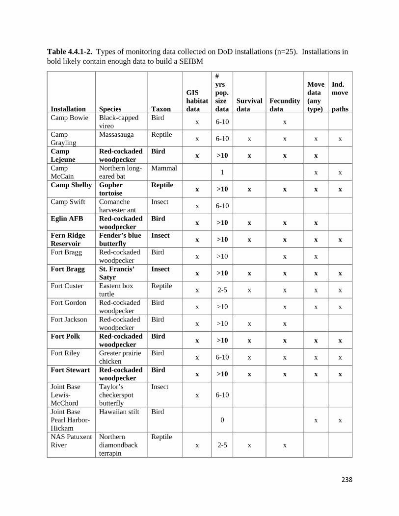
238
Table 4.4.1-2. Types of monitoring data collected on DoD installations (n=25). Installations in bold likely contain enough data to build a SEIBM
Installation Species Taxon
GIS habitat data
# yrs pop. size data
Survival data
Fecundity data
Move data (any type)
Ind. move paths
Camp Bowie Black-capped vireo
Bird x 6-10 x
Camp Grayling
Massasauga Reptile x 6-10 x x x x
Camp Lejeune
Red-cockaded woodpecker
Bird x >10 x x x
Camp McCain
Northern long-eared bat
Mammal 1 x x
Camp Shelby Gopher tortoise
Reptile x >10 x x x x
Camp Swift Comanche harvester ant
Insect x 6-10
Eglin AFB Red-cockaded woodpecker
Bird x >10 x x x
Fern Ridge Reservoir
Fender’s blue butterfly
Insect x >10 x x x x
Fort Bragg Red-cockaded woodpecker
Bird x >10 x x
Fort Bragg St. Francis’ Satyr
Insect x >10 x x x x
Fort Custer Eastern box turtle
Reptile x 2-5 x x x x
Fort Gordon Red-cockaded woodpecker
Bird x >10 x x x
Fort Jackson Red-cockaded woodpecker
Bird x >10 x x
Fort Polk Red-cockaded woodpecker
Bird x >10 x x x x
Fort Riley Greater prairie chicken
Bird x 6-10 x x x x
Fort Stewart Red-cockaded woodpecker
Bird x >10 x x x x
Joint Base Lewis-McChord
Taylor’s checkerspot butterfly
Insect x 6-10
Joint Base Pearl Harbor-Hickam
Hawaiian stilt Bird 0 x x
NAS Patuxent River
Northern diamondback terrapin
Reptile x 2-5 x x

239
Naval Base Guam
Green sea turtle
Reptile x 6-10 x x x
Naval Support Activity Monterey
Smith’s blue butterfly
Insect
2-5
Pueblo Chemical Depot
Mountain plover
Bird x >10
USAF Academy
Preble’s meadow jumping mouse
Mammal
x >10 x x x x
Vandenberg AFB
El Segundo blue butterfly
Insect x 6-10
Vandenberg AFB
Western snowy plover
Bird x >10 x x
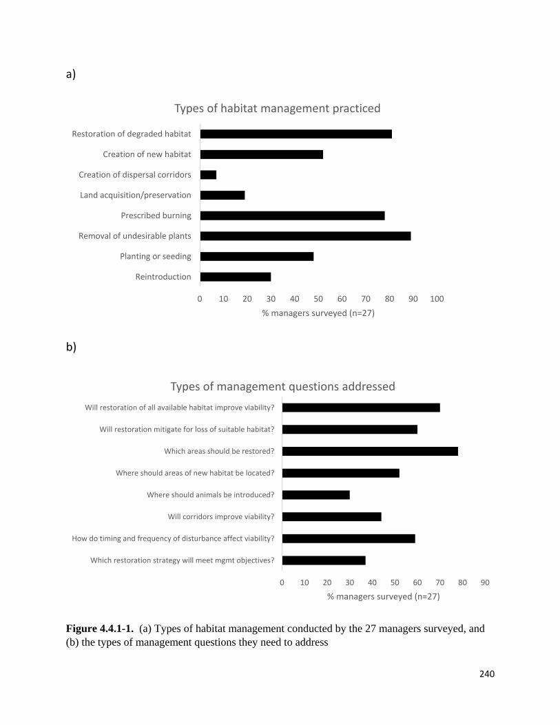
240
a)
b)
Figure 4.4.1-1. (a) Types of habitat management conducted by the 27 managers surveyed, and (b) the types of management questions they need to address
0 10 20 30 40 50 60 70 80 90 100
Reintroduction
Planting or seeding
Removal of undesirable plants
Prescribed burning
Land acquisition/preservation
Creation of dispersal corridors
Creation of new habitat
Restoration of degraded habitat
% managers surveyed (n=27)
Types of habitat management practiced
0 10 20 30 40 50 60 70 80 90
Which restoration strategy will meet mgmt objectives?
How do timing and frequency of disturbance affect viability?
Will corridors improve viability?
Where should animals be introduced?
Where should areas of new habitat be located?
Which areas should be restored?
Will restoration mitigate for loss of suitable habitat?
Will restoration of all available habitat improve viability?
% managers surveyed (n=27)
Types of management questions addressed
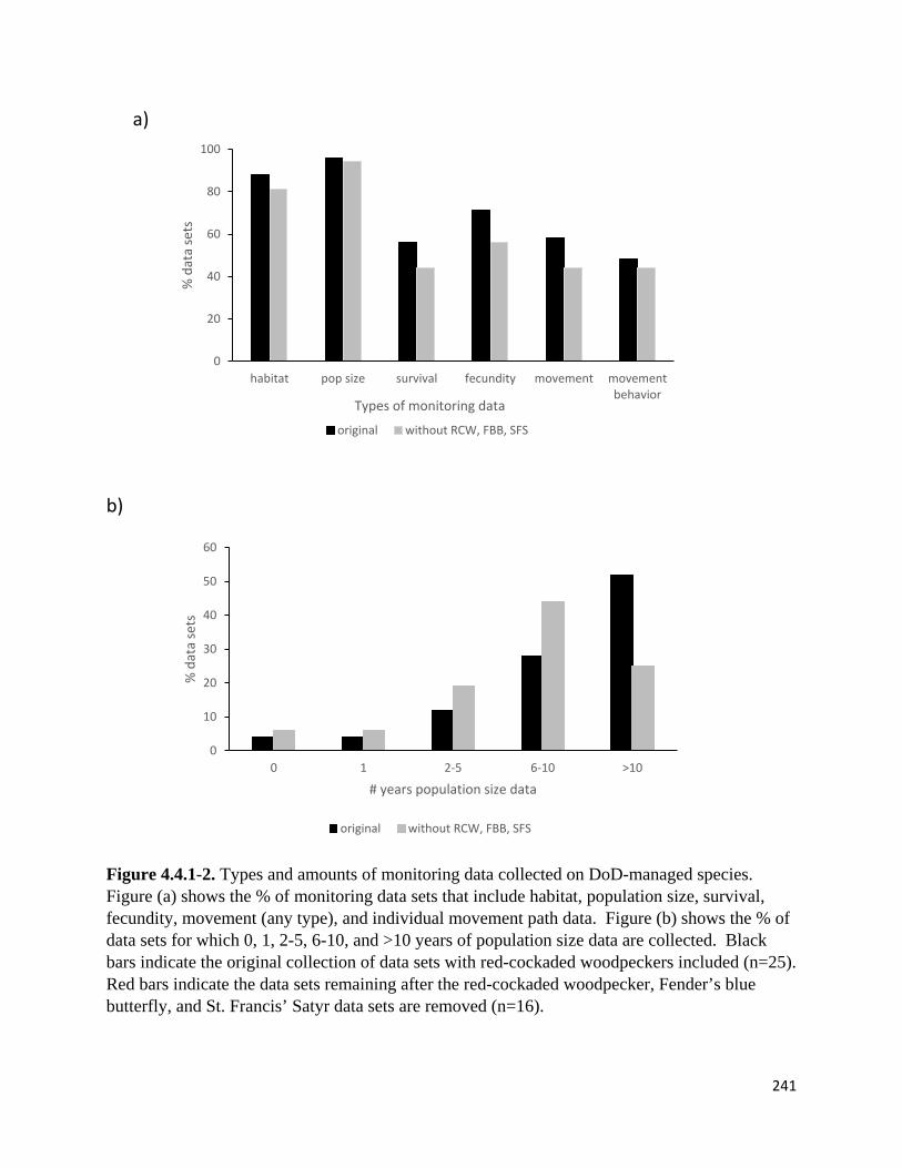
241
a)
b)
Figure 4.4.1-2. Types and amounts of monitoring data collected on DoD-managed species. Figure (a) shows the % of monitoring data sets that include habitat, population size, survival, fecundity, movement (any type), and individual movement path data. Figure (b) shows the % of data sets for which 0, 1, 2-5, 6-10, and >10 years of population size data are collected. Black bars indicate the original collection of data sets with red-cockaded woodpeckers included (n=25). Red bars indicate the data sets remaining after the red-cockaded woodpecker, Fender’s blue butterfly, and St. Francis’ Satyr data sets are removed (n=16).
0
20
40
60
80
100
habitat pop size survival fecundity movement movementbehavior
% d
ata
sets
Types of monitoring data
original without RCW, FBB, SFS
0
10
20
30
40
50
60
0 1 2-5 6-10 >10
% d
ata
sets
# years population size data
original without RCW, FBB, SFS
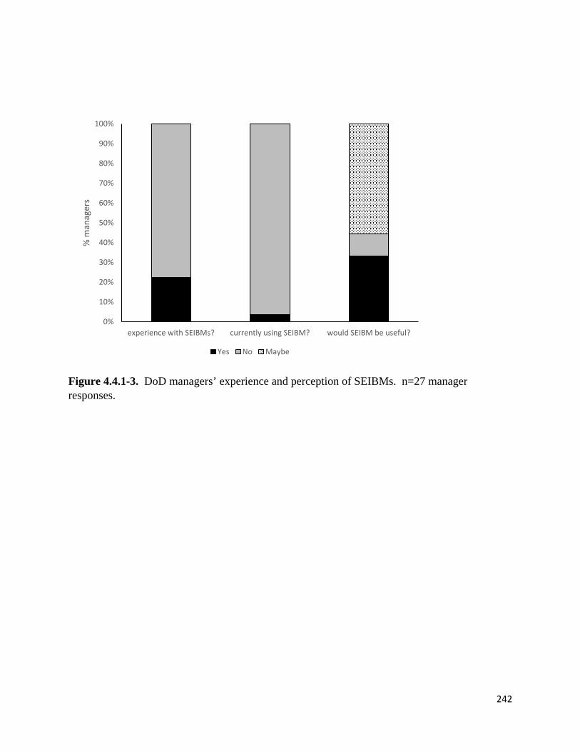
242
Figure 4.4.1-3. DoD managers’ experience and perception of SEIBMs. n=27 manager responses.
0%
10%
20%
30%
40%
50%
60%
70%
80%
90%
100%
experience with SEIBMs? currently using SEIBM? would SEIBM be useful?
% m
anag
ers
Yes No Maybe
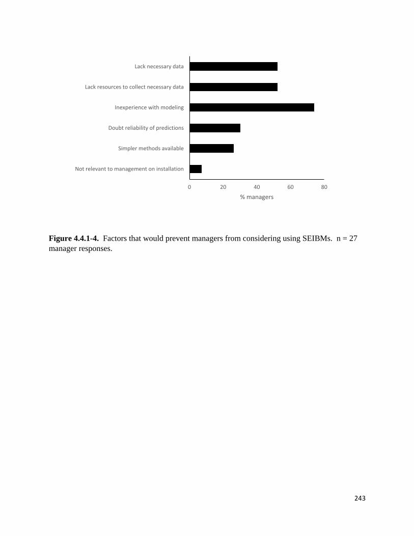
243
Figure 4.4.1-4. Factors that would prevent managers from considering using SEIBMs. n = 27 manager responses.
0 20 40 60 80
Not relevant to management on installation
Simpler methods available
Doubt reliability of predictions
Inexperience with modeling
Lack resources to collect necessary data
Lack necessary data
% managers
244
4.4.2 User guide to SEIBMs
Our review of the literature found that SEIBMs are best suited for addressing questions
for species with complex life histories in which dynamics may be driven by individual variation,
and viability depends on the synergy between demography, behavior, dispersal ability, and
landscape structure. Under these conditions, SEIBMs have outperformed simpler methods for
addressing habitat management questions. Thus, they have been well suited for modeling small
populations that are disproportionately affected by variation in individual behavior or
demography, and social species whose population dynamics are driven by dispersal or carrying
capacity rather than solely by vital rates. Although SEIBMs are generally not reliable enough to
predict the exact outcomes of management (i.e., the population will reach x individuals if plan A
is implemented), they have proven robust enough for comparative analysis (i.e., the population is
more likely to reach x individuals if plan A is implemented vs. no restoration). This makes
SEIBMs a scientifically defensible method for ranking proposed management alternatives.
Of the 9 working SEIBMs we reviewed, all had data on variables such as vegetation,
stand age, canopy cover, topography, soils, or hydrology to produce GIS maps of the study area
that explicitly describe spatial distribution of habitat (Table 4.4.2-1). Five had at least 10 years
of population count data that could be used to either validate models or estimate unknown
parameters. Six were parameterized with empirical survival data from the species of interest,
mostly obtained from capture-recapture studies or monitoring of marked or radio-tagged
individuals (Table 4.4.2-2). All of these survival data sets were age- or stage-specific, and 2
were habitat-specific. The amount of survival data varied widely, with sample sizes ranging
from 87 to over 5000 individuals, and number of years of data ranging from 1 to 24 years. Of
the 3 remaining SEIBMs, 2 (Bachman’s sparrow, St. Francis’ satyr) estimated survival using

245
other methods (see Table 4.4.2-2). For the third SEIBM (wood stork), mortality was imposed
not by a predetermined survival rate but by whether an indvidual’s energy reserves fell below a
minimum threshold. Thus, this model did not require survival data per se. All SEIBMs were
parameterized with empirical fecundity data, mostly gathered from observing nests or monitoring
reproductive activities of marked individuals (Table 4.4.2-3). Only 2 fecundity data sets were
age- or stage-specific, and only 2 were habitat-specific. Studies ranged from 1 to 24 years, and
sample sizes ranged from 24 nests to 11,450 individuals.
Seven of the 9 SEIBMs based their movement simulations on at least some field-
collected data from the species of interest (Table 4.4.2-4). Four movement data sets (Cape Sable
seaside sparrow, gray wolf, northern spotted owl, red-cockaded woodpecker) were obtained by
tracking radio-marked individuals or recording locations of marked individuals. These types of
studies ranged from less than 1 year with 31 individuals to 15 years and over 1000 individuals,
and provided information on dispersal distances and probability of dispersal. Only one of these 4
studies (northern spotted owl) collected data on dispersal direction. Movement data for the 2
butterfly SEIBMs were collected by recording movement paths of individuals released in
different habitats. These single year studies had samples of 42-606 individuals, and yielded fine
scale data on habitat-specific move lengths and turn angles. For the Saint Francis’ satyr model,
probabilities of crossing habitat boundaries were parameterized with habitat-specific data from
the Saint Francis’ satyr and a surrogate species, the Appalachian brown butterfly. Resting times
and habitat-specific move lengths and turn angles were estimated solely from individual flight
paths of the surrogate species. Only 2 SEIBMs included field-collected estimates of dispersal
mortality.
246
Of the 25 data sets collected by managers on DoD installations (see section 3.4.1), 10
contained data equivalent to those used to parameterize working SEIBMs (section 4.4.1. Table
4.4.1-2). In other words, the DoD data sets contained GIS habitat data; survival, fecundity, and
movement data; and at least 10 years of population size estimates. Six of these data sets were for
species (red-cockaded woodpecker, Fender’s blue butterfly, St. Francis’ satyr) whose habitats are
already being managed with input from SEIBMs. However, there appear to be sufficient data to
construct SEIBMs for four additional species: gopher tortoise (Gopherus polyphemus), Preble’s
meadow jumping mouse (Zapus hudsonius preblei), massasauga (Sistrurus catenatus), and
greater prairie chicken (Tympanuchus cupido).
Although only 10 installations appeared to have data equivalent to those used in working
SEIBMs, more installations likely have sufficient data to consider building an SEIBM. Most of
the data sets had sufficient habitat data to build maps. Although half of the data sets lacked data
to empirically estimate survival and fecundity, most had at least 5 years of population size data
to estimate these parameters using a process called “pattern-oriented modeling”, which looks for
the set of parameter values that are most likely to produce the observed trends in population size.
The greatest data limitation would be the paucity of information on how animals move across the
landscape. Although most of the working SEIBMs were parameterized with some empirical
movement data, less than half the managers surveyed collected this type of data, probably due to
differences in monitoring goals. Some analyses have suggested that uncertainty in dispersal
parameters, especially dispersal mortality, may translate to large errors in SEIBM predictions
(Wennergren et al. 1995, Ruckelshaus et al. 1997, but see Mooij and DeAngelis 1999, South
1999). Thus, managers wishing to build SEIBMs might focus more resources towards obtaining
accurate estimates of dispersal capability and movement characteristics.

247
Obviously, the most reliable model predictions will come from models that are based on
copious amounts of species-specific empirical data. However, managers who are interested in
building SEIBMs need not necessarily wait for complete data sets to consult with a modeler
about building models with the data they have. Data gaps can be filled using estimates from the
literature, surrogate species, or pattern-oriented modeling. Validation and sensitivity analyses
should be applied to evaluate reliability of model predictions and parameter estimates, and
identify studies that can be undertaken to reduce parameter uncertainty and improve model
performance. Initial predictions may not be accurate or robust enough to make credible
conservation decisions. However, each iteration of data collection, updating, and validating the
model yields new insights about the system and refines model predictions. Thus, when treated as
a component of a long term adaptive management program, SEIBMs can improve the
understanding of complex systems and be a useful tool in guiding habitat management decisions.
The user guide has been submitted to the DoD as part of this project. It will also be
disseminated to all of the DoD managers who participated in the survey described in section
3.4.1.
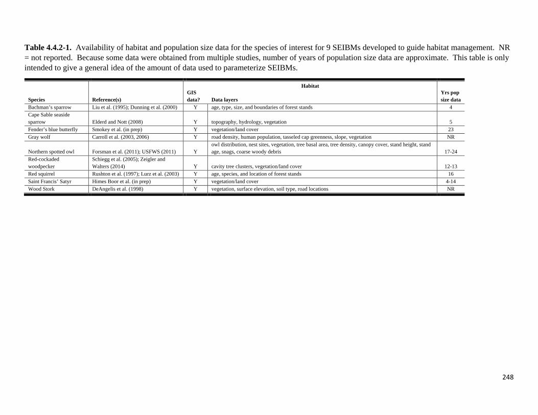
248
Table 4.4.2-1. Availability of habitat and population size data for the species of interest for 9 SEIBMs developed to guide habitat management. NR = not reported. Because some data were obtained from multiple studies, number of years of population size data are approximate. This table is only intended to give a general idea of the amount of data used to parameterize SEIBMs.
Species Reference(s)
Habitat Yrs pop size data
GIS data? Data layers
Bachman’s sparrow Liu et al. (1995); Dunning et al. (2000) Y age, type, size, and boundaries of forest stands 4 Cape Sable seaside sparrow Elderd and Nott (2008) Y topography, hydrology, vegetation 5 Fender’s blue butterfly Smokey et al. (in prep) Y vegetation/land cover 23 Gray wolf Carroll et al. (2003, 2006) Y road density, human population, tasseled cap greenness, slope, vegetation NR
Northern spotted owl Forsman et al. (2011); USFWS (2011) Y owl distribution, nest sites, vegetation, tree basal area, tree density, canopy cover, stand height, stand age, snags, coarse woody debris 17-24
Red-cockaded woodpecker
Schiegg et al. (2005); Zeigler and Walters (2014) Y cavity tree clusters, vegetation/land cover 12-13
Red squirrel Rushton et al. (1997); Lurz et al. (2003) Y age, species, and location of forest stands 16 Saint Francis’ Satyr Himes Boor et al. (in prep) Y vegetation/land cover 4-14 Wood Stork DeAngelis et al. (1998) Y vegetation, surface elevation, soil type, road locations NR
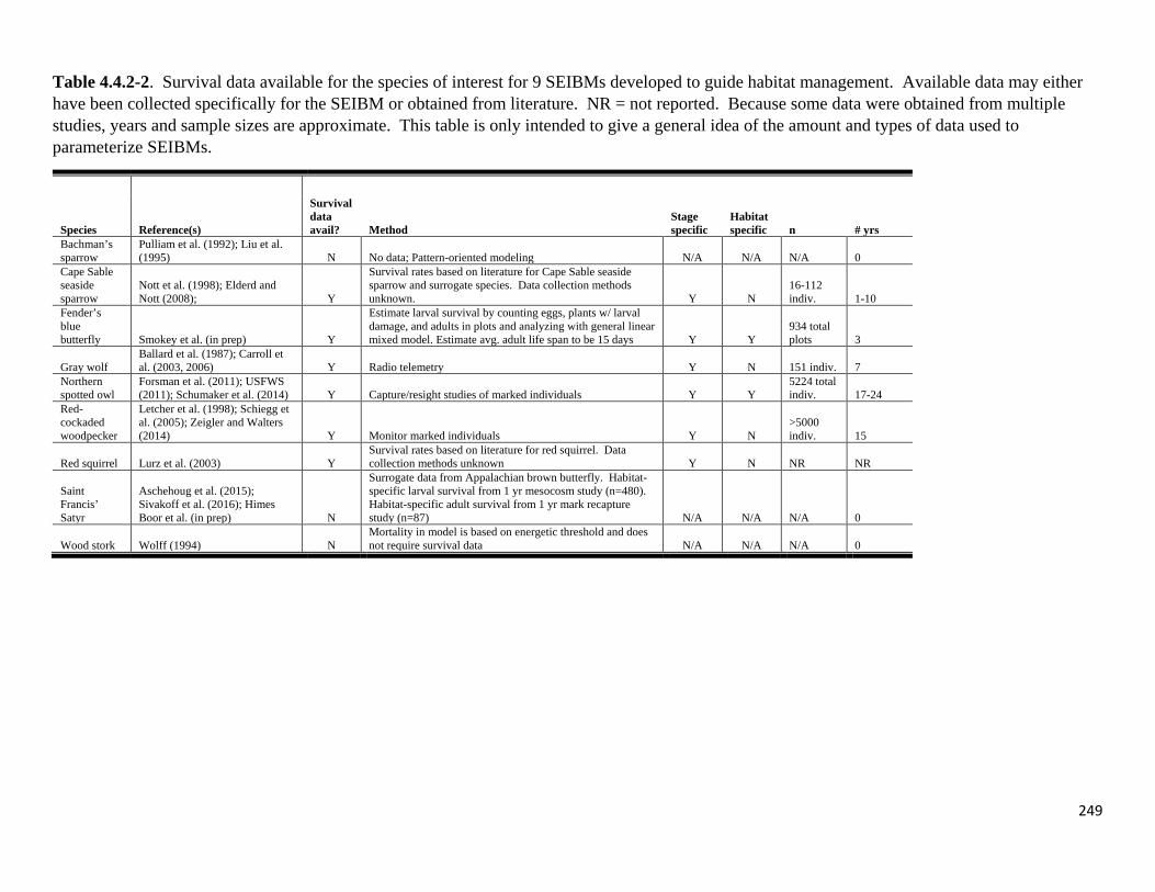
249
Table 4.4.2-2. Survival data available for the species of interest for 9 SEIBMs developed to guide habitat management. Available data may either have been collected specifically for the SEIBM or obtained from literature. NR = not reported. Because some data were obtained from multiple studies, years and sample sizes are approximate. This table is only intended to give a general idea of the amount and types of data used to parameterize SEIBMs.
Species Reference(s)
Survival data avail? Method
Stage specific
Habitat specific n # yrs
Bachman’s sparrow
Pulliam et al. (1992); Liu et al. (1995) N No data; Pattern-oriented modeling N/A N/A N/A 0
Cape Sable seaside sparrow
Nott et al. (1998); Elderd and Nott (2008); Y
Survival rates based on literature for Cape Sable seaside sparrow and surrogate species. Data collection methods unknown. Y N
16-112 indiv. 1-10
Fender’s blue butterfly Smokey et al. (in prep) Y
Estimate larval survival by counting eggs, plants w/ larval damage, and adults in plots and analyzing with general linear mixed model. Estimate avg. adult life span to be 15 days Y Y
934 total plots 3
Gray wolf Ballard et al. (1987); Carroll et al. (2003, 2006) Y Radio telemetry Y N 151 indiv. 7
Northern spotted owl
Forsman et al. (2011); USFWS (2011); Schumaker et al. (2014) Y Capture/resight studies of marked individuals Y Y
5224 total indiv. 17-24
Red-cockaded woodpecker
Letcher et al. (1998); Schiegg et al. (2005); Zeigler and Walters (2014) Y Monitor marked individuals Y N
>5000 indiv. 15
Red squirrel Lurz et al. (2003) Y Survival rates based on literature for red squirrel. Data collection methods unknown Y N NR NR
Saint Francis’ Satyr
Aschehoug et al. (2015); Sivakoff et al. (2016); Himes Boor et al. (in prep) N
Surrogate data from Appalachian brown butterfly. Habitat-specific larval survival from 1 yr mesocosm study (n=480). Habitat-specific adult survival from 1 yr mark recapture study (n=87) N/A N/A N/A 0
Wood stork Wolff (1994) N Mortality in model is based on energetic threshold and does not require survival data N/A N/A N/A 0
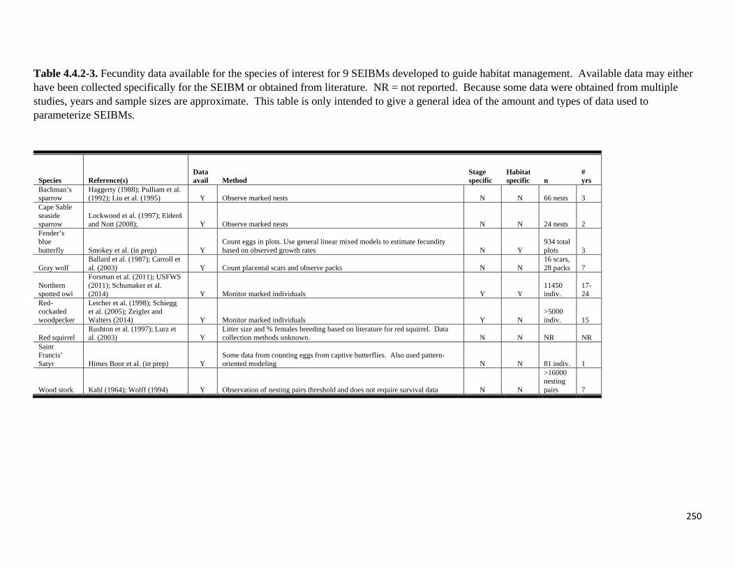
250
Table 4.4.2-3. Fecundity data available for the species of interest for 9 SEIBMs developed to guide habitat management. Available data may either have been collected specifically for the SEIBM or obtained from literature. NR = not reported. Because some data were obtained from multiple studies, years and sample sizes are approximate. This table is only intended to give a general idea of the amount and types of data used to parameterize SEIBMs.
Species Reference(s)
Data avail Method
Stage specific
Habitat specific n
# yrs
Bachman’s sparrow
Haggerty (1988); Pulliam et al. (1992); Liu et al. (1995) Y Observe marked nests N N 66 nests 3
Cape Sable seaside sparrow
Lockwood et al. (1997); Elderd and Nott (2008); Y Observe marked nests N N 24 nests 2
Fender’s blue butterfly Smokey et al. (in prep) Y
Count eggs in plots. Use general linear mixed models to estimate fecundity based on observed growth rates N Y
934 total plots 3
Gray wolf Ballard et al. (1987); Carroll et al. (2003) Y Count placental scars and observe packs N N
16 scars, 28 packs 7
Northern spotted owl
Forsman et al. (2011); USFWS (2011); Schumaker et al. (2014) Y Monitor marked individuals Y Y
11450 indiv.
17-24
Red-cockaded woodpecker
Letcher et al. (1998); Schiegg et al. (2005); Zeigler and Walters (2014) Y Monitor marked individuals Y N
>5000 indiv. 15
Red squirrel Rushton et al. (1997); Lurz et al. (2003) Y
Litter size and % females breeding based on literature for red squirrel. Data collection methods unknown. N N NR NR
Saint Francis’ Satyr Himes Boor et al. (in prep) Y
Some data from counting eggs from captive butterflies. Also used pattern-oriented modeling N N 81 indiv. 1
Wood stork Kahl (1964); Wolff (1994) Y Observation of nesting pairs threshold and does not require survival data N N
>16000 nesting pairs 7
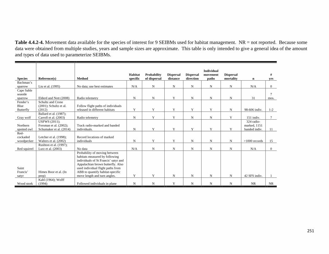
251
Table 4.4.2-4. Movement data available for the species of interest for 9 SEIBMs used for habitat management. NR = not reported. Because some data were obtained from multiple studies, years and sample sizes are approximate. This table is only intended to give a general idea of the amount and types of data used to parameterize SEIBMs.
Species Reference(s)
Method Habitat specific
Probability of dispersal
Dispersal distance
Dispersal direction
Individual movement
paths Dispersal mortality n
# yrs
Bachman’s sparrow Liu et al. (1995) No data; use best estimates N/A N N N N N N/A 0 Cape Sable seaside sparrow Elderd and Nott (2008) Radio telemetry N N Y N N N 31
7 mos.
Fender’s Blue Butterfly
Schultz and Crone (2001); Schultz et al. (2012)
Follow flight paths of individuals released in different habitats Y Y Y Y Y N 98-606 indiv. 1-2
Gray wolf Ballard et al. (1987); Carroll et al. (2003) Radio telemetry N Y Y N N Y 151 indiv. 7
Northern spotted owl
USFWS (2011); Forsman et al. (2002); Schumaker et al. (2014)
Track radio-marked and banded individuals. N Y Y Y Y Y
324 radio-marked, 1151 banded indiv. 11
Red-cockaded woodpecker
Letcher et al. (1998); Walters et al. (2002)
Record locations of marked individuals N Y Y N N N >1000 records 15
Red squirrel Rushton et al. (1997); Lurz et al. (2003) No data N/A N N N N N N/A 0
Saint Francis’ satyr
Himes Boor et al. (In prep)
Probability of moving between habitats measured by following individuals of St Francis’ satyr and Appalachian brown butterfly. Also used individual flight paths from ABB to quantify habitat-specific move length and turn angles. Y Y N N N N 42 SFS indiv. 1
Wood stork Kahl (1964); Wolff (1994) Followed individuals in plane N N Y N N N NR NR
252
4.4.3 Apply tools to additional case studies
4.4.3.1 Diffusion and Density
We observed a total of 2287 butterflies from 42 species, and recorded 1868 movement
paths in 19 sites. After excluding observations at a distance of 10 m from field margins, we
obtained a dataset of 1260 movement paths from 40 species. Diffusion rates were calculated for
the 25 species among these 40 that had at least 4 complete moves (i.e., included 5 move lengths,
5 move durations, and 4 turn angles) in at least one of the four land cover classes (Fig. 4.4.3.1-1).
Sufficient observations to calculate land cover class-specific diffusion rates were available for 22
species in semi-natural areas, 19 species in field margins, 14 species in olive groves and 7
species in wheat fields.
As predicted by general theory, diffusion was associated with density: butterfly densities
were higher in land cover types through which they moved more slowly (Table 4.4.3.1-1, Fig.
4.4.3.1-2). Neither body size nor the interaction of body size and diffusion were significant
predictors of density (fixed effects of wingspan and fixed effects of wingspan × diffusion, Table
4.4.3.1-1). When including land cover class in models, diffusion, wingspan and land cover class
were strong predictors of density (Table 4.4.3.1-2), and densities differed significantly among
land cover classes (Table 4.4.3.1-2, Fig. 4.4.3.1-2). Smaller butterfly species (≤ 30 mm,
Apharitis acamas, Freyeria trochylus, Pseudophilotes vicrama, Satyrium spini, Thymelicus
hyrax, Thymelicus sylvestris and Ypthima asterope) tended to occur with higher frequency (i.e.
high enough frequency to be included in our movement dataset, Fig. 4.4.3.1-1, Table 4.4.3.1-3)
only in field margins and semi-natural areas and most of the observed species × land cover class
combinations for these species had diffusion rates of < 3 m2/sec. Based on models including
diffusion, wingspan, and land cover class as predictors, expected densities were highest in the
253
field margins (median = 24.2 butterflies/ha, CI = 14.5 – 38.8), intermediate in semi-natural areas
(median = 10.3 butterflies/ha, CI = 6.5 – 16.3), and lowest in agricultural areas (wheat: median
= 2.8 butterflies/ha, CI = 0.9 – 7.5; olive groves: median = 1.7 butterflies/ha, CI = 0.7 – 3.2).
Move length, turning angle and expected net squared displacement were not significant
predictors of density (Table 4.4.3.1-1). Move time, however, was a significant predictor of
density with more time per step in areas with higher density (Table 4.4.3.1-1). Wingspan and the
interaction of wingspan with length, time, turning angle and expected net squared displacement
were all non-significant predictors of density (P > 0.10, Table 4.4.3.1-1). When land cover class
was included as a fixed effect, move time was not a predictor of density, most likely because
land cover class accounted for differences in move time and move times were shortest (least time
per step) in olive groves and longest in wheat fields.
Analysis of diffusion among species as a function of wingspan indicated that diffusion
was strongly associated with wingspan and that larger butterflies had higher diffusion rates (F
=21.23, P = 0.001). Analysis of density among species as a function of wingspan indicated that
wingspan is not strongly associated with density (F = 0.028, P = 0.869).
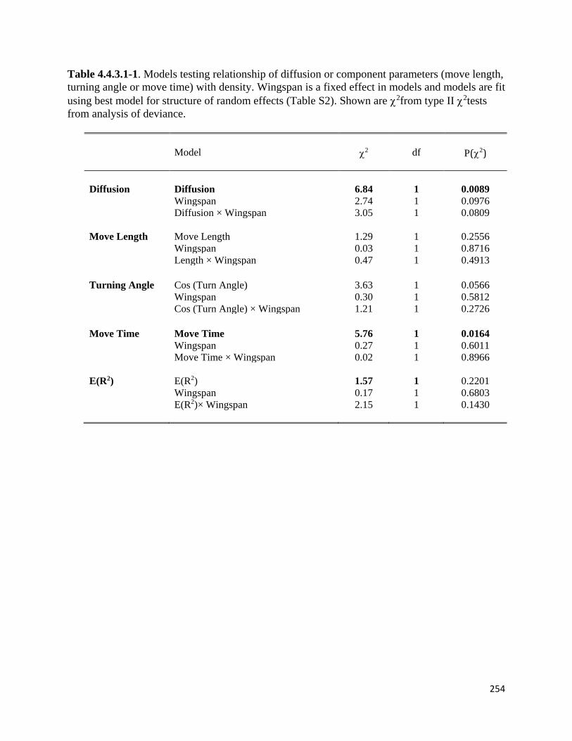
254
Table 4.4.3.1-1. Models testing relationship of diffusion or component parameters (move length, turning angle or move time) with density. Wingspan is a fixed effect in models and models are fit using best model for structure of random effects (Table S2). Shown are χ2from type II χ2tests from analysis of deviance.
Model χ2 df P(χ2) Diffusion Diffusion 6.84 1 0.0089 Wingspan 2.74 1 0.0976 Diffusion × Wingspan 3.05 1 0.0809 Move Length Move Length 1.29 1 0.2556 Wingspan 0.03 1 0.8716 Length × Wingspan 0.47 1 0.4913 Turning Angle Cos (Turn Angle) 3.63 1 0.0566 Wingspan 0.30 1 0.5812 Cos (Turn Angle) × Wingspan 1.21 1 0.2726 Move Time Move Time 5.76 1 0.0164 Wingspan 0.27 1 0.6011 Move Time × Wingspan 0.02 1 0.8966 E(R2) E(R2) 1.57 1 0.2201 Wingspan 0.17 1 0.6803 E(R2)× Wingspan 2.15 1 0.1430
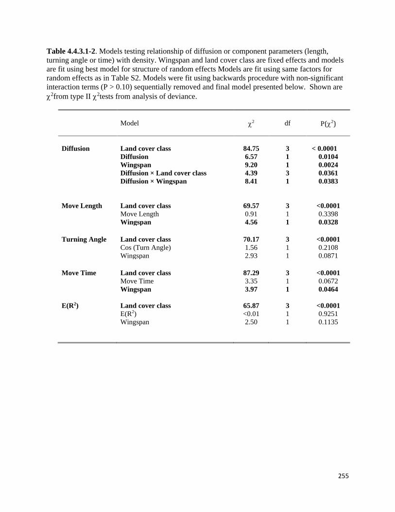
255
Table 4.4.3.1-2. Models testing relationship of diffusion or component parameters (length, turning angle or time) with density. Wingspan and land cover class are fixed effects and models are fit using best model for structure of random effects Models are fit using same factors for random effects as in Table S2. Models were fit using backwards procedure with non-significant interaction terms (P > 0.10) sequentially removed and final model presented below. Shown are χ2from type II χ2tests from analysis of deviance.
Model χ2 df P(χ2) Diffusion Land cover class 84.75 3 < 0.0001 Diffusion 6.57 1 0.0104 Wingspan 9.20 1 0.0024 Diffusion × Land cover class 4.39 3 0.0361 Diffusion × Wingspan 8.41 1 0.0383 Move Length Land cover class 69.57 3 <0.0001 Move Length 0.91 1 0.3398 Wingspan 4.56 1 0.0328 Turning Angle Land cover class 70.17 3 <0.0001 Cos (Turn Angle) 1.56 1 0.2108 Wingspan 2.93 1 0.0871 Move Time Land cover class 87.29 3 <0.0001 Move Time 3.35 1 0.0672 Wingspan 3.97 1 0.0464 E(R2) Land cover class 65.87 3 <0.0001 E(R2) <0.01 1 0.9251 Wingspan 2.50 1 0.1135
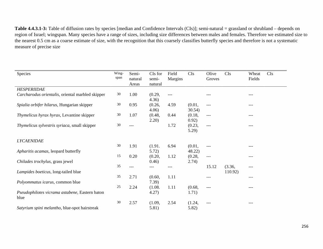
256
Table 4.4.3.1-3: Table of diffusion rates by species [median and Confidence Intervals (CIs)]; semi-natural = grassland or shrubland – depends on region of Israel; wingspan. Many species have a range of sizes, including size differences between males and females. Therefore we estimated size to the nearest 0.5 cm as a coarse estimate of size, with the recognition that this coarsely classifies butterfly species and therefore is not a systematic measure of precise size
Species Wing-
span Semi-natural Areas
CIs for semi-natural
Field Margins
CIs Olive Groves
CIs Wheat Fields
CIs
HESPERIIDAE Carcharodus orientalis, oriental marbled skipper 30 1.00 (0.29,
4.36) --- --- ---
Spialia orbifer hilarus, Hungarian skipper 30 0.95 (0.26, 4.06)
4.59 (0.01, 30.54)
--- ---
Thymelicus hyrax hyrax, Levantine skipper 30 1.07 (0.48, 2.20)
0.44 (0.18, 0.92)
--- ---
Thymelicus sylvestris syriaca, small skipper 30 --- 1.72 (0.23, 5.29)
--- ---
LYCAENIDAE
Apharitis acamas, leopard butterfly 30 1.91 (1.91.
5.72) 6.94 (0.01,
48.22) --- ---
Chilades trochylus, grass jewel 15 0.20 (0.20,
0.46) 1.12 (0.28,
2.74) --- ---
Lampides boeticus, long-tailed blue 35 --- --- --- 15.12 (3.36,
110.92) ---
Polyommatus icarus, common blue 35 2.71 (0.60,
7.39) 1.11 --- ---
Pseudophilotes vicrama astabene, Eastern baton blue
25 2.24 (1.08. 4.27)
1.11 (0.68, 1.71)
--- ---
Satyrium spini melantho, blue-spot hairstreak 30 2.57 (1.09,
5.81) 2.54 (1.24,
5.82) --- ---
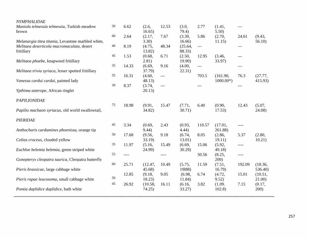
257
NYMPHALIDAE Maniola telmessia telmessia, Turkish meadow brown
50 6.62 (2.6, 16.65)
12.53 (3.0, 79.4)
2.77 (1.41, 5.50)
---
Melanargia titea titania, Levantine marbled white, 60 2.64 (2.17,
3.30) 7.67 (3.39,
16.66) 5.86 (2.70,
11.15) 24.61 (9.43,
56.10) Melitaea deserticola macromaculata, desert fritillary
40 8.19 (4.75, 13.82)
48.34 (25.64, 88.33)
--- ---
Melitaea phoebe, knapweed fritillary 45 1.53 (0.68,
2.81) 6.71 (2.50,
19.90) 12.95 (3.46,
33.97) ---
Melitaea trivia syriaca, lesser spotted fritillary 35 14.33 (6.69,
37.79) 9.16 (4.00,
22.31) --- ---
Vanessa cardui cardui, painted lady 55 16.31 (4.60,
48.13) --- 703.5 (161.90,
1000.00*) 76.3 (27.77,
415.93)
Ypthima asterope, African ringlet 30 8.37 (3.74,
20.13) --- --- ---
PAPILIONIDAE
Papilio machaon syriacus, old world swallowtail, 75 18.98 (9.91,
34.82) 15.47 (7.71,
30.71) 6.40 (0.90,
17.53) 12.43 (5.07,
24.08) PIERIDAE
Anthocharis cardamines phoenissa, orange tip 45 3.34 (0.69,
9.44) 2.43 (0.93,
4.44) 110.57 (17.01,
261.88) ----
Colias croceus, clouded yellow 50 17.68 (9.56,
33.19) 9.18 (6.74,
13.01) 8.05 (2.86,
19.11) 5.37 (2.80,
10.21)
Euchloe belemia belemia, green striped white 35 11.97 (5.16,
24.99) 15.49 (6.69,
30.29) 15.06 (5.92,
49.18) ----
Gonepteryx cleopatra taurica, Cleopatra butterfly 55 ---- ---- 50.56 (8.25,
200) ----
Pieris brassicae, large cabbage white 60 25.71 (12.47,
45.68) 10.49 (5.75,
19l88) 11.59 (7.51,
16.79) 192.09 (18.36,
536.40)
Pieris rapae leucosoma, small cabbage white
50 12.85 (9.18,
18.23) 9.05 (6.98,
11.84) 6.74 (4.72,
9.52) 15.01 (10.51,
21.00)
Pontia daplidice daplidice, bath white 45 26.92 (10.58,
74.25) 16.11 (6.16,
33.27) 3.82 (1.09.
102.8) 7.15 (0.17,
200)
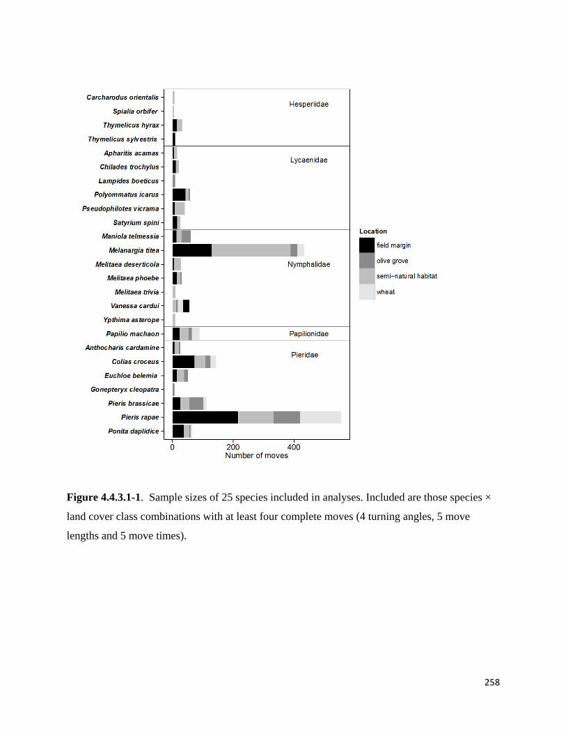
258
Figure 4.4.3.1-1. Sample sizes of 25 species included in analyses. Included are those species ×
land cover class combinations with at least four complete moves (4 turning angles, 5 move
lengths and 5 move times).
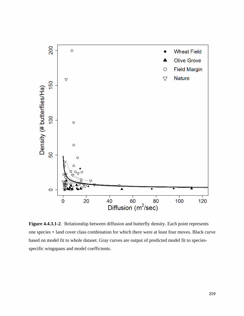
259
Figure 4.4.3.1-2. Relationship between diffusion and butterfly density. Each point represents
one species × land cover class combination for which there were at least four moves. Black curve
based on model fit to whole dataset. Gray curves are output of predicted model fit to species-
specific wingspans and model coefficients.
260
4.4.3.2 Edge behavior mini meta analysis
Overall, butterflies preferred habitat over matrix at patch edges. Edge preference differed
among edge types (c2 = 28.6, df = 2, P < 0.001, n = 18 species x edge type combinations).
Therefore, we analyzed preference separately for each edge type (Figure 4.4.3.2-1). In general,
butterflies had the strongest preference at structural open/forest patch edges (probability of
choosing matrix = 0.201, 95% CI 0.152, 0.264; logit-scale among species SD =0.239, 95% CI:
0.000 – 0.677; z = -8.7, P < 0.001 ). Butterflies showed weaker preference at host plant patch
edges (probability of choosing matrix = 0.307, 95% CI 0.187, 0.483; among species SD =0.426,
95% CI: 0.000 – 1.309 ; z = -2.9, P = 0.003). Butterflies showed the weakest preference at
boundaries of roads or other developed habitat types (probability of choosing matrix = 0.390,
95% CI 0.263, 0.519; among species SD =0.410, 95% CI: 0.099– 1.063 ; z = -1.9, P = 0.056).
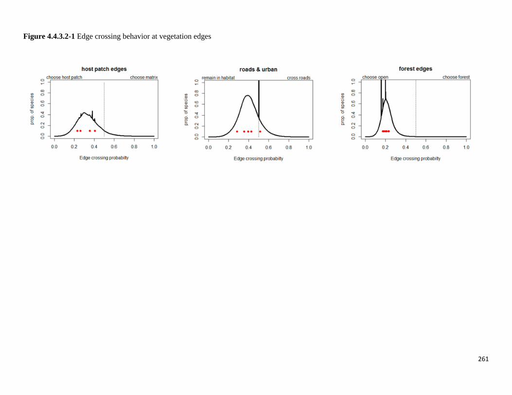
261
Figure 4.4.3.2-1 Edge crossing behavior at vegetation edges
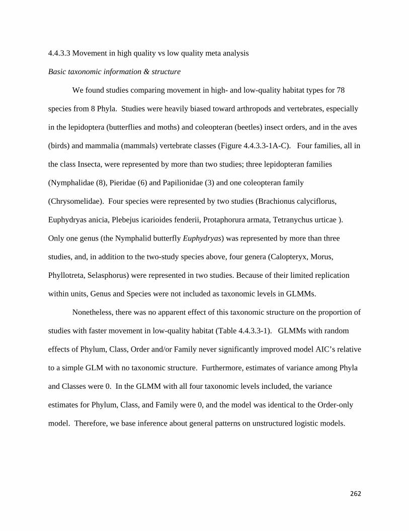
262
4.4.3.3 Movement in high quality vs low quality meta analysis
Basic taxonomic information & structure
We found studies comparing movement in high- and low-quality habitat types for 78
species from 8 Phyla. Studies were heavily biased toward arthropods and vertebrates, especially
in the lepidoptera (butterflies and moths) and coleopteran (beetles) insect orders, and in the aves
(birds) and mammalia (mammals) vertebrate classes (Figure 4.4.3.3-1A-C). Four families, all in
the class Insecta, were represented by more than two studies; three lepidopteran families
(Nymphalidae (8), Pieridae (6) and Papilionidae (3) and one coleopteran family
(Chrysomelidae). Four species were represented by two studies (Brachionus calyciflorus,
Euphydryas anicia, Plebejus icarioides fenderii, Protaphorura armata, Tetranychus urticae ).
Only one genus (the Nymphalid butterfly Euphydryas) was represented by more than three
studies, and, in addition to the two-study species above, four genera (Calopteryx, Morus,
Phyllotreta, Selasphorus) were represented in two studies. Because of their limited replication
within units, Genus and Species were not included as taxonomic levels in GLMMs.
Nonetheless, there was no apparent effect of this taxonomic structure on the proportion of
studies with faster movement in low-quality habitat (Table 4.4.3.3-1). GLMMs with random
effects of Phylum, Class, Order and/or Family never significantly improved model AIC’s relative
to a simple GLM with no taxonomic structure. Furthermore, estimates of variance among Phyla
and Classes were 0. In the GLMM with all four taxonomic levels included, the variance
estimates for Phylum, Class, and Family were 0, and the model was identical to the Order-only
model. Therefore, we base inference about general patterns on unstructured logistic models.
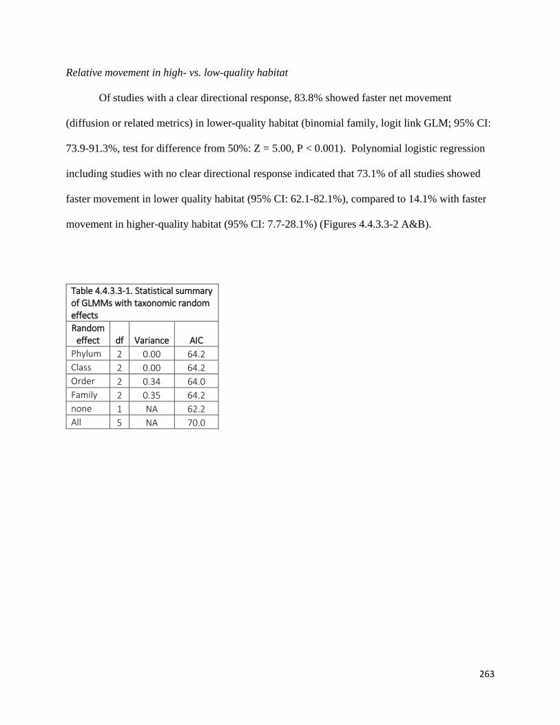
263
Relative movement in high- vs. low-quality habitat
Of studies with a clear directional response, 83.8% showed faster net movement
(diffusion or related metrics) in lower-quality habitat (binomial family, logit link GLM; 95% CI:
73.9-91.3%, test for difference from 50%: Z = 5.00, P < 0.001). Polynomial logistic regression
including studies with no clear directional response indicated that 73.1% of all studies showed
faster movement in lower quality habitat (95% CI: 62.1-82.1%), compared to 14.1% with faster
movement in higher-quality habitat (95% CI: 7.7-28.1%) (Figures 4.4.3.3-2 A&B).
Table 4.4.3.3-1. Statistical summary of GLMMs with taxonomic random effects Random
effect df Variance AIC Phylum 2 0.00 64.2 Class 2 0.00 64.2 Order 2 0.34 64.0 Family 2 0.35 64.2 none 1 NA 62.2 All 5 NA 70.0
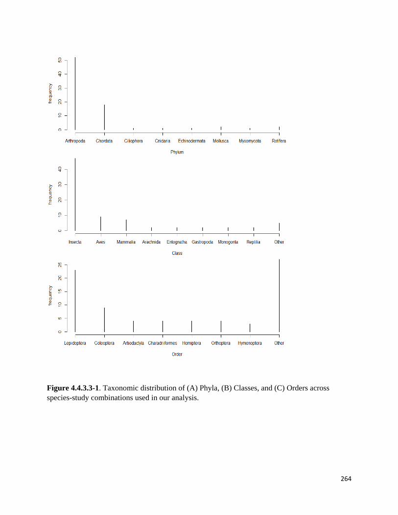
264
Figure 4.4.3.3-1. Taxonomic distribution of (A) Phyla, (B) Classes, and (C) Orders across species-study combinations used in our analysis.
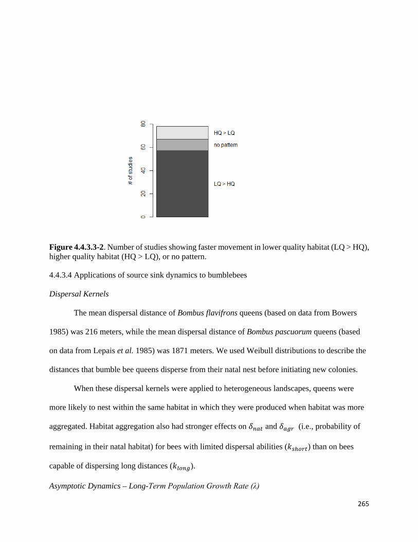
265
Figure 4.4.3.3-2. Number of studies showing faster movement in lower quality habitat (LQ > HQ), higher quality habitat (HQ > LQ), or no pattern. 4.4.3.4 Applications of source sink dynamics to bumblebees
Dispersal Kernels
The mean dispersal distance of Bombus flavifrons queens (based on data from Bowers
1985) was 216 meters, while the mean dispersal distance of Bombus pascuorum queens (based
on data from Lepais et al. 1985) was 1871 meters. We used Weibull distributions to describe the
distances that bumble bee queens disperse from their natal nest before initiating new colonies.
When these dispersal kernels were applied to heterogeneous landscapes, queens were
more likely to nest within the same habitat in which they were produced when habitat was more
aggregated. Habitat aggregation also had stronger effects on 𝛿𝛿𝑛𝑛𝑚𝑚𝑡𝑡 and 𝛿𝛿𝑚𝑚𝑔𝑔𝑟𝑟 (i.e., probability of
remaining in their natal habitat) for bees with limited dispersal abilities (𝑘𝑘𝑠𝑠ℎ𝑡𝑡𝑟𝑟𝑡𝑡) than on bees
capable of dispersing long distances (𝑘𝑘𝑙𝑙𝑡𝑡𝑛𝑛𝑔𝑔).
Asymptotic Dynamics – Long-Term Population Growth Rate (λ)
266
Population dynamics in heterogeneous landscapes followed the general expectations of
any density-independent matrix model. After the stable stage structure was attained, the entire
source-sink population, including sub-populations within each habitat type, grew or declined at
the same constant rate, λ. In other words, populations could not persist indefinitely in one habitat
while going extinct in another if dispersal was maintained between habitat types.
Loss of natural habitat (η) strongly reduced the long-term growth rate (λ) of the source-
sink population (Fig. 4.4.3.4-1; conditions resulting in positive population growth are shaded in
blue). However, the effect of habitat loss depended on the dispersal ability of bees (𝑘𝑘𝑠𝑠ℎ𝑡𝑡𝑟𝑟𝑡𝑡 vs.
𝑘𝑘𝑙𝑙𝑡𝑡𝑛𝑛𝑔𝑔) and the degree of habitat aggregation (α). Increased aggregation of habitat patches
increased λ when queens were only capable of short-distance dispersal from their natal colonies
(𝑘𝑘𝑠𝑠ℎ𝑡𝑡𝑟𝑟𝑡𝑡), but had modest effects when queens were capable of dispersing long distances (𝑘𝑘𝑙𝑙𝑡𝑡𝑛𝑛𝑔𝑔).
Consequently, when landscapes were highly aggregated, more natural habitat was required to
sustain long-distance dispersers than short-distance dispersers. When landscapes were highly
fragmented, a similar and large amount of natural habitat (35-40% of the landscape) was
required to sustain both short- and long-distance dispersers.
Asymptotic Dynamics – Long-Term Population Distribution
In our habitat-structured population models, the long-term stable population structure can
be represented as either relative abundance of colonies in each habitat type (as in conventional
stage-structured population models), or as relative density, calculated by dividing the relative
abundances in each habitat by the relative area of each habitat type. Here, we present the stable
population structure as relative densities, as this is likely to be the quantity measured in field
settings.

267
The long-term relative density of colonies in each habitat type depended on landscape
structure and dispersal ability of queens (Figure 4.4.3.4-2). The relative density of colonies in
natural habitat increased when landscapes contained more natural habitat. More aggregated
landscapes also led to higher relative densities of colonies in natural habitat, although the effect
of habitat aggregation was weak for long-distance dispersers (cf. Fig. 4.4.3.4-2 a&b).
The landscape conditions that led to long-term population stability (λ = 1; depicted by
solid white lines in Figure 4.4.3.4-2) differed from the conditions that caused relative densities to
be equal in each habitat (depicted by dotted white lines in Figure 4.4.3.4-2). At the threshold
where landscape conditions produced population stability, nest densities were higher in natural
habitat than agricultural habitat. However, under conditions that led to long-term population
declines (below the solid white line in Figure 4.4.3.4-2), natural habitats could either contain
higher or lower nest densities than agricultural habitats, demonstrating that habitat-specific
density monitoring can be a misleading indicator of habitat quality in source-sink systems.
Transient Dynamics – Rapid Loss of Natural Habitat
Transient dynamics were generated when a proportion of completely natural landscape
was abruptly converted to agricultural habitat, leading to 20% annual decline in abundance (λ =
0.8). These simulations assumed that land conversion initially destroyed bumble bee colonies
(see Methods), leading to an unstable (i.e., non-equilibrium) initial population structure.
Depending on bee dispersal ability and level of habitat aggregation, conversion of 82.5% to
92.5% of a natural landscape to agriculture was required to achieve λ = 0.8.
In all of these cases, the density of the total population initially increased (Fig. 4.4.3.4-3,
black lines) as population growth and dispersal from highly productive natural habitats caused
populations in agricultural habitats to initially increase (Fig. 4.4.3.4-3, orange dashed lines).
268
These transient dynamics dissipated quickly and populations converged on λ = 0.8 within 4-7
years (Fig. 4.4.3.4-3, black dots). Convergence on λ took longest for short-distance dispersers in
highly aggregated landscapes. However, transient dynamics experienced in the first several years
caused populations to remain larger in the long-term than if they had immediately and steadily
declined at λ = 0.8 from the beginning (Fig. 4.4.3.4-3, gray lines), and total population density
even remained above the initial density (i.e., immediately after the landscape change) for up to 4
years. Scenarios in which landscape change did not initially remove bees in converted patches
produced dynamics that more closely matched asymptotic dynamics because the population
structure was closer to the long-term stable distribution, though some transient dynamics
remained (D. Iles, unpubl. models).
Transient Dynamics – Rapid Restoration of Natural Habitat
Transient dynamics were also generated when a proportion of completely agricultural
landscape was abruptly restored to natural habitat, leading to 20% long-term annual increase in
abundance (λ = 1.2). These simulations also assumed that restoration removed bees from
restoration sites, so that the population started at a non-equilibrium spatial structure with no
colonies in the restored sites. To achieve λ = 1.2, conversion of 45-50% of an agricultural
landscape to natural habitat was required (Fig. 4.4.3.4-4).
In these cases, the density of the total population initially decreased, driven by rapid
population declines in agricultural habitats that occurred until a sufficient number of queens
dispersed into natural habitats to facilitate population growth (Fig. 4.4.3.4-4). These transient
dynamics also dissipated quickly and populations converged on λ = 1.2 within 4-6 years (Fig.
4.4.3.4-3, black dots). As with the simulations of rapid loss of natural habitat, convergence on λ
took longest for short-distance dispersers in highly aggregated landscapes. Yet, the transient
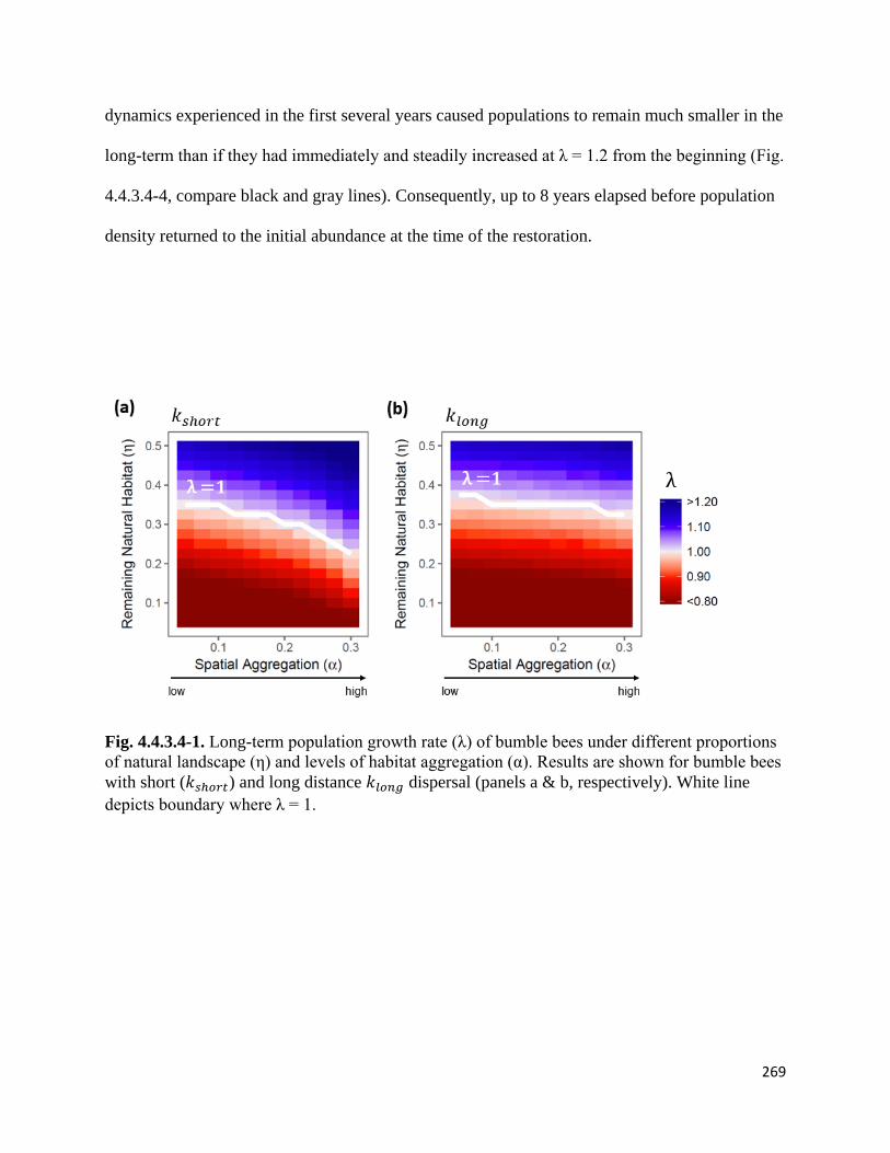
269
dynamics experienced in the first several years caused populations to remain much smaller in the
long-term than if they had immediately and steadily increased at λ = 1.2 from the beginning (Fig.
4.4.3.4-4, compare black and gray lines). Consequently, up to 8 years elapsed before population
density returned to the initial abundance at the time of the restoration.
Fig. 4.4.3.4-1. Long-term population growth rate (λ) of bumble bees under different proportions of natural landscape (η) and levels of habitat aggregation (α). Results are shown for bumble bees with short (𝑘𝑘𝑠𝑠ℎ𝑡𝑡𝑟𝑟𝑡𝑡) and long distance 𝑘𝑘𝑙𝑙𝑡𝑡𝑛𝑛𝑔𝑔 dispersal (panels a & b, respectively). White line depicts boundary where λ = 1.
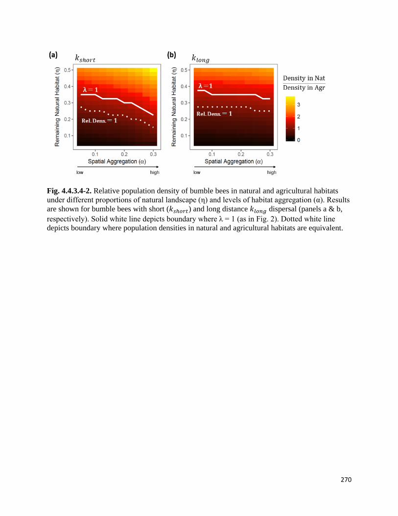
270
Fig. 4.4.3.4-2. Relative population density of bumble bees in natural and agricultural habitats under different proportions of natural landscape (η) and levels of habitat aggregation (α). Results are shown for bumble bees with short (𝑘𝑘𝑠𝑠ℎ𝑡𝑡𝑟𝑟𝑡𝑡) and long distance 𝑘𝑘𝑙𝑙𝑡𝑡𝑛𝑛𝑔𝑔 dispersal (panels a & b, respectively). Solid white line depicts boundary where λ = 1 (as in Fig. 2). Dotted white line depicts boundary where population densities in natural and agricultural habitats are equivalent.
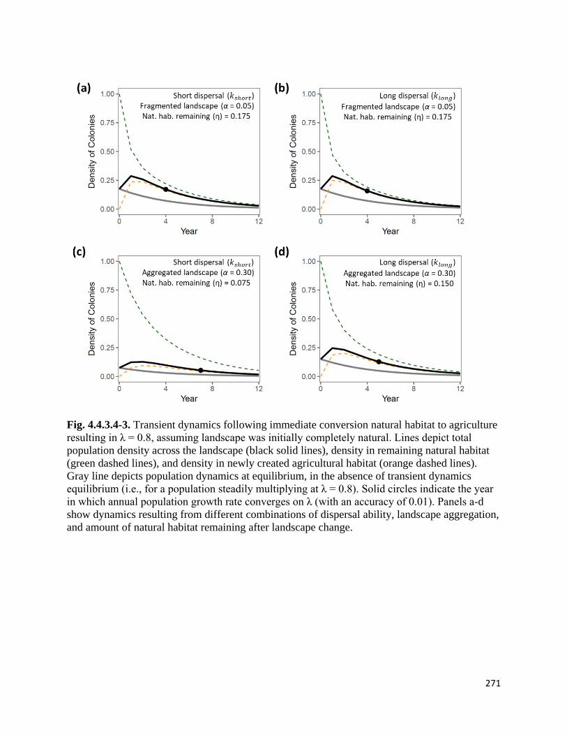
271
Fig. 4.4.3.4-3. Transient dynamics following immediate conversion natural habitat to agriculture resulting in λ = 0.8, assuming landscape was initially completely natural. Lines depict total population density across the landscape (black solid lines), density in remaining natural habitat (green dashed lines), and density in newly created agricultural habitat (orange dashed lines). Gray line depicts population dynamics at equilibrium, in the absence of transient dynamics equilibrium (i.e., for a population steadily multiplying at λ = 0.8). Solid circles indicate the year in which annual population growth rate converges on λ (with an accuracy of 0.01). Panels a-d show dynamics resulting from different combinations of dispersal ability, landscape aggregation, and amount of natural habitat remaining after landscape change.
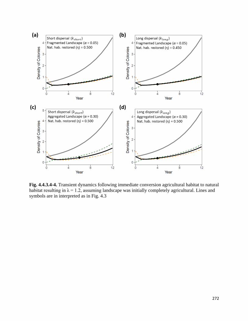
272
Fig. 4.4.3.4-4. Transient dynamics following immediate conversion agricultural habitat to natural habitat resulting in λ = 1.2, assuming landscape was initially completely agricultural. Lines and symbols are in interpreted as in Fig. 4.3
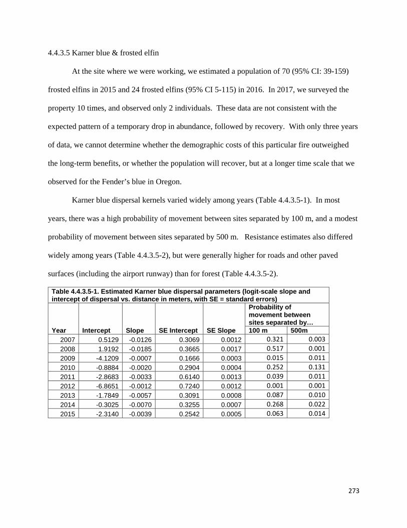
273
4.4.3.5 Karner blue & frosted elfin
At the site where we were working, we estimated a population of 70 (95% CI: 39-159)
frosted elfins in 2015 and 24 frosted elfins (95% CI 5-115) in 2016. In 2017, we surveyed the
property 10 times, and observed only 2 individuals. These data are not consistent with the
expected pattern of a temporary drop in abundance, followed by recovery. With only three years
of data, we cannot determine whether the demographic costs of this particular fire outweighed
the long-term benefits, or whether the population will recover, but at a longer time scale that we
observed for the Fender’s blue in Oregon.
Karner blue dispersal kernels varied widely among years (Table 4.4.3.5-1). In most
years, there was a high probability of movement between sites separated by 100 m, and a modest
probability of movement between sites separated by 500 m. Resistance estimates also differed
widely among years (Table 4.4.3.5-2), but were generally higher for roads and other paved
surfaces (including the airport runway) than for forest (Table 4.4.3.5-2).
Table 4.4.3.5-1. Estimated Karner blue dispersal parameters (logit-scale slope and intercept of dispersal vs. distance in meters, with SE = standard errors)
Year Intercept Slope SE Intercept SE Slope
Probability of movement between sites separated by… 100 m 500m
2007 0.5129 -0.0126 0.3069 0.0012 0.321 0.003 2008 1.9192 -0.0185 0.3665 0.0017 0.517 0.001 2009 -4.1209 -0.0007 0.1666 0.0003 0.015 0.011 2010 -0.8884 -0.0020 0.2904 0.0004 0.252 0.131 2011 -2.8683 -0.0033 0.6140 0.0013 0.039 0.011 2012 -6.8651 -0.0012 0.7240 0.0012 0.001 0.001 2013 -1.7849 -0.0057 0.3091 0.0008 0.087 0.010 2014 -0.3025 -0.0070 0.3255 0.0007 0.268 0.022 2015 -2.3140 -0.0039 0.2542 0.0005 0.063 0.014
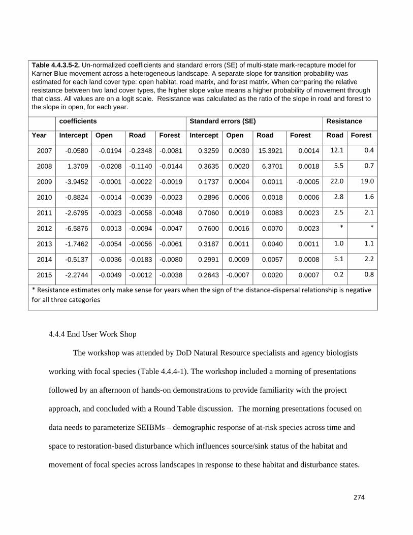
274
4.4.4 End User Work Shop
The workshop was attended by DoD Natural Resource specialists and agency biologists
working with focal species (Table 4.4.4-1). The workshop included a morning of presentations
followed by an afternoon of hands-on demonstrations to provide familiarity with the project
approach, and concluded with a Round Table discussion. The morning presentations focused on
data needs to parameterize SEIBMs – demographic response of at-risk species across time and
space to restoration-based disturbance which influences source/sink status of the habitat and
movement of focal species across landscapes in response to these habitat and disturbance states.
Table 4.4.3.5-2. Un-normalized coefficients and standard errors (SE) of multi-state mark-recapture model for Karner Blue movement across a heterogeneous landscape. A separate slope for transition probability was estimated for each land cover type: open habitat, road matrix, and forest matrix. When comparing the relative resistance between two land cover types, the higher slope value means a higher probability of movement through that class. All values are on a logit scale. Resistance was calculated as the ratio of the slope in road and forest to the slope in open, for each year.
coefficients Standard errors (SE) Resistance
Year Intercept Open Road Forest Intercept Open Road Forest Road Forest
2007 -0.0580 -0.0194 -0.2348 -0.0081 0.3259 0.0030 15.3921 0.0014 12.1 0.4
2008 1.3709 -0.0208 -0.1140 -0.0144 0.3635 0.0020 6.3701 0.0018 5.5 0.7
2009 -3.9452 -0.0001 -0.0022 -0.0019 0.1737 0.0004 0.0011 -0.0005 22.0 19.0
2010 -0.8824 -0.0014 -0.0039 -0.0023 0.2896 0.0006 0.0018 0.0006 2.8 1.6
2011 -2.6795 -0.0023 -0.0058 -0.0048 0.7060 0.0019 0.0083 0.0023 2.5 2.1
2012 -6.5876 0.0013 -0.0094 -0.0047 0.7600 0.0016 0.0070 0.0023 * *
2013 -1.7462 -0.0054 -0.0056 -0.0061 0.3187 0.0011 0.0040 0.0011 1.0 1.1
2014 -0.5137 -0.0036 -0.0183 -0.0080 0.2991 0.0009 0.0057 0.0008 5.1 2.2
2015 -2.2744 -0.0049 -0.0012 -0.0038 0.2643 -0.0007 0.0020 0.0007 0.2 0.8
* Resistance estimates only make sense for years when the sign of the distance-dispersal relationship is negative for all three categories

275
The afternoon demonstrations included an introduction to SEIMBs, focal efforts with Fender’s
blue and Taylor’s checkerspot, and a hands-one session with the St. Francis Satyr model.
The afternoon concluded with a round table discussion including the following questions and
discussions:
• Are the predictions of SEIBMs reliable?
• What are examples of models being used by managers that are acceptable to USFWS ?
• If you are still hesitant about these models, what can we address?
• How would they like to use models such as these SEIBMs?
• What would they like to know about the models?
• What would they like to know from these models/from our output? (We are NOT
expecting at the end of the day- that attendees be able to make one of these models from
scratch; rather to have a broad familiarity to think about when such an approach may be
valuable
• What data collection methods are feasible for at-risk species that each works with? What
are the alternatives?
• What is the value/use of SEIBMs vs either spatial models with less biology or stylized
models without the maps
• How else might SEIBMs be used? That is, under what other restoration or management
situations might SEIBMs be valuable?
• What is about this approach is surprising and/or counter-intuitive responses?
Finally, because the timing of the workshop co-occurred with the flight season of
Fender’s blue in Oregon and Taylor’s checkerspot in Washington. The workshop included site
visits to Washington sites that are part of JBLM’s ACUB program (Army Compatible Buffer

276
Use program - Scatter Creek Wildlife Area and Glacial Heritage preserve) and to DoD sites in
Oregon – US Army Corps of Engineers Fern Ridge Reservoir. Workshop participants left with a
broad knowledge of a novel approach to managing habitat to endangered species as well as
benefiting from the collaborative process of a small workshop designed to educate project
participants and to learn from their experiences about how to develop tools to enhance the
efficiency and effectiveness of managing DoD land for Threatened, Endangered and At-risk
species.

277
Table 4.4.4-1 Attendees at End-user workshop

278
5. General lessons and tools:
5.1 Modeling approaches & statistical tools:
Our set of case studies led to innovations in three categories of statistical and modeling
tools:
5.1.1 GLMMs and parameter estimation: We adapted generalized linear mixed models
(GLMMs) for use in estimating demographic and movement parameters for all our case studies.
The general technique (GLMMs) is not new to our work; however, until now, ecologists and
statisticians have tended to perceive GLMMs simply as a way to account properly for structured
data and obtain correct p-values. The innovation of our work is interpretation of the variance
terms as ecologically-important variation among individual animals, among species, among sites
and/or among years.
5.1.2. Analytically tractable source-sink models: One key aim of our project was to evaluate the
level of information needed to understand and predict source-sink status of habitat patches. In
the process of evaluating spatially explicit models (section 5.1.3, below), we also developed two
simpler methods of modeling spatial population dynamics. These are especially useful in
providing rules of thumb for management, in cases where the exact landscape context is
unknown, or may change through time.
5.1.2.1. Spatial matrix population models for source-sink environments: We adapted the
technique of spatial mega-matrix population models to describe source-sink dynamics in
spatially heterogeneous environments. These models provide a general first step to

279
understanding source-sink dynamics when exact landscape configurations are unknown. They
also allow users to evaluate spatial heterogeneity using familiar tools from nonspatial population
ecology.
5.1.2.2. Integrodifference equations for isolated patches and heterogeneous landscapes: Source
sink status of a habitat patch depends both on its size and on its quality. We developed a general
framework for estimating the critical minimum size at which a patch switches from source to
sink based on the balance between emigration and local reproduction. This simple model is an
example of an integrodifference equation, in that the continuous-time processes associated with
the mobile phase of the adult butterfly life cycle – movement, adult survival, and oviposition –
are separated from larval growth and hibernation, which are approximately spatially fixed and
occur over several months. We are continuing to develop this approach for application to
additional ecological situations.
5.1.3. Spatially explicit individual-based models (SEIBMS): We developed spatially explicit-
individual based models as tools to guide each management scenario. The basis of these models
is movement described by a correlated random walk with preference at patch boundaries,
combined with habitat-specific demographic parameters (stage-specific survival and fecundity).
These approaches differ from many existing frameworks (e.g., the HexSim platform) in that they
are more naturally related to the way in which movement is incorporated into analyticial
reaction-diffusion and integrodifference models, so the assumptions and outputs are more
similar. They are also more naturally suited to some species, including the insect taxa we have
studied here.
280
5.2 Cross-species patterns
At the most fundamental level, the general lesson that managers took from our work was
the importance of knowing vital rates – including movement – throughout species’ life cycles, in
order to assess the impacts of management. Though this may seem obvious in hindsight, there
were situations for each species in which different vital rates showed qualitatively different
responses to management (i.e., one vital rate would increase while the other decreased)
emphasizing the importance of measuring vital rates throughout the life cycle, in order to
determine the net effects of management actions.
In addition, our cross-species analyses confirmed assumptions of our underlying model.
Specifically, for animal species like butterflies, movement can be modeled as a correlated
random walk within habitat patches, with preference at patch boundaries. “Like butterflies”
refers specifically to not having a central foraging place or den, and not during strongly directed
migration. Furthermore, for animals in general, movement is faster in lower-quality habitat.
This latter result sets up an interesting tradeoff for landscape planners who want to promote
connectivity. Higher quality habitat (by definition) leads to higher population growth rates, but
lower quality habitat increases permeability, if animals need to track moving habitat windows.
The costs and benefits of including sink habitat in landscapes will depend on their effects on
movement speed, as well as vital rates and habitat selection. We plan to continue to explore this
result in the future.
Finally, all of our conclusions about the effects of habitat restoration were modified in
one way or another by biotic interactions at higher trophic levels. Restoration ecologists
typically adopt a bottom-up approach, and assume that, if suitable habitat for animals is created,
they will be able to persist there. Our three case studies included one in which the effects of
281
restoration depended on a mutualist-consumer, one in which the effects were moderated by the
increase in habitat quality for generalist predators, and one in which population dynamics appear
to be driven strongly by intra-specific competition and population cycles (boom-bust dynamics
even in optimal environments). These effects are implicitly included in field-measured vital
rates, but the mechanisms help us evaluate the consequences of specific restoration practices, and
how they may play out in novel circumstances.
References : Amano, T., K. Ushiyama, G. Fujita; and H. Higuchi. 2007. Predicting grazing damage by white-fronted
geese under different regimes of agricultural management and the physiological consequences for the geese. Journal of Applied Ecology 44(3):506-515.
Aschehoug, E.T., F.S. Sivakoff, H.L. Cayton, W.F. Morris, and N.M. Haddad. 2015. Habitat restoration affects immature stages of a wetland butterfly through indirect effects on predation. Ecology 96:1761-1767.
Balbach, H., M. Perez-Martinez, and E. Keane. 2010. The Army Priority List of A-Risk Species. US Army Corps of Engineers report ERDC/CERL TR-10-21. 40 pp.
Ballard, W.B., J.S. Whitman, and C.L. Gardner. 1987. Ecology of an exploited wolf population in south- central Alaska. Wildlife Monographs 98:3-54.
Banks S.C., Dujardin M., McBurney L. et al. 2011. Starting points for small mammal population recovery after wildfire: recolonization or residual populations? Oikos 120:26-37
Barclay, E., M. Arnold, M. J. Anderson, and D. Shepherdson. 2009. Husbandry manual: Taylor's checkerspot (Euphydryas editha taylori). Oregon Zoo, Portland, OR.
Barton, K. A., B. L. Phillips, J. M. Morales, and J. M. J. Travis. 2009. The evolution of an 'intelligent' dispersal strategy: biased, correlated random walks in patchy landscapes. Oikos 118:309-319.
Bates D, M Maechler, S Walker. 2015. lme4: Linear mixed-effects models using Eigen and S4. R package version 1.1-9: https://CRAN.R-project.org/package=lme4
Bates, D., M. Maechler, B. Bolker, and S. Walker. 2013. lme4: linear mixed-effects models using Eigen and S4. R package version 1.0-4. http://CRAN.R-project.org/package=lme4
Bates, D., M. Maechler, B. Bolker, and S. Walker. 2015. Fitting linear mixed-effects models using lme4. Journal of Statistical Software 67:1-48.
Battin, J. 2004. When good animals love bad habitats: Ecological traps and the conservation of animal populations. Conservation Biology 18:1482-1491.
282
Bennett, V. J., S. M. Pack, W. P. Smith, and M. G. Betts. 2013. Sex-biased dispersal in a rare butterfly and the implications for its conservation. Journal of Insect Conservation 17:949-958.
Boggs, C. L., W. B. Watt, and P. R. Ehrlich. 2003. Butterflies: Ecology And Evolution Taking Flight. University of Chicago Press, Chicago.
Bolnick, D. I., P. Amarasekare, M. S. Araujo, R. Burger, J. M. Levine, M. Novak, V. H. W. Rudolf, S. J. Schreiber, M. C. Urban, and D. A. Vasseur. 2011. Why intraspecific trait variation matters in community ecology. Trends in Ecology & Evolution 26:183-192.
Boughton, D. A. 1999. Empirical evidence for complex source–sink dynamics with alternative states in a butterfly metapopulation. Ecology 80:2727–2739.
Boughton, D. A. 2000. The dispersal system of a butterfly: a test of source-sink theory suggests the intermediate-scale hypothesis. American Naturalist 156:131–144.
Bowers MD, NE Stamp, SK Collinge. 1992. Early stage of host range explansion by a specialist herbivore, Euphydryas phaeton (Nymphalidae). Ecology 73: 526-536
Bowers MD, NE Stamp. 1992. Chemical variation within and between individuals of Plantago lanceolata (Plantaginaceae). Journal of Chemical Ecology 18: 985-995
Bowers MD. 1983. The role of iridoid glycosides in host-plant specificity of checkerspot butterflies. Journal of Chemical Ecology 9: 475-493
Bowers MD. 1991. Iridoid glycosides. In GA Rosenthal and MR Berenbaum (eds), Herbivores: Their interactions with secondary plant metabolites. Academic Press, San Diego. pp 297-326
Bowers, M. D., and J. Schmitt. 2013. Overcrowding leads to lethal oviposition mistakes in the Baltimore checkerspot, Euphydryas phaeton Drury (Nymphalidae). Journal of the Lepidopterists' Society 67:227-229.
Bowers, M. D., N. E. Stamp, and S. K. Collinge. 1992. Early stage of host range expansion by a specialist herbivore, Euphydryas Phaeton (Nymphalidae). Ecology 73:526-536.
Bowers, M.A. 1985. Bumble bee colonization, extinction, and reproduction in subalpine meadows in northeastern Utah. Ecology, 66, 914-927.
Breed, G. A., S. Stichter, and E. E. Crone. 2013. Climate-driven changes in northeastern US butterfly communities. Nature Climate Change 3:142-145.
Breuer, L. (ed.). 2016. Conservation Directory. 2017. The Guide to Worldwide Environmental Organizations. Carrel Books. New York, NY. 624 pp.
Brouwers, N. C., and A. C. Newton. 2010. Movement analyses of wood cricket (Nemobius sylvestris) (Orthoptera: Gryllidae). Bulletin of Entomological Research 100:623-634.
Brown L, EE Crone. 2016. Minimum area requirements for an at-risk butterfly based on movement and demography. Conserv. Biol. 30: 103-112
Brown, L. M., and E. E. Crone. 2016. Individual variation changes dispersal distance and area requirements of a checkerspot butterfly. Ecology 97:106-115.
283
Brown, L. M., and E. E. Crone. 2016a. Individual variation changes dispersal distance and area requirements of a checkerspot butterfly. Ecology 97:106-115.
Brown, L. M., G. A. Breed, P. M. Severns, and E. E. Crone. 2017. Losing a battle but winning the war: moving past preference-performance to understand native herbivore-novel host plant interactions. Oecologia 183:441-453.
Brown, L. M., R. K. Fuda, N. Schtickzelle, H. Coffman, A. Jost, A. Kazberouk, E. Kemper, E. Sass, and E. E. Crone. in review. Animal movement in heterogeneous landscapes: using movement behavior to categorize land cover and predict consequences for connectivity and residence times. Landscape Ecology.
Brown, L. M., R. K. Fude, N. Schtickzelle, H. Coffman, A. Jost, A. Kazberouk, E. Kemper, E. Sass, and E. E. Crone. 2017b. Using animal movement behavior to categorize land cover and predict consequences for patch residence times. 32: 1657-1670.
Carleton, A., and C. B. Schultz. 2013. Restoration action and species response: oviposition habits of Plebejus icarioides fenderi (Lepidoptera: Lycaenidae) across a restoration chronosequence in the Willamette Valley, Oregon, USA. Journal of Insect Conservation 17:511-520.
Carroll, C., M.K. Phillips, C.A. Lopez-Gonzalez, and N.H. Schumaker. 2006. Defining recovery goals and strategies for endangered species: the wolf as a case study. Bioscience 56(1):25-37.
Carroll, C., M.K. Phillips, N.H. Schumaker, and D.W. Smith. 2003. Impacts of landscape change on wolf restoration success: planning a reintroduction program based on static and dynamic spatial models. Conservation Biology 17(2):536-548.
Caswell, H. 1989. Analysis of life table response experiments I. Decomposition of effects on population growth rate. Ecological Modeling, 46, 221-237.
Caswell, H. 2000. Prospective and retrospective perturbation analyses: Their roles in conservation biology. Ecology, 81, 619-627.
Caswell, H. 2001) Matrix population models: construction, analysis and interpretation, 2 edn. Sinauer Associates Inc., Sunderland, Massechusetts.
Caswell, H. 2001. Matrix population models. Wiley Online Library.
Cayton, H., N. Haddad, B. Ball, E. Henry, and E. Aschehoug. 2015. Habitat Restoration as a Recovery Tool for a Disturbance-Dependent Butterfly, The Endangered St. Francis' Satyr. Pages 147-159 in J. C. Daniels, editor. Butterfly Conservation in North America. Springer Netherlands.
Collier, N., Mackay, D.A. & Benkendorff, K. 2008. Is relative abundance a good indicator of population size? Evidence from fragmented populations of a specialist butterfly (Lepidoptera: Lycaenidae). Population Ecology, 50, 17-23.
Conlisk, E., S. Motheral, R. Chung, C. Wisinski, and B. Endress. 2014. Using spatially-explicit population models to evaluate habitat restoration plans for the San Diego cactus wren (Campylorhynchus brunneicapillus sandiegensis). Biological Conservation 175:42-51.
Cosner, C. 2008. Reaction-diffusion equations and ecological modeling. Pages 77-115 in A. Friedman, editor. Tutorials in Mathematical Biosciences IV. Springer-Verlag, Berlin.
284
Costa JT, KG Ross. 2003. Fitness effects of group merging in a social insect. Proc. R. Soc. B-Biol. Sci. 270: 1697-1702
Cranmer, L., D. McCollin, and J. Ollerton. 2012. Landscape structure influences pollinator movements and directly affects plant reproductive success. Oikos 121:562-568.
Crone, E. E. 2013. Responses of Social and Solitary Bees to Pulsed Floral Resources. American Naturalist 182:465-473.
Crone, E. E., and C. B. Schultz. 2003. Movement behavior and minimum patch size for butterfly population persistence. Pages 561-576 Butterflies as model systems: ecology and evolution taking flight. University of Chicago Press, Chicago.
Crone, E. E., D. Doak, and J. Pokki. 2001. Ecological influences on the dynamics of a field vole metapopulation. Ecology 82:831-843.
Crone, E.E. & Williams, N.M. 2016. Bumble bee colony dynamics: quantifying the importance of land use and floral resources for colony growth and queen production. Ecology Letters, 19, 460-468.
Crone, E.E. 2016. Contrasting effects of spatial heterogeneity and environmental stochasticity on population dynamics of a perennial wildflower. Journal of Ecology, 104, 281-291.
Crowder, L.B., J.A. Priddy, and J.R. Walters. 1998. Demographic isolation of red-cockaded woodpecker groups: a model analysis. USFWS Project Final Report. Duke University Marine Laboratory, Beaufort, NC. And Virginia Polytechnic Institute and State University. Blacksburg VA.
DeAngelis, D.L., L.J. Gross, M.A. Huston, W.F. Wolff, D.M. Fleming, E.J. Comiskey, and S.M. Sylvester. 1998. Landscape modeling for Everglades ecosystem restoration. Ecosystems 1:64-75.
Dias, P. C. 1998. Sources and sinks in population biology. Trends in Ecology and Evolution 11:326-330.
Dickinson, J. L., and R. L. Rutowski. 1989. The function of the mating plug in the chalcedon checkerspot butterfly. Animal Behaviour 38:154-162.
Donovan, T. M. and F. R. Thompson. 2001. Modeling the ecological trap hypothesis: A habitat and demographic analysis for migrant songbirds. Ecological Applications 11:871-882.
Dover, J., and T. Sparks. 2000. A review of the ecology of butterflies in British hedgerows. Journal of Environmental Management 60:51-63.
Dunning, J.B. Jr., B. Danielson, B. Noon, T.L. Root, R.H. Lamberson, and E.E. Stevens. 1995. Spatially explicit population models: current forms and future uses. Ecological Applications 5(1):3-11.
Dunwiddie, P. W., N. L. Haan, M. Linders, J. D. Bakker, C. Fimbel, and T. B. Thomas. 2016. Intertwined fates: opportunities and challenges in the linked recovery of two rare species. Natural Areas Journal 36:207-215.
Ehrlich, P. R., and I. Hanski, editors. 2004. On the wings of checkerspots: a model system for population biology. Oxford University Press, New York.
Elderd, B.D. and M.P. Nott. 2008. Hydrology, habitat change and population demography: an individual- based model for the endangered Cape Sable seaside sparrow Ammodramus maritimus mirabilis.
285
Elston, D.A., Moss, R., Boulinier, R., Arrowsmith, C., and Lambin, X. 2001. Analysis of aggregation, a worked example: numbers of ticks on red grouse chicks. Parasitology, 122,563-569.
ESRI. 2015. ArcMap 10.3. Environmental Systems Resource Institute, Redlands, California, USA.
Fahrig, L. 2007. Estimating minimum habitat for population persistence. Pages 64-80 in D. B. Lindenmayer and R. J. Hobbs, editors. Managing and Designing Landscapes for Conservation: Moving from Perspectives to Principles. Blackwell Publishing, Ltd, Malden, MA.
Fiske, I. J., and R. B. Chandler. 2011. Unmarked: an R package for fitting hierarchical models of wildlife occurrence and abundance. Journal of Statistical Software 43: 1-23.
Fitzpatrick G.S. 2015. 2015 Status of the Fender's Blue butterfly (Icaricia icarioides fenderi) in the Willamette Valley, Oregon. Report to Oregon Natural Heritage Program and United States Fish and Wildlife Service
Forsman, E.D., R.G. Anthony, K.M. Dugger, E.M. Glenn, A.B. Franklin, G.C. White, C.J. Schwarz, K.P. Burnham, D.R. Anderson, J.D. Nichols, J.E. Hines, J.B. Lint, R.J. Davis, S.H. Ackers, L.S. Andrews, B.L. Biswell, P.C. Carlson, L.V. Diller, S.A. Gremel, D.R. Herter, J.M. Higley, R.B. Horn, J.A. Reid, J. Rockweit, J.P. Schaberl, T.J. Snetsinger, and S.G. Sovern. 2011. Population demography of northern spotted owls: published for the Cooper Ornithological Society. Studies in Avian Biology 40. University of California Press. Oakland, CA. 120 pp.
Fox, J., and S. Weisberg. 2011. An R companion to applied regression. Second edition. Sage, Thousand Oaks, California, USA.
Frye, J., P. Durkin, D. Gibbs, R. Gibbs, and M. Lustig. 2013. Conservation and Management of the Baltimore Checkerspot (Euphydryas phaeton, Drury) in Maryland: Strategies for statewide monitoring and for wetland resotration, captive breeding and release in the Piedmont region.in W. a. H. S. Maryland Department of Natural Resources, Natural Heritage Program, editor., Annapolis, Maryland, USA.
Gardner DR, FR Stermitz. 1988. Host plant utilization and iridoid glycoside sequestration by Euphydryas anicia (Lepidoptera: Nymphalidae). Journal of Chemical Ecology 14: 2147-2168
Gaston, K.J. & Lawton, J.H. 1988. Patterns in the distribution and abundance of insect populations. Nature, 331, 709-712.
Gilroy, J. J. and W. J. Sutherland. 2007. Beyond ecological traps: perceptual errors and undervalued resources. Trends In Ecology & Evolution 22:351-356.
Gotelli, N. 2001. A Primer of Ecology. Third edition. Sinauer Associates, Inc, Sunderland, Massachusetts, USA.
Grimm V., Berger U., Bastiansen F. et al. 2006. A standard protocol for describing individual-based and agent-based models. Ecological Modelling 198:115-126
Grimm V., Berger U., DeAngelis D.L., Polhill J.G., Giske J., Railsback S.F. 2010. The ODD protocol: A review and first update. Ecological Modelling 221:2760-2768
Grunau, L. R. Schorr, D. Green, B. Rosenlund, C. Pague, and J. Armstrong. 1999. Conservation and Management Plan for Preble's meadow jumping mouse on the U.S. Air Force Academy. USAF Academy, CO. 48 pp.
286
Gundersen, G., E. Johannesen, H. P. Andreassen, and R. A. Ims. 2001. Source-sink dynamics: how sinks affect demography of sources. Ecology Letters 4:14-21.
Haddad, N.M. 1999. Corridor use predicted from behaviors at habitat boundaries. American Naturalist, 153, 215-227.
Hadley, A. S., and M.G. Betts. 2012. The effects of landscape fragmentation on pollination dynamics: absence of evidence not evidence of absence. Biological Reviews 87:526-544.
Haggerty, T.M. 1988. Aspects of the breeding biology and productivity of Bachman's sparrow in central Arkansas. Wilson Bulletin 100(2):247-255.
Hamman S.T., Dunwiddie P.W., Nuckols J.L., McKinley M. 2011. Fire as a restoration tool in Pacific Northwest prairies and oak woodlands: challenges, successes, and future directions. Northwest Science 85:317-328
Hanski, I. 1999. Metapopulation Ecology. Oxford University Press, Oxford.
Hanski, I., and M. Gilpin. 1997. Metapopulation Biology. Acaedemic Press, San Diego.
Harper M.G., Dietrich C.H., Larimore R.L., Tessene P.A. 2000. Effects of Prescribed Fire on Prairie Arthropods: An Enclosure Study. Natural Areas Journal 20:325-335
Hellmann, J. J., S. B. Weiss, J. F. McLaughlin, P. R. Ehrlich, D. D. Murphy, and A. E. Launer. 2004. Structure and dynamics of Euphydryas editha populations. Pages 34-62 in P. R. Ehrlich and I. Hanski, editors. On the wings of checkerspots: a model system for population biology. Oxford University Press, New York.
Himes Boor, G.K., N.M. Haddad, E. Aschehoug, and W.F. Morris. In prep. Are inter-patch distance and patch size enough to accurately predict metapopulation dynamics. Journal of Applied Ecology.
Holl, K. D., and E. E. Crone. 2004. Applicability of landscape and island biogeography theory to restoration of riparian understorey plants. Journal of Applied Ecology 41:922-933.
Hollander, F. A., N. Titeux, M. J. Holveck, and H. Van Dyck. 2017. Timing of Breeding in an Ecologically Trapped Bird. American Naturalist 189:515-525.
Holt, R. D. 1985. Population-dynamics in 2-patch environments - some anomalous consequences of an optimal habitat distribution. Theoretical Population Biology 28:181-208.
Horvitz, C.C. and Schemske, D.W. 1986. Seed dispersal and environmental heterogeneity in a neotropical herb: a model of population and patch dynamics. Frugivores and Seed Dispersal (eds A. Estrada and T.H. Fleming), pp. 169-186. Dr. W. Junk Publishers, Boston.
Hothorn T, F Bretz, P Westfall. 2008. Simultaneous inference in general parametric models. Biometrical Journal 50: 346-363
Hudgens, B. R., W. F. Morris, N. M. Haddad, W. R. Fields, J. W. Wilson, D. Kuefler, and T. Jobe. 2012. How complex do models need to be to predict dispersal of threatened species through matrix habitats? Ecological Applications 22:1701-1710.
James D, D Nunnallee. 2011. Life Histories of Cascadia Butterflies. Oregon State University Press, Corvallis, OR

287
Kahl, M.P. Jr. 1964. Food ecology of the wood stork (Mycteria Americana in Florida. Ecological Monographs 34(2):97- 117.
Kalarus, K., P. Skórka, and P. Nowicki. 2013. Resource use in two contrasting habitat types raises different challenges for the conservation of the dryad butterfly Minois dryas. Journal of Insect Conservation 17:777-786.
Kanagaraj, R., T. Wiegand; S. Kramer-Schadt; and S.P. Goyal. 2013. Using individual-based movement models to assess inter-patch connectivity for large carnivores in fragmented landscapes. Biological Conservation 167:298- 309.
Kareiva, P. M., and N. Shigesada. 1983. Analyzing insect movement as a correlated random walk. Oecologia 56:234-238.
Kindlmann, P., and F. Burel. 2008. Connectivity measures: a review. Landscape Ecology 23:879-890.
Kot, M. 2001. Elements of mathematical ecology. Cambridge University Press.
Kuefler, D., B. Hudgens, N. M. Haddad, W. F. Morris, and N. Thurgate. 2010. The conflicting role of matrix habitats as conduits and barriers for dispersal. Ecology 91: 944-950.
Kuefler, D., Haddad, N.M., Hall, S., Hudgens, B., Bartel, B. and Hoffman, E. 2008. Distribution, population structure and use of the endangered Saint Francis Satyr butterfly, Neonympha mitchellii francisci. The American Midland Naturalist, 159(2), pp.298-320.
Lehtila, K., Syrjanen, K., Leimu, R., Garcia, M.B. and Ehrlen, J. 2006. Habitat change and demography of Primula veris: Identification of management targets. Conservation Biology, 20, 833-843.
Leidner, A. K., and N. M. Haddad. 2011. Combining Measures of Dispersal to Identify Conservation Strategies in Fragmented Landscapes. Conservation Biology 25:1022-1031.
Lepais, O., Darvill, B., O’CONNOR, S., Osborne, J.L., Sanderson, R.A., Cussans, J., Goffe, L. & Goulson, D. 2010. Estimation of bumblebee queen dispersal distances using sibship reconstruction method. Molecular Ecology, 19, 819-831.
Letcher, B.H., J.A. Priddy, J.R. Walters, and L.B. Crowder. 1998. An individual-based, spatially-explicit simulation model of the population dynamics of the endangered red-cockaded woodpecker, Picoides borealis. Biological Conservation 86:1-14.
Lindenmayer D.B., MacGregor C., Wood J.T. et al. 2009. What factors influence rapid post-fire site re-occupancy? A case study of the endangered Eastern Bristlebird in eastern Australia. International Journal of Wildland Fire 18:84-95
Liu, J., J.B. Dunning Jr., and H.R. Pulliam. 1995. Potential effects of a forest management plan on Bachman's sparrows (Aimophila aestivalis): linking a spatially explicit model with GIS. Conservation Biology 9(1):62-75.
Lockwood, J.L., K.H. Fenn, J.L. Curnutt, D. Rosenthal, K.L. Balent, and A.L. Mayer. 1997. Life history of the endangered Cape Sable seaside sparrow. The Wilson Bulletin 109(4):720-731.
Longcore, T., R. Mattoni, C. Zonneveld, and J. Bruggeman. 2003. INsect Count Analyzer: a tool to assess responses of butterflies to habitat restoration. Ecological Restoration 21:60-61. See http://www.urbanwildlands.org/INCA/.
288
Lurz, P.W.W., N. Geddes, A.J. Lloyd, M.D.F. Shirley, S.P. Rushton, and B. Burlton. 2003. Planning a red squirrel conservation area: using a spatially explicit population dynamics model to predict the impact of felling and forest design plans. Forestry 76(1):95-108.
Marschalek D.A., Klein M.W. 2010. Distribution, ecology, and conservation of Hermes copper (Lycaenidae: Lycaena [Hermelycaena] hermes). Journal of Insect Conservation 14:721-730
MassGIS. 2014. USGS Color Ortho Imagery 2013/2014. http://www.mass.gov/anf/research-and-tech/it-serv-and-support/application-serv/office-of-geographic-information-massgis/datalayers/colororthos2013.html.
Mattoni, R., G. F. Pratt, T. R. Longcore, J. F. Emmel, and J. N. George. 1997. The endangered quino checkerspot butterfly, Euphydryas editha quino (Lepidoptera: Nymphalidae). Journal of Research on the Lepidoptera 34:99-118.
McIntire, E.J.B., C.B. Schultz, and E.E. Crone. 2007. Designing a network for butterfly habitat restoration: where individuals, populations, and landscapes interact. Journal of Applied Ecology 44:725-736.
MDNR. 2014. Baltimore Checkerspot. Maryland Department of Natural Resources. http://www.dnr.state.md.us/wildlife/Plants_Wildlife/BaltimoreCheckerspot.asp Accessed 17 June 2014.
Mississippi Army National Guard. 2014. Camp Shelby Joint Forces Training Center updated Integrated Natural Resources Management Plan. Camp Shelby, MS. 336 pp.
Mooij, W.M. and D.L. DeAngelis. 1999. Error propagation in spatially explicit population models: a reassessment. Conservation Biology 13(4):930-933.
Moore SD. 1989. Patterns of juvenile mortality within an oligophagous insect population. Ecology 70: 1726-1737
Morefield, P.E., LeDuc, S.D., Clark, C.M. & Iovanna, R. 2016. Grasslands, wetlands, and agriculture: the fate of land expiring from the Conservation Reserve Program in the Midwestern United States. Environmental Research Letters, 11, 094005.
Nott, P., J. Comiskey, J. Curnutt, and L. Gross. 1988. A spatially-explicit individual-based object-oriented simulation model for the Cape Sable seaside sparrow in the Everglades and Big Cypress landscapes. Retrieved from atlss.org/simspar_mod.html.
O'Neil, S. T., J. M. Warren, J. Y. Takekawa, S. E. W. De la Cruz, K. A. Cutting, M. W. Parker, and J. L. Yee. 2014. Behavioural cues surpass habitat factors in explaining prebreeding resource selection by a migratory diving duck. Animal Behaviour 90:21-29.
Ovaskainen, O. & Cornell, S.J. 2003. Biased movement at a boundary and conditional occupancy times for diffusion processes. Journal of Applied Probability, 40, 557-580.
Ovaskainen, O. 2004. Habitat-speclfic movement parameters estimated using mark-recapture data and a diffusion model. Ecology 85:242-257.
Panzer R. 2003. Importance of in situ survival, recolonization, and habitat gaps in the postfire recovery of fire-sensitive prairie insect species. Natural Areas Journal 23:14-21
289
Parmesan, C., N. Ryrholm, C. Stefanescu, J. K. Hill, C. D. Thomas, H. Descimon, B. Huntley, L. Kaila, J. Kullberg, T. Tammaru, W. J. Tennent, J. A. Thomas, and M. Warren. 1999. Poleward shifts in geographical ranges of butterfly species associated with regional warming. Nature 399:579-583.
Pascarella, J.B., Aide, T.M. and Zimmerman, J.K. 2007. The demography of Miconia prasina (Melastomataceae) during secondary succession in Puerto Rico. Biotropica, 39, 54-61.
Pe'er, G., van Maanen, C., Turbe, A., Matsinos, Y.G. & Kark, S. 2011b. Butterfly diversity at the ecotone between agricultural and semi-natural habitats across a climatic gradient. Diversity and Distributions, 17, 1186-1197.
Pickens B.A., Root K.V. 2009. Behavior as a tool for assessing a managed landscape: a case study of the Karner blue butterfly. Landscape Ecology 24:243-251
Plummer, M. 2003. JAGS: A program for analysis of Bayesian graphical models using Gibbs sampling. http://citeseer.ist.psu.edu/plummer03jags.html.
Pulliam, H. R. 1988. Sources, sinks, and population regulation. American Naturalist 132:652-661.
Pulliam, H.R., J.B. Dunning, and J. Liu. 1992. Population dynamics in complex landscapes: a case study. Ecological Applications 2(2):165-177.
Pyle RM. 2002. The Butterflies of Cascadia. Seattle Audobon Society, Seattle
R Development Core Team. 2013. R: a language and environment for statistical computing. R Foundation for Statistical Computing, Vienna, Austria. www.R-project.org
Reeve, J. D., J. T. Cronin, and K. J. Haynes. 2008. Diffusion models for animals in complex landscapes: incorporating heterogeneity among substrates, individuals and edge behaviours. Journal of Animal Ecology 77:898-904.
Reinhart KO, Dangi SR, Vermeire LT 2016. The effect of fire intensity, nutrients, soil microbes, and spatial distance on grassland productivity. Plant Soil 409:203-216
Ries, L., and D. M. Debinski. 2001. Butterfly responses to habitat edges in the highly fragmented prairies of Central Iowa. Journal of Animal Ecology 70:840-852.
Ricketts, TH. 2001. The Matrix Matters: Effective Isolation in Fragmented Landscapes. The American Naturalist 158(1): 87-99.
Rimpler H. 1991. Sequestration of iridoids by insects. In J Harborne and F Thomas (eds), Ecological Chemistry and Biochemistry of Plant Terpnoids. Oxford Science Publications, Oxford. pp 314-330
Robertson, B. A., J. S. Rehage, and A. Sih. 2013. Ecological novelty and the emergence of evolutionary traps. Trends in Ecology and Evolution 28:552-560.
Roland, J., N. Keyghobadi, and S. Fownes. 2000. Alpine Parnassius butterfly dispersal: Effects of landscape and population size. Ecology 81:1642-1653.
Rubinoff, J., S. Sekscienski; S. Belfit; and T. Wills. 2006. Installation summaries from the 2005 survey of threatened and endangered species. U.S. Army Environmental Center report SFIM-AEC-TS-TR-2006002

290
Ruckleshaus, M., C. Hartway, and P. Kareiva. 1997. Assessing the data requirements of spatially explicit dispersal models. Conservation Biology 11:1298-1306.
Ruel, J. J., and M. P. Ayres. 1999. Jensen's inequality predicts effects of environmental variation. Trends in Ecology & Evolution 14:361-366.
Rushton, S.P., P.W.W. Lurz, and R. Fuller. 1997. Modelling the distribution of red squirrels (Sciurus vulgaris) on the Isle of Wight. Animal Conservation 2:111-120.
Rushton, S.P., P.W.W. Lurz, R. Fuller, and P.J. Garson. 1997. Modelling the distribution of the red and grey squirrel. Journal of Applied Ecology 34(5):1137-1154.
Saura, S. & Martínez-Millán, J. 2000. Landscape patterns simulation with a modified random clusters method. Landscape ecology, 15, 661-678.
Schiegg, K., J.R. Walters, and J.A. Priddy. 2005. Testing a spatially explicit, individual-based model of red-cockaded woodpecker population dynamics. Ecological Applications 15(5):1495-1503.
Schlaepfer, M. A., M. C. Runge, and P. W. Sherman. 2002. Ecological and evolutionary traps. Trends In Ecology & Evolution 17:474-480.
Scholtens, B. G. 1991. Host plants and habitats of the Baltimore cherspot butterfly, Euphydryas phaeton (Lepidoptera: Nymphalidae) in the Great Lakes regions. Great Lakes Entomologist 24:207-218.
Schultz C.B., Crone E.E. 1998. Burning prairie to restore butterfly habitat: a modeling approach to management tradeoffs for the Fender's blue. Restoration Ecology 6:244-252
Schultz C.B., Franco A.M.A., Crone E.E. 2012. Response of butterflies to structural and resource boundaries. Journal of Animal Ecology 81:724-734
Schultz C.B., Hammond P.C. 2003. Using population viability analysis to develop recovery criteria for endangered insects: case study of the Fender's blue butterfly. Conservation Biology 17:1372-1385
Schultz, C. B. 1998. Dispersal behavior and its implications for reserve design in a rare Oregon butterfly. Conservation Biology 12:284-292.
Schultz, C. B. 2015. Flying towards recovery: Conservation of Fender's blue butterfly News of the Lepidopterists' Society 57:210-213.
Schultz, C. B., and E. E. Crone. 2001. Edge-mediated dispersal behavior in a prairie butterfly. Ecology 82:1879-1892.
Schultz, C. B., and K. Dlugosch. 1999. Nectar and hostplant scarcity limit populations of an endangered Oregon butterfly. Oecologia 119:231-238.
Schultz, C. B., E. Henry, A. Carleton, T. Hicks, R. Thomas, A. Potter, M. Collins, M. Linders, C. Fimbel, S. Black, H. E. Anderson, G. Diehl, S. Hamman, R. Gilbert, J. Foster, D. Hays, D. Wilderman, R. Davenport, E. Steel, N. Page, P. L. Lilley, J. Heron, N. Kroeker, C. Webb, and B. Reader. 2011. Conservation of prairie-oak butterflies in Oregon, Washington, and British Columbia. Northwest Science 85:361-388.
Schultz, C., and E. Crone. 2015. Using ecological theory to develop recovery criteria for an endangered butterfly. Journal of Applied Ecology.
291
Schumaker, N.H., A. Brookes, J.R. Dunk, B. Woodbridge, J.A. Heinrichs, J.J. Lawler, C. Carroll, and D. LaPlante. 2014. Mapping sources, sinks, and connectivity using a simulation model of northern spotted owls. Landscape Ecology 29:579-592.
Scott, J. A. 1986. The Butterflies of North America, A Natural History and Field Guide. Stanford University Press, Standford, California.
Severns P.M., McIntire E.J.B., Schultz C.B. 2013. Evaluating functional connectivity with matrix behavior uncertainty for an endangered butterfly. Landscape Ecology 28:559-569
Severns P.M., Meyers, S. C., Tran, T. 2012. Taxonomic clarification of Lupinus oreganus and Lupinus biddlei in the Pacific Northwest, USA. Western North American Naturalist, 72, 407-411.
Severns PM, AD Warren. 2008. Selectively eliminating and conserving exotic plants to save an endangered butterfly from local extinction. Anim. Conserv. 11: 476-483
Severns, P. M., and G. A. Breed. 2014a. Behavioral consequences of exotic host plant adoption and the differing roles of male harassment on female movement in two checkerspot butterflies. Behavioral Ecology and Sociobiology:1-10.
Severns, P. M., and G. A. Breed. 2014b. Behavioral consequences of exotic host plant adoption and the differing roles of male harassment on female movement in two checkerspot butterflies. Behavioral Ecology and Sociobiology 68:805-814.
Severns, P.M. 2011. Habitat restoration facilitates an ecological trap for a locally rare, wetland- restricted butterfly. Insect Conservation and Diversity 4:184-191.
Singer M, B Wee, S Hawkins, M Butcher. 2008. Rapid natural and anthropogenic diet evolution: three examples from checkerspot butterflies. In KJ Tilmon (ed), Specialization, speciation and radiation: The evolutionary biology of herbivorous insects. University of California Press., Berkley, California. pp 311-324
Singer MC, CS McBride. 2010. Multitrait, host-associated divergence among sets of butterfly populations: implications for reproductive isolation and ecological speciation. Evolution 64: 921-933
Sivakoff, F.S., W.F. Morris, E.T. Aschehoug, B.R. Hudgens, and N.M. Haddad. 2016. Habitat restoration alters adult butterfly morphology and potential fecundity through effects on host plant quality. Ecosphere 7(11):
Skellam, J. G. 1951. Random Dispersal in Theoretical Populations. Biometrika 38:196-218.
Skorka, P., P. Nowicki, M. Lenda, M. Witek, E. B. Sliwinska, J. Settele, and M. Woyciechowski. 2013. Different flight behaviour of the endangered scarce large blue butterfly Phengaris teleius (Lepidoptera: Lycaenidae) within and outside its habitat patches. Landscape Ecology 28:533-546.
Smokey, J., N. Warchola, E.E. Crone, G.K. Himes Boor, and C.B. Schultz. In prep. Is fine-scale fire disturbance better for animal populations? Evaluating growth rate response to management plans for an endangered butterfly metapopulation. Landscape Ecology.
South, A. 1999. Dispersal in spatially explicit population models. Conservation Biology 13(5):1039-1046. U.S. Fish and Wildlife Service. 2011. Revised recovery plan for the northern spotted owl (Strix occidentalis caurina). U.S. Fish and Wildlife Service, Portland, OR. xvi+258 pp.
292
Stamp NE. 1981. Effect of group-size on parasitism in a natural-population of the Baltimore Checkerspot Euphydryas phaeton. Oecologia 49: 201-206
Stamp, N. E. 1982. Aggregation behavior in Baltimore checkerspot caterpillars, Euphydryas phaeton (Nymphalidae). Journal of the Lepidopterists Society 36:31-41.
Stamp, N. E. 1984. Effect of defoliation by checkerspot caterpillars (Euphydryas phaeton) and sawfly larvae (Macrophya nigra and Tenthredo grandis) on their host plants (Chelone spp.). Oecologia 63:275-280.
Stasek, D. J., C. Bean, and T. O. Crist. 2008. Butterfly abundance and movements among prairie patches: The roles of habitat quality, edge, and forest matrix permeability. Environmental Entomology 37:897-906.
Stephens, P.A., F. Frey-Roos, W. Arnold, and W.J. Sutherland. 2002. Model complexity and population predictions. The alpine marmot as a case study. Journal of Animal Ecology 71:343-361.
Stott, I., Townley, S. & Hodgson, D.J. 2011. A framework for studying transient dynamics of population projection matrix models. Ecology Letters, 14, 959-970.
Su, Y.-S., and M. Yajima. 2015. R2jags: Using R to run ‘JAGS’. R package version 0.5-7. https://CRAN.R-project.org/package=R2jags.
Tennent, W.J. 1995. Field observations of the "hilltopping" phenomenon in North-West Africa - and an introduction to "Ravining" (Lep.: Rhopalocera). Entomologists' Record, 106:, 57-67.
Thom M.D., Daniels J.C., Kobziar L.N., Colburn J.R.. 2015. Can butterflies evade fire? Pupa location and heat tolerance in fire prone habitats of Florida. PLoS ONE 10(5):e0126755
Thomas, J. 2005. Monitoring change in the abundance and distribution of insects using butterflies and other indicator groups. Philosophical Transactions of the Royal Society of London B: Biological Sciences, 360, 339-357.
Thomas, R. C., and C. B. Schultz. 2016. Resource selection in an endangered butterfly: Females select native nectar species. Journal of Wildlife Management 80:171-180.
Turchin, P. 1998. Quantitative analysis of movement: Measuring and modeling population redistribution in animals and plants. Sinauer Associates, Inc., Sunderland, MA, USA.
U.S. Fish and Wildlife Service. 2003. Recovery plan for the red-cockaded woodpecker (Picoides borealis): second revision. U.S. Fish and Wildlife Service, Atlanta, GA. 296 pp.
U.S. Fish and Wildlife Service. 2010. Recovery plan for prairie species of Western Oregon and Southwestern Washington. USFWS, Portland, Oregon.
van Horne, B. 1983. Density as a misleading indicator of habitat quality. Journal of Wildlife Management 47:893-901.
van Mantgem E.F., Keeley J.E., Witter M. 2015. Faunal responses to fire in chaparral and sage scrub in California, USA. Fire Ecology 11:128-148
Wahlberg N. 2001. The phylogenetics and biochemistry of host-plant specialization in Melitaeine butterflies (Lepidoptera : Nymphalidae). Evolution 55: 522-537
293
Wahlberg, N., P. R. Ehrlich, and C. L. Boggs. 2004. Bay checkerspot and Glanville fritillary compared with other species.
Walker KA, SM Ridley, T Lewis, JL Harwood. 1988. Fluazifop, a grass-selective herbicide which inhibits acetyl-CoA carboxylase in sensitive plant species. Biochemical Journal 254: 307-310
Walters, J.R., L.B. Crowder, and J.A. Priddy. 2002. Population viability analysis for red-cockaded woodpeckers using an individual-based model. Ecological applications 12:249-260.
Warchola N., Crone E.E., Schultz C.B. (in press) Balancing ecological costs and benefits of fire for population viability of disturbance-dependent butterflies. Journal of Applied Ecology
Warchola, N., Bastianelli, C., Schultz, C.B. and Crone, E.E. 2015. Fire increases ant-tending and survival of the Fender's blue butterfly larvae. Journal of Insect Conservation, 19, 1063-1073.
Weldon, A. J. and N. M. Haddad. 2005. The effects of patch shape on indigo buntings: Evidence for an ecological trap. Ecology 86:1422-1431.
Wennergren, U., M. Ruckelshaus, and P. Kareiva. 1995. The promise and limitations of spatial models in conservation biology. Oikos 74:349-356.
White R, M Singer. 1974. Geographical distribution of hostplant choice in Euphydryas editha (Nymphalidae). Journal of the Lepidopterists' Society 28: 103-107
White, G. C. and K. P. Burnham. 1999. Program MARK: survival estimation from populations of marked animals. Bird Study 46: 120-139.
Wilensky, U. 1999. NetLogo. http://ccl.northwestern.edu/netlogo/. Center for Connected Learning and Computer-Based Modeling, Northwestern University, Evanston, IL.
Williams, N.M., Regetz, J. & Kremen, C. 2012. Landscape‐scale resources promote colony growth but not reproductive performance of bumble bees. Ecology, 93, 1049-1058.
Wolff, W.F. 1994. A individual-oriented model of a wading bird nesting colony. Ecological Modelling 72:75-114.
Xiao, M. Q., J. D. Reeve, D. S. Xu, and J. T. Cronin. 2013. Estimation of the diffusion rate and crossing probability for biased edge movement between two different types of habitat. Journal of Mathematical Biology 67:535-567.
Zeigler, S.L. and J.R. Walters. 2014. Population models for social species: lessons learned from models of Red- cockaded Woodpeckers (Picoides borealis). Ecological Applications 24(8):214
Zurita, G., Pe'er, G., Bellocq, M.I. & Hansbauer, M.M. 2012. Edge effects and their influence on habitat suitability calculations: a continuous approach applied to birds of the Atlantic forest. Journal of Applied Ecology, 49, 503-512.
Zuur, A.F., Ieno, E.N., Walker, N.J., Saveliev, A.A., & Smith, G.M. 2009. Mixed effects models and extensions in ecology with R. Springer. United Kingdom.