emoting with their feet: bohemian attraction to creative milieu

Journal of Economic Geography 7 (2007) pp. 711–736 doi:10.1093/jeg/lbm029Advance Access Published on 31 August 2007

Emoting with their feet: Bohemian attraction tocreative milieuy

Timothy R. Wojan*, Dayton M. Lambert** and David A. McGranahan*

AbstractCreative class theory posits that creative people are attracted to places most conduciveto creative activity. The association of the share of employment in the arts with variousindicators of economic dynamism provides plausible support for this conjecture.We explicitly test this conjecture by modeling the 1990 share of employment in thearts at the county level, and then use the residual from this regression to explaindifferences in various measures of economic dynamism between 1990 and 2000. Ourresults support the hypothesis that an unobserved creative milieu that attracts artistsincreases local economic dynamism.

Keywords: artist location, human-scale interaction, economic dynamism, spatial econometricsJEL classifications: Z11, R11, O18, C31

Date submitted: 25 January 2007 Date accepted: 18 July 2007

1. Introduction

A central conjecture of the creative class theory is that creative people are attractedto those places most conducive to creative activity. Workers in highly creativeoccupations supposedly move to those places able to support rich opportunities forsocial and cultural interaction. In contrast to the more venerable innovative milieuconstruct that initially focused on creative interaction among workers and betweenfirms and research institutes to examine innovation and economic competitiveness,members of the creative class seek to imbue creativity in all aspects of their lives.The posited parallel between interaction that fulfills personal lives and interactionthat energizes productive lives has spawned a growing number of initiatives topromote urban creative milieus that give rise to ‘creative cities.’

However, creative milieu remains an amorphous construct relative to the concreteidentification of actors, structures and mechanisms comprising innovative milieus.Knowledge spillovers in a creative milieu are characterized as ‘spillacrosses’,

*Economic Research Service, USDA, Washington, DC 20036, [email protected],[email protected]**Department of Agricultural Economics, University of Tennessee, Knoxville, TN 37996–[email protected] The views expressed here are those of the authors, and may not be attributed to the Economic Research

Service, the U.S. Department of Agriculture, or the University of Tennessee. An earlier version of thisarticle was presented at a workshop on Opportunities and Challenges Facing the Rural Creative Economyheld in Mystic, Connecticut, June 2006.

� 2007 The Author(s)This is an Open Access article distributed under the terms of the Creative Commons Attribution Non-Commercial License (http://creativecommons.org/licenses/by-nc/2.0/uk/) which permits unrestricted non-commercial use, distribution, and reproduction in any medium, provided the original work isproperly cited.

http://creativecommons.org/

recognizing the diverse set of actors that may contribute ideas from a range ofknowledge domains (Stolarick and Florida, 2006). This greater diversity of knowledgealso differentiates creative milieus from artistic milieus. A creative milieu is a placewhere ‘face-to-face interaction [among a critical mass of entrepreneurs, intellectuals,social activists, artists, administrators, power brokers or students] creates new ideas,artefacts, products, services and institutions and, as a consequence, contributes toeconomic success.’ (Landry, 2000, 133). Yet, the mere agglomeration of a diverse set ofcreative agents in a place may not be sufficient to ensure interaction across diversedomains that define a creative milieu.

Evidence to date linking creative milieu to economic success has been suggestive.An association between the share of employment in the arts and specialization in high-tech industry or the rate of new firm formation provide plausible support for theconjecture that a vibrant creative milieu increases economic competitiveness (Florida,2002a; Lee et al., 2004). The focus on ‘Bohemians’ (visual, applied and performingartists and authors) in these studies addresses the problem of conflating inputs andoutcomes in the isolation of creative milieu. Since Bohemians are not reasonablyexpected to have a direct influence on high-tech industry or entrepreneurial dynamism,their association stems from common unobserved factors that could include creativemilieu. Unfortunately, the available findings are unable to refute alternativeexplanations making them inconclusive and thus unproductive for informing localdevelopment policy.

This article provides an explicit test of the hypothesis that the same unobservablefactors that attract a relative abundance of Bohemians positively influencelocal economic dynamism. The success of this approach depends on the validity ofcharacterizing arts occupations as an indicator species, whose relative abundance orscarcity indicates the environmental level of creative milieu. Two characteristics of artsoccupations are compelling. Most importantly, creativity is the essential job function ofthe arts occupations, more so than any other occupational group. If a creative milieudoes confer competitive advantages, then artists would have a strong incentive to moveto the most creative places. Second, high levels of self-employment and the exceedinglyhigh labor content of arts output makes it more likely that Bohemians are able to realizetheir locational preferences, as they tend to be more footloose than other workers.If creative people are in fact attracted to creative places, then the location decisions ofartists should reveal these preferences. Alternatively, no association between economicdynamism and a relative surplus of Bohemians would refute their validity as indicatorsof creative milieu.

We define our study area as all counties in the continental US, delineating aninclusive geography of Bohemia. This choice is clearly at odds with the acceptedwisdom that the arts are predominantly central place functions that are rare in non-metropolitan areas. We identify a significant number of rural counties with high artsemployment shares making our findings more compelling. Since these non-traditionalart magnets are most dependent on the location decisions of footloose artists, non-metro arts specializations should be especially effective in flushing out an allegedcreative milieu. Additionally, the structural simplicity of non-metro economies impartsa more direct relationship between creative milieu and any observed economicdynamism. From a purely empirical basis, the greater variation in the non-metro artsemployment share increases the likelihood of identifying a significant creative milieueffect if it exists.

712 . Wojan et al.

Relying on a residual as the principal explanatory variable of interest puts a premiumon generating an error structure that allows valid inference. Both the arts share ofemployment and the various output measures are likely to display varying degrees ofspatial dependence. If the dependent variables measuring artist employment and otherindicators of economic dynamism in a given location are a function of neighboringlocations, then estimates of the factors explaining these outcomes may be biased andinconsistent. On the other hand, if unobserved factors are correlated between counties,then there may be gains in efficiency if spatial error structure is appropriately modeled.Our findings, after testing then controlling for various types of spatial dependenceevident in the data, support the hypothesis that an unobserved creative milieu thatattracts artists increases local economic dynamism.

2. Beyond the tautology of creative people in creative places

‘Creativity’ as an explanation for differences in regional performance is prone tofuzzy conceptual logic (Markusen, 2006). Within the creative class construct, a creativeplace is identified as one that has a high share of nominally creative workers inits workforce (Florida, 2002b). This high share seemingly confirms a capability foreliciting creativity. Unfortunately, the class of nominally creative workers isdefined using broad occupational categories that conflates high human capitalrequirements with creativity and includes some detailed occupations withlittle requirement for either (Markusen, 2006, McGranahan and Wojan, 2007). Yet,the reason that creativity is of most interest is the belief that the stimulation of creativeenergies in a place will generate new economic opportunities that are resilient to thecost minimization logic of globalization. Assessing the role of creativity in a regionaldevelopment strategy must ultimately address outcomes. In this section, we reviewthe literature linking creativity to competitiveness in a place, and suggest howthe location preferences of artists may provide an empirical means for identifyingthis link.

2.1. Creative milieu and economic dynamism

The two dominant views on how the local environment shapes economic dynamism canbe traced back to Marshall and Jacobs. The Marshallian view that ‘the secrets ofindustry are in the air’ examines innovation among geographically proximate firmswithin an industry (1920). This view has emphasized the importance of a supportenvironment that may include actors outside of the industry. However, in this view theinteraction that is critical to creativity and innovation is industry specific, similar tomore modern variants including the work on innovative milieus and new industrialspaces (Moulaert and Sekia 2003). This interaction is possible because of the informalnetworks that develop in a place, often reliant on trust and reciprocity. But this ‘milieu’is not thought to be instrumental in attracting creative people to a place:

There is no reference to improving the non-(market) economic dimensions of the quality of lifein local communities or territories. This becomes particularly clear when the meaning of

culture is considered: culture is ‘economic culture’ or ‘community culture’ to the extent that it

Bohemian attraction to creative milieu . 713

is functional to improving the competitiveness of the local or regional economy. (Moulaert and

Sekia, 2003, 295)

In contrast, insights from Jacobs (1961) have stressed the importance of the cross-fertilization of ideas to innovation, both between industries and between economicactors and the wider community. The emphasis on serendipity in this creativeprocess favored large urban areas. Jacob’s concern that the dominant urban designprinciples following the Second World War worked to impede this serendipity putsthe essential elements of a creative milieu in stark relief. In this view, uncreativeplaces are highly dependent on the automobile, partitioned into single-use tractsthat often result in the segregation of the population by class or wealth. Creativeplaces would be characterized by a high degree of human-scale interaction:street-level interaction resulting from the co-location of housing and commercialactivity; diversity in the housing stock and in commercial space that would retainaffluent residents amongst working class residents, and support emerging activitiesthat tend to be economically marginal alongside established businesses; andcommon civic spaces providing venues for chance interaction marked with a senseof place.

Florida’s conception of the creative city relies heavily on Jacob’s concept of human-scale interaction but also finds a way to incorporate Marshall. The critical differencewith Marshall is the assumption that secrets adhere to occupations as well as toindustries. An agglomeration of workers tackling the same types of problems creates a‘buzz’ similar to firms in an industrial district exploring around a common engineeringproblem. However, potentially productive interactions also occur across creativeoccupations (Stolarick and Florida, 2006). If creative workers seek out creativeexperience in all aspects of their lives then this cross-fertilization is more likely, providedvenues for social and cultural interaction outside of work are available. In contrast,creative workers in places lacking these opportunities for human-scale interaction willforego this cross-fertilization.

Yet, the idea that creativity is a powerful unifying influence, aligning theaspirations and preferences of very different types of creative workers is stronglycontested. Empirically, Markusen’s (2006) in-depth study of artists questions theputative affinity between high-tech industry and the arts, noting that high-tech centerssuch as Silicon Valley and Chicago have a relative deficiency of artists. This doubt isreinforced conceptually in an analysis of the knowledge bases that differentiateoccupations within an aggregate creative class (Hansen et al., 2005). Engineers,scientists and artists are likely to display different migration tendencies given differencesin the spatial scale pertaining to synthetic, analytic and symbolic knowledge basesthat underlie their work, respectively. Occupations reliant on an analyticknowledge base that is highly codified will be most mobile and thus most receptiveto policies attracting talent. In contrast, workers in creative industries having an affinityfor the amenities of large cities may be much less mobile given the dual tacit/codifiednature of symbolic knowledge.

The creative class critiques do not deny that interactions across domains orknowledge bases may be important to innovation and growth. Indeed, empiricalevidence strongly supports the diversity arguments of Jacobs relative to thespecialization arguments of Marshall in explaining the comparative advantage ofcities (Glaeser et al., 1992). Rather, the main concern is with the policy

714 . Wojan et al.

recommendations suggesting that any city can develop this advantage by attracting adiverse set of creative workers by appealing to a single, albeit complex, creative ethic.From this perspective, the attraction of artists may say little about the rest of theeconomy.

The tautological view holds that creative workers will compare opportunities forcreative interaction and concentrate in creative places. A parallel, testable hypothesis isthat greater opportunities for human-scale interaction increase economic dynamism.The critical intermediate step requires that human-scale interaction, this creative milieu,is disproportionately attractive to artists (Florida, 2002a; Lee et al., 2004).

2.2. Flushing out creative milieu

We find a strong analogy between the signal role of artists in identifying a creativemilieu and the work in ecology on the role of indicator species in identifying complexenvironmental conditions (Landres et al., 1988). In both cases, the environmentalphenomena of interest are observable, although very costly or difficult to measure.Similarly, the relative prevalence of an easily observable quantity (i.e. species oroccupation) hypothetically provides information on the environmental phenomena ofinterest. The frequent application of the indicator species model within a natural scienceparadigm that is much more hostile to fuzzy conceptual logic provides robust criteriafor identifying flaws in the ‘geography of Bohemia’ methodology of Florida (2002a) andLee et al. (2004) and for specifying a more valid analogue.

The failure to conform with two guidelines for valid indicator species studies mayimpair statistical inference in Florida (2002a) and Lee et al. (2004). First, an indicatorspecies analysis should develop a strategy that accounts for natural variability inpopulation attributes. Reliance on the Bohemian index—the arts employment share—simply as an explanatory factor of high-tech specialization (Florida, 2002a) or new firmformation (Lee et al., 2004) fails to control for confounding factors that may beassociated with both the explanatory and outcome variable. That is, a putative ‘creativemilieu’ may be explained by an observable omitted variable. The primary omittedvariable suspect in Florida (2002a) and Lee.et al. (2004) is the size of the universitysector given a potentially strong association with both the arts employment share andeconomic dynamism, particularly related to support of the analytic knowledge base(Hansen et al., 2005). Second, merely assuming that the location behavior of artists isgermane in only the largest metro areas omits potentially pertinent observations,possibly biasing results. The admonition to investigate the biology of an indicatorspecies in detail has its parallel in investigating the urban ecology of an indicatoroccupation in detail. In the next section, we establish the relevant geography for testingthe posited relationship between Bohemians and creative milieu, and examine factorsrelated to the variability of the arts employment share.

3. An inclusive geography of Bohemia

Arriving at the most appropriate geography for examining the location preferences ofBohemians is not trivial. It requires balancing the selection of those types of places,where the concentration of artists follows a systematic process thus increasing statisticalpower, against the desire for an inclusive, unbiased sample.


3.1. Trends in artist location across settlement size2

Past research has limited analysis to major metropolitan areas (Heilbrun, 1992;Florida, 2002a and 2002b, Markusen, 2006). The common belief that the arts areoverwhelmingly urban activities is confirmed by the location of 89.4% of all artsoccupations in metro areas (Table 1).

On the basis of these percentages of the arts share of employment, Florida’s analysisof Bohemia in the largest 50 Metropolitan Statistical Areas (MSAs) appears reasonable.Clearly, if artist location in much of the US were rare, indistinguishable from randomdispersal, then the likelihood of identifying a statistical association between artistlocation and economic dynamism would be reduced.

Table 1. Arts Employment across the settlement hierarchy

Settlement hierarchy 1990 2000 Growth

0. Central city metro areas4 1 million

Arts employment 796,538 859,633 7.92%

Total employment 54,813,418 59,384,093 8.34%

Share 1.45% 1.45% �0.39%

1. Surrounding counties metro areas4 1 million

Arts employment 37,358 52,781 41.28%


Share 0.87% 0.94% 8.03%

2. Intermediate metro 250k–1 million

Arts employment 260,267 306,817 17.89%


Share 1.03% 1.06% 2.84%

3. Small metro5 250,000

Arts employment 81,005 99,700 23.08%


Share 0.90% 0.96% 6.81%

4. Non-metro with place of more than 10,000

Arts employment 31,269 40,163 28.44%


Share 0.74% 0.83% 13.12%

5. Non-metro no place of more than 10,000

Arts employment 107,885 136,933 26.92%


Share 0.63% 0.69% 10.85%

2 For the purposes of this study, arts occupations are defined by the most detailed occupationalclassification available at the county level for 2000. Within the 94 detailed occupations included in theCensus STF4 file, ‘Art and design workers’ and ‘Entertainers and performers, sports and related worker’are the only two categories that are not substantially co-mingled with non-arts occupations. Fortunately,511 detailed occupations are available at the county level for 1990 from the EEOC special tabulation ofthe Census, which allows constructing comparable measure for the 2 years despite significant changes inthe Standard Occupational Classification. The corresponding 1990 occupational categories are‘Designers’, ‘Painters, sculptors, craft-artists and artist printmakers’, ‘Photographers’ and ‘Artists,performers and related workers, n.e.c.’, ‘Musicians and composers’, ‘Actors and directors’, ‘Dancers’ and‘Athletes’. The 2000 aggregation does not allow purging athletes from the data series, though theycomprise a minimal share of the total, nor does it allow the inclusion of authors who are co-mingled withthe considerably larger number of technical writers.

716 . Wojan et al.

However, Florida’s own finding that the arts are highly concentrated in the largest50 metro areas suggests the possibility that artist location across the settlementhierarchy is highly concentrated. Examining the arts share distribution (Figure 1)demonstrates that the recognized large metro centers in New York, Los Angeles andSan Francisco have arts magnet peers in nearly all of the settlement types. Arts magnetsare found in smaller metro areas (e.g. Santa Fe), the largest non-metro counties(e.g. Ulster County NY, containing Woodstock), extending down to completelyrural counties (e.g. San Juan and San Miguel counties in Colorado containing Silvertonand Telluride, respectively). Limiting the analysis to large metro areas exacerbatessmall sample problems and biases the findings by giving undue influence to placeslike New York City and Los Angeles. At the same time, one cannot assumethat processes across the settlement hierarchy with respect to artist location andcreative milieu are identical. Factors associated with the location of arts activity inpast research are now discussed along with insights from anecdotal accounts of smallarts towns and findings of different location proclivities for rural and urban members ofthe creative class.

3.2. Controlling for natural variability—traditional factors associated withartist location

If artists tend to concentrate in areas endowed with factors that boost economicdynamism, then the association between the arts employment share and this dynamism

Figure 1. Boxplot of arts share across settlement hierarchy. See Table 1 for categorydescriptions.


identified by Florida (2002a) and Lee et al. (2004) may be spurious. Factors identified inpast research increasing the demand for, or supply of, artists in a location aresummarized subsequently.

Conventional demand factors associated with the level of arts activity at the state-level include the size of metropolitan areas and income per capita (Heilbrun, 1996).In addition, greater ethnic diversity, measured as the share of the population madeup of Hispanics and non-whites, was also associated with greater arts activity,thought to result from a wider range of genres supported by a more diverse population(Heilbrun, 1996). Both these findings reinforce the accepted wisdom that the arts arepredominantly an urban phenomenon. However, the size of the tourism sector was alsoassociated with increased arts activity, that may help to mitigate otherwise thin marketsfor the arts in rural areas. The one factor thought to be associated with the supply ofartists was the educational attainment of the population, which Heilbrun interprets as aproxy for area attractiveness to footloose professionals.

Findings from the emerging creative class literature are more commonly interpretedas factors affecting supply, given its focus on an area’s attractiveness to creativeprofessionals. Florida (2002a) examines the correlation between the employment sharein the arts (his Bohemian index referenced earlier) and various indices constructed forthe 50 largest MSAs with a population of more than 700,000. As with Heilbrun,educational attainment and ethnic diversity are associated with greater arts activity.However, ethnic diversity is measured as the percent of population that is foreign born(a melting pot index). In combination with the positive association between theBohemian index and a gay index (percentage of households in which a householder andan unmarried partner are both of the same sex), Florida posits than an area’s toleranceof foreign cultures and alternative lifestyles is a strong draw for artists, as well as othermembers of the creative class.

In non-metropolitan counties, McGranahan and Wojan (2007) identify a strongassociation between natural and recreational amenities and the share of highly creativeoccupations in the local workforce. These characteristics may factor into the locationdecisions of non-metro artists. They also found that the rural creative class is older andmore likely to be married compared with urban peers, suggestive of the lifecycle choicesof rural artists identified in anecdotal accounts (Markusen and Johnson, 2006).

Anecdotal accounts provide the richest source of information on the factorsmotivating the non-metropolitan location of artists. In the popular literature,John Villani’s (1998) guide to small arts towns in America identifies a number ofgenuine rural towns that contain distinctive arts communities. Consonant with Jacob’snotion of human-scale interaction, special note is made of the historic buildings andold town squares that contribute to distinctive village street scenes. The book alsoidentifies the ‘third places’ contributing to the social and cultural interaction of thesearts towns such as coffee houses, bookstores and microbreweries. Stirring vistas orwaterfront is present in many of these towns, rounding out the factors that may attractartists. However, the book’s main function is to serve as a travel guide for thoseinterested in rural arts tourism, identifying charming bed and breakfasts andindependent hotels in these towns.

Markusen and Johnson (2006) examine the role that artists’ centers play inpromoting and sustaining a local arts community. The study provides a detailed lookat the importance of an arts infrastructure (e.g. gallery, performance and rehearsalspace; collective provision of darkrooms, kilns or other expensive arts equipment;

718 . Wojan et al.

focal points for arts education, for interaction of professional and amateur artistsand for exchange with the wider community) for both rural and urban communities inMinnesota. The report speculates on the lifecycle choices of artists that results inthe concentration of artists under the age of 34 in Minneapolis, while artists over55 are more prominent in northern and central Minnesota. Schooling, training and aricher set of arts experiences pull young artists into the city, while the lower cost ofliving and the possibilities for a high quality of life in amenity-rich rural areas may beattractive to artists that have established their reputations in urban arts markets.

4. Model specification

Linking the location of Bohemians to a creative milieu is a two-step process. The firststep requires modeling the arts employment share as a function of observable countylevel characteristics (Z),

Arts employment share ð1990Þ ¼ fðZÞ þ v ð1Þ

The residual (v) from this regression will contain measurement, sampling andspecification error along with effects associated with unobserved factors and whitenoise. The extent to which the unobserved effects represent an ‘artistic milieu’—asurplus of Bohemians beyond what would be expected—will depend on the explanatorypower of the model and consensus on the appropriate specification of equation (1). Thisapproach does not solve potential omitted variable problems, but it does make theempirical derivation of artistic milieu transparent. In the second step, the ostensibleartistic milieu (v�) is included in a regression to explain an indicator of economicdynamism, along with observable county attributes (X),

Economic dynamism ¼ gðXÞ þ yv� þ e: ð2Þ

A positive association between the artistic milieu and an indicator of economicdynamism (y) would support the hypothesis of a common unobserved factor—acreative milieu—that both attracts artists and benefits local economic activity byattracting more creative workers in other fields. Differences between an artistic andcreative milieu are outlined in Table 2, along with a comparison with innovative

Table 2. Typology of interactive milieus

Interactive

milieu

Sectoral

focus

Principal

knowledge

bases

Artists

potential

indicators?

Performance

outcomes

Artistic Arts Symbolic Yes Population growth

stimulated by

consumption amenityInnovative Single or linked Synthetic No Industry

set of industries Analytic competitiveness

Creative Dispersed across sectors Symbolic Yes Attraction of creative class

Synthetic Regional competitiveness

Analytic


milieus, which are not thought to be associated with the arts employment share.The details of this strategy are provided below.

4.1. Explaining the arts share of employment

Following the earlier discussion, our model of art sector employment is based on twobroad sets of conditions. First, we expect the arts share to be higher where demandfor the arts is likely to be high. Thus, the proportion of the young adult populationin college, employment in business services (more likely to employ designers thanother industries), the lodging payroll, the prevalence of smaller lodging establishments(based on anecdotal evidence, a more suitable setting for artists), the proportionof young adults with at least a high school degree and median household income areall expected to be associated with a larger arts share of employment. We alsoincluded the share of employment in manufacturing, expecting that large shares inmanufacturing would dampen the arts share.

Second, we expected, given their relative mobility, that the arts share of employmentwould be associated with residential amenities. Some measures may apply particularlyto artists: the percent foreign born (Florida’s ‘diversity index’), the percentnon-family households, an approximation of Florida’s ‘tolerance’ or gay index, thenumber of non-profit organizations, the number of historic preservation sites, thepresence of a winery and (negatively) the presence of big-box retailers.

Natural amenities included four measures of climate: average January temperature,average January days of sun, temperate Julys and average July humidity(coded negatively). Expected to be most relevant in non-metropolitan areas aremeasures of landscape. Following landscape preferences literature, areas withtopographic variation, water area and a mix of forest and open land are allexpected to be positively associated with share of arts employment—the mix of forestand open land is captured by including both forest and the square of forest, withthe expectation of a positive and a negative coefficient, respectively (see Ulrich, 1986).

Rural residence contains a tension. On the one hand, there is little point inliving outside a metropolitan area unless one has access to the outdoors, a qualitythat increases as population density decreases. On the other hand, services becomeless available as population density declines. Population density and its squarewere included on the expectation of a u-shaped relationship, with artists mostconcentrated in counties with some degree of density. The relationship of artsemployment share to density in metropolitan counties is more ambiguous.The proportion of the employed residents commuting outside the county is expectedto have a negative effect on arts share, given the lower level of interaction typical of‘bedroom communities’. Finally, population growth 1980–1990 may capture somelocal amenities not included in the study. Descriptive statistics for these variables areprovided in Table 3.

4.2. Indicators of economic dynamism

In the second stage, we estimate the impact of the first stage residual on severalvariables that address different dimensions of growth and development. Thecomparative importance of the arts share residual in these regressions providesvaluable information in characterizing parallels between artistic and creative milieu.

720 . Wojan et al.

Table 3. Descriptive statistics for arts employment share equation variables

Variable Description and source N Mean SD Minimum Maximum

BOHEMSH90 Arts employment share, 1990a 3135 0.00597 0.003814 0 0.037005

College enrollment Percent 18–25 population enrolled in collegeb 3135 23.98216 14.48488 0 92.57315

Producer services Percent business services, 1990b 3135 5.278235 3.013499 0 51.11648

Lodging payroll 1990 Payroll in all lodging establishmentsd 3135 6006.22 46734.49 0 1809747

Lodging size index Number of lodging estabs/herfindahl employment concentrationd 3115 48.06584 186.1942 0 5812.78

HS completion, age 25–44 Percent high school diploma or more, 1990, ages 25–44b 3066 82.24716 9.01038 39.66768 98.71371

Median household income Ln of median household income, 1990a 3075 3.138591 0.254794 2.151181 4.08234

Manufacturing Percent manufacturing, 1990b 3135 18.48827 10.60255 0 53.67465

Foreign born (%) Percent population foreign bornb 3102 0.0245 0.038586 0 1

Nonfamily households Percent of all households non-familyb 3102 0.113853 0.02815 0 0.39949

Nonprofit organizations Number of tax exempt non-profit organizationsf 3107 40.71291 152.4586 0 4244

Historical registrations 1990 National historic registrationse 3135 17.77129 40.84095 0 1161

Winery Winery in countyd 3135 0.057097 0.232065 0 1

Big box retailers Number of retail establishments w/4 100 employeesd 3135 2.533971 7.925711 0 217

January temperature January temperature (Z-score)c 3107 0.003021 0.993994 �2.62742 2.80765

January sun-days January days of sun (Z-score)c 3107 0.000991 0.996282 �3.11652 3.44725

Moderate July July residual temperaturec 3107 0.002462 0.996879 �2.85779 6.50064

July low humidity July humidity (�1�Z-score)c 3107 �0.00963 0.999787 �1.64342 2.87475

Terrain variation Multiplicative topography elevation and peakednessc 3107 5.945929 4.952801 1 20

Land in forest Percent of land in forestc 3107 36.56271 30.32346 0 97.28653

Forest squared Square of percent of land in forestc 3107 2256.05 2531.08 0 9464.67

Water area Ln of water area (Z-score)c 3107 0.022234 0.9775 �2.35103 2.37209

Population density Population density, 1990 (Ln)b 3067 5.668869 1.595532 0.889337 12.91529

Density squared Square of Ln of 1990 densityb 3067 34.68096 18.80329 0.790919 166.8047

Commuting rate Percent commute outside county, 1990b 3135 27.74442 17.43661 0.874636 88.5485

Population change, 1980–90 Ln of population change, 1980–90b 3073 4.630261 0.155947 2.61105 5.572147

a1990 EEOC Special Tabulation of the Census of Population.b1990 Census of Population.cMcGranahan 1999.d1990 Enhanced County Business Patterns.eNational Park Service, National Register Information System.fRupasingha et al. (2006).

Bohem

ianattra

ctionto

creative

milieu

.721

The dependent variables in the second stage are net growth in the creative class3 otherthan Bohemians, net firm growth, net employment growth and net migration. Growthrates for all variables were computed over the 1990–2000 interval.

Estimating the growth in the creative class over the decade allows a direct test ofthe central conjecture that creative people are attracted to creative places. By estimatingthe association between an ostensible creative milieu and the attraction of workers increative occupations, this exercise is able to confirm whether an unobserved factorattracts both artists and other creative professionals. However, this test is not fullysatisfying as the dependent variable is still an input, not an outcome of creative activity.To examine whether an ostensible creative milieu is associated with the attraction oftalent that enables creative interaction, we examine the association between anostensible creative milieu and net growth in the number of establishments, standardizedby total nonfarm, private sector employment (Armington and Acs, 2002). An increasingnumber of establishments serve as a proxy for entrepreneurial dynamism, comminglingfirm formation with firm failure.

Net employment growth is commonly used as an indicator of economic dynamismthat commingles the positive attributes of competitiveness with the generation of newopportunities and the negative attributes associated with low productivity growth andgreater wage flexibility. A positive association between the arts share residual and netemployment growth would support alternative interpretations. Nevertheless, itscommon use as a benchmark of economic performance would help corroborate thecreative milieu interpretation of the residual.

Estimating the association between the arts share residual and net migration couldsupport alternative interpretations of artistic milieu. The strongest case for analternative interpretation would come from a positive association with net migrationand an indeterminate result for the other indicators. In this instance, unobserved factorsrelated to consumption amenities could explain an attraction of artists only associatedwith net migration. This interpretation would support the consumer city—or consumervillage in non-metro counties—construct (Glaeser et al., 2001).

Many of the independent variables used in the arts share equation are also used in thesecond stage equation. Descriptive statistics of variables not included in the first stageare provided in Table 4. With the exception of the density squared variable, all of thesettlement and natural amenities variables are included in the indicator equations.Economic structure variables now include employment shares in farming, mining andrecreation, in addition to manufacturing and producer services. For the human capitalvariable, we replace the HS completion, age 25–44 variable with the college graduate,ages 25–44 variable, and remove the college enrollment variable. The indicatorequations also include a number of demographic variables related to age-compositionand racial composition. Given the strong association between the creative classemployment share and employment growth identified in previous work, we alsoincluded the Creative class (excl. artists) employment share. The spatial lag of thearts employment share (W�bohemsh90) is included in the outcome equations.

3 We use a modified definition of the creative class that has a stronger association with employment growthand has stronger construct validity relative to Florida’s original measure. The modified measure excludesmost health care and education occupations, and those detailed occupations within the original creativeclass summary occupations requiring little creativity. The construction of this recast measure isdocumented in McGranahan and Wojan (2007).

722 . Wojan et al.

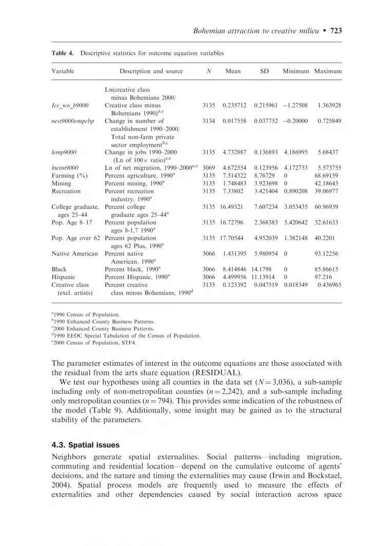
The parameter estimates of interest in the outcome equations are those associated withthe residual from the arts share equation (RESIDUAL).

We test our hypotheses using all counties in the data set (N¼ 3,036), a sub-sampleincluding only of non-metropolitan counties (n¼ 2,242), and a sub-sample includingonly metropolitan counties (n¼ 794). This provides some indication of the robustness ofthe model (Table 9). Additionally, some insight may be gained as to the structuralstability of the parameters.

4.3. Spatial issues

Neighbors generate spatial externalities. Social patterns—including migration,commuting and residential location—depend on the cumulative outcome of agents’decisions, and the nature and timing the externalities may cause (Irwin and Bockstael,2004). Spatial process models are frequently used to measure the effects ofexternalities and other dependencies caused by social interaction across space

Table 4. Descriptive statistics for outcome equation variables

Variable Description and source N Mean SD Minimum Maximum

Ln(creative class

minus Bohemians 2000/Icc_wo_b9000 Creative class minus

Bohemians 1990)d,e3135 0.235712 0.215961 �1.27508 1.363928

nest9000empcbp Change in number of

establishment 1990–2000/

Total non-farm private

sector employmentb,c

3134 0.017558 0.037752 �0.20000 0.725849

lemp9000 Change in jobs 1990–2000

(Ln of 100� ratio)a,e3135 4.732887 0.136893 4.186995 5.68437

lnetm9000 Ln of net migration, 1990–2000a,e 3069 4.672554 0.123956 4.172733 5.573755

Farming (%) Percent agriculture, 1990a 3135 7.514322 8.76729 0 68.69159

Mining Percent mining, 1990a 3135 1.748483 3.923698 0 42.18643

Recreation Percent recreation

industry, 1990a3135 7.33802 3.421404 0.890208 39.06977

College graduate,

ages 25–44

Percent college

graduate ages 25–44a3135 16.49321 7.607234 3.053435 60.96939

Pop. Age 8–17 Percent population

ages 8-1,7 1990a3135 16.72796 2.368383 5.420642 32.61633

Pop. Age over 62 Percent population

ages 62 Plus, 1990a3135 17.70544 4.952039 1.382148 40.2201

Native American Percent native

American, 1990a3066 1.431395 5.980954 0 93.12256

Black Percent black, 1990a 3066 8.414846 14.1798 0 85.86615

Hispanic Percent Hispanic, 1990a 3066 4.499956 11.13914 0 97.216

Creative class

(excl. artists)

Percent creative

class minus Bohemians, 1990d3135 0.123392 0.047519 0.018349 0.436965

a1990 Census of Population.b1990 Enhanced County Business Patterns.c2000 Enhanced County Business Patterns.d1990 EEOC Special Tabulation of the Census of Population.e2000 Census of Population, STF4.


(see Anselin et al., 2004 for a recent review). Assuming that the determinants ofBohemian location and economic dynamism are measurable using linear, first-orderexpansions of an arbitrary function, the spatial process models considered here are:

Spatial lag model : y ¼ rWyþ Xbþ e,e � iidð0,:Þ, ð3Þ

Spatial error model : y ¼ Xbþ e,e ¼ �Weþ u,u � iidð0,:Þ, ð4Þ

whereW is a n� nmatrix identifying spatial relationships between observations4; y is ann� 1 vector of dependent variables (Bohemian share or indictors of economicdynamism), X is an n� k matrix of observable county attributes (including v� in thesecond-stage regression); b is a k� 1 vector of parameters relating Bohemian share orindictors of economic dynamism to explanatory factors; r and � are spatial lagand error autoregressive terms, respectively; and : is a (possibly non-spherical)covariance matrix. When r 6¼ 0, ordinary least squares (OLS) estimates are inconsistentand biased. When � 6¼ 0, OLS estimates are unbiased and consistent, but efficiencyis compromised. The spatial lag and error models are estimated using Kelejianand Prucha’s (1998, 1999) General Method of Moment (GMM) procedures. To attendto problems due to non-spherical disturbances in 1 and 2, Davidson and MacKinnon’s(1993) heteroskedastic-consistent jackknife covariance estimator is used to calculatestandard errors.

5. Results: explaining Bohemian location

5.1. Spatial diagnostics and model selection

Robust Lagrange Multiplier (LM) residual diagnostics provide evidence about the typeof spatial dependence—spatial lag or spatial error (Florax and de Graff, 2004).Specifically, the null hypothesis is r¼ 0 under the assumption that � 6¼ 0 for the spatiallag process. For the spatial error process, the null hypothesis is �: ¼ 0 under theassumption that r 6¼ 0. In the forward model specification search, model specification(3: spatial lag) or (4: spatial error) is selected based on the magnitude of the robust LMtests. For the first-stage regression, the null hypothesis of spatial lag or errorindependence was tested using the OLS residuals and the weighting matrix. Spatialdependence between the residuals was detected using the metropolitan andnon-metropolitan sub-samples, as well as the entire data set at the 5% level(Table 5). The first-stage regression was re-estimated as a spatial error model usingKelejian and Prucha’s GMM approach.

In the second stage non-metropolitan (n¼ 2,242) and pooled county regressions(N¼ 3,064), business establishment growth in a given location is positively influenced

4 Continuous spatial representations (as opposed to discrete or contiguous representations) are useful formodeling knowledge or information spillovers, since they originate locally then tend to decay over space(Fingleton, 2003). An inverse distance matrix defined connectivity between counties. The elementsof W are wij¼ dij

��, where dij is the distance between the centroid of county i to neighbor j, and� is a decay parameter describing the 1990 Bohemian residential patterns over space. The distancedij¼ [(xi –xj)

2þ (yi – yj)

2], where x and y are Cartesian coordinates of county centroids. The decayparameter was estimated using the non-parametric procedure described by Fotheringham et al. (2002).The optimal bandwidth (�) was 1.25. The spatial weights matrix was row-standardized so that theelements of each row of W summed to one. Standardization has the dual effect of reducing neighborhoodinteractions to relative terms, and facilitating estimation.

724 . Wojan et al.

by business growth in surrounding counties. Significant spillover is apparent inthe second-stage metropolitan counties (n¼ 794), suggesting positive feedback/feed-forward effects of economic growth between these counties. Residual patternanalysis suggests these scenarios should be modeled using the spatial lag processesspecification (3). The dominance of the LM error statistics for the remaining scenariossuggests significant spillover effects of unobservable factors between counties,5 and thatmodel (4) is the appropriate specification in the second-stage regressions.

5.2. Observable characteristics attracting artists

Table 6 provides coefficient estimates for variables hypothesized to be associated withthe arts employment share for all counties, and for sub-samples of metro and non-metrocounties. Differences between metro and non-metro estimates do not appear to be large;however, a Chow test of the equality of metro and non-metro coefficients is stronglyrejected.6 There are some strong similarities between the preferences of metro and non-metro artists, but with some notable differences.

College towns and university cities are powerful draws for artists (Collegeenrollment). This result alone raises questions about conjectures of Florida (2000a)and Lee et al. (2004) as this provides an instance of an observable covariate with artsemployment that may be associated with economic dynamism, omitted from their

Table 5. Robust Lagrange multiplier (LM) tests for spatial lag and errora

First stage regression Second stage regression

Spatial error Spatial lag Spatial error Spatial lag

Combined

Bohemsh90 47.83 9.51

Employment 242.54 74.66

Creative class 62.17 14.19

Net firms 38.12 41.10

Net migration 205.58 56.32

Non-metro

Bohemsh90 5.86 0.004



Net firms 1.96 12.58


Metro

Bohemsh90 12.41 5.96



Net firms 0.26 5.81


Notes: aLM tests are ��2 with 1 degree of freedom. Critical value at the 5% level of significance is 3.84.

5 Some empirical studies interpret the error autocorrelation coefficient as explaining knowledge spilloversattributable to agglomeration economies (Cohen and Paul, 2005).

6 In the spatial econometrics literature, this test is used to identify spatial regimes (Anselin, 1988).


analyses. Other shared characteristics of metro and non-metro arts magnets include aspecialization in business services (Producer services) and the presence of an educatedpopulation (HS completion, age 25–44). Given the relatively low human capitalthreshold of a high school degree, this might better explain an aversion to poorlyeducated locales. The negative effect of large retail establishments (Big box retailers) inboth samples is surprising, as the debate over large establishments threateningtraditional main streets has focused on rural areas. This variable may be picking upsimilarities in automobile dependent planning in both samples, which the findingssuggest tend to repel artists. Finally, arts magnets are also characterized by diversityin lodging options (Lodging size index) in both metro and non-metro counties.

Table 6. First stage regression (bohemsh90 is dependent variable)

Non-metro counties Metro counties All counties

Variable Estimate t-testa Estimate t-test Estimate t-test

Constant �0.023364 �4.93 �0.016030 �3.68 �0.019457 �5.74

Art demand measures

College enrollment 0.000019 3.67 0.000042 5.02 0.000026 5.84

Producer services 0.000527 6.09 0.000259 2.43 0.000369 4.36

Lodging payroll 0.000013 0.60 0.000003 1.67 0.000001 0.64

Lodging size index 0.000012 2.64 0.000002 2.19 0.000003 2.88

HS completion, age 25–44 0.000054 3.58 0.000096 3.35 0.000068 5.09

Median household income 0.000788 1.31 0.000976 0.94 0.001067 2.00

Manufacturing 0.000017 1.89 �0.000003 �0.16 0.000003 0.39

Community amenities

Foreign born (%) 0.001823 0.65 0.005027 0.91 0.004060 1.63

Nonfamily households 0.019103 3.68 0.010121 1.17 0.019744 4.24

Nonprofit organizations 0.000003 0.28 0.000001 0.47 0.000000 �0.26

Historical registrations 0.000001 0.22 0.000001 0.42 0.000002 0.89

Winery 0.000210 0.66 �0.000115 �0.36 0.000035 0.16

Big box retailers �0.000179 �2.00 �0.000039 �1.91 �0.000053 �2.33

Climate

January temperature �0.000019 �0.17 0.000539 3.19 0.000116 1.17

January sun-days 0.000294 2.01 0.000112 0.79 0.000259 2.26

Moderate July 0.000146 0.98 0.000401 2.20 0.000292 2.40

July low humidity 0.000310 1.80 0.000281 1.48 0.000366 2.67

Landscape

Terrain variation 0.000055 2.40 0.000018 0.60 0.000047 2.38

Land in forest 0.002190 2.05 0.001718 1.06 0.002300 2.53

Forest squared �0.002257 �1.91 �0.002738 �1.42 �0.002190 �2.21

Water area 0.000043 0.49 0.000010 0.08 0.000086 1.15

Settlement

Population density 0.000655 1.25 0.002096 2.54 0.000905 2.68

Density squared �0.000030 �0.55 �0.000122 �2.00 �0.000038 �1.33

Commuting rate 0.000004 0.60 �0.000002 �0.36 �0.000002 �0.43

Population change, 1980–90 0.002835 3.06 �0.000173 �0.26 0.001524 2.27

Spatial error coefficient 0.198354 7.97 0.142044 4.46 0.257626 11.97

N 2,242 794 3,036

Adj. R2 0.33 0.51 0.44

Notes: at-tests calculated using jackknifed standard errors.

726 . Wojan et al.

This finding suggests that artists locate in metro and non-metro areas able to promotehigh value tourism characterized by the small independent hotels and bed andbreakfasts picked up by this variable.

Some of the differences between metro and non-metro areas in their attractiveness toartists were expected. Natural amenities such as mountain topography (Terrainvariation), dry winters (January sun-days) and combinations of forest and open space(Land in forest and Forest squared) are more strongly associated with artist location innon-metro areas. However, metro artists tended to locate in warmer cities (Januarytemperature and Moderate July). Population growth in the previous decade(Population change, 1980–1990) was associated with a larger arts share in non-metroareas, but not associated with the metro arts share. This is consistent with artistsmoving to amenity rich rural areas that have also seen substantial population growth,and artists not flocking to the fastest growing metro counties.

Unexpected results and differences include the effect of population density and theeffect of percent non-family households (a rough proxy for Florida’s gay index) on thearts employment share. The rural creative class as a whole demonstrates a strongproclivity for counties of moderate density. However, population density does not havea significant association with the non-metro arts employment share. Instead, moderatedensity (at least relative to other metro areas) in metro counties was associated with artistlocation. Since some of the more notable metro arts magnets (LA, NYC, San Francisco)are the most densely populated areas in the US, this result is surprising. Finally, the shareof the population in non-family households did have a positive effect on the artsemployment share in non-metro counties but not in metro counties. Data on same sexcouples were not available in the published 1990 Census, and this variable serves asa rough proxy for Florida’s gay index. The positive result in non-metro countieswarrants closer study of the components that make up this variable, available in the 2000Census. This would also shed light on the unexpected result for metro counties.

The ability of the arts employment share equations to explain a substantial share ofvariation satisfies the guideline that factors explaining variability in the indicator arecontrolled (Landres et al., 1988). The unexplained variation in the arts employmentshare, an ostensible creative milieu, is the critical output of this first stage, examinedmore closely subsequently.

5.3. The arts share residual—statistical and spatial distribution

The pattern of the arts share residual, plotted against actual and predicted values, isconsistent with the results of the Chow test for parameter equivalence betweenmetropolitan and non-metropolitan counties (Figure 2). The magnitude and variabilityof the residual effects are greater in non-metropolitan counties relative to metropolitancounties.

Residuals from the first-stage metropolitan and non-metropolitan regression weregrouped into quintiles and mapped to get some sense of the spatial distribution(Figure 3). Clusters of metropolitan counties with relatively high residual values areapparent in the Taos–Santa Fe region encompassing the Sangre de Cristo Mountainrange and the Denver–Fort Collins corridor. There are numerous metropolitan clusterslocated throughout the Great Plains, and Midwest, particularly in Minnesota, Kansasand Illinois. The metropolitan counties surrounding Nashville are dominated by highresidual values, perhaps reflecting the attractive pull of the musical tradition associated


Figure 2. First-stage residual, actual and predicted values of the artist employment share(BOHEMSH90) in 1990.

Sources: authors’ estimates.

Metropolitan county rankLowest 20%Middle 60%Top 20%

Nonmetropolitan county rank Lowest 20% Middle 60% Top 20%

County ranking for bohemian residual scores, 1990

Wallowa, ORCuster, SD

Holmes, OH

Figure 3. Spatial distribution of residuals from the first-stage regression, metro- andnon-metropolitan counties.

728 . Wojan et al.

with this city. Other metropolitan areas with relatively large residuals are located in oraround the Smokey Mountains and New York’s Hudson Valley.

The spatial distribution of the residuals associated with the first-stage regressionincluding only non-metropolitan counties has some surprises, some of which may beattributed to sampling error from counties with very small workforces. On the onehand, prior expectations about high-amenity regions in the Mountain West areconfirmed. In addition, large residuals in the Catskills of New York, the Ozarks inMissouri and some counties flanking the Great Lakes are consistent with anecdotalaccounts of concentrations of artists in these regions. However, strong residual patternsalso emerge in the Texas and Oklahoma panhandle, through the heart of Nebraska, andinto the Dakotas. Our failure to identify an artistic renaissance in this region suggeststhis result may stem from sampling error. Since occupational data are compiled fromthe 1 in 6 long-form sample of the decennial census, the estimated number of workers inrelatively rare occupations may be imprecise in counties with few workers, prevalent inthe Great Plains. We retain these counties in the analysis, as censoring very smallcounties would be arbitrary. This will tend to dilute the effect of the ostensible creativemilieu on economic dynamism in the non-metropolitan sample, especially given therelatively poor economic performance of many small Great Plains counties in the1990s.7

5.4. Intangible factors that attract artists boost economic dynamism

Table 7 provides parameter estimates for the four outcome equations using the non-metropolitan sample. The two central parameters of interest are the ostensible creativemilieu (RESIDUAL) and the share of employment in the Creative class (excl. artists).We first discuss the association between the creative class share and indicators ofeconomic dynamism, as this is central to the argument that attracting creative workersboosts local economic growth. The results confirm a strong positive effect of a largercreative class employment share on net migration (lnetm9000), employment growth(lemp9000) and net increase in number of business establishments (nest9000empcbp).The parameter estimates in Table 8 find similar effects in metro areas for net migrationand employment growth, but no significant effect with respect to firm formation. It isnotable that the creative class variable is much more powerful in explaining differentialperformance across counties than is our proxy for human capital (College graduate,ages 25–44), with the exception of the metro nest9000empcbp equation. The negative

7 The more genuine surprise is the dispersal of rural counties throughout the U.S. with large residuals.To get some sense why these areas might be attractive to artists, counties with residuals in the top 5%were isolated. Here, we discuss three examples identified in Figure 3. Holmes County, Ohio is home to the‘largest Amish population in the world’. (http://www.amishtraditions.com/about_holmes_co.htm). Forty-five percent of the forty-thousand citizens residing in Holmes are of Amish descent, making it a populartourist destination. There are also at least 15 family-owned wood shops and galleries, focusing onproduction of handcrafted furniture. Custer County, South Dakota is located in the Black Hills ofsouthwestern South Dakota. The tourism and recreation industries play a prominent role in the economy.Local attractions include archeological sites and wildlife. Performances at the Black Hills playhouse haveentertained Custer residents year-round, staging off-Broadway musicals since 1946. Other performinggroups entertain tourists by staging western re-enactments. Wallowa County, Oregon owns the monikerof the ‘Bronze Capital of the West’. (http://www.wallowacountychamber.com/). There are 20 art galleriesregistered with the Wallowa chamber of commerce, specializing in bronze casting and sculpture, and glassblowing. Outdoor recreation is a popular pastime for locals and tourists. The county flanks the SnakeRiver, and is home to the scenic Wallowa mountain range.


http://www.amishtraditions.com/about_holmes_co.htm

http://www.wallowacountychamber.com/

effect of the 1990 creative class share on creative class growth (lcc_wo_b9000) isconsistent with earlier findings and appears to be an artifact of regression to the mean.8

The statistical significance of the ostensible creative milieu (RESIDUAL) on creativeclass growth (lcc_wo_b9000) provides an explicit test of the conjecture that artistsand other creative class workers are attracted by the same unobserved characteristics.The conjecture is confirmed in both the metro and non-metro samples. The magnitude

Table 7. Stage two (outcome), non-metropolitan regressions with bohemsh90 residual

lcc_wo_b9000 nest9000empcbp lemp9000 lnetm900

Variable Estimate t-test Estimate t-test Estimate t-test Estimate t-testa

CONSTANT �2.5485 �8.99 �0.2079 �2.54 3.3385 17.59 3.3270 19.01

Settlement

Density, 1990 (ln.) 0.0095 1.09 �0.0066 �2.87 0.0023 0.42 �0.0081 �1.76

Commuting (%) 0.0029 7.88 0.0006 7.63 0.0024 12.71 0.0020 11.68

Pop. change, 1990–2000 0.4946 9.12 0.0532 3.26 0.3291 8.23 0.2718 7.19

Natural amenity

Topography 0.0048 3.16 0.0007 2.29 0.0031 3.39 0.0027 3.41

Forest land (%) 0.2954 3.93 0.0085 0.74 0.1914 4.25 0.1918 5.16

Forest squared �0.2879 �3.79 �0.0213 �1.70 �0.2049 �4.65 �0.1813 �4.79

Water area 0.0146 2.60 0.0002 0.25 0.0040 1.28 0.0044 1.58

January temperature �0.0084 �1.00 �0.0015 �1.17 0.0063 1.08 0.0220 4.27

January sun days 0.0077 0.93 0.0035 2.11 0.0037 0.63 0.0082 1.65

Temperate July 0.0114 1.35 0.0032 1.83 0.0010 0.19 0.0050 0.99

Low humidity 0.0199 1.98 �0.0034 �1.94 0.0133 2.19 0.0190 3.66

Industry

Farming (%) �0.0015 �0.99 �0.0002 �0.88 �0.0017 �2.42 �0.0012 �1.98

Mining �0.0059 �3.43 �0.0006 �2.51 �0.0063 �5.40 �0.0057 �5.66

Manufacturing �0.0001 �0.17 �0.0001 �0.67 �0.0012 �2.56 0.0000 0.04

Producer services 0.0293 7.52 0.0002 0.12 0.0010 0.45 0.0011 0.58

Recreation 0.0101 4.50 �0.0001 �0.15 0.0054 3.69 0.0038 2.93

College graduate, ages 25–44 0.0116 8.61 0.0002 0.94 �0.0014 �1.90 �0.0018 �2.75

Median household income (ln) 0.1422 3.63 �0.0158 �2.66 �0.1050 �4.76 0.0056 0.31

Demography

Pop. Age 8–17 0.0067 1.80 0.0014 1.89 0.0055 2.57 �0.0045 ��2.51

Pop. Age over 62 0.0015 0.95 0.0000 �0.17 �0.0012 �1.27 0.0043 5.03

Native American 0.0006 0.62 �0.0005 �2.37 �0.0012 �2.42 �0.0005 �1.37

Black �0.0020 �3.86 �0.0002 �3.46 �0.0026 �7.85 �0.0013 �4.85

Hispanic �0.0018 �2.34 �0.0004 �3.25 �0.0018 �3.84 �0.0011 �2.96

Creative class (excl. artists) �5.5465 �15.77 0.1999 2.74 0.6487 3.71 0.4466 2.94

RESIDUAL 4.5718 2.77 1.1758 2.78 2.0699 2.07 1.7087 1.97

W�bohemsh90 �0.2445 �0.06 �1.2851 �1.40 �0.5527 �0.20 �1.1307 �0.44

Spatial error coefficient 0.4304 18.72 0.7139 5.13 0.6368 35.20 0.6132 32.90

N 2,242 2,242 2,242 2,242

Adj. R2 0.35 0.32 0.72 0.56


8 Quantile regression from an earlier analysis confirms that this finding should not be interpreted as strongconvergence of creative class occupations (McGranahan and Wojan 2007).

730 . Wojan et al.

of this parameter in both metro and non-metro samples suggests that a vibrantcreative milieu is a critical asset in local development strategies aimed at attractingtalent.

However, metro and non-metro differences are more pronounced, when comparingthe magnitude and significance of the ostensible creative milieu (RESIDUAL) with theother indicators of economic dynamism. The relationship with net firm formation(nest9000empcbp) is arguably the most important in assessing economic dynamismgiven the claim that a creative milieu will generate new products and services(Landry, 2000, 133). This association is confirmed for the non-metro sample (Table 7)but cannot be confirmed for the metro sample (Table 8—the reported t-statistic of

Table 8. Stage two (outcome), metropolitan regressions with bohemsh90 residual.



CONSTANT �1.2768 �3.33 �0.1555 �2.33 1.5281 4.03 1.1055 2.89

Settlement

Density, 1990 (ln.) �0.0399 �4.45 �0.0073 �5.10 �0.0360 �6.34 �0.0381 �6.83

Commuting (%) 0.0035 9.15 0.0006 7.46 0.0019 7.65 0.0020 8.37

Pop. change, 1990–2000 0.2294 2.65 0.0299 2.49 0.1905 2.63 0.1737 2.59

Natural amenity

Topography 0.0006 0.38 0.0002 0.78 �0.0002 �0.22 0.0003 0.27

Forest land (%) 0.1324 1.60 0.0020 0.15 0.1232 2.23 0.1143 2.10

Forest squared �0.2259 �2.24 �0.0040 �0.22 �0.1685 �2.54 �0.1393 �2.07

Water area 0.0069 0.93 0.0013 1.23 0.0033 0.72 �0.0008 �0.18

January temperature 0.0296 3.00 0.0016 0.83 0.0139 1.97 0.0207 3.00

January sun days �0.0054 �0.70 �0.0001 �0.05 �0.0027 �0.49 �0.0026 �0.52

Temperate July �0.0054 �0.68 0.0002 0.14 �0.0083 �1.68 �0.0111 �2.23

Low humidity �0.0012 �0.12 �0.0003 �0.27 0.0014 0.22 0.0045 0.70

Industry

Farming (%) �0.0031 �1.00 �0.0013 �2.95 �0.0036 �1.93 �0.0020 �1.13

Mining �0.0063 �1.80 �0.0013 �2.29 �0.0050 �2.11 �0.0011 �0.26

Manufacturing 0.0015 1.41 �0.0001 �0.69 0.0002 0.34 0.0019 2.76

Producer services 0.0077 1.62 �0.0005 �1.04 �0.0045 �1.84 �0.0030 �1.11

Recreation 0.0015 0.43 0.0004 0.87 0.0061 2.52 0.0072 3.27

College graduate, ages 25–44 0.0069 4.11 0.0004 1.46 0.0001 0.12 0.0005 0.54

Median household income (ln) 0.0964 1.71 0.0090 0.54 �0.0409 �0.99 0.0490 1.23

Demography

Pop. Age 8–17 0.0112 2.08 0.0016 1.85 0.0079 2.28 0.0030 0.82

Pop. Age over 62 �0.0037 �1.91 �0.0001 �0.17 �0.0032 �2.76 0.0021 1.67

Native American �0.0074 �2.41 0.0008 0.62 �0.0064 �3.23 �0.0052 �2.67

Black �0.0022 �2.62 0.0001 0.23 �0.0021 �3.90 �0.0012 �2.30

Hispanic �0.0013 �1.61 0.0000 0.01 �0.0007 �1.37 �0.0003 �0.64


RESIDUAL 4.9128 1.99 1.0332 1.60 1.2875 0.80 0.1628 0.11

W�bohemsh90 5.2643 1.25 �0.4910 �0.86 2.9596 1.08 1.0455 0.41


N 794 794 794 794

Adj. R2 0.40 0.46 0.55 0.54



1.60 corresponds to a P-value of 0.1097, failing the 10% significance threshold).Although we cannot identify the components of this creative milieu (greater human-scale interaction, better restaurants, etc.) it does appear to increase entrepreneurialdynamism in non-metro counties.

The metro and non-metro comparison adds additional insight in interpreting theeffect of creative milieu on net migration and employment growth. The 1990 Creativeclass (excl. artists) share has a positive impact on both outcome indicators for bothmetro and non-metro counties. This likely represents faster growth in knowledgeintensive industries over the decade and the greater ability for creative workers to createnew employment opportunities. Yet, the creative milieu in metro areas had no impact

Table 9. Stage two (outcome), regressions with bohemsh90 residual, all counties



CONSTANT �2.2473 �6.53 �0.1525 �2.97 3.7070 16.03 3.5001 15.99

Settlement

Density, 1990 (ln.) 0.0057 0.79 �0.0059 �3.98 �0.0093 �2.32 �0.0182 �5.16

Commuting (%) 0.0036 11.46 0.0006 11.23 0.0022 12.87 0.0021 13.28

Pop. change, 1990–2000 0.3671 4.84 0.0379 4.14 0.2686 5.05 0.2380 4.66

Natural amenity

Topography 0.0034 2.29 0.0005 2.41 0.0018 2.20 0.0016 2.22

Forest land (%) 0.2743 4.05 0.0091 1.11 0.2001 5.44 0.1860 5.92

Forest squared �0.2668 �3.81 �0.0179 �1.83 �0.2190 �5.88 �0.1810 �5.53

Water area 0.0113 2.16 0.0006 0.72 0.0027 0.96 0.0019 0.77

January temperature 0.0108 1.14 �0.0012 �1.13 0.0114 2.14 0.0256 5.43

January sun days �0.0018 �0.21 0.0025 1.87 0.0016 0.32 0.0058 1.35

Temperate July 0.0019 0.26 0.0028 2.00 �0.0039 �0.90 �0.0017 �0.43

Low humidity 0.0159 1.54 �0.0022 �1.94 0.0137 2.53 0.0175 3.71

Industry

Farming (%) �0.0004 �0.31 �0.0004 �1.68 �0.0027 �4.62 �0.0017 �3.27

Mining �0.0059 �3.56 �0.0008 �3.88 �0.0071 �6.66 �0.0057 �6.03

Manufacturing �0.0003 �0.39 �0.0002 �2.30 �0.0015 �3.70 0.0001 0.37

Producer services 0.0216 4.43 �0.0006 �0.89 �0.0026 �1.69 �0.0011 �0.64

Recreation 0.0063 2.96 0.0002 0.36 0.0054 4.09 0.0043 3.65

College graduate, ages 25–44 0.0110 9.61 0.0002 1.02 �0.0017 �2.86 �0.0016 �2.91

Median household income (ln) 0.1954 5.03 �0.0072 �1.18 �0.0984 �4.80 0.0097 0.56

Demography

Pop. Age 8–17 0.0089 2.46 0.0014 2.25 0.0058 3.01 �0.0029 �1.72

Pop. Age over 62 �0.0002 �0.14 �0.0001 �0.60 �0.0026 �3.11 0.0033 4.21

Native American 0.0005 0.49 �0.0005 �2.27 �0.0017 �3.39 �0.0009 �2.45

Black �0.0023 �4.57 �0.0002 �2.85 �0.0027 �9.46 �0.0014 �5.73

Hispanic �0.0016 �2.06 �0.0003 �3.05 �0.0018 �4.38 �0.0011 �3.29


RESIDUAL 4.6144 3.07 1.1364 3.13 2.2682 2.62 1.5486 2.00

W�bohemsh90 4.1528 0.96 �1.3497 �1.80 1.3871 0.59 0.0219 0.01


N 3,036 3,036 3,036 3,036

Adj. R2 0.36 0.31 0.52 0.53


732 . Wojan et al.

on net migration or employment growth. This suggests that places attracting artiststended to be growth constrained relative to the fastest growing edge cities. In contrast,the creative milieu in non-metro counties also contributed to net migration andemployment growth. This could result from the induced effect of attracting morecreative workers, increasing the competitiveness of local firms or increasing consump-tion amenities desired by migrants and new employees. Regardless of the precisechannels through which the creative milieu operates, the implications of this analysisare direct: non-metro environments conducive to arts activity also tend to promotefaster rates of growth.

6. Implications of Bohemian attraction to creative Milieu

The largest benefit of empirically deriving an ostensible creative milieu has been thesharpening of an amorphous construct in the literature. Our results support twodefinitions of creative milieu that have been discussed but never differentiated. What wewill call a ‘weak definition’ of creative milieu requires that unobserved interactionattract a diverse set of creative workers (Florida, 2002a, 2002b). The weak definitionsupports the central conjecture that creative people are attracted to creative places.What we will call a ‘strong definition’ of creative milieu additionally requires thatinteraction across these diverse creative domains increase the economic dynamism ofthe local economy (Landry, 2000; Lee et al., 2004; Stolarick and Florida, 2006).Our findings are consistent with the weak definition in both metropolitan and non-metropolitan counties. To wit, those places with a surplus of Bohemians beyond thatpredicted by observable characteristics related to supply and demand for artistsexperienced faster rates of growth of other members of the creative class between 1990and 2000. However, evidence of a strong creative milieu is conclusive only in the non-metropolitan sample, where a surplus of Bohemians was also associated with fasterrates of new firm formation and employment growth. The findings in metro areas aresuggestive but are not reliable enough to conclude that a creative milieu contributesdirectly to economic dynamism. These mixed results have important implications forevaluating past critiques of the creative class thesis, for directions of further researchand for policy.

At one level, support for the weak definition of creative milieu seemingly dismissesthe critiques by Hansen et al. (2005) and Markusen (2006) that the location proclivitiesof constituent occupations within the creative class are likely to be very different.The analysis provides the most definitive evidence to date that growth of the creativeclass is associated with a creative milieu. However, the test of the theory necessarilyutilizes an aggregate creative class construct. The composition of creative class growthassociated with creative milieu was not examined. Growth induced by a creative milieumight be limited to particular types of creative workers, such as those primarilyconcerned with symbolic knowledge bases. Though possible, this type of creative classgrowth would not be expected in rural areas (Hansen et al., 2005), reducing theplausibility of this alternative explanation. Decomposing the creative class intooccupations primarily concerned with analytic, synthetic or symbolic knowledgecould resolve this debate empirically.

Moving beyond the attraction of creative workers, our strong definition of creativemilieu is more germane to the policy debate animated by discussion of the creative class.


For metro areas, our findings are unsatisfying as they identify a potentially large effect,

but one that fails to meet conventional standards of reliability. Given the point

estimate, metro counties in the top decile of creative milieu would generate close to

twice the number of new establishments per worker compared to metro counties in the

bottom decile. This is confirmed in the sample, where the top decile generated three

establishments per hundred workers, on average, compared to 1.6 establishments

generated in the bottom decile. Unfortunately, the standard error associated with the

point estimate is large. The prudent conclusion is to suspend judgment on the existence

of a strong creative milieu in metro areas.On the one hand, this result makes the claimed association between entrepreneurship

and creative milieu identified in Lee et al. (2004) tentative. On the other, our results

cannot refute this association (Ziliak and McCloskey, 2004). The argument put forward

by Malanga (2004) of a fabricated arts-innovation nexus to justify large, wasteful

expenditures on cultural amenities appears premature, especially given definitive

evidence of a strong creative milieu in non-metro counties. Replication of this analysis

in other time-periods or countries may provide valuable information. However, it may

be that structural complexity disadvantages the identification of a strong creative milieu

in cities, generally. Spatial lag in the metro equations is a tell-tale sign of the importance

of clustering and agglomeration, which may swamp effects from a creative milieu.Our indeterminate results on the existence of a strong creative milieu in metro areas

will not be welcomed by opposing sides in the creative cities debate. However, arts

communities may benefit the most from the caution inherent in the findings. Public

spending on the arts, justified on the basis of increased regional competitiveness may

very well be wasteful if directed to high visibility projects that do nothing to increase

human-scale interaction. At the same time, evidence of a weak creative milieu ensures a

city’s attractiveness to artists is an important indicator of its ability to retain and attract

creative workers. Any metropolitan region pursuing a creative economy strategy in

earnest should engage local artists in devising the best ways to encourage the social and

cultural interaction that engender creative milieus. The research community can

contribute to this effort by empirically examining the evolution of creative milieus

across all cities.It is important to stress that our definitive findings of a strong creative milieu in non-

metro counties do not resolve the debate over the importance of local arts communities

to regional innovation and competitiveness. Our main contribution is empirical

confirmation that a relative surplus of Bohemians is likely to reveal a vibrant creative

milieu. Our empiricism is intentional in first generating an ostensible creative milieu

variable that is then confirmed by an association with indicators of economic

dynamism. This indefiniteness does not allow concluding that a particular strategy for

promoting the arts will increase economic dynamism.Rather, these non-metro results demonstrate a true contribution of place to economic

dynamism where a creative milieu effect is not conflated with the density of creative

agents randomly ‘rubbing elbows’ in the city (Stolarick and Florida, 2006). In contrast

to more conventional studies examining industrial location or the geography of

innovation, our explanation of regional performance does not rely on the location of

particular quantities in a place (e.g. human capital, R&D spending, transportation

infrastructure) but on a proxy for a particular quality of place. Our reliance on a

residual makes the analysis susceptible to omitted variable critiques, where creative

734 . Wojan et al.

milieu is reduced to a misspecification error. However, we know of no other techniqueallowing a generalizable analysis of processes thought to be reliant on interaction.

Confirming that our empirically derived proxy for creative milieu is reliant oninteraction will require qualitative research. A central difficulty in doing case studyresearch in rural communities is the identification of informative cases. By comparing‘creative places’—identified by a large arts share residual—with similarly situated‘uncreative places’, a relatively small number of cases should generate useful insightsregarding the intangible factors critical to rural development strategies premised on theattraction of talent. However, practice in the area of cultural community developmenthas far out-paced applied rural research on the arts, dating back to at least the 1930s(Strom, 2001). Our findings bolster longstanding and newly emerging efforts to ‘acceptthe goodness of art where we are, and expand its worth in the places where people live’(Gard, 1968, 4).

Acknowledgements

The authors thank workshop participants, three anonymous reviewers and Neil Wrigley forcomments that improved the article. Funding to pay the Open Access publication charges for thisarticle was provided by the Economic Research Service, U.S. Department of Agriculture.

References

Anselin, L. (1988) Spatial Econometrics: Methods and Models. London: Kluwer AcademicPublishers.

Anselin, L., Florax, R. J. G. M., Rey, S. (2004) Advances in Spatial Econometrics: Methodology,Tools and Applications. Berlin: Springer.

Armington, C. and Acs, Z. J. (2002) The determinants of regional variation in new firmformation, Regional Studies, 36(1): 33–45.

Cohen, J. P. and Paul, C. J. M. (2005) Agglomeration economies and industry location decisions:the impacts of spatial and industrial spillovers, Regional Science and Urban Economics, 35(3):215–237.

Davidson, R. and MacKinnon, J. G. (1993) Estimation and Inference in Econometrics. Oxford:Oxford University Press.

Fingleton, B. (2003) Externalities, economic geography, and spatial econometrics: conceptual andmodeling developments, International Regional Science Review, 26(2): 197–207.

Florax, R. J. G. M. and de Graff, T. (2004) The performance of diagnostic tests for spatialdependence in linear regression models: a meta-analysis of simulation studies. In L. Anselin,R. J. G. M. Florax, S. Rey (eds) Advances in Spatial Econometrics: Methodology, Tools andApplications. Berlin: Springer, 359–80.

Florida, R. (2002a) Bohemia and economic geography. Journal of Economic Geography, 2: 55–71.Florida, R. (2002b) The Rise of the Creative Class: And How it’s Transforming Work, Leisure,Community, and Everyday Life. New York: Basic Books.

Fotheringham, A.S., Brunson, C., Charlton, M. (2002) Geographically Weighted Regression.Hoboken, New Jersey: Wiley.

Gard, R. E. (1968) The Arts in the Small Community—A National Plan. Madison, WI: Office ofCommunity Arts Development, University of Wisconsin-Extension.

Glaeser, E. L., Kallal, H. D., Scheinkman, J. A., Shleifer, A. (1992) Growth in cities. Journal ofPolitical Economy, 100(6): 1126–1152.

Glaeser, E. L., Kolko, J., Saiz, A. (2001) Consumer city. Journal of Economic Geography,1: 27–50.

Hansen, H. K., Vang, J., Asheim, B. T. (2005) The creative class and regional growth: towardsa knowledge based approach. Paper presented at ‘Regional Growth Agendas’ conference,Regional Studies Association, Aalborg, Denmark, May 28–31.


Heilbrun, J. (1992) Art and culture as central place functions. Urban Studies, 29(2): 205–215.Heilbrun, J. (1996) Growth, accessibility and the distribution of arts activity in the United States:1980 to 1990, Journal of Cultural Economics, 20(4): 283–296.

Irwin, E. and Bockstael, N. (2004) Endogenous spatial externalities: empirical evidenceand implications for the evolution of exurban residential land use pattern. In L. Anselin,R. J. G. M. Florax, S. Rey (eds) Advances in Spatial Econometrics: Methodology, Tools andApplications. Berlin: Springer, 359–380.

Jacobs, J. (1961) Death and Life of Great American Cities. New York: Random House.Kelejian, H. H. and Prucha, I. R. (1998) A generalized spatial two stage least squares procedurefor estimating a spatial autoregressive model with autoregressive disturbances. Journal of RealEstate Finance and Economics, 17: 99–121.

Kelejian, H. H. and Prucha, I. R. (1999) A generalized moments estimator for the autoregressiveparameter in a spatial model. International Economic Review, 40: 509–533.

Landres, P. B., Verner, J., Thomas, J. W. (1988) Ecological uses of vertebrate indicator species: acritique. Conservation Biology, 2(4): 316–328.

Landry, C. (2000) The Creative City: A Toolkit for Urban Innovators. London: EarthscanPublications Ltd.

Lee, S. Y., Florida, R., Acs, Z. J. (2004) Creativity and entrepreneurship: a regional analysis ofnew firm formation. Regional Studies, 38(8): 879–891.

Malanga, S. (2004) The curse of the creative class. City Journal, available at http://www.city-journal.org/html/14_1_the_curse.html.

Markusen, A. (2006) Urban development and the politics of a creative class: evidence from thestudy of artists. Environment and Planning A, 38(10): 1921–1940.

Markusen, A. and Johnson, A. (2006) Artists’ Centers: Evolution and Impact on Careers,Neighborhoods and Economies. Minneapolis: Hubert H. Humphrey Institute of Public Affairs,University of Minnesota.

Marshall, A. (1920) Industry and Trade. London: Macmillan.McGranahan, D. A. and Wojan, T. R. (2007) Recasting the creative class to examine growthprocesses in rural and urban counties. Regional Studies, 41(2): 197–216.

Moulaert, F. and Sekia, F. (2003) Territorial innovation models: a critical survey. RegionalStudies, 37(3): 289–302.

Rupasingha, A., Goetz, S., Freshwater, D. (2006) The production of social capital in US counties.Journal of Socio-Economics, 35(1): 83–101.

Stolarick, K. and Florida, R. (2006) Creativity, connection and innovation: a study of linkages inthe Montreal Region. Environment and Planning A, 38: 1799–1817.

Strom, E. (2001) Strengthening Communities Through Culture. Washington: Center for Arts andCulture, available at http://www.culturalpolicy.org/pdf/communities.pdf.

Ulrich, R. S. (1986) Human responses to vegetation and landscapes. Landscape and UrbanPlanning, 13: 29–44.

Villiani, J. (1998) The 100 Best Small Art Towns in America. 3rd Edition. Berkeley: John MuirPublications.

Ziliak, S. T. and McCloskey, D. N. (2004) Size matters: the standard error of regressions in theAmerican Economic Review. The Journal of Socio-Economics, 33(5): 527–546.

736 . Wojan et al.

http://www.cityjournal.org/html/14_1_the_curse.html

http://www.culturalpolicy.org/pdf/communities.pdf

emoting with their feet: bohemian attraction to creative milieu

Documents