emerging issues in the natural and applied sciences
TRANSCRIPT

ISBN: 978-9952-8071-4-1
EMERGING ISSUES IN THE NATURAL AND APPLIED SCIENCES Academic book
“PROGRESS” Baku, Azerbaijan-2011
Academic book
2
LCC: AY10-29 UDC: 002
Editorial board:
Ángel F. Tenorio, Prof. Dr. Polytechnic School, Pablo de Olavide University (Spain)
Maybelle Saad Gaballah, Prof. Dr. National Research Centre, Cairo (Egypt)
Manuel Alberto M. Ferreira, Prof. Dr. ISCTE-Lisbon University Institute (Portugal)
Eugen Axinte, Prof. Dr. "Gheorghe Asachi" Technical University of Iasi (Romania)
Sarwoko Mangkoedihardjo, Prof. Dr. Sepuluh Nopember Institute of Technology (Indonesia)
Cemil Tunc, Prof. Dr. Yuzuncu Yil University (Turkey)
Peng Zhou, Prof. Dr. School of Medicine, Wake Forest University (USA) Editor-in-chief: J.Jafarov Coordinator: A. Alimoglu
Emerging issues in the natural and applied sciences. “Progress” LLC, Baku, 2011, 308 p.
This research book can be used for teaching modern science, including for teaching undergraduates in their final undergraduate course in all fields of natural and applied sciences. More generally, this book should serve as a useful reference for academics, sciences researchers.
ISBN: 978-9952-8071-4-1
© Progress IPS LLC, 2011
© IJAR, 2011

EMERGING ISSUES IN THE NATURAL AND APPLIED SCIENCES
3
TABLE OF CONTENTS
Chapter 1.
Ali Hakan Işık, Osman Özkaraca, İnan Güler
EVALUATION OF BIOTELEMETRY SYSTEMS AND NOVEL PROPOSAL FOR CHRONIC DISEASES ANAGEMENT…………………...……………5
Chapter 2.
Sarwoko Mangkoedihardjo APPLIED PHYTOTECHNOLOGY IN ENVIRONMENTAL SANITATION FOR THE TROPICS AND THE OCEAN COUNTRIES.........................20
Chapter 3.
Khalisanni Khalid, Rashid Atta Khan, Sharifuddin Mohd. Zain A RELATIVE NEW TECHNIQUE TO DETERMINE RATE AND DIFFUSION COEFFICIENTS OF PURE LIQUIDS......................................................36
Chapter 4.
Manuel Coelho, José António Filipe, Manuel Alberto M. Ferreira “CRIME AND PUNISHMENT”: THE ETHICAL FUNDAMENTS IN THE CONTROL REGIME OF COMMON FISHERIES POLICY………................…...45
Chapter 5.
Ussy Andawayanti SEDIMENT DISTRIBUTION İN THE ESTUARY OF SENDANG BIRU COAST, MALANG REGENT-INDONESIA.........................................................58
Chapter 6.
Abu Hassan Abu Bakar, Arman Abd Razak, Mohamad Nizam Yusof ESTABLISHING KEY DETERMINANTS CONTRIBUTING TO GROWTH OF CONSTRUCTION COMPANIES: AN EMPIRICAL EXAMINATION..….................73
Chapter 7.
Manuel Alberto M. Ferreıra, Marina Andrade DIFFUSION MODEL FOR THE FINANCING OF A FUND THAT RISKS RUIN…......89
Chapter 8.
Dwi Priyantoro, Lily Montarcih L. SPAN WELL, AN INNOVATION IN IRRIGATION DESIGN.......................................102
Chapter 9.
Mahyuddin Ramli, Amin Akhavan Tabassi ENGINEERING PROPERTIES OF POLYMER MODIFIED MORTAR......................119
Chapter 10.
Mohammad Bisri WATER CONSERVATION AND ANALYSIS OF SURFACE RUN OFF SPATIALLY AT KALI SUMPIL WATERSHED, EAST JAVA-INDONESIA.................136

Academic book
4
Chapter 11. Amin Akhavan Tabassi, Mahyuddin Ramli, Abu Hassan Abu Bakar TRAINING AND DEVELOPMENT OF WORKFORCES IN CONSTRUCTION INDUSTRY..............................................................................150
Chapter 12.
Lily Montarcih SYNTHETIC UNIT HYDROGRAPH FOR WATERSHED IN SOME AREAS OF INDONESIA............................................................................167
Chapter 13.
B.S.E. Iyare F.E.U. Osagıede THE MATHEMATICS OF VECTOR - BORNE DISEASES........................................179
Chapter 14.
Marina Andrade, Manuel Alberto M. Ferreıra FORENSIC IDENTIFICATION WITH BAYES’ LAW………………................….…….206
Chapter 15.
Khalisanni Khalid, Khalizani Khalid PRODUCTION OF BIODIESEL FROM PALM OIL VIA TRANSESTERIFICATION PROCESS - THE RECENT TRENDS......................221
Chapter 16.
Lasmini A., A.K. Indriastuti PEDESTRIAN FACILITIES AND TRAFFIC MANAGEMENT CAUSED BY INAPPROPRIATE ACTIVITIES ON SIDEWALK AT CENTRAL BUSINESS DISTRICT IN CITY OF DEVELOPING COUNTRY................................232
Chapter 17.
Khaled Smaili, Seifedine Kadry IMPACT OF SOFTWARE AND HARDWARE TECHNOLOGIES ON GREEN COMPUTING...........................................................251
Chapter 18.
Ishak Aydemir, Elif Gökçeaslan RESTRUCTION OF MEDICAL SOCIAL WORK IN TURKEY....................................276
Chapter 19.
João Pedro Couto, Armanda Bastos Couto ESTABLISHING MEASURES TO MINIMIZE CONSTRUCTION SITES IMPACTS: A STUDY OF PORTUGUESE HISTORICAL CENTERS.........................293

EMERGING ISSUES IN THE NATURAL AND APPLIED SCIENCES
5
EVALUATION OF BIOTELEMETRY SYSTEMS AND NOVEL PROPOSAL FOR CHRONIC
DISEASES MANAGEMENT
Ali Hakan Işık, Osman Özkaraca, İnan Güler
The Department of Electronics and Computer Education,
Gazi University, 06500 Ankara (TURKEY) E-mails: [email protected], [email protected], [email protected]
ABSTRACT During recent years, aging population is the most important
challenge especially for developed countries. Therefore they seek cost-effective healthcare solutions to overcome this problem. New innovations in electronic and communications technologies provide reliable and long-term solutions for this issue. Developments and ex-cellence in biotelemetry also support elderly and vulnerable people in their own homes comfort and offer health services at anytime and when they wish. In order to meet these changes, emerging innova-tions must be evaluated carefully. It is found that one of the most challenges of chronic diseases care that biotelemetry applications encounter is patient’s cooperation and compliance. These problems can be accomplished by using supervised, unsupervised or blended method. In supervised method, doctor or nurse visit patients in their home. Insufficient number of supporting person and extensive cost are main challenges of this method. In unsupervised method, pati-ents are informed and tracked by using distance learning and appli-cation software. Patient computer competence and usability, internet accession problem are main challenges of this method. In blended method, firstly medical expert person visit patients and they are informed about computer, drug usage and their disease. Then treat-ment plan is carried out by using video enhancement distance lear-ning and application software. With this way, major problems of both systems can be overcome. Main aims of this chapter are compre-hensive analysis of biotelemetry systems and suggestion of innova-tive solution for chronic diseases management in home environ-ment. With this chapter finding, scientists can receive detailed infor-

Academic book
6
mation about biotelemetry in all aspects and innovative solution is proposed for chronic diseases management. It is believed that wire-less technology such as zigbee or bluetooth to obtain biological and physiological data, data transmission technology such as third generation (3G), patient management and tracking method, decision support system will be used together in one unique application to provide effective and efficient solution in the future.
Key words: Biotelemetry, chronic diseases, mobile communi-
cation, distance learning 1. INTRODUCTION In today's information age, rapid developments in information
and communication technologies have led to fundamental changes in the areas of people's cultural, social, educational, health care. Without the concept of time and space, providing our needs at any time and anywhere has emerged. This change showed it's effect in health care field. These changes in health care field led to the emergence of new concepts [1, 2]. In this context, general access to information and health resources that result will contribute impor-tantly to individual and community health, as well as to the health care systems that support it, especially in the realms of chronic dise-ase monitoring and management. It is, therefore, essential that barri-ers to universal broadband access be overcome, and that obstacles to adequate reimbursement for such tele-health services are remo-ved. Biotelemetry is one of the typical examples of such a success, or the application in biomedical measurement [3]. It provides remote measurement of biological or physiological quantities and transmis-sion of these data from patient environment to the remote center. Chronic diseases and it’s management are very important issue in biotelemetry. By 2020, chronic diseases accounted for 80% of deaths of in the world. Each year, many people lose their life due to various chronic diseases which shows the importance of ECG signals monitoring that is heart's electrical activity [4].
In first part of this study, we deal with biotelemetry and tele-homecare with all aspects. In the last part of this study, chronic

EMERGING ISSUES IN THE NATURAL AND APPLIED SCIENCES
7
diseases management and distance learning is offered as a solution method, obtained findings are discussed and founded results are presented. Main aim of this study is to evaluate past, present and future of biotelemetry systems and predictions about the future application. It is also presented an innovative proposal for chronic diseases management in home environment.
2. BIOTELEMETRY Biotelemetry means collecting and transmitting biological or
physiological data from one location to another location so as to interpret the data [5]. Biotelemetry measurements are biological data such as ECG, EEG and physiological data such as blood pressure, temperature, glucose [6].
Biotelemetry can be employed for the measurement of a wide variety of applications. Most important ones are follows;
In many areas ambulances and emergency rescue teams are equipped with telemetry equipment to allow electrocardiograms and other physiological data to be transmitted to a nearby hospital for interpretation.
Collection of medical data from a home or office. Research on unrestrained, unanesthized animals in their natu-
ral habitat. Isolation of an electrically susceptible patient from power line
operated ECG equipment to protect him from accident or shock. Measurement of the temperature and position of the egg in a
nest by telemetry system. This works describes a biotelemetry sys-tem for continuous monitoring of temperature and position of an artificial radio transmitter egg in a mall bird nest.
Space life sciences research [7]. As it shown in figure 1, wireless systems are designed to pro-
vide “anytime, anywhere” service, enabling data entry and data access by medical personnel at the point of care, direct data acquisi-tion from medical devices, patient and device identification, and remote patient management [8].

Academic book
8
Fig. 1. Wireless biotelemetry system [8]. 2.1. Biotelemetry for emergency case Continuous connection in biotelemetry provides immediate
intervention to the patient who is in the emergency condition. In Pav-lopoulos and colleagues’ study, by using the GSM mobile telephony network, they transmitted vital biosignals and images of the patient from the emergency site such as ambulance to the consultation site. This study concludes that early and specialized prehospital manage-ment contributes to emergency case survival [9].
2.2. XML based bio-information transmission With the development in biotelemetry, there is a need to make
the electronic medical information (EMI) exchange, sharing the huge amount of data, accession data through any type of web application. In this context, XML provide simple, standard, platform and opera-ting system independent data transmission and retrieval. In this field, donglan’s study takes advantages of XML and web technology. This system is platform, system- and application-independent as well as user-driven and open standard for exchanging data via the Internet. Study show that XML based electronic medical information (EMI)

EMERGING ISSUES IN THE NATURAL AND APPLIED SCIENCES
9
does not only increase the readability and exchangeability of EMI, but also make our system compatible with PACS and Hospital infor-mation system [10].
3. BIOTELEMETRY AND TELE-HOMECARE STUDIES There are so many studies related to the biotelemetry and
tele-homecare. It is important to evaluate these studies so as to understand biotelemetry and tele-homecare with all aspects. To achieve this goal, most important ones are presented below;
In a tele-homecare research project conducted in Sacrament, researchers concluded that tele-homecare is capable of maintaining quality of care while producing cost savings [11]. In another study, authors found that tele-homecare can provide home monitoring services to the same number of patients at lower cost than in person [12]. Cerny and colleagues article focused on the designing of homecare system that include patient’s movement and circadian rhythm parameters. The Circadian rhythm measurement and its usa-ge in the homecare system are discussed [13]. In Krejcar and collea-gues article, researchers create a system that controls important information about the state of a wheelchairbound person (monitoring of ECG and pulse in early phases, temperature or oxidation of blood). Values are sent to the smart device communicates with the module for processing via Bluetooth wireless communication techno-logy. Most of the data (according to heftiness) is processed directly in PDA or Embedded equipment to a form that is acceptable for simple visualization [14]. In home healthcare study that is performed in Minnesota, patients divide into three groups. In first one, patients received traditional nursing care at home. In second one, virtual visits using videoconferencing technology. In third one both virtual visits and physiologic monitoring is performed. Within six months of study, these participations that received both virtual visits and physiologic monitoring required that lower level care [15]. In Fidan’s study, four channel biotelemetry device was designed and imple-mented for monitoring body temperature, respiratory rate, heart rate, electrocardiogram (ECG) and electromyogram (EMG) signals of the patients at indoor [16]. Cleland and colleagues concluded that

Academic book
10
remote monitoring of patients with congestive heart failure (CHF) and patients using implantable cardiac defibrillators can lead to better management of medications and patient behavior. CHF is a deadly disease and one of the primary causes of hospital admissi-ons. Once a person has been hospitalized with CHF, there is a 25 percent chance that he or she will die or be re-hospitalized within three months. In Cleland study, home visits were reduced 65 percent for the remote monitoring group [17]. In another study, home monitoring device that captured and transmitted weight of heart failure patients reduced the six-month mortality rate 56.2 percent [18].
Benefits of Biotelemetry and Tele-homecare Many studies show that biotelemetry and tele-homecare are
cost effective and supportive solution. It is believed that increased intensity of disease monitoring and management will create impro-ved patient healthcare with resulting reduction of acute and chronic complications, and that these will translate directly into decreased consumption of expensive emergency health care resources (emer-gency room visits and rehospitalizations) and decreased long-term disease complications. This, in turn, should translate directly to dec-reased consumption of expensive medications, personnel, equip-ment and hospitalization days required to manage those long-term complications [19, 20, 21, 22].
Management of energy and power in biotelemetry A crucial attribute of anybody sensor system is its power con-
sumption and management. Researchers have proposed many solutions to tackle the power problem. One solution is energy scavenging - using circuits powered by energy from the environment to power sensor nodes autonomously. A second solution is sub threshold circuit design, in which voltages are significantly less than the nominal supply voltage. A third solution, improved network pro-tocols, is based on the fact that the wireless radio’s transmission is often the most power-hungry element of a circuit. Relatively new net-working standards, such as Zigbee (IEEE 802.15.4), Bluetooth Low-Energy Wireless Technology, and the work-in progress Body Area

EMERGING ISSUES IN THE NATURAL AND APPLIED SCIENCES
11
Network protocol (IEEE 802.15.6), target the resource constrained embedded-systems market [23]. In many applications of short range biotelemetry, long operational life of the remote unit is a prime requirement. Many different types of biotelemetry systems featuring low battery drain have been developed over the years, but adequate battery life can still be a problem [24].
Implantable Units in Biotelemetry Implantable sensors measure parameters inside the body.
Because surgery is often involved, they’re subject to stringent requirements. Wearable sensors, although not as invasive as their implantable counterparts, nevertheless must withstand the human body’s normal movements and infringe on them as little as possible. These sensors must coexist with the body, both inside and outside, whereas other types of sensors - for example, environmental sen-sors - might have no such constraint. They provide bidirectional communication interfaces between a person and a remote informati-on system that provides healthcare services, diagnosis, or upgrades [25].
One of the most important challenges of implantable units is battery life, transmission signal length, and encapsulation. There are some requirements for the usage of an implantable telemetry. Implantable units must have relatively small size and be lightweight. Internal power source has to be used for a long time. Miniaturization and long-term use of implant electronic systems for medical applica-tions have resulted in growing necessity for an external powering system. Another requirement is encapsulation of the unit. Implan-table parts of the system must be encapsulated in a biocompatible material. The use of implantable units also restricts the distance of transmission of the signal. This disadvantage has been overcome by picking up the signal with a nearby antenna and external power [26, 27]. Long operating life of implantable electronic circuits can be obtained by using low power transmission techniques. For example, pulse code modulation combined with remote switching systems to turn the circuit on only when monitoring is necessary [28]. Inductive powering of implantable monitoring devices is a widely accepted

Academic book
12
solution for replacing implanted batteries. Inductive powering is based on the magnetic coupling between an internal coil and an external coil that is driven by an alternating current.[29]
Chronic diseases management Remote monitoring is increasingly recognized as valuable
tools for enhancing care quality in chronic disease management. They have the potential to deliver new savings for both patients and providers. For patients, this means fewer office and emergency room visits, fewer and reduced duration of hospitalizations, reduced patient travel time and expense, and increased access (for the elderly, the physically challenged, the homebound, and especially for rural patients). For clinicians, it means more informed decision-making, enhanced patient compliance and more efficient outreach case management [30].
Monitoring of this kind can enable more sophisticated home
care, detect deterioration prior to symptom development and minimi-ze the need for complicated and cumbersome patient transportation to hospital/office appointments. Because they can now be reliably monitored at home, home-bound COPD patients may be able to receive better care in other ways. When the home-care program is carefully designed and implemented, early release from the hospital will not endanger patient health, will reduce patient exposure to hospital-acquired infections and will minimize risks associated with return to the hospital/office for routine clinical examinations [31, 32, 33]. Further, although it is not possible to make the home environ-ment as safe as the intensive care unit, clearly defined steps can be taken to minimize risk [34].
In all these contexts, biotelemetry studies have demonstrated
health benefits in terms of reduced hospitalization days, reduced clinic visits, enhanced quality of life and satisfaction with technology. Cost benefits have been demonstrated for patients, home care agencies and the health care system [35].

EMERGING ISSUES IN THE NATURAL AND APPLIED SCIENCES
13
4. DISTANCE LEARNING Distance learning is a new trend in education that gives a
chance to everyone and offers options to learn better under the constructivist approach [36]. Similarly, Moore defines distance learning as “the family of instructional methods in which the teaching behaviors are executed apart from the learning behaviors so that communication between the teacher and the learner must be facilita-ted by print, electronic, mechanical or other devices” [37] Distance learning and training result from the technological separation of instructor and learner which make free the learner from the neces-sity of traveling to “a fixed place, at a fixed time, to meet a fixed per-son, in order to be trained” [38]. Service that gives the clinician the ability to monitor and measure patient health data and information over geographical, social and cultural distances using video and non-video technologies. Remote monitoring may include video-con-ferencing, messaging reminder and surveillance questioning, and/or one or more sensors - such as electrocardiogram, pulse oximetry, vi-tal signs, weight, glucose, and movement or position detectors [39]. In this context, by using distance learning in chronic patients care provide time independent, cost effective, interactive solution.
5. CONCLUSION An ease of use, replaceability, wearability are key issues and
most important features of the biotelemetry system. Through the development in sensor, communication, decision support system, increase in patients number and demand, decrease in power con-sumption and cost, it is possible to perform many offline advanced applications in real time accompanying with the real-time detection of signal. Main applying areas of the biotelemetry are diabetes, con-gestive heart diseases and chronic obstructive pulmonary diseases. Biotelemetry ensures significantly greater improvement with redu-cing visiting number of doctors, health expenditure in the field of chronic patient treatment. Recent studies demonstrated that chronic pulmonary patients often makes mistake in self management and

Academic book
14
drug usage. Evaluated studies concluded that biotelemetry solutions for healthcare are feasible and acceptable.
In addition, evaluated studies concluded that it is required to developed new approach to follow their own treatment plan. In this context, in proposed system firstly expert person visit, then interacti-ve audio/video enhancement distance learning emerged as an innovative solution to overcome this issue. Another important com-ponent of proposed system for chronic pulmonary patients include next generation sensors, zigbee as a transmission technique between patient and remote environment, xml format as flexible data exchange, smart mobile phone as a communication device, advan-ced decision support system as a processing unit.
There was a rapid growth in medical technology especially telemetry. By using biotelemetry, wireless measurements of biolo-gical and physiological data and monitor of patients’ symptoms and movements, decision making regarding this data, treatment plan are provided. One of the main aims of the biotelemetry is to provide qua-lity healthcare by means of innovative technology. We can evaluate biotelemetry by using cost-effectivity, patient satisfaction, and bene-fit and improvement for health. This study introduces a general sur-vey and evaluation of biotelemetry system and innovative solution for chronic pulmonary patients care. In addition, findings of this stu-dy showed the usability and benefit for healthcare.
Application areas of biotelemetry system tend to increase. It enhances the health services and management of chronic and com-plex disease. Other benefits are reductions in hospital admissions, patient visits and the overall cost of the patient’s care. Continual growth of biotelemetry is driven by the ease of use and installation, flexibility. Mobile solution provides ease of use and XML technology provides flexibility. XML based bio-information transmission and ret-rieval provide more flexible data exchange, integration, standardiza-tion in biotelemetry. In promising results obtained revealing the fea-sibility of biotelemetry system for patients.
Today more effectively decision support systems are used than ever before. Most important ones are artificial neural network, support vector machine, fuzzy logic. These algorithms processed data and produced useful information about patient healthcare. In

EMERGING ISSUES IN THE NATURAL AND APPLIED SCIENCES
15
addition, Infrared, Bluetooth, ZigBee, Wi-Fi and GPRS wireless com-munication technologies are widely used in biotelemetry. Among these communication technologies, ZigBee provide network enhan-cement, effective, long term and low power solution in implantable unit.
In this study, two-way interactive audio/video telecommunica-tion is proposed as innovative solution for chronic diseases manage-ment together with medical expert person consultation. In distance learning people's educational background and computer usability is very important. The average age of COPD or other chronic pulmona-ry patient is very high, so their educational background and compu-ter usability is not enough. They need face to face consultation before remote tracking and treatment. Therefore we propose blen-ded method to track and support patients in home environment. By using this solution emerging challenges can be eliminated. With time and place independent concept,
Future biotelemetry applications will use smaller implantable device such as cardiac pacemakers and defibrillators, radio interface of implantable device provide signal amplification and use advanced modulation techniques. In addition, application will integrate with other system such as hospital information system. It is believed that main role of biotelemetry is support traditional personal care and not to replace.
REFERENCES 1. Zach S., “Telemedicine overview and summary”, Nine-
teenth Convention of the IEEE, 1996; 409-412. 2. Kyriacou E., Pavlopoulo, S., Koutsouris D., “Multipurpose
Health Care Telemedicine System”, Proceeding of the 23rd Annual EMBS International Conference of the IEEE, 2001; 3544-3547.
3. Shimizu K., “Optical Biotelemetry”, Advances in Electro-magnetic Fields in Living Systems, Springer Science+ Business Media, New York, 2005; 131-154.
4. World Health Organization, Chronic diseases and health promotion, http://www.who.int/ 2011.

Academic book
16
5. Wolcott T. G., New options in physiological and behavioral ecology through multichannel telemetry. J. Exp. Marine Biol. Ecol. 1995; 193:257-275,.
6. Cromwell L., Weibell F. J., Pfeiffer E. A., Biotelemetry. In Huebner, V. (ed.), Biomedical Instrumentation and Measu-rements, Prentice-Hall, Englewood Cliffs, 1980; 12: 316-343.
7. Mathew T., Shanavas K. P., “Wireless Technology Based Biotelemetry”, 2010; 1-6.
8. Robert S. H. Istepanian, Swamy Laxminarayan, Constan-tinos S. Pattichis, “M:Health: Emerging Mobile Health Sys-tems” Springer Science+Business Media, 2006; 3-617.
9. Pavlopoulos S., Kyriacou E., Berler A., Dembeyiotis S., Koutsouris D., “A Novel Emergency Telemedicine System Based on Wireless Communication Technology-Ambulan-ce, IEEE Transactıons On Information Technology In Biomedicine”, 1998: 2(4): 261-266.
10. Donglan Y., Shuqun X., Xianli W., Zhensheng Z., Kuijian W., A XML-based remote EMI sharing system conformable to Dicom, International Symposium & Summer School on Biomedical and Health Engineering, China, 2008: 556-559.
11. Johnston B., Weeler L., Deuser J., Sousa K. Outcomes of the Kaiser Permanente Tele-Home Health Research project. Arch Fam Med., 20009: 40-45.
12. Dansky K.H., Palmer L., Shea D., Bowles KH. Cost analysis of telehomecare. Telemedicine Journal and e-Health 2001: 7(3): 225-232.
13. M. Cerny, M. Penhaker, “The HomeCare and Circadian Rhythm”, Proceedings of the 5th International Conference on Information Technology and Application in Biomedicine, China 2008: 245-248.
14. Krejcar O., Janckulik D., Martinovic J., “Smartphone, PDA and Embedded Devices as mobile monitoring stations of Biotelemetric System”, COMPUCHEM'08 Proceedings, 2008: 65-69.

EMERGING ISSUES IN THE NATURAL AND APPLIED SCIENCES
17
15. Finkelstein S.M., Speedie S.M., Potthoff S. Home Tele-health Improves Clinical Outcomes at Lower Cost for Home Health care. Telemedicine J and e-Health, 2006: 12(2): 128-136.
16. Fidan U., Guler N. F., “A Design and Construction of 4 Channel Biotelemetry Device Employing Indoor”, J Med Syst, 2007: 31: 159-165.
17. Cleland J., Louis A.A., Rigby A.S., and etc. Noninvasive Home Tele-monitoring for Patients with Heart Failure at High Risk of Recurrent Admission and Death, Journal of the American College of Cardiology 2005; 45(10):1654,.
18. Goldberg L.R., Piette J.D., Wals M.N., and etc. Randomi-zed trial of a daily electronic home monitoring system in patients with advanced heart failure the Weight Monitoring in Heart Failure (WHARF) trial. Am Heart J 2003;146:705-712,.
19. Hebert M.A., Korabek B., Scott R.E. Moving Research into Practice: A Decision Framework for Integrating Home Tele-health into Chronic Illness Care. International Journal of Medical Informatics 2006;75, 786-794.
20. Whitten P.S., Mair F.S., Haycox A., May C.R., Williams T.L., Hellmich S. Systematic review of cost effectiveness studies of telemedicine interventions. BMJ 2002; 234: 1434-1437.
21. Hersh W., Helfand M., Wallace J., Kraemer D., Patterson P., Shapiro S., Greenlick, M. A systematic review of the efficacy of telemedicine for making diagnostic and manage-ment decisions. Journal of Telemedicine and Telecare, 2002; 8:197-209.
22. Aoki N, Dunn K, Johnson-Throop KA, Turley JP. Outcomes and Methods in Telemedicine Evaluation. Telemedicine Journal and e-Health, 2003; 9:(4) 393-401.
23. Andrew D. Jurik, Alfred C., Weaver, Body Sensors: Wire-less Access to Physiological Data, IEEE Software Journal, 2009; 26:(1), 71-73.

Academic book
18
24. Ko W. H., Liang S. P., Fung C.D. F., Design of radio fre-quency powered coils for implant instruments. Med. Biol. Eng. Comput. 1977; 15:634-640.
25. Andrew D., Jurik Alfred C., Weaver, Body Sensors: Wire-less Access to Physiological Data, IEEE Software Journal, 26(1), 71-73 2009.
26. Park J., Choi S., Seo H., Nakamura T., Fabrication of CMOS IC for telemetering biological signals from multiple subjects. Sens. Actuat. A 43:289-295, 1994.
27. Guler N. F., Ubeyli E. D., “Theory and Applications of Biotelemetry”, Journal of Medical Systems, 2002; 26:(2) 159-178.
28. Leung A. M., Ko W. H., Spear T. M., Bettice J. A., Intracra-nial pressure telemetry system using semicustom integra-ted circuits. IEEE Trans. BE 1986; 33:386-395.
29. Donaldson N., Perkins N., Analysis of resonant coupled coils in the radio frequency transcutaneous links. Med. Biol. Eng. Comput. 1983; 21:612-627.
30. Stachura M. E., Khasanshina E. V., Telehomecare and Remote Monitoring: An Outcomes Overview, Advanced Medical Technology Association 2008;1-36.
31. Morlion B., Knoop C., Paiva M., Estenne M. Internet-based home monitoring of pulmonary function after lung transplan-tation. American J Respir Crit Care Med 2002; 165:694-697.
32. Ruggiero C., Sacile R., Giacomini M. Home telecare. Journal of Telemedicine and Telecare 1999;5:11-17.
33. McIntosh A., Thie J., The development of a new model for community telemedicine services. Journal of Telemedicine and Telecare 2001; 7:( 1): 69-72,.
34. Simonds A.K., Discharging the ventilator dependent patient. Eur Respir Mon, 2001; 16: 137-1146.
35. Jennett P.A., Hall L.A., Hailey D., Ohinmaa A., Anderson C., Thomas R., Young B, Lorenzetti D, The socio-economic impact of telehealth: A systematic review. Journal of Telemedicine and Telecare 2003; 9:(6) 311-320.

EMERGING ISSUES IN THE NATURAL AND APPLIED SCIENCES
19
36. Galusha J. M. Barriers to Learning in Distance Education, Interpersonal Computing and Technology, 1997; 5(3) 6-14.
37. Moore M. Three types of interaction. The American Journal of Distance Education, 1989; 3(2), 1-7.
38. Keegan, D. Distance education technology for the new mil-lennium: compressed video teaching, Germany: Institute for Research into Distance Education, 1995; 1-43.
39. Max E. Stachura, Elena V. Khasanshina, Telehomecare and Remote Monitoring: An Outcomes Overview, Advanced Medical Technology Association 20081-36.
Academic book
20
APPLIED PHYTOTECHNOLOGY IN ENVIRONMENTAL SANITATION FOR THE TROPICS AND THE OCEAN COUNTRIES
Sarwoko Mangkoedihardjo
Department of Envionmental Engineering, Sepuluh Nopember
Institute of Technology (ITS), Surabaya (INDONESIA) [email protected]
ABSTRACT This paper presented an applied phytotechnology to increase
the diversity of technology in solving complex problems of environ-mental sanitation. The selected technology was prospective for application in the tropics and the countries bordering the sea. Vari-ous studies had been collected, selected and evaluated to formulate the important and meaningful issues to management and environ-mental protection. The basic principle of phytotechnology was the management of materials and energy in a loop system, which was based on the basic theory of all life activities. Applied phytotechno-logy included quality management of air, water and land; manage-ment of sanitation practices, and reduction the impact of sea water overflow due to global warming to the mainland. Quantitative figures were shown for the practical implementation and emergency measu-res. Framework for scientific study was prepared for the further research direction, which would be suitable for the implementation according to local conditions.
Key words: Environmental Protection, Quality Management,
Sanitation Practices, İmpact Reduction, Practical İmplementation, Scientific Framework
1. INTRODUCTION
Plants are natural sources, which can function as a source of
food and environmental problem solving resources. Plants in the

EMERGING ISSUES IN THE NATURAL AND APPLIED SCIENCES
21
terminology of "crops" are used for the production of foodstuffs, which become the field of agricultural sciences. Plants in the termi-nology of "plants" are used for the processing environment, which become the field of phytotechnology. Practically, phytotechnology is the empowerment plants for the solution of environmental problems. In accordance with the function of plants, the plant species in phyto-technology are a group of non-consumptive plant. In practical terms, when plant used as a processing environment, the postharvest uses are not used for food consumption. Similarly, if plants as food produ-cer, the plants are not used in phytotechnology. Various studies have shown that plants are capable of processing wastes and conta-minated environment [1-5]. As a processing environment, it is clear that the plant is part of environmental sanitation technology and explained by the formula respiration and photosynthesis. A short example is decomposition of organic waste by respiration, which processes organic material into carbon dioxide and then carbon dioxide is absorbed by plants into organic matter.
In connection with the process of photosynthesis, the energy source is sunlight. ıt is well known that the tropics are exposed to sunlight throughout the year and almost 12 hours a day. Meanwhile, non-tropic regions, exposure of sunlight is fluctuating throughout the year and throughout the day. Therefore, the potential application of phytotechnology in tropical area is supposed to be more intensive than the application of phytotechnology in non-tropical regions. In addition, global warming is a major environmental issue, that one result is an increase in sea level [6-8]. The biggest pressure is the rising sea levels in coastal areas, where the beach is exposed to ocean waves. Responding to pressures on the coastal land, phyto-technology deemed capable of controlling the spread of sea water towards the mainland. Manning’s formula [9-10] can be used to explain the ability of plants to increase the roughness of the beach, so the dispersion of sea water can be shortened to the mainland.
Therefore, this paper describes the application of phytotechno-logy to tropical regions and the countries whose territory borders the sea. The main objective is to provide phytotechnology as the tech-nology to manage environmental sanitation and protection of coastal

Academic book
22
areas. As the potential of technology, of course phytotechnology adds technology diversity for maximum environmental protection.
2. LOOP SYSTEM OF MATERIAL AND ENERGY MANAGEMENT 2.1. Theoretıcal foundatıon for actıvıtıes of lıvıng organısms. The complexity of activities for all living organisms are repre-
sented as the process of respiration. In aerobic conditions for all li-ving organisms and in anaerobic conditions for living organisms that do not require oxygen, respectively respiration process is as follows:
nME + C6H12O6 + 6O2 ↔ 6CO2 + 6H2O + nME (1) nME + C6H12O6 + 6H2O → 3CO2 + 3CH4 + 6H2O + nME (2) In both equations, nME stands for a variety of materials and
energies. Simplifying the process of equation (2) into the Global Warming Potential (GWP), where 1mol CH4 = 21mol CO2 [11] resulted in the following equation:
nME + C6H12O6 + 6O2 ↔ 66CO2(e) + 6H2O + nME (3)
In equation (3), CO2(e) stands for CO2 equivalent. By compa-
ring the equation (3) and equation (1), then the GWP in anaerobic conditions amounted to eleven times the GWP in aerobic conditions.
Clearly, by equation (1) and (3) to suppress the GWP, the environment should be maintained in aerobic conditions. Aerobic conditions can be achieved naturally using phytotechnology, beca-use only plants are living organisms that capable of running the process of equation (1) towards the left, namely photosynthesis.
2.2. Phytotechnology for sustaınable envıronmental sanıtatıon Application of the above theory on environmental sanitation
can be explained as follows. Environmental sanitation is defined as an intervention to cut the chain cycle of human disease [12]. By tra-
EMERGING ISSUES IN THE NATURAL AND APPLIED SCIENCES
23
dition, a way to cut the cycle chain disease intervention was imple-mented through the disposal and processing of human waste, gar-bage and sewage, control of disease vectors, and provision of facili-ties and domestic hygiene. The conventional approach to environ-mental sanitation is man-made process technology and waste management is characterized as linear. An example is a septic tank, which treat wastewater and dispose of the effluent into the ground. The management system pointed linear nutrients contained in waste is wasted.
Referring to Annan [13], a concrete format of sustainable envi-ronmental sanitation includes water supply and sanitation, biodiver-sity and ecosystem management, energy, agricultural productivity and health. The format of sustainable environmental sanitation takes clearly into account the components of living organisms, which in particular is a plant. When the wastewater used for agricultural irri-gation, the nutrients contained in them can be used to plant needs. Wastewater management that provide opportunities for utilization of wastewater content makes the management of it is the loop.
The historical record shows that the practice of environmental sanitation is already done in Greece in 3000 years BC [14]. The next period of history there is darkness sanitation integrated with agricul-ture for 4,500 years. However, the history of sanitation reappears in the period of 1531-1897, when Germany and the countries of Europe and the United States of America use of land including a wastewater processing plant [15]. It is clear that loop system of was-tewater management has actually done a long time. It is generally agreed that phytotechnology is the application of science to study and prepare a technology solution to environmental problems using plants [16-20]. Therefore, the practice of recovery of materials and nutrients has been promising positive output through the approach of phytotechnology.
3. SECURING THE QUALITY OF PHYSICAL
ENVIRONMENT The physical environment consists of the compartment air,
water and soil. In practice, these three are an integral compartment

Academic book
24
to give an impact on living organisms. Conversely, the results of the dynamic activity of living organisms give effect to all compartments. However, to understand where the main problem, it is deemed necessary to study the three separate compartments.
3.1. Air quality The complexity of resident life activities are represented as the
process of respiration. Release of carbon from fossil fuel combustion is known as primary carbon footprint, the rest is secondary carbon footprint. Release of carbon into the air is in the form of carbon dioxide (CO2). The gas is used to be an equivalent parameter to evaluate the GWP for all greenhouse gases (CO2, CH4, N2O, HFCs) [11]. The increase of CO2 in air has resulted in global warming and climate change. Natural approach to reduce CO2 is the gas absorption by the plant according to equation (3). It is clearly pointed that phytotechnology has important role in maintaining air quality.
3.2. Water qualıty In line with a release of carbon into the air, releases carbon
into the soil and water is in the form of organic compounds, expres-sed as BOD and COD. The proportion and concentration of BOD and COD stated condition of water quality, whether it is toxic, easily biodegradable or stable [21]. Consequences of hot air temperature is to increase soil water evaporation, thus decreasing soil water availability. Despite the attenuation technique with injection of CO2 into the ocean waters [22-24], but this can cause water to become acidic and negative impacts on marine life. Water acidity dissolves heavy metals and other salts, resulting in increased water salinity and declining availability of fresh water. Air temperatures also decre-ase the water solubility of oxygen (DO), so that the carrying capacity of the waters to be down. Accordingly, organic waste is thrown into the waters of lower DO. Combinations can spend DO, which indica-tes septic waters and undergo an anaerobic process and produces gases such as methane (CH4).
The decline of organic matter in waste water can of course be done with various techniques of physical, chemical and biological. But naturally, the decrease of organic materials can be used phyto-
EMERGING ISSUES IN THE NATURAL AND APPLIED SCIENCES
25
technology. Biodegradable organic matter would be decomposed by microbial plant roots, whereas non-biodegradable portion would be absorbed by plants. As a results, the waste effluent BOD/COD ratio approaches to stable level. In addition, water temperature and water bodies could be reduced by shade plants, so as to increase DO. Clearly, phytotechnology is promising to maintain water quality.
3.3. Land qualıty Land cover refers to cover an area of natural and man-made
coverage. Natural land cover, for example, forests tend to decline as a result of increased activities and human settlements. The relationship between land cover and the spread of pollutants into water bodies has been documented by researchers [25-26]. It was stated that the increase in impermeability of land cover will increase runoff. Increased runoff will cause erosion of soil and contaminants in the eroded soil and carried into surface water bodies. Thus, there is a relationship between increasing impermeability of land cover and increased pollution in surface water bodies. In these conditions, it is clear that the way to reduce pollution of surface water bodies is the reduction of impermeability or increased permeability of land cover. Therefore, an extension of greenspace for the city is an approach of phytotechnological measure in order to increase permeability of land cover and reduce surface water pollution.
3.4. Quantıtatıve fıgures for determınıng cıty phytostructure Reviews of environmental quality within each compartment
above point out the important phytotechnology in the form of green-space. City phytostructure is defined as the greenspace area and its distribution as part of the physical structure of the city. Determination of greenspace area is based on equation (1), where the nME is substituted by nH2O. The substituent of nH2O is used to calculate the volume of water reservoirs on the basis of the number of people in using energy (C6H12O6). The result is a number of releases of CO2, which is absorbed by a number of plants. By analogy in determining the volume of water reservoir, the reservoir volume of CO2 can be known. Carbon dioxide reservoir volume is none other

Academic book
26
than the greenspace area. Thus there is the quantitative relationship between greenspace area with a population of an area, which was formulated by Samudro and Mangkoedihardjo [27] as follows:
GA = [29P0.7 – 3.2P] (4)
Where GA is a greenspace area in units of km2 and P is the
total population in units of millions of people. As an example is given to the largest coastal cities in Java, namely Surabaya, Semarang and Jakarta. Prediction of the total population in 2025 for each city is respectively 3.2, 1.8 and 11.0 million inhabitants. The data is ente-red into the equation (4) and each city should provide greenspace area for 55, 38 and 120 km2 respectively.
Along with the establishment of greenspace area is the distribution of greenspace in urban areas. The distribution of green-space area is based on equation (1), where the nME substituted with nH2O Absorption of CO2 can be maximized by maximizing the exposure of sunlight on plants for north-south direction (if the green-space distribution in east-west direction, so not all greenspace get the same sunlight all day). Similarly, the process of maximum photo-synthesis is near to the water sources, ie along the water bodies or rivers. As an example, the idealized city phytostructure is presented for the city of Surabaya (fig. 1).
Fig.1. Idealized city phytostructure for the city of Surabaya

EMERGING ISSUES IN THE NATURAL AND APPLIED SCIENCES
27
4. SANITATION PRACTICES In addition to the way the expansion of greenspace use of
plants for planting gardens, along rivers, along roads, cemetery, etc., then the expansion of greenspace can also be directed in the practice of sanitation. On-site sanitation system is a technique appli-ed in many cities in Java in particular and Indonesia generally [28-29]. On-site sanitation system in the form of septic tanks and the like, where the supply of wastewater from household activities and the effluent disposed through the soil absorption system. Thus, the on-site system depending on soil permeability. However, permeabi-lity of soil in the bed of waste can contaminate water recharge to ground water. How to reduce wastewater infiltration into the soil is to divert the flow of wastewater into the air, through the placement of plants on wastewater infiltration beds. Beds for wastewater treat-ment using plant known as evapotranspiration beds. Thus, evapot-ranspiration bed is phytotechnology application for transfer of waste-water into the air through plant absorption [30]. The treatment mechanism of wastewater is to drain water as well as reduce pollu-tants that escape into the soil and air.
Similarly, the implementation of a centralized sanitation, for example in the constructed wetlands, which use plants as proces-sing contaminants, is very significant for the reduction of pollution level [31]. In accordance with the mechanism of drainage of wastewater in evapotranspiration beds and constructed wetlands, the technology is not dependent on the impermeability of land. Therefore, both technologies can be applied in all conditions of the soil permeability, including in coastal urban areas.
5. SECURING THE LAND FROM THE SEA PRESSURE 5.1. Theoretıcal foundatıon for land protectıon agaınts overflow water Assuming the earth's surface is a channel of water flow, the
velocity of water flow depends on the characteristics of the soil surface. Therefore, the Manning’s formula [9-10] for open channel hydraulics can be applied as follows:

Academic book
28
Vr = (1/n)*R2/3*S1/2 (5) Characteristics of ground surface is represented as a soil
surface roughness constant (n). R is the radius of the horizontal hydraulic face. Land slope (S) was defined as the hydraulic slope, the difference in water levels along the water spread, which is not less than the friction head loss (hf) over the length of the spread of water (L).
In order to compare between coastal regions and coastal areas free greenspace, equation (5) is rearranged as follows:
hf/L = n2*(Vr*R2/3)2 (6)
Hydraulic parameters in square brackets are the same in both
conditions, and was assigned to be a constant factor (fc). Therefore the following equation to examine the long spread of water has been applied:
hf/L = n2fc2 (7) 5.2. Quantıtatıve fıgures for the span of coastal greenspace As a result of global warming is rising sea water level, threate-
ning land area of coastal cities. Field observations over the past few years, in several large cities on the coast of Java, such as Jakarta and Semarang has occurred storm tides. Storm tides is flowing water from sea that brings about inland flood. The flood can be seen as small tsunami. Hydraulic model using Manning’s formula for open channel (equation 5) and its simplifications (equation 6 and 7) were applied to reduce the wave travel.
Based on observations of tsunami event that occurred in Aceh
on 26 december 2004 shows the sea wave height is 15m (as hf) and spread to the mainland as far as 6km (as L). Before the tsunami, it is considered for the roughness of the land (n) of 0.05. Thus the amount of fc2 is 1 m/m. With the placement of greenspace along coastal zones, it would increase the roughness of the land (n) of

EMERGING ISSUES IN THE NATURAL AND APPLIED SCIENCES
29
0.15. using the same constant factor and for the worst condition to prevent impact similar to tsunami Aceh, the greenspace length of 0.7 km is probably safe. The hypothetical coastal greenspace span to minimize the dispersion of tsunami wave into mainland is presented in fig. 2 [32-33]. Indeed, the greenspace length could be applied along the coastline for prevention safety reason in addition to the need of greenspace near the water bodies. The result would be valuable method for countries that potentially have similar sea-based impacts.
Fig. 2. Hypothetical coastal greenspace span for aceh In recent years the study of re-vegetation processes on past
landslide is increasing attention from both ecological and geomor-phological prospective [34-35]. A variety of ecosystem protection services could be provided by plants in the form of greenspace. Plants could be applied to provide ecosystem structural services in excess sea wave mitigation instead of functional services such as food resources.
5.3. Suıtable plants In condition that the land coast is flat, the engineered green-
space is to provide salt tolerance plant species of various heights. According to PPRI [33], some plant species such as mangrove Bruguiera sp, sea pine Casuarina equisetifolia and coconut Cocos nucifera were shown to exist after tsunami disaster. These are the

Academic book
30
potential plants for mitigating tsunami-like wave impaction, however, more plant resistance species should be examined to find out roughness constant variability.
Greenspace density is another ecosystem parameter that is an important in developing roughness constant. PPRI [33] reported that the densely coconut plants of 100m - 200m width was less impacted than mangrove of 250m width. In an ecosystem approach, the greenspace density could be engineered based on the biotic diver-sity, involving various native plants species such as avicennia, rhizopora sp, soneratia, xylocarpus, and terminalia catappa.
For pollutant respon purposes, ecotoxicological study should be conducted to select the suitable plant species. Plants that have high evapotranspiration factor, high pollutant removal efficiency, low growth rate, no significant effect, adapted to local conditions, low maintenance, etc. are preferable.
6. PHYTOTECHNOLOGICAL SANITATION FRAMEWORK FOR COASTAL CITIES It is proposed a phytotechnological framework in response to
inland sanitation practices and sea-based pressures that is empha-sized for coastal cities. Steps are vary depending on prevailing conditions and whether the steps are to be a baseline for decision for the need of coastal greenspace. It is assumed that sea-based pressures are the limiting conditons for environmental management and therefore, the coastal greensapace is absolutely required.
Coastal greenspace design requires at least two steps. Plants
selection study is needed for plants resistance against flowrate, i.e. storm tides and tsunami wave, and roughness constant. The rough-ness constant is an input for hydraulic model, aiming to design greenspace size. For selected resistance plants, they need phytotoxicological study for broader ranges of pollutants to accomo-date other pollution sources in addition to sanitation practices from mainland activities.

EMERGING ISSUES IN THE NATURAL AND APPLIED SCIENCES
31
For mainland areas, greenspace should be provided in a suffi-cient area in accordance with long-term population. The remaining areas can be developed for residential and other urban infrastruc-ture, where on-site and off-site sanitation systems are attempted to use phytotechnology. Those are the way to reduce pollution of groundwater, surface water pollution, and to ensure the recycling of materials as well as addition an area of greenspace.
It is possible to use the existing on-site sanitation by using evapotranspiration bed. Since the off-site sanitation using conventio-nal treatment is introduced, the effluent discharge has to be monito-red. When the quality of effluent is frequently beyond the harmful level, an alternative phytotreatment could be introduced. Then, the effluent could be discharged safely to the existing water bodies or constructing wetlands inside the coastal greensapce. It is absolutely necessary to conduct phytotoxicological study to select effective plants for specific pollutants.
7. CLOSING REMARKS Applied phytotechnology with the provision of urban green-
space would protect environmental quality in general. Sanitation practices by using the plant as a waste treatment system to ensure that the material used is recyclable. As a result, pollution levels would decrease in the mainland area. The addition of greenspace along the coastline would be more significant in reducing the export of pollutants to the estuary and marine pollution. In response to the impact of global warming, coastal greenspace can reduce the negative impact of sea-based pressures, which leads to prevent mainland degradation.
REFERENCES
1. Shimp J.F., Tracy J.C., Davis L.C., Lee E., Huang W., Erick-son L.E. and J.L. Schnoor, 1993. Beneficial effects of plants in the remediation of soil and groundwater contaminated with organic materials. Critical Review in Environ. Sci. Tech., 23: 41-77.

Academic book
32
2. Schnoor J.L., Light L.A., McCutcheon S.C., Wolfe N.L. and L.H. Carriera, 1995. Phytoremediation of Organic and Nutrient Chemicals. Environ. Sci. Tech., 29: 318-323.
3. Bich N.N., Yaziz M.I. and N.B.K. Bakti, 1999. Combination of Chlorella vulgaris and Eichhornia crassipes for wastewater N removal. Water Res., 33(10): 2357-2362.
4. Coleman J., Hench K., Garbutt K., Sexstone A., Bissonnette G. and J.Skousen, 2001. Treatment of domestic wastewater by three plant species in constructed wetlands. Water, Air, and Soil Pollution, 128: 283-295.
5. Yirong C. and U. Puetpaiboon, 2004. Performance of cons-tructed wetland treating wastewater from seafood industry. Water Sci. Tech., 49(5-6): 289-294.
6. Warrick R. A., C. L. Provost, M. F. Meier, J. Oerlemans, and P. L. Woodworth, 1996. Changes in sea level, in Climate Change 1995: The Science of Climate Change, 359-405, (Eds J.T., Houghton L.G., Meira Filho B.A., Calander N. Harris, A. Kattenburg and K. Maskell), Cambridge University Press, Cambridge.
7. Shriner D.S. and R.B. Street, 1998. North America in the Regional Impacts of Climate Change: An Assessment of Vul-nerability, 253-330, Eds R.T. Watson, M.C. Zinyowera, R.H. Moss, Cambridge University Press, Cambridge.
8. Meehl G.A., W.M. Washington, W.D. Collins, J.M. Arblaster, A. Hu, L.E. Buja, W.G. Strand and H. teng. 2005. How Much More Global Warming and Sea Level Rise?. Science, 307 (5716): 1769-1772.
9. Dooge J.C.I., İn Channel Wall Resistance: Centennial of Manning’s Formula, Edited by B. C. Yen, Water Resources Publications, Littleton, Colorado, 1992.
10. Chow V.T. Open-Channel Hydraulics. McGraw-Hill, New York, 1988.
11. USEPA, 2005. Metrics for Expressing Greenhouse Gas Emissions: Carbon Equivalents and Carbon Dioxide Equiva-lents. EPA420-F-05-002. http://www.carbonfootprint.com/carbonfootprint.html (accessed 1 September 2010).

EMERGING ISSUES IN THE NATURAL AND APPLIED SCIENCES
33
12. Simpson-Hébert M., and S. Woods (Eds), 1998. Sanitation Promotion. Who, Geneva.
13. Annan K.A. 2002. Toward A. Sustainable future. Environ-ment, 44 (7): 10-15. Proquest, USC, Los Angeles, 8 May 2004.
14. Angelakis A.N., MHF Marecos D.E. Monte, L. Bontoux and T. Asano. 1999. The Status of Wastewater Reuse Practice in the Mediterranean Basin: Need For Guidelines. Water Res., 33 (10): 2201-2218.
15. Shuval H.I., A. Adin, B. Fattal, E. Rawitz and P. Yekutiel. 1986. Wastewater Irrigation in Developing Countries. Health Effects and Technical Solutions. World Bank TP 51, Washington D.C.
16. Flathman PE.. and G.R. lanza. 1998. Phytoremediation: Cur-rent Views on an Emerging Green Technology. J. Soil Con-tam., 7: 415-432.
17. ITRC-Interstate Technology Regulatory Council, 2001. Technical and Regulatory Guidance Document, Phytotech-nology. Available at http://www.itrcweb.org
18. USEPA, 1999. Phytoremediation Resource Guide. EPA/542/B-99/003. Available at http://www.epa.gov/tio
19. USEPA, 2000. Introduction to Phytoremediation. EPA/600/R-99/107. Available at http://www.epa.gov/clariton/clhtml/pubtitle.html
20. USEPA, 2001. Ground Water Issue. Phytoremediation of Contaminated Soil and Ground Water at Hazardous Waste Sites. EPA/540/S-01/500, February 2001.
21. Samudro G. and S. Mangkoedihardjo. 2010. Review on BOD, COD and BOD/COD ratio: A Triangle Zone for Toxic, Biodegradable and Stable Levels. Int. J. of Acad. Res., 2 (4): 235-239.
22. Brewer P.G. 1997. Ocean chemistry of the fossil fuel CO2 signal: The haline signature of "Business as Usual". Geophys. Res. Lett., 24: 1367-1369.
23. Caldeira K. and M.E. Wickett. 2003. Anthropogenic carbon and ocean pH. Nature 425: 365.

Academic book
34
24. We J. and T. Ohsumi. 2004. Perspectives on biological research for CO2 ocean sequestration. J. Oceanogra., 60 (4): 695-703.
25. Frink C.R, 1991. Estimating nutrient exports to estuaries. J. Environ. Qual., 20 (4): 717-724.
26. McCreary S., R. Twiss B. Warren C. White S. Huse K. Gardels and D. Roques. 1992. Land use change and impacts on the San Francisco Estuary: a regional assessment with national policy implications. Coastal Management, 20:219-253.
27. Samudro G. and S Mangkoedihardjo. 2006. Water Equiva-lent Method for City Phytostructure of Indonesia. Int. J. Envi-ron. Sci. Tech., 3 (3): 261-267.
28. LPSU Jakarta, 2002. Annual State Environmental Review (ASER). Western Java Environmental Management Prog-ramme. CPSU Jakarta.
29. RISPKS, 2008. Rencana Induk Sanitasi Perkotaan Kota Surabaya, a project review by BPLHD Kota Surabaya.
30. Mangkoedihardjo S. 2007. Phytopumping Indices for eva-potranspiration Bed. Trends in Appl. Sci. Res., 2 (3): 237-240.
31. Coleman J., Hench K., Garbutt K., Sexstone A., Bissonnette G. and J. Skousen, 2001. Treatment of Domestic Waste-water by three plant species in constructed wetlands. Water, Air and Soil Pollution, 128: 283-295.
32. Mangkoedihardjo S. 2007. The Significance of Greenspace in Coastal Area of Indonesia. Global J. Environ. Res., 1 (3): 92-95.
33. PPRI, 2005. Lampiran 3 Peraturan Presiden Republik Indo-nesia Nomor 30 Tahun 2005 Tentang Rencana Induk Rehabilitasi dan Rekonstruksi Wilayah dan Kehidupan Mas-yarakat Provinsi Nanggroe Aceh Darussalam dan Kepulauan Nias Provinsi Sumatera Utara. Buku Rinci Bidang Ling-kungan Hidup dan Sumber Daya Alam.
34. Bimala D.D., Omura H., Kubota T., Paudel P. and Inoue S., 2006. Revegetation condition and Morphological Characte-ristics of Grass Species Observed in Landslide Scars,

EMERGING ISSUES IN THE NATURAL AND APPLIED SCIENCES
35
Shintategawa Watershed, Fukuoka, Japan. J. Appl. Sci., 6 (10): 2238-2244.
35. Puigdefabregas J., 2005. The Roles of Vegetation Patterns in Structuring Runoff and Sediment Fluxes in Drylands. Earth Surface Processes and Landforms, 30: 133-147.

Academic book
36
A RELATIVE NEW TECHNIQUE TO DETERMINE RATE AND DIFFUSION COEFFICIENTS
OF PURE LIQUIDS
Khalisanni Khalid*, Rashid Atta Khan, Sharifuddin Mohd. Zain
Department of Chemistry, Faculty of Science, University of Malaya, 50603 Kuala Lumpur (MALAYSIA)
*Corresponding author: [email protected]
ABSTRACT
Reversed - Flow Gas Chromatography (RF-GC) is a relatively new technique in the area of physical and environmental sciences. It requires a gas chromatography machine with slight modification on it. The method is fast and precise. As the importance of the techni-que is concerned, the present paper will discuss on the application of RF-GC technique to determine the physicochemical properties (rate coefficients, diffusion coefficients) of pure liquids.
Key words: RF-GC, physicochemical properties, diffusion
coefficients 1. INTRODUCTION During the last decades, the environmental pollution issues
have captured the attention of peoples from of world. The leaders from respective countries give the opinions on the control of polluti-on attack [1-2]. One and most contributed pollution type is via liquids effluence. A lot of analytical techniques were reported earlier to determine the physicochemical properties of sample under study [3-5]. However, it seems to say that those methods are relatively time consuming, tedious with high deviation of findings. In order to perform a robust analysis, the RF-GC technique is selected for quick, precise and effective methodology to characterize physico-chemical properties of pure liquids [6-7].

EMERGING ISSUES IN THE NATURAL AND APPLIED SCIENCES
37
RF-GC is a novel inverse gas chromatography (IGC) method. In this technique, instead of basing physicochemical measurements on retention volumes of elution peaks, their broadening and their shape distortion, due to physicochemical processes is under study. The application of the method implies continuously switches the system under study from a flow dynamic one to a static system and vice versa, by repeatedly closing and opening the carrier-gas flows. Diffusion and other related phenomena, which are usually negligible during the gas flow, may become important when the flow is stopped [8].
The technique is based on reversals of the direction of the carrier-gas flow at various time intervals. In this way, a repeated sampling of slow rate processes taking place within the chromatog-raphic column can be carried out. Using suitable mathematical ana-lysis of the experimentally obtained chromatographic data, the physicochemical parameters can be estimated. As the matter is con-cerned, the technique of RF-GC is applicable and relevant for diver-se research areas such as environment, pharmaceutical, medicine, food, physical and biological sciences [9-11].
2. EXPERIMENTAL
In this type of chromatography, the column was unfilled with
any material and sampling process was carried out by reversing of the carrier gas from time to time producing sample peaks. Selected liquid (methanol, ethanol, etc.) of 99.9-9% purity will be used as solute, while carrier gas was nitrogen of 99.99% purity. After the injection of 1 cm3 s-1 of liquid pollutant at atmospheric pressure and selected temperature, a continuous concentration–time curve was recorded passing through a maximum and then declining with time. By means of a six-port valve, the carrier gas flow direction is reversed for 5 s, which was a shorter time period than the gas hold-up time in both column sections l and l’, and then the gas was again turned to its original direction. This procedure creates extra chroma-tographic peaks (sample peaks) superimposed on the continuous elution curve. This was repeated many times during the experiment lasting a few hours. The height, h of the sample peaks from the con-

Academic book
38
tinuous signal, taken as baseline, to their maximum was plotted as ln (h-h) versus time, giving a diffusion band, whose shape and slope both depend on vessel L which is empty, as well as on the geometric characteristics of the vessel and the temperature. In all experiments, the pressure drop along l + l’ will negligible, while the carrier gas flow-rate will keep constant (1.0 cm3 s-1).
3. RESULTS AND DISCUSSION
The results obtained from the preliminary experiments were evaluated for physicochemical quantities of the liquid under study.
Fig. 1. The rise of the sample peak height with time for the diffusion
of liquid vapor into nitrogen (v=cm3 s-1), 313.15K and 1 atm
In Figure 1, the height, h of the sample peaks as a function of the time t0, when the flow reversal was made, was plotted on a semilogarithmatic scale [12]. It shows the steep rise and then the leveling off with time of the sample peak height. As an example using equation,

EMERGING ISSUES IN THE NATURAL AND APPLIED SCIENCES
39
ln(h-h)=ln h - [2(kcL+D)/L2]t0 Equation 1
ln[h(L/2t01/2 + kct01/2)] = ln[4kcc0/v(D/)1/2] – (L2/4D)( 1/t0) Equation 2
which derived from Katsanos [13] to analyze the experimental findings, the data on Figure 1 were treated as follows. Iterated some points, which correspond to small times, the rest of the experimental points were plotted according to Equation 1, as shown in Figure 2.
Fig. 2. Diffusion of liquid vapor into nitrogen (v=1cm3 s-1), t 3135K and 1atm
As infinity value h was taken the mean of the values found in
the time interval, which differed little from one another. From the slope of this plot, which was equal to - 2(kcL+D)/L2, according to Equation 1, using the theoretically calculated value, and the actual value of L, a value of kc was calculated. This approximate value was used to plot all but the few point closed to h according to Equation 2 as shown in Figure 3.

Academic book
40
Fig. 3. Data from evaporation of liquid into nitrogen (v=1cm3 s-1), at 313.15K and 1atm.
From the slope of this latter plot, a value of D was found. If this
is combined with the slope of the previous plot (Figure 2), a second value for kc was calculated and further used to re-plot the data according to Equation 2. The new value for D found coincides with the previous one and thus the iteration procedure must be stopped.
By using this chromatographic sampling equation, one can simply determine the experimental diffusion coefficients and rate coefficients of the interest analytes based on the perturbation of reversed-flow gas chromatographic methodologies [14]. The appli-cation of the sampling equation also contributes to analytical appro-ach for determining physicochemical properties of the sample. The precision of the method, defined as the relative standard deviation (%), can be judged from the data of the theoretical values [15]. The experimental values of diffusion coefficient compared with those calculated theoretically by the Equation of Fuller-Schettlar-Giddings (FSG) equation [16]. The precision was a measure of the deviation of the values found by the RF-GC method from the calculated ones, defined as:

EMERGING ISSUES IN THE NATURAL AND APPLIED SCIENCES
41
Precision (%) = 100[(Dfound-Dtheory)/Dfound]
The precision between the experimental and theoretical values will give high precision [17]. This verifies the low deviation values between theoretical and experimental diffusion coefficients which obtained from RF-GC methodologies for analyzing interest analytes. In comparison of literature and experimental values of diffusion coefficients to find the accuracies of the data, the assessments are difficult because limited literatures were reported for the temperatu-res ranged from 40-100°C [18-19]. In addition, correlative studies with previous literature are impossible for the reason that earlier papers have used different temperatures, liquid pollutants samples and carrier gas flow rate [20-21]. However, the precision of the tech-nique is undeniably amazing [22-24].
4. CONCLUSION
The uniqueness of the method is its precision and simplicity.
The presented style of reversed-flow gas chromatography can be used to simultaneously determine correct absolute evaporation rates and vapours diffusivities of liquids.
ACKNOWLEDGEMENTS The author is indebted to University Malaya, who supported
the research project and Ministry of Science and Technology Malay-sia (MOSTI) for the scholarship. Last but not least, special thanks to the staff from Department of Chemistry, University of Malaya for their technical support.
REFERENCES 1. M. Matouq, N. Kloub and K. Inoue. The role of quality con-
trol and everyone’s participation in Japan to prevent polluti-on during last five decades. Am. J. Applied Sci. 4(1): 14-18 (2007).
2. A.E. Ghaly, D.G. Rushton and N.S. Mahmoud. Potential air and groundwater pollution from continuous high land appli-

Academic book
42
cation of cheese whey. Am. J. Applied Sci. 4 (9): 619-627 (2007).
3. M. Tsuchiya, Y. Shida, K. Kobayashi, O. Taniguchi and S. Okouchi. Cluster composition distribution at the liquid surfa-ce of alcohol-water mixtures and evaporation processes studied by liquid ionization mass spectrometry. Int. J. Mass Spectrom. 235: 229-241 (2004).
4. S.E. Friberg. Effect of relative humidity on the evaporation path from a phenethyl alcohol emulsion. J. Colloid Interface Sci. 336: 786-792 (2009).
5. W.L.H. Hallett and S. Beauchamp-Kiss. Evaporation of single droplets of ethanol-fuel oil mixtures. Fuel 89: 2496-2504 (2010).
6. N.A. Katsanos and G. Karaiskakis. Measurement of diffusi-on coefficients by reversed-flow gas chromatography instrumentation. J. Chromatogr. A 237: 1-14 (1982).
7. N. A. Katsanos and G. Karaiskakis. Temperature variation of gas diffusion coefficients measured by the reversed-flow sampling technique. J. Chromatogr. A, 254:15-25 (1983).
8. S. Reich, O. Trapp and V. Schurig. Enantioselective stop-ped-flow multidimensional gas chromatography: Determina-tion of the inversion barrier of 1-chloro-2,2-dimethylaziri-dine. J Chromatogr A 892: 487-498 (2000).
9. G.Ch. Lainioti, J. Kapolos, A. Koliadima and G. Karaiskakis. New separation methodologies for the distinction of the growth phases of Saccharomyces cerevisiae cell cycle. J. Chromatogr. A 1217: 1813-1820 (2010).
10. S. Nikolakaki, Ch. Vassilakos and N.A. Katsanos. Chromatographic determination of the rate and extent of absorption of air pollutants by sea water. Chromatographia 38: 191-198 (1994).
11. M. Pekar. Inverse gas chromatography for liquid polybuta-dienes. Polymer 43:1013-1015 (2002).
12. G. Karaiskakis, P. Agathonos, A. Niotis and N.A Katsanos. Measurement of mass transfer coefficients for the evapora-tion of liquids by reversed-flow gas chromatography. J. Chromatogr. A 364:79-85 (1986)

EMERGING ISSUES IN THE NATURAL AND APPLIED SCIENCES
43
13. N.A. Katsanos, A.R. Khan, G. Dimitrios and G. Karaiskakis. Flux of gases across the air-water interface studied by inverse gas chromatograph. J. Chromatogr. A 934:31-39 (2001)
14. A.K. Rashid, D. Gavril, V. Loukopoulos and G. Karaiskakis. Study of the influence of surfactants on the transfer of gases into liquids by inverse gas chromatography. J. Chro-matogr. A 1023:287-296 (2004).
15. K. Khalisanni, A.K. Rashid and M.Z. Sharifuddin. Analysis of diffusion coefficient using reversed-flow gas chromatog-raphy-A review. Am. J. Applied Sci. 8(5):428-435 (2011).
16. G. Dimitrios, A.K. Rashid and G. Karaiskakis. Study of the evaporation of pollutant liquids under the influence of sur-factants, AIChE. 52: 2381-2390 (2006).
17. G. Dimitrios, A.K. Rashid and G. Karaiskakis. Study of the mechanism of the interaction of vinyl chloride with water by reversed-flow gas chromatography. J. Chromatogr. A 919:349-356 (2001).
18. N.A. Katsanos. Physicochemical measurements by the reversed-flow version of inverse chromatography. J Chro-matogr A 969:3-8 (2002).
19. G. Karaiskakis and G. Dimitrios. Determination of diffusion coefficients by gas chromatography. J Chromatogr A 1037:147-189 (2004).
20. G. Dimitrios, A.K. Rashid and G. Karaiskakis. Determination of collision cross-sectional parameters from experimentally measured gas diffusion coefficients. Fluid Phase Equilibria 218:177-188 (2004).
21. G. Dimitrios and A.K. Rashid. Inverse gas chromatographic study of the factors affecting surface diffusivity of gases over heterogeneous solids, Instrum. Sci. Technol. 36(1):56 - 70 (2008).
22. A.K. Rashid, G. Dimitrios and G. Karaiskakis. New metho-dology for the measurement of diffusion coefficients of pure gases into gas mixtures, Instrum. Sci. Technol. 30(1):67 - 78 (2002).

Academic book
44
23. A. Georgaka, G. Dimitrios, V. Loukopoulos, G. Karaiskakis and B.E. Nieuwenhuys. H2 and CO2 co-adsorption effects in CO adsorption over nanosized Au/γ-Al2O3 catalysts, J. Chromatogr. A 1205:128-136 (2008).
24. E. Metaxa, T. Agelakopoulou, I. Bassiotis, S. Margariti and V. Siokos. Time-resolved gas chromatography applied to submonolayer adsorption: Modeling and experimental approach. App. Surf. Sci. 253:5841-5845 (2007).

EMERGING ISSUES IN THE NATURAL AND APPLIED SCIENCES
45
“CRIME AND PUNISHMENT”: THE ETHICAL FUNDAMENTS IN THE CONTROL REGIME
OF COMMON FISHERIES POLICY
Manuel Coelho1, José António Filipe2, Manuel Alberto M. Ferreira2
1ISEG/UTL, 2ISCTE - Lisbon University Institute (PORTUGAL)
E-mails: [email protected], [email protected], [email protected] ABSTRACT Monitoring and enforcement in fisheries have been largely
neglected in the study of management in this field. A formal model of fisheries law enforcement is presented to show how fishing compa-nies perform their activities and how fisheries policies are affected by costly, imperfect enforcement of fisheries law. The model develo-ped combines standard Economics of Fisheries analysis (Gordon/ Schaefer model) and the Theory of “Crime and Punishment” of Becker. The Common Fisheries Policy (CFP) is discussed. And in the model presented is considered its possible use.
Key words: Ethics, Fisheries, Enforcement, Common Fishe-
ries Policy 1. INTRODUCTION Resources and tragedies are very closely related in the fishe-
ries’ literature. When people can access to a resource freely, usually the resource is overexploited and tragedies may happen. An ethical problem gets evident with its formulation. For transposing this kind of dilemma, agents are confronted with rules. Sometimes rules are violated and punishment is necessary. It is what happens with fishe-ries problem in which overexploitation is very usual and it is neces-sary to preserve species form extinction.
Public enforcement of law, that is, the use of public agents to detect and sanction violators of legal rules is an obvious important

Academic book
46
theoretical and empirical subject for Social Sciences. First literature on the subject of law enforcement dates from eighteen century: Montesquieu, Beccaria and Bentham. Curiously, after the sophisti-cated analysis of Bentham, the subject of enforcement “lay essenti-ally dormant in economic scholarship” (Polinsky and Shavell, 2000), until the influential article of Gary Becker (1968), “Crime and Punish-ment: An Economic Approach”.
2. CRIME AND PUNISHMENT IN FISHERIES ECONOMICS In the context of Fisheries Economics, the problem of crime
and punishment can be seen as an externality arising when exclusi-ve property rights are absent (Cheung, 1970) and that absence depends on, among other things, the costs of defining and enforcing exclusivity.
Efficiency considerations, don't dictate, only by itself, the choice of a certain property rights regime. In some systems of pro-perty rights (as it is the case of “common property") the realignment of the property rights can have a very high or even prohibitive cost. The establishment and enforcement of a system of rights depends, of course, on efficiency considerations, but also on the individual preferences and the ethical, political and social realities in a commu-nity. These include the lack of means (or other insufficiencies) of the administration to control and enforce the execution of legal rules (Demsetz, 1967).
Monitoring and enforcement considerations have been largely ignored in the study of fishery management. This chapter explores this issue with a formal model of fisheries law enforcement to show how fishing firms behave and fisheries policies are affected by costly, imperfect enforcement of fisheries law. This model combines standard Economics of Fisheries analysis (Gordon/Schaefer model) with the Theory of “Crime and Punishment” of Becker.
The conclusions of the model are used to discuss ethical rea-sons in the design and reform of the control and monitoring regime of the Common Fisheries Policy.
By definition, anything that is an infringement of the law is ille-gal. Illegal fishing therefore covers a wide range of behaviour, which

EMERGING ISSUES IN THE NATURAL AND APPLIED SCIENCES
47
can take place at three levels for members of the European Union: national, Community and international.
Illegal fishing has always existed, but, in recent decades, there has been a sharp rise in violating activities, due to technical prog-ress: motorization, freezing techniques, improved gear, new forms of stocks detection and information. This process was majored by the evolution of the Law of the Sea, a “creeping jurisdiction” process which seems to have given an end to the principle of open access.
Obviously it’s impossible to quantify or qualify infringements. They are known to take place at all levels and take different forms at different times; some violations are detected but many remain unnoticed. Infringements take the traditional forms of fishing over the quota or using non-permitted mesh-size, but are also in situations of non-permitted by-catches or transhipment; even in the fake world of convenience flags. Illegal fishing occurs at all stages of fishing acti-vity. A large number of offenders are fishermen motivated by various interests, the fundamental being the lure of short term profit. But fishermen are not the only ones involved. Fraud can take place along the entire channel. Note that the possibilities after landing are tremendous.
National administrations sometimes bear part of the blame. Every state is responsible for enforcing the existing rules and moni-toring activities (policing its territory, conducting controls and penali-sing offenders). Its inefficacy in controlling activities is the reason of a lot of enforcement problems.
3. THE FUNDAMENTAL RESULTS OF THE THEORETICAL ANALYSIS The main basis to have in mind in order to perform a theoreti-
cal analysis of crime and punishment are the following: First, the model sustains a rule of optimal behaviour for a rati-
onal (“homo economicus”) operator: For a given stock size x , the firm sets its catch rate at a level
in excess of its quota, where marginal profits equal the expected marginal penalty. If there were no penalty for fishing beyond legal

Academic book
48
quota, or if there were no probability of being detected and convic-ted, the firm would set its catch at the open access catch rate. If the expected marginal penalty schedule lies above the marginal profit schedule for all catch level above the legal quota, the firm’s optimum catch equals its quota. So, firms with no quota have an expected net gain for entering, illegally, in the fishery, if their expected marginal penalty schedule begins below their marginal profit schedule.
Second, it can be concluded that the presence of costly,
imperfect enforcement results in a smaller optimal stock size than otherwise, and, similarly, higher enforcement costs result in a lower optimal stock. The rationale is not difficult to follow. Assuming that some kind of quota system is in effect to ration access, enforcement activity would involve monitoring compliance with these quotas and assigning penalties on those found in violation. If the quotas were so large as to be consistent with free access equilibrium, enforcement costs would be zero because no enforcement would be necessary to ensure compliance. Moving away from free access equilibrium incre-ases both net benefits and enforcement costs. For this model, as the steady-state population size is increased, marginal enforcement costs increase and marginal net benefits decrease. At the efficient population size, with enforcement costs, the net marginal benefit equals the marginal enforcement costs. This necessarily involves a smaller population size than the efficient population size ignoring enforcement costs, because the latter occurs when the marginal net benefit is zero (Tietenberg, 2003).
4. THE COMMON FISHERIES POLICY The conclusions of the model are used to discuss the design
and the reform of Common Fisheries Policy control regulation. The main objective of the Common Fisheries Policy (CFP) is to provide sustainable exploitation of fish resources. In order to ensure the achievement of this objective, Community rules shall be applied, in an effective and uniform manner. The effectiveness of the Common Fisheries Policy depends on the compliance of the various operators concerned, with the CFP rules. Member States are responsible for

EMERGING ISSUES IN THE NATURAL AND APPLIED SCIENCES
49
ensuring the correct application of the CFP rules on their territory and in the waters under their jurisdiction. They must also ensure that all vessels flying their flags comply with the rules. To ensure the equity and fairness of control and monitoring throughout the Com-munity, Commission inspectors oversee the activities of the national enforcement services and report to the Commission.
This Code of Conduct reflects the CFP philosophy of interven-tion. This philosophy has always insisted in the ethical framework of such a system of Regulation. In its early days, the Commission put the problem of control in terms of ethical reasons:
“It’s the only way to assure that the sacrifices of some member
states in the recovery of the stocks are not in vain because of the irresponsible action of others” (Comissão Europeia, 1976).
Since 2003, Common Fisheries Policy (CFP) is developing a
process of Reform. The Control and Monitoring Regime of common fisheries is one of the most important subjects where this reform takes place.
Applying theoretical analysis to the guidelines of CFP reform, the following remark may be suggested:
Implementing Community policies in Member States is never
easy, especially when myopic individual interests do not match with long term collective interests. This is the case in fisheries. Fisher-men do not have greater propensity to altruism than the rest of the society; so, they are little inclined to refrain catches for the sake of a clear conscience, if they think their competitors are less scrupulous (European Comission/ DGF (2000)). Without a clear and effective policy of control and enforcement, the Commission is certain that the “Tragedy of the Commons” will result and that over-fishing and over-capacity will occur.
5. THE CFP AND THE IMPLEMENTATION OF PENALTIES
According to Becker (1968), individuals rationally decide whether or not engage in criminal activities by comparing the expec-ted returns to crime with the legitimate business. The analysis of the

Academic book
50
Commission proposals seems to give a special attention to the increase of the probability of detection as a means to deter criminal behaviour and increase compliance with regulation. Introduction of severe penalties is not in the first line of measures to control illegal fishing. Of course they are considered and an important effort to clear define the legal procedures to penalise the violators, is made. But they are not in the centre of the policy.
The reasons stand, perhaps, in this: The Commission believes that the financial support will guarantee the indispensable means of surveillance and control to the Member States. This will increase the deterrence capacity of control in Member States, in uniform manner, and increase transparency and trust between partners.
The Commission also knows that legal administration, in the Member States, have significant differences and that judicial machi-nery has a great inertia. The capacity and efficiency of Member States justice is not only a question of financial means devoted to his mission. It has also cultural and historical roots. It’s virtually impossible to put all the Member States in uniform position in terms of speed and severity of penalties application.
6. A CRIME AND PUNISHMENT MATHEMATICAL MODEL
Law and ethics are very closely related. Law is the first pillar
for a “rational” exploitation of commons’ resources and the support on the preservation of resources, as it is the case of fishing resour-ces. Illegal fishing has been traditionally a big problem on this matter. Therefore it covers a wide range of behaviours. Any violation of national laws or international regulations, or any failure to comply with the recommendations of international bodies, especially those of Regional Fisheries Organisations, constitutes an infringement. The fundamental problem in fisheries management is to obviate the tendency towards overexploitation of the resources under common waters in the regime of open access. Regulation methods used to curb this tendency of overfishing and overcapacity includes gear restrictions, area and seasonal closures, TACs, ITQs, limiting entry and other forms of reducing fishing effort (Clark, 1980; Coelho & Lopes, 2000).

EMERGING ISSUES IN THE NATURAL AND APPLIED SCIENCES
51
Public enforcement of law, that is to say, the use of public agents to detect and sanction violators of legal rules, is important for fighting illegal fishing (Polinsky & Shavell, 2000).
A formal model of fisheries’ law enforcement is introduced to show how fishing firms behave and fisheries policies are affected by costly, imperfect enforcement of fisheries regulation (Sumaila, Alder & Keith, 2006; Sutinen & Anderson, 1985). This permits to give a very definite idea about the ethical problem created in such a situa-tion.
This model combines standard Gordon /Schaefer fisheries model (Clark & Munro, 1975) and the theory of crime and punish-ment of Becker, 1968.
Let’s assume that, whatever means are applied to reduce catch rates, any catch level above the level of the permitted quota for a certain fishing, *q , is illegal. If we suppose a system of indivi-dual non-transferable quotas, the amount of the individual firm catch above its quota *( )i iq q is illegal.
If detected and convicted, a penalty fee is imposed on the firm in an amount given by f ,
*)( ii qqff , where 0f , if *
i iq q ; and
0f , otherwise; being
0qf
; 02
2
qf
; iq > *iq .
An individual firm’s profit before penalty is given by
i (qi,x) = pqi – ci(qi,x),

Academic book
52
where p denotes the price of fish, x is the size of fish stock and (.)c is the cost function.
Let’s assume that firms are price takers. In an imperfect law enforcement regime not every violator is
detected and convicted. Let the probability of detection and convic-tion be given by , and, to simplify, let’ s assume that all firms face the same probability.
If detected and convicted of a violation, a firm’s profit will be
i(qi,x) - *)( ii qqf ; if not,
i(qi,x).
So, expected profits are
i(qi,x) - *)( ii qqf + (1- ) i(qi,x).
Assuming that firms are risk neutral and maximising expected profits, each iq is determined by the first order condition (subscripts other than i denote partial derivatives)
i
q(qi,x) *)( iiq qqf .
This solution has a clear economic meaning. For a given stock
size ( x ), the firm sets its catch rate at a level in excess of its quota, where marginal profits equals the expected marginal penalty. If there were no penalty for fishing beyond legal quota, or if there were no probability of being detected and convicted ( 0f or 0 ) the firm would set its catch at the open access catch rate.
This approach reveals the importance of empirical studies trying to estimate the factors that ensure compliance with the regu-

EMERGING ISSUES IN THE NATURAL AND APPLIED SCIENCES
53
lation (Sutinen & Gauvin, 1989). These studies give important basis for public authority decision about the actions to be implemented.
Stigler (1970) argues that public authorities have four basic means to improve compliance:
minimising the chances that violations will go undetected, maximising the probability that sanctions will follow the detec-
tion of violations, speeding up the process from time to detection to assign-
ment of sanction, making the sanctions larger. There is a dispute among experts about the best alternatives.
Some scholars have argued that the probability of being detected is more important than the size or magnitude of the sanction, while others argue that making the charging time follow as closely as pos-sible to the detection of illegal behaviour is the most important factor in enhancing compliance. Others, also, put in evidence the level of expenditure oriented to monitoring activities (Tietenberg, 2003).
An ethical vision is seen as a reflex of the model. That is, the
authority practices of enforcement have an ethical reason. Govern-ments can impose measures to create fairness and trust among the players and raise the compliance of fishermen because it is the only way to assure that the financial and economical sacrifices of some fishermen, who do not fish aiming the recovery of the stocks, are not in vain in consequence of the irresponsible action of others.
7. CONCLUDING REMARKS
Ethics represents a set of principles and rules that are inhe-
rent to human behaviors. In this study, it is shown that law and penalties’ fees are a way to bring some commitment and conformity to the mode by which resources are exploited. The proposal of this model aims to show how ethics’ construct reflects the problem of human actions when exploiting common resources. The need of

Academic book
54
governmental measures on this field is patent to get mutual obligati-ons in the fisheries.
Common Fisheries Policy in EU shows how these principles are important in order to preserve the marine species. The Europe-an Union policies on this area reflect very important concerns about the tragedy of marine commons and intend, in a pragmatic way, to develop rules that oblige European countries fleets. Penalties were established for the violators taking in account, for instance in the establishing of the amounts, the maximization of their efficiency in imposing the acceptance of the rules by the fleets.
REFERENCES 1. Alchian A. & Demsetz H. (1973), The Property Rights Para-
digm, Journal of Economic History, 33, 16-27. 2. Becker G. (1968), Crime and Punishment: An Economic
Approach, Journal of Political Economy, 86, 169-217. 3. Bjorndal T. & Conrad J. (1987), The dynamics of an open
access fishery, Canadian Journal of Economics, 20(1). 4. Buchanan & Yoon (2000), Symmetric Tragedies: Commons
and Anticommons, Journal of Law and Economics, 43(1), 1-13.
5. Clark C. W. (1974), «Possible effects of schooling on the dynamics of exploited fish populations», Journal du Conseil Internatinal pour L'Exploration de la Mer, 36(1).
6. Clark C. (1980), Towards a Predictive Model for the Econo-mic Regulation of Commercial Fisheries, Canadian Journal of Fisheries and Aquatic Sciences, Vol.37, pp. 1111-1129.
7. Clark C. (1985), Bioeconomic Modelling and Fisheries Management, John Wiley & Sons.
8. Clark C. & Munro G. (1975), The Economics of Fishing and Modern Capital Theory: A Simplified Approach, Journal of Environmental Economics and Management, Vol. 2, pp. 92-106.
9. Coelho M. & Lopes R. (2000), The Common Fisheries Poli-cy and the Feasibility of ITQs, in Hatcher e Robinson (eds),

EMERGING ISSUES IN THE NATURAL AND APPLIED SCIENCES
55
The Definition and Allocation of Use Rights in European Fisheries, CEMARE/university of Portsmouth.
10. Coelho M., Filipe J. A. & Ferreira M. A. M. (2010), On Com-mons, Anti-commons and Tragedies. Livro de Homenagem ao Prof. Dr. Adelino Torres, in António Romão, Joaquim Ramos Silva and Manuel Ennes Ferreira (Org). Almedina, Colecção Económicas, 2ª Série, nº 14, pp 587-600. Lisboa.
11. Demsetz H. (1967), Toward a Theory of Property Rights, American Economic Review, Vol. 57, pp. 347-359.
12. DGPA (2007). Programa Operacional da Pesca 2007-2013, DGPA
13. Filipe J. A. (2006), O Drama dos Recursos Comuns. Um caso de Aplicação da Teoria dos Jogos aos Comuns da Pesca. Estudo da Cooperação aplicada à pesca da sar-dinha nas Divisões VIIIc e IXa do ICES. Unpublished doc-toral dissertation, ISCTE. Lisboa.
14. Filipe J. (2007), The Drama of Fishing Commons: Cournot-Nash Model and Cooperation. Working Paper ISEG/DE. http://www.iseg.utl.pt/departamentos/economia/wp/wp0302007de.pdf.
15. Filipe J. A., Coelho M. & Ferreira, M.A.M. (2005), Sistemas Dinâmicos, Caos e os Comuns da Pesca. Revista de Eco-nomia Global e Gestão. N.º 2/2005. ISCTE. Lisboa.
16. Filipe J. A., Coelho M. & Ferreira M.A.M. (2006a), A Tragé-dia dos Anti-Comuns: um novo problema na gestão da pesca? ISEG. UTL. Seminário do Departamento de Econo-mia (Nº15/2005/2006). Working paper.
17. Filipe J. A., Coelho M. & Ferreira M.A.M. (2006b), The Dra-ma of the Commons: an application of Cournot-Nash Model to the sardine in Portuguese Waters. In Thirteen Annual International Conference on Advances in Management (ICAM 2006). Lisboa.
18. Filipe J. A., Coelho M. & Ferreira M.A.M. (2007), O Drama dos Recursos Comuns. À Procura de Soluções para os Ecossistemas em Perigo. Lisboa. Portugal. Sílabo.

Academic book
56
19. Filipe J., Ferreira M., Coelho M. & Pedro M. (2008), Anti-Commons: How tragedies happen. Some cases and the evidences on Fisheries, China - USA Business Review, Volume 7, Number 11, pp. 9-13.
20. Filipe J., Ferreira M., Coelho M. & Pedro M. (2009), Com-plexity, Theory of Chaos and Fishing, in Update Inter-national Special Edition, Wirtschaft FH Mainz, University of Applied Sciences, pp. 28-33.
21. Filipe J. A., Ferreira M. A. M. & Coelho M. (2011), Utiliza-tion of Resources: An ethical issue. The anti-commons and the aquaculture case, in Costa, G. J. M. (Ed.), Ethical Issues and Social Dilemmas in Knowledge Management: Organizational Innovation (pp. 63-78), Hershey, USA: IGI Global.
22. Hardin (1968), The Tragedy of the Commons, Science, 162, 124-148.
23. Maynard Smith, J. (1968), «Mathematical Ideas in Biolo-gy», Cambridge University Press, Cambridge.
24. Neher P. (1990), «Natural Resource Economics: Conserva-tion and Exploitation», Cambridge University Press.
25. Polinsky A. & Shavell S. (2000), The Economic Theory of Public Enforcement of Law, Journal of Economic Literature, Vol. 38, pp. 45-76.
26. Scones I. (1999), «New ecology and the social sciences: what prospects for a fruitful engagement? », Annual Revi-ew of Anthropology, 28.
27. Scott A. (1979), Development of Economic Theory on Fish-eries Regulation, Journal of the Fisheries Research Board of Canada, Vol. 36, pp. 725-741.
28. Stigler G. (1970), The Optimum Enforcement of Laws, Journal of Political Economy, 78, 526-536.
29. Sumaila U., Alder J. & Keith H. (2006), Global Scope and Economics of Illegal Fishing, Marine Policy, Vol 30, pp. 696-703.
30. Sutinen, J. & Andersen, P., The Economics of Fisheries Law Enforcement, Land Economics, Vol. 61 (1985)), pp. 387-397.

EMERGING ISSUES IN THE NATURAL AND APPLIED SCIENCES
57
31. Sutinen J. & Gauvin J. (1989), An Econometric Study of Regulatory Enforcement and Compliance in the Commer-cial Inshore Lobster Fishery of Massachusetts”, in Neher (ed), Rights Based Fishing, Kluwer Academic Publishers.
32. Tietenberg T. (2003), Environmental and Natural Resource Economics, sixth edition, Addison Wesley.

Academic book
58
SEDIMENT DISTRIBUTION IN THE ESTUARY OF SENDANG BIRU COAST,
MALANG REGENT-INDONESİA
Ussy Andawayanti
Department of Water Resources, Faculty of Engineering, Brawijaya University (INDONESIA)
[email protected] ABSTRACT This paper studied sediment transport, the rate of sedimen-
tation and sediment distribution patterns in the estuary of the river. This study consisted of analyzing sediment speed, carrying out the pattern of sediment transport, analyzing sediment distribution in river and coastal and then carrying out the direction and pattern of sediment distribution Sediment speed and transport would cause the estuary become shallow and narrow. Sediment transport in river was influenced by river stream but in coastal was influenced by tidal. Result was shown that sediment rate in estuary was: Qsout = 66042.94 m3/year, Qnorth = 73790.85 m3/year, Qsungai=15369.73 m3/year. The sediment was come from river and coast. The sedi-ment transport was 23117.64 m3/year, its direction was to the left of coastal normal line. Therefore the most distribution of sediment was to the coast which was located in the north of estuary. Result of this study was intended to give any alternative solution for this condition.
Key words: sediment speed, estuary river sediment, coastal
sediment, pattern of sediment distribution 1. INTRODUCTION The impact of river variable flows on fluvial geomorphologic
processes has only received the adequate attention in dry land environment [1]. However many variable river do not fit into the cate-

EMERGING ISSUES IN THE NATURAL AND APPLIED SCIENCES
59
gory of dry land rivers as defined by geo-morphologists even though they may experience similar hydrology in term of variability. The quantitative understanding of hydrodynamic and sediment transport on intertidal mudflats are necessary for the environmental protection and management of bays and estuaries. [2]. The hydrodynamics and sediment transport on the mudflats are influences by processes with a range of times scales due to freshwater discharge, wind waves, tides and their interactions.
Various flow regulation structures constructed on the rivers have an adverse impact on the sediment carried by the respective rivers if no measurement is taken [3]. If the rivers discharging to the sea are controlled by flow regulation structures, deltas are under the risk of significant adverse impact. There is any problem is often occurred in the estuary of little river such as narrowing caused by sediment process. If the process was continued, the estuary would be closed by sediment. In this condition, it would get hold of dis-charge and would increase water level in the upstream. Tidal effect to water circulation (velocity or discharge, profile of water level, intrusion of sea water) in estuary could be so far to the upstream of river, it was depend on the height of tidal, discharge of river and the characteristic of estuary [4].
Sedimentation occurs naturally from erosion of soil in the catchment area, with the degree of severity depending on the topog-raphy, soil type, vegetation cover and intensity of rainfall. Impor-tantly, the presence of human activities such as agriculture, livestock rearing, burning and deforestation within the catchment affects the rate of sedimentation. The rate sedimentation can be reduced, at some cost, by changing catchment management [5]. From an eco-nomics perspective reservoir were asserts that provided services across a period of time. Since sedimentation reduces the available storage volume, it reduces the flow of benefits that can be derived from services provided by the reservoir over time and ultimately shortens its economics life.
The quantitative understanding of hydrodynamic and sediment transport on intertidal mudflats are necessary for the environmental protection and management of bays and estuaries. [6]. The hydrody-namics and sediment transport on the mudflats are influences by

Academic book
60
processes with a range of times scales due to freshwater discharge, wind waves, tides and their interactions.
Intensive utilization of estuaries could lead to siltation due to sedimentation processes so that the estuary would be closed by sediment that could impede the flow of river and raise the water level at upstream of estuary. Then it could be happened shoreline change. Thus the necessary research on sediment distribution patterns in the estuary of river was to determine the effect of sedi-ment distribution in stability of coast line. This study intended to determine the rate of sedimentation and sediment distribution pat-terns in the estuary of river. Therefore, the other aim of this study was to provide input for analyzing the shoreline changes.
Research of flow and transport phenomena in the vicinity of estuarine and coastal waters was important to be carried out espe-cially in the estuary which was involving river flow and tidal. There-fore, for knowing the distribution pattern of sediment in estuary, it was required an analysis of sediment transport in rivers that were influenced by the river flow and sediment transport on the coast which was influenced by waves tides.
This study would fulfill the effect of sediment transport in the estuary of Bang River. The estuary of Bang River was the top down-stream of Bang catchment that directly connected with Sendang Biru Coast.
2. LOCATION OF STUDY Location of this study was on Bang River, Sumbermanjing
Wetan District, Malang Regent. The length of Bang River was 9.4 km and the catchment area was ± 2.341,706 ha. Bang River Catchment Area was as Figure 1. The estuary of Bang river was located at Sendang Biru coast. Erossion rate at this catchment during 1997-2000 was 494.614 ton/ha/year [7]. The dominant factor that influenced sedimentation in estuary was come from coastal sediment. Sedimentation in estuary affected to shoreline change and would impact the estuary narrower [8].

EMERGING ISSUES IN THE NATURAL AND APPLIED SCIENCES
61
Fig. 1. Bang River Catchment 3. RESEARCH METHOD FOR SEDIMENT TRANSPORT IN ESTUARY Some datas were needed for this study such as map of bathi-
metry, islands map of location study, direction and velocity of wind, characteristic of sediment and river, tidal of sea, some datas of soil mechanic. The steps of analyses were as below:
1. To analyze fetch area, using map of location study. Result
was used to calculate wave generation. 2. To analyze wave generation. Result was used to determine
the length and period of wave according to the correction factor of windy stress.
3. To analyze wind rose that gave interpretation the frequency of wave, according to the direction group and the classification for the length of wave.
4. To analyze design wave. Result was used to determine the length of wave with return period. Analyses used the method of Log

Academic book
62
Pearson III that was controlled with Chi Square and Smirnov Kolmo-gorof Test.
5. To analyze the deformation of wave and the broken wave. 6. To analyze sediment transport in the river, using the
methods of Engelund and Hansen. Result to detect sediment distri-bution to coast. Thus the budget sediment of coast was detected.
7. According to budget sediment, it could be analyzed the estuary problem, so that could determine the available alternative of handle the estuary.
4. RESEARCH METHOD FOR THE DIRECTION AND PATTERN OF SEDIMENT SISTRIBUTION IN THE ESTUARY Some datas were needed for this study such as map of
bathimetry, islands map of location study, direction and velocity of wind, characteristic of sediment and river, tidal of sea, some datas of soil mechanic. The steps of analyses were as below:
1. To generate wave for determining the height and period of
wave. It was analyzed and based on the crated wind of tension factor. Wind velocity was got from shore recorder at the certain height above sea level. Therefore the data had to be corrected as follow: [9]
a. Elevation correction
7
1
1010
zUU z , for z < 20m
: U10 = wind velocity at 10 m above the ground (m/s). Uz = wind velocity at elevation of Z from the ground (m/s). z = measurement elevation (m).

EMERGING ISSUES IN THE NATURAL AND APPLIED SCIENCES
63
b. Stability correction
10URU T
U = corrected wind velocity (m/s). RT = correction, impact of the temperature difference between
air and water
c. Location correction
Data was generally got from the ground but analysis was carried out at the sea, so there was needed transformation from ground to sea.
d. Duration correction
fUt 1609
LTLf RRUU ..10
T = time needed through 1 mil of distance (s) Uf = wind velocity (m/s). (U10)L = wind velocity at the height of 10 m above the ground
(m/s).
- 1 s < t < 3600 s -
- 3600 s < t < 360.000 s -
tUU t 45log9,0tanh296,0277,1 10
3600

Academic book
64
3600
3600
UU
UUt
tt
Ut = wind velocity through 1 mil of distance (m/s). U3600 = wind velocity within 1 hour (m/s). Ut=3600 = average wind velocity with 1 hour (m/s) e. Factor of wind tension
23,171,0 UUA
UA = factor of wind tension (m/s).
2. To analyze rose wave based on group of direction and classi-fication of wave height (percentage of wave)
3. To analyze yearly significance wave statistically:
12 10433,2
A
s
UHg
134,8
A
s
UTg
41015,7
AUtg
HS = significant height of wave (m) TS = significant period of wave (s) t = duration of blowing wind (s) F = effective height of fetch (m) g = gravitation (m/s2) UA = factor of wind tension (m/s)
5334,1log15,0 103600
tUU t

EMERGING ISSUES IN THE NATURAL AND APPLIED SCIENCES
65
4. To analyze desogn wave for determining height of wave with certain return period. Log Pearson iIII method was used to analyze this part then carried out testing of goodness of fit by checking with Smirnov Kolomogorof Test and Chi Square.
To analyze refraction of wave and broken wave a. Broken wave in the deep sea
142,071
o
o
LH
Velocity and height of wave was formulated as follow:
2TgC o
2
2TgLo
b. Broken wave in shallow sea
31
/'3,3
1'
ooo
b
LHHH
28,1b
b
Hd
c. Analysis of refraction was formulated as follow:
xCos
BCos
BSin
LSin
L
o
o
o
o
CosCos
BBKr oo

Academic book
66
Note L = height of wave (m). Lo = height of wave in deep sea (m). Co = velocity of wave in deep sea (m/s). T = period of wave (dt). α = angle between depth line and peak of wave Kr = coefficient of refraction Ks = coefficient of shoaling Ho = height of deep sea wave (m) H = height of wave (m).
5. Formulation of transport sediment:
ls
Pag
KQ'..
: Q = transport discharge parallel to the coast (m3/year). K = constant (K = 0.39 if use Hs and K = 0,77 if use Hrms.)
6. To analyze sediment balance.
7. To analyze stability of estuary.
8. To analyze distribution pattern of sediment based on sea level fluctuation and the area number of river.
5. ANALYSIS OF SEDIMENT TRANSPORT IN ESTUARY Wind Rose from 2005 to 2009 as Figure 2, Testing of
Goodness of Fit: Log Pearson III as Figure 3, Presentation of Wind Rose from 2005-2009 as Figure 4, and Sketch of sediment Budget as Figure 5.

EMERGING ISSUES IN THE NATURAL AND APPLIED SCIENCES
67
Fig. 2. Wind Rose, 2005-2009 Fig. 3. Testing of Goodness of Fit: Log Pearson III
Fig. 4. Presentation of Wind Rose, Fig. 5. Sketch of Sediment Budget 2005-2009 After carrying out the whole analyses, sediment transport was
427,005.72 m3/year, the direction was to the right side of coastal normal line. The problem of closing estuary was occurred at dry season, the comparison between rainy season and dry season was 40 : 60. The sediment transport that influenced in this location and structures surround it, was 256,203.43 m3/year or about 701.93 m3/day.

Academic book
68
6. THE DIRECTION AND PATTERN OF SEDIMENT DISTRIBUTION IN THE ESTUARY 6.1. Analysis of wave distribution Wind rose was drawn after analyzing the percentage of signifi-
cant height of wave. In the wind rose, there was shown that the most dominant wind direction was from east with percentage of 38.969% and eastern-west with percentage of 29,579%. Range of dominant velocity: for velocity range of <0,5 was 20,949% and velocity range between 0,5-1 was 59,684%. The information was described as Figure 6 and 7 as follow.
Fig. 6. Wind Rose Fig. 7. Wave Rose
6.2. Analysis of wave refraction Incident angle of wave was formulated by the direction of
coming wave and normal line with perpendicular to coastal line. Figure 4 showed that incident angle for each direction of east, south-east, west and south west was 72º, 27º, 18º and 63º.
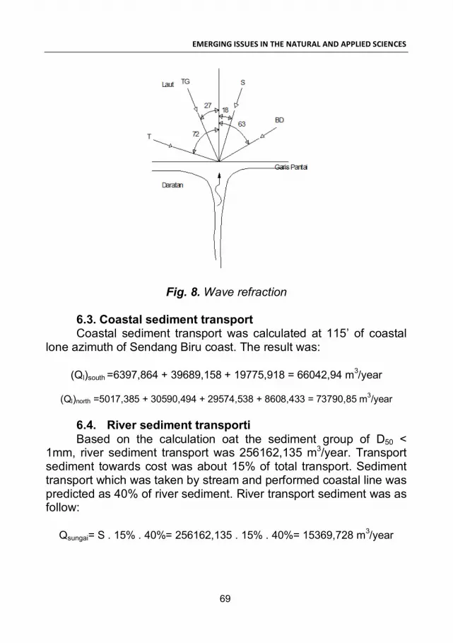
EMERGING ISSUES IN THE NATURAL AND APPLIED SCIENCES
69
Fig. 8. Wave refraction 6.3. Coastal sediment transport Coastal sediment transport was calculated at 115’ of coastal
lone azimuth of Sendang Biru coast. The result was:
(Ql)south =6397,864 + 39689,158 + 19775,918 = 66042,94 m3/year
(Ql)north =5017,385 + 30590,494 + 29574,538 + 8608,433 = 73790,85 m3/year 6.4. River sediment transporti Based on the calculation oat the sediment group of D50 <
1mm, river sediment transport was 256162,135 m3/year. Transport sediment towards cost was about 15% of total transport. Sediment transport which was taken by stream and performed coastal line was predicted as 40% of river sediment. River transport sediment was as follow:
Qsungai= S . 15% . 40%= 256162,135 . 15% . 40%= 15369,728 m3/year

Academic book
70
6.5. Sediment balance and distribution pattern of sediment in estuary Transport sediment balance was performed at normal coastal
line. The result was as follow:
Qsouth = 66042.94 m3/year Qnorth = 73790,85 m3/year Qsungai = 15369,73 m3/uear
Analysis of sediment balance was as follow:
Qsource = Qnorth + Qsungai = 73790,85 + 15369,73 = 89160,58 m3/year Qsink = Qsouth = 66042,94 m3/year
Qnetto = Qsource - Qsink = 89160,58 - 66042,94 = 23117,64 m3/year Transport sediment was 23117,64 m3/year with the distribution
pattern towards left side of normal coastal line. 6.6. Stability analysis of estuary Based on tidal analysis, the tidal prism was 30003,501 m3/0,5
cycle. Budget sediment showed that Bang river had unstable river estuary and it often closed because S < 20. Figure 9 was described as sediment balance and Figure 10 was described distribution pattern of sediment.
Fig. 9. Sketch of sediment balance
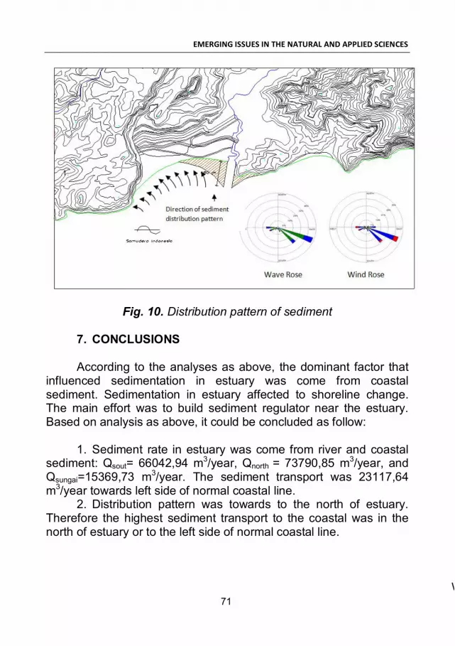
EMERGING ISSUES IN THE NATURAL AND APPLIED SCIENCES
71
Fig. 10. Distribution pattern of sediment 7. CONCLUSIONS According to the analyses as above, the dominant factor that
influenced sedimentation in estuary was come from coastal sediment. Sedimentation in estuary affected to shoreline change. The main effort was to build sediment regulator near the estuary. Based on analysis as above, it could be concluded as follow:
1. Sediment rate in estuary was come from river and coastal
sediment: Qsout= 66042,94 m3/year, Qnorth = 73790,85 m3/year, and Qsungai=15369,73 m3/year. The sediment transport was 23117,64 m3/year towards left side of normal coastal line.
2. Distribution pattern was towards to the north of estuary. Therefore the highest sediment transport to the coastal was in the north of estuary or to the left side of normal coastal line.
Wind Rose

Academic book
72
REFERENCES
1. Grenfell S.E.& Ellfay W.N., 2009, Hydrology, Sediment Transport Dynamics and Geomorphology of a Variable Flow River: the Mfolozi River, South Africa, http://www.wrc.org.za
2. Sakanshi, Yoshihiro; & Tamaki, Akio, 2009, Phase Avera-ged Suspended Sediment Fluxes on intertidal Mudflat Adja-cent to River Mouth, Journal of Coastal Research, West Palm Beach, Florida, March 2009, Vo; 25/2, 350-358.
3. Ali Kokpinar, Mehmat; Daram, Yakub & Guler, Isikhan, 2007, Physical and Numerical Modeling of Shoreline Evalu-ation of the Kizilizmak River Mouth, Turkey, Journal of Coastal Research, March 2007, 23,2, Pro Quest Biology Journals, pg 445
4. Triatmojo,Bambang. 1999. Teknik Pantai. Yogyakarta: Ilmu Teknik Universitas Gajah Mada
5. Predan, Dcepa; Ansev, Tihomir; Dryuan, Ross; and Harris, Michael, Management of Water Reservoirs (Embungs) in West Timoe, Indonesia, Journal of Water Resource Mana-ge, 2011 (25): 339-356
6. Sakanshi, Yoshihiro; & Tamaki, Akio, 2009, Phase Avera-ged Suspended Sediment Fluxes on intertidal Mudflat Adjacent to River Mouth, Journal of Coastal Research, West Palm Beach, Florida, March 2009, Vo; 25/2, 350-358
7. Ikhsan, 2010, Aplikasi Model AVSWAT untuk Pendugaan Sedimentasi Di DAS Bang Kabupaten Malang Akibat Perubahan Tata Guna Lahan, Jurusan Teknik Pengairan, Universitas Brawijaya.
8. Ussy, Suhardjono, 2010, Sediment Transport In Estuary In Bang River Malang, Indonesia, International Journal of Academic Research, Vol 2 No 5.
9. Anonim. 1984. Shore Protection Manual volume dan III, Washington. DC : US Army Corps of Engineers

EMERGING ISSUES IN THE NATURAL AND APPLIED SCIENCES
73
ESTABLISHING KEY DETERMINANTS CONTRIBUTING TO GROWTH OF
CONSTRUCTION COMPANIES: AN EMPIRICAL EXAMINATION
Abu Hassan Abu Bakar, Arman Abd Razak,
Mohamad Nizam Yusof
School of Housing, Building and Planning Universiti Sains
Malaysia, Pulau Pinang, Malaysia (MALAYSIA) E-mails: [email protected], [email protected], [email protected]
ABSTRACT The paper examines the key determinants of firms’ growth of
construction companies in Malaysia. The objectives of this study are to identify which factors play key roles in determining growth as well as to analyze the impact these factors have on growth performance of companies. Data collection for the purpose of this study was done through a questionnaire survey which was carried out involving large construction companies from grade G7 as classified under the Cons-truction Industry Development Board of Malaysia (CIDB). Question-naires were sent to 600 respondents via postal service and by hand. From 600 questionnaires disseminated, 102 of the questionnaires were returned, completed and useable. Data was analyzed by using relevance statistical methods such as relative important index (RII) and regression analysis to establish findings. Findings of this research indicate that the customer orientation factors were found to be the utmost important factor in determining growth of Malaysian construction companies. The results also indicate that management and product quality factor and human factor had a positive significant influence with growth performance.
Key words: Construction companies, firms’ growth, constructi-
on industry, Malaysia

Academic book
74
1. INTRODUCTION In business, change is inevitable for better effectiveness and
efficiency in order to survive and success. As a complex industry comprising a wide array of firms, discipline and practices, change to the organization and activities of the sector might be beneficial to some, but disadvantages for others (1). In the face of these chan-ges, it is increasingly difficult to manage the construction business in today’s environment (2).
The assumption of the traditional economic theory is that firms will pursue an objective of profit maximization. However, according to Weinzimmer (3), organizations can benefit from growth in many ways, including greater efficiencies through economies of scale, increased power, the ability to withstand environmental change, increased profits and increased prestige for organizational mem-bers. As noted by Bonaccorsi and Giannangeli (4), growth does not come at zero cost for firms. A firm’s decision to grow is essentially the result of an assessment regarding the profitability of a new mar-ket opportunity. Hisatomi (5) emphasize that efficiency, effective-ness, reputation as well as increasing market share is important for the survival of a firm.
Contracting is a very complex business, yet registering as a contractor in Malaysia is relatively easy. The Construction Industry Development Board of Malaysia or CIDB (6) notes that low barriers to entry into the industry swell the ranks of contractors with many small scale companies registered as grade G1 contractors under the CIBD grade of registration with G1 being the entry level grade. This grading of contractors, from G1 to G7, is also directly commensurate to the magnitude of projects the contractors may be involved in. Currently, there are approximately 64,000 contractors registered with CIDB, out of which approximately 57% are G1 grade contrac-tors (7), however studies have shown that the failure rate and bankruptcies in Malaysian construction companies are high (8,9).
During the economic crisis of the 1980s and 1990s, many Malaysian construction companies and contractors especially those that were Bumiputera (comprising of individuals of Malay and/or indigenous descent) owned, could not successfully execute their

EMERGING ISSUES IN THE NATURAL AND APPLIED SCIENCES
75
construction projects and had to diversify into other business acti-vities. Contractors of the lower grades suffered more hardship than their higher counterparts, which led them to total bankruptcy (10).
Abu Bakar (11) reports that most construction companies in Malaysia started as small, local market companies during the 1970-1980s period of construction boom. They expanded at different rates and levels of success and growth. About a quarter failed to progress beyond the local level, and one-third made the local-regional-natio-nal transition in 3-5 years. In recent years, with the completion of ‘mega-projects’ and subsequent economic prudence, local projects were insufficient to sustain the 70,000 odd contractors. Thus, many of the lower ranking contractors have left the industry (6). This leads to the question of why is there inconsistency in growth among construction companies within the Malaysian construction industry.
The objectives of this paper are to identify which factors play a more important role in determining growth and to analyze the impact that these factors have on growth performance of construction com-panies.
2. FIRMS’ GROWTH Penrose’s original contribution in 1959 shaped the direction of
growth. From a totally ‘inside-out’ perspective, firms’ growth is now conceived as the endogenous outcome of perennial intra-firm know-ledge creation (12). Firms’ growth demands the ability to master technologies, engender labor skill, organize the production process as well as efficiently serve a market. A firm will exploit a growth opportunity as long as the benefits outweigh the costs, given the level of ability with which the firm was endowed at start-up (4).
According to Skrt and Antoncic (13), in order for the firm to grow, the entrepreneur needs to formulate an exact, clear mission and vision for his or her firm. Strategic planning can be considered important in driving firms’ growth. Strategies such as precisely for-mulating visions and strategy, incorporating the elements of interna-tionalization and networking within the vision of the firm, focusing on growth, profit, and market, performing analyses of market and com-petition, accurately formulating generic business strategies and

Academic book
76
achieving company wide support for strategies can all be beneficial for the growth of smaller firms.
Weinzimmer (3) conclude that many researchers have exami-ned the influence of strategy factors on organizational growth; the relationship between characteristics of top management and organi-zational growth; strategy and industry characteristics on organizatio-nal growth; and industry and top management characteristics on organizational growth. In his conclusion, three sets of determinants had been identified; namely, industry attributes, organization strate-gies and top management characteristics.
Schneider et al. (14) informs that the literature suggests that employee development is especially important for start-up compa-nies to achieve organizational performance and in particular high growth. Bonaccorsi and Giannangeli (4) conclude that the relation-ship between initial size and growth is more complex. By specifically considering very small firms in the sample, several show a positive relationship where a minimum size below which no growth whatso-ever occurs. Entrepreneurs’ competencies may be a triggering factor only if they are associated with larger initial size. True growth is more than adding something to the company - people, office space, sales force (15).
3. FACTORS DETERMINING FIRMS’ GROWTH Several factors contribute to firms’ growth. It differs between
small and large firms and also may vary from country to country, depending on their economic, geographical and cultural differences. In the study on small business growth, Morrison et al. (16) notes that the human factor was considered to be the overwhelming force that determines whether a business will prosper or not. Hillebrant and Cannon (17) identify management as the most important determi-nant of the capacity as well as capability of construction firms. Based on the study of small firms in the island nations of the South Pacific, Yusuf (18) found that good management, access to financing, personal qualities of the entrepreneur, and satisfactory government support were the most important factors to success. Wjewardena and De Zoysa (19) have identifies six principal factors that are
EMERGING ISSUES IN THE NATURAL AND APPLIED SCIENCES
77
perceived to be major contributors to the success or growth of manufacturing firms in Sri Lanka. These factors, in their order of importance, are customer orientation, product quality, efficient management, supportive environment, capital accessibility and mar-keting strategy. Meanwhile CIDB (6) has identifies 8 critical success factors that are pertinent for a successful business in the construc-tion industry, which include productivity, quality, human resources, innovation, environment friendly practices, knowledge, industry sustainability and professionalism.
The factors considered in the study were identified based on studies done by Abu Bakar (11), Abraham and Chinowsky (20), Wjewardena and De Zoysa (19) and Arslan and Kivrak (21). A total of 5 possible factors that were felt to have an effect on the growth of construction companies in Malaysia were determined. These main factors are as follows:
3.1. Human Factor Human Factor is one of the most important factors to be
considered by construction firms in achieving firms’ growth. It is important because it is what really motivates individuals involved in a project and how they act. Managing human factors is vital for project success. It involves all positive and negative aspects of human nature including competition, skill, motivation, loyalty and revenge, and is not noted for its randomness (22). The acquisition of relevant skills, knowledge and competencies for the day-to-day management of construction activities in an increasingly competitive environment is an overriding concern for construction practitioners (23).
3.2. Management Factor A management factor is most likely to be found in firms that
recognize its potential for improving company performance. Good management implies an awareness of all factors making up a suc-cessful business namely good strategy, marketing, pricing and finan-cial control. Organizational infrastructure serves the direct activities of a company - the construction, procurement and marketing. It com-

Academic book
78
prises the organizational setup, its procedures for planning and con-trol, and its information system. The measure of performance, in this respect, is a company’s ability to plan its operations and to conform to the plan in terms of quality, cost and schedule. It is also a company’s ability to adapt itself to changes and new tasks (24).
3.3. Product Quality Factor All buildings constructed are unique. Quality is seen as con-
sisting of those product features which meet the personalized needs of the customers and thereby provide product satisfaction, supple-mented with a proviso of freedom from deficiencies (25).Technology has been identified by many researchers as a source for innovation and growth. Penrose (26) recognizes the valuable role of technology and human resources in defining pools of resources from which the company can draw impetus. Penrose (26) believes that while the economy will provide profitable opportunities for expansion, it is up to the firm to establish an adequate technological ’base’ to realize these opportunities (26).
3.4. Customer Orientation Customer orientation has become increasingly important in
construction. As construction companies face increasing competi-tion, greater attention continues to be placed on customer relation-ships and satisfied customers. Customer satisfaction enables cons-truction companies to differentiate themselves from their competitive and create sustainable advantage. Customer satisfaction also has become an important factor alongside traditional parameters such as quality, schedule and costs. This factor can be seen as a part of the total quality management (TQM) philosophy and recently, it has become a significant part of the key performance indicators (KPIs) in the industry. Many researchers propose the importance of customer satisfaction and its use for evaluating quality from the customers’ perfective (27, 28, 29).
3.5. Environmental Factor Environmental factors can significantly influence construction
opportunities. This factor is those impacting on a business which is

EMERGING ISSUES IN THE NATURAL AND APPLIED SCIENCES
79
beyond the control of a company’s management. In general, they are independent of contractor’s performance, but could directly affect the success of a contractor or even their survival (37). Since some of these external factors could be triggered by the society, their influence may vary from time to time depending upon the change in public interests, market fluctuations, policy changes, etc. For example in order to growth, the construction companies must identify new market opportunities to expand their share of the mar-ketplace and utilizing any process to assess the current political con-ditions.
These factors were used for the purpose of establishing factors determining growth of construction companies in Malaysia.
4. RESEARCH FRAMEWORK The main variable of interest to this study is the dependent
variable of growth performance which is measured by the annual turnovers. The independent variables that may influence the depen-dent variable are the main factors that contribute to the firms’ growth namely, Human Factor, Management Factor, Product Quality Factor, Customer Orientation and Environmental Factor. The relationship between the dependent and independent variables is visualized in Figure 1:
Fig. 1. Research framework

Academic book
80
5. METHODS This study is using quantitative methods and provides questi-
onnaire as the prime source of getting primary data. This question-naire was divided into four main sections that covered respondents’ background, firm’s background, firm’s performance and firm’s growth factors. Questionnaires were sent to 600 randomly selected respon-dents (large construction companies registered as grade G7 con-tractors under CIDB classification) via postal service and by hand, out of a total population of 3,000 G7 contractors. From 600 question-naires disseminated, 102 (17% response rate) of the questionnaires were returned, completed and useable. Data was analyzed by using relevance statistical methods such as confirmatory factor analysis and regression analysis to establish findings. Besides this, the collected data was also analyzed using the relative importance index (RII) of the various factors that contribute to firm growth factors (30).
The dependent variable in this study is firms’ growth. Firms’
growth can be measured by several attributes such as turno-ver/sales, employment, assets, market shares, and profits. However, in the context of this study, growth in turnover is used as an indicator of growth performance. In order to carry out regression analysis, the dependent variable was split into high growth (increase of more than 50%), low growth (increase below than 50%) and unchanged growth.
6. ANALYSIS 6.1. Respondent’s Background The respondent’s position in the firm is important in acquiring
the desired feedback. From the analysis, the job designations of the respondents were mainly managing directors representing 27.2%. Engineer/quantity surveyors contributed the second highest percent-tage of 25.5%. Other positions of the respondents were project managers (15.7%), general managers (10.8%) and others, contribu-ting to 6.9%. In terms of status of the firm of the respondents, 80.4%

EMERGING ISSUES IN THE NATURAL AND APPLIED SCIENCES
81
were from private limited companies, 16.7% came from partnership companies and only 2% were from cooperation/consortium based companies. In terms of value of the respondents’ firm’s annual work, 26.5% of the respondents were involved in projects worth between RM11 - RM20 million, 24.5% of the respondents dealt with projects worth more than RM41 million, 16.7% of the respondents from pro-jects worth between RM 5 million - RM 10 million and 15.7% of the respondents were handling projects worth between RM 31 million - RM 40 million. In terms of firms’ age, 52.4% of the respondents were from firms that were set up more than 10 years ago. Firms founded between 5 - 10 years constituted 38.1%, followed by 7.1% for firms established between 3 - 5 years. Firms that began operations for less than 3 years contributed to only 2.4%. This clearly shows that most of the firms involved in this study are well experienced in construction works
6.2. Frequency distribution on Turnover Growth from Company Start Up to Current Operation Table 1 shows the frequency distribution on turnover growth
level from the company start up to current operation. From the Table 1, it can be seen that 48% of the respondents can be considered as having undergone high growth in turnover growth, while 29.5% of the respondents can be considered as having low growth. The analysis shows that most of the respondents have a high growth in turnover growth.
Table 1. Frequency distribution on Turnover Growth from
the Company Start Up to Current Operation
Growth Levels Number of Firm (%) Turn Over
High Growth (> 50%) 48 Low Growth (<50%) 29.5 Unchanged (0%) 22.5
Total 100

Academic book
82
6.3. Ranking of Factors of Firms’ Growth Table 2 shows the main factors of firm growth and their overall
ranking. The importance of these factors, as perceived by the res-pondents, has been ranked on the basis of their RII values. The closer the RII to 1, the higher is the importance of the factor. From Table 2, it shows that customer orientation presents the most impor-tant factor influencing the growth of construction companies with an average RII = 0.8601, followed by management factors, human factor, environmental factor and product quality with an average RII of 0.8546, 0.8473, 0.7976 and 0.78112 respectively.
Table 2. Ranking of Factors of Firm Growth
Firms’ Growth Factors
∑w RII Rank
Customer Orientation 438 0.8601 1 Management Factor 435 0.8546 2 Human Factor 432 0.8473 3 Environmental Factor 406 0.7976 4 Product Quality 398 0.78112 5
6.4. Multiple Regression of Turnover Growth on the independent variables (Firms’ Growth Factors) Table 3 summarizes the multiple regression results of the
dependent variable (turnover growth) and progress with firms’ growth factors. The enter method was used to run this analysis. As a result, the 4 combined variables together significantly explained 59.8% of the variance in employment growth (F=36.029, p<0.01, R2= 0.598), while the remaining 40.2% is not explained. From Table 7, it is noted that there are three variables that are significant in influencing turnover growth. The significant variables are manage-ment and product quality factor (β =.359, p< 0.01), human factor (β =.269, p< 0.01) and customer orientation factor (β =.329, p< 0.01). Only environmental factor was found not significant in influencing the turnover growth in this study.

EMERGING ISSUES IN THE NATURAL AND APPLIED SCIENCES
83
Table 3. Result of Multiple Regression analysis for Turnover Growth
Firms’ Growth Factors Turnover Growth
R2=0.598 F=36.029*
β t Sig. Constant -7.705 .000 Human Factor .269 4.002** .000 Management and Product Quality Factor .359 4.372** .000
Customer Orientation .329 3.745** .000 Environmental Factor .102 1.403 .164
Dependent Variable: Turnover Growth *Significant level at p<0.05 **Significant level at p<0.01 7. DISCUSSION
Several findings have been discovered through this study.
From the analysis, customer orientation was found to be the utmost important factor that contributes to the growth of construction companies. In construction, customer orientation has been conside-red as a dimension of quality (29,27, 31) and as an important factor indicating a project’s success (32, 33). It also can be observed as a tool for developing the construction process (34, 35) and a tool for mutual learning (36). This factor should be aptly given more atten-tion by construction companies that aim to achieve growth in their firms. The second important factor in determining firm’s growth is management factor, followed by human factor, environmental factor and product quality factor.
As been mentioned before, firm growth can be measured by several of indicators such as profit, sales, market coverage, employ-ment and many more other factors. However, this study used annual turnover as the basis for growth measurement. From the analysis, management and product quality, human factor and customer orien-tation had a substantial relation with turnover growth. The factor of

Academic book
84
management and product quality can be considered to be the highest significant factor that determines turnover growth. These fin-dings, shows that management and product quality factor, human factor and customer orientation are the most significant factors that have a positive relationship with growth performance of Malaysian construction companies. A study done by Wjewardena and De Zoysa (19) confirms these findings where a positive relationship amongst product quality, customer orientation and efficient manage-ment was found crucial to a company’s performance.
8. CONCLUSION AND RECOMMENDATION The study had successfully achieving the objectives of this
study, which was to identify which factors play a more important role in determining growth and to analyze the impact of these factors have on growth performance of construction companies that had been explained and adduced through the findings.
These findings can act as a basic guideline for construction companies in Malaysia that have the aim to further develop and grow. Companies that achieve growth will subsequently go on to contribute more actively towards the development of nation’s econo-my and social elements. However, the study is not suggested that a firm will automatically succeed or grow by addressing all these issu-es, but rather, it is almost certain that a firm will have a more possib-le tendency to decline if these factors are ignored.
This result provides important implications for the construction companies. Companies with growth ambitions should not only rely on a competitive strategy; they should also rationally evaluate the overall capabilities of the firm. The results of this study can be utili-zed as a basis for the top management of a firm to make a strategic choice in enabling the company to grow. Correct and appropriate decisions are crucial for construction companies to remain active and grow in today’s challenging business environment.
Future research should be carried out on the barriers or challenges to a firm’s growth. This area is important due to the fact that as companies grow, there are a number of challenges that must be faced and ultimately overcome. By using the findings from this

EMERGING ISSUES IN THE NATURAL AND APPLIED SCIENCES
85
and future studies as a guide, construction companies, would be able to progressively grow and emerge as key players within the industry, either locally, regionally or even at a global scale.
ACKNOWLEDGEMENT The authors acknowledge the financial support provided by
Research University Grant of the Universiti Sains Malaysia (USM), Penang, Malaysia for the success of this research.
REFERENCES 1. Harty, Chris et. all. (2006). The Future of Construction: a
Critical Review of Construction Future Studies. Construc-tion Management and Economics, Vol.25 pp. 477-493.
2. Betts M. and Ofori G. (1992). Strategic Planning for Compe-titive Advantage. Construction Management and Econo-mics, 10, 511-32.
3. Weinzimmer L. G. (2000). A Replication and Extension of Organizational Growth Determinants. Journal of Business Research, Vol. 48, pp. 35-41.
4. Bonaccorsi A. and Giannangeli S. (2008), One or More Growth Process? Evidence From New Italian Firms. Small Business Economics.
5. Hisatomi Y. (1990). An Introduction to Japanese Construction Industry and General Contractors, CIB 90, (5), (247-255). http://www.cidb.gov.my/cidbweb/bin/corporate/cimp/CIMP_Fwd.pdf
6. CIDB (2006). Malaysia Construction Industry Master Plan 2005-2015. Construction Industry Development Board Malaysia, Kuala Lumpur.
7. CIDB (2008a). Contractors Registered [online]. Available: http://www.cidb.gov.my.
8. Yin K.Y. (2006). How to become a competent contractor. The Monthly Bulletin of the institution of Engineers, Journal of Jurutera, Malaysia, 2, pp. 38-39.

Academic book
86
9. CIDB (2008b). Dormant and Non- Active Contractors 2006-2008, Kuala Lumpur, Malaysia
10. Ghani A.M.M. (1988). Kemelesetan Ekonomi dan kesannya ke atas penglibatan kontraktor- kontraktor bumiputera di wilayah utara Malaysia, Unpublished Master Thesis, School of Housing, Building and Planning, University Science of Malaysia.
11. Abu Bakar A. H. (1993). Growth Strategy for Construction Companies in Developing Countries, A Malaysian Experien-ce. CIB W-65 Symposium 93, Port of Spain, Trinidad.
12. Volpe L. and Biferali D. (2008). Edith Tilton Penrose, The Theory of the Growth of the Firm. Journal Manage Governance, Vol. 12, pp. 119-125.
13. Skrt B. and Antoncic B. (2004). Strategic Planning and Small Firm Growth: An Empirical Examination. Managing Global Transition, Vol. 2, Number 2, pp. 107-122.
14. Schneider J.,Dowling M. and Raghuram S. (2007). Empowerment As a Succes Factor in Start-up. RMS, 1:167-184.
15. Recklies O. (2001). Managing Growth - Barriers and Pre-conditions, Recklies Management Project GmbH, http://themanager.org/pdf/ManagingGrowthII.PDF
16. Morrison L., Breen J. and Shameen A. (2003) Small Busi-ness Growth: Intention, Ability and Opportunity, Journal of Small Business Management, Vol.41 (4): 417-425.
17. Heffernal P. (2007). Constraint on the Growth of Techno-logy-Based Firm- Perception and Effects (paperback), Uni-ted Kingdom: University of Cambridge, Institute for Manu-facturing.
18. Yusuf, Attahir (1995). "Critical Success Factors for Small Business: Perceptions of South Pacific Entrepreneurs," Journal of Small Business Management 33(1), 68-73.20.
19. Wijewardena H. and De Zoysa A. (2005). A Factor Analytic Study of the Determinants of Success in Manufacturing SMEs, 35th EISB Conference - Sustaining the Entrepreneu-rial Spirit Over Time, Barcelona, Spain, 12-14 September, 2005, pp. 1-11.

EMERGING ISSUES IN THE NATURAL AND APPLIED SCIENCES
87
20. Abraham L.G. and Chinowsky P. (2002) Critical Success Factors for the Construction Industry. First International Conference on Construction in the 21st Century, pp. 427-434.
21. Arslan G. and Kivrak S. (2008) Critical Factors to Company Success in the Construction Industry. World Academy of Science, Engineering and Technology. 45, pp. 43-46.
22. Pender S. (2001) Managing Incomplete Knowledge: Why Risk Management is Not Sufficient. International Journal of Project Management, 19(2), pp. 79-87.
23. Egbu C.O. (1999) Skills, Knowledge and Competencies for Managing Construction Refurbishment Works. Construction Management and Economics Journal 17(1), pp. 29 - 43.
24. Warszawski A. (1996). Strategic Planning in Construction Companies. Journal. of Construction Engineering and Management, pp. 133-140.
25. Sommerville, J. and Robertson, H.W. (2000) A Scorecard Approach To Benchmarking For Total Quality Construction. International Journal Quality Reliability Management, 17(4), pp. 453-466.
26. Penrose E. (1959). The Theory of the Growth of the Firm, Oxford University Press.
27. Barrett P. (2000). Systems and Relationships for Construc-tion Quality. International Journal of Quality and Reliability Management, 17(4), pp. 377-392.
28. Maloney W.F. (2002) Construction Product/ Service and Customer Satisfaction. Journal of Construction Engineering and Management, pp 522-529.
29. Yasamis F., Arditi D. and Mohammadi J. (2002). Assessing Contractor Quality Performance. Construction Management and Economics, 20, pp. 211-223.
30. Tam C.M., Deng Z.M., Zeng S.X. and Ho C.S., (2000). Quest for continuous quality improvement for public housing construction in Hong Kong. Construction Manage-ment and Economics, Vol.18 (4), pp. 437-446.

Academic book
88
31. Palaneeswaran E., Ng T. and Kumaraswamy M. (2006). Client Satisfaction and Quality Management Systems in Contactor Organisations. Building and Environment,41(11), pp. 1557-1570.
32. Sanvido V., Grobler F., Parfitt K., Guvenis M. and Coyle M. (1992). Critical Success Factors for Construction Projects. Journal of Construction Engineering and Management, 118(1), pp. 94-112.
33. Chan A.P.C and Chan A.P.L, (2004). Key performance indi-cators for measuring construction success, Benchmarking an International Journal, Vol 11 No.2, pp.203-221.
34. Egan, J. (1998). Rethinking Construction: The Report of the Construction Task Force to the Deputy Prime Minister, Department of the Environment, Transport and the Regi-ons, Norwich.
35. Mbachu J. and Nkado R. (2006). Conceptual Framework for Assessment of Client Needs and Satisfaction in the Building Development Process. Construction Management and Eco-nomics, 24, pp. 31-44.
36. Love P.E.D., Smith J., Treloar G.J. and Li H. (2000). Some Empirical Observations of Service Quality in Construction. Engineering Construction and Architectural Management, 7(2), pp. 191-201.
37. Ng S.T., Tang Z. and Palaneeswaran E. (2009). Factors Contributing to the Success of Equipment-Intensive Sub-contractors in Construction. International Journal of Project Management, 27(7), pp. 736-744.

EMERGING ISSUES IN THE NATURAL AND APPLIED SCIENCES
89
DIFFUSION MODEL FOR THE FINANCING OF A FUND THAT RISKS RUIN
Prof. Dr. Manuel Alberto M. Ferreıra, Dr. Marina Andrade
Instituto Universitário de Lisboa (ISCTE-IUL),
UNIDE - IUL, Lisboa (PORTUGAL) E-mails: [email protected], [email protected]
ABSTRACT It is proposed initially a diffusion process to represent a system
subject to systematic ruin, with a stochastic regime of inflows and outflows of capital, establishing an analogy between this process and a pensions fund. Based the system in a periodic reflection scheme, it is valued the additional necessary financing to overcome the ruin. It is used, with this propose the Renewal Theorem for “renewal-reward” processes. That valuation is discussed, when it is applicable a deterministic interest rate, after the first passage times Laplace Transform.
Key words: Pensions funds, diffusion, ruin, first passage
times, Renewal, Laplace Transform. 1. THE MODEL This approach was originally motivated by the search of a
stochastic model to represent the reserves of a fund, subject to an operation regime similar to the social security pensioners systems one, where the inflows through the so called social security contribu-tions are regularly insufficient for the compromised pensions pay-ments. In a more general perspective, it was intended to model a stochastic system with expenditures greater than the resources got during its operation, so needing a compensation external source of that unbalance. It was also intended to evaluate those external needs.

Academic book
90
The objective is to do so based on diffusion processes, a spe-cial class of stochastic processes with continuous path. The work of (Karlin and Taylor, 1981) will be often used in this application.
So be a diffusion process 푋 , 푡 ≥ 0, that represents the system reserves value at time t, defined by
푋 = 푋 + 푋 − 푋
where 푋 is a diffusion that represents the inflows total value,
inputs or contributions till time t, and 푋 is another diffusion that represents the outflows total value, outputs or pensions, till time t, and be the particular form
푋 = 훼 + 푎푡 + 푐푊 − 푏푥 푑푠 = 훼 + (푎 − 푏푋 ) 푑푠 + 푐푑푊 (1.1)
where 푊 is the standard Brownian motion, see (Arnold, 1974)
and 훼, 푎, 푏 and 푐 assume positive values. Here is, 푋 = 푎 and 푋 = 푎푡 + 푐푊 , the Brownian motion begin at the origin with infinitesimal mean and variance given by 푎 and 푐 , respectively. The Brownian motion is acceptable as approximation to the process when a is conveniently greater than c so that the Brownian motion approximates a process with non negative increments. It is advanced also with 푋 = ∫ 푏푋 푑푠, that is with output process with differential at instant t given by b times its own value 푋 . Note that this representation only makes sense while 푋 ≥ 0. Later this question will be analysed. For the instant it will be considered the process 푋 with states space in the set of real numbers, with no restrictions.
Emphasise from (1.1) that 푋 is a diffusion process with
infinitesimal mean and variance, 휇 (푥) = 푎 − 푏푥 and 휎 (푥) = 푐 , where may be recognized the Ornstein-Uhlenbeck “mean-reverting” process, see (Arnold, 1974). The stochastic integral equation (1.1) is a linear equation, strictu sensum, that admits an explicit solution

EMERGING ISSUES IN THE NATURAL AND APPLIED SCIENCES
91
푋 =푎푏
1 − 푒 + 훼푒 + 푐푒 ( ) 푑푊 (1.2).
It is enough to observe that in (1.2) 푋 may be given in the
form
푋 = 푒 푌 , with 푌 = 훼 + 푎 푒 푑푠 + 푐 푒 푑푊 (1.3)
in order to verify, trough Itô’s Theorem that the present solu-
tion satisfies the initial equation, see again (Arnold, 1974). Although an alternative approach will be presented, in some aspects simpler.
Observe that in the solution (1.2) the process 푋 results from the transformation
푋 = 푈 + 푓(푠) 푑푠 (1.4)
where
푈 = 훼푒 + 푐푒 ( ) 푑푊 (1.5)
is the Ornstein-Uhlenbeck diffusion process with origin at
푈 = 훼 and infinitesimal mean and variance 휇 (푥) = −푏푥 and 휎 (푥) = 푐 and
푓(푠)푑푠 = 푎푒 푑푠 =푎푏
1 − 푒 (1.6)
Knowing that the type (1.4) diffusions elementary
transformations originate diffusion processes with the coefficients, see (Bhattacharya and Waymire, 1990),
휇 (푡, 푥) = 휇 푥 − 푓(푠) 푑푠 + 푓(푡) and 휎 (푡, 푥)
= 휎 푥 − 푓(푠) 푑푠 ,

Academic book
92
it is obtained
휇 (푡, 푥) = −푏 푥 − 푎 푒 푑푠 + 푎푒 = 푎 − 푏푥 and 휎 (푡, 푥) = 푐
as it had to be. The present situation is a special case where
through a type (1.4) modification, an homogeneous diffusion generates another homogeneous diffusion – time homogeneity – that is, with coefficients 휇 and 휎 independent of t.
Note 1.1. It may be used immediately (1.4) and the known characterris-
tics of the Ornstein-Uhlenbeck process to conclude that 푋 is a Gaussian process with, (Arnold, 1974),
퐸(푋 ) = 퐸 푈 + 푓(푠) 푑푠 = 훼푒 +푎푏
1 − 푒 (1.7)
퐶표푣(푋 , 푋 ) = 퐶표푣(푈 , 푈 ) = 푒 ( ) 푐2푏
푒 − 1 , 0 ≤ 푠 ≤ 푡 (1.8). Observe in particular that 퐸(푋 ) = for 훼 = and that in
general lim →∞퐸(푋 ) = . ∎ Note 1.2. In the conditions initially presented, clear that it is obtained for
the output process
푋 = 푏푋 푑푠 = 훼 + 푋 − 푋
= 훼 1 − 푒
+ 푎 1 − 푒 ( ) 푑푠 + 푐 1 − 푒 ( ) 푑푊
= 훼 −푎푏
1 − 푒 + 푐푏 푒 ( ) 푊 푑푠 (1.9)

EMERGING ISSUES IN THE NATURAL AND APPLIED SCIENCES
93
where, only by reference the last integral is obtained through integration by parts of 푐 ∫ 1 − 푒 ( ) 푑푊 ; 푋 is still a Gaussian process, but not now a Markov process, with expected value and covariance functions that are obtained here with the help of (1.4) and the integrated Ornstein-Uhlenbeck process characteristics, (Arnold, 1974):
퐸(푋 ) = 퐸 푏푋 푑푠 = 푏퐸 푈 푑푠 + 푓(푢) 푑푢푑푠
= 훼 −푎푏
1 − 푒 + 푎푡 (1.10)
퐶표푣(푋 , 푋 ) = 퐶표푣 푏푋 푑푢, 푏푋 푑푢
= 푏 퐶표푣 푈 푑푢, 푈 푑푢
= 푐 푠
+푐2푏
−2 + 2푒 + 2푒 − 푒 ( ) − 푒 ( ) , 0 ≤ 푠≤ 푡 (1.11).
In particular, 퐸(푋 ) = 푎푡 when 훼 = , and there is an
asymptote 훼 = + 푎푡 to the function 퐸(푋 ). ∎ 2. TIME TO RUIN Call 푇 , the first passage time by 푦, −∞ < 푦 < ∞, of the푋
process, 푇 , = 푖푛푓{푡 ≥ 0: 푋 = 푦}, 푇 = 푇 , and 휌(훼, 푦) the probabi-lity of being finite: 휌(훼, 푦) = 푃 푇 , < ∞ .
Consider the ruin problem, that is the evaluation of 휌(훼) =휌(훼, 0), the probability of the 푋 time of first passage by 0 to be finite. The problem may be solved with a support of the scale and velocity functions of the considered diffusion process. This will be done following (Bhattacharya and Waymire, 1990). Attending the coeffi-

Academic book
94
cients 휇 (푥) = 푎 − 푏푥 and 휎 (푥) = 푐 , it is obtained for the scale function
푠(푥) = 푒푥푝 −2휇 (푧)휎 (푧) 푑푧 푑푦
= 푒푥푝(푏푦 − 푎)
푏푐푑푦, any 푢 (2.1)
and for the velocity function
푚(푥) =2
휎 (푦) 푒푥푝 −2휇 (푧)휎 (푧) 푑푧 푑푦
=2√휋푐√푏
Φ√2(푏푥 − 푎)
푐√푏−
12
, any 푢, Φ(푥)
=1
√2휋푒 푑푦
∞ (2.2).
Evaluating the scale function in the bounds of the state space
it may be concluded that the process 푋 is a recurrent diffusion process, once 푠(−∞) = −∞ and 푠(∞) = ∞ lead to 휌(훼, 푦) =1 for any − ∞ < 푦 < ∞. Considering additionally the velocity function, the conditions 푚(−∞) = −푚(∞) = − √
√, 푚(−∞) > −∞ and 푚(∞) < ∞
lead to the positive recurrence for the diffusion process in the states space (−∞, ∞), that is first passage time with finite expected value: 퐸 푇 , < ∞. In particular, for the case interesting to define 퐸(푇 ):
퐸 푇 , =2√휋푐√푏
Φ√2(푎 − 푏푧)
푐√푏푒푥푝
(푏푧 − 푎)푏푐 푑푧, 푦 < 훼 (2.3).
So for the diffusion process 푋 , initially proposed, the ruin is a
sure event, 휌(훼) = 1, in a time with finite expected value, 퐸(푇 ) < ∞.

EMERGING ISSUES IN THE NATURAL AND APPLIED SCIENCES
95
Note 2.1. Pay attention that 푇 , , the 푋 process first passage time by y,
훼 > 푦, may be interpreted also as the Ornstein-Uhlenbeck process 푈 first passage time by the curve 1 − 푒 .
It may be also referred that it may be used immediately the scale function in (2.1) to define the function
휙(푦) = 푃 푇 , < 푇 , , 0 ≤ 훼 ≤ 푦,
corresponding to the probability of not being lesser than y the
maximum of 푋 before the ruin, with value 1 for 훼 > 푦. After (Bhattacharya and Waymire, 1990)
휙(푦) =푠(훼) − 푠(0)푠(푦) − 푠(0) =
∫ 푒푥푝 (푏푧 − 푎)푏푐 푑푧
∫ 푒푥푝 (푏푧 − 푎)푏푐 푑푧
(2.4). ∎
Note 2.2. The formulae (2.3) and (2.4) are relevant results without direct
numerical resolution. For the first case, formulae (2.3), some numerical results are presented in Table 1,
Table 1. Numerical results for 퐸(푇 ).
휶 a b c 푬(푻휶) 휶 a b c 푬(푻휶)
1 10 1 3 32353.20 2 6 2 2 42.42 10 10 1 3 37472.41 3 6 2 2 43.47 1 10 10 3 0.45 2 6 3 2 8.11 10 10 10 3 0.73 3 6 3 2 8.46 1 10 2 3 110.51 5 6 1 2 5117.45 1 10 5 3 2.07 1 6 5 2 1.66 10 10 5 3 3.08 5 6 5 2 2.24
obtained with basis in the approximation by Simpson’s rule:

Academic book
96
퐸(푇 ) = 푔(푥)푑푥, being 푔(푥)
=2√휋푐√푏
Φ√2(푎 − 푏푧)
푐√푏푒푥푝
(푏푧 − 푎)푏푐
≅훼
300푔(0) + 4푔
훼100
+ 2푔2훼
100+ 2푔
98훼100
+ 4푔99훼100
+ 푔(훼) . ∎
3. FINANCING VALUE As it was seen, 휌(훼, 푦) = 1 and 퐸 푇 , < ∞ with any 푦 < 0
holds for the diffusion process 푋 defined in section 1.. These conditions are not compatible with the interpretation advanced initially once, as it was mentioned that interpretation only make sense for 푋 ≥ 0.
So consider the reserves value evolution of the fund, under external financing, stochastic process 푋 , obtained from 푋 under the following financing scheme: whenever the reserves end it is donate to the fund a provision in a value equal to the initial one, that is, with value 훼. This corresponds to consider a reflecting barrier at 0 that produces an instantaneous reposition effect of the process in 훼. Having in mind that the origin diffusion is homogeneous in relation with time, the process 푋 under the action of this barrier is a regene-rative process, as it reinitiate in each reflection instant, that is, regeneration epoch. Clear that will be considered 푋 paths righteous continuous, with 푋 = 훼 in any regeneration epoch 휏 > 0.
The sequence of time intervals between regeneration epochs Δ = 푇 , Δ , Δ , … is a sequence of i.i.d. random variables and the sequence 휏 , 휏 , 휏 , … of waiting times for the first, the second, the third, …, regeneration is so defined for the sequence of i.i.d random variables partial sums 휏 = Δ ; 휏 = 휏 + Δ , 푛 = 2, 3, ….
Be now the renewal process 푁 defined for the sequence, enlarged, of waiting times 휏 = 0, 휏 , 휏 , … , 푁 = 푠푢푝{푛: 푡 ≤ 푡} through which it is possible to define in a more formal way the financing

EMERGING ISSUES IN THE NATURAL AND APPLIED SCIENCES
97
process 퐴 , as it was formerly described, by 퐴 = ∑ 푅 , 퐴 =0 푖푓 푁 = 0, where 푅 = 훼 designates the n-th provision given to the fund.
The process 퐴 is a typical “renewal-reward” process for which is valid the Renewal Theorem, see (Tijms, 1994),
푙 = lim→∞
퐴푡
= lim→∞
퐸(퐴 )푡
=퐸(푅 )퐸(푇 )
=훼
∫ 2√휋푐√푏
Φ √2(푎 − 푏푧)푐√푏
푒푥푝 (푏푧 − 푎)푏푐 푑푧
(3.1).
In particular, only to the protection value against the ruin risk,
using L’Hospital’s Rule to determine the following iterated limit
푙 = lim→
lim→∞
퐴푡
= lim→
lim→∞
퐸(퐴 )푡
=1
2√휋푐√푏
Φ 푎√2푐√푏
푒푥푝 푎푏푐
(3.2).
It may be useful to consider, in relation with the operation
scheme presented at the beginning of this section, the placement of a reflection barrier in a point different from 0, say in 훽, 0 < 훽 < 훼. The adaptation of the results (3.1) and (3.2) to this situation is immediate considering 푇 , instead of 푇 and making 푅 = 훼 − 훽. Consequently,
푙 , = lim→∞
퐴푡
= lim→∞
퐸(퐴 )푡
=퐸(푅 )
퐸 푇 ,
=훼 − 훽
∫ 2√휋푐√푏
Φ √2(푎 − 푏푧)푐√푏
푒푥푝 (푏푧 − 푎)푏푐 푑푧
(3.3)
and

Academic book
98
푙 , = lim→
lim→∞
퐴푡
= lim→
lim→∞
퐸(퐴 )푡
=훼 − 훽
2√휋푐√푏
Φ √2(푎 − 푏훽)푐√푏
푒푥푝(푏훽 − 푎)
푏푐
(3.4).
Note 3.1. It is used the following numerical example to emphasize the
utilization of the financing scheme presented in the formation of the implicit output process rate at 푋 , say the process푋 . Remembering the observations presented ate section 1., in particular to the case 훼 = , that rate will be
푎∗(푡) =푑퐸 푋
푑푡≅ 푎 + 푙
= 푎 +푎
푏 ∫ 2√휋푐√푏
Φ √2(푎 − 푏푧)푐√푏
푒푥푝 (푏푧 − 푎)푏푐 푑푧
(3.5).
Choosing, for instance, a = 6, c = 2 and 푎∗(푡) ≅ 1.1푎 = 6.6, the
expression (3.5) is fulfilled to the value b = 4.61.∎ Note 3.2. In this note it is presented briefly the formulation of the finan-
cing actual value when this proceeding is applicable, namely when the process described runs under the influence of a capitalization function, and the problems found in that valorisation. So when it is appropriate the application of a deterministic actualization rate, say with value 푟, 푟 > 0, the perpetual financing actual value is the random variable

EMERGING ISSUES IN THE NATURAL AND APPLIED SCIENCES
99
퐵 = 훼푒∞
(3.6)
with expected value
퐸(퐵 ) = 퐸 훼푒∞
=훼퐸(푒 )
1 − 퐸(푒 ) (3.7).
The resolution of (3.7) demands the knowledge of 퐸(푒 )
that while function of r is the Laplace Transform of the first passage time 푇 . Instead, consider that function dependent of 훼, that is, 휈(훼) = 퐸(푒 ). It is known, see (Karlin and Taylor, 1981) and (Feller, 1971) that 휈 satisfies the 2nd order differential equation
휎 휈′′ + 휇 휈′ = 푟휈, with 휈(0) = 1, that is
푐2
휈′′ + (푎 − 푏훼)휈′ = 푟휈, with 휈(0) = 1 (3.8). The equation (3.8) has a general solution expressed as a
power series, see (Apostol, 1969), ∑ 푘 훼 ,∞ in the form
휈(훼) = 푘 휈 (훼) + 푘 휈 (훼) = 푘훼푛!
푘 , +∞
푘훼푛!
푘 ,
∞
where the coefficients 푘 , and 푘 , may be obtained through
the following recursive scheme
푘 , = 1, 푘 , = 0, … , 푘 , =−2푎
푐푘 , +
2(푟 + (푛 − 2)푏)푐
푘 , ,
푘 , = 0, 푘 , = 1, … , 푘 , =−2푎
푐푘 , +
2(푟 + (푛 − 2)푏)푐
푘 , (3.9).

Academic book
100
The border condition 휈(0) = 1 implies the specialization of this solution 푘 = 1, so obtaining 휈(훼) = 휈 (훼) + 푘 휈 (훼). To get a particular solution depends only on
푘 = 휈′(0) = lim→
휈(휀) − 휈(0)휀
= lim→
퐸(푒 ) − 1휀
. Important for this subject are the papers (Gerber and Pafumi,
1998) and (Figueira and Ferreira, 2000) that developed the solution of this problem in the case where the Brownian motion is the support model.∎
ACKNOWLEDGMENT The authors gratefully thank to Professor J. Figueira from
ISCTE – IUL his cooperation in this paper and permission to use results from (Figueira and Ferreira, 2000) and (Figueira, 2003).
REFERENCES
1. S. Karlin and H. Taylor. A Second Course in Stochastic
Processes. Academic Press, New York, (1981). 2. L. Arnold. Stochastic Differential Equations: Theory and
Applications. John Wiley & Sons, New York, (1974). 3. R. N. Bhattacharya and E. Waymire. Stochastic Processes
with Applications. John Wiley & Sons, New York, (1990). 4. H. C. Tijms. Stochastic Models: An Algorithmic Approach.
John Wiley & Sons, Chichester, (1994). 5. W. Feller. An Introduction to Probability Theory and Its
Applications, vol. II 2nd Edition. John Wiley & Sons, New York, (1971).
6. T. Apostol. Calculus, vol. II. John Wiley & Sons, New York, (1969).
7. J. Figueira and M. A. M. Ferreira. Modelo para o estudo da ruína num fundo de pensões. Working paper, (2000).

EMERGING ISSUES IN THE NATURAL AND APPLIED SCIENCES
101
8. H. Gerber and G. Pafumi. Stop-loss a tempo continua e protezione dinamica di un fondo d’investimento. Rivista di Matematica per le Scienze Economiche e Sociali, vol. 21, 125-146, (1998).
9. J. Figueira and M. A. M. Ferreira. Financiamento dum fundo sujeito a ruína com base num modelo de difusão. Instituto dos Actuários Portugueses - Boletim, 40, 7-20, (2000).
10. J. Figueira. Aplicação dos Processos de Difusão e da Teoria do Renovamento num estudo de reservas aleatóri-as. Phd Thesis, presented at ISCTE, Lisboa. Supervisor M. A. M. Ferreira. (2003).

Academic book
102
SPAN WELL, AN INNOVATION IN IRRIGATION DESIGN
Dwi Priyantoro, Lily Montarcih L.
Water Resources Department, Faculty of Engineering,
University of Brawijaya (INDONESİA) E-mails: [email protected], [email protected]
ABSTRACT This paper studied the system of water supply and design
analysis of span well at Tibunangka Irrigation Area. Tibunangka was located at Central Area Lombok Island, Indonesia. The methodology consisted of irrigation water supply analysis, analysis of average discharge, water requirement, surplus and deficit of water, well volu-me which was used to reserve surplus discharge at rainy season, construction material of span, and the location of span. Results were used as a pattern of irrigation water supply, the rule and procedure of distributing irrigation water need at the location. And as a recommendation of developing span well. Span well was a new idea which was developed for supplying water at irrigation area.
Key words: irrigation water supply, span well, design,
procedure 1. INTRODUCTION An integrated water resource management approach is requi-
red to balance environmental, social and economic issues, rather than the conventional technique of “hydraulic mission” [1]. It was suggested that such an approach would increate the efficiency of water use and enable society to achieve sustainability, while optimi-zing the economic return on water [2]. In some area of the world, especially regions with high population density and intense econo-mic actively, the demand for fresh water has overtaken the supply.
EMERGING ISSUES IN THE NATURAL AND APPLIED SCIENCES
103
The correct management of water resources requires the maintaining of environmental-economics balance under which the damage inflicted on natural objects, and their resources is compen-sated for the water environmental investments from the funds deri-ved from water use [3]. The implementation of such management regime is hampered by the uncertainty of many factors that affect the decision-making and create the risk of ineffective investments in water protection measures. The improvement of management effici-ency requires studying the relationships between water quality indices, water use characteristics, and the volume and direction of investments [4].
Watershed restoration efforts have sought to balance poverty alleviation against conservation, and local governance versus tech-nical expertise. Poverty alleviation is often central to any effort and watershed development is no exception [5]. Since poverty alleviation was central to the guidelines, criteria used to select micro-water-sheds for restoration were designed to reduce poverty by increasing agricultural productivity and access to water and biomass from common lands. White these should have been consistent with Kerr’s goal of managing “hydrological relationships to optimize resource use for conservation, productivity, and poverty alleviation” [6].
The challenge of how to plan and manage common pool water resources is one of greatest of our time. Increasing demand for water from multiple users, and recognition of environmental flow requirements and a range of other values are adding to this challenge. Water managers are increasingly consulting community and stakeholder groups to incorporate preferences and work through the tensions between users. A range of tools that combine deliberative and analytical capacities are being used for this purpose in water planning processes in various parts of the world [7] One way to improve water planning and the likely effectiveness of chosen institutional arrangements is to use a tool that enables stakeholders to develop and evaluate alternative water allocation scenarios..
There is surplus water in the component and partial deficit in the peninsular component, especially during the dry season, resul-ting in inundation of agricultural land in areas with high precipitation and water scarcity and crop failure in area with low precipitation,

Academic book
104
Water transfer in based on the view that the transfer of surplus water from one river basin to another, could permanently solve the prob-lems of droughts and floods, thus increasing flood grain production. Experts in the fields have acknowledged that there may not be any real surplus of water despite the fact that there are real shortages. Thus, an integrated water resource management plan is required to ensure that both water and profits are properly distributed [3].
Droughts have been dramatically increased in number and intensity in many parts of the world. It is estimated that in many countries the number of affected people was increased by 20% over the last three decades [8]. As known, drought is a natural hazard but with temporarily imbalanced water availability caused mainly by low precipitation and high evapotranspiration, thus resulting in reduced water availability. To face drought, a preparedness planning process is required to reduce the vulnerability of the affected system so as to become capable to withstand drought [9]. It is easily understood that totally unprotected system is more vulnerable to drought than a well protected system.
Demand for water and water related services have increased throughout the world as a result of growing population, incomes and food demand. Availability of water resources in a gives area is affec-ted to a large extent by the prevailing climate. The occurrence of a distinct seasonal rainfall pattern brings fluctuations in water availa-bility: water shortage during dry periods of the year, and excess water availability during wet seasons. Management of this variability in water availability is often crucial for agricultural production. This is even more important in developing countries that have a large pro-portion of the population living in poverty or near poverty conditions in many rural areas. Various management approaches have been used to deal with the distribution of water availability over time. Some of the excess water from the wet season can be stored and then be used to grow crops and support livestock during the dry season [10].
In the last decade, Indonesia had 90 millions farmers. It was about 45% of populations in Indonesia. In fact, Nusa Tenggara Timur, one of provinces in Indonesia that had great potency for producing rice, had a bad experience for supplying rice in the own

EMERGING ISSUES IN THE NATURAL AND APPLIED SCIENCES
105
area [11]. Area number of irrigation was decreased in the center of Lombok, the area in 2007 was 65,489 ha. It meant that there was decreased at about 346,607 ton to 327,353 ton in the year of 2006 [12]. Based on the fact as above, there was needed a study to develop the whole potential area there.
2. LOCATION OF STUDY This study was carried out at Tibunangka irrigation area,
which was located in Central Area Lombok Island, Indonesia. Tibunangka was included 3 villages such as Beleka, Ganti, and Semoyang. This irrigation area was handled by the management of Renggong watershed and was as a potential area to be cropped with rice and tobacco Tibunangka irrigation area was one of irri-gation scheme inter connection system such as Jurang sate and got water from Ganti River and Babak-Renggong-Rutus. The average water capacity at Rutus was 2 m3/s. Map of location was as Figure 1, scheme of water supply interconnection at Lombok Island was as Figure 2, and watershed map of Tibunangka weir was as Figure 3.
Fig. 1. Map of Location

Academic book
106
Fig. 2. Scheme of Water Supply Interconnection at Lombok Island
Fig. 3. Map of Tibunangka

EMERGING ISSUES IN THE NATURAL AND APPLIED SCIENCES
107
3. WATER SUPPLY SYSTEM Water need for irrigation was included of water need for crop-
ping and area preparation, consumptive use, percolation and seepa-ge, changes for pond, efficiency of irrigation, and effective rainfall. Water need for cropping was formulated by the factor of relative second crop. The method was developed from Pasten Method which was used in Netherland. The formulation was as follows:
FPR= (1)
with FPR = factor of relative second crop Q = discharge flow in river (l/s/ha) LPR = area number of relative second crop Value of FPR for operation of water distribution at tertiary main
of irrigation scheme could be classified as follow [9]: *Enough: FPR = 0,25 – 0,35 l/s/ha (October to June) *Exactly: FPR = 0,35 – 0,45 l/s/ha (March to June) *Less: FPR = 0,45 – 0,55 l/s/ha (Jul to Oct) Based on texture of land, the factor of relative second crop
was as Table 1 [13]
Table 1. Factor of relative second crop
Texture of land
FPR (l/s/ha.second crop) Less water Enough water Available water
Alluvial 0,18 0,18-0,36 0,36 Latosol 0,12 0,12-0.23 0,23 In turn Yes Possible No Area number of relative second crop was as comparison water
need between one kind of cropping and the other one. Comparison

Academic book
108
cropping was kind of second crop which had value of 1. All of crop-ping need was conversed to this one. The criteria of area number of second crop were as Table 2 [9].
Table 2. Criteria of second crop
Type of crop Water need (x second crop)
Second crop 1 Rainy rice a.for seeding, cultivating area and crop b.for rice, cultivating area c.for old rice
20 6 4
Rice of allowance “gadu” The same as rainy rice Rice of not allowance “gadu” 1 Sugar reed a.seed b.young c.old
1,5 1,5 0
Tobacco or rosella 1 3.1. System of water distribution due to K factor There were two kinds of water distribution for irrigation, such
as 1) continuous and proportional distribution at the peak discharge and changeable discharge; 2) in turn at remain discharge. Continuous distribution could be given if K > 1, but in turn one if K < 1. Formulation of K factor was as follow:
K factor = discharge available at main structure / needed
discharge …………….. (2) The criteria of water distribution due to K factor were described
as Table 3 and the conversion of K factor and FPR was as Table 4 below.[11].

EMERGING ISSUES IN THE NATURAL AND APPLIED SCIENCES
109
Table 3. Criteria of water distribution due to K factor 1. K factor = 0,75-1,00 Continuous 2. K factor = 0,60-0,75 In turn at tertiary channel 3. K factor = 0,25-0,50 In turn at secondary channel 4. K factor < 0,25 In turn at primary channel
Table 4. Conversion of K factor and FPR for in turn water distribution
No
K Factor FPR
(l/s/ha.pol) Water distribution
K Factor FPR 1. > 0,75 > 0,12 continuous available 2. 0,25-0,75 0,06-0,12 In turn at tertiary channel enough 3. < 0,25 < 0,06 In turn at secondary channel less
Span well was one of irrigation technology which was suitable
to develop at sandy land. This kind of land had high ability to loosen water so that did not save water for a long time. The principal of span well was to reserve water for irrigation in a cylinder made wells which was interconnected through capillary pipe. The advantages of span well were [6]: 1) efficient, because irrigation was supplying at the reservoir pool; 2) risk of water losses during distribution could be minimized because irrigation supplying water at the root zone of the crop.
4. DESIGN ANALYSIS OF SPAN WELL One of some methods to flow water of span well was using
pipe. The pipes were connected from one well to another one. Formulas using at hydraulic design were as follow: [14]
1. Formula of losses water pressure in pipe:
ℎ푓 = 푓.퐿퐷
.푉2푔
(2)
With

Academic book
110
hf= losses of pressure head in pipe (m) h = friction coefficient of Darcy equation, it was based on: - Roughness of pipe: the more roughness caused higher f - Water temperature: the higher temperature caused smaller f L = length of pipe (m) D= diameter of pipe (m) V= velocity of water in pipe (m/s) g = gravity (m/s2) 2. Volume of well was formulated as:
푉 = . 휋. 퐷 . ℎ (3)
With V = volume of well (m3) Π = or 3.14 D = diameter of well (m) H = depth of well (m) 3. Discharge in pipe was formulated as:
푄 = 퐴 푥 푉 (4)
With Q = discharge in pipe (m3/s) A = number area of pipe (m2) V = water velocity in pipe (m/s) 4. Time of well filling was formulated as:
푄 = (5)

EMERGING ISSUES IN THE NATURAL AND APPLIED SCIENCES
111
With: Q = discharge in pipe (m3/s) V = volume of well (m3) T = time of filling (s) 5. RESULTS OF WATER SUPPLY SYSTEM Based on survey and data at the office of Technical Working
Unit at Renggong II watershed from 2003 to 2008, The analysis of LPR-FPR due to dependable discharge of modus and flow characteristic was described as Table 5 and 6 below..
Table 5. Value of LPR-FPR with modus
dependable discharge
No Item Unit Cropping season I
Cropping season II
Cropping season III
1. Area number of rice
Area number of second crop
ha ha
2284 0
34.75 2243.25
0 184
2. The average of water need for
cultivating The average of water need for
maintaining crop
l/s/ha
l/s/ha
1.96
0.81
0.00
0.18
0.00
0.18
3. 80% of dependable discharge
l/s 161 92 86
4. LPR of cultivating LPR of maintaining
ha.pol ha.pol
11.18 4.65
0.00 1.00
1.00
5. FPR l/s/ha.pol 0.02 0.04 0.,47

Academic book
112
Table 6. Value of LPR-FPR with flow characteristic dependable discharge
No. Item Unit Cropping
season I Cropping season II
Cropping season III
1. Area number of rice Area number of second
crop
ha ha
2284 0
34.75 2243.25
0 184
2. The average of water need for cultivating
The average of water need for maintaining
crop
l/s/ha
l/s/ha
1.96
0.81
0.00
0.18
0.00
0.18
3. Maximum discharge (Q)
50% of dependable discharge
80% of dependable discharge
Minimum of discharge
l/s
1098 631 269 0
810 52 19 0
583 0 50 0
4. LPR of cultivating LPR of maintaining
ha.pol ha.pol
11.18 4.65
0.00 1.00
1.00
5. FPR with maximum Q FPR with 50% of Q FPR with 80% of Q
FPR with minimum Q
l/s/ha.pol
0.10 0.06 0.03 0.00
0.36 0.02 0.01 0.00
3.17 0.00 0.27 0.00
6. FPR with maximum Q FPR with 50% of Q FPR with 80% of Q
FPR with minimum Q
l/s/ha.pol
0.10 0.06 0.03 0.00
Value of relative second crop factor and criteria of second crop
area at Tibunangka irrigation area was described at Table 7 and 8 This information had been analyzed at location of study.

EMERGING ISSUES IN THE NATURAL AND APPLIED SCIENCES
113
Table 7. Value of relative second crop factor (FPR) at Tibunangka irrigation area
Rule FPR (l/s/ha)
Less water Enough water Available water Water distribution < 0.06 0.06 - 0.10 > 0.10 Cropping season I 0.08 Cropping season II 0.06 Cropping season III 0.03 In turn Yes possible No
Table 8. Criteria of second crop area at Tibunangka
irrigation area
Type of crop Water need (x second crop)
Second crop 1 Rainy rice a.for seeding, cultivating area and crop b.for rice, cultivating area c.for old rice
5
11 4
Rice of allowance “gadu” The same as rainy rice Rice of not allowance “gadu” 1 Sugar reed a.seed b.young c.old
1,5 1,5 0
Tobacco or rosella 1 Arrangement of cropping with blocking system and water
irrigation distribution at Tibunangka irrigation area followed by the rules:1) the irrigation area was divided to 3 blocks A, B, and C, 2) each block had approximate the area number, 3) the blocks was divided due to unit of structure system, water resources and administrative territory. Upstream Tibunangka was named as block A and had area number of 675 ha, it was divided to A1 = 179 ha, A2 = 343 ha, and A3 = 153 ha. Center Tribunangka was named as

Academic book
114
block B and had area number of 549 ha, it was divided to B1 = 286 ha and B2 = 263 ha. Downstream Tibunangka was named as block C and had area number of 2284 ha, it was divided to C1 = 401 ha and C2 = 659 ha. The evaluation of cropping area number which compared between plan and realization was as Table 9
Table 9. Evaluation of cropping area at the year 2003 - 2008
Type of crop
Precentage of area number (%) Total (%)
Cropping season I
Cropping season II
Cropping season III
plan real Plan real Plan real plan real
Rice 100 92 0 4 0 0 100 96
Second crop 0 0 0 39 0 0 108 41
Others 0 0 0 39 0 0 0 39
Crop intensity 100 92 100 78 8 5 208 175
6. RESULTS OF DESGN ANALYSIS OF SPAN WELL Based on daily discharge at Tibunangka intake weir in the
year of 1999-2008, it was got 3 value of potential discharge for filling span well. The potential discharge was 1,549 l/2, 1,818 l/s, and 2,300 l/s, which each probability was 33%, 65%, and 2%.Dimension of pipe for taking water from secondary channel was 2” for the discharge of 2.5 - 3 l/s. Time of filling for 150 span wells by assumption constant discharge of 6 hours/day was 4.7 days (no more than in turn schedule of 5 days/month). Second scenario was to combine some span wells related serially to some wells which were directly taking water from tertiary channel. Time of taking for second scenario was described as Table 18below.

EMERGING ISSUES IN THE NATURAL AND APPLIED SCIENCES
115
Table 8. Scenario pf Combine some span wells related to some wells
No. Secondary Channel Number of Time Time
operation pattern (second) (second) I Ganti Channel
Operation pattern I 15 10048,00 2,79 Operation pattern II 9 18523,06 5,15
II Tibunangka Channel Operation pattern I 8 5358,93 1,49 Operation pattern II 2 4202,74 1,17
III Lengko Lauq channel Operation pattern I 20 13397,33 3,72 Operation pattern II 11 18518,88 5,14
IV Montong Lisung channel
Operation pattern I 3 2009,60 0,56 Operation pattern II 1 1792,35 0,50
V Batu Belah channel Operation pattern I 1 669,87 0,19 Operation pattern II 1 1706,40 0,47
VI Legu channel Operation pattern I 10 6698,67 1,86 Operation pattern II 5 11799,74 3,28
VII Range channel Operatiin pattern I 5 3349,33 0,93 Operatiin pattern II 0 0,00 0,00
Total 98074,91 27,24 The priority of using water of span well at dry season was for
tobacco, Operation pattern was classified into two scenarios. The scenarios were 1) all of span wells were taken water from secondary

Academic book
116
channel; and 2) part of span wells were taken water from secondary channel and the other part was interconnected by serial pipes between the span wells.
Based on the 2 scenario as above, ot was recommended to use the second one because ot was needed shorter time for operation and it had ability to reach the difficult topography of irrigation area. The principle of span well was used at dry season. In this location, the span well was mainly focused for supplying tobacco and the intensity was 223,41% now. It was meant that the intensity was increased 48.22%.
7. CONCLUSIONS The pattern of water irrigation distribution at Tibunangka
irrigation area was in turn with divided the area into 3 blocks; A (upstream Tibunangka) with area number of 675 ha and 3 sub-blocks, B (center Tibunangka) with area number of 549 ha and 2 sub-blocks, and C (downstream Tibunangka) with area number of 1060 ha and 2 sub-blocks. Cropping intensity had increased from 175% to 219% (= 44%)
Based on analysis as above, discharge in intake of Tibunangka irrigation area was 1,549 l/s at probability of 33%, 1,818 l/s at probability of 65%, and 2,300 l/s at probability of 2%. Water requirement for irrigation by using span wells was 1,486.59 l/s. Design of span wells at Tibunangka irrigation area was classified into 2 scenarios such as 1) all of span wells were taken water from secondary channel, in this scenario time needed for filling 130 span wells was 4.7 days or less than time in turn schedule: 5 days; and 2) part of span wells were taken water from secondary channel and the other part was interconnected by serial pipes between the span wells, ot was needed 3.5 days for filling span wells.
REFERENCES 1. Gupta I. and Zaag P.V.D., Interbasin Water Transfers and
Integrated Water Resources Management: Where Engine-

EMERGING ISSUES IN THE NATURAL AND APPLIED SCIENCES
117
ering, Science and Politics Interlock, Journal of Physics and Chemistry of the Earth, 2007, 33, pp. 28-40
2. Gupta N; Pilesjo P; and Maathuis D. Use of Geoinformatics for Inter-Basin Water Transfer Assessment, Journal of Water Resources: Water Resources and The Regime of Water Bodies, 2010, Vol 37, No 3, pp. 623-637
3. Danilow-Danil’yan, V.I. and Losev, K.S., Potreblenie vody, Ekologicheskil, ekonomicheskli, sosial’nyi I politicheskli aspekty (Water Users: Ecological, Economical, Social, and Political Aspects), Moscow: Nauka, 2006.
4. Kopnova E.D. and Rozental O.M., Efficiency Analysis of Investments to the Restoration of Water Resources in an Industrial Region, Journal of Water Resources: Water Resources Development: Economics and Legal Aspects, 2010, Vol 37, No 5, pp. 727-732
5. Bhalla R.S.; Pelkey N.W.; and Prasad K.V.D., Application of GIS for Evaluation and Design of Watershed Guidelines, Journal of Water Resource Manage, 2011, 25: 113-140
6. Kerr J.; Milne G; Ghhotray V.; Bauman P., James A, Mana-ging Watershed Externalities in India: theory and practice. Environ Dev Sustain 9(3): 263-281, doi: 19.1007/s 10668-005-9022-3
7. T. Anna; Straton; Jackson, Sur; Marinoni, Oswald; Proctor, Wendy; and Woodward, Emma, Exploting and Evaluating Scenarios for River Catchment in Northern Australia Using Scenario Development, Multi-criteria Analysis and a Delibe-rative Process as a Tool for Water Planning, Journal of Water Resource Manage, 2011 (25): 141-164
8. Vangelis, Harris; Spiliotis, Mike; and Tsakiris, George, Drought Severity Assessment Based on Bivariate Probabi-lity Analysis, Journal of Water Resource Management, 2011 (25): 357-371
9. Tsakiris G., Uni-dimensuonal Analysis of Drought for mana-gement Decisions, Eur Water, 2008
10. Predan, Dcepa; Ansev, Tihomir; Dryuan, Ross; and Harris, Michael, Management of Water Reservoirs

Academic book
118
(Embungs) in West Timoe, Indonesia, Journal of Water Resource Manage, 2011 (25): 339-356
11. Lassa, J. 2007. Politik Ketahanan Pangan Indonesia 1950-2005, 2005, Jakarta.
12. Anonymous. 2007, Lombok Tengah Dalam Angka. Badan Pusat Statistik Praya.
13. Anonymous. 1986. Standar Perencanan Irigasi. Direktorat Jenderal Pengairan Departemen Pekerjaan Umum. Jakarta
EMERGING ISSUES IN THE NATURAL AND APPLIED SCIENCES
119
ENGINEERING PROPERTIES OF POLYMER MODIFIED MORTAR
Mahyuddin Ramli, Amin Akhavan Tabassi
University Science Malaysia (MALAYSIA)
E-mails: [email protected], [email protected]
ABSTRACT There are many factors influencing the engineering properties
of polymer-modified cement mortar and concrete. This chapter, based on a laboratory program, compared the engineering proper-ties, over various aging, of three commercial polymer-modified mor-tars (SBR, PAE and VAE) and unmodified conventional mortar mix-es exposed to different curing conditions. The results show that the SBR mixes appeared to possess better engineering properties than the PAE and the VAE mixes; furthermore, a well-designed polymer-modified mortar mix can retain its engineering properties over a long period of time.
Key words: Polymer-modified mortar; curing conditions;
compressive strength; flexural strength. 1. INTRODUCTION Throughout the period of 1920s to 1930s, polymer-modified
cement systems using natural rubber latexes were developed. This was subsequently followed by the development of synthetic rubber latexes in the 1940s in response to the wartime decline in the availa-bility of natural rubber and the increased demand of the war effort [1]. Since then, there has been a continuing research and develop-ment on the polymer-modified mortar (PMM) and concrete to enhan-ce our understanding of the underlying mechanisms of the polymer modification process, and the resulting improvements in the various properties of the unmodified Portland cement mortar and concrete

Academic book
120
[2, 3]. Lefebure’s patent [4] has become important for a historical point of view, when the present concept of polymer- hydraulic cement systems is considered.
Incorporation of synthetic polymers in Portland cement mortars and concrete, such as polyvinyl acetate (PVAC) and polyacrylic ester (PAE) started in the 1950s [5]. Since then, a greater interest on the use of synthetic polymer latexes instead of the natural rubber latexes in polymer-modified cement systems began to take place. Synthetic polymer latexes, such as styrene-butadiene rubber (SBR) latex in the Portland cement system, has gained acceptance in many applications [6]. As a result, various types of synthetic polymer latexes have been widely employed in construction industries.
In the 1980s, polymer-modified mortar and concrete became a widely-used construction material all over the world. In the United States, for example, polymer-modified concrete using styrene-butadiene latex is the most widely used polymer material for bridge deck overlays and patching works. It is mostly because of normal air-entrained concrete is relatively porous, moisture, oxygen and chlorides from de-icing salts can migrate through the surface and reach the reinforcing steel, causing corrosion and subsequent spal-ling. Polymer-modified mortar and concrete seal the pores and micro cracks developed during hardening of the cement matrix, by disper-sing a polymer phase throughout the concrete. Apart from improving chemical resistance, polymer modification improves workability at low water-cement ratios. This reduction in water also contributes to improved strength and durability characteristics [7].
Ohama [8] suggests that some 60,000 cu.m. of polymer-modified concrete are placed each year on both new and existing deteriorated in concrete structures. In Japan, on the other hand, polymer-modified mortar is the most widely used material system, mainly for repair and finishing operations [9]. Other known uses of polymer-modified mortars and concrete are parking garages, industrial floors, precast concrete members, and many more.
Various efforts have been exerted around the world to disse-minate information and discuss the issues pertaining to the new development of polymer materials, particularly in engineering appli-cations. However, little attention has been given to the engineering

EMERGING ISSUES IN THE NATURAL AND APPLIED SCIENCES
121
properties of polymer modified mortars, particularly on compressive and flexural strengths. Accordingly, based on a literature survey and laboratory program, this chapter explored the factors influencing the engineering properties of the PMMs, and compared the engineering properties, over various aging, of three commercial polymer-modi-fied mortars (SBR, PAE and VAE) and unmodified conventional mortar mixes exposed to different curing conditions.
2. FACTORS INFLUENCING THE ENGINEERING PROPERTIES OF PMM There are many factors influencing the engineering properties
of polymer-modified cement mortar and concrete. The mix proporti-ons and the properties of the materials used, such as type of poly-mer materials, type of cement, admixtures and aggregates, are some of the main factors, which have shown a significant influence on the engineering performance of polymer-modified cement mortar and concrete [6, 10, 11]. Despite the fact that polymer-modified cement concrete (PMC) has been widely used as a material for major road constructions, either as road surfacing material or as repair material for bridges [12], the extensive use of this promising material may be hampered due to lack of published data on their durability performance. As a result, not many people are prepared to use this material in other construction works such as pavements and off-shore structures, although in many of these cases, normal rein-forced concrete pose durability problems [13,14]. Polymer-modified cement mortar (PMM) may have a greater potential in construction, particularly in aggressive environments. Deterioration of concrete roads and bridges pursuant to atmospheric corrosion, and de-icing salt spray in winter has incurred a large amount of maintenance cost. This could possibly be avoided using more durable construc-tion materials, such as PMM. In engineering practice, the strength of cement mortar is commonly considered to be the most valuable pro-perty, although, in many practical cases, other characteristics, such as durability and permeability, may in fact be more important. The problems of low tensile strength, and flexural strength properties, high drying shrinkage, high permeability and water absorption, are

Academic book
122
some of the typical disadvantages of ordinary cement mortar. This research emphasizes the factors influencing the engineering proper-ties of PMM such as the mix proportions, types of polymer latexes and curing conditions.
2.1. Mix Proportions The specific mix proportions selected for any particular
application depend on the specific needs and type of polymer used. For higher resistance to chloride intrusion, a dense, well compacted concrete is required. Proper mix proportioning requires the proper balance of several factors: aggregate size and gradation, aggregate void volume, excess paste, and needed workability. The main objec-tive is to achieve a strong, dense mix with an optimum amount of cement and latex that will provide the desired workability. In general, polymer-cement ratio, water-cement ratio, binder-void ratio, air con-tent, etc., are the control factors for a mix proportions.
Water-cement ratios for a workable latex-modified mix are typically 0.30 to 0.40 and 0.25 to 0.35 for those containing epoxies. These low water requirements result from an apparent lubricating quality contributed by the polymer which achieves workability without excess water.
Polymer levels of between 10 to 20 percent are generally required for optimum performance, where the percentage is based on the weight of polymer solids to weight of Portland cement. Lower percentages will not only significantly detract from the contribution of the polymer itself, but also minimize the water-reducing effects of the latex, and thus require more water in the mix for equivalent workabi-lity. The use of excess latex solids is not economical, and can cause excessive air entrainment. Hence, it is important to achieve a reaso-nable balance between the two extreme percentages, and an opti-mum level of polymer content is always sought after in order to pro-duce a polymer-modified cement mortar and concrete of high durabi-lity characteristics.
Hence, the selection of suitable mix proportion is essential in producing high durability performance of concrete and mortar. It seems that very low water-cement ratios are normally required, and suitable type of admixtures must be employed in order to have a

EMERGING ISSUES IN THE NATURAL AND APPLIED SCIENCES
123
significant influence on the strength and other properties of the mor-tar. The type of aggregate and its percentage composition do need some consideration due to its influence on dimensional stability. Therefore, a large number of laboratory trial mixes would be needed to arrive at suitable mix design proportions, which would also satisfy strength, dimensional stability as well as long term durability for a given environmental condition.
2.2. Types of Polymer Latexes Polymer latex has been used quite extensively in concrete
construction, particularly in the bridge deck surfacing and in concrete repairs. There are many types of latex that have been used with hydraulic cements today such as: polyvinyl acetate, acrylic copolymers, styrene acrylic copolymers, styrene butadiene copoly-mers (SBR), epoxy resin latexes, etc. Each part of polymer latex imparts different properties when used as an additive or modifier to hydraulic cement mixtures.
Latex is defined as a dispersion of organic polymer particles in water, giving a milky fluid that is generally white to off-white in colour. Its consistency may also vary from very fluid to high viscous. It is unlike natural rubber latex, which is obtained from trees known as hevea brasilienis and is also called as rubber tree. The latex is tapped from the tree, then concentrated in the form of natural latex or may be coagulated and dried to form rubber.
A polymer is a substance composed of giant molecules formed from the reaction of simple organic molecules known as monomers. Monomers normally link either in a straight chain or a cross-linked structure pursuant to a chemical reaction process also known as po-lymerization. The polymer is classified as homopolymer if it is made by polymerization of one monomer, or a copolymer when two or more monomers are polymerized. Among the most common synthe-tic polymer available in the form of latexes, emulsions and redisper-sable powder are styrene-butadiene rubber (SBR), polychloroprene rubber (CR), polyvinyl acetate (PVA) latexes, polyacrylic ester (PAE), styrene-acrylic and ethylene vinyl acetate (EVA) emulsions, and vinyl acetate-ethylene (VAE) redispersable powder. Typical

Academic book
124
recipes for some of the latexes that commonly are used with Portland cement are given in Tables 1-3.
Table 1. Polyvinyl Acetate Latex
Latex composition Part by weight vinyl acetate 100.0 partially hydrolyzed polyvinyl alcohol 6.0 sodium bicarbonate 0.3 hydrogen peroxide, 35 % 0.7 sodium formaldehyde sulfoxylate 0.5 Water 80.0
Source: [15]
Table 2. Acrylic Copolymer Latex
Latex composition Parts by weight Ethyl acrylate 98.0 A vinyl carboxylic acid 2.0 Nonionic surfactant 6.0 Anionic surfactant 0.3 Sodium formaldehyde sulfoxylate 0.1 Caustic soda 0.2 Peroxide 0.1 Water 100.0
Source: [15]
Table 3. Styrene-Butadiene Copolymer Latex
Latex composition Parts by weight Styrene 64.0 Butadiene 35.0 A vinyl carboxylic acid 1.0 Nonionic surfactant 7.0 Anionic surfactant 0.1 Ammonium persulfate 0.2 Water 105.0
Source: [15]

EMERGING ISSUES IN THE NATURAL AND APPLIED SCIENCES
125
Mortars modified with polymer latex are another area of inte-rest. It has been reported to have significant influence on the flexural properties. Polymer latex modified mortars are Portland cement mor-tars to which polymer latex emulsions are added during the process of mixing. The modified mortar has useful role in surface coatings, pavement toppings and in structural concrete repairs.
3. EXPERIMENTAL SET-UP
3.1. Polymer Materials Used in the Study Although polymers and monomers such as latexes and water-
soluble polymers are used in cement composites such as mortar and concrete, it is essential that both cement hydration and polymer phase formation proceed well to form a monolithic matrix structure in which the hydrated cement paste and the polymer phase interpenet-rate into each other. This also differentiates the superior quality of polymer-modified cement mortar and concrete over conventional mortar and concrete in many engineering applications. Among the polymers, which have been mentioned in section 2.2, SBR latex shows a simple application in construction industry [16]. Polyacrylic ester emulsion (PAE) has been reported to improve various engine-ering properties of mortars and concrete [6]. Vinyl acetate-ethylene (VAE) copolymer re-dispersible powders are commercially used as admixtures in hydraulic cement formulations [17]. Accordingly, in the tests reported here, three types of latexes were used. Styrene-butadiene rubber latex (SBR), with the trade name of Resibond SBR, a polyacrylic ester emulsion (PAE), known as Mowilith VDM 758, and a vinyl acetate/ethylene copolymer (VAE) was used together with the ordinary Portland cement mortar. Resibond SBR is a water-based emulsion of a styrene acrylic copolymer, containing 45% by weight of polymer solids. Mowilith VDM 758 is also a water-based dispersion of a copolymer based on acrylic esters, containing 60% by weight of polymer solids. However, the vinyl aceta-te/ethylene (VAE), known as Vinnapas RE 545 Z, is a copolymer powder which re-disperses readily in water. Vinnapas RE 545 Z is

Academic book
126
white powder resin having relatively high ethylene content with glass transition temperature below the freezing point.
3.2. Super-plasticizer Super-plasticizers (SP) are admixtures that reduce water and
are also known to improve the workability properties of concrete and mortars. The two most common types of super-plasticizer are sulfo-nated melamine-formaldehyde condensates; and sulfonated naph-thalene-formaldehyde condensates. The latter of the two, sulfonated naphthalene-formaldehyde condensate known as Cormix SP6, was used in this experimental investigation.
3.3. Mixes The mortar mix proportions used in this study were cement:
sand: 1:3, all by weight with a water-cement (w/c) ratio of 0.40 for the initial mixes. Irrespective of the final w/c ratio used, all the mixes were designed for a slump of 100 - 150 mm. The SP was also used as and when necessary. Table 4 shows the details of different mix design for the study.
Table 4. Details of mix design
Type
of Mix
OPC [kg/m3]
Polymer solids [%]
Super-plasticiser
[%]
Sand [kg/m3]
water-cement
ratio
Slump [mm]
CON1 506 0 0.65 1518 0.400 130 SBR1 506 6.75 0.3 1518 0.400 145 SBR3 506 15.0 0 1518 0.273 150 CON2 506 0 9.0 1518 0.273 140 PAE 506 15.0 0 1518 0.281 150 VAE 506 15.0 0 1518 0.320 150
3.4. Specimens The mortar prisms were cast in steel moulds at dimension of
100100500 mm, and compacted in three layers using an internal

EMERGING ISSUES IN THE NATURAL AND APPLIED SCIENCES
127
vibrator. The Portland cement (PC) used in the tests was a typical ASTM Type I PC conforming to the British Standard BS 12:1991. Quartzite sand was used as a fine aggregate for all the mixes. It forms the major ingredient of the polymer-modified mortar mix. To ensure that the batches of fine aggregates used always comply with the grading zone, sieve analysis was carried out in accordance with the British Standard BS 882: 1983. The water used for the prepa-ration of the mortar was ordinary tap water, complying with the British Standard B.S. 3148:1980. Once the finish was trowelled, the specimens were covered with polythene sheet to prevent rapid loss of water that may lead to surface cracking. Wet hessian was laid on the surface of the specimens and allowed to cure for 24 hours before demoulding. Finally, the tests were conducted on the prisms at the ages of 1, 3, 7, 28, 182, 364 and 546 days.
3.5. Curing Regimes To investigate the effect of different curing conditions on the
behaviour of polymer-modified cement systems, mortar prisms were subjected to three curing regimes as follows:
Curing I: Immediately after de-moulding, the specimens were
submerged in water for six days (wet curing), followed by exposure to ambient air conditions (air curing) until the time of test;
Curing II: The specimens were kept in the laboratory air
conditions for seven days after de-moulding, followed by continuous exposure to water for the rest of curing period until the time of test; and
Curing III: After de-moulding, the specimens were kept in a
water tank for six days initially, they were then taken out to the ambient air conditions for seven days, and subsequently placed in water and air cyclically for seven days each until the time of test.

Academic book
128
4. RESULTS AND DISCUSSIONS A number of different geometries of test specimens were cast
in this way to investigate the engineering and durability properties of the polymer-cement systems. Each set of test prisms comprised of control specimens [CON1, CON2] and polymer-modified specimens [SBR1, SBR3, PAE and VAE]. Accordingly, the mechanical proper-ties of mortar prisms are presented through the followings.
4.1. Compressive Strength The results of compressive strength of all mix tested up to
eighteen months are presented in Figures 1-3, for the three different curing regimes, respectively. The results show conclusively that an initial seven days water curing leads to better compressive strength development for all the mixes than initial seven days air curing. The two control unmodified mixes CON1 and CON2 were generally unaffected, at least so far as compressive strength was concerned, as to whether the initial curing was in water or air; it appears that so long as water curing was effected during the early stages of the concretes’ life, the strength was only slightly influenced by lack of early age water curing (although durability properties could be seriously affected by lack of such an early age curing). Obviously, these comments are only valid, so long as there is no rapid drying and loss of moisture from the concrete, which could, on the other hand, dramatically influence the rate of strength development and durability. The control mix CON2 required a SP content of 9% by weight of cement; SPs are known to cause set retardation [18], but amounts of the order of 9% are excessively high with inevitable consequences on early age strength development. The early age strength of CON2 mix was low, only about 8-10 MPa. Nevertheless, with ageing, this mix could be able to develop about 60% of the strength of the other control mix CON1, and comparable strength to the PAE and the VAE polymer mixes. With initial seven days air curing, the mixes CON2, PAE and VAE had a comparable compres-sive strength from 28 days onwards up to one and a half years, whereas with initial water curing, it took about a year before these mixes had a comparable compressive strength. The results indicate

EMERGING ISSUES IN THE NATURAL AND APPLIED SCIENCES
129
that the conventional mixes containing a very high amount of SP behave, in effect, like PMM materials with a high polymer loading. Figures 1 and 2 also reveal that for all the PMM mixes, the initial seven days water curing was more beneficial in the long term than the initial seven days air curing. This perhaps implies that the cement hydration is more important than the polymer film formation, so far as strength development is concerned. Further, the SBR mixes registered higher strengths, of 30% to 40% compared to the PAE and VAE mixes. The SBR polymer loading appeared to have little influence on the compressive strength, and thus both SBR1 and SBR3 mixes with 6.75 % and 15 % polymer loading had almost similar strengths, particularly after 28 days, irrespective of the type of initial curing. Furthermore, the results of Figure 1 confirm that PMM materials have generally lower compressive strength compa-red to the unmodified mixes. The SBR mixes attained compressive strength of about 35 MPa at 28 days and 50 MPa at one year; about 80% of the strength of the unmodified mix. However, at one and a half years, the SBR mix with 15% polymer loading shows remarkable improvement in compressive strength of nearly 56 MPa which is comparable to the unmodified mix, CON1 of 60 MPa. The PAE and VAE mixes attained about 30 MPa at 28 days, 37 MPa at one year, and 41 MPa at one and a half years, about 65% of the control unmodified mix.
Figure 3 gives the compressive strength results for all the mixes under cyclic wetting and drying conditions. Both the unmodi-fied and modified mixes showed no adverse effect under this type of curing regime, and the compressive strengths at one and a half years were generally of the same order as those obtained from seven days water curing, followed by air curing. The only exception was the VAE mix, which appeared to benefit from such cyclic curing regimes, and could be able to achieve similar strength to that of the SBR mixes. In fact, the effect of cyclic wetting/drying was similar to that of the initial water curing regime, and the development of strength was marginally better in the former than in the latter. The results also reveal that in the long term, a higher rate of strength development may be achieved by polymer-modified mixes, as indi-

Academic book
130
cated by steeper slope of the curves for all the PMM specimens after 18 months of age, compared to that of the unmodified mixes.
Fig. 1. Compressive strength development -curing
7 days in water + air
Fig. 2. Compressive strength development-curing
7 days in air + water
Fig. 3. Compressive strength development-cyclic curing 7 days each water and air
0
10
20
30
40
50
60
70
0 50 100 150 200 250 300 350 400 450 500 550 600
AGE, days
CO
MPR
ESSI
VE S
TREN
GTH
, M
Pa
CON1 CON2 SBR1
SBR3 PAE VAE
0
10
20
30
40
50
60
70
0 50 100 150 200 250 300 350 400 450 500 550 600
AGE, days
CO
MPR
ESSI
VE S
TREN
GTH
, MP
a
CON1 CON2 SBR1
SBR3 PAE VAE
0
10
20
30
40
50
60
70
0 50 100 150 200 250 300 350 400 450 500 550 600
AGE, days
CO
MPR
ESSI
VE S
TREN
GTH
, M
Pa
CON1 CON2 SBR1SBR3 PAE VAE

EMERGING ISSUES IN THE NATURAL AND APPLIED SCIENCES
131
4.2. Flexural Strength The flexural strength results of all mixes, which were tested
under the three different curing conditions, are shown in Figures 4-6. These data confirm some of the trends observed in the compressive strength development while contradicting some others. The results also confirm that, as in the case of compressive strength, initial water curing, rather than initial air curing, is far more beneficial for the PMM materials to enable them to develop their full flexural strength potential. Here, the polymer loading has the same signifi-cant effect, the higher the polymer loading, the higher the flexural strength by some 15% to 20%. Irrespective of the type of initial curing, wet or dry, the PMM materials show higher flexural strength compared to the control unmodified mortar mixes. The initial water curing, however, gives a higher margin of strength difference than the material is subjected to initial air curing. The initial air curing at early ages had an adverse effect on the flexural strength develop-ment as can be seen from Figure 5. Under cyclic wetting/drying con-ditions, there is a slower development of flexural strength, similar to the effect observed on the compressive and flexural strengths when the PMM composite is exposed to the continuous high humid environment after the initial air drying. Indeed, the effect of cyclic wetting/drying on the flexural strength is quite different to that on the compressive strength - under such the curing conditions, the PAE and the VAE mixes showed only marginal improvements in flexural strength compared to the control unmodified mixes, CON1 and CON2. The SBR mixes showed much higher flexural strength, and the mix SBR1 with a lower polymer loading retained a higher strength than the mix SBR3 with a higher polymer loading.
In addition, Figure 6 implies that penetration of moisture into PMC materials somehow weakens the polymer films and that the strength development is then adversely affected, and this applies to both compressive and flexural strength. However, cyclic exposure to drying seems to restore the quality of the films to enable the PMM material to retain its compressive strength potential, but not its flexural strength potential. In practice, cyclic wetting and drying is more likely to occur in the life of a structure, and under such circumstances, the figure implies that the PMM mixes will only have

Academic book
132
marginally improved the flexural strengths compared to the unmodi-fied mixes. Under such exposure conditions, a lower polymer loa-ding gives better strength performance than a higher polymer loa-ding. In cyclic wetting and drying conditions, a lower polymer loading ensures a high retention of compressive and flexural strength properties, at least for the SBR mix.
Fig. 4. Flexural strength of PMM - curing 7 days in water + air
Fig. 5. Flexural strength of PMM - curing 7 days in air + water
0
2
4
6
8
10
12
14
0 50 100 150 200 250 300 350 400 450 500 550 600AGE, days
FLEX
UR
AL
STR
ENG
TH, M
Pa
CON1 CON2 SBR1SBR3 PAE VAE
0
2
4
6
8
10
12
0 50 100 150 200 250 300 350 400 450 500 550 600AGE, days
FLEX
UR
AL
STR
ENG
TH,
MP
a
CON1 CON2 SBR1SBR3 PAE VAE

EMERGING ISSUES IN THE NATURAL AND APPLIED SCIENCES
133
Fig. 6. Flexural strength of PMM - cyclic curing 7 days each, in water and air
5. CONCLUSIONS AND RECOMMENDATIONS From the results of this investigation, the following conclusions
can be drawn. (1) The compressive strength development of polymer-
modified cement mortars was greatly enhanced by initial water curing compared to initial air curing. Under these conditions, they generally attained lower compressive strength than the unmodified mixes. Cyclic wetting and drying showed no adverse effects on compressive strength development of PMM materials. In fact, VAE mixes benefited more by such exposure than the other PMM materials.
(2) Initial water curing benefited the development of flexural strength of PMM materials than an initial air curing. Under these conditions, the SBR mixes attained the highest flexural strengths.
(3) Polymer loading influenced the flexural strength more than the compressive strength, and is a factor to be reckoned with for flexural strength values. Unlike for compressive strength, prolonged exposure to water and cyclic wetting and drying slowed down flexural strength development. Under these conditions, PMM materials demonstrated only modestly higher
0
2
4
6
8
10
12
0 50 100 150 200 250 300 350 400 450 500 550 600
AGE, days
FLEX
UR
AL
STR
ENG
TH, M
Pa
CON1 CON2 SBR1SBR3 PAE VAE

Academic book
134
flexural strength compared to the unmodified mixes, some 20% to 30% more than the unmodified mixes.
REFERENCES 1. J.T. Dikeou and D.W. Fowler, Polymer concrete-Uses,
materials, and properties. American Concrete Institute 89 245 (1985).
2. ACI Committee 548. Guide for the use of polymers in con-crete. Journal of the American Concrete Institute, 1086; Sept.-Oct.:798-829.
3. D. Fowler, Polymers in concrete - where have we been and where are we going?, 10th international congress on poly-mers in concrete, Hawaii, USA (2001).
4. D.W. Fowler, and L.E. Kukacka, Application of polymer concrete. American Concrete Institute 69, 222 (1981).
5. H.B. Wagner, Polymer-modified hydraulic cements. Indus-trial and Engineering Chemistry Product Research and Development 4: 191-196 (1965).
6. E.-H. Hwang, Y.S. Ko and J.-K. Jeon, Effect of polymer cement modifiers on mechanical and physical properties of polymer-modified mortar using recycled artificial marble waste fine aggregate. Journal of Industrial and Engineering Chemistry 14: 265-271 (2008).
7. J.M.L. Reis, Mechanical characterization of polymer mor-tars exposed to degradation solutions. Construction and Building Materials 23: 3328-3331 (2009).
8. Y. Ohama, Recent Developments in Polymer-Modified Mor-tar and Concrete. In: G. Singh, (Ed.), R.N.Swamy Sympo-sium Real World Concrete, 251-270 (1995).
9. H.B. Wagner and D.G. Grenley, Interphase effects in poly-mer-modified hydraulic cements. Journal of Applied Poly-mer Science 22: 813-822 (1978).
10. C. Pellegrino, F.D. Porto and C. Modena, Rehabilitation of reinforced concrete axially loaded elements with polymer-modified cementicious mortar. Construction and Building Materials 23: 3129-3137 (2009).

EMERGING ISSUES IN THE NATURAL AND APPLIED SCIENCES
135
11. K.-R. Wu, D. Zhang and J.-M. Song, Properties of polymer-modified cement mortar using pre-enveloping method. Cement and Concrete Research 32: 425-429 (2002).
12. D. Casey, C. McNally, A. Gibney and M.D. Gilchrist, Deve-lopment of a recycled polymer modified binder for use in stone mastic asphalt. Resources, Conservation and Recycling 52: 1167-1174 (2008).
13. R. Folić and D. Zenunović, Durability problem of RC struc-tures in Tuzla industrial zone-Two case studies. Engi-neering Structures 32: 1846-1860 (2010).
14. Y.-P. Song, L.-Y. Song and G.-F. Zhao, Factors affecting corrosion and approaches for improving durability of ocean reinforced concrete structures. Ocean Engineering 31: 779-789 (2004).
15. ACI Committee 548, Subcommittee 548A, State-of-the Art Report on Polymer Modified Concrete, American Concrete Institute, Detroit (1992).
16. E.-H. Hwang and Y.S. KO, Comparison of mechanical and physical properties of SBR-polymer modified mortars using recycled waste materials. Journal of Industrial and Engi-neering Chemistry 14: 644-650 (2008).
17. M.H.F. Medeiros, P. Helene and S. Selmo, Influence of EVA and acrylate polymers on some mechanical properties of cementitious repair mortars. Construction and Building Materials 23: 2527-2533 (2009).
18. I. Papayianni, G. Tsohos, N. Oikonomou and P. Mavria, Influence of superplasticizer type and mix design parame-ters on the performance of them in concrete mixtures. Cement and Concrete Composites 27: 217-222 (2005).

Academic book
136
WATER CONSERVATION AND ANALYSIS OF SURFACE RUN OFF SPATIALLY
AT KALI SUMPIL WATERSHED, EAST JAVA-INDONESIA
Mohammad Bisri
Department of Water Resources, Faculty of Engineering,
Brawijaya University, Malang 65145 (INDONESİA) [email protected]
ABSTRACT This paper studied the analyses of water conservation
mapping, the depth and distribution analyses of surface run off. This study intended to analyze the infiltration depth divided by duration of rainfall and to determine the depth rate of surface run off spatially and to know the depth distribution of it too. Rainfall simulation with return period of 2 years and 5 years were used for supporting this study. Case study was selected at Kali Sumpil Watershed. The distribution of water conservation mapping were due to soil texture, watershed characteristic mainly slope of area and rainfall. The results were recommended for spatial design by considering the comparison between opened and closed space so that do not produce more run off.
Key words: conservation, mapping, infiltration, rainfall, surfa-
ce run off, spatial, depth run off, distribution run off 1. INTRODUCTION Conservation and demand management are the keys to sus-
tained use of any resource. [1]. Water is one of resources to be very important for human life. So that water supply has to be kept conti-nuously. With the rapid increase of population, a secure water future

EMERGING ISSUES IN THE NATURAL AND APPLIED SCIENCES
137
for much of the world remains elusive. Conservation is the effort to fulfill this condition.
Hydrological approaches in the watershed systems have granted great many contributions to hydraulic structured planning. It is very difficult to understand the process of runoff thoroughly [2]. The change of land cover from pervious area into impervious area gives an impact on the increasing of runoff depth and will diminish natural recharge into groundwater storage. This condition will increase surface run off that causes pond or flood and minimize infiltration. Infiltration is due to condition of soil surface, vegetation, porosity and conductivity [3]. It influences the continuity of ground-water too because the rainfall which breaks into the ground is as natural recharge. By the way, the rainfall model differentiates bet-ween high and low intensity events. [4]. High flow is great important to recommend for analyses water conservation, because it will give some supports on run off.
Economic development and the implementation of water reso-
urce projects in the basins, human activities have altered the conditi-ons for runoff generation [5]. Surface run off will occur when the quantity of rainfall higher than infiltration rate. If infiltration rate reach maximize, water will begin to fill depression in the soil surface and then water will flow as surface run off. Infiltration as one of hydrologi-cal aspect that influenced by land use change becomes an essential aspect to be considered in the land management and planning development [6]. This is merely to accommodate the variability of watershed characteristic which influences infiltration and run off process.
Many factors will influence surface runoff such as time of rain-
fall duration, intensity and distribution of rainfall. The other impacts are the shape and area of watershed, topography, geology and land use. Considering the spatially characteristic of land use in watershed scale, the development of an integrated approach that can simulate land use changes and their effects on infiltration process at the watershed level is crucial to land use and water resource planning and management [7]. Vegetations and cropping system will decre-

Academic book
138
ase surface run off and increase surface detention so that the surface run off will minimize [8].
Distributed parameter models are more suited to predict the hydrology effect of land use change because their parameters have a physical interpretation and the structure allows for an improved representation of spatial variability [9]. Many methods for predicting surface runoff were established by researchers such as Rational, Melchior, Weduwen, Haspers, Soil Conservation Service (SCS), and Kineros. Kineros Model which was part of AGWA Program would use in this study. This model simulates infiltration process and sur-face runoff in the small watershed.
This study has been carried out on Kali Sumpil watershed,
Province East Java-Indonesia. The purpose of this study was to analyze the depth rate and distribution of surface runoff spatially.
This study has been carried out on Kali Sumpil watershed,
Province East Java-Indonesia. The purpose of this study was to pattern the procedure on analyses of water conservation mapping, to research the distribution of water conservation., to determine the depth rate of surface run off spatially and to know the depth distribution of it too
2. LOCATION OF STUDY Location of this study was on Kali Sumpil watershed. Kali
Sumpil was Kali Bango Sub-watershed and it was part of Kali Brantas at East Java Indonesia. The area of Kali Sumpil watershed was 15,392 km2 with the length of river was approximately 7,5 km. There was 6 difference land use included farm, residential area, plantation, irrigated rice field, dry field, and shrub. The mapping of land use at Kali Sumpil Watershed was as Figure 1.

EMERGING ISSUES IN THE NATURAL AND APPLIED SCIENCES
139
3. RESEARCH METHOD FOR WATER CONSERVATION MAPPING The data was used for this study consist of soil texture, rainfall
depth from 1990 - 1999, type of soil in 2004, mapping of topography in scale 1 : 25,000, mapping of land use in scale 1 : 30,000. The steps of analyses were: 1) Analyses using Kineros Model included: a) Digital Elevation Model (DEM), for approaching the model of ground level relief, b) Analyses of land use map, c) Analyses of soil texture map and determination of soil texture, d) Analyses of hydro-logy data; 2) The result of Kineros Model was the value and mapping of infiltration depth (in mm); 3) Analyses of water conserva-
Fig. 1. Mapping of Land Use at Kali Sumpil Waterhed
Academic book
140
tion mapping: it was carried out by calculating the infiltration depth in each land use at Kali Sumpil sub-watersheds with using Kineros Model. The infiltration depth was divided by design rainfall of 2 years and 5 years return periods and then multiply by 100%.
4. RESEARCH METHOD FOR THE DEPTH AND DISTRIBUTION ANALYSIS OF SURFACE RUN OFF The data was used for this study consist of primary and secon-
dary data. Primary data was soil texture, which consisted of soil, clay and silt. Soil samples were taken at the depth of 0-20 cm, 20-40 cm and 40-60 cm of soil profile. Secondary data was needed for model analyses. It was included rainfall depth from 1990 - 1999, type of soil in 2004, mapping of topography in scale 1:25,000, mapping of land use in scale 1:30,000
The steps of analyses were: 1) Analyses using Kineros Model
included: a) Digital Elevation Model (DEM), for approaching the model of ground level relief. It was used to determine the slope, flow direction and flow length from upstream to downstream; b) Analyses of land use map. It was needed to classify the polygon and based data record of land use; c) Analyses of soil texture map and determi-nation of soil texture. It was needed to classify the polygon, defini-tion and based data record of soil texture; d) Analyses of hydrology data. It was needed for determining rainfall depth for 2 years and 5 years return period; 2) The result of Kineros Model was the value and mapping of surface run off depth (in mm)
5. WATER CONSERVATION MAPPING Analysis of soil texture which has resulted consisted of: 1)
Percentage of sand, as Table 1; 2) Percentage of dust, as Table 2; Percentage of solid, as Table 3. The results were used as data of Kineros Model.

EMERGING ISSUES IN THE NATURAL AND APPLIED SCIENCES
141
Table 1. Percentage of sand
Type of
Land Use Sand (%) depth of
0-20 cm 20-40 cm 40-60 cm Residential area 19,97 12,61 11,28 Dry field 8,71 10,26 8,57 Farm 21,85 11,72 11,97 Shrub 14,12 15,44 9,00 Irrigated rice field 8,61 7,62 7,65 Ground 11,38 25,17 30,55
Table 2. Percentage of Dust
Type of
Land Use dust (%) in depth of
0-20 cm 20-40 cm 40-60 cm Residential area 52,36 49,13 45,08 Dry field 53,94 52,08 49,36 Farm 40,44 39,57 38,39 Shrub 42,22 32,62 36,08 Irrigated rice field 37,80 35,11 31,78 Ground 65,00 41,38 32,69
Table 3. Percentage of Solid
Type of Land Use
Solid (%) in depth of 0-20 cm 20-40 cm 40-60 cm
Residential area 27,67 38,26 43,64 Dry field 42,88 37,67 42,07 Farm 37,64 48,71 49,64 Shrub 43,67 51,94 54,92 Irrigated rice field 53,59 57,27 60,57 Ground 23,62 33,48 36,76
The results of Kineros Model included: 1) Digital Elevation
Model (DEM) has resulted the boundary mapping if of Kali Sumpil

Academic book
142
watershed, 44 sub-watersheds and synthetic river distribution; 2) Land use distribution of Kali Sumpil watershed; 3) Soil texture distri-bution in horizontal and vertical parts of area; 4) Hydrology Analyses has resulted rainfall simulation, potency and mapping of water conservation. Mapping of water conservation was as Figure2 and 3.
Fig. 2. Mapping of Water Conservation at Kali Sumpil Watershed (2 years return period)

EMERGING ISSUES IN THE NATURAL AND APPLIED SCIENCES
143
Fig. 3. Mapping of Water Conservation at Kali Sumpil Watershed (5 years return period)
6. THE DEPTH AND DISTRIBUTION ANALYSIS OF SURFACE RUN OFF Analyses of soil texture which has resulted consisted of: 1)
Percentage of sand, as Table 4; 2) Percentage of dust, as Table 5; Percentage of solid, as Table 6. The results were used as data of Kineros Model.

Academic book
144
Table 4. Percentage of sand
Type of Land Use
Sand (%) depth of 0-20 cm 20-40 cm 40-60 cm
Residential area 19,97 12,61 11,28 Dry field 8,71 10,26 8,57 Farm 21,85 11,72 11,97 Shrub 14,12 15,44 9,00 Irrigated rice field 8,61 7,62 7,65 Ground 11,38 25,17 30,55
Table 5. Percentage of Clay
Type of
Land Use dust (%) in depth of
0-20 cm 20-40 cm 40-60 cm Residential area 52,36 49,13 45,08 Dry field 53,94 52,08 49,36 Farm 40,44 39,57 38,39 Shrub 42,22 32,62 36,08 Irrigated rice field 37,80 35,11 31,78 Ground 65,00 41,38 32,69
Table 6. Percentage of Silt
Type of
Land Use Solid (%) in depth of
0-20 cm 20-40 cm 40-60 cm Residential area 27,67 38,26 43,64 Dry field 42,88 37,67 42,07 Farm 37,64 48,71 49,64 Shrub 43,67 51,94 54,92 Irrigated rice field 53,59 57,27 60,57 Ground 23,62 33,48 36,76
The results of Kineros Model was included: 1) Digital Eleva-
tion Model (DEM) has resulted: the depth and distribution of surface run off mapping for 2 years and 5 years return period as Table 7, Figure 5 and 6.

EMERGING ISSUES IN THE NATURAL AND APPLIED SCIENCES
145
Table 7. The Depth of Surface Run off in Kali Sumpil Sub-Watersheds
(Return period: 2 years and 5 years)
No Sub DAS Luas area
(m2)
Kedalaman limpasan permukaan (mm) Hujan kala ulang
2 tahun Hujan kala ulang
5 tahun 1 1 497.711,706 11,263 23,352 2 2 859.484,032 10,572 22,770 3 3 1.504.408,330 11,010 23,098 4 4 477.715,169 11,516 23,618 5 5 296.857,678 8,268 20,472 6 6 1.045.584,233 10,143 22,298 7 7 378.000,764 10,912 18,056 8 8 15.643,768 6,711 18,951 9 9 82.867,510 7,170 19,182
10 10 470.216,289 6,062 17,940 11 11 31.250,000 7,550 19,577 12 12 110.939,895 6,635 18,595 13 13 468.580,710 6,280 18,265 14 14 16.064,453 6,726 18,978 15 15 52.580,051 7,478 19,515 16 16 408.234,685 6,355 18,309 17 17 147.252,544 6,385 18,441 18 18 165.343,840 6,785 18,742 19 19 457.220,924 6,749 18,603 20 20 153.135,043 8,404 20,293 21 21 622.832,926 8,043 19,755 22 22 378.305,301 9,002 20,743 23 23 11.621,094 10,492 22,324 24 24 480.480,286 9,268 21,011 25 25 17.812,500 7,977 19,980 26 26 413.287,379 8,243 19,972 27 27 110.593,347 10,630 22,430 28 28 125.370,325 8,829 20,532 29 29 581.635,501 6,788 18,640 30 30 851.922,267 6,561 18,443 31 31 139.788,755 6,950 18,978 32 32 430.773,992 7,670 19,661 33 33 262.925,469 7,848 19,679 34 34 698.859,710 6,762 18,564 35 35 401.186,142 6,140 18,085

Academic book
146
36 36 723.405,374 7,154 18,931 37 37 44.592,919 6,541 18,685 38 38 71.976,695 8,534 20,420 39 39 102.473,240 7,092 19,142 40 40 261.209,892 9,472 21,256 41 41 137.001,674 9,000 20,805 42 42 330.613,038 9,877 21,664 43 43 165.957,907 9,568 21,352 44 44 252.924,035 7,270 19,073
Fig. 5. Depth and Distribution of Surface Run off at Kali Sumpil Watershed
(2 years return period)

EMERGING ISSUES IN THE NATURAL AND APPLIED SCIENCES
147
7. CONCLUSIONS The analyses procedure of water conservation mapping spati-
ally was carried out by calculating the depth of conservation in each land use at Kali Sumpil sub-watersheds. Kineros Model was used to analyze this problem. After that, the depth of infiltration was divided by the depth of rainfall with 2 years and 5 years return period and then was multiplied by 100%. The distribution potency of water con-servation at Kali Sumpil watershed was great depended on the phy-
Fig. 6. Depth and Distribution of Surface Run off at Kali Sumpil Watershed
(5 years return period)

Academic book
148
sical characteristic of soil and watershed mainly the slope of area and rainfall. It showed that Kali Sumpil watershed had water conser-vation of 635,847 m3 highly potency and 253,968 m3 low potency.
The analyses procedure of surface run off mapping spatially was carried out by calculating the depth of surface run off at Kali Sumpil sub-watersheds. Kineros Model was used to analyze this problem. The depth rate was 8.043 mm with 2 years return period and 19.981 mm with 5 years return period. The distribution of surfa-ce run off for 2 return periods was ranged from 10.610 mm to 11.516 mm in the upstream but in the downstream from 5,502 mm to 9,010 mm. For 5 years return periods, the distribution of surface run off was ranged from 20,510 mm to 23.618 mm in the upstream and from 17.940 mm to 19.510 mm in the downstream.
REFERENCES
1. Limantara Lily Montarcih, 2010, Optimization of Water Needs at Kepanjen Dam and Sengguruh Dam, East Java, Indone-sia, International Journal of Academic Research, Volume 2, Issue 5.
2. Tung B.Z.; Yeh Y. K.; Chia K. and Chuang J. Y., 1987, Storm Resampling for Uncertainty Analysis of a Multiple-Storm Unit Hydrograph, Journal of Hydrology 194: 66-384.
3. Chow. Ven Te; David R., Maidment & Larry W., Mays, 1988, Applied Hydrology, Prentice Hall, New York
4. Holko L. and A. Lepsito. 1997. Modelling the Hydrological Behaviour of Mountain Catchment Using TOPMODEL, Journal Hydrology 196: 361-3773
5. Hoybey Jan and Rosbjerg Dan, 1999, Effect of Input and Parameter Uncertainties in Rainfall Runoff Simulations, Journal of Hydrology Engineering, Vol. 4, No. 3, pp. 214-223
6. Verburg P.H. and Vedkamp A., 2004, Projecting Land Use Transactions at Forest in Philippines at Two Spatial Scales, Landscape Ecology, Vol. 19, pp. 77-98
7. Yu P.L., Nien M.H.; Pei J.W.; Chen F.W. and Verburg P.H., 2005, Impacts of Land Use Charge Change Scenarios on Hydrology and Land Use Patterns on the Wu-Tu Watershed

EMERGING ISSUES IN THE NATURAL AND APPLIED SCIENCES
149
in Northern Taiwan, Environmental Informatics Archives, Vol. 3, pp 14-23, International Society for Environmental Informa-tion Sciences
8. Asdak, Chay. 1995. Hidrologi dan Pengelolaan Daerah Aliran Sungai. Gajah Mada University Press. Yogyakarta.
9. Nandakumar N; and Mein R.G., 1997. Uncertainty in Rainfall-Runoff Model Simulations and The Implications for Predicting The Hydrologic Effects of Land Use Change. Journal of Hydrology, 192: 211-232.

Academic book
150
TRAINING AND DEVELOPMENT OF WORKFORCES IN CONSTRUCTION INDUSTRY
Amin Akhavan Tabassi, Mahyuddin Ramli,
Abu Hassan Abu Bakar
University Science Malaysia (MALAYSIA) E-mails: [email protected], [email protected],
ABSTRACT Human resource development strategies play a critical role in
order to have a successful organization. Based on a combination of literature research and an exploratory survey, the chapter explores the methods of training and development in HRD practices in cons-truction firms. The survey was conducted by sending 50 sets of questionnaires to the nominated contractor firms in Mashhad, Iran. The analysis methods in this research were mainly descriptive and the type of investigation was a co-relational study. The research found some of the barriers and solutions of training and develop-ment of workforces.
Key words: Human resource development; training, develop-
ment, construction; Iran. 1. INTRODUCTION Having a powerful human resource development (HRD) orga-
nization is a worthwhile asset of companies, and an enterprise’s effi-ciency is closely connected to human capital’s managerial and deve-lopmental systems [1, 2]. Currently, human capitals play an impres sive role in order to success an organization. Consequently, people with high skills and expertise increase their chances of being at work [3]. Thus, successful companies and/or organizations will be those that are able to engage, educate, develop and retain highly skilled employees. In order to do so, developing a learning environment is,

EMERGING ISSUES IN THE NATURAL AND APPLIED SCIENCES
151
therefore, essential to the future of HRD. Human resource (HR) can create values for an enterprise by
finding ways to improve workforce managements that have a positive impact on performance. Since HR has a significant influence on the overall management system, it is well positioned to create substantial benefits. Nowadays, it is a common belief in both the business and the academic world that the HRs of an organisation can be a source of competitive advantage and one of the hidden forces behind growth, profits and lasting value of the firms. The importance of involving HR in development, planning, and implementation of competency strategies has been emphasized by researchers [4,1].
HRs are becoming the most important asset of an organization if they are adequately nurtured, educated and developed [5]. In this regard, the dynamic external environments within which many businesses currently operate requires that they develop a capacity for training and learning faster than competitors, to find solutions to novel and complex problems and to enhance the quantity of what they do through effective training and development practices [6]. Therefore, the main core thread of this chapter is methods of training and development in HRD practices within the construction firms.
2. HUMAN RESOURCE DEVELOPMENT Since the term of HRD arose, it has been applied in various
fields of studies. This has guided to a great deal of perplexity with different individuals, organizations and practitioners. The term of HRD has been applied to widely varying activities. For instance, Garavan et al. [7] in their article indicate that American Society for Training and Development asserted that HRD includes training and development, organization development and career development. Furthermore, Garavan [8] defines it as the strategic management of training development and professional education interventions aimed at facilitating the achievement of organizational goals, while at the same time ensuring the full utilization of the knowledge and skills of employees.

Academic book
152
HRD, as an academic discipline, is defined as the develo-pment of learning including knowledge and expertise and the enhancement of performance. It considers a multi-level concept in that it focuses on individual, team and organizational issues. As a discipline, it relies on theories that describe the process of learning and theories of organizational learning and changes. However, HRD is still considered with formless and permeable boundaries [9].
Since the inception of the term HRD emerged (attributed to Leonard Nadler in the early 1970s), two approaches developed to HRD [10]. On one side, the British researchers have followed a learning and development paradigm, which concentrated on strengthened training and development issues [11, 12]. On the other, the American researchers emphasized performance outcome paradigms, which concentrated on developing employees to enhan-ce and improve organisational performance [13, 14]. Much of the American approach emerged through organisational development theory and there has been an emphasis on coaching, mentoring, and leadership development [15, 10]. Though earlier definitions of the term HRD stressed individual rather than organisational learning [16], by the early 1990s, HRD observed as a much broader notion based on organisational performance and capability in the US litera-ture [13, 14]. In the late 1980s, the American Society for Training and Development (ASTD) defined HRD as a process of enhancing the ability of the HR through development, and a process of adding value to individuals, teams or an organisation as a human system [17 cited in 18]. In this definition, HRD is concerned with the capaciti-es of individuals not only with their work skills but also with the bene-fit that the overall organisation derived from development. Accor-dingly, the US literature is strongly biased towards performance in HRD definitions [19]. For instance, Sambrook [14] by synthesizing the US definitions posits that HRD is a process concerned with developing human expertise for the purposes of improving perfor-mance. As a result, a minority of US contributors [13] and the gene-rality of European academics focused on learning as the primary purpose of HRD [20, 21]. Some UK commentators, however, focu-sed on performance in HRD practices [22]. The learning perspective asserts that HRD as a field of study and practice is responsible for

EMERGING ISSUES IN THE NATURAL AND APPLIED SCIENCES
153
fostering the long term, work-related learning capacity at an individual, group and organisational level. The learning school tends to explain the role of HRD, as one concerned with the enhancement of an individual's capacity to learn. Therefore, the two core threads of HRD are individual and organizational learning and individual and organizational performance [14, 23].
As it has been defined so variously and broadly, HRD has remained a complex and nebulous entity, variously interpreted by practitioners and researchers [24]. Slotte et al. [25] understand HRD as “covering functions related primarily to training, career develop-ment, organizational development and research and development. HR functions are intended to foster learning capacity at all levels of the organization, to integrate learning culture into its overall busi-ness strategy and to promote the organizations’ efforts to achieve high quality performance”. Within this context, training and develop-ment are important both for organizations competing on markets and for individual operating in the organizations.
The expectation is that HRD systems can create performance improvements for organizations. Thus, the operational definition of HRD that presented by Swanson [23] has seemed more comprehen-sive. He defined HRD as “a process of developing and unleashing human expertise through organization development and personnel training and development for improving performance”. The domains of performance include organizations, work processes, groups and individuals. Moreover, organization development is the process of systematically implementing organizational change for improving performance. In general, HRD is the process of helping employees become better at their tasks, their knowledge, their experiences and their lives. There are lots of things that go into this, but training and development are the main issues [18].
3. HRD IN CONSTRUCTION ORGANIZATIONS The construction industry has been considered to be one of
the most dynamic and complex industrial environments [26, 27]. It is a project-based industry within which individual projects are usually custom-built to client specifications [28, 27]. The dynamic environ-

Academic book
154
ment and changing demands of construction activities required the formation of the teams each time a new project is committed [29]. This is particularly appeared in larger contractor companies, which are focused on managing the construction phases and the proces-ses with a few directly employed managers and professional staff in order to lead the outsource teams [30]. Most importantly, however, the external sources of workforces are very common in the industry [27, 31]. Whilst the increasing use of external sources of labour has allowed the managing contractors to pass on risk and achieve grea-ter flexibility, it has also made employee development and project co-ordination more complex, with a requirement for more highly skilled and experienced management [30, 27].
Despite these challenging characteristics of the industry, litera-ture on HRD within large construction organisations is scarce and much of the evidence relies on data gathered over last decades [26, 32]. For instance, Raiden et al. [33] found that the companies demonstrated significant commitment toward strategic HRD with the benefits of staff retention and improved organisational performance. On the other hand, the success of an organisation, particularly a construction organization, is largely dependent upon the quality and morale of its people [34]. HRD provides an influential approach to the development of people in many business sectors [35]. In this regard, the construction industry, however, presents a challenging environment for the effective management and development of human resources due to the dynamic and fast changing organisatio-nal, project and skill requirements.
Meanwhile, construction projects have seen as project-based environment by many researchers [36, 34, 29]. Accordingly, some internal and external factors can influence the HRD processes in project-based environments. The researchers define the organisa-tion’s strategic choice in terms of HRD, organisational structure, organisational culture and factors central to the individual employees within the organisation as some of the internal factors [30, 37]. These parameters, by maintaining employee commitment, contribute to the employee resourcing strategies and achievement of project goals at a minimum risk. In addition to the internal factors, several parameters are external to the organisation and affecting the way

EMERGING ISSUES IN THE NATURAL AND APPLIED SCIENCES
155
HRD practices are organised. The challenges comprise those that apply to the construction industry, specifically, and those, which apply to all business sectors. Common throughout all different busi-ness sectors are:
1) Technological, legislative and demographic change; 2) Changes in people’ values and beliefs, quality standards
and expectations; and 3) Changes in the economic/labour markets. Particular challenges typical for the construction industry
include: • Unique product [36, 34]; • Transient workforce moving between different work locations
and/or projects [30]; • Male dominated, macho culture of the industry [37]; • Short-term teams formed, disbanded, mixed and changed in
composition [29]; • Projects won at short notice [38]; • Changing proficiency, skill and competency requirements
[34]; and • Client pressures. Regarding the unique and dynamic environment of the
industry, one of the company’s strengths, in terms of HRD, lies in the managerial aim for good people development practices. Although, employees do not feel this is always realised, this forms a positive foundation for opening future opportunities through the development of more organised HRD practices.
All the above statements indicate on the importance of HRD practices and its applications in construction industry in order to improve the performance of construction activities. Nevertheless, little attention has been also given to the importance of staff training and motivation in HRD practices in the construction industry’s literature. Therefore, the research aims to investigate and find the ways of employees’ training and development in HRD practices.

Academic book
156
4. TRAINING AND DEVELOPMENT The Oxford English Dictionary defines training as the action of
teaching a person a practical skill or type of behaviour in any profes-sion, art or craft. The HRD definitions do not also differ significantly. It is generally defined as a planned and systematic effort to modify or develop knowledge, skills, behaviour and attitudes through learning experiences, to achieve effective performance in an activity or a range of activities [7]. Many definitions and interpretations of training and development can be found within the HRD literature. For instance, Van Wart et al. [39], suggest that “training is the application driven and aims to impart skills that are useful immedia-tely, in particular situations”. Swanson and Holton [13], define training and development as a process of systematically developing work-related knowledge and expertise in people for improving per-formance. In this regard, a training and development effort can further be designed to increase an individual's level of self-aware-ness, proficiency, skills and motivation to perform his or her job well. Furthermore, training and development are generally considered as a systematic endeavour by an organization to facilitate the learning of job-related behaviour on the part of the employees. Job-related behaviours can include any knowledge and skill acquired by an employee who can be related to organizational goals [40]. McLagan [17] defines training and development as “identifying, assuring and helping to develop the key competencies, aspects of successful professional performance” that enable individuals to perform current or future jobs. Smith [41], defines the term of training as “a planned process to modify attitudes, knowledge or skill behaviour through learning experience to achieve effective performance in an activity or range of activities” [cited in 18]. In these definitions, training is defined as a process, and needs the effective ways and methods in order to improve the performance. Furthermore, learning and indivi-duals in organizations have been considered as the key themes of training and development [42].
According to Koestler [43], skills are either innate or acquired and the key characteristic of any acquired skill is that it is learned. Even simple skills are better learnt; they become more flexible, when

EMERGING ISSUES IN THE NATURAL AND APPLIED SCIENCES
157
the learner understands the principles behind them. In order to facili-tate the acquisition of skills and expertise for employees, Garavan [8] suggests that training must become a mainstream function and an integral part of any organization’s strategic direction. In addition, Bowen [44] asserts that HRD strategies must be intrinsically linked to overall business strategy.
On the other hand, the nature of construction industry, as mentioned earlier, shows that most of the construction firms faced with many barriers and difficulties in order to apply effective training and development practices for the staff and labour [27, 29, 45]. The-refore, managers, executives and supervisors can have a significant and constructive impact on transfer of training [46]. The training of personnel contributes directly to the development of HRs within construction organizations. Training also plays a critical role in incre-asing workers’ adaptability and flexibility, which employers have found is becoming increasingly important. Thus, it is important for an organization to maintain a necessary competence in its employees through adequate training [47]. Training has to start with the recog-nition of training needs through job analysis, performance assess-ment and organizational analysis. Once the training needs of exten-sion personnel have been identified, the next step is to organize training programs. Methods such as role-playing, simulation exercises, case study, on-the-job training, off-the-job training, and distance education can be used in construction industry to create learning situations based on experience. In this regard, the most effective methods, which emphasised by researchers, are on-the-job training, off-the-job training [48] and distance education [49].
4.1. On-the-Job Training In the traditional model of on-the-job training (OJT), to promote
the new practices, workers would typically receive pre-prepared courses in defined regulations, procedures, or processes, often at a different location than their place of work, and be expected to apply this abstracted knowledge later in their workplace. In contrast, in current methods of OJT training organizations send trainers to the site and offer OJT as well as facilities [45]. OJT and experience are probably the most common methods of employee development used at all levels, particularly in construction organizations. Where cons-

Academic book
158
truction organizations utilize a large number of “skilled” bricklayers, carpenters, plumbers, steel workers, welders, etc., they may utilize a special type of OJT called apprenticeship training. This training is mostly done under standards, which are established (i.e. curriculum, number of hours, affirmative action goals, etc.) by governmental parts [50].
Popular OJT methods include job rotation and understudy assignments [51]. Job rotation involves “lateral transfers” that enable employees to work at different jobs. Both job rotation and understudy assignments can apply to the learning of construction technical skills.
4.2. Off-the-Job Training There are a number of off-the-job training methods, which can
be used by managers for training the employees. Methods that are more popular are classroom lectures, films and simulation exercises [51]. In this, classroom lecture is well fitted for delivering particular knowledge and information. This method can be employed effecti-vely for developing technical and problem-solving abilities. Films can also be used to explicitly demonstrate the technical and vocational skills. Simulation exercises regenerate the real project-life cycles and are used to assess the required capabilities for successful task performance. All off-the-job methods are often progressed in deve-lopment centres. Table 1 makes a comparison between off-the-job and on-the-job training. It indicates the essential parts as well as the differences between these two methods of training.
Table 1. Off-the-job training versus On-the-Job training
Off-the-Job Training On-the-Job Training
Emphasis On: Learning basic facts and skills
Getting the job done
Ultimate Goal: “Knowing” Developing “Best Practices” Knowledge: Static, Decontextualized,
General Dynamic, Situated, Practice-oriented
Topics / Problems: Given by curriculum Arise from and embedded in work situation
Scope of Learning: Primarily Individual Individual, Group, Organization
Source: [45]
EMERGING ISSUES IN THE NATURAL AND APPLIED SCIENCES
159
4.3. Distance Education Distance education techniques can be useful in the provision
of learning materials as well as the structural learning. In an earlier investigation by Smith [48], it was suggested that the methods of distance education can be effective where there is a learning relati-onship established on-the-job between the learner and the trainer such that both use the distance learning materials to structure activi-ties, to access content knowledge and to determine sequences and progression of learning. It is important that the apprentices are not left alone to the course structure and employ the materials by them-selves. Rather, what is needed is support from a trainer who is avai-lable and accessible to them at the workplace.
5. AN EXPLORATORY SURVEY An exploratory survey was approached through contractor
firms, which were registered in Management and Planning Organiza-tion of Iran (MPO), Khorasan-e-razavi branch. According to the statistics of the MPO, 67 companies were registered as contractor companies in Grades One, Two and Three at the date of the survey. Contractor companies in Iran are ranked in five grades from one to five by the MPO of the country. Grade One is the largest and Grade Five is the smallest company’s grad. The survey was conducted where 50 sets of questionnaires were sent out to the group of respondents at random by postal mail and e-mail for a period of two months and 32 sets (64%) of surveys were returned and usable. After all the primary data collected and processed, the data was analyzed according to the descriptive analysis method, and the type of investigation was a co-relational study.
The companies in this research were in three categories: governmental (12.5%), semi governmental (6.25%) and private (81.25%). The respondents’ responsibilities were project managers, executive managers and company managers. The result shows that all the respondents were directly related to HRD strategies in their companies. Therefore, their responses and ideas have strong effects on the results of the study.

Academic book
160
The findings show that nearly 56% of the companies had specific training courses and programs for their labour. In contrast, almost 44% of the respondents declared that there were no well-defined training courses or programs in their companies. They were also asking for the type of training programs that applied in regard to developing the employees. The result indicates that the most com-mon methods of training were on-the-job training (34.5%), training the staff by supervisors during the construction (25%), sending the trainees to general construction industries training centres (12.5%), sending the trainees to private construction industries training centres (12.5%) and training courses by the company training centre (6.5%). In addition, the respondents did not utilize distance educa-tion as a method of training.
According to the respondents who did not have any integrated training programs, their companies faced with many problems and barriers for employing effective training policies. Some of their barri-ers were:
i. Variations in the number, size and type of projects underta-ken by the companies;
ii. High expenses of construction training courses; iii. Dynamic and complex environment of the industry; iv. Financial problems faced by the companies; v. Short term contract of most of the workers; vi. Large number and various types of construction learning
points; vii. Low knowledge and lack of incentive among the workers for
training; viii. Time-consuming; and ix. Little attention of client to the importance of skilled labour in
the projects. Accordingly, the companies faced with many barriers and
problems in training their staff and workers. However, most of the respondents point to the government as the main reason for these problems. Of course, the government plays an important role in removing the barriers, but some of the mentioned difficulties can be solved or reduced by the companies and managers as well. For ins-tance, the companies can make a friendly environment within which

EMERGING ISSUES IN THE NATURAL AND APPLIED SCIENCES
161
the managers, staff, and workers can discuss and learn from each other. This will create a work environment that influences emplo-yees’ innovative and personal commitment. Managers also need to develop ways to measure the performance of their workers. As indi-cated by Nesan and Holt [52], a system of ‘‘performance measure-ment” is needed in order to monitor improvements (or lack of improvements) among construction teams.
Furthermore, the research found some of the main problems, which the Iranian construction workers faced with, were low levels of education, poor salaries, lack of motivation, and family struggles. Some of the endeavours that the government can apply are increa-sing social security, paying towards their costs of living, requiring companies to use labour with certification of fitness of occupation, social insurance, and developing the training institutes in both priva-te and governmental sectors.
In addition, we found some of the helpful methods for educating the construction workers as below:
i. Short term training courses at fixed centers (off-the-job training): In this case, the government must prepare facilities for workers to pay their essential cost of living. Most of them faced with many problems and without this incentive they will not be motivated to learn. This method needs a lot of training facilities and spaces.
ii. Send trainers to the construction sites (on-the-job training): Until now, training and development have been largely restricted to local and regional efforts. Furthermore, an increasing emphasis should be placed upon internal training and the use of OJT, rather than external courses. This method is less expensive than the previ-ous one. In this case, training organizations send trainers to the construction sites and offer OJT as well as facilities.
iii. Self-learning and taking part in standard exams: There is a greater need for motivation in this method compared to the others. In this regard, the government can use effective incentives such as increasing the wages of labour with technical and vocational certifi-cates and/or requiring the companies to entrust the works to skilled workers. The labour can learn independently and take an examina-tion to assess their ability to meet the standards of authoritative organizations.

Academic book
162
6. SUMMARY Some of the main results which are found by this research are
as follows: - Low levels of education, small income, lack of motivation,
and family struggles are some of the most difficulties of construction labour.
- Some of the endeavours in order to develop the construction work forces, which can be applied by the government, are increasing social security, paying some of their costs of living, requiring companies to use labour with certification of fitness of occupation in the projects, and social insurance.
- Some profitable methods which may be utilized by training organizations are:
i. Short-term training courses at fixed centres; ii. Sending trainers to the construction sites (OJT); and iii. Self-learning and taking part in standard exams.
REFERENCES 1. L.-H. Chen, S.-Y. Liaw and T.-Z. Lee, Using an HRM
pattern approach to examine the productivity of manufactu-ring firms - an empirical study. Int. J. Manpow. 24: 299-318 (2003).
2. M. Iatagana, C. Dinu and A.M. Stoica, Continuous training of human resources - a solution to crisis going out. Proce-dia Soc. Behav. Sci. 2: 5139-5146 (2010).
3. J.P. Wilson, Human Resource Development, Learning & Training for Individuals & Organizations, Kogan Page, Lon-don, 1999.
4. R.W. Beatty and C.E. Schneier, New HR roles to impact organizational performance: from ‘partners’ to ‘players’. Hum. Resour. Manag. J. 36: 29-37 (1997).
5. D. Buyens, K. Wouters and K. Dewettinck, Future challen-ges for human resource development professionals in Euro-pean learning-oriented organizations. J. Eur. Ind. Train. 25: 442-453 (2001).

EMERGING ISSUES IN THE NATURAL AND APPLIED SCIENCES
163
6. T.N. Garavan, M. Morley, P. Gunnigle and D. McGuire, Hu-man resource development and workplace learning: emer-ging theoretical perspectives and organisational practices. J. Eur. Ind. Train. 26: 60-71(2002).
7. T.N. Garavan, P. Costine and N. Heraty, Training and Development in Ireland: Context, Policy and Practice, Oak Tree Press, Dublin, 1995.
8. T.N. Garavan, Strategic human resource development. J. Eur. Ind. Train. 15: 17-31(1991).
9. T.N. Garavan and M.J. Morley, Re-dimensionalising boun-daries in the theory and practice of Human Resource Development. Learn. Intellect. Cap. 3(1): 3-13 (2006).
10. D. Simmonds, and C. Pedersen, HRD: the shapes and things to come. J. Workplace Learn. 18: 122-134 (2006).
11. T.N. Garavan, N. Heraty and B. Barnicle, Human resource development literature: current issues, priorities and dilem-mas. Journal of European Industrial Training 23: 169-79 (1999).
12. J. McGoldrick, J. Stewart and S. Watson, Understanding Human Resource Development: A research-based Approach, Routledge, London, 2002.
13. R.A. Swanson and E.F. Holton, Foundations of Human Resource Development, Berrett-Koehler, San Francisco, CA, 2001.
14. S. Sambrook, A “critical” time for HRD? J. Eur. Ind. Train. 28: 611-624 (2004).
15. R.L. DeSimone, J.M. Werner and D.M. Harris, Human Resource Development, Harcourt College Publishers, Fort Worth, TX, 2002.
16. L. Nadler and Z. Nadler, Developing Human Resources, Jossey-Bass, San Francisco, CA, 1970.
17. P. McLagan, "The models'', in Models for HRD Practice, ASTD, Alexandria, 1989.
18. H.L. Wan, Human capital development policies: enhancing employees’ satisfaction. J. Eur. Ind. Train. 31: 297-322 (2007).

Academic book
164
19. C.A. Lengrick-Hall and M.L. Lengrick-Hall, Strategic human resource management: a review of the literature and a pro-posed typology. Acad. Manag. Rev. J. 13: 454-70 (1988).
20. T. Kilcourse, Human resource development - a contingency function? J. Eur. Ind. Train. 20: 3-9 (1996).
21. T.N. Garavan, P. Gunnigle and M. Morley, Contemporary HRD research: a triarchy of theoretical perspectives and their prescriptions for HRD. J. Eur. Ind. Train. 24: 65-93 (2000).
22. D. Kerr and M. McDoughall, The small business of developing people. Int. Small Bus. J. 17: 65-75 (1999).
23. R.A. Swanson, In Praise of the Dependent Variable. Hum. Resour. Dev. Q. 7: 203-207 (1996).
24. S. Mavin, P. Wilding, B. Stalker, D. Simmonds, C. Rees and F. Winch, Developing “new commons” between HRD research and practice Case studies of UK universities. J. Eur. Ind. Train. 31: 4-18 (2007).
25. V. Slotte, P. Tynjala and T. Hytonen, How do HRD practitio-ners describe learning at work? Hum. Resour. Dev. Int. 7: 541-4 (2004).
26. J. Druker, G. White, A. Hegewisch and L. Mayne, Between hard and soft HRM: human resource management in the construction industry. Constr. Manag. Econ. 14: 405-416 (1996).
27. M. Loosemore, A.R.J. Dainty and H. Lingard, Human Resource Management in Construction Projects, Strategic and Operational Approaches, Spon Press, London, 2003.
28. M.J. Bresnen, Organising Construction, Project Organisa-tion and Matrix Management, Routledge London, 1990.
29. A.B. Raiden and R.J.D. Andrew, Human resource develop-ment in construction organisations an example of a “chaordic” learning organisation? The Learn. Organ. 13: 63-79 (2006).
30. J. Druker and G. White, Misunderstood and undervalued? Personnel Management in Construction. Hum. Resour. Manag. J. 5: 77-91(1995).

EMERGING ISSUES IN THE NATURAL AND APPLIED SCIENCES
165
31. G. Winch, The growth of self-employment in British cons-truction. Manag. Econ. 16: 531-42 (1998).
32. D. Langford, M. Hancock, R. Fellows, and A. Gale, Human Resource Management in Construction, Longman, Harlow, 1995.
33. A.B. Raiden, A.R.J. Dainty and R.H. Neale, Human reso-urce information systems in construction: are their capabili-ties fully exploited? Proceedings of the ARCOM 2001 Con-ference, Salford 1: 133-142 (2001).
34. R. Clough, G. Sears and S. Sears, Construction project management, John Wiley & Sons, New York, 2000.
35. I. Beardwell and L. Holden, Human resource management, a contemporary perspective, Financial Times, London, 1997.
36. P. Chinowsky and J. Meredith, Strategic management in construction. J. Constr. Eng. Manag. January/ February 1-9 (2000).
37. W. Maloney, Strategic planning for human resource mana-gement in construction. J. Manag. Eng. May/ June: 49-56 (1997).
38. M. Hillebrandt and J. Canon, The modern construction firm, The MacMillan Press, Basingstoke, 1990.
39. M. Van Wart, N.J. Cayer and S. Cork, Handbook of Training and Development for the Public Sector, Jossey-Bass, San Francisco, CA, 1993.
40. K. Wexley and G. Latham, Developing andTraining Human Resources in Organizations, Harper Collins, New York, NY, 1991.
41. A. Smith, Training and Development in Australia, Butter-worths, Sydney, 1992.
42. D. Russ-Eft, C. Sleezeer and H. Preskill, Human Resource Development Review: Research and Implications, Sage, Thousand Oaks, CA, 1997.
43. A. Koestler, Janus: A Summing Up, Picador, London, 1983. 44. P. Bowen, The trainer as manager, Gower Handbook of
Training and Development, Gower, Aldershot, 1994.

Academic book
166
45. A.A. Tabassi and A.H.A. Bakar, Training, motivation, and performance: The case of human resource management in construction projects in Mashhad, Iran. Int. J. Proj. Manag. 27: 471-480 (2009).
46. J.A. Jan, L.J. Frieda and J.G. Thijssen, HRD tasks of first-level managers. J. Workplace Learn. 11: 176-83(1999).
47. W.-T. Tai, Effects of training framing, general self-efficacy and training motivation on trainees’ training effectiveness. Pers. Rev. 35: 51-65 ( 2006).
48. P.J. Smith, "Modern'' learning methods: rhetoric and reality - further to Sadler-Smith et al. Pers. Rev. 31:103-113 (2002).
49. E. Sadler-Smith, S. Down and J. Lean, Modern learning methods: rhetoric and reality. Per. Rev. 29: 474-490 (2000).
50. B.C. Vaught, F. Hoy and W.W. Buchanan, Employee Deve-lopment Programs, Quorum Books, London, 1985.
51. M.-T. Wu, P.-W. Liao and Y.-S. Cheng, the Study of Semi-conductor Industry Manager’ Management Competence and Training and Development in Taiwan, International Conference on Engineering Education - ICEE 2007, Coimbra, Portugal, 2007.
52. L.J. Nesan and G.D. Holt, Empowerment in Construction: The Way Forward for Performance Improvement, Baldock, Hertfordshire, Research Studies Ltd., England, 1999.

EMERGING ISSUES IN THE NATURAL AND APPLIED SCIENCES
167
SYNTHETIC UNIT HYDROGRAPH FOR WATERSHED IN SOME AREAS OF INDONESIA
Lily Montarcih
Water Resources Department, Faculty of Engineering,
University of Brawijaya (INDONESİA) [email protected]
ABSTRACT This paper studied Synthetic Unit Hydrograph Model. The
methodology consisted of analyses of observed unit hydrograph, the primary physical parameters of watershed, formulation of peak discharge, rising curve and recession equation. Results revealed that length of river and area of watershed were the primary physical parameters and it showed that there were forests and some dry fields, rice fields, real estate etc in the watershed. Forest with many big trees would produce high roughness coefficient, because there were not many rains became to be run off. Further research was needed focusing on roughness coefficient of the river.
Key words: physical parameter, model, watershed area, SUH,
peak discharge, rising curve, recession equation 1. INTRODUCTION Rainfall-runoff processes can be considered a single input-
output system. Runoff estimates can be obtained by using observed data to determine the relationship between input-output. The simple linear model and the linear perturbation model are typically used to model daily rainfall-runoff relationships [1]. The linear perturbation model considers variation in observed seasonal data. Despite the structural simplicity, the linear perturbation model is widely used in hydrology [1].

Academic book
168
The optimal combination of flood protection options is determi-ned to minimize flood damaged and construction cost of flood con-trol options along the river [2]. The needed design flood values for decided options especially when the lengths of recorded data are short may require usage of various statistical distributions. These distributions enable us to predict values having return periods grea-ter than the length of recorded series [2]. Therefore, choice of the distribution most suitable to the recorded sample series is important from these aspects. The primary of frequency analysis is to relate the magnitude of extreme events to their frequency of occurrence through the use of probability distributions [3]. The preciseness of hydrologic frequency analysis depends on the type of statistical distributions and parameter estimation techniques. A lot of model has been developed to describe the distribution of hydrological data. However, the choice of a suitable model is still one of the major problem in frequency analysis.
The insufficient knowledge of the nature of long-term variati-
ons in river water regime and the impossibility of their long-term pre-diction in designing various facilities, results in the use of proba-bilistic estimates, based on the laws of mathematical statistics and mathematical modeling [4]. Such estimate use one of several sam-ples to derive a conclusion referring to the total population. This is of particular importance as far as the available observational series in the hydrological gage network (which has not been dense before, and it varies scarce now) have different duration and not coinciding boundaries [4].
The hydrological approaches in the watershed systems have
granted great many contributions to the hydraulic structures plan-ning, though it is still difficult to understand thoroughly the process of run-offs [5]. Researchers had come up successfully with models which in nowadays hydrology are known well as the Synthetic Unit Hydrographs. There are many patterns of SUH development in this study field. One pattern of SUH development which relates to this subject, out of them is based on a regression analysis [6]. Statistical regression is one of the patterns for analyzing hydrological models

EMERGING ISSUES IN THE NATURAL AND APPLIED SCIENCES
169
[7]. It has been learned a good deal that watershed is too complex and heterogeneous to identify its parameters in detail. This is one reason why this paper studied the SUH model. It was intended to (1) find out the nature of watershed responses against the precipitation data input by which it could further become the supportive warning systems to areas that are vulnerable to flooding, (2) resume up the necessary hydrograph data that are previously unavailable because of operation problems on the Automatic Water Level Recorder (AWLR), and (3) produce a specifically different SUH model for Indo-nesia, in the form of a simple mathematical formula (as of the SUH Limantara) which can be applied directly or without (the usual) more calibration works on its parameters.
The lacks of hydrograph data presentation in the field had long
become the drawback of the hydraulic structure planning. Such a conditional deficiency in particular however, had in turn placed SUH models to be quite great utilities. SUH could become the necessary source of some important information for making the hydraulic struc-tures planning be more reliable [8]. It is very difficult to understand the mechanical process of run-off thoroughly [5]. Ideally, every watershed has to have its own particular unit hydrograph. If the physical and hydrological conditions in general are quite homogene-ous, it would be quite possible to create a new SUH model that re-sembles the ones made up by previous researchers. Realizing that SUH Models have been researched and developed in areas where watersheds are far different than those being applied with, they therefore very often come up with inaccurate results which further affect the design of hydraulic structure. So, it was definitely needed to calibrate some parameters for such ideal outcomes [9]. There are many patterns in developing the SUH. One of the patterns is based on regression analysis [6] and limiting physical parameters of the SUH, which have been studied previously [10]. One of the parameters is roughness coefficient. Therefore, this paper evaluates the roughness constant of river in a SUH.

Academic book
170
2. FORMULATION OF SYNTHETIC UNIT HYDROGRAPH 2.1. Analysis of Observed Unit Hydrograph The Observed Unit Hydrograph of each watershed was analy-
sed by mean of Collins Method which was to follow these next written approaches step wisely:(1) The stage hydrograph was to be transformed to discharge hydrograph by mean of calibration curve; (2) The base flow was separated out from the (total) hydrograph by mean of an empirical method, the Straight Line Method [3]; (3) The effective rainfall which produced flood was analysed by making use of ǿ index; (4) Any unit hydrograph value was to be fixed with any of its ordinates given; (5) The unit hydrograph of first trial was timed with all of the effective rainfalls but the one that has the highest value; (6) The gauged direct run-off hydrograph was subtracted from the hydrograph of direct run-off. In this session, it was gained the direct run-off hydrograph which was a product of the maximum rain-fall and regarded as the second trial unit hydrograph; (7) the unit hydrograph of second trial was to be compared with that of the first one. If the difference was more (than the standard margin of error that was predetermined initially), then the step 5 and 6 were repea-ted for a number of times needed in order to get all values of those qualified unit hydrographs; (8) And etcetera, until the least error margin of the targeted unit hydrograph from among those tried out was finally identified and nominated.
For each watershed was to be found its observed unit hydro-graph. To produce the observed unit hydrographs for all watersheds, an average value of all ordinates of the observed unit hydrographs was to be taken for the same hour, peak discharge and time to peak by following this next stepwise approach; (1) To calculate the avera-ge of time to peak and peak discharge, (2) To calculate the (dimen-sionless) average value of observed unit hydrograph, and (3) To calculate the average value of observed unit hydrograph.
2.2. The primary physical parameters of watershed The watersheds’ parameters were the easiest to get and
relatively unchanging. They were geographical and morphological to the quality of watershed [3]. According to the concept of storage, if all

EMERGING ISSUES IN THE NATURAL AND APPLIED SCIENCES
171
of the watersheds had contributed their parts in the run-off, the maxi-mum flow would soon be reached while the storage was remaining indifferent [11].
2.3. Formulation of peak discharge, rising curve and reces-
sion equations Peak discharge equation is the function of limiting physical para-
meters. The parameters consist of the area of watershed (A), length of main river (L), length of river which is a distance measured from the starting point of a river upstream to a nearest point about the weight centre of watershed (Lc), slope of river (S) and roughness coefficient (n) [6]. Rising curve and recession equations were formulated by means of the regression analyses. There were trials for the three reg-ression equations such as, the linear, non-linear and exponential equations
3. ANALYSIS OF DATA The analysis of data was valid for each watershed. As it had
been described before, to get the observed unit hydrograph which could be valid for all of the watersheds, it had to be carried out by taking the average value of ordinates of the hydrograph for the same hour, peak discharge and time to peak. The formulations of peak discharge, rising curve, and recession equations had made use of the regression analyses. And, they were controlled by the observed hydrograph.
4. MODEL OF SYNTHETIC UNIT HYDROGRAPH 4.1. Observed Unit Hydrograph In order to obtain the observed unit hydrograph, it would need to
analyse an observed unit hydrograph for every watershed by means of Collins method [12]. Data of discharge hydrograph which was used to transform observed unit hydrograph for each watershed was selected for the maximum one and which just had a single peak. The date for collecting data (of the discharge hydrograph) from AWLR had to be the same as for that doing from ARR (data of hourly rainfall) for each

Academic book
172
of the watersheds. But, it was not necessary to get mere data of the homogeneous ones from among the watersheds. It was as well considered that the aim of a unit hydrograph analysis was only for finding the high flow.
According to the analyses of the average of observed unit hyd-rographs in all of the watersheds, it was produced actually the time to peak of 5.773 hours, recession time of 9.859 hours and so that the base time became 15.632 hours. It was concluded that the discharge hydrograph in this location of study had the characteristic of that its time to peak was shorter than its recession time. Thus, it was said that some of the selected watersheds in this study had a long shape.
4.2. The Limiting Physical Parameters of a Model If peak discharge was as permanent variable and physical cha-
racteristics of the watershed (A, L, Lc, S and n) were as independent variables, there would be consequential products of 62 alternatives of regression curves. The selection of a model was supposed to be compliant with such a rational model that it might have the characteris-tics as those of above. From the 62 alternatives of regression curves (with five, four, three, two, and one variables), it will be selected a one general model of the peak discharge (for all of the watersheds), such as this following Equation (1):
Qp = 0.042 A0.451 L0.497 Lc
0.356 S-0.131 n0.168 (1) With the determination coefficient R2 equals 0.841 (level of
significant = 5%) and the estimation of the standard margin of error, SEY = 0.809. From this Equation (1), it was concluded that the primary five physical parameters were very influential in the model building of the peak discharge. And, they are the area of watershed (A), length of main river (L), length of a river (Lc) which was a distance measured to the nearest point around the weight centre of the watershed, the slope of a river (S), and the roughness coefficient (n).
From the selected equation, it was concluded that the most dominant parameters of watershed was the length of main river (L), with its exponent of 0.497, after that it had to do with area of watershed (A), with its exponent of 0.451, the length of a river (Lc) which was a distance measured to the nearest point around the weight centre of

EMERGING ISSUES IN THE NATURAL AND APPLIED SCIENCES
173
watershed and with its exponent of 0.356, the roughness coefficient (n) with its exponent of 0.168, and the slope of a river (S) with its exponent of 0.131. The formula of stream flow continuity, Equation (2) was as follows:
Q = =V x A (V = 1/n x R2/3 x S1/2) (2) It showed here that a discharge was the functions of radius (R)
which was analogous with the length of main river (L) and of area (A) which was analogous with the area of watershed (A). Therefore the relationship of primary parameters of watershed with the discharge model was analogous with the formula of stream flow continuity.
Asdak [13] found that length of the main river would be as long as the distance between rainfall dropping point and the outlet. It was a cause that would response inclusively to the length of a river. It gave the rainfalls chances to flow as run-offs so that the losses of water was much more. It was meant that if the length of river became longer, the lesser peak discharge would then be resulted in. This explanation however, was not applicable for the production of this study. The length of main river (L) was the primary factor of the discharge model and its exponent was 0.497. It was meant that the longer length of a river would result in the higher of its peak discharge.
In a bigger or longer watershed area, run-off needed a longer time to reach outlet. And so that, the base time of hydrograph was longer and whiles its peak discharge was being lesser [9]. That was not the same as with the products of this study. If the watershed area was the second primary factor and its exponent was 0.451, it was meant that in a bigger area of watershed, a higher peak discharge would be resulted. The interwoven network of rivers in the bigger area of watersheds would cause the rainfalls distribution not averaging up evenly in the whole area. He said that the unit hydrograph has been as the direct run-off hydrograph which was produced by the average of effective rainfalls in the watershed. Moreover, an effective size of watershed had to be determined in order that the maximum usefulness standard of unit hydrograph could as well be achieved. Yet, there was not really a precise determination for this case, but according to Soemarto [11], it was still considerably realistic to take the maximum size of 5000 km2 as it had already been used in this study. So that if it

Academic book
174
happened to be an average rainfall distribution already in a watershed, the bigger the watershed area was, the faster its run-off would reach outlet and also the sooner the peak discharge would rise up.
The length of river which was a measured distance to the nearest point around the weight centre of watershed (Lc) was the third primary factor in this study, and its exponent was 0.356. It was meant that the longer Lc would produce the bigger peak discharge. But, if the exponent was relatively smaller, Lc would not be too influential to its peak discharge. Of course, there was a difference between the Lc which inclined in the direction of upstream and Lc which lay flat in the central area of watershed though, the difference was relatively small.
The roughness coefficient (n) was estimated in the range of 0.035 and 0.070. In watersheds which were rich in forest, the roughness coefficient of each was commonly taken as 0.070. On the other case, if there was no forest, the roughness coefficient of the watershed was 0.035. It was known that forest was generally cropping with big trees, so that it was assumed as a rough surface that could be pursued as the entrance of rainfall. But, dry fields, rice fields, real estates, etc were assumed as not-too-rough surfaces, so that they were not supported by calculation of roughness coefficient of the watershed. The surface roughness would be pursued as the entrance of rainfall to river. So that, the roughness coefficient was not rationally too supportive to the peak discharge, it was meant that it was inversely comparable to the peak discharge (Qp). Because a discharge in this context was the flood discharge, this also meant that the land had been saturated. In a saturated condition of land, the rainfall was running off though, it was not as big as if there was no forest. So, the roughness coefficient of watershed would not pursue the peak discharge. In this study, the roughness coefficient of watershed was remained to be influential to the peak discharge model which had an exponent of 0.168. And, it was the fourth primary factor of 5 parameters of watershed which were used in this study. Having a positive value of exponent in this case also meant that the roughness coefficient was directly comparable with the peak discharge. According to the above explanation, the roughness coefficient of watershed was estimated to give support to peak discharge, but it was only in little amount.
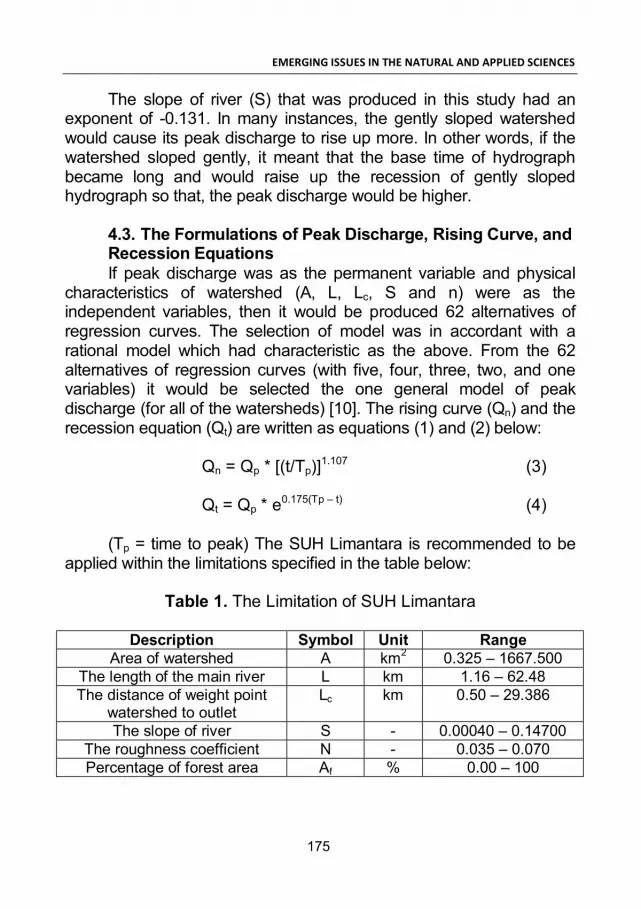
EMERGING ISSUES IN THE NATURAL AND APPLIED SCIENCES
175
The slope of river (S) that was produced in this study had an exponent of -0.131. In many instances, the gently sloped watershed would cause its peak discharge to rise up more. In other words, if the watershed sloped gently, it meant that the base time of hydrograph became long and would raise up the recession of gently sloped hydrograph so that, the peak discharge would be higher.
4.3. The Formulations of Peak Discharge, Rising Curve, and Recession Equations If peak discharge was as the permanent variable and physical
characteristics of watershed (A, L, Lc, S and n) were as the independent variables, then it would be produced 62 alternatives of regression curves. The selection of model was in accordant with a rational model which had characteristic as the above. From the 62 alternatives of regression curves (with five, four, three, two, and one variables) it would be selected the one general model of peak discharge (for all of the watersheds) [10]. The rising curve (Qn) and the recession equation (Qt) are written as equations (1) and (2) below:
Qn = Qp * [(t/Tp)]1.107 (3)
Qt = Qp * e0.175(Tp – t) (4)
(Tp = time to peak) The SUH Limantara is recommended to be
applied within the limitations specified in the table below:
Table 1. The Limitation of SUH Limantara
Description Symbol Unit Range Area of watershed A km2 0.325 – 1667.500
The length of the main river L km 1.16 – 62.48 The distance of weight point
watershed to outlet Lc km 0.50 – 29.386
The slope of river S - 0.00040 – 0.14700 The roughness coefficient N - 0.035 – 0.070 Percentage of forest area Af % 0.00 – 100

Academic book
176
SUH Limantara has been verified on Garang watershed in Indonesia as Figure 1 (Data for Garang watershed: located in Central Java, time to peak: Tp = 1.56 hours, A = 73.5 km2; L = 34.264 km; Lc = 22.16 km; S = 0.0129 and n = 0.0506).
Fig. 1. Verification to Garang watershed
Among stakeholders, the application of SUH model is meant for analyzing designed floods by utilizing inputs from the rain data. However, thus far in Indonesia the stakeholders are still very fanatic in the use of SUH Nakayasu, for they readily considered it as the most practical one. Though in fact, the application of this model on the Java Island still at first requires several calibration works on its parameters. The comparisons between the SUH Nakayasu and SUH Model to the Observed Hydrograph were tabulated as in this following table:
Table 2. Comparison between SUH Limantara and Nakayasu
SUH Time to peak (Tp) (hours)
Peak Discharge (Qp) (m3/s/mm)
Observed Hydrograph 5.773 20.956 SUH Limantara 5.773 20.956 SUH Nakayasu
without calibration 124.103 16.617
SUH Nakayasu with calibration α parameter
5.773 20.956

EMERGING ISSUES IN THE NATURAL AND APPLIED SCIENCES
177
5. CONCLUSIONS Based on these results, it was concluded that: 1) The obser-
ved hydrograph really typifies the elongated shaped of watershed which had a faster rising characteristic than that of its recession (hydrograph rising time < hydrograph recession time); 2) There were 5 dominant watershed parameters that influenced the peak dischar-ge; they were the length of main river/stream (L) followed by the areal size of watershed (A), length of the main river to be measured from a starting point location upstream to the point location about the weight centre of watershed (Lc), roughness coefficient (n) and ri-ver slope (S); 3) The SUH of this research was compared with the observed hydrograph and used as a control model. The coefficient of determination (R2) with the significance level of 5% are for the peak discharge (R2 = 0.841), rising curve (R2 = 0.980) and recession curve (R2 = 0.990). Besides, the SUH Limantara is also compared with the SUH Nakayasu and the deviation obtained was 1.224%.
The characteristic of average unit hydrograph showed that the shape of watershed was pursued long. This study suggested that the length of main river (L) and area of watershed (A) were the primary factors. In addition, it was suggested to study the roughness coefficient of watershed (n).
REFERENCES 1. Chou, Chien Ming. 2011. A threshold Based Wavelet Deno-
ising Method for Hydrological Data Modelling. Journal of Water Resource Manage, 25: 1809-1830
2. Oztekin, Tekin. 2011. Estimation of the Parameters of Wakeby Distribution by a Numerical Least Squares Method and Applying it to the Annual Peak Flows of Turkish Rivers. Journal of Water Resource Manage. 25: 1299-1313
3. Hassanzadeh, Yousef; Abdi, Amin; Talatahari, Slamak; and Singh, Vijay P. 2011. Meta-Heuristic Algorithms for Hydrolo-gic Frequency Analysis, Journal of Water Resource Mana-ge, 25: 1855-1879

Academic book
178
4. Trofimov N.A. and Kalinin V.G. 2011. Estimating the Neces-sary Duration of Observation Period in Studying Water River Runoff. Journal of Water Resources, 38 (2): 149-154
5. Holko L. and A. Lepsito. 1997. Modelling the Hydrological Behaviour of Mountain Catchment Using TOPMODEL, Journal Hydrology 196: 361-377.
6. Blazkova S. and K. Beven. 1997. Flood Frequency Predicti-on for Data Limited Catchments in the Czech Republic Using a Stochastic Rainfall Model and TOPMODEL, Jour-nal of Hydrology 195: 256-278.
7. Sri Harto, 1993, Hidrologi, Universitas Gajah Mada, Yogyakarta
8. Tung B.Z.; Yeh Y. K.; Chia K. and Chuang J. Y., 1987, Storm Resampling for Uncertainty Analysis of a Multiple-Storm Unit Hydrograph, Journal of Hydrology, 194: 66-384
9. Nandakumar N. and R. G. Mein, 1987, Uncertainty in Rain-fall- Runoff Model Simulations And The Implications for Pre-dicting the Hydrologic Effect of Land Use Change, Journal of Hydrology 192: 211-232
10. Montarcih, Lily, 2009, The Limiting Physical Parameters of Synthetic Unit Hydrograph, World Applied Science Journal 7 (6), 802-804
11. Chow, Ven Te, 1988 Engineering Hydrology, John Wiley & sons
12. Montarcih, Lily (2011), Hidrologi Praktis, CV Lubuk Agung, Bandung.
13. Asdak C. 1995. Hidrologi dan Pengelolaan DAS, University Press, Gajah Mada Yogyakarta.

EMERGING ISSUES IN THE NATURAL AND APPLIED SCIENCES
179
THE MATHEMATICS OF VECTOR - BORNE DISEASES
B.S.E. Iyare*, F.E.U. Osagiede
Department of Mathematics, Faculty of Physical Sciences University of Benin, P.M.B. 1154, Benin City (NIGERIA)
*Corresponding author: [email protected] ABSTRACT We described and analyzed various compartmental models for
the transmission dynamics of vector-borne diseases. We begin with the simplest model, the SIS with no immunity, SIR with permanent immunity, SIRS with temporary immunity and SIRS with direct trans-mission and temporary immunity. We show how to calculate the basic reproduction number. Finally,we study the asymptotic stability of equilibria (Local and Global) for each of the models.
Key words: Vector-borne disease, Local Stability, Global
Stability 1. INTRODUCTION Infectious diseases have ever been a great concern of human
kind since the very beginning of our history. The first major epidemic which we can find in the records of historians and scholars is the Plague of Athens (430- 428 BC).
Epidemics, which were killing in millions, occurred in the 14th century when 25 million people died in Europe due to the bubonic plague, (Black Death, 1347-1350). The Black Death virus stayed within the population after the end of the epidemic outbreak and reappeared in Britain (Plague of London) in 1665.
A Vector-borne disease is a disease that is transmitted to humans by insect or other arthropods carriers, such diseases includes Malaria, Dengue fever, west Nile Virus, sleeping sickness

Academic book
180
e.t.c. Vector-borne diseases have been and are among the leading causes of death, they remain the major challenges for many coun-tries in the world, claiming the lives of millions of people every year, children and pregnant women are the most affected. The healths well as the socio-economic impacts of emerging and re-emerging vector-borne disease are significant. Together with the threat of biological weapons, whose research is lately concerned about micro-organisms and lethal infectious diseases, we have great moti-vation to understand the spread and control of vector-borne disea-ses and their transmission characteristics.
Compartmental modeling and Notation Epidemic modeling has three main aims. The first is under-
standing the spreading mechanism of the disease. This entails a mathematical equation that gives us threshold values and constants which are used to describe the bahaviour of the disease. The second is to predict the future trend of the epidemic. The third is to understand how we can control the spread of the epidemic.
The approach for modeling the transmission of infectious disease in human population is usually to subdivide the population under consideration into subpopulation of small number of epidemio-logical class called compartments. The resulting model is called compartmental model. The classes usually considered are primarily the following
Susceptible class (S): This is a collection of individual in a
population who is not infected but is risk of being infected with the disease.
Exposed class (E): These are individuals who have been infected with the disease but are not able to infect others. This class is also known as the Latent class.
Infective class (I): These are individuals who are infected and are infectious.
Recovered/Removed class (R) : These are individuals who recover and acquire temporary or permanent immunity and may not contact or transmit the disease, either because they are no longer infectious and are immune or because they have been vaccinated.

EMERGING ISSUES IN THE NATURAL AND APPLIED SCIENCES
181
Compartmental models have provided valuable insights into the epidemiology of infectious diseases including vector-borne diseases. Diseases that confer immunity have a different compart-mental structure from disease without immunity. For diseases which confer immunity, the SIR terminology is used, describing the passage of individuals from Susceptible class (S) to the Infective (I) and them to the Removed class (R). The term SIS describes a dise-ase with no immunity, indicating the movement of individual from Susceptible class to the infective and then back to the Susceptible class. Other possibilities include the MSEIR, MSEIRS, SEIR and SEIS models with an exposed period, a stage of being infective and becoming infectious after a period of time and maternal antibodies which is passed on to new born babies. Some other classes may be added to increase accuracy. Specifically, a class V or vaccinated individuals. The size of each class at time t are represented by M(t), S(t), E(t), I(t) and R(t) respectively. N (t) denotes the total population size. That is,
N (t) = M(t) + S(t) + E(t) + I(t) + R(t)
2. MODEL WITH HOST SIS AND VECTOR SI WITH NO IMMUNITY The is the simplest vector – borne disease model. Susceptible
host HS become infectious host HI at a rate vH H
H
ISN
through
contact with infected vectors vI . Similarly, susceptible vectors vS
become infectious vector HI at a rate Hv v
H
ISN
by contact with
infected hosts. The model is given by the following differential equations

Academic book
182
vHH H H H H H H
H
vHH H H H H
H
v Hv v v v v v
H
v Hv v v v
H
Ids N I S Sdt N
IdI S Idt N
ds IN S Sdt NdI IS Idt N
2.1.
where
Per capita birth rate of human population H Per capita death rate of human population H Recovery rate in the human population v Birth/death rate in the vector population
All parameters in the system (2.1) are non-negative. 3. ANALYTICAL RESULTS OF THIS MODEL Here, we present some results concerning the existence of
local and global stability properties of our model using analytical method.
3.1. Basıc Reproductıon Number Using the next generation approach, the next generation
operator, G, which provides the number of secondary infections in human and mosquitoes caused by one generation of infectious human and mosquitoes in system 2.1, is given as
v
v
H
OG
O

EMERGING ISSUES IN THE NATURAL AND APPLIED SCIENCES
183
The off] - diagonal structure of G comes from the fact that infected human produced infected mosquitoes and infected mosquitoes produced infected human. The reproduction number
OR
is the geometric mean of the two entries of G.
O OR R
Where
H v
Ov H H
R is the threshold parameter
And OR
is the basic reproduction number of the disease. Theorem 3.1. If 10 R , the disease-free equilibrium point 0E is locally
asymptotically stable, if 00 ,1 ER is unstable.
Proof: This is given in section 4.0 Theorem 3.2. If RO < 1, the disease – free equilibrium point EO of the
systemis globally asymptotically stable and unstable if. RO >1. Proof: In establishing the global stability of the disease free
equilibrium point EO, we construct the following Lyapunov function.
, , , log logH H vH
H v v v
sSH H v v H H H H v v v vN N NL s I S I S N N I S N N I
The time derivative of L (SH, IH, Sv, Iv) computed along the
solutions of (2.1) is

Academic book
184
1 1
1
1
v v vH H H
H v v v
v vH
H H H
vH H H H
v v v H H
N dS dIN dS dIdLdt S dt dt N S dt dt
I INH H H H H H H H H HS N N
N I Iv v v v v v v v v vN S N N
N S S S I
N S S S I
Note That 0dldt if and only if , 0, 0H H H vS N I I
v vS N . Therefore, the largest compact invariant set in
, , , : 0dLH H v v dts I S I D is the singleton 0E containing the
origin, where EO is the disease – free equilibrium point in system (2.1). Using LaSalle’s invariance principle, EO is globally asymptotically stable.
4. MODEL WITH HOST SIR AND VECTOR SI WITH PERMANENT IMMUNITY The differential equations for this model is given below
vHH H H H H
H
vHH H H H H
H
Ids N S Sdt N
IdI S Idt N
HH H H H
v Hv v v v v v
H
v Hv v v v
H
dR I Rdt
ds IN S Sdt NdI IS Idt N
4.1.

EMERGING ISSUES IN THE NATURAL AND APPLIED SCIENCES
185
where
Per capita birth rate of human population H Per capita death rate of human population H Recovery rate in the human population
Disease-induced death rate v Birth/death rate in the vector population
All parameters in the system (4.1) are non-negative to simplify the analysis of our malaria model (4.1), we convert the actual populations to fractional quantities by scaling the population of each class by the total population.
Let
, , v
v
Rh h vi r i 4.2.
With
1 1v
v
SSh h h v vs i r and s i 4.3.
Differentiating equation (4.2), we have
1h hdi id ddt dt dt
4.4a.
1h hH H
H
dr rdR dNdt dt dt 4.4b.
1v v v v
v v
di dI i dNdt N dt N dt 4.4c.
Using equations (4.2 - 4.4), we obtain the system describing
the dynamics of the proportion of individual in each class. This is given below
21hdi
h h H h hdt i r i r i i 4.5a.
hdrh h hdt r i r 4.5b.
1vdiv v h v vdt i i i 4.5c.

Academic book
186
The differential equations (4.5) is epidemiologically and mathe-matically well-posed in the domain
D = 3, : , ,h h v h h vi r i R i o r o i o
And the equilibrium points are defined. The trivial equilibrium
point OE = , ,o o oh h mi r l = , ,O O O and endemic equilibrium point E* =
* * *, ,h h mi r i . 5. ANALYTICAL RESULTS OF THIS MODEL Here, we present some results concerning the existence of
local and global stability properties of our model using analytical method.
5.1. Basıc Reproductıon Number Using the next generation approach, the next generation
operator, M, which provides the number of secondary infections in human and mosquitoes caused by one generation of infectious human and mosquitoes in system 4.5 is given as
0
0vM
The off - diagonal structure of M comes from the fact that
infected human produced infected mosquitoes and infected mosquitoes produced infected human. The reproduction number
OR
is the geometric mean of the two entries of M.
O OR R
Where

EMERGING ISSUES IN THE NATURAL AND APPLIED SCIENCES
187
H v
Ov H
R is the threshold parameter
And OR
is the basic reproduction number of the disease. Theorem 5.1. If 10 R , the disease-free equilibrium point 0E is locally
asymptotically stable, if 00 ,1 ER is unstable.
Proof:
Let Piiiridtdi
hhHvhhHh 21
Qrirdtdr
hhhHh
Riiidtdi
vvhvvv 1
The Jacobian of the model is
vhh
vhh
vhh
didR
drdR
didR
didQ
drdQ
didQ
didP
drdP
didP
J

Academic book
188
vhvvv
hH
hhHvHhHvH
ii
r
riiii
01
0
12
at the disease-free equilibrium 0E
vv
H
HH
J
0
0
0
The characteristic equation is given by
0
100
010
001
0
0
0
A
B
IAJ
vv
H
H
Where HB
0
0
0
0
A
A
AB
vv
H
H
0 AAAAB vHv
vvHvv BAABAAAB 322

EMERGING ISSUES IN THE NATURAL AND APPLIED SCIENCES
189
02 vHv AABA
vvvHvv ABAABAAAB 322
02 vHAAB Re arranging we have
ABBABA vHvvv 23
0 vHvB
ABBABA vHvvv 23
01
v
vHv B
B
ABBABA vHvvv 23 01 0 RB v
The eigenvalues in the characteristic equation above have
negative real part if and only if the coefficients are positive. This occur when 10 R . Therefore 0E locally asymptotically stable for
10 R . It is unstable if 10 R Theorem 5.2. If RO < 1, the disease – free equilibrium point EO of system
(4.5) is globally asymptotically stable and unstable if. RO >1, Proof: In establishing the global stability of the disease free
equilibrium point EO, we construct the following Lyapunov function.
HHH
HHHHvvHHH RI
NSNNSISRISL
log,,,,

Academic book
190
v
v
vvvv
vv
HH INSNNS
N
log
L is C on the interior of 0, ED is the global minimum of
LDL and,on 0,,,, 00000 vvHHH ISRISL . The time derivative of L (SH, IH, RH, SM, IM) computed along the
solutions of (4.1) is
1 1
1
1 0
v v vH H H H
H v v v
v vH
H H H
vH H H H
v v v H H
N dS dIN dS dI dRdLdt S dt dt dt N S dt dt
I INH H H H H H H H HS N N
N I IH H H H v v v v v v v v v vN S N N
N S S S I
I R N S S S I
Note That 0dl
dt if and only if , 0, 0H H H vS N I I
v vS N . Therefore, the largest compact invariant set in
, , , , : 0dLH H H v v dts I R S I D is the singleton 0E containing
the origin and since D can be assumed to be compact, each solution beginning in lC , actually converges to 0 as t . Using LaSalle’s invariance principle, EO is globally asymptotically stable.
6. MODEL WITH HOST SIRS AND VECTOR SI WITH TEMPORARY IMMUNITY. The differential equation for this model is given below.
vHH H H H H H H
H
Ids N R S Sdt N

EMERGING ISSUES IN THE NATURAL AND APPLIED SCIENCES
191
( )
vHH H H H H
H
HH H H H H
v Hv v v v v v
H
v Hv v v v
H
IdI S Idt N
dR I Rdt
ds IN S Sdt NdI IS Idt N
6.1.
Where the parameters are as defined in section 4.0
H = rate of loss of immunity. All parameters in the system (6.1) are non-negative. To
simplify the analysis of our model, Let
, , v
v
Rh h vi r i
With
1 1v
v
SSh h h v vs i r and s i
Differentiating, we have
1h hdi id d
dt dt dt
1h hH H
H
dr rdR dNdt dt dt
1v v v v
v v
di dI i dNdt N dt N dt
Using the above equations we obtain the system describing
the dynamics of the proportion of individual in each class. This is given below

Academic book
192
21hdih h H h hdt i r i r i i
hdrh h hdt r i r 6.2.
1vdiv v h v vdt i i i
Also, the differential equation above is epidemiologically and
mathematically well-posed in the domain D = 3, : , ,h h v h h vi r i R i o r o i o
And the equilibrium points are defined. The trivial equilibrium point OE = , ,o o o
h h mi r l = 0,0,0 and the endemic equilibrium point
E* = * * *, ,h h mi r i . PROPOSITION 6.1. The malaria model (6.2) has the disease – free equilibrium
(DFE) point EO = , ,o o oh h mi r i = 0,0,0 with no disease in the
population. Proof: From equation (6.2)
1v h
v
i roh ii 6.3.
And
h
H
iohr 6.4.
If vi o in equation (6.3), we have o
hi o and in (6.4) ohr o .
This implies that EO always exists and is the only diseases free equilibrium point.

EMERGING ISSUES IN THE NATURAL AND APPLIED SCIENCES
193
7. ANALYTICAL RESULTS OF THE MODEL Here, we present some results concerning the existence of
local and global stability properties of our model using analytical method.
7.1. Basıc Reproductıon Number As in section 3.0 the next generation operator, K, which provi-
des the number of secondary infections in human and mosquitoes caused by one generation of infectious human and vector in system (6.2) is given as
H
v
v
OK
O
The off – diagonal structure of K comes from the fact that
infected human produced infected mosquitoes and infected mosquitoes produced infected human. The reproduction number
OR
is the geometric mean of the two entries of K.
O OR R
Where
H v
Ov H
R is the threshold parameter
And OR
is the basic reproduction number of the disease. 7.2. Dısease - Free Equılıbrıum (Dfe) Theorem 7.1. If 1OR , the disease – free equilibrium point EO of system
(6.2) is locally asymptotically stable, if 1OR EO is unstable.

Academic book
194
Proof: At the disease – free equilibrium EO, the Jacobian of the matrix
is given by
H
H
v
J 0( )0
H
0H
v
The characteristics equation is given by
H
M
BJ IA
0
0Z
1
0H
M
-100
010
001
A
Where B = H , Z = H
0
H
v
B AJ
0
0Z
0H
v A=0
= 0v H vA B Z A A Z A
3 2 0v v v v H v H vA Z B A Z B BZ A BZ Z A
3 2 0v v v H v v H vA Z A Z B BZ A BZ Z
3 2 1 0H v
vv v v H v v BA Z B A Z B BZ A BZ
3 201 0v v v H v vA Z B A Z B BZ A BZ R
The Eigenvalues in the characteristic equation above have
negative real part if and only if the coefficients are positive. This occur when RO <1. This means that EO is locally asymptotically stable for RO < 1.

EMERGING ISSUES IN THE NATURAL AND APPLIED SCIENCES
195
This complete the proof of theorem 7.1 Theorem 7.2. If RO < 1, the disease – free equilibrium point EO of system
(6.2) is globally asymptotically stable. Proof: In establishing the global stability of the disease free equilib-
rium point EO, we construct the following Lyapunov function.
,, , , log logH H vH
H v v v
sSH H H v v H H H H H v v v vN N NL s I R S I S N N I R S N N I
The time derivative of L (SH, IH, RH, SM, IM) computed along the
solutions of (6.1) is
1 1
1
( ) 1
v v vH H H H
H v v v
v vH
H H H
vH H H H
v v v H H
N dS dIN dS dI dRdLdt S dt dt dt N S dt dt
I INH H H H H H H H H H HS N N
N I IH H H H H v v v v v v v v v vN S N N
N R S S S I
I R N S S S I
Note That 0dl
dt if and only if , 0, 0H H H vS N I I
v vS N . Therefore, the largest compact invariant set in
, , , , : 0dLH H H v v dts I R S I D is the singleton 0E containing
the origin, where EO is the disease – free equilibrium point in system (6.1). Using LaSalle’s invariance principle, EO is globally asymptotically stable.
7.3. Endemic Disease Equilibrium (EDE) Theorem 7.3. If RO >I, the endemic disease equilibrium E* of system (6.2) is
locally asymptotically stable.

Academic book
196
Proof: At the endemic disease equilibrium, E*, the characteristic
equation is given as
3
5
B AJ IA B
B
1
4
0
BB A
2
6
0B
B A =0=J*
*4 6 1 3 6 2 5 4( ) 0J B A B A B A B B B A B B B A
* 3 22 1 0 0J A Y A Y A Y 7.1.
Where
1 3 6 2 4 5
1 4 6 4 6 1 3 2 5
2 4 6
OY B B B B B BY BB BB B B B B B BY B B B
And
1 2 2 2
* * * *2 2H m H h H H h H hB l l r l
2
1
* *1 1
* *2
*3
*4
*5
*6
1
1
H m H h
H h h
H h
H h
M m
M h m
B l l
B i r
B rB i
B l
B i

EMERGING ISSUES IN THE NATURAL AND APPLIED SCIENCES
197
Since the coefficients of (7.1) are positive, then the three eigenvalues of *j have negative real parts. Therefore *E is locally asymptotically stable for 0 1R .
This complete the proof of theorem 7.3. 8. MODEL WITH HOST SIRS AND VECTOR SI WITH DIRECT TRANSMISSION AND TEMPORARY IMMUNITY
Here, the assumption is made that susceptible human can be
infected via two modes of transmission, that is by being bitten by an infectious vectors and directly through contact with an infectious human (as a result of blood transfusion). We denote the biting rate that a vector has to susceptible human as 1
,the incidence of new
infections is given by a standard incidence rate 1
v
HHS .The
rate of direct transmission is denoted by2H so that the incidence of
new infection through this mode is given by a standard incidence rate
2 HS .The host infections to vector - susceptible
transmission rate is given by
v vs .
The above assumptions lead to the following different equations.
1 2
vH H H H
H
ds s s sdt
1 2
v
H
ddt s s
( )dRHdt R 8.1.
vdS
v v v v v vdt s s
vdI I
v v v vdt s

Academic book
198
Where = per capital birth rate of human population = per capital death rate of human population
= recovering rate in the human population = disease – induced death rate v = birth / death rate in the mosquito population 1
= contact / biting rate of human by mosquito 2
= rate of direct transmission.
H = rate of loss of immunity. All parameters in the system (8.1) are non-negative to simplify
the analysis of our malaria model (8.1), we convert the actual populations to fractional quantities by scaling the population of each class by the total population.
Let
, , v
v
Rh h vi r i 8.2.
With
1 1v
v
SSh h h v vs i r and s i 8.3.
Differentiating equation (2.2), we have
1h hdi id ddt dt dt
8.4a.
1h hH H
H
dr rdR dNdt dt dt 8.4b.
1v v v v
v v
di dI i dNdt N dt N dt 8.4c.
Using equations (8.2) – (8.4), we obtain the system describing
the dynamics of the proportion of individual in each class. This is given below
1 2
21 1hdih h v h h h H h hdt i r i i r i r i i 8.5a.
( )hdrh h H hdt r i r 8.5b.

EMERGING ISSUES IN THE NATURAL AND APPLIED SCIENCES
199
1vdiv v h v vdt i i i 8.5c.
The differential equations (8.5) is epidemiologically and mathe-
matically well-posed in the domain
D = 3, : , ,h h v h h vi r i R i o r o i o And the equilibrium points are defined. The trivial equilibrium
point OE = , ,o o oh h vi r l = , ,O O O and endemic equilibrium point E* =
* * *, ,h h vi r i . PROPOSITION 8.1. The malaria model (8.5) has the disease – free equilibrium
(DFE) point EO = , ,o o o
h h vi r i = 0,0,0 with no disease in the population. Proof: From equation (8.5a)
1
1
1v h
v
i roh ii 8.6.
And
h
H
iohr 8.7.
If vi o in equation (8.6), we have o
hi o and in (8.7) ohr o .
This implies that EO always exists and is the only diseases free equilibrium point.

Academic book
200
9. ANALYTICAL RESULTS OF THE MODEL Here, we present some results concerning the existence of
local and global stability properties of our model using analytical method.
9.1. Basıc Reproductıon Number We used the next generation operator approach to define the
basic reproduction number, OR
as the expected number of secondary infections that one infectious individual would produced in a completely susceptible population. The next generation operator, P, which provides the number of secondary infections in human and mosquitoes caused by one generation of infectious human and mosquitoes in system (8.5), is given as
1
2
vv
OP
O
The off - diagonal structure of P comes from the fact that infec-
ted human produced infected mosquitoes and infected mosquitoes
produced infected human. The reproduction number OR
is the geometric mean of the two entries of P.
O OR R
Where
2
1H vO
v H H
R is the threshold parameter
And OR
is the basic reproduction number of the disease.

EMERGING ISSUES IN THE NATURAL AND APPLIED SCIENCES
201
9.2. Dısease – Free Equılıbrıum (Dfe) Theorem 9.1. If 1OR , the disease – free equilibrium point EO of system
(8.5) is locally asymptotically stable, if 1OR EO is unstable. Proof: At the disease – free equilibrium EO, the Jacobian of the matrix
is given by
2H H
H
v
J 0( )0
H
1
0H
v
The characteristics equation is given by
H
v
BJ IA
0
0Z
1
0H
v
-100
010
001
A
Where B =
2H , Z = H
0
H
v
B AJ
0
0Z
1
0H
v A=0
= 1
0v H vA B Z A A Z A

Academic book
202
1 1
3 2 0v v v v H v H vA Z B A Z B BZ A BZ Z A
1 1
3 2 0v v v H v v H vA Z A Z B BZ A BZ Z
1
1
3 2 1 0H v
vv v v H v v BA Z B A Z B BZ A BZ
1
3 201 0v v v H v vA Z B A Z B BZ A BZ R
The Eigenvalues in the characteristic equation above have
negative real part if and only if the coefficients are positive. This occur when RO <1. This means that EO is locally asymptotically stable for RO < 1.
This complete the proof of theorem 9.1 Theorem 9.2. If RO < 1, the disease – free equilibrium point EO of system
(8.5) is globally asymptotically stable. Proof: In establishing the global stability of the disease free
equilibrium point EO, we construct the following Lyapunov function.
,, , , log logH HH V
H v v V
S SH H H V V H H H H H V V V VN N NL s I R S I S N N I R S N N I
The time derivative of L (SH, IH, RH, SV, IV) computed along the
solutions of (8.1) is
1 2 1 2
1 1
1
( ) 1
v v vH H H H
H v v v
v vH H H
H H H H H
vH H H H
v v v H H
N dS dIN dS dI dRdLdt S dt dt dt N S dt dt
I IN I IH H H H H H H H H H H H H H HS N N N N
N I IH H H H H v v v v v v v vN S N N
N R S S S S S I
I R N S S S v vI
Note That 0dl
dt if and only if , 0, 0H H H vS N I I
v vs N .

EMERGING ISSUES IN THE NATURAL AND APPLIED SCIENCES
203
Therefore, the largest compact invariant set in , , , , : 0dL
H H H V V dts I R S I D is the singleton 0E containing the origin, where EO is the disease – free equilibrium point in system (8.1). Using LaSalle’s invariance principle, EO is globally asymptotically stable.
9.3. Endemic Disease Equilibrium (EDE) Theorem 9.3. If RO >I, the endemic disease equilibrium E* of system (8.5) is
locally asymptotically stable. Proof: At the endemic disease equilibrium, E*, the characteristic
equation is given as
3
5
B AJ IA B
B
1
4
0
BB A
2
6
0B
B A =0=J*
*4 6 1 3 6 2 5 4( ) 0J B A B A B A B B B A B B B A
* 3 22 1 0 0J A Y A Y A Y 3.1.
Where
1 3 6 2 4 5
1 4 6 4 6 1 3 2 5
2 4 6
OY B B B B B BY BB BB B B B B B BY B B B
And
1 2 2 2
* * * *2 2H V H h H H h H hB l l r l

Academic book
204
2
1
* *1 1
* *2
*3
*4
*5
*6
1
1
H v H h
H h h
H h
H h
v v
v h v
B l l
B i r
B rB i
B l
B i
Since the coefficients of (8.1) are positive, then the three
eigenvalues of *j have negative real parts. Therefore *E is locally asymptotically stable for 0 1R .
This complete the proof of theorem 9.3 REFERENCES 1. Anderson R.M and May.R.M. (1991). Infectious Disease of
Human, Dynamics and Control, Oxford University Press, Oxford, UK.
2. Aron J.L and May R.M. (1982). The Population dynamics of Malaria, Dynamics of Infectious Diseases. Theory and Application. Chapman and Hall, London.
3. Chitris N. Cushing J.M. and Hyman J.M. (2006). Bifurcation Analysis of a mathematical model for malaria disease transmission. SIAM J. Applied Math. 67, 1, 24-45
4. Koella C. and Boete C. (2003). A Model for the Co-evolution of immunity and immune evasion in vector – borne disease with implication for the epidemiology of Malaria. The American Naturalist, 161, 698-707
5. Kwon H., Blayneh K.W., and Cao Y. (2009) Optimal control of Vector - Borne Diseases: Treatment and Prevention. Discrete and continuous dynamical systems series vol.II no. 3

EMERGING ISSUES IN THE NATURAL AND APPLIED SCIENCES
205
6. Inaba H and Sekine H. (2004) A Mathematical model for chagas disease with infection – age - dependent infectivity. Math. Biosciences, Vol. 190 no. 1, pp 39-69
7. Iyare B.S.E and Osagiede F.E.U. (2010) A Vector-Host Model for Malaria disease Transmission with variable human population. International Journal of Computational and Applied Mathematics. ISSN 1819-4966 Volume 5, Number 6 (2010), pp. 769-778.
8. Iyare B.S.E. (2011). A Model for Malaria disease Transmis-sion in Pregnant and Non-Pregnant women: International Journal of Academic Research Vol.3, No.3.May 30,2011
9. Liming Cai and Xuezhi Li (2010) Analysis of a simple Vec-tor-Host Epidemic Model with direct transmission. Discrete Dynamic in Nature and Society volume 2010.
10. Wei H.M, Li x z and Martcheva M. (2008): An epidemic model of a vector - borne disease with direct transmission and time delay. Journal of Mathematical Analysis and Appli-cations vol. 342, no. 2, pp 895 - 908.
11. Ngwa G.A and Shu W.S (1999). A Mathematical Model for endemic Malaria with variable human and mosquito popula-tions. www.ictp.trieste.it~pub-off
12. Vargas de Leon C. and Hermadez J.A.C (2008) Local and Global Stability of Host-Vector disease model. Journal of Mathematical Biology.
16. Yang H. M. (2000), Malaria transmission model for different levels of acquired immunity and temperature independent parameters (vector), Revista de Sailde Publia, 34 pp. 223-231.
17. Yang H. M. and Ferreira M. U. (2000); Assessing the effects of global warming and local social and economic condition on the malaria transmission, Revista de Saude Publica, 34 pp. 214-222.

Academic book
206
FORENSIC IDENTIFICATION WITH BAYES’ LAW
Dr. Marina Andrade, Prof. Dr. Manuel Alberto M. Ferreira
Instituto Universitário de Lisboa (ISCTE-IUL),
UNIDE - IUL, Lisboa (PORTUGAL) E-mails: [email protected], [email protected]
ABSTRACT The probabilistic fundaments for the evaluation of DNA
evidences, based mainly on Bayes’ Law, are presented emphasizing the famous island problem. Identification problems are considered, in particular the paternity dispute problem and the crime scene analysis.
Key words: DNA evidence, island problem, paternity dispute,
crime scene analysis. 1. INTRODUCTION It is intended in this section to consider a forensic identification
problem in generic terms. Having been committed a crime, the accused identification may be based in accordance with the charac-teristics that are known to belong to the potential (or true) criminal. The identification may be done through fingerprints, by witnesses, for the type of the used weapon or by the DNA profile (Dawid and Mortera, 1996). For the determination of the DNA fingerprint or of the DNA profiling, since 1984, the forensic scientists used the gene-tic material (DNA) information as evidence in murder and/or rape cri-mes, as well as in paternity identification cases.
When the equality of profiles is measured, it is also measured indirectly the prosecuted culpability, since that calculation assumes that the accused is not guilty (Berry, 1991). If the two profiles are not alike it is possible to state that the accused is not the criminal. But,

EMERGING ISSUES IN THE NATURAL AND APPLIED SCIENCES
207
when the similarity is declared it is not possible to state that the accused is the criminal.
In this context, a natural way to quantify the evidence weight in favour of the accused guiltiness, is to determine the conditional pro-bability of the guiltiness given the evidence, that implies necessarily the application of Bayes’ Law (Dawid and Mortera, 1996).
So two hypotheses must be evaluated, one of the defence and the other of the prosecution, i. e.:
HD: The accused and the criminal are distinct persons versus HP: The accused and the criminal are one and the same
person. In order to use the Bayes’ Law suppose that the evidence
(called E), in the crime scene, states that the criminal has a deter-mined characteristic C, that is not for itself incriminating, being p the probability of any individual from the population to possess that characteristic. It is known that the accused individual possesses the characteristic (evidence), and be π the probability of any individual from the population, randomly chosen, to be guilty, having in mind the whole remaining evidence, for which it is admitted to be conditio-nally independent from the identification evidence, given the inno-cence or the guiltiness.
Be 퐶 = 1 and 퐺 the events: “The accused possesses the characteristic C” and “The accused is guilty”, respectively, being 퐶 a binary random variable that indicates the characteristic C presence or absence in the accused individual. By the evidence E the criminal possesses C. If the accused is the criminal then 푃(퐶 = 1|퐺 ) =1 and 푃(퐶 = 1|퐺 ) = 푝, the likelihood ratio favouring the guiltiness is 푝 and the individual, that is under accusation, guiltiness posterior probability is
푃(퐺 |퐶 = 1, 퐸) =푃(퐶 = 1|퐺 )푃(퐺 |퐸)
푃(퐶 = 1|퐺 )푃(퐺 |퐸) + 푃(퐶 = 1|퐺 )푃(퐺 |퐸)

Academic book
208
and so
푃(퐺 |퐶 = 1, 퐸) =휋
휋 + 푝 − 휋푝 (1.1).
2. ALGEBRAIC APPROACH The Island Problem The forensic scientists, to quantify the evidence weight in
favour of the accused guiltiness, developed a theoretical formulation in order to quantify the HP probability, given the presented evidence.
The island problem was extensively studied by Lindley (1987), Yellin (1979), Eggleston (1983), Dawid (1984) and Balding and Donnelly (1995) and is as follows:
Consider a isolated island, from the rest of the World, at which a murder was performed. Suppose that in the island there are N + 1 inhabitants, from which one is the criminal and the remaining ones are not guilty. Each one of the inhabitants has equal probability of being the criminal. Let us still admit that each individual has a proba-bility p of possessing a certain characteristic C, that is independent for two any distinct individuals.
The evidence found at the crime scene may be synthesized in the allegation of that the criminal possesses the characteristic C. So designate by E the evidence that represents the event “the criminal possesses the characteristic C, i. e., Cc = 1”. An individual is arrested and presented to the court. The only evidence against him is that he possesses C, event already designated by Ca = 1. The interesting question is to determine the guiltiness probability, i. e., of the accused to be guilty, given the available evidence.
Following the Bayesian approach it is admitted a priori that any inhabitant has equal probability, 휋 = , of being the criminal. Substituting in the equation (1.1) it is obtained:
푃(퐺 |퐶 = 1, 퐸) =1
1 + 푁푝 (2.1).

EMERGING ISSUES IN THE NATURAL AND APPLIED SCIENCES
209
This result is easy to explain in court. In the island there is a criminal that possesses the characteristic C and Np not guilty persons that also possess C. Based on the available information the accused is among the N + 1 individuals, among which is also the criminal.
The Search Strategies In the former analysis of the island problem it was assumed
that the accused was identified in a random way among the popula-tion, and it is verified that possesses the characteristic C. Such a supposition is not always very real. In fact, sometimes is more easily accepted that it is identified through a search proceeding in the population. Being known that the criminal possesses that characte-ristic C it is natural that the police proceeds to a random search in the N + 1 individuals of the island, and arrest the first that has C presented.
So it is important to evaluate the effect caused by the search proceeding in the probability of guiltiness of the individual that is going to be accused. It is still admitted that to possess the characte-ristic C it is no enough to be considered guiltiness and that distinct individuals possess C independently of each other, with probability p. Suppose that is performed a search in the population, that may be completely random, either in some way deterministic or in other way stochastic, that is independent of the C values and of the criminal identity.
The way the search is performed is not relevant if it is assu-med the permutation of the random variables Ci, that is, if it is admitted that the join distribution of any vector of n individuals, {퐶 , … , 퐶 } is the same for any set with n elements, i.e., 푃(퐶 , … , 퐶 ) = 푃 퐶 ( ), … , 퐶 ( ) for any permutation 휓 of n individu-als. In this way, the whole strategies are equivalent. Even, to simplify may be admitted that the population is numbered from 1 till N + 1, and the search is made by order.
Keeping the notation be Ci = 1 and Gi the event “the individual i possesses the characteristic C and the individual i is guilty”, respectively. In this way, the event “the accused is guilty” will be

Academic book
210
designated by 퐺 , . Note that with this strategy 퐶 = 퐶 = 퐶 , = 1 is redundant, because the accused was chosen for having character-ristic C. So the events “the accused has the order k and is guilty” and “the accused has the order k and the characteristic C are 퐺 , and 퐶 , = 1, respectively.
Two Possibilities In the exposed context two perspectives are posed. First,
given the evidence collected in the crime scene, E, that is the guilty person has characteristic C, if it is known K = k it is concluded that the k – 1 first individuals do not possess C, and it is possible to think that the individual k was randomly chosen among the remaining N – k + 2 inhabitants of the island, form which one is the criminal and N – k + 1 are not guilty and may exhibit the characteristic.
So, following the Bayesian argument:
푃 퐺 , |퐸, 퐶 , = 1, 퐾 = 푘 =1
1 + (푁 − 푘 + 1)푝 (2.2).
It corresponds to the assumption that the a priori guiltiness
probability is 휋 = . For 푘 > 1 the value of this probability is greater than the one given by (1.1).
Consider now that K is unknown, that is, it is done a search in the population till finding the first individual that exhibits C, that so it is accused. But it is not known how many individuals were observed till finding the accused.
To calculate the accused guiltiness probability conditional to that he is the kth individual to be analyzed and possesses C, the whole possible values that K may assume must be considered. Then the whole disjoint partitions operated by k of the event “퐺 and K = k” must be taken in account and to sum in its domain, that is the Total Probability Law must be applied. In consequence:

EMERGING ISSUES IN THE NATURAL AND APPLIED SCIENCES
211
푃(퐺 |퐶 = 1, 퐸) = 푃 퐺 , , 퐾 = 푘|퐶 , = 1, 퐸
=1 − (1 − 푝)
(푁 + 1)푝 (2.3).
This result obtained by Dawid (1994) shows that the Bayesian
approach, given by equation (1.1), is not always valid. Indeed, if the accused is found through a search proceeding in the population, the individual guiltiness probability must not be calculated using Bayes’ Law; this is appropriated when the suspect is determined in a random way. But the Bayes’ Law fails by precaution, what in general is recommended following the innocence presumption.
The interest in the determination of the guiltiness probability of an accused individual is in general caught in the legal context having, because of it, the preoccupation that that result is always advantageous to the accused, that is so conservative.
Note that the former result had been already presented by Yellin (1979) as solution for the island problem. In the context followed by Yellin the result fails for not considering the additional information that the criminal possesses the characteristic C.
3. DNA EVIDENCE ALGEBRAIC APPROACH In a DNA forensic identification simple problem one is in front
of a biological trace, of unknown origin, and still biological “informa-tion” of unknown individuals based on the collected information it is intended to investigate which is the origin of that trace.
3.1. Paternity Dispute It matters to think that in any paternity investigation action
what firstly is in cause is the official recognizing of the individual parentage whose paternity is being searched, respecting his/her elementary rights.
In a simple way the information that generally is presented in a court decision, that may be called value of the biological evidence W, to be evaluated demands the knowledge of a classification table

Academic book
212
– the Hummel table1. When there is not paternity exclusion the laboratories calculate the value of the paternity probability – W.
The laboratories proceeding results from the admission that the paternity and non paternity a priori probabilities are equal, 푃(퐻 ) = 푃(퐻 ) = 0.5, and so the expression of the paternity a posteriori probability is 푊 = , where W is the paternity probability, X is the probability that the biological father is the putative father and Y is the probability that the biological father is an individual picked up randomly from the population. This formula is also known as Essen-Möller equation2.
Now the hypotheses outlined in the Introduction may be mathematically detailed. Becoming the assumption of paternity litigious, in formal terms are constituted the prosecution and the defence hypotheses, i.e.,
HP: The putative father is the true father. versus HD: The true father is another individual, chosen randomly
among the population, not related with either the mother or the putative father.
Indeed the court has to decide about the child true paternity in
relation with the putative father. In fact, it has to evaluate the dispu-ting hypotheses ratio:
푃(퐻 |퐸)푃(퐻 |퐸) =
푃(퐸|퐻 )푃(퐸|퐻 ) ×
푃(퐻 )푃(퐻 )
being E the available evidence vector. Admitting that 푃(퐻 ) =
푃(퐻 ),
1 Table of verbal predicates used and indicated by the laboratories to the court to
classify the value obtained in laboratorial analysis. Nowadays it is often questioned. 2 Obtained by Essen-Möller in 1938.

EMERGING ISSUES IN THE NATURAL AND APPLIED SCIENCES
213
푃(퐻 |퐸)푃(퐻 |퐸) =
푃(퐸|퐻 )푃(퐸|퐻 ),
and in any paternity case at which it is possible to get mother
genetic information (mgt), child genetic information (cgt) and putative father genetic information (pfgt), the forensic biology laboratories may compute the likelihood ratio (in the behind mentioned notation ).
Likelihood Ratio Calculus in Paternity Dispute In the hypotheses above considered, and disposing of the trip-
let 퐸 = (푚푔푡, 푐푔푡, 푝푓푔푡), assuming the independence between and across markers it is possible to calculate the LR value for each one of the markers separately. And then to multiply those values to obtain the value related to the whole observed markers.
So consider that for a certain marker there is the triplet formula 퐸 = {(퐴, 퐵); (퐵, 퐵); (퐴, 퐵)}, and 푝 and 푝 are the A and B allele fre-quencies, respectively, in the population for the considered marker. It is easily acceptable that, before knowing the child genetic informa-tion, it may be assumed that the true father identity is independent from the mother and from the putative father.
So it must be determined the conditional probability of the child genotype given the other two available genotypes. Consequently, to determine 푃(퐸|퐻 ) it is only necessary to apply the Mendel’s Laws. To calculate 푃(퐸|퐻 ) the markers allelic frequencies must be known. So
푃(퐸|퐻 ) = 푃[(푚푔푡, 푐푔푡, 푝푓푔푡)|(푚푔푡, 푝푓푔푡)]
= 푃[푐푔푡 = (퐵, 퐵)|푚푔푡 = (퐴, 퐵), 푝푓푔푡 = (퐴, 퐵)]= 0.5 × 0.5
and
푃(퐸|퐻 ) = 푃[(푚푔푡, 푐푔푡, 푝푓푔푡)|(푚푔푡, 푟푔푡)]= 푃[푐푔푡 = (퐵, 퐵)|푚푔푡 = (퐴, 퐵), 푟푔푡] = 0.5 × 푝

Academic book
214
where rgt is related to the genotype of an individual chosen randomly in the population not related either with the mother or with the putative father. The genotype rgt is not known. It is only known that the child inherits the allele B from the father, and so inherits with the frequency if this allele in the population. In consequence
퐿푅 =푃(퐸|퐻 )푃(퐸|퐻 ) =
0.5푝
.
It is important to emphasise that the decision on the child
paternity, for any case presented in court, is taken by the judge. Its decision results from the knowledge taken from the whole relevant evidences and facts for each case in appreciation, each one with its own particularities.
This kind of evidence initiated a revolution in the form of appreciating the attribution or not of the paternity. But today it is accepted without any hesitation in court.
3.2. A Complex Mixture Case The use DNA profiles and quantitative evidences in the appre-
ciation of criminal cases has become more and more trivial, after 1985. But the knowledge of the cases ate which this tools are misunderstood and generate difficulties during the process are still common, contrarily to the desired. The case considered reports to a crime that was committed, in which two persons were violently mur-dered (Andrade and Faria, 2006). In what follows they will be desig-nated by V1 (female) and V2 (male). V1 and V2, married, were at home and were murdered in unknown circumstances. During the in-vestigations the police identified an individual, S1, son of the victims that confessed to the crime, having been signed another individual as being involved in the crime, S2.
About the Non-DNA Evidence Of course it is not possible to specify the whole reasons,
connected to non-DNA evidences, that driven the police to the sus-

EMERGING ISSUES IN THE NATURAL AND APPLIED SCIENCES
215
pects, even because it overcomes this work scope. About the non-DNA evidence the interesting elements may be synthesized as follows:
- There were found some inconsistencies and contradictions
during the interrogatories; - The testimony of someone that said to have seen two human
figures going away from the victims’ car, in the morning at which the bodies were found;
- The coroner stated, after the autopsy, that the wounds in the body of V2 almost surely had not been inflicted for only one person.
The DNA Evidence In what concerns DNA evidences, it was found a mixture in the
crime scene. The analysis of haematic evidences allowed to identify genetic material matching to the victims’, to S1 the victims’ son3 and to S2.
The Hypotheses to Consider The interpretation of a mixture depends very much on the
circumstances surrounding the crime, (Evett and Weir, 1998). This is a complex case, but the confession of S1 allowed some simplificati-on in the case, and consequently in the hypotheses to consider. After the confession of S1 there is only a suspect: S2. So, the testing hypotheses are:
HP: The crime sample contains DNA from both victims (the S1
profile results from a combination of the victims profiles and, in con-sequence, it is necessarily in the mixture) and from the suspect S2.
3The victims’ son could not be excluded, because any individual has in its genetic
heritage, for each gene, a part inherited from the father and another inherited from the mother. So if the parents are in the mixture composition their descendents cannot be excluded.

Academic book
216
versus HD: The crime sample contains DNA from both victims (the S1
profile results from a combination of the victims profiles and, in consequence, it is necessarily in the mixture) and from an unknown individual.
Model and Analysis As it was already referred, in front of each case the judge or
the jury has to decide. To do so it matters to evaluate the whole evi-dences (now designated as DNA evidence – E and non-DNA evi-dence – I) and then to determine the a posteriori guiltiness probabi-lity given the evidences, i.e., has to answer the question:
푃(퐻 |퐸, 퐼)?
Before going on with the analysis some notation must be
introduced. So - 퐸 is the sample collected in the crime scene, - 퐺 is the genotype of the victim V1, - 퐺 is the genotype of the victim V2, - 퐺 is the genotype of S1, - 퐺 is the genotype of S2. The likelihood ratio for the mixture may be written in the form:
퐿푅 =푃 퐸 |퐺 , 퐺 , 퐺 , 퐺 , 퐻 , 퐼
푃 퐸 |퐺 , 퐺 , 퐺 , 퐻 , 퐼.
As S1 is necessarily in the mixture it was placed, in the above
formula, between parenthesis. The numerator has the value 1 since under the prosecution
hypothesis that DNA mixture comes from the victims and the S2, and so the presence of S1 cannot be excluded. In the denominator the

EMERGING ISSUES IN THE NATURAL AND APPLIED SCIENCES
217
probability of that collected DNA mixture to have contributions from an unknown individual, not related with the victims, must be calcula-ted not excluding the possibility of having the contribution of S1. So
퐿푅 =1
푃 퐸 |퐺 , 퐺 , 퐺 , 퐻 , 퐼.
Dealing any practical case the appropriate should be to pre-
sent the synthesis of the impact of the evidence, that is the LR value and to let the judge to determine its odds a posteriori, combining the odds a priori with the supplied LR. But, not being common the Bayesian methodology use among those who deal with Law and the courts, in general, that does not happens.
4. FINAL REMARK The proceedings described in this work are often very compli-
cated to implement analytically. A way to overcome these difficulties is to use the so called Probabilistic Expert Systems (PES) to model the DNA interconnections, genetic and others, allowing the applica-tion of Bayes’ Law in very complicate contexts.
To perform the final calculations it must be used computatio-nal software. One of the most used is Hugin4.
To see practical applications see, for instance, references 8-30.
REFERENCES 1. A. P. Dawid and J. Mortera. Coherent use of identification
evidence, Journal of the Royal Statistical Society, series B, 58, 425-443 (1996).
2. D. A. Berry. Inferences using DNA profilling in forensic iden-tification and paternity cases, Statistical Science, 6, 175-205 (1991).
4 www.hugin.com.

Academic book
218
3. D. V. Lindley. The probability approach to the treatment of uncertainty in artificial intelligence and expert systems, Sta-tistical Science, 2, 17-24 (1987).
4. J. Yellin. Review of Evidence, Proof and Probability (by R. Eggleston), Journal of Economic Literature, 17, 583-584 (1979).
5. R. Eggleston. Evidence, Proof and Probability, Weidenfeld & Nicholson, London (1983).
6. A. P. Dawid. The island problem: coherent use of identifica-tion evidence. Aspects of Uncertainty: a Tribute to D. V. Lindley. eds P. R. Freeman and A. F. M. Smith, ch 11, 159-170. Chichester:Wiley (1994).
7. D. Balding and P. Donnelly. Inference in forensic identifica-tion (with discussion), Journal of the Royal Statistical Society, series A, 158, part 1, 21-53 (1995).
8. M. Andrade and J. P. Faria. DNA evidence: a mixture sample. In Maria de Fátima Salgueiro, Maria João Lopes e António Teixeira, eds.: Temas em Métodos Quantitativos 5. 133-139, Edições Sílabo, (2006).
9. M. Andrade and M. A. M. Ferreira. Paternities Search in a very uncommon situation through object-oriented Bayesian networks, Journal of Mathematics and Technology, (2011) Forthcoming.
10. M. Andrade and M. A. M. Ferreira. Some considerations about forensic DNA evidences, International Journal of Aca-demic Research, 3 (1,Part I), 7-10, (2011).
11. M. Andrade and M. A. M. Ferreira. Paternities Search with Object-Oriented Bayesian Networks, Aplimat-Journal of Applied Mathematics, (2011). Forthcoming.
12. M. Andrade and M. A. M. Ferreira. Paternities Search with Object-Oriented Bayesian Networks", 10th International Conference-APLIMAT 2011.Proceedings, 1 (1), 1409-1418, (2011).
13. M. Andrade and M. A. M. Ferreira. Solving civil identification cases with DNA profiles databases using Bayesian net-works, Journal of Mathematics and Technology, 1 (2), 37-40, (2010).

EMERGING ISSUES IN THE NATURAL AND APPLIED SCIENCES
219
14. M. Andrade and M. A. M. Ferreira. Civil Identification Prob-lems with Bayesian Networks using Official DNA Databa-ses, Aplimat- Journal of Applied Mathematics, 3 (3), 155-162, (2010).
15. M. Andrade and M. A. M. Ferreira. Janus Probability two faces in court, Statistical Review-Journal of the Greek Sta-tistical Association, (2010) Forthcoming.
16. M. Andrade and M. A. M. Ferreira. Evaluation of Paternities with less usual Data using Bayesian Networks, IEEE Xplore (BMEI 2010 IEEE Catalog Number CFP1093D-PRT), 10 (93), 2475-2477, (2010).
17. M. Andrade, M. A. M. Ferreira, D. Abrantes, M. L. Pontes, and M. F. Pinheiro. Object-oriented Bayesian Networks in the evaluation of paternities in less usual environments, Journal of Mathematics and Technology, 1 (1), 161-164, (2010).
18. M. Andrade and M. A. M. Ferreira. Civil Identification Problems with Bayesian Networks using Official DNA Databases, 9th International Conference-APLIMAT 2010. Proceedings, 1 (1), 813-820, (2010).
19. M. Andrade. A Note on Foundations of Probability, Journal of Mathematics and Technology, vol.. 1 (1), pp 96-98, (2010).
20. M. Andrade and M. A. M. Ferreira. Bayesian Networks in Forensic Identification Problems, Aplimat- Journal of Applied Mathematics, 2 (3), 13-30, (2009).
21. M. A. M. Ferreira and M. Andrade. A note on Dawnie Wolfe Steadman, Bradley J. Adams and Lyle W. Konigsberg, “Statistical Basis for Positive Identification in Forensic Anthropology”. American Journal of Physical Anthropology 131:15-26 (2006), International Journal of Academic Research, 1 (2), 23-26, (2009).
22. M. Andrade and M. A. M. Ferreira. Criminal and Civil Identification with DNA Databases Using Bayesian Networks, International Journal of Security-CSC Journals, 3 (4), 65-74, (2009).

Academic book
220
23. M. Andrade and M. A. M. Ferreira. Bayesian Networks in Forensic Identification Problems, 8th international confe-rence-APLIMAT 2009. Proceedings, 1 (1), 699-716, (2009).
24. M. Andrade, M. A. M. Ferreira. J. A. Filipe and M. Coelho. Paternity Dispute: is it importante to be conservative?, Aplimat- Journal of Applied Mathematics, 1 (2), (2008).
25. M. Andrade, M. A. M. Ferreira and J. A. Filipe. Evidence Evaluation in DNA Mixture Traces, Journal of Mathematics Statistics and Allied Fields, 2 (2), (2008).
26. D. Abrantes, M. L. Pontes, M. F. Pinheiro, M. Andrade and M. A. M. Ferreira. Towards systematic probabilistic evalua-tion of parentage casework in forensic genetics: A modest attempt to define a general standardized approach to simple and complex cases, Forensic Science International : Genetics Supplement Series.Elsevier, 1 (1), 351-354, (2008).
27. M. Andrade, M. A. M. Ferreira, J. A. Filipe and M. P. Coelho. Paternity Dispute: Is it important to be con-servative?, 7th International Conference-APLIMAT 2008. Proceedings, 1 (1), 1031-1036, (2008).
28. M. Andrade, M. A. M. Ferreira, D. Abrantes, M. L. Pontes and M. F. Pinheiro. Redes bayesianas object-oriented na apreciação de paternidades em contextos menos usuais, XV Congresso Anual da SPE, Lisboa. Portugal, (2008).
29. M. Andrade and M. A. M. Ferreira. Analysis of a DNA Mix-ture Sample using Object-Oriented Bayesian Networks, 6th International Conference-APLIMAT 2007. Proceedings, 1 (1), 295-306, (2007).
30. M. Andrade and M. A. M. Ferreira. Mixture Traces: compari-son of several hypotesis, 56th Session of the ISI-ISI 2007, Lisboa. Portugal, (2007).

EMERGING ISSUES IN THE NATURAL AND APPLIED SCIENCES
221
PRODUCTION OF BIODIESEL FROM PALM OIL VIA TRANSESTERIFICATION
PROCESS- THE RECENT TRENDS
Khalisanni Khalid1, Khalizani Khalid2
1Department of Applied Chemistry, Faculty of Applied Sciences, Universiti Teknologi MARA, 40450 Shah Alam, Selangor 2Faculty of Business Administration, Universiti Teknologi
MARA, Kampus Seri Iskandar, 32610 Bandar Baru Seri Iskandar, Perak (MALAYSIA)
ABSTRACT Transesterification process is the most important reaction for
the production of biodisesel in this recent decade. Numerous papers were published in related to the process. The present paper will dis-cuss the most concerning niches methods for the production of bio-diesel via tranesterification, namely alkali, acid, enzymetic and supercritical alcohol. Concerning the importance of this reaction, the contribution of biodiesel towards diminution of fossil fuel is undeni-ably important.
Key words: Transesterification, biodiesel, catalyst 1. INTRODUCTION
Biodiesel is a promising fuel considering the green gasses
emitted after the fuel combusted (as compared to the fossil fuel). The most potential vegetable oil which can be used as raw material to manufacture biodiesel is palm oil (Elais Guineensis). The usage of palm oil is also meant to anticipate oversupply [1]. As the golden crop of Malaysia, oil palm is regarded as the most cost effective ve-getable oil crop with average yields of 3.5-5.0 tonnes of palm oil per hectare per year. Thus, it offers a potential environmental friendly alternative fuel source. As biodiesel is gaining considerable global

Academic book
222
attention and market, standards are vital for its commercialization and market introduction. It is necessary for the authorities to evalu-ate the safety risk and environmental impact, while giving quality assurance to the users. There is an increasing campaign for cleaner burning fuel in order to safeguard the environment and protect man from the inhalation of genotoxic substances. The exhaust from pet-roleum products, especially diesel is known to be toxic and carcino-genous in nature, since they contain polycyclic aromatic hydrocar-bons. Apart from these reasons, there has also been a surge in the prices of petroleum products worldwide and it is doubtful if these pri-ces would ever again down-plunge since their rising trend has been consistent since late 2004 [2].
Biodiesel, meanwhile, is an alternative or additive to standard diesel fuel that is made from biological ingredients instead of petro-leum. Biodiesel is usually made of bio oils through a series of chemi-cal reactions but is non-toxic and renewable. There are a few diffe-rent ways to make biodiesel, but most manufacturing facilities in the world produce industrial biodiesel through a process called transes-terification, because it easier and saving. In this process, the fat or oil is first purified and then reacted with an alcohol, usually methanol (CH3OH) or ethanol (CH3CH2OH), in the presence of a catalyst such as potassium hydroxide (KOH) or sodium hydroxide (NaOH). When this happens, the triacylglycerol (oil or fat) is transformed to form esters and glycerol. The esters that remain are called biodiesel [3-5].
Biodiesel blend is the blend of petroleum diesel and biodiesel (methyl ester). A blend of 5% biodiesel and 95% regular diesel is called a B5 blend. Biodiesel has similar physical characteristic as diesel oil, and in addition it is a renewable energy and safe for the environment. Biodiesel can be used easily because it can be mixed at any proportion with diesel oil, hence enabling us to apply it imme-diately for diesel engines that are available without much modifica-tion; easy biodegradability; 10 times less poisonous compared to the ordinary diesel oil, the waste product is not black, less sulphur and other aromatic contents, hence the combustion emission produced is safe for environment and perform less accumulation of carbon dioxide gas in atmosphere thus lessen furthermore global heating effect [6-11].

EMERGING ISSUES IN THE NATURAL AND APPLIED SCIENCES
223
2. MATERIALS AND METHODS
Transesterification process are divided as follows; alkali/ base catalyst, acid catalyst, enzymatic (lipase) and supercritical alcohol process. In all cases, the triglycerides (palm oil) is used as raw materials for the production of biodiesel [12].
3. RESULTS AND DISCUSSION For a basic catalyst, either sodium hydroxide (NaOH) or potas-
sium hydroxide (KOH) should be used with methanol or ethanol as well as any kind of oils, refine, crude or frying [13-15]. In this process it is better to produce the alcoxy before the reaction to obtain a better global efficiency (Fig. 1).
Fig. 1. Mechanism of alkali alcoholysis The alcohol-oil molar ratio that should be used varies from
N=1:1-6:1. However N=6:1 is the most used ratio giving an important conversion for the alkali catalyst without using a great amount of alcohol. The types of alcohol are usually methanol and ethanol. The last one has fewer safety problems because it is less toxic. The oils used could come from any vegetable, e.g., corn, canola, peanut, sunflower, soybean, olive, palm, palm kernel. As you may see there are quite a few sources that can be used as raw material and all of them are equally relevant only consideration is in the choice is which has lower price on the market. The amount of catalyst that should be added to the reactor varies from 0.5% to 1% w/w, but some authors prefer advice any values between 0.005% and 0.35% w/w should be used. The last but not least important variable is the reaction temperature. The standard value for the reaction to take place is 60°C, but depending on the type of catalyst different temperatures will give different degrees of conversion, and for that reason the

Academic book
224
temperature range should be from 25 to 120 °C. The reason why there is a great interest in the alkali process is it is more efficient and less corrosive than the acid process, making it a preferred catalyst to be used in industries [16-20].
The limits of this technology are due to the sensitivity that this process has to purity of reactants, to the fatty acid, as well as to the water concentration of the sample. If too much water, it increase the risk of making some soap instead of the desired product. If soap is the end product, a consummation of the reactive will take place and the formation of an emulsion, which makes downstream recovery and purification very difficult and expensive. A normal amount of free fatty acid on the waste cooking oils is about 2% w/w. If the amount is big, it is recommend a pretreatment via esterification with alcohol and sulfuric acid. After this, the normal alkali process should be continued [21-23].
Acid catalyst transesterification is the second conventional way of making the biodiesel. The idea is to use the triglycerides with alcohol and instead of a base to use an acid; the most commonly used is sulfuric acid, sulfonic acid or solid acid catalyst [24-25]. This type of catalyst gives very high yield in esters but the reaction is very slow, requiring almost always more than one day finishing (Fig.2).
Fig. 2. Mechanism of acid alcoholysis Acid-catalyzed transesterification is more suitable for waste or
unrefined oil. The process has not gained as much attention as the base-catalyzed transesterification because of the slower reaction

EMERGING ISSUES IN THE NATURAL AND APPLIED SCIENCES
225
rate and the very high methanol to oil molar ratio requirements. The two-step biodiesel process addressed this issue by using an acid ca-talyst followed by a normal base-catalyzed transesterification. Com-pared with homogeneous catalysts such as NaOH, the conditions of acid catalyzed transesterification also make the process impractical and uneconomical. Therefore, a process for the conversion of fatty acids and triglycerides to the corresponding ester in a manner that is mild, fast, convenient, and universally applicable is required [26-30].
Lipases are enzymes used to catalyze some reaction such as hydrolysis of glycerol, alcoholysis and acidolysis, but it has been dis-covered that they can be used as catalyst for tranesterification and esterification reactions too. Biocompatibility, biodegradability and environmental acceptability of the biotechnical procedure are the desired properties in agricultural and medical applications. The extra cellular and the intracellular lipases are also able to catalyze the transesterification of triglycerides effectively [31-35]. Table 1 shows the advantages and disadvantages of using enzymetic process.
Table 1. The vis-à-vis of using lipase enzyme
Advantages of using lipases Disadvantages of using lipases
Possibility of regeneration and reuse of the immobilized residue, because it can be left in the reactor with the ingredients flowing continuously. Use of high concentration of enzyme prolongs the activation of the lipases. A bigger thermal stability of the enzy-me due to the native state. Immobilization of lipase could protect it from the solvent that could be used in the reaction and that will prevent all the enzyme particles getting together. Separation of product will be easier using this catalyst.
Lost of some initial activity due to volume of the oil molecule. Number of support enzyme is not uniform. Biocatalyst is more expensive that the natural enzyme
Supercritical alcohols method (>200°C) has several advanta-
ges over that of catalytic process, including high production efficien-cy and environmentally friendliness. Supercritical fluid transesterifi-

Academic book
226
cation does not require catalysts, therefore, the neutralization, washing, and drying steps can be omitted from the process in com-paring with conventional biodiesel production process (Fig. 3).
Large energy consumed to perform the transesterification pro-cess with supercritical alcohols is compensated by more high reac-tion rate and no requirement of additional clean stages. Finally, this has lead to general reduction of production prime cost by 10-15% in comparing with catalytic method. The advantage of this method is that FFA present in the oil could be simultaneously esterified in su-percritical methanol. These methods allow reaching the conversion value up to 100%, however this caused the increasing of the cost of electrical energy and capital cost (increasing the size of the reactor). Therefore, the method of solubility increasing of the oil in methanol without using the catalytic is needed [36-38].
Fig. 3. Process flow diagram for biodiesel production
using supercritical methanol
The properties of biodiesel depend very much on the nature of its raw material as well as the technology or process used for its pro-

EMERGING ISSUES IN THE NATURAL AND APPLIED SCIENCES
227
duction. In this respect, the aforementioned standards have speci-fied relevant parameters to govern the quality of biodiesel. Inherent properties from vegetable oils or animal fats that have an effect on the performance of biodiesel as diesel substitute, such as iodine value (I.V.), density, viscosity, cetane number, copper strip corro-sion, linolenic acid methyl esters content, polyunsaturated (more or having four double bonds) methyl esters content and phosphorus content, have been included. On the other hand, the properties of biodiesel related to the production technology are, namely, the con-tents of ester, sulphated ash, water, partial glycerides (mono-, di- and tri-glycerides), alkali, free and total glycerol, flash point and the acid value [39-40].
4. CONCLUSION
In concern the importance of transesterification, it could be
concluded that this reaction is still a robust and wise technique in compared to the latest methods such as microwave, catalytic and thermal cracking. However, extended research should be performed to simulate and optimize the yield of biodiesel, period of reaction and cost of production.
REFERENCES 1. M.H. Jayed, H.H. Masjuki, R. Saidur, M.A. Kalam and M.I.
Jahirul. Environmental aspects and challenges of oilseed produced biodiesel in Southeast Asia. Renew. Sustain. Energy Rev. 13: 2452-2462 (2009).
2. A.B Aqeel., Z. Gholamreza and H. Haslenda. Progress and challenges in utilization of palm oil biomass as fuel for decentralized electricity generation. Renew. Sustain. Ener-gy Rev. 15: 574-583 (2011).
3. R. Ghanei, G.R. Moradi, R. TaherpourKalantari and E. Arjmandzadeh. Variation of physical properties during tran-sesterification of sunflower oil to biodiesel as an approach to predict reaction progress. Fuel Process. Technol., 92: 1593-1598 (2011).

Academic book
228
4. L. Sylvain, N. Karthikeyan, D. Erik, McC. Ian and O. Michael. Optimizing biodiesel production in India. Appl. Energ., 86: S125–S131 (2009).
5. L.R. Mário and R.S. José. Exhaust emissions from a diesel powered vehicle fuelled by soybean biodiesel blends (B3-B20) with ethanol as an additive (B20E2-B20E5). Fuel 90: 98-103 (2011).
6. A.Z. Abdullah, B. Salamatinia, H. Mootabadi and S.Bhatia. Current status and policies on biodiesel industry in Malaysia as the world’s leading producer of palm oil. Energ. Policy 37: 5440-5448 (2009).
7. R.C. Christian, A.deC.Jr. João and L.S.José. Biodiesel CO2 emissions: A comparison with the main fuels in the Brazilian market. Fuel Process. Technol. 90:204-211 (2009).
8. M.C. Sérgio and A. Graciela. Aromatic hydrocarbons emis-sions in diesel and biodiesel exhaust. Atmos. Environ. 40: 6821-6826 (2006).
9. L.N.G. Lìlian, A.deP.P. Pedro, A.T. Ednildo, O.daR. Gisele and B.deA. Jailson. Carbonyl compounds emitted by a die-sel engine fuelled with diesel and biodiesel-diesel blends: Sampling optimization and emissions profile. Atmos. Environ. 42: 8211-8218 (2008).
10. A.S.M.A. Haseeb, M.A. Fazal, M.I. Jahirul and H.H. Masju-ki. Compatibility of automotive materials in biodiesel: A review. Fuel 90: 922-931 (2011).
11. I. Cumali, A. Selman, B. Rasim and A. Hüseyin. Biodiesel from safflower oil and its application in a diesel engine. Fuel Process. Technol. 92: 356-362 (2011).
12. K. Khalisanni, K. Khalizani, M.S. Rohani and P.O. Khalid. Analysis of waste cooking oil as raw material for biofuel production. Global J. Environ. Res. 2(2):81-83 (2008).
13. A.Mehdi and K. Hamid-Reza. Characterization and transes-terification of Iranian bitter almond oil for biodiesel produc-tion. Appl. Energ. 88: 2377-2381 (2011).
14. K.B. Rajesh and P.O. Jeffrey. Heterogeneous catalytic tran-sesterification of phosphatidylcholine. Bioresource Technol. 102: 1942-1946 (2011).

EMERGING ISSUES IN THE NATURAL AND APPLIED SCIENCES
229
15. C. Amornmart, P. Nisarat and G.G.Jr. James. Kinetics of hydrotalcite catalyzed transesterification of tricaprylin and methanol for biodiesel synthesis. Chem. Eng. J., 168: 333-340 (2011).
16. M.D. Zahir, S. Abdurrahman and O. Gulsen. Alkali cataly-zed transesterification of safflower seed oil assisted by mic-rowave irradiation Fuel Process. Technol. 92: 308-313 (2011).
17. I. Oguzhan. Dolomite as a heterogeneous catalyst for tran-sesterification of canola oil. Fuel Process. Technol. 92: 452-455 (2011).
18. J. Siddharth, M.P. Sharma and R. Shalini. Acid base cataly-zed transesterification kinetics of waste cooking oil. Fuel Process. Technol. 92:32-38 (2011).
19. N.M.K. Ruzaimah, Y. Suzana, R. Umer. Optimization of pol-yol ester production by transesterification of Jatropha-based methyl ester with trimethylolpropane using Taguchi design of experiment. Fuel, 90: 2343-2345 (2011).
20. J.K. Mi, K. Mi-Young, O.Z. Kwon and S. Gon. Transesterifi-cation of vegetable oils over a phosphazenium hydroxide catalyst incorporated onto silica. Fuel Process. Technol., 92: 126-131 (2011).
21. K. Ritesh, G.R. Kumar and N. Chandrashekar. Microwave assisted alkali-catalyzed transesterification of Pongamia pinnata seed oil for biodiesel production. Bioresource Tech-nol., 102: 6617-6620 (2011).
22. R. Romain, L. Ying, D. Brigitte, T.-R. Sophie and P. Lau-rent. On-line monitoring of the transesterification reaction between triglycerides and ethanol using near infrared spec-troscopy combined with gas chromatography. Bioresource Technol., 102: 6702-6709 (2011).
23. P. Sivakumar, K. Anbarasu and S. Renganathan. Bio-diesel production by alkali catalyzed transesterification of dairy waste scum. Fuel 90: 147-151 (2011).
24. F. Shigeki, U. Yoshihiro and Y. Hiroshi. Variables affecting the reactivity of acid-catalyzed transesterification of vege-

Academic book
230
table oil with methanol. Bioresource Technol. 101: 3325-3332 (2010).
25. J. Siddharth and M.P. Sharma. Kinetics of acid base cataly-zed transesterification of Jatropha curcas oil. Bioresource Technol. 101: 7701-7706 (2010).
26. F. Habib, I. Nasser and F. Soghra. Solid trichlorotitanium (IV) trifluoromethanesulfonate TiCl3(OTf) catalyzed efficient acylation of -OH and -SH: Direct esterification of alcohols with carboxylic acids and transesterification of alcohols with esters under neat conditions. J. Mol. Catal. A- Chem. 289: 61-68 (2008).
27. L. Hyunjoo, J.K. Sung, S.A. Byoung, K.L. Won and S.K. Hoon. Role of sulfonic acids in the Sn-catalyzed transesteri-fication of dimethyl carbonate with phenol. Catal. Today 87: 139-144 (2003).
28. Y.C.L. Dennis, W. Xuan and M.K.H. Leung. A review on biodiesel production using catalyzed transesterification. Appl. Energ. 87: 1083-1095 (2010).
29. E.L. Dora, G.G.Jr. James and A.B. David. Transesterifica-tion of triacetin with methanol on Nafion® acid resins. J. Catal. 245: 381-391 (2007).
30. M. Xiaoling, L. Rongxiu and Y. Hongyan. Effective acid-catalyzed transesterification for biodiesel production. Energ. Conver. Manage. 50: 2680-2684 (2009).
31. A. Andreina, F. Marco, F-L. Gloria, M.P. Jose and M.G. Jose. Kinetically controlled synthesis of monoglyceryl esters from chiral and prochiral acids methyl esters catalyzed by immobilized Rhizomucor miehei lipase. Bioresource Technol. 102: 507–512 (2011).
32. C. Giovana, C.daS. Patrícia, L. Lindomar, J.O. Vladimir, T. Geciane, T. Helen, G.O. Enrique and deO. Débora. Ultra-sound-assisted enzymatic transesterification of methyl benzoate and glycerol to 1-glyceryl benzoate in organic sol-vent. Enzyme Microb. Technol. 48: 169-174 (2011).
33. A.P. Ríos, F.J.H. Fernández, D. Gómez, M. Rubio and G. Víllora. Biocatalytic transesterification of sunflower and

EMERGING ISSUES IN THE NATURAL AND APPLIED SCIENCES
231
waste cooking oils in ionic liquid media. Process Biochem. 46: 1475-1480 (2011).
34. D. Junmin, H. Xianglin H, W. Dong and F. Cuiping. Rapid and efficient gas chromatographic method for measuring the kinetics of lipase-catalyzed transesterification of phos-phatidylcholine. J. Mol. Catal. B: Enzym. 69: 103-106 (2011).
35. S.K. Shiva and A. Patrick. Lipase-catalyzed synthesis and characterization of 1-butanoyl-2-palmitoyl phosphatidylcho-line, a potential lipidic prodrug of butyric acid. Chem. Phys. Lipids 164: 246-250 (2011).
36. D. Ayhan. Biodiesel from waste cooking oil via base-cata-lytic and supercritical methanol transesterification. Energ Conver. Manage. 50: 923-927 (2009).
37. F. Masafumi, K. Takashi, S. Takashi, M. Tomoko, O. Tsuto-mu and H. Tadao. Transesterification of supercritical ethyl acetate by higher alcohol. J. Supercrit. Fluids 54: 231-236 (2010).
38. G. Alessandro, S. Onofrio and T. Emanuele. Transesterifi-cation of rapeseed oil over acid resins promoted by super-critical carbon dioxide J. Supercrit. Fluids 56: 186-193 (2011).
39. R. Karl, Q. Robert, B. Joe, L. Hu, D. Basil, T. James, B. Margaret, A. Gordon. Real-world comparison of probe vehicle emissions and fuel consumption using diesel and 5% biodiesel (B5) blend. Sci. Total Envir. 376: 267-284 (2007).
40. O.S. Scott, E.L. Amy, M.B. Melissa, O.C. William and X. Xiaobo. A comparative analysis of performance and cost metrics associated with a diesel to biodiesel fleet transition. Energ. Policy 38: 7451-7456 (2010).

Academic book
232
PEDESTRIAN FACILITIES AND TRAFFIC MANAGEMENT CAUSED BY INAPPROPRIATE
ACTIVITIES ON SIDEWALK AT CENTRAL BUSINESS DISTRICT IN CITY OF
DEVELOPING COUNTRY
A. Lasmini, A.K. Indriastuti
Department of Civil Engineering, Faculty of Engineering, Brawijaya University (INDONESIA)
E-mails: [email protected], [email protected] ABSTRACT
Walking is the most dominant mode on CBD where is taken
place most of activities in big cities of developing countries. In big cities of Indonesia particularly Malang City, huge pedestrian popula-tion and poor pedestrian infrastructure force pedestrian to walk on roadway and contribute to the pedestrian accident increase. For this reason, it is necessary to propose appropriate sidewalk condition, identify black spot and to develop traffic. Most sidewalks have bad performance caused by its effective width less than 50%, even thought it contributes less influences in the service level of road. Several roads are as black spot due to insufficient width related o pedestrian volume passing on these roads. An effort from local government should be planned to relocate hawkers and widen the sidewalks in CBD, and coordinated with traffic management in some locations.
Key words: pedestrian accident, pedestrian characteristics,
pedestrian accident model, pedestrian safety, traffic management. 1. INTRODUCTION Walking is the main element of transportation in the city
center. All activities in the city will affect each other (Dewar, 1992). Walking is one activity for assessing the vitality and viability of city

EMERGING ISSUES IN THE NATURAL AND APPLIED SCIENCES
233
centers. A city with a high population growth commonly has a high population density. This situation results in the needs of infrastruc-ture for facilitating all of the residents’ social-economic activities. It includes the needs of pedestrian’s infrastructure such as sidewalks, zebra crosses, and pedestrian bridges. The development of infras-tructure of pedestrian should assure that the ideal condition of the pedestrian movement could be achieved. The ideal condition for pedestrian preference is safe, comfortable, smooth, and economical. Since the main factor which influences the pedestrian walking is safety, furthermore comfort, continuity, system coherence, level of congestion, convenience (Lasmini, 2006). The design and operation of infrastructure of pedestrian should also consider the pedestrian characteristics: speed, flow rate, and density of pedestrian.
Location around the sidewalk affects potentially increasing the
pedestrian. In some big cities in Indonesia, sidewalks do not attract pedestrians only, but they are also utilized by hawkers and vehicles, particularly for side parking of motorcycles. Increasing pedestrian flow together with rising obstacles on sidewalk such as five-foot seller (pedagang kaki lima/PKL/ hawker) and park (Ridwan, 2003). They use sidewalks area, and locate themselves on the sidewalks. The other activity is the parking for the motor cycles, and cars, and car’s movement out of or in to the parking lot. Those activities use most of the sidewalk area, so that they block pedestrian’s access to the sidewalk. This condition forces pedestrian to walk on the shoulder or lane of the road, which put pedestrians in a danger and uncomfortable circumstance.
It was recorded that pedestrians are as the victims of traffic
accidents approximately five percent (65%) during June-August 2003 at Blok M-Kota in Jakarta (Sumabrata, Rahma, 2003). Other researchers found that the decreasing effective width of the sidewalk due to parking and hawkers activities reached up to 100% at Agus Salim street (Semarang, Central Java) (Agung et al, 2001), and similar condition at Malioboro street, Yogyakarta (Nursyamsu & Fachrurrozy, 2000).

Academic book
234
This study presents the manner to improve safety for pedes-trian movements and the road management in CBD of Malang Muni-cipality as the case study. For this purpose, a proposed plan of sidewalk width suitable with pedestrian volume, in which it influences road performance will be presented. At the end of the study, requirements to identify black spot and traffic management at several roads in this CBD of Malang Municipality are designed and should be undertaken by local government..
2. METHODS Malang City has several business and trading areas. Mostly
are located at CBD where includes in Kidul Dalem and Kasin villa-ges. In these areas, as many activities take place, the traffic volume is higher than that in other place as well as the pedestrian flow. The case areas are chosen at eight roads, that are, Aris Munandar St., Merdeka Timur St., Merdeka Utara St., Agus Salim St., Merdeka Barat St., Merdeka Selatan St., Wiryo Pranoto St., and Pasar Besar St. as seen at Figure 1. Each road has about 200 meters length and 1.5-2 meters sidewalk width. Most roads is used by many impedi-ment activities which decrease effective width of the sidewalk. This condition forces pedestrians to walk on the roadway, as a consequ-ence, it causes conflict with vehicle flow, increase delay and reduce pedestrian safety which is indicated by increase of accident with pedestrian as a victim.
The method of the research is explained in Figure 2. The rese-
arch mainly used primary data from a pedestrian and traffic counting survey, spot speed study and road inventory survey were held to support the analysis of sidewalk performance and service level of road. The secondary data was obtained from police and hospital to find out pedestrian accident rate and the location of back spot. The other secondary data are highway network and traffic volume, and detail of Malang City Land Use to assess road capacity and the level of service.

EMERGING ISSUES IN THE NATURAL AND APPLIED SCIENCES
235
Fig. 1 Study Area - 8 Places on Central Business District (CBD) of Malang Municipality
Fig. 2. Method of this research The concept of an analysis method applied in this research
covered three main steps as follow: 1. Pedestrian Characteristics 2. Sidewalk performance
Bumi Citra

Academic book
236
3. Traffic volume that describes exactly vehicle volume on the case area, side friction, and road geometry that indicates its capacity. The result is used for the service level of road analysis
Road capacity analysis uses VCR method which determines level of service of each road as explained as follow (IHCM, 1997):
C = Co x FCw x FCsp x FCsf x FCcs (1)
within C= real capacity( pcu/jam), Co= basic capacity
(pcu/jam), FCW= road width factor, FCsp= factor of separated way, FCsf= side friction factor
4. Accident characteristics, that describes the accident cha-
racteristics in Malang municipality especially at CDB, such as level of accident fatality, type of accident, vehicle involved, accident time, characteristics of the drivers and victims (age, sex, and occupancy), etc.
5. Analysis of accident black-spots, that includes: a. The calculation of accident rate: - Accident occurrence - Accident rate based on characteristics/rate of accident
victims per kilometer, using the EAN (Equivalent Accident Number)
EAN = W1*Fatality + W2*Seriously Injured + W3*Lightly Injured + W4 * Property Damage (2)
where W1, W2, W3 and W4 are the scaling value from Transport
Research Laboratory/Institute of Road Engineering (TRL/IRE, 1997) and equal to 12, 3, 3 and 1 respectively; fatality, seriously injured, lightly injured and property damage are rate of accident victims based on its severity per kilometer.
-Number of accident involved per 100 million vehicle kilometer (Rsc)
Accident rate is defined as number of accident that is predicted to be occurred at a certain period based on the road

EMERGING ISSUES IN THE NATURAL AND APPLIED SCIENCES
237
length and the traffic volume flowing on those segments every 100 millions vehicle kilometer. The equation of accident rate is given by:
RSC = LTADT
A***365
000,000,100*
(3)
where Rsc is number of accident involved per 100 million
vehicle kilometer, A is number of accident at the observation period, ADT is average daily traffic (in vehicle per day), T is observation period and L is road length (in kilometer).
b. The determination of accident black-spot locations is based
on assumptions: - The location has the highest accident number in its kilometer - The accident number correspond to the accident rate should
exceed a value namely the upper limit. - The number of accident involved per 100 million vehicle kilo-
meter should exceed the upper limit. The upper limit is obtained by the following equation: The upper limit = C + 3 C where C is the accident rate approximation (correspond to the
observed accident rate, either EAN or Rsc). 6. Existing road and sidewalk condition, to identify road and
sidewalk geometric as a recommendation input in pedestrian infras-tructure and traffic management.
7. Improvement of road management which is designed based
on the existing road service level and prediction its level within improvement pedestrian facilities. Intention to safety for pedestrian movements is based on the demand of pedestrian sidewalk related to pedestrian volume at peak hour.

Academic book
238
3. RESULTS 3.1. Pedestrian Characteristics Pedestrian characteristics are important factors in planning
and design for their infrastructure. Their characteristics include sex, income, purpose of their trip, and transport mode to CBD. The characteristics of pedestrian at CBD of Malang municipality on weekend and weekdays are as follows:
a. Most of pedestrian are female (more than 70% and on the
weekdays, and more than 60% on the weekend) and the purpose of walking to CBD is for shopping of their daily needs (36.66% on the weekdays, 51.67% on the weekend).
b. The pedestrians with age category between 16 and 25
years old are the biggest group in walking activities (69%). Regar-ding to this age category, most of the pedestrian are university stu-dents who often go around on Merdeka Utara and Wiryo Street since there are department stores on those streets.
c. To reach the CBD area, most of pedestrians (66.7%) take
public transportations. It means that to improve the performance of public transportations; a better pedestrian infrastructure may require. The improvement of public transportation and pedestrian infrastruc-tures, for instance, by developing a pedestrian precinct or pedestrian mall at CBD area, could restore the image of the city centre and could decrease the automobile dependence.
3.2. Sidewalk Performance The presence of improper activities on sidewalk reduces side-
walk width and influences the sidewalk functions. Consequently, more pedestrian choose to walk on the shoulder or the left lane of carriageway. Table 3 and Table 4 show the sidewalk condition, namely, the geometric, obstacles, and also the number of pedestri-

EMERGING ISSUES IN THE NATURAL AND APPLIED SCIENCES
239
ans, whether they walk on sidewalk or walk on road shoulder or the left lane of carriageway.
The obstacles on the sidewalks in the research location mostly are hawkers, pots, and access roads. The highest sidewalk width decrease are on Agus Salim Street (more than 80%) as center of shopping and business and offices) and Merdeka Barat (as religious center), meanwhile the lowest decrease is on Wiryo Pranoto (21%), as showed at Table 3.
Due to the narrow effective sidewalk width, the number of
pedestrian walking on road shoulder or the left lane of carriageway is high, about 29%-100%. As seen in Table 4, the highest number of pedestrian walking on road shoulder or the left lane of carriageway is happened on Merdeka Timur Street. The number of pedestrian in this location is quite high, while pedestrian way is blocked by the big pots and trees, and also the hawkers. The pots and trees are meant for esthetics and comfort, however, those elements become obstac-les instead. On Aris Munandar Street, although the pedestrian num-ber is not too extreme, but all pedestrian used the left lane of carria-geway because of the inexistence of proper sidewalks.
Tabel 3. Sidewalk Condition

Academic book
240
Table 4. Pedestrian Flow
3.3. Traffic Volume Traffic volume on the Merdeka Barat St., Merdeka Timur St.,
Merdeka Selatan St. and Merdeka Utara St. is 1,250.6, 3,276.2, 3,46.2, and 2,193.9 pcu/hour respectively. While the volume on Aris Munandar St., Wiryo Pranoto St., Agus Salim St., and pasar Besar St. is 1,006.2, 1,628.9, 1,047.8, and 1,650.2 pcu/hour respectively. These conditions were taken on peak hour, since pedestrian acci-dent mostly happened on peak hour.
The highest traffic volume occurred on Merdeka Timur St. at 18.00-19.00 pm (3,276.2 pcu/hour). There is an accumulation of vehicles which intend to go home and go shopping around CBD area. The lowest traffic volume equal to 297.2 pcu/hour occurred at 11.00-12.00 am on Merdeka Selatan St., since this is a one-way road with only one attractive land use.
3.4. Accident Characteristics of Pedestrian The characteristics data of accidents from general hospital and
police in Malang municipality during five years (2003-2007) is inclu-ded data of the number of accident, the types of vehicle involved, time of accident, sex of victims, and age of drivers. The accident characteristics which involve pedestrian as victim are as follows.
1) The total of accident at CBD which pedestrian is as victim is
28 incidents. Based on the severity of accident victims, there were 3.4% fatalities, 27.9% heavy-injured victims, and 62.1% light-injured

EMERGING ISSUES IN THE NATURAL AND APPLIED SCIENCES
241
victims during years 2003 to 2007. And during five years, the fatality is only one incident on 2007. With light injured victim as the biggest accident, this term show that pedestrian accident is judged unim-portance. So infrastructure for pedestrian is poor facilitation (68.2% pedestrian have opinion that infrastructure for them is not flat and narrow width). One of the factors cause accident is pedestrian use left lane of the road. This term is also revealed that pedestrian choose to walk at sidewalk only 31% from them (Lasmini et al, 2006).
2) The types of vehicle involved in accidents within pedestrian
as victim are dominated by motorcycle (more than 50%), followed by car (15.3%), car (13.4%), and paratransit (11.5%).
3) As many as 67.85% pedestrian accidents occurred on
weekdays, and the rest on weekends. Most of the accidents happe-ned in the morning until afternoon (39.27% accidents occurred at 06.00-12.00 am and 32.13% occasions were at 12.00-18.00). In the evening, the accident occurrences decreased (21.42% accidents were at 18.00-24.00 and whilst the rest happened at 00.00-06.00).
4) Most of the drivers involved in the crashes during 2003-
2007 were male (96.1%). Psychologically, male are more careless such as speeding, overtaking, or unfit physical condition. The youn-ger drivers (17-25 years old) tend to be the highest proportion (33.9%), followed by the 26-35 cluster (28.9%) and 36-45 cluster (23.4%). The group of 17-25 years old is generally active, but care-less and demonstrative. This group may have more opportunity for various occupation and activities, so that they have higher mobility than others.
5) The dominant accident victims were female (57.12%)
because more than 70% pedestrian were also female who go around CBD to fulfill daily needs. They were from the group of age more than 45 years old. This reveals that this group is non produc-tive person, so they walk slowly and less attention while walking at left lane of the road.

Academic book
242
3.5. Analysis of Accident Rate and Black-spots Black-spots are determined based on the accident occurrence
rate, accident rate (EAN) and number of accident involved per 100 million vehicle kilometer (Rsc). A segment would be categorized as a black-spot if one of the indicators exceeds their upper limits.
From data analysis, the highest pedestrian accident is occur-
red on Merdeka Utara and Pasar Besar streets. The number of pedestrian fatalities on Merdeka Utara and Pasar Besar streets are high, so that the accident rate is high on both streets, as shown by the EAN equals to18 and 12, respectively (see Table 5). The highest pedestrian accident per 100 million vehicle kilometer (Rsc) is found on Merdeka Selatan street due to the road has low traffic volume (346.20 pcu/day) so that it enable the car drivers do a speeding.
The analysis of the black-spots resulted that there are 2 black-
spot locations at CBD area from the data during the period of 2003-2007. The black-spots are occurred on Merdeka Utara and Pasar Besar streets. The other places such as Merdeka Selatan and Aris Munandar streets have a high Rsc, so that these places are also judged as potential black-spot area. The determination of black-spot area is also supported by the pedestrian opinions about the location where they advice to be careful in walking. The potential black-spot locations, according to the pedestrian opinions, are the east and west side of Pasar Besar, Merdeka Timur and Merdeka Utara streets. At these locations, the sidewalk width is less than 2 meter. In addition, these streets has high traffic volume (more than 1,650 pcu/hour on off-peak hour), high side friction caused by car park and so forth (more than 1000 cases/hour/200 meter), and high pedestrian flow (more than 500 pedestrian/hour on off-peak hour). Table 5 presents the determination of the ranking of black-spot locations on each road at CBD area.

EMERGING ISSUES IN THE NATURAL AND APPLIED SCIENCES
243
Table 5. Result Analysis for Determining Black-spot Location
3.6. Road and Sidewalk Condition 3.6.1. Road Condition The road condition is described by level of service (LoS) and
average journey speed, as presented on Tables 6 and 7, analyzed by IHCM method. Table 1 shows the LoS of the roads with two side friction scenarios in capacity calculation: (1) counting all type of side friction (pedestrian, parking and stopping vehicle, un-motorized vehicle, and vehicle accessing building) and (2) counting only pedestrian as side friction. The result is that the performance of the roads in case area was mostly in good level, except on Merdeka Timur St. and Pasar Besar St. On both roads, there are significant differences of LoS on peak and off-peak hour. On Merdeka Timur St., there is a department store which attracts visitors and other type of side frictions. The consequences are that the traffic volume is higher on peak time and the road capacity is higher on off-peak time, and they, consequently, raise the road performance signifi-cantly. While on Pasar Besar St., there is a market that is only con-centrated in the morning up to afternoon, so that on peak time traffic volume is much higher, but there is no difference in capacity on peak and off-peak time, so that the road performance increases, but not as significantly as Merdeka Timur St. On other locations, there are no significant differences between peak and off-peak time.
Streets Distance (m)
Total of Pedestrian accident
EAN upper limitR sc
100 million vehicle km
R sc
100 million vehicle km
Black spot
Merdeka Utara 150 4 18 8.846 332.996 156.146 1Merdeka Timur 200 2 6 8.846 83.63 156.146Merdeka Barat 160 1 3 8.846 136.877 156.146Merdeka Selatan 160 1 3 8.846 494.893 156.146 3Wiryo Pranoto 200 1 3 8.846 84.092 156.146Agus Salim 200 2 6 8.846 261.424 156.146Pasar Besar 200 4 12 8.846 332.088 156.146 2Aris Munandar 150 2 6 8.846 363.118 156.146 4

Academic book
244
One interesting finding is that there is no significant difference in capacity value between the two scenarios, both in peak and off-peak hour. This means that pedestrian takes big part as side friction, but in IHCM method, this variable only weighted 0.7, which is lower than parking and stopping vehicle (weighted 1) and vehicle acces-sing building (weighted 0.7), and a little higher than un-motorized vehicle (weighted 0.4).
From Table 7, the lowest speed on peak time is 12.66 km/hour
on Pasar Besar St. and the highest is 25.4 km/hour on Merdeka Timur St. On Pasar Besar St. and Agus Salim St., the speeds are relatively low because of the combination of several types of side frictions. The narrow effective width of sidewalk (only 17 to 40% of the existing width of sidewalk) on both streets forced the pedestrians to walk on the roadway and became side friction (Lasmini et al, 2006). As a result, the vehicles passing those streets experienced long delay and low travel speed.
Table 6. LoS of the roads with two side friction scenarios
Note: (1) Aris Munandar St., (2) Merdeka Timur St., (3) Merdeka Utara St., (4) Agus Salim St., (5) Merdeka Barat St., (6) Merdeka Selatan St., (7) Wiryo Pranoto St., (8) Pasar Besar St.

EMERGING ISSUES IN THE NATURAL AND APPLIED SCIENCES
245
Table 7. Journey speed of the roads
Note: (1) Aris Munandar St., (2) Merdeka Timur St., (3) Merdeka
Utara St., (4) Agus Salim St., (5) Merdeka Barat St., (6) Merdeka Selatan St., (7) Wiryo Pranoto St., (8) Pasar Besar St.
3.6.2. Sidewalk Condition The sidewalk condition is presented in Table 8. The presence
of improper activities (hawkers, trees, etc) on sidewalk reduces sidewalk width and forces pedestrian to walk on roadway rather than on sidewalk. Those roads which are used by pedestrian to walk on are potential for pedestrian accident occurrence.
Table 8. Sidewalk condition
In addition, according to the respondents, pedestrian infra-
structure quality in CBD of Malang City is poor (68.2% pedestrian have opinion that pedestrian infrastructure are narrow and not smooth). With the existence of improper activities on the sidewalks, pedestrian choose to walk on the roadway. Only 31% respondents choose to walk at sidewalk (Lasmini et al, 2006).

Academic book
246
3.7. Pedestrian Infrastructure and Traffic Management in Malang CBD Considering the function of sidewalk and traffic pattern, some
roads must be limited for automobile movement. The remaining space of the right of way will be facilitated for better pedestrian infra-structure, such as pedestrian precinct or pedestrian mall. Conside-ring that the sidewalk LoS in CBD, the sidewalk performance in CBD; in Agus Salim, Merdeka Timur, and Pasar Besar are worst, it is necessary to widen the sidewalk width to accommodate pedes-trian volume. Thus, the traffic needs to be re-arranged, due to the adjustment. Pedestrian infrastructure and traffic management in three areas mentioned are shown on the sketches in Figure 3 to Figure 5.
Fig. 3. Pedestrian infrastructure and traffic management in Agus Salim
The existing road in Agus Salim Street was two lanes for
vehicles each 3.25 m wide, with 1 m pedestrian path in both sides. In order to accommodate the pedestrians (3,128 ped/h), and consi-der the traffic volume slightly high (1,048 pcu/h), this study suggests to widen the pedestrian path. This condition will lessen the number of road lane.

EMERGING ISSUES IN THE NATURAL AND APPLIED SCIENCES
247
Fig. 4. Pedestrian infrastructure and traffic management in Merdeka Timur
The existing road in the northern Merdeka Timur Street was
three lanes each 3.75 m wide, with 0.9 m pedestrian path in both sides. Two lanes were for the north-bound journey and one lane was for the south-bound. Due to the pedestrian volume (2,232 ped/h) and traffic volume (3,276 pcu/h), this study also suggests widening the pedestrian path. This condition will also lessen the number of road lanes. Since traffic volume at the south-bound was slightly high, it is recommended for the route alteration from Aris Munandar Street to Mgr. Sugito, Merdeka Barat and Merdeka Utara, and finally to the southern Merdeka Timur. A lay-by-lay bus stop must be prepared for paratransit access, to load and unload passengers, so the traffic flow will not be blocked by these activities.

Academic book
248
Fig. 5. Pedestrian infrastructure and traffic management in Pasar Besar
The existing road in Pasar Besar Street has two lanes each
4.00 m width, with 0.85 m pedestrian path in both sides. Due to the pedestrian volume (1,292 ped/h) and traffic volume (1,650 pcu/h), this study proposed to widen the pedestrian path. This condition will affect to the lessening road lane width.
4. CONCLUSIONS This paper identified and evaluated the factors contributing
pedestrian accidents in order to produce a solution that could improve the pedestrian safety. A comprehensive evaluation was per-formed in this study, starting with the calculation of traffic volume of the roads on the case area, the identification of road and sidewalk condition, the development of pedestrian accident model that predict the factors influencing pedestrian accidents and planning the traffic management surrounding the CBD.
The presence of improper activities (hawkers, trees, etc) on sidewalk reduces sidewalk width and forces pedestrian to walk on roadway rather than on sidewalk. Those roads which are used by pedestrian to walk on are potential for pedestrian accident incident.
From the road condition analysis, one interesting founding is that no significant differences in capacity value between two side friction scenarios: all type side friction and only pedestrian as side friction, both in peak and off-peak hour. This means that pedestrian

EMERGING ISSUES IN THE NATURAL AND APPLIED SCIENCES
249
takes big part as side friction, although in IHCM method this variable only weighted lower than other side friction variables.
A model of pedestrian accident was also developed in this study. The model was affected by two influencing factors, sidewalk width and type of lane road. The utility function in the model predicted that the possibility of the pedestrian accidents was high, especially on road without median and having narrow sidewalk width and less of lane road.
Local government plans to relocate hawkers and widen the sidewalks in CBD, and this should be coordinated with traffic management in some locations. Considering the function of sidewalk and traffic pattern, some roads are limited for automobile movement. The rest space of the right of way will be facilitated for better pedestrian infrastructure, such as pedestrian precinct or pedestrian mall.
This research recommends that local government should conduct better pedestrian infrastructures especially sidewalk at CBD of Malang City. The quality improvement and management of pe-destrian infrastructures should accommodate pedestrian volume on limited land. This policy must be in line with traffic mmanagement on the area.
ACKNOWLEDGEMENTS The authors would like to thank the following government
agencies for their support: 1. Department of Research and Community Service,
University of Brawijaya for the facilitations of accomplishing this research and monitoring the progress achieved.
2. Department of General Higher Education (DIKTI) for funding of this research during 2007-2008
REFERENCES 1. Abbess C. Jarrett D. and Wright C.C., 1981, Accidents at
Black-spots: Estimating the Effectiveness of Remedial Treatment with Special Reference to Regression-to-mean

Academic book
250
Effect, Traffic Engineering and Control, 22(10), 1981, pp. 535-543
2. Agung I., Saputro N. and Setijowarno, 2001, Analysis of the Use of Sidewalks for Pedestrians (Case study: Agus Salim street - Semarang), Proceeding of the 4th National Sym-posium of Inter-University Transportation Studies Forum (FSTPT), Udayana University, Bali (in Bahasa Indonesia).
3. Department of Public Works, Republic of Indonesia, 1997, Indonesia Highway Capacity Manual (IHCM), Indonesia.
4. Lasmini A and A.K. Indriastuti, 2006, The Influence of Other Activities on Sidewalks towards the Level of service of pedestiran infrastructure and roads, Journal of FSTPT (Forum Studi Transportasi Antar Perguruan Tinggi), Volume 6, No. 1 (in Bahasa Indonesia).
5. Lasmini A. and Hokao, 2006, An Analysis of the Impedi-ment to Pedestrian Walking: A Case Study in Malang City, Indonesia, Proceeding of the International Symposium on Lowland Technology, September 14-16, 2006, Saga, Japan.
6. Lasmini A. and A.K. Indriastuti, 2009, Contributing Factors to Pedestrian Accident Characteristics: Case Study Busi-ness District of Malang Municipality, Indonesia, 6th Asia Pa-cific Conference Transportation and Environment (6th APTE 2009), 18-20 March 2009, Shanghai, China.
7. Nursyamsu dan Fachrurrozy (2000) Pengaruh Prsarana Pejalan Kaki Terhadap Karakteristik Pejalan Kaki (Studi Kasus Di Jalan Malioboro, Yogyakarta, Proceeding of the 3rd National Symposium of Inter-University Transportation Studies Forum (FSTPT ).
8. Sumabrata and rahmah a. (2003) behavior of transportation system in jakarta, SPEKTRUM online, volume 3. (In Baha-sa Indonesia)

EMERGING ISSUES IN THE NATURAL AND APPLIED SCIENCES
251
IMPACT OF SOFTWARE AND HARDWARE TECHNOLOGIES ON
GREEN COMPUTING
Khaled Smaili, Seifedine Kadry
Lebanese University, Faculty of Sciences (LEBANON) E-mails: [email protected], [email protected]
ABSTRACT In 2008, Murugesan [1] has defined Green computing or
Green IT by the study and practice of designing, manufacturing, using, and disposing of computers, servers, and associated subsys-tems - such as monitors, printers, storage devices, and networking and communications systems - efficiently and effectively with mini-mal or no impact on the environment. Recently, many researches are conducted to study the basic component impact of the IT systems to the environment and how to improve the usage of these components in order to reduce their pollution, maximize their energy efficiency during the product's lifetime, and promote their recyclabi-lity. Based on the study of Ruth [2,3], 3% of global energy, i.e. 111 Tera Watts, is conducting by information technology systems: software, Hardware and communications. You may think that 3% percent is a negligible value, but sooner or later the green compu-ting will be an integral and important part of the wider green asso-ciation. The good news is that awareness is the first part of positive change, and you’ll have lots of opportunity for that in this chapter. Therefore, the goal of this chapter is to study the influence of the IT system components: hardware, software and some case studies to the environment and how to use them resourcefully in addition to some recommendations.
Key words: ımpact of software, green computing, communi-
cations systems, IT, hardware and communications

Academic book
252
1. INTRODUCTION 1.1. History of Green Computing The story of the green computing goes back to 1992, when the
U.S. environmental protection agency [7] launched the Energy Star program [8]. Energy Star served as a kind of voluntary label awar-ded to computing products that succeeded in minimizing use of energy while maximizing efficiency. Energy Star applied to products like computer monitors, television sets and temperature control devices like refrigerators, air conditioners, and similar items. One of the first results of green computing was the sleep mode option of computer monitors which places a consumer's electronic equipment on standby mode when a pre-set period of time passes when user activity is not detected. In parallel, the Swedish organization TCO Development (Tjänstemännens Centralorganisation) [9] launched the TCO Certification program to promote low magnetic and electri-cal emissions from CRT-based computer displays. As the concept developed, green computing began to encompass thin client soluti-ons, energy cost accounting, virtualization practices, etc.
Actually, the entire green field came goes a few years back
when the news that the environment was not a renewable resource really hit home and people started realizing that they had to do their part to protect the environment.
2. THE BAD EFFECT OF THE COMPUTER AND IT TO THE ENVİRONMENT The quantity of electronic products unwanted globally, i.e. e-
waste, has been increased recently, with 25-55 million tones generated every year. Greenpeace [10] claims: if the estimated amount of e-waste generated every year would be put into contai-ners on a train it would go once around the world! Some important information about the e-waste:

EMERGING ISSUES IN THE NATURAL AND APPLIED SCIENCES
253
Much of the e-waste ends up in countries like China, India, Pakistan, Ghana and Nigeria.
E-Waste is dangerous due to the many heavy metals like and
hazardous chemicals that make up the electronic devices. Heavy Metals like: lead, mercury, cadmium, and beryllium.
Polluting PVC plastic (PVC stands for polyvinyl chloride or
vinyl is the worst plastic from an environmental health perspective) is also commonly found in e-waste.
About 70% of office waste is made of paper and most of the
paper waste is a result of unnecessary printing of files and emails. Obviously, like other electronic devices, computers require
power. Currently the norm to generate power is still the coal power plants which is not environmentally-friendly or eco-friendly. In addition the computer components often contain large amounts of lead and mercury. When inappropriately disposed of, these toxic materials can leech into soil and water supplies. Newer components are usually manufactured to meet RoHs standards (Restriction of the use of certain Hazardous Substances. As of July 2006 this directive became law, restricting the use of six substances in electrical and electronic equipment (EEE) sold within and to the European Union (EU) countries.), meaning they will contain far less lead and mercury, and less toxic materials will be used to etch the electronic traces in the boards.
According to a report published by the Climate Group [11], a
think-tank based in London, computers, printers, mobile phones and the widgets that accompany them account for the emission of 830m tones of carbon dioxide around the world in 2010. That is about 2.2% of the estimated total of emissions from human activity. And that is the same as the aviation industry’s contribution. According to the report, about a quarter of the emissions in question are generated by the manufacture of computers and so forth. The rest come from their use.

Academic book
254
The same report estimates that the spread of computers will increase these associated emissions by about 6% a year until 2020, when one person in three will own a personal computer, half will have a mobile phone and one household in 20 will have a broad-band internet connection. Yet computing can also be used to tackle climate change. For example, domestic consumption could be cut by the large-scale employment of smart meters in houses and flats. Households are the biggest users of electricity after manufacturing and transport. In Britain, they accounted for 29% of consumption in 2004, according to a government
3. COMPUTER COMPONENTS AND RESOURCES The main contributor of the type of CO2, that we want to redu-
ce it, is the fossil fuels that we burn to generate energy. Materials we use for manufacturing burn some kind of fossil fuel. Fossil fuel consumption has increased over the last 60 years. These fossil fuels can be recognized as:
Oil Coal Natural gas
The following figures, from the Institute for Energy Research
[12], show a sample on the production and usage of the energy in the united state. As we can see, fossil fuels are the most abundantly produced resources, and electricity gets the lion’s share of use. That’s a great reason to get serious about reducing our carbon foot-print! 50% of all the electricity used in the U.S. comes from burning coal, in addition coal is a nonrenewable energy source (meaning, when it’s gone, it’s gone), and is dirty when it burns, it pumps bad stuff into the air, adding to global warming, creating acid rain, and polluting water.

EMERGING ISSUES IN THE NATURAL AND APPLIED SCIENCES
255
Where energy comes from
Where the energy goes

Academic book
256
As we said previously, half of the electricity generated comes from coal, where coal is the major contributors to the CO2 pumping into the atmosphere. In this section, we will study in details the components of computer system: software and hardware and how to green each one by reducing their electricity usage.
The basic question to start analyzing our carbon (electricity) fingerprint is: how many laptops, computers, printers, scanners, sets of speakers, game consoles, and more are in your house/office? Also, take a closer look at when you bought those items and whether they’re Energy Star certified (ENERGY STAR is a government-backed program helping businesses and individuals save energy and fight climate change [8]). We can use the following table to get started:
Component Manufacturer Model Year purchased Energy
star? How
many? Laptop Desktop Monitor Router Printer Scanner Digital cam Speakers
After we fill the previous table, we can use the following table
to find our average power consumption:
Component Average power consumption (watts) Laptop 22 Desktop 100 Monitor 50-150 Router 6 Printer 12 (inkjet) – 100 (laser) Scanner 3.5 – 21 Digital cam 26 Speakers 7

EMERGING ISSUES IN THE NATURAL AND APPLIED SCIENCES
257
These are general estimates, but some computer uses diffe-rent amounts of energy depending on what it’s doing. If the compu-ter or peripheral device is in Sleep mode, for example, it consumes less power than a printer pumping out a 20-page report.
If we take our computer equipment only may not break the
bank in terms of energy expense, but when we add up all your tech equipment (that’s right, desktops, laptops, digital cameras, printers, MP3 players, game consoles, and more) and then add our neighbor’s tech items, and their neighbor’s, and our whole city, state, region... we get the idea. A little savings can mean a lot, if those little savings are made to scale. We really are cutting back on CO2 when we conserve power. We can reduce carbon emissions by as much as 67 kg per desktop per year when we just shut it down when it’s not in use. If 10,000 people decide to do this regularly, that keeps 600 tons of CO2 out of the atmosphere!
The three biggest energy consumption components in the
computer system are: the CPU (central processing unit or microprocessor that is the brain of the whole machine), the graphics card, and the monitor. Two others components may influence saving energy consumption: RAM and Printer.
CPU: functionality, pollution and how to greening it Some computer systems, it may be possible to change the
computer’s Basic Input / Output System (BIOS) so that the CPU (central processing unit) functions at a minimal power level. The computer manufacturer determines whether you can control those settings. Personally, I chose the Intel Core 2 Duo E6700 processor [13]. This CPU runs 42 percent faster (per SYSmark 2004 SE scores) than the Intel Pentium D 960 yet consumes 40 percent less energy. According to an Intel study (available at Intel's Capabilities Forum site), the E6700 costs just $13.94 in energy to run every workday for a year, compared with $23.48 for the Pentium D. The CPU uses Wide Dynamic Execution (hence there are more instruc-tions per clock cycle) and Advanced Smart Cache (to make sure that

Academic book
258
more executions are completed) and therefore uses less energy to do the same tasks. The CPU can also enter a deep-sleep state that uses less than 5 watts or a hibernation state that uses less than 3 watts - the best ever for Intel.
VGA: functionality, pollution and how to greening it
The video graphics card (VGA) in the system is a big power
draw - in some cases requiring up to a 750- watt power supply to keep things moving. The graphics card has a lot of work to do; tur-ning bits of information into the image you see and interact with on the screen. The graphics card displays everything visible - text, ima-ges, buttons, game characters, animations; but it’s all just moving dots on a screen. The graphics card works hand-in-hand with the monitor, converting the data into information that’s displayed on the screen. Different graphics cards have different capabilities. The pro-cessing power and cooling system of the card have a big impact on the card’s energy efficiency and life. Knowing the minimum system requirements for a graphics card is helpful because the system requirements indicate how much peak power the graphics card will use. Read the specs, when you’re considering a new video card, to find out about its energy consumption habits.

EMERGING ISSUES IN THE NATURAL AND APPLIED SCIENCES
259
Monitor: functionality, pollution and how to greening it
Early monitors - those old cathode-ray tube (CRT) displays
that took up half of your desktop - slurped up a huge percentage of the total wattage your computer needed. Today’s monitors are con-siderably more energy-efficient, smaller, lighter, and better in just about every sense of the word (including the display technology and screen resolution). Monitor manufacturers take the Energy Star seriously and live up to its standards. But one misconception is that any monitor that is Energy Star approved comes configured with energy-saving features already in place. In fact, the opposite is true - your Energy Star monitor has energy-saving features, but you’ll need to consult the manual (sorry) either in the box or on the CD with the monitor’s drivers to find out how to make the display as energy-efficient as possible. Here are a few ideas for saving energy that might otherwise shine out through the monitor’s face:
Turn it off, when we don’t need it. Don’t use a screen saver. It wastes energy and can mess up
fast recovery from Sleep mode. Consider upgrading the monitor to be more saved energy. CRT (which stands for cathode ray tube) monitors are still sold
today, even they consume a lot of energy and pump out a lot of

Academic book
260
heat. CRT monitors offer high quality and a level of flexibility, clear resolution whether we look at the monitor from the side or spot on. Some CRTs are also lower cost than LCDs, at least initially; but LCDs live longer, use less energy, and radiate a lot less heat - all of which add up to some extra green.
LCD (which stands for liquid crystal display) monitors are
smaller and more compact, uses considerably less energy, and don’t ramp up the heat in our office. Monitors for home use have, on average, 15- to 20-inch screens. Some popular LCD manufacturers include Acer, Asus, HP, Samsung, and Sony. Trading in the CRT for the LCD is an easy place to start when we want to make a big impact on our power bottom line.
The CRT may slurp down 100 watts of power all by itself, but the threat to the environment doesn’t stop there. CRT monitors may contain up to five different toxic substances: lead, mercury, barium, cadmium, and phosphorous. Dumped in a landfill or burned in a village, these elements can leach into groundwater or be released into the air.
RAM: functionality, pollution and how to greening it RAM (Random Access Memory) stores the programs and files
you open and work with during a single work session. When you turn the computer off, whatever is stored in RAM goes away (the actual program and your saved data file remain in storage on your hard disk, however). Computers that don’t have enough RAM run slowly and spend a substantial amount of time retrieving information and updating memory; this causes more processing and increases wear and tear on the system. Adding RAM to the computer can help speed up things and reduce the amount of energy the computer consumes because it won’t be forever churning away, paging through programs and data, trying to swap important things in and out of the available memory space. In addition to that, there is a types of RAM are lead-free, i.e. more greener.

EMERGING ISSUES IN THE NATURAL AND APPLIED SCIENCES
261
Lead-free RAM.
Printer: functionality, pollution and how to greening it The printer uses less energy than monitor but still consumes
its share. Here are some rough figures that give us a general idea of the operating costs, in kilowatt-hours (kWh), of various printers:
A small inkjet printer uses about 156 kWh per year. A medium inkjet printer uses 184 kWh annually. A small laser printer jumps to 1,173 kWh per year. A medium laser printer weighs in at 1,568 kWh per year. A small multifunction printer (with scanning, copying, and
faxing capabilities) uses only 119 kWh per year. A medium multifunction printer uses 171 kWh per year
For instance, the new multifunction printers from Hewlett-
Packard (HP): a Photosmart C6380 multifunction printer [14], accor-ding to HP, requires a maximum of 42 watts, 5.2 watts while

Academic book
262
sleeping, 6.6 watts while in the ready state (ready to print, but not printing), 0.6 watts when turned off, and 24 watts while active or printing.
As we can see based on these estimates, the printer we choose really does make a difference, both in the CO2 you’re pumping out and the cost. The multifunction printers - devices that do printing, copying, scanning, and sometimes faxing - really save a whopping amount of wattage. For that reason, if we can pack two devices that we need into one (such as a scanner and printer), we reduce our power consumption dramatically, so we recommend the multifunction printers.
Here are some questions to ask when you’re considering a new green multifunction printer purchase:
Is the printer Energy Star compliant? What functions does it offer? Does it offer duplex printing? How fast does it print? Does it use inkjet or toner cartridges? Inkjet cartridges are
generally better because they require less oil. To qualify for the Energy Star certification, a printer needs to
meet the following standards: It must demonstrate a 25 percent energy savings compared
with conventional models. It must be able to print double-sided pages. Some recommendations to green printer: Keep the printer unplugged until you need it. Use recycled paper and recycled (or soy-based) ink
cartridges. Proofread and preview your document before you print it. Do a test print. When you have to print multiple copies of
something, print one first to make sure it looks right before printing the whole job.
Print only the pages you need. If you need only the table on page 2 in a 20-page document, just print that page.

EMERGING ISSUES IN THE NATURAL AND APPLIED SCIENCES
263
Go electronic. Send documents by e-mail, in PDF format, whenever possible. Don’t print e-mail messages you receive. Save them electronically and include them in your regular backups. Fight the temptation to print Web pages; instead, save them to your Favorites folder.
Make the page bigger. The margins of your document are probably set by default to 1.25 inches, all around the page. You can reduce the size of the margins to 1 inch and fit more words on the page.
Change your type, change your life. Change the font and reduce the size to create a more compact document that is still readable.
Turn any paper forms you use into electronic forms. You can easily do this in Word 2007 and there are a number of free online Web-form tools you can use as well.
Case studies C1) use thin client instead of desktop PC
In these times of economic uncertainty, businesses need to
think about how to maximize profits - not just by increasing sales, but also by minimizing costs wherever possible. A major cost of run-ning a business in the modern economy comes from supporting a

Academic book
264
business’ information technology (IT) infrastructure. With thousands of computers, hundreds of servers, dozens of software applications, and the energy to power the computers and a fulltime IT staff to keep things running, businesses spend millions of dollars on IT each year. Probably the most well-known and expensive part of this infrastructure is the personal computer (PC).
The purpose of this case study is to quantify one such cost and how to reduce it by replacing, if possible, PC with thin client, which in turn reduces the pollution. Energy consumption is a major concern for businesses and the global population as a whole, and an important part of a bigger IT concern called total cost of ownership (TCO). One way to reduce TCO is to use server-based computing, a computing model in which applications run on a central back-end server and are displayed on desktop devices. A single server can support dozens of devices. Server based computing reduces TCO in several ways. It allows network administrators to maintain applications on a single server or small group of servers instead of on every desktop device. It allows access to application suites from any device connected to the server without having to install the applications on each individual device. Both PCs and thin clients can be used in a server-based computing environment; however thin clients are the preferred desktops for server-based computing.
Thin-client devices are simple computers designed to run applications from a central server. For example, both PCs and thin clients display the same commonly used Windows desktop interface to the end-user, and have the same features such as keyboard, mouse, serial and parallel ports and network connectivity. At the same time, thin clients are very different. They have lower micropro-cessor requirements and lower memory requirements than PCs while providing an identical end-user experience. Thin clients are literally smaller, some the size of a CD case, and most lack remo-vable drives (or any drives), making it impossible for those using them to steal electronic data on floppy disk or introduce viruses to the network. There are many more benefits, but in short, thin-client devices are designed to cost less than PCs to run and maintain.

EMERGING ISSUES IN THE NATURAL AND APPLIED SCIENCES
265
Using thin client devices with server-based computing reduces TCO even more than server-based computing with PCs.
An additional factor makes thin-client devices even more attractive than PCs: they use significantly less power. In this case study, we compare a Wyse Winterm 3200LE Windows-based thin clients [15] (intended for those using office productivity applications) and desktop PC (1.5 GHz with 512MB RAM). The following table represents the power requirements for networks using thin client devices/PC with monitors:
Client device type Single unit 100 computers 5000 computers 3200 90 watts 9200 watts 460000 watts PC 170 watts 17000 watts 850000 watts
We can use the following formula to compute the computer
energy consumption: 52 hpn = the number of kWh the computers use each
year, where: n: is the number of desktop/thin client devices p: is the power (in kilowatts) used by each device h: is the number of hours each week that the devices are
turned on 52 is the number of weeks in a year Multiply the result by the power costs in a given region, and
businesses can see how a change in power consumption of desktop/thin client devices affects the amount of money spent each year on power. For example, assume that a network has 5,000 clients and those clients are on 50 hours a week. If these clients are PCs, then they’re using 2,210,000 kilowatt-hours each year. At 0.20 per kilowatt-hour, that comes to $442,000 to power the devices each year. Make those devices the Wyse Winterm 3200LE, however, and the numbers drop significantly: those 5,000 devices use 460,000 kilowatts each year for an annual cost of $92,000 - one-fourth the cost of powering the PCs. It is possible to lower the power con-sumption costs of computing environments through the use of desk-top monitors that consume less power; however the cost savings are minimal in comparison to changing from a PC to a thin-client

Academic book
266
environment. Based on this result, it is clear that thin-client devices are more energy-efficient than personal computers, with some models using 85 percent less power than their PC rivals in real world environments. This energy efficiency translates into significant, measurable cost savings for businesses both in the short term and the long term.
C3) Energy savings in large distributed systems The problem of energy savings in the mobile distributed
systems and battery-constrained systems has been a matter of concern since a long time. However, for large-scale non mobile distributed systems, which nowadays reach impressive sizes, the energy dimension (electrical consumption) just starts to be taken into account.
On this case study [4], the authors describe the energy analy-sis consumption of experimental Grids by relying on the case study of Grid5000, a French experimental Grid. Based on this analysis, we describe the proposed GREEN-NET software framework which allows energy savings at large scale. Figure 1 presents the GREEN-NET framework with the main three components:
• an Energy Aware Resource Infrastructure (EARI) which col-
lects energy logs from distributed autonomic energy sensors. EARI enforces Green decisions to the scheduler and requests some network presence decisions to the Network Presence Proxies. More-over, EARI proposes some “Green advices” to the Grid end users;
• an adapted Resource Management System (OAR) which
provides: a workload prediction module for automatic node shut down during cluster ’underutilization’ periods and a new Power Saving type of jobs for device energy conservation.
• a trust evaluation component: when some nodes are
switched OFF for energy reduction choices, this component evalu-ates and chooses trusted target Network Presence Proxies where basic services can be migrated.

EMERGING ISSUES IN THE NATURAL AND APPLIED SCIENCES
267
Fig. 1. The GREEN-NET framework Lots of computing and networking equipments are concerned
by overall observations on the waste of energy: PCs, switches, routers, servers, etc, because they remain fully powered-on during idle periods. In a grid context, different policies can be applied depending on the level of savings: node level, data center level or network level.
The Grid5000 platform is an experimental testbed for research in grid computing which owns more than 3400 processors geogra-phically distributed in 9 sites in France. This platform can be defined as highly reconfigurable, controllable and monitor able experimental Grid equipment. Its utilization is specific: each user can reserve in advance some nodes and use them as super user in order to deploy his own system image. The node is entirely dedicated to the user during his reservation. So Grid5000 is different from an operational Grid (exclusive usage, deployment, etc.), but the energy issue is still the same and we can propose solutions which fit for both experimental and operational Grids as well. Currently, we are monitoring 18 nodes on Grid5000: 6 in Lyon, 6 in Toulouse and 6 in Grenoble. The electric consumption of these nodes is available in live on line with some graphs as shown in Figure 3. A one data per second for each node is collected and provided different views (hour, day, week, month and year) for each node. This monitoring allows conducting power experiments between these three sites.

Academic book
268
EARI model: In order to reduce the electric consumption, an Energy-Aware
Reservation Infrastructure (EARI) has been designed. The global idea is to design an infrastructure that works like a garbage collector: it switches off the unused nodes, and switches them on again when a user makes a reservation on them. A reservation is a reservation of some resources by a user during a certain period of time. The developed infrastructure is based on three ideas:
• To switch off the unused resources; • To predict the next reservation; • To aggregate the reservations. The goal is to predict the next reservation in order not to
switch off resources that will be used in a really near future. Indeed, such a behavior would consume more energy than keeping the resources powered on. A variable Ts is defined as the minimum time which ensures an energy saving if it turns off a resource compared to the used energy we use if it powered on. We need to define an imminent reservation: it is a reservation that will start in less than Ts seconds in relation to the present time. So the infrastructure maintains an agenda of the reservations. They use average values of the last few reservations. The reservations are also aggregate in order to avoid frequent switching between off and on. Aggregate means to “glue” the reservations in terms of time and resources. So, when a reservation will arrive, it we place it after or before (in terms of time) a reservation which is in the agenda. In order to do that and by assuming that the user gives a wished start time, six different policies are defined:
• user: we always select the solution that fits the most with the
user’s demand (we select the date asked by the user or the nearest possible one);
• fully-green: we always select the solution that saves the most energy (where we need to boot and to shut down the smallest number of resources);

EMERGING ISSUES IN THE NATURAL AND APPLIED SCIENCES
269
• 25%-green: we treat 25% of the submissions, taken at ran-dom, with the previous fully-green policy and the remaining ones with the user policy;
• 50%-green: we treat 50% of the submissions, taken at ran-dom, with the fully-green policy and the others with the user policy;
• 75%-green: we treat 75% of the submissions, taken at ran-dom, with the fully-green policy and the others with the user policy;
• deadlined: we use the fully-green policy if it doesn’t delay the reservation from the initial user’s demand for more than 24 hours, otherwise we use the user policy.
So, we expect that the fully-green policy is the most energy efficient (ie. consumes the less).
This case study presents a first step to better understand the usage of large-scale distributed systems and to propose methods and energy-aware tools to reduce the energy consumption in such systems. The GREEN-NET framework is based on 3 distinct soft-ware components:
• A ON/OFF model which includes prediction heuristics and green advice for the users and takes the decision to switch on or off the nodes;
• An adapted energy efficient Resource Management System ; • A trust delegation framework which allows proxying techni-
ques to ensure the network presence of the sleeping nodes. Case 3) the energy consumption in Torrent systems with
malicious content BitTorrent implements an unstructured overlay network custo-
mized for file sharing. In the BitTorrent terminology nodes of the overlay are called peers and the collection of peers involved in the distribution of a given file is called a torrent or swarm. The basic idea of BitTorrent is that peers both download and upload (equal-size) chunks of the shared files1. This results in the fact that each peer downloads a given file from a multitude of other peers, instead of downloading it from a single server as in a conventional client-server model. The resulting capacity of such cooperative downloading process is higher than that of the traditional client-server architec-tures [5]. As shown in Figure 2, a tagged peer wishing to download a

Academic book
270
file from scratch needs to get a corresponding torrent file - hereafter referred to as torrent - from the system. Torrents are very small files, typically hosted by conventional Web servers (torrent servers), and can be found through standard Internet search engines. A torrent contains the name of the file’s tracker. This is a node that constantly tracks which peers have chunks of the file (i.e., belong to the swarm). When a peer joins a swarm it registers with the tracker and, then, periodically informs the tracker that it is still in the swarm.
Fig. 2. File Distribution Process. The figure gives a snapshot of the system at the time when the tagged
peer starts the download process.
Once obtained the tracker’s address, the tagged peer opens a TCP/IP connection to the tracker and receives a random list of peers to be contacted for starting the download process. At any given time the tagged peer will be in touch with a set of peers, called neighbors, with which it exchanges parts of the file. The neighbor set changes dynamically since, as time elapses, some peers may leave the swarm and others may join. In addition, each peer preferentially selects, for downloading chunks, those peers from which it can achieve the highest download rate (see below). Furthermore, every

EMERGING ISSUES IN THE NATURAL AND APPLIED SCIENCES
271
30 seconds neighbors are selected completely at random, as a way to discover new neighbors and allow new peers in a swarm to start-up.
This legacy BitTorrent architecture is not energy efficient. BitTorrent peers have to stay connected to the overlay network du-ring the whole download process of requested files, which, typically, may take several hours. Periodically turning off peers without modi-fying the BitTorrent architecture is not a viable solution for several reasons. First of all, if a peer is downloading content, powering it off does not save any energy (related to the current download), as the download itself stops when the peer turns off. Also, powering off peers that are not downloading anything (but are sharing content) is also not an efficient solution in general, as this can result in decreasing the overall download performance of the swarms they participate to. Thinking at coordinated ways of powering those peers is also not appropriate, as it would require central control, and is thus at odds with the BitTorrent P2P design paradigm.
Fig. 3. High-level representation of the Energy-Efficient BitTorrent architecture
The authors in [5] are proposed a proxy-based Energy Effici-
ent BitTorrent (EE-BT) architecture to overcome these drawbacks. The basic idea of this architecture is illustrated in Figure 3. It assu-mes a standard LAN environment where a certain number of users run BitTorrent peers on their PCs. One computer in the LAN beha-ves as a proxy between the peers and the rest of the BitTorrent network. The proxy can either be a dedicated computer, or a

Academic book
272
machine that has to be continuously powered on for providing other network services (e.g., DHCP, Web proxy, etc.). Clearly, the latter case is preferable from an energy saving standpoint. Peers “behind” the BitTorrent proxy ask the proxy itself to download the requested content on behalf of them. The proxy participates to the conventional BitTorrent overlay, and takes care of all downloads of the peers behind it. While downloads are in progress, the peers behind the proxy can be switched off without stopping the requested downlo-ads. Finally, the requested files are transferred from the proxy to the peers upon completion. The proposed architecture is evaluated in a realistic testbed, measuring the file download time with the legacy and proxy-based architectures, respectively. The experimental re-sults have shown that the proxy-based architecture can save up to 95% of the energy consumed by each PC when using the legacy solution. This shows the effectiveness of the approach from the energy efficiency point of view. In addition, the results have shown that using the BitTorrent Proxy does not introduce any degradation to the QoS. Rather, the average time to download a file reduces by approximately 22% when using the proxy-based architecture since the number of files shared with the overlay network by the proxy is greater than the number of files shared by any single peer. There-fore, this architecture is also scalable, as it does not require modifications of the BitTorrent global architecture, nor global coordi-nation between sets of BitTorrent peers.
Case 4) Green algorithm: how to write a green code? One of the essential elements to write a green code is to avoid
as much as we can the inner loops in order to reduce the processing power. We will take a basic example of lottery and we solve it with two inner loops (direct solution) then with one loop (more sophistica-ted solution):
The function uses a modified version of the linear search algo-rithm in order to check how many numbers on a given lottery lottery match the winning numbers, assuming that both the numbers on the lottery and the numbers drawn are in ascending order:

EMERGING ISSUES IN THE NATURAL AND APPLIED SCIENCES
273
/* * Function: lotteryCheck * * @param struct lottery * @param array winningNums[10] * * Takes in a lottery, counts how many numbers * in the lottery match, and returns the number * of matches. * * Uses a modified linear search algorithm, * in which the index of the successor to the * last matched number is used as the index of * the first number tested for the next lottery value. * * @return int numMatches */ int lotteryCheck( struct lottery lottery, int winningNums[10] ) { int numMatches = 0; int offset = 0; int i; int j; for( i = 0; i < 10; i++ ) { for( j = 0 + offset; j < 10; j++ ) { if( lottery.lotteryNum[i] == winningNums[j] ) { numMatches++; offset = j + 1; break; } if( lottery.lotteryNum[i] < winningNums[j] ) { i++;

Academic book
274
j--; continue; } } } return numMatches; } The complexity of this code is O(n2) if every lotteryNum is
greater than every winningNum. (This is because the inner j loop doesn't break when j==10 like it should, but runs the next i iteration instead.)
For instance, the previous code can be written in more sophis-ticated way by using one loop:
for (i=0,j=0; i<10 && j<10; /* no increment step here */) { if (lotteryNum[i] == winningNum[j]) { numMatches++; i++; j++; } else if (lotteryNum[i] < winningNum[j]) { /* lotteryNum[i] won't match any winningNum, discard it */ i++; } else { /* lotteryNum[i] > winningNum[j] */ /* discard winningNum[j] similarly */ j++; } } Clearly this is O(n); at each stage, it either increments i or j, so
the most steps it can do is 2*n-1. This has almost the same behavior as previous one but it’s more efficient and consumes less power.
4. CONCLUSION In this chapter, we showed the pollution effect of the computer
and its resources and how to use them an efficient way in order to

EMERGING ISSUES IN THE NATURAL AND APPLIED SCIENCES
275
save power consumption, hence to reduce the emission of CO2 (One of the major contributors to climate change and global war-ming). In addition, we study four different cases of green computing to provide the latest trend research in this domain.
REFERENCES 1. San Murugesan, “Harnessing Green IT: Principles and
Practices,” IEEE IT Professional, January-February 2008, pp 24-33.
2. Ruth S., “Reducing ICT-related Carbon Emissions: An Exemplar for Global Energy Policy?”. IETE technical review, volume 28, issue 3 pp. 207-211.
3. Ruth S., “Green IT - More Than a Three Percent Solution?”. IEEE INTERNET COMPUTING, 2009 pp. 80-84.
4. Da Costa G., Gelas J-P., Georgiou Y., Lefevre L., Orgerie A., Pierson J-M., Richard O., Sharma K. “The GREEN-NET Framework: Energy Efficiency in Large Scale Distributed Systems”. IPDPS 2009 pp. 1-8.
5. Zhang P., Helvik B.E. “Towards Green P2P: Understanding the Energy Consumption in P2P under Content Pollution”. GreenCom 2010 pp. 332-337.
6. Anastasi G., Conti M., Giannetti L., Passarella A. “Design and Evaluation of a BitTorrent Proxy for Energy Saving”. ISCC 2009 pp. 116-121.
7. www.epa.gov 8. www.energystar.gov 9. www.tco.se
10. www.greenpeace.org 11. www.theclimategroup.org 12. www.instituteforenergyresearch.org 13. ark.intel.com 14. h10025.www1.hp.com 15. www.wyse.com

Academic book
276
RESTRUCTION OF MEDICAL SOCIAL WORK IN TURKEY
Ishak Aydemir1, Elif Gökçeaslan2
1Phd, Social Worker Turkey High Specialization Hospital
2Assistant Profesor, Ankara University Health Sciences Faculty Social Work Department (TURKEY)
ABSTRACT Medical social work is all of subjects that economical, social,
educational and supportive works fulfilled by social work personnel to every patient staying in hospital in order to recieve maximum efficiency from their treatment and regulating patient’s relationship with their family and neighbourhood and solving their personal or family problems after being discharged from hospital.
Reconstruction of medical social work area was started in 2010 in parallel with other developments in health area by the Health Reform Project of Ministry of Health. Therefore, Patient Rights and Social Work Department was established in the General Directorate of Treatment Services. In this study, we will mention medical social work in Turkey.
Key words: medical social work, Turkey, developments
1. INTRODUCTION Rapid developments occur in science, technology and medici-
ne nowadays, new methods and technics are presented to human being each passing day. Changes and improvements occured also affect people’s social life directly. As Duyan (1992) stated, it is obvi-ous that today’s improvement in social area have not reach at tech-nological development’s speed yet. Those changes not only make it easier for people to live, but also help many psycho-social problems to exist. Rapid changes and improvements happened bring into

EMERGING ISSUES IN THE NATURAL AND APPLIED SCIENCES
277
question many problems which form changes and focus of social work in relationship between people or society.
Social works in medical area have a belief that they can offer effective cures while considering other life conditions apart from medical problems. Medical social work, which is a speciality of social work, is being executed in facilities like hospitals, dispensery, health centres, mother-child health centers etc. In parallel with medical cure, rehabilitation and publich health programs nowadays.
1.1. Medical Social Work and its Hıstorical Progress in Turkey Medical social work is all of subjects that economical, social,
educational and supportive works fulfilled by social work personnel to every patient staying in hospital in order to recieve maximum efficiency from their treatment and regulating patient’s relationship with their family and neighbourhood and solving their personal or family problems after being discharged from hospital (Formal Newspaper 1973).
According to Barker (1999:296) medical social work is an area of social work which includes preventing diseases, improving health, helping with solving pscyho-social problems that patient and their families experience on subjects of illness and disability applied in health-related facilities.
According to Turan (1978:1) medical social work is that adap-ting social work method and philosophy to health and treatment works, applied within medicine and public security programme.
It is seen that medical social work practices in health area is commonly developed in three areas. These areas are, basic health works, home care works and medical social work practices in hospi-tals. It is known that medical social work practices don’t become widespread in basic health works and home care works in our country. However, medical social work practices are usually focused in hospitals.

Academic book
278
1.1.1. Medical Social Work In Basic Health Work Technically, the term basic health suggests focusing on the
first entry of patient in disease care system. The term basic health care is explained in meeting of WHO happened in 1978 like that: Basic health is a work which defends focusing on preserving health, preventing from diseases, adapting to mental and physical health works, holistic approach to all mental, social and physical effects affecting health (Cowles 1999: 95).
Medical social work in basic health works is improving as a new concept and this improvement is based on the need of social work experts’s skills on the subject of understanding enviromental and psycho-social effects by doctors working in basic health works (Cooper ve Rock 2000: 3).
Basic health works are known as protective and preventive health works. With the beginning of family practice, preventive and protective works are offered in family health centres, public health centres, family care physicians, dispensaries and maternal and child health centres. Social workers working in these centres are almost non existing.
1.1.2. Medical Social Work In Home Care Work Home care work is a kind of work which requires multipronged
work. The main goal of home care works is supporting family by ful-filling dependant individual’s needs as good as possible and impro-ving functionality of family and all the family members by doing so (Bulut 2001: 34).
Home care work means providing personal success on the rate of nurse work, curing therapy, social work, personal care, inde-pendence, activities and health. As a result, it means improving capability of doing daily activities (Cowles 1999: 159). Because of this reason, it comes true by the help of professional members who work for different works according to features of the problem. Those members are doctors, nurses, social workers, dietitian, physiothera-pist, psychologists, midwifes, child developer etc. Social work focu-

EMERGING ISSUES IN THE NATURAL AND APPLIED SCIENCES
279
ses on psycho-social aspects of works for this area and concerned problems (Bulut 2001: 35).
Social workers help patients and their families to meet their emotional, physical and social needs, direct them about medical care and they also advocate patient’s right (Lee 2002: 25). This regulation includes home care work in independent places of employment or medical centre, branch centre, polyclinic and private hospital and those health organizations’s owner and administrators and also health organizations opened with the aim of serving care at home. It is stated that social worker can work home care according to the 35 th rule of this regulation.
The instruction of presenting home care work (2005) includes examination, investigation, analysis, treatment, medical care and rehabilitation to patients who need to be presented health care home work with their parents with the principle of being social state. The presentation of home care work is carried out by health works units at home which are formed in health organizations. Moreover, Home Care Coordination Centre is established by the Ministry of Health and not only enroll them but also direct care centre to related home by taking patient’s applications with telephones directly. Social workers who work in groups of home care work take active roles while solving the psycho-social and economic problems which patients and their families run into.
1.1.3. Medical Social Work Applications In Hospitals Medical Social Work Applications are applied in maternity
hospital, dispensary for children, chest diseases, chest, heart and vein surgery, mental health and diseases, bone diseases, child illnesses, eye diseases, physiotherapy and rehabilitation, oncology, venereal diseases, leprosy diseases, urgent aid and traumatology hospitals and dental health centres.
Social works are units which work with patients individually, guide them, get funds to them, give consultancy work about their illness, consider their enviromental, emotional and social problems with their families about their disability, coordinate psycho-social works for patients and their families. Social works fulfill people’s and

Academic book
280
their families’s social and emotional needs about their illness (Cowles 1999: 130).
1.1.4. Historical Progress Of Medical Social Work In Turkey The first official orginization of social work took place in the
Ministry of Health in Turkey. With the law No. 7355 dated 12.06.1959, Social Works Institution was founded and with this law official prop was formed to medical social works. With this law Medical Social Works Branch was formed in the organizational structure of the Ministry of Health. In the 7th branch of this law, the duties of this branch was stated (Duyan 1996).
In 1961, the Academy of Social Works was established to train social workers. Its students have begun to practice in hospitals of the Ministry of Health and university hospitals.
In 1963, with Law No. 225, Health and Social Works General Directorate was established within the Ministry of Social Welfare (Duyan 1996).
The first scientific and medical social work practice in Turkey
was started by a group of trainee social workers under the adminis-tration of Miss Bemmels in Hacettepe Hospital (Çakmaklı 1976).
In 1967 Department of Social Work was opened within the Faculty of Social and Administrative Sciences in Hacettepe University in order to train more social workers to social work area.
In addition to social work practice in hospitals, on the need for Gülveren Maternal and Child Health Center, social workers took charge in actively under the leadership of Ankara Çubuk and İzmir Torbalı Health Group after 1967. Besides that, in 1976, they worked in a project entitled “Human Power Development” with the support of the World Health Organization (Duyan 1996).
Social works are seperated from the Ministry of Health and
social works unit is abolished with Social Works And Child Protecting Institution Rule 2828 in 1983. Social Works coordinator was established in the Ministry of Health with the official consent on 17.04.1992 with the purpose of making up for this deficiency later.

EMERGING ISSUES IN THE NATURAL AND APPLIED SCIENCES
281
Nowadays, it is still directing its duty. But it does not work according to medical social work appications.
Legal plan according to medical social work was done by Inpatient Hospitals Operating Regulations which was published on Formal Newspaper 17927 on 13.01.1983 and is still in validity. This regulation was restructed in 2005 and stated that social work chief’s and social worker’s duty and authority according to the 35th 125 th and 126 th rules ofthis regulations’s. Morever, the fact that a social worker can carry out public relations came into force under the headline that the 159 th rule was public relations official’s duties. According to this regulation, a social worker will be appointed for each 100 beds.
According to Inpatient Hospitals Operating Regulations, medi-
cal social work are defined and social works chief’s and social workers’s duties and authorities take place in law. Regarding this regulation, social work chief’s duties and authorities are defined In the 125th rule and it is stated that one of the social workers will be appointed as a social work chief in hospitals having more than one social worker. Furthermore, it shows that social work chief should make plans for social work by taking into consideration social work chief’s institution’s needs, practicing and performing them and divide other staff’s labours and examining their working with social workers in the work, carry out necessary cooperation and coordination with different job groups and institutions in and out of the institution, coordinate with consultant’s permission.
A social worker’s duties and authorities are stated in 126th
rule and according to this, social workers cooperate with patient’s family and nearby place (hospital, work, school etc.) while solving personal and parental problems, provide help from them; if it is necessarry, they take into consideration patients’s socio-economic situations and they research and evaluate whether it will be added to hospital expenditure or not; they want other institutions help poor patients; they prepare activities in order that patients who will stay in the hospital can spend their free time and increase their happi-ness; they provide cooperation between hospital and other social

Academic book
282
works, instutions related to health with consultant’s permission and work hard and attend meetings; they put in order volunteer’s works in the hospital; otherwise, direct such works to such institutions; Firstly, they help to open day nursery and child dispensary for bedridden patient’s children taking into consideration the rate of the hospital’s staffs and opportunities; to solve personal and parental problems which will come after the hospital and regulate the econo-mic situition.
Accordance with the 35th rule of the regulation social work
must be founded in every hospital which have social worker. Howe-ver, in many hospitals social work couldn’t be founded and couldn’t work actively because of many reasons. Namely, because the low number of social workers(about 500 social workers) working in the Ministry of Health, institution administrations’ inadequate know-ledge, that the job social worker having recognition issues in health area, large number of social workers working in education and re-search hospitals in major cities like Ankara, İstanbul and İzmir, that one third of social workers are working as a patients’ rights unit manager because of patients’ rights practices (Patients’ right office 2011) and the due to a lack of interest of social workers. Because of these problems, social work couldn’t be founded in many hospi-tals and couldn’t work actively.
Due to the fact that social services could not be established
and could not work because of the reasons stated above and in order to solve experinced psycho-social and socio-economic prob-lems during the treatment of all patients who need medical social work intervention including patients who are disabled, homeless, poor, without social security, old, refugee, defector, exposed to violence in family and from other cities and get work from health institutions and organizations in time by the Ministry of Health con-sidering Transformation Of Health Project, also standardize, put into effect, spread and improve medical social work application, ‘‘Medical Social Work Instruction’’ was published on 16.02.2011with writings 7465 by the Ministry Treatment Works General Management.

EMERGING ISSUES IN THE NATURAL AND APPLIED SCIENCES
283
2. RESTRUCTION OF MEDICAL SOCIAL WORK APPLICATION
Restruction of medical social work area was started in 2010 in
parallel with other developments in health area by the Health Reform Project of Ministry of Health. Therefore, Patient Rights and Social Work Department was established in the General Directorate of Treatment Services. After that, Medical Social Work Branch was established within this department. After the establishment of branch, a study to constitute Medical Social Work Directive was star-ted and many workshop and informing meetings were conducted in this context. After all these meetings, the Social Work Department Directive came into force with Authority and the approval of Law No. 7465 dated February 16, 2011. It includes second and third step health institutions of Ministry of Health.
So as to solve patients’s psycho-social and socio-economic
problems affecting the length of the treatment, who get work from health institutions and organizations within the instruction with social work job and dicipline’s method and technics in time, medical social work applications have a goal that they help to achieve with conside-ration of basically human rights, equality and social justice and in an attainable way by determining methods and principles related to making plans, practicing, evaluating and examining medical social work (Medical Social Work Application Instruction, 2011).
Scientific Advice Commission and Social Work Units were established with the purpose of forming medical social works policy, activating and improving practices by the Ministry of Health with the publishing of the intruction oriented this aim.
2.1. Scientific Advice Commission Scientific Advice Commission is formed by seven members
including four academician on duty in university’s social work units and having works in medical social work area by the ministry of Treatment Work General Management or a Managerial chief who will be employed at the same level of at least a department mana-

Academic book
284
ger, and two custodian for social work unit in education and rese-arch hospitals related to the Ministry.
Medical Social Work Scientific Advice Commission has duties such as evaluating topics related medical social work application and giving ideas and advices on this topics to the Ministry, giving ideas about regulations prepared according to medical social work applications, supporting the Ministry on determining politics and pro-tocols about medical social work, helping the Ministry to prepare each kind of education materials, brochures, boks etc. on media activities and carrying out other duties about the topic (Medical Social Work Application Introduction, 2011).
Scientific Advice Commission’s working methods and princip-les;
The commission get together for at least two times after the
Ministry’s offer. If there is an emergency, the manager of the com-mission can invite its members to the meeting.
The commission get together with the absolute majority of its members. Decisions are taken by the absolute majority of partici-pants. If there is an equality among votes, the commission mana-ger’s vote will be accepted.
Members who do not support the taken decisions sing the decisions providing annotation. It is an obligation to point out their excuses under their dissentient decision or in appendix.
The commission’s secretaryship is performed by Medical Social Work Unit.
Agenda is fixed by the commission manager or commission members and is announced by writing with meeting offer before at least 15 days by the unit except for emergency.
Commission’s agenda rules are interviewed, taken decisions are written on commission decision book, signed by members and sended to Ministry’s related units as a report by the Unit (Medical Social Work Application Introduction, 2011).

EMERGING ISSUES IN THE NATURAL AND APPLIED SCIENCES
285
2.2. Medical Social Work Branch Medical Social Work Branch is a central unit established
under General Directorate of Treatment Works Patient Rights and Social Work Department. Medical Social Work Branch is respon-sible for developing medical social work practices, planning across the country, implementation, supervision and coordination of them in order to solve psycho-social and socio-economic problems of patients applied to the Ministry of Health hospitals.
Mental Health and Social Conditions and Diseases Branch is the responsible unit operating under the Provincial Health Directorates for execution, coordination and supervision of medical social work practices and fulfilling the task given by Ministry about the subject. Those are the duties and responsbilities of Mental Health and Social Conditions and Diseases Branch related to medi-cal social work throughout the province;
To make assignments of social workers in the province by
provincial planning in order to provide social worker employment. To appoint social workers from hospitals that contain more than one social worker to hospitals that have no social worker in a way to every single hospital has at least one social worker. If that is not enough, to meet the needs by demanding for new personnel in line with recruitment policies of the Ministry,
To establish social work units in group A, group B and other hospitals in order of priority,
To conduct meetings with social workers and hopsital admi-nistrators in order to solve problems about practices and improving efficiency,
To ensure coordination between hospital social work unit and hospital administration and between institutions and organiza-tions like governor in the province, municipalities, the provincial directorate of social works, social assistance and solidarity founda-tions and so on in order to solve problems of every patient’s prob-lem requiring the intervention of social works during the treatment,
To carry out traning activities of social workers, hospital administrators and workers about medical social work practices,

Academic book
286
To control registrations and statics of social work units and to send their activity reports in one report to the Ministry until the end of the january and the end of the july each year with Social Work Unit Activity Form, annually,
To inform citizens, patients and their relatives about medical social work practices,
To inspect and report social work unit’s activities, To carry out duties given by the Ministry within the scope of
this directive. 2.3. Medical Social Work Unit In accordance with Medical Social Work Application Introduc-
tion, since the date when this introduction came into force, establi-shing social work unit has became a compulsory in one month in hospitals with a social worker. Since the date when the social worker started to work, it has been necessary to establish a social work unit in one month in hospitals without a social worker. Furthermore, social work department activate according to consultant.
2.3.1. Unit’s Working Methods And Principles All of the social workers working in hospitals works according
to the unit. If a social worker who works full-time or part-time is neces-
sary in units such as emergency, psychiatry, oncology, physiothe-rapy etc. clinics-services and dialysis, child watching centre etc. where patient who need social work intervention are frequently seen, the social work unit custodian makes plan, according to the number of social workers in the hospital.
Social workers cannot be employed in other unit or clinic-service except for social work unit custodian’s permission. If social workers is needed in those units or clinic-services, it is demanded with Social Consultation Form.
Necessary conditions are provided in order that social wor-kers can carry out their professional works in clinic-service or other work units within related clinic-service or unit.

EMERGING ISSUES IN THE NATURAL AND APPLIED SCIENCES
287
Patients who applied to the hospital and need social work during the medical treatment are directed to the unit relating to Social Consultation Form by patient’s doctor.
Patient Interview Form is prepared for each patient who inter-viewed professionally with a social worker. Each interview duration is recorded to this form related to the patient.
Forms are protected in the unit. If there is a require, Patient Interview Form will be added to patient’s file. After the interview, if the patient is directed by the doctor, Social Consultation Form will be given.
Social research is done within social work intervention, in hospital, patient’s home, work, school or social place, providing a necessity.
Social worker who finished researching prepares Social Research Report. Social worker, providing a necessity, help related institutions and organizations to send this report in added writing. A copy of this report is kept in the unit according to privacy and another copy is attached to patient’s file. Demand of work from insti-tutions except for hospitals with a formal writing.
Social work intervention done is recorded for each day in Social Work Unit Record Book. More than one enrollment are not taken in the same day for the same person.
Works of social work units are prepared according to Social Work Unit Activity Form or forms determined by the Ministry whene-ver wanted by the Ministry and routinely until the first week of the january and july each year and are sent to Mental Health and Social Conditions and Diseases Branch via e-mail or official letter. All forms are added to hospital automation system. Registrations and reports are kept on time and regular (Medical Social Work Practice Guidelines, 2011).
Social work standards for medical care institutions are came under eleven topic by American Association of Social Workers. These standards are taken up by Duyan(1996: 23) and necessary adaptations were made. These standards are listed as follows;
Standard 1. In every health care facility, there should be a
written plan about how the social service works are done. That plan

Academic book
288
is prepared by a social worker. That person must be experienced in medical care, and must have a certificate in accordance with Professional standards and state standards.
Standard 2. Social work services shall function under the
direction of a social worker. That person must be prone to the management of social services and must be responsible to admi-nistrator of institution in terms of managing.
Standard 3. The scope, purposes and organization of social
Works must be defined clearly. Standard 4. Social work program involves specific works
such as direct works to public and applicant group within the scope of the responsibilities and duties of the institution, consultancy, edu-cation, policy and program planning, improving the quality of works, advocacy and regulation of social relations. If the institution has research function, social works must involve those functions also. Researchs are appropriate and recommended functions for social work field, social work education and social work programs.
Standard 5. Enough social workers should be recruited for
planning, carrying out and evaluating social works. Standard 6. Social workers should be trained for carrying out
social works and its responsibities by approriate education, orien-tation, continuing education and practice programs, supervision and evaluation practices.
Standard 7. Social works should be carried out in accordan-
ce with written policies and rules. Standard 8. Institutions and social work department must
have a written personnel policy and every single personnel must be chosen according to the rules of social work ethics.

EMERGING ISSUES IN THE NATURAL AND APPLIED SCIENCES
289
Standard 9. Social service work must be written in the patient file and in the social work department file. They must be based on the principle of confidentiality.
Standard 10. The relevancy of social work practices’s quailty
should be looked over and be evaluated. Standard 11. Enough budget, physical place, necessary facili-
ties and necessary materials should be provided in order to meet social work programme’s professional, educational and managerial needs.
Furthermore, in accordance with the instruction, the consultant was held responsible for establishing social work unit in places where patient and close relatives can easily reach on hospital’s entrance floor for choice, forming as two parts having unit room, enough aircondition, warmer and equipment where chamber works and patient interviews can be done, providing equipments such as telephone line which opens to local and long-distance call, fax, computer connecting to the internet, printer, enough seat, chair, table, stationery items.
2.3.2. Unit Custodian’s Duties And Responsibilities Unit Custodian is a social worker employed by the consultant
among the experinced social workers and especially postgraduates in the unit.
Social worker in the unit makes plan and practices social work intervention for patients needing to medical social work including patients getting work from the hosp ital, homeless, lack of care, disabled, without social security, poor, exposed to violence in family, neglected and abused child, refugee and defector, victim of com-merce of people, old, widowed and orphan, cronic, losed balanced of mind, addicted to alcohol or drug, unable to get treatment beca-use of being foreigner, coming from out of town.
Moreover, social worker do necessary social work intervention in order to help patients having troubles with getting used to illnes-ses and treatment and also coordinate transference of patients who

Academic book
290
cannot go their home although their treatment finish and alone or do not taken by their families. In this situation, coordinate with local administration, makes plan and practices necessary social work intervention in disasters, educates hospital officer, patients and their relatives about topics related to medical social work, attends vocatio-nal conference, symposium, education etc., makes plans vocational projects and practices, keep reports and registrations according to privacy rule, is responsible for his/her works to the unit custodian, when there is one social worker, carries out unit custodian’s duties and also duties given by unit custodian.
While looking generally, as a result of Medical Social Work
Application Introduction, Social Work Unit (Social Service) was established according to the consultant in hospitals having a social worker, Social worker’s duties were divided, the demand of ‘‘social work unit’’ concultation was added to hospital’s automation system, a circular was published and sended to all of the units in order that doctors can demand concultation from automation system since this date for necessary patients in this direction and social workers in units are given passwords in order to see concultations about the automation system. Furhermore, social workers record each dura-tion of interviews with patients to Patient Interview Form prepared for each vocationally interviewed patient. The social worker who finished researching prepares Social Research Report, records the social work intervention for every single day on the SocialWork Unit Registration Book and records social work unit’s works on the Social Work Unit Activity Form.
REFERENCES
1. Barker L. R. (1999) The Social Work Dictionary. 4th Edition,
NASAW Press. 2. Bulut I. (2005). “Home Care Work and SocialWork”, Perso-
nal Improvement and SocialWork a present to Prof. Dr. Nesrin KOŞAR, H.Ü.Social Works Academy Publication, No: 009, Ankara.

EMERGING ISSUES IN THE NATURAL AND APPLIED SCIENCES
291
3. Cooper M. and Rock. D. (2000). “ Social Work in Primary Care: A Demonstration Student Unit Utulizing Practise Research”. Social Work in Health Care, Volume 31, Number 1.
4. Cowles L. A.F. (1999). Social Work in The Health Field, 1999.
5. Çakmaklı K. (1976) “Medical Social Work’s Importance on Integration of Health Works in Turkey.” İstanbul: İstanbul University Medical Faculty, Medical Sciences Doctoral Thesis.
6. Duyan V. (1992) “Medical Social Work Practices.” Hacette-pe University, Institute of Social Sciences, Master’s thesis, Ankara.
7. Duyan V. (1996). “Psycho-social Dimension in Health.” H.Ü, Social Work Academy, Ankara.
8. Duyan V. (2003). Medical social work focusing patient’s problems and solutions. Cumhuriyet University, Medical Faculty Journal 25 (4), s.39-44.
9. Instruction About Presentation of Home Care Works (2005). Ministry of Health, Formal Newspaper 25751, 10.03.2005.
10. Instruction Related to Alteration in The Instruction About Home Care Work’s Practice Methods and Principles (2011). Ministry of Health, 24.02.2011 and authority’s approval 8751.
11. Kut S. (1988). Social Work Vocation, Features, Basic Facts, Methods of Intervention, Ankara.
12. Lee J. S. (2002). “Social Work Services in Health Care: Challenges for The New Prospective Payment System Era”. Social Work in Health Care, Volume 35, Number 3, 2002, Published by The Haworth Pres, Inc.
13. Medical Social Work Practicing Regulations(2011). Ministry of Health, 16 February 2011 7465 Authority’s approval.
14. Turan N. (1978). “Medical Social Work”, Social Work Academy, Ankara.
15. Inpatient Hospitals Operating Regulations (1983). Ministry of Health, Formal Newspaper 5319, 13.01.1983. Novem-ber 1973 and 14724.

Academic book
292
16. Inpatient Hospitals Operating Regulations (2005). Ministry of Health, Formal Newspaper 8720, 01.04.2005.

EMERGING ISSUES IN THE NATURAL AND APPLIED SCIENCES
293
ESTABLISHING MEASURES TO MINIMIZE CONSTRUCTION SITES IMPACTS: A STUDY OF PORTUGUESE HISTORICAL CENTERS
João Pedro Couto, Armanda Bastos Couto
Department of Civil Engineering, School of Engineering,
University of Minho (PORTUGAL) [email protected]
1. INTRODUCTION The problem of environmental impact has long been addres-
sed by European Countries. Accordingly the European Community Council produced Directive 85/337/CEE of 27th June 1985 (later updated by Directive 97/11/CE of the 3rd March 1997), about the evaluation of the effects in the environment caused by some type of projects. The study of environmental impacts is compulsory for pro-ject types listed in Annex I and recommended for project types listed in Annex II of the Directives. From the list of projects mentioned in those Annexes, it may be concluded that some presuppose large construction projects, usually associated with extensive construction sites. Their effect is implicit in the study of the environmental impact of the main project.
However, this is a small set which tends to leave apart those projects that take place in cities and are thereby environmentally im-portant. The environment of historical city centres is particularly sen-sible to new or refurbishment building projects and to installation of public infrastructures. The design phase of such projects is mostly concerned with their final impact in the city, but the construction pha-se often introduces considerable impact in the environment and in the quality of life of resident and visiting population (1). Accordingly, considerable impact as result of construction activity in Portuguese historical city centres has been reported both by resident and visiting population. Main complains refer to inconveniences to mobility,

Academic book
294
several forms of pollution, leak of safety of site facilities and negative visual impacts (2).
Historical city centres are presently protected areas because of their points of interest that communities aim to defend and promo-te. Special care has to be taken with construction activities that may affect them and any way prevent their fruition both by residents and by visiting people. Moreover, increasing demands of visitors presup-pose special attention to environment, while residents aim to make from tourism a way of life. Construction sites must take this reality into consideration through careful planning, erection, maintenance and removal, so that reported inconveniences may be minimised.
A research project has been carried at the University of Minho aiming at studying sources, effects and possible remedies of nega-tive impacts form construction sites in historical city centres.
Generally speaking, the research methodology implemented has been comprised mainly in steps following described: historical city centres, several types of construction sites may be found:
firstly, a bibliographic research was carried out to identify and
characterized and possible classification the mains impacts; after that researched the Attitude of Portuguese Historic
Cities; subsequently, an inquiry was prepared to acknowledge how
municipalities with act upon this situation; finally, the results and adequate measures were presented. In this document a review is made on the most significant
inconveniences of construction activity in historical centres. The results of two inquiries made to historical Portuguese city authorities are presented and conclusions are drawn.
2. IMPACTS OF THE CONSTRUCTION SITES ON THE ENVIRONMENT Recently, the impact of the construction industry on the envi-
ronment has been increasingly recognized. The evaluation of envi-ronmental impacts is presently required by law in most countries of

EMERGING ISSUES IN THE NATURAL AND APPLIED SCIENCES
295
the European Union, but this only applies to those projects requiring large construction sites. For other projects, namely most of those ta-king place in urban areas, the evaluation of environmental impact is not compulsory. However, construction sites may cause damage to the environment, interfering in the day to day of local residents, that frequently claim against dust, mud, noise, traffic delay, space reduc-tion, materials or waste deposition in public space, etc..
Negative impacts of construction sites in Historical city centres are presently protected areas because of their points of interest that communities aim to defend and promote. Special care has to be taken with construction activities that may affect them and any way prevent their fruition both by residents and by visiting people. Moreo-ver, increasing demands of visitors presuppose special attention to environment, while residents aim to make from tourism a way of life. Construction sites must take this reality into consideration through careful planning, erection, maintenance and removal, so that repor-ted inconveniences may be minimised.
As above mentioned construction in Historical city centres introduces considerable impacts both on the sites and on the its sur-roundings, affecting environment and quality of life of citizens and visiting people. Inconveniences of construction activity are nume-rous but not yet adequately detailed and classified (3).
A possible classification according to their relevance in inter-national literature is as follows: waste production, mud, dust, soil and water contamination and damage to public drainage systems, destruction of pants, visual impact, noise, traffic increase and par-king space shortage, damaging to public space.
Construction works in historical city centres may have different nature and encompass several objectives. Both infra-structures and building works may be found, the former generally promoted by pub-lic entities and the latter promoted both by public and private entities (4). In order to support construction works taking place inside histori-cal city centres, several types of construction sites may be found:
those located outside the historical area; those located inside the historical area using or not public
space.

Academic book
296
Obviously, construction sites outside the historical area are preferred while those using public space inside the historical area should be limited.
Teixeira (2005) concluded that the environmental impact of construction activity also has gained increasing importance in the last few years and become a key subject for civil engineering educa-tion. A survey of Portuguese higher education institutions shows that concern with this topic is mostly directed at the impact of large construction projects and especially focused on their operational stage. The impact of construction sites of smaller projects in urban areas tends to merit less attention, despite their importance for citi-zens and other economic activities taking place in the neighbour-hood. Site management is a typical course in most Portuguese undergraduate curricula for civil engineering, the syllabus of which should cater for the above concerns (5).
3. ESTABLISHING MEASURES 3.1. General Aspects Previous research and the nature of reported complaints
showed that solutions must be found and implemented in order to overcome negative effects described above. Firstly, the following organisational aspects should be taken into consideration when dealing with construction sites in historical city centres (2):
site plans should be precise and previously approved by local
authorities; work duration should be minimised. Besides, the permission
for site installation should be independent from the permission for construction work proper, thus encouraging contractors to consider the possibility of freeing public space earlier. Accordingly, external space used for construction site of buildings should be dismantled as soon as possible and facilities transferred to the plot area;
working hours, working days and working season should be carefully planned and put into practice;

EMERGING ISSUES IN THE NATURAL AND APPLIED SCIENCES
297
evacuation of construction waste should be carefully plan-ned, take place during a specified time lapse; transporting lorries should follow a pre-defined path, carry goods protected and drive with their tyres cleaned;
supplies should also be planned and be concentrated at spe-cified day time. Secondly, the specific aspects discussed below should be considered for this particular environment.
3.2. Relations to the Neighbourhood Neighbourhood of a construction site is here understood as
the set of citizens likely affected, including residents, eg tenants and working people and visitors, like buyers, tourists and users of public facilities nearby. In order to minimise effects on these people, the following actions should be taken prior to the installation of the site:
activities taking place in the surroundings should be studied
so that sensibility to inconveniences can be studied in advance; critical schedules should be taken into account; buildings in the neighbourhood should be evaluated in what
concerns maintenance; population should be informed about the characteristics of
the site, the duration of the works and inconveniences likely to occur;
citizens more heavily affected should be approached and inquired about the effects of such inconveniences;
before the opening of the site, a meeting should take place in order to inform population on the measures to be implemented aiming at the minimisation of negative effects of the site;
the possibility of specific parking for vehicles related to the site is convenient;
a communication channel between population and the direc-tion of the project is also desirable;
fences should also contribute for the communication between population and the site.

Academic book
298
About this last item, it should be referred that experience evi-dences that most fences reach a high level of degradation at the end of the projects. Instead of being re-used, they merely contribute to increase the amount of waste contractors have to get rid of. An effort should be made by contractors in order to keep them well preserved and painted throughout the duration of the project - uniform colour seems to be preferred but decorative painting allusive to special events is also well tolerated. An alternative solution is to substitute opaque fences 'by wire fences, thus allowing direct visual contact from the outside. This tends to allow for cheaper solutions and often allows for reuse.
3.3. Noise Reduction Generally speaking, all relevant emissions of noise should be
object of reflection. At least, regulations should be accomplished, but in a historical city centre further criteria should be taken into account. Some examples are given below (1-6-7):
Construction equipment: obtain probable values for noise emission from the equip-
ment to be used before commencement of works. This is a valuable aid to the choice of equipment;
planning the choice of site or sites where the loudest equip-ment is to be placed; plant such as generators, compressors, etc., so as to cause the least possible inconvenience;
preparing the personnel so as to avoid inadequate use of plant and equipment, namely, running full power when the work does not necessitate it;
careful planning of construction activities. It helps avoid loud verbal exchanges between the intervening parties
organizing the construction site so plant, equipment and vehicles can do a u-tum, rather than back out - which avoids the call sign for gears in reverse.

EMERGING ISSUES IN THE NATURAL AND APPLIED SCIENCES
299
Construction equipment: internal combustion engines should preferably be substituted
by electric devices; high power equipment should be limited, so that main con-
struction components may be manufactured outside and adjusted in place, thus requiring smaller electric tools;
whenever possible emissions should be reduced through noise isolation materials;
ready mix concrete should be preferred, otherwise concrete, mixers should be electrical;
cranes should be substituted by electric lifts if possible; adjustment nuts should be preferred to wing nuts so that
hammer shocks can be avoided when operating concrete shuttering. Operation procedures: walkie-talkies should be preferred to screaming at communi-
cating with the crane operator; operation time for a noisy equipment should be minimised,
especially if it can be replaced by an alternative less noisy construc-tion process (eg the use of pneumatic hammer for cutting concrete can be reduced if shuttering is carefully levelled, boles are precisely located and irregular shapes are cut soon after dismoulding);
duplicate noisy equipment is there is space available (more noisy but less time of emission);
preview enough roam for machinery to turn back if rearward movement can be avoided (and also rear horn);
instruct workers to avoid the use of machinery in full power if it is not required.
3.4. Waste Reduction Construction waste is also an important topic to analyse despi-
te the lower volume generated in comparison with demolition waste, because it is more difficult to recycle due to high levels of contami-nation, a large degree of heterogeneity and a considerable amount

Academic book
300
of chemicals (8). But it is produced in small quantities of a variety of construction materials during the project development and may be selected at the source prior to the recycling process (9). Additionally, an effort should be made in order to reduce their production on site and to increase their recycling value. The following actions may contribute for this purpose purpose (4-6-10-11):
Construction planning: co-ordination between designers and construction companies
should be attended in the definition of materials and construction products;
promote adequate communication among owners, project designers and contractors. Lack of communication is often the cau-se of partial demolition and removal of applied material, contributing towards needless output of debris;
keeping the workers and concerned parties up to date, whe-ther on the steps taken to minimize debris or the importance of such steps, as it is easier to take action when one knows the motives for it;
before commencement of construction works, assess needed materials and make an effort to locate and acquire used materials beforehand, whenever possible;
arrival of materials and products should be planned, accor-ding to available place on site and to production flow, to avoid excessive stocks and possible deterioration of goods and packs;
stockpiles of sand, gravel, soil and other similar material should be located so that they do not spill and cannot be washed onto the adjacent street;
accident spills of those materials should be removed prior to the completion of the day's work;
quality control should reject defective materials at the time of delivery thus avoiding later disposal;
materials should be delivered packed on site so that cracking can be reduced during transportation and on handling operations on site;

EMERGING ISSUES IN THE NATURAL AND APPLIED SCIENCES
301
packing conditions should be discussed with suppliers in order to reduce the number of packs and the amount of packaging materials, especially those not possible to reuse or difficult to have recycling waste;
orders to suppliers of materials should respect sizing needs so that size adjustments can be avoided during construction;
select products that output the least possible amount of resi-due or, at least, less toxic residue. A good example would be oil-based paint, which contain organic solvents that may render paint residue more dangerous. Water-based paint (latex) is safer to users and easier to handle. One should also try to use paints without metallic pigments, as these may also make the residue dangerous;
cut down as few trees and bushes as possible when cleaning
out terrain to implant a construction site. Trees, trunks, branches and other vegetables matter are solid residue that must be conveni-ently handled, at considerable cost;
label packages of material as it comes in, and record the date for the reception of materials that deteriorate easily, so that the first to come in are employed first.
Construction processes: cutting concrete due to lack of precision in design implemen-
tation shuttering and placement of holes should be avoided because it produces waste besides it is time consuming and involves noisy operations;
re-usable shuttering materials with eventual wreck value should be preferred even if investment costs are higher;
protect materials from deterioration. Store them in sheltered areas if they are subject to degradation by rain or sunshine. Materi-als that can be degraded by mud or dust must be stored away from heavy traffic areas;
waste selection. Residue must be stored in segregated con-tainers, according to the material origin; wood, metal, packages, aggregates, etc. Storing residue inconveniently has costs – the sto-rage of dangerous residue is much more expensive than that of

Academic book
302
harmless materials - and may make the construction site unsafe. Piles of waste scattered throughout the site make accidents more likely; storing residue correctly not only bolsters reuse and recycling as it contributes towards health and hygiene at the site. Waste selection involves roam enough on site to dispose containers and allow for the operation of trucks and cranes and skill workers to the selection procedure, but these conditions are often difficult to achie-ve, especially in historical City Centres. Some private companies already operate in the area of waste selection and possible re-use of materials in the construction industry;
Fig. 1. Container by type of waste each container must clearly indicate what kind of waste it is
meant for; storing in safe areas using adequately labelled containers for
chemicals and oils; avoiding the mixing of unsafe waste, such as oil filters, batte-
ries, paints and solvents, with hamless residue, as that would make the resulting mix a dangerous residue. Segregation of waste must maximize the potencial for reuse and recycling;
to effect selective demolition.

EMERGING ISSUES IN THE NATURAL AND APPLIED SCIENCES
303
4. NATIONAL INQUIRIES RESULTS
4.1. Noise Impact The national inquiries carried out to the Portuguese associati-
on of cities with historic centers, which 50% and 66% respectively in 2002 (4) and 2010 (12) of the members answered had the following results regarding the most habitual prevention attitude for noise im-pact imposed by municipal authorities:
Table 1. Common prevention attitudes towards noise
Common prevention attitude - noise Answers (%) 2002 2010
Generally Compulsive Prevention – In the licensing of the construction project according to municipal norms/regulations
6 40
Sporadically Require Prevention – in the licensing of the construction project, in some circumstances 20 16
Eventually Require Prevention – during the work execution due to complaints from affected citizens 47 31
Without Prevention – considering the inconveniences caused by the normal execution of the construction project 27 13
4.2. Waste The national inquiries carried out to the Portuguese associati-
on of cities with historic centers, which 50% and 66% respectively in 2002 (4) and 2010 (12) of the members answered had the following results regarding the most habitual prevention attitude for waste impact imposed by municipal authorities:
Table 2. Common prevention attitudes towards waste
Common prevention attitude - waste Answers (%) 2002 2010
Generally Compulsive Prevention – In the licensing of the construction project according to municipal norms/regulations
54 76
Sporadically Require Prevention – in the licensing of the construction project, in some circumstances 29 16
Eventually Require Prevention – during the work execution due to complaints from affected citizens 14 5
Without Prevention – considering the inconveniences caused by the normal execution of the construction project 3 3

Academic book
304
5. CONCLUSIONS Lastly some legislation came into force either about noise and
waste. However, presently, few measures have been carried out to improve the relationship among construction site activities the environment and citizens. Maybe due to the mobility of construction activity is difficult to make the construction companies - specially the smallest - to observe the law. There are some good examples but they are still insufficient. These suggestions pretend to make evident that some actions that are easily done can make the construction site environmentally efficient.
Comparing the results of historic cities centers inquiries in 2002 and 2010, there is a significant increase in prevention gene-rally compulsive, especially with regards to noise, which in 2002 had very low levels of prevention. REFERENCES
1. A. Pinto (1997). Construction Sites and the Environment -
Internal Report (in Portuguese). MSc in Municipal Engi-neering, University of Minho, Portugal.
2. L. Afonso (1998). Urban Intervention in Historical Centers. The Problem of the Construction Sites. Internal Report (in Portuguese). MSc in Municipal Engineering, University of Minho, Portugal
3. J. Teixeira and A. Couto (2002). Building Refurbishment in Historical City Centres, XXX IAHS World Congress on Housing Construction - An Interdisciplinary Task, Septem-ber 9-13, Coimbra, Portugal.
4. A. Couto (2002). Prevention of construction sites impacts in historic city centers (in Portuguese). MSc. In Municipal Engineering, University of Minho, Guimarães.
5. J. Teixeira (2005). Construction Site Environnent Impact in Civil Engineering Education, European Journal of Engi-neering Education, Vol. 30, Nº 1, March, 51-58

EMERGING ISSUES IN THE NATURAL AND APPLIED SCIENCES
305
6. J. Teixeira and A. Couto (2000). Construction Sites and Environment in Historic Portuguese Cities, In CIB Sympo-sium on Construction and Environment Theory into Prac-tice, 23-24 November, S. Paulo, Brazil.
7. Worker’s Compensation Board of BC (Canada) (2000). Engineering Section Report. Construction Noise. [http://www.nonoise.org/resouce/construc/bc.htm].
8. Ministére de L'Équipement, du Logement des Transports et du Tourisme; Direction de L'Habitat et de la Construc-tion - Les Chantiers Verts. Qualité Environnementale des Operations de la Construction.
9. B. Bossinick and H. Brouwers (1996). Construction Was-te: Quantification and Source Evaluation Journal of Con-struction Engineering and Management, Vol. 122, No 1 March.
10. EnviroSense, Delawere Department of Natural Resouces and Environmental Control. 1996. A Pollution Prevention Guide for Building Construction and Demolition. [http://es.epa.gov/program/regional/state/delaware/del-cnst.html].
11. Construction Industry Research and Information Associati-on (CIRIA) (1997). Waste minimisation in construction - SITE GUIDE. Special Publication 133.
12. C. Lopes (2010). Social and Environmental effects Cau-sed by the Activity of the Construction Sites (in Portu-guese). MSc in Civil Engineering. University of Minho, Guimarães.

Academic book
306
Index of authors Abu Hassan Abu Bakar 73, 150 Arman Abd Razak, 73 Amin Akhavan Tabassi 119, 150 Armanda Bastos Couto, 293 Ali Hakan Işık, 5 A.K. Indriastuti, 232 Barry Iyare, 179 Dwi Priyantoro, 102 Elif Gökçeaslan, 276 İnan Güler, 5
Ishak Aydemir, 276 José António Filipe, 45 João Pedro Couto, 293 Khalisanni Khalid, 36 Khaled Smaili, 251 Khalizani Khalid, 206 Khalisanni Khalid 36, 206 Lily Montarcih L. 102, 167 Lasmini A., 232 Marina Andrade 89, 206 Manuel Alberto M. Ferreıra 45, 89, 206 Mohammad Bisri, 136 Manuel Coelho, 45 Mohamad Nizam Yusof, 73 Mahyuddin Ramli 119, 150 Osagıede F.E.U, 179 Osman Özkaraca, 5 Rashid Atta Khan, 36 Seifedine Kadry, 251 Sharifuddin Mohd. Zain, 36 Sarwoko Mangkoedihardjo, 20 Ussy Andawayanti, 58

EMERGING ISSUES IN THE NATURAL AND APPLIED SCIENCES
307
TƏBİƏT VƏ TƏTBİQİ ELMLƏRİN AKTUAL PROBLEMLƏRİ
Ingilis dilində elmi nəşr
Nəşriyyat redaktoru: C.A. Cəfərov Nəşrə məsul: R.M. Məmmədov
Texniki redaktor: A.A. Xankişiyev
Çapa təsdiqlənib: 10.10.2011. Ofset çapı. Həcmi: 18.5 f.ç.v. Tiraj: 300. “Proqres” Nəşriyyatında çap olunub. Bütün hüqüqlar qorunur.
Nəşriyyatın icazəsi olmadan materialların tərcümə olunaraq nəşr edilməsinə icazə verilmir.
Ünvan: AZ1006, Bakı ş. İ. Qutaşınlı küç. 97/2. Tel: 5100280, E-mail: [email protected]
Veb: www.proqres.com

Academic book
308
Notes/ Qeydlər
__________________________________________________________________
__________________________________________________________________
__________________________________________________________________
__________________________________________________________________
__________________________________________________________________
__________________________________________________________________
__________________________________________________________________
__________________________________________________________________
__________________________________________________________________
__________________________________________________________________
__________________________________________________________________
__________________________________________________________________
__________________________________________________________________
__________________________________________________________________
__________________________________________________________________
__________________________________________________________________
__________________________________________________________________
__________________________________________________________________
__________________________________________________________________
__________________________________________________________________
__________________________________________________________________
__________________________________________________________________
__________________________________________________________________
__________________________________________________________________
__________________________________________________________________
__________________________________________________________________
__________________________________________________________________
__________________________________________________________________