EM Algorithm for Estimation of the Offspring Distribution in

Multitype Branching Processes with Terminal Types

Nina Daskalova

June 17, 2012

Abstract

Multitype branching processes (MTBP) model branching structures, where the nodesof the resulting tree are objects of different types. One field of application of such modelsin biology is in studies of cell proliferation. A sampling scheme that appears frequently isobserving the cell count in several independent colonies at discrete time points (sometimesonly one). Thus, the process is not observable in the sense of the whole tree, but onlyas the ”generation” at given moment in time, which consist of the number of cells ofevery type. This requires an EM-type algorithm to obtain a maximum likelihood (ML)estimation of the parameters of the branching process. A computational approach forobtaining such estimation of the offspring distribution is presented in the class of Markovbranching processes with terminal types.

MSC: Primary 60J80, 62G05; Secondary 60J80, 62P10Keywords: multitype branching processes, terminal types, offspring distribution, maximumlikelihood estimation, expectation maximization, inside-outside algorithm.

1 Introduction

Branching processes (BP) are stochastic models used in population dynamics. The theory ofsuch processes could be found in a number of books ([12], [2], [1]), and application of branchingprocesses in biology is discussed in [14], [22], [15], [11]. Statistical inference in BP dependson the kind of observation available, whether the whole family tree has been observed, oronly the generation sizes at given moments. Some estimators considering different samplingschemes could be found in [10] and [24]. The problems get more complicated for multitypebranching procesess (MTPB) where the particles are of different types (see [18]). Yakovlevand Yanev [23] develop some statistical methods to obtain ML estimators for the offspringcharacteristics, based on observation on the relative frequencies of types at time t. Otherapproaches use simulation and Monte Carlo methods (see [13], [8]).

When the entire tree was not observed, but only the objects existing at given moment, anExpectation Maximization (EM) algorithm could be used, regarding the tree as the hiddendata. Guttorp [10] presents an EM algorithm for the single-type process knowing generationsizes and in [9] an EM algorithm is used for parametric estimation in a model of Y-linked genein bisexual BP. Such algorithms exist for strictures, called Stochastic Context-free Grammars

1

(SCFG). A number of sources point out the relation between MTBPs and SCFGs (see [20],[7]). This relation has been used in previous work [5] to propose a computational scheme forestimating the offspring distribution of MTBP using the Inside-Outside algorithm for SCFG([16]). A new method, related to this, but constructed entirely for BP will be presented here.

The EM algorithm specifies a sequence that is guaranteed to converge to the ML estimatorunder certain regularity conditions. The idea is to replace one difficult (sometimes impossible)maximization of the likelihood with a sequence of simpler maximization problems whose limitis the desired estimator. To define an EM algorithm two different likelihoods are considered –for the ”incomplete-data problem” and for ”complete-data problem”. When the incomplete-data likelihood is difficult to work with, the complete-data could be used in order to solvethe problem. The conditions for convergence of the EM sequence to the incomplete-data MLestimator are known and should be considered when such an algorithm is designed. Moreabout the theory and applications of the EM algorithm could be found in [17].

The paper is organized as follows. In Section 2 the model of MTBP with terminal typesis introduced. Section 3 shows the derivation of an EM algorithm for estimating the offspringprobabilities in general, and then proposes a recurrence scheme that could be used to ease thecomputations. A comprehensive example is given in Section 4 and the results of a simulationstudy are shown in Section 5.

2 The Model

A MTBP could be represented as Z(t) = (Z1(t), Z2(t), . . . Zd(t)), where Zk(t) denotes thenumber of objects of type Tk at time t, k = 1, 2, . . . d. An individual of type k has offspring ofdifferent types according to a d-variate distribution pk(x1, x2, . . . , xd) and every object evolvesindependently. If t = 0, 1, 2, . . ., this is the Bienayme-Galton-Watson (BGW) process. Forthe process with continuous time t ∈ [0,∞), define the embedded generation process as follows(see [2]). Let Yn = number of objects in the n-th generation of Z(t). If we take the sampletree π and transform it to a tree π′ having all its branches of unit length but otherwiseidentical to π, then Yn(π) = Zn(π′), where Zn is a BGW process. We call Yn the embeddedgeneration process for Z(t). The trees associated either with BGW process, or the embeddedgeneration BGW process will be used to estimate the offspring probabilities.

Now we consider MTBP where certain terminal types of objects, once created, neitherdie nor reproduce (see [20]). If T = {T1, T2, . . . , Tm} is the set of non-terminal types andT T = {T T1 , T T2 , . . . , T Td−m} is the set of terminal types, then an object of type Ti produces

offspring of any type and an object of type T Tj does not reproduce any more. Here each

T Ti ∈ T T constitutes a final group (see [12]). This way we model a situation where ”dead”objects do not disappear, but are registered and present as ”dead” through the succeedinggenerations. The process described above is reducible, because once transformed into aterminal type, an object remains in it’s final group. For irreducible processes some statisticaltheory has been developed (see [3] for example), but for reducible ones statistical inferenceis case-dependent.

We are interested in estimation of the offspring probabilities. If the whole tree π is

2

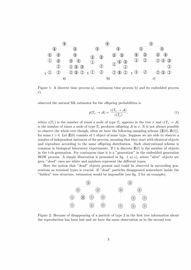
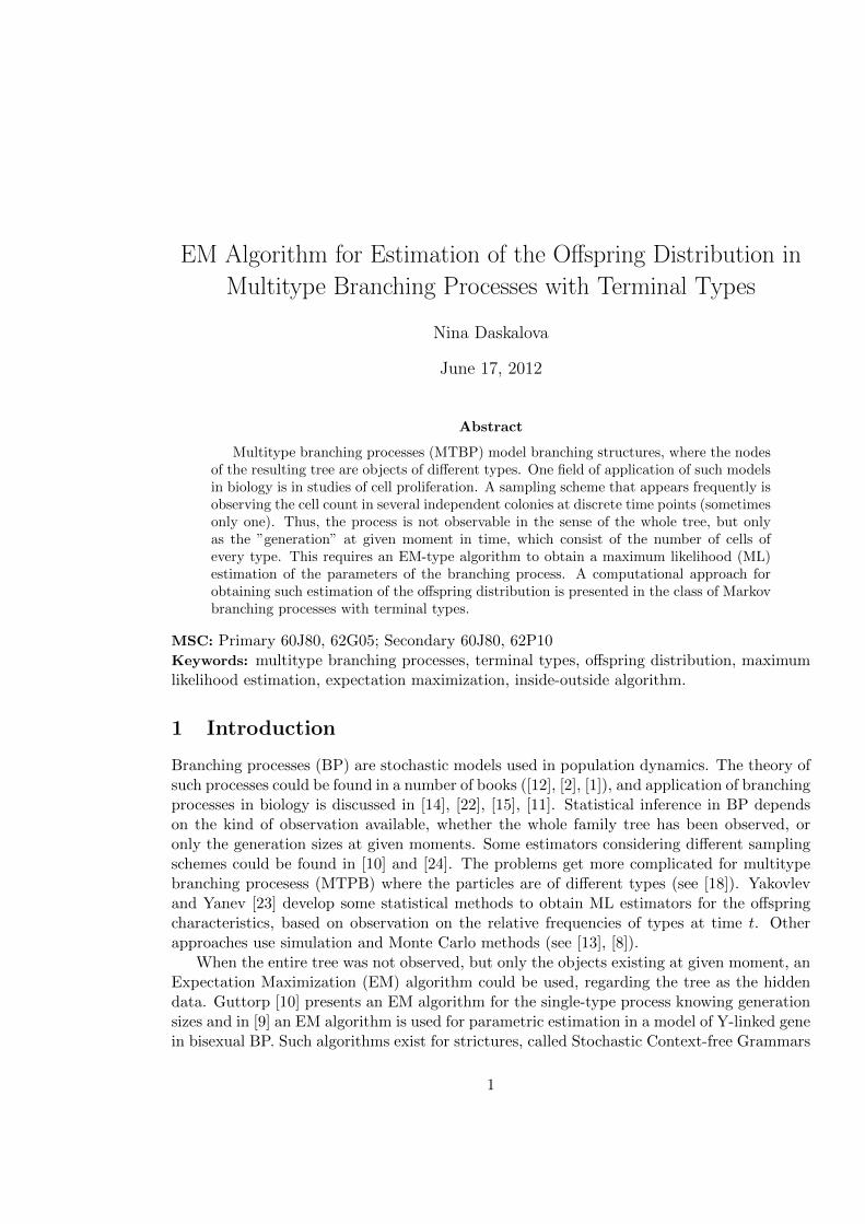
Figure 1: A discrete time process a), continuous time process b) and its embedded processc).

observed the natural ML estimator for the offspring probabilities is

p(Tv → A) =c(Tv → A)

c(Tv), (1)

where c(Tv) is the number of times a node of type Tv appears in the tree π and c(Tv → A)is the number of times a node of type Tv produces offspring A in π. It is not always possibleto observe the whole tree though, often we have the following sampling scheme {Z(0),Z(t)},for some t > 0. Let Z(0) consists of 1 object of some type. Suppose we are able to observe anumber of independent instances of the process, meaning that they start with identical objectsand reproduce according to the same offspring distribution. Such observational scheme iscommon in biological laboratory experiments. If t is discrete Z(t) is the number of objectsin the t-th generation. For continuous time it is a ”generation” in the embedded generationBGW process. A simple illustration is presented in fig. 1 a)–c), where ”alive” objects aregrey, ”dead” ones are white and numbers represent the different types.

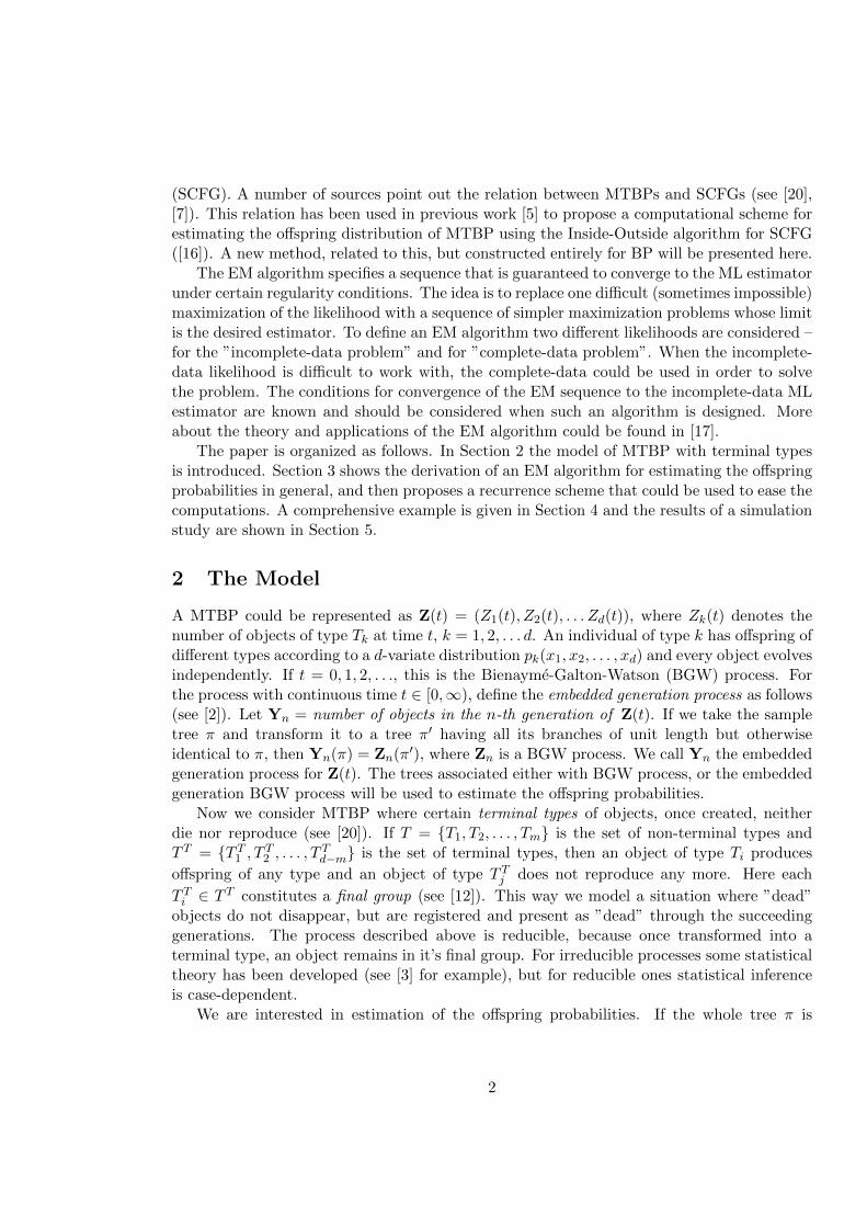
Here the notion that ”dead” objects present and could be observed in succeeding gen-erations as terminal types is crucial. If ”dead” particles disappeared somewhere inside the”hidden” tree structure, estimation would be impossible (see fig. 2 for an example).

Figure 2: Because of disappearing of a particle of type 2 in the first tree information aboutthe reproduction has been lost and we have the same observation as in the second tree.

3

3 The EM Proposal

3.1 The EM Algorithm

The EM algorithm was explained and given its name in a paper by Dempster, Laird, andRubin in 1977 [6]. It is a method for finding maximum likelihood estimates of parameters instatistical models, where the model depends on unobserved latent variables. Let a statisticalmodel be determined by parameters θ, x is the observation and Y is some ”hidden” data,which determines the probability distribution of x. Then the density of the ”complete”observation is f(x, y|θ) and the density of the ”incomplete” observation is the marginal oneg(x|θ) =

∫f(x, y|θ)dy. We can write the likelihoods and the conditional density of Y given

x and θ this way:

L(θ|x, y) = f(x, y|θ), L(θ|x) = g(x|θ), and k(y|θ, x) =f(x, t|θ)g(x|θ)

.

The aim is to maximize the log likelihood

logL(θ|x) = log g(x|θ) = logL(θ|x, y)− log k(y|θ, x).

As y is not observed the right side is replaced with its expectation under k(y|θ′, x):

logL(θ|x) = Eθ′ [logL(θ|x, Y )]− Eθ′ [log k(Y |θ, x)].

Let Q(θ|θ′) = Eθ′ [logL(θ|x, Y )]. It has been proved that

logL(θ|x)− logL(θ(i)|x) ≥ Q(θ|θ(i))−Q(θ(i)|θ(i))

with equality only if θ = θ(i), or if k(Y |x, θ(i)) = k(Y |x, θ) for some other θ 6= θ(i). Choosingθ(i+1) = argmaxθQ(θ|θ(i)) will make the difference positive and so, the likelihood could onlyincrease in each step. The Expectation Maximization Algorithm is usually stated formallylike this:

E-step: Calculate function Q(θ|θ(i)).M-step: Maximize Q(θ|θ(i)) with respect to θ.The convergence of the EM sequence {θ(i)} depends on the form of the likelihood L(θ|x)

and the expected likelihood Q(θ|θ(i)) functions. The following condition, due to Wu ([21]),guarantees convergence to a stationary point. It is presented here as cited in [4].

If the expected complete-data log likelihood Eθ′ [logL(θ|x, Y )] is continuous both in θ andθ′, then all limit points of an EM sequence {θ(i)} are stationary points of L(θ|x), and L(θ(i)|x)converges monotonically to L(θ|x) for some stationary point θ.

3.2 Derivation of an EM Algorithm for MTBP

Let x be the observed set of particles, π is the unobserved tree structure and p is the set ofparameters – the offspring probabilities p(Tv → A) (the probability that a particle of typeTv produces the set of particles A). Then the likelihood of the ”complete” observation is:

L(p|π, x) = P (π, x|p) =∏

v,A:Tv→Ap(Tv → A)c(Tv→A;π,x),

4

where c is a counting function – c(Tv → A;π, x) is the number of times a particle of type Tvproduces the set of particles A in the tree π, observing x. The probability of the ”incomplete”observation is the marginal probability P (x|p) =

∑π P (π, x|p). For the EM algorithm we

need to compute the function

Q(p|p(i)) = Ep(i)(logP (π, x|p)) =∑π

P (π|x,p(i)) logP (π, x|p)

=∑π

P (π|x,p(i))∑Tv→A

c(Tv → A;π, x) log p(Tv → A)

=∑Tv→A

∑π

P (π|x,p(i))c(Tv → A;π, x) log p(Tv → A)

=∑Tv→A

Ep(i)c(Tv → A) log p(Tv → A). (2)

We need to maximize the function (2) under the condition∑A p(Tv → A) = 1, p(Tv →

A) ≥ 0 for every v and A. The Lagrange method requires to introduce the function

Φ(p) =∑Tv→A

Ep(i)c(Tv → A) log p(Tv → A) + λ(1−∑Ap(Tv → A)).

Taking partial derivatives with respect to p(Tv → A) and obtaining the Lagrangian multiplierλ =

∑AEp(i)(Tv → A), we get to the result that the re-estimating parameters are the

normalized expected counts, which look like the ML estimators in the ”complete” observationcase (1), but the observed counts are replaced with their expectations.

p(i+1)(Tv → A) =Ep(i)c(Tv → A)∑AEp(i)c(Tv → A)

=Ep(i)c(Tv → A)

Ep(i)c(Tv), (3)

where the expected number of times a particle of type Tv appears in the tree π is:

Ep(i)c(Tv) =∑π

P (π|x,p(i))c(Tv;π, x),

and the expected number of times a particle of type Tv gives offspring A in the tree π is:

Ep(i)c(Tv → A) =∑π

P (π|x,p(i))c(Tv → A;π, x).

It is easy to check that in this case the convergence condition stated above is fulfilled. Weconsider the representation

Q(p|p(i)) =∑Tv→A

∑π

P (π|x,p(i))c(Tv → A;π, x) log p(Tv → A),

where P (π|x,p(i)) is a polynomial function of p(i)-s – the offspring probabilities, estimatedon the i-th step. Then Q(p|p(i)) is a sum of continuous functions in all the parameters p andp(i), so it is also continuous. This way we are sure to converge to a stationary value, thoughit might not always be a global maximizer.

It is a case of EM where the M-step is explicitly solved, so the computational effort willbe on the E-step. The problem is that in general enumerating all possible trees π is ofexponential complexity. The method proposed below is aimed to reduce complexity.

5

3.3 The Recurrence Scheme

We have shown that the E-step of the algorithm consists of determining the expected numberof times a given type Tv or a given production Tv → A appears in a tree π. A general methodwill be proposed here for computing these counts. The algorithm consists of three parts –calculation of the inner probabilities, the outer probabilities and EM re-estimation, whichare shown below.

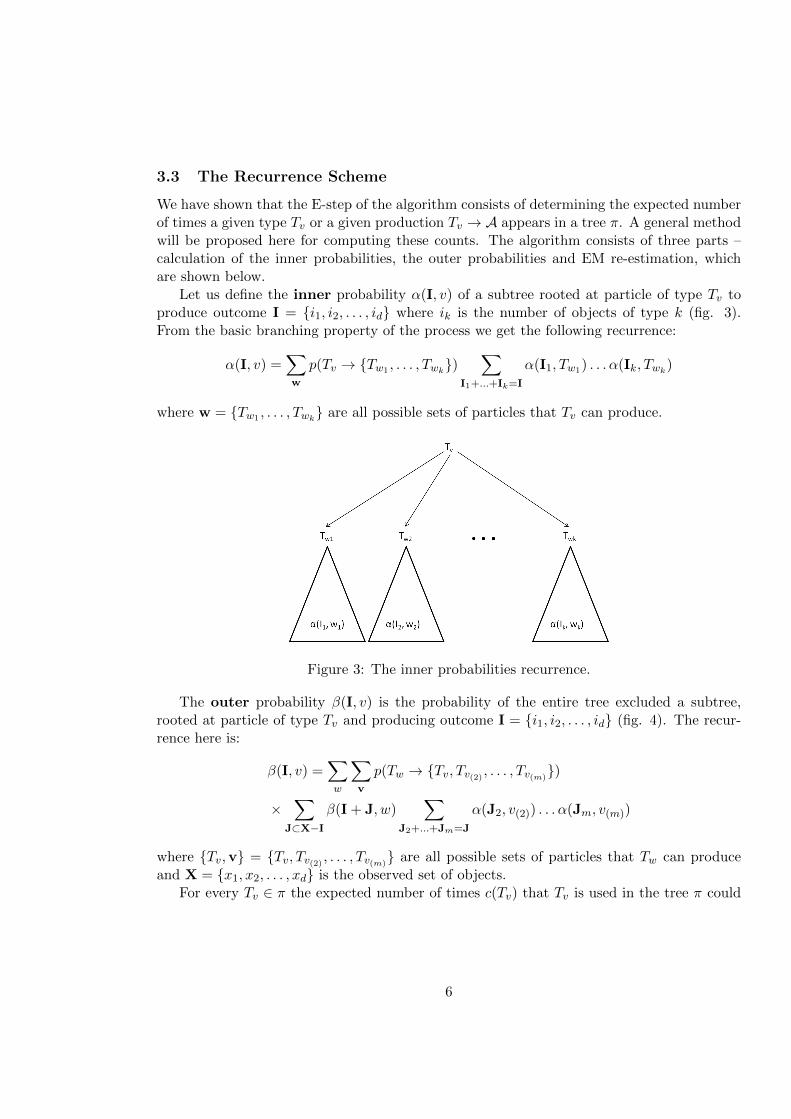
Let us define the inner probability α(I, v) of a subtree rooted at particle of type Tv toproduce outcome I = {i1, i2, . . . , id} where ik is the number of objects of type k (fig. 3).From the basic branching property of the process we get the following recurrence:

α(I, v) =∑w

p(Tv → {Tw1 , . . . , Twk})

∑I1+...+Ik=I

α(I1, Tw1) . . . α(Ik, Twk)

where w = {Tw1 , . . . , Twk} are all possible sets of particles that Tv can produce.

Figure 3: The inner probabilities recurrence.

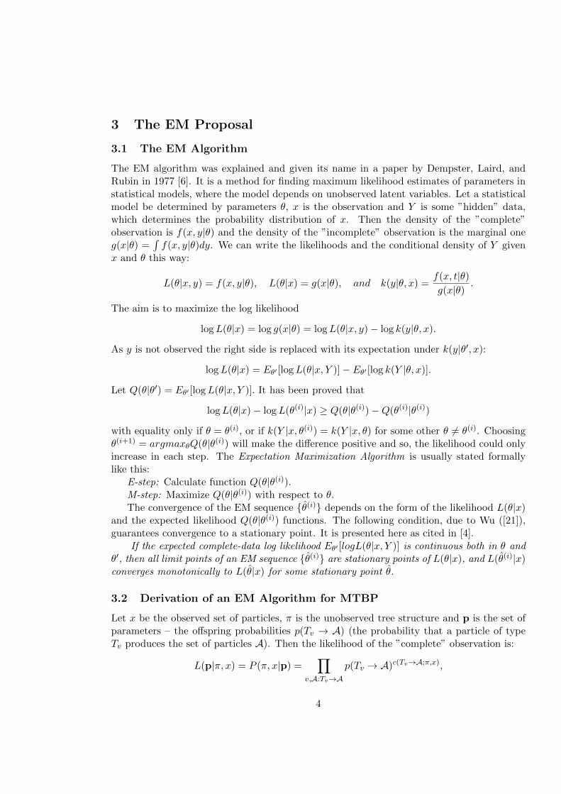
The outer probability β(I, v) is the probability of the entire tree excluded a subtree,rooted at particle of type Tv and producing outcome I = {i1, i2, . . . , id} (fig. 4). The recur-rence here is:

β(I, v) =∑w

∑v

p(Tw → {Tv, Tv(2) , . . . , Tv(m)})

×∑

J⊂X−Iβ(I + J, w)

∑J2+...+Jm=J

α(J2, v(2)) . . . α(Jm, v(m))

where {Tv,v} = {Tv, Tv(2) , . . . , Tv(m)} are all possible sets of particles that Tw can produce

and X = {x1, x2, . . . , xd} is the observed set of objects.For every Tv ∈ π the expected number of times c(Tv) that Tv is used in the tree π could

6

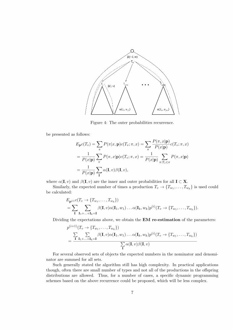
Figure 4: The outer probabilities recurrence.

be presented as follows:

Epc(Tv) =∑π

P (π|x,p)c(Tv;π, x) =∑π

P (π, x|p)

P (x|p)c(Tv;π, x)

=1

P (x|p)

∑π

P (π, x|p)c(Tv;π, x) =1

P (x|p)

∑π:Tv∈π

P (π, x|p)

=1

P (x|p)

∑I

α(I, v)β(I, v),

where α(I, v) and β(I, v) are the inner and outer probabilities for all I ⊂ X.Similarly, the expected number of times a production Tv → {Tw1 , . . . , Twk

} is used couldbe calculated:

Ep(i)c(Tv → {Tw1 , . . . , Twk})

=∑I

∑I1+...+Ik=I

β(I, v)α(I1, w1) . . . α(Ik, wk)p(i)(Tv → {Tw1 , . . . , Twk

}).

Dividing the expectations above, we obtain the EM re-estimation of the parameters:

p(i+1)(Tv → {Tw1 , . . . , Twk})

=

∑I

∑I1+...+Ik=I

β(I, v)α(I1, w1) . . . α(Ik, wk)p(i)(Tv → {Tw1 , . . . , Twk

})∑I

α(I, v)β(I, v)

For several observed sets of objects the expected numbers in the nominator and denomi-nator are summed for all sets.

Such generally stated the algorithm still has high complexity. In practical applicationsthough, often there are small number of types and not all of the productions in the offspringdistributions are allowed. Thus, for a number of cases, a specific dynamic programmingschemes based on the above recurrence could be proposed, which will be less complex.

7

4 A Comprehensive Example

We consider a MTBP with four types of particles – two nonterminal T1, T2 and two terminalT T1 , T T2 , and the productions that are allowed (with nonzero probability) are:

T1p111−→{T1, T1}, T1

p112−→{T1, T2}, T1p1T−→{T T1 }, T2

p222−→{T2, T2}, T2p2T−→{T T2 }. (4)

To cover the possibility of observing particles of types T1 and T2 the additional productions

T1p1−→{T1} and T2

p2−→{T2} are introduced.Now, let X = {1, 0, 1, 1} and the process has started with one particle of type T1. We

don’t have further information about the distribution, so an uniform one is assumed for everytype: p111 = p112 = p1T = p11 = 1/4 and p222 = p2T = p22 = 1/3.

Let α({i1, i2, iT1 , iT2 }, v) be the probability of a tree rooted at a particle of type Tv toproduce the number of particles of types T1, T2, T

T1 , T

T2 respectively. The initialization of α

should be as follows:

α1(1,0,0,0) = p11 = 1/4, α1

(0,0,1,0) = p1T = 1/4, α2(0,1,0,0) = p22 = 1/3, α2

(0,0,0,1) = p2T = 1/3.

For the level of two particles we are interested in all possible subsets of {1, 0, 1, 1} con-taining two 1-s. The values of α are calculated below:

α1(1,0,1,0) = p111α

1(1,0,0,0)α

1(0,0,1,0) + p112α

1(1,0,0,0)α

2(0,0,1,0) + p112α

1(0,0,1,0)α

2(1,0,0,0)

= 1/4.1/4.1/4 + 1/4.1/4.0 + 1/4.1/4.0 = 1/64,

Similarly,α1(1,0,0,1) = 1/48 and α1

(0,0,1,1) = 1/48.

Alsoα2(1,0,1,0) = 0, α2

(1,0,0,1) = 0, and α2(0,0,1,1) = 0.

Finally

α1(1,0,1,1) = p111[α

1(1,0,1,0)α

1(0,0,0,1) + α1

(1,0,0,1)α1(0,0,1,0) + α1

(1,0,0,0)α1(0,0,1,1)] + p112[α

1(1,0,1,0)α

2(0,0,0,1)

+ α1(1,0,0,1)α

2(0,0,1,0) + α1

(1,0,0,0)α2(0,0,1,1) + α2

(1,0,1,0)α1(0,0,0,1) + α2

(1,0,0,1)α1(0,0,1,0) + α2

(1,0,0,0)α1(0,0,1,1)]

= 1/4.(1/64.0 + 1/48.1/4 + 1/4.1/48) + 1/4.(1/64.1/3 + 1/48.0 + 1/4.0 + 0.0 + 0.1/4 + 0.1/48)

= 1/256.

Next follow the calculations of the outer probabilities β({i1, i2, iT1 , iT2 }, v). The initialvalues are β({1, 0, 1, 1}, 1) = 1 and β({1, 0, 1, 1}, 2) = 0. Then:

β1(1,0,1,0) = β1(1,0,1,1)[p111α

1(0,0,0,1) + p112α

2(0,0,0,1)] = 1.(1/4.0 + 1/4.1/3) = 1/12,

β1(1,0,0,1) = 1/16, β1(0,0,1,1) = 1/16,

β2(1,0,1,0) = β1(1,0,1,1)p112α

1(0,0,0,1) + β2(1,0,1,1)p

222α

2(0,0,0,1)= 1.1/4.0 + 0.1/3.1/3 = 0,

β2(1,0,0,1) = 1/16, β2(0,0,1,1) = 1/16,

8

β1(1,0,0,0) = β1(1,0,1,0)[p111α

1(0,0,1,0) + p112α

2(0,0,1,0)]

+ β1(1,0,0,1)[p111α

1(0,0,0,1) + p112α

2(0,0,0,1)] + β1(1,0,1,1)[p

111α

1(0,0,1,1) + p112α

2(0,0,1,1)]

= 1/12.(1/4.1/4 + 1/4.0) + 1/16.(1/4.0 + 1/4.1/3) + 1.(1/4.1/48 + 1/4.0) = 1/64,

β1(0,0,1,0) = 1/64 and β1(0,0,0,1) = 3/256,

β2(1,0,0,0) = β1(1,0,1,0)p112α

1(0,0,1,0) + β2(1,0,1,0)p

222α

2(0,0,1,0) + β1(1,0,0,1)[p

112α

1(0,0,0,1)

+ β2(1,0,0,1)p222α

2(0,0,0,1)] + β1(1,0,1,1)[p

112α

1(0,0,1,1) + β1(1,0,1,1)p

222α

2(0,0,1,1)]

= 1/12.1/4.1/4 + 0.1/3.0 + 1/16.1/4.0 + 1/16.1/3.1/3 + 1.1/4.1/48 + 1.1/3.0 = 5/288,

β2(0,0,1,0) = 5/288, and β2(0,0,0,1) = 1/256.

Using that P (x|θ) = α(X, 1) = α({1, 0, 1, 1}, 1) = 1/256, we are able to compute theexpected values we need:

Eθc(T1) =1

P (x|θ)∑I

α1Iβ

1I =

1

1/256(1/4.1/64 + 1/4.1/64 + 0

+ 1/64.1/12 + 1/48.1/16 + 1/48.1/16 + 1/256) =4/256

1/256= 4,

Eθc(T1 → {T1, T1}) =1

P (x|θ)∑I

∑I1+I2=I

β1Iα1I1α

1I2p(T1 → {T1, T1}) =

1/256

1/256= 1

Eθc(T1 → {T1, T2}) =1

P (x|θ)∑I

∑I1+I2=I

β1Iα1I1α

2I2p(T1 → {T1, T2}) =

1/256

1/256= 1

Eθc(T1 → {T T1 }) =1

P (x|θ)β1TT1p(T1 → {T T1 }) =

1

1/2561/4.1/64 =

1/256

1/256= 1,

Eθc(T1 → {T1}) =1

P (x|θ)β1T1p(T1 → {T1}) =

1

1/2561/4.1/64 =

1/256

1/256= 1.

Thus, the estimated distribution for T1 is

p111 =Eθc(T1 → {T1, T1})

Eθc(T1)= 1/4, p112 =

Eθc(T1 → {T1, T2})Eθc(T1)

= 1/4,

p11 =Eθc(T1 → {T1})

Eθc(T1)= 1/4, p1T =

Eθc(T1 → {T T1 })Eθc(T1)

= 1/4,

which is the same as the initially chosen one, so this would be the final estimation.For the offspring distribution of T2 similar computations lead to the result:

Eθc(T2) = 1, Eθc(T2 → {T2, T2}) = 0, Eθc(T2 → {T2}) = 0, Eθc(T2 → {TT2 }) = 1,

so the estimation is:

p222 = 0, p22 = 0, p2T = 1,

which converges on the next iteration also.

9

5 Simulation study

Simulation experiment has been performed to study behaviour of the estimates obtained viathe algorithm. Observations have been simulated according to the model (4) in the previoussection with offspring probabilities p111 = p112 = p1T = 1/3 and p222 = p2T = 1/2. Estimationhas been performed using different sample sizes both for the number of observations, and thetree sizes as well. All the computations were made in R [19].

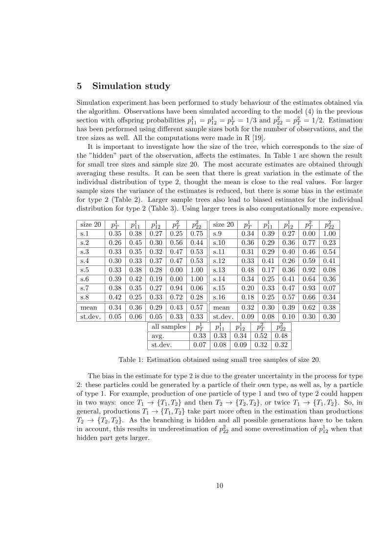
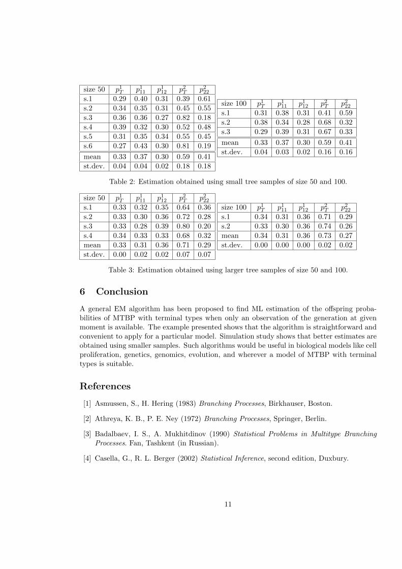
It is important to investigate how the size of the tree, which corresponds to the size ofthe ”hidden” part of the observation, affects the estimates. In Table 1 are shown the resultfor small tree sizes and sample size 20. The most accurate estimates are obtained throughaveraging these results. It can be seen that there is great variation in the estimate of theindividual distribution of type 2, thought the mean is close to the real values. For largersample sizes the variance of the estimates is reduced, but there is some bias in the estimatefor type 2 (Table 2). Larger sample trees also lead to biased estimates for the individualdistribution for type 2 (Table 3). Using larger trees is also computationally more expensive.

size 20 p1T p111 p112 p2T p222s.1 0.35 0.38 0.27 0.25 0.75

s.2 0.26 0.45 0.30 0.56 0.44

s.3 0.33 0.35 0.32 0.47 0.53

s.4 0.30 0.33 0.37 0.47 0.53

s.5 0.33 0.38 0.28 0.00 1.00

s.6 0.39 0.42 0.19 0.00 1.00

s.7 0.38 0.35 0.27 0.94 0.06

s.8 0.42 0.25 0.33 0.72 0.28

mean 0.34 0.36 0.29 0.43 0.57

st.dev. 0.05 0.06 0.05 0.33 0.33

size 20 p1T p111 p112 p2T p222s.9 0.34 0.39 0.27 0.00 1.00

s.10 0.36 0.29 0.36 0.77 0.23

s.11 0.31 0.29 0.40 0.46 0.54

s.12 0.33 0.41 0.26 0.59 0.41

s.13 0.48 0.17 0.36 0.92 0.08

s.14 0.34 0.25 0.41 0.64 0.36

s.15 0.20 0.33 0.47 0.93 0.07

s.16 0.18 0.25 0.57 0.66 0.34

mean 0.32 0.30 0.39 0.62 0.38

st.dev. 0.09 0.08 0.10 0.30 0.30

all samples p1T p111 p112 p2T p222avg. 0.33 0.33 0.34 0.52 0.48

st.dev. 0.07 0.08 0.09 0.32 0.32

Table 1: Estimation obtained using small tree samples of size 20.

The bias in the estimate for type 2 is due to the greater uncertainty in the process for type2: these particles could be generated by a particle of their own type, as well as, by a particleof type 1. For example, production of one particle of type 1 and two of type 2 could happenin two ways: once T1 → {T1, T2} and then T2 → {T2, T2}, or twice T1 → {T1, T2}. So, ingeneral, productions T1 → {T1, T2} take part more often in the estimation than productionsT2 → {T2, T2}. As the branching is hidden and all possible generations have to be takenin account, this results in underestimation of p222 and some overestimation of p112 when thathidden part gets larger.

10

size 50 p1T p111 p112 p2T p222s.1 0.29 0.40 0.31 0.39 0.61

s.2 0.34 0.35 0.31 0.45 0.55

s.3 0.36 0.36 0.27 0.82 0.18

s.4 0.39 0.32 0.30 0.52 0.48

s.5 0.31 0.35 0.34 0.55 0.45

s.6 0.27 0.43 0.30 0.81 0.19

mean 0.33 0.37 0.30 0.59 0.41

st.dev. 0.04 0.04 0.02 0.18 0.18

size 100 p1T p111 p112 p2T p222s.1 0.31 0.38 0.31 0.41 0.59

s.2 0.38 0.34 0.28 0.68 0.32

s.3 0.29 0.39 0.31 0.67 0.33

mean 0.33 0.37 0.30 0.59 0.41

st.dev. 0.04 0.03 0.02 0.16 0.16

Table 2: Estimation obtained using small tree samples of size 50 and 100.

size 50 p1T p111 p112 p2T p222s.1 0.33 0.32 0.35 0.64 0.36

s.2 0.33 0.30 0.36 0.72 0.28

s.3 0.33 0.28 0.39 0.80 0.20

s.4 0.34 0.33 0.33 0.68 0.32

mean 0.33 0.31 0.36 0.71 0.29

st.dev. 0.00 0.02 0.02 0.07 0.07

size 100 p1T p111 p112 p2T p222s.1 0.34 0.31 0.36 0.71 0.29

s.2 0.33 0.30 0.36 0.74 0.26

mean 0.34 0.31 0.36 0.73 0.27

st.dev. 0.00 0.00 0.00 0.02 0.02

Table 3: Estimation obtained using larger tree samples of size 50 and 100.

6 Conclusion

A general EM algorithm has been proposed to find ML estimation of the offspring proba-bilities of MTBP with terminal types when only an observation of the generation at givenmoment is available. The example presented shows that the algorithm is straightforward andconvenient to apply for a particular model. Simulation study shows that better estimates areobtained using smaller samples. Such algorithms would be useful in biological models like cellproliferation, genetics, genomics, evolution, and wherever a model of MTBP with terminaltypes is suitable.

References

[1] Asmussen, S., H. Hering (1983) Branching Processes, Birkhauser, Boston.

[2] Athreya, K. B., P. E. Ney (1972) Branching Processes, Springer, Berlin.

[3] Badalbaev, I. S., A. Mukhitdinov (1990) Statistical Problems in Multitype BranchingProcesses. Fan, Tashkent (in Russian).

[4] Casella, G., R. L. Berger (2002) Statistical Inference, second edition, Duxbury.

11

[5] Daskalova N. (2010) Using Inside-Outside Algorithm for Estimation of the OffspringDistribution in Multitype Branching Processes Serdica Journal of Computing, 4(4), 463–474.

[6] Dempster, A. P., N. M. Laird, D. B. Rubin (1977) Maximum likelihood from incompletedata via the EM algorithm. Journal of the Royal Statistical Society, B, 39, 1–38.

[7] Geman, S., M. Johnson (2004) Probability and statistics in computational linguistics, abrief review Mathematical foundations of speech and language processing. Johnson, M.;Khudanpur, S.P.; Ostendorf, M.; Rosenfeld, R. (Eds.)

[8] Gonzalez M., J. Martın, R. Martınez, M. Mota (2008) Non-parametric Bayesian estima-tion for multitype branching processes through simulation-based methods, ComputationalStatistics & Data Analysis, 52(3), 1281–1291.

[9] Gonzalez, M. and Gutierrez, C. and Martınez, R. (2010) Parametric inference for Y-linked gene branching model: Expectation-maximization method, proceeding of Workshopon Branching Processes and Their Applications, Lecture Notes in Statistics, 197, 191–204.

[10] Guttorp, P. (1991) Statistical inference for branching processes, New York: Wiley.

[11] Haccou, P., P. Jagers, V. A. Vatutin (2005) Branching Processes: Variation, Growth andExtinction of Populations. Cambridge University Press, Cambridge.

[12] Harris, T. E. (1963) Branching Processes, Springer, New York.

[13] Hyrien O. Pseudo-likelihood estimation for discretely observed multitype Bellman-Harrisbranching processes (2007) Journal of Statistical Planning and Inference, 137(4), 1375–1388.

[14] Jagers, P. (1975) Branching Processes with Biological Applications, London, Wiley.

[15] Kimmel, M., D. E. Axelrod (2002) Branching Processes in Biology, Springer, New York.

[16] Lari, K., S. J. Young (1990) The Estimation of Stochastic Context-Free Grammars Usingthe Inside-Outside Algorithm, Computer Speech and Language, 4, 35–36.

[17] McLachlan, G. J., T. Krishnan (2008) The EM Algorithm and Extensions, Wiley.

[18] Mode, C. J. (1971) Multitype Branching Processes: Theory and Applications, Elsevier,New York.

[19] R Development Core Team (2010) R: A language and environment for statisti-cal computing. R Foundation for Statistical Computing, Vienna, Austria, URLhttp://www.R-project.org.

[20] Sankoff, D. (1971) Branching Processes with Terminal Types: Application to Context-Free Grammars Journal of Applied Probability 8(2), 233–240.

12

[21] Wu, C. F. J. (1983) On the Convergence of the EM Algorithm. Ann. Stat. 11, 95–103.

[22] Yakovlev, A. Y., N. M. Yanev (1989) Transient Processes in Cell Proliferation Kinetics.Berlin, Springer.

[23] Yakovlev, A. Y., N. M. Yanev (2009) Relative frequencies in multitype branching pro-cesses Ann. Appl. Probab. 19(1), 1–14.

[24] Yanev, N. M. (2008) Statistical Inference for Branching Processes. In: M. Ahsanullah,G. P. Yanev (Eds), Records and Branching Processes, Nova Sci. Publishers, Inc, 143 –168.

Nina DaskalovaSofia University ”St.Kliment Ohridski”,Faculty of Mathematics and Informatics,Sofia, Bulgaria,e-mail: ninad@fmi.uni-sofia.bg

13