Electronic structure calculations with GPAW: a real-space implementation of the projector

augmented-wave method

This article has been downloaded from IOPscience. Please scroll down to see the full text article.

2010 J. Phys.: Condens. Matter 22 253202

(http://iopscience.iop.org/0953-8984/22/25/253202)

Download details:

IP Address: 157.89.65.129

The article was downloaded on 19/02/2013 at 10:10

Please note that terms and conditions apply.

View the table of contents for this issue, or go to the journal homepage for more

Home Search Collections Journals About Contact us My IOPscience

IOP PUBLISHING JOURNAL OF PHYSICS: CONDENSED MATTER

J. Phys.: Condens. Matter 22 (2010) 253202 (24pp) doi:10.1088/0953-8984/22/25/253202

TOPICAL REVIEW

Electronic structure calculations withGPAW: a real-space implementation of theprojector augmented-wave methodJ Enkovaara1, C Rostgaard2, J J Mortensen2, J Chen2, M Dułak2,L Ferrighi3, J Gavnholt4, C Glinsvad2, V Haikola5, H A Hansen2,H H Kristoffersen3, M Kuisma6, A H Larsen2, L Lehtovaara5,M Ljungberg7, O Lopez-Acevedo8, P G Moses2, J Ojanen6,T Olsen4, V Petzold2, N A Romero9, J Stausholm-Møller3,M Strange2, G A Tritsaris2, M Vanin2, M Walter10, B Hammer3,H Hakkinen8, G K H Madsen11, R M Nieminen5, J K Nørskov2,M Puska5, T T Rantala6, J Schiøtz4, K S Thygesen2

and K W Jacobsen2

1 CSC—IT Center for Science Ltd, PO Box 405 FI-02101 Espoo, Finland2 Center for Atomic-scale Materials Design, Department of Physics, Technical University ofDenmark, DK-2800 Kongens Lyngby, Denmark3 Interdisciplinary Nanoscience Center (iNANO) and Department of Physics and Astronomy,Aarhus University, DK-8000 Aarhus C, Denmark4 Danish National Research Foundation’s Center for Individual Nanoparticle Functionality(CINF), Technical University of Denmark, DK-2800 Kongens Lyngby, Denmark5 Department of Applied Physics, Aalto University School of Science and Technology,PO Box 11000, FIN-00076 Aalto, Espoo, Finland6 Department of Physics, Tampere University of Technology, PO Box 692, FI-33101 Tampere,Finland7 FYSIKUM, Stockholm University, Albanova University Center, SE-10691 Stockholm,Sweden8 Departments of Physics and Chemistry, Nanoscience Center, University of Jyvaskyla,PO Box 35 (YFL), FI-40014, Finland9 Leadership Computing Facility, Argonne National Laboratory, Argonne, IL, USA10 Freiburg Materials Research Center, Stefan-Meier-Strasse 21, 79104 Freiburg, Germany11 ICAMS, Ruhr Universitat Bochum, 44801 Bochum, Germany

Received 6 April 2010, in final form 14 May 2010Published 10 June 2010Online at stacks.iop.org/JPhysCM/22/253202

AbstractElectronic structure calculations have become an indispensable tool in many areas of materialsscience and quantum chemistry. Even though the Kohn–Sham formulation of thedensity-functional theory (DFT) simplifies the many-body problem significantly, one is stillconfronted with several numerical challenges. In this article we present the projectoraugmented-wave (PAW) method as implemented in the GPAW program package (https://wiki.fysik.dtu.dk/gpaw) using a uniform real-space grid representation of the electronicwavefunctions. Compared to more traditional plane wave or localized basis set approaches,real-space grids offer several advantages, most notably good computational scalability andsystematic convergence properties. However, as a unique feature GPAW also facilitates alocalized atomic-orbital basis set in addition to the grid. The efficient atomic basis set iscomplementary to the more accurate grid, and the possibility to seamlessly switch between thetwo representations provides great flexibility. While DFT allows one to study ground stateproperties, time-dependent density-functional theory (TDDFT) provides access to the excited

0953-8984/10/253202+24$30.00 © 2010 IOP Publishing Ltd Printed in the UK & the USA1

J. Phys.: Condens. Matter 22 (2010) 253202 Topical Review

states. We have implemented the two common formulations of TDDFT, namely thelinear-response and the time propagation schemes. Electron transport calculations underfinite-bias conditions can be performed with GPAW using non-equilibrium Green functions andthe localized basis set. In addition to the basic features of the real-space PAW method, we alsodescribe the implementation of selected exchange–correlation functionals, parallelizationschemes, �SCF-method, x-ray absorption spectra, and maximally localized Wannier orbitals.

(Some figures in this article are in colour only in the electronic version)

Contents

1. Introduction 22. General overview 3

2.1. Projector augmented-wave method 32.2. Atomic setups 52.3. Uniform 3d real-space grids 52.4. Localized functions and Fourier filtering 52.5. Iterative solution of eigenproblem 62.6. Density mixing 6

3. Exchange–correlation functionals in GPAW 63.1. Meta-GGA 63.2. Exact exchange 73.3. GLLB approximation for the exact exchange 83.4. van der Waals functional 9

4. Error estimation 115. Time-dependent density-functional theory 12

5.1. Real-time propagation 125.2. Linear-response formalism 125.3. Optical absorption spectra 125.4. Non-linear emission spectra 135.5. Photoelectron spectra 13

6. Localized atomic-like basis functions 146.1. Non-equilibrium electron transport 15

7. Additional features 167.1. �SCF 167.2. X-ray absorption spectra 177.3. Wannier orbitals 187.4. Local properties 19

8. Parallel calculations 209. Summary and outlook 21Acknowledgments 21References 22

1. Introduction

Electronic structure calculations have become an indispensabletool for simulations of condensed-matter systems. Nowadayssystems ranging from atoms and small molecules tonanostructures with several hundreds of atoms are studiedroutinely with density-functional theory (DFT) [1, 2].

In principle, only ground state properties such as totalenergies and equilibrium geometries can be investigated withDFT. However, several interesting material properties such asexcitation energies and optical spectra are related to the excitedstates of a system. These excited state properties can be studiedwith time-dependent density-functional theory (TDDFT) [3].

Even though the DFT equations are much easierto solve than the full many-body Schrodinger equation,

several numerical approximations are usually made. Theapproximations can be related to the treatment of core electronsand the region near the atomic nuclei (pseudopotential versusall-electron methods) [4–8] or to the discretization of equations(plane waves, localized orbitals, real-space grids, finiteelements) [9–19]. In this work, we present a real-space-based implementation of the projector augmented-wave (PAW)method in the open-source program package GPAW [20]. Wenote that there are several software packages that currentlyimplement the PAW method using a plane-wave basis [21–23].

The PAW method [7, 24] is formally an all-electronmethod which provides an exact transformation between thesmooth pseudo-wavefunctions and the all-electron wavefunc-tions. While in practical implementations the PAW methodresembles pseudopotential methods, it addresses several short-comings of norm-conserving or ultrasoft pseudopotentials.The PAW method offers a reliable description over the wholeperiodic table with good transferability of PAW potentials.The pseudo-wavefunctions in the PAW method are typicallysmoother compared to norm-conserving pseudopotential meth-ods so that the wavefunctions can be represented with fewerdegrees of freedom. The PAW approximation contains all theinformation about the nodal structure of wavefunctions near thenuclei, and it is always possible to reconstruct the all-electronwavefunctions from the pseudo-wavefunctions.

In the solid state community, plane-wave basis sets[9, 22, 25, 26] are the most popular choice for discretizing thedensity-functional equations while localized basis sets [11, 27]have been more popular in quantum chemistry. A more recentapproach is the use of uniform real-space grids [13, 28–30].Real-space methods provide several advantages over planewaves. A plane-wave basis imposes periodic boundaryconditions, while a real-space grid can flexibly treat both freeand periodic boundary conditions. The plane-wave methodrelies heavily on fast Fourier transforms, which are difficultto parallelize efficiently due to the non-local nature of theoperations. On the other hand, in real space it is possibleto work entirely with local and semi-local operations, whichenables efficient parallelization with small communicationoverhead. The accuracy of a real-space representation canbe increased systematically by decreasing the grid spacing,similar to increasing the kinetic energy cutoff in a plane-wave calculation. This systematic improvement of accuracyis also the main advantage of both real-space and plane-wavemethods compared to localized basis sets, where the accuracyof representation cannot be controlled as systematically.However, as localized functions can provide a very compactbasis set, we have also implemented atom-centered basis

2

J. Phys.: Condens. Matter 22 (2010) 253202 Topical Review

functions for situations where the high accuracy of a real-space grid is not needed. The atom-centered basis is especiallyconvenient in the context of electron transport calculationswithin the non-equilibrium Green function approach alsoimplemented in GPAW. To our knowledge, GPAW is the firstpublicly available package to implement the PAW method withuniform real-space grids and atom-centered localized orbitals.

In tandem with numerical approximations, physicalapproximations are needed in DFT since the exact formof the exchange–correlation (XC) functional is unknown.The traditional local density and generalized gradientapproximations have been surprisingly successful, but due towell-known shortcomings, there are continuing efforts to gobeyond them. Some of the new developments in this field,such as meta-GGA and exact-exchange-based approximationsare available in GPAW.

Time-dependent density-functional theory (TDDFT) canbe realized in two different formalism. In the most generalform, the time-dependent Kohn–Sham equations are integratedover the time-domain [31]. In the linear-response regimeit is also possible to obtain excitation energies by solvinga matrix equation in an electron–hole basis [32]. Thereal-time propagation and the linear-response approaches arecomplementary. For example, the linear-response schemeprovides all the excitations in a single calculation, while thereal-time formalism provides the excitations corresponding toa given initial perturbation. On the other hand, the real-timepropagation scheme can also address non-linear effects. Whilethe linear-response scheme is more efficient for small systems,the real-time propagation approach scales more favorably withsystem size. Both the linear-response and real-time forms areimplemented in GPAW, to our knowledge for the first timewithin the PAW method.

In addition to the standard total energy calculations,GPAW contains several more specific features. Forexample, excitation energies can be estimated with the �SCFmethod [33] as an alternative to the TDDFT approaches. X-rayabsorption spectra and maximally localized Wannier functionscan also be calculated.

This article is organized as follows. First, the generalfeatures of the PAW method and the implementation on a real-space grid are described in section 2. In section 3 we givean overview of the different exchange–correlation functionalsavailable, and in section 4 we discuss a recent method for errorestimations within DFT. An overview of TDDFT is presentedin section 5, and the localized basis set and its use in finite-biastransport calculations are described in section 6. In section 7,other features, such as �SCF, x-ray absorption spectra andWannier functions are described. The parallelization strategyand parallel scaling are presented in section 8. Finally, weprovide a summary and an outlook in section 9.

2. General overview

In this section, we present the main features of our PAWimplementation. Some of the details have been publishedearlier [34], so we provide here a general overview and discussin more detail only the parts where our approach has changedfrom the earlier publication. The notation is similar to the one

used in the original references [7]. We use Hartree atomic units(h = m = e = 4π

ε0= 1) throughout the article. Generally,

the equations are written for the case of a spin-paired andfinite system of electrons and the spin and k-point indices areincluded when necessary.

2.1. Projector augmented-wave method

In the Kohn–Sham formulation of DFT, we work withsingle-particle all-electron wavefunctions to describe core,semi-core and valence states. The PAW method is alinear transformation between smooth valence (and semi-core)pseudo (PS) wavefunctions, ψn (n is the state index) and all-electron (AE) wavefunctions, ψn . The core states of the atoms,φ

a,corei , are fixed to the reference shape for the isolated atom.

Here a is an atomic index and i is a combination index for theprincipal, angular momentum, and magnetic quantum numbersrespectively (n, � and m). Note, that the PAW method can beextended beyond the frozen core approximation [35], but wehave not done that.

Given a smooth PS wavefunction, the corresponding AEwavefunction, which is orthogonal to the set of φa,core

i orbitals,can be obtained through a linear transformation

ψn(r) = T ψn(r). (1)

The transformation operator, T , is given in terms of atom-centered AE partial waves, φa

i (r), the corresponding smoothpartial waves, φa

i (r), and projector functions, pai (r), as

T = 1 +∑

a

∑

i

(|φai 〉 − |φa

i 〉)〈 pai |, (2)

where atom a is at the position Ra. The defining propertiesof the atom-centered functions are that AE partial wavesand smooth PS partial waves are equal outside atom-centeredaugmentation spheres of radii ra

c ,

φai (r) = φa

i (r), |r − Ra| > rac (3)

and that the projector functions are localized inside theaugmentation spheres and are orthogonal to the PS partialwaves

〈 pai1|φa

i2〉 = δi1i2 . (4)

In principle, an infinite number of atom-centered partialwaves and projectors is required for the PAW transformationto be exact. However, in practical calculations it is usuallyenough to include one or two functions per angular momentumchannel. The projectors and partial waves are constructed froman AE calculation for a spherically symmetric atom.

Inside the augmentation sphere of atom a, we can defineone-center expansions of an AE and PS state as [7]

ψan (r) =

∑

i

Painφ

ai (r) (5)

andψa

n (r) =∑

i

Pain φ

ai (r), (6)

where the expansion coefficients are

Pain = 〈 pa

i |ψn〉. (7)

3

J. Phys.: Condens. Matter 22 (2010) 253202 Topical Review

For a complete set of partial waves, we have ψn = ψan and

ψn = ψan for |r − Ra| < ra

c , which leads to

ψn = ψn +∑

a

(ψan − ψa

n ). (8)

Here, the term in the parenthesis is a correction inside theaugmentation spheres only.

We define a PS electron density

n(r) =∑

n

fn |ψn(r)|2 +∑

a

nac (r), (9)

where fn are occupation numbers between 0 and 2, and nac is a

smooth PS core density equal to the AE core density nac outside

the augmentation sphere. From the atomic density matrix Dai1i2

Dai1i2

=∑

n

〈ψn | pai1〉 fn〈 pa

i2|ψn〉, (10)

we define one-center expansions of the AE and PS densities,

na(r) =∑

i1,i2

Dai1i2φa

i1(r)φa

i2(r)+ na

c (r), (11)

andna(r) =

∑

i1,i2

Dai1i2φa

i1(r)φa

i2(r)+ na

c (r), (12)

respectively.From n, na and na , we can construct the AE density in

terms of a smooth part and atom-centered corrections

n(r) = n(r)+∑

a

(na(r)− na(r)). (13)

The PAW total energy expression has three contributions:kinetic, Coulomb and XC energy, all of which are composedof a PS part and atomic corrections. For the kinetic energy, weget

Ekin = − 12

∑

n

fn

∫dr ψn(r)∇2ψn(r), (14)

�Eakin = − 1

2 2core∑

i

∫dr φa

i (r)∇2φai (r)

− 12

∑

i1i2

Dai1i2

∫dr (φa

i1(r)∇2φa

i2(r)− φa

i1(r)∇2φa

i2(r)).

(15)

Before we can write down the expression for the PAWCoulomb energy, we must define one-center AE and PS chargedensities

ρa(r) = na(r)− Zaδ(r − Ra), (16)

ρa(r) = na(r)+∑

�m

Qa�m ga

�m(r), (17)

where Za is the atomic number of atom a, ga�m(r) = ga

� (|r −Ra|)Y�m(r − Ra) is a shape function localized inside theaugmentation sphere fulfilling

∫r 2 dr r �ga

� (r) = 1, and Qa�m

are multipole moments that we choose as described below. Wedefine a PS charge density as

ρ(r) = n(r)+∑

a

∑

�m

Qa�m ga

�m(r), (18)

so that the AE charge density is ρ = ρ + ∑a(ρ

a − ρa).By choosing Qa

�m so that ρa and ρa have the same multipolemoments, augmentation spheres on different atoms will beelectrostatically decoupled and the Coulomb energy is simply

Ecoul = 1

2

∫dr dr′ ρ(r)ρ(r

′)|r − r′| , (19)

�Eacoul = 1

2

∫dr dr′ ρ

a(r)ρa(r′)− ρa(r)ρa(r′)|r − r′| . (20)

For local and semi-local XC functionals, the contributions tothe XC energy is

Exc = Exc[n], (21)

�Eaxc = Exc[na] − Exc[na]. (22)

There is one extra term in the PAW total energy expressionwhich does not have a physical origin

Ezero =∫

dr n(r)∑

a

va(r), (23)

�Eazero = −

∫dr na(r)va(r). (24)

The only restriction in the choice of the so called zero potential(or local potential) va is that it must be zero outside theaugmentation sphere of atom a. For a complete set of partialwaves and projectors, Ezero+∑

a �Eazero is exactly zero, but for

practical calculations with a finite number of partial waves andprojector functions, va can be used to improve the accuracy ofa PAW calculation [36].

The final expression for the energy is

E = E +∑

a

�Ea (25)

= Ekin + Ecoul + Exc + Ezero

+∑

a

(�Eakin +�Ea

coul +�Eaxc +�Ea

zero). (26)

The smooth PS wavefunctions ψn are orthonormal only withrespect to the PAW overlap operator S: 〈ψn |S|ψm〉 = δnm ,where

S = T †T = 1 +∑

a

∑

i1i2

| pai1〉�Sa

i1i2〈 pa

i2|, (27)

�Sai1i2

= 〈φai1|φa

i2〉 − 〈φa

i1|φa

i2〉. (28)

This leads to the generalized eigenproblem

H ψn = εn Sψn, (29)

where

H = − 12∇2 + v +

∑

a

∑

i1i2

| pai1〉�H a

i1i2〈 pa

i2|, (30)

�H ai1i2

= ∂�Ea

∂Dai1i2

+∫

dr vcoul(r)∂ρ(r)∂Da

i1i2

, (31)

and the effective potential

v = δ E

δn= vcoul + vxc +

∑

a

va, (32)

where the Coulomb potential satisfies the Poisson equation∇2vcoul = −4πρ and vxc is the XC potential.

4

J. Phys.: Condens. Matter 22 (2010) 253202 Topical Review

2.2. Atomic setups

For each type of atom, we construct an atomic setup consistingof the following quantities: φa

i , φai , pa

i , nac , na

c , g�m, va and rac .

From a scalar-relativistic reference calculation for the isolatedneutral spin-paired spherically symmetric atom, we calculatethe required AE partial waves φa

i and the core density nac .

We choose a cutoff radius rac for the augmentation sphere and

a shape for g�m , which is usually a Gaussian. The smoothPS partial waves φa

i and the smooth PS core density nac are

constructed by smooth continuation of φai and na

c , respectively,inside the augmentation sphere. The projector functions pa

iare constructed as described in [7] and va is chosen so thatthe effective potential v becomes as smooth as possible or toproduce good scattering of f-states [36]. For more details,see [34].

All the functions in an atomic setup are of the form ofa radial function times spherical harmonics and each radialfunction is tabulated on a radial grid. Since φa

i and nac can

contain tightly bound localized electrons, the radial grid usedhas a higher grid density close to r = 0 than further from thenucleus (we use ri = βi/(N − i) for i = 0, 1, . . . , N). All thefunctions comprising a setup need only be known for r < ra

c ,except for φa

i and nac , which are used also for initialization of

wavefunctions and density.

2.3. Uniform 3d real-space grids

Uniform real-space grids provide a simple discretization for theKohn–Sham and Poisson equations. Physical quantities such aswavefunctions, densities, and potentials are represented by thevalues at the grid points. Derivatives are calculated using finitedifferences. The accuracy of discretization is determined bythe grid spacing and the finite difference approximations usedfor the derivatives.

For a general unit cell with lattice vectors aα (α = 1, 2, 3)and Nα grid points along the three directions, we define gridspacing vectors hα = aα/Nα . For an orthorhombic unit cell,the Laplacian is discretized as

∇2 f (r) =D∑

α=1

N∑

n=−N

bαcNn f (r + nhα)+ O(h2N ), (33)

where D = 3, bα = 1/h2α and cN

n are the N th order finitedifference coefficients for the second derivative expansion.

In the case of a non-orthorhombic unit cell, we extendthe set of grid spacing vectors with more nearest neighbordirections. The D coefficients bα are determined by theconventional method of undetermined coefficients, insertingthe six functions f (r) = x2, y2, z2, xy, yz, zx in equation (33)and solving for bα at r = (0, 0, 0). The number of directionsneeded to satisfy the six equations depends on the symmetry ofthe lattice: For hexagonal or body-centered cubic symmetry,D = 4 directions are needed, while D = 6 directions are usedfor a face-centered cubic cell or a general unit cell without anysymmetry. This procedure allows for finite difference stencilswith only 1 + 2DN points, which is similar to the stencilsdefined by Natan et al [37].

It must be noted that the performance of a given stencil isto an extent structure-dependent. For example, for calculationsof individual molecules, where large gradients are present,a more compact stencil may outperform a higher accuracybut less compact one. However, good accuracy is typicallyobtained for a combination of a grid spacing of h = 0.2 Aand a finite difference stencil with O(h6) error for the kineticenergy.

The PS electron density is evaluated on the same grid asthe wavefunctions. It is then interpolated to a finer grid witha grid spacing of h/2, where the XC energy and potentialare calculated. The fine grid is also used for constructing thePS charge density and for solving the Poisson equation. Thediscretization of the Poisson equation is done with a finitedifference stencil like equation (33) with an error of O(h6).For orthorhombic unit cells a more compact Mehrstellen-typestencil [16] can also be used for solving the Poisson equation.The effective potential, equation (32), is then restricted to thecoarse grid where it can be applied to the wavefunctions.

Boundary conditions for the quantities represented on 3dgrids can be zero for an isolated system or periodic for aperiodic system (or any combination). When using k-pointsampling, a wavefunction can also have Bloch-type boundaryconditions

ψnk(r + R) = ψnk(r)eik·R, (34)

where R is any Bravais vector. For charged systems,the boundary condition for vcoul can be determined from amultipole expansion.

2.4. Localized functions and Fourier filtering

Special care is needed when dealing with integrals involvingproducts of localized functions centered on an atom andfunctions spanning the whole simulation cell. As an example,consider the projection of a wavefunction onto a projectorfunction pa

i (r) = pani�i(|r−Ra|)Y�i mi (r−Ra) centered on atom

a. This integral is approximated by a sum over grid points:

〈 pai |ψ〉 =

∑

g

pai (rg)ψ(rg)�v, (35)

where �v is the volume per grid point. In order to make theintegration as accurate as possible, it is important that the radialfunction pa

ni�i(r) contains as few short wavelength components

as possible. To achieve this, we Fourier filter our projectorfunctions using the mask function technique [38]. Here,the radial function is divided by a mask function that goessmoothly to zero at approximately twice the original cutoffradius. We use m(r) = exp(−γ r 2). After a Fourier transform,the short wavelength components are cut off by multiplying thespectrum by a smooth cutoff function. Transforming back toreal-space, the final result is obtained by multiplying by m(r),which will remove the oscillating and decaying tail beyond thecutoff of the chosen mask function.

In the PAW formalism, there are four different typesof localized functions that need to be evaluated on the gridpoints: projector functions pa

i , the zero potential va , the shapefunctions ga

�m (for the compensation charges), and the PS coredensity na

c ; we apply the mask function technique to pai and

5

J. Phys.: Condens. Matter 22 (2010) 253202 Topical Review

va . The radial part of the shape functions are chosen asr �e−αa ra

and are therefore optimally smooth [39], and the PScore densities can always be chosen very smooth.

2.5. Iterative solution of eigenproblem

The Hamiltonian and overlap operators appearing in thegeneralized eigenvalue problem equation (29) are large sparsematrices in the real-space grid representation. Due to the largesize of the matrices, direct diagonalization schemes whichscale O(N3)with the matrix size are not tractable. On the otherhand, sparsity of the matrices makes iterative diagonalizationschemes [9, 40] appealing due to their dominant O(N2)

scaling.We have implemented three different iterative eigen-

solvers which share some common ingredients: the residualminimization method-direct inversion in iterative subspace(RMM-DIIS) [41, 40], the conjugate gradient method [9, 42],and Davidson’s method [43, 40]. A basic concept in all themethods is the update of the eigenvectors ψn with the residuals

Rn = (H − εn S)ψn . (36)

The convergence of iterative methods can be accelerated withpreconditioning, and we calculate preconditioned residualsRn = P Rn , by solving approximately a Poisson equation

12∇2 Rn = Rn (37)

with a multigrid method [16].A subspace diagonalization is always performed before

the iteration steps. The RMM-DIIS method does notconserve the orthonormality of eigenvectors, and thus explicitorthonormalization is done after each RMM-DIIS step. A goodinitial guess for the wavefunctions is especially important forthe robustness of the RMM-DIIS algorithm. We take the initialguess from an atomic orbital basis calculation, the details ofwhich are described in section 6.

2.6. Density mixing

During the self-consistency cycles both wavefunctions andthe density are updated iteratively. New PS density n(r)and atomic density matrices Da

i1i2are calculated from the

wavefunctions, equations (9) and (10) and mixed with the olddensities using Pulay’s method [44, 40].

Pulay’s method requires a good metric M for measuringthe change from input to output density 〈�n|M |�n〉, where�n = nout − nin, in order to determine the optimal linearcombination of old output densities. It is important that Mputs more weight on long wavelength changes, as these canintroduce charge sloshing in systems with many states at theFermi level [40], who, for example, use the metric

M =∑

q

fq |q〉〈q|, with fq = q2 + q21

q2, (38)

where q1 ∼ 1 and |q〉 is a plane wave with wavevector q.Expressed on a real-space grid, where |R〉 is a grid point at

R, we have

M =∑

RR′MRR′ |R〉〈R′|, with MRR′ =

∑

q

fq eiq·(R′−R).

(39)We would like to calculate scalar products from the densityon the real-space grid, but the non-locality of equation (39)makes this intractable. We therefore seek a more local metricM , which can be represented as a finite difference operator

M =∑

R

N∑

i=0

∑

v∈Vi

ci |R〉〈R + v|, (40)

where Vi is the set of vectors pointing to the i th nearestneighbors of a grid point. We enforce M to be semi-local byincluding only up to N th nearest neighbors. In reciprocal spaceM has matrix elements

fq = 〈q|M |q′〉 =∑

i

ci

∑

v∈Vi

eiq·vδq,q′ . (41)

The coefficients ci should be determined so that equation (41)mimics the behavior of fq in equation (38). This means thatfq should decay monotonically from a weight factor w > 1at q = 0–1 for the largest wavevectors at the zone boundaryin reciprocal space: f (3)(π/h,qy ,qz)

= 1 for |qy| � π/h and|qz| � π/h. For an orthorhombic grid with grid spacingh, including up to 3rd nearest neighbors, we can fulfil theseboundary conditions with the coefficients

c0 = w + 7

8, c1 = w − 1

16, c2 = w − 1

32,

c3 = w − 1

64.

(42)

We find the metric to improve convergence significantlywhen there are many states near the Fermi level. A value ofw = 100 seems to be a good choice.

3. Exchange–correlation functionals in GPAW

The exact form of the exchange–correlation (XC) functionalin the DFT is not known. Thus, it has to be approximated,which constitutes the fundamental physical approximation inpractical calculations. GPAW provides several forms of XCfunctionals ranging from the basic local density (LDA) andgeneralized gradient (GGA) approximations to the more exotichybrid functionals; a van der Waals density-functional and theHubbard-corrected DFT + U are also available. For the basicfunctionals GPAW uses libxc [45], which is an open-sourcelibrary of popular XC functionals: LDA, GGA, and meta-GGA. The exchange and correlation parts of libxc can be freelycombined. In the following we describe the more advancedfunctionals implemented in GPAW.

3.1. Meta-GGA

Meta-GGAs use the kinetic energy density in addition todensities and density gradients in standard GGAs so that more

6

J. Phys.: Condens. Matter 22 (2010) 253202 Topical Review

of the known properties of the exact XC functional can befulfilled [46]. The kinetic energy density is defined as

τ (r) = 12

∑

n

fn |∇ψn(r)|2. (43)

The MGGAs currently implemented in GPAW [47–49] dependon the reduced (dimensionless) quantities τ/τHEG and τ/τ vW,where

τHEG = 310 (6π

2)2/3n5/3 (44)

is the kinetic energy density of the homogeneous electron gas(HEG), and

τ vW = |∇n|28n

(45)

is the von Weizsacker (vW) kinetic energy density.Just like the AE density, equation (13), the kinetic energy

density can be written as τ = τ + ∑a(τ

a − τ a), where thesmooth part is

τ (r) = 12

∑

n

fn|∇ψn(r)|2 +∑

a

τ ac (r), (46)

and the atom-centered parts are

τ a(r) = 12

∑

i1i2

Dai1i2

∇φi1(r) · ∇φi2(r)+ τ ac (r), (47)

τ a(r) = 12

∑

i1i2

Dai1i2

∇φi1(r) ·∇φi2(r)+ τ ac (r). (48)

The AE and PS core kinetic energy densities τ ac (r) and τ a

c (r)are simple radial functions that are calculated during atomicsetup generation.

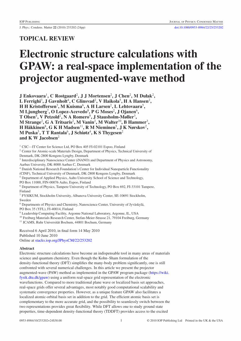
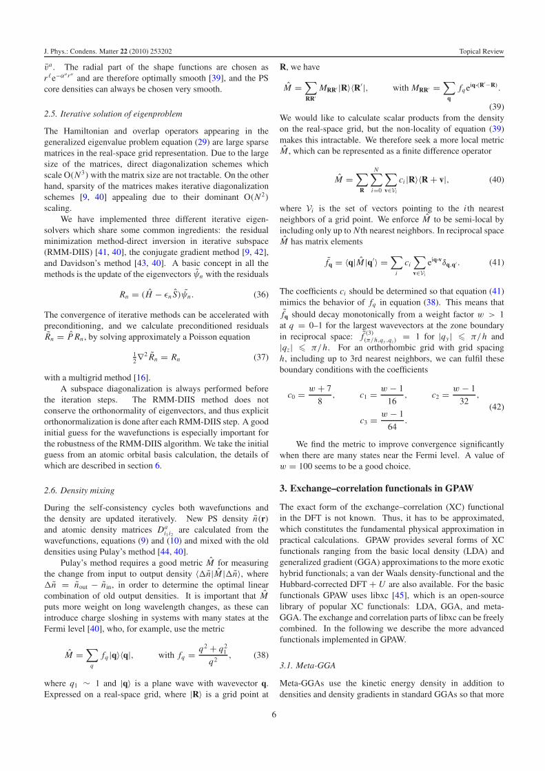
Currently, GPAW enables calculation of non-self-consistent TPSS [47], revTPSS [49] and M06-L [48] energies.The use of PBE orbitals in non-self-consistent calculations ofatomization energies and bond lengths for small molecules hasbeen determined to be accurate [50]. In figure 1 the GPAWatomization energies errors, with respect to experiments, arereported both for the PBE and MGGA functionals. TheTPSS mean absolute error with respect to experimental valuesobtained with GPAW is 0.13 eV, and this is consistent with thevalue of 0.14 eV of [50]. All MGGA functionals employedimprove over the PBE atomization energies whose meanabsolute error is 0.33 eV.

3.2. Exact exchange

GPAW offers access to the Fock exchange energy (exactexchange), as well as fractional inclusion of the Fock operatorin the hybrid XC functionals. The exact-exchange (EXX)functional was implemented within the PAW method in aplane-wave basis [51], but to the authors’ knowledge this isthe first implementation in a real-space PAW method. As thePAW related expressions are independent of the basis, we referto [51] for their derivation, and sketch only the main featureshere.

The EXX energy functional is given by

Exx = − 12

∑

i jσ

fiσ f jσ K Ci jσ,i jσ , (49)

Figure 1. PBE, TPSS, revTPSS and M06-L non-self-consistentatomization energies errors, with respect to experiments, calculatedwith GPAW for small molecules, in eV. The MGGA GPAW valuesare obtained from PBE orbitals at experimental geometries.Experimental values are as in [50].

where i and j are the state indices, and σ is the spin index. TheCoulomb matrix K C is defined as

K Ci jσ1,klσ2

= (ni jσ1 |nklσ2 ) :=∫

dr dr′

|r − r′|n∗i jσ1(r)nklσ2 (r

′),

(50)where the orbital pair density is ni jσ (r) = ψ∗

iσ (r)ψ jσ (r).When i, j both refer to valence states, the pair density

can be partitioned into a smooth part and atom-centeredcorrections, similar to the AE density in equation (13), as

ni jσ = ni jσ +∑

a

(nai jσ − na

i jσ ). (51)

Due to the non-local nature of the Coulomb kernel 1/|r −r′|, direct insertion of equation (51) into (50) leads to crossterms between different augmentation spheres. The sameproblem appeared already in the evaluation of the PAWCoulomb energy, and it can be solved similarly by introducingcompensation charges (from now on we drop the spin indicesfor brevity)

Z ai j(r) =

∑

�m

Qa�m,i j g

a�m(r), (52)

which are chosen to electrostatically decouple the smoothcompensated pair densities

ρi j = ni j +∑

a

Z ai j . (53)

The Coulomb matrix now has a simple partitioning in terms ofa smooth part and local corrections,

K Ci j,kl = (ρi j |ρkl )+

∑

a

�K C,ai j,kl . (54)

We refer to [52] for the exact form of the correction term�K C,a

i j,kl , which is also used to evaluate equation (20). Wenote that the Coulomb matrix K C

i j,kl appears also in the linear-response TDDFT (see section 5) and in the GW method [53].

The formally exact partitioning in equation (54) retains allinformation about the nodal structure of the AE wavefunctions

7

J. Phys.: Condens. Matter 22 (2010) 253202 Topical Review

in the core region, which is important due to the non-localprobing of the Coulomb operator. In standard pseudopotentialschemes this information is lost, leading to an uncontrolledapproximation to K C

i j,kl .As a technical issue, we note that integration over the

Coulomb kernel 1/|r − r′| is done by solving the associatedPoisson equation, ∇2vi j = −4πρi j , for the Coulomb potential.However, the compensated pair densities ρii have a non-zero total charge, which leads to an integrable singularity inperiodic systems. For periodic systems, the problem is solvedby subtracting a homogeneous background charge from thepair densities and adding a correction term to the calculatedpotential afterward [51, 54]. For non-periodic systems, thePoisson equation is solved by adjusting the boundary valuesaccording to the multipole expansion of the pair density.

Terms in the Coulomb matrix, where either i or j refersto a core orbital, can be reduced to trivial functions ofthe expansion coefficients Pa

in , equation (7). Although thevalence–core interaction is computationally trivial to include,it is not unimportant, and we will return to the effect ofneglecting it, as it is unavailable in pseudopotential schemes.The core–core exchange is simply a constant energy that canbe calculated once and for all for every atom given the frozencore orbitals.

The Fock operator vF(r, r′) corresponding to the exact-exchange energy functional of equation (49) is non-local, andit is difficult to represent on any realistic grid. Fortunately, inthe iterative minimization schemes used in GPAW the explicitform is never needed, but it suffices to evaluate only the actionof the operator on a wavefunction. By taking into account thePAW transformation, the action on the PS wavefunction can bederived by the relation.

fnˆvF|ψn〉 = ∂Exx/∂〈ψn|, (55)

which results in

fnˆvF|ψn〉 = −

∑

m

fm vnm(r)|ψm〉

+∑

a

∑

i

| pai 〉�vFa[vnm, {Pa

jm}]. (56)

The computationally demanding first term is related to smoothpseudo-quantities only, which can be accurately represented oncoarse grids, making it possible to do converged self-consistentEXX calculations at a relatively modest cost. Applyingthe Fock operator is, however, still expensive, as a Poissonequation must be solved for all pairs of orbitals. The atomiccorrection �vFa depends both on vnm and on the set ofexpansion coefficients Pa

in . The details of the derivation as wellas the exact form of the correction term can be found in [55].

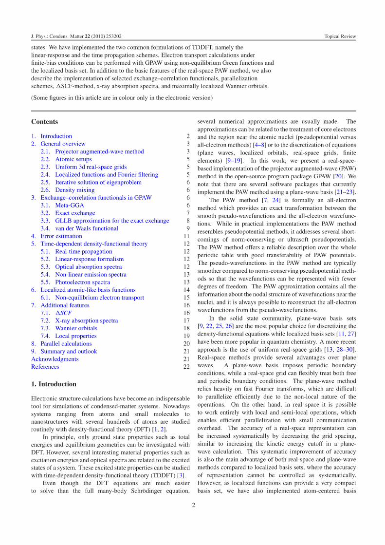
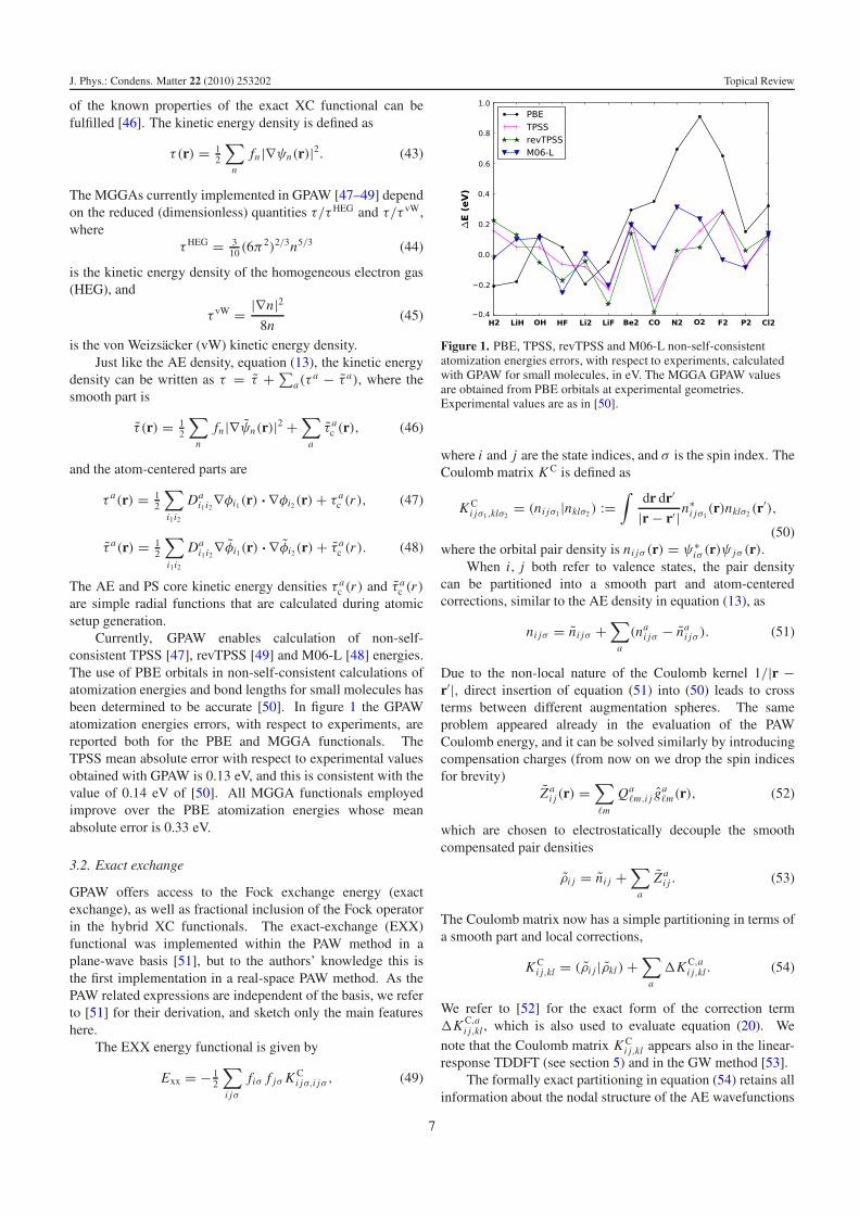
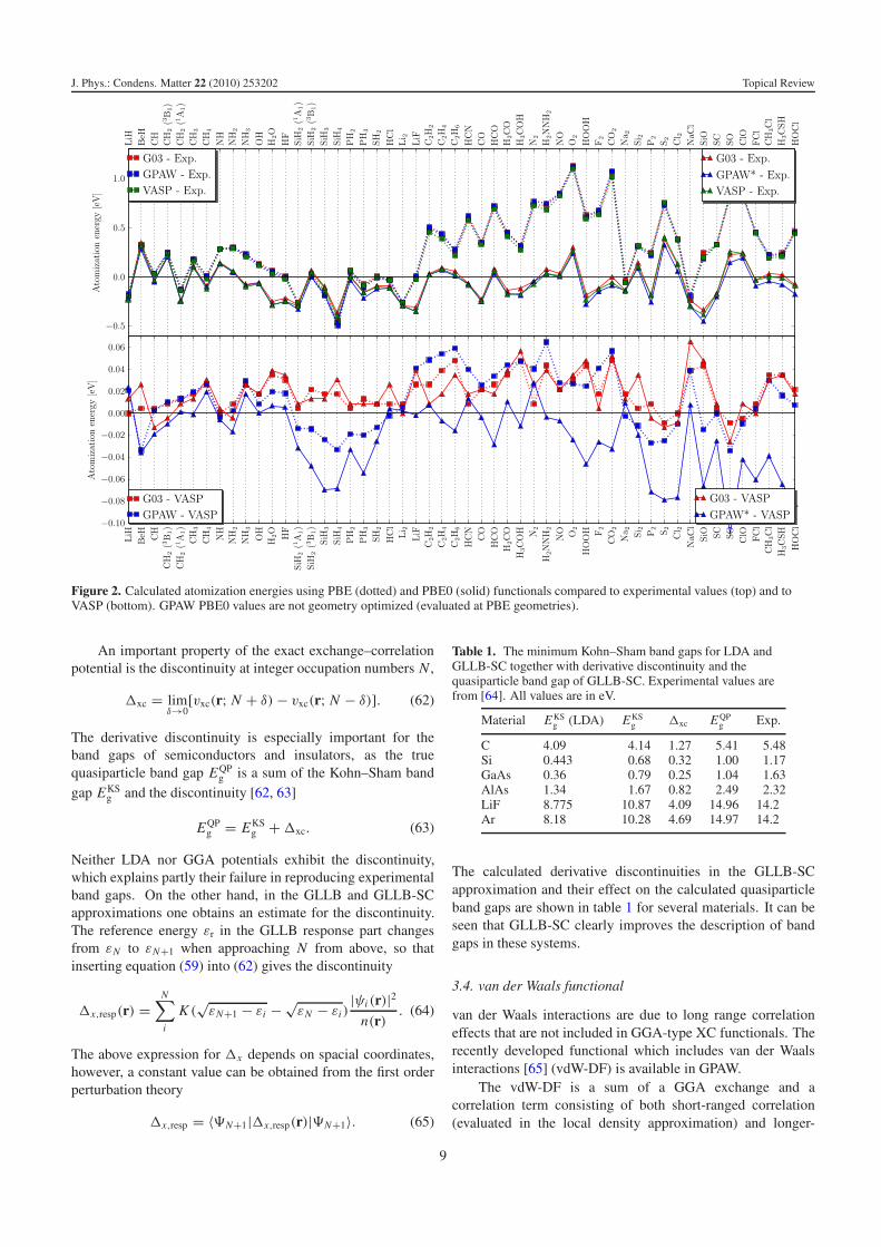
As a benchmark of the implementation, and for comparingthe PBE and hybrid PBE0 [56] functionals, we havecomputed the atomization energies of the G2-1 database ofmolecules [57] using these two functionals. The results arecompared to the experimental values as well as to the resultsof the plane-wave PAW implementation VASP, and of the all-electron atomic orbital code Gaussian 03, as reported in [51].

The PBE0 functional includes a fraction (25%) ofFock exchange in PBE, which improves the agreement with

experiments significantly, as shown in figure 2. The figureshows also that the different implementations deviate fromone another by less than 0.05 eV on average. The GPAWPBE0 energies are all slightly too small because they have notbeen geometry optimized with the hybrid functional (they areevaluated at PBE geometries).

The importance of the valence–core exchange interactionfor this test suite is typically a few tenths of eV for theatomization energy, but can induce a shift of several eV in theeigenvalues of the frontier orbitals.

The difference in atomization energy between EXXevaluated using PBE orbitals and self-consistent EXX orbitalsis less than 13 meV on average suggesting that PBE and HForbitals are very similar. The difference in self-consistency iseven less for PBE0. Also, for the eigenvalues of the EXX (orPBE0) Hamiltonian the use of PBE orbitals has a small effect,differences being less than 0.1 eV in the worst case (CO2).

3.3. GLLB approximation for the exact exchange

One drawback of the EXX approach is that the evaluationof the Fock operator is computationally quite expensive.Thus, it would be desirable to have computationallyinexpensive approximations to the exact exchange. One suchapproximation (GLLB) is provided in [58], where the exchangepotential vx is separated into a screening part vS and a responsepart vresp,

vx(r) = vS(r)+ vresp(r), (57)

and the two parts are approximated independently.In the original work vS is approximated with the GGA

exchange energy density εGGAx of Becke [59]

vS(r) = 2εGGAx (r; n)

n(r). (58)

Using the common denominator approximation, exchangescaling relations and asymptotic behavior, the response part isapproximated as

vresp(r) =occ∑

i

K [n]√εr − εi|ψi (r)|2

n(r), (59)

where εr is the highest occupied eigenvalue. The coefficientK [n] can be determined for the homogeneous electron gas,where it is a constant

K = 8√

2

3π2≈ 0.382. (60)

In addition to the above GLLB potential, we haveimplemented an extension (GLLB-SC) which contains alsocorrelation and is targeted more to solids [60]. Insteadof the exchange potential, the whole exchange–correlationpotential vxc(r) is separated into two parts. The screeningpart is approximated now with the PBEsol [61] exchange–correlation energy density and the response part contains alsothe contribution from the PBEsol response potential,

vresp(r) =occ∑

i

K√εr − εi

|ψi (r)|2n(r)

+ vPBEsolresp (r). (61)

8

J. Phys.: Condens. Matter 22 (2010) 253202 Topical Review

Figure 2. Calculated atomization energies using PBE (dotted) and PBE0 (solid) functionals compared to experimental values (top) and toVASP (bottom). GPAW PBE0 values are not geometry optimized (evaluated at PBE geometries).

An important property of the exact exchange–correlationpotential is the discontinuity at integer occupation numbers N ,

�xc = limδ→0

[vxc(r; N + δ)− vxc(r; N − δ)]. (62)

The derivative discontinuity is especially important for theband gaps of semiconductors and insulators, as the truequasiparticle band gap EQP

g is a sum of the Kohn–Sham bandgap EKS

g and the discontinuity [62, 63]

EQPg = EKS

g +�xc. (63)

Neither LDA nor GGA potentials exhibit the discontinuity,which explains partly their failure in reproducing experimentalband gaps. On the other hand, in the GLLB and GLLB-SCapproximations one obtains an estimate for the discontinuity.The reference energy εr in the GLLB response part changesfrom εN to εN+1 when approaching N from above, so thatinserting equation (59) into (62) gives the discontinuity

�x,resp(r) =N∑

i

K (√εN+1 − εi − √

εN − εi)|ψi (r)|2

n(r). (64)

The above expression for �x depends on spacial coordinates,however, a constant value can be obtained from the first orderperturbation theory

�x,resp = 〈�N+1|�x,resp(r)|�N+1〉. (65)

Table 1. The minimum Kohn–Sham band gaps for LDA andGLLB-SC together with derivative discontinuity and thequasiparticle band gap of GLLB-SC. Experimental values arefrom [64]. All values are in eV.

Material EKSg (LDA) EKS

g �xc EQPg Exp.

C 4.09 4.14 1.27 5.41 5.48Si 0.443 0.68 0.32 1.00 1.17GaAs 0.36 0.79 0.25 1.04 1.63AlAs 1.34 1.67 0.82 2.49 2.32LiF 8.775 10.87 4.09 14.96 14.2Ar 8.18 10.28 4.69 14.97 14.2

The calculated derivative discontinuities in the GLLB-SCapproximation and their effect on the calculated quasiparticleband gaps are shown in table 1 for several materials. It can beseen that GLLB-SC clearly improves the description of bandgaps in these systems.

3.4. van der Waals functional

van der Waals interactions are due to long range correlationeffects that are not included in GGA-type XC functionals. Therecently developed functional which includes van der Waalsinteractions [65] (vdW-DF) is available in GPAW.

The vdW-DF is a sum of a GGA exchange and acorrelation term consisting of both short-ranged correlation(evaluated in the local density approximation) and longer-

9

J. Phys.: Condens. Matter 22 (2010) 253202 Topical Review

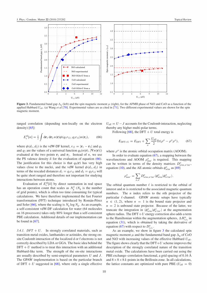
Figure 3. Fundamental band gap�g (left) and the spin magnetic moment μ (right), for the AFMII phase of NiO and CoO as a function of theapplied Hubbard Ueff. (a) Wang et al [70]. Experimental values are as cited in [71]. Two different experimental values are shown for the spinmagnetic moment.

ranged correlation (depending non-locally on the electrondensity) [65]:

Enlc [n] = 1

2

∫dr1 dr2 n(r)φ(q1r12, q2r12)n(r2), (66)

where φ(d1, d2) is the vdW-DF kernel, r12 = |r1 − r2| and q1

and q2 are the values of a universal function q0(n(r), |∇n(r)|)evaluated at the two points r1 and r2. Instead of n, we usethe PS valence density n for the evaluation of equation (66).The justification for this choice is that q0(r) has very highvalues close to the nuclei, and the vdW kernel φ(d1, d2) interms of the rescaled distances d1 = q1r12 and d2 = q2r12 willbe quite short ranged and therefore not important for studyinginteractions between atoms.

Evaluation of Enlc [n] by direct summation in real space

has an operation count that scales as N2g (Ng is the number

of grid points), which is often too time consuming for typicalcalculations. We have therefore implemented the fast Fouriertransformation (FFT) technique introduced by Roman-Perezand Soler [66], where the scaling is Ng log Ng. As an example,a self-consistent vdW-DF calculation for water (64 moleculeson 16 processors) takes only 80% longer than a self-consistentPBE calculation. Additional details of our implementation canbe found in [67].

3.4.1. DFT + U. In strongly correlated materials, such astransition metal oxides, lanthanides or actinides, the strong on-site Coulomb interaction of the localized d or f electrons is notcorrectly described by LDA or GGA. The basic idea behind theDFT + U method is to treat this interaction with an additionalHubbard-like term. The strength of the on-site interactionsare usually described by semi-empirical parameters U and J .The GPAW implementation is based on the particular branchof DFT + U suggested in [68], where only a single effective

Ueff = U − J accounts for the Coulomb interaction, neglectingthereby any higher multi-polar terms.

Following [68], the DFT + U total energy is

EDFT+U = EDFT +∑

a

Ueff

2Tr(ρa − ρaρa), (67)

where ρa is the atomic orbital occupation matrix (AOOM).In order to evaluate equation (67), a mapping between the

wavefunctions and AOOM ρamm′ is required. This mapping

can be written in terms of the density matrices Dan�m,n′�m′ ,

equation (10), and the AE atomic orbitals φan�m as [69]

ρamm′ =

∑

n,n′Da

n�m,n′�m′ 〈φan�m |φa

n′�m′ 〉.

The orbital quantum number � is restricted to the orbital ofinterest and m is restricted to the associated magnetic quantumnumbers. The n index refers to the nth projector of theparticular �-channel. GPAW atomic setups have typicallyn ∈ (1, 2), where n = 1 is the bound state projector andn = 2 is unbound state projector. Because of the latter, wetruncate the integration in 〈φa

n�m |φan′�m′ 〉 at the augmentation

sphere radius. The DFT+U energy correction also adds a termto the Hamiltonian within the augmentation spheres, �H a

i1i2in

equation (31), which is obtained by taking the derivative ofequation (67) with respect to Da

i1i2.

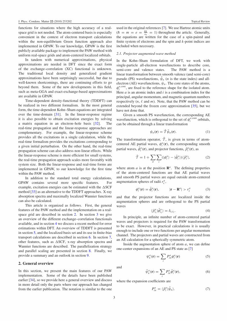
As an example, we show in figure 3 the calculated spinmagnetic moment μ and the fundamental band gap�g of CoOand NiO with increasing values of the effective Hubbard Ueff.The figure shows clearly that the DFT+U scheme improves thedescription of the strongly correlated nature of the transitionmetal oxide. The calculations have been carried out using thePBE exchange–correlation functional, a grid spacing of 0.16 Aand 8×8×8 k-points in the Brillouin zone. In all calculations,the lattice constants are optimized with pure PBE (Ueff = 0)

10

J. Phys.: Condens. Matter 22 (2010) 253202 Topical Review

Figure 4. Left: ensemble of enhancement factors as optimized to the experimental fragmentation energies of 148 molecules. The thin blacklines running parallel to the best-fit mark the width of the ensemble. The PBE and RPBE enhancement factors are also shown for comparison,s is the reduced density gradient. Right: fragmentation energies predicted with the best-fit enhancement factor versus the experimental values.The error bars are calculated from the ensemble in the left panel.

with a grid spacing of 0.16 A, the obtained values are 4.19 Afor NiO and 4.24 A for CoO. The corresponding experimentalvalues are 4.17 A and 4.25 A for NiO and CoO, respectively.

4. Error estimation

Density-functional theory is used extensively to calculatebinding energies of different atomic structures ranging fromsmall molecules to extended condensed-matter systems.A number of different approximations to the exchange–correlation energy have been developed with different scopesin mind and with different virtues. When it comes to thepractical use of DFT, it is therefore usually very much up tothe user to obtain experience with the different xc functionalsand gain insight into how accurate the calculations are fora particular application. This learning process can be ratherslow and, also for other more general reasons, it would beadvantageous to have a reliable and unbiased way to estimateerrors on DFT calculations.

The error estimation implemented in GPAW is inspired byideas from Bayesian statistics [72]. The ingredients in a typicalstatistical model construction consist of (1) a database witha number of (possibly noisy) data points which the model issupposed to reproduce as closely as possible and (2) the modelwhich is described by a number of parameters which can beadjusted to improve the model. The quality of the model canfor example be estimated by a least-squares cost which is asum over all data points of the squared difference between thedatabase value and the value predicted by the model. Thecost thus becomes a function of the model parameters andminimization of the cost leads to the best-fit model. (Animportant issue here is to control the effective number ofparameters in the model to avoid over-fitting, but we shall notgo into this here.) So far we have described a common least-squares fit. What the Bayesian approach adds to this is the ideaof not only a single best-fit model but an ensemble of modelsrepresenting a probability distribution in model space. Usingthe ensemble, the model no longer predicts only a single value

for a data point but a distribution of values which will be moreor less scattered depending on the ability of the model to makean accurate prediction for that point.

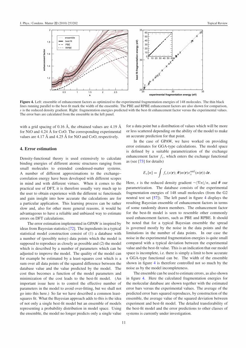
In the case of GPAW, we have worked on providingerror estimates for GGA-type calculations. The model spaceis defined by a suitable parametrization of the exchangeenhancement factor fx , which enters the exchange functionalas (see [73] for details)

Ex [n] =∫

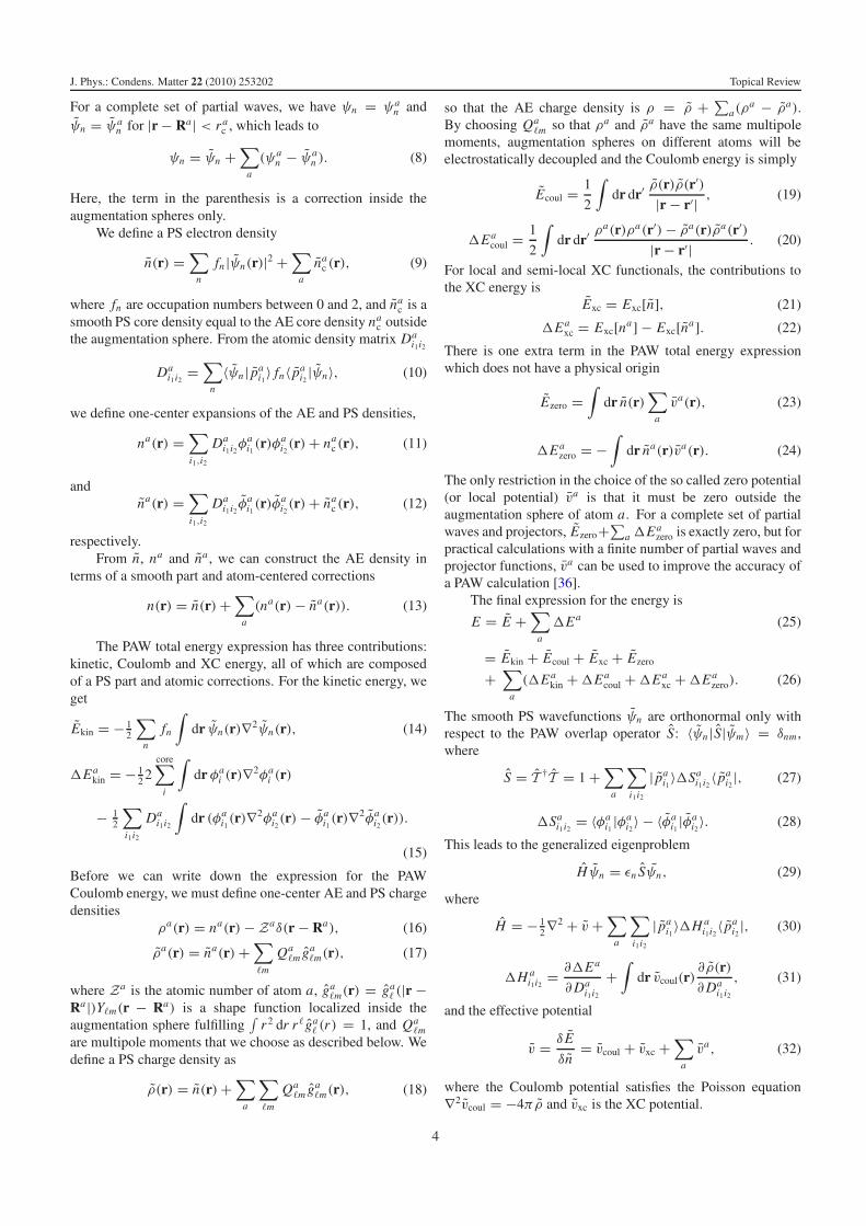
fx(s(r); θ)n(r)εunifx (n(r)) dr.

Here, s is the reduced density gradient ∼|∇n|/n, and θ ourparametrization. The database consists of the experimentalfragmentation energies of 148 small molecules (from the G2neutral test set [57]). The left panel in figure 4 displays theresulting Bayesian ensemble of enhancement factors in termsof some randomly drawn members. The enhancement factorfor the best-fit model is seen to resemble other commonlyused enhancement factors, such as PBE and RPBE. It shouldbe noted that for a typical Bayesian ensemble the spreadis governed mostly by the noise in the data points and thelimitations in the number of data points. In our case thenoise in the experimental fragmentation energies is quite smallcompared with a typical deviation between the experimentalvalue and the best-fit value. This is an indication that our modelspace is incomplete, i.e. there is simply a limit to how accuratea GGA-type functional can be. The width of the ensembleshown in figure 4 is therefore controlled not so much by thenoise as by the model incompleteness.

The ensemble can be used to estimate errors, as also shownin figure 4. Here the calculated fragmentation energies forthe molecular database are shown together with the estimatederror bars versus the experimental values. The average of thepredicted error bars squared reproduces, by construction of theensemble, the average value of the squared deviation betweenexperiment and best-fit model. The detailed transferability ofthe best-fit model and the error predictions to other classes ofsystems is currently under investigation.

11

J. Phys.: Condens. Matter 22 (2010) 253202 Topical Review

5. Time-dependent density-functional theory

Standard DFT is applicable only to the ground state propertiesof a system. However, there are many properties of greatinterest which are related to the excited states, e.g. opticalabsorption spectrum. Time-dependent density-functionaltheory (TDDFT) [3] is the extension of standard DFT intothe time-domain enabling the study of excited state properties.There are two widely used formulations of TDDFT, thereal-time propagation scheme [74] and the linear-responsescheme [75]; both of these are available in GPAW. The detailsof the implementations are described in [52], and we presentonly a brief overview here.

5.1. Real-time propagation

The time-dependent AE Kohn–Sham equation is

i∂

∂ tψn(t) = H(t)ψn(t), (68)

where the time-dependent Hamiltonian H(t) can include alsoan external time-dependent potential. Assuming that theoverlap matrix S is independent of time, this equation can bewritten in the PAW formalism as

iS∂

∂ tψn(t) = H(t)ψn(t). (69)

This time-dependent equation can be solved using theCrank–Nicolson propagator with a predictor–corrector step asdescribed in [52].

5.2. Linear-response formalism

Within the linear-response regime, the excitation energies canbe calculated from the eigenvalue equation of the form

ΩFI = ω2I FI , (70)

where ωI is the transition energy from the ground state to theexcited state I , and FI denotes the associated eigenvector. Thematrix Ω can be expanded in Kohn–Sham single particle–holeexcitations leading to

�i jσ,klτ = δikδ j lδστε2i jσ + 2

√fi jσ εi jσ fklτ εklτ Ki jσ,klτ , (71)

where εi jσ = ε jσ − εiσ are the energy differences and fi jσ =fiσ − f jσ are the occupation number differences of the Kohn–Sham states. The indices i, j, k, l are state indices, whereasσ, τ denote spin indices. The coupling matrix can be split intotwo parts Ki jσ,klτ = K C

i jσ,klτ + K xci jσ,klτ . The former Coulomb

matrix has exactly the same form as in the context of exactexchange, equation (50)

K Ci jσ,klτ = (ni jσ |nklτ ) (72)

and is often called the random phase approximation part. Itdescribes the effect of the linear density response via theclassical Hartree energy. The second contribution is theexchange–correlation part

K xci jσ,kqτ =

∫dr1 dr2 n∗

i jσ (r1)δ2 Exc

δnσ (r1)δnτ (r2)nkqτ (r2), (73)

Table 2. Calculated excitation energies of the CO molecule withinthe LDA approximation in eV. Bond length is 1.128 A.

State Spin GPAW AE [76]

a 3� Triplet 5.95 6.03A 1� Singlet 8.36 8.44a′ 3�+ Triplet 8.58 8.57b 3�+ Triplet 9.01 9.02B 1�+ Singlet 9.24 9.20d 3� Triplet 9.25 9.23I 1�− Singlet 9.87 9.87e 3�− Triplet 9.87 9.87D 1� Triplet 10.35 10.36

where nσ is the spin density. The functional derivative can becalculated with a finite difference scheme.

Diagonalization of the linear-response equation (70) givesdirectly all the excitation energies in the linear-responseregime. As an example, table 2 shows the calculated excitationenergies of a CO molecule together with reference calculations.The agreement between our results and numerically accurateAE results [76] is generally good.

Within the time propagation scheme, one obtains only theexcitations corresponding to a particular initial perturbation.Thus, different types of perturbations would be needed to reachdifferent excited states. In the case of a singlet ground statemolecule like CO, the often applied delta pulse perturbation(as introduced in section 5.3) can lead only to dipole allowedsinglet–singlet excitations. Therefore the triplet excitations anddipole forbidden singlet excitation at 9.87 eV do not appear inthe time propagation scheme.

5.3. Optical absorption spectra

In the real-time formalism the linear absorption spectrum canbe obtained by exciting the system first with a weak delta pulse,

E(t) = εkoδ(t), (74)

where ε is a unitless perturbation strength parameter and ko isa unit vector giving the polarization direction of the field. Thedelta pulse changes the initial wavefunctions to

ψ(t = 0+) = exp

(iε

a0ko · r

)ψ(t = 0−). (75)

The system is then allowed to evolve freely and during thetime-evolution the time-dependent dipole moment μ(t) isrecorded. At the end of the calculation, the dipole strengthtensor and oscillator strengths are obtained via a Fouriertransform.

In the linear-response formalism one also needs theeigenvectors of equation (70) when calculating the absorptionspectrum. Together with the Kohn–Sham transition dipoles

μi jσ = 〈ψiσ |r|ψ jσ 〉 (76)

the oscillator strengths are given by

f Iα =∣∣∣∣∣

fiσ > f jσ∑

i jσ

(μi jσ )α√

fi jσ εi jσ (FI )i jσ

∣∣∣∣∣

2

. (77)

12

J. Phys.: Condens. Matter 22 (2010) 253202 Topical Review

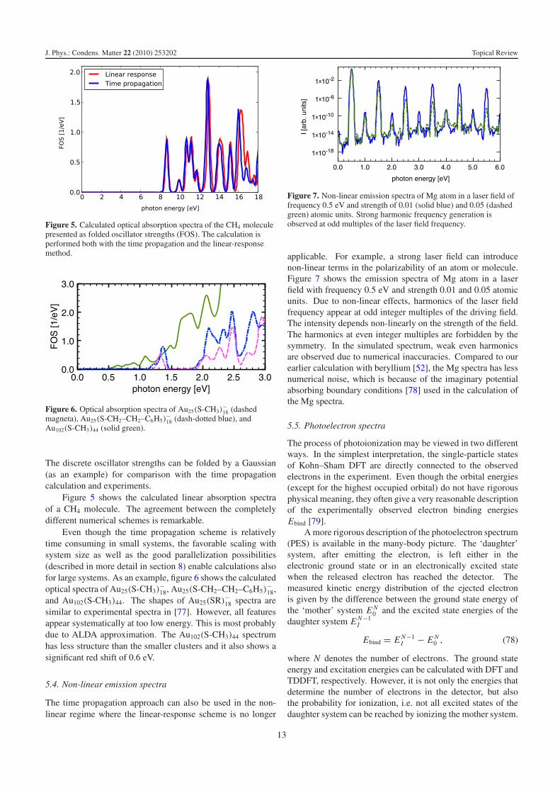
Figure 5. Calculated optical absorption spectra of the CH4 moleculepresented as folded oscillator strengths (FOS). The calculation isperformed both with the time propagation and the linear-responsemethod.

Figure 6. Optical absorption spectra of Au25(S-CH3)−18 (dashed

magneta), Au25(S-CH2–CH2–C6H5)−18 (dash-dotted blue), and

Au102(S-CH3)44 (solid green).

The discrete oscillator strengths can be folded by a Gaussian(as an example) for comparison with the time propagationcalculation and experiments.

Figure 5 shows the calculated linear absorption spectraof a CH4 molecule. The agreement between the completelydifferent numerical schemes is remarkable.

Even though the time propagation scheme is relativelytime consuming in small systems, the favorable scaling withsystem size as well as the good parallelization possibilities(described in more detail in section 8) enable calculations alsofor large systems. As an example, figure 6 shows the calculatedoptical spectra of Au25(S-CH3)

−18, Au25(S-CH2–CH2–C6H5)

−18,

and Au102(S-CH3)44. The shapes of Au25(SR)−18 spectra aresimilar to experimental spectra in [77]. However, all featuresappear systematically at too low energy. This is most probablydue to ALDA approximation. The Au102(S-CH3)44 spectrumhas less structure than the smaller clusters and it also shows asignificant red shift of 0.6 eV.

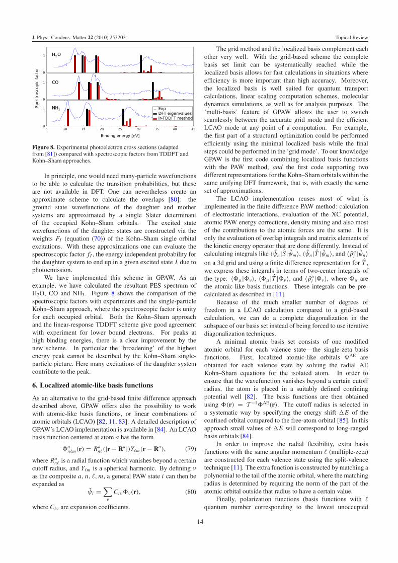
5.4. Non-linear emission spectra

The time propagation approach can also be used in the non-linear regime where the linear-response scheme is no longer

Figure 7. Non-linear emission spectra of Mg atom in a laser field offrequency 0.5 eV and strength of 0.01 (solid blue) and 0.05 (dashedgreen) atomic units. Strong harmonic frequency generation isobserved at odd multiples of the laser field frequency.

applicable. For example, a strong laser field can introducenon-linear terms in the polarizability of an atom or molecule.Figure 7 shows the emission spectra of Mg atom in a laserfield with frequency 0.5 eV and strength 0.01 and 0.05 atomicunits. Due to non-linear effects, harmonics of the laser fieldfrequency appear at odd integer multiples of the driving field.The intensity depends non-linearly on the strength of the field.The harmonics at even integer multiples are forbidden by thesymmetry. In the simulated spectrum, weak even harmonicsare observed due to numerical inaccuracies. Compared to ourearlier calculation with beryllium [52], the Mg spectra has lessnumerical noise, which is because of the imaginary potentialabsorbing boundary conditions [78] used in the calculation ofthe Mg spectra.

5.5. Photoelectron spectra

The process of photoionization may be viewed in two differentways. In the simplest interpretation, the single-particle statesof Kohn–Sham DFT are directly connected to the observedelectrons in the experiment. Even though the orbital energies(except for the highest occupied orbital) do not have rigorousphysical meaning, they often give a very reasonable descriptionof the experimentally observed electron binding energiesEbind [79].

A more rigorous description of the photoelectron spectrum(PES) is available in the many-body picture. The ‘daughter’system, after emitting the electron, is left either in theelectronic ground state or in an electronically excited statewhen the released electron has reached the detector. Themeasured kinetic energy distribution of the ejected electronis given by the difference between the ground state energy ofthe ‘mother’ system E N

0 and the excited state energies of thedaughter system E N−1

I

Ebind = E N−1I − E N

0 , (78)

where N denotes the number of electrons. The ground stateenergy and excitation energies can be calculated with DFT andTDDFT, respectively. However, it is not only the energies thatdetermine the number of electrons in the detector, but alsothe probability for ionization, i.e. not all excited states of thedaughter system can be reached by ionizing the mother system.

13

J. Phys.: Condens. Matter 22 (2010) 253202 Topical Review

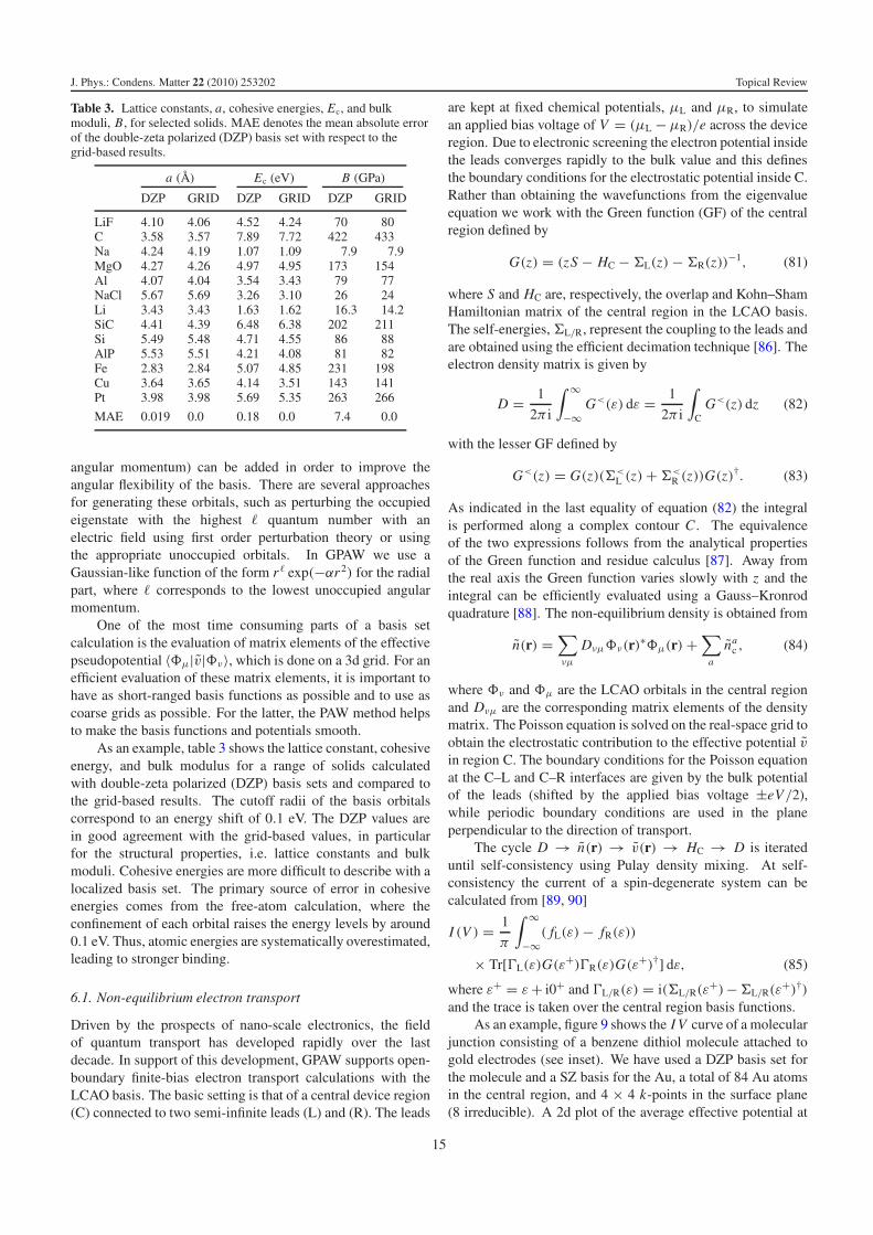
Figure 8. Experimental photoelectron cross sections (adaptedfrom [81]) compared with spectroscopic factors from TDDFT andKohn–Sham approaches.

In principle, one would need many-particle wavefunctionsto be able to calculate the transition probabilities, but theseare not available in DFT. One can nevertheless create anapproximate scheme to calculate the overlaps [80]: theground state wavefunctions of the daughter and mothersystems are approximated by a single Slater determinantof the occupied Kohn–Sham orbitals. The excited statewavefunctions of the daughter states are constructed via theweights FI (equation (70)) of the Kohn–Sham single orbitalexcitations. With these approximations one can evaluate thespectroscopic factor fI , the energy independent probability forthe daughter system to end up in a given excited state I due tophotoemission.

We have implemented this scheme in GPAW. As anexample, we have calculated the resultant PES spectrum ofH2O, CO and NH3. Figure 8 shows the comparison of thespectroscopic factors with experiments and the single-particleKohn–Sham approach, where the spectroscopic factor is unityfor each occupied orbital. Both the Kohn–Sham approachand the linear-response TDDFT scheme give good agreementwith experiment for lower bound electrons. For peaks athigh binding energies, there is a clear improvement by thenew scheme. In particular the ‘broadening’ of the highestenergy peak cannot be described by the Kohn–Sham single-particle picture. Here many excitations of the daughter systemcontribute to the peak.

6. Localized atomic-like basis functions

As an alternative to the grid-based finite difference approachdescribed above, GPAW offers also the possibility to workwith atomic-like basis functions, or linear combinations ofatomic orbitals (LCAO) [82, 11, 83]. A detailed description ofGPAW’s LCAO implementation is available in [84]. An LCAObasis function centered at atom a has the form

�an�m(r) = Ra

n�(|r − Ra|)Y�m(r − Ra), (79)

where Ran� is a radial function which vanishes beyond a certain

cutoff radius, and Y�m is a spherical harmonic. By defining νas the composite a, n, �,m, a general PAW state i can then beexpanded as

ψi =∑

ν

Ciν�ν(r), (80)

where Ciν are expansion coefficients.

The grid method and the localized basis complement eachother very well. With the grid-based scheme the completebasis set limit can be systematically reached while thelocalized basis allows for fast calculations in situations whereefficiency is more important than high accuracy. Moreover,the localized basis is well suited for quantum transportcalculations, linear scaling computation schemes, moleculardynamics simulations, as well as for analysis purposes. The‘multi-basis’ feature of GPAW allows the user to switchseamlessly between the accurate grid mode and the efficientLCAO mode at any point of a computation. For example,the first part of a structural optimization could be performedefficiently using the minimal localized basis while the finalsteps could be performed in the ‘grid mode’. To our knowledgeGPAW is the first code combining localized basis functionswith the PAW method, and the first code supporting twodifferent representations for the Kohn–Sham orbitals within thesame unifying DFT framework, that is, with exactly the sameset of approximations.

The LCAO implementation reuses most of what isimplemented in the finite difference PAW method: calculationof electrostatic interactions, evaluation of the XC potential,atomic PAW energy corrections, density mixing and also mostof the contributions to the atomic forces are the same. It isonly the evaluation of overlap integrals and matrix elements ofthe kinetic energy operator that are done differently. Instead ofcalculating integrals like 〈ψn |S|ψm〉, 〈ψn |T |ψm〉, and 〈 pa

i |ψn〉on a 3d grid and using a finite difference representation for T ,we express these integrals in terms of two-center integrals ofthe type: 〈�μ|�ν〉, 〈�μ|T |�ν〉, and 〈 pa

i |�ν〉, where �μ arethe atomic-like basis functions. These integrals can be pre-calculated as described in [11].

Because of the much smaller number of degrees offreedom in a LCAO calculation compared to a grid-basedcalculation, we can do a complete diagonalization in thesubspace of our basis set instead of being forced to use iterativediagonalization techniques.

A minimal atomic basis set consists of one modifiedatomic orbital for each valence state—the single-zeta basisfunctions. First, localized atomic-like orbitals �AE areobtained for each valence state by solving the radial AEKohn–Sham equations for the isolated atom. In order toensure that the wavefunction vanishes beyond a certain cutoffradius, the atom is placed in a suitably defined confiningpotential well [82]. The basis functions are then obtainedusing �(r) = T −1�AE(r). The cutoff radius is selected ina systematic way by specifying the energy shift �E of theconfined orbital compared to the free-atom orbital [85]. In thisapproach small values of �E will correspond to long-rangedbasis orbitals [84].

In order to improve the radial flexibility, extra basisfunctions with the same angular momentum � (multiple-zeta)are constructed for each valence state using the split-valencetechnique [11]. The extra function is constructed by matching apolynomial to the tail of the atomic orbital, where the matchingradius is determined by requiring the norm of the part of theatomic orbital outside that radius to have a certain value.

Finally, polarization functions (basis functions with �

quantum number corresponding to the lowest unoccupied

14

J. Phys.: Condens. Matter 22 (2010) 253202 Topical Review

Table 3. Lattice constants, a, cohesive energies, Ec, and bulkmoduli, B, for selected solids. MAE denotes the mean absolute errorof the double-zeta polarized (DZP) basis set with respect to thegrid-based results.

a (A) Ec (eV) B (GPa)

DZP GRID DZP GRID DZP GRID

LiF 4.10 4.06 4.52 4.24 70 80C 3.58 3.57 7.89 7.72 422 433Na 4.24 4.19 1.07 1.09 7.9 7.9MgO 4.27 4.26 4.97 4.95 173 154Al 4.07 4.04 3.54 3.43 79 77NaCl 5.67 5.69 3.26 3.10 26 24Li 3.43 3.43 1.63 1.62 16.3 14.2SiC 4.41 4.39 6.48 6.38 202 211Si 5.49 5.48 4.71 4.55 86 88AlP 5.53 5.51 4.21 4.08 81 82Fe 2.83 2.84 5.07 4.85 231 198Cu 3.64 3.65 4.14 3.51 143 141Pt 3.98 3.98 5.69 5.35 263 266

MAE 0.019 0.0 0.18 0.0 7.4 0.0

angular momentum) can be added in order to improve theangular flexibility of the basis. There are several approachesfor generating these orbitals, such as perturbing the occupiedeigenstate with the highest � quantum number with anelectric field using first order perturbation theory or usingthe appropriate unoccupied orbitals. In GPAW we use aGaussian-like function of the form r � exp(−αr 2) for the radialpart, where � corresponds to the lowest unoccupied angularmomentum.

One of the most time consuming parts of a basis setcalculation is the evaluation of matrix elements of the effectivepseudopotential 〈�μ|v|�ν〉, which is done on a 3d grid. For anefficient evaluation of these matrix elements, it is important tohave as short-ranged basis functions as possible and to use ascoarse grids as possible. For the latter, the PAW method helpsto make the basis functions and potentials smooth.

As an example, table 3 shows the lattice constant, cohesiveenergy, and bulk modulus for a range of solids calculatedwith double-zeta polarized (DZP) basis sets and compared tothe grid-based results. The cutoff radii of the basis orbitalscorrespond to an energy shift of 0.1 eV. The DZP values arein good agreement with the grid-based values, in particularfor the structural properties, i.e. lattice constants and bulkmoduli. Cohesive energies are more difficult to describe with alocalized basis set. The primary source of error in cohesiveenergies comes from the free-atom calculation, where theconfinement of each orbital raises the energy levels by around0.1 eV. Thus, atomic energies are systematically overestimated,leading to stronger binding.

6.1. Non-equilibrium electron transport

Driven by the prospects of nano-scale electronics, the fieldof quantum transport has developed rapidly over the lastdecade. In support of this development, GPAW supports open-boundary finite-bias electron transport calculations with theLCAO basis. The basic setting is that of a central device region(C) connected to two semi-infinite leads (L) and (R). The leads

are kept at fixed chemical potentials, μL and μR, to simulatean applied bias voltage of V = (μL − μR)/e across the deviceregion. Due to electronic screening the electron potential insidethe leads converges rapidly to the bulk value and this definesthe boundary conditions for the electrostatic potential inside C.Rather than obtaining the wavefunctions from the eigenvalueequation we work with the Green function (GF) of the centralregion defined by

G(z) = (zS − HC −�L(z)−�R(z))−1, (81)

where S and HC are, respectively, the overlap and Kohn–ShamHamiltonian matrix of the central region in the LCAO basis.The self-energies,�L/R, represent the coupling to the leads andare obtained using the efficient decimation technique [86]. Theelectron density matrix is given by

D = 1

2π i

∫ ∞

−∞G<(ε) dε = 1

2π i

∫

CG<(z) dz (82)

with the lesser GF defined by

G<(z) = G(z)(�<L (z)+�<

R (z))G(z)†. (83)

As indicated in the last equality of equation (82) the integralis performed along a complex contour C . The equivalenceof the two expressions follows from the analytical propertiesof the Green function and residue calculus [87]. Away fromthe real axis the Green function varies slowly with z and theintegral can be efficiently evaluated using a Gauss–Kronrodquadrature [88]. The non-equilibrium density is obtained from

n(r) =∑

νμ

Dνμ�ν(r)∗�μ(r)+∑

a

nac , (84)

where �ν and �μ are the LCAO orbitals in the central regionand Dνμ are the corresponding matrix elements of the densitymatrix. The Poisson equation is solved on the real-space grid toobtain the electrostatic contribution to the effective potential vin region C. The boundary conditions for the Poisson equationat the C–L and C–R interfaces are given by the bulk potentialof the leads (shifted by the applied bias voltage ±eV/2),while periodic boundary conditions are used in the planeperpendicular to the direction of transport.

The cycle D → n(r) → v(r) → HC → D is iterateduntil self-consistency using Pulay density mixing. At self-consistency the current of a spin-degenerate system can becalculated from [89, 90]

I (V ) = 1

π

∫ ∞

−∞( fL(ε)− fR(ε))

× Tr[�L(ε)G(ε+)�R(ε)G(ε+)†] dε, (85)

where ε+ = ε+ i0+ and �L/R(ε) = i(�L/R(ε+)−�L/R(ε

+)†)and the trace is taken over the central region basis functions.

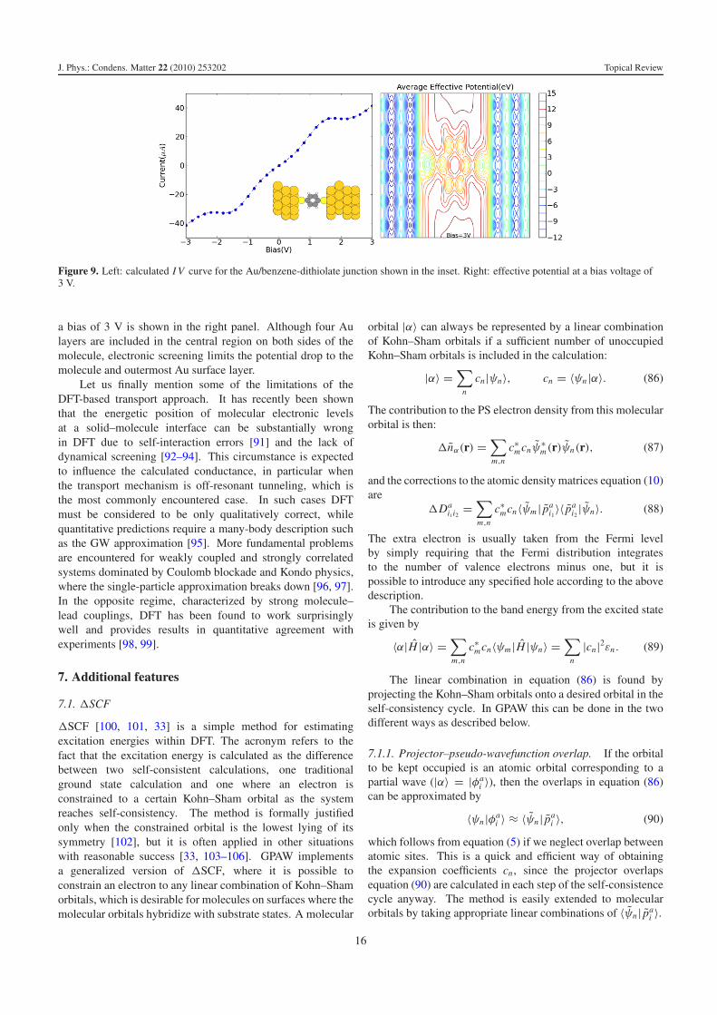
As an example, figure 9 shows the I V curve of a molecularjunction consisting of a benzene dithiol molecule attached togold electrodes (see inset). We have used a DZP basis set forthe molecule and a SZ basis for the Au, a total of 84 Au atomsin the central region, and 4 × 4 k-points in the surface plane(8 irreducible). A 2d plot of the average effective potential at

15

J. Phys.: Condens. Matter 22 (2010) 253202 Topical Review

Figure 9. Left: calculated I V curve for the Au/benzene-dithiolate junction shown in the inset. Right: effective potential at a bias voltage of3 V.

a bias of 3 V is shown in the right panel. Although four Aulayers are included in the central region on both sides of themolecule, electronic screening limits the potential drop to themolecule and outermost Au surface layer.

Let us finally mention some of the limitations of theDFT-based transport approach. It has recently been shownthat the energetic position of molecular electronic levelsat a solid–molecule interface can be substantially wrongin DFT due to self-interaction errors [91] and the lack ofdynamical screening [92–94]. This circumstance is expectedto influence the calculated conductance, in particular whenthe transport mechanism is off-resonant tunneling, which isthe most commonly encountered case. In such cases DFTmust be considered to be only qualitatively correct, whilequantitative predictions require a many-body description suchas the GW approximation [95]. More fundamental problemsare encountered for weakly coupled and strongly correlatedsystems dominated by Coulomb blockade and Kondo physics,where the single-particle approximation breaks down [96, 97].In the opposite regime, characterized by strong molecule–lead couplings, DFT has been found to work surprisinglywell and provides results in quantitative agreement withexperiments [98, 99].

7. Additional features

7.1. �SCF

�SCF [100, 101, 33] is a simple method for estimatingexcitation energies within DFT. The acronym refers to thefact that the excitation energy is calculated as the differencebetween two self-consistent calculations, one traditionalground state calculation and one where an electron isconstrained to a certain Kohn–Sham orbital as the systemreaches self-consistency. The method is formally justifiedonly when the constrained orbital is the lowest lying of itssymmetry [102], but it is often applied in other situationswith reasonable success [33, 103–106]. GPAW implementsa generalized version of �SCF, where it is possible toconstrain an electron to any linear combination of Kohn–Shamorbitals, which is desirable for molecules on surfaces where themolecular orbitals hybridize with substrate states. A molecular

orbital |α〉 can always be represented by a linear combinationof Kohn–Sham orbitals if a sufficient number of unoccupiedKohn–Sham orbitals is included in the calculation:

|α〉 =∑

n

cn|ψn〉, cn = 〈ψn |α〉. (86)

The contribution to the PS electron density from this molecularorbital is then:

�nα(r) =∑

m,n

c∗mcnψ

∗m(r)ψn(r), (87)

and the corrections to the atomic density matrices equation (10)are

�Daii i2

=∑

m,n

c∗mcn〈ψm | pa

i1〉〈 pa

i2|ψn〉. (88)

The extra electron is usually taken from the Fermi levelby simply requiring that the Fermi distribution integratesto the number of valence electrons minus one, but it ispossible to introduce any specified hole according to the abovedescription.

The contribution to the band energy from the excited stateis given by

〈α|H |α〉 =∑

m,n

c∗mcn〈ψm |H |ψn〉 =

∑

n

|cn|2εn . (89)

The linear combination in equation (86) is found byprojecting the Kohn–Sham orbitals onto a desired orbital in theself-consistency cycle. In GPAW this can be done in the twodifferent ways as described below.

7.1.1. Projector–pseudo-wavefunction overlap. If the orbitalto be kept occupied is an atomic orbital corresponding to apartial wave (|α〉 = |φa

i 〉), then the overlaps in equation (86)can be approximated by

〈ψn |φai 〉 ≈ 〈ψn | pa

i 〉, (90)

which follows from equation (5) if we neglect overlap betweenatomic sites. This is a quick and efficient way of obtainingthe expansion coefficients cn, since the projector overlapsequation (90) are calculated in each step of the self-consistencecycle anyway. The method is easily extended to molecularorbitals by taking appropriate linear combinations of 〈ψn | pa

i 〉.16

J. Phys.: Condens. Matter 22 (2010) 253202 Topical Review

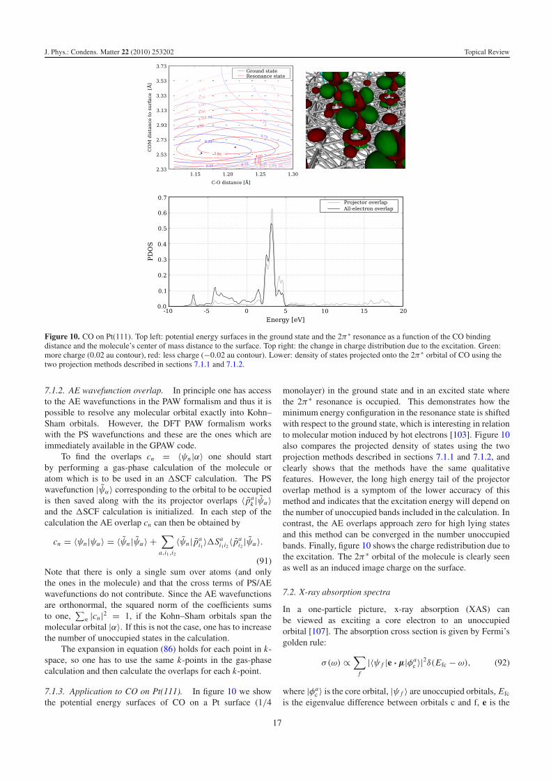
Figure 10. CO on Pt(111). Top left: potential energy surfaces in the ground state and the 2π∗ resonance as a function of the CO bindingdistance and the molecule’s center of mass distance to the surface. Top right: the change in charge distribution due to the excitation. Green:more charge (0.02 au contour), red: less charge (−0.02 au contour). Lower: density of states projected onto the 2π∗ orbital of CO using thetwo projection methods described in sections 7.1.1 and 7.1.2.

7.1.2. AE wavefunction overlap. In principle one has accessto the AE wavefunctions in the PAW formalism and thus it ispossible to resolve any molecular orbital exactly into Kohn–Sham orbitals. However, the DFT PAW formalism workswith the PS wavefunctions and these are the ones which areimmediately available in the GPAW code.

To find the overlaps cn = 〈ψn |α〉 one should startby performing a gas-phase calculation of the molecule oratom which is to be used in an �SCF calculation. The PSwavefunction |ψα〉 corresponding to the orbital to be occupiedis then saved along with the its projector overlaps 〈 pa

k |ψα〉and the �SCF calculation is initialized. In each step of thecalculation the AE overlap cn can then be obtained by

cn = 〈ψn|ψα〉 = 〈ψn |ψα〉 +∑

a,i1,i2

〈ψn | pai1〉�Sa

i1i2〈 pa

i2|ψα〉.

(91)Note that there is only a single sum over atoms (and onlythe ones in the molecule) and that the cross terms of PS/AEwavefunctions do not contribute. Since the AE wavefunctionsare orthonormal, the squared norm of the coefficients sumsto one,

∑n |cn|2 = 1, if the Kohn–Sham orbitals span the

molecular orbital |α〉. If this is not the case, one has to increasethe number of unoccupied states in the calculation.

The expansion in equation (86) holds for each point in k-space, so one has to use the same k-points in the gas-phasecalculation and then calculate the overlaps for each k-point.

7.1.3. Application to CO on Pt(111). In figure 10 we showthe potential energy surfaces of CO on a Pt surface (1/4

monolayer) in the ground state and in an excited state wherethe 2π∗ resonance is occupied. This demonstrates how theminimum energy configuration in the resonance state is shiftedwith respect to the ground state, which is interesting in relationto molecular motion induced by hot electrons [103]. Figure 10also compares the projected density of states using the twoprojection methods described in sections 7.1.1 and 7.1.2, andclearly shows that the methods have the same qualitativefeatures. However, the long high energy tail of the projectoroverlap method is a symptom of the lower accuracy of thismethod and indicates that the excitation energy will depend onthe number of unoccupied bands included in the calculation. Incontrast, the AE overlaps approach zero for high lying statesand this method can be converged in the number unoccupiedbands. Finally, figure 10 shows the charge redistribution due tothe excitation. The 2π∗ orbital of the molecule is clearly seenas well as an induced image charge on the surface.

7.2. X-ray absorption spectra

In a one-particle picture, x-ray absorption (XAS) canbe viewed as exciting a core electron to an unoccupiedorbital [107]. The absorption cross section is given by Fermi’sgolden rule:

σ(ω) ∝∑

f

|〈ψ f |e · μ|φac 〉|2δ(Efc − ω), (92)

where |φac 〉 is the core orbital, |ψ f 〉 are unoccupied orbitals, Efc

is the eigenvalue difference between orbitals c and f, e is the

17

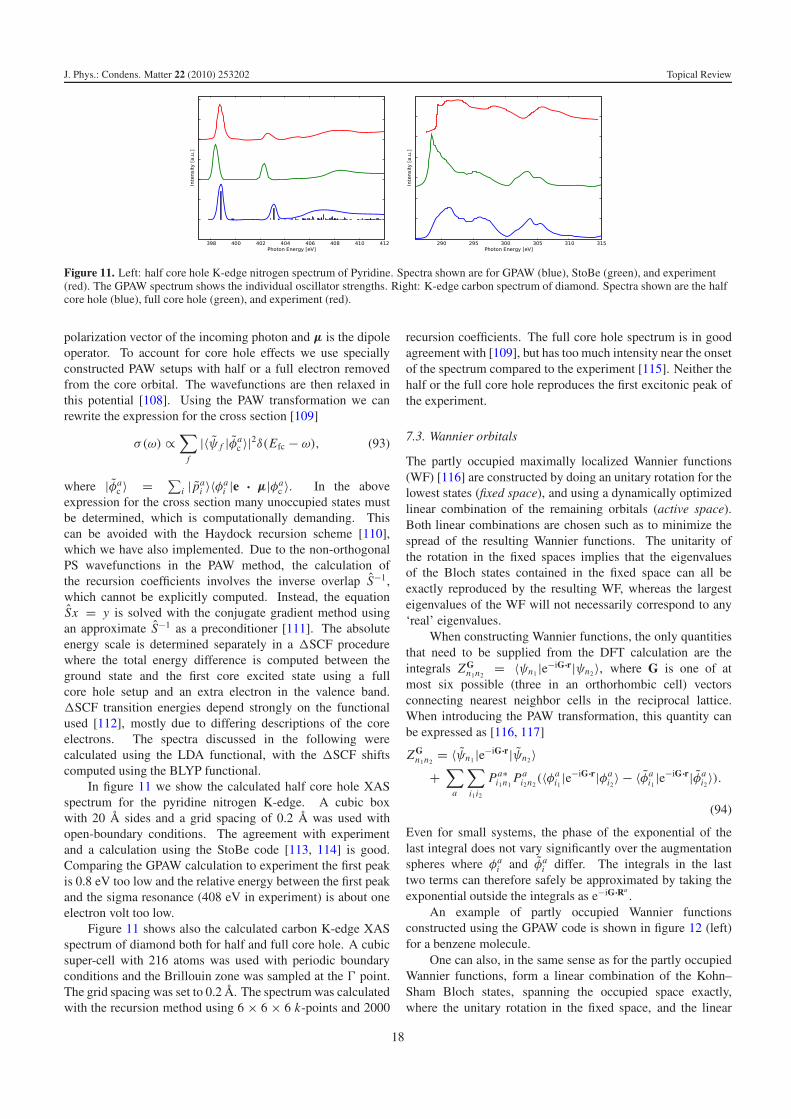
J. Phys.: Condens. Matter 22 (2010) 253202 Topical Review

Figure 11. Left: half core hole K-edge nitrogen spectrum of Pyridine. Spectra shown are for GPAW (blue), StoBe (green), and experiment(red). The GPAW spectrum shows the individual oscillator strengths. Right: K-edge carbon spectrum of diamond. Spectra shown are the halfcore hole (blue), full core hole (green), and experiment (red).

polarization vector of the incoming photon and μ is the dipoleoperator. To account for core hole effects we use speciallyconstructed PAW setups with half or a full electron removedfrom the core orbital. The wavefunctions are then relaxed inthis potential [108]. Using the PAW transformation we canrewrite the expression for the cross section [109]

σ(ω) ∝∑

f

|〈ψ f |φac 〉|2δ(Efc − ω), (93)

where |φac 〉 = ∑

i | pai 〉〈φa

i |e · μ|φac 〉. In the above

expression for the cross section many unoccupied states mustbe determined, which is computationally demanding. Thiscan be avoided with the Haydock recursion scheme [110],which we have also implemented. Due to the non-orthogonalPS wavefunctions in the PAW method, the calculation ofthe recursion coefficients involves the inverse overlap S−1,which cannot be explicitly computed. Instead, the equationSx = y is solved with the conjugate gradient method usingan approximate S−1 as a preconditioner [111]. The absoluteenergy scale is determined separately in a �SCF procedurewhere the total energy difference is computed between theground state and the first core excited state using a fullcore hole setup and an extra electron in the valence band.�SCF transition energies depend strongly on the functionalused [112], mostly due to differing descriptions of the coreelectrons. The spectra discussed in the following werecalculated using the LDA functional, with the �SCF shiftscomputed using the BLYP functional.

In figure 11 we show the calculated half core hole XASspectrum for the pyridine nitrogen K-edge. A cubic boxwith 20 A sides and a grid spacing of 0.2 A was used withopen-boundary conditions. The agreement with experimentand a calculation using the StoBe code [113, 114] is good.Comparing the GPAW calculation to experiment the first peakis 0.8 eV too low and the relative energy between the first peakand the sigma resonance (408 eV in experiment) is about oneelectron volt too low.

Figure 11 shows also the calculated carbon K-edge XASspectrum of diamond both for half and full core hole. A cubicsuper-cell with 216 atoms was used with periodic boundaryconditions and the Brillouin zone was sampled at the � point.The grid spacing was set to 0.2 A. The spectrum was calculatedwith the recursion method using 6 × 6 × 6 k-points and 2000

recursion coefficients. The full core hole spectrum is in goodagreement with [109], but has too much intensity near the onsetof the spectrum compared to the experiment [115]. Neither thehalf or the full core hole reproduces the first excitonic peak ofthe experiment.

7.3. Wannier orbitals

The partly occupied maximally localized Wannier functions(WF) [116] are constructed by doing an unitary rotation for thelowest states (fixed space), and using a dynamically optimizedlinear combination of the remaining orbitals (active space).Both linear combinations are chosen such as to minimize thespread of the resulting Wannier functions. The unitarity ofthe rotation in the fixed spaces implies that the eigenvaluesof the Bloch states contained in the fixed space can all beexactly reproduced by the resulting WF, whereas the largesteigenvalues of the WF will not necessarily correspond to any‘real’ eigenvalues.

When constructing Wannier functions, the only quantitiesthat need to be supplied from the DFT calculation are theintegrals Z G

n1n2= 〈ψn1 |e−iG·r|ψn2〉, where G is one of at

most six possible (three in an orthorhombic cell) vectorsconnecting nearest neighbor cells in the reciprocal lattice.When introducing the PAW transformation, this quantity canbe expressed as [116, 117]

Z Gn1n2

= 〈ψn1 |e−iG·r|ψn2〉+

∑

a

∑

i1i2

Pa∗i1n1

Pai2n2(〈φa

i1|e−iG·r|φa

i2〉 − 〈φa

i1|e−iG·r|φa

i2〉).

(94)

Even for small systems, the phase of the exponential of thelast integral does not vary significantly over the augmentationspheres where φa

i and φai differ. The integrals in the last

two terms can therefore safely be approximated by taking theexponential outside the integrals as e−iG·Ra

.An example of partly occupied Wannier functions

constructed using the GPAW code is shown in figure 12 (left)for a benzene molecule.

One can also, in the same sense as for the partly occupiedWannier functions, form a linear combination of the Kohn–Sham Bloch states, spanning the occupied space exactly,where the unitary rotation in the fixed space, and the linear

18

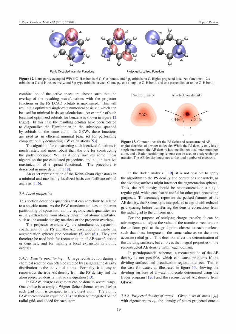
J. Phys.: Condens. Matter 22 (2010) 253202 Topical Review

Figure 12. Left: partly occupied WF; 6 C–H σ bonds, 6 C–C σ bonds, and 6 pz orbitals on C. Right: projected localized functions; 12 sorbitals on C and H respectively, and 3 p-type orbitals on each C, one pz , one along the C–H bond, and one perpendicular to the C–H bond.

combination of the active space are chosen such that theoverlap of the resulting wavefunctions with the projectorfunctions or the PS LCAO orbitals is maximized. This willresult in a optimized single-zeta numerical basis set, which canbe used for minimal basis set calculations. An example of suchlocalized optimized orbitals for benzene is shown in figure 12(right). In this case the resulting orbitals have been rotatedto diagonalize the Hamiltonian in the subspaces spannedby orbitals on the same atom. In GPAW, these functionsare used as an efficient minimal basis set for performingcomputationally demanding GW calculations [53].

The algorithm for constructing such localized functions ismuch faster, and more robust than the one for constructingthe partly occupied WF, as it only involves some linearalgebra on the pre-calculated projections, and not an iterativemaximization of a spread functional. The procedure isdescribed in more detail in [118].

An exact representation of the Kohn–Sham eigenstates ina minimal and maximally localized basis can facilitate orbitalanalysis [116].

7.4. Local properties

This section describes quantities that can somehow be relatedto a specific atom. As the PAW transform utilizes an inherentpartitioning of space into atomic regions, such quantities areusually extractable from already determined atomic attributes,such as the atomic density matrices or the projector overlaps.

The projector overlaps Pain are simultaneous expansion

coefficients of the PS and the AE wavefunctions inside theaugmentation spheres (see equations (5) and (6)). They cantherefore be used both for reconstruction of AE wavefunctionor densities, and for making a local expansion in atomicorbitals.

7.4.1. Density partitioning. Charge redistribution during achemical reaction can often be studied by assigning the densitydistribution to the individual atoms. Formally, it is easy toreconstruct the true AE density from the PS density and theatom projected density matrix via equation (13).

In GPAW, charge assignment can be done in several ways.One choice is to apply a Wigner–Seitz scheme, where n(r) ateach grid point is assigned to the closest atom. The atomicPAW corrections in equation (13) can then be integrated on theradial grid, and added for each atom.

Figure 13. Contour lines for the PS (left) and reconstructed AE(right) densities of a water molecule. While the PS density only has asingle maximum, the AE density has one distinct local maximum peratom, and a Bader partitioning scheme can be used to analyze chargetransfer. The AE density integrates to the total number of electrons.

In the Bader analysis [119], it is not possible to applythe algorithm to the PS density and corrections separately, asthe dividing surfaces might intersect the augmentation spheres.Thus, the AE density should be reconstructed on a singleregular grid, which can also be useful for other post-processingpurposes. To accurately represent the peaked features of theAE density, the PS density is interpolated to a grid with reducedgrid spacing before transferring the density corrections fromthe radial grid to the uniform grid.

For the purpose of studying charge transfer, it can beadvantageous to adjust the value of the atomic corrections onthe uniform grid at the grid point closest to each nucleus,such that these integrate to the same value as on the moreaccurate radial grid. This does not affect the determination ofthe dividing surfaces, but enforces the integral properties of thereconstructed AE density within each domain.

In pseudopotential schemes, a reconstruction of the AEdensity is not possible, which can cause problems if thedividing surfaces and pseudization regions intersect. This isthe case for water, as illustrated in figure 13, showing thedividing surfaces of a water molecule determined using theBader program [120] and the reconstructed AE density fromGPAW.

7.4.2. Projected density of states. Given a set of states |ψn〉with eigenenergies εn, the density of states projected onto a

19

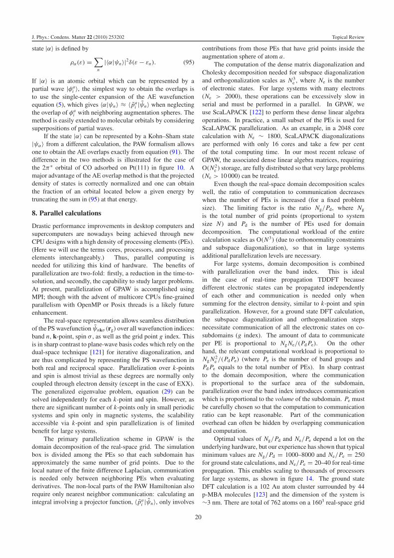
J. Phys.: Condens. Matter 22 (2010) 253202 Topical Review

state |α〉 is defined by

ρα(ε) =∑

n

|〈α|ψn〉|2δ(ε − εn). (95)

If |α〉 is an atomic orbital which can be represented by apartial wave |φa

i 〉, the simplest way to obtain the overlaps isto use the single-center expansion of the AE wavefunctionequation (5), which gives 〈α|ψn〉 ≈ 〈 pa

i |ψn〉 when neglectingthe overlap of φa

i with neighboring augmentation spheres. Themethod is easily extended to molecular orbitals by consideringsuperpositions of partial waves.

If the state |α〉 can be represented by a Kohn–Sham state|ψα〉 from a different calculation, the PAW formalism allowsone to obtain the AE overlaps exactly from equation (91). Thedifference in the two methods is illustrated for the case ofthe 2π∗ orbital of CO adsorbed on Pt(111) in figure 10. Amajor advantage of the AE overlap method is that the projecteddensity of states is correctly normalized and one can obtainthe fraction of an orbital located below a given energy bytruncating the sum in (95) at that energy.

8. Parallel calculations

Drastic performance improvements in desktop computers andsupercomputers are nowadays being achieved through newCPU designs with a high density of processing elements (PEs).(Here we will use the terms cores, processors, and processingelements interchangeably.) Thus, parallel computing isneeded for utilizing this kind of hardware. The benefits ofparallelization are two-fold: firstly, a reduction in the time-to-solution, and secondly, the capability to study larger problems.At present, parallelization of GPAW is accomplished usingMPI; though with the advent of multicore CPUs fine-grainedparallelism with OpenMP or Posix threads is a likely futureenhancement.

The real-space representation allows seamless distributionof the PS wavefunction ψnkσ (rg) over all wavefunction indices:band n, k-point, spin σ , as well as the grid point g index. Thisis in sharp contrast to plane-wave basis codes which rely on thedual-space technique [121] for iterative diagonalization, andare thus complicated by representing the PS wavefunction inboth real and reciprocal space. Parallelization over k-pointsand spin is almost trivial as these degrees are normally onlycoupled through electron density (except in the case of EXX).The generalized eigenvalue problem, equation (29) can besolved independently for each k-point and spin. However, asthere are significant number of k-points only in small periodicsystems and spin only in magnetic systems, the scalabilityaccessible via k-point and spin parallelization is of limitedbenefit for large systems.

The primary parallelization scheme in GPAW is thedomain decomposition of the real-space grid. The simulationbox is divided among the PEs so that each subdomain hasapproximately the same number of grid points. Due to thelocal nature of the finite difference Laplacian, communicationis needed only between neighboring PEs when evaluatingderivatives. The non-local parts of the PAW Hamiltonian alsorequire only nearest neighbor communication: calculating anintegral involving a projector function, 〈 pa

i |ψn〉, only involves

contributions from those PEs that have grid points inside theaugmentation sphere of atom a.

The computation of the dense matrix diagonalization andCholesky decomposition needed for subspace diagonalizationand orthogonalization scales as N3

e , where Ne is the numberof electronic states. For large systems with many electrons(Ne > 2000), these operations can be excessively slow inserial and must be performed in a parallel. In GPAW, weuse ScaLAPACK [122] to perform these dense linear algebraoperations. In practice, a small subset of the PEs is used forScaLAPACK parallelization. As an example, in a 2048 corecalculation with Ne ∼ 1800, ScaLAPACK diagonalizationsare performed with only 16 cores and take a few per centof the total computing time. In our most recent release ofGPAW, the associated dense linear algebra matrices, requiringO(N2

e ) storage, are fully distributed so that very large problems(Ne > 10 000) can be treated.

Even though the real-space domain decomposition scaleswell, the ratio of computation to communication decreaseswhen the number of PEs is increased (for a fixed problemsize). The limiting factor is the ratio Ng/Pd, where Ng

is the total number of grid points (proportional to systemsize N) and Pd is the number of PEs used for domaindecomposition. The computational workload of the entirecalculation scales as O(N3) (due to orthonormality constraintsand subspace diagonalization), so that in large systemsadditional parallelization levels are necessary.

For large systems, domain decomposition is combinedwith parallelization over the band index. This is idealin the case of real-time propagation TDDFT becausedifferent electronic states can be propagated independentlyof each other and communication is needed only whensumming for the electron density, similar to k-point and spinparallelization. However, for a ground state DFT calculation,the subspace diagonalization and orthogonalization stepsnecessitate communication of all the electronic states on co-subdomains (g index). The amount of data to communicateper PE is proportional to Ng Ne/(Pd Pe). On the otherhand, the relevant computational workload is proportional toNg N2

e /(Pd Pe) (where Pe is the number of band groups andPd Pe equals to the total number of PEs). In sharp contrastto the domain decomposition, where the communicationis proportional to the surface area of the subdomain,parallelization over the band index introduces communicationwhich is proportional to the volume of the subdomain. Pe mustbe carefully chosen so that the computation to communicationratio can be kept reasonable. Part of the communicationoverhead can often be hidden by overlapping communicationand computation.

Optimal values of Ng/Pd and Ne/Pe depend a lot on theunderlying hardware, but our experience has shown that typicalminimum values are Ng/Pd = 1000–8000 and Ne/Pe = 250for ground state calculations, and Ne/Pe = 20–40 for real-timepropagation. This enables scaling to thousands of processorsfor large systems, as shown in figure 14. The ground stateDFT calculation is a 102 Au atom cluster surrounded by 44p-MBA molecules [123] and the dimension of the system is∼3 nm. There are total of 762 atoms on a 1603 real-space grid

20

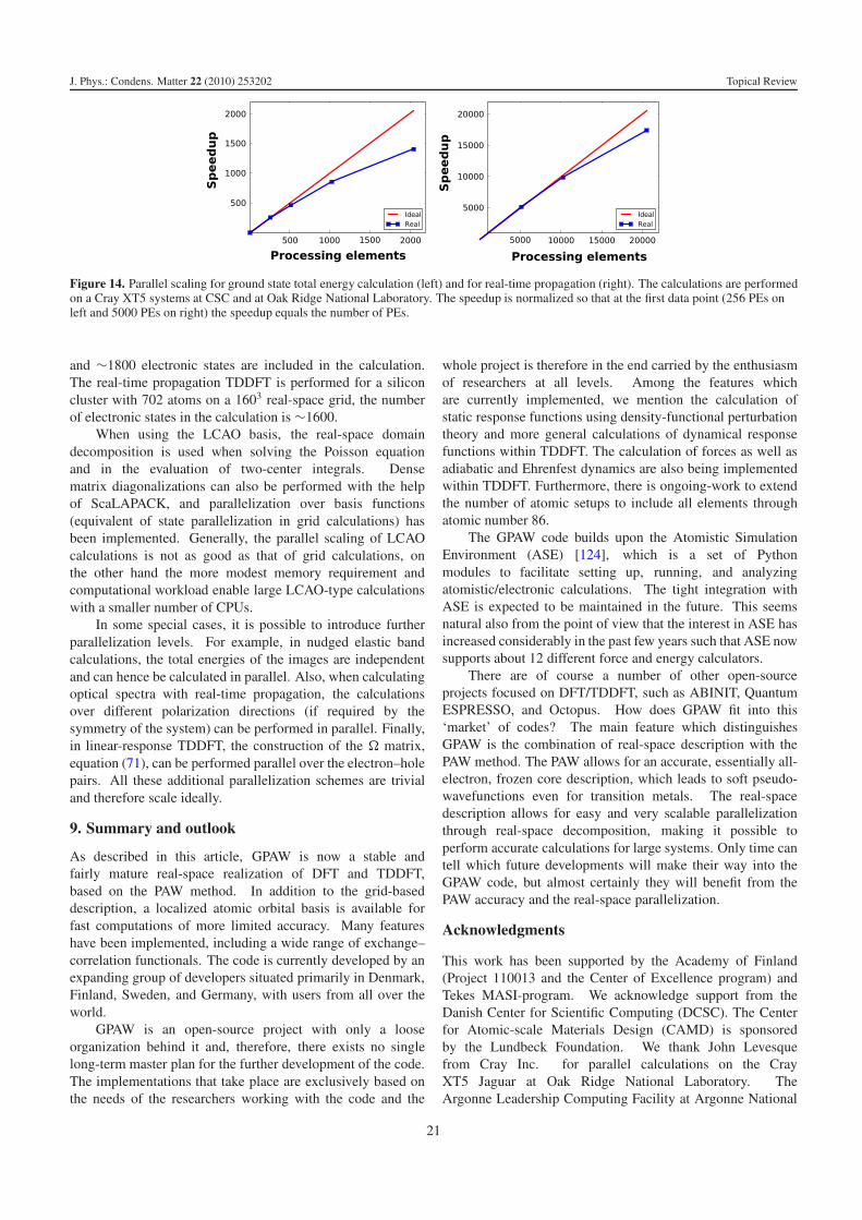
J. Phys.: Condens. Matter 22 (2010) 253202 Topical Review

Figure 14. Parallel scaling for ground state total energy calculation (left) and for real-time propagation (right). The calculations are performedon a Cray XT5 systems at CSC and at Oak Ridge National Laboratory. The speedup is normalized so that at the first data point (256 PEs onleft and 5000 PEs on right) the speedup equals the number of PEs.

and ∼1800 electronic states are included in the calculation.The real-time propagation TDDFT is performed for a siliconcluster with 702 atoms on a 1603 real-space grid, the numberof electronic states in the calculation is ∼1600.

When using the LCAO basis, the real-space domaindecomposition is used when solving the Poisson equationand in the evaluation of two-center integrals. Densematrix diagonalizations can also be performed with the helpof ScaLAPACK, and parallelization over basis functions(equivalent of state parallelization in grid calculations) hasbeen implemented. Generally, the parallel scaling of LCAOcalculations is not as good as that of grid calculations, onthe other hand the more modest memory requirement andcomputational workload enable large LCAO-type calculationswith a smaller number of CPUs.

In some special cases, it is possible to introduce furtherparallelization levels. For example, in nudged elastic bandcalculations, the total energies of the images are independentand can hence be calculated in parallel. Also, when calculatingoptical spectra with real-time propagation, the calculationsover different polarization directions (if required by thesymmetry of the system) can be performed in parallel. Finally,in linear-response TDDFT, the construction of the � matrix,equation (71), can be performed parallel over the electron–holepairs. All these additional parallelization schemes are trivialand therefore scale ideally.

9. Summary and outlook

As described in this article, GPAW is now a stable andfairly mature real-space realization of DFT and TDDFT,based on the PAW method. In addition to the grid-baseddescription, a localized atomic orbital basis is available forfast computations of more limited accuracy. Many featureshave been implemented, including a wide range of exchange–correlation functionals. The code is currently developed by anexpanding group of developers situated primarily in Denmark,Finland, Sweden, and Germany, with users from all over theworld.

GPAW is an open-source project with only a looseorganization behind it and, therefore, there exists no singlelong-term master plan for the further development of the code.The implementations that take place are exclusively based onthe needs of the researchers working with the code and the

whole project is therefore in the end carried by the enthusiasmof researchers at all levels. Among the features whichare currently implemented, we mention the calculation ofstatic response functions using density-functional perturbationtheory and more general calculations of dynamical responsefunctions within TDDFT. The calculation of forces as well asadiabatic and Ehrenfest dynamics are also being implementedwithin TDDFT. Furthermore, there is ongoing-work to extendthe number of atomic setups to include all elements throughatomic number 86.

The GPAW code builds upon the Atomistic SimulationEnvironment (ASE) [124], which is a set of Pythonmodules to facilitate setting up, running, and analyzingatomistic/electronic calculations. The tight integration withASE is expected to be maintained in the future. This seemsnatural also from the point of view that the interest in ASE hasincreased considerably in the past few years such that ASE nowsupports about 12 different force and energy calculators.

There are of course a number of other open-sourceprojects focused on DFT/TDDFT, such as ABINIT, QuantumESPRESSO, and Octopus. How does GPAW fit into this‘market’ of codes? The main feature which distinguishesGPAW is the combination of real-space description with thePAW method. The PAW allows for an accurate, essentially all-electron, frozen core description, which leads to soft pseudo-wavefunctions even for transition metals. The real-spacedescription allows for easy and very scalable parallelizationthrough real-space decomposition, making it possible toperform accurate calculations for large systems. Only time cantell which future developments will make their way into theGPAW code, but almost certainly they will benefit from thePAW accuracy and the real-space parallelization.

Acknowledgments

This work has been supported by the Academy of Finland(Project 110013 and the Center of Excellence program) andTekes MASI-program. We acknowledge support from theDanish Center for Scientific Computing (DCSC). The Centerfor Atomic-scale Materials Design (CAMD) is sponsoredby the Lundbeck Foundation. We thank John Levesquefrom Cray Inc. for parallel calculations on the CrayXT5 Jaguar at Oak Ridge National Laboratory. TheArgonne Leadership Computing Facility at Argonne National

21

J. Phys.: Condens. Matter 22 (2010) 253202 Topical Review

Laboratory is supported by the Office of Science of the USDepartment of Energy under contract DE-AC02-06CH11357.

References

[1] Hohenberg P and Kohn W 1964 Inhomogeneous electron gasPhys. Rev. 136 B864–71

[2] Kohn W and Sham L J 1965 Self-consistent equationsincluding exchange and correlation effects Phys. Rev.140 A1133–8

[3] Runge E and Gross E K U 1984 Density-functional theory fortime-dependent systems Phys. Rev. Lett. 52 997–1000

[4] Phillips J C and Kleinman L 1959 New method for calculatingwavefunctions in crystals and molecules Phys. Rev.116 287–94

[5] Kleinman L and Bylander D M 1982 Efficacious form formodel pseudopotentials Phys. Rev. Lett. 48 1425–8

[6] Vanderbilt D 1990 Soft self-consistent pseudopotentials in ageneralized eigenvalue formalism Phys. Rev.B 41 7892–5

[7] Blochl P E 1994 Projector augmented-wave method Phys.Rev. B 50 17953–79

[8] Wimmer E, Krakauer H, Weinert M and Freeman A J 1981Full-potential self-consistentlinearized-augmented-plane-wave method for calculatingthe electronic structure of molecules and surfaces: O2molecule Phys. Rev. B 24 864–75

[9] Payne M C, Teter M P, Allan D C, Arias T A andJoannopoulos J D 1992 Iterative minimization techniquesfor ab initio total-energy calculations: molecular dynamicsand conjugate gradients Rev. Mod. Phys. 64 1045–96

[10] Hehre W J, Stewart R F and Pople J A 1969 Self-consistentmolecular-orbital methods. i. Use of Gaussian expansionsof Slater-type atomic orbitals J. Chem. Phys. 51 2657–64

[11] Soler J M, Artacho E, Gale J D, Garcıa A, Junquera J,Ordejon P and Sanchez-Portal D 2002 The SIESTA methodfor ab initio order-N materials simulation J. Phys.:Condens. Matter 14 2745

[12] Blum V, Gehrke R, Hanke F, Havu P, Havu V, Ren X,Reuter K and Scheffler M 2009 Ab initio molecularsimulations with numeric atom-centered orbitals Comput.Phys. Commun. 180 2175–96

[13] Chelikowsky J R, Troullier N and Saad Y 1994Finite-difference-pseudopotential method: electronicstructure calculations without a basis Phys. Rev. Lett.72 1240–3

[14] Beck T L 2000 Rev. Mod. Phys. 72 1041[15] Junquera J, Paz O, Sanchez-Portal D and Artacho E 2001

Numerical atomic orbitals for linear-scaling calculationsPhys. Rev. B 64 235111

[16] Briggs E L, Sullivan D J and Bernholc J 1996 Real-spacemultigrid based approach to large scale electronic structurecalculations Phys. Rev. B 54 14362–75

[17] Tsuchida E and Tsukada M 1995 Electronic-structurecalculations based on the finite-element method Phys. Rev.B 52 5573–8

[18] Pask J E and Sterne P A 2005 Finite element methods in abinitio electronic structure calculations Modelling Simul.Mater. Sci. Eng. 13 R71–96

[19] Lehtovaara L, Havu V and Puska M 2009 All-electron densityfunctional theory and time-dependent density functionaltheory with high-order finite elements J. Chem. Phys.131 054103

[20] https://wiki.fysik.dtu.dk/gpaw[21] Kresse G and Joubert D 1999 From ultrasoft pseudopotentials

to the projector augmented-wave method Phys. Rev. B59 1758

[22] Gonze X et al 2002 First-principle computation of materialproperties: the ABINIT software project Comput. Mater.Sci. 25 478

[23] Holzwarth N A W, Matthews G E, Dunning R B, Tackett A Rand Zeng Y 1997 Comparison of the PAW, pseudopotential,and LAPW formalisms for density functional calculationsof solids Phys. Rev. B 55 2005

[24] Blochl P E, Forst C J and Schimpl J 2003 The projectoraugmented wave method: ab initio molecular dynamicswith full wavefunctions Bull. Mater. Sci. 26 33

[25] Kresse G and Furthmuller J 1996 Efficiency of ab initio totalenergy calculations for metals and semiconductors using aplane-wave basis set Comput. Mater. Sci. 6 15–50

[26] Giannozzi P et al 2009 QUANTUM ESPRESSO: a modularand open-source software project for quantum simulationsof materials J. Phys.: Condens. Matter 21 395502

[27] Ahlrichs R, Bar M, Haser M, Horn H and Kolmel C 1989Electronic structure calculations on workstation computers:the program system turbomole Chem. Phys. Lett.162 165–9

[28] Briggs E L, Sullivan D J and Bernholc J 1995 Large-scaleelectronic-structure calculations with multigrid accelerationPhys. Rev. B 52 R5471–4

[29] Marques M A L, Castro A, Bertsch G F and Rubio A 2003Octopus: a first-principles tool for excited electron–iondynamics Comput. Phys. Commun. 151 60–78

[30] Heiskanen M, Torsti T, Puska M J and Nieminen R M 2001Multigrid method for electronic structure calculations Phys.Rev. B 63 245106

[31] Yabana K and Bertsch G F 1996 Time-dependent local-densityapproximation in real time Phys. Rev. B 54 4484

[32] Casida M E 1996 Time-dependent density functional responsetheory of molecular systems: theory, computationalmethods, and functionals Recent Developments andApplications in Modern Density-Functional Theoryed J M Seminario (Amsterdam: Elsevier) p 391

[33] Gavnholt J, Olsen T, Engelund M and Schiøtz J 2008 �self-consistent field method to obtain potential energysurfaces of excited molecules on surfaces Phys. Rev. B78 075441

[34] Mortensen J J, Hansen L B and Jacobsen K W 2005Real-space grid implementation of the projector augmentedwave method Phys. Rev. B 71 035109

[35] Marsman M and Kresse G 2006 Relaxed coreprojector-augmented-wave method J. Chem. Phys.125 104101

[36] Kiejna A, Kresse G, Rogal J, De Sarkar A, Reuter K andScheffler M 2006 Comparison of the full-potential andfrozen-core approximation approaches todensity-functional calculations of surfaces Phys. Rev. B73 035404

[37] Natan A, Benjamini A, Naveh D, Kronik L, Tiago M L,Beckman S P and Chelikowsky J R 2008 Real-spacepseudopotential method for first principles calculations ofgeneral periodic and partially periodic systems Phys. Rev. B78 075109

[38] Tafipolsky M and Schmid R 2006 A general and efficientpseudopotential Fourier filtering scheme for real spacemethods using mask functions J. Comput. Phys. 124174102

[39] Hartwigsen C, Goedecker S and Hutter J 1998 Relativisticseparable dual-space Gaussian pseudopotentials from H toRn Phys. Rev. B 58 3641–62

[40] Kresse G and Furthmuller J 1996 Efficient iterative schemesfor ab initio total-energy calculations using a plane-wavebasis set Phys. Rev. B 54 11169–86

[41] Wood D M and Zunger A 1985 A new method fordiagonalising large matrices J. Phys. A: Math. Gen.18 1343

[42] Feng Y T and Owen D R J 1996 Conjugate gradient methodsfor solving the smallest eigenpair of large symmetriceigenvalue problems Int. J. Num. Methods Eng.39 2209–29

[43] Davidson E R 1975 The iterative calculation of a few of thelowest eigenvalues and corresponding eigenvectors of largereal-symmetric matrices J. Comput. Phys. 17 87–94

[44] Pulay P 1980 Convergence acceleration of iterative sequences.The case of SCF iteration Chem. Phys. Lett. 73 393–8

22

J. Phys.: Condens. Matter 22 (2010) 253202 Topical Review

[45] http://www.tddft.org/programs/octopus/wiki/index.php/Libxc[46] Perdew J P, Ruzsinszky A, Tao J, Staroverov V N,

Scuseria G E and Csonka G I 2005 Prescription for thedesign and selection of density functional approximations:more constraint satisfaction with fewer fits J. Chem. Phys.123 062201

[47] Tao J, Perdew J P, Staroverov V N and Scuseria G E 2003Climbing the density functional ladder: nonempirical metageneralized gradient approximation designed for moleculesand solids Phys. Rev. Lett. 91 146401

[48] Zhao Y and Truhlar D G 2006 A new local density functionalfor main-group thermochemistry, transition metal bonding,thermochemical kinetics, and noncovalent interactionsJ. Chem. Phys. 125 194101

[49] Perdew J P, Ruzsinszky A, Csonka G I, Constantin L A andSun J 2009 Workhorse semilocal density functional forcondensed matter physics and quantum chemistry Phys.Rev. Lett. 103 026403

[50] Perdew J P, Tao J, Staroverov V N and Scuseria G 2004Meta-generalized gradient approximation: explanation of arealistic nonempirical density functional J. Chem. Phys.120 6898–911

[51] Paier J, Hirschl R, Marsman M and Kresse G 2005 ThePerdew–Burke–Ernzerhof exchange–correlation functionalapplied to the G2-1 test set using a plane-wave basis setJ. Chem. Phys. 122 234102

[52] Walter M, Hakkinen H, Lehtovaara L, Puska M, Enkovaara J,Rostgaard C and Mortensen J J 2008 Time-dependentdensity-functional theory in the projector augmented-wavemethod J. Chem. Phys. 128 244101

[53] Rostgaard C, Jacobsen K W and Thygesen K S 2010 Fullyself-consistent GW calculations for molecules Phys. Rev. B81 085103

[54] Massidda S, Posternak M and Baldereschi A 1993Hartree–Fock LAPW approach to the electronic propertiesof periodic systems Phys. Rev. B 48 5058–68

[55] Rostgaard C 2009 The projector augmented-wave methodarXiv:0910.1921 [cond-mat.mtrl-sci]

[56] Adamo C and Barone V 1999 Towards reliable densityfunctional methods without adjustable parameters: thePBE0 model J. Chem. Phys. 110 6158–70

[57] Curtiss L A, Raghavachari K, Redfern P C and Pople J A 1997Assessment of Gaussian-2 and density functional theoriesfor the computation of enthalpies of formation J. Chem.Phys. 106 1063–79

[58] Gritsenko O, van Leeuwen R, van Lenthe E andJan Baerends E 1995 Self-consistent approximation to theKohn–Sham exchange potential Phys. Rev. A 51 1944–54

[59] Becke A D 1988 Density-functional exchange-energyapproximation with correct asymptotic behavior Phys. Rev.A 38 3098–100

[60] Kuisma M, Ojanen J, Enkovaara J and Rantala T T 2010arXiv:1003.0296

[61] Perdew J P, Ruzsinszky A, Csonka G I, Vydrov O A,Scuseria G E, Constantin L A, Zhou X and Burke K 2008Restoring the density-gradient expansion for exchange insolids and surfaces Phys. Rev. Lett. 100 136406

[62] Perdew J P and Levy M 1983 Physical content of the exactKohn–Sham orbital energies: band gaps and derivativediscontinuities Phys. Rev. Lett. 51 1884–7

[63] Sham L J and Schluter M 1983 Density-functional theory ofthe energy gap Phys. Rev. Lett. 51 1888–91

[64] Levinshtein M, Rumyantsev S and Shur M 1996 HandbookSeries on Semiconductor Parameters (Singapore: WorldScientific)

[65] Dion M, Rydberg H, Schroder E, Langreth D C andLundqvist B I 2004 Van der Waals density functional forgeneral geometries Phys. Rev. Lett. 92 246401

[66] Roman-Perez G and Soler J M 2009 Efficient implementationof a van der Waals density functional: application todouble-wall carbon nanotubes Phys. Rev. Lett. 103 096102

[67] Wellendorff J, Kelkkanen A, Mortensen J J, Lundqvist B I andBligaard T 2010 RPBE-vdW description of benzeneadsorption on Au(111) Top. Catal. 53 378–83

[68] Dudarev S L, Botton G A, Savrasov S Y, Humphreys C J andSutton A P 1998 Electron-energy-loss spectra and thestructural stability of nickel oxide: an LSDA + U studyPhys. Rev. B 57 1505–9

[69] Rohrbach A, Hafner J and Kresse G 2004 Molecularadsorption on the surface of strongly correlatedtransition-metal oxides: a case study for Co/NiO(100)Phys. Rev. B 69 075413

[70] Maxisch T, Wang L and Ceder G 2006 Oxidation energies oftransition metal oxides within the GGA + U frameworkPhys. Rev. B 73 195107

[71] Tran F, Blaha P, Schwarz K and Novak P 2006 Hybridexchange–correlation energy functionals for stronglycorrelated electrons: applications to transition-metalmonoxides Phys. Rev. B 74 155108

[72] Mortensen J J, Kaasbjerg K, Frederiksen S L, Nørskov J K,Sethna J P and Jacobsen K W 2005 Bayesian errorestimation in density-functional theory Phys. Rev. Lett.95 216401

[73] Perdew J P, Burke K and Ernzerhof M 1996 Generalizedgradient approximation made simple Phys. Rev. Lett.77 3865–8

[74] Yabana K and Bertsch G F 1999 Time-dependentlocal-density approximation in real time: application toconjugated molecules Int. J. Quantum Chem. 75 55–66

[75] Casida M E 1995 Time-dependent density-functional responsetheory for molecules Recent Advances in DensityFunctional Methods, Part I ed D P Chong (Singapore:World Scientific) p 155

[76] Grabo T, Petersilka M and Gross E K U 2000 Molecularexcitation energies from time-dependent density functionaltheory J. Mol. Struct.: THEOCHEM 501/502 353–67

[77] Negishi Y, Chaki N K, Whetten R L and Tsukuda T 2007Origin of magic stability of thiolated gold clusters: casestudy on Au25(Sc6h13)18 J. Am. Chem. Soc. 129 11322

[78] Neuhasuer D and Baer M 1989 The time-dependentSchrodinger equation: application of absorbing boundaryconditions J. Chem. Phys. 90 4351–5

[79] Chong D P, Gritsenko O V and Baerends E J 2002Interpretation of the Kohn–Sham orbital energies asapproximate vertical ionization potentials J. Chem. Phys.116 1760–72

[80] Walter M and Hakkinen H 2008 Photoelectron spectra fromfirst principles: from the many-body to the single-particlepicture New J. Phys. 10 043018

[81] Allison D A and Cavell R G 1978 Photoelectron spectroscopywith Zr Mζ (151 eV) radiation. A study of the variation ofrelative photoionization cross sections of moleculescontaining first row atoms (C, N, O) with exciting radiationfrom He1 to Kα limits J. Chem. Phys. 68 593–601

[82] Sankey O F and Niklewski D J 1989 Phys. Rev. B 40 3979[83] Delley B 2000 From molecules to solids with the Dmol3

approach J. Chem. Phys. 113 7756[84] Larsen A H, Vanin M, Mortensen J J, Thygesen K S and

Jacobsen K W 2009 Localized atomic basis set in theprojector augmented wave method Phys. Rev. B 80 195112

[85] Anglada E, Soler J M, Junquera J and Artacho E 2002 Phys.Rev. B 66 205101

[86] Guinea F, Tejedor C, Flores F and Louis E 1983 Effectivetwo-dimensional Hamiltonian at surfaces Phys. Rev. B28 4397

[87] Brandbyge M, Mozos J L, Ordejon P, Taylor J andStokbro K 2002 Density-functional method fornonequilibrium electron transport Phys. Rev. B 65 165401

[88] Patterson T N L 1968 Optimum addition of points toquadrature formulae Math. Comput. 22 847

[89] Meir Y and Wingreen N S 1992 Landauer formula for thecurrent through an interacting electron region Phys. Rev. B68 2512

[90] Thygesen K S 2006 Electron transport through an interactingregion: the case of a nonorthogonal basis set Phys. Rev. B73 035309

[91] Toher C and Sanvito S 2008 Effects of self-interactioncorrections on the transport properties of phenyl-basedmolecular junctions Phys. Rev. B 77 155402

23

J. Phys.: Condens. Matter 22 (2010) 253202 Topical Review

[92] Neaton J B, Hybertsen M S and Louie S G 2006Renormalization of molecular electronic levels atmetal–molecule interfaces Phys. Rev. Lett. 97 216405

[93] Garcia-Lastra J M, Rostgaard C, Rubio A and Thygesen K S2009 Polarization-induced renormalization of molecularlevels at metallic and semiconducting surfaces Phys. Rev. B80 245427

[94] Thygesen K S 2008 Impact of exchange–correlation effects onthe IV characteristics of a molecular junction Phys. Rev.Lett. 100 166804

[95] Thygesen K S and Rubio A 2008 Conserving GW scheme fornonequilibrium quantum transport in molecular contactsPhys. Rev. B 77 115333

[96] Wang X, Spataru C D, Hybertsen M S and Millis A J 2008Electronic correlation in nanoscale junctions: comparisonof the gw approximation to a numerically exact solution ofthe single-impurity anderson model Phys. Rev. B77 045119

[97] Jacob D, Haule K and Kotliar G 2009 Kondo effect andconductance of nanocontacts with magnetic impuritiesPhys. Rev. Lett. 103 016803

[98] Scheer E, Agrait N, Cuevas J C, Yeyati A L, Ludoph B,Martin-Rodero A, Bollinger G R, van Ruitenbeek J M andUrbina C 1998 The signature of chemical valence in theelectrical conduction through a single-atom contact Nature394 154–7

[99] Djukic D, Thygesen K S, Untiedt C, Smit R H M,Jacobsen K W and van Ruitenbeek J M 2005 Stretchingdependence of the vibration modes of a single-moleculept-h-2-pt bridge Phys. Rev. B 71 161402

[100] Jones R O and Gunnarsson O 1989 The density functionalformalism, its applications and prospects Rev. Mod. Phys.61 689–746

[101] Hellman A, Razaznejad B and Lundqvist B I 2004Potential-energy surfaces for excited states in extendedsystems J. Chem. Phys. 120 4593–602

[102] Gunnarsson O and Lundqvist B I 1976 Exchange andcorrelation in atoms, molecules, and solids by thespin-density-functional formalism Phys. Rev.B 13 4274–98

[103] Olsen T, Gavnholt J and Schiøtz J 2009 Hot-electron mediateddesorption rates calculated from excited-state potentialenergy surfaces Phys. Rev. B 79 035403

[104] Olsen T 2009 Inelastic scattering in a local polaron modelwith quadratic coupling to bosons Phys. Rev. B 79 235414

[105] Olsen T and Schiøtz J 2009 Origin of power laws for reactionsat metal surfaces mediated by hot electrons Phys. Rev. Lett.103 238301

[106] Olsen T and Schiøtz J 2010 Vibrationally mediated control ofsingle-electron transmission in weakly coupledmolecule–metal junctions Phys. Rev. B 81 115443

[107] Stohr J 1992 NEXAFS Spectroscopy (Berlin: Springer)

[108] Triguero L, Pettersson L G M and Agren H 1998 Calculationsof near-edge x-ray-absorption spectra of gas-phase andchemisorbed molecules by means of density-functional andtransition-potential theory Phys. Rev. B 58 8097–110

[109] Taillefumier M, Cabaret D, Flank A-M and Mauri F 2002X-ray absorption near-edge structure calculations with thepseudopotentials: application to the k edge in diamond andα-quartz Phys. Rev. B 66 195107

[110] Haydock R, Heine V and Kelly M J 1972 Electronic structurebased on the local atomic environment for tight-bindingbands J. Phys. C: Solid State Phys. 5 2845–58

[111] Hasnip P J and Pickard C J 2006 Electronic energyminimisation with ultrasoft pseudopotentials Comput.Phys. Commun. 174 24–9

[112] Takahashi O and Pettersson L G M 2004 Functionaldependence of core-excitation energies J. Chem. Phys.121 10339–45

[113] Kolczewski C et al 2001 Detailed study of pyridine at the C 1sand N 1s ionization thresholds: the influence of thevibrational fine structure J. Chem. Phys. 115 6426–37

[114] http://w3.rz-berlin.mpg.de/∼hermann/StoBe/[115] Ma Y, Wassdahl N, Skytt P, Guo J, Nordgren J, Johnson P D,

Rubensson J-E, Boske T, Eberhardt W and Kevan S D 1992Soft-x-ray resonant inelastic scattering at the C k edge ofdiamond Phys. Rev. Lett. 69 2598–601

[116] Thygesen K S, Hansen L B and Jacobsen K W 2005 Partlyoccupied Wannier functions: construction and applicationsPhys. Rev. B 72 125119

[117] Ferretti A, Calzolari A, Bonferroni B and Di Felice R 2007Maximally localized Wannier functions constructed fromprojector-augmented waves or ultrasoft pseudopotentialsJ. Phys.: Condens. Matter 19 036215

[118] Quek S Y, Venkataraman L, Choi H J, Louie S G,Hybertsen M S and Neaton J B 2007 Amine-gold linkedsingle-molecule circuits: experiment and theory Nano Lett.7 3477–82

[119] Tang W, Sanville E and Henkelman G 2009 A grid-basedBader analysis algorithm without lattice bias J. Phys.:Condens. Matter 21 084204

[120] http://theory.cm.utexas.edu/henkelman/research/bader/[121] Martins J L and Cohen M L 1988 Diagonalization of large

matrices in pseudopotential band-structure calculations:dual-space formalism Phys. Rev. B 37 6134

[122] Blackford L S et al 1997 ScaLAPACK Users’ Guide(Philadelphia, PA: Society for Industrial and AppliedMathematics)

[123] Walter M, Akola J, Lopez-Acevedo O, Jadzinsky P D,Calero G, Ackerson C J, Whetten R L, Gronbeck H andHakkinen H 2008 A unified view of ligand-protected goldclusters as superatom complexes Proc. Natl Acad. Sci.105 9157–62

[124] Bahn S and Jacobsen K W 2002 Comput. Sci. Eng. 4 56https://wiki.fysik.dtu.dk/ase

24