electrodialysisof salts, acids and bases - university of pretoria
TRANSCRIPT
ELECTRODIALYSISOF SALTS,ACIDS AND BASES
A thesis submitted in partial fulfilment of the prerequisites for the
degree of Doctor of Philosophy in the Faculty of Science,
University of Pretoria, Pretoria.
(March 1992)
©© UUnniivveerrssiittyy ooff PPrreettoorriiaa
ELECTRODIALYSIS OF SALTS, ACIDS AND BASES
BY ELECTRO·OSMOTIC PUMPING
Jakob Johannes Schoeman
Promoter: Professor Jacobus F van Staden
Department of Chemistry, University of Pretoria
Degree: Doctor of Philosophy
Salts, acids and bases frequently occur in industrial effluents and usually have considerable pollution
potential. Preliminarywork has indicated that electro-osmotic pumping electrodialysis (EOP·ED) has
the potential to recover chemicals and water for reuse and to reduce effluent volumes significantly.
However, with respect to this technology, the following needs were identified:
a) consider and fully document the relevant EOP·ED and ED theory;
b) study the EOP·ED characteristics (transport numbers, brine concentration, current efficiency,
current density, electro-osmotic coefficients, etc.) of commercially available and other
membranes in a single cell pair (cp) with the aim of identifying membranes suitable for
EOP·ED;
c) evaluate a simple method and existing models with which membrane performance for
concentration by EOP·ED can be predicted and described;
d) evaluate EOP·ED for industrial effluent treatment in a conventional ED and in a sealed-cell ED
(SCED) membrane stack.
A conventional ED membrane stack which was converted into an EOP·ED stack performed
satisfactorily for concentration/desalination of sodium chloride, hydrochloric acid and caustic soda
solutions. Dialysate concentrations of less than 500 mg/Qcould be obtained in the feed water and cell
pair voltage ranges from 1 000 to 10 000 mg/Qand 0,5 to 4,0 V/cp. Small brine volumes were
obtained. Brine volume varied between 1,5 and 4,0%; 2,4 and 7,8%; and between 2,3 and 7,3% in
the case of sodium chloride, hydrochloric acid and caustic soda solutions (1 000 to 5 000 mg/Qfeed).
Current efficiency was high. Current efficiency varied between 75,2 and 93,6%; 29,2 and 46,3%; and
between 68,9 and 81,2% when sodium chloride, hydrochloric acid and caustic soda solutions were
eleetrodialyzed, respectively. Low electrical energy consumptions were obtained. Electrical energy
consumption was less than 2,5 kWh/m3 product for sodium chloride solutions in the 1 000 to
3 000 mg/~ feed concentration range; between 0,2 and 3,2 kWh/m3 product at 1 000 mg/~
hydrochloric acid feed concentration; and between 0,4 and 2,2 kWh/m3 product for caustic soda in the
1 000 to 3 000 mg/~feed concentration range. Water yield increased with increasing cell pair voltage
and increasing linear flow velocity through the stack and decreased with decreasing feed water
concentration. It would be advantageous to operate an EOP·ED stack at the highest possible linear
flow velocity.
Sealed-cell ED should be very effectively applied for concentration/desalination of relatively dilute (500
to 3 000 mg/~IDS) non-scale-forming salt solutions. Product water with a IDS of less than 300 mg/~
could be produced in the feed water concentration range from 500 to 10 000 mg/~ TDS. Electrical
energy consumption of 0,27 to 5,9 kWh/m3 product was obtained (500 to 3 000 mg/~ feed water
concentration range). Brine volume comprised approximately 2% of the initial feed water volume.
Therefore, brine disposal cost should be reduced significantly with this technology. Sealed-cell ED
became less efficient in the 5 000 to 10 000 mg/~ TDS feed water concentration range due to high
electrical energy consumption (3,3 to 13,0 kWh/m3 product). However, SCED may be applied in this
IDS range depending on the value of the product that can be recovered.
A relatively concentrated ammonium nitrate effluent (TDS 3 600 mg/~) could be successfully treated
with SCED. Brine volume comprised only 2,8% of the treated water volume. Electrical energy
consumption was determined at 2,7 kWh/m3 product. It should be possible to reuse the brine and the
treated water in the process. Membrane fouling, however, may affect the process adversely and this
matter needs further investigation. Treatment of scale forming waters will affect the process adversely
because scale will precipitate in the membrane bags, which cannot be opened for cleaning. Membrane
scaling may be removed by current reversal or with cleaning solutions. However, this matter needs
further investigation. Scale forming waters, however, should be avoided or treated with ion-exchange
or nanofiltration prior to SCED treatment.
Sealed-cell ED has potential for treatment of relatively dilute « 3 000 mg/~ IDS) non-scaling waters
for chemical and water recovery for reuse. However, high IDS waters (up to approximately
16 000 mg/Q) may also be worth treating, depending on the value of the product that can be
recovered. The successful application of SCED technology seems to depend on the need to apply this
technology in preference to conventional ED for specific applications where high brine concentrations
and small brine volumes are required. Capital cost of SCED equipment should be less than that of
conventional ED due to the simpler design of the SCED stack. The membrane utilization factor of 95%
is much higher than in conventional ED (approximately 80%).
Brine concentration increased with increasing current density and increasing feed water concentration
and levels off at high current density dependent on the electro-osmotic coefficients of the membranes.
Current efficiency was nearly constant in a wide range of current densities and feed water
concentrations in the case of the Selemion (salt and acid concentration) and Raipore membranes (salt
concentration). However, all the other membranes showed a slight decrease in current efficiency
indicating that the limiting current density was exceeded. Water flow through the membranes (salt and
base concentration) increased with increasing current density and increasing feed water concentration.
Increasing water flow increased current efficiency significantly, especially in the case of the more porous
heterogeneous membranes. It will therefore not be necessary for membranes to have very high
permselectivities (> 0,9) for use in EOP·ED because efficiency will be increased by water flow through
the membranes. Consequently, water flow through ED membranes also has a positive effect in ED and
this effect is often neglected. The electro-osmotic coefficients decreased with increasing feed water
concentration until a constant value was obtained at high current density. Osmotic flow in EOP·ED
decreased relative to the total flow with increasing current density while the electro-osmotic flow
increased relative to the osmotic flow. Osmotic flow contributes significantly to the total water flow in
EOP·ED. Membrane permselectivity decreased with increasing brine and feed concentration and
increasing concentration gradient across the membranes.
Selemion AMV and CMV and lonac membranes; Selemion AAV and CHV and the newly developed
Israeli ABM membranes; and Selemion AMV and CMV, Selemion AMP and CMV and lonac membranes
performed well for salt, acid and base concentration, respectively. Current efficiencies varied between
62 and 91% (Selemion AMV and CMV); 34 and 60% (ABM-3 and Selemion CHV); and between 47
and 76% (Selemion AMV and CMV) for salt, acid and base concentration, respectively, in the feed water
concentration range from 0,05 to 1,0 mol/Q.
A simple membrane potential measurement has been demonstrated to function satisfactory to predict
membrane performance for salt, acid and base concentration. Membrane performance could be
predicted with an accuracy of 10; 20 and 20% and better for salt, acid and base concentration,
respectively. Brine concentration could be predicted satisfactorily from apparent transport numbers
and water flows. Maximum brine concentration, cb max, could be predicted satisfactorily from two simple
models.
The correct Onsager relationships to be used for potential measurements and for the transport number
are at zero current and zero volume flow, and at zero concentration gradient and zero volume flow,
respectively. In practical ED, measurements are conducted at zero pressure and in the presence of
concentration gradients and volume flows. These factors will influence the results considerably in all
systems in which volume flow is important and where the concentration factor is high as encountered
in EOP·ED. In measurement of membrane potential, the volume flow is against the concentration
potential and in general will decrease potential. In ED water flow helps to increase current efficiency,
but the concentration gradient is against current efficiency.
Models describe the system satisfactorily for concentration of salt, acid and base solutions. Brine
concentration approached a limiting value (plateau) at high current density dependent on the electro-
osmotic coefficients of the membranes. A constant slope (electro-osmotic coefficient) was obtained
when water flow was plotted against current density. Straight lines were obtained when cell pair
resistance was plotted against the specific resistance of the dialysate. Current efficiency increased with
increasing flow of water through the membranes, decreased when the concentration gradient was high
and the apparent transport numbers were low.
ELEKTRODIALISE VAN SOUTE, SURE EN BASI SSE
DEUR MIDDEL VAN ELEKTRO·OSMOTIESE POMPING
Jakob Johannes Schoeman
Promoter: Professor Jacobus F van Staden
Departement Chemie, Universiteit van Pretoria
Graad: Philosophia Doctor
Soute, sure en basisse kom dikwels in industriele uitvloeisels voor en het gewoonlik 'n aansienlike
besoedelingspotensiaal. Voorlopige werk het aangedui dat elekto-osmotiese pomping elektrodialise
(EOP·ED) die potensiaal het om chemikaliee en water vir hergebruik te herwin en om
uitvloeiselvolumes betekenisvol te verminder. Daar is egter geTdentifiseerdat behoeftes bestaan om:
a) EOP€D- en ED-teorie deeglik in oenskou te neem en om die relevante teorie ten volle te
dokumenteer;
b) EOP·ED eienskappe (transportgetalle, loogkonsentrasie, stroomdoeltreffendheid,
stroomdigtheid, elektro-osmotiese koeffisiente, ens.) van kommersieel beskikbare en ander
membrane in 'n enkelselpaar (sp) te bestudeer met die doel om membrane wat vir EOP·ED
geskik is, te identifiseer;
c) 'n eenvoudige metode en bestaande modelle te evalueer waarmee membraanwerkverrigting
vir konsentrasie met EOP·ED voorspel en beskryf kan word;
d) EOP€D vir industriele uitvloeiselbehandeling in 'n konvensionele ED en in 'n geseeldesel ED
(GSED) membraanpak te evalueer.
'n Konvensionele ED-membraanpak wat na 'n EOP·ED membraanpak omgeskakel is, het
bevredigende werkverrigting vir die konsentrering/ontsouting van natriumchloried-, soutsuur- en
bytsodaoplossings gelewer. Produkwaterkonsentrasies van minder as 500 mg/Q kon in die
toevoerwater- en selpaarspanninggebiede van 1 000 tot 10 000 mg/Q en 0,5 tot 4,0 V/sp verkry word.
Klein loogvolumes is verkry. Loogvolumes het tussen 1,5 en 4,0%; 2,4 en 7,8%; en 2,3 en 7,3% in
die geval van natriumchloried-, soutsuur- en bytsodaoplossings, gewissel. Stroomdoeltreffendhede
was hoog. Stroomdoeltreffendhede het tussen 75,2 en 93,6%; 28,2 en 46,3%; en tussen 68,9 en
81,2%gewissel toe natriumchloried-, soutsuur- en bytsodaoplossings respektiewelik, geelektrodialiseer
is. Lae elektriese energieverbruike is verkry. Elektriese energieverbruik was minder as 2,5 kWh/m3
produk vir natriumchloriedoplossings in die 1 000 tot 3 000 mg/Q toevoerwaterkonsentrasiegebied;
tussen 0,2 en 3,2 kWh/m3 produk vir soutsuur by 1 000 mg/Q toevoerkonsentrasie; en tussen 0,4 en
2,2 kWh/m3 prod uk vir bytsodaoplossings in die 1 000 tot 3 000 mg/Q toevoerwaterkonsentrasiegebied.
Wateropbrengs het met toenemende selpaarspanning en toenemende liniere vloeisnelheid deur die
membraanpak toegeneem en met afnemende toevoerkonsentrasie afgeneem. Dit sal dus voordelig
wees om 'n EOP-ED membraanpak by die hoogste moontlike liniere vloeisnelheid te bedryf.
Geseeldeselelektrodialise behoort effektief vir die konsentrering/ontsouting van relatief verdunde (500
tot 3 000 mg/Q TOVS) nie-skaalvormende soutoplossings toegepas te kan word. Produkwater met 'n
TOVS inhoud van minder as 300 mg/Q kan geproduseer word in die toevoerwaterkonsentrasiegebied
van 500 tot 10 000 mg/Q TOVS. Elektriese energieverbruik van 0,29 tot 5,9 kWh/m3 produkwater is
verkry (500 tot 3 000 mg/Q toevoerwaterkonsentrasiegebied). Loogvolume het ongeveer 2% van die
aanvanklike toevoervolume beslaan. Loogwegdoenkoste behoort dus betekenisvol met hierdie
tegnologie verminder te kan word. Geseeldeselelektrodialise het minder doeltreffend in die 5 000 tot
10 000 mg/Q TOVS toevoerkonsentrasiegebied geword as gevolg van hoe elektriese energieverbruik
(3,3 tot 13,0 kWh/m3). Geseeldeselelektrodialise kan egter in hierdie TOVS gebied toegepas word
afhangende van die waarde van die prod uk wat herwin kan word.
'n Relatief gekonsentreerde ammoniumnitraatoplossing (TOVS 3 600 mg/Q) kon suksesvol met GSED
behandel word. Loogvolume het slegs 2,8% van die behandelde water volume beslaan. Elektriese
energieverbruik is as 2,7 kWh/m3 produk bepaal. Beide die loog- en die behandelde water behoort in
die proses hergebruik te kan word. Membraanbevuiling mag egter die proses nadelig affekteer en
hierdie saak behoort verdere aandag te geniet. Behandeling van skaalvormende waters sal die proses
nadelig be'invloed omdat skalie in die membraansakkies kan neerslaan wat nie vir
skoonmaakdoeleindes oopgemaak kan word nie. Skalie kan met stroomruiling of met
skoonmaakmiddels verwyder word. Hierdie saak vereis egter verdere ondersoek. Skaalvormende
waters behoort egter vermy te word of met ioonuitruiling of nanofiltrasie voor GSED behandel te word.
Geseeldesel ED het potensiaal om vir die behandeling van relatief verdunde « 3 000 mg/Q TOVS) nie-
skaalvormende waters vir chemiekaliee- en waterherwinning vir hergebruik aangewend te word. Waters
met hoe TOVS-vlakke (tot ongeveer 16 000 mg/Q) behoort egter ook behandel te kan word afhangende
van die waarde van die prod uk wat herwin kan word. Die suksesvolle toepassing van GSED-tegnologie
blyk om van die behoefte af te hang om hierdie tegnologie in voorkeur bo konvensionele ED vir
spesifieke toepassings aan te wend waar hoe loogkonsentrasies en klein loogvolumes vereis word.
Kapitaalkostevan GSED-toerusting behoort minderte wees as die van konvensionele ED as gevolg van
'n meer eenvoudige ontwerp van die GSED-membraanpak. Die membraanbenuttingsfaktor van 95%
Loogkonsentrasie neem met toenemende stroomdigtheid en toenemende toevoerwaterkonsentrasie
toe en plat at by hoe stroomdigthede athanklik van die elekto-osmotiese koeffisientevan die membrane.
Stroomdoeltreffendheid was bykans konstant oor 'n groot gebied van stroomdigthede en
toevoerwaterkonsentrasies in die geval van Selemion- (sout- en suurkonsentrasie) en Raipore
membrane (soutkonsentrasie). AI die ander membrane het egter 'n geringe atname in
stroomdoeltreffendheid getoon wat daarop dui dat die beperkende stroomdigtheid oorskry is.
Watervloei deur die membrane (sout- en basiskonsentrasie) het met toenemende stroomdigtheid en
toenemende toevoerwaterkonsentrasie toegeneem. Toenemende watervloei het
stroomdoeltreffendheid aansienlik laat toeneem veral in die geval van die meer poreuse heterogene
membrane. Dit sal dus nie nodig vir membrane wees om 'n baie hoe permselektiwiteit (> 0,9) vir
gebruik in EOP·ED te he nie omdat watervloei deur die membrane doeltreffend sal verhoog.
Watervloeideur ED-membrane het gevolgfik ook 'n positiewe effek, wat dikwels nie in ag geneem word
nie. Die elektro-osmotiese koeffisiente van die membrane neem met toenemende toevoerkonsentrasie
at totdat 'n konstante waarde by hoe stroomdigtheid verkry word. Osmotiese vloei in EOP-ED neemmet toenemende stroomdigtheid relatiet tot die totale vloei at terwyl die elektro-osmotiese vloei relatiet
tot die osmotiese vloei toeneem. Osmotiese vloei dra betekenisvol by tot die totale watervloei in
EOP·ED. Membraanpermselektiwiteit neem met toenemende loog-, toevoerkonsentrasie en
toenemende konsentrasiegradient oor die membrane at.
SelemionAMV- en CMV- en lonac-membrane; SelemionAAV- en CHV- en die nuut ontwikkelde Israeli
ABM membrane; Selemion AMV- en CMV-, Selemion AMP- en CMV- en lonac membrane het
respektiewelik goeie werkverrigting vir sout-, suur- en basiskonsentrasie gelewer.
Stroomdoeltreffendhede het tussen 62 en 91% (Selemion AMV en CMV); 34 en 60% (ABM-3 en
Selemion CHV); en tussen 47 en 76% (Selemion AMV en CMV) respektiewelik vir sout-, suur- en basis-
konsentrasie in die toevoerwaterkonsentrasiegebiedvan 0,05 tot 1 moV~,gewissel.
Daar is gedemonstreer dat 'n eenvoudige membraanpotensiaalmeting suksesvol gebruik kan word om
membraanwerkverrigting vir sout-, suur- en basiskonsentrasie te voorspel. Membraanwerkverrigting
kan met 'n akkuraatheid van respektiewelik 10, 20 en 20% en beter voorspel word vir sout-, suur- en
basiskonsentrasie. Loogkonsentrasie kan bevredigend met oenskynlike transportgetalle enwatervloeie
voorspel word. Maksimum loogkonsentrasie; cb mak, kan bevredigend met twee eenvoudige modelle
voorspel word.
Die korrekte Onsager verwantskappe wat respektiewelik vir potensiaalmetings en vir transportgetalle
gebruik moet word is by zero stroom en zero volumevloei, en by zero konsentrasiegradient en zero
volumevloei. In praktiese ED word metings egter by zero druk in die teenwoordigheid van
konsentrasiegradiente en volumevloeie uitgevoer. Hierdie faktore sal die resultate aansienlik be'invloed
in aile sisteme waar volumevloeie belangrik is en waar die konsentrasiefaktor hoog is soos wat in
EOP·ED aangetref word. In die meting van membraanpotensiaal werk volumevloei teen die
konsentrasiepotensiaal en sal in die algemeen die potensiaal verlaag. In ED help watervloei om die
stroomdoeltreffendheid te verhoog maar die konsentrasiegradient sal die stroomdoeltreffendheid
verlaag.
Modelle beskryf die sisteem vir konsentrering van sout-, suur- en basisoplossings bevredigend.
Loogkonsentrasie bereik 'n limietwaarde (plato) by hoe stroomdigtheid afhanklik van die elektro-
osmotiese koeffisiente van die membrane. 'n Konstante helling (elektro-osmotiese koeffisient) is verkry
toe watervloeie teen stroomdigtheid geplot is. Reguit Iyne is verkry toe selpaarweerstand teen die
spesifieke weerstand van die produkwater geplot is. Stroomdoeltreffendheid het met toenemende
watervloei deur die membrane toegeneem, afgeneem toe die konsentrasie-gradient hoog en die
oenskynlike transportgetalle laag was.

• the Steering Committee of the Water Research Commission under the chairmanship of Dr H
M Saayman for their assistance and enthusiasm throughout the project
• Dr B M van Vliet for the role he played to make a visit to the Weizmann Institute of Science in
Israel possible
• Professor O. Kedem of the Weizmann Institute of Science in Israel for her valuable advice and
fruitful discussions during visits to Israel and abroad
• Professor J F van Staden, my promoter, for his assistance and enthusiasm throughout the
project
• Mrs G M Enslin, Mrs H Macleod, Mrs E Hill and Mr A Steyn for their valuable technical
assistance
SYNOPSIS .
SAMEVATIING v
ACKNOWLEDGEMENTS x
1. INTRODUCTION .
2. LITERATURESURVEY 3
2.1 Electro-Osmotic Pumping of Salt Solutionswith
Homogeneous lon-ExchangeMembranes 3
2.2 Electro-Osmotic Pumping of SalineSolutions
in a Unit-CellStack 5
2.3 Electro-Osmotic and Osmotic Flows 9
2.4 Structural Properties of Membrane lonomers 13
2.5 Measurementof Transport Number 16
2.6 Transport Properties of Anion-ExchangeMembranes
in Contact with Hydrochloric Acid Solutions. Membranes
for Acid Recoveryby ElectrodialysiS 17
2.7 ElectrodialysisApplications 18
3. THEORY 21
3.1 Theories of MembraneTransport 21
3.2 Conductance and Transport Number 34
3.3 Ion Coupling from ConventionalTransport Coefficients 38
3.4 Transport ProcessesOccurring During Electrodialysis 49
3.5 Current Efficiencyand Transport Phenomenain Systems
with Charged Membranes 50
3.6 Efficiencyof Energy Conversion in Electrodialysis 57
3.7 Conversion of Osmotic into MechanicalEnergy in Systems
with Charged Membranes 65
3.8 DonnanExclusion 71
3.9 RelationshipBetweenTrue and Apparent Transport Numbers 72
3.10 Electro-Osmotic Pumping - The StationaryState - Brine
Concentration and Volume Flow 77
3.11 Flux Equations, MembranePotentialsand Current Efficiency 87
3.12 ElectrodialysisTheory 92
4. ELECTRODIALYSISIN PRACTICE 117
4.1 ElectrodialysisProcessesand Stacks 117
4.2 lon-ExchangeMembranes 120
4.3 Fouling 123
4.4 Pretreatment 124
4.5 Post-treatment 125
4.6 Seawater Desalination 125
4.7 Brackish Water Desalination for Drinking-Water Purposes 126
4.8 Energy Consumption 126
4.9 Treatment of a High Scaling, High TDS Water with EDR 127
4.10 Brackish Water Desalination for Industrial Purposes 128
4.11 ED/IX System 128
4.12 Industrial Wastewater Desalination for Water Reuse,
Chemical Recovery and Effluent Volume Reduction 129
4.13 Other Possible Industrial Applications 131
4.14 Polarisation. . . . . . . . . . . . . . . . . . . . . . . . . . . . . . . . . . . . . . . . . . . . . . . . . . . . . . . . 132
4.15 Cell Stack 133
4.16 Process Design 135
5. EXPERIMENTAL 136
5.1 Membranes. . . . . . . . . . . . . . . . . . . . . . . . . . . . . . . . . . . . . . . . . . . . . . . . . . . . . . . . 136
5.2 Membrane Preparation 136
5.3 Unit-Cell Construction 137
5.4 Determination of Brine Concentration, Current Efficiency and
Water Flow as a Function of Feed Concentration and Current
Density 138
5.5 Determination of Membrane Characteristics 140
5.6 Determination of Salt and Acid Diffusion Rate through Membranes ., 141
5.7 Bench-Scale EOP-EDStack 142
5.8 Sealed-Cell ED Stack 146
6. ELECTRO-OSMOTICPUMPINGOF SODIUM CHLORIDESOLUTIONSWITH DIFFERENT
ION-EXCHANGEMEMBRANES 148
6.1 Brine Concentration 148
6.2 Current Efficiency 184
6.3 Water Flow 207
6.4 Membrane Permselectivity 223
6.5 Membrane Characteristics 227
7. ELECTRO-OSMOTICPUMPINGOF HYDROCHLORICACID SOLUTIONSWITH DIFFERENT
ION-EXCHANGEMEMBRANES 229
7.1 Brine Concentration 229
7.2 Current Efficiency 253
7.3 Water Flow 270
7.4 Membrane Permselectivity 283
7.5 Acid and Salt Diffusion through Membranes ..............................•. 286
7.6 Membrane Characteristics 287
8. ELECTRO-OSMOTICPUMPINGOF CAUSTICSODA SOLUTIONSWITH DIFFERENT
ION-EXCHANGEMEMBRANES 289
8.1 Brine Concentration 289
8.2 Current Efficiency 306
8.3 Water Flow 319
8.4 Membrane Permselectivity 328
8.5 Membrane Characteristics 330
9. ELECTRO-OSMOTICPUMPINGOF SODIUM CHLORIDE-, HYDROCHLORICACID
AND CAUSTIC SODA SOLUTIONS IN A CONVENTIONALELECTRODIALYSIS
STACK 332
9.1 Concentration/Desalination of Sodium Chloride Solutions
with lonac MA-3475 and MC-3470 Membranes 332
9.2 Concentration/Desalination of Hydrochloric Acid Solutions
with Selemion AAVand CHV Membranes 342
9.3 Concentration/Desalination of Caustic Soda Solutions with
Selemion AMV and CMV Membranes 351
10. CONCENTRATION/DESALINATIONOF SALT SOLUTIONSAND INDUSTRIAL
EFFLUENTSWITH SCED 360
10.1 Concentration of Salt Solutions 360
10.2 Concentration/Desalination of Industrial Effluents 369
11. GENERAL DISCUSSION 376
11.1 Requirements for ED Membranes 376
11.2 Permselectivity with Acids and Bases 377
11.3 Brine Concentration, Electro-Osmotic and Osmotic Flows 377
11.4 Discrepancy between Transport Numbers Derived from Potential
Measurements and Current Efficiency Actually Obtained 378
11.5 Current Efficiency and Energy Conversion in ED 380
11.6 Water Flow, Concentration Gradient and Permselectivity 381
11.7 Prediction of Brine Concentration 382
11.8 Membranes for Sodium Chloride, Hydrochloric Acid and
Caustic Soda Concentration 383
11.9 Conventional EOP-EDStack 384
11.10 Sealed-Cell Electrodialysis 384
12. SUMMARYAND CONCLUSIONS 386
13. NOMECLATURE 393
14. LITERATURE 404
APPENDIXA
APPENDIXB
APPENDIXC
APPENDIXD
Electro-osmotic pumping (EOP) is a variant of conventional electrodialysis (ED) that should be
suitable for concentration/desalination of salinewaters(1). In EOP, brine is not circulated through
the brine compartments, but is evolved in a closed cell. Brine enters the cell as electro-osmotic
and osmotic water and leaves the cell by electro-osmotic pumping. This leads to very high
concentration factors (high brine concentration) and thus high recovery of product water and
small volume of brine to be disposed of. The relatively simple design of an EOP-ED staCk, the
possibility that an EOP-ED stack may be cheaper than conventional ED and the small brine
volume produced, are the major advantages of EOP-ED(1).
Electro-osmotic pumping of sodium chloride solutions has been described by Garza(1); Garza
and Kedem(2); Kedem et al (3);Kedem and Cohen(4) and Kedem and Bar-On(5). Water and salt
fluxes were studied through ion-exchange membranes as a function of current density and feed
concentration and mathematical models were developed to describe the experimental data(1).
Kedem has reported that current efficiency determined in EOP experiments was close to the
value expected from transport number determinations when sodium chloride solutions were
electrodialyzed(5). Kedem has also reported that apparent transport numbers gave a lower
estimate of current efficiency in ED(2). However, only results for sodium chloride solutions and
one commercially available ion-exchange membrane, viz. Selemion AMV and CMV were
reported. It would be very useful if membrane performance for concentration/desalination
applications could be accurately predicted from transport numbers obtained from simple
potential measurements. Information in this regard for ion-exchange membranes to be used
for saline, acidic and basic effluent treatment, is limited.
A sealed-cell ED (SCED - membranes are sealed together at the edges) laboratory stack
(EOP-ED stack) was also developed for evaluation of desalination/concentration of sodium
chloride solutions(3, 4,5). However, only one membrane type that is presently not commercially
available, viz., polysulphone based membranes, have been used in the SCED studies. Only
desalination/concentration of sodium chloride solutions has been reported in the studies.
Saline, acidic and alkaline effluents frequently occur in industry. These effluents have the
potential to be treated with EOP-ED for water and chemical recovery and effluent volume
reduction. No information, however, could be found in the literature regarding EOP
characteristics (brine volume, current efficiency, electro-osmotic coefficients, etc.) of membranes
suitable for EOP-ED of acidic and alkaline solutions. In addition, little information is available
in the literature regarding EOP characteristics of membrane types to be used for EOP-ED of
saline solutions. Consequently, information regarding EOP characteristics of commercially
available ion-exchange membranes suitable for saline, acidic and basic solution treatment is
insufficient and information in this regard will be necessary to select membranes suitable for
EOP-ED of saline, acidic and basic effluents. In addition, no information exists regarding the
performance of an EOP-ED stack for industrial effluent treatment. Information on the theory of
EOP-ED and ED is scattered throughout the literature(1- 5,6- 19)and is not well documented in
any single publication.
Much information, on the other hand, is available in the literature regarding electro-osmosis in
general and factors affecting water transport through ion-exchange membranes(5,2O-32). Much
information is also available in the literature regarding concentration/desalination of saline
solutions and saline industrial effluents with conventional ED(6,7,33-37)and electrodialysis reversal
(EDR) (8) , Conventional ED and EDR, however, are established processes for brackish
water desalination and to a lesser extent for wastewater treatment. These processes are
applied with success, especially for brackish water treatment for potable use(6, 8, 38,39).
Conventional ED and EDR, however, have the potential to be applied more for industrial effluent
treatment.
Consider and document the relevant EOP-ED theory properly;
Study the EOP-ED characteristics (transport numbers, brine concentration, current
density, current efficiency, electro-osmotic coefficients, etc.) of commercially available
ion-exchange and other membranes in a single cell pair with the aim to identify
membranes suitable for saline, acidic and alkaline effluent treatment;
Determine whether membrane performance can be predicted effectively from simple
transport number determinations and existing models;
Study EOP-ED of saline solutions in a conventional ED stack;
Study EOP-ED of saline solutions and industrial effluents in a SCED stack.
2.1 Electro-osmotic Pumping of Salt Solutions with Homogeneous lon-Exchange
Membranes
Garza(1)and Garza and Kedem(2)have described electro-osmotic pumping of salt
solutions with homogeneous membranes in a single cell pair. Brine concentrations,
volume flows and current efficiencieswere determined at different current densities (0 -
60 mNcm2) for three different sodium chloride feed water concentrations (0,01; 0,1
and 0,5 moltO). Selemion AMV and CMV and polyethylene-based membranes,
however, were the only membranes used.
It was found that model calculations described the system in an appropriate way. The
results predicted important results such as:
a) approaching of a limiting (plateau) value of the maximum brine concentration
(cbmllX) as the current density is increased;
b) dependence of cbmax on the electro-osmotic coefficient (EOC) of the
membranes;
c) approaching of a limiting value (plateau) of current efficiency (€p) at high
current density (below its limiting value);
d) approaching of a constant slope for curves of volume flow (J) through the
membranes versus effective current density (Ielf).
It was experimentally found (1,2)that graphs of brine concentration (cb) versus current
density levelled off at high values of current and that cb approached a maximum
plateau, cbmax, which depended only on the electro-osmotic coefficients (J3)of the
membrane pair (cbmax = % FJ3).The smaller the ratio between the osmotic and electro-
osmotic water flows, the smaller the current necessary to reach this plateau.
Graphs of volume flow versus effective current density became straight lines at high
values of the current. The electro-osmotic and osmotic coefficients could be
determined from the slope and the intercept of the lines, respectively. The results have
agreed quite well with values obtained from a standard method(1)which is very time
consuming.
(Xl's) was determined from the membrane potential for a concentration difference
similar to that obtained in the EOP experiments at high current densities(2). It was
found to give a good (lower) estimate of the actual Coulomb efficiency of the process
at a salt concentration of 0,1 mol/Q. However, no results at higher or lower
concentrations were reported. Selemion AMV and CMV ion-exchange membranes
were the only commercially available membranes used.
The maximum brine concentration, cbmax, was predicted from the following two
relationships(2):
b) cbmax = cb (1 + Josm/Jelosm) (2.2)
(Note: J = Josm + Jelosm)'
Good correlations between the two methods were obtained with the membranes and
the salt solutions used.
The EOP results have shown that with appropriate membranes and control of
polarization, EOP may be used as a good alternative to conventional ED for
desalination/concentration of saline solutions. Laboratory scale EOP experiments may
also be conducted as an alternative and convenient way of determining osmotic and
electro-osmotic coefficients.
Experimental results were obtained for non-porous membranes. Current efficiencies
were in the range of 60 - 85%. It was suggested by Garza(1)that a current efficiency
of 90% could be obtained with a porous ion-exchange membrane. However, no other
results were reported.
Most of the energy consumption in the EOP system will take place in the dialysate
compartments(1). Therefore, to reduce it and to suppress concentration polarization,
it would be advisable to combine the membranes with open dialysate compartments
containing ion-conducting spacers.
It was suggested by Garza(1)that EOP would have the following advantages in relation
to conventional ED when used for desalination:
construction of the unit-cell stack compared to the conventional plate-and-
frame stack;
b) the membrane utilization factor in the membrane bags could be about 95%
compared to about 70 to 75% for membranes in conventional ED stacks;
c) higher current densities would be possible in unit-cell stacks because of the
higher linear flow velocities that could be obtained. These higher current
densities would result in higher production rates;
d) there would be a decrease in brine volume, and as a consequence, less brine
disposal problems.
The only disadvantages could be the fact that more electrical energy per unit of
product water would be experienced in the unit-cell stack because higher current
densities were used. However, the increased cost for electrical energy would be more
than off-set by the decrease in the cost of membrane replacement and amortization of
the capital investment, according to Garza(1).
No information could be found in the literature regarding EOP characteristics (brine
concentration, current efficiency, electro-osmotic coefficient, etc.) of membranes for
acid and alkaline solution treatment in a single cell pair similar to that described for
saline solutions.
The so-called unit-cell stack was described by Nishiwaki(6)for the production of
concentrated brine from seawater by ED. It consisted of envelope bags formed of
cation- and anion-exchange membranes sealed at the edges and provided with an
outlet, alternated with feed channels. The direction of volume flow through the stack
was such to cause ionic flow into the membrane bags. The only water entering the
bags was the electro-osmotic water drawn along with the ions plus the osmotic flow
caused by the higher pressure of the brine compared to the feed. This variant of ED
is called electro-osmotic pumping (EOP) and is used for production of concentrated
brine from seawater for salt production.
A simple sealed-cell ED stack (SeED) was described by Kedem et al (3) in 1978. This
cell consisted of thermally sealed polyethylene based membranes (21 bags, 5 x 9 cm).
The membranes were not very selective at high salt concentration. It was found that
smooth continuous operation was obtained with stable voltage and pH in the
concentration range from 0,01 to 0,04 mol/~ and current densities from 5 to 20
mNcm2•
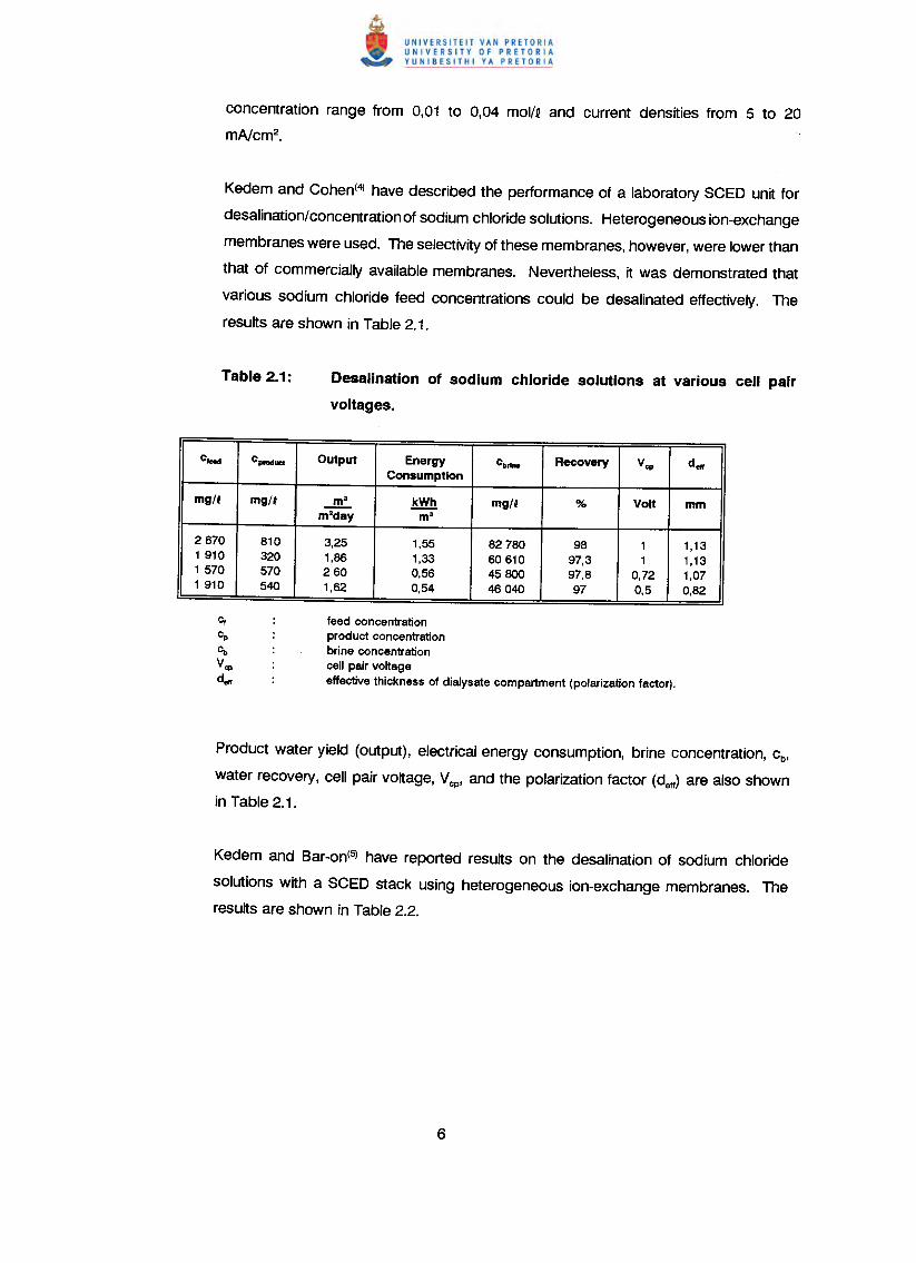
Kedem and Cohen(4) have described the performance of a laboratory SCED unit for
desalination/concentration of sodium chloride solutions. Heterogeneous ion-exchange
membranes were used. The selectivity of these membranes, however, were lower than
that of commercially available membranes. Nevertheless, it was demonstrated that
various sodium chloride feed concentrations could be desalinated effectively. The
results are shown in Table 2.1.
Desalination of sodium chloride solutions at various cell pair
voltages.
c_ c_ ••• output Energy Cb~" Recovery Vep d•••Consumption
mg/f mg/f m3 kWh mg/f % Volt mmm'day m3
2670 810 3,25 1,55 82780 98 1 1,131 910 320 1,86 1,33 60610 97,3 1 1,131570 570 260 0,56 45800 97,8 0,72 1,071 910 540 1,62 0,54 46040 97 0,5 0,82
feed concentrationproduct concentrationbrine concentrationcell pair voltageeffective thickness of dialysate compartment (polarization factor).
Product water yield (output), electrical energy consumption, brine concentration, cb,
water recovery, cell pair voltage, Vcp, and the polarization factor (deft) are also shown
in Table 2.1.
Kedem and Bar-on(5) have reported results on the desalination of sodium chloride
solutions with a SCED stack using heterogeneous ion-exchange membranes. The
results are shown in Table 2.2.
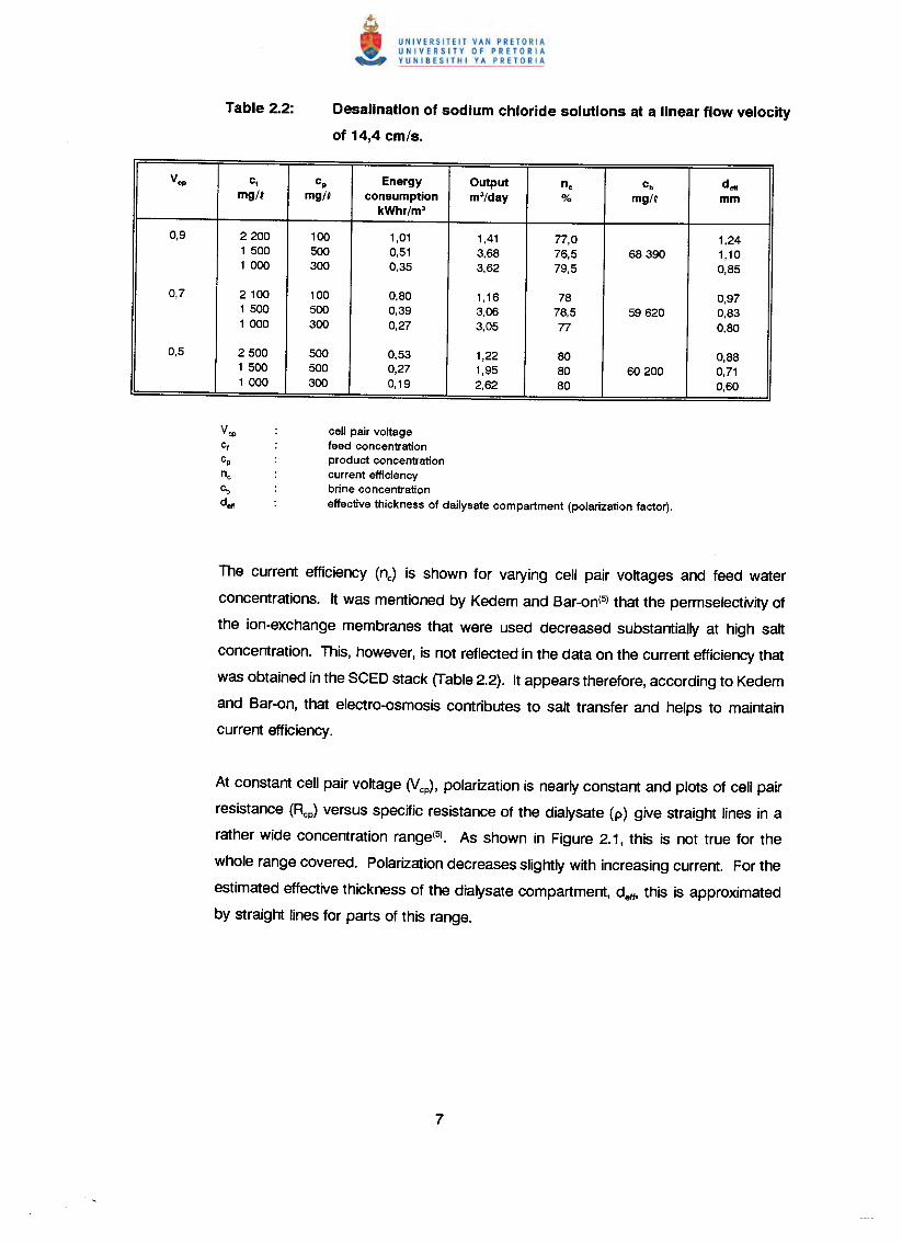
Desalination of sodium chloride solutions at a linear flow velocity
of 14,4 cm/s.
vep c, cp Energy Output n. cb d..,mgN mg/~ consumption m3/day % mg/~ mm
kWhr/m3
0,9 220O 100 1,01 1,41 77,0 1,24150O 500 0,51 3,68 76,5 68390 1,101 000 300 0,35 3,62 79,5 0,85
0,7 210O 100 0,80 1,16 78 0,971 500 500 0,39 3,06 78,5 59620 0,831 000 300 0,27 3,05 77 0,80
0,5 250O 500 0,53 1,22 80 0,881 500 SOO 0,27 1,95 80 60200 0,71100O 300 0,19 2,62 80 0,60
cell pair voltagefeed concentrationproduct concentrationcurrent efficiencybrine concentrationeffective thickness of dailysate compartment (polarization factor).
The current efficiency (nJ is shown for varying cell pair voltages and feed water
concentrations. It was mentioned by Kedem and Bar-on(5) that the permselectivity of
the ion-exchange membranes that were used decreased substantially at high salt
concentration. This, however, is not reflected in the data on the current efficiency that
was obtained in the SeED stack (Table 2.2). It appears therefore, according to Kedem
and Bar-on, that electro-osmosis contributes to salt transfer and helps to maintain
current efficiency.
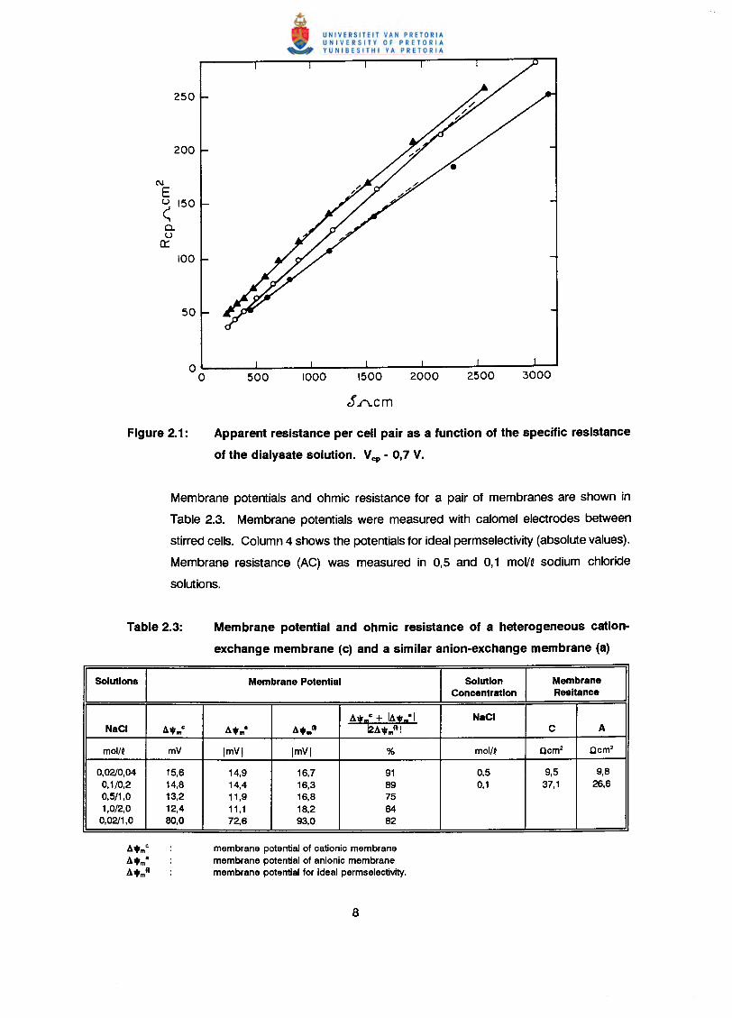
At constant cell pair voltage CVcp), polarization is nearly constant and plots of cell pair
resistance (Rcp) versus specific resistance of the dialysate (p) give straight lines in a
rather wide concentration range(5). As shown in Figure 2.1. this is not true for the
whole range covered. Polarization decreases slightly with increasing current. For the
estimated effective thickness of the dialysate compartment. deft. this is approximated
by straight lines for parts of this range.
1500
J.f"\.Cm
C\I
Eu 150
<0.Ua::
Apparent resistance per cell pair as a function of the specific resistance
of the dialysate solution. Vcp - 0,7 V.
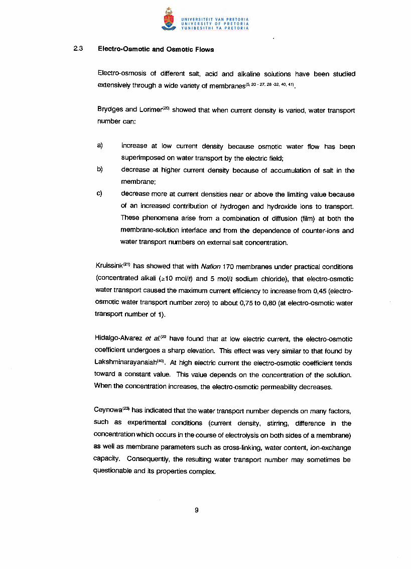
Membrane potentials and ohmic resistance for a pair of membranes are shown in
Table 2.3. Membrane potentials were measured with calomel electrodes between
stirred cells. Column 4 shows the potentials for ideal permselectivity (absolute values).·
Membrane resistance (AC) was measured in 0,5 and 0,1 molN sodium chloride
solutions.
Membrane potential and ohmic resistance of a heterogeneous cation-
exchange membrane (c) and a similar anion-exchange membrane (a)
Solutions Membrane Potential Solution MembraneConcentration Resitance
atrC + la~.·1 NaCINaCI a•• c at.· a •• 1t 12.1•• 1' c A
moll' mV ImVI ImVI % moll' Ccm" Ccm"
0,02/0,04 15,6 14,9 16,7 91 0,5 9,5 9,80,1/0,2 14,8 14,4 16,3 89 0,1 37,1 26,60,5/1,0 13,2 11,9 16,8 751,0/2,0 12,4 11,1 18,2 640,02/1,0 80,0 72,6 93,0 82
membrane potential of cationic membranemembrane potential of anionic membranemembrane potential for ideal permselectivity.
Electro-osmosis of different salt, acid and alkaline solutions have been studied
extensively through a wide variety of membranes(5,20-27,28-32,40,41),
Brydges and Lorimer(20)showed that when current density is varied, water transport
number can:
a) increase at low current density because osmotic water flow has been
superimposed on water transport by the electric field;
b) decrease at higher current density because of accumulation of salt in the
membrane;
c) decrease more at current densities near or above the limiting value because
of an increased contribution of hydrogen and hydroxide ions to transport.
These phenomena arise from a combination of diffusion (film) at both the
membrane-solution interface and from the dependence of counter-ions and
water transport numbers on external salt concentration.
Kruissink(21)has showed that with Nation 170 membranes under practical conditions
(concentrated alkali (~10 mol/Q)and 5 moV~ sodium chloride), that electro-osmotic
water transport caused the maximum current efficiency to increase from 0,45 (electro-
osmotic water transport number zero) to about 0,75 to 0,80 (at electro-osmotic water
transport number of 1).
Hidalgo-Alvarez et al(22 have found that at low electric current, the electro-osmotic
coefficient undergoes a sharp elevation. This effect was very similar to that found by
Lakshminarayanaiah(4O).At high electric current the electro-osmotic coefficient tends
toward a constant value. This value depends on the concentration of the solution.
When the concentration increases, the electro-osmotic permeability decreases.
Ceynowa(23jhas indicated that the water transport number depends on many factors,
such as experimental conditions (current density, stirring, difference in the
concentration which occurs in the course of electrolysis on both sides of a membrane)
as well as membrane parameters such as cross-linking, water content, ion-exchange
capacity. Consequently, the resulting water transport number may sometimes be
questionable and its properties complex.
The decrease of the water transport number with an increase in concentration of the
external solution is usually given as the main non-controversial property(23). However,
Tombalakian et al(24) found constant values of the water transport number for the
homogeneous sulphonic acid membranes of high cross-linking and low water content
in hydrochloric acid solution. Demarty et al (41) stated the same for the heterogeneous
lonac MC 3470 XL membrane in hydrochloric acid solutions. Similarly Oda and
Yawataya(27) reported that in some membranes in the presence of hydrochloric acid
solution the water transport number remained constant at about 1,0 and the hydrogen
ion transfer number only drops from 1,0 to 0,99. They also suggested that membranes
deswell with increasing electrolyte concentration.
Ceynowa(23) found that the water and ion transport numbers at low sulphuric acid
concentrations were in a wide range (5 - 70 mNcm~ independent of current density
in the case of the heterogeneous MRF-26 ion-exchange membrane. However, at high
concentration (2,26 mol/kg water) the increase in water transport number with current
density was remarkable. It was also found that the water transport number in the MRF
membrane decreased with increasing concentration (0,5 to 2,0 mol/kg water). With
Nafion-120 membrane the water transport number remained almost constant with
increasing feed concentration.
Rueda et al(25) stated that the decrease of water transport number with increase in
external salt concentration could be attributed to the decrease of the selectivity of the
membrane. At very dilute solutions, the current is carried by the cations because the
anions are almost completely excluded from the cationic cellulose acetate membrane.
As the external solution concentration increases, the permselectivity of the membrane
decreases. Anions are now present in the membrane and cations and anions
participate in the transport of current across the membrane in opposite directions.
Obviously, water transport will be reduced. An increase of external salt concentration
leads to an increase of charge concentration in the neighbourhood of the matrix and
consequently a decreasing of the electro-osmotic permeability.
Electro-osmotic permeability of several cellulose acetate membranes have been
determined using solutions of alkali-chlorides(25). The electro-osmotic permeability has
been studied as a function of the external electrolyte concentration (0,001 to 0,1 moVQ)
and of current density applied. The results showed that the electro-osmotic
permeability depended on the thickness of the membranes and the nature of the
cations. The electro-osmotic permeability has been found to be strongly dependent
on the external salt concentration. However, the electro-osmotic permeability was not
significantly affected by current density.
Tasaka et al (66) have also studied electro-osmosis in charged membranes. At low
electrolytic concentrations the direction of electro-osmosis is the same as that of
counter-ion flow, because most of the movable ions in the membrane are counter-ions.
With increasing external salt concentration the concentration of co-ions in the
membrane increases, and then electro-osmosis decreases. In many instances electro-
osmosis tends towards zero at the limit of high electrolyte concentrations.
Oda and Yawataya(27)have found that the electro-osmotic coefficient of hydrochloric
acid through a cation-exchange membrane remains almost constant over the
concentration range from 0,5 to 4,0 mol/Q. In hydrochloric acid solutions the electro-
osmotic water transference is merely about one mole water per Faraday through a
membrane.
Narebska et al (28)have investigated the isothermal transport of ions and water across
the perfluorinated Nafion 120 membrane in contact with sodium chloride solutions at
a concentration of 0,05 up to 4 mol/Qbased on irreversible thermodynamics of
transport. It was found that the specific conductivity of the membrane increased at low
external electrolyte concentration. The apparent transport number of the cation
decreased significantly at higher externalelectrolyte concentration. The electro-osmotic
coefficient also decreased significantly at higher external electrolytic concentration. The
osmotic volume flux, and salt diffusion flux increased with increasing electrolyte
concentration while the hydrodynamic volume flow decreased with increasing
electrolytic concentration. The membrane also deswelled significantly with increasing
electrolyte concentration.
Narebska and Koter(29)have studied the conductivity of ion-exchange membranes on
the grounds of irreversible thermodynamics of transport. They have found that
convection conductivity covers 50 to 55% of the total membrane conductivity and even
more at increased temperature. This means that the flowing water doubles the ability
of the membrane to transport the ionic current. This confirms the substantial role that
water plays in the transport behaviour of a membrane.
Narebska et al, (30) have performed a detailed analysis of membrane phenomena in the
system Nafion 120/NaOHaq• They have determined the phenomenological resistance -
(r;k) and friction coefficient (f;k). They have found that the resistance imposed by the
membrane on the permeating OH- ions is much lower that that for Ct ions. The three
factors contributing to this effect - i.e. the frictions imposed by the cation (f21), water
(f2w) and the polymer matrix (f2m) - influence the flow of OH" and 0 to a different
degree. Chloride ions are hindered mainly by water, especially at increasing sorption.
The flow of OH- ions in diluted solution is hindered by the matrix and, at a higher
concentration, by the cation and then by water.
Considering these results, it is apparent that the easy flow of NaOH results not only
from the high mobility of OH- ions, but also from the low osmotic flux (2 to 3 times less
than in NaCI solutions) opposing the stream of electrolyte and the very low friction of
the OH" ions with water.
The water transport number decreased from 1a mollF araday to 2 mollFaraday over the
concentration range of 0,05 to 4 mol/Q. The apparent transport number (ate) also
decreased significantly with increasing caustic soda concentration.
The transport of aqueous NaCI solutions across the perfluorinated Nafion 120
membrane have been studied on the basis of irreversible thermodynamics by
Narebska et al (31).The straight resistance coefficients ri;, partial frictions fik and diffusion
indexes have been determined.
Since the Donnan equilibrium and TMS theory were published, it is a well known and
documented fact that co-ions are rejected from a charged polymer by the high
potential of the polymer network. It was found by Narebska et al, that friction of this
co-ion with the charged polymer was not the main force which resisted the flow of
negative ions in the negatively charged polymer network. Except at 289 K and
mext = 0,5, the anion-polymer frictional force (2m)was below the friction with water (2w)
and it decreases with increasing electrolyte concentration and temperature. As a
result, at high temperature and mext, the resistance against flowing anions is imposed
by water; the lower the amount of water in the membrane, the higher this resistance.
Koter and Narebska(32)have investigated the mobilities of Na+, CI-and OH' ions and
water in Nafion 120 membranes. They have found that the interactions of Na+ and 0
ions running in opposite directions are negligible in the whole concentration range
(0,05 to 4 mol/Q)studied. However, hydroxide ions impede cations, particularly at
higher external concentrations (high sorption). This fact can be attributed to the higher
partial friction between Na+ and OH- ions caused by the phenomenon called "local
hydrolysis".
The mobility of hydroxide ions exceeds that of chloride ions even more in the
membrane than in the free solution. The mobility of hydroxide ions is much more
sensitive to concentration than that of chloride ions. The mobility of the hydroxide ions
declines much more rapidly than the mobility of the chloride ions. This reflects the
dehydration of the membrane with increasing sorption of an electrolyte.
Kedem and Bar-on(5)have mentioned that the current efficiency (nc) for a single
membrane pair was sometimes equal to and even higher than the apparent transport
number of the membrane pair (Xt) measured with calomel electrodes. According to
them, this is due to the substantial influence of electro-osmotic and osmotic flow into
the brine cells during ED which increase the current efficiency. Both osmotic and
electro-osmotic water flow enters the brine cell through both membranes. It increases
the flows of counter-ions leaving the brine. The total effect of volume flow into a brine
cell is increased salt flow. There will also be a slight influence of osmotic flow on the
potential measurements. This will decrease the potential measurement and therefore
the apparent transport number(5).
Mauritz and Hopfinger(42)have described structural properties of ion-exchange
membranes. Common functionalities of ion-exchange membranes are: -503-; -COO-;
-NH3+; =NH2 +. These hydrophillic groups are responsible for the swelling of the
hydrophobic network of ion-exchange membranes on exposure to water. Swelling of
ion-exchange membranes may be inhibited by the presence of crystalline domains
within the membrane matrix.
The approach to equilibrium for an initially dry ion-exchange membrane (in a given
counter-ion salt form and containing no co-ions) that is subsequently immersed in pure
water, can be visualized in the following way: Although the interaction between the
organic polymer backbone is endothermic and may influence the rate of swelling, the
strongly exothermic tendency of the counter-ions and ionogenic side chains to hydrate
results in having the initially arrived water molecules strongly bound in ionic solvation
shells resulting in little or no volume expansion of the network. In the truly dry state,
the counter-ions are strongly bound by electrostatic forces in contact ion pairs. Further
uptake of water beyond that which is barely required for maximum occupancy of all the
hydration shells results in moving the association - dissociation equilibrium between
bound and unbound counter-ions toward increased counter-ion mobility. The driving
force for swelling is the tendency for the water to dilute the polymer network. Stated
in precise thermodynamic formalism, the difference between the water activity in the
interior (~ < 1) and exterior (a.. = 1) of the membrane gives rise to a membrane
internal osmotic pressure, II, that results in a deformation of the polymer chain
network:
This equation is a statement of the free energy balance across the membrane - water
interface at eqUilibrium and that Vw the partial molar volume of the internal water
component may, in reality, not be the same as for the bulk water, nor be of a uniform
value throughout the polymer because of local structuring effects.
As the water uptake proceeds, the increased side-chain counter-ion dissociation allows
for more complete ionic hydration. The deformation of the polymer chain network
upon further incorporation of water molecules also proceeds by a shift in the
distribution of rotational isomers to higher energy conformations and changes in other
intra-molecular, as well as inter-molecular interactions. Consequently, the increased
overall energy state, for a given membrane water content of n moles, per eqUivalent
of resin, is manifested by polymer chain retractive forces that resist expansion of the
network. Accordingly, the configurational entropy decreases as less conformations
become available within the matrix. Eventually, an equilibrium water content, no, is
reached at which the osmotic swelling pressure is balanced by the cohesive energy
density.
A qualitative set of rules that describe the equilibrium water swelling of polymeric ion-
exchangers are as follows according to Mauritz and Hopfinger:
a) Increasing the cross-link density reduces the swelling by decreasing the
average inter-chain separation;
b) Swelling will greatly depend on the pK of the ionogenic groups as well as their
number per unit volume. For example, the eqUilibriumwater uptake for strong
acid resins exceeds that of resins containing the less hydrophillic weak acid
groups;
c) The nature of the counter-ion can influence swelling in a number of ways.
Firstly, water uptake naturally increases with increasing hydrative capacity of
the counter-ion. In general, for alkali counter-ion forms, the following
progression is noted: Li+ > Na+ > K+ >Rb+ > Cs+. Increased valence
reduces swelling by: (0 reducing the number of counter-ions in the resin
through the electroneutrality requirement; (i0 forming ionic cross-links; and
(iiO reducing the hydrative capacities by the formation of triplet associations
such as: -S03- .... Ca2+ ....S03-;
d) The internal resin osmotic pressure is enhanced as the association -
dissociation equilibrium between bound and unbound counter-ions shifts to
greater dissociation by allowing for more complete hydration shell formation.
Narebska and Wodzki(43)have investigated water and electrolyte sorption (sulphuric
acid) in perfluorosulphonic and polyethylene-poly (styrene sulphonic acid) membranes
of different cross-linking in the temperature range of 293 to 333 K and a concentration
of external electrolyte up to 5,7 mol/kg H20. As the hydration of the membranes is an
exothermic process, a decrease of swelling with increasing temperature could be
predicted. Also due to the nature of sulphuric acid one could expect dehydration of
the membranes with an increasing concentration of acid. It was found that an increase
of both variables, Le. temperature and concentration, caused deswelling of the
membranes in a higher degree when the cross-linking is lower. Only for the
membranes with a low degree of cross-linking (2 and 5% OVB)equilibrated with diluted
solutions of sulphuric acid, a small increase of swelling is visible at a temperature range
of 293 to 303 K.
Narebska et al, (44)have studied swelling and sorption equilibria for Nafion membranes
in concentrated solutions of sodium chloride (0 to 6 mol/kg H20), and sodium
hydroxide (0 to 18 mol/kg H20), at 293 to 363 K. It was found that significant
deswelling of the membranes took place with increasing electrolyte concentration.
Increasing temperature (above 333 K), also caused a loss of water. Narebska et al,have stated that deswelling of a membrane depends on the kind of membrane,
temperature and the nature of the external electrolyte.
The efficiency with which a membrane transport selectively any particular ionic species
may be inferred by measuring the transport number of the species in the membrane.
Two methods are normally used to determine membrane transport number. They are:
a) the emf method(45)and;
b) the Hittorf's method(45).Inthese methods different concentrations of electrolyte
exist on either side of the membrane, even though in the Hittorf's method one
might start initially with the same concentration. Therefore, the transport
number values derived by these methods cannot be directly related to a
definite concentration of the external solution.
Membrane potentials measured using concentrations c' and c" on either side of the
membrane may be used in the following equation to derive an average transport
number:
EIB :::2t - l' -tmax + , +
If Ag-AgCI electrodes immersed in two chloride solutions are used, t+ is derivedfrom(45l:
E :::21 RT In ~+(app) F a"
The derived transport number value has been called the apparent transport number
because in this type of measurement water transport has not been taken into account.
This apparent value will be close to the true value when very dilute solutions are used.
In the Hittorf's method a known quantity of electricity is passed through the membrane
cell containing two chambers filledwith the same electrolyte separated by a membrane.
Cations migrate to the cathode and anions migrate to the anode. The concentration
change brought about in the two chambers, which is not more than about 10%, is
estimated by the usual analytical methods. The transport number is calculated from
tj = FJ/I.
The determination of meaningful transport numbers for any membrane-electrolyte
system calls for careful control of a number of factors. The important factors for the
a) external concentration;
b) current density; and
c) difference in concentration on either side of the membrane.
The effect of current density on the values of t; has been demonstrated by Kressman
and Tye(46) using multi-compartment cells and by Lakshminarayanaih and
Subrahmanyan(47)using simple cells. When external concentrations are small « 0,1
mol/~) an increase of current density decreases ~ values. This is attributed to
polarization effects at the membrane-solution interface facing the anode.
The amount of polarization decreases as the concentration is increased. When the
external concentration is 0,1 mol/~,t; exhibits a maximum at a certain current density
below which the T; values decrease as the current density is decreased and above
which also 1; values decreased as the current density is increased. The decrease as
the current density is lowered is attributed to back diffusion of the electrolyte(47).
When external concentrations> 0,1 mol/~are used, polarization effects are negligible
but back diffusion becomes dominant. As the quality of back flux due to diffusion is
determined by the concentration differences allowed to build-up during electrodialysis,
it should be made as small as possible to derive meaningful values for t;.
2.6 Transport Properties of Anion Exchange membranes in contact with Hydrochloric
Acid Solutions. Membranes for Acid recovery by Electrodialysis
Boudet-Dumy et al(48) have recently investigated chloride ion fluxes through Selemion
AAV and ARA Morgane membranes specially designed for the recovery of acids by
ED. In addition, measurement of the electrical conductance of the membranes and of
the amount of sorbed electrolyte (HCQ, at equilibrium, have been carried out. The
analysis of the results suggested a low dissociation degree of acid present in the
membrane. The lower dissociation of sorbed acid is a factor which decreases the
proton leakage of the anion-exchange membrane. It was also shown that the flux of
chloride ions from the anode to the cathode steadily increased as the amount of
sorbed electrolyte increased. This result means that chloride ions are associated with
the movement of positively charged species. This fact may be due to the formation of
an aggregate form such as (H40CQ + resulting from the solvation of a proton by a water
molecule and an HCI molecule - ion association inside the membrane overcoming the
state of a neutral HCI molecule. This result confirms the role of ion association in the
membrane.
Electrodialysis applications and potential applications(6 - 8, 33- 39,49 - 62) are widely
discussed in the literature. Electrodialysis is a membrane based separation technique
that is appealing because of its capability to deionize one stream while concentrating
the electrolytes in another stream. Thus, ED produces a purified stream that can either
be discharged or reused, and a concentrated electrolyte stream that can be disposed
of or processed for reclamation of the dissolved salt. Some applications of ED include
desalination of brackish waters(56), desalting of whey and stabilization of wine(57),
purification of protein solutions(58), recovery of metals from plating rinse waters(38),
recovery of acids(59), recovery of heavy metals from mining mill process(60), and the
treatment of cooling-tower blowdown for water recovery and effluent volume
reduction(61).
When concentration polarization is absent in ED, there are two main causes of the
decrease in current efficiency(62): Co-ion intrusion and counter-ion back diffusion. Co-
ion intrusion is the passage of co-ions through an ion-exchange membrane from the
concentrate to the diluate, and is due to the electrical potential and concentration
gradients across the membrane. Counter-ion backdiffusion is the backward passage
of counter-ions through an ion-exchange membrane from the concentrate to the diluate
due to a high concentration gradient across the membrane. The effects of counter-ion
back diffusion can be decreased by increasing stack voltage, that is, increasing the
electrical potential driving force. However, such an increase in stack voltage is limited
by the limiting current density and high energy costs. Co-ion intrusion can be reduced
by using ion-exchange membranes that exclude co-ions to a greater degree.
Kononov et al.(33)have described the removal of hydrochloric acid from waste waters
containing organic products. The possibility was demonstrated of concentrating
hydrochloric acid by ED. The model effluent contained 4,4 g/Q hydrochloric acid, 58
g/~ sofolene-3 and 20 g/~ chlorohydrin. At a current density of 10 mA/cm2 a brine
was obtained containing 51 g/~ acid with a current efficiency of 35%. The low current
efficiency is explained by diffusion of acid from the brine into the dialysate and the
decrease in the selectivity of the membranes in contact with concentrated hydrochloric
Korngold(34)has described the recovery of sulphuric acid from rinsing waters used in
a pickling process. Sulphuric acid was concentrated from 9 100 mg/Q to 34300 mg/Q
while the diluate contained 3 700 mg/Q sulphuric acid. Approximately 70% of the
sulphuric acid in the rinsing water could be recovered by ED treatment.
Urano et al (37)have described concentration/desalination of model hydrochloric and
sulphuric acid solutions in a laboratory scale conventional electrodialyzer. Newly
developed Selemion AAV anion-exchange membrane were used. The transport
number for hydrogen ions of this membrane is much smaller than that of conventional
anion-exchange membranes with the result that the acid could be efficiently
concentrated. However, no acid feed and brine concentrations were given.
The concentration of carbonate solutions by ED was reported by Laskorin et al (35).
The feed solution had the following composition: sodium carbonate (4 to 7 g/Q);
sodium bicarbonate (4 - 7 g/Q) and sodium sulphate (2 to 3 g/Q). The total salt
content of the solution did not exceed 15 g/Q. The first series of experiments was
carried out with liquid circulation in both the diluating and concentrating compartments.
A linear liquid velocity and a current density of 5 to 6 cm/s and 20 mNcm2 was used,
respectively. The duration of the desalting cycle was 1,5 to 2,0 hour. A fresh portion
of feed was introduced after each desalting cycle. The portion of concentrate
remained unchanged for 10 cycles. MKK cation- and MAK anion selective membranes
were used. The brine concentration was increased from 22,9 g/Q at the end of the first
cycle to 87, 8 g/Q at the end of the 10th cycle at a current efficiency of 81%. The
diluate concentration at the end of the cycles varied between 0,16 and 0,47 g/Q.
A second series of experimentswas conducted without circulation of liquid through the
brine compartments. The solvent entered the brine compartments as a result of
electro-osmotic transport through the membranes. The brine salt content reached a
value of 182,8 g/Q after 3 cycles. The current efficiency varied between 70 and 75%
and the electrical energy consumption was approximately 2,7 kWh/kg salt. A higher
brine concentration was obtained without circulation of brine through the brine
compartments.
chloride with ED. Caustic soda and sodium chloride concentrations of 0,07 and 1,07
mol/Q, respectively, were chosen as the feed solutions. No circulation of brine was
used in a conventional ED stack. The change of brine concentration in relation to the
current density was determined. MA-40 and MK-40 ion-exchange membranes were
used. Maximum brine concentrations of 346 g/Q caustic soda and 365 g/Q sodium
chloride were obtained at current densities of 249 and 117 mA/cm2, respectively.
Theories of membrane transport and the application of non-equilibrium
thermodynamics to transport processes have been described by Meares et al(9).
Many of the earlier treatments of membrane transport use the Nernst-Planck equations
to describe the relationships between the flows of the permeating species and the
forces acting on the system(10,63) according to Meares et al According to these
equations the flux Jj of species i at any point is equal to the product of the local
concentration cj of i, the absolute mobility uj of i, and the force acting on i. This force
has been identified with the negative of the local gradient of the electrochemical
potential 11; of i. Thus, at a distance x from a reference plane at right angles to the
direction of unidimensional flow through a membrane
The electrochemical potential of i can be divided into its constituent parts giving in
place of equation eq. (3.1.1.1)
where Yil Vil Zil p, and 1Jrrepresent the activity coefficient, the partial molar volume, the
valence charge on i, the hydrostatic pressure, and the electrical potential, respectively.
R is the gas constant, T the absolute temperature, and F the Faraday. It is apparent
from eq. (3.1.1.2) that the Nernst-Planck equations make use of the Nernst-Einstein
relation between the absolute mobility uj and the diffusion coefficient OJof species i.
This is
\<;G~ 8310IGGQ~ 3:5
On replacing the electrochemical mobility in eq. (3.1.1.2) by the diffusion coefficient, the
more usual form of the Nernst-Planck flux equation is obtained according to Meares
et al
On the basis of the Nernst-Planck equations, the flow of species i is regarded as
unaffected by the presence of any other permeating species except in so far as the
other species either influences the force acting on i by, for example, affecting the
values of Yi or lJr,or alters the state of the membrane and hence alters the value of 01'
To obtain relationships between the flows of the permeating species and the
observable macroscopic differences in concentration, electrical potential, and
hydrostatic pressure between the solutions on the two sides of the membrane, it is
necessary to integrate the Nernst-Planck equation (eq. 3.1.1.4) for each mobile
component across the membrane and the membrane/solution boundaries. In order
to carry out this integration an additional assumption has to be made. The differences
between the various treatments derived from the Nernst-Planck equations lie in the
different assumptions used. For example, in the theory of Goldman (63), which is widely
applied to biological membranes, it is assumed that the gradient of electrical potential
dlJr/dx is constant throughout the membrane. It is usually assumed also that
thermodynamic equilibrium holds across the membrane/solution interfaces and that the
system is in a steady state so that the flows Jj are constant throughout the membrane.
Generally these integrations do not lead to linear relationships between the flows and
the macroscopic differences of electrochemical potential between the two bathing
solutions.
The main disadvantage of the Nernst-Planck approach according to Meares(9)is that
it fails to allow for interactions between the flows of different permeating species. Such
interactions are most obvious when a substantial flow of solvent, usually water, occurs
at the same time as a flow of solute. For example, during the passage of an electric
current across a cation-exchange membrane, the permeating cations and anions both
impart momentum to the water molecules with which they collide. Since the number
of cations is greater than the number of anions, the momentum imparted to the water
by the cations is normally greater than the momentum imparted by the anions and an
electro-osmotic flow of water is set up in the direction of the cation current. The
resultant bulk flow of the water has the effect of reducing the resistance to the flow of
cations and increasing the resistance to the flow of anions. This flow of water occurs
under the difference of electrical potential and in the absence of a concentration
gradient of water. The appropriate Nernst-Planck equation would predict no flow of
water under these conditions according to Meares et al Furthermore the flows of
cations and anions differ from those which would be predicted from the respective
Nernst-Plank equations on account of the effect of the water flow on the resistances
to ionic flow.
This effect of solvent flow on the flows of solute molecules or ions can be allowed for
by adding a correction term to the Nernst-Planck equations(9). Thus, it can be written
where v is the velocity of the local centre of mass of all the species(ll). The term cjv is
often called the convective contribution to the flow of i and some authors have
preferred to define v as the velocity of the local centre of volume.
The addition of this convection term to the Nernst-Planck equation for the flow of a
solute is probably a sufficient correction in most cases involving only the transport of
solvent and nonelectrolyte solutes across a membrane in which the solvent is driven
by osmotic or hydrostatic pressure according to Meares et al The situation is much
more complex when electrolyte solutes are considered according to Meares et alEven at low concentrations the flows of cations and anions may interact strongly with
each other. Interactions between the different ion flows may be of similar size to their
interactions with the solvent flow. Under these circumstances the convection-corrected
Nernst-Planck equations may still not give a good description of the experimental
situation regarding the ion flows.
The theoretical difficulties arising from interacting flows can be formally overcome by
the use of theories of transport based on nonequilibrium thermodynamics. Such
theories are described in the next section.
Since the original papers of Staverman(12)and Kirkwood(64),•many papers have
appeared on the application of nonequilibrium thermodynamics to transport across
synthetic and biological membranes. In particular, major contributions have been
made by Katchalsky, Kedem, and co-workers. In view of the appearance of extensive
texts(13.14), this account is intended only as a brief summary of the general principles.
The theory of nonequilibrium thermodynamics allows that, in a system where a number
of flows are occurring and a number of forces are operating, each flow may depend
upon every force. Also, if the system is not too far from equilibrium, the relationships
between the flows and forces are linear. Therefore, the flow Jj may be written as
follows
where the Xk are the various forces acting on the system and the Ljk are the
phenomenological coefficients which do not depend on the sizes of the fluxes or
forces. The flow Jj may be a flow of a chemical species, a volume flow, a flow of
electric current, or a flow of heat. The forces Xk may be expressed in the form of local
gradients or macroscopic differences across the membrane of the chemical potentials,
electric potential, hydrostatic pressure, or temperature. If a discontinuous formulation
is used so that the macroscopic differences in these quantities across the membrane
are chosen as the forces, then the Lik coefficients in eq. (3.1.1.6) are average values
over the membrane interposed between a particular pair of solutions.
Equation (3.1.1.6) imply, for example, that the flow of a chemical species i is dependent
not only on its conjugate force Xi' i.e., the difference or negative gradient of its own
chemical or electrochemical potentials but also on the gradients or differences of the
electrochemical potentials of the other permeating species. Hence eq. (3.1.1.6) imply
that a difference of electrical potential may cause a flow of an uncharged species, a
fact which, as previously indicated, the Nernst-Planck equations do not recognize
according to Meares et al In general, eq. (3.1.1.6) allow that any type of vectorial force
can, under suitable conditions, give rise to any type of vectorial flow.
In a system where n flows are occurring and n forces are operating, a total of n2
phenomenological coefficients Ljk are required to describe fully the transport properties
of the system. This must be compared with the n mobilities used in the Nernst-Planck
description of the system. A corresponding number n2 experimental transport
measurements would have to be made to permit the evaluation of all the Ljk
coefficients.
Fortunately a simplification can be made with the help of Onsager's reciprocal
relationship(13). This states that under certain conditions
The conditions required for eq. (3.1.1.7) to be valid are that the flows be linearly related
to the forces and that the flows and forces be chosen such that
where a is the local rate of production of entropy in the system when the Xi are the
local potential gradients. The quantity Ta is often represented by the symbol ~ and
called the dissipation function because it represents the rate at which free energy is
dissipated by the irreversible processes. In fact there is no completely general proof
of eq. (3.1.1.7) but its validity has been shown for a large number of situations(14).
With the help of the reciprocal relationship the number of separate Lik coefficients
required to describe a system of n flows and n forces is reduced from n2 to
%n (n + 1).
This nonequilibrium thermodynamic theory holds only close to thermodynamic
equilibrium. The size of the departure from equilibrium for which the linear relationship
between flow and force, eq. (3.1.1.6), and the reciprocal relationship, eq. (3.1.1.7), are
valid, depends upon the type of flow considered. Strictly, the range of validity must be
tested experimentally for each type of flow process. In the case of molecular flow
processes, electronic conduction, and heat conduction the linear and reciprocal
relationships have been found to be valid for flows of the order of magnitude
commonly encountered in membranes(65). In describing the progress of chemical
reactions the relationships are valid only very close to equilibrium. Systems in which
chemical reactions are taking place will be excluded from this discussion.
In an isothermal membrane system the most obvious choice of flows is the set of flows
of the permeating species--solvent, nonelectrolyte solutes, and ions. The conjugate
forces are then the differences or local gradients of the electrochemical potentials of
these species. To accord with eq. (3.1.1.8), in which Ta must be positive, increasing
potentials in the direction of positive fluxes constitute negative forces. A set of
phenomenological equations corresponding to eq. (3.1.1.6) can be written relating the
flows to the forces. The values of the L;k coefficients appearing in these equations
depend on the interactions occurring in the membrane, i.e., on the chemical nature of
the permeating species and of the membrane, on the detailed microstructure of the
membrane, and on the local concentrations of the permeating species.
In principle it should be possible to obtain values for the 1f2n(n + 1) Lik coefficients by
carrying out a suitable set of 1f2n(n+ 1) independent experiments. For example, if all
the forces except one, Xa, were held at zero and the flows J;, Jj, etc. of all the n species
were measured, then the values of the coefficients Lia, Lja etc. could be obtained
directly. Similar experiments would give the values for the remaining Lik coefficients.
Other sets of experiments may be used, and one may combine experiments where
some of the forces are kept at zero, experiments where some of the flows are kept at
zero, and experiments where some forces and some flows are kept at zero(14).
Although the set of flows and conjugate forces outlined above may seem to be
convenient for the molecular interpretation of the interactions occurring in a membrane
system, the equations written in terms of these flows and forces are not convenient for
the design of experiments for the evaluation of the Lik coefficients. For example, the
forces which are usually controlled experimentally are not differences of electrochemical
potential, but differences of concentration, electrical potential, and hydrostatic pressure.
Also, it may be more convenient to measure the total volume of the flows across a
membrane rather than the flow of solvent, or to measure the electric current and one
ionic flow rather than two ionic flows. For these reasons, sets of practical flows and
forces are often chosen to describe membrane transport(14). These practical sets of
flows and their conjugate forces must satisfy the relationship of eq. (3.1.1.8), which
gives the dissipation function.
A system involving the transport of water and a nonelectrolyte solute across a
membrane can be described by giving the flows of water Jw and of solute Js' The
conjugate forces are then the differences, or the local gradients, of the chemical
potentials of water J.Lw and solute J.Ls' The transport properties of this system are
described by the following equations:
where according to the reciprocal relationship L.w = lws and the dissipation function
of the system is given by the expression
When considering ideal external solutions the forces /1J.Lwand /1 J.Ls are often expanded
into separate terms giving the contributions of the concentration differences and
pressure difference to the total driving forces. Thus
Here Vw is an average partial molar volume of water and Cw is an average concentration
of water. When /1J.Lw and /1 J.Ls in eq. (3.1.1.10) are expanded in this way and the
resulting concentration and pressure terms are grouped separately the expression for
the dissipation function becomes(50)
where Jv the total volume flow is equal to (vwJw + VsJs) and Jo is equal to (Js/es - Jw/cw).Jo is sometimes called the exchange flow and represents the apparent mean velocity
of the solute relative to the water. According to eq. (3.1.1.11) the system can be
described in terms of Jv and Jo as flows and /1p and RT/1cs (or /11ts) as their conjugate
forces. Thus
where Lop equals Lpo and /11ts is the difference in osmotic pressure between the
solutions. Experimentally it is easier to control the values of the forces appearing in eq.
(3.1.1.12) than those appearing in eq. (3.1.1.9).
Similarly a system involving flows of water and a salt dissociated into a cationic species
and an anionic species can be described in terms of the flows Jw, J" and J2 of these
molecular species or by the set comprising the total volume flow, the electric current,
and the defined flow of salt, i.e., Jv, I and Js (14). In the former case the conjugate forces
are the differences of the electrochemical potentials of the species across the
membrane. in the latter case the conjugate forces are the pressure difference minus
the osmotic pressure difference, the electrical potential difference, and the difference
of the pressure-independent part of the chemical potential of the salt. Care must be
taken in the precise definition of these forces, particularly of the electrical potential
difference(67).
Since the choice of flows and forces is to some extent open as long as the flows and
forces satisfy eq. (3.1.1.8) a set can be chosen primarily for ease of theoretical
interpretation of Lik coefficients or for ease of experimental evaluation of the Lik
coefficients. Furthermore, given values of the Lik coefficients relevant to one set of
flows and forces, it is a straightforward operation to calculate the values of Lik
coefficients relevant to another set of flows and forces(67j.
It is of course possible and often convenient to describe the transport properties of a
system in terms of flows and forces which are not conjugate and which do not obey
eq. (3.1.1.8). The system where the membrane is permeated by a flow of water and
a flow of a solute can be described in terms of the flow of water Jw• the flow of solute
J., the pressure difference Ap, and the difference in concentration of the solute RTAC.
or Att.. These flows and forces are interrelated by the equations
Here Lp has the same significance as in eq. (3.1.1. 12). a is called the reflection
coefficient of the solute and is equal to Ap/Atts at zero Jv, c:.> is the solute permeability
J.!Att. at zero Jv• and C. is the average concentration of the solute in the twosolutions(67).
In practice eq. (3.1.1. 13) may be easier to use than eq. (3.1.1.12) because the flows
generally measured are Jv and J. rather than Jv and JD• However, eq. (3. 1.1.13) are not
a proper set of phenomenological equations in the sense of eq. (3.1.1.6). Neither are
a and <U phenomenological coefficients in the sense used so far. They are related to
the Lik coefficients of eq. (3.1 .1.12) by the relationships(55).
The theory of nonequilibrium thermodynamics has been applied to membranes in a
number of papers where the aim has been to obtain general relationships between
observable macroscopic flows and forces. Topics investigated in this way have
included: isotopic tracer flows and flux ratios(66,59),electrokinetic phenomena(70), the
transport properties of complex membranes(14), and the coupling of transport
processes with chemical reactions, so-called active transport(13). However, the main
concern of these investigations has been the transport of non-electrolyte solutes and
ions across charged and uncharged membranes(12, 13,46).
The Lik coefficients obtained from experimental measurements of transport phenomena
under one set of conditions can either be used to predict values of flows and forces
under other sets of conditions or they can be analyzed for the purpose of interpreting,
at a molecular level, the various interactions which occur between the permeating
molecules and ions and the membrane material. This second use of the L1k coefficients
is especially interesting but it is by no means simple.
An inspection of any of the sets of phenomenological equations [(3.1.1.6), (3.1.1.9),
(3.1.1.12), and (3.1.1.13)] shows that nowhere is any direct reference made to the
membrane or its properties. The L1k coefficients relate the flows of the permeating
species to the gross thermodynamic forces acting on these species and, in general,
no particular coefficient represents only the interaction of a permeating species with the
membrane. Instead the properties of the membrane material affect the values of each
of the Lik coefficients to a greater or lesser extent.
The physical interpretation of measurements of transport properties is made more
straightforward by inverting the matrix of the phenomenological equations [eq.
(3.1.1.6)] to give the set of eqs. (3.1.1.14)
These represent the forces as linear functions of the flows. The Rik and L;k coefficients
of eq's. (3.1.1.14) and (3.1.1.6) are related by the expression
where A;k is the minor of Lik and IL I is the determinant of the Lik coefficients. If the
reciprocal relation is valid for the L;k coefficients, it is valid also for the Rik coefficients.
Whereas the L;k coefficients have the dimensions of conductance (i.e., flow per unit
force), the R;k coefficients have the dimensions of resistance (i.e., force per unit flow)
and are frequently called resistance coefficients.
The R;k coefficients are easier to interpret at the molecular level than the Lik coefficients.
A non-zero Rik (i* k) implies a direct interaction between i and k, that is, the molecular
flow of k directly causes a force to act on species i. On the other hand, a non-zero L;k
(i * k) does not necessarily imply a direct molecular interaction between species i and
k, it means that the force acting on k affects the flow of i, perhaps directly or indirectly.
In effect eq. (3.1.1.14) means that, in the steady state, the gross thermodynamic force
XI acting on species i is balanced by the forces R;kJk summed over all species k,
including i. The term R;;J;is the drag force per mole which would act on i when moving
at a rate J/c; through a medium where there was no net flow of any other species.
Thus the R;; coefficients are still complex quantities inclUding contributions from the
interactions between i and all other species present, including the membrane.
However, each Rik (i * k) coefficient represents only the single interaction between the
flows of i and k. The Ril coefficients, like the LI;, must always be positive but Rik (i * k)
and the L;k coefficients may be positive, negative, or zero.
The frictional model of membrane transport has been described by Meares et al (9).
The idea of describing steady-state transport processes in a membrane as balances
between the gross thermodynamic forces acting on the system and frictional
interactions between the components of the system is one of long standing. More
recently, the term molecular friction coefficient has been applied to the coefficient which
relates the frictional force between two components to the difference between their
velocities. This approach has been used to describe transport processes across
membranes by several authors. The precise treatment that will be considered here is
the frictional model as proposed by Spiegler(71).
The fundamental statement of the frictional model is that when the velocity of a
permeating species has reached a constant value, the gross thermodynamic force Xi
acting on one mole of that species must be balanced by the interactive forces, Fik,
acting between one mole of the same species and the other species present.
Mathematically this is expressed by
~X. = - - Fik1 k*i
Furthermore, these interactions are assumed to be frictional in character so that each
force Fjk is equal to a friction coefficient fik multiplied by the difference between the
velocities vj and vk of the two species. Thus
~X. = -. fik(v. - Vk)1 k*l 1
It should be noted that fik is the force acting on one mole of i owing to its interaction
with the amount of k normally in the environment of i and under unit difference between
the mean velocities of i and k. In general the concentrations of i and k are not equal
and consequently the coefficients fik and fki are not equal. When the balance of forces
is taken over unit volume of the system it is readily seen that
The quantity fjick or fk/cj represents the force acting between one mole of i and one
mole of k at unit velocity difference. Its value obviously depends on the chemical types
of the two species.
Besides containing a term such as fik(vj - vJ for the interactions between i and each of
the other permeating species, the right-hand side of eq. (3.1.3.3) also includes a term
fim(vi- vm)which allows for the interaction between i and the membrane. Usually the
membrane is taken as the velocity reference so that vmis zero.
1".: 1".:X. = (J/c.) -. file - • (J,jU/ct)
I I K*l k*l
Equation (3.1.3.6) has the same form as eq. (3.1.1.14) which relate the forces to the
flows via the Aikcoefficients. Each Aiicoefficient can be equated to the corresponding
~fik/ci' This illustrates the complex nature of the Aii coefficient. Each Aik (i=k)
coefficient is equivalent to the corresponding -fik/ck.
In a system with n flows, (n - 1) friction coefficients are required to describe the
interactions of anyone permeating species with the other permeating species. One
further coefficient is required to describe its interaction with the membrane. A total of
rj friction coefficients is thus required to describe the transport properties of the
system but with the use of eq. (3.1.3.4) this number is reduced to 1hn(n+ 1), i.e., the
same as the minimum number of independent Lik or Aik coefficients. Hence the
minimum number of experimental measurements required to characterize the system
fully is the same whether it is described in terms of the Lik coefficients, the Aik
coefficients, or the fikcoefficients. The most convenient set of experimental parameters
to be measured may depend on which set of coefficients is chosen to represent the
properties of the system.
The choice of coefficients can be made mainly on the basis of experimental
convenience because, having obtained values of one set of coefficients, it is no
problem to obtain values for the other sets from these. The relationships between the
Aikand Likcoefficients, and between these and the friction coefficients have already
been given briefly above and are discussed in more detail elsewhere(9). Direct
relationships between the friction coefficients and experimentally measurable quantities
have also been discussed in several papers(9). The method of obtaining one such
relationship is mentioned here as an illustration of Spiegler's treatment.
In a system consisting of a membrane, water, one species of univalent cation and one
species of univalent anion, the electrical conductivity k is given by the expression
where J'1 and J'2 are the flows of univalent cations and anions per unit area,
respectively, under an electrical potential gradient of 1 V cm-1• Under these conditions
the forces acting on the cations, anions and. water are F, -F, and a J cm-1 mole-j,
respectively. On substituting these forces into the set of eqs. (3.1.3.6) describing the
system, the equations can be solved for the flows J'1 and J'2 in terms of the friction
coefficients and the concentrations of the ions and water. These expressions for J'1
and J'2 can then be substituted into eq. (3.1.3.7) to give an expression for k in terms
of the friction coefficients operating in the system and the concentrations of the
permeating species.
It is possible to obtain expressions for other transport parameters, such as the electro-
osmotic permeability, transport numbers of the ions, and the self-diffusion coefficients
of the permeating species in terms of the friction coefficients in a somewhat similar
manner. A set of such expressions can then be solved to give the individual friction
coefficients in terms of the transport parameters and the concentrations.
The procedure outlined above becomes rather tedious as the expressions giving the
individual transport parameters in terms of the friction coefficients may be very
complicated. Under certain circumstances a simpler procedure can be used to obtain
values for the friction coefficients(9).
The main advantage claimed for the use of the frictional model to describe transport
processes in membranes, is that each friction coefficient represents the interaction
between a particular pair of flows. They are not complex combinations of several
interactions as are the Lik and Rjj coefficients. The model also permits a direct
evaluation of the interactions between the various permeating species and the
membrane, interactions which are hidden in treatments which use only the Lik and Rik
coefficients.
It may be possible under favourable conditions to neglect some of the frictional
interactions on the basis of previous knowledge of the properties of the membrane and
permeants. A smaller number of experimental measurements is then necessary to
describe the system. For example Spiegler(71)suggested that, in a system where a
cation-exchange membrane is in equilibrium with a dilute electrolyte solution, the friction
coefficient f12 (where 1 represents cations and 2 represents anions) can be set equal
to zero because of the low concentration of diffusible anions.
Simplifications such as that described above should be made only with great care. It
is possible that even though fik may be negligibly small fki may be quite large because
the ratio Ck/Ci [c.f. eq. (3.1.3.4)] may be large. In such a case the full number of
experimental measurements must still be made.
The quantitative application of the frictional model to biological membrane systems is
restricted by the difficulty of measuring or estimating values for the average or local
concentrations of the permeating species in the membrane. These values are required
for the calculation of the friction coefficients from the measured experimental
parameters. Thus, although values for sets of Lik coefficients (particularly Lp, (J, and c.u)
have been obtained for some biological systems, it has been possible to interpret these
in terms of the friction coefficients in only a qualitative manner(9). With homogeneous
synthetic resin membranes the situation seems to be simpler. Some limited
measurements of friction coefficients for such systems have been reported(9).
3.2.1 Conductance and Transport Number and their Relation to Flows and
Forces in Electrodialysis
The author has derived the following relationships for conductance and transport
number and their relation to flows and forces in electrodialysis
Consider a system consisting of two aqueous solutions containing only one permeable
electrolyte separated by a membrane(14). Different concentrations, pressures, and
electric$il potentials are allowed on both sides of the membrane. Envisage further the
operation of two forces with two conjugated flows which may pass from one side of
the membrane to the other. The simplest choice of flows and forces would be the flow
of cation J1• driven by the difference in electrochemical potential A~l' and the flow of
anion J2, driven by the corresponding force A i:L2' The following simple
phenomenological equations can then be set-up(13). (see eq. 3.1.1.6)
The chemical potential of the electrolyte, ..:1lJ.s' is equal to the electrochemical potentials
of the cation and the anion(14).
The electrical current, I, through a membrane is related to the ionic flows by the
relationship(13).
The electromotive force, E, acting on the system can be determined by introducing a
pair of electrodes reversible to one of the ions, say ion 2, and measuring the potential
difference. The value of E is related thermodynamically to the difference in
electrochemical potential of ion 2(14):
Membrane conductance is usually carried out under isothermal, isobaric conditions
with constant salt concentrations across the membrane.
when Ll ~s = 0, then Ll iiI = -Ll ii'2
.-= -Ll~2
But EF = -Ll!i2
. [~L.o.JY'O = p2(LI + ~) = Conductance
and AiizLt
A~sLt + Lz
or-EFLt
A~s= L1 + Lz
.. [:,1... Jv. 0
Lt( -A iT2)
-d~2(L1 + L2) . F
1=F
.. [JFlllA",. = 0; Iv = 0 =
Note: The membrane potential a 1fr is related to the electromotic force measured
between reversible electrodes by the expression(13):
Kedem(15) has described ion association and coupling of flows, charged hydrophobic
membranes and the association model, transport properties and transport coefficients
in the absence of volume flows and transport coefficients in the absence of a pressure
gradient.
Anions and cations will exist in part as neutral ion pairs or molecules when the
dielectric constant of the membrane is low. Three mobile species can be identified in
the membrane phase according to Kedem: free anion, free cation and ion pair (only
a univalent electrolyte will be considered). The dissipation function for ion flows,
in this case, can be expressed either in terms of the two stoichiometric ion flows, J1
and J2, or in terms of three species: free ion, J,* and J2*, and neutral molecule, J•.
Assuming dissociation equilibrium, the thermodynamic potential of the molecule is
equal to that of the sum of the ions:
Assuming that no frictional interactions exist between the free ions and the neutral
molecule and that volume flow is either negligible or absent, a linear relationship
between flows and forces can be described by the following set of equations:
from which Js is expressed in terms of individual resistance coefficients of the three
mobile species and the flow of the free ions,
R;lJl* + &{2J;J =----s ~R
From the relations one obtains the phenomenological equations which describe the
total stoichiometric ionic flows and forces by means of the individual resistance
coefficients of the free and associated mobile species:
y = - R;lR; J + R * (1 _ &{2) J~"'2 ~R 1 22 ~R 2
RttRz"z
R;t + Rz*2 + Rs
The relative importance of the ion-coupling, according to Kedem, is best expressed in
terms of the degree of coupling, q2 = Rl//R11R22' where q2 = 1 means that the
coupling between the flows is complete, and q2 = 0 indicates absence of coupling(72).
R"D"11""22
If Rs » R11* and Rs » R22* then R11 •• Rl1*, R22 • R22* and q2 - 0; i.e. there is no
significant coupling. If, on the other hand, Rs is much smaller than the Rii* terms,
coupling can be practically complete.
The physical significance of these limits becomes clear if we introduce concentration
and friction coefficients for the R's, Rn = fn/cj•
Negligible coupling, i.e. q2 - 0, is found when the concentration of the free ion are
much larger than the concentrations of associated molecules; on the other hand,
strong association leads to a high degree of coupling, that is q2 - 1. In other words,
the degree of coupling and degree of association are closely related.
Consider first a matrix, which does not carry fixed charges, i.e. c1* = c2* = c*. The
expression for the coupling coefficient will be given by
(cJc *)2
1 + 2 cJc *2
2cc" + c"s
In these media q2 also remains small in the presence of fixed charges, i.e.
c,* ~ ~*
For slight dissociation, as is to be expected in hydrophobic membranes, Cs > > c*,
and:
The presence of fixed charges in hydrophobic membranes complicates the analysis of
coupling effects, according to Kedem and requires a detailed consideration of a model.
Consider a polymeric membrane matrix with chemically bound ionizable groups at a
total concentration of ><t, and low water content(73). Several ion-exchange and
dissociation equilibria are established when immersing such a membrane in an
aqueous salt solution with a concentration co'.
Assuming ideality in the aqueous solutions, dissolution equilibria of the free counter-ion
c, * and free co-ion c2* between the membrane and the aqueous solution are obtained
Adding the respective terms and applying the condition for ion pair formation reaction
in the membrane: IJ.s = ~1 + ~2' we obtain after rearrangement:
where co' is the concentration of the fully dissociated salt in water; Cs is the
concentration of the undissociated salt in the membrane phase; c,*, c2* are the
concentrations of free ions in the membrane; and k = exp [(lJ.so - 1J.101- 1J.201)/RT].
where c2!, Cs indicate the concentration of the total and the undissociated salt in the
membrane phase. Ion pair formation at the fixed ionic sites is given by:
where Xl is the total concentration of fixed groups and X· is its free fraction.
Introducing electroneutrality for the dissociated species, c1* = c2* + X·, into the above
expressions and rearranging the equations for the modified Donnan equilibrium for
non-aqueous membranes, we obtain a polynomial of 3rd degree with respect to c2·:
where ex = K)c;
For analysis of the coupling coefficient, explicit expressions for the concentrations of
the co-ion or counter-ion are obtained from eqs. (3.3.14) and (3.3.15) and the
K~ [_c~_-_c_;J x *
K~ LXt x~
c2* « C21 ~ Cs and X' « XI
At these conditions, free co-ion concentration becomes
m - K:tK~ and a = X*!Xr. < < 1
Free counter-ion concentration is given by
* '"'" I X* ( I X'C1 = m c2a + = am C2 + t)"
1
(l + c1*/c) (1 + C;/c)15lI _
* t * t(1 + Cl/~ (1 + C2/c0
(m ~ + ~)- a ---- - a(m + XJ~
~
According to Kedem, high coupling will be observed in non-charged hydrophobic
membranes with small salt dissociation constants; in charged hydrophobic
membranes a high degree of coupling will be observed only in the case of large salt
invasion.
Phenomenological equations for two stoichiometric ionic flows in the absence of
volume flow is given by:
Electric current, electric potential and concentration are measured in practice and the
conventional transport coefficients are defined accordingly. The relation between the
driving forces and the Rij's are obtained from the constraints imposed for each
measurement. The expression for driving force for ion transport, i.e. the difference in
the electrochemical potential for equal concentrations on both sides of the membrane,
is given by:
x. = Ari: = -z.FE1 r-l 1
K = (~L~= 0;
The current I can be expressed in terms of resistance coefficients and two driving
forces by substituting eq. (3.3.24) into eq. (3.3.26).
= (~) ;2 =Rll + Rz2 + 2R12
2RllRz2 - R12
Transport numbers t1 ,2 are defined as the fraction of the electric current carried by each
of the ions, without concentration gradients. In practice, membrane potentials are
measured assuming Onsager's symmetry.
t1J1 ~2 + R12 (3.3.31)= =
J1 - J2 Rll + ~2 + 2R12
tz 1 - tRll + R12 (3.3.32)= 1 Rll + ~2 + 2R12
The product of t, and t2 is
t1tz(Rll + R12)<Rz2 + R12)
(3.3.33)=(Rll + ~2 + 2R12)2
Salt permeability or salt ·Ieak·, ws' is measured in the absence of electric current, so
that
In aqueous charged ion-exchange membranes where the total amount of co-ions is
very small compared to that of the counter-ions, the electro-neutral salt leak will
become a very small fraction of total membrane conductance. Comparing the
expression for the leak-conductance (LC) ratio obtained from eqs. (3.3.30) and (3.3.37),
the following equation is obtained:
This and the expression for the product of the transport numbers, eq. (3.3.33), shows
that
In the case of zero volume flow and no coupling between the co- and counter-ions
R12 = 0; a plot of the permeability ratio vs. the product of the two transport numbers
should give a straight line with slope of 1, intersecting the origin:
In general, R12 -:/ 0 should lead to a substantial deviation from this curve which will
depend on the type and the extent of coupling.
Mutual drag reflects positive coupling between ion flows by any type of mechanism and
is represented by a negative value of R12• In this case the relation between the LC ratio
and the product of the two transport numbers will be characterized by an inequality.
An estimate of R12 is readily obtained from measured values of salt leak, membrane
conductance and transport numbers as is shown in eq. (3.3.42).
1K[F2
In practice, membrane conductance is usually measured in open cells with atmospheric
pressure on both sides of the membrane and with equal salt concentrations. Under
these conditions, volume flow is in general not zero. Thus in charged membranes,
electro-osmotic volume flow is to be expected.
The electric conductance (liE) Ap = 0 == le'
is related to le by(14)
where le and PE are the electric conductance and the electro-osmotic pressure
respectively, measured under conditions of zero volume flow and salt gradient, and Ilis the electro-osmotic permeability, measured at zero pressure and salt gradient.
Lp and le are straight coefficients and therefore always positive. This implies that
le' > le, i.e. electro-osmosis enhances membrane conductivity as a consequence of
water-ion frictional drag; its direction is that of counter-ion flow. Similarly salt
permeability is usually measured at zero pressure and osmotic flow is allowed to take
place. In this case, however, volume flow is opposed to the direction of salt diffusion
and therefore,
where (") is used for measurement at ~p = O. From eqs. (3.3.30), (3.3.43) and
(3.3.44), the interaction between water flow and ion flows leads to the inequality.
Therefore, salt diffusion in the presence of volume flow is less than salt diffusion in the
absence of volume flow. The membrane potential at Ap = 0 in practice would also
differ from that measured in the absence of water flow. In general, existence of volume
flow would result in the flattening of the concentration difference between the two
membrane-solution interfaces. In charged ion-exchange membranes, this will mostly
affect the counter-ions, and therefore the observed membrane potential would be
lowered by water flow, even with ideal stirring which would give in effect no unstirred
layers. In real measurement, the existence of unstrirred layers would make this effect
even larger. Maximum values of t, t2 = 0,25 is obtained in completely non-
permselective membranes,i.e. t, = t2 = 0,5; in highly permselective membranes this
product will approach zero. Volume flow will thus result in a smaller membrane
potential of which will shift the measured data towards larger t,t2 values.
In general, ion-water coupling, causes the experimental data to be shifted in the
opposite direction to that affected by ion-ion coupling, according to Kedem.
Correlations (3.3.42) and (3.3.45) show that from customary measurements of
conductance and membrane potential plus salt permeation, one gets a sharp
distinction between ion-water coupling as found in usual ion-exchange membranes on
the one hand, and ion-ion coupling as expected in hydrophobic membranes on the
other hand. Zero coupling in the absence of volume flow was given by eq. (3.3.40).
A number of transport processes occur simultaneously during ED, and these are
illustrated in Figure 3.4.1(7).
Counter-ion transport constitutes the major electrical movement in the process; the
counter-ions transport with them by electro-osmosis a certain quantity of water. Co-ion
transport is comparatively small and is dependent upon the quality of the ion-selective
membrane and upon the brine concentration. Water is also transported electro-
osmotically with the co-ions. Diffusion of electrolyte occurs from the brine to the
dialysate compartment because in the ED process the brine stream is usually more
concentrated that the dialysate stream. Water transport is also associated with
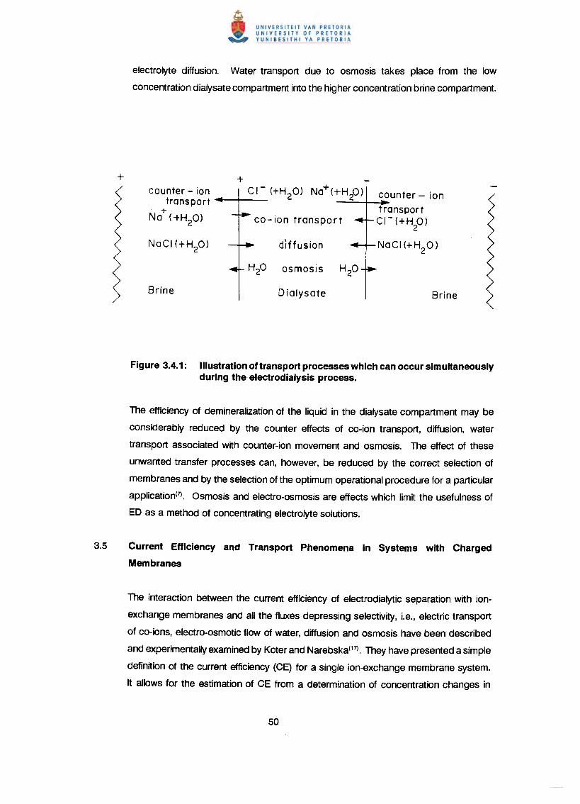
electrolyte diffusion. Water transport due to osmosis takes place from the low
concentration dialysate compartment into the higher concentration brine compartment.
+ +counter - ion CI- (+H2O) Na+(+H;P) counter - ion
transport+ transport
Na (+H20) co- ion transport C/- (+HP)
NaCI (+H2O) diffusion NaCI(+H2O)
osmosIs
Brine Dialysate Brine
Figure 3.4.1: Illustration of transport processeswhich canoccur simultaneouslyduring the electrodialysis process.
The efficiency of demineralization of the liquid in the dialysate compartment may be
considerably reduced by the counter effects of co-ion transport, diffusion, water
transport associated with counter-ion movement and osmosis. The effect of these
unwanted transfer processes can, however, be reduced by the correct selection of
membranes and by the selection of the optimum operational procedure for a particular
application(7). Osmosis and electro-osmosis are effects which limit the usefulness of
ED as a method of concentrating electrolyte solutions.
3.5 Current Efficiency and Transport Phenomena in Systems with Charged
Membranes
The interaction between the current efficiency of electrodialytic separation with ion-
exchange membranes and all the fluxes depressing selectivity, i.e., electric transport
of co-ions, electro-osmotic flow of water, diffusion and osmosis have been described
and experimentally examined by Koter and Narebska(17).They have presented a simple
definition of the current efficiency (CE) for a single ion-exchange membrane system.
It allows for the estimation of CE from a determination of concentration changes in
cathode and anode solutions. With the proposed definition, CE can be expressed as
a simple function of different kinds of transport taking place in the system. This fact
makes it possible to examine the effects of these transports on current efficiency, that
is to calculate the losses of CE due to:
a) electric transport of co-ions;
b) electro-osmotic flow of water;
c) diffusion of a salt; and
d) osmotic transport of water.
Thus, the full characteristics of a single ion-exchange membrane (cation- or anion-
exchange) for a separation process like ED can be obtained. The mathematical
solution has been examined for computing the current efficiency and its losses for the
system NaClaq/Nafion 120 membrane and NaOHaq/Nafion 120 membrane based on the
experimental results published earlier(17).
Consider the one membrane system as shown in Figure 3.5.1. The ion-exchange
membrane (M) separates two solutions of an Av1Bv2 electrolyte differing in
concentrations. For the cation-exchange membrane (sign W =- 1) the cathode is on
the more concentrated side whereas for the anion-exchange membrane (W =+ 1) it
is on the diluted side. The electrodes and electrode reactions do not belong to the
system. They are separated from the system by ideal membranes of reverse sign to
the investigated membrane.
At t = 0, the concentration difference across the membrane is aco = co, - CO". After
passing an electric current through the membrane for time t, the concentration
difference changes to act. The ratio of (act - aCO) for the real membrane to
(ad - ac') for the ideal membrane system (t2,, tw, Js, Jwos = 0) is a measure of the
current efficiency:
(act - aCO)
(act - aCO)ideal
Rearrangement of this formula(17) leads to the following equation relating the current
efficiency to the total counter-ions (J1) and water (Jw) fluxes (see Appendix B).
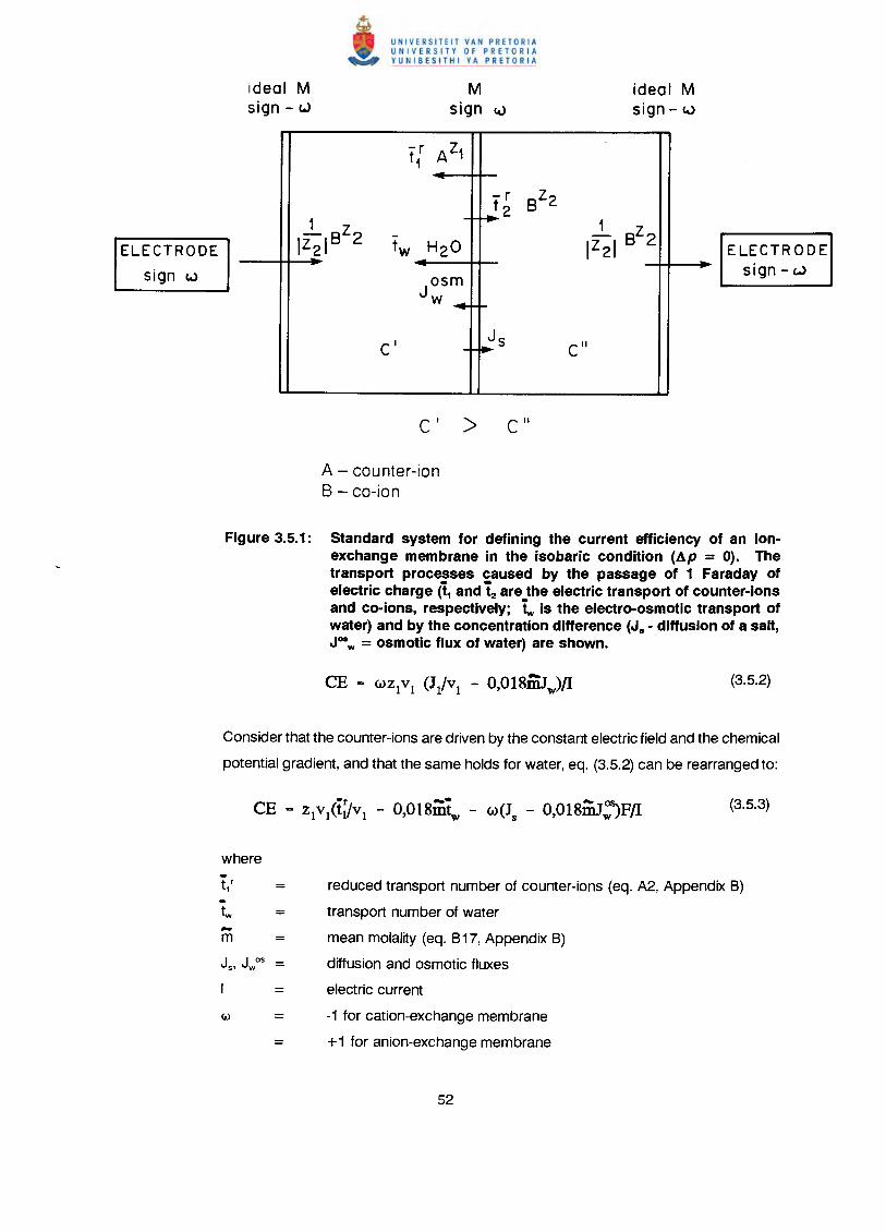
ELECTRODEsign c..>
ideal Msign - w
Msign \.J
ideal Msign-c..>
-r AZ1t1
-r BZ2t21 Z - ....
1 Z-IZ21B 2 tw H2O IZ21 B 2
Josmw.,
elJs e"- ~
E LECTR 0 D Esign - w
A - counter-ionB - co-ion
Figure 3.5.1: Standard system for defining the current efficiency of an ion-exchange membrane in the isobaric condition (l1p = 0). Thetransport processes caused by the passage of 1 Faraday ofelectric charge (t1 andt2 are the electric transport of counter-ionsand co-ions, respectively; t is the electro-osmotic transport ofwater) and by the concentration difference (J. - diffusion of a salt,Josw = osmotic flux of water) are shown.
Consider that the counter-ions are driven by the constant electric field and the chemical
potential gradient, and that the same holds for water, eq. (3.5.2) can be rearranged to:
where-t,' =-tw =•..m
Js' Jwos =
=
=
reduced transport number of counter-ions (eq. A2, Appendix B)
transport number of water
mean molality (eq. B17, Appendix B)
diffusion and osmotic fluxes
electric current
-1 for cation-exchange membrane
+1 for anion-exchange membrane
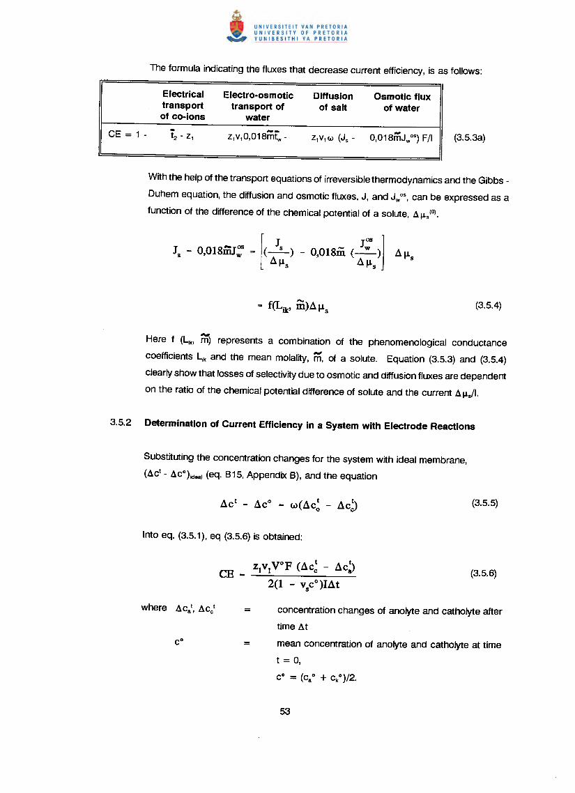
Electrical Electro-osmotic Diffusion Osmotic fluxtransport transport of of salt of waterof co-ions water
CE = 1 - - ,..-O,018mJwOS)F/I (3.5.3a)t2 - Z1 ZlVl0,018mtw - Z1 V1 <a> (Js -
With the help of the transport equations of irreversible thermodynamics and the Gibbs -
Duhem equation, the diffusion and osmotic fluxes, J, and Jwos,can be expressed as a
function of the difference of the chemical potential of a solute, a!Ls(9).
Here f (Lik, iii) represents a combination of the phenomenological conductance
coefficients Lik and the mean molality, m, of a solute. Equation (3.5.3) and (3.5.4)
clearly show that losses of selectivity due to osmotic and diffusion fluxes are dependent
on the ratio of the chemical potential difference of solute and the current a !Ls/I.
Substituting the concentration changes for the system with ideal membrane,
(act - aCoh:leaJ(eq. B15, Appendix B), and the equation
ZtVtVOP (ac: - ac:)CE--------
2(1 - VsCO)Idt
concentration changes of anolyte and catholyte after
time at
mean concentration of anolyte and catholyte at time
t = 0,
CO = (caO + ckO)/2.
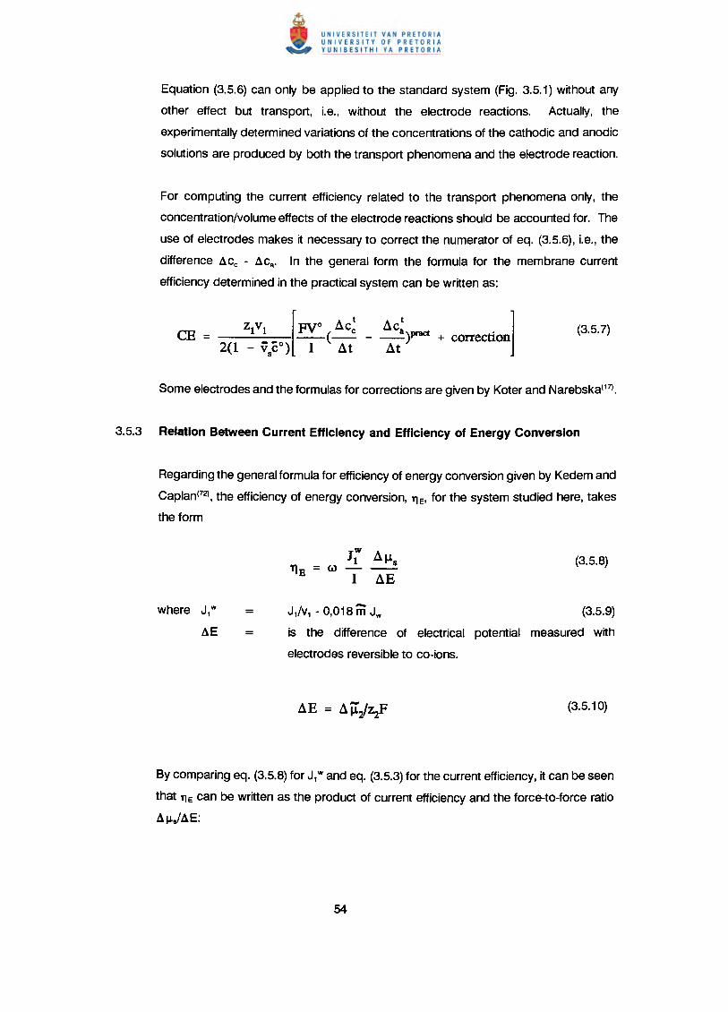
Equation (3.5.6) can only be applied to the standard system (Fig. 3.5.1) without any
other effect but transport, i.e., without the electrode reactions. Actually, the
experimentally determined variations of the concentrations of the cathodic and anodic
solutions are produced by both the transport phenomena and the electrode reaction.
For computing the current efficiency related to the transport phenomena only, the
concentration/volume effects of the electrode reactions should be accounted for. The
use of electrodes makes it necessary to correct the numerator of eq. (3.5.6), i.e., the
difference aCe - aCa' In the general form the formula for the membrane current
efficiency determined in the practical system can be written as:
ZtVt [FVO ~c~ ~c~ ]____ ,__ (_ - _)pract + correction2(1 - vl,O) I ~t ~t
Regarding the general formula for efficiency of energy conversion given by Kedem and
Caplan(72),the efficiency of energy conversion, TJ e, for the system studied here, takes
the form
I~ ~lJs'I1B = <a> I ~E
J1/V1 - 0,018 m Jw (3.5.9)
is the difference of electrical potential measured with
electrodes reversible to co-ions.
By comparing eq. (3.5.8) for J1Wandeq. (3.5.3) for the current efficiency, it can be seen
that TJe can be written as the product of current efficiency and the force-to-force ratio
a!J.s/aE:
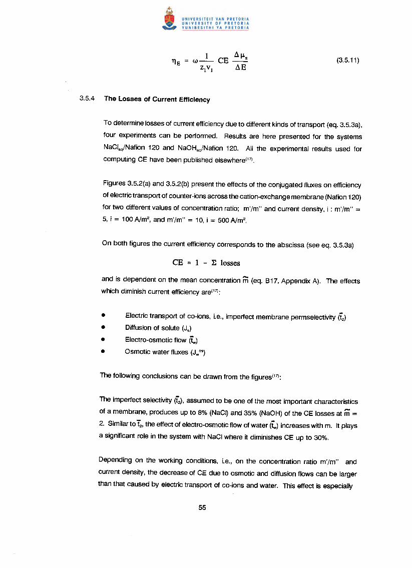
To determine losses of current efficiency due to different kinds of transport (eq. 3.5.3a),
four experiments can be performed. Results are here presented for the systems
NaClaq!Nafion 120 and NaOHaq/Nafion 120. All the experimental results used for
computing CE have been published elsewhere(17).
Figures 3.5.2(a) and 3.5.2(b) present the effects of the conjugated fluxes on efficiency
of electric transport of counter-ions across the cation-exchange membrane (Nafion 120)
for two different values of concentration ratio; m'/m" and current density, i : m'/m" =5, i = 100 Nm2
, and m'/m" = 10, i = 500 Nm2•
and is dependent on the mean concentration m (eq. 817, Appendix A). The effects
which diminish current efficiency are(17):
• Electric transport of co-ions, i.e., imperfect membrane permselectivity (t2)
• Diffusion of solute (Js)
• Electro-osmotic flow <lw)• Osmotic water fluxes (JWOS)
The imperfect selectivity (r~.assumed to be one of the most important characteristics
of a membrane, produces up to 8% (NaCQ and 35% (NaOH) of the CE losses at m =2. Similar to t. the effect of electro-osmotic flow of water (tw) increases with m. It plays
a significant role in the system with NaCI where it diminishes CE up to 30%.
Depending on the working conditions, i.e., on the concentration ratio m'/m" and
current density, the decrease of CE due to osmotic and diffusion flows can be larger
than that caused by electric transport of co-ions and water. This effect is especially
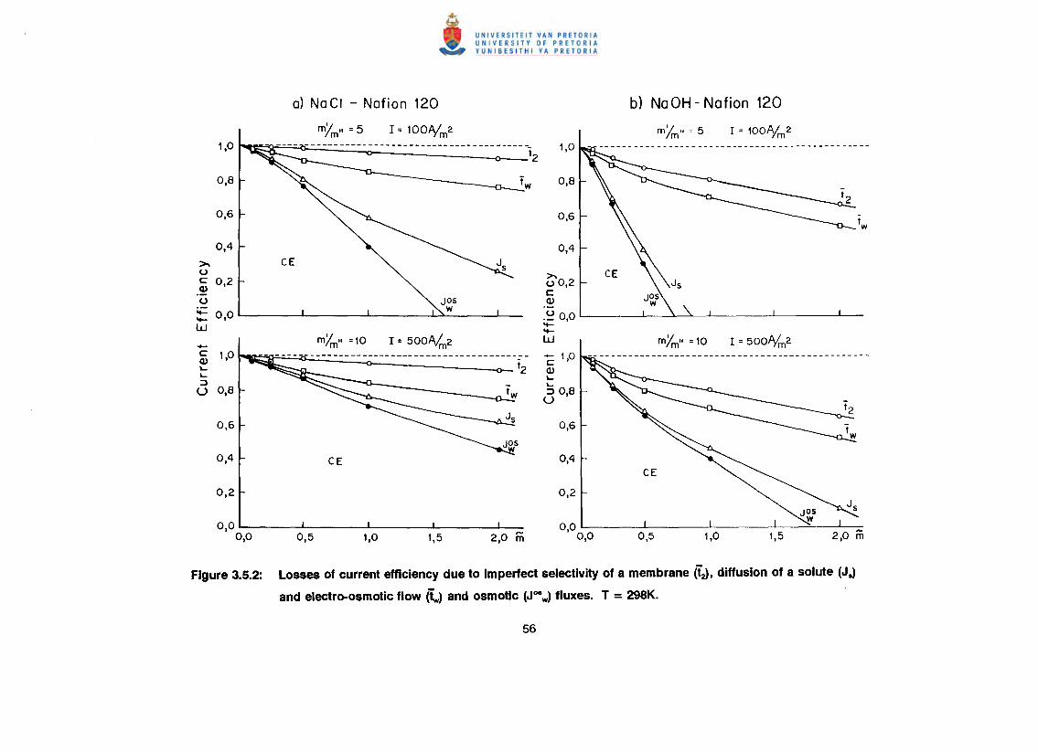
1,0
0,8
0,6
0,4>.uc 0,2Q)
u- 0,0-W+-c 1,0Q)
'-'-:)U 0,8
0,6
0,4
0,2
0,00,0
Figure 3.5.2:
0,6
0,4
>.uO,2cQ)
.~ 0,0--Wt2
c1,oQ)
'-'-:)0,8U
0,6
0,4
0,2
0,00,0
Losses of current efficiency due to Imperfect selectivity of a membrane (tJ, diffusion of a solute (J.)
and electro-osmotic flow (t) and osmotic (JOlIw) fluxes. T = 298K.
seen at higher mean concentrations where the current efficiency can even be reduced
to zero.
Efficiency of energy conversion in separation processes with Nafion 120 membranes
from phenomenological transport coefficients has been described by Narebska and
Koter(18).
In systems devised for desalination/concentration processes with ion-exchange
membranes separating single electrolyte solutions of different concentrations, electrical
energy is used to drive a solute against its concentration gradient. In these processes,
the electrical energy is converted into free energy of mixing and in that way it is stored
in the system. The efficiency of energy conversion (1")) depends both on the degree
of coupling between the driving process and the driven flow (q), as well as the
operating conditions.
Kedem and Caplan(72) have defined 1") and q in terms of irreversible thermodynamics
and outlined the methods available to access both parameters for thermocouples, fuel
cells, osmionic batteries and desalination stacks by treating the system as a two-flow
process. Later, Caplen(74) published some data on the overall degree of coupling q
and 1")max for hyperfiltration, concentration cells and ED, taking for the calculations the
experimental results for a few points in dilute solutions.
Narebska and Koter(18)have presented results for the degree of coupling and efficiency
of energy conversion calculated for the system composed of a perfluorinated Nafion
120 membrane and sodium chloride solutions of different concentrations. Their aim
have been to conduct a detailed analysis of input-output relations by treating the
system and the transport involved as a three-flow process and describing quantitatively
the transport of water which consumes energy unprofitably.
The system consisted of a cation exchange membrane and aqueous solutions of
1 : 1 electrolyte of different concentrations in the adjacent compartments. Sodium are
driven by the applied electrical potential difference opposite the concentration
difference of NaCI.
3.6.1.1 The degree of coupling and the efficiency of energy conversion in the two-flow
system (basic definitions)
The efficiency of energy conversion'll is based in the dissipation function <l> which for
the two-flow system takes the general form:
According to Kedem and Caplan(72), with one flow producing entropy (J2X2),which is
always positive and the other flow consuming entropy, being negative (J1X1), the
efficiency of energy conversion can be expressed as:
Denoting the force ratio as X1/X2 and the ratio of the straight conductance coefficients
Lj; appearing in the flow equations
q+Zx.
q + l/Zx
The conversion of energy of process 2 to process 1 is only possible when the two
flows are coupled, therefore, the degree of coupling can be defined as:
(J1)12
= 0
(Jl)~ = 0
where J1is the flux of counterions, IllJ.s the difference of chemical potential of an
electrolyte, I the electric current and E the potential difference between the solutions
on opposite sides of the membrane measured with electrodes reversible to the anions.
Kedem and Caplan have presented the general solution for the degree of coupling in
ED. They admitted, however, that in their solution the contribution of water flow was
neglected. This means that they have treated the process as a two-flow system.
In any real system with a single electrolyte and the ion-exchange membrane separating
solutions of different concentrations, the flow of water is another process which
participates in the entropy production. Consequently, the equation describing the
dissipation function should contain the third component, JwlllJ.w:
n-'~ IX.i = 1 I I
In~
As for ED JnXn = IE and :E JXj = J11lIJ.s + JwlllJ.w, one gets:j
T) = (- _Il_a_~_SJ + (- _Iw_a_~_wJ = T) + T)IE IE IE wE
The first term of eq. (3.6.9) is the same as before, i.e. it expresses the storage of
energy in producing a concentration difference in the permeant. The second term
corresponds to the transport of water which acts opposite to the separation of the
components. It causes a waste of energy by decreasing the concentration difference.
To find the degrees of coupling in both processes, the equations for transport of ions
(J1), water (Jw) and current (I) should be used in a general formula:
Defining the degree of coupling according to Kedem and Caplan, three coefficients for
the three-flow system are obtained which denote sodium ion-current coupling (qE),
water-current coupling (qWE)and sodium ion-water coupling (qw).
2Lik i,k = 1,w,E,L).'kk
All the degrees of coupling were calculated according to eq. (3.6.11) using
conductance coefficients Lik, of eq. (3.6.10).
For the more practical discussion of the input-output relation, such as finding the
maximum output or the driven region for ED, the overall degree of coupling qE is also
helpful. This can be derived from the general formula
2 2'hE + qwE - 2qmqwE%w
21 - qlw
At ap = 0, which corresponds to operating conditions in ED, and applying the Gibbs-
Duhem equation Csdl-Ls+ Cwdl-Lw= 0, the flow equations can be written in the form:
Cs= J~
, ,(3.6.14)J1 - - J = Lu.l1 ~s + LmEwCw
,I = Lm.l1~s + ~E
where
2, Cs Cs (3.6.15)Lll = Lll - 2-L + -Llw 2 wwCw Cw
,Lm=Lm-
'2LIE
Introducting eq. (3.6.10) into eq. (3.6.9) and assuming that Ap = 0, it is possible to
derive the equations for both components of TJ (eq. 3.6.9), Le. TJIE and TJwE
11m =_ [Zm - :: ~q!w] X + q!E
(3.6.17)Cs 1
qm - -;- ~lqwE +--~E'Cw
C[Zmqlw - _s ZwJ x + qwE
Cs Cw (3.6.18)T1wE =Cw Cs 1
Zlwqlw - -qwE + -- XCw ~E
The meaning of qk is as before eq. (3.6.11), x = AIJ..IE and llk =/Li/Lkkwhere
i, k = 1, cu, E, i '¢ k. These equations are appropriate for calculating TJ for ED.
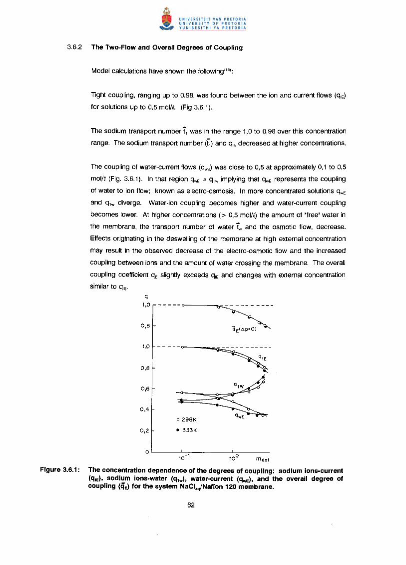
Tight coupling, ranging up to 0.98, was found between the ion and current flows (qE)
for solutions up to 0,5 molN. (Fig 3.6.1).
The sodium transport number 11was in the range 1,0 to 0,98 over this concentration
range. The sodium transport number (~) and qE decreased at higher concentrations.
The coupling of water-current flows (qWE) was close to 0,5 at approximately 0,1 to 0,5
mol/O(Fig. 3.6.1). In that region qwE ;:: q1w implying that qwE represents the coupling
of water to ion flow; known as electro-osmosis. In more concentrated solutions qwEand q1w diverge. Water-ion coupling becomes higher and water-current coupling
becomes lower. At higher concentrations (> 0,5 mol/O)the amount of "free"water in
the membrane, the transport number of water tw and the osmotic flow, decrease.
Effects originating in the deswelling of the membrane at high external concentration
may result in the observed decrease of the electro-osmotic flow and the increased
coupling between ions and the amount of water crossing the membrane. The overall
coupling coefficient qE slightly exceeds qE and changes with external concentration
similar to qE'
Figure 3.6.1: The concentration dependence of the degrees of coupling: sodium ions-current(qle), sodium ions-water (q1W), water-current (qwe) , and the overall degree ofcoupling (qe) for the system NaClaq/Nafion 120 membrane.
The component efficiencies of energy conversion are not only of different meaning but
of different sign (Fig. 3.6.2). The positive term TJIEindicates the fraction of the free
energy of mixing produced by the driving process IE and stored in the system by the
uphill transport of ions J,AjJ." against their spontaneous flow. The negative term TJwE
means that the transport of water proceeds in the direction of the conjugated force
A jJ.w(downhill). The energy input increases the rate of flow. Thus, this term causes
the entropy of the system to increase and the energy supplied to the system to be
wasted.
Both TJIE and TJwE change with the ratio A jJ..JFE and with the concentration of
electrolyte. The maximum in the TJIEcurve means that for any concentration range of
NaCI solutions there is an optimal concentration difference for which the efficiency of
energy conversion is at a maximum. There is no such maximum in the TJwEcurve. The
waste of energy due to water flow becomes much higher as the electrolyte becomes
more concentrated and the concentration difference between the NaCI solutions in the
adjacent compartments is higher.
The sum of TJIEand TJwEgives the total efficiency as TJ. The total efficiency, TJ,
decreases with increasing concentration. The degree of coupling, (lE' also decreases
with increasing concentration.
Computations of q (coupling) and TJ(efficiency) employing the derived equations and
phenomenological conductance coefficients determined for the system Nafion 120
membrane/sodium chloride solutions led to the following conclusions(18):
• Coupling of the current to the flow of sodium ions (q0, of importance for the
efficiency of energy conversion, is close to unity when the membrane is in
contact with dilute solutions and is going down with increasing external
concentration.
• Coupling of the current to the flow of water (qw0, which is achieved by water-
cation coupling (qw), reaches a value as high as half that of qE' pointing to the
unavoidable loss of energy during ED.
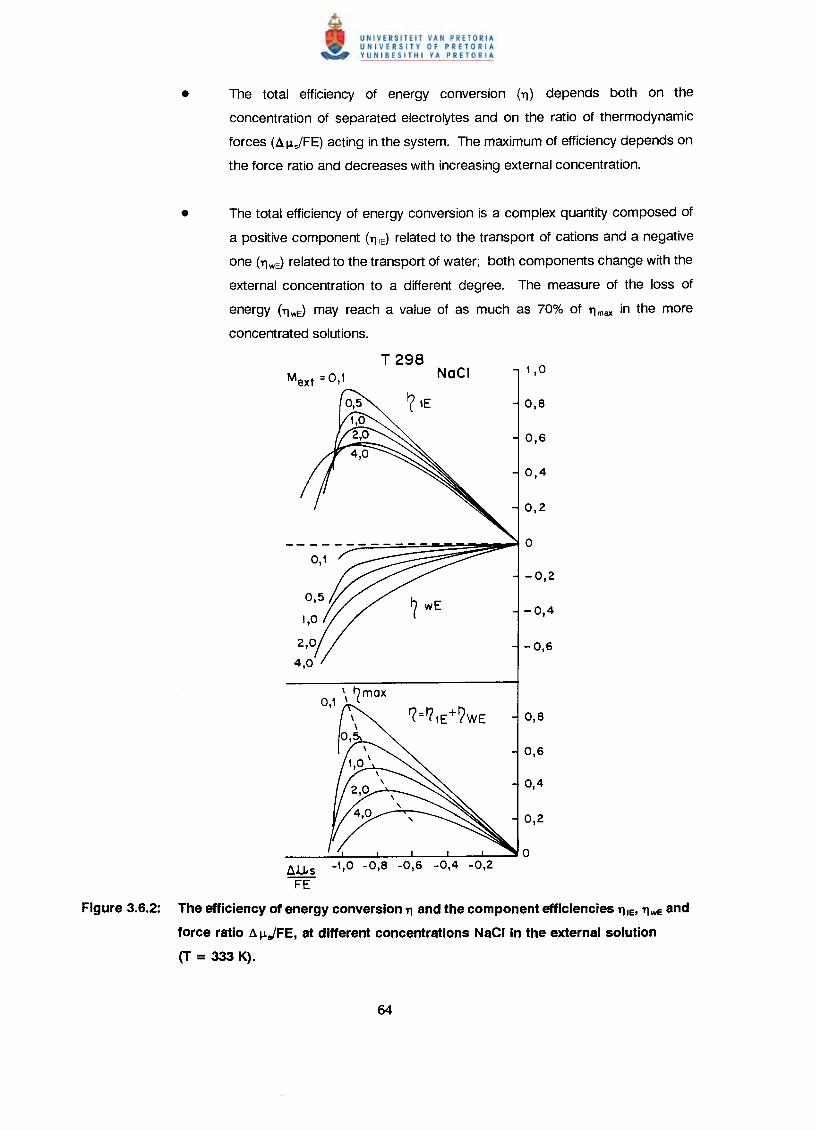
• The total efficiency of energy conversion (11) depends both on the
concentration of separated electrolytes and on the ratio of thermodynamic
forces (A IJ.s/FE) acting in the system. The maximum of efficiency depends on
the force ratio and decreases with increasing external concentration.
• The total efficiency of energy conversion is a complex quantity composed of
a positive component (11 IE) related to the transport of cations and a negative
one (11wE) related to the transport of water; both components change with the
external concentration to a different degree. The measure of the loss of
energy (11WE) may reach a value of as much as 70% of 11max in the more
concentrated solutions.
~.lJ,s -1,0 -0,8 -0,6 -0,4 -0,2"FE
Figure 3.6.2: The efficiency of energy conversion 11 and the component efficiencies 11IE, 11wE and
force ratio A IJ.JFE, at different concentrations NaCI in the external solution
(T = 333 1<).
3.7 Conversion of Osmotic into Mechanical Energy in Systems with Charged
Membranes
Narebska et al,(19) have described the problem of conversion of osmotic energy into
mechanical energy within the framework of irreversible thermodynamics. Using the
numerical results for the conductance coefficients for the system Nafion 120
membrane/single salt and alkali solutions, the couplings between the volume and the
osmotic fluxes, q, and the efficiency of osmotic into mechanical energy conversion, TJ,
have been computed.
The standard application of membrane systems is for separation of suspensions and
molecular mixtures, gaseous or liquid, into components on an expense of supplied
energy. Mechanical, thermal or electric energy can be used. More than twenty
membrane separation techniques are known. In each of these systems, however, the
difference in concentration of components on both sides of a membrane presents the
effective source of osmotic energy, generating the spontaneous osmotic flux affecting
the separation. For example, in ED, the osmotic flow of water dilutes the brine, thus
lowering the energetic efficiency of desalination. In reverse osmosis, the osmotic
pressure is a powerful force to overcome. Osmotic energy is thereby a native energy
of a membrane system affecting both the income of energy and the separation process
itself.
Conversion of osmotic energy into electric energy was postulated and theoretically
described by Kedem and Caplan(72). Systems converting osmotic energy into
mechanical energy called "osmotic pumps" were proposed by Lee et al, (75). The
energetic efficiency of the process, however, still seems to be a problem.
The work by Narebska et al, (19) has been aimed at a theoretical analysis of osmotic into
mechanical energy conversion, using irreversible thermodynamics as the underlying
theory.
The system consists of an ion-exchange membrane separating electrolyte solutions of
different molalities. Assuming ideal membrane permselectivity (totally impermeable to
a solute) and the zero current condition, the only flow in the system should be the
osmotic flow of water which is driven to the more concentrated side. However, for real
polymer membranes and particularly when they are in contact with concentrated
solutions, diffusion of a solute across the membrane should be admitted as an
additional phenomenon. The solute permeates the membrane towards the dilute
solution side, that is, opposite to the osmotic flow.
the osmotic flow of water Jw and
the diffusional flow of the solute Js are described by the following equations:
a IJ.s' a IJ.w are the differences of chemical potential of a solute and water, respectively.
Lik denotes the phenomenological conductance coefficients.
J ' = L' a II C + L' apw w row wp
Here J'w denotes the flow of water against the flow of a solute conjugated to the
concentration part of the chemical potential difference of water, a IJ.w C:
l' =J -CJc *Jw w s s
Jv of equation (3.7.2b) denotes the total volume flow conjugated to the difference of
pressure in the compartments on the opposite sides of the membrane, ap.
The relation between the fluxes and forces of equations (3.7.1a and 3.7.1b) and of
equations (3.7.2a and 3.7.2b) can be expressed in a matric form
Is I
J i,w
With the flows of equations (3.7.2a and 3.7.2b) the dissipation function 4>consists of
two components:
JvAp
mechanical
energy
component
energy
component
The efficiency of energy conversion, 11, as defined by Kedem and Caplan(72)I can be
written as follows:
For the system discussed here, 11, means the output of mechanical energy produced
by the input of unit osmotic energy. To acquire computational verification of various
systems this equation should be transformed by substituting equations (3.7.2a and
3.7.2b) into equation (3.7.10) to give
q + Z * AP/A~~
q + l/(Z * Ap/A~~)
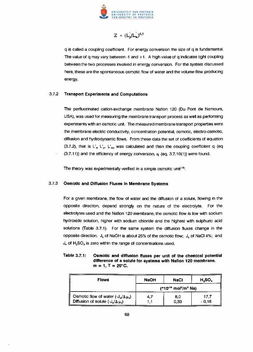
q is called a coupling coefficient. For energy conversion the size of q is fundamental.
The value of q may vary between -1 and +1. A high value of q indicates tight coupling
between the two processes involved in energy conversion. For the system discussed
here, these are the spontaneous osmotic flow of water and the volume flow producing
energy.
The perfluorinated cation-exchange membrane Nafion 120 (Du Pont de Nemours,
USA), was used for measuring the membrane transport process as well as performing
experiments with an osmotic unit. The measured membrane transport properties were
the membrane electric conductivity, concentration potential, osmotic, electro-osmotic,
diffusion and hydrodynamic flows. From these data the set of coefficients of equation
(3.7.2), that is L'w L'p, L'wp was calculated and then the coupling coefficient q (eq
(3.7.11)) and the efficiency of energy conversion, TJ (eq. 3.7.10(1)) were found.
For a given membrane, the flow of water and the diffusion of a solute, flowing in the
opposite direction, depend strongly on the nature of the electrolyte. For the
electrolytes used and the Nafion 120 membrane, the osmotic flow is low with sodium
hydroxide solution, higher with sodium chloride and the highest with sulphuric acid
solutions (Table 3.7.1). For the same system the diffusion fluxes change in the
opposite direction. Js of NaOH is about 25% of the osmotic flow; Js of NaCI4%; and
Js of H2S04 is zero within the range of concentrations used.
Table 3.7.1: Osmotic and diffusion fluxes per unit of the chemical potentialdifference of a solute for systems with Nafion 120 membrane.m = 1, T = 25° C.
Flows NaOH NaCI H~04
(*10-'0 mol2/m3 Ns)
Osmotic flow of water (-Jwl4j.Ls) 4,7 8,0 17,7Diffusion of solute (-Js/ 4 j.Ls) 1,1 0,33 - 0,16
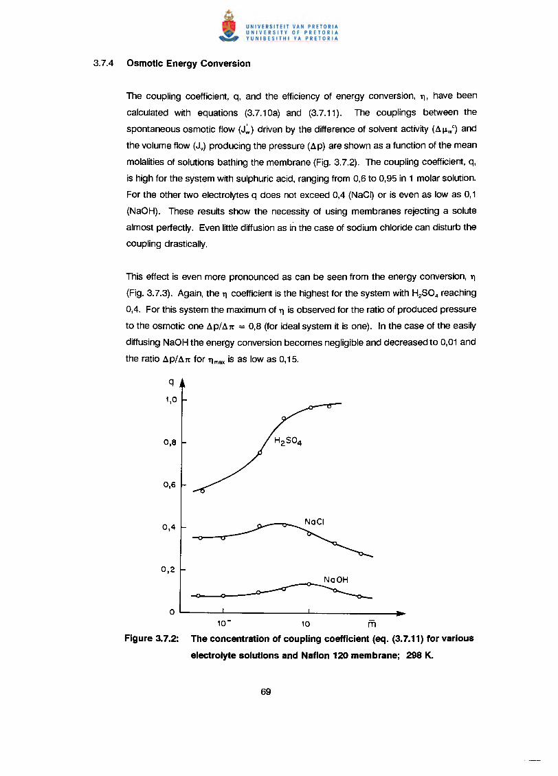
The coupling coefficient, q, and the efficiency of energy conversion, TJ, have been
calculated with equations (3.7.10a) and (3.7.11). The couplings between the
spontaneous osmotic flow (J~) driven by the difference of solvent activity (~j.1wC) and
the volume flow (Jv) producing the pressure (~p) are shown as a function of the mean
molalities of solutions bathing the membrane (Fig. 3.7.2). The coupling coefficient, q,
is high for the system with sulphuric acid, ranging from 0,6 to 0,95 in 1 molar solution.
For the other two electrolytes q does not exceed 0,4 (NaCQ or is even as low as 0,1
(NaOH). These results show the necessity of using membranes rejecting a solute
almost perfectly. Even little diffusion as in the case of sodium chloride can disturb the
coupling drastically.
This effect is even more pronounced as can be seen from the energy conversion, TJ
(Fig. 3.7.3). Again, the TJ coefficient is the highest for the system with H2S04 reaching
0,4. For this system the maximum of TJ is observed for the ratio of produced pressure
to the osmotic one ~p/~1t = 0,8 (for ideal system it is one). In the case of the easily
diffusing NaOH the energy conversion becomes negligible and decreased to 0,01 and
the ratio ~ pi ~ 1t for TJ max is as low as 0,15.
10- 10 mFigure 3.7.2: The concentration of coupling coefficient (eq. (3.7.11) for various
electrolyte solutions and Nafion 120 membrane; 298 K.
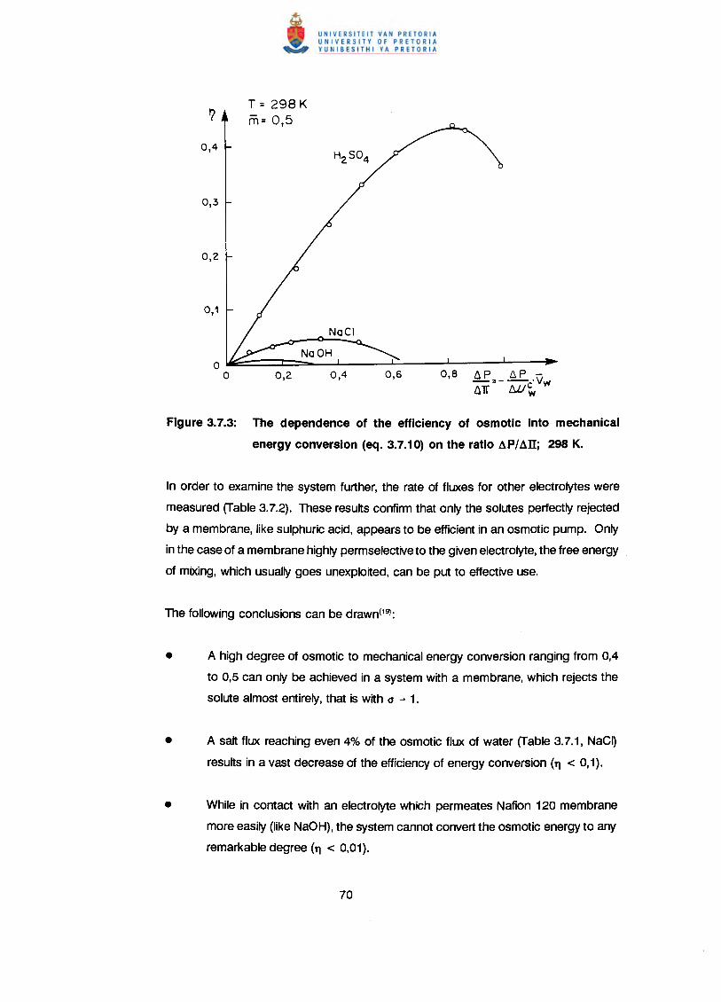
T = 298 Km= 0,5
~p t.P--=-_·vw~1f W~
Figure 3.7.3: The dependence of the efficiency of osmotic Into mechanical
energy conversion (eq. 3.7.10) on the ratio I1P/I1IT; 298 K.
In order to examine the system further, the rate of fluxes for other electrolytes were
measured (Table 3.7.2). These results confirm that only the solutes perfectly rejected
by a membrane, like sulphuric acid, appears to be efficient in an osmotic pump. Only
in the case of a membrane highly permselective to the given electrolyte, the free energy
of mixing, which usually goes unexploited, can be put to effective use.
• A high degree of osmotic to mechanical energy conversion ranging from 0,4
to 0,5 can only be achieved in a system with a membrane, which rejects the
solute almost entirely, that is with (1 - 1.
• A salt flux reaching even 4% of the osmotic flux of water (Table 3.7.1, NaC~
results in a vast decrease of the efficiency of energy conversion (1') < 0,1).
• While in contact with an electrolyte which permeates Nafion 120 membrane
more easily (like NaOH), the system cannot convert the osmotic energy to any
remarkable degree (1') < 0,01).
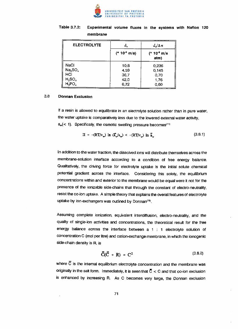
Experimental volume fluxes in the systems with Nafion 120
membrane
ELECTROLYTE Jv J)!J.1t
(* 10-8 m/s) (* 10-8 m/satm)
NaCI 10,8 0,236Na2S04 4,59 0,145HCI 36,7 0,70H2SO4 42,0 1,76H3P04 6,72 0,60
If a resin is allowed to equilibrate in an electrolyte solution rather than in pure water,
the water uptake is comparatively less due to the lowered external water activity,
aw« 1). Specifically, the osmotic swelling pressure becomes(11)
In addition to the water fraction, the dissolved ions will distribute themselves across the
membrane-solution interface according to a condition of free energy balance.
Qualitatively, the driving force for electrolyte uptake is the initial solute chemical
potential gradient across the interface. Considering this solely, the equilibrium
concentrations within and exterior to the membrane would be equal were it not for the
presence of the ionizable side-chains that through the constant of electro-neutrality,
resist the co-ion uptake. A simple theory that explains the overall features of electrolyte
uptake by ion-exchangers was outlined by Donnan(76).
Assuming complete ionization, equivalent interdiffusion, electro-neutrality, and the
quality of single-ion activities and concentrations, the theoretical result for the free
energy balance across the interface between a 1 : 1 electrolyte solution of
concentration C (mol per litre) and cation-exchange membrane, in which the ionogenic
side-chain density is R, is
where C is the internal equilibrium electrolyte concentration and the membrane was
originally in the salt form. Immediately, it is seen that C < C and that co-ion exclusion
is enhanced by increasing R. As C becomes very large, the Donnan exclusion
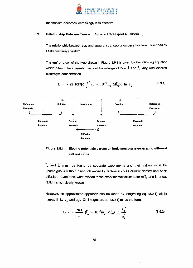
The relationship between true and apparent transport numbers has been described by
Laskshminarayanaiah(45).
The emf of a cell of the type shown in Figure 3.9.1 is given by the following equation
which cannot be integrated without knowledge of how 1; and t: vary with external
electrolyte concentration.
(I) (ii)
Reference Solution Membrane Solution
Electrode
l .J
i T\.
Electrode Donnan Donnan
Potential Potential Potential
IE ~Diffusion
Potential
'-- J'I
Electrode
Potential
Figure 3.9.1: Electric potentials across an ionic membrane separating different
salt solutions.
t+ and t must be found by separate experiments and their values must be
unambiguous without being influenced by factors such as current density and back
diffusion. Even then, what relation these experimental values bear to T+ andt of eq.
(3.9.1) is not clearly known.
However, an approximate approach can be made by integrating eq. (3.9.1) within
narrow limits a:l:'and a:l:'" On integration, eq. (3.9.1) takes the form:
E = - 2RT (tF ±
,a
1O-3m± M~) In -;.a±
The emf of a cell of the type shown in Figure 3.9.1 can be calculated from the modified
Nernst equation.
E = it RT In ~+(app) F a H
Hale and McCouley tested eq. (3.9.4) using different heterogeneous membranes and
found good agreement between true t+ measured directly and t+ calculated using eq.
(3.9.4). Their measurements although confined to a number of different membranes,
were made with one set of electrolyte solutions only (0,667 and 1,333 mol/~ NaCQ.
Lakshiminarayanaiah(78) checked eq. (3.9.4) over a wide concentration range. He found
that the t+ values calculated from eq. (3.9.4) were higher than the measured values
particularly in high electrolyte concentrations. This discrepancy existing in the case of
strong solutions is difficult to reconcile in view of the fact that Lakshminarayanaiah and
SUbrahmanyas(47) showed that eq. (3.9.1) is able to generate values for E (however
from measured values of t+ and fw) agreeing with observed values. A more recent
evaluation by Lakshminarayanaiah(79) has shown that eq. (3.9.4) is able to give values
for t+ agreeing with those measured directly.
The relationship of t+(apP)obtained from emf measurements to t+ measured directly,
unlike eq. (3.9.4), has been approached from a different standpoint by Oda and
Yawataya(80). The apparent transport number (t+(apP)calculated from emf data was
related to the concentration of the external solution by an "interpolation technique".
This consists in measuring E using two solutions, c' and c", in the cell shown in Figure
3.9.1. In the first measurement of membrane potential, solution (") is so chosen that
c" is less than c' and in the second measurement c' is held constant and c" is so
chosen that it is now greater than c'. Each of the two values of t+(apPlcalculated from
the two measurements is now referred to that particular concentration of c' used in the
experiment and plotted. The value of t+(apP)pertaining to c' which is kept constant in
the two experiments is obtained by interpolation. Usually, t+(8PP)is related to the mean
external electrolyte concentration, Le. (c' + C")/2.
True values of 't and t.. were determined by Oda and Yawataya from the same
experiment by the mass method which consisted in estimating the mass changes in
both the salt and the water in the cathode chamber following the passage of a known
quantity of current through the system, electrolyte solution (c) ,.,. membrane •.•
electrolyte solution (c). The relationship between t+ and t+(app) was derived in the
following manner(80).
A selective membrane of fixed charge density X (equivalent per unit volume of swollen
membrane) in equilibrium with an external electrolyte solution contains )«(1 - s)equivalents of counter-ions and Xs equivalents of co-ions where s is the equivalent of
co-ions per equivalent of fixed group present in the membrane. This arises from the
Donnan absorption of the electrolyte by the membrane.
When an electric field is applied, ions and water move. In a membrane in which
interactions between different membrane components, viz., counter-ion, co-ion, water
and membrane, matrix, are absent, one may assume that the fixed water in the
membrane is negligible and that all mobile water moves with the same velocity and in
the same direction as the counter-ion. As a result, counter-ions move faster and co-
ions move slower than they would otherwise if water stood still. Consequently, the
mobilities (u's) of the counter-ion and co-ion may be written as:
where +, -, and w stand for cation, anion and water, respectively. u+' and u.' are the
increased and decreased mobilities due to the transport of water.
Due to water transport, the specific conductance of the membrane is increased. If k'
is the membrane specific conductance, then
-, - - -, ---'k = F[X (1 + s) u+ + XSuJ
il = Fx[(1 + s)u+ + suJ
It follows from eqs. (3.9.8) and (3.9.9) that the increase in conductance due to water
transport is given by
- ••I(l + s)u+t+ = ------- --'(l + s)u+ + su
(1 + S)u+
(l + S)ii+ + sii~
Substituting from eqs. (3.9.5) - (3.9.10) into eqs. (3.9.11) and (3.9.12) and remembering
that t+(app) + t.(apPl = 1, it can be shown that(80):
- - - . -/ --,t+ - t+(app) = (t_(app) i- s)[(l{ - k)!k]
Substituting from eq. (3.9.10), eq. (3.9.13) becomes
- ~ - . ---}t+ - t+(app) = [t_(app) + s][FXUJk]
When a potential of E volts acts along length Acm of a membrane capillary, the water
in the pore moves with a mobility, Uw cm/s (i.e., E/q is unity). The volume (millilitres)
of water flowing per second through a membrane subject to unit potential gradient is
given by 6E and is equal to (UwA) where A is the pore area. But 6, the volume of water
flowing per Coulomb is given by:
where V is millilitres of water flowing per second and i is the current in amperes. But
i = k;A per unit potential gradient and kj is the specific conductance of the pore liquid
of an infinitely swollen membrane (kj is really a modified membrane conductance).
Consequently, it follows that
Equation (3.9.16) differs from the original equation of Oda and Yawataya which is
dimensionally incorrect(45).
- - -- -,t+ = t+(app) + (t_(app) + s)~Pfk
But k' may be equated to CPwl<i where CPw is the volume fraction of water in the
membrane. Equation (3.9.17), therefore, becomes
- -where Xv = X/CPw, equivalent of fixed groups per unit volume of interstitial water.
Since the method usually used to measure the transport number of watertw which is
equal to (F6/18), depends on following volume changes in the anode and cathode
chambers, the observed volume changes, which measures only solution flow, have to
be corrected for both salt transport and electrode reactions to give values for water
flow only. If reversible Ag-AgCI electrodes are used, the passage of a Faraday of
current produces at the cathode, a mole of Ag and T+ moles of MCI (M = univalent
cation) and in the same time a mole of AgCI disappears. The actual increase in
volume !!..Vc, which is equal to the volume decrease at the anode, due to water
transport, is given by
where the V's are partial molar volumes and!!..Va is the observed volume change. As
V AgCI = 25,77 and VAg = 10,28, eq. (3,9.19) becomes
VMC1 values can be evaluated using the usual equations(81)and ''t values must be
obtained by experiment using the appropriate concentration. Then
FXv6 may be written as ·eiNc
where tw = F6/18 and We = 1/18Xv; Le., moles of water per equivalent of ion-exchange
site. Substitution of these values in eq. (3.9.18) gives
Oda and Yawataya computedt+ values from eq. (3.9.18) by measuring t+(app),s, X, and
6. Although these values were lower than the observed values of T+, they considered
the agreement good since the divergence of the calculated values from the observed
values was within the limits of experimental error.
3.10 Electro-Osmotic Pumping - The Stationary State - Brine Concentration and Volume
Flow
In the unit cell flow regime ED becomes a three-port system like reverse osmosis. The
feed solution is introduced between the concentrating cells, passes between the cells
and leaves the system. The permeate composition is completely determined by
membrane performance under the conditions of the process. A schematic diagram of
a unit cell showing ion and water fluxes in the system is shown in Figure 3.10.1 (1). For
a un i-univalent salt-like sodium chloride, the current density through a cation-exchange
membrane is related to the ion fluxes according to Garza (1) by:
I = F(Zli1C + z~C)
= F(j1c- hC
)
= F( Ii1C I + IkC I)
(3.10.1 )
(3.10.2)
(3.10.3)
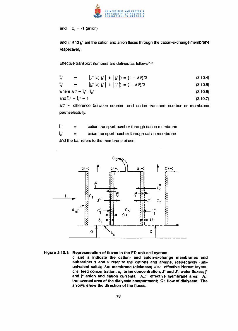
and j, Cand kCare the cation and anion fluxes through the cation-exchange membrane
respectively .
Ij,C 1/( Ij,C I + Ikc I) = (1 + a~)/2
Ikc 1/( Ikc I + Ij,C I) = (1 - a~)/2
(3.10.4)
(3.10.5)
(3.10.6)
(3.10.7)
where atC = t,C - t2C
and i,c + t2c = 1
atC = difference between counter- and co-ion transport number or membrane
perm selectivity .
t,C = cation transport number through cation membrane
t2C = anion transport number through cation membrane
and the bar refers to the membrane phase.
0(-) t c(+) 0(-) t C(+)II:.11·c 1
J I1 .0
o. J 2
I .- JC CfCb C"
6x f
Figure 3.10.1: Representation of fluxes in the ED unit-cell system.c and a indicate the cation- and anion-exchange membranes andSUbscripts 1 and 2 refer to the cations and anions, respectively (uni-univalent salts); ax: membrane thickness; a's: effective Nernst layers;c,'s: feed concentration; cb: brine concentration; JC and J8: water fluxes; rand jC anion and cation currents. Am: effective membrane area; Ac:transversal area of the dialysate compartment; Q: flow of dialysate. Thearrows show the direction of the fluxes.
Further,
i,c = t1C (/i1c 1 + Ihc I) = t1C IIF = (1 + AtC) 1/2F
hC = t2C (li,C I + li2c /) = t2C I/F = (1 - Ate) 1/2F
(3.10.8)
(3.10.9)
(Note: Effective transport numbers are to be distinguished from the usual transport
numbers which refer to the above ratio's in the absence of concentration gradients).
The brine concentration, cb, can be obtained from the following material balance
(Figure 3.10.1):
c - li~I-li~1 _li~I-li~1b-~-~
where JC and Ja are the water fluxes (flows) through the cation and anion membranes,
respectively .
c _ IJ~I -I i~Ib-~
cb(f ~ I/F) - (f ~ I/F) (3.10.12)..
=~
_ (1 +Atc) 1/2F - (1 -Ata) 1/2F (3.10.13)-~
_1/2F [(1 +Atc) - (1 -A~)] (3.10.14)-~
_ I (Atc+Ata) (3.10.15)-~
c _ I At (3.10.16)b-~
IAt (3.10.17)='2FJ
The volume flow through every membrane is equal to the sum of the electro-osmotic
and osmotic contributions(2).
JCelosm= (B,"t,c - B2"t2C)I
Jaelosm= (B2&f2a- B,~,a)1
(3.10.21)
(3.10.22)
The assumption here according to Garza & Kedem(2) is that the electro-osmotic water
flow is governed by the drag exerted by the ions. The B's are 'drag' coefficients. They
represent the amount of water dragged along with every type of ion by electro-
osmosis. For tight membranes, the value of the B's should not be very different from
the primary hydration water associated with the ions. For porous membranes,
however, the value of the B's may be several ten folds larger.
where R is the universal gas constant, T the absolute temperature, g the osmotic
coefficient, a the reflection coefficient and Lp the hydraulic permeability.
Therefore,
JCosm+ Jaosm= 2RT(gbcb-gfCt) (aCLpC+ aaLpa)
Introduction of equations (3.10.20); (3.10.21); (3.10.22) into equation (3.10.16) and
neglecting the terms (B,C- B2C)~Cand (B2a- B,a)t,a in comparison with B,c atC and
B2aaf&, gives: (note: use was made of eq. (3.10.6)
(dt"+dta)/2F(8~dt"+8~dta) + 2FRT(gbCb-gfCf)aCL~+aaL~)71
Equation (3.10.26) is justified for very permselective membranes where t2 c and t1a are
small, or where 8, c :::: 82aand 82c :::: 8,a.
For high current densities, the second term (osmotic contribution) in the denominater
of equation (3.10.26) may be neglected.
c.:'ax- (dt" + dra)/2b - F(8cdtc+8adta)
cmax_ 1 1b - F (8~+8~ ="2FB'
where 28 = 81c + 82
a.
81c and 82aare the drag coefficients associated with the counterions. These coefficients
are identical with the electro-osmotic coefficient, 8 = (J/I)~p= ~T = 0 measured at low
concentration where co-ion exclusion is practically complete, Le.
The cases for which equation (3.10.28) applies (Le. for very permselective and/or for
approximately symmetric membranes, at high current densities) are of considerable
interest and importance according to Garza and Kedem(2) since the brine concentration
depends only on the electro-osmotic coefficients, 81c and 82a. cbmaxcan also be
determined from equations (3.10.26); (3.10.27) and (3.10.28)
IdtF Jelosm{1 +Josll/JeloslTJ
cmaxb
1 + Josm/Jelosm
The theory of EOP in general leads to difficult computations which must be carried out
numerically according to Garza(1). However, there is one case in which results can be
given in terms of simple closed formula. This case depends on the assumption of a
symmetric cell(1). In a symmetric cell the cation- and anion-exchange membranes have
identical physical properties in all regards except for the sign of their fixed charges.
Because of cell symmetry, the magnitudes of the counter-ion fluxes through both
membranes are the same. When a symmetric salt is chosen like potassium chloride,
the anion and cation have equal mobilities. In other words, the magnitude of the cation
flux through the cation exchange membrane is the same as the magnitude of the anion
flux through the anion-exchange membrane. Also the magnitudes of the co-ion fluxes
through both membranes are the same, i.e., the magnitude of the anion flux through
the cation-exchange membrane is the same as the magnitude of the cation flux through
the anion-exchange membrane.
The amount of salt leaving through the brine outlet per unit time and membrane area,
2J cb• is related to the cation flows by (eqs. 3.10.10 and 3.10.19):
The amount of salt transferred per Faraday of current passed through a symmetric unit
cell is given from equation 3.10.36 by
The overall efficiency, e, is, however, somewhat smallerthan ep, since water is also lost
with the salt. The effective current density, i.e. the purification of the product achieved,
is given by(1):
where Q is the amount of feed solution entering a channel per unit time, Am the
effective membrane area (Figure 3.10.1), A the degree of mineralization given by:
where
Ct is the concentration of the feed solution entering the stack, and cp the concentration
of the product leaving it.
As is customary in ED, the overall efficiency is presented as the product of two terms,
one due to the lack of ideal permselectivity in the membranes, £p' the other reflecting
the loss of water to the brine, £W'
Electro-osmotic flow is measured under the restrictions(1):
ac = 0, dUw/dx = 0
Under these conditions are:
Jelosm = 01 B, + b B2) F
= [B,at + (B, - B2)t2]1
For small values of t2, or for B, = B2 = B equation (3.10.47) becomes:
where SO is the customary electro-osmotic coefficient measured at low ionic strength
where co-ion exclusion is high and at '" 1, i.e.:
(absence of electric current, hydrostatic pressure and impermeable sOlutes). In this
case is(1):
The volume flow into the membrane concentrating cells in EOP is the sum of the
electro-osmotic and osmotic water flows and is given by(1):
In the previous section a simplified theory of the electro-osmotic pumping process was
given where only the symmetric cell case was treated. By 'symmetric cell' is meant that
the cation- and anion-exchange membranes are assumed to have the same values for
the physical properties of interest in the process, namely, absolute effective charge
density, electro-osmotic coefficient, and hydraulic permeability. If this were not the
case, the calculations would become much more complicated since At (difference
between the effective transport numbers of counter- and co-ions) may have different
values for the two types of membranes, and the expression for the brine concentration,
cb, will not be as simple as for the symmetric case(1). cb may be found in the general
case from material balance considerations to be equal to : -
c - 1f,1-lj~1b-~
From the definition of 'effective' transport numbers given before (eqs. 3.10.4 and
3.10.5), it can be written:
/JC I + /Ja I= I(B,9:1c- B29:2c+ B2"t2
a - B,at,a) + 2RT (<PbCb- <PfCf)x (aCLpC+ aa Lpa)
= I[B1C(t,C- t2C) + (B1C- B2C)t2C+ B2a(t2a- t,a) + (B2a- B,a)t,a] + + 2RT (<PbCb- <PfCf)
x (aCLpC+ aa Lpa) (3.10.53)
for small values of t2Cand t1a, or for B,C= B2a = Bc0, and B2C = B1a = Ba0 ; equation
(3.10.53) becomes:
c _ (atc+a~)/2b-F(B~ atc+B~a~)+2RT(<pbcb - <PfCf)(aCL~+aapa)7I/F
In the case of high current density, the second term in the denominator of equation
(3.10.55) can be neglected. Therefore,
Plots of at versus current density for every membrane are expected to have the same
.kind of behaviour as for the symmetric cell case, as no new elements have been
added. The value of cb, however, depends now on the properties of both membranes,
and not on those of only one of them. Therefore, for high current densities the values
of at become independent on I, and can be calculated(1). Since the values of at
depends on cb, which in its turn depends on atC and ata, trial and error calculations are
necessary according to Garza.
In conclusion, for the non-symmetric-cell case (as for the symmetric cell) the following
is expected(l):
The Coulomb efficiency of the concentrating cell will reach a maximum
(plateau) value at high current densities (below the limiting value of the current)
e = at = t1C
- t1a = (1 + atC)/2 - (1-ata)/2
= (atC + ata)/2
The brine concentration, cb, to reach a maximum value (also at high current
densities below the limiting value) independent of I and of the feed
concentration;
The volume flow (3.10.54) versus lat plots will become straight lines at high
current densities since the osmotic contribution becomes almost independent
of current density when the latter is sufficiently high (because cb becomes
constant and c' - the concentration at the feed interface (Fig. 3.10.1) may be
kept within certain limits by controlling concentration polarization); and the
electro-osmotic contribution is directly proportional to lat (at = (atC +ata)/2, when either atC = ata or B1c= B2a.
Flux equations, membrane potentials and current efficiency relevant to EOP-ED have
been described by Kedem and Bar-On(5). The total ED process comprises three
independent flows and forces; electric current and potential; volume flow and
pressure/osmotic pressure; salt flow and concentration difference. For small flows and
gradients linear equations can be written for each of the flows, including the influence
of all gradients(14).
In practical ED, especially in EOP, flows and forces are large and one can not expect
linear equations to hold, even if the usually defined membrane transport coefficients are
constant, according to Kedem and Bar-on. In fact, transport coefficients may vary
considerably in the concentration range between feed and brine. For an adequate
discussion of flows under these conditions, Kedem and Bar-On have followed the
analysis given previously for reverse osmosis(82).
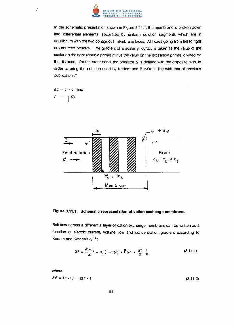
In the schematic presentation shown in Figure 3.11.1, the membrane is broken down
into differential elements, separated by uniform solution segments which are in
equilibrium with the two contiguous membrane faces. All fluxes going from left to right
are counted positive. The gradient of a scalar y, dy/dx, is taken as the value of the
scalar on the right (double prime) minus the value on the left (single prime), divided by
the distance. On the other hand, the operator a is defined with the opposite sign, in
order to bring the notation used by Kedem and Bar-On in line with that of previous
pUblications(5) :
I~
Feed solutionCiS ~
BrineCs = cb > cf
Salt flow across a differential layer of cation-exchange membrane can be written as a
function of electric current, volume flow and concentration gradient according to
Kedem and Katchalsky(14):
In a discontinuous system containing water and one uni-valent salt in the absence of
hydrostatic pressure, the rate of free energy dissipation is :
aii"1 + aii"2 = ails
aii'1 + a~2 = 2Fa 1J1(ap= 0)
I = F(J1 - J2)
allw = -Vwails
Jy = Vw Jw
(A2)
(A3)
(A4)
(AS)
(A6)
J1 = wan. + Cs (1 - a) Jv + t11/F
and
J2 = wan. + Cs (1 - a) Jv - (1 - t1) I/F
J + J at1 2 = cs(1-o)Jv + Walts + ""7T'"I/F2 ~
where w = solute permeability
and a lts = difference in osmotic pressure of permeable solute
P in equation (3.11.1) is the specific salt permeability, ac the concentration difference
and a the reflection coefficient. In an ideally permselective cation-exchange membrane
will ate - 1, P - 0, a - 1, so that se = 1/2F. Similarly, in an ideal anion-exchange
membrane will ata - 0, P - 0, 0-1, and _SA = 1/2F and TIc = 1.
Consider now a cation-exchange membrane in which salt exclusion is not complete
with co-ions carrying a significant fraction of the current(5). In this case at will be
smaller than 1 and will decrease with increasing Cs (salt concentration) as salt invasion
becomes pronounced. Salt permeability will increase when Cs increases. If the
influence of volume flow is negligible, a constant stationary value of se is possible only
if the concentration profile is concave, i.e. dc/dx decreases from the feed to the brine
surtace(5). A region of constant Cs may then develop near the brine surtace at high
current density. The upper limit of the partial current efficiency Tleeis then determined
by at" characterizing the membrane equilibrated with the brine solution. The same
argument holds for the anion-exchange membrane. Therefore, according to Kedem
and Bar-on, without the influence of volume flow
The conventional method for determination of transport numbers is the measurement
of membrane potential, i.e. a'lJ" between two solutions separated by the examined
membrane without electric current. The potential across a differential layer is given by
the expression(5):
-F d'lJ" = at 1 dJ1s _ F BJax '205< '[Rvp
term represents a streaming potential. If this can be neglected, the potential between
feed and brine solution is given by :
This average transport number, according to Kedem and Bar-on, is closer to the value
for cf than for cb• The conclusion from equations (3.11.7), (3.11.9) and (3.11.11) is that
for concentration dependent transport numbers, the actual current efficiency is
expected to be less than predicted from membrane potentials, i.e.
The correlation given by equation (3.11.12) is valid only if the influence of volume flow
is negligible.
The potential per cell pair, Vcp (in volt), at a given current density (i = l/cm2, mA/cm~,
is the sum of several terms(4):
where Vn is the concentration potential, a counter driving force built up by the
concentration process. Its magnitude depends on the concentration ratio between the
brine and dialysate and the permselectivity of the membrane at the given conditions.
Vn is measured during interruption of the current for a few seconds - long enough to
disperse concentration gradients near the membranes, short enough to avoid changes
of bulk concentration.
Vcp - Vn
i is the resistance of the cell pair; Am membrane resistance;
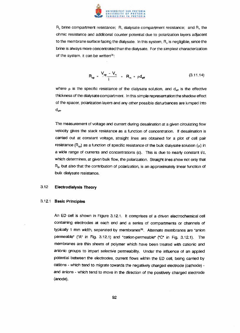
Rb brine compartment resistance; Rd dialysate compartment resistance; and Rp the
ohmic resistance and additional counter potential due to polarization layers adjacent
to the membrane surface facing the dialysate. In this system, Rb is negligible, since the
brine is always more concentrated than the dialysate. For the simplest characterization
of the system, it can be written(4);
Vcp - VnR = ---- = Rm + pdeffcp i
where p is the specific resistance of the dialysate solution, and deft is the effective
thickness of the dialysate compartment. In this simple representation the shadow effect
of the spacer, polarization layers and any other possible disturbances are lumped into
deft·
The measurement of voltage and current during desalination at a given circulating flow
velocity gives the stack resistance as a function of concentration. If desalination is
carried out at constant voltage, straight lines are obtained for a plot of cell pair
resistance (Rcp) as a function of specific resistance of the bulk dialysate solution (p) in
a wide range of currents and concentrations (c). This is due to nearly constant i!c,which determines, at given bulk flow, the polarization. Straight lines show not only that
Rd, but also that the contribution of polarization, is an approximately linear function of
bulk dialysate resistance.
An ED cell is shown in Figure 3.12.1. It comprises of a driven electrochemical cell
containing electrodes at each end and a series of compartments or channels of
typically 1 mm width, separated by membranes(8). Alternate membranes are "anion
permeable" ("A" in Fig. 3.12.1) and "cation-permeable" ("C· in Fig. 3.12.1). The
membranes are thin sheets of polymer which have been treated with cationic and
anionic groups to impart selective permeability. Under the influence of an applied
potential between the electrodes, current flows within the ED cell, being carried by
cations - which tend to migrate towards the negatively charged electrode (cathode) -
and anions - which tend to move in the direction of the positively charged electrode
(anode).
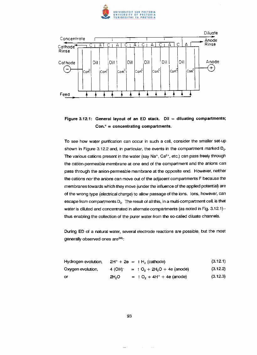
Concentrate
Cathode CRinse
Diluate
AnodeRinse
Anode
+
Figure 3.12.1: General layout of an EO stack. Oil = diluating compartments;
Con.e = concentrating compartments.
To see how water purification can occur in such a cell, consider the smaller set-up
shown in Figure 3.12.2 and, in particular, the events in the compartment marked D2•
The various cations present in the water (say Na+, Ca2+, etc.) can pass freely through
the cation-permeable membrane at one end of the compartment and the anions can
pass through the anion-permeable membrane at the opposite end. However, neither
the cations nor the anions can move out of the adjacent compartments F because the
membranes towards which they move (under the influence of the applied potentia~ are
of the wrong type (electrical charge) to allow passage of the ions. Ions, however, can
escape from compartments D2• The result of all this, in a multi-compartment cell, is that
water is diluted and concentrated in alternate compartments (as noted in Fig. 3.12.1) -
thus enabling the collection of the purer water from the so-called diluate channels.
During ED of a natural water, several electrode reactions are possible, but the most
generally observed ones are(83):
Hydrogen evolution,
Oxygen evolution,
or
2H+ + 2e = 1 H2 (cathode)
4 (OH)' = 1 O2 + 2H20 + 4e (anode)
2H20 = 1 O2 + 4H+ + 4e (anode)
(3.12.1)
(3.12.2)
(3.12.3)
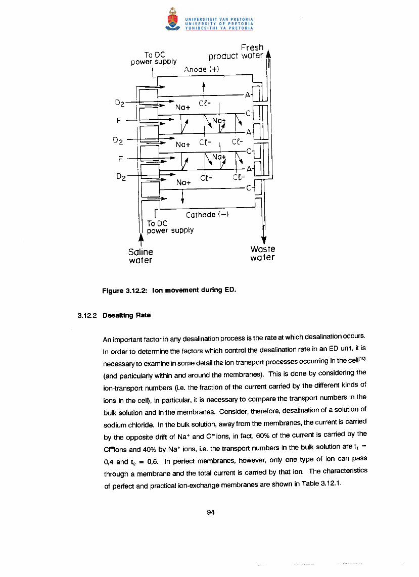
To DCpower supply
L
Freshproduct water m
Anode (+) , I
D~ Na+
~~
~ Cathode (-)To DC+ power supply
Salinewater
1Wastewater
An important factor in any desalination process is the rate at which desalination occurs.
In order to determine the factors which control the desalination rate in an ED unit, it is
necessary to examine in some detail the ion-transport processes occurring in the ceW16)
(and particularly within and around the membranes). This is done by considering the
ion-transport numbers (i.e. the fraction of the current carried by the different kinds of
ions in the cel~, in particular, it is necessary to compare the transport numbers in the
bulk solution and in the membranes. Consider, therefore, desalination of a solution of
sodium chloride. In the bulk solution, away from the membranes, the current is carried
by the opposite drift of Na+ and cr ions, in fact, 60% of the current is carried by the
CMons and 40% by Na+ ions, i.e. the transport numbers in the bulk solution are t1 =0,4 and l:! = 0,6. In perfect membranes, however, only one type of ion can pass
through a membrane and the total current is carried by that ion. The characteristics
of perfect and practical ion-exchange membranes are shown in Table 3.12.1.
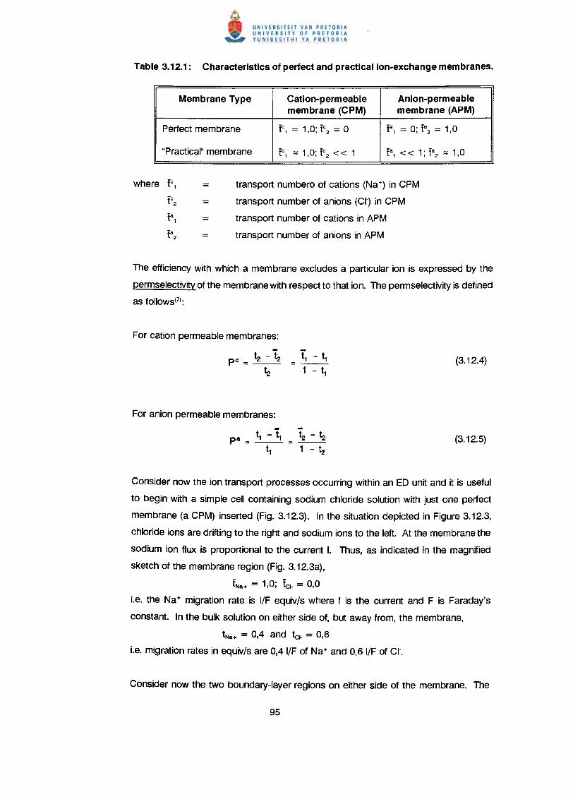
Membrane Type Cation-permeable Anion-permeablemembrane (CPM) membrane (APM)
Perfect membrane tCl = 1,0; tC2 = a tal = 0; ta2 = 1,0
"Practical" membrane tCl ;;::1,0; tC2 « 1 tal« 1;ta2;;:: 1,0
where tCl = transport numbero of cations (Na+) in CPM
tC2 = transport number of anions (CI-) in CPM
tal = transport number of cations in APM
ta2 transport number of anions in APM
The efficiency with which a membrane excludes a particular ion is expressed by the
permselectivity of the membrane with respect to that ion. The permselectivity is defined
as follows(7J:
- -t - t = t2 - t_pa = _1__ '1 '2
t1 1 - ~
Consider now the ion transport processes occurring within an ED unit and it is useful
to begin with a simple cell containing sodium chloride solution with just one perfect
membrane (a CPM) inserted (Fig. 3.12.3). In the situation depicted in Figure 3.12.3,
chloride ions are drifting to the right and sodium ions to the left. At the membrane the
sodium ion flux is proportional to the current I. Thus, as indicated in the magnified
sketch of the membrane region (Fig. 3.12.3a),
tNa+ = 1,0; tel- = 0,0
i.e. the Na+ migration rate is IIF equiv/s where I is the current and F is Faraday's
constant. In the bulk solution on either side of, but away from, the membrane,
tNa+ = 0,4 and te~ = 0,6
i.e. migration rates in equiv/s are 0,4 IIF of Na+ and 0,6 IIF of CI-.
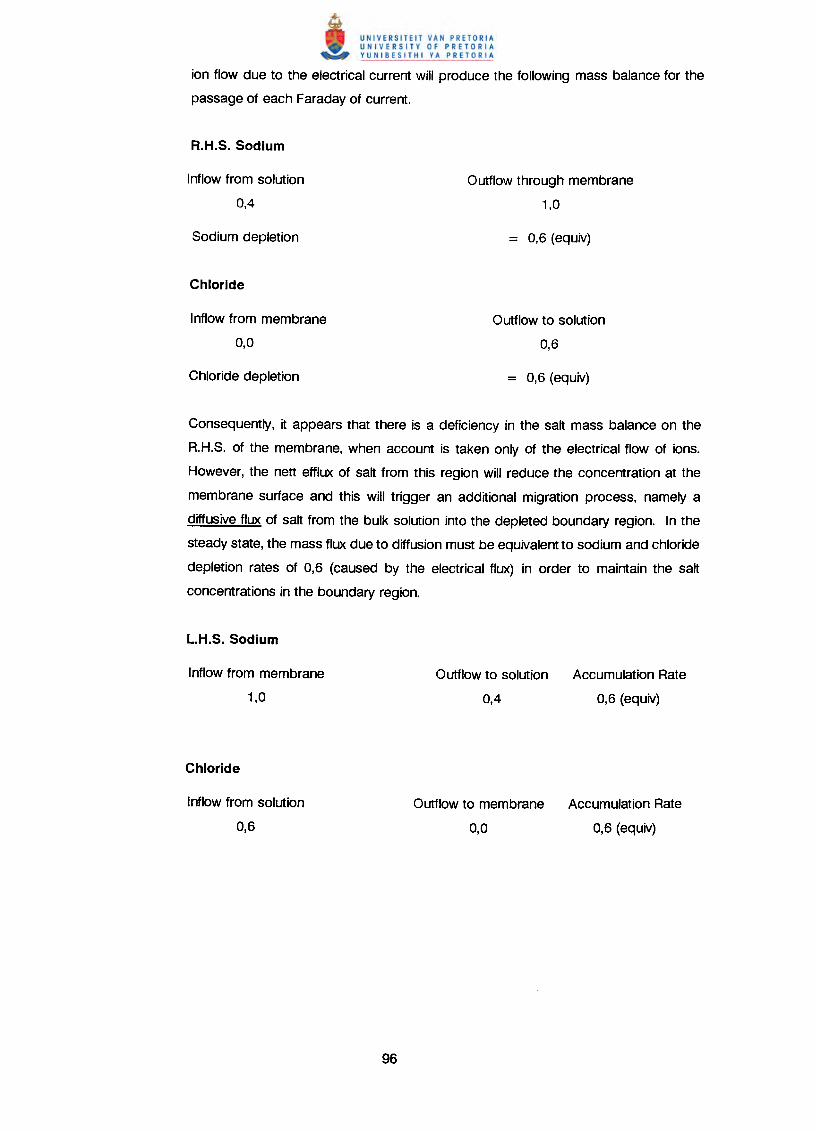
ion flow due to the electrical current will produce the following mass balance for the
passage of each Faraday of current.
Inflow from solution
0,4
Outflow through membrane
1,0
= 0,6 (equiv)
Inflow from membrane
0,0
Outflow to solution
0,6
Consequently, it appears that there is a deficiency in the salt mass balance on the
R.H.S. of the membrane, when account is taken only of the electrical flow of ions.
However, the nett efflux of salt from this region will reduce the concentration at the
membrane surface and this will trigger an additional migration process, namely a
diffusive flux of salt from the bulk solution into the depleted boundary region. In the
steady state, the mass flux due to diffusion must be equivalent to sodium and chloride
depletion rates of 0,6 (caused by the electrical flux) in order to maintain the salt
concentrations in the boundary region.
Inflow from membrane
1,0
Outflow to solution0,4
Accumulation Rate
0,6 (equiv)
Inflow from solution
0,6
Outflow to membrane Accumulation Rate
0,0 0,6 (equiv)
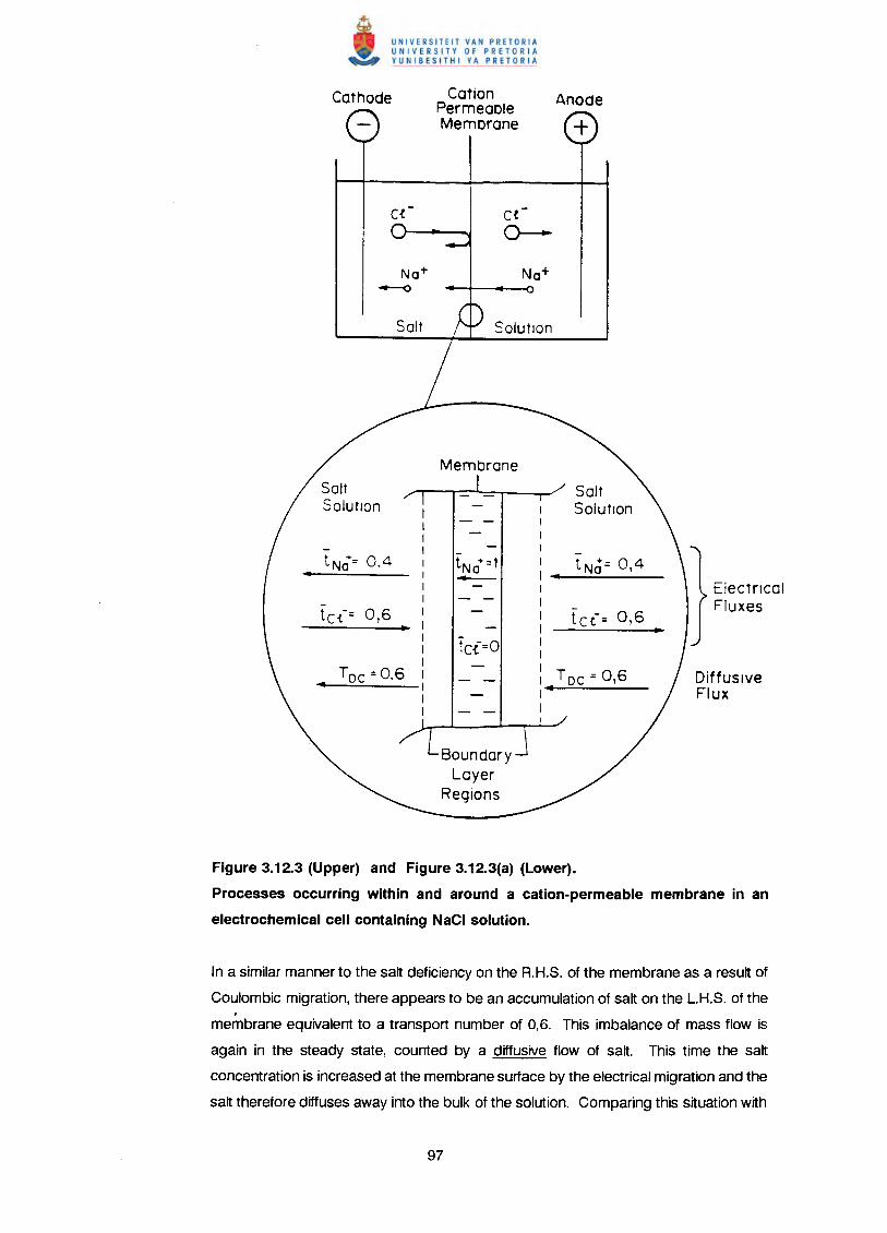
CationPermeableMembrane
Na+---0
Membrane
SaltI SolutionII
- I -tNo+= 0,4 tNa+=1 I tNd= 0,4.• - I ..•I ElectrIcalI Fluxes
t({-= 0,6 I tc(= 0,6• I •
tcf=O II
TDC = 0,6 IT DC = 0,6 Diffusive.. I
I • Flux
BoundaryLayer
Regions
Figure 3.12.3 (Upper) and Figure 3.12.3(a) (Lower).
Processes occurring within and around a cation-permeable membrane in an
electrochemical cell containing NaCI solution.
In a similar manner to the salt deficiency on the R.H.S. of the membrane as a result of
Coulombic migration, there appears to be an accumulation of salt on the L.H.S. of the.membrane equivalent to a transport number of 0,6. This imbalance of mass flow is
again in the steady state, counted by a diffusive flow of salt. This time the salt
concentration is increased at the membrane surface by the electrical migration and the
salt therefore diffuses away into the bulk of the solution. Comparing this situation with
the straightforward electrolysis process without the membrane, the nett effect of
inserting the membrane is to produce an apparent diffusion of salt from right to left
across the membrane. The rate (in equivs per Faraday) of this apparent diffusion
transport number, Toemay be expressed in terms of the transport numbers. For the
present case, it is clear that Toe = 0,6 equiv/Faraday, i.e. Toe = t2• However, in the
general case for imperfect membranes, a similar analysis as that above leads to:
TDC = t2 - t2C
A similar analysis and argument may be set up for an anion-permeable membrane.
In this case, if the membrane was perfect (i.e. t,a = ° and t2a = 1,0), there would
appear to be a salt depletion on the L.H.S. To balance these there would have to be
an apparent diffusion of salt from left to right across the membrane. In this case for
an imperfect membrane, TOA = t, - t,a which reduces to TOA = 0,4 for the case of
a perfect APM in a NaCI solution.
Consider now what will happen if an anion-permeable membrane is inserted on the
right hand side of the cation permeable membrane in Figure 3.12.3. Such a set up is
depicted in Figure 3.12.4. Passage of current through this system will produce an
apparent effect of salt diffusion out of the space between the two membranes. For the
simple example of perfect membranes in NaCI solution, the rates of these apparent
diffusions will be
To the left across the C.P.M., Toe = 0,6
To the right across the A.P.M., TOA = 0,4
Therefore, the total apparent diffusive flux out of the central compartment of a set-up
like Figure 3.12.4 is:
To = Toe + TOA = t2 t2C + t, - t,a (3.12.6)
= 1 - t2C - t,a equiv per Faraday (3.12.7)
= 1 for perfect membranes. (3.12.8)
To, the salt flux out of the central compartment, is clearly a measure of the desalting
rate, i.e. for a current flow of I amp,
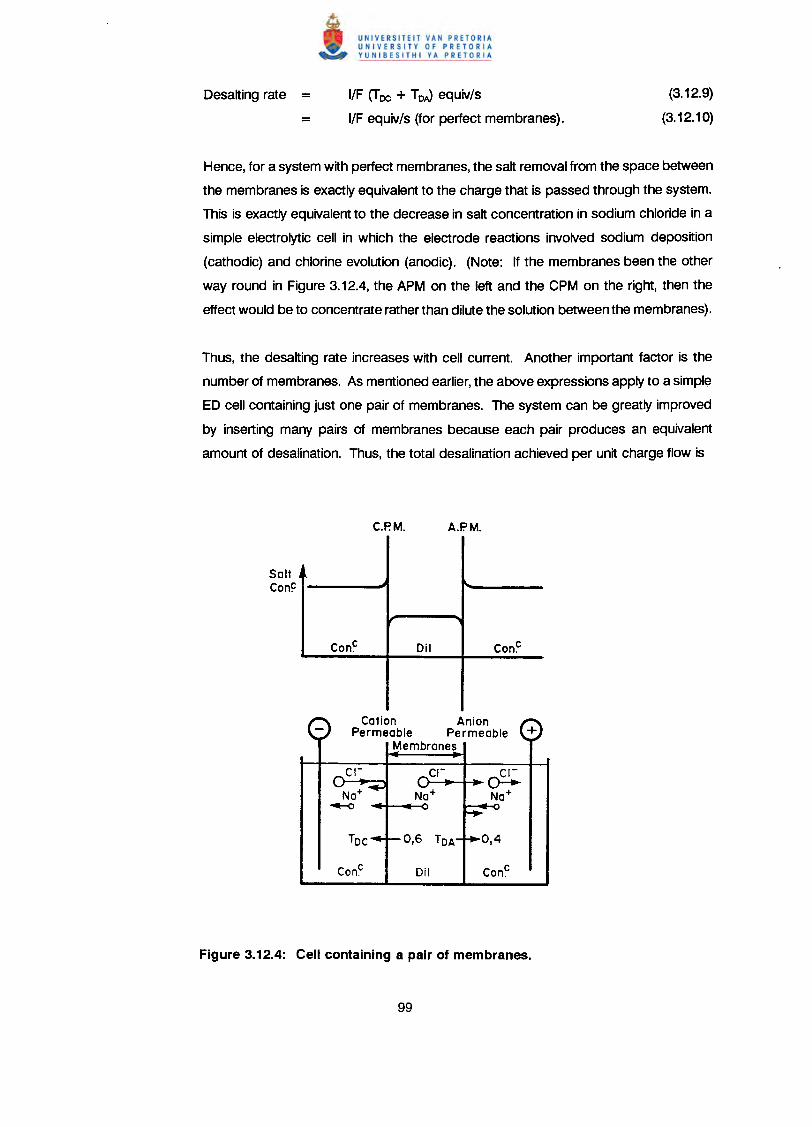
IIF (TDC + ToJ equivls
IIF equivls (for perfect membranes).
(3.12.9)
(3.12.10)
Hence, for a system with perfect membranes, the salt removal from the space between
the membranes is exactly equivalent to the charge that is passed through the system.
This is exactly equivalent to the decrease in salt concentration in sodium chloride in a
simple electrolytic cell in which the electrode reactions involved sodium deposition
(cathodic) and chlorine evolution (anodic). (Note: If the membranes been the other
way round in Figure 3.12.4, the APM on the left and the CPM on the right, then the
effect would be to concentrate rather than dilute the solution between the membranes).
Thus, the desalting rate increases with cell current. Another important factor is the
number of membranes. As mentioned earlier, the above expressions apply to a simple
ED cell containing just one pair of membranes. The system can be greatly improved
by inserting many pairs of membranes because each pair produces an equivalent
amount of desalination. Thus, the total desalination achieved per unit charge flow is
SaltCon~
Cone Oil Con~
Cation AnionPermeable Permeable +
Membranes
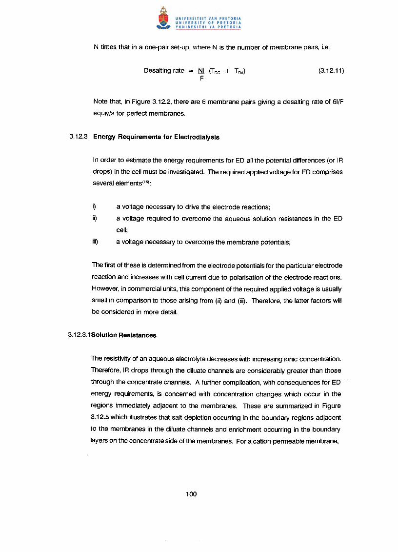
Desalting rate = NI (Toc + Top,)F
Note that, in Figure 3.12.2, there are 6 membrane pairs giving a desalting rate of 61/F
equiv/s for perfect membranes.
In order to estimate the energy requirements for ED all the potential differences (or IR
drops) in the cell must be investigated. The required applied voltage for ED comprises
several elements(16):
o a voltage necessary to drive the electrode reactions;
iO a voltage required to overcome the aqueous solution resistances in the ED
cell;
iiO a voltage necessary to overcome the membrane potentials;
The first of these is determined from the electrode potentials for the particular electrode
reaction and increases with cell current due to polarisation of the electrode reactions.
However, in commercial units, this component of the required applied voltage is usually
small in comparison to those arising from (iO and (iiO. Therefore, the latter factors will
be considered in more detail.
The resistivity of an aqueous electrolyte decreases with increasing ionic concentration.
Therefore, IR drops through the diluate channels are considerably greater than those
through the concentrate channels. A further complication, with consequences for ED
energy requirements, is concerned with concentration changes which occur in the
regions immediately adjacent to the membranes. These are summarized in Figure
3.12.5 which illustrates that salt depletion occurring in the boundary regions adjacent
to the membranes in the diluate channels and enrichment occurring in the boundary
layers on the concentrate side of the membranes. For a cation-permeable membrane,
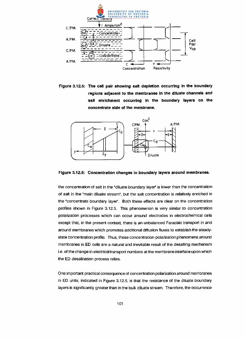
Current Density
~I Amps/cm2
~~rt_~-- ~~9-~~~r;~~~~---- --------~-: c< = 0-:1- -t -:.. ----. N~ _ _ I ua e __ .. - - - - - - - - --
~~_~_=~~if~~~C
Concentration
-[L(
-]·cellPair__ Vcp
yResistivity
Figure 3.12.5: The cell pair showing salt depletion occurring In the boundary
regions adjacent to the membranes In the dlluate channels and
salt enrichment occurring In the boundary layers on the
concentrate side of the membrane.
the concentration of salt in the "diluate boundary layer" is lower than the concentration
of salt in the "main diluate stream", but the salt concentration is relatively enriched in
the "concentrate boundary layer". Both these effects are clear on the concentration
profiles shown in Figure 3.12.5. This phenomenon is very similar to concentration
polarization processes which can occur around electrodes in electrochemical cells
except that, in the present context, there is an unbalanced Faradaic transport in and
around membranes which promotes additional diffusion fluxes to establish the steady-
state concentration profile. Thus, these concentration-polarization phenomena around
membranes in ED cells are a natural and inevitable result of the desalting mechanism
i.e. of the change in electrical transport numbers at the membrane interface upon which
the ED desalination process relies.
One important practical consequence of concentration polarization around membranes
in ED units, indicated in Figure 3.12.5, is that the resistance of the diluate boundary
layers is significantly greaterthan in the bulk diluate stream. Therefore, the occurrence
When an ion-selective membrane separates two solutions of a salt at different
concentrations, a potential difference is set-up across the membrane. This happens
because, in the absence of any applied potentials, Na + ions will tend to migrate across
the cation-exchange membrane from the concentrated solution to the diluate solution.
This will lead to a charge imbalance across the membrane with the diluate side
becoming positively charged relative to the concentrated side. Eventually this potential
difference across the membrane will build up to such a level that further ion transfer is
discouraged and the value of the potential difference at this equilibrium condition is
known as the membrane potential. For a salt consisting of single-charged ions, and
assuming that activities can be equated to concentrations, the magnitude of the
membrane potential is given by
where CW1 and Cw2 are the concentrations of the salt in the concentrated and dilute
solutions respectively.
The important point about the above is that natural flow across a membrane is from
concentrate to diluate (i.e. the opposite to that required in desalination) and, to reverse
this natural flow direction requires the application of a potential of magnitude greater
than Em, i.e. the membrane potential represents a potential drop which has to be
overcome by the external applied voltage in order for desalination to occur. However,
this is not the whole story. The magnitude of the membrane potential indicated by the
above equation only applies to the eqUilibrium (i.e. infinitely-low current) state. As
previously discussed, an inevitable consequence of desalination at finite currents is the
occurrence of concentration polarization. The consequent concentrate enrichment and
diluate depletions at the membrane/solution interface means that CW1 will be greater
than the bulk concentrate composition and Cw2 will be less than the bulk diluate
concentrations. Therefore, another important effect of concentration polarization is to
increase the membrane potential and hence the energy requirements for desalination.
The major part of the energy requirements for ED comprises the voltage necessary to
overcome the solution resistances and membrane potentials. Estimation of the voltage
is conveniently done by considering one cell pair which, as shown in Figure 3.12.5,
encompasses a pair of membranes. The cell pair potential Vep, is the sum of all the
potential drops across the membranes and solutions comprising one cell pair.
Consider the basic conflict between attempts to maximise desalting rate and to
minimize energy requirements. The flux of salts from the diluate channel is given by
d = ITo equiv cm-2 S-1
F
(using current density, i, instead of current I). The power required to drive a cell pair
is:
Therefore, increases in i, whilst raising the desalting rate, also lead to higher energy
consumption - not only directly but also by increasing Vep due to higher IR drops and
concentration-polarization effects.
The major contributor to Vep is the resistance of the diluate stream. It is normal practice
to keep the concentration of the concentrate high enough for its resistance to be
negligible in comparison to that of the diluate. Modern membranes have, however,
negligible small resistances. As a first approximation, it can be considered that the
diluate stream is providing all the resistance. To calculate the resistance, the main
stream and the boundary layers must be considered separately.
Considering the total thickness (including boundary layers) of the diluate stream to be
't' cm (typically 0,1 cm) (see Fig. 3.12.6). Let the thickness of the boundary layers
(adjacent to the membranes) be a (determined by hydrodynamic conditions and
typically 0,01 cm).
But the conductivity, K, depends on the concentration Cd (equivicm3) of the diluate
stream via K = I\Cd (3.12.17)
Faradaic transport (i.e. under the influence of the applied electric field) of ions, across
the membranes out of the diluate compartment, leads to a depletion of salt in the
boundary layers which, in turn, causes a diffusion flux from the bulk diluate. The
concentration gradient across the boundary layer stabilises (i.e. steady-state conditions
are established) when the two fluxes are equal.
Diffusion flux = -D dcdy
Resistance of element oy = oy = ~1< Ac
(3.12.22)(see Fig. 3.12.6)
R = (I} dyBe Jo Ac
de- =dy
An alternative expression for RBC can be produced by using the previously formulated
steady-state relation.
-0 de = ~ ldy F
~()i
FO
FO ( ~()' )- __ In 1 - __ 1-~ 1/\ FDCd
A similar analysis can be carried out to obtain an expression for the resistance, ABA' of
the diluate boundary layer at the APM (right hand side of Figure 3.12.6). This leads to
the following expression:-
The depletion of solute in the boundary layers arises from the rapid flux of solute
species through the membranes - this flux being directly proportional to the current
flowing in the cell. In other words, as i increases from zero, the concentration gradient
in the boundary layer increases (Cw decreases as i increases). It follows, therefore, that
there are limits to the current that can be carried by the solute ions in an ED system -
this limit being reached when Cw approaches zero.
Another aspect of this "limiting current density phenomenon concerns the transport of
H+ and OH ions across CPM and APM membranes, respectively. At low current
densities, the current is carried almost exclusively by solute ions rather than by H+ and
OH-. This is because of the very low concentrations of H+ and OH- in neutral solution
(10'7 moVQ) - and is despite the approximately ten times higher mobilities of H+ and
OH' compared with solute ions. But, as i increases, the flux of H+ and OH' across the
membranes increases until, as imax is approached, the flux of H+ at the CPM and of OH-
at the APM becomes a substantial fraction of the total current. In rather more precise
terms, because of their tenfold higher mobilities, an appreciable fraction of the current
will be carried by H+ and OH-, present at concentrations of 10-7 mollO,when the solute
concentration at the membrane/diluate interface Cw, falls towards a value of about 5 x
10-6 mol/Q. Such a situation not only results in an obvious decreased efficiency of
desalination but also in highly undesirable pH changes in the solutions. One
consequence of such pH changes is that they can lead to an increased tendency
towards scale precipitation if the pH increases significantly in any local region.
The contribution of membrane potentials to the cell-pair potential is most conveniently
predicted by considering ED of a solution of a single salt comprising of univalent ions.
As was noted earlier, for this case the membrane potential was given by:
where CW1 and Cw2 now represent the bulk concentrations of the salt in the
compartments on either side of the membrane. Note, though, that the membrane
potential is determined by the salt concentrations at the membrane/salt interface. It
was noted earlier that finite cell-current flow resulted in salt depletions and enrichments
within the boundary region beside the membrane. In such circumstances, Em will no
longer be determined by the bulk-salt concentrations (CW1 and Cw2) but by the
concentration-polarised membrane/boundary layer interfacial values (CWbc and CwdC, in
the C.P.M. in Figure 3.12.7). Therefore, in order to obtain an expression for Em in these
practically-relevant conditions, it is necessary to estimate the concentrations Cwbc and
CwdC for C.P.M.and Cwda and Cwba for the AP.M.. This exercise is considerably
simplified if it is assumed (see Figure 3.12.7) that the four boundary layers have
identical effective thickness, a. If we assume a perfect cation permeable membrane
(C.P.M.) and use the notation of Figure 3.12.7, the polarised C.P.M. membrane
potential is given by:-
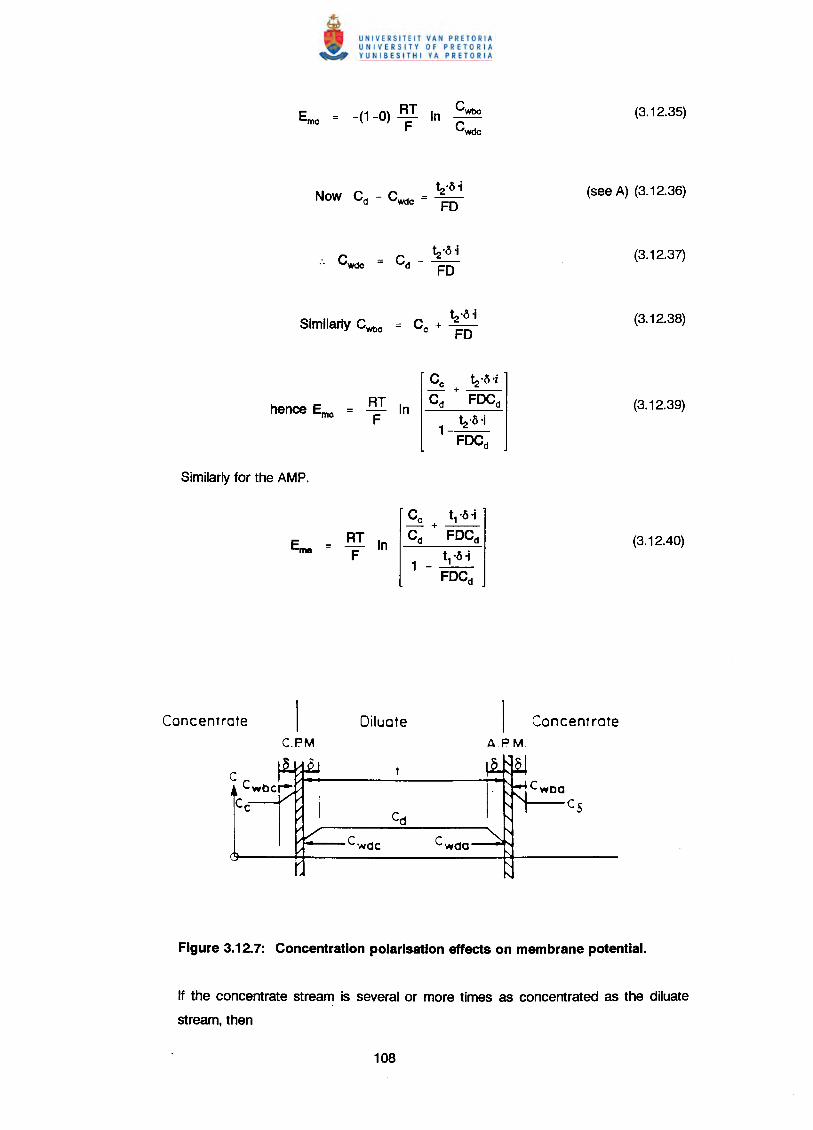
-(1-0) RT In Cwbc
F Cwdc
~·01Now Cd - CwdC = FD
~·01C +--c FD
RT InF
RT InF
CdCwdc CwdO
Cwbo
Cs
If the concentrate stream is several or more times as concentrated as the diluate
stream, then
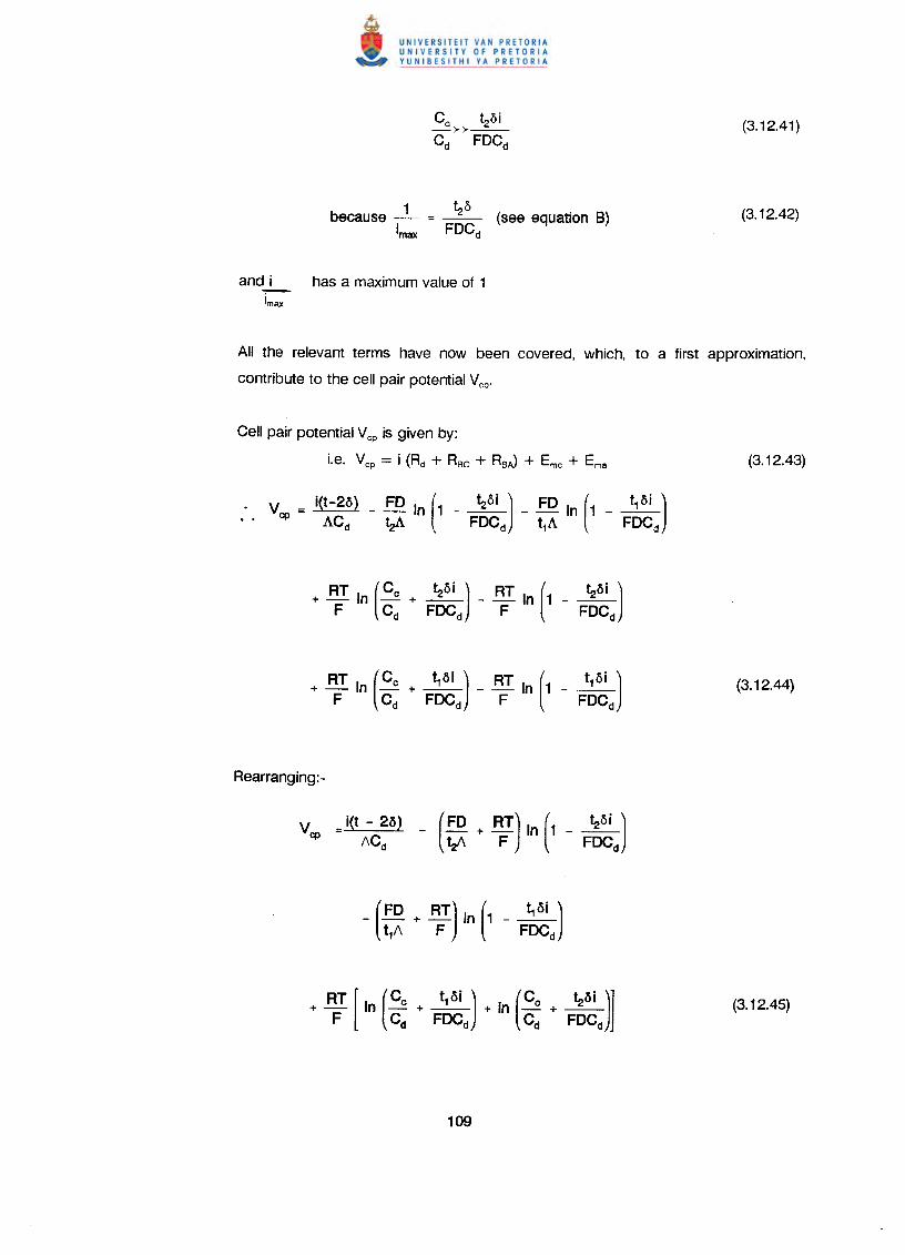
because _1_ = ~ (see equation B)imax FDCd
and i has a maximum value of 1imax
All the relevant terms have now been covered, which, to a first approximation,
contribute to the cell pair potential Vep'
Cell pair potential Vep is given by:
i.e. Vep = i (Ad + ABc + ABJ + Eme + Ema
AT (Co ~ai) AT ( ~ai )+ F In Cd + FDC
d- F In 1 - FDC
d
+ AT In (Co + ~) _ AT In (1 _ ~)F Cd FDCd F FDCd
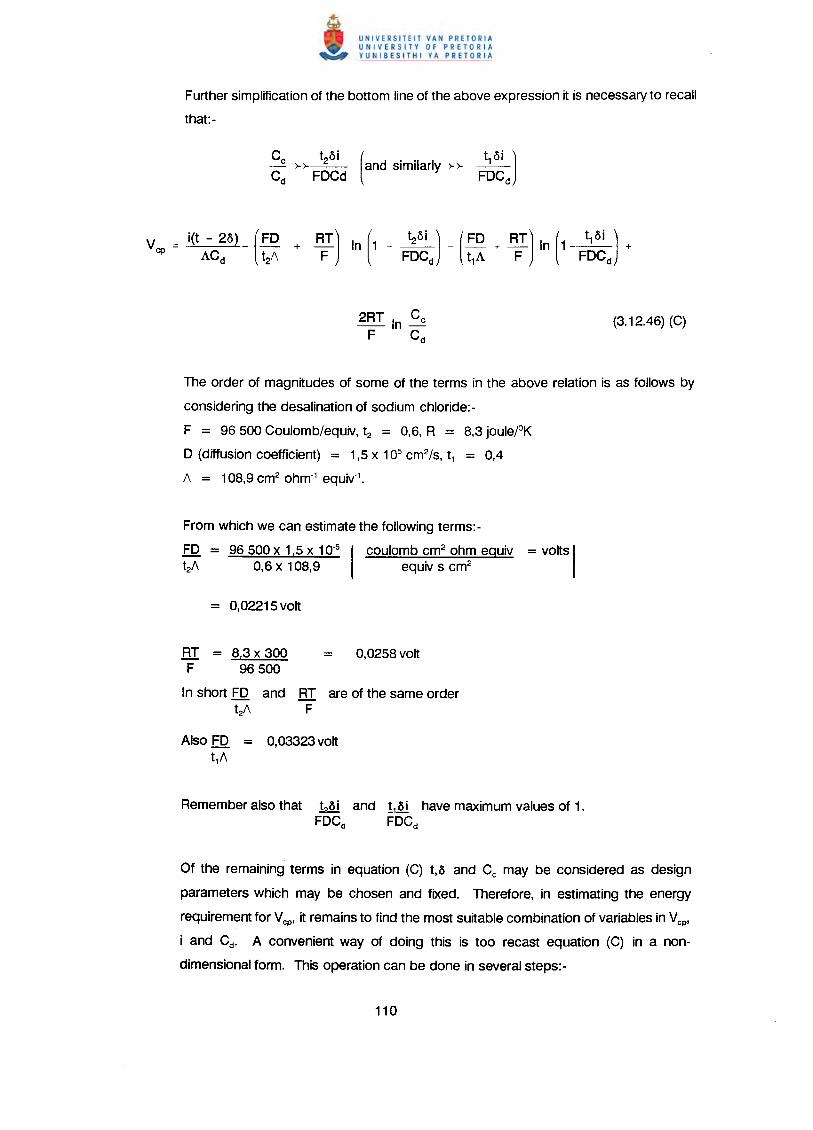
Further simplification of the bottom line of the above expression it is necessary to recall
that:-
(t oi )and similarly ~~ _1_
FDCd
v = i(t - 20)cP AC
d
The order of magnitudes of some of the terms in the above relation is as follows by
considering the desalination of sodium chloride:-
F = 96500 Coulomb/equiv, t2 = 0,6, R = 8,3 joule/oK
o (diffusion coefficient) = 1,5 x 105 cm2/s, t1 = 0,4
/\ = 108,9 cm2 ohm-1 equiv-1•
From which we can estimate the following terms:-
FD = 96 500 x 1,5 x 10-5 coulomb cm2 ohm eguiv = volts It2/\ 0,6 x 108,9 equiv s cm2
RT = 8,3 x 300F 96500
In short FD and RT are of the same ordert2/\ F
Also FD = 0,03323 voltt1/\
Remember also that t?3i and 113 i have maximum values of 1.FDCd FDCd
Of the remaining terms in equation (C) t,3 and Cc may be considered as design
parameters which may be chosen and fixed. Therefore, in estimating the energy
requirement for Vcp, it remains to find the most suitable combination of variables in Vcp,
i and Cd. A convenient way of doing this is too recast equation (C) in a non-
dimensional form. This operation can be done in several steps:-
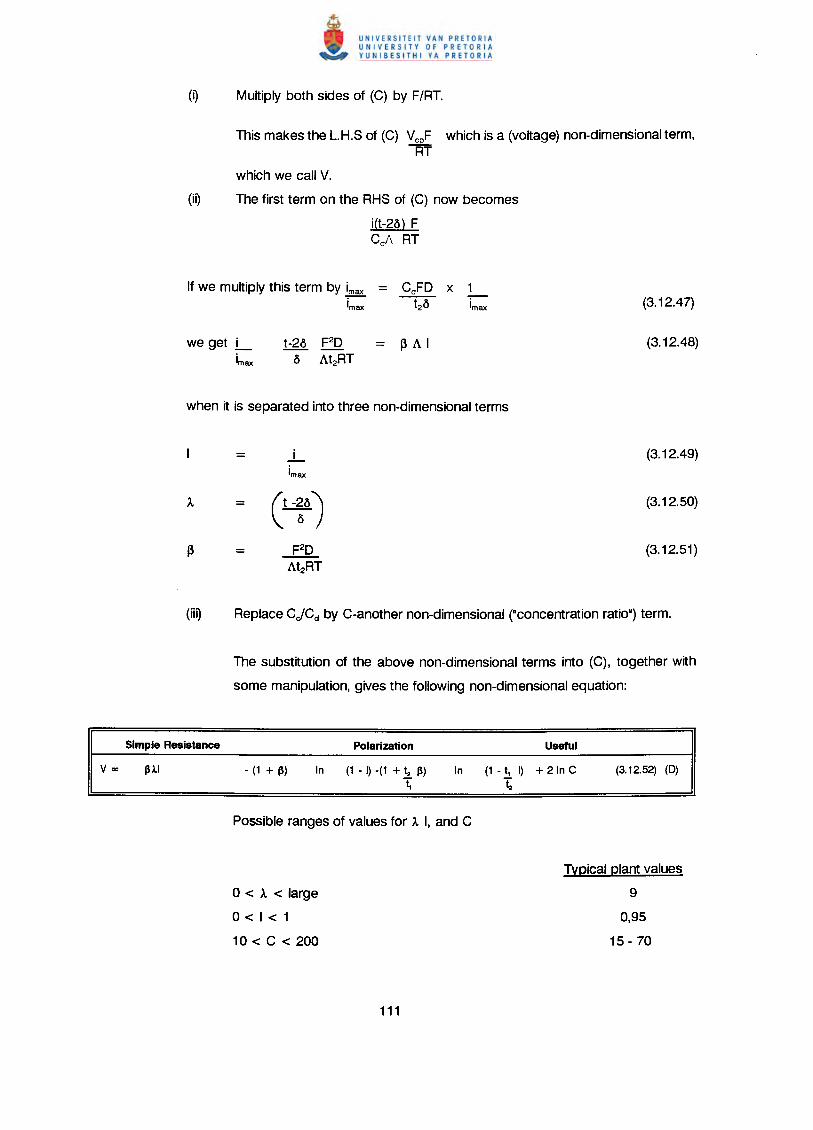
This makes the L.H.S of (C) Vel which is a (voltage) non-dimensional term,RT
which we call V.
(iQ The first term on the RHS of (C) now becomes
j(t-2c5) FCdA RT
If we multiply this term by imax = CdFD x 1imax ~ imax
we get _i_ t-2c5 F2D = ~ AIimax c5 At2RT
= _i_ (3.12.49)imax
= (t -~c5)(3.12.50)
= F2D (3.12.51)At2RT
The substitution of the above non-dimensional terms into (C), together with
some manipulation, gives the following non-dimensional equation:
Simple Resistance
In (1 - I) -(1 + 1, Ii)T,
In (1 - t, I) + 2 In C1;
0< 1<large
0<1 < 1
10 < C < 200
Typical plant values
9
0,95
15 - 70
Equation (D) is divided into terms coming from simple resistive losses (since the ~AI
term is derived from the first term on the RHS of equation (C) which represents the
bulk dilate resistance), and the work done against the membrane potentials (said to
be "useful"because it represents the minimum energy without polarization effects), and
the polarization-losses (all these terms being derived from all the terms in (C) except
the first and the last (simple membrane potentia~. These contributions to the cell pair
potential may be plotted separately as they are in Figure 3.12.8. The ·useful" potential
is only a function of C and the two "loss" potentials are both functions of I, the resistive
loss being a function of A as well. This graph then covers the total likely range of
conditions to be found in practical ED stacks. Thus, the various curves for different
values of A are plots of the contributions of the resistance loss (~AI) to the V term for
different values of A (the cell to boundary layer thickness ratiO). Note that, as A
increases (i.e. as the cell size increases) the energy requirements increase. Note also,
that, for the calculations of the value of ~ (used in the A-plots and also in the
polarization plot) that a temperature of 300 0 K has been used.
No account of the effects of flow of solution through the compartments of the ED stack
have been taken up to now. This matter can be estimated by investigating how
conditions vary as the diluate passes along its channel(16).This procedure can be
started by carrying out a salt mass balance on an element, dx, in which the
concentration changes from Cd by a small amount dCd (See Figure 3.12.9).
Area of element = 1 x t = t cm2
Therefore, rate of salt flow into element is CdUdtequiv S-1.
Salt flux out of element along diluate channel is (Cd + dCd) t Udequiv s-'.
Flux of salt through membranes (= desalting rate)
1= F equiv/cm2 s
(3.12.52)
(3.12.53)
(3.12.54)
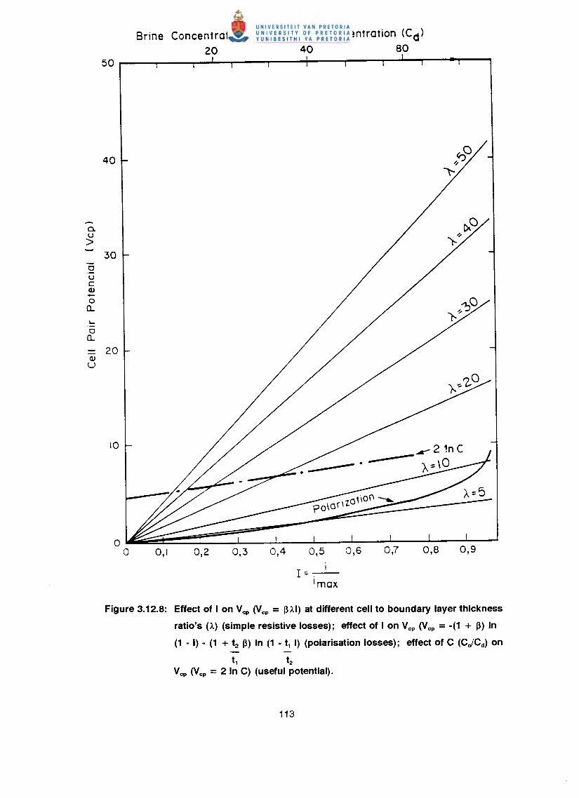
a.u>
300ucQ)-0a..L-
0a..20
Q)
u
Brine Concentration (Ce)/ Diluate Concentration (Cd)20 40 80
oo
I1=-. -'max
Figure 3.12.8: Effect of Ion Vep 0Jep = ~>"I)at different cell to boundary layer thickness
ratio's (>..) (simple resistive losses); effect of I on Vep 0Jep = -(1 + ~) In
(1 - I) - (1 + t2 ~) In (1 - t, I) (polarisation losses); effect of C (CJCd) on
t, t2
Vep 0Jep = 2 In C) (useful potential).
~5tUd:. X = - DI [In Cd (x) - In Cd (x = 0)]
~5tUd= - --In
01
(01 )X
= C, e t:/6tUd
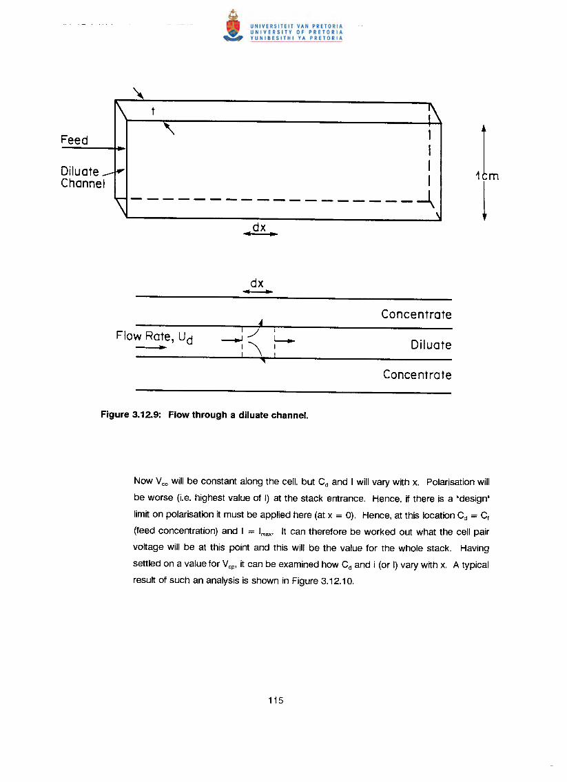
DiluateChannel
IIII
------------------~dx•• •••
Flow Rate, Ud••
I~ I~\L....I I! I
"'
Now Vep will be constant along the cell, but Cd and I will vary with x. Polarisation will
be worse (Le. highest value of I) at the stack entrance. Hence, if there is a "design"
limit on polarisation it must be applied here (atx = 0). Hence, at this location Cd = Cf
(feed concentration) and I = Imax• It can therefore be worked out what the cell pair
voltage will be at this point and this will be the value for the whole stack. Having
settled on a value for Yep, it can be examined how Cd and i (or I) vary with x. A typical
result of such an analysis is shown in Figure 3.12.10.
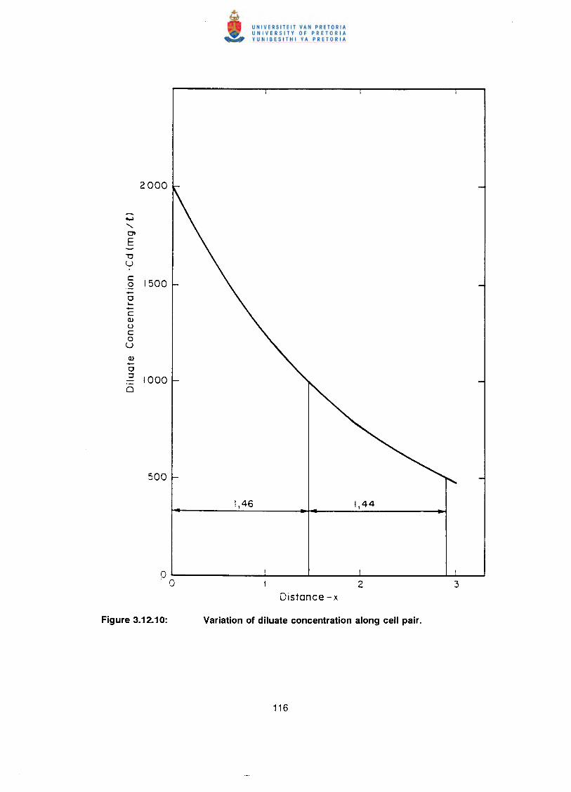
2000
...•"-C'E"0UI
c1500a
0•...-CQ.lUCaU
Q.l-0:J 10000
oo
Electrodialysis technology has progressed significantly during the past 40 years since the
introduction of synthetic ion-exchange membranes in 1949(53). The first two decades of this
period saw the development of classical or unidirectional standard electrodialysis. However,
during the past decade, the main feature has been the development of the polarity reversal
process - the so-called electrodialysis reversal (EDR) (84). This form of electrodialysis
desalination has virtually displaced unidirectional ED for most brackish water applications and
is slowly gaining a significant share of this market.
EDR is at present mainly used for the desalination of brackish waters to produce fresh potable
and industrial water. Unidirectional ED is used on a large scale in Japan for concentrating
seawater to produce brine for salt production(85) and is also used on a small scale for seawater
desalination(86) and for brackish water desalination(8?).
Outside the water desalination field, ED is also being used on a large and increasing scale in
North America and Europe to de-ash cheese whey to produce a nutritious high quality protein
food supplement(53). It is also finding application in the treatment of industrial waste waters for
water recovery, reuse and effluent volume reduction(81, 88l.
Different types of ED processes and stacks are used commercially for ED
applications(6). The filter-press- and the unit-cell stacks are the most familiar.
The filter press stack configuration(6,8) in which alternate cation- and anion-exchange
membranes are arranged between compartment frames in a plate-and-frame filter
press assembly is shown in Figure 4.1.
Salt solution flows between the alternately placed cation and anion permeable
membranes in the ED stack. Direct current (DC) provides the motive force for ion
migration through the ion-exchange membranes and the ions are removed or
concentrated in the alternate water passage by means of permselective ion-exchange
membranes. This process is called the standard ED process.
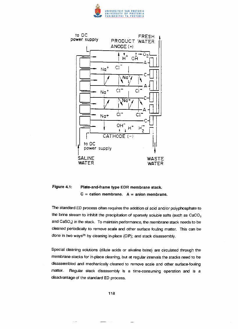
to DCpower supply
Na+
- V- Na+
- VNa+
SALINEWATER
WASTEWATER
Plate-and·frame type EDR membrane stack.
C = cation membrane. A = anion membrane.
The standard ED process often requires the addition of acid and/or polyphosphate to
the brine stream to inhibit the precipitation of sparsely soluble salts (such as CaC03
and CaS04) in the stack. To maintain performance, the membrane stack needs to be
cleaned periodically to remove scale and other surface fouling matter. This can be
done in two ways(B)by cleaning in-place (CIP); and stack disassembly.
Special cleaning solutions (dilute acids or alkaline brine) are circulated through the
membrane stacks for in-place cleaning, but at regular intervals the stacks need to be
disassembled and mechanically cleaned to remove scale and other surface-fouling
matter. Regular stack disassembly is a time-consuming operation and is a
disadvantage of the standard ED process.
The electrodialysis reversal process (EDR) operates on the same basic principles as
the standard ED process. In the EDR process, the polarity of the electrodes is
automatically reversed periodically (about three to four times per hour) and, by means
of motor operated valves, the 'fresh product water' and 'waste water' outlets from the
membrane stack are interchanged. The ions are thus transferred in opposite directions
across the membranes. This aids in breaking up and flushing out scale, slime and
other deposits from the cells. The product water emerging from the previous brine
cells is usually discharged to waste for a period of one to two minutes until the desired
water quality is restored.
The automatic cleaning action of the EDR process usually eliminates the need to dose
acid and/or poly phosphate, and scale formation in the electrode compartments is
minimized due to the continuous change from basic to acidic conditions. Essentially,
therefore, three methods of removing scale and other surface fouling matter are used
in the EDR process(8), viz., cleaning in place, stack disassembly as used in the
standard ED process; and reversal of flow and polarity in the stacks. The polarity
reversal system greatly extends the intervals between the rather time-consuming task
of stack disassembly and reassembly, with an overall reduction in maintenance time.
The capability of EDR to control scale precipitation more effectively than standard ED
is a major advantage of this process, especially for applications requiring high water
recoveries. However, the more complicated operation and maintenance requirements
of EDR equipment necessitate more labour and a greater skill level and may be a
disadvantage of the process.
A unit cell stack is shown in Figure 4.2. In this case the cation- and anion exchange
membranes are sealed together at the edges to form a concentrating cell which has
the shape of an envelope-like bag'S). Many of these concentrating cells can be placed
between electrodes in an ED stack.
The concentrating cells are separated by screen-like spacers. The feed flows between
these concentrating cells and the direction of current through the stack is such as to
cause ionic flow into the bags. Water flow into the cells is due to electro-osmosis
(water is drawn along with the ions), and osmosis (water flows from the feed solution
to the more concentrated brine). Small tubes are attached to each unit cell to allow
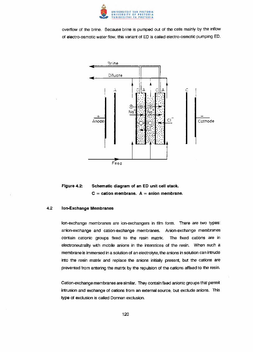
overflow of the brine. Because brine is pumped out of the cells mainly by the inflow
of electro-osmotic water flow, this variant of ED is called electro-osmotic pumping ED.
+Anode
A C
.. ' .:.:. I.. :.:.
••Feed
Schematic diagram of an ED unit cell stack.
C = cation membrane. A = anion membrane.
lon-exchange membranes are ion-exchangers in film form. There are two types:
anion-exchange and cation-exchange membranes. Anion-exchange membranes
contain cationic groups fixed to the resin matrix. The fixed cations are in
electroneutrality with mobile anions in the interstices of the resin. When such a
membrane is immersed in a solution of an electrolyte, the anions in solution can intrude
into the resin matrix and replace the anions initially present, but the cations are
prevented from entering the matrix by the repulsion of the cations affixed to the resin.
Cation-exchange membranes are similar. They contain fixed anionic groups that permit
intrusion and exchange of cations from an external source, but exclude anions. This
type of exclusion is called Donnan exclusion.
Details of methods for making ion-exchange membranes are presented in the
literature(89- 91) Heterogeneous membranes have been made by incorporating ion-
exchange particles into film-forming resins (a) by dry molding or calendering mixtures
of the ion-exchange and film-forming materials; (b) by dispersing the ion-exchange
material in a solution of the film-forming polymer, then casting films from the solution
and evaporating the solvent; and (c) by dispersing the ion-exchange material in a
partially polymerized film-forming polymer, casting films, and completing the
polymerization.
Heterogeneous membranes with usefully low electrical resistances contain more than
65% by weight of the cross-linked ion-exchange particles. Since these ion-exchange
particles swell when immersed in water, it has been difficult to achieve adequate
mechanical strength and freedom from distortion combined with low electrical
resistance.
To overcome these and other difficulties with heterogeneous membranes,
homogeneous membranes were developed in which the ion-exchange component
forms a continuous phase throughout the resin matrix. The general methods of
preparing homogeneous membranes are as follows(6):
• Polymerization of mixtures of reactants (e.g., phenol, phenolsulfonic acid, and
formaldehyde) that can undergo condensation polymerization. At least one of
the reactants must contain a moiety that either is, or can be made, anionic or
cationic.
• Polymerization of mixtures of reactants (e.g., styrene, vinylpyridine, and
divinylbenzene) that can polymerize by additional polymerization. At least one
of the reactants must contain an anionic or cationic moiety, or one that can be
made so. Also, one of the reactants is usually a cross-linking agent to provide
control of the solubility of the films in water.
• Introduction of anionic or cationic moieties into preformed films by techniques
such as imbibing styrene into polyethylene films, polymerizing the imbibed
monomer, and then sulfonating the styrene. A small amount of cross-linking
agent (e.g., divinylbenzene) may be added to control leaching of the ion-
exchange component. Other similar techniques, such as graft polymerization
of imbibed monomers, have been used to attach ionized groups onto the
molecular chains of preformed films.
• Casting films from a solution of a mixture of a linear film-forming polymer and
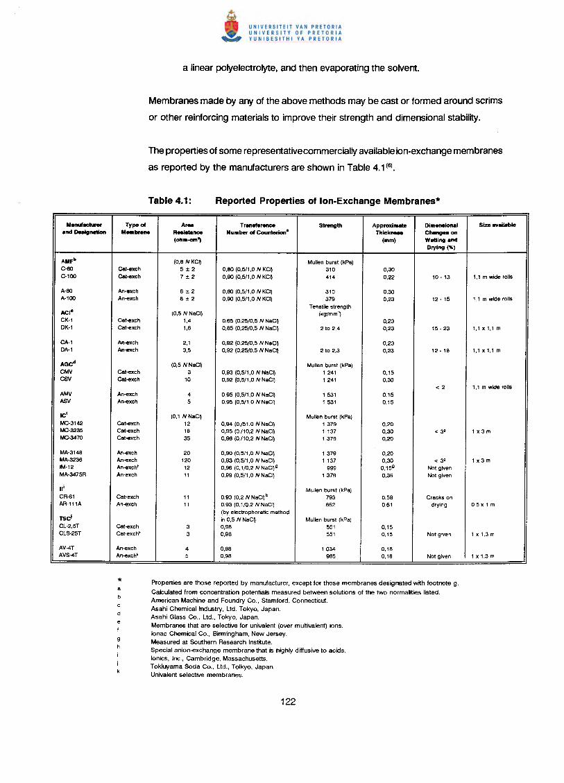
Membranes made by any of the above methods may be cast or formed around scrims
or other reinforcing materials to improve their strength and dimensional stability.
The properties of some representative commercially available ion-exchange membranes
as reported by the manufacturers are shown in Table 4.1 (6).
Menuf __Type of A••• T •.• nafttrtHlCe Strength Approximllte Dim_ionel Size ."eilebie
end Deeignelion M_b •.• ne Reeilltence N umber of Counterion" Thick •••• Cheng_on
(ohm-em') (mm) Welting endDrying (%)
AMFb (0,6 NKC9 Mullen burst (kPa)e-eo cat-exch 5±2 0,60 (0,5/1,0 N KCQ 310 0,30e-100 Cat-exch 7±2 0,90 (0,5/1,0 N KCQ 414 0,22 10 - 13 1,1 m wide rolls
A-60 An·exch 6±2 0,60 (0,5/1,0 N KCQ 310 0,30A·100 An-exch 8±2 0,90 (0,5/1,0 N KCQ 379 0,23 12·15 1,1 m wide rolls
Tenstile strengthACI· (0,5 NNaC9 (kg/mm')CK·1 Cat-exch 1,4 0,85 (0,25/0,5 N NaC9 0,23DK-1 Cat-exch 1,8 0,85 (0,25/0,5 N NaCQ 2to 2,4 0,23 15 - 23 1,1 x 1,1 m
CA-1 An-exch 2,1 0,92 (0,25/0,5 N NaCQ 0,23DA-1 An-exch 3,5 0,92 (0,25/0,5 N NaCQ 2to 2,3 0,23 12·18 1,1 x 1,1 m
AGCd (0,5 NNaCQ Mullen burst (kPa)CMV cat-exch 3 0,93 (0,5/1,0 N NaC9 1241 0,15CSV cat-exch 10 0,92 (0,5/1,0 N NaC9 1241 0,30
<2 1,1 m wide rolls
AMV An-exch 4 0,95 (0,5/1,0 N NaCQ 1531 0,15ASV An-exch 5 0,95 (0,5/1,0 N NaC9 1531 0,15
ICI (0,1 NNaCQ Mullen burst (kPa)MC-3142 cat·exch 12 0,94 (0,/51,0 NNaCQ 1379 0,20Me-3235 Cal-exch 18 0,95 (0'/10,2 N NaC9 1137 0,30 < 3· 1x3mMe-347O Cat-exch 35 0,98 (0,/10,2 NNaCQ 1379 0,20
MA·3148 An-exch 20 0,90 (0,5/1,0 N NaC9 1379 0,20MA·3236 An-exch 120 0,93 (0,5/1,0 N NaC9 1137 0,30 < 3· 1 x3 mIM·12 An-exchh 12 0,96 (0,1/0,2 N NaCQ g 999 0,15g Not givenMA-3475R An-exch 11 0,99 (0,5/1,0 N NaCQ 1379 0,36 Not given
III Mullen burst (kPa)CR-61 Cat-exch 11 0,93 (0,2 N NaCQb 793 0,58 Cracks onAR-111A An-exch 11 0,93 (0,1/0,2 N NaC9 862 0,61 drying 0,5 x 1 m
TSCJ(by electrophoretic methodin 0,5 NNaCQ Mullen burst (kPa)
CL-2,ST cat·exch 3 0,98 551 0,15CLS-25T Cat~exchk 3 0,98 551 0,15 Not given 1 x 1,3 m
AV-4T An-exch 4 0,98 1034 0,18AVS-4T An-exchk 5 0,98 965 0,18 Not given 1 x 1,3 m
Properties are those reported by manufacturer, except for those membranes designated with footnote g.
Calculated from concentration potentials measured between solutions of the two normalities listed.American Machine and Foundry Co., Stamford, Connecticut.Asahi Chemical Industry, Ltd. Tokyo, Japan.Asahi Glass Co., Ltd., Tokyo, Japan.Membranes that are selective for univalent (over muilivalent) ions.Ionac Chemical Co., Birmingham, New Jersey.Measured at Southern Research Institute.Special anion-exchange membrane that is highly diffusive to acids.lonics, Inc., Cambridge, Massachusetts.Tokluyama Soda Co .. Ltd., Tolkyo, Japan.Univalent selective membranes.
Fouling of ED membranes by dissolved organic and inorganic compounds may be a
serious problem in practical electrodialysis(6,92, 93) unless the necessary precautions
(pretreatment) are taken. Organic fouling is caused by the precipitation of large
negatively charged anions on the anion-permeable membranes in the dialysate
compartments.
a) The anion is small enough to pass through the membrane by electromigration
but causes only a small increase in electrical resistance and a decrease in
permselectivity of the membrane;
b) The anion is small enough to penetrate the membrane, but its electromobility
in the membrane is so low that its hOld-up in the membrane causes a sharp
increase in the electrical resistance and a decrease in the permselectivity of the
membrane;
c) The anion is too big to penetrate the membrane and accumulates on the
surface (to some extent determined by the hydrodynamic conditions and also
by a phase change which may be brought about by the surface pH). The
decrease in electrical resistance and permselectivity of the membrane is slight.
The accumulation can be removed by cleaning.
In case (c) the electrodialysis process will operate without serious internal membrane
fouling and only mechanical (or chemical) cleaning will be necessary. Case (b) would
make it almost impossible to operate the electrodialysis process. In case (a), the
electrodialysis process can be used if the concentration of large anions in solution is
low or if the product has a high enough value to cover the high electrical energy costs.
Inorganic fouling is caused by the precipitation (scaling) of slightly soluble inorganic
compounds (such as CaS04 and CaC03) in the brine compartments and the fixation
of multivalent cations (such as Fe and Mn) on the cation-permeable membranes.
Organic anions or multivalent cations can neutralize or even reverse the fixed charge
of the membranes, with a significant reduction in efficiency. Fouling also causes an
increase in membrane stack resistance which, in turn, increases electrical consumption
and adversely effects the economics of the process.
The following constituents are, to a greater of lesser extent, responsible for membrane
fouling(94):
• Traces of heavy metals such as Fe, Mn and Cu.
• Dissolved gases such as O2, CO2 and H2S.
• Silica in diverse polymeric and chemical forms.
• Organic and inorganic colloids.
• Fine particulates of a wide range of sizes and composition.
• Alkaline earths such as Ca, Ba and Sr.
• Dissolved organic materials of both natural and man-made origin in a wide
variety of molecular weights and compositions(92).
• Biological materials - viruses, fungi, algae, bacteria - all in varying stages of
reproduction and life cycles.
Many of these foulants may be controlled by pretreatment steps which usually stabilize
the ED process. However, according to Katz(94),the development of the EDR process
has helped to solve the pretreatment problem more readily in that it provides self-
cleaning of the vital membrane surfaces as an integral part of the desalting process.
Pretreatment techniques for ED are similar to those used for ROle). Suspended solids
are removed by sand and cartridge filters ahead of the membranes. Suspended
solids, however, must be reduced to a much lower level for RO than for ED. The
precipitation of slightly soluble salts in the standard ED process may be minimized by
ion-exchange softening and/or reducing the pH of the brine through acid addition
and/or the addition of an ihibiting agent.
Organics are removed by carbon filters, and hydrogen sulphide by oxidation and
filtration. Biological growths are prevented by a chlorination-dechlorination step. The
dechlorination step is necessary to protect the membranes from oxidation. Iron and
manganese are removed by green sand filters, aeration, or other standard water
treatment methods. It has been suggested that multivalent metal and organic ions, and
hydrogen sulphide, however, must be reduced to a lower level for EDR than for RO(95).
The overall requirements for pretreatment in ED, may be somewhat less rigorous than
for RO due to the nature of the salt separation and the larger passages provided(e).
In ED, the ions (impurities) move through the membranes, while in RO the water moves
under a high pressure through the membranes while the salts are rejected. Salts with
a low solubility can, therefore, more readily precipitate on spiral and hollow fine fibre
RO membranes to cause fouling and to block the small water passages. Suspended
solids can also more readily form a deposit. However, this might not be the case with
tubular RO membranes. With the EDR process, precipitated salts in the brine
compartments can be more readily dissolved and flushed out of the system using
polarity reversal without the need for chemical pretreatment.
However, high removals of suspended solids, iron, manganese, organics and hydrogen
sulphide are still critical to avoid fouling and suppliers of EDR equipment recommend
pretreatment of the feed water(B), if it contains the following ions: Fe > 0,3 mg/Q; Mn
> 0,1 mg/Q; H2S > 0,3 mg/Q; free chlorine and turbidity > 2 NTU. In every case, of
course, a careful examination of the prospective water would be necessary to
determine suitability and pretreatment.
A certain degree of fouling is, however, unavoidable. Membranes should, therefore,
be washed regularly with dilute acid and alkali solutions to restore performance.
The EDR product water is usually less aggressive than the RO product because acid
is usually not added in EDR for scale control(95). Post-pH adjustment may, therefore,
not be required as with RO. Non-ionic matter in the feed such as silica, particulates,
bacteria, viruses, pyrogens and organics will not be removed by the ED process and
must, if necessary, be dealt with during post-treatment.
There is limited application of ED for seawater desalination because of high costS(B).
A small batch system (120 m3/d) has been in operation in Japan since 1974 to produce
water of potable quality at a power consumption of 16,2 kWh/m3 product water(96). A
200 m3/d seawater EDR unit was evaluated in China(97J. This unit operated at 31°C;
its performance was stable; total electric power consumption was 18,1 kWh/m3
product water and the product water quality of 500 mg/Q TDS met all the requirements
for potable water. When the stacks were disassembled for inspection, there were no
signs of scale formation.
With .the commercial ED units currently available, the energy usage for seawater
desalination is relatively high compared with that of RO. However, work under the
Office of Water Research and Technology (OWRT) programmes has indicated that
high-temperature ED may possibly be competitive with RO (98).Results have shown that
the power consumption can be reduced to the levels required for seawater RO (8
kWh/m3) and that a 50% water recovery can probably be attained.
A considerable number of standard ED plants for the production of potable water from
brackish water are in operation(8, 87). These plants are operating suc<?essfully.
However, after the introduction of the reversal process in the early 1970's, lonics
Incorporated shifted almost all their production to this process(94).
The major application of the EDR process is for the desalination of brackish water. The
power consumption and, to some degree, the cost of equipment required is directly
proportional to the TDS to be removed from the feed water(8). Thus, as the feedwater
IDS increases, the desalination costs also increase. In the case of the RO process,
a cost: IDS removal relationship also exists, but it is not as pronounced. Often the
variation in the scaling potential of the feed water and its effect on the percentage of
product water recovery can be more important than the cost: IDS relationship.
Thus, for applications requiring low IDS removals, ED is often the most energy-efficient
method, whereas with highly saline feed waters RO may be expected to use less
energy and is preferred. The economic crossover point between ED and RO based
on operating costs is, however, difficult to define precisely and needs to be determined
on a site-specific basis. Apart from local power costs, other factors must also be
considered in determining the overall economics. Among these, to the advantage of
ED, are the high recoveries possible (up to 90%), the elimination of chemical dosing
(with EDR), and the reliability of performance that is characteristic of the ED process.
The energy consumption of a typical EDR plant is as follows(8):
Pump 0,5 to 1,1 kWh/m3 product water
Membrane stack 0,7 kWh/m3 product water/1 000 mg of IDS removed
Power losses 5% of total energy usage
The major energy requirement, therefore, is for pumping the water through the ED unit
and for the transport of the ions through the membranes.
The successful performance of EDR on high calcium sulphate waters has been
reported(84). Brown(99)has described the performance of and EDR plant treating 300
m3/d of a high calcium sulphate water with a TDS of 9 700 mg/Q. The only
pretreatment applied was iron removal on green sand. The quality of the feed, product
and brine is shown in Table 4.2
The water recovery and energy consumption were 40% and 7,7 kWh/m3 of product
water, respectively. No attempt was made to optimize water recovery. The stack
resistance increased by only 3% after one year of operation, which clearly indicates the
successful operation of the EDR unit in spite of the super saturated condition of the
brine with respect to calcium sulphate. Membrane life times are estimated to be 10
years.
• EDR has achieved CaS04 saturation in the brine stream of up to 440%
without performance decline on tests of several hundred hours' duration(99).
• EDR has desalted a hard (Ca2+ approx. 150 mg/~) brackish water of 4 000
mg/~ IDS at water recoveries of up to 93% without cumbersome and
expensive pre-softening(94).
• An EDR test unit has achieved 95% or greater recovery of a limited 4 000
mg/~ IDS brackish water resource by substituting a more abundant 14 000
mg/~ saline water in the brine stream(l00).The substitution of seawater in the
brine stream would be freely available in coastal or island locations with limited
high quality brackish water resources.
• The development, extensive field testing and subsequent large-scale
commercial usage of a new family of thick (0,5 mm), rugged anti-fouling anion-
permeable membranes in the USA with much higher current efficiencies and
chlorine resistance than those formerly available(100).
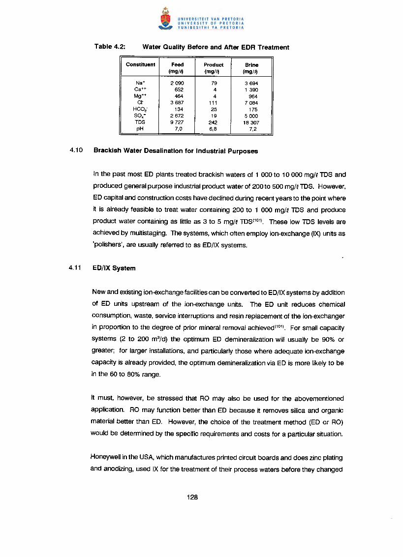
Constituent Feed Product Brine(mgN) (mg/~) (mg/~)
Na+ 2090 79 3694Ca++ 652 4 1 390Mg++ 464 4 964
CI- 3687 111 7084HCO; 134 25 175SO.- 2672 19 5000TOS 9727 242 18307pH 7,0 6,8 7,2
In the past most ED plants treated brackish waters of 1 000 to 10 000 mg/~ TDS and
produced general purpose industrial product water of 200 to 500 mgN TDS. However,
ED capital and construction costs have declined during recent years to the point where
it is already feasible to treat water containing 200 to 1 000 mgN TDS and produce
product water containing as little as 3 to 5 mg/~ TDS(101). These low TDS levels are
achieved by multistaging. The systems, which often employ ion-exchange (IX) units as
'polishers', are usually referred to as ED/IX systems.
New and existing ion-exchange facilities can be converted to ED/IX systems by addition
of ED units upstream of the ion-exchange units. The ED unit reduces chemical
consumption, waste, service interruptions and resin replacement of the ion-exchanger
in proportion to the degree of prior mineral removal achieved(101). For small capacity
systems (2 to 200 m3/d) the optimum ED demineralization will usually be 90% or
greater; for larger installations, and particularly those where adequate ion-exchange
capacity is already provided, the optimum demineralization via ED is more likely to be
in the 60 to 80% range.
It must, however, be stressed that RO may also be used for the abovementioned
application. RO may function better than ED because it removes silica and organic
material better than ED. However, the choice of the treatment method (ED or RO)
would be determined by the specific requirements and costs for a particular situation.
Honeywell in the USA, which manufactures printed circuit boards and does zinc plating
and anodizing, used IX for the treatment of their process waters before they changed
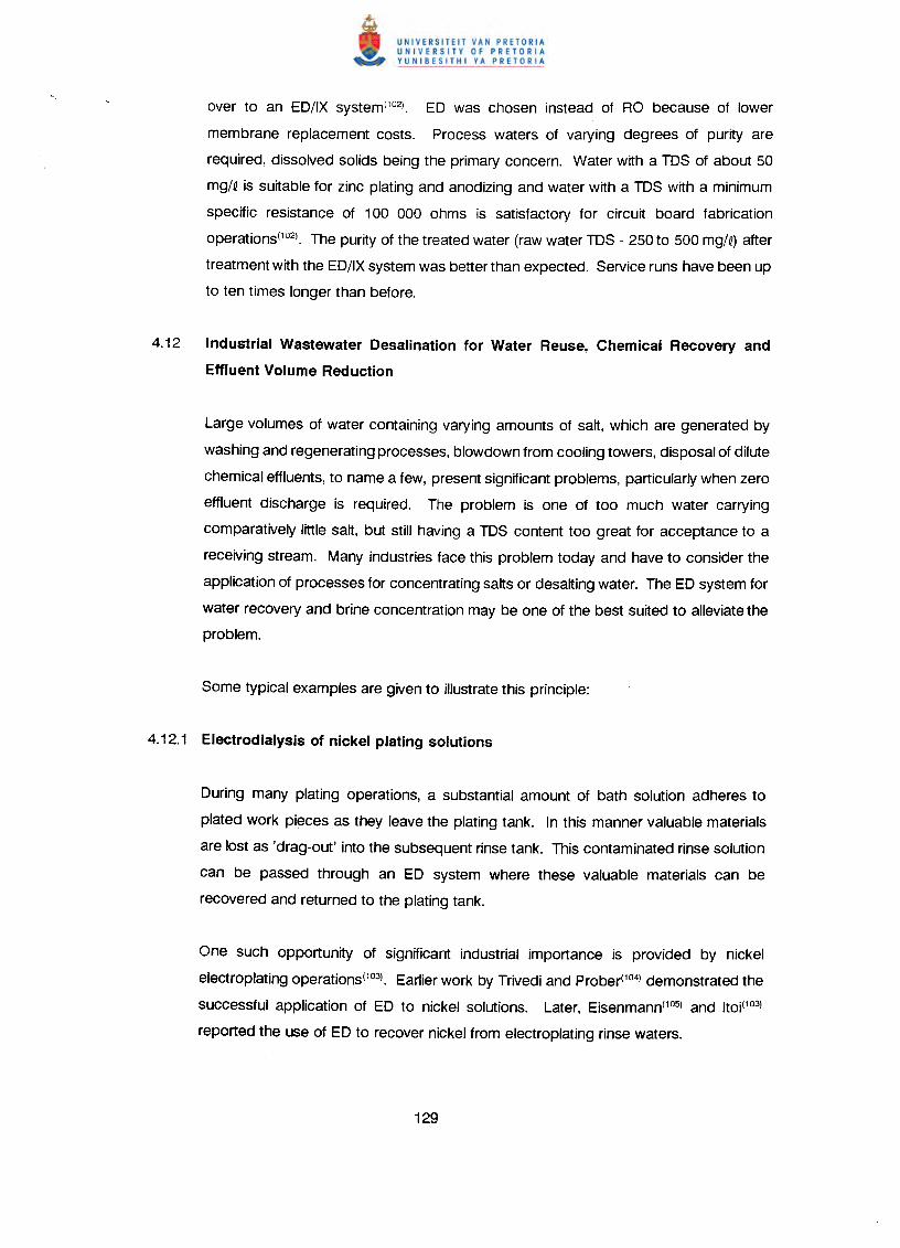
over to an ED/IX system(102). ED was chosen instead of RO because of lower
membrane replacement costs. Process waters of varying degrees of purity are
required, dissolved solids being the primary concern. Water with a TDS of about 50
mg/~ is suitable for zinc plating and anodizing and water with a TDS with a minimum
specific resistance of 100 000 ohms is satisfactory for circuit board fabrication
operations(102). The purity of the treated water (raw water TDS - 250 to 500 mg/~) after
treatment with the ED/IX system was better than expected. Service runs have been up
to ten times longer than before.
4.12 Industrial Wastewater Desalination for Water Reuse, Chemical Recovery and
Effluent Volume Reduction
Large volumes of water containing varying amounts of salt, which are generated by
washing and regenerating processes, blowdown from cooling towers, disposal of dilute
chemical effluents, to name a few, present significant problems, particularly when zero
effluent discharge is required. The problem is one of too much water carrying
comparatively little salt, but still having a TDS content too great for acceptance to a
receiving stream. Many industries face this problem today and have to consider the
application of processes for concentrating salts or desalting water. The ED system for
water recovery and brine concentration may be one of the best suited to alleviate the
problem.
During many plating operations, a substantial amount of bath solution adheres to
plated work pieces as they leave the plating tank. In this manner valuable materials
are lost as 'drag-out' into the subsequent rinse tank. This contaminated rinse solution
can be passed through an ED system where these valuable materials can be
recovered and returned to the plating tank.
One such opportunity of significant industrial importance is provided by nickel
electroplating operations(103). Earlier work by Trivedi and Prober(104)demonstrated the
successful application of ED to nickel solutions. Later, Eisenmann(105) and Itoi(103)
reported the use of ED to recover nickel from electroplating rinse waters.
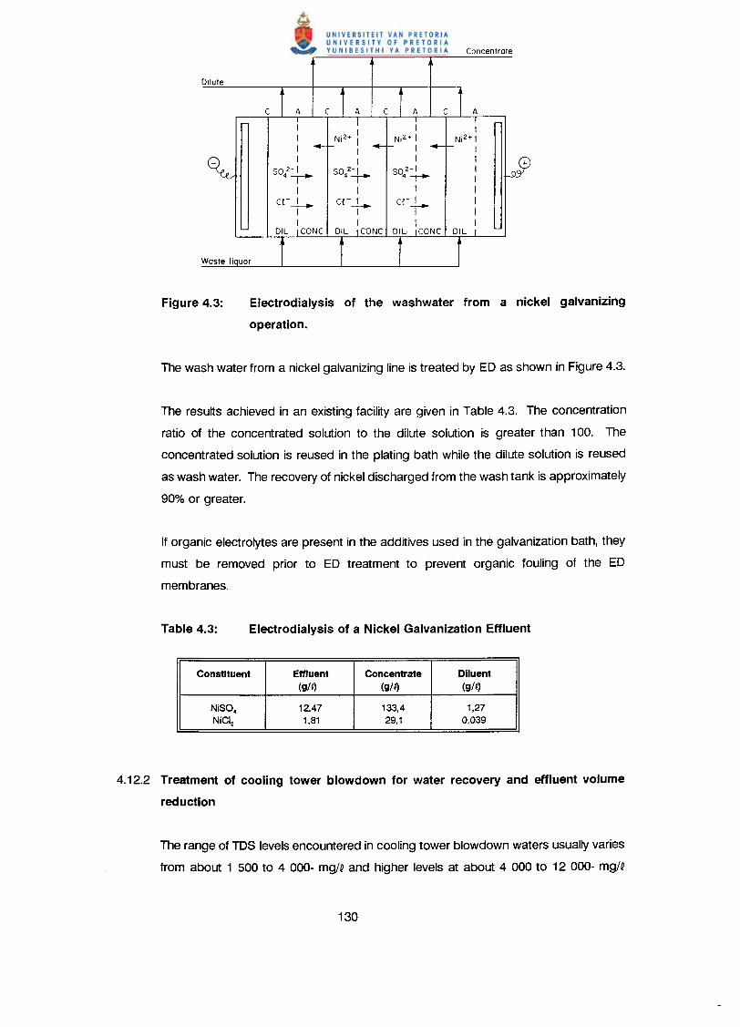
Concentrate
Dilute
C A
INi2+ I
II +IIIIII
Electrodialysis of the washwater from a nickel galvanizing
operation.
The results achieved in an existing facility are given in Table 4.3. The concentration
ratio of the concentrated solution to the dilute solution is greater than 100. The
concentrated solution is reused in the plating bath while the dilute solution is reused
as wash water. The recovery of nickel discharged from the wash tank is approximately
90% or greater.
If organic electrolytes are present in the additives used in the galvanization bath, they
must be removed prior to ED treatment to prevent organic fouling of the ED
membranes.
Constituent Effluent Concentrate Diluent(gN) (g/#) (g/#)
NiSO. 12,47 133,4 1,27NiCI2 1,81 29,1 0,039
4.12.2 Treatment of cooling tower blowdown for water recovery and effluent volume
reduction
The range of IDS levels encountered in cooling tower blowdown waters usually varies
from about 1 500 to 4 000- mg/~ and higher levels at about 4 000 to 12 000- mg/~
have also been reported(106). The disposal of large volumes of this saline effluent can
be a serious problem. The application of ED for the treatment of blowdown streams
to recover good quality water for reuse and produce a small volume of concentrate
promises to be the best prospective system available(107,108).
Slowdown waters from cooling towers can be concentrated tenfold or more using ED,
while recovering and recycling the desalted water to the cooling tower at one-half its
original concentration(88). To accomplish this, blowdown is pretreated, filtered and
passed through the ED system. Sy recirculation of the brine, it is possible to
concentrate the salts into a small stream, while allowing for recovery of about 90% of
the water.
The concentration of cooling blowdown waters in an EDR pilot plant at one of Eskom's
power stations was evaluated(61). Pretreatment of the blowdown water with lime
softening, clarification, pH reduction, filtration and chlorination was found to be a basic
precondition for successful operation. The operating experience on the EDR pilot plant
was sufficiently positive to warrant full-scale application.
Detailed design studies and cost estimates for ED and several other alternative
blowdown recovery/concentration systems have been reported(88). The side stream
process design which utilizes ED results in the lowest capital costs for the conditions
specified. According to Wirth and Westbrook (86), it is expected that if the cost
comparison were made on overall annual operating costs, the same results would
occur.
4.13.1 Concentration of sodium sulphate and its conversion into caustic soda and
suiphuric acid
A pilot stUdy has demonstrated the feasibility of the concentration of a sodium sulphate
solution with ED in a first stage and the subsequent conversion into caustic soda and
sulphuric acid in a second stage(109). The sodium sulphate solution (20 to 40 g/~) was
treated in a multi-compartment electrodialyzer to yield a brine (260 - 320 g/~, 10% of
feed volume) and a product (2 g/Q, 90% of feed volume) which could be used as
reclaimed water.
The brine was treated further in a three-compartment electrodialyzerto produce caustic
soda and sulphuric acid at a concentration of 17 to 19% by mass and a power
consumption of approximately 3,1 to 3,3 kWh/kg sodium sulphate decomposed. The
sodium sulphate content of both products was about 1%.
Laboratory results of an electrodialytic process for acid and caustic recovery from ion-
exchange regenerant wastes have been described(110). The object of the study was to
minimize the discharge of dissolved salts from a water treatment plant producing boiler
feed water while recovering some of the pollution abatement process costs from the
savings in regenerant chemical costs.
It was shown that the electrodialytic process for recovery of sulphuric acid and sodium
hydroxide from ion-exchange regenerant wastes, and substantially reducing the
amount of salt discharged to drain, is technically feasible. The nett costs for acid and
caustic waste treatment was estimated at US $4,20 and $3,00/m3 waste treated,
respectively .
Laboratory investigations have shown that dilute (approximately 2%) solutions of
NH4N03, N~S04' NaN03 and NaCI can be concentrated to approximately 20% by EDat an energy consumption of about 1 kWh/kg salt(111). The brine volumes were less
than 10% of the original volume.
The current which is passed through an ED stack is carried almost exclusively by ions
of the same sign. In the solution, all types of ions carry this current. The rate at which•the current can pass through the solution is limited by the diffusion rate of ions to the
membrane surface since there will inevitably be changes in the concentration of the
solution close to the membrane surface. It is apparent that as the current density is
increased, it becomes more difficult for the ions in the solution to carry the required
current. This effect is know as concentration polarization(ll). The greater the current
density used the greater are these polarization effects. Polarization also becomes a
problem the more dilute the solution becomes.
o the differences in concentration result in increased membrane potentials and
so the power required per unit charge passed is increased.
iO The current efficiency can also be reduced which means that the current
required per unit of output is also increased.
iiO When it is attempted to carry current in excess of the ions available to be
transported through the membrane, the water "splits" into hydroxide and
hydrogen ions. At the anion membrane the current is carried by hydroxide
ions through the membrane and hydrogen ions are re:jectedto the solution.
At the cation membrane the opposite effect occurs: hydroxide ions are
transported to the membrane and are rejected to the solution. This effect is
to be avoided since, firstly, both the current and the voltage efficiency are
reduced (some of the current serves to split the water instead of desalting it
and there is an increased voltage requirement) and secondly, when the water
splits the pH in the boundary layer on the membrane surface can change
increasing the likelihood of scale formation.
It has already been shown that the basic unit in an ED plant is the cell pair where
cation and anion permeable membranes are alternately arranged so as to produce
adjacent diluate and concentrate streams. A number of cell pairs are located between
a pair of electrodes to form what is known as a cell stack. The number of cell pairs
varies depending on the manufacturer but is usually about 300.
In any cell pair the membranes are separated by a spacer. The hydrodynamic design
of the flow between the membranes is of extreme importance(6). It is essential that as
far as it is practicable turbulent flow exists in individual cell pairs. Streamline flow
produces a relativelystagnant or slow moving layer on the membrane surface. Since
the current carrying ions have to diffuse through this film at low solution concentration,
polarization becomes more likely. There are a number of requirements a spacer must
meet. The fluid should flow at the same rate across the whole active membrane area
and should be turbulent within the limits of pressure drop. The manifold must supply
each spacer equally. The spacer should support the membrane, this being particularly
important in the region between the manifolds. The spacer material should be inert,
should possess physical properties so as to permit a hydraulic seal when pressurised
and be dimensionally stable.
The spacers are usually perforated PVC nets and, depending on the design, are 0,5
mm to 1 mm thick(6). The size of the spacer depends on the size of the membrane
used. In general, large components tend to cost less per unit of effective membrane
area. However, practical considerations such as the ease of handling and mechanical
strength must be taken into account. Components which are thin result in lower
operating costs but there are difficulties in providing good flow distribution. It is
apparent that the presence of the spacer reduces the active membrane area since it
also serves to support the membrane. There is an advantage in utilising as much of
the membrane surface area as possible but this results in difficulties in supporting and
sealing the membranes. A membrane of about 1,5 m2 is probably the maximum
practicable, usually the area is 0,5 m2 to 1 m2• The effective membrane area is about
85 % of the total membrane area.
Stack sealing is of importance to stack operation. The spacer should seal easily since
the lower compression force required to seal the stack, the less likely will be the
chance of damaging components. This aspect of design becomes most complex in
the region of manifolds. This area should be as small as possible but should not
cause a high pressure drop. Also, since a seal must be made round this area the
support in this region must be able to withstand the compressive scaling forces of the
stack.
The stack itself should be easy to maintain. It often occurs that only a few cell pairs
in the stack require maintenance. In a large stack it is desirable to be able to open the
stack at any section and remove a cell pair without disturbing any of the other cell
pairs.
The electrodes must be made of a material which is corrosion resistant, since at the
cathode the flow becomes alkaline while at the anode gaseous chlorine and oxygen
are formed. It is normal to have separate feeds to the anode and cathode, the anode
rinse going to a drain while the cathode rinse is treated with acid and then recirculated.
The maximum voltage across a stack is 3 volts per cell pair and so a normal stack
voltage will be about 900 volts.
Since the amount of desalting depends directly on the current level it is a straight-
forward exercise to calculate the performance of a given stack at a particular current
density. In order to achieve a given level of desalination the plant can either be run in
a batch process or in a once-through process(6).
In a batch process, the water to be desalinated is stored in a tank and then partially
desalted by passing it through the stack to a second tank having been further
desalted. After each pass the concentration is checked and the process is repeated
until the required levelof demineralization is achieved. This method is often used when
the feed water is subject to changes in composition. For example, in a lot of cases
brackish well water is liable to increase in salinity at high pumping rates.
In a once-through system, the required desalting is achieved by passing the diluate
stream through successive stacks arranged hydraulically in series. This process tends
to be used in the higher capacity plants and requires less control systems. Where
possible (i.e. where the feed water salinity can be guaranteed) a continuous type of
plant is always to be preferred. Since plant operation is simpler, the likelihood of
breakdown is reduced and the capital cost is reduced.
In both systems the concentrate streams are recycled to minimize blow-down and
possible use of chemicals. The flow of the concentrate stream is normally 25% or less
than that of the diluate stream. To minimize the electrical resistance of the stack it is
desirable to have the concentrate stream at the maximum concentration possible (this
also minimizes the blow-down to waste). The normal limiting factor for the degree of
concentration is the solubility of calcium sulphate.
In both systems the limiting current density controls the amount of desalination
possible. The onset of polarization manifests itself in the change of chemical conditions
in the plant and also in an increase in the voltage requirements maintaining the current.
The lower the salt content in the water, the lower will be the limiting current density.
Electrodialysis, therefore, is not applicable in the production of high purity waters.
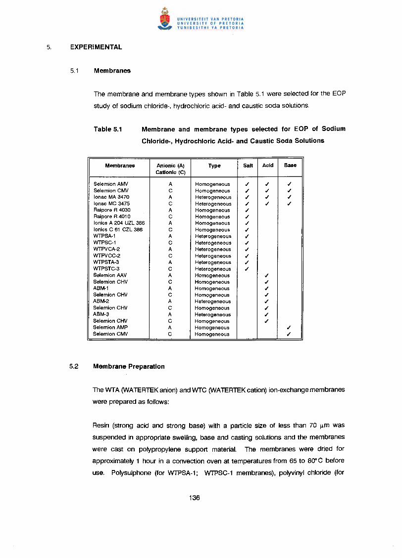
The membrane and membrane types shown in Table 5.1 were selected for the EOP
study of sodium chloride-, hydrochloric acid- and caustic soda solutions.
Membrane and membrane types selected for EOP of Sodium
Chloride-, Hydrochloric Acid- and Caustic Soda Solutions
Membranes Anionic (A) Type Salt Acid BaseCationic (C)
Selemion AMV A Homogeneous ,/ ,/ ,/
Selemion CMV C Homogeneous ,/ ,/ ,/
lonac MA 3470 A Heterogeneous ,/ ,/ ,/
lonac MC 3475 C Heterogeneous ,/ ,/ ,/Raipore R 4030 A Homogeneous ,/
Raipore R 4010 C Homogeneous ,/
lonics A 204 UZl 386 A Homogeneous ,/
lonics C 61 CZl 386 C Homogeneous ,/WTPSA·1 A Heterogeneous ,/
WTPSC-1 C Heterogeneous ,/
WTPVCA-2 A Heterogeneous ,/
WTPVCC-2 C Heterogeneous ,/
WTPSTA-3 A Heterogeneous ,/WTPSTC-3 C Heterogeneous ,/Selemion AAV A Homogeneous ,/
Selemion CHV C Homogeneous ,/ABM-1 A Homogeneous ,/
Selemion CHV C Homogeneous ,/
ABM·2 A Heterogeneous ,/
Selemion CHV C Homogeneous ,/ABM-3 A Heterogeneous ,/
Selemion CHV C Homogeneous ,/Selemion AMP A Homogeneous ,/
Selemion CMV C Homogeneous ,/
The WTA (WATERTEKanion) and WTC (WATERTEKcation) ion-exchange membranes
were prepared as follows:
Resin (strong acid and strong base) with a particle size of less than 70 ~m was
suspended in appropriate swelling, base and casting solutions and the membranes
were cast on polypropylene support material. The membranes were dried for
approximately 1 hour in a convection oven at temperatures from 65 to 800 C before
use. Polysulphone (for WTPSA-1; WTPSC-1 membranes), polyvinyl chloride (for
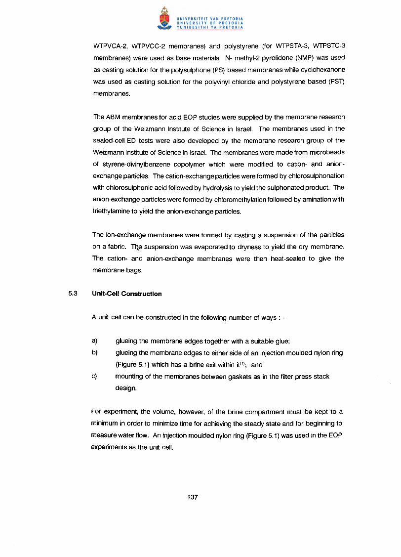
WTPVCA-2, WTPVCC-2 membranes) and polystyrene (for WTPSTA-3, WTPSTC-3
membranes) were used as base materials. N- methyl-2 pyrolidone (NMP) was used
as casting solution for the polysulphone (PS) based membranes while cyclohexanone
was used as casting solution for the polyvinyl chloride and polystyrene based (PST)
membranes.
The ABM membranes for acid EOP studies were supplied by the membrane research
group of the Weizmann Institute of Science in Israel. The membranes used in the
sealed-cell ED tests were also developed by the membrane research group of the
Weizmann Institute of Science in Israel. The membranes were made from microbeads
of styrene-divinylbenzene copolymer which were modified to cation- and anion-
exchange particles. The cation-exchange particles were formed by chlorosulphonation
with chlorosulphonic acid followed by hydrolysis to yield the sulphonated product. The
anion-exchange particles were formed by chloromethylation followed by amination with
triethylamine to yield the anion-exchange particles.
The ion-exchange membranes were formed by casting a suspension of the particles
on a fabric. TIle suspension was evaporated to dryness to yield the dry membrane.
The cation- and anion-exchange membranes were then heat-sealed to give the
membrane bags.
a) glueing the membrane edges together with a suitable glue;
b) glueing the membrane edges to either side of an injection moulded nylon ring
(Figure 5.1) which has a brine exit within it(1); and
c) mounting of the membranes between gaskets as in the filter press stack
design.
For experiment, the volume, however, of the brine compartment must be kept to a
minimum in order to minimize time for achieving the steady state and for beginning to
measure water flow. An injection moulded nylon ring (Figure 5.1) was used in the EOP
experiments as the unit cell.
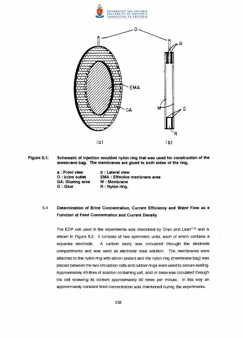
Schematic of injection moulded nylon ring that was used for construction of themembrane bag. The membranes are glued to both sides of the ring.
a : Front viewo : brine outletGA: Glueing areaG: Glue
b : Lateral viewEMA : Effective membrane areaM : MembraneR : Nylon ring.
5.4 Determination of Brine Concentration, Current Efficiency and Water Flow as a
Function of Feed Concentration and Current Density
The EOP cell used in the experiments was described by Oren and Litan(112)and is
shown in Figure 5.2. It consists of two symmetric units, each of which contains a
separate electrode. A carbon slurry was circulated through the electrode
compartments and was used as electrode rinse solution. The membranes were
attached to the nylon ring with silicon sealant and the nylon ring (membrane bag) was
placed between the two circulation cells and rubber rings were used to secure sealing.
Approximately 40 litres of solution containing salt, acid or base was circulated through
the cell renewing its content approximately 60 times per minute. In this wayan
approximately constant feed concentration was maintained during the experiments.
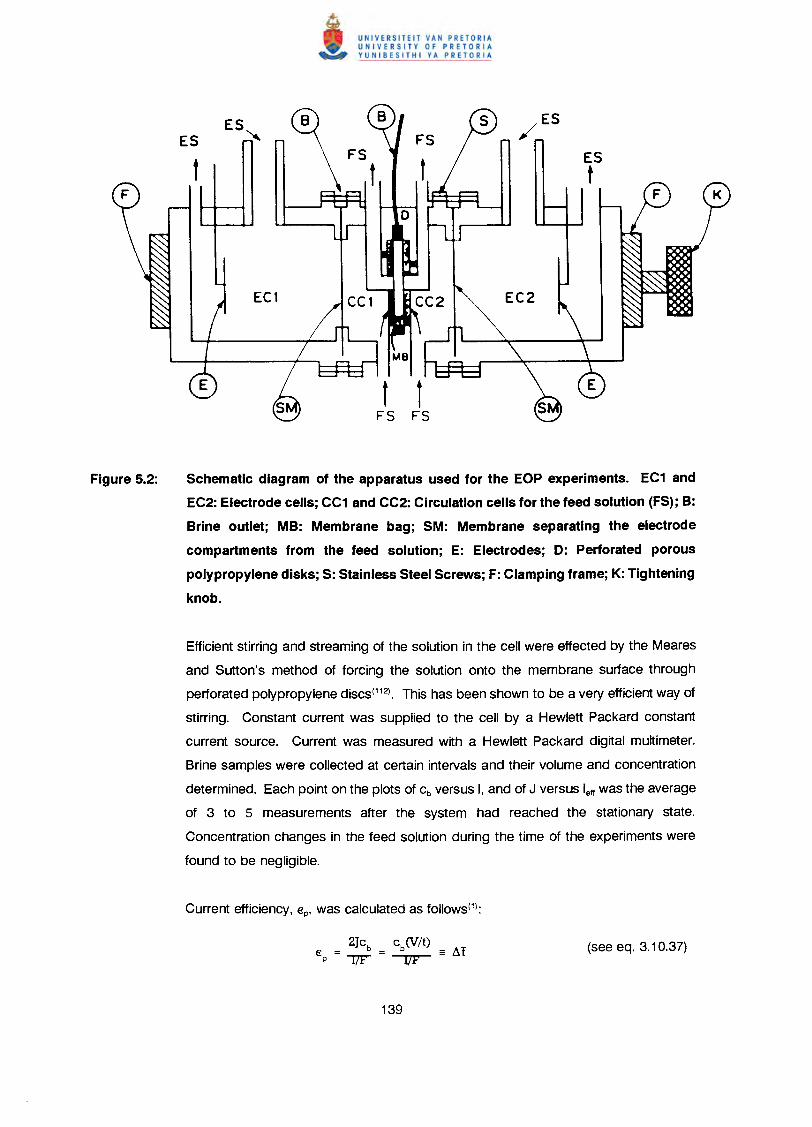
ES~
ESt
Schematic diagram of the apparatus used for the EOP experiments. EC1 and
EC2: Electrode cells; CC1 and CC2: Circulation cells for the feed solution (FS); B:
Brine outlet; MB: Membrane bag; SM: Membrane separating the electrode
compartments from the feed solution; E: Electrodes; D: Perforated porous
polypropylene disks; S: Stainless Steel Screws; F: Clamping frame; K: Tightening
knob.
Efficient stirring and streaming of the solution in the cell were effected by the Meares
and Sutton's method of forcing the solution onto the membrane surface through
perforated polypropylene discs(112). This has been shown to be a very efficient way of
stirring. Constant current was supplied to the cell by a Hewlett Packard constant
current source. Current was measured with a Hewlett Packard digital multimeter.
Brine samples were collected at certain intervals and their volume and concentration
determined. Each point on the plots of cb versus I, and of J versus lelfwas the average
of 3 to 5 measurements after the system had reached the stationary state.
Concentration changes in the feed solution during the time of the experiments were
found to be negligible.
where cb represents the brine concentration, V the volume of the solution that enters
the bag per unit area (7,55 cm2) in t seconds (V/t = 2J), I the applied current density
(mA/cm2) and F is Faraday's constant.
where 2B is the electro-osmotic coefficient determined from the slope of the J versus
leftplots and F is Faraday's constant.
The difference between the counter- and co-ion transport number, at, which is called
the apparent transport number or membrane permselectivity, was measured as follows:
The potential (a1f m) of a membrane is usually measured between 0,1/0,2 molN or
0,5/1,0 mol/Q sodium chloride solutions in a specially designed cell with calomel
electrodes. The theoretical potential, a1f;, is calculated from the activities of the two
solutions. Membrane permselectivity, at, can then be calculated from these values
where a1f m is the measured potential and a"11/a" 1 is the ratio of salt activities on both
sides of the membrane.
Approximately 3 g dried membrane sample (weighed accurately) was equilibrated with
150 ml 1 mol/Q hydrochloric acid for 16 hours at room temperature. The membrane
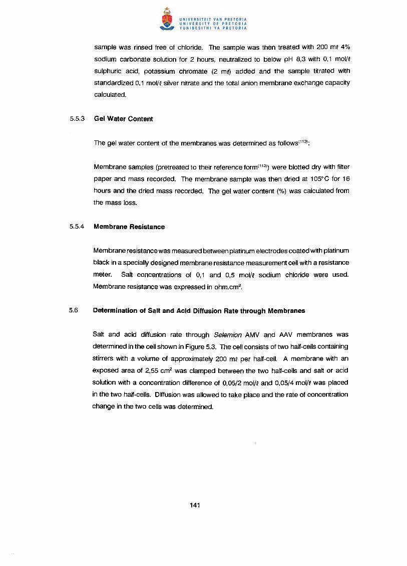
sample was rinsed free of chloride. The sample was then treated with 200 mQ 4%
sodium carbonate solution for 2 hours, neutralized to below pH 8,3 with 0,1 mol/Q
sulphuric acid, potassium chromate (2 mQ) added and the sample titrated with
standardized 0,1 mol/Q silver nitrate and the total anion membrane exchange capacity
calculated.
Membrane samples (pretreated to their reference form(113))were blotted dry with filter
paper and mass recorded. The membrane sample was then dried at 1050 C for 16
hours and the dried mass recorded. The gel water content (%) was calculated from
the mass loss.
Membrane resistance was measured between platinum electrodes coated with platinum
black in a specially designed membrane resistance measurement cell with a resistance
meter. Salt concentrations of 0,1 and 0,5 mol/o sodium chloride were used.
Membrane resistance was expressed in ohm.cm2•
Salt and acid diffusion rate through Selemion AMV and AAV membranes was
determined in the cell shown in Figure 5.3. The cell consists of two half-cellscontaining
stirrers with a volume of approximately 200 mQ per half-cell. A membrane with an
exposed area of 2,55 cm2 was clamped between the two half-cells and salt or acid
solution with a concentration difference of 0,05/2 mot/oand 0,05/4 molN was placed
in the two half-cells. Diffusion was allowed to take place and the rate of concentration
change in the two cells was determined.
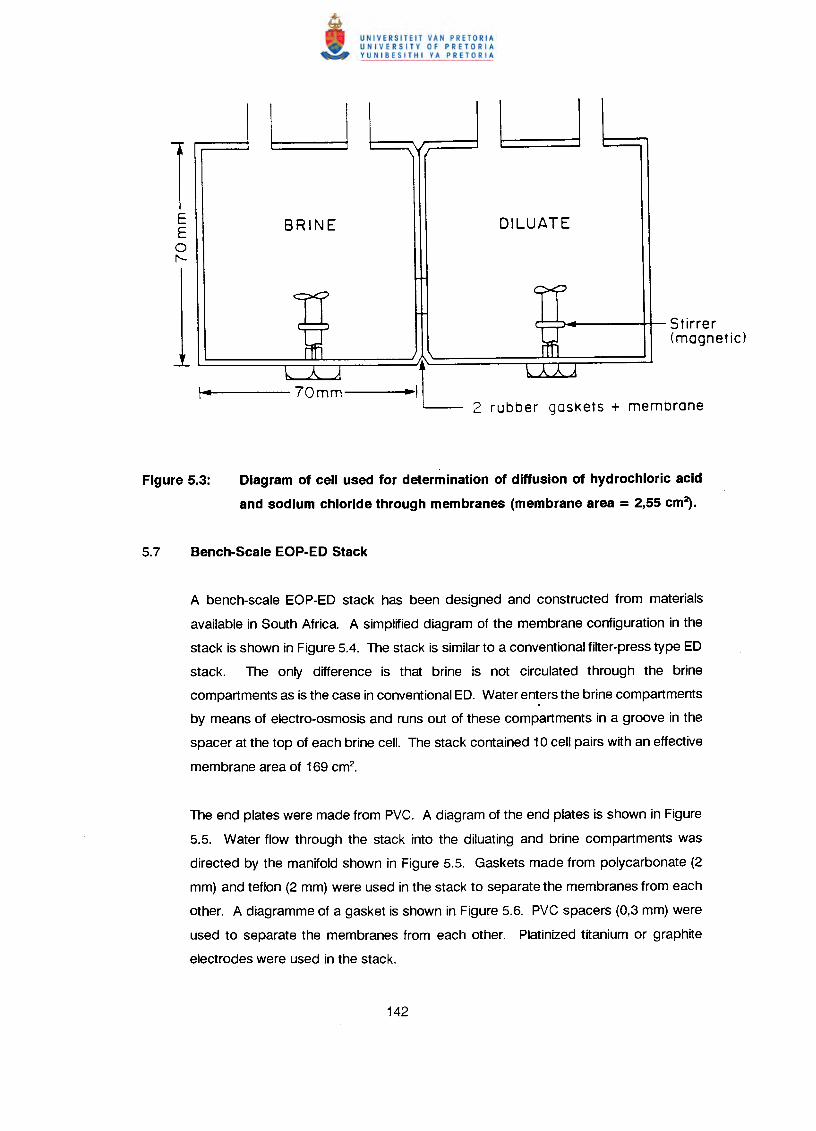
1 LJ LJE BRINE DILUATEE0I'-
70mm-------IL 2 rubber gaskets + membrane
Stirrer(magnetic)
Diagram of cell used for determination of diffusion of hydrochloric acid
and sodium chloride through membranes (membrane area = 2,55 cm~.
A bench-scale EOP-ED stack has been designed and constructed from materials
available in South Africa. A simplified diagram of the membrane configuration in the
stack is shown in Figure 5.4. The stack is similar to a conventional filter-press type ED
stack. The only difference is that brine is not circulated through the brine
compartments as is the case in conventional ED. Water enters the brine compartments
by means of electro-osmosis and runs out of these compartments in a groove in the
spacer at the top of each brine cell. The stack contained 10 cell pairs with an effective
membrane area of 169 cm2.
The end plates were made from PVC. A diagram of the end plates is shown in Figure
5.5. Water flow through the stack into the diluating and brine compartments was
directed by the manifold shown in Figure 5.5. Gaskets made from polycarbonate (2
mm) and teflon (2 mm) were used in the stack to separate the membranes from each
other. A diagramme of a gasket is shown in Figure 5.6. PVC spacers (0,3 mm) were
used to separate the membranes from each other. Platinized titanium or graphite
electrodes were used in the stack.
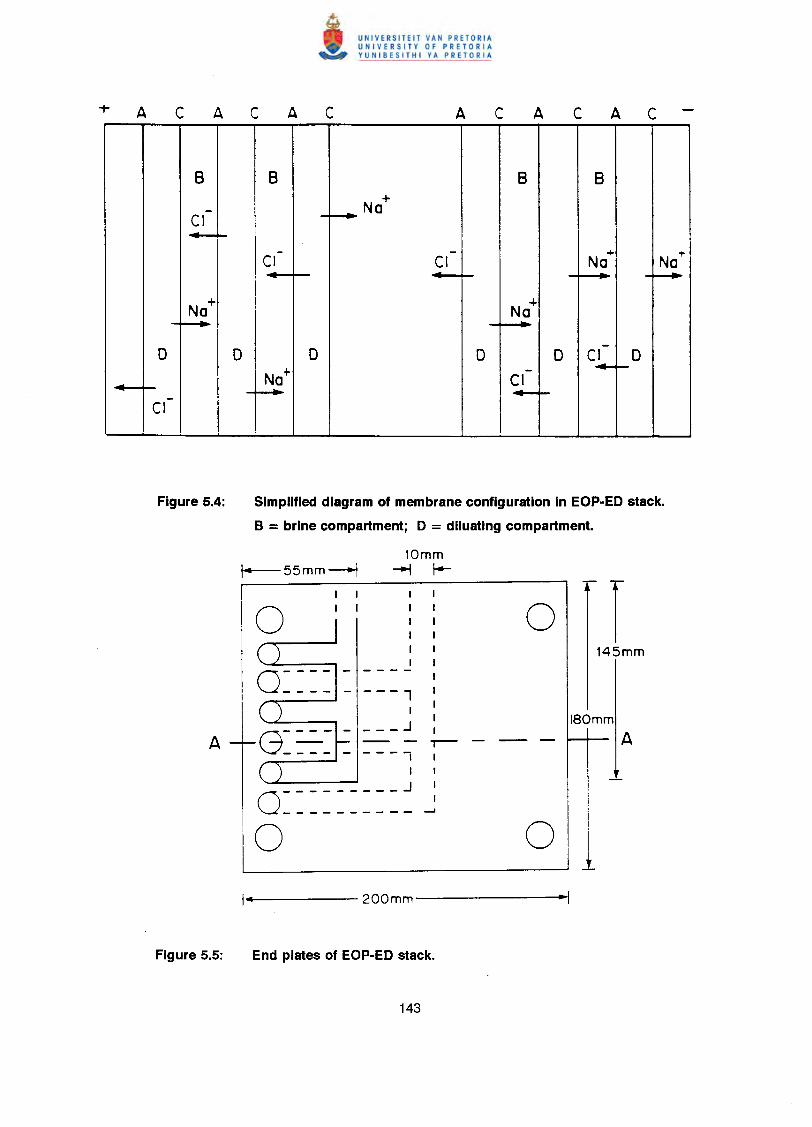
B B B B+- - ~NaCI...--
- - + No+CI CI No-~
No+ No+
0 -0 0 0 0 CI 0Na+ - .•..-CI- ~ ..-.--CI
Simplified diagram of membrane configuration in EOP-ED stack.
S = brine compartment; 0 = diluating compartment.
lOmm-i I--
- ---1I
G===~ = =-=--=----II
IIIIIIIIIII.-II
I
I
o I180mm
A
0---------...1---------- ~
1
0 011
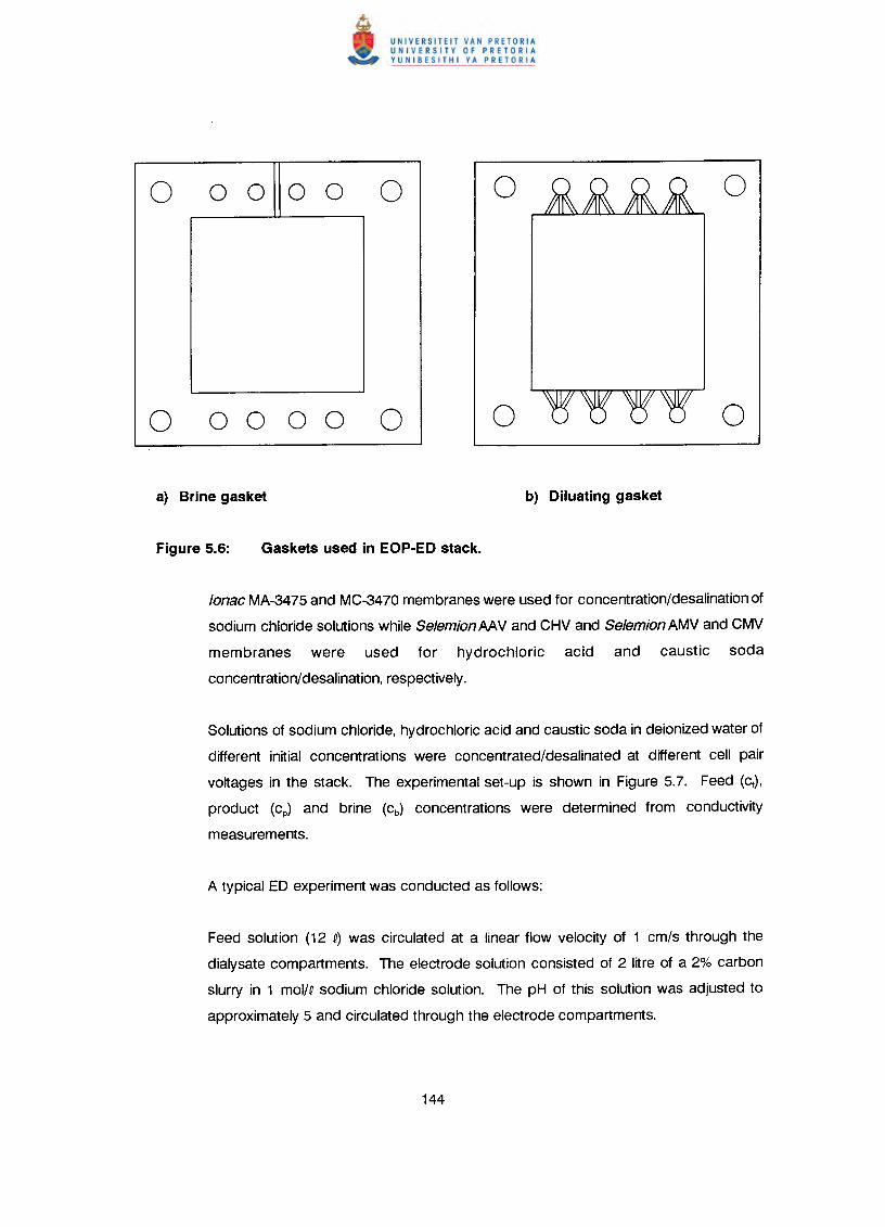
0 0 0 0 0 0
0 0 0 0 0 0
o 0
o 0
lonac MA-3475 and MC-3470 membranes were used for concentration/desalination of
sodium chloride solutions while Selemion AAV and CHV and Selemion AMV and CMV
membranes were used for hydrochloric acid and caustic soda
concentration/desalination, respectively.
Solutions of sodium chloride, hydrochloric acid and caustic soda in deionized water of
different initial concentrations were concentrated/desalinated at different cell pair
voltages in the stack. The experimental set-up is shown in Figure 5.7. Feed (cf) ,
product (cp) and brine (cb) concentrations were determined from conductivity
measurements.
Feed solution (12 Q) was circulated at a linear flow velocity of 1 cm/s through the
dialysate compartments. The electrode solution consisted of 2 litre of a 2% carbon
slurry in 1 mol/Q sodium chloride solution. The pH of this solution was adjusted to
approximately 5 and circulated through the electrode compartments.
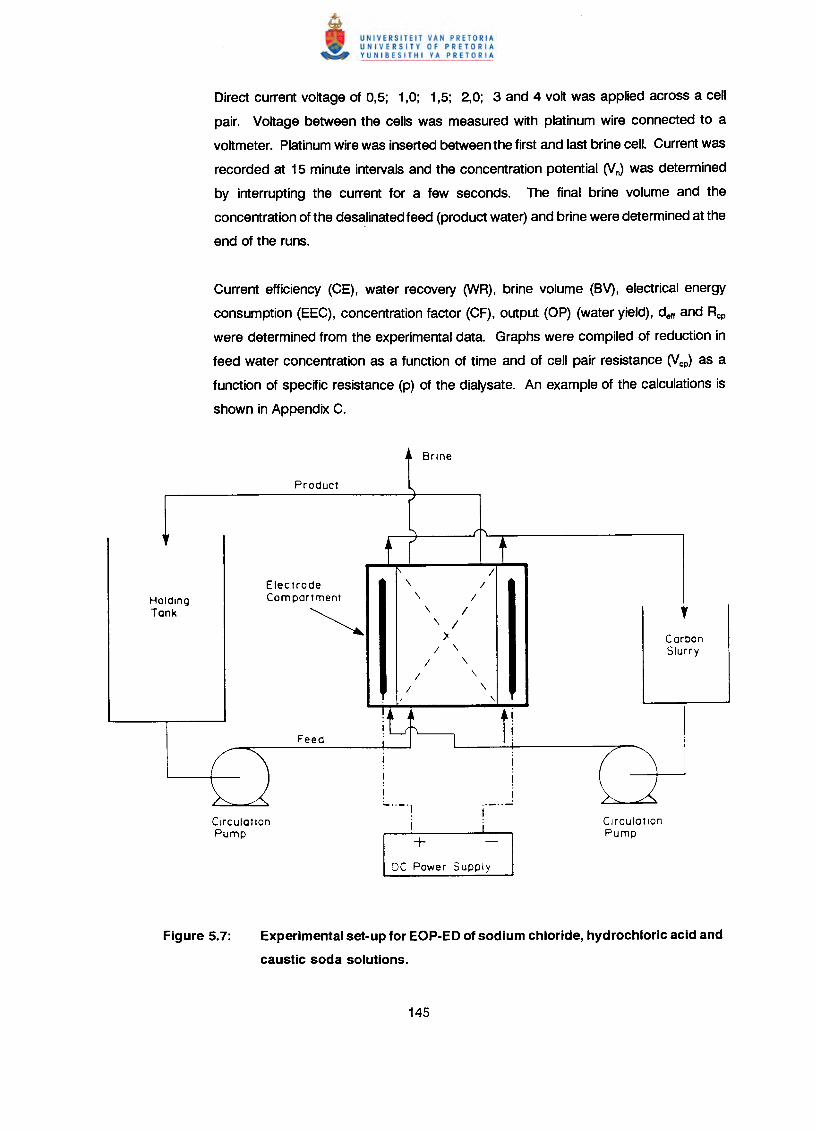
HoldingTonk
Direct current voltage of 0,5; 1,0; 1,5; 2,0; 3 and 4 volt was applied across a cell
pair. Voltage between the cells was measured with platinum wire connected to a
voltmeter. Platinumwire was inserted between the first and last brine cell. Current was
recorded at 15 minute intervals and the concentration potential \V n) was determined
by interrupting the current for a few seconds. The final brine volume and the
concentration of the desalinated feed (product water) and brine were determined at the
end of the runs.
Current efficiency (CE), water recovery (WR), brine volume (BV), electrical energy
consumption (EEC), concentration factor (CF), output (OP) (water yield), delland Rcp
were determined from the experimental data. Graphs were compiled of reduction in
feed water concentration as a function of time and of cell pair resistance \Vcp) as a
function of specific resistance (p) of the dialysate. An example of the calculations is
shown in Appendix C.
ElectrodeCom partment
~
/\ /
\ /\ I\ I
)</ \
/ \/ \
/ \\
CarbonSlurry
I
I_'0_0)
i+
CirculatIOnPump
CirculationPump
Experimental set-up for EOP·ED of sodium chloride, hydrochloric acid and
caustic soda solutions.
A simplified diagram of the sealed-cell (SCED) membrane stack is shown in Figure 5.8.
The brine sealed cells with outlets are arrayed in an open vessel, separated by spacers
(0,3 mm). The dialysate enters through a suitable port at the bottom of the vessel and
runs out through an overflow. Direct current is applied through carbon suspension
electrodes(4). The external dimensions of the sealed brine cells are 60 x 80 mm, giving
an effective membrane area of 100 cm2 per cell pair (cp).
Solutions of sodium chloride, ammonium nitrate, sodium sulphate, sodium nitrate and
calcium chloride in deionized water of different initial concentrations were
concentrated/desalinated at different cell pair voltages in the SCED unit. Feed (cf) ,
product (cp) and brine (cb) concentrations were determined from conductivity
measurements. Various industrial effluents were also treated with SCED.
Feed solution (15 D)was circulated at a linear flow velocity of 15 cm/s through the
dialysate compartments. The electrode solution consisted of 2 D of a 2 % carbon
slurry in 1 mol/D sodium chloride solution. The pH of the solution was adjusted to
approximately 5 and circulated through the electrode compartments.
Electrodialysis was started by applying a DC voltage of approximately 0,5 Volt per cell
pair across 17 membrane bags. Voltage between the membrane bags was measured
with calomel electrodes connected to a salt bridge. Current was recorded at 10 or 20
minute intervals during ED and Vn was determined during interruption of the current for
a short period. The final brine volume, concentration of the desalinated feed (product
water) and brine were determined at the end of the runs.
Current efficiency (CE), water recovery (WR), brine volume (BV), electrical energy
consumption (EEC), concentration factor (CF), output (OP) (water yield), effective
thickness of dialysate compartment (dell)' and membrane resistance (Rcp) were
determined from the experimental data. Graphs were plotted of feed water
concentration, brine concentration, current efficiency and electrical energy consumption
as a function of time, and of cell pair voltage as a function of the specific resistance (p)
of the dialysate.
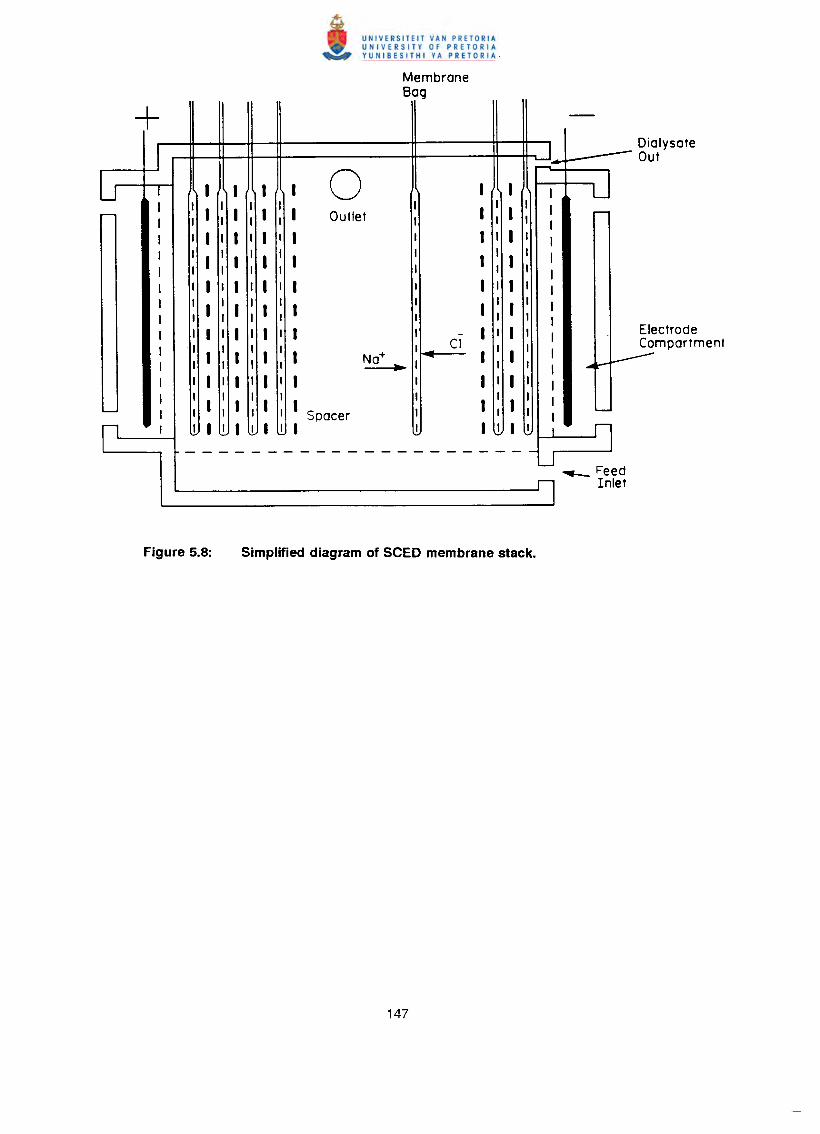
MembraneBag
+ -I-Lr I I I I I 0 I I U
II
II I I I I I -- OutletI I ,
I I I I I I I I III
I I I I I I II I II I I I I I I I II I I
I II I I II I I
I I I I I I I - I II I I CII I I I I I I Na+ I I ..• 10--••I I I I I t I I III
II I
II I I I--- I I I Spacer I ---r I I , I I I I I I I fl----------------------
u~ Feed.ll Inlet
DialysateOut
ElectrodeCompartment
6. ELECTRO-OSMOTIC PUMPING OF SODIUM CHLORIDE SOLUTIONS WITH DIFFERENT
ION-EXCHANGE MEMBRANES
Brine concentrations, water flows and current efficiencies were determined at different current
densities for different sodium chloride feed water concentrations. Membrane permselectivities
(apparent transport numbers - At'S) were measured at the same concentration differences as
encountered during EOP experiments when brine concentration had reached the steady state.
The EOP results are summarized in Tables 6.1 to 6.28 for the different membranes.
Brine concentration (cb) as a function of current density (I) is shown in Figures 6.1 to
6.7. Initially brine concentration increases rapidly and then levels off at higher current
densities. Brine concentration increases with increasing current density and increasing
feed water concentration. Highest brine concentrations were obtained with Selemion
and lonac membranes (Table 6.29). Brine concentrations of 25,1 and 23,4% were
obtained at high current density (0,1 mol/~ feed) with Selemion and lonac membranes,
respectively. Lower brine concentrations were obtained with the lonics and WTPS
membranes (19,0 and 20,9%, respectively) while the lowest concentrations were
obtained with the Raipore, WTPVC and WTPST membranes (14,4, 15,1 and 15,4%,
respectively). The concentration performance of the WTPS membranes compares
favourably with that of the commercially available membranes.
It appears that the brine concentration will reach a maximum value, cb max. This was
predicted from the flow equations(1). Maximum brine concentration was nearly reached
in the case of the Raipore- (Fig. 6.3), WTPVC- (Fig. 6.6) and WTPST- (Fig. 6.7)
membranes at 0,05 mol/~ feed concentration at high current density. Maximum brine
concentration was also nearly reached in the case of the Selemion- (Fig. 6.1), lonac-
(Fig. 6.2), Raipore- (Fig. 6.3), lonics- (Fig. 6.4), WTPS- (Fig 6.5), WTPVC- (Fig. 6.6) and
WTPST- (Fig. 6.7) membranes in the 0,1 to 1,0 mol/Q feed concentration range at high
current densities.
Maximum brine concentration, cb max, was calculated from the following two
relationships, viz.
max 1<1> =
2f}F
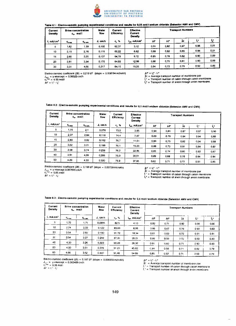
Table 6.1 : Electro-oamotlc pumping experlmenta con ona an reau .Current Brine concentretlon Weter Current Effective Transport Numbers
Density c•• molll flow Efficiency CurrentDensity
J. cm/h E:p, % I••••mAtcm' .1t< .11" 6t i,· i;I. mAtcm' c._ c._
0,102 62,37 3,12 0,91 0,82 0,87 0,96 0,915 1,62 1,59
66,22 6,62 0,88 0,82 0,85 0,94 0,9110 2,15 2,76 0,115
64,79 9,72 0,85 0,78 0,82 0,93 0,8915 2,65 3,35 0,137
0,170 64,93 12,99 0,86 0,75 0,81 0,93 0,8820 2,81 3,54
64,15 19,25 0,84 0,73 0,79 0,92 0,8630 3,31 4,05 0,217
Electro-osmotic coefficient (2B) = 0,2191/F (slope = 0,008194 ml/mAh)J"m = v-intercept = 0,06023 cmlhc,mu = 4,55 moVI&f;:;:; tIC -t/'
6o•• =t2&-1,• .6t = Average transport number of membrane pairi,' = Transport number of cation through catIOn membranei,. = Transport number of anion through anIOn membrane.
Current Brine concentration Water Current Effective Transport NumbersDensity c., molll flow Efficiency Current
Density
I, mAtcm' c" ••p c._ J, cm/h .,.% I••••mAtcm' .1t< .11" 6t i1~ 12-
5 1,79 2,1 0,076 73,0 3,65 0,94 0,81 0,87 0.97 0,90
10 2,37 2,64 0,118 74,4 7,47 0,89 0,78 0,84 0.94 0,89
15 2,83 3,02 0,152 76,7 11,51 0,89 0,75 0,82 0,94 0,88
20 3,02 3,21 0,188 76,1 15,23 0,88 0,73 0.81 0,94 0,87
30 3,58 3,74 0,238 76,2 22,86 0,85 0,74 0.80 0,93 0,87
40 3,91 4,09 0,286 75,0 30,01 0,89 0,68 0,78 0.94 0.84
50 4,29 4,33 0,330 75,9 37,95 0,82 0,71 0,77 0.91 0,85
Electro-osmotic coefficient (2B) = 0,198 I/F (slope = 0,00739 mt'mAh)J"m = v-intercept 0,067696 cmlhc,mu = 5,05 moVIAt' = tIC - t/
Ata = 12" - t,"Xt = Average transport number of membrane pairi,' = Transport number of cation through cation membranei,' = Transport number of anion through anion membrane.
Current Brine concentration Water Current Effeclive Transport NumbersDensity c., molll flow Efflclencv Current
Density
I, mAtcm' cbnp Cbr:ek:. J. cm/h €p. % I•• , mAtcm' ,1t< M" Xt i' i", ,5 1,72 1,71 0,0895 82.5 4,13 0,92 0,71 0,82 0.96 0,86
10 2,74 2,33 0,122 89,66 8.96 0,86 0,67 0,76 0.93 0,83
20 3,54 2,82 0,190 91,72 18.34 0,81 0,63 0,72 0.91 0,81
30 3.94 3,27 0,248 87,35 26.21 0.86 0,59 0.72 0.93 0,80
40 4,20 3,26 0,323 90.89 36.36 0,81 0,60 0.71 0.90 0.80
50 4,50 3,51 0,378 91.23 45.62 0,84 0,58 0.71 0.92 0.79
60 4.66 3.62 0.440 91,46 54.88 0,85 0,57 0,71 0.93 0,79
Electro-osmotic coeffiCient (2B) = 0,187 t'F (Slope = 0,006959mt'mAh)Jo._ = V-Intercept = 0,062409 cm/hc, m•• = 5.36 molll,1t' = I.' - t,'
6.t8;:;:; t/" - 11"
Xt = Average transport number of membrane pairr.' = Transport number of cation through cation membraner,' = Transport number of anion through anton membrane.
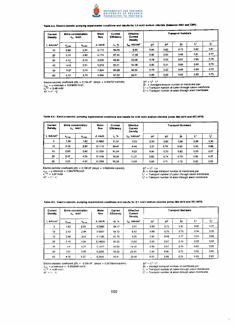
Current Brine concentration Water Current Effective Tranaport Numbera
Densby c.. mol/I flow Efficiency CurrentDensby
I, mAlcm' e••••p. cbMklo J. cmlh ep1 % I••••mAlcm' At' AI" At i,• iz'
10 2,95 2,41 0,113 89,00 8,90 0,84 0,62 0,73 0,92 0,81
20 3,73 2,90 0,174 87,14 17,43 0,82 0,55 0,68 0,91 0,77
30 4,12 3,16 0,236 86,95 26,09 0,79 0,55 0,67 0,90 0,78
40 4,55 3,51 0,279 85,21 34,08 0,80 0,51 0,66 0,90 0,76
50 5,07 3,70 0,328 89,28 44,64 0,79 0,52 0,65 0,89 0,76
60 5,10 3,79 0,384 87,52 52,51 0,80 0,50 0,65 0,90 0,75
Electro-osmotic coefficient (2fl) = 0,154 I/F (slope = 0.005757 ml/mAh)Jo•m = y-intercept = 0,078991 cm/hcbmu = 6,48 moVIAf;;; t,' -t2'
Ar- = t2- - .,.
At = Average transport number of membrane pairi,' = Transport number of catiOn through catiOn membranei,' = Transport number of aniOn through anion membrane.
Current Brine concentration Water Current Effective Transport NumbersDensby c•• mol/I flow Efficiency Current
Densby
I, mAlcm' c••••••. c._ J, cmlh ·P. % I.", mAlcm2 AI" AI" At ',. iz-
5 1,50 1,82 0,0883 71,01 3,55 0,93 0,80 0,86 0,96 0,90
10 2,16 2,80 0,1112 64,41 6,44 0,91 0,76 0,83 0.95 0,88
15 2,60 3,45 0,1324 61,54 9,23 0,90 0,73 0,82 0.95 0,87
20 2,87 4,05 0,1456 56,04 11,21 0.83 0,74 0,79 0.92 0,87
25 3,25 4,60 0,1589 55,39 13,85 0.86 0,71 0,78 0,93 0,85
Electro-osmotic coefficient (26) = 0,1861/F (slope = 0.0069464ml/mAh)Jo•m = y-intercept = 0,0657676cm/hc, mu = 5.37 moVIAt' ;;; tIC - tz'
Ata = 12- - t,a&t = Average transport number of membrane pairC' = Transport number of cation through cation membranei,' = Transport number of anion through aniOn membrane.
Current Brine concentration Water Current Effective Transport NumbersDensby c•• molll flow Efficiency Current
Density
I, mAlcm' c••••p. CbQIc J, cmlh ep. % I•• , mAlcm' At' AI" 6t i,c t2•
5 1,92 2,29 0,0662 68.17 3,41 0.89 0,73 0.81 0,95 0,87
10 2.49 2.94 0,0997 64.19 6.42 0,88 0,70 0.79 0.94 0.85
15 2.89 3,65 0.1186 61.70 9.25 0.86 0,68 0,77 0.93 0.84
20 3.18 3,84 0,14834 63.23 12.65 0,86 0.67 0,76 0.93 0.83
30 3,4 4.27 0.1977 60.09 18.03 0.84 0.67 0.75 0.92 0.83
40 3.81 4.89 0.2295 58.62 23.45 0.84 0.66 0.75 0.92 0.83
50 4.00 5.32 0,2649 56.81 28.40 0.85 0.66 0,76 0.93 0.83
Electro-osmotic coefllcient (26) = 0.2061/F (Slope = 0.0076844ml/mAh)J"m = y-intercept = 0.0503481 cmlhc,mu = 4.85 moVI.6.tC == t,~ - t/
.6ta = t/ - t,·6t = Average transport number of membrane pairi,' = Transport number of catiOn through calion membranei,' = Transport number of anion through anion membrane .
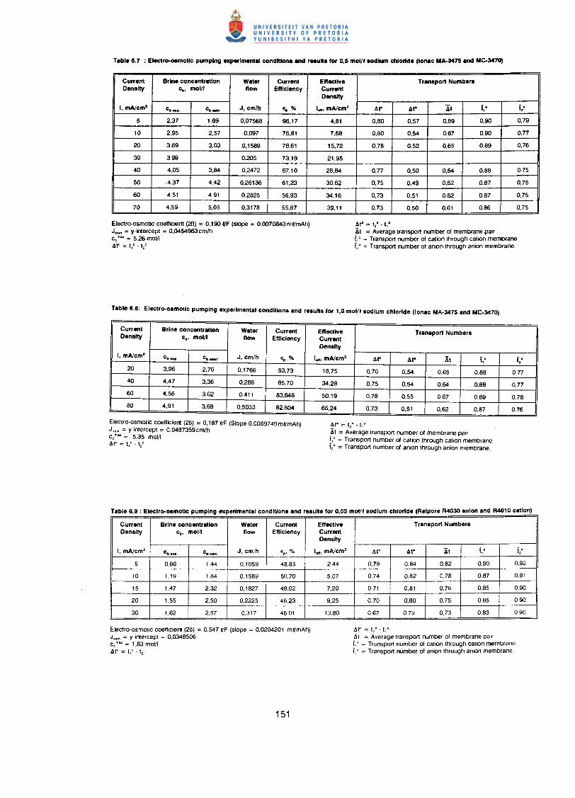
Current Brine concentration Water Current Effective Transport NumbersDensity c•• mol/l flow Efficiency Current
Density
I. mA/cm" c••.••,. c._ J, cm/h ••.% I••• mA/cm" 61" 6l" 6t i1c 12-
5 2,37 1,69 0,07568 96,17 4,81 0,80 0,57 0,69 0,90 0,79
10 2,95 2,57 0,097 76,81 7,68 0,80 0,54 0,67 0,90 o,n20 3,69 3,03 0,1589 78,61 15,72 0,78 0,52 0,65 0,89 0,76
30 3,99 0,205 73,19 21,95
40 4,05 3,84 0,2472 67,10 26,84 0,77 0,50 0,64 0,88 0,75
50 4,37 4,42 0,26136 61,23 30,62 0,75 0,49 0,62 0.87 0,75
60 4,51 4,91 0,2825 56,93 34,16 0,73 0,51 0,62 0,87 0,75
70 4,59 5,05 0,3178 55,87 39,11 0.73 0,50 0,61 0,86 0,75
Electro-osmotic coefficient (2B) = 0,190 I/F (slope = 0,0070843 ml/mAh)Jo•m = y-intercept = 0,0454963 cm/hc, mu = 5.26 moVIAt';:: t,' ·t/
Af& = t2• - t,·At = Average transpor1 number of membrane pairi.' = Transpor1 number of cation through catIOn membranei: = Transpor1 number of anion through anion membrane.
Current Brine concentrstlon Water Current Effective Transport NumbersDensity c., molll flow Efficiency CurrentDensity
I, mA/cm" cb •• p. Cit oak" J, cm/h €p, % I••• mA/cm" 61" 6l" At i1c i;/
20 3,96 2,76 0,1766 93.73 18,75 0.76 0,54 0.65 0.88 0,7740 4,47 3,36 0,286 85,70 34,28 0,75 0,54 0,64 0.88 0,7760 4,56 3.62 0,411 83,648 50,19 0,78 0,55 0,67 0.89 0,7880 4,91 3,68 0,5033 82.804 66,24 0,73 0,51 0,62 0.87 0,76
Electro-osmotic coefficient (28) = 0,187 I/F (Slope 0,0069749 ml/mAh)Joom = y-intercept = 0,0487359cm/hc, mu = 5.35 moVIAtC = .,' ·t/
At8;:: t/·t,al~t = Average transpor1 number of membrane pair!,' = Transpor1 number of cation through cation membranet,' = Transpor1 number of anion through anion membrane.
Current Brine concentration Water Current Effective Transpor1 NumbersDensity c., molll flow Efficiency Current
Density
I, mA/cm" cba •.p cbule. J, cm/h €pl o~ I•••, mA/cm" .11' .1t' XI i' t/,5 0,86 1.44 0,1059 48.85 2,44 0,79 0.84 0,82 0,90 0.92
10 1,19 1,84 0.1589 50.70 5.07 0.74 0,82 0.78 0.87 0.91
15 1,47 2,32 0,1827 48,02 7,20 0,71 0,81 0,76 0,85 0.90
20 1,55 2.50 0.2225 46.23 9.25 0.70 0.80 0.75 0.85 0.90
30 1.62 2,57 0.317 46.01 13.80 0.67 0,79 0.73 0.83 0.90
Electro-osmotic coefficient (28) = 0,547 I/F (slope = 0.0204201 ml/mAhjJo•m = v-intercept = 0.0348506C,mu = 1,83 moVI.1t' = t,' -t,'
At" ;:: t/' ~111
6t = Average transpor1 number of membrane pairL' = Transpon number of cation through cation membraneV = TranspOr1 number of anion through anion membrane .
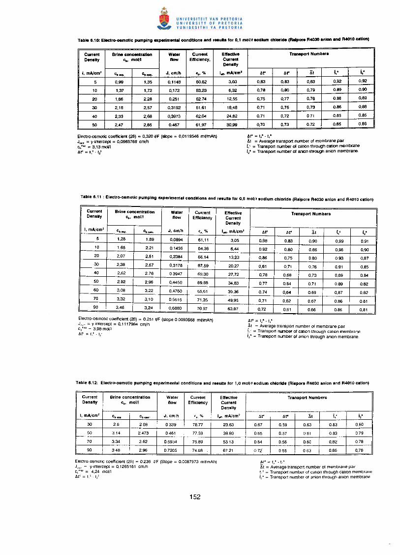
Current Brine concentration Water Currenl Effective Transport NumbersDensity c., molll flow Efficiency , Current
Density
I, mAtcm' c••• p. c._ J, cm/h e,,% I•••, mAtem' 4t" 4t" 41 i: t.,"
5 0,99 1,35 0,1148 60,62 3,03 0,83 0,83 0,83 0,92 0,92
10 1,37 1,72 0,172 63,23 6,32 0,78 0,80 0,79 0,89 0,90
20 1,86 2,28 0,251 62,74 12,55 0,75 0,77 0,76 0,88 0,89
30 2,16 2,57 0,3192 61,61 18,48 0,71 0,75 0,73 0,86 0,88
40 2,33 2,68 0,3973 62,04 24,82 0,71 0,72 0,71 0,85 0.86
50 2,47 2,86 0,467 61,97 30,99 0,70 0,73 0,72 0,85 0,86
Electro-osmotic coefficient (26) = 0,320 I/F (slope = 0,0119546 mlfmAh)Jo•m = y-intercept = 0,0985769 cmlhc,mu = 3,13moVI4t' = tIC -t2
C
At- = t2- - .,.
At = Average transport number of membrane pairi,' = Transport number of cation through cation membranei," = Transport number of anion through anion membrane.
Current Brine coneenlrallon Water Currenl Effective Transport NumbersDensity c., molll flow Efficiency CurrenlDensity
I, mAtcm' cbup. c.ule. J, cm/h € % I•• , mAtcm' 41" 4f' At i,c t2-P.
5 1,28 1,89 0,0894 61,11 3,05 0,98 0,83 0,90 0,99 0,9110 1,65 2.21 0,1456 64,36 6,44 0,92 0,80 0.86 0,96 0,9020 2,07 2,51 0,2384 66,14 13,23 0,86 0,75 0,80 0,93 0,8730 2,38 2,67 0,3178 67,59 20,27 0,81 0,71 0.76 0.91 0,8540 2,62 2,76 0,3947 69,30 27,72 0.78 0,68 0.73 0,89 0,8450 2,92 2,96 0,4450 69,66 34,83 0,77 0,64 0,71 0.89 0,8260 3,08 3,22 0,4760 65,61 39,36 0,74 0,64 0.69 0.87 0,8270 3,32 3,10 0,5615 71,35 49,95 0,71 0,62 0.67 0,86 0.8190 3,46 3,24 0,6880 70,97 63,87 0,72 0,61 0,66 0.86 0,81
Electro-osmotic coefficient (2B) = 0,251 ifF (slope 0,0093668 ml/mAh)Jw = v-intercept = 0,1117984 cmlhc, m~ = 3,98 molll.1.t'= t,'-I,'
~t4 = t/ - t1"
At = Average transport number of membrane pairt,' = Transport number of cation through cation membranei,' = Transport number of anion through anion membrane.
Current Brine concenlrallon Waler Current Effecllve Transport NumbersDensity c., molll flow Efficiency Currenl
Density
I, mAtern' c.up Cbc.k:° J, cm/h €p, % I•• , mAtern' .1.1" .1.f' At i' i2-,30 2.6 2.08 0.339 78.77 23.63 067 0.59 063 0.83 0.80
50 3.14 2473 0461 77.59 38.80 0.65 0.57 061 0.83 0.79
70 3.34 2.62 0.5934 75.89 53.13 064 0.56 0.60 0,82 0.78
90 348 2.96 0.7205 7468 67.21 072 0.55 063 0.86 0,78
Electro-osmotic coefficient (2B) = 0,236 I/F (Slope = 0.0087973 ml/mAhjJ,," = v-intercept = 0,1265161 cmfhc, m~ = 4,24 moll I.1.t' = t.' - t,'
.1.t· = r: -t,'
At = Average transport number of membrane pairt,' = Transport number of cation through calion membraneV = Transport number of anion through anion membrane
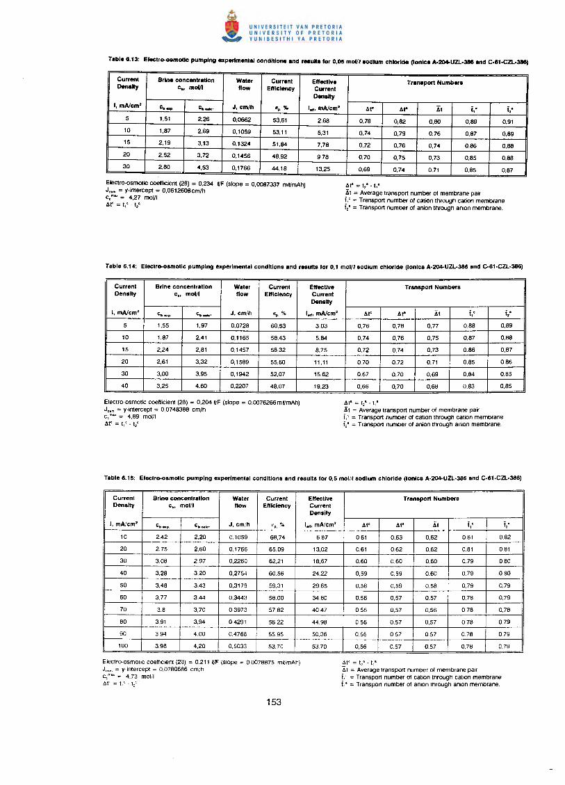
Current Brine concentration Water Current Effective Traneport NumbersDenalty c., molll flow Efficiency Current
Density
I, mAlcm' c.up. c._. J, cm/h £p. % I•• , mAlcm' AI" At" At i,c f2-
5 1,51 2,26 0.0662 53.61 2,68 0,78 0,82 0,80 0,89 0,9110 1,87 2,69 0,1059 53,11 5,31 0,74 0,79 0,76 0,87 0,8915 2,19 3,13 0,1324 51,84 7,78 0,72 0,76 0,74 0,86 0,8820 2,52 3,72 0,1456 48,92 9,78 0,70 0,75 0,73 0,85 0,88
30 2,80 4,53 0,1766 44,18 13,25 0,69 0,74 0,71 0.85 0,87
Electro-osmotic coefficient (28) = 0,234 ifF (slope = 0,0087337 mlfrnAh)Jo•m = v-intercept = 0,06126OBcm/hComu = 4,27 moVIAf :;;:;t,' ~t2'
Ata = t/ -I,·,1t = Average transport number of membrane pairi,' = Transport number of cation through cation membranei,' = Transport number of anion through anion membrane.
Current Brine concentration Water Current Effective Trsnsport NumbersDensity c" molll flow Efficiency Current
Density
I, mAlcm' ell .,p. c. C\ek' J, cmih E % lef'I' mAJcm2 At< At' At i1c tz•P.
5 1,55 1,97 0,0728 60,53 3,03 0,76 0,78 0,77 0,88 0.89
10 1,87 2,41 0,1165 58,43 5,84 0,74 0,76 0,75 0,87 0,88
15 2,24 2,81 0,1457 58,32 8,75 0,72 0,74 0,73 0.86 0,87
20 2,61 3,32 0,1589 55,60 11,11 0,70 0,72 0,71 0.85 0.86
30 3,00 3,95 0,1942 52,07 15,62 0,67 0,70 0,69 0,84 0,85
40 3,25 4,60 0,2207 48,07 19,23 0,66 0,70 0,68 0,83 0.85
Electro-osmotic coefficient (28) = 0,204 I/F (slope = 0.0076266 ml/mAh)J"m = v-intercept = 0,0748388 cmlhc,.mu = 4,89 molllAt' = t,' - t2'
Are;:; t2
& -t1-
At = Average transport number of membrane pairi,' = Transport number of cation through cation membranei: = Transport number of anion through anion membrane.
Current Brine concentration Water Current Effective Transport NumberaDensity c" molll flow Efficiency Current
Density
I, mA/cm' Cb •• p. CIICllk'J, cmih €p, % I••• mA/cm' Ate At' ,1t i1
c it10 2,42 2,20 0,1059 68,74 6,87 0,61 0,63 0,62 0,81 0,82
20 2,75 2,60 0,1766 65.09 13,02 0.61 0,62 0,62 0.81 0.81
30 3,08 2,97 0,2260 62,21 18,67 0.60 0,60 0,60 0.79 0,80
40 3,28 3,20 0,2754 60.56 24.22 0,59 0,59 0,60 0.79 0.80
50 3,48 3,43 0,3178 59.31 29.65 0,58 0,59 0,58 0.79 0.79
60 3.77 3,44 0,3443 58.00 34.80 0,56 0,57 0,57 0,78 0,79
70 3.8 3,70 0.3973 57.82 40,47 0,56 0.57 0,56 0.78 0,78
80 3.91 3,94 0,4291 56.22 44.98 0,56 0,57 0,57 0.78 0.79
90 3,94 4.00 0,4768 55.95 50.36 0.56 0.57 057 0.78 0.79
100 3.98 4,20 0,5033 53.70 53.70 0,56 0,57 0,57 0,78 0.79
Electro-osmollc coeffiCient (28) = 0.211 I/F (slope = 0.0078875 ml/mAh)J"m = y-Intercept = 0.0780686 cmihc,mu = 4,73 mol;1At' = I.' - t,'
.6.t'" = t/ -t~·At = Average transport number 01 membrane pairi.' = Transport number of catIon through catIon membranei,' = Transport number of anion through artlon membrane.
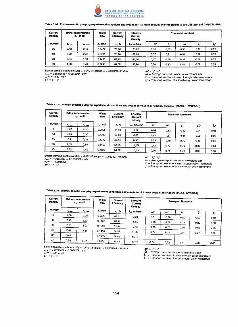
Current Brine concentration Water Current Effective Tranaport Numbera
Denalty c•• mol/I flow Efficiency CurrentDenalty
I. mA/cm2 c-'u:p. CboMc" J. cm/h ep, % I••• mA/cm2 41" 4t" At t.o i2-
30 3,48 2,49 0,2472 76,88 23,06 0,58 0,52 0,55 0,79 0,76
50 3,72 2,72 0,3708 73,96 36,98 0,57 0,51 0,54 0,79 0,75
70 3,94 3,13 0,4450 67,15 47,00 0,57 0,50 0,53 0,78 0,75
90 4,08 3,46 0,5298 64,38 57,94 0,59 0,50 0,54 0,79 0,75
Electro-osmotic coefficient (2B) = 0,216 ifF (slope = 0,0080659ml/mAh)Jo•m = y-intercept = 0,0655084 cm/hc. mu = 4,63 moVIAf = t/ ·t2C
Ata = t/· .,.3t = Average transport number of membrane pairf,' = Transport number of cation through cation membranef: = Transport number of anion through anion membrane.
Current Brine concentration Water Current Effective Transport NumbersDensity c•• mol/I flow Efficiency Current
Density
I, mA/cm2 c• .,. c._ J, cm/h €p, % I•• , mA/cm2 4t' 4t" At 4i,c i'25 1,66 2,20 0,0695 61,88 3,09 0,82 0,83 0.82 0,91 0,91
10 1,99 2,36 0,1280 60,78 6,08 0,81 0,81 0,81 0,90 0,90
15 2,4 3,16 0,1390 59,64 8,95 0,78 0,79 0,79 0.89 0,89
20 2,85 3,85 0,1456 55,65 11,13 0,72 0,77 0,75 0.86 0,88
25 3,32 4,45 0,1523 54,22 13,55 0,70 0,75 0.73 0,85 0.86
Electro-osmotic coefficient (2B) = 0,087 ifF (slope = 0,0032427 mlfmAh)Jo•m = v-intercept = 0,1090328 cm/hc.mu = 11.50 moVIAf::::: tIC ·t/
Ar-::::: 128• I,·
Kt = Average transport number of membrane pairf,' = Transport number of cation through cation membranei,' = Transport number of anion through anion membrane.
Current Brine concentration Water Current Effective Transport NumbersDensity c•• mol/I flow Efficiency Current
Density
I, mA/cm' c.up. cb Ale" J, cm/h €P. % I.,., mAlcm2 4t' 4t" Kt.,c f',
5 1.68 2.06 0,0728 65.61 3,28 0.81 0,79 0.80 0.90 0.90
10 2,10 2,52 0,1165 65,46 6,55 0,79 0,78 0,79 0.89 0.89
15 2.53 3,07 0,1390 62,87 9,43 0,76 0.76 0.76 0.88 0.88
20 2.91 3.81 0,1456 56.82 11,36 0,74 0,74 0,74 0.87 0.87
30 3,42 0,1655 50.59 15,17
40 3.58 5,74 0.1854 44,48 17,79 0.711 0,72 0.71 0.86 0.86
Electro-osmotic coeffIcient (2B) = 0,156 I/F (slope = 0.0058244 ml/mAh)Jo" = v-intercept = 0.0801568 cm/hc, mu = 6,41 moVI4t' = I: - t,'
At"'::::: t/ -.,.KI = Average transport number of membrane pairf,' = Transport number of cation through catIon membrane1: = Transport number of anion through anion membrane.
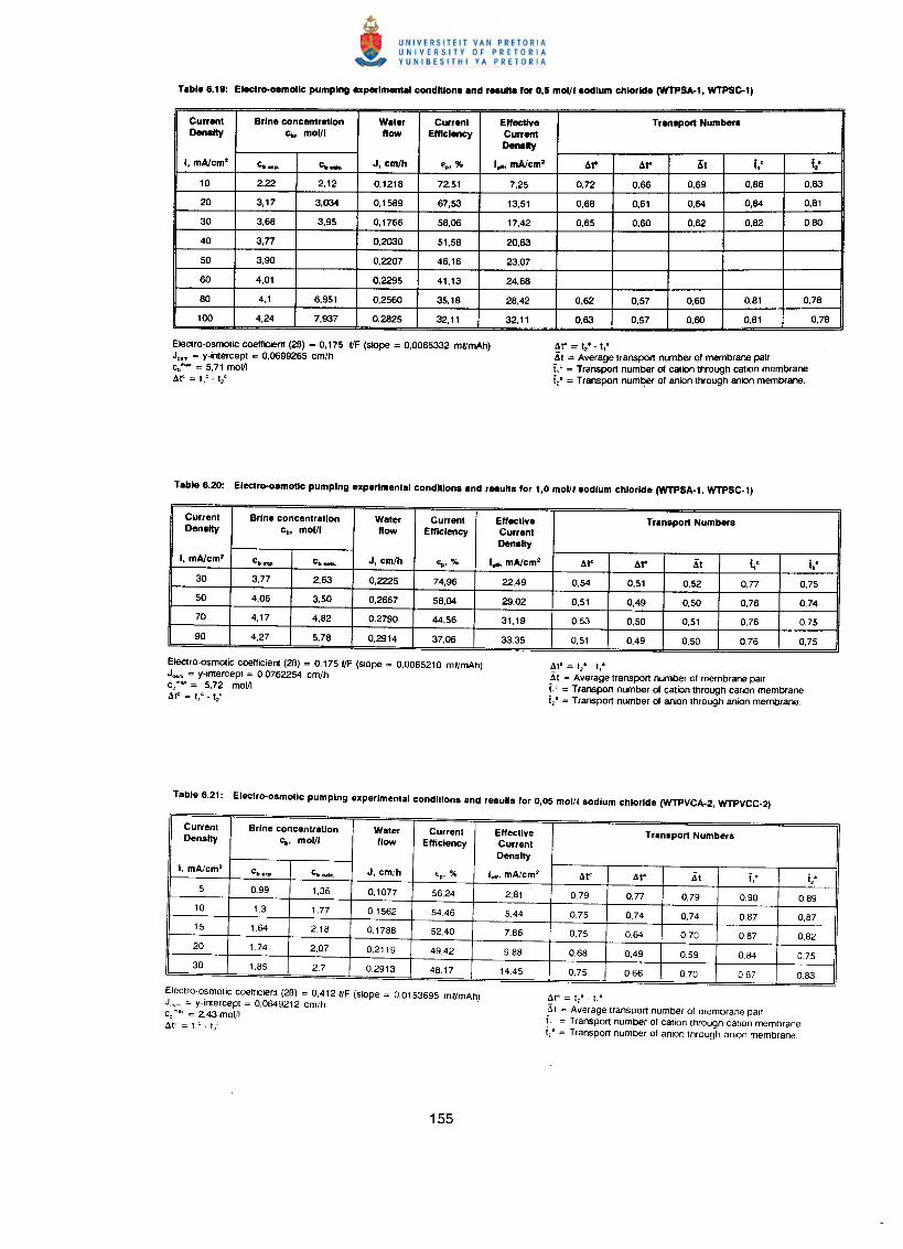
Current Brine concentrMlon Water Current Effective Transport NumbersD_1ty c:". molll flow Efficiency Current
D_1ty
I, mAtcm' c•••. c•••••. J. cm/h €p, % I••••mAtcm' .11" .11" At i,c tz-
10 2.22 2.12 0.1218 72.51 7.25 0.72 0.66 0.69 0.86 0.83
20 3.17 3,034 0.1589 67.53 13.51 0.68 0,61 0,64 0.84 0,81
30 3.68 3.95 0,1766 58.06 17,42 0.65 0,60 0.62 0,82 0,80
40 3.n 0,2030 51,58 20,63
50 3,90 0.2207 46.16 23.07
60 4.01 0.2295 41.13 24.68
80 4,1 6,951 0.2560 35.18 28,42 0.62 0,57 0.60 0.81 0.78
100 4,24 7.937 0.2825 32.11 32.11 0.63 0,57 0.60 0,81 0.78
Electro-osmotic coefficient (26) = 0.175 I/F (slope = 0.0065332 ml/mAh)J"m = y-intercept = 0.0699265 cmlhCbm", = 5.71 moVI4t' = tiC ·t21:
Ar- = t28• t,·At = Average transport number of membrane pairi,' = Transport number 01 cation through cation membranei:= Transport number of anion through anion membrane.
Current Brine concentration Water Current Effective Transport NumbersDensity c•• molll flow Efficiency Current
Density
I, mAtern' c••••p. c•••••. J. cm/h e,.,% I••••mAtern' .11' .11" At i,c i2-
30 3.77 2.63 0,2225 74.96 22,49 0.54 0.51 0.52 0.77 0.75
50 4.06 3.50 0.2667 58.04 29.02 0.51 0.49 0,50 0.76 0.74
70 4.17 4.82 0,2790 44.56 31,19 0.53 0,50 0.51 0,76 0.75
90 4.27 5.78 0.2914 37.06 33,35 0.51 0,49 0.50 0,76 0.75
Electro-osmotic coefficient (28) = 0.175I/F (slope = 0.0065210 ml/mAh)J"m = y-intercept = 0.0762254 cmlhCbm", = 5.72 moVIAf = t,C -t2
C
Al'l = t:/ - t1•
At = Average transport number 01 membrane pairi,' = Transport number of cation through catIOn membranei,' = Transport number of anion through amon membrane.
Current Brine concentration Water Current Effective Transport NumbersDensity c•• molll flow Efficiency CurrentDensity
I, mAtern' c.eJ:P cbc.lc;;. J, cm/h ep, % left! mAlcm2 .1t' .1\' At itC i/
5 0.99 1,36 0,1077 56,24 2,81 0,79 0,77 0,79 0.90 0,8910 1.3 1,77 0,1562 54,46 5,44 0,75 0,74 0,74 0.87 0,8715 1.64 2,18 0,1788 52,40 7,86 0,75 0,64 0,70 0.87 0,8220 1.74 2,07 0,2119 49,42 9,88 0,68 0,49 0.59 0.84 0,7530 1,85 2,7 0,2913 48.17 14.45 0,75 0,66 0.70 0.87 0.83
Electro-osmotic coefficient (28) = 0,4121/F (slope = 0,0153695 ml/mAh)J"c = y'lntercept = 0.0649212 cm/hc~me... = 2.43 molllAt' = t.'· t,'
At' = t,' - t,'
~t = Average transpon number of membrane pairi.' = Transpon number of cation through calIOn membraneV = Transpon number of anion through anion membrane
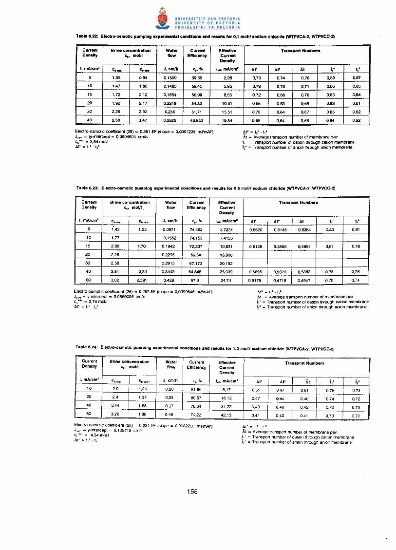
Current Brine eoneemrlllion Willer Current Effective Transport NumbersDensity c.. mol/l flow Efftelency Current
Density
I. mAtem· e._ c. •••• J. em/h ",."- I•••mAtem· ~r ~r At i,o 'a-5 1,05 0,94 0,1509 59,65 2,96 0,79 0,74 0,76 0,69 0,67
10 1,47 1,60 0,1463 56,45 5,65 0,73 0,70 0,71 0,66 0,65
15 1,72 2,12 0,1654 56,99 6,55 0,72 0,66 0,70 0,66 0,64
20 1,92 2,17 0,2219 54,53 10,91 0,66 0,63 0,65 0,63 0,61
30 2,26 2,92 0,256 51,71 15,51 0,70 0,64 0,67 0,65 0,62
40 2,56 3,47 0,2625 46,653 19,54 0,66 0,64 0,66 0,64 0,62
Electro-osmotic coefficient (26) = 0,261 I/F (slope = 0,0097235 ml/mAh)J",m = (y·intercept = 0,0994504 cmlhc,mu = 3,64 moVIAf" = tIC -t2'
4r' = 12&- 11·Xt = Average transpon number of membrane pairi,' = Transpon number of cation through cation membranei,' = Transpon number of anion through anion membrane.
Current Brine concentration Weter Current Effective Transport NumbersDensity c•• molll flow Efficiency Current
Denelty
I, mAtcm· CD up. Cb~k, J, cm/h €pI % I•••, mAJcm2 ~tC .1t· ~t i,.~ i2•
5 1,43 1,23 0,0971 74,463 3,7231 0,6620 0,6146 0,6364 0,63 0,61
10 1,77 0,1562 74,153 7,4153
15 2,06 1,70 0,1942 72,207 10,631 0,6126 0,5666 0,5697 0,61 0,76
20 2,26 0,2295 69,54 13,906
30 2,56 0,2913 67,173 20,152
40 2,61 2,33 0,3443 64,646 25,939 0,5696 0,5070 0,5363 0,76 0,75
60 3,02 2,561 0,429 57,9 34,74 0,5179 0,4715 0,4947 0,76 0,74
Electro-osmotic coefficient (26) = 0,267 I/F (slope = 0,0099646 ml/mAh)Jo•m = y-intercept = 0,0669006 cmlhc,mu = 3,74 moVIdte = .,c -1/:
4tl = 121
- 11•
Xt = Average transpon number of membrane pairi,' = Transpon number of cation through cation membranei:= Transpon number of anion through anion membrane.
Current Brine concentretlon Weter Current Effective Trensport NumbersDensity c., molll flow Efficiency Current
Density
I, mAtcm· cb ••. p. cb c.ko J, cm/h E % l«fl mAJcm2 ~tC ~t' .1t i' 12-p. ,10 2,0 1,25 0,20 81.66 8,17 0,55 0,47 0.51 0,78 0,73
20 2,4 1,37 0,25 80.67 16,13 0,47 0,44 0,46 0,74 0,72
40 3,14 1,68 0,37 78.04 31.22 0,43 0,40 0,42 0.72 0,70
60 3.26 1,66 0,48 70.22 42,13 0,41 0,40 0,41 0,70 0.70
Electro-osmotic coefficient (26) = 0.221 ifF (slope = 0,0082250 mlimAh)Jo•c = y-Intercept = 0,125719 cm/hc, m" = 4,54 mo!;1At' = t1~ - t;;'
At" = t~·- tl'.11= Average transpon number of membrane pairi,' = Transpon number of catIOn through cation membraneV = Transpon number of anion through anion membrane.
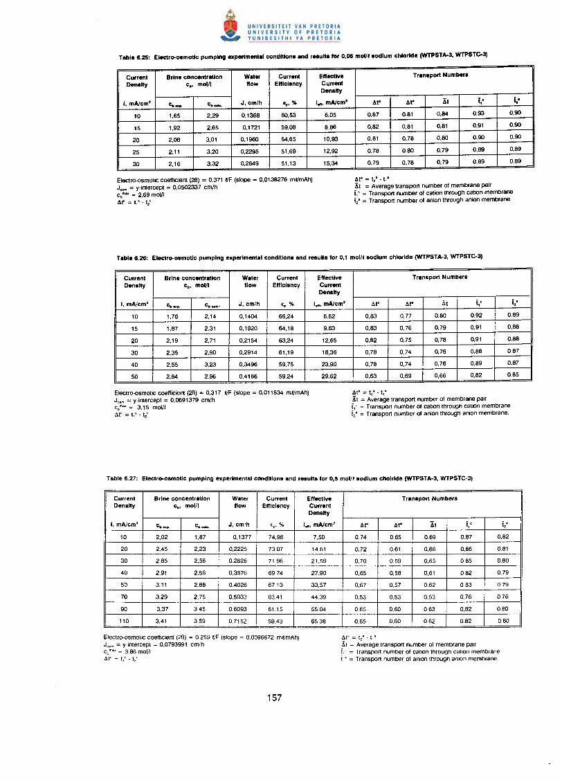
Current Brine concentration Water Current Effective Tranaport Numbers
Density c•• molll flow Efficiency CurrentDensity
I. mA/cm2 c~_,. c._ J. cm/h e.,.% I••••mA/cm2 At< At" At i: i,0
10 1.65 2,29 0,1366 60,53 6,05 0,67 0,61 0,64 0,93 0,90
15 1,92 2,65 0,1721 59,06 6,66 0,62 0,61 0,61 0,91 0,90
20 2,06 3,01 0,1960 54,65 10,93 0,61 0,76 0,60 0,90 0,90
25 2,11 3,20 0,2295 51,69 12,92 0,76 0,60 0,79 0,69 0,69
30 2,16 3,32 0,2649 51,13 15,34 0,79 0,76 0,79 0,69 0,69
Electro-osmotic coefficient (28) = 0,371 f/F (slope = 0,0136276 mf/mAh)Jo•m = y-intercept = 0,0502337 cmlhc,m•• = 2,69 moVI4f == 1,' -t2'
.dr- = 12& - I,·30t = Average transport number of membrane pairi,' = Transport number of cation through cation membranei,. = Transport number of anion through anion membrane.
Currenl Brine concentrallon Water Current Effective Transport NumbersDensity c•• molll flow Efficiency Current
Density
I, mA/cm2cb_p. CttCllk:' J. cm/h Ep, % I••••mA/cm2 At' At" At i,c j,0
10 1,76 2,14 0,1404 66,24 6,62 0,63 0,77 0,60 0,92 0,69
15 1,67 2,31 0,1920 64,16 9,63 0,63 0,76 0,79 0,91 0,66
20 2,19 2,71 0,2154 63,24 12,65 0,62 0,75 0,76 0,91 0,66
30 2,35 2,90 0,2914 61,19 16,36 0,76 0,74 0,76 0,66 0,67
40 2,55 3,23 0,3496 59,75 23,90 0,76 0,74 0,76 0,69 0,67
50 2,64 2,96 0,4166 59,24 29,62 0,63 0,69 0,66 0,62 0,65
Electro-osmotic coefficient (28) = 0,317 f/F (slope = 0,011634 mf/mAh)J"m = y-intercept = 0,0691379 cmlhc,m•• = 3,15 moVI.dtG= t1' -t
2(;
Ata :;:; t2& - t1•
At = Average transport number of membrane pairi,' = Transport number of cation through cation membranei,' = Transport number of anion through anion membrane .
Current Brine concentration Waler Current Effective Transport NumbersDensity c•• molll flow Efficiency Current
Density
I, mA/cm' cbup. cbCllk. J. cmlh £p, % I.tt', mAJcm2 At< At" Xt j' i2-,10 2,02 1,67 0,1377 74,96 7,50 0,74 0,65 0.69 0.67 0,62
20 2,45 2,23 0,2225 73.07 14,61 0,72 0,61 0,66 0,66 0,61
30 2,65 2,56 0.2626 71,96 21,59 0,70 0,59 0,65 0.65 0.60
40 2,91 2,56 0,3576 69.74 27,90 0,65 0,56 0,61 0.62 0,79
50 3,11 2,66 0.4026 67.13 33,57 0,67 0,57 0.62 0.63 0.79
70 3,29 2,75 0,5033 63.41 44,39 0,53 0,53 0,53 0.76 0.76
90 3,37 3,45 0,6093 61.15 55.04 0,65 0,60 0.63 0,62 0.80
110 3,41 3,59 0,7152 59,43 65.38 0,65 0,60 0.62 0.82 0,80
Electro-osmOlic coefficient (28) = 0,259 ifF (slope = 0,0096672 mlfmAh)J,.m = y-Intercept = 0,0793991 cm/hc, mu = 3,66 moVIAt<. = tt'· t;/
At' = t,' - t,'At = Average transport number of membrane pairi.' = Transport number of catIOn through cation membranei.' = Transport number of anion through anion membrane.
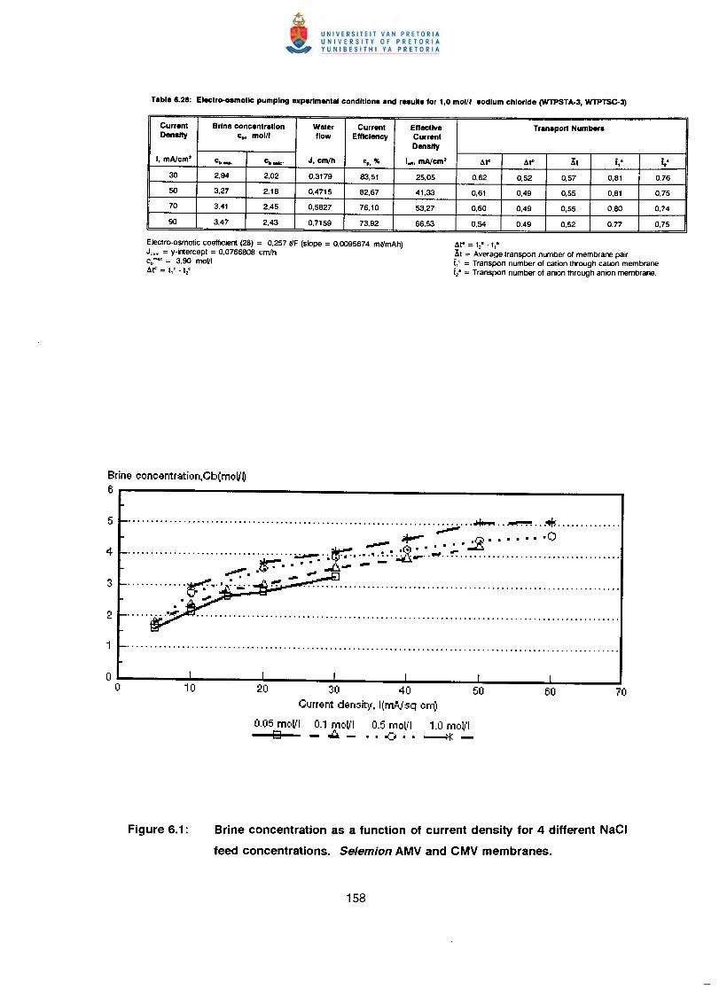
Current Brine concentration Water Current Effective Transport NumbersDensity c., mol/l flow Efficiency Current
Density
I, mAlcm2 c._ Crt •• • J, cm/h €p, % I•••, mAlcm2 4t" 4'- ~t i,c i..'
30 2,94 2,02 0,3179 83,51 25,05 0,62 0,52 0,57 0,61 0,76
50 3,27 2,16 0,4715 62,67 41,33 0,61 0,49 0,55 0,61 0,75
70 3,41 2,45 0,5627 76,10 53,27 0,60 0,49 0,55 0,60 0,74
90 3,47 2,43 0,7159 73,92 66,53 0,54 0,49 0,52 0,77 0,75
Electro-osmotic coefficient (2B) = 0,257 ifF (slope = 0,0095674 mlfmAh)J". = v-intercept = 0,0766606 cmlhCb·~ = 3,90 moVIArc = t,t -t2C
4t' = t2- ~ 1,·~t = Average transport number of membrane pairi,' = Transport number of cation through cation membranei,' = Transport number of anion through anion membrane.
Brine eoneentration.Cb(moV~6
........................................................................... ~ ..~ ~ .,.,.,-••••••• .-:-a •••••• ·O
~ ~ ~~ •••••• J _.................................... ........-:.. ~l;I" • .•.•.•.... ~~ .. .., ................•....•........•........
~ .' to. --• • • ..-..:a.-.IJII. ~'!'!~
20 30 40 50Current density, l(mNsq em)
0.05 molll 0.1 Telll'l 0.5 moll'l 1.0 moll'lo - .••- .. -:j .. --;:f;-
Brine concentration as a function of current density for 4 different NaCI
feed concentrations. Selemion AMV and CMV membranes.
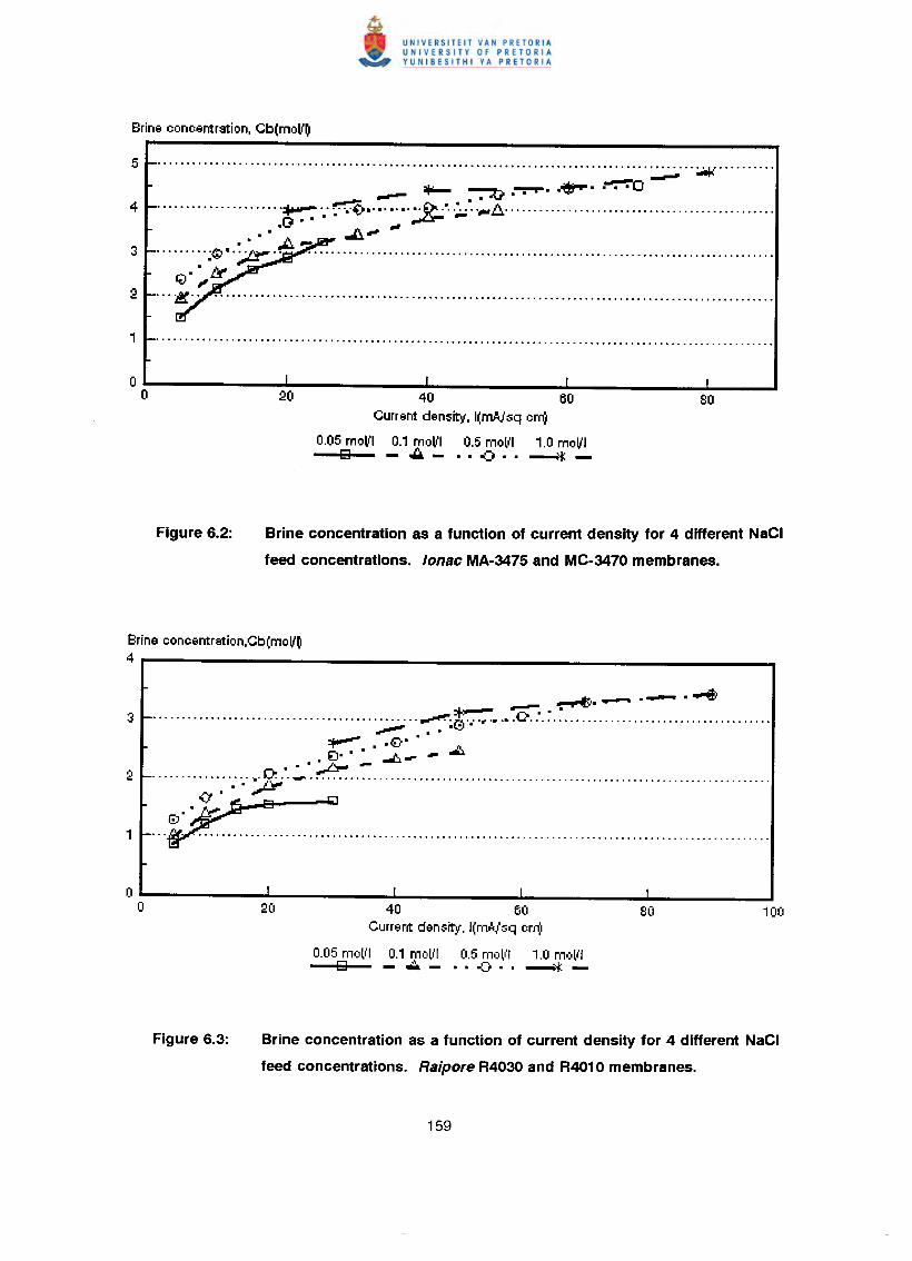
••••••••••••••••••••••••••••••••••••••••••••••••••••••••••••••••••••••••••••••••••••• :.::.:.:.: •• :..11<' ••••••••••
~ :+-- :-:-:tJ. .-r-- ~. ~······················r·: ~ ~ ~ ,..,1::.. .
•• A~'".. - A ~
.........~¢'•.~ ..
~.~«... :/!!... . .
20 40 60Current density, 1(mA/sq em)
0.05 moVI 0.1 moVI 0.5 molll 1.0 moVIg -...:i.-··oO··~-
Brine concentration as a function of current density for 4 different NaCI
feed concentrations. lonae MA-3475 and MC-3470 membranes.
Brine eoneentration,Cb(moV~4
~.-.- . ...-$:+:- - ........................................ :,;.;;;. .. ~~Qr •..•..r ••• 0 .
=+""""""' ••• 0· ... ~• €:I. • ...t:..--..~ -.................... ~ .•. ~ .
(J ••• ~
40 60Current densit)', l(mA,Isq em)
0.05 molll 0.1 moll'l 0.5 moll'l 1.0 m')ll'lo - .••.- .. -8 .. -i:f:-
Brine concentration as a function of current density for 4 different NaCI
feed concentrations. Raipore R4030 and R4010 membranes.
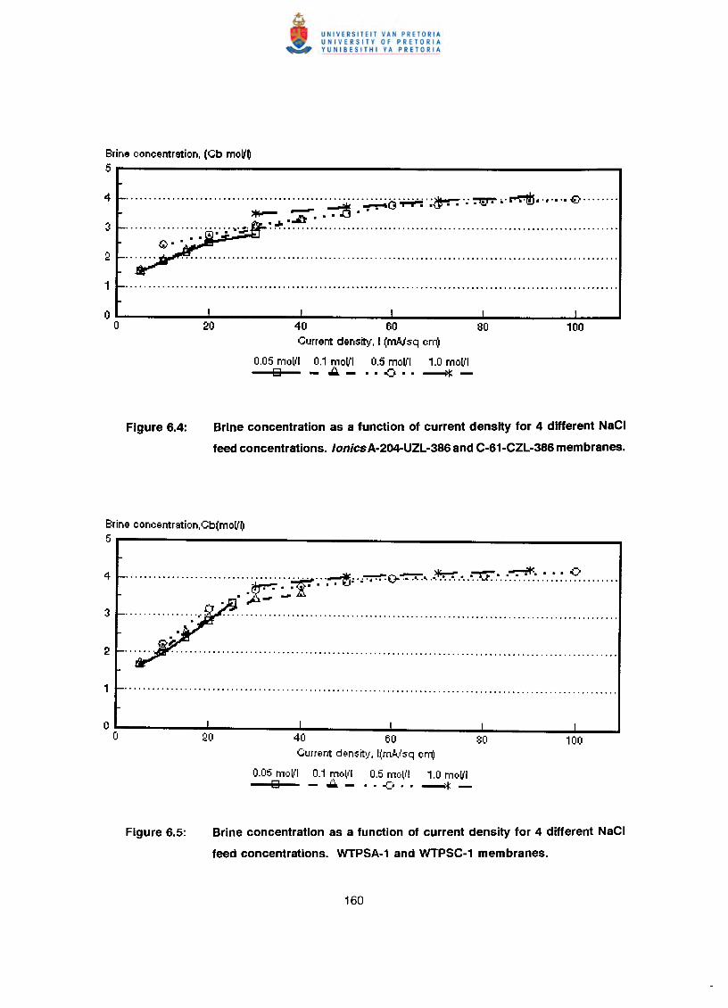
Brine concentration, (Cb moVO5
........................... ~ ~ ~. ~.:;.::40·.p;.;.:.:·:~'.'~ o' r"':'!ftj •.•.•.• ~ .• ~ • ..a..i"................... ".' ".' .•..;;. .
40 60 80Current density, I (mNsq crr(!
0.05 moVI 0.1 mo~'1 0.5 mo~'1 1.0 moVI121 ..::..- •• -o .. ~-
Brine concentration as a function of current density for 4 different NaCI
feed concentrations. lonics A·2Q4.UZL·386 and C·61·CZL·386 membranes.
Brine concentration,Cb(moVO5
........................... ~ ~.:.~ •.•~o-~" .Z~·..•..•...:"XI- ..•. :.: ..•~ •..•..•. ~.? .r".••••••••• ~~.
• • ~.... •••• li!.
40 60 80Cum.nt density, l(mo!."lsq crr(!
0.05 moll'l 0.1 Toll'l 0.5 melll'l 1.0 mo~'1121 ••••. - •• .() •• _*-
Brine concentration as a function of current density for 4 different NaCI
feed concentrations. WTPSA-1 and WTPSC-1 membranes.
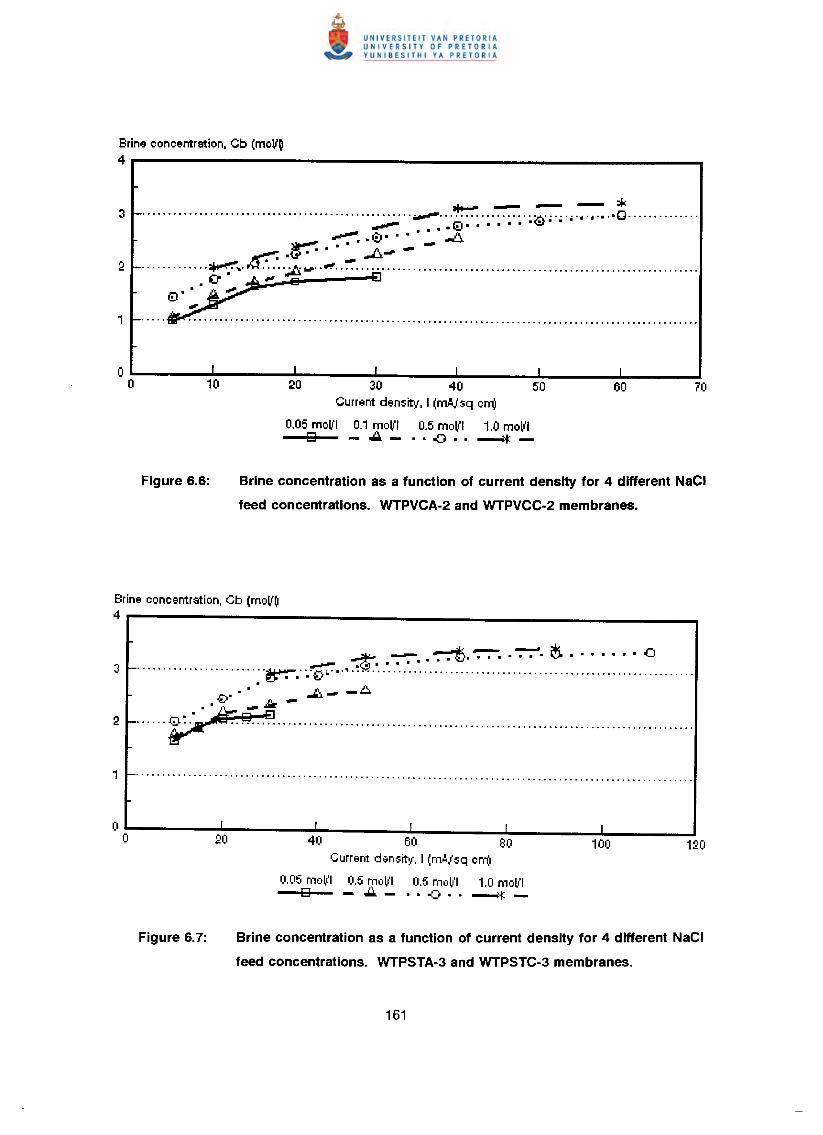
Brine concentration. Cb (moV~4
aIoIo----*.................................................... ~ ....................••........•.•.•··0··············~ ~ ~ .
"...,.... • t;-.. • • • A~ ....•... -~.G . . .. A -.It ~.".;:. -............·r..·,Q·~··,;"fj.•.•.· .~ .
. ",.
20 30 40 50Current density, I (rn.oVsqcm)
0.05 moVI 0.1 mol'l 0.5 molfl 1.0 mol'lo -A- .. ~ .. --.."i:-
Brine concentration as a function of current density for 4 different NaCI
feed concentrations. WTPVCA-2 and WTPVCC-2 membranes.
Brine concentration, Cb (moV~4.--------------------------..,~ - '7":1S. ':'7". . -:-:-". i±i. . . • • • . • 00
3 _ ~ •. ·.V···.~~:.:.:.:."." .• • A ~ _1::J.
0· - -.:..
2- .. ~ .
I I I
40 60 80Current density, I (m,!./sq crn)
0.05 moll'l 0.5 moll'l 0.5 moll'l 1.0 moVID -..:;:.,- ..• ~j1 •• ~-
I
100
Brine concentration as a function of current density for 4 different NaCI
feed concentrations. WTPSTA-3 and WTPSTC-3 membranes.
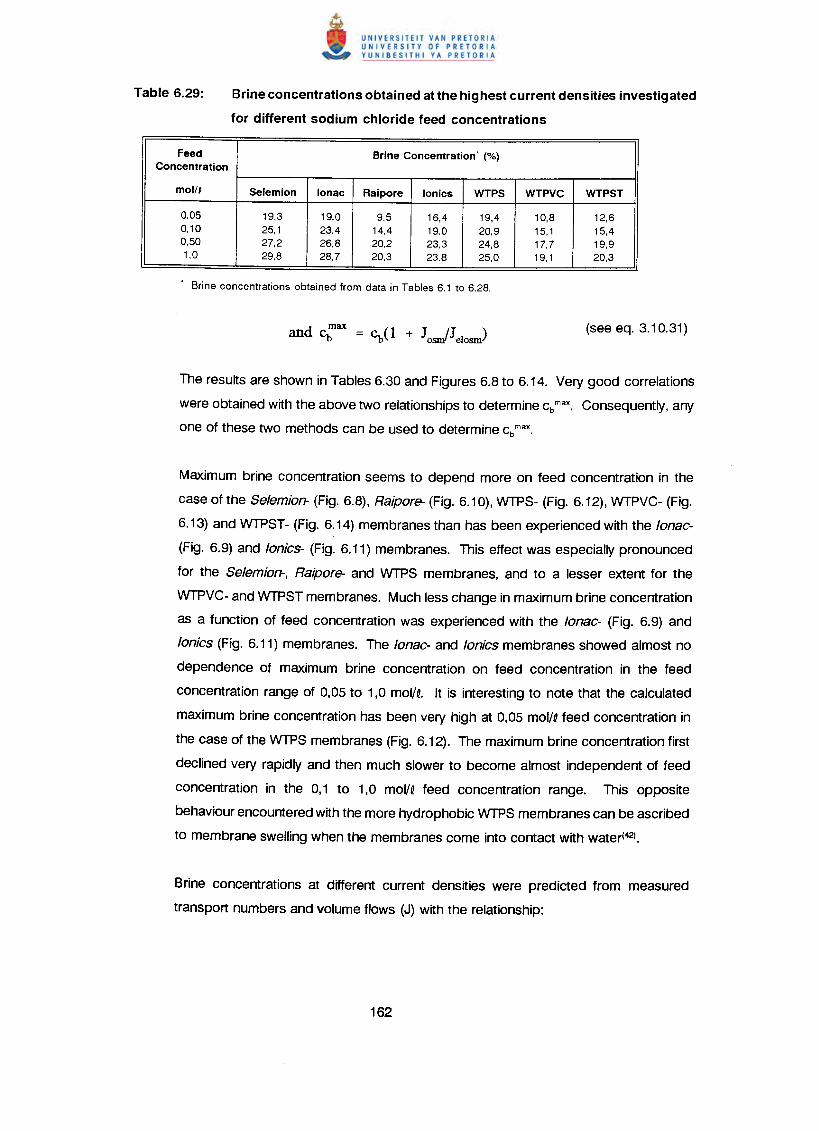
Brine concentrations obtained at the highest current densities investigated
for different sodium chloride feed concentrations
Feed Brine Concentration' (%)Concentration
molO Selemion lonac Raipore lonics WTPS WTPVC WTPST
0.05 19,3 19,0 9.5 16,4 19,4 10,8 12,60,10 25,1 23,4 14,4 19.0 20,9 15,1 15,40,50 27,2 26.8 20.2 23.3 24,8 17,7 19,91.0 29.8 28,7 20,3 23.8 25,0 19,1 20.3
The results are shown in Tables 6.30 and Figures 6.8 to 6.14. Very good correlations
were obtained with the above two relationships to determine cb max. Consequently, any
one of these two methods can be used to determine cb max.
Maximum brine concentration seems to depend more on feed concentration in the
case of the Selemion- (Fig. 6.8), Raipore- (Fig. 6.10), WTPS- (Fig. 6.12), WTPVC- (Fig.
6.13) and WTPST- (Fig. 6.14) membranes than has been experienced with the lonac-
(Fig. 6.9) and lonics- (Fig. 6.11) membranes. This effect was especially pronounced
for the Selemion-, Raipore- and WTPS membranes, and to a lesser extent for the
WTPVC-and WTPSTmembranes. Much less change in maximum brine concentration
as a function of feed concentration was experienced with the lonac- (Fig. 6.9) and
lonics (Fig. 6.11) membranes. The lonac- and lonics membranes showed almost no
dependence of maximum brine concentration on feed concentration in the feed
concentration range of 0,05 to 1,0 mol/~. It is interesting to note that the calculated
maximum brine concentration has been very high at 0,05 mol/~feed concentration in
the case of the WTPS membranes (Fig. 6.12). The maximum brine concentration first
declined very rapidly and then much slower to become almost independent of feed
concentration in the 0,1 to 1,0 mol/~ feed concentration range. This opposite
behaviour encountered with the more hydrophobic WTPSmembranes can be ascribed
to membrane swelling when the membranes come into contact with water(42).
Brine concentrations at different current densities were predicted from measured
transport numbers and volume flows (J) with the relationship:
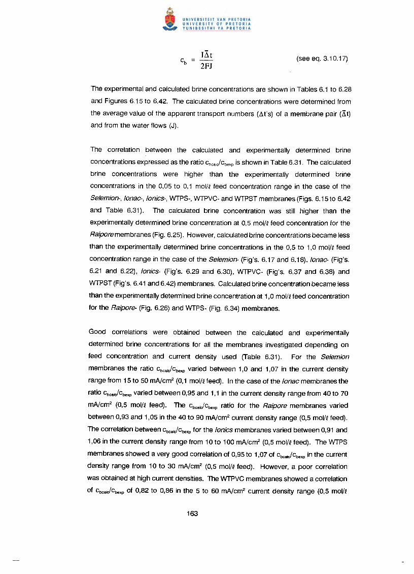
IXt2FJ
The experimental and calculated brine concentrations are shown in Tables 6.1 to 6.28
and Figures 6.15 to 6.42. The calculated brine concentrations were determined from
the average value of the apparent transport numbers (At'S) of a membrane pair (Xt)
and from the water flows (J).
The correlation between the calculated and experimentally determined brine
concentrations expressed as the ratio Cbcalc/Cbexpis shown in Table 6.31. The calculated
brine concentrations were higher than the experimentally determined brine
concentrations in the 0,05 to 0,1 mol/Q feed concentration range in the case of the
Selemion-, lonac-, lonics-, WTPS-, WTPVC- and WTPST membranes (Figs. 6.15 to 6.42
and Table 6.31). The calculated brine concentration was still higher than the
experimentally determined brine concentration at 0,5 mol/Q feed concentration for the
Raiporemembranes (Fig. 6.25). However, calculated brine concentrations became less
than the experimentally determined brine concentrations in the 0,5 to 1,0 molN feed
concentration range in the case of the Selemion- (Fig's. 6.17 and 6.18), lonac- (Fig's.
6.21 and 6.22), lonics- (Fig's. 6.29 and 6.30), WTPVC- (Fig's. 6.37 and 6.38) and
WTPST (Fig's. 6.41 and 6.42) membranes. Calculated brine concentration became less
than the experimentally determined brine concentration at 1,0 mol/Qfeed concentration
for the Raipore- (Fig. 6.26) and WTPS- (Fig. 6.34) membranes.
Good correlations were obtained between the calculated and experimentally
determined brine concentrations for all the membranes investigated depending on
feed concentration and current density used (Table 6.31). For the Selemion
membranes the ratio cbca..JCbeXPvaried between 1,0 and 1,07 in the current density
range from 15 to 50 mNcm2 (0,1 mol/Qfeed). In the case of the lonac membranes the
ratio CbcaJCbexpvaried between 0,95 and 1,1 in the current density range from 40 to 70
mNcm2 (0,5 mol/Q feed). The CbcaJCbexpratio for the Raipore membranes varied
between 0,93 and 1,05 in the 40 to 90 mNcm2 current density range (0,5 mol/Q feed).
The correlation between CbcalJCbexpfor the lonics membranes varied between 0,91 and
1,06 in the current density range from 10 to 100 mA/cm2 (0,5 mol/Q feed). The WTPS
membranes showed a very good correlation of 0,95 to 1,07 of Cbca..JCbexpin the current
density range from 10 to 30 mNcm2 (0,5 mol/Q feed). However, a poor correlation
was obtained at high current densities. The WTPVC membranes showed a correlation
of CbcaJCbeXPof 0,82 to 0,86 in the 5 to 60 mNcm2 current density range (0,5 mol/Q
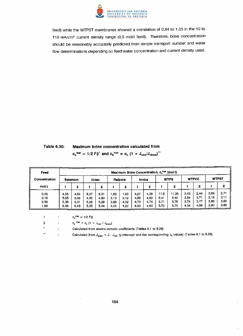
feed) while the WTPST membranes showed a correlation of 0,84 to 1,05 in the 10 to
110 mA/cm2 current density range (0,5 molN feed). Therefore, brine concentration
should be reasonably accurately predicted from simple transport number and water
flow determinations depending on feed water concentration and current density used.
Maximum brine concentration calculated from
cb mllX = 1/2 F 13* and cb mllX = cb (1 + Josm/Jelosm)**
Feed Maximum Brine Concentration, cb-- (mol/~
Concentration Selemion ionac Ralpore lonics WTPS WTPVC WTPST
molN 1 2 1 2 1 2 1 2 1 2 1 2 1 2
0,05 4,55 4,54 5,37 5,31 1,83 1,83 4,27 4,29 11,5 11,38 2,43 2,44 2,69 2,710,10 5,05 5,06 4,85 4,80 3,13 3,12 4,89 4,83 6,41 6,42 3,84 3,71 3,15 3,110,50 5,36 5,31 5,26 5,29 3,98 4,02 4,73 4,74 5,71 5,76 3,74 3,77 3,86 3,851,00 6,48 6,49 5,35 5,44 4,24 4,22 4,63 4,63 5,72 5,74 4,54 4,66 3,90 3,89
cb mlllC = cb (1 + Jo•m / Jelo•m)
Calculated from electro-osmotic coefficients (Tables 6.1 to 6.28)
Calculated from Jelosm = J - Josm (y-intercept and the corresponding cb values) (Tables 6.1 to 6.28).
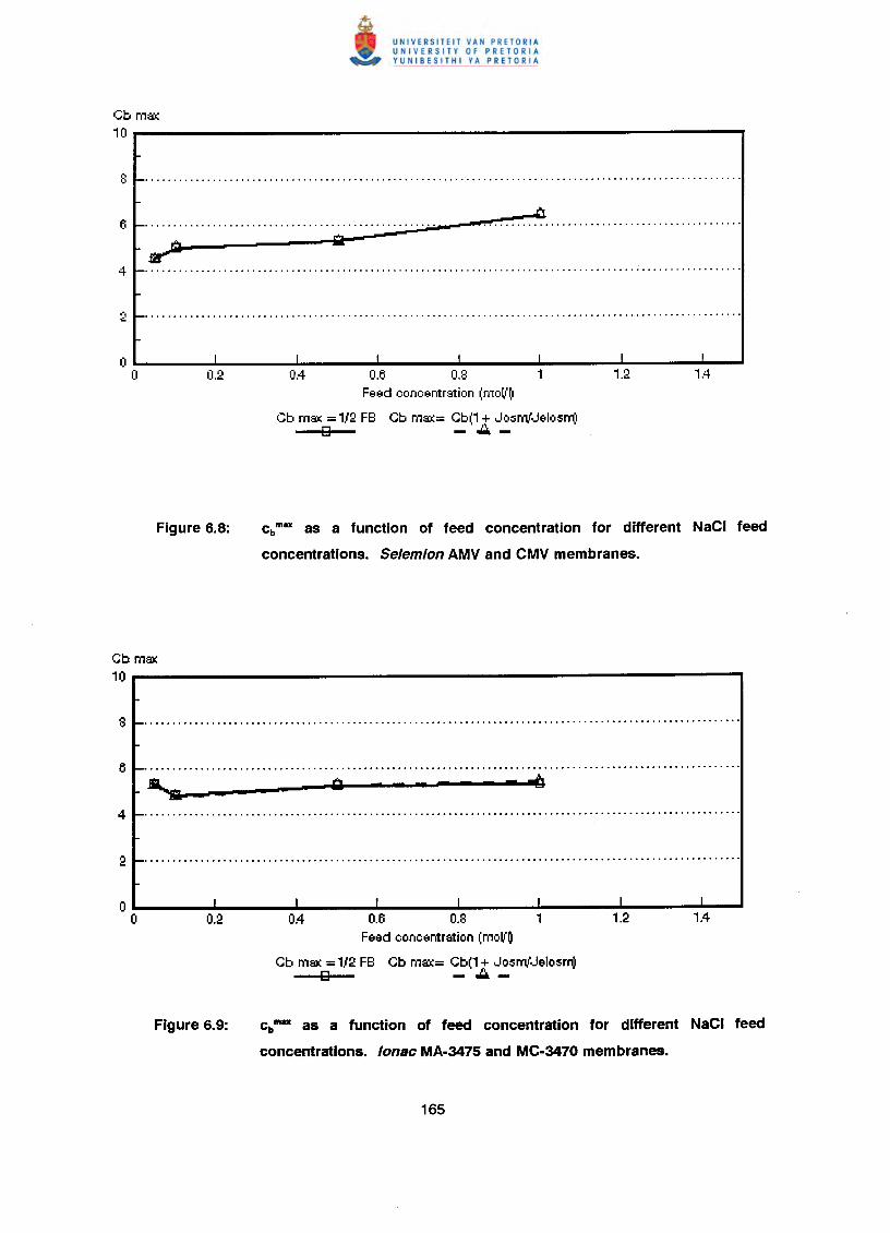
Gbm;;u::10
Gbm;;u::
10
0.6 0.8 1Feed concentrstion (mr)ll'~
Gb m"=£(= 1/2 FB Gb m;;u::= Gb(1 + JosmlJelosm,lg -A-
cbmu as a function of feed concentration for different NaCI feed
concentrations. Selemion AMV and CMV membranes.
-~
0.6 0.8Feed concentrstion (mo~'~
Cb m;;u::= 1/2 FB Gb m;;u::= Cb(1 + JosmlJelosm)g -A-
cbmu as a function of feed concentration for different NaCI feed
concentrations. lonae MA-3475and MC-3470membranes.
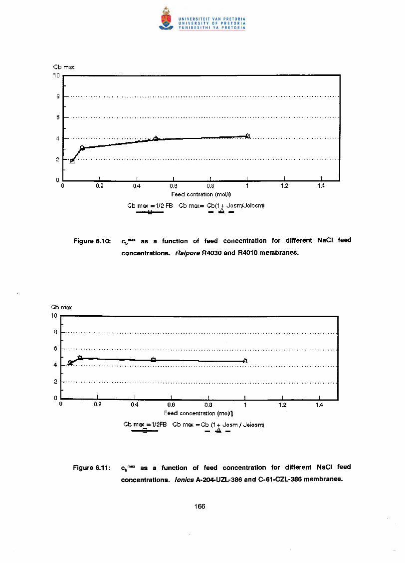
Gb max10
4 b' ~
./. .
0.6 0.8Feed contration (moll'~
Gb max = 1/2 FB Gb n1::£<:=Gbl:1 t ,Josrn,(,Jelosm)o - ••. -
Figure 6.10: cbmu as a function of feed concentration for different NaCI feed
concentrations. Raipore R4030 and R4010 membranes.
Cb max10
.~ ~ ~ .
0.6 0.8 1Feed concentration (moV~
Cb ml:(( = 1/2FB Cb max = Cb (1 + Josm 1Jeiosm)g -~-
Figure 6.11: cbmllX as a function of feed concentration for different NaCI feed
concentrations. tonics A·204-UZL·386 and C·61·CZL·386 membranes.
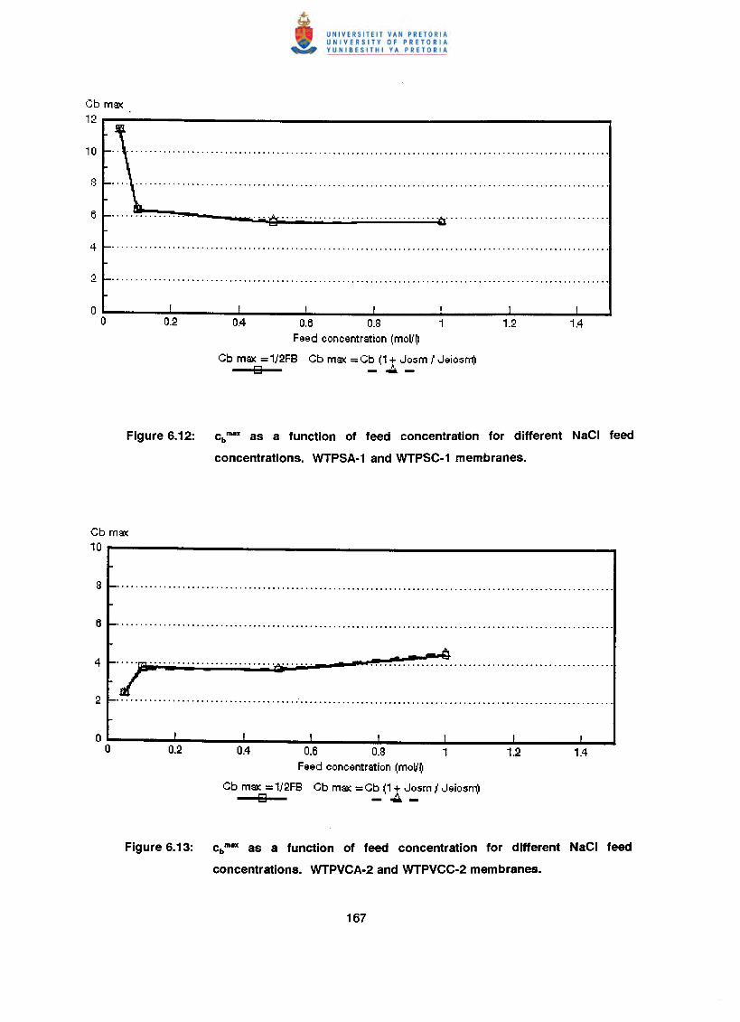
(::bm~12
0.6 0.8 1Feed concentration (moV~
Cb max = 1/2FB Cb max = Cb (1+ Josm I Jeiosm)o -~-
Figure 6.12: cb m8X as a function of feed concentration for different NaCI feed
concentrations. WTPSA·1 and WTPSC-1 membranes.
Cb max10
·7············· ..···..·..·.~ . c -~
w .
0.4 0.6 0.8 1Feed concentration (moV~
Cb max = 1/2FB Cb max =Cb (1+ Josm I Jeiosm)o -~-
Figure 6.13: cb mu as a function of feed concentration for different NaCI feed
concentrations. WTPVCA-2 and WTPVCC-2 membranes.
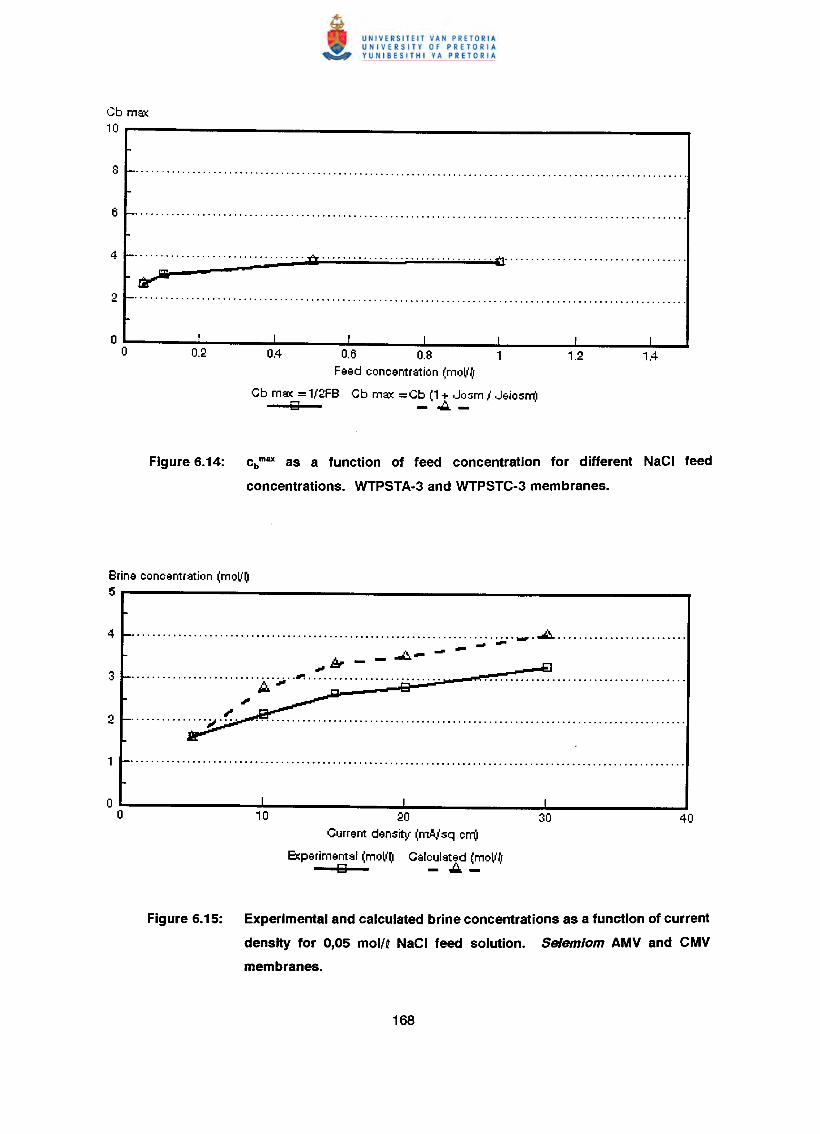
Gb m::£(
10
.................................* (3: .
~
0.4 0.6 0.8 1Feed concentration (moV~
Cb m::£(=1/2FB Cb m::£(=Gb (1+ Josm I Jeiosm)9 --:..-
Figure 6.14: cbmax as a function of feed concentration for different NaCI feed
concentrations. WTPSTA·3and WTPSTC-3membranes.
Brine concentration (moV~5
..........................................................................••••.. ..1::.. .- -.J::..- - -At---##................................ " .A,##
10 20Current density (mNsq cm)
Experimentsl (moV~ Cslculated (moV~9 -..::..-
Figure 6.15: Experimentaland calculated brine concentrations as a function of current
density for 0,05 mol/q NaCI feed solution. Selemiom AMV and CMV
membranes.
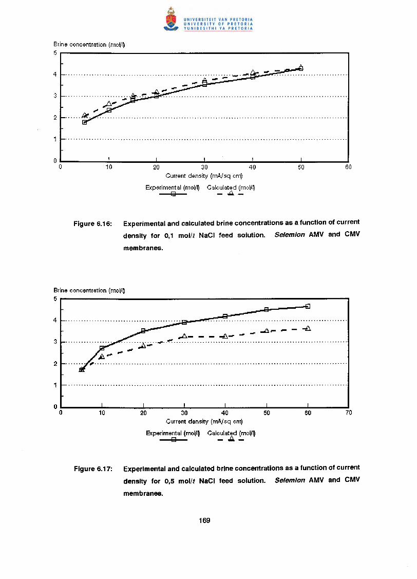
Brine concentration (moll'~5
20 30 40Current density (mo!oisqcm:,
Experimental I:moll'r) C"lcul;~t~d (moll'~o - .••-
Figure 6.16: Experimental and calculated brine concentrations as a function of current
density for 0,1 mol/Q NaCI feed solution. Selemion AMV and CMV
membranes.
Brine concentration (mo~'~5
...I:J.- - - ~A- - - ~.".."...".
""*...... 'J;.;';" ._ .•••• ""*A •.•., .
20 30 40 50Current density (nWsq crn)
Experimental (moll~ Calculated (moll~o -..::..-
Figure 6.17: Experimental and calculated brine concentrations as a function of current
density for 0,5 mol/Q NaCI feed solution. Selemion AMV and CMV
membranes.
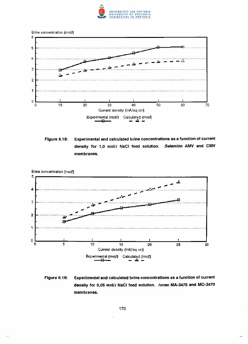
Brine cl)ncentration (mQll'~I)
................................................................it .".~_~,.._-il--~,air'"............&.._.._..~ .- ~~-
30 40Current densit'lj (rrto\lsq cm)
&perimental (mo~'~ Calculated l'mo~'~1o - .••..:..
Figure 6.18: Experimental and calculated brine concentrations as a function of current
density for 1,0 mol/Q NaCI feed solution. Selemion AMV and CMV
membranes.
Brine concentration (moV~5
.... -.................................................................... ~ ..~ .,.. ".
_f:ro ~~................................. ·ik··•••·.~ ....
•••.................... "., .~
10 15 20Current density (rrto\Isq cm)
&perimental (moV~ Calculated (moV~o - .••.-
Figure 6.19: Experimental and calculated brine concentrations as a function of current
density for 0,05 mol/Q NaCI feed solution. lonse MA·3475 and MC·3470
membranes.
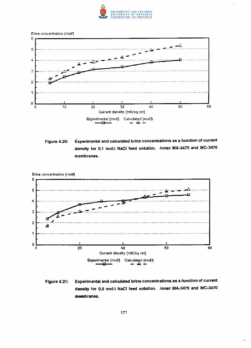
Brine eoneentrstion (moV'r!8
20 30 40Current density (mAlsq em)
Er:perimentsl (moll'~o
Csleulst~d (moV~~- --Figure 6.20: Experimental and calculated brine concentrations as a function of current
density for 0,1 mol/Q NaCI feed solution. lonac MA-3475 and MC-3470
membranes.
Brine eoneentrstion (moVO6
5 'l:r,,' . .:.;,' .•••.. .,,/J,. .----~..f.:i, ~-"';",;."~ .
A-....~ ..~ .
20 40Current density (mA,!sq ern)
Er:perimentsl (moVO Csleulsted (moVOo - .••.-
Figure 6.21: Experimental and calculated brine concentrations as a function of current
density for 0,5 mol/Q NaCI feed solution. lonac MA-3475 and MC-3470
membranes.
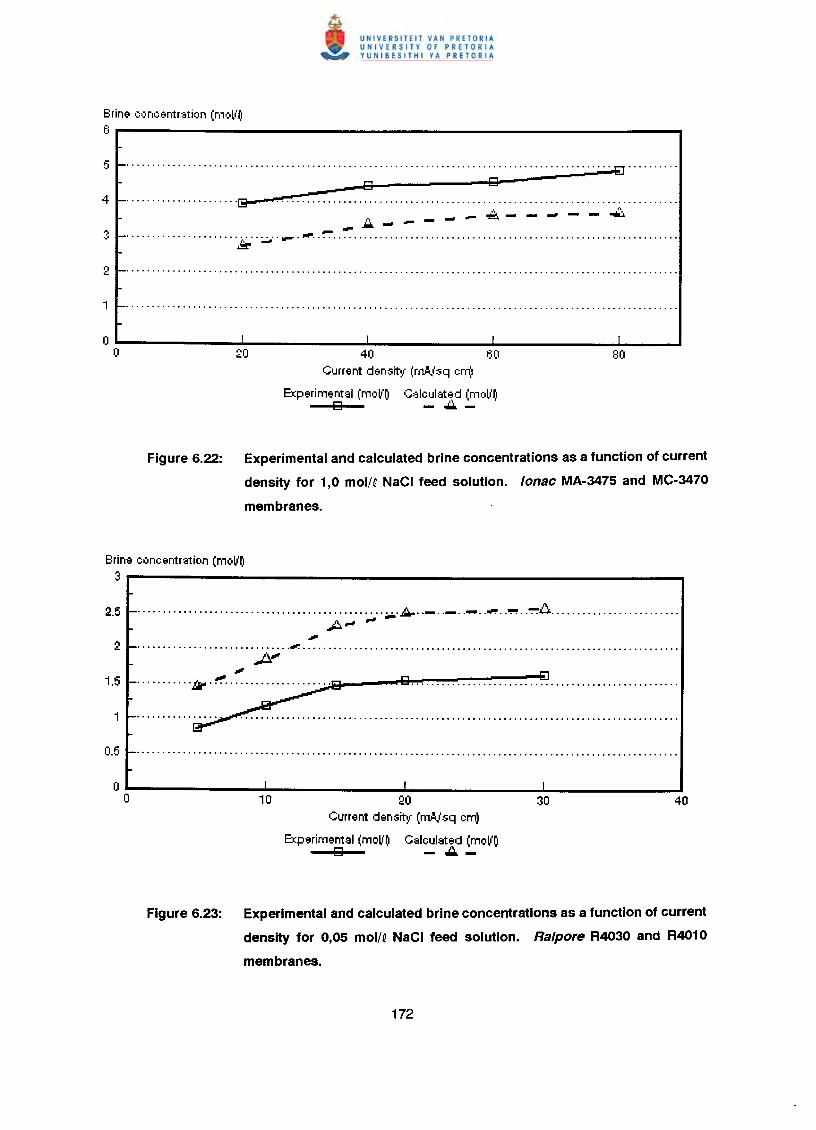
Brine concentration (moll'~6
.............................................................................................. .:eJ .
13 13~......................e- .~~~--..,--~..• .,.,~-
" ;',"';.:..' ~ .. ~ ..~ .~
Current density (n1~/sq cm:,
Experimental (moll'~ G:~lculat?dI:rnoll'~13 - .••. -
Figure 6.22: Experimental and calculated brine concentrations as a function of current
density for 1,0 mol/Q NaCI feed solution. lonac MA-3475 and MC-3470
membranes.
............................................... ';.i." ~ .. _ .. _ ..••.. ~ .. ~ .. ~A .A~ •.•
".............................. ,. .p
•••,-···········w························ .
10 20Current density (rno!t.lsqcrn)
Experimentsl (moV~ Calculated (mo~'~13 - ..::..-
Brine concentration (mo~'~3
Figure 6.23: Experimental and calculated brine concentrations as a function of current
density for 0,05 mol/Q NaCI feed solution. Ralpore R4030 and R4010
membranes.
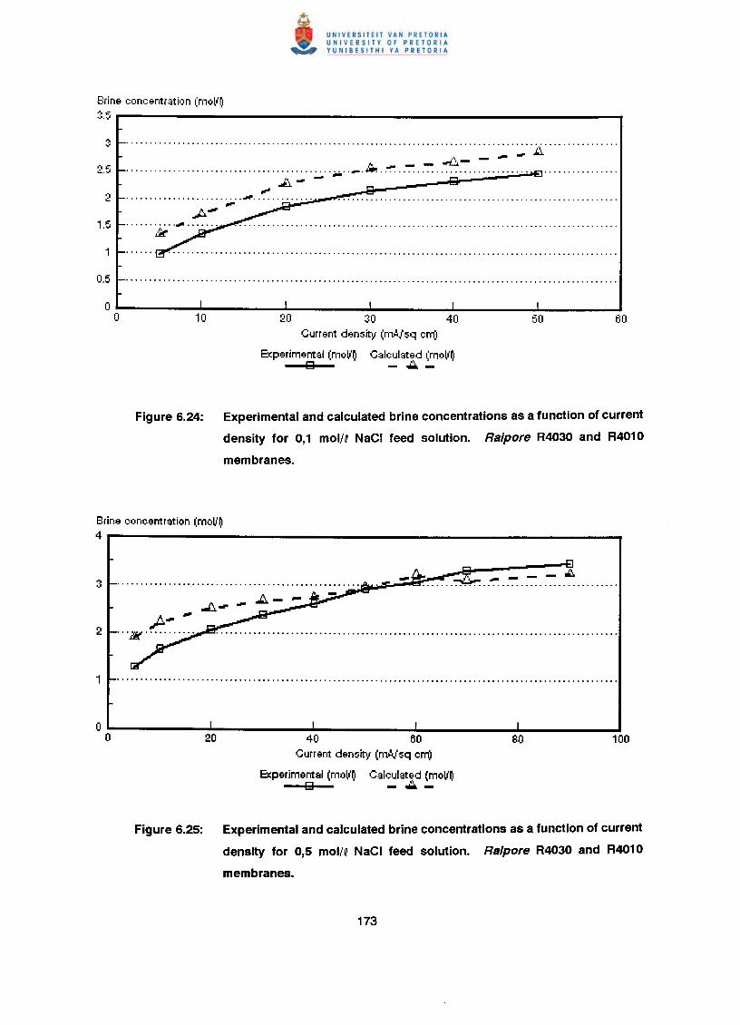
Brine con(~entratil)n(moll'tl3.5
3 {; .,\ _ _ ~ ••• J..l
,",,:: ,~ ~ - - ~.:..:.,1 ••••.•••••••••••••••••••.•••...••..••••.••••••••••. ~._ .......•••••••••••••••••••••••.•••••••.•.•••••..
A"'-"'#;......................... ...,. .-
20 30 40Current density (mAJsq crn)
Er:perimental (mo~'~ Calculated (mo~'~o - A-
Figure 6.24: Experimental and calculated brine concentrations as a function of current
density for 0,1 molN NaCI feed solution. Raipore R4030 and R4010
membranes.
Brine concentration (moll~4
p.- "....;if .
"". ~ ..~ ..-:-: ..-:-: ..-:-: ..~ .
40 60Current density (rnA,isq crn)
Er:perimental (moll~ Calculated (moll~o - A-
Figure 6.25: Experimental and calculated brine concentrations as a function of current
density for 0,5 mol/q NaCI feed solution. Raipore R4030 and R4010
membranes.
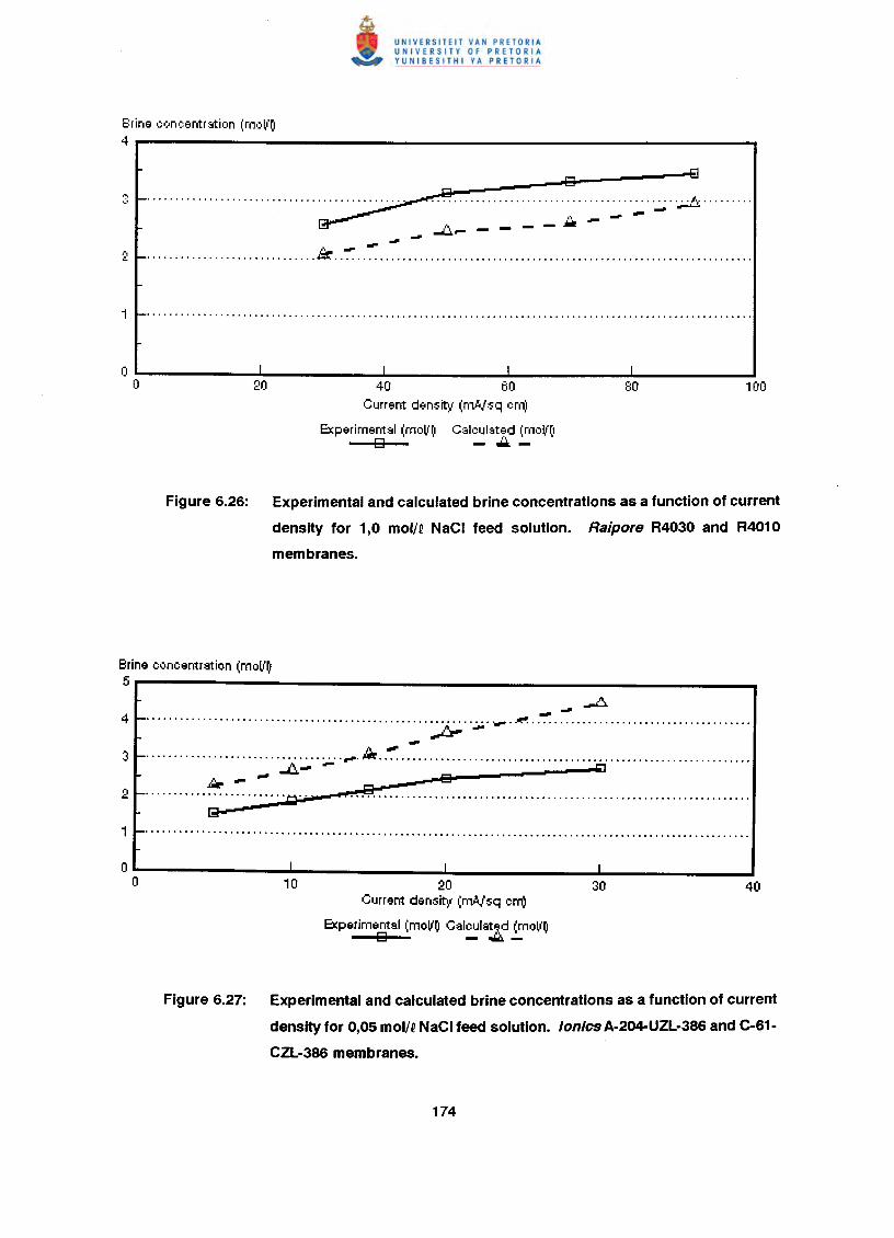
Brine concentr::.tion (ml:lll'~4
__---.e-----Elr:l 0.............................. ~ ~ ..~ ..~ ..~ ..~ ..~ ..~ /', .
~~ --- -~ --.............................. ~ .
40 60Current density (m.!tJsq cm)
Experiment::.' (mo~'~ C::"cuI3t~d (molt'~1o - .••.-
Figure 6.26: Experimental and calculated brine concentrations as a function of current
density for 1,0 mol/~ NaCI feed solution. Raipore R4030 and R4010
membranes.
Brine concentration (molt'~5 -~............................................................. --.~..~ .~-.....................................,..'*.."":..."": ,, , , .
~- - n5l,&p_.... 8, , , .. , ,. 'C" ., .J;! " " ,., , " .
em
20Current density (mAlsq crn)
Experimentsl (molt'~ C3lculat~d (mol(~o - ...:.'1.-
Figure 6.27: Experimental and calculated brine concentrations as a function of current
density for 0,05 mol/~ NaCI feed solution. lonicsA-204-UZL-386 and C-61-
CZL-386 membranes.
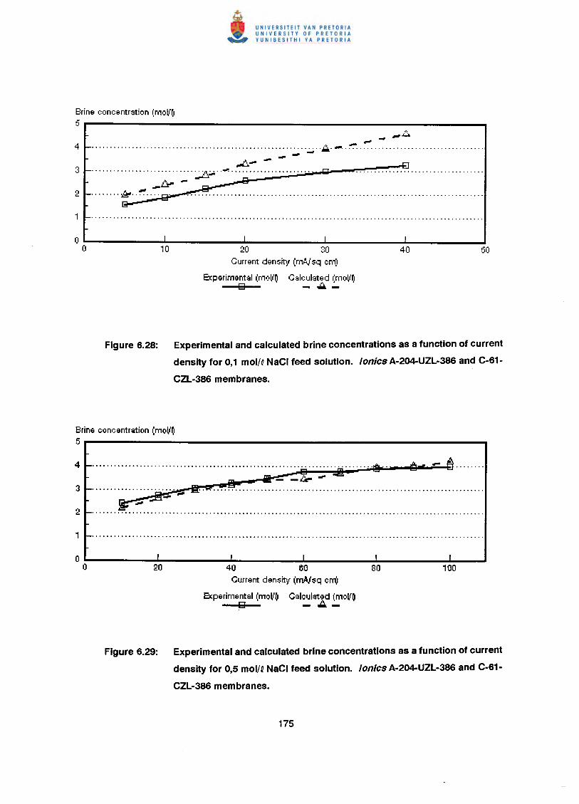
Brine eoneentrstion (mollf)5
.~.""* ~ ,-.J.....I.
............................................................... ~ .."...~ .- -- -~~~~~~ ..~ ~ ~ ~ .
20 30Current density (mAlsq em)
Ec:perimental I:mo~'~o
Calculated I'mo~'~i...· ,- --Figure 6.28: Experimental and calculated brine concentrations as a function of current
density for 0,1 mol/QNaCI feed solution. tonics A·204-UZL·386 and C·61·
CZL·386 membranes.
Brine concentrstion (moV~5
.............................................................................•.ill ~_- :i!~ --~....... ~iI' .k ..'?' .
...........................................................................................................
~- - it .
40 60 80Current density (rn,AJsq crr(!
Ec:perimental (moV~ Calculsted (moV~o -oA-
Figure 6.29: Experimental and calculated brine concentrations as a function of current
density for 0,5 mol/QNaCI feed solution. tontcs A·204-UZL·386 and C·61·
CZL·386 membranes.
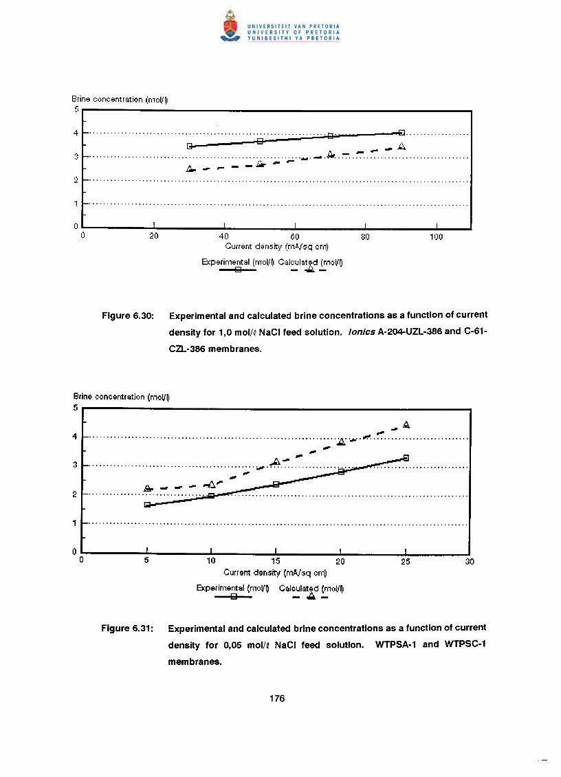
Brine c,:,ncentrstion (moll'~5
4 ··············0· ....t!J .l3- 0 _I::...
3 .............................................................•••. ~ . .;:::.,.. ~ .. ~ .. ~ .~.",.,..- -~"..,,-
40 60Current den::;it~((mo!oJ::;qcm)
Experimentsl (moll'~ Cslculst~d I'moll'rlo -...:::...:.'
Figure 6.30: Experimental and calculated brine concentrations as a function of current
density for 1,0 mol/QNaCI feed solution. tonics A-204-UZL-386 and C·61·
CZL-386 membranes.
Brine concentration (moV~5
_A~...................................................................... :1:1.... ,#< • .,.. •••••••••••••••••••.••••••••.,..
A- ~••••••••••••••••••••••••••••••••••••••••••••••• ;.Jt#' •••••••••••••••••••••••••".
10 15 20Current density (mNsq em)
Experimental (mo~'~ Csleulsted (moll~o - .,.;j,-
Figure 6.31: Experimental and calculated brine concentrations as a function of current
density for 0,05 mol/Q NaCI feed solution. WTPSA·1 and WTPSC·1
membranes.
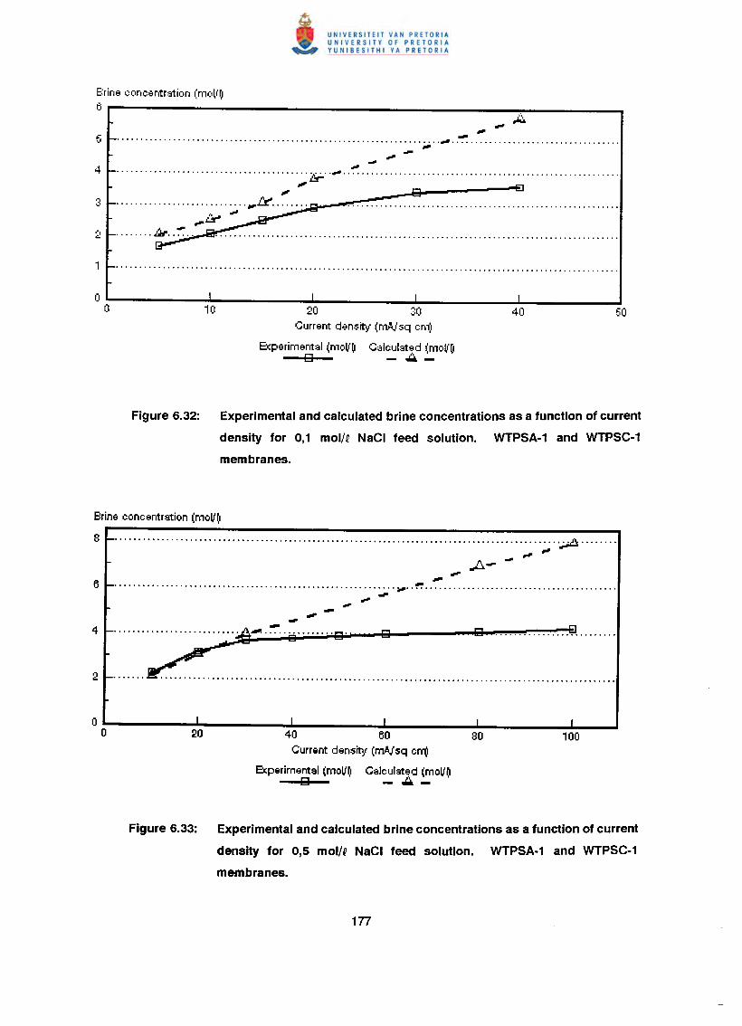
Brine eoneentr:~tion (moll'~ti
".5 ". ..~ .".~......................................... ~ ..". .....
<I'
............................ ~~ .&~"......... Ao .. :':'..
20 30Current density (mAlsq em:1
Experimental (mo~'~ Calculat~d (moll'~1o - .••.-
Figure 6.32: Experimental and calculated brine concentrations as a function of current
density for 0,1 mol/~ NaCI feed solution. WTPSA·1 and WTPSC-1
membranes .
............................................................................................... ~ ....,. ~
A- -".
•••••••••••••••••••••••••••••••••••••••••••••••••••••••••••• ifI'I •• ~ •••••••••••••••••••••••••••••••••••••••••--.......................... ~_. -::..8········ 8' g lei ~ , .
....~........................................ .
40 60 80Current density (mA,lsq crn)
Experimental (moV~ Calculated (moV~o - ..::..-
Figure 6.33: Experimental and calculated brine concentrations as a function of current
density for 0,5 mol/~ NaCI feed solution. WTPSA·1 and WTPSC·1
membranes.
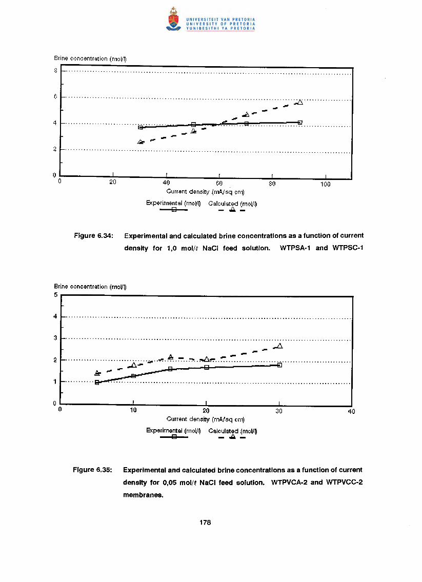
....................................................................................... ,.. ..",. ~ A..l-o •. •••••......0 ~ ...•. ~ .,.
40 60 80Current den::;ity (mA,I::;qcm)
&:perimentsl (moll~ Cslculsted {mol,'rlo - """~ '
Figure 6.34: Experimental and calculated brine concentrations as a function of current
density for 1,0 mol/Q NaCI feed solution. WTPSA·1 and WTPSC·1
Brine concentration (moV~5
_A.-A --...............................•••.. ~ ~ ..~ ..~~ ..-:: .A- 0 ---EJ
~ ~ - ~QB
........... Q-' .
10 20Current density' (rn.Nsq cm)
Experimental (moV~ Calculated (mo~'~o - """-
Figure 6.35: Experimental and calculated brine concentrations as a function of current
density for 0,05 mol/Q NaCI feed solution. WTPVCA·2 and WTPVCC·2
membranes.
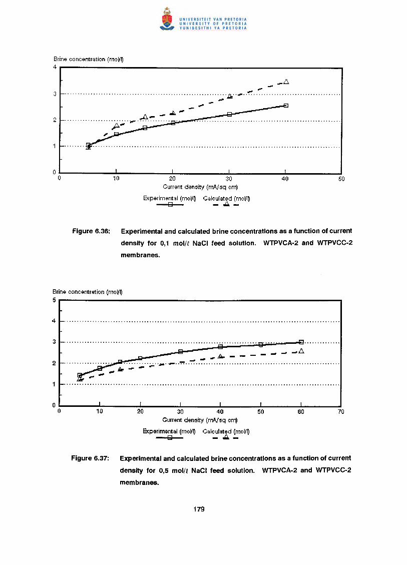
Brine concentration (rnoll~14
,#I'
............................................................... ....,. .. .". ..~ .JIil:~
.-=:..~A""""......................... _ .p.~
20 ~:OCurrent density (rnAisq crn)
E(perirnental (rno~'~ C8lcul8t~d (rnoll'~o - ••.•.-
Figure 6.36: Experimental and calculated brine concentrations as a function of current
density for 0,1 mol/~ NaCI feed solution. WTPVCA-2 and WTPVCC-2
membranes.
Brine concentration (moll~5
...................... , , , '9··'·········· "1:1..... ,..e] .o f:!..
~ __ n...- ••• ~ .".~ - - - -.....~.:;:.~ .."' .._ .._ ..~ .
20 30 40 50Current density (mNsq cm)
&:perimentsl (mo~'~ Calculated (moll~o - ~-
Figure 6.37: Experimental and calculated brine concentrations as a function of current
density for 0,5 mol/~ NaCI feed solution. WTPVCA-2 and WTPVCC-2
membranes.
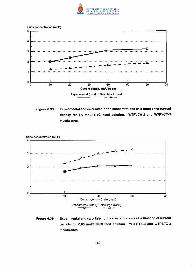
Brine concentration (moVO5
82 ~ ~ .
..,.fJ"". - - - - - .,..- --~---~~--
20 30 40 50Current density (mNsq cm)
Experimentsl (moVO Cslculated (moVOg - ~-
Figure 6.38: Experimental and calculated brine concentrations as a function of current
density for 1,0 mol/Q NaCI feed solution. WTPVCA·2 and WTPVCC·2
membranes.
Brine concentration (moVO4
~--~................................................ ~ .. i:I., .~ .. -:. .
.e q ~ .......................... ~.
20Current density (rl1.o!.isqcm)
Experimentsl (moll'~1Cslculst.;.d (moll'rlg -",:,::,,-'
Figure 6.39: Experimental and calculated brine concentrations as a function of current
density for 0,05 mol/Q NaCI feed solution. WTPSTA-3 and WTPSTC·3
membranes.
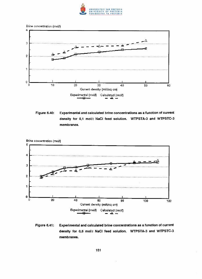
Brine concentration (mov'~4
_D-0 •••••••••••••••••••••••••••••••••••••••••••••••••••••••••••••••••••••••••••••••••• ~ •••••••••••••••••••••••
r't '"I ~
L},. - - - ~- - - - .•••.~ g ~
.iJu.' g~-~......................... ;;. . .[;0&
20 30 40Current density (rnAJsq cm)
Experimental (moV~ Calculated (moV~g - ~-
Figure 6.40: Experimental and calculated brine concentrations as a function of current
density for 0,1 mol/Q NaCI feed solution. WTPSTA-3 and WTPSTC-3
membranes.
Brine concentration (moV~5
"'----ftQ •..................................:£ ,."~ _ :: ~ .. ··.:..:...:..:...:..:··i· ••. ·~ .. ··· .. · .... ······ .. · .. ······ .. · .... ·...... ...•••..............................................................................................
40 60 80Current density (rn,AJsq cm)
Experimental (moV~ Calculated (moV~g - ~-
Figure 6.41: Experimental and calculated brine concentrations as a function of current
density for 0,5 mol/Q NaCI feed solution. WTPSTA-3 and WTPSTC-3
membranes.
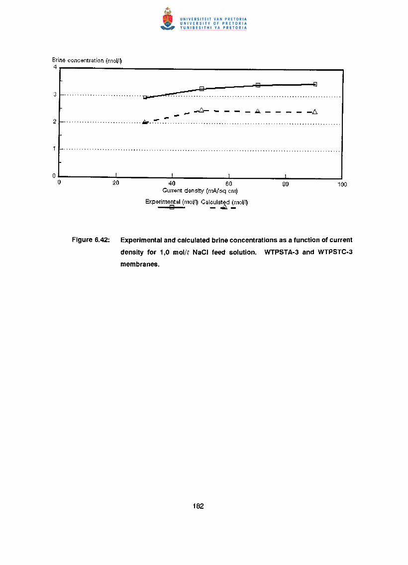
Brine eonl~entration (mov'O4
_-a-----.....ED3------0~ g
••••.••••••••••••••••••••••••• r:g.;a""'. _~--~.- ••••••••••• ~••••••••••••••••••••••••••••••••••••••••••••••••••••••••••••••
40 60Current density (mNsq em)
Experimental (moll'O Caleulat:;d (mov'Oo - .•.•.-
Figure 6.42: Experimental and calculated brine concentrations as a function of current
density for 1,0 mol/QNaCI feed solution. WTPSTA·3 and WTPSTC·3
membranes.
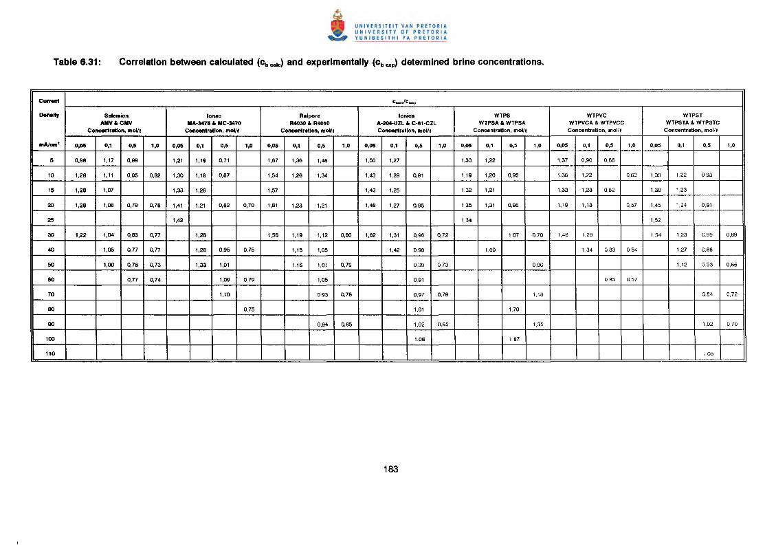
Current C.•• ..'C•• p
Denelly Selemion lonac Raipore lonics WTPS WTPVC WTPSTAMVleCMV MA·3475 Ie MC-3470 R4030 Ie R4010 A-204-UZl Ie C-61-CZl WTPSA Ie WTPSA WTPVCA Ie WTPVCC WTPSTA" WTPSTC
Concentrelion, moVl Concentretion, moVI Concentration, moVI Concentration, mol/l Concentration, mol/t Concentration, mol/t Concentration, mol/'
mAlcm' 0,05 0,1 0,5 1,0 0,05 0,1 0,5 1,0 0,05 0,1 0,5 1,0 0,05 0,1 0,5 1,0 0,05 0,1 0,5 1,0 0,05 0,1 0,5 1,0 0,05 0,1 0,5 1,0
5 0,98 1,17 0,99 1,21 1,19 0,71 1,67 1,36 1,48 1,50 1,27 1,33 1,22 1,37 0,90 0,86
10 1,28 1,11 0,85 0,82 1,30 1,18 0,87 1,54 1,26 1,34 1,43 1,29 0,91 1,19 1,20 0,95 1,36 1,22 0,63 1,39 1,22 0,93
15 1,28 1,07 1,33 1,26 1,57 1,43 1,25 1,32 1,21 1,33 1,23 0,82 1,38 1,23
20 1,26 1,06 0,79 0,78 1,41 1,21 0,82 0,70 1,61 1,23 1,21 1,48 1,27 0,95 1,35 1,31 0,96 1,19 1,13 0,57 1,45 1,24 0,91
25 1,42 1,34 1,52
30 1,22 1,04 0,83 0,77 1,26 1,58 1,19 1,12 0,80 1,62 1,31 0,96 0,72 1,07 0,70 1,46 1,29 1,54 1,23 0.99 0,69
40 1,05 0,77 0,77 1,28 0,95 0,75 1,15 1,05 1,42 0,98 1,60 1,34 0,83 0,54 1,27 0,88
50 1,00 0,78 0,73 1,33 1,01 1,16 1,01 0,79 0,99 0,73 0,86 1,12 0,93 0,66
60 0,77 0,74 1,09 0,79 1,05 0,91 0,85 0,57
70 1,10 0,93 0,78 0;97 0,79 1,16 0,84 0,72
80 0,75 1,01 1,70
90 0,94 0,85 1,02 0,85 1,35 102 0,70
100 1,06 1,87
110 1,05
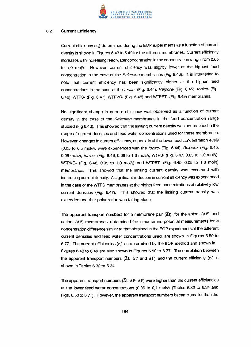
Current efficiency (€p) determined during the EOP experiments as a function of current
density is shown in Figures 6.43 to 6.49 for the different membranes. Current efficiency
increases with increasing feed water concentration in the concentration range from 0,05
to 1,0 mol/Q. However, current efficiency was slightly lower at the highest feed
concentration in the case of the Selemion membranes (Fig 6.43). It is interesting to
note that current efficiency has been significantly higher at the higher feed
concentrations in the case of the lonac- (Fig. 6.44), Raipore- (Fig. 6.45), lonics- (Fig.
6.46), WTPS- (Fig. 6.47), WTPVC- (Fig. 6.48) and WTPST- (Fig 6.49) membranes.
No significant change in current efficiency was observed as a function of current
density in the case of the Selemion membranes in the feed concentration range
studied (Fig 6.43). This showed that the limiting current density was not reached in the
range of current densities and feed water concentrations used for these membranes.
However, changes in current efficiency, especially at the lower feed concentration levels
(0,05 to a,s mol/Q), were experienced with the lonac- (Fig. 6.44), Raipore- (Fig. 6.45,
0,05 mol/Q), lonics- (Fig. 6.46, 0,05 to 1,0 mol/Q), WTPS- (Fig. 6.47, 0,05 to 1,0 mol/Q),
WTPVC- (Fig. 6.48, 0,05 to 1,0 mollQ) and WTPST- (Fig. 6.49, 0,05 to 1,0 mol/Q)
membranes. This showed that the limiting current density was exceeded with
increasing current density. A significant reduction in current efficiency was experienced
in the case of the WTPS membranes at the higher feed concentrations at relatively low
current densities (Fig. 6.47). This showed that the limiting current density was
exceeded and that polarization was taking place.
The apparent transport numbers for a membrane pair (Kt), for the anion- (Ata) and
cation- (MC) membranes, determined from membrane potential measurements for a
concentration difference similar to that obtained in the EOP experiments at the different
current densities and feed water concentrations used, are shown in Figures 6.50 to
6.77. The current efficiencies (€p) as determined by the EOP method and shown in
Figures 6.43 to 6.49 are also shown in Figures 6.50 to 6.77. The correlation between
the apparent transport numbers (Xt, At" and AtC) and the current efficiency (€p) is
shown in Tables 6.32 to 6.34.
The apparent transport numbers (Kt, Ata, A~) were higher than the current efficiencies
at the lower feed water concentrations (0,05 to 0,1 mol/Q) (Tables 6.32 to 6.34 and
Figs. 6.50to 6.77}. However, the apparent transport numbers became smaller than the
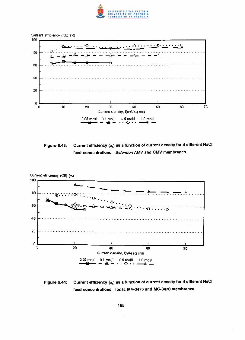
Gurrent efficiency (GE) (%)100
.a'>_ • • • • • • G>. • • • .:]0 • • • • • • 1itJ· • • • .~. l• .1. - '~.,r....... ••• , _1'--. "..- ~ -t-
.... ':"'~ 'A." :.:,:~' .~.~. '':'':' '.:.:' '':':~''~' ..:.... :;.;;;;. .. ~. '~":.;,ji""""""""""""""
13- 8 0..... 8':":" ~ .
20 30 40 50Gurrent density, 1(m,AJsqcm)
0.05 mol,'1 0.1 molll 0.5 molll 1.0 mo~'18 .e.- .. ~ .. --+<-
Figure 6.43: Current efficiency (€p) as a function of current density for 4 different NaCI
feed concentrations. Selemion AMV and CMV membranes.
Current efficiency (CE) (%)
100 r--------------------------*-- --80 1-•••••••••• €;: (IF; ~ .. ~ ~ ~ ~ ~ ~ .. ?¥ .
~····~·· ...a
60 1-............... ~ .._ .._ .. "fJ- ..••.•...-lz;..' . ;.;..' l() .•.•.•. ; .;r,.' .. ....A ~ -0
I I I
20 40 60Current density, 1(m,AJsqcm)
0.05 molll 0.1 molll 0.5 molll 1.0 molll8 -..::r.- .. ~ .. ----o>f(-
Figure 6.44: Current efficiency (€p) as a function of current density for 4 different NaCI
feed concentrations. lonac MA·3475 and MC-3470 membranes.
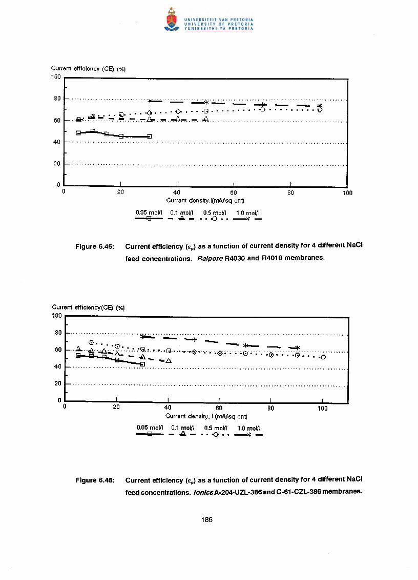
Current efficiency (CE) (%)100
............................. ~ ~ :...: .-,...- - ~ - - tI"':. • '" • • • .n • • • • • • • • • .:J • • • • • • • • •~ ii::l, , ' , ''V' ,'....... <..:!
.. J£jp.- •.. , .. ~: . ~~ .~ •.. ~ .. ~ ~ .. ~ .. ~~ .. ~ .. ~ .
[3-'9 """""3-- 0 0
20 40 60Current density,l(mA.,lsq em)
0.05 molll 0.1 Toill 0.5 molll 1.0 molllo - - , , .(j , , ----0>1::
Figure 6.45: Current efficiency (€p) as a function of current density for 4 different NaCI
feed concentrations. Raipore R4030 and R4010 membranes.
Current efficiency(CE) (%)100
........................... ~ ..r,>. - -..... -~' , , '0 - :+--..A ..~: .~ ..... '.....'..'.G.~.•.•. ,Q., • - --+ce--lid s::t - oA_ .6.' ····~··~·~..··<!l'·······£:?)···~·~·~~· •.·•.·•.···(;i·:·:·:·.o .
""€J _
........................................................................................................
40 60 80Current density. I (mNsq em)
0.05 molll 0.1 molll 0.5 molll 1.0 molllo -.:..- .. -0 .. ----0>1::-
Figure 6.46: Current efficiency (€p) as a function of current density for 4 different NaCI
feed concentrations. tonics A-204-UZL-386 and C-61-CZL-386 membranes.
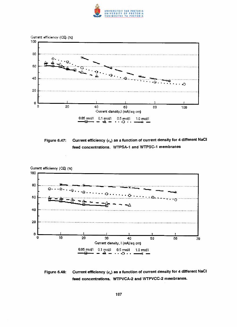
Current efficiency (CE) (%)
100 r---------------------------.......... ~ .•..•...............~ .
~~.~. . . •....••.··_--~··O·:· ..·········~·~····························· .
~ • 0() • • •••••••••-~ ."<)'" *'-.......................................................• ,Q. •.•.•. ~ ~ .. ~ ........... -.,.....,.. .()
I I I I r
20 40 60 30 100Current density,l (mA,isq cm)
0.05 molll 0.1 molll 0.5 molll 1.0 molllg -~- • • -:J • • ---+0: -
Figure 6.47: Current efficiency (€p) as a function of current density for 4 different NaCI
feed concentrations. WTPSA·1 and WTPSC·1 membranes
Current efficiency (CE) (%)100
............. ~ ..~.~ ......••... ~ ~~ .0· . -tz,. . ~ ~"6' ••• ~ -.....I..:JI······O ~······0.... '&:"'" 'S'" ~'1t'.~.~ :.:.:.~.~.~.~ " ·..0········· .
-- e-IiiiiI - - - -.6.
20 30 40 50Current density, I (mA,isq cm)
0.05 molll 0.1 molll 0.5 molll 1.0 molllo - .••- .. ~ .. ~-
Figure 6.48: Current efficiency (€p) as a function of current density for 4 different NaCI
feed concentrations. WTPVCA·2 and WTPVCC·2 membranes.
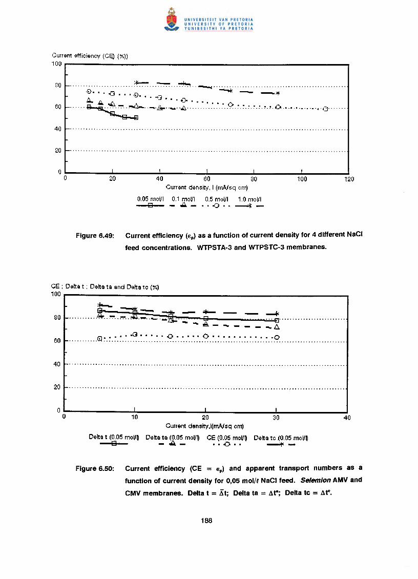
Current efficiency (CE) (%))
100 .------------------------------..
*-- - ••...80 _ __ .v ",'"1 ~..... --.+: - -:0+:- . . . ·u· . . .G~~ ... c..
60 _ 8 ~ ~_ .. _.iJ!I.. .. _ .. ~ ....•..•..•..•..•. : ..C!:.~.~.:.:.:.~.~. 00 .•.•.•.•.•.•.• ·0..·····
40 _ .
I 1 I
40 60 80Current density. I (mA,lsq cm)
0.05 mov'l 0.1 molll 0.5 molll 1.0 molllo ~- .. -0 •• --i>j::-
I
100
Figure 6.49: Current efficiency (€p) as a function of current density for 4 different NaCI
feed concentrations. WTPSTA-3and WTPSTC-3membranes.
CE ; Delta t : Delta ta and Delta tc (%)100
*-~3- ~-~ -................... ~ ....••..~ ..~ ....- - ...-.- - -4o ...0·························~-~---~~
t:J ••••• -£3 0 0 -0......................................................................................................
10 20 30Current density,I(mA./sq crr(!
Delta t (0.05 mollO Delta ta (0.05 mov'O CE (0.05 moVO Delta tc(0.05 mollOo -..:..- ··0.· -+:-
Figure 6.50: Current efficiency (CE = €p) and apparent transport numbers as a
function of current density for 0,05 mol/QNaCI feed. Selemion AMV and
CMV membranes. Delta t = Kt; Delta ta = at"'; Delta tc = ato.
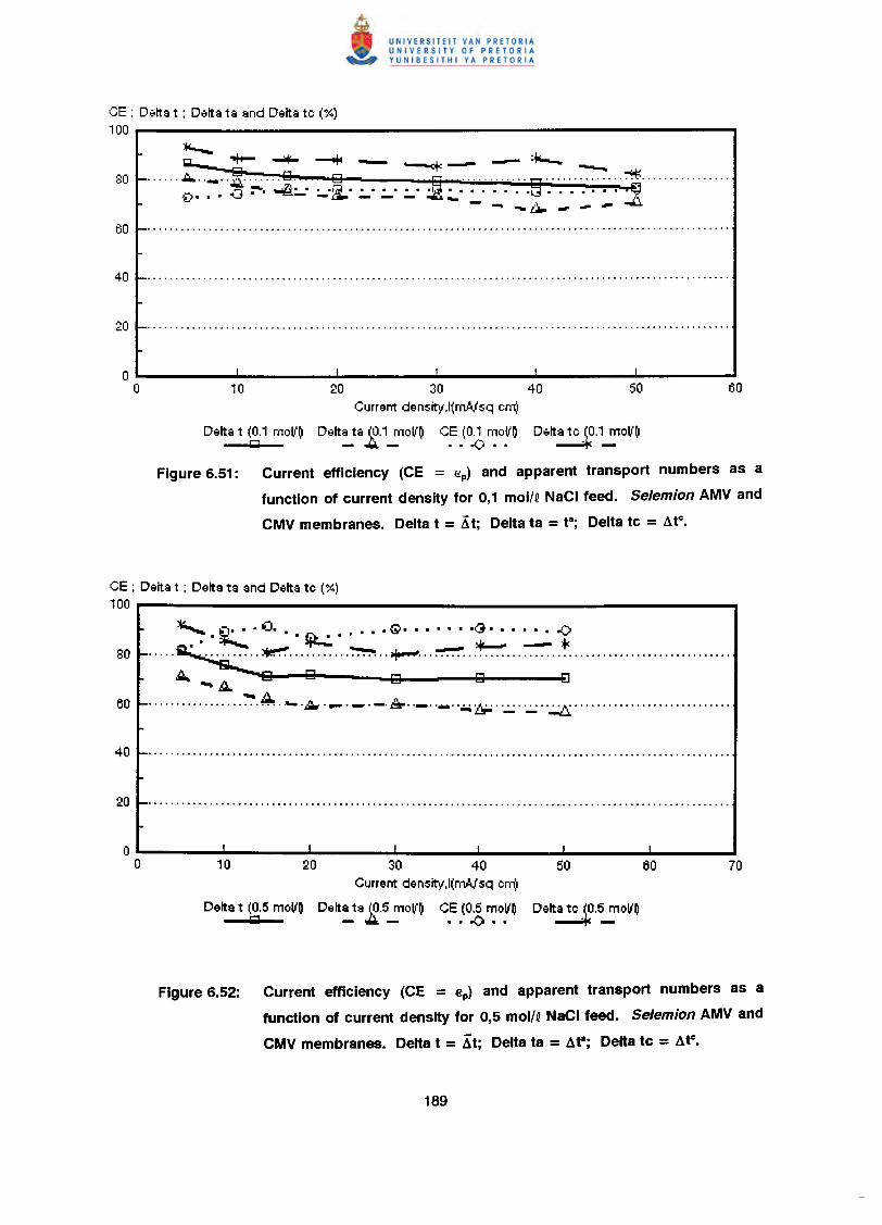
CE ; Delta t ; Delta ta and Delta te (%)100
~c... -,+-....,;,jIo-,-"" - -=+: _ - *-_......:.._..~..~...J~..·1······· J ...·..·.··..·..···9 ..····?·~~··············..
••• ••••••••••• r
- - -~- - - ~
20 30 40 50Current density.I(rn,AJsq em)
Delt~ta ~.1_moVO c~.(01. ~o~O Delta te _~.~OVODelta t (0.1 moVO1;1
Figure 6.51: Current efficiency (CE = €p) and apparent transport numbers as a
function of current density for 0,1 mol/~NaCIfeed. Selemion AMV and
CMVmembranes. Deltat = Xt; Deltata = t8; Deltatc = Atc•
CE ; Delta t ; Delta ta and Delta te (%)100
~ 1;;)_.. O. . . • . G· . . . . . .<3-. . . . .. ('-..... ~ .~.. ~ .....••.•-X.....~ ~ ..+-'- ~ .A. .•.•.A 0 0 0 0
•••••.Q"........................ --.~. _. _. _ ..&r .. _ .. _ ..... 1. •.•....•.••••• ,\ •••••••••••••••••••••••••••••••••~ - - -l;;,.
30 40Current density,I(rn,AJsq em)
Delt~ta ~.5_movo C~ .(0.6 ~o~ODelta t (0.5 moVO1;1
Figure 6.52: Current efficiency (CE = €p) and apparent transport numbers as a
function of current density for 0,5 mol/~NaCIfeed. Selemion AMV and
CMVmembranes. Deltat = At; Deltata = Ar; Delta tc = Atc•
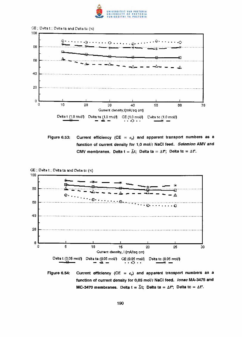
<::E; Delta t : Delta ta and Delta te (%)100
@ ••• () .,:;.,•••1.,. • • •• •••••• 0 . . ······0~ ..-.- • • • • • • Ii)- • • •.................. .~ ..'-':0+:-" '-'>f:-" .~¥~ -:+' .R-
13............ ..sr.. .. __ ~ ~ ~ !? .
.•••---Ll. - - -LJ.. - - -':!- - - -::..- - - .,I;:..
30 40Current density,l(mA,lsq em)
Delta t (1.0 moV~ Delta ta ~~.OmoV~ CE (1.0 moll~ Delta te 11.0 moV~I5iiI _ ••••. _ • • .() • • -----+-: _
Figure 6.53: Current efficiency (CE = €p) and apparent transport numbers as a
function of current density for 1,0 mol/Q NaCI feed. Selemion AMV and
CMV membranes. Delta t = Xt; Delta ta = ata; Delta tc = atc.
CE ; Delta t ; Delta ta and Delta te (%)100 *"- _ .....=.10<.--,.... - ~HH HH H::",H,"H~ .l.~~.~H':;:' :-:. ~~H:::-~ ~H.H.H...·...
• • • .i::L.... (;) ..... .... .• . .....• ..... ........... ... .............~.~.~ ,. .• • • ~. • • • • • • • tP:I
5 10 15 20 25Current density, I (m,AJsq em)
Delta t (0.05 moV~ Delta ta (Q.05 moV~ CE (0.05 moV~ Delta te (0.05 moV~IMI -1llIi&- •• 0.. ~-
Figure 6.54: Current efficiency (CE = €p) and apparent transport numbers as a
function of current density for 0,05 mol/QNaCI feed. lonse MA·3475 and
MC.3470 membranes. Delta t = Xt; Delta ta = ,1ta; Delta tc = atc.
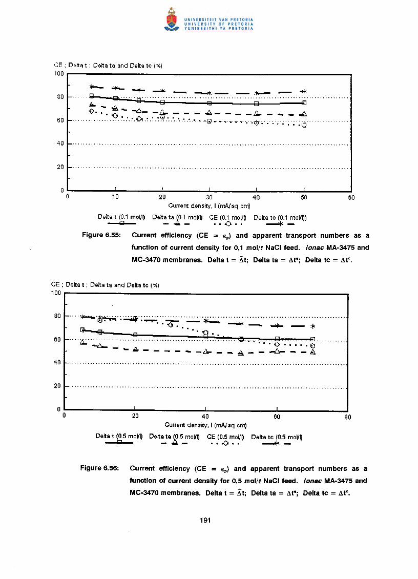
GE ; D8lta t ; D8lta ta and Delta te (%)100
*"--+'-....o+------=J.<. ~----.- _ --.....;:j::: _ _::jOI.- - -r'...... 1; 1iiZI··················.·········· ················· .
~ 0 0 8 0 0~-.....- ~ - -.::J.... l\"<:/ ••• ...", - -~ - - - "*-l. - - __ ~ ..::..
v ••• ~ ••• I~ •••.. . . . . . ..•.. . . -.. -, .••.•.• @ ." ••••..•..•..•. '.' '.'l!r ~. ~. ~.;.; .; .;. ~0" .
10 20 30 40 50Current density, I (rn.tVsq em)
Delta t (0.1 moV~ Delta ta (0.1 moV~ CE (0.1 moV~ Delta te (0.1 moV~)IiiiI - •••••. - •• ~.. ----+c-
Figure 6.55: Current efficiency (CE = €p) and apparent transport numbers as a
function of current density for 0,1 molN NaCI feed. lonae MA·3475 and
MC·3470 membranes. Delta t = At; Delta ta = ata; Delta tc = atc.
CE : Delta t ; Delta ta and Delta te (%)100
....~.~~.~.~.~~.~.~~..~ ~..= ~ =..~ .9-- 0 ····28 .. ,.....,. ~ a EJ ..•....••...s:.iI. ~ ···o ~
- ••• JJ. - - - - ••• _~ _ ••• ~ __ ~ •••. _ A
20 40 60Current density, I (rn.tVsq em)
Delta t ~.5 moV~ Delt~ta ~.5_moV~ C~ .(0.6 ~o~~ Delta te .~.:=OV~Figure 6.56: Current efficiency (CE = €p) and apparent transport numbers as a
function of current density for 0,5 mol/~ NaCI feed. lonse MA·3475 and
MC·3470 membranes. Delta t = Xt; Delta ta = ata; Delta tc = atc.
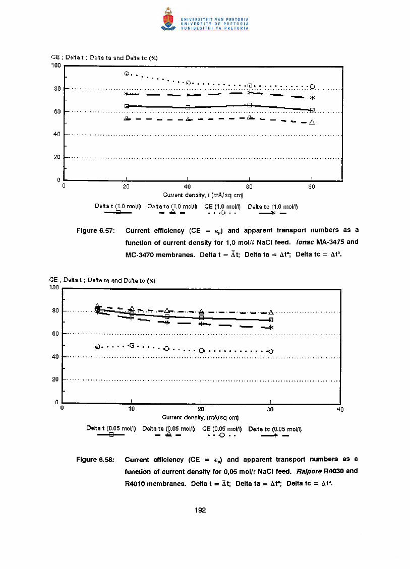
GE : Delta t : Delta ta and Delta te (%)100
~ .. . ..• • • • • •£'
............... • •••••••••• 1:;) •••••••••• -t:t......~ = ~..~ ~ ~..~ ~ .- :;<
GOO........................................................................•................... oj;;] .
oo 20 40 60 SO
Current density, I (mNsq em)
Delta t (1.0 moV~ Delta ta I~!.OmoV~ CE (1.0 moV~ Delta te 11.0 mol(~lid - .••. - • • .() • • ----4c -
Figure 6.57: Current efficiency (CE = €p) and apparent transport numbers as a
function of current density for 1,0 mol/Q NaCI feed. lonae MA-3475 and
MC-3470 membranes. Delta t = Lit; Delta ta = ae; Delta tc = atc.
CE : Delta t ; Delta ta and Delta te (%)100
~. . . . . ·G . . .. 0. .. . . . 0 . . . . . . . . . . . -0
10 20 30Current density,l(mNsq em)
Delta t (0.05 moV~ Delta ta (0.05 moV~ CE (0.05 moV~ Delta te (0.05 moV~o -~- ··0·· ----+c-
Figure 6.58: Current efficiency (CE = €p) and apparent transport numbers as a
function of current density for 0,05 mol/QNaCI feed. Raipore R4030 and
R4010 membranes. Delta t = ~t; Delta ta = ate; Delta tc = atc.
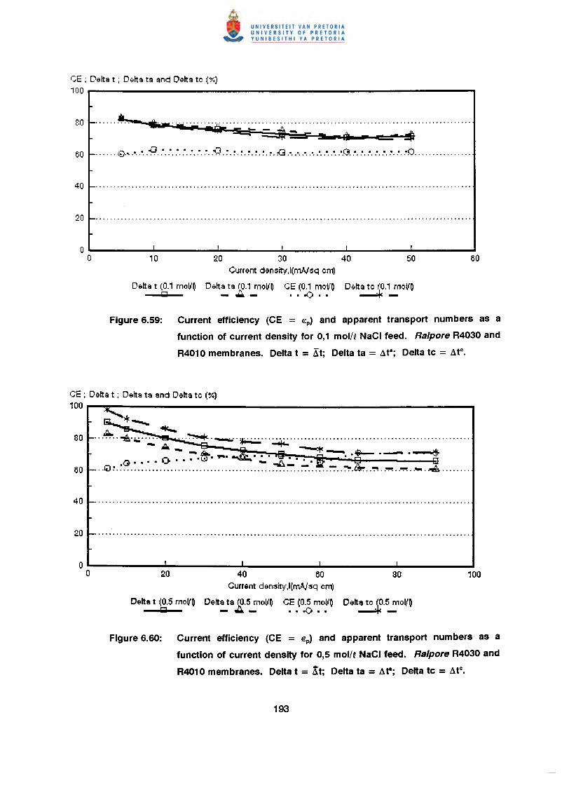
GE : D8lta t ; D8lta ta and Delta te (%)100
... , ,. ~ •• *"" ' , , , , ''':''';, '~ '.' , , , , , .. , , . , . , , , , , , , ,~"'~--.A=. =:::::a;:t - -. ••• - •• !$
...... .g.•..", ,",.~ ..•..•..• , .•.."..", ,".,~. ~. :. :. :. :. : . ~. :(3 .".,",,".. ".. ",,",.", ,".c:,. ,".. " .. " .. " .. " .. ". ,".. "0 , , ..
Current density,l(mA,lsq em)
Delta t (0.1 moVO D8lta ta (0.1 moVO CE (0.1 mov'O D8lta te (0,1 moVOIMI -_- •• ~ •• ---t-:-
Figure 6.59: Current efficiency (CE = €p) and apparent transport numbers as a
function of current density for 0,1 mol/QNaCI feed. Raipore R4030 and
R4010 membranes. Delta t = At; Delta ta = ~ta; Delta tc = ~tc.
CE ; Delta t ; Delta ta and Delta te (%)100 * .
.&. ~....... ~'~"~'.:.. ~. -..~ ...•.................................. " .
- _ E.- ~ _~. "-"---?1'i-~ ~. ,... -........ . . . . .~ .~Go •••• I,.J't ••• a..:, ~ ••• ~ •••• I
... !i) ~.~ ~ .. ~ ~ .. ~.~ ..~ ..~ ..~ ..••••.~ .
Delta t (0.5 moVOIj;iI
40 60 80Current density,l(mA,lsq em)
Delta ta (0.5 moVO CE (0.5 moVO Delta to _~.5_moVO-~- .. -0 ..
Figure 6"60: Current efficiency (CE = €p) and apparent transport numbers as a
function of current density for 0,5 mol/QNaCI feed" Ralpore R4030 and
R4010 membranes" Delta t = At; Delta ta = ata; Delta tc = ~tc"
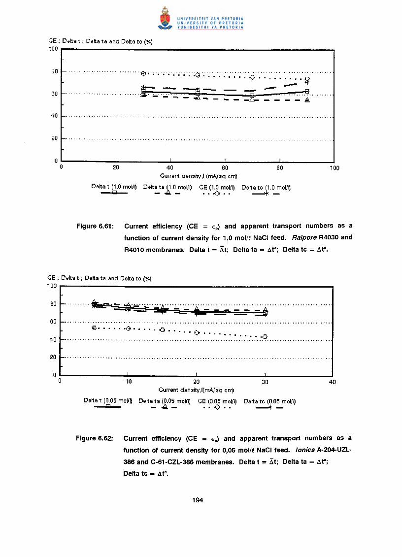
GE ; Delta t ; Delta ta and Delta to (%)100
............................. ~.;.~.~.~.~.~.~.~.~.;0 ~ .. . . . ~ ¥h --. - ...-.............................~ ..~..~..~ - - =5 ~ .
- 'OIILl._ - __ -..:...:0- - - - - A
40 60 80Current density,l (n1.t\isq em)
Delt~ta 2.0_moll~ C.E.(1~~O.lI~ Delta to .~ .~oll~Delta t (1.0 n1oll~'WI
Figure 6.61: Current efficiency (CE = €p) and apparent transport numbers as a
function of current density for 1,0 mol/D NaCI feed. Raipore R4030 and
R4010 membranes. Delta t = Llt; Delta ta = ata; Delta tc = atc.
CE ; Delta t : Delta ta and Delta te (%)100
...........• :r' -....:.$ ';:.' h' ••••••••••• ~••••••••••••••••••••••••••••••••••••••.•••••••••••••- •• ==- •• - =-- ::.: =J:Q. • • • • -<3-. • • • • ~ • • • . . '""- ..'-or ••••• 0.............................................................................................................
10 20 30Current density,l(n1.t\isq em)
Delta t (0.05 moll~ Delta ta (0.05 moll~ CE (0.05 mol{~ Delta te (0.05 moll~'WI _ .;A, - • • .() • • ----* -
Figure 6.62: Current efficiency (CE = €p) and apparent transport numbers as a
function of current density for 0,05 mol/D NaCI feed. tonics A·204-UZL-
386 and C-61·CZL·386 membranes. Delta t = ;it; Delta ta = ar;
Delta tc = atc.
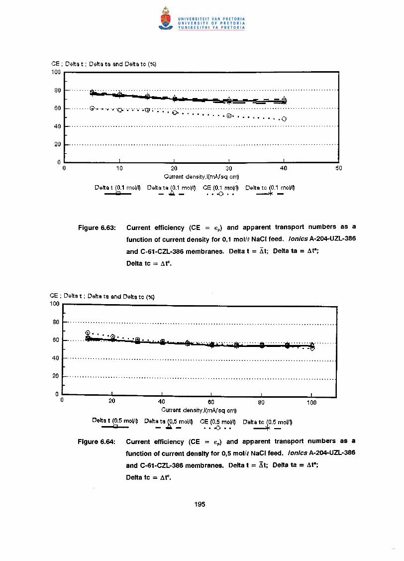
O:::::E; D~lts t ; D~lts ts snd Delts te (%)100
........ ~ , .•.••• ~ ".h." h• • ~::...:= :!!Eo::: Z:ij
........ -Go.•.•. ~ .~ '0' '.' '.' '.' '''1::::r ~. ~ . ~ . ; .0 .• • • • • • • • • G) •• . . . . . . . ·0
20 30 40Current density,l(mAJsq em)
Deltsts (0.1 moll~ CE (0.1 moll~ Delts te .~.1_moll~• ..:... ..-<) ..Deltst (0.1 moll~IWI
Figure 6.63: Current efficiency (CE = €p) and apparent transport numbers as a
function of current density for 0,1 mol/QNaCI feed. lonics A·204-UZL·386
and C·61·CZL·386 membranes. Delta t = Llt; Delta ta = dt8;
Delta tc = dtc•
CE : Delts t ; Delts ts snd Delts te (%)100
~ ·i.......• .. ·1· . r ·iI· ••'bbt' S" "'f;' j" wid····· ., "II"' 'j' '."'.~""""
20 40 60 80Current density,l(mAJsq em)
Delta t ~.5 moll~ Delt~ta1.5.moll~ C.E.(0.;5~o~~ Delta te .~.~oV~
Figure 6.64: Current efficiency (CE = €p) and apparent transport numbers as a
function of current density for 0,5 mol/QNaCI feed. tonics A·204-UZL·386
and C·61·CZL·386 membranes. Delta t = 'xt; Delta ta = dt8;
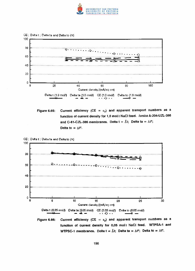
GE ; D€tlta t ; D€tltata and Delta te (%)100
.......................... ·ct; ; . ; . ; . ; . : . : . : . : . :<i '.' ' .<J •• ·····i..........................t='t ~ ..'--:f"';";"';"';';"'';'';''';''';';'F'' .~... . .
- - - -1!t- ••••- - _ _ _
20 40 60 80Current density,l(mAJsq em)
Delta t (1.0 moll~ D€tlta ta Q.O moll~ CE (1.0 moli'~ DElltate 11.0 moli'~IiiiiI - ••••. - •• .() •• ---+:-
Figure 6.65: Current efficiency (CE = €p) and apparent transport numbers as a
function of current density for 1,0 mol/QNaCI feed. lonics A-204-UZL-386
and C-61-CZL-386 membranes. Delta t = Kt; Delta ta = ae;
Delta tc = Me.
CE : Delta t : Delta ta and Delta te (%)100
80 ...............•...... •••• •• m .w .••.... ", :,::.~':";""~"':":' '':':~'" ..•.••..••.. ~ - ..
. . . . . . . . . . . . . . . 0.-. 0-0 ••••••••••••••••••• (;) ••••••••••• ,. ••••••• ~ •••••••••••••••••••••••••••••••••••••••••••••••••••v· ••• . • • • -u- •..•••• .v
5 10 15 20 25Current density,I(mA./sq em)
Delta t (0.05 moll~ Delta ta (~.05 moll~ CE (0.05 moll~ Delta te (0.05 moll~(iiI - ••••. - •• 0.. ---f:-
Figure 6.66: Current efficiency (CE = €p) and apparent transport numbers as a
function of current density for 0,05 mol/Q NaCI feed. WTPSA·1 and
WTPSC.1 membranes. Delta t = Xt; Delta ta = at-; Delta tc = ate.
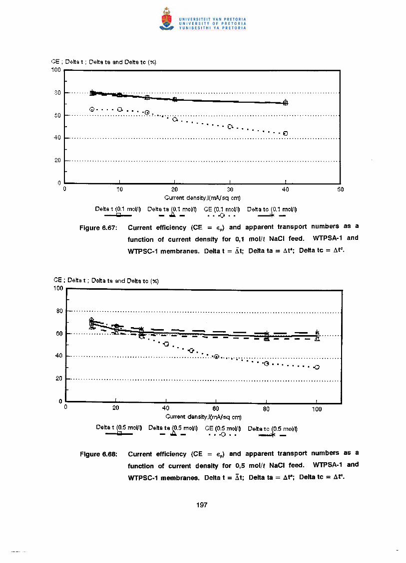
C:E ; D8tta t ; D8tta ta and Detta te (%)100
........• - S···················································································$ • j
<;> •••• CI. •••• Q •······································;·6··.··.··.··.· .
. . . . . ~ . . . . . •••• £I........................................................................................................
~ 30 ~Current density,l(mVsq em)
D8tta ta (t~.1moll~ CE (0.1 rnoli'~ D8tta te .~.1_moll~- .... - .. .() ..Detta t (0.1 rnoll~ISil
Figure 6.67: Current efficiency (CE = €p) and apparent transport numbers as a
function of current density for 0,1 mol/O NaCI feed. WTPSA-l and
WTPSC-l membranes. Delta t = Kt; Delta ta = At-; Delta tc = Ate.
CE ; Detta t : Delta ta and Delta te (%)100
"HH.~.=t'::::::'H-:- - - - ;;:f - - ~. . •... - - .•.. - - - - - - - - - .• '0
•.. -0.•••••••••••• •••••• 0 ••••••• 0 ••••••• 0 •••••••••••••••••• '-0 .·.~.o.o." o .. o o .
• • • • • .I"':l....,. •••••••• rJ;:)
20 40 60 80Current density,l(mVsq em)
Delta t ~.5 moll~ Delt~ta ~.5_moll~ C.E.(O~ ~o~~ Delta te _~.~Oll~
Figure 6.68: Current efficiency (CE = €p) and apparent transport numbers as a
function of current density for 0,5 mol/O NaCI feed. WTPSA·l and
WTPSC.l membranes. Delta t = Xt; Delta ta = At-; Delta tc = Atc.
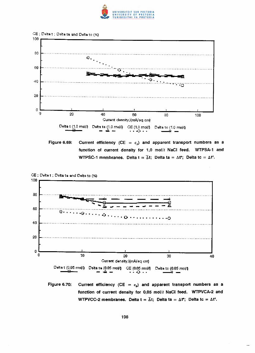
':::E; Delta t ; Delta ta and Delta te (%)100
80 .8.
........................................... ~.•.. ""'( .~...•••••• WJ'IL ••• ' i'. - .& - •. l!!
• •. ·G.o ••••••••••••••••••••••••••••••••••••••••••••••••••••••••••••••••••••• ~ • ~ • ! .•.•. ~ .
. '0
20 40 60 80Current density.l(nWsq em)
Delta t (1.0 mo(i'~ Delta ta ~~.Omo(i'~ CE (1.0 moll~ Deltate .V .O_moll~IiiiiI _ •••. _ •• -<) ••
Figure 6.69: Current efficiency (CE = €p) and apparent transport numbers as a
function of current density for 1,0 mol/Q NaCI feed. WTPSA·1 and
WTPSC.1 membranes. Delta t = Lit; Delta ta = Ae; Delta tc = Atc•
CE ; D",lta t : Delta ta and Delta te (%)100
...........••.........................................................................................--. --e+-----__+:
-...... B 1;;1.•. ~ ~ - - - - ~ - - - ~.......... 'Q':":":':" :":G -;.., 0 ••••••••••••••••••••••••••••• '0 •••••••••••••••••••
..... ~ .Q ••••••••••• ·0
10 20 30Current density.l(nWsq em)
Delta t (0.05 moll~ Delta ta (0.05 moll~ CE (0.05 moll~ Delta te (0.05 moll~IiiJ -.A- .. .().. ----+:-
Figure 6.70: Current efficiency (CE = €p) and apparent transport numbers as a
function of current density for 0,05 mol/Q NaCI feed. WTPVCA·2 and
WTPVCC.2 membranes. Delta t = Xt; Delta ta = At-; Delta tc = Atc•
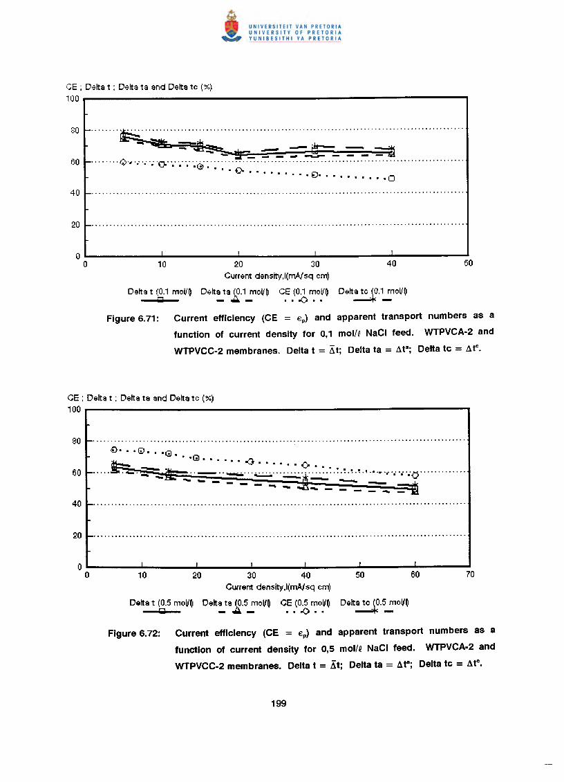
':::E; D8lta t ; D8lta ta and Delta te (%)100 ........~ = .
::r~ - - gp- - ==a..... ...F- - - .".........-- - - -....... ·<.;r~·"·,,·,,'0";';'; ·,'0·:·······································································... ~ . • • • I!:). • • • • • • • • • 0
Delta t (0.1 mollOb:d
20 30 40Current density,I(mA./sq em)
Delta ta ~0.1 mollO CE (0.1 mov'O Delta te .~.1_moIlO- .••. - .. -0 ..
Figure 6.71: Current efficiency (CE = €p) and apparent transport numbers as a
function of current density for 0,1 mol/~ NaCI feed. WTPVCA·2 and
WTPVCC·2 membranes. Delta t = llt; Delta ta = ae; Delta tc = atc.
CE : Delta t : Delta ta and Delta te (%)100
i}.. -@ •• -Gl.. • .Q ....•• -:J ······0 ... _ .. ~ .. 0-":':':';'0' o:..:.:.:..:.o ~.~ .•.• ··-rl°." ••••••0 ······ .... '- - - ~ ••....•.•• --- . ~-------
10 20 30 40Current density,I(m,AJsq em)
Delta t (0.5 mollO Delta ta (0.5 moVO CE (0.5 moVOIiiiI -~- •• .0 ..
Figure 6.72: Current efficiency (CE = €p) and apparent transport numbers as a
function of current density for 0,5 mol/~ NaCI feed. WTPVCA·2 and
WTPVCC·2 membranes. Delta t = ,1t; Delta ta = ae; Delta tc = atc.
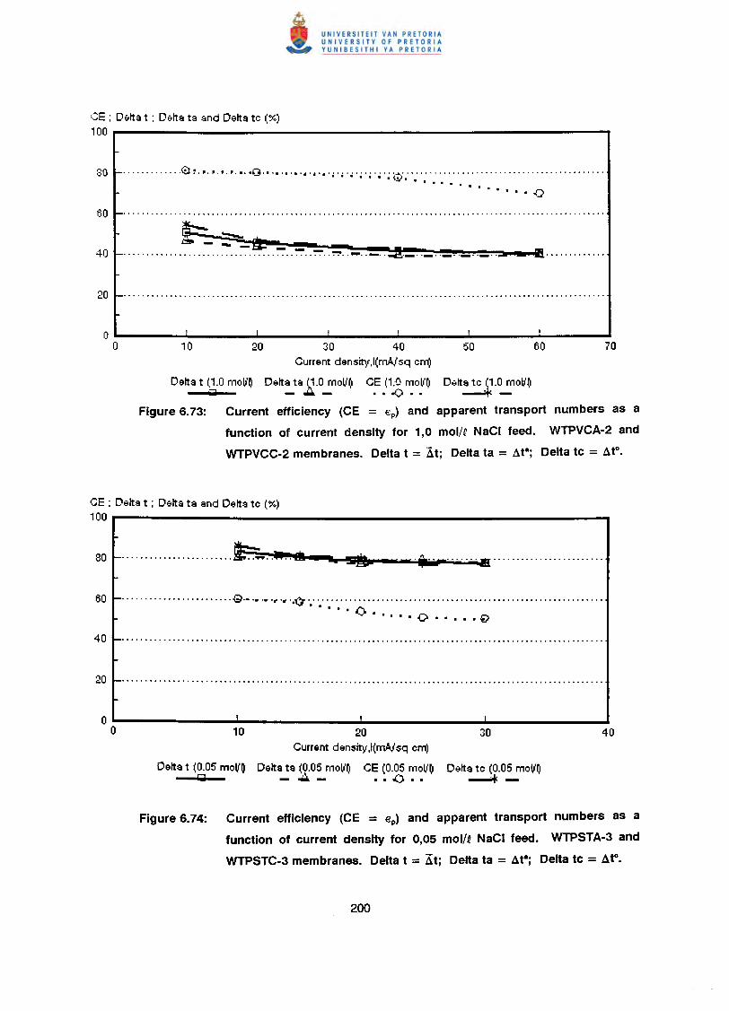
GE ; Delta t ; Delta ta and Delta te (%)100
......•....•. ~!t. II. II. 11•••• 0 -0 .. '. '.". OJ OJ 0' ••••••••••••••••••••••••••••••••••••••••••••••••••••••••••••••••• • • •••• {,:.J. • • . . . . . . . . • • • -0
~~............. ~ .. ~ .. ~ ~::~ .. ~. ~.. ~.. ~. :::.. :. ~.. ~.. ~. ;=:.. ~. -~.. ~.. lI;_~.~.-~ ..~:Jk.~..~_~."'._~_-.·----e- .
10 20 30 40 50 60 70Current density,l(mAlsq em)
Delta t (1.0 mo~'~ Delta ta (1.0 moll~ CE (1:0 mo~'~ Delta te .~.o_mo~'~I5iiI - ~- •• .() ••
Figure 6.73: Current efficiency (CE = €p) and apparent transport numbers as a
function of current density for 1,0 mol/Q NaCI feed. WTPVCA-2 and
WTPVCC-2 membranes. Delta t = Xt; Delta ta = ~ta; Delta tc = MC•
CE : Delta t : Delta ta and Delta te (%)100
........................ ~ ••~.~.~~..~da~ ••_~_~~~.~~h •••••~~m - _!:!III - .•. ·tt······ .~ .
....................... ·G··".".·~0Ji ".1::1"." .····0 . ·O·· ... '€>
10 20 30Current density,l(mAlsq em)
Delta t (0.05 moV~ Delta ta (0.05 moll~ CE (0.05 moll~ Delta te (0.05 moV~1;1 -~- •• .{).. ---"'Ic-
Figure 6.74: Current efficiency (CE = €p) and apparent transport numbers as a
function of current density for 0,05 mol/Q NaCI feed. WTPSTA·3 and
WTPSTC-3 membranes. Delta t = ~t; Delta ta = Ata; Delta tc = Atc•
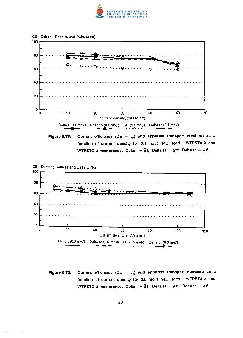
CE : Delta t : Delta ta and Delta tc (%)100
G)•• " ~• ~ ••• '-!Ja ••••. . . . . . . . . . . . . . . . . . . . . . . . . . . . . . . . . . . . . . . . . . . . . ~.~.•. Ij) •. • .•.•.•.•.•.• ttt-" •.•.•...• ".•..'II' 'II' ••••••••••••••••
20 30Current density,l(rnAJsq cnV
Delt~ta 2·1_moIlO C~ .(0;6 ~o~ODelta t (0.1 mollOIiiil
Figure 6.75: Current efficiency (CE = €p) and apparent transport numbers as a
function of current density for 0,1 mol/~ NaCI feed. WTPSTA·3 and
WTPSTC·3 membranes. Delta t = Xt; Delta ta = Ae; Delta tc = Ate.
CE : Delta t : Delta ta and Delta tc (%)100
...... ~ .
.::='1""~.;;;t........ ••.•..•.~c;--- - -•••••••••••••••••••••• ~ -..-··· ••••••••••••••••••••••• 00 •• 0 •• bo o'..~ .. 0 •••
Delta t (0.5 mol"~Iiiil
40 60 80 100Current density,I(mA/sq cm)
Delta ta (0.5 mol"O CE (0.5 mollO Delta te (0.5 mollO--- .. -0 .. ----4:-
Figure 6.76: Current efficiency (CE = €p) and apparent transport numbers as a
function of current density for 0,5 mol/Q NaCI feed. WTPSTA·3 and
WTPSTC-3 membranes. Delta t = Kt; Delta ta = Ae; Delta tc = Ate.
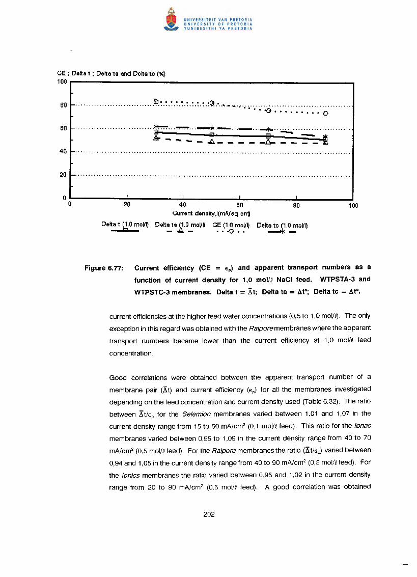
CE : Delta t : Delta ta and Delta te (%)100
G). • • • • • • • • .t"'::lI •••••••••••••••••••••••••••••••••••••••••••••••••••• "'7. ••••••••••• ~ •••••••••••••••••••••••••••••••••••••••••.... ~~·········O.............................. ~ ~ .....elk ._ _ ...;+1.0 ...•• ;"':••;"':.: .
I!r fiiI 9 --I•.•. ••• .•.• - ~ - - - - -f:!.,.. - - - -
40 60Current density,l(mAJsq err(!
Delt~ta £.O_moV~ C~ p~~oy~Delta t (1.0 moV~fiiI
Figure 6.77: Current efficiency (CE = ep) and apparent transport numbers as a
function of current density for 1,0 mol/Q NaCI feed. WTPSTA·3 and
WTPSTC.3 membranes. Delta t = Xt; Delta ta = ate; Delta tc = ate.
current efficiencies at the higher feed water concentrations (0,5 to 1,0 mol/Q). The only
exception in this regard was obtained with the Raipore membranes where the apparent
transport numbers became lower than the current efficiency at 1,0 mol/Q feed
concentration.
Good correlations were obtained between the apparent transport number of a
membrane pair (Xt) and current efficiency (ep) for all the membranes investigated
depending on the feed concentration and current density used (Table 6.32). The ratio
between Xt/ep for the Selemion membranes varied between 1,01 and 1,07 in the
current density range from 15 to 50 mA/cm2 (0,1 molN feed). This ratio for the lonac
membranes varied between 0,95 to 1,09 in the current density range from 40 to 70
mA/cm2 (0,5 mol/Qfeed). For the Raipore membranes the ratio (Xt/ep) varied between
0,94 and 1,05 in the current density range from 40 to 90 mA/cm2 (0,5 mol/Qfeed). For
the lonics membranes the ratio varied between 0,95 and 1,02 in the current density
range from 20 to 90 mA/cm2 (0,5 mol/Q feed). A good correlation was obtained
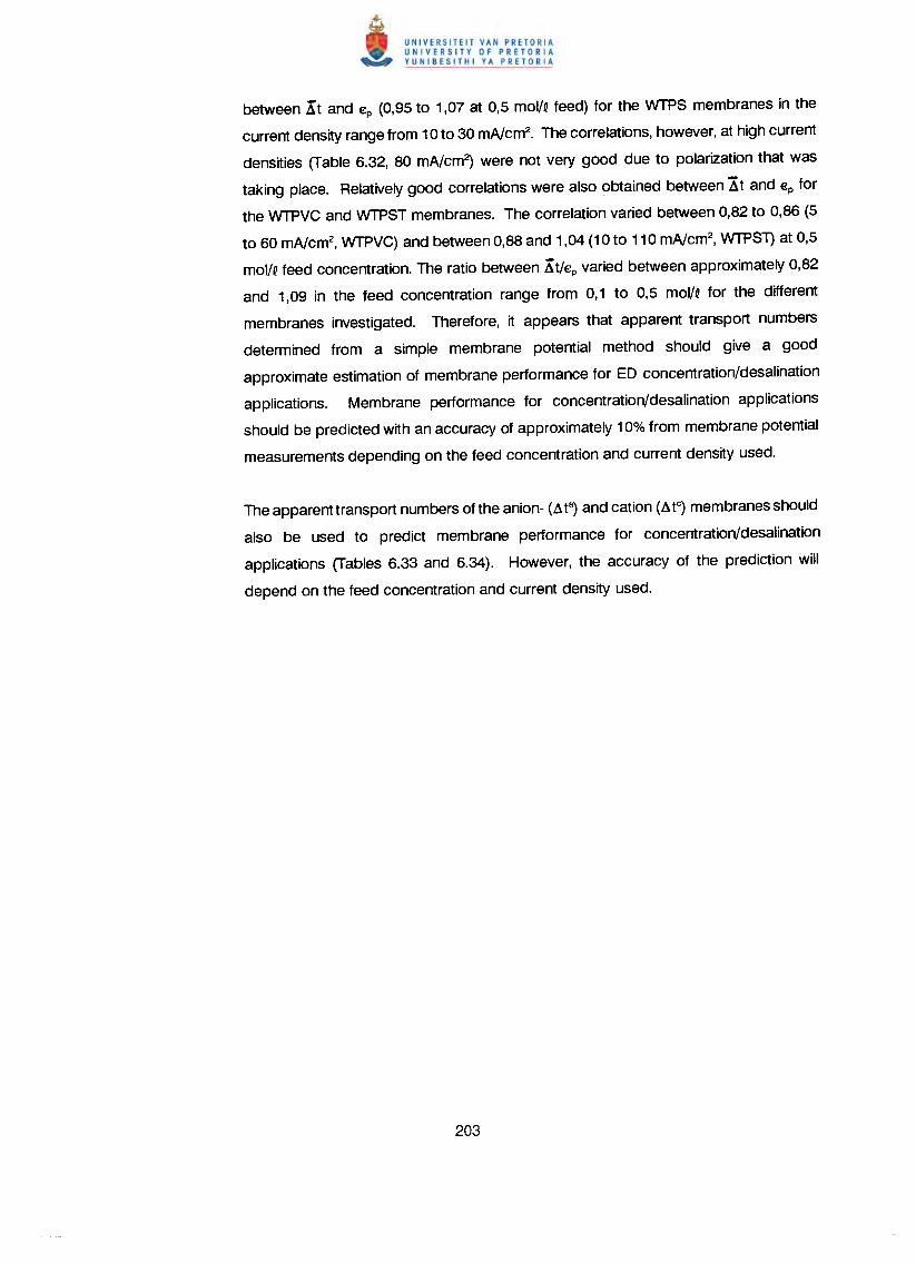
between Kt and €p (0,95 to 1,07 at 0,5 mol/~ feed) for the WTPS membranes in the
current density range from 10 to 30 mNcm2• The correlations, however, at high current
densities (Table 6.32, 80 mNcm~ were not very good due to polarization that was
taking place. Relativelygood correlations were also obtained between Xt and €p for
the WTPVC and WTPST membranes. The correlation varied between 0,82 to 0,86 (5
to 60 mNcm2, WTPVC) and between 0,88 and 1,04 (10 to 110 mNcm2, WTPS1) at 0,5
mol/~feed concentration. The ratio between Kt/€p varied between approximately 0,82
and 1,09 in the feed concentration range from 0,1 to 0,5 mol/~ for the different
membranes investigated. Therefore, it appears that apparent transport numbers
determined from a simple membrane potential method should give a good
approximate estimation of membrane performance for ED concentration/desalination
applications. Membrane performance for concentration/desalination applications
should be predicted with an accuracy of approximately 10% from membrane potential
measurements depending on the feed concentration and current density used.
The apparent transport numbers of the anion- (Ata) and cation (AtC)membranes should
also be used to predict membrane performance for concentration/desalination
applications (Tables 6.33 and 6.34). However, the accuracy of the prediction will
depend on the feed concentration and current density used.
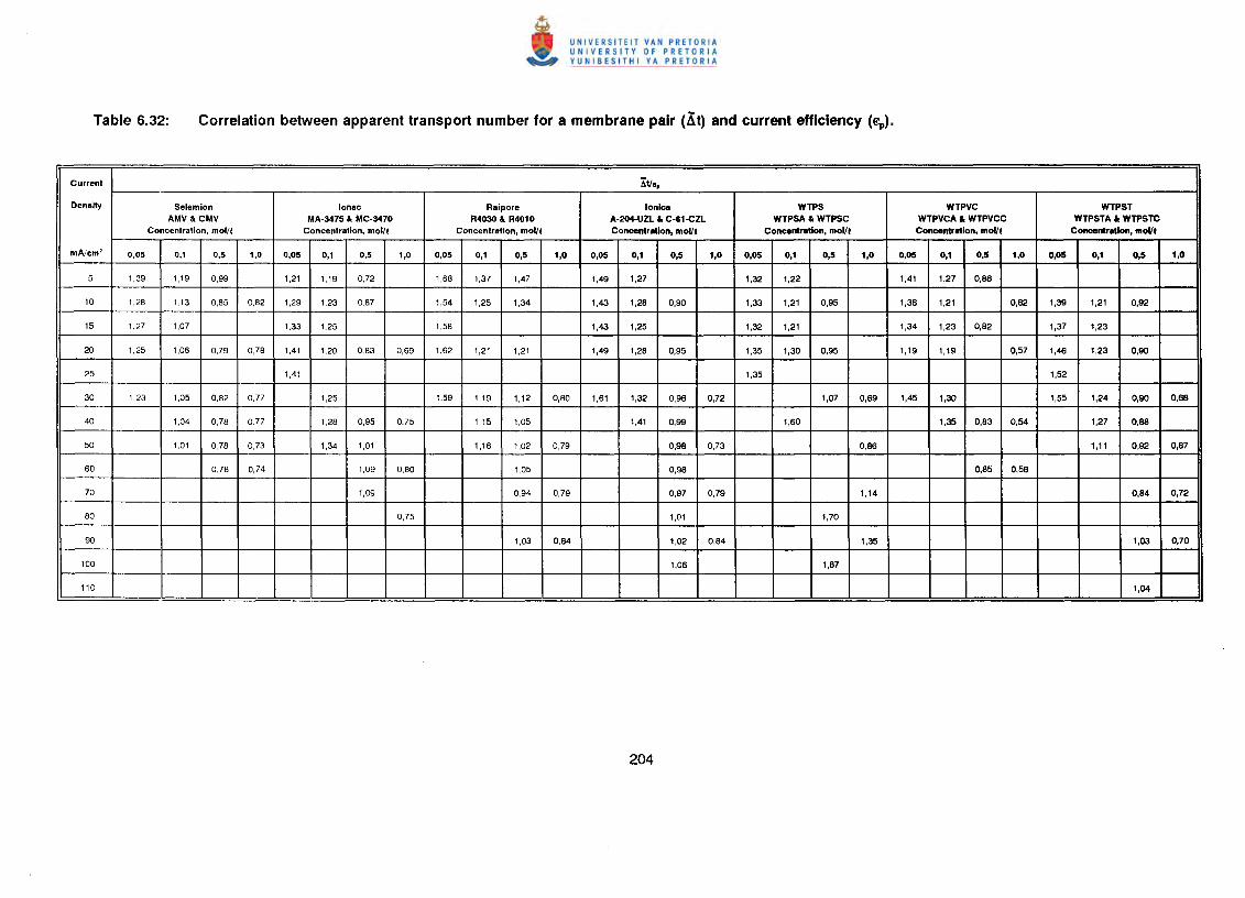
Current All••
Density Selemion lonae Reipore lonlce WTPS WTPVC WTPSTAMV& CMV MA·3475 & MC·3470 R4030 & R4010 A·204-UZL & C·6l-eZL WTPSA & WTPSC WTPVCA & WTPVCC WTPSTA & WTPSTC
Concentration, mol/f Concentration, mol/f Concentration, moll. Concenlrelion, molll Concenlretion, mol/l Concenlrelion, molll Concenlrellon, mol/I
mA/em' 0,05 0,1 0,5 1,0 0,05 0,1 0,5 1,0 0,05 0,1 0,5 1,0 0,05 0,1 0,5 1,0 0,05 0,1 0,5 1,0 O,OS 0,1 0,5 1,0 0,05 0,1 0,5 1,0
5 1,39 1,19 0,99 1,21 1,19 0,72 1,68 1,37 1,47 1,49 1,27 1,32 1,22 1,41 1,27 0,86
10 1,28 1,13 0,85 0,82 1,29 1,23 0,87 1,54 1,25 1,34 1,43 1,28 0,90 1,33 1,21 0,95 1,36 1,21 0,62 1,39 1,21 0,92
15 1,27 1,07 1,33 1,25 1,58 1,43 1,25 1,32 1,21 1,34 1,23 0,82 1,37 1,23
20 1,25 1,06 0,79 0,78 1,41 1,20 0,83 0,69 1,62 1,21 1,21 1,49 1,28 0,95 1,35 1,30 0,95 1,19 1,19 0,57 1,46 1,23 0,90
25 1,41 1,35 1,52
30 1,23 1,05 0,82 0,77 1,25 1,59 1,19 1,12 0,80 1,61 1,32 0,96 0,72 1,07 0,69 1,45 1,30 1,55 1,24 0,90 0,66
40 1,04 0,78 0.77 1,28 0,95 0,75 1,15 1,05 1,41 0,99 1,60 1,35 0,83 0,54 1,27 0,88
50 1,01 0,78 0,73 1,34 1,01 1,16 1,02 0,79 0,98 0,73 0,88 1,11 0,92 0,67
60 0,78 0,74 1,09 0,80 1,05 0,98 0,85 0,58
70 1,09 0,94 0,79 0,97 0,79 1,14 0,84 0,72
00 0,75 1,01 1,70
90 1,03 0,84 1,02 0,84 1,35 1,03 0,70
100 1,06 1,87
110 1,04
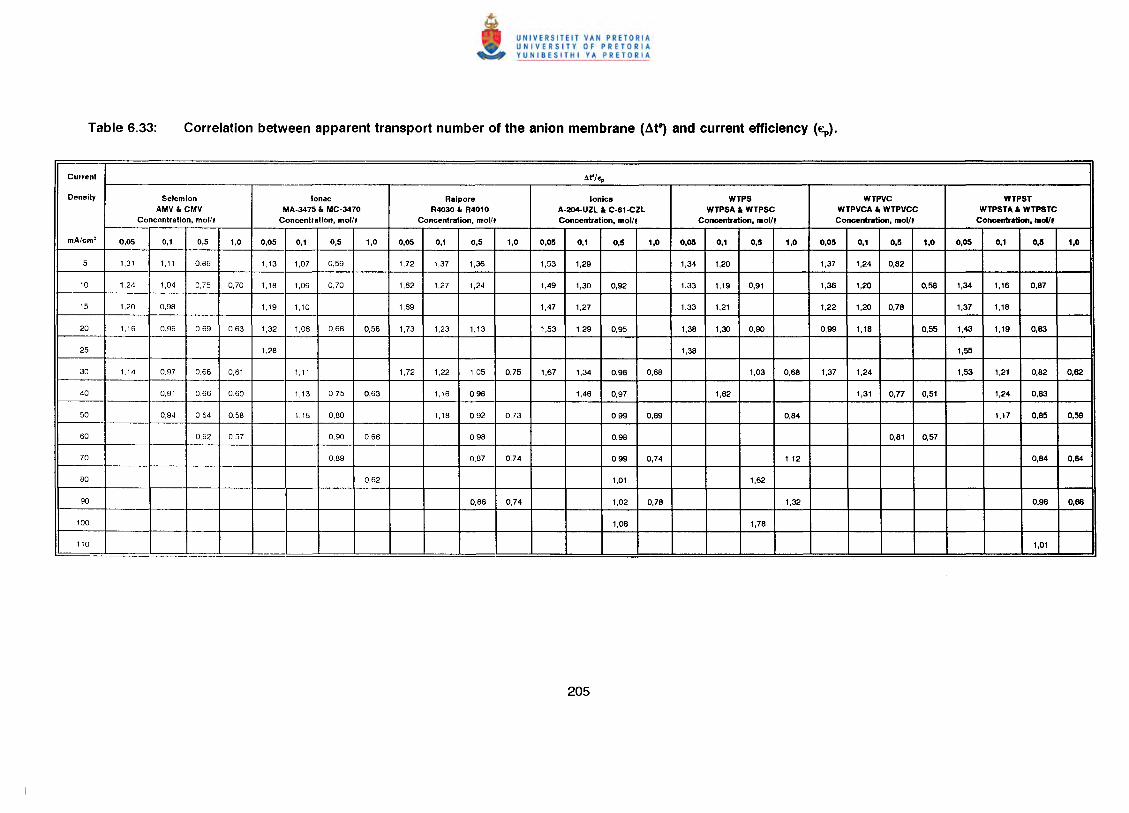
Current IJ.t'l",
Density Selemion lonac Raipore Ionic" WTPS WTPVC WTPSTAMV& CMV MA-3475 & MC-3470 R4030 & R40l0 A-204-UZL & C-61-CZL WTPSA & WTPSC WTPVCA & WTPVCC WTPSTA & WTPSTC
Concentration, moll' Concentration, moU' Concentration, moll. Concentration, mol/l Concentration, mol/l Concentration, molll Concentration, mol/I
mA/cm2 0,05 0,1 0,5 1,0 0,05 0,1 0,5 1,0 0,05 0,1 0,5 1,0 0,05 0,1 0,5 1,0 0,05 0,1 0,5 1,0 0,05 0,1 0,5 1,0 0,05 0,1 0,5 1,0
5 1,31 1,11 0,86 1,13 1,07 0,59 1,72 1,37 1,36 1,53 1,29 1,34 1,20 1,37 1,24 0,82
10 1.24 1,04 0,75 0,70 1,18 1,09 0,70 1,62 1,27 1,24 1,49 1,30 0,92 1,33 1,19 0,91 1,36 1,20 0,58 1,34 1,16 0,87
15 1.20 0,98 1,19 1,10 1,69 1,47 1,27 1,33 1,21 1,22 1,20 0,78 1,37 1,18
20 1,16 0,96 0,69 0,63 1,32 1,06 0,66 0,58 1,73 1,23 1,13 1,53 1,29 0,95 1,38 1,30 0,90 0,99 1,t6 0,55 1,43 1,19 0,83
25 1,28 1,38 1,55
30 1,14 0,97 0,68 0,61 1,11 1,72 1,22 1,05 0,75 1,67 1,34 0,96 0,68 1,03 0,68 1,37 1,24 1,53 1,21 0,82 0,62
40 0,91 0,66 0,60 1,13 0,75 0,63 1,16 0,98 1,48 0,97 1,62 1,31 0,77 0,51 1,24 0,83
50 0,94 0,64 0,58 1,16 0,80 1,18 0,92 0,73 0,99 0,69 0,84 1,17 0,85 0,59
60 0,62 0,57 0,90 0,66 0,98 0,98 0,81 0,57
70 0,89 0,87 0,74 0,99 0,74 1,12 0,84 0,64
80 0,62 1,01 1,62
90 0,86 0,74 1,02 0,78 1,32 0,98 0,66
100 1,06 1,78
110 1,01
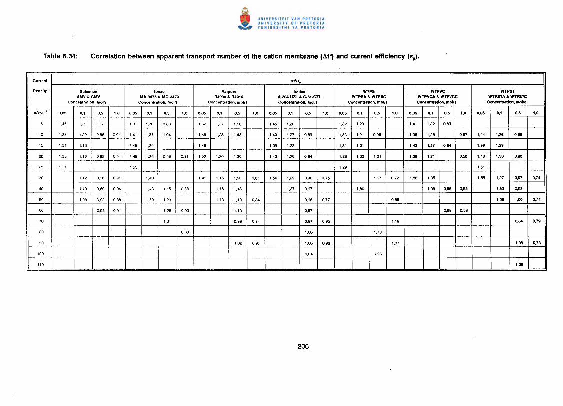
Current ",ro/ ••Density Selemion lonac Raipore lonlca WTPS WTPVC WTPST
AMV" CMV MA-3475" MC-3470 R4030 •• R40l0 A-204-UZl •• C·81·CZL WTPSA •• WTPSC WTPVCA•• WTPVCC WTPSTA •• WTPSTCConcentration, moll' Concentration, moll. Concentrstion, mol/l Concentr.tlon, mol/l Concentration, mol/l Concentration, molll Concentration, molll
mA/cm2 0,05 0,1 0,5 1,0 0,05 0,1 0,5 1,0 0,05 0,1 0,5 1,0 0,05 0,1 0,5 1,0 0,05 0,1 0,5 1,0 0,05 0,1 0,5 1,0 O,OS 0,1 0,5 1,0
5 1,46 1,29 1,12 1,31 1,30 0,83 1,62 1,37 1,60 1,46 1,26 1,32 1,23 1,41 1,32 0,89
10 1,33 1,20 0,96 0,94 1,41 1,37 1,04 1,46 1,23 1,43 1,40 1,27 0,89 1,33 1,21 0,99 1,38 1,25 0,67 1,44 1,26 0,99
15 1,31 1,16 1,46 1,39 1,48 1,39 1,23 1,31 1,21 1,43 1,27 0,84 1,39 1,29
20 1,33 1,16 0,88 0,94 1,48 1,36 0,99 0,81 1,52 1,20 1,30 1,43 1,26 0,94 1,29 1,30 1,01 1,38 1,21 0,58 1,48 1,30 0,98
25 1,31 1,55 1,29 1,51
30 1,12 0,98 0,91 1,40 1,46 1,15 1,20 0,85 1,56 1,29 0,96 0,75 1,17 0,72 1,56 1,35 1,55 1,27 0,97 0,74
40 1,19 0,89 0,94 1,43 1,15 0,88 1,15 1,13 1,37 0,97 1,60 1,39 0,86 0,55 1,30 0,93
50 1,08 0,92 0,88 1,50 1,23 1,13 1,10 0,84 0,98 0,77 0,88 1,08 1,00 0,74
60 0,93 0,91 1,28 0,93 1,13 0,97 0,88 0,58
70 1,31 0,99 0,84 0,97 0,85 1,19 0,84 0,79
80 0,88 1,00 1,76
90 1,02 0,95 1,00 0,92 1,37 1,06 0,73
100 1,04 1,96
110 1,09
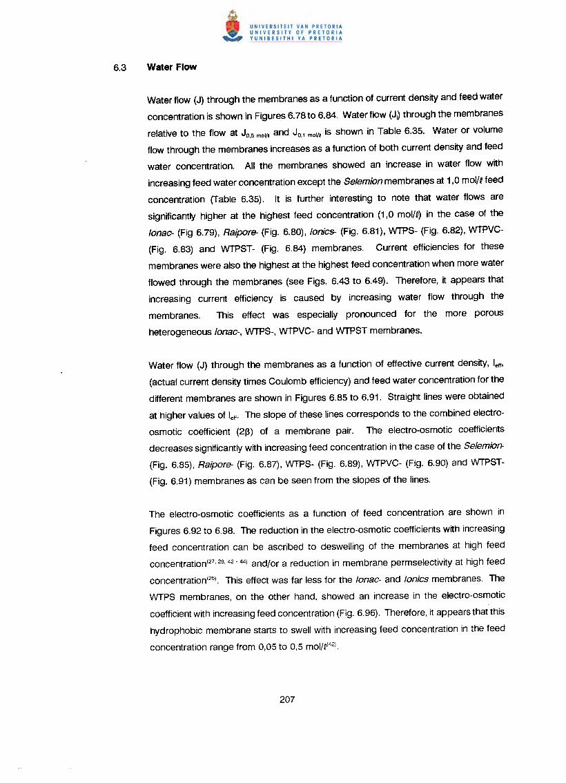
Water flow (J) through the membranes as a function of current density and feed water
concentration is shown in Figures 6.78 to 6.84. Water flow (J~through the membranes
relative to the flow at JO,5 moV, and JO,1 moV, is shown in Table 6.35. Water or volume
flow through the membranes increases as a function of both current density and feed
water concentration. All the membranes showed an increase in water flow with
increasing feed water concentration except the Selemion membranes at 1,0 mol/Qfeed
concentration (Table 6.35). It is further interesting to note that water flows are
significantly higher at the highest feed concentration (1,0 mol/Q)in the case of the
lonac- (Fig 6.79), Raipore- (Fig. 6.80), lonics- (Fig. 6.81), WTPS- (Fig. 6.82), WTPVC-
(Fig. 6.83) and WTPST- (Fig. 6.84) membranes. Current efficiencies for these
membranes were also the highest at the highest feed concentration when more water
flowed through the membranes (see Figs. 6.43 to 6.49). Therefore, it appears that
increasing current efficiency is caused by increasing water flow through the
membranes. This effect was especially pronounced for the more porous
heterogeneous lonac-, WTPS-,WTPVC- and WTPST membranes.
Water flow (J) through the membranes as a function of effective current density, leff'
(actual current density times Coulomb efficiency) and feed water concentration for the
different membranes are shown in Figures 6.85 to 6.91. Straight lines were obtained
at higher values of leff' The slope of these lines corresponds to the combined electro-
osmotic coefficient (2[3) of a membrane pair. The electro-osmotic coefficients
decreases significantly with increasing feed concentration in the case of the Selemion-
(Fig. 6.85), Raipore- (Fig. 6.87), WTPS- (Fig. 6.89), WTPVC- (Fig. 6.90) and WTPST-
(Fig. 6.91) membranes as can be seen from the slopes of the lines.
The electro-osmotic coefficients as a function of feed concentration are shown in
Figures 6.92 to 6.98. The reduction in the electro-osmotic coefficients with increasing
feed concentration can be ascribed to deswelling of the membranes at high feed
concentration(27,28,42-44) and/or a reduction in membrane permselectivity at high feed
concentration(25). This effect was far less for the lonac- and lonics membranes. The
WTPS membranes, on the other hand, showed an increase in the electro-osmotic
coefficient with increasing feed concentration (Fig. 6.96). Therefore, it appears that this
hydrophobic membrane starts to swell with increasing feed concentration in the feed
concentration range from 0,05 to 0,5 moI!Q(42).
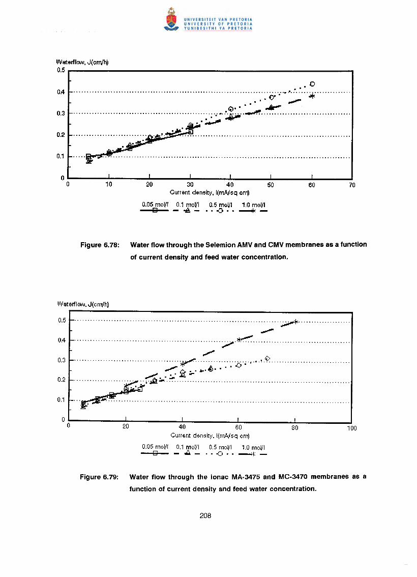
Waterflcw. J(errv'h)0.5
.0..................................................................................• ~ .~. '*•• _v ~. . A..-c:t>- • .....-................................................. :.~ ..~ ..~ .
20 30 40 50Current density, l(mNsq em)
0.05 moVI 0.1 mo~'1 0.5 moVI 1.0 moVIg ~- •• -a .. ----.+<-
Figure 6.78: Water flow through the Selemion AMV and CMV membranes as a function
of current density and feed water concentration.
0.5 _ ~ .
.",-
0.4 _ 7'*~"""""""""""""""""'"
/'0.3 _ 'r' ".(j .; .•.•. ~.~~ .
",."0 . . •. ~. . . .~ .. :-.~-:~~.~ .•~~ ••••..••••••••••••••••••••••••••••••••••••••••••••••••••••••••••..••
I I
40 60Current densiW, I(m,o!•./sq em)
0.05 mol'" 0.1 molt'l 0.5 moll'l 1.0 moll'lg ~- ... {) .. -..;*-
Figure 6.79: Water flow through the lonac MA-3475 and MC-3470 membranes as a
function of current density and feed water concentration.
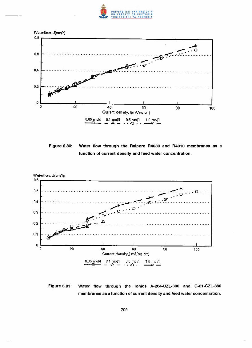
WaterflOO\l, J(errv'1V0.8
--*~ .• 0
•••..••••.••••.•••.••••..•••••.•••.••••••••••••••••••••..•••....••••.•• :...:.i<' .~ •• ~ •• '. ~ • ~ .•••.•.•••••••..~ .. -
.""". . ..~~ •• €'"'
. ~~ .• • . . . • • . . . . . • . . . • • . • • • . . . • • • . . . . . . . . . • ;,:;J!It1":' ..••••...••.........•••..••••...••..•••..•••••......•••..•••.-
40 60Current density, l(rnAfsq err(!
0.05 moVI 0.1 moVI 0.5 molfl 1.0 moVII2l - ~- •• -8" ~-
Figure a.80: Water flow through the Raipore R4030 and R4010 membranes as a
function of current density and feed water concentration.
WaterflOO\l. J(errv'1V0.6
:+:.................................................................... ······· ... ·~··· .. ····.·C.·······
",,- , CI' ' ,...•••.... ' ,................................................. ~ ~.; ','13" ~.=. ~.~ , .
••••••••.1: 0 ' ,o ' , ,................................... / ...•.•............................................................
@' ,
~"~•••••••••••••••••••• i." •••• ,;. ••.• ~ •••••.•.•••••••••••••••••••.••••••••••••••••••••.••••••••.•••••••••••••
, . "*
40 60Current dens~(,( mo!./;sq em)
0.05 moll'l 0.1 n1"ll'l 0.5 n1o(i'1 1.0 moll'lo ~- ... ::~.. ---.f.:-
Figure 6.81: Water flow through the lonics A-204-UZL·386 and C-61-CZL-386
membranes as a function of current density and feed water concentration.
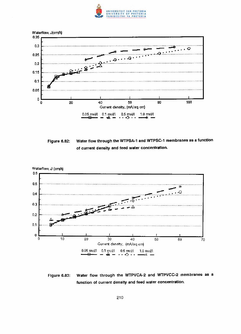
Waterfkw, J(env'h)0.35
.................................................................................. ~ ......Jio - ~ - ••• 0~ ~ h.····.................................... ~ ...................................•....•............................
.'--' -- ~ .~ .() ....~::2. ..•••••••••••••••••..••..••••.••••••• .'! •••••••••.••••••••..••••.••••••.••••••••••••••••.•••••.•••..••••..
. ... j .....
40 60Current density, (rM/sq err(J
0.05 mol'l 0.1 mol'l 0.5 mol'l 1.0 mol'l121 -~- •• -o .. ---.+<-
Figure 6.82: Water flow through the WTPSA·1 and WTPSC-1 membranes as a function
of current density and feed water concentration.
WaterflOO\l,J (env'h)0.6
............................................................... ...............':;';';'.'*' .. . . . . . . . . . . . . . . . . . . . . . . . . . . . . . . . . . . . . . . . . . . . . . . . . . . . . . . . . . . . . . . . . . . ~ ~ .•. ~ . ~ . : .•.C? ."",...~ .__ .. 0'·..................................... ~. ····~·~······ft········································ .....~. ~ .l..i
~ a...:...i ~ •••............. ~ ~ .
30 40Current den:5it~(, (n1.'!'isq em)
0.05 mell,'1 0.1 mol,'1 0.5 molJ'1 1.0 molJ'1121 -...::..- ••• ::, •• --i*-
Figure 6.83: Water flow through the WTPVCA-2 and WTPVCC·2 membranes as a
function of current density and feed water concentration.
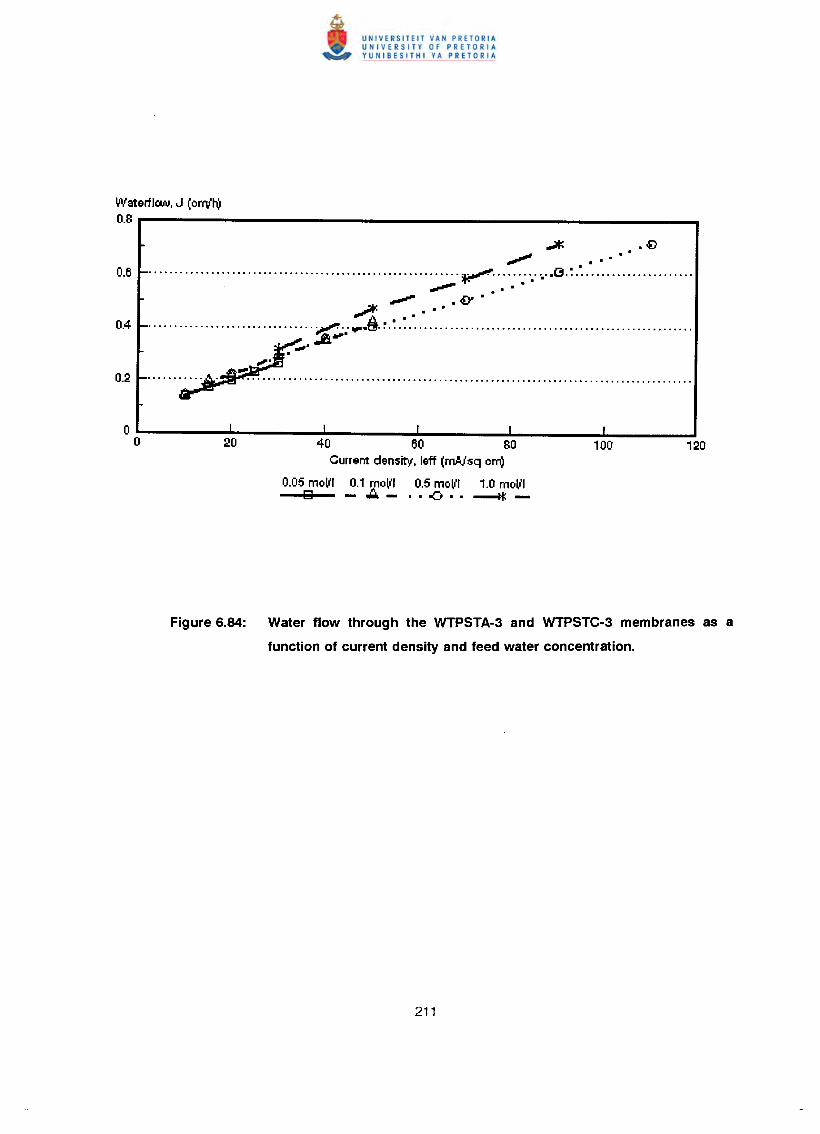
WaterflOAl. J (orrv't\J0.8
'""* .€>"". ........•. .............................................................. ~ ~ .."", .
A .,."....()"...8 ••••
• • • • • • . • • • . • • • . • • • . . • • • • . • • • • • . . -:;;:;.: W"".~' ••••.•.••••.•••••.••••••••.•••••••••••••••••.•.•.•••••••••••
.,..
40 60 80Current density. left (mAJsq om)
0.05 moVI 0.1 moVI 0.5 moVI 1.0 moVID -"'::'- .. .() .. ~-
Figure 6.84: Water flow through the WTPSTA·3 and WTPSTC·3 membranes as a
function of current density and feed water concentration.
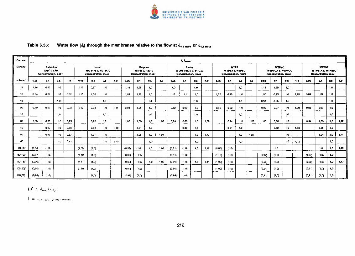
Current JJJ ••••• "
Density Selemion lonac Raipore lonlce WTPS WTPVC WTPSTAMV. CMV MA-3475 • MC-3470 R4030 • R4010 A-204-UZL. C-S1-CZL WTPSA • WTPSC WTPVCA • WTPVCC WTPSTA • WTPSTC
Concentration, moll' Concentration, moll 1 Concentration, molll Concenlretlon, molll Concentretlon, mol/I Concentretlon, mol/I eo.-ntretlon, mol/I
mAlcm2 0,05 0,1 0,5 1,0 0,05 0,1 0,5 1,0 O,OS 0,1 0,5 1,0 O,OS 0,1 0,5 1,0 0,05 0,1 0,5 1,0 O,OS 0,1 0,5 1,0 O,OS 0,1 0,5 1,0
5 1,14 0,85 1,0 1,17 0,87 1,0 1,18 1,28 1,0 1,0 1,0 1,0 1,11 1,55 1,0 1,0
10 0,94 0,97 1,0 0,93 1,15 1,03 1,0 1,09 1,18 1,0 1,0 1,1 1,0 1,05 0,96 1,0 1,00 0,95 1,0 1,29 0,99 1,02 1,0
15 1,0 1,0 1,0 1,0 1,0 0,92 0,95 1,0 1,0
20 0,89 0,99 1,0 0,92 0,92 0,93 1,0 1,11 0,93 1,05 1,0 0,62 0,90 1,0 0,92 0,92 1,0 0,92 0,97 1,0 1,09 0,88 0,97 1,0
25 1,0 1,0 1,0 1,0 1,0 1,0 1,0
30 0,88 0,98 1,0 0,95 0,96 1,0 1,00 1,00 1,0 1,07 0,78 0,86 1,0 1,09 0,94 1,0 1,26 1,00 0,88 1,0 0,94 1,03 1,0 1,12
40 0,89 1,0 0,86 0,93 1,0 1,16 1,01 1,0 0,80 1,0 0,91 1,0 0,82 1,0 1,08 0,98 1,0
50 0,87 1,0 0,87 1,01 1,0 1,05 1,0 1,04 1,0 1,17 1,0 1,21 1,0 1,04 1,0 1,17
60 1,0 0,87 1,0 1,45 1,0 1,0 1,0 1,0 1,12 1,0
70 (5)- (1,34) (1,0) (1,33) (1,0) (0,92) (1,0) 1,0 1,06 (0,91) (1,0) 1,0 1,12 (0,95) (1,0) 1,0 1,0 1,0 1,16
80(10)' (0,97) (1,0) (1,12) (1,0) (0,92) (1,0) (0,91) (1,0) (1,10) (1,0) (0,97) (1,0) (0,97) (1,0) 1,0
90(15)' (0,90) (1,0) (1,11) (1,0) (0,89) (1,0) 1,0 1,05 (0,91) (1,0) 1,0 1,11 (1,00) (1,0) (0,90) (1,0) (0,90) (1,0) 1,0 1,17
100(20)- (0,90) (1,0) (0,98) (1,0) (0,89) (1,0) (0,91) (1,0) (1,00) (1,0) (0,91) (1,0) (0,91) (1,0) 1,0
110(30)' (0,91) (1,0) (1,0) (0,99) (1,0) (0,92) (1,0) (0,91) (1,0) (0,91) (1,0) 1,0
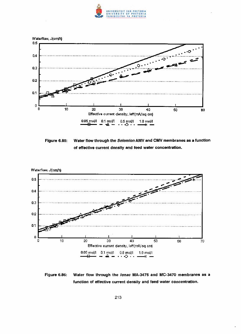
WaterflOJll, J(cnv'h)0.5
. -0 .. ........... " •.................... . -0 .
20 30 40Effective current density, leff(mAJsq crrO
0.05 mol'l 0.1 mol'l 0.5 mol'l 1.0 mol'lg -~- •• -:3 •• ---tI<
Figure 6.85: Water flow through the Selemion AMV and CMV membranes as a function
of effective current density and feed water concentration .
.,....................................................................................... , . ."'1':.~* ....
~ ----', .--""' .•. ~ .
20 30 40 50Effeetr •.•.e current density-, leff(rAA,lsq crrO
0.05 molll 0.1 moll'l 0.5 moll'l 1.0 moll'jo - .••.- .. 00 •• ~~-
Figure 6.86: Water flow through the lonac MA-3475 and MC·3470 membranes as a
function of effective current density and feed water concentration.
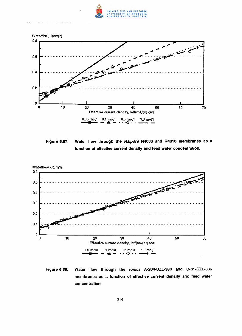
WaterflOO\l,J(crrv'h)0.8 , .~ ~ •• .:,;.:t<
••.' .~u••••••••••••••••••••••••••••••••••••••••••••••••••••••••••••• JIf"; •••••••••••• ~ ••••••••••••••••••••,.' .~,. ~
.,. f!!t ••••~.r·........A, ~Q'''''''-'''''''''''''''''''''''''''''''''''''''''''''''''''''''''''
~~~.
20 30 40 50Effective current density, leff(rnAJsq crrO
0.05 moVI 0.1 moVI 0.5 moVI 1.0 moVI9 -"::"- •• <) •• --t:
Figure 6.87: Water flow through the Raipore R4030 and R4010 membranes as a
function of effective current density and feed water concentration.
WaterflOO\l,J(crrv'h)0.6
20 30 40Effeetwe current density, leff(rnAJsq cm,\
0.05 moVI 0.1 molll 0.5 moll') 1.0 mo(i'l9 -oA- ·· ..D··--+-:-
Figure 6.88: Water flow through the lonics A·204-UZL·386 and C·61·CZL·386
membranes as a function of effective current density and feed water
concentration.
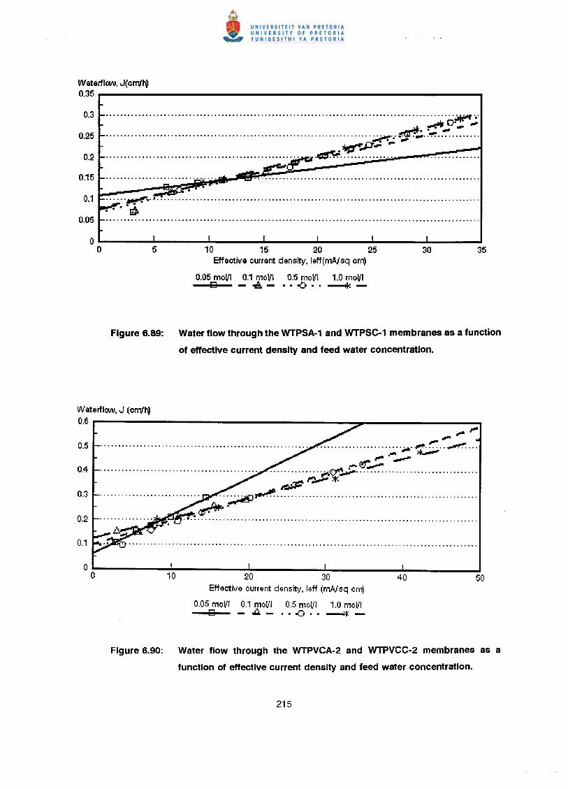
WaterflCAAl,J(cmlh)0.35
................................................................................................. ~ .•.~ O· ..,.
............................................................................ ~ .. ~.~"!':' ..~ .."':.....~-.-". ..,.*frJ:f- -.................................................. ~.~ .
0.1 ..... '~.".'.'.".'.""""."' .. """""""""""""'.""" ... ".' ... "'.'.""" .. """"....~
10 15 20 25Effective current density, leff(m,AJsq crr(J
0.05 mol'l 0.1 mol'l 0.5 mo~'1 1.0 mol'lo ~- •. -o .• -+c-
Figure 6.89: Water flow through the WTPSA-1 and WTPSC-1 membranes as a function
of effective current density and feed water concentration.
WaterflCAAl,J (cmlh)0.6
20 30Effective current density, leff (rnNsq cm)
0.05 molfl 0.1 mo(J'1 0.5 mol!! 1.0 molllo ~- ··00·· --*-
Figure 6.90: Water flow through the WTPVCA-2 and WTPVCC-2 membranes as a
function of effective current density and feed water concentration.
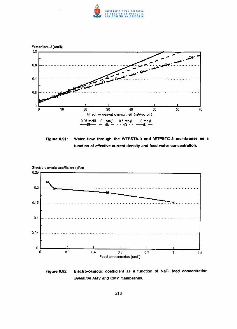
Waterflcw. J (cmit.)0.8
20 30 40 50Effective current density, leff (mAJsq crr(!
0.05 molll 0.1 molll 0.5 molll 1.0 molllo -~_ .. -QI •• ~-
Figure 6.91: Water flow through the WTPSTA·3 and WTPSTC·3 membranes as a
function of effective current density and feed water concentration.
Electro-osmotic coefficient (IIFa~
0.25 .------------------------------_
0.2 - .. ~, ; .
-----------------0.15 _ ~~ .
I I I
0.4 0.6 0.8F€t8dconc8ntrstion (moll'~
Figure 6.92: Electro-osmotic coefficient as a function of NaCI feed concentration.
Selemion AMV and CMV membranes.
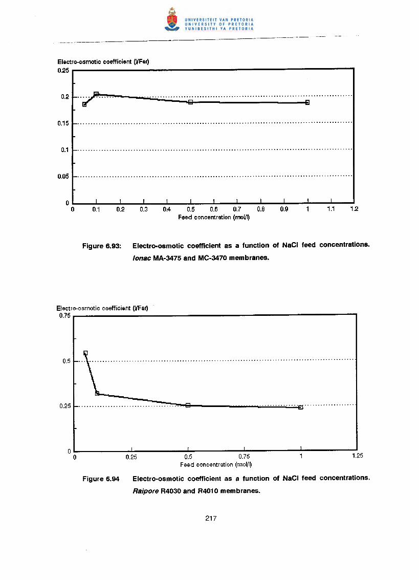
Electro-osmotic coefficient (JlFa~0.25
0.4 0.5 0.6 0,7 0,8Feed concentration (moJl~
Figure 6.93: Electro-osmotic coefficient as a function of NaCI feed concentrations.
lonae MA-3475 and MC-3470 membranes.
Electro-osmotic coefficient (JiFar)0.75
0.5 0.75Feed concentrstion (moV~1
Electro-osmotic coefficient as a function of NaCI feed concentrations.
Raipore R4030 and R4010 membranes.
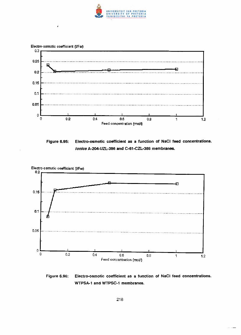
Electro-osmotic coefficient (VFa~0.3
~ g 0....... .
0.4 0.6 0.8Feed concentration (moV~
Figure 6.95: Electro-osmotic coefficient as a function of NaCI feed concentrations.
lonics A·204-UZL·386 and C·61·CZL·386 membranes.
Electro-osmotic coefficient (VFa~0.2
0.4 0.6Feed concentration (moll'~1
Figure 6.96: Electro-osmotic coefficient as a function of NaCI feed concentrations.
WTPSA-1 and WTPSC-1 membranes.
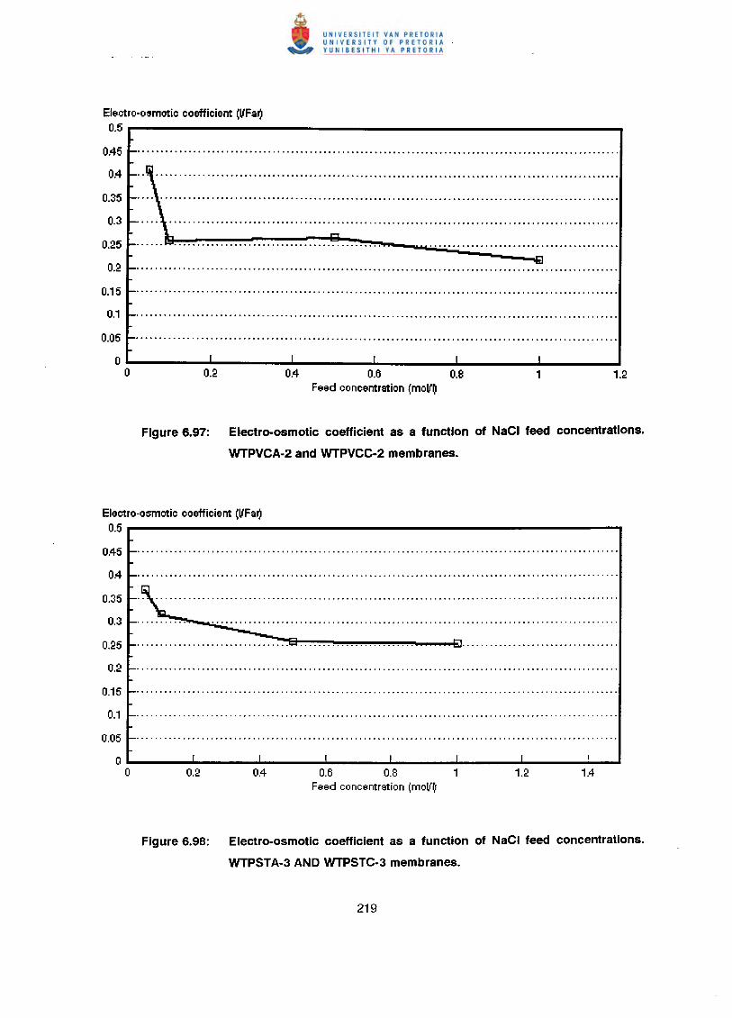
Electro-osmotic coefficient (VFa~0.5
0.45
0.4
0.35
0.3
0.:25
0.:2
0.15
0.1
0.05
0.4 0.6 0.8Feed concentration (moV~
Figure 6.97: Electro-osmotic coefficient as a function of NaCI feed concentrations.
WTPVCA-2 and WTPVCC-2 membranes.
Electro-osmotic coefficient (VFa~0.5
0.45
0.4
0.35
0.3 '"-.....,.0.:25 e1 .
0.:2
0.15
0.1
0.05
0.6 0.8 1Feed concentration (mol(~
Figure 6.98: Electro-osmotic coefficient as a function of NaCI feed concentrations.
WTPSTA-3 AND WTPSTC-3 membranes.
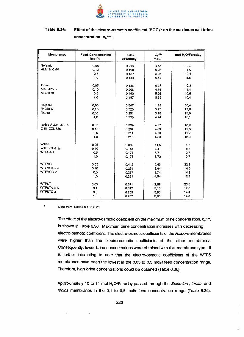
Effect of the electro-osmotic coefficient (EOC) * on the maximum salt brine
concentration, cbmax.
Membranes Feed Concentration EOC Cb""'" mol H2O/Faraday
(mol/C) C/Faraday mol/C
Selemion 0,05 0,219 4,55 12,2AM>! & CM>! 0,10 0,198 5,05 11,0
0,5 0,187 5,36 10,4
1,0 0,154 6,48 8,6
lonac 0,05 0,186 5,37 10,3MA-3475 & 0,10 0,206 4,85 11,4
MC-3470 0,5 0,190 5,26 10,6
1,0 0,187 5,35 10,4
Raipore 0,05 0,547 1,83 30,4R4030 & 0,10 0,320 3,13 17,8
R4010 0,50 0,251 3,98 13,9
1,0 0,236 4,24 13,1
lonics A-204-UZL & 0,05 0,234 4,27 13,0C-61-CZL-386 0,10 0,204 4,89 11,3
0,5 0,211 4,73 11,7
1,0 0,216 4,63 12,0
WTPS 0,05 0,087 11,5 4,8WTPSCA-1 & 0,10 0,156 6,41 8,7WTPSA-1 0,5 0,175 5,71 9,7
1,0 0,175 5,72 9,7
WTPVC 0,05 0,412 2,43 22,8WTPVCA-2 & 0,10 0,261 3,84 14,5WTPVCC-2 0,5 0,267 3,74 14,8
1,0 0,221 4,54 12,3
WTPST 0,05 0,371 2,69 20,6WTPSTA-3 & 0,1 0,317 3,15 17,6WTPSTC-3 0,5 0,259 3,86 14,4
1,0 0,257 3,90 14,3
The effect of the electro-osmotic coefficient on the maximum brine concentration, cb max,
is shown in Table 6.36. Maximum brine concentration increases with decreasing
electro-osmotic coefficient. The electro-osmotic coefficients of the Raipore membranes
were higher than the electro-osmotic coefficients of the other membranes.
Consequently, lower brine concentrations were obtained with this membrane type. It
is further interesting to note that the electro-osmotic coefficients of the WTPS
membranes have been the lowest in the 0,05 to 0,5 mol/~feed concentration range.
Therefore, high brine concentrations could be obtained (Table 6.36).
Approximately 10 to 11 mol H20/Faraday passed through the Setemio~, tonac- and
tonics membranes in the 0,1 to 0,5 moV~ feed concentration range (Table 6.36).
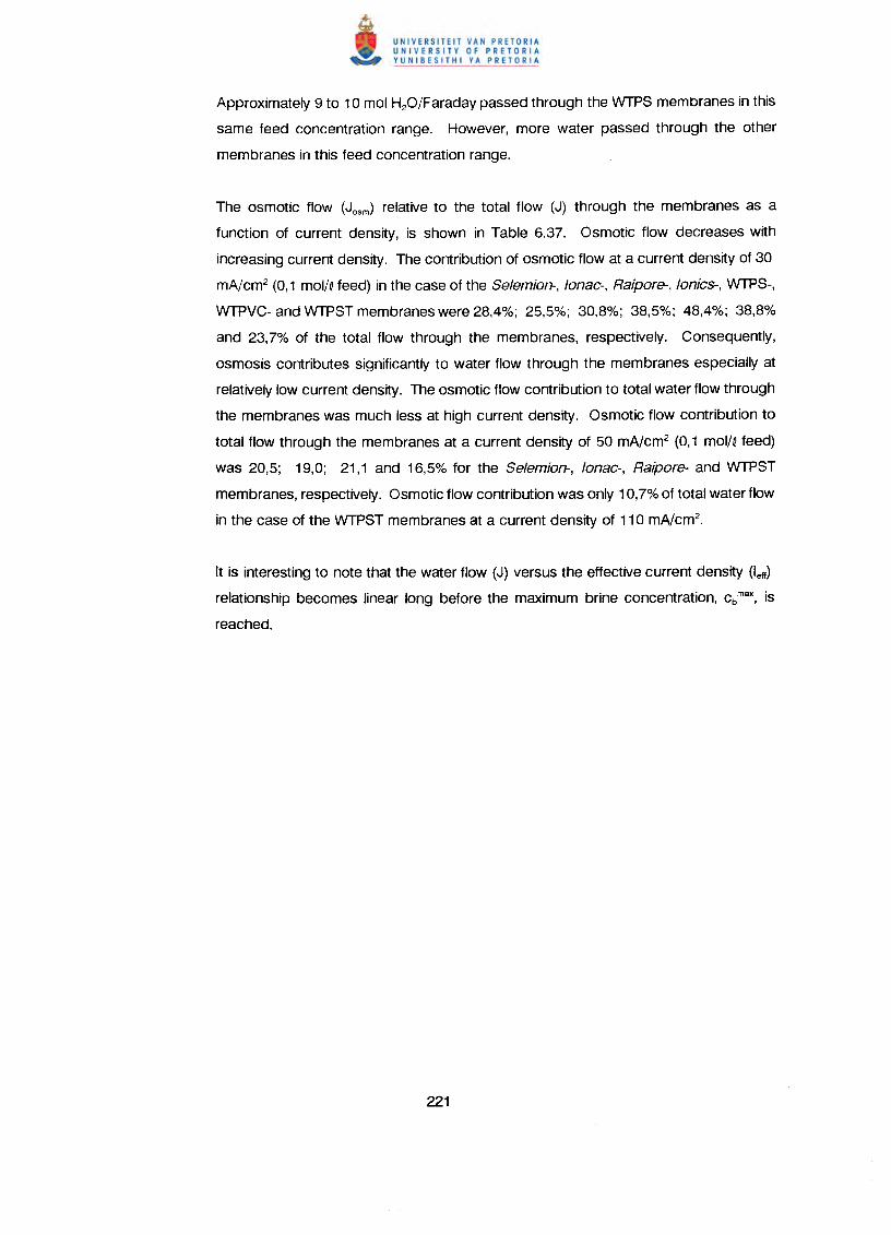
Approximately 9 to 10 mol H20/Faraday passed through the WTPS membranes in this
same feed concentration range. However, more water passed through the other
membranes in this feed concentration range.
The osmotic flow (Josm) relative to the total flow (J) through the membranes as a
function of current density, is shown in Table 6.37. Osmotic flow decreases with
increasing current density. The contribution of osmotic flow at a current density of 30
mA/cm2 (0,1 mol/Q feed) in the case of the Selemion-, lonac-, Raipore-, lonics-, WTPS-,
WTPVC- and WTPST membranes were 28,4%; 25,5%; 30,8%; 38,5%; 48,4%; 38,8%
and 23,7% of the total flow through the membranes, respectively. Consequently,
osmosis contributes significantly to water flow through the membranes especially at
relatively low current density. The osmotic flow contribution to total water flow through
the membranes was much less at high current density. Osmotic flow contribution to
total flow through the membranes at a current density of 50 mA/cm2 (0,1 maiN feed)
was 20,5; 19,0; 21,1 and 16,5% for the Selemion-, lonac-, Raipore- and WTPST
membranes, respectively. Osmotic flow contribution was only 10,7% of total water flow
in the case of the WTPST membranes at a current density of 11 °mA/cm2•
It is interesting to note that the water flow (J) versus the effective current density (Ielf)
relationship becomes linear long before the maximum brine concentration, cb max, is
reached.
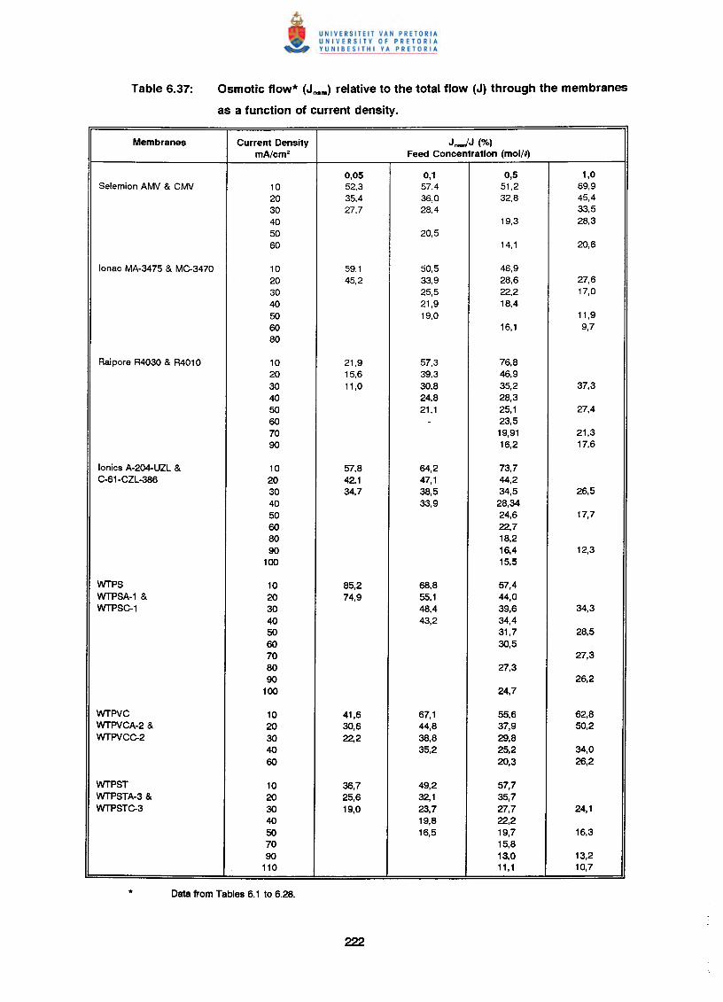
Osmotic flow* (Josm) relative to the total flow (J) through the membranes
as a function of current density.
Membranes Current Density J-IJ (%)mA/cm' Feed Concentration (mol/g)
0,05 0,1 0,5 1,0Selemion ArvrJ & CrvrJ 10 52,3 57.4 51,2 69,9
20 35.4 36,0 32,8 45,4
30 27,7 28.4 33,5
40 19,3 28,3
50 20,560 14,1 20,6
lonac MA-3475 & MC-3470 10 59,1 50,5 46,920 45,2 33,9 28,6 27,6
30 25,5 22,2 17,0
40 21,9 18.4
50 19,0 11,9
60 16,1 9,7
80
Raipore R4030 & R4010 10 21,9 57,3 76,820 15,6 39,3 46,930 11,0 30,8 35,2 37,3
40 24,8 28,350 21,1 25,1 27,4
60 - 23,570 19,91 21,3
90 16,2 17,6
lonics A-204-UZL & 10 57,8 64,2 73,7C-61-CZL-386 20 42,1 47,1 44,2
30 34,7 38,5 34,5 26,5
40 33,9 28,3450 24,6 17,7
60 22,780 18,290 16,4 12,3
100 15,5
WTPS 10 85,2 68,8 57,4WTPSA-l & 20 74,9 55,1 44,0WTPSC-l 30 48,4 39,6 34,3
40 43,2 34,450 31,7 28,5
60 30,570 27,3
80 27,390 26,2
100 24,7
WTPVC 10 41,6 67,1 55,6 62,8WTPVCA·2 & 20 30,6 44,8 37,9 50,2WTPVCC-2 30 22,2 38,8 29,8
40 35,2 25,2 34,0
60 20,3 26,2
WTPST 10 36,7 49,2 57,7WTPSTA-3 & 20 25,6 32,1 35,7WTPSTC-3 30 19,0 23,7 27,7 24,1
40 19,8 22,250 16,5 19,7 16,370 15,890 13,0 13,2
110 11,1 10,7
Membrane permselectivity (£\t) as a function of brine concentration for various initial
feed concentrations, is shown in Figures 6.99 to 6.105. Membrane permselectivity
decreased with increasing brine concentration for all the membranes investigated.
Permselectivity decreased with increasing feed concentration in the case of the
SeJemio~, /onac-, WTPS-,WTPVC-and WTPSTmembranes. However, permselectivity
was slightly higher at 1,0 mol/Q feed concentration than at 0,5 mol/Q feed
concentration in the case of the lonac membranes (Fig. 6.100). Permselectivityshowed
an increase with increasing feed concentration in the case of the Raipore membrane
(Fig. 6.101).
Permselectivity1
g.. A: I:I:::Q.••........•......•••........••. if) .•.1'... . S I!i A A •.•.•.• • ~~·~····'-T···:""··A················'·····... 0- -.a.....-IIII ~
~ •• ....:...ltL. -1.,. i).. ~ .. .::&1-0~ ~ =+-- -+.........................................................................................................
234Brine concentration (moll~
0.05 molll 0.1 molll 0.5 moll'l 1.0 mo~'1o -""_ .. -0 •• _*-
Figure 6.99: Membrane permselectivity (t.t) as a function of brine concentration for
different NaCI feed concentrations. Se/em/on AMV and CMV membranes.
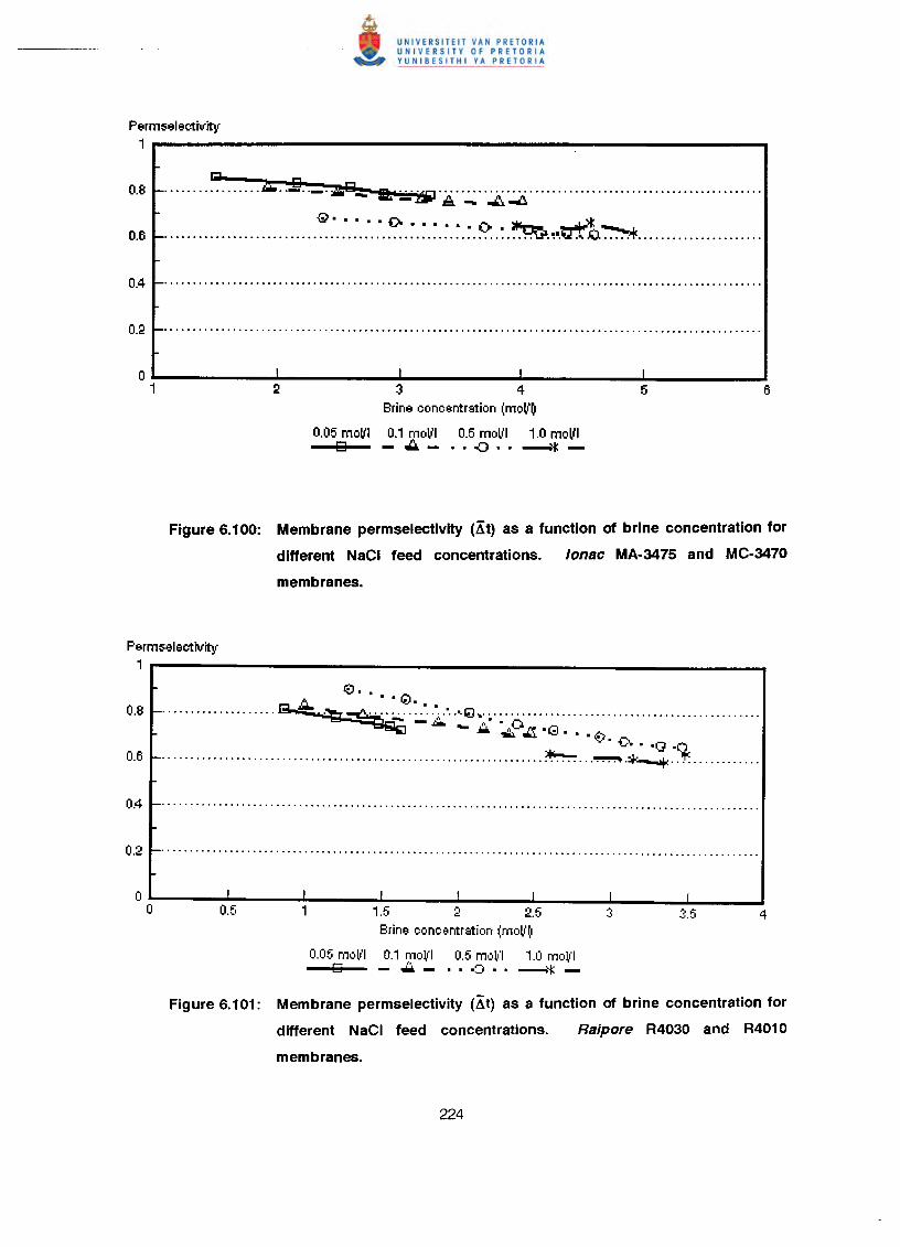
Perm:seleetivity1
e- g................. ~ .._ .._._1:1_ It :.:.·Mi!·A··.:.:,··.:..i·..:,a·········································
........................... ~ ?:.~.~.~.~.~.~.~.:. ~.~ ..~~ .
3 4Brine concentration (moV~
0.05 moVI 0.1 moVI 0.5 moll' I 1.0 moVI9 ~_··oO··~-
Figure 6.100: Membrane permselectivity (Xt) as a function of brine concentration for
different NaCI feed concentrations. lonac MA-3475 and MC-3470
membranes.
Perm:seleetivity1r------------------------...,&tJ •••• Q
08 ~~.:..:-.-'". ~.................... .~':.:.' ~..':'~~'~o:~.:~ : ~ .
0.6 1- ~ ~~~ .•~ .
1.5 2 2.5Brine conc8ntration (moll~
0.05 mo~'1 0.1 moll'l 0.5 molll 1.0 molllo ~_ .. .c" •• ~~-
Figure 6.101: Membrane permselectivity (Xt) as a function of brine concentration for
different NaCI feed concentrations. Raipore R4030 and R4010
membranes.
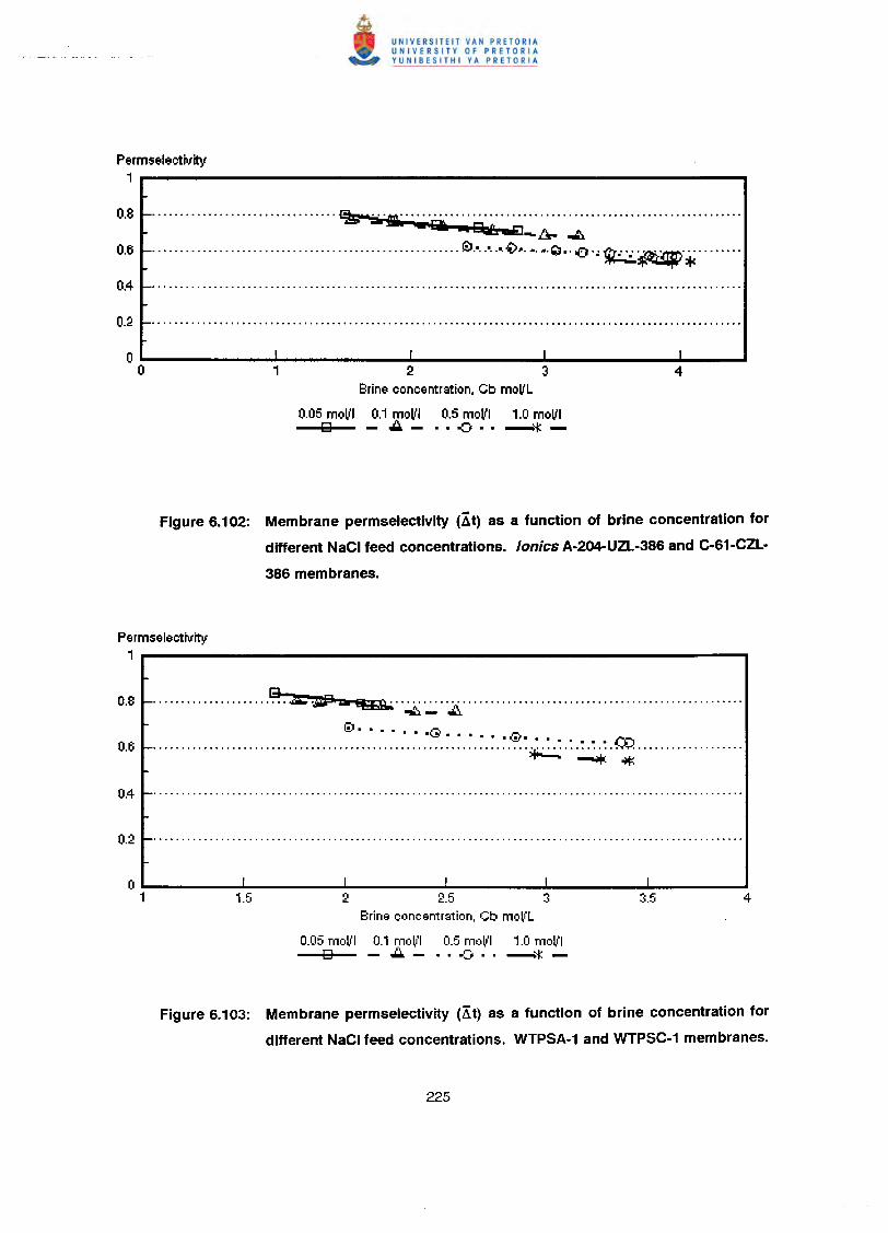
Permselectrv-ity1
................................. ~ a·:Si····························································•• ~ 24 Iiil:6 uEl_ fJ,. .,A
..•..........................•......•.................. ~ .•..•..•. (;> .••.•.•• ~ •. tCJ·· m.· ',' ~:t'I1'I">""""'".~JI'---'- :+<
2 3Brine concentration, Cb mol'L
0.05 mol'l 0.1 mol'l 0.5 mol'l 1.0 mol'l9 -.l:l- .. -0 •• ~-
Figure 6.102: Membrane perm selectivity (Xt) as a function of brine concentration for
different NaCI feed concentrations. lonics A·2~UZL·386 and C·61·CZL·
386 membranes.
Permseleetrv-ity1
8........................k .• _~ .~-~@ ••••• r"•• ~- • • • •• G..............................................................~.~.:.:.:.~.~.~.~.~.ro .
:+-- --0+: "'!=:
2 2.5 3Brine concentration, Cb moll'L
0.05 moll'l 0.1 moll'l 0.5 moll'l 1.0 molflo ••. - ···8··-i*
Figure 6.103: Membrane permselectivity (Kt) as a function of brine concentration for
different NaCI feed concentrations. WTPSA·1 and WTPSC-1 membranes.
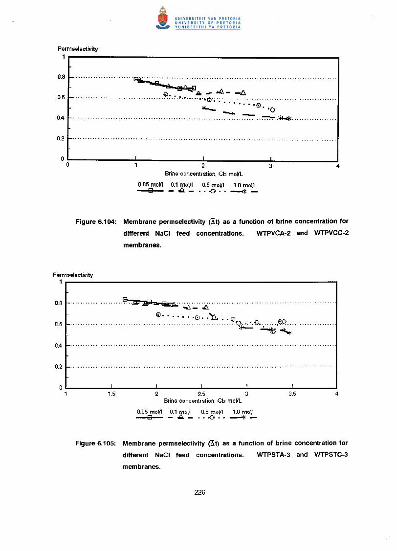
Permselectilfity1
........................ fSAi. .!SA""
(>•• ~.A - J.i- -b.-............................................•.•.•.•. • Gt" ~ . ; . ; . ; . ~ ... ..~
~ . '0~-........................................................................... ~ ..~ .
2Brine concentration. Cb moVL
0.05 moVI 0.1 moVI 0.5 moVI 1.0 moVI9 -.:i.-"-8 .. ~f;:-
Figure 6.104: Membrane permselectivity (3t) as a function of brine concentration for
different NaCI feed concentrations. WTPVCA·2 and WTPVCC·2
membranes.
Permselectilfity1
9···· .. ······ .. ···········W .02FI- ~ .~- .I:!..1::) •••••• -0 .. ~ .. ~
..................................................................()..'.~.0 W .=+-~~
2 2.5 3Brine concentration, Cb moVL
0.05 mol1'l 0.1 rnoVI 0.5 moll'l 1.0 moVI9 - .•••.- •. .(l •• --"'t=-
Figure 6.105: Membrane permselectivity (3t) as a function of brine concentration for
different NaCI feed concentrations. WTPSTA-3 and WTPSTC·3
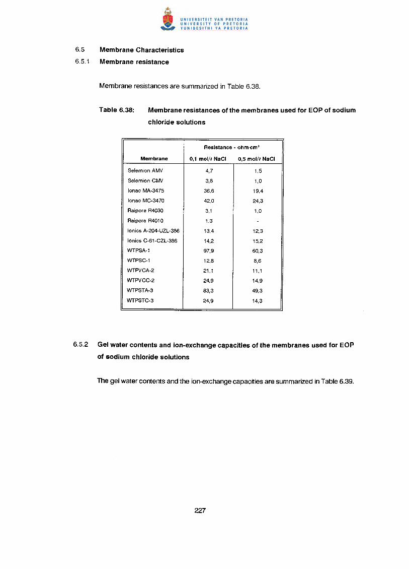
6.5 Membrane Characteristics
6.5.1 Membrane resistance
Membrane resistances of the membranes used for EOP of sodium
chloride solutions
Resistance - ohm-em2
Membrane 0,1 mol/c NaCI 0,5 mol/C NaCI
Selemion AMV 4,7 1,5
Selemion CMV 3,8 1,0
lonac MA-3475 36,6 19,4
lonac MC-3470 42,0 24,3
Raipore R4030 3,1 1,0
Raipore R4010 1,3 -lonics A-204-UZL-386 13.4 12,3
lonics C-61-CZL-386 14,2 15,2
WTPSA-1 97,9 60,3
WTPSC-1 12,8 8,6
WTPVCA-2 21,1 11,1
WTPVCC-2 24,9 14,9
WTPSTA-3 83,3 49,3
WTPSTC-3 24,9 14,3
6.5.2 Gel water contents and ion-exchange capacities of the membranes used for EOP
of sodium chloride solutions
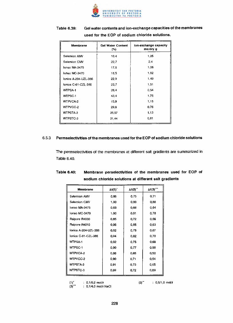
Gel water contents and ion-exchange capacities of the membranes
used for the EOP of sodium chloride solutionso
Membrane Gel Water Content lon-exchange capacity(%) meldry g
Selemion AMV 18,4 1,26
Selemion CMV 22,7 2,4
lonac MA-3475 17,8 1,06
lonac MC-3470 18,5 1,82
lonics A-204-UZL-386 22,9 1,49
lonics C-61-CZL-386 23,7 1,51
WTPSA-1 26,4 0,54
WTPSC-1 43,4 1,75
WTPVCA-2 15,9 1,15
WTPVCC-2 29,8 0,76
WTPSTA-3 35,57 1,13
WTPSTC-3 31,44 0,61
The permselectivities of the membranes at different salt gradients are summarized in
Table 6.40.
Membrane perselectivities of the membranes used for EOP of
sodium chloride solutions at different salt gradients
Membrane at(1)" at (2)"0 at (3)"00
Selemion AMV 0,86 0,75 0,71
Selemion CMV 1,00 0,99 0,88
lonac MA-3475 0,83 0,66 0,64
lonac MC-3470 1,00 0,91 0,78
Raipore R4030 0,85 0,72 0,66
Raipore R4010 0,96 0,85 0,63
lonics A-204-UZL-366 0,92 0,75 0,67
lonics C-61-CZL-386 0,94 0,82 0,70
WTPSA-1 0,92 0,75 0,68
WTPSC-1 0,90 0,77 0,58
WTPVCA-2 0,86 0,65 0,50
WTPVCC-2 0,90 0,71 0,54
WTPSTA-3 0,91 0,73 0,65
WTPSTC-3 0,89 0,72 0,69
(1)"(3)"··
0,1/0,2 mol/l0,1/4,0 mol/l NaCI
7. ELECTRO-OSMOTIC PUMPING OF HYDROCHLORIC ACID SOLUTIONS WITH DIFFERENT
ION-EXCHANGE MEMBRANES
Acid brine concentrations, water flows and current efficiencies were determined at different
current densities for different hydrochloric acid feed water concentrations. Membrane
permselectivities (apparent transport numbers) were measured at concentration differences
similar to those obtained during EOP experiments. The results are summarized in Tables 7.1
to 7.17.
Acid brine concentration (cb) as a function of current density is shown in Figures 7.1
to 7.5. Acid concentration increases more rapidly in the beginning as has been
experienced with the salt solutions and then starts to level off. The levelling off in acid
concentration is more pronounced at the lower acid feed concentrations (0,05 mol/~,
Figs. 7,3 and 7,5). The acid concentration curves were steeper than the curves
obtained during sodium chloride concentration. Higher current densities could be
obtained easier with the acid feed solutions.
Acid brine concentration increases with increasing current density and increasing acid
feed water concentration as has been the case with sodium chloride solutions. The
highest acid concentrations were obtained with the Selemion AAV and CHV
membranes followed by the ABM-3 and CHV and ABM-2 and CHV membranes (Table
7.18). Acid brine concentrations of 25,0; 22,6 and 22,9% could be obtained from 0,5
mol/~ feed solutions with Selemion AAV and CHV, ABM-3 and CHV and ABM-2 and
CHV membranes, respectively. The ABM-1 and CHV membranes did not perform as
well as the other membranes for acid concentration while very low acid brine
concentrations were obtained with the Selemion AMV and CMV membranes. The
reason for the low acid concentrations obtained with the Selemion AMV and CMV
membranes compared to the other anion membranes could be ascribed to the very
low permselectivity of the Selemion AMV membrane for chloride ions (Tables 7.1 to
7.17). The permseleetivity (A ta) of the Selemion AMV membrane was only 0,2 at 0,1
moV~ hydrochloric acid feed (20 mA/cm~ compared to 0,64 for the Selemion AAV;
0,62 for the ABM-3; approximately 0,5 for the ABM-2 and 0,57 for the ABM-1
membranes (Tables 7.1; 7.5; 7.9; 7.13; 7.16). The concentration gradients across
the Selemion AAV, ABM-3, ABM-2 and ABM-1 membranes were also much higher than
the concentration gradient across the Selemion AMV membrane during determination
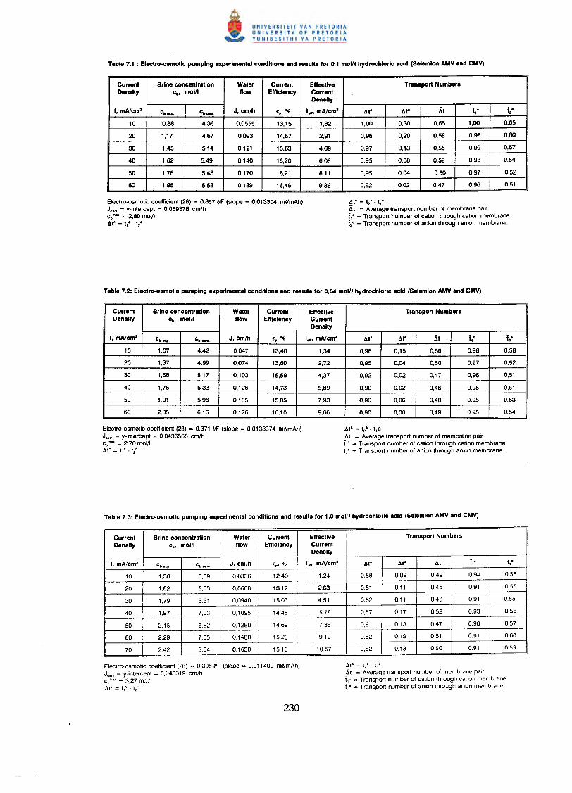
Current Brine concentration WlIler Current Effective Transport NumbersDenalty c.. molll flow Efficiency Current
Density
I. mAtcm' cb ap. c••••• J. cm/h e,..% I•• , mAtcm' .11" .11" .it I," I."10 0.88 4.36 0.0555 13.15 1.32 1.00 0,30 0,65 1,00 0.65
20 1,17 4,67 0,093 14.57 2.91 0,96 0,20 0,58 0,98 0,60
30 1,45 5,14 0,121 15,63 4,69 0,97 0,13 0,55 0,99 0,57
40 1,62 5,49 0,140 15,20 6,08 0,95 0.08 0,52 0,98 0,54
50 1,78 5,43 0,170 16,21 8,11 0.95 0,04 0,50 0,97 0,52
60 1,95 5,58 0,189 16,46 9,88 0,92 0,02 0,47 0,96 0,51
Electro-osmotic coefficient (28) = O,3571/F (slope = 0,013304 ml/mAh)Jo•m = y-intercept = 0,059376 cm/hCbmu = 2,80 moVIAf = .1C - 12
c
A.ta = t28
- 11-
Xt = Average transport number of membrane pairt,' = Transport number of cation through cation membranet,a = Transport number of anion through anion membrane.
Current Brine concentr81lon Wster Current Effective Trsnsport NumbersDensity c•• mol/I flow Efficiency Current
Density
I, mAtcm' cbup. c._ J, cm/h ·P. % I••••mAtcm' .11" .11" Xt i,c I."
10 1,07 4,42 0,047 13,40 1,34 0,96 0,15 0,56 0,98 0,58
20 1,37 4,99 0,074 13,60 2,72 0,95 0,04 0,50 0,97 0,52
30 1,58 5,17 0,103 15,58 4,37 0,92 0,02 0,47 0,96 0,51
40 1,75 5,33 0,126 14,73 5,89 0,90 0,02 0,46 0,95 0,51
50 1,91 5,96 0,155 15,85 7,93 0,90 0,06 0,48 0,95 0,53
60 2,05 6,16 0,176 16,10 9,66 0,90 0,06 0,49 0,95 0,54
Electro-osmotic coefficient (28) = 0,371 I/F (slope = 0,0136374 ml/mAh)J"m = y-intercept = 0,0436566 cm/hcb mu = 2,70 moVIAte = .,c .t2C
4ta = 12a - t,a
.it = Average transport number of membrane pairt,' = Transport number of cation through cation membranet,a = Transport number of anion through anion membrane.
Current Brine concentration Water Current Effective Transport NumbersDensity Cb. mol/I flow Efficiency Current
Density
I. mA/cm' cbaxp. Cbca1e. J. cm/h €p, % I.", mA/cm2 .1t' .11" .1t t' t', 2
10 1,36 5,39 0,0336 12,40 1,24 0,66 0,09 0,49 0,94 0,55
20 1,62 5,63 0,0606 13,17 2,63 0,61 0,11 0,46 0,91 0,55
30 1,79 5,51 0,0940 15,03 4,51 0,62 0,11 0,46 0,91 0,55
40 1,97 7,03 0,1095 14,45 5,78 0,87 0,17 0.52 0.93 0.58
50 2,15 6,82 0,1280 14,69 7,35 0,81 0,13 0,47 0,90 0,57
60 2.29 7,65 0,1460 15,20 9,12 0.62 0,19 0,51 0,91 0,60
70 2,42 8,04 0,1630 15,10 10,57 0,82 0,18 0,50 0,91 0,59
Electro-osmotic coefficient (28) = 0.306 ifF (slope = 0,011409 ml/mAh)J"" = y-intercept = 0,043319 cm/hc,mu = 3,27 moVIAte ;::: t~C - t/
A.ta = t2a _ t/l
Et = Average transport number of membrane pairt,' = Transport number of cation through cation membraneV = Transport number of anion through anion membrane,
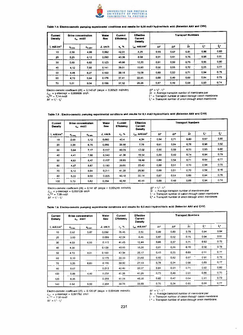
Current Brine concentration Water Current Effective Transport NumbersDensity c., mol/I flow Efficiency Current
Density
I, mAtcm' Clio..,. cltNk:' J, cm/h e., % I•• , mAtcm' IU" AI' 6t i1c i2-
10 2,59 4,88 0,062 42,91 4,29 0,95 0,67 0,81 0,98 0,83
20 3,25 6,13 0,093 40,38 8,08 0,91 0,61 0,76 0,96 0,81
30 3,69 6,83 0,123 40,66 12,20 0,91 0,59 0,75 0,95 0,80
40 4,12 7,66 0,141 39,01 15,60 0,90 0,55 0,72 0,95 0,77
50 4,45 8,27 0,160 38,16 19,08 0,89 0,53 0,71 0,94 0,76
60 4,70 9,64 0,178 37,41 22,45 0,88 0,49 0,69 0,94 0,75
70 5,01 9,04 0,196 37,52 26,26 0,87 0,49 0,68 0,93 0,74
Electro-osmotic coefficient (26) = 0,140 ifF (slope = 0,00523 mlfmAh)J"m = y-intercept = 0,059609 cm/hcb mu = 7,14 moVI4ft: = t,1: -t2
C
&t& = 12& - fl·Xt = Average transport number of membrane pairi,' = Transport number of cation through cation membranei,' = Transport number of anion through anion membrane,
Current Brine concentration Water Current Effective Transport NumbersDensity c•• mol/I flow Efficiency Current
Density
I, mAtcm' cb_p. CbOllk:. J. cm/h €p, % I••• mAtcm' Al" AI' Xt t1C 12-
1O 2,68 5,12 0,060 43,4 4,34 0,94 0,71 0,83 0,97 0,85
20 3,36 6,76 0,086 38,88 7,78 0,91 0,64 0,78 0,96 0,82
30 3,84 7,17 0,117 40,05 12,02 0,90 0,59 0,75 0,95 0,80
40 4,41 7,86 0,140 41,36 16,54 0,89 0,59 0,74 0,94 0,79
50 4,63 8,47 0,157 3B,95 19,4B 0,8B 0,54 0,71 0,94 0,77
60 4,B7 B,67 O,lBO 39,05 23,43 O,BB 0,51 0,70 0,94 0,76
70 5,12 B,64 0,211 41,29 2B,90 O,BB 0,51 0,70 0,94 0,76
BO 5,33 9,03 0,225 40,lB 32,14 0,B7 0,51 0,69 0,94 0,76
100 5,73 9,62 0,264 40,4B 40,4B O,BB 0,4B 0,6B 0,94 0,74
Electro-osmotic coefficient (2B) = 0,141 ifF (slope = 0,005249 ml/mAh)J"m = y-intercept = 0,055129 cm/hcb mu = 7,09 moVIAtC;;:;: t1
C-t2C
dta;;:;: t2
& - t/I
X"t = Average transport number of membrane pairi,' = Transport number of cation through cation membranei,' = Transport number of anion through anion membrane.
Current Brine concentration Water Current Effective Transport NumbersDensity c•• mol/I flow Efficiency Current
Density
i, mA/cm' cb •• p. cbc:.1c. J, cm/h €P. % I••• mA/cm' At" At' At f, c i2-
10 2,62 5,B7 0,050 35,45 3,55 0,B9 0,69 0,79 0,94 0,84
20 3,53 0,OB9 42,24 B,45 0,B7 0,62 0,75 0,94 O,Bl
30 4,03 6,95 0,115 41,45 12,44 0,B6 0,57 0,71 0,93 0,79
40 4,39 0.138 40,65 16,26 0,81 0,56 0,70 0,92 0,7B
50 4,72 B,OI 0,160 40,34 20,17 0,83 0,55 0,69 0,91 0,77
60 5,10 0,173 39,33 23,60 0,82 0,52 0,67 0,91 0.76
70 5,35 8,83 0,195 39,90 27,93 0,78 0,54 0,66 0,89 0,77
80 5,67 0,213 40,46 32,37 0.84 0,59 0,71 0,92 0,80
100 5,96 8,80 0,258 41,26 41,26 0,73 0,49 0,61 0,86 0,75
120 6,35 0,289 41,08 49,30 0,82 0,47 0,64 0.91 0.73
140 6,84 9,50 0,304 39,78 55,69 0,76 0,54 0,65 0,88 0,77
Electro-osmotic coefficient (2B) = 0,126 ifF (slope = 0.004688 ml/mAhjJw' = y-Intercept = 0,061762 cmlhc,ma> = 7,93 molllAt' = t,' - to'
At' = l! - t,'.it = Average transport number of membrane pairt,' = Transport number of cation through cation membraneIe' = Transport number of anion through anion membrane.
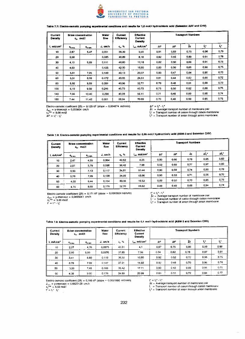
Current Brine concentr8tlon W8ter Current Effective Transport NumberaDensity c., molll flow Efficiency Current
Denalty
I, mAlcm2 c"ap. Cbukl. J, cm/h "",% I•• , mAlcm2 "'t" "'t" 4t i,c j,,'
10 2,87 5,47 0,051 39,30 3,93 0,91 0,59 0,75 0,96 0,79
20 3,58 0,085 40,89 8,18 0,82 0,56 0,69 0,91 0,78
30 4,10 6,69 0,111 40,60 12,18 0,82 0,50 0,66 0,91 0,75
40 4,63 0,135 42,00 16,80 0,80 0,50 0,65 0,90 0,75
50 5,01 7,95 0,149 40,13 20,07 0,80 0,47 0,64 0,90 0,73
60 5,31 8,08 0,172 40,85 24,51 0,81 0,44 0,62 0,90 0,72
80 5,86 8,69 0,209 40,96 32,77 0,76 0,46 0,61 0,88 0,73
100 6,19 9,50 0,245 40,73 40,73 0,75 0,50 0,62 0,88 0,75
140 7,00 10,40 0,299 40,08 56,11 0,71 0,48 0,60 0,86 0,74
180 7,44 11,42 0,351 38,94 70,09 0,70 0,49 0,60 0,85 0,75
Electro-osmotic coefficient (26) = 0,1251/F (slope = 0,004674 ml/mAh)Jo•m = y-intercept = 0,055604 cm/hCbmu= 8,00 moVIAt'::;: l,c -12'
Ata = t/-tl-,1t = Average transport number of membrane pairi,' = Transport number of cation through cation membranei,' = Transport number of anion through anion membrane.
Current Brine concentr8tlon Water Current Effective Transport NumbersDensity c., mol/I flow Efficiency Current
Density
I, mAlcm2 cbnp. c•••••. J, cm/h ep. % I•• , mAlcm2 "'t" "'t" At ",i,· "'j,,'10 2,47 4,55 0,064 42,53 4,25 0,90 0,66 0,78 0,95 0,83
20 2,91 5,79 0.098 38,42 7,68 0,93 0,60 0,77 0,97 0,80
30 3,33 7,13 0,117 34,81 10,44 0,90 0,59 0,74 0,95 0,79
40 3,78 7,69 0,138 34,89 13,96 0,90 0,53 0,71 0,95 0,76
50 4,00 8,44 0,154 33,06 16,53 0,89 0,50 0,70 0,95 0,75
60 4,16 8,68 0,176 32.70 19,62 0.88 0,48 0,68 0,94 0,74
Electro-osmotic coefficient (26) = 0,171 I/F (slope = 0,0063924 ml/mAh)Jo•m = y-intercept = 0,0495041 cm/hCo mu = 5.85 moVIte = .,' -t2'
ta = 128 •• 1·
Xt = Average transport number of membrane pairi,' = Transport number of cation through cation membranei,' = Transport number of anion through anion membrane.
Current Brine concentration Water Current Effective Transport NumbersDensity c., mol/I flow Efficiency Current
Density
I, mAlcm2C" ••p Cb_1c: J, cm/h €p, °/0 len, mAlcm2 "'t' "'t" It i,c i2•
10 2,27 4,76 0,0675 41,01 4,1 0,97 0,75 0,86 0,99 0,88
20 2,90 5,95 0,0976 37.80 7,56 0,94 0,62 0,78 0,97 0.81
30 3,41 6,80 0.119 36,32 10,90 0,92 0,52 0,72 0,96 0,76
40 3,78 7,09 0,147 37,31 14,92 0,92 0,48 0.70 0,96 0,74
50 3,99 7,46 0,166 35.42 17,71 0,90 0,43 0,66 0,95 0,71
60 4,38 9,00 0,178 34.99 20,99 0,89 0,55 0,72 0,94 0,77
Electro-osmotic coefficient (26) = 0,166 I/F (slope = 0,0061880 mQjmAh)J••m = y-intercept = 0,0523128 cm/hc,mu = 6,02 mol/Ite = .,' _12
c
td = t/ - t,aXt = Average transport number of membrane pairi,' = Transport number of cation through cation membranei:= Transport number of anion through anion membrane.
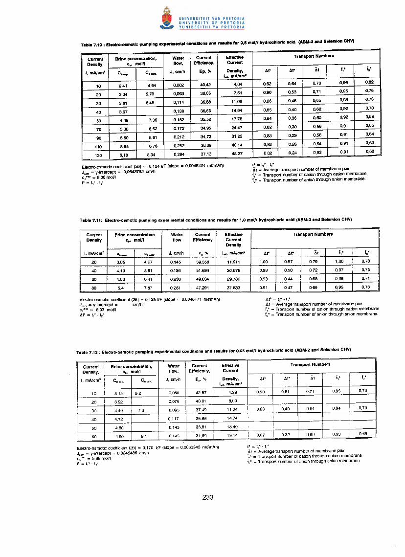
Current Brine concentration, Water Current Effective Tranaport NumberaDenalty, c., mol/l flow, Efficiency , Current
I, mA/cm2 C._ C••••• J, cm/h Ep,% Denalty, At" At" lt fo f..,I••••mA/cm"
10 2,41 4,64 0,062 40,42 4,04 0,92 0,64 0,78 0,96 0,82
20 3,04 5,70 0,093 38,05 7,61 0,90 0,53 0,71 0,95 0,76
30 3,61 6,48 0,114 36,88 11,06 0,86 0,46 0,66 0,93 0,73
40 3,97 0,138 36,65 14,64 0,85 0,40 0,62 0,92 0,70
50 4,35 7,36 0,152 35,52 17,76 0,84 0,36 0,60 0,92 0,68
70 5,30 8,52 0,172 34,95 24,47 0,82 0,30 0,56 0,91 0,65
90 5,50 8,81 0,212 34,72 31,25 0,83 0,29 0,56 0,91 0,64
110 5,95 8,76 0,252 36,09 40,14 0,82 0,26 0,54 0,91 0,63
120 6,18 8,34 0,284 37,13 48,27 0,82 0,24 0,53 0,91 0,62
Electro-osmotic coefficient (26) = 0,124 f/F (slope = 0,0046224 ml/mAh)Jo•m = v-intercept = 0,0643752 cm/hcb m •• = 8,06 moVIr = t1
C -t2C
t· =~.-.1·lt = Average transport number of membrane pairi,' = Transport number of cation through cation membranei,. = Transport number of anion through anion membrane.
Current Brine concentration Water Current Effective Tranaport NumberaDenalty c., mol/l flow Efficiency Current
Denalty
I, mA/cm' ca._p. cbClltco J, cm/h €p, % I••,mA/cm' At" At" lt i,o ia·20 3.05 4.07 0.145 59.558 11.911 1.00 0.57 0.79 1,00 0,7840 4.19 5.81 0.184 51.694 20.678 0.93 0.50 0.72 0,97 0,7560 4.66 6.41 0.238 49.634 29.780 0.93 0.44 0.68 0,96 0,7180 5.4 7.87 0.261 47.291 37.833 0.91 0.47 0.69 0,95 0,73
Electro-osmotic coefficient (26) = 0,1251/F (slope = 0,0046471 ml/mAh)Jo•m = y-intercept = cm/hcb m •• = 8.03 moVIAte = .,c -t;/
At' = t,. - t·.1.t= Avera~e transport number of membrane pairt,' = Transpon number of cation through cation membranei,' = Transport number of anion through anion membrane.
Current Brine concentration, Water Current Effective Tranaport NumbersDensity, c., mol/l flow, Efficiency, Current
I, mA/cm' Cb expo CbCII1c J, cm/h EPl % Density, At' At· At i1
c: iz'I••, mA/crn'
10 3,15 5,2 0,050 42,87 4,29 0,90 0,51 0,71 0,95 0,76
20 3,92 0,076 40,01 8,00
30 4,40 7,6 0,095 37,49 11,24 0,88 0,40 0.64 0,94 0,70
40 4,72 0,117 36,86 14,74
50 4,80 0,143 36,81 18,40
60 4,90 9,1 0,145 31,89 19,14 0,87 0.32 0,59 0,93 0.66
Electro-osmotic coefficient (26) = 0,170 I/F (slope = 0,0063345 ml/mAh)Jo•m = y-Intercept = 0,0245486 cm/hc," = 5,88 mollltt =t,C-t2'
t~:= t/ - t~".b.t= Average transpon number of membrane pairt,' = Transpon number of cation through cation membranei,' = Transpon number of anion through anion membrane.
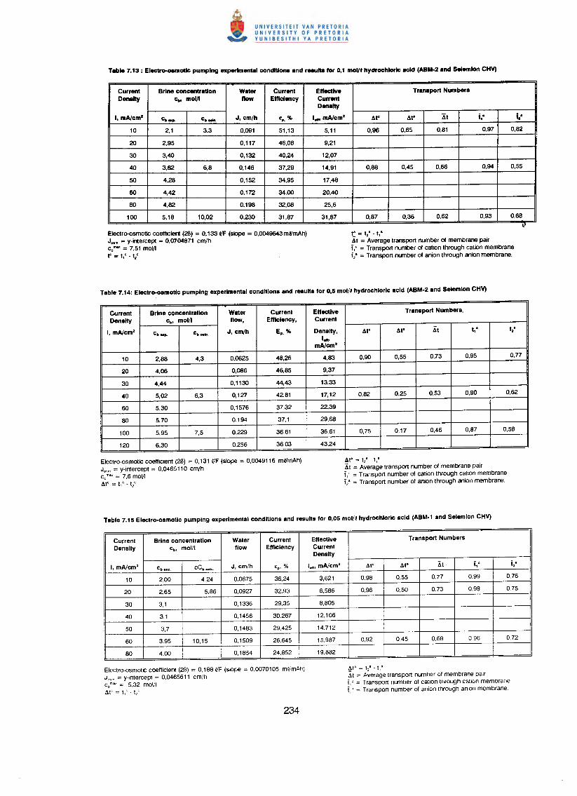
Currenl Brine concentr8llon W8ler Currenl Effective Transport NumberaDensity c", moVI flow Efficiency Current
Denelty
I, mA/cm' c._ c._ J, cm/h e,.% I•• , mA!cm' .11" .11" .11 i· I..,10 2.1 3,3 0,091 51,13 5,11 0,96 0,65 0.81 0,97 0,82
20 2,95 0,117 46,08 9,21
30 3,40 0,132 40,24 12,07
40 3,82 6,8 0,146 37,29 14,91 0,88 0,45 0,66 0,94 0,55
50 4,28 0,152 34,95 17,48
60 4,42 0,172 34,00 20,40
80 4,82 0,198 32,08 25,6
100 5,18 10,02 0,230 31,87 31,87 0,87 0,36 0,62 0,93 0,68L
Electro-osmotic coefficient (2B) = O,l33l/F (slope = O,0049643ml/mAh)J••m = y-intercept = 0,0704871 cm/hc,m•• = 7,51 moVIr: = t,c. t2
C
r = 12•• t,·.1t = Average transport number of membrane pairf,' = Transport number of cation through calion membranef,' = Transport number of anion through anion membrane.
Currenl Brine concenlr8llon Waler Currenl Effective Transport Numbers,Density c", mol/l flow, Efficiency, Current
I, mA/cm' cbup. c••••• J, cm/h E•. % Density, .11' .11· KI I,' I:I•• ,
mA/cm'
10 2,88 4,3 0,0625 48,26 4,83 0,90 0,55 0,73 0,95 0,77
20 4,06 0,086 46.85 9,37
30 4,44 0,1130 44,43 13,33
40 5,02 6,3 0,127 42,81 17,12 0,82 0,25 0,53 0,90 0,62
60 5,30 0.1576 37,32 22,39
80 5,70 0.194 37,1 29,68
100 5,95 7,5 0,229 36.61 36.61 0.75 0.17 0,46 0,87 0,58
120 6,30 0,256 36,03 43,24
Electro-osmotic coefficient (2B) = 0.131 f/F (slope = 0,0049116 mf/mAh)Jo•m = y-intercepl = 0.0465110 cm/hc:"' = 7,6 moVI&tt =.lc•t/
ata = 128- .1·
L\t = Average transport number of membrane pairf,' = Transport number of calion through cation membranet: = Transport number of anion through anion membrane.
Currenl Brine concenlrallon Water Current Effecllve Transport NumbersDenslly c" mol/l flow Efficiency Currenl
Denslly
I, mAtcm' cb •• p cCbc.1c.. J, cm/h €p, 0/0 len, mA/cm2 .1t' .1t' ~t t,C (2-
10 2,00 4,24 0,0675 36.24 3,621 0,98 0.55 0.77 0.99 0,76
20 2.65 5.86 0,0927 32.93 6.586 0,96 0.50 0.73 0.98 0,75
30 3,1 0,1336 29.35 8.805
40 3,1 0,1456 30.267 12,106
50 3,7 0.1483 29,425 14,712
60 3.95 10,15 0,1509 26,645 15,987 0,92 0,45 0,68 0.96 0,72
80 4,00 0,1854 24.852 19,882
Electro-osmotic coefficient (28) = 0,188 t'F (slope = 0,0070105 mt'mAh)J". = y-Inlercept = 0.0465611 cm/hc,m", = 5.32 moVIb.F = t,t - t/
.1to = t,' -1,-~t = Average transport number of membrane pairt,' = Transport number at cation through cation membraneV = Transport number of anion through anion membrane
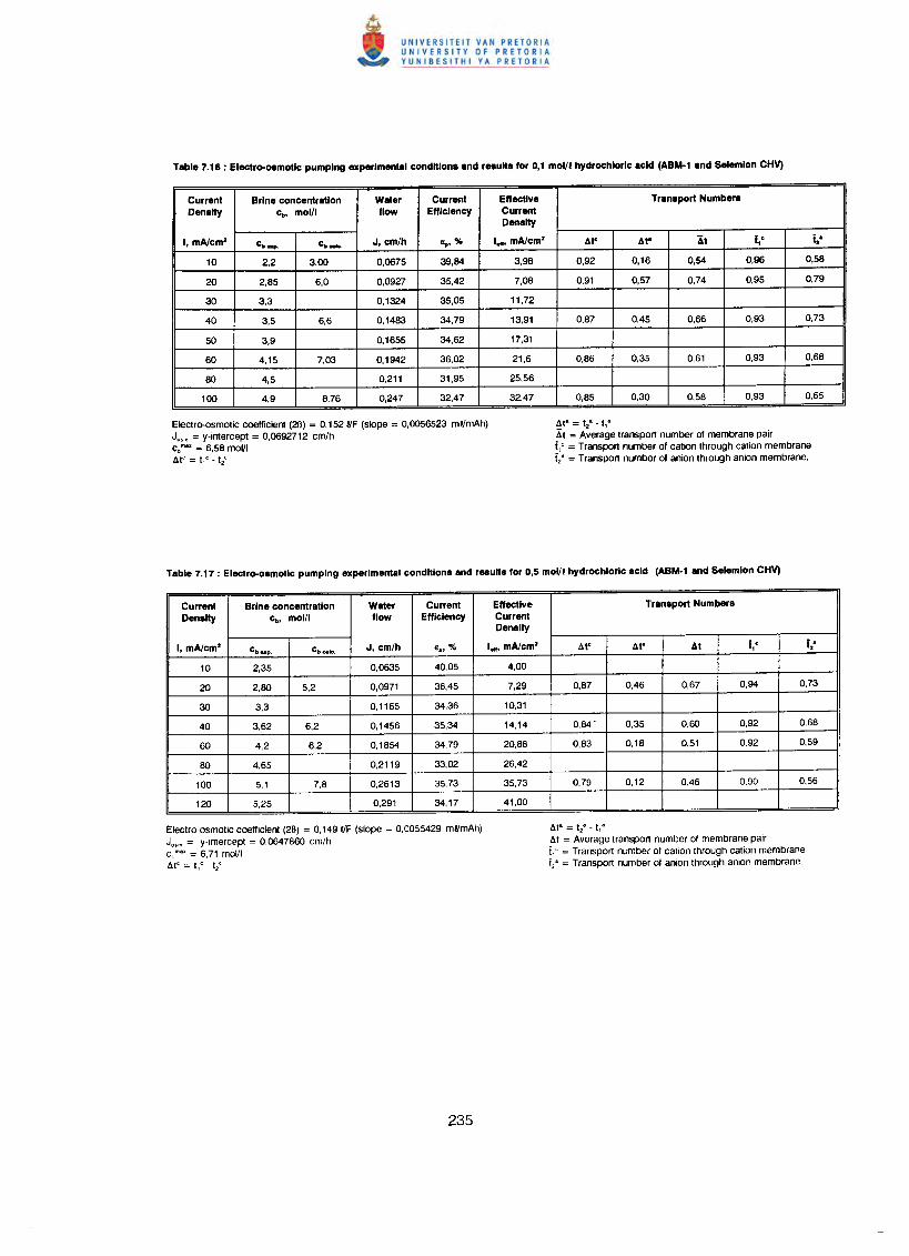
Current Brine concentration Water Current Effective Tranaport NumbersDensity c., mol/I flow Efficiency Current
D_1ty
I, mAtcm' ctt.,. c•••••. J, cm/h ,,",% I•• , mAtcm' At" At" It 1,' t.'10 2,2 3,00 0,0675 39,84 3,98 0,92 0,16 0,54 0,96 0,58
20 2,85 6,0 0,0927 35,42 7,08 0,91 0,57 0,74 0,95 0,79
30 3,3 0,1324 35,05 11,72
40 3,5 6,6 0,1483 34,79 13,91 0,87 0,45 0,66 0,93 0,73
50 3,9 0,1655 34,62 17,31
60 4,15 7,03 0,1942 36,02 21,6 0,86 0,35 0,61 0,93 0,68
80 4,5 0,211 31,95 25,56
100 4,9 8,76 0,247 32,47 32,47 0,85 0,30 0,58 0,93 0,65
Electro-osmotic coefficient (26) = 0,152 ifF (slope = 0,0056523 mlfmAh)J"m = y-intercept = 0,0692712 cm/hCbmu = 6,58 moVI~tC = t,<: -t2'
Ata=t2"-ta
3t = Average transpon number of membrane pairi,' = Transpon number of cation through cation membranei,' = Transpon number of anion through anion membrane.
Current Brine concentrstlon Water Current Effective Transport NumbersDenalty c., mol/I flow Efficiency Current
Density
I, mAtcm' clJaxp. Cbc.tc. J, cm/h €p, % I•• , mAtcm' At' At' At i,c i2"
10 2,35 0,0635 40,05 4,00
20 2,80 5,2 0,0971 36,45 7,29 0,87 0,46 0,67 0,94 0,73
30 3,3 0,1165 34,36 10,31
40 3,62 6.2 0,1456 35,34 14,14 0,84 . 0,35 0,60 0,92 0,68
60 4,2 6,2 0,1854 34,79 20,88 0,83 0,18 0,51 0,92 0,59
80 4,65 0,2119 33,02 26,42
100 5,1 7,8 0,2613 35,73 35,73 0,79 0,12 0,46 0.90 0,56
120 5,25 0,291 34,17 41,00
Electro-osmotic coefficient (26) = 0,149 ifF (Slope = 0,0055429 mlfmAh)J"m = v-intercept = 0,0647860 cm/hCbmu = 6,71 moVIdte
:::. t,' -t/
Ata = 12" - t,a4t = Average transpon number of membrane pairi,' = Transpon number of cation through cation membrane1: = Transpon number of anion through anion membrane.
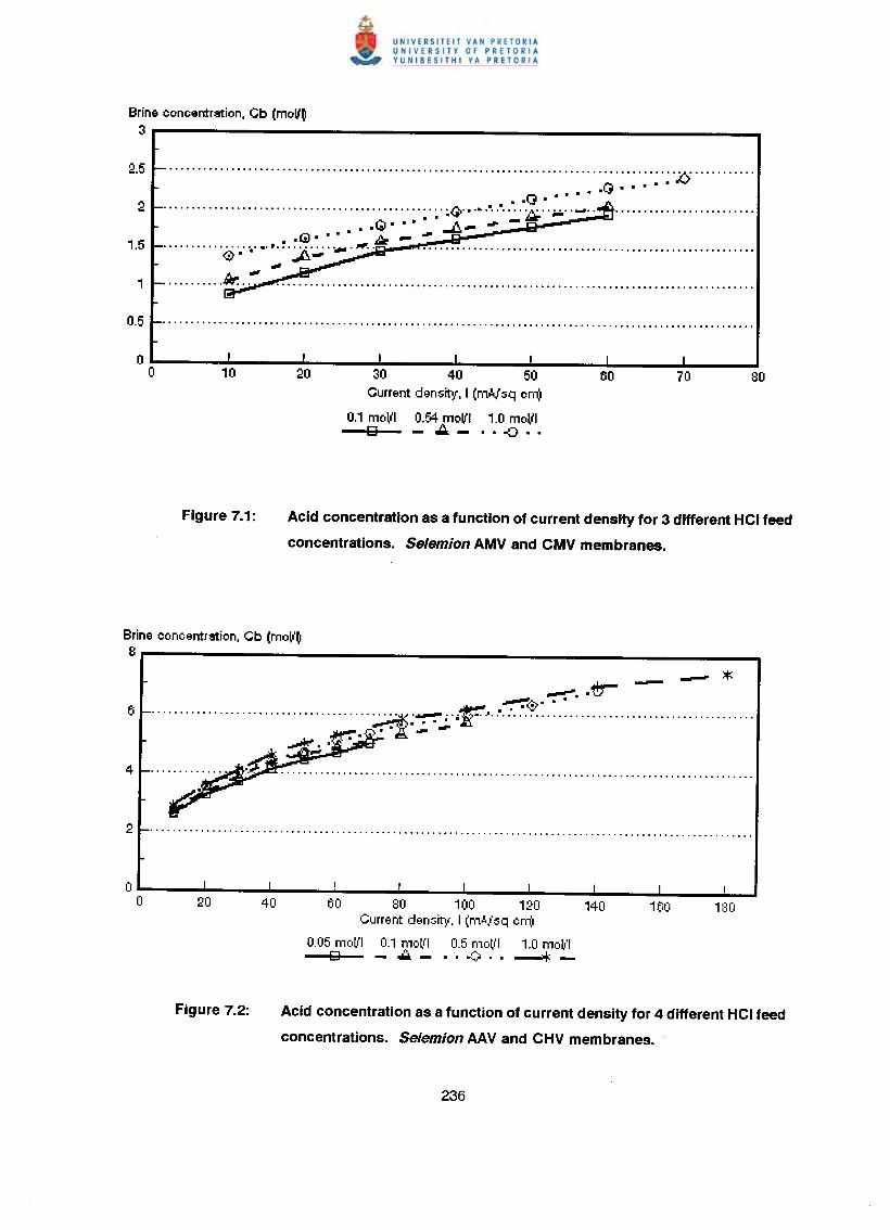
Brine concentration, Cb (moVO3
.............................................................................. Q ~.~.~.;,e, ...M •••••
• • au •.............................................. :.~.~Q'.'.o· ~. ..•••. .••.•.. . .. .Q. • • ~ .•.•••• -
•• (!l •••• ~~~•••••••••••••••••••••••••••••• 0rlJJtt' • ",.. • • ••••••••••••••••••••••••••••••••••••••••••••••••••••••••••
<E>' • A-"*
........... 1Jr. .. "* •••••••••••••••••••••••••••••••••••••••••••••••••••••••••••••••••••••••••••••••••••••
30 40 50Current density, I (moVsq cm)
0.1 moVI 0.54 moVI 1.0 molllD A- .. -0 ..
Acid concentration as a function of current density for 3 different HCI feed
concentrations. Selemion AMV and CMV membranes.
Brine concentration, Cb (moVO8
60 80 100 120Current density, I (m'!'hq cm)
0.05 moll'l 0.1 moll'l 0.5 moll'l 1.0 moll'lo -..::..- .. .0 .. ---*-
Acid concentration as a function of current density for 4 different HCI feed
concentrations. Selemion AAV and CHV membranes.
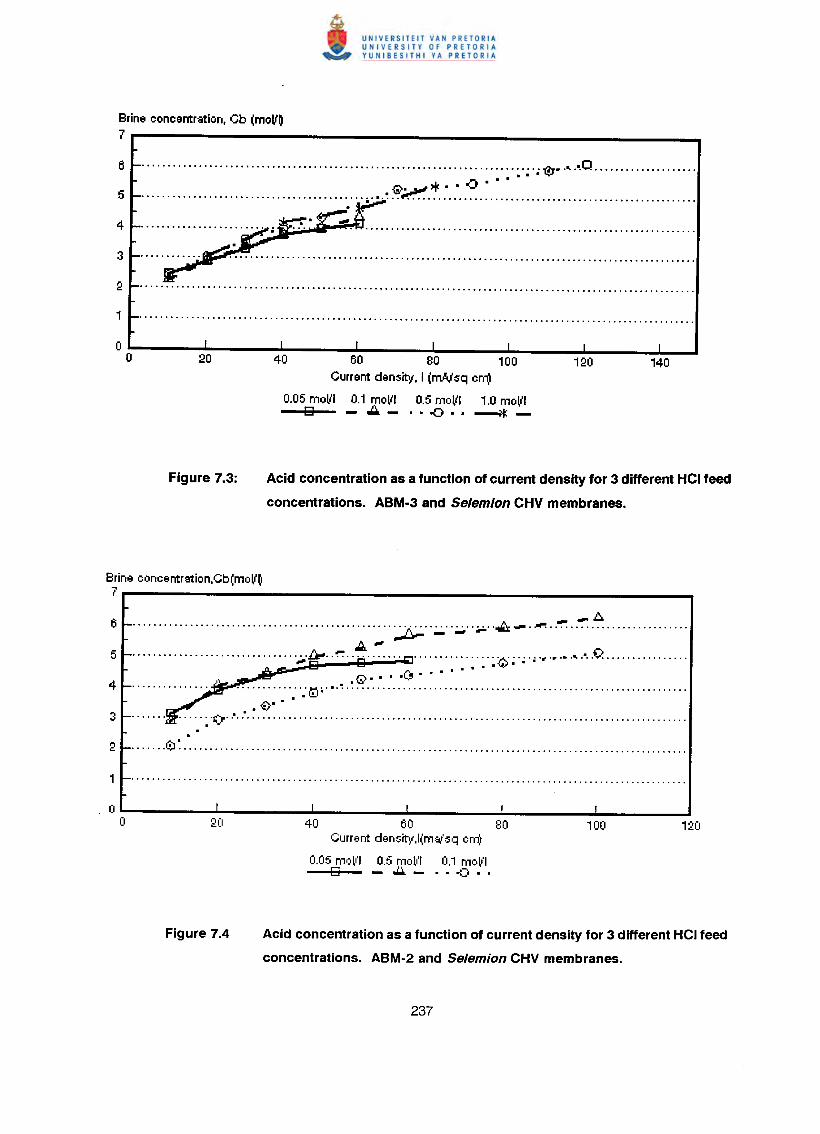
Brine concentration. Cb (moll~7
............................................................................. ~ •.•..•.Q .• • • "Y'
•••...••..••.•••..•••.•••••••••....•••••... o' •. ~ ~~.~.:.: .• ~. ~.~. ~••..•••...•••••..••••••••.•.....••.•
~ M M 100Current density. I (mA,/sq cm)
0.05 molll 0.1 molll 0.5 molll 1.0 molllo -":::"-,,-0 .. -*-
Acid concentration as a function of current density for 3 different HCI feed
concentrations. ABM-3 and Selemion CHV membranes.
Brine concentration.Cb(moll~7
__ l:........................................................................ ~_.~ .
,..l:i- - - -JA'"................................ ~.~ .. ~........... . :~;:.~ .•. " .•.•. " .•..-0. .
,<;>, ' , ,0 ' , ' ' , ' ' '•••••••••.••• '~Io' ,.~ ...•••••.•••••••.....••••..••••••••...••••••...••.•.•••••.•....•.•
, 0;£>' ' ' '....... . .... : '(.P' .'..•.....................................................................................
40 50 80Current density,l(ma/sq cm)
0.05 mol,'1 0.5 TCll'" 0.1 mc'l,'1o - .....- ... ::JI ••
Acid concentration as a function of current density for 3 different HCI feed
concentrations. ABM-2 and Selemion CHV membranes.
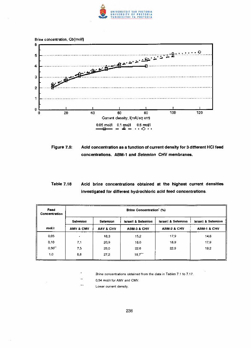
Brine concentration, Cb(moll~6
...............................................................................•.• ~.~.~.~.~.~.~.~.~ .. . ~,:..S:..• ..IJ •••. .- ~..,1- • .:.. • .,.
40 60 80Current density, l(mAlsq cm)
0.05 molll 0.1 molll 0.5 molllo - ..••- .. -8 ••
Acid concentration as a function of current density for 3 different HCI feed
concentrations. ABM·1 and Selemion CHV membranes.
Acid brine concentrations obtained at the highest current densities
investigated for different hydrochloric acid feed concentrations.
Feed Brine Concentration· (%)Concentration
Selemion Selemion Israeli & Selemion Israeli & Selemion Israeli & Selemion
mol/p AMV & CMV AAV & CHV ABM-3 & CHV ABM-2 & CHV ABM-l & CHV
0,05 - 18,3 15,2 17,9 14,6
0,10 7,1 20,9 16,0 18,9 17,9
0,50"" 7,5 25,0 22,6 22,9 19,2
1,0 8,8 27,2 19,7"""
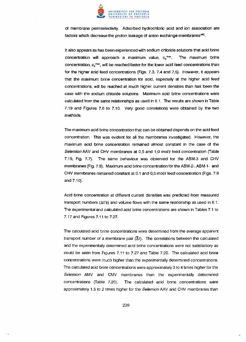
of membrane permselectivity. Adsorbed hydrochloric acid and ion association are
factors which decrease the proton leakage of anion exchange membranes(48).
It also appears as has been experienced with sodium chloride solutions that acid brine
concentration will approach a maximum value, cbmax• The maximum brine
concentration, cb max, will be reached faster for the lower acid feed concentrations than
for the higher acid feed concentrations (Figs. 7.3, 7.4 and 7.5). However, it appears
that the maximum brine concentration for acid, especially at the higher acid feed
concentrations, will be reached at much higher current densities than has been the
case with the sodium chloride solutions. Maximum acid brine concentrations were
calculated from the same relationships as used in 6.1. The results are shown in Table
7.19 and Figures 7.6 to 7.10. Very good correlations were obtained by the two
methods.
The maximum acid brine concentration that can be obtained depends on the acid feed
concentration. This was evident for all the membranes investigated. However, the
maximum acid brine concentration remained almost constant in the case of the
Selemion AAV and CHV membranes at 0,5 and 1,0 mol/Q feed concentration (Table
7.19, Fig. 7.7). The same behaviour was observed for the ABM-3 and CHV
membranes (Fig. 7.8). Maximum acid brine concentration for the ABM-2-, ABM-1- and
CHV membranes remained constant at 0,1 and 0,5 mol/Q feed concentration (Figs. 7.9
and 7.10).
Acid brine concentration at different current densities was predicted from measured
transport numbers (At'S) and volume flows with the same relationship as used in 6.1.
The experimental and calculated acid brine concentrations are shown in Tables 7.1 to
7.17 and Figures 7.11 to 7.27.
The calculated acid brine concentrations were determined from the average apparent
transport number of a membrane pair (X t). The correlations between the calculated
and the experimentally determined acid brine concentrations were not satisfactory as
could be seen from Figures 7.11 to 7.27 and Table 7.20. The calculated acid brine
concentrations were much higher than the experimentally determined concentrations.
The calculated acid brine concentrations were approximately 3 to 4 times higher for the
Selemion AMV and CMV membranes than the experimentally determined
concentrations (Table 7.20). The calculated acid brine concentrations were
approximately 1,5 to 2 times higher for the Selemion AAV and CHV membranes than
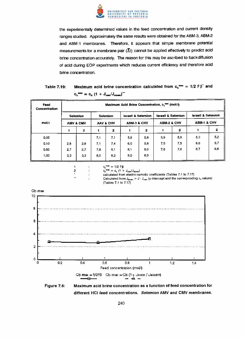
the experimentally determined values in the feed concentration and current density
ranges studied. Approximately the same results were obtained for the ABM-3, ABM-2
and ABM-1 membranes. Therefore, it appears that simple membrane potential
measurements for a membrane pair (It) cannot be applied effectively to predict acid
brine concentration accurately. The reason for this may be ascribed to back diffusion
of acid during EOP experiments which reduces current efficiency and therefore acid
brine concentration.
Maximum acid brine concentration calculated from cbmex = 1/2 F~* and
cbmu = cb (1 + Josm/J.loemr*
Feed Maximum Acid Brine Concentration, cb- (mol/f)Concentration
Selemion Selemion Israeli & Selemion Israeli & Selemion Israeli & Selemion
mol/Q AMV & CMV AAV & CHV ABM-3 & CHV ABM-2 & CHV ABM-1 & CHV
1 2 1 2 1 2 1 2 1 2
0,05 7,1 7,1 5,9 5,8 5,9 5,9 5,3 5,2
0,10 2,8 2,8 7,1 7,4 6,0 5,8 7,5 7,5 6,6 6,7
O,SO 2,7 2,7 7,9 8,1 8,1 8,0 7,6 7,6 6,7 6,6
1,00 3,3 3,3 8,0 8,2 8,0 8,0
cbmax = 1/2 F~
~ max = ~ (1 + Josm/J..,,,,,,)calculated from electro-osmotic coefficients (Tables 7.1 to 7.17)Calculated from J.,o"", = J - Josm (y-intercept and the corresponding cb values)(Tables 7.1 to 7.17)
Cb mS)(
10
"" ......::...------lig Q
0.6 0.8 1Feed concentration (moll~
Cb mS)( = 1/2FB Cb max = Cb (1 + Josm I Jeiosrr(J8 -.A-
Maximum acid brine concentration as a function of feed concentration for
different HCI feed concentrations. Selemion AMV and CMV membranes.
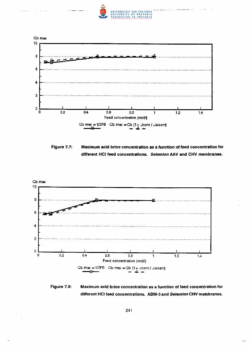
Cb mSK10
•.......•...•••...... ~ .. _ .. pc •.• = = - = - = c - =it .~---
0.4 0.6 0.8 1Feed concentration (moVO
Cb mSK = 1/2FB Cb max = Cb (1 + Josm I Jeiosm)o -~-
Maximum acid brine concentration as a function of feed concentration for
different HCI feed concentrations. Selemion AAV and CHV membranes.
Cb mSK10
0.6 0.8 1Feed concentration (moVO
Cb max = 1/2FB Cb max = Cb (1 + Josm I Jeiosm)o -~-
Maximum acid brine concentration as a function of feed concentration for
different HCI feed concentrations. ABM·3 and Selemion CHV membranes.
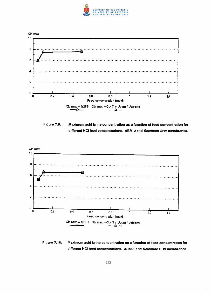
Cb max10
0.4 0.6 0.8 1Feed concentration (moll~
Cb max = 1/2FB Cb max = Cb (1+ Jo:sm I Jeiosm)o -'llli.-
Maximum acid brine concentration as a function of feed concentration for
different HCI feed concentrations. ABM·2 and Selemion CHV membranes.
Cb max10
/ i!........................................................................................................
0.6 0.8 1Feed concentration (moll~
Cb max =1/2FB Cb max =Cb (1+ Josm / Jeiosm)o -'llli.-
Figure 7.10: Maximum acid brine concentration as a function of feed concentration for
different HCI feed concentrations. ABM-1 and Selemion CHV membranes.
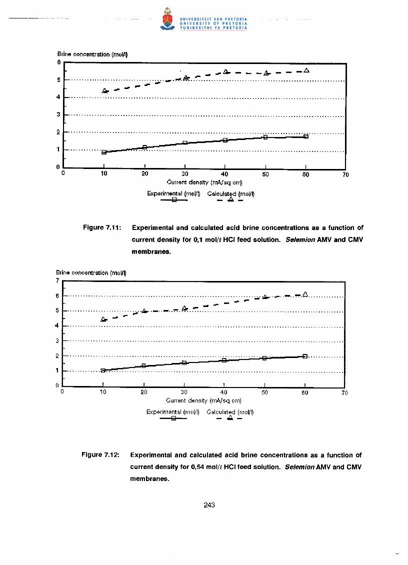
Brine concentration (moVO6
r ~~ __ -..1P 6.....................................•••..••••. .G!r:: .. ~ .. ~ .~--..Qr.--
...................................................... ······················S··············Iiii··············Iii! 9
20 30 40 50Current density (mAlsq em)
Experimentsl (mol"O Cslculated (molfO9 - ~-
Figure 7.11: Experimental and calculated acid brine concentrations as a function of
current density for 0,1 mol/Q HCI feed solution. Selemion AMV and CMV
membranes.
Brine concentration (moVO7
........................................................................ ~.:&,.... _ .. _ .. ~.A .- -- -.........................•.•... ~ .. _ ..•.•..~.~ ..-:-: ..~ ...Qr.--
...................................................... ·····················8··o 0o............. t3'7+ .
Current den::;itv (m.!.isq em)
Experiment:~1 (mc'll'(1 C:~leulst?,j (moll'(1o - .....-
Figure 7.12: Experimental and calculated acid brine concentrations as a function of
current density for 0,54 mol/Q HCI feed solution. Selemion AMV and CMV
membranes.
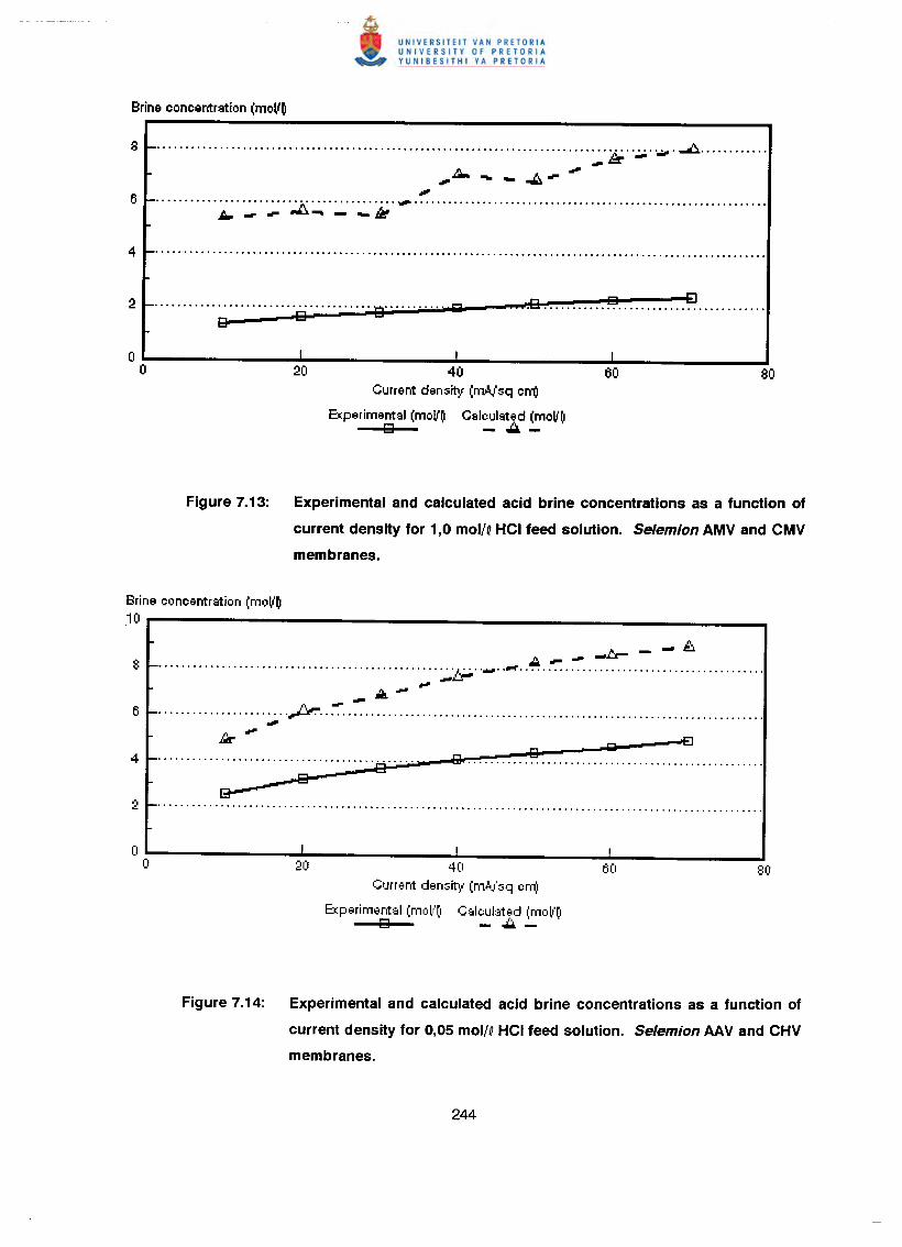
· ....••.......•..•.........•••...•••••.....••••.....••.....•..............••.......••...••••. ....tt6. .•..•.••••..1i!r--,.tM __ ~_ -
•••.......................................... .,.,.. .lJ. _ - ..f:.. - - - IJ!
•••••••••••••••••••••••••••••••••••••• "0 •••••••••• iiiiIeo 9.E3: .•.....•••• ~ ..••••.•. ~ ...•....••••
20 40Current density (mNsq cm)
Experimental (mol(~ Calculated (moV~9 - ~-
Figure 7.13: Experimental and calculated acid brine concentrations as a function of
current density for 1,0 molN HCI feed solution. Selemion AMV and CMV
membranes.
Brine concentration (moV~10.-----------------------------,_I::- - - i:..
8 _ :;.;&.._ ..0I'f •• ~ •• ":":.~ ••••••••••••••••••••••••••••••••
~.J;k~--6 _·······················fr····························· .'"
tJr-4 _ .
9~ 13-'
2 _ .
IiiI - r=F.loiii .
I
40Current density (m.•••/sq cm:1
Experimental (moll'~1 Calcul:~tt.d (mclll'~9 - ••••.-
Figure 7.14: Experimental and calculated acid brine concentrations as a function of
current density for 0,05 mol/QHCI feed solution. Selemion AAV and CHV
membranes.
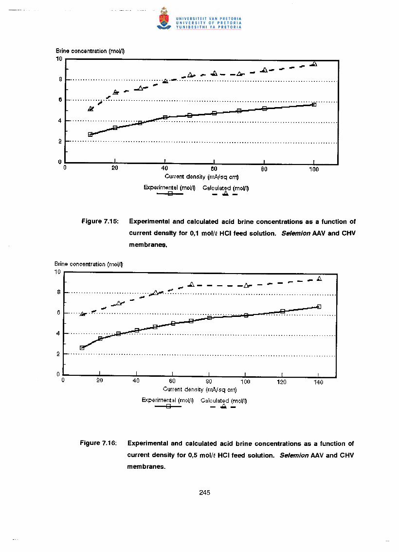
Brine concentration (moV~10
-l:l... .•. ~ ~f:J.,. _ ..&:.. - -Lr -
..................................... .6li,._ .. ':": .,fiJr - ..Jj.-,........... ;; .£:1 .
~ 8 8888
.......................... ~ .
~
40 60Current density (rnoVsq cm)
Experimental (moll~ Calculated (moV~8 -A-
Figure 7.15: Experimental and calculated acid brine concentrations as a function of
current density for 0,1 mol/Q HCI feed solution. Selemion AAV and CHV
membranes.
Brine concentration (moV~10 ,.._"..J::..
.,.. .,.. ~ - - - - -~ - ".. -............................ ,;,.:. ..~ '" .~-
0#1
.....~.~ .
40 60 80 100Current d ••n:srt;j (m •••./sq cm)
Exp ••rim ••ntal (moli(1 C:~lclJlst~d (mo:Nr!o - .••.-
Figure 7.16: Experimental and calculated acid brine concentrations as a function of
current density for 0,5 mol/Q HCI feed solution. Selemion AAV and CHV
membranes.
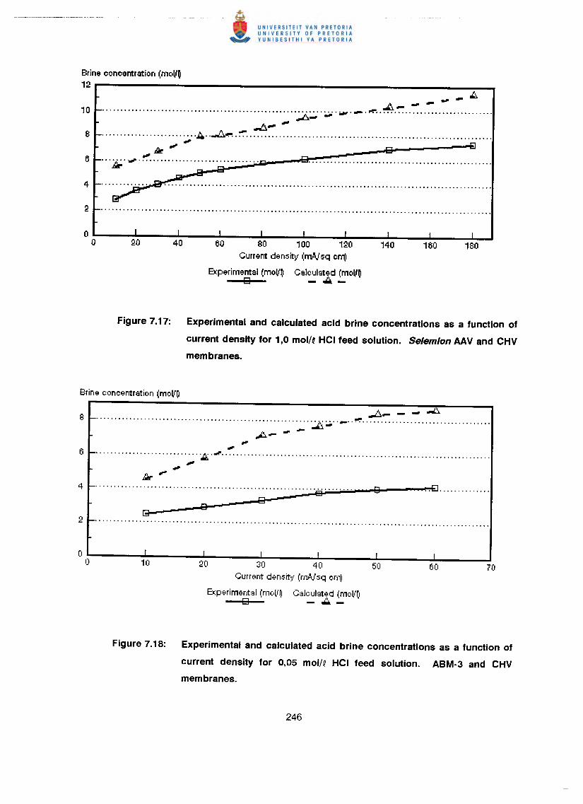
Brine concentration (moV~12 _,/;J,-.I:!.. - - -................................................................ ~._._ .".J::,.- -".6.~""
··························A··....I:J.~·~····················· ."JIr',
... .l;;j,;. . ." .
80 80 100 120Current density (mA.,Isqcm)
Experimental (mol'~ Calculated (moV~o - ..:::..-
Figure 7.17: Experimental and calculated acid brine concentrations as a function of
current density for 1,0 mol/QHCI feed solution. Selemlon AAV and CHV
membranes.
-b.- - - ".,L:,............................................................ ~ :';'0 '''-_ . ~ .
A- --".,............................. ..:t; . oIf' ••••••••••••••••••••••••••••••••••..••••••••••••••••••••••••..•••••••••••,
Ii;..................................................... ·······8········
Current densit~l (nv.isq cm)
E"t;periment:~1(moll'(1 C:~lcIJI:~ted(moll'r,o - ..:::...:...'
Figure 7.18: Experimental and calculated acid brine concentrations as a function of
current density for 0,05 mol/Q HCI feed solution. ABM-3 and CHV
membranes.
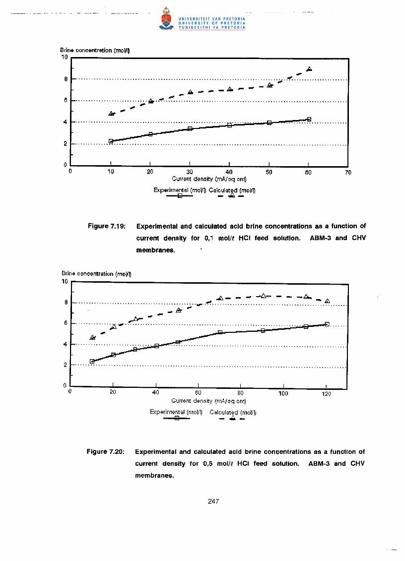
Brine concentration (moll~10 r--------------------------------.,
~8 _ ;;. ..~ .
A __ fir~--_~-.... -6 _ ~ ..~ .~.,..
Jlr'"4 _ tl .
138e---:2 _ ..•...••.••........•...•.......••...........................••.•...........•....•....•...••.....•.........
I I
30 40Current density (mNsq crr(!
Experimentsl (moll~ Cslculat.;.d (moll~o -~-
Figure 7.19: Experimental and calculated acid brine concentrations as a function of
current density for 0,1 mol/Q HCI feed solution. ABM·3 and CHV
membranes.
Brine concentration (moll~10
~ __ .." ~ - - -.t................................................... _ ..~ ':':.~ .
_ fl:r ".,--~............. ',Jd ..••.....................................................................,
bt
60 80Current densit~l (m,!,/sq cm)
Experimental (moll'(1 CalclJlat~d (mol"(113 - •••. -
Figure 7.20: Experimental and calculated acid brine concentrations as a function of
current density for 0,5 mol/Q HCI feed solution. ABM·3 and CHV
membranes.
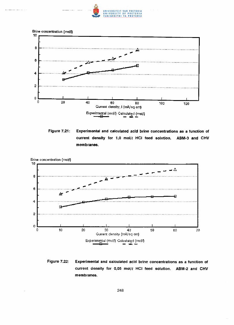
Brine concentration (moVO10
................................................................ /:1 .•••".••.- -~............................. '.;J:i;Jo' . _ .
". ~"..•• Q.............. ~ .
40 60 80Current density, I (mA.,isq cm)
Experimentsl (moll'O CslculstAd (moVOg -~-
Figure 7.21: Experimental and calculated acid brine concentrations as a function of
current density for 1,0 mol/~ HCI feed solution. ABM·3 and CHV
membranes.
Brine coneentrstion (moVO10
__ 6.---.........................................................•.•..••.•. ~ ..~ .A--",.",...................... ..,...~ .
/l:r~ goDg~ ............................. rn
~
30 40Current den:;it~( (m..!.isq em)
Experimentsl (moll'r! Csleulst~d (mclll'~1g - "Il1o:..-
Figure 7.22: Experimental and calculated acid brine concentrations as a function of
current density for 0,05 mol/~ HCI feed solution. ABM-2 and CHV
membranes.
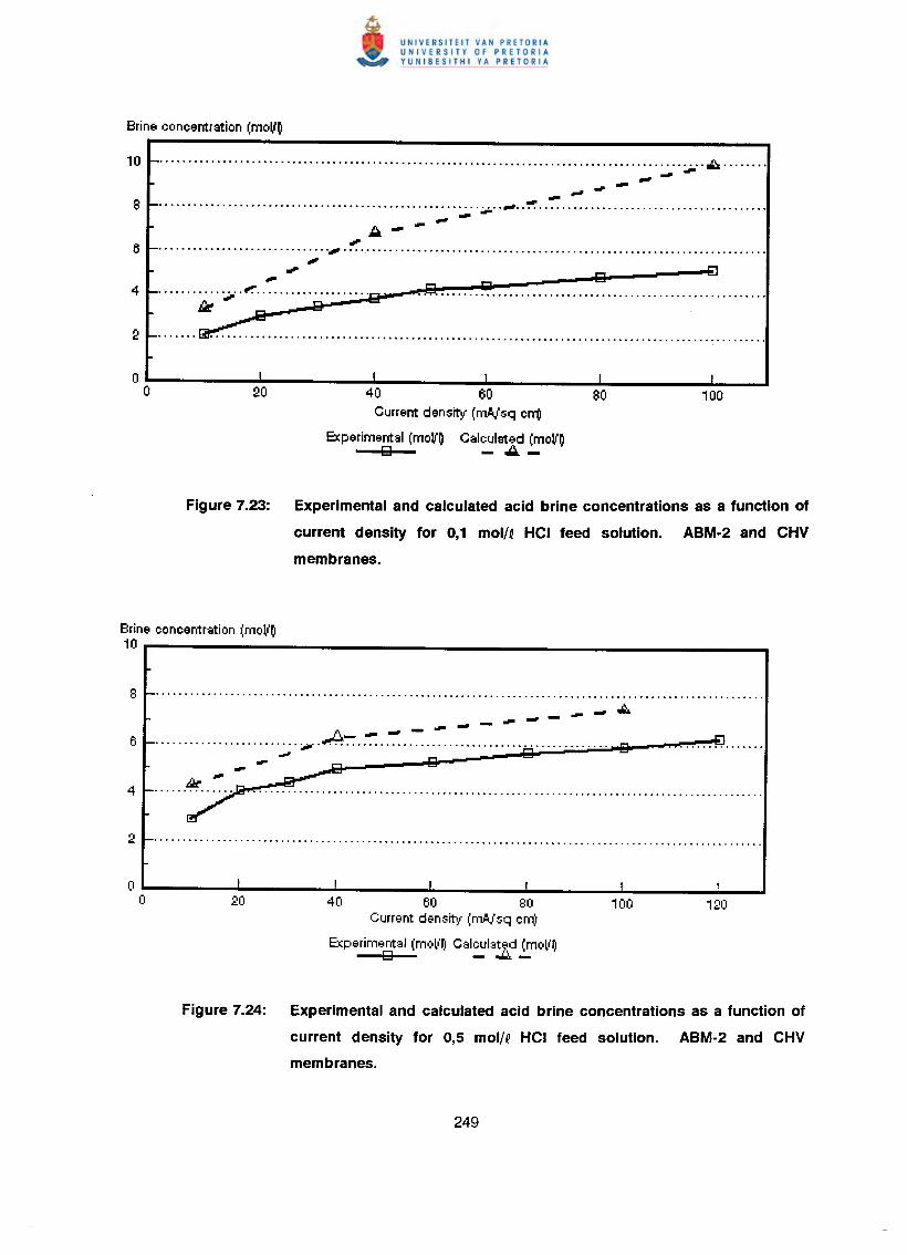
........................................................................................... ;;...~ .~-- --~•••••••••••••••••••••••••••••••••••••••••••••••••••••••••••• #fII# •• ~ ••••••••••••••••••••••••••••••••••••••••--A--~,•.....•••.....••.......•...... J' •....••.....••....••...•.....•...........••.........•.•••.................
••• 121 -E:la ~ .,
• • • • • • •~ • ',;' • f": •••••••••• Q 'iiiii
....... ~ .
40 60Current density (mAjsq em)
Ec:perimental(moV~ Calculated (moV~121 - -'l -
Figure 7.23: Experimental and calculated acid brine concentrations as a function of
current density for 0,1 mol/q HCI feed solution~ ABM·2 and CHV
membranes.
Brine concentration (moV~10
8 ...::....• -,.,. ..•.,.~-.,.6 ;,;00' .A~..~..-:...~ .-
40 60 80Current densitv (nWsq em)
Ec:perimental(moll'~ Calculato;cd(moll'rlo -...w..- I
Figure 7.24: Experimental and calculated acid brine concentrations as a function of
current density for 0,5 mol/Q HCI feed solution. ABM·2 and CHV
membranes.
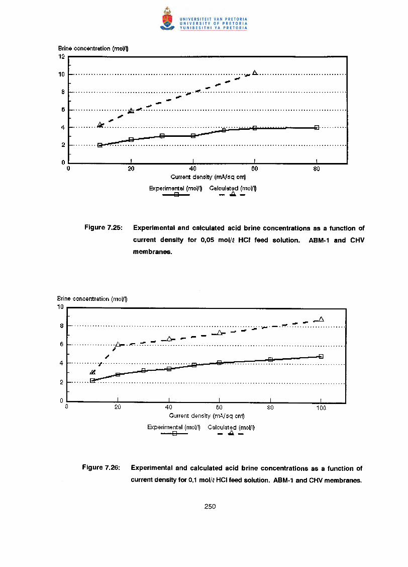
Brine concentration (moV~12 _-----------------------------....,
10 ••.................................................................... .1<' t:... ."..
".-8 ••............................................. ,iII. rI!'.••.••••••.•...•••....••............•••.....•.•.........."..-6 ••...................... /1:i ,.P, •••••••••••••••••••••••••••••••••••••••••••••••••••••••••••••••••••••••••••••••
••••~4 1- /1( Q 1:] .__ 8
~ ~ ~ 82 1-......•.. 9-'"4~ .
I I
40 60Current density (m.A.lsqcm)
Experimental (moll~ Calculated (moV~~ - ..:::..-
Figure 7.25: Experimental and calculated acid brine concentrations as a function of
current density for 0,05 mol/Q HCI feed solution. ABM·1 and CHV
membranes.
Brine concentration (moV~10
-~- -.......................................................................... .,...._ .~.- ..•. -~ .•... ~-
.................fp. ~ ..~ ..~ .~,
···········~··································13M 13 ~
....... ~ .
~ -EJ51 .
Experimental l:molJ'~ C8lcul8t~d I:moll'~~ - oW. -
Figure 7.26: Experimental and calculated acid brine concentrations as a function of
current density for 0,1 mol/QHCI feed solution. ABM·1 and CHV membranes.
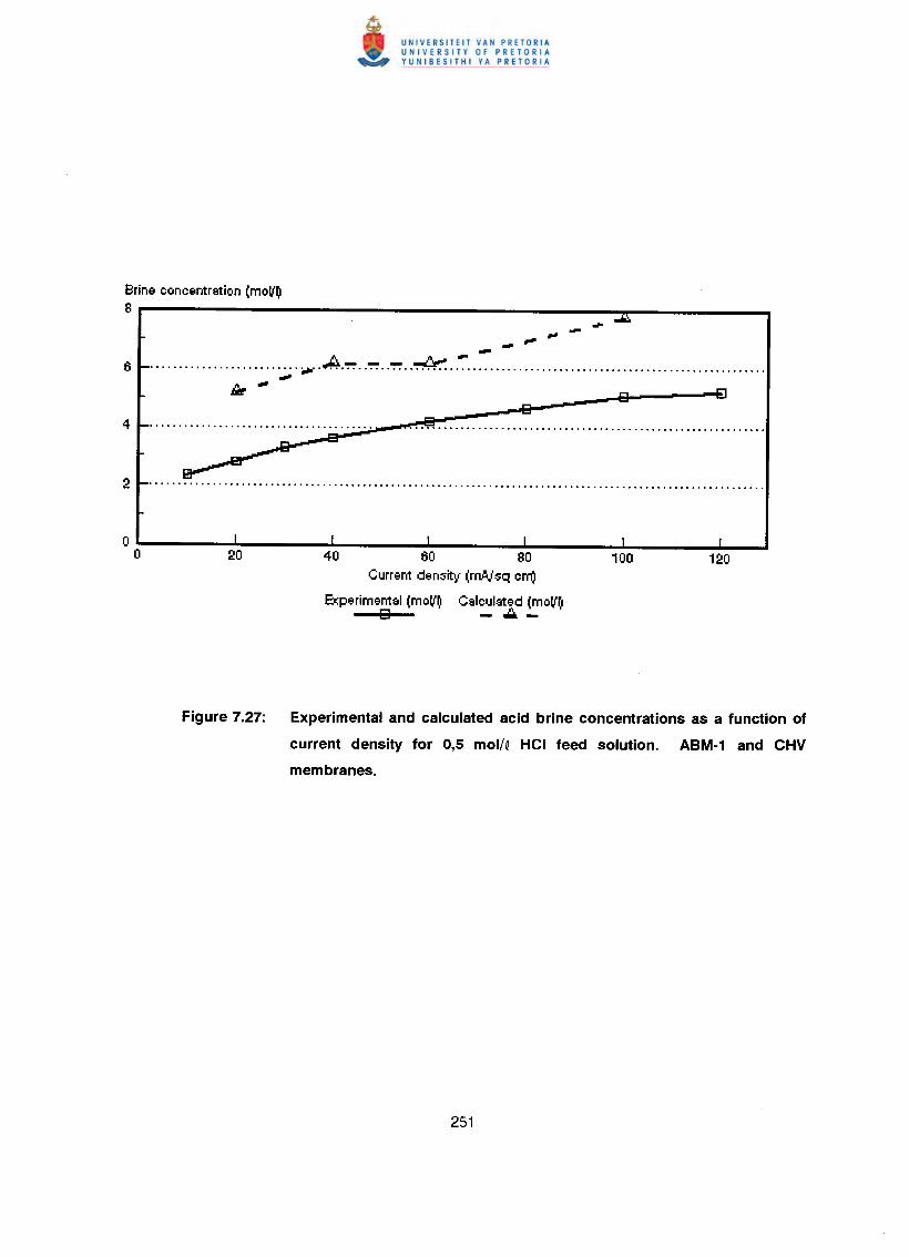
Brine concentration (moll~8
~ --~..........................~ .A.~..":,,,,:,..~..~ ..":..~ ..,.
Ilir~
40 60 80Current density (mVsq cm)
Experimental (moll~ Calculated (mollOo - ~-
Figure 7.27: Experimental and calculated acid brine concentrations as a function of
current density for 0,5 mol/Q HCI feed solution. ABM-1 and CHV
membranes.
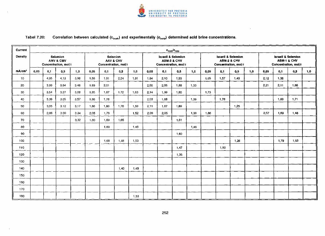
Current ct>a.Jc,,-
Density Selemion Selemlon Israeli & Selem/on Israeli & Selemlon Israeli & SelemlonAMV & CMV AAV & CHV ABM-3 & CHV ABM-2 & CHV ABM-1 & CHV
Concentration, molO Concentration, moll ~ Concentration, moll ~ Concentration, mol/f Concentration, molN
mAlcm' 0,05 0,1 0,5 1,0 0,05 0,1 0,5 1,0 0,05 0,1 0,5 1,0 0,05 0,1 0,5 1,0 0,05 0,1 0,5 1,0
10 4,95 4,13 3,96 1,88 1,91 2,24 1,91 1,84 2,10 1,93 1,65 1,57 1,49 2,12 1,36
20 3,99 3,64 3,48 1,89 2,01 2,00 2,05 1,88 1,33 2,21 2,11 1,86
30 3,54 3,27 3,08 1,85 1,87 1,72 1,63 2,14 1,99 1,80 1,73
40 3,39 3,05 3,57 1,86 1,78 2,03 1,88 1,39 1,78 1,89 1,71
50 3,05 3,12 3,17 1,86 1,83 1,70 1,59 2,11 1,87 1,69 1,25
60 2,86 3,00 3,34 2,05 1,78 1,52 2,09 2,05 1,38 1,86 2,57 1,69 1,48
70 3,32 1,80 1,69 1,65 1,61
80 1,69 1,48 1,46
90 1,60
100 1,68 1,48 1,53 1,26 1,79 1,53
110 1,47 1,93
120 1,35
130
140 1,40 1,49
150
160
170
180 1,53
Current efficiency (€p) determined during EOP experiments as a function of current
density is shown in Figures 7.28 to 7.32. Current efficiency was determined to be very
low (approximately 13 to 16%) for the Selemion AMV and CMV membranes (Fig. 7.28).
This low current efficiency can be ascribed to the low permseleetivity of the Selemion
AMV membranes for chloride ions (proton leakage) (Tables 7.1 to 7.3). The
permselectivity (4 t8) of the Selemion AMV membrane was shown to vary between 0,3
and 0,02 at 0,1 mol/Q acid feed concentration at different concentration gradients in
the current density range from 10 to 60 mNcm2• Perm selectivities varied from 0,15 to
0,08 and from 0,09 to 0,18 at 0,54 and 1,0 mol/Q acid feed concentration, respectively.
Therefore, the Selemion AMV membrane has a very low permselectivity for chloride
ions.
Current efficiencies obtained with the Selemion AAV and CHV membranes were much
higher than current efficiencies obtained with the Selemion AMV and CMV membranes
(Fig. 7.29). Current efficiency of the Selemion AAV and CHV membranes was
determined at approximately 40%. The apparent transport numbers of the anion-
exchange membrane were much higher in this case (Table 7.4 to 7.7) than in the case
of the Selemion AMV membrane. The apparent transport numbers for the AAV anion-
exchange membrane (4t8) varied between 0,67 and 0,49 at 0,05 mol/Q feed
concentration (Table 7.4). Approximately the same values were obtained for the
apparent transport number of the Selemion AAV membrane in the 0,1 to 1,0 molN
feed concentration range. Current efficiencies obtained for the ABM-3 and CHV
membranes were slightly lower than that obtained for the Selemion AAV and CHV
membranes in the 0,05 to 0,5 molN feed concentration range (Fig. 7.30). Current
efficiency was determined at approximately 37%. However, current efficiency for the
ABM-3 and CHV membranes was much higher at 1,0 mol/Q feed concentration.
Current efficiency varied between 60 and 47%. Current efficiency for the ABM-2 and
CHV membranes was initially higher than 40% (Fig. 7.31) but then decreased to
between 30 and 40%. Current efficiency for the ABM-1 and CHV membranes was
determined at between 25 and 40%. It is interesting to note that current efficiency has
increased with increasing acid feed concentration in the case of the ABM and CHV
membranes.
Current efficiency remained almost constant with increasing current density and
increasing acid feed concentration in the case of the Selemion AMV and CMV and
SelemionAAV and CHV membranes (Figs. 7.28 and 7.29). However, current efficiency
decreased somewhat with increasing current density in the case of the ABM-3, ABM-2
and ABM-1 membranes (Fig's. 7.30 to 7.32). This was more pronounced at the lower
acid feed concentrations. Therefore, it appeared that the limiting current density was
exceeded. However, current efficiency remained approximately constant at the higher
acid feed concentrations (0,5 mollq) at high current densities showing that polarization
was absent.
The apparent transport numbers (~t, 1.1 ta and 1.1 tC) for a concentration difference similar
to that obtained in the EOP experiments are shown in Figures 7.33 to 7.49. The
current efficiencies (€p) as determined by the EOP method and shown in Figures 7.28
to 7.32 are also shown in Figures 7.33 to 7.49. The correlation between the apparent
transport numbers (Xt, l1ta, l1tC) and current efficiency is shown in Tables 7.21 to 7.23.
The apparent transport numbers (Xt's) were much higher than the current efficiencies
(€p's) as determined by the EOP method (Tables 7.21 to 7.23 and Figs. 7.33 to 7.49).
The apparent transport numbers were from 3 to 5 times higher than the current
efficiencies in the case of the Selemion AMV and CMV membranes in the acid feed
concentration and current density ranges investigated (Table 7.21). In the case of the
Selemion AAV and CHV membranes the apparent transport numbers were 1,5 to 2
times higher than the current efficiencies. Much the same results were found for the
ABM and CHV membranes. Therefore, it appears that a simple membrane potential
measurement cannot be used effectively in the case of acids to predict membrane
performance accurately. The reason for the big difference between the apparent
transport number and the current efficiency may be ascribed to back diffusion of acid
during EOP of acids.
It is interesting to note that much better correlations have been obtained between the
apparent transport numbers of the anion membranes (l1ta) and current efficiencies
(Table 7.22). The apparent transport numbers were approximately 1,3 to 1,4 times
higher than the current efficiencies in the case of the Selemion AAV and CHV
membranes in the current density range from 30 to 70 mA/cm2 (0,5 molle feed). An
even better correlation was obtained at 1,0 mol/q feed concentration in the current
density range from 40 to 140 mA/cm2• The apparent transport numbers were from
1,05 to 1,19 times higher than current efficiencies in this range. The ratio between
apparent transport number and current efficiency (l1ta/€p) varied between 1,22 and
0,86 for the ABM-3 and CHV membranes in the current density range from 30 to 70
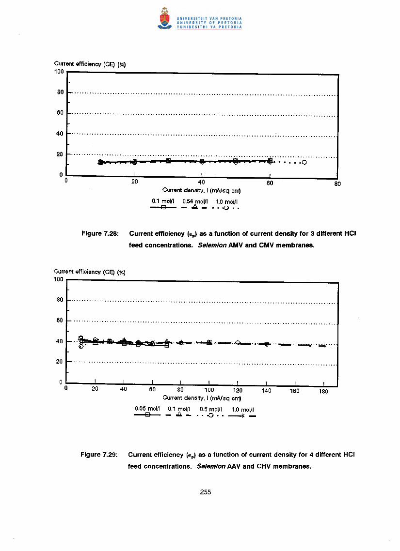
Current efficiency (CE) (%)100
,..........•'~.~.~.4'~ .; a ~.';.'.•.','.,'.~.','@.:' :. : . , .~ ti: ':.:.:.:':0' .
40Current density, I (mAJsq crr(!
0.1 moltl 0.54 moltl 1.0 moltlo ~- .. -0 ..
Figure 7.28: Current efficiency (€p) as a function of current density for 3 different HCI
feed concentrations. Selemion AMV and CMV membranes.
Current efficiency (CE;I (%)100 r----------------------------.
40 _ ... !:~ .•.ft· ....,--rlt.~.-.... I'._ ..Q- ...•...•.._ .._ ...,"*'"
0 I I I I I I , I I
0 20 40 60 80 100 120 140 160 180Current density, I (mAJsq err(!
0.05 moltl 0.1 moltl 0.5 moltl 1.0 moltl0 - .•.. - • • ooC) • • -;lj( -
Figure 7.29: Current efficiency (€p) as a function of current density for 4 different HCI
feed concentrations, Selemion AAV and CHV membranes.
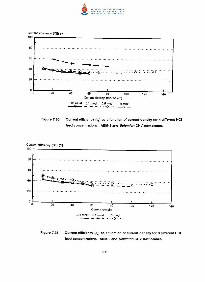
Current efficiency (CE) (%)100
............ ~ .--*_ -.-L---.... - -...c
.... ~';"~" '~:':":'OQ'~'~'~'~0':':':':':': .€J.•..•. '.' .•..•. '.':0 ';'~'~'~';·;0······ .
60 80 100Current density,l(mAJsq cniJ
0.05 mol'l 0.1 mol'l 0.5 mol'l 1.0 mol'lt3 oA- .. -o .. --4:-
Figure 7.30: Current efficiency (€p) as a function of current density for 4 different HCI
feed concentrations. ABM-3 and Selemion CHV membranes.
Current efficiency (CE) (%)100
60 80Current density
0.05 mol'l 0.1 Tol'l 0.5 mol'lE3 •••. - •• -0 ••
Figure 7.31: Current efficiency (€p) as a function of current density for 3 different HCI
feed concentrations. ABM-2 and Selemion CHV membranes.
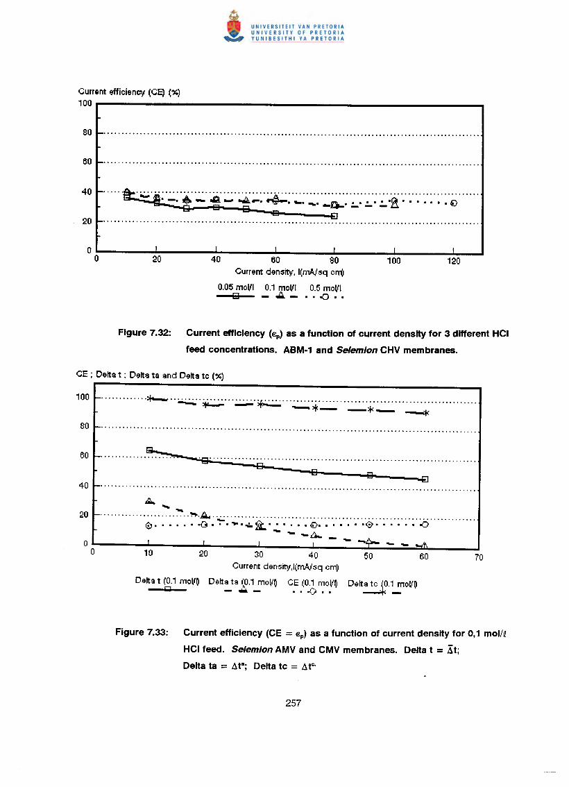
Current efficiency (CE) (%)100
40 60 80Current density, 1(rAA/sq crr(!
0.05 moVI 0.1 moVI 0.5 moVIo -..:i.- .. -o ..
Figure 7.32: Current efficiency (€p) as a function of current density for 3 different HCI
feed concentrations. ABM-1 and Selemion CHV membranes .
............. ~ .. ;.;.;..;.;...~ ~.~ .-*- -:+<- -*
·13········································································· .13 GI
GI a-EJ
&...•.......
......................... ~ ..A. .0. . . . . . ·0 . ~ . ."..~ ~ . . . . . . 'i). • . • • • •0'. . . . . . -':J- --~ - -10 20 30 40 50 60 70
Current density,I(rAA/sq crr(!
Delta t (0.1 moVO Delta ta (0.1 moVO CE (0.1 moVO Delta tc .~o.~OVOIiiiI - ...•. - .. ..() ..
Figure 7.33: Current efficiency (CE = €p) as a function of current density for 0,1 mol/Q
HCI feed. Selemion AMV and CMV membranes. Delta t = Xt;
Delta ta = At8; Delta tc = Ate.
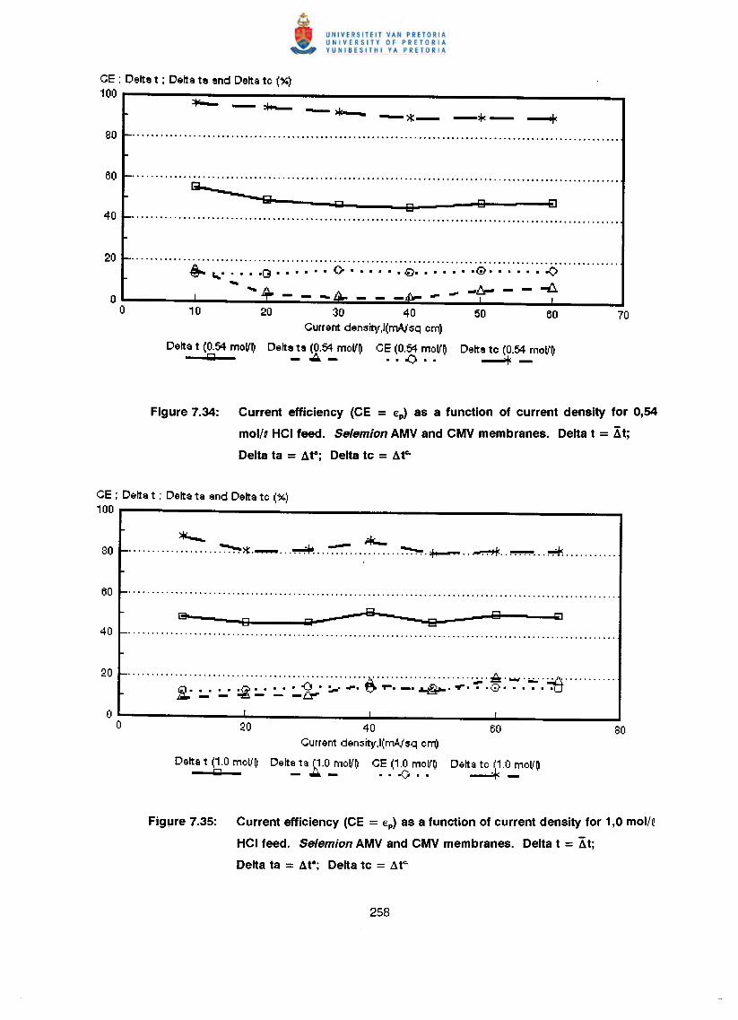
CE : Delta t ; Delta ta and Delta te (%)100
.........................................................................................................@p.. •.••• • • • .13 • • • • • • 0 . . . . . .€-. • • • • • •(;). • • • • • -0
.••. ..••. _ - ..f:..
10 20 30 40Current density,l(mA.,i5q em)
Delta t (0.54 moV~ Delta ta (0.54 moV~ CE (0.54 moV~Jiid - ~- •• ~ ••
Delta te (0.54 moV~----. -Figure 7.34: Current efficiency (CE = €p) as a function of current density for 0,54
mol/Q HCI feed. Selemion AMV and CMV membranes. Delta t = At;
Delta ta = ata; Delta tc = ate.
CE : Delta t ; Delta ta and Delta te (%)100
*"- "*-80 ~~._ ~ ~ ~.~ .. ~ .. ~ ~ .
• • • • • . • • • • • • • . • • • • • • • • • • • • • • • • • • • • • • • • • • • • • • • • • • • • • l\' •.•.••••••••••••••..•••• ~ •••••.••• ~ ••••••..•••
G:). • • • • .G. • • • • <'} • :..-- ••• ~ .•••• _. ~ • .,.. -:- • .:;.. • .:-. .'0'...w.. - - ~- --~
20 40 60Current den5ity,I(mA,r'5q em)
Delta t (1.0 moV~ Delta ta (1.0 moV~ CE (1.0 moV~ Delta te (1.0 moV~IMl - •••. - • • .() • • ----4: -
Figure 7.35: Current efficiency (CE = €p) as a function of current density for 1,0 mol/Q
HCI feed. Selemion AMV and CMV membranes. Delta t = Xt;
Delta ta = ae; Delta tc = Ate.
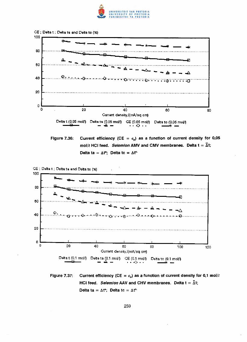
CE : Delta t : Delta ta and Delta to (%)100
........... s.., .&I eI eI
~ eI 8 ----il...............:":'"..~..~._.._..-&. .- _ .A---~ --A--~
........... ~ ~.~.~.~.•. ·G·· .•.•.•. - ..()..•.•. ~.~Off • .-r-. . "." "." ~ ~ "0" .~ • • • "'=J"- • • • • • ~. • • • • •
20 40 60Current deMity,l(mAJsq orr(!
Delta t (0.05 moV~ Delta ta (0.05 moV~ CE (0.05 moV~ Delta to (0.05 moV~Iiiil - .:A - •• .() •• ---Ie -
Figure 7.36: Current efficiency (CE = €p) as a function of current density for 0,05
mol/QHCI feed. Selemion AMV and CMV membranes. Delta t = At;
Delta ta = ~t"; Delta tc = ~t""
CE : Delta t ; Delta ta and Delta to (%)100 *--~"""*- -+ ~ --:+< - *"-- =+-- - ...of<
... ' ..~ .. , , , , .~ e 8_ &I Iiiil ~ 8 ~
~~.... , , , .. , ...••. ~. '.•••. /,j.,." , , , , , " .-~ __ A , .f>,
~ -& - =.- - - -Ll.. , ... S>.•", .• 'Q' •.•.•. {)w •••• ,.G"'.'r '()..'.'~'~'0•.. ,•...0:.",., "£)- ••••••••••••••• ~ ••••• " •....••••
40 60Current density,l(mAJsq orr(!
Delta ta (0.1 moll'O CE (0.1 moVO- ..•.•. - .. .:.) ..Delta t (0,1 moV~Iiiil
Figure 7.37: Current efficiency (CE = €p) as a function of current density for 0,1 mol/Q
HCI feed. Selemion AAV and CHV membranes. Delta t = Xt;
Delta ta = ~t"; Delta tc = ~tc.
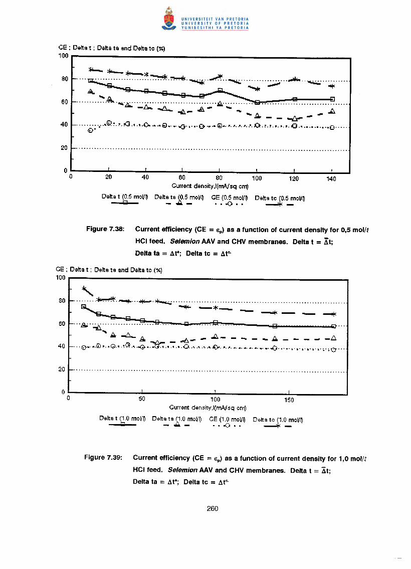
CE ; Delta t ; Delta ta and Delta to (%)100
:+i-. *-- *'--*....~ ~ ,.~.~. -......A _.;,.;;..................••....~ .A .~ ••••••• ~ ~
•••• ~ •• ~.~ • 0010-"~~'-'.-•.:..o.i:!ioo.. _.. _~Q~_.. -.. ~~.~!I-.. _- ..,j.~ ..•.....•• He. HH.: ..... ~ - -- - "-f::r'"
.........•..•. G'- ~. !'. :t3 .•.•. .(). .•.• ~ •.•. -.<3" •.•. e- .•.• Q•. ~.~.~.~.0·. O.:.:.•.•.•..Q' .•.•.•.•.•.• O· ....09'
Delta t (0.5 moV~IiiiI
60 80 100 120Current density.l(rnAJsq orn)
Delt~ta 2.5_moV~ C.E.(O~ ~o.V~ Delta to .~.~OV~
Figure 7.38: Current efficiency (CE = €p) as a function of current density for 0,5 mol/Q
HCI feed. Selemion AAV and CHV membranes. Delta t = At;
Delta ta = at8; Delta tc = ate.
CE ; Delta t : Delta ta and Delta to (%)100
"......... ~ ..-.., ..-. *-.;,,; .
~ """""'"-*- - --0+< - - ~... "g,,; ....•..•...••. ~ .... ~ .... EJ. ... Iii! .... a..... g 'U ...~,
~ ~ A _ ~ __ .1::..- - _ - _ ~ _ - _ - -f::.." '09.' •.Ii)P. ·G·· .~Q.•..~ •.~ .•.•.•. 0. .•..•..•..•..(:l.o.~.~.•.•.•.•.•.•.•. ..t:) .•.•. ,. ,. ,. ,. ,. , .•.• '()" ...
100Current density,l(rnAJsq ern)
Delta t (1.0 mov'~ Delta ta ~~.Omoll'~1 CE (1.0 moV~1 Detta te .~.o_mov~IiiiI - _- •• .() ••
Figure 7.39: Current efficiency (CE = €p) as a function of current density for 1,0 mol/Q
HCI feed. Selemion AAV and CHV membranes. Delta t = Xt;
Delta ta = a t8; Delta tc = a tc.
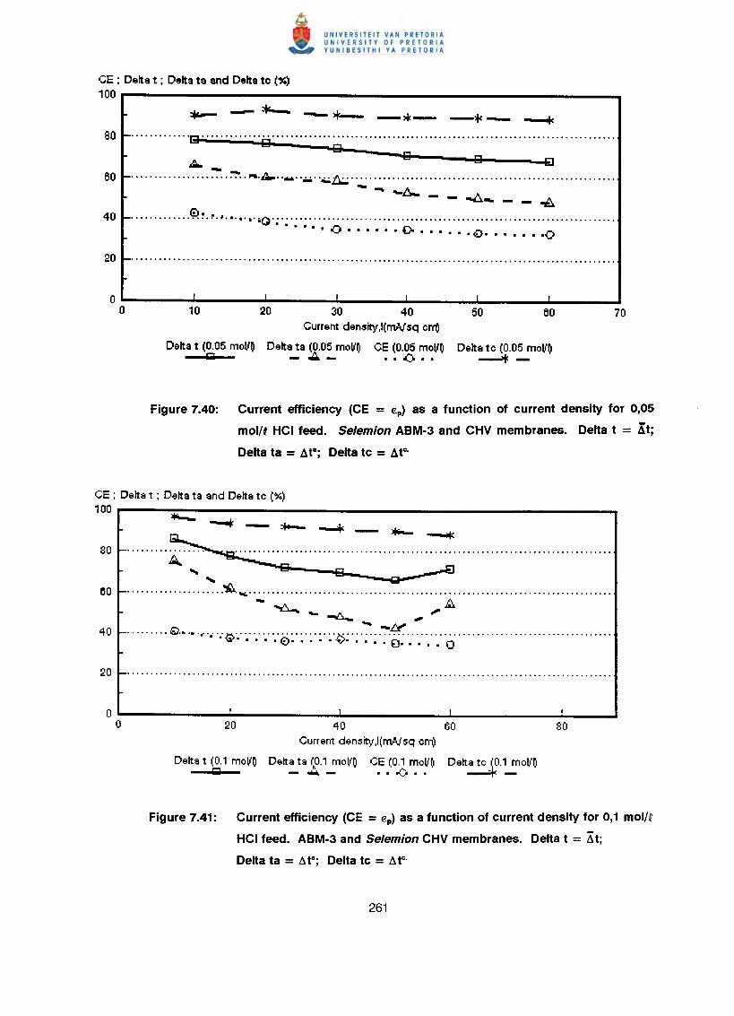
CE ; Delta t : Delta ta and Delta to (%)100
*"- - *-- ->f- -*- -If<- --+c............. e-:- .
9 9~ Q Q ~--.........................••. ~ .._. ',,;,;,'.~tJ.:.; .
- _ 10•••• ~ .A
-....:a. ••• __ ~
G) ••••••••••••••••••••••• eo •• ,. _00;' ~.;.; .
. . 0 . . . . . . 0- • • . . • ..[}. • • • • • -0
10 20 30 40Current density,I(rn.AJsq om)
Delta t (0.05 moV~ Delta ta (0.05 moV~ CE (0.05 moV~C -~_ •• -:) ••
Delta to (0.05 moV~---* -
Figure 7.40: Current efficiency (CE = €p) as a function of current density for 0,05
mol/q HCI feed. Selemion ABM·3 and CHV membranes. Delta t = Kt;
Delta ta = Me; Delta tc = ate.
CE : Delta t : Delta ta and Delta to (%)100
•••..................... ~""' .- ~
~ - _10. .,"""""- .•.• '
€) -~••••••••• • •••• ~ ••• ".0 ~'.""'."'.""'.""').(""""""""""""".""""""""""""""". . . . 0· . . . .v· . . . . 0. . . . . Q
oo 20 40 60 80
Current density,l(mNsq om)
Delta t (0.1 moV~ Delta ta ~~.1mol{~ CE (0.1 mo~'~ Delta to fO.1 moll'~I;;;;l - •••• - •• -<) •• ~-
Figure 7.41: Current efficiency (CE = €p) as a function of current density for 0,1 moll Q
HCI feed. ABM·3 and Selemion CHV membranes. Delta t = X t;
Delta ta = ae; Delta tc = a tc.
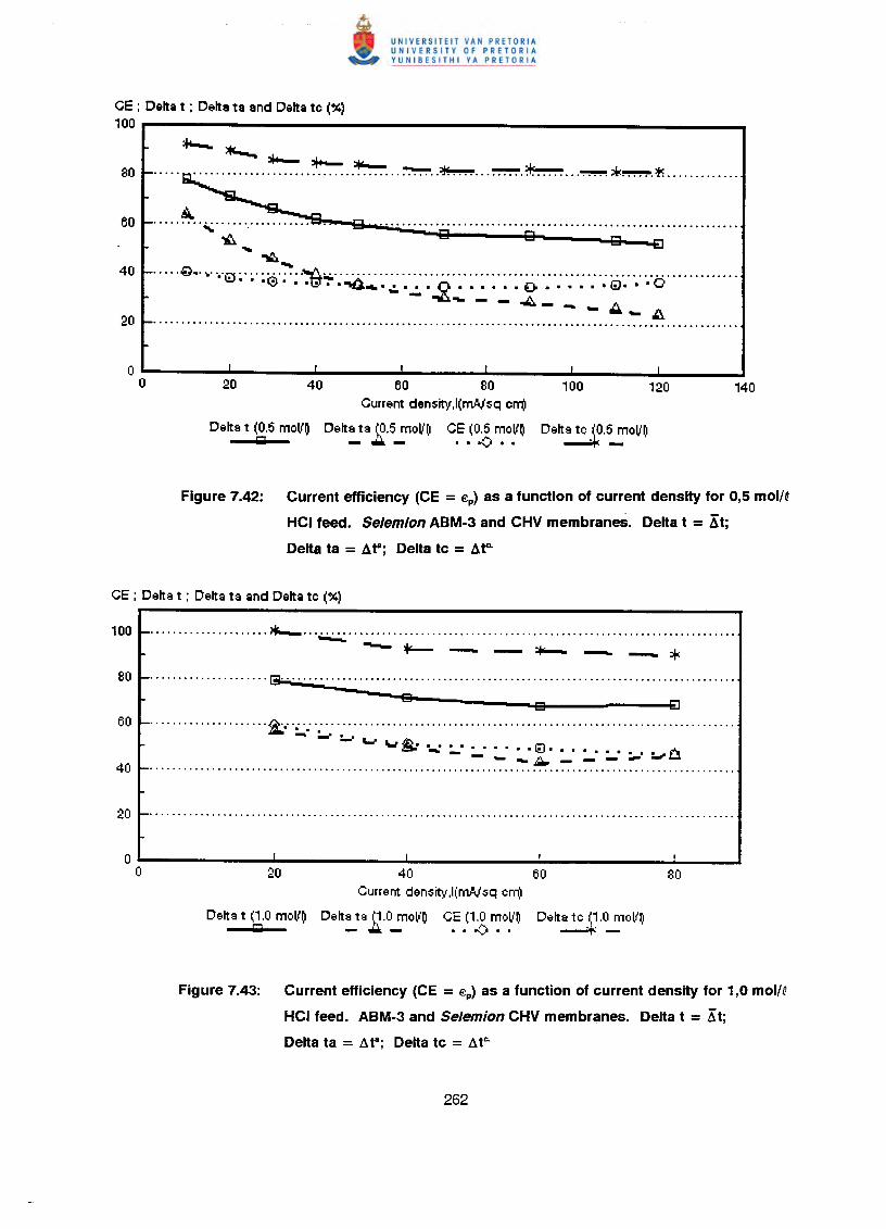
CE : Delta t : Delta ta and Delta te (%)100
~*-...... ~ *:":-::- "",. .. - ",.".. ~ ~ ;I<~.", .
......... ,.................. 13 .............................................•..•............•..~ 13 13 13, ~
~ .•.•.• . . • . ~ •• ". '.'G::i ~• ~. ~0'; "'-1\:";" . :.:;..' ••••..••.••••••••••••••••••.•••••.•••.••••. ;";' •••• '0" .
• •'@. • -.....•••• ~ •.:.. 0 • • • • • •D • • • • • •~. • •~- - -..I::.. - - -..::..- I:!..
........................................................................................................
Delta t (0.5 moV~1;1
60 80 100 120Current density,I(mA/sq em)
Delta ta ~0.5moV~ CE (0.5 moV~ Delta to .~.5_mov~- .••. - .. -0 ..
Figure 7.42: Current efficiency (CE = €p) as a function of current density for 0,5 mol/Q
HCI feed. Selemion ABM-3 and CHV membranes. Delta t = Xt;
Delta ta = At"; Delta tc = At""
.....................*'- ~ ~ .*""-- - - =+'- - - :+:
..................... B-- .
..................... ~ •..•..:.: ...• =--w ...,~ ~. :..-. . . . • .~. • . . . . • . .. .0.- ......•~ - - - ~ •...
oo 20 40 60 80
Current density,l(mNsq em)
Delta t ~.o moV~ Delt~ta £..O_moll'~ C.E.(1~ ~o.~'~ Delta te V .~OV~
Figure 7.43: Current efficiency (CE = €p) as a function of current density for 1,0 mol/Q
HCI feed. ABM-3 and Selemion CHV membranes. Delta t = Xt;
Delta ta = Ata; Delta te = Ate.
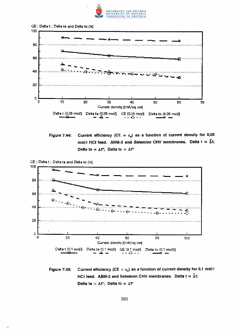
CE : Delta t : Delta ta and Delta te (%)100
---- >Ic---. - _ ••.•.•.• _ ~80 .
.&..- --~... - - - h-.....................•.•... -0·,·.·.· ii'; .:--c:=-: ...-: 0';';': .~.~. 0":':'" o.;.:..".~: .o..t~_~
10 20 30 40Current density,l(mNsq err(!
Delta t (0.05 moVO Delta ta (0.05 moVO CE (0.05 moVOIiiI -~- •• 0 ..
Delta te (0.05 moVO........;c -
Figure 7.44: Current efficiency (CE = €p) as a function of current density for 0,05
mol/~ HCI feed. ABM-2 and Selemion CHV membranes. Delta t = Kt;
Delta ta = ata; Delta tc = ate.
CE : Delta t : Delta ta and Delta te (%)100 --~----r --... - - - -..- _:+:
....... ~ .
A -i!!8!i-- _
•••••••••••• ~. __ •••••••••••••••••••••••••••••••••••••••••••••••••••••••••••••••••••••••••• to;ooo:or[I •••••••••.•.G>. '" -
••• €>. - ~-.. ...~"--~··························0· 0r! •••••• iI:)" ~ ..••.._. "_..•.•.'•.•" .• • • • -€>- • • • -t:-- • • • • • - - - ~• • •€I. • • • • • • • -0
20 40 60 80Current density,l(mNsq err(!
Delta t (0.1 moVO Delta ta (0.1 moVO CE (0.1 moVO Delta te (0.1 moVO)IiiZI - ••••. - ··0.. -*-
Figure 7.45: Current efficiency (CE = €p) as a function of current density for 0,1 mol/Q
HCI feed. ABM-2 and Selemion CHV membranes. Delta t = Xt;
Delta ta = ata; Delta tc = ate.
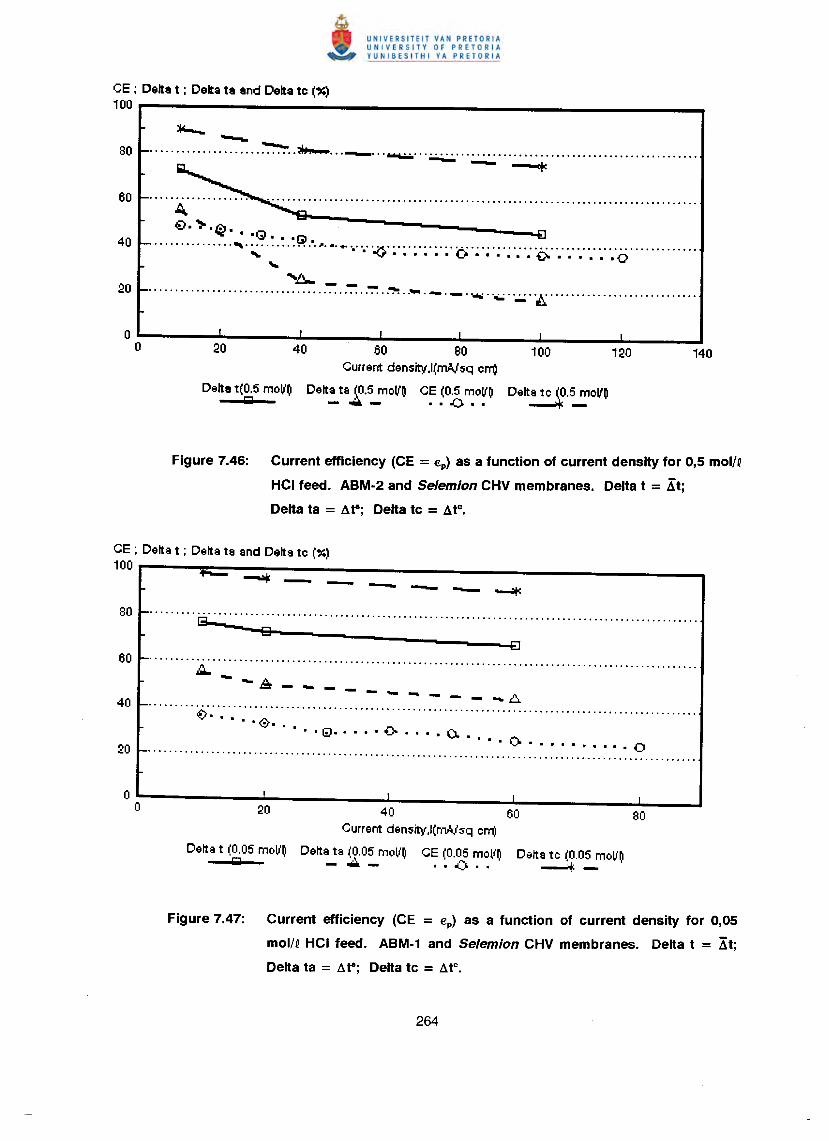
CE : Delta t ; Delta ta and Delta te (%)100
:+0-- __80 ~ .. ~ _ __ .
- - ---.:+c
~ • .,..r.'t.~ •• (;1................••••.... : . ~ . ~ ~ .-0 ,Ij ••••• 0•. "•. "_x..•••••••••••••••••••••••••••••••••••••••••••••••••••••••••••, ....,.······O······{)-······O
"•••..•••.•••.••••••••••••• ~ .. ":': ••"':"':.•"':":.. ~ •.•••. - • - • w,; . ''';'; • ''';'; . 'ji, .
40 60 80Current density,l(mNsq em)
Delt~tal·:'moVO C~ .(ot~o~ODelta t(0.5 moVO'MI
Figure 7.46: Current efficiency (CE = €p) as a function of current density for 0,5 mol/Q
HCI feed. ABM-2 and Selemion CHV membranes. Delta t = Kt;
Delta ta = .I1r; Delta tc = .I1tc•
CE ; Delta t ; Delta ta and Delta te (%)100
......... g:.;, .13 ----EJ
·········A············································ .••.• ....&:i - ••.• _
- - .••• ~ - - - •.•.6-......... 'iJ' ., .
. . . . ·0· .. • • IU- •••• 0- ••••......••..... . .. •.....•· ··········0........................................................................................................
20 40 60 80Current density.l(nWsq em)
Delta t (0.05 moVO Delta ta (0.05 mollO CE (0.05 mollO Delta te (0.05 moVO'MI - ~ - • • 0/:) • • -----.+: -
Figure 7.47: Current efficiency (CE = €p) as a function of current density for 0,05
mol/Q HCI feed. ABM-1 and Selemion CHV membranes. Delta t = At;
Delta ta = .I1r; Delta tc = .I1tc•
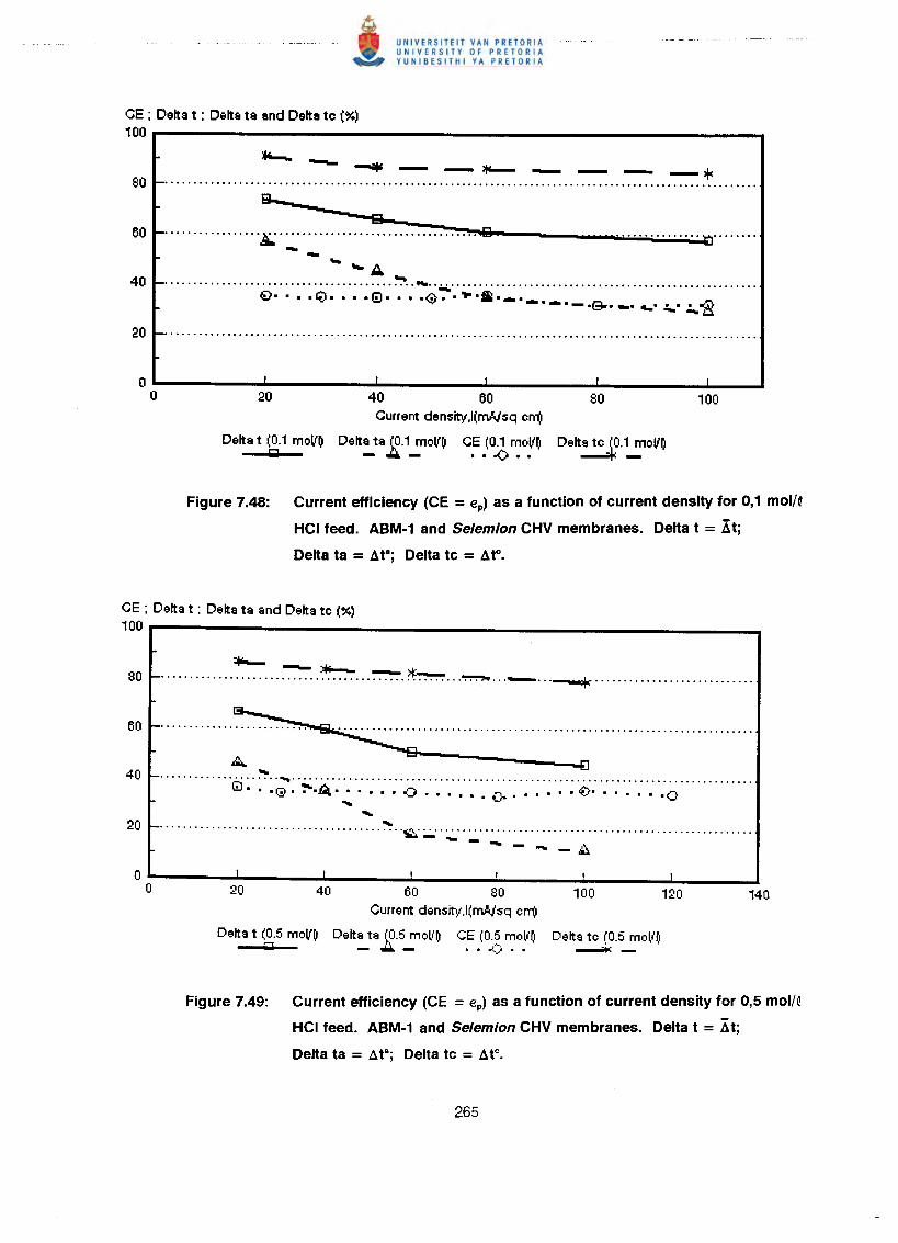
CE : Delta t : Delta ta and Delta to (%)
100 r----------------------------- .....~- --. - -'I'-- - - - _*80 - .B..___....60 _ ;;;,. ~.. ~..~.~.. ~..~..:~~.. ~..~..~.~..~..~.:":'.. ~..~..~Qi-- •.••.••..••.••.',;,;'''';'''';';''';'';'''';'';'.~.~~, .- •••..•••A40 - :":".. _ ..••.......................................................
.[) •••• ~ •••• (!) ••• -0- .~._ ..•.•.•.. .•• . - .t,;... •.. 4.. .:... .:..-a
0 I I I I I
0 20 40 60 80 100Current density,l(mAJsq err(!
Delta t (0.1 moV~ Delt~ta ~.1_moV~ CE (0.1 moV~ Delta to .~o.~OV~bOI •• -0 ••
Figure 7.48: Current efficiency (CE = €p) as a function of current density for 0,1 mol/Q
HCI feed. ABM·1 and Selemion CHV membranes. Delta t = Xt;
Delta ta = ate; Delta tc = atc.
CE : Delta t : Delta ta and Delta te (%)100
*---~.....................................~.~ ~ _ -+<- .
A.. .•.............. @ .......••..................................................................................• • • 'G;l' ~·A· -0 •••••• 0- ~ .•..•. ·0.••. .••. .••............................................ ~.;.;.:.:.:. .- _~-~
60 80 100 120Current density,l(mAJsq err(!
Delta ta (0.5 moll'~ CE (0.5 moll'~ Delta te (0.5 mol{~-..::r..- .. 01.) •• ----4:-Delta t (0.5 moV~IMI
Figure 7.49: Current efficiency (CE = €p) as a function of current density for 0,5 mol/Q
HCI feed. ABM·1 and Selemion CHV membranes. Delta t = Xt;
Delta ta = ate; Delta tc = atc.
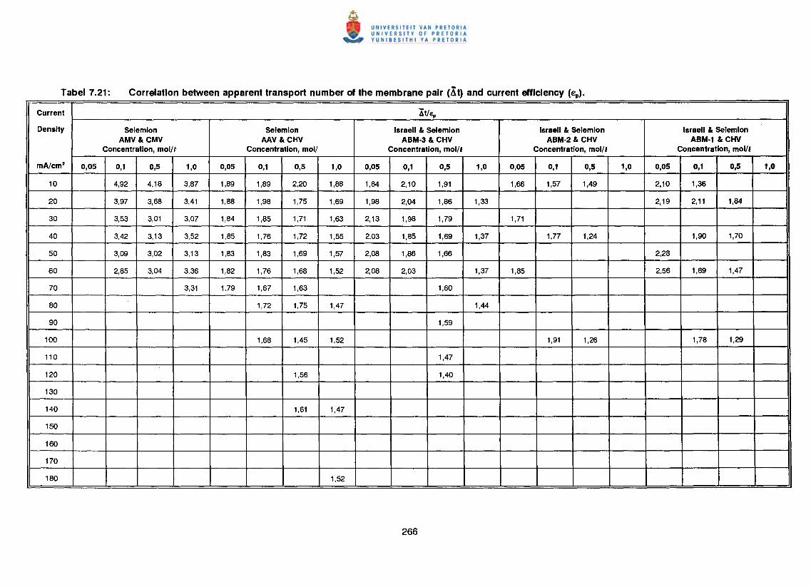
Current Xt/e,.
Density Selemlon Selemlon Israeli & Selemlon Israeli & Selemlon Israeli & SelemlonAMV & CMV AAV &CHV ABM-3 & CHV ABM-2 & CHV ABM-1 & CHV
Concentration, mol/t Concentration, moll Concentration, mollt Concentration, mol/t Concentration, mol! t
mA/cm· 0,05 0,1 0,5 1,0 0,05 0,1 0,5 1,0 0,05 0,1 0,5 1,0 0,05 0,1 0,5 1,0 0,05 0,1 0,5 1,0
10 4,92 4,18 3,87 1,89 1,89 2,20 1,88 1,84 2,10 1,91 1,66 1,57 1,49 2,10 1,36
20 3,97 3,68 3,41 1,88 1,98 1,75 1,69 1,98 2,04 1,86 1,33 2,19 2,11 1,84
30 3,53 3,01 3,07 1,84 1,85 1,71 1,63 2,13 1,98 1,79 1,71
40 3,42 3,13 3,52 1,85 1,76 1,72 1,55 2,03 1,85 1,69 1,37 1,77 1,24 1,90 1,70
50 3,09 3,02 3,13 1,83 1,83 1,69 1,57 2,08 1,86 1,66 2,28
60 2,85 3,04 3,36 1,82 1,76 1,68 1,52 2,08 2,03 1,37 1,85 2,56 1,69 1,47
70 3,31 1,79 1,67 1,63 1,60
80 1,72 1,75 1,47 1,44
90 1,59
100 1,68 1,45 1,52 1,91 1,26 1,78 1,29
110 1,47
120 1,56 1,40
130
140 1,61 1,47
150
160
170
180 1,52
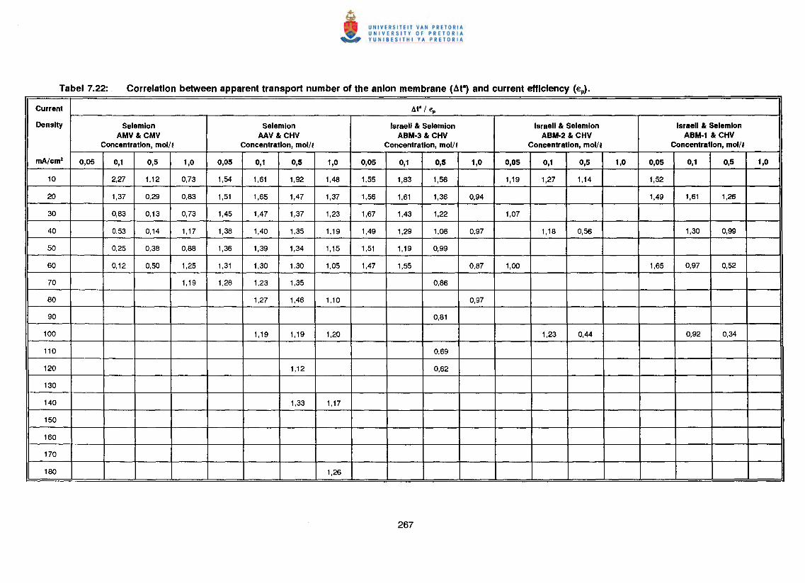
Current At" I €p
Density Selemlon Selemlon Israeli & Selemlon Israeli & Selemlon Israeli & SelemlonAMV & CMV AAV & CHV ABM-3 & CHV ABM-2 & CHV ABM-1 & CHV
Concentration, moll' Concentration, moll' Concentration, moll' Concentration, moll' Concentration, mol/l
mAlcm' 0,05 0,1 0,5 1,0 0,05 0,1 0,5 1,0 0,05 0,1 0,5 1,0 0,05 0,1 0,5 1,0 0,05 0,1 0,5 1,0
10 2,27 1,12 0,73 1,54 1,61 1,92 1,48 1,55 1,83 1,56 1,19 1,27 1,14 1,52
20 1,37 0,29 0,83 1,51 1,65 1,47 1,37 1,56 1,61 1,36 0,94 1,49 1,61 1,26
30 0,83 0,13 0,73 1,45 1,47 1,37 1,23 1,67 1,43 1,22 1,07
40 0,53 0,14 1,17 1,38 1,40 1,35 1,19 1,49 1,29 1,06 0,97 1,18 0,56 1,30 0,99
50 0,25 0,38 0,88 1,36 1,39 1,34 1,15 1,51 1,19 0,99
60 0,12 0,50 1,25 1,31 1,30 1,30 1,05 1,47 1,55 0,87 1,00 1,65 0,97 0,52
70 1,19 1,28 1,23 1,35 0,86
80 1,27 1,46 1,10 0,97
90 0,81
100 1,19 1,19 1,20 1,23 0,44 0,92 0,34
110 0,69
120 1,12 0,62
130
140 1,33 1,17
150
160
170
180 1,26
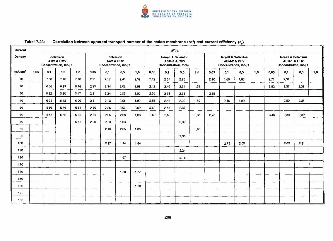
Current li.tc/ep
Density Selemlon Selemion Israeli & Selemlon Israeli & Selemlon Israeli & SelemlonAMV & CMV AAV & CHV ABM·3 & CHV ABM·2 & CHV ABM-1 & CHV
Concentration, mol/ ~ Concentration, mol/~ Concentration, mollf Concentration, molN Concentration, mollf
mA/cm" 0,05 0,1 0,5 1,0 0,05 0,1 0,5 1,0 0,05 0,1 0,5 1,0 0,05 0,1 0,5 1,0 0,05 0,1 0,5 1,0
10 7,58 7,16 7,10 2,21 2,17 2,48 2,32 2,12 2,37 2,28 2,10 1,86 1,86 2,71 2,31
20 6,58 6,99 6,14 2,25 2,34 2,06 1,98 2,42 2,46 2,34 1,68 2,92 2,57 2,38
30 6,22 5,90 5,47 2,21 2,24 2,05 2,02 2,59 2,53 2,33 2,35
40 6,25 6,12 6,00 2,31 2,13 2,06 1,90 2,55 2,44 2,29 1,80 2,36 1,89 2,50 2,38
50 5,86 5,66 5,51 2,30 2,26 2,03 2,00 2,69 2,54 2,37
60 5,58 5,59 5,39 2,35 2,25 2,06 1,96 2,69 2,52 1,85 2,73 3,46 2,39 2,39
70 5,43 2,29 2,13 1,93 2,32
80 2,16 2,05 1,83 1,90
90 2,36
100 2,17 1,74 1,84 2,73 2,05 2,62 2,21
110 2,24
120 1,97 2,18
130
140 1,88 1,77
150
160 1,80
170
180
mNcm2 (0,1 moV~ feed). The correlation was even better at 1,0 moV~ feed
concentration and varied between 0,97 and 0,84 in the 20 to 80 mNcm2 current density
range.
A satisfactory correlation was obtained between the apparent transport number (At8)
and current efficiency at 0,05 moV~feed concentration in the case of the ABM-2 and
CHV membranes (30 to 60 mNcm~. The ratio of A~/ep varied between 1,07 and 1,0.
The ratio was approximately 1,18 at 0,1 mol/~feed concentration in the same current
density range. A very poor correlation, however, was obtained at 0,5 moV~ feed
concentration for the same membranes.
The ABM-1 and CHV membranes showed the best correlation (0,92 to 0,97) at 0,1
moV~feed concentration in the current density range from 60 to 100 mNcm2• A poor
correlation, however, was obtained with the Selemion AMV and CMV membranes.
The correlations between the apparent transport numbers ofthe cation membrane (Ate)
and current efficiencies (Table 7.23) were not as good as the correlations obtained
between the apparent transport numbers of the membrane pair (Kt) (Table 7.21) and
that of the anion membrane (At8) and current efficiency (Fig. 7.22). It therefore seems
that the best correlation between transport numbers and current efficiency for acid can
be obtained from the apparent transport number of the anion membrane. It also
seems that the apparent transport number of the anion membrane gives the best
approximate estimation of the performance of membranes for acid
concentration/desalination. However, accuracy of performance depends on the acid
feed concentration used. The performance of a membrane for acid concentration
should be estimated with an accuracy of approximately 20% from the apparent
transport number of the anion membrane, depending on the acid feed concentration
used.
Water flow (J) through the membranes as a function of current density and acid feed
water concentration is shown in Figures 7.50 to 7.54. Water flow (Jj) through the
membranes relative to the flow at JO,5 moV' is shown in Table 7.24. Water flow through
the membranes decreased significantly with increasing acid feed concentration in the
case of the Selemion AMV and CMV membranes. A slight decrease in water flow was
also experienced in the case of the Selemion AAV and CHV membranes. Therefore,
there appeared to be no support (water flow) to improve current efficiency as had been
experienced with the sodium chloride solutions (see Figs. 7.28 and 7.29 and Figs. 6.43
to 6.49). However, a definite increase in water flow was observed for the ABM-3 and
CHV membranes, especially at the highest feed concentration (Table 7.24) and an
increase in current efficiency was experienced for this membrane type at 1,0 mol/Q
feed concentration (see Fig. 7.30). Increase in water flows were also experienced for
the ABM-2, ABM-1 and CHV membranes with increasing acid feed concentration.
Current efficiency also increased slightly in these cases (see Figs. 7.31 and 7.32). The
high water flow that was experienced with the ABM-2 membranes at 0,1 mol/Q feed
concentration may be ascribed to membrane leakage due to a partially torn
membrane.
Waterflow (J) through the membranes as a function of effective current density, leff'and
feed water concentration are shown in Figures 7.55 to 7.59. Straight lines were
obtained at higher values of leffas were experienced with the sodium chloride solutions.
The slope of these lines corresponds to the combined electro-osmotic coefficient (2~)
of a membrane pair. The electro-osmotic coefficients decreased as a function of
increasing acid feed concentration in the feed concentration range from 0,05 to 1,0
mol/Q (Figs. 7.60 to 7.64). The electro-osmotic coefficient of the Selemion AMV and
CMV membranes remained almost constant in the 0,1 to 0,5 mol/Q feed concentration
range and then decreased more significantly to a lower value at 1,0 molN feed
concentration (Fig. 7.60). The electro-osmotic coefficient of the Selemion AAV and
CHV membranes remained constant in the 0,05 to 0,1 mol/Q feed range (Fig. 7.61) and
then decreased somewhat to remain almost constant in the 0,5 to 1,0 molN feed
concentration range. The electro-osmotic coefficients of the ABM-3 and CHV
membranes decreased significantly in the 0,05 to 0,5 mol/Q feed concentration range
and then remained constant (Fig. 7.62). Both the ABM-2 and ABM-1 membranes
showed a reduction in the electro-osmotic coefficient in the 0,05 to 0,1 mol/Q feed
concentration ranges and then remained constant in the 0,1 to 0,5 mol/Q feed
concentration range (Figs. 7.62 to 7.63). It, therefore, appears that the membranes
deswell somewhat with increasing acid feed concentration.
The effect of the electro-osmotic coefficient on the maximum acid brine concentration
cbmex, is shown in Table 7.25. Maximum acid brine concentration increases with
decreasing electro-osmotic coefficient. The electro-osmotic coefficients of the Selemion
AMV and CMV membranes were much higher than that of the other membranes. The
electro-osmotic coefficients of the Selemion AMV and CMV membranes were
determined at 0,357 and 0,371 ~/Faraday at 0,1 and 0,54 molN feed concentration,
respectively. The electro-osmotic coefficients of the SelemionAAV and CHV; ABM-3
and CHV; ABM-2 and CHV and ABM-1 and CHV were determined at 0,141 and 0,126
Q/Faraday; 0,166 and 0,124 ~/Faraday; 0,133 and 0,131 Q/Faradayand 0,152 and
0,149 ~/Faraday under the same feed water conditions as above, respectively.
Consequently, much higher acid brine concentrations could be obtained with these
membranes.
Approximately 7 to 8 mol H20 per Faraday passed through the Selemion AAV and
CHV membranes in the acid feed concentration range from 0,1 to 0,5 moV~ (Table
7.25). Approximately 7 to 9; 7 and 8 mol H20/Faraday passed through the ABM-3
and CHV; ABM-2 and CHV and ABM-1 and CHV membranes under the same feed
conditions as above, respectively. Therefore, the newly developed Israeli ABM
membranes compare favourably with the commercially available Selemion AAV and
CHV membranes for acid concentration.
The osmotic water flow (Josm) relativeto the total water flow (J) through the membranes
as a function of current density, is shown in Table 7.26. The osmotic flow (Josm) relative
to the total flow (J) decreases with increasing current density. Osmotic water flow
contributes to approximately 50% of the total water flow through the membranes at a
current density of 30 mNcm2 at 0,1 moV~feed concentration. However, the osmotic
water flow contribution relative to the total water flow was much less at high current
densities. Approximately 21% of the total water flow through the membranes was
caused by osmosis in the case of the Selemion AAV and CHV membranes at a current
density of 100 mA/cm2 (0,1 mol/~ feed). The osmotic water flow contribution in the
case of the ABM-3 and SelemionCHV membranes comprised 29,4% of the total water
flow at a current density of 60 mNcm2 (0,1 mol/Q feed).
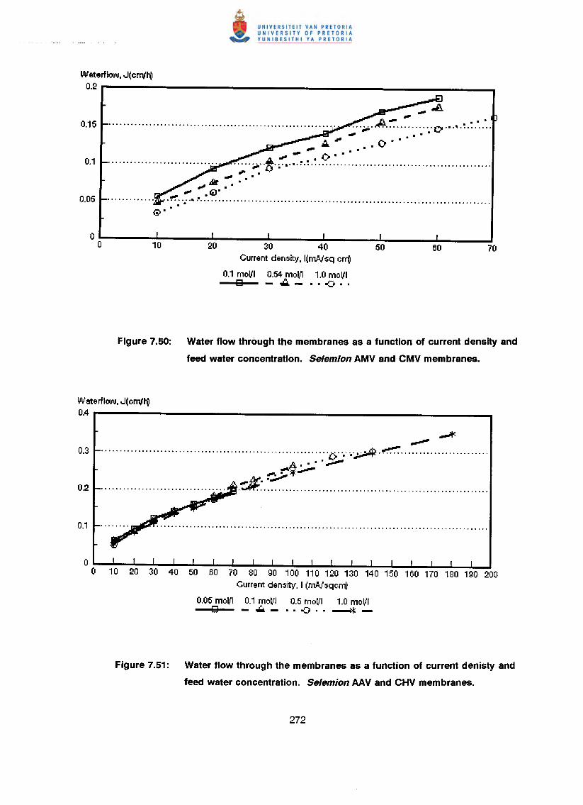
WaterflOO\l, J(errv'h)0.2
,.,...A~
A~ ••••.. .~. iIf¥ ....•.•...••• 0' .•.•............ . .. ..
fA'" •• 0·...,. .•.. ~ .......•.•..·t·~ ~.~ .,. ..&Ir ..., • • •
•••••Ii). • •.~ ....•...................................................................................
20 30 40Current density, l(mNsq em)
0.1 molll 0.54 molll 1.0 molllD -~_ .. .() ..
Figure 7.50: Water flow through the membranes as a function of current density and
feed water concentration. Selemion AMV and CMV membranes.
WaterflOO\l, J(errv'h)0.4
..,...aI<,.,...-...................................................... ········b·······~·~························
~.... ~_. --
~.=f!I:~ .
50 60 70 80 90 100 110 120 130 140 150 160 170 180 190 200Current density, I (mNsqem)
0.05 molll 0.1 molll 0.5 molll 1.0 moll I121 -""'-_ •• O() •• -i:-
Figure 7.51: Water flow through the membranes as a function of current denisty and
feed water concentration. Selemion AAV and CHV membranes.
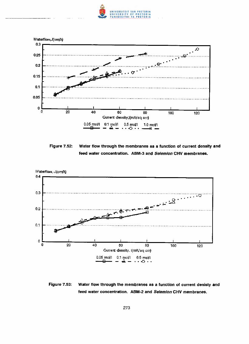
Waterflcw.J(cnv'h)0.3
,0~ "•••...•••....•••••••...••••••••....•••••••..•••.... ;.;.;-' •••.....••....••....•••..•••.• G).' .............•
~ ' '
••••••.•••••••••••••••••••••••••••••• ~ •.••.•••..••••••••••••••••• 1'. "'~:"'''' .' •••.•••.•••.•..•••.........J1If"" •••
"",.. • • • <:J •.............. ~........... ...•..•.: .
40 60 80Current density,l(moVsq Cn1J
0.05 mol'l 0.1 mol'l 0.5 mol'l 1.0 mol'lD -~_ .. ~ .. ~-
Figure 7.52: Water flow through the membranes as a function of current density and
feed water concentration. ABM-3 and Selemion CHV membranes.
lfIIaterflcw, J(cnv'h)0.4
............................................................................................... : '0' .
. 0······.. ::.....:::... •... "..•••••••••••••••••••••••••••.••••••••••••••••••• ~ •• _; ••••••• "I"! ~ .~ ':": •••••••••••••••••••••••••••••••••••••
f1tI. ~. lV- •-40 60 80
Current density. l(moVsq cn1J
0.05 mol'l 0.1 molJ'J 0.5 mol'Jo .••.- .. -0 ••
Figure 7.53: Water flow through the membranes as a function of current denisty and
feed water concentration. ABM·2 and Selemion CHV membranes.

Waterflcw, J (env'h)0.3
............................................................................•.•. D .. .• (;1 • • • A. . -.. ..,.
•......•...•.......••..••.............••••.... 'fi:J'" .•.•.....•••• ·ik· ~ .. - .,....:..~~............................. ,;.i:::..-. . .
,A- .it.. ..,. ••• €I-······k··"'"·····~···· .
40 60 80Current density, 1(mA./sq err(!
0.05 moVI 0.1 moVI 0.5 moVIo -~_ .. -o ..
Figure 7.54: Water flow through the membranes as a function of current density and
feed water concentration. ABM-1 and Selemion CHV membranes.
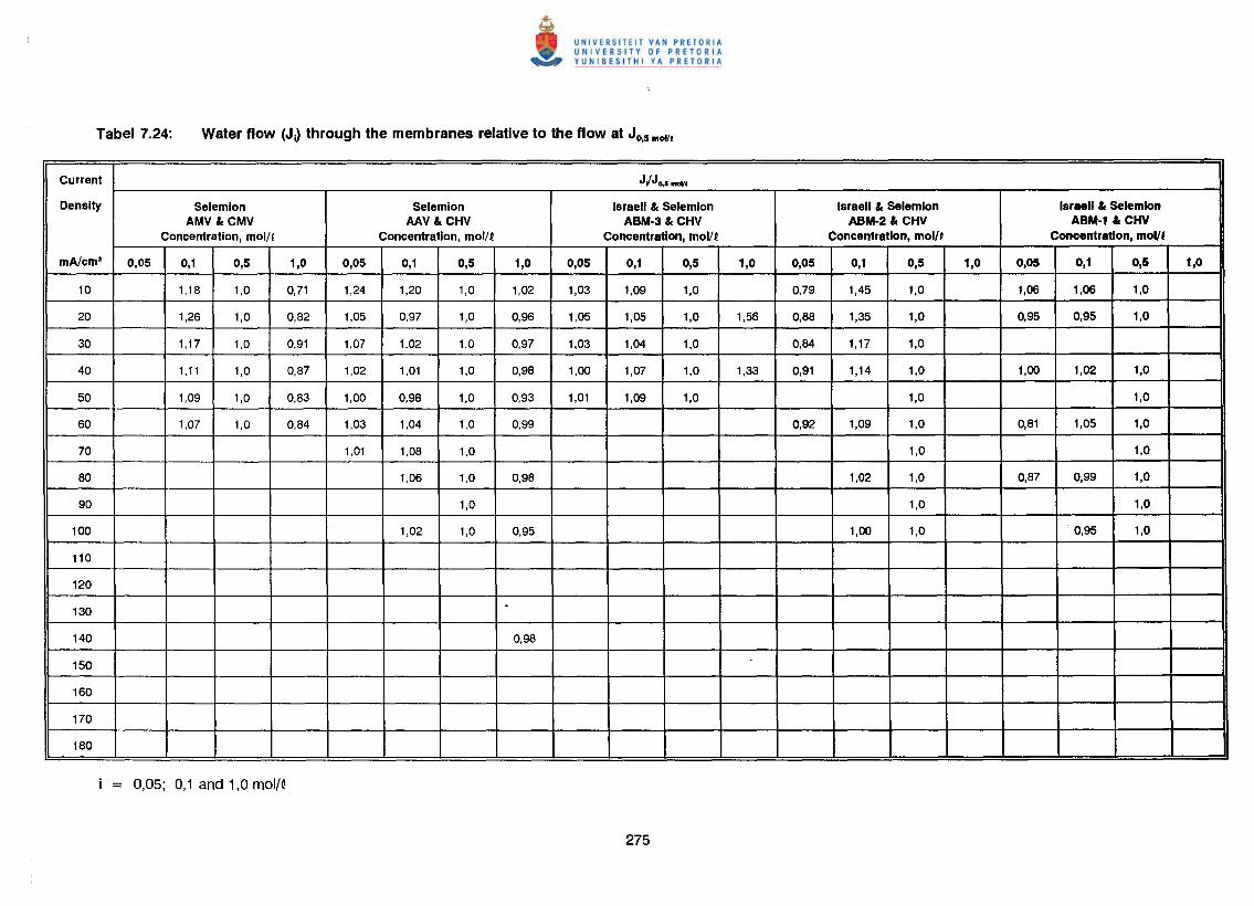
Current J/Jo,s moll'
Density Selemlon Selemlon Israeli & Selemlon Israeli & Selemlon Israeli & 5elemlonAMV & CMV AAV & CHV ABM·3 & CHV ABM·2 & CHV ABM-1 & CHV
Concentration, moll ~ Concentration, mol/~ Concentration, mol/f Concentration, mol/f Concentration, mol/f
mA/cm2 0,05 0,1 0,5 1,0 0,05 0,1 0,5 1,0 0,05 0,1 0,5 1,0 0,05 0,1 0,5 1,0 0,05 0,1 0,5 1,0
10 1,18 1,0 0,71 1,24 1,20 1,0 1,02 1,03 1,09 1,0 0,79 1,45 1,0 1,06 1,06 1,0
20 1,26 1,0 0,82 1,05 0,97 1,0 0,96 1,05 1,05 1,0 1,56 0,88 1,35 1,0 0,95 0,95 1,0
30 1,17 1,0 0,91 1,07 1,02 1,0 0,97 1,03 1,04 1,0 0,84 1,17 1,0
40 1,11 1,0 0,87 1,02 1,01 1,0 0,98 1,00 1,07 1,0 1,33 0,91 1,14 1,0 1,00 1,02 1,0
50 1,09 1,0 0,83 1,00 0,98 1,0 0,93 1,01 1,09 1,0 1,0 1,0
60 1,07 1,0 0,84 1,03 1,04 1,0 0,99 0,92 1,09 1,0 0,81 1,05 1,0
70 1,01 1,08 1,0 1,0 1,0
80 1,06 1,0 0,98 1,02 1,0 0,87 0,99 1,0
90 1,0 1,0 1,0
100 1,02 1,0 0,95 1,00 1,0 0,95 1,0
110
120
130.
140 0,98
150
160
170
180
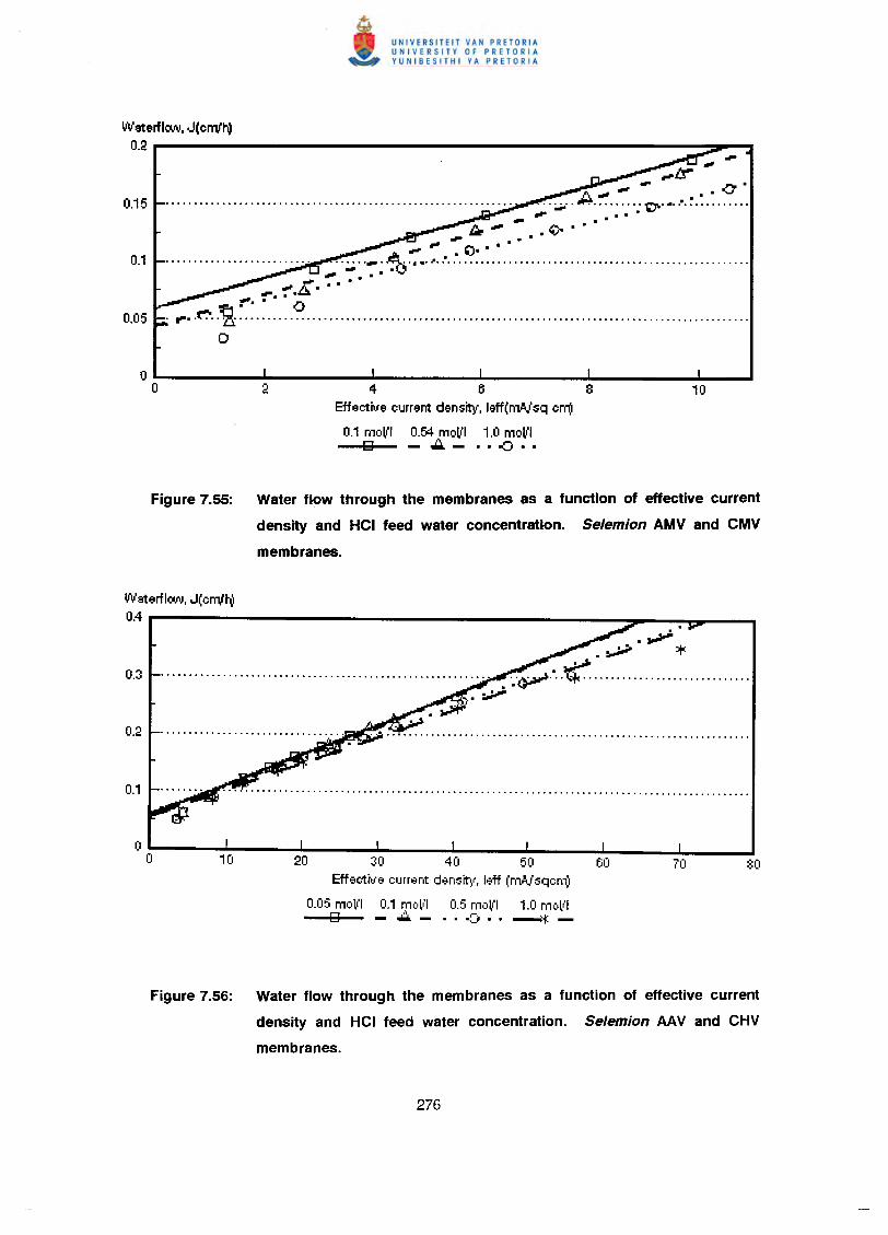
WaterflOAl, J(crnilV0.2
- o·..•...A.~ .."':...'0-'.' .•.~.:.: .~, .....~~ .0- ..- ..",.... CI· • • •
•••••••••••••••••••••••••• ~ •• ;; •• :- ~ ~ •••• 1' ••••••••••••••••••••••••••••••••••••••••••••••••••••••••••- ..•••~.A· ••f". •• 0
. •....~ ..~ .o
468Effective current density, leff(mA./sq cIT\l
0.1 moVI 0.54 moVI 1.0 moVID -":;:"_ .. -0 ..
Figure 7.55: Water flow through the membranes as a function of effective current
density and HCI feed water concentration. Selemion AMV and CMV
membranes.
WaterflOAl, J(crnilV0.4
.~.~ =+:.~..¥ ~ ..~.
;}. ......-.~
30 40 50 60Effectr.Je current densit~(. leff (mA./sqcnil
0.05 moll'l 0.1 rYlClVI 0.5 mcoll'l 1.0 moll"o -.w.- .. -c- •• --.;:f;-
Figure 7.56: Water flow through the membranes as a function of effective current
density and HCI feed water concentration. Selemion AAV and CHV
membranes.
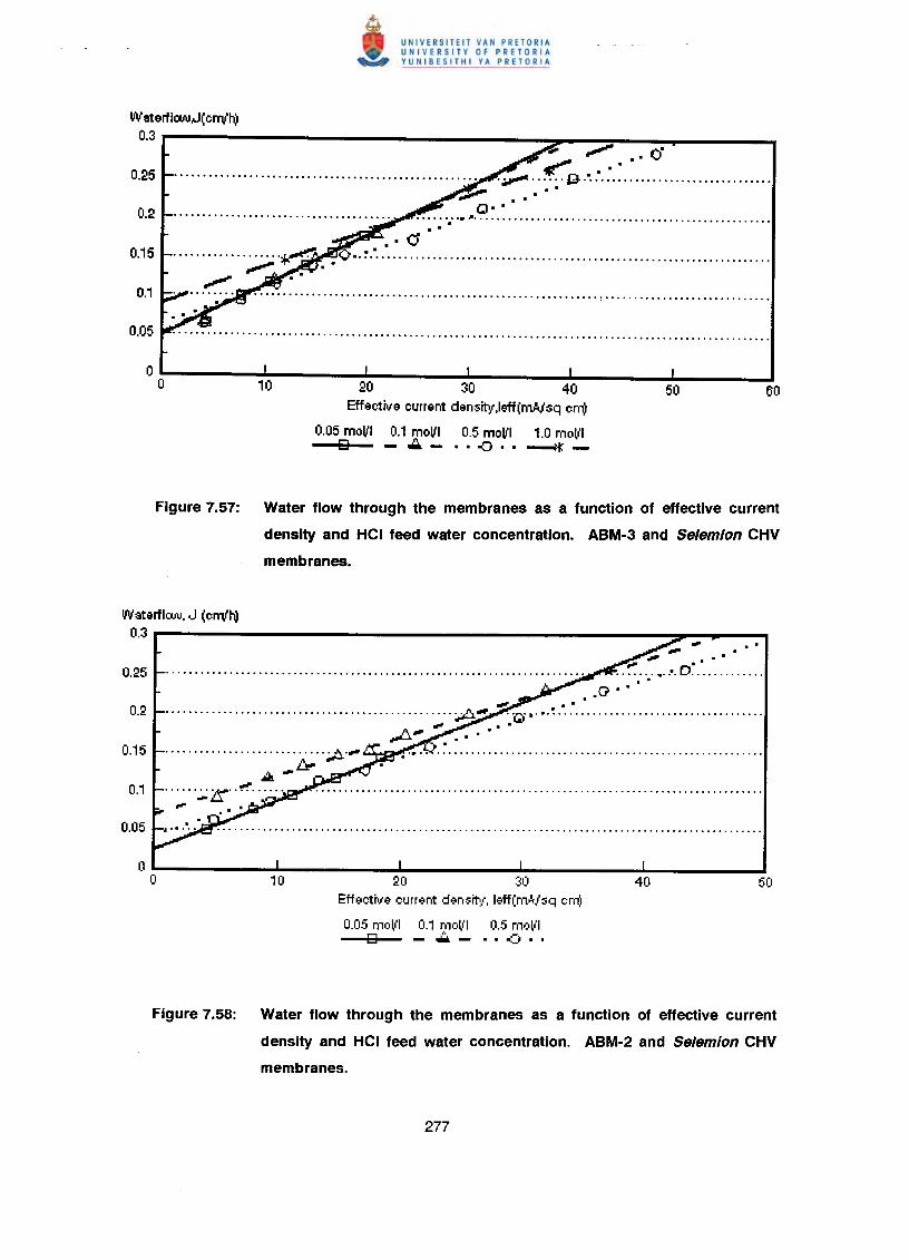
WaterfIOOl.l.J(cnv'h)0.3
~ .' O'0.•..•5 .._ ~I""s ••• ,c:; ';"- _ •••• :.1"" .
20 30 40Effective current density,leff(mA.,r':sq crr(t
0.05 moltl 0.1 moltl 0.5 moltl 1.0 moltlo -~_ .. -o •• ~-
Figure 7.57: Water flow through the membranes as a function of effective current
density and HCI feed water concentration. ABM·3 and Selemion CHV
membranes.
WaterflOOl.l,J (cnv'h)0.3 .,. .'~ .
flII# •••
..~. ".".'.-.D~ .
""- ... . .. . . . .. . . . . . . . . . . .. . . . . . . . . . . . . . . . . . . . .. . .. . . . . .A...t' . 'Gi •.•. ~ ."" ..~' .....
····························A·".olIik-~
..... ':;'t!: ..~ .,
20 30Effective current densmj. leff(m.!t/:sq ere\1
0.05 mo~'1 0.1 moll'l 0.5 moll'lE3 -...::..- ···8··
Figure 7.58: Water flow through the membranes as a function of effective current
density and HCI feed water concentration. ABM-2 and Selemion CHV
membranes.
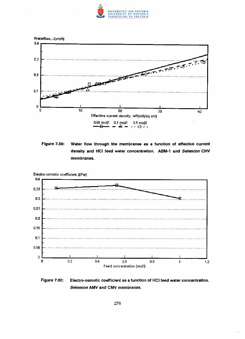
Waterflcw, J(crrv'h)0.4
20 30Effective current density. leff(rAAJsq cnit
0.05 moVI 0.1 moVI 0.5 moVID - .••. - .. -0 ..
Figure 7.59: Water flow through the membranes as a function of effective current
density and HCI feed water concentration. ABM-1 and Selemion CHV
membranes.
Electro-osmotic coefficient (VFar)0.4
0.4 0.6Feed concentration (moll'r!
Figure 7.60: Electro-osmotic coefficient as a function of HCI feed water concentration.
Selemion AMV and CMV membranes.
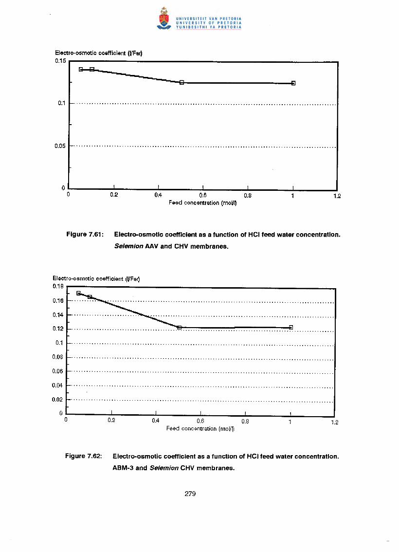
Electro-osmotic coefficient (VFa~0.15
0.4 0.6 0.8Feed concentration (moV~
Figure 7.61: Electro-osmotic coefficient as a function of HCI feed water concentration.
Selemion AAV and CHV membranes.
Electro-osmotic cO&fficient (VFa~0.18
0.4 0.6 0.8Feed concentration (mo(i'(r
Figure 7.62: Electro-osmotic coefficient as a function of HCI feed water concentration.
ABM-3 and Selemion CHV membranes.
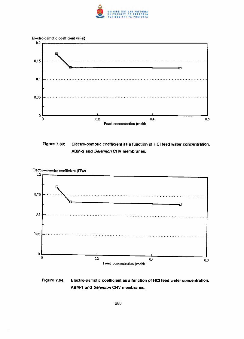
Electro-osmotic coefficient (VF8~0.2
0.15 ~ ~ .
Figure 7.63: Electro-osmotic coefficient as a function of HCI feed water concentration.
ABM-2 and Selemion CHV membranes.
Electro-osmotic coefficient (VF8~0.2
.... ~................................................................ .....
o
Figure 7.64: Electro-osmotic coefficient as a function of HCI feed water concentration.
ABM-1 and Selemion CHV membranes.
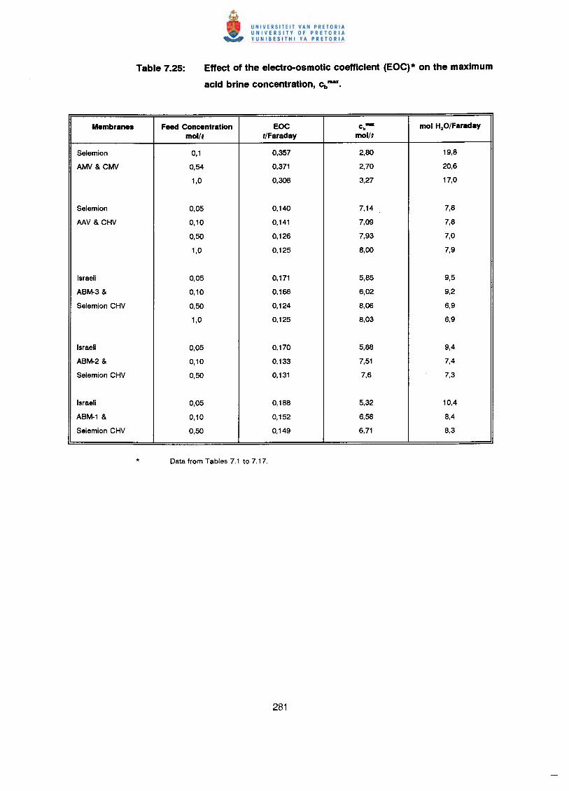
Effect of the electro-osmotic coefficient (EOC)* on the maximum
acid brine concentration, cbmu
•
Membranes Feed Concentration EOC cb- mol H2O/Faradaymol/l NFaraday mol/'
Selemion 0,1 0,357 2,80 19,8
AMI! & CMI! 0,54 0,371 2,70 20,6
1,0 0,306 3,27 17,0
Selemion 0,05 0,140 7,14 7,8
AAV &CHV 0,10 0,141 7,09 7,8
0,50 0,126 7,93 7,0
1,0 0,125 8,00 7,9
Israeli 0,05 0,171 5,85 9,5
ABM-3 & 0,10 0,166 6,02 9,2
Selemion CHV 0,50 0,124 8,06 6,9
1,0 0,125 8,03 6,9
Israeli 0,05 0,170 5,88 9,4
ABM-2 & 0,10 0,133 7,51 7,4
Selemion CHV 0,50 0,131 7,6 7,3
Israeli 0,05 0,188 5,32 10,4
ABM-1 & 0,10 0,152 6,58 8,4
Selemion CHV 0,50 0,149 6,71 8,3
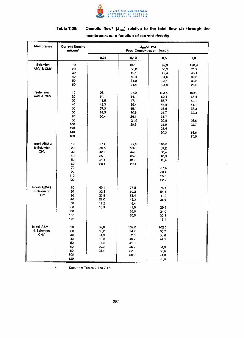
Osmotic flow* (J""",) relative to the total flow (J) through the
membranes as a function of current density.
Membranes Current Denshy J-IJ (%)mAlcm2 Feed Concentration (moIN)
0,05 0,10 0,5 1,0
Selemion 10 107,6 92,9 128,9
AWN & CWN 20 63,8 58,9 71,230 49,1 42,4 46,140 42,4 34,6 39,650 34,9 28,1 33,860 31,4 24,8 26,6
Selemion 10 96,1 91,9 123,5 109,0AAV & CHV 20 64,1 64,1 69,4 65,4
30 48,5 47,1 53,7 50,140 42,3 39,4 44,8 41,150 37,3 35,1 38,6 37,360 33,5 30,6 35,7 32,370 30,4 26,1 31,780 24,5 29,0 26,6
100 20,9 23,9 22,7120 21,4140 20,3 18,6180 15,8
Israeli ABM-3 10 77,4 77,5 103,8& Selemion 20 50,5 53,6 69,2
CHV 30 42,3 44,0 56,4
40 35,9 35,6 46,650 31,1 31,5 42,460 28,1 29,470 37,490 30,4
110 25,5120 22,7
Israeli ABM-2 10 49,1 77,5 74,4& Selemion 20 32,3 60,2 54,1
CHV 30 25,8 53,4 41,240 21,0 48,3 36,650 17,2 46,460 16,9 41,0 29,580 35,6 24,0
100 30,6 20,3120 18,1
Israeli ABM-1 10 69,0 102,6 102,0& Selemion 20 50,2 74,7 66,7
CHV 30 34,9 52,3 55,640 32,0 46,7 44,550 31,4 41,960 30,9 35,7 34,980 25,1 32,8 30,6
100 28,0 24,8120 22,3
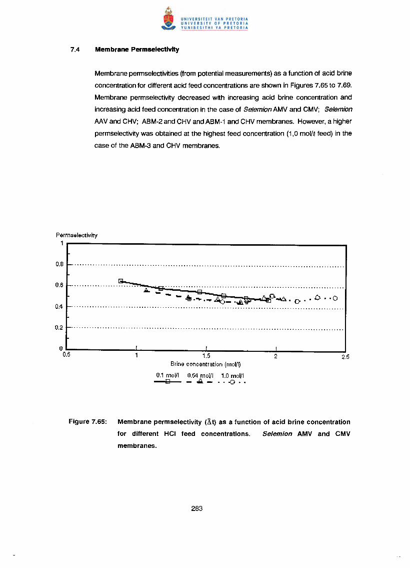
Membrane permseleetivities (from potential measurements) as a function of acid brine
concentration for different acid feed concentrations are shown in Figures 7.65 to 7.69.
Membrane permseleetivity decreased with increasing acid brine concentration and
increasing acid feed concentration in the case of Selemion AMV and CMV; Selemion
MV and CHV; ABM-2 and CHV and ABM-1 and CHV membranes. However, a higher
permseleetivity was obtained at the highest feed concentration (1,0 mol/Qfeed) in the
case of the ABM-3 and CHV membranes.
Permseleethtity1
g...........................~ ..----g .
.••• 13 ~ 0..•.~.- 45- .'-'l~ ~ ~. 0 .. [) . ·0
o0.5 1.5
Brine concentration (mol(~
0.1 moll'l 0.54 mo(i'l 1.0 mo(i'l13 A- .. -G ••
Figure 7.65: Membrane permselectivity (Lit) as a function of acid brine concentration
for different HCI feed concentrations. Selemion AMV and CMV
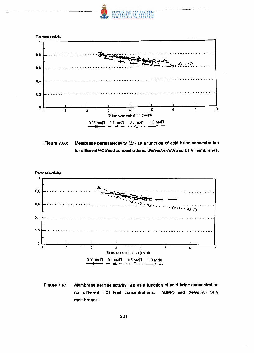
Perm:selectivity
1
................................ ~.gQ .
....................................~ ..~~.":..~~,.9..:.:() .
345Brine concentration (moV~
0.05 moVI 0.1 moVI 0.5 moVI 1.0 moVIIi2l -A-··-o··~-
Figure 7.66: Membrane permselectivity (Xt) as a function of acid brine concentration
for different HCI feed concentrations. Selemion AAV and CHV membranes.
Perm:selectivity1
A...................................~ "';§S, .
. .0~"+- --t<...................................................... ····~····G·.·····································.. '. .::-. ~
• 'CJ • ...:> •• <) 0
3 4Brine concentration (moll'~1
0.05 mo~'1 0.1 moll'l 0.5 moll'l 1.0 molllo -.w.- .. -C:_ •. -i*-
Figure 7.67: Membrane permselectivity (Xt) as a function of acid brine concentration
for different HCI feed concentrations. ABM-3 and Selemion CHV
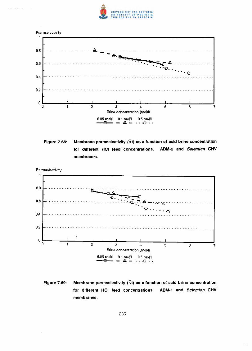
Permselectivity1
............................. .£:l.. .-- ~ .•.. . . A
......................................................... :........•~ ..~ .• • • • • t;"t
\:.J ••
····0
3 4Brine concentration (moVO
0.05 moVI 0.1 moVI 0.5 moVI9 ~- .. -0 ••
Figure 7.68: Membrane permselectivity (Xt) as a function of acid brine concentration
for different HCI feed concentrations. ABM·2 and Selemion CHV
membranes.
Permselectivity1
............................ B:~'~'~'~~'~'~~,:A"""""""""""""""""""""""""""""'"0$ •• " ~ oEJ
............................................... : '. ·G· ;~ ..~. - . -..,;. 'i:;. .
·0 ' .• '.0()
Brin€t conc€tntrstion (moll'r)
0.05 m,)ll'l 0.1 Toll'I 0.5 moll'l9 - .••.- .. -0 ••
Figure 7.69: Membrane permselectivity (Xt) as a function of acid brine concentration
for different HCI feed concentrations. ABM-1 and Se/emion CHV
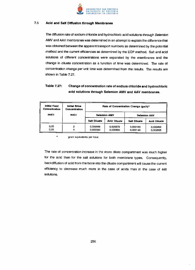
The diffusion rate of sodium chloride and hydrochloric acid solutions through Selemion
AMV and AAV membranes was determined in an attempt to explain the difference that
was obtained between the apparent transport numbers as determined by the potential
method and the current efficiencies as determined by the EOP method. Salt and acid
solutions of different concentrations were separated by the membranes and the
change in diluate concentration as a function of time was determined. The rate of
concentration change per unit time was determined from the results. The results are
shown in Table 7.27.
Change of concentration rate of sodium chloride and hydrochloric
acid solutions through Selemion AMV and AAV membranes.
Initial Feed Initial Brine Rate of Concentration Change (ge/h)*Concentration Concentration
mol" mol/~ Selemion AMV Selemion AAV
Sa" Diluate Acid Diluate Sa" Diluate Acid Diluate
0,05 2 0,000568 0,005872 0,000165 0,0004940,05 4 0,000390 0,002800 0,000145 0,002805
The rate of concentration increase in the more dilute compartment was much higher
for the acid than for the salt solutions for both membrane types. Consequently,
backdiffusion of acid from the brine into the diluate compartment will cause the current
efficiency to decrease much more in the case of acids than in the case of salt
solutions.
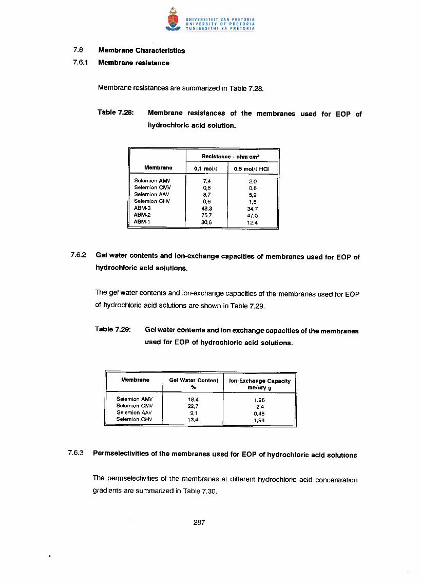
7.6 Membrane Characteristics
7.6.1 Membrane resistance
Membrane resistances of the membranes used for EOP of
hydrochloric acid solution.
Resistance - ohm -em'
Membrane 0,1 molN 0,5 molN HCI
Selemion AM.! 7,4 2,0Selemion CM.! 0,8 0,8Selemion MV 8,7 5,2Selemion CHV 0,6 1,5ABM-3 48,3 34,7ABM-2 75,7 47,0ABM-1 30,6 12,4
7.6.2 Gel water contents and ion-exchange capacities of membranes used for EOP of
hydrochloric acid solutions.
The gel water contents and ion-exchange capacities of the membranes used for EOP
of hydrochloric acid solutions are shown in Table 7.29.
Gelwater contents and ion exchange capacities of the membranes
used for EOP of hydrochloric acid solutions.
Membrane Gel Water Content lon-Exchange Capacity% me/dry 9
Selemion AM.! 18,4 1.26Selemion CMV 22,7 2,4Selemion M V 9,1 0,48Selemion CHV 13,4 1,98
The permselectivities of the membranes at different hydrochloric acid concentration
gradients are summarized in Table 7.30.
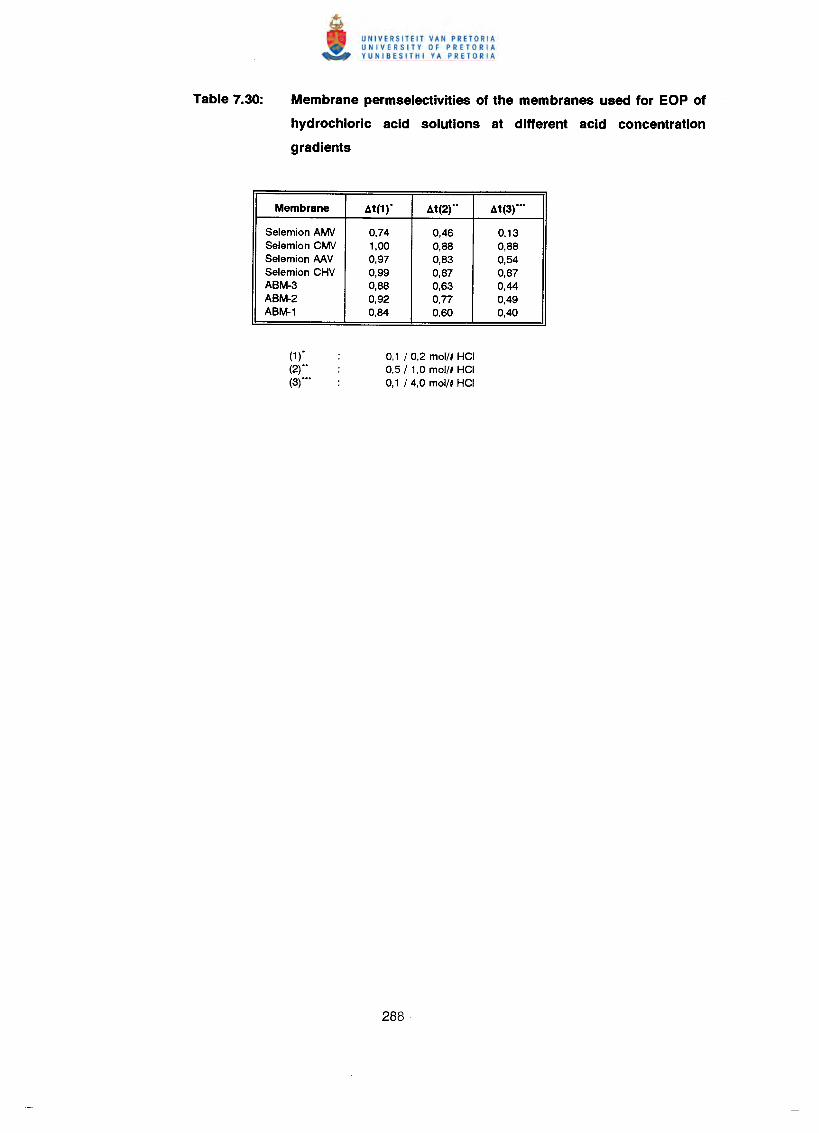
Membrane permselectivities of the membranes used for EOP of
hydrochloric acid solutions at different acid concentration
gradients
Membrane t\t(t )" t\t(2)"" t\t(3r""
Selemion AWN 0,74 0,46 0,13Selemion CWN 1,00 0,88 0,88Selemion AAV 0,97 0,83 0,54Selemion CHV 0,99 0,87 0,87ABM-3 0,88 0,63 0,44ABM-2 0,92 0,77 0,49ABM-1 0,84 0,60 0,40
(1 )"(2)""(3)"""
0,1 I 0,2 mol/~ HCI0,5 I 1,0 moll~HCI0,1 I 4,0 mol/l HCI
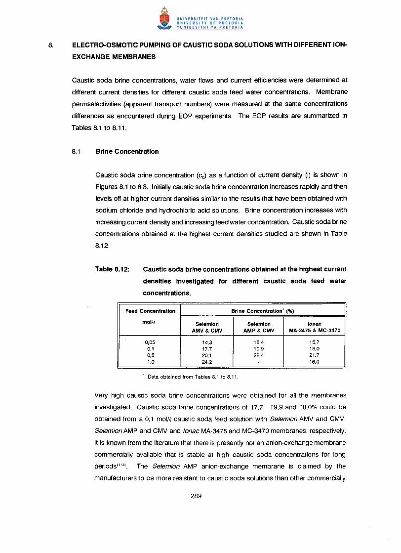
8. ELECTRO-OSMOTIC PUMPING OF CAUSTIC SODA SOLUTIONS WITH DIFFERENT ION-
EXCHANGE MEMBRANES
Caustic soda brine concentrations, water flows and current efficiencies were determined at
different current densities for different caustic soda feed water concentrations. Membrane
permseleetivities (apparent transport numbers) were measured at the same concentrations
differences as encountered during EOP experiments. The EOP results are summarized in
Tables 8.1 to 8.11.
Caustic soda brine concentration (cb) as a function of current density (I) is shown in
Figures 8.1 to 8.3. Initially caustic soda brine concentration increases rapidly and then
levels off at higher current densities similar to the results that have been obtained with
sodium chloride and hydrochloric acid solutions. Brine concentration increases with
increasing current density and increasing feed water concentration. Caustic soda brine
concentrations obtained at the highest current densities studied are shown in Table
8.12.
Caustic soda brine concentrations obtained at the highest current
densities investigated for different caustic soda feed water
concentrations.
Feed Concentration Brine Concentration" (%)
mol/e Selemion Selemion lonacAMV & CMV AMP & CMV MA-3475 & MC-3470
0,05 14,3 15,4 15,70,1 17,7 19,9 18,00,5 20,1 22,4 21,71,0 24,2 - 16,0
Very high caustic soda brine concentrations were obtained for all the membranes
investigated. Caustic soda brine concentrations of 17,7; 19,9 and 18,0% could be
obtained from a 0,1 mol/~ caustic soda feed solution with Selemion AMV and CMV;
Selemion AMP and CMV and lonac MA-3475 and MC-3470 membranes, respectively.
It is known from the literature that there is presently not an anion-exchange membrane
commercially available that is stable at high caustic soda concentrations for long
periods(1141• The Selemion AMP anion-exchange membrane is claimed by the
manufacturers to be more resistant to caustic soda solutions than other commercially
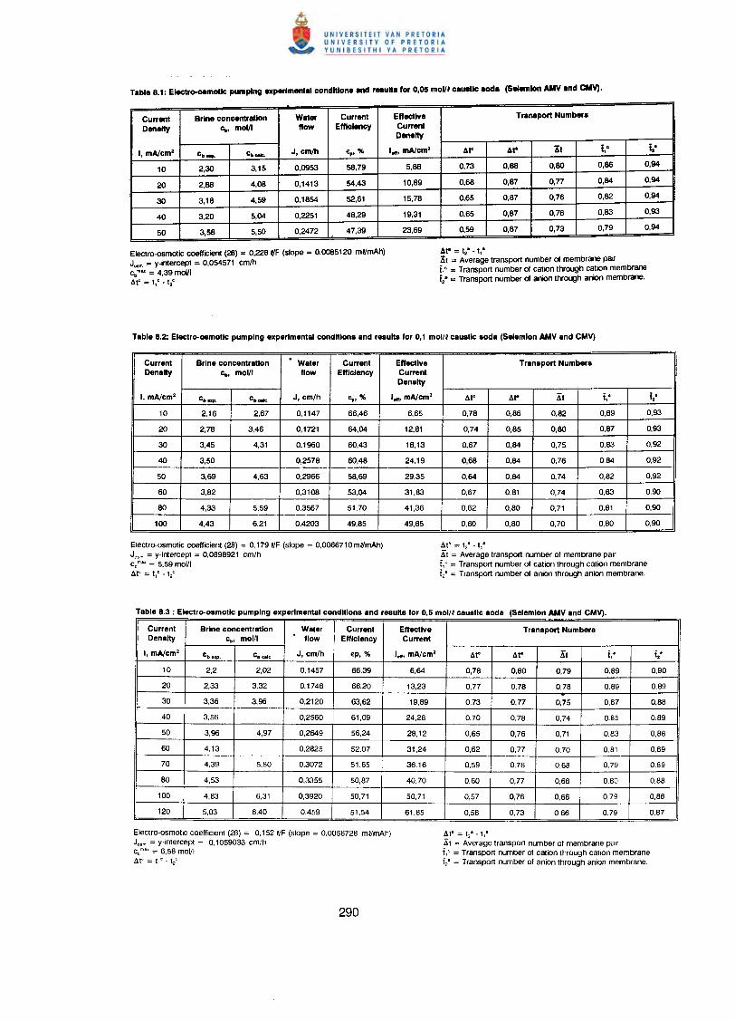
Current Brine concentration Water Current Effective Transport Numbers
Density c., molll flow Efficiency CurrentD_1ty
I, mA/cm' c._ c••••. J, cm/h e,,% I•••, mA/cm' .1t" At' "1t i,o j,'
10 2,30 3,15 0,0953 58,79 5,88 0,73 0,88 0,80 0,86 0,94
20 2,88 4,08 0,1413 54,43 10,89 0,68 0,87 0,77 0,84 0,94
30 3,18 4,59 0,1854 52,61 15,78 0,65 0,87 0,76 0,82 0,94
40 3,20 5,04 0,2251 48,29 19,31 0,65 0,87 0,76 0,83 0,93
50 3,58 5,50 0,2472 47,39 23,69 0,59 0,87 0,73 0,79 0,94
Electro-osmotic coefficient (26) = O,228I/F (slope = 0,0085120 ml/rnAh)Jo•m = y-intercept = 0,054571 cmlhc
bm •• = 4,39 moVI
Af = t,C • t2(.
4ta = 12& • 11•
At = Average transport number of membrane pairi,' = Transport number of cation through cation membranei,. = Transport number 01 anion through anion membrane.
Current Brine concentration Water Current Effective Transport NumberaDensity c., moVI flow Efficiency Current
Density
I, mA/cm' cbup. CbMtc J. cm/h e,,% I••••mA/cm' At' At' It i1c i2-
10 2,16 2,67 0,1147 66,46 6,65 0,78 0,86 0,82 0,89 0,93
20 2,78 3,46 0,1721 64,04 12,81 0,74 0,85 0,80 0,87 0,93
30 3,45 4,31 0,1960 60,43 18,13 0,67 0,84 0,75 0,83 0,92
40 3,50 0,2578 60,48 24,19 0,68 0,84 0,76 0,84 0,92
50 3,69 4,63 0,2966 58,69 29,35 0,64 0,84 0,74 0,82 0,92
60 3,82 0,3108 53,04 31,83 0,67 0,81 0,74 0,83 0,90
80 4,33 5,59 0,3567 51,70 41,36 0,62 0,80 0,71 0,81 0,90
100 4,43 6,21 0,4203 49,85 49,85 0,60 0,80 0,70 0,80 0,90
Electro-osmotic coefficient (28) = O,1791/F (slope = 0,0066710ml/mAh)J"m = y-intercept = 0,0898921 cm/hc, m •• = 5,59 moVIdt" = t," -t2(.
.6.18 = 12&. t1•
At = Average transport number of membrane pairi,' = Transport number of cation through cation membranei,' = Transport number of anion through anion membrane.
Current Brine concentration Water Current EffectIve Transport NumbersDensity c., mol/l flow Efficiency Current
I, mA/cm' cb ••. p. Cbca1c J, cm/h ep, % I••••mA/cm' At" .1t' It i,c i',10 2,2 2,02 0,1457 66,39 6,64 0,78 0,80 0,79 0,89 0,90
20 2,33 3,32 0,1748 66,20 13,23 0,77 0,78 0,78 0.89 0,89
30 3,36 3,96 0,2120 63,62 19,89 0,73 0,77 0,75 0,87 0,88
40 3,56 0,2560 61,09 24,28 0.70 0,78 0,74 0.85 0.89
50 3,96 4,97 0,2649 56,24 28,12 0,65 0,76 0,71 0.83 0,88
60 4,13 0,2825 52,07 31,24 0,62 0,77 0,70 0,81 0,89
70 4,39 5,80 0,3072 51,65 36,16 0,59 0,78 0,68 0,79 0,89
80 4,53 0,3355 50,87 40.70 0,60 0,77 0,68 0,80 0,88
100 4,83 6,31 0,3920 50,71 50,71 0,57 0,76 0,66 0,79 0,88
120 5,03 6,40 0,459 51,54 61.85 0.58 0,73 0,66 0,79 0,87
Electro-osmotic coeffiCient (28) = O,1521/F (slope = 0,0056728 ml/mAh)Jo,e = y-intercept = 0,1059033 cm/hc, m •• = 6,58 moVI4t" = Ill: -t/
Ala:;;; t/ -t111
At = Average transport number of membrane pairi,' = Transport number of cation through cation membranei,' = Transport number of anion through anion membrane.
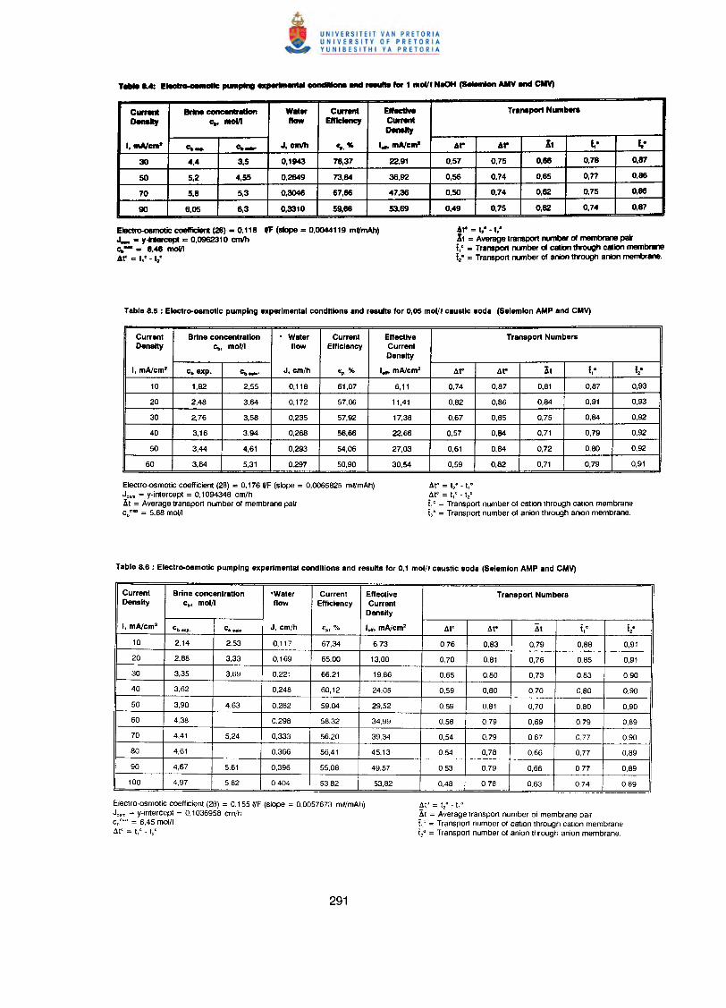
CurnnI Brine concenlr8tlon w••• CIIl'nftI EtreclIve Tr• .,.port Number8o-IIy c., moIII flow Emctency CumnI
o-Ity
I, mAlCffI' 0._ 0.__J,cmJh "." I•• ml4/cm' AI" AI" it 1,- ..-
30 4,4 3,5 0,1943 76,37 22,91 0,57 0,75 0,66 0,78 0,87
50 5,2 4,55 0,2649 73,84 36,92 0,56 0,74 0,65 o,n 0,86
70 5,8 5,3 0,3046 67,66 47,36 0,50 0,74 0,62 0,75 0,86
90 8,05 6,3 0,3310 59,66 53,69 0,49 0,75 0,62 0,74 0,87
Electro-osmollc coelficler1 (28) = 0,118 6'F (slope = 0,0044119 ml/mAh)J_ - y.-.ercept = 0,0962310 cm'hc,,- = 8,46 moVIAt' = I,' - •••
AI" = I,' - I,'il = Average Iransport runber 01 membr_ pari,' = Transport number 01 cation Ihrough cation membrWWi:= Transport number of anion Ihrough anion membr_.
Currenl Brine concenlratlon Water Currenl Effective Tranaport NumberaDensity c., mol/I flow Efficiency Current
Density
I, mAtcm' c. expo Cboek° J, cm/h €p, % I•• , mAtcm' At' AI" ;il i,o i2-
10 1,92 2,55 0,118 61,07 6,11 0,74 0,87 0,81 0,87 0,93
20 2,48 3,64 0.172 57.06 11,41 0,82 0,86 0.84 0.91 0,93
30 2,76 3,58 0.235 57,92 17,38 0,67 0,85 0,75 0.84 0,92
40 3,16 3,94 0,268 56,66 22,66 0,57 0,84 0,71 0,79 0,92
50 3,44 4,61 0,293 54,06 27,03 0,61 0,84 0,72 0,80 0,92
60 3,84 5,31 0,297 50,90 30,54 0,59 0,82 0,71 0,79 0,91
Electro-osmotic coefficient (2B) = 0,176 I/F (slope = 0,0065825 ml/mAh)J"m = y-intercepl = 0,1094348 cm/h11 = Average Iransport number of membrane pairc. ma< = 5,68 moVI
ata = t28 - fl·ate; = tiC -t2(;
i,' = Transport number of calion through cation membranei,' = Transport number of anion through anion membrane.
Current Brine concenlratlon 'Waler Currenl Effecllve Transport NumbersDensity c., mol/I flow Efficiency Currenl
Density
I, mAtem' cb expo CbRK:. J, em/h €pl % I•• , mA/em' AI' AI' Al i' 12-,10 2,14 2,53 0,117 67,34 6,73 0,76 0,83 0,79 0,88 0,91
20 2,88 3,33 0,169 65,00 13,00 0,70 0,81 0,76 0,85 0,91
30 3,35 3,69 0.221 66.21 19,86 0.65 0.80 0.73 0,83 0,90
40 3,62 0,248 60,12 24,05 0,59 0,80 0,70 0,80 0.90
50 3,90 4,63 0,282 59.04 29,52 0,59 0,81 0,70 0,80 0,90
60 4,38 0,298 58,32 34,99 0.58 0,79 0.69 0,79 0.89
70 4,41 5,24 0,333 56,20 39,34 0,54 0,79 0,67 0,77 0,90
80 4,61 0,366 56,41 45.13 0,54 0,78 0,66 0,77 0,89
90 4,67 5,61 0,396 55.08 49.57 0,53 0,79 0,66 0,77 0,89
100 4,97 5,82 0,404 53,82 53,82 0,48 0,78 0,63 0,74 0,89
Electro-osmotic coefficient (2B) = 0,155 I/F (slope = 0,0057673 ml/mAh)J"m = y-intercept = 0,1036958 cm/hcoma<= 6,45 mol/l4to;; = t,' - 1
2(;
.dtd = t/ ~tjll
3t = Average transport number of membrane pairi,' = Transport number of cation through cation membranei,' = Transport number of anion through anion membrane.
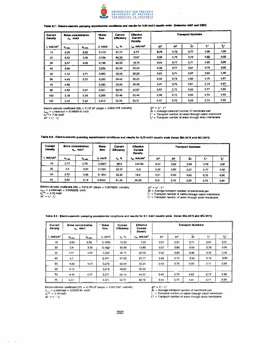
Currenl Brine concentration 'Water Current Effective Tranaport NumbersD_1ty c., mol/l flow Efficiency Currenl
Density
I, mAtcm' c._ c._ J, cm/h e,.,% I•• , mAtcm' "'l" "'I" Al i,c i••
10 2,29 2,62 0,110 67,75 6,78 0,76 0,79 0,77 0,88 0,89
20 3,02 3,36 0,159 64,33 12,87 0,66 0,78 0,72 0,83 0,89
30 3,57 4,05 0,196 62,63 18,79 0,65 0,77 0,71 0,83 0,88
40 3,98 0,236 62,99 25,20 0,56 0,77 0,67 0,78 0,88
50 4,12 4,71 0,265 58,58 29,29 0,60 0,74 0,67 0,80 0,88
60 4,43 5,02 0,295 58,42 35,05 0,58 0,74 0,66 0,79 0,87
70 4,89 0,282 52,83 36,98 0,47 0,75 0,61 0,74 0,87
80 4,83 5,67 0,331 53,59 42,87 0,53 0,72 0,63 0,77 0,86
100 5,19 5,59 0,399 55,46 55,46 0,48 0,72 0,60 0,74 0,86
120 5,59 6,29 0,419 52,76 63,31 0,47 0,70 0,59 0,74 0,85
Electro-osmotic coefficient (26) = 0,1371/F (slope = 0,0051179 ml/mAh)Jo•m = y-intercept = 0,1068910 cm/hcbmu= 7,30 moVI4.tC = 1,I:-t
2C
At- = t28 - 11•
Xt = Average transport number of membrane pairi,' = Transport number of cation through cation membranei,' = Transport number of anion ttvough anion membrane.
Currenl Brine concentrallon Water Currenl Effective Transport NumbersDensity c", mol/l flow Efficiency Current
Density
I, mAtcm' c._ c,,_ J, cm/h e,.,% I•• , mAtcm' "'l" "'I" 41 it" 1.010 2,77 2,79 0,0927 68,8 0,8196 0,57 0,82 0,69 0,78 0,9120 3,4 3,61 0,1391 63,37 12.6 0,55 0,80 0,67 0.77 0,9030 3,76 3,96 0,1854 62.29 18.6 0,51 0,80 0,66 0,76 0,9040 3,92 4,14 0,2344 61,59 24,63 0,51 0,79 0,65 0,75 0,90
EieC1ro-osmotic coefficient (26) = 0,2121/F (slope = 0,0079229 ml/mAh)J••m = y-intercep1 = 0,0388302 cm/hComu = 4,72moVI4~ ==: t,C M t~C
Ar- = t28 - t,-
~t = Average transport number 01 membrane pair!.' = Transport number 01 cation through cation membranet,' = Transport number of anion through anion membrane.
Current Brine concentrallon • Waler Currenl Eflectlve Transport NumbersDenslly c., mol/l flow, Efficiency Currenl
Denslly
I, mA/cm' cb •• p. Cbca1c. J, cmlh €p, % left! mAlcm2 "'Ie "'10 "'t 11e 12-
10 2.63 2,58 0,1033 72.22 7,22 0.61 0,81 0,71 0,81 0,91
20 3,4 3.38 0,1522 69,38 13,88 0,57 0,80 0,69 0,79 0,90
30 3,71 3,69 0,200 66,77 20,03 0.52 0,80 0,66 0,76 0.90
40 4,1 0.247 67,93 27,17 0,48 0.79 0,64 0.74 0.89
50 4,26 4.04 0,279 64.50 32,25 0,43 0,78 0,60 0,71 0,89
60 4.15 0,318 58.93 35.35
70 4,45 4.37 0,371 63,19 44.23 0,45 0,79 0,62 0,73 0,89
75 4,51 0,371 59.71 44.78 0,43 0,79 0.61 0,71 0.89
Electro-osmotic coefficient (26) = 0,1931/F (slope = 0.0071947 ml/mAh)J"m = y-Intercept = 0.0529144 cmlhcbm~ = 5,18mol/lAt';:;: l,c. t/
Ala;;;; t/, - t/I
Xt = Average transport number of membrane pairt.' = Transport number of cation through cation membranei,' = Transport number of anion through anion membrane.
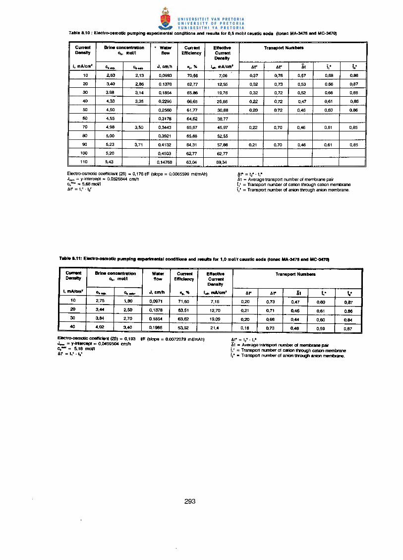
Current Brine concentrlltlon . Wilt., Current Eff«:tlve Trall8port NumbersDenalty c", molll flow Efficiency Current
Denalty
I, mA/cm' c••••. c._ J, cm/h e,,% I•• , mA/cm' AI' Ar it i10 j,'
10 2,63 2,13 0,0993 70,56 7,06 0,37 0,76 0,57 0,68 0,88
20 3,40 2,86 0,1378 62,77 12,55 0,32 0,73 0,53 0,66 0,87
30 3,98 3,14 0,1854 65,86 19,76 0,32 0,72 0,52 0,66 0,86
40 4,33 3,35 0,2296 66,65 26,66 0,22 0,72 0,47 0,61 0,86
50 4,50 0,2560 61,77 30,88 0,20 0,72 0,46 0,60 0,86
60 4,55 0,3178 64,62 38,77
70 4,98 3,50 0,3443 65,67 45,97 0,22 0,70 0,46 0.61 0,85
80 5,00 0,3921 65,68 52,55
90 5,23 3,71 0,4132 64,31 57,88 0,21 0,70 0,46 0,61 0,85
100 5,20 0,4503 62,77 62,77
110 5,43 0,14768 63,04 69,34
Electro-osmotic coefficient (26) = 0, 1761/F (slope = 0,0065599 ml/mAh)Jo•m = v-intercept = 0,0526844 cmlhcbm" = 5,68 molll4.r: = t1
C - t2C
4ta = t2- - fl·Xt = Average transport number of membrane pairi,' = Transport number of cation through cation membranei,' = Transport number 01 anion through anion membrane.
Current Brine concentrlltlon Wllter ClIlT8f1l E"ec:tlve Tranaport NumbersD_1ty c", mol/l flow Emclency Current
Denalty
I, mA/cm· c,,_ c" ••• J, cmlh ...." I••• mA/cm· Ar AI' it ft' •••10 2,75 1,80 0,0971 71,60 7,16 0,20 0,73 0,47 0,60 0,87
20 3,44 2,50 0,1378 63,51 12.70 0,21 0,71 0,46 0,61 0.86
30 3,84 2.70 0.1854 63,62 19.09 0,20 0,68 0,44 0,60 0,84
40 4,02 3,40 0,1986 53,52 21,4 0,18 0.73 0,46 0,59 0,87 IElectro-osmotic coetIiclert (28) = 0,193 IfF (slope = 0.0072019 ml/mAh)J_ = y••.•ercept = 0,0459504 cmIhc,,- = 5,t8 moVl41" = 1,'.1,'
.1t- = f2-· t,-3'! = Average Iransport runber of membrane paa-i,' = Transport runber of cation through cation membranei,' = Transport number 01 anion through anion membrane.
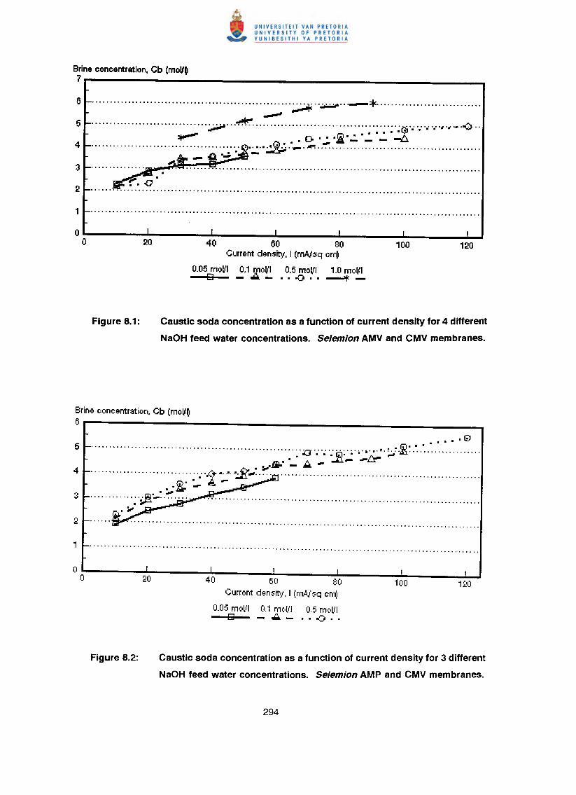
Brine concentration, Cb (mollO7
.......................................................~ ..~ _* .~
................................ ~ ~ )-;................•.-0 ... . . . . . .~ ....~ 00 0 0 01.)0 ~
~oG>-o~ 0 _ ill....................................... "." ~.,....~ ....• 41..;. -
40 60 80Current density, I (mAlsq cm)
0.05 moVI 0.1 moVI 0.5 moVI 1.0 moVIo ----_ .. -o .. ---+:-
Caustic soda concentration as a function of current density for 4 different
NaOH feed water concentrations. Selem/on AMV and CMV membranes.
Brine concentration. Cb (moVO6
00 0 0 €I/OJ 0
0
:.:.·:::·:::·:.·..:··:··:::·:.o'~~:~:,~~.:;~:;.' ~ .:~..~ ..~.:~~.~~..:":"::':.:":::::::Go 0 ,A-..~ .•.0-............ ~.~~ .
i).0 •••
40 60 80Current densITy. I (mAtsq em)
0.05 moll'l 0.1 ~'lCIl"1 0.5 molll[;J - ••••. _ oo~oo
Caustic soda concentration as a function of current density for 3 different
NaOH feed water concentrations. Selemion AMP and CMV membranes.
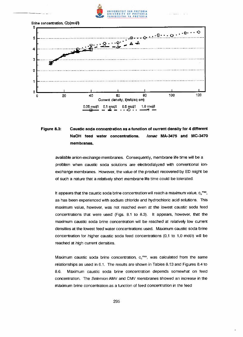
Brine concentration, Cb(moll~6
.ew···<).ID···O·-......................................................... ·•.19 •.•.•. O· !II. ~ •••••••••••••••••••••••••••••••••
, 0 ••• ~ •• ' A../A.~ .~ -L!J!' ,."........................................................................
40 60 80Current density, l(mAJsq crrV
0.05 moVI 0.1 moVI 0.5 moVI 1.0 moVIo - •• - .. ..QI •• ---+:-
Caustic soda concentration as a function of current density for 4 different
NaOH feed water concentrations. lonae MA·3475 and MC·3470
membranes.
available anion-exchange membranes. Consequently, membrane life time will be a
problem when caustic soda solutions are electrodialyzed with conventional ion-
exchange membranes. However, the value of the product recovered by ED might be
of such a nature that a relatively short membrane life time could be tolerated.
It appears that the caustic soda brine concentration will reach a maximum value, cbmax,
as has been experienced with sodium chloride and hydrochloric acid solutions. This
maximum value, however, was not reached even at the lowest caustic soda feed
concentrations that were used (Figs. 8.1 to 8.3). It appears, however, that the
maximum caustic soda brine concentration will be reached at relatively low current
densities at the lowest feed water concentrations used. Maximum caustic soda brine
concentration for higher caustic soda feed concentrations (0,1 to 1,0 molM will be
reached at high current densities.
Maximum caustic soda brine concentration, cb max, was calculated from the same
relationships as used in 6.1. The results are shown in Tables 8.13 and Figures 8.4 to
8.6. Maximum caustic soda brine concentration depends somewhat on feed
concentration. The Selemion AMV and CMV membranes showed an increase in the
maximum brine concentration as a function of feed concentration in the feed
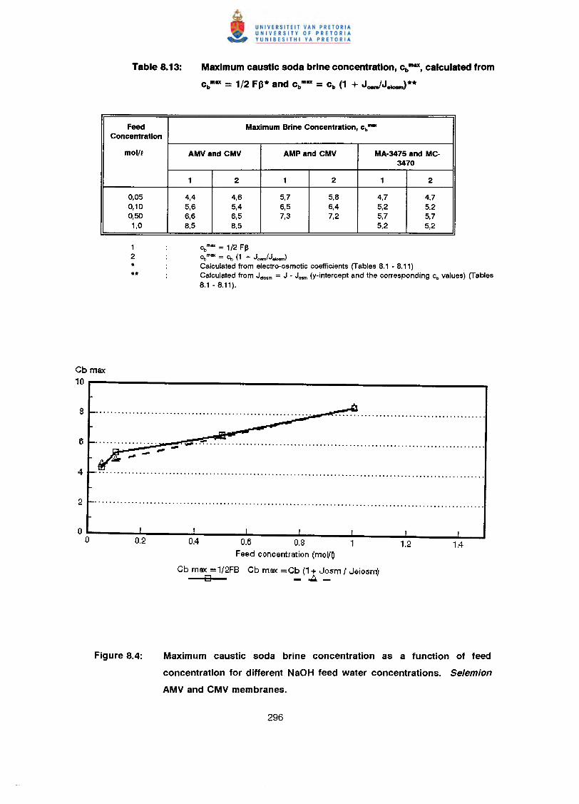
Maximum caustic soda brine concentration, cbMa, calculated from
cbma = 1/2 FIJ* and cb
ma = cb (1 + Joem/J_)**
Feed Maximum Brine Concentration, cb-
Concentration
mol!~ AMVand CMV AMP and CMV MA-3475 and MC-3470
1 2 1 2 1 2
0,05 4,4 4,6 5,7 5,8 4,7 4,70,10 5,6 5,4 6,5 6,4 5,2 5,20,50 6,6 6,5 7,3 7,2 5,7 5,71,0 8,5 8,5 5,2 5,2
cbmOl<= 1/2 Ff3cbmOl<= cb (1 + Josm/JeIosm)
Calculated from electro-osmotic coefficients (Tables 8.1 - 8.11)Calculated from J_m = J - Josm(y-intercept and the corresponding cb values) (Tables8.1 - 8.11).
Cb max10
- -..•. ~
0.4 0.6 0.8 1Feed concentration (moV~
Cb max = 1I2FB Cb max = Cb (1 + Josm I Jeiosm)D -..::.._
Maximum caustic soda brine concentration as a function of feed
concentration for different NaOH feed water concentrations. Selemion
AMV and CMV membranes.
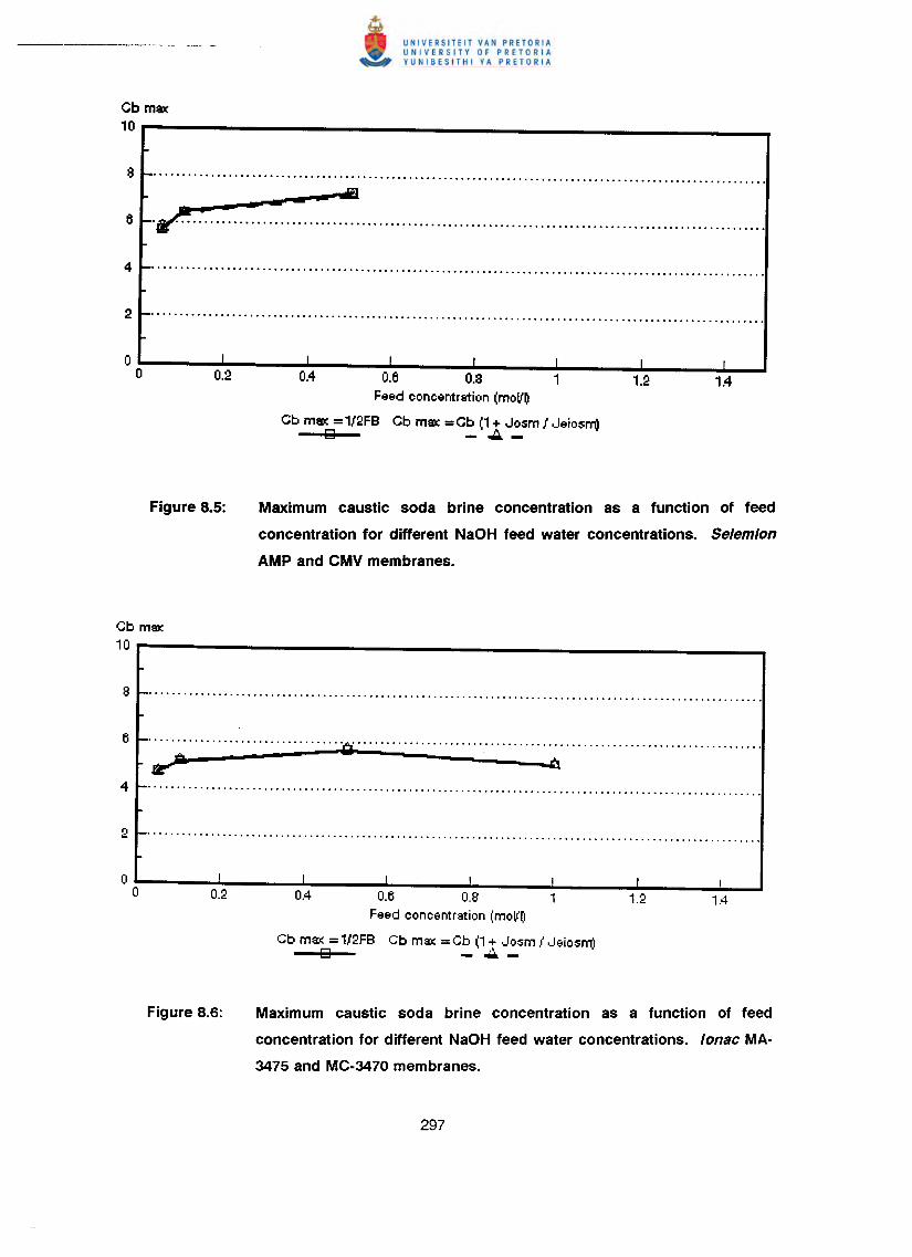
Cb m8:l:10
6 .? .••
Cb m8:l:10
0.4 0.6 0.8 1Feed concentration (moV~
Cb m8:l: =1/2FB Cb m8:l: =Cb (1 + Josm / JeiosrTOg - .••.-
Maximum caustic soda brine concentration as a function of feed
concentration for different NaOH feed water concentrations. Selemion
AMP and CMV membranes.
................................. ~ .~ -n
0.4 0.6 0.8 1Feed concentration (moV~
Cb m8:l: = 1/2FB Cb m8:l: = Cb (1 + Josm I JeiosrTOg - .••.-
Maximum caustic soda brine concentration as a function of feed
concentration for different NaOH feed water concentrations. lonac MA·
3475 and MC·3470 membranes.
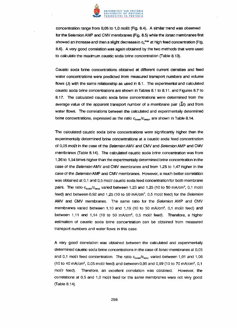
concentration range from 0,05 to 1,0 mol!f (Fig. 8.4). A similar trend was observed
for the Selemion AMP and CMV membranes (Fig. 8.5) while the lonac membranes first
showed an increase and then a slight decrease in cbmax at high feed concentration (Fig.
8.6). A very good correlation was again obtained by the two methods that were used
to calculate the maximum caustic soda brine concentration (Table 8.13).
Caustic soda brine concentrations obtained at different current densities and feed
water concentrations were predicted from measured transport numbers and volume
flows (J) with the same relationship as used in 6.1. The experimental and calculated
caustic soda brine concentrations are shown in Tables 8.1 to 8.11. and Figures 8.7 to
8.17. The calculated caustic soda brine concentrations were determined from the
average value of the apparent transport number of a membrane pair (At) and from
water flows. The correlations between the calculated and experimentally determined
brine concentrations, expressed as the ratio CbcaIJCbeXP' are shown in Table 8.14.
The calculated caustic soda brine concentrations were significantly higher than the
experimentally determined brine concentrations at a caustic soda feed concentration
of 0,05 mol!Q in the case of the Selemion AMV and CMV and Selemion AMP and CMV
membranes (Table 8.14). The calculated caustic soda brine concentration was from
1,36 to 1,54 times higher than the experimentally determined brine concentration in the
case of the Selemion AMV and CMV membranes and from 1,25 to 1,47 higher in the
case of the Selemion AMP and CMV membranes. However, a much better correlation
was obtained at 0,1 and a,s mol/Qcaustic soda feed concentration for both membrane
pairs. The ratio CbcaJCbeXP varied between 1,23 and 1,25 (10 to 50 mNcm2, 0,1 mol/Q
feed) and between 0,92 and 1,25 (10 to 50 mNcm2, a,s mol/Q feed) for the Selemion
AMV and CMV membranes. The same ratio for the Selemion AMP and CMV
membranes varied between 1,10 and 1,19 (10 to 50 mNcm2, 0,1 mol/Q feed) and
between 1,11 and 1,14 (10 to 50 mNcm2, a,s mol/Q feed). Therefore, a higher
estimation of caustic soda brine concentration can be obtained from measured
transport numbers and water flows in this case.
A very good correlation was obtained between the calculated and experimentally
determined caustic soda brine concentrations in the case of lonac membranes at 0,05
and 0,1 mol/Q feed concentration. The ratio CbcalJCbexp varied between 1,01 and 1,06
(10 to 40 mA/cm2, 0,05 mol/Q feed) and between 0,95 and 0,99 (10 to 70 mA/cm2, 0,1
mol/Q feed). Therefore, an excellent correlation was obtained. However, the
correlations at 0,5 and 1,0 mol/Q feed for the same membranes were not very good
(Table 8.14).
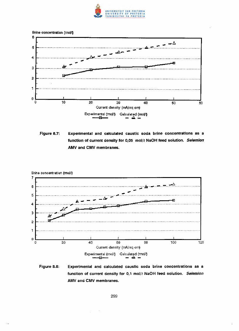
Brine concentration (moV~6 ••••------------- _
- -~5 •..................................................................... .,. .. ..::..,.~ .. -:: ...1::..- ----4 _ p ..~ ....-I!!r-3 - •••••.•.•••.••••••••.•••••••••••• '1!!iI ••
~2 _ .
0 I I I I I
0 10 20 30 40 50 60Current density (mAJosqcrr(!
Experimental (moV~ Calculated (moV~I!!iI -""'--
Experimental and calculated caustic soda brine concentrations as a
function of current density for 0,05 mol/Q NaOH feed solution. Selemlon
AMV and CMV membranes.
Brine concentration (moV~7
...................................................................... :A._. -..!"'!"' .. ~ .~-",.-................................................... ",.. .A- - - _fH - I!!iI ......eJ
.....................•••............................·tr· .. ~.: .•••. ~ Iii! I!!iI.:::::~:...::~.••.:::::::::::::::::: ..::::::: ....•.•.:::.:: ..:.:.::•.•.:::::•....:.:::: ....:.:
40 60 80Current density (rnt!c,losqcm)
Experimental (moll'~1 Calc'Jlat~d (mo~'~1I!!iI - ••. -
Experimental and calculated caustic soda brine concentrations as a
function of current density for 0,1 mol/Q NaOH feed solution. Selemion
AMV and CMV membranes.
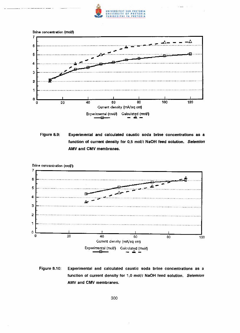
Brine concentration (moll~7
~ -I::..-•••••••••••••••••••••••••••••••••••••••••••••••••••••••• ~ •• ;,;. •• __ • _ •• ot#'!' •••••••••••••••••••••••••••••••••...~~......................................p .
"....4 .A.~ .,
40 60 80Current density (m>Vsq crr(!
Experimental (moll~ Calculated (moll~I2l - ..:.. -
Experimental and calculated caustic soda brine concentrations as a
function of current density for 0,5 mol/Q NaOH feed solution. Selemlon
AMV and CMV membranes.
Brine concentration (moll~7.---- --,6 1-.......•......................•........................................................
I2l •••A- -5 I- ~ _.l"!"' .e----- _~ --~4 _ ,.~ .
j;a.-3 _ .
-.it .
I I
40 60Current deMit~( (m~./sq cm,l
Experimental (moll'(1I2l
Figure 8.10: Experimental and calculated caustic soda brine concentrations as a
function of current density for 1,0 mol/Q NaOH feed solution. Selemion
AMV and CMV membranes.
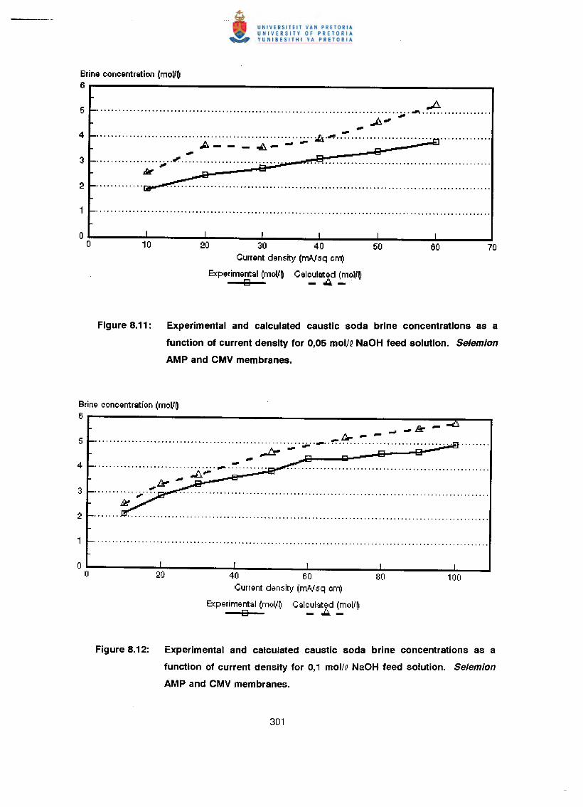
Brine concentration (moV~6
A..................................................................................... ~ .J::. .••. .,..... . . . . . . . . . . . . . . . . . . . . . . . . . . . . . . . . . . . . . . . . . . . . . . . . . . ~ .. ;,;.: . ;,ls. .~ .. ~ ,:.t'l' .
,.A---~- e................. :.;...~............................ ...~ .
M 1!11............. ~ .
20 30 40 50Current density (mAlsq crr(!
Experimental (moV~ Calculated (moV~g - •••-
Figure 8.11: Experimental and calculated caustic soda brine concentrations as a
function of current density for 0,05 mol/QNaOH feed solution. Selemlon
AMP and CMV membranes.
Brine concentration (moV~6 _ i!r - -e:::.
1Jr---.............................................................••.. '!":'............................... .., .....,i::r" - --................................. _ .
~~,
40 60Current density (mo!t.,1sq cm,'
Experimental (mclll'~1 Calculsted (moll'rlg - ••• - '
Figure 8.12: Experimental and calculated caustic soda brine concentrations as a
function of current density for 0,1 mol/Q NaOH feed solution. Selemlon
AMP and CMV membranes.
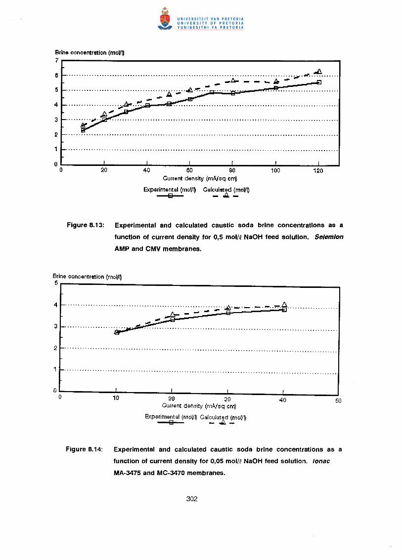
Brine concentration (moV~7
.J:!...........................................................................................••.... ~ ._t.- - - _ JJ" ---............................................... ~."!"'. ,_1:&-,..-...................... ~ ....,.,.~ ...•
•••••••••• IfI".. • ••••••••••••••••••••••••••••••••••••••••••••••••••••••••••••••••••••••••••••••••••.••••••
Ir
40 60 80Current density (mA,lsq cniJ
Experimental (moll~ Calculated (moV~g - ~-
Figure 8.13: Experimental and calculated caustic soda brine concentrations as a
function of current density for 0,5 mol/Q NaOH feed solution. Selemlon
AMP and CMV membranes.
Brine concentration (moV~5
··················· 0 0';':' o£o ••••.._. _ .••••.. ~~ .-tr--- 13
~~
........................ ~ .
20 30Current densit~( (mo!.isq cm;r
Experimental (m(o~'~Calc1Jlat.;.d (m(oll'~g , - ...:.::..-
Figure 8.14: Experimental and calculated caustic soda brine concentrations as a
function of current density for 0,05 mol/Q NaOH feed solution. lonac
MA-3475 and MC-3470 membranes.
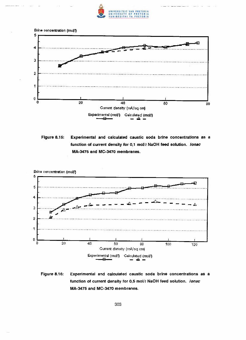
Brine concentration (moV~5
20 40Current density (rnoVsqcrr(!
Experimental (moll~ Calculated (moV~o -.A-
Figure 8.15: Experimental and calculated caustic soda brine concentrations as a
function of current density for 0,1 mol/QNaOH feed solution. lonse
MA-3475 and MC-3470 membranes.
Brine concentration (moV~6
&" ~';;,."~"~"~'.~..~ ..~.~..~..~..~ ..~..~..~..~..~.~ .
.A·•••..JOf'•••••••••••••••••••••••••••••••••••••••••••••••••••••••••••••••••••••••••••••••••••••
,.,......k .
60 80Current densit~((m.!.,"sq em,\
Experiment::.1(mol1f) CalelJlat~d (moll'f)o - .•• -
Figure 8.16: Experimental and calculated caustic soda brine concentrations as a
function of current density for 0,5 mol/QNaOH feed solution. lonse
MA-3475 and MC-3470 membranes.
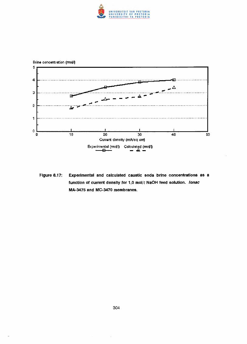
Brine concentration (moV~5
........................................~ ~ ~ ~ ~ ~ ~..~ ~~.~~ ~ ~.~-EU .
.••••••.••••••••••• ~ ••••••..•....••••....•.••.. ;,;or.~ •. ~ •• ~.':-. .••...•••........•..
A_ - - ..:)" -~--~~................... ~ .. .itJ'._ .
20 30Current density (mAlsq crr(!
Experimentsl (moV~ Cslculated (moV~13 - ..:i. -
Figure 8.17: Experimental and calculated caustic soda brine concentrations as a
function of current density for 1,0 mol/ONaOH feed solution. lonae
MA·3475 and MC-3470membranes.
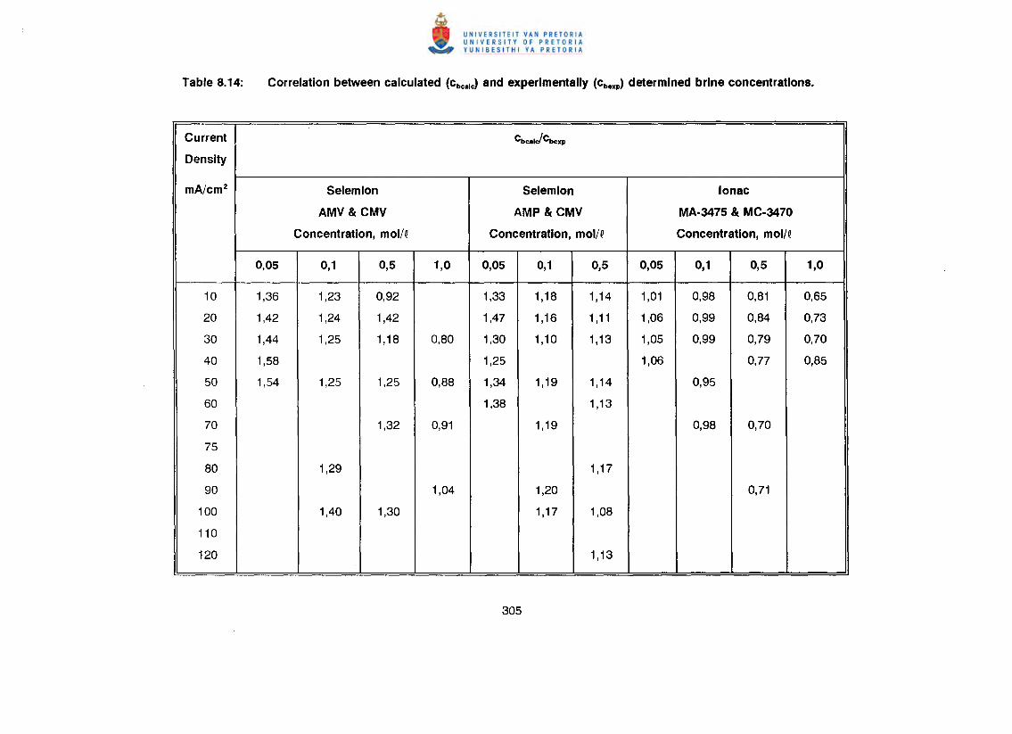
Current CbcalJCbexp
Density
mA/cm2 Selemion Selemion lonac
AMV & CMV AMP & CMV MA·3475 & MC·3470
Concentration, mol/Q Concentration, mol/Q Concentration, mol/Q
0,05 0,1 0,5 1,0 0,05 0,1 0,5 0,05 0,1 0,5 1,0
10 1,36 1,23 0,92 1,33 1,18 1,14 1,01 0,98 0,81 0,65
20 1,42 1,24 1,42 1,47 1,16 1,11 1,06 0,99 0,84 0,73
30 1,44 1,25 1,18 0,80 1,30 1,10 1,13 1,05 0,99 0,79 0,70
40 1,58 1,25 1,06 0,77 0,85
50 1,54 1,25 1,25 0,88 1,34 1,19 1,14 0,95
60 1,38 1,13
70 1,32 0,91 1,19 0,98 0,70
75
80 1,29 1,17
90 1,04 1,20 0,71
100 1,40 1,30 1,17 1,08
110
120 1,13
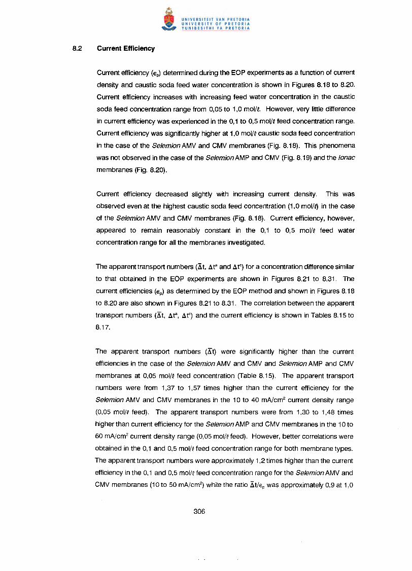
Current efficiency (ep) determined during the EOP experiments as a function of current
density and caustic soda feed water concentration is shown in Figures 8.18 to 8.20.
Current efficiency increases with increasing feed water concentration in the caustic
soda feed concentration range from 0,05 to 1,0 mol/~. However, very little difference
in current efficiency was experienced in the 0,1 to 0,5 mol/~feed concentration range.
Current efficiency was significantly higher at 1,0 mol/~caustic soda feed concentration
in the case of the Selemion AMV and CMV membranes (Fig. 8.18). This phenomena
was not observed in the case of the Selemion AMP and CMV (Fig. 8.19) and the lonac
membranes (Fig. 8.20).
Current efficiency decreased slightly with increasing current density. This was
observed even at the highest caustic soda feed concentration (1,0 molN) in the case
of the Selemion AMV and CMV membranes (Fig. 8.18). Current efficiency, however,
appeared to remain reasonably constant in the 0,1 to 0,5 mol/~ feed water
concentration range for all the membranes investigated.
The apparent transport numbers (X t, !J.ta and !J.tC) for a concentration difference similar
to that obtained in the EOP experiments are shown in Figures 8.21 to 8.31. The
current efficiencies (ep) as determined by the EOP method and shown in Figures 8.18
to 8.20 are also shown in Figures 8.21 to 8.31. The correlation between the apparent
transport numbers (X t, !J.e, !J.tC) and the current efficiency is shown in Tables 8.15 to
8.17.
The apparent transport numbers (Xt) were significantly higher than the current
efficiencies in the case of the Selemion AMV and CMV and Selemion AMP and CMV
membranes at 0,05 mol/~ feed concentration (Table 8.15). The apparent transport
numbers were from 1,37 to 1,57 times higher than the current efficiency for the
Selemion AMV and CMV membranes in the 10 to 40 mA/cm2 current density range
(0,05 maiN feed). The apparent transport numbers were from 1,30 to 1,48 times
higher than current efficiency for the Selemion AMP and CMV membranes in the 10 to
60 mA/cm2 current density range (0,05 mol/qfeed). However, better correlations were
obtained in the 0,1 and 0,5 mol/~feed concentration range for both membrane types.
The apparent transport numbers were approximately 1,2 times higher than the current
efficiency in the 0,1 and 0,5 mol/Qfeed concentration range for the Selemion AMV and
CMV membranes (10 to 50 mA/cm2) while the ratio Xt/ep was approximately 0,9 at 1,0
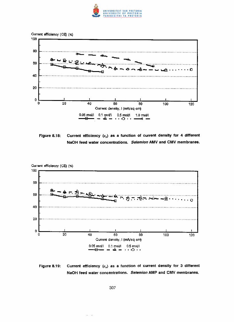
Current efficiency (CE) (%)100
....................... ~ .- """-• ~a ... (;1 -- ~...... ~ .. :o:-.. ~.:..~ . ....n_. 'oI"'lo,&:-:' ~ ~ .. ~ .........•............................,8 --il .•• - €' - ~- - - ....0. 'J
40 60 80Current density, I (rn.AJsq cm)
0.05molll 0.1molll 0.5molll 1.0molllo -~_ .. -o .• -...t::-
Figure 8.18: Current efficiency (€p) as a function of current density for 4 different
NaOH feed water concentrations. Selemion AMV and CMV membranes.
Current efficiency (CE) (%)100.---------------------------- __
60 _ ~ ::-,i 17,.*.''t~;':'.6:':':;:.e::.:·~':;;ii':':': .::.:.:.~..40 _ .
0 I I I I I I
0 20 40 60 80 100 120Current density, I (rn.AJsq cm)
0.05molll 0.1molll 0.5molll0 ~- •• .(J ••
Figure 8.19: Current efficiency (€p) as a function of current density for 3 different
NaOH feed water concentrations. Selemion AMP and CMV membranes.
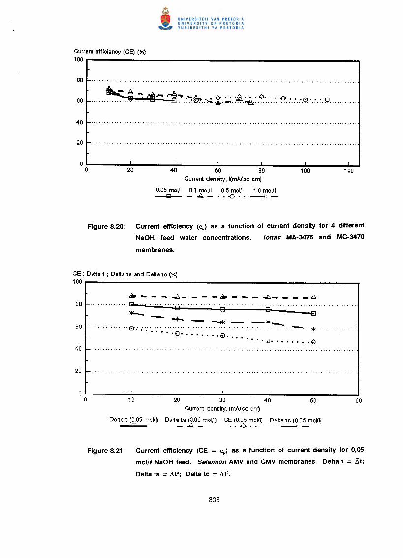
Current efficiency (CE) (%)100.---------------------------_
80 _ .
~60 _ P"~':' .~ '-:. :":';~ ~..~. :..:.~.~: .?.:.:..~ 0.~.~.~.Q .
I I I
40 60 80Current density, l(mAjsq cm)
0.05moVI 0.1moVI 0.5moVI 1.0moVIg -":'- •• -0 •• ---4:-
I
100I
120
Figure 8.20: Current efficiency (€p) as a function of current density for 4 different
NaOH feed water concentrations. lonse MA·3475 and MC·3470
membranes.
CE : Delta t : Delta ta and Delta tc (%)100
~ .••• - -.. ~- - - - ~ - ~ - -J::J.- - - - ~............... ~ ·tr···············8··············· .g .
::+0..- of]- ....;r... _ --L -,L.~ - --T- ••..•..•....... ..(;)'; , ",",-..* .
·······0 ~ .. . . . . . .• G) •••••••• 0
20 30Current density,l(m.!..lsq Cnil
Delta ta (0.05 moV~ CE (O.~5 moll'~-.;:.,- .. .() ..Delta t (0.05 moll~Ul
Delta tc (0.05 moll' (I--of -
Figure 8.21: Current efficiency (CE = €p) as a function of current density for 0,05
mol/Q NaOH feed. Selemion AMV and CMV membranes. Delta t = &t;
Delta ta = ae; Delta te = Ate.
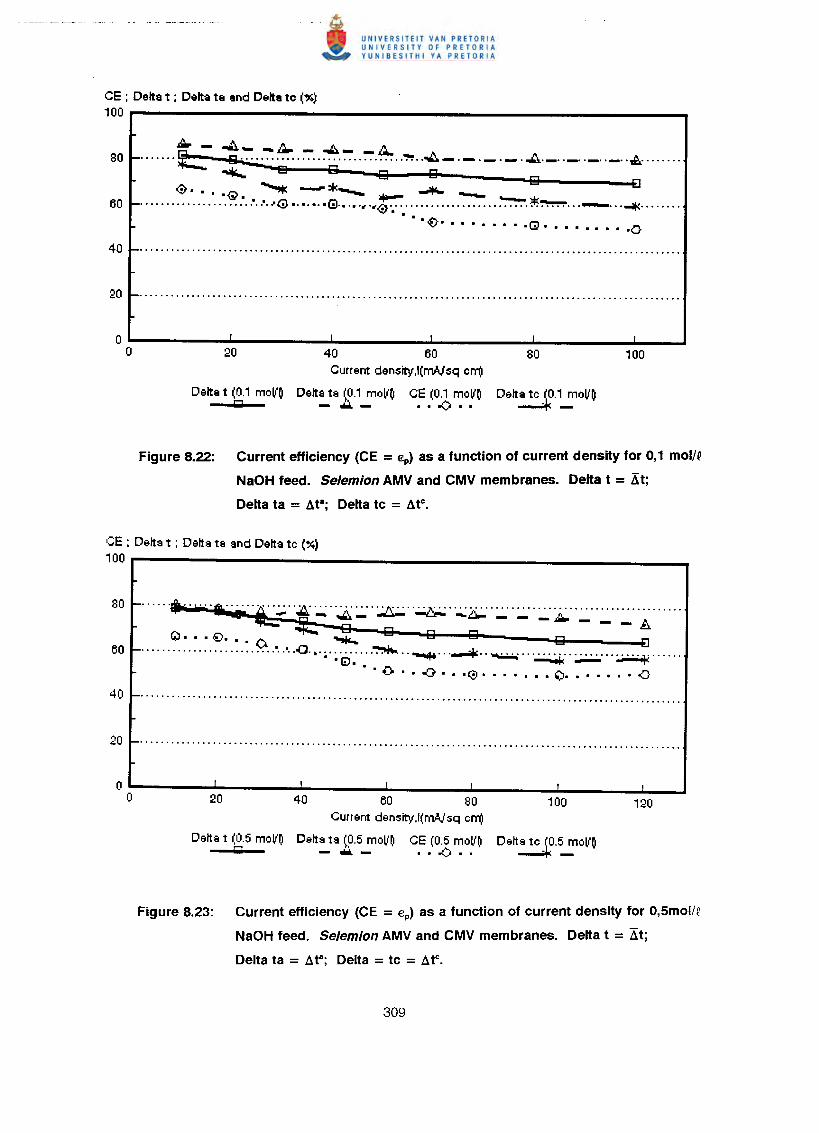
CE : Delta t ; Delta ta and Delta tc (%)'00
~ -1:.. __ ~ _ ~_ -A........ Q ~ .. ~ _. -.. _. __ . ",,/;;},.._.. _ .. _ .. _. o£ .
•••••• 8 eJ eJ QeJ il••••••••• -..... _ ~__ ->IL
'" ... = ~_........ -or- _-..:.-.. ..,.....--*•••••••••••••••••••••••• a· •••G···· eo -G·.·.·~'''0".""." ~ ~ -..t< .
•• <€> •••••••• •Q. • • • • • • • ·0
40 60 80Current density,I(m,AJsq crrV
Delta ta ~~., mollO CE (0.' mollO Delta tc _~,'_moIlO- ••••.- .• .0 ..
Delta t (0.' mol'OIUI
Figure 8.22: Current efficiency (CE = €p) as a function of current density for 0,1 mol/Q
NaOH feed. Selemion AMV and CMV membranes. Delta t = Kt;
Delta ta = ata; Delta tc = ate.
CE : Delta t ; Delta ta and Delta tc (%)'00
....,.~.....S·.··t:f· ':(~"~~"~ ..~. '':';~''~..~..~~..~..~..~.·A······e;,. • • 09. • • .() • ~ eJ Q eJ eJ il
............................•.. 0() ...•..... ~ _-.L.••• @. ..~ ~ ...••••••.•."~":.;..;.;.;.:" ~ .• • {)o • • -r:::s • • • @. • • • • • • Q. • • • • • • -::)-
20 40 60 80 '00Current density.l(mAlsq crrV
Delta t (0.5 mollO Delta ta ~~.5mollO CE (0.5 mollO Delta tc iO.5 mollOIUI - •••. - • • .0 . . ----4: -
Figure 8.23: Current efficiency (CE = €p) as a function of current density for 0,5mol/Q
NaOH feed. Selemion AMV and CMV membranes. Delta t = ~t;
Delta ta = ata; Delta = tc = ate.
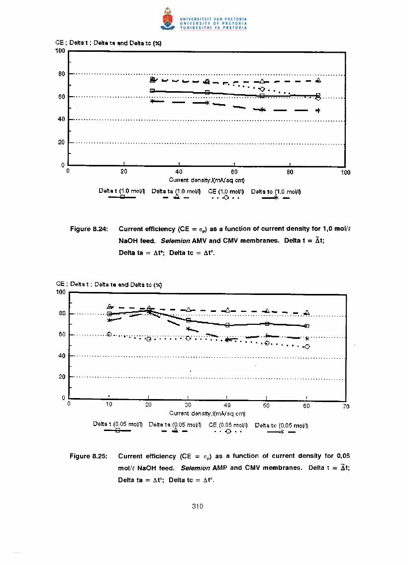
CE : Delta t : Delta ta and Delta tc (%)100
........................................................................................................~----4_~--~----£.....J:I Q .-0- .....
....................................................................... . Ea ...............•.•. g .=+-- - ~--
-- -.. - - .jc
20 40 60 80Current density,l(rnAjsq crr(J
Delta t 11.0 moV~ Delt~ta .2.0_moV~ C~ .('~ ~o~~ Delta tc .~.~OV~
Figure 8.24: Current efficiency (CE = €p) as a function of current density for 1,0 mol/~
NaOH feed. Selemion AMV and CMV membranes. Delta t = Xt;
Delta ta = ~ta; Delta tc = ~tc.
CE : Delta t ; Delta ta and Delta tc (%)100 .............:.-~..=-~~ ..~..~..~.~..~..~..~~..~..~..4 .
•••••••. 0 0 LoooEJ~
............. iLl•.•.•.•. ;... ·0··············· J" •••••• ~ ••• ~ ••••• _ •• *"-..._ ..d.> •••••••••••••.. --..... ..•..• • ••••• .L"\
.,.....1" •••••• -0
, 0 20 30 40 50 60Current density,l(mA,isq crr(J
Delta t (0.05 moV~ Delta ta (0.05 moV~ CE (0.05 mO~'~1 Delta tc (0.05 moV~Ea -.;.;.:.,- •• .().. -#:-
Figure 8.25: Current efficiency (CE = €p) as a function of current density for 0,05
mol/~ NaOH feed. Selemion AMP and CMV membranes. Delta t = Xt;
Delta ta = ~tC; Delta te = ~tc.
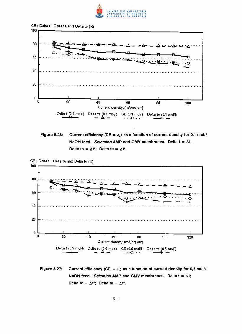
CE : Delta t : Delta ta and Delta te (%)100
•••••••••• ":"'!' •• ..I::.._._ A ._ .to. _ A .". .A.. .A. ~ .~.. ._ .•.••..•••.. ~ 0"-' '.;,I~' _o';-.:a,0';':'" ._.~ .. ~ .. ~ .......•
G. ~-tl:l•• a<i) •• ~ •............................... ~~ ..•.~.~.~.~ .
.L.or.J •••• ~ ••• ·liI. . 0-----..: ~. ~ ..~
40 60Current density,l(mNsq err(!
Delt~ta 2·~mov~ C.E .(0.6 ~oy~Delta t (0.1 moV~(;I
Figure 8.26: Current efficiency (CE = €p) as a function of current density for 0,1 mol/~
NaOH feed. Selemion AMP and CMV membranes. Delta t = Xt;
Delta tc = atC; Delta ta = ata•
CE ; Delta t : Delta ta and Delta te (%)100
......~ ..~ ..~ ..~ ..~ ..~ ..~~ ..~ ..~. '~;;.'~"~"~'~"~"~"~'.~ .
0 .•• ,*=- ~ ---e D tiI................:.:.:.~~.'..,~~.~.'.~?e ~...... 0 .. ·EJ······,,-0 ~ 0 -8*""'" -- :+-- - +:
40 60 80 100Current density,l(rnAjsq err(!
Delta ta ~~.5moV~ CE (0.5mol(~ Delta te .~.5_mo~'~- -- .. ..() ..Delta t (0.5 mo~'~IiOl
Figure 8.27: Current efficiency (CE = €p) as a function of current density for 0,5 mol/Q
NaOH feed. Selemion AMP and CMV membranes. Delta t = At;
Delta tc = a tC; Delta ta = a e.
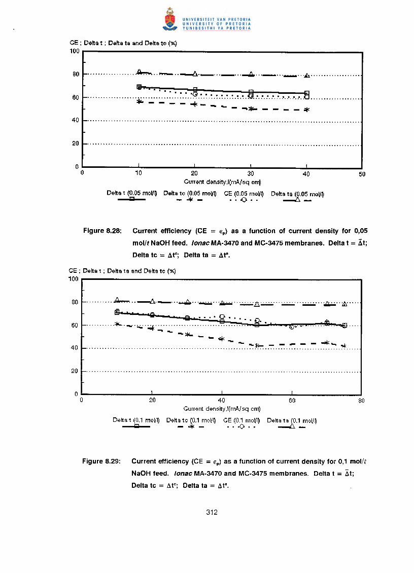
CE : Delta t : Delta ta and Delta to (%)100
••••••••••• 0.0 ••••• ~. ~. ~. ~. ~. ~. ~. ~. ~. ~~.:.:. ~. ~. ~. ~. ~. ~ .~ •• " •• " •• ". 0"' ." •• " •• " •• " •• " •• f3 .*"- -..1..0-r"-~~ - •••::i'- - - - - .:t:
20 30Current density,l(rlLt\isq orr(!
Delta t (0.05 moV~ Delta to (0.05 moV~ CE (0.05 moV~ Delta ta (0.05 moV~IiiiI --+:_ ""~"" ~_
Figure 8.28: Current efficiency (CE = €p) as a function of current density for 0,05
mol/QNaOH feed. lonac MA-3470 and MC·3475 membranes. Delta t = Xt;
Delta tc = AtC; Delta ta = Ate.
CE ; Delta t : Delta ta and Delta to (%)100
Ilk ' ,
, , , .. , 'O*"-. _";,,;." ;, ~, ,', ,",,",,",.•, .~. ~.~,~,~ " B" " ,- - -*- - - "* -, , , .. , , , , , , , .. , , . , , , , , . , , , , , , ~, ,~ J~ ..~ ..-:-:, .":":, .-:-:, ,~ ..~ ~ ..~:, , , , ,
• 0~' ~.i, , , , , ..31.,~ , . , .
40Current densit,,!,I(mAhq cnil
D8lta t W1 moll'~1 Delta tc (0,1 moll'~1 CE (0,1 Mtjll'~ Delta ta m.1 moll'rlIiiiI -4- "".c.". --.1::,,-'
Figure 8.29: Current efficiency (CE = €p) as a function of current density for 0,1 mol/Q
NaOH feed. lonac MA-3470 and MC-3475 membranes. Delta t = ~t;
Delta tc = atC; Delta ta = ae.
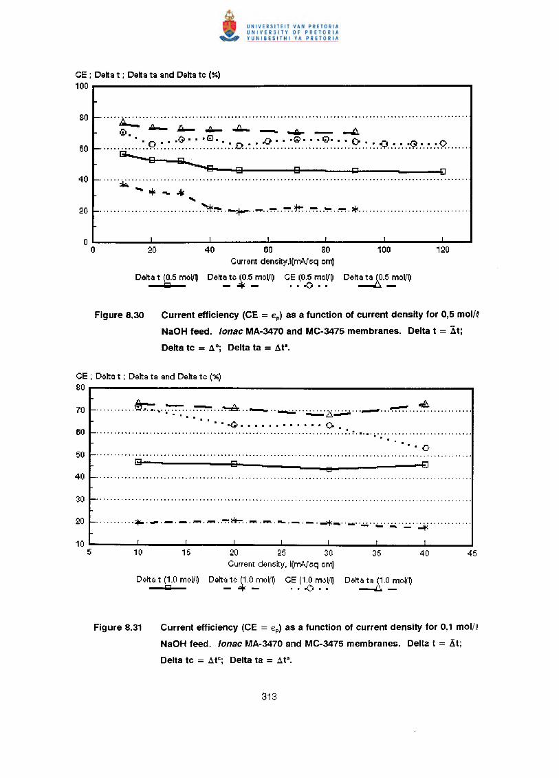
CE : Delta t : Delta ta and Delta to (%)100
......~ .@ • ill-- i:J.- ~ ~ _ .•..••••_ ....I::..
• • 0 • • .Q. • •lEI. • .0 • • •G· • •~. • • O· ~ ~ 0.................................... : . .Q. ~.~ ~.:'-:'.0-0 0-. o-.-..;JI.:.:. 0-0 .
..... .:iI',. ......• -"'" •••
............................ .~~ .. -=f+'- .. _ .. ~ .. ,:",:".~..":"':..~ .."!"'l. * .
20 40 60 80 100Current density,l(rMJsq om)
Delta t ~.5 molJ~ Delt~to .f.5_mOIJ~ C; .(0;& ~oy~ Delta ta 2.~olJ~
Current efficiency (CE = €p) as a function of current density for 0,5 mol/~
NaOH feed. lonse MA-3470 and MC-3475 membranes. Delta t = Xt;
Delta tc = aC; Delta ta = ata•
CE : Delta t : Delta ta and Delta to (%)80
........... ~ .•..~ ~ ~ _ ....•...••....................-- ~ ~ .. . .. . . . --....- ~~• • -Q. • • • • • • • • • • • 0 .
.. ............. ......... ....... . ............... .. .... . ... . ............ .•.~.....•............................ . .
. .... . ... ..~ . .,.. .- ._ .....•...•....~~ ....•............... _. - .~ ..•...••.................................-'--~-..if:
Current density, l(m,Vsq om)
Delta t (1.0 m(oll'~ Detta_to _(~.O_m(oll·(1 CE (1.0 moll'(1 Dett:~ta (1.0 moll'~c 4: . . .() . . -....L:.. _
Current efficiency (CE = €p) as a function of current density for 0,1 mol/Q
NaOH feed. lonse MA-3470 and MC-3475 membranes. Delta t = ~t;
Delta tc = a tC; Delta ta = a ta•
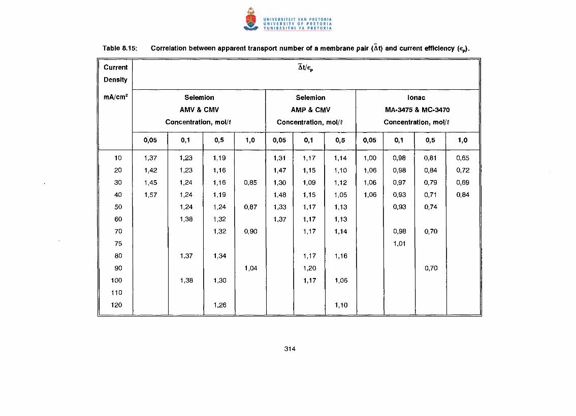
Current At/€p
Density
mA/cm2 Selemion Selemion lonac
AMV & CMV AMP & CMV MA·3475 & MC·3470
Concentration, mol/Q Concentration, mol/Q Concentration, mol/Q
0,05 0,1 0,5 1,0 0,05 0,1 0,5 0,05 0,1 0,5 1,0
10 1,37 1,23 1,19 1,31 1,17 1,14 1,00 0,98 0,81 0,65
20 1,42 1,23 1,16 1,47 1,15 1,10 1,06 0,98 0,84 0,72
30 1,45 1,24 1,16 0,85 1,30 1,09 1,12 1,06 0,97 0,79 0,69
40 1,57 1,24 1,19 1,48 1,15 1,05 1,06 0,93 0,71 0,84
50 1,24 1,24 0,87 1,33 1,17 1,13 0,93 0,74
60 1,38 1,32 1,37 1,17 1,13
70 1,32 0,90 1,17 1,14 0,98 0,70
75 1,01
80 1,37 1,34 1,17 1,16
90 1,04 1,20 0,70
100 1,38 1,30 1,17 1,06
110
120 1,26 1,10
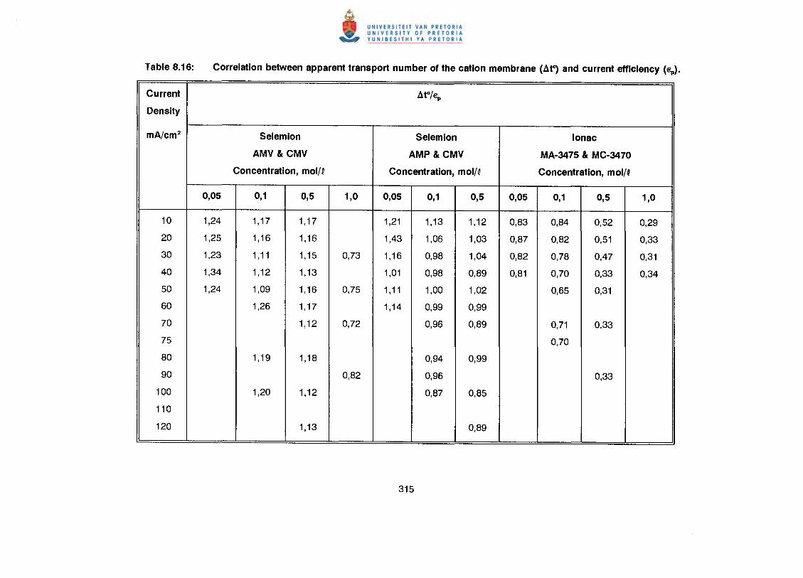
Current I1tC/€p
Density
mA/cm2 Selemion Selemlon lonac
AMV & CMV AMP & CMV MA-3475 & MC·3470
Concentration, moll ~ Concentration, moll ~ Concentration, mol/q
0,05 0,1 0,5 1,0 0,05 0,1 0,5 0,05 0,1 0,5 1,0
10 1,24 1,17 1,17 1,21 1,13 1,12 0,83 0,84 0,52 0,29
20 1,25 1,16 1,16 1,43 1,06 1,03 0,87 0,82 0,51 0,33
30 1,23 1,11 1,15 0,73 1,16 0,98 1,04 0,82 0,78 0,47 0,31
40 1,34 1,12 1,13 1,01 0,98 0,89 0,81 0,70 0,33 0,34
50 1,24 1,09 1,16 0,75 1,11 1,00 1,02 0,65 0,31
60 1,26 1,17 1,14 0,99 0,99
70 1,12 0,72 0,96 0,89 0,71 0,33
75 0,70
80 1,19 1,18 0,94 0,99
90 0,82 0,96 0,33
100 1,20 1,12 0,87 0,85
11O
120 1,13 0,89
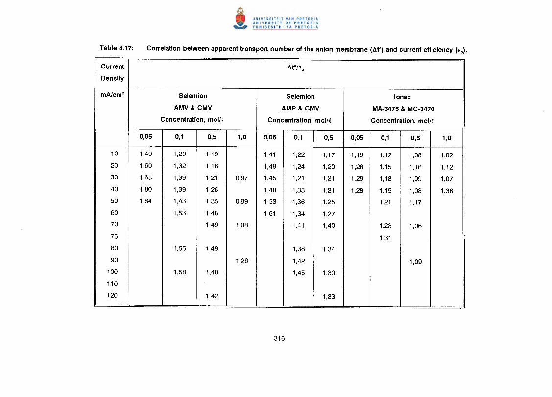
Current /1t8/€p
Density
mA/cm2 Selemion Selemion lonac
AMV & CMV AMP & CMV MA·3475 & MC·3470
Concentration, mol/Q Concentration, mol/Q Concentration, mol/Q
0,05 0,1 0,5 1,0 0,05 0,1 0,5 0,05 0,1 0,5 1,0
10 1,49 1,29 1,19 1,41 1,22 1,17 1,19 1,12 1,08 1,02
20 1,60 1,32 1,18 1,49 1,24 1,20 1,26 1,15 1,16 1,12
30 1,65 1,39 1,21 0,97 1,45 1,21 1,21 1,28 1,18 1,09 1,07
40 1,80 1,39 1,26 1,48 1,33 1,21 1,28 1,15 1,08 1,36
50 1,84 1,43 1,35 0,99 1,53 1,36 1,25 1,21 1,17
60 1,53 1,48 1,61 1,34 1,27
70 1,49 1,08 1,41 1,40 1,23 1,06
75 1,31
80 1,55 1,49 1,38 1,34
90 1,26 1,42 1,09
100 1,58 1,48 1,45 1,30
11O
120 1,42 1,33
mol/q feed (30 to 50 mNcm~. The ratio Xt/€p for the Selemion AMP and CMV
membranes varied between 1,1 and 1,2 (0,1 mol/q feed, 10 to 70 mNcm~ and was
1,1 at 0,5 mol/q feed concentration (10 to 70 mNcm~. Therefore, satisfactory
correlations were obtained between the apparent transport numbers and current
efficiency in the 0,1 to 0,5 mol/q feed concentration ranges.
Very satisfactory correlations were obtained between at/€p in the 0,05 to 0,1 mol/q
feed concentration range for the lonac membranes (Fig's 8,28 and 8,29). The ratio
at/€p varied between 1 and 1,1 (10 to 40 mNcm2, 0,05 mol/D) and between 0,9 and
1,0 (10 to 70 mNcm2, 0,1 mol/q feed). The correlation, however, at 0,5 and 1,0 mol/D
feed concentration was not satisfactory. The ratio at/€p varied between 0,7 and 0,8
at 0,5 mol/D feed concentration and between 0,7 and 0,8 at 1,0 mol/D feed
concentration. Therefore, it should be possible to predict membrane performance for
caustic soda concentration/desalinationwith ED with an accuracy of approximately 20%
from the apparent transport numbers of the membrane pair. However, the accuracy
of the predictions will depend on the feed concentration used.
Satisfactory correlations were obtained between the apparent transport numbers of the
cation membrane (atC) and current efficiency in the case of the Selemion and lonac
membranes (Table 8.16). The ratio between MC/€p varied between 1,1 and 1,2 in the
0,1 to 0,5 mol/D feed concentration range (10 to 120 mNcm~ for the Selemion AMV
and CMV membranes (Table 8.16). The same correlation was approximately 1,2 at 0,5
mol/D feed concentration (10 to 50 mNcm~ and varied between 0,7 and 0,8 at 1,0
mol/D feed concentration (30 to 90 mA/cm~. The ratio between atc/€p varied between
1,1 and 1,2 (0,05 mol/D feed; 10 to 60 mNcm2); 1,0 and 1,1 (0,1 mol/D feed; 10 to
90 mNcm~ and between 0,9 and 1,1 (0,5 mol/D feed; 10 to 80 mNcm2) for the
Selemion AMP and CMV membranes. The ratio atc/€p was approximately 0,8 (0,5
mol/D feed; 10 to 40 mNcm2) and varied between 0,7 and 0,8 (0,1 mol/D feed; 10
to 70 mNcm~ in the case of the lonac membranes. However, a much poorer
correlation was obtained at 0,5 and 1,0 mol/D feed concentration as a result of the low
selectivity of the cation membrane for sodium ions as a result of the high mobility of
the hydroxyl ion(30)(Table 8.16). Therefore, it appears that membrane performance for
caustic soda concentration/desalination can also be predicted from the apparent
transport number of the cation membrane with an accuracy of approximately 20%.
Satisfactory correlations were obtained between the apparent transport number of the
anion membrane (a e) and current efficiency in the case of the Selemion AMV and CMV
- (1,0 mol/Q feed) and lonac membranes (1,0 mol/Q feed) (Table 8.17). The ratio
I!..ta/epvaried between approximately 1 and 1,1 in the case of the Selemion AMV and
CMV membranes (30 to 70 mNcm~. The ratio I!..ta/epvaried between 1 and 1,1 in the
case of the lonac membranes (10 to 30 mNcm~. Poorer correlations of I!..~/epwere
obtained at the other feed concentrations (Table 8.17). Consequently, it should be
possible to predict membrane performance for caustic soda concentration/desalination
applications with an accuracy of approximately 10% from the apparent transport
number of the anion membrane at high (1,0 molN) feed concentration.
Water flow (J) through the membranes as a function of current density and feed water
concentration is shown in Figures 8.32 to 8.34. Water flow (J;) through the membranes
relative to the flow at JO,5 moVI is shown in Table 8.18. Water flow through the
membranes increases as a function of current density. Volume flow through the
Selemiom AMV and CMV membranes increased in the 0,05 to 0,1 mol/Q feed
concentration range (Table 8.18). However, volume flow decreased slightly in the 0,1
to 0,5 mol/Q feed concentration range at higher current densities and volume flow
remained approximately constant at 1,0 mol/Q feed concentration. Current efficiency
increased significantly in the 0,05 to 0,1 mol/Q feed concentration range (Fig. 8.18) as
a result of the increased water flow. Current efficiency, however, was significantly
higher at 1,0 mol/Q feed concentration (Fig. 8.18) than at 0,01 and 0,5 mol/Q feed,
despite a slightly lower volume flow.
Volume flow decreased in the case of the Selemion AMP and CMV membranes in the
feed concentration range from 0,05 to 0,5 mol/Q (Table 8.18). Current efficiencies,
however, were approximately the same especially at the two higher feed concentrations
(Fig. 8.19).
Volume flow was slightly higher at 0,1 mol/Q feed concentration in the case of the
lonac membranes in the beginning of the run. It is interesting to note that current
efficiency has also been slightly higher at this feed concentration (Fig. 8.20). However,
current efficiency was approximately the same in the feed concentration range from
0,05 to 1,0 mol/Q. Nevertheless, it also appears with caustic soda solutions as has
been the case with sodium chloride solutions that increasing water flow can cause an
increase in current efficiency.
Waterflow (J) through the membranes as a function of effective current density, I.ff, and
feed concentration is shown in Figures 8.35 to 8.37. Straight lines were obtained at
higher values of I.ff• The slope of these lines corresponds to the combined electro-
osmotic coefficient (2~) of a membrane pair. The electro-osmotic coefficients as a
function of caustic soda feed water concentration is shown in Figures 8.38 to 8.40. The
electro-osmotic coefficients decreased sharply with increasing feed concentration in the
case of the Selemion AMV and CMV membranes (Figs. 8.38). It is interesting to note
that the electro-osmotic coefficients have decreased over the entire feed concentration
range from 0,05 to 1,0 mol/Q. A similar effect was observed with the Selemion AMP
and CMV membranes but the decrease in the electro-osmotic coefficients were far less
(Fig. 8.39). These membranes, therefore, deswelliess than the Selemion AMV and
CMV membranes with increasing feed concentration. The lonac membranes also
showed less deswelling than the Selemion AMV and CMV membranes (Fig. 8.40).
The effect of the electro-osmotic coefficient on the maximum caustic soda brine
concentration, cb max, is shown in Table 8.19. Maximum caustic soda brine
concentration increases with decreasing electro-osmotic coefficient. The electro-
osmotic coefficient of the Selemion AMP and CMV membranes were lower than that
of the Selemion AMV and CMV and lonac membranes. The electro-osmotic coefficient
of the Selemion AMP and CMV membranes were determined at 0,155 Q/Faraday at 0,1
mol/Q feed concentration. The coefficients for the Selemion AMV and CMV and lonac
membranes at the same feed concentration were 0,179 and 0,193 Q/Faraday,
respectively. Therefore, higher caustic soda brine concentrations could be obtained
with the Selemion AMP and CMV membranes.
Approximately 8 to 9 mol H20/Faraday passed through the Selemion AMP and CMV
membranes in the feed concentration range between 0,1 and 0,5 mol/Q (Table 8.19).
Approximately 8 to 10 and 10 to 11 mol H20/Faraday passed through the membranes
in the case of the Selemion AMV and CMV and lonac membranes, respectively (0,1 to
0,5 mol/Q feed).
The osmotic flow (Josm) relative to the total flow (J) through the membranes as a
function of current density is shown in Table 8.20. The osmotic water flow through the
membranes decreases with increasing current density. Osmotic water flow
represented 45,9; 46,9 and 26,5% of the total flow through the membranes at a
current density of 30 mA/cm2 in the case of the Selemion AMV and CMV; Selemion
AMP and CMV and lonac membranes, respectively. Therefore, osmosis makes a
significant contribution to water flow through the membranes at relative low current
density. The osmotic contribution to total flow through the membranes (Selemion AMV
and CMV and Selemion AMP and CMV) at a current density of 100 mA/cm2 (0,1 mol/Q
feed) was 21,4 and 25,7%, respectively. The osmotic contribution to the total flow in
the case of the lonac membranes at a current density of 70 mA/cm2 (0,1 mol/Q feed)
was 14,2%. Therefore, the contribution of osmotic water flow to total water flow
through the membranes is much lower at high current density.
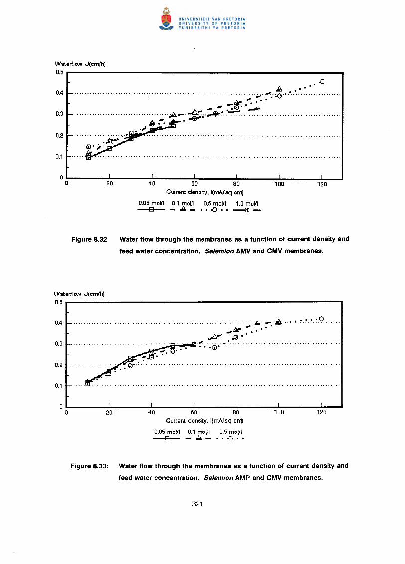
Waterflcw, J(errv'h)0.5
• • .0.&:.. ••••
..•...••••.•..............••••.......••••••........••••..•.................••............ ;.;.0 .~. ~,=".. " ..... " .... """""""."fir"' .•
~ ~GJ·-';"+..................................... 'J;J._. ~~ ..::.. .•.:~ .
A ~ • ..t!!l"'.oil!'- ••..~
0.2 ....................•.••"ftJ-@.;,
40 60 80Current density, l(nWsq em)
0.05 moVI 0.1 moVI 0.5 moVI 1.0 moVI9 -~_ •• -8 •• ~-
Figure 8.32 Water flow through the membranes as a function of current density and
feed water concentration. Selemion AMV and CMV membranes.
Waterflcw. J(errv'h)0.5
•••• 0·0 •••••••••••••••••••••••••••••••••••••••••••••••••••••••••••••••••••••••••• ·A· .~ ..-b...•. ~.~.~.~.~.9 .fir~ .•..,.. ..
~ IJ··.'="= ........•. ~ .............•...................•...................... • ·0-
......................... ..0··~"····"··"··o""""",,,,, .. ..
40 60 80Current densit"!f. l(rMJsq em)
0.05 moll'l 0.1 moll'l 0.5 moVID -~_ .. -::-..
Figure 8.33: Water flow through the membranes as a function of current density and
feed water concentration. Selemion AMP and CMV membranes.
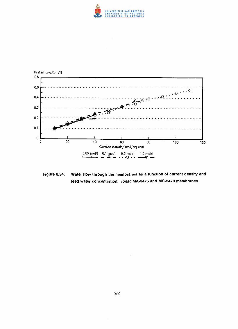
Waterflcw,J(emflV0.6
0' ••. 0
.......................................................... ''A,;;.:j; .~G'" .•.•...0.~.~.: .01'. • -tJ- •
........................................ .~ .. , ..:-.~.: .."".ooI'! • •
~ .
40 60 80Current density,I(m.Nsq em)
0.05 moll I 0.1 mo~'1 0.5 molll 1.0 molll9 ...:i.- .. -o .. ~-
Figure 8.34: Water flow through the membranes as a function of current density and
feed water concentration. lonac MA-3475 and MC-3470 membranes.
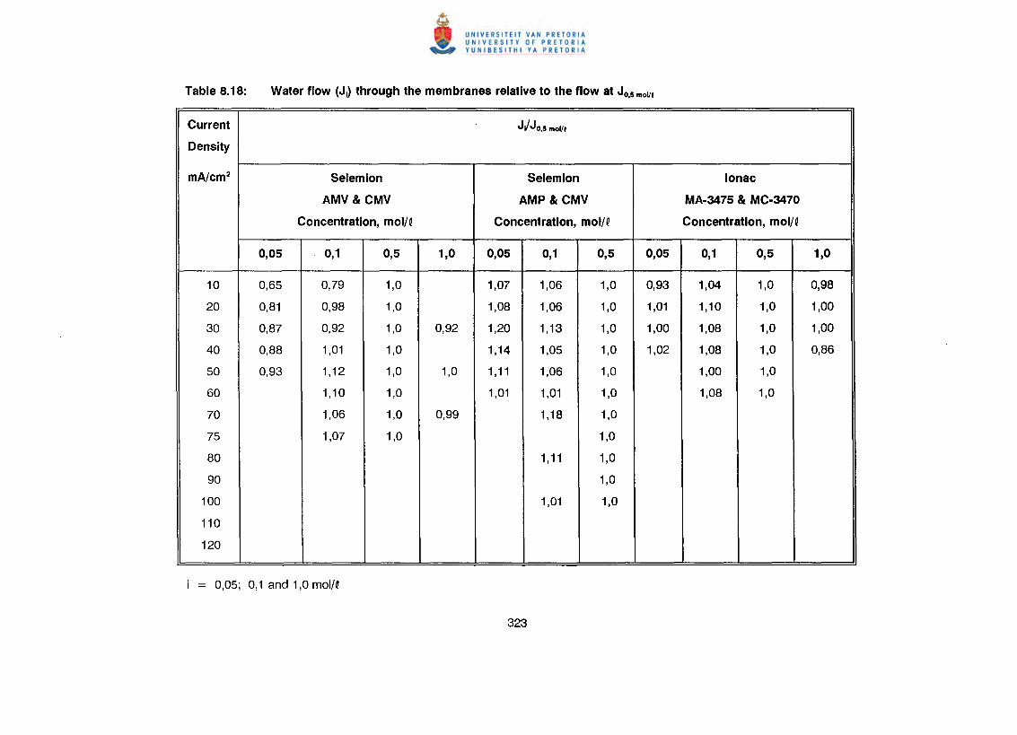
Current JJJO,5 mol/l
Density
mA/cm2 Selemion Selemlon lonac
AMV & CMV AMP & CMV MA·3475 & MC·3470
Concentration, mol/Q Concentration, mol/Q Concentration, mol/Q
0,05 0,1 0,5 1,0 0,05 0,1 0,5 0,05 0,1 0,5 1,0
10 0,65 0,79 1,0 1,07 1,06 1,0 0,93 1,04 1,0 0,98
20 0,81 0,98 1,0 1,08 1,06 1,0 1,01 1,10 1,0 1,00
30 0,87 0,92 1,0 0,92 1,20 1,13 1,0 1,00 1,08 1,0 1,00
40 0,88 1,01 1,0 1,14 1,05 1,0 1,02 1,08 1,0 0,86
50 0,93 1,12 1,0 1,0 1,11 1,06 1,0 1,00 1,0
60 1,10 1,0 1,01 1,01 1,0 1,08 1,0
70 1,06 1,0 0,99 1,18 1,0
75 1,07 1,0 1,0
80 1,11 1,0
90 1,0
100 1,01 1,0
110
120
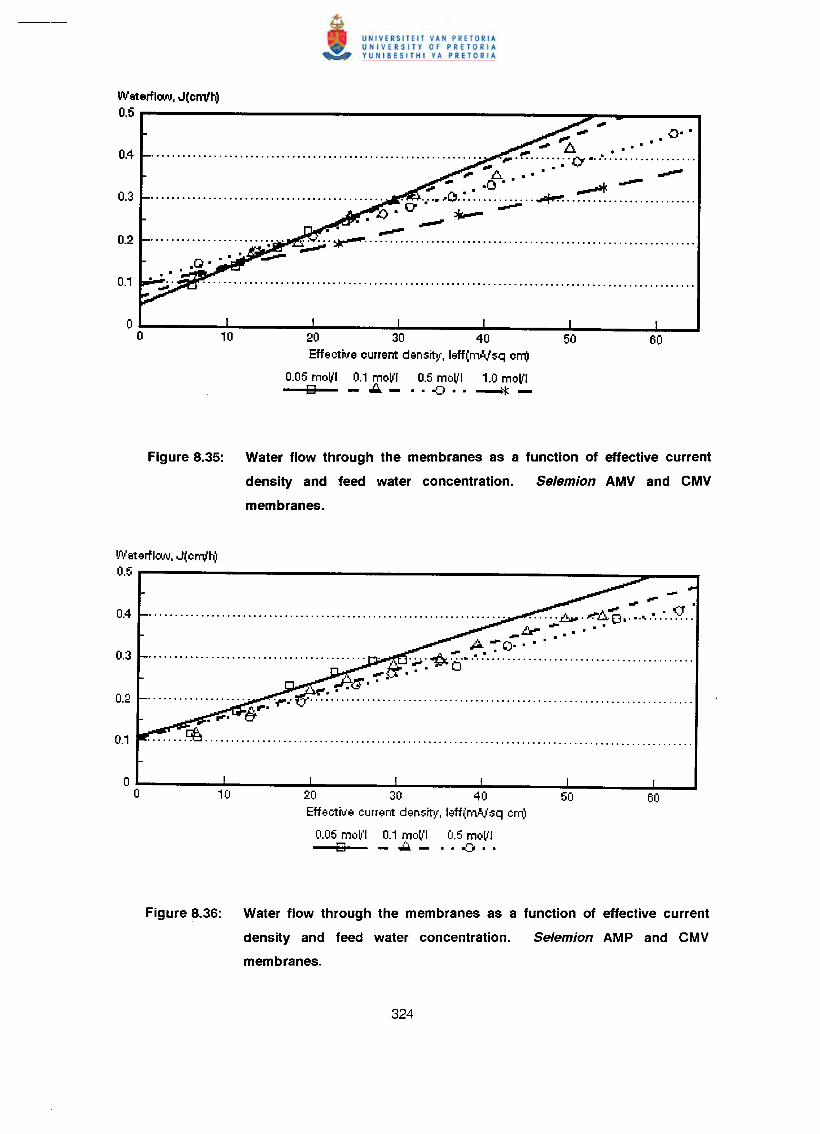
Waterflcw, J(crrv'h)0.5
~ . o· .,,~ .................................................................... ~ ..~ , :. ~ . t:';1 •....................
... ~ --CttI' ~ .0· . ..........-* --
............................................. . ....•..0. ~.: ~ .;;0.0' ~--. ".,.-~:;::.:".;...;.;..~ .
~
20 30 40Effeetwe current density, leff(mAJsq crr(!
0.05 moltl 0.1 moltl 0.5 mo~'1 1.0 molt(D -..:.. - •• ~ • • --.."1: -
Figure 8.35: Water flow through the membranes as a function of effective current
density and feed water concentration. Selemion AMV and CMV
membranes.
Waterfl(((IJ, J(crrv'h)0.5
20 30 40Effeetro/e current densrr\l, leff(rrt,!,Jsq em,'
0.05 moll'l 0.1 moll'l 0.5 moll'lo -~_ .. .() ..
Figure 8.36: Water flow through the membranes as a function of effective current
density and feed water concentration. Selemion AMP and CMV
membranes.
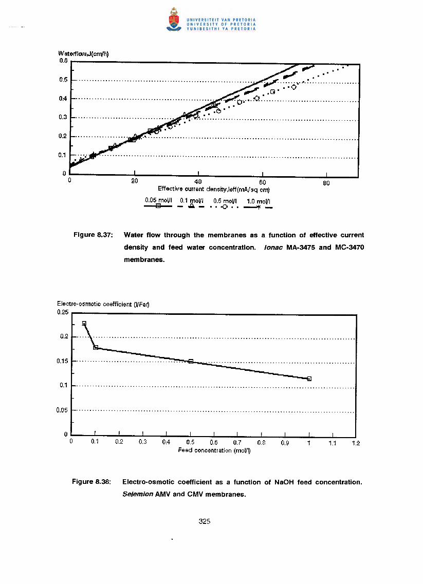
WaterfIOO\l,J( cml~0.6
20 40 60Effective current density,leff(rnAlsq cni
0.05 moltl 0.1 moltl 0.5 moltl 1.0 moltl9 -"- •• .() •• --t:-
Figure 8.37: Water flow through the membranes as a function of effective current
density and feed water concentration. lonac MA-3475 and MC-3470
membranes.
Electro-osmotic coefficient (ltFa~0.25
0.4 0.5 0.6 0.7 0.8Feed concentration (mol1r)
Figure 8.38: Electro-osmotic coefficient as a function of NaOH feed concentration.
Selemion AMV and CMV membranes.
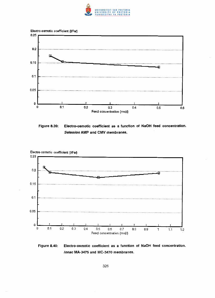
Electro-osmotio ooeffioient (VF8~0.25
•••••• ~"JII!I •• :"""!'••• -...... ...---....,;,,;,,;~:..:.:.:..:.:..~=............................................................~
02 O~ OAFeed ooncentration (moVO
Figure 8.39: Electro-osmotic coefficient as a function of NaOH feed concentration.
Selemion AMP and CMV membranes.
Electro-osmotio ooefficient (VF8~0.25
0.2 .. ~ ~ .
zEIo:
0.5 o.e; 0.7Feed concentration (moll'(1
Figure 8.40: Electro-osmotic coefficient as a function of NaOH feed concentration.
lonac MA·3475 and MC-3470 membranes.
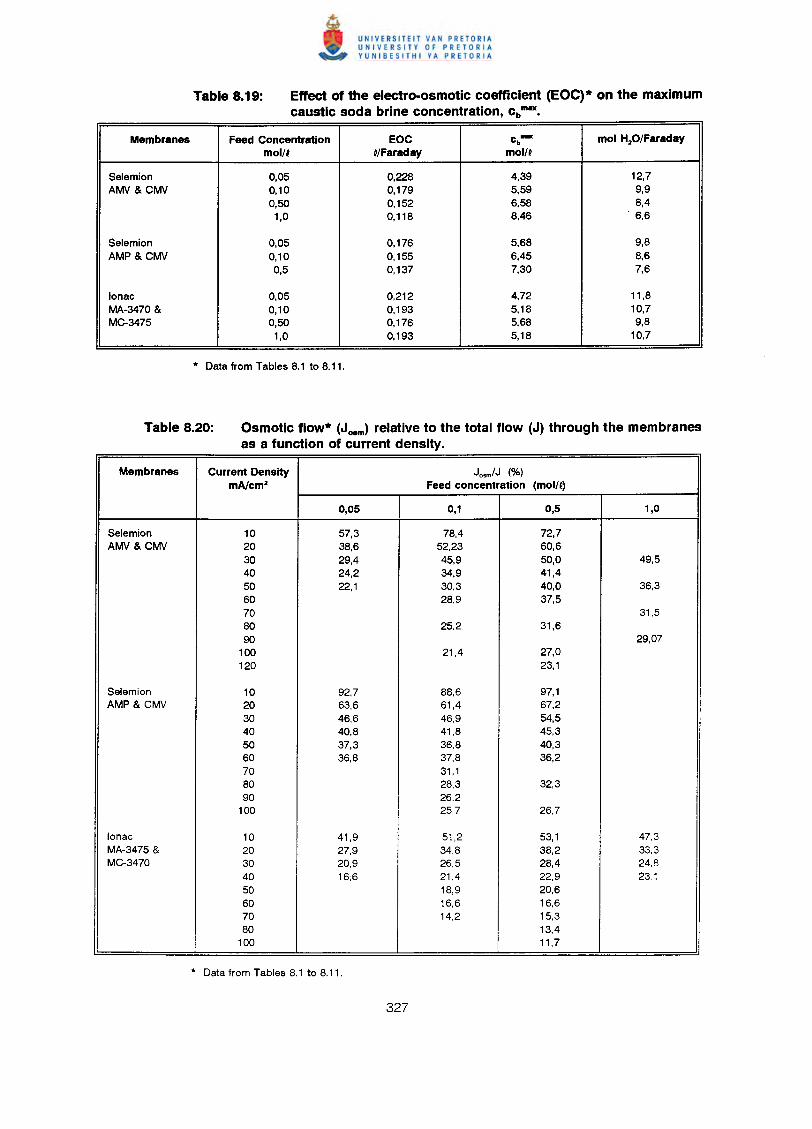
Effect of the electro-osmotic coefficient (EOC)* on the maximumcaustic soda brine concentration, cb mG.
Membranes Feed Concentration EOC c- mol H.O/Faradayb
mol/' #lFaraday mol/'
Selemion 0,05 0,228 4,39 12,7AMV &CMV 0,10 0,179 5,59 9,9
O,SO 0,152 6,58 8,41,0 0,118 8,46 6,6
Selemion 0,05 0,176 5,68 9,8AMP & CMV 0,10 0,155 6,45 8,6
0,5 0,137 7,30 7,6
lonae 0,05 0,212 4,72 11,8MA-3470 & 0,10 0,193 5,18 10,7MC-3475 O,SO 0,176 5,68 9,8
1,0 0,193 5,18 10,7
Osmotic flow* (Joem) relative to the total flow (J) through the membranesas a function of current density.
Membranes Current Density Josm/J (%)mAtcm' Feed concentration (mol/,>
0,05 0,1 0,5 1,0
Selemion 10 57,3 78,4 72,7AMV &CMV 20 38,6 52,23 60,6
30 29,4 45,9 50,0 49,540 24,2 34,9 41,450 22,1 30,3 40,0 36,360 28,9 37,570 31,580 25,2 31,690 29,07
100 21,4 27,0120 23,1
Selemion 10 92,7 88,6 97,1AMP & CMV 20 63,6 61,4 67,2
30 46,6 46,9 54,S40 40,8 41,8 45,350 37,3 36,8 40,360 36,8 37,8 36,270 31,180 28,3 32,390 26,2
100 25,7 26,7
lonae 10 41,9 51,2 53,1 47,3MA-3475 & 20 27,9 34,8 38,2 33,3MC-3470 30 20,9 26,5 28,4 24,8
40 16,6 21,4 22,9 23,150 18,9 20,660 16,6 16,670 14,2 15,380 13,4
100 11,7
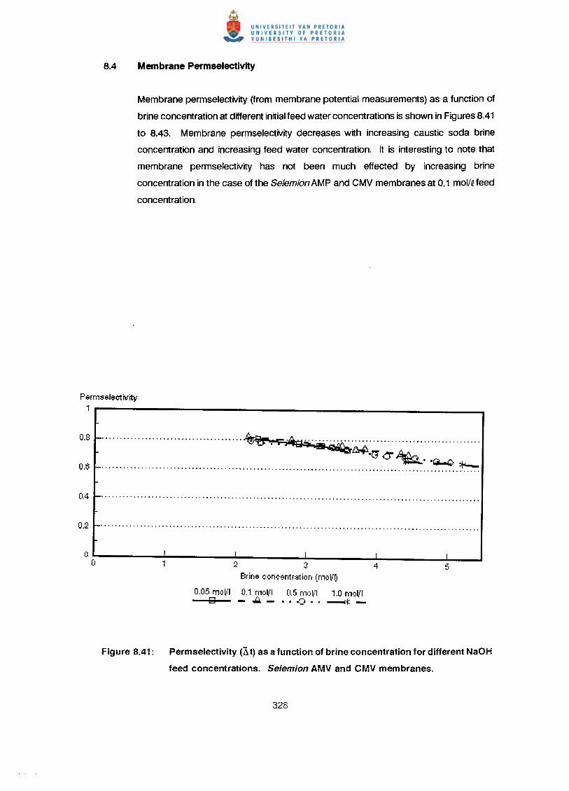
Membrane permselectivity (from membrane potential measurements) as a function of
brine concentration at different initialfeed water concentrations is shown in Figures 8.41
to 8.43. Membrane permselectivity decreases with increasing caustic soda brine
concentration and increasing feed water concentration. It is interesting to note that
membrane permselectivity has not been much effected by increasing brine
concentration in the case of the Selemion AMP and CMV membranes at 0,1 mol/~feed
concentration.
Permselectivity1
....................................... ~~. 'F"i~")r' .•. ~ .lIiIO~.L1 ~ Af.o..~
.~ •. G-O .................................................................................................... ~
234Brine concentration (m.)ll'(1
0.05 mClll'l 0.1 moll'l 0.5 moll'l 1.0 moll'l13 - ••• - ••• ::j •• -f:-
Figure 8.41: Permselectivity (X t) as a function of brine concentration for different NaOH
feed concentrations. Selem/on AMV and CMV membranes.
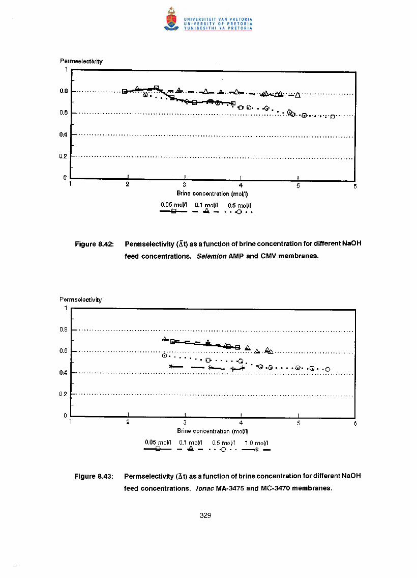
Perm:selectivity1
......••.....•... 9'+<.oi;&r•••..-)o', •• ~•• '- •• ~~ -. A A -- A .Ao. --All..~. • • • ~ .-......-._ ..-...-._ ..~~ .. _.f:l .
... .~ ~.~~. ::. ~ ..~:. :..~.:.~.~ .~ .•Gj.•.•.•.• ·0·······
3 4Brine concentration (moV~
0.05 moVI 0.1 mo~'1 0.5 moVID -':;:"_ .. -:.J! ••
Figure 8.42: Permselectivity (!t) as a function of brine concentration for different NaOH
feed concentrations. Selemion AMP and CMV membranes.
Perm:selectivity1
&.ec - - ~• 'p 'f3:.Q ~ ,................................ ';": .&:. . ~ .
~ .. . • • • . D • . • • .0:+-- - =+-- ~.'.Q.03- •••• @ •• G •• 0
.........................................................................................................
3 4Brine concentration (moll'r)
0.05 moln 0.1 1)10ll'l 0.5 moVI 1.0 moll'lo ..••.- ... ::~.. -H:-
Figure 8.43: Permselectivity (ilt) as a function of brine concentration for different NaOH
feed concentrations. lonac MA-3475 and MC-3470 membranes.
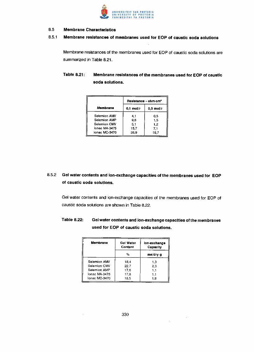
8.5 Membrane Characteristics
8.5.1 Membrane resistances of membranes used for EOP of caustic soda solutions
Membrane resistances of the membranes used for EOP of caustic soda solutions are
summarized in Table 8.21.
Membrane resistances of the membranes used for EOP of caustic
soda solutions.
Resistance - ohm-cm'
Membrane O,t mol/~ 0,5 mollt
Selemion AMI/ 4,1 0,5Selemion AMP 9,6 1,5Selemion CMI/ 5,1 1,2lonac MA-3475 15,7 7,1lonac MC-3470 26,9 15,7
8.5.2 Gel water contents and ion-exchange capacities of the membranes used for EOP
of caustic soda solutions.
Gel water contents and ion-exchange capacities of the membranes used for EOP of
caustic soda solutions are shown in Table 8.22.
Gel water contents and ion-exchange capacities of the membranes
used for EOP of caustic soda solutions.
Membrane Gel Water lon-exchangeContent Capacity
0/0 me/dry g
Selemion AMV 18,4 1,3Selemion CMV 22,7 2,3Selemion AMP 17,6 1,1lonac MA-3475 17,8 1,1lonac MC-3470 18.5 1,8
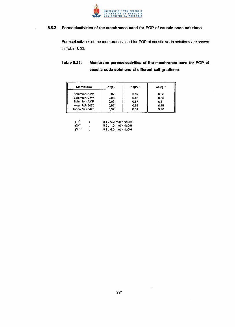
Permselectivities of the membranes used for EOP of caustic soda solutions are shown
in Table 8.23.
Membrane permselectivities of the membranes used for EOP of
caustic soda solutions at different salt gradients.
Membrane At(1)" At(2)"· At(3)"··
Selemion AWN 0,87 0,87 0,83Selemion CWN 0,98 0,83 0,65Selemion AMP 0,93 0,87 0,81lonac MA-3475 0,87 0,82 0,79lonac MG-3470 0,92 0,61 0,46
(1 )"(2)"·(3)"··
0,1 / 0,2 mol/~ NaOH0,5 / 1,0 mol/~ NaOH0,1 / 4,0 mol/~ NaOH
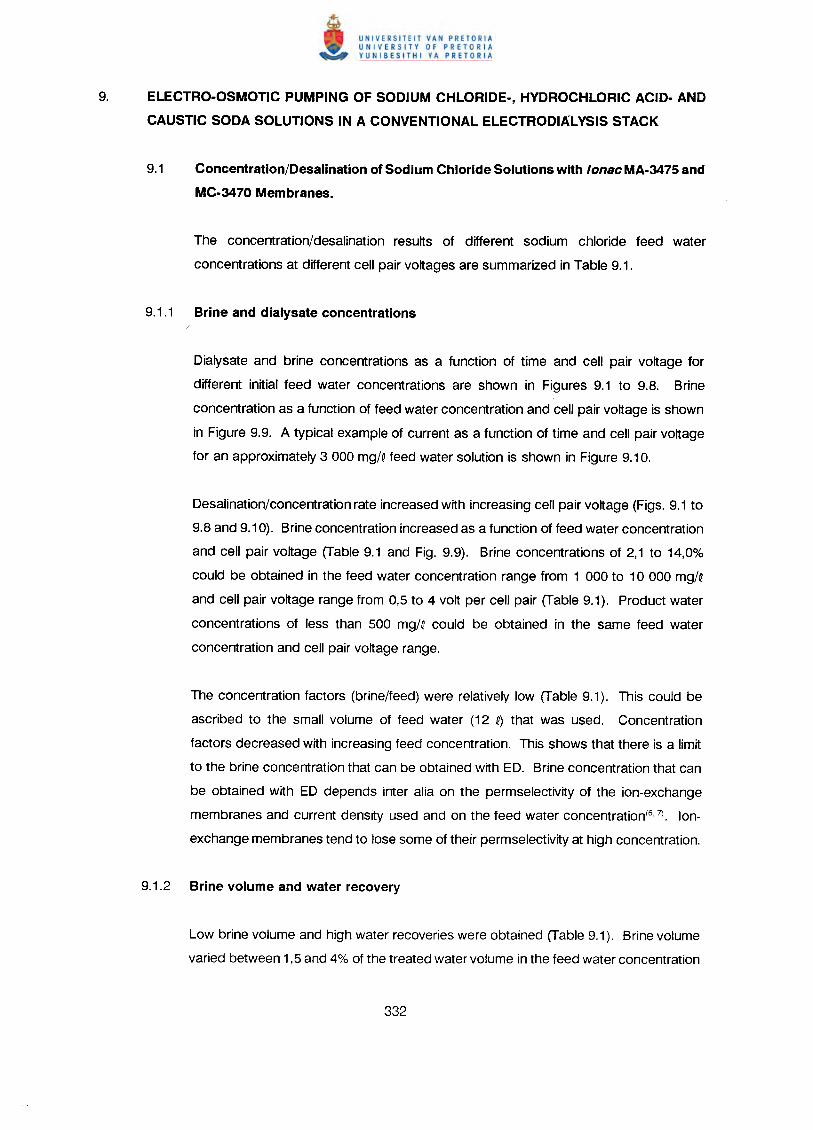
9. ELECTRO-OSMOTIC PUMPING OF SODIUM CHLORIDE-, HYDROCHLORIC ACID- AND
CAUSTIC SODA SOLUTIONS IN A CONVENTIONAL ELECTRODIALYSIS STACK
9.1 Concentration/Desalination of Sodium Chloride Solutions with lonac MA-3475 and
MC-3470 Membranes.
The concentration/desalination results of different sodium chloride feed water
concentrations at different cell pair voltages are summarized in Table 9.1.
Dialysate and brine concentrations as a function of time and cell pair voltage for
different initial feed water concentrations are shown in Figures 9.1 to 9.8. Brine
concentration as a function of feed water concentration and cell pair voltage is shown
in Figure 9.9. A typical example of current as a function of time and cell pair voltage
for an approximately 3 000 mg/Q feed water solution is shown in Figure 9.10.
Desalination/concentration rate increased with increasing cell pair voltage (Figs. 9.1 to
9.8 and 9.10). Brine concentration increased as a function of feed water concentration
and cell pair voltage (Table 9.1 and Fig. 9.9). Brine concentrations of 2,1 to 14,0%
could be obtained in the feed water concentration range from 1 000 to 10 000 mg/Q
and cell pair voltage range from D,S to 4 volt per cell pair (Table 9.1). Product water
concentrations of less than 500 mg/Q could be obtained in the same feed water
concentration and cell pair voltage range.
The concentration factors (brine/feed) were relatively low (Table 9.1). This could be
ascribed to the small volume of feed water (12 Q) that was used. Concentration
factors decreased with increasing feed concentration. This shows that there is a limit
to the brine concentration that can be obtained with ED. Brine concentration that can
be obtained with ED depends inter alia on the permselectivity of the ion-exchange
membranes and current density used and on the feed water concentration(6 7) • lon-
exchange membranes tend to lose some of their permselectivity at high concentration.
Low brine volume and high water recoveries were obtained (Table 9.1). Brine volume
varied between 1,5 and 4% of the treated water volume in the feed water concentration
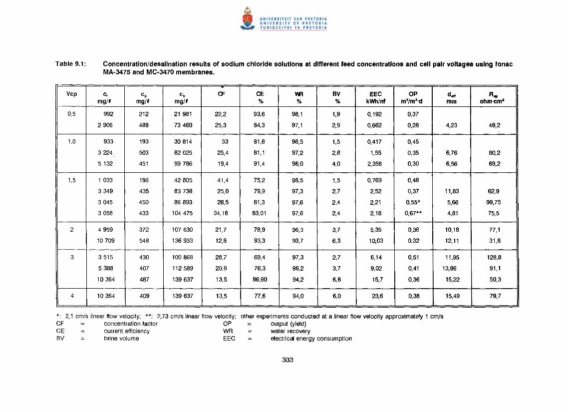
Concentration/desalination results of sodium chloride solutions at different feed concentrations and cell pair voltages using lonacMA·3475 and MC·3470 membranes.
VCp <; cp Cb CF CE VIR BV EEC OP dell Ropmg/I mg/I mg/I % % % kWh/nf m3/m21:1 mm ohm'Cm2
0,5 992 212 21 981 22,2 93,6 98,1 1,9 0,192 0,37
2906 488 73460 25,3 84,3 97,1 2,9 0,662 0,28 4,23 49,2.
1,0 933 193 30814 33 81,8 98,5 1,5 0,417 0,45
3224 503 82025 25,4 81,1 97,2 2,8 1,55 0,35 6,76 80,2
5132 451 99786 19,4 91,4 96,0 4,0 2,358 0,30 6,56 69,2
1,5 1 033 196 42805 41,4 75,2 98,5 1,5 0,769 0,48
3349 435 83738 25,0 79,9 97,3 2,7 2,52 0,37 11,83 62,9
3045 450 86893 28,5 81,3 97,6 2,4 2,21 0,55* 5,66 99,75
3058 433 104475 34,16 83,01 97,6 2,4 2,18 0,67** 4,81 75,5
2 4959 372 107630 21,7 78,9 96,3 3,7 5,35 0,36 10,18 77,1
10709 548 136933 12,8 93,3 93,7 6,3 10,03 0,32 12,11 31,8
3 3515 430 100868 28,7 69,4 97,3 2,7 6,14 0,51 11,95 128,8
5388 407 112589 20,9 76,3 96,2 3,7 9,02 0,41 13,86 91,1
10364 487 139637 13,5 86,90 94,2 6,8 15,7 0,36 15,22 50,3
4 10364 409 139637 13,5 77,6 94,0 6,0 23,6 0,38 15,49 79,7
*: 2,1 cm/s linear flow velocity; **: 2,73 cm/s linear flow velocity;CF concentration factor OPCE current efficiency WRBV == brine volume EEC
other experiments conducted at a linear flow velocity approximately 1 cm/s== output (yield)== water recovery== electrical energy consumption
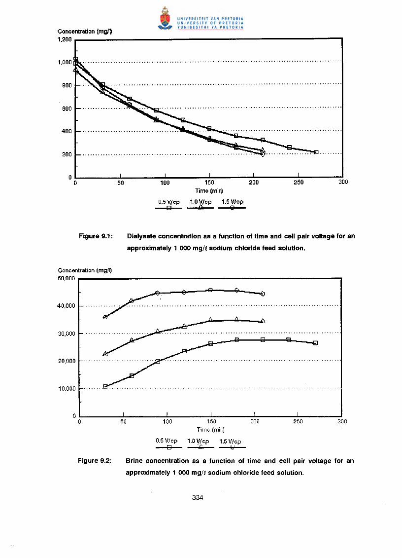
Concentration (mglO1,200
100 150 200Time (mir!)
0.5 Vlcp 1.0 Vlcp 1.5 Vlcpg ~ E?
Dialysate concentration as a function of time and cell pair voltage for an
approximately 1 000 mg/Qsodium chloride feed solution.
Concentration (mg(~50,000
......./: ~ ~ ~ ~ .
00 50 100 150 200 250 300
Time (mir~
0.5 V/cp 1.0 V/cp 1.5 V/cp0 J.d, b'
Brine concentration as a function of time and cell pair voltage for an
approximately 1 000 mg/Qsodium chloride feed solution.
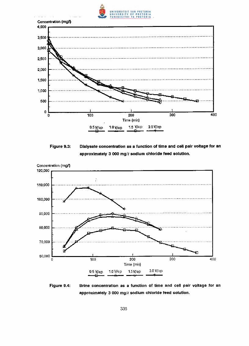
Concentration (mglO4,000
100 200Time (miriJ
0.5V/cp 1.0Vlcp 1.5 V/cp 3.0Vlcpo ~ & *
Dialysate concentration as a function of time and cell pair voltage for an
approximately 3000 mg/q sodium chloride feed solution.
Concentration (mgiO120,000
200Time (miriJ
0.5 Vlcp 1.0 V/cp 1.5V/cpo •• b?3.0 V/cp
••••
60,000 o
Brine concentration as a function of time and cell pair voltage for an
approximately 3 000 mg/Qsodium chloride feed solution.
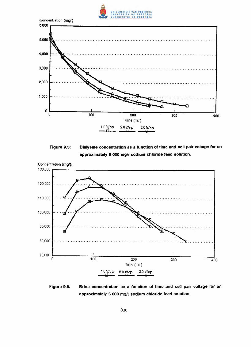
Concentration (mg/~6,000
200Time (mi~
1.0 \fIcp 2.0\ilcp 3.0 \ilcpo "* E?
Dialysate concentration as a function of time and cell pair voltage for an
approximately 5000 mgjQsodium chloride feed solution.
Concentration (mg/~130,000
70,000 o 200Time (mir~
1.0 VI cp 2.0 \il cp 3.0 \iIcpo aIoiL G
Brine concentration as a function of time and cell pair voltage for an
approximately 5000 mgjQsodium chloride feed solution.
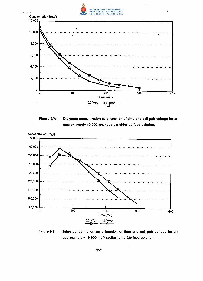
Concentration (mgl~12,000
Concentration (mQ'~170.000
200Time (mi~
2.0 V!cp 4.0 V/cpo .,}
Dialysate concentration as a function of time and cell pair voltage for an
approximately 10 000 mg/~sodium chloride feed solution.
90,000o 200
Time (mirv
2.0 V/cp 4.0 'lJ/cpo ••
Brine concentration as a function of time and cell pair voltage for an
approximately 10 000 mg/~ sodium chloride feed solution.
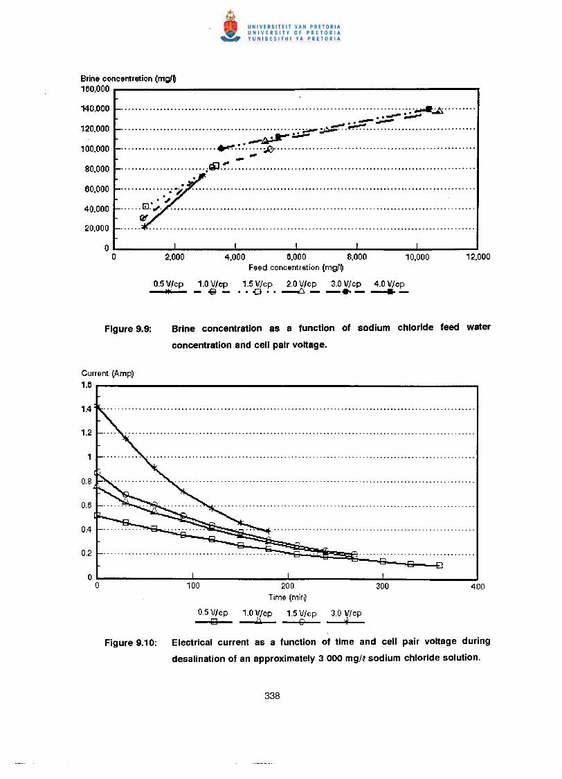
Brine concentration (mgl~160,000
120,000
100,000
80,000
60,000
40,000
20,000
Current (Amp)1.6
................................................................................... ~ ...~~..~~................................................... -.,.- ~.~ , .~:.;.-
.••......•.••••.••......... ~.~: ..... ;J::) .......................•.........••.••••••...................-........................ ,;9J.~ .
.......••..... '.' .,i!; ..........••.................................•.....•.•...••••••.•...•............."
...... I:J." ",. . .•.••.............•.........................................•.....••.................f¥
4,000 6,000 8,000Feed concentration (mgl~
0.5 Vlcp 1.0 Vlcp 1.5 Vlcp 2.0 V/cp 3.0 V/cp 4.0 V/cpl+' -oQ- ··a··~--.- -
Brine concentration as a function of sodium chloride feed water
concentration and cell pair voltage.
200Time (mir~
0.5 Vlcp 1.0 V/cp 1.5 V/cp 3.0 V/cpo ~ G *
Figure 9.10: Electrical current as a function of time and cell pair voltage during
desalination of an approximately 3 000 mg/Qsodium chloride solution.
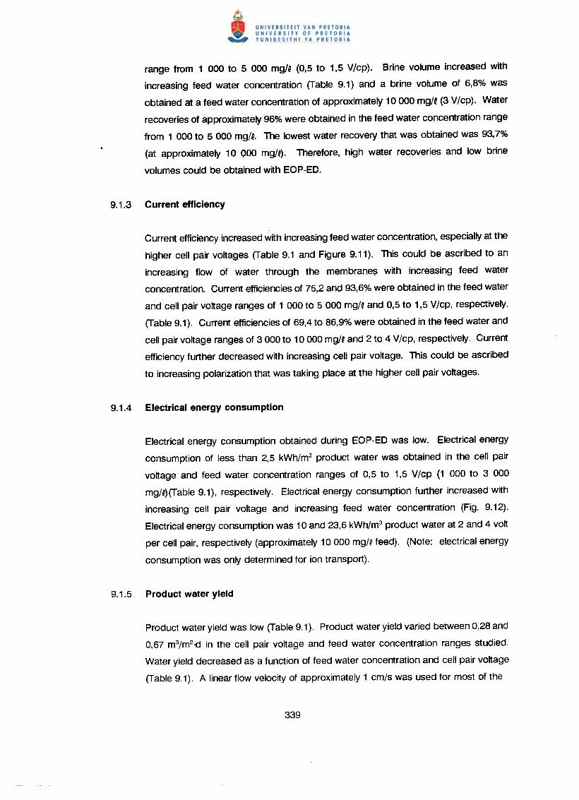
range from 1 000 to 5 000 mg/. (0,5 to 1,5 V/cp). Brine volume increased with
increasing feed water concentration (Table 9.1) and a brine volume of 6,8% was
obtained at a feed water concentration of approximately 10 000 mg/Q (3 V/cp). Water
recoveries of approximately 96% were obtained in the feed water concentration range
from 1 000 to 5 000 mg/•. The lowest water recovery that was obtained was 93,7%
(at approximately 10 000 mg/Q). Therefore, high water recoveries and low brine
volumes could be obtained with EOP-ED.
Current efficiency increased with increasing feed water concentration, especially at the
higher cell pair voltages (Table 9.1 and Figure 9.11). This could be ascribed to an
increasing flow of water through the membrane$ with increasing feed water
concentration. Current efficiencies of 75,2 and 93,6% were obtained in the feed water
and cell pair voltage ranges of 1 000 to 5 000 mg/Q and 0,5 to 1,5 V/cp, respectively.
(Table 9.1). Current efficiencies of 69,4 to 86,9% were obtained in the feed water and
cell pair voltage ranges of 3 000 to 10 000 mg/. and 2 to 4 V/cp, respectively. Current
efficiency further decreased with increasing cell pair voltage. This could be ascribed
to increasing polarization that was taking place at the higher cell pair voltages.
Electrical energy consumption obtained during EOP-ED was low. Electrical energy
consumption of less than 2,5 kWh/m3 product water was obtained in the cell pair
voltage and feed water concentration ranges of 0,5 to 1,5 V/cp (1 000 to 3 000
mg/Q)(Table9.1), respectively. Electrical energy consumption further increased with
increasing cell pair voltage and increasing feed water concentration (Fig. 9.12).
Electrical energy consumption was 10 and 23,6 kWh/m3 product water at 2 and 4 volt
per cell pair, respectively (approximately 10 000 mg/. feed). (Note: electrical energy
consumption was only determined for ion transport).
Product water yield was low (Table 9.1). Product water yield varied between 0,28 and
0,67 m3/m2<l in the cell pair voltage and feed water concentration ranges studied.
Water yield decreased as a function of feed water concentration and cell pair voltage
(Table 9.1). A linear flow velocity of approximately 1 cm/s was used for most of the
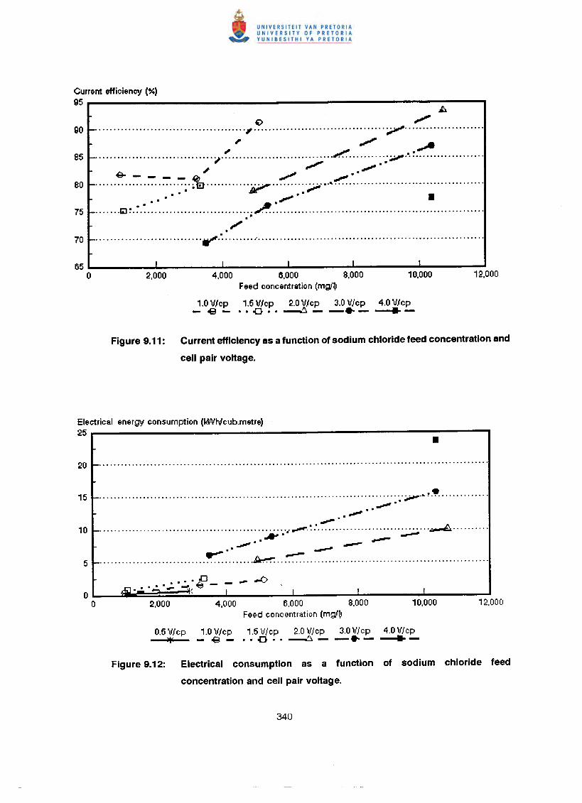
Current efficiency (%)g5 ••••------- ......,JA.
€> """gO ~ ~ T······················, "",.,A
85 f- -; .~ ..............•............. L ;.i'* .•.: ./ ..
80 ~ ~ .. ~ .. :':".. ~ .. ~~. ~"""""'i;i;'" ~.: .? ~:.~.~ ..-.- "".- .
75 ,- ILI ~ • ~ • : •••••••••••••••••••••••••••• ; ~ : •••••••••.••••••.••••••••••••••••••••••••••••••••••••••••,;
70 _ w'." .t ••••••••••••••••••••••••••••••••••••••••••••••••••••••••••••••
65o
I
2,000I
4.000I
6,000Feed concentration (mgl~
I
8,000I
10,000
1.0 Vlcp 1.5 V/cp 2.0 V/cp 3.0 Vlcp 4.0 V/cp- 08 - •• a .. ~ - -. - -
Figure 9.11: Currentefficiencyas afunction of sodium chloride feed concentrationand
cell pair voltage.
Electrical energy consumption (I#VtVcub.metre)25 ••••---------------------------------,
15 ~ ;';-'. ~.~ ...".." ...~ ..,,- .10 f- ~. ~.•............................... ~ .
A".. --.. ~.~ -- --•...... -- ---5~··········································~········· .
.. ···E_ -..".Ai]. • •.:.. ~ ~, -..:::::' I
2,000 4,000I
6,000Feed concentration (mgl~
I
8,000I
10,000
0.5 Vlcp 1.0 V/cp 1.5 V/cp 2.0 V/cp 3.0 V/cp 4.0 V/cpJoin" - 08 - •• a .. ~ - -. - -
Figure 9.12: Electrical consumption as a function of sodium chloride feed
concentration and cell pair voltage.
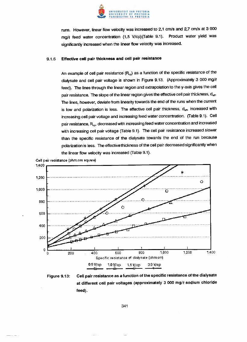
runs. However, linear flow velocity was increased to 2,1 cm/s and 2,7 cm/s at 3 000
mg/Q feed water concentration (1,5 V/cp)(Table 9.1). Product water yield was
significantly increased when the linear flow velocity was increased.
An example of cell pair resistance (R.,p) as a function of the specific resistance of the
dialysate and cell pair voltage is shown in Figure 9.13. (Approximately 3 000 mg/Q
feed). The lines through the linear region and extrapolation to the y-axis gives the cell
pair resistance. The slope of the linear region gives the effective cell pair thickness, deft.
The lines, however, deviate from linearity towards the end of the runs when the current
is low and polarization is less. The effective cell pair thickness, dell! increased with
increasing cell pair voltage and increasing feed water concentration. (Table 9.1). Cell
pair resistance, Rep, decreased with increasing feed water concentration and increased
with increasing cell pair voltage (Table 9.1). The cell pair resistance increased slower
than the specific resistance of the dialysate towards the end of the run because
polarization is less. The effective thickness of the cell pair decreased significantly when
the linear flow velocity was increased (Table 9.1).
Cell pair resistance (ohm.cm square)1,400
400 600 800 1,000Specific re~istance of diatysste (ohm.em)
0.5 V/ep 1.0 V/cp 1.5 V/cp ·3.0 V/cpo •• G "'I
Figure 9.13: Cell pair resistance as a function of the specific resistance of the dialysate
at different cell pair voltages (approximately 3 000 mg/Q sodium chloride
feed).
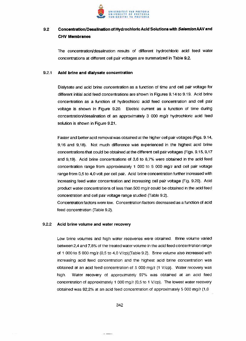
9.2 Concentration/Desalination of Hydrochloric Acid Solutions with Selemlon AAV and
CHV Membranes
The concentration/desalination results of different hydrochloric acid feed water
concentrations at different cell pair voltages are summarized in Table 9.2.
Dialysate and acid brine concentration as a function of time and cell pair voltage for
different initial acid feed concentrations are shown in Figures 9.14 to 9.19. Acid brine
concentration as a function of hydrochloric acid feed concentration and cell pair
voltage is shown in Figure 9.20. Electric current as a function of time during
concentration/desalination of an approximately 3 000 mg/Q hydrochloric acid feed
solution is shown in Figure 9.21.
Faster and better acid removal was obtained at the higher cell pair voltages (Figs. 9.14,
9,16 and 9,18). Not much difference was experienced in the highest acid brine
concentrations that could be obtained at the different cell pair voltages (Figs. 9.15, 9,17
and 9,19). Acid brine concentrations of 3,6 to 8,7% were obtained in the acid feed
concentration range from approximately 1 000 to 5 000 mg/Q and cell pair voltage
range from 0,5 to 4,0 volt per cell pair. Acid brine concentration further increased with
increasing feed water concentration and increasing cell pair voltage (Fig. 9.20). Acid
product water concentrations of less than 500 mg/Q could be obtained in the acid feed
concentration and cell pair voltage range studied (Table 9.2).
Concentration factors were low. Concentration factors decreased as a function of acid
feed concentration (Table 9.2).
Low brine volumes and high water recoveries were obtained. Brine volume varied
between 2,4 and 7,8% of the treated water volume in the acid feed concentration range
of 1 000 to 5 000 mg/Q (0,5 to 4,0 V/cp) (Table 9.2). Brine volume also increased with
increasing acid feed concentration and the highest acid brine concentration was
obtained at an acid feed concentration of 5 000 mg/Q (1 V/cp). Water recovery was
high. Water recovery of approximately 97% was obtained at an acid feed
concentration of approximately 1 000 mgiQ (0,5 to 1 V/cp). The lowest water recovery
obtained was 92,2% at an acid feed concentration of approximately 5 000 mg/~ (1,0
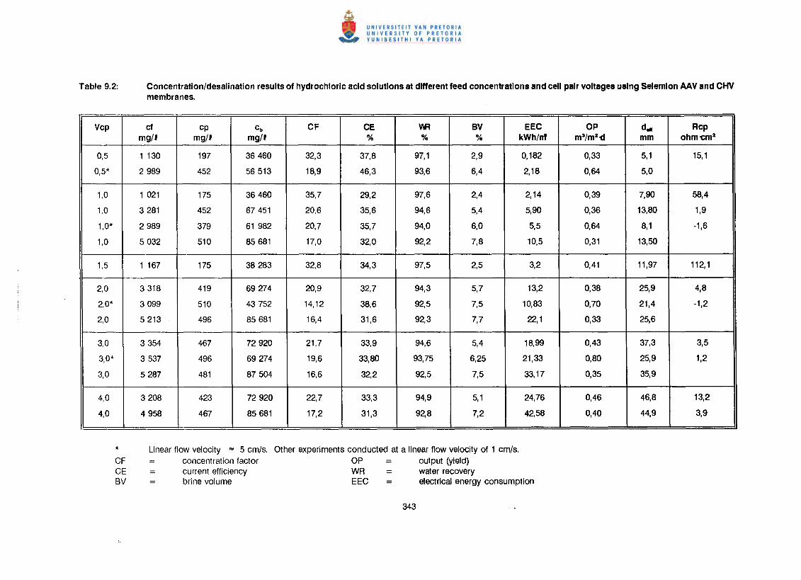
Concentration/desalination results of hydrochloric acid solutions at different feed concentrations and cell pair voltages using Selemlon AAV and CHVmembranes.
Vcp cf cp cb CF CE VIR BV EEC OP dell Rcpmg/f mg/f mg/f % % % kWh/nf m3/m2'CJ mm ohm'Cm2
0,5 1 130 197 36460 32,3 37,8 97,1 2,9 0,182 0,33 5,1 15,1
0,5* 2989 452 56513 18,9 46,3 93,6 6,4 2,18 0,64 5,0
1,0 1 021 175 36460 35,7 29,2 97,6 2,4 2,14 0,39 7,90 58,4
1,0 3281 452 67451 20,6 35,6 94,6 5,4 5,90 0,36 13,80 1,9
1,0* 2989 379 61 982 20,7 35,7 94,0 6,0 5,5 0,64 8,1 -1,6
1,0 5032 510 85681 17,0 32,0 92,2 7,8 10,5 0,31 13,50
1,5 1 167 175 38283 32,8 34,3 97,5 2,5 3,2 0,41 11,97 112,1
2,0 3318 419 69274 20,9 32,7 94,3 5,7 13,2 0,38 25,9 4,8
2,0* 3099 510 43752 14,12 38,6 92,5 7,5 10,83 0,70 21,4 -1,2
2,0 5213 496 85681 16,4 31,6 92,3 7,7 22,1 0,33 25,6
3,0 3354 467 72920 21,7 33,9 94,6 5,4 18,99 0,43 37,3 3,5
3,0* 3537 496 69274 19,6 33,80 93,75 6,25 21,33 0,80 25,9 1,2
3,0 5287 481 87504 16,6 32,2 92,5 7,5 33,17 0,35 35,9
4,0 3208 423 72920 22,7 33,3 94,9 5,1 24,76 0,46 46,8 13,2
4,0 4958 467 85681 17,2 31,3 92,8 7,2 42,58 0,40 44,9 3,9
Linear flow velocity '" 5 cm/s.concentration factor
= current efficiencybrine volume
Other experiments conducted at a linear flow velocity of 1 cm/s.OP output (yield)WR water recoveryEEC = electrical energy consumption
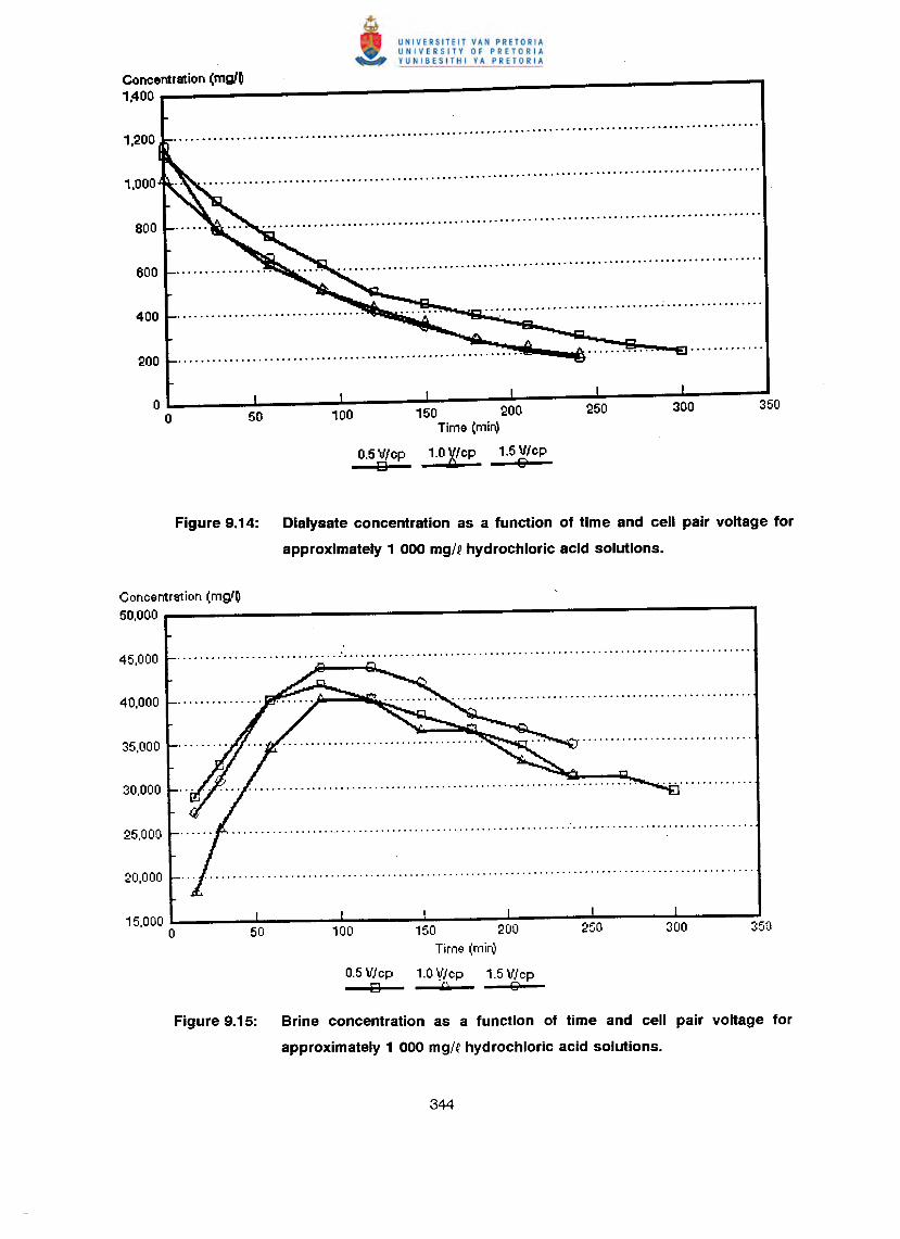
Concentration (mg/~1,400
100 150 200Time (mir.)
0.5~cp 1.0Yl,cP 1.5 ~/cp
Figure 9.14: Dialysate concentration as a function of time and cell pair voltage for
approximately 1 000 mg/Qhydrochloric acid solutions.
Concentration (mgl~50.000
15,000o 150 200
Time (mir~
0.5 V/cp 1.0 Vlcp 1.5 Vlcpo •• E?
Figure 9.15: Brine concentration as a function of time and cell pair voltage for
approximately 1 000 mg/~ hydrochloric acid solutions.
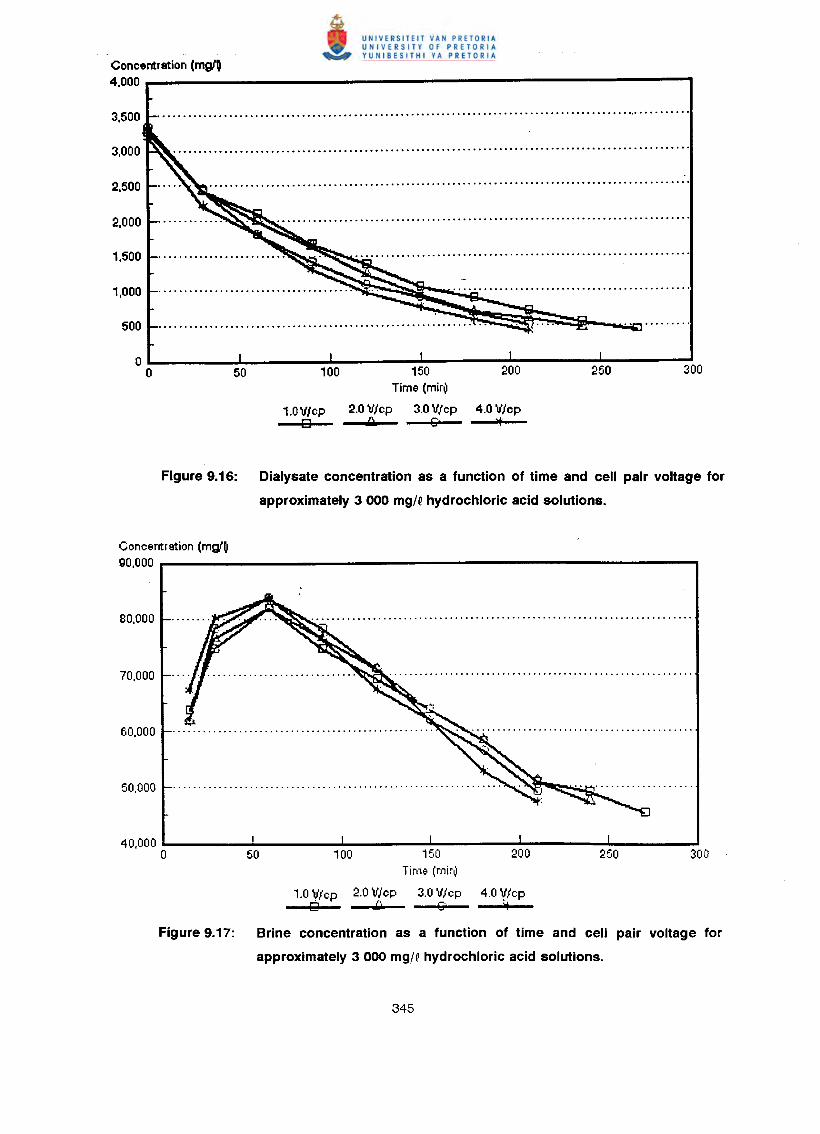
Concentration (mgO4,000
100 '50 200Time (mi~
,.O\flcp 2.0 \fIcp 3.0 \fIcp 4.0 WcpE3 J.:l, 6' •••.
Figure 9.16: Dialysate concentration as a function of time and cell pair voltage for
approximately 3 000 mg/Qhydrochloric acid solutions.
Concentration (mglO90,000
40,0000 50 '00 150 200 250 300
Time (mir~
'.0V/cp 2.0V/cp 3.0V/cp 4.0V/cp0 ••• G
).Figure 9.17: Brine concentration as a function of time and cell pair voltage for
approximately 3000 mg/Qhydrochloric acid solutions.
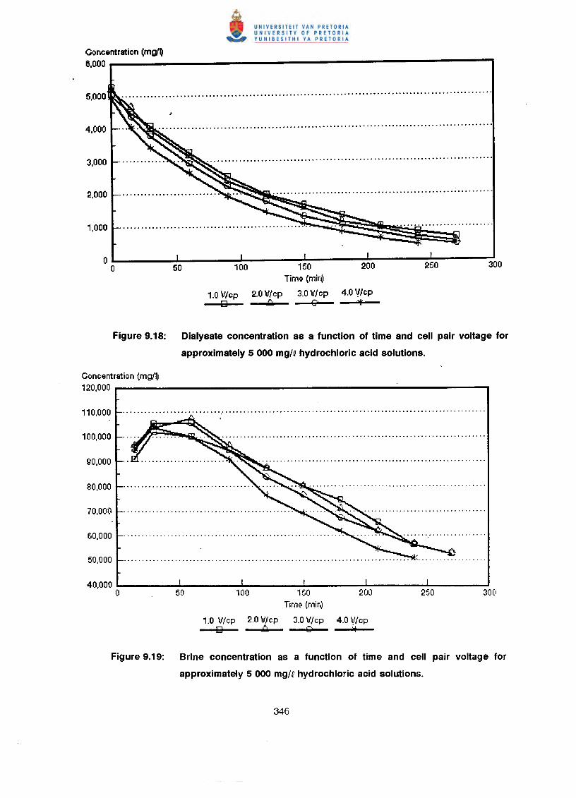
Concentration (mgl~6.000
50 100 150 200 250 300Time (miril
1.0 V/cp 2.0 V/cp 3.0V/cp 4.0Vlcpg .Q- Q •••
Figure 9.18: Dialysate concentration as a function of time and cell pair voltage for
approximately 5000 mg/Qhydrochloric acid solutions.
Concentration (mg(~120,000
40,000o 50 100 150 200 250 300
Time (mirv
1.0 Vlcp 2.0 Vlcp 3.0 V/cp 4.0 V/cp0 1:L G •••
Figure 9.19: Brine concentration as a function of time and cell pair voltage for
approximately 5000 mg/Qhydrochloric acid solutions.
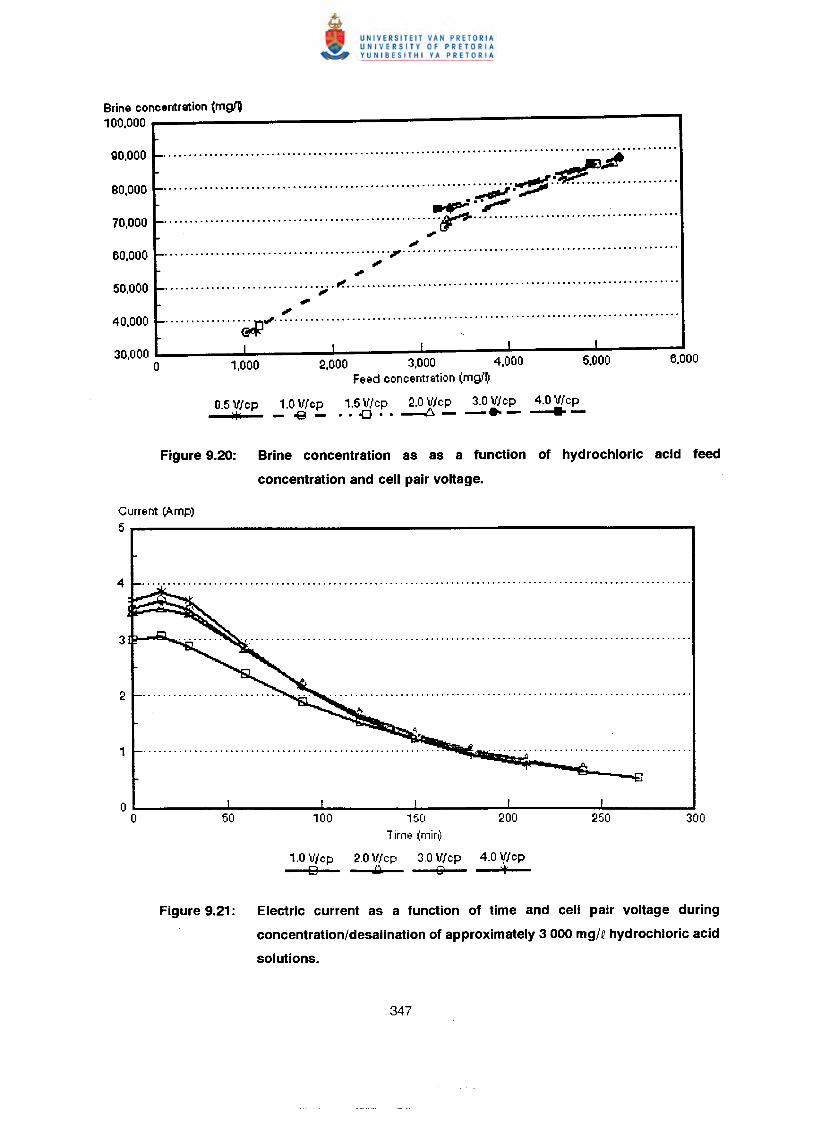
Brine concentretion (mglO100,000
..................................................................................J .
....................................................~ :~ ..•:::p1t? .
......................................................r········································,.,.
............................................ i' ..,.,••••••••••••••••••••••••••••• ';'; • tI"! •••••••••••••••••••••••••••••••••••••••••••••••••••••••••••••••••,.,................ ~ ••••....................................~ .
30,000o 2,000 3,000 4,000
Feed concentr&tion (mglO
0.5 V/cp 1.0 V/cp 1.5 Vlcp 2.0 V/cp 3.0 Vlcp 4.0 Vlcp*' _ oQ - •• o(} •• ~ - -.---4--Figure 9.20: Brine concentration as as a function of hydrochloric acid feed
concentration and cell pair voltage.
Current .;Amp}5
00 50 100 150 200 250 300
Time (mirv
1.0 Vlcp 2.0 Vlcp 3.0 V/cp 4.0 Vlcp0 •• IS .,..
Figure 9.21: Electric current as a function of time and cell pair voltage during
concentration/desalination of approximately 3 000 mg/Qhydrochloric acid
solutions.
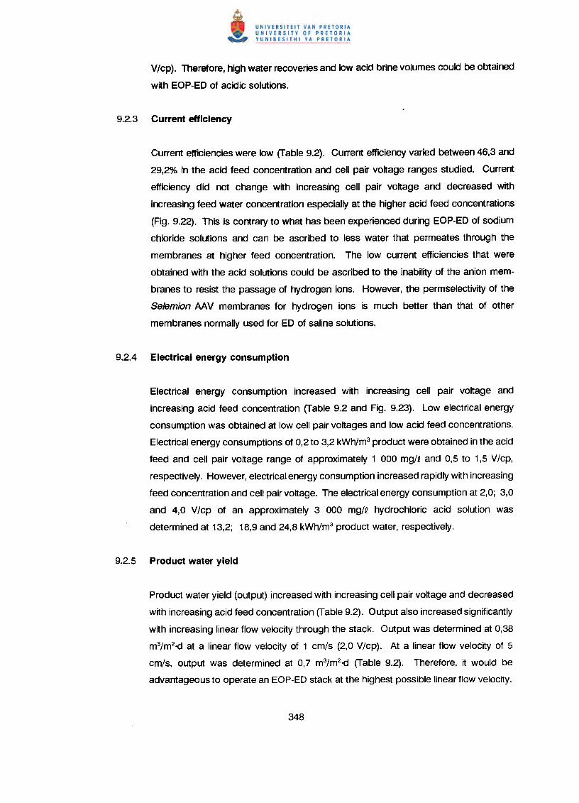
V/cp). Therefore, high water recoveries and low acid brine volumes could be obtained
with EOP-ED of acidic solutions.
Current efficiencies were low (Table 9.2). Current efficiency varied between 46,3 and
29,2% in the acid feed concentration and cell pair voltage ranges studied. Current
efficiency did not change with increasing cell pair voltage and decreased with
increasing feed water concentration especially at the higher acid feed concentrations
(Fig. 9.22). This is contrary to what has been experienced during EOP-ED of sodium
chloride solutions and can be ascribed to less water that permeates through the
membranes at higher feed concentration. The low current efficiencies that were
obtained with the acid solutions could be ascribed to the inability of the anion mem-
branes to resist the passage of hydrogen ions. However, the permselectivity of the
Selemion AAV membranes for hydrogen ions is much better than that of other
membranes normally used for ED of saline solutions.
Electrical energy consumption increased with increasing cell pair voltage and
increasing acid feed concentration (Table 9.2 and Fig. 9.23). Low electrical energy
consumption was obtained at low cell pair voltages and low acid feed concentrations.
Electrical energy consumptions of 0,2 to 3,2 kWh/m3 product were obtained in the acid
feed and cell pair voltage range of approximately 1 000 mg/o and 0,5 to 1,5 V/cp,
respectively. However, electrical energy consumption increased rapidly with increasing
feed concentration and cell pair voltage. The electrical energy consumption at 2,0; 3,0
and 4,0 V/cp of an approximately 3 000 mg/O hydrochloric acid solution was
determined at 13,2; 18,9 and 24,8 kWh/m3 product water, respectively.
Product water yield (output) increased with increasing cell pair voltage and decreased
with increasing acid feed concentration (Table 9.2). Output also increased significantly
with increasing linear flow velocity through the stack. Output was determined at 0,38
m3/m2o(j at a linear flow velocity of 1 cm/s (2,0 V/cp). At a linear flow velocity of 5
cm/s, output was determined at 0,7 m3/m2o(j (Table 9.2). Therefore, it would be
advantageous to operate an EOP-ED stack at the highest possible linear flow velocity.
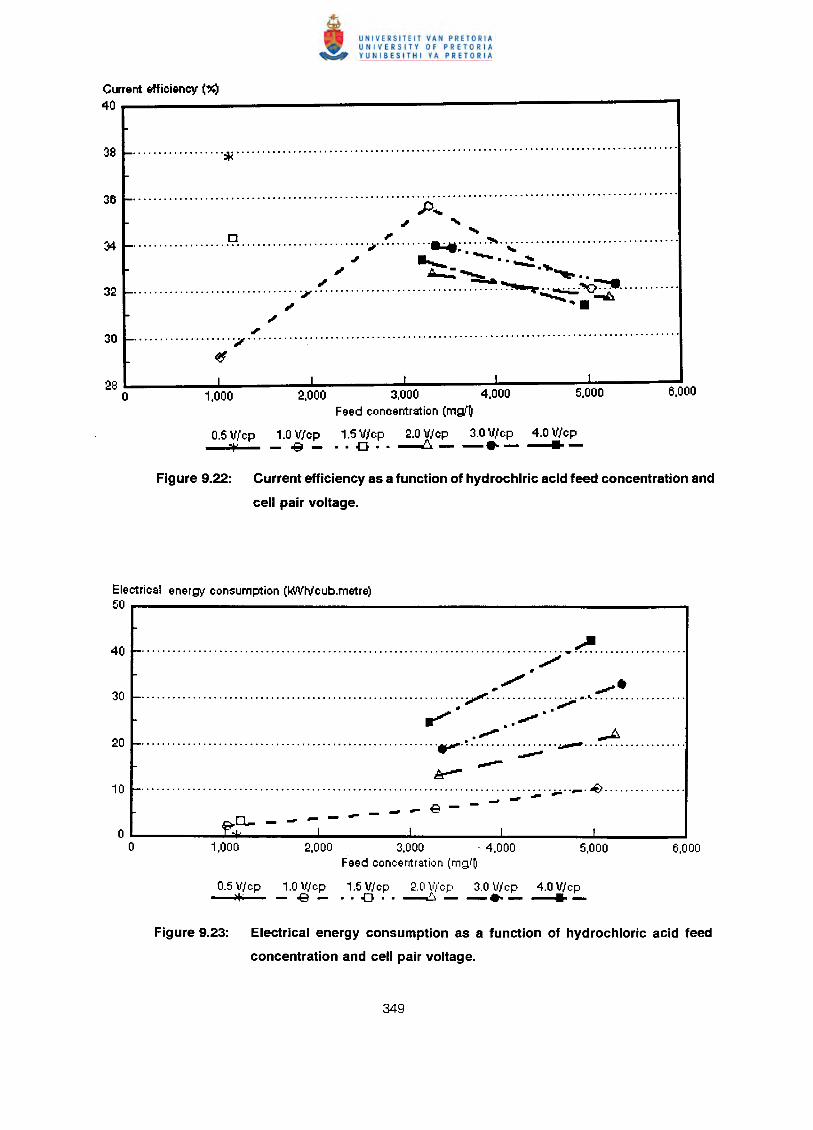
Current efficiency (%.)
40 r-----------------------------,
36 ~ .,I)•••
" """ .34 ~ ~ ·iI·········· .•.•• ;.: '!Io •• .;., ••.•••..••...•••••••..•.•.••••••" a...- '""-. . ....::::" ~ ~ ..•.~ ..32 _ ,J!'."!. ~ ~.""O 7::t .
" .."30 _ ~.~ .
~I I I I I
283,000 4,000 5,000 6,000
0 1,000 2,000Feed concentration (mgl~
0.5 V/cp 1.0 V/cp 1.5V/cp 2.0 Vlcp 3.0 V/cp 4.0 Vlcp
* -08- ··0·· ~--.- -----Figure 9.22: Current efficiency as a function of hydrochlric acid feed concentration and
cell pair voltage.
Electrical energy consumption (kilVtv'cub.metre)50 .._-------------------------------- ••
40 _ -~ ./'
,./ ,....30 ~ /- .................•.••................... ~•....... .", ..
.".,. . ~20 ,.............................................................•••••.. ~ ~ .--,...,-1 0 _ .:.; .. .;.;... _. ~ .- ----_oS -
~~1,000
- --I2,000
I I
3,000 - 4,000Feed concentration (mg!O
I
5,000
0.5 Vlcp 1.0 V/cp 1.5 V/cp 2.0 Vlcp 3.0 V/cp 4.0 Vlcp~.-~- ...[}..~ - -.---+-Figure 9.23: Electrical energy consumption as a function of hydrochloric acid feed
concentration and cell pair voltage.
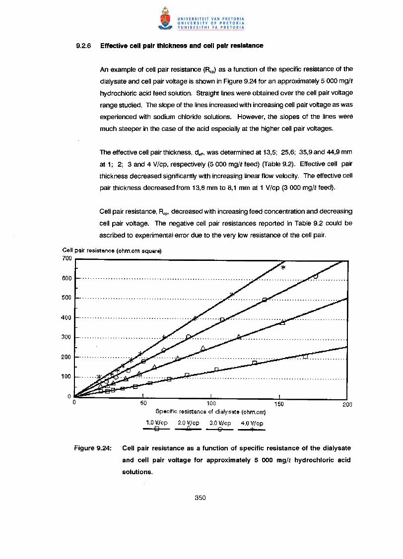
An example of cell pair resistance (Rcp) as a function of the specific resistance of the
dialysate and cell pair voltage is shown in Figure 9.24 for an approximately 5 000 mg/~
hydrochloric acid feed solution. Straight lines were obtained over the cell pair voltage
range studied. The slope of the lines increased with increasing cell pair voltage as was
experienced with sodium chloride solutions. However, the slopes of the Jineswere
much steeper in the case of the acid especially at the higher cell pair voltages.
The effective cell pair thickness, deff,was determined at 13,5; 25,6; 35,9 and 44,9 mm
at 1; 2; 3 and 4 V/cp, respectively (5 000 mg/Ofeed) (Table 9.2). Effective cell pair
thickness decreased significantly with increasing linear flow velocity. The effective cell
pair thickness decreased from 13,8 mm to 8,1 mm at 1 V/cp (3 000 mg/Ofeed).
Cell pair resistance, Rep, decreased with increasing feed concentration and decreasing
cell pair voltage. The negative cell pair resistances reported in Table 9.2 could be
ascribed to experimental error due to the very low resistance of the cell pair.
Cell pair re$istance (ohm.cm $quare)700
50 100 150Specific re$istance of diatysste (ohm.cm)
1.0V/cp 2.0V/cp 3.0V/cp 4.0 V/cpo •• G *"
Figure 9.24: Cell pair resistance as a function of specific resistance of the dialysate
and cell pair voltage for approximately 5 000 mg/Q hydrochloric acid
solutions.
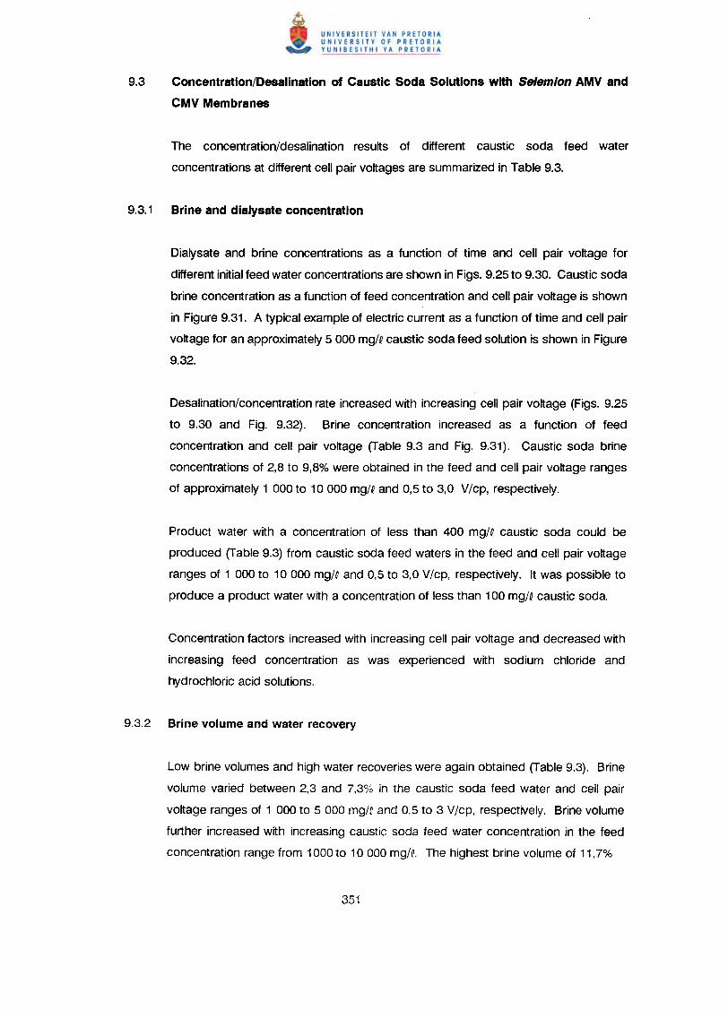
9.3 Concentration/Desalination of Caustic Soda Solutions with Selemlon AMV and
CMV Membranes
The concentration/desalination results of different caustic soda feed water
concentrations at different cell pair voltages are summarized in Table 9.3.
Dialysate and brine concentrations as a function of time and cell pair voltage for
different initial feed water concentrations are shown in Figs. 9.25 to 9.30. Caustic soda
brine concentration as a function of feed concentration and cell pair voltage is shown
in Figure 9.31. A typical example of electric current as a function of time and cell pair
voltage for an approximately 5 000 mg/~ caustic soda feed solution is shown in Figure
9.32.
Desalination/concentration rate increased with increasing cell pair voltage (Figs. 9.25
to 9.30 and Fig. 9.32). Brine concentration increased as a function of feed
concentration and cell pair voltage (Table 9.3 and Fig. 9.31). Caustic soda brine
concentrations of 2,8 to 9,8% were obtained in the feed and cell pair voltage ranges
of approximately 1 000 to 10 000 mg/~ and 0,5 to 3,0 V/cp, respectively.
Product water with a concentration of less than 400 mg/~ caustic soda could be
produced (Table 9.3) from caustic soda feed waters in the feed and cell pair voltage
ranges of 1 000 to 10 000 mg/~ and 0,5 to 3,0 V/cp, respectively. It was possible to
produce a product water with a concentration of less than 100 mg/~ caustic soda.
Concentration factors increased with increasing cell pair voltage and decreased with
increasing feed concentration as was experienced with sodium chloride and
hydrochloric acid solutions.
Low brine volumes and high water recoveries were again obtained (Table 9.3). Brine
volume varied between 2,3 and 7,3% in the caustic soda feed water and cell pair
voltage ranges of 1 000 to 5 000 mg/Q and 0,5 to 3 V/cp, respectively. Brine volume
further increased with increasing caustic soda feed water concentration in the feed
concentration range from 1000 to 10 000 mg/Q. The highest brine volume of 11,7%
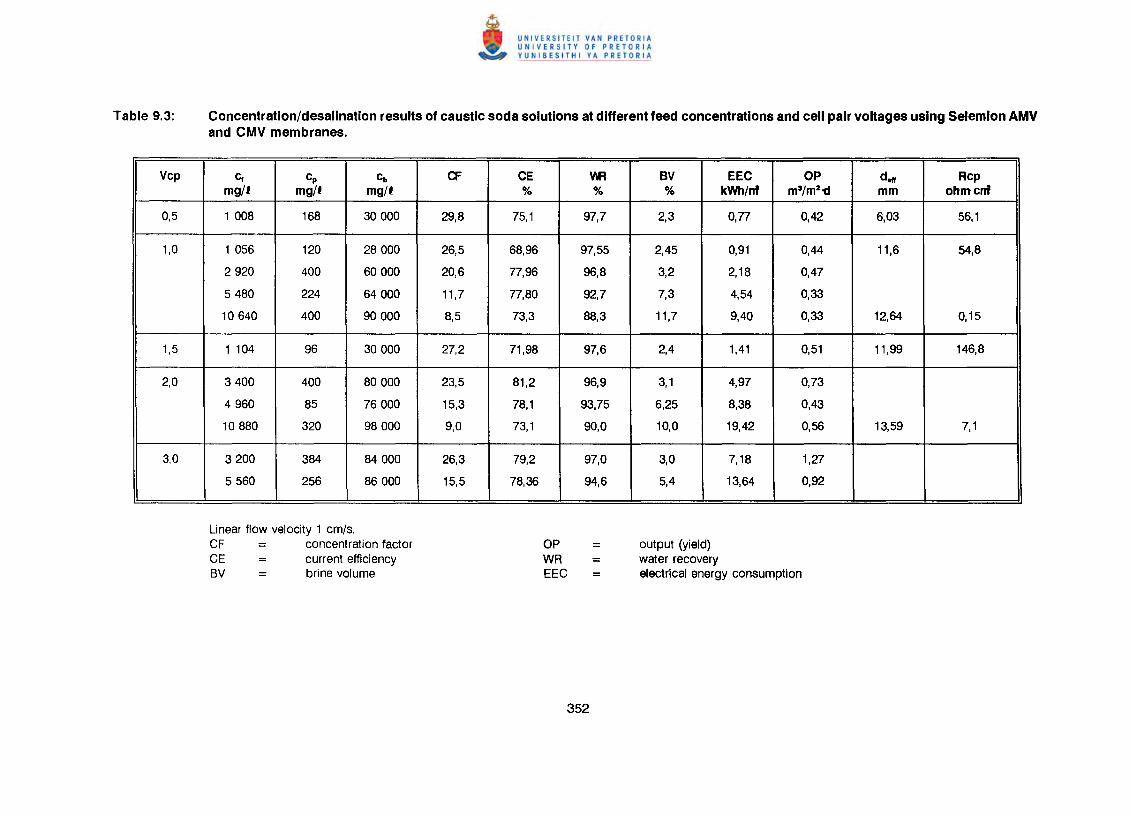
Concentration/desalination results of caustic soda solutions at different feed concentrations and cell pair voltages using Selemlon AMVand CMV membranes.
Vep G cp Cb a= CE VIR BV EEC OP dell Rcpmg/f mg/f mg/f % % % kWh/nf m3/m2t1 mm ohmcnf
0,5 1 008 168 30000 29,8 75,1 97,7 2,3 0,77 0,42 6,03 56,1
1,0 1 056 120 28000 26,5 68,96 97,55 2,45 0,91 0,44 11,6 54,8
2920 400 60000 20,6 77,96 96,8 3,2 2,18 0,47
5480 224 64000 11,7 77,80 92,7 7,3 4,54 0,33
10640 400 90000 8,5 73,3 88,3 11,7 9,40 0,33 12,64 0,15
1,5 1 104 96 30000 27,2 71,98 97,6 2,4 1,41 0,51 11,99 146,8
2,0 3400 400 80000 23,5 81,2 96,9 3,1 4,97 0,73
4960 85 76000 15,3 78,1 93,75 6,25 8,38 0,43
10880 320 98000 9,0 73,1 90,0 10,0 19,42 0,56 13,59 7,1
3,0 3200 384 84000 26,3 79,2 97,0 3,0 7,18 1,27
5560 256 86000 15,5 78,36 94,6 5,4 13,64 0,92
Linear flow velocity 1 cm/s.CF = concentration factorCE current efficiencyBV = brine volume
OP =WR =EEC =
output (yield)water recoveryelectrical energy consumption
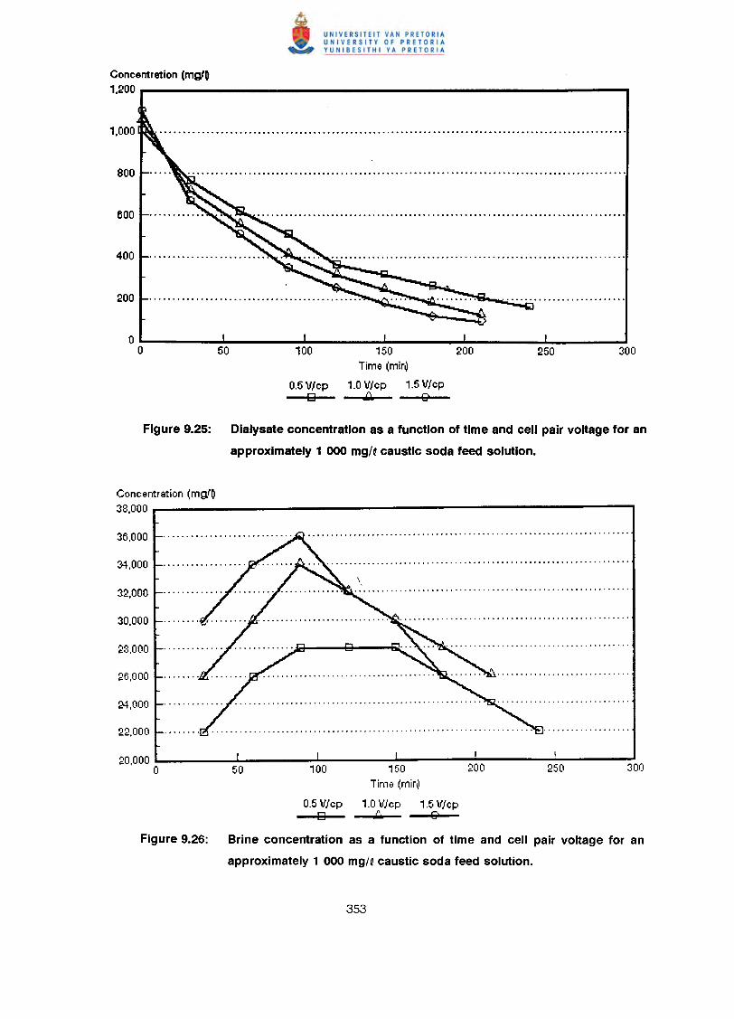
Concentration (mgl~1.200
100 150 200Time (mir~
0.5 Vlcp 1.0 Vlcp 1.5 Vlcpo "" l;>
Figure 9.25: Dialysate concentration as a function of time and cell pair voltage for an
approximately 1 000 mg/Qcaustic soda feed solution.
Concentration (mgfO38,000
20,000o
I
50 100 150 200 250 300Time (mir\\
0.5 V/cp 1.0 V/cp 1.5 V/cp0 A l;>
Figure 9.26: Brine concentration as a function of time and cell pair voltage for an
approximately 1 000 mg/Qcaustic soda feed solution.
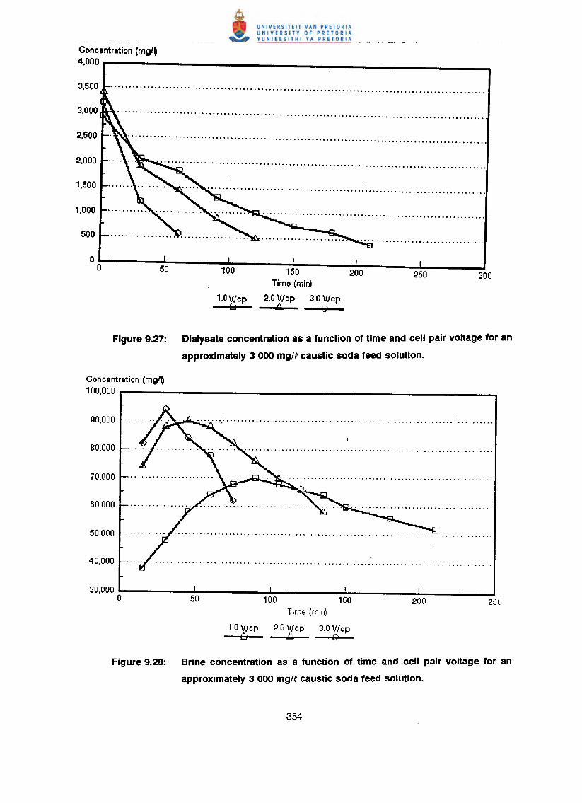
Concentration (mglO4.000
50 100 150 200 250 300Time (miiV
1.0 V/cp 2.0V/cp 3.0 V/cpt3 A 19
Figure 9.27: Dialysate concentration as a function of time and cell pair voltage for an
approximately 3 000 mg/Qcaustic soda feed solution.
Concentration (mg(~100,000
30,000o
Tim€' (mirv
1.0 V/cp 2.0 V/cp 3.0 V/cpu .•• G
Figure 9.28: Brine concentration as a function of time and cell pair voltage for an
approximately 3000 mg/Qcaustic soda feed solution.
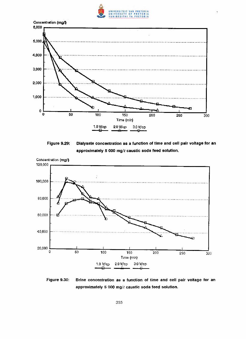
Concentration (mglO6.000
'00 '50 200Time (mi~
'.0 V/cp 2.0 V/cp 3.0 Vlcpo ..:.is EI
Figure 9.29: Dialysate concentration as a function of time and cell pair voltage for an
approximately 5 000 mg/Qcaustic soda feed solution.
Concentration (mgfO'20,000
20.000 o '50Time (mir~
'.0 ¥lcp 2.0 V/cp 3.0V/cpo •• G
Figure 9.30: Brine concentration as a function of time and cell pair voltage for an
approximately 5 000 mg/Qcaustic soda feed solution.
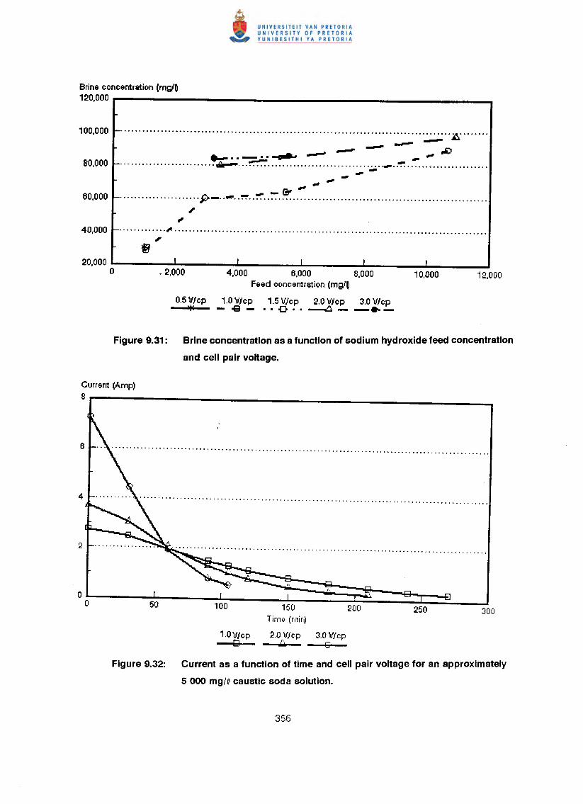
Brine concentration (mgl~120,000.--------------------------- __ ~ .--..-- - ,Ii)
~ •• _ •••••••••• ~ rfIIIIII_ ~ ~ _ ..~ ..~ .-~..,-~-~",.60,000 1-.••••.••••.••..•••••.• p._ ..~ .,
.,40,000 ~ '" .,20,000
oI
. 2,000I I I
4,000 6,000 8,000Feed concentration (m9(~
0.5V1cp 1.0V/cp 1.5V/cp 2.0V/cp 3.0V/cp*' -oQ- •• oQ •• ~--.-
I
10,000
Figure 9.31: Brine concentration as a function of sodium hydroxide feed concentration
and cell pair voltage.
Current (.A.mp)8
00 50 100 150 200 250 300
Tim€< (mirv
1.0V/cp 2.0 V/cp 3.0 V/cptJ •• G
Figure 9.32: Current as a function of time and cell pair voltage for an approximately
5 000 mg/Qcaustic soda solution.
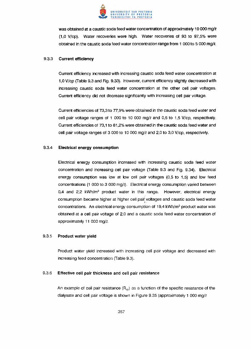
was obtained at a caustic soda feed water concentration of approximately 10 000 mg/q
(1,0 V/cp). Water recoveries were high. Water recoveries of 93 to 97,5% were
obtained in the caustic soda feed water concentration range from 1 000 to 5 000 mg/Q.
Current efficiency increased with increasing caustic soda feed water concentration at
1,0 V/cp (Table 9.3 and Fig. 9.33). However, current efficiency slightly decreased with
increasing caustic soda feed water concentration at the other cell pair voltages.
Current efficiency did not decrease significantly with increasing cell pair voltage.
Current efficiencies of 73,3 to 77,9% were obtained in the caustic soda feed water and
cell pair voltage ranges of 1 000 to 10 000 mg/D and 0,5 to 1,5 V/cp, respectively.
Current efficiencies of 73,1 to 81,2% were obtained in the caustic soda feed water and
cell pair voltage ranges of 3 000 to 10 000 mg/q and 2,0 to 3,0 V/cp, respectively.
Electrical energy consumption increased with increasing caustic soda feed water
concentration and increasing cell pair voltage (Table 9.3 and Fig. 9.34). Electrical
energy consumption was low at low cell pair voltages (0,5 to 1,5) and low feed
concentrations (1 000 to 3 000 mg/D). Electrical energy consumption varied between
0,4 and 2,2 kWh/m3 product water in this range. However, electrical energy
consumption became higher at higher cell pair: voltages and caustic soda feed water
concentrations. An electrical energy consumption of 19,4 kWh/m3 product water was
obtained at a cell pair voltage of 2,0 and a caustic soda feed water concentration of
approximately 11 000 mg/D.
Product water yield increased with increasing cell pair voltage and decreased with
increasing feed concentration (Table 9.3).
An example of cell pair resistance (Rcp) as a function of the specific resistance of the
dialysate and cell pair voltage is shown in Figure 9.35 (apprOXimately 1 000 mg/~
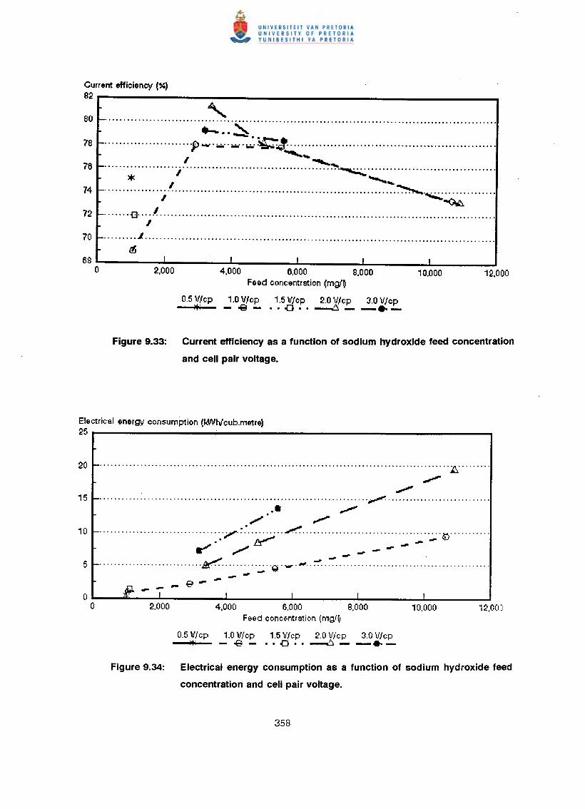
Current efficiency (%)82.-------- _,80 _ .-- ..~78 _ ;>__. ;";'".••.•.~ ~:: .
I ~ .••.---...76 _ "j ~.~ .
* I ~ .••.74 _ j ~.~~ .
72 _ £:) ...• .1. .I
70 _ .L ..............................•.............................................••.•...............
68o
I
2,000I I
4,000 6,000Feed concentration (mg'O
0.5 V/cp 1.0 V/cp 1.5 V/cp 2.0 Vlcp 3.0 V/cp*' - oS - •• o{) •• ~ - -.-
I
8,000I
10.000
Figure 9.33: Current efficiency as a function of sodium hydroxide feed concentration
and cell pair voltage.
Electrical energy consumption (kWtv'cub.metre)25
............................................................................................... ~ ."",
~......................................................................... ~ ... ",.
;'" ,.",·.·.····· ···.· ·······.······r ~ L: 1"'. •.•......•.. ~ -~•...... -' ----
~ --•....••••...•••......•....• '~"""""""'Ii'''''''''''''~''~'''''''''''''''''''''''' .' .............•...- -- -e-
4,000 6,000 8,000Feed conc<ontration (mgl~
0.5 V/cp 1.0 V/cp 1.5 V/cp 2.0 Vlcp 3.0 Vlcp~' - oS - •• {] •• ~ - -.-
Figure 9.34: Electrical energy consumption as a function of sodium hydroxide feed
concentration and cell pair voltage.
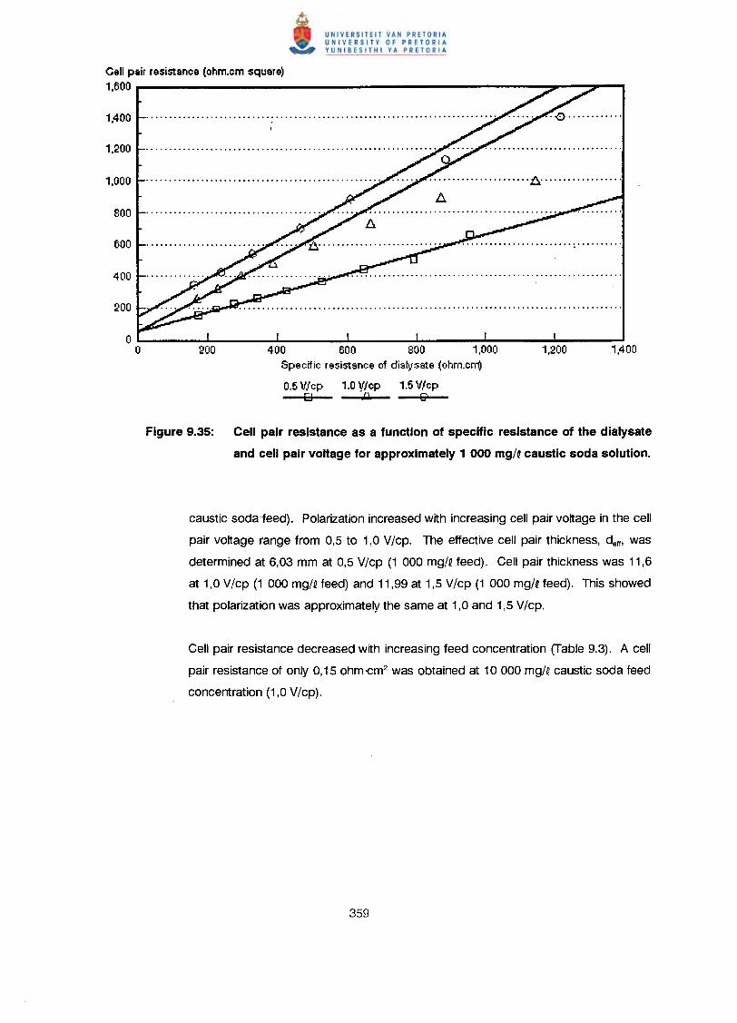
Cell pair resistance (ohm.em square)"600
400 600 BOO 1,000Specific resistance of diat)'sate (ohm.err(!
0.5V/ep 1.0Vlep 1.5Vlepo bL 6'
Figure 9.35: Cell pair resistance as a function of specific resistance of the dialysate
and cell pair voltage for approximately 1 000 mg/~caustic soda solution.
caustic soda ·feed). Polarization increased with increasing cell pair voltage in the cell
pair voltage range from 0,5 to 1,0 V/cp. The effective cell pair thickness, delll was
determined at 6,03 mm at 0,5 V/cp (1 000 mg/Q feed). Cell pair thickness was 11,6
at 1,0 V/cp (1 000 mg/~ feed) and 11,99 at 1,5 V/cp (1 000 mg/~ feed). This showed
that polarization was approximately the same at 1,0 and 1,5 V/cp.
Cell pair resistance decreased with increasing feed concentration (Table 9.3). A cell
pair resistance of only 0,15 ohm -cm2 was obtained at 10 000 mgl~caustic soda feed
concentration (1,0 V/cp).
10. CONCENTRATION/DESALINATION OF SALT SOLUTIONS AND INDUSTRIAL EFFLUENTS
WITH SCED
A summary of the concentration/desalination results of the different salt solutions is
shown in Tables 10.1 to 10.5.
Examples of the desalination/concentration of sodium chloride, ammonium nitrate and
sodium sulphate solutions as a function of time at constant cell pair voltage are shown
in Figures 10.1 to 10.3. The effect of increasing cell pair voltage on
desalination/concentration of an approximately 1 000 mg/Q sodium sulphate solution
is shown in Figure 10.4.
Desalination rate decreased with decreasing feed concentration (Figs. 10.1 to 10.3) and
decreasing cell pair voltage (Figure 10.4). However, approximately the same initial
desalination rate was obtained at 1,18 and 1,76 V/cp (Figure 10.4). The optimum cell
pair voltage for desalination regarding polarization and electrical energy consumption
should be determined for each feed concentration, because this information is required
to operate an ED stack under optimum conditions. This, however, was not the main
purpose of this investigation. The main purpose of this investigation was to evaluate
the performance of the SCED unit for concentration/desalination of saline solutions at
cell pair voltages normally applied in ED.
All the different salt solutions could be easily desalinated from approximately 10 000
mg/Q to 300 mg/Q and less (Figs. 10.1 to 10.3 and Tables 10.1 to 10.5). Product
concentrations of less than 100 mg/Q could be obtained with ease in some cases.
Therefore, SCED appears to be effective for the production of low TDS water.
Brine concentration increased with increasing feed concentration and increasing cell
pair voltage (Tables 10.1 to 10.5and Figure 10.5). Sodium chloride, ammonium nitrate,
sodium sulphate, sodium nitrate and calcium chloride brine concentrations of 2,2 to
16,1%; 4,9 to 15%; 7,8 to 16,3%; 6,0 to 12,5% and 3,8 to 7,5% could be obtained,
in the feed concentration and cell pair voltage range of 0,1 to 1% and 0,59 to 1,76
V/cp, respectively. Therefore, relatively high brine concentrations could be obtained
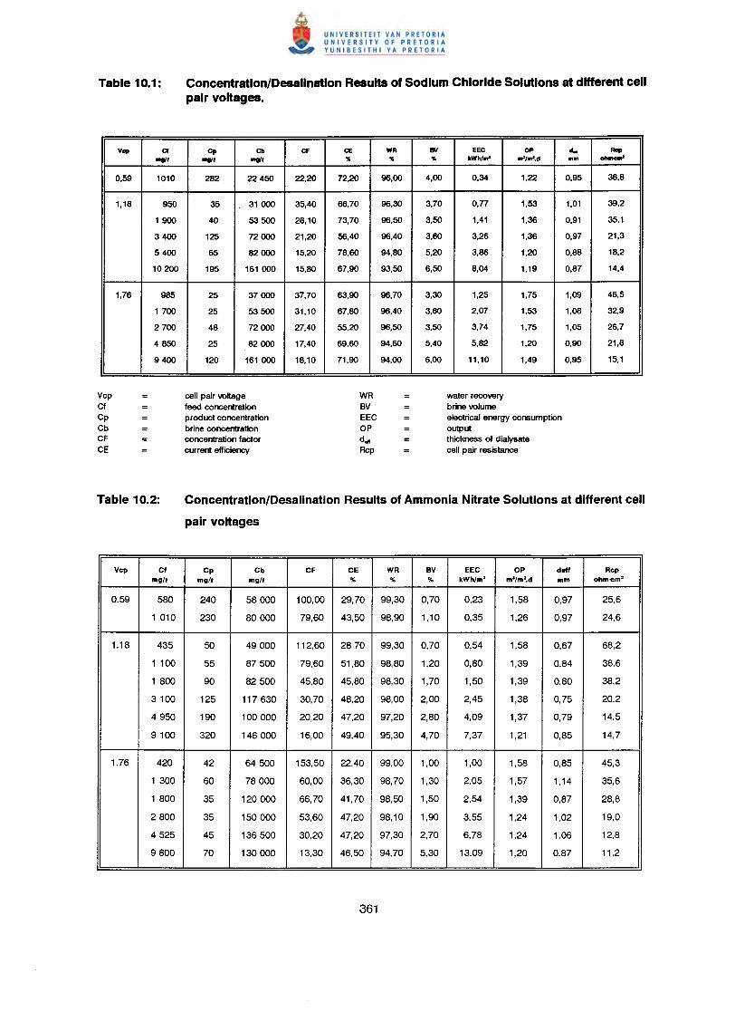
Concentration/Desalination Results of Sodium Chloride Solutions at different cellpair voltages.
Yep Of Cp Cb Cf CE WR BY EEC OP d", Rcp
""", """, """, " " " kWh/ ••• ""rn'.d •••• 01>_
0,59 1010 282 22450 22,20 72,20 96,00 4,00 0,34 1,22 0,95 38,8
1,18 950 35 31000 35,40 66,70 96,30 3,70 o,n 1,53 1,01 39,2
1900 40 53 500 28,10 73,70 96,50 3,50 1,41 1,36 0,91 35,1
3400 125 72000 21,20 56,40 96,40 3,60 3,26 1,36 0,97 21,3
5400 65 82000 15,20 78,60 94,80 5,20 3,86 1,20 0,88 18,2
10200 195 161000 15,80 67,90 93,50 6,50 8,04 1,19 0,87 14,4
1,76 985 25 37000 37,70 63,90 96,70 3,30 1,25 1,75 1,09 46,5
1700 25 53500 31,10 67,80 96,40 3,60 2,07 1,53 1,08 32,9
2700 48 72000 27,40 55,20 96,50 3,50 3,74 1,75 1,05 26,7
4850 25 82000 17,40 69,60 94,60 5,40 5,82 1,20 0,90 21,8
9400 120 161 000 18,10 71,90 94,00 6,00 11,10 1,49 0,95 15,1
cell pair voltagefeed concentrationproduct concentrationbrine concentrationconcentration factorcurrent efficiency
WRBVEECOPd•••Rcp
water recoverybrine volumeelectrical energy consumptionoutputthickness of dialysatecell pair resistance
Concentration/Desalination Results of Ammonia Nitrate Solutions at different cell
pair voltages
Yep Cf Cp Cb CF CE WR BY EEC OP I deff Repmg/, mg/l mg/, % % % kWh/m' ma/m2.d mm ohm-cm2
0.59 580 240 58000 100,00 29,70 99,30 0,70 0,23 1,58 0,97 25,6
1 010 230 80000 79,60 43,50 98,90 1,10 0,35 1,26 0,97 24,6
1.18 435 50 49000 112,60 2870 99,30 0,70 0,54 1,58 0,67 68,2
1 100 55 87500 79,60 51,80 98,80 1,20 0,80 1,39 0,84 38,6
1 800 90 82500 45,80 45,80 98,30 1,70 1,50 1,39 0,80 38,2
3100 125 117630 30,70 48,20 98,00 2,00 2,45 1,38 0,75 20,2
4950 190 100000 20,20 47,20 97,20 2,80 4,09 1,37 0,79 14,5
9100 320 146000 16,00 49,40 95,30 4,70 7,37 1,21 0,85 14,7
1.76 420 42 64500 153,50 22,40 99,00 1,00 1,00 1,58 0,85 45,3
1 300 60 78000 60,00 36,30 98,70 1,30 2,05 1,57 1,14 35,6
1 800 35 120000 66,70 41,70 98,50 1,50 2,54 1,39 0,87 28,8
2800 35 150000 53,60 47,20 98,10 1,90 3,55 1,24 1,02 19,0
4525 45 136500 30,20 47,20 97,30 2,70 6,78 1,24 1,06 12,8
9800 70 130000 13,30 46,50 94,70 5,30 13,09 1,20 0,87 11,2
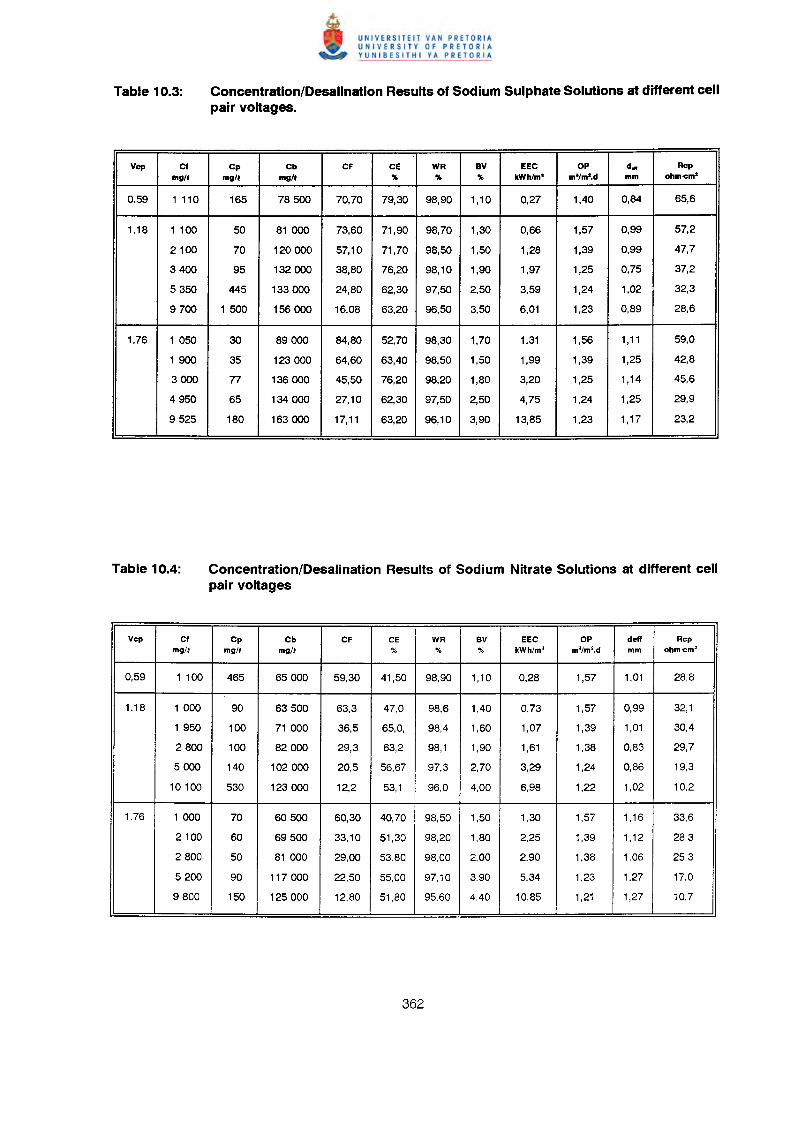
Concentration/Desalination Results of Sodium SUlphate Solutions at different cellpair voltages.
Yep Cf Cp Cb CF CE WR BY EEC OP d•• Repmgtl mgtl mgtl % % % kWhtm' m'tm'.d mm ohmocm'
0.59 1 110 165 78500 70,70 79,30 98,90 1,10 0,27 1,40 0,84 65,6
1.18 1 100 50 81 000 73,60 71,90 98,70 1,30 0,66 1,57 0,99 57,2
2100 70 120000 57,10 71,70 98,50 1,50 1,28 1,39 0,99 47,7
3400 95 132000 38,80 76,20 98,10 1,90 1,97 1,25 0,75 37,2
5350 445 133000 24,80 62,30 97,50 2,50 3,59 1,24 1,02 32,3
9700 1 500 156000 16,08 63,20 96,50 3,50 6,01 1,23 0,89 28,6
1.76 1050 30 89000 84,80 52,70 98,30 1,70 1,31 1,56 1,11 59,0
1900 35 123000 64,60 63,40 98,50 1,50 1,99 1,39 1,25 42,8
3000 77 136000 45,50 76,20 98,20 1,80 3,20 1,25 1,14 45,6
4950 65 134 000 27,10 62,30 97,50 2,50 4,75 1,24 1,25 29,9
9525 180 163000 17,11 63,20 96,10 3,90 13,85 1,23 1,17 23,2
Concentration/Desalination Results of Sodium Nitrate Solutions at different cellpair voltages
Yep Cf Cp Cb CF CE WR BV EEC OP deft Repmgtl mgtl mgtl % % % kWhtm' m3/m2.d mm ohm-em2
0,59 1 100 465 65000 59,30 41,50 98,90 1,10 0,28 1,57 1,01 28,8
1.18 1 000 90 63500 63,3 47,0 98,6 1,40 0,73 1,57 0,99 32,1
1 950 100 71 000 36,5 65,0, 98,4 1,60 1,07 1,39 1,01 30,4
2800 100 82000 29,3 63,2 98,1 1,90 1,61 1,38 0,83 29,7
5000 140 102000 20,5 56,67 97,3 2.70 3,29 1,24 0,86 19,3
10 100 530 123000 12,2 53,1 96,0 4,00 6,98 1,22 1,02 10,2
1.76 1 000 70 60500 60,30 40,70 98,50 1,50 1,30 1,57 1,16 33,6
2100 60 69500 33,10 51,30 98,20 1,80 2,25 1,39 1,12 28,3
2800 50 81 000 29,00 53.80 98,00 2,00 2,90 1,38 1,06 25,3
5200 90 117000 22,50 55,00 97,10 3.90 5,34 1,23 1,27 17,0
9800 150 125000 12,80 51,80 95,60 4,40 10,85 1,21 1,27 10,7
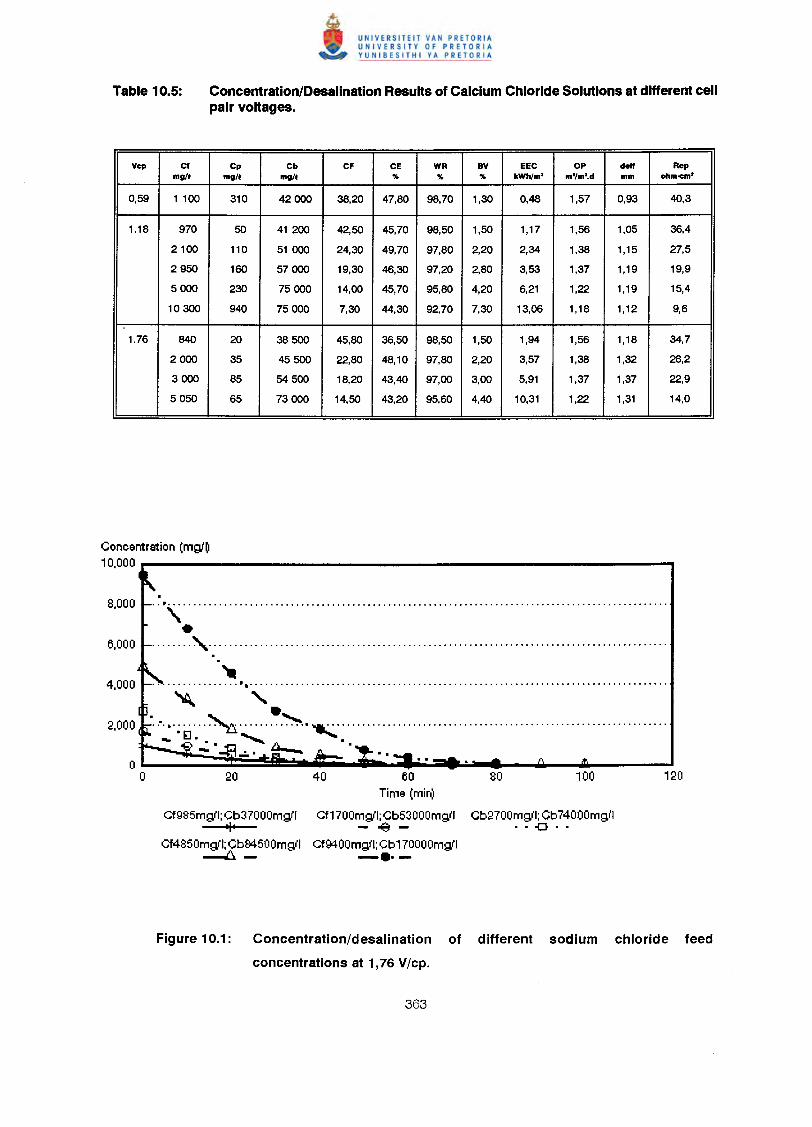
Concentration/DesalinationResults of Calcium Chloride Solutions at different cellpair voltages.
Yep Cf Cp Cb CF CE WR BY EEC OP dell Rcpmill' mill' mill' % % % kWhlm' m'/m'.d mm ohln-eml
0,59 1 100 310 42000 38,20 47,80 98,70 1,30 0,48 1,57 0,93 40,3
1.18 970 50 41 200 42,50 45,70 98,50 1,50 1,17 1,56 1,05 36,4
2100 110 51 000 24,30 49,70 97,80 2,20 2,34 1,38 1,15 27,5
2950 160 57000 19,30 46,30 97,20 2,80 3,53 1,37 1,19 19,9
5000 230 75000 14,00 45,70 95,80 4,20 6,21 1,22 1,19 15,4
10300 940 75000 7,30 44,30 92,70 7,30 13,06 1,18 1,12 9,6
1.76 840 20 38500 45,80 36,50 98,50 1,50 1,94 1,56 1,18 34,7
2000 35 45500 22,80 48,10 97,80 2,20 3,57 1,38 1,32 28,2
3000 85 54 500 18,20 43,40 97,00 3,00 5,91 1,37 1,37 22,9
5050 65 73000 14,50 43,20 95,60 4,40 10,31 1,22 1,31 14,0
Concentration (mgJ~10,000
...., .
•........, .'.
'-'" ". '- - •............; ~ , ._ EJ.......... ...:..~..:.. ~ ..•...
60Time (mir~
Cf985mgll; Cb37000mgll Cf1700mgil; Cb53000mgll Cb2700mgll; Cb 74000mgllIII - ~ - •• o(} ••
Cf4850mgJl: Cb84500mgil CfMOOmgJl;Cb170000mgll~- -..-Figure 10.1: Concentration/desalination of different sodium chloride feed
concentrations at 1,76V/cp.
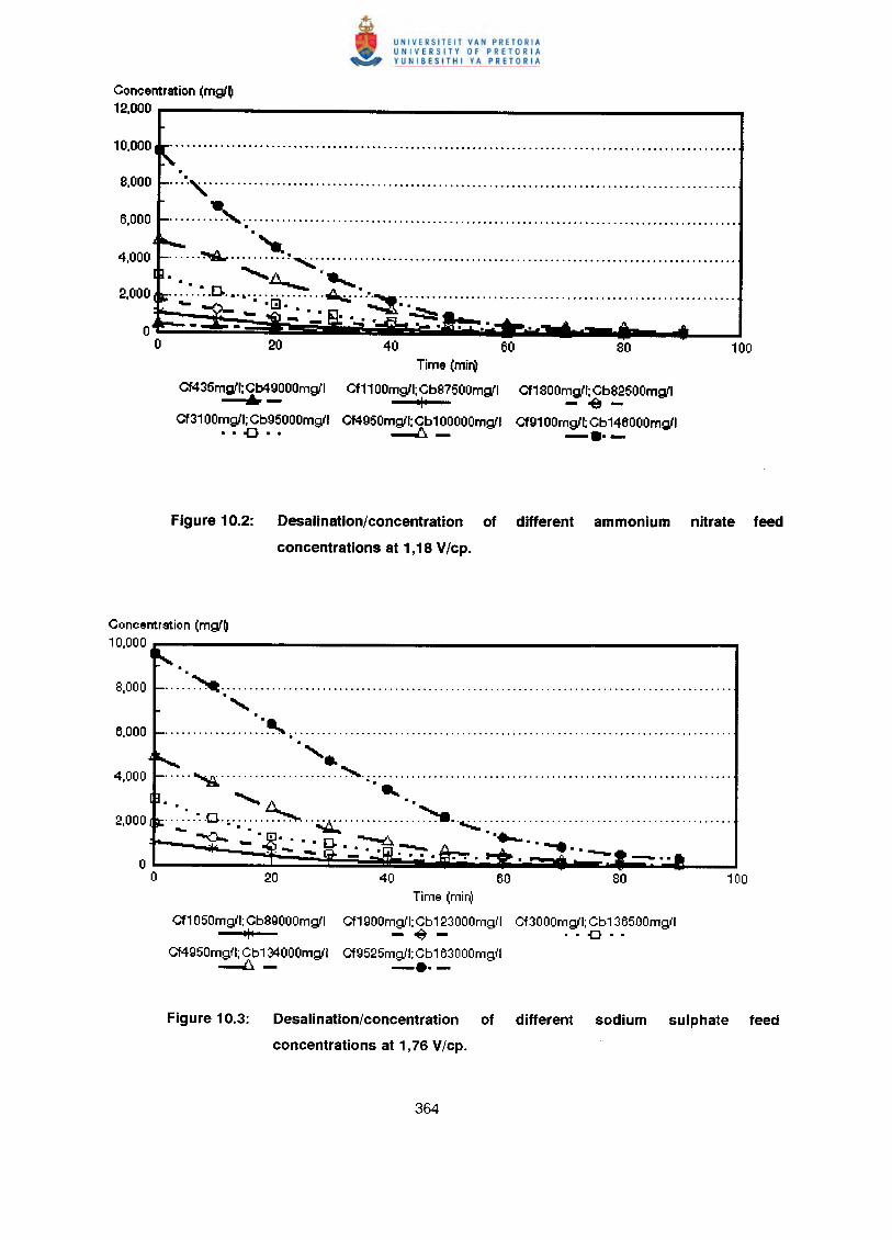
Concentration (mglO12.000
....•., .
........, .
......~ ~~~ ..... ~ .•......
.':.;,'".n...•.~.~GJ':"""~" .~~.: .~ -: ~
Cf435mgll; Cb49000mgll~-Cf3' OOmgll:Cb95000mgll
··0··
Time (mil\\
Cf1' OOmgll;CbS7500mgliIII
Cf4950mgll; Cb1 OOOOOmgll~-Cf' SOOmgll:CbS2500mgli--e-Cf9' OOmgll;Cb'46000mgll- ..-
Figure 10.2: Desalination/concentration of different ammonium nitrate feed
concentrations at 1,18 V/cp.
Concentration (mglO'0,000
....•.~ ..,
................ ~~~ •..............................................................................
'....... ~ , .•••••" ..
~.~:0.•.~ ~. ·:....A ······· ~ •. ~ ..•.. . ~ .-....... . . .•....~ '"- •••• [J. ~ •• -......... ....: ... ~. ... ..~
Time (mir~
Cf' 050mgll; CbS9000mgli Cf' 900mgll; Cb' 23000mgll Cf3000mgll; Cb' 36500mg"1III - ~ - •• G ••
Cf4950mgll; Cb' 34000mgll Cf9525mgl'l; Cb' 63000mgll~- -..-Figure 10.3: Desalination/concentration of different sodium sulphate feed
concentrations at 1,76 V/cp.
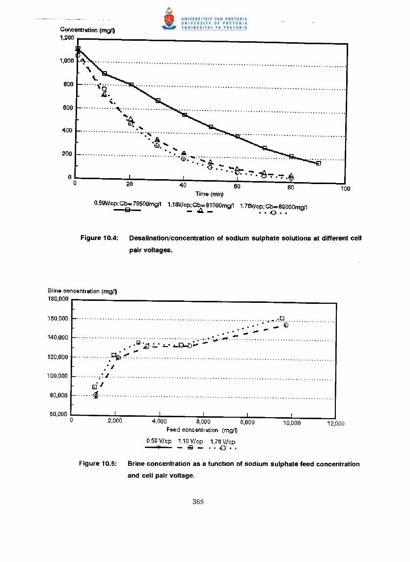
Concentration (mg/OU!OO
~ .,\....... \........... . .
2..............., .
~ . "-•••••••••••••••••••••• ' •.•• ''\iO ••••••••••••••••••••••••••••
'. A•G) ••••'. ....
.................................. :..'..~:.••...,,;: .. . . 0'.": o..e:-. . -•••• ..fJ. __
0 ....
Time (min)
0.5W/cp; Cb= 78500mg/J 1.18'u'/cp;Cb= 81OOOmg/1 1.76V/cp; Cb= 89000mg/1e -.::..- ··0··
Figure 10.4: Desalination/concentration of sodium sulphate solutions at different cell
pair voltages.
Brine concentration (mg/O180,000,--------------------------- •.•
_..........................................................................•.•... q ... . ~. . ~."".... ~.,.,..._...............................................•...•..•..... ..t .• • r&J ~ .:.: .:.,.- •••• [)....O~ "".
.' ".f- .............•. ~.":". .
100,000 '- ; ~.J .
r::i'80,000 f- ~ .
60,000 I I I I I
0 2,000 4,000 6,000 8,000 10,000 12,000Feed concentration (mglO
0.59 V/cp 1.18 V/cp 1.76 V/cp',' - 061- ··0.·Figure 10.5: Brine concentration as a function of sodium sulphate feed concentration
and cell pair voltage.
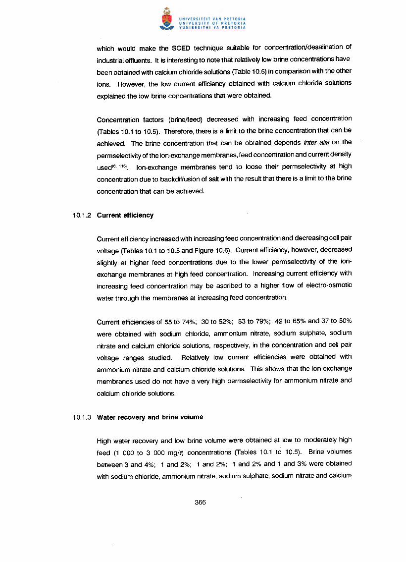
which would make the SCED technique suitable for concentration/desalination of
industrial effluents. It is interesting to note that relatively low brine concentrations have
been obtained with calcium chloride solutions (Table 10.5) in comparison with the other
ions. However, the low current efficiency obtained with calcium chloride solutions
explained the low brine concentrations that were obtained.
Concentration factors (brine/feed) decreased with increasing feed concentration
(Tables 10.1 to 10.5). Therefore, there is a limit to the brine concentration that can be
achieved. The brine concentration that can be obtained depends inter alia on the
permseleetivityof the ion-exchange membranes, feed concentration and current density
used (6, 115). Ion-exchange membranes tend to loose their permseleetivity at high
concentration due to backdiffusion of salt with the result that there is a limit to the brine
concentration that can be achieved.
Current efficiency increased with increasing feed concentration and decreasing cell pair
voltage (Tables 10.1 to 10.5 and Figure 10.6). Current efficiency, however, decreased
slightly at higher feed concentrations due to the lower permseleetivity of the ion-
exchange membranes at high feed concentration. Increasing current efficiency with
increasing feed concentration may be ascribed to a higher flow of electro-osmotic
water through the membranes at increasing feed concentration.
Current efficiencies of 55 to 74%; 30 to 52%; 53 to 79%; 42 to 65% and 37 to 50%
were obtained with sodium chloride, ammonium nitrate, sodium sulphate, sodium
nitrate and calcium chloride solutions, respectively, in the concentration and cell pair
voltage ranges studied. Relatively low current efficiencies were obtained with
ammonium nitrate and calcium chloride solutions. This shows that the ion-exchange
membranes used do not have a very high permselectivity for ammonium nitrate and
calcium chloride solutions.
High water recovery and low brine volume were obtained at low to moderately high
feed (1 000 to 3 000 mg/~) concentrations (Tables 10.1 to 10.5). Brine volumes
between 3 and 4%; 1 and 2%; 1 and 2%; 1 and 2% and 1 and 3% were obtained
with sodium chloride, ammonium nitrate, sodium sulphate, sodium nitrate and calcium
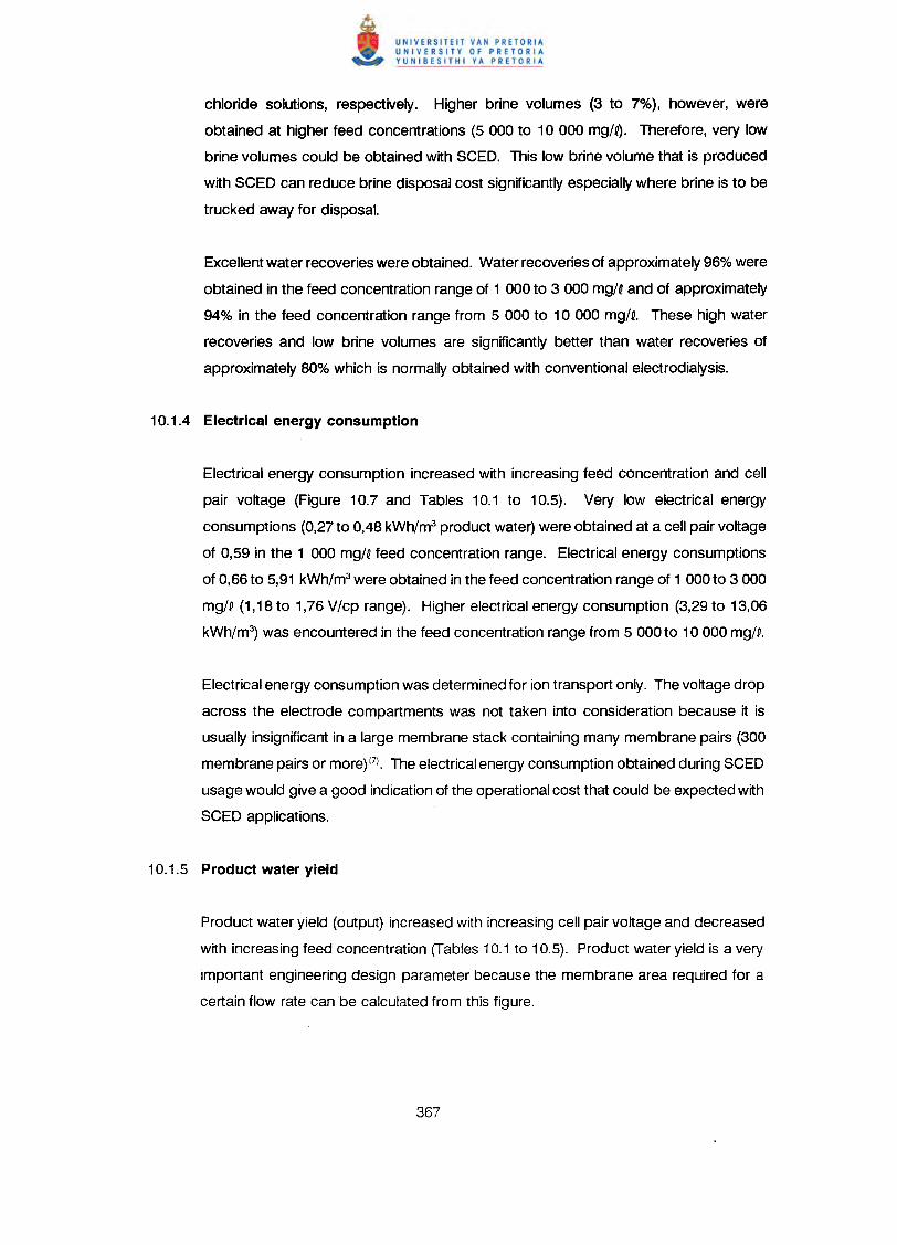
chloride solutions, respectively. Higher brine volumes (3 to 7%), however, were
obtained at higher feed concentrations (5 000 to 10 000 mg/~). Therefore, very low
brine volumes could be obtained with SCED. This low brine volume that is produced
with SCED can reduce brine disposal cost significantly especially where brine is to be
trucked away for disposal.
Excellent water recoveries were obtained. Water recoveries of approximately 96% were
obtained in the feed concentration range of 1 000 to 3 000 mg/~ and of approximately
94% in the feed concentration range from 5 000 to 10 000 mg/Q. These high water
recoveries and low brine volumes are significantly better than water recoveries of
approximately 80% which is normally obtained with conventional electrodialysis.
Electrical energy consumption increased with increasing feed concentration and cell
pair voltage (Figure 10.7 and Tables 10.1 to 10.5). Very low electrical energy
consumptions (0,27 to 0,48 kWh/m3 product water) were obtained at a cell pair voltage
of 0,59 in the 1 000 mg/~ feed concentration range. Electrical energy consumptions
of 0,66 to 5,91 kWh/m3 were obtained in the feed concentration range of 1 000 to 3 000
mg/~ (1,18 to 1,76 V/cp range). Higher electrical energy consumption (3,29 to 13,06
kWh/m3) was encountered in the feed concentration range from 5 000 to 10 000 mg/~.
Electrical energy consumption was determined for ion transport only. The voltage drop
across the electrode compartments was not taken into consideration because it is
usually insignificant in a large membrane stack containing many membrane pairs (300
membrane pairs or more) (7). The electrical energy consumption obtained during SCED
usage would give a good indication of the operational cost that could be expected with
SCED applications.
Product water yield (output) increased with increasing cell pair voltage and decreased
with increasing feed concentration (Tables 10.1 to 10.5). Product water yield is a very
important engineering design parameter because the membrane area required for a
certain flow rate can be calculated from this figure.
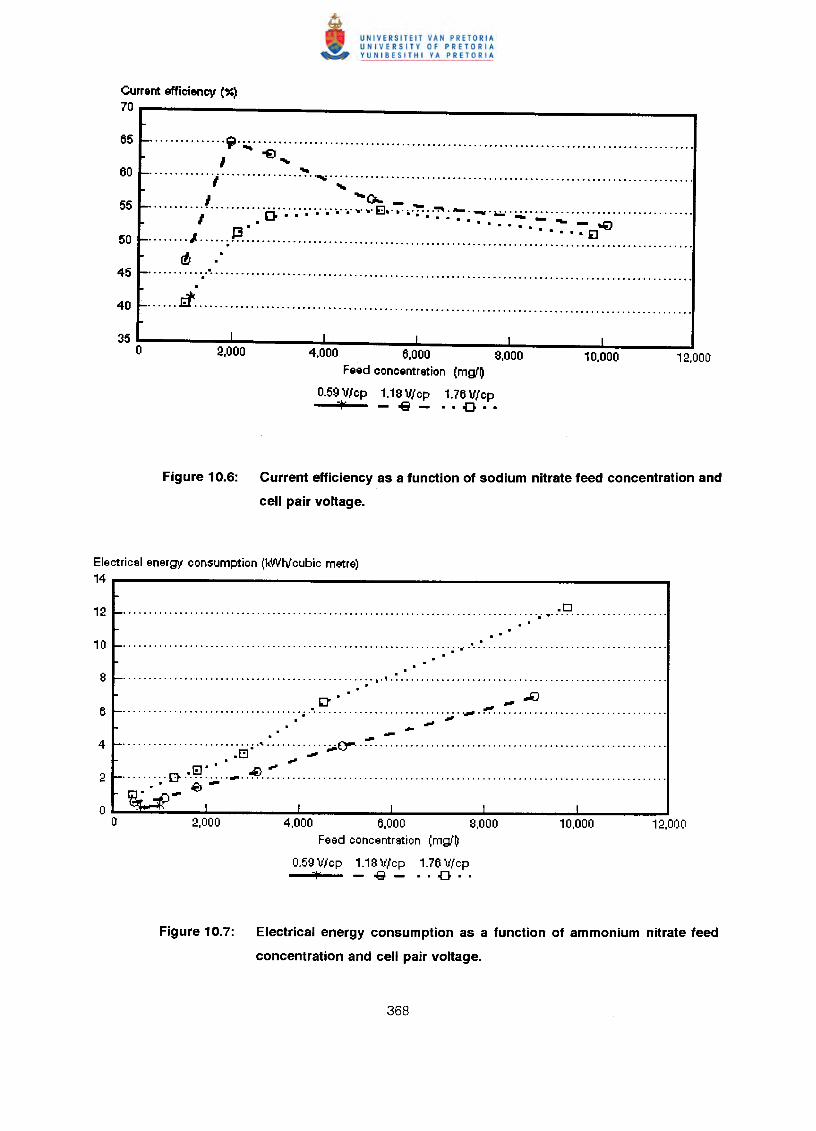
Current effioiency (%)
70 r---------------------------...65 _ ~.~ .
, "€J ••••60 .••._ "j ..,;...;., .
55 ••............ ,.1 t}..•..•....'.''.''.''.':-~ •.:: •.~~.~;--:-._ .••...;,0.•. ;,:. .....••...••.......•.......•..- _~J3 ·····il50 ~ /. ~ .
r!J45 ~ ...........•.•...............................................................................................40 ~ Iit .
35 oI
2.000I I
4,000 6,000Feed oonoentration (mgl~
0.59 Vlop 1.18 V/op 1.76 V/op* -o€i- .. {] ••
,8,000
I
10.000
Figure 10.6: Current efficiency as a function of sodium nitrate feed concentration and
cell pair voltage.
Electrical energy consumption (kWtv'oubic metre)14
(l" • ,.,. .Ji]. "..................................... ; ;.; ...•.•...................................... "... -. -. -...........................•.....•......... C1"" ......................................•.....................• [:1" , ~. ~
.I!J" .oi>~......... [}- _ .• o€J-
4,000 6,000 8.000Feed concentration (mg(~
0.59 V/cp 1.18 V/cp 1.76 V/cpi' -o€i- .. {] ..
Figure 10.7: Electrical energy consumption as a function of ammonium nitrate feed
concentration and cell pair voltage.
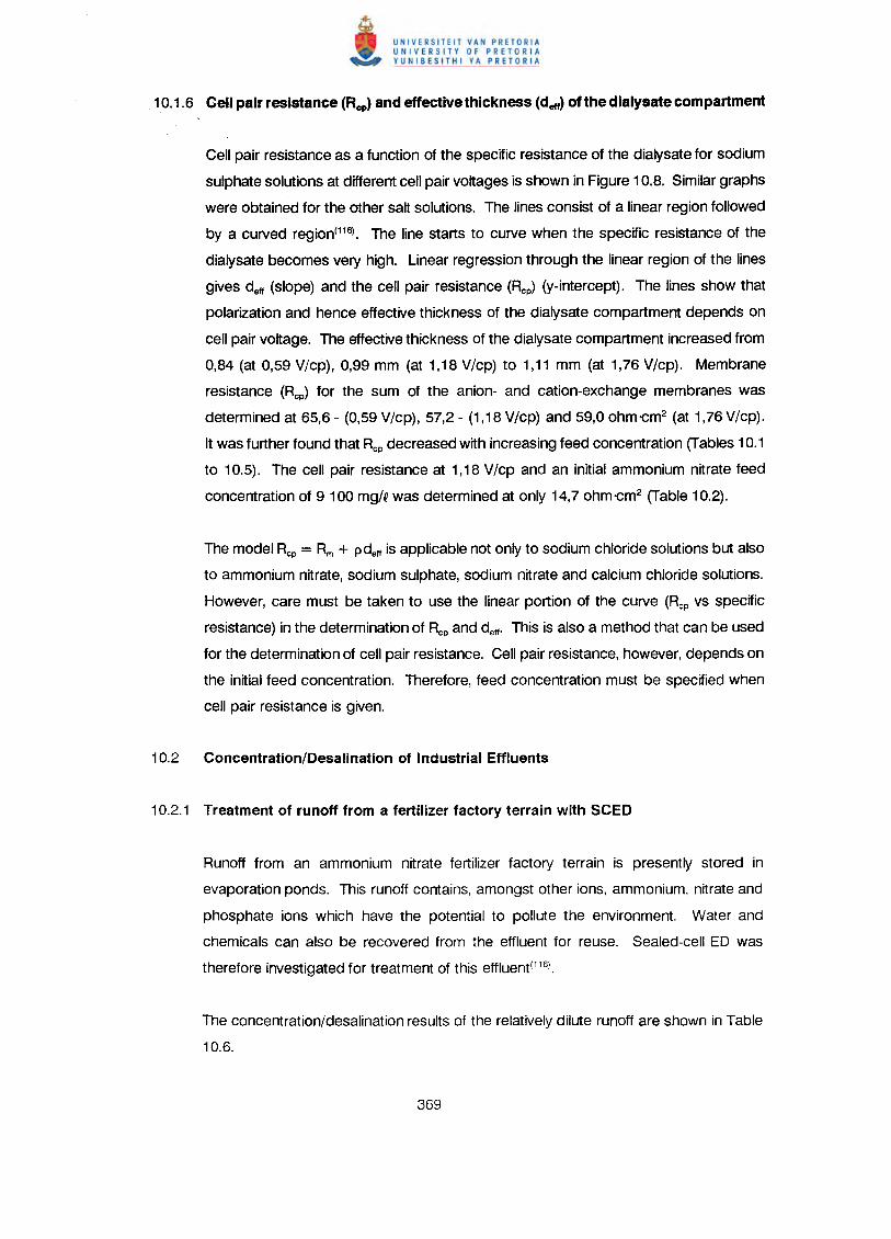
Cell pair resistance as a function of the specific resistance of the dialysate for sodium
sulphate solutions at different cell pair voltages is shown in Figure 10.8. Similar graphs
were obtained for the other salt solutions. The lines consist of a linear region followed
by a curved region(116).The line starts to curve when the specific resistance of the
dialysate becomes very high. Linear regression through the linear region of the lines
gives dell (slope) and the cell pair resistance (Rcp) (y-intercept). The lines show that
polarization and hence effective thickness of the dialysate compartment depends on
cell pair voltage. The effective thickness of the dialysate compartment increased from
0,84 (at 0,59 V/cp), 0,99 mm (at 1,18 V/cp) to 1,11 mm (at 1,76 V/cp). Membrane
resistance (Rcp) for the sum of the anion- and cation-exchange membranes was
determined at 65,6 - (0,59 V/cp), 57,2 - (1,18 V/cp) and 59,0 ohm-cm2 (at 1,76 V/cp).
It was further found that Rcp decreased with increasing feed concentration (Tables 10.1
to 10.5). The cell pair resistance at 1,18 V/cp and an initial ammonium nitrate feed
concentration of 9100 mg/Q was determined at only 14,7 ohm-cm2 (Table 10.2).
The model Rcp = Rm + pdellis applicable not only to sodium chloride solutions but also
to ammonium nitrate, sodium sulphate, sodium nitrate and calcium chloride solutions.
However, care must be taken to use the linear portion of the curve (Rcp vs specific
resistance) in the determination of Rcp and dell' This is also a method that can be used
for the determination of cell pair resistance. Cell pair resistance, however, depends on
the initial feed concentration. Therefore, feed concentration must be specified when
cell pair resistance is given.
Runoff from an ammonium nitrate fertilizer factory terrain is presently stored in
evaporation ponds. This runoff contains, amongst other ions, ammonium, nitrate and
phosphate ions which have the potential to pollute the environment. Water and
chemicals can also be recovered from the effluent for reuse. Sealed-cell ED was
therefore investigated for treatment of this effluent(116).
The concentration/desalination results of the relatively dilute runoff are shown in Table
10.6.
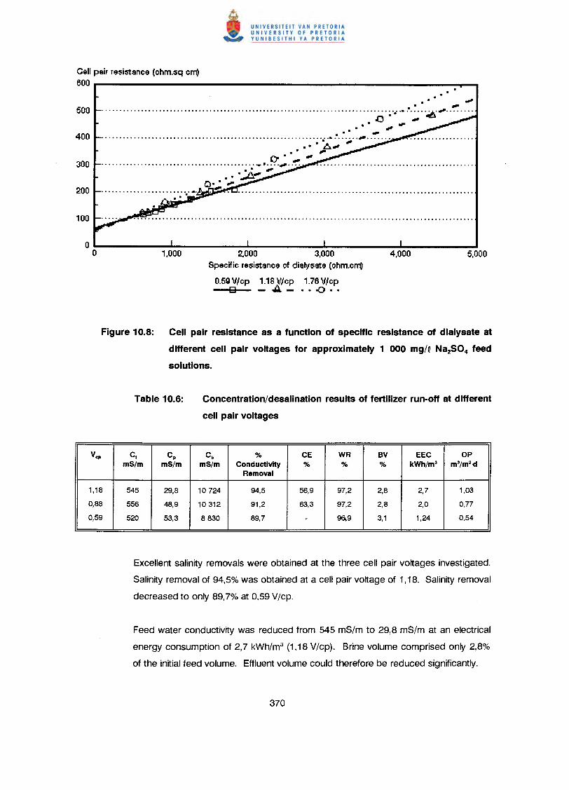
Cell pair resistance (ohm.sq crT"O600
" -....................................................................................•........ ~."""' ..0"" ~
" " -
2,000 3,000Specific resistance of dialy"sate (ohm.crT"O
0.59 V/cp 1.18 Vlcp 1.76 Vlcpo -..:..- .. <) ••
Figure 10.8: Cell pair resistance as a function of specific resistance of dialysate at
different cell pair voltages for approximately 1 000 mg/q Na2S04 feed
solutions.
Concentration/desalination results of fertilizer run-off at different
cell pair voltages
V"f' Cf cp cb % CE WR BV EEC OPmS/m mS/m mS/m Conductivity % % % kWh/m3 m3/m2-d
Removal
1,18 545 29,8 10724 94,5 56,9 97,2 2,8 2,7 1,03
0,88 556 48,9 10312 91,2 63,3 97,2 2,8 2,0 0,77
0,59 520 53,3 8830 89,7 - 96,9 3,1 1,24 0,54
Excellent salinity removals were obtained at the three cell pair voltages investigated.
Salinity removal of 94,5% was obtained at a cell pair voltage of 1,18. Salinity removal
decreased to only 89,7% at 0,59 V/cp.
Feed water conductivity was reduced from 545 mS/m to 29,8 mS/m at an electrical
energy consumption of 2,7 kWh/m3 (1,18 V/cp). Brine volume comprised only 2,8%
of the initial feed volume. Effluent volume could therefore be reduced significantly.
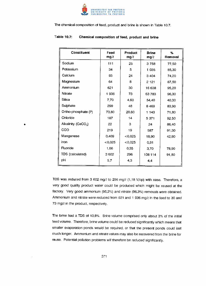
Constituent Feed Product Brine %mg/Q mg/Q mg/Q Removal
Sodium 111 25 3758 77,50
Potassium 34 5 1 035 85,30
Calcium 93 24 3404 74,20
Magnesium 64 8 2121 87,50
Ammonium 621 30 16638 95,20
Nitrate 1 936 73 63783 96,30
Silica 7,70 4,60 54,40 40,30
Sulphate 299 48 8469 83,90
Ortho-phosphate (P) 73,80 20,80 1 143 71,80
Chloride 187 14 5371 92,50
Alkalinity (CaC03) 22 3 24 86,40
COD 219 19 587 91,30
Manganese 0,409 <0,025 18,90 42,90
Iron <0,025 <0,025 0,91
Fluoride 1,66 0,35 3,70 78,90
TDS (calculated) 3602 296 108114 91,80
pH 5,7 4,3 4,4
TDS was reduced from 3 602 mg/Q to 296 mg/Q (1,18 V/cp) with ease. Therefore, a
very good quality product water could be produced which might be reused at the
factory. Very good ammonium (95,2%) and nitrate (96,3%) removals were obtained.
Ammonium and nitrate were reduced from 621 and 1 936 mg/Q in the feed to 30 and
73 mg/Q in the product, respectively.
The brine had a TDS of 10,8%. Brine volume comprised only about 3% of the initial
feed volume. Therefore, brine volume could be reduced significantly which means that
smaller evaporation ponds would be required, or that the present ponds could last
much longer. Ammonium and nitrate values may also be recovered from the brine for
reuse. Potential pollution problems will therefore be reduced significantly.
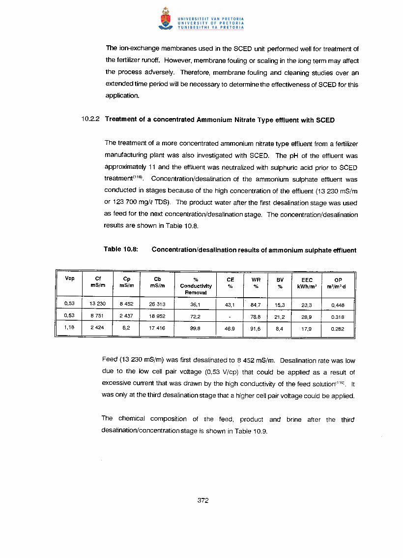
The ion-exchange membranes used in the SCED unit performed well for treatment of
the fertilizer runoff. However, membrane fouling or scaling in the long term may affect
the process adversely. Therefore, membrane fouling and cleaning studies over an
extended time period will be necessary to determine the effectiveness of SCED for this
application.
The treatment of a more concentrated ammonium nitrate type effluent from a fertilizer
manufacturing plant was also investigated with SCED. The pH of the effluent was
approximately 11 and the effluent was neutralized with sulphuric acid prior to SCED
treatment(11S,. Concentration/desalination of the ammonium sulphate effluent was
conducted in stages because of the high concentration of the effluent (13230 mS/m
or 123 700 mg/~ IDS). The product water after the first desalination stage was used
as feed for the next concentration/desalination stage. The concentration/desalination
results are shown in Table 10.8.
Vcp Cf cp Cb % CE WR BV EEC opmS/m mS/m mS/m Conductivity % % % kWh/m3 m3/m'.(j
Removal
0.53 13230 8452 26313 36,1 43,1 84,7 15,3 23,3 0,448
0,53 8751 2437 18952 72,2 - 78.8 21.2 28,9 0,318
1,18 2424 6,2 17416 99,8 46,9 91,6 8,4 17,9 0,282
Feed (13 230 mS/m) was first desalinated to 8 452 mS/m. Desalination rate was low
due to the low cell pair voltage (0,53 V/cp) that could be applied as a result of
excessive current that was drawn by the high conductivity of the feed solutionl' 'S). It
was only at the third desalination stage that a higher cell pair voltage could be applied.
The chemical composition of the feed, product and brine after the third
desalination/concentration stage is shown in Table 10.9.
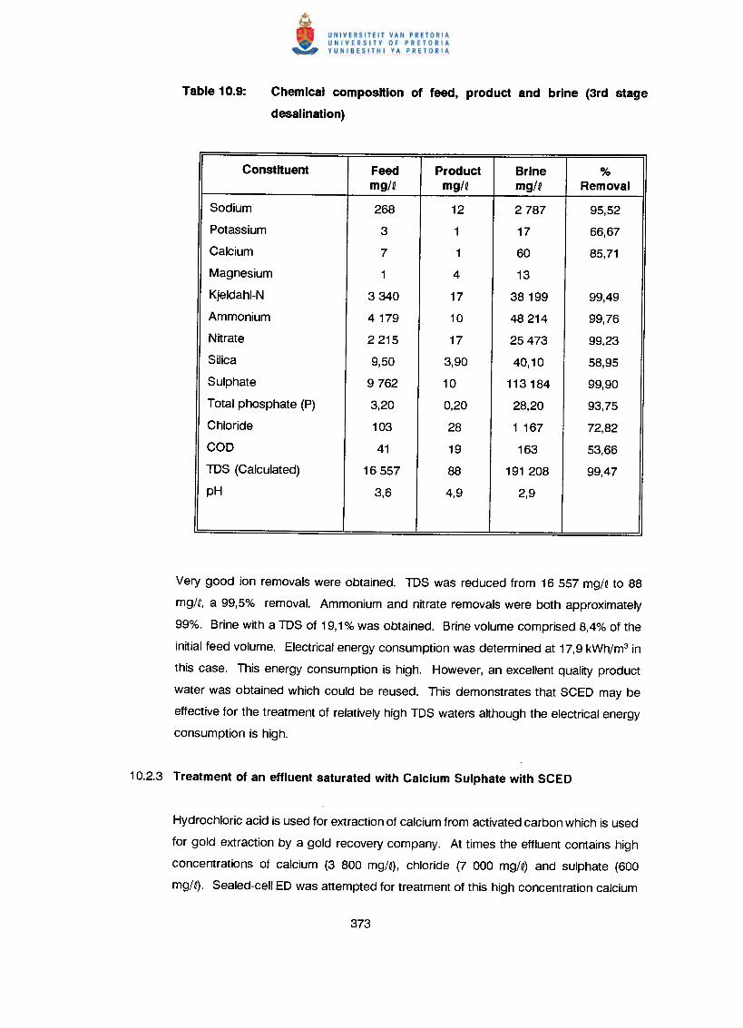
Chemical composition of feed, product and brine (3rd stage
desalination)
Constituent Feed Product Brine %mg/Q mg/Q mg/Q Removal
Sodium 268 12 2787 95,52
Potassium 3 1 17 66,67
Calcium 7 1 60 85,71
Magnesium 1 4 13
Kjeldahl-N 3340 17 38199 99,49
Ammonium 4179 10 48214 99,76
Nitrate 2215 17 25473 99,23
Silica 9,50 3,90 40,10 58,95
Sulphate 9762 10 113184 99,90
Total phosphate (P) 3,20 0,20 28,20 93,75
Chloride 103 28 1 167 72,82
COD 41 19 163 53,66
IDS (Calculated) 16557 88 191 208 99,47
pH 3,6 4,9 2,9
Very good ion removals were obtained. IDS was reduced from 16 557 mg/Q to 88
mg/Q, a 99,5% removal. Ammonium and nitrate removals were both approximately
99%. Brine with a TDS of 19,1% was obtained. Brine volume comprised 8,4% of the
initial feed volume. Electrical energy consumption was determined at 17,9 kWh/m3 in
this case. This energy consumption is high. However, an excellent quality product
water was obtained which could be reused. This demonstrates that SCED may be
effective for the treatment of relatively high TDS waters although the electrical energy
consumption is high.
Hydrochloric acid is used for extraction of calcium from activated carbon which is used
for gold extraction by a gold recovery company. At times the effluent contains high
concentrations of calcium (3 800 mg/Q), chloride (7 000 mg/Q) and sulphate (600
mg/Q). Sealed-cell ED was attempted for treatment of this high concentration calcium
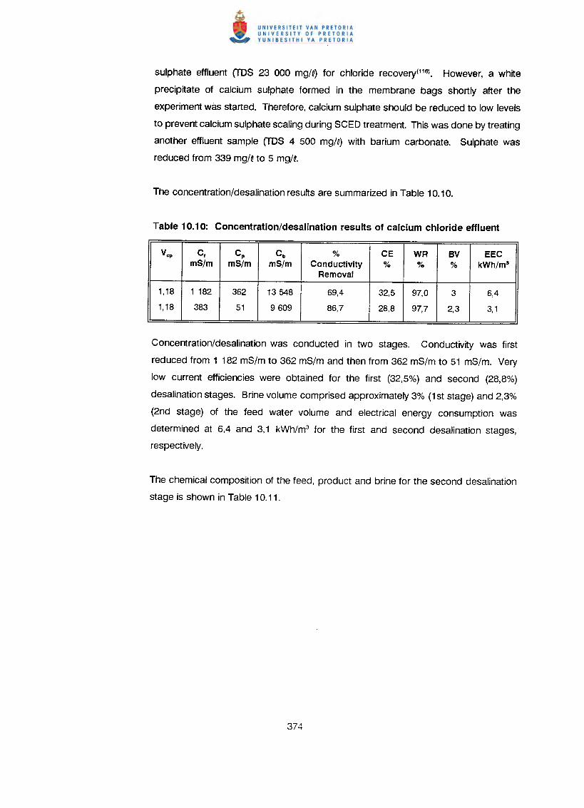
sulphate effluent (TDS 23 000 mg/Q) for chloride recovery(ll6). However, a white
precipitate of calcium sulphate formed in the membrane bags shortly after the
experiment was started. Therefore, calcium sulphate should be reduced to low levels
to prevent calcium sulphate scaling during SCED treatment. This was done by treating
another effluent sample (TDS 4 500 mg/e) with barium carbonate. Sulphate was
reduced from 339 mg/Q to 5 mg/Q.
Vcp Cf Cp Cb % CE WR BV EECmS/m mS/m mS/m Conductivity % % % kWh/m3
Removal
1,18 1 182 362 13548 69,4 32,5 97,0 3 6,4
1,18 383 51 9609 86,7 28,8 97,7 2,3 3,1
Concentration/desalination was conducted in two stages. Conductivity was first
reduced from 1 182 mS/m to 362 mS/m and then from 362 mS/m to 51 mS/m. Very
low current efficiencies were obtained for the first (32,5%) and second (28,8%)
desalination stages. Brine volume comprised approximately 3% (1st stage) and 2,3%
(2nd stage) of the feed water volume and electrical energy consumption was
determined at 6,4 and 3,1 kWh/m3 for the first and second desalination stages,
respectively .
The chemical composition of the feed, product and brine for the second desalination
stage is shown in Table 10.11.
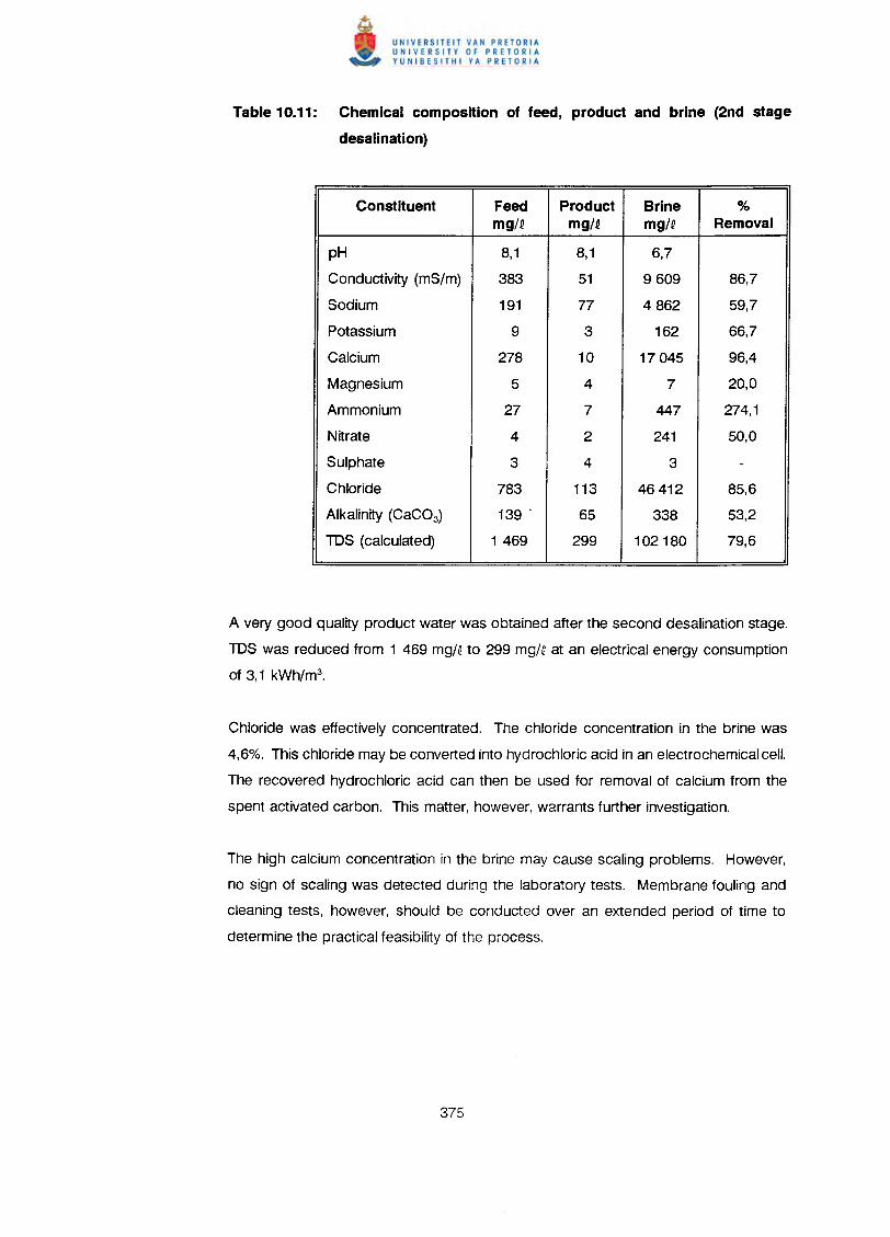
Table 10.11: Chemical composition of feed, product and brine (2nd stage
desalination)
Constituent Feed Product Brine %mg/Q mg/Q mg/Q Removal
pH 8,1 8,1 6,7
Conductivity (mS/m) 383 51 9609 86,7
Sodium 191 77 4862 59,7
Potassium 9 3 162 66,7
Calcium 278 10 17045 96,4
Magnesium 5 4 7 20,0
Ammonium 27 7 447 274,1
Nitrate 4 2 241 50,0
Sulphate 3 4 3 -Chloride 783 113 46412 85,6
Alkalinity (CaC03) 139 . 65 338 53,2
IDS (calculated) 1 469 299 102180 79,6
A very good quality product water was obtained after the second desalination stage.
IDS was reduced from 1 469 mg/Q to 299 mg/Q at an electrical energy consumption
of 3,1 kWh/m3•
Chloride was effectively concentrated. The chloride concentration in the brine was
4,6%. This chloride may be converted into hydrochloric acid in an electrochemical cell.
The recovered hydrochloric acid can then be used for removal of calcium from the
spent activated carbon. This matter, however, warrants further investigation.
The high calcium concentration in the brine may cause scaling problems. However,
no sign of scaling was detected during the laboratory tests. Membrane fouling and
cleaning tests, however, should be conducted over an extended period of time to
determine the practical feasibility of the process.
a) low electrical resistance(6)« 20 ohm 'Cm~;
b) high permselectivity(6)(> 0,9);
c) low electro-osmotic coefficient(7)« 12 mol H20/Faraday);
d) good chemical and dimensional stability(114);and
e) satisfactory polarization characteristics(7).
These requirements are also necessary for ED membranes for use in EOP. However,
an additional requirement for EOp·ED is finite transport of water through the
membranes. It has been shown that increasing flow of water through the membranes
causes an increase in current efficiency.
It was shown by Narebska and Koter(1B)that ion-water coupling became higher in more
concentrated solutions (approximately 0,5 mol/Q). At higher concentrations (> 0,5
mol/Q),the amount of free water in the membrane, the water transport number and the
osmotic flow decrease. Effects originating from the deswelling of the membrane at
high external concentration, may result in the observed decrease of the electro-osmotic
flow and the increased coupling between ions and the amount of water, crossing the
membrane(1B).
It has been found by Narebska et al.(31) that the resistance against flowing anions in
a cation membrane is imposed by water; the lower the amount of water in the
membrane, the higher the resistance. Consequently, increased ion-water coupling
causes increased resistance to the penetration of co-ions into the membrane matrix.
The result is an increase in current efficiency. It is therefore not necessary for ED
membranes for use in EOP to have very high permselectivities,because permselectivity
will be increased with increasing flow of water through the membranes. This was
especially observed for the more porous heterogeneous membranes at high feed
concentration (1 mol/Q). Consequently, membranes with a relatively low permselectivity
(approximately 0,6) should be suitable for concentration of salt solutions with
EOp·ED.
An increasing amount of water flowed through the membranes with an increase in feed
water concentration during EOP of salt solutions. However, a decrease in water flow
was experienced with an increase in feed concentration during EOP of acid solutions.
The anion membranes used for acid EOP had a very low permselectivity for chloride
ions due to the very high mobility of the protons in the membrane(11).Consequently,
the protons which flowed in the opposite direction to the flow of water would inhibit
water flow through the membranes. Therefore, very little water will pass through the
anion membrane in the case of acid EOP.
The cation membranes used for acid EOP, on the other hand, had a very high
permselectivity for protons (> 0,9). Back diffusion should be very low in this case
because back diffusion would be inhibited by the opposite flow of protons(19).Osmotic
flow, however, can be high through the cation membrane(19).
The cation membranes had a lower current efficiency than the anion membranes
during EOP of caustic soda solutions. This is due to the high mobility of the hydroxyl
ion(3O).It was shown by Koter and Narebska(32)that hydroxide ions impeded cations,
particularly at high external concentration, much more than chloride ions. This can be
attributed to the higher partial friction between sodium and hydroxyl ions.
The resistance imposed by a membrane matrix on the permeating hydroxyl ions is
much lower than that for chloride ions according to Narebska et al (30).Three factors
contributing to this effect, viz: the friction imposed by the cation (f21),water (f2w);and
the polymer matrix (f2m)- influence the flow of hydroxyl and chloride ions to different
degrees. Chloride ions are hindered mainly by water, especially at increasing sorption.
The flow of hydroxyl ions in diluted solution is hindered by the matrix and at high
concentration by the cation and then by water(30).
Brine concentration increases with increasing feed water concentration and current
density. This happens because the membranes become increasingly dewatered at
high current density. Consequently, the electro-osmotic coefficient decreases.
increasing current density. Consequently, the relative amount of electro-osmotic flow
through the membranes, increased as a function of current density. Osmotic flow,
however, appears to contribute significantly to the total flow in EOP. The osmotic flow
through the lonac membranes at a current density of 20 mA/cm2 (0,1 mol/Q feed)
comprised 33,9% of the total flow through the membranes. Osmotic flow was reduced
to 19,0% of the total flow at a current density of 50 mA/cm2 (0,1 molN feed). Osmotic
flow through the Selemion AAV and CHV membranes contributed 64,1 % to the total
flow at a current density of 20 mA/cm2 (0,1 mol/Q feed). Osmotic flow decreased to
20,9% at a current density of 100 mA/cm2 (0,1 mol/Q feed). Osmotic flow through the
Selemion AMP and CMV membranes contributed 61,4% to the total flow through the
membranes at a current density of 20 mA/cm2 (0,1 mol/Q feed). Osmotic contribution
decreased to 25,7% at a current density of 100 mA/cm2 (0,1 mol/Q).
Approximately 7 mol H20/Faraday permeated through the Selemion AAV and CHV
membranes in the feed concentration range from 0,5 to 1,0 mol/Q. It is known that little
water « 1 mol/Faraday) can permeate acid blocking anion membranes(48). Therefore,
the water could have entered the membranes only through the cation membrane.
Osmotic flow increased with increasing feed water concentration. It was also observed
that the osmotic flow decreased in some cases at the highest feed concentrations.
This can be ascribed to stronger back diffusion at the highest feed water
concentrations. It was also interesting to note that a decrease in osmotic flow had
taken place with increasing feed water concentration in the case of the more
hydrophobic lonac and WTPS membranes. The osmotic flow also increased through
the Israeli ABM and Selemion membranes with increasing feed concentration and
higher current efficiencies were experienced.
11.4 Discrepancy between Transport Numbers Derived from Potential Measurements
and Current Efficiency Actually Obtained
The correct relationships to be used when measuring membrane potential for the
prediction of desalting in ED, are as follows:
The correct Onsager relationship for potential measured is at zero current and at zero
volume flow, and for the transport number, at zero concentration gradient and zero
volume flow(117l.In practical ED, measurements are conducted at zero pressure and
in presence of concentration gradients and volume flows. These factors will influence
the results considerably in all systems in which volume flow is important and where the
concentration factor is high as is encountered in EOP. In the measurement of
membrane potential, the volume flow is against the concentration potential and in
general will decrease the potential. In ED water flow helps to increase current
efficiency, but the concentration gradient acts against current efficiency.
In the case of sodium chloride solutions, the apparent transport number of the
membrane pair (At) was higher than current efficiency (€p) at low feed water
concentrations (approximately 0,05 mol/~). This was predicted with the following
relationship:
a1p~+ I a'P~" <------I 2a'Pl I
The apparent transport number (at) decreased with increasing feed water
concentration. Current efficiency, however, increased with increasing feed water
concentration as a result of increasing water flow. Consequently, current efficiency
became higher than the apparent transport number at higher feed water concentrations
(0,5 to 1 mol/~). Current efficiency, however, decreased at very high feed
concentrations as a result of back diffusion. Similar results were obtained with EOP
of caustic soda solutions.
Current efficiency was much lower than ~t during EOP of acid solutions. This can be
ascribed to back diffusion of acid through the membranes during EOP which reduces
current efficiency significantly.
pair (!t) gave a good lower estimate of the actual Coulomb efficiency of the EOP
process in the case of sodium chloride solutions (0,1 mol/Q feed) using Selemion AMV
and CMV and polyethylene based membranes. However, it was found in this study
that the apparent transport number of a membrane pair gave a higher estimate of the
Coulomb efficiency of the EOP process in the 0,05 to 0,1 mol/Q feed concentration
range. The apparent transport number of a membrane pair gave a lower estimation
of the actual current efficiency in the feed water concentration range from
approximately 0,5 to 1,0 mol/Q. However, the apparent transport number of a
membrane pair gave a much too high estimation of current efficiency of the EOP
process for hydrochloric acid concentration. The apparent transport number of the
anion membrane, however, gave a much better estimation of current efficiency.
a) electric transport of co-ions;
b) diffusion of solute;
c) electro-osmotic flow; and
d) osmotic water flows.
The imperfect selectivity, f2, assumed to be one of the most important characteristics
of a membrane can produce up to 8% (NaCO and 35% (NaOH) of the current efficiency
losses at m = 2(17). Similar to t2, the effect of electro-osmotic flow of water (tw)
increases with m. It plays a significant role in the system with sodium chloride where
it diminishes current efficiency up to 30% according to Koter and Narebska(17).
However, it was found in this study that electro-osmotic flow of water increased current
efficiency significantly in the 0,05 to 1,0 mol/Q feed concentration range.
Depending on the working conditions, i.e. on the concentration ratio m'/m" and current
density, the decrease in current efficiency due to osmotic and diffusion flows can be
larger than that caused by electric transport of co-ions and water. This effect is
especially seen at the higher mean concentrations where the current efficiency can be
reduced to zero(17).
Efficiency of energy conversion in ED consists of the following two terms, viz., fJ IE (ion-
current coupling) and fJWE (ion-water coupling) according to Narebska and Koter(18l.
The first term expresses the storage of energy in producing a concentration difference
in the permeant. The second term corresponds to the transport of water, which acts
opposite to the separation of the components. It causes a waste of energy by
decreasing the concentration difference. This water flow has a negative effect on
energy conversion in ED. However, electro-osmosis can also have a positive effect on
ED by increasing current efficiency as has been demonstrated in this study.
Salt flux (SC)through a cation-exchange membrane can be predicted with the following
relationship:
Salt flux (both cation and anion) through ion-exchange membranes depends on water
flow (Jv) through the membranes, concentration gradient (AC) across the membrane
and membrane perm selectivity (at). It was shown that increasing water flow through
the membranes increased current efficiency. It was also shown that an increasing
concentration gradient (AC) across the membranes decreased current efficiency.
Current efficiency or salt flux was also low when the permselectivity of the membranes
was low. The experimental data for salt, acid and base EOP can therefore be
satisfactorily described by eq. (3.11.1).
Back diffusion through ion-exchange membranes in presence (at zero pressure) and
absence of water flow can be predicted with the following relationship according to
Kedem(15):
Back diffusion of salt through a membrane is less when water flows from the opposite
side (I.h.s. of eq. 3.3.45). However, back diffusion of salt is more in the absence of
volume flow (r.h.s. of eq. 3.3.45). Therefore, current efficiency will be higher when salt
diffusion is lower and this will occur when water flows through the membrane. This
was illustrated especially during EOP of sodium chloride solutions.
A decreasing amount of water permeated the membranes during acid EOP with
increasing acid feed water concentration. It was also found that back diffusion was
high during acid EOP. Therefore, the right hand side of equation (3.3.45) is applicable
to the experimental data that have been observed with EOP of hydrochloric acid
solutions.
c:ax = _1_2FB
Brine concentration (salt, acid or base) at high current density, cb max, appeared to attain
a constant value, independent of current density and dependent on the feed water
concentration. Maximum brine concentration was more dependent on feed
concentration where the membranes deswelled more with increasing feed water
concentration.
Maximum brine concentration could be predicted accurately with equations (3.10.28)
and (3.10.31). Therefore, anyone of these two methods can be used to predict cb max.
Brine concentration, cb, was predicted from the water flow through the membranes and
the apparent transport of the membrane pair (Xt) with the following relationship:
G, = lat2FJ
Brine concentration could be predicted more accurately in the case of sodium chloride
and caustic soda solutions than in the case of hydrochloric acid solutions. This can
be explained by back diffusion of acid that has been experienced during EOP of the
hydrochloric acid solutions. However, a much better prediction of acid brine
concentration should be obtained by using the apparent transport number of the anion
membrane (at") in the above equation.
The permselectivity of the membranes (Xl's) decreased with increasing feed water
concentration. Brine concentration, on the other hand, increased with increasing feed
water concentration. Therefore, the ratio cb carJcbexp decreased with increasing feed
concentration. The accuracy of prediction of brine concentration will therefore depend
on the feed concentration used for the determination of the apparent transport number.
11.8 Membranes for Sodium Chloride, Hydrochloric Acid and Caustic Soda
Concentration
The Selemion and lonac membranes performed satisfactorily for concentration of
sodium chloride solutions. The Raipore membranes, however, did not perform well,
due to the high water transport that was experienced with this membrane type.
Consequently, lower concentrations and efficiencies were obtained. The lonics, WTPS,
WTPVC and WTPST membranes all gave good results in terms of brine concentration
and current efficiency. However, serious polarization was experienced with the WTPS
membranes and ways to improve the polarization characteristics of these membranes
should be investigated.
The presently commercially available anion-exchange membranes are not stable for
long periods when exposed to high pH values(114). Consequently, the membranes that
were evaluated for caustic soda concentration would have a relatively short life time
when treating caustic soda effluents. Nevertheless, satisfactory results were obtained
with the Selemion and lonac membranes that were used for caustic soda
concentration. Membrane life time studies, however, should be conducted to
determine the effectiveness of these membranes for caustic soda concentration.
The newly developed Israeli ABM membranes compared favourably with the Selemion
AAV membrane for acid concentration. The Selemion AAV membranes were specially
designed for acid concentration. It was shown that the Selemion AAV membrane
adsorbed a substantial amount of acid(48). The low dissociation of sorbed acid in the
membrane was shown to be a factor which was responsible for the decrease in proton
leakage of this anion membrane.
A high degree of ion-coupling will be observed in the case of charged hydrophobic
membranes when acid is absorbed by the membrane. It was shown that the flux of
chloride ions from the anode to the cathode steadily increased as the amount of
sorbed acid was increased(48). This result showed that chloride ions are associated
with the movement of positively charged species. This may be due to the formation
of an aggregate form such as (CH40CQ+ resulting from the solvation of a proton by a
water and an hydrochloric acid molecule(48).This shows that ion association is taking
It was demonstrated that a conventional ED stack can be used as an EOP·ED stack
for concentration of sodium chloride, hydrochloric acid and caustic soda solutions
using commercially available ion-exchange membranes. Relatively high brine
concentrations and low brine volumes were obtained. Electrical energy consumption
was also low at low cell pair voltages.
An advantage of using a conventional ED stack as an EOP·ED stack is that the
membranes can be taken out of the stack for cleaning purposes if it should be
required. It is not possible to open sealed-cell ED membranes for cleaning. A
disadvantage of using a conventional ED stack as an EOP·ED stack is that the
membrane utilization factor will be low (approximately 80%). However, it should be
possible to improve the membrane utilization factor with improved gasket design and
this matter needs further investigation.
The sealed-cell ED unit performed satisfactorily for concentration/desalination of salt
solutions and industrial effluents. High brine concentrations and low brine volumes
were obtained. Low electrical energy consumptions were also obtained at low feed
concentrations.' Electrical energy consumptions obtained with the conventional
EOP·ED stack were comparable to the electrical energy consumptions obtained with
the sealed-cell ED stack.
The effective thickness of the dialysate compartment, deff• was much lower in the case
of the sealed-cell ED unit than in the case of the EOP·ED stack. This can be ascribed
to the thinner dialysate compartments that have been used in the sealed-cell unit and
to the higher linear flow velocities used.
The advantages and disadvantages of SCED are as follows: The capital cost of SCED
equipment should be less than that of a conventional plate-and-frame ED stack,
because of the simpler construction of the SCED stack. The membrane utilization
factor in the membrane bags is approximately 95% compared to approximately 80%
for membranes in conventional ED stacks. Higher current densities can be used in
SCED than in conventional sheet flow ED because higher linear flow velocities can be
obtained with ease. The higher current densities will result in higher water production
rates. Brine volumes produced by SCED are smaller than those obtained with
conventional ED. Therefore, the brine disposal problem will be reduced.
More electrical energy per unit of product water produced, will be used in the SCED
stack due to the higher current densities used. However, the increased cost for
electrical energy should be off-set by a decrease in capital cost. Scale may form more
readily in the membrane bags because the SCED stack does not have a built-in self
cleaning device such as encountered in the EDR system(S). It will be difficult to remove
scale from the membrane bags once it has formed because the bags cannot be
opened for cleaning. Therefore, scale forming chemicals should be removed by ion-
exchange or nanofiltration prior to SCED treatment. This will affect the economics of
the process adversely, especially if large flows are involved.
Scale-up of a laboratory size SCED unit (100 cm2jcp) to a pilot or full-scale plant would
be possible. It would be possible to manufacture large-scale membrane bags
commercially and the bags would be robust. An advantage of the membranes that
were used in the SCED stack was that they could be stored dry. This is usually not
the case with ion-exchange membranes normally used in conventional ED. The
successful application of SCED technology seems to depend on the need to apply this
technology in preference to conventional ED for specific applications where high brine
concentrations and small brine volumes are required.
Salts, acids and bases frequently occur in industrial effluents. These effluents usually have a
large pollution potential. Often the effluents also contain valuable chemicals and water that can
be recovered for reuse. Effluent disposal cost can be high, especially where effluents must be
trucked away for safe disposal. However, it would be possible to reduce disposal cost
significantly if effluent volume could be reduced to a significant extent.
Electro-osmotic pumping ED has the potential to be applied for industrial effluent treatment.
Preliminary work has indicated that small brine volumes and high brine concentrations could
be achieved with EOP·ED at attractive electrical energy consumptions. However, it was
determined that the following needs still existed regarding the application of EOP·ED for
industrial effluent treatment:
a) to consider and document the relevant EOP·ED and ED theory properly;
b) to study the EOP·ED characteristics (transport numbers, brine concentration, current
efficiency, current density, electro-osmotic coefficient, etc.) of commercially available
and other ion-exchange membranes in a single cell pair with the aim to identify
membranes suitable for EOP·ED;
c) to develop a simple method and to evaluate existing models with which membrane
performance for salt, acid and base EOP'ED, can be predicted; and
d) to evaluate the EOP·ED process for industrial effluent treatment.
The following conclusions can be drawn as a result of this investigation:
• A conventional ED stack which was converted into an EOP·ED stack performed
satisfactorily for concentration/desalination of sodium chloride, hydrochloric and caustic
soda solutions. Dialysate concentrations of less than 500 mg/Q could be obtained in
the feed water and cell pair voltage ranges from 1 000 to 10 000 mg/Q and 0,5 to 4
V/cp, respectively. Brine concentrations of 2,1 to 14,0%; 3,6% to 8,7% and 2,3% to
7,3% were obtained for sodium chloride, hydrochloric acid and caustic soda solutions,
respectively.
Current efficiency increased with increasing feed water concentration during EOP·ED
of sodium chloride and caustic soda solutions. This is in contrast to what is usually
happening. Increasing feed water concentration causes increasing water flow through
the membranes which inhibits co-ion invasion. Therefore, higher current efficiency is
obtained. This supported the results that were obtained in a single cell pair. Current
efficiencies varied between 75,2 and 93,6%; 29,2 and 46,3% and 68,9 and 81,2% for
sodium chloride (1 000 to 5 000 mg/Q feed; 0,5 to 1,5 V/cp); hydrochloric acid (1 000
to 5 000 mg/~ feed: 0,5 to 4,0 V/cp); and caustic soda solutions (1 000 to 10 000
mg/~ feed; 0,5 to 3 V/cp), respectively.
Low brine volumes and high water recoveries were obtained. Brine volume increased
with increasing feed water concentration and decreased with increasing cell pair
voltage. Brine volume varied between 1,5 and 4,0% for sodium chloride (1 000 to
5 000 mg/~ feed; 0,5 to 1,0 V/cp); between 2,4 and 7,8% for hydrochloric acid (1 000
to 5 000 mg/~ feed; 0,5 to 1,5 V/cp); and between 2,3 to 7,3% for caustic soda
solutions (1 000 to 5 000 mg/Q feed; 0,5 to 1,5 V/cp).
Electrical energy consumption was low at low feed water concentrations and low cell
pair voltages. Electrical energy consumption increased with increasing feed water
concentration and increasing cell pair voltage. Electrical energy consumption of less
than 2,5 kWh/m3 product water was obtained for sodium chloride (0,5 to 1,5 V/cp;
1 000 to 3 000 mg/~ feed); between 0,2 and 3,2 kWh/m3 product for hydrochloric acid
(0,5 to 1,5 V/cp; approximately 1 000 mg/~ feed); and between 0,4 and 2,2 kWh/m3
product for caustic soda solutions (0,5 to 1,5 V/cp; 1 000 to 3 000 mg/~ feed).
Water yield increased with increasing cell pair voltage and decreased with decreasing
feed water concentration. Water yield was 0,38 m3/m2.d at a linear flow velocity of 1
cm/s through the stack when hydrochloric acid was concentrated (2 V/cp; 3 000 mg/~
feed). Water yield was increased to 0,7 m3/m2.d when linear flow velocity was
increased to 5 cm/s. A higher linear flow velocity will also depress polarisation.
Therefore, it would be advantageous to operate an EOP·ED stack at the highest
possible linear flow velocity.
• Sealed-cell ED should be effective for concentration/desalination of relatively dilute (500
to 3 000 mg/~ IDS) non-scaling forming salt solutions. Product water with a TDS of
less than 300 mg/Q could be produced in the feed water concentration range from 500
to 10 000 mg/~ IDS. Electrical energy consumption of 0,27 to 5,9 kWh/m3 product
was obtained (500 to 3 000 mg/~ feed range). Brine volume comprised approximately
2% of the initial feed water volume. Therefore, brine disposal costs should be
significantly reduced with this technology.
concentration range due to high electrical energy consumption (3,3 to 13,0 kWh/m3
product). However, SCEO may be applied in this TOS range depending on the value
of the products that can be recovered.
Treatment of scale forming waters will affect the process adversely because scale will
precipitate in the membrane bags which cannot be opened for cleaning. Membrane
scaling may be removed by current reversal or with cleaning solutions. However, this
matter needs further investigation. Scale-forming waters, however, should be avoided
or treated with ion-exchange or nanofiltration prior to SCEO.
It was demonstrated that a relativelydilute ammonium nitrate effluent (TDS 3 600 mg/Q)
could be successfully treated in the laboratory with SCEO. Brine volume comprised
only 2,8% of the treated water volume. Electrical energy consumption was determined
at 2,7 kWh/m3 product. Both the brine and the treated water could be reused.
Membrane fouling or scaling, however, may affect the process adversely and this
matter needs further investigation.
It was difficult to concentrate/desalinate a concentrated ammonium sulphate effluent
(approximately 13 200 mS/m or 123 700 mg/Q TOS) with SCEO.
Concentration/desalination was conducted in stages. Nevertheless, it was possible to
desalinate the effluent to 6,2 mS/m (88 mg/Q TDS). However, electrical energy
consumption was high (59 kWh/m3 product). Brine volume comprised 45% of the
treated volume. A very high brine concentration (approximately 26 300 mS/m or 332
000 mg/Q TDS) could be obtained after the first desalination stage. However, a more
dilute (16 557 mg/Q TOS) ammonium sulphate effluent (3rd stage) could be more
easily concentrated/desalinated to 88 and 191208 mg/QTOS product water and brine,
respectively, at water recovery and electrical energy consumption of 91,6% and 17,9
kWh/m3, respectively. Therefore, SCEO could also be effectively applied for the
desalination/concentration of relatively high TDS waters.
It was not possible to concentrate/desalinate an effluent saturated with calcium
sulphate with SCEO due to membrane scaling which took place. However, it was
possible to concentrate/desalinate the effluent effectively after sulphate removal by
chemical precipitation. It was possible to concentrate/desalinate the effluent from
1 182 mS/m (4461 mg/Q TOS) to 51 mS/m (299 mg/Q TDS) at an electrical energy
consumption of 9,5 kWh/m3 product. Brine volume comprised 5,3% of the treated
feed. The cost effectiveness of these procedures need to be evaluated.
The ion-exchange membranes used in the SCED stack performed very well for
ammonium and nitrate removal. Ammonium and nitrate ions were removed from 4 179
and 2 215 mg/Q in one case to 10 - (99,8% removaQ and 17 mg/Q (99,2% removaQ,
respectively.
Capital cost of SCED equipment should be less than that of conventional ED due to
the simpler design of the SCED stack. The membrane utilization factor of 95% is much
higher than in conventional (approximately 80%) ED.
Sealed-cell ED has potential for treatment of relatively dilute « 3 000 mg/Q TDS) non-
scaling waters for water and chemical recovery for reuse. However, high TDS (up to
16 000 mg/Q) waters can also be treated depending on the value of the products that
can be recovered.
• Brine concentration increased with increasing current density and increasing feed water
concentration. Brine concentration appeared to attain a constant value at high current
density dependent on the electro-osmotic coefficients of the membranes.
• Current efficiencies were nearly constant in a wide range of current densities (0 to 70
mNcm~ and feed water concentrations (0,05 to 1,0 mol/Q) in the case of the Selemion
and Raipore membranes used for sodium chloride concentration. The same
phenomenon was observed for the Selemion membranes used for acid concentration.
However, all the other membranes showed a slight decrease in current efficiency with
increasing current density. This showed that the limiting current density was exceeded
and that polarization was taking place. Significant polarization took place with the
WTPS membranes at relatively low current density (> 20 mNcm~.
• Water flow through the membranes increased with increasing current density. Water
flow through the membranes also increased with increasing feed water concentration,
especially for the membranes that were used for salt and caustic soda concentration.
This increasing water flow improved current efficiency and water flow can therefore also
have a positive effect on ED. However, water flow decreased through the Selemion
membranes that were used for acid concentration when feed water concentration was
increased and no increase in current efficiency was observed. Current efficiency,
The electro-osmotic coefficients were determined to be a function of feed water
concentration. The coefficients decreased with increasing feed water concentration
until a constant value was obtained at high current density. The decrease in electro-
osmotic coefficients with an increase in feed water concentration can be ascribed to
deswelling of the membranes with increasing feed water concentration or to a
reduction in membrane permselectivity when the feed water concentration is increased.
Osmotic flow in EOP decreases relative to the total flow with increasing current density
while the electro-osmotic flow increases relative to the osmotic flow. Osmotic flow,
however, contributes significantly to the total water flow in EOP. Osmotic flow through
the Selemion AAV and CHV membranes contributed 64,1% of the total flow through the
membranes at a current density of 20 mNcm2 (0,1 mol/Q feed). Osmotic flow was
20,9% of the total flow at a current density of 100 mA/cm2 (0,1 mol/Q feed).
• Membrane permselectivity decreased with increasing brine and feed water
concentration and increasing concentration gradient across the membranes.
• Selemion AMV and CMV and lonac membranes performed satisfactorily for
concentration of sodium chloride solutions. Salt brine concentrations of 19,3%; 25,1%;
27,2% and 29,8% were obtained at feed water concentrations of 0,05; 0,1; a,s and1,0 mol/Q, respectively, with the Selemion AMV and CMV membranes. Current
efficiency in this feed water concentration range varied from 62 to 91%. Performance
of the lonics and WTPS membranes were poorer while the poorest results were
obtained with the WTPVC, WTPST and Raipore membranes.
Satisfactory results were obtained with the Selemion AAV and CHV and newly
developed Israeli ABM-3 and ABM-2 membranes for hydrochloric acid concentration.
Acid brine concentrations of 18,3%; 20,9%; 25,0% and 27,2% were obtained at 0,05;
0,1; 0,5 and 1,0 mol/Q feed water concentration, respectively, for the Selemion AAV
and CHV membranes. Current efficiency varied between 35 and 42%. Higher current
efficiencies, however, were obtained with the Israeli ABM-3 membranes. Current
efficiency varied between 34 and 60% in the same feed water concentration range.
Selemion AMV and CMV, Selemion AMP and CMV and lonac membranes performed
well for caustic soda concentration. Caustic soda brine concentrations of 14,3%;
17,7%; 20,1% and 24,4% were obtained at high current density at 0,05; 0,1; 0,5 and
1,0 mol/Q feed water concentration, respectively, with the Selemion AMV and CMV
membranes. Current efficiency varied from 47 to 76%.
Membrane current efficiency in EOP increased with increasing water flow through the
membranes. This was especially observed for the more porous heterogeneous
membranes at high feed water (1,0 mol/Q) concentration. It will therefore not be
necessary for membranes to have very high (> 0,9) permselectivities for use in
EOP·ED.
• It has been found that a simple potential measurement can be used effectively to
predict membrane performance for salt, acid and base concentration with ED. The..ratio between the apparent transport number (at) and current efficiency (€p),however,
depends on the feed concentration and current density used. Ratio's of Xt/€p varied
between 1,° and 1,07 (0,1 moll Q feed, Selemion AMV and CMV, salt concentration);
0,95 to 1,09 (0,5 mol/Q feed, lonac); 1,02 and 1,05 (0,5 mol/Q feed, Raipore); 0,95
and 1,02 (0,5 mol/Q, lonics). Consequently, it should be possible to predict current
efficiency for concentration of sodium chloride solutions with an accuracy of
approximately 10% and better from the apparent transport number of the membrane
pair.
Correlations obtained between the apparent transport number (Xt) and current
efficiency for membranes used for acid concentration, were unsatisfactory. The
apparent transport number of the membrane pair (Xt) was from 1,5 to 4 times higher
than current efficiency in the feed acid concentration range from 0,05 to 1,0 mol/Q.
Back diffusion of hydrochloric acid through the membranes caused the lower current
efficiency. However, the apparent number of the anion membrane (ae) gave a much
better indication of membrane performance for acid concentration. Ratio's of ata/€p
of 1,1 to 1,2 (1,0 mol/Q, Selemion AAV); 0,97 to 0,84 (1,0 mol/Q, ABM-2); 0,92 to 0,97
(0,1 mol/Q, ABM-1) were obtained. Consequently, it should be possible to predict
current efficiency for concentration of hydrochloric acid solutions with an accuracy of
approximately 20% and better from the apparent transport number of the anion
membrane.
•Correlations obtained between the apparent transport number (at) and current
efficiency of the membranes investigated for caustic soda concentration were
satisfactory. Ratio's of ~t/€P of 1,0 to 1,1 (0,05 molN, lonad); 0,9 to 1,0 (0,1 molN,
lonad); 0,9 (1,0 mol/Q, SelemionAMV and CMV); 1,1 to 1,2 (0,1 mol/Q, SelemionAMP
and CMV); 1,1 (0,5 molle, Selemion AMP and CMV) were obtained. Therefore, it
should be possible to predict current efficiency for concentration of caustic soda
solutions with an accuracy of approximately 20% and better from the apparent
transport number of the membrane pair. Good correlations were also obtained
between the apparent transport number of the cation membrane (LltC) and current
efficiency. Consequently, it should also be possible to predict current efficiency with
an accuracy of approximately 20% and better from the apparent transport number of
the cation membrane.
• The correct Onsager relationships to be used for potential measurement (Ll'lt) and for
the transport number (JF/I) are at zero current and zero volume flow, and at zero
concentration gradient and zero volume flow, respectively. In practical ED,
measurements are conducted at zero pressure and in the presence of concentration
gradients and volume flows. These factors will influence the results considerably in all
systems in which volume flow is important and where the concentration factor is high
as is encountered in EOP. In measurement of membrane potential, the volume flow
is against the concentration potential and in general will decrease potential. In ED,
water flow helps to increase current efficiency, but the concentration gradient is against
current efficiency.
-• Brine concentration can be predicted from apparent transport numbers (Llt'S) and
water flows through the membranes. The ratio Cbca0Cbexp decreased with increasing
feed concentration.
• Maximum brine concentration, cbmax, can be predicted from two simple models. A very
good correlation was obtained by the two methods. Maximum brine concentration
increased with increasing feed concentration and appeared to level off at high feed
concentration (0,5 to 1,0 molle).
• Models described the system satisfactorily for concentration of sodium chloride,
hydrochloric acid and caustic soda solutions with commercially available membranes.
Brine concentration approached a limiting value (plateau) at high current density
dependent on the electro-osmotic coefficients of the membranes. A constant slope
(electro-osmotic coefficient) was obtained when water flow was plotted against current
density. Straight lines were obtained when cell pair resistance was plotted against the
specific resistance of the dialysate. Current efficiency increased with increasing flow
of water, decreased when back diffusion was high and transport numbers were low.
Maximum brine concentration (mol/Q)
current efficiency (%)
volume flow through membranes (em/h)
effective current density (Coulomb efficiency x current density)
brine concentration (mol/Q)
electro-osmotic coefficient (Q/Faraday)
Faraday's constant (96 500 Coulomb/ge)
osmotic water flow (em/h)
electro-osmotic waterflow (em/h) (J = Josm + Jelosm)
feed concentration (mg/Q)
product concentration (mg/Q)
effective thickness of dialysate compartment (mm) (polarisation factor)
cell pair voltage (volt)
cell pair resistance (0 -em~
specific resistance of dialysate (0 -em)
anion membrane
cation membrane
membrane potential (mV)
apparent transport number of membrane pair
p
acA1JFm
At
phenomenological resistance coefficient
phenomenological friction coefficient
friction imposed by cation (1) on anion
friction imposed by water (w) on anion (2)
friction imposed by polymer matrix (m) on anion (2)
straight resistance coefficients
external concentration
anion-polymer frictional force
anion-water frictional force
apparant transport number of membrane pair
2m
2w
Ai
water activity in interior of membrane
water activity outside membrane
membrane internal osmotic pressure
gas constant
absolute temperature
partial molar volume of internal water component of membrane
equilibrium water content
membrane potential
maximum membrane potential
transport number
apparent transport number
activity on one side of the membrane
activity on the other side of the membrane
Faraday's constant
electric current
ion flux of species i
transport number of species i inside the membrane
Flux density of i (mol/cm-2s-1)
concentration of i (mol cm-3)
electrochemical potential of i
distance from reference plane in membrane
gas constant
absolute temperature
activity coefficient of i
partial molar volume of i
pressure
number of positive charges per ion (valency)
Faraday's number
electrical potential

diffusion coefficient of i
absolute mobility of i
velocity of local center of mass
phenomenological conductance coefficient
force on k per mole
rate of entropy production, reflection coefficient
dissipation function
number of components
exchange flow
osmotic pressure
phenomenological coefficient
phenomenological coefficient
phenomenological coefficient
total volume flux density (cm/s-1)
solute permeability
phenomenological resistance coefficient
minor of Lik in IL I •determinant of Lik
chemical potential of electrolyte
electric current density (amp/cm~
electromotive force
concentration of i (mol.cm-3)
Faraday's number
frictional force of k on i per mol of i
molar frictional coefficient of i with k
flux density of i (mol.cm-2s-1)
specific electrical conductance
mean velocity of i
force on i per mol
flow of cation J1
flow of anion J2
J1
J" J2
J.J,", J2" -
difference in electrochemical potential
phenomenological coefficient
chemical potential
electric current
valance of cation
valance of anion
Faraday's constant
electromotive force
volume flow
apparent transport number
potential difference across the membrane
a = X"IX!total concentration of salt in membrane
salt concentration in the aqueous solution
average concentration of salt in the two solutions adjacent to the membrane
concentration of the free counter- and co-ions in the membrane
concentration of associated salt in the membrane
electromotive force
Faraday's constant
frictional coefficient
frictional coefficient between co- and counter-ions
electrical current
flow of species i
stoichiometric flows of counter-ions and co-ions, respectively
flow of salt
flow of free counter-ions and co-ions, respectively
distribution coefficient of salt between membrane and aqueous phases
dissociation constant of salt in the membrane
dissociation constant of fixed group in the membrane
filtration coefficient
m = ~'/K,}
pressure difference
electro-osmotic pressure measured at zero volume flow and the absence of
salt gradients
c.u~,., c'ay _""s s
degree of coupling
straight resistance coefficients for transport of counter-ions, co-ions
and salt, respectively
coupling resistance coefficient between flows of ion 1 and 2
universal gas constant
absolute temperature
driving force for species i
driving forces for transport of counter -ions, co-ions and salt,
respectively
total concentration of fixed groups in the membrane
concentration of dissociated fixed groups in the membrane
associated fixed groups in the membrane
valency of ion i
a: = ~s kCs'2
electro-osmotic permeability measured at zero pressure and salt gradient
transport number of counter-ions and co-ions, respectively
electric potential in aqueous and membrane phases
standard chemical potential of species i in membrane and aqueous solution,
respectively
electrochemical potential of counter-ion 1 and of co-ion 2 in membrane,
respectively
difference in electrochemical potential of species i
electrochemical potential of counter-ion 1 and of co-ion 2 in aqueous solution,
respectively
chemical potential of salt in membrane
difference in electrochemical potentials of species i
membrane conductance measured in the absence of salt gradient and volume
flow
membrane conductance measured in the absence of a pressure gradient
salt permeability defined for Jy = 0
salt permeability defined for a p - a 1t = 0 and I = 0
salt permeability defined for ap = 0 and I = 0
leak conductance (LC) ratio defined for
Jy = 0
reflection coefficient
adJ1
Jw
t2
tw
11
concentration difference across membrane at time t = 0
concentration at one side of the membrane at time t = 0
concentration at other side of memtrane at time t = 0
concentration difference across membrane after time t
total counter-ions
water flux
co-ion transport number
water transport number
counter-ion transport number
reduced transport number of counter-ions
mean molality
diffusion and osmotic fluxes
electric current
-1 for cation-exchange membrane; +1 for anion-exchange membrane
combination of the phenomelogical conductance coefficient Lik and the mean
mobility, ni, of a solute
chemical potential difference of the solute
electric current
concentration changes of anolyte and catholyte after time at
mean concentration of anolyte and catholyte at time t = 0, CO = (caO + ckO)/2
efficiency of energy conversion•...J1/V1 - 0,018 m Jw
difference of electrical potential measured with electrodes reversible to co-ions
concentration of species i, mol.m-3
potential difference. V
current density, A ·m2
flux density of species i, mol.m-2.s-1
conductance coefficients
external molality of NaCI
coupling coefficients
transport number of water, mol per Faraday
thermodynamic force
Jw
Js
a!J.s, a!J.w -
Lik
J'w
TJ
q
ale
force ratio
square route of the straight conductance coefficients
efficiency of energy conversion
chemical potential of species i, J.mol-1
osmotic pressure, Pa
dissipation function
sodium ions
osmotic flow of water
diffusion flow of solute
differences of chemical potential of solute and water, respectively
phenomenological conductance coefficient
flow of water against the flow of solute conjugated to the concentration part of
the chemical potential difference of water, a!J.wC
total volume flow conjugated to the difference of pressure in the compartments
on the opposite side of the membrane, ap
dissipation function
efficiency of energy conversion
coupling coefficient
difference in osmotic pressure
reflection coefficient
osmotic swelling pressure
water activity in membrane
water activity outside membrane
gas constant
absolute temperature
internal equilibrium electrolyte concentration
concentration mol/q
partial molar volume of the internal water component
total electromotic force of membrane cell
molecular mass of solvent
water transport number
transport number
gas constant
absolute temperature
Faraday
activity
apparent transport number
true transport number
fixed charge density (equivalent per unit volume of swollen membrane)
equivalent of co-ions per equivalent of fixed group present in the membrane
mobilities of ions
specific conductance of membrane
volume of water flowing per Coulomb
volume of water flowing per second (millilitre)
current in amperes
specific conductance of pore liquid
pore area
volume fraction of water in the membrane
equivalent of fixed groups per unit volume of interstitial water
volume decrease at anode due to water transport
observed volume change
partial molar volume
activity of species i (mol/Q)
effective membrane area (cm~
concentration of species i (mol/Q)
Faraday's constant - 96500 (amp.sec/moQ
driving force acting on species i
electric current density (amp/cm~
effective current density (amp/cm~
flux of species i through a membrane (mol/(sec.cm2))
volume flow through a membrane (cm/sec = cm3/cm2.sec)
filtration coefficient
solute permeability
amount of feed solution entering a diluate channel per unit time
universal gas constant
salt flux (cation)
salt flux (anion)
transport number of ionic species i
effective transport number of the ionic species i
difference between counter-ion and co-ion effective transport members
effective transport number of a membrane pair
absolute temperature, 0 K
water flow through a membrane (cm/s)
volume of solution that enters a membrane bag per unit area
molar volume of species i
membrane thickness
drag coefficients associated with the ionic species i
activity coefficient of species i
thickness of the unstirred layer next to a solid surface
overall current efficiency
Coulomb efficiency (current efficiency)
efficiency associated with water transport through membranes
degree of demineralization
chemical potential of ionic species i
electrochemical potential of ionic specie i
electrical potentical difference between reversible electrodes, due to a
difference of concentration at both sides of the membrane
osmotic pressure
reflection coefficient
salt permeability
current efficiency
anion-exchange membrane
cation-exchange membrane
Faraday's constant (Coulomb equiv-1)
current density, amp cm-2
molar flux, mol cm-2 sec-1
volume flux, cm- sec-1
hydraulic permeability cm . sec-1 per unit pressure
local solute permeability, cm2·sec-1
universal gas constant
apparent resistance of cell pair ohm cm2
resistance of membrane pair ohm cm2
rate of salt removal, mol/cm2.s
absolute temperature
voltage per cell pair, volts
salt concentration, mol/cm3
concentration of brine, feed, product
respectively, mol/cm3
effective thickness of dialysate cell, mm
electro-osmotic coefficient, cm3 Coulomb -1
activity coefficient
thermodynamic potential
electrochemical potential
efficiency, current efficiency
osmotic pressure
specific resistance of dialysate, ohm-em
transport number
potential, volt
Permeability coefficient
transport number of cations in solution
transport number of anions in solution
transport number of cations in CPM
transport number of anions in CPM
transport number of cations in APM
transport number of anions in APM
apparent diffusion transport number of anion near cation membrane
apparent diffusion transport number of cation near anion membrane
number of membrane pairs
Faraday's constant
gas constant
absolute temperature
membrane potential
flux of salt from the diluate channel
desalting rate (equiv cm-2.s'1)
permselectivity of cation membrane
permselectivity of anion membrane
power required to drive cell pair
current density
cell pair voltage
thicknes of boundary layer
resistance 1 cm2 cross section, d.
conductivity (ohm/cm)-1
concentration of diluate stream (equiv/cm3)
brine concentration (equiv/cm3)
C = non-dimentsional concentration ratio term
equivalent conductivity in cm2/ohm equiv.
boundary layer resistance at cation membrane
boundary layer resistance at anion membrane
solute concentration at membrane/diluate interface
bulk concentration of concentrated salt on one side of membrane
bulk concentration of dilute salt solution on other side of membrane
concentration-polarized membrane/boundary layer concentration at brine side
of cation membrane
concentration-polarization membrane/boundary layer concentration at diluate
side of anion membrane
flow rate
cell to boundary layer thickness ratio
diffusion coefficient (cm2/s)
gas constnt
F2DAt2RT
RBC
RBA
Cw
CW1
Cw2
Cwbc
1. Garza, G. (1973): Electrodialysis by Electro-Osmotic Pumping and Ion Separation with
Charged Membranes. Thesis submitted to the Weizmann Institute of Science, Rehovot,
Israel.
2. Garza, G., and Kedem, O. (1976): Electro-Osmotic Pumping in Unit-Cells. 5th International
Symposium on Fresh Water from the Sea, g 79-87.
3. Kedem, 0., Tanny, G. and Maoz, G. (1978): A simple Electrodialysis Stack. Desalination, ~
313-319.
5. Kedem, 0., and Bar-On, Z. (1986): Electro-Osmotic Pumping in a Sealed-Cell ED Stack.
AIChE Symposium Series, Industrial Membrane Processes, 248, g, 19-27.
6. Nishiwaki, T. (1972): Concentration of Electrolytes prior to Evaporation with an
Electromembrane Process, In: R.E.Lacey and S. Loeb (Ed.), Industrial Processing with
Membranes, Wiley-Inter-Science, New York.
7. Wilson, J.R. (1960): Demineralization by Electrodialysis, London, Butterworth Scientific
Publications.
8. U.S.A.I.D. Desalination Manual (1980). CH & M, International Corporation, 7201 NW, 11th
Place, Gainesville, Florida, USA, 32601.
9. Meares, P., Thain, J.F., and Dawson, D.G. (1972): Transport Across lon-Exchange Resin
Membranes: The Frictional Model of Transport, In: Eisenmann, G. (Ed), Membranes,
A Series of Advances, Volume 1, Macroscopic Systems and Models, Marcel Dekker,
Inc. New York.
10. Teorell, T. (1953): Transport Processes and Electrical Phenomena in Ionic Membranes. Progr.
Biophys. Biophys. Chem., ~ 305.
12. Staverman, AJ. (1952): Non-Equilibrium Thermodynamics of Membrane Processes. Trans.
Faraday soc.,1§, 176.
13. Catchalsky, A, and Curren, P.F. (1965): Non-Equilibrium Thermodynamics In Biophysics,
Harvard University Press, Cambridge Mass.
14. Kedem, 0., and Katchalsky, A (1963): Permeability of Composite Membranes. Trans. Faraday
Soc.,.§g, 1918,1931,1941.
15. Kedem, O. (1983): A Simple Procedure for Estimating Ion Coupling from Conventional
Transport Coefficients. Journal of Membrane Science, 1.1. 249-262.
17. Koter, S., and Narebska, A (1989/90): Current Efficiency and Transport Phenomena in
Systems with Charged Membranes. Separation Science and Technology, £i, (15),
1337-1354.
18. Narebska, A., and Koter, S. (1987): Irreversible Thermodynamics of Transport Across Charged
Membranes. Part III - Efficiency of Energy Conversion in Separation Processes with
Nation 120 Membrane from Phenomenological Transport Coefficients. Journal of
Membrane Science,.2Q, 141 - 152.
19. Narebska, A, koter, S., and Kujowski, W. (1990): Conversion of Osmotic Energy in Systems
with Charged Membranes. Journal Non-Equilibrium Thermodynamics,.1.§., 1 - 10.
20. Brydges, T.G., and Lorimer, J.w. (1983): The Dependence of Electro-Osmotic Flow on Current
Density and Time. Journal of Membrane Science, g 291-305.
21. Kruissink, C.H.A. (1983): The effect of Electro-Osmotic Water Transport on Current Efficiency
and Cell Performance in Chlor-Alkali Membrane Electrolysis. Journal of Membrane
Science, 14, 331-366.
22. Hidalgo-Alvarez, R., de las Nieves, F.J. and Pardo, G. (1984): Anamalous Electro-Osmotic
Flow through a Heteroporous lon-Exchange Membrane - A Test Based upon the
Reciprocity Relations. Journal of Non-Equilibrium Thermodynamics, Q, 157-1643.
23. Ceynowa, Josef (1983): Electro-Osmosis in the System lon-Exchange Membrane-Bulphuric
Acid Solution. Die Angewandte Makromolekulare Chemie, 116, 165-174 (No 1824).
25. Rueda, C., Ruiz-Bauza, C., and Aguiar, J. (1977): Electro-Osmotic Permeability of Cellulose
Acetate Membranes. Journal Physical Chemistry,.§1, 789.
26. Tasaka, Masayasu., Tamura, Staoski., and Takemura, Naota (1082): Concentration
Dependence of Electro-Osmosis and Streaming Potential across Charged Membranes.
Journal of Membrane Science, g 169-182.
27. Oda, Goshio., and Yawataya, Tadaski (1957): On the Distribution and Behaviour of Water in,
Cation-Exchange Resin Membranes. Bulletin of the Chemical Society of Japan, .2Q, (3),
213.
28. Narebska, A, Koter, S., and Kujowski, W. (1984): Ions and Water Transport Across Charged
Nafion Membranes. Irreversible Thermodynamic Approach. Desalination,.§1, 3 - 17.
29. Narebska, A and Koter, S. (1987): Conductivity of lon-Exchange Membranes - Convection
Conductivity and Other Components. Electro-Chimica Acta, ~ (3),449 - 453.
30. Narebska, A, Kujowski, w., and Koter, S. (1987): Irreversible Thermodynamics of Transport
Across Charged Membranes, Part II - lon-Water Interactions in Permeation of Alkali.
Journal of Membrane Science, ~ 125 - 140.
31. Narebska, A, Koter, S., and Kujowski, W. (1985): Irreversible Thermodynamics of Transport
Across Charged Membranes. 1. Macroscopic Resistance Coefficients for a System with
Nafion 120 Membrane. Journal of Membrane Science, £§., 153 - 170.
32. Koter, S., and Narebska,A (1987): Conductivity of lon-Exchange Membranes. Electrochimica
Acta, ~ (3), 455 - 458.
33. Kononov, AN., Ponomarev, M.I., Shkaraputa, L.N., Grebenyuk, V.D., and Sklyar, V.T. (1984):
Removal of Hydrochloric Acid from Waste Waters Containing Organic Synthesis
Products. Khimiya i Teckhnologiya Vody, §, (1), 66-68.
34. Korngold, E. (1978): Concentration of sulphuric and Hydrochloric Acids. Electrodialysis in
Advanced Waste Water Treatment, ~ 129-139.
35. Laskorin, B.M., Smirnova, N.M., Tisov, Y., Gorina, G.N., and Borisov, AV. (1973): Use of
Electrodialysis with lon-Selective Membranes for Concentrating Carbonate Solutions.
Zhurnal Prikladnoi Khimii, §, (9), 2117-2119.
36. Smagin, V.N., and Chukkin, VA (1975): Concentration of Brines of Desalination Plants with
Electrodialysis. 5th International symposium on Fresh Water from the Sea, ~ 139-148.
37. Urano, K., Ase, T., and Naito, Y. (1984): Recovery of Acid from Wastewater by Electrodialysis.
Desalination,.§1, 213-226.
38. Itoi, S., Nakamura, I., and Kawahara, T. (1980): Recovery of Metals from Plating Rinse Waters.
Desalination, ~ 383.
39. Schoeman, J.J. (1985): The Status of Electrodialysis Technology for Brackish and Industrial
Water Treatment. Water SA, 11. (2), 79-86.
40. Lakshminarayanaih, N. (1962): Electro-Osmotic Permeability of lon-Exchange Resin
Membranes. Proceedings Indian Academy, ScL, A55, 200.
41. Demarty, M., Maurel, A, and Selegny, E. (1974). Journal Chim. Phys., Phys. Chim. Biol, z:L811.
42. Mauritz, KA, and Hopfinger, AJ. (1982): Structural Properties of Membrane lonomers, In:
Modern Aspects of Electrochemistry, ll,J.O.M. Bockris, B.E. Conway, and R.E. White,
Eds., Plenum Publishing Corp., Ch.6.
43. Narebska, A, and Wodzki, R. (1982): Swelling Equilibria and Structure Variations of Nafion
and Polyethylene (Polystyrene Sulphonic Acid) Membranes at High Electrolyte
Concentrations and Increased Temperature. Die Angewandte Makromolekulare
Chemie, 107, 51 - 60 (No. 1679).
44. Narebska, A, Wodzki, R., and Erdmann, K. (1983): Properties of Perflurosulphonic Acid
Membranes in Concentrated Sodium Chloride and Sodium Hydroxide Solutions. Die
Angewandte Makromolekulare Chemie, ill 85 - 95 (No. 1711).
45. Lakshminarayanaih, N. (1969): Transport Phenomena In Membranes. Academic Press, Inc.
111 Fifth Avenue, New York, New York 10003.
48. Boudet-Dumy, M., Lindheimer, A, and Gavach, C. (1991): Transport Properties of
Anion-Exchange Membranes In Contact with Hydrochloric Acid Solutions. Membranes
for Acid Recovery by Electrodialysis. Journal of Membrane Science, g 57-68.
49. Cherif, AT., and Gavach, C. (1988): Sulphuric Acid Concentration with an Electrodialysis
Process, Hydrometallurgy, £1, 191.
50. Huang, T.C., and Juang, R.S. (1986): Recovery of Sulphuric Acid with Multi-Compartment
Electrodialysis. Ind. Eng. Chern. Processes Des. Dev., g§" 537.
51. Nott, B.R. (1981): Electrodialysis for Recovering Acid and Caustic from lon-Exhange
Regeneration Wastes. Ind Eng. Chern. Prod. Res. Dev., gQ, 170.
52. Grebenyuk, V.D., Penkalo, 1.1., and Chalaya, L.M. (1986): Desalination of Water with
Simultaneous Production of Alkali and Acid. Khirn. Teknol Vody,.§, 76.
53. Leitz, F.B. (1976): Electrodialysis for Industrial Water Clean-Up. Environ. Sci. Technol.,l.Q,
136.
54. Eisenmann, J.L. (1979): Membrane Processes for Metal Recovery from Electroplating Rinse
Water. Second Conference on Advanced Pollution Control for the Metal Finishing
Industry, E.P.A., Cincinnati, OH, 99.
55. Hanley, T.R., Chiu, H.K., and Urban, R.J. (1985): Phosphoric Acid Concentration by
Electrodialysis. AIChE Symp. Ser., g 121.
56. McRae, W.A. (1983): In Desalination Technology, Developments and Practice (A Porteous, ed),
Applied Science, Chapter 8.
57. laconelli, W.B. (1973): The Use of Electrodialysis in the Food Industry, Paper presented at the
1FTAnnual Meeting.
61. Melzer, J., and Van Deventer, D. (1983): Electrodialysis Used for Desalination of Waste Water
in an Eskom Power Station. Presented at a Symposium on Desalination: New
Developments and Industrial Application, CSIR Conference Centre, Pretoria, 27 October
1983.
62. Gering, K.L., and Scamehorn, J.F. (1988): Use of Electrodialysis to Remove Heavy Metals from
Water. Separation Science and Technology, g (14 & 15), 2231-2267.
63. Goldman, D.E. (1943): Potential, Impedance and Rectification in Membranes. J. Gen.
Physiol, ?L 37.
64. Kirkwood, J.G. (1954): In Ion Transport Across Membranes (H.T. Clarke, ed), Academic, New
York, 119.
66. Kedem, 0., and Katchalsky, A. (1958): Thermodynamic Analysis of the Permeability of
Biological Membranes to Non-Electrolytes. Biochim. Biophys. Acta. ?L 229.
67. Kramer, H., and Meares, P. (1969): Correlation of Electrical and Permeability Properties of lon-
Selective Membranes. Biophys. J., g, 1006.
68. Kedem, 0., and Essig, A. (1965): Isotope Flows and Flux Ratios in Biological Membranes. J.
Gen. Physiol, 1§., 1047.
69. Coster, H.G.L. and George, E.P. (1968): A Thermodynamic Analysis of Fluxes and Flux-Ration
in Biological Membranes. Biophys. J., .§, 457.
70. Mazur, P. and Overbeek, J.T. (1951): On Electro-Osmosis and Streaming-Potentials in
Diaphragms. Rec. Trav. Chim., ZQ, 83.
72. Kedem, O. and Caplan, S.A. (1965): Degree of Coupling and its Relation to Efficiency of
Energy Conversion. Trans. Faraday Soc., §1, (9), 1897.
73. Kedem, 0., and Perry, M. (1977): Proc. Symp. on the Behaviour of Ions in Macromolecular
and Biological Systems, Colston, England, 134.
74. Caplan, S.A. (1965): The Degree of Coupling and Efficiency of Fuel Cells and Membrane
Desalination Processes. J. Phys. Chem.,.§., 3801.
75. Lee, KH., Baker, A.W., and Lonsdale, H.K (1981): Membranes for Power Generation by
Pressure Retarded Osmosis. Jour. Membrane Science,!!. 141.
81. Harned, H.S., and Owen, B.B. (1958): ·The Physical Chemistry of Electrolytic
Solutions·, 3rd ed., p. 359. Reinhold, New York.
82. Spiegler, KS., and Kedem, O. (1966): Thermodynamics of Hyperfiltration (Reverse Osmosis):
Criteria for Efficient Membranes. Desalination,.1. 311-326.
84. Katz, W.E. (1977): The Electrodialysis Reversal (EDR) Process. Presented at the International
Congress on Desalination and Water Reuse, Tokyo, November/December 1977.
Published by lonics, Inc., 65 Grove Street, Watertown, MA, USA 02172 (Bulletin TP.
307).
85. Leitz, F.B. and Eisenmann, J.L. (1981): Electrodialysis as a Separation Process. A.I.Ch.E.
Symposium Series IL 204-209.
86. Tani, Y. (1981): Energy Saving Electrodialyzerfor Seawater Desalination. Technical
Proceedings, Ninth Annual Conference, National Water Supply Improvement
Association, Washington, D.C. Published by NIWSA, 26 Newbury Road, Ipswich, NA,
USA,01938.
88. Wirth, J.R. and Westbrook, G. (1977): Cooling Water Salinity and Brine Disposal Optimized with
Electrodialysis Water Recovery/Brine Concentration System. Combusion, May, 33-37.
91. Molau, G.E. (1981): Heterogeneous Ion-Exchange Membranes. Journ. of Membrane Science,
§., 309-330.
92. Korngold, E., De Korosy, F., Rahav, R. and Taboch, M.F. (1970): Fouling of Anion-Selective
Membranes in Electrodialysis. Desalination, §., 195.
93. Van Duin, P.J. (1973): Poisoning of Electrodialysis Membranes. Proceedings of 4th
International Symposium on Fresh Water from the Sea, ~ 253-259.
94. Katz, W.E. (1982): Desalination by ED and EDR-State-of-the-Art in 1981. Desalination, ~
129.
95. Fraivillig, J.B. (1983): Reverse Osmosis/Electrodialysis Reversal Comparison. Permasep
Products (Du Pont), Maylands Avenue, Hemel Hampstead, Herts, HP2-7DP.
97. Song, Shi and Pei-Oi Chem (1983): Design and Field Trials of a 200 m3/day Seawater
Desalination by Electrodialysis. Desalination, §, 191.
98. Parsi, E.J., Prato, TA and P'Donoghue, K. (1980): Status of High Temperature Electrodialysis.
Presented at the Eighth Annual Conference of the National Water Supply Improvement
Association, San Francisco, 6-10 July.
99. Brown, D.R. (1981): Desalting High Salinity Water Using 10-Stage EDR. Proceedings of the
Ninth Annual Conference and International Trade Fair of the National Water Supply
Association, g.
100. Elyanow, D., Parent, R.G. and Mahoney, J. (1980): Parametric Tests of an Electrodialysis
Reversal System with Aliphatic Anion Membranes. Report to WRT, US Department of
the Interior (Contract No. 14-34-0001-9510),Washington, D.C.
101. Katz, W.E. (1971): Electrodialysis for Low TDS Waters. Ind. Water Engng., June/July (Bulletin
TP.301).
102. Highfield, W.H. (1980): Electrodialysis in Industrial Water Treatment. Presented at the 41st
Annual Meeting of the International Water Conference, Pittsburgh, Pennsylvania,
October, 1980. (Bulletin TP.316).
103. Itoi, S. (1979): Electrodialysis of Effluents from Treatment of Metallic Surfaces. Desalination
~ 193.
104. Trivedi, D.S., and Prober, R. (1972): On the Feasibility of Recovering Nickel from Plating
Wastes by Electrodialysis. Ion Exch. Membr., .1, 37.
105. Eisenmann, J.T. (1977): Recovery of Nickel from Plating Bath Rinse Waters by ED. Plat. Surf.
Finish., 64 (11), 34.
106. Jordan, D.R., Bearden, M.D. and Mclhenny, W.R. (1975): Blowdown Concentration by
Electrodialysis. Chern. Engineering. Prog., Z1(7), 77.
107. Jordan, D.R., Mclhenny, W.F., and Westbrook, G.T. (1976): Cooling Tower Effluent Reduction
by Electrodialysis. American Power Conference.
108. Westbrook, G.T. and Wirth, L.F. Jr. (1976): Water Reuse by Electrodialysis. Ind. Water Engng.,
April/May 8.
109. Smirnova, N.M., Laskorin, B.N., Mishukova, J.S. and Borisov, A.V. (1983): The Application of
Electrodialysis with lon-Exchange Membranes for Treatment of Sodium Sulphate
Solutions. Desalination, §, 197.
110. Nott, B.R. (1981): Electrodialysis for Recovering Acid and Caustic Soda from lon-Exchange
Regeneration Wastes. Ind. Engng. Chern. Product Des. and Dev., gQ, (1).
111. Schoeman, J.J. and Botha, G.R. (1981): Behandeling van Industriele Uitvloeisels met
Elektrodialise. Presented at a Symposium on Industrial Effluents, 23 November,
Pretoria.
112. Oren, G. and Litan, J. (1974): The State of the Solution Membrane Interface during Ion
Transport Across and lon-Exchange Membrane. Joum. Physical Chemistry, Z§., 1805.
113. Simon, G.P. and Calmon, C. (1986): Experimental Mehtods for the Determination of Non-
Transport Properties of Membranes. Desalination, ~ 106, 103.
114. Kneifel, K., and Hattenbach, K. (1980): Properties and Long-Term Behaviour of lon-Exchange
Membranes. Desalination, M. 77.
115. Schoeman, J.J., Hill, E., Enslin, G.M. and MacLeod, H. (1990): Electro-Osmotic Pumping of
Salts, Acids and Bases. Contract Report to the Water Research Commission.
116. Schoeman, J.J. and Enslin, G. M. (1989): Evaluation of Sealed-Cell Electrodialysis for Industrial
Effluent Treatment. Contract Report to the Water Research Commission.
where I is the electric current, Jj is the flux of species i, Zj is its charge, and F is the
Faraday constant.
r (FJw)~==lw== -I ~c = 0
where nt is the number of moles of an electrolyte in the "i" solution. The volumes of both
solutions are equal and denoted by VO. After passing the current I during time At, the
concentrations in both compartments change to
where Anj and AVj are the changes of the amount of an electrolyte and of the volume in the
"i" compartment, respectively. Assuming AVj « VO, from eqs. (81) and (82) we obtain
zj(Anm + Anmid)
Zj<..>J1/v,At(moles of Av,8v2)
Zj(Avm + Avmid)
Zj<..>(VSJ1/V1+ vwJs1)At, i = a or c
Anm and Avm denote changes in the amounts of ions and of volume due to the transport
across the investigated membrane, respectively
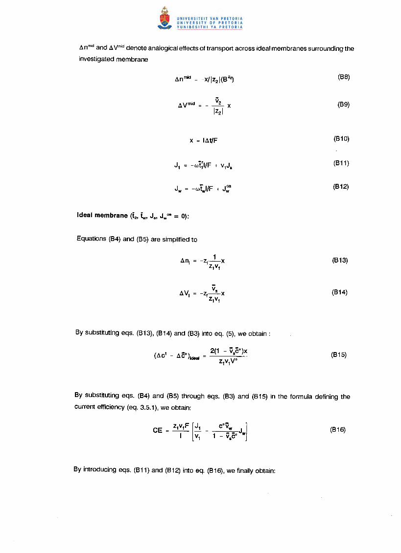
d nmid and d Vmid denote analogical effects of transport across ideal membranes surrounding the
investigated membrane
8y substituting eqs. (84) and (85) through eqs. (83) and (815) in the formula defining the
current efficiency (eq. 3.5.1), we obtain:
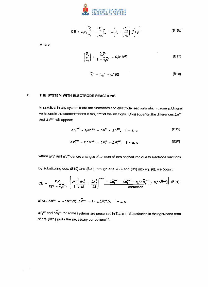
(~) =
v COw = O,018m1 - V COs
In practice, in any system there are electrodes and electrode reactions which cause additional
variations in the concentrations in mol/dm3 of the solutions. Consequently, the differences an1cor
and a Vicorwill appear:
an,corand a Vlcorfor some systems are presented in Table 1. Substitution in the right-hand term
of eq. (821) gives the necessary corrections(17).
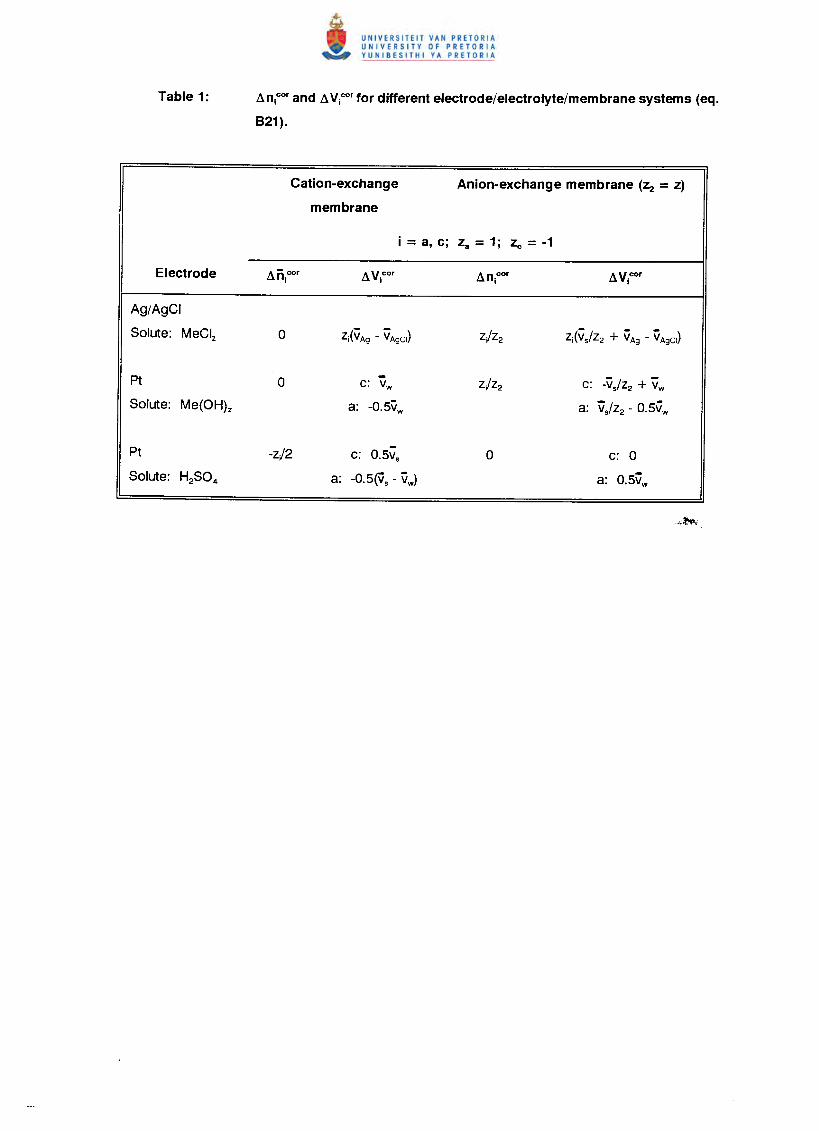
Cation-exchange
membrane
Ag/AgCI
Solute: MeClz
Pt
Solute: Me(OH)z
Pt
Solute: H2S04
-c: Vw
a: -O.SVw
C: -VS/Z2 + Vw
a: VS/Z2 - O.SVw
C: 0
a: O.SVw
C: O.SVs
a: -O.S(Vs - Vw)
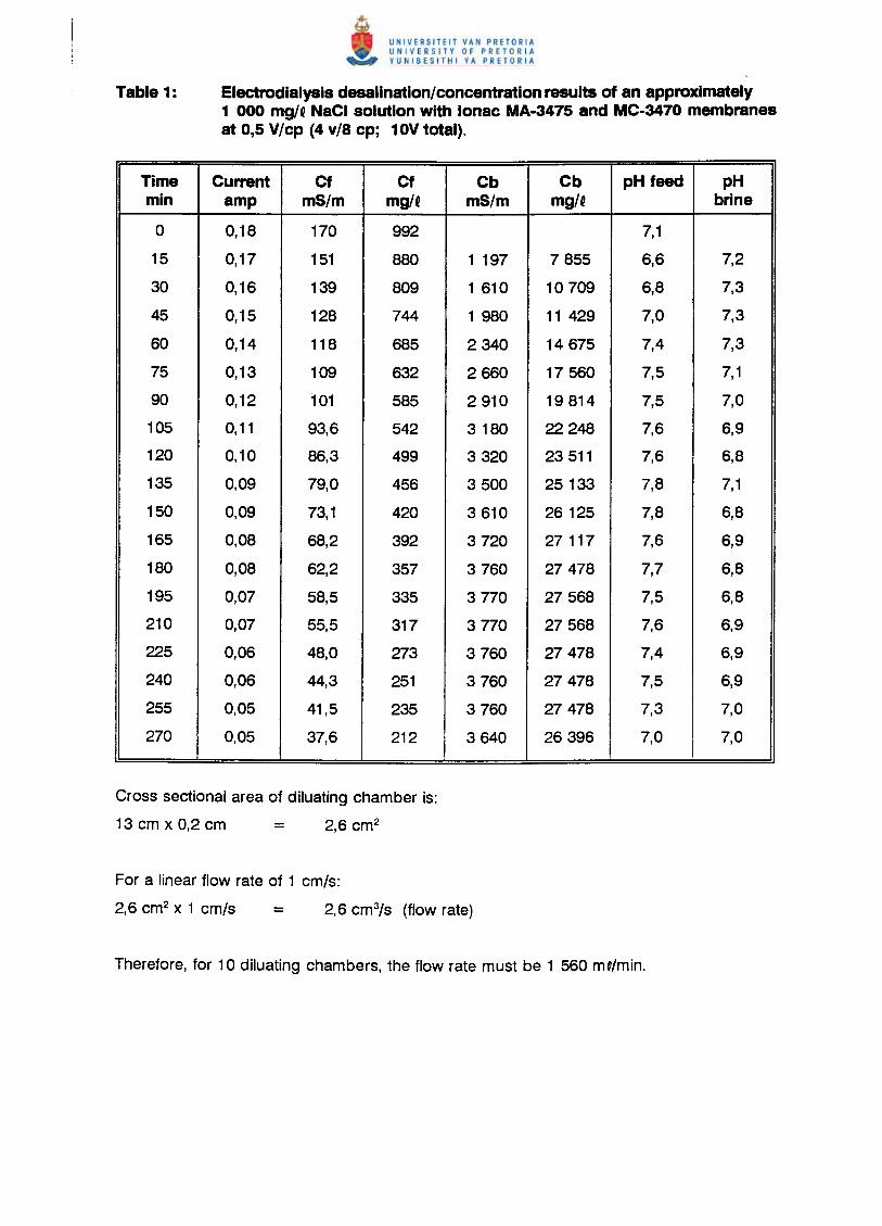
Electrodialysis desalination/concentration results of an approximately1 000 mg/, NaCI solution with lonac MA·3475 and MC·3470 membranesat 0,5 V/cp (4 v/8 cp; 10V total).
Time Current Cf Cf Cb Cb pH feed pHmin amp mS/m mg/. mS/m mg/. brine
° 0,18 170 992 7,1
15 0,17 151 880 1 197 7855 6,6 7,2
30 0,16 139 809 1 610 10709 6,8 7,3
45 0,15 128 744 1 980 11 429 7,0 7,3
60 0,14 118 685 2340 14675 7,4 7,3
75 0,13 109 632 2660 17560 7,5 7,1
90 0,12 101 585 291O 19814 7,5 7,0
105 0,11 93,6 542 3180 22 248 7,6 6,9
120 0,10 86,3 499 332O 23511 7,6 6,8
135 0,09 79,0 456 350O 25133 7,8 7,1
150 0,09 73,1 420 361O 26 125 7,8 6,8
165 0,08 68,2 392 372O 27117 7,6 6,9
180 0,08 62,2 357 376O 27478 7,7 6,8
195 0,07 58,5 335 377O 27568 7,5 6,8
210 0,07 55,5 317 377O 27568 7,6 6,9
225 0,06 48,0 273 376O 27478 7,4 6,9
240 0,06 44,3 251 376O 27478 7,5 6,9
255 0,05 41,5 235 376O 27478 7,3 7,0
270 0,05 37,6 212 364O 26396 7,0 7,0
Cross sectional area of diluating chamber is:
13 cm x 0,2 cm = 2,6 cm2
For a linear flow rate of 1 cm/s:
2,6 cm2 x 1 cm/s = 2,6 cm3/s (flow rate)
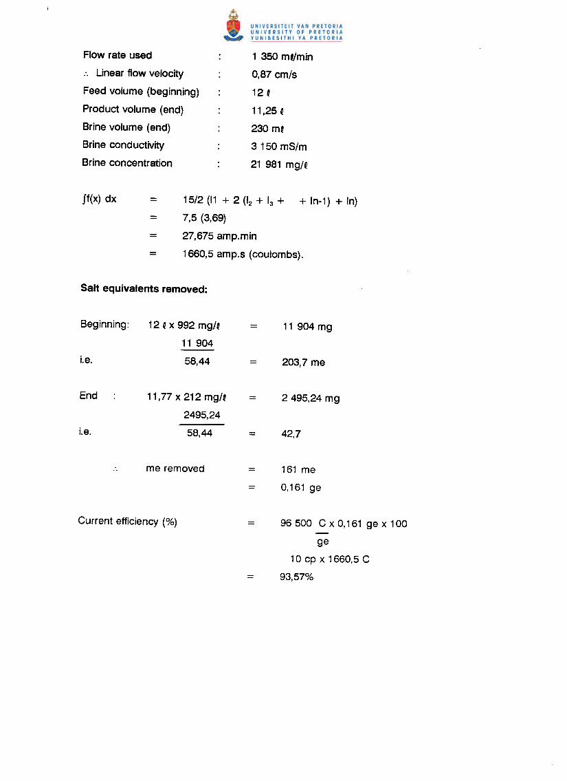
Flow rate used
:. Linear flow velocity
Feed volume (beginning)
Product volume (end)
Brine volume (end)
Brine conductivity
Brine concentration
1 350 ml/min
0,87 cm/s12 f
11,25 f
230 mf
3150 mS/m
21 981 mg/f
15/2 (11 + 2 (12 + 13 + + In-1) + In)
7,5 (3,69)
27,675 amp.min
1660,5 amp.s (coulombs).
12 f x 992 mg/f
11 904
58,44
11,77 x 212 mg/f
2495,24
58,44
96 500 C x 0,161 ge x 100
ge10 cp x 1660,5 C
93,57%
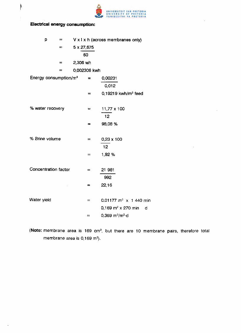
p = v x I x h (across membranes only)
= 5 x 27,675
60
= 2,306 wh
= 0,002306 kwh
Energy consumption/m3 = 0,00231
0,012
= 0,19219 kwh/m3 feed
% water recovery = 11,77x100--12
= 98,08 %
% Brine volume = 0,23 x 100--12
= 1,92 %
Concentration factor = 21 981
992
= 22,16
Water yield = 0,01177 m3 x 1 440 min
0,169 m2 x 270 min d
= 0,369 m3/m2-d
(Note: membrane area is 169 cm2, but there are 10 membrane pairs, therefore total
membrane area is 0,169 m~.
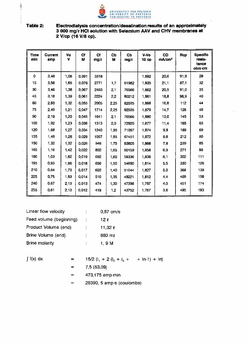
Electrodialysis concentration/desalination results of an approximately3000 mg/. HCI solution with Selemium AAV and CHV membranes at2 Vlcp (16 VIS cp).
Time Current Vo Cf Cf Cb Cb V-Vo CD Rcp Specificmln amp V M mg/f M mg/f 10 cp mAtcmz resis-
tanceohm-cm
0 3,48 1,08 0,091 3318 1,892 20,6 91,9 28
15 3,56 1,65 0,076 2n1 1,7 61982 1,835 21,1 87,1 32
30 3,46 1,38 0,067 2463 2,1 76566 1,862 20,5 91,0 35
45 3,18 1,39 0,061 2224 2,2 80212 1,861 18,8 98,9 40
60 2,83 1,32 0,055 2005 2,25 82035 1,868 16,8 112 44
75 2,49 1,21 0,047 1714 2,25 82035 1,879 14,7 128 49
90 2,19 1,20 0,045 1641 2,1 76566 1,880 13,0 145 53
105 1,92 1,23 0,036 1313 2,0 72920 1,8n 11,4 165 63
120 1,68 1,27 0,034 1240 1,95 71097 1,874 9,9 189 69
135 1,49 1,28 0,029 1057 1,85 67451 1,872 8,8 212 80
150 1,32 1,32 0,026 948 1,75 63805 1,868 7,8 239 85
165 1,16 1,42 0,022 802 1,65 60159 1,858 6,9 271 99
180 1,03 1,62 0,019 692 1,60 58336 1,838 6,1 302 111
195 0,93 1,86 0,018 656 1,50 54690 1,814 5,5 330 126
210 0,84 1,73 0,017 602 1,40 51044 1,827 5,0 368 139
225 0,75 1,83 0,014 510 1,35 49221 1,812 4,4 409 156
240 0,67 2,13 0,013 474 1,30 47398 1,787 4,0 451 174
255 0,61 2,13 0,012 419 1,2 43752 1,787 3,6 495 193
Linear flow velocity
Feed volume (beginning)
Product Volume (end)
Brine Volume (end)
Brine molarity
0,87 cm/s
12 @
11,32 •
680 m'
1,9 M
15/2 (11 + 2 (12 + 13 +7,5 (63,09)
= 473,175 amp ·min
= 28390, 5 amp-s (coulombs)
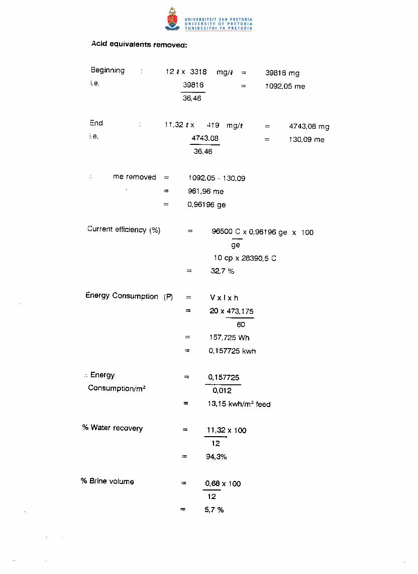
Beginning
i.e.
12 Q x 3318 mglQ =39816 =36.46
39816 mg
1092.05 me
11,32 Q x 419 mgl Q
4743.08
36.46
4743.08 mg
130.09 me
= 961,96 me
= 0,96196 ge
Current efficiency (%) = 96500 C x 0,96196 ge x 100
ge
10 cp x 28390,5 C
= 32,7%
Energy Consumption (P) = V x I x h
= 20 x 473,175
60
= 157,725 Wh
= 0,157725 kwh
:. Energy = 0,157725
Consumption/m3 0,012
= 13,15 kwh/m3 feed
% Water recovery = 11,32 x 100
12
= 94,3%
% Brine volume = 0,68 x 100-12
= 5,7%
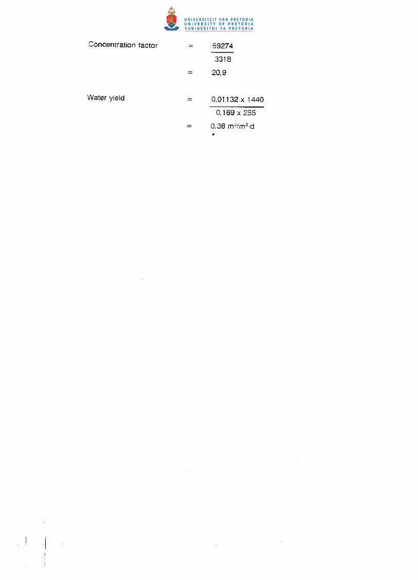
Concentration factor = 69274
3318
= 20,9
Water yield = 0,011 32 x 1440
0,169 x 255
= 0.38 mJ/m2-d•
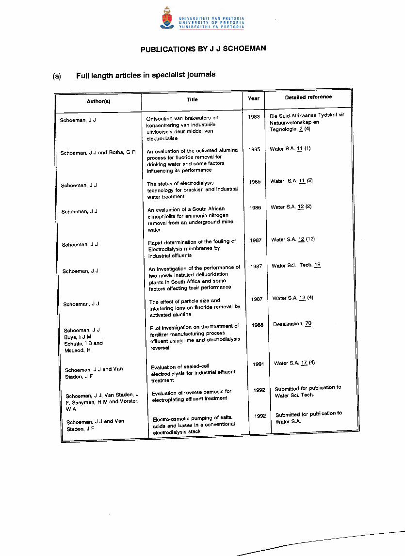
Author(s) TItle Year Detailed reference
Schoeman, J J Ontsouting van brakwaters en 1983 Die Suid-Afrikaanse Tydskrif virkonsentrering van industriele Natuurwetenskap enuitvloeisels deur middel van Tegnologie, g (4)elektrodialise
Schoeman, J J and Botha, G R An evaluation of the activated alumina 1985 Water SA .1! (1)process for fluoride removal fordrinking water and some factorsinfluencing its performance
Schoeman, J J The status of electrodialysis 1985 Water SA.1! (2)technology for brackish and industrialwater treatment
Schoeman, J J An evaluation of a South African 1986 Water SA,g (2)clinoptilolite for ammonia-nitrogenremoval from an underground minewater
Schoeman, J J Rapid determination of the fouling of 1987 Water S.A ,g (12)Electrodialysis membranes byindustrial effluents
Schoeman, J J An investigation of the performance of 1987 Water Sci. Tech. ,lgtwo newly installed defluoridationplants in South Africa and somefactors affecting their performance
Schoeman, J J The effect of particle size and 1987 Water SA II (4)interfering ions on fluoride removal byactivated alumina
Schoeman, J J Pilot investigation on the treatment of 1988 Desalination, ZQBuys, I J M fertilizer manufacturing processSchutte, I Band effluent using lime and electrodialysis
McLeod, H reversal
Schoeman, J J and Van Evaluation of sealed-cell 1991 Water SA .1Z. (4)
Staden, J F electrodialysis for industrial effluenttreatment
Schoeman, J J, Van Staden, J Evaluation of reverse osmosis for 1992 Submitted for pUblication to
F, Saayman, H M and Vorster, electroplating effluent treatment Water Sci. Tech.
WA
Schoeman, J J and Van Electro-osmotic pumping of salts, 1992 Submitted for publication to
Staden, J F acids and bases in a conventional Water SA
electrodialysis stack