lable at ScienceDirect

Energy 34 (2009) 1413–1421

Contents lists avai

Energy

journal homepage: www.elsevier .com/locate/energy

Electricity consumption forecasting in Italy using linear regression models

Vincenzo Bianco, Oronzio Manca*, Sergio NardiniDIAM, Seconda Universita degli Studi di Napoli, Via Roma 29, 81031 Aversa (CE), Italy

a r t i c l e i n f o

Article history:Received 28 November 2008Received in revised form2 June 2009Accepted 4 June 2009Available online 12 July 2009

Keywords:Electricity consumptionForecastingElasticityLinear regression

* Corresponding author: Tel.: þ39 081 5010 217; faE-mail address: oronzio.manca@unina2.it (O. Man

0360-5442/$ – see front matter � 2009 Elsevier Ltd.doi:10.1016/j.energy.2009.06.034

a b s t r a c t

The influence of economic and demographic variables on the annual electricity consumption in Italy hasbeen investigated with the intention to develop a long-term consumption forecasting model.

The time period considered for the historical data is from 1970 to 2007. Different regression modelswere developed, using historical electricity consumption, gross domestic product (GDP), gross domesticproduct per capita (GDP per capita) and population.

A first part of the paper considers the estimation of GDP, price and GDP per capita elasticities ofdomestic and non-domestic electricity consumption. The domestic and non-domestic short run priceelasticities are found to be both approximately equal to �0.06, while long run elasticities are equal to�0.24 and �0.09, respectively. On the contrary, the elasticities of GDP and GDP per capita present highervalues.

In the second part of the paper, different regression models, based on co-integrated or stationary data,are presented. Different statistical tests are employed to check the validity of the proposed models.

A comparison with national forecasts, based on complex econometric models, such as Markal-Time,was performed, showing that the developed regressions are congruent with the official projections, withdeviations of �1% for the best case and �11% for the worst. These deviations are to be consideredacceptable in relation to the time span taken into account.

� 2009 Elsevier Ltd. All rights reserved.

1. Introduction

Time series forecasting is a great challenge in many fields. Infinance, one forecasts stock exchange courses or indices of stockmarkets, while data processing specialists forecast the flow ofinformation on their networks.

Worldwide energy consumption is rising fast because of theincrease in human population, continuous pressures for betterliving standards, emphasis on large-scale industrialization indeveloping countries and the need to sustain positive economicgrowth rates. Given this fact, a sound forecasting technique isessential for accurate investment planning of energy production/generation and distribution.

The common difficulty to the development of reliable forecastsis the determination of sufficient and necessary information fora good prediction. If the information level is insufficient, a fore-casting will be poor; similarly, if information is useless or redun-dant, modelling will be difficult or even skewed.

x: þ39 081 5010 204.ca).

All rights reserved.

It is common that complex models, even though they provideaccurate predictions, are difficult to manage and often a lessaccurate model, but much simpler, is appreciated especially if theforecasting module is just a part of a more complex planning tool,as often is the case.

Some authors studied the electric consumption, in order tounderstand which are the demand drivers [1–3] and which are thefundamental pillars in building a forecasting model.

Jannuzzi and Shipper [1] analyzed the consumption of electricalenergy for the residential sector in Brazil. They observed that theincrease in electricity demand was faster than the income. Harrisand Lon-Mu [2] studied the dynamic relationships between elec-tricity consumption and several potentially relevant variables, suchas weather, price, and consumer income. They used a 30 years dataseries from south east USA, finding a high seasonality of electricitydemand. Ranjan and Jain [3] analyzed the consumption pattern ofelectrical energy in Delhi for the period 1984–1993 as a function ofpopulation and weather sensitive parameters. They developedmultiple linear regression models of energy consumption fordifferent seasons.

In the last 15 years, owing to the strong and constant increase inelectricityconsumption, which imposes an accurate planning in orderto avoid electricity shortage and guarantee adequate infrastructures,

V. Bianco et al. / Energy 34 (2009) 1413–14211414

many papers [4–11] focused on the forecasting of electricity demandusing different techniques.

Abdel-Aal et al. [5] applied an AIM (abductory inductionmechanism) model to the domestic consumption in the easternprovince of Saudi Arabia in terms of key weather parameters,demographic and economic indicators. It is found that an AIMmodel which uses only the mean relative humidity and airtemperature, gives an average forecasting error of about 5–6% overthe year. Yan [4] also presented residential consumption modelsusing climatic variables for Hong Kong.

Egelioglu et al. [6] investigated the influence of economic vari-ables on the annual electricity consumption in Northern Cyprusand they found that a model using number of customers, number oftourists and electricity prices has a strong predictive ability.

Mohamed and Bodger [7] studied a model for electricity fore-casting in New Zealand. The model is based on multiple linearregression analysis, taking into account economic and demographicvariables. Saab et al. [8], instead, investigated different univariatemodelling methodologies to forecast monthly electric energyconsumption in Lebanon.

Recently Al-Ghandoor et al. [9] presented a model developed toforecast electricity consumption of the Jordanian industrial sectorbased on multivariate linear regression of time series in order toidentify the main drivers behind electricity consumption.

Erdogdu [10] proposed a model based on ARIMA (autoregressiveintegrated moving average) providing an electricity demand esti-mation and forecast for Turkish electricity demand.

Very recently Amarawickrama and Hunt [11] presented a timeseries analysis of electricity demand in Sri Lanka. They studied howdifferent time series estimation methods perform in terms of model-ling past electricity demand, estimating the key income and priceelasticities, and hence forecasting future electricity consumption.

As for the analysis of Italian electricity demand, only a paper byGori and Takanen [12] is found in the literature. Their analysis isfocused on energy consumption and the possible substitution amongthe different energy resources is investigated, including electricity.They use a modification of the econometric model EDM (EnergyDemand Model) to forecast the national energy consumption.

The scope of the present paper is to investigate and forecast thelong-term electricity consumption in Italy using different econo-metric models, based on cointegration and stationary time series.

According to the authors’ best knowledge, this represents a firstattempt to specifically study the Italian electricity consumptionforecasting. In fact, the scientific literature facing Italian electricityconsumption is extremely limited. The main studies and researchesare provided by the firms involved in the electricity business or by

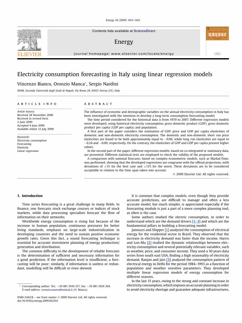
Fig. 1. Historical data for electricity consumption.

the government, evidencing a lack of third party contributions,with the exception of [12] and of studies that include Italy in G7,OECD countries, etc. [13–15].

The first target of the present paper is the estimation of priceand GDP consumption elasticities. The second target is to providean accurate model for electricity consumption forecasting. Multiplelinear regressions using GDP and population as selected variables toforecast electricity consumption in Italy up to 2030 are presented.Moreover a simplification is proposed considering regressionmodels using the ratio between GDP and population (GDP percapita) as independent variable.

The model results are compared with the official Italianauthority forecast [16] and with the forecast of a public/privateresearch institution [17] active in the field of energy. It is shown thatthere is a good agreement among the different predictions.

2. Methods

2.1. Data sets

For the period 1970–2007, the annual values of electricityconsumption categorized in terms of usage (domestic and non-domestic) were obtained by Terna reports [16]. Terna is a public–private company involved in the management of the high andmedium voltage electricity distribution network and its datarepresent the official Italian statistics about electricity consumption.

The annual data for the population and GDP for the same periodwere taken by the ISTAT [18], the Italian statistic service office,while the source for electricity prices is EUROSTAT [19], which isthe European statistic office.

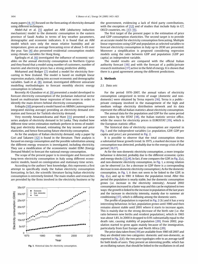
The historical data of electricity consumption are reported inFig. 1 and the independent variables (i.e. population, GDP, GDP percapita and price) are presented in Fig. 2.

It is possible to observe that the total consumption showsa substantial linear growth trend. In 1975, a marked decrease in theconsumption was detected, probably due to the energy crisis of thatperiod [16,17].

As for the non-domestic electricity consumption, a more irregularbehaviour is detected, probably due to the different economic cyclesand energy shocks [13,14]. In fact, if one compares the GDP, in Fig. 2(a),and non-domestic electricity consumption, in Fig. 1, a strong relationcan be observed (i.e. for a decrease in GDP there is a correspondingdecrease in non-domestic electricityconsumption). As for the domesticconsumption, in Fig. 1, it does not seem to be linked to the GDP, inFig. 2(a), and up to 1981 it follows the population trend. After thisperiod the population is nearly stable, but the domestic consumptiongrows (i.e. increase in the electricity intensity). Around 2002consumption increased in a faster way and this can be explained in twoways: the growth is linked to the increase inpopulation of the last yearsand the increase in electricity intensity, mainly due to summer airconditioning [17], which is diffusing among the domestic users.

The profile of population is reported in Fig. 2 (b) and it has a veryinteresting behaviour. In fact, population grows until 1980 and thenremains almost stable until 2001 where it starts to increase again.This is mainly due to the strong decrease of the birth rate (i.e. theratio between new births and resident population), which in 1965was about 1.8%. In 2000 it dropped to 0.9% substantially equal to thedeath rate, causing stability of population [20]. From 2002, pop-ulation started to grow again mainly because of the immigration,particularly from East Europe and North Africa [20].

The price data taken from [19] are available from 1985 till 2007 andthey are divided into two categories: domestic and non-domestic, asreported in Fig. 2(d); the two price typologies refer to an average tarifffor both kinds of users. They present an interesting profile, which hasan oscillating nature, that should be linked to the oscillations in oil and

Fig. 2. Historical data for the explaining variables considered: (a) GDP, (b) population, (c) GDP per capita and (d) price.

V. Bianco et al. / Energy 34 (2009) 1413–1421 1415

gas prices, which represent the main primary energy sources used inItaly to generate electricity. For example there is an increase startingfrom 1990 with a peak around 1992–1993, which should reflect theeffects of the First Gulf War or the marked growing trend observedfrom 2005 up to 2007 which reflects the record prices reached by oiland gas on the financial markets during that period.

2.2. Elasticities estimation

In this sub-section, two single equation consumption models,one for domestic and another for non-domestic consumption, arepresented. They are expressed in linear logarithmic form linkingthe quantity of annual domestic electricity consumption to elec-tricity price and GDP per capita in the first case, while in the secondcase the equation links annual non-domestic electricity consump-tion to GDP, electricity price and a time trend, which may beregarded as a proxy for technical progress [10].

The models take the form of a standard dynamic constantelasticity function of the consumption [10,13]:

Model 1

log�Ydom;t

�¼a0þa1log

�X3;t

�þa2logðPRtÞþa3logðPRt�3Þ

þa4log�Ydom;t�3

�(1)

where Ydom,t is the domestic electricity consumption, X3,t is the GDPper capita, PRt is the electricity price for domestic users, a0, a1, a2,a3, a4 are the regression coefficients, and t� i as subscript indicatesthe lag term (i.e. t� 1 indicates lag 1)

Model 2

log�Yndom;t

�¼ b0 þ b1log

�X1;t

�þ b2logðPRNDtÞ

þ b3logðINDt�3Þ þ b4log�Yndom;t�3

�(2)

where Yndom,t is the non-domestic electricity consumption, X1,t isthe GDP, PRNDt is the electricity price for non-domestic users, INDt

is a time trend, b0, b1, b2, b3, b4 are the regression coefficients.The coefficients a1 and a2 are very important, because they

represent the short run income and price elasticities [10,13] ofdomestic consumption, whereas b1 and b2 represent the short runGDP and price elasticities of non-domestic consumption.

As for the expected signs in Eqs. (1) and (2), one expects that a1

and b1 are greater than zero, because higher real GDP and GDP percapita should result in greater economic activity and acceleratepurchases of electrical goods and services. The coefficients of priceare expected to be less than zero for usual economic reasons [21].

Long run elasticities are calculated by dividing short run elas-ticities by (1� a4) and (1� b4) for Model 1 and Model 2, respec-tively, as indicated in [10,13]:

Ed1 ¼ a1=ð1� a4Þ

Ed2 ¼ a2=ð1� a4Þ

End1 ¼ b1=ð1� b4Þ

End2 ¼ b2=ð1� a4Þ

where Ed1 and Ed2 are the long run income and domestic priceelasticities, whereas End1 and End2 are the GDP and non-domesticprice elasticities.

Table 2Augmented Dickey�Fuller (ADF) unit root test on the logarithms of the consideredvariables. The confidence level, at which the hypothesis that the series containsa unit root can be rejected, is reported in parenthesis.

Variables ADF test statistic Test equation

Ydom,t �2.822 (92.8%) ConstantYndom,t �3.760 (95.7%) Constantþ trendX1,t �3.439 (92.7%) Constantþ trendX3,t �3.384 (97.7%) ConstantPRt �2.167 (77.7%) ConstantPRNDt �3.408 (92.1%) Constantþ trend

First differencePRt �3.071 (95.6%) Constant

V. Bianco et al. / Energy 34 (2009) 1413–14211416

The results of these estimates for electricity consumption arereported in Table 1. The Breusch–Godfrey Serial Correlation LM testis applied to the two models, indicating the absence of serialcorrelation in the residuals. Moreover the Augmented Dickey–Fuller (ADF) test is used to test for the presence of unit roots andestablish the order of integration of the variables (i.e. the naturallogarithm of Ydom,t, Yndom,t, X3,t, X1,t, PRt and PRNDt) in the twomodels. On the basis of ADF statistics, reported in Table 2, the nullhypothesis of a unit root cannot be rejected at 10% level of signifi-cance for the series PRt. Stationarity is obtained running the ADFtest on the first difference of the variables, indicating that the seriesPRt is integrated of order 1, I(1), in nature. On the other hand, nullhypothesis of unit root cannot be accepted for all the other series at10% level of significance, showing that they are integrated of order0, I(0), in nature.

2.3. Multiple regression models

To investigate the annual consumption of electricity up to 2030,a multiple regression model is used, considering the annual GDPand population time series, while price is not included because ofits low estimated elasticity. A similar approach is also used in [10] inthe case of Turkey.

The proposed model is represented by the following equations:

Ytot;t ¼ aþ b1X1;t þ b2X2;t þ b3X2;t�1 þ b4Ytot;t�1 þ e (3a)

Ydom;t¼aþb1X1;tþb2X2;tþb3X2;t�3þb4X1;t�3þb5Ydom;t�1þe

(3b)

Yndom;t ¼ aþb1X1;t þb2X2;t þb3X2;t�1þb4Yndom;t�1þ e (3c)

where Ytot,t, Ydom,t, Yndom,t are total, domestic and non-domesticannual consumption in GWh, X1,t is the annual GDP in Euro million,X2,t is the annual population in thousands, a, b1, b2, b3, b4 and b5 arethe regression coefficients, and e is the error.

The independent variables, X1,t and X2,t, are estimated andforecasted by a simple linear regression over the time t. They cantherefore be represented by the following equations:

X1;t ¼ m1 þ k1t (4)

X2;t ¼ m2 þ k2t (5)

m1, m2, k1, k2 are the simple linear regression coefficients.It is important to mention that for the year 1970 the corre-

sponding time, t, is equal to 1970. Eqs. (4) and (5) are used toforecast GDP and population, in order to allow for electricityconsumption forecast.

Another model is then proposed, which represents a simplifi-cation of the first one. The GDP per capita, ratio between GDP and

Table 1Summary of statistics, coefficients and estimation of price elasticities over the period1985–2007, for Model 1 and Model 2 (the t statistics are reported in parenthesis).

Model 1 Model 2

a0 1.615 (1.56) b0 �11.770 (�11.17)a1 0.292 (2.00) b1 1.409 (13.22)a2 �0.060 (�1.70) b2 �0.0562 (�3.24)a3 �0.120 (6.059) b3 �0.0463 (�3.45)a4 0.751 (�4.16) b4 0.358 (5.92)Ed1 �0.241 End1 �0.0875Ed2 1.172 End2 2.195R2 adjusted 0.979 R2 adjusted 0.998F 228 F 2915

population, is taken into account as explaining variable, thereforea simpler linear regression model is obtained, which results in thefollowing equation:

Ytot;t ¼ aþ b1X3;t þ b2Ytot;t�1 þ e (6a)

Ydom;t ¼ aþ b1X3;t þ b2Ydom;t�1 þ e (6b)

Yndom;t ¼ aþ b1X3;t þ b2Yndom;t�1 þ e (6c)

where Yt is the annual electricity consumption in GWh, X3,t is theannual GDP per capita in Euro, c and b3 are the regression coeffi-cients, and e is the error.

The independent variable, X3,t, is obtained by a simple linearregression over the time t, as previously done for X1,t and X2,t,leading to the following equation:

X3;t ¼ m3 þ k3t (7)

m3 and k3 are the linear regression coefficients.Table 3 shows the correlation matrix for all the variables

considered in Eqs. (3a)–(3c) for the data ranging from 1970 to 2007.All the independent variables show a high degree of correlationversus the dependent variables, only the non-domestic and totalconsumption show a lower degree of correlation versus population.The correlation coefficient for GDP versus population (the twoexplaining variables) is 0.820 and the corresponding varianceinflationary factor (VIF) is 5.56. In order to avoid multicollinearity,the VIF for some authors [22] should be less than 10 and for otherauthors [23, 24] should be less than 5; in the present case, becausethe VIF is considerably less than 10 and close to 5, it is reasonable tothink that multicollinearity is not present.

The Breusch–Godfrey Serial Correlation LM test is applied to Eqs.(3a)–(3c) and (6a)–(6c), indicating the absence of serial correlationin the residuals.

To determine if the variables are stationary or not, the ADF test isperformed on the variables (Yt, Ydom,t, Yndom,t, X1,t, X2,t, X3,t) anda unit root problem was observed, meaning that they are non-stationary. In order to make them stationary, they were differen-tiated once and the ADF test was executed on the first differencevariables, without detecting any unit root problem, as reported inTable 4. Therefore, it can be concluded that they are integrated oforder 1, I(1).

Table 3Correlation matrix for variables considered in Eqs. (3a)–(3c).

Ydom,t Yndom,t Ytot,t X1,t X2,t

Ydom,t 1 0.989 0.989Yndom,t 1 0.963 0.762Ytot,t 1 0.982 0.791X1,t 1 0.820X2,t 1

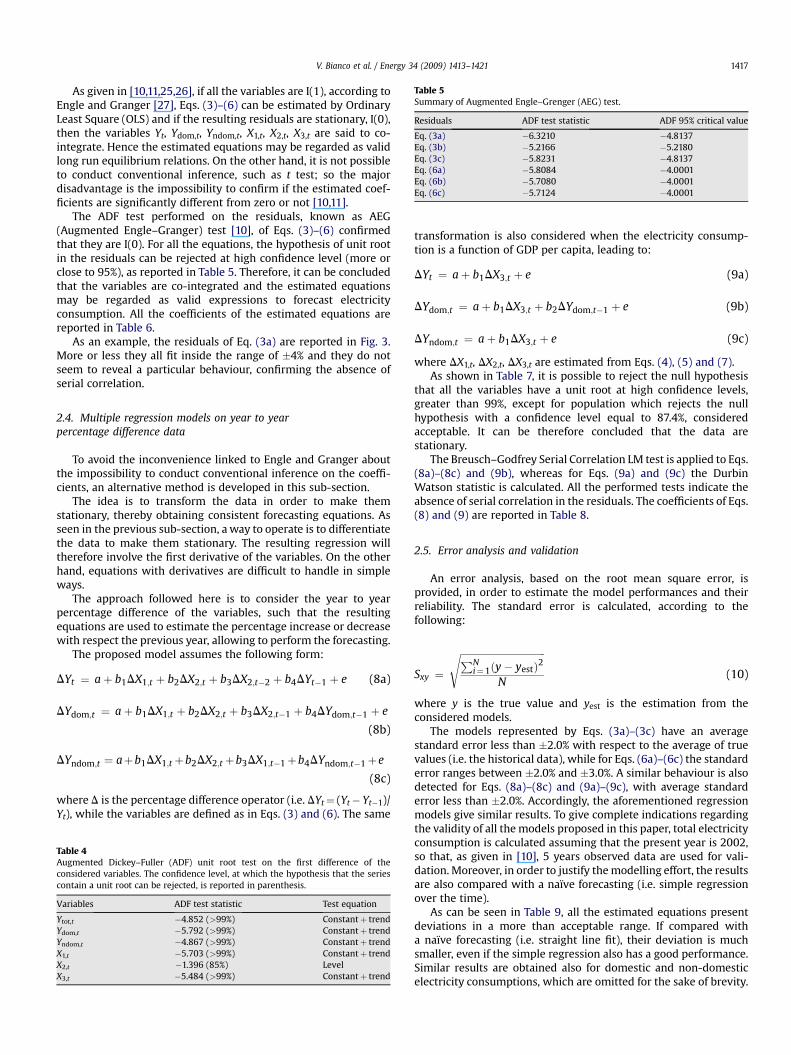
Table 5Summary of Augmented Engle–Grenger (AEG) test.

Residuals ADF test statistic ADF 95% critical value

Eq. (3a) �6.3210 �4.8137Eq. (3b) �5.2166 �5.2180Eq. (3c) �5.8231 �4.8137Eq. (6a) �5.8084 �4.0001Eq. (6b) �5.7080 �4.0001Eq. (6c) �5.7124 �4.0001

V. Bianco et al. / Energy 34 (2009) 1413–1421 1417

As given in [10,11,25,26], if all the variables are I(1), according toEngle and Granger [27], Eqs. (3)–(6) can be estimated by OrdinaryLeast Square (OLS) and if the resulting residuals are stationary, I(0),then the variables Yt, Ydom,t, Yndom,t, X1,t, X2,t, X3,t are said to co-integrate. Hence the estimated equations may be regarded as validlong run equilibrium relations. On the other hand, it is not possibleto conduct conventional inference, such as t test; so the majordisadvantage is the impossibility to confirm if the estimated coef-ficients are significantly different from zero or not [10,11].

The ADF test performed on the residuals, known as AEG(Augmented Engle–Granger) test [10], of Eqs. (3)–(6) confirmedthat they are I(0). For all the equations, the hypothesis of unit rootin the residuals can be rejected at high confidence level (more orclose to 95%), as reported in Table 5. Therefore, it can be concludedthat the variables are co-integrated and the estimated equationsmay be regarded as valid expressions to forecast electricityconsumption. All the coefficients of the estimated equations arereported in Table 6.

As an example, the residuals of Eq. (3a) are reported in Fig. 3.More or less they all fit inside the range of �4% and they do notseem to reveal a particular behaviour, confirming the absence ofserial correlation.

2.4. Multiple regression models on year to yearpercentage difference data

To avoid the inconvenience linked to Engle and Granger aboutthe impossibility to conduct conventional inference on the coeffi-cients, an alternative method is developed in this sub-section.

The idea is to transform the data in order to make themstationary, thereby obtaining consistent forecasting equations. Asseen in the previous sub-section, a way to operate is to differentiatethe data to make them stationary. The resulting regression willtherefore involve the first derivative of the variables. On the otherhand, equations with derivatives are difficult to handle in simpleways.

The approach followed here is to consider the year to yearpercentage difference of the variables, such that the resultingequations are used to estimate the percentage increase or decreasewith respect the previous year, allowing to perform the forecasting.

The proposed model assumes the following form:

DYt ¼ aþ b1DX1;t þ b2DX2;t þ b3DX2;t�2 þ b4DYt�1 þ e (8a)

DYdom;t ¼ aþ b1DX1;t þ b2DX2;t þ b3DX2;t�1 þ b4DYdom;t�1 þ e

(8b)

DYndom;t ¼ aþb1DX1;tþb2DX2;tþb3DX1;t�1þb4DYndom;t�1þe

(8c)

where D is the percentage difference operator (i.e. DYt¼ (Yt� Yt�1)/Yt), while the variables are defined as in Eqs. (3) and (6). The same

Table 4Augmented Dickey–Fuller (ADF) unit root test on the first difference of theconsidered variables. The confidence level, at which the hypothesis that the seriescontain a unit root can be rejected, is reported in parenthesis.

Variables ADF test statistic Test equation

Ytot,t �4.852 (>99%) Constantþ trendYdom,t �5.792 (>99%) Constantþ trendYndom,t �4.867 (>99%) Constantþ trendX1,t �5.703 (>99%) Constantþ trendX2,t �1.396 (85%) LevelX3,t �5.484 (>99%) Constantþ trend

transformation is also considered when the electricity consump-tion is a function of GDP per capita, leading to:

DYt ¼ aþ b1DX3;t þ e (9a)

DYdom;t ¼ aþ b1DX3;t þ b2DYdom;t�1 þ e (9b)

DYndom;t ¼ aþ b1DX3;t þ e (9c)

where DX1,t, DX2,t, DX3,t are estimated from Eqs. (4), (5) and (7).As shown in Table 7, it is possible to reject the null hypothesis

that all the variables have a unit root at high confidence levels,greater than 99%, except for population which rejects the nullhypothesis with a confidence level equal to 87.4%, consideredacceptable. It can be therefore concluded that the data arestationary.

The Breusch–Godfrey Serial Correlation LM test is applied to Eqs.(8a)–(8c) and (9b), whereas for Eqs. (9a) and (9c) the DurbinWatson statistic is calculated. All the performed tests indicate theabsence of serial correlation in the residuals. The coefficients of Eqs.(8) and (9) are reported in Table 8.

2.5. Error analysis and validation

An error analysis, based on the root mean square error, isprovided, in order to estimate the model performances and theirreliability. The standard error is calculated, according to thefollowing:

Sxy ¼

ffiffiffiffiffiffiffiffiffiffiffiffiffiffiffiffiffiffiffiffiffiffiffiffiffiffiffiffiffiffiffiffiffiffiffiPNi¼1ðy� yestÞ2

N

s(10)

where y is the true value and yest is the estimation from theconsidered models.

The models represented by Eqs. (3a)–(3c) have an averagestandard error less than �2.0% with respect to the average of truevalues (i.e. the historical data), while for Eqs. (6a)–(6c) the standarderror ranges between �2.0% and �3.0%. A similar behaviour is alsodetected for Eqs. (8a)–(8c) and (9a)–(9c), with average standarderror less than �2.0%. Accordingly, the aforementioned regressionmodels give similar results. To give complete indications regardingthe validity of all the models proposed in this paper, total electricityconsumption is calculated assuming that the present year is 2002,so that, as given in [10], 5 years observed data are used for vali-dation. Moreover, in order to justify the modelling effort, the resultsare also compared with a naıve forecasting (i.e. simple regressionover the time).

As can be seen in Table 9, all the estimated equations presentdeviations in a more than acceptable range. If compared witha naıve forecasting (i.e. straight line fit), their deviation is muchsmaller, even if the simple regression also has a good performance.Similar results are obtained also for domestic and non-domesticelectricity consumptions, which are omitted for the sake of brevity.

Table 6Regression coefficients for Eqs. (3a)–(3c) and (6a)–(6c).

a b1 b2 b3 b4 b5 m k

Eq. (3a) 145,200 10.413 0.107 �13.589 0.690Eq. (3b) �23,528 �0.345 �0.0105 0.779 0.006 0.685Eq. (3c) 145,047 6.650 0.065 �9.670 0.789Eq. (4) �3.89� 107 2.00� 104

Eq. (5) �1.36� 105 9.67� 101

Eq. (6a) �6700 2.156 0.884Eq. (6b) 114 0.482 0.852Eq. (6c) �5062 1.319 0.920Eq. (7) �6.36� 105 3.28� 102

V. Bianco et al. / Energy 34 (2009) 1413–14211418

Another validation test is performed estimating the forecastingequations on the data ranging from 1970 to 2002, such that theremaining 5 years are reserved for model evaluation on new data[28]. In this way, it is possible to assess equations validity on actualdata. It should be noted that this training procedure gave slightlydifferent coefficient values from those presented in Tables 6 and 8as might be expected, since the 2003–2007 data are now excludedfrom the estimation.

As one can notice in Table 10, the equations seem to forecast theelectricity consumption with a good accuracy and with acceptabledeviation respect to the actual data. It is important to observe thatfor the years 2006 and 2007, the deviation is higher because theincrease of electricity consumption in these two years was lowerthan the average increase rate. Accordingly, it is important toconsider all the annual data available (i.e. 1970–2007) to developthe model, in order to include this information in the futureprojections. On the base of the performed validation test and erroranalysis, it is possible to say that the equations presented in thispaper can be seen as valid models to estimate the Italian electricityconsumption.

3. Results and discussion

3.1. Price and income elasticities

The estimated elasticities from Eqs. (1) and (2) showed thatthere is a low consumption elasticity to the price and high elasticityto the income. Expectedly, long run elasticities are greater thanshort run elasticities.

This result seems to be consistent with previous study. In fact,a short run price elasticity for domestic electricity consumption of

Fig. 3. Residual plots of Eq. (3a).

�0.06 during the period 1985–1993 is reported in [13], practicallythe same calculated from Eq. (1). Instead in [15] the same elasticityis reported to be �0.096, using annual data ranging from 1978 to2003. Also the short run income elasticity is in good agreementwith [13], which reports a value of 0.28 very close to 0.29 obtainedby Eq. (1); whereas [15] reports a value of 0.17.

The low price elasticity for domestic consumption implies thatthe level of electricity consumption cannot be regulated extensivelythrough price policies.

An estimation of short and long run price and GDP elasticitiesfor non-domestic consumption is given using Eq. (2). The priceelasticity is quite low, �0.056 in the short run and �0.088 in thelong run. On the contrary GDP elasticity is high, 1.41 in the short runand 2.20 in the long run. This shows that the Italian GDP is closelylinked to the electricity consumption. For instance, if GDP doubles,the electricity consumption increases by 220%. In fact in the period1985–2003, there was an increase in GDP of about 60%, while thecorresponding increase in non-domestic electricity consumptionwas about 120%, provoking an increase similar to the estimatedelasticity.

To the best of our knowledge, other estimations of Italian non-domestic consumption price and GDP elasticities are not availablein literature, therefore a comparison is not possible. However,Narayan and Prasad [14] concluded that there is a positive causalitybetween electricity consumption and GDP in Italy, which isconsistent with the high GDP elasticity calculated for non-domesticconsumption. As given in [14], recessions or any shocks that havenegative impact on GDP will result in a negative impact on elec-tricity consumption. Similarly economic growth will stimulate theelectricity consumption.

The higher price elasticity presented by domestic users can beexplained with their major flexibility in the use of electricity. Whenelectricity bill increases, users can react saving energy. For exampleusing the air conditioners for less time or turning off all theappliances rather than having them in stand-by. As pointed out in[12], other possibilities seem rather limited for Italian users, also inconsideration of the fact that most of the heating systems andcooking facilities are fuelled with natural gas, gasoline or LPG(Liquid Petroleum Gas). A possible alternative is the diffusion of

Table 7Augmented Dickey–Fuller (ADF) unit root test on the variables considered in Eqs.(8a)–(8c) and (9a)–(9c). The confidence level, at which the hypothesis that the seriescontain a unit root can be rejected, is reported in parenthesis.

Variables ADF test statistic Test equation

DYtot,t �5.827 (>99%) Constantþ trendDYdom,t �5.501 (>99%) Constantþ trendDYndom,t �5.026 (>99%) Constantþ trendDX1,t �5.230 (>99%) Constantþ trendDX2,t �1.488 (¼87.4%) LevelDX3,t �5.233 (>99%) Constantþ trend

Table 8Summary of coefficients for Eqs. 8(a)–(c) and 9(a)–(c) (the t statistics are reported in parenthesis).

a b1 b2 b3 b4

Eq. (8a) 0.0137 (4.328) 0.642 (0.938) 1.025 (12.272) �1.923 (�2.821) �0.176 (�2.342)Eq. (8b) 0.0033 (0.593) �2.097 (�1.140) 0.595 (3.397) 2.904 (1.595) 0.361 (2.737)Eq. (8c) 0.0128 (3.448) �0.923 (�1.445) 1.045 (10.77) �0.640 (�3.704) 0.304 (2.118)Eq. (9a) 0.0104 (3.887) 0.949 (9.611)Eq. (9b) 0.0053 (1.007) 0.581 (3.375) 0.415 (3.365)Eq. (9c) 0.0082 (2.710) 1.016 (9.136)

V. Bianco et al. / Energy 34 (2009) 1413–1421 1419

photovoltaic plants for autonomous generation of electricity amongdomestic users, but the investment costs, including the govern-ment contribution, are still high.

As for the non-domestic users, the situation is more complex,because the possibility to save electricity is more limited andexpensive. For example the replacement of relatively old electricalengines with new ones require a very high financial strength, whichis justified only for energy intensive businesses.

Another common way proposed to increase price elasticity is thedevelopment of tariffs with different prices between day and night,or between working days and weekends [29]. These tariffs can beprofitable for non-domestic costumers, if they are able toreschedule production plans and store some of the factor ofproductions, for example fresh food delivered during the week tobe processed at the week end. Moreover the trade off betweenelectricity savings and extra salary, due to evening or weekendworking hours, must be carefully assessed.

Another idea could be to replace electricity with other forms ofenergy, for example natural gas which is evenly distributed in Italy,but also this way is difficult to follow [12]. In fact, as mentionedbefore, the substitution of electrical engines, with others alterna-tively fuelled, requires high investments and, moreover, natural gasis also subjected to price fluctuations.

A new perspective in the Italian electricity market is given bythe market liberalization which started in 1999 and ended in 2007,because, as observed in [30], competition among generators shouldincrease efficiency, by reducing costs and therefore price to finalconsumers. At the moment, the market is concentrated among fewplayers and the competition is scarce.

3.2. Electricity consumption forecasting

The forecasts obtained on the basis of the regression models arecompared with the results presented by Gori and Takanen [12] andtwo national forecasts published by Terna [16] and CESI [17].

The forecast provided by Terna represents the official statistic ofthe Italian Ministry of Productivities. Their forecasts are based ona macroeconomic model which takes into account historicalconsumption, GDP, value added per activity sector and the energyintensity of the different sectors. Terna furnishes the forecast up to2017.

CESI is an important player in the energy sector in Italy andabroad. It was part of the national electricity company (ENEL), but

Table 9Validation of the presented forecasting equations on total electricity consumption (the dewith a naıve forecasting (i.e. simple linear regression over time of total electricity consu

Year Eq. (3a) Eq. (6a)

2002 291.28 (0.11%) 291.71 (0.26%)2003 298.24 (�0.52%) 296.36 (�1.16%)2004 307.56 (1.00%) 304.34 (�0.05%)2005 309.98 (0.05%) 308.35 (�0.47%)2006 311.40 (�1.97%) 313.71 (�1.22%)2007 318.56 (�0.12%) 320.86 (0.59%)

with market liberalization it became an independent public/privatecompany. They provided electricity consumption forecasts basedon the MARKAL-TIMES model.

MARKAL is a linear-programming model of a generalised energysystem. It is demand-driven for which feasible solutions areobtained only if all specified end-use demands for energy aresatisfied for every time period. The objective is to determine theoptimum activity levels of processes that satisfy the constraints ata minimum cost. Examples of constraints in the model includeavailability of primary energy resources, production/use balances,electricity/heat peaking, availability of certain technologies, andupper bounds on pollution emissions. CESI furnishes forecasts from2010 to 2030.

Terna [16] and Gori and Takanen [12] data are available justfor the total electricity consumption, while CESI [17] data are splitfor the different sectors (domestic and non-domestic), allowing fora more detailed comparison.

The total electricity consumption is reported in Fig. 4(a). All thefour equations seem to be in agreement with the data given in[16,17] until about 2020; after Eqs. (8a) and (9a) tend to over-estimate, by about 10%, the total electricity consumption withrespect to the other forecasts.

As for the forecast proposed in [12], it leads to underestimatedvalues and the deviation increases with time, with a maximumdeviation of 15% in 2020.

Eqs. (3a) and (6a) seem to furnish the same forecast, in verygood accord with [16,17] and also the results given by Eqs. (8a) and(9a) are very similar.

Fig. 4(b) shows the domestic electricity consumption,evidencing that Eq. (8b) fits almost perfectly the data given in [17].Eq. (3b) leads to an estimation very close to [17], while Eqs. (6b) and(9b) give underestimated values, of 10% and 17% in 2030, respec-tively. It is important to remark that the explaining variables in Eqs.(3b) and (8b) are GDP and population, whereas in Eqs. (6b) and (9b)the GDP per capita is considered as the only explaining variable.

Finally, the non-domestic electricity consumption is presentedin Fig. 4(c). In this case, a situation similar to that of Fig. 4(a) isdetected, where Eqs. (8c) and (9c) give overestimated values ofabout 17% and 10% in 2030, respectively, while Eqs. (3c) and (6c)lead to nearly the same result, which almost perfectly fits the datagiven in [17].

The most outstanding outcome from the comparisons is thatthere is a substantial agreement between the available national

viation with respect to the historical data is reported in parenthesis) and comparisonmpation). The values reported in the table are in TWh.

Eq. (8a) Eq. (9a) Naıve For.

289.24 (�0.60%) 289.23 (�0.60%) 287.00 (�2.4%)295.18 (�1.56%) 292.90 (�2.35%) 292.81 (�2.4%)307.97 (1.13%) 303.97 (�0.17%) 298.61 (�2.0%)308.50 (�0.43%) 306.78 (�0.99%) 304.42 (�1.8%)314.16 (�1.07%) 317.10 (�0.14%) 310.23 (�2.4%)320.16 (0.38%) 322.97 (1.24%) 316.04 (�0.9%)

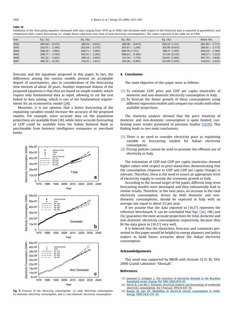
Table 10Validation of the forecasting equation estimated with data ranging from 1970 up to 2002 (the deviation with respect to the historical data is reported in parenthesis) andcomparison with a naıve forecasting (i.e. simple linear regression over time of total electricity consumpation). The values reported in the table are in TWh.

Year Eq. (3a) Eq. (6a) Eq. (8a) Eq. (9a) Naıve For.

2002 289.44 (�0.52%) 289.16 (�0.62%) 289.18 (�0.61%) 294.22 (1.11%) 283.28 (�2.71%)2003 292.93 (�2.34%) 292.84 (�2.37%) 295.97 (�1.29%) 301.09 (0.43%) 288.91 (�3.77%)2004 298.54 (�1.99%) 299.71 (�1.59%) 309.79 (1.71%) 308.17 (1.19%) 294.54 (�3.38%)2005 298.77 (�3.70%) 302.91 (�2.28%) 308.63 (�0.38%) 311.44 (0.52%) 300.17 (�3.22%)2006 301.22 (�5.42%) 308.14 (�3.05%) 312.14 (�1.73%) 324.61 (2.18%) 305.79 (�3.84%)2007 306.32 (�4.13%) 314.51 (�1.41%) 318.38 (�0.18%) 323.89 (1.52%) 316.04 (�2.42%)

V. Bianco et al. / Energy 34 (2009) 1413–14211420

forecasts and the equations proposed in this paper. In fact, thedifferences among the various models present an acceptabledegree of uncertainties, also in consideration of the forecastingtime horizon of about 20 years. Another important feature of theproposed equations is that they are based on simple models, whichrequire only fundamental data as input, allowing to cut the costlinked to data mining, which is one of the fundamental require-ments for an econometric model [24].

Moreover, it is our opinion, that a better forecasting of theexplaining variables would increase the accuracy of the proposedmodels. For example, more accurate data on the populationprojections are available from [18], while more accurate forecastingof GDP could be available from the Italian National Bank orpurchasable from business intelligence companies or merchantbanks.

Fig. 4. Forecast of the electricity consumption: (a) total electricity consumption,(b) domestic electricity consumption, and (c) non-domestic electricity consumption.

4. Conclusion

The main objective of this paper were as follows.

(1) To estimate GDP, price and GDP per capita elasticities ofdomestic and non-domestic electricity consumption in Italy.

(2) To forecast the future growth of these consumptions usingdifferent regression models and compare our results with otheravailable projections.

The elasticity analysis showed that the price elasticity ofdomestic and non-domestic consumption is quite limited, con-firming some results presented in previous studies [13,15]. Thisfinding leads to two main conclusions.

(1) There is no need to consider electricity price as explainingvariable in forecasting models for Italian electricityconsumption;

(2) Pricing policies cannot be used to promote the efficient use ofelectricity in Italy.

The estimation of GDP and GDP per capita elasticities showedhigher values with respect to price elasticities, demonstrating thatthe consumption response to GDP and GDP per capita changes isrelevant. Therefore, there is the need to assure an appropriate levelof electricity supply to sustain the economic growth in Italy.

According to the second target of the paper, different long-termforecasting models were developed and they substantially lead tosimilar results. Therefore, in the next years, an increase in the totalelectricity consumption, driven by both domestic and non-domestic consumptions, should be expected in Italy with anaverage rate equal to about 2% per year.

If we assume that the data reported in [16,17] represent thereference benchmark, it can be concluded that Eqs. (3a), (8b) and(6c) guarantee the most accurate projections for total, domestic andnon-domestic electricity consumptions respectively, because theyfit the data given in [16,17] very well.

It is believed that the elasticities, forecasts and comments pre-sented in this paper would be helpful to energy planners and policymakers to build future scenarios about the Italian electricityconsumption.

Acknowledgements

This work was supported by MIUR with Articolo 12 D. M. 593/2000 Grandi Laboratori ‘‘EliosLab’’.

References

[1] Jannuzzi G, Schipper L. The structure of electricity demand in the Brazilianhousehold sector. Energy Pol 1991;19(9):879–91.

[2] Harris JL, Lon-Mu L. Dynamic structural analysis and forecasting of residentialelectricity consumption. Int J Forecast 1993;9:437–55.

[3] Ranjan M, Jain VK. Modelling of electrical energy consumption in Delhi.Energy 1999;24(4):351–61.

V. Bianco et al. / Energy 34 (2009) 1413–1421 1421

[4] Yan YY. Climate and residential electricity consumption in Hong Kong. Energy1998;23(1):17–20.

[5] Abdel-Aal RE, Al-Garni AZ, Al-Nassar YN. Modelling and forecasting monthlyelectric energy consumption in eastern Saudi Arabia using abductivenetworks. Energy 1997;22(9):911–21.

[6] Egelioglu F, Mohamad AA, Guven B. Economic variables and electricityconsumption in Northern Cyprus. Energy 2001;26(4):355–62.

[7] Mohamed Z, Bodger P. Forecasting electricity consumption in New Zealandusing economic and demographic variables. Energy 2005;30(10):1833–43.

[8] Saab S, Badr E, Nasr G. Univariate modeling and forecasting of energyconsumption: the case of electricity in Lebanon. Energy 2001;26(1):1–14.

[9] Al-Ghandoor A, Al-Hinti I, Jaber JO, Sawalha SA. Electricity consumption andassociated GHG emissions of the Jordanian industrial sector: empirical anal-ysis and future projection. Energy Pol 2008;36(1):258–67.

[10] Erdogdu E. Electricity demand analysis using cointegration and ARIMAmodelling: a case study of Turkey. Energy Pol 2007;35(2):1129–46.

[11] Amarawickrama HA, Hunt LC. Electricity demand for Sri Lanka: a time seriesanalysis. Energy 2008;33(5):724–39.

[12] Gori F, Takanen C. Forecast of energy consumption of industry and householdand services in Italy. Heat Technol 2004;22(2):115–21.

[13] Haas R, Schipper L. Residential energy demand in OECD-countries and the roleof irreversible efficiency improvements. Energy Econ 1998;20(4):421–42.

[14] Narayan PK, Prased A. Electricity consumption-real GDP casuality nexus:evidence from a bootstrapped causality test for 30 OECD countries. Energy Pol2008;36(2):910–8.

[15] Narayan PK, Smyth R, Prased A. Electricity consumption in G7 countries:a panel cointegration analysis of residential demand elasticities. Energy Pol2007;35(9):4485–94.

[16] Terna. Forecasting of electricity demand and power needs in Italy for the years2007–2017. [Previsioni della domanda elettrica in Italia e del fabbisogno dipotenza necessario. Anni 2007–2017]. Terna, http://www.terna.it/default/Home/SISTEMA_ELETTRICO/statistiche/dati_statistici/tabid/418/Default.aspx;2007 [in Italian].

[17] CESI. Forecasting of the electricity demand for the years 2010-2030 on regionalbasis and variability elements to build alternative scenarios. [Previsione

tendenziale della domanda elettrica 2010 – 2030 su base regionale ed elementidi variabilita per la costruzione di scenari alternativi]. Report no. A5023397.CESI, http://www.ricercadisistema.it/Documenti/rapportip.aspx?idP¼ 115&idT ¼1&idN¼ 1244; 2005 [in Italian].

[18] National Institute of Statistics. Statistics on Italian population. Rome: ISTAT.See also: http://www.istat.it/popolazione; 2008.

[19] Eurostat. Energy statistics prices for 1985–2007. Bruxelles: Eurostat. See also:http://ec.europa.eu/eurostat/; 2008.

[20] Institute of Population and Social Policy Researches. Report on demographicsituation in Italy. [Rapporto sulla situazione demografica italiana]. Reportno. 2001. IRPPS, http://www.irpps.cnr.it/ricdin/osservatorio.htm; 2001 [inItalian].

[21] Halicioglu F. Residential electricity demand dynamics in Turkey. Energy Econ2007;29(2):199–210.

[22] O’Brien RM. A caution regarding rules of thumb for variance inflation factors.Qual Quant 2007;41(5):673–90.

[23] Snee RD. Some aspects of nonorthogonal data analysis, part I. Developingprediction equations. J Qual Technol 1973;5(1):67–79.

[24] Marquardt DW. You should standardize the predictor variables in yourregression models. J Am Stat Assoc 1980;75(1):87–91.

[25] Gujarati DN. Basic econometrics. New York: The Mc Graw Hill Companies;2004.

[26] Wooldridge JM. Introductory econometrics: a modern approach. New York:South Western, Division of Thomson Learning; 2005.

[27] Engle RF, Granger CWJ. Co-integration and error correction: representation,estimation and testing. Econometrica 1987;55(2):251–76.

[28] Mirasgedis S, Sarafidis Y, Georgopoulou E, Lalas DP, Moschovits M,Karagiannis F, et al. Models for mid-term electricity demand forecastingincorporating weather influences. Energy 2006;31(2):208–27.

[29] Bruno S, De Benedictis M, La Scala M, Wangesteen I. Demand elasticityincrease for reducing social welfare losses due to transfer capacity restriction:a test case on Italian cross border imports. Electr Power Syst Res2006;76(6–7):557–66.

[30] Ferrari A, Giulietti M. Competition in electricity markets: international expe-rience and the case of Italy. Utilities Pol 2003;13(3):247–55.