sensors

Article

EGM Toolbox—Interface for Controlling ABBRobots in Simulink

Paweł Obal * and Piotr Gierlak

�����������������

Citation: Obal, P.; Gierlak, P. EGM

Toolbox—Interface for Controlling

ABB Robots in Simulink. Sensors 2021,

21, 7463. https://doi.org/10.3390/

s21227463

Academic Editor: Andrey V. Savkin

Received: 22 September 2021

Accepted: 6 November 2021

Published: 10 November 2021

Publisher’s Note: MDPI stays neutral

with regard to jurisdictional claims in

published maps and institutional affil-

iations.

Copyright: © 2021 by the authors.

Licensee MDPI, Basel, Switzerland.

This article is an open access article

distributed under the terms and

conditions of the Creative Commons

Attribution (CC BY) license (https://

creativecommons.org/licenses/by/

4.0/).

Department of Applied Mechanics and Robotics, Faculty of Mechanical Engineering and Aeronautics,Rzeszow University of Technology, al. Powstanców Warszawy 12, 35-959 Rzeszów, Poland; pgierlak@prz.edu.pl* Correspondence: p.obal@prz.edu.pl; Tel.: +48-17-743-2010

Abstract: The development of industrial robotics requires the use of increasingly sophisticatedcontrol algorithms. In modern tasks posed by industry, it is not sufficient for the manipulator tomove along a programmed path, reaching individual points with the greatest accuracy. There isa need for solutions that can allow detection and avoidance of obstacles appearing on the robot’spath and that can compensate the path for low-repetitive workpieces, adjust the strength of theimpact of manipulator tools on the workpiece or enable safe cooperation of manipulators withpeople. To support this development, this work proposes an interface for controlling industrialrobots in the Simulink environment. With its use, we can easily test our control algorithms usingan external controller without the need to write an extensive program in the RAPID language. Therobot controller’s task is to control the drives to achieve the set trajectory.

Keywords: industrial robot; robot control interface; position–force control

1. Introduction

Industrial robots are being used in increasingly complex production tasks that requirethe use of more sophisticated algorithms for controlling the movements of manipulatorsand sensory systems. These include machining processes such as deburring, edge rounding,grinding, or polishing [1–3]. These processes use force control systems that control theforce exerted on the tool by contact with the workpiece. For example, in the processes ofdeburring and edge rounding, the force control system corrects the tool path in order toeliminate the influence of inaccuracies of the workpiece surface, which cannot be avoidedin the case of cast elements [4]. In grinding and polishing processes, the downforce ofthe tool has a large impact on the quality of the surface finish and the thickness of thematerial removed. There are different ways to implement force control systems. Forexample, studies [5–8] have proposed tools mounted on a manipulator, which controlthe effector force independently of the movements of the manipulator itself. The toolhas an additional mobile axis that moves the tool’s tip to obtain a specific downforce. Aseparate controller, independent of the robot controller, is responsible for controlling theforce. Another approach is to control the manipulator’s motion trajectory depending onthe force exerted on its working tip [9,10]. Leading manufacturers of industrial robotsoffer just such a force control solution for their manipulators. They use a 6-axis force andmoment sensor usually mounted on the manipulator’s flange [11–13].

Our experience of using a force control system in ABB robots (ABB Ltd., Zürich,Switzerland) for robotic machining prompted us to work on its improvement. The factoryadd-on integrated force control (ABB Ltd., Zürich, Switzerland) allows us to program thetrajectory of the robot based on two strategies [14]:

• FC SpeedChange—consists in reducing the linear velocity of the tool when the forceacting on the tool in the direction tangent to the programmed path exceeds the setvalues;

Sensors 2021, 21, 7463. https://doi.org/10.3390/s21227463 https://www.mdpi.com/journal/sensors

Sensors 2021, 21, 7463 2 of 17

• FC Pressure—where the set downforce of the tool against the surface of the workpieceis maintained.

This solution has limitations that make it impossible to use for machining workpieceswith low geometrical repeatability, e.g., cast workpieces. The excesses that result from thecasting process can come in a variety of shapes and sizes. Excessive geometrical variancemakes it very difficult to achieve reproducible process results by selecting Force Controlparameters and appropriate tools. Therefore, work was undertaken to find a better forcecontrol algorithm, which is presented in more detail in [15]. The experimental work wascarried out on a stand equipped with a SCORBOT-ER 4pc robot (ESHED ROBOTEC LTD,Rosh Ha’ayin, Israel). However, this robot is not suitable for research on robotic machiningin industrial conditions. It has low lifting capacity and stiffness, which prevents it fromoperating with a heavy spindle for machining hard metal alloys. Therefore, it was decidedto build a stand equipped with an industrial robot with high capacity, which allows thetesting of modern control algorithms for industrial processes at full scale.

By default, robot controllers do not allow full access to the control of the manipulator’sdrives. The trajectory of the tool center point (TCP) or individual joints is generated basedon a program written in the programming language of a given robot manufacturer. Theprogram defines points on the path along which the manipulator is to move, the maximumvelocity with which the path should be followed, the spatial accuracy within which thepoint should be reached, and some other parameters. On the basis of the determinedtrajectory, the control system only determines the signals for individual drives. Therobot programmer cannot interfere with the algorithm for determining the trajectory andcontrolling the drives. To deal with this problem, we could build our own controller, usingonly mechanical units of industrial manipulators available on the market [16,17]. Basedon the available documentation of the manipulator, it is possible to select appropriatemotor controllers and power supply systems. Such an approach was described in [18,19], where for Estun robots (Estun Automation, Nanjing, China), a controller was builtbased on an industrial computer with a real-time system, which generates a trajectory forindividual manipulator drives and sends it in real-time via EtherCAT to drivers poweringdrives. There are many ready-made solutions of universal drive controllers for multi-axismachines on the market, allowing the control of open kinematic chains. However, thisis a very costly and labor-intensive approach. In addition, it carries a significant risk ofdamaging the mechanical unit as a result of the incorrect configuration of the drivers.In addition, the accuracy and repeatability of the manipulator control must be reliablydetermined. This requires proper research, preferably with a laser tracker, which is also avery expensive device.

Some robot manufacturers make it possible to set the trajectory from an externaldevice in real-time. KUKA robots (KUKA AG, Augsburg, Germany) have the Robot SensorInterface (RSI) [20] option, which can be used to correct the position of the robot or TCP axisbased on signals from external sensors measuring the current position of the manipulator.Correction data can be sent via an I/O system or Ethernet using the User Datagram Protocol(UDP.) Weng in [21] used an RSI to correct the position of a manipulator while drillingand milling a workpiece made of aluminum. Much greater possibilities are provided bythe KUKA Sunrise.OS system software (KUKA AG, Augsburg, Germany). It allows anexternal controller to fully control individual drives and control the manipulator’s TCPtrajectory, and even control its compliance [3,22]. Unfortunately, this software is onlyavailable for the KUKA LBR iiwa series (KUKA AG, Augsburg, Germany). The largestrobot in this series has a 14 kg load capacity. It is therefore not suitable for use in machining.An innovative solution, which is universal, is the uniVAL controller (Stäubli InternationalAG, Pfäffikon, Switzerland) for Stäubli robots. It allows an external controller to moveindividual manipulator drives, control the TCP trajectory and program entire sequencesof paths. An ordinary programmable logic controller (PLC) can be used as an externalcontroller. The manufacturer provides an application programming interface (API) for PLCcontrollers from various manufacturers, including: Beckhoff (Beckhoff, Verl, Germany),

Sensors 2021, 21, 7463 3 of 17

Siemens (Siemens AG, Berlin, Germany), Rockwell (Rockwell Automation, Inc., Milwaukee,WI, USA). This solution was used in [23] to implement a proprietary force control systemin order to improve the quality of the drilling process in CFRP material. The role of theexternal controller was performed by the Beckhoff C6930 industrial computer (Beckhoff,Verl, Germany), which performed the position–force control of the manipulator. Ultimately,due to the experience in working with ABB robots, it was decided to choose this company’srobot to construct a new test stand. The robot controller is equipped with the softwareadd-on External Guided Motion (ABB Ltd., Zürich, Switzerland), EGM for short. As in thecase of RSI for KUKA robots, this add-on allows us to correct the programmed path of therobot but also allows control of the manipulator’s trajectory from an external device [24].

We decided to use the application in the Simulink environment (The MathWorks, Inc.,Natick, MA, USA) as a platform for an external controller. Article [22] presents the KUKASunrise Toolbox (KUKA AG, Augsburg, Germany) that allows control of robots with theKUKA Sunrise.OS system from the Matlab environment (The MathWorks, Inc., Natick,MA, USA). The creators extended this tool with the Simulink-iiwa interface that enablescontrol of KUKA robots in Simulink [25]. Simulink makes it possible to easily simulate andtest all control systems, e.g., manipulators. It has several ready-made tools, such as theRobotics Toolbox, which includes functions for determining the transformation of referencesystems, solving simple and inverse kinematics and dynamics tasks, etc. Currently, thereis no tool in Simulink that allows control of ABB robots via EGM. This paper presents aproprietary solution of an EGM interface in the form of an S-function block for the Simulinkenvironment. Its task is to exchange information about the state of the manipulator andsend the trajectory to be performed by the robot. In addition, it receives data from a six-axisforce sensor, which is part of the factory Force Control option. The block is universal andcan be implemented in any Simulink application. The main novelty of the work is that itwill be possible to simulate the operation of control systems and conduct experiments on areal object within one environment.

Section 2 describes the construction of the robotic test stand and the equipmentenabling its use for testing force control systems. Section 3 describes the structure andoperation of the ABB EGM Toolbox interface. As an example of the interface operation,Section 4 presents the results of an experiment carried out on the operation of the interfacebased on a simple positional force controller.

2. Construction of the Robotic Station

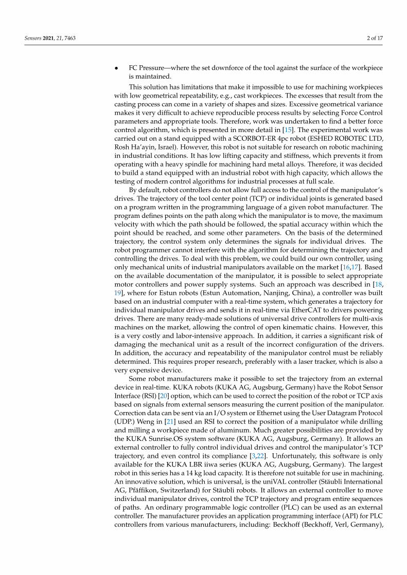
The robotic station consists of an ABB IRB 2400 industrial robot (ABB Ltd., Zürich,Switzerland) equipped with the Force Control and EGM systems. Force Control is an add-on to ABB robots that allows us to program the robot’s trajectory based on the measuredforce exerted on the robot’s tool by the environment. The EGM add-on allows us to movethe robot with an external device. The described case is a program run in the Simulinkenvironment using the Desktop Real-Time toolbox, which provides a real-time kernel formodels in Simulink. A schematic diagram of the station is shown in Figure 1.

Sensors 2021, 21, x FOR PEER REVIEW 4 of 17

Figure 1. Diagram of the robotic station.

2.1. External Guided Motion The EGM addition to the IRC5 controller system allows the manipulator arm to be

moved based on signals from an external device [24]. The EGM can operate in three modes: • Position Stream—the current and planned position of the manipulator are sent to an

external device; • Position Guidance—the robot follows the trajectory from an external device in real-

time; • Path Correction—the robot corrects the programmed trajectory based on data from an

external device. Data can be transferred to the EGM via a digital and analog I/O interface or Ethernet

User Datagram Protocol Unicast Communication (UdpUc) using Google Protocol Buffers (Protobuf) to encode the data. EGM enables feedback on the current state of the manipu-lator to an external device, but only by sending data via the UdpUc. According to the EGM documentation, we can read information about: • the manipulator TCP position; • manipulator TCP orientation in Euler angles and quaternions; • the angular position of individual connectors of the manipulator; • controller operation status; • controller clock time; • test signal values; • force sensor signal values.

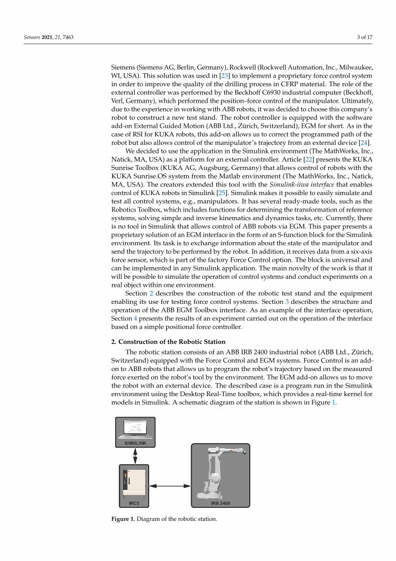
The manufacturer ensures that the frequency of information exchange by UdpUc is 250 Hz. Such communication is the best solution to control the manipulator from the level of a program running on a PC. Moreover, it does not require the use of additional physical I/O systems, intermediating in the information exchange. A diagram of EGM communi-cation with the Simulink program as an external device is shown in Figure 2.

Figure 2. Communication diagram.

Figure 1. Diagram of the robotic station.

Sensors 2021, 21, 7463 4 of 17

2.1. External Guided Motion

The EGM addition to the IRC5 controller system allows the manipulator arm to bemoved based on signals from an external device [24]. The EGM can operate in three modes:

• Position Stream—the current and planned position of the manipulator are sent to anexternal device;

• Position Guidance—the robot follows the trajectory from an external device in real-time;• Path Correction—the robot corrects the programmed trajectory based on data from an

external device.

Data can be transferred to the EGM via a digital and analog I/O interface or EthernetUser Datagram Protocol Unicast Communication (UdpUc) using Google Protocol Buffers(Protobuf) to encode the data. EGM enables feedback on the current state of the manipulatorto an external device, but only by sending data via the UdpUc. According to the EGMdocumentation, we can read information about:

• the manipulator TCP position;• manipulator TCP orientation in Euler angles and quaternions;• the angular position of individual connectors of the manipulator;• controller operation status;• controller clock time;• test signal values;• force sensor signal values.

The manufacturer ensures that the frequency of information exchange by UdpUcis 250 Hz. Such communication is the best solution to control the manipulator from thelevel of a program running on a PC. Moreover, it does not require the use of additionalphysical I/O systems, intermediating in the information exchange. A diagram of EGMcommunication with the Simulink program as an external device is shown in Figure 2.

Sensors 2021, 21, x FOR PEER REVIEW 4 of 17

Figure 1. Diagram of the robotic station.

2.1. External Guided Motion The EGM addition to the IRC5 controller system allows the manipulator arm to be

moved based on signals from an external device [24]. The EGM can operate in three modes: • Position Stream—the current and planned position of the manipulator are sent to an

external device; • Position Guidance—the robot follows the trajectory from an external device in real-

time; • Path Correction—the robot corrects the programmed trajectory based on data from an

external device. Data can be transferred to the EGM via a digital and analog I/O interface or Ethernet

User Datagram Protocol Unicast Communication (UdpUc) using Google Protocol Buffers (Protobuf) to encode the data. EGM enables feedback on the current state of the manipu-lator to an external device, but only by sending data via the UdpUc. According to the EGM documentation, we can read information about: • the manipulator TCP position; • manipulator TCP orientation in Euler angles and quaternions; • the angular position of individual connectors of the manipulator; • controller operation status; • controller clock time; • test signal values; • force sensor signal values.

The manufacturer ensures that the frequency of information exchange by UdpUc is 250 Hz. Such communication is the best solution to control the manipulator from the level of a program running on a PC. Moreover, it does not require the use of additional physical I/O systems, intermediating in the information exchange. A diagram of EGM communi-cation with the Simulink program as an external device is shown in Figure 2.

Figure 2. Communication diagram. Figure 2. Communication diagram.

The exchanged data is encoded according to the Protobuf protocol. This forces the useof a serialization procedure for data sent to the EGM and deserialization of the receiveddata so that it can be processed in Simulink. This protocol allows data to be transferredin a shorter time than standard protocols based, for example, on encoding information inASCII. Unfortunately, Simulink does not have ready-made tools to conduct communicationin accordance with the Protobuf protocol. Therefore, a custom S-function block was writtento process the data and communicate with the EGM.

The EGM system is an intermediate arrangement between the external controller andthe system generating control signals for individual manipulator drives. Through the EGM,it is possible to control the motion of the manipulator in joint space or in a task spacedefined in relation to the selected coordinate system. The EGM receives the set position andvelocity data of the manipulator, then determines the set axis velocity from the formula:

speed = k·(pose− pose_re f ) + speed_re f (1)

Sensors 2021, 21, 7463 5 of 17

where k—proportional gain factor, pose_re f —reference position, pose—set position, speed_re f —reference velocity. The set velocity reference value is transmitted to the motion control ofthe mechanical unit, which controls the individual drives.

2.2. Force Control

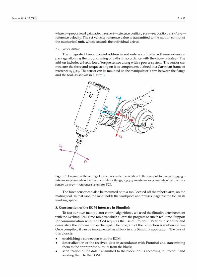
The Integrated Force Control add-on is not only a controller software extensionpackage allowing the programming of paths in accordance with the chosen strategy. Theadd-on includes a 6-axis force/torque sensor along with a power system. The sensor canmeasure the force and torque acting on it as components defined in a Cartesian frame ofreference xSySzS. The sensor can be mounted on the manipulator’s arm between the flangeand the tool, as shown in Figure 3.

Sensors 2021, 21, x FOR PEER REVIEW 5 of 17

The exchanged data is encoded according to the Protobuf protocol. This forces the use of a serialization procedure for data sent to the EGM and deserialization of the re-ceived data so that it can be processed in Simulink. This protocol allows data to be trans-ferred in a shorter time than standard protocols based, for example, on encoding infor-mation in ASCII. Unfortunately, Simulink does not have ready-made tools to conduct communication in accordance with the Protobuf protocol. Therefore, a custom S-function block was written to process the data and communicate with the EGM.

The EGM system is an intermediate arrangement between the external controller and the system generating control signals for individual manipulator drives. Through the EGM, it is possible to control the motion of the manipulator in joint space or in a task space defined in relation to the selected coordinate system. The EGM receives the set po-sition and velocity data of the manipulator, then determines the set axis velocity from the formula: 𝑠𝑝𝑒𝑒𝑑 = 𝑘 ∙ (𝑝𝑜𝑠𝑒 − 𝑝𝑜𝑠𝑒_𝑟𝑒𝑓) + 𝑠𝑝𝑒𝑒𝑑_𝑟𝑒𝑓 (1)

where 𝑘—proportional gain factor, 𝑝𝑜𝑠𝑒_𝑟𝑒𝑓—reference position, 𝑝𝑜𝑠𝑒—set position, 𝑠𝑝𝑒𝑒𝑑_𝑟𝑒𝑓—reference velocity. The set velocity reference value is transmitted to the mo-tion control of the mechanical unit, which controls the individual drives.

2.2. Force Control The Integrated Force Control add-on is not only a controller software extension pack-

age allowing the programming of paths in accordance with the chosen strategy. The add-on includes a 6-axis force/torque sensor along with a power system. The sensor can meas-ure the force and torque acting on it as components defined in a Cartesian frame of refer-ence 𝑥 𝑦 𝑧 . The sensor can be mounted on the manipulator’s arm between the flange and the tool, as shown in Figure 3.

Figure 3. Diagram of the setting of a reference system in relation to the manipulator flange, 𝑥𝑅𝑦 𝑧 —reference system related to the manipulator flange, 𝑥𝑆𝑦 𝑧 —reference system related to the force sensor, 𝑥𝑇𝑦 𝑧 —reference system for TCP.

Figure 3. Diagram of the setting of a reference system in relation to the manipulator flange, xRyRzR—reference system related to the manipulator flange, xSySzS —reference system related to the forcesensor, xTyTzT —reference system for TCP.

The force sensor can also be mounted onto a tool located off the robot’s arm, on themating tool. In that case, the robot holds the workpiece and presses it against the tool in itsworking space.

3. Construction of the EGM Interface in Simulink

To test our own manipulator control algorithms, we used the Simulink environmentwith the Desktop Real-Time Toolbox, which allows the program to run in real-time. Supportfor communication with the EGM requires the use of Protobuf libraries to serialize anddeserialize the information exchanged. The program of the S-function is written in C++.Once compiled, it can be implemented as a block in any Simulink application. The task ofthis block is:

• establishing a connection with the EGM;• deserialization of the received data in accordance with Protobuf and transmitting

them to the appropriate outputs from the block;• serialization of the data transmitted to the block inputs according to Protobuf and

sending them to the EGM.

Sensors 2021, 21, 7463 6 of 17

During S-function tests, it was found that the EGM in Position Guidance mode can onlyreceive force sensor signal values when the Force Control system is activated. Moreover,while Force Control is active, it is not possible to move the robot using the EGM. Therefore,when Force Control is on, EGM works only as in Position Stream mode.

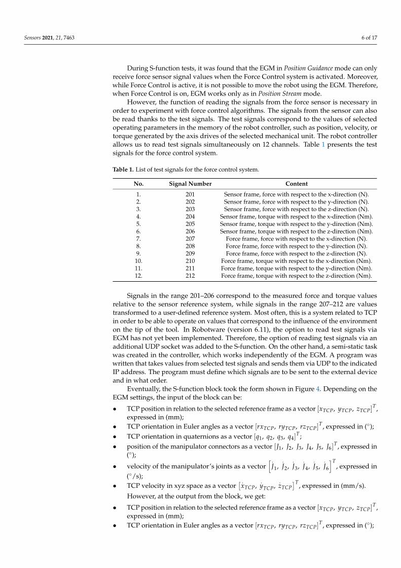
However, the function of reading the signals from the force sensor is necessary inorder to experiment with force control algorithms. The signals from the sensor can alsobe read thanks to the test signals. The test signals correspond to the values of selectedoperating parameters in the memory of the robot controller, such as position, velocity, ortorque generated by the axis drives of the selected mechanical unit. The robot controllerallows us to read test signals simultaneously on 12 channels. Table 1 presents the testsignals for the force control system.

Table 1. List of test signals for the force control system.

No. Signal Number Content

1. 201 Sensor frame, force with respect to the x-direction (N).2. 202 Sensor frame, force with respect to the y-direction (N).3. 203 Sensor frame, force with respect to the z-direction (N).4. 204 Sensor frame, torque with respect to the x-direction (Nm).5. 205 Sensor frame, torque with respect to the y-direction (Nm).6. 206 Sensor frame, torque with respect to the z-direction (Nm).7. 207 Force frame, force with respect to the x-direction (N).8. 208 Force frame, force with respect to the y-direction (N).9. 209 Force frame, force with respect to the z-direction (N).10. 210 Force frame, torque with respect to the x-direction (Nm).11. 211 Force frame, torque with respect to the y-direction (Nm).12. 212 Force frame, torque with respect to the z-direction (Nm).

Signals in the range 201–206 correspond to the measured force and torque valuesrelative to the sensor reference system, while signals in the range 207–212 are valuestransformed to a user-defined reference system. Most often, this is a system related to TCPin order to be able to operate on values that correspond to the influence of the environmenton the tip of the tool. In Robotware (version 6.11), the option to read test signals viaEGM has not yet been implemented. Therefore, the option of reading test signals via anadditional UDP socket was added to the S-function. On the other hand, a semi-static taskwas created in the controller, which works independently of the EGM. A program waswritten that takes values from selected test signals and sends them via UDP to the indicatedIP address. The program must define which signals are to be sent to the external deviceand in what order.

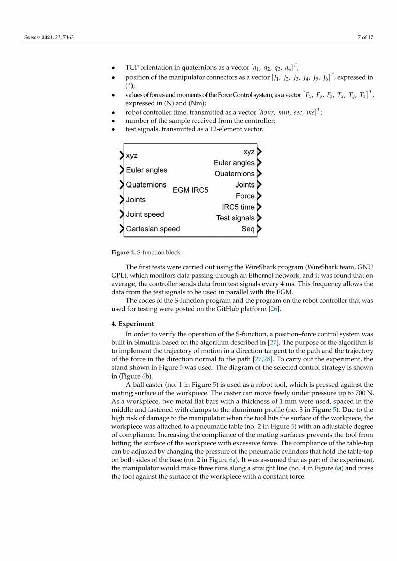
Eventually, the S-function block took the form shown in Figure 4. Depending on theEGM settings, the input of the block can be:

• TCP position in relation to the selected reference frame as a vector [xTCP, yTCP, zTCP]T ,

expressed in (mm);• TCP orientation in Euler angles as a vector [rxTCP, ryTCP, rzTCP]

T , expressed in (◦);• TCP orientation in quaternions as a vector [q1, q2, q3, q4]

T ;• position of the manipulator connectors as a vector [J1, J2, J3, J4, J5, J6]

T , expressed in(◦);

• velocity of the manipulator’s joints as a vector[ .

J1,.J2,

.J3,

.J4,

.J5,

.J6

]T, expressed in

(◦/s);• TCP velocity in xyz space as a vector

[ .xTCP,

.yTCP,

.zTCP

]T , expressed in (mm/s).

However, at the output from the block, we get:

• TCP position in relation to the selected reference frame as a vector [xTCP, yTCP, zTCP]T ,

expressed in (mm);• TCP orientation in Euler angles as a vector [rxTCP, ryTCP, rzTCP]

T , expressed in (◦);

Sensors 2021, 21, 7463 7 of 17

• TCP orientation in quaternions as a vector [q1, q2, q3, q4]T ;

• position of the manipulator connectors as a vector [J1, J2, J3, J4, J5, J6]T , expressed in

(◦);• values of forces and moments of the Force Control system, as a vector

[Fx, Fy, Fz, Tx, Ty, Tz

]T,expressed in (N) and (Nm);

• robot controller time, transmitted as a vector [hour, min, sec, ms]T ;• number of the sample received from the controller;• test signals, transmitted as a 12-element vector.

Sensors 2021, 21, x FOR PEER REVIEW 7 of 17

address. The program must define which signals are to be sent to the external device and in what order.

Eventually, the S-function block took the form shown in Figure 4. Depending on the EGM settings, the input of the block can be: • TCP position in relation to the selected reference frame as a vector 𝑥 , 𝑦 , 𝑧 ,

expressed in (mm); • TCP orientation in Euler angles as a vector 𝑟𝑥 , 𝑟𝑦 , 𝑟𝑧 , expressed in (°); • TCP orientation in quaternions as a vector 𝑞 , 𝑞 , 𝑞 , 𝑞 ; • position of the manipulator connectors as a vector 𝐽 , 𝐽 , 𝐽 , 𝐽 , 𝐽 , 𝐽 , expressed in

(°); • velocity of the manipulator’s joints as a vector 𝐽 , 𝐽 , 𝐽 , 𝐽 , 𝐽 , 𝐽 , expressed in (°/s); • TCP velocity in xyz space as a vector 𝑥 , 𝑦 , 𝑧 , expressed in (mm/s).

However, at the output from the block, we get: • TCP position in relation to the selected reference frame as a vector 𝑥 , 𝑦 , 𝑧 ,

expressed in (mm); • TCP orientation in Euler angles as a vector 𝑟𝑥 , 𝑟𝑦 , 𝑟𝑧 , expressed in (°); • TCP orientation in quaternions as a vector 𝑞 , 𝑞 , 𝑞 , 𝑞 ; • position of the manipulator connectors as a vector 𝐽 , 𝐽 , 𝐽 , 𝐽 , 𝐽 , 𝐽 , expressed in

(°); • values of forces and moments of the Force Control system, as a vector 𝐹 , 𝐹 , 𝐹 , 𝑇 , 𝑇 , 𝑇 , expressed in (N) and (Nm); • robot controller time, transmitted as a vector ℎ𝑜𝑢𝑟, 𝑚𝑖𝑛, 𝑠𝑒𝑐, 𝑚𝑠 ; • number of the sample received from the controller; • test signals, transmitted as a 12-element vector.

Figure 4. S-function block.

The first tests were carried out using the WireShark program (WireShark team, GNU GPL), which monitors data passing through an Ethernet network, and it was found that on average, the controller sends data from test signals every 4 ms. This frequency allows the data from the test signals to be used in parallel with the EGM.

The codes of the S-function program and the program on the robot controller that was used for testing were posted on the GitHub platform [26].

4. Experiment In order to verify the operation of the S-function, a position–force control system was

built in Simulink based on the algorithm described in [27]. The purpose of the algorithm is to implement the trajectory of motion in a direction tangent to the path and the trajec-tory of the force in the direction normal to the path [27,28]. To carry out the experiment, the stand shown in Figure 5 was used. The diagram of the selected control strategy is shown in (Figure 6b).

Figure 4. S-function block.

The first tests were carried out using the WireShark program (WireShark team, GNUGPL), which monitors data passing through an Ethernet network, and it was found that onaverage, the controller sends data from test signals every 4 ms. This frequency allows thedata from the test signals to be used in parallel with the EGM.

The codes of the S-function program and the program on the robot controller that wasused for testing were posted on the GitHub platform [26].

4. Experiment

In order to verify the operation of the S-function, a position–force control system wasbuilt in Simulink based on the algorithm described in [27]. The purpose of the algorithm isto implement the trajectory of motion in a direction tangent to the path and the trajectoryof the force in the direction normal to the path [27,28]. To carry out the experiment, thestand shown in Figure 5 was used. The diagram of the selected control strategy is shownin (Figure 6b).

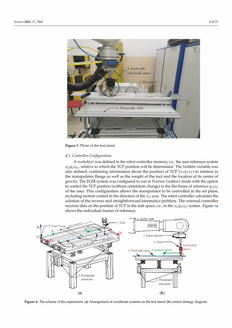
A ball caster (no. 1 in Figure 5) is used as a robot tool, which is pressed against themating surface of the workpiece. The caster can move freely under pressure up to 700 N.As a workpiece, two metal flat bars with a thickness of 1 mm were used, spaced in themiddle and fastened with clamps to the aluminum profile (no. 3 in Figure 5). Due to thehigh risk of damage to the manipulator when the tool hits the surface of the workpiece, theworkpiece was attached to a pneumatic table (no. 2 in Figure 5) with an adjustable degreeof compliance. Increasing the compliance of the mating surfaces prevents the tool fromhitting the surface of the workpiece with excessive force. The compliance of the table-topcan be adjusted by changing the pressure of the pneumatic cylinders that hold the table-topon both sides of the base (no. 2 in Figure 6a). It was assumed that as part of the experiment,the manipulator would make three runs along a straight line (no. 4 in Figure 6a) and pressthe tool against the surface of the workpiece with a constant force.

Sensors 2021, 21, 7463 8 of 17Sensors 2021, 21, x FOR PEER REVIEW 8 of 17

Figure 5. Photo of the test stand.

A ball caster (no. 1 in Figure 5) is used as a robot tool, which is pressed against the mating surface of the workpiece. The caster can move freely under pressure up to 700 N. As a workpiece, two metal flat bars with a thickness of 1 mm were used, spaced in the middle and fastened with clamps to the aluminum profile (no. 3 in Figure 5). Due to the high risk of damage to the manipulator when the tool hits the surface of the workpiece, the workpiece was attached to a pneumatic table (no. 2 in Figure 5) with an adjustable degree of compliance. Increasing the compliance of the mating surfaces prevents the tool from hitting the surface of the workpiece with excessive force. The compliance of the table-top can be adjusted by changing the pressure of the pneumatic cylinders that hold the table-top on both sides of the base (no. 2 in Figure 6a). It was assumed that as part of the experiment, the manipulator would make three runs along a straight line (no. 4 in Figure 6a) and press the tool against the surface of the workpiece with a constant force.

4.1. Controller Configuration A workobject was defined in the robot controller memory, i.e., the user reference sys-

tem 𝑥 𝑦 𝑧 , relative to which the TCP position will be determined. The tooldata variable was also defined, containing information about the position of TCP (𝑥 𝑦 𝑧 ) in relation to the manipulator flange as well as the weight of the tool and the location of its center of gravity. The EGM system was configured to run in Position Guidance mode with the option to control the TCP position (without orientation change) in the flat frame of reference 𝑦 𝑧 of the user. This configuration allows the manipulator to be controlled in the set plane, excluding motion control in the direction of the 𝑥 axis. The robot controller cal-culates the solution of the inverse and straightforward kinematics problem. The external controller receives data on the position of TCP in the task space, i.e., in the 𝑥 𝑦 𝑧 system. Figure 6a shows the individual frames of reference.

Figure 5. Photo of the test stand.

4.1. Controller Configuration

A workobject was defined in the robot controller memory, i.e., the user reference systemxOyOzO, relative to which the TCP position will be determined. The tooldata variable wasalso defined, containing information about the position of TCP (xTyTzT) in relation tothe manipulator flange as well as the weight of the tool and the location of its center ofgravity. The EGM system was configured to run in Position Guidance mode with the optionto control the TCP position (without orientation change) in the flat frame of reference yOzOof the user. This configuration allows the manipulator to be controlled in the set plane,excluding motion control in the direction of the xO axis. The robot controller calculates thesolution of the inverse and straightforward kinematics problem. The external controllerreceives data on the position of TCP in the task space, i.e., in the xOyOzO system. Figure 6ashows the individual frames of reference.

Sensors 2021, 21, x FOR PEER REVIEW 9 of 17

(a) (b)

Figure 6. The scheme of the experiment: (a) Arrangement of coordinate systems on the test stand; (b) control strategy diagram.

Configuration and commissioning of the EGM are performed in a program launched on the IRC5 robot controller. For the experiment, a program was written that set the ma-nipulator TCP to the starting point of the planned path (point A in Figure 6a), set the EGM parameters, and waited for connection to an external device. At this point, the Simulink application running on the PC can establish a connection with the EGM and take control of the mechanical unit.

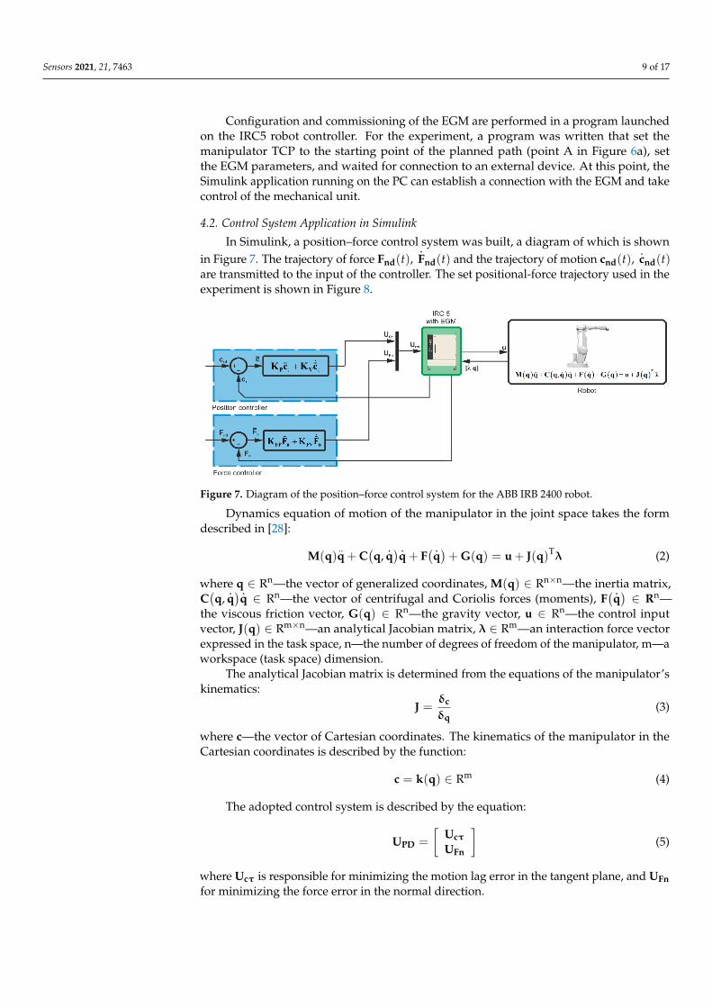
4.2. Control System Application in Simulink In Simulink, a position–force control system was built, a diagram of which is shown

in Figure 7. The trajectory of force 𝐅𝐧𝐝(𝑡), 𝐅𝐧𝐝(𝑡) and the trajectory of motion 𝐜𝐧𝐝(𝑡), 𝐜𝐧𝐝(𝑡) are transmitted to the input of the controller. The set positional-force trajectory used in the experiment is shown in Figure 8.

Figure 7. Diagram of the position–force control system for the ABB IRB 2400 robot.

Dynamics equation of motion of the manipulator in the joint space takes the form described in [28]: 𝐌(𝐪)𝐪 + 𝐂(𝐪, 𝐪)𝐪 + 𝐅(𝐪) + 𝐆(𝐪) = 𝐮 + 𝐉(𝐪) 𝛌 (2)

where 𝐪R —the vector of generalized coordinates, 𝐌(𝐪)R —the inertia matrix, 𝐂(𝐪, 𝐪)𝐪R —the vector of centrifugal and Coriolis forces (moments), 𝐅(𝐪)𝐑 —the vis-cous friction vector, 𝐆(𝐪)R —the gravity vector, 𝐮R —the control input vec-

Figure 6. The scheme of the experiment: (a) Arrangement of coordinate systems on the test stand; (b) control strategy diagram.

Sensors 2021, 21, 7463 9 of 17

Configuration and commissioning of the EGM are performed in a program launchedon the IRC5 robot controller. For the experiment, a program was written that set themanipulator TCP to the starting point of the planned path (point A in Figure 6a), setthe EGM parameters, and waited for connection to an external device. At this point, theSimulink application running on the PC can establish a connection with the EGM and takecontrol of the mechanical unit.

4.2. Control System Application in Simulink

In Simulink, a position–force control system was built, a diagram of which is shownin Figure 7. The trajectory of force Fnd(t),

.Fnd(t) and the trajectory of motion cnd(t),

.cnd(t)

are transmitted to the input of the controller. The set positional-force trajectory used in theexperiment is shown in Figure 8.

Sensors 2021, 21, x FOR PEER REVIEW 9 of 17

(a) (b)

Figure 6. The scheme of the experiment: (a) Arrangement of coordinate systems on the test stand; (b) control strategy diagram.

Configuration and commissioning of the EGM are performed in a program launched on the IRC5 robot controller. For the experiment, a program was written that set the ma-nipulator TCP to the starting point of the planned path (point A in Figure 6a), set the EGM parameters, and waited for connection to an external device. At this point, the Simulink application running on the PC can establish a connection with the EGM and take control of the mechanical unit.

4.2. Control System Application in Simulink In Simulink, a position–force control system was built, a diagram of which is shown

in Figure 7. The trajectory of force 𝐅𝐧𝐝(𝑡), 𝐅𝐧𝐝(𝑡) and the trajectory of motion 𝐜𝐧𝐝(𝑡), 𝐜𝐧𝐝(𝑡) are transmitted to the input of the controller. The set positional-force trajectory used in the experiment is shown in Figure 8.

Figure 7. Diagram of the position–force control system for the ABB IRB 2400 robot.

Dynamics equation of motion of the manipulator in the joint space takes the form described in [28]: 𝐌(𝐪)𝐪 + 𝐂(𝐪, 𝐪)𝐪 + 𝐅(𝐪) + 𝐆(𝐪) = 𝐮 + 𝐉(𝐪) 𝛌 (2)

where 𝐪R —the vector of generalized coordinates, 𝐌(𝐪)R —the inertia matrix, 𝐂(𝐪, 𝐪)𝐪R —the vector of centrifugal and Coriolis forces (moments), 𝐅(𝐪)𝐑 —the vis-cous friction vector, 𝐆(𝐪)R —the gravity vector, 𝐮R —the control input vec-

Figure 7. Diagram of the position–force control system for the ABB IRB 2400 robot.

Dynamics equation of motion of the manipulator in the joint space takes the formdescribed in [28]:

M(q)..q + C

(q,

.q) .q + F

( .q)+ G(q) = u + J(q)Tλ (2)

where q ∈ Rn—the vector of generalized coordinates, M(q) ∈ Rn×n—the inertia matrix,C(q,

.q) .q ∈ Rn—the vector of centrifugal and Coriolis forces (moments), F

( .q)∈ Rn—

the viscous friction vector, G(q) ∈ Rn—the gravity vector, u ∈ Rn—the control inputvector, J(q) ∈ Rm×n—an analytical Jacobian matrix, λ ∈ Rm—an interaction force vectorexpressed in the task space, n—the number of degrees of freedom of the manipulator, m—aworkspace (task space) dimension.

The analytical Jacobian matrix is determined from the equations of the manipulator’skinematics:

J =δc

δq(3)

where c—the vector of Cartesian coordinates. The kinematics of the manipulator in theCartesian coordinates is described by the function:

c = k(q) ∈ Rm (4)

The adopted control system is described by the equation:

UPD =

[UcτUFn

](5)

where Ucτ is responsible for minimizing the motion lag error in the tangent plane, and UFnfor minimizing the force error in the normal direction.

Sensors 2021, 21, 7463 10 of 17

These control elements are defined as PD control:

Ucτ = KP~cτ + KV

.~cτ (6)

UFn = KFP~Fn + KFV

.~Fn (7)

where KP and KV are successive matrices of proportional and differentiating gains ofthe position control system, while KFP and KFV are successive matrices of proportionaland differentiating gains of the force control system. The error of the motion trajectoryimplementation in Equation (6) was written as:

~cτ = cτd − cτ (8)

where cτd is the set TCP position in a direction tangent to the surface of the workpiece, cτis the actual TCP position in a direction tangent to the surface of the workpiece. Theuser reference system was defined so that the xOyO axes are tangent to the plane of theworkpiece. Therefore:

cτ =

[xTyT

](9)

where xT and yT are the coordinates specifying the position of the TCP in relation to theuser’s system xOyOzO. The error of the force trajectory implementation in Equation (7) waswritten as: ~

Fn = Fnd − Fn (10)

where Fnd is the set downforce in the direction normal to the surface of the workpiece,Fn is the downforce measured by the sensor in the direction normal to the surface of theworkpiece.

4.3. Setting the Parameters of the Control System

It was assumed in the research that the robot tool would move along the workpiece,making three passes in a straight line, smoothly changing direction at the ends of theworkpiece. The relationship describing the set TCP velocity was adopted as:

.yTd =

.yTd max

(1

1 + exp(−cv(t− tns))− 1

1 + exp(−cv(t− tnk))

)(11)

where.yTd max is the maximum TCP velocity, cv is the rate of rise and fall of velocity, tns, tnk

define the time range during which the function reaches its maximum value, t ∈ [0, 100] s,n = 1, 2, 3. The set velocity was composed of three successive runs of this relationship.

It was also assumed that the tool downforce should smoothly reach a certain value ofFnd max, which will be maintained throughout the motion. Therefore, the set value of theforce is described, like the set velocity, by the relationship:

Fnd = Fnd max

(1

1 + exp(−cF(t− tFs))− 1

1 + exp(−cD(t− tFk))

)(12)

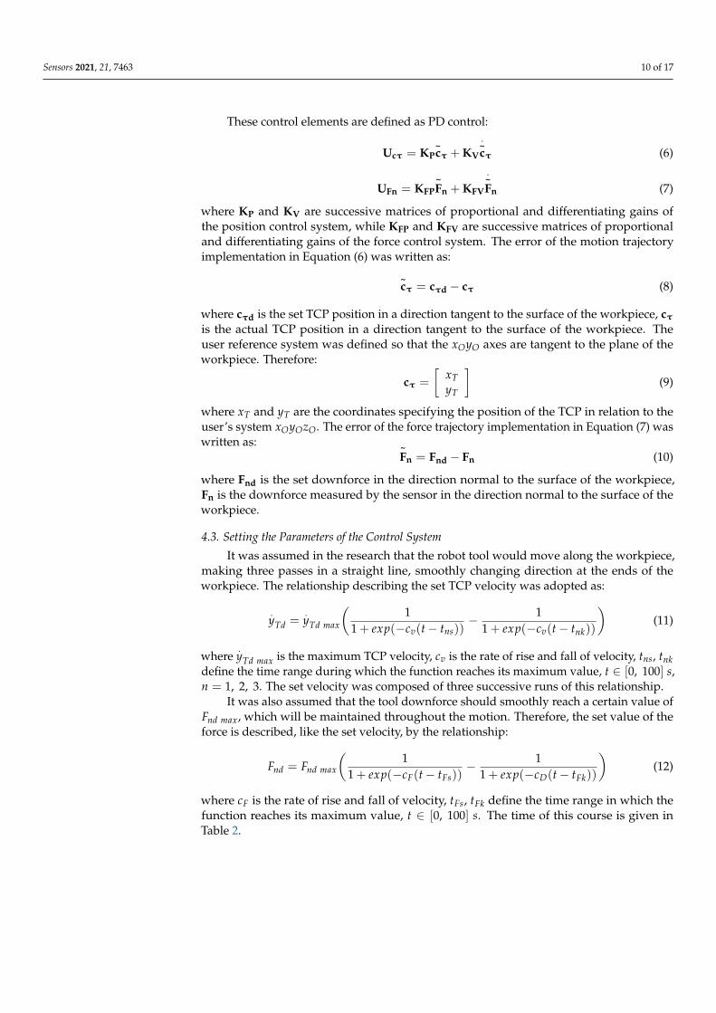
where cF is the rate of rise and fall of velocity, tFs, tFk define the time range in which thefunction reaches its maximum value, t ∈ [0, 100] s. The time of this course is given inTable 2.

Sensors 2021, 21, 7463 11 of 17

Table 2. Parameters of the set trajectory.

Parameter Unit Value.yTd max m/s 0.01Fnd max N 30[t1s , t1k) s [5 , 35)[t2s , t2k) s [35 , 65)[t3s, t3k] s [65, 95][tFs, tFk] s [5, 95]

The controller realizing the set trajectory requires the gain parameters to be set inaccordance with the adopted control system (5). The parameters of the PD controller arewritten as the gain matrices KP = diag

(KPx, KPy

), KV = diag

(KVx, KVy

)for the controller

controlling the position and the parameters KFP and KFV for the controller controlling theforce should be selected. They were selected experimentally on the basis of several testruns. The values of the applied parameters of the controller are given in Table 3.

Table 3. Control system parameters.

Parameter Value

KPx 0KVx 0KPy 5KVy 0.1KFP 0.5KFV 0.05

The PD controller gain values for the xO axis motion were set to 0 because the EGMwas configured to control TCP motion only on the other two axes. This allowed us to checkhow the EGM system copes with maintaining a constant value of this coordinate excludedfrom the coordinate motion without the participation of an external controller. The controlsignals from the controller in Simulink were connected to the CartesianSpeed input ofthe EGM IRC5 S-function block. The values from this input are sent to the EGM, whichinterprets them as speed_re f , according to formula (1). The k factor was set to 0 so that theTCP velocity would be generated based on the velocity control signal from the externalcontroller.

Sensors 2021, 21, x FOR PEER REVIEW 11 of 17

0, 100 𝑠, 𝑛 = 1, 2, 3. The set velocity was composed of three successive runs of this rela-tionship.

It was also assumed that the tool downforce should smoothly reach a certain value of 𝐹 , which will be maintained throughout the motion. Therefore, the set value of the force is described, like the set velocity, by the relationship: 𝐹 = 𝐹 11 + 𝑒𝑥𝑝 −𝑐 (𝑡 − 𝑡 ) − 11 + 𝑒𝑥𝑝 −𝑐 (𝑡 − 𝑡 ) (12)

where 𝑐 is the rate of rise and fall of velocity, 𝑡 , 𝑡 define the time range in which the function reaches its maximum value, 𝑡 ∈ 0, 100 𝑠. The time of this course is given in Table 2.

Table 2. Parameters of the set trajectory.

Parameter Unit Value 𝑦 m/s 0.01 𝐹 N 30 𝑡 , 𝑡 ) s 5, 35) 𝑡 , 𝑡 ) s 35, 65) 𝑡 , 𝑡 s 65, 95 𝑡 , 𝑡 s 5, 95

The controller realizing the set trajectory requires the gain parameters to be set in accordance with the adopted control system (5). The parameters of the PD controller are written as the gain matrices 𝑲𝑷 = 𝑑𝑖𝑎𝑔 𝐾 , 𝐾 , 𝑲𝑽 = 𝑑𝑖𝑎𝑔 𝐾 , 𝐾 for the controller controlling the position and the parameters 𝐾 and 𝐾 for the controller controlling the force should be selected. They were selected experimentally on the basis of several test runs. The values of the applied parameters of the controller are given in Table 3.

Table 3. Control system parameters.

Parameter Value 𝐾 0 𝐾 0 𝐾 5 𝐾 0.1 𝐾 0.5 𝐾 0.05

(a) (b)

0 10 20 30 40 50 60 70 80 90 100

t [s]

-35

-30

-25

-20

-15

-10

-5

0

Figure 8. Cont.

Sensors 2021, 21, 7463 12 of 17Sensors 2021, 21, x FOR PEER REVIEW 12 of 17

(c) (d)

Figure 8. Graphs of set trajectory of control systems: (a) TCP coordinates on directions tangent to the surface of the work-piece; (b) downforce; (c) TCP velocity in tangent directions; (d) derivative of downforce.

The PD controller gain values for the 𝑥 axis motion were set to 0 because the EGM was configured to control TCP motion only on the other two axes. This allowed us to check how the EGM system copes with maintaining a constant value of this coordinate excluded from the coordinate motion without the participation of an external controller. The control signals from the controller in Simulink were connected to the CartesianSpeed input of the EGM IRC5 S-function block. The values from this input are sent to the EGM, which interprets them as 𝑠𝑝𝑒𝑒𝑑_𝑟𝑒𝑓, according to formula (1). The 𝑘 factor was set to 0 so that the TCP velocity would be generated based on the velocity control signal from the external controller.

4.4. Results of the Experiment Figure 9 shows the realized TCP motion path, on which it is possible to observe how

the coordinate 𝑧 changes reflecting the shape of the workpiece surface against which the tool is pressed. The motion in the tangential direction is divided into three phases: • The first phase begins the motion from point A to point B. As the motion begins, the

force control system begins to increase the downforce of the tool in the direction nor-mal to the surface of the workpiece.

• The second phase begins after reaching point B, where the direction of motion changes. The tool from point B begins to move towards point A. The downforce is still maintained.

• The third phase begins when it reaches point A, where the robot again changes its direction of motion, stopping at point B. The downforce decreases smoothly, reach-ing 0 at point B. The place where the flat bars spread apart is distinguished on the graph. It can be

seen that the robot in this place lowered the height by about 1 mm in relation to the flat bar surface in order to be able to maintain a constant downforce, bracing the tool against the table surface.

Figure 8. Graphs of set trajectory of control systems: (a) TCP coordinates on directions tangent tothe surface of the workpiece; (b) downforce; (c) TCP velocity in tangent directions; (d) derivative ofdownforce.

4.4. Results of the Experiment

Figure 9 shows the realized TCP motion path, on which it is possible to observe howthe coordinate zT changes reflecting the shape of the workpiece surface against which thetool is pressed. The motion in the tangential direction is divided into three phases:

• The first phase begins the motion from point A to point B. As the motion begins,the force control system begins to increase the downforce of the tool in the directionnormal to the surface of the workpiece.

• The second phase begins after reaching point B, where the direction of motion changes.The tool from point B begins to move towards point A. The downforce is still main-tained.

• The third phase begins when it reaches point A, where the robot again changes itsdirection of motion, stopping at point B. The downforce decreases smoothly, reaching0 at point B.

The place where the flat bars spread apart is distinguished on the graph. It can beseen that the robot in this place lowered the height by about 1 mm in relation to the flat barsurface in order to be able to maintain a constant downforce, bracing the tool against thetable surface.

Sensors 2021, 21, x FOR PEER REVIEW 13 of 17

(a) (b)

(c)

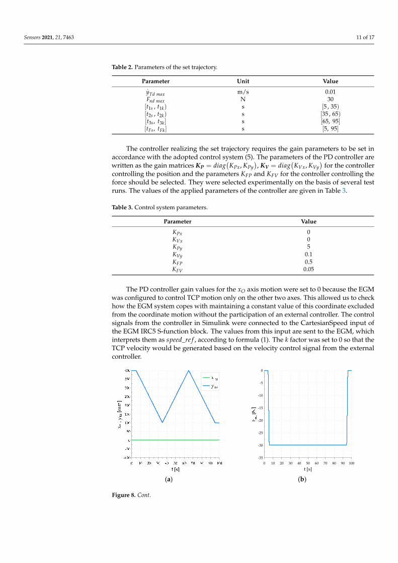
Figure 9. Graphs of the completed motion path, divided into 3 phases: (a) Motion phase No. 1 from point A to B, for the range 𝑡 , 𝑡 ); (b) motion phase No. 2 from point B to A, for the range 𝑡 , 𝑡 ); (c) motion phase No. 3 from point A to B, for the range 𝑡 , 𝑡 .

During the second pass, it was observed that the tool, leaving the fault between the flat bars, does not return to the position 𝑧 = −0.6 mm, but reaches the position 𝑧 =−0.8 mm. This is due to the frictional forces between the surfaces of the piston and the cylinder of the pneumatic table actuators, which prevent the table from fully returning to its original position. As a result, the tool has to lower its position to achieve the set down-force. Figure 10 shows the realized positional trajectory in the tangential direction and the trajectory of the force in the normal direction. The contact force curve shows that the force value is kept at the set value. The successive decreasing and increasing pressure peaks occur at the fault of the workpiece surface. The control system reacts quite quickly to sud-den changes in the contact surface.

z T [m

m]

80 120 160 200 240 280 320 360 400

yT [mm]

-1.8

-1.6

-1.4

-1.2

-1

-0.8

-0.6

-0.4

-0.2

0

0.2

A

B

Direction of movement

Figure 9. Cont.

Sensors 2021, 21, 7463 13 of 17

Sensors 2021, 21, x FOR PEER REVIEW 13 of 17

(a) (b)

(c)

Figure 9. Graphs of the completed motion path, divided into 3 phases: (a) Motion phase No. 1 from point A to B, for the range 𝑡 , 𝑡 ); (b) motion phase No. 2 from point B to A, for the range 𝑡 , 𝑡 ); (c) motion phase No. 3 from point A to B, for the range 𝑡 , 𝑡 .

During the second pass, it was observed that the tool, leaving the fault between the flat bars, does not return to the position 𝑧 = −0.6 mm, but reaches the position 𝑧 =−0.8 mm. This is due to the frictional forces between the surfaces of the piston and the cylinder of the pneumatic table actuators, which prevent the table from fully returning to its original position. As a result, the tool has to lower its position to achieve the set down-force. Figure 10 shows the realized positional trajectory in the tangential direction and the trajectory of the force in the normal direction. The contact force curve shows that the force value is kept at the set value. The successive decreasing and increasing pressure peaks occur at the fault of the workpiece surface. The control system reacts quite quickly to sud-den changes in the contact surface.

z T [m

m]

80 120 160 200 240 280 320 360 400

yT [mm]

-1.8

-1.6

-1.4

-1.2

-1

-0.8

-0.6

-0.4

-0.2

0

0.2

A

B

Direction of movement

Figure 9. Graphs of the completed motion path, divided into 3 phases: (a) Motion phase No. 1 frompoint A to B, for the range [t1s , t1k); (b) motion phase No. 2 from point B to A, for the range [t2s , t2k);(c) motion phase No. 3 from point A to B, for the range [t3s, t3k].

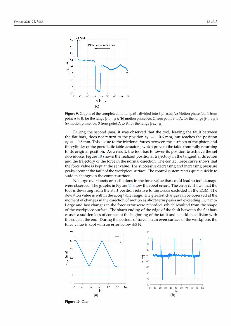
During the second pass, it was observed that the tool, leaving the fault betweenthe flat bars, does not return to the position zT = −0.6 mm, but reaches the positionzT = −0.8 mm. This is due to the frictional forces between the surfaces of the piston andthe cylinder of the pneumatic table actuators, which prevent the table from fully returningto its original position. As a result, the tool has to lower its position to achieve the setdownforce. Figure 10 shows the realized positional trajectory in the tangential directionand the trajectory of the force in the normal direction. The contact force curve shows thatthe force value is kept at the set value. The successive decreasing and increasing pressurepeaks occur at the fault of the workpiece surface. The control system reacts quite quickly tosudden changes in the contact surface.

No large overshoots or oscillations in the force value that could lead to tool damagewere observed. The graphs in Figure 11 show the robot errors. The error cx shows that thetool is deviating from the start position relative to the x-axis excluded in the EGM. Thedeviation value is within the acceptable range. The greatest changes can be observed at themoment of changes in the direction of motion as short-term peaks not exceeding ±0.3 mm.Large and fast changes in the force error were recorded, which resulted from the shapeof the workpiece surface. The sharp ending of the edge of the fault between the flat barscauses a sudden loss of contact at the beginning of the fault and a sudden collision withthe edge at the end. During the periods of travel on an even surface of the workpiece, theforce value is kept with an error below ±5 N.

Sensors 2021, 21, x FOR PEER REVIEW 14 of 17

(a) (b)

(c) (d)

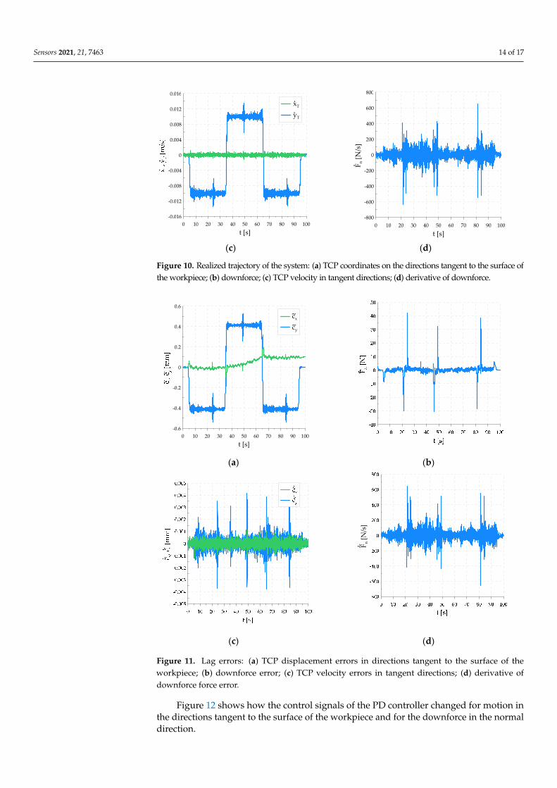
Figure 10. Realized trajectory of the system: (a) TCP coordinates on the directions tangent to the surface of the workpiece; (b) downforce; (c) TCP velocity in tangent directions; (d) derivative of downforce.

No large overshoots or oscillations in the force value that could lead to tool damage were observed. The graphs in Figure 11 show the robot errors. The error �� shows that the tool is deviating from the start position relative to the x-axis excluded in the EGM. The deviation value is within the acceptable range. The greatest changes can be observed at the moment of changes in the direction of motion as short-term peaks not exceeding ±0.3 mm. Large and fast changes in the force error were recorded, which resulted from the shape of the workpiece surface. The sharp ending of the edge of the fault between the flat bars causes a sudden loss of contact at the beginning of the fault and a sudden collision with the edge at the end. During the periods of travel on an even surface of the workpiece, the force value is kept with an error below ±5 N.

0 10 20 30 40 50 60 70 80 90 100

t [s]

-80

-70

-60

-50

-40

-30

-20

-10

0

10

0 10 20 30 40 50 60 70 80 90 100

t [s]

-0.016

-0.012

-0.008

-0.004

0

0.004

0.008

0.012

0.016

xT

yT..

0 10 20 30 40 50 60 70 80 90 100

t [s]

-800

-600

-400

-200

0

200

400

600

800

F n[N

/s]

.

Figure 10. Cont.

Sensors 2021, 21, 7463 14 of 17

Sensors 2021, 21, x FOR PEER REVIEW 14 of 17

(a) (b)

(c) (d)

Figure 10. Realized trajectory of the system: (a) TCP coordinates on the directions tangent to the surface of the workpiece; (b) downforce; (c) TCP velocity in tangent directions; (d) derivative of downforce.

No large overshoots or oscillations in the force value that could lead to tool damage were observed. The graphs in Figure 11 show the robot errors. The error �� shows that the tool is deviating from the start position relative to the x-axis excluded in the EGM. The deviation value is within the acceptable range. The greatest changes can be observed at the moment of changes in the direction of motion as short-term peaks not exceeding ±0.3 mm. Large and fast changes in the force error were recorded, which resulted from the shape of the workpiece surface. The sharp ending of the edge of the fault between the flat bars causes a sudden loss of contact at the beginning of the fault and a sudden collision with the edge at the end. During the periods of travel on an even surface of the workpiece, the force value is kept with an error below ±5 N.

0 10 20 30 40 50 60 70 80 90 100

t [s]

-80

-70

-60

-50

-40

-30

-20

-10

0

10

0 10 20 30 40 50 60 70 80 90 100

t [s]

-0.016

-0.012

-0.008

-0.004

0

0.004

0.008

0.012

0.016

xT

yT..

0 10 20 30 40 50 60 70 80 90 100

t [s]

-800

-600

-400

-200

0

200

400

600

800

F n[N

/s]

.

Figure 10. Realized trajectory of the system: (a) TCP coordinates on the directions tangent to the surface ofthe workpiece; (b) downforce; (c) TCP velocity in tangent directions; (d) derivative of downforce.

Sensors 2021, 21, x FOR PEER REVIEW 15 of 17

(a) (b)

(c) (d)

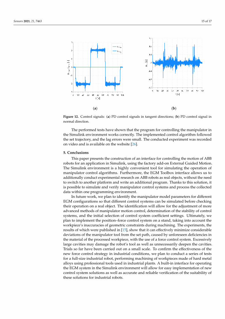
Figure 11. Lag errors: (a) TCP displacement errors in directions tangent to the surface of the workpiece; (b) downforce error; (c) TCP velocity errors in tangent directions; (d) derivative of downforce force error.

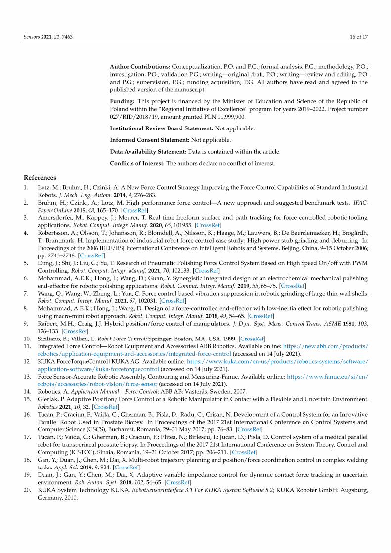
Figure 12 shows how the control signals of the PD controller changed for motion in the directions tangent to the surface of the workpiece and for the downforce in the normal direction.

(a) (b)

Figure 12. Control signals: (a) PD control signals in tangent directions; (b) PD control signal in normal direction.

0 10 20 30 40 50 60 70 80 90 100

t [s]

-0.6

-0.4

-0.2

0

0.2

0.4

0.6

cx

cy

~~

F n[N

/s]

. ~

Figure 11. Lag errors: (a) TCP displacement errors in directions tangent to the surface of theworkpiece; (b) downforce error; (c) TCP velocity errors in tangent directions; (d) derivative ofdownforce force error.

Figure 12 shows how the control signals of the PD controller changed for motion inthe directions tangent to the surface of the workpiece and for the downforce in the normaldirection.

Sensors 2021, 21, 7463 15 of 17

Sensors 2021, 21, x FOR PEER REVIEW 15 of 17

(a) (b)

(c) (d)

Figure 11. Lag errors: (a) TCP displacement errors in directions tangent to the surface of the workpiece; (b) downforce error; (c) TCP velocity errors in tangent directions; (d) derivative of downforce force error.

Figure 12 shows how the control signals of the PD controller changed for motion in the directions tangent to the surface of the workpiece and for the downforce in the normal direction.

(a) (b)

Figure 12. Control signals: (a) PD control signals in tangent directions; (b) PD control signal in normal direction.

0 10 20 30 40 50 60 70 80 90 100

t [s]

-0.6

-0.4

-0.2

0

0.2

0.4

0.6

cx

cy

~~

F n[N

/s]

. ~

Figure 12. Control signals: (a) PD control signals in tangent directions; (b) PD control signal innormal direction.

The performed tests have shown that the program for controlling the manipulator inthe Simulink environment works correctly. The implemented control algorithm followedthe set trajectory, and the lag errors were small. The conducted experiment was recordedon video and is available on the website [26].

5. Conclusions

This paper presents the construction of an interface for controlling the motion of ABBrobots for an application in Simulink, using the factory add-on External Guided Motion.The Simulink environment is a highly convenient tool for simulating the operation ofmanipulator control algorithms. Furthermore, the EGM Toolbox interface allows us toadditionally conduct experimental research on ABB robots as real objects, without the needto switch to another platform and write an additional program. Thanks to this solution, itis possible to simulate and verify manipulator control systems and process the collecteddata within one programming environment.

In future work, we plan to identify the manipulator model parameters for differentEGM configurations so that different control systems can be simulated before checkingtheir operation on a real object. The identification will allow for the adjustment of moreadvanced methods of manipulator motion control, determination of the stability of controlsystems, and the initial selection of control system coefficient settings. Ultimately, weplan to implement the position–force control system on a stand, taking into account theworkpiece’s inaccuracies of geometric constraints during machining. The experiments, theresults of which were published in [15], show that it can effectively minimize considerabledeviations of the manipulator tool from the set path, caused by unforeseen deficiencies inthe material of the processed workpiece, with the use of a force control system. Excessivelylarge cavities may damage the robot’s tool as well as unnecessarily deepen the cavities.Trials so far have been carried out on a small scale. To confirm the effectiveness of thenew force control strategy in industrial conditions, we plan to conduct a series of testsfor a full-size industrial robot, performing machining of workpieces made of hard metalalloys using professional tools used in industrial plants. A built-in interface for operatingthe EGM system in the Simulink environment will allow for easy implementation of newcontrol system solutions as well as accurate and reliable verification of the suitability ofthese solutions for industrial robots.

Sensors 2021, 21, 7463 16 of 17

Author Contributions: Conceptualization, P.O. and P.G.; formal analysis, P.G.; methodology, P.O.;investigation, P.O.; validation P.G.; writing—original draft, P.O.; writing—review and editing, P.O.and P.G.; supervision, P.G.; funding acquisition, P.G. All authors have read and agreed to thepublished version of the manuscript.

Funding: This project is financed by the Minister of Education and Science of the Republic ofPoland within the “Regional Initiative of Excellence” program for years 2019–2022. Project number027/RID/2018/19, amount granted PLN 11,999,900.

Institutional Review Board Statement: Not applicable.

Informed Consent Statement: Not applicable.

Data Availability Statement: Data is contained within the article.

Conflicts of Interest: The authors declare no conflict of interest.

References1. Lotz, M.; Bruhm, H.; Czinki, A. A New Force Control Strategy Improving the Force Control Capabilities of Standard Industrial

Robots. J. Mech. Eng. Autom. 2014, 4, 276–283.2. Bruhm, H.; Czinki, A.; Lotz, M. High performance force control—A new approach and suggested benchmark tests. IFAC-

PapersOnLine 2015, 48, 165–170. [CrossRef]3. Amersdorfer, M.; Kappey, J.; Meurer, T. Real-time freeform surface and path tracking for force controlled robotic tooling

applications. Robot. Comput. Integr. Manuf. 2020, 65, 101955. [CrossRef]4. Robertsson, A.; Olsson, T.; Johansson, R.; Blomdell, A.; Nilsson, K.; Haage, M.; Lauwers, B.; De Baerclemaeker, H.; Brogårdh,

T.; Brantmark, H. Implementation of industrial robot force control case study: High power stub grinding and deburring. InProceedings of the 2006 IEEE/RSJ International Conference on Intelligent Robots and Systems, Beijing, China, 9–15 October 2006;pp. 2743–2748. [CrossRef]

5. Dong, J.; Shi, J.; Liu, C.; Yu, T. Research of Pneumatic Polishing Force Control System Based on High Speed On/off with PWMControlling. Robot. Comput. Integr. Manuf. 2021, 70, 102133. [CrossRef]

6. Mohammad, A.E.K.; Hong, J.; Wang, D.; Guan, Y. Synergistic integrated design of an electrochemical mechanical polishingend-effector for robotic polishing applications. Robot. Comput. Integr. Manuf. 2019, 55, 65–75. [CrossRef]

7. Wang, Q.; Wang, W.; Zheng, L.; Yun, C. Force control-based vibration suppression in robotic grinding of large thin-wall shells.Robot. Comput. Integr. Manuf. 2021, 67, 102031. [CrossRef]

8. Mohammad, A.E.K.; Hong, J.; Wang, D. Design of a force-controlled end-effector with low-inertia effect for robotic polishingusing macro-mini robot approach. Robot. Comput. Integr. Manuf. 2018, 49, 54–65. [CrossRef]

9. Raibert, M.H.; Craig, J.J. Hybrid position/force control of manipulators. J. Dyn. Syst. Meas. Control Trans. ASME 1981, 103,126–133. [CrossRef]

10. Siciliano, B.; Villani, L. Robot Force Control; Springer: Boston, MA, USA, 1999. [CrossRef]11. Integrated Force Control—Robot Equipment and Accessories|ABB Robotics. Available online: https://new.abb.com/products/

robotics/application-equipment-and-accessories/integrated-force-control (accessed on 14 July 2021).12. KUKA.ForceTorqueControl|KUKA AG. Available online: https://www.kuka.com/en-us/products/robotics-systems/software/

application-software/kuka-forcetorquecontrol (accessed on 14 July 2021).13. Force Sensor-Accurate Robotic Assembly, Contouring and Measuring-Fanuc. Available online: https://www.fanuc.eu/si/en/

robots/accessories/robot-vision/force-sensor (accessed on 14 July 2021).14. Robotics, A. Application Manual—Force Control; ABB AB: Västerås, Sweden, 2007.15. Gierlak, P. Adaptive Position/Force Control of a Robotic Manipulator in Contact with a Flexible and Uncertain Environment.

Robotics 2021, 10, 32. [CrossRef]16. Tucan, P.; Craciun, F.; Vaida, C.; Gherman, B.; Pisla, D.; Radu, C.; Crisan, N. Development of a Control System for an Innovative

Parallel Robot Used in Prostate Biopsy. In Proceedings of the 2017 21st International Conference on Control Systems andComputer Science (CSCS), Bucharest, Romania, 29–31 May 2017; pp. 76–83. [CrossRef]

17. Tucan, P.; Vaida, C.; Gherman, B.; Craciun, F.; Plitea, N.; Birlescu, I.; Jucan, D.; Pisla, D. Control system of a medical parallelrobot for transperineal prostate biopsy. In Proceedings of the 2017 21st International Conference on System Theory, Control andComputing (ICSTCC), Sinaia, Romania, 19–21 October 2017; pp. 206–211. [CrossRef]

18. Gan, Y.; Duan, J.; Chen, M.; Dai, X. Multi-robot trajectory planning and position/force coordination control in complex weldingtasks. Appl. Sci. 2019, 9, 924. [CrossRef]

19. Duan, J.; Gan, Y.; Chen, M.; Dai, X. Adaptive variable impedance control for dynamic contact force tracking in uncertainenvironment. Rob. Auton. Syst. 2018, 102, 54–65. [CrossRef]

20. KUKA System Technology KUKA. RobotSensorInterface 3.1 For KUKA System Software 8.2; KUKA Roboter GmbH: Augsburg,Germany, 2010.

Sensors 2021, 21, 7463 17 of 17

21. Wang, Z.; Zhang, R.; Keogh, P. Real-Time Laser Tracker Compensation of Robotic Drilling and Machining. J. Manuf. Mater. Process.2020, 4, 79. [CrossRef]

22. Safeea, M.; Neto, P. KUKA Sunrise Toolbox: Interfacing Collaborative Robots with MATLAB. IEEE Robot. Autom. Mag. 2019, 26,91–96. [CrossRef]

23. Lee, J.; Hong, T.; Seo, C.-H.; Jeon, Y.H.; Lee, M.G.; Kim, H.-Y. Implicit force and position control to improve drilling quality inCFRP flexible robotic machining. J. Manuf. Process. 2021, 68, 1123–1133. [CrossRef]

24. ABB Application Manual Externally Guided Motion RW7; ABB AB: Västerås, Sweden, 2019.25. GitHub—Modi1987/Simulink-iiwa-Interface: An Interface for Controlling KUKA iiwa Manipulators from Simulink. Available

online: https://github.com/Modi1987/Simulink-iiwa-interface (accessed on 15 July 2021).26. pobal/ABB_EGM. Available online: https://github.com/pobal/ABB_EGM (accessed on 15 July 2021).27. Gierlak, P.; Szuster, M. Adaptive position/force control for robot manipulator in contact with a flexible environment. Rob. Auton.

Syst. 2017, 95, 80–101. [CrossRef]28. Gierlak, P. Position/Force Control of Manipulator in Contact with Flexible Environment. Acta Mech. Autom. 2019, 13, 16–22.

[CrossRef]