efficient eigenvalue assignments for general linear mimo systems

Pergamon ooos-1098(95)ooo91-7

Automotica, Vol. 31, No. II, pp. 160-1617, 1995 Copyright 0 1995 Elsevier Science Ltd

Printed in Great Britain. All rights reserved cn?o5-1098/95 $9.50 + 0.00

Efficient Eigenvalue Assignments for General Linear MIMO Systems*

MICHAEL VAL&EKt$ and NEJAT OLGACt

A general class of time-varying linear MZMO systems is considered. These are first tranformed into Frobenius form. Then a feedback pole placement technique is implemented in the sense of Lyapunov equivalence. A step-by-step development is given for SZSO time-invariant and time-

varying and for MZMO time-invariant and time-varying systems.

Key Words-Pole assignment; eigenvalue placement; Lyapunov equivalent; Frobenius form; linear MIMO system: feedback stabilization; characteristic equation; linear SISO systems.

Abstrad-This paper deals with the transformation of linear, multi-input multi-output (MIMO) systems into Frobenius canonical form, with the ultimate objective of developing a new, computationally efficient methodology for a pole- placement procedure. Both time-invariant and time-varying systems are considered. The conventional pole placement steps for time-invariant SISO (single-input single-output) systems are generalized for both classes. This is a unique study of the expansion of the pole placement capability, in particular for time-varying MIMO systems. This depth of generalization has been neglected in the past due to its complex formulation. The practical advantage of the proposed technique is that it does not require the coefficients of the characteristic polynomial, the eigenvalues of the original system, or the coefficients of the characteristic polynomial of the transformed system. The repercussions of such a development are expected in nonlinear systems theory as well, considering the fact that some recently developed techniques yield exact I/O linearization with time-varying coefficients.

1. INTRODUCTION

This paper deals primarily with the transformation of general linear multi-input multi-output (MIMO) systems into Frobenius canonical form. In this transformed domain, a new, computationally efficient, state feedback structure is introduced for a desired output behavior. Similar transformations into different canonical forms

*Received 15 April 1993; revised 14 September 1994; received in final form 7 June 1995. This paper was not presented at any IFAC meeting. This paper was recommended for publication in revised form by Associate Editor V. Ku&a under the direction of Editor Huibert Kwakernaak. Corresponding author Professor Nejat Olgac. Tel. + 1203 486 2382; Fax + 1203 486 5088; E-mail [email protected].

t University of Connecticut, Mechanical Engineering Department, Storrs, CT 06269-3139, U.S.A.

$ Permanent address: Faculty of Mechanical Engineering, Department of Mechanics, Czech Technical University, Prague, Czech Republic.

(in particular, Frobenius and Hessenberg) have been treated extensively in the literature (Silverman, 1966; Tuel, 1966; Luenberger, 1967; Kailath, 1980; Varga, 1981; Kuo, 1982; Miminis and Paige, 1982; Petkov et al., 1984, 1985; Kautsky et al., 1985). In this study, particular attention is directed towards the Frobenius canonical form, because of its unparalleled position in arriving at the desired pole placement for time-varying systems. With awareness of the numerical instabilities arising during this procedure (particularly for higher-dimensional states), we take the necessary steps towards developing a technique to handle linear time-varying MIMO systems. For the curious reader, a treatment that alleviates this instability for SISO structures can be found in ValaSek and Olgac (1995). It should also be noted that at present there is no transformation that is numerically robust for linear time-varying systems.

Generally pole placement requires the computation of the characteristic polynomial coefficients for either the original or the new state matrices or the eigenvalues of the original system matrix. Blanchini (1989) introduced a technique that removes this requirement for SISO (single-input single-output) systems by utilizing an intermediate transformation to a bidiagonal Frobenius form. This technique has been further extended for time-varying linear systems in Tsai et al., 1991. Nguyen (1987) introduced the Frobenius transformation for time-varying systems; however, his treatment requires that the characteristic polynomial coefficients of the desired behavior be computed as well as the complete Frobenius transformation of the system. All these requirements are

1605

1606 M. Val&Zek and N. Olgac

removed in the technique presented in this paper.

Investigations of linear MIMO time-varying systems by Nguyen (1987) resulted in a claim that his methodology does not function except for some particular class of controllability matrix structures. The steps of Tsai et al. (1991) require that the transformation of the system dynamics into the bidiagonal Frobenius form be done through a time-invariant transformation matrix. Both of these conditions are very restrictive, and can easily be violated. In contrast, the procedure detailed in this paper has a very general domain of validity, so long as the combined system considered is controllable. Therefore the procedure defined here represents a unique treatment for MIMO systems in the literature.

It is clear that both the transformation and pole-placement efforts are of significant and continuing interest to the systems and controls community. Our current work brings a different perspective to addressing these issues and, furthermore, it offers a unique and numerically simplified procedure to achieve this objective.

In summary, the text consists of the following. In Section 2 a brief summary of results for the SISO time-invariant and time-varying case is presented. Section 3 deals with the basics of the time-invariant MIMO pole-placement procedures, with the following highlights:

G-4

(b)

the procedure presented here provides a simple generalization of classical Acker- mann’s formula for MIMO cases;

an efficient pole-placement technique is introduced that does not require the characteristic polynomial coefficients, nor the eigenvalues for the original system.

Section 4 covers the critical contributions of this research: the extension of a numerically efficient pole placement technique to the time-varying MZMO dynamics. The Frobenius transformation is again pursued. Pole-placement feedback is then introduced, with a novel generalization of classical formulae from SISO time-invariant to MIMO time-varying systems. We restate that this approach is unique and imposes no restrictions on the dynamics in hand except controllability. Section 5 contains an example to illustrate the theory. Conclusions follow in Section 6.

2. AN OVERVIEW OF POLE PLACEMENT FOR LINEAR SISO SYSTEMS; TIME-VARYING

AND TIME-INVARIANT CASES

Let us first consider a controllable time- invariant SISO system given by

i=Ax+bu, (1)

where x (n X 1) is the state vector, u is the control variable, A (n X n) and B (n X 1) are system and control gain matrices respectively. The intermediate objective to reach is the Frobenius canonical form

0’ ‘i’ -an-2 -a,_,

I u =A&+++

5

(2)

where 5 (n X 1) is the tranformed state variable vector, a = [a0 al . . . a,_,] are the coefficients of the characteristic polynomial

det [zI - A] = Do(z) = z” + u,_~z”-’ + u,_g”-*

+ * . . +a,z +ao=o (3)

of the original system (l), AF (n X n) and BF (n X 1) are the transformed system matrix and the control gain vector, respectively. The passage from (1) to (2) is simply achieved by a similarity transformation using a matrix Q (n X n). That is,

6 = Q-*x, AF = Q-‘AQ, BF = Q-‘B. (4)

For the ultimate objective of pole placement, a state feedback is used over the Frobenius canonical form at hand, as

u = K&. (5)

Following some earlier work of Kalman (1963), Lefschetz (1965) and Tuel (1966) and the final formulation of Luenberger (1967), the transformation matrix Q-’ has the form

(6)

where q1 (1 X n) is a row vector computed as

q, = e:R-’ (7)

from the controllability matrix

R= [B AB A*B . . . A”-‘B] (8)

of the system (l), which is taken as full rank. Here e, = [0 0 . . . 0 11’ is a unit vector.

Eigenvalue assignments for linear MIMO systems 1607

The above steps complete the transformation into Frobenius form. It is well known that this form is extremely convenient for executing a feedback stabilization with desired characteristic behavior (i.e. the pole-placement problem).

The objective stabilized system is given by either a desired characteristic polynomial or by the eigenvalues (roots) of this polynomial. We treeat both cases below, and present a simplified form of the feedback gain vector KF to be used in the control u = K& of (2).

First, we consider the case with a given characteristic equation. A simple substitution of u into (2) yields

KF=a-d (9)

where d = [do d, . . . d,_,] is the vector of the desired characteristic polynomial coefficients parallel to (3). The transformation of (9) into the original state space (i.e. of x), yields the traditional formula of Ackermann (1972, 1977, 1985):

K = -q,(A” + d,_,A”-’ + dn_2An-2

+ . . . + d,A + dJ)

= -qIDd(A) = -ezR-‘D,(A), (10)

where D,(A) denotes the evaluation of the desired characteristic polynomial Dd with the state matrix A. In this formula, if the vector q, is not taken outside the parentheses, a more efficient way of computing the gain vector K is obtained compared with those procedures that are traditionally followed (Franklin and Powell, 1980; Kailath, 1980; Lewis, 1992; MathWorks, 1988). The simple reason for this is that the computation with row vectors is more efficient than that with the full square matrices. The efficient numerical algorithm is straightforward.

q;=q,, q ;+I = q;A,

( n-1

K= - &+, + c diql+, 1 . i=o

(11)

Next, we consider a stabilizing feedback control defined by a set of desired eigenvalues A,; instead of the evaluated coefficients d of the characteristic equation. An alternate form of (10) is

K = -ql ir (A - AjI) j=l

= -e;fR-’ ,Q (A - A,I). (12)

Similar algorithmic simplifications as in the above discussion of (10) result in

, q1= Ql, q;+l = &(A - &I), K = -i+,. (13)

Equations (12) and (13) constitute the generalized version of Ackermann’s formula, utilizing

the desired poles Aj only, for linear time- invariant systems. This concludes the pole- placement process for SISO time-invariant systems.

The above described treatment can be extended for the general SISO linear time- uarying dynamic system of

i = A(t)x + B(t)u, (14)

with the state vector x (n X 1) and the scalar control u. The objective is to stabilize the system by means of a linear feedback that enforces a desired characteristic behavior for the state. Note that the eigenvalues of the time-varying dynamic system do not have any meaning regarding its behavior or its stability features. Therefore there is very little on the subject in the literature. One study addressing the issue for time-varying system is that by Nguyen (1987), who uses similar steps as described above for the time-invariant cases. In his treatment the original system is manipulated by a state feedback

u = K(t)x, (1%

which enforces the plant behavior to be Lyapunov-equivalent to the one with prescribed and fixed eigenvalues. Lyapunov equivalence of two linear systems imply similar stability properties, and also the existence of a Lyapunov transformation from one system to the other that preserves these properties. This manipulation as well utilizes the Frobenius transformation as an intermediate step (Chen, 1984). Essentially, the original system is stabilized by a time-dependent linear state feedback.

Let us take a transformation (Chen, 1984) from x to the new state variable 5 (n X 1) via the matrix Q(t):

x = Q(t)& E = Qp’(t)x. (16)

If Q(t), Q-‘(t) and dQ(t)ldt are continuous and bounded matrices and Q-‘(t) is full rank at the time interval of interest, (to, co), then this transformation is called a Lyapunov transformation. Additionally, the original and transformed systems manifest similar stability properties. The system matrices of the new structure are

AF = Q-‘(AQ - Q), B, = Q-‘B. (17)

In the following sections all the time arguments are suppressed for simplicity.

The Frobenius canonical form of (2) is again considered, but with time-varying a = a(t) =

[a,(t) a,(t) . . . a,_,(t)]. The time-dependent

1608 M. ValiSek and N. Olgac

state transformation matrix Q(r) is determined first, similarly to the work of Silverman (1966) and Nguyen (1987). The matrix Q-’ =

rows [sly q2,. . . , qnl is defined by the recursive computation of the rows qi of the matrix Q-‘,

qi+ 1 = q;A + Qi, (18)

starting with first row q1 determined as in (7). Note that the controllability matrix R for the time-varying system is different from the time-invariant version (8) (Chen, 1984):

R = (ri r2 . . . rn], rI = B, q+, = Ari - i;.

(19)

Assuming that the above transformation to Frobenius canonical form is of Lyapunov type, we proceed with the desired pole placement. A compact equivalent of Ackermann’s formula in this case is not possible. However, an efficient algorithm like (11) and (13) can be obtained. Leaving the intermediary steps and proofs to ValaSek and Olgac (1995), we give the final form of this algorithm below.

If the objective characteristic polynomial is given by its coefficients d;, the feedback gain is selected as

K= - ( qncl (20)

starting with q1 = e;fR-‘. If the characteristic polynomial is given by its

poles hk (k = 1,. . . , n) then the required feedback gain K is directly computed as

K = -de,, (21) where

I q1 = 41, q;+, = q;(A - AJ) + 4; (22)

These formulae state the fact that the pole- placement process can be substantially simplified compared with the technique proposed by Nguyen (1987) owing to the fact that the feedback gain calculations are not done in the intermediate Frobenius domain as in (9). Instead, direct evaluations are performed in the original state space. It also removes the severe restriction in the results of Tsai et al. (1991) that the transformation matrix Q be time-invariant for time-varying systems. This summary concludes the description of the state of the art concerning time-varying SISO cases.

3. POLE PLACEMENT FOR LINEAR MIMO TIME-INVARIANT SYSTEMS

Let us now consider the MIMO time-invariant dynamic system of

i=Ax+Bu, (23)

with state variable x (n X l), control vector u (m x l), m in, and matrices A and B of appropriate dimensions. The first objective is again to reduce the system into a generalized Frobenius canonical form, assuming that the pair [A, B] is controllable, and the m columns bi (n x 1) of the B matrix

B = [b, b2 . . . b,] (24)

are linearly independent. The ultimate objective is to design a linear feedback for this system in accordance with some desired eigenvalues. For the MIMO case at hand, the generalized canonical form, i.e. the corresponding Frobenius form, is defined in Luenberger (1967) as

A,=

1 0

. .

0 X

X

X

0 1 ‘b’ ::: . . . -. 0 . . 0 X . . . X

. .

. .

. * X . . . X

. .

. .

. . X . . . X

0- 0 . . 1 Y

X

X

. .

X . . . x x

X

X

1 0 . . 0 X

X . . . x x

X . . . x x

0 . . . . . . 0 1 0 . . . 0

.

*

. . . . . .

.

.

0 . . 1 0 X . . . x . . 1 1

x

(25)

BF=

0. 0 . . . 0 1. 0 0

0 0

0 0

0 0

. . . . . . . . . . . .


0 . . . 0 where e,k (n X 1) are unit vectors with 1 at 0 . . . 0 position rk. From the definition of R-‘,

. . . 0 . . . 0 1

qk@-‘bk = 1, k = 1, . . . , m, (30) X . . . X

-“I . . . . . . 0 0 . . . . . . 0

. . .

I . . . . . .

0 . . . . . . 0 1 X

L -2

0 . . . . 0 . . . . . . 0 . . . 0 . . .

. . . .., .,

I . 0. 0 0 . . 1. II

(26)

where X denotes generally nonzero elements. Under the above stated assumptions, this canonical form can be obtained from the original system (23). The corresponding system matrices are

AF = Q-‘AQ, BF = Q-‘B, (27)

as explained in the following section. The mathematical details of this process are treated here with a systematic rigor for the first time in the literature.

3.1. Transformation into Frobenius canonical form for time-invariant systems

A reordered controllability matrix R is formed first, following Chen (1984):

R = [b, Ab, . . . A“l-lb, b2 Abz

. . . AW’b 2 . . . b, Ab, . . . ACLm-lb,],

(28)

where pj represents the controllability index corresponding to bj. The [A, B] controllability assumption is nothing other than pl + p2 + . . . +&?I = n. These controllability indices are defined in a selection process for independent columns Ak-‘bi. The process starts with all columns bk of the matrix B. At step j, the columns Ai-‘bi are studied for their dependence on all previous ones in the order i = 1,2, . . . , m from left to right. The formation of R terminates when n linearly independent vectors are found. The selected vectors are arranged in the reordered controllability matrix (28).

Next, the inverse of this controllability matrix R-’ is defined by its m rows designated by qk, k=l,..., m, and they are defined as

qk = e:R-’ 7 rk = 5 pi, k= l,..., m, (29)

qkAi-‘b, = 0 for k=p and j<pk, (3la) for k#p and jSpP. (3lb)

The transformation matrix Q-’ is then con- structed following Luenberger (1967):

Q-’ =

This matrix Q-i h; the transformation form (25), (26) can

91 qA

q,A.W’

42 q2A

q2AiW 1 (32)

to be nonsingular, so that the generalized Frobenius made.

Lemma 1. If the system (23) is controllable in the general sense of a full-rank controllability matrix (B, AB, A2B. . . ) and all columns of the matrix B are independent then the transformation matrix (32) is of full rank.

Proof. This is done by contradiction. If the matrix Q-i were not of full rank then there would exist nonzero rij such that

-g 2 yijqiAj-’ = 0.

i=l j=l

(33)

Now consider postmultiplying (33) by columns of the form A’bk in some sequence as described below. In a particular step of the sequence, (33) is

2 i yiiqiAj-’ = 0

i=lj=1

(34)

and yij are nonzero only for i = 1,. . . , m, j = 1, . . . , Vi, 05 Vi 5 pi* Obviously at the beginning, vi = Fi is taken. In each step, we choose k such that

Vk=GXVi, 1 = ,.&I, - Vk. i=l

Postmultiplication of (33) by A’bk yields

together with (30) and (31). This result is due to the fact that for all i Zk and the additional

1610 M. Val%ek and N. Olgac

condition j+I=j+Elk-v~vkvi+~k-v~vkI~ the terms qiAj+‘-‘bk = 0 (from (31b)). What remains from the original summation is

$ Y.+IkA’+‘-‘hk = Yk,v,qkArk-‘hk = Yk,v*, (36b)

using (31a), since j + 15 j.&k. Finally, (30) dictates the last step, yielding

Yk,vk = 0. (36~)

In the next step we can decrease vk by 1. Continuing this sequence of steps, we find that vi = 0, i = 1, e * . ) m, i.e. all yji are zero, which contradicts the assumption; therefore the matrix (32) is of full rank. cl

The principal theorem of the transformation is stated next with its proof.

Theorem 1. If the system (23) is controllable and all columns of the matrix B are independent then the transformation defined by (27) and (32) recasts the system (23) into the Frobenius canonical form defined by (25) and (26).

Proof. (a) The construction of the matrix AF can be seen simply by rewriting the. identity (27) as AFQ-’ = Q-‘A. This equation yields identities for first j_&k - 1 rows in each kth group of rows, and for the pkth row we obtain a relation indicating the linear dependence of the pkth row to the previous j.& - 1 ones.

(b) The structure of the matrix BF is a consequence of (30), (31) and the definition (32). Its form has been stated by Luenberger (1967) as ‘easily verified by (tedious) inspection rather than by algebraic manipulation’. There has not been a rigorous treatment of this point since Luenberger. The following is the first such attempt to clarify the mathematics behind the structure of BF by algebraic means.

The matrix BF is divided into m layers consisting of j& rows (k = 1, . . . , m). Each of these layers is subdivided into the following submatrices with corresponding values

(Br)r,_,+tik.k = 1, (37)

(BF)rk_,+j,i = 0, 1 I j < pk, 15 i 4 m, (38)

(Br)rk_,+pLt,i = 0, 15 i < k (39)

where

k-l

(W

The only components of BF that are not covered in the above groups are

(BF)~~_,+~~.~, k < i 5 m, (41)

and they are free, as designated by X in (26). Let us elaborate on (37)-(39).

For the submatrix (37) it is obvious from (30) that

(Br)r,_,+rk,k = (Q-‘B),k_,cpk,k = (qkA@)hk = 1.

(42)

For the submatrix (38) the objective is to show that

(BF)rk_l+j.i = (Q-lB)rk_,+i,i = (QkA’-‘)bi = 0,

llj<&, lsism. (43)

(i) For the case i = k, (43) becomes

(BF)rk_l+j,k = (Q-lB)r,_,+j,k = (QkAj-I)bk = 0,

1 “j < pk, (Ml

which holds because of (31a).

(ii) For i # k we observe two separate cases. (a) For pi 2 j&, (43) fOlloWS easily from

(31b), because j < & % pi.

(b) For jJ+ < /-& from the construction process of the reordered controllability matrix R (as described immediately after (28)),

Ai-‘bi = 2 Ly”hAV-‘bh v,h

(u I ph) and ((u 5 pi and h < i)

or (U < pi and h 1 i)), (45)

with some constants c&h, which indi- cates that Ai-‘bi is linearly dependent on the previously selected columns of R. Premultiplying (45) by qk,

qkA’-‘bi = ~ (Y,hqkAV-‘bh = 0 u,h

(LJ 5 &) and ((u 5 pi and h < i)

or (u <pi and h 2 i)) (46)

is obtained. For k f h, (46) follows from (31b) because u ‘ph. For k = h, (46) fOllOWS from (31b) because u I j < pk.

For the submatrix (39), the equality

(Br)rlr-,+Pk,i = (Q-‘B)r,_,+pk,i = (q/A’““-‘Pi = 0,

15 i < k, (47)

is analyzed again in two cases.

(i) For j_&k 5 pi, (47) iS a consequence Of (31b).


(ii) If pk > /Li then the same argUment follows as in (ii)(b):

qkA’“-‘bi = C avhqkA”-‘bh = 0 v.h

(U 5 ph) and ((u 5 pi and h <i)

or (u < pj and h 2 i)). (48)

(a) If k # h then (48) follows from (31b) because v 5 ph.

(b) If k = h then (48) follows from (31a) because v 5 pi < pk.

This completes the proof for each and every submatrix format in one generic layer k. The formation of the general structure of BF, as in (26) is therefore proven. Cl

With that, the generalized Frobenius transformation, i.e. (25) and (26), is finalized.

3.2. Direct solution of the pole-placement problem for a time-invariant system

Starting with the above given Frobenius form, the system can now be manipulated by a linear feedback for a desired behavior (i.e. the pole-placement problem).

In the following, the generalized Frobenius canonical form (25), (26) is decomposed into several matrices as in Nguyen (1987). Accord- ingly, the matrices AF and BF are partitioned as follows:

AF = Ao + AI& - A& (49)

BF = A&, (50)

where & (n X n), A, (n X m) and A2 (m X n) are

Ao= o(n-,I;* [ 1xn

“-I] (51)

AI = diag [wlr,, wFz, . . . , w,,l,

W ~“x = [0 . . . 0 l]=, (52)

, (53)

where w@k (pk x 1) is a unit vector, and -aj (1 X n) are the nonzero rows in the matrix AF and they satisfy

ak = -qkAr*Q.

Further, the matrix A3 (m X n) is

(54)

A3 = O(m-,)xl diag b’E,, wz2, . . , wi,,,-,I %-IM,,,-1)

0 1xn 1. (55)

The matrix B1 (m X m) is

B,=[;]=[; ; .!. I;: ,1 (56)

where bj (1 X m) are the nonzero rows in the matrix BF, and

b; = qkA”‘-‘B (57)

holds. These operations are self-evident once (51)-(57) are substituted into (49) and (50).

The matrix B, is invertible, since it is a triangular matrix with all main diagonal elements +l. Therefore the control u affects only those elements corresponding to the r,th, r2th, . . . , r,,,th rows of AF. Then we propose a feedback gain for the pole placement as

KF = B;‘(-A2 + A& (58)

where the matrix A4 (m X n) is critical in dictating the desired pole placement. It can be formed using either the coefficients of the desired characteristic equation or directly the eigenvalues desired. Both cases are presented below. A simple approach is to allude to the SISO Frobenius canonical case

A,=A,+ [“‘m’;xn], (59)

where d is the vector of the desired characteristic polynomial coefficients. Utilizing (58), (59) and (32), the feedback gain K is found as

where

’

(60)

pi” = qkAj-‘. (61)

Instead of the characteristic polynomial

1612 M. Val@ek and N. Olgac

coefficients d, the designated poles can be used, similarly to the SISO case. The sum in (60) can also be computed when the desired poles hk are prescribed instead of the di. It is rewritten as

n-l

C djp,“, l = qmD,(A) - PZ+ 1. j=O

(62)

Then the feedback gain K becomes

(63)

We underline the computational ease introduced by a recursive mode for D,(A), as

PY = p?, pjll;, = pZ”(A - M), (W

P %:c, = qmD&A). (65)

However, according to Chen (1984), this choice of the matrix A, (m X n) for the desired pole placement is not advantageous, since if the Frobenius canonical form of order k has all distinct eigenvalues then the largest magnitude in the transient system behavior is proportional to

(I&ax)k-l, (66)

where [Almax is its largest eigenvalue in magnitude and the magnitudes of feedback gains are proportional to k. To minimize these, generally undesired, transient variations, a novel procedure is proposed in what follows. We first divide the desired poles into m groups

{A;], {A;], . . . , {Aj”), with pi poles in each, and we divide these poles among the Frobenius blocks in such a way that the magnitude of the transient, which is proportional to

max {[max (IAfl)]“‘-‘,

[max (lA~l)]“‘-‘, . . . , bax (I~jVlpm-‘h (67)

is mimimal. Thus the best selection of the matrix A4 divides the desired poles among all Frobenius blocks such that the (magnitude-wise) largest eigenvalue lies within the smallest blocks. If the respective characteristic polynomial D&z) were factored into m polynomials D&z), with corresponding degrees pi,

Dd(z) = fi Ddi(z), (68) i=l

D&) = Z“L’ + d;,_Izp’-l + d~,_2z?‘-2

+ . . . + d;z + db = 0, (69)

and with corresponding vectors di = [d; df . . . dL,_,, d’,,_ J of desired coefficients,

then the matrix & should be selected as

-d, Olx(n-r,)

A,=A,+ 0 ixcL.1 -d2 Oix(n-~,-~2)

1 * (70)

L &+-pm) -4, 1 The desired feedback gain K is given by (58) and

(W,

K=

I PI-’

1 -P&+1 - 2 di’p;+,

j=O

1 -1

-Pi,+, - w2’ d&T+, j=O

Cm-l m

-Pp”,+l - c di”pj’i,

and, using parallel steps from the SISO case, we obtain the direct generalization of Ackermann’s formula for MIMO linear time-invariant systems:

-1 -ei,R-‘Ddl(A)

-ei,R-‘D&A) ] (72)

-eTmR-‘Ddm(A)

where D,(A;” denotes the evaluation of the desired characteristic polynomial Ddi with the state matrix A.

KE,~,~, i

j=O -I

(71)

As indicated above, the desired eigenvalues of the dynamics, Aj, could also be explicitly prescribed instead of the characteristic polynomial coefficients that yield these poles. We divide the eigenvalues into m groups {A;}, {AT}, . . . , {A?}, with pi (i = 1, . . . , WZ) eigenvalues in each, and we obtain -1

K= 1 _ -P;‘,! (A - $“I)

-P: ,Q (A - ~$1)

-P: ,! (A - $1) * (73)

This gain computation could be done more efficiently following a similar philosophy as in the SISO case:

1 -1 1r

-P/q+1

K= -PC*+,

[-

(74)

-P;:+l

where il

Pl = Pi p;+i = p;(A - Ail). (75) The above procedures are valid for desired eigenvalues that are either real or complex- conjugate. Note that the complex-conjugate


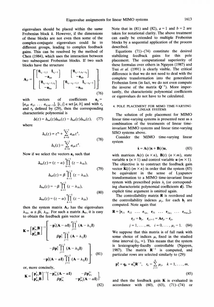
eigenvalues should be placed within the same Frobenius block k. However, if the dimensions of these blocks are not even then some of the complex-conjugate eigenvalues could lie in different groups, leading to complex feedback gains. This can be resolved by the method of Chen (19&l), which uses the interaction between two subsequent Frobenius blocks. If two such blocks have the structure

[

[

AF =

%y&*ro-l] [ “d;-q

[ L;;,q [ L-~a*L-‘u-l] 1 ’

(76)

with vectors of coefficients 8ij =

[aijo aijl . . . aij,,j_l], [i, j] E set [a, b] and with r, and r, defined by (29), then the corresponding characteristic polynomial is

A(z) = A&z )A&) - &(Z )A& ), (77)

where n,-1

A,,(z) = Z”’ + C aiikZk, k=O

&j(z) = IzI aijkzk.

NOW if we select the vectors aij such that no-l

L(z) = (Z - 0) kF, (Z - hlk),

nb-1 Aab(z) = p n (Z - ‘bkh

(79)

k=l

n,-1

ha(z) = -p fl (Z - hlk),

k=l

q-1

A&Z) = (Z - a) n (Z - A2k) k=l

then the system matrix AF has the eigenvalues hik, (Y f pi, h2k. For such a matrix AF, it is easy to obtain the feedback gain vector as

-pi(A - c~I) I-I (A - A,jI) j=l

cL1-1 PP: ,G (*-AI&

-ppf pfi’ (A - A,I) 1 j=l

Pz-1 9 C-31)

-pf(A - aI) n (A - AzjI) j=l

or, more concisely,

-PPX -p2,:(A - aI)

1.

(82)

Note that in (81) and (82), a = 1 and b = 2 are taken for notational clarity. The above treatment can easily be extended to multiple Frobenius blocks by a sequential application of the process described.

Equations (71)-(74) constitute the desired stabilizing feedback gains for this pole placement. The computational superiority of these formulas over others in Nguyen (1987) and Tsai et al. (1991) is clearly visible. The critical difference is that we do not need to deal with the complete transformation into the generalized Frobenius form (in fact, we do not even compute the inverse of the matrix Q-‘). More impor- tantly, the characteristic polynomial coefficients or eigenvalues do not have to be calculated.

4. POLE PLACEMENT FOR MIMO TIME-VARYING LINEAR SYSTEMS

The solution of pole placement for MIMO linear time-varying systems is presented next as a combination of the treatments of linear time- invariant MIMO systems and linear time-varying SISO systems above.

Consider the MIMO time-varying linear system

x = A(t)x + B(t)u, (83)

with matrices A(t) (n X n), B(t) (n X m), state variable x (n X 1) and control variable u (m X 1).

The objective is to construct the feedback gain vector K(t) (m X n) in order that the system (83) be equivalent in the sense of Lyapunov transformation to a MIMO time-invariant linear system with prescribed poles Aj (or corresponding characteristic polynomial coefficients d). The explicit time argument is omitted again.

The controllability matrix R is reordered and the controllability indexes ~j, for each bj are computed. Note again that

R = [rll r12 . . . rlrl r21 . . . r2p2 . . . rm,,l,

rg = bj, rj,i+l = Arji - iii,

i= 1,. . . , m, i=O,. , . , pj- 1. (84)

We suppose that this matrix is of full rank with some choice of indices pi fixed in the studied time interval (to, w). This means that the system is lexicography-fixedly controllable (Nguyen, 1987). The matrix R-’ is computed, and particular rows are selected similarly to (29):

P: = qk = e:R-‘, rk = $ pj, k = 1,. . . , m, j=l

(85)

and then the feedback gain K is evaluated in accordance with (60) (63) (71)-(74) or

1614 M. ValSek and N. Olgac

(81)-(82), with slightly different definitions:

Q-‘=rows[pi,pi ,..., p:,, 2 2 2

Pl,Pz,.*.,P~p~~~ m

7PT,P2,.. . 9 PLJ,

I$+, = p:A + fi”, (86)

P:' = p:, p:;, = p:‘(A - A$ + 16”‘. (87)

This treatment is a generalized version of Ackermann’s formula for MIMO linear time- varying systems, and it is the first attempt at such a study for this class of systems. There are some superior features of this approach compared with other similar work. For instance, in Nguyen (1987) the treatment requires the pole placement to be completed in the transformed space first instead of the initial state space. Tsai et al. (1991) utilize a bidiagonal Frobenius form for pole placement, which has already been proven inferior to the approach here from the numerical complexity point of view (ValiSek and Olgac, 1995).

0 2e-’ 3ee3’ + 8e-’

R2 = e-’ 3e-‘+ 0.5ee3’ 4ee3’+ 9e-’ .

0.5 1.5 2ee2’ + 4.5 1 cw The controllability indexes are p, = 3 and p2 = 3. We construct the reordered controllability matrix (84):

02

R= [ 1 2

0

0 0 e-’ 1 . (91) 0.5

Its inverse is

-1 1

R-’ = [ 0.5 0

-2e-’

0 1 . (92) 00 2

Hence, from (85),

q! = [0.5 0 01, q: = [0.5e-” 1 01, s: = [O 0 21, (93)

and, from (56) and (57),

With the above development, we open an interesting direction for nonlinear systems control. When a nonlinear system is I/O linearized following recent techniques of Isidori (1985) the dynamics presents itself as a time-varying MIMO in the vicinity of the nominal state trajectory. A pole-placement stabilizer of this presentation can now be directly implemented. However, there is a great deal to achieve for assuring global stability, considering the nonlinear nature of the I/O linearization. This is mentioned here simply to lead the way for future studies on the matter.

B = l e-’ 1

[ 1 0 1’ (94)

Jj;’ = [; -f’]. (95)

5. EXAMPLES

Given the system from Nguyen (1987),

i(t)= [ z i e:]x(l)+ [X ,O;II(~),

(88)

Because the first Frobenius block is larger (pi = 2), we divide the eigenvalues as hi = -1, A: = -2, A: = -3, and obtain

pi’ = [0.5 0 01, (94)

p:’ = p:‘[A - (-l)I] + fi:’

= [0.5e-” + 0.5 1 01, (97)

p:’ = p:‘[A - (-2)1] + fi;’

= [0.5ev4’ + 0.5e-*’ + 1 e-” + 5 eP3q, (98)

p:’ = [O 0 21,

pz’ = pf’[A - (-3)1] + $’ = [2e-’ 0 121, (99)

_e-2l - 5 -e-31

0 -12 1 we are looking for a time-varying feedback gain vector K(t) such that the system (88) would be equivalent in the Lyapunov sense to the time-invariant system with constant poles -1, -2 and -3.

-0.5e-4' + 1.5ee2’ - 1 _e-2r _ CJ -em3’ + 12e-’ =

-2eC’ 0 1 -12

W)

We compute the controllability matrices R1 = R(A, b,) and R2 = R(A, b2) corresponding to the control variables u1 and u2:

This completes the computation of the feedback gain vector. In order to verify this result and compare the above procedure with that of Nguyen (1987), we need the transformation matrix Q. From (85) and (86),

0 2 2ed2’+4

[ 1 0.5 0 0

RI=12 4 (89) Q-’ = 0.5eP2’ 1 0 , (101)

0 0 2e-’ [ 1 0 0 2


2 0 0

Q = -e-” 1 0 c 1 . (102) 0 0 0.5

Note that Q-’ and Q are both bounded, as required by Lyapunov equivalence. From (17),

0 1 0

Ar= -4e-” e-2r + 2 0.5ep3’ 1 (103) 4e-’ 0 3 0 0 B,= 1 e-’ ,

[ 1 ww

0 1

K,=KQ

&-2’_ 2 _e-2f _ 5 -()5e-3' + (je-' =

-4e-’ 0 1 -6 . ww

Finally, 0 1 0

A,+B,K,= -2 -3 0 ,

[ 1 (106) 0 0 -3

as expected. In order to compare these results with those of

Nguyen, a conversion matrix T from Q (ours) to QN (Nguyen’s) is introduced:

o-1 0

T=-1 0 0,

[ 1 (107) 0 0 1

QN = QT. (108)

Then

AF = Q-‘(AQ - Q) = TQ,‘(AQ,T - &T)

= T[Q-‘(AQ - Q)]T = TAFNT (109)

BF = Q-‘B = TQ,‘B = TBFN. (110)

The search is for a state feedback gain vector K’ that materializes the same pole placement as in Nguyen (1987). If, in addition,

KF = KFNT (111)

then

K’ = K;Q-’ = KFNTQ-’ = KFNQ;’ = KN, (112)

and the desired constant system matrix can be transferred after pole placement according to Nguyen (1987) into

AF + BkK; = T(AFN + BFNKFN)T

-6 -11 -6

Following steps similar to (71) and (74) and utilizing (58) and (60), the following gain matrix is obtained:

K’ = B;’ -p: - lip] - 6~; + 6~: 1 -PCP] ’ (114)

K’=KN= [

-5.5 + 0.5e-’ - 0.5e-4’

-2e-’ - 0.5 _e-2t_8 _e-3t+6e-r+ 12

0 -6 1 (115)

0 I 2 3 4 5 6 7 8

tcs1

Fig. 1. Comparison of transient behavior: x,, x2, x3, with our new pole placement; xIN, xZN, .qN, with Nguyen’s approach. Initial conditions x,” = -1.4, x*0=0.2, x,,=o.45.

1616 M. Val&k and N. Olgac

Fig. 2. Comparison of Lyapunov-equivalent transient behaviors: x,, x2, x3, with our new pole placement: xjN, xZN, xXN, with Nguyen’s approach.

This is in full agreement with the results of Nguyen (1987), after the correction of an obvious printing error in his paper. Finally, we compare the transient of the different resulting system matrices A f BK from (100) and A + BK’ = AN + BNKN from (115). The simula- tion results are given in Fig. 1 for the original state dynamics. In Fig. 2 the transients are shown for the Lyapunov equivalents corresponding to our method and that of Nguyen as expressed in (106) and (113) respectively. They demonstrate a better performance for our feedback as in (100) than that of Nguyen. This is in agreement with the prediction of Chen (1984) for the time- invariant case. Note, however, that the exercise presented above is for time-varying systems, and the prediction still holds true.

6. CONCLUSIONS

The ultimate objective of pole placement for time-varying MIMO linear systems has been treated. A review has been given for complete- ness, covering SISO time-invariant and time- dependent cases, followed by MIMO time- invariant and finally time-variant systems. A number of transformation steps have been carefully analyzed in order to obtain the expanded version of the Frobenius form for MIMO cases. Different ways of subdividing the state matrix in the form of lower-dimensional Frobenius structures has been discussed for smoother transient response characteristics in addition to the desired exponential behavior. An

interesting end result is a generalization of Ackermann’s formula to MIMO/time-varying linear systems for the first time in the literature, accompanied by fully developed intermediate proofs. The impact of this development is foreseen for nonlinear dynamic systems as well.

Acknowledgement-M.V. gratefully acknowledges the finan- cial support of CIES through the Fulbright Scholar Program, which made possible his visit to the University of Connecticut.

REFERENCES

Ackermann, J. (1972). Der Entwurf linearer Regelungssy- steme im Zustandraum. Regelungsrechnik und Prozess- Datenverarbeitung, 7, 297-300.

Ackermann, J. (1977). Entwurf durch Polvorgabe. Regelungstechnik und Prozess-Datenverarbeirung, 6, 173- 179; 7,209-215.

Ackermann, J. (1985). Sampled-data Control Systems. Springer-Verlag, Heidelberg.

Blanchini, F. (1989). New canonical form for pole placement. IEE Proc., Pt D, 136,314-316.

Chen, Ch. T. (1984). Linear System Theory and Design. Holt, Rinehart and Winston, New York.

Franklin, G. F. and J. D. Powell (1980) Digital Control. Addison-Wesley, Reading, MA.

Isidori, A. (1985). Nonlinear Control Systems, An Introduc- tion. Springer-Verlag, New York.

Kailath, T. (1980). Linear Systems. Prentice-Hall, Englewood Cliffs, NJ.

Kalman, R. E. (1963) Liapunov functions for the problem of Lure in automatic control. Proc. Natl. Acad. Sci. U.S.A., 49,201-205.

Kautsky, J., N. K. Nichols and P. Van Dooren (1985). Robust pole assignment in linear state feedback. Znt. J. Control, 41, 1129-1155.

Kuo, B. C. (1982). Automatic Control Systems. Prentice-Hall, Englewood Cliffs, NJ.

Lefschetz, S. (1965). Stability of Nonlinear Control Systems. Academic Press, New York.

Lewis, F. L. (1992). Applied Optimal Control and Estimation, Digital Design and Implementation. Prentice-Hall and Texas Instruments, Englewood Cliffs, NJ.


Luenberger, D. G. (1967). Canonical forms for linear multivariable systems. IEEE Trans. Autom. Control, AC-U, 290-292.

MathWorks, Inc. (1988). MATLAB ver. 3.5, source codes. Miminis, G. S. and C. C. Paige (1982) An algorithm for pole

assignment of time invariant linear systems. Int. J. Control, 35,341-354.

Nguyen, Ch. (1987). Arbitrary eigenvalue assignments for linear time-varying multivariable control systems. Znt. J. Control, 45,1051-1057.

Petkov, P. H., N. D. Christov and M. M. Konstantinov (1984). A computational algorithm for pole placement of linear single-input systems. IEEE Trans. Autom. Control, AC-29,1045-1048.

Petkov, P. H., M. M. Konstantinov and N. D. Christov (1985). Computational algorithms for linear control

systems: a brief review. Int. J. Syst. Sci., 16,465-477. Silverman, L. M. (1966). Transformation of time-variable

systems to canonical (phase-variable) form. IEEE Trans. Autom. Control, AC-11,300-303.

Tsai, J. S. H., H. K. Chiang and Y. Y. Sun (1991). Novel canonical forms for linear time-varying multivariable systems and their applications. In Proc. 1991 American Control Conf, Boston, MA, Vol. 1, pp. 337-342.

Tuel, W. G. (1966). On the transformation to (phase- variable) canonical form. IEEE Trans. Autom. Control, AC-11,607.

Val&k, M. and N. Olgac (1995). An efficient pole placement technique for linear time variant SISO systems. IEE Control Theory Applic., to be published.

Varga, A. (1981). A Schur method for pole assignment. IEEE Trans. Autom. Control, AC-26,517-519.

efficient eigenvalue assignments for general linear mimo systems

Documents