on the rate of asymptotic eigenvalue degeneracy

Communications inCommun. math. Phys. 60, 73—95 (1978) Mathematical

Physics© by Springer-Verlag 1978

On the Rate of Asymptotic Eigenvalue Degeneracy

Evans M. Harrell*

Institut fur theoretische Physik der Universitat Wien, A-1090 Wien, Austria

Abstract. The gap between asymptotically degenerate eigenvalues of one-dimensional Schrόdinger operators is estimated. The procedure is illustratedfor two examples, one where the solutions of Schrodinger's equation areexplicitly known and one where they are not. For the latter case a comparisontheorem for ordinary differential equations is required. An incidental result isthat a semiclassical (W-K-B) method gives a much better approximation tothe logarithmic derivative of a wave-function than to the wave-function itself;explicit error-bounds for the logarithmic derivative are given.

1. Introduction

The operator

2 4H(β) = -+x2-2βx* + β2x

on L2(IR), with β^O, and other similar operators have been studied because theyexhibit asymptotic eigenvalue degeneracy as /?-»0 [1,2,3]. The operator H(β) isessentially self-adjoint on (̂R). As /?->Ό, it approaches the harmonic oscillator

Hamiltonian, H(Q)= — -^ +x2 (in the strong operator sense), and it is known

that two distinct eigenvalues of H(β) converge to each eigenvalue of H(Q). Forexample, the two lowest eigenvalues of (1.1), E0(β) and E±(β\ both converge toE0(0) = 1 [the Number 1 will frequently be called E0(0), so that it will be clear howthe formulae generalize]; and in fact both E0(β) and E^β) have the sameasymptotic — but almost certainly not convergent — power-series expansions in β,

* Present address: Department of Mathematics, MIT, Cambridge, MA 02139, USA; (NationalNeeds Fellow)

0010-3616/78/0060/0073/S04.60

74 E. M. Harrell

given by the Rayleigh-Schrδdinger formula [4,5]. For β>0, E0(β) and E^β) arecertainly different, and Dirichlet-Neumann bracketing techniques have been usedto show that

CLQxp(-kJ-2)^E^)-E^)^CuQxp(-k^-2) (1.2)

for suitable positive constants CL, Cv, kL, and kv [3]. Of course, the functionCexp( — kβ~2) has an asymptotic Taylor series at β = Q that is identically zero.

The existence of long-range order, and hence of phase transitions, in statisticalsystems is generally equivalent to the degeneracy or asymptotic degeneracy of theprinciple eigenvalue of some linear operator for a discussion of this see the articleby Kac [6], and for field-theory aspects see [7]. A new proof of the asymptoticdegeneracy of the eigenvalues of (1.1) is implicit in the argument to be presentedhere. However, the emphasis is on constructing exact, calculable formulae toreplace (1.2); in other words, on the exact critical behavior.

Operator (1.1) is invariant under the exchange x+-*(l/β) — x9 i.e., reflectionabout x = i/2β. By a well-known argument, the eigenfunctions ψn

β such thatH(β)ιp»=En(β)ψ"β, and E0(β)<E1(β)<...9 £>0, satisfy

The potential x2 — 2βx3+β2x4 has two nearly harmonic wells, which are sepa-rated by ever greater distances and an ever higher barrier as j3->0. A roughphysical explanation for the asymptotic degeneracy is that the two wells asymp-totically decouple into independent oscillators. The effects of a second well on theenergy (eigenvalue) should be inversely proportional to the time a quantum-mechanical particle would take to tunnel through the barrier, by the uncertaintyprinciple. Thus

δ(β) = E^(β)- EQ(β) oc tunneling probability

exp -2J }/x2-2βx3+β2x4-Edx ,

where tί and t2 are the "classical turning points", the values of x where x2 — 2βx3

+ β2x4-E = 0, 0<x<l/β, and where E should be roughly E0(0). This is in factqualitatively correct, for

= const exp -1 f \/x2-2βx* + β2x4-Edx\ ίi

= 0(Qxp(-Kβ~2)) for some K,

to the leading asymptotic order. The overall constant is calculated as —j= e~1/2 inl/π

(7.3), below. Note that the exact formula is proportional to the barrier penetrationprobability for only half the barrier.

2. A Soluble Example

The calculation of the rate of convergence of the asymptotically degenerateeigenvalues of (1.1) involves some functional estimates that might obscure the

On the Rate of Asymptotic Eigenvalue Degeneracy 75

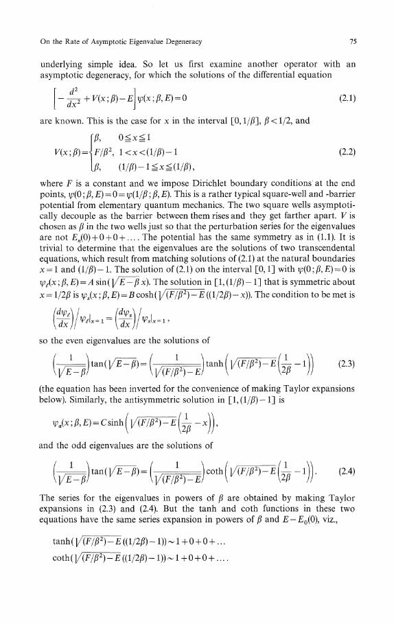
underlying simple idea. So let us first examine another operator with anasymptotic degeneracy, for which the solutions of the differential equation

(x;j8,E) = 0 (2.1)

are known. This is the case for x in the interval [0, l/j8], β< 1/2, and

V(χ 9β)=\F/β2

9 l<x<(l/β)-l (2.2)

where F is a constant and we impose Dirichlet boundary conditions' at the endpoints, ψ(0 /?, E) = 0 = ψ(ί/β I β, E). This is a rather typical square-well and -barrierpotential from elementary quantum mechanics. The two square wells asymptoti-cally decouple as the barrier between them rises and they get farther apart. V ischosen as β in the two wells just so that the perturbation series for the eigenvaluesare not En(0) + 0 + 0 + ... . The potential has the same symmetry as in (1.1). It istrivial to determine that the eigenvalues are the solutions of two transcendentalequations, which result from matching solutions of (2.1) at the natural boundariesx- 1 and (l/β)- 1. The solution of (2.1) on the interval [0, 1] with t/?(0; jB,E) = 0 is

Ψt(x ;β,E) = A sin(|/E — β x). The solution in [1, (l/β) — 1] that is symmetric about

x - ί/2β is ψs(x ;β,E) = B cosh(}/(F/β2)-E ((l/2β) - x)). The condition to be met is

so the even eigenvalues are the solutions of

1(2.3)

(the equation has been inverted for the convenience of making Taylor expansionsbelow). Similarly, the antisymmetric solution in [!,(!//?) — 1] is

φα(x;β,E) = Csinh|

and the odd eigenvalues are the solutions of

/ , / 1 \\(2.4)

The series for the eigenvalues in powers of β are obtained by making Taylorexpansions in (2.3) and (2.4). But the tanh and coth functions in these twoequations have the same series expansion in powers of β and E — £0(0), viz.,

coth(}/(F/β2)-E ((1/2)5)-!))-1+0 + 0+....

76 E. M. Harrell

The two functions differ to O(exρ(-2y(F/β2)-E((l/2β)-1))), which is o(βm) forall positive m< oo. Thus the power-series solutions of (2.3) and (2.4) are identical.Specifically [using £0(0) = π2]

(2.5)u/t

which must equal

VfBy writing E ~ ]JΓ cβj and collecting terms, one finds

7 = 0

for E = E0(β) or E^jβ). Note that for F<4π4 the tunneling effect is strong enoughto lower the energy for small β, but for F > 4π4 it is not. An asymptotic expressionfor δ(β) = Eί(β)-E0(β) is obtained from (2.5) and (2.6) by treating the differencebetween the tanh and coth functions as a small variation. Fix β > 0, and supposethat the exact solution E0(β) of Gj(E,β) = Gs(E,β) is known. Then using Taylor'stheorem about the point E = E0(β)9 we can expand the equation G^(E9β) = Ga(E9β)as

= Ga(E,β)

= GjE, β) coth2 ( }/(F/β2)-E I — -11

Keeping terms to first order in E — E0(β\ the solution E1 of this equation is

1coth2(( γ(F/β2)-E1 -1 -1 GS(E0)

^ Ί i + 0((E, - E0)2),

~dE^ f~ S'\E = E°


SO

e x p - ί l/Ktefl-E^x (1 + 0(0))1

π=βexp(-

If higher-order terms in the Taylor series are kept, δ(β) can be estimated to

arbitrary order as exp(—|/F(1//? —2)/j?) times a series in powers of β. Theexponent is half the barrier penetration exponent.

3. Outline of the Analogous Calculation for Operator (1.1)

Henceforth we consider Equation (2.1) with V=x2 — 2βx^ + β2x4 and for x on thewhole real line. In this case there is no natural boundary at which to matchsolutions, so the arbitrary choice x = 0 is made. Define ψ^ ψs, and ψa to be thenontrivial solutions of (2.1) with the conditions

lim t/ Λx β, E) = 0 (overall scaling not yet specified)-> — o

Then the eigenvalues of (1.1) for β>0 are given as the solutions of

1 dψe(0;β,E)= 1 dψs(0;β,E)

ψj dx ψs dx

and

dx ψa dx

(3.1)

(3.2)

The functions p (0 β, E\ p (0 β, E\ and f^ (0 β, E) are continuouslyψ^ αx ψs dx ψa dx

differentiable in £ in a neighborhood of £0(0) and in β in [0, C) for some positiveconstant C. (In fact it is elementary that ψs, and \pa are entire in x and E, and thatthere exists a solution ιp^ that is also entire in x and E. It is possible to showanalyticity in β in a region of C containing (0, C) and continuity as β->0 byfollowing similar calculations for the harmonic oscillator ([8,9], see also [10])after suitable scaling and translation of the variables.) Then (3.1) can be put in theform

78 E. M. Harrell

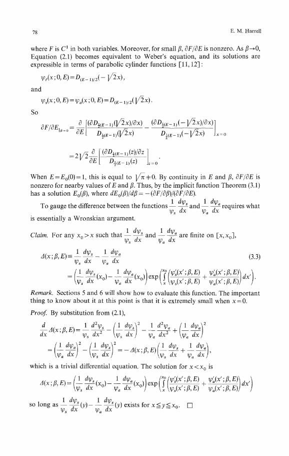
where F is C1 in both variables. Moreover, for small β, dF/dE is nonzero. As /?->(),Equation (2.1) becomes equivalent to Weber's equation, and its solutions areexpressible in terms of parabolic cylinder functions [11, 12] :

and

ψs(x 0, E) = ψa(x 0, E) = D(E_ 1)/2( |/2x) .

So

dF/δE = 1_l p =°

-21/2K

When E = E0(0) = 1, this is equal to j/πφO. By continuity in E and β, dF/dE isnonzero for nearby values of E and β. Thus, by the implicit function Theorem (3.1)has a solution E0(j8), where dE0(β)/dβ=-(dF/dβ)/(dF/dE).

To gauge the difference between the functions -- ^ and -- f-^ requires whatψs dx ψa dx

is essentially a Wronskian argument.

Claim. For any x n >x such that -- — - and -- ^ are finite on [x,xn],φs dx φ dx

(3.3)

Remark. Sections 5 and 6 will show how to evaluate this function. The importantthing to know about it at this point is that it is extremely small when x = 0.

Proof. By substitution from (2.1),

_, , — , 2 j ~~ϊ — 9 — r -- —dx ψs dx2 \ιps dx] ψa dx2 \ιpa dx j

dψ 1 dψ-- Ί -- 1 --- Ί

Ψa x/ \Ψs x/ VPs

which is a trivial differential equation. The solution for x<x 0 is

1 di/v, 1 dtp, , ,so long as — - ( j > ) -- -τ^(^) exlsts for

On the Rate of Asymptotic Eigenvalue Degeneracy

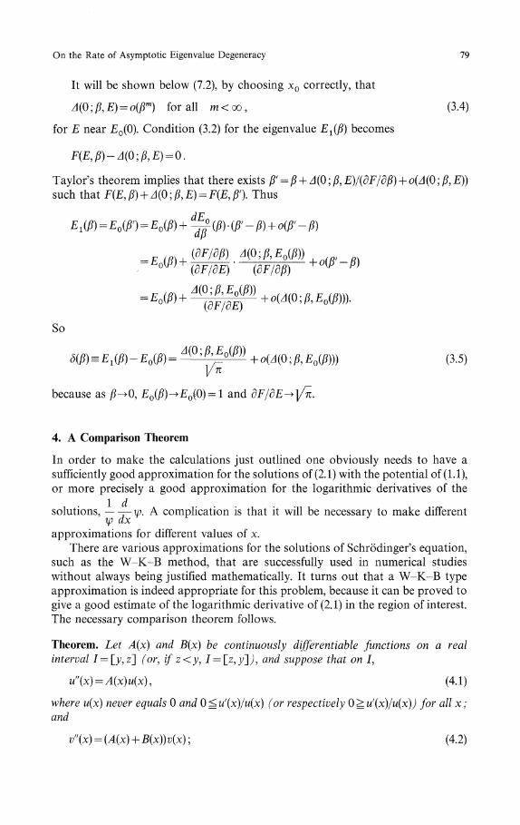
It will be shown below (7.2), by choosing x0 correctly, that

A(Oιβ,E) = o(βm) for all m<oo,

for E near E0(0). Condition (3.2) for the eigenvalue E^(β) becomes

79

Taylor's theorem implies that there exists β' = β + A(Q;β,E)/(dF/dβ) + o(A(Q;β,such that F(E,β) + A(Q;β,E) = F(E,β'). Thus

=£o(ffl+ (sF}dE) +^(0;/UoC»))).

So

δ(β) = E1(β)-E0(β)= ^ 'P'jj'oU*)) +o(J(0;)8,E0(j8))) (3.5)ι/^because as j8-»0, E0G8)->E0(0) = 1 and dF/dE-+]/π.

4. A Comparison Theorem

In order to make the calculations just outlined one obviously needs to have asufficiently good approximation for the solutions of (2.1) with the potential of (1.1),or more precisely a good approximation for the logarithmic derivatives of the

solutions, —— w. A complication is that it will be necessary to make differentψ dx

approximations for different values of x.There are various approximations for the solutions of Schrodinger's equation,

such as the W-K-B method, that are successfully used in numerical studieswithout always being justified mathematically. It turns out that a W-K-B typeapproximation is indeed appropriate for this problem, because it can be proved togive a good estimate of the logarithmic derivative of (2.1) in the region of interest.The necessary comparison theorem follows.

Theorem. Let A(x) and B(x) be continuously differentiable functions on a realinterval I = \_y,z] (or, if z<y, / = [z,y]Λ and suppose that on /,

u"(x) = A(x)u(x), (4.1)

where u(x) never equals 0 and 0 rg u'(x)/u(x) (or respectively 0 ̂ u'(x)/u(x)) for all xand

v"(x) = (A(x) + B(x))v(x); (4.2)

80 E. M. Harrell

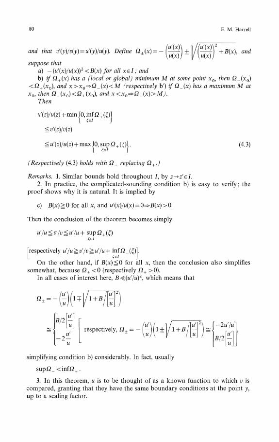
, andand that vf(y)/v(y) = uf(y)/u(y). Define Ω±(x)=-lU^

suppose thata) - (u'(x)/u(x))2 <B(x) for allxel andb) if Ω + (x) has a (local or global) minimum M at some point x0, then Ω_(x0)

<Ω+(x0), and x>x0=>Ω_(x)<M (respectively b') if Ω_(x) has a maximum M atx0, then Ω_(x0)<Ω+(x0\ and x<x0=>Ω + (x)>M).

Then

u'(z)/u(z) + min ίO, mfΩ+(ξ)\( & J

(4.3)^ u'(z)lu(z) + max ίO, sup Ω, (ξ)\.\ &

(Respectively (4.3) holds with Ω_ replacing Ω+.)

Remarks. 1. Similar bounds hold throughout /, by z-»z'e/.2. In practice, the complicated-sounding condition b) is easy to verify; the

proof shows why it is natural. It is implied by

c) B(x) ̂ 0 for all x, and u'(x)/u(x) = 0=>B(x) > 0.

Then the conclusion of the theorem becomes simply

[respectively u'/u ^ υ'/v ^ u'/u + inf Ω _ (ξ)\ .

On the other hand, if B(x) ^ 0 for all x, then the conclusion also simplifiessomewhat, because Ω± <0 (respectively Ω± >0).

In all cases of interest here, B<ζ(u'/u)2, which means that

°± = " b

B/2

respectively, Ω+ = - I — 1 |1 + 1 + Bί-2u'/u

simplifying condition b) considerably. In fact, usually

suρί2_

3. In this theorem, u is to be thought of as a known function to which v iscompared, granting that they have the same boundary conditions at the point y,up to a scaling factor.


4. The conditions of the theorem are sufficient but not minimal. All that isrequired is that the solutions of (4.1) and (4.2) are sufficiently differentiable for allthe calculations in the proof to be defined, and that a) and b) hold. For adiscussion of the smoothness of solutions of differential equations see, e.g., [13].

5. Moreover, the condition that u'/u = v'/v at y can be relaxed. In fact, if

sup Ω _ (ξ) < v'(y)/v(y} - u'(y)/u(y) ^ sup Ω+(ξ),ξel ξel

then

min ίυ'(y)/υ(y) - u'(y)/u(y\ inf Ω + (ξ)( &

Respectively, if

inf β + (ξ) > υ!(y}/v(y} - u'(y)/u(y) ^MΩ + (ξ) ,ξel ξel

then

max \v'(y)/v(y) ~ u'(y)/u(yl sup Ω _ (ξ)

This follows from only a slight modification of the proof.

Proof. The case z<y, given by the respectively' s in parentheses, follows simply byreflection of the coordinate from the more natural direction. Both directions areincluded because both are needed below. We may assume y = 0. Define thefunction w(x) so that φc) = w(x)w(x). Substitution into (4.2) and use of (4.1) readilyyields the equation for w :

Letting Ω(x) = w'(x)/w(x), we then find

Ω'(χ) = w"(x)/w(x) - (w7(x)/w(x))2

= B(x) - 2(w'(x)/M(x)) Ω - Ω2 . (4.4)

The assumptions of the theorem imply that Ω(x) is continuously differentiable.Since v'/v = u'/u + w'/w = u'/u + Ω, v'(ty/v(Q) = u'(Q)/u(ty^Ω(ty = 0. Without solving(4.4) with this boundary condition, it is elementary to determine where in the Ωxx-plane dΩ/dx would be positive, negative, or zero. The boundaries between these

82 E. M. Harrell

regions are the lines where Ω' = Q, i.e., from (4.4) and the quadratic formula, at

Q±(x)= -ιφ)/φ)± +B(x) .

Thus

Ω(x)<Ω_(x)^Ω'(x)<0, and (4.5)

Ω_(x)<Ω(x)<Ω+(x)=>Ω'(x)>Q.

[And if Ω±(x) are not real, then Ω'(x) is always negative.]Since B > — (u'(x)/u(x))2 by assumption, Ω±(x) are real for all x and Ω + (x)

>Ω_(x). Suppose that Ω(z)>max ίθ,supΩ+(f)l. Since ΩeCl(I] and ί2(0) = 0, there

exists x<z such that Ω(x)>max ίθ,supΩ+(ξ)l ^Ω+(x) and dΩ(;x)/ώc>0 (by the

intermediate- value theorem). But this contradicts the first of relationships (4.5), sowe conclude that

The upper bound of (4.3) then follows from v'/v = uf/uThe lower bound is similar but requires an extra step. Assume first that

min{0, Ω+(x)} is a monotonically decreasing function, and suppose that for some

z', Ω(z')<min ίO, inf Ω+(ξ)\, which equals min{0,Ω+(z')}. Since Ω(x)eC1(I) and1 ξ e [ y , z ' } J

Ω(0) — 0, and the function min{0, Ω+(x)} is also continuous, there must exist z" <z'such that Ω(z")<nιin{0,Ω + (z")}, and Ω'(z")<0 again by the intermediate valuetheorem. In fact, z" can clearly be chosen so that min {0, Ω + (z")} — Ω(z") < ε for anyε>0, by continuity. Thus z" can be chosen so that Ω(z//)>Ω_(z//), because, from itsdefinition and the condition that ί//w>0, Ω_(x) is strictly less than min{0, Ω+(x)}.But then the statement Ω'(z")<0 contradicts the last of relationships (4.5), so we

conclude that Ω(x)^min JO, inf Ω+(ξ)\ as long as min{0,Ω+} is monotonically1 ξe[y,x] J

decreasing between y and x.If min{0, Ω+(x)} is not monotonically decreasing throughout /, then it, and

therefore also Ω + (x\ must attain a minimum, which is negative, at some point x0.Assume the minimum is global. The uniqueness theorem for first-order differentialequations of the type of (4.4) (here we again need some minimal smoothness)implies that since, as already established, Ω(XQ)^Ω+(XO\ it follows for all x>x0

that Ω(x)>Ω(x0), where Ω(x) satisfies (4.4) with the boundary condition Ω(x0)= Ω+(x0).

Because Ω+(x)>Ω_(x) for all x, continuity and (4.5) imply that throughoutsome interval (x0,x0 + 7"]> r>0, Ω'(x)>0, and thus Ω(x0 + r)>Ω+(x0). By assump-tion b), Ω_(x)^Ω+(x0) for all x>x0. Thus for all x>x0, the function Ω(x) eitherincreases monotonically, or else Ω(x)g;Ω+(x)">Ω+(x0) [because of (4.5)].


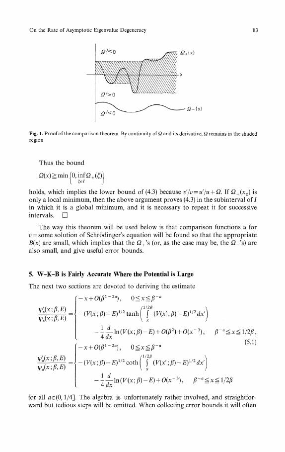
Fig. 1. Proof of the comparison theorem. By continuity of Ω and its derivative, Ω remains in the shadedregion

Thus the bound

holds, which implies the lower bound of (4.3) because vf/v = u'/u + Ω. If Ω + (x0) isonly a local minimum, then the above argument proves (4.3) in the subinterval o f /in which it is a global minimum, and it is necessary to repeat it for successiveintervals. D

The way this theorem will be used below is that comparison functions u forv = some solution of Schrodinger's equation will be found so that the appropriateB(x) are small, which implies that the ί2+'s (or, as the case may be, the Ώ_'s) arealso small, and give useful error bounds.

5. W-K-B is Fairly Accurate Where the Potential is Large

The next two sections are devoted to deriving the estimate

ψ's(x;β,E) '

ιp'a(x;β9E)

l / 2 β

f (V(xf ;β)-E)ll2dx'

4 ax

-x + 0(β1~2a),

-(V(x;β)-E)ll2coth( ί (V(x';β)-E)ll2dx'\ X

4

for all a e (0,1/4]. The algebra is unfortunately rather involved, and straightfor-ward but tedious steps will be omitted. When collecting error bounds it will often

84 E. M. Harrell

be understood that Taylor expansions have been made and higher-order termsdropped.

Let us first consider the intervals where the potential in (1.1) is large.Nonrigorous arguments lead one to expect that the W-K-B solutions in theseregions should be reasonably accurate. Thus one expects ψ to be approximately alinear combination of

(V-EΓ1/4exp($(V(xf;β)-E)1/2dxf

and

(- l(V(x'\β)-E)ll2dx').

In particular, as x-> — oo,

- (V(x';β)-E)1/2dx'

has the right asymptotic behavior. We will use this as the comparison function (ύ)of the theorem for v = ψf. By substitution, ψ' ̂ /, = A(x; β, E)ψw, where

,E) = V(x;β)-E~B(χ ,β,E),

and

Thus ψj = (A + E)\pe, and

E) (5.2)

- \x\Ul - βx)2 - E/x2)1'2 - x - --\x\((l βx) h / x ) 2(x2(l-βx)2-E)

For calculational simplicity we make some crude estimates, assuming that

Q>B(x;β9E) =

^ |x|((l - E/C2)112 - 1/(C3 - EC))

(essentially |x| for large enough C); (5.3)

2(1 - 6βx + 6(βx)2) 5(1 - βx)2(l - 2βx)2

4x2((l - βx)2 - E/x2) 4x2((l - βx)2 - E/x2)2

5/(l-E/C2)2-2

x2

(essentially — 3/x2).

These expressions have been factorized for the convenience of the reader whowishes to check the straightforward algebra leading to the estimates. Recall that if


— 1 ̂ z ̂ 0, then (1 + z)1/2 ̂ 1 + z. Therefore, if x is less than some constant (e.g., the

lesser of —2 and — 10J/E) then 0>B/(ψ'w J\pw ^)2^1, and for the appropriate

= (Ψw, t/Ψw, t)( - 1 +

> B(x β, E)/(ιp'w>,(x β, E)/ψw^x β, £)) £ - const/M3 ,

where the constant is arbitrarily close to 3 for C large enough. A similarcalculation for Ω_ shows that it is roughly — 2ψr

w^/ιpw^9 and so from (5.3) C maybe chosen so that sup Ω_(x)< inf Ω+(x). Thus conditions a) and b) of the

x^-C x^-C

theorem are fulfilled on the interval (- oo, C]. Letting y-> - oo, we conclude

Proposition 1. Ifip, is the solution of(2Λ) that behaves like ψw^ as x^ — oo, then forsmall enough β and x less than some negative constant, — C, and C large enough,

(V(x ;β)-E)112- iF(x β)/(V(x ;β)-

Remark. Thus the W-K-B method estimates the logarithmic derivative of thewave function uniformly in x to 0(1). But if x is taken as a function of β, andx-> — oo as β->0, then the W-K-B method estimates the logarithmic derivativewith a vanishingly small error, 0(x(β)~3). The Number 4 is really 3 + (function ofC). This estimate is not needed below, but is given for completeness and forillustrative purposes, as the calculation is simpler than in the other cases.

A similar argument allows the solutions of (2.1) that are symmetric andantisymmetric about the point x = l/2β to be estimated. The potential is large inthe barrier and relatively flat near x = 1/2)8, for

x2-2βx3+β2x* = l/l6β2-^(x-l/2β)2 + β2(x-l/2β)4. (5.4)

The exponential W-K-B solutions do not have the proper symmetry, so weconsider their symmetric and antisymmetric combinations.

and

/1/20 \

VV>;/U)^(F-EΓ1/4sinh J (V(x' 9β)-E)U2dx'\.\ x I

In the region of interest, x < 1/2)8.

/1/2/3 \

s(x;β,E)=-(V(xιβ)-E)ίl2tarιh( f (V(x'ιβ)-E)ll2dx'\\ x I

-±V'(χ β}l(V(χ β}-E), (5.5)

86 E. M. Harrell

which is negative so long as x<l/2β and V— E>0, i.e., for xe[E + ε, 1/2/?), εarbitrarily small.

Proposition 2. For smα// enough β and C^x^ l/2ft and C large enough,

ψf

w,s(x β, E)/ψWίS(x ft E) ̂ ψ's(x β, E)/ψs(x ft £)

Proo/ It is actually necessary to make two separate estimates, because it turns outthat in the vicinity of x = l/2ft ψs is better approximated by

/2/? \

J (V(x' 9β)-E)ίl2dx'\ than by Ψw,s = (V-EΓυ4φw,s. In the firstX I

step the subscript 1 will indicate that a given function is associated with φw s, andin the second step the subscript 2 will indicate that \pWtS is used.

Step 1. It is straightforward to calculate

ll2β

J (V(xf β}

We will use the comparison theorem with v = ψs and uί =φw>s', this means that

V' ίί/2β

f

Note that £x ̂ 0 on the interval [E + ε, l/2]8),ε>0 (and =0 only at x= l/2j8), andthat

/1/2/

0^φ'w>s/φ'w>s=-(V(x;β}-E^2tanh( J\ x

Thus the estimate

φ^, 5(x ft £)/φ^5 s(x ft E) ̂ ̂ ;(x; ft E)/ψs(x ft E) (5.6)

would follow from the theorem [unnatural direction, Remark 2, condition c)],with y = 1/2/?, except that

, E ) , (5.7)

so one part of condition c) is violated. A limiting argument saves the estimate :Equation (5.7) implies that Ω1±(l/2/?) = 0. Since ί21(l/2j8) = 0, it is a priori possiblethat either

i) Ω^x^β^x) as x/l/2ft orii) O^Ω^xJ^Ωj.ίx) as x/l/2ft

because by the intermediate value theorem all other possibilities contradict (4.5)(see Fig. 2). If ii) holds, then for some / < l/2ft

inf Ω1 + (ί)>0>Ω1(/)^φ;(/;ftE)/φs(3;/;ft£)

x^ξZy'

-φ'Wa(y',β,E)/φWaW',β,E)> inf Ω^tf),


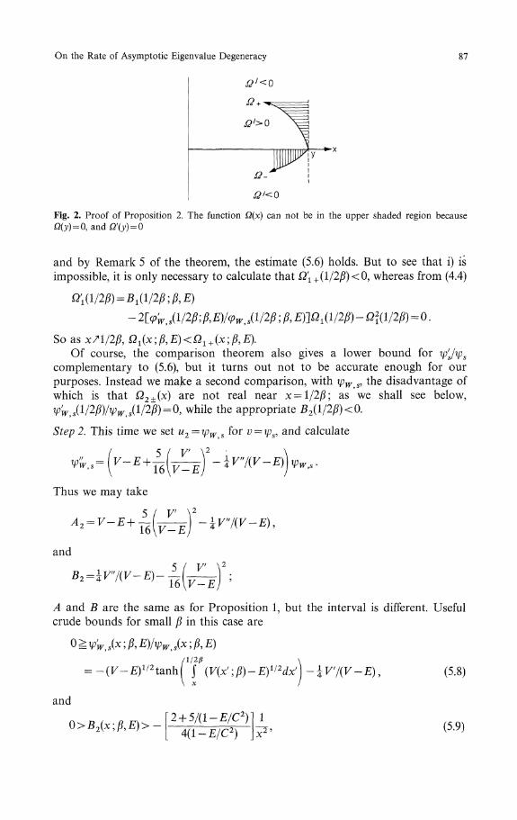
Fig. 2. Proof of Proposition 2. The function Ω(x) can not be in the upper shaded region because) = 0, anάΩ'(y) = Q

and by Remark 5 of the theorem, the estimate (5.6) holds. But to see that i) isimpossible, it is only necessary to calculate that Ω'1+ (1/2)8) <0, whereas from (4.4)

β,

So as x/1/2/?, Ω1(x;β,E)<Ωί + (x;β,E).Of course, the comparison theorem also gives a lower bound for ψ's/ψs

complementary to (5.6), but it turns out not to be accurate enough for ourpurposes. Instead we make a second comparison, with ψWtS, the disadvantage ofwhich is that Ω2±(x) are not real near x=l/2/J; as we shall see below,ΨwtS(l/2β)/ψWtS(l/2β) = 0, while the appropriate B2(ί/2β)<0.

Step 2. This time we set u2 = ψWtSϊor v = ψs, and calculate

5 / V χ 2

Thus we may take

and/' \ 2

16\V-E

A and B are the same as for Proposition 1, but the interval is different. Usefulcrude bounds for small β in this case are

= -(F-£)1/2tanh J (V(x';β)-E)1/2dx') -^Vf

t

\ X

and

0>B2(x;jβ,E)>-[2 + 5/(l-£/C2)

[ 4(1 -E/C2)

(5.8)

(5.9)

E. M. Harrell

and this constant is essentially — 7/4 for large C.On the interval [C, l/2j8), if Ω2(x)^0, then

Ω'2(X) = B2(χ ,β,E)-2(™^\Ω2(x)-Ωi(x)<0.\Ψw,sl

This is because Ω2_(x) is easily seen from its definition and (5.8) and (5.9) to bepositive whenever it is real on this interval. On the other hand, if Ω±(x) are notreal, then Ω'(x) is automatically negative regardless of the value of Ω(x). Thus, sinceΩ2(l/2j8) = 0,

(from the formula v'/v = u'/u + Ω).Combining this with (5.6) yields

Now set y=ί/2β — 1 (arbitrarily). For small enough β, and C^x^y,

so Ω2±(x) are real, and the following estimates can be made:

b) Jnf Ω2 + (ξ)>Ω2(y);

c) Ψw,s/Ψw,s< -(V-E)1/2(l-ε)^ -±x}/l-E/c2, ε arbitrarily small;

d) sup Ω2_(ξ)= sup (--^^

^ sup B2(ξ)/ rgconst/ c3

(again using — 1 ̂ z ̂ 0=> j/1 + z ̂ 1 + z). The constant is essentially +7/2 forlarge C.

Thus by Remark 5 to the comparison theorem and (5.10),

0^-^-y^ - > s ^max{(4+ε)β2, const/x3},

from which the proposition follows (4 + ε < 5,7/2 < 4). DThe analogous argument for ιpa produces

Proposition 3. For small enough β and C^x^ l/2β, and C large enough,

ψ'Wί a(x β, £)/W, a(X lβ>E)^ Ψa(X & E)/Ψa(X > ̂ £)

Remark. We see from (3.3) that in fact the functions ψf

s/ψs and ψ'α/ψα are highlycorrelated for x not near l/2β, because the integral in (3.3) is a large negativequantity. It is not clear from Propositions 2 and 3 that they are so well correlated.


Proof. This proposition is substantially the same as the previous one. Step 1,however, is not needed. We identify u = ψw>a and v = ιpa. A calculation shows thatA and B are the same as the ones in Proposition 1 (or the A2 and B2 ofProposition 2). But now Ω±(x) are real throughout the interval, because

'\!2β

\ (F(x';#)

which -> — oo as x->l/2j8. This time one finds

lim Ω+(x)=co,

and

i P ί A J V y / L V W , α V / v"A y ' J

rg const/*3.

The proposition follows from the comparison theorem (see Remark 2) as before.(The constant is the same as before.) D

6. The Unperturbed Solution is Fairly AccurateWhere the Perturbation is Small

The two regions where the W-K-B approximations are accurate do not meet, so adifferent comparison must be made in the intervening region. As might beexpected, the solutions of

u" = (x2-E)u (6.1)

are suitable for this purpose.

Proposition 4. Let αe (0,1/4), and consider E such that E-E0(0) = 0(/?). For

ψ's(x;β,E)/ψs(x;β,E)= -x + O(βl~2a). (6.2)

and

ψ'a(χ 9β9E)/ψa(χ β9E)= -x + 0(β1-2*). (6.3)

For -5

ψf,(xiβ,E)/ψ,(x;β,E)= -χ + 0051-2*). (6.4)

The implied constants are independent of x and E.

Proof. The comparison theorem and Proposition 2 will be used to prove (6.2). Theproofs of (6.3) and (6.4) using the other propositions are similar. We know from theRayleigh-Schrodinger theory (or from a preliminary but cruder calculation likethe one given in this paper) that E0(β)-EQ(Q) and E^)-EQ(0) are 0(β2\ so therestriction on E is not serious.

90 E. M. Harrell

We work first on the interval xe[l,/?~α], avoiding x — Q for later convenience(so Ω± are real). Let u be as in (6.1) and v = ψs. The boundary condition is

the function A is x2 — E, and thus B is the perturbation, — 2βx3+β2x4<0.B(x,β,E)^Q uniformly as j8->0, when x^β~a, α<l/3.

Some facts about parabolic-cylinder functions are needed [11, 12]. The

solutions of (6.1) are linear combinations of u-(x) = D±(E_ί)(]/2x) andM + (x) = D_i(£+1)(z|/2x)5 which have the asymptotic expansions2

g-3)_ J Λ ; ~ C Λ P V — Λ /±)\y ^Λ;^ - < ι ——^

and

(6.5)

the accuracy of which improves as x-»oo (uniformly in E on a compact set).Normalizing so that u(x) = u_(x) + ηu+(x), and using Proposition 2, we see that

f

i V(β-a;β)/(V(β-° 9β)-E)

(6.6)

Another fact about the parabolic-cylinder functions (which could also be shownsimply with the comparison theorem!) is

u'_(x)/tt_(x)= -x + 0((E- l)/x)

and (6.7)

u'+ (x)/u + (x) -

Substituting from (6.5) and (6.7) into (6.6) and solving for η to leading order inβ yields

η = 0(β(2-E)aexp(-β-2a)), i.e., o(βn) for all n< oo . (6.8)

Using this and (6.5), for x<β~a,

, / A Λ / , . A Λ _ W / - W + ̂ VW

(6.9)M_(X)

The rather complicated error term is 0(βa) when x = 0(β α), but if x <β α/, wherea'<a, then it is o(βn) for all n< oo. For small β, (6.7) and (6.9) together imply that


/uf(χ}\2

u'/u is nonzero and |£(x β, E)| <d -fy when 1 ̂ x ̂ β ~a. Therefore

sup Ω_(x)= sup -'" 7ί«(*)J

/ /Γ*/YvΛ"l\

^<Sjap (B(x;j8,E)

= 0/ sup (-2βx2

This is certainly less than

inf Ω , f x ) « i n f l —

for small β. The conditions of the comparison theorem are satisfied, and hence

uf(x)/u(x) ^ ψ's(x β, E)/ψs(x β, E) £ u'(x)/u(x) + 0(β1~ 2a) .

As remarked after (6.9), if we restrict the interval now to l^x^β~a, a'<a,u'/u = u'_/u_ +o(βn) for all n, and by (6.7), this means that

This establishes (6.2) for x^ 1. For O^x^ 1, recall that \p'J\ps is analytic in £ andC1 in j?; therefore if E-E0(0) is 0(]8),

= φ;(x 0, E0(0))/ψ8(x 0, E0(0)) + 0(]8) - - x + 0()8) .

By taking the supremum over the compact set [0, 1], the 0(β) estimate holdsindependently of x. D

Remark: the interval O r g x r g l can also be handled with a more complicatedcomparison argument, without using analyticity.

7. Conclusion

Using the results of Sections 5 and 6, Equation (3.3) can be evaluated as a constanttimes an exponential function of j8, with a higher-order error. ChoosexQ = (l/2β) — β. From Propositions 2-4,

ψ's(x0;β,E) ιp'a(x0;β,E)

n/2β--(V(x0;β)~E)112\cothi J (V(x;β)-E)1/2dx

\ ^0

-tanh f (F(x;|6)-E)1/2ίix +0()S2)\ ^0 /

= ̂ {coth (1/4) - tanh (1/4)} + 0(β2)

92 E. M. Harrell

andx?lψ's(x;β,E) ψ'a(x;β,E)\

i\ψs(x;β,E) + ψa(x;β,E)Γ

= -β-2a + 0(βi~3a)- I dx(V(x;β)-E)1/2

β-a

fl/2β \ n/2β \

coth f (V(x'\β)-E)ίl2dx' +tanh J (V(x';β)-E)ll2dx'\\ X I \ X I

β-adx

1/2/3-1

- J dx(V(x β)-E)1/2\cothl J (V(x';β)-E)ίl2dx'\1/20-1 I \ x /

/1/2/3 \>ι

+ tanh J (F '̂ ^-^^^^H+O^20)\ x I)

1/2/3-1 ι

— _2 Γ (Ffx'jS) - "" - - "

[after making a couple of Taylor expansions, and noting that the last integral is0(1)].

Thus

*° MX ;/?,£) ψ'a(x;β,E)\

i\ψs(χ ,β,E) + ψa(x;β,E))Γ 1/2/S-l

= -2 ί (V(x;β)-E)1/2dx-β-2a-\nβa

I β~"

). (7.1)

This can be somewhat simplified

ln(sinh(l/4fl) = ln((exp(l/4)8) + exp( -

= l/4β - In 2 + 0(exp( - l/2j8))1/2/8

= j (V(x;β)-E)i/2dx-\n2 + 0(β)1/2/3-1

and likewise

1/2/3

ln(cosh(l/4)8))= J1/2/3-1


Moreover, the expression in brackets of (7.1) is independent of α to O(β2"), despite

appearances. If tt(β) is the turning point near x= J/E0(0), then t\ = E0(0) + 0(β),and

J (V(x;β)-E)ί/2dx= J [(x2-£)1

t,(β) tι(β)

Substituting, and recalling £0(0)=1,

Γ 1/2)5-1 I

-2 f dx(V(x;β)-E)1/2-β~2a-\nβa\[ β« J

1/20-1

= -2 jf (

Finally,

' ' ' H—α ? ? J dx

_ _2 Γ (Vxιβ)—E)ί/2dx + ln(8β)

+ ln(sinh(l/4) cosh(l/4)) + 0(β2a).

Substituting into (3.3) yields

/ 1/20zl(0;jS,£) = 2e-1/2{cosh2(l/4)-sinh2(l/4)}exp 1-2 J

/ 1/20 \

-2β~1/2exp -2 j (V(xιβ)-E)1/2dx . (7.2)\ ίl /

Therefore, by (3.5),

2 _„„-^ -2 J (F(x;jβ)-£)1/2Jx {l + 0(β2α)}. (7.3)I/7C

The exponent a is still arbitrary but at most 1/4, so we take a = 1/4, making theerror 0(β1/2).

A similar formula can be determined for the rate of asymptotic eigenvaluedegeneracy of most other non-pathological, one-dimensional Schrodinger oper-

94 E. M. Harrell

ators with asymptotic degeneracies coming from double-well potentials. Thedominant part of the calculation will be similar to a barrier-penetration probabili-ty, and the overall constant will depend on the unperturbed eigenfunctions. Itshould be possible to generate higher orders in the perturbation expansion (barrierpen. x power series in β) by

1) using n-th-order perturbed approximations of some kind for the eigenfunc-tion where the perturbation is small, rather than the unperturbed eigenfunction,and

2) using more sophisticated semiclassical approximations to the solutions inthe large-potential region.

Potentials that are only asymptotically symmetric should be susceptible of asimilar treatment, with more involved algebra. It may also be possible to study theasymptotic degeneracy of higher eigenvalues, but the comparison theorem can notbe applied in the neighborhoods of the zeroes of the unperturbed eigenfunctions.

On the other hand, it is not clear that the comparison theorem generalizes in auseful way to higher dimensions, except where a separation of variables can beeffected. If the theorem could be extended, a formula like (7.2) would result foroperators with asymptotic degeneracy, using a higher-dimensional semiclassicalmethod.

Since the acceptance of this paper, the author has learned of an earliercalculation of the eigenvalue gap in the physics literature, using functional integralmethods. The rigorous results of the method given above agree precisely with theresults of [14].

Acknowledgements, I am grateful to Barry Simon for suggesting this problem and for encouragement,and to Ricardo Schor for correcting a multiplicative factor and telling me about Ref. [14]. Parts of thisresearch were completed while I enjoyed the hospitality of Haverford College and of the NavajoNation, as well as of the University of Vienna.

References

1. Thompson,C.J., Kac,M.: Phase transitions and eigenvalue degeneracy of a one-dimensionalanharmonic oscillator. Studies Appl. Math. 48, 257—264 (1969)

2. Isaacson, D.: Singular perturbations and asymptotic eigenvalue degeneracy. Commun. Pure Appl.Math. 29, 531—551 (1976)

3. Reed,M., Simon, B.: Methods of modern mathematical physics, Vol. 4. New York: Academic Press1978

4. Kato,T.: Perturbation theory for linear operators. Die Grundlehren der mathematischenWissenschaften, Vol. 132. Berlin-Heidelberg-New York: Springer-Verlag 1966

5. Reed,M., Simon,B.: Methods of modern mathematical physics, Vol. III. New York: AcademicPress 1978

6. Kac,M.: Mathematical mechanisms of phase transitions. In: Brandeis University SummerInstitute in Theoretical Physics 1966, Vol. 1 (eds. M. Chretien, E. P. Gross, S. Deser). New York:Gordon and Breach 1968

7. Glimm, J., Jaffe, A., Spencer, T.: Phase transitions for φ\ quantum fields. Commun. math. Phys. 45,203—216 (1975)

8. Simon,B.: Coupling constant analyticity for the anharmonic oscillator. Ann. Phys. 58, 76—136(1970)

9. LoeffelJ.J., Martin,A.: Proprietes analytiques des niveaux de Γoscillateur anharmonique etconvergence des approximants de Pade. CERN Ref. TH. 1167 (1970)


10. Hsieh,P.-F., Sibuya,Y.: On the asymptotic integration of second order linear ordinary differentialequations with polynomial coefficients. J. Math. Anal. Appl. 16, 84—103 (1966)

11. Whittaker,E.T., Watson,G.N.: A course of modern analysis. Cambridge: Cambridge UniversityPress 1969

12. Abramowitz, M., Stegun,!. A., (eds.): Handbook of mathematical functions. Washington: NationalBureau of Standards 1964

13. Coddington,E.A., Levinson,N.: The theory of differential equations. New York: McGraw-Hill1955

14. Gildener,E., Patrascioiu, A.: Pseudoparticle contributions to the energy spectrum of a one-dimensional system. Phys. Rev. D 16, 423—430 (1977)

Communicated by A. Jaffe

Received November 7, 1977

on the rate of asymptotic eigenvalue degeneracy

Documents