eeg system design for vr viewers and emotions recognition
TRANSCRIPT
AAllmmaa MMaatteerr SSttuuddiioorruumm –– UUnniivveerrssiittàà ddii BBoollooggnnaa
DOTTORATO DI RICERCA IN
Ingegneria elettronica, telecomunicazioni e tecnologie
dell’informazione
Ciclo XXXI
Settore Concorsuale: 09/E3 - ELETTRONICA
Settore Scientifico Disciplinare: ING-INF/01 – ELETTRONICA
EEG system design for VR viewers and
emotions recognition
Presentata da: ANDREA VERDECCHIA
Coordinatore Dottorato Supervisore
ALESSANDRA COSTANZO BRUNO RICCO’
Esame finale anno 2019

Abstract
BACKGROUND: Taking advantage of virtual reality today is within ev-eryone’s reach and this has led the large commercial companies and researchcenters to re-evaluate their methodologies. In this context the interest inproposing the Brain Computer Interfaces (BCIs) as an interpreter of the per-sonal experience induced by virtual reality viewers is increasing more andmore.OBJECTIVE: The present work aims to describe the design of an elec-troencephalographic system (EEG) that can easily be integrated with virtualreality viewers currently on the market. The final applications of such systemare several, but our intention, inspired by Neuromarketing, wants to analyzethe possibility of recognize the mental state of like and dislike.METHODS: The design process involved two phases: the first relating tothe development of the hardware system that led to the analysis of tech-niques to obtain the most possible clean signals; the second one concerns theanalysis of the acquired signals to determine the possible presence of char-acteristics which belong and distinguish the two mental states of like anddislike, through basic statistical analysis techniques.RESULTS: Our analysis shows that differences between the like and dislikestate of mind can be found analyzing the power in the different frequenciesband relative to the brain’s activity classification (Theta, Alpha, Beta andGamma): in the like case the power is slightly higher respect the dislikeone. Moreover we have found through the use or logistic regression that theEEG channels F7, F8 and Fp1 are the most determinant component in thedetection, along with the frequencies in the Beta-high band (20-30 Hz).CONCLUSIONS: At the end of this work we have obtained a system com-pletely integrable in virtual reality viewers and fully functional. However, itis necessary to continue with a more in-depth analysis regarding the recogni-tion of the mental states of like and dislike because, given the vastness of therelative theoretical field, it is certainly possible to arrive at better results.
Contents
Introduction iii
1 The VeeRg : an EEG system for VR 1
1.1 Neuromarketing and virtual shops . . . . . . . . . . . . . . . . . . . 2
1.2 Medical rehabilitation and virtual reality . . . . . . . . . . . . . . . 6
1.3 How the brain works . . . . . . . . . . . . . . . . . . . . . . . . . . 7
1.3.1 Brain’s waves classification . . . . . . . . . . . . . . . . . . . 9
1.4 Electrodes’ placement . . . . . . . . . . . . . . . . . . . . . . . . . . 10
1.5 The prototype idea . . . . . . . . . . . . . . . . . . . . . . . . . . . 12
2 The VeeRg design: deals and choices 15
2.1 Hardware design . . . . . . . . . . . . . . . . . . . . . . . . . . . . 15
2.1.1 Analog power supply and input referred noise . . . . . . . . 18
2.1.2 The common mode noise and the feedback loop . . . . . . . 20
2.1.2.1 CM2DM in electrodes mismatch . . . . . . . . . . 31
2.1.2.2 CM2DM in input stages mismatch . . . . . . . . . 33
2.1.2.3 Limits for stability . . . . . . . . . . . . . . . . . . 38
2.2 Firmware design . . . . . . . . . . . . . . . . . . . . . . . . . . . . . 43
2.2.1 Filtering . . . . . . . . . . . . . . . . . . . . . . . . . . . . . 46
2.2.1.1 FIR and IIR . . . . . . . . . . . . . . . . . . . . . 47
2.2.1.2 The high-pass filter . . . . . . . . . . . . . . . . . . 50
2.2.1.3 Filtering effect . . . . . . . . . . . . . . . . . . . . 51
3 Like and dislike recognition 61
3.1 Related research . . . . . . . . . . . . . . . . . . . . . . . . . . . . . 64
3.2 Test definition and data recording . . . . . . . . . . . . . . . . . . . 67
3.3 Analysis of data . . . . . . . . . . . . . . . . . . . . . . . . . . . . . 69
Conclusion 79
i

ii CONTENTS
A Schematics and Code 81A.1 Schematics . . . . . . . . . . . . . . . . . . . . . . . . . . . . . . . . 81A.2 Code . . . . . . . . . . . . . . . . . . . . . . . . . . . . . . . . . . . 94
A.2.1 Biquad filters . . . . . . . . . . . . . . . . . . . . . . . . . . 94A.2.2 Commands decoder . . . . . . . . . . . . . . . . . . . . . . . 95
List of figures 99
Bibliography 101
Introduction
Many things have changed since Ivan Edward Sutherland in 1968 introduced thefirst prototype virtual reality (VR) viewer. Perhaps, it would be better to specifythat there have been many progresses made since that day in the technological field,but few have been made in the cultural one. Virtual reality has always arousedgreat curiosity in the imagination of us all. Curiosity often contaminated by thecountless stories that literature and cinema have given us over the years and thathave brought virtual relativity to be seen with a look of wonder and at the sametime concern. This until 2014, when it can be said that the era of virtual realityavailable to anyone actually began. In that year a new company, the Oculus VR,puts on the market the first development kit based on a wearable virtual realityviewer. The product boom was imminent and at least inevitable, attracting toitself the interest of those who until then thought that virtual reality belonged to adistant future. Let’s be clear that we are talking about a relative young technologythat currently involves only the sight and the hearing, still far from that describedby literature and cinema, and still characterized by the impossibility of completelyimmersing oneself in an artificial world that simultaneously involves all our senses.But if we consider that the dominant sense is the sight, then it is clear that amongthe various types of settings that can be proposed through virtual reality, are those3D (and therefore visual) to receive and to convey a greater interest today. This isthe reason why virtual environments must be characterized first of all by excellentvisual qualities, therefore able of propose themselves as substitutes for reality, whilethe other senses seem to have a less influential weight, at least until nowadayssince that technological progress is aiming to fill this gap (see, for example, hapticsensors).
It is quite normal to think that virtual reality has as its main applicationfield the recreational one or, more generally, the entertainment, given its highcommercial potential. Some companies in the sector have put their own viewerson the market for a few years to try and get their market share. Consequence ofthis is that currently you can find virtual reality viewers of various brands thatmeet the needs of everyone. And the really interesting thing is that they satisfy
iii
iv INTRODUCTION
especially the need of the world of scientific research. For example, the medical isone of those areas where the use of virtual reality viewers is currently having veryinteresting and satisfying results. In fact, medical devices are being released that,for example, allow patients suffering from severe deficit due to stroke to acceleratetheir rehabilitation through sessions in which, immersed in a virtual world, theyhave to complete what apparently may appear to be games but which in realitythey are used to stimulate and restore the injured part of the body. Anotherexample, this time belonging to the field of psychology, is the use of the viewersto put in certain mental conditions the patients who suffer from pathologies suchas anxiety, depression, phobias etc .: bring the patient in state of stress recreatinga virtual environment that represents the cause of his pathology allows to keepunder control the triggering stimuli and go deeper in the therapeutic investigation.
Another example of the use of VR viewers that we want to describe is the onewhich allows us to introduce more effectively the reason of present work. Examplethat regards a new branch of marketing aimed at investigating the interests ofconsumers, studying their behavior during their shopping times, through the useof new technologies made available by the progress: this branch is called Neuro-marketing. The idea for our work arose from the request of a company that wasinterested in the creation of a virtual reality system that re-proposed a commoninvestigatory test to analyze what was the best arrangement of a product on thesupermarket shelves. This test was and still is carried out through the analysis ofthe behavior of physical peoples placed inside a real shop: the tester is asked toperform normally shopping, then they takes note of his behavior and at the end ofthe shopping session he is asked what were the most interested products and whichwere not. Given the lack of practicality of the test and the time needed to preparedifferent scenarios to analyze (products arranged differently on the shelves), thecompany requested to transpose everything in virtual reality. In this way therewould not have been any need of ample space to recreate a real supermarket andespecially it would have drastically reduced the setting time. Leaving aside allthe problems related to the creation of such virtual environments, what has beenextremely interesting was to consider the possibility of integrating the final phaseof the test (asking if a product had been appreciated or not) directly during thesession of shopping without being interrupted in any way. At first it was thought touse the technique of tracking the pupil to understand what the tester was actuallyobserving, but this alone could not give clear information on its real intentions andalso there would be problems at the implementation level. The idea then was touse an electroencephalographic (EEG) system that, in order to make everything aspractical as possible, would go to integrate discretely into the virtual reality viewer
v
already available for use and applied only on the front of the face.The main question at this point was: is it possible through electroencephalog-
raphy to understand if someone is liking something or not? The answer was notdifficult to find, given that at the moment there are many researches carried out es-pecially in the neurological field on the analysis of the brain’s activity in the phasesof liking and not. Numerous articles have highlighted certain characteristics in thebrain wave trends, taken through the use of electroencephalographic systems madefor medical investigation, which have led to the possibility of discriminating thesetwo states of mind. These characteristics are very different and concern both thetrend in time and frequency domain. The results of these studies, however, donot fully meet our demand because in them it has been normally used a completeelectroencephalographic systems, i.e. with electrodes that cover the entire area ofthe brain which means the whole head. A question then remained: can the twostates of like and dislike be discerned through the use of the frontal electrodes only?Hence the idea of our project.
It’s undoubtedly the applicative utility of a viewer that, in addition to bringingthe user into a virtual environment, simultaneously analyzes his emotional state.Big companies for the shopping on-line are currently starting to invest in the de-velopment of their virtual stores; the intention is to bring users to be able to makepurchases at home in virtual environments built ad hoc. If the system were tobe able to know what is being felt during use, then the whole virtual store couldbe adapted to the user’s wishes at that precise moment. And this for companiescertainly means increasing sales. The application field of this system is not lim-ited only to that of Neuromarketing, but would also extend to those previouslydescribed, such as the medical. Having a virtual device able to perform an elec-troencephalographic acquisition in real-time and eventually specific elaborationson them can represent the key point to get that extra information which can bedeterminant in a certain type of medical investigation. If the user’s emotional statecould be detected, the virtual environment could consequently adapt itself to thebest in order to recreate the optimal conditions and increase its effectiveness.
Then, the present work is intended to design and implement an electroen-cephalographic system (EEG) specially for the use in the virtual reality viewer(VR), that could be seen as an hardware plug-in. The final target is to recognizethe like and/or dislike state of mind, specially for Neuromarketing purpose, start-ing from the information coming from the brain’s waves acquisition. We namedour prototype system VeeRg which is a merge between EEG and VR acronyms.
In the first chapter we’ll introduce the reader to the main conceptual argumentsrelate to the design of such system: we’ll came back to the neuromarketing and
vi INTRODUCTION
medical arguments, we’ll show how the brain works and the way we can readinformation from it, and finally we’ll show the taken choices for our VeeRg system.
In the second chapter we’ll see the main problem a designer of electroencephalo-graphic systems is used to deal with. In the first part an hardware point of view ofthe design will be proposed, focusing on the most important target reached to ob-tain an high quality electroencephalographic signal: the implementation of perfectanalog references for the analog to digital conversion and the analysis of CommonMode Rejection (CMR) which is a fundamental technique in such systems. In thesecond part, the VeeRg design will be analyzed from a software point of view,where the choices about the signals post-processing will be treated.
In the third and last chapter we’ll introduce the state of the art of the emotionalrecognition through the description of two research made on the detection of thelike and dislike state of mind in commercial field. Then we’ll present our testimplementation to acquire the data from a sample of ten subjects and finally we’llanalyze them following the method proposed by one previous research to find themost discriminative frequencies and EEG channels in the like/dislike recognition.
Chapter 1
The VeeRg : anelectroencephalographic system forthe virtual reality
The Brain-Computer Interface (BCI) concept steams from the older Human-Computer Interface (HCI). The reasonable difference is that the BCI are bornnecessarily when the HCI become useless in particular contexts. Take as examplea patient unable to command his electrical wheelchair through the common joystick(seen as HCI) because his illness affected the hands; in this particular, but not sounusual, case what is used to do is to interface the patient to the machine throughthe acquisition of the bio-electrical signals which can derive from the arm’s musclesor directly form the brain. With the BCI term then we intend a wide type of systemthat have all the characteristic to acquire informations from the brain, useful tohelp the user in all kinds of ways. From this point of view it’s easy understand theimportance of the BCI application in the medical aid environment, but in the lastyears the interest on this systems has grown also in other fields, like the commercialone.
The purpose of the present research is born right from the growing request bymany commercial companies of a system which simplifies the investigation testto improve own proceeds. Take for example a supermarket chain which want toanalyzes the better solution in the product’s disposition on the shelfs. There are alot of studies that describe the influence of disposal and visual impact of productsinside a store, but the most effective test is to recreate in vitro a similar environ-ment in which real people can make shopping under the attention of commercialresearchers which analyze their behaviors relative to different disposition of prod-ucts. But reproduce such test is so expensive in terms of money and time that they
1
2 CHAPTER 1. THE VEERG: AN EEG SYSTEM FOR VR
begin to use the virtual reality as substitute. In this case the tester is asked towear a VR viewer which brings him in a virtual store where move and reproduce ashopping session. And if we could know automatically what the tester is liking ordisliking without ask to him through a simple and discrete electroencephalographicacquisition, that would be gold for all the companies which want to improve theirown proceeds. This kind of strategies belong to a new branch of marketing whichuse all the informations coming from the unconscious (but unaffected) signals ofthe customer: the Neuromarketing.
Also in the medical field the interest for the virtual reality grew up in the lastyears thanks to the power of its immersive characteristic useful to speed up therehabilitation of patients affected by illness like strokes, phobias, motion issue andso on. And again, in this medical contest, featuring an virtual reality viewer withan electroencephalographic system could bring to a deeper investigation of illnessin the diagnosis phase or rehabilitation session.
Anyway, the two cases above should be enough to understand the importanceof the growing use of virtual reality systems in both the medical and commercialfields, and the usefulness to integrate an electroencephalographic system in themas a generic BCI, creating in this way a powerful device for deep investigation(specifically for the marketing).
The present work is intended to design and implement an electroencephalo-graphic system (EEG) specially for the use in the virtual reality viewer (VR); titshould be seen as an hardware plug-in. The final target is to recognize the likeand/or dislike state of mind, specially fro Neuromarketing purpose, starting fromthe information coming from the brain’s waves acquisition. We named our proto-type system VeeRg which is a merge between EEG and VR acronyms. In the nextsections of the present chapter, we’ll introduce the reader to the main conceptualarguments relate to the design of such system: we’ll came back to the Neuromar-keting and medical arguments, we’ll show how the brain works and the way we canread information from it, and finally we’ll show the taken choices for our VeeRg.
1.1 Neuromarketing and virtual shops
The Neuromarketing is a powerful instrument available to marketers which al-low them to “enter in consumer’s minds” in order to discover what kind of emotiondrive purchase decisions. By definition, the Neuromarketing can also be describedas a place where Neurosciences, which study the functioning mechanisms of ourbrain, meet marketing. Since several years it is used by brands with the aim of

1.1. NEUROMARKETING AND VIRTUAL SHOPS 3
increasing publicity effects on consumers, to create successful new products andbrands, to find new methods able to convince people in doing or buying things.But understanding the human mind’s mechanisms has always been a complex mys-terious work so that marketing experts, in the last ten years, became always morepassionate about man’s brain. In this context, Neuromarketing became helpful forour study.
We are constantly overwhelmed by the information and also if we are convincedabout our rational decision, actually, the choice is always also emotive. There’sno choice in life which disregards emotions. Therefore, in the company’s creativedepartments, the research focuses on the ability to create an emotional response toan advertisement or a promotion. During the last decades, marketing’s studies re-searched different methods to comprehend and measure those emotional responsesin order to determine advertisers’ messages efficiency. The Neuromarketing stud-ies created and offer tools able to predict the performance of the product on themarket. In a certain level, it represents the evolution of focus group1, apart fromthe fact that it requires more effort for the brain trying to lie or to give an uncer-tain answer because of the suffering from colleagues’ pressure. Indeed, the rationalresponse of consumers to surveys or questionnaires is often conditioned by variousfactors, whether they are more or less aware of it. From one side, often individualstry to give “the right” answer because, being social for nature, they continuouslyseek other people approval, and that factor influences their choices and behaviors.On the other side, what individuals think to feel doesn’t correspond to the reality.
“It is not possible to ask people their impression on a smell or a tactilesensation or a flavor. It is difficult to verbalize a sensation because we don’thave the right vocabulary to do that. In 2008, I conducted the biggest Neuro-marketing experiment in the world using the functional magnetic resonanceto scan costumer’s brain in order to understand what really happened in theunconscious part of the brain. The idea of the experiment is based on thefact that if we are able to give a sense to the unconscious part of the brain– which manages the 85% of what we do every day – we will be closer todiscover what we really feel when we daily buy something. Basing on that
1A focus group is a small, but demographically diverse group of people and whose reactionsare studied especially in market research or political analysis in guided or open discussions abouta new product or something else to determine the reactions that can be expected from a largerpopulation. It is a form of qualitative research consisting of interviews in which a group of peopleare asked about their perceptions, opinions, beliefs, and attitudes towards a product, service,concept, advertisement, idea, or packaging. Questions are asked in an interactive group settingwhere participants are free to talk with other group members. During this process, the researchereither takes notes or records the vital points he or she is getting from the group. Researchersshould select members of the focus group carefully for effective and authoritative responses.(Wikipedia)
4 CHAPTER 1. THE VEERG: AN EEG SYSTEM FOR VR
Neuromarketing Tools
Metabolic Brain’sActivities
Electrical Brain’s Activities Without Brain’sActivities
• Position Emis-sion Tomogra-phy (PET)
• FunctionalMagneticResonanceImaging(FMRI)
• Electroencephalography(EEG)
• Magnetoencephalography(MEG)
• Steady State Topography(SST)
• Transcranial MagneticStimulation (TMS)
• Eye tracking
• Skin conduc-tance
• Facial coding
• Facial elec-tromyography
Table 1.1: Classification of Neuromarketing tools.
fact, we could maybe search advertising campaigns a little more successfulthan the ones which are present nowadays."2
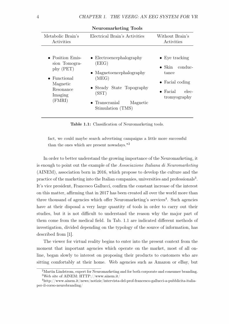
In order to better understand the growing importance of the Neuromarketing, itis enough to point out the example of the Associazione Italiana di Neuromarketing(AINEM), association born in 2016, which propose to develop the culture and thepractice of the marketing into the Italian companies, universities and professionals3.It’s vice president, Francesco Gallucci, confirm the constant increase of the intereston this matter, affirming that in 2017 has been created all over the world more thanthree thousand of agencies which offer Neuromarketing’s services4. Such agencieshave at their disposal a very large quantity of tools in order to carry out theirstudies, but it is not difficult to understand the reason why the major part ofthem come from the medical field. In Tab. 1.1 are indicated different methods ofinvestigation, divided depending on the typology of the source of information, hasdescribed from [1].
The viewer for virtual reality begins to enter into the present context from themoment that important agencies which operate on the market, most of all on-line, began slowly to interest on proposing their products to customers who aresitting comfortably at their home. Web agencies such as Amazon or eBay, but
2Martin Lindstrom, expert for Neuromarketing and for both corporate and consumer branding.3Web site of AINEM: HTTP://www.ainem.it/4http://www.ainem.it/news/notizie/intervista-del-prof-francesco-gallucci-a-pubblicita-italia-
per-il-corso-neurobranding/
1.1. NEUROMARKETING AND VIRTUAL SHOPS 5
also physical companies as the American Wallmart, which shops are all over theU.S. area, are pushing in creating what is going to be their virtual shop, wherecustomers can access simply wearing a virtual viewer. But is not such an easymatter as it can seem, because if the idea is to use the viewer as a means torecreate a conventional shop, then it will be completely lost the fundamental pointunder which such technologies, together, can radically change the way people useto shop, and not only that: entering into a place where products adapt to yourinterest in that specific moment, interact with shop workers who understand whatyou really search, enter into the recording studio with the musician who shows theprocess he lived until the creation of his last album which you would like to buy,etc. This is the reason we need to change the concept of interactivity, which untilnowadays is characterized by the conscious willing of the customer to make useof a physical tool to interface to the web and virtual worlds. It is exactly at thispoint that became useful the Neuromarketing tools, described in Tab. 1.1. Thisis the starting point of the process which brought to the realization of the VeeRg:recognize if what we are observing is to your liking or not, under certain points ofview, is an invaluable information, as it would allow to automatically adapt thevirtual experience (whatever it is, A/N) to its own interests of the moment.
It is necessary to specify that although the interest toward the virtual vieweris constantly increasing, their technologies are relatively young and there are stillmany problems related to them. It is known, for example, that during the firstsections of tests, wearing the virtual mask can bring into an uncomfortable statewhich can also lead to nausea and vomit. For example, into a virtual experiencewhere the subject can move walking through a controller when actually the body isstill, the player brain get destabilized, causing the sensation of vertigo. Everythingis strictly linked to the typology of experience and to the ability of the virtualreality programmers to reduce this nausea effect. That defects also represents thereason why the market of AR (Augmented Reality) viewer is still competitive, asthey make use of common transparent and not focused glasses on which advancedtechnologies project the information about the surrounding environment. In thisway, the consumer never loses completely the connection with the reality, avoidingthat the brain goes haywire. Although if with a high level of quality, these systemsof increased reality have also very high costs5 and obviously they will never be ableto give the sense of a complete immersion into a totally artificial world.
5At present the state of the art of AR viewers is represented by the Magic Leap.
6 CHAPTER 1. THE VEERG: AN EEG SYSTEM FOR VR
1.2 Medical rehabilitation and virtual reality
As for Neuromarketing, virtual reality offers an innovative approach in support-ing the functional recovering of the physical skills in patients affected by cognitivedisorders (during the initial phases), motor disorders caused by medical conditionslike strokes or Parkinson, psychological disorders like anxiety, stress, or phobias.This methodology consists of the execution of specific virtual programs aimed toimprove the exercise upon the compromised body functions, in order to manage,reduce, overcome, or compensate the deficit. The recovering program is based onthe execution of activities with a gradual level of difficulty within an immersivedevice which simulates in a realistic and interactive way different situation takenfrom the daily life context. Big medical companies already began to approachthis kind of therapies creating specific recovering areas fitted with virtual environ-ments, using their own denomination: for example, in Italy, they talk about theTelepresenza Immersiva Virtuale (TIV)6, in America it has been implemented theVirtual Reality Exposure Therapy (VRET), and other examples can be listed. Dif-ferent names with a common objective: the immersion into a virtual environmentwhich allows patients to feel certain sensations and to live situations as they wouldhappen in the real place, facing their phobias or anxieties due to certain traumaslived in the past which created psychological difficulties in present life.
The physical therapy could offer a huge number of examples of potential appli-cations of virtual reality for medical purposes, and all of them are characterized bythe necessity to give to the subject the sensation of total immersion into an environ-ment specifically created for the therapy which doctors are taking in consideration.Often the aim is to push the patient toward the boundaries of his pathology; incase of paralysis due to an stroke, for example, what should be better to do is toput the patient into a context where he is brought to make determined movementswhich born spontaneously on an unconscious level, because of the specific environ-ment proposed it. Another field where the virtual reality is already considered isPsychology7. An emblematic example is represented by a patient who developed aform of acute anxiety which blocked him in driving the car in the place where hemade an accident. This patient was hilled through the (VRET): doctor and patientcame back on the specific place of the accident making use of virtual reality and
6The TIV recovering programs bases on the execution of activities with a gradual level ofdifficulty within an immersive device (CAVE) which simulates in an extremely realistic andinteractive way different situation taken from the daily life context. The CAVE is a systemachieved in dialogue with the Italian Ministry of Helth and with the support of Forge Reply,agency expert in the implementation on innovative hardware and software.
7Is to notice the Limbix system.

1.3. HOW THE BRAIN WORKS 7
the doctor could guide the patient into this emotional experience. Other emblem-atic cases can be represented by therapies which took care of those pathologies dueto traumas coming from the war [24] or particular terrifying events like the WordTrade Center attempt [4][23]. The virtual reality could become a valid help toafford not only the fear of driving, as the previous example, or the fear of high, orthe one of talking in front of a public, or of spider, just to mention some examples;it can also create a calm and relaxing environments when patients live a momentof anxiety.
Also in the medical environment is not difficult to note the increasing helpwhich virtual reality can and will bring. It is consequently easy to come to theconclusion that a virtual system already equipped with electroencephalographicfunctions can represent an interesting product to facilitate the process of therapyof a patient, whatever is his pathology. As is known, on the market are alreadypresent solutions to integrate the electroencephalography into the virtual viewers.This solutions have all got a good level of quality, but integrate a viewer with theelectroencephalographic functions means work to improve its comfortableness andits size because, the more the patient will be unaware about the presence of themask, the more he will concentrate on the action, improving the results comingfrom its use. And even if some companies already began to try to produce such all-in-one system, we must observe that this kind of production is still at the beginningof its process of growth.
1.3 How the brain works and which informations
we are dealing with
The electroencephalography is a medical inspection technique which reads thedistributed electrical activity (or potential) on scalp’s area of the patient, generatedby the particular structure of the brain. Unlike electrocorticogram, which requiresthe use of electrodes on the cerebral cortex, or even electrogram, which makes useof probes pushed deep inside different brain’s areas, the electroencephalography isa completely non-invasive practice since it utilizes electrodes softly leaned againstthe head surface. This is a fundamental characteristic, which allows the practiceto be safe, reproducible and practically without limitations.
How can the superficials potentials related to the internal activity of the brainbe created?
As soon as the brain’s cells (neurons) are activated, local electrical flows startto be generated. The EEG measures the currents related to the synaptic excitation
8 CHAPTER 1. THE VEERG: AN EEG SYSTEM FOR VR
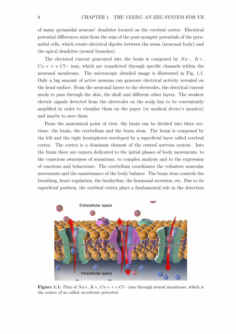
of many pyramidal neurons’ dendrites located on the cerebral cortex. Electricalpotential differences arise from the sum of the post-synaptic potentials of the pyra-midal cells, which create electrical dipoles between the soma (neuronal body) andthe apical dendrites (neural branches).
The electrical current generated into the brain is composed by Na+, K+,Ca + + e Cl− ions, which are transferred through specific channels within theneuronal membrane. The microscopic detailed image is illustrated in Fig. 1.1.Only a big amount of active neurons can generate electrical activity revealed onthe head surface. From the neuronal layers to the electrodes, the electrical currentneeds to pass through the skin, the skull and different other layers. The weakestelectric signals detected from the electrodes on the scalp has to be convenientlyamplified in order to visualize them on the paper (or medical device’s monitor)and maybe to save them.
From the anatomical point of view, the brain can be divided into three sec-tions: the brain, the cerebellum and the brain stem. The brain is composed bythe left and the right hemispheres enveloped by a superficial layer called cerebralcortex. The cortex is a dominant element of the central nervous system. Intothe brain there are centers dedicated to the initial phases of body movements, tothe conscious awareness of sensations, to complex analysis and to the expressionof emotions and behaviours. The cerebellum coordinates the volunteer muscularmovements and the maintenance of the body balance. The brain stem controls thebreathing, heart regulation, the biorhythm, the hormonal secretion, etc. Due to itssuperficial position, the cerebral cortex plays a fundamental role in the detection
Figure 1.1: Flux of Na+, K+, Ca+ + e Cl− ions through neural membrane, which isthe source of so called membrane potential.

1.3. HOW THE BRAIN WORKS 9
Figure 1.2: Brain’s waves classification. Starting from lower frequencies we find theDelta waves, then Theta, Alpha and last Beta.
of the neurological activity through EEG.
1.3.1 Brain’s waves classification
The EEG potentials, resulting from the activity of the neurons, are in the rangeof about 1-150 µV. Although there are a lot of analysis based on the time-domainresponse to specific sensory stimuli (evoked potentials, EP), the main informationis still their frequency characteristic with the band between about 0.4-80 Hz.
The most significant frequencies discovered in the medical field are divided intofour bands related to the different states of mind:
• Delta: the band from 1 to 3 Hz. Detectable in children’s temporoparietalareas, they often appear in adults exposed to emotional stresses.
• Theta: the band from 4 to 7 Hz. They are indicators of the deep sleep of anindividual and have an amplitude between 1 µV and 200 µV.
• Alpha: the band from 8 to 12 Hz. They have an amplitude of around 50µVand are detectable mostly in the occipital area of the cerebral cortex. Theycorrespond to an awake state with eyes closed or to a resting state; for thisreason, this typology of waves completely disappear as the individual switchinto an attentive and concentrated state of mind.
• Beta: the band from 13 to 30 Hz. They can be classified into three subcate-gories: low-Beta waves (13-16 Hz, Beta 1 ), Beta waves (16-20 Hz, Beta 2 ) andhigh-Beta waves (20-30 Hz, Beta 3 ). These typologies of waves are strictlyconnected to a conscious state of mind. That is the reason why they are the
10 CHAPTER 1. THE VEERG: AN EEG SYSTEM FOR VR
most interesting for our analysis but, at the same time, they are the mostcomplex as they appear during different phases of general active thought: fo-cusing in the resolution of a problem or concentrating in the study or carryingout a particular activity or simply thinking on specific thing.
• Gamma: the band from 30 to around 100 Hz. Involved in the formation ofpercepts and memory, linguistic processing, and other behavioral and precep-tual functions. Increased gamma-band activity is also involved in associativelearning.
Basing on the description of the main brainwaves, it is easy to understand whythe VeeRg system, object of the present work, has been implemented focusingon the Beta waves. Their engagement in almost the totality of the action thatan individual can perform in daily activities, make them particularly interestingin the design of a digital systems able to detect the intentions and the differentstates of mind of the user who is wearing it. Furthermore, this typology of waves isconcentrated mostly in the frontal part of the cortex, which makes them an optimalobject of analysis as soon as our system’s electrodes will be positioned exactly inthat area of the cerebral cortex (see Par. 1.4).
The fact that Beta waves are basically associated with awake actions does notnecessarily rule out the presence involved by the other typologies of waves; actually,in an EEG acquisition during an awake state of mind, it’s easy to notice the Delta,Theta waves appearing, or even Alpha waves, which are usually positioned in theoccipital part of the cerebral cortex. Then we have to keep in mind that the finalinformation will result from a combination of all that waves, technically speakingfrom all the band ranging in 0.4-80 Hz, no matter of which signals are going to beacquired.
1.4 Electrodes’ placement
There is an international Standard for the placement of the electrodes, whichname is characterized by a couple of numbers (e.g. the 10-20 system, Fig. 1.3a).These numbers referred to the distance, expressed in percentage, between twocontiguous electrodes, referred to the total one between the point of the skull namedinion (protrusion located at the base of the occipital bone) and the starting point ofthe nose bone (a total of around twenty electrodes in the 10-20 system). It neededto keep in mind that it is not a strict rule for electroencephalographic measurement;anyone can place the electrodes in his own way, but following the standard helps

1.4. ELECTRODES’ PLACEMENT 11
(a)
FP1 GF7F8
FP2
ELER
BIASREF
ERD
(b)
Figure 1.3: Electrodes’ placement in the 10-20 standard configuration (a) and theplacement’s in the VeeRg system (b).
to indicate and recognize specific electrode connected to specific areas of headwithout ambiguity. Then, each electrode is marked by an abbreviation (commonlyone or a couple of characters) which identifies the region of the cerebral cortex(Fp = Frontal-Parietal, F = Frontal, C = Central, P = Parietal, T = Temporal eO = Occipital) and a number which refers to one hemispheres (odd number = lefthemisphere, even number = right hemisphere) or a "z" in case the electrode isplaced on the midline saggital plane of skull.
The electroencephalographic data recording use a couple of electrodes; eachcouple represents a specific channel for the reading device, corresponding to thepotentials difference between the two electrodes. Consequently, there can be dif-ferent EEG lectures, but all of them starts from the basic assumption that eachelectrode placed on the head has a specific reference. That reference can be chosenbased on the type of test we are going to perform; for example, it can be relatedto the electrode signal coming from the top of the skull (Cz in 10-20); it can resultfrom the average of all signals coming from all electrodes (average reference); itcan refer to a specific electrode placed on the orbit of the eye or on the mastoid(only two electrodes each mastoid/ear can be used) or even on the nose. Oncethat the electrode has been chosen, there can be the possibility to interpret thesingle electrode signals (single-ended system acquisition) or the difference betweena couples of electrodes signals (differential system acquisition).
The VeeRg consist of a ski mask properly modified in order to host the elec-trodes and an acquisition/processing board. For this reason, it became necessaryto take in consideration, for our study, the area of the cerebral cortex where themask is placed, namely the frontal (F) and the frontal–parietal (Fp) zones. Inparticular, there had been placed four electrodes related to Fp1, Fp2, F7 and F8in the system 10-20, and one another electrode in the center of the cortex whichwe called G. Thanks to the versatility of the mask, there had been introduced also
12 CHAPTER 1. THE VEERG: AN EEG SYSTEM FOR VR
three different channels, added in order to reach the electro-ocular signals: ER =right eye, EL = left eye, ERD = right low eye; the fourth electrode, necessary tocomplete the electro-oculographic system, is the same Fp2 used for EEG. Theseadditional electrodes could be useful to add some specific features to the systemlike eye tracking or eye’s blink removal. In Fig. 1.3b is illustrated the system justexplained above.
1.5 The prototype idea
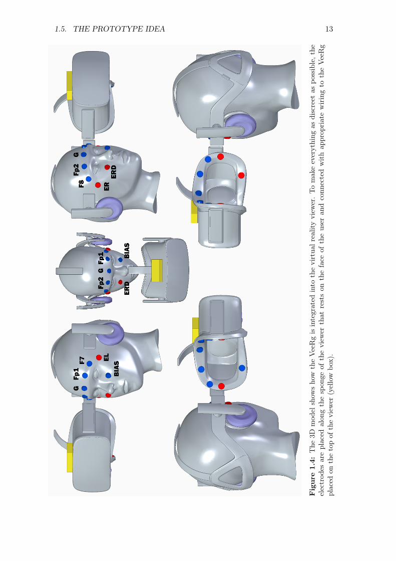
In Fig. 1.4 it is shown how the VeeRg was thought when we stated to think aboutit. Wanting to make it invisible to the user, it come to us naturally to choose toplacing the electrodes along the thickness of the sponge of the viewer that rests onthe face. The ADS1299 front-end provides 8 acquisition channels for EEG signals,one channel for the reference electrode and one channel for correcting the commonpotential due to the isolation of the body from the earth (common mode CM,see Par. 2.1.2). There are overall ten electrodes to be disposed. Regarding thoseintended for electroencephalography, it was not a big deal to understand what theirposition was, as already cited in the previous paragraph, we have complied withthe standard arrangement 10-20 for the electrodes Fp1, Fp2, F7 and F8. However,we have introduced a fifth electrode, not provided for by the standard, we havecalled G and which we have placed right in the middle of the front; the usefulnessof this electrode is twofold: on the one hand it can very well act as a normalencephalographic electrode by using signals that can be useful in the analysis ofthe cerebral activity; on the other, it can be considered a reference electrode forthe remaining four, allowing to calculate the potential of the frontal points withrespect to the point placed along the midline saggital plane of skull. The remainingthree channels are dedicated to the electrodes for the oculographic signals usefulin the moment we want to implement an algorithm for removing artifacts due tothe movement of the eye or, even more interestingly, implement an algorithm thatis able to trace their movements. The last electrode to put on the display, is thebias for the elimination of the common mode signal. Regarding the reference, aclip was constructed with an electrode to be placed on the earlobe.
The rest of the system made up of the cards and the battery doesn’t represent abig problem about the positioning but we must however take into account the typeof viewer on which it will be applied since not all of them give the same freedom.In Fig. 1.4 for example the model represents an Oculus Rift viewer, which has alarge area in the upper part on which the VeeRg can be placed (represented by the
1.5. THE PROTOTYPE IDEA 13
Fig
ure
1.4:
The
3Dmod
elshow
sho
wtheVeeRgis
integrated
into
thevirtua
lrealityview
er.Tomakeeverything
asdiscreet
aspo
ssible,t
heelectrod
esareplaced
alon
gthespon
geof
theview
erthat
restson
theface
oftheuser
andconn
ectedwithap
prop
riatewiringto
theVeeRg
placed
onthetopof
theview
er(yellow
box).

14 CHAPTER 1. THE VEERG: AN EEG SYSTEM FOR VR
yellow box in the figure).Obviously for the creation of a prototype it is not necessary to use, at least in
the first versions, a real virtual reality viewer. Rather, it is more practical to usea mask for generic use, such as those used for skiing, for more freedom of action.In the first phase, in fact, it will be necessary to understand if the system actuallyworks correctly and if the position of the electrodes is right or must be corrected.Following, the basic idea is to provide the users having already a viewer, a practicehardware plug-in that can easily integrate with it. Only then can we think ofdeveloping a new product that integrates both the functions of virtual visor andelectroencephalography.
Chapter 2
The VeeRg design
The intent of this chapter is to describe the main steps that have characterizedthe design of the VeeRg system. The contents we are going to talk about arethe most common challenges that a designer can encounter during the design ofsuch systems. These challenges do not depend on the use of particular circuitcomponents or particular programming techniques, which we preferred to omitgiven their relative lack of scientific interest, but they represent a higher conceptuallevel and for this reason they become the fundamental bases for a good design.Anyway, a little description of the devices used on the boards will be done in nextparagraph.
The milestones we have fixed in our mind during the design of such kind ofsystem are essentially two, the second of which is strictly dependent from the firsone. The first step was to obtain an acquired signal, representative of the brainactivity coming from the electrodes, as accurate and clear as possible; the secondstep was to clean and isolate the frequency bands relative to the common brainactivity’s classification (Alpha, Beta, etc. . . ) seen in the Chap 1, to extract all theuseful informations.
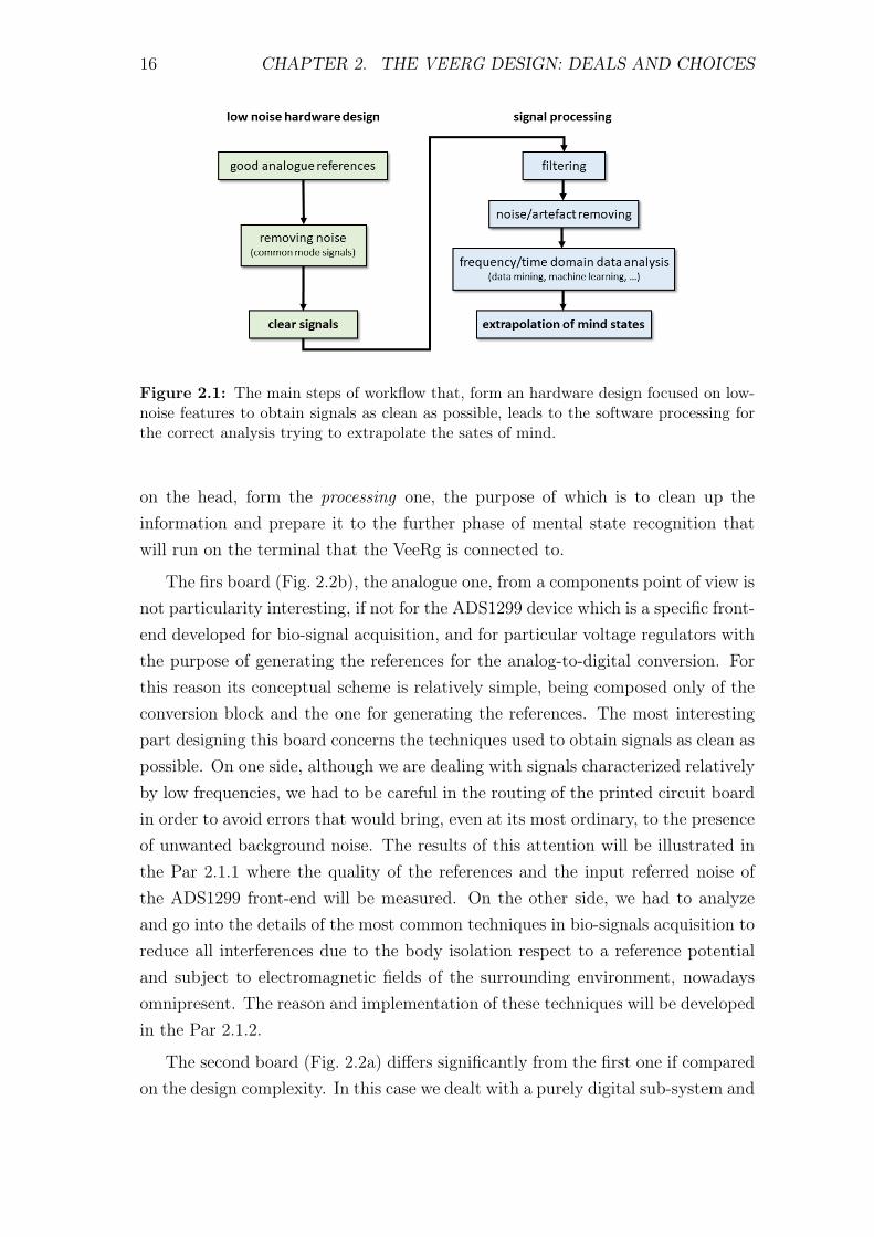
From this point of view, two different phases of workflow could be defined, thehardware and the software ones, and so we’ve done in the description of the VeeRgsystem in the following sections. In Fig. 2.1 is shown the whole work process whichwill lead to the final results.
2.1 Hardware design
An overview on how the our electroencephalographic system is composed isgiven by the Fig. 2.2. The basic idea was to divide the strictly analogue part, forthe acquisition and digitalization of the signals coming from the electrodes placed
15
16 CHAPTER 2. THE VEERG DESIGN: DEALS AND CHOICES
Figure 2.1: The main steps of workflow that, form an hardware design focused on low-noise features to obtain signals as clean as possible, leads to the software processing forthe correct analysis trying to extrapolate the sates of mind.
on the head, form the processing one, the purpose of which is to clean up theinformation and prepare it to the further phase of mental state recognition thatwill run on the terminal that the VeeRg is connected to.
The firs board (Fig. 2.2b), the analogue one, from a components point of view isnot particularity interesting, if not for the ADS1299 device which is a specific front-end developed for bio-signal acquisition, and for particular voltage regulators withthe purpose of generating the references for the analog-to-digital conversion. Forthis reason its conceptual scheme is relatively simple, being composed only of theconversion block and the one for generating the references. The most interestingpart designing this board concerns the techniques used to obtain signals as clean aspossible. On one side, although we are dealing with signals characterized relativelyby low frequencies, we had to be careful in the routing of the printed circuit boardin order to avoid errors that would bring, even at its most ordinary, to the presenceof unwanted background noise. The results of this attention will be illustrated inthe Par 2.1.1 where the quality of the references and the input referred noise ofthe ADS1299 front-end will be measured. On the other side, we had to analyzeand go into the details of the most common techniques in bio-signals acquisition toreduce all interferences due to the body isolation respect to a reference potentialand subject to electromagnetic fields of the surrounding environment, nowadaysomnipresent. The reason and implementation of these techniques will be developedin the Par 2.1.2.
The second board (Fig. 2.2a) differs significantly from the first one if comparedon the design complexity. In this case we dealt with a purely digital sub-system and
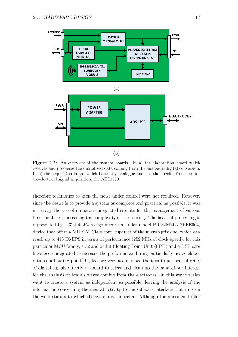
2.1. HARDWARE DESIGN 17
(a)
(b)
Figure 2.2: An overview of the system boards. In a) the elaboration board whichreceives and processes the digitalized data coming from the analog-to-digital conversion.In b) the acquisition board which is strictly analogue and has the specific front-end forbio-electrical signal acquisition, the ADS1299.
therefore techniques to keep the noise under control were not required. However,since the desire is to provide a system as complete and practical as possible, it wasnecessary the use of numerous integrated circuits for the management of variousfunctionalities, increasing the complexity of the routing. The heart of processing isrepresented by a 32-bit Microchip micro-controller model PIC32MZ0512EFE064,device that offers a MIPS M-Class core, superset of the microAptiv one, which canreach up to 415 DMIPS in terms of performance (252 MHz of clock speed); for thisparticular MCU family, a 32 and 64 bit Floating Point Unit (FPU) and a DSP corehave been integrated to increase the performance during particularly heavy elabo-rations in floating point[19], feature very useful since the idea to perform filteringof digital signals directly on-board to select and clean up the band of our interestfor the analysis of brain’s waves coming from the electrodes. In this way we alsowant to create a system as independent as possible, leaving the analysis of theinformation concerning the mental activity to the software interface that runs onthe work station to which the system is connected. Although the micro-controller

18 CHAPTER 2. THE VEERG DESIGN: DEALS AND CHOICES
has the ability to manage a USB OTG communication, in order to reduce the com-putational load we have considered the use of the FTD232 from FTDI company, anUSB/UART interpreter that independently manages all the stack layer necessaryfor communication through the USB standard. The same was done for the wirelessbluetooth communication with the use of the SPBT2632C2A.AT2 module by STMicroelectronics which integrates a Cortex core for the independent managementof the bluetooth stack layer and for the communication with the micro-controllerthrough UART. Finally, to complement the processing board, we have the blockfor the management of power supplies and the charge/discharge of the 900mAhbattery, which with the present elaboration load guarantees an autonomy of ap-proximately 5 hours of continuous acquisition, and the block consisting of an IMU(inertial measurement unit) MPU9250 by InvenSense that provides the ability toimplement an AHRS (attitude and heading reference system) if the system wasnot used with a virtual reality viewer but still wanted to have information on themovements of the head in 3D space.
Both the boards and the complete final system prototype are shown in theFig. 2.26 at the end of this chapter. The schematics of the VeeRg system areavailable in App. A.1.
2.1.1 Analog power supply and input referred noise
In Par. 1.3.1 we introduced the cassification of the different brain waves accord-ing to their frequency band (Delta, Theta, Alpha, Beta and Gamma). We havealso mentioned that these waves have a very small amplitude, of the order of mi-crovolt (µV). Being dealing with signals so small it’s essential try to not introduceany noise through wrong design choices. From this point of view, the ADS1299front-end gives us already some good low-noise features, but if the designer doesn’tenter into this perspective, then the situation may be worse. The choice aboutseparating the digital part from the analogue part in the VeeRg into two differ-ent PCB essentially stems from these points. We wanted to isolate the analoguepart to avoid a priori the additional noise due to possible coupling with the digitalsignals of the communication interfaces. Moreover, the board has been designedfollowing the practice of the shielding through the use of an external metallic boxand a suitable plane placed in a inner layer of the board, both connected to thesystem ground (Fig. 2.26c).
In Fig: 2.2b the Power Adapter block plays a fundamental role in keeping thebackground noise of the whole system as low as possible. In fact this block is the onethat generates the analog power supplies for the ADS1299 front-end and the voltage
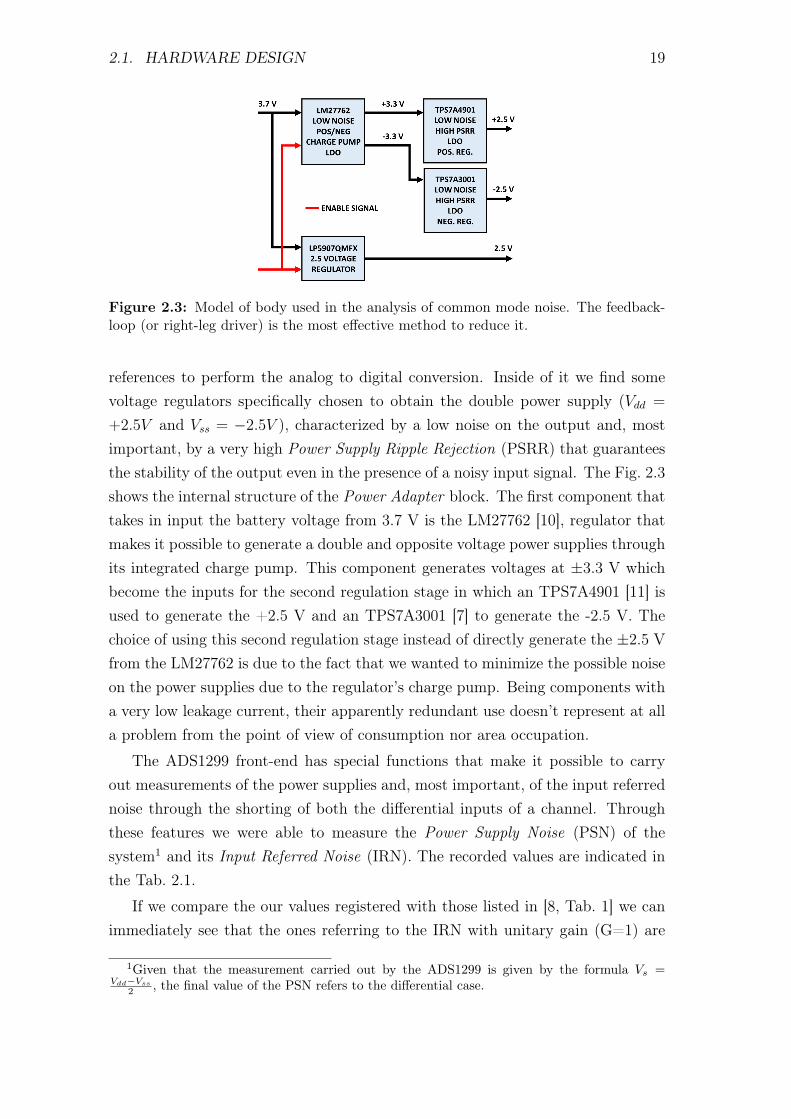
2.1. HARDWARE DESIGN 19
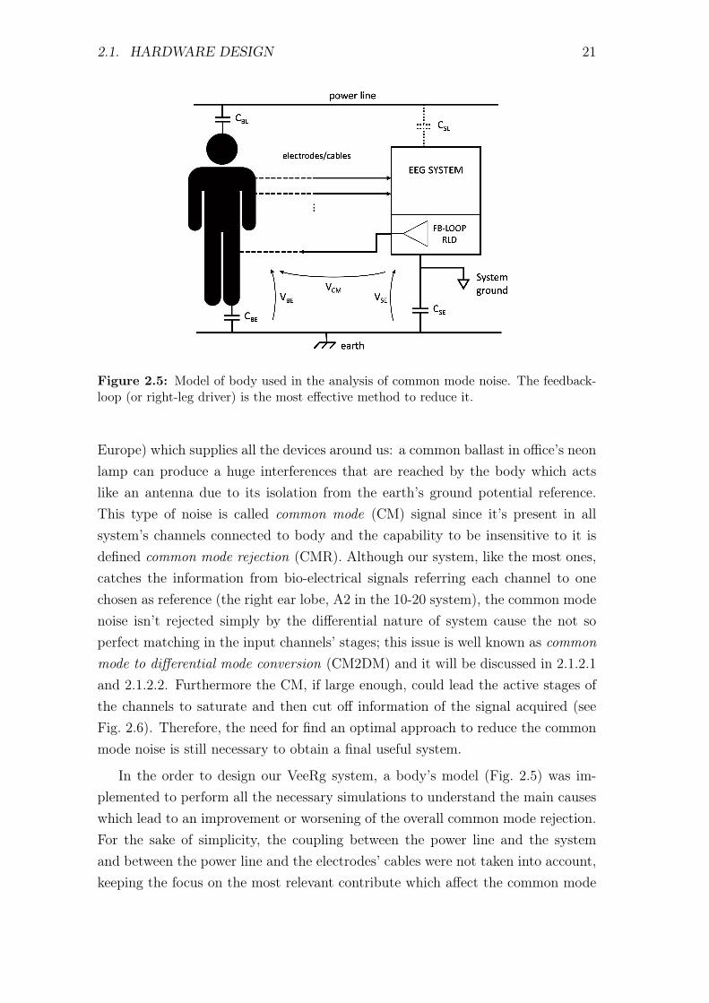
Figure 2.3: Model of body used in the analysis of common mode noise. The feedback-loop (or right-leg driver) is the most effective method to reduce it.
references to perform the analog to digital conversion. Inside of it we find somevoltage regulators specifically chosen to obtain the double power supply (Vdd =
+2.5V and Vss = −2.5V ), characterized by a low noise on the output and, mostimportant, by a very high Power Supply Ripple Rejection (PSRR) that guaranteesthe stability of the output even in the presence of a noisy input signal. The Fig. 2.3shows the internal structure of the Power Adapter block. The first component thattakes in input the battery voltage from 3.7 V is the LM27762 [10], regulator thatmakes it possible to generate a double and opposite voltage power supplies throughits integrated charge pump. This component generates voltages at ±3.3 V whichbecome the inputs for the second regulation stage in which an TPS7A4901 [11] isused to generate the +2.5 V and an TPS7A3001 [7] to generate the -2.5 V. Thechoice of using this second regulation stage instead of directly generate the ±2.5 Vfrom the LM27762 is due to the fact that we wanted to minimize the possible noiseon the power supplies due to the regulator’s charge pump. Being components witha very low leakage current, their apparently redundant use doesn’t represent at alla problem from the point of view of consumption nor area occupation.
The ADS1299 front-end has special functions that make it possible to carryout measurements of the power supplies and, most important, of the input referrednoise through the shorting of both the differential inputs of a channel. Throughthese features we were able to measure the Power Supply Noise (PSN) of thesystem1 and its Input Referred Noise (IRN). The recorded values are indicated inthe Tab. 2.1.
If we compare the our values registered with those listed in [8, Tab. 1] we canimmediately see that the ones referring to the IRN with unitary gain (G=1) are
1Given that the measurement carried out by the ADS1299 is given by the formula Vs =Vdd−Vss
2 , the final value of the PSN refers to the differential case.
20 CHAPTER 2. THE VEERG DESIGN: DEALS AND CHOICES
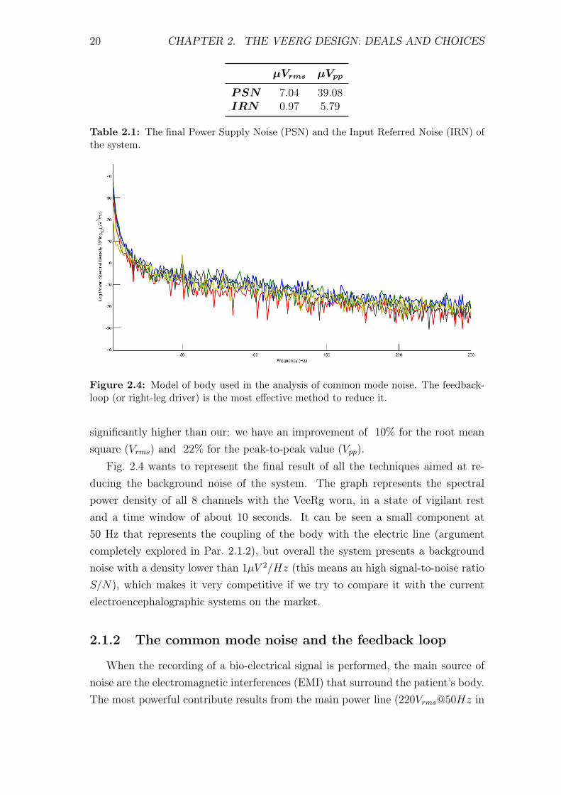
µVrms µVpp
PSN 7.04 39.08IRN 0.97 5.79
Table 2.1: The final Power Supply Noise (PSN) and the Input Referred Noise (IRN) ofthe system.
Figure 2.4: Model of body used in the analysis of common mode noise. The feedback-loop (or right-leg driver) is the most effective method to reduce it.
significantly higher than our: we have an improvement of 10% for the root meansquare (Vrms) and 22% for the peak-to-peak value (Vpp).
Fig. 2.4 wants to represent the final result of all the techniques aimed at re-ducing the background noise of the system. The graph represents the spectralpower density of all 8 channels with the VeeRg worn, in a state of vigilant restand a time window of about 10 seconds. It can be seen a small component at50 Hz that represents the coupling of the body with the electric line (argumentcompletely explored in Par. 2.1.2), but overall the system presents a backgroundnoise with a density lower than 1µV 2/Hz (this means an high signal-to-noise ratioS/N), which makes it very competitive if we try to compare it with the currentelectroencephalographic systems on the market.
2.1.2 The common mode noise and the feedback loop
When the recording of a bio-electrical signal is performed, the main source ofnoise are the electromagnetic interferences (EMI) that surround the patient’s body.The most powerful contribute results from the main power line (220Vrms@50Hz in
2.1. HARDWARE DESIGN 21
Figure 2.5: Model of body used in the analysis of common mode noise. The feedback-loop (or right-leg driver) is the most effective method to reduce it.
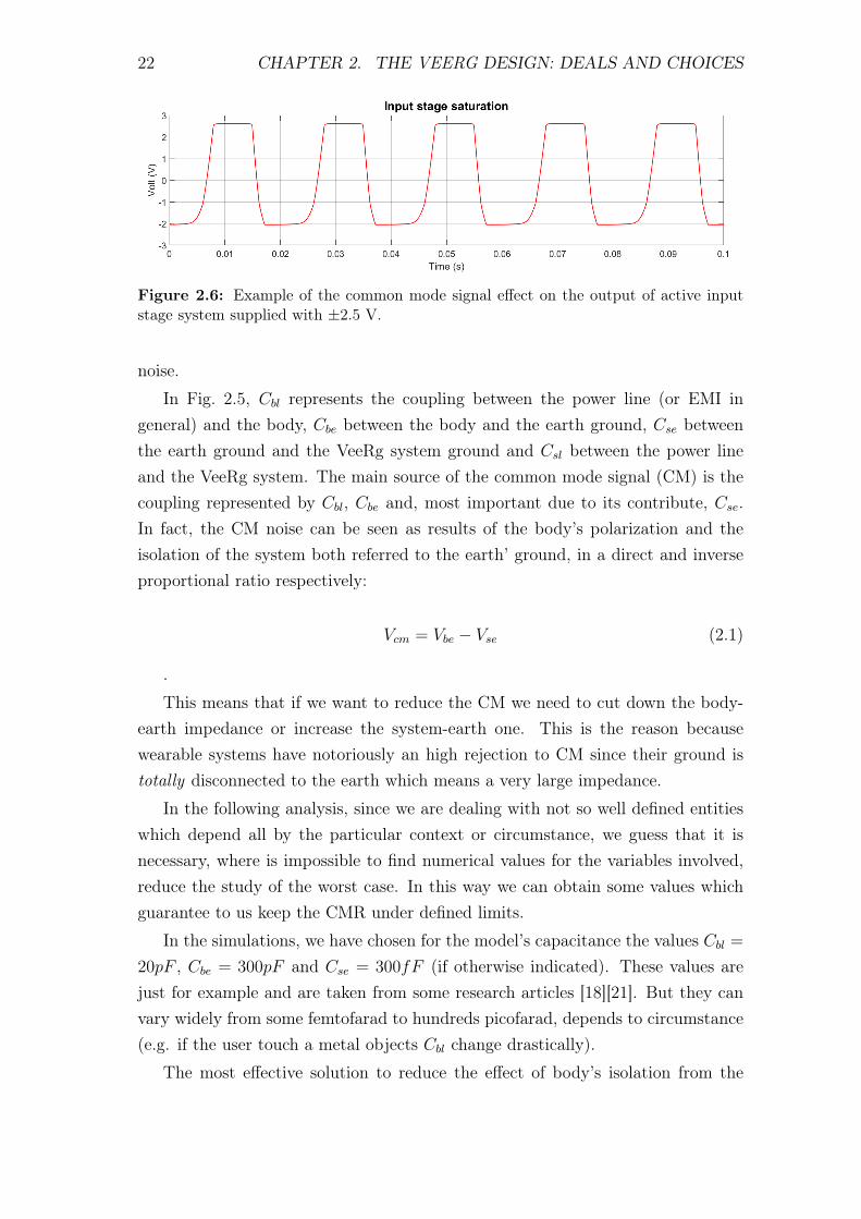
Europe) which supplies all the devices around us: a common ballast in office’s neonlamp can produce a huge interferences that are reached by the body which actslike an antenna due to its isolation from the earth’s ground potential reference.This type of noise is called common mode (CM) signal since it’s present in allsystem’s channels connected to body and the capability to be insensitive to it isdefined common mode rejection (CMR). Although our system, like the most ones,catches the information from bio-electrical signals referring each channel to onechosen as reference (the right ear lobe, A2 in the 10-20 system), the common modenoise isn’t rejected simply by the differential nature of system cause the not soperfect matching in the input channels’ stages; this issue is well known as commonmode to differential mode conversion (CM2DM) and it will be discussed in 2.1.2.1and 2.1.2.2. Furthermore the CM, if large enough, could lead the active stages ofthe channels to saturate and then cut off information of the signal acquired (seeFig. 2.6). Therefore, the need for find an optimal approach to reduce the commonmode noise is still necessary to obtain a final useful system.
In the order to design our VeeRg system, a body’s model (Fig. 2.5) was im-plemented to perform all the necessary simulations to understand the main causeswhich lead to an improvement or worsening of the overall common mode rejection.For the sake of simplicity, the coupling between the power line and the systemand between the power line and the electrodes’ cables were not taken into account,keeping the focus on the most relevant contribute which affect the common mode
22 CHAPTER 2. THE VEERG DESIGN: DEALS AND CHOICES
Figure 2.6: Example of the common mode signal effect on the output of active inputstage system supplied with ±2.5 V.
noise.
In Fig. 2.5, Cbl represents the coupling between the power line (or EMI ingeneral) and the body, Cbe between the body and the earth ground, Cse betweenthe earth ground and the VeeRg system ground and Csl between the power lineand the VeeRg system. The main source of the common mode signal (CM) is thecoupling represented by Cbl, Cbe and, most important due to its contribute, Cse.In fact, the CM noise can be seen as results of the body’s polarization and theisolation of the system both referred to the earth’ ground, in a direct and inverseproportional ratio respectively:
Vcm = Vbe − Vse (2.1)
.
This means that if we want to reduce the CM we need to cut down the body-earth impedance or increase the system-earth one. This is the reason becausewearable systems have notoriously an high rejection to CM since their ground istotally disconnected to the earth which means a very large impedance.
In the following analysis, since we are dealing with not so well defined entitieswhich depend all by the particular context or circumstance, we guess that it isnecessary, where is impossible to find numerical values for the variables involved,reduce the study of the worst case. In this way we can obtain some values whichguarantee to us keep the CMR under defined limits.
In the simulations, we have chosen for the model’s capacitance the values Cbl =
20pF , Cbe = 300pF and Cse = 300fF (if otherwise indicated). These values arejust for example and are taken from some research articles [18][21]. But they canvary widely from some femtofarad to hundreds picofarad, depends to circumstance(e.g. if the user touch a metal objects Cbl change drastically).
The most effective solution to reduce the effect of body’s isolation from the
2.1. HARDWARE DESIGN 23
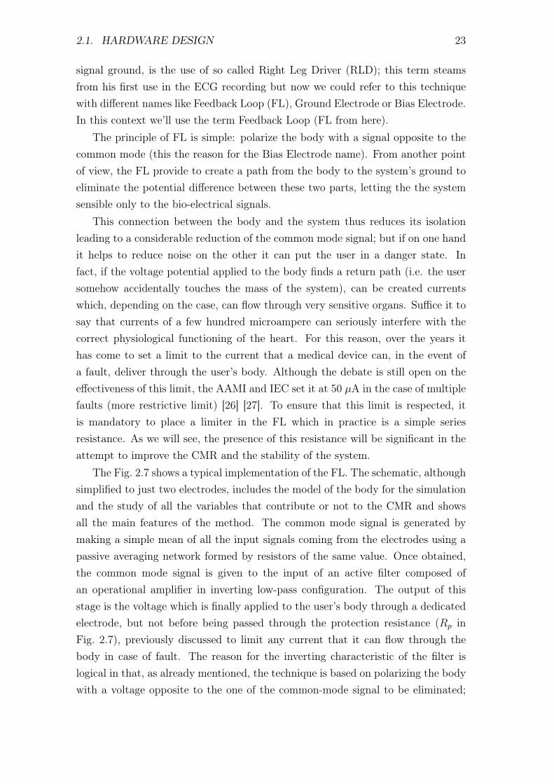
signal ground, is the use of so called Right Leg Driver (RLD); this term steamsfrom his first use in the ECG recording but now we could refer to this techniquewith different names like Feedback Loop (FL), Ground Electrode or Bias Electrode.In this context we’ll use the term Feedback Loop (FL from here).
The principle of FL is simple: polarize the body with a signal opposite to thecommon mode (this the reason for the Bias Electrode name). From another pointof view, the FL provide to create a path from the body to the system’s ground toeliminate the potential difference between these two parts, letting the the systemsensible only to the bio-electrical signals.
This connection between the body and the system thus reduces its isolationleading to a considerable reduction of the common mode signal; but if on one handit helps to reduce noise on the other it can put the user in a danger state. Infact, if the voltage potential applied to the body finds a return path (i.e. the usersomehow accidentally touches the mass of the system), can be created currentswhich, depending on the case, can flow through very sensitive organs. Suffice it tosay that currents of a few hundred microampere can seriously interfere with thecorrect physiological functioning of the heart. For this reason, over the years ithas come to set a limit to the current that a medical device can, in the event ofa fault, deliver through the user’s body. Although the debate is still open on theeffectiveness of this limit, the AAMI and IEC set it at 50 µA in the case of multiplefaults (more restrictive limit) [26] [27]. To ensure that this limit is respected, itis mandatory to place a limiter in the FL which in practice is a simple seriesresistance. As we will see, the presence of this resistance will be significant in theattempt to improve the CMR and the stability of the system.
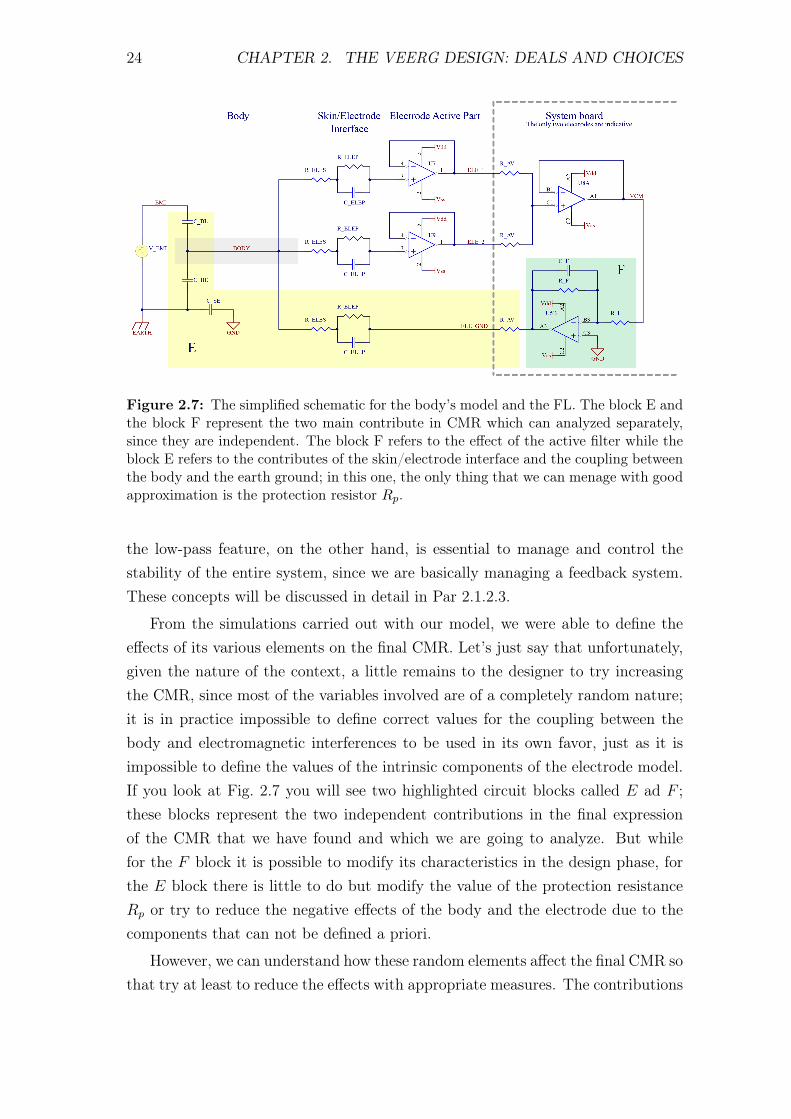
The Fig. 2.7 shows a typical implementation of the FL. The schematic, althoughsimplified to just two electrodes, includes the model of the body for the simulationand the study of all the variables that contribute or not to the CMR and showsall the main features of the method. The common mode signal is generated bymaking a simple mean of all the input signals coming from the electrodes using apassive averaging network formed by resistors of the same value. Once obtained,the common mode signal is given to the input of an active filter composed ofan operational amplifier in inverting low-pass configuration. The output of thisstage is the voltage which is finally applied to the user’s body through a dedicatedelectrode, but not before being passed through the protection resistance (Rp inFig. 2.7), previously discussed to limit any current that it can flow through thebody in case of fault. The reason for the inverting characteristic of the filter islogical in that, as already mentioned, the technique is based on polarizing the bodywith a voltage opposite to the one of the common-mode signal to be eliminated;
24 CHAPTER 2. THE VEERG DESIGN: DEALS AND CHOICES
Figure 2.7: The simplified schematic for the body’s model and the FL. The block E andthe block F represent the two main contribute in CMR which can analyzed separately,since they are independent. The block F refers to the effect of the active filter while theblock E refers to the contributes of the skin/electrode interface and the coupling betweenthe body and the earth ground; in this one, the only thing that we can menage with goodapproximation is the protection resistor Rp.
the low-pass feature, on the other hand, is essential to manage and control thestability of the entire system, since we are basically managing a feedback system.These concepts will be discussed in detail in Par 2.1.2.3.
From the simulations carried out with our model, we were able to define theeffects of its various elements on the final CMR. Let’s just say that unfortunately,given the nature of the context, a little remains to the designer to try increasingthe CMR, since most of the variables involved are of a completely random nature;it is in practice impossible to define correct values for the coupling between thebody and electromagnetic interferences to be used in its own favor, just as it isimpossible to define the values of the intrinsic components of the electrode model.If you look at Fig. 2.7 you will see two highlighted circuit blocks called E ad F ;these blocks represent the two independent contributions in the final expressionof the CMR that we have found and which we are going to analyze. But whilefor the F block it is possible to modify its characteristics in the design phase, forthe E block there is little to do but modify the value of the protection resistanceRp or try to reduce the negative effects of the body and the electrode due to thecomponents that can not be defined a priori.
However, we can understand how these random elements affect the final CMR sothat try at least to reduce the effects with appropriate measures. The contributions
2.1. HARDWARE DESIGN 25
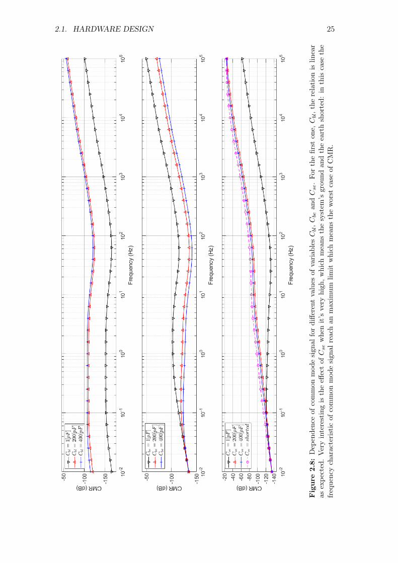
Fig
ure
2.8:
Dep
endenceof
common
mod
esign
alfordiffe
rent
values
ofvariab
lesCbl,C
bean
dCse.Fo
rthefirst
one,Cbl,t
herelation
islin
ear
asexpe
cted.Veryinterestingis
theeff
ectofCse
whe
nit’s
very
high
,which
means
thesystem
’sgrou
ndan
dtheearthshorted:
inthis
case
the
frequencycharacteristic
ofcommon
mod
esign
alreachan
max
imum
limitwhich
means
theworst
case
ofCMR.

26 CHAPTER 2. THE VEERG DESIGN: DEALS AND CHOICES
related to the isolation of the body are particularly interesting in this sense andtherefore the couplings represented by the capacities Cbl, Cbe and Cse. For thispurpose we performed a simulation maintaining an unity gain for the FL filter anda cutoff frequency of about 1.6 kHz; a frequency analysis was performed on a bandranging from 10 mHz to 100 kHz. Keep in mind that in this analysis the CMR isexpressed in negative form, so an increase in it results in a decrease in the value ofthe expressions found.
In Fig. 2.8 we have the results of the analysis. With regard to the capacitanceCbl the inversely proportional dependence between its value and the final CMR canbe immediately noticed; this behavior is easily understandable since an increase incapacity corresponds to a reduction in the impedance seen between the noise sourceand the body. It is a different matter for Cbe, given the fact that its value is linkedto the CMR by a relationship of inverse proportionality: the higher its value, thelower the impedance between body and earth and therefore less isolation of thebody from a reference potential (non floating body). Of particular interest is thecase of Cse related to the CMR by an inverse proportionality ratio; this explainswhy battery-powered systems have a notoriously better rejection to the commonmode signal due to electromagnetic interference since the coupling between thesystem ground and the earth has a very small value. The interest in this parameterincreases if we observe the case in which Cse →∞, i.e. when the two ground andearth references are shorted together: the CMR in this case reaches an upper limitvalue that represents the worst case for the Cse parameter. This can be very usefulin simplifying the analysis of the whole system considering already from begin thetwo masses shorted and focusing on the other parameters, knowing however thatany change related to Cse can only lead to an improvement of the Final CMR. Aswe will see shortly, removing from the calculations Cse, the final formulas describingthe CMR (poles and zeros also) will be simplified.
Fixed to mind the effects of the parameters which are parts of body system, wecan now move the attention to an deeper analysis of the CMR and in articular of itstwo independent components that previously in the schematic we have indicatedas block F , representing the active filter part, and block E, representing the totalimpedance seen by the F block. We have to keep in mind that the validity of thisanalysis is limited to the use of active electrodes or, at least, characterized by avery high input impedance.
Fig. 2.8 gives a general idea of CMR trend vs. frequency. During the calculationof its general expression, the possibility of separate the two independent blocks Fand E was noticed. The relationship found is thus expressible as:

2.1. HARDWARE DESIGN 27
(a)
(b)
(c)
Figure 2.9: The CM characteristic (c) disjointed into the two contributions F and E.In (a) the frequency characteristic of the contribution F (ω) with the presence of one poleand one zero. In (b) the E(ω) and two of its three zeros. Unlike F (ω), it was not possibleto find clear and simple analytical expressions of the poles given the complexity of thecalculations.

28 CHAPTER 2. THE VEERG DESIGN: DEALS AND CHOICES
VcmVemi
(ω) = F (ω)E(ω) =Zi
Zf + Zi
ZeZbeZbl(Ze + Zse + Zbe) + Zbe(Ze + Zse)
(2.2)
that in decibel becomes
∣∣∣∣ VcmVemi
∣∣∣∣dB
(ω) = 20log
(∣∣∣∣ ZiZi + Zf
∣∣∣∣)+20log
(∣∣∣∣ ZeZbeZbl(Ze + Zse + Zbe) + Zbe(Ze + Zse)
∣∣∣∣)(2.3)
with
Zi = Ri
Zf = Rf ‖ Cf =Rf
1 + jωRfCf
Zbe =1
jωCbe
Zbl =1
jωCbl
Zse =1
jωCse
Ze = Rp +Reles + (Relep ‖ Celep) =Rp +Reles +Relep + jωRelepCelep(Rp +Reles)
1 + jωRelepCelep
(2.4)
.
Note that the impedance Ze is no more that the result of electrode in serieswith the protection resistance.
In Fig. 2.9a the frequency characteristic of the contribution F (ω) is depicted,also highlighting the presence of one pole and one zero. We have already mentionedthat this contribution, even if it can theoretically lead to an infinite CMR, is limitedby the condition of stability of the system (see Par 2.1.2.3). Its expression as afunction of ω is
F (ω) =Zi
Zi + Zf= Ri
1 + jωRfCfRi +Rf + jωRiRfCf
(2.5)
and his analysis shows the presence of two limits for ω → ±∞, of a pole fp andof a zero fz. Their expressions are as follows:
|F | (ω → 0) =Ri
Ri +Rf
(2.6)

2.1. HARDWARE DESIGN 29
|F | (ω →∞) = 1 (2.7)
fz =1
2πRfCf(2.8)
fp =Ri +Rf
2πRiRfCf(2.9)
.
Regard the contribution E(ω), its characteristic is shown in Fig. 2.9b withexpression given by
E(ω) =ZeZbe
Zbl(Ze + Zse + Zbe) + Zbe(Ze + Zse)(2.10)
.
Like for F (ω), the analysis of E(ω) leads to find the characteristic values of itstrend vs. frequency for ω → ±∞ and the values of its three zeros fz0, fz1 andfz2. Unlike F (ω) however, it was not possible to find clear and simple analyticalexpressions of the poles given the complexity of the calculations. The results are
|E| (ω → 0) = 0 (2.11)
|E| (ω →∞) =∞ (2.12)
fz0 = 0 (2.13)
fz1 =1
2πCse(2.14)
fz2 =Rp +Reles +Relep
2πRelepCelep(Rp +Reles)(2.15)
.
Although we only have the expressions of the zeros, we can however say that tooptimize the final CMR we should try to have such points at the highest possiblefrequencies; this would guarantee that with the increase of the frequency the rela-tive decrease of the CMR happens with greater delay. To move the zeros fz1 andfz2 at high frequencies means, observing their expressions, to decrease the capacityCse and to decrease the resistance Rp (for the latter we will see shortly how itsvalue affects the position of zero fz2).
Consider now the much simpler case in which Cse → ∞ i.e. with the massof the system and the earth shorted. We have already found how this particularcontext turns out to be a worst case limit for what concerns this parameter suchthat every possible random variation could only lead to an improvement of theCMR. The general expression resulting from this change is

30 CHAPTER 2. THE VEERG DESIGN: DEALS AND CHOICES
Figure 2.10: The relation between the values of Rp and fz1 is inversely proportional.The graph has been drawn as example with Reles = 4kHz, Relep = 150kHz and Celep =180nF [16][3].
VcmVemi
(ω) = F (ω)E(ω) =Zi
Zf + Zi
ZeZbeZbl(Ze + Zbe) + ZbeZe
(2.16)
with F (ω) as the previous case. It changes only E(ω) which become
E(ω) =ZeZbe
Zbl(Ze + Zbe) + ZbeZe(2.17)
with its new values for ω → ±∞ and the missing of one zero:
|E| (ω → 0) = 0 (2.18)
|E| (ω →∞) =Cbl
Cbl + Cbe(2.19)
fz0 = 0 (2.20)
fz1 =Rp +Reles +Relep
2πRelepCelep(Rp +Reles)(2.21)
.The graph of the new contribution E(ω) is shown in Fig. 2.9c, where the zero
fz1 is highlighted (note that it has the same expression as the previous fz2). Alsoin this case the concept is the same: to improve the overall CMR we need to movefz1 at high frequencies. But the only parameter that we can change is just thevalue of the resistance Rp, related to the found formula of fz1 through an inverseproportionality ratio (Fig. 2.10).
The results just obtained so far want to highlight the strong random componentin the final value of the CMR of our system and, more generally, in a system for
2.1. HARDWARE DESIGN 31
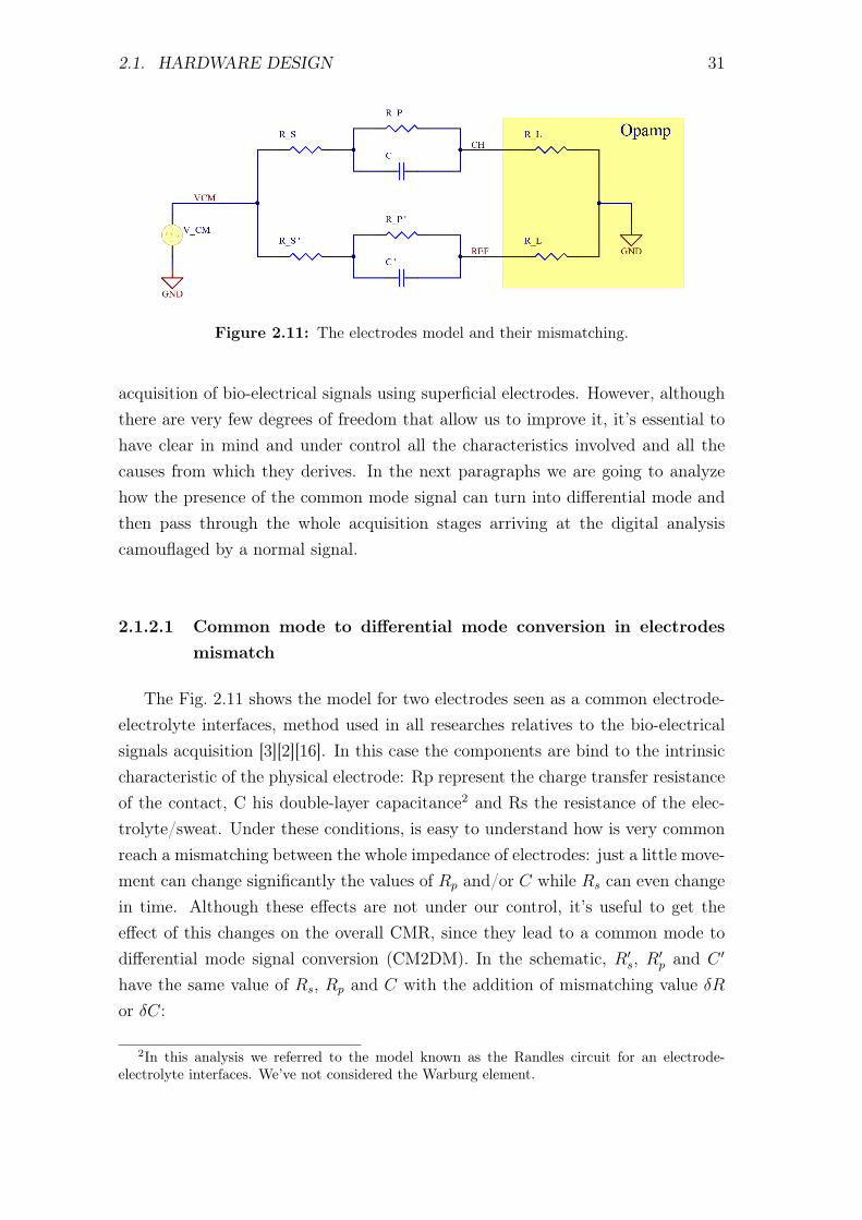
Figure 2.11: The electrodes model and their mismatching.
acquisition of bio-electrical signals using superficial electrodes. However, althoughthere are very few degrees of freedom that allow us to improve it, it’s essential tohave clear in mind and under control all the characteristics involved and all thecauses from which they derives. In the next paragraphs we are going to analyzehow the presence of the common mode signal can turn into differential mode andthen pass through the whole acquisition stages arriving at the digital analysiscamouflaged by a normal signal.
2.1.2.1 Common mode to differential mode conversion in electrodesmismatch
The Fig. 2.11 shows the model for two electrodes seen as a common electrode-electrolyte interfaces, method used in all researches relatives to the bio-electricalsignals acquisition [3][2][16]. In this case the components are bind to the intrinsiccharacteristic of the physical electrode: Rp represent the charge transfer resistanceof the contact, C his double-layer capacitance2 and Rs the resistance of the elec-trolyte/sweat. Under these conditions, is easy to understand how is very commonreach a mismatching between the whole impedance of electrodes: just a little move-ment can change significantly the values of Rp and/or C while Rs can even changein time. Although these effects are not under our control, it’s useful to get theeffect of this changes on the overall CMR, since they lead to a common mode todifferential mode signal conversion (CM2DM). In the schematic, R′
s, R′p and C ′
have the same value of Rs, Rp and C with the addition of mismatching value δRor δC:
2In this analysis we referred to the model known as the Randles circuit for an electrode-electrolyte interfaces. We’ve not considered the Warburg element.

32 CHAPTER 2. THE VEERG DESIGN: DEALS AND CHOICES
R′s = Rs + δR
R′p = Rp + δR
C ′ = C + δC
(2.22)
with δRR
and δCC
the entity of mismatching in percentage. For simplicity, thesevalues are the same in following analysis.
From the schematic in Fig. 2.11 we can find the relation
∣∣∣∣Vch1 − Vch2Vcm
∣∣∣∣ (ω) =
Rl
√ω4τ 4β2 (1 + E)2 + ω2τ 2
((γ (1 + E) + δ)2 − 2αβ (1 + E)
)+ α2√
ω4τ 4θ2 (1 + E)2 + 2ω2τ 2((φ (1 + E) + ρ)2 − 2ηθ (1 + E)
)+ η2
(2.23)
with
τ = RC
E =δR
R+δC
C
α =δR
R(Rs +Rp)
β =δR
RRs
γ =δR
RRs −Rp
δ =δR
R(Rs +Rp) +Rp
η = R2l +Rl
(2 +
δR
R
)(Rs +Rp) +
(1 +
δR
R
)(Rs +Rp)
2
θ = R2l +Rl
(2 +
δR
R
)Rs +
(1 +
δR
R
)R2s
ρ = R2l +Rl
((1 +
δR
R
)(Rs +Rp) +Rs
)+
(1 +
δR
R
)(R2s +RsRp
)φ = R2
l +Rl
((2 +
δR
R
)Rs +Rp
)+
(1 +
δR
R
)(R2s +RsRp
)
(2.24)
The 2.23 and the 2.24 describe the effect of these mismatches in the electrodeswhen they are feed by the same common signal: even if we perform the differencebetween the values on input channels (CH1 and CH2 in the Fig. 2.11), the common
2.1. HARDWARE DESIGN 33
signal remains as noise. The parameters values are: Rs = 4kΩ, Rp = 140kΩ,C = 180nF , Rl = 10MΩ and δR/R = 0.1 (10% tolerance). The analysis of 2.23gives us some important characteristics of this conversion from the common modeand the differential mode: the presence of two horizontal asymptotes for ω → 0
and ω → ∞, the first one of them represents the absolute maximum which couldhelp us to keep under control the CM2DM effect (Fig. 2.12). Its value is∣∣∣∣Vch − VrefVcm
∣∣∣∣ (ω → 0) = Rlα
η≈ δR
R
Rs +Rp
Rl
(2.25)
, while for ω →∞ we have∣∣∣∣Vch − VrefVcm
∣∣∣∣ (ω →∞) = Rlβ
θ≈ δR
R
Rs
Rl
(2.26)
.To complement the analysis of 2.23, the expressions of the two poles and two
zeros were found. The poles are at lower frequency respect the zeros, which canbecome complex conjugates depending on the values of the parameters involved,changing significantly the trend of the CM2DM in the frequencies domain. InFig. 2.12b we can see the effect of complex conjugates zeros. However, the presenceof the asymptotes remains for both ω → 0 and ω →∞, the first of which continuesto represent the absolute maximum. For the poles and for the zeros we found thefollowing expressions:
fp1 =Rl +Rs +Rp
2πRpC(Rl +Rs)(2.27)
fp2 =Rl + (Rs +Rp)(1 + δR
R)
2πRpC(1 + E)[Rl +Rs(1 + δRR
)](2.28)
fz1,z2 =−RpC(γ(1 + E) + δ)±
√R2pC
2(γ(1 + E) + δ)2 − 4R2pC
2(1 + E)βα
2πR2pC
2(1 + E)β(2.29)
.
2.1.2.2 Common mode to differential mode conversion in input stagesmismatch
Designing an input stage for analog pre-processing signals could represent aserious deal due to the odd to introduce additional noise, or unwanted new signals,which degrade the final S
Nratio of EEG information. Let’s take just for example
the choice to use an low-pass RC filter before the inputs of the ADC, like shown in
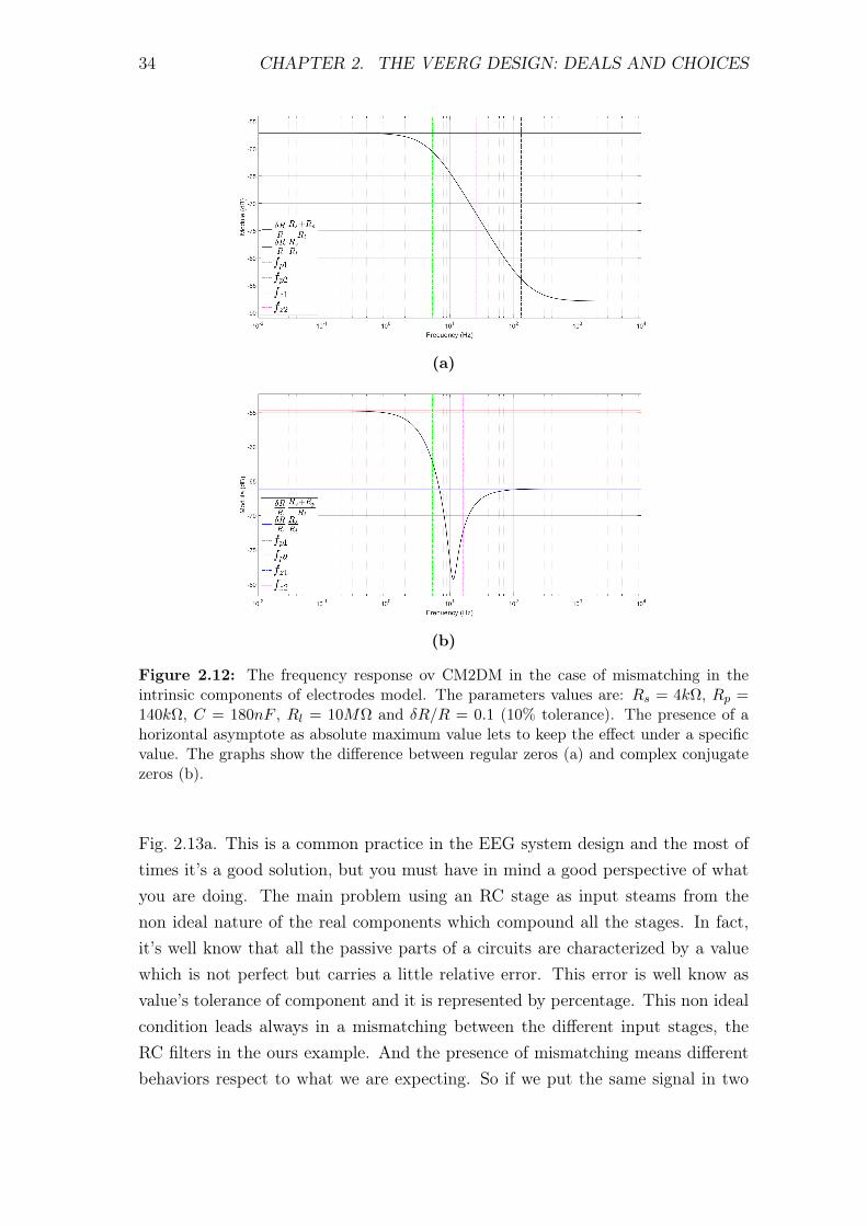
34 CHAPTER 2. THE VEERG DESIGN: DEALS AND CHOICES
(a)
(b)
Figure 2.12: The frequency response ov CM2DM in the case of mismatching in theintrinsic components of electrodes model. The parameters values are: Rs = 4kΩ, Rp =140kΩ, C = 180nF , Rl = 10MΩ and δR/R = 0.1 (10% tolerance). The presence of ahorizontal asymptote as absolute maximum value lets to keep the effect under a specificvalue. The graphs show the difference between regular zeros (a) and complex conjugatezeros (b).
Fig. 2.13a. This is a common practice in the EEG system design and the most oftimes it’s a good solution, but you must have in mind a good perspective of whatyou are doing. The main problem using an RC stage as input steams from thenon ideal nature of the real components which compound all the stages. In fact,it’s well know that all the passive parts of a circuits are characterized by a valuewhich is not perfect but carries a little relative error. This error is well know asvalue’s tolerance of component and it is represented by percentage. This non idealcondition leads always in a mismatching between the different input stages, theRC filters in the ours example. And the presence of mismatching means differentbehaviors respect to what we are expecting. So if we put the same signal in two
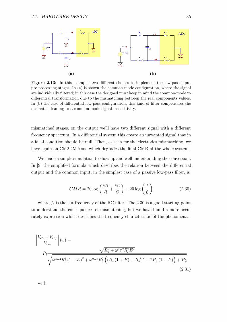
2.1. HARDWARE DESIGN 35
(a) (b)
Figure 2.13: In this example, two different choices to implement the low-pass inputpre-processing stages. In (a) is shown the common mode configuration, where the signalare individually filtered; in this case the designed must keep in mind the common-mode todifferential transformation due to the mismatching between the real components values.In (b) the case of differential low-pass configuration; this kind of filter compensates themismatch, leading to a common mode signal insensitivity.
mismatched stages, on the output we’ll have two different signal with a differentfrequency spectrum. In a differential system this create an unwanted signal that ina ideal condition should be null. Then, as seen for the electrodes mismatching, wehave again an CM2DM issue which degrades the final CMR of the whole system.
We made a simple simulation to show up and well understanding the conversion.In [9] the simplified formula which describes the relation between the differentialoutput and the common input, in the simplest case of a passive low-pass filter, is
CMR = 20 log
(δR
R+δC
C
)+ 20 log
(f
fc
)(2.30)
where fc is the cut frequency of the RC filter. The 2.30 is a good starting pointto understand the consequences of mismatching, but we have found a more accu-rately expression which describes the frequency characteristic of the phenomena:
∣∣∣∣Vch − VrefVcm
∣∣∣∣ (ω) =
Rl
√R2d + ω2τ 2R2
lE2√
ω4τ 4R4l (1 + E)2 + ω2τ 2R2
l
((Rs (1 + E) +Rs
′)2 − 2Rp (1 + E)
)+R2
p
(2.31)
with

36 CHAPTER 2. THE VEERG DESIGN: DEALS AND CHOICES
R′ = R + δR
C ′ = C + δC
τ = RC
E =δR
R+δC
C
Rs = R +Rl
R′s = R′ +Rl
Rd = R′s −Rs
Rp = R′sRS
(2.32)
.
Although the 2.31 could seems more complex and unclear, a deep analysis ofit leads to know some useful attribute of function. Taking a look to the graph inFig. 2.14 we can see the presence of an asymptote for ω → 0 with value∣∣∣∣Vch − VrefVcm
∣∣∣∣ (ω → 0) =Rl (Rs
′ −Rs)
Rs′Rs
(2.33)
and an absolute maximum for a frequency that we call ωmax,
ωmax ≈1√
τ 2 (1 + E)(2.34)
which help us to find the maximum value of module as∣∣∣∣Vch − VrefVcm
∣∣∣∣ (ωmax) ≈ E
E + 2(2.35)
.
These formulas allow to find the better components in order to keep the degra-dation of CMR under a specific limit. Keep in mind that the case described aboveis particular and simple but its easy for a designer to reach a worst condition sincethe complexity of the issue grows as much as the number of the passive compo-nents involved (adding an high-pass CR filter to the example should be enough tounderstand).
Fortunately, we can reduce this kind of problem since in the our case the ac-quisition is purely differential, that is every channels (the electrodes) is referred toone, the reference on ear lobe. The improvement comes with the use of filters in dif-ferential configuration (and so called differential filters); in Fig. 2.13b the low-passof these kind of filters is shown. The main differences between the common mode
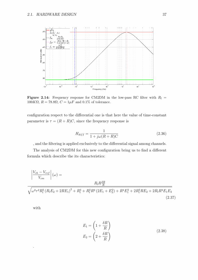
2.1. HARDWARE DESIGN 37
Figure 2.14: Frequency response for CM2DM in the low-pass RC filter with Rl =100KΩ, R = 78.8Ω, C = 1µF and 0.1% of tolerance.
configuration respect to the differential one is that here the value of time-constantparameter is τ = (R +R)C, since the frequency response is
Hdiff =1
1 + jω(R +R)C(2.36)
, and the filtering is applied exclusively to the differential signal among channels.
The analysis of CM2DM for this new configuration bring us to find a differentformula which describe the its characteristics:
∣∣∣∣Vch − VrefVcm
∣∣∣∣ (ω) =
RlRδRR√
ω2τ 2R2l (RlE2 + 2RE1)
2 +R4l +R2
lR2 (2E1 + E2
2) +R4E21 + 2R3
lRE2 + 2RlR3E1E2
(2.37)
with
E1 =
(1 +
δR
R
)E2 =
(2 +
δR
R
) (2.38)
.

38 CHAPTER 2. THE VEERG DESIGN: DEALS AND CHOICES
Figure 2.15: Frequency response for CM2DM in the differential low-pass RC filter withRl = 100KΩ, R = 78.8Ω, C = 1µF and 0.1% of tolerance.
In Fig. 2.15 the frequency response of the CM2DM shows again the presenceof an horizontal asymptote for ω → 0 as in the case of common mode filter config-uration, but now it represents even the maximum values reached:
∣∣∣∣Vch − VrefVcm
∣∣∣∣ (ω → 0) =RlR
δRR
R4l +R2
lR2 (2E1 + E2
2) +R4E21 + 2R3
lRE2 + 2RlR3E1E2
(2.39)
Comparing Fig. 2.14 with Fig. 2.15 we easily get the benefit using in our systemfilters in differential configuration, as the nature of acquisition lets us to do it.
2.1.2.3 Limits for stability
As said in Par 2.1.2, the CMR improvement requires a feedback in the systemand therefore an accurate analysis it’s necessary to ensure its stability. For thisreason, we had to break the loop before the active low-pass filter to be able tostudy the trend of open-loop gain A (active filter) and β gain (electrodes) in thefrequency domain. Rather than calculate the loop-gain Aβ to analyze the phasemargin, the simplest method to ensure the system’s stability is to look at the RateOf Closure (ROC) between the open-loop gain A and the 1/β curves: the stabilityis guaranteed when the ROC is less or equal to 20dB per decade, in the other caseinstability occurs. A look to Fig. 2.16 and Fig. 2.17 gives a first overview of theconcept.
The curve A and the curve 1/β respectively represent the transfer function of
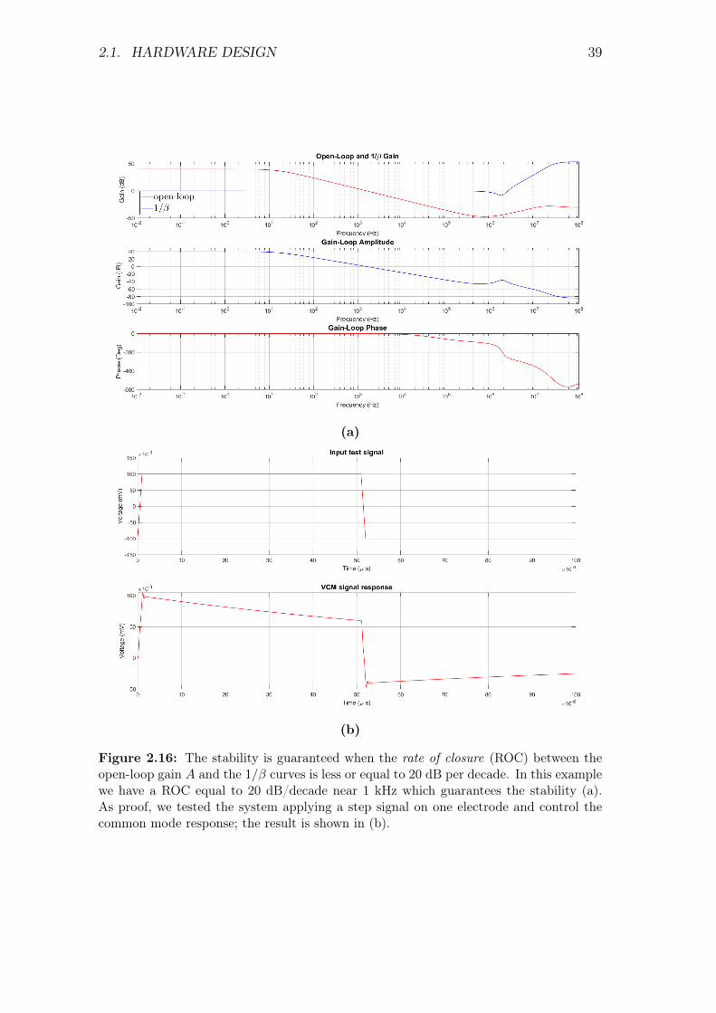
2.1. HARDWARE DESIGN 39
(a)
(b)
Figure 2.16: The stability is guaranteed when the rate of closure (ROC) between theopen-loop gain A and the 1/β curves is less or equal to 20 dB per decade. In this examplewe have a ROC equal to 20 dB/decade near 1 kHz which guarantees the stability (a).As proof, we tested the system applying a step signal on one electrode and control thecommon mode response; the result is shown in (b).
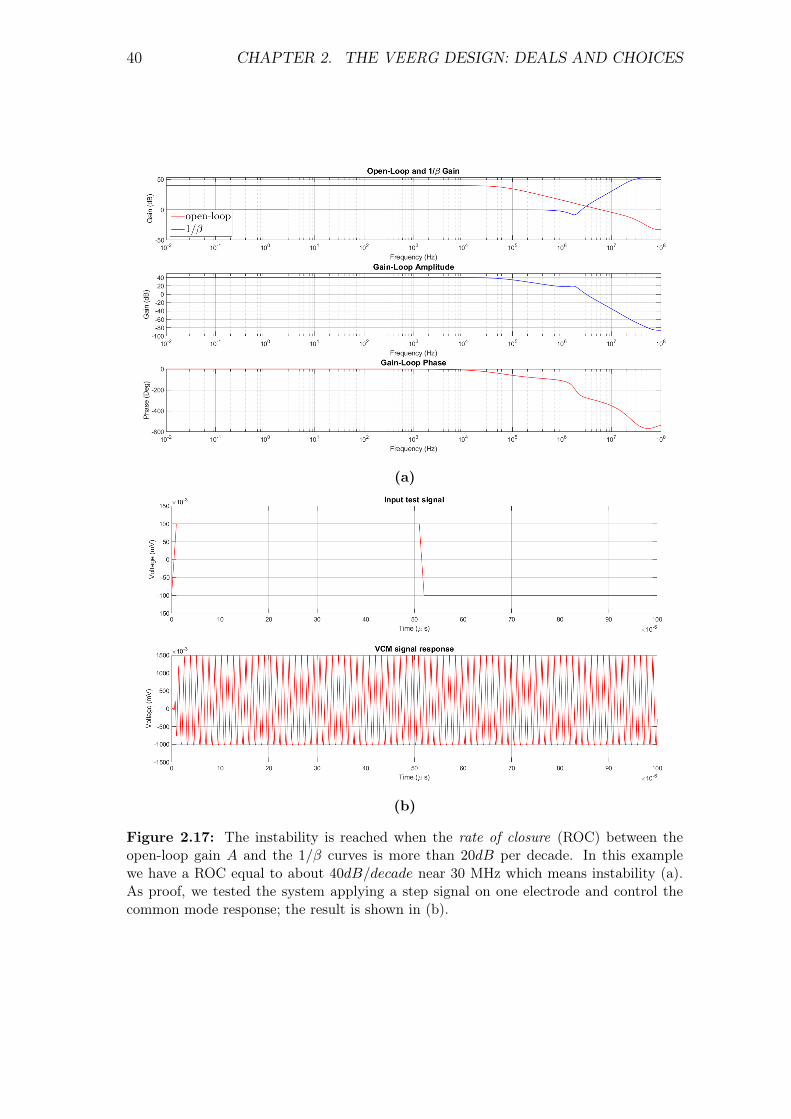
40 CHAPTER 2. THE VEERG DESIGN: DEALS AND CHOICES
(a)
(b)
Figure 2.17: The instability is reached when the rate of closure (ROC) between theopen-loop gain A and the 1/β curves is more than 20dB per decade. In this examplewe have a ROC equal to about 40dB/decade near 30 MHz which means instability (a).As proof, we tested the system applying a step signal on one electrode and control thecommon mode response; the result is shown in (b).
2.1. HARDWARE DESIGN 41
the low pass filter and the inverse of the transfer function of the FL electrode, i.e.the whole section from the filter output to the user body (skin/electrode interfaceincluded). In general, in the expression of the β curve should also come into playthe characteristics of paths relative to the electrodes of acquisition channels, whichtogether bring the common mode signal to the buffer (U8A in the schematic ofFig. 2.7), but in our case the most significant contributions end at the inputs ofthe operational amplifiers mounted the individual active electrodes. Thus, if wewant simplify, in the expression of β we will find only the input impedance valueof the active electrode (usually very high). Taking these concepts into account wefind the following expressions for A and β:
A(ω) = −ZfZi
(2.40)
β(ω) ≈ ZiopZiop + 2Ze + Zp
(2.41)
with
Zi = Ri
Zf =Rf
1 + jωRfCf
Ziop =Riop
1 + jωRiopCiop
Ze = Res +Relep
1 + jωRelepCelep
Zp = Rp
(2.42)
where Riop and Ciop represent the generic parallel of the input impedance ofelectrodes’ operational amplifier.
To study the stability of the system we must therefore analyze the character-istics of 2.40 and 2.41 and in particular their dominant poles. This is because theROC between A and 1/β necessarily depends on the relative position of their poles.To clarify the concept, we have to look at Fig. 2.18 in which the two curves arerepresented. As can be seen, the condition necessary for the ROC to not exceed20dB/decade is that the zero fzβ of the curve 1/β (which is nothing more than theβ pole3) is as far as possible from the point fA0dB where the curve A goes at 0dB,value that 1/β keeps constant until its zero fpβ, point from which it begins to rise.
We can therefore define useful relationships that allow us to keep these points
3The curve 1/β is the inverse of β, so in the transition the poles and zeros exchange roles.

42 CHAPTER 2. THE VEERG DESIGN: DEALS AND CHOICES
Figure 2.18: To study the stability of the system we must therefore analyze the char-acteristics of open-loop gain and the 1/β curves. In this simplified representation, thecondition necessary for the ROC to not exceed 20dB/decade is that the zero of the curve1/β is as far as possible from the point fA0dB where the curve A goes at 0dB.
far enough to guarantee stability. We express the values of fA0dB and fpβ:
fA0dB =1
2π
√G(0)2 − 1
τ 2(2.43)
with
G(0) =Rf
Ri
τ = RfCf
(2.44)
,
fpβ =Rt1 +Rt2 +
√[Rt1 −Rt2]2 − 4RepCeRiopCiopRepRiop
2RepCeRiopCiop(Rp + 2Res)(2.45)
with
Rt1 = RelepCelep(Rp + 2Reles +Riop)
Rt2 = RiopCiop(Rp + 2Relep + 2Reles)(2.46)
.
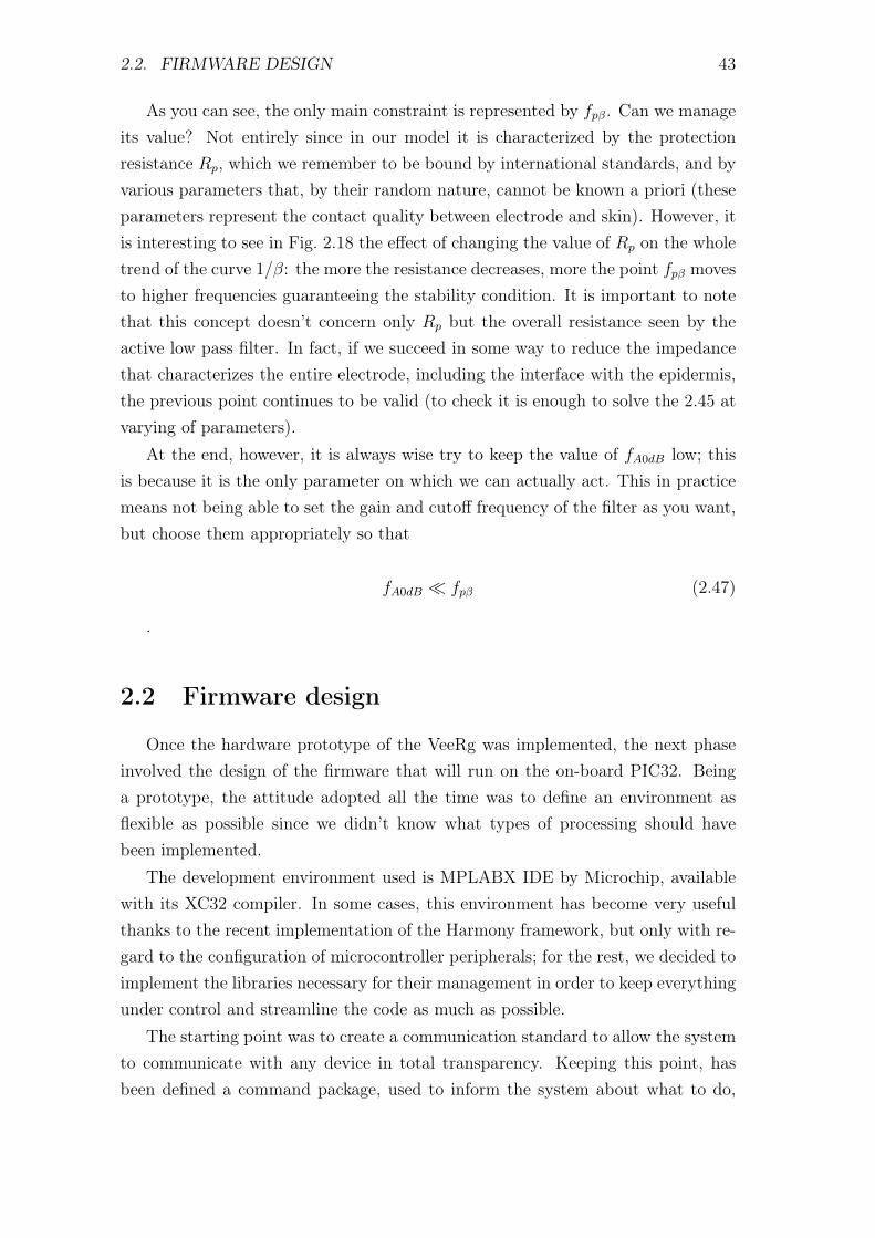
2.2. FIRMWARE DESIGN 43
As you can see, the only main constraint is represented by fpβ. Can we manageits value? Not entirely since in our model it is characterized by the protectionresistance Rp, which we remember to be bound by international standards, and byvarious parameters that, by their random nature, cannot be known a priori (theseparameters represent the contact quality between electrode and skin). However, itis interesting to see in Fig. 2.18 the effect of changing the value of Rp on the wholetrend of the curve 1/β: the more the resistance decreases, more the point fpβ movesto higher frequencies guaranteeing the stability condition. It is important to notethat this concept doesn’t concern only Rp but the overall resistance seen by theactive low pass filter. In fact, if we succeed in some way to reduce the impedancethat characterizes the entire electrode, including the interface with the epidermis,the previous point continues to be valid (to check it is enough to solve the 2.45 atvarying of parameters).
At the end, however, it is always wise try to keep the value of fA0dB low; thisis because it is the only parameter on which we can actually act. This in practicemeans not being able to set the gain and cutoff frequency of the filter as you want,but choose them appropriately so that
fA0dB fpβ (2.47)
.
2.2 Firmware design
Once the hardware prototype of the VeeRg was implemented, the next phaseinvolved the design of the firmware that will run on the on-board PIC32. Beinga prototype, the attitude adopted all the time was to define an environment asflexible as possible since we didn’t know what types of processing should havebeen implemented.
The development environment used is MPLABX IDE by Microchip, availablewith its XC32 compiler. In some cases, this environment has become very usefulthanks to the recent implementation of the Harmony framework, but only with re-gard to the configuration of microcontroller peripherals; for the rest, we decided toimplement the libraries necessary for their management in order to keep everythingunder control and streamline the code as much as possible.
The starting point was to create a communication standard to allow the systemto communicate with any device in total transparency. Keeping this point, hasbeen defined a command package, used to inform the system about what to do,
44 CHAPTER 2. THE VEERG DESIGN: DEALS AND CHOICES
(a)
(b)
Figure 2.19: The definition of data (a) and command (b) packets.
and a data package, used to send the acquisition data and the internal status ofthe VeeRg.
In Fig. 2.19 the two configurations of data (a) and command (b) packets areshown. The SOH, STX and ETX4 represent markers for check the correct trans-mission of information. These markers delimit the status bytes and data/commandbytes.
Once it has been defined the way in which the system communicates with theterminal connected to, the firmware has been developed from the lowest processinglevel, the one of the relevant drivers useful for the correct communication betweenthe peripheral devices and the microcontroller. In Fig. 2.20 we show the over-all structure of the implemented code, whose layered layout wants to underlinethe hierarchy of the libraries (every individual box) each developed for a partic-ular processing level that increases in complexity from the bottom towards up.The dashed boxes represent those functionalities implemented but which currentlyhave been disabled as not useful for the purposes of our work (in particular themanagement of the IMU and the AHRS system) or cause has yet to be optimized(the removal of eye’s artifacts); this means that their functionality it can be easily
4These elements have been borrowed from ASCII encoding and represent acronyms for StartOf Header (SOH), Start Of Text (SOT) and End Of Text (EOT).

2.2. FIRMWARE DESIGN 45
Figure 2.20: The overall structure of the implemented firmware with its layered layout tounderline the hierarchy of the libraries (every individual box) that increases in complexityfrom the bottom towards up.
rehabilitated simply by appropriately recompiling the source code and reloading iton the microcontroller.
Starting from the bottom level we have the functionality for the most basicprocesses, which means the communication drivers between microcontroller andexternal peripherals. During the hardware design phase we have chosen the inter-preters for USB and Bluetooth communication interfacing with the PIC32 throughthe UART serial standard, this the reason two separate serial drivers have beencreated for the independent management of the aforementioned communicationdevices. After them we have the driver that manages the exchange with A/DADS1299 front-end which uses the SPI standard and the driver for the managementof communication with the IMU MPU9250 through the use of the I2C standard(actually this device is disabled). Finally, for the sake of completeness, the libraryfor the management of the microcontroller’s I/O ports suitable for the controlsignals, such as the status LEDs or the activation of analog power supplies.
In the upper level we find the routines that allow the connection between theinterface drivers and the processing algorithms. Of particular interest, the statemachine used for decoding and managing the commands that the system receivesfrom the terminal (Command Manager in Fig. 2.20). During the decoding, thecontrol over the integrity of the command packet also occurs through the markersdescribed above; in the event that the system recognizes an anomaly in the struc-ture of the packet, it’s excluded waiting for the next one and setting an error flagto trace the error occurred. Regarding the data, a shared memory allocation wascreated and accessible from both the remaining levels (Data Manager in Fig. 2.20).This is basically a data structure in which are stored temporarily the raw data ofA/D conversion coming from the driver and also the subsequent results of their
46 CHAPTER 2. THE VEERG DESIGN: DEALS AND CHOICES
processing carried out by the upper level, which will then be collected and managedby the USB/Bluetooth communication drivers.
Finally, we find the most interesting and complex part that includes the effec-tive processing of signals, designed to clean up and prepare data for the subsequentprocessing on the connected terminal where the higher performances allow to per-form much more complex calculations and eventually extrapolate further additionalinformation. At the higher processing level we find all the algorithms that allowthe user to process the acquired data. In this context we enter the most interestingpart of the firmware design, as it relates to the particular choices made to try toextract the wanted information. It should be clear that this type of processing isnot strictly necessary for systems of this nature, but it has been considered usefulto give the user the possibility of reading already clean data, reducing the load ofdownstream processing. Such processing can therefore be enabled or disabled atthe discretion of the user simply by sending appropriate commands. The two mostimportant processes concerning the filtering will be described in more detail in thefollowing paragraphs. Regards the AHRS, we won’t deal with it in this work dueto its particular complexity and the non-strict correlation with the EEG systems;the reader can anyway find numerous articles about this argument, such as [35][28].
2.2.1 Filtering
In Par. 2.1.2 we mentioned the fact that analog input stages placed close thefront-end ADS1299 are substantially first order RC low-pass filters; this base con-figuration helps to eliminate all the high-frequency disturbances beforehand andit doesn’t represent a definitive solution at all. This is a pre-filtering phase whichdoes not affect the useless signals in any way. Moreover, depending also on the ap-plications in which the EEG system will be used, filter the signals permanently inan analogical way before the conversion does not appear to be a functional choicesince the signals in their raw form can be useful to apply on them different typesof analysis at a later stage. However, the adoption of a digital post-conversion pro-cessing is the optimal solution for a system which requires as much as flexibility aspossible.
As we explained in Chap. 1, we are interested in the band between the ∼4Hz and the ∼80 Hz composed by theta, alpha, beta e gamma waves. The finalobjective of the filtering is to reduce as much as possible the signal-to-noise ratiocutting all the disturbances which don’t fit with the band of our interest. Froman energy point of view, the most heavy disturbances are those at low frequencies,
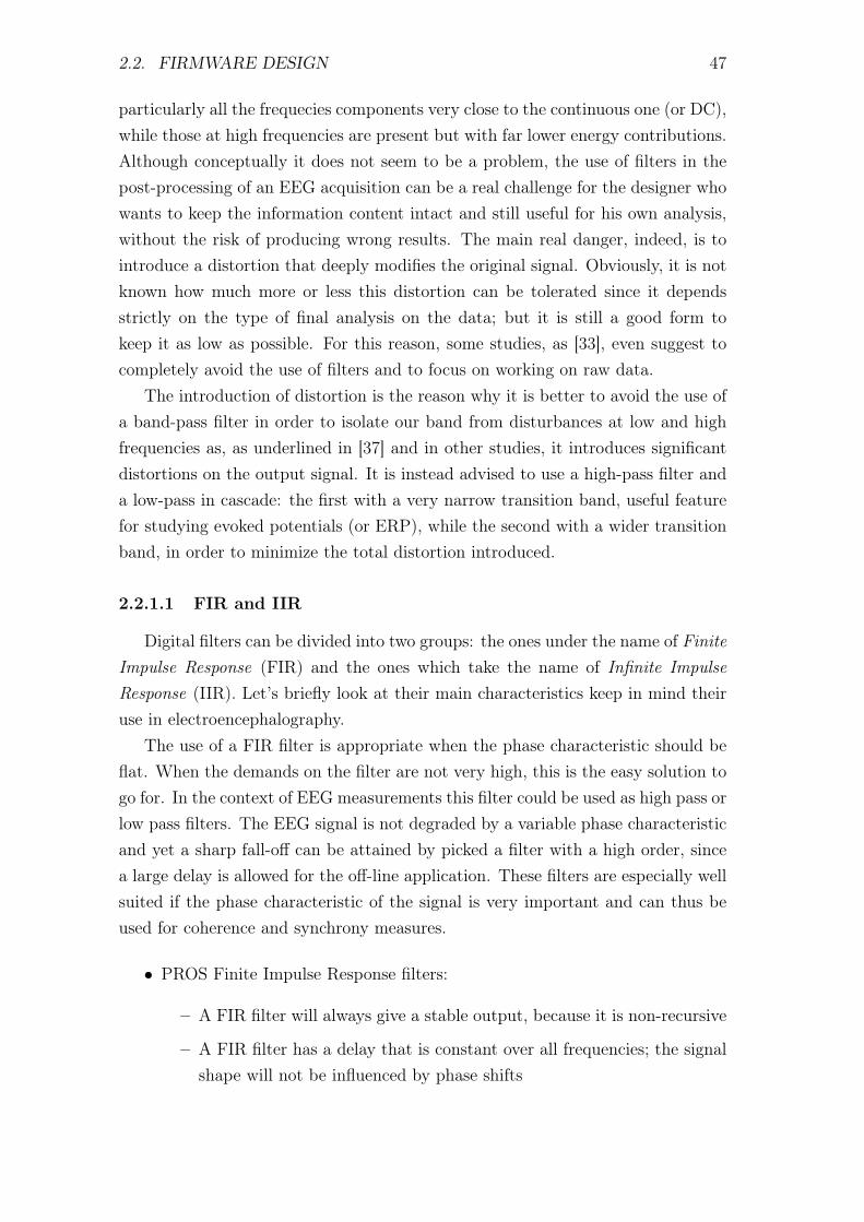
2.2. FIRMWARE DESIGN 47
particularly all the frequecies components very close to the continuous one (or DC),while those at high frequencies are present but with far lower energy contributions.Although conceptually it does not seem to be a problem, the use of filters in thepost-processing of an EEG acquisition can be a real challenge for the designer whowants to keep the information content intact and still useful for his own analysis,without the risk of producing wrong results. The main real danger, indeed, is tointroduce a distortion that deeply modifies the original signal. Obviously, it is notknown how much more or less this distortion can be tolerated since it dependsstrictly on the type of final analysis on the data; but it is still a good form tokeep it as low as possible. For this reason, some studies, as [33], even suggest tocompletely avoid the use of filters and to focus on working on raw data.
The introduction of distortion is the reason why it is better to avoid the use ofa band-pass filter in order to isolate our band from disturbances at low and highfrequencies as, as underlined in [37] and in other studies, it introduces significantdistortions on the output signal. It is instead advised to use a high-pass filter anda low-pass in cascade: the first with a very narrow transition band, useful featurefor studying evoked potentials (or ERP), while the second with a wider transitionband, in order to minimize the total distortion introduced.
2.2.1.1 FIR and IIR
Digital filters can be divided into two groups: the ones under the name of FiniteImpulse Response (FIR) and the ones which take the name of Infinite ImpulseResponse (IIR). Let’s briefly look at their main characteristics keep in mind theiruse in electroencephalography.
The use of a FIR filter is appropriate when the phase characteristic should beflat. When the demands on the filter are not very high, this is the easy solution togo for. In the context of EEG measurements this filter could be used as high pass orlow pass filters. The EEG signal is not degraded by a variable phase characteristicand yet a sharp fall-off can be attained by picked a filter with a high order, sincea large delay is allowed for the off-line application. These filters are especially wellsuited if the phase characteristic of the signal is very important and can thus beused for coherence and synchrony measures.
• PROS Finite Impulse Response filters:
– A FIR filter will always give a stable output, because it is non-recursive
– A FIR filter has a delay that is constant over all frequencies; the signalshape will not be influenced by phase shifts
48 CHAPTER 2. THE VEERG DESIGN: DEALS AND CHOICES
• CONS Finite Impulse Response filters:
– A FIR filter is inefficient, it uses lots of input to calculate the output,therefore:
– A FIR filter has a large delay
The use of an IIR filter is appropriate when, a small absolute delay is requiredor when strong requirements on amplitude characteristic are necessary. Wherethere is only one type of FIR filter, there are several types of IIR filters.
• PROS Infinite Impulse Response filters:
– An IIR filter is very efficient, it uses only a few previous output valuesto calculate the current output, therefore:
– An IIR filter has only a small delay
• CONS Infinite Impulse Response filters:
– An IIR filter can become unstable, if coefficients are not well chosen
– Because the requirement of causality and an infinite impulse responsethat converges to 0 for n → ∞, the impulse response cannot be sym-metrical. This implies a phase characteristic that is not constant overfrequencies. Therefore, different frequencies will appear at the outputwith a different shift in phase. The shape of the output signal willchange as a consequence of different phase shifts
The three most common IIR filters are the Butterworth, the Chebyshev andthe Elliptic, and everyone has a specific characteristic for specific contexts.
The use of a Butterworth IIR filter is appropriate when a maximally flat pass-and stop-bands are important, when less stringent restrictions on fall-off and phasecharacteristics are allowed. Choice to put emphasis on fall-off or phase characteris-tics can be tuned by choosing an appropriate filter order. The phase characteristicof a Butterworth filter is poor, therefore synchrony or other phase related analysisare not recommended with this filter. An example of the use of Butterworth filtersin EEG would be an on-line EEG frequency band analysis (theta, gamma, alpha,etc). The pass- and stop-bands are maximally flat, thus resulting in a qualityoutput signal for the different frequency bands. Furthermore, a reasonably sharpfall-off can be reached. Care has to be taken in selecting the correct trade-offbetween fall-off and phase characteristic.

2.2. FIRMWARE DESIGN 49
The use of a Chebyshev IIR filter is appropriate when some ripple in the pass-band is allowed and more emphasis is placed on good stop-band behavior andfall-off. The phase characteristic of a Chebyshev filter is poor. The use of thisfilter is recommended with intermediate frequency ranges e.g. alpha 1 vs. alpha 2.
The use of an elliptic IIR filter is appropriate when the fall-off is the verycritical design criterion. The sensori-motor rythm (SMR) is a good example ofsuch a critical design criterion. The SMR is a very specific rhythm of 12-14 Hz.For a quantification of the SMR –and only the SMR– a very narrow frequencyband has to remain at the filter output, thus implying a very steep fall-off. Somewaveform degradation has to be accepted (ripple, phase characteristic) to attainthis sharp fall-off, but this is a small price to pay knowing that you analyze a truesensor-motor rhythm.
From this brief overview of the main differences between the FIR and IIRfilters, we can already make choices for our system. Bearing in mind the limitedprocessing and memory resources made available by our system: in [19] we canread that the PIC32MZ0512EFE064 in use has a maximum frequency of 200 MHzand a volatile data memory of 128 KB. These values are completely acceptable forthe vast majority of applications but can become a limitation as soon as we dealwith operations which involves a large amount of data. From this point of viewthe FIR filters can easily represent a problem if their order is very high (as oftenhappens with particularly selective filters); with the same frequency characteristics,the IIR filters certainly represent a more suitable solution thanks to their lowercomputational weight. We can take as example the implementation of a high-passfilter designed through the MATLAB application Filter Designer. In Fig. 2.21are shown the characteristics that can be set for the generation of the filter’scoefficients. Fixed Astop = 80dB, Apass = 1dB, Fstop = 3Hz and Fpass = 4Hz, theimplementation of a FIR Equiripple filter generates 687 floating point coefficientswhile for a IIR Butterwhort filter requires only 126 5. Considering that inside theprogram they become 4-byte floating-point numbers, it will be occupied a space of2744 and 504 bytes respectively. This without any temporary variables used duringcode execution and only for one channel: in our particular case, using 8 channelsand considering also the space occupied by the past values, necessary during theFIR execution, we easily arrive at about 45 KB of memory occupied only for thehigh-pass filtering.
Furthermore, in addition to a computational and memory’s occupation advan-
5In the case of IIR filter, are used sections of the second-order which provide three coefficientsto the numerator, three to the denominator and one factor of correction. For the implementationof the code see App. A.2.1
50 CHAPTER 2. THE VEERG DESIGN: DEALS AND CHOICES
Figure 2.21: The characteristic of an high-pass filter as shown in the MATLAB’s appFilter Designer.
tage, IIR filters have less delay, making them particularly suitable for real-timeapplications, as in our case. Always referring to the example above, we can assumethat the response of an IIR filter is almost immediate while the FIR filter presentsa delay in the response of about 1.4 seconds. The only sore point regarding theuse of IIR filters is that their phase is non-linear with respect of the frequencies.This means having a greater distortion on the output signal than in some cases,depending on the types of analysis, it can represent a crucial issue. As far as weare concerned, we considered this defect less relevant since our initial intention isto analyze exclusively the Power Spectral Density (PSD) of the acquired signals,an analysis which takes in consideration only the amplitude of the frequency com-ponents. However, it is good to keep in mind that, in case of switching into ananalysis in the time domain, the use of IIR filters could be a problem if their phasein the passband is not monitored.
2.2.1.2 The high-pass filter
We have seen how the IIR are the most suitable filters for our system thanks totheir characteristics which are perfectly suited to a real-time acquisition. At thispoint, it became important to choose between the three main categories of IIR:Butterworth, Chebyshev and Elliptical. Due to their characteristics, the most usedare the Butterworth filters, because of their flat trend in the pass-band, and theElliptical filters which have a narrow transition band and a limited ripple in thepass-band. These characteristics of the Elliptical filter make it a perfect candidateto implement the high-pass filter, able to eliminate the low frequencies close tothe DC component and trying at the same time to keep intact those following,which can convey useful information. However, as we will see in the Par. 2.2.1.3,
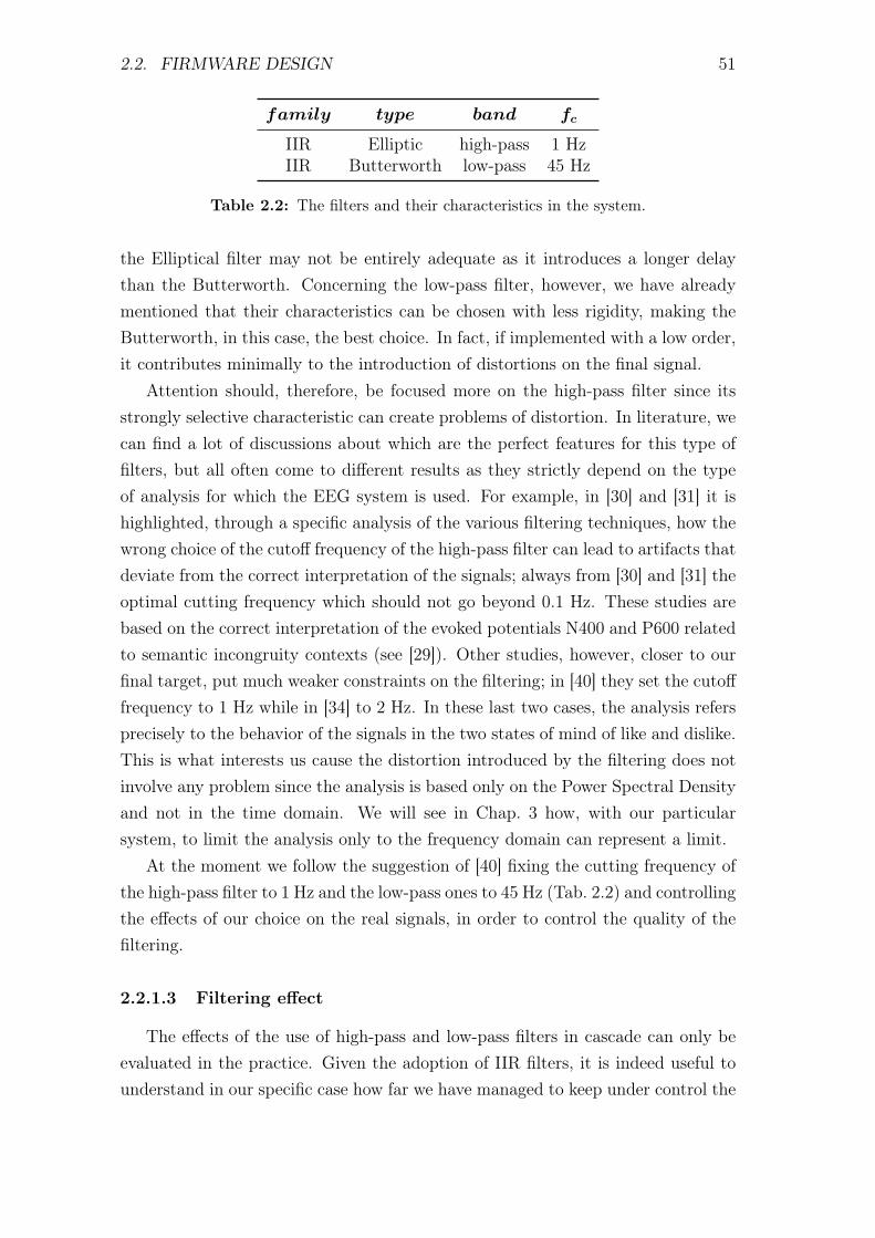
2.2. FIRMWARE DESIGN 51
family type band fc
IIR Elliptic high-pass 1 HzIIR Butterworth low-pass 45 Hz
Table 2.2: The filters and their characteristics in the system.
the Elliptical filter may not be entirely adequate as it introduces a longer delaythan the Butterworth. Concerning the low-pass filter, however, we have alreadymentioned that their characteristics can be chosen with less rigidity, making theButterworth, in this case, the best choice. In fact, if implemented with a low order,it contributes minimally to the introduction of distortions on the final signal.
Attention should, therefore, be focused more on the high-pass filter since itsstrongly selective characteristic can create problems of distortion. In literature, wecan find a lot of discussions about which are the perfect features for this type offilters, but all often come to different results as they strictly depend on the typeof analysis for which the EEG system is used. For example, in [30] and [31] it ishighlighted, through a specific analysis of the various filtering techniques, how thewrong choice of the cutoff frequency of the high-pass filter can lead to artifacts thatdeviate from the correct interpretation of the signals; always from [30] and [31] theoptimal cutting frequency which should not go beyond 0.1 Hz. These studies arebased on the correct interpretation of the evoked potentials N400 and P600 relatedto semantic incongruity contexts (see [29]). Other studies, however, closer to ourfinal target, put much weaker constraints on the filtering; in [40] they set the cutofffrequency to 1 Hz while in [34] to 2 Hz. In these last two cases, the analysis refersprecisely to the behavior of the signals in the two states of mind of like and dislike.This is what interests us cause the distortion introduced by the filtering does notinvolve any problem since the analysis is based only on the Power Spectral Densityand not in the time domain. We will see in Chap. 3 how, with our particularsystem, to limit the analysis only to the frequency domain can represent a limit.
At the moment we follow the suggestion of [40] fixing the cutting frequency ofthe high-pass filter to 1 Hz and the low-pass ones to 45 Hz (Tab. 2.2) and controllingthe effects of our choice on the real signals, in order to control the quality of thefiltering.
2.2.1.3 Filtering effect
The effects of the use of high-pass and low-pass filters in cascade can only beevaluated in the practice. Given the adoption of IIR filters, it is indeed useful tounderstand in our specific case how far we have managed to keep under control the
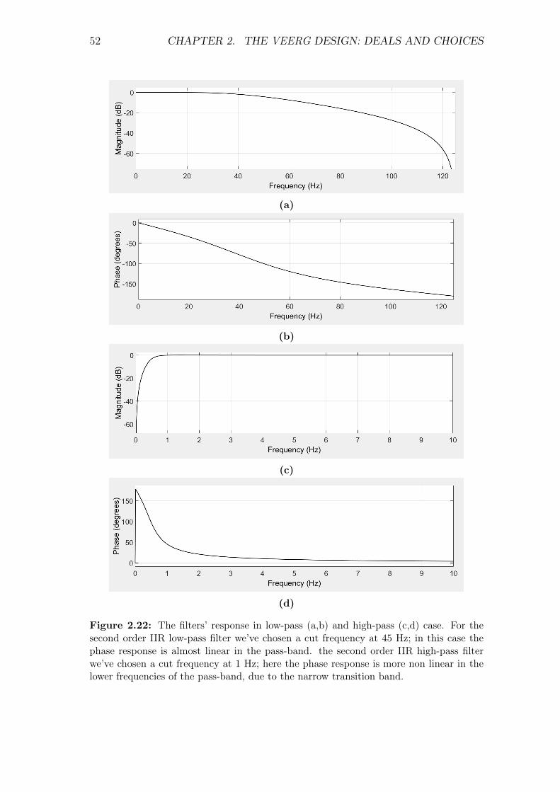
52 CHAPTER 2. THE VEERG DESIGN: DEALS AND CHOICES
(a)
(b)
(c)
(d)
Figure 2.22: The filters’ response in low-pass (a,b) and high-pass (c,d) case. For thesecond order IIR low-pass filter we’ve chosen a cut frequency at 45 Hz; in this case thephase response is almost linear in the pass-band. the second order IIR high-pass filterwe’ve chosen a cut frequency at 1 Hz; here the phase response is more non linear in thelower frequencies of the pass-band, due to the narrow transition band.
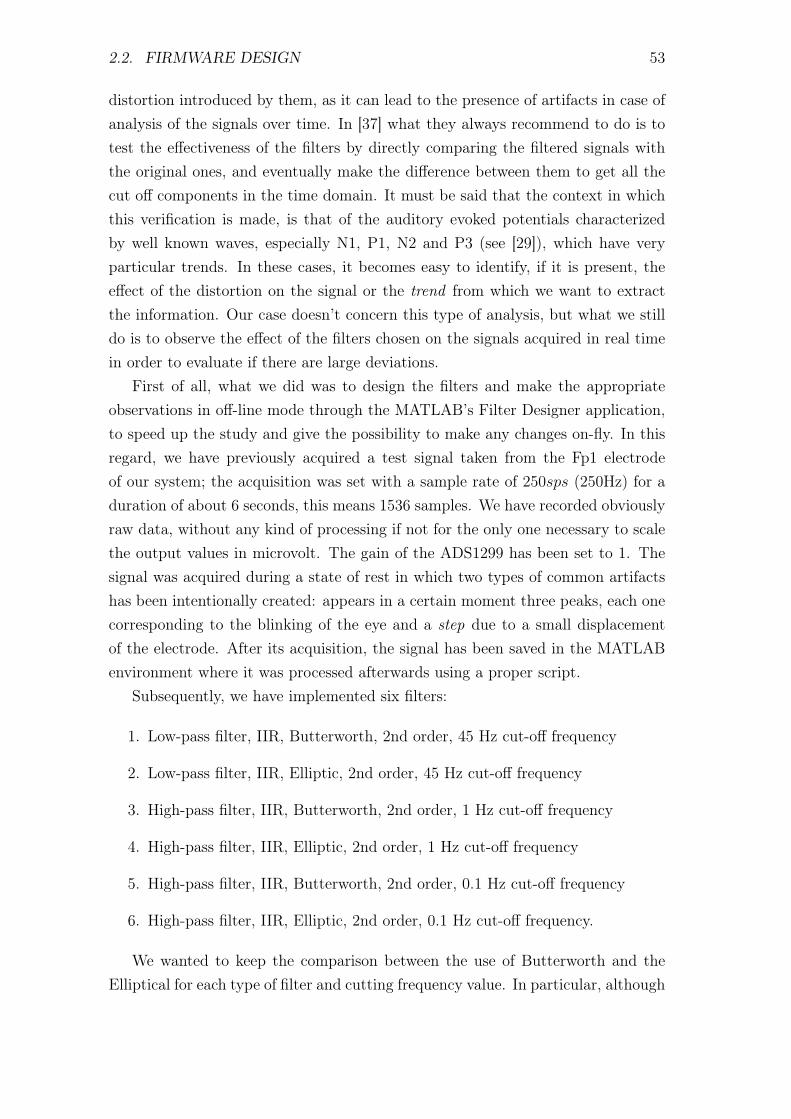
2.2. FIRMWARE DESIGN 53
distortion introduced by them, as it can lead to the presence of artifacts in case ofanalysis of the signals over time. In [37] what they always recommend to do is totest the effectiveness of the filters by directly comparing the filtered signals withthe original ones, and eventually make the difference between them to get all thecut off components in the time domain. It must be said that the context in whichthis verification is made, is that of the auditory evoked potentials characterizedby well known waves, especially N1, P1, N2 and P3 (see [29]), which have veryparticular trends. In these cases, it becomes easy to identify, if it is present, theeffect of the distortion on the signal or the trend from which we want to extractthe information. Our case doesn’t concern this type of analysis, but what we stilldo is to observe the effect of the filters chosen on the signals acquired in real timein order to evaluate if there are large deviations.
First of all, what we did was to design the filters and make the appropriateobservations in off-line mode through the MATLAB’s Filter Designer application,to speed up the study and give the possibility to make any changes on-fly. In thisregard, we have previously acquired a test signal taken from the Fp1 electrodeof our system; the acquisition was set with a sample rate of 250sps (250Hz) for aduration of about 6 seconds, this means 1536 samples. We have recorded obviouslyraw data, without any kind of processing if not for the only one necessary to scalethe output values in microvolt. The gain of the ADS1299 has been set to 1. Thesignal was acquired during a state of rest in which two types of common artifactshas been intentionally created: appears in a certain moment three peaks, each onecorresponding to the blinking of the eye and a step due to a small displacementof the electrode. After its acquisition, the signal has been saved in the MATLABenvironment where it was processed afterwards using a proper script.
Subsequently, we have implemented six filters:
1. Low-pass filter, IIR, Butterworth, 2nd order, 45 Hz cut-off frequency
2. Low-pass filter, IIR, Elliptic, 2nd order, 45 Hz cut-off frequency
3. High-pass filter, IIR, Butterworth, 2nd order, 1 Hz cut-off frequency
4. High-pass filter, IIR, Elliptic, 2nd order, 1 Hz cut-off frequency
5. High-pass filter, IIR, Butterworth, 2nd order, 0.1 Hz cut-off frequency
6. High-pass filter, IIR, Elliptic, 2nd order, 0.1 Hz cut-off frequency.
We wanted to keep the comparison between the use of Butterworth and theElliptical for each type of filter and cutting frequency value. In particular, although

54 CHAPTER 2. THE VEERG DESIGN: DEALS AND CHOICES
(a)(b
)
(c)(d
)
Figu
re2.23:
The
low-pass
filtereffects.
Itintroduces
avery
lowdistortion
with
apractically
nulldelay.Wecan
verifythis
bothon
theGaussian
testsignal(a)
andon
therealtest
(c)where
theoutputs
overlap;also
observingin
(b)and
(c)wecan
confirmthe
actuallowdistortion.
The
amplitude
oftheoscillations,indeed,is
anindication
oftheam
ountofdistortion
introduced:the
greaterthe
amplitude,the
greaterwillbe
thedistortion.
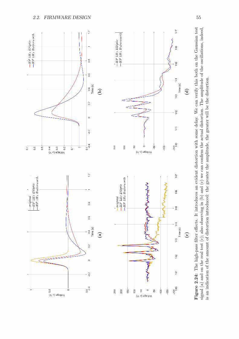
2.2. FIRMWARE DESIGN 55
(a)
(b)
(c)
(d)
Fig
ure
2.24
:The
high
-passfiltereff
ects.It
introd
uces
anevidentdistortion
withsomede
lay.
Wecanverify
this
both
ontheGau
ssiantest
sign
al(a)an
don
thereal
test
(c);also
observingin
(b)an
d(c)wecanconfi
rmtheactual
distortion
.The
amplitud
eof
theoscilla
tion
s,inde
ed,
isan
indication
oftheam
ount
ofdistortion
introd
uced
:thegreatertheam
plitud
e,thegreaterwill
bethedistortion
.
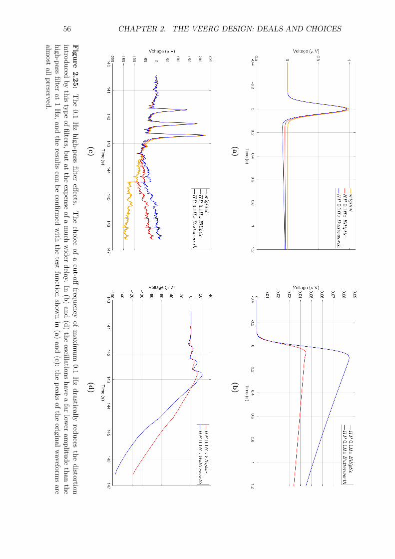
56 CHAPTER 2. THE VEERG DESIGN: DEALS AND CHOICES
(a)(b
)
(c)(d
)
Figu
re2.25:
The
0.1Hzhigh-pass
filtereffects.
The
choiceof
acut-off
frequencyof
maxim
um0.1
Hzdrastically
reducesthe
distortionintroduced
bythis
typeoffilters,but
atthe
expenseofa
much
wider
delay.In
(b)and
(d)the
oscillationshave
afar
lower
amplitude
thanthe
high-passfilter
at1Hz,and
theresults
canbe
confirmed
with
thetest
functionshow
nin
(a)and
(c):the
peaksof
theoriginalw
aveformsare
almost
allpreserved.

2.2. FIRMWARE DESIGN 57
we are convinced about putting the cutoff frequency of the high-pass filters at 1Hz, in any case, we wanted to test the effectiveness of the same filters with a cutofffrequency of 0.1 Hz, as suggested by [17] and [30].
The results of the six elaborations are grouped in Fig. 2.23, Fig. 2.24 andFig. 2.25. For each elaboration, we illustrated a specific cut-off frequency and itscomparison between the use of the Butterworth and the Elliptical. In the boxes(a) and (b) there are the effects of the filters on the Gaussian test signal, which iscommonly used for this purpose due to its large spectral component; in this way, itis easier to consider the distortions and the delays introduced by the filters. In (a)are simply compared the outputs of the two filters with the original input signal,while in (b) it is made the difference between them in order to get an idea of thefiltered components, of the delays and, in general, of the distortions introduced.
The first to be examined is the low-pass filter (Fig. 2.23). From the functionalpoint of view, it is the most efficient because it introduces a very low distortionwith a practically null delay. We can verify this both on the Gaussian test sig-nal (Fig. 2.23a) and on the real test (Fig. 2.23c) where the outputs overlap; alsoobserving in Fig. 2.23b and Fig. 2.23d we can confirm the actual low distortionhaving already observed the almost null entity of the heavy variations in the aver-age trend of the curves. The amplitude of the oscillations, indeed, is an indicationof the amount of distortion introduced: the greater the amplitude, the greater willbe the distortion. The use of this filter, therefore, does not affect the final qualityof the signal 6.
The second filter analyzed is the high-pass with a cut-off frequency at 1 Hz(Fig. 2.24). Here the distortion is certainly more evident and we can immediatelynotice it from the filter response to the Gaussian test signal in Fig. 2.24a. It isevident that the amplitude of the signal is considerably reduced provoking also anunder-shoot which was not present originally, gradually stabilizing with a delay thatdiffers according to the type of filter under examination. Indeed, we can observeconsiderable differences between the Butterworth and the Elliptical response. Inthe first one, although it has a lower delay, the distortion is visibly greater asconfirmed in Fig. 2.24b. Also in the case of the real-time continuous signal, itwould seem to have better characteristics considering how much time the signaltakes to return to its originally state, but things changes as soon as we consider thedistortion, since in Fig. 2.24d the oscillations in the Butterworth gap are wider.Starting from these considerations, the Elliptical filter has got a less significant
6The fact that the low-pass does not contribute to the distortion of the signal is given by itscharacteristic of being only second-order, which means a very low selectivity but still adequatefor our purpose.

58 CHAPTER 2. THE VEERG DESIGN: DEALS AND CHOICES
distorting characteristic than its competitor, to the detriment of a little largerdelay. It is precisely this compromise which got us choosing the Elliptical filter forour system.
The third and last filter we are analyzing here is the high-pass filter with acut-off frequency at 0.1 Hz (Fig. 2.25). This filter has been tested to clarify andconfirm what has been shown in [17] and [30] and effectively, without explain whythis value, the choice of a cut-off frequency of maximum 0.1 Hz drastically reducesthe distortion introduced, but at the expense of a much wider delay. In Fig. 2.25band Fig. 2.25d the oscillations have a far lower amplitude than the high-pass filterat 1 Hz, and the results can be confirmed with the test function shown in Fig. 2.25aand Fig. 2.25c: the peaks of the original waveforms are almost all preserved.
It has to be clear that the observations just made upon the filters we havechosen, do not lead to a precise confirmation about which is the best filter, butnevertheless we can have an idea of which filter is more appropriate to be used forthis analysis. We must always keep clarity about which is the information we wantto extract from the acquired signals. In our case, considering that it is the creationof a prototype, it would be ideal to give to the user the possibility to choose real-time which type of filter and characteristics he would like to adopt; which wouldnot be a problem if the processing would take place on the terminal, but couldbecome a problem if we would think about giving in charge of it to the on-boardmicrocontroller, so that it would be more decisive an optimization of the code andoccupation of memory.
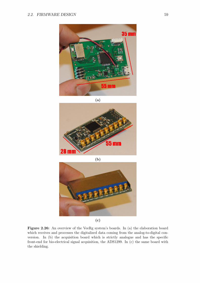
2.2. FIRMWARE DESIGN 59
(a)
(b)
(c)
Figure 2.26: An overview of the VeeRg system’s boards. In (a) the elaboration boardwhich receives and processes the digitalized data coming from the analog-to-digital con-version. In (b) the acquisition board which is strictly analogue and has the specificfront-end for bio-electrical signal acquisition, the ADS1299. In (c) the same board withthe shielding.

60 CHAPTER 2. THE VEERG DESIGN: DEALS AND CHOICES
(a)
(b)
Figure 2.27: An overview of the VeeRg prototype. In (a) the frontal side and in (b) theback side. The black clip is for the earlobe reference.

Chapter 3
Like and dislike recognition
For decades the interest of the research to identify and recognize the emotionalstates has always been high. So much so that over time we have been consolidat-ing a branch of inter-disciplinary research that sees psychologists, neuroscientists,researchers of artificial intelligence, scholars of cognitive processes, etc. strugglingwith the analysis of all those processes that can objectively determine the moodof a person. The reason for this interest is inherent in its vast field of applicationthat can range from pure commercial entertainment to the medical rehabilitation.
We can distinguish two main methodologies in the recognition of emotions. Thefirst provides that the analysis is done on non-physiological signals such as facialexpression or modulation of the vocal tone. This method proved to be the simplestto apply because it did not include the use of particularly complex instrumentationand data processing, at least until today where the current technology allows us toperform advanced analysis on video images. Its main problem, however, is given bythe ambiguous facial expressions, easily controllable or not evaluable due to deficitssuch as paralysis. The second methodology for the recognition of emotions, on theother hand, is based on the analysis of the physiological signals coming from theinner part of our body and therefore apparently hidden from the outside. Thesesignals are acquired through the use of techniques that have long been the exclusiveheritage of medicine: the electroencephalogram (EEG) which allows the reading ofbrain activity in the form of variable electrical potentials, electromyography (EMG)that monitors and transforms the activity of the muscles still into electrical po-tentials, the electrocardiogram (ECG) that records the pattern of cardiac activity,the resistance of the skin (SR), the blood pressure and so on. It is importantto underline that many studies relative the field of the emotion recognition use amethodology that is nothing but the fusion of the two described above, but arecharacterized by a very high systematic and computational complexity required
61

62 CHAPTER 3. LIKE AND DISLIKE RECOGNITION
Figure 3.1: This is an example of the bi-dimensional emotional space defined by thearousal and valence values and described in [39].
only for very advanced analysis. Currently the methodology that uses only physio-logical signals is the one on which the attention of the greater part of the researchcommunity is being focused. The reason is mainly due to the strong diffusion ofelectroencephalographic systems on the market that, if properly designed, can alsoact as electromyographic systems. The fact that they have become the most usedacquisition devices is due, however, not only to their low market price, but alsoto the fact that electroencephalographic systems have a high degree of practicalitygiven their non-invasive characteristics. The possibility of acquiring brain signalsthrough the use of surface dry electrodes placed on the epidermis (or in some caseseven through contact-less capacitive electrodes) obtaining a good temporal andspatial resolution is the key to these systems.
Another very controversial subject concerns the way in which emotions canbe described. There are two possible points of view: the discrete one and thedimensional one. Discreet classification is based on the fact that emotions canbe seen as combinations of discrete and well-defined moods. Foe example in [22]are defined anger, fear, sadness, disgust, surprise, expectation, acceptance and joy.In [5] are shown the relationships between facial expression and emotion renderedby anger, disgust, fear, happiness, sadness and surprise. The dimensional pointof view in the classification of emotions is the one that is usually used startingfrom a two-dimensional space: two concepts are used, the valence that represents
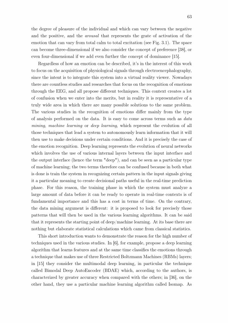
63
the degree of pleasure of the individual and which can vary between the negativeand the positive, and the arousal that represents the grate of activation of theemotion that can vary from total calm to total excitation (see Fig. 3.1). The spacecan become three-dimensional if we also consider the concept of preference [38], oreven four-dimensional if we add even further the concept of dominance [15].
Regardless of how an emotion can be described, it’s in the interest of this workto focus on the acquisition of physiological signals through electroencephalography,since the intent is to integrate this system into a virtual reality viewer. Nowadaysthere are countless studies and researches that focus on the recognition of emotionsthrough the EEG, and all propose different techniques. This context creates a lotof confusion when we enter into the merits, but in reality it is representative of atruly wide area in which there are many possible solutions to the same problem.The various studies in the recognition of emotions differ mainly from the typeof analysis performed on the data. It is easy to come across terms such as datamining, machine learning or deep learning, which represent the evolution of allthose techniques that lead a system to autonomously learn information that it willthen use to make decisions under certain conditions. And it is precisely the case ofthe emotion recognition. Deep learning represents the evolution of neural networkswhich involves the use of various internal layers between the input interface andthe output interface (hence the term "deep"), and can be seen as a particular typeof machine learning; the two terms therefore can be confused because in both whatis done is train the system in recognizing certain pattern in the input signals givingit a particular meaning to create decisional paths useful in the real-time predictionphase. For this reason, the training phase in which the system must analyze alarge amount of data before it can be ready to operate in real-time contexts is offundamental importance and this has a cost in terms of time. On the contrary,the data mining argument is different: it is proposed to look for precisely thosepatterns that will then be used in the various learning algorithms. It can be saidthat it represents the starting point of deep/machine learning. At its base there arenothing but elaborate statistical calculations which came from classical statistics.
This short introduction wants to demonstrate the reason for the high number oftechniques used in the various studies. In [6], for example, propose a deep learningalgorithm that learns features and at the same time classifies the emotions througha technique that makes use of three Restricted Boltzmann Machines (RBMs) layers;in [15] they consider the multimodal deep learning, in particular the techniquecalled Bimodal Deep AutoEncoder (BDAE) which, according to the authors, ischaracterized by greater accuracy when compared with the others; in [36], on theother hand, they use a particular machine learning algorithm called Isomap. As
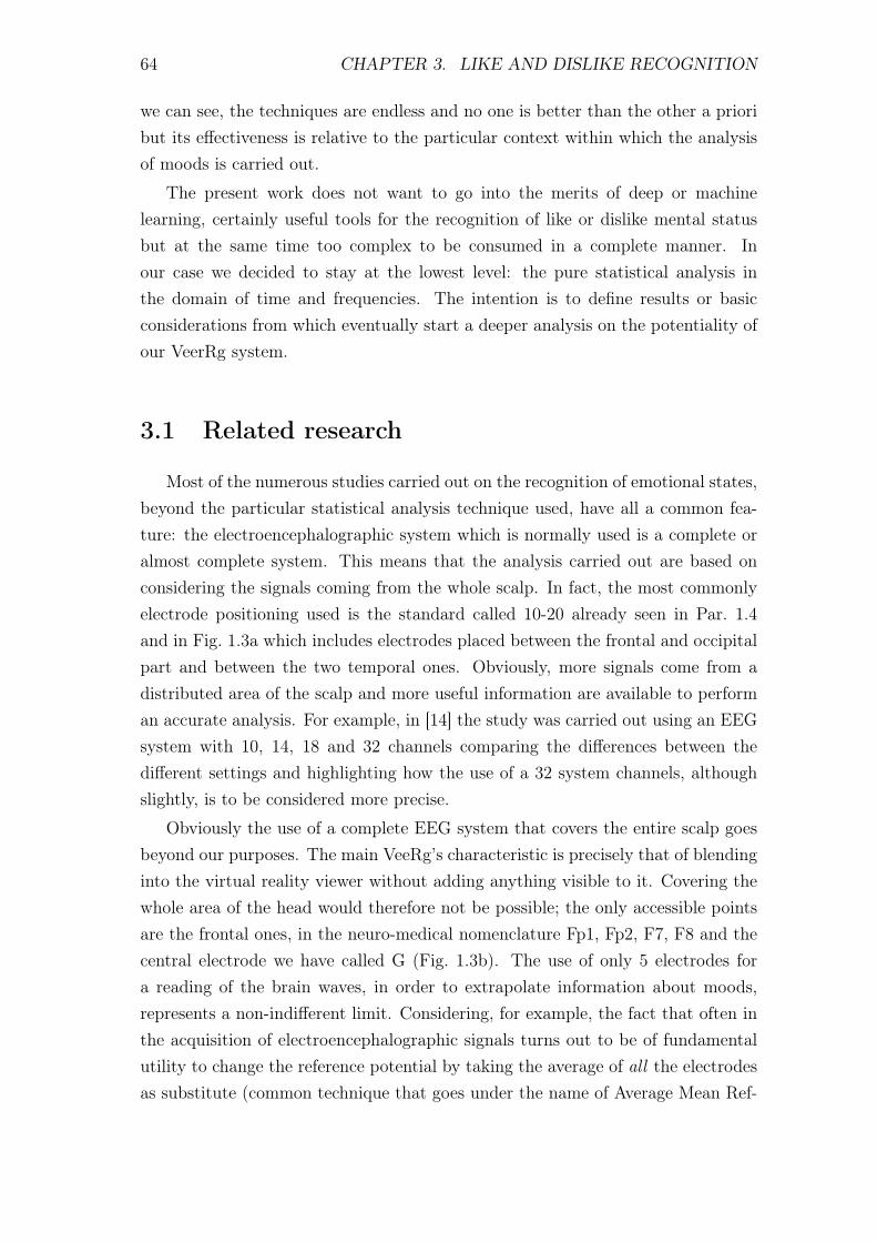
64 CHAPTER 3. LIKE AND DISLIKE RECOGNITION
we can see, the techniques are endless and no one is better than the other a prioribut its effectiveness is relative to the particular context within which the analysisof moods is carried out.
The present work does not want to go into the merits of deep or machinelearning, certainly useful tools for the recognition of like or dislike mental statusbut at the same time too complex to be consumed in a complete manner. Inour case we decided to stay at the lowest level: the pure statistical analysis inthe domain of time and frequencies. The intention is to define results or basicconsiderations from which eventually start a deeper analysis on the potentiality ofour VeerRg system.
3.1 Related research
Most of the numerous studies carried out on the recognition of emotional states,beyond the particular statistical analysis technique used, have all a common fea-ture: the electroencephalographic system which is normally used is a complete oralmost complete system. This means that the analysis carried out are based onconsidering the signals coming from the whole scalp. In fact, the most commonlyelectrode positioning used is the standard called 10-20 already seen in Par. 1.4and in Fig. 1.3a which includes electrodes placed between the frontal and occipitalpart and between the two temporal ones. Obviously, more signals come from adistributed area of the scalp and more useful information are available to performan accurate analysis. For example, in [14] the study was carried out using an EEGsystem with 10, 14, 18 and 32 channels comparing the differences between thedifferent settings and highlighting how the use of a 32 system channels, althoughslightly, is to be considered more precise.
Obviously the use of a complete EEG system that covers the entire scalp goesbeyond our purposes. The main VeeRg’s characteristic is precisely that of blendinginto the virtual reality viewer without adding anything visible to it. Covering thewhole area of the head would therefore not be possible; the only accessible pointsare the frontal ones, in the neuro-medical nomenclature Fp1, Fp2, F7, F8 and thecentral electrode we have called G (Fig. 1.3b). The use of only 5 electrodes fora reading of the brain waves, in order to extrapolate information about moods,represents a non-indifferent limit. Considering, for example, the fact that often inthe acquisition of electroencephalographic signals turns out to be of fundamentalutility to change the reference potential by taking the average of all the electrodesas substitute (common technique that goes under the name of Average Mean Ref-

3.1. RELATED RESEARCH 65
(a)
(b)
Figure 3.2: Example of Normalized Power Values (NPVs) for the signals coming fromelectrode F7 following the analysis in [40]. In (a) the case of like shows a higher activityin the band between 4 and 5 Hz respect the same band in the dislike case (b).
erencing, AMR), we understand how the VeeRg is limited in some aspects. Thisis the fundamental point from which the question arises: is it possible to recognizethe status of like and dislike through only the use of frontal electrodes? The answerthat has fueled hope came from two specific studies carried out to determine thecerebral activity in cases of like and dislike state of mind.
In [40] Yilmaz et al. performed an analysis of the electroencephalographicsignals trying to understand which frequencies and channels were the most dis-criminating indicators in the process that leads an individual to a like or dislikestate. The test proposed by them consists in the acquisition of EEG signals from15 different subjects that have been asked to observe 16 images of shoes for 10seconds and indicate in that time window whether they liked them or not. Inthis way, for every image the signals of all the channels have been clustered andmarked with like or dislike. Once the data were collected from all 15 subjects, thePower Spectral Densities (PSD) were calculated for each EEG channel through theBurg method and then normalized to eliminate the inter-subject and intra-subjectvariability. These normalized spectral density values (Normalized Power Values,NPVs) were finally used as input data for an analysis technique that goes underthe name of logistic regression where the two cases of like and dislike represent thebinary output variables. The major advantage in using this technique is that thecontributions of all the predictors are taken into account all at once avoiding mis-leading conclusions due to multiple tests. After completing the analysis, Yilmazet al. finally determined the most discriminative components in the prediction ofthe status of like and dislike: with regard to the frequencies, the band that showed
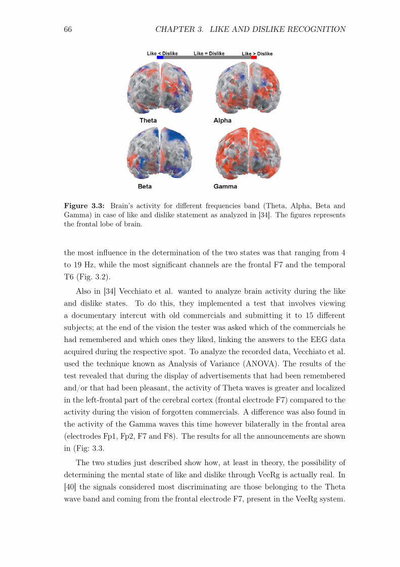
66 CHAPTER 3. LIKE AND DISLIKE RECOGNITION
Figure 3.3: Brain’s activity for different frequencies band (Theta, Alpha, Beta andGamma) in case of like and dislike statement as analyzed in [34]. The figures representsthe frontal lobe of brain.
the most influence in the determination of the two states was that ranging from 4to 19 Hz, while the most significant channels are the frontal F7 and the temporalT6 (Fig. 3.2).
Also in [34] Vecchiato et al. wanted to analyze brain activity during the likeand dislike states. To do this, they implemented a test that involves viewinga documentary intercut with old commercials and submitting it to 15 differentsubjects; at the end of the vision the tester was asked which of the commercials hehad remembered and which ones they liked, linking the answers to the EEG dataacquired during the respective spot. To analyze the recorded data, Vecchiato et al.used the technique known as Analysis of Variance (ANOVA). The results of thetest revealed that during the display of advertisements that had been rememberedand/or that had been pleasant, the activity of Theta waves is greater and localizedin the left-frontal part of the cerebral cortex (frontal electrode F7) compared to theactivity during the vision of forgotten commercials. A difference was also found inthe activity of the Gamma waves this time however bilaterally in the frontal area(electrodes Fp1, Fp2, F7 and F8). The results for all the announcements are shownin (Fig: 3.3.
The two studies just described show how, at least in theory, the possibility ofdetermining the mental state of like and dislike through VeeRg is actually real. In[40] the signals considered most discriminating are those belonging to the Thetawave band and coming from the frontal electrode F7, present in the VeeRg system.
3.2. TEST DEFINITION AND DATA RECORDING 67
In [34] this result is confirmed by emphasizing a difference of activity always inthe Theta wave band located in the left-frontal area, with the addition also ofGamma wave band activity difference in the whole frontal area, practically the onecompletely covered by our VeeRg system.
3.2 Test definition and data recording
For the VeeRg we have developed a simple test inspired by those read in variousstudies on the tracking of emotions through EEG acquisition. The session for eachtest subject (10 in total) consists in placing him in front of a computer screenon which runs a graphical interface properly designed in LabView. Then a totalof 20 images are shown spaced with a pause picture completely black. Duringthe visualization it’s possible to press a button through the computer’s mouse toindicate if the image is liked or not. The button is only one because if the tester hasnot been pleased to see the image or remained in a state of indecision can simplyavoid pressing it (button pressed = like; button not pressed = dislike/indecision).The duration of the image is 6 seconds, while for the pause one is 4 seconds. Theacquisition of data coming from the EEG channels is performed only during the6 seconds in which the image is displayed, then is collected in a numbered CSVfile and marked with the like or dislike response given by the tester. At the end oftest we have a total of 20 CSV files per subject divided between like and dislike.The analysis of the data is done later through scripts appropriately written inMATLAB.
Test guidelines
Sample frequency 250HzEEG’s electrodes Fp1, Fp2, F7, F8, G
Image time window 6sRelax time window 4s
N. of images per dataset 20picsN. of dataset 3(Tattoos,War/Cubs,Models/Growths)
Table 3.1: The filters and their characteristics in the system.
In the design of the test we came across the very trivial problem of the imagedataset to be used. In this regard, there are numerous studies such as [41] where thedifficulty in classifying images according to the effect they have on the emotionalstate of a person is underlined, since not all people will react in the same wayto the same image: some may find it pleasant, some not. For this reason theyare even trying to find a relationship between the chromatic characteristics of the
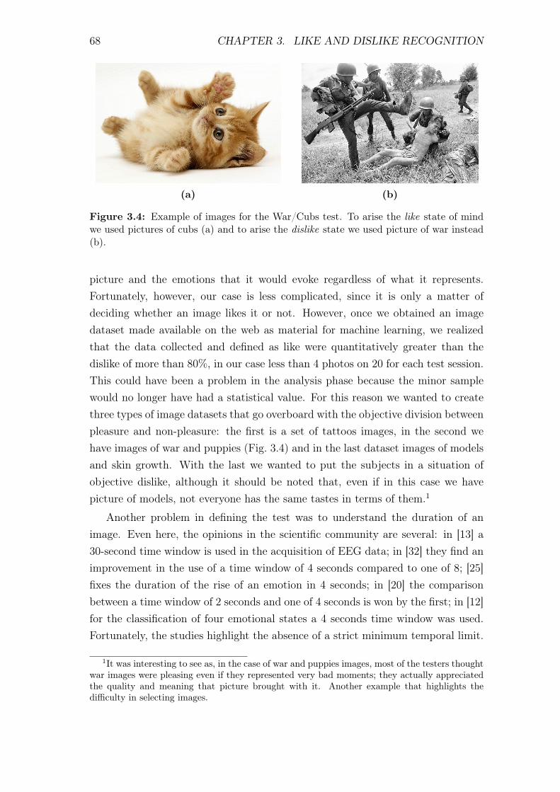
68 CHAPTER 3. LIKE AND DISLIKE RECOGNITION
(a) (b)
Figure 3.4: Example of images for the War/Cubs test. To arise the like state of mindwe used pictures of cubs (a) and to arise the dislike state we used picture of war instead(b).
picture and the emotions that it would evoke regardless of what it represents.Fortunately, however, our case is less complicated, since it is only a matter ofdeciding whether an image likes it or not. However, once we obtained an imagedataset made available on the web as material for machine learning, we realizedthat the data collected and defined as like were quantitatively greater than thedislike of more than 80%, in our case less than 4 photos on 20 for each test session.This could have been a problem in the analysis phase because the minor samplewould no longer have had a statistical value. For this reason we wanted to createthree types of image datasets that go overboard with the objective division betweenpleasure and non-pleasure: the first is a set of tattoos images, in the second wehave images of war and puppies (Fig. 3.4) and in the last dataset images of modelsand skin growth. With the last we wanted to put the subjects in a situation ofobjective dislike, although it should be noted that, even if in this case we havepicture of models, not everyone has the same tastes in terms of them.1
Another problem in defining the test was to understand the duration of animage. Even here, the opinions in the scientific community are several: in [13] a30-second time window is used in the acquisition of EEG data; in [32] they find animprovement in the use of a time window of 4 seconds compared to one of 8; [25]fixes the duration of the rise of an emotion in 4 seconds; in [20] the comparisonbetween a time window of 2 seconds and one of 4 seconds is won by the first; in [12]for the classification of four emotional states a 4 seconds time window was used.Fortunately, the studies highlight the absence of a strict minimum temporal limit.
1It was interesting to see as, in the case of war and puppies images, most of the testers thoughtwar images were pleasing even if they represented very bad moments; they actually appreciatedthe quality and meaning that picture brought with it. Another example that highlights thedifficulty in selecting images.
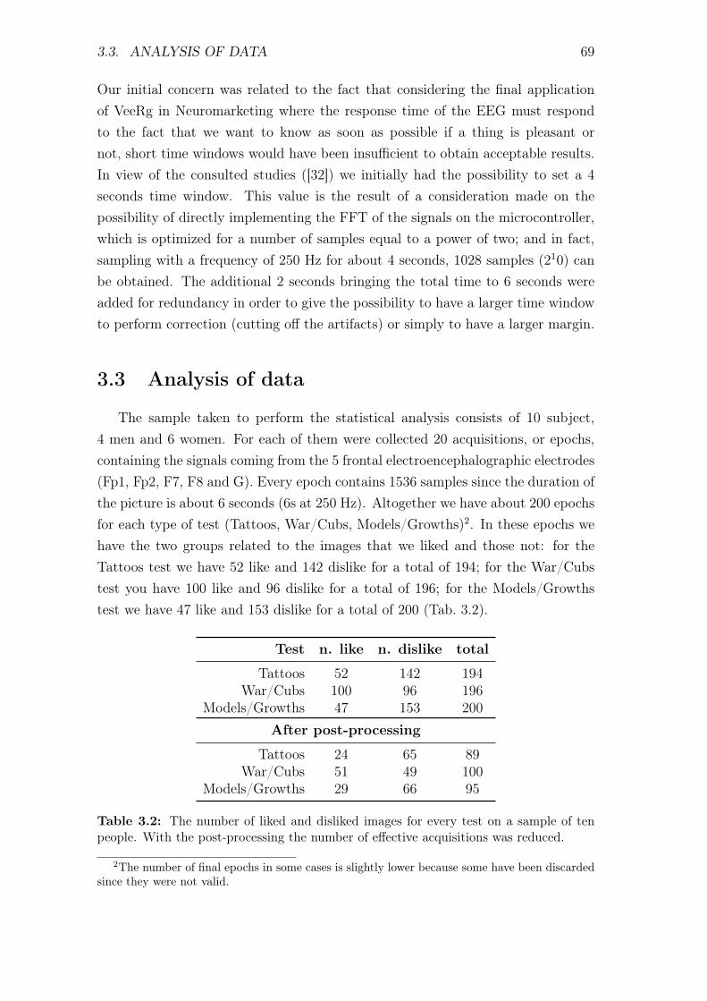
3.3. ANALYSIS OF DATA 69
Our initial concern was related to the fact that considering the final applicationof VeeRg in Neuromarketing where the response time of the EEG must respondto the fact that we want to know as soon as possible if a thing is pleasant ornot, short time windows would have been insufficient to obtain acceptable results.In view of the consulted studies ([32]) we initially had the possibility to set a 4seconds time window. This value is the result of a consideration made on thepossibility of directly implementing the FFT of the signals on the microcontroller,which is optimized for a number of samples equal to a power of two; and in fact,sampling with a frequency of 250 Hz for about 4 seconds, 1028 samples (210) canbe obtained. The additional 2 seconds bringing the total time to 6 seconds wereadded for redundancy in order to give the possibility to have a larger time windowto perform correction (cutting off the artifacts) or simply to have a larger margin.
3.3 Analysis of data
The sample taken to perform the statistical analysis consists of 10 subject,4 men and 6 women. For each of them were collected 20 acquisitions, or epochs,containing the signals coming from the 5 frontal electroencephalographic electrodes(Fp1, Fp2, F7, F8 and G). Every epoch contains 1536 samples since the duration ofthe picture is about 6 seconds (6s at 250 Hz). Altogether we have about 200 epochsfor each type of test (Tattoos, War/Cubs, Models/Growths)2. In these epochs wehave the two groups related to the images that we liked and those not: for theTattoos test we have 52 like and 142 dislike for a total of 194; for the War/Cubstest you have 100 like and 96 dislike for a total of 196; for the Models/Growthstest we have 47 like and 153 dislike for a total of 200 (Tab. 3.2).
Test n. like n. dislike total
Tattoos 52 142 194War/Cubs 100 96 196
Models/Growths 47 153 200
After post-processing
Tattoos 24 65 89War/Cubs 51 49 100
Models/Growths 29 66 95
Table 3.2: The number of liked and disliked images for every test on a sample of tenpeople. With the post-processing the number of effective acquisitions was reduced.
2The number of final epochs in some cases is slightly lower because some have been discardedsince they were not valid.

70 CHAPTER 3. LIKE AND DISLIKE RECOGNITION
Once the data were collected, we wanted to carry out the analysis inspired bythe methods adopted in [40], curious to compare the results to find or not a match.First we performed a post-processing on the signals collected eliminating the epochswhere the presence of artifacts due to eye movement was evident. Following thiscleaning the number of epochs available for analysis has been reduced: for theTattoos test, 24 likes and 65 dislike remained for a total of 89 epochs; for theWar/Cubs test, 51 like and 49 dislike remained for a total of 100 epochs; forthe Models/Growths test there are 29 like and 66 dislike for a total of 95 epochs(Tab. 3.2).
Then, a script was created in MATLAB to automate the analysis of the currentdata. First of all, the script calculates the Power Spectral Densities for each epochand normalizes it with respect to the power of the entire band we are going toconsider ( 0-45 Hz). In this way we try to minimize the variability inter-subjectsand intra-subjects obtaining for each epoch Normalized Power Values (NPVs) onwhich to base our analysis.
The first step was to compare the two cases of like and dislike through theNPVs of all the epochs and for each channel. Fig. 3.5-3.6-3.7 are the result ofthis comparison which, at first glance, would seem to highlight the significantdifferences in NPV trends between the like and dislike case. If we take as anexample the Fig. 3.5a and the Fig. 3.5c we could notice a greater activity in thedislike, both at the low frequencies of the Theta band and in the medium/highfrequencies that characterize the Beta band. In reality this difference is illusorydue to the signifier greater number of epochs belonging to the dislike case (seeTab. 3.2). Also going to compare the average of all the NPV represented by thered curve would not seem to be significant differences. But things start to changewhen we analyze the power in the different bands. Fig. 3.5b and Fig. 3.5d showthe distribution of the power values in the bands 4-8 Hz, 8-13 Hz, 13-20 Hz, 20-30Hz and 30-42 Hz (Theta, Alpha, Beta-low, Beta-high and Gamma respectively).Also here the red circles indicate the average values of the powers in the band.In Tab. 3.3 the values of these averages are indicated for both the like and dislikecases and for all the three tests performed. In this context the difference betweenthe two cases becomes clearer: in fact, even if only slightly, the average of thepowers in the like case would seem to be almost always greater than those of thedislike cases. This would effectively confirm the actual presence of a greater brainactivity when the subject had in front of himself an image of his liking.
In the second step of analysis, statistical elaboration has been carried out, usinglogistic regression to try and determine which are the most discriminating chan-nels and frequencies for the recognition of the like or dislike state of mind. The
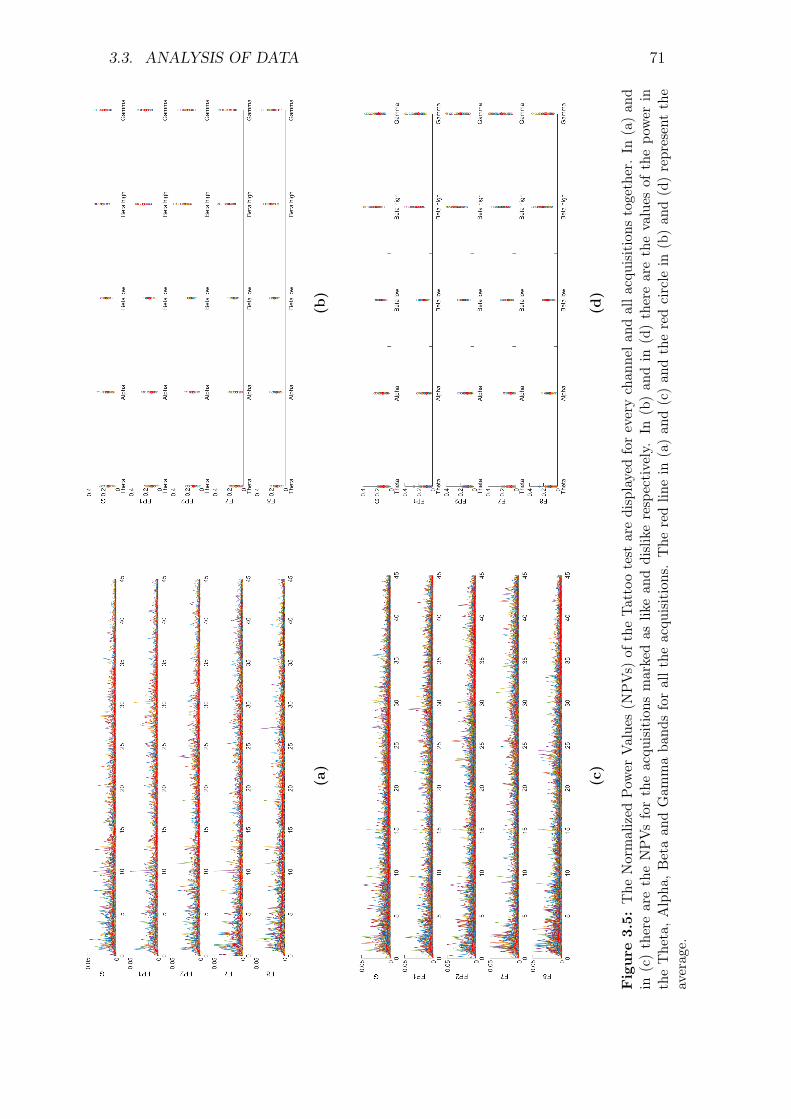
3.3. ANALYSIS OF DATA 71
(a)
(b)
(c)
(d)
Fig
ure
3.5:
The
Normalized
Pow
erValues(N
PVs)
oftheTattootest
aredisplayedforeverychan
nela
ndalla
cquisition
stogether.In
(a)an
din
(c)therearetheNPVsfortheacqu
isitions
markedas
likean
ddislikerespectively.In
(b)an
din
(d)therearethevalues
ofthepo
wer
intheTheta,Alpha
,Betaan
dGam
maba
ndsforallt
heacqu
isitions.The
redlin
ein
(a)an
d(c)an
dtheredcircle
in(b)an
d(d)representthe
averag
e.

72 CHAPTER 3. LIKE AND DISLIKE RECOGNITION
(a)(b
)
(c)(d
)
Figu
re3.6:
The
Norm
alizedPow
erValues
(NPVs)
oftheTattoo
testare
displayedfor
everychanneland
allacquisitionstogether.
In(a)
andin
(c)there
arethe
NPVsfor
theacquisitions
marked
aslike
anddislike
respectively.In
(b)and
in(d)
thereare
thevalues
ofthe
power
inthe
Theta,
Alpha,
Beta
andGam
mabands
forallthe
acquisitions.The
redline
in(a)
and(c)
andthe
redcircle
in(b)
and(d)
representthe
average.
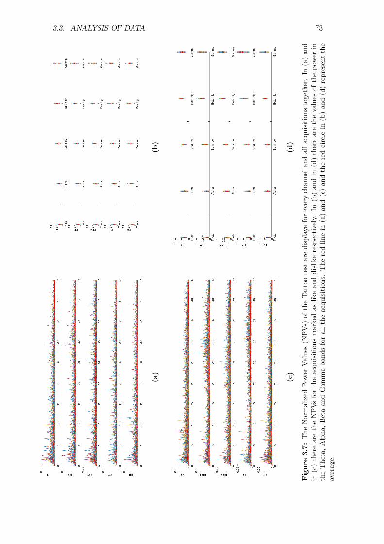
3.3. ANALYSIS OF DATA 73
(a)
(b)
(c)
(d)
Fig
ure
3.7:
The
Normalized
Pow
erValues(N
PVs)
oftheTattootest
aredisplaye
foreverychan
nela
ndalla
cquisition
stogether.In
(a)an
din
(c)therearetheNPVsfortheacqu
isitions
markedas
likean
ddislikerespectively.In
(b)an
din
(d)therearethevalues
ofthepo
wer
intheTheta,Alpha
,Betaan
dGam
maba
ndsforallt
heacqu
isitions.The
redlin
ein
(a)an
d(c)an
dtheredcircle
in(b)an
d(d)representthe
averag
e.
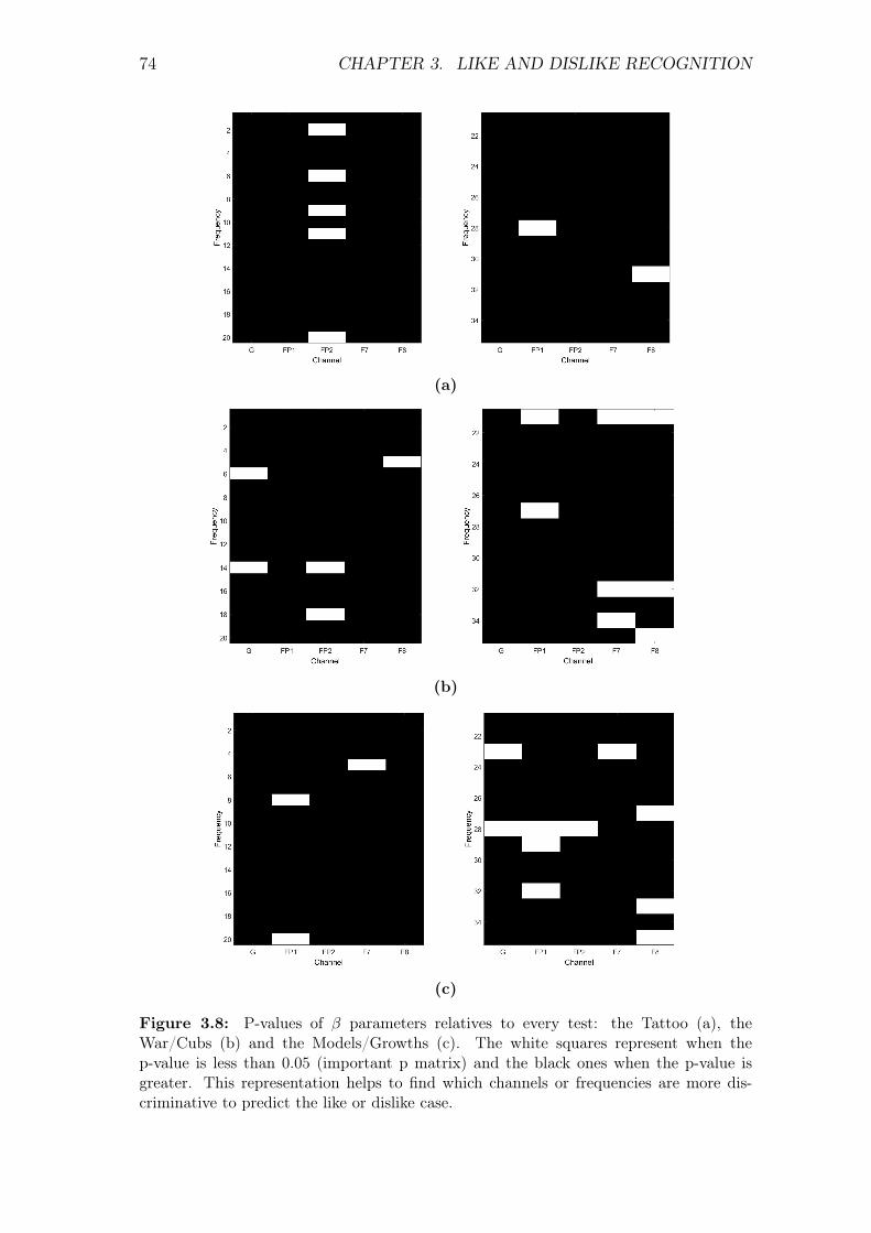
74 CHAPTER 3. LIKE AND DISLIKE RECOGNITION
(a)
(b)
(c)
Figure 3.8: P-values of β parameters relatives to every test: the Tattoo (a), theWar/Cubs (b) and the Models/Growths (c). The white squares represent when thep-value is less than 0.05 (important p matrix) and the black ones when the p-value isgreater. This representation helps to find which channels or frequencies are more dis-criminative to predict the like or dislike case.
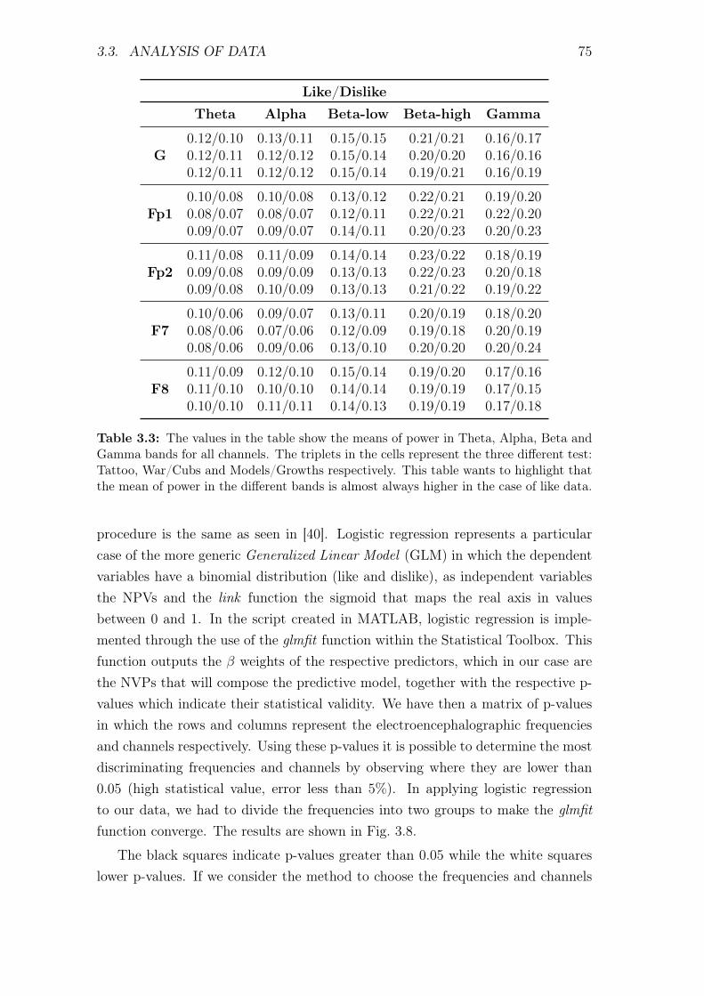
3.3. ANALYSIS OF DATA 75
Like/Dislike
Theta Alpha Beta-low Beta-high Gamma
G0.12/0.100.12/0.110.12/0.11
0.13/0.110.12/0.120.12/0.12
0.15/0.150.15/0.140.15/0.14
0.21/0.210.20/0.200.19/0.21
0.16/0.170.16/0.160.16/0.19
Fp10.10/0.080.08/0.070.09/0.07
0.10/0.080.08/0.070.09/0.07
0.13/0.120.12/0.110.14/0.11
0.22/0.210.22/0.210.20/0.23
0.19/0.200.22/0.200.20/0.23
Fp20.11/0.080.09/0.080.09/0.08
0.11/0.090.09/0.090.10/0.09
0.14/0.140.13/0.130.13/0.13
0.23/0.220.22/0.230.21/0.22
0.18/0.190.20/0.180.19/0.22
F70.10/0.060.08/0.060.08/0.06
0.09/0.070.07/0.060.09/0.06
0.13/0.110.12/0.090.13/0.10
0.20/0.190.19/0.180.20/0.20
0.18/0.200.20/0.190.20/0.24
F80.11/0.090.11/0.100.10/0.10
0.12/0.100.10/0.100.11/0.11
0.15/0.140.14/0.140.14/0.13
0.19/0.200.19/0.190.19/0.19
0.17/0.160.17/0.150.17/0.18
Table 3.3: The values in the table show the means of power in Theta, Alpha, Beta andGamma bands for all channels. The triplets in the cells represent the three different test:Tattoo, War/Cubs and Models/Growths respectively. This table wants to highlight thatthe mean of power in the different bands is almost always higher in the case of like data.
procedure is the same as seen in [40]. Logistic regression represents a particularcase of the more generic Generalized Linear Model (GLM) in which the dependentvariables have a binomial distribution (like and dislike), as independent variablesthe NPVs and the link function the sigmoid that maps the real axis in valuesbetween 0 and 1. In the script created in MATLAB, logistic regression is imple-mented through the use of the glmfit function within the Statistical Toolbox. Thisfunction outputs the β weights of the respective predictors, which in our case arethe NVPs that will compose the predictive model, together with the respective p-values which indicate their statistical validity. We have then a matrix of p-valuesin which the rows and columns represent the electroencephalographic frequenciesand channels respectively. Using these p-values it is possible to determine the mostdiscriminating frequencies and channels by observing where they are lower than0.05 (high statistical value, error less than 5%). In applying logistic regressionto our data, we had to divide the frequencies into two groups to make the glmfitfunction converge. The results are shown in Fig. 3.8.
The black squares indicate p-values greater than 0.05 while the white squareslower p-values. If we consider the method to choose the frequencies and channels
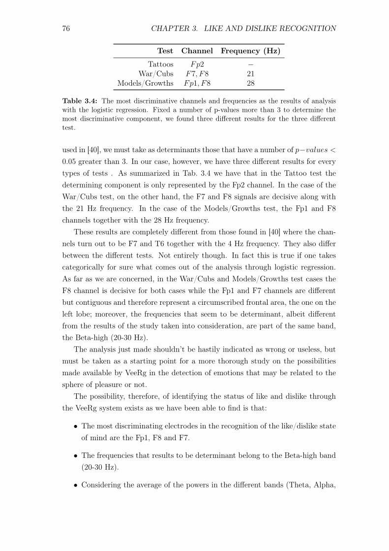
76 CHAPTER 3. LIKE AND DISLIKE RECOGNITION
Test Channel Frequency (Hz)
Tattoos Fp2 −War/Cubs F7, F8 21
Models/Growths Fp1, F8 28
Table 3.4: The most discriminative channels and frequencies as the results of analysiswith the logistic regression. Fixed a number of p-values more than 3 to determine themost discriminative component, we found three different results for the three differenttest.
used in [40], we must take as determinants those that have a number of p−values <0.05 greater than 3. In our case, however, we have three different results for everytypes of tests . As summarized in Tab. 3.4 we have that in the Tattoo test thedetermining component is only represented by the Fp2 channel. In the case of theWar/Cubs test, on the other hand, the F7 and F8 signals are decisive along withthe 21 Hz frequency. In the case of the Models/Growths test, the Fp1 and F8channels together with the 28 Hz frequency.
These results are completely different from those found in [40] where the chan-nels turn out to be F7 and T6 together with the 4 Hz frequency. They also differbetween the different tests. Not entirely though. In fact this is true if one takescategorically for sure what comes out of the analysis through logistic regression.As far as we are concerned, in the War/Cubs and Models/Growths test cases theF8 channel is decisive for both cases while the Fp1 and F7 channels are differentbut contiguous and therefore represent a circumscribed frontal area, the one on theleft lobe; moreover, the frequencies that seem to be determinant, albeit differentfrom the results of the study taken into consideration, are part of the same band,the Beta-high (20-30 Hz).
The analysis just made shouldn’t be hastily indicated as wrong or useless, butmust be taken as a starting point for a more thorough study on the possibilitiesmade available by VeeRg in the detection of emotions that may be related to thesphere of pleasure or not.
The possibility, therefore, of identifying the status of like and dislike throughthe VeeRg system exists as we have been able to find is that:
• The most discriminating electrodes in the recognition of the like/dislike stateof mind are the Fp1, F8 and F7.
• The frequencies that results to be determinant belong to the Beta-high band(20-30 Hz).
• Considering the average of the powers in the different bands (Theta, Alpha,

3.3. ANALYSIS OF DATA 77
Beta-low/high and Gamma) among all the acquisitions made, it appears tobe greater in the case like rather than in the case of dislike.
These results must be considered in light of the fact that the test developed forour purpose can be improved by choosing a more appropriate image dataset or,better, by choosing to use videos; moreover, in order to have a greater statisticalvalue, it is advisable to enlarge the number of subject from which the electroen-cephalographic signals can be acquired.

78 CHAPTER 3. LIKE AND DISLIKE RECOGNITION

Conclusion
The realization of VeeRg has put us in front of numerous challenges, common toall those who have our own target: the recognition of emotional states, in particularthat of pleasure. This is a vast subject if you start from scratch the designing ofan EEG system to use it then in the analysis of brain activity, but on the otherhand it is necessary if you want to have a completely flexible system for a completeintegration with the viewers of virtual reality.
The biggest problem was to obtain electroencephalographic signals as cleanas possible through an accurate analysis of the most common techniques used toreduce the onset of noise.
Starting from a design aimed at low-noise, we have generated analog referencesfor the analog-to-digital conversion with a very low incidence of noise, obtaining asystem with Input Referred Noise (IRN) of 0.97µVrms and 5.79µVpp, values morethan enough for this type of application.
We then addressed the typical Common-Mode issue in the acquisition of bio-electrical signals. An in-depth analysis of the typical technique of the Bias electrode(or Ground, or Feedback-loop) has shown what are the elements that improve theCommon Mode Rejection (CMR) keeping it, at least theoretically (N/A), alwaysbelow a certain limit. The development of these techniques led to the realizationof an EEG system with a Power Spectrum Density (PSD) at rest (system worn ina relaxed position) that, already at low frequency, has a characteristic below the1µV
2
Hz(-120dB).
Finally, the topic of filtering was introduced, useful but nevertheless dangerous,trying to define the risks that can be met if one is not aware of it. Depending onthe type of application, the filters may be more or less useful as they introducedistortions that can severely change the results of a subsequent analysis.
At this point, with a working prototype in our hand,s we entered the delicatephase of our journey: the recognition of the status of like/dislike. A delicate phasebecause, although there are numerous studies to confirm the possibility and al-though such devices have already been proposed, the question is still widely open.Inspired by a research article, we have created a test for the collection of elec-
79
80 CHAPTER 3. LIKE AND DISLIKE RECOGNITION
troencephalographic signals drawing from a sample of 10 subjects; subsequently,still referring to the methodology used in the article, we applied the logistic re-gression technique to determine which frequencies and EEG channels are the mostdeterminant of the recognition of the like/dislike. At the end of the elaborationwe discovered a slight difference in the power of the brain’s waves between thetwo mental states and, as a result of the statistical analysis, we have obtained asdiscriminating elements the electrodes F7, F8 and Fp1 (standard position system)and the frequencies in the Beta-high band (20-30 Hz). These results, however,differ from those obtained in the article and that we expected to confirm.
However, even if our case deviates from what we expected, we must keep in mindthat we are in an area not yet fully explored in which the studies and research willcontinue in the coming years to try to improve what we are already doing today.The possibility of the recognition of emotions through electroencephalography ispossible and is a fact, but we have to consider that nowadays there aren’t devices onthe market able to do it, since they are all still in the embryonic stage. Prototypesthat exist and work, but that can’t keep high reliability in all the contexts in whichthey could be used.
The main problem is reduced in trying to get the bio-electric signals in the bestway, without being contaminated by external interference or due mainly to suddenchanges of the interface between the body and the system, in our case the skin/-electrode interface. It is our opinion that the main focus should be concentratedon the problem of acquisition, because it is obvious that with better and cleanersignals the analysis on it can lead to more significant results.

Appendix A
Schematics and Code
A.1 Schematics
In the following pages are available the schematics of the whole VeeRg system.
81
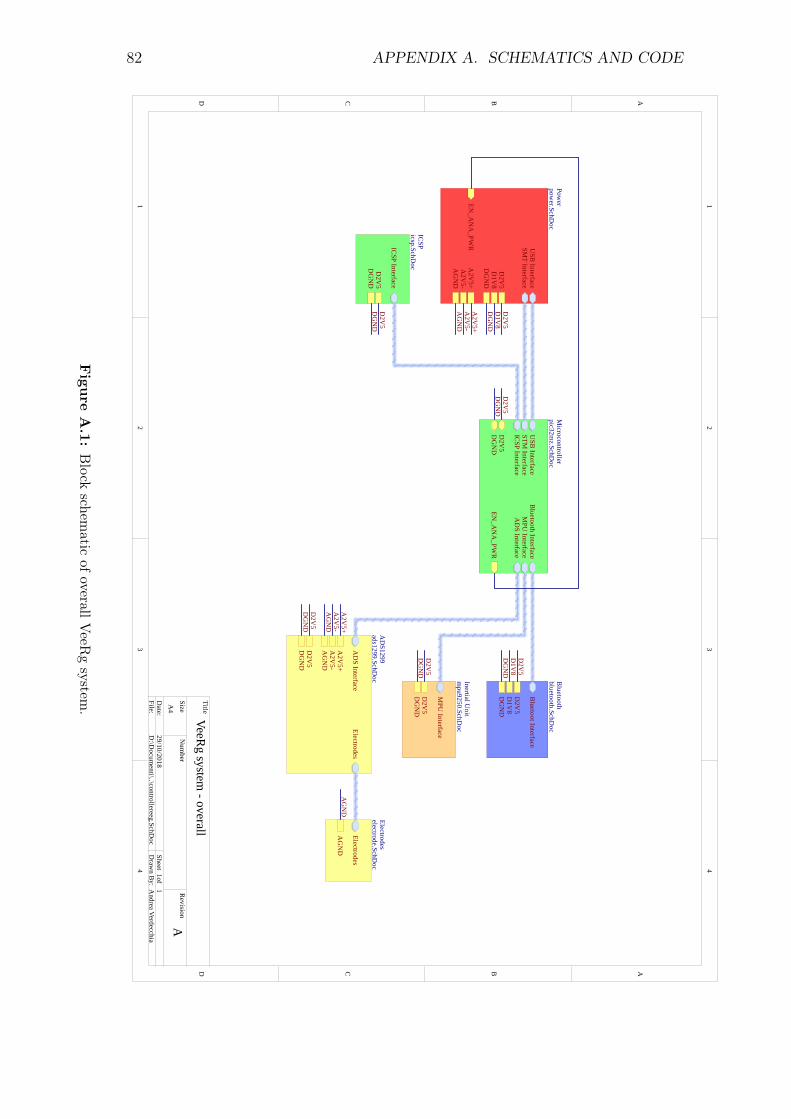
82 APPENDIX A. SCHEMATICS AND CODE
1 1
2 2
3 3
4 4
DD
CC
BB
AA
Title
Num
berR
evisionSize
A4
Date:
29/10/2018Sheet of
File:D
:\Docum
enti\..\controllereeg.SchDoc
Draw
n By:
Bluetooth Interface
MPU
InterfaceA
DS Interface
ICSP Interface
USB
InterfaceSTM
Interface
DG
ND
D2V
5EN
_AN
A_PW
R
Microcontroller
pic32mz.SchD
oc
MPU
Interface
DG
ND
D2V
5
Inertial Unit
mpu9250.SchD
oc
Bluetoot Interface
D2V
5D
1V8
DG
ND
Bluetooth
bluetooth.SchDoc
ICSP Interface
D2V
5D
GN
D
ICSPicsp.SchD
oc
SMT Interface
D2V
5
DG
ND
D1V
8
USB
Interface
A2V
5+A
2V5-
AG
ND
EN_A
NA
_PWR
Power
power.SchD
oc
D2V
5
D2V
5
D2V
5
D2V
5
D1V
8
D1V
8
DG
ND
DG
ND
DG
ND
DG
ND
D2V
5D
GN
D
A2V
5+A
2V5-
AG
ND
A2V
5+A
2V5-
AG
ND
DG
ND
D2V
5
AD
S InterfaceElectrodes
AD
S1299ads1299.SchD
oc
A2V
5+A
2V5-
AG
ND
D2V
5D
GN
D
Electrodes
AG
ND
Electrodeselectrode.SchD
oc
AG
ND
A
VeeRg system
- overall
Andrea Verdecchia
11
Figu
reA
.1:Block
schematic
ofoverallV
eeRgsystem
.
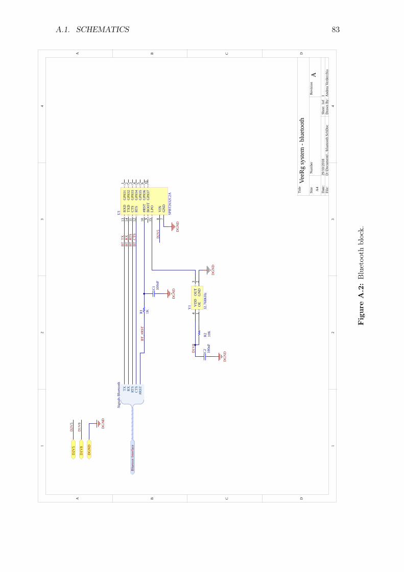
A.1. SCHEMATICS 83
11
22
33
44
DD
CC
BB
AA
Title
Num
ber
Rev
isio
nSi
ze A4
Dat
e:29
/10/
2018
Shee
t o
fFi
le:
D:\D
ocum
enti\
..\bl
ueto
oth.
SchD
ocD
raw
n B
y:
OE
1G
ND
2O
UT
3V
DD
4Y
1
32.7
68K
Hz
DG
ND
100n
FC
2
DG
ND
10K
R2
BT_
TXB
T_R
X
BT_
CTS
BT_
RTS
GPI
O1
1
GPI
O2
2
GPI
O3
3
GPI
O4
4
GPI
O5
5
GPI
O6
6
GN
D7
VIN
8
BO
OT
9#R
ST10
CTS
11
RTS
12
RX
D13
TXD
14
LPO
15G
PIO
716
U1
SPB
T263
2C2A
BT_
#RST
100n
FC
1
1KR1
DG
ND
DG
ND
TX RX
RTS
CTS
#RST
Sign
als B
luet
ooth
Blu
etoo
t Int
erfa
ce
D2V
5
DG
ND
DG
ND
D1V
8
D2V
5
D1V
8
D2V
5
D1V
8
A
VeeR
g sy
stem
- bl
ueto
oth
And
rea
Verd
ecch
ia1
1
PIC101 PIC102 COC
1
PIC201 PIC202 COC
2
PIR1
01
PIR1
02 COR1
PIR2
01
PIR2
02 COR2
PIU101
PIU102
PIU103
PIU104
PIU105
PIU106
PIU107
PIU108
PIU109
PIU1010
PIU1011
PIU1012
PIU1013
PIU1014
PIU1015
PIU1016
COU1
PIY101
PIY102
PIY103
PIY104 COY
1
POBLUETOOT INTERFACE
POBL
UETO
OT I
NTER
FACE
0#RS
T POBLUETOOT INTERFACE0CTS
POBLUETOOT INTERFACE0RTS
POBLUETOOT INTERFACE0RX
POBLUETOOT INTERFACE0TX
POD1V8
POD2V5
PODGND
Fig
ure
A.2
:Bluetoo
thblock.
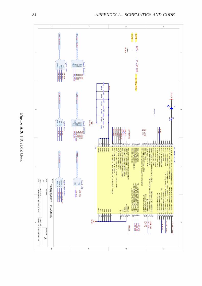
84 APPENDIX A. SCHEMATICS AND CODE
1 1
2 2
3 3
4 4
DD
CC
BB
AA
Title
Num
berR
evisionSize
A4
Date:
29/10/2018Sheet of
File:D
:\Docum
enti\..\pic32mz.SchD
ocD
rawn B
y:
100nFC
12100nFC11
100nFC
10100nFC
9100nFC
8100nFC
7
DG
ND
AD
S_SCK
AD
S_SDO
#AD
S_CSA
DS_SD
I
DG
ND
#MC
LR
BT_TX
BT_R
X
PGED
PGEC
350R
R7
AN
17/ETXEN
/RPE5/PM
D5/R
E51
AN
16/ETXD
0/PMD
6/RE6
2
AN
15/ETXD
1/PMD
7/RE7
3
AN
14/C1IN
D/R
PG6/SC
K2/PM
A5/R
G6
4
AN
13/C1IN
C/R
PG7/SD
A4/PM
A4/R
G7
5
AN
12/C2IN
D/R
PG8/SC
L4/PMA
3/RG
86
VSS
7
VD
D8
#MC
LR9
AN
11/C2IN
C/R
PG9/PM
A2/R
G9
10
AN
45/C1IN
A/R
PB5/R
B5
11A
N4/C
1INB
/RB
412
AN
3/C2IN
A/R
PB3/R
B3
13A
N2/C
2INB
/RPB
2/RB
214
PGEC
1/VR
EF-/CV
REF-/A
N1/R
PB1/R
B1
15PG
ED1/V
REF+/C
VR
EF+/AN
0/RPB
0/PMA
6/RB
016
PGEC
2/AN
46/RPB
6/RB
617
PGED
2/AN
47/RPB
7/RB
718
AVD
D19
AVSS
20
AN
48/RPB
8/PMA
10/RB
821
AN
49/RPB
9/PMA
7/RB
922
TMS/C
VR
EFOU
T/AN
5/RPB
10/PMA
13/RB
1023
TDO
/AN
6/PMA
12/RB1124
VSS
25
VD
D26
TCK
/AN
7/PMA
11/RB
1227
TDI/A
N8/R
B13
28
AN
9/RPB
14/SCK
3/PMA
1/RB
1429
AN
10/EMD
C/A
EMD
C/R
PB15/O
CFB
/PMA
0/RB
1530
OSC
1/CLK
I/RC
1231
OSC
2/CLK
O/R
C15
32
VB
US
33V
USB
3V3
34
VSS
35
D-
36D
+37
RPF3/U
SBID
/RF3
38
VD
D39
VSS
40
RPF4/SD
A5/PM
A9/R
F441
RPF5/SC
L5/PMA
8/RF5
42
AER
XD
0/ETXD
2/RPD
9/SDA
1/PMC
S2/PMA
15/RD
943
ECO
L/RPD
10/SCL1/SC
K4/R
D10
44
AER
XC
LK/A
EREFC
LK/EC
RS/R
PD11/PM
CS1/PM
A14/R
D11
45
AER
XD
1/ETXD
3/RPD
0/RTCC
/INT0/R
D0
46
SOSC
I/RPC
13/RC
1347
SOSC
O/R
PC14/T1C
K/R
C14
48
EMD
IO/A
EMD
IO/R
PD1/SC
K1/R
D1
49
ETXER
R/A
ETXEN
/RPD
2/SDA
3/RD
250
AER
XER
R/ETX
CLK
/RPD
3/SCL3/R
D3
51
#SQIC
S0/RPD
4/PMW
R/R
D4
52
#SQIC
S1/RPD
5/PMR
D/R
D5
53
VD
D54
VSS
55
ERX
D3/A
ETXD
1/RPF0/R
F056
TRC
LK/SQ
ICLK
/ERX
D2/A
ETXD
0/RPF1/R
F157
TRD
0/SQID
0/ERX
D1/PM
D0/R
E058
VSS
59V
DD
60
TRD
1/SQID
1/ERX
D0/PM
D1/R
E161
TRD
2/SQID
2/ERX
DV
/ECR
SDV
/AEC
RSD
V/PM
D2/R
E262
TRD
3/SQID
3/ERX
CLK
/EREFC
LK/R
PE3/PMD
3/RE3
63
AN
18/ERX
ERR
/PMD
4/RE4
64
U3
PIC32M
Z0512EFE064D
1
DG
ND
MPU
-SCL
MPU
-SDA
MPU
-INT
MPU
-FSYN
C
BT_C
TS
BT_RTS
BT_#R
ST
EN_A
NA
_PWR
USB
_TXU
SB_R
X
SMT_IN
T
SMT_PSH
OLD
SMT_PB
OU
T
RXTX
CTS
RTS#R
ST
Signals BluetoothB
T_TXB
T_RX
BT_C
TSB
T_RTSB
T_#RST
Bluetooth Interface
SCL
SDA
INT
FSYN
C
Signals MPU
MPU
Interface
MPU
-SCL
MPU
-SDA
MPU
-INT
MPU
-FSYN
C
SCK
SDO
SDI
#DR
DY
#CS
Signals AD
S1299
AD
S Interface#A
DS_D
RD
Y
AD
S_SCK
AD
S_SDO
AD
S_SDI
#AD
S_CS
PGEC
PGED
#MC
LR
Signals ICSP
ICSP InterfacePG
EDPG
EC
#MC
LR
Use IN
T3
TX
RX
Signals USB
USB
InterfaceU
SB_R
X
USB
_TX
PSHO
LDPB
OU
T#M
CLR
Signals Smart B
utton
STM Interface
SMT_IN
TSM
T_PSHO
LD
SMT_PB
OU
T
D2V
5
DG
ND
DG
ND
D2V
5
D2V
5
EN_A
NA
_PWR
EN_A
NA
_PWR
#AD
S_DR
DY
A
VeeRg system
- PIC32MZ
Andrea Verdecchia
11
PIC701 PIC702 COC7
PIC801 PIC802 COC8
PIC901 PIC902 COC9
PIC1001 PIC1002 COC10
PIC1101 PIC1102 COC11
PIC1201 PIC1202 COC12
PID101
PID102
COD1
PIR701 PIR702
COR7
PIU301
PIU302
PIU303
PIU304
PIU305
PIU306
PIU307
PIU308
PIU309
PIU3010
PIU3011
PIU3012
PIU3013
PIU3014
PIU3015
PIU3016
PIU3017
PIU3018
PIU3019
PIU3020
PIU3021
PIU3022
PIU3023
PIU3024
PIU3025
PIU3026
PIU3027
PIU3028
PIU3029
PIU3030
PIU3031
PIU3032
PIU3033
PIU3034
PIU3035
PIU3036
PIU3037
PIU3038
PIU3039
PIU3040
PIU3041
PIU3042
PIU3043
PIU3044
PIU3045
PIU3046
PIU3047
PIU3048
PIU3049
PIU3050
PIU3051
PIU3052
PIU3053
PIU3054
PIU3055
PIU3056
PIU3057
PIU3058
PIU3059
PIU3060
PIU3061
PIU3062
PIU3063
PIU3064
COU3
POADS INTERFACE
POADS INTERFACE0#CS POADS INTERFACE0#DRDY POADS INTERFACE0SCK POADS INTERFACE0SDI POADS INTERFACE0SDO
POBLUETOOTH INTERFACE POBLUETOOTH INTERFACE0#RST POBLUETOOTH INTERFACE0CTS POBLUETOOTH INTERFACE0RTS POBLUETOOTH INTERFACE0RX POBLUETOOTH INTERFACE0TX
POD2V5
PODGND
POEN0ANA0PWR POICSP INTERFACE
POICSP INTERFACE0#MCLR POICSP INTERFACE0PGEC POICSP INTERFACE0PGED
POMPU INTERFACE
POMPU INTERFACE0FSYNC POMPU INTERFACE0INT POMPU INTERFACE0SCL POMPU INTERFACE0SDA
POSTM INTERFACE
POSTM INTERFACE0#MCLR POSTM INTERFACE0PBOUT POSTM INTERFACE0PSHOLD
POUSB INTERFACE
POUSB INTERFACE0RX POUSB INTERFACE0TX
Figu
reA
.3:PIC
23MZblock.
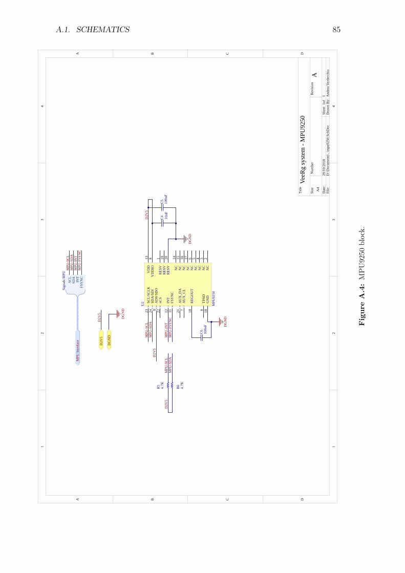
A.1. SCHEMATICS 85
11
22
33
44
DD
CC
BB
AA
Title
Num
ber
Rev
isio
nSi
ze A4
Dat
e:29
/10/
2018
Shee
t o
fFi
le:
D:\D
ocum
enti\
..\m
pu92
50.S
chD
ocD
raw
n B
y:
RES
V1
NC
2N
C3
NC
4N
C5
NC
6
AU
X_C
L7
VD
DIO
8
AD
0/SD
O9
REG
OU
T10
FSY
NC
11IN
T12
VD
D13
NC
14
NC
15
NC
16
NC
17
GN
D18
RES
V19
RES
V20
AU
X_D
A21
nCS
22
SCL/
SCLK
23
SDA
/SD
I24
TPA
D0
U2
MPU
9250
MPU
-SC
LM
PU-S
DA
100n
FC
6
DG
ND
DG
ND
100n
FC
510
nFC
4M
PU-I
NT
MPU
-FSY
NC
MPU
-SC
LM
PU-S
DA
4.7K
R5
4.7K
R6
SCL
SDA
INT
FSY
NC
Sign
als M
PU
MPU
Inte
rface
MPU
-SC
LM
PU-S
DA
MPU
-IN
TM
PU-F
SYN
C
D2V
5
DG
ND
DG
ND
D2V
5
D2V
5
D2V
5
D2V
5
A
VeeR
g sy
stem
- M
PU92
50
And
rea
Verd
ecch
ia1
1
PIC401 PIC402 COC
4 PIC501 PIC502
COC5
PIC601 PIC602 COC
6
PIR5
01
PIR5
02 COR
5
PIR6
01
PIR6
02 COR
6
PIU200
PIU201
PIU202
PIU203
PIU204
PIU205
PIU206
PIU207
PIU208
PIU209
PIU2010
PIU2011
PIU2012
PIU2013
PIU2014
PIU2015
PIU2016
PIU2017
PIU2018
PIU2019
PIU2020
PIU2021
PIU2022
PIU2023
PIU2024 COU2
POD2V5
PODGND
POMPU INTERFACE
POMPU INTERFACE0FSYNC
POMPU INTERFACE0INT
POMPU INTERFACE0SCL
POMPU INTERFACE0SDA
Fig
ure
A.4
:MPU92
50block.

86 APPENDIX A. SCHEMATICS AND CODE
1 1
2 2
3 3
4 4
DD
CC
BB
AA
Title
Num
berR
evisionSize
A4
Date:
29/10/2018Sheet of
File:D
:\Docum
enti\..\ads1299.SchDoc
Draw
n By:
IN8N
1
IN8P
2
IN7N
3
IN7P
4
IN6N
5
IN6P
6
IN5N
7
IN5P
8
IN4N
9
IN4P
10
IN3N
11
IN3P
12
IN2N
13
IN2P
14
IN1N
15
IN1P
16
VR
EFP24
VR
EFN25
DIN
34
#CS39
SCLK
40
CLK
SEL52
#PWD
N35
#RESET
36
START
38
CLK
37
DA
ISY_IN
41
AVSSCP58
AVSS20
AVSS23
AVSS32
AVSS57
AVSS153
DGND51
DGND33
DGND49
RESV
131
GPIO
446
GPIO
345
GPIO
244
GPIO
142
DO
UT
43
#DR
DY
47
RESERV
ED64
VC
AP4
26V
CA
P355
VC
AP2
30V
CA
P128
NC
27N
C29
SRB
218
SRB
117
BIA
SOU
T63
BIA
SIN62
BIA
SINV
61B
IASR
EF60
AVDDCP 59
AVDD 19
AVDD 21
AVDD 22
AVDD 56
AVDD1 54
DVDD 50
DVDD 48
U13
AD
S1299
5
31
2
4U
12TLV2221
1uFC
56100nFC
571uFC
58100nFC
591uFC
60100nFC
611uFC
62100nFC
63
1uFC
491uFC
50100nFC
511uFC
52100uFC
53
DG
ND
1uFC
54100nFC
55
10uFC
47100nFC
48
DG
ND
AG
ND
DG
ND
1uFC
41100nFC
42
AG
ND
100nFC
431uFC
44
DG
ND
1meg
R26
1nFC
45
1uF
C40
1uF
C46 A
GN
DAG
ND
BIA
S_SHIELD
REF
SHIELD
V1
V2
V3
V4
V5
V6
V7
V8
AD
S_SDI
#AD
S_CSA
DS_SC
K#A
DS_D
RD
Y
AD
S_SDO
0R R27
n.m.
R28
DG
ND
A2V
5+A
2V5+
A2V
5-A
2V5-
AG
ND
DG
ND
DG
ND
D2V
5D
2V5
D2V
5
D2V
5
AG
ND
A2V
5+
A2V
5+A
2V5+
A2V
5+A
2V5+
A2V
5+
A2V
5-
A2V
5-
A2V
5-A
2V5-
A2V
5-A
2V5-
A2V
5- A2V
5-
SCK
SDO
SDI
#DR
DY
#CS
Signals AD
S1299
AD
S Interface#A
DS_D
RD
Y
AD
S_SCK
AD
S_SDO
AD
S_SDI
#AD
S_CS
REF
BIA
SV
[1..8]SH
IELD
Electrodes
Electrodes
REF
BIA
S
V[1..8]
V[1..8]
SHIELD
AG
ND
SHIELD
1
SHIELD
1
BIA
S
A
VeeRg system
- AD
S1299
Andrea Verdecchia
11
PIC4001 PIC4002
COC40 PIC4101 PIC4102
COC41 PIC4201 PIC4202
COC42 PIC4301 PIC4302
COC43 PIC4401 PIC4402
COC44
PIC4501 PIC4502 COC45
PIC4601 PIC4602
COC46
PIC4701 PIC4702 COC47
PIC4801 PIC4802 COC48
PIC4901 PIC4902 COC49
PIC5001 PIC5002 COC50
PIC5101 PIC5102 COC51
PIC5201 PIC5202 COC52
PIC5301 PIC5302 COC53
PIC5401 PIC5402 COC54 PIC5501 PIC5502
COC55
PIC5601 PIC5602 COC56 PIC5701 PIC5702 COC57
PIC5801 PIC5802 COC58 PIC5901 PIC5902 COC59
PIC6001 PIC6002 COC60 PIC6101 PIC6102
COC61 PIC6201 PIC6202
COC62 PIC6301 PIC6302
COC63
PIR2601 PIR2602 COR26
PIR2701 PIR2702
COR27
PIR2801 PIR2802
COR28
PISHIELD101 COSHIELD1
PIU1201
PIU1202
PIU1203
PIU1204
PIU1205 COU12
PIU1301
PIU1302
PIU1303
PIU1304
PIU1305
PIU1306
PIU1307
PIU1308
PIU1309
PIU13010
PIU13011
PIU13012
PIU13013
PIU13014
PIU13015
PIU13016
PIU13017
PIU13018
PIU13019 PIU13020 PIU13021 PIU13022 PIU13023
PIU13024
PIU13025
PIU13026
PIU13027
PIU13028
PIU13029
PIU13030
PIU13031
PIU13032 PIU13033
PIU13034
PIU13035
PIU13036
PIU13037
PIU13038
PIU13039
PIU13040
PIU13041
PIU13042
PIU13043
PIU13044
PIU13045
PIU13046
PIU13047
PIU13048 PIU13049
PIU13050 PIU13051
PIU13052
PIU13053 PIU13054
PIU13055
PIU13056 PIU13057 PIU13058 PIU13059
PIU13060
PIU13061
PIU13062
PIU13063
PIU13064
COU13
POA2V50
POADS INTERFACE
POADS INTERFACE0#CS POADS INTERFACE0#DRDY POADS INTERFACE0SCK POADS INTERFACE0SDI POADS INTERFACE0SDO
POAGND
POD2V5
PODGND
POELECTRODES POELECTRODES0BIAS POELECTRODES0REF POELECTRODES0SHIELD POELECTRODES0V1 POELECTRODES0V2 POELECTRODES0V3 POELECTRODES0V4 POELECTRODES0V5 POELECTRODES0V6 POELECTRODES0V7 POELECTRODES0V8 POELECTRODES0V010080
Figu
reA
.5:ADS1299
block.
A.1. SCHEMATICS 87
11
22
33
44
DD
CC
BB
AA
Title
Num
ber
Rev
isio
nSi
ze A4
Dat
e:29
/10/
2018
Shee
t o
fFi
le:
D:\D
ocum
enti\
..\el
ectro
de.S
chD
ocD
raw
n B
y:
n.m
.C
6447
0nC
65
1.5k
R29
AG
ND
V1
n.m
.C
6947
0nC
70
1.5k
R32
AG
ND
V2
n.m
.C
7347
0nC
74
1.5k
R35
AG
ND
V3
n.m
.C
7747
0nC
78
1.5k
R37
AG
ND
V4
n.m
.C
6647
0nC
67
1.5k
R30
AG
ND
V5
n.m
.C
7147
0nC
72
1.5k
R33
AG
ND
V6
n.m
.C
7547
0nC
76
1.5k
R36
AG
ND
V7
n.m
.C
7947
0nC
80
1.5k
R38
AG
ND
V8
SHIE
LD
SHIE
LD
SHIE
LD
SHIE
LD
SHIE
LD
SHIE
LD
SHIE
LD
SHIE
LD
BIA
S
n.m
.C
68
1.5k
R31
AG
ND
REF
SHIE
LD
SHIE
LD
REF
BIA
SV
[1..8
]SH
IELD
Elec
trode
s
Elec
trode
s
REF
BIA
S
SHIE
LD
AG
ND
AG
ND
V8
V7
V6
V5
V4
V3
V2
V1
REF
REF
REF
REF
REF
REF
REF
REF
V[1
..8]
A2V
5+A
2V5+
A2V
5-A
2V5-
1kR34
12
V1
12
V2
12
V3
12
V4
12
V5
12
V6
12
V7
12
V8
12
REF
1
12
BIA
S1
A
VeeR
g sy
stem
- el
ectro
des
And
rea
Verd
ecch
ia1
1
PIBIAS101
PIBI
AS10
2
COBIAS1
PIC6401 PIC6402 CO
C64
PIC6501 PIC6502 CO
C65
PIC6601 PIC6602 CO
C66
PIC6701 PIC6702 CO
C67
PIC6801 PIC6802 CO
C68
PIC6901 PIC6902 CO
C69
PIC7001 PIC7002 CO
C70
PIC7101 PIC7102 CO
C71
PIC7201 PIC7202 CO
C72
PIC7301 PIC7302 CO
C73
PIC7401 PIC7402 CO
C74
PIC7501 PIC7502 CO
C75
PIC7601 PIC7602 CO
C76
PIC7701 PIC7702 CO
C77
PIC7801 PIC7802 CO
C78
PIC7901 PIC7902 COC
79 PIC8001 PIC8002
COC80
PIR2
901
PIR2
902
COR2
9 PI
R300
1 PI
R300
2 CO
R30
PIR3
101
PIR3
102
COR3
1
PIR3
201
PIR3
202
COR32
PIR3
301
PIR3
302
COR33
PIR3
401
PIR3
402
COR3
4
PIR3
501
PIR3
502
COR35
PIR3
601
PIR3
602
COR3
6
PIR3
701
PIR3
702
COR3
7 PI
R380
1 PI
R380
2 CO
R38
PIREF101
PIREF102
CORE
F1
PIV101
PIV102
COV1
PIV201
PIV202
COV2
PIV301
PIV302
COV3
PIV401
PIV402
COV4
PIV501
PIV502
COV5
PIV601
PIV602
COV6
PIV701
PIV702
COV7
PIV801
PIV802
COV8
POA2V50
POAGND
POELECTRODES
POEL
ECTR
ODES
0BIA
S POELECTRODES0REF
POEL
ECTR
ODES
0SHI
ELD
POEL
ECTR
ODES
0V1
POEL
ECTR
ODES
0V2
POEL
ECTR
ODES
0V3
POEL
ECTR
ODES
0V4
POEL
ECTR
ODES
0V5
POEL
ECTR
ODES
0V6
POEL
ECTR
ODES
0V7
POEL
ECTR
ODES
0V8
POEL
ECTR
ODES
0V01
0080
Fig
ure
A.6
:Electrode
sblock.
88 APPENDIX A. SCHEMATICS AND CODE
1 1
2 2
3 3
4 4
DD
CC
BB
AA
Title
Num
berR
evisionSize
A4
Date:
29/10/2018Sheet of
File:D
:\Docum
enti\..\icsp.SchDoc
Draw
n By:
D2V
5
DG
ND
PGED
PGEC
#MC
LR
100nFC
3
1K R4
10KR
3
DG
ND
PGEC
PGED
#MC
LR
Signals ICSP
ICSP InterfacePG
EDPG
EC
#MC
LR
D2V
5
DG
ND
DG
ND
D2V
5
D2V
5
12345
P1
A
VeeRg system
- ICPS
Andrea Verdecchia
11
PIC301 PIC302 COC3
PIP101
PIP102
PIP103
PIP104
PIP105 COP1
PIR301 PIR302 COR3
PIR401 PIR402
COR4
POD2V5
PODGND
POICSP INTERFACE
POICSP INTERFACE0#MCLR POICSP INTERFACE0PGEC POICSP INTERFACE0PGED
Figu
reA
.7:IC
SPblock.
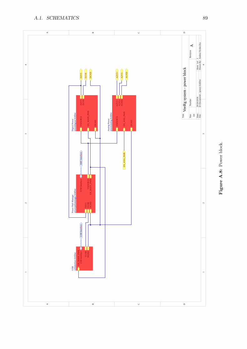
A.1. SCHEMATICS 89
11
22
33
44
DD
CC
BB
AA
Title
Num
ber
Rev
isio
nSi
ze A4
Dat
e:29
/10/
2018
Shee
t o
fFi
le:
D:\D
ocum
enti\
..\po
wer
.Sch
Doc
Dra
wn
By:
DG
ND
D2V
5V
SOU
RC
E
EN_M
AIN
_PW
R
D1V
8
Dig
ital P
ower
pow
erdi
gita
l.Sch
Doc
VSO
UR
CE
EN_M
AIN
_PW
RD
GN
D
STM
Inte
rface
VU
SBD
2V5
Pow
er P
ath
Man
ager
pow
erpa
thm
enag
er.S
chD
oc
DG
ND
USB
Inte
rface
VU
SB
EN_M
AIN
_PW
R
USB
usbi
nter
face
.Sch
Doc
USB
Inte
rface
SMT
Inte
rface
D2V
5
D1V
8
DG
ND
VSO
UR
CE
EN_A
NA
_PW
R
A2V
5+
DG
ND
A2V
5-A
GN
D
Ana
log
Pow
erpo
wer
anal
og.S
chD
oc
A2V
5+
A2V
5-
AG
ND
EN_A
NA
_PW
R
A
VeeR
g sy
stem
- po
wer
blo
ck
And
rea
Verd
ecch
ia1
1
POA2V50
POAGND
POD1V8
POD2V5
PODGND
POEN0ANA0PWR
POSMT INTERFACE
POSM
T IN
TERF
ACE0
#MCL
R PO
SMT
INTE
RFAC
E0PB
OUT
POSM
T INTE
RFACE0
PSHO
LD
POUSB INTERFACE
POUS
B IN
TERF
ACE0
RX
POUS
B IN
TERF
ACE0
TX
Fig
ure
A.8
:Pow
erblock.
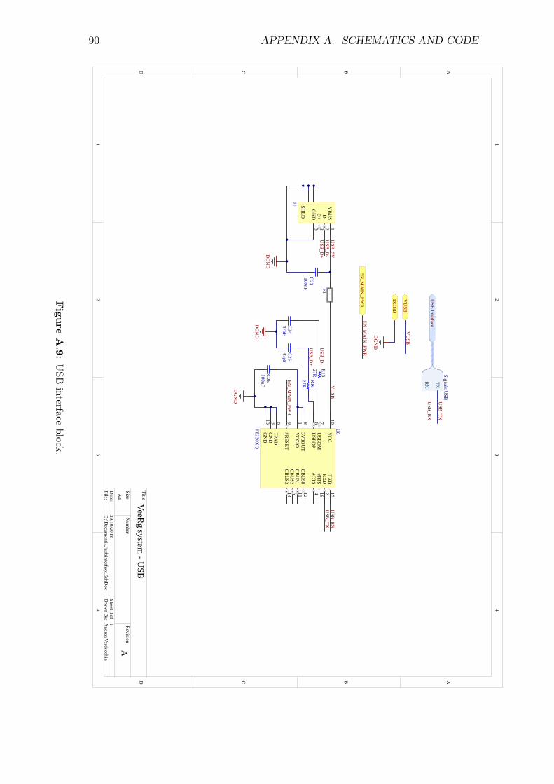
90 APPENDIX A. SCHEMATICS AND CODE
1 1
2 2
3 3
4 4
DD
CC
BB
AA
Title
Num
berR
evisionSize
A4
Date:
29/10/2018Sheet of
File:D
:\Docum
enti\..\usbinterface.SchDoc
Draw
n By:
47pFC
2447pFC
25
27R
R16
27R
R15100nFC
26
DG
ND
DG
ND
USB
_D-
USB
_D+
USB
_TXU
SB_R
X
USB
DM
7
USB
DP
6
#RESET
9
VC
CIO
1
VCC
10
CB
US3
14C
BU
S25
CB
US1
11
TXD
15
GN
D3
GN
D13
CB
US0
12
RX
D2
#RTS16
#CTS
4
3V3O
UT
8
TPAD
0
U8
FT230XQ
EN_M
AIN
_PWR
100nFC
23
DG
ND
VB
US
1
D-
2
D+
3
GN
D5
SHLD
J1
F1U
SB_D
-U
SB_D
+
TX
RX
Signals USB
USB
InterfaceU
SB_R
X
USB
_TX
VU
SB
DG
ND
DG
ND
EN_M
AIN
_PWR
EN_M
AIN
_PWR
VU
SB
VU
SBU
SB_5V
A
VeeRg system
- USB
Andrea Verdecchia
11
PIC2301 PIC2302 COC23
PIC2401 PIC2402 COC24
PIC2501 PIC2502 COC25
PIC2601 PIC2602 COC26
PIF101 PIF102
COF1
PIJ100
PIJ101
PIJ102
PIJ103
PIJ105
PIJ107
PIJ108
PIJ109 COJ1
PIR1501 PIR1502
COR15
PIR1601 PIR1602 COR16
PIU800
PIU801
PIU802
PIU803
PIU804
PIU805
PIU806
PIU807
PIU808
PIU809
PIU8010
PIU8011
PIU8012
PIU8013
PIU8014
PIU8015
PIU8016
COU8
PODGND
POEN0MAIN0PWR
POUSB INTERFACE
POUSB INTERFACE0RX POUSB INTERFACE0TX
POVUSB
Figu
reA
.9:USB
interfaceblock.
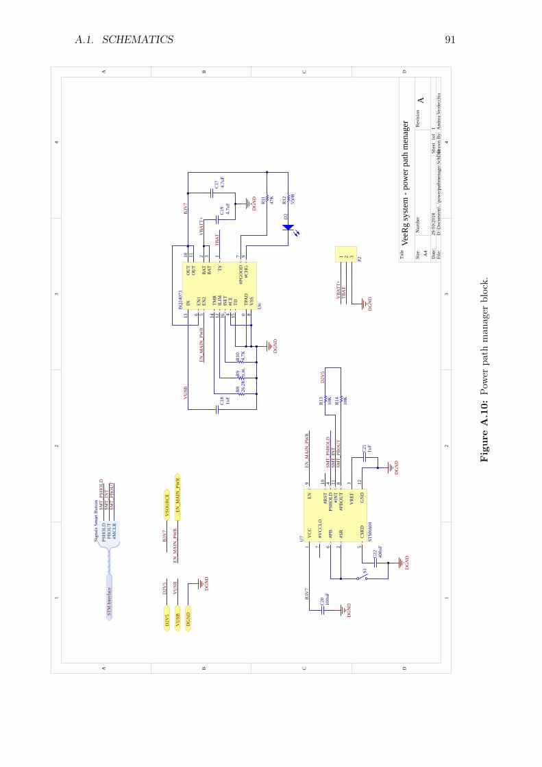
A.1. SCHEMATICS 91
11
22
33
44
DD
CC
BB
AA
Title
Num
ber
Rev
isio
nSi
ze A4
Dat
e:29
/10/
2018
Shee
t o
fFi
le:
D:\D
ocum
enti\
..\po
wer
path
men
ager
.Sch
DocD
raw
n B
y:
TS1
BAT
2
BAT
3
#CE
4
EN2
5EN
16
#PG
OO
D7
VSS
8#C
HG
9
OU
T10
OU
T11
ILIM
12
IN13
TMR
14
TD15
ISET
16
TPA
D0
U6
BQ
2407
3
1uF
C18
DG
ND
26.2
KR
8n.
m.
R9
4.7K
R10
D2
47K
R11
550R
R12
TBA
T
4.7u
FC
194.
7uF
C17
DG
ND
VBA
TT+
B3V
7
S1
VCC
1
#SR
2
VR
EF3
PSH
OLD
4
CSR
D5
#PB
6
#VC
CLO
7
#PB
OU
T8
EN9
#RST
10
#IN
T11
GN
D12
U7
STM
6600
DG
ND
DG
ND
1uF
C21
EN_M
AIN
_PW
R
100n
FC
20
DG
ND
SMT_
PSH
OLD
SMT_
INT
SMT_
PBO
UT
10K
R13
10K
R14
400n
FC
22
VU
SB
DG
ND
DG
ND
VSO
UR
CE
EN_M
AIN
_PW
REN
_MA
IN_P
WR
PSH
OLD
PBO
UT
#MC
LR
Sign
als S
mar
t But
ton
STM
Inte
rface
SMT_
INT
SMT_
PSH
OLD
SMT_
PBO
UT
D2V
5B
3V7
D2V
5
D2V
5
B3V
7
VU
SB
VU
SB
1 2 3
P2
VBA
TT+
TBA
T
DG
ND
EN_M
AIN
_PW
R
A
VeeR
g sy
stem
- po
wer
pat
h m
enag
er And
rea
Verd
ecch
ia1
1
PIC1701 PIC1702 CO
C17
PIC1801 PIC1802
COC18
PIC1901 PIC1902
COC19
PIC2001 PIC2002 CO
C20
PIC2101 PIC2102 CO
C21
PIC2201 PIC2202 COC
22
PID201
PID202
COD2
PIP201
PIP202
PIP203 COP
2
PIR801 PIR802 COR8
PIR901 PIR902 COR9
PIR1001 PIR1002 COR1
0
PIR1
101
PIR1
102 COR
11
PIR1
201
PIR1
202 COR1
2
PIR1
301
PIR1
302 COR1
3
PIR1
401
PIR1
402 COR
14
PIS101 PIS102 COS1
PIU600
PIU601
PIU602
PIU603
PIU604
PIU605
PIU606
PIU607
PIU608
PIU609
PIU6
010
PIU6011
PIU6012
PIU6
013
PIU6014
PIU6
015
PIU6016 COU
6
PIU701
PIU702
PIU703
PIU704
PIU705
PIU706
PIU707
PIU708
PIU709
PIU7010
PIU7011
PIU7012
COU7
POD2V5
PODGND
POEN0MAIN0PWR
POSTM INTERFACE
POST
M IN
TERF
ACE0
#MCL
R PO
STM
INTE
RFAC
E0PB
OUT
POST
M IN
TERF
ACE0
PSHO
LD
POVSOURCE
POVUSB
Fig
ure
A.1
0:Pow
erpa
thman
ager
block.
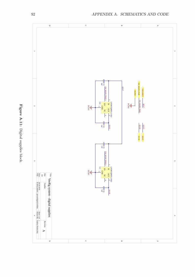
92 APPENDIX A. SCHEMATICS AND CODE
1 1
2 2
3 3
4 4
DD
CC
BB
AA
Title
Num
berR
evisionSize
A4
Date:
29/10/2018Sheet of
File:D
:\Docum
enti\..\powerdigital.SchD
ocD
rawn B
y:
1uFC
131uFC
14EN
_MA
IN_PW
R
DG
ND
IN1
OU
T5
2
EN3
NC
4
GN
DU
4
LP5907QM
FX-3.3Q
1
IN1
OU
T5
2
EN3
NC
4
GN
DU
5
LP5907QM
FX-1.8Q
1
1uFC
151uFC
16
DG
ND
EN_M
AIN
_PWR
VSO
UR
CE
EN_M
AIN
_PWR
EN_M
AIN
_PWR
D2V
5
D1V
8
DG
ND
DG
ND
B3V
7
B3V
7D
2V5
D2V
5D
1V8
D1V
8
A
VeeRg system
- digital supplies
Andrea Verdecchia
11
PIC1301 PIC1302 COC13
PIC1401 PIC1402 COC14
PIC1501 PIC1502 COC15
PIC1601 PIC1602 COC16
PIU401
PIU402
PIU403
PIU404
PIU405
COU4
PIU501
PIU502
PIU503
PIU504
PIU505
COU5
POD1V8
POD2V5
PODGND
POEN0MAIN0PWR
POVSOURCE
Figu
reA
.11:Digitalsupplies
block.

A.1. SCHEMATICS 93
11
22
33
44
DD
CC
BB
AA
Title
Num
ber
Rev
isio
nSi
ze A4
Dat
e:29
/10/
2018
Shee
t o
fFi
le:
D:\D
ocum
enti\
..\po
wer
anal
og.S
chD
ocD
raw
n B
y:
VSO
UR
CE
EN_A
NA
_PW
REN
_AN
A_P
WR
A2V
5+
DG
ND
DG
ND
B3V
7A
2V5+
OU
T1
FB2
NC
3
GN
D4
EN5
NR
/SS
6
DN
C7
IN8
TPA
D0
U11
TPS7
A30
01
OU
T1
FB2
NC
3
GN
D4
EN5
NR
/SS
6
DN
C7
IN8
TPA
D0
U9
TPS7
A49
01
PGO
OD
1FB
+2
VIN
3
GN
D4
CP5
OU
T-6
FB-
7
EN-
8
C1-
9C
1+10
OU
T+11
EN+
12
TPA
D0
U10
LM27
762
10uF
C36
10nF
C37
10uF
C38
10nF
C39
11.3
KR
24
10K
R25
AG
ND
AG
ND
AG
ND
10uF
C27
10nF
C28
10uF
C29
10nF
C31
11.1
KR
18
10K
R20
AG
ND
AG
ND
AG
ND
10K
R21
4.7u
FC
32
1uF
C33
DG
ND
89.8
KR
17
51K
R19
2.2u
FC
30
86.6
KR
23
51K
R22
4.7u
FC
35
DG
ND
2.2u
FC
34
AG
ND
EN_A
NA
_PW
R
B3V
7
A2V
5-A
2V5-
AG
ND
AG
ND
A2V
5+
A2V
5-
AG
ND
DG
ND
OU
T+
OU
T-
FB-
FB+
A
VeeR
g sy
stem
- an
alog
supp
lies
And
rea
Verd
ecch
ia1
1
PIC2701 PIC2702 CO
C27
PIC2801 PIC2802 CO
C28
PIC2901 PIC2902 CO
C29
PIC3001 PIC3002 CO
C30
PIC3101 PIC3102 CO
C31
PIC3201 PIC3202 CO
C32
PIC3
301
PIC3
302
COC3
3
PIC3401 PIC3402 CO
C34
PIC3501 PIC3502 CO
C35
PIC3601 PIC3602 CO
C36
PIC3701 PIC3702 COC
37 PIC3801 PIC3802
COC3
8
PIC3901 PIC3902 CO
C39
PIR1701 PIR1702 COR1
7 PIR1801 PIR1802 CO
R18
PIR1901 PIR1902 COR1
9 PIR2001 PIR2002 CO
R20
PIR2
101
PIR2
102
COR2
1
PIR2201 PIR2202 COR2
2
PIR2301 PIR2302 COR2
3
PIR2401 PIR2402 COR2
4
PIR2501 PIR2502 COR2
5
PIU900
PIU901
PIU902
PIU903
PIU904
PIU905
PIU906
PIU907
PIU908 COU
9
PIU1000
PIU1001
PIU1002
PIU1003
PIU1004
PIU1005
PIU1006
PIU1007
PIU1008
PIU1009
PIU10010
PIU10011
PIU10012 COU10
PIU1100
PIU1101
PIU1102
PIU1103
PIU1104
PIU1105
PIU1106
PIU1107
PIU1108 COU
11
POA2V50
POAGND
PODGND
POEN0ANA0PWR
POVSOURCE
Fig
ure
A.1
2:Ana
logsupp
liesblock.

94 APPENDIX A. SCHEMATICS AND CODE
A.2 Code
A.2.1 Biquad filters
Following the code that implements a digital biquad filter in direct form 2 whichrequires only two delay registers. This type of filter is a second-order recursivelinear filter containing two poles and two zeros.
1 /****2 Function:3 double Filter_IIR_Biquad_Sec( double , double *, double *,
uint32_t )4
5 Remarks:6 See prototype in filters.h.7 */8
9 double10 Filter_IIR_Biquad_Sec( double signal , double *coeffs , double *
scaleValues , double *delayLine , uint32_t nSections )11 12 uint32_t i, j;13 double y = signal;14 double w = 0.0;15
16 for ( j = 0; j < nSections; j++ )17 18 // The denominator19 w = y;20 for ( i = 0; i < 2; i++ )21 w -= coeffs[ ( j << 2 ) + i ] * delayLine[ ( j << 1 ) + i
];22
23 // The numerator24 y = w;25 for ( i = 0; i < 2; i++ )26 y += coeffs[ ( j << 2 ) + i + 2 ] * delayLine[ ( j << 1 )
+ i ];27
28 y *= scaleValues[ j ];29
30 // Shift the register values31 delayLine[ ( j << 1 ) + 1 ] = delayLine[ j << 1 ];32 delayLine[ j << 1 ] = w;33 34
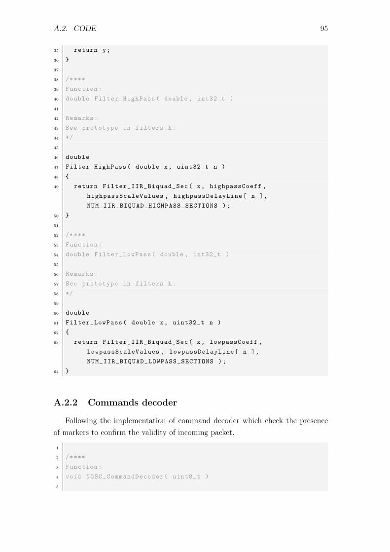
A.2. CODE 95
35 return y;36 37
38 /****39 Function:40 double Filter_HighPass( double , int32_t )41
42 Remarks:43 See prototype in filters.h.44 */45
46 double47 Filter_HighPass( double x, uint32_t n )48 49 return Filter_IIR_Biquad_Sec( x, highpassCoeff ,
highpassScaleValues , highpassDelayLine[ n ],NUM_IIR_BIQUAD_HIGHPASS_SECTIONS );
50 51
52 /****53 Function:54 double Filter_LowPass( double , int32_t )55
56 Remarks:57 See prototype in filters.h.58 */59
60 double61 Filter_LowPass( double x, uint32_t n )62 63 return Filter_IIR_Biquad_Sec( x, lowpassCoeff ,
lowpassScaleValues , lowpassDelayLine[ n ],NUM_IIR_BIQUAD_LOWPASS_SECTIONS );
64
A.2.2 Commands decoder
Following the implementation of command decoder which check the presenceof markers to confirm the validity of incoming packet.
1
2 /****3 Function:4 void NGSC_CommandDecoder( uint8_t )5

96 APPENDIX A. SCHEMATICS AND CODE
6 Remarks:7 See prototype in NGSC.h.8 */9
10 void NGSC_CommandDecoder( uint8_t data )11 12 static uint8_t tempCommand , tempChannelMask;13
14 switch( commandDecoderState )15 16 case NGSCCheckHeadingState:17 if ( data == COMMAND_SOH )18 commandDecoderState = NGSCCheckStartOfPacketState;19 else20 21 if ( NGSCVerbose )22 printf( "\nNGSC Error: Wrong packet" );23 commandDecoderState = NGSCCheckHeadingState;24 25 break;26
27 case NGSCCheckStartOfPacketState:28 if ( data == COMMAND_STX )29 commandDecoderState = NGSCDecodeCommandState;30 else31 32 if ( NGSCVerbose )33 printf( "\nNGSC Error: Wrong packet" );34 commandDecoderState = NGSCCheckHeadingState;35 36 break;37
38 case NGSCDecodeCommandState:39 switch( data )40 41 case NGSCCommandCheckSPIComunication:42 tempCommand = NGSCCommandCheckSPIComunication;43 commandDecoderState = NGSCCheckEndOfPacketState;44 break;45
46 case NGSCCommandStartConversions:47 tempCommand = NGSCCommandStartConversions;48 commandDecoderState = NGSCCheckEndOfPacketState;49 break;50
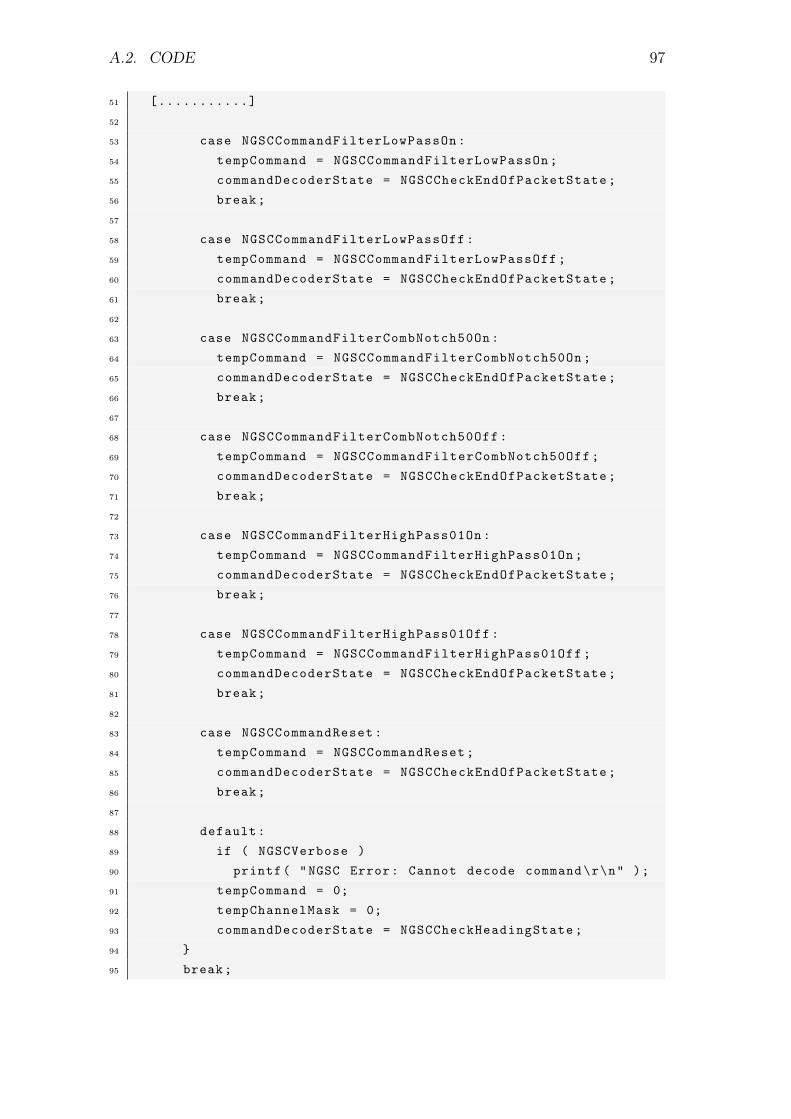
A.2. CODE 97
51 [...........]52
53 case NGSCCommandFilterLowPassOn:54 tempCommand = NGSCCommandFilterLowPassOn;55 commandDecoderState = NGSCCheckEndOfPacketState;56 break;57
58 case NGSCCommandFilterLowPassOff:59 tempCommand = NGSCCommandFilterLowPassOff;60 commandDecoderState = NGSCCheckEndOfPacketState;61 break;62
63 case NGSCCommandFilterCombNotch50On:64 tempCommand = NGSCCommandFilterCombNotch50On;65 commandDecoderState = NGSCCheckEndOfPacketState;66 break;67
68 case NGSCCommandFilterCombNotch50Off:69 tempCommand = NGSCCommandFilterCombNotch50Off;70 commandDecoderState = NGSCCheckEndOfPacketState;71 break;72
73 case NGSCCommandFilterHighPass01On:74 tempCommand = NGSCCommandFilterHighPass01On;75 commandDecoderState = NGSCCheckEndOfPacketState;76 break;77
78 case NGSCCommandFilterHighPass01Off:79 tempCommand = NGSCCommandFilterHighPass01Off;80 commandDecoderState = NGSCCheckEndOfPacketState;81 break;82
83 case NGSCCommandReset:84 tempCommand = NGSCCommandReset;85 commandDecoderState = NGSCCheckEndOfPacketState;86 break;87
88 default:89 if ( NGSCVerbose )90 printf( "NGSC Error: Cannot decode command\r\n" );91 tempCommand = 0;92 tempChannelMask = 0;93 commandDecoderState = NGSCCheckHeadingState;94 95 break;

98 APPENDIX A. SCHEMATICS AND CODE
96
97 case NGSCChannelMaskState:98 tempChannelMask = data;99 commandDecoderState = NGSCCheckEndOfPacketState;
100 break;101
102 case NGSCCheckEndOfPacketState:103 if ( data == COMMAND_ETX )104 105 Command_Received.command = tempCommand;106 Command_Received.channelMask = tempChannelMask;107 Command_Received.valid = true;108 tempCommand = 0;109 tempChannelMask = 0;110 commandDecoderState = NGSCCheckHeadingState;111
112 NGSC_CommandHandler ();113 114 else115 116 if ( NGSCVerbose )117 printf( "\nNGSC Error: Wrong packet" );118 tempCommand = 0;119 commandDecoderState = NGSCCheckHeadingState;120 121 break;122
123 default:124 if ( NGSCVerbose )125 printf( "\nNGSC Error: Wrong state identifier" );126 tempCommand = 0;127 commandDecoderState = NGSCCheckHeadingState;128 129
130 return;131

List of Figures
1.1 Membrane potential. . . . . . . . . . . . . . . . . . . . . . . . . . . 81.2 Brain’s waves classification. . . . . . . . . . . . . . . . . . . . . . . 91.3 10-20 electrodes’ arrengement. . . . . . . . . . . . . . . . . . . . . . 111.4 3D model for the placement of electrodes. . . . . . . . . . . . . . . 13
2.1 The main steps of workflow. . . . . . . . . . . . . . . . . . . . . . . 162.2 Overview of system’s boards. . . . . . . . . . . . . . . . . . . . . . . 172.3 Backgound noise of the system. . . . . . . . . . . . . . . . . . . . . 192.4 Backgound noise of the system. . . . . . . . . . . . . . . . . . . . . 202.5 The body and the common mode noise. . . . . . . . . . . . . . . . . 212.6 The common mode effect. . . . . . . . . . . . . . . . . . . . . . . . 222.7 The FL schematic. . . . . . . . . . . . . . . . . . . . . . . . . . . . 242.8 Dependence of common mode signal from variable Cbl, Cbe and Cse. 252.9 The CM characteristic disjointed into the two contributions F and E. 272.10 The effect of Rp on the fz1 value. . . . . . . . . . . . . . . . . . . . 302.11 Electrodes mismatch schematic. . . . . . . . . . . . . . . . . . . . . 312.12 CM2DM in electrodes mismatch. . . . . . . . . . . . . . . . . . . . 342.13 Single-ended and differential nput stages mismatch. . . . . . . . . . 352.14 CM2DM in single-ended input stages mismatch. . . . . . . . . . . . 372.15 CM2DM in differential input stages mismatch. . . . . . . . . . . . . 382.16 Stability in the feedback loop. . . . . . . . . . . . . . . . . . . . . . 392.17 Instability in the feedback loop. . . . . . . . . . . . . . . . . . . . . 402.18 Simplified representation of the condition necessary between A and
1/β to keep stability. . . . . . . . . . . . . . . . . . . . . . . . . . . 422.19 The data and command packets. . . . . . . . . . . . . . . . . . . . . 442.20 The overall structure of the implemented firmware. . . . . . . . . . 452.21 Example of characteristics of an high-pass filter. . . . . . . . . . . . 502.22 The filters’ response in low-pass and high-pass cases. . . . . . . . . 522.23 The low-pass filter effects. . . . . . . . . . . . . . . . . . . . . . . . 54
99

100 LIST OF FIGURES
2.24 The high-pass filter effects. . . . . . . . . . . . . . . . . . . . . . . . 552.25 The 0.1 Hz high-pass filter effects. . . . . . . . . . . . . . . . . . . . 562.26 Overview of system’s boards. . . . . . . . . . . . . . . . . . . . . . . 592.27 Overview of systems. . . . . . . . . . . . . . . . . . . . . . . . . . . 60
3.1 Arosual and valence space in emotion classification. . . . . . . . . . 623.2 Example of NPVs in case of like and dislike statment. . . . . . . . . 653.3 Brain’s activity for different frequencies band in case of like and
dislike statement. . . . . . . . . . . . . . . . . . . . . . . . . . . . . 663.4 Example of images for the War/Cubs test. . . . . . . . . . . . . . . 683.5 Normalized Power Values of the Tattoo test. . . . . . . . . . . . . . 713.6 Normalized Power Values of the War/Cubs test. . . . . . . . . . . . 723.7 Normalized Power Values of the Models/Growths test. . . . . . . . 733.8 P-values of β paramenters relatives to every test. . . . . . . . . . . 74
A.1 Block schematic of overall VeeRg system. . . . . . . . . . . . . . . . 82A.2 Bluetooth block. . . . . . . . . . . . . . . . . . . . . . . . . . . . . 83A.3 PIC23MZ block. . . . . . . . . . . . . . . . . . . . . . . . . . . . . . 84A.4 MPU9250 block. . . . . . . . . . . . . . . . . . . . . . . . . . . . . 85A.5 ADS1299 block. . . . . . . . . . . . . . . . . . . . . . . . . . . . . . 86A.6 Electrodes block. . . . . . . . . . . . . . . . . . . . . . . . . . . . . 87A.7 ICSP block. . . . . . . . . . . . . . . . . . . . . . . . . . . . . . . . 88A.8 Power block. . . . . . . . . . . . . . . . . . . . . . . . . . . . . . . . 89A.9 USB interface block. . . . . . . . . . . . . . . . . . . . . . . . . . . 90A.10 Power path manager block. . . . . . . . . . . . . . . . . . . . . . . . 91A.11 Digital supplies block. . . . . . . . . . . . . . . . . . . . . . . . . . 92A.12 Analog supplies block. . . . . . . . . . . . . . . . . . . . . . . . . . 93

Manuals
[7] Texas Instruments. -36V, -200mA, ULTRALOW-NOISE, NEGATIVE LIN-EAR REGULATOR. url: http://www.ti.com/lit/ds/symlink/tps7a3001-ep.pdf.
[8] Texas Instruments. ADS1299-x Low-Noise, 4-, 6-, 8-Channel, 24-Bit, Analog-to-Digital Converter for EEG and Biopotential Measurements. Rev. C. url:http://www.ti.com/lit/ds/symlink/ads1299.pdf.
[9] Texas Instruments. Improving Common-Mode Rejection Using the Right-LegDrive Amplifierl. url: http://www.ti.com/lit/an/sbaa188/sbaa188.pdf.
[10] Texas Instruments. LM27762 Low-Noise Positive and Negative Output Inte-grated Charge Pump Plus LDO. Rev. B. url: http://www.ti.com/lit/ds/symlink/lm27762.pdf.
[11] Texas Instruments. TPS7A49 36-V, 150-mA, Ultralow-Noise, Positive LinearRegulator. Rev. E. url: http://www.ti.com/lit/ds/symlink/tps7a49.pdf.
[19] Microchip. PIC32MZ Embedded Connectivity with Floating Point Unit (EF)Family. Rev. E. url: http://ww1.microchip.com/downloads/en/DeviceDoc/60001320E.pdf.
101

102 MANUALS

Articles
[2] C. Assambo et al. “Determination of the Parameters of the Skin-ElectrodeImpedance Model for ECG Measurement”. In: (2007).
[4] Joann Difede and Hunter G. Hoffman. “Virtual Reality Exposure Therapyfor World Trade Center Post-traumatic Stress Disorder: A Case Report”. In:CyberPsychology and Behavior 5.6 (2004).
[6] Yongbin Gao, Hyo Jong Lee, and Raja Majid Mehmood. “Deep learninig ofEEG signals for emotion recognition”. In: 2015 IEEE International Confer-ence on Multimedia and Expo Workshops (ICMEW) (2015).
[12] Zhang J. et al. “ReliefF-Based EEG Sensor Selection Methods for EmotionRecognition”. In: Sensors 16.10 (2016).
[13] Nitin Kumar, Kaushikee Khaund, and Shyamanta M. Hazarika. “BispectralAnalysis of EEG for Emotion Recognition”. In: Procedia Computer Science84 (2016), pp. 31–35.
[14] Mi Li et al. “Emotion recognition from multichannel EEG signals using K-nearest neighbor classification”. In: Technology and Health Care 26 (2018).
[15] Wei Liu, Wei-Long Zheng, and Bao-Liang Lu. “Emotion Recognition Us-ing Multimodal Deep Learning”. In: Neural Information Processing (2016),pp. 521–529.
[16] M. A. Lopez-Gordo, D. Sanchez-Morillo, and F. Pelayo Valle. “Dry EEGElectrodes”. In: MDPI - Sensors (2014).
[17] Burkhard Maess, Erich Schröger, and Andreas Widmann. “High-pass filtersand baseline correction in M-EEG analysis”. In: Journal of NeuroscienceMethods 266 (2016), pp. 164–165.
[18] I. Marshall and J. M. Neilson. “Mains interference in ECG recording”. In:Journal of Medical Engineering and Technology 8.4 (1984), pp. 177–180.
103
104 ARTICLES
[20] Zeynab Mohammadi, Javad Frounchi, and Mahmood Amiri. “Wavelet-basedemotion recognition system using EEG signal”. In: Neural Computing andApplications 28.8 (2017), pp. 1985–1990.
[21] R. Pallas-Areny. “Interference-rejection characteristics of biopotential ampli-fiers: a comparative analysis”. In: IEEE Transactions on Biomedical Engi-neering 35.11 (1988), pp. 953–959.
[23] Albert Rizzo et al. “Virtual Reality Exposure for PTSD Due to MilitaryCombat and Terrorist Attacks”. In: Journal of Contemporary Psychotherapy45.4 (2015), pp. 255–264.
[24] Barbara O. Rothbaum et al. “Virtual reality exposure therapy for Vietnamveterans with post-traumatic stress disorder”. In: The Journal of ClinicalPsychiatry 68.8 (2001), pp. 617–622.
[25] Levenson R.W. et al. “Emotion and autonomic nervous system activity inthe Minangkabau of west Sumatra”. In: Journal of Personality and SocialPsychology 62.6 (1992), pp. 972–988.
[28] Zhongbin Su et al. “AHRS Design based on STM32 and MEMS Sensors”. In:International Journal of Control and Automation 8.7 (2015), pp. 55–66.
[29] Shravani Sur and V. K. Sinha. “Event-related potential: An overview”. In:Industrial Psychiatry Journal 18.1 (2009), pp. 70–73.
[30] Darren Tanner, Kara Morgan-Short, and Steven J. Luck. “How inappropriatehigh-pass filters can produce artifactualeffects and incorrect conclusions inERP studiesof language and cognition”. In: Psychophysiology (2015).
[31] Darren Tanner et al. “On high-pass filter artifacts (they’re real) and base-line correction (it’s a good idea) in ERP-ERMF analysis”. In: Journal ofNeuroscience Methods 266 (2016), pp. 166–170.
[32] Nattapong Thammasan, Ken-Ichi Fuki, and Masayuki Numao. “Applicationof deep belief networks in EEG-based dynamic music-emotion recognition”.In: International Joint Conference on Neural Networks (2016).
[33] Rufin VanRullen. “Four common conceptual fallacies in mapping the timecourse of recognition”. In: Frontiers in Psychology 365.2 (2011).
[34] Giovanni Vecchiato et al. “Changes in Brain Activity During the Observationof TV Commercials by Using EEG, GSR and HR Measurements”. In: BrainTopography 23 (2010), pp. 165–179.

ARTICLES 105
[35] Li Wang, Zheng Zhang, and Ping Sun. “Quaternion-based Kalman Filter forAHRS Using an Adaptive-step Gradient Descent Algorithm”. In: Interna-tional Journal of Advanced Robotic Systems (2015).
[36] Xiao-Wei Wang, Dan Nie, and Bao-Liang Lu. “Emotional state classificationfrom EEG data using machine learning approach”. In: Neurocomputing 129(2014), pp. 94–106.
[37] Andreas Widmann, Erich Schröger, and Burkhard Maess. “Digital filter de-sign for electrophysiological data – a practical approach”. In: Journal of Neu-roscience Methods 250 (2015), pp. 34–46.
[38] Haiyan Xu and Konstantinos N. Plataniotis. “Affective states classificationusing EEG and semi-supervised deep learning approaches”. In: 2016 IEEE18th International Workshop on Multimedia Signal Processing (MMSP) (2017).
[39] Ashkan Yazdani et al. “Multimedia content analysis for emotional charac-terization of music video clips”. In: EURASIP Journal on Image and VideoProcessing (2013).
[40] Bülent Yilmaz et al. “Like/dislike analysis using EEG: Determination of mostdiscriminative channels and frequencies”. In: Computer Methods and Pro-grams in Biomedicine 113 (2014), pp. 705–713.
[41] Quanzeng You et al. “Building a Large Scale Dataset for Image EmotionRecognition: The Fine Print and the Benchmark”. In: Association for theAdvancement of Artificial Intelligence (2011).

106 ARTICLES

Books
[3] Cédric Assambo and Martin J. Burke. Low-Frequency Response and the Skin-Electrode Interface in Dry-Electrode Electrocardiography, Advances in Elec-trocardiograms - Methods and Analysis. Richard Millis, 2012.
[22] Robert Plutchik. Emotions and life : perspectives from psychology, biology,and evolution. 1st. American Psychological Association, 2003.
[26] American National Standard. Ambulatory electrocardiographs. Arlingon (VA):Association for the Advancement of Medical Instrumentation, 1999.
[27] International Electrotechnical Commission Standard.Medical electrical equip-ment. International Standards et al., 2008.
107

108 BOOKS

Other References
[1] Sharad Agarwal. Advertising with and without social messages: insights fromneuro marketing. FPM - IIM Ranchi. 2013.
[5] Paul Ekman. “Handbook of Cognition and Emotion”. In: ed. by Power-M.Dalgleish T. 1999. Chap. Basic emotions.
109