1

Economic versus Psychological Forecasting.

Evidence from Consumer Confidence Surveys

BY MAURIZIO BOVI••••

ISAE - Institute for Studies and Economic Analyses

Department of Macroeconomics

E-mail: m.bovi@isae.it

"There are two kinds of forecasters:

those who don't know, and those who don't know they don't know.''

John Kenneth Galbraith (Wall Street Journal, Jan 22, 1993)

Abstract

Permanent and widespread psychological biases affect both the subjective

probability of future economic events and their retrospective interpretation. They may

give rise to a systematic gap between (over-critical) judgments and (over-optimistic)

expectations - the “forecast” error. When things go bad, then, psychology suggests that

people tend to become particularly bullish, amplifying the forecast error. Also,

psychology argues that personal/future conditions are systematically perceived to be

better than the aggregate/past ones. All this sharply contrasts with standard economic

assumptions. Evidence from a unique dataset covering ten European countries over

twenty-two years confirms the presence of structural psychologically driven distortions

in people’s judgments and expectations formation.

JEL Codes: C42, C53, C82, D12, D84.

Keywords: Cognitive Psychology; Expectations; Forecasting; Survey Data.

• The opinions expressed herein are those of the author and not necessarily reflect the views of the ISAE. This paper

won the I. Kerstenetzky Best Paper Award at the 29th CIRET Conference (Santiago, Chile, October 8-11, 2008).

2

1. Introduction

By tradition and necessity, economics is a behavioral science and people’s

expectations play a pivotal role in it. Nevertheless, by recent tradition and analytical

necessity, economists tend to approach expectations in a rather axiomatic way. The

standard economic literature merely assumes that the representative agent is an

unemotional computer which, in the long run, cannot repeat the same mistake. Given a

long enough time span and conditional on an information set, objective (i.e. in some

sense statistically optimal) and subjective expectations must, on average, coincide. The

logic behind is twofold – i) erring is costly; ii) people learn by doing. Although the way

in which agents form expectations is not addressed by standard economics homo

economicus has, thus, both the motivation and the occasion for operating rationally1.

Arguably because of its less axiomatic and more descriptive approach, cognitive

psychology tells a different story: biases are likely to be the rule, not the exception

(Kahneman & Tversky, 1973, 1974, 1982). Kahneman and Tversky (1974) argued that

heuristic short-cuts create probability judgments which deviate from statistical

principles. Intuitive strategies and simple heuristics are reasonably effective some of the

time, but they also produce biases and give rise to systematic incongruities when

assessing economic conditions/evolutions. Two things are worth emphasizing here.

First, individuals may persist with biased beliefs because they are unaware of being

self-incoherent or because they convince themselves that they are right. Whatever the

case may be, considering the presence of costs due to errors or waiting for people to

change their mind may be misleading. More in general, despite market forces

(competition and arbitrage) and learning by doing, psychologists suggest that irrational

behavior is not contingent (Mullainathan & Thaler, 2000). Second, psycho-biases affect

a significant share of the population: that is, they are not isolated quirks, but deep-seated

and systematic behavioral patterns which impinge on people’s judgments/expectations

formation.

Consumer confidence surveys (CCS) are useful and in fact widely accepted devices

with which to gather information about common people’s expectations over time

(Ludvigson, 2004). A number of recent papers have studied micro data from CCS in an

1 The rational expectation hypothesis implies more than unbiasedness (Pesaran and Weale, 2006), but

here we are only interested in biases.

3

attempt to identify individual-level forecast errors from consecutive or matched surveys

(Brown & Taylor, 2006; Das & van Soest, 1997; Das, Dominitz & van Soest, 1999;

Mitchell & Weale, 2007; Souleles, 2004). On studying the difference between ex ante

expectations and subsequent realizations, i.e. the “survey” forecast error (SFE), these

works usually find a non-zero SFE and they reject the rational expectations hypothesis

(REH). Notwithstanding the pivotal role of REH in mainstream economic models, it is

hard to understand why so few authors seek to explain the enduring presence of non

standard behaviors. Within the economic tradition, Carroll (2003) and Branch (2004)

suggest that the REH is rejected because the costs of forming rational expectations

exceeding the benefits. Another strand of research, which roughly and somewhat

timidly draws on psychology, i) points to belief distortions that may increase the well-

being (Brunnermeier & Parker, 2005; Caplin & Leahy, 2001; Yariv, 2001), or it

assumes that agents, although rational, ii) have limited information processing capacity

(Sims, 2003), or iii) update information infrequently (Reis, 2006).

Against this background the novelty, and the aim, of this study is twofold. First, we

propose an unusual psychological interpretation of the SFE and of other similar ex

ante/post incongruities in people’s judgments/expectations as collected by CCS (Section

2). There are several reasons for addressing CCS data in the light of cognitive

psychology. First, as argued by Katona (1958), CCS should/could collect information

on sentiments. To the extent that replies reflect moods, they are not statistically-based

forecasts and the gaps between judgments and expectations can be well interpreted by

means of psychological arguments.2 Moreover, cognitive psychology allows

consideration even of problems linked to retrospective questions. Indeed, by definition,

incoherent views may stem from both overly pessimistic judgments and overly

optimistic expectations. Instead, however, ex post realizations are often conceived as the

“objective (unbiased) benchmark” against which ex ante subjective expectations must

be compared. Thus, the psychological approach makes one wonder whether people

suffer from biases in both backward- and forward-looking exercises.

When ordinary persons are surveyed, moreover, some questions can be considered

2 Typically, in fact, the economic literature examines whether CCS data add independent (i.e. beyond

economic data/models) information about the economy (for a recent survey, see Ludvigson, 2004).

4

vague and/or hard-to-assess by the respondent (e.g., “How do you expect the general

economic situation in the country to develop over the next 12 months?”). These may

trigger heuristic, and hence biased, answers (Kahneman & Tversky 1973, 1974, 1982).

As regards the SFE, psychology suggests that it may be significantly different from zero

considering both many individuals and long periods of time, and that amid real or

psychological economic hardships the SFE may be even larger. Other gaps suggested by

the psychological analysis of people’s replies refer to personal/future conditions, which

may be systematically perceived as more bullish than the aggregate/past ones.

The paper’s second contribution is that it offers evidence on these psychological

biases by taking advantage of a unique dataset covering more than twenty years and ten

European countries (Section 3). To our knowledge, then, this paper is the first attempt to

conduct empirical analyses of the differences between ex ante expectations and ex post

perceptions about “general economic conditions”. Apart from being informative about

judgments/expectations formation on key macroeconomic situations, the relative

categorical answers are not affected by the so-called “Manski critique” (Manski, 1990;

Subsection 5.1). On the negative side, respondents are randomly selected so that there

are no genuine re-interviews.3 Also, our basic data are the percentages of respondents

who have chosen a particular option (a lot better, better, etc.). Thus, we have no

individual-level data even within the same wave. In the present setting, however, these

issues do not hamper useful econometric analyses. The study’s main empirical goal, in

fact, is to test whether judgments and expectations formation is structurally consistent

with the innate biases uncovered by psychologists. To this end we regress survey data

only on a constant, basing our identification strategy on the logic that the only (main)

factors captured by the intercept are psychological biases. That this can be done is

because of our unique dataset, dissolving the effects of temporary/localized/disparate

elements (mismeasurements, economic shocks, etc.) and, above all, because of the rich

set of testable a priori stemming from the analysis of CCS via cognitive psychology. We

also control for heteroskedasticity and autocorrelation by computing Newey-West

robust standard errors (Newey & West, 1987).

3 Van Oest and Franses (2008) analyze consumer confidence indicators based on non genuine panels.

They fairly argue that this complicates a straightforward interpretation of shifts in confidence and propose

a methodology to address the related issues. It should be made clear, instead, that our empirical aim here

is to find evidence on innate psycho-phenomena rather than on shifts in confidence.

5

Confirming previous results based on genuine (but short and single nationwide)

panels, the data show that a perennial non-zero survey forecast error pervades Europe.

This outcome is consistent with both the recent economic literature and psychology. But

we furnish still more findings and interpretations of people’s replies. As the interplay

between prospect theory and illusion of control leads one to expect, e.g., conditional on

having reported an unpleasant situation respondents tend to become particularly

optimistic and, consequently, to over-err. More in general, and this is our main point,

only psychological suggestions seem to offer a fully comprehensive explanation of the

detected structural distortions affecting the formation of Europeans’

judgments/expectations as they emerge from CCS data.

2. Psychological biases in judgments and expectations.

2.1. Overview

Humans receive and must arrange massive amount of data. Most of the latter are

immediately ignored, discarded or abstracted away by neurological machinery. When

new information is “zipped”, converted into symbolic format and memorized, it is

subject to certain biasing effects. The main problem is not the cost/amount/availability

of information, but its handiness. As Simon (1971, p. 40) put it, “(…) a wealth of

information creates a poverty of attention”. As mentioned, some recent economic study

has rediscovered Simon’s hints (Reis, 2006; Sims, 2003). However, Kahneman and

Tversky (1973, 1974, 1982) have suggested that the processes of intuitive judgment are

not merely simpler than rational models demand, but are categorically different in kind.

Their theory of heuristics and biases points out that because of the ways in which people

process information, having accurate information does not necessarily improve

decision-making, and sometimes may detract from it. Rather than accumulate the

optimal amount of information, individuals often uncritically accept information that

confirms their beliefs while they over-critically reject disconfirming data. They are

overconfident in their judgments and are prone to base judgments on information that is

vivid and available to memory rather than on information that is more accurate but dull

and unmemorable. It is worth noting that these heuristic processes are not exceptional

6

responses to problems of excessive complexity or to an overload of information; rather,

they are normal intuitive responses to even the simplest questions about likelihood,

frequency, and prediction. Following the seminal studies of Kahneman and Tversky,

many authors have documented numerous ways in which prospective and retrospective

views do not cohere, do not follow basic principles of logic and probability, and depend

systematically on irrelevant factors such as mood, context, or mode of presentation.

Intuitive strategies and simple heuristics are reasonably effective some of the time, but

they also produce biases and give rise to systematic incongruities. Therefore, although

psychology has not (and may never) develop a unified theory that explains or predicts

the full range of human behavior (Kopcke et al., 2004), it nonetheless offers a pragmatic

collection of situation-specific mini-theories usefully exploitable in connection with

CCS data. Some of the lessons from psychology can be recalled in the present context,

and it is important to observe since now that all of them coherently point to the

persistence of structural discrepancies in lay people’s views on economic developments.

2.2. Why may lay people be prospectively over-optimistic about (especially personal)

economic changes?

Representativeness is a heuristic for making probability judgments. A byproduct

of representativeness is the law of small numbers. According to this law, people believe

that the mean value from a small sample also has a distribution concentrated at the

expected value of the random variable. This gives rise to a bias due to “overinference”

from (too) short sequences of observations. In an overview of behavioral finance,

Shleifer (2000) argues that the law of small numbers may explain the excess sensitivity

of stock prices as a result of investors’ overreacting to short strings of good news. A

related aspect of this law is overconfidence. People tend to make forecasts in uncertain

situations by looking for familiar patterns and assuming that future favorable patterns

will resemble past ones, often without taking sufficient consideration of the reasons for

the pattern or the probability of the pattern repeating itself (Shiller, 2000). Illusion of

control (DeBondt & Thaler, 1995) may then explain why people believe that their own

future situation will get better “against all odds”. Its definition is highlighting: “an

expectancy of a personal success probability inappropriately higher than the objective

7

probability would warrant” (Langer 1975, p. 313). Irrational exuberance, in Mr.

Greenspan’s famous 1996 speech, may thus be interpreted in the present context as the

interplay between overconfidence and illusion of control: the former induces people to

overestimate the precision of the signals that they receive; the latter induces individuals

to overweight positive signals and to be over-optimistic. Closely related to the illusion

of control is the theory of depressive realism. In a seminal paper, Alloy and Abramson

(1979) found that non-depressed people are more likely than depressed people to think

that outcomes are contingent on their actions when they are not. They concluded that as

opposed to depressed persons, whose perceptions are apparently accurate, normal

people distort reality in an optimistic fashion.4

2.3. Why could lay people be retrospectively over-critical of (especially macro)

economic changes?

People suffer from the availability heuristic and unduly emphasize recent events:

an economic shock may have psychological effects. These latter, in turn, affect the

correct reading of past economic events. According to the so-called availability bias,

individuals base their prediction of the frequency of an event on how easily an example

can be brought to mind. Because an example is easily brought to mind or mentally

“available”, the single example is considered to be representative of the whole rather

than just a single example in a range of data. This bias may help to explain why, as

recently found (Brachinger, 2008), people can overweight the overall inflation rate

when price changes hit especially frequently bought goods with small expenditure

weight. That said it can also be added that, compared to unfamiliar information, familiar

information is more easily accessible from memory, and it is therefore believed to be

more real or relevant. It turns out that the mere repetition of certain information in the

media, regardless of its accuracy, makes it more easily available and therefore falsely

perceived as more accurate. The explanation is completed by observing that, as

emphasized by Doms and Morin (2004), the media tend to overweight bad economic

4 We may also speculate that non-depressed individuals distort reality in an optimistic fashion because

being overconfident is an optimal choice. In other words, while psychology is silent on the causality

issue, i.e. realism may induce depression, there is a body of economic literature which maintains that

overconfidence may increase well-being (see Introduction).

8

news. Whilst this pertains to the nature itself of the news media, Blendon et al. (1997)

have pointed out that the public’s biases can be attributed to the media’s focus on bad

news. It has been argued that the over-critical information flow may also run from

people to media (Curtin, 2003), although Blood and Phillips (1994) found a reverse

causality. When individuals judge past economic conditions, a perverse spiral may in

any case lock them into “backward-looking” pessimism. As over critical judgments are

magnified in bad times (due to the media coverage) and expectations are “sticky” due to

the illusion of control, economic hardships might enlarge the forecast error. It is also

important to note that, ex post, economy-wide actual conditions are objectively equal

for everyone. Only exploiting psychological considerations one may wonder whether

people have a distorted reading of past situations even in the long run.

2.4. Why may lay people be both over-critical ex post and over-optimistic ex ante

when asked about economic changes?

Both prospective and retrospective biases are congruent with mental accounting

(Thaler, 1999), which posits that people mentally frame assets as belonging to either

current or future income. From the individual’s standpoint, therefore, judging and

forecasting are “time separable” exercises that need not be self-consistent. When

inserted in the present setting, then, the prospect theory (Kahneman & Tversky, 1979)

suggests another reason why the survey forecast error may not be a zero-mean reverting

process due to both ex ante and ex post arguments. Basically, the theory argues that

people’s attitude toward risk is conditional on some neutral or status quo point, which

may vary from situation to situation. If the reference point is defined so that an outcome

is viewed as a “gain”, then the individual will tend to be risk averse. On the other hand,

if the reference point is defined so that an outcome is viewed as a “loss”, then the

individual will be risk seeking. It turns out that individuals suffering from a reduction in

their income tend to become risk lovers. In this event, which may be induced/magnified

by retrospective pessimism, illusion of control may interact with prospect theory and

over-optimistic expectations may be associated with over-critical judgments – economic

hardships enlarge the SFE referring to personal situations.

9

2.5. Testable implications.

Psychology is silent on the magnitude of the biases and on whether the effects of

the biases are constant over time and/or homogeneous across individuals. Nevertheless,

all the distortions mentioned are innate and therefore so enduring and diffuse that they

affect, at least in the long run, the representative individual. In addition, psychology

indicates several factors that prevent people from adequately learning from the past and

from being aware of their forecast errors. For example, experiments performed by

Wason (1969) regarding the difficulty of people in making use of disconfirming

information indicate that the inability to learn stems from the unwillingness to examine

information that would disprove the position held. Staw and Ross (1989) discuss

escalation, a situation in which a course of action has resulted in initial losses, but where

action can be taken to modify and possibly reverse the original outcome. They observe

that individuals can become locked into the existing course of action, “throwing good

money or effort after bad” (page 216). A similar bias stems from conservatism, which is

the tendency to change previous probability estimates more slowly than warranted by

new data. Usually, slowness is defined relative to the amount of change prescribed by

normative rules such as Bayes’ theorem. Conservatism is the result of a combination of

overconfidence with anchoring-and-adjustment. Consider, finally, the

“hindsight/confirmation bias” (Bernstein, 1994). Suppose there is an unexpected event.

People tend naturally to concoct explanations for it after the fact, which makes the event

more predictable, and less random, than it is. More in general, as argued by Camerer

(Kopcke et al., 2004), self-awareness is surprisingly limited.

To summarize, there are well-known psychological departures from

statistical/rational expectations which may help understanding of widespread and

ineradicable discrepancies between people’s judgments and expectations. Whether or

not these biases are conscious the point remains: psychological considerations

univocally underline the enduring presence of a nonrandom mental “environment”

potentially triggering inconsistent views on economic matters. Hence, by exploiting

CCS data (Section 3), we may fruitfully test whether:

1. judgments and expectations on the economic situation consistently differ;

10

2. survey forecast errors are consistently greater in bad than in good times;

3. the personal economic situation is perceived to be structurally brighter (or

less dark) than the economy-wide one;

4. the Future is perceived to be systematically brighter (or less dark) than the

Past.

3. Data

For the purpose of examining the foregoing psychological implications empirically,

a unique dataset can be obtained from the Business Surveys Unit of the European

Commission. The dataset is based on monthly surveys carried out at a national level by

public and private institutes in the framework of the Joint Harmonised European Union

Programme of Business and Consumer Surveys.5 The surveys are designed to capture

the representative European consumer across twenty-seven countries. Almost 40,000

persons are usually selected by a random stratified sampling procedure or by simple

random sampling.

Here we focus on four questions concerning general and personal financial

situations/evolutions referring to the same past/next year (Appendix A). Respondents

may choose among six qualitative reply options (a lot better, better, a lot better, better,

the same, worse, a lot worse, don’t know) and the individual-level answers are then

used to compute the percentages of respondents having chosen a particular option. Only

these six aggregate shares are available, and only four of them form the basis of this

study. The exceptions are the proportions relative to the options “don’t know” and “the

same”, which are set aside because results based on them are hard-to-interpret. We

exclude the former because it is a “non response”, i.e. it is not the outcome of an explicit

elaboration but, rather, a declaration of no information6. In this regard, the European

Commission Users’ Manual (1997, p. 18) states that: “(…) there are six reply options:

five “real” ones and a “do not know” option”. Hence, for example, it is not easy to

5 Detailed information on the Joint Harmonised EU Programme of Business and Consumer Surveys can

be found in European Commission (1997, 2007). 6 However, the data show a reliable distribution: on average, as expected, the greatest number of “do not

knows” refer to future macroeconomic changes, the lowest to past personal stances (see Graph. 1,

Appendix A).

11

decipher a survey forecast error computed by comparing prospective and retrospective

“don’t know”. As for the other exclusion, it is important to note that the questions are

about “developments/changes” (Appendix A). Thus, one might suspect a priori (Theil,

1961) that individuals respond “the same” on most occasions because it is hard to think

of constantly improving/worsening economic conditions (whatever that means for lay

people7) over many years. Psychology suggests that an over-preference for this neutral

choice may be induced by the presence of uninformed and/or uninterested respondents.

Part of the problem derives from the respondents’ reluctance to admit to a lack of an

attitude. Simply because the surveyor is asking the question, respondents believe that

they should have an opinion about it. Since unbiased answers may be due to both

psychological neutrality and analytical rationality,8 we prefer to focus on replies in

which psychological distortions may play a dominant role. We have rescaled the

percentages accordingly9 - rescaled Z=100*Z/(100-E-N), where Z=LB, B, W, LW.

Despite the fact that only dealt with are questions about general and personal

economic conditions, national surveys contain other questions about the labor market,

spending intentions on major purchases (furniture, electrical/electronic devices, etc.),

savings, etc. Needless to say, each question has potential information content but the

questions selected seem particularly suited to the empirical side of this study. When

asked about “financial conditions/evolutions”, indeed, ordinary people may use

heuristic shortcuts to manage large quantities of information that may lead them astray.

This is exactly what we want to study: do lay people answer according to a specific

underlying framework? Is this latter congruent with the psychological indications of

Section 2? Moreover, these data make it possible to match, repeatedly over almost three

hundred months and across several European countries, expectations and judgments

referring to the same time span (one year). Lastly, there is no need for respondents to

address and quantify general economic10 situations/evolutions exactly: only compared

7 To the extent that i) GDP growth coincides with people’s view of “development in economic condition”,

and ii) GDP growth follows a stationary process agents should, on average, accumulate towards the

“stationary” item of the questionnaire. 8 Interestingly, the data show that this is in fact the most frequently preferred reply option (see Graph. 1,

Appendix A). Similar outcomes, based on genuine panel data, have been found for the UK (Mitchell &

Weale, 2007). 9 LB=a lot better; B=a little better; W=a little worse; LW=a lot worse (Appendix A). If not otherwise

stated we henceforth refer to rescaled values. The overall picture is not affected when using non-rescaled

percentages (results available upon request). 10

Although the average value of variables such as GDP, Consumption, Wealth, etc., has been growing

12

are qualitative answers to the same question (see Sections 4 and Appendix A).

The data suffer from some change throughout the sample. Since 1995, for instance,

Italy has replaced on-the-spot interviews with the telephone method. In Germany, apart

from the issues arising from the re-unification of 1991, some modifications have been

made to both the order and the wording of some questions. Consequently, there are

some problems11

in the time series comparability of the data. In an attempt to reduce

temporary data issues and to increase the reliability of the econometric tools employed

(see Section 4), we focus on the countries with the longest and most time-comparable

datasets. Moreover, a long-lasting dataset reduces the time inconsistencies due to shocks

hitting consumers after they have made the forecast and before they make the

retrospective judgment - even more so considering that we examine full sample average

values, and that we do so for several countries. We end up with ten countries12

(Belgium, Germany, Ireland, Greece, France, Italy, Finland, Spain, Netherlands, UK)

and 268 monthly interviews13

(from January 1985 to April 2007).

4. Econometric methodology

To examine formally the first psychological suggestion of Subsection 2.5, we test

the hypothesis βZ_Gen ≠ 0 in the following regression

SFE_ Zt _Gen ≡ Q3_Zt - Q4_Zt-12 = βZ_Gen + ut (1)

where

Q3_Zt = % of respondents to the question Q3 having chosen the Z reply option in the

survey carried out in month t

Q4_Zt-12 = % of respondents to the question Q4 having chosen the Z reply option in the

survey carried out in month t-12

during the period across the countries under analysis, Europeans have been, on average, more pessimistic

than optimistic. On summing over time and across Europe all the proportions relative to the eight

pessimistic answers (four queries, two pessimistic reply options, see Appendix A), one obtains a number

more than double that emerging from the sum of all the eight optimistic answers. 11 Other problems affecting the data are more general; e.g., it is easily understood that there are no

incentives/disincentives related to a particular answer. The fact that CCS are increasingly widely

performed, commented upon and studied indirectly corroborates their reliability (see also Appendix A). 12 About 20,000 consumers are surveyed each month across the ten European countries examined. 13

Data for Spain start in June 1986, for Finland in November 1987.

13

Q3 = How do you think the general economic situation in the country has changed over

the past 12 months? It has…

Q4 = How do you expect the general economic situation in the country to develop over

the next 12 months? It will…

Z = LB, B, W, LW

LB = get/got a lot better

B = get/got a little better

W = get/got a little worse

LW = get/got a lot worse

βZ_Gen = coefficient

ut = random disturbance.

Similarly, mutatis mutandis,14

for the survey forecast error referring to the

personal questions: SFE_ Zt _Per ≡ Q1_Zt - Q2_Zt-12 = βZ_Per + ut. An example may

help clarify the matter. Let the share of individuals forecasting that the system-wide

economic situation will be “a little worse” in the next year be, according to the survey

performed in January 2000, 35%. After a year, inter alia, interviewees are asked to

answer question Q3. If people’s forecasts were not affected by psychological distortions

and if no shock hits consumers before they respond to Q3, then the share of citizens

judging that the economic situation has got “a little worse” should be 35%. Needless to

say, people may sometimes err even if they are Muth-rational – according to standard

economics the SFEs must cancel out over time, that is to say, βZ_Gen=0 (and βZ_Per=0)

whatever Z. According to psychology, instead, βZ_Gen (and βZ_Per) should be both

significantly positive for Z=LW, W and significantly negative for Z=LB, B. For

instance, if Q3_LWt is significantly greater than Q4_LWt-12, i.e. if βLW_Gen>0, then

judgments prove to be consistently darker than expectations. Likewise, if βLB_Gen,

βB_Gen<0, then judgments are structurally less bright than expectations. Hence,

psychology gives rise to a rich set of testable indications about the SFE (and not only).

Equation 1) has several good features in the present context. First, measurement

errors that influence in the same way the two different waves of surveys used to

14

Q1=How has the financial situation of your household changed over the last 12 months?

Q2=How do you expect the financial position of your household to change over the next 12 months?

14

compute the SFE (i.e., those carried out in period t and t-12 for t=1,…,n) disappear when

differencing. This may happen with respect to sampling errors, which are likely to be a

common factor influencing relatively consecutive surveys. Then mismeasurements do

not affect the OLS estimate of the constant term (Greene, 2002). It should also be noted

that examining the intercept is a necessary and sufficient condition (Boero et al., 2008)

for testing immanent psychological implications. In general, our identification strategy

relies on the fact that psycho-biases are the only (or, at least, the most important)

structural factor captured by the constant. The underlying logic is that psychological

biases are natural traits, and it is likely that they emerge when mean values referring to

hundreds of observations are examined – all the more so when tests are replicated for

ten countries. By the same token, measurement errors and time inconsistencies due to

shocks hitting consumers after they have made the forecast and before they make the

retrospective judgment do not matter: it is likely that both of them cancel out in the

sample. Finally, the logic behind equation 1) can be straightforwardly used to assess the

other testable psychological indications pointed out in Subsection 2.5. In fact, all the

tests proposed basically amount to compute the average of the dependent variable.

Therefore, to verify whether the mean value of the SFE is larger during times of

economic hardships (i.e. when individuals respond LW or W) than in good times, we

may test βGen>0 in the following15

(suppressing the error term, see also equation 1):

(SFE_LWt _Gen + SFE_Wt _Gen) – ( SFE_LBt _Gen + SFE_Bt _Gen) =

(βLW_Gen + βW_Gen) – (βLB_Gen + βB_Gen) = βGen (2)

where Gen=(Q3, Q4)=General questions; and likewise, mutatis mutandis, for the

Personal questions (Q1, Q2).

So far, we have contrasted the ex ante/post views of different representative

consumers about the same year. In order to verify the last two psychological

implications and to offer some robustness checks, we also examine judgments and

expectations collected in the same survey. As compared to the previous regressions, the

gain is that we study the replies given by the same statistical respondent. Clearly,

15

We do not report all the four possible combinations (βLW v βLB, βLW v βB, etc.,) in order to save space

and, above all, to address the drawbacks discussed in Section 5.

15

because beliefs refer to different years, the difference is not exactly16

a SFE. The

motivation is that our main empirical aim is to find evidence on psycho-biases and the

SFE is just one of them. The logic is that over-critical judgments and over-optimistic

expectations do not depend on the time period to which they refer: the tendency of

past/general situations to be felt darker than future/personal ones should emerge even in

tests examining different years. Basically, we perform regressions similar to equation 1)

with two main differences. First, as said, we use contemporaneous proportions; second,

we use balances. These latter are computed17

as follows: Qibt=2∗LBt+Bt-Wt-2∗LWt,

where i=1,…4 refers to the number of the query (so that Q1b is the balance relative to

the question Q1, etc.). Thus, in order to test the third psychological bias, for example,

we regress (Q2b-Q4b) on a constant. A significantly positive intercept would mean that,

ex ante, the respondent expects that his/her future economic condition (Q2b) will get

systematically better (or less bad) than the economy-wide one (Q4b).

5. Empirical issues and results

5.1. Empirical issues

When categorical expectations and realizations referring to personal stances are

compared the results, as argued by Manski (1990), may be misleading. The reason is

that expectations reflect some location measure (mean, mode, etc.) of the individual’s

subjective distribution of the income change, the outcome is one draw from the actual

income change distribution. Therefore, even if actual and subjective distributions

coincide (i.e., if people are rational), the two categorical variables are not necessarily

equal. A simple example makes the point forcefully. Assume that, as for the questions

Q1 and Q2 (Section 4), individuals have just two option replies18

, say “better” (B) and

“worse” (W). Suppose, then, 65% of the population think there is a 40% chance of the

16

Although they are not-proper SFE, we refer to them as errors (gaps, discrepancies, etc.). 17

This is how European Commission computes balances (European Commission, 1997). This makes it

possible to save space. More disaggregated tests do not modify the overall picture (results available upon

request). 18

Das, Dominitz and van Soest (1999) extend the Manski critique to surveys with multiple qualitative

reply options and alternative response models.

16

outcome W and 60% of B, whilst 35% think there is a 60% chance of it being W and a

40% chance of it being B. Hence, 35% will predict W and 65% will predict B. In the

present context (Section 4), for the SFE to be zero the ex post distribution must be 35-

65, too. However, if everyone has rational expectations (that is, if the subjective

distributions of the future variables are correct) and there are no aggregate shocks (that

is, realizations are independent of each other), then the realizations will be as follows:

47% (=0.65*40+0.35*60) will experience “worse” and 53% (=0.65*60+0.35*40) will

experience “better”. Therefore, with the data at hand, a persistent non-zero SFE may

emerge even with rational expectations: how can we be sure that non-zero SFEs depend

on psycho-biases only?

If anything, the Manski critique is weak in our context. First, it merely states that

the SFE may be misleadingly different from zero. In contrast, we have a priori on i) the

sign of the SFE, ii) the effect of hard times on it and iii) non SFE-based inconsistencies

such as the last two psycho-distortions of Subsection 2.5. It is unlikely that evidence

coherently supporting all the psychological implications be seriously affected by the

critique. Moreover, when macroeconomic conditions are considered (questions Q3 and

Q4, Section 4), all citizens will experience the same objective19

realization (say, GDP

growth). Thus, if rational, they should tend to have the same expectations about

nationwide economic performances and, in our empirical framework, zero-SFEs should

emerge.20

Finally, as argued by Katona (1958), CCS should/could collect information

on sentiments. Sometimes attitude changes conform with changes in income, sometimes

attitudes change autonomously,21

regardless objective developments. As Keynes (1936,

pp. 161-162) put it: “most, probably, of our decisions to do something positive, (…) can

only be taken as the result of animal spirits - a spontaneous urge to action rather than

inaction, and not as the outcome of a weighted average of quantitative benefits multiplied

by quantitative probabilities.”. This is in stark contrast with the above mentioned concept

of expectations formation based on the individual’s subjective distribution. More in

general, to the extent that replies reflect moods they are not statistically-based forecasts,

the Manski critique loses force and the SFE can validly be addressed/interpreted via

19

As mentioned in Section 2 the psychological approach, unlike economics, makes one wonder whether

people suffer from biases even in backward-looking exercises. 20

Graph. 1 compares the long run distribution of Europeans’ replies on economic stances (Appendix A). 21

In fact, this is the case in which CCS data may be very useful to forecasters of economic activity.

17

psychological arguments.

The intercepts that we analyze may be different from zero because of over-critical

judgments and/or over-optimistic expectations; that is, the lack of an objective “hard”

benchmark (e.g., GDP) implies that we can not establish whether people are more over-

critical than overconfident. Moreover, we have no a priori on the relative magnitude of

the biases: does the illusion of control affect expectations more than, say, the

availability and media biases affect the retrospective reading of economic situations?

It is also useful to recall that we are examining i) percentages of respondents based

on ii) qualitative reply options. As for the first item, it means that we have not

individual-level data. Percentages of respondents are nonetheless useful to our aim. In

fact, what we want to verify is whether a significant share of population has distorted

judgments/expectations and, conditional upon that, whether the intercepts detected

support psychological theories. To this end, individual-level data are not strictly

necessary: when the evidence points to non-zero SFEs a significant share of respondents

doubtless has distorted judgments/expectations. As for the qualitative nature of data, it

is due to the fact that we are inspecting “adjectives” (worse, better, etc). Consequently,

even with individual-level data, we would not know the precise magnitude of the gaps.

Despite the fact that qualitative data have limited information content, they are not

entirely worthless considering that our aim is to test widespread psycho-distortions. The

presence of quantitatively very large individual-level intercepts, in fact, may lead to the

detection of market-level ex ante/post incoherence even if the number of

psychologically biased individuals is relatively (insignificantly?) low. When working

with qualitative answers, by contrast, what we study is the share of individuals whose

views on economic matters are psychologically driven, and hence are biased, not the

average amount of their errors.

Last but not least, the proposed empirical procedure requires a careful treatment of

standard errors (more details in Appendix B). For instance, we use monthly data on one-

year forecasts. This naturally induces serial correlation – respondents will definitively

know that their expectations are erroneous only twelve months after the initial

projection, and overlapping same-sign errors are the likely outcome. Once again, this

situation can be addressed even via psychological insights. From the psychological

standpoint, indeed, conservatism may induce people to hold their expectations for

18

longer than warranted by objective computations (Section 2). In addition, it should be

pointed out that measurement errors affect the disturbance of the regression at least by

inflating it (Greene, 2002). All in all, a procedure to compute robust standard errors

seems necessary.

5.2. Results

The results set out in Table 1 show that, over the last twenty years, the average

SFE has been significantly different from zero in practically all European countries.

TABLE 1 ABOUT HERE

As well-known, few exceptions out of eighty regressions can occur just by

chance, especially for the cases of zero SFE referring to the LB option reply. In fact, the

LB-proportions have very small values and volatility.22

This, together with the fact that

figures are rounded up to the first decimal, implies that the data somewhat resemble to

zero-one binary time series. All this clearly increases the probability of observing zero

SFEs just by chance. More importantly, the overall picture strongly supports our

psychological interpretation: we obtain both significant positive signs for LW and W

and significant negative signs for LB and B. It also confirms existing findings based on

genuine, but shorter and single-nation, panel data (Brown & Taylor, 2006; Das & van

Soest, 1997; Das, Dominitz & van Soest, 1999; Mitchell & Weale, 2007; Souleles,

2004). Unluckily, and this holds for all our empirical results, data issues and disparate

nation-wide objective developments prevent reliable cross section analyses. Although

interesting, however, such analyses are outside the empirical scope of this paper.

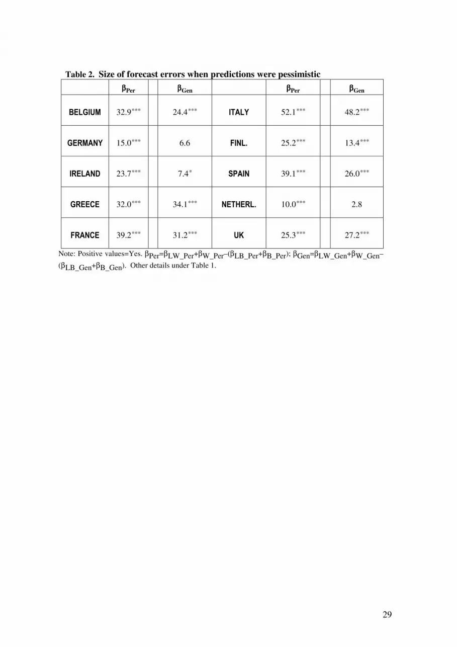
TABLE 2 ABOUT HERE

22

For instance, the sample mean for Spain is 2.8 for both Q1_LBt and Q2_LBt-12 (hence the recorded

βLB=0.0 in Table 1) with a standard deviation of, respectively, 1.2 and 1.3. This is perhaps why other

CCS allow only the replies “better” or “worse” without any other qualification (such as “a lot”, “a little”

and the like). To be noted on passing is that the number of “a lot worse” replies is, on average, much

higher than that of “a lot better” throughout Europe – is there no (psychological?) limit to the Worse? (see

also footnote 10).

19

As regards the second psychological implication stated in Subsection 2.5, not

reported here are all the four possible combinations23

(βLW v βLB, βLW v βB, etc.). This

saves space and, more importantly, it avoids the drawbacks arising from the presence of

dichotomic proportions affecting the LB option reply. The results set out in Table 2

show that people’s forecast errors on the economic stance are structurally larger in hard

than in good times. This finding is consistent with the interplay between prospect theory

and illusion of control: after a negative shock giving rise to bad judgments people’s

expectations become more over-optimistic, and their SFEs consequently become larger.

This evidence confirms the results reported for the UK by Mitchell and Weale (2007).

As mentioned, we also perform tests on non-proper SFEs. In particular,

psychological arguments suggest testing whether:24

(Q1b-Q3b)>0. If this is verified, then the respondent judges ex post that his/her

financial condition (Q1b) has, on average, got better (or less bad) than the

economy-wide one (Q3b). This is compatible with the backward-looking

pessimism stemming from the media and availability biases, which especially

affect beliefs on macroeconomic conditions.

(Q2b-Q4b)>0. If this is verified, then the respondent expects that her future

economic condition (Q2b) will get systematically better (or less bad) than the

economy-wide one (Q4b). This tests the third psychological implication and it is

implied by the illusion of control.

(Q2b-Q1b), (Q4b-Q3b)>0. If these are verified, the respondent believes that the

next year will always be more bullish (or less bearish) than the last one as far as,

respectively, personal and general economic stances are concerned. This allows

the fourth psychological implication to be tested and it stems from both illusion of

control and availability/media biases.

(Q2b-Q3b)>0. This is a sort of “mini-max” overall test: all the psycho-distortions

here studied minimize the magnitude of the balance Q3b and maximize that of

23

Some insights can be obtained by comparing the intercepts reported in Table 1. For instance, it is

evident that, conditional on a large and positive βLW (or βW), a negative βLB (or βB) in all likelihood

supports the psychological suggestions emphasized. Table 1 shows that this event frequently happens. 24

Qibt=2∗LBt+Bt-Wt-2∗LWt, where i=1,…4 refers to the number of the question. So, e.g., Q1b is the

balance relative to the question Q1 (Section 4).

20

Q2b. Accordingly, this gap should show the greatest values.

TABLE 3 ABOUT HERE

Table 3 shows that there is no (quasi) exception to psychological arguments. By

contrast, these results are hard-to-interpret in the light of objective statistical

computations: although they refer to different years, ex ante and ex post perceptions on

yearly developments should tend to be self-consistent over time. For instance, the

significantly positive intercepts obtained for (Q1b-Q3b) and (Q2b-Q4b) imply that the

average citizen judges, and expects, that his/her particular situation has got, and will get,

systematically better than that of “his/herself”. More in general, and according to the

findings of cognitive psychology, the data exhibit that Europeans relentlessly repeat the

following mantra: “as usual, it has got worse than I expected. Especially for the others.

Nevertheless, I still think that it will get better. Especially for me.”.

6. Concluding remarks

In this paper we have examined consumer confidence surveys data across ten

European countries. We have compared average values of the differences between

prospective vs. retrospective as well as personal vs. general views on economic stances

over almost three hundred months. A systematic pattern has emerged whereby lay

people’s replies are incoherent from an objective, statistical, standpoint. We have

argued that the issues stemming from the Manski critique, macroeconomic shocks and

the lack of re-interviews may affect the results, if any, only partially and occasionally.

Owing to the unique time/space dimension of the dataset, in fact, it is likely that their

potential effects have not significantly perturbed our findings. In any case, they cannot

totally explain our unequivocal record on the enduring presence of a nonrandom

structural framework permeating the data.

In contrast, we have shown that cognitive psychology offers a fully comprehensive

reading of the overall evidence. Psychological biases such as illusion of control,

availability bias, etc., are natural traits. It comes as no surprise to find that they emerge

as statistically significant intercepts when the enduring information content of long-

21

lasting surveys, aimed to capture the average citizen, is analyzed. On the other hand,

psychologists put forward a large number of competing theories on human behavior. In

the absence of an agreed-upon paradigm, empirical analyses are paramount, and our

findings are based upon a dataset with an unparalleled time/space dimension.

Addressing CCS data via cognitive psychology, therefore, may be useful for both

economists and psychologists.

Acknowledgment

I would like to thank two anonymous referees and, in particular, the Editor for helpful comments. I

also thank Pieraldo and MariaPia Bovi for their technical support.

22

REFERENCES

Alloy, L.B., & L.Y. Abramson (1979). Judgment of contingency in depressed and nondepressed students.

Sadder but wiser? Journal of Experimental Psychology, 108, 441–485.

Bernstein, M.A. (1994). Foregone Conclusions: Against Apocalyptic History. Berkeley: University of

California Press.

Blendon, R., J. Benson, M. Brodie, R. Morin, D. Altman, D. Gitterman, M. Brossard, & M. James:

(1997). Bridging the Gap Between the Public’s and Economists’ Views of the Economy. Journal of

Economic Perspectives 11, 105-188.

Blood D.J. & Phillips, P.C.B. (1995). Recession Headline News, Consumer Sentiment, The State of the

Economy and Presidential Popularity: A Time Series Analysis 1989-1993. International Journal of

Public Opinion Research, 7, 2-22

Boero, G., J. Smith & K.F. Wallis (2008). Evaluating a Three-Dimensional Panel of Point Forecasts: The

Bank of England Survey of External Forecasters, International Journal of Forecasting, 24, 354-367.

Brachinger, (2008). A new index of perceived inflation: Assumptions, method, and application to

Germany. Journal of Economic Psychology, 29, 433-457.

Branch, W. (2004). The Theory of Rationally Heterogeneous Expectations: Evidence from Survey Data

on Inflation Expectations, Economic Journal 114, 592–621.

Brown, S. & Taylor, K. (2006). Financial expectations, consumption and saving: a microeconomic

analysis, Fiscal Studies 27.

Brunnermeier, M.K. & J.A. Parker (2005). Optimal Expectations, American Economic Review, 95, 1092-

1118.

Caplin, A. J., & J. Leahy (2001). Psychological Expected Utility Theory and Anticipatory Feelings,

Quarterly Journal of Economics, 106, 55-80.

Carroll, C. (2003). Macroeconomic Expectations of Households and Professional Forecasters, Quarterly

Journal of Economics, 118, 269-298.

Curtin, R. (2003). Unemployment Expectations: The Impact of Private Information on Income

Uncertainty, Review of Income and Wealth, vol. 49, no. 4.

Das, M. & A. van Soest. (1997). Expected and Realized income changes: evidence from the Dutch Socio-

Economic Panel, Journal of Economic Behaviour and Organization, 32, 137–154.

Das, M., Dominitz, J., & A. van Soest. (1999). Comparing Predictions and Outcomes: Theory and

Applications to Income Changes, Journal of the American Statistical Association, 94, 75–85.

DeBondt, W., & R. Thaler (1995). Financial decision-making in markets and firms: a behavioral

perspective, in Handbooks in OR and MS, Jarrow, R. V. Maksimovic and W. Ziemba, eds.

Doms, M., & N. Morin (2004). Consumer Sentiment, the Economy, and the News Media, Finance and

Economics Discussion Series, Divisions of Research & Statistics and Monetary Affairs Federal Reserve

Board, 51, Washington, D.C.

EUROPEAN COMMISSION (1997). The Joint Harmonised EU Programme of Business and Consumer

Surveys. User Guide, 6, D.G. ECONOMIC AND FINANCIAL AFFAIRS

EUROPEAN COMMISSION (2007). The Joint Harmonised EU Programme of Business and Consumer

Surveys. User Guide, D.G. ECONOMIC AND FINANCIAL AFFAIRS

23

Greene, W.H. (2002). Econometric Analysis. Prentice Hall; 5th edition.

Kahneman, D. & A. Tversky (1973). Availability: A heuristic for judging frequency and probability,

Cognitive Psychology, 5, 207-232.

Kahneman, D. & A. Tversky (1974). Judgment under uncertainty: Heuristics and biases, Science 185,

1124-1131.

Kahneman, D. & A. Tversky (1979). Prospect theory: an analysis of decision under risk, Econometrica

47, 263–292.

Kahneman, D. & A. Tversky (1982). Judgment of and by representativeness, in Judgment Under

Uncertainty: Heuristics and Biases, Kahneman, D., P. Slovic, & A. Tversky, eds. Cambridge University

Press, Cambridge.

Katona, G. (1958). Business Expectations in the Framework of Psychological Economics, in

Expectations, Uncertainty, and Business Behavior, Bowman, M.J., ed. Social Science Research Council,

59-74.

Keynes, J. M., (1936). The General Theory of Employment Interest and Money McMillan London.

Kopcke, R.W., J.S. Little & G.M.B. Tootell (2004). How humans behave: implications for economics and

economic policy, New England Economic Review. First Quarter.

Langer, E. (1975). The Illusion of Control. Journal of Personality and Social Psychology, 32, 311-328.

Ludvigson, S. (2004). Consumer Confidence and Consumer Spending, Journal of Economic Perspectives,

18, 29-50.

Manski, C. (1990), The Use of Intentions Data to Predict Behavior: A Best-Case Analysis, Journal of the

American Statistical Association, 85, 934–940.

Mitchell J. & M. Weale (2007). The Rationality and Reliability of Expectations Reported by British

Households: Micro Evidence from the British Household Panel Survey, NIESR WP.

Mullainathan S. & R.H. Thaler (2000). Behavioral Economics. MIT Dept. of Economics Working Paper,

Sept., 00-27.

Newey W.K. & K.D. West (1987). A simple, positive definite, heteroskedasticity and autocorrelation

consistent covariance matrix. Econometrica, 55, 703-708.

Pesaran, M. H. & M. Weale (2006). Survey Expectations. in Handbook of Economic Forecasting, G.

Elliott, C. Granger and A. Timmermann, eds. North Holland: Amsterdam

Reis, R. (2006). Inattentive Consumers. Journal of Monetary Economics, 53, 1761-1800.

Shiller, R. (2000). Irrational Exuberance. Princeton: Princeton University Press.

Shleifer, A. (2000). Inefficient Markets. An Introduction to Behavioral Finance. Oxford: Oxford

University Press.

Simon H. (1971). Designing Organizations for an Information-Rich World. in Computers,

Communication, and the Public Interest, M. Greenberger, ed.,The Johns Hopkins Press.

Sims, C. (2003). Implications of Rational Inattention. Journal of Monetary Economics, 50, 665-690.

Souleles, N. (2004). Expectations, Heterogeneous Forecast Errors, and Consumption: Micro Evidence

from the Michigan Consumer Sentiment Surveys. Journal of Money, Credit and Banking, 36, 39-72.

24

Staw, B. M. & Ross, J. (1989), Understanding Behavior in escalation Situations. Science, 13 October

1989, 246, 216-20.

Theil, H. (1961). Economic Forecasts and policy. North-Holland, Amsterdam.

Thaler, R.H. (1999). Mental Accounting Matters. Journal of Behavioral Decision Making, 12, 183-206

Van Oest R. And Franses P.H. (2008). Testing changes in consumer confidence indicators, Journal of

Economic Psychology, 29, 3, 255-275.

Wason, P.C. (1969). Regression in Reasoning? British Journal of Psychology, November, 471-80.

Yariv, L. (2001). Believe and Let Believe: Axiomatic Foundations for Belief Dependent Utility. Cowles

Foundation Discussion Paper, 1344, Yale University.

25

Appendix A. Data: definitions and distributions.

Participants in the survey are asked the following questions, which are harmonized in

all countries according to the EU guidelines (European Commission, 1997, 2007):

Q1=How has the financial situation of your household changed over the last 12 months?

It has ...

Q2=How do you expect the financial position of your household to change over the next

12 months? It will ...

Q3=How do you think the general economic situation in the country has changed over

the past 12 months? It has ...

Q4=How do you expect the general economic situation in the country to develop over

the next 12 months? It will ...

LB=got/get a lot better;

B=got/get a little better;

E=stayed/stay the same;

W=got/get a little worse;

LW=got/get a lot worse;

N=don't know.

LB, B, E, etc. are the percentage of respondents having chosen the corresponding option

so that LB+B+E+W+LW+N=100.

Graph. 1. The long run distribution of Europeans’ replies on economic stances

Note: Histograms report average values (%). Europeans=Belgium, Germany, Ireland, Greece, France,

Italy, Finland, Spain, The Netherlands, UK. Starting date for Spain 1987:06, for Finland 1988:11.

1985:01 - 2007:04

LB

B

E

W

LW

N LB

B

E

W

LW N LB

B

E W

LW

N LB

B

E

W

LW N

0

10

20

30

40

50

60

70

Q1 Q2 Q3 Q4

26

Appendix B. Econometric Methodology: computing robust standard errors.

A critical component of the proposed empirical approach is the variance-

covariance matrix of OLS parameter estimates. This is addressed it via the covariance

estimator proposed by Newey and West (1987), which is robust to both

heteroskedasticity and autocorrelation of unknown form (NW-HAC). The present

setting calls for this correction. For instance, we use monthly data on one-year forecasts.

This naturally induces serial correlation – respondents will definitively know that their

expectations are erroneous only twelve months after the initial projection, and

overlapping same-sign errors are the likely outcome. Once again, this situation can be

addressed even via psychological insights. From the psychological standpoint, indeed,

conservatism may induce people to hold their expectations for longer than warranted by

objective computations (Section 2). As for heteroskedasticity, it should be pointed out

that measurement errors affect the disturbance of the regression at least by inflating it

(Greene, 2002). Clearly, a robust procedure increases the reliability of the outcome. As

well known, the NW-HAC covariance estimator needs long-lasting samples and this is

another reason why we prefer countries for which full-sample data is available (Section

3).

That said, consider the general regression model (k-dimensional regressor xi

with coefficient vector β)

yi= xi

Tβ + ui

(i=1,…,n) or, in matrix notation, y=X β + u. (3)

The covariance matrix is usually denoted in one of the following ways:

Ψ= VAR[β] = (XT

X)-1

XT

ΩX(XT

X)-1

(4)

= (n-1

XT

X)-1

XT

n-1

φ(n-1

XT

X)-1

(4a)

where VAR[u] = Ω and φ = n-1

XT

ΩX. φ =is essentially the covariance matrix of the

scores or estimating functions Vi(β) = xi( y

i- xi

Tβ). The estimating functions

evaluated at the parameter estimates V i = Vi( β ) have sum zero. For inference in the

linear regression model, it is essential to have a consistent estimator for Ψ. What kind of

estimator should be used depends on the assumptions about Ω. In the classical linear

model independent and homoskedastic errors with variance σ2

are assumed, yielding Ω

27

= σ2

Ιn and Ψ = σ2

(XT

X)-1

, which can be consistently estimated by plugging in the usual

OLS estimator σ 2

= (n-k)-1∑

=

n

i 1 u

2

. As noted, instead, in the present context Ω is likely

to be both not diagonal (i.e. errors may be autocorrelated) and/or have non constant

diagonal elements (i.e. errors may be heteroskedastic). If the form of heteroskedasticity

and autocorrelation is unknown, a solution is to estimate φ instead of Ω. Newey and

West suggest computing ψ by plugging, into equation (4a), the following: φ = n-1

∑=

−

n

jiji

w1,

|| V i

T

V j where w=(w0, …,wn-1)T

is a vector of weights. A reasonable

assumption is that the autocorrelations should decrease with increasing lag l = |i-j|.

Otherwise, in fact, β can typically not be estimated consistently by OLS. So, the weights

wl should also decrease. We follow the suggestion of Newey and West by i) using

linearly decaying weights, wl= 1- l/(L+1), where L is the maximum lag, and ii) setting25

L=4=floor[4(n/100)2/9

].

25 Correlograms, not reported, confirm that this choice is palatable. Floor=largest integer.

28

Table 1. Size of forecast errors

Per Gen Per Gen

βLW 6.1*** 8.3*** βLW 6.6*** 15.1***

βW 10.4*** 3.9*** βW 19.5*** 9.0***

βB -15.6*** -12.0*** βB -25.3*** -22.1*** BE

LG

IUM

βLB -0.8*** -0.2

ITA

LY

βLB -0.7*** -2.0***

βLW 4.2*** 6.9*** βLW 5.3*** 5.9***

βW 3.3*** -3.6 βW 7.3*** 0.8

βB -7.7*** -4.3* βB -12.9*** -7.5***

GE

RM

AN

Y °

βLB 0.2 1.0***

FIN

LA

ND

βLB 0.3 0.8***

βLW 5.3*** 7.0*** βLW 6.0*** 5.4***

βW 6.5*** -3.3** βW 13.5*** 7.6***

βB -12.6*** -7.5*** βB -19.6*** -13.5*** IRE

LA

ND

βLB 0.7*** 3.8***

SP

AIN

βLB -0.0 0.5***

βLW 1.9 0.4 βLW 7.5*** 7.5***

βW 14.1*** 16.7*** βW -2.5*** -6.1**

βB -15.0*** -15.3*** βB -7.8** -5.8*** GR

EE

CE

βLB -1.0*** -1.7***

NE

TH

ER

LA

ND

βLB 2.8*** 4.4***

βLW 9.4*** 12.5*** βLW 8.0*** 9.3***

βW 10.2*** 3.1*** βW 4.6*** 4.3***

βB -17.3*** -14.7*** βB -12.9*** -13.0*** FR

AN

CE

βLB -2.3*** -0.9***

UK

βLB 0.2 -0.6* Note. Sample 1985:12 – 2007:04 (starting date for Spain 1987:06, for Finland 1988:11). Reported values

are the intercepts of Per=(Q1_Zt-Q2_Zt-12)=βZ_Per; Gen=(Q3_Zt-Q4_Zt-12)=βZ_Gen. (Z=LW, W, B,

LB). Percentages are rescaled: Z=100*Z/(100-E-N). Q1=How has the financial situation of your household

changed over the last 12 months? It has...Q2=How do you expect the financial position of your household

to change over the next 12 months? It will...Q3=How do you think the general economic situation in the

country has changed over the past 12 months? It has...Q4=How do you expect the general economic

situation in the country to develop over the next 12 months? It will...LB=got/get a lot better; B=got/get a

little better; W=got/get a little worse; LW=got/get a lot worse. ***=p-value<1% (**<5%, *<10%) with

Newey-West robust standard errors. The answer is “Yes” if βZ_Gen and βZ_Per are significantly positive for

Z=LW, W and significantly negative for Z=LB, B. Results significantly rejecting the presence of psycho-

biases are in bold.

° As mentioned (Section 3), data for Germany suffer from the country’s reunification. We consequently

ran regressions starting from January 1992. Few parameters substantially changed: βW_Gen=0.1;

βLB_Per = -0.4*; βLB_Gen=0.2.

29

Table 2. Size of forecast errors when predictions were pessimistic

ββββPer ββββGen ββββPer ββββGen

BELGIUM 32.9*** 24.4*** ITALY 52.1*** 48.2***

GERMANY 15.0*** 6.6 FINL. 25.2*** 13.4***

IRELAND 23.7*** 7.4* SPAIN 39.1*** 26.0***

GREECE 32.0*** 34.1*** NETHERL. 10.0*** 2.8

FRANCE 39.2*** 31.2*** UK 25.3*** 27.2***

Note: Positive values=Yes. βPer=βLW_Per+βW_Per–(βLB_Per+βB_Per); βGen=βLW_Gen+βW_Gen–

(βLB_Gen+βB_Gen). Other details under Table 1.

30

Table 3. Differences in responses to personal and general economic situation

questions

Q1b-Q3b Q2b-Q4b Q2b-Q1b Q4b-Q3b Q2b-Q3b

33.3 21.8 15.5 27.0 48.8 BELGIUM

3.64 2.33 0.64 2.37 3.70

22.8 18.1 11.1 15.8 33.9 GERMANY

3.69 2.04 1.21 2.99 4.41

7.4 4.0 10.7 14.1 18.1 FINLAND

5.51 3.20 0.93 5.87 5.90

7.06 2.65 23.6 28.0 30.7 GREECE

1.55 1.55 0.93 1.69 1.72

14.8 11.0 17.8 21.6 32.6 SPAIN

2.86 1.46 0.91 2.83 3.37

51.4 31.9 17.4 37.0 68.9 FRANCE

2.55 1.75 0.51 1.96 2.75

3.46 8.14 18.9 14.2 22.3 IRELAND

5.14 2.51 1.41 4.73 5.98

41.4 14.0 23.7 51.1 65.1 ITALY

3.12 1.76 1.65 3.62 3.91

13.6 14.9 7.46 6.16 21.1 NETHER.

6.18 3.79 1.72 5.02 6.64

32.1 22.5 20.0 29.7 52.2 UK 3.00 2.56 1.11 3.44 3.57

Note: Positive values=Yes. Qibt=2∗LBt+Bt-Wt-2∗LWt, where i=1,…4 refers to the number of the query

(so, Q1b is the balance relative to question Q1, etc.). For each country, the first row reports the mean value

of the corresponding difference between balances; Newey-West robust standard errors are reported in the

corresponding second row. Insignificant values in bold. The tests can be read as follow: (Q1b-Q3b)>0

implies that people judge their financial condition as having got systematically better (or less bad) than the

economy-wide one. This is consistent with the availability and media biases. (Q2b-Q4b)>0 implies that

people expect that their future economic condition will be systematically better (or less bad) than the

economy-wide one. This is consistent with the presence of illusion of control. (Q2b-Q1b) and (Q4b-

Q3b)>0 imply that people expect that, respectively, both personal and general next-year financial

conditions will get systematically better (or less bad) than those of the previous year. This is consistent with

both the illusion of control and availability and media biases. That said, it should be clear that (Q2b-Q3b)

refers to a sort of “mini-max” overall test and that, according to the psycho-biases under scrutiny, it should

show the greatest positive values.