economic tradeoff between biochar and bio-oil production via pyrolysis
TRANSCRIPT
Working Paper Series WP 2009-25
School of Economic Sciences
Economic tradeoff between biochar and bio-oil production via
pyrolysis
By
Jonathan Yoder, Suzette Galinato, David
Granatstein, and Manuel Garcia-Perez
December 2009
Economic tradeoff between biochar and biooil production via pyrolysis
oJ nathan Yodera,*, Suzette Galinatob, David Granatsteinc and Manuel Garcia‐Perezd a School of Economic Sciences, Washington State University, Pullman, WA 99164 USA b A IMPACT Center, School of Economic Sciences, Washington State University, Pullman, W99164 USA c Center for Sustaining Agriculture and Natural Resources, Washington State University, 1100 N. Western Ave., Wenatchee, WA 98801 US
n, WA d Department of Biological Systems Engineering, Washington State University, Pullma99164 USA Corresponding author. Tel.: +1 509 335 8596; fax: +1 509 335 1173. Email address: [email protected] (Jonathan Yoder) *y
Abstract
This paper examines some of the economic tradeoffs in the joint production of biochar and bio‐oil from cellulosic biomass. The pyrolysis process can be performed with different final temperatures, and with different heating rates. While most carbonization technologies operating at low heating rates result in higher yields of charcoal, fast pyrolysis is the technology of choice to produce bio‐oils. Varying operational and design parameters can change the relative quantity and quality of biochar and bio‐oil produced for a given feedstock. These changes in quantity and quality of both products affect the potential revenue from their production and sale. We estimate quadratic production functions for biochar and bio‐oil. The results are then used to calculate a product transformation curve that characterizes the yields of bio‐oil and biochar that can be produced for a given amount of feedstock, movement along the curve corresponds to changes in temperatures, and it can be used to infer optimal pyrolysis temperature settings for a given ratio of biochar and bio‐oil prices.
Keywords: biochar, bio‐oil, pyrolysis, biomass conversion, economic tradeoff
1. Introduction
The pyrolysis of biomass produces a combination of gases, biochar, and bio‐oil, each of
which has potential economic value for various uses. Biochar can be used as a soil
amendment, for further combustion for energy, and other uses. Some studies have found
2
increased crop productivity from adding biochar to the soil by itself [[1],[2]] or by adding it
jointly with fertilizer [[3],[4]]. Much of the recent interest in biochar, however, is its
potential for as a soil amendment for carbon sequestration, due to its high carbon stability
[5]. Bio‐oil can be used as a substitute for heating oil, and can be refined into biogasoline,
ethanol and/or other chemical compounds [[6],[7]]. The gas is generally used as an energy
source to sustain the pyrolysis process. Pyrolysis can be performed with different final
temperatures, and with different heating rates. Varying these and other factors can change
the relative quantity and quality of biochar and bio‐oil produced for a given feedstock.
These changes in quantity and quality of both products affect the potential revenue from
their production and sale. Depending on the heating rate achieved pyrolysis technologies
can be classified into slow (less than 10°C/s) and fast (more than 10°C/s)[8]. Because of
the low thermal conductivity of biomass (0.1 W/m K along the grain and 0.05 cross grain)
[9] only particles with diameter below 2 mm can reach fast pyrolysis regimes.
In general, yield of solid (char) decreases and the yield of gases increase at higher
temperatures. A maximum yield of bio‐oil is attained at approximately 500°C.
Furthermore, for a given feedstock type, the quality of both bio‐oil and biochar depends in
part on temperature. If producers can receive high prices for bio‐oil but receive low prices
for biochar, then they can increase sales revenue if they produce bio‐oil at the expense of
biochar by choosing a temperature and a heating rate that best suits these market price
conditions.

3
In this paper, we develop a conceptual model for maximizing revenue with two
products, bio‐oil and biochar. Using this model we develop a decision rule that provides
the optimal temperature for a given set of biochar and bio‐oil market prices. We also
consider the case in which market prices for a given quantity of bio‐oil and biochar depend
on the quality of these products. In order to apply the model, the production relationships
between temperature and both biochar and bio‐oil must be estimated. That is, an estimate
is required of how much bio‐oil and biochar are produced for a given final pyrolysis
temperature. Data collected from a number of published studies were used in conjunction
with primary data reported in [10]. Standard statistical regression methods were used to
estimate these production relationships.
The estimated production relationships are then used to simulate examples of optimal
pyrolysis temperature under different economic conditions. For example, if a market
supports the production of biochar at a break‐even price of $600 per ton ($0.60 per kg) and
if we assume $1.00 per gallon ($0.22 per kg) of bio‐oil, this provides a ratio of bio‐oil price
to biochar price of 0.37, suggesting heavy emphasis on low temperature slow pyrolysis (at
or around a minimum acceptable final temperature of 350±C). In contrast, if biochar is of
relatively little value, say $50 per ton, then the price ratio is 4.4, suggesting that fast
pyrolysis at higher temperatures (about 522±C) is optimal. Biochar yield declines from
about 40% of the original dry feedstock mass at 350°C to 26% at 540°C for slow pyrolysis.
For fast pyrolysis, it declines from 32% to 18% for the same temperature range. We
4
further examine the case in which bio‐oil and biochar quality changes at temperature
changes, and provide simulations based on the energy content value of each product.
The next section develops an economic model of revenue maximization. Section 3
develops an econometric model of the effect of temperature and other factors on the
outputthe two products, bio‐oil and biochar. Section 4 discusses the data and section 5
presents estimation and simulation results corresponding to fixed price and quality‐
dependent price scenarios, respectively. Section 6 concludes.
2. Economic foundations
Although the quality of the biochar and bio‐oil will change according to the final
pyrolysis temperature, as well as the heating rate, data in published studies generally do
not include quality characteristics. However, a few studies include data on the heating
value of biochar and bio‐oil as a function of temperature. So we perform two types of
analyses: we first provide an analysis in which quality characteristics are not accounted for,
and then extend the analysis to allow for prices to change according to changing product
quality (called endogenous prices), which in turn depends on temperature.
Given that temperature is a primary variable of choice in the pyrolysis process, we
focus on choosing the optimal temperature for a given set of prices, conditional on the type
5
of process (fast or slow pyrolysis) and the type of feedstock being used.1 Below we develop
a two product objective, to maximize the sum of the revenues from the two outputs (bio‐oil
and biochar) minus the input costs, by choosing temperature:
max P , , , (1)
where V is net value of production, T is final temperature, and are biochar price and
bio‐oil price respectively, Z is a vector (a set) of other factors affecting yield, · and ·
are production functions relating T and Z to biochar yield (C) and bio‐oil yield (L)
respectively, and K is a fixed cost of production per unit of feedstock (feedstock cost),
which may include market purchase of supplemental energy to sustain the pyrolysis
process, as well as other costs. The fixed cost K has little relevance for the main focus of this
paper, but is relevant when assessing profit levels for a given revenue choice.
As temperature increases, biochar quantity decreases, but bio‐oil increases up to a
point, then declines. Thus, an increase in temperature increases bio‐oil revenues at the
expense of biochar revenues. To maximize revenue, temperature should be increased to
the point at which the increase in revenue from bio‐oil no longer outweighs the revenue
losses from biochar with an increase in temperature. In other words, the temperature that
1 For a given temperature, the bio‐oil and biochar yields as a percentage of biomass will tend to be independent of the scale of production. This characteristic allows the production relationships estimated in this study to be applicable to larger pyrolysis units. Although it does not mean that the pyrolysis process is scale independent in terms of optimal total production output and profitability, it does imply that the optimal pyrolysis temperature is independent of scale.
6
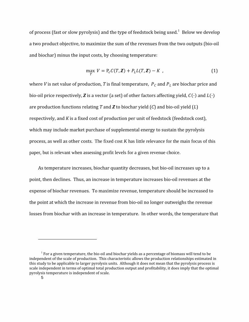
maximizes V in equation (1) is that which equates the marginal revenue gains from bio‐oil
to the revenue losses from biochar.2
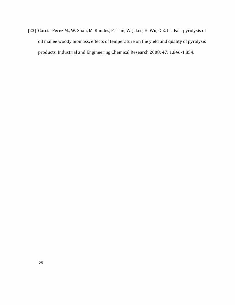
This condition is shown graphically in Figure 1. The curved line is the product
transformation curve (PTC) [11]. Any point on this line represents the output of biochar
(on the vertical axis) and bio‐oil (on the horizontal axis) that will be produced from
pyrolysis at a given temperature for a given feedstock quantity and type. An increase in
temperature will lead to a movement along this line down and to the right, providing more
bio‐oil and less biochar. The straight line from axis to axis in Figure 1 is an isorevenue line.
This is the set of combinations of biochar and bio‐oil that provides a given total revenue for
a given pair of biochar and bio‐oil prices.3 A combination that provides the highest
possible revenue for a unit of feedstock is provided by the specific combination where the
product transformation curve is tangent with the isorevenue line. In Figure 1, C1* and L1* is
the optimal combination of yields for the price ratio shown. The dotted (partial)
isorevenue line implies a higher bio‐oil price relative to biochar price, and is associated
with a higher optimal bio‐oil yield (L2*) and lower biochar yield (C2*).
In the discussion above, bio‐oil and biochar prices do not depend on temperature. This
is economically equivalent to assuming that the quality does not vary in terms of economic
value over the feasible temperature range, or at least, that market prices would not vary
2 The mathematical treatment of this condition is provided in Appendix A. 3 If revenue is , rearranging this with C alone on the left hand side provides the line . This is the straight line from axis to axis in Fig. 5.1, with intercept R/Pc and slope of ‐PL/PC.
7
according to quality. This may be a misleading assumption in some cases. For example if
energy content is the basis for economic value, both bio‐oil and biochar increase in energy
value as pyrolysis temperature increases over the relevant temperature range. In general,
if the price increases with temperature, there is an additional revenue gain from each
incremental temperature increase. This means that for otherwise similar circumstances,
the incremental price increase will tend to push the optimal temperature higher than if
prices were fixed and constant.4 In the production setting under consideration here, the
combination of C and L are chosen indirectly by choosing the temperature at which
pyrolysis is performed, and the pair of production relationships C(T) and L(T) imply a
product transformation curve between C and L. At this point, specific equations
representing the relationships between process factors (temperature, feedstock, heating
rate, etc.) and the two products (biochar and bio‐oil), are necessary to proceed. Regression
analysis is applied to the data we collected from published research on pyrolysis.
3. Econometric model and yield function estimation
A large literature exists for estimating production functions for application to
economic problems. This literature provides a wide range of production relationships and
estimation methods, ranging from restrictive to highly flexible functions to represent
(global or local) production relationships, and restrictive to highly flexible estimation
4 The mathematical treatment of this problem is provided in Appendix A.
8
erature and the product tra
methods. 5 After exploratory analysis, given the limited published data on biochar and bio‐
oil, and to provide a practical foundation for interpretation, this analysis relies on a
relatively simple quadratic production relationship between the input (temperature) and
the outputs (biochar and bio‐oil).6
he regression model us e n as: T
ed can be represent d in ge eral
where i is an observation index, and are parameters to be
estimated (bold represents a vector containing several parameters); C(Ti), and L(Ti) are
biochar and bio‐oil yield for observation i, respectively; Ti, and Zi are factors that affect
yield; and and are random disturbance terms. Using Ti and the square of Ti as
regressors allows for temperature to have a nonlinear effect on yields, which is important
for solving for the optimal pyrolysis temperatures. The derivation of the optimal
temp nsformation curve is given in Appendix A.
(2a)(2b)
5 General theoretical foundations are provided in [9]and [10]. Among many seminal papers, an example of foundations and estimation of flexible production frontiers is given in [11]. More recently, some studies look at the productivity and utilization of scarce natural resources such as: fisheries (e.g., using a transformation production function [12]; short‐run translog cost function [13]; Generalized Leontief production function [14]); forest resources (e.g., natural disturbance (forest fires, invasive species) production functions [15]; forest collection production functions of different household labor categories [16]). There are also studies that examine issues related to agriculture such as: technical efficiency of enterprises or farmers (e.g., stochastic frontier production function [18]); and risks in production of using pest control and GM crop technologies (e.g., 'flexible risk' production function models [19]; micro‐data based agricultural production functions [20]).
6 This simplicity economizes on degrees of freedom in estimation, and allows for ease of interpretation within the sampling range (and economically meaningful range) of the available data, and provides a second‐order approximation to more flexible forms for the relationship between temperature and yields. One issue arises because the dependent variables in these regressions are percentages, and do not range outside of the [0,100] interval. This in principle can cause complications for Ordinary Least Squares (OLS) if there are numerous observations near or on the range limit. This is generally not the case with the data used here, so we ignore this issue.
9
The data for this analysis are taken from published studies that are based on fast
pyrolysis and/or slow pyrolysis, and numerous different types of feedstocks. The variables
in the matrix Z include factors other than temperature that affect product yield per unit of
feedstock mass, such as feedstock type and heating rate (fast or slow). In the regression
results presented below, we include as explanatory variables in Z an indicator variable to
distinguish between fast (fast=1) and slow (fast=0), as well as indicator variables for four
different feedstock categories: agricultural crop residues, other agricultural feedstocks,
forest products, and other feedstocks.7
If we allow for price response to temperature differences, price response functions
and must be specified. Our data do not allow direct estimation of these
functions. However, assuming linear price response functions as an approximation, they
can be characterized as
,
If prices increase with temperature in the relevant temperature range, then all
coefficients will be positive. The consequence is that there is an additional incremental
benefit from increasing temperature: not only do you have an incremental increase in bio‐
oil yield, but prices tend to increase with temperature, so that the optimal temperature will
tend to be higher than when price is independent of temperature. The optimal temperature
(3a)
(3b)
7 These categories include several different specific feedstock types, but are aggregated to larger categories in order to economize on degrees of freedom in estimation.
1
s of revenue is how fast the
0
given these price functions is derived in Appendix A. Further, an explanation of how a
practitioner can customize these calculations is provided in Appendix A as well.
4. Data
Data on biochar and bio‐oil yields from different feedstocks were collected from
various studies on pyrolysis and are classified as follows: 8
• Agricultural field residue — includes tobacco stalk, rice straw, cotton stalk, corn stover,
and wheat straw;
• Agricultural feedstock (other) — includes hazelnut shell, sugarcane bagasse, coconut
shell, sorghum bagasse, sunflower hulls, flax shives, corn cob, and olive waste (from oil
production);
• Forest products — includes pine chips/wood/bark, pine sawdust, beech, poplar‐aspen
cellul se, mapleo bark, softwood bark, poplar sawdust, spruce sawdust, birch wood;
• Other feedstock — bamboo, tea factory waste, newsprint, fine paper, pulp mill waste,
peat moss.
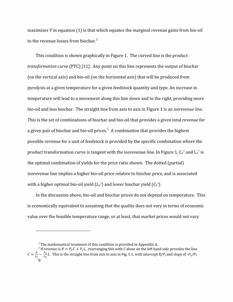
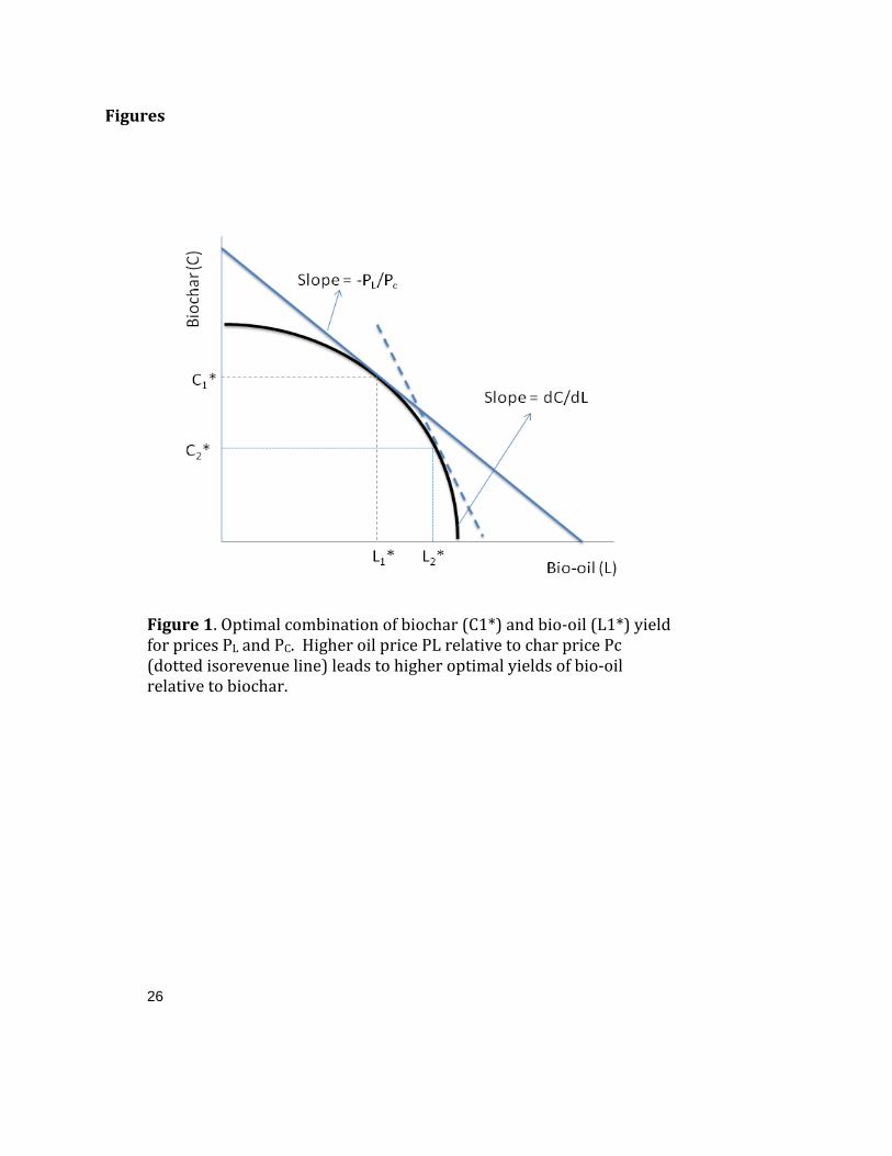
Figure 2 provides raw scatter plots of the data used in our analysis for the above set of
feedstock types.
Biochar and bio‐oil are joint products of a pyrolysis process, categorized into two
types: fast pyrolysis and slow pyrolysis. The main difference in the two technologies in
term materials are heated (i.e., the rate of increase in
8 Data are obtained from studies listed in Appendix B.
11
temperature per minute up to the final process temperature). Faster heating rates in fast
pyrolysis favor reactions leading to the formation of higher yields of oil and lower yields of
biochar.
Slow pyrolysis, on the other hand, results in higher yields of biochar compared to fast
pyrolysis, and in the formation of two liquid phases – a much lower amount of oil relative
to the fast pyrolysis process, and an aqueous phase (water plus a variety of organo‐oxygen
compounds of low molecular weight). This phenomenon is due an intensification of
dehydratation and polycondensation reactions leading to the formation of extra‐water and
more charcoal. Different rates of temperature increase, final pyrolysis temperatures, and
feedstock type alter the quality characteristics of bio‐oil and biochar. This in turn will
affect their economic value for different uses. The temperatures in our dataset correspond
to the final heating temperature. Although our data differentiate between fast and slow
pyrolysis applications, information is not available to control for differences in heating
rates and other characteristics within these two categories. Further, data are not
sufficiently available to allow modeling bio‐oil and biochar quality differences. We
therefore use a simple binary categorical distinction between fast and slow pyrolysis in the
regression estimation.
Note that the above discussion relates to outputs and revenues specifically. There are
also likely to be cost differences between fast and slow pyrolysis as well. In particular, fast
pyrolysis requires the use of small (usually <2 mm), pre‐processed feedstock particles [8],
whereas slow pyrolysis does not require such preprocessing to be effective. Therefore, the
12
variable K in equation (1) may be different for slow and fast pyrolysis, and the higher
revenues for fast pyrolysis may not imply higher net revenues (revenues minus costs).
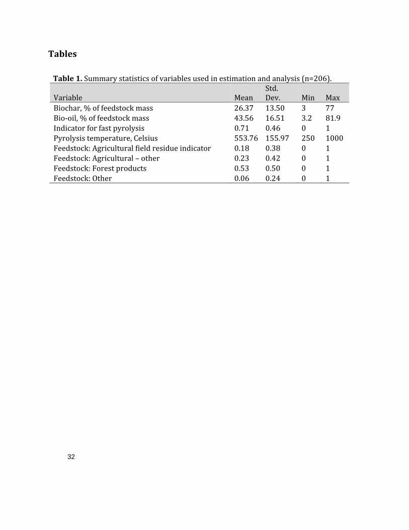
Table 1 provides undifferentiated summary statistics for the data used in the analysis.
Seventy‐one percent of our sample data from the published studies relied on were
generated using fast pyrolysis, and the majority of the sample data (53%) are based on
various (woody) forest product feedstocks. A fundamental choice variable in the pyrolysis
process is temperature. Temperatures in our sample data range from 250± to 1000±
Celsius.
Figure 2 is a series of descriptive scatter plots showing the relationship between bio‐oil
yield and biochar yield, by feedstock and pyrolysis type. The estimated regressions
performed below are designed to be able to, among other things, define a relationship
between biochar and bio‐oil yields as a function of temperature, and holding constant other
factors such as feedstock type. These quadratic fits are imprecise because they do not
control for feedstock type.
5. Results and discussion
In this section we summarize the regression results, generate estimates of product
transformation curves and optimal temperature for a given set of prices, and discuss
revenue optimization.
Tables 2 and 3 provide the regression results for biochar yield and bio‐oil yield,
estimated for slow and fast pyrolysis separately. Indicator variables are included for
13
tions (2a), (2b), and append
feedstock categories, although no observations exist for other feedstocks under slow
pyrolysis. The coefficients on the other indicator variables represent the intercepts of the
regression lines for each feedstock type. A constant was omitted from each regression to
avoid perfect collinearity of the indicator variables. The difference in these parameter
estimates then represents the difference in yield among feedstocks for any given
temperature. For example, in the first (left hand) regression in Table 2 slow pyrolysis, the
feedstocks included in the Ag[ricultural field] residue category tend to provide
approximately 0.04 percent less biochar than the feedstocks included in the Forest Products
category (103.43‐ 103.39 = 0.04).9 The R‐square measures in Tables 2 and 3 show that the
regression explains approximately ninety percent of the variation in each regression.
Estimation is carried out equation by equation using Ordinary Least Squares, and White’s
Heteroskedastic‐consistent standard errors are reported.
These regressions provide a foundation for understanding the revenue tradeoffs
implicit in the choice of temperatures, feedstock types, and pyrolysis types. They also
provide the information necessary to develop product transformation curves and construct
the relationship between output prices and optimal temperature settings. For example, the
estimates for the temperature (Temp(C)) parameters in the slow pyrolysis biochar and bio‐
oil regressions provide the values 0.2253 and 0.1371, respectively, in
equa ix equations (A.3a), (A.3b), (A.4), (A.9) and (A.10). The
9 There are only two observations that correspond to slow pyrolysis applied to agricultural field residues. Most of the explanatory power relating to agricultural field residues comes from the 35 observations of fast pyrolysis applied to field residues.
14
parameters associated with temperature squared (Temp(C) sq.) are 1.5E 04
0.00015 (Table 2) and 1.2E 04 0.00012 (Table 3).
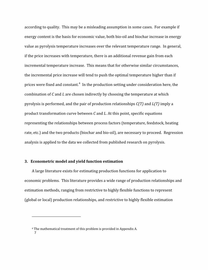
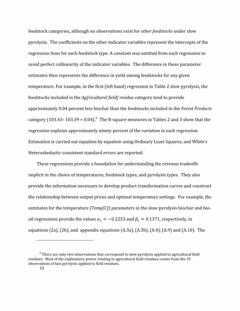
Figure 3 plots the yields of biochar and bio‐oil from woody forest products as a
function of temperature, for slow and fast pyrolysis, respectively.10 The two graphs have
common scales for clear comparison. First consider the differences between the fast and
slow pyrolysis functions. Together, the graphs show that for any given temperature, slow
pyrolysis is estimated to provide more biochar and less bio‐oil for a given amount of
feedstock than fast pyrolysis does. This implies that the relative economic efficacy of slow
and fast pyrolysis will depend, in part, on the relative prices of the two outputs.
Second, the graphs show that for our temperature range, bio‐oil yield increases with
temperature for low temperatures, but then begins to decline. For slow pyrolysis, the
temperature that provides maximum bio‐oil is about T=549°C (at the vertical dotted line in
the first panel of Figure 3). For fast pyrolysis, the temperature that provides maximum bio‐
oil is 524.92°C. In contrast, biochar yields decline over the entire range. Given the specific
shapes of these two functions, the economic region of temperature must be lower than that
which provides the maximum bio‐oil yield, i.e., the area to the left of the vertical dotted
lines.
10 Note that in Figure 3 and some subsequent figures, the horizontal axis includes temperatures below our minimum in‐sample temperature of 250°C for exposition of the quadratic functions. This area of these graphs should be interpreted with some skepticism, both because they represent extrapolations beyond the sample region, and also because pyrolysis is usually not effective below 250°C.
15
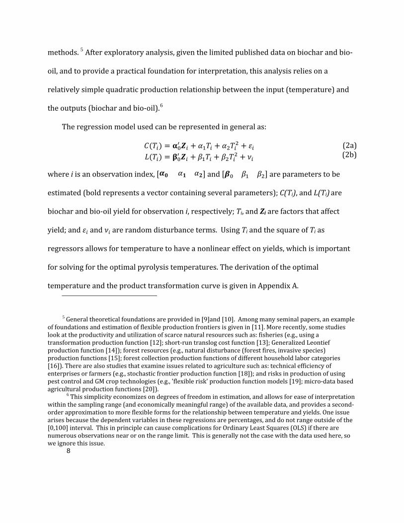
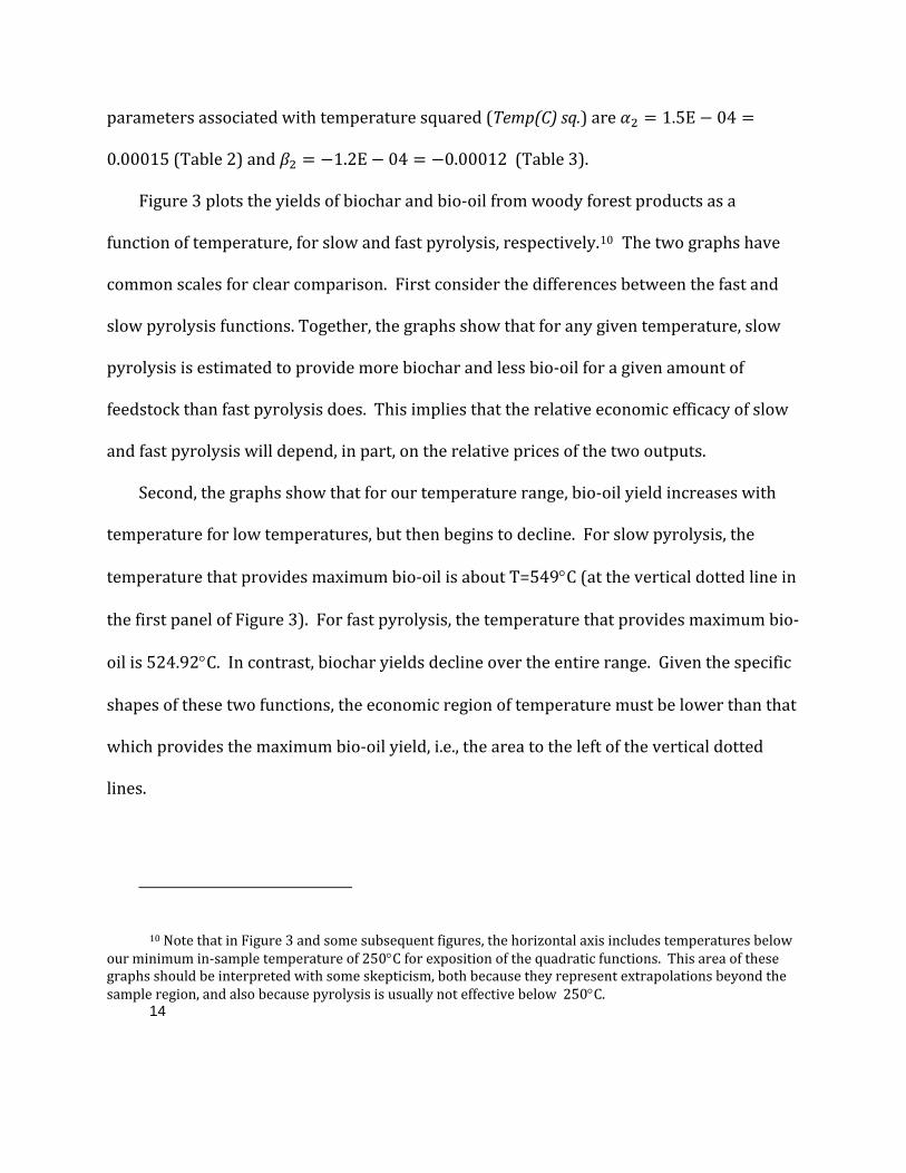
At low temperatures, there is a tradeoff; biochar yield declines but bio‐oil increases as
temperature increases. The optimal temperature depends on the relative prices of the two
outputs. At higher temperatures, both yields decline, so in this region, a further increase in
temperature necessarily reduces revenue (and reducing temperature necessarily increases
revenue), thus making production at and above the temperature where bio‐oil yields begin
to decline uneconomical regardless of relative prices. Figure 4 shows the estimated
product transformation curves (PTC) under slow and fast pyrolysis. These two curves
cross, such that slow pyrolysis PTC is above that for fast pyrolysis on the left, but below on
the right. This is of some interest because it implies that slow pyrolysis may tend to
provide higher revenues per unit of feedstock than fast pyrolysis under some price
conditions, and vice versa.11 As Figure 1 shows, revenue maximization for a given quantity
of feedstock entails choosing the combination of biochar and bio‐oil (indirectly through
pyrolysis temperature) subject to the prices of these two outputs.
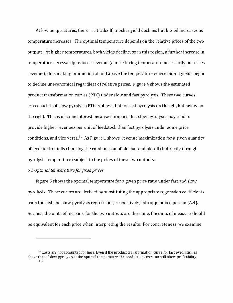
5.1 Optimal temperature for fixed prices
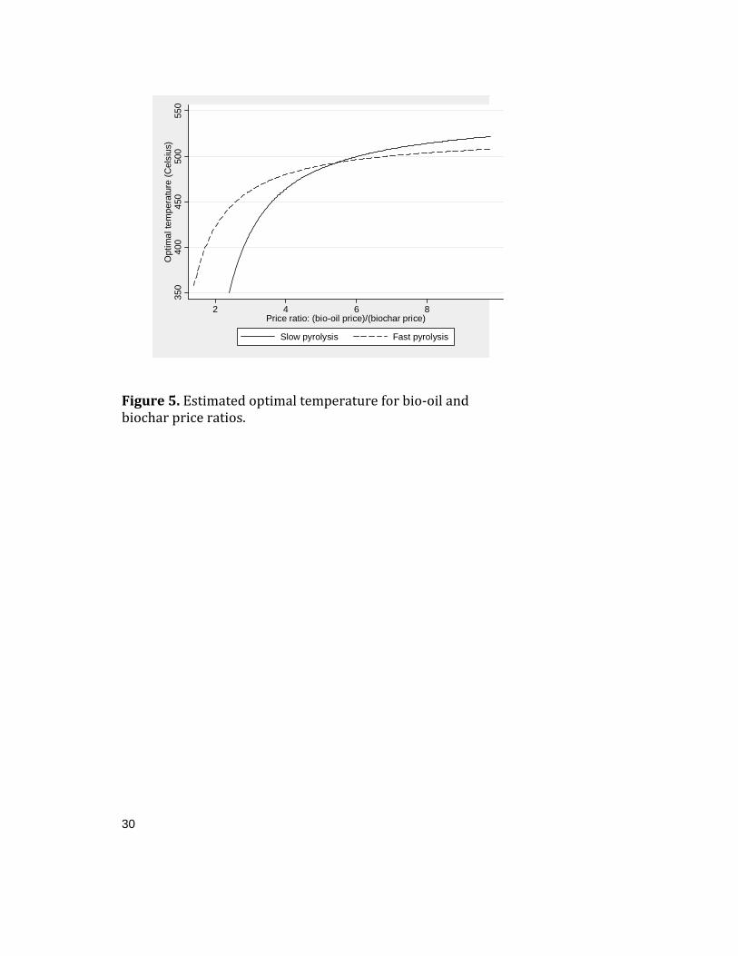
Figure 5 shows the optimal temperature for a given price ratio under fast and slow
pyrolysis. These curves are derived by substituting the appropriate regression coefficients
from the fast and slow pyrolysis regressions, respectively, into appendix equation (A.4).
Because the units of measure for the two outputs are the same, the units of measure should
be equivalent for each price when interpreting the results. For concreteness, we examine
11 Costs are not accounted for here. Even if the product transformation curve for fast pyrolysis lies above that of slow pyrolysis at the optimal temperature, the production costs can still affect profitability.
16
specific cases below based on price per kilogram (kg) for each output. At relatively low
bio‐oil prices, the optimal temperature under fast pyrolysis is higher than for slow
pyrolysis, but the opposite is true for higher ratios of bio‐oil and biochar. Notice that the
upper bounds on these curves (to the right on the graph) approach the economic maxima
of temperature discussed earlier.
The minimum temperature in our data sample is 250±C. However, little pyrolysis
occurs below about 300±C, and the valuable characteristics of both biochar and bio‐oil
deteriorate below about 350±C. This (latter) temperature is optimal under slow pyrolysis
for a price ratio of PL/PC = 2.40. For fast pyrolysis, the price ratio implying an optimal
temperature of 350±C is 1.36. Anything below this price ratio would call for more emphasis
on biochar. On the other end of the economic spectrum, profits necessarily decline
(regardless of prices) at about 549.3±C (slow) and 524.9±C (fast), so this will be an upper
bound economically valid temperature, and would apply if, for example, the price of
biochar is very small so that the price ratio PL/PC becomes very large.
It is useful to consider a set of feasible or possible prices and their outcomes as an
example. Because the data on biochar and bio‐oil yield (and therefore the estimated
parameters and the analysis developed above) are based on percent of feedstock mass, the
units of measure for biochar and bio‐oil, as well as the prices for each, must be in the same
unit of measure. This analysis below uses kilograms as units, and dollars per kilogram as
the price unit. The range of estimates for bio‐oil is from about $0.60 to about $1.06 per
gallon [22]. If we assume $1.00 per gallon of bio‐oil, this translates to $0.22 per kg of bio‐
17
oil. The price of biochar could vary significantly depending on the market. Suppose a
market supports biochar production at a break‐even price of $600 per ton, this translates
to $0.60 per kg.12 The result is a price ratio of PL/PC = 0.37, suggesting heavy emphasis on
low temperature, slow pyrolysis. In contrast, if biochar is of relatively little value, say $50
per ton, then the price ratio is 4.4, suggesting that fast pyrolysis at higher temperatures
(about 522±C) is optimal.
5.2 Optimal temperature for endogenous prices
When price is a function of quality, which in turn is a function of temperature, the price
ratio itself is determined in part by the chosen temperature. Therefore, there is no fixed
price ratio determining the optimal temperature. Instead, optimal temperature and price
are simultaneously determined. A specific set of price parameters is developed here and
used to solve for the optimal temperature. The data for this relationship between bio‐oil
quality (and therefore price) and temperature are very limited. The following analysis
relies on linear extrapolation of the price‐temperature relationship, putting some of the
calculated results outside the range of the original data. This example begins with the
assumption that both biochar and bio‐oil will be used as an energy source, with price
related to energy content of the product. Further, we assume that bio‐oil is a substitute in
use for fossil crude oil, and biochar is a substitute for coal. The energy content of biochar
tends to be higher than coal, and the energy content of bio‐oil tends to be lower than that of
12 This break‐even price was based on one of several scenarios developed for an economic analysis presented in [10].
fossil crude oil. However, as an approximation, we assume that the price per unit of energy
of bio‐oil is equal to that of fossil oil, and that the price per unit energy of biochar is equal
to that of coal.13
Let the high heating calorific value of crude oil and bio‐oil be 45.7 MJ/kg and 18 MJ/kg,
respectively. If the price of crude oil is $52/barrel, the price is also equivalent to $0.398/kg
or $0.008709/MJ. Figure 10 in [23] provides an estimated regression that relates fast
pyrolysis temperature to high heating value (dry) based on temperatures between 350°C
and 575°C. Substituting these numbers into equation (3b), we approximate the energy
content function for bio‐oil to be
, ( ) CT 50.007 7.851 o+=kgMJCalories
that price in dollars per kilogram is so
18
( ) C.T 0.0000658 0.15545514 $ o+=kgPL
This
(4)
provides a price of $0.188 per kilogram of bio‐oil at T=500°C.
A price of $68.10/metric ton of coal provides a price of $0.068/kg or $0.002528/MJ
from coal [i.e., ($0.068/kg) /(26.9 MJ/kg)]. Substituting these numbers into equation (3a)
provides an estimated relationship between calorific content of biochar as a function of
pyrolysis temperature:
13 This equal price reflects a market outcome driven by the assumed (perfect) substitutability of the two related goods (e.g. biochar and coal). If production cost of one of them is higher than the other — that is, if the market supply curves differ, then the quantities produced of the two goods will differ. If the two goods are not perfect substitutes in consumption, then prices will tend to differ also. In particular, if one has some disadvantages in terms of refinement (an intermediate demand), then it will tend to fetch a lower price per MJ.
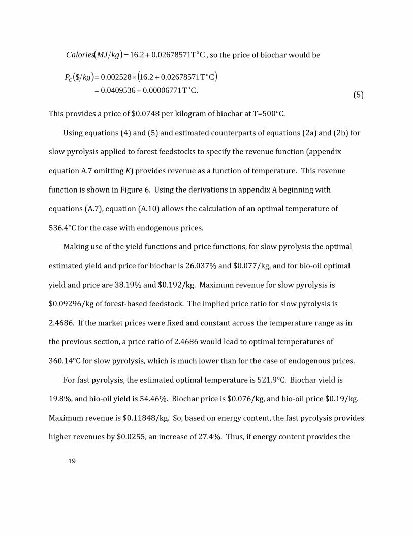
( ) CT 0.02678571 2.16 o+=kgMJCalories , so the price of biochar would be
( ) ( )C.T 0.00006771 0.0409536
CT 0.026785712.61 0.002528 $o
o
+=
+×=kgPC
This
(5)
provides a price of $0.0748 per kilogram of biochar at T=500°C.
Using equations (4) and (5) and estimated counterparts of equations (2a) and (2b) for
slow pyrolysis applied to forest feedstocks to specify the revenue function (appendix
equation A.7 omitting K) provides revenue as a function of temperature. This revenue
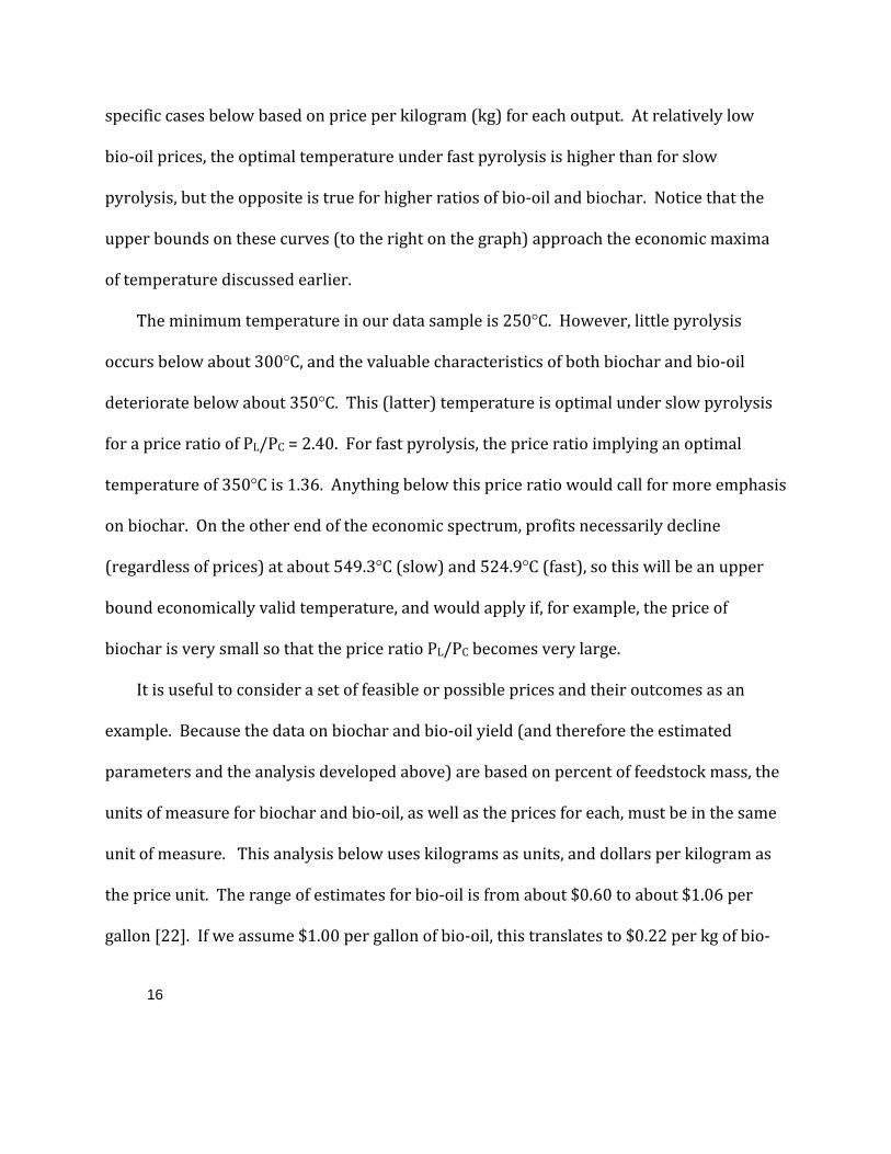
function is shown in Figure 6. Using the derivations in appendix A beginning with
equations (A.7), equation (A.10) allows the calculation of an optimal temperature of
536.4°C for the case with endogenous prices.
Making use of the yield functions and price functions, for slow pyrolysis the optimal
estimated yield and price for biochar is 26.037% and $0.077/kg, and for bio‐oil optimal
yield and price are 38.19% and $0.192/kg. Maximum revenue for slow pyrolysis is
$0.09296/kg of forest‐based feedstock. The implied price ratio for slow pyrolysis is
2.4686. If the market prices were fixed and constant across the temperature range as in
the previous section, a price ratio of 2.4686 would lead to optimal temperatures of
360. es.
19
14°C for slow pyrolysis, which is much lower than for the case of endogenous pric
For fast pyrolysis, the estimated optimal temperature is 521.9°C. Biochar yield is
19.8%, and bio‐oil yield is 54.46%. Biochar price is $0.076/kg, and bio‐oil price $0.19/kg.
Maximum revenue is $0.11848/kg. So, based on energy content, the fast pyrolysis provides
higher revenues by $0.0255, an increase of 27.4%. Thus, if energy content provides the
20
highest value for both products, fast pyrolysis provides higher revenues. Again, Appendix
A contains details and a summary of parameter values to facilitate the calculation of
ptimal temperatures for a given setting. o
6. Conclusion
This paper presents a model and estimates for maximizing the sum of revenues from
the joint production of bio‐oil and biochar. The primary control variables in this process
are the type of pyrolysis used (either fast or slow), and the final pyrolysis temperature, but
feedstock type is important as well. We provide a method for choosing the revenue
maximizing pyrolysis temperature in two cases: first, when market prices are fixed and do
not vary with temperature, and second, when output quality and therefore price changes as
pyrolysis temperature is altered. The dataset is limited, and relies on several different
types of feedstocks to estimate the yield parameters, using a relatively restrictive
functional form. Further, the price response functions in the final example above are
limited to only one, albeit fundamental, use of biochar and bio‐oil, so these results are
relatively narrow in scope. Nonetheless, the results are generally plausible and provide a
foundation for refinement.
Maximizing revenues by choosing process temperature can be economically
important. However, even if the optimal combination of bio‐oil and bio‐char is produced, it
may not provide an economically viable (profitable) enterprise. This ultimately depends
on whether the revenues from production outweigh the costs. The data used in this
21
analysis of the tradeoffs between biochar and bio‐oil production do not allow a cost
analysis.
Acknowledgments
This work is part of the project, Use of Biochar from the Pyrolysis of Waste Organic Material
as a Soil Amendment [10]. We would like to thank the Washington State Department of
Ecology for funding the project.
22
References
[1] Baum, E. and S. Weitner. Biochar application on soils and cellulosic ethanol
production. Clean Air Task Force, Boston, MA, U.S.A.; 2006.
[2] Chan, K.Y., L. Van Zwieten, I. Meszaros, A. Downie, and S. Joseph. Using poultry litter
biochars as soil amendments. Australian Journal of Soil Research 2008; 46(5): 437–
444.
[3] Steiner, C., W.G. Teixeira, J. Lehmann, T. Nehls, J.L. Vasconcelos de Macêdo, W.E.H.
Blum and W. Zech. Long term effects of manure, charcoal and mineral fertilization on
crop production and fertility on a highly weathered Central Amazonian upland soil.
Plant Soil 2007; 291: 275‐290.
[4] Van Zwieten, L., S. Kimber, K. Sinclair, K.Y. Chan and A. Downie. Biochar potential for
climate change mitigation, improved yield and soil health. In Proceedings of the New
South Wales Grassland Conference, NSW, Australia; 2008.
[5] Lehmann, J. and Joseph, S., Eds. Biochar for Environmental Management: Science and
Technology. Earthscan, London, UK; 2009.
[6] Dynamotive Energy Systems. BioOil. Available from:
http://www.dynamotive.com/industrialfuels/biooil; 2009.
[7] Jones, S.B., C. Valkenburg, C. Walton, D.C. Elliott, J.E. Holladay, D.J. Stevens, C. Kinchin
and S. Czernik. Production of gasoline and diesel from biomass via fast pyrolysis,
hydrotreating and hydrocracking: A design case. PNNL‐18284. Available from:
23
http://www.pnl.gov/main/publications/external/technical_reports/PNNL‐
18284.pdf; 2009.
[8] Graham R.G., M.A. Bergougnou and R.P. Overend. Fast pyrolysis of biomass. Journal of
Analytical and Applied Pyrolysis 1984; 6: 95‐135.
[9] Bridgewater A.V., D. Meier and D. Radlein. An overview of fast pyrolysis of biomass.
Organic Geochemistry 1999; 30: 1,479‐1,493.
[10] Granatstein, D., C.E. Kruger, H. Collins, S. Galinato, M. Garcia‐Perez, and J. Yoder. Use of
biochar from the pyrolysis of waste organic material as a soil amendment. Final
project report. Center for Sustaining Agriculture and Natural Resources, Washington
State University, Wenatchee, WA. 137 pp.; 2009.
[11] Beattie, B. and R. Taylor. The Economics of Production. Kriegar Publishing Co.
Malabar, FL.; 1993.
[12] Chambers, R. Applied Production Analysis. Cambridge University Press, New York,
NY.; 1988.
[13] Christensen, L., D. Jorgenson and L. Lau. Transcendental logarithmic production
frontiers. The Review of Economics and Statistics 1973; 5(1): 28‐45.
[14] Felthoven, R.G., C.J. Morrison Paul and M. Torres. Measuring productivity and its
components for fisheries: the case of the Alaskan pollock fishery, 1994‐2003. Natural
Resource Modeling 2009; 22(1):105‐136.
24
[15] Lazkano, I. Cost structure and capacity utilisation in multi‐product industries: an
application to the Basque trawl industry. Environmental and Resource Economics
2008; 41(2):189‐207.
[16] Hutchinson, S.D. Input use and incentives in the Caribbean shrimp fishery: the case of
345‐360. the Trinidad and Tobago fleet. Marine Resource Economics 2008; 23(3):
[17] Holmes, T.P., J.P. Prestemon and K.L. Abt (eds). The Economics of Forest
Disturbances: Wildfires, Storms, and Invasive Species. Forestry Sciences Series 79.
New York: Springer; 2008.
[18] Ajibefun, I.A. Technical efficiency analysis of micro‐enterprises: theoretical and
methodological approach of the stochastic frontier production functions applied to
Nigerian data. Journal of African Economies 2008; 17(2): 161‐206.
[19] Nyemeck Binam, J., J. Tonye and N. Wandji. Source of technical efficiency among small
holder maize and peanut farmers in the slash and burn agriculture zone of Cameroon.
Journal of Economic Cooperation among Islamic Countries 2005; 26(1): 193‐210.
[20] Shankar, B., R. Bennett and S. Morse. Production risk, pesticide use and GM crop
technology in South Africa. Applied Economics 2008; 40(19‐21): 2,489‐2,500.
[21] Christiaans, T., T. Eichner and R. Pethig. Optimal pest control in agriculture. Journal of
Economic Dynamics and Control 2007; 31(12): 3,965‐3,985.
[22] Zeman, N. Thermochemical versus biochemical. Biomass Magazine 2007 (June).
Available from: http://www.dynamotive.com/assets/articles/2007/070523BMM.pdf.
25
[23] Garcia‐Perez M., W. Shan, M. Rhodes, F. Tian, W‐J. Lee, H. Wu, C‐Z. Li. Fast pyrolysis of
oil mallee woody biomass: effects of temperature on the yield and quality of pyrolysis
products. Industrial and Engineering Chemical Research 2008; 47: 1,846‐1,854.
Figures
Figure 1. Optimal combination of biochar (C1*) and bio‐oil (L1*) yield for prices PL and PC. Higher oil price PL relative to char price Pc (dotted isorevenue line) leads to higher optimal yields of bio‐oil relative to biochar.
26
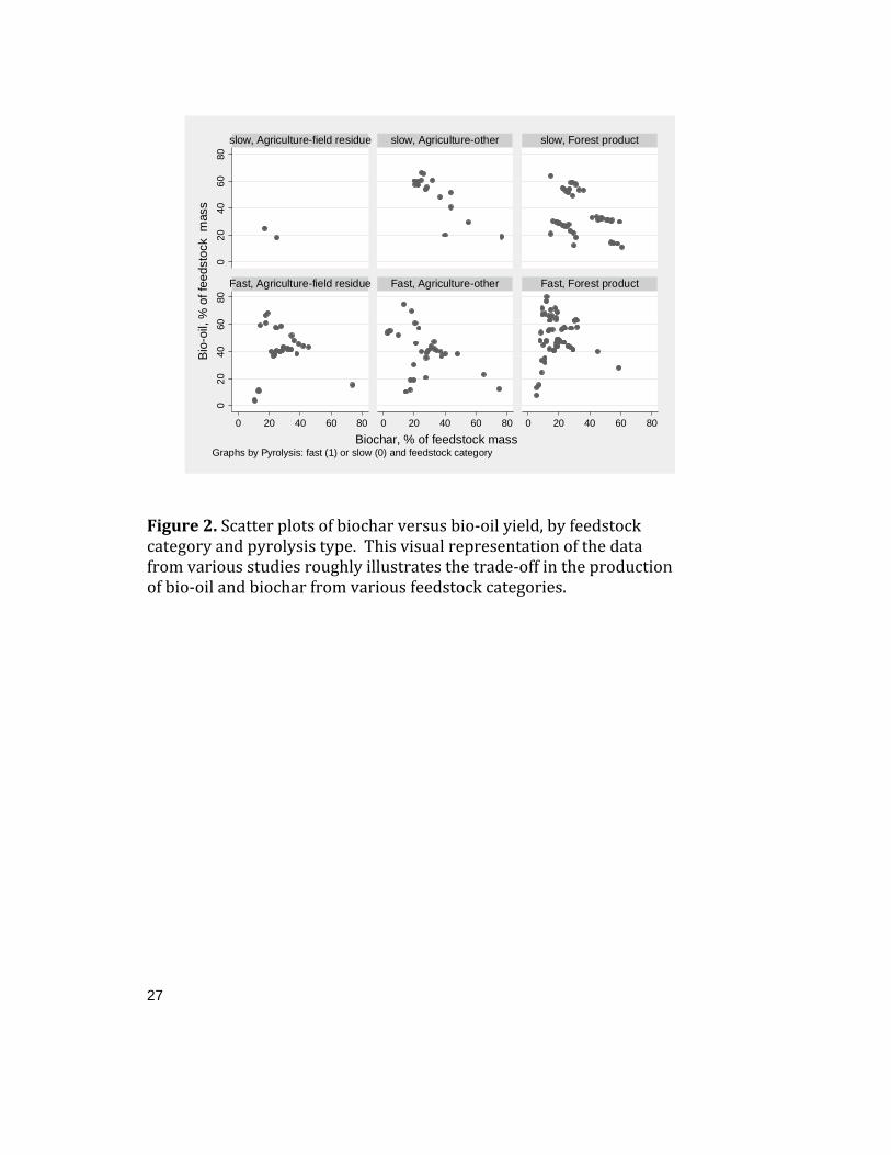
Figure 2. Scatter plots of biochar versus bio‐oil yield, by feedstock f the data e production
category and pyrolysis type. This visual representation ofrom various studies roughly illustrates the trade‐off in thof bio‐oil and biochar from various feedstock categories.
020
4060
800
2040
6080
0 20 40 60 80 0 20 40 60 80 0 20 40 60 80
slow, Agriculture-field residue slow, Agriculture-other slow, Forest product
Fast, Agriculture-field residue Fast, Agriculture-other Fast, Forest product
Bio-
oil,
% o
f fee
dsto
ck m
ass
Biochar, % of feedstock massGraphs by Pyrolysis: fast (1) or slow (0) and feedstock category
27
Figure 3. Biochar and bio‐oil yields under slow and fast pyrolysis.
1020
3040
5060
% o
f fee
dsto
ck m
ass
200 300 400 500 600 700Temperature (celsius)
Biochar Bio-oil
Slow pyrolysis
1020
3040
5060
% o
f fee
dsto
ck m
ass
200 300 400 500 600 700Temperature (celsius)
Biochar Bio-oil
Fast pyrolysis
28

Figure 4 Product transformation curves under slow and fast pyrolysis.
2040
6080
100
Bio
char
% o
f fee
dsto
ck m
ass
10 20 30 40 50 60Bio-oil % of feedstock mass
Slow pyrolysis Fast pyrolysis
29
30
Figure 5. Estimated optimal temperature for bio‐oil and biochar price ratios.
500
450
400
550
Opt
imal
tem
pera
ture
(Cel
sius
)35
0
2 4 6 8Price ratio: (bio-oil price)/(biochar price)
Slow pyrolysis Fast pyrolysis
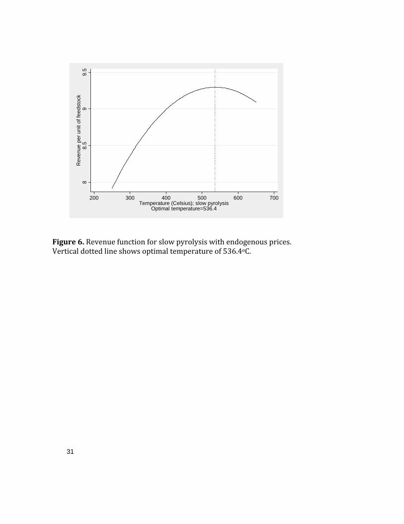
Figure 6. Revenue function for slow pyrolysis with endogenous prices. Vertical dotted line shows optimal temperature of 536.4oC.
88.
59
9.5
Rev
enue
per
uni
t of f
eeds
tock
200 300 400 500 600 700Temperature (Celsius); slow pyrolysis
Optimal temperature=536.4
31
Tables
Table 1. Summary statistics of variables used in estim an lysis 06ation d ana (n=2 ).
Variable Mean Std. Dev. Min Max
Biochar, % of feedstock mass 26.37 13.50 3 77 Bio‐oil, % of feedstock mass 43.56
6
16.51
7
3.2
0
81.9
00 Indicator for fast pyrolysis
idue indicator
0.71 0.46 0 1 Pyrolysis temperature, Celsius
resher
553.7 155.9 25 10Feedstock: Agricultural field
ltural – ot products
0.18 0.38 0 1 Feedstock: AgricuFeedstock: ForestFeedstock: Other
0.23 0.53 0.06
0.42 0.50 0.24
0 0 0
1 1 1
32

Table 2. Regres iochsion results. Dependent variable: Bhar, % fe ma sis
ar as a percent feedstock mass. har, % fe ma isDependent
variable Ø Bioc edstock ss, slow pyroly Bioc edstock ss, fast pyrolys
Indep. variablsq.1
e Est. Std. Err.
95% conf. int. Est. Std. Err.
95% conf. int. Temp (C) 1.5E‐04 5.8E‐05 3.5E‐05 2.7E‐04 9.4E‐05 2.5E‐05 4.5E‐05 1.4E‐04 Temp (C)
.2 ‐0.2253 0.0623 ‐0.3501 ‐0.1005 ‐0.1655 0.0322 ‐0.2291 ‐0.1019
Forest prode
103.43 15.60 72.17 134.70 80.67 9.97
60.96 100.37 Ag residu
g 103.39 06.14
15.12 6.39
73.09 3.29
133.69 38.99
91.27 10.12 71.26 111.29 Other A
er3 1 1 7 1 89.67
9.97 0.40
69.96 8.07
109.38 09.19 Oth 88.63 1 6 1
R2 0.93 0.89 N 60 146 1The estimates for the temperature (Temp(C)) parameters in the biochar regressions correspond to in equations 2a and 2b, and appendix equations A3a, A3b, A4, A7 and A8. The parameters associated with temperature squared (Temp sq.) correspond to . 2Coefficients associated with feedstock types (the four last rows of coefficients) represent the intercept for s e constant is omitted to avoid perfect low pyrolysis applied to each respective feedstock type. Thulticollinearity. No obserm3 vations are available for slow pyrolysis applied to Other Feedstock. Table 3. RDependent
egre Bio‐ossion results. Dependent variable:Bio‐oil, % feedstock mass, slow pyrolysis
il as a percent feedstock mass. Bio‐oil, % fe ock mass, fast pyrolysis
variable Ø edst
Indep. variablsq.1
e Est.
Std. Err.
95% conf . int.
Est.
Std. Err.
95% conf
. int.
Temp (C) ‐1.2E‐04 8.3E‐05 ‐2.9E‐04 4.2E‐05 ‐2.1E‐04 3.4E‐05 ‐2.8E‐04 ‐1.4E‐04Temp (C)
.2 0.1371 0.0894 ‐0.0421 0.3163 0.2205 0.0444 0.1328 0.3083
Forest prode
0.556 22.396 ‐44.327 45.438 ‐3.420
13.753 ‐30.610 23.770 Ag residu
g ‐4.871 4.552
21.702 3.533
‐48.363 32.609
38.621 1.714
‐11.090 13.969 ‐38.707 16.528 Other A
er3 1 2 ‐ 6 ‐9.531
6 13.757 4.351
‐36.730 35.819
17.667 0.927 Oth ‐7.44 1 ‐ 2
R2 0.88 0.94 N 60 146 1The estimates for the temperature (Temp(C)) parameters in the bio‐oil regressions correspond to in equations 2a and 2b, and appendix equations A3a, A3b, A4, A7 and A8. The parameters associated with temperature squared (Temp sq.) correspond to . 2Coefficients associated with feedstock types (the four last rows of coefficients) represent the intercept for s e constant is omitted to avoid perfect low pyrolysis applied to each respective feedstock type. Thmulticollinearity. 3 No observations are available for slow pyrolysis applied to Other Feedstock.
33
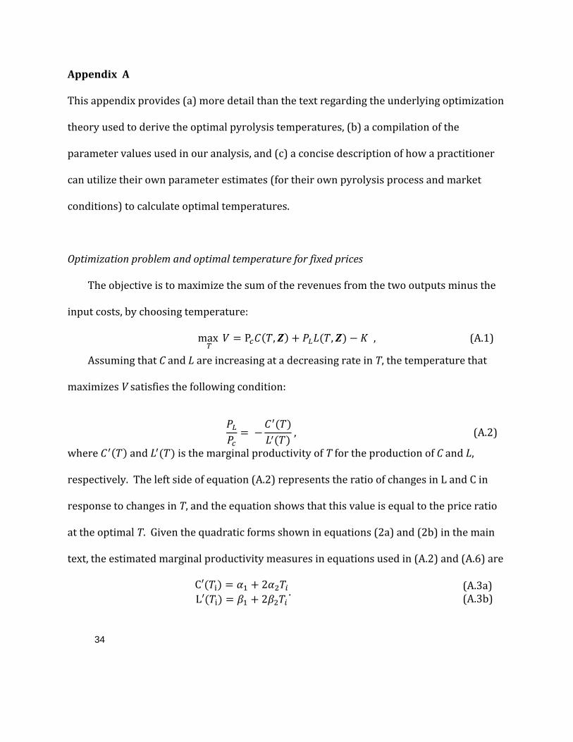
Appendix A
This appendix provides (a) more detail than the text regarding the underlying optimization
theory used to derive the optimal pyrolysis temperatures, (b) a compilation of the
parameter values used in our analysis, and (c) a concise description of how a practitioner
can utilize their own parameter estimates (for their own pyrolysis process and market
onditions) to calculate optimal temperatures. c
Optimization problem and optimal temperature for fixed prices
The objective is to maximize the sum of the revenues from the two outputs minus the
input costs, by choosing temperature:
max P , , , (A.1
Assuming that C and L are increasing at a decreasing rate in T, the temperature that
maximizes V satisfies the following condition:
)
where and is the marginal productivity of T for the production of C and L
respectively. The left side of equation (A.2) represents the ratio of changes in L and C in
response to changes in T, and the equation shows that this value is equal to the price ratio
at the optimal T. Given the quadratic forms shown in equations (2a) and (2b) in the main
text, the estimated margin o sures in equations used in (A.2) and (A.6) are
,
, (A.2)
al pr ductivity mea
C 2L 2 . (A.3a)
(A.3b)
34
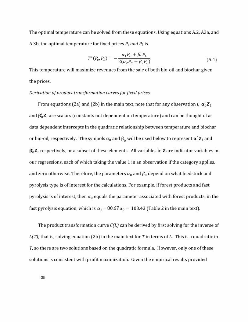
The optimal temperature can be solved from these equations. Using equations A.2, A3a, and
A.3b, the optimal temperature for fixed price P a s s c nd PL i
, 2 . (A.4
This temperature will maximize revenues from the sale of both bio‐oil and biochar given
the prices.
)
Derivation of product transformation curves for fixed prices
From equations (2a) and (2b) in the main text, note that for any observation i,
and are scalars (constants not dependent on temperature) and can be thought of as
data dependent intercepts in the quadratic relationship between temperature and biochar
or bio‐oil, respectively. The symbols α and β will be used below to represent and
respectively, or a subset of these elements. All variables in Z are indicator variables in
our regressions, each of which taking the value 1 in an observation if the category applies,
and zero otherwise. Therefore, the parameters and depend on what feedstock and
pyrolysis type is of interest for the calculations. For example, if forest products and fast
pyrolysis is of interest, then equals the parameter associated with forest products, in the
fast pyrolysis equation, which is 67.800 =α 103.43 (Table 2 in the main text).
The product transformation curve C(L) can be derived by first solving for the inverse of
L(T); that is, solving equation (2b) in the main text for T in terms of L. This is a quadratic in
T, so there are two solutions based on the quadratic formula. However, only one of these
solutions is consistent with profit maximization. Given the empirical results provided
35
36
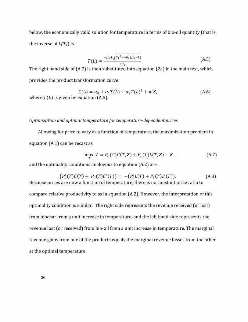
below, the economically valid solution for temperature in terms of bio‐oil quantity (that is,
the inverse of L(T)) is
(A.5)
The right hand side of (A.7) is then substituted into equation (2a) in the main text, which
provides the product tra tinsforma on curve:
, C Lhere is given by equation (A.5).
(A.6) w
Optimization and optimal temperature for temperaturedependent prices
Allowing for price to vary as a function of temperature, the maximization problem in
equation (A.1) can be recast as
, max , ,
and the optimality conditio
(A.7)
ns analogous to equation (A.2) are
. Because prices are now a function of temperature, there is no constant price ratio to
compare relative productivity to as in equation (A.2). However, the interpretation of this
optimality condition is similar. The right side represents the revenue received (or lost)
from biochar from a unit increase in temperature, and the left hand side represents the
revenue lost (or received) from bio‐oil from a unit increase in temperature. The marginal
revenue gains from one of the products equals the marginal revenue losses from the other
at the optimal temperature.
(A.8)
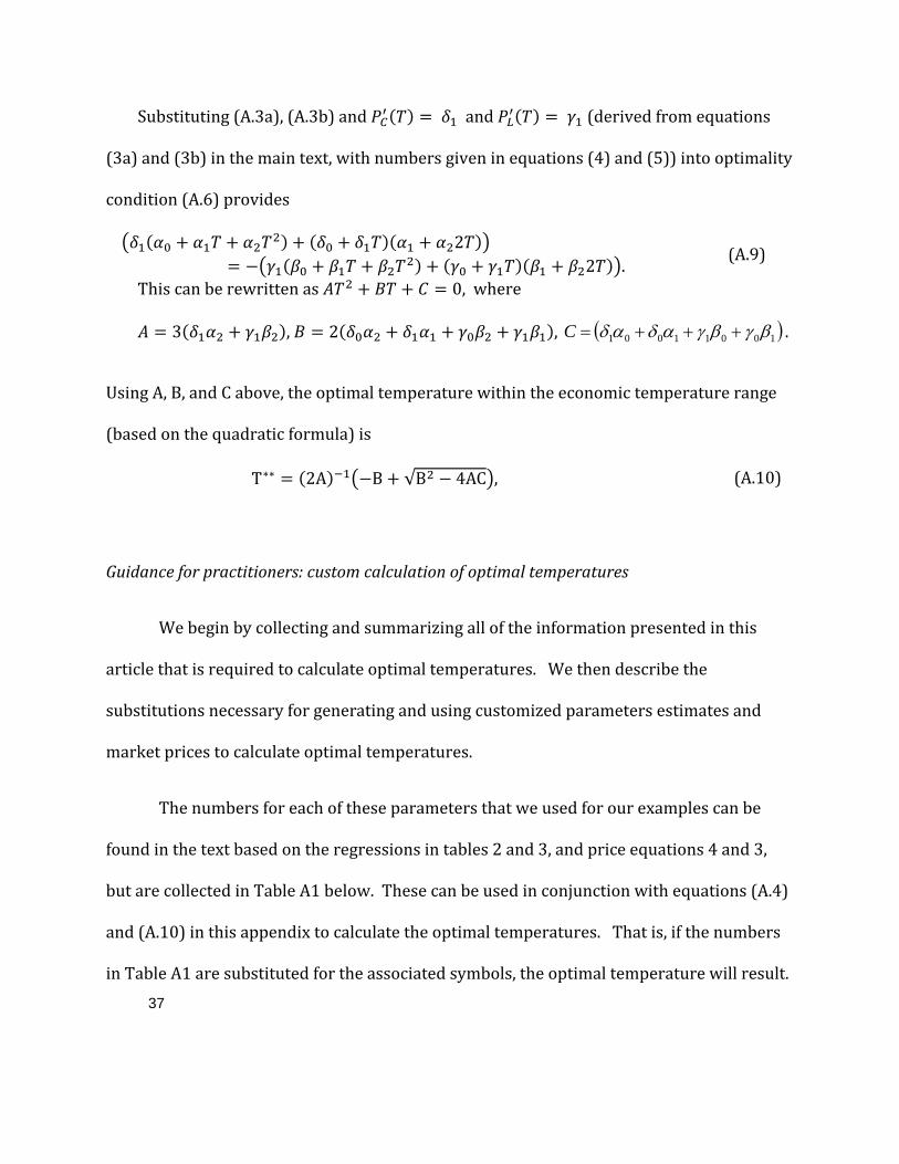
Substituting (A.3a), (A.3b) and and (derived from equations
(3a) and (3b) in the main text, with numbers given in equations (4) and (5)) into optimality
condition e (A.6) provid s
2 . 2
t
(A.9)
This can be rewrit en as 0, where
3 , 2 , ( )10011001 βγβγαδαδ +++=C .
Using A, B, and C above, the optimal temperature within the economic temperature range
(based on the quad tic o la)ra f rmu is
T 2A B √B 4AC , (A.10)
Guidance for practitioners: custom calculation of optimal temperatures
We begin by collecting and summarizing all of the information presented in this
article that is required to calculate optimal temperatures. We then describe the
substitutions necessary for generating and using customized parameters estimates and
market prices to calculate optimal temperatures.
37
The numbers for each of these parameters that we used for our examples can be
found in the text based on the regressions in tables 2 and 3, and price equations 4 and 3,
but are collected in Table A1 below. These can be used in conjunction with equations (A.4)
and (A.10) in this appendix to calculate the optimal temperatures. That is, if the numbers
in Table A1 are substituted for the associated symbols, the optimal temperature will result.
38
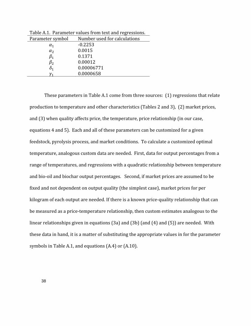
Table A.1 ParametParameter symbol
. er v s. alues from text and regression used for calculations Number
‐0.2253 0.0015 0.1371
0.00012 0.000067710.0000658
These parameters in Table A.1 come from three sources: (1) regressions that relate
production to temperature and other characteristics (Tables 2 and 3), (2) market prices,
and (3) when quality affects price, the temperature, price relationship (in our case,
equations 4 and 5). Each and all of these parameters can be customized for a given
feedstock, pyrolysis process, and market conditions. To calculate a customized optimal
temperature, analogous custom data are needed. First, data for output percentages from a
range of temperatures, and regressions with a quadratic relationship between temperature
and bio‐oil and biochar output percentages. Second, if market prices are assumed to be
fixed and not dependent on output quality (the simplest case), market prices for per
kilogram of each output are needed. If there is a known price‐quality relationship that can
be measured as a price‐temperature relationship, then custom estimates analogous to the
linear relationships given in equations (3a) and (3b) (and (4) and (5)) are needed. With
these data in hand, it is a matter of substituting the appropriate values in for the parameter
symbols in Table A.1, and equations (A.4) or (A.10).
39
Appendix B
Study Feedstock biomass A. Fast Pyrolysis Darmstadt, Hans, Dana Pantea, Lydia Summchen, Ulf Roland, Serge Kaliaguine, and Christian Roy. 2000. “Surface and Bulk Chemistry of Charcoal Obtained by Vacuum Pyrolysis of Bark:
ical Influence of Feedstock Moisture Content.” Journal of Analytand Applied Pyrolysis, 53:1‐17.
Maple bark, softwood bark
Demirbas, Ayhan. 2002. “Analysis of Liquid Products from Biomass via Flash Pyrolysis.” Energy Sources, 24:337–345.
Yellow pine, tobacco stalk
Dogan Gullu. 2003. “Effect of catalyst on yield of liquid products from Biomass via pyrolysis.” Energy Sources, 25(8):753‐765.
Yellow pine, hazelnut ste, shell, tea factory wa
tobacco stalk Drummond, Ana‐Rita F. and Ian W. Drummond. 1996. “Pyrolysis of Sugar Cane Bagasse in a Wire‐Mesh Reactor.” Industrial and Engineering Chemistry Research, 35(4):1,263‐1,268.
Sugarcane bagasse
Kang, Bo‐Sung, Kyung Hae Lee, Hyun Ju Park, Young‐Kwon Park, Joo‐Sik Kim. 2006. “Fast Pyrolysis of Radiata Pine in a Bench Scale Plant with a Fluidized Bed: Influence of a Char Separation
il.” System and Reaction Conditions on the Production of Bio‐oJournal of Analytical and Applied Pyrolysis, 76:32–37.
Radiata pine
Garcia‐Perez, Manuel, Xiao Shan Wang, Jun Shen, Martin J. Rhodes, Fujun Tian, Woo‐Jin Lee, Hongwei Wu, and Chun‐Zhu Li. 2008. “Fast Pyrolysis of Oil Mallee Woody Biomass: Effect of Temperature on the Yield and Quality of Pyrolysis Products.” Industrial and Engineering Chemistry Research, 47(6):1,846‐1,854.
Pine pellets
Ioannidou, O., A. Zabaniotou, E.V. Antonakou, K.M. Papazisi, A.A. Lappas, and C. Athanassiou. 2009. “Investigating the Potential for Energy, Fuel, Materials and Chemicals Production from Corn Residues (Cobs and Stalks) by Non‐catalytic and Catalytic Pyrolysis in Two Reactor Configurations.” Renewable and Sustainable Energy Reviews, 13:750–762.
Corn cob
Luo, Zhongyang, Shurong Wang, Yanfen Liao, Jinsong Zhou, t –462.
Yueling Gu, and Kefa Cen. 2004. “Research on Biomass Faspyrolysis for Liquid Fuel.” Biomass and Bioenergy, 26:455
P. indicus (wood feedstock)
Scott, Donald S., Jan Piskorz, and Desmond Radlein. 1985. “Liquid Products from the Continuous Flash Pyrolysis of iomass.” Industrial and Engineering Chemistry Process Design nd Development, 24(3): 581‐588. Ba
Poplar aspen cellulose, corn stover, wheat straw
40
Appendix B (continued)
Study Feedstock biomass A. Fast Pyrolysis (continued) Scott, Donald S., Piotr Majerski, Jan Piskorz, and Desmond Radlein. 1999. “A Second Look at Fast Pyrolysis of Biomass — he RTI Process.” Journal of Analytical and Applied Pyrolysis, 1:23–37. T5
Poplar sawdust, spruce sawdust, sugarcane bagasse, sorghum bagasse, wheat chaff, sunflower hulls, wheat straw, flax shives, newsprint, fine paper, pulp mill waste, peat moss
Tsai, W.T., M.K. Lee, and Y.M. Chang. 2006. “Fast Pyrolysis of Rice Straw, Sugarcane Bagasse and Coconut Shell in an Induction‐Heating Reactor.” Journal of Analytical and Applied Pyrolysis, 76:230‐237.
Rice straw, sugarcane bagasse, coconut shell
Wang, Xiaoquan, Sascha R. A. Kersten, Wolter Prins, and Wim P. M. van Swaaij. 2005. “Biomass Pyrolysis in a Fluidized Bed Reactor. Part 2: Experimental Validation of Model Results.” Industrial and Engineering Chemistry Research, 44(23):8,786‐8,795.
Pine, beech, bamboo
Zanzi, Rolando, Krister Sjöström,Emilia Björnbom. 2002. “Rapid Pyrolysis of Agricultural Residues at High Temperature.” Biomass and Bioenergy, 23:357–366.
Wheat straw‐untreated, wheat straw‐pellets, olive waste (from oil production), birch wood
B. Slow Pyrolysis Asadullah, M., M.A. Rahman, M.M. Ali, M.S. Rahman, M.A. Motin,
rom M.B. Sultan, and M.R. Alam. 2007. “Production of Bio‐oil fFixed Bed Pyrolysis of Bagasse.” Fuel, 86:2,514‐2,520.
Sugarcane bagasse
Chen, G., J. Andries, H. Spliethoff and D.Y.C. Leung. 2003. “Experimental Investigation of Biomass Waste (Rice Straw, Cotton Stalk, and Pine Sawdust) Pyrolysis Characteristics.” Energy Sources, 25:331–337.
Rice straw, cotton stalk, and pine sawdust
Garcia‐Perez, Manuel, Thomas T. Adams, John W. Goodrum, Daniel P. Geller, and K. C. Das. 2007. “Production and Fuel roperties of Pine Chip Bio‐oil/Biodiesel Blends.” Energy and uels, 21:2,363‐2,372. PF
Pine chips, pine pellets
41
Appendix B (continued)
Study Feedstock biomass B. Slow Pyrolysis (continued) Ioannidou, O., A. Zabaniotou, E.V. Antonakou, K.M. Papazisi, A.A. Lappas, and C. Athanassiou. 2009. “Investigating the Potential for Energy, Fuel, Materials and Chemicals Production from Corn Residues (Cobs and Stalks) by Non‐catalytic and Catalytic
Pyrolysis in Two Reactor Configurations.” Renewable andSustainable Energy Reviews, 13:750–762.
Corn cob
Sensoz, Sevgi. 2003. “Slow Pyrolysis of Wood Barks from Pinus logy, brutia Ten. and Product Compositions.” Bioresource Techno
89:307–311.
Pine bark
Sensoz, Sevgci and Mukaddes Can. 2002. “Pyrolysis of Pine and ‐355.
(Pinus brutia Ten.) Chips: 1. Effect of Pyrolysis TemperatureHeating Rate on the Product Yields.” Energy Sources, 24:347
Pine Chips
Williams, Paul T. and Serpil Besler. 1996. “The Influence of Temperature and Heating Rate on the Slow Pyrolysis of Biomass.” Renewable Energy, 7(3):233‐250.
Pine wood
Zandersons, J., J. Gravitis, A. Kokorevics, A. Zhurinsh, O. Bikovens, A. Tardenaka, and B. Spince. 1999. “Studies of the Brazilian ugarcane Bagasse Carbonisation Process and Products roperties.” Biomass and Bioenergy, 17:209‐219. SP
Sugarcane bagasse